Measurement and Identification of Capital Inflow Surges | OECD
Upload
khangminh22Category
view
1download
0
i
Temporal Variation of Inflow to the Dams of
Rajasthan State with Special Reference to
Ramgarh and Bisalpur Dams
This thesis is submitted as a partial fulfilment of the Ph.D. programme in
Engineering
Naveen Kumar Gupta
ID No.: 2011RCE7135
Department of Civil Engineering
MALAVIYA NATIONAL INSTITUTE OF TECHNOLOGY
JAIPUR-302017
July, 2016

ii
MALAVIYA NATIONAL INSTITUTE OF TECHNOLOGY,
JAIPUR-302017
CERTIFICATE
This is to certify that the thesis report entitled “Temporal Variation of Inflow to the
Dams of Rajasthan State with Special Reference to Ramgarh and Bisalpur Dams”
which is being submitted by Naveen Kumar Gupta, ID No.: 2011RCE7135, for the
partial fulfillment of the degree of Doctor of Philosophy in Civil Engineering in the
Malaviya National Institute of Technology, Jaipur has been carried out by him under
my supervision and guidance.
Date: July 8, 2016
Place: Jaipur
(Dr. Ajay Singh Jethoo)
Supervisor
Associate Professor, Civil Engineering Department
Malaviya National Institute of Technology
Jaipur- 302017
Rajasthan
India

iii
MALAVIYA NATIONAL INSTITUTE OF TECHNOLOGY,
JAIPUR-302017
CANDIDATE’S DECLARATION
I hereby certify that the work which is being presented in the thesis entitled
„Temporal Variation of Inflow to the Dams of Rajasthan State with Special
Reference to Ramgarh and Bisalpur Dams’ in partial fulfilment of the requirements
for the award of the Degree of Doctor of Philosophy and submitted in the Department
of Civil Engineering, Malaviya National Institute of Technology Jaipur, is an
authentic record of my own work carried out at Department of Civil Engineering
during a period from December 27, 2011 to July 08, 2016 under the supervision of Dr.
Ajay Singh Jethoo, Associate Professor of Civil Engineering Department, Malaviya
National Institute of Technology Jaipur.
The matter presented in this thesis has not been submitted by me for the award of any
other degree of this or any other Institute.
Dated: July 8, 2016 (Naveen Kumar Gupta)
Place: Jaipur ID No.: 2011RCE7135
This is to certify that the above statement made by the candidate is true to the best of
my knowledge.
Date: July 8, 2016
Place: Jaipur
(Dr. Ajay Singh Jethoo)
Supervisor
Associate Professor, Civil Engineering Department
Malaviya National Institute of Technology
Jaipur- 302017
Rajasthan
India

iv
Acknowledgement
The present work for all its outcomes owes a lot to a large number of people. First and
foremost being Dr. Ajay Singh Jethoo, Associate Professor, Department of Civil
Engineering, Malaviya National Institute of Technology, Jaipur, Rajasthan, India my
guide and supervisor to whom I owe gratitude for his valuable guidance without
which this research work would not have been a success. Apart from being my
supervisor, he was always there when I needed him. He taught me that for going
deeper into the field, I must start playing with things and must not stop till the last
stage is conquered. His perceptual inspiration, encouragement, and understanding
have been a mainstay of this work. From his busy schedule, he always spared time for
assessing the progress of my work. His wide knowledge regarding the subject helped
me in writing this thesis. I am indebted to Dr. Sandeep Choudhary, Associate
Professor, Department of Civil Engineering, for his kind help and support which made
it possible for me to stand up to the challenges offered by the task and come out
successfully. I thank him sincerely for his inspiration and guidance he showered on
me.
I extend my deep sense of gratitude to Prof. A.B. Gupta, Director and Prof.
I.K. Bhatt, Ex-Director, MNIT, Jaipur for strengthening the research environment of
the Institute by providing all necessary facilities. I am thankful to Prof. Ravindra
Nagar Dean (Academics), Officers, and Staff of academic affairs for their cooperation
in academic work and help throughout the course of study. I am not able to find words
in any of the dictionaries for thanking Prof. Gunwant Sharma, Prof. Y.P. Mathur,
Prof. A.K.Vyas, Prof. Sudhir Kumar, Dr. Mahendra Choudahry and Dr. Urmila
Brighu, Department of Civil Engineering, MNIT, Jaipur for their valuable guidance,
unfailing encouragement, keeping my moral high during the course of the work and
helped me out whenever I needed them. I am extremely thankful to members of
DPGC and DREC, for their support and guidelines regarding my thesis work. I also
pay my sincere regards to Prof. K.C. Jain for helping me out in the analysis of my
thesis results.
I deeply acknowledge Er. B.K. Gupta, Chief Engineer, PHED (Retd.); Er.
Pradeep Mathur, Chief Engineer (Retd.); Er. Raja Ram Yadav, Chief Engineer
(Retd.); Er. Vinay Chandwani Executive Engineer; Er. Sunil Vyas, Executive

v
Engineer; Er. Kiran Ahuja, Executive Engineer; Er. N.P. Singh, Executive Engineer;
Er. Dharmesh Yadav, Executive Engineer and all other engineers and staff of Water
Resources Department, Government of Rajasthan, India, whose regular support,
guidance, motivation, and contribution towards my thesis cannot be unseen.
I am also thankful to Dr. S.K Tiwari, Dr. Sumit Khandelwal, Dr. Nivedita
Kaul, Dr. Mahesh Jat, Dr. Pawan Kalla, Dr. Arun Gaur, Prof. Rohit Goyal, Prof. B.L.
Swami, Dr. M.K. Shrimali, Dr. S.D. Bharti, Dr. J.K. Jain, Dr. Rajesh Gupta, Dr.
Sanjay Bhatter and all other faculty members of Malaviya National Institute of
Technology Jaipur.
I am grateful to the Head, Civil Engineering Department, and Dean R&D for
providing me with the environment and space to carry out my research work.
I give my thanks to Mr. Rajesh Saxena, Office-in-Charge, Civil Engineering
Department, MNIT Jaipur, Mr. Ramjilal Meena and Mr. Sher Singh, who were
always ready to extend me every possible help throughout my work.
From the bottom of my heart, I ever realize the inspiration given by my father,
Late Mr. Subhash Chand Gupta and mother, Mrs. Shanti Devi. The most valued
efforts and guidance from my brother, Mr. Amolak Khandelwal, Chartered
Accountant, provided me with the urge of doing the best work. I cannot forget to
acknowledge here the tolerance and patience of my kids, Mansi and Umang, which
they kept during the progress of my research work. Lastly but not the least, I would
like to acknowledge the efforts made by my wife, Mrs. Poonam Gupta, in providing
me with the environment to carry on my thesis work at home with ease. I would like
to thank Almighty God, without whose blessings, it was not possible to even think
about doing this work.
Finally, I would like to thank all those people who helped, guided, and
supported me in my study. Thank you all!
Dated: July 8, 2016 (Naveen Kumar Gupta)
Place: Jaipur ID No.: 2011RCE7135

vi
Abstract
The study aims to investigate the temporal variation of inflow to the existing dams of
Rajasthan State especially related to Ramgarh and Bisalpur dams. Inflows to these
dams in Rajasthan have been decreasing in recent decades. Population in the state is
regularly increasing. Because of droughts, overuse of surface and subsurface water
resources, construction of small water harvesting structures and changes in land use
and other anthropogenic impacts, water levels have decreased tremendously. The
attribution of inflow variability to anthropogenic activities is a challenging problem
and an active research area.
Rajasthan is a semi-arid state with the highest of the geographical area of the
Indian subcontinent. Rainfall variation is very high over the state, ranging from 190
mm to 1000 mm from west to south/east. Average rainfall over the state is 575 mm
against the national average of 1182 mm. Matters of water resources planning are of
prime importance for the state. There are 243 blocks, out of which 172 blocks are
overexploited. Only 25 blocks, i.e. only 10% blocks in the state may be considered
safe for groundwater withdrawal. The average inflow to the surface water reservoirs is
around 39% only. It has been observed from the storage data of the dams of the
Rajasthan State that there are temporal variations in inflows. Reduced inflows to the
dams are creating a water stress condition in the state. Detailed study of Ramgarh and
Bisalpur dams has been taken in this research because these two dams are related to
the drinking water supply need of the capital city Jaipur.
Methodology to conduct the study includes the formation of the null
hypothesis to test the observed dependabilities and inflows of the existing dams of
various river basins. Results of t-test and Chi-square test infer the rejection of the null
hypothesis, i.e. dependabilities have been changed, and inflow to the dams is not as
per their expected standards. Simulated inflows have been computed with the help of
Thiessen polygon and Strange‟s table, as per the prevailing practices of Water
Resources Department of Government of Rajasthan. Performance statistics and Nash-
Sutcliff Efficiency results infer that the observed mean values are better indicators
than the simulated values. The analysis of rainfall, simulated yield and observed
inflow showed that the inflow pattern is decreasing even after a slightly increasing
pattern of rainfall. Time series analysis and sequential cluster analysis have been done

vii
to find out the critical year, which divides two consecutive non-overlapping epochs‟
namely, pre-disturbance and post-disturbance.
The study revealed that 1994-1998 were critical years. Correlation matrix has
been made to assess the mutual correlation of the factors with each other. The work is
extended to determine the main factors, which reduce the inflow to the existing dams.
Results of correlation and regression analysis along with Cosine Amplitude Method
(CAM) showed the significance of land use changes over the inflow. Land use has a
significant correlation with population density. The same analysis has been conducted
for Rajasthan state as a whole and Ramgarh and Bisalpur dams specifically.
The study has highlighted that in spite of an increasing trend in rainfall
witnessed during the last 113 years, the inflow to the dams is decreasing at a fast pace
owing to a decrease in the percentage area contributing to surface runoff. In these
circumstances, it becomes pertinent to plan conjunctively the storage and uses of the
surface as well as subsurface water in the state of Rajasthan along with maintaining
the ecological sustainability.

viii
TABLE OF CONTENTS
Inner Title Page i
Certificate ii-iii
Acknowledgement iv-v
Abstract vi-vii
Table of Contents viii-xiii
List of Tables xiv-xv
List of Figures xvi-xviii
List of Appendices xix
List of Abbreviations xx-xxii
S.N. CONTENTS PAGE NO.
1 INTRODUCTION 1-13
1.1 General 2-5
1.2 Study Area 6-10
1.2.1 Rajasthan 6-8
1.2.2 Ramgarh Dam 8-9
1.2.3 Bisalpur Dam 9-10
1.3 Need of the Study 10-11
1.4 Objective of the Study 11-12
1.5 Organization of Thesis 12-13
2 LITERATURE REVIEW 14-57
2.1 Introduction 16-18
2.2 Data Period and Data Collection 18-20
2.3 Runoff and Inflow Variability to the Dams 20-25
2.4 RainfallVariability and Trends 25-27
2.5 Climatic Factors and Climate Changes 27-28

ix
2.6 Human Interventions and LULC changes 28-30
2.7 Groundwater Recharge/Depletion 30-32
2.8 Population Growth and Economic Expansion 32-33
2.9 Critical Year and Sensitive Analysis 34
2.10 Environmental Flow and Ecological Sustainability 34-36
2.11 Water Resources Planning and Management 36-53
2.11.1 Conjunctive Use of Surface and Subsurface
Water
40-41
2.11.2 River Basin Management 41-42
2.11.3 Small WHS and Large Dams 42-44
2.11.4 Micro Watershed Planning 44
2.11.5 IWRM and INRM 44-45
2.11.6 Transboundary Water Transfer and Water
Sharing
45-48
2.11.7 Water Pricing, Water Market, Water Trading,
and Water Privatization
48-50
2.11.8 Rain Water Harvesting 50-51
2.11.9 Reuse and Recycle of Waste Water 51-52
2.11.10 Water Balance 52-53
2.11.11 Water Use Efficiency 53
2.12 Summary 53-57
3 MATERIALS AND METHODS 58-80
3.1 Introduction 59
3.2 Materials: Data Collection 59-71

x
3.2.1 Inflow Data 60-61
3.2.2 Rainfall Data 61-64
3.2.3 Climate Data 64
3.2.4 Land Use Land Cover Data 64-69
3.2.5 Groundwater Levels 70-71
3.2.6 Population Data 71
3.3 Methodology 72-78
3.3.1 Sampling 72
3.3.2 Inflow Trend Analysis 72-73
3.3.3 Formulation and Testing of Hypothesis 73
3.3.4 Performance Measures and Performance
Statistics
74-76
3.3.5 Determination of Critical Year 76
3.3.6 Various Factors, their Trend Analysis and
Correlation Matrix
76
3.3.7 Regression Analysis and Determination of
Principal Components
76-77
3.3.8 Cosine Amplitude Method of Sensitivity
Analysis and Determination of Principal
Components
77-78
3.3.9 Multiple Linear Regression (MLR) for
Generation of Inflow Equation
78
3.3.10 Regression Analysis and Determination of
Factors Responsible for Principal Components
78
3.4 Methodology Flow Chart 79
3.5 Underlying Assumptions 80

xi
4 TEMPORAL VARIATION OF INFLOW TO THE DAMS
OF RAJASTHAN STATE
81-115
4.1 Formulation and Testing of Hypothesis 85-86
4.2
Performance Study and Performance Statistics 86-89
4.3 Determination of Critical Year 90-92
4.3.1 Determination of Possible Critical Years: Time
Series Analysis
90-91
4.3.2 Determination of Critical Year: Sequential
Cluster Analysis
91-92
4.4 Various Parameters and Their Trends 92-110
4.4.1 Rainfall and other Climatic Parameters 92-98
4.4.2 Land Use Land Cover Changes 98-101
4.4.3 Groundwater Level Changes 101-106
4.4.4 Population Growth and Trends 106-108
4.4.5 Various Factors, Trend Lines and their Rate of
Changes
108-109
4.4.6 Correlation Matrix 109-110
4.5 Determination of Principal Components 111-115
4.5.1 Regression Analysis 111-114
4.5.2 Cosine Amplitude Method 115
5 TEMPORAL VARIATION OF INFLOW TO THE
RAMGARH DAM
116-144
5.1 Formulation and Testing of Hypothesis 120
5.2 Performance Study and Performance Statistics 120-122
5.3 Determination of Critical Year 122-125

xii
5.3.1 Determination of Possible Critical Years: Time
Series Analysis
122-123
5.3.2 Determination of Critical Year: Sequential
Cluster Analysis
123-125
5.4 Various Parameters and Their Trends 125-137
5.4.1 Rainfall and other Climatic Parameters 125-129
5.4.2 Land Use Land Cover Changes 129-132
5.4.3 Groundwater Level Changes 132-134
5.4.4 Population Growth 134-135
5.4.5 Various Parameters, Trend Lines and their Rate
of Changes
135-136
5.4.6 Correlation Matrix 136-137
5.5 Determination of Principal Components 138-142
5.5.1 Regression Analysis 138-141
5.5.2 Cosine Amplitude Method 141-142
5.6 MLR for Generation of Inflow Equation 142-143
5.7 Factors Responsible for Principal Components 143-144
6 TEMPORAL VARIATION OF INFLOW TO THE
BISALPUR DAM
145-172
6.1 Formulation and Testing of Hypothesis 149-150
6.2 Performance Study and Performance Statistics 151-152
6.3 Determination of Critical Year 152-156
6.3.1 Determination of Possible Critical Years: Time
Series Analysis
152-154

xiii
6.3.2 Determination of Critical Year: Sequential
Cluster Analysis
154-156
6.4 Various Parameters and Their Trends 156-165
6.4.1 Rainfall and other Climatic Parameters 156-158
6.4.2 Land Use Land Cover Changes 159-161
6.4.3 Groundwater Level Changes 161-162
6.4.4 Population Growth 162-163
6.4.5 Various Parameters, Trend Lines and their Rate
of Changes
163-164
6.4.6 Correlation Matrix 164-165
6.5 Determination of Principal Components 165-170
6.5.1 Regression Analysis 165-169
6.5.2 Cosine Amplitude Method 169
6.6 MLR for Generation of Inflow Equation 170-171
6.7 Regression Analysis and Determination of Factors
Responsible for Principal Components
171-172
7 CONCLUSIONS AND RECOMMENDATIONS 173-179
7.1 Conclusions 174-175
7.2 Recommendations 176-177
7.3 Major Contributions of Present Study 177-178
7.4 Limitations of Findings 178-179
7.5 Scope of Further Research 179
REFERENCES 180-192
APPENDICES 193-218
AUTHOR’S BIO-DATA 219
RESEARCH PAPERS PUBLISHED/UNDER REVIEW 219-220

xiv
LIST OF TABLES
Table No. Particular Page No.
Table 1.1 State parameters in comparison to the country 6
Table 1.2 Details of basin wise dams in Rajasthan state 8
Table 1.3 Salient features of Ramgarh dam 9
Table 1.4 Salient features of Bisalpur dam 10
Table 1.5 Drinking water requirements from Bisalpur dam (MCM) 10
Table 1.6 Summary detail of study area 10
Table 2.1 Classification of intensity of rainfall 26
Table 2.2 Spatial distribution of weather phenomenon (percentage
area covered)
26
Table 3.1 Surface water infrastructure of the state 60
Table 3.2 Computation of influence factor: Ramgarh 61
Table 3.3 Land utilization of the Rajasthan state (000 ha) 65-66
Table 3.4 Trend of contributing and reducing effect of land use of
Rajasthan state on runoff (000 sqkm)
67-68
Table 3.5 Variation of operational land holdings in the state 68
Table 3.6 Land utilization of the Ramgarh dam catchment (%) 69
Table 3.7 Land utilization of the Bisalpur dam catchment (%) 69
Table 3.8 Year wise average depth to water table below ground
level of the state
70-71
Table 3.9 Population data 71
Table 4.1 Year wise inflow (%) to the dams of Rajasthan state 83
Table 4.2 Testing of hypothesis (Basin wise): Chi-Square test 86
Table 4.3 Performance study of the dams of Tonk district 88-89
Table 4.4 Performance statistics for the dams of Tonk district 89
Table 4.5 Time series analysis: Dams of Rajasthan state 90
Table 4.6 Sequential cluster analysis: Dams of Rajasthan state 91

xv
Table 4.7 Scenario of groundwater development: Rajasthan 105
Table 4.8 Various parameters, trend lines and their rate of change 108
Table 4.9 Correlation matrix: Rajasthan 110
Table 4.10 Correlation and regression of inflow with various factors
(Rajasthan)
114
Table 5.1 Year wise inflow to the Ramgarh dam 118
Table 5.2 Performance Statistics: Ramgarh dam 121
Table 5.3 Time series analysis: Ramgarh dam (Trend elimination
using least square method)
122-123
Table 5.4 Sequential cluster analysis: Ramgarh dam 124
Table 5.5 Number of events for different rainfall intensities at four
RGS
127
Table 5.6 Factors and their trends: Ramgarh dam 136
Table 5.7 Correlation matrix: Ramgarh dam 137
Table 5.8 Correlation and regression of inflow with various
parameters: Ramgarh
140
Table 5.9 MLR summary output: Inflow to the Ramgarh dam 142
Table 6.1 Year wise inflow to the Bisalpur dam 147-148
Table 6.2 Performance statistics: Bisalpur dam 152
Table 6.3 Time series analysis: Bisalpur dam (Trend elimination
using least square method)
153
Table 6.4 Sequential cluster analysis: Bisalpur dam 155
Table 6.5 Factors and their trends: Bisalpur dam 163
Table 6.6 Correlation matrix: Bisalpur dam 165
Table 6.7 Correlation and regression of inflow with various
parameters: Bisalpur
168
Table 6.8 MLR summary output: Inflow to the Bisalpur dam 170

xvi
LIST OF FIGURES
Fig. No. Particular Page No.
Fig. 1.1 Declining trend of inflow even after good rainfall 4
Fig.1.2 Per capita water availability 5
Fig. 1.3 Study area 7
Fig. 2.1 Scheme of formation and aggravation of freshwater
deficiency
33
Fig. 3.1 Thiessen polygon for Ramgarh dam catchment 62
Fig. 3.2 Thiessen polygon for Bisalpur dam catchment 63
Fig. 3.3 Methodology flow chart 79
Fig. 4.1 Temporal variation of water inflow to the dams of
Rajasthan State
84
Fig. 4.2 Variation of inflow with dependability in the dams of
Rajasthan state
85
Fig. 4.3 Number of dams spillover in the state 85
Fig. 4.4 Rainfall trend and its distribution: Rajasthan 93-95
Fig. 4.5 Trends of other climatic factors: Rajasthan 97
Fig. 4.6 Land use (contributing effect): Rajasthan 98
Fig. 4.7 Land use changes (1957-2013): Rajasthan 99-100
Fig. 4.8 Development of agriculture and irrigation facilities in
Rajasthan
102
Fig. 4.9 Groundwater level changes: Rajasthan 103
Fig. 4.10 Scenario of groundwater development: Rajasthan 105
Fig. 4.11 Population and its growth: Rajasthan 106-107
Fig. 4.12 Cross plots showing the relationship between inflow (%)
and independent variables: Rajasthan
111-113
Fig. 4.13 Relative importance of the factors responsible for inflow
(Rajasthan): CAM
115
Fig. 5.1 Temporal variation of water inflow to the Ramgarh dam 117

xvii
Fig. 5.2 Water inflow trend for different time segment: Ramgarh 119
Fig. 5.3 Variation of inflow with dependability in Ramgarh dam 119
Fig. 5.4 Time series inflow of Ramgarh dam 123
Fig. 5.5 Rainfall trend: Ramgarh 125-126
Fig. 5.6 Trends of other climatic factors: Ramgarh 128-129
Fig. 5.7 Land use (contributing effect) and cultivation area trend:
Ramgarh
129
Fig. 5.8 Land use changes: Ramgarh 130-131
Fig. 5.9 Groundwater level changes: Ramgarh 132-134
Fig. 5.10 Population density and its growth: Ramgarh 135
Fig. 5.11 Cross plots: Between inflow and independent variables:
Ramgarh
138-139
Fig. 5.12 Relative influences of the factors responsible for inflow:
CAM for Ramgarh
141
Fig. 5.13 Goodness of fit for the developed equation (MLR):
Ramgarh
143
Fig. 6.1 Temporal variations of rainfall, theoretical yield, and
observed inflow to the Bisalpur dam
146
Fig. 6.2 Water inflow trend for different time segments: Bisalpur 149
Fig. 6.3 Variations of inflow with dependability in Bisalpur dam 151
Fig. 6.4 Time series inflow of Bisalpur dam 154
Fig. 6.5 Rainfall trend: Bisalpur 156-167
Fig. 6.6 Trends of other climatic factors: Bisalpur 158-159
Fig. 6.7 Land use (contributing effect): Bisalpur 159
Fig. 6.8 Land use changes: Bisalpur 159-160
Fig. 6.9 Pre-monsoon and Post-monsoon GWL below GL: Bisalpur 162
Fig. 6.10 Population density and its growth: Bisalpur 163
Fig. 6.11 Cross plots: Between inflow and independent variables:
Bisalpur
166-167

xviii
Fig. 6.12 Relative influence of the factors responsible for inflow:
CAM for Bisalpur dam
169
Fig. 6.13 Goodness of fit for the developed equation (MLR):
Bisalpur
171
Fig. 6.14 Correlation between factors responsible and principal
components
172

xix
LIST OF APPENDICES
Appendix No. Particular Page No.
Appendix-1 Detail of 115 major and medium dams of Rajasthan
State
193-196
Appendix-2 113-year rainfall data for ANOVA test (A3 Sheet
attached)
197
Appendix-3 Weather data of Ramgarh dam catchment 198
Appendix-4 Weather data of Bisalpur dam catchment 199
Appendix-5 Various input and output data: Rajasthan 200
Appendix-6 Various input and output data: Ramgarh 201-202
Appendix-7 Various input and output data: Bisalpur 203-204
Appendix-8a Cosine Amplitude Method (CAM): Rajasthan 205
Appendix-8b Cosine Amplitude Method (CAM): Ramgarh 206
Appendix-8c Cosine Amplitude Method (CAM): Bisalpur 207-208
Appendix-9 Weighted rainfall in the catchment of Ramgarh Dam 209
Appendix-10 Groundwater resources of Rajasthan state as on
31.03.2011
210
Appendix-10b Abstractions in the catchment area of existing dams
and resulting nearly nil inflow to these dams
211-216
Appendix-11 Some actual site photographs showing the changes in
LULC in the catchment areas of dams
217-218

xx
LIST OF ABBREVIATIONS
A 20-year data series
Ag. Agriculture
ANN Artificial Neural Network
ASMO Area Sown More than Once
Avg. Average
B 10-year data series
BCM Billion Cubic Metre
CAM Cosine Amplitude Method
Cum Cubic Metre
df Degree of Freedom
Dn Dependability
DNA Data Not Available
E.C.D. Earthen Check Dam
Ei Expected Weighted Dependability
ET Evapotranspiration
EWR Environmental Water Requirement
GIS Geographical Information System
GoR Government of Rajasthan
GPS Global Positioning System
GWD Groundwater Department
GWL Groundwater Level
GWL BGL Groundwater Level Below Ground Level
ha Hectare
hrs Hours
ICOLD International Commission On Large Dams
IF Influence Factor

xxi
IMD Indian Meteorological Department
INRM Integrated Natural Resources Management
IWRM Integrated Water Resources Management
LULC Land Use Land Cover
Max. Maximum
MCFT/mcft Million Cubic Feet
MCK Million Cubic Kilometre
MCM Million Cubic Metre
MEF Minimum Environmental Flow
mh Million Hectare
Min. Minimum
MLR Multiple Linear Regression
NA Not Applicable
NPS Non Point Source
NSE Nash-Sutcliffe Efficiency
Oi Observed Weighted Dependability
Q & Q Quality and Quantity
Resi. Residential
RGS Rain Gauge Station
RH Relative Humidity
Ri Relative Influence
R-R Rainfall-Runoff
RWH Rain Water Harvesting
sqkm Square Kilometre
Temp. Temperature
TMC Thousand Million Cubic Feet

xxii
U/S Upstream
WHS Water Harvesting Structure
WRD Water Resources Department
WT and WTRTBL Water Table
Wtd Weighted
Yr. Year

Study of Temporal Variation of Inflow to the Dams of Rajasthan state with Special Reference to Ramgarh and Bisalpur Dams.
1
1 INTRODUCTION
1.1 General
1.2 Study Area
1.2.1 Rajasthan
1.2.2 Ramgarh Dam
1.2.3 Bisalpur Dam
1.3 Need of the Study
1.4 Objective of the Study
1.5 Organization of Thesis

Study of Temporal Variation of Inflow to the Dams of Rajasthan state with Special Reference to Ramgarh and Bisalpur Dams.
2
CHAPTER-1
INTRODUCTION
1.1 General
The importance of water for life was well explained by Mikhail Gorbachev (2000) as
cited by Draper (2008) as “Water, not unlike religion and ideology, has the power to
move millions of people. Since the very birth of human civilization, people have moved
to settle close to water. People move when there is too little of it; people move when there
it too much of it. People move on it. People write and sing and dance and dream about it.
People fight over it. And everybody, everywhere and every day, needs it. We need water
for drinking, for cooking, for washing, for food, for industry, for energy, for transport, for
rituals, for fun, for life. And it is not only we humans who need it; all life is dependent
upon water for its very survival”. Water stress or water scarcity is a burning problem
being faced by the present world. It is a threat to mankind, but a bigger threat to the
speechless creatures (Biodiversity i.e. animals and vegetations). The core issue is how
scarce water is allocated to meet the various demands (Liu et al. 2005; Draper 2007a; Han
et al. 2012). As per Human Development Report (UNDP 2006), as cited by Shah and
Kumar (2008), against the average consumption of 580 l water per person per day in US
and 500 l in the Australia, India gets 140 l only. Water demand is to be fulfilled keeping
in view the water available and minimum d/s flow. All three factors are largely dependent
upon precipitation, which is not under our control. Correct and dependable assessment of
the inflow to the dams is the first and primary step in the field of water management.
“Dams are modern temples of India”- Pt. Jawahar Lal Nehru quoted this statement
in 1952 and then a planned development of dams was taken up in India. Afterward
because of various reasons, many of the temples i.e. dams are waiting for their Lords i.e.
Water. Scientific research is required to answer the questions related to this issue. This
phenomenon is being observed in many river basins in the world, and several researchers
have studied this phenomenon (Liu et al. 2007; Wang et al. 2011; Hassanzadeh et al.
2012; Han et al. 2012). The effect of human activity on hydrology is becoming a point of
focus in the world with the developing society (Sang et al. 2010). Runoff in major rivers
in China has been decreasing in recent decades. The attribution to hydrologic variability

Study of Temporal Variation of Inflow to the Dams of Rajasthan state with Special Reference to Ramgarh and Bisalpur Dams.
3
to human activity is a challenging problem and an active research area. Human activity
was the main driver behind 68% of the runoff reduction that occurred for the period of
1980 to 2008. A key aspect of anticipating and managing future variability is to
understand its causes. Such information would support the sustainable use of water
resources, but also inform efforts to maintain and restore natural ecosystem (Wang et al.
2011).
Temporal variations of inflow are being observed in many dams all over the
world, creating a crucial condition for drinking as well as agricultural water supply
besides the other demands of water (Fig. 1.1). Several field visits to the catchment areas
of the dams including Ramgarh and Bisalpur dams have been made during the last couple
of years. Drying up of wells and tube wells are showing lowering groundwater table.
Huge anthropogenic changes in the land use like increased cultivation and ploughing up
to the rock toe line, various form of encroachments and other infrastructural development,
construction of field bunds/field dams/weirs/check dams, etc. within the catchment areas
of the existing dams were observed. Drinking water supply of capital city Jaipur has been
suffered very much. Earlier the Ramgarh dam was being used for drinking water supply
to the city, but now it is completely dry even after a good rainfall. Now, Bisalpur dam is
being used for drinking water supply to the city, but it is also facing the same situation of
temporal variation of inflow. Therefore, it becomes essential to study the phenomenon of
temporal variation of inflow to the dams in the state. The issue of water resources
estimation and use has long been of particular scientific importance, but now it acquires
extremely acute social and political character. This is due, on the one hand, to the
increasing role of anthropogenic factors associated with water consumption by the
population, industry, and agriculture and, on the other hand, to changes in global and
regional climate (Shiklomanov et al. 2011). Piman and Babel (2012) explained the
importance of reduction of uncertainty in hydrologic predictions for water resources
development and management. The Ramgarh and Bisalpur dams are past and present
drinking water sources for Jaipur city respectively, therefore, are ideal sites to evaluate
the effects of changes in climate and human activities on the inflow to these dams.

Study of Temporal Variation of Inflow to the Dams of Rajasthan state with Special Reference to Ramgarh and Bisalpur Dams.
4
(a) Hoover dam (b) Bhakra dam
(c) Ramgarh dam (d) Bisalpur dam
Fig. 1.1 Declining trend of inflow
The aim of this research study is to formulate and test the hypothesis for temporal
variation of inflow to the dams of the state. Time scale data 1990-2013, 1983-2014, and
1979-2013 are used for inflow analysis of dams of Rajasthan state, Ramgarh dam, and
Bisalpur dam respectively. Trends of rainfall, inflow, climatic factors, and land use
factors are to be analyzed; correlated and most significant factor responsible for declining
trend of inflow is to be determined. In the present study, an effort has been made to test
the inflow trend and to assess the reasons for declining trend which may be attributed to
some disturbances in rainfall pattern, catchment and climate characteristics. Sequential
Cluster analysis has been done to get the critical year and to show the pre-disturbance and
post-disturbance epochs. Correlation between water inflow and various factors has been
developed in this study and found that declining trend of water inflow in Ramgarh and
Bisalpur dams is attributed to various reasons like changes in land use land cover

Study of Temporal Variation of Inflow to the Dams of Rajasthan state with Special Reference to Ramgarh and Bisalpur Dams.
5
(LULC), change in hydrogeological conditions, changes in climatic factors, and
indiscriminate infrastructure development. Population in the state is regularly increasing.
Ramgarh dam is situated near Jaipur city. Therefore, immigration of population in and
around the city is very fast. The land area is limited, but the population is regularly
increasing in and around the city. This situation is creating more and more value for every
piece of land. Firstly, divisions of land are making the operational land holding per
person very small and the secondly, the price hike is compelling every person to confine
his or her share of the land by making any type of boundary demarcation. Due to the
anthropogenic impacts and various types of human activities and infrastructure
development works which are taking place regularly to give room to every person in the
society, surface water availability is reducing. LULC is regularly changing at a very fast
pace, increasing the surface roughness thereby regularly decreasing the surface flow to
existing dams. Per capita water availability in the country is shown and compared in
Fig.1.2.
Fig. 1.2 Per capita water availability
The sample is selected through cluster sampling (Major and Medium dams in the
state); hypotheses have been framed and tested by applying the Chi-Square test and found
that there exist temporal variations of inflow to the dams of Rajasthan state. Detailed
study of Ramgarh and Bisalpur dams has been undertaken in this research because these
two dams are related to the drinking water supply need of the capital city Jaipur.
Temporal variations of inflow to Ramgarh and Bisalpur dams are also tested and found
5.3 4.6
10.6
19.6
2.3
14.9
2.5 2.4 4.0
8.7
2.1
9.9
1.5 1.8 1.8
4.2
2.0
7.7
0
2
4
6
8
10
12
14
16
18
20
India China Pakistan Nepal UK USA
00
0, m
3
Per capacity water availability
1955
1990
2025

Study of Temporal Variation of Inflow to the Dams of Rajasthan state with Special Reference to Ramgarh and Bisalpur Dams.
6
that there exist declining trend of inflow to these dams. This is a descriptive type of
research describing the phenomenon in nature incorporating inferential statistics. Both
types of approach have been adopted to portray a complete picture of the problem.
1.2 Study Area
Study area comprises the Rajasthan state in general with special reference to Ramgarh
and Bisalpur dams.
1.2.1 Rajasthan State
The study area comprises the western part of India, with a geographical area of 3,43,000
km2, in a region of flat terrain that includes 15 different river basins, 33 districts, and
Ramgarh and Bisalpur dams (Fig. 1.3).
State parameters in comparison to the country parameters are shown in Table 1.1.
Western districts of the state are part of the Great Thar Desert. The study area always
faces the problems of runoff variability. There are no major and medium dams in four
river basins. Therefore, only 11 river basins are considered for testing the hypothesis.
Table 1.1 State parameters in comparison to the country
Parameter Country (India) State (Rajasthan) Percentage
(%)
Area (km2) 3,287,300 343,000 10.40
Population 2011 (million) 1210 68.50 5.66
Live stock (million) 292 54.7 18.70
Cultivable area (km2) 1,843,700 257,000 13.90
Food production (MT) 211 13.82 6.50
Average rainfall (mm) 1182 575 48.65
Per capita water availability (Cum) 1760 740 42.05
Total precipitation (BCM) 4000 197 4.90
Water availability (BCM) 1869 21.71 1.16
Utilizable water availability (BCM) 1121 16.05 1.43
Surface water utilization (BCM) 690 12.55 1.82
Replenishable groundwater (BCM) 431 8.13 1.89
Over-exploited blocks as on 2009 (nos.) 802 166 20.70
Desert blocks 142 85 60

Study of Temporal Variation of Inflow to the Dams of Rajasthan state with Special Reference to Ramgarh and Bisalpur Dams.
7
Fig 1.3 Study area

Study of Temporal Variation of Inflow to the Dams of Rajasthan state with Special Reference to Ramgarh and Bisalpur Dams.
8
There are 3302 minor, medium and major dams in the state. Total 2609 dams
having culturable command area up to 300 ha have been transferred to the „Gram
Panchayats‟ (Village Government). Remaining 693 dams are under the jurisdiction of
Water Resources Department of Government of Rajasthan state (Table 1.2). There are
214 dams classified in Large Dams as per definition of International Commission on
Large Dams (ICOLD). There are 22 major and 93 medium dams making a total of 115
major and medium dams in the state, which are used for drinking water supply schemes
for various districts and towns of the Rajasthan state. Detail of 115 dams is given in
Appendix-1.
Table 1.2 Details of basin wise dams in Rajasthan state
S.N. Name of
Basin
Dams transferred to villages
governments
Dams under Water
Resources Department Total Dams
Nos. Storage
(MCM)
CCA
(ha) Nos.
Storage
(MCM)
CCA
(ha) Nos.
Storage
(MCM)
CCA
(ha)
1 Shekhawati 47 30 5311 16 60 10917 63 90 16228
2 Ruparail 32 31 2229 22 71 32869 54 102 35097
3 Banganga 134 70 11854 62 342 55333 196 412 67187
4 Gambhir 75 46 8997 23 185 31591 98 232 40587
5 Parwati 9 7 794 8 151 30669 17 157 31463
6 Sabi 55 37 5252 12 71 14570 67 108 19821
7 Banas 1092 606 102367 222 3033 640289 1314 3640 742656
8 Chambal 135 112 18481 115 2795 1034932 250 2907 1053414
9 Mahi 190 133 19062 54 2594 222630 244 2727 241692
10 Sabarmati 39 101 4862 15 99 9117 54 200 13979
11 Luni 785 240 47947 119 897 162253 904 1137 210200
12 West Banas 4 2 456 15 77 14481 19 79 14937
13 Sukli 0 0 0 8 44 11194 8 44 11194
14 Other Nala 0 0 0 0 0 0 0 0 0
15 Out side 12 6 1085 2 3 818 14 9 1903
Total 2609 1421 228697 693 10421 2271662 3302 11842 2500359
1.2.2 Ramgarh dam
Ramgarh dam was being used as the major source of water supply in Jaipur city, but due
to some negligence and lack of proper management and maintenance, at present, the dam
is dry. This problem needs intensive study and research into the area. Keeping this view
in mind, the Ramgarh dam has been chosen as the study area.
It is an artificial dam created by constructing a dam across Banganga River. There
are hills on both side of the dam and have good storage space. The dam is situated at 25

Study of Temporal Variation of Inflow to the Dams of Rajasthan state with Special Reference to Ramgarh and Bisalpur Dams.
9
Km. in the northeast direction from Jaipur city. The River Banganga rises from the
northeast part of the catchment area as a head-stream and flows down through southern
and then eastern sinuous path towards its destination to meet the dam near Ramgarh. The
Madhobini River accounts as another contributory to the Ramgarh dam, whereas the
Gumti ka Nala and its tributaries are lying towards its south. Salient features of the
Ramgarh dam are as shown in Table 1.3.
Table 1.3 Salient features of Ramgarh dam
S.N. Particular Detail
1 Catchment area (km2) 832.00
2 Average monsoon precipitation (mm) 559.00
3 Gross storage capacity (MCM) 75.00
4 Live storage capacity (MCM) 74.30
5 Length of dam (m) 1143 m
6 Height of dam (m) 23.16 m
7 Maximum flood discharge (m3/sec) 962.00
8 Culturable Command area (ha) 12125.00
1.2.3 Bisalpur Dam
Bisalpur dam is constructed in Banas basin. The catchment area of Banas basin is
bounded by the Luni basin in the west, the Shekhawati, Banganga and Gambhir basins in
the north, the Chambal basin in the east, and the Mahi and Sabarmati basins in the south.
The basin extends over parts of Jaipur, Dausa, Ajmer, Tonk, Bundi, Sawai Madhopur,
Udaipur, Rajsamand, Pali, Bhilwara and Chittorgarh districts. Geographically, the
western part of the basin is marked by hilly terrain belonging to the Arawali chain. East
of the hills lies an alluvial plain with a gentle eastward slope. The main tributaries of
Banas are Berach and Menali on the right, and Kothari, Khari, Dai, Dheel, Sohadara,
Morel and kalisil on the left. The Berach, Kothari, Khari are the rivers which flow
through districts Bhilwara, Chittorgarh, and Ajmer. Salient features are shown in Table
1.4.

Study of Temporal Variation of Inflow to the Dams of Rajasthan state with Special Reference to Ramgarh and Bisalpur Dams.
10
Table 1.4 Salient features of Bisalpur dam
S.N. Particular Detail
1 Catchment area (km2) 27726.00
2 Average monsoon precipitation (mm) 588.00
3 Gross storage capacity (MCM) 1095.84
4 Live storage capacity (MCM) 1040.95
5 Length of dam (m) 574 m
6 Height of dam (m) 39.5 m
7 Maximum flood discharge (m3/sec) 33800.00
8 Culturable Command area (ha) 81800.00
The water stored in the dam is used for drinking water supply in Ajmer & Jaipur
districts (Table 1.5). The stored water is also used for irrigation of 81800 ha of
agricultural land in 256 villages of Tonk district for which 226.63 MCM water has been
allocated.
Table 1.5 Drinking water requirements from Bisalpur dam (MCM)
District 1991 2001 2011 2021
Ajmer 50.98 73.63 104.79 144.44
Jaipur 62.31 135.94 215.24 314.36
Total 113.28 209.57 320.02 458.79
Summary detail of the study area comprising Rajasthan state, Bisalpur dam, and
Ramgarh dam are shown in Table 1.6.
Table 1.6 Summary detail of study area
Particular Rajasthan state Bisalpur dam Ramgarh dam
Catchment area (Km2) 343,000 27,726 832
Latitude 23003‟00‟‟ to
30012‟00” N
24015” to 26015‟ N
(Dam: 25055‟20‟‟ N)
26055‟40” to 27026‟22” N
(Dam: 27˚02‟43” N)
Longitude 69030‟00” to
78017‟00” E
73025‟ to 75030‟E
(Dam: 75027‟30‟‟ E)
75040‟05” to 76016‟37” E
(Dam: 76˚03‟38” E)
River basin 15 River basins Banas basin Banganga basin
1.3 Need of the Study
The dams in the Rajasthan state are receiving less water than their theoretical yield/
designed capacity. The probable reasons are to be explored that have changed the

Study of Temporal Variation of Inflow to the Dams of Rajasthan state with Special Reference to Ramgarh and Bisalpur Dams.
11
hydrological characteristics of water inflow to the dams. The regular phenomenon of
decreased water inflow to the dams has resulted in disruption of water resources planning
of the state. Non-receipt of computed water results in failure of water management plan
of the state. It leads to formation and execution of contingency plan on war footing every
year. No scientific research has been undertaken to investigate these issues and to develop
strategies, particularly in Rajasthan.
Due to less water inflow to the dams and an increase in the number of dark zone
blocks, the state is facing the severe water stress problem. With the increasing population
in the future, it will become more severe with the passage of time. Earlier Ramgarh dam,
which is now completely dry, had been used as drinking water source of Jaipur city. Since
the year 2000, the water level in the Ramgarh dam remains around zero level (Fig. 1c).
Bisalpur dam is being used for the same purpose, but Fig. 1(d) is showing the alarming
situation of this dam also. This has put water administrators, stakeholders, and decision
makers in an extremely problematic situation because of its severity and length. Ramgarh
and Bisalpur dams are related to the drinking water supply of capital city Jaipur;
therefore, special attention to Ramgarh and Bisalpur dams is needed. It is necessary to
manage decreasing water resources & increasing demand of water by maintaining the
ecological sustainability (Saito et al. 2012; Andrew et al. 2011; Takayanagi et al. 2011).
The author could not find any previous papers that studied scientifically the temporal
variation of inflow, causes, effects, and management specifically for Rajasthan state.
1.4 Objectives of the Study
Presently, the Water Resources Department (WRD) uses Strange‟s Table for
computations of theoretical yield and dependability analysis to assess the performance of
existing dams. Temporal variation of inflow has not been tested and scientifically
analyzed especially in Rajasthan. Moreover, the Ramgarh dam, a past source of the
drinking water supply to Jaipur city, has completely dried up. Bisalpur dam, the present
source of the drinking water supply is also facing the phenomenon of temporal variation
of inflow. Groundwater sources have been extracted and gone to the level of the dark
zone. Future of the city‟s drinking water supply is uncertain.

Study of Temporal Variation of Inflow to the Dams of Rajasthan state with Special Reference to Ramgarh and Bisalpur Dams.
12
This thesis is aimed to test the hypotheses, whether there is an appreciable change
in water inflow to the dams of Rajasthan state with special reference to Ramgarh and
Bisalpur dams, determination of critical year which divides two consecutive non-
overlapping epochs- pre-disturbance and post-disturbance, to test the applicability of
prevailing method of inflow determination, and factors responsible for temporal variation
of inflow.
Looking to the gap in the existing knowledge and a burning issue to be
investigated, this research study has been carried out. The main objectives of this study
are (i) to test the temporal variation of inflow to the dams (ii) to analyze and estimate
changes in the inflow to the dams and various parameters affecting it (iii) to check the
applicability of the prevailing method of computation of theoretical inflow (iv) to find out
the critical year to bifurcate pre and post-disturbance period and to find out the principal
factor responsible for temporal variation of inflow.
By getting the critical year and principal components responsible for temporal
variation of inflow to the dams, results of this thesis will be useful to arrive at a
preventive and curative measure for less water inflow to the dams and for maintaining the
ecological sustainability.
1.5 Organization of Thesis
The thesis is documented in seven chapters. General introduction, study area, the need of
the study, and objectives of the present study are given in chapter 1.
Chapter 2 presents a comprehensive review of the literature, contains the various
research work undertaken in India and other parts of the world.
Chapter 3 consists material and methods, includes the data collection part and method
adopted for analysis.
Chapter 4 deals with the analysis, results, and discussion for the dams of Rajasthan state.
This chapter covers the data analysis adopting the methods discussed in chapter 3 along
with their results and discussion.

Study of Temporal Variation of Inflow to the Dams of Rajasthan state with Special Reference to Ramgarh and Bisalpur Dams.
13
Chapter 5 deals with the analysis, results, and discussion for Ramgarh dam. This chapter
covers the data analysis adopting the methods discussed in chapter 3 along with their
results and discussion.
Chapter 6 deals with the analysis, results, and discussion for Bisalpur dam. This chapter
covers the data analysis adopting the methods discussed in chapter 3 along with their
results and discussion.
Chapter 7 presents the conclusions, highlights the significant conclusions derived by the
results and discussions.
These are followed by a list of references which are mentioned in this thesis and
appendices of some important tabulated data.

Study of Temporal Variation of Inflow to the Dams of Rajasthan State with Special Reference to Ramgarh and Bisalpur Dams.
14
2 LITERATURE REVIEW
2.1 Introduction
2.2 Data Period and Data Collection
2.3 Runoff and Inflow Variability to the Dams
2.4 Rainfall Variability and Trends
2.5 Climatic Factors and Climate Changes
2.6 Human Interventions and LULC changes
2.7 Ground Water Recharge/Depletion
2.8 Population Growth and Economic Expansion
2.9 Critical Year and Sensitive Analysis
2.10 Environmental Flow and Ecological Sustainability
2.11 Water Resources Planning and Management
2.11.1 Conjunctive Use of Surface and Subsurface
Water
2.11.2 River Basin Management
2.11.3 Small WHS and Large Dams
2.11.4 Micro Watershed Planning
2.11.5 IWRM and INRM
2.11.6 Transboundary Water Transfer and Water
Sharing
2.11.7 Water Pricing, Water Market, Water Trading,
and Water Privatization
2.11.8 Rain Water Harvesting

Study of Temporal Variation of Inflow to the Dams of Rajasthan State with Special Reference to Ramgarh and Bisalpur Dams.
15
2.11.9 Reuse and Recycle of Waste Water
2.11.10 Water Balance
2.11.11 Water Use Efficiency
2.12 Summary

Study of Temporal Variation of Inflow to the Dams of Rajasthan State with Special Reference to Ramgarh and Bisalpur Dams.
16
CHAPTER-2
LITERATURE REVIEW
2.1 Introduction
Water is central to the survival of life itself, and without it plant and animal life would be
impossible. Water is a central component of Earth‟s system, providing important controls
on the world‟s weather and climate. Water is also central to our economic well-being,
supporting rain-fed and irrigated agriculture, forestry, navigation, waste processing, and
hydroelectricity. Recreation and tourism are other primary uses supported by water
(Draper 2007). United Nation estimates as cited by Central Water Commission (CWC
2000), the total amount of water on earth is about 1400 million cubic kilometers (MCK)
which is enough to cover the earth with a layer of 3 km depth. Fresh water constitutes
only 2.7 percent of this enormous quantity, i.e. 37.5 MCK. About 75.2 percent of this
available fresh water, i.e. 28.43 MCK lies frozen in Polar Regions, and another 22.6
percent, i.e. 8.54 MCK is present as deep groundwater. The rest, 2.2 percent of available
freshwater or 0.06 percent of total available water, i.e. 0.83 MCK is in lakes, rivers, the
atmosphere, moisture, soil and vegetation of which small proportion i.e. 0.0487 MCK
(48700 BCM) is effectively available for consumption and other uses.
Average annual precipitation in India is 1182 mm which estimates about 4000
BCM precipitation over the country. The geographical area of the country is 3,287,300
km2. Average annual natural runoff in the rivers is 1869 BCM. Due to various constraints
of topography, uneven distribution of resources over space and time, it has been estimated
that only 1122 BCM can put to beneficial use. India is a second highest populated country
in the world, i.e. about 16.5 percent of world population (1.21 billion out of 7.35 billion
of the world population) resides in the country while utilizable water availability is only
2.3 percent.
Average annual precipitation of Rajasthan State is only 575 mm against the
national average of 1182 mm, i.e. less than half of the national average. As reported by
Majaya and Srinivasa (2014), Kerala receives an average rainfall of 3600 mm with
summer rains constitute about 10%. Spatial distribution of this rainfall is highly uneven
ranging 190 mm in Jaisalmer district (Western Rajasthan) to more than 1000 mm in

Study of Temporal Variation of Inflow to the Dams of Rajasthan State with Special Reference to Ramgarh and Bisalpur Dams.
17
Jhalawar district (Southern Rajasthan). The geographical area of the state is 343,000 km2,
which is 10.4% of the country‟s geographical area. The population of the state is 68.6
million, which is 5.67% of the country‟s population. Livestock in the state is 60 million,
which is 20.5% of the country‟s livestock (292 million). After having this large
proportion of geographical area, population, and livestock the state is having only 16.05
BCM i.e. 1.43% of country‟s utilizable surface water resource. The crisis about water
resources development and management thus arises in Rajasthan firstly because of the
disproportionate availability of utilizable water and secondly it is characterized by its
highly uneven spatial distribution. Accordingly, the importance of water has been
recognized in the state, and greater emphasis is being laid on its economic use and better
management.
Changes in water level of the dams and reservoirs have been observed in different
parts of the world. Although the water in the dams, lakes and reservoirs represents a
relatively small percentage of total available water on earth, dams are used as a reliable
source of drinking water supply. Water availability in the dams is also an important
source of agricultural water need, power generation, and recreation. Changes in the water
levels are because of temporal variation of inflow to the existing dams. These changes
mainly reflect changes in rainfall, evapotranspiration (ET), infiltration, runoff and human
activities over the catchment area. Tiercelin et al. (1988) as cited by Yildirim et al. (2011)
observed that these fluctuations constitute a sensitive indicator of past and present climate
and human activity changes at a local and regional scale.
Many investigations in different parts of the world (De et al. 2001, Yan et al.
2002; Penny and Kealhofer 2005; Legesse and Ayenew 2006; Kiage et al. 2007; and
Kravtsova et al. 2009 as cited by Yildirim et al. 2011) have noted shrinkage of lakes due
to anthropogenic activities such as land cover and land use changes, deforestation, rising
water demands for agriculture and livestock, urbanization, water abstractions upstream of
the lakes, dam construction and irrigation. However, further drying of dry areas in Asia is
very likely (Kravtsova et al. 2009). Han et al. (2012) revealed the fact that today, 1.4
billion people live in river basins where water utilization exceeds sustainability
thresholds; of this 4 % live in China. More than 70% of the waters in these basins (Hai,

Study of Temporal Variation of Inflow to the Dams of Rajasthan State with Special Reference to Ramgarh and Bisalpur Dams.
18
Huai, and Yellow river basins of China) are polluted, runoff decreased 60%, and
groundwater withdrawal is 150% of the sustainability threshold. In some cases, changes
in climatic fluctuations, especially precipitation, are believed to be the major causes of
lake shrinkages (Birkett 1995; 2000; Moln‟ar et al. 2002; Mercier et al. 2002; Mendoza et
al. 2006; Medina et al. 2008 as cited by Yildirim et al. 2011). The hydrological-
environmental changes that took place in the recent decades in the Indus Delta can serve
as an example of the catastrophic consequences that can be expected to take place in the
deltas of world rivers with anthropogenic drop in water and sediment runoff, especially
under the conditions of extremely dry climate and progressive global warming
accompanied by sea level rise and increasing sea waves. In recent years, the population
suffered from freshwater deficiency. Part of the population had to leave the sites of their
former residence (Kravtsova et al. 2009). Analysis of temporal variations of inflow to the
dams is an important task that has applications in different fields of water resources
planning and management.
Various recent studies, literature, newspapers (Rajasthan Patrika, Dainik Bhaskar),
water experts and even Rajasthan High Court are continuously reporting about the great
concern of less water inflow in the dams, lakes and reservoirs in the state. All land as
drainage channels like streams, rivers, tributaries, etc. as of 15.08.1947 should be
declared as Government land. Any conversions made after 15.08.1947 should be declared
illegal. The relevant rules and act must be amended accordingly (Decision Rajasthan
High Court 2004). The major concern was put forward by the expert committee
constituted by the Court towards restricting the encroachment in the drainage channels
and catchment area of the existing dams in the state. A scientific study is essential to be
conducted about the problem cited above.
2.2 Data Period and Data Collection
Accurate and reliable data and information of source water supplies are key requirements
in effective water planning and management (Draper and Kundell 2007). Fulp and Frevert
(1998) and Davidson et al. (2002) as cited by Frevert et al. (2006) explained the data-
centered approach allows for a variety of data sets to be used. The required datasets are
rarely available, even in the highly instrumented watersheds (Pundik 2014). The most
commonly used is the Hydrologic Data Base (HDB), HDB is a relational database

Study of Temporal Variation of Inflow to the Dams of Rajasthan State with Special Reference to Ramgarh and Bisalpur Dams.
19
designed for the storage of hydrologic time series data, attribute data, statistical
information, and other data related to water resources management activities. HDB is
capable of maintaining over 100 types of data, including, for example, stream flow,
reservoir content and releases, water demands, temperature, snow water equivalent,
precipitation, evaporation, power generation, and total dissolved solids. In so doing, it
provides a reliable and consistent view of the past, present, and the future state of the
river system. Only a few quantitative analyses have been performed due to lack of
information (data), have been mentioned in the respective research article (Kim et al.
2012). Information technologies provide significant support in the management of lakes
and reservoirs. The aim of the data analysis is to determine still unknown relations
(dependence) between entity attributes, their mutual characteristics, and prediction of
future behaviour. Data analysis enables making conclusions and conducting appropriate
measures within managing lakes and reservoirs according to proposed objectives.
Information System (IS) provides all forms of management and sustainable exploitation
of water resources in whole and enables the transfer of information and knowledge as
well as the creation of a network of researchers. It is a necessary step towards improving
the current situation in the management of lakes and reservoirs (Stefanovic et al. 2012).
The question of reliability of past hydrologic records may be a significant
problem. Even what appear to be long-duration records (say 50 or 100 years) may not be
representative of the cycles of hydrologic variation. Man-made changes in flow
conditions (from storage, diversions, and changes to impervious surfaces) may skew the
reliability of historical data (Guo 2006 as cited by Dourte et al. 2012, Draper 2007a). A
case study of Chicago urban drainage systems showed that drainage system using updated
IDF relationships, using shorter records of more recent data, performed significantly
better than those developed from older rainfall records (Dourte et al. 2012). Karamouz et
al. (2010) used 23 years length of historical data as a planning horizon of the model. The
task of data collection is difficult, time-consuming and can be impossible for a huge
region when using traditional ground survey techniques. Remotely sensed data acquired
by operational satellites are more and more widely used for the identification, monitoring,
and delineation of lake mapping at regional or global scales (Yildirim et al. 2011). The
government conducts regular ground survey for day to day activity and events happening

Study of Temporal Variation of Inflow to the Dams of Rajasthan State with Special Reference to Ramgarh and Bisalpur Dams.
20
within the state. Directorate of Economics and Statistics (DES) publishes various forms
of data and information every year for the state and every district within the state. The
government of India through its various departments, e.g. Indian Meteorological
Department (IMD), Planning Department, Agriculture Department, and Forest
Department, etc. also publishes various forms of information and data. Frevert et al.
(2006) suggest that it takes the full 3 to 4 year time frame to conduct the new research and
development, demonstrate the applicability, and deploy the system. Hassanzadeh et al.
(2012) used 40 years data set for system dynamic modeling. Section 4.2 of IS 5477 (Part-
3): 2002 recommends stream flow data at the site of interest or for upstream, downstream
or nearby station for 25 to 40 year period. In the present study, around 25-35 years of data
has been used for input-output analysis. Some of the data available are irregular, which
has been filled up by interpolation technique. State Water Resources Department
measures daily rainfall; therefore, hourly rainfall data is not available.
2.3 Runoff and Inflow Variability to the Dams
Surface runoff and inflow assessment to the dams is important for study of hydrological
behavior of any reservoir. Runoff variability and changes in water inflow to the dams
have been observed by many researchers all over the world. At many places catchments
are found ungauged. At many places hydrological models have been developed for runoff
computations. Performance statistics have also been applied at many places.
River runoff in Africa has reportedly declined by about one-third in the last ten
years (Draper 2007a). In a recent study by Selyutin et al. (2007) explained that
hypertrophic withdrawal and consumptive use of surface waters, results in a decline in the
volume and qualitative characteristics of freshwater runoff, and wide occurrence of soil
erosion. A commonly used ranking describes three levels of severity (i.e. Can be named
pre-alarm, alarm, and emergency). Ground water resources play a vital role in meeting
water demands, not only as regards quality and quantity, but also in space and time, and
are of vital importance for alleviating the effects of droughts. Ground water reserves have
been and continue to be the largest buffer in water scarcity situations, but a large range of
negative effects has been documented for its overuse (Iglesias et al. 2007, Sang et al.
2010). As reported by Shah and Kumar (2008), many dams in India do not get sufficient
storage, due to inadequate inflows from their catchments. Reliable data on Indus sediment

Study of Temporal Variation of Inflow to the Dams of Rajasthan State with Special Reference to Ramgarh and Bisalpur Dams.
21
runoff are practically impossible to obtain (Kravtsova et al. 2009). Annual discharge
records on the Akarçay River and its tributaries decreased over the basin during the same
period. Irrigation systems, three dams and seven pounds built in recent decades for
agricultural irrigation and domestic use, made the major impact on lowering the lake
levels because they derive water from the river for human use upstream of the lake
catchments. Human activities related to water resources management under dry farming
conditions sometimes lead to a considerable decrease in river water runoff; therefore, dry
farming is included into the group of water consumers. Intensive agricultural practices,
the organization of field protective forest strips, special technical methods meant to retain
moisture in the soil (deep fall ploughing, high stubble left after harvesting, snow
detention, and contour ploughing) result in an increase in soil moisture capacity, and crop
yields and, thus in a decrease in surface flow discharge into water receivers (Denim
2010). According to an assessment of N.I. Koronkevich as cited in Denim A.P. (2010),
under the impact of agrotechnical methods and agricultural afforestation “the river water
runoff decrease in the entire Russian plain was less than five km3/year, including the
Volga river water runoff decrease equaling two km3/year.
In China, with the development of the economy, increasing population and
improved standard of living, the industrial and living water use is increasing, which is
affecting the runoff (Sang et al. 2010). Russia is also observing inflow changes at global
warming in the 21st century (Lemeshko 2011). Sun et al. (2012) reported that the water
level of Three Gorges Dam (TGD) decreased 2.03 m in 2006 and 2.11 m in 2009 at the
outlet of the lake, with an extreme decrease up to 3.30 m and 3.02 m, respectively. For an
ungauged basin to be similar to a gauged basin, it is not sufficient to have basin
characteristics only. Soil type, land use, as well as climatic conditions are equally
essential to be similar (Piman and Babel 2012). Zhao and Xu (2013) state that biocrusts
play an important role in soil erosion control from water erosion in semiarid regions,
although there was a potential increase in runoff yield. The percentage coverage of
biocrusts may be 70% in such regions, which play several critical roles in arid and
semiarid ecosystems, such as increasing soil fertility, inhibiting or promoting surface
water infiltration, influencing soil moisture evaporation, and improving soil properties,
e.g. fertility, texture, and so on. There is less certainty on how the presence of biocrust

Study of Temporal Variation of Inflow to the Dams of Rajasthan State with Special Reference to Ramgarh and Bisalpur Dams.
22
actually influences the water infiltration and runoff relationships. A major part of the state
and its river are ungauged and therefore very less, and irregular data are available for
river discharges over different time and space. According to Parmar et al. (2014), runoff
information is needed for a multitude of purposes such as water resources management,
assessment of hydropower potential, the design of spillways, culverts, dams, and levees,
for reservoir management, water quality issues, etc. Most of the river basins are ungauged
and predicting runoff in these catchments need to adopt an alternative approach. Surface
runoff has been computed with the help of inflow data of the existing dams. Predicting
hydrologic quantities (rainfall, runoff, sediment, nutrients, etc.) is a major challenge for
hydrologists and water resources managers since hydrological observations are either
absent, insufficient or of questionable quality and reliability (Chunale et al. 2014a).
Estimation of peak flow and the total volume of water becomes a difficult task for the
ungauged catchment (Nayak 2014). The relationship between rainfall and runoff is
uncertain. There are two types of relationships, i.e. linear and non-linear. The linear
relationship between rainfall and runoff is found for small catchments while the non-
linear relationship for large catchments. The non-linear relationship may be in power,
logarithmic or exponential form (Parmar et al. 2014).
Runoff computation is one of the most requirements in hydrology. The rational
method AICKQpeak is one of the simplest and well-known methods of
hydrology. It computes peak discharge for a drainage area based on rainfall intensity and
hydrograph shape. Williams et al. (2008) evaluated hydrological response from
watersheds influenced by various agricultural land management practices using a daily
time step hydrology model based on the temple water yield model with
evapotranspiration (ET) and percolation components added. Dune (1978) as cited by Alfa
et al. (2011) proposed saturated excess overland flow (SOF). If rainfall intensity exceeds
infiltration capacity of the soil, rain will accumulate on the surface depending upon the
surface roughness, the gradient of the land surface and the available depression storage,
Hortonian Overland Flow (HOF) may occur, which is also termed as infiltration excess
overland flow (IOF). Different catchments respond differently to rainfall in terms of the
hydrological processes on the land surface. The nature of the overlying soil and the type

Study of Temporal Variation of Inflow to the Dams of Rajasthan State with Special Reference to Ramgarh and Bisalpur Dams.
23
of bedrock determine the amount of runoff that will be generated and the path it will
follow to reach a stream channel (Alfa et al. 2011). Wang et al. (2011) describe the VIC
model (Variable Infiltration Capacity) that is used to simulate the physical exchange
processes of water and energy in the soil, vegetation and atmosphere in a surface
vegetation atmospheric transfer scheme. Three types of evaporation are considered:
evaporation from the wet canopy, evapotranspiration from the dry canopy, and
evaporation from bare soil. The total runoff estimates consist of surface flow and base
flow. Soil column is divided into three layers. Surface flow, including infiltration excess
flow and saturation excess flow, is generated in the top two layers only (Wang et al.
2011). Chang et al. (2011) used System Dynamics model, which is a computer-aided
approach to evaluating the interrelationships of components and activities within complex
systems Hydrological model component is applied in SWAT using the Thiessen
weighting technique (Kim et al. 2012). The SCS-CN is also an empirical, event-based
rainfall-runoff model. The dimensionless curve number (CN) takes into account, in a
lumped way, the effect of land use/cover, soil type, and hydrologic conditions on surface
runoff and relates direct surface runoff with rainfall (Migliaccio and Srivastava 2007,
Chunale 2014a, Nayak 2014). However, using software like Watershed Modeling System
(WMS) requires both knowledge and experience on watersheds and physical hydrology,
as well as computer skills (Erturk et al. 2014). Mortin et al. (2006) as cited by
Laxminarayana et al. (2014) found that complex interactions exist between the
spatiotemporal distributions of rainfall systems and hydrological responses in a
watershed. Artificial Neural Network (ANN) and other soft computing techniques are
inherently suited to the problems that are mathematically difficult to describe. Due to
acceptable performance in R-R modeling, ANN remains a topic of continuing interest.
Radial Basic Function (RBF) ANN has mostly used a type of ANN in hydrological
modeling. Levenberg-Marquardt (L-M) algorithm is much more robust and outperformed
other algorithms. Most commonly used transfer functions are sigmoidal type in hidden
layers and linear type in output layer due to its advantage in extrapolation beyond the
range of the training data. Early stopping approach (split sampling method) & so called
batch training approach, i.e. the whole training data set is presented once, after which the
weights and biases are updated according to the average error, was used (Pundik et al.

Study of Temporal Variation of Inflow to the Dams of Rajasthan State with Special Reference to Ramgarh and Bisalpur Dams.
24
2014). Hydrological modeling for inflow using Water Evaluation and Planning System
(WEAP), ET Toolbox, River ware, Stochastic Analysis Modeling and Simulation
(SAMS), System Dynamic and Impact Analysis, Sensitivity Analysis, Storm Water
Management Model (SWMM), Multivariate Statistical Methods (MSM), Soil and Water
Assessment Tool (SWAT/modified SWAT), General Circulation Model (GCM), SCS-CN
methods, TOPMODEL (a type of saturation excess runoff prediction model),
MODFLOW, HEC-HMS, Implicit Stochastic Optimization(ISO), Water Resources Yield
Model (WRYM) etc. techniques can be undertaken. These techniques have been used by
many researchers (Frevert et al. 2006; Migliaccio and Srivastava 2007;, Jain et al. 2008;
Wang et al. 2008; Yates et al. 2009; Karamouz et al. 2010; Mantel et al. 2010; Sang et al.
2010; Carrasco et al. 2011; Chang et al. 2011; Hen et al. 2011; Wang et al. 2011; Bobba
A. G. 2012; Hassenzadeh et al. 2012; Kim et al. 2012; Lany et al. 2012; Piman and Babel
2012; Chunale et al. 2014a; Chunale 2014b; Nayak 2014; Sadeghi et al. 2014). For
limited availability of regional data, conceptual or empirical methods like Strange‟s Table
were also suggested (Water Resources Department 2002; Reddy n.d.; Sharma and Sharma
n.d.; Punmia n.d.; Satyanarayana murty 2006; State Water Resources Planning
Department 2011; Subramanya 2013). Due to limited availability of regional data, the
Strange‟s table method of computation of theoretical inflow has been adopted in this
thesis and applicability of this method has also been tested using various statistical
parameters.
T-test, Chi Square test and some other statistical test are applied to test the
hypothesis whether the existing dams are getting the designed water or not. Six different
statistical parameters were employed in judging the performance of the simulation model.
Several researchers have used many of the following statistical parameters for judging the
performance of simulation model: Sum of Square Error (SSE), Relative Error (RE),
Percent Error, Mean Absolute Error (MAE), Root Mean Square Error (RMSE), Mean
Absolute Percentage Error (MAPE), Nash-Sutcliff Efficiency (NSE), Coefficient of
Correlation (R), root mean square error of the observation‟s standard deviation ratio
(RSR), Normalized Mean Bias Error (NMBE), Percentage of Peak flow Error (PPE), and
Percentage of runoff Volume Error (PVE) (Hayashi et al. 2008; Wang et al. 2011;

Study of Temporal Variation of Inflow to the Dams of Rajasthan State with Special Reference to Ramgarh and Bisalpur Dams.
25
Hassanzadeh et al. 2012; Piman and Babel 2012; Kumar et al. 2014; Chunale 2014a;
Chandwani et al. 2015).
A positive NMBE indicates over-prediction, and a negative NMBE indicates
under-prediction of the model (Srinivasulu and Jain 2006). The coefficient of efficiency
(E) or Nash-Sutcliffe efficiency (Nash and Sutcliffe 1970) is a ratio of residual error
variance of measured variance in observed data. A value close to unity indicates the
accuracy of the model. RSR statistics was formulated by Moriasi et al. (2007). RSR
incorporates the benefits of error index statistics and includes a scaling/normalization
factor so that the resulting statistic and reported values can apply to various constituents
(Chen et al. 2012). The optimal value of RSR is zero. Hence, a lower value of RSR
indicates good prediction. RMSE statistic compares the observed values to the predicted
values and computes the square root of the average residual error. A lower value of
RMSE indicates good prediction performance of the model. But RMSE gives more
weight to large errors (Kisi et al. 2013). MAPE is a dimensionless statistic that provides
an effective way of comparing the residual error for each data point on the observed or
target value. Smaller values of MAPE indicate better performance of the model and vice
versa. Pearson‟s correlation coefficient (R) and coefficient of determination (R2) measure
the strength of association between the two variables. R and R2 statistics are dependent on
the linear relationships between the observed, and predicted values may sometimes give
biased results when this relationship is not linear or when the values contain many
outliers. In perfect association between the observed and predicted values, the value of R2
is unity. The t-test can be conducted to test the hypothesis (H0: r=0). NMBE measures the
ability of the model to predict a value which is situated away from the mean value. A
combined use of the performance metrics narrated above can provide an unbiased
estimate for prediction ability of any simulation model (Chandwani et al. 2015).
2.4 Rainfall Variability and Trends
Accurate and current rainfall characterization is an important tool for water-related
system design and management. To study the hydrology of any catchment area or any
basin, it is the first requirement to get an idea about the existing rain gauges in and around
the catchment. Rainfall data of the stations are collected from authentic sources for
further analysis and various related computations. General terminology used by Indian

Study of Temporal Variation of Inflow to the Dams of Rajasthan State with Special Reference to Ramgarh and Bisalpur Dams.
26
Meteorological Department (IMD) in weather bulletins is mentioned in Table 2.1 & Table
2.2.
Table 2.1 Classification of intensity of rainfall
S.N. Rainfall Period Type of rain
1 00.1 mm to 02.4 mm In 24 hrs. Very Light Rain
2 02.5 mm to 07.5 mm In 24 hrs. Light Rain
3 07.6 mm to 34.9 mm In 24 hrs. Moderate Rain
4 35.0 mm to 64.9 mm In 24 hrs. Rather Heavy Rain
5 65.0 mm to 124.9 mm In 24 hrs. Heavy Rain
6 Exceeding 125 mm In 24 hrs. Very Heavy Rain
Table 2.2 Spatial distribution of weather phenomenon (percentage area covered)
S.N. Percentage Terminology used
1 01 to 25 Isolated
2 26 to 50 Scattered
3 51 to 75 Fairly Wide Spread
4 76 to 100 Wide Spread
Dourte et al. (2012) classifies high-intensity events if daily rainfall 50 mm/day
and low to moderate in case of 5-50 mm/day. Precipitation over the state is very scanty
and non-uniform over time and space. Annual rainfall varies from 190 mm in the west to
1000 mm in the south/east. As cited by Iglesias et al. (2007), climate change projections
for the Mediterranean region derived from global climate model driven by socio-
economic scenarios result in an increase of temperature (1.5 to 3.60C in the 2050s) and
precipitation decreases in most of the territory (about 10 to 20% decreases, depending on
the season in the 2050s). Climate change projections also indicate an increased likelihood
of droughts and variability of precipitation – in time, space, and intensity – that would
directly influence water resources availability.
Daily precipitation data of 48 years were analyzed by Erturk et al. (2014) to obtain
average annual rainfall, average monthly rainfall, and average daily rainfall for integrated
management of a watershed in Turkey. Daily precipitation data are available in Rajasthan

Study of Temporal Variation of Inflow to the Dams of Rajasthan State with Special Reference to Ramgarh and Bisalpur Dams.
27
state also, and the same have been used in this study. However, some other researchers
like Dourte et al. (2012) developed IDF curves for return periods of 2, 5, 10, 15, 20, 50,
75, and 100 years for 1, 2, 4, 8, and 24-hour duration. Thiessen polygon technique can be
used to compute the weighted rainfall (Jain et al. 2008, Piman and Babel 2012); the same
has been used in this study. In the present study IDF curves could not be prepared
because of non-availability of hourly precipitation record in WRD. Piman and Babel
(2012) emphasizes that a number of rain gauges for rainfall estimates affects the
magnitude of rainfall estimates significantly and, subsequently has a considerable effect
on calibrated model parameters. The linear relationship is the most common method used
for detecting rainfall trends. Besides Man Kendall test can be used to assess the
significant trends in hydrological and climatological data sets (Laxminarayana et al.
2014).
2.5 Climatic Factors and Climate Changes
The intergovernmental panel on climate change (IPCC 2007) as cited by Draper and
Kundell (2007) published a report substantiating the argument that global warming is
occurring. The IPCC reported that while sustainable water yields may or may not be
reduced in long-term average, they will almost certainly be less reliable in the short term.
The climate change challenges existing water resource management practices by adding
uncertainty. Climate change will substantially reduce available water in many of the
water-scarce areas of the world, but will increase it in some other areas. Freshwater
availability in central, south, east and southeast Asia, particularly in large river basins are
projected to decrease due to climate change which, along with population growth and
increasing demand arising from higher standards of living, could adversely affect more
than a billion people by 2050‟s. Runoff and water availability is expected to decrease in
arid and semiarid Asia (Cosgrove 2005; Wurbs et al. 2005;, Draper and Kundell 2007;
Shiklomanov et al. 2011; Acharya et al. 2011; Keng et al. 2012). Climate change and
overuse of surface water resources, constructing four dams in u/s, less precipitation are
the main factors responsible for declining Urmia Lake‟s level in the recent years
(Hassanzadeh et al. 2011). Effect of climate change resulted in decreased annual rainfall
leading to drought. Water inflow into Bhakra and Pong dams remains low (BBMB
Report as cited by www.dnaindia.com). The impact of global warming is uncertain

Study of Temporal Variation of Inflow to the Dams of Rajasthan State with Special Reference to Ramgarh and Bisalpur Dams.
28
(Draper 2007, Lemeshko 2011). A study done by Comair et al. (2012) showed that 88%
of all precipitation within the Jordan River Basin is lost to ET. This matches well with
estimates in the literature, which ranges 85 to 90%. The basin-wide ET average is 247
mm/year. Kar D. (2011) pointed the effect of global warming, climate change and various
other factors that availability of water in the rivers and lakes in India is diminishing at an
alarming rate and also mentioned that impact of global climate change is making the
prediction of rainfall pattern quite uncertain. Because of the dry climate, water resources
in this region serve as a factor that limits the socio-economic development (Selyutin et al.
2009). Both water availability by storage in small reservoirs and the yield of large
reservoirs are strongly sensitive to plausible climate change (Krol et al. 2011). Five daily
climatic parameters viz. max. temp., min. temp., precipitation, wind speed, relative
humidity, and solar radiation have been used in this thesis.
2.6 Human Interventions and LULC Changes
Rapidly increasing population and economic development in many basins often tightly
constrain the allocation of limited water supply (Rebecca and Teasley 2011). Population
growth, rising water consumption for agricultural and domestic purposes and building
dams has led to lake levels declining (Unal et al. 2010; Sang et al. 2010; Lemeshko 2011;
Shiklomanov 2011). Kim et al. (2012) shown that changes in streamflow responses
attributable to the farm dam development were not easily distinguishable from those
attributable to land use and a more mechanistic loss module that accounts for direct losses
caused by farm dams is required. A Study done by Petrov and Normatov (2010) reveals
that excessive development of irrigated farming in the region in 1960‟s-1990‟s, resulting
in a strict demand for practically complete regulation of river runoff, both seasonally and
over years, and its complete consumption for irrigated farming. It was this approach that
has resulted in drying of the Aral Sea with catastrophic environmental consequences. Due
to the effects of man-made structures, the recharge quantity for impermeable zones is zero
(Chang et al. 2011). The type of anthropogenic impact that are hazardous to the
reproduction of water resources include excessive water withdrawal (from both surface
and subsurface sources), mine workings, melioration systems, hydraulic structures, road
construction, pollution of water bodies by wastewater discharges, washout of pollutants
from agricultural lands and urban areas by floods or rains, airborne pollution, and the like.

Study of Temporal Variation of Inflow to the Dams of Rajasthan State with Special Reference to Ramgarh and Bisalpur Dams.
29
The mechanism of such impacts is not completely understood (Danil‟yan 2005). The
response of river channels of TGD to human intervention has been long recognized and
well documented (Sun et al. 2012).
Population rise is giving impetus to agricultural development and agriculture is
the lion‟s share of overall water use, with substantial in-stream and environmental
requirements, while urban water use is only about 5% of the total annual requirement
(Yates et al. 2009). The consequences of large-scale hydraulic engineering activity (large
dams and reservoirs, numerous low head barrages on the Indus and its tributaries and an
increase in water withdrawal for dry land irrigation are a subject of intense studies in
recent decades (Kravtsova et al. 2009). According to an assessment of Hayashi et al.
(2008), approximately half of the world‟s population is living in urban areas. Land use
modification associated with urbanization, such as removal of vegetation, replacement of
previously areas with impervious surfaces and drainage channel modification invariably
results in changes to the characteristics of the surface runoff hydrology. In a basin,
reservoir density is considered high, when the capacity of reservoirs exceeds 40% of
average runoff, a situation plausibly nearing basin closure, as an indicator for
unsustainable human interferences in the river basin. Hayashi et al. (2008) classified the
land cover into seven types: forest, bush and shrubs, grassland, farmland, paddy field,
urban area, and wastelands such as bare land and rocky land. A key objective of water use
regulation in foreign documents is the achievement of a “good condition of water bodies”
by which is meant their general state when equilibrium is attained between variations and
anthropogenic impact on the one hand, and the ecological functions of water on the other
hand (Kravtsova et al. 2009; Khaustov and Redina 2010). Since the 1960s, water
depletion in the Western Inner Mongolia basin has increased very rapidly due to intensive
irrigation development in the middle stream area of the basin. As a result, the downstream
Erjina Oasis gradually receded and the destination inland lake disappeared. Xu and Li
(2010) as cited by Han et al. (2012) show that water demands in Chinese river basins are
increasing by 2-10% annually. At the same time, flow in the Hai, Huai, and Yellow
Rivers is decreasing due not only to water demands, but potentially due to climate
change, construction of dams and reservoirs, and land use change. As human activity
intensifies changes in land cover and disturbs the natural hydrological cycle, the

Study of Temporal Variation of Inflow to the Dams of Rajasthan State with Special Reference to Ramgarh and Bisalpur Dams.
30
behaviour of the of the runoff time series will change (Wang et al. 2011). Human
interventions, anthropogenic changes, and LULC changes has been considered in this
study as a principal component responsible for temporal variation of inflow to the dams.
2.7 Groundwater Recharge/Depletion
In the study of Hayashi et al. (2008), it is explained that soil layer is vertically divided
into three storages (upper zone, lower zone, and active groundwater) in each hydrological
response unit (HRU). Runoff and evapotranspiration are calculated by the moisture
condition in each of the storage. Three runoff components- surface runoff, interflow, and
active groundwater runoff are considered in the hydrological processes. Each runoff
volume is obtained according to a nonlinear function of the storage volume in each zone.
When groundwater resources are not very much reliant and irrigation, major urban and
industrial uses in the basin are extremely reliant upon surface water, the groundwater
resources may not be considered in the study (Wang et al. 2008).
In an average year, a larger share of demand is met from surface supplies, where
in times of shortage, groundwater supplies make up a larger share, and there is greater
water shortage or unmet demand (Yates et al. 2009). Karamouz et al. (2010) used the
method of Thiessen area for computation of drawdown of groundwater level as shown
below:
AS
Vh
(2.1)
Where A= Thiessen area; ∆h= drawdown of groundwater level; ∆V= change in aquifer
volume; and S= storage coefficient.
Chang et al. (2011) used the following equations for the determination of recharge
quantity as shown below:
tAR 4 (For wetlands) (2.2)
Where A4 is the total area of wetland, t is a time interval of each time step, denotes
the constant infiltration rate of saturated soil (L/T) varies according to soil coverage type.
PAR 5 (For dry lands) (2.3)
Where A5 is the total area of dry land, P is the total rainfall quantity in the time interval,
denotes rainfall recharge coefficient varies according to soil type.
Study of Temporal Variation of Inflow to the Dams of Rajasthan State with Special Reference to Ramgarh and Bisalpur Dams.
31
Ground water resources may be termed as subsurface hydrosphere resources. It
includes all waters below land surface and in the saturation zone that are in direct contact
with soil or grounds (Khaustov and Redina 2011). Due to this situation, infiltration and
further percolation are increasing, making less contribution of base flow to the surface
flow and thereby reducing the surface runoff. Due to excessively pumped withdrawal of
groundwater and corresponding negligible recharge by a natural process, the groundwater
is steadily dropping. Also, contamination of groundwater due to arsenic, various salts and
saline water intrusion in the coastal areas is a great hazard to public health (Kar D. 2011,
Dourte et al. 2012). The water planning and management policies of the Rio Grande
basin, one of the most stressed basins, not only due to the increase of population and
industry, but because of the natural water scarcity in the region, no longer respond to the
sustainable needs of economy, environment, health and quality of life for the people and
international commitments of this transboundary basin between Mexico and the United
States. In these circumstances, results (Solis et al. 2011) show that groundwater banking
can significantly improve water management in the basin, increasing system storage,
improving water supply for users in the basin, and enhancing compliance with the treaty
obligations. Thomas et al. (2001) as cited by Solis et al. (2011) pointed out that since the
1970s; groundwater banking studies have considered the economic and the hydraulic
feasibility of storing water in aquifers in wet periods and recovering it later in dry periods.
The development of groundwater banks requires the assessment of hydrogeology and
water quality, legal and financial issue, as well as proper water planning and
management. We should also think of cities that are green with vegetation that effectively
and substantially reduces the need for stormwater, sewers and instead promotes runoff
infiltration into the ground (Saito et al. 2012). With urbanization, the permeable soil
surface area through which recharge by infiltration can occur is reducing. An infiltration
trench alone or in combination with another stormwater management practice is a key
element in present-day sustainable urban drainage system (Chahar et al. 2012). Intensive
use of groundwater resources for agricultural production is proving to be catastrophic in
many arid and semiarid regions of the world, including some developed countries like
Spain, Mexico, Australia, and parts of the US, and developing countries like India, China,
and Pakistan, etc. (Shah and Kumar 2008). Total (761BCM) and agricultural (688 BCM)

Study of Temporal Variation of Inflow to the Dams of Rajasthan State with Special Reference to Ramgarh and Bisalpur Dams.
32
water withdrawals in India are highest in the world. More than half of the irrigation
requirements of India are met from groundwater, and the number of mechanized bore
wells in India increased from 1 million in 1960 to more than 20 million in 2000. A recent
groundwater depletion study in the northwestern Indian states of Haryana, Punjab, and
Rajasthan, is illustrative of common regional groundwater depletion problem in India. For
the agricultural regions of semi-arid India, groundwater recharge is of major concern:
groundwater depletion is common as a result of large withdrawals. Given the scarcity and
seasonality of surface water resources in the region, increased rainfall variability
increases the reliance on groundwater resources for irrigation (Dourte et al. 2012).
With the increasing demand for water due to population growth and resulting
increase in agricultural and economic activities, groundwater extraction is increasing at a
very fast pace, resulting in rapidly lowering of water table year after year (Parmar et al.
2014, Nayak 2014). Decline of ground water level below ground level is assessed in this
study as one of the principal component responsible for less water inflow to Ramgarh and
Bisalpur dam.
2.8 Population Growth and Economic Expansion
India is having one-sixth of world mankind and showing a steady growth in the economy
and technology. By 2050, India‟s population will grow to approximately 2.0 billion. The
population of Rajasthan state is 70 million and will grow to 125 million by 2050. Urban
population has increased from 10.84% to 31.16% and 15.6% to 24.89% from 1901 to
2011 in India and Rajasthan respectively. An important recommendation of Ministry of
Water Resources, China, as cited by Lui et al. (2005), has been made for considering the
carrying capacity “determining the size of grasslands, according to water availability and
determining the stockbreeding size according to the stock-carrying capacity of grasslands.
Considering the rate of increasing population and the improving economy, it is
necessary to have long-term planning to balance the supply and the demand
distribution. As the water demand keeps increasing, the available water supply in
some years will be unable to meet the high demand which is also described by Liu et
al. (2005) and by Danil’yan (2005) as shown in fig 2.1.

Study of Temporal Variation of Inflow to the Dams of Rajasthan State with Special Reference to Ramgarh and Bisalpur Dams.
33
Fig. 2.1 Scheme of formation and aggravation of freshwater deficiency (Danil‟yan 2005)
Some analysts have concluded that globally, water availability has declined
twofold during the past 25 years because of population growth and drier trends in the
climate (Draper 2007a). A study done by Kar D. (2011) shows the country is heading
towards rapid urbanization inhabitation pattern whereby 50% of the Indian population
will perhaps be living in cities and urban conglomerates in the near future. The problem
of water resources planning and implementation is somewhat unique in nature because of
its very high population density and its well established democratic set-up. India and
China together constitute about one-third of mankind. They are frequently compared as
both are having the mega population, little realizing that China has three times the area
with a marginally higher population hence, a much thinner population density. China has
strict land acquisition act for national projects while such laws are yet to be enacted in
India. Many researchers (Liu et al. 2005; Iglesias et al. 2007; Wang et al. 2008;
Karamouz et al. 2010; Wang et al. 2011; Shiklomanov et al. 2011; Han et al. 2012; Lany
et al. 2012; Uniyal et al. n.d.) have emphasized the negative impact of population growth
and economic expansion of water resources management. This study also highlights the
effect of increase in population density on inflow to the Ramgarh and Bisalpur dams.
Population growth, desire
to improve living
standard
Orientation to extensive
factors
Extension of water use
Growing anthropogenic
load onto water bodies
Depletion of water,
water quality deterioration
Water deficiency

Study of Temporal Variation of Inflow to the Dams of Rajasthan State with Special Reference to Ramgarh and Bisalpur Dams.
34
2.9 Critical Year and Sensitivity Analysis
Time series analysis and sequential cluster analysis are applied to determine the critical
year, which divides two consecutive non-overlapping epochs; pre-disturbance and post-
disturbance (Wang et al. 2001).
Karamouz et al. (2010) conducted a sensitivity analysis to evaluate the effects of
agricultural price and the crop per drop (CPD) coefficient on the net benefit. International
norms for CPD coefficient is above 1 kg/m3 of water use. Several researchers (Wang et
al. 2008, Karamouz et al. 2010) conducted the sensitivity analysis to see the impacts of
various input parameters in the output parameter. In this study critical year has been
identified using the time series analysis and sequential cluster analysis. Cosine amplitude
method of sensitivity analysis has been used in this study to determine the principal
components responsible for temporal variation of inflow to the dams of the Rajasthan
state and specifically to Ramgarh and Bisalpur dams.
2.10 Environmental Flow and Ecological Sustainability
Reduced water inflows to the dams not only affect the human society but also adversely
affect the ecology also. It becomes very difficult to release the minimum environmental
flow (MEF) for ecological sustainability, which allows the fish to reach the spawning
sites in the periods of mass spawning run. There are many evidences when MEF was not
released because of the reduced inflow to the dams and requirement of irrigated farming
resulting in catastrophic environmental consequences with negative implications towards
current and future sustainability (Liu et al. 2005; Iglesias et al. 2007; Jain et al. 2008;
Yates et al. 2009; Petrov and Normatov 2012; Sun et al. 2012; Kumar 2014). Riverine
ecosystems and riparian rights should be appropriately considered during water resources
planning and management (Liu et al. 2005; State Water Policy 2010). Ecological runoff
(unregulated river) and ecological release (regulated river) along with admissible water
withdrawal (AWW, which varies from 5 to 20% of the annual mean value of the natural
river runoff) is computed for ecological equilibrium. Twice of the AWW is termed as
crisis state and more than twice is considered as disaster state (Danil‟Yan et al. 2006).
Lee et al. (2008) conducted a study and concluded that hog farming and municipal waste
water are the major causes of the deterioration of water quality. GIS and GPS were
applied to aid in non-point source (NPS) pollutants investigation and analysis. Both GIS

Study of Temporal Variation of Inflow to the Dams of Rajasthan State with Special Reference to Ramgarh and Bisalpur Dams.
35
and GPS systems are important means for catchment land use identification. Use of water
banks, water exchange, and other best management practices (BMP) and enforcement of
relevant regulations are essential to manage effectively the river and control the pollution
(Frevert et al. 2006; Lee et al. 2008). The concentration of population and industrial
production in the region, unpractical industrial specialization, the anti-environmental
structure of the economy along with the degradation of resource-saving and high
technology plants have resulted in a heavy environmental pollution (Demin 2005).
Neumann et al. (2002) as cited by Frevert et al. (2006) specified the key issues in the
Truckee River basin and the Columbia Basin Project are Native American water rights,
endangered species issues, competing uses of water including agricultural, municipal,
recreational, and hydropower, and water quality. Applications of technology and
development work in these basins have been on a need-driven basis. Hernandez et al.
(2011) developed a hydrologic-economic-institutional model of environmental flow
strategies for environmental flow allocations in managing river systems to protect or
restore river ecosystems. Several methodologies have been applied worldwide to estimate
flows for environmental requirements. Specification of flow can range from a simple,
fixed percentage of annual discharge to a more complex matching of historical
frequencies, durations, timing, and rate of change of discharges. In South Africa,
environmental water requirement (EWR) as laid out in the National Water Act (Act no.
36 of 1998), refers to the amount of water, both quantity, and quality, required to protect
the aquatic ecosystems is released (Mantel 2010). In most of the developing countries in
Asia and Africa, the development of irrigation to alleviate hunger and poverty has
primarily been the dominant goal. Because of this, there is little use of EWR at the policy
level, which has led to an overdraft of rivers and aquifers and significant ecological
degradation (Liu et al. 2005).
In Rajasthan State, the policy is not being strictly enforced to ensure the MEF.
However, provision to release water in downstream of irrigation projects has been
mentioned in subsection 1.4.9 of State Water Policy of Rajasthan (2010). Regulatory
reservoirs could be used to mimic natural flows that are needed for ecosystem health.
Matteau et al. (2009) as cited by Kim et al. (2012) mentioned a new paradigm, the
“natural flow regime” concept, was developed in the 1990s for the ecological restoration

Study of Temporal Variation of Inflow to the Dams of Rajasthan State with Special Reference to Ramgarh and Bisalpur Dams.
36
of rivers altered by anthropogenic activities. Liu et al. (2005) mentioned in their study
that in the late 1990s, the Chinese government initialized activities for the ecological
restoration of the region, including annual flow release to downstream by administrative
order. In particular, research on the determination of environmental flow requirement and
livestock carrying capacity will be important for decision-making support in the
sustainable development of the region. In these situations drinking water needs become
the first priority and even agricultural releases have to be curtailed. Danil‟Yan et al.
(2006) and Lany et al. (2012) reaffirmed that, a critical moment for the assessment of the
admissible water withdrawal is the assessment of the quantitative values of the
environmental runoff (release) of the small rivers, i.e. the minimum runoff that should
persist in the river permanently for the preservation of the environmental equilibrium
within its watershed and prevention of degradation of aquatic and riverbank ecosystem.
Yildirim et al. (2011) have pointed out that besides the scientific and ecological points of
view, knowledge of the size and shape of lake level changes has social effects because the
lakes‟ resources support the economy of communities settled around them. The
environmental health of the Big Bend National Park is affected by the quantity, quality,
and timing of the Rio Grande stream flows (Solis et al. 2011). By the environmental
release is meant the flow of a regulated river, which ensures the reproduction and
functioning of aquatic and on-shore ecosystems in the lower pool of water works (Frevert
et al. 2006, Denim 2010). The forest is an intricate device for catching, holding, using and
recycling water. The forest wealth must be preserved and protected and expanded through
planned large-scale plantation (Kar D. 2011). In this study MEF has been discussed in
detail looking to the importance of this parameter for sustainability of bio-diversity.
Presently in Rajasthan state this phenomenon is not being followed and adhered.
2.11 Water Resources Planning and Management
Water management is the branch of science and technology covering the account, studies,
use and conservation of water resources as well as control of adverse effect of water , OR
a sphere of activities responsible for water resources management with a view to meet the
demands of population and national economy for water, to ensure rational use of water
resources and their protection from pollution and depletion, to ensure operation of water
management schemes, as well as to prevent and eliminate the adverse effect of water

Study of Temporal Variation of Inflow to the Dams of Rajasthan State with Special Reference to Ramgarh and Bisalpur Dams.
37
(Demin 2010). Human activities have played a conclusive role in the water cycle. The
management of decreasing water resources, as a result of the climate changes within the
Mediterranean region, is challenged in particular, as climate change coincides with high
development pressure, increasing population, and high agricultural demands. Effective
measures to cope with long term, drought and water scarcity are limited and difficult to
implement due to a variety of stakeholders involved and lack of adequate means to
negotiate new policies (Iglesias et al. 2007). Without water survival of mankind is
impossible. Therefore, water resource plans and management policies are essentially be
adopted to manage this scarce resource with maintaining the environmental sustainability.
Water allocation under conditions of water scarcity is looming issue that threatens the
economic well-being and quality of life of many of the world‟s people. Mexico has some
similarity with Rajasthan state viz. Arid to a semi-arid climate with an average rainfall of
527 mm/year and a mean temperature of 22oC. Water scarcity issues in the basin were
highlighted during the 1994-2003 droughts when reservoir storage dropped below 20% of
capacity, and agricultural planting was severely curtailed. The main crop within the basin
is wheat. 13% of the Mexican federal budget was allocated to subsidies in agriculture.
Water Users Associations (WUA) has been transferred the control of water to a local
group of farmers. Crop prices and crop costs are derived from the database compiled by
the Mexican government. Competition among water use sectors is expected to increase in
the next several decades, as the urban population increases and variability in precipitation
may increase due to climate change. Historically, the majority of the flow in the basin has
been allocated to human uses without regards to ecological impacts (Hernandez et al.
2011). The main difference between the two states is attributed to the Mexican people,
who have a willingness to pay (WTP) for uses of water. World Bank (2001), Wang
(2003), and Cai (2008) as cited by Han et al. (2012) defines, Water resources
management efforts have been shifted from engineering (e.g. Dam and water channel
construction) to economic/resource based water management approach (Han et al. 2012).
Kar D. (2011) pointed out that India‟s water crisis, particularly in the cities is
mainly due to poor management and water management in the urban areas of India is said
to be the worst in the world. The UN Charter of the year 2002 accepts the Rights to Safe
Water with respect to safety, affordability and accessibility as a basic human right. Water

Study of Temporal Variation of Inflow to the Dams of Rajasthan State with Special Reference to Ramgarh and Bisalpur Dams.
38
is the most precious natural resource and is a critical element in any development
planning. We should aim at providing adequate water supply at a suitable pressure for
various uses such as domestic, irrigation, drinking, sanitation, industrial, commercial,
construction and other uses and at the same time protecting the environment. Irrigation
activities in India alone consume about 80% of available water as the practices adopted
are outdated and largely wasteful. Improved methods of irrigation are available today
whereby the same amount of crops can be grown using only about 20% of the irrigation
water presently being used. So, water conservation is an urgent necessity with enough
storage by rainwater harvesting, economizing on water use, reducing waste to the
minimum, recycling, and reusing of used water (Kar D. 2011). Water savings from
agriculture are considered the most critical measure for long-term, sustainable
management of the watershed (Lui et al. 2005; Sun et al. 2012). The major components of
the water management system should include assessment and optimization of supply,
demand management, participatory and transparent management operating system,
market-based regulatory mechanism, and combining authority with responsibility taking
care of ecological sustainability. Zajac (1995) as cited by Draper (2008) described two
important characterizations: Rule Fairness (or Procedural Justice) and Outcome Fairness
(or Distributive Justice) for effective water management. Sustainable plans and policies
are more likely to be those that reflect a consensus, to the extent possible, among all
impacted stakeholders. Compromises are often necessary for participatory water
resources planning and management (Takayanagi et al. 2011). The various demands for
water are all essential to our way of life: economic growth and prosperity, agriculture, and
improved quality of life.
In many river basins in the western United States, water management agencies are
charged with tracking the legal ownership of water in storage and water delivered to users
who have legal rights to the water. An independent panel of technical experts meets on a
regular basis to review the progress of the program and provide recommendations for
future directions. The Stochastic analysis, modeling, and simulation (SAMS) program can
also be very useful for policy planning studies. For water resource planning and
management, we have to consider our stakeholders and their interest; our legal and
political constraints; and technical information and knowledge, which has also been

Study of Temporal Variation of Inflow to the Dams of Rajasthan State with Special Reference to Ramgarh and Bisalpur Dams.
39
described by Liu et al. (2005); Frevert et al. (2006); Lemeshko (2011). Kar D. (2011)
emphasizes to use benchmarking techniques to improve the operating efficiency of the
entire distribution system. Some of the possible solutions to the problem of safe water as
suggested by Kar D. (2011) are: Water conservation; Technological up-gradation;
Innovation; Making more water available by finding new sources; Recycling and Reusing
used water; Equitable access and distribution; Desalination of sea water; Eliminating
contamination in storage and distribution network; Growing awareness amongst the
common people and developing a change in mindset; Privatization in selected areas;
Decentralization and reduce Government intervention. The long term holistic planning is
a must but is becoming all the more difficult due to uncertainties in forecasting the
oncoming weather pattern. Permeable Pavement System (PPS), which are sustainable and
cost effective processes, is suitable for a wide variety of residential, commercial and
institutional applications. Infiltration supports groundwater recharge, decrease
groundwater salinity, allows smaller diameters for sewers (resulting in cost reduction),
and improves the water quality of receiving waters. Therefore, Best Management
Practices (BMP‟s) based on infiltration are the foundation of many low-impact
development and green infrastructure practices (Chahar et al. 2012). Groundwater
banking is one approach leading to better water management. Deficits occur when the
bank is empty, and the other two sources are unable to satisfy the demand. Municipal and
industrial accounts have the highest priority, and they are guaranteed an amount for each
year. The rest of the users are not guaranteed, and their allocation depends on the water
remaining in their accounts from the previous years. If there is surplus water remaining, it
is allocated to agricultural users, then mining, and finally other uses (Solis et al. 2011).
State Water Policy (2010) of Rajasthan State fixes water use priority for water resources
management and planning purposes:
1. Human drinking water
2. Livestock drinking water
3. Other domestic, commercial and municipal water uses
4. Agriculture
5. Power generation
6. Environmental and ecological

Study of Temporal Variation of Inflow to the Dams of Rajasthan State with Special Reference to Ramgarh and Bisalpur Dams.
40
7. Industrial
8. Non-consumptive uses, such as cultural, leisure, and tourism uses.
9. Others
All existing problems become even more acute in low-water periods, the large lengths of
which, along with extreme runoff deficiencies have a strong effect on the strategy and
tactics of water management (Danil‟Yan et al. 2006)
2.11.1 Conjunctive Use of Surface and Subsurface Water
In watersheds with stressed water balance, as well as with the purpose to enhance the
utilization efficiency of water resources, admissible runoff withdrawals can be estimated
based on a combined or joint use of surface and subsurface water resources. It is highly
desirable that the groundwater reserves exhausted during the low-flow period will be
replenished almost completely in the subsequent high-flow period before the following
low-water period (Danil‟Yan et al. 2006). Sinovic and Li (2003) as cited by Chang et al.
(2011) represented that the climate changes caused by global warming have made
hydrological conditions increasingly unstable spatially and temporally. Because surface
water resources are highly related to climate changes global warming increases the risk of
water deficits. Tsur (1990) as cited by Chang et al. (2011) states that groundwater
provides a more stable water resource, and rich groundwater areas play a vital role in
regional water resources. Therefore, the conjunctive use of surface and subsurface water
can enhance the water supply reliability.
It is the best way to manage the scarce water resource by conjunctive use of
surface and subsurface water. Simulation results indicate that conjunctive use with
artificial recharge indeed reduces the frequency of extreme water shortages (Valazquez et
al. 2006; Yates et al. 2009; Chang et al. 2011; Bolgov et al. 2012). Solis et al. (2011)
developed water evaluation and planning system (WEAP) software to evaluate the
groundwater banking policy. In lieu groundwater banking is a conjunctive water
allocation policy applicable to water users supplied from surface water and groundwater
sources. Chang et al. (2011) and Oel et al. (2011) infers from the study that conjunctive-
use with artificial recharge indeed reduces the frequency of extreme water shortages.

Study of Temporal Variation of Inflow to the Dams of Rajasthan State with Special Reference to Ramgarh and Bisalpur Dams.
41
Groundwater and surface water are in a continuous dynamic interaction. They
interact in a variety of physiographic and climatic landscapes. Thus, alteration or
contamination of one commonly affects the other. For instance, pumping of groundwater
can deplete the quantity of water in streams, lakes or wetlands; and withdrawal from
surface water bodies can degrade groundwater quality and vice versa. It is true that the
interaction between surface water and groundwater system is very complex, and it is a
very difficult task to simulate the interaction. Quantity and quality of one system
eventually affect the other. Streams interact with many types of in streams and subsurface
storage zones with varying sizes and time scales of exchange. Lakes are surface water
systems which impound water and either form a hydrological link between groundwater
up gradient and down gradient to the lake or uniformly recharge or discharge into
groundwater. Lakes interact with groundwater in a complex fashion, allowing for many
different flow regimes (Hassanzadeh et al. 2012; Nield et al. 1994 as cited by Bobba 2012
found 39 distinct flow regimes) and seepage patterns. Stable isotopes have been used
fairly extensively in understanding lake-groundwater interactions (Bobba 2012).
2.11.2 River Basin Management
River basin management is as varied as each basin (Teasley and McKinney 2011). Frevert
et al. (2006) pointed out that efficient management of resources is critical, particularly as
the competing demands for water in the river system increase. Improved watershed and
river system operational decision-making is an integral part of improving efficient use of
our limited resources, and decision support systems are necessary. Water management
must respect political boundaries, but effective planning and management requires
consideration of hydrologic realities that water functions in a watershed and river basin
framework. Unfortunately, there is no incentive for the marketplace to engage in river
basin planning (Draper 2008).
Walker (2006) shown that many political factors impacted the development of the
Colorado River Basin Water Agreement (CRBWA). These political factors included
politicians, political agencies, legislation, and political pressure groups/lobbyists. Politics
will always be present in government; there is no way to separate completely it from the
administration. Recommendations have been formulated that will minimize the impact of
politics on the agreement and assist in the attainment of the goals of CRBWA (equitable

Study of Temporal Variation of Inflow to the Dams of Rajasthan State with Special Reference to Ramgarh and Bisalpur Dams.
42
water distribution and removal of interstate controversy). Due to record population
growth and drought, river basin management becomes very significant. The United State
Bureau of Reclamation„s mission was to manage, develop, and protect water and related
resources in an environmentally and economically sound manner in the interest of the
American public. The present use of water resources should take account of future
generations. It is fair to say that the number of stakeholders involved in the negotiations
probably helped to reduce the nature of any political impact that occurred. A Political
process can have a positive impact when knowledgeable, fair politicians are involved in
the process and are willing to reach consensus, this can be a very positive process and the
impacts can be beneficial to all involved. It was mentioned that there was excitement
about the drought because, in the long run, we will have learned to utilize better this
resource that we have all taken for granted. History has shown that we cannot continue to
take and waste without consequence. The current drought is teaching us to be more
responsible which will make us successful when we are challenged by any real „doom and
gloom‟ and to that point of consequence. For a semiarid state like Rajasthan, it is essential
to conserve every drop of rain water. River basin management by micro watershed
planning should be done and finally any surplus water of the basin, leaving the MEF,
should be stored at the terminal dam of the basin. In Rajasthan State, Isarda dam of
capacity 305 MCM is sanctioned on the same principal as a terminal dam of Banas Basin.
2.11.3 Small WHS and Large Dams
In water resources management, a dam is useful for ensuring a stable water supply and
mitigating floods. Semiarid river basins like Rajasthan often rely on reservoirs for water
supply. To ensure the availability of water near small habitations, public need to construct
small Water Harvesting Structures (WHS). There is a great debate on the issue of small
v/s large dams all over the world. Small reservoirs get silted up much faster than the large
dams. Krol et al. (2011) explain that small reservoirs may impact on large-scale water
availability both by enhancing availability in a distributed sense and by subtracting water
for large downstream user communities, e.g. served by large reservoirs. Large scale
distributed water availability supplied by storage in small reservoirs is more vulnerable
than large scale availability towards downstream, supplied by storage in large scale
strategic reservoirs. Upstream small reservoirs would enhance the climate change effect

Study of Temporal Variation of Inflow to the Dams of Rajasthan State with Special Reference to Ramgarh and Bisalpur Dams.
43
on strategic reservoirs. There is also a debate on „Dams or No Dams‟. The greatest
opposition which dam builders around the world face is on environmental, financial,
economic, and human rights front, whereas the proponents of large dam push their agenda
on the ground of enhanced food and drinking water security, hydropower generation, and
flood control. Large dams are important for human development and economic growth.
(Shah and Kumar 2008). When people are allowed to construct small WHS in a
decentralized manner over a large catchment, then it shows a tremendous impact on the
inflow to the large dams downstream. A study conducted by Mantel et al. (2010) proved
that the cumulative effect of a high number of small dams is impacting the quality and
quantity of waters in South African rivers and that these impacts need to be systematically
incorporated into the monitoring protocol of the environmental water requirements. South
Africa receives 497 mm of rainfall against a global average of 860 mm. High potential
evaporation rates (1100 to 3000 mm), leading to a value of mean annual runoff to mean
annual precipitation of only 8.6%, similar to Australia (9.8%) but much lower than other
parts of the globe (e.g. Canada 65.7%). Interbasin transfers and large dams have been
emphasized as solutions to improve water security in the past in South Africa. Regional
and global surveys have hypothesized that small dams can have a significant impact on
river systems because of their large number and the total area covered. Numbers of farm
dams (i.e. Small dams that do not require a license) are not accounted in the inventory of
dams. There is a paucity of analyses of cumulative impacts of small dams and weirs on
quantity and quality of rivers and river ecosystems. It is widely recognized that dams
usually have negative impacts on the downstream flow regime required by riverine
ecosystem (Liu et al. 2005). Recently, the population of the Indus delta area has carried
out demonstrations of protest under the slogan “No more dams in the Indus! Protect the
Indus delta (Kravtsova et al. 2009). The World Commission on Dams has emphasized the
wide range problems associated with dams (Sun et al. 2012). However, the importance of
dams for providing water for human use in a semi-arid country cannot be underestimated
(Mantel et al. 2010).
Kar D. (2011) suggests preserving and protecting wetlands and new ponds, lakes
and reservoirs created in a planned manner. This helps in aquaculture, fishery and raising
the sub-soil water table apart from generating employment for the local people. Since

Study of Temporal Variation of Inflow to the Dams of Rajasthan State with Special Reference to Ramgarh and Bisalpur Dams.
44
annual evaporation losses in the state are to the tune of 1.8m, therefore, the proposal of
large dams is preferred for any virgin catchment remaining in the state. However, after
considering the recharge strata, consent of the local village government and ecological
and forest aspects, small dams in the form of WHS are also constructed in the state. A
large terminal reservoir can be made at low dependability to store the surplus water of the
basin as cited by Shah and Kumar (2008) that in Narmada basin, the Sardar Sarovar
reservoir being the terminal reservoir, it can receive all surplus flows from the reservoirs
upstream.
2.11.4 Micro Watershed Planning
To ameliorate the situation of water scarcity and environmental degradation, watershed
restoration is being contemplated for the Western Inner Mongolia region as the
fundamental element of a new ecosystem management philosophy (Liu et al. 2005). The
popularity of watershed models is no surprise due to their ability to provide holistic
interpretation of how natural systems that are driven by hydrologic processes are
impacted by anthropogenic disturbances (Migliaccio and Srivastava 2007). River basin
and watershed planning and management have been acknowledged as one of the most
important techniques to be used in managing water (Draper 2008). It was felt (Kim et al.
2012) to identify the effects of flow regulation on dams on the downstream flow regimes
of a basin. In Rajasthan, micro watershed planning is being adhered before sanctioning
any new surface water storage project.
2.11.5 IWRM and INRM
Integrated water resources management is simply the management of available water for
allocation to stakeholders keeping in view the environmental sustainability. Integrated
water resources planning and management typically involve the considerations of
multiple economic, environmental, social, financial, institutional; and technical impact
and the participation of multiple interest groups and stakeholders (Liu et al. 2005;
Selyutin et al. 2009; State Water Policy 2010 (2.0); Takayanagi et al. 2011; Maheshwari
et al. 2012; Nayak 2014). Singh (1995) as cited by Wang et al. (2008) stated that because
of increasing demand for water in the face of deteriorating water quality, it is essential to
adopt an integrated water resources management (IWRM). Water allocation models

Study of Temporal Variation of Inflow to the Dams of Rajasthan State with Special Reference to Ramgarh and Bisalpur Dams.
45
possess common deficiencies, they only consider quantity constraints, and do not include
water quality constraints. Gupta and Zaag (2008) as cited by Karamouz et al. (2010) have
assessed the interbasin water transfers from a multidisciplinary perspective and attempted
to answer whether such transfers are compatible with the concept of integrated water
resources management and the criteria for assessing such transfers. We should consider
sustainability and how we develop and manage our natural and cultural resources to
benefit both us and future generations. It is essential to plan and manage water and
environmental resources with adaptable, robust and integrated approaches (Saito et al.
2012). Integrated watershed modeling approaches provide methods to link groundwater
and surface water systems in the model hydrologic domain. The development of the
integrated model is at present hindered by the lack of efficient algorithms for coupling
both water masses whose time steps are very disparate (Bobba 2012). Winter (1999) as
cited by Bobba (2012) explained that several factors have a significant effect on
groundwater-surface water interactions. These can be enumerated as (a) regional
physiographical framework; (b) local water table configuration and geologic
characteristics of surface water beds, such as the distribution of sediment types possessing
different hydraulic conductivities and orientation of sediment particles; and (c) climatic
effects on seepage distribution in surface water beds.
2.11.6 Transboundary Water Transfer and Water Sharing
Sharing water across political boundaries is not an unusual phenomenon. There are 268
transboundary river basins worldwide. Two hundred fifty major rivers are shared between
and among two or more nations. Over fifty rivers are shared by three or more nations,
with the Danube being shared by 13 riparian countries. These basins cover almost two-
thirds of the global landmass; forty percent (40%) of the world's population depends on
these shared river basins for water (Draper 2007a). Several writers (Draper 2007b; Draper
and Kundell 2007; Eleftheriadou and Mylopoulos 2008; Wang et al. 2008; Karamouz et
al. 2010; State Water Policy 2010 (1.5); Teasley and McKinney 2011; Shiklomanov et al.
2011; Bhandari and Liebe 2012; Lany et al. 2012) stated that transboundary water sharing
agreements provide a solution for water scarce areas and management of transboundary
water resources has been the focus of many studies due to the observed water stress all
over the globe combined with the continually increasing water demand. Teasley and
Study of Temporal Variation of Inflow to the Dams of Rajasthan State with Special Reference to Ramgarh and Bisalpur Dams.
46
McKinney (2011) shows the usefulness of the agreement on the allocation of water and
energy resources of the Syr Darya basin considering transboundary cooperation and
benefits sharing using the river basin model and game theory concept. Water-sharing
agreements increase benefits to all countries in the basin if they follow the agreement.
The shapely allocation provides each country with increased economic benefits. Likely
actions of the upstream countries have to be considered, and provision of compensatory
payment for compliance with the treaty should be made. Transboundary water allocation
and sharing in river basins that border or pass through two or more countries can be
difficult because they are subject to politics, laws, and regulations. It is sometimes
observed that trade policies, military affairs, immigration, and a host of other issues might
come into play in water negotiations (Teasley and McKinney 2011). The effectiveness of
any law, regulation, contract, or legally enforceable agreement, regardless of the subject
matter, depends on how effectively it is administered and how rigorously its provisions
are enforced. Without an effective institutional framework, the parties will spend much of
their time and resources in dispute resolution rather than effective water management.
The institutional provisions must provide for effective cooperation, coordination, and
communication. They can ensure that conflicts are resolved in a timely and cost-effective
manner. These institutional provisions will involve far more than just engineering
management of the water resources in question. They must also involve establishing
procedures to manage the complicated coordination among a number a private and public
institutions, addressing critical social issues, responding to complex environmental and
ecological sustainability needs (Draper 2007b). International water laws (Comair et al.
(2012) such as Helsinki Rules on the uses of the waters of international rivers of 1966
(ILA 1966) and the 1997 United Nations Convention on the law of the non-navigational
uses of international watercourses, mention main components to be considered for water
allocations in international river basins. Eleftheriadou and Mylopoulos (2008) used game
theoretical approach (negotiation analysis or science of strategy) and multi-criterion
decision analysis (MCDA) for conflict resolution in transboundary water resources. At
the point of Nash equilibrium all players profit the most (i.e. Have high payoffs), taking
into account all possible moves of the counter-players. An early study of Rogers (1969)
as cited by Eleftheriadou and Mylopoulos (2008) on the cooperation of India and Pakistan

Study of Temporal Variation of Inflow to the Dams of Rajasthan State with Special Reference to Ramgarh and Bisalpur Dams.
47
in the Lower Ganges case is one of the first attempts to implement the game theory in the
sector of water resources management. Russia has 37 large water management systems,
which are used for interbasin river flow redistribution from water abundant areas to water
deficit areas. The total length of water transfer canals on the territory of Russia exceeds
3000 km, the volume of transferring flow approximates 17 BCM.
Transferring water from an area may cause a variety of negative impacts, social
and environmental impacts; the water quality simulation model was used to consider
environmental impacts of the water transfer model. In the national arena, water is equity
for all. Equity for those who are in need of water and do not have access to water and
those who have the water rights and may have a surplus that is wasted in a variety of
ways. When water is intended to be used in another basin, water rights could be traded for
financial resources. Temporal and spatial distribution of water resources pose a challenge
to the demand and supply management of this scarce resource. The interbasin water
transfer project is an alternative to balance the non-uniform temporal and spatial
distribution of water resources and water demand, especially in arid and semiarid regions,
but it should be environmentally and economically justified. Water transfer leads to
pollution of sending river due to withdrawal water and wastewater discharge as already
taking place (Karamouz et al. 2010). Feng et al. (2007) as cited by Karamouz et al. (2010)
developed a decision support system (DSS) for accessing the social-economic impact of
china‟s South to North water transfer project. To determine the operating rules, a KNN
model is developed to be used in real time operation. It is cited by Shah and Kumar
(2008) that bulk water transfer in China from water rich Yangtze River basin to seven
provinces, including Beijing for drinking water needs and the Yellow River for ecological
needs.
In Rajasthan, for the sake of state water resources planning and management,
following transboundary water transfer proposal are under investigation:
Transfer of 355 MCM surplus water by the interlinking of Chambal and Brahmani
Rivers to Bisalpur dam to augment the drinking water supply of Jaipur city and
other nearby towns.
Transfer of 1077 MCM surplus water by interlinking of Parwati and Kalisindh
Rivers to Banas, Gambhir and Parbati Rivers.

Study of Temporal Variation of Inflow to the Dams of Rajasthan State with Special Reference to Ramgarh and Bisalpur Dams.
48
Transfer of 328 MCM surplus water by interlinking of Mej River to Ramgarh and
en route dams.
Transfer of 107 MCM surplus water by interlinking of Chambal River to
Jaisamand dam of Alwar district.
Parwati-Kalisindh-Chambal link scheme under National River Linking Project to
transfer 1085 MCM surplus water.
Sharda-Yamuna Link, Yamuna-Rajasthan Link, and Rajasthan-Sabarmati Link are
also proposed to be investigated for transboundary water transfer from outside
surplus water to the state.
2.11.7 Water Pricing, Water Market, Water Trading, and Water Privatization
Water cannot be considered as a common article of merchandise subject to purchase and
sell. This is an inherited good, which should be preserved, protected, and treated
appropriately. Surface and subsurface waters are regarded as natural resources, renewable
in principle (Khaustov and Redina 2011). A major problem of public allocation is that no
mechanism exists for public water allocation to shift water from older, lower-valued uses
to newer, higher-valued uses. The artificially low cost of water, due to government
subsidies, certainly lowers the incentive to conserve and may result in a waste of water.
The unwillingness of the public to pay for essential infrastructure maintenance lead to
sacrifice long-term vision and our political leaders fail to demonstrate that long-term
vision and tend to pander to short-term, self-interests (Saito et al. 2012). The Dublin
statement that water is an economic good prompted the World Bank, among others, to
propose the privatization of a source water; that nations and states introduce tradable
property rights to water in order to "increase the productivity of water use, improve
operations and maintenance, stimulate private investment and economic growth, reduce
water conflicts, rationalize ongoing and future irrigation development, and free up
government resources. Under such conditions, demand and supply forces will determine
the quantities to be traded and the unit price of the commodity in this market. A sense of
“willingness to pay” is developed in the society. Market institution models have been
implemented in Chile, Canada, Australia, Western United States and Mexico. Draper
(2008) advocated the water privatization stating “Although the causes of water scarcity
are varied, many assert the inefficiencies and failures of water allocation by the public

Study of Temporal Variation of Inflow to the Dams of Rajasthan State with Special Reference to Ramgarh and Bisalpur Dams.
49
sector are to blame. One solution offered by proponents is to privatize the water
allocation process, thereby allowing the efficiencies of the marketplace to resolve these
issues. While the legal right to the use of water may be placed in the hands of the private
sector, these rights along with core functions must be closely controlled and managed by
public institutions. The central theme of some books, professional journals, and magazine
articles on water scarcity is that inefficient water management is an inherent consequence
of the inefficiencies and failures of water management by the public sector. The solution
in their views is to privatize water allocation. The scarce water resource will,
consequently, be used for the “highest and best” uses. Freshwater is a finite and
vulnerable resource; essential to sustain life, development, and the environment. Water
has an economic value in all its competing uses and should be recognized as an economic
good. Mechanisms for water allocation exist across a wide continuum of strategies. At
one end of the continuum is the public allocation and the other end is private allocation”.
Some authors as cited by Draper (2008) have suggested that water can be managed in
more productive and efficient manner when treated as a “tradable standardized
commodity” rather than as a product of engineering or an integral part of nature. The
argument for tradable rights to water is based on the principles of the economics of
scarcity and neoclassical economic theory. Australian‟s Water Policy Agreement in 1994
endorsed the adoption of tradable water entitlements and clarification of property rights in
water. Water as a product requires large expenses for its transportation in comparison
with its use. The increase in the cost of a resource is undoubtedly an incentive to its
economy and more efficient use though the efficiency of this incentive is essentially
dependent on the elasticity of demand with respect to cost (Danil'yan 2005).
Water intra stakeholder transfer and inter-stakeholder trading will lead to an
increase in the annual net benefit of the basin. The cooperation of all stakeholders can
produce the largest overall gain; the government may need to regulate the water market
and provide information to guide water trading to achieve optimal allocation in a river
basin (Wang et al. 2008). Good quality water at adequate pressure cannot be supplied free
of cost round the clock. The consumers need to bear a part of the water cost, hence; water
pricing has to be introduced, and this calls for a change in the mindset of the Indian
people. Introducing a water pricing structure would be effective in motivating water
Study of Temporal Variation of Inflow to the Dams of Rajasthan State with Special Reference to Ramgarh and Bisalpur Dams.
50
conservation (Kar D. 2011). The primary responsibility for ensuring equitable and
sustainable water resource management rests with the government. Public responsibility
includes the task to set and enforce stable and transparent rules that enable all water users
to gain equitable access to, and make use of, water. One of the most serious disadvantages
of exclusively private allocation is to consider the effect of the transaction on the third
party, public, or environmental interests. A private allocation system will impede basin-
wide planning and management of public institutions as well as environmental and
ecological protection needed to sustain public health. A myriad of potential water
allocation alternatives exist in the continuum between these two poles, and a logical
choice is a form of public-private allocation that retains the best of both systems and must
involve government oversight and controls (Draper 2008). Out of the important problems
of water supply is the development of an economic mechanism of chargeable water use,
which will dramatically reduce water losses and improve the reliability of water supply
(Demin 2005). Models that integrate hydrology with economic, environmental, and
institutional aspects into a coherent analytical framework can be useful for managing
water resources at the basin level. Incorporating the value of water through economic
analyses can provide critical information for decision about the efficient and equitable
allocation of water among competitive users, efficient and equitable infrastructure
investment in the water sector, and the design of appropriate economic instruments, such
as pricing schemes and water trading markets ( Cai and Wang 2006, Hernandez et al.
2011, Han et al. 2012). Policy for water pricing, water metering, and water tariffs has
been discussed in Chapter 8 of State Water Policy (2010). Water scarcity and ability to
pay are the only current variables for calculating water abstraction charges for each
province. 1998 Water Law implemented water abstraction charges nationwide in China,
and the law was restructured in 2002 to reduce bureaucracy.
2.11.8 Rainwater Harvesting (RWH)
Rainwater is perhaps, the best source of fresh water. It comes only during the monsoon
period and, if not conserved this fresh water may not be available for the rest of the year.
Benefits of RWH include a rise in the groundwater table, thus improving water quality
and yield of aquifers, the salinity of groundwater will reduce augmentation of water
supply system and sustainability of drinking water sources. Rainwater harvesting is useful

Study of Temporal Variation of Inflow to the Dams of Rajasthan State with Special Reference to Ramgarh and Bisalpur Dams.
51
for effective water conservation and management. The US western states could no longer
afford to continue “wasting” its waste water. There is a lot of interest among the
California, Los Angeles, Colorado, Phoenix, Arizona and some other western cities of
USA in making use of their treated wastewater. Reclaimed water is an uninterrupted
supply. That is why it has become a powerful incentive in the California area for
reclaiming and reusing the wastewater (Kar D. 2011). In Rajasthan, it is made
compulsory for the owners of land of size more than 200 sqm by the Government to store
the rain water through RWH.
Makropoulos and Butler (2010) advocated the distributed water infrastructure for
sustainable communities saying that “Distributed water infrastructure (located at
community or household level) is relatively untried and unproven, compared with
technologies for managing urban water at higher (e.g. Regional) level. Decentralized
options are defined as those being applied at the development level (for example, up to
5000 households). This includes in-house options, water saving devices, conventional,
novel technologies. Both local rainwater and local groundwater are collected in this case
for both non-potable and potable use. Water is treated at the point of use for potable
applications. Bottled water is used to back-up the potable supply when necessary. The
rainwater harvesting system is also used for stormwater management through the
existence of sufficient storage. It is assumed that all water needs (including potable) are
met by rainwater harvesting (and/or local groundwater), with any deficit met by bottled
water.
2.11.9 Reuse and Recycle of Waste Water
As cited by Liu et al. (2005) and Saito et al. (2012), we should treat the wastewater
generating from apartments and office buildings on the site in a cost effective way,
eliminating the need for sewers in urban areas. Makropoulos and Butler (2010) said: "The
amount of waste water produced is assumed to be 94% of the water consumed, and
energy use is associated with water treatment (assumed to be 700 kWh/ML) and waste
water treatment (assumed to be 820 kWh/ML)." Relatively unconventional schemes such
as desalination and effluent re-use to meet the temporary seasonal increase in demand
(critical periods) are essential for the regional solution in the south east of England (Lany

Study of Temporal Variation of Inflow to the Dams of Rajasthan State with Special Reference to Ramgarh and Bisalpur Dams.
52
et al. 2008). Shiklomanov et al. (2011) insisted on recycling of water for an effective
water management.
2.11.10 Water balance
ET toolbox estimates the losses (Frevert et al. 2006). The purpose of studying the water
balance is to determine whether the inputs (rainfall/inflow) balance the outputs
(evaporation, outflows and changes in storage) (Yildirim et al. 2010, Baynes et al. 2011).
Annual water balance components of the Indus are as follows: the precipitation is 568
mm, and the runoff at the mouth is 98 mm. Therefore, evaporation accounts for 470 mm.
The runoff coefficient is 0.17. The potential evaporation in the Indus Delta is very high,
of the order of 1750-2000 mm/year. Taking into account that the Indus runoff has
abruptly dropped, and the area of the active delta has declined the estimate of the water
balance of the Indus Delta needs refinement (Kravtsova et al. 2009). The potential
evaporation in the Rajasthan state is also very high, of the order of 1820 mm/year
(Bisalpur Report-1991). According to an assessment of Dourte et al. (2012) annually,
about 70% of rainfall infiltrates the soil, and about 11% of rainfall infiltration becomes
groundwater recharge in the region near Hyderabad. For the purpose of applying
hydrological models for water balance analysis and describing hydrological processes,
daily rainfall data do not provide sufficient rainfall inputs (Alfa et al. 2011). At present,
water used in agriculture accounts for 66.7% of total water use in China, most of which is
used for irrigation. It is the biggest factor affecting the basin water cycle (Sang et al.
2010). The WASA model developed mostly in the Brazilian state, describes the water
cycle in a river basin, simulating the water balance of soils and water reservoirs,
generation of runoff and routing of flow through the river network, in which the
reservoirs are located (Krol et al. 2011). Chunale et al. (2014b) found 23.47% of total
seasonal rainfall as total runoff after satisfying all losses like canopy interceptions and
surface depressions (10.64%), soil ET (19.38%) and percolation to upper GW layer
(46.55%) in the Sub-Montane zone of Maharashtra. According to the results of the study
conducted by Chunale et al. (2014b) in Maharashtra, the storage capacities of canopy
vegetation and surface depression vary from 0.75 to 1.80 mm and 0.85 to 1.90 mm
respectively, percolation rates of soil and upper ground water layer from 0.9 to 1.55
mm/hr and 0.80 to 1.39 mm/hr, respectively, and the storage capacity and storage

Study of Temporal Variation of Inflow to the Dams of Rajasthan State with Special Reference to Ramgarh and Bisalpur Dams.
53
coefficient of upper GW layer vary from 20.00 to 23.90 mm and 2.00 to 2.50 h
respectively (Chunale 2014b). Nayak (2014) used Thornthwaite and Mather model to
compute the total volumetric runoff through the water balance of the Bina River
watershed. Nayak (2014) further explains that hydrological model includes subroutines
for the most significant hydrological processes, such as precipitation at different
locations, soil moisture dynamics, evapotranspiration, recharge of ground water, runoff
generation, and routing in reservoirs and rivers. Most runoff models are based on water
balance, using precipitation as a deriving variable and calculating the quantities directed
as runoff, R, from the water balance equation.
SEPR (2.4)
Runoff= Precipitation- PET- Various storage terms
2.11.11 Water use efficiency
In Rajasthan, to improve the water use efficiency, various programs have been undertaken
like water auditing and benchmarking, repair and rehabilitation of dams and their canals,
lining of unlined reaches of canals, formation of water users associations, formation of
community participation units, and state partnership program under European
Commission for reforms in water sector etc., some of the recommendations have been
made by several researchers (Liu et al. 2005, Gurjar 2011). The major share of water use
is attributed to irrigation requirements. The basis of agricultural water management
involves the replenishment of irrigation water into the root zone of soil that lost due to
evapotranspiration. Evapotranspiration includes evaporation from the surface and
transpiration of water from the plant stomatal activities (Kumar et al. 2014). A Study
done by Han et al. (2012) shows that many opportunities exist to improve water use
efficiency, particularly through agricultural irrigation technology and urban water
conservation efforts. We need technologies that will enable the maximum efficiency in
water consumption in all fields of its use (Danil‟Yan et al. 2005). Correct assessment of
water losses from canal is vital for proper water management system (Akkuzu 2011)
2.12 Summary
Water is the most critical element to human survival and progress. Water is essential for
all economic activities and prosperity of mankind. With the dawn of 21st Century, world

Study of Temporal Variation of Inflow to the Dams of Rajasthan State with Special Reference to Ramgarh and Bisalpur Dams.
54
stared experiencing the consequences of water scarcity. Draper (2007) stated that in some
areas, water scarcity can be attributed primarily to an arid climate and the lack of
sufficient rainfall. In other areas, even where sufficient source water is available, water
scarcity may still emerge, for a variety of reasons including, many assert misguided
government policies, ineffective public management, or inequitable distribution. Water
scarcity caused by government inefficiencies, ineffectiveness, neglect or negligence has
been described as a “water governance” crisis (UN 2002; World Water Commission
1999; as cited by Draper 2008). To tackle the water scarcity problem and to manage the
supply and demand of water, it is essential to take administrative commands based on
nationwide interest and the interest of individual branches and republics are of secondary
significance (Petrov and Normatov 2010). The reasons for water scarcity are many and
vary from one place to other (Carrasco et al. 2012).
Decreasing water levels of the dams, lakes, and reservoirs and increasing water
stress is being observed in different parts of the world. Excessive ground water
withdrawal during low flow periods for human demands will continue to affect river
runoff until the complete filling of the depression cone that has formed due to water
withdrawal (Danil‟yan et al. 2006). The analysis of rainfall and runoff data revealed that
the flow is reduced at Harike. The reasons for this are the over-exploitation of
groundwater. All the ecological and economic benefits of this wetland are going to be
affected due to the declining trend of flow at Harike (Jain et al. 2008). Yates et al. (2009)
inferred that human interventions in the hydrologic cycle have greatly disrupted the
natural hydrology. Runoff in major rivers in China has been decreasing in recent decades.
The attribution of hydrologic variability to increasing water withdrawal for irrigation,
human activity or climate change is a challenging problem and an active research area
(Kravtsova et al. 2009, Wang et al. 2011). The decrease in precipitation and rise in
temperature may result in runoff reduction (Wang et al. 2011). Water stress in
southeastern England is projected to increase over the next 25 years, influenced by factors
such as population growth; demographic change; changes in water use; water
requirements for environmental protection; and, the potential effects of climate variability
and change (Lany et al. 2012). Study results of Hassanzadeh et al. (2012) shows changes
in inflows to Urmia lake due to the climate change and overuse of surface water resources

Study of Temporal Variation of Inflow to the Dams of Rajasthan State with Special Reference to Ramgarh and Bisalpur Dams.
55
is the main factor and accounts for 65% of the effect, constructing four dams is
responsible for 25% of the problem, and less precipitation on the lake has 10% effect on
decreasing the lake level in the recent years. Study results of Hassanzadeh et al. (2012)
shows that precipitation has least effect and climate change and overuse of surface water
resources has major effect on inflow to Urmia Lake, while this study reveals that
precipitation is the principal component for inflow to the dams of the Rajasthan state.
Various studies revealed different factors to be responsible for declining trend of
inflow and resulting water stress. Excessive ground water withdrawal is observed as main
factor by many researchers. Some researchers found climate change and human activities
(anthropogenic activities) along with population growth as main factors responsible for
decreasing runoff. Most of the researchers have not carried out analysis for all the
climatic factors and also not conducted the sensitivity analysis to prioritize the factors.
This study reveals that rainfall, anthropogenic activities, ground water level, climatic
factors (such as mean of relative humidity, wind speed, and daily max. temp.), and
population growth are major factors responsible for less water inflow to the dams of
Rajsthan state, specifically to Ramgarh and Bisalpur dam. Sensitivity analysis for
identification of principal component has also been carried out for dams of the state as a
whole and specifically for Ramgarh and Bisalpur dams.
Rain-fed agriculture is a complex, diverse and a risk prone ecosystem that
occupies near about 70% of the total cultivable land (180.5 Mha) in India. Out of this
about 20.0 Mha land depend on rainfall for cultivation falls in Rajasthan. As the rainfall
in the state is erratic and uneven, with an average annual rainfall of 531 mm, state need to
use efficient methods of irrigation like drip, sprinkler, greenhouses, and shed net systems,
which is also recommended by several researchers (Liu et al. 2005). Influence of excess
groundwater withdrawal on inflow to the reservoirs has also been explained by Liu et al.
(2005) and Danil'yan et al. (2006). Jain et al. (2008) showed that wetland area of Harike
has reduced approximately 30% over the last 13 years. It was also explained that during
last five-decade percentage groundwater utilization has almost doubled and the surface
water utilization has increased many fold. There are arguments that extensive rice and
wheat growth has encouraged the people to extract more and more groundwater causing

Study of Temporal Variation of Inflow to the Dams of Rajasthan State with Special Reference to Ramgarh and Bisalpur Dams.
56
the decline in the water table. Danil‟yan et al. (2005) concluded that the problem of water
deficiency is shown to be insoluble without the development of intensive water use,
conservation, and protection. Iglesias et al. (2007) and Tarun (2007) also emphasized that
water saving is the key strategy for overall reduction of societal vulnerability to drought.
Jain et al. (2008) concluded that all the ecological and economic benefits of Harike
wetland are going to be affected due to the declining trend of flow. The impact of
population density on the water resources have been illustrated by many researchers.
With the high population density and its rapid growth in the Central Asia, this has already
resulted in a deficiency in water resources in the region. In the future, this deficiency can
acquire even more acute and crisis forms. Various measures have been proposed for
solving this problem, including the diversion of Siberian River's runoff into Central Asia
or serious evolutionary changes of the type of water consumption, implying a change to a
new national economic strategy and social policy (Petrov and Normatov 2010).
Hassanzadeh et al. (2012) also found some similar results in declining the Urmia Lake's
level. He also cited that with the increasing population, farmlands would increase in the
future. Unfortunately new dams would be constructed in this region. It is necessary to
construct hydrometric stations in near the lake to understand the exact hydrological
behavior. Hassanzadeh et al. (2012) concluded in their study that managing water supply
and irrigation, introducing water market, strict water rights, modifying the farming, public
awareness to conserve water and averting new dams construction in the basin, can help
the lake to keep its current level, furthermore, conveying water from other basins to
satisfy the agricultural demands in this region could be a proper alternative. The declining
water table reduces runoff due to baseflow and hence the inflow to a wetland. Population
growth and demographic and land use changes also creating water scarcity in the
southeast of England (Lany et al. 2012). The terrain of the study area is flat and with the
increased agricultural and developmental activities it is becoming flatter. The flat
topography favours for more infiltration opportunity time leading to considerable entry
from runoff water below the soil surface (Parmar et al. 2014).
The increase in population density of the state is leading to increase in
abstractions in the catchment area of existing dams. These types of abstractions may be in
the form of infrastructural development (residential, institutional, industrial, road network

Study of Temporal Variation of Inflow to the Dams of Rajasthan State with Special Reference to Ramgarh and Bisalpur Dams.
57
etc.), agricultural development (net crop area, area sown more than once), water
harvesting structures (WHS, check dams, subsurface barrier, up steam dam development,
field confinement, field dams, soil conservation structures etc.), forest development
measures (contour vegetation hedging (CVH), Ditch Cum Bund (DCB) etc. (Appendix-
10b and 11 a to f). Various hydrological methods can be employed to simulate the inflow
to the dams. Various management techniques should be employed to cope up with water
scarcity situations. Stringent policies may be implemented to safeguard the catchment
area of natural streams (Appendix-11) and to manage the demand and supply of this
scarce resource.
The work on rainfall-runoff modeling has been done all around the world a lot.
Decreasing water levels in the reservoirs has been studied in many parts of the world by
various scientists. Scientific research for temporal variation of inflow to the dams of
Rajasthan state specifically for Ramgarh & Bisalpur dams have not been undertaken.
Determination of critical year along with principal component responsible for temporal
variation of inflow has not been determined scientifically earlier. This study
encompasses towards testing the temporal variation of inflow, determination of critical
year, and identification of principal components responsible for less water inflow to the
dams of the state and specifically to the Ramgarh and Bisalpur dams. Sequential Cluster
Analysis found to be very good approach for determination of critical year, understood
through this literature, will help in determination of critical year. Cosine Amplitude
Method of sensitivity analysis is also very helpful method for determination of principal
component responsible for temporal variation of inflow to the dams. The steps taken
forward all over the globe for water resources planning and management have been
discussed in detail. This may help in finding some of the effective solutions for the
problem of less water inflow to the dams of the state and to combat with the resulting
water crisis.

Study of Temporal Variation of Inflow to the Dams of Rajasthan State with Special Reference to Ramgarh and Bisalpur Dams.
58
3 MATERIALS AND METHODS
3.1 Introduction
3.2 Materials: Data Collection
3.2.1 Inflow Data
3.2.2 Rainfall Data
3.2.3 Climate Data
3.2.4 Land Use Land Cover Data
3.2.5 Ground Water Levels
3.2.6 Population Data
3.3 Methodology
3.3.1 Sampling
3.3.2 Inflow Trend Analysis
3.3.3 Formulation and Testing of Hypothesis
3.3.4 Performance Measures and Performance Statistics
3.3.5 Determination of Critical Year
3.3.6 Various Factors, their Trend Analysis, and
Correlation Matrix
3.3.7 Regression Analysis and Determination of Principal
Components
3.3.8 Cosine Amplitude Method of Sensitivity Analysis
and Determination of Principal Components
3.3.9 Multiple Linear Regression (MLR) for generation of
Inflow Equation
3.3.10 Regression Analysis and Determination of Factors
Responsible for Principal Components
3.4 Methodology Flow Chart
3.5 Underlying Assumptions

Study of Temporal Variation of Inflow to the Dams of Rajasthan State with Special Reference to Ramgarh and Bisalpur Dams.
59
CHAPTER-3
MATERIALS AND METHODS
3.1 Introduction
It is essential to analyze the different types of data regarding changes in rainfall, climatic
factors, land use land cover, and water inflow to existing dams because there are many
factors affecting the decline in water levels in the dams. Different types of data were
obtained from various sources. There data were used and analyzed using several
techniques in this study. The basic data used in this study includes: (i) rainfall data
(source: Water Resources Department, Rajasthan); (ii) data of water inflow to the dams
(source: Water Resources Department, Rajasthan); (iii) other climate data e.g.
temperature, wind speed, relative humidity fraction, solar radiation (source:
globalweather.swat.tamu.edu); (iv) land use land cover data (source: basic statistics &
agricultural statistics published by Directorate of Economics and Statistics,
bhuvan.nrsc.gov.in of National Remote Sensing Center, glfc.com, envfor.nic.in of
Ministry of Environment and Forest, and iscgm.org of International Steering Committee
for Global Mapping); (v) population data (source: basic statistics published by
Department of Economics and Statistics), (vi) ground water level data (source: ground
water department) and (vii) field studies and results of other relevant studies.
3.2 Materials: Data Collection
For any hydrological analysis, it is necessary to obtain the real-time data of rainfall,
inflow, land use land cover (LULC), and other anthropogenic changes. Various types of
data have been collected from various departments of Government of Rajasthan by
personal visit, purchase, and Right to Information Act-2005. Data related to rainfall and
inflows have been collected from the Water Resources Department (WRD). LULC data
has been collected from the various publications viz. Some facts about Rajasthan, Basic
Statistics of Rajasthan, Statistical Abstract of Rajasthan, Statistical Outlines of various
districts of Rajasthan, Agricultural Statistics of Rajasthan, website of National Remote
Sensing Centre of Government of India (http://bhuvan.nrsc.gov.in) and other related
websites. The consistency of data is maintained to get the reliability.

Study of Temporal Variation of Inflow to the Dams of Rajasthan State with Special Reference to Ramgarh and Bisalpur Dams.
60
3.2.1 Inflow Data
Real-time inflow data have been collected from the Water Resources Department (WRD)
of Government of Rajasthan. There are 693 dams under the jurisdiction of WRD. There
are 460 dams in the state, which are having the capacity more than 4.5 MCM. Out of
these 460 dams, there are 115 major and medium dams in 11 river basins, inflow data of
which are used for testing the hypothesis. For health performance study of the dams,
inflow data of 32 dams of Tonk district selected through area sampling has been used in
this study. Detail of basin wise dams in Rajasthan state is shown in Fig. 1.2. Surface
water infrastructure of the state is shown in Table 3.1.
Table 3.1 Surface water infrastructure of the state
S.N. Name of basin No. of dams
1 Total no. of water bodies in the Rajasthan State 72569
2 Small+ Minor+ Medium+ Major Dams 3302
3 Minor+ Medium+ Major Dams 693
4 Medium+ Major Dams 115
5 Major Dams 22
Inflow data of dams of Rajasthan State has been collected from 1990 to 2013 as
per availability of continuous data. For special reference to Bisalpur dam, the simulation
period was set from 1979, when the measurement of inflow to Bisalpur dam site was
started, to 2013, when the measured inflow to the dam is available. Annual mean inflow
to Bisalpur dam is 1170 MCM; however, the minimum inflow decreased to 17 MCM
during the year 2002. For special reference to Ramgarh dam, the simulation period was
set from 1983, when the measurement of inflow to dam site is available, to 2010, when
the measured inflow to the dam significantly changed. Until 2010, the mean annual
inflow to Ramgarh dam was approximately 13.81 MCM; however, the minimum inflow
decreased to 0.0 MCM during 2009. From 2011 and onward, the inflow to the dam
remained to zero even after above average rainfall. Although this decrease represents a
change in the hydrologic properties of the catchment area, the exact cause is unclear.
Therefore, the chosen simulation period was considered reasonable to evaluate the
temporal variation of inflow.

Study of Temporal Variation of Inflow to the Dams of Rajasthan State with Special Reference to Ramgarh and Bisalpur Dams.
61
3.2.2 Rainfall Data
For analysis of the state, daily precipitation data was obtained for 544 Rain Gauge
Stations (RGS), spread all over the state, from the Water Resources Department for 113
years (1901-2013). Rainfall data for 34 stations are shown in Appendix 2.
For analysis of the Ramgarh dam, daily precipitation data was obtained for 4 Rain
Gauge Stations (RGS), spread within and around the catchment area, from the Water
Resources Department for 32 years (1983-2014). Annual weighted rainfall is computed
using the Thiessen weighting technique as depicted in Fig 3.1. Computation of influence
factor for the 4 RGS is shown in Table 3.2. Average rainfall during the simulation period
(1983-2014) in the catchment area of Ramgarh dam was 551mm.
Table 3.2 Computation of influence factor: Ramgarh
S.N. Name of RGS Area Influenced, Ai (km2) IF
1 Shahpura 408 0.49
2 Amer 67 0.08
3 Jamwa Ramgarh 250 0.30
4 Virat Nagar 107 0.13

Study of Temporal Variation of Inflow to the Dams of Rajasthan State with Special Reference to Ramgarh and Bisalpur Dams.
62
Fig. 3.1 Thiessen polygon for Ramgarh dam catchment

Study of Temporal Variation of Inflow to the Dams of Rajasthan State with Special Reference to Ramgarh and Bisalpur Dams.
63
Fig. 3.2 Thiessen polygon for Bisalpur dam catchment

Study of Temporal Variation of Inflow to the Dams of Rajasthan State with Special Reference to Ramgarh and Bisalpur Dams.
64
For analysis of the Bisalpur dam, daily precipitation data was obtained for 11 Rain
Gauge Stations (RGS), spread within the catchment area, from the Water Resources
Department for 35 years (1979-2013). Annual weighted rainfall is computed using the
Thiessen weighting technique as depicted in Fig 3.2. Average rainfall during the
simulation period in the catchment area of Bisalpur dam was 573 mm.
3.2.3 Climate Data
Five climatic parameters, namely maximum and minimum temperature (oC), relative
humidity (fraction), wind speed (m/sec), solar radiation (MJ/m2) were obtained on the
daily basis for four stations of Ramgarh catchment and 36 stations of Bisalpur catchment
from the SWAT website (http://swat.tamu.edu). For Ramgarh dam catchment, mean
minimum and maximum temperature, wind speed, relative humidity, and solar radiation
during the period (1983-2010) were 33.550C, 17.46
0C, 2.62 m/s, 0.40, and 18.53 MJ/m2,
respectively (Appendix-3). For Bisalpur dam catchment, mean minimum and maximum
temperature, wind speed, relative humidity, and solar radiation during the period (1979-
2013) were 33.670C, 18.95
0C, 2.9 m/s, 0.39, and 19.26 MJ/m2, respectively (Appendix-
4).
3.2.4 LULC Data
Land use/land cover data has been extracted from district wise, year wise various
publications issued by Directorate of Economics and Statistics, Rajasthan. For
Rajasthan State, the LULC (1957-2012) is shown in Table 3.3 and Table 3.4 is showing
specific areas of barren, culturable waste and fallow land having the contributing effect to
runoff, and agriculture, forest, residential areas, roads, mining, etc. having the reducing
effect on runoff.

Study of Temporal Variation of Inflow to the Dams of Rajasthan State with Special Reference to Ramgarh and Bisalpur Dams.
65
Table 3.3 Land utilization of the Rajasthan state (000 ha)
Year Forest
Area
put to
non-
Ag.
uses Barren &
Un-
culturable
land
Other uncultivated lands Fallow land
Net
area
sown
Total
cropped
area
Area
sown
more
than
once Resi.
roads,
mining,
etc.
Pasture
&
Grazing
land
Miss.
trees
crops
&
grooves
Culturable
waste
Other than
current
fallow<5yr
Current
fallow
(this
yr.)
1 2 3 4 5 6 7 8 9 10 11 12
1957 1438 1090 4912 1380 46 7326 3311 2248 12425 13711 1286
1958 1159 1125 4911 1397 21 7313 3758 2320 12103 12944 841
1959 1146 1168 4896 1526 23 7063 3639 2066 12588 13728 1140
1960 777 1341 4892 1641 13 6848 3380 1735 13215 14466 1251
1961 814 1095 5153 1684 16 6841 3104 2022 13112 14013 901
1962 879 1090 5223 1735 14 6684 2829 1797 13743 15045 1302
1963 852 1142 5220 1770 12 6488 2779 1902 13821 14833 1012
1964 958 1141 5121 1752 10 6689 2802 2036 13497 14464 967
1965 1057 1164 4988 1784 14 6470 2556 1537 14453 15502 1049
1966 1128 1149 4886 1812 22 6476 2289 2129 14132 14972 840
1967 1146 1166 4844 1810 13 6421 2114 1913 14597 15446 849
1968 1163 1163 4828 1817 13 6235 2007 1706 15097 16657 1560
1969 1236 1171 4760 1828 14 6293 2316 3114 13311 14257 946
1970 1342 1173 4709 1835 11 6378 3008 2556 13095 14267 1172
1971 1355 1162 4716 1807 9 6112 2326 1443 15179 16729 1550
1972 1401 1346 4705 1805 9 6112 1884 1762 15263 16773 1510
1973 1437 1376 4720 1799 8 5881 2033 2168 14859 16097 1238
1974 1549 1386 4568 1808 8 5636 1884 1461 15966 17885 1919
1975 1640 1407 4479 1823 9 5705 2030 3218 13958 15711 1753
1976 1874 1427 3132 1803 11 6647 2251 1933 15105 17163 2058
1977 1986 1454 3044 1814 13 6606 2223 1992 15060 16898 1838
1978 1967 1461 3006 1825 9 6604 2192 1991 15168 16923 1755
1979 2023 1469 2959 1833 10 6881 2118 1936 15470 17495 2025
1980 2069 1509 2931 1841 9 6406 2275 2988 14207 16371 2164
1981 2087 1507 2916 1833 24 6415 2089 2085 15267 17349 2082
1982 2077 1511 2959 1836 32 6206 2063 1969 15577 18596 3019
1983 2150 1510 2891 1835 50 6195 1920 2020 15659 18394 2735
1984 2162 1519 2879 1845 82 5740 1854 1915 16234 18877 2643
1985 2193 1500 2867 1851 29 6054 2024 2505 15215 17286 2071
1986 2227 1521 2816 1840 34 5988 2228 2016 15563 18137 2573
1987 2247 1658 2800 1824 26 5754 2237 2256 15429 17640 2211
1988 2272 1603 2868 1817 32 5985 3006 5139 11514 13308 1794
1989 2307 1656 2801 1799 26 5717 2287 1526 16123 18838 2715
1990 2324 1624 2819 1802 23 5628 2082 2340 15606 17903 2297
1991 2353 1490 2789 1912 22 5566 1927 1814 16377 19379 3002
1992 2369 1638 2754 1787 19 5567 2174 2458 15489 18093 2603

Study of Temporal Variation of Inflow to the Dams of Rajasthan State with Special Reference to Ramgarh and Bisalpur Dams.
66
1993 2394 1647 2727 1770 17 5351 1864 1539 16938 20167 3228
1994 2425 1661 2684 1763 15 5282 1984 2194 16231 19254 3022
1995 2450 1667 2670 1751 17 5165 1832 1670 17021 20380 3359
1996 2458 1679 2656 1745 15 5103 1972 2035 16575 19672 3097
1997 2476 1685 2647 1735 14 5043 2020 1826 16789 20693 3903
1998 2528 1698 2621 1722 14 5017 1988 1596 17074 22325 5250
1999 2556 1705 2602 1717 14 5069 2287 2237 16073 21401 5327
2000 2580 1725 2580 1714 14 4987 2511 2637 15509 19286 3777
2001 2606 1739 2566 1707 13 4907 2444 2415 15864 19230 3365
2002 2645 1751 2520 1698 13 4730 2321 1819 16765 20798 4033
2003 2651 1764 2514 1703 12 4866 3259 6688 10807 13217 2410
2004 2660 1760 2498 1708 14 4546 2407 1275 17394 21664 4269
2005 2660 1775 2490 1708 13 4602 2162 2302 16548 21062 4513
2006 2675 1823 2439 1708 21 4590 2264 1910 16836 21699 4863
2007 2698 1835 2427 1706 20 4611 2265 1939 16764 21534 4770
2008 2713 1903 2361 1702 19 4474 2186 1752 17158 22153 4995
2009 2728 1970 2295 1699 18 4336 2108 1565 17551 22771 5220
2010 2742 1889 2379 1694 21 4233 1726 1235 18349 26002 7653
2012 2747 1884 2387 1694 21 4169 1855 1475 18034 24504 6471
(Source: Table 1 of 50 years Agricultural Statistics of Rajasthan 1956-57 to 2005-06-
May 2008; Table 13.3 of Statistical Abstract-2012 published by Directorate of Economics
and Statistics, Rajasthan; and Rajasthan Agricultural statistics at a glance for the year
2012-13-October 2014 published by Commissionerate of Agriculture, Rajasthan)
Barren, culturable waste and fallow land give smooth surface without obstruction,
thereby having the contributing effect on runoff. Area put to non-agricultural uses viz.
forest+pasture+tree crops and the net area sown increases the surface roughness, thereby
having the reducing effect on runoff. Levels of roads and highways are kept above the
natural ground level and are formed by digging soil along the roads, highways, and other
nearby borrow areas, which obstruct the natural surface runoff. Rainwater harvesting in
the residential areas, poor drainage system for storm water, and other constructional
activities increases the surface roughness, thereby area put to non-agricultural uses is
considered as having the reducing effect on runoff. Accordingly, year wise bifurcation of
the geographical area of the state has been done in two categories viz. an area having the
contributing effect on surface runoff and area having reducing effect on surface runoff.

Study of Temporal Variation of Inflow to the Dams of Rajasthan State with Special Reference to Ramgarh and Bisalpur Dams.
67
Table 3.4 Trend of contributing and reducing effect of land use of Rajasthan State on
runoff (000 sqkm)
Year
Contributing effect Reducing effect
Barren Culturable
Waste Fallow Total
Non-Ag.
Uses
Forest+
pasture+
tree crops
Net area
sown Total
1 2 3 4 5 6 7 8 9
1957 49.12 73.26 55.59 177.9
7
10.90 28.64 124.25 163.79
1958 49.11 73.13 60.78 183.0
2
11.25 25.77 121.03 158.05
1959 48.96 70.63 57.05 176.6
4
11.68 26.95 125.88 164.51
1960 48.92 68.48 51.15 168.5
5
13.41 24.31 132.15 169.87
1961 51.53 68.41 51.26 171.2
0
10.95 25.14 131.12 167.21
1962 52.23 66.84 46.26 165.3
3
10.90 26.28 137.43 174.61
1963 52.20 64.88 46.81 163.8
9
11.42 26.34 138.21 175.97
1964 51.21 66.89 48.38 166.4
8
11.41 27.20 134.97 173.58
1965 49.88 64.70 40.93 155.5
1
11.64 28.55 144.53 184.72
1966 48.86 64.76 44.18 157.8
0
11.49 29.62 141.32 182.43
1967 48.44 64.21 40.27 152.9
2
11.66 29.69 145.97 187.32
1968 48.28 62.35 37.13 147.7
6
11.63 29.93 150.97 192.53
1969 47.60 62.93 54.3 164.8
3
11.71 30.78 133.11 175.60
1970 47.09 63.78 55.64 166.5
1
11.73 31.88 130.95 174.56
1971 47.16 61.12 37.69 145.9
7
11.62 31.71 151.79 195.12
1972 47.05 61.12 36.46 144.6
3
13.46 32.15 152.63 198.24
1973 47.20 58.81 42.01 148.0
2
13.76 32.44 148.59 194.79
1974 45.68 56.36 33.45 135.4
9
13.86 33.65 159.66 207.17
1975 44.79 57.05 52.48 154.3
2
14.07 34.72 139.58 188.37
1976 31.32 66.47 41.84 139.6
3
14.27 36.88 151.05 202.20
1977 30.44 66.06 42.15 138.6
5
14.54 38.13 150.60 203.27
1978 30.06 66.04 41.83 137.9
3
14.61 38.01 151.68 204.30
1979 29.59 68.81 40.54 138.9
4
14.69 38.66 154.70 208.05
1980 29.31 64.06 52.63 146.0
0
15.09 39.19 142.07 196.35
1981 29.16 64.15 41.74 135.0
5
15.07 39.44 152.67 207.18
1982 29.59 62.06 40.32 131.9
7
15.11 39.45 155.77 210.33
1983 28.91 61.95 39.4 130.2
6
15.10 40.35 156.59 212.04
1984 28.79 57.40 37.69 123.8
8
15.19 40.89 162.34 218.42
1985 28.67 60.54 45.29 134.5
0
15.00 40.73 152.15 207.88
1986 28.16 59.88 42.44 130.4
8
15.21 41.01 155.63 211.85
1987 28.00 57.54 44.93 130.4
7
16.58 40.97 154.29 211.84
1988 28.68 59.85 81.45 169.9
8
16.03 41.21 115.14 172.38
1989 28.01 57.17 38.13 123.3
1
16.56 41.32 161.23 219.11
1990 28.19 56.28 44.22 128.6
9
16.24 41.49 156.06 213.79
1991 27.89 55.66 37.41 120.9
6
14.90 42.87 163.77 221.55
1992 27.54 55.67 46.32 129.5
3
16.38 41.75 154.89 213.02
1993 27.27 53.51 34.03 114.8
1
16.47 41.81 169.38 227.66
1994 26.84 52.82 41.78 121.4
4
16.61 42.03 162.31 220.95
1995 26.70 51.65 35.02 113.3
7
16.67 42.18 170.21 229.06
1996 26.56 51.03 40.07 117.6
6
16.79 42.18 165.75 224.72
1997 26.47 50.43 38.46 115.3
6
16.85 42.25 167.89 226.99
1998 26.21 50.17 35.84 112.2
2
16.98 42.64 170.74 230.36
1999 26.02 50.69 45.24 121.9
5
17.05 42.87 160.73 220.65

Study of Temporal Variation of Inflow to the Dams of Rajasthan State with Special Reference to Ramgarh and Bisalpur Dams.
68
2000 25.80 49.87 51.48 127.1
5
17.25 43.08 155.09 215.42
2001 25.66 49.07 48.59 123.3
2
17.39 43.26 158.64 219.29
2002 25.20 47.30 41.4 113.9
0
17.51 43.56 167.65 228.72
2003 25.14 48.66 99.47 173.2
7
17.64 43.66 108.07 169.37
2004 24.98 45.46 36.82 107.2
6
17.60 43.82 173.94 235.36
2005 24.90 46.02 44.64 115.5
6
17.75 43.81 165.48 227.04
2006 24.39 45.90 41.736
6
112.0
3
18.23 44.04 168.36 230.63
2007 24.27 46.11 42.044
37
112.4
3
18.35 44.23 167.64 230.22
2008 23.61 44.74 39.387
475
107.7
3
19.03 44.34 171.58 234.94
2009 22.95 43.36 36.730
58
103.0
4
19.70 44.44 175.51 239.66
2010 23.79 42.33 29.61 95.73 18.89 44.57 183.49 246.95
2012 23.87 41.69 33.3 98.86 18.84 44.62 180.34 243.80
Due to regular increase in the population of the state, fields are being regularly
subdivided resulting in regularly reducing the value of average field size. Accordingly,
changes in number and area of operational holdings and the average size of the field in
the state is shown in Table 3.5.
Table 3.5 Variation of operational land holdings in the state
Year
Aver
age
Marginal
<1.0 ha
Small
1 to 2 ha
Semi-medium
2 to 4 ha
Medium 4
to 10 ha
Large
> 10.0 ha Total
Size
(ha)
Nu
mb
ers
(mil
lio
ns)
Area
(mh
)
Nu
mb
ers
(mil
lio
ns)
Area
(mh
)
Nu
mb
ers
(mil
lio
ns)
Area
(mh
)
Nu
mb
ers
(mil
lio
ns)
Area
(mh
)
Nu
mb
ers
(mil
lio
ns)
Area
(mh
)
Nu
mb
ers
(mil
lio
ns)
Area
(mh
)
1970 5.46 0.94 0.46 0.69 1.00 0.77 2.24 0.80 5.02 0.52 11.62 3.73 20.34
1975 4.65 1.32 0.58 0.80 1.15 0.87 2.48 0.87 5.49 0.51 10.59 4.37 20.30
1980 4.44 1.32 0.63 0.88 1.27 0.92 2.62 0.89 5.52 0.41 9.88 4.49 19.93
1985 4.34 1.36 0.64 0.92 1.33 0.98 2.79 0.99 6.15 0.50 9.68 4.74 20.59
1990 4.11 1.52 0.73 1.02 1.47 1.06 3.02 1.02 6.33 0.49 9.42 5.11 20.97
1995 3.96 1.61 0.78 1.09 1.57 1.12 3.19 1.06 6.62 0.49 9.10 5.36 21.25
2000 3.65 1.85 0.89 1.21 1.74 1.20 3.42 1.10 6.81 0.46 8.39 5.82 21.25
2005 3.38 2.07 1.02 1.32 1.90 1.26 3.57 1.10 6.80 0.43 7.66 6.19 20.94
For Ramgarh dam, the land use of the catchment area is shown in Table 3.6. It
consists of 17.25% barren, culturable waste and fallow land having contributing effect to
runoff, and 82.75% agriculture, forest, residential areas, roads, mining, etc. having
reducing effect to the runoff in the year 2010.

Study of Temporal Variation of Inflow to the Dams of Rajasthan State with Special Reference to Ramgarh and Bisalpur Dams.
69
Table 3.6 Land utilization of the Ramgarh dam catchment (%)
Year
Contributing effect Reducing effect
Barren Culturable
waste Fallow Total
Non-Ag.
uses
Forest
+pasture
+tree crops
Net area
sown Total
1978 14.09 2.86 12.65 29.60 4.09 18.66 47.65 70.40
1980 13.82 2.83 11.55 28.20 4.01 19.79 48.00 71.80
1983 16.45 3.77 10.16 30.37 4.01 21.16 44.46 69.63
1985 15.38 4.09 7.56 27.03 4.19 21.42 47.35 72.97
2003 8.64 2.64 14.57 25.84 4.85 27.83 41.48 74.16
2005 4.93 3.30 13.98 22.20 7.11 14.43 56.25 77.80
2010 5.38 3.44 8.44 17.25 7.35 14.22 61.17 82.75
(Source: Table 4.5 of Statistical outlines of Jaipur District of various years and Statistical
Abstract published by Directorate of Economics and Statistics, Rajasthan)
For Bisalpur dam, the land use of the catchment area is shown in Table 3.7,
consisting of 30.97% barren, culturable waste and fallow land having contributing effect
to runoff, and 69.03% agriculture, forest, residential areas, roads, mining, etc. having the
reducing effect on the runoff in the year 2012.
Table 3.7 Land Utilization of the Bisalpur Dam Catchment (%)
Year
Contributing effect Reducing effect
Barren Culturable
Waste Fallow Total
Non-Ag.
Uses
Forest+
pasture+
tree crops
Net area
sown Total
1978 16.03 21.41 8.15 45.59 5.43 17.91 31.07 54.41
1980 15.94 21.52 8.44 45.90 5.53 18.09 30.48 54.10
1985 14.49 19.66 7.66 41.80 5.84 18.50 33.85 58.20
1992 14.51 16.86 8.07 39.45 4.99 19.27 36.30 60.55
1995 12.88 16.14 7.93 36.94 5.28 20.21 37.57 63.06
2000 12.06 15.61 10.76 38.43 5.60 21.06 34.91 61.57
2003 11.87 15.04 12.08 38.99 5.71 21.30 34.01 61.01
2006 11.37 12.59 6.63 30.58 5.76 21.98 41.68 69.42
2008 11.22 12.64 7.44 31.30 5.78 22.02 40.89 68.70
2010 12.10 12.68 9.12 33.90 6.13 20.71 39.26 66.10
2012 12.15 11.50 7.32 30.97 6.08 20.78 42.17 69.03
(Source: Table 4.5 of the statistical outline of Ajmer, Bhilwara, Chittorgarh and Jaipur
Districts; Table 13.3 of Statistical Abstract-2001, 2003, 2010, and 2012 published by
Directorate of Economics and Statistics, Rajasthan; and Rajasthan Agricultural statistics
at a glance for the year 2012-13-October 2014 published by Commissionerate of
Agriculture, Rajasthan)

Study of Temporal Variation of Inflow to the Dams of Rajasthan State with Special Reference to Ramgarh and Bisalpur Dams.
70
3.2.5 Ground Water Levels
Pre and Post monsoon groundwater levels below ground levels of the year 1984 to 2013
(30 years) of 9628 gauge sites of the state have been obtained from Senior Hydro-
Geologist (D.S.P.C.), Ground Water Department, Jodhpur vide his letter no. 52 dated
23.04.2015, under Right to Information Act-2005. Data was also obtained from Senior
Hydro-Geologist (Survey and Investigation), Ground Water Department, Jaipur vide his
letter no. F./SHG/Estt./GWD/Jaipur/2015/2846 dated 17.03.2015. It is not possible to
attach the data of 9628 gauge sites of the last 30 years. However, year wise average pre
and post monsoon water levels of the state are shown in Table 3.8, and average pre and
post-monsoon groundwater levels below the ground level of districts and basins are
shown in Appendix 2(b).
Table 3.8 Year wise average depth to water table below ground level of the state
S.N. Year Pre-monsoon Avg.
GWL BGL (m)
Post-monsoon Avg.
GWL BGL (m)
Difference of Avg.
GWL BGL (m)
1 1984 18.0 17.3 0.68
2 1985 19.1 17.5 1.59
3 1986 19.6 19.1 0.54
4 1987 20.1 19.9 0.21
5 1988 21.9 19.4 2.42
6 1989 21.0 19.1 1.90
7 1990 21.6 18.5 3.07
8 1991 20.3 18.6 1.67
9 1992 20.9 17.7 3.20
10 1993 19.9 18.4 1.46
11 1994 20.8 17.4 3.39
12 1995 19.9 17.5 2.44
13 1996 19.6 19.5 0.05
14 1997 18.8 16.5 2.27
15 1998 18.6 17.3 1.33
16 1999 19.7 18.4 1.25
17 2000 20.0 19.1 0.89
18 2001 21.3 18.3 3.00
19 2002 21.2 21.3 -0.03
20 2003 23.5 19.3 4.18
21 2004 22.5 19.8 2.69
22 2005 22.1 19.5 2.61
23 2006 22.9 19.2 3.61
24 2007 21.9 20.2 1.71
25 2008 22.9 21.3 1.64

Study of Temporal Variation of Inflow to the Dams of Rajasthan State with Special Reference to Ramgarh and Bisalpur Dams.
71
26 2009 23.4 21.9 1.51
27 2010 24.6 20.1 4.48
28 2011 23.0 18.8 4.20
29 2012 22.1 18.6 3.49
30 2013 21.8 20.2 1.64
Min. 18.0 16.5 -0.03
Max. 24.6 21.9 4.50
The groundwater table of the state is showing an improvement after the year 2010.
During the year 2002, post monsoon water table decreased due to scanty rainfall leading
to more withdrawal than recharge even during the monsoon period.
3.2.6 Population Data
Population data of the state have been obtained from Department of Economics and
Statistics. The decadal population of the country, state, and Jaipur district has been shown
in Table 3.9.
Table 3.9 Population data
Year
India Rajasthan State Jaipur District
Millions
%
Decadal
increase
Millions % Share in
country
%
Decadal
increase
Millions % Share
in state
%
Decadal
increase
1901 238.4
10.3 4.3
1911 252.1 5.7 11.0 4.4 6.8
1921 251.3 -0.3 10.3 4.1 -6.4
1931 279.0 11.0 11.7 4.2 13.6
1941 318.7 14.2 13.9 4.4 18.8
1951 361.1 13.3 16.0 4.4 15.1
1961 439.2 21.6 20.2 4.6 26.3
1971 548.6 24.9 25.8 4.7 27.7 2.5 9.6
1981 683.3 24.6 34.3 5.0 32.9 3.4 10.0 37.9
1991 846.4 23.9 44.0 5.2 28.3 4.7 10.7 38.0
2001 1028.7 21.5 56.5 5.5 28.4 5.3 9.3 11.2
2011 1210.2 17.6 68.6 5.7 21.4 6.6 9.7 26.3
2021 1394.0 15.2 82.6 6.2 20.4 8.0 9.7 21.1
(Source: Population facts and figures-Rajasthan June 2008; Table 1.32 of Some facts
about Rajasthan-September 2012; Statistical Abstracts; and Basic Statistics of Rajasthan
published by Directorate of Economics and Statistics, Rajasthan)

Study of Temporal Variation of Inflow to the Dams of Rajasthan State with Special Reference to Ramgarh and Bisalpur Dams.
72
3.3 Methodology
To test the temporal variation of inflow to the dams of Rajasthan state, t-test and Chi-
Square test has been applied. Detailed computations have been done for Exceedance
Probability, which is mentioned as Dependability as per prevailing nomenclature in
Government of Rajasthan. This can also be termed as reliability. Performance measures
and performance statistics have been applied. Time series analysis and sequential cluster
analysis has been done to determine the critical year, which divides two consecutive
nonoverlapping epochs- pre-disturbance and post-disturbance (Wang et al. 2001).
Regression analysis and Cosine Amplitude Method (CAM) of sensitivity analysis have
been used to find out the most effective input parameters on the output parameters
(Sayadi et al. 2013). Trend analysis and regression analysis can be used to find the
various correlations (Kumar et al. 2014, Parmar et al. 2014). These techniques have been
used in this study.
3.3.1 Sampling
Cluster sampling method has been used to take the sample for this study. Further special
analyses have been done for Ramgarh and Bisalpur dams. The major and medium dams
are situated in eleven river basins. Therefore, the test has been applied for these eleven
river basins only out of total fifteen river basins in the state. Four river basins do not have
any major or medium dam within their catchment area. By the storage capacity of the
basins, weights have been considered to arrive at weighted dependability. The
Government of Rajasthan (Water Resources Department 2002, State Water Resources
Planning Department 2011) has declared expected dependability as 50% for minor dams
and 75% for medium and major dams. Observed dependabilities have been computed for
each of 115 selected dams. Furthermore, area-sampling method has been used to select 33
dams of the Tonk District to conduct performance analysis.
3.3.2 Inflow Trend Analysis
Rainfall and water inflow series are plotted to see the temporal variation of rainfall and
inflow to the dams or reservoirs (Yildirim et al. 2011). The results of these series reveal
the trend of inflow and precipitation based on real time data. Dependability is the
exceedance probability, which ensures the certain percentage of time when inflow will

Study of Temporal Variation of Inflow to the Dams of Rajasthan State with Special Reference to Ramgarh and Bisalpur Dams.
73
exceed the desired quantum of water (Liu et al. 2005, Mantel et al. 2010, Chang et al.
2011; Kim et al. 2012). It can be computed as shown below:
1001
m
nDn
(3.1)
Where Dn= dependability, n= number of years when inflow exceeds the design
capacity of the dam, m= total number of years of observation. Daily precipitation data are
analyzed to obtain average annual rainfall, average monthly rainfall, and average daily
rainfall in rainy days etc. (Erturk et al. 2014)
3.3.3 Formulation and Testing of Hypothesis
Change in water inflow can be tested by the formation of the null hypothesis and testing
the same. In this study, null hypotheses claiming no change in expected dependability are
formed and tested with the Chi-Square test.
iii
n
i
EEO /2
1
2
(3.2)
Where 2 = computed Chi-Square value, Oi= observed weighted dependability,
Ei= expected weighted dependability and n= total number of years i.e. sample size. To
test the hypothesis computed Chi-Square value is compared with the tabulated Chi-
Square value. After testing the hypothesis, it can be inferred whether there is a change in
expected dependability and inflow to the dams or not.
In case n<30, the t-test is applied to check whether the inflow is equal to certain
acceptable value. The t-value is computed as
xt ; Where
n
S ; where
1
)(1
2
n
xx
S
n
i
(3.3)
Where t = computed t-value, S.E.= standard error of population, S= standard
error of sample, and n= total number of years i.e. sample size, x = sample mean value.
This computed t-value is compared with the critical t-value obtained from standard t-
distribution table. In case n>30, Z-test has been applied.

Study of Temporal Variation of Inflow to the Dams of Rajasthan State with Special Reference to Ramgarh and Bisalpur Dams.
74
3.3.4 Performance Measures and Performance Statistics
Hashimoto et al. (1982) and Loucks and van Beek (2005) as cited by Solis et al. (2011)
used performance criteria to characterize the hydrologic scenario viz. reliability,
vulnerability, and resilience. Reliability is the frequency with which a water demand is
satisfied over the simulation period, which can be described as below:
(3.4)
Where, m= simulation period and n= frequency with which a water demand is satisfied.
Vulnerability is the magnitude of water delivery deficits over the period of Simulation as
a percentage of the demand (average deficit over the period of simulation as percent of
total demand), which can be described as below:
100Demand
Deficit Average(%) ityVulnerabil
(3.5)
Resilience is the probability that a deficit period will be followed by a successful period
during the simulation period, which can be described as below:
100'
'(%)
m
nResilience
(3.6)
Where n’= number of years when deficit period is followed by a successful period and
m’= total number of deficit years.
Sustainability index can be used to summarize the three performance criteria discussed
above. The geometric average of reliability, resilience, and vulnerability is termed as
sustainability index, which can be described as below:
31
Vul1ResRelSust (3.7)
Maximum deficit (%) is also calculated for the simulation period and the year
corresponding to the maximum deficit is determined. The performance indices were also
used by Hashimoto et al. (1982) and Loucks (1997) as cited by Carrasco et al. (2012).
Theoretical inflow has been computed by employing Thiessen polygon and Strange’s
Table techniques (Subramanya 2013, Reddy n.d., Sharma and Sharma, Punmia,
Satyanarayana Murty 2006, Water Resources Department 2002, 2011). Comparison of
theoretical and observed inflow is based on the Nash-Sutcliffe Efficiency- Ens (Nash and
100(%) m
nyReliabilit

Study of Temporal Variation of Inflow to the Dams of Rajasthan State with Special Reference to Ramgarh and Bisalpur Dams.
75
Sutcliffe 1970; Hayashi et al. 2008; Sang et al. 2010; Pundik et al. 2014). Some other
statistical parameters are also employed for judging the performance of simulation
method.
2
1
N
i
ii SOSSE
(3.8)
2
1
1
N
i
ii SON
RMSE
(3.9)
1001
(%)1
N
i i
ii
O
SO
NMAPE
(3.10)
N
i i
ii
O
SO
NMAE
1
1
(3.11)
N
i
N
i
ii
N
i
ii
SSOO
SSOO
R
1 1
22
1
(3.12)
N
i
i
N
i
ii
OO
SO
NSE
1
2
1
2
1
(3.13)
N
i
i OON
RMSERSR
1
21
(3.14)
100
/1
/1
(%)
1
1
N
i
i
N
i
ii
ON
OSN
NMBE
(3.15)
Where Oi and Si denote the observed values and simulated values; O and S
represent the mean observed and mean simulated values respectively. N= total number of

Study of Temporal Variation of Inflow to the Dams of Rajasthan State with Special Reference to Ramgarh and Bisalpur Dams.
76
data; SSE= sum of square error; RMSE= root mean square error; MAPE= mean absolute
percentage error; MAE= mean absolute error; R= Karl Pearson’s correlation coefficient;
NSE= Nash-Sutcliffe Efficiency; RSR= RMSE to observation’s standard deviation ratio;
NMBE= normalized mean bias error.
3.3.5 Determination of Critical Year
Time Series Analysis has been carried out to find out the possible critical years (Bolgov
et al. 2012, Dourte et al. 2012). Further, the critical year has been determined by
Sequential Cluster Analysis. The critical year divides two consecutive nonoverlapping
epochs- pre-disturbance and post-disturbance. The minimum sum of squared deviations
for the hydrological series before and after the possible critical years gives the unique
critical year (Wang et al. 2001).
2
1
)(
n
i
nin OOV ;
N
ni
nNinN OOV1
2)( (3.16)
Where Oi = observation of ith year; nO = mean of first ‘n’ observations; nNO = mean of
(n+1) to Nth observation; Vn= squared deviation for the hydrological series before the
possible critical year; VN-n= squared deviation for the hydrological series after the
possible critical year.
3.3.6 Various Factors, their Trend Analysis, and Correlation Matrix
Graph of various factors has been plotted against the time scale. The trend analysis gives
us an idea about the direction and rate of change of various factors, which may influence
the inflow to the dams (Yates et al. 2009, Kravtsova et al. 2009, Khaustov and Redina
2010). A correlation matrix (N x N) has been prepared to identify the mutual correlation
of each of the parameters and correlation of each parameter with the inflow (output).
3.3.7 Regression Analysis and Determination of Principal Components
Various trends can be plotted for rainfall pattern, climatic factors, GWL BGL, population
density etc. with actual inflow. LULC trends and correlations can also be plotted to assess
the effect of anthropogenic changes over catchment areas (Liu et al. 2005, Danil’yan
2005; Danil’Yan et al. 2006, Draper and Kundele 2007, Shah and Kuma 2008, Mantel et
al. 2010, Shiklomanov et al. 2011, Lemeshko 2011, Yildirim et al. 2011, Chang et al.

Study of Temporal Variation of Inflow to the Dams of Rajasthan State with Special Reference to Ramgarh and Bisalpur Dams.
77
2011, Wang et al. 2011, Handhong et al. 2012, Kumar et al. 2014). The correlation
coefficient (r) was used to measure the degree of fitness of the relationship between
model parameters and basin properties to find out which basin property is most closely
related to the model parameter (Piman and Babel 2012, Parmar et al. 2014).
Regression analysis is performed between independent (x) and dependent variables (y).
The Karl Pearson’s correlation coefficient (r) is computed as
22
1
yyxx
yyxx
r
ii
n
i
ii
(3.17)
The strength of relationship is tested by applying t-test with the help of computed r-value.
The Hypothesis is formed as
H0: r=0
H1: r≠ 0 for a two-tailed test or it may be framed for a one-tailed test.
2
1 2
n
r
rtr
(3.18)
Where tr= computed value of‘t’; r = correlation coefficient as computed in equation 3.17;
n= number of observations. Computed value of tr is compared with the tabulated value of
t (tc) to test the hypothesis.
3.3.8 Cosine Amplitude Method of Sensitivity Analysis and Determination of
Principal Components
Sensitivity analysis using Cosine Amplitude Method (CAM) is used for finding the
relative importance of the factors responsible for the observed output. This technique was
employed to find out the most effective input parameters on the output parameters.
(Sayadi et al. 2013). Firstly, data are normalized by employing the formula
minmax
min
xx
xxx i
n
(3.19)
Where xn= normalized value of ith
observation; xi= value of ith observation; xmin=
minimum value in all observations; xmax= maximum value in all observations.
The strength of this relation (Ri) is calculated by

Study of Temporal Variation of Inflow to the Dams of Rajasthan State with Special Reference to Ramgarh and Bisalpur Dams.
78
n
i
ii
n
i
ii
i
yx
yx
R
1
22
1 (3.20)
Where xi= value of normalized ith
observation of the input parameter; yi= value of
normalized ith observation of the output parameter.
Many researchers used various methods of sensitivity analysis for varied purposes,
noticeable of them are Cosine Amplitude Method (CAM), Principal Component Analysis,
MLR, Profile Method, Partial Derivative (PaD) Method, Perturb Method, Weights and
Improved Weights Method etc (Jain et al. 2008, Wang et al. 2008, Sang et al. 2010,
Karamouz et al. 2010, Carrasco et al. 2012)
3.3.9 Multiple Linear Regressions (MLR) for generation of Inflow Equation
Multiple linear regression analysis has been done using the Excel software employing
add-ins of the analysis tool pack, which provides data analysis tools for statistical and
engineering analysis. The results of MLR have been correlated with observed values to
assess the significance of (R) correlation coefficient; t-test has been applied. Runoff
equation using multiple linear regressions was used by Jain et al. (2008) to compute
runoff using rainfall and ground water table data.
6655443322110 ****** xxxxxxInflow (3.21)
3.3.10 Regression Analysis and Determination of Factors Responsible for Principal
Components
Regression analyses have been conducted to find out the factors, which may be
considered responsible for principal components.

Study of Temporal Variation of Inflow to the Dams of Rajasthan State with Special Reference to Ramgarh and Bisalpur Dams.
79
3.4 Methodology Flow Chart
Fig. 3.3 Methodology Flow Chart
Summary of Methodology by Flow Chart
Need of the study, Objective of the Study,
Generation of Hypothesis
Data Collection and Field Visit
Data from
WRD
Data from
GWD
Data from
Statistical
Department
Data from
online
sources
Testing of Hypothesis, Trend Analysis, t-test, Z-test, and Chi-square test,
Dependability Analysis, Performance measure and Performance Statistics
Determination of Critical Year:
Time Series Analysis and Sequential Cluster Analysis
Determination of Principal Components: Correlation & Regression Analysis, t-test,
Cosine Amplitude Method (CAM) of Sensitivity Analysis
Determination of Factors responsible:
Correlation & Regression Analysis, t-test
Generation of Inflow Equation using Multiple Linear
Regression Technique and Finding Goodness of Fit

Study of Temporal Variation of Inflow to the Dams of Rajasthan State with Special Reference to Ramgarh and Bisalpur Dams.
80
3.5 Underlying Assumptions
Following assumptions are made for the present study, which is described below:
Regular data of reasonable nos. of gauge discharge sites are not recorded by Water
Resources Department of the state. Therefore, theoretical inflows have been computed
based on Strange’s table, which assumes the whole catchment of the dam as uniform
and accordingly some constant is assumed.
Monsoon rainfall during 15 June to 30 September is considered as annual rainfall, as
approx. 90% of the annual rainfall occurs during monsoon season.
Inflow data recorded during monsoon period is assumed as annual inflow.
Some data, which are not available, have been interpolated.
There are thousands of water bodies in the state. To study the temporal variation of
inflow to the dams of the Rajasthan state, only medium and major dams have been
considered. These dams have large amount of storage capacity. Important drinking
water supply schemes in the state are mainly dependent on these dams. Therefore, it is
assumed that medium and major dams represent the whole state.
Mean of climatic data of all stations within the catchment has been used, assuming the
uniform climatic conditions.
Even though residential areas, roads, pavements are smooth surface, but for surface
runoff it is assumed rough/obstructed catchment due to poor drainage conditions and
resulting water accumulation at various points leading to reducing effect on surface
runoff.
It is assumed that small land holdings increase the roughness the catchment due to
increased network of boundaries.
Forest, pasture, and tree crops increase the soil moisture and infiltration. It is assumed
that these land uses also increase the surface roughness, which leads to less surface
runoff.
Agricultural activities loose the upper crust of the catchment. Therefore, it is assumed
that these land use have reducing effect on the surface runoff.
Barren, culturable waste and fallow land provide smooth surface. Therefore, it is
assumed that these land uses have contributing effect on surface runoff.

Study of Temporal Variation of Inflow to the Dams of Rajasthan State with Special Reference to Ramgarh and Bisalpur Dams.
81
4 TEMPORAL VARIATION OF INFLOW TO THE DAMS
OF RAJASTHAN STATE
4.1 Formulation and Testing of Hypothesis
4.2
Performance Study and Performance Statistics
4.3 Determination of Critical Year
4.3.1 Determination of Possible Critical Years: Time
Series Analysis
4.3.2 Determination of Critical Year: Sequential
Cluster Analysis
lysis
4.4 Various Parameters and their Trends
4.4.1 Rainfall and other Climatic Parameters
4.4.2 Land Use Land Cover Changes
4.4.3 Ground Water Levels
4.4.4 Population Growth
4.4.5 Various Parameters, Trend Lines and their Rate
of Changes
4.4.6 Correlation Matrix
4.5 Determination of Principal Components
4.5.1 Regression Analysis
4.5.2 Cosine Amplitude Method
4.6 MLR for Generation of Inflow Equation
4.7 Regression Analysis and Determination of Factors
Responsible for Principal Components

Study of Temporal Variation of Inflow to the Dams of Rajasthan State with Special Reference to Ramgarh and Bisalpur Dams.
82
CHAPTER-4
TEMPORAL VARIATION OF INFLOW TO THE DAMS OF
RAJASTHAN STATE
Rajasthan is a semi-arid state where, only 25% of time three months in a year, rainfall
takes place which is also erratic and spatial in nature. There are average 35 rainy days in a
year. Therefore, water availability in surface water reservoirs plays an important role in
state water resources planning and management. Conjunctive use of surface and
groundwater becomes essential when critical (very small) total runoff values are
maintained over several successive years, which is also termed as critical N-year groups
(Bolgov et al. 2012). This type of situation arises in many dams of the state, which is also
reflected in the inflow data of Ramgarh and Bisalpur dams.
Temporal variation of inflow to the dams of Rajasthan State has been shown in
Fig. 4.1. Year wise inflow data have been shown in Table 4.1. It is evident that the water
inflow trend to the dams is declining. Inflow to the dams was around 74% during 1990-
1997 which has reduced to around 60% during 1998-2013. The average inflow by last 24
years data (1990-2013) is 65%. Fig. 4.1 shows that there was a slight improvement in
inflow during 2010-2013. The percent inflow was nearly constant around 62-78% during
first time segment (1990-1997), it was very less during second time segment (1998-2005),
while it is improving during third time segment (2006-2013) primarily because of more
than average rainfall. It can be observed from Fig. 4.1(b) that inflow during third-time
segment is near to second time segment during low annual rainfall, and it is touching to
the first-time segment during high annual rainfall.
Total storage capacity of the state increases with the construction of new storage
reservoirs in the state. Total utilizable water availability in the state is 16050 MCM
(Table 1.1 Column 3). The storage capacity of new dams is designed as per the
hydrological computations, which is considered as expected inflow to the dam, without
intercepting the inflow to the existing dams (Table 4.1 Column 2). Sustainability of the
projects are considered when they perform as per design dependability. Total inflow to
the dams of the state in the year 1992 was 6109 MCM out of total expected inflow of

Study of Temporal Variation of Inflow to the Dams of Rajasthan State with Special Reference to Ramgarh and Bisalpur Dams.
83
9233 MCM, yielding 66.2% inflow, while it was 6433 MCM against total expected
inflow of 12486 MCM in the year 2010, yielding only 51.5 % inflow. This infers that
there was lesser inflow to the dams of the state in the year 2010 than the year 1992 even
after getting a more total inflow of water. Therefore, percentage inflow is considered for
analysis of inflow to the dams of Rajasthan state.
Inflow (%) with respect to dependability is plotted as shown in Fig 4.2. 1998-2003
and 2008-2010 may be considered as the critical N-years groups when inflow was below
60% of the capacity. The graph shows that there was only 30.9% inflow (which is 100%
reliable) during 2002 (which was the year of the maximum deficit). Dependability,
reliability and exceedance probability are considered similar in a broad sense. 100%
reliability is considered for drinking water projects (IS 5477 Part-3:2002).
Table 4.1 Year wise inflow (%) to the dams of Rajasthan state
S.N. Year Total gross
storage (MCM)
Total inflow
(MCM)
Inflow
(%)
Inflow in
descending order
Dn
1 1990 9233 6556 71.0 85.8 4.0
2 1991 9233 7251 78.5 83.6 8.0
3 1992 9233 6109 66.2 78.5 12.0
4 1993 9233 5780 62.6 77.6 16.0
5 1994 9233 7919 85.8 76.78 20.0
6 1995 9233 7165 77.6 76.71 24.0
7 1996 9233 7082 76.7 76.7 28.0
8 1997 9233 6564 71.1 73.35 32.0
9 1998 9321 5386 57.8 71.1 36.0
10 1999 11121 4847 43.6 71.0 40.0
11 2000 11121 4674 42.0 71.0 44.0
12 2001 11121 6495 58.4 71.0 48.0
13 2002 11121 3433 30.9 69.7 52.0
14 2003 11121 6459 58.1 66.2 56.0
15 2004 11121 7897 71.0 62.6 60.0
16 2005 11124 7898 71.0 58.4 64.0
17 2006 11124 9298 83.6 58.1 68.0
18 2007 11124 7756 69.7 57.8 72.0
19 2008 11124 6252 56.2 56.2 76.0
20 2009 11475 4735 41.3 51.5 80.0
21 2010 12486 6433 51.5 43.6 84.0
22 2011 12486 9158 73.3 42.0 88.0
23 2012 12535 9624 76.8 41.3 92.0
24 2013 12535 9615 76.7 30.9 96.0
Average= 65.0

Study of Temporal Variation of Inflow to the Dams of Rajasthan State with Special Reference to Ramgarh and Bisalpur Dams.
84
(a) Water inflow trend
(b) Water inflow trends for different time segments
Fig. 4.1 Temporal variations of water inflow to the dams of Rajasthan state
3000
5000
7000
9000
11000
13000
15000
10.0
20.0
30.0
40.0
50.0
60.0
70.0
80.0
90.0
1990 1995 2000 2005 2010 2015
Gross
in
flow
(M
CM
)
Percen
tage I
nfl
ow
(%
)
Temporal Variation of Inflow 1990-2013
Percentage inflow Gross inflow
Linear (Percentage inflow) Linear (Gross inflow )
0.00
10.00
20.00
30.00
40.00
50.00
60.00
70.00
80.00
90.00
100.00
200 300 400 500 600 700 800
Infl
ow
(%
)
Rainfall (mm)
Inflow (%) trend for differenct time segment
1990-1997 1998-2005 2005-2013
Linear (1990-1997) Linear (1998-2005) Linear (2005-2013)

Study of Temporal Variation of Inflow to the Dams of Rajasthan State with Special Reference to Ramgarh and Bisalpur Dams.
85
Fig. 4.2 Variations of inflow with dependability in the dams of Rajasthan state
Fig. 4.3 Number of dams spillover in the state
The number of dams spillover reduced after the year 2001 as shown in Fig. 4.3, which
shows a reduced inflow to the dams of Rajasthan State.
4.1 Formulation and Testing of hypothesis
(1) T-test: T-test can be applied to check the sample mean for size of the sample n<30. In
this case, we want to check the average inflow and sample size is n=24 (<30), therefore t-
test has been applied.
Ho (Null Hypothesis): 75
H1 (Alternate Hypothesis): 75
65x ; S= 14.58; SE= 2.98; t= 3.36
0.0
20.0
40.0
60.0
80.0
100.0
0.0 10.0 20.0 30.0 40.0 50.0 60.0 70.0 80.0 90.0 100.0
Infl
ow
(%
)
Dependability (%)
Dependability-Inflow (%) Curve
0
200
400
600
800
1000
19
94
19
96
19
98
20
00
20
02
20
04
20
06
20
08
2010
20
12
Nos.
of
da
ms
Number of the dams spill over
Number Poly. (Number)

Study of Temporal Variation of Inflow to the Dams of Rajasthan State with Special Reference to Ramgarh and Bisalpur Dams.
86
tc for 23 degree of freedom (n-1) for left tail test at 5% significance level= 1.714
t>tc; therefore null hypothesis is rejected and alternate hypothesis is accepted, i.e. dams
are getting less than the desired 75% inflow of water.
(2) Chi-square-test: Chi-square test can be applied to test, whether there is any effect of
any change on expected result. Therefore, Chi-square test has been applied to test whether
there is any effect of time series (A=10 year/B=20 year) on the dependability of dams of
the state or not.
Table 4.2 Testing of hypothesis (Basin wise): Chi-square test
S.N. Name of Basin
Capacity of
the Basin
(MCM)
Ei % Oi % Oi % Chi2 Chi2
(A) (B) (A) (B)
1. Banas 2243 11.94 6.25 4.16 2.71 5.08
2. Shekhawati 9 0.05 0.00 0.00 0.04 0.05
3. Ruparail 27 0.14 0.01 0.00 0.12 0.14
4. Banganga 148 0.79 0.12 0.00 0.57 0.79
5. Gambhir 147 0.78 0.21 0.05 0.42 0.69
6. Parbati 16 0.08 0.02 0.00 0.05 0.08
7. Sabi 24 0.13 0.00 0.00 0.13 0.13
8. Chambal 3414 18.17 10.91 9.77 2.91 3.89
9. Mahi 2791 14.86 14.42 9.30 0.01 2.08
10. Luni 533 2.84 1.27 0.67 0.86 1.65
11. West Banas 39 0.21 0.14 0.08 0.02 0.08
Total 9391 50.00 33.36 24.02 7.84 14.66
Chi-square value for 11 numbers of basins, d1=10 (11-1); d2= (2-1) and
d=d1xd2=10 degree of freedom, at the 5% level of significance is 18.307. The computed
value is 22.5 (7.84+14.66), which is more than the critical value, this infers that there is a
change in the expected dependability with time series. Observed dependability of the
state surface water resources has reduced to 33.36% for 20 years data series and
24.02% for 10 years data series against expected dependability 50%. This shows a
sign of temporal variation of inflow to the dams of Rajasthan State.
4.2 Performance Study and Performance Statistics
On the basis of year wise inflow data (Table 4.1) hydrological performance of the dams is
measured as below. The historical minimum value of the inflow was observed in the year
2002.
Reliability: 29.17%

Study of Temporal Variation of Inflow to the Dams of Rajasthan State with Special Reference to Ramgarh and Bisalpur Dams.
87
Resilience: 23.53%
Vulnerability: 15.52%
Maximum deficit: 44.13% (2002)
Sustainability: 38.70%
32 dams, comprising minor, medium and major dams, of Tonk District have been
selected through area sampling method. Actual inflow (at 50% dependability) as
percentage of design capacity is categorized on interval scale and health status of the dam
has been assessed (Table 4.3). Only 17 dams are performing safe; 6 dams are put in
critical scale; and 9 dams are under hyper-critical scale. In brief, it can be said that 17
dams (around 50% dams) are getting water more than 75% of their design capacity in
Tonk district. Theoretical values have been computed and compared with observed
values. Performance statistics of the computed values shows that the theoretical values
are not in correlation with the actual observed values. Therefore, it is inferred that the
Strange’s table method of computation of theoretical yield should not be used for inflow
assessment of the dams (Table 4.4).
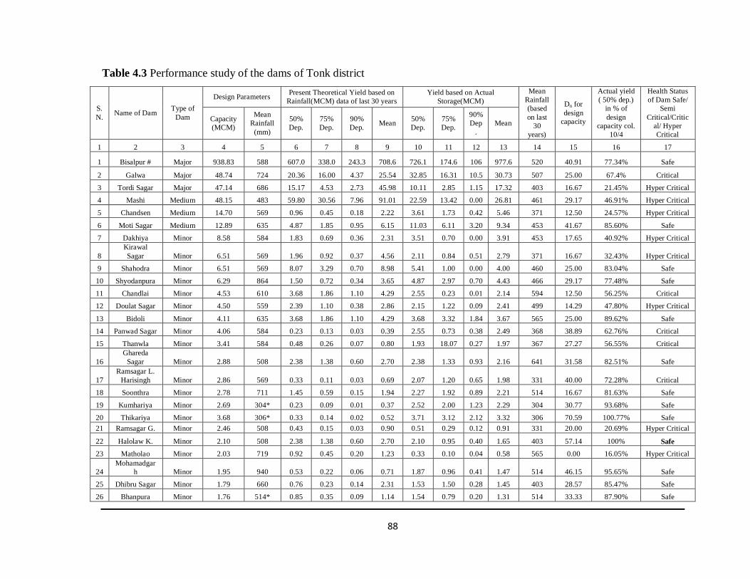
Study of Temporal Variation of Inflow to the Dams of Rajasthan State with Special Reference to Ramgarh and Bisalpur Dams.
88
Table 4.3 Performance study of the dams of Tonk district
S.
N. Name of Dam
Type of
Dam
Design Parameters Present Theoretical Yield based on
Rainfall(MCM) data of last 30 years
Yield based on Actual
Storage(MCM)
Mean
Rainfall
(based
on last
30
years)
Dn for
design
capacity
Actual yield
( 50% dep.)
in % of
design
capacity col.
10/4
Health Status
of Dam Safe/
Semi
Critical/Critic
al/ Hyper
Critical
Capacity
(MCM)
Mean
Rainfall
(mm)
50%
Dep.
75%
Dep.
90%
Dep. Mean
50%
Dep.
75%
Dep.
90%
Dep
.
Mean
1 2 3 4 5 6 7 8 9 10 11 12 13 14 15 16 17
1 Bisalpur # Major 938.83 588 607.0 338.0 243.3 708.6 726.1 174.6 106 977.6 520 40.91 77.34% Safe
2 Galwa Major 48.74 724 20.36 16.00 4.37 25.54 32.85 16.31 10.5 30.73 507 25.00 67.4% Critical
3 Tordi Sagar Major 47.14 686 15.17 4.53 2.73 45.98 10.11 2.85 1.15 17.32 403 16.67 21.45% Hyper Critical
4 Mashi Medium 48.15 483 59.80 30.56 7.96 91.01 22.59 13.42 0.00 26.81 461 29.17 46.91% Hyper Critical
5 Chandsen Medium 14.70 569 0.96 0.45 0.18 2.22 3.61 1.73 0.42 5.46 371 12.50 24.57% Hyper Critical
6 Moti Sagar Medium 12.89 635 4.87 1.85 0.95 6.15 11.03 6.11 3.20 9.34 453 41.67 85.60% Safe
7 Dakhiya Minor 8.58 584 1.83 0.69 0.36 2.31 3.51 0.70 0.00 3.91 453 17.65 40.92% Hyper Critical
8
Kirawal
Sagar Minor 6.51 569 1.96 0.92 0.37 4.56 2.11 0.84 0.51 2.79 371 16.67 32.43% Hyper Critical
9 Shahodra Minor 6.51 569 8.07 3.29 0.70 8.98 5.41 1.00 0.00 4.00 460 25.00 83.04% Safe
10 Shyodanpura Minor 6.29 864 1.50 0.72 0.34 3.65 4.87 2.97 0.70 4.43 466 29.17 77.48% Safe
11 Chandlai Minor 4.53 610 3.68 1.86 1.10 4.29 2.55 0.23 0.01 2.14 594 12.50 56.25% Critical
12 Doulat Sagar Minor 4.50 559 2.39 1.10 0.38 2.86 2.15 1.22 0.09 2.41 499 14.29 47.80% Hyper Critical
13 Bidoli Minor 4.11 635 3.68 1.86 1.10 4.29 3.68 3.32 1.84 3.67 565 25.00 89.62% Safe
14 Panwad Sagar Minor 4.06 584 0.23 0.13 0.03 0.39 2.55 0.73 0.38 2.49 368 38.89 62.76% Critical
15 Thanwla Minor 3.41 584 0.48 0.26 0.07 0.80 1.93 18.07 0.27 1.97 367 27.27 56.55% Critical
16
Ghareda
Sagar Minor 2.88 508 2.38 1.38 0.60 2.70 2.38 1.33 0.93 2.16 641 31.58 82.51% Safe
17
Ramsagar L.
Harisingh Minor 2.86 569 0.33 0.11 0.03 0.69 2.07 1.20 0.65 1.98 331 40.00 72.28% Critical
18 Soonthra Minor 2.78 711 1.45 0.59 0.15 1.94 2.27 1.92 0.89 2.21 514 16.67 81.63% Safe
19 Kumhariya Minor 2.69 304* 0.23 0.09 0.01 0.37 2.52 2.00 1.23 2.29 304 30.77 93.68% Safe
20 Thikariya Minor 3.68 306* 0.33 0.14 0.02 0.52 3.71 3.12 2.12 3.32 306 70.59 100.77% Safe
21 Ramsagar G. Minor 2.46 508 0.43 0.15 0.03 0.90 0.51 0.29 0.12 0.91 331 20.00 20.69% Hyper Critical
22 Halolaw K. Minor 2.10 508 2.38 1.38 0.60 2.70 2.10 0.95 0.40 1.65 403 57.14 100% Safe
23 Matholao Minor 2.03 719 0.92 0.45 0.20 1.23 0.33 0.10 0.04 0.58 565 0.00 16.05% Hyper Critical
24
Mohamadgar
h Minor 1.95 940 0.53 0.22 0.06 0.71 1.87 0.96 0.41 1.47 514 46.15 95.65% Safe
25 Dhibru Sagar Minor 1.79 660 0.76 0.23 0.14 2.31 1.53 1.50 0.28 1.45 403 28.57 85.47% Safe
26 Bhanpura Minor 1.76 514* 0.85 0.35 0.09 1.14 1.54 0.79 0.20 1.31 514 33.33 87.90% Safe

Study of Temporal Variation of Inflow to the Dams of Rajasthan State with Special Reference to Ramgarh and Bisalpur Dams.
89
27
Bhavalpur
Kerwaliya Minor 1.74 402* 0.36 0.11 0.06 0.52 1.54 1.09 0.48 1.45 403 25.00 88.53% Safe
28
Mansagar
Arnia Minor 1.64 584 0.35 0.19 0.05 0.59 1.64 1.30 0.18 1.34 367 64.71 100% Safe
29 Nasirda Minor 1.61 584 0.23 0.13 0.03 0.39 1.36 0.92 0.25 1.22 367 44.44 84.57% Safe
30 Duni Sagar Minor 1.42 584 0.68 0.41 0.34 0.74 0.65 0.48 0.06 0.77 576 20.00 46.00% Hyper Critical
31
Sangrampura
Newariya Minor 1.36 584 0.18 0.08 0.02 0.23 0.77 0.40 0.19 0.75 368 18.75 56.46% Critical
32 Dudi Sagar Minor 0.42 711 0.53 0.22 0.06 0.71 0.33 0.18 0.08 0.30 514 50.00 78.00% Safe
Safe: Actual yield (50% dep.) in % of design capacity: 75-100%= 17 dams
Critical: Actual yield (50% dep.) in % of design capacity: 50-74%= 6 dams
Hyper Critical: Actual yield (50% dep.) in % of design capacity: <50%= 9 dams
15 dams out of 32 dams of Tonk district fall under critical and hyper critical stage as per above mentioned interval
scale. We can say that around 50% of the dams may be considered safe, which are receiving more than 75% of their design
capacity at 50% dependability. Average observed rainfall in the district is less than the average design rainfall, which is one of
the reasons for less inflow.
Data are normalized with respect to design capacity of dams. RMSE and MAPE values are higher and R-values are
very low (<0.2), showing no correlation between computed and theoretical values (Table 4.4). Computed t-values are less than
critical t-value at 5% level of significance (2.07) i.e. accept null hypothesis (H0: R=0). NSE values are negative, showing that
average of the observed value is better predictor than the theoretical value. Simulation results are not in correlation with the
observed values.
Table 4.4 Performance statistics for the dams of Tonk district
Dependability RMSE MAPE (%) R T-Value NSE
50% 0.47 57.93 0.15 0.83 -2.40
75% 0.36 95.13 0.07 0.38 -1.13
90% 0.18 370.40 0.04 0.22 -0.64
Mean 0.49 63.66 0.03 0.16 -6.36

Study of Temporal Variation of Inflow to the Dams of Rajasthan State with Special Reference to Ramgarh and Bisalpur Dams.
90
4.3 Determination of Critical Year
Critical year separates the pre-disturbance and post-disturbance two non-overlapping
epochs. Determination of critical year is an essential requirement for investigation of
inflow behaviour of the dams.
4.3.1 Determination of Possible Critical Years: Time Series Analysis
In the first step of determination of critical year, possible critical years are identified.
Possible critical years have been identified with the help of time series analysis by trend
elimination using least square method as shown in Table 4.5.
The trend equation U = a + bt has been derived as
Inflow = (64.77) + (-0.27) x Time
Where U= Inflow, a = 64.77, b = -0.27 and t= time
Table 4.5 Time series analysis: Dams of Rajasthan state (Trend elimination using least
square method)
Year Inflow, U
(%) t tUi t*t Trend Elimination
of trend Possible critical
years
1990 71.01 -11 -781.11 121 67.72 3.28
1991 78.53 -10 -785.3 100 67.45 11.07
1992 66.16 -9 -595.44 81 67.18 -1.02 ***
1993 62.6 -8 -500.8 64 66.91 -4.31
1994 85.76 -7 -600.32 49 66.65 19.1 ***
1995 77.6 -6 -465.6 36 66.38 11.21
1996 76.7 -5 -383.5 25 66.11 10.58
1997 71.09 -4 -284.36 16 65.84 5.24
1998 57.78 -3 -173.34 9 65.57 -7.79
1999 43.58 -2 -87.16 4 65.3 -21.72
2000 42.03 -1 -42.03 1 65.04 -23.01
2001 58.4 0 0 0 64.77 -6.37 ***
2002 30.87 1 30.87 1 64.50 -33.63
2003 58.08 2 116.16 4 64.23 -6.15 ***
2004 71.01 3 213.03 9 63.96 7.04
2005 71 4 284 16 63.69 7.3
2006 83.58 5 417.9 25 63.43 20.14
2007 69.72 6 418.32 36 63.16 6.55 ***
2008 56.2 7 393.4 49 62.89 -6.69
2009 41.27 8 330.16 64 62.62 -21.35
2010 51.52 9 463.68 81 62.35 -10.83 ***
2011 73.35 10 733.5 100 62.09 11.25
2012 76.78 11 844.58 121 61.82 14.95
2013 76.71 12 920.52 144 61.55 15.15
Sum 1551.33 12 467.16 1156 1551.33

Study of Temporal Variation of Inflow to the Dams of Rajasthan State with Special Reference to Ramgarh and Bisalpur Dams.
91
Exceptional periods are marked ***, which are considered as possible critical years, when
drastic changes were observed. In this analysis year 1992, 1994, 2001, 2003, 2007, and
2010 are identified as possible years (Table 4.5).
4.3.2 Determination of Critical Years: Sequential Cluster Analysis
It is essential to determine the critical year, which divides two consecutive non-
overlapping epochs, pre-disturbance and post-disturbance. The final critical year can be
obtained by applying Sequential Cluster Analysis on the possible critical years which
have been identified in Table 4.5. The minimum sum of squared deviations for the
hydrological series before and after the possible critical years, gives the unique critical
year (Table 4.6). The method of computation has been described in section 3.3.5.
Table 4.6 Sequential cluster analysis: Dams of Rajasthan state
S.N. Year Inflow
(%)
Sequential Cluster Analysis
1992 1994 2001 2003 2007 2010
1 1990 71.0 0.8 3.2 26.1 65.7 32.6 62.5
2 1991 78.5 44.0 32.9 159.6 244.4 175.1 238.2
3 1992 66.2 32.9 44.1 0.1 10.6 0.7 9.4
4 1993 62.6 1.0 104.0 10.9 0.1 7.3 0.2
5 1994 85.8 491.1 168.0 394.5 522.7 418.7 513.6
6 1995 77.6 195.9 227.9 136.8 216.0 151.2 210.1
7 1996 76.7 171.5 201.6 116.6 190.4 129.9 184.9
8 1997 71.1 56.1 73.8 26.9 67.1 33.5 63.9
9 1998 57.8 33.9 22.3 66.0 26.2 56.6 28.3
10 1999 43.6 400.8 357.9 498.1 373.2 471.7 381.0
11 2000 42.0 465.4 419.1 569.9 435.7 541.6 444.1
12 2001 58.4 27.0 16.8 56.2 20.2 47.6 22.1
13 2002 30.9 1071 1000.3 1051.5 1025.8 1185.3 1038.6
14 2003 58.1 30.5 19.6 27.3 23.3 52.2 25.2
15 2004 71.0 54.9 72.4 59.4 15.3 32.6 62.6
16 2005 71.0 54.7 72.2 59.3 15.2 32.5 62.4
17 2006 83.6 399.4 444.5 411.4 271.7 334.3 419.6
18 2007 69.7 37.5 52.1 41.2 6.9 50.7 43.8
19 2008 56.2 54.7 39.7 50.4 118.7 40.9 47.6
20 2009 41.3 498.8 450.9 485.5 667.4 455.2 476.7
21 2010 51.5 145.9 120.6 138.8 242.7 122.8 134.1
22 2011 73.3 95.0 117.6 100.9 39.0 115.5 5.1
23 2012 76.8 173.6 203.8 181.6 93.6 201.0 1.4
24 2013 76.7 171.7 201.8 179.7 92.3 199.0 1.2
Sum
4708 4467 4849 4784 4888 4477
The minimum sum of squared deviations is correspond to the year 1994.
Therefore, the year 1994 is considered as the critical year for the hydrological behavior

Study of Temporal Variation of Inflow to the Dams of Rajasthan State with Special Reference to Ramgarh and Bisalpur Dams.
92
of the dams of Rajasthan state. This shows that, some disturbances have taken place after
1994 which is attributed to low inflow to the dams. Determination of critical year will
help in policy formulation for an effective water resources planning and management of
the state.
4.4 Various Parameters and their Trends
The declining trend of inflow to the dams of Rajasthan State has been tested. The critical
year of initiation of post-disturbance epoch is determined as 1994. Climate change and
global warming are posing a serious threat to the water resource availability. Climatic
parameters such as average daily minimum and maximum temperature, precipitation,
wind speed, relative humidity and solar radiation are studied and graphs are plotted to
determine the variation of these parameters with time (Fig. 4.4 and 4.5). Various
parameters which are considered responsible for surface runoff are to be analyzed and
discussed. Trends of various factors are plotted and shown in fig 4.4 to 4.11.
4.4.1 Rainfall and Other Climatic Parameters
Accurate and correct rainfall characterization is an important tool for water related system
design and management. Although the spatial distribution of the change in precipitation
character is uncertain, it would mean greater risk of both dry spells and floods for some
region even though annual precipitation totals may increase slightly (Dourte et al. 2012).
Temporal variation of average annual precipitation of the state for long time series (1901-
2013) is on slightly increasing trend (Fig. 4.4 a). The trend of rainy days for simulation
period (1990-2013) is also slightly increasing and plotted along with the rainfall trend in
Fig. 4.4 (b). It infers that rainy days and annual rainfall has a positive and good
correlation which is shown in Fig. 4.4 (c). For a constant amount of annual rainfall (e.g.
700-715mm), inflow has a negative correlation with rainy days (Fig. 4.4 d). This infers
that the annual rainfall spreads over more rainy days and gives lesser inflow and more
infiltration. Temporal distribution of monthly rainfall shows that rainy season remains
during only four months in a year i.e. June to September (Fig. 4.4 e). There is a spatial
distribution of average annual rainfall over the state ranging from 190mm in Jaisalmer to
1000mm in Banswara (Fig. 4.4 f) therefore, it becomes essential to judiciously plan and
manage the available water resources within the state. Rainfall distribution is following

Study of Temporal Variation of Inflow to the Dams of Rajasthan State with Special Reference to Ramgarh and Bisalpur Dams.
93
the Gaussian distribution. Highest frequency of annual rainfall of the state ranges between
500-600mm as shown in Fig. 4.5 (g). For constant amount of annual rainfall (e.g. 700-
715mm), inflow decreases with increase of rainydays.
(a) Rainfall trend (1901-2013)
(b) Rainfall and rainy days trend (1990-2013)
0
200
400
600
800
1000
1200
1900 1920 1940 1960 1980 2000 2020
Rain
fall
(m
m)
Rainfall trend (1901-2013)
10
20
30
40
50
60
70
80
90
100
0
100
200
300
400
500
600
700
800
900
1985 1990 1995 2000 2005 2010 2015
Ra
iny
da
ys
(nos.
)
Ra
infa
ll (
mm
)
Rainfall and rainy days trend (1990-2013)
Rainfall trend Rainy days Linear (Rainfall trend) Linear (Rainy days)

Study of Temporal Variation of Inflow to the Dams of Rajasthan State with Special Reference to Ramgarh and Bisalpur Dams.
94
(c) Rainy days and rainfall
(d) Rainy days and inflow at constant rainfall
(e) Monthly rainfall distribution
R² = 0.5693
0
200
400
600
800
1000
0 10 20 30 40 50 60
Rain
fall
(m
m)
Rainydays (nos.)
Rainy days and rainfall
Rainy days and rainfall Linear (Rainy days and rainfall)
R² = 0.361
30
40
50
60
70
80
90
100
20 30 40 50 60
Infl
ow
(%)
Rainy days (nos.)
Rainydays-Inflow at constant annual rainfall (700-715mm)
Rainydays-Inflow at Constant rainfall
Linear (Rainydays-Inflow at Constant rainfall)
0
50
100
150
200
250
JAN
FE
B
MA
R
AP
R
MA
Y
JUN
JUL
AU
G
SE
PT
OC
T
NO
V
DE
C
Rain
fall
(m
m)
Month
Monthly rainfall distribution of Rajasthan state

Study of Temporal Variation of Inflow to the Dams of Rajasthan State with Special Reference to Ramgarh and Bisalpur Dams.
95
(f) District wise average annual rainfall
(g) Frequency distribution of rainfall
Fig. 4.4 Rainfall trend and its distribution (Rajasthan)
The Rainfall trend of the state varies significantly over the years and during the
year, showing the temporal variation of rainfall. It also varies significantly between
various districts, showing the spatial variation of rainfall (Fig. 4.4). We proposed one
way ANOVA to study the impact of districts and year on the annual rainfall. Table (a)
shows that impact of year on annual rainfall was highly significant (p value <0.01),
calculated value of F= 7.705 >F (tabulated) at df= 111, 3341 at 1% level of significance.
Table (b) shows that impact of districts on annual rainfall was also significant (p value <
0.01) and calculated value of F=95.136 >F (tabulated) at df= 32, 3420 at 1% level of
significance.
0
200
400
600
800
1000
1200
Rain
fall
(m
m)
District
District wise average annual rainfall
05
10152025303540
10
0-2
00
20
0-3
00
30
0-4
00
40
0-5
00
50
0-6
00
60
0-7
00
70
0-8
00
80
0-9
00
90
0-1
00
0
10
00-1
10
0
Freq
uen
ty
Rainfall (mm)
Frequency distribution of rainfall over 113 years (1901-2013)

Study of Temporal Variation of Inflow to the Dams of Rajasthan State with Special Reference to Ramgarh and Bisalpur Dams.
96
Table (a) One way ANOVA using year as factor
Sum of Squares df Mean square F Significance
Between Groups 68690485 111 618833.198 7.705 0.000
Within Groups 2.68E+08 3341 80314.481
Total 3.37E+08 3452
Table (b) One way ANOVA using district as factor
Sum of Squares df Mean square F Significance
Between Groups 1.59E+08 32 4959945.535 95.136 0.000
Within Groups 1.78E+08 3420 52135.353
Total 3.37E+08 3452
The impact of global climate change is making the precipitation of rainfall pattern
quite uncertain (Kar 2011). Climate change challenges existing water resources
management practices by adding uncertainty (Draper and Kundell 2007).
Intergovernmental Panel on Climate Change (IPCC 2001) as described by Iglesias et al.
2007 states that climate change projections derived from global climate models driven by
socio-economic scenario results in an increase in temperature of 1.5 to 3.6oC and a
precipitation decrease of about 10 to 20% by 2050. This may lead to increased likelihood
of droughts and variability of precipitation in time-space, and intensity. That would
directly influence water resources availability. As described above the importance of
climatic parameters; trends of daily max. and min. temperature, wind speed, relative
humidity and solar radiation have been plotted in Fig. 4.5.

Study of Temporal Variation of Inflow to the Dams of Rajasthan State with Special Reference to Ramgarh and Bisalpur Dams.
97
(a) Mean daily max. temp. (b) Mean of daily min. temp.
(c) Wind speed (d) Relative Humidity
(e) Solar radiation
Fig. 4.5 Trends of other climatic factors (Rajasthan)
31
32
33
34
35
36
1980 1990 2000 2010 2020
Tem
p. (
0 C)
Mean of daily max. temp.
17
18
19
20
21
1980 1990 2000 2010 2020
Tem
p. (
0 C)
Mean of daily min. temp.
0.00
0.50
1.00
1.50
2.00
2.50
3.00
3.50
1980 1990 2000 2010 2020
Win
d s
peed
(m
/sec)
Mean of daily Wind speed
trend
0.30
0.35
0.40
0.45
0.50
0.55
0.60
1980 1990 2000 2010 2020
RH
(fr
acti
on
)
Mean of daily RH trend
18
19
19
20
20
21
1980 1990 2000 2010 2020
Sola
r ra
dia
tio
n (M
J/m
2)
Mean of daily solar radiation
trend

Study of Temporal Variation of Inflow to the Dams of Rajasthan State with Special Reference to Ramgarh and Bisalpur Dams.
98
There is an increasing trend of the mean of daily maximum temperature, daily
relative humidity, and daily solar radiation while a slightly decreasing trend of the mean
of daily minimum temperature and daily wind speed. Increased daily maximum
temperature and solar radiation cause evaporation of soil moisture thereby may cause
increased infiltration and reduced inflow. Trends and rate of changes of various climatic
parameters are listed in Table 4.8.
4.4.2 Land Use Land Cover Changes
Land use data from 1957-2013 have been plotted in Fig. 4.6. A comparison has been
made in Fig. 4.6 and 4.7 that contributing area is decreasing while crop area is increasing.
This infers that the increasing crop area results in decreasing contributing area for runoff,
thereby less water inflow to the dams. Land holding data have been presented for the
available duration. Data of all the factors related to the study of the state are presented
from 1990 to 2013 as per the availability of the data of all the factors.
Fig. 4.6 Land use (Contributing effect): Rajasthan
The mean of daily data has been analyzed for the sake of getting the trends of climatic
parameters and further correlating them with the inflow. A detailed analysis of land use
changes has been presented for Rajasthan state for the data available from the year 1957
onwards (Fig. 4.7).
0
10
20
30
40
50
60
1957
1962
1967
1972
1977
1982
1987
1992
1997
2002
2007
2013
Area
(%
)
Land use trend (Contributing effect)

Study of Temporal Variation of Inflow to the Dams of Rajasthan State with Special Reference to Ramgarh and Bisalpur Dams.
99
(a)
(b)
(c)
0
50
100
150
200
250
300
1957
1962
1967
1972
1977
1982
1987
1992
1997
2002
2007
2013
Area (
000 s
qk
m)
Area sown (Rajasthan state)
Area sown more than onceNet area sown
0%
20%
40%
60%
80%
100%
1957 1962 1967 1972 1977 1982 1987 1992 1997 2002 2007 2013
Area
(%
)
Land use changes (Rajasthan State)
Barren land Culturable waste Fallow land Non Ag. uses Forest and pasture Net area sown
0
50
100
150
200
250
300
1957
1962
1967
1972
1977
1982
1987
1992
1997
2002
2007
2013
Area
(0
00 s
qk
m)
Contributing area-reducing area (Rajasthan state) Contributing area
Reducing area
Linear (Contributing area)
Linear (Reducing area)

Study of Temporal Variation of Inflow to the Dams of Rajasthan State with Special Reference to Ramgarh and Bisalpur Dams.
100
(d)
(e)
(f)
Fig. 4.7 Land use changes (1957-2013): Rajasthan
Agricultural area is increasing with time and population. It has increased from
124, 000 sqkm to 180,000 sqkm from 1957 to 2013. The area sown more than once is also
increasing; it has increased from around 10,000 sqkm to 65,000 sqkm (Fig. 4.7 a).
Irrigation area increased from around 20,000 sqkm to 63,000 sqkm from 1968 to 2006.
1.00
3.00
5.00
7.00
2.00
3.00
4.00
5.00
6.00
1965 1970 1975 1980 1985 1990 1995 2000 2005 2010
mil
lion
Average l
an
d h
old
ing (
ha
)
Average field size and number of fields:
Rajasthan state
Average field sizeNumber of fields
0%
20%
40%
60%
80%
100%
1970 1975 1980 1985 1990 1995 2000 2005
Area
(%
)
Land holdings (Area %):
Rajasthan State
Large fieldsMedium fieldsSemi-medium fieldsSmall fieldsMarginal fields
0.00
2.00
4.00
6.00
8.00
1970 1975 1980 1985 1990 1995 2000 2005
mil
lion
Land holdings (million):
Rajasthan State
Large fields >10 hect.Medium fields 4-10 hect.Semi-medium 2-4 hect.Small fields 1-2 hect.Marginal fields <1.0 hect.
Study of Temporal Variation of Inflow to the Dams of Rajasthan State with Special Reference to Ramgarh and Bisalpur Dams.
101
The contribution of groundwater irrigation to the total irrigated area was around 10,000
sqkm in 1968 and 45,000 sqkm in 2006 (Fig. 4.8 a). With the development of electrical
facilities, irrigation from tube wells increased from 120 sqkm in 1968 to 19,000 sqkm in
2006 (Fig. 4.8 b). Due to this tremendous increase in agricultural areas, land use pattern
changed at a very fast pace. The increase in groundwater irrigation facilities resulted in
lowering of water table and increase in dark zones within the state.
Land utilization of the state is plotted in graphs as shown in Fig. 4.6 & 4.7 shows
that the land utilizations which are having reducing effect on the surface runoff viz.
agricultural, forest and infrastructural uses are increasing and the land utilization which is
having a contributing effect on the surface runoff viz. barren land, culturable waste, and
fallow land are decreasing with the passage of time (Fig. 4.7 b). The area which is having
contributing effect on surface runoff has decreased to half of the area which was available
in 1957 (Fig. 4.7 c). These types of land use changes, viz. agricultural, forest and
infrastructural uses of land increase the surface roughness, are not favorable to the surface
runoff. The total cropped area has increased from 137 (000 sqkm) to 245 (000 sqkm)
during 1957 to 2012. The double crop area has increased from 12.86 (000 sqkm) to 64.71
(000 sqkm) during this period.
Due to continuous partitions of the fields, the average size of the field is
decreasing, and the total number of fields is increasing with time. The average size of the
land holding has decreased from 5.46 ha to 3.38 ha from 1970 to 2005, and a total number
of fields has increased from 3.7 million to 6.2 million during this period (Fig. 4.7 d). The
percentage area of large fields is decreasing while under marginal, small and semi-
medium category it is increasing. Accordingly the number of land holdings under
marginal, small and semi-medium category is increasing (Fig. 4.7 e,f). This reflects that
total number of fields are increasing because of partitions of large fields, thereby more
length of periphery boundaries increasing the surface roughness and decreasing the
resultant runoff to the reservoir.
4.4.3 Groundwater Level Changes
Agricultural area of the state is increasing due to increase in irrigation facilities. Irrigation
by ground water sources increased at a fast pace than surface water sources (Fig. 4.8 a).
Underground water sources such as wells and tube wells increased due to the

Study of Temporal Variation of Inflow to the Dams of Rajasthan State with Special Reference to Ramgarh and Bisalpur Dams.
102
development of digging and boring system along with rapid electrification (Fig. 4.8 b),
resulting in overexploitation of ground water.
(a) Sources of irrigation
(b) Various sources of irrigation
Fig. 4.8 Development of agricultural and irrigation facilities in Rajasthan
Over-exploitation of groundwater has resulted in lowering of ground water level
below ground level. Fluctuations of basin wise ground water level below ground level are
shown in Fig. 4.9 (a). Groundwater level changes in the state are shown in Fig. 4.9 (b).
0.00
10.00
20.00
30.00
40.00
50.00
60.00
70.00
1968
1970
1972
1974
1976
1978
1980
1982
1984
1986
1988
1990
1992
1994
1996
1998
2000
2002
2004
2006
Irrig
ati
on
('0
00 S
q.k
m)
Surface water and ground water irrigation
Irrigation by surface water sources Irrigation by ground water sources Total Irrigation
0.00
10.00
20.00
30.00
40.00
50.00
60.00
70.00
19
68
19
70
19
72
1974
19
76
19
78
19
80
19
82
19
84
19
86
19
88
19
90
19
92
19
94
1996
19
98
20
00
20
02
20
04
20
06
Irrig
ati
on
Area
('0
00
Sq
.km
)
Development of various sources of irrigation
WellsTube WellsCanalsOther SourcesTanks

Study of Temporal Variation of Inflow to the Dams of Rajasthan State with Special Reference to Ramgarh and Bisalpur Dams.
103
(b) Basin wise GWL below GL
(b) Rajasthan
Fig. 4.9 Groundwater level changes: Rajasthan
0
5
10
15
20
25
30
35
40
45
50
Pre
2013
Pre
2012
Pre
2011
Pre
2010
Pre
2009
Pre
2008
Pre
2007
Pre
2006
Pre
2005
Pre
2004
Pre
2003
Pre
2002
Pre
2001
Pre
2000
Pre
19
99
Pre
1998
Pre
1997
Pre
19
96
Pre
1995
Pre
1994
Pre
19
93
Pre
1992
Pre
1991
Pre
1990
Pre
1989
Pre
1988
Pre
1987
Pre
1986
Pre
1985
Pre
1984
GW
L b
elo
w G
L (
m)
Shekhawati basin Ruparail basin Banganga basinGambhir basin parbati basin Sabi basinBanas basin Chambal basin Mahi basinSabarmati basin Luni basin West banas basinSukli basin Other nallah of Jalore Outside basin
10.0
12.0
14.0
16.0
18.0
20.0
22.0
24.0
26.0
19
84
19
85
19
86
19
87
19
88
19
89
19
90
19
91
19
92
1993
19
94
19
95
19
96
19
97
19
98
19
99
20
00
20
01
2002
20
03
20
04
20
05
20
06
20
07
20
08
20
09
20
10
2011
2012
20
13
GW
L b
elo
w G
L (
m)
Temporal variation of GWL below GL (Rajasthan state)
Pre-monsoon GWL Post-monsson GWL
Linear (Pre-monsoon GWL) Linear (Post-monsson GWL)

Study of Temporal Variation of Inflow to the Dams of Rajasthan State with Special Reference to Ramgarh and Bisalpur Dams.
104
Basin wise fluctuations of ground water level below ground level shows that
Shekhawati basin is adversely affected by ground water withdrawal and showing the
deepest ground water level below ground level. A major part of Sikar and Jhunjhunu
districts lie in the Shekhawati basin. Water inflows to the dams of these districts are also
negligible. Looking to these adverse situations, it is planned to provide water for drinking,
irrigation and other necessary requirements from Yamuna water through the
transboundary management of surplus water through an interstate agreement between
Rajasthan and Haryana. Sikar district has also been covered in Model District Irrigation
Plan under Pradhan Mantri Krishi Sinchai Yojna (PMKSY). In the first phase, water is to
be received through Yamuna water agreement and in successive phases it is to be
received from Sharda-Yamuna Link. Major parts of Barmer, Churu, Ganganagar,
Hanumangarh, Jaisalmer, Jodhpur and Nagaur districts are falling under Outside Basin.
Though groundwater level below ground level in this basin is very low but it is not going
further low at accelerating rate as part of the basin is under Gang Canal and Indira Gandhi
Canal system.
Development of lift facilities through pump sets resulted in a tremendous increase
in irrigation from groundwater using wells and tube wells (Fig. 4.8 b). Overexploitation
of groundwater has resulted in only 25 blocks out of total 243 in the safe category in the
year 2011, which were 135 in the year 1998 (Table 4.7, Fig. 4.10). Tara Nagar of Churu
district and Khajuwala of Bikaner district have been declared as total saline blocks;
therefore, they have not been assessed by Central Ground Water Board (CGWB 2014).
Declining water table reduces runoff due to base flow and hence the inflow to the wetland
(Jain et al. 2008). Over exploitation of surface water results in many rivers dying, and
outflow amount decreasing drastically, and overexploitation of groundwater has also
induced the groundwater level to go down continuously and form several underground
funnels. Over-exploitation of water has greatly changed the transfers among precipitation,
surface water, soil water, and groundwater. As is seen in Hai He basin, the river is dying,
and funneled groundwater is increasing, and this once natural water cycle has evolved
into a semiartificial water cycle (Sang et al. 2010). Losses due to evaporation and water
withdrawal reduce the runoff towards the mouth by a factor 2.3. The runoff changes as
large as these are due to the increasing water withdrawal for irrigation (Kravtsova et al.

Study of Temporal Variation of Inflow to the Dams of Rajasthan State with Special Reference to Ramgarh and Bisalpur Dams.
105
2009). It has been observed during the last five decade that, percentage groundwater
utilizations have almost doubled, and the surface water utilization has increased
manifold, causing a decline in the water table. The declining water table reduces
runoff due to baseflow and hence the inflow to the wetland (Jain et al. 2008). In
Rajasthan state also, over-exploitation of water has greatly changed the transfers among
precipitation, surface water, soil water, and groundwater. The rivers are dying and
funneled ground water is increasing leading to the diminishing base flow and decreasing
surface runoff.
Table 4.7 Scenario of Groundwater Development: Rajasthan Year Over-exploited blocks
(>100%) Critical blocks (90%-100%)
Semi-critical blocks (70%-90%)
Safe blocks (<70%)
1998 41 26 34 135
2004 102 82 27 25
2009 166 25 16 31
2011 172 24 20 25
Graphical presentation of Table 4.7 is shown in Fig. 4.10 in the form of stacked
bar chart. This shows that about 70% of the blocks of the state are over-exploited while
safe blocks are only around 10%.
Fig. 4.10 Scenario of groundwater development: Rajasthan
0
50
100
150
200
250
1998 2004 2009 2011
No.
of
blo
ck
s
Ground water scenario of the state
Safe block
Semi critical
Critical
Overexploited

Study of Temporal Variation of Inflow to the Dams of Rajasthan State with Special Reference to Ramgarh and Bisalpur Dams.
106
Grond water development <70% may be considered as safe, 70% to 90% may be
considered as semi-critical, 90% to 100% may be considered as critical, and >100% is
considered as overexploited. Groundwater development is regularly increasing due to less
water availability in surface water resources. Districtwise groundwater development is
shown in appendix-10. Only 3 districts in safe, 2 districts in semi-critical, 2 districts in
critical and rest 27 districts lies under overexploited categories out of a total of 33
districts in the state. In whole, the complete state may be considered as overexploited.
Overall stage of groundwater development of the state is around 137% (CGWB 2014).
4.4.4 Population Growth and Trends
Land use and cultivation area are influenced by the population growth. The state
population is regularly increasing. However it is a good sign that decadal growth rate of
population is on decreasing trend after the year 1981 (Fig. 4.11 a). Country population
and its decadal growth rate are also on the same trend (Fig. 4.11 b). The percentage share
of the state population in country population is on increasing trend (Fig. 4.11 c).
(a) State population and its growth
10
.3
11
.0
10
.3
11
.7
13
.9
16
.0
20
.2
25
.8
34
.3 44
.0 56
.5 68
.6
-10.0
-5.0
0.0
5.0
10.0
15.0
20.0
25.0
30.0
35.0
0.0
20.0
40.0
60.0
80.0
100.0
120.0
140.0
1901
1911
1921
1931
1941
1951
1961
1971
1981
1991
2001
2011
2021
2031
2041
2051
Deca
da
l g
row
th r
ate
%
Mil
lion
s
Population of the State and Decadal growth rate %
Population
Decadal growth %
Poly. (Population)
Poly. (Decadal growth %)

Study of Temporal Variation of Inflow to the Dams of Rajasthan State with Special Reference to Ramgarh and Bisalpur Dams.
107
(b) Country population and its growth
(c) State population share with India
(d) Per capita water availability in the state
Fig. 4.11 Population and its growth: Rajasthan
-5.0
0.0
5.0
10.0
15.0
20.0
25.0
30.0
0.0200.0400.0600.0800.0
1000.01200.01400.01600.01800.02000.02200.02400.0
1901
1911
1921
1931
1941
1951
1961
1971
1981
1991
2001
2011
2021
2031
2041
2051
Deca
da
l g
row
th r
ate
%
Mil
lion
s
Population of India and Decadal growth rate % Population
Decadal growth %
Poly. (Population)
Poly. (Decadal growth %)
y = 0.0002x2 - 0.5937x + 572.47
3.0
3.5
4.0
4.5
5.0
5.5
6.0
6.5
19
01
19
11
1921
19
31
1941
19
51
19
61
19
71
19
81
19
91
20
01
20
11
20
21
2031
20
41
2051
% S
ha
re
State Population: % share in India
% share in IndiaPoly. (% share in India)
0200400600800
1000120014001600180020002200240026002800
19
11 -
1920
1921 -
1930
1931 -
1940
1941 -
1950
1951 -
1960
1961 -
1970
1971 -
1980
19
81 -
1990
1991 -
2000
2001 -
2010
Cu
m/y
ear
Per capita water availability
Per capita water availability
Water scarcity level
Absolute water scarcity level
Linear (Per capita water availability)

Study of Temporal Variation of Inflow to the Dams of Rajasthan State with Special Reference to Ramgarh and Bisalpur Dams.
108
Fig. 4.11 (‘c) shows that the impact of population growth on natural resources will
be more severe than the average condition of the country. This impact on water resources
availability will be more severe in future because per capita water availability in the state
has gone down below the level of water scarcity (1000 cum per capita per year) and it is
touching to the level of absolute water scarcity (500 cum per capita per year) (Fig. 4.11
d). There is an alarm to adopt most efficient practices of water resources planning and
management in the state. Han et al. (2012) also mention that available water resources per
capita are decreasing in river basins around the world.
4.4.5 Various Factors, Trend Lines and their Rate of Changes
Trend lines showed in Fig. 4.4 to 4.11give an idea about the various factors, whether they
are on increasing or decreasing trend and at what rate. The results are summarized in
Table 4.8.
Table 4.8 Various factors, trend lines and their rate of change
S.N. Factor Trend Rate of Change
1 Rainfall 1901-2013 (mm) Increasing 10 mm in 25 yrs.
2 Rainfall 1990-2013 (mm) Increasing 10mm in 22 yrs.
3 Rainy days/ year 1990-2013 (nos.) Increasing 1 day in 6 yrs.
4 Mean of daily max. temp. (0C) Increasing 1 deg. in 500 yrs.
5 Mean of daily min. temp. (0C) Decreasing 1 deg. in 77 yrs.
6 Mean of daily wind speed (m/sec) Decreasing 1 m/sec in 143 yrs.
7 Mean of daily RH (fraction) Constant NA
8 Mean of daily solar radiation (MJ/m2) Increasing 1MJ/m2 in 40 yrs.
9 Land use (Contributing effect) (%) Decreasing 1% in 3 yrs.
10 Cultivation area (%) Increasing 1.37% in 2 yrs.
11 Groundwater level below ground level (m) Increasing 1m in 6 yrs.
12 State population (million) Increasing 80 million in 2021
13 State population decadal growth Decreasing 15-20% in 2021
14 Country population Increasing 1400 million in 2021
15 Country population decadal growth Decreasing 15% in 2021
16 State population share with country Increasing 6.2% in 2021

Study of Temporal Variation of Inflow to the Dams of Rajasthan State with Special Reference to Ramgarh and Bisalpur Dams.
109
Rainfall and rainy days during 1990-2013 are on increasing trends (Fig. 4.4 b).
Rainy days have positive correlations with annual rainfall and inflow if plotted
independently (Fig. 4.4 c and 4.12 b). A graph between rainy days and inflow for the
nearly constant amount of annual rainfall (700-710mm) has been plotted in Fig. 4.4 (d).
This shows a decreasing trend of inflow with increasing rainy days for a constant rainfall.
This infers that precipitations are shifting towards fewer common higher intensity storms
and more light and moderate events resulting in lesser runoff. This pattern shows that
nearly constant amount of monsoon rainfall is spreading over the longer time
duration than earlier, which may result in reduced percentage inflow.
Land use having a contributing effect is on decreasing trend. Cultivation area,
state population, state population share with the country, and groundwater level below
ground level is on increasing trend. A stable tendency towards a decrease in water
resources can be seen in recent decades, which is largely due to the intense economic
activities on watersheds (Shiklomanov et al. 2011). Irrigation systems, three dams and
seven ponds built recent decades for agricultural irrigation and domestic use made the
major impact on lowering the lake levels because they derive water from the river for
human use upstream of the lake’s catchments. Population growth, rising water
consumption for agricultural and domestic purposes and building dams has led to lake
levels declining. The change of lake levels might depend more on anthropogenic factors
than on climate factors (Yildirim et al. 2011).
4.4.6 Correlation Matrix: Rajasthan
A 14x14 correlation matrix has been developed. Mutual correlations of most of the
factors are insignificant, being quite low. But, some factors have significant mutual
correlations. Significant correlations at 2-tailed test at 1% and 5% level of significance
has been shown by * and **. However, the matrix has been derived to show the mutual
correlations of all the factors with each other (Table 4.9), for the sake of mutual
dependence. This matrix can be utilized for determining the sensitivity of each parameter
with other remaining parameters.

Study of Temporal Variation of Inflow to the Dams of Rajasthan State with Special Reference to Ramgarh and Bisalpur Dams.
110
Correlations
1.000 -.130 -.480* .999** .915** -.059 .114 .020 -.165 -.404 .125 .584** .366 .824**
. .545 .018 .000 .000 .786 .596 .926 .442 .050 .559 .003 .079 .000
24 24 24 24 24 24 24 24 24 24 24 24 24 24
-.130 1.000 -.097 -.108 -.264 .685** .326 -.738** -.518** -.696** .577** -.502* .129 -.106
.545 . .651 .614 .213 .000 .120 .000 .009 .000 .003 .013 .547 .621
24 24 24 24 24 24 24 24 24 24 24 24 24 24
-.480* -.097 1.000 -.493* -.385 -.049 .048 .157 .013 .388 -.242 -.193 -.991** -.734**
.018 .651 . .014 .063 .819 .823 .464 .952 .061 .255 .367 .000 .000
24 24 24 24 24 24 24 24 24 24 24 24 24 24
.999** -.108 -.493* 1.000 .906** -.040 .132 -.009 -.176 -.424* .154 .571** .380 .830**
.000 .614 .014 . .000 .854 .539 .968 .411 .039 .473 .004 .067 .000
24 24 24 24 24 24 24 24 24 24 24 24 24 24
.915** -.264 -.385 .906** 1.000 -.250 -.003 .178 -.180 -.244 -.082 .701** .281 .751**
.000 .213 .063 .000 . .239 .990 .406 .401 .252 .704 .000 .184 .000
24 24 24 24 24 24 24 24 24 24 24 24 24 24
-.059 .685** -.049 -.040 -.250 1.000 .715** -.746** -.272 -.511* .800** -.549** .071 .060
.786 .000 .819 .854 .239 . .000 .000 .199 .011 .000 .005 .742 .781
24 24 24 24 24 24 24 24 24 24 24 24 24 24
.114 .326 .048 .132 -.003 .715** 1.000 -.742** -.375 -.370 .810** -.274 -.060 .139
.596 .120 .823 .539 .990 .000 . .000 .071 .075 .000 .196 .782 .518
24 24 24 24 24 24 24 24 24 24 24 24 24 24
.020 -.738** .157 -.009 .178 -.746** -.742** 1.000 .650** .591** -.900** .498* -.177 -.059
.926 .000 .464 .968 .406 .000 .000 . .001 .002 .000 .013 .408 .783
24 24 24 24 24 24 24 24 24 24 24 24 24 24
-.165 -.518** .013 -.176 -.180 -.272 -.375 .650** 1.000 .521** -.336 -.001 -.001 .001
.442 .009 .952 .411 .401 .199 .071 .001 . .009 .108 .996 .996 .996
24 24 24 24 24 24 24 24 24 24 24 24 24 24
-.404 -.696** .388 -.424* -.244 -.511* -.370 .591** .521** 1.000 -.545** .011 -.358 -.419*
.050 .000 .061 .039 .252 .011 .075 .002 .009 . .006 .959 .086 .041
24 24 24 24 24 24 24 24 24 24 24 24 24 24
.125 .577** -.242 .154 -.082 .800** .810** -.900** -.336 -.545** 1.000 -.444* .245 .286
.559 .003 .255 .473 .704 .000 .000 .000 .108 .006 . .030 .249 .176
24 24 24 24 24 24 24 24 24 24 24 24 24 24
.584** -.502* -.193 .571** .701** -.549** -.274 .498* -.001 .011 -.444* 1.000 .124 .503*
.003 .013 .367 .004 .000 .005 .196 .013 .996 .959 .030 . .562 .012
24 24 24 24 24 24 24 24 24 24 24 24 24 24
.366 .129 -.991** .380 .281 .071 -.060 -.177 -.001 -.358 .245 .124 1.000 .665**
.079 .547 .000 .067 .184 .742 .782 .408 .996 .086 .249 .562 . .000
24 24 24 24 24 24 24 24 24 24 24 24 24 24
.824** -.106 -.734** .830** .751** .060 .139 -.059 .001 -.419* .286 .503* .665** 1.000
.000 .621 .000 .000 .000 .781 .518 .783 .996 .041 .176 .012 .000 .
24 24 24 24 24 24 24 24 24 24 24 24 24 24
Pearson Correlation
Sig. (2-tailed)
N
Pearson Correlation
Sig. (2-tailed)
N
Pearson Correlation
Sig. (2-tailed)
N
Pearson Correlation
Sig. (2-tailed)
N
Pearson Correlation
Sig. (2-tailed)
N
Pearson Correlation
Sig. (2-tailed)
N
Pearson Correlation
Sig. (2-tailed)
N
Pearson Correlation
Sig. (2-tailed)
N
Pearson Correlation
Sig. (2-tailed)
N
Pearson Correlation
Sig. (2-tailed)
N
Pearson Correlation
Sig. (2-tailed)
N
Pearson Correlation
Sig. (2-tailed)
N
Pearson Correlation
Sig. (2-tailed)
N
Pearson Correlation
Sig. (2-tailed)
N
YEAR
INFLOW
LULC
POPDEN
WTRTBL
RAINFALL
RDAYS
MAXTMP
MINTMP
WINDSPD
RELHUM
SOLAR
NA
ASMO
YEAR INFLOW LULC POPDEN WTRTBL RAINFALL RDAYS MAXTMP MINTMP WINDSPD RELHUM SOLAR NA ASMO
Correlation is signif icant at the 0.05 level (2-tailed).*.
Correlation is signif icant at the 0.01 level (2-tailed).**.
Table 4.9 Correlation Matrix: Rajasthan

Study of Temporal Variation of Inflow to the Dams of Rajasthan State with Special Reference to Ramgarh and Bisalpur Dams.
111
4.5 Determination of Principal Components
Correlations of various components with inflow have been established after drawing the
trend line and regression equation.
4.5.1 Regression Analysis
To reduce the dimensionality of the proposed equation, linear regression analyses of
inflow (%) with various factors have been carried out independently, as shown in fig 4.12
and summarized in Table 4.10.
(a) Rainfall (b) Rainy days
(c) Land use (d) GWL Below GL
y = 0.0843x + 14.115
R² = 0.5056
0102030405060708090
100
0 500 1000
Infl
ow
(%
)
Rainfall (mm)
Rainfall-Inflow
y = 0.4284x + 50.21
R² = 0.1095
0102030405060708090
100
0 20 40 60
Infl
ow
(%
)
Rainy days
Rainy days-Inflow
y = -0.277x + 74.04
R² = 0.00
0102030405060708090
100
20 25 30 35 40 45 50 55
Infl
ow
(%
)
Contributing land use (%)
Land use-Inlfow
y = -0.574x + 76.92
R² = 0.00
0102030405060708090
100
15 20 25 30
Infl
ow
(%
)
GWL BGL (m)
GWL BWL-Inflow regression

Study of Temporal Variation of Inflow to the Dams of Rajasthan State with Special Reference to Ramgarh and Bisalpur Dams.
112
(e) Mean daily max. Temp. (f)Mean daily min. temp.
(g) Wind speed (h) Relative humidity
(i) Solar radiation (j) Population density
y = -11.532x + 453.5
R² = 0.5426 0
20
40
60
80
100
31.00 32.00 33.00 34.00 35.00 36.00
Infl
ow
(%
)
Mean of daily max. temp. (0C)
Mean daily max. temp.-Inflow
y = -13.501x + 320.45 R² = 0.2666
0
20
40
60
80
100
17 18 19 20 21
Infl
ow
(%
)
Mean of daily min. temp. (0C)
Mean daily min. temp.-Inflow
y = -73.989x + 277.45
R² = 0.4864 0
20
40
60
80
100
2.5 3.0 3.5
Infl
ow
(%
)
Wind speed (m/sec)
Wind speed-Inflow
y = 215.39x - 19.437
R² = 0.3485
0
20
40
60
80
100
0.30 0.35 0.40 0.45 0.50
Infl
ow
(%
)
Relative humidity
Relative humidity-Inflow
y = -14.982x + 352.86
R² = 0.2525 0
20
40
60
80
100
18.00 18.50 19.00 19.50 20.00 20.50
Infl
ow
(%
)
Mean of solar radiation (MJ/m2)
Mean daily solar radiation-
Inflow
y = -0.0582x + 74.448
R² = 0.012 0
20
40
60
80
100
100 150 200 250
Infl
ow
(%
)
Population density
Population density-Inflow

Study of Temporal Variation of Inflow to the Dams of Rajasthan State with Special Reference to Ramgarh and Bisalpur Dams.
113
(k) Gross inflow-rainfall
Fig. 4.12 Cross plots: Between inflows and independent variables: Rajasthan
Several cross plots showing the relationship between independent variables and
inflows have been generated to develop empirical relations for the indirect estimation of
the output. These relations are obtained using statistical methods such as regression
analysis. However, although empirical equations are cost- effective and not too time-
consuming, they include uncertainties relating to the limited data available (Majdi et al.
2010). To determine the parameters affecting the inflow more than others, several cross
plots showing the relationship between independent variables and inflows (%) have been
generated for a total of 24 datasets (Fig. 4.12 a to J and Table 4.10). A regression plot
between gross inflow and rainfall has been developed in Fig. 4.12 (k) which shows a
highly significant correlation with t-value of 3.33 but less than the t-value of inflow (%)
and rainfall.
y = 7.8494x + 2192.6
R² = 0.3359
0
2000
4000
6000
8000
10000
12000
0 200 400 600 800 1000
Gross
In
flow
(M
CM
)
Rainfall (mm)
Rainfall-Gross inflow

Study of Temporal Variation of Inflow to the Dams of Rajasthan State with Special Reference to Ramgarh and Bisalpur Dams.
114
Table 4.10 Correlation and regression of inflow (%) with various factors: Rajasthan
S. N.
Factor Regression
equation
Type of
correlation Coefficient of
correlation (R)
t-
value Strength of
correlation
1 Rainfall (mm) y = 0.084x + 14.11 Positive 0.71 4.74 HS
2 Rainy days (nos.) y = 0.428x + 50.21 Positive 0.33 1.64 NS
3 Land use (Cont. effect) NS - 0.08 0.39 NS
4 GWL BGL (m) NS - 0.05 0.26 NS
5 Population density NS - 0.11 0.52 NS
6 Mean of daily max. temp. (0C) y = -11.53x + 453.5 Negative 0.74 5.1 HS
7 Mean of daily min. temp. (0C) y = -13.50x + 320.4 Negative 0.52 2.82 S
8 Mean of daily wind speed (m/sec) y = -73.98x + 277.4 Negative 0.70 4.56 HS
9 Mean of daily RH (fraction) y = 215.3x - 19.43 Positive 0.59 3.43 HS
10 Mean of daily solar radiation
(MJ/m2)
y = -14.98x + 352.8 Negative 0.50 2.72 S
Here, NS=Not Significant, S= Significant, HS= Highly Significant
Here no. of years (n)=24<30, therefore, to determine correlations of inflows (%)
with the variables independently, t-tests have been applied. Here df=n-2=22, and
corresponding critical value of tc=2.074 and 2.819 at 5% and 1% level of significance.
Jain et al. (2008) developed a regression equation showing the relationship of runoff with
rainfall and depth to water table. For Rajasthan state as a whole, applying linear
regression on the available 24 years datasets, we find that rainy days and GWL BGL have
weak correlations with runoff. Land use and population density do not have any
correlation with inflow. Regression analysis of land use (contributing area) is showing a
negative correlation with inflow with R=0.08 and t-value=0.39 against the critical value
of tc=2.074 and 2.819 at 5% and 1% level of significance. Rainfall and other climate
parameters have moderate to strong correlations with inflow. This shows that land use
have no correlation with the inflows to the dams of the state as a whole and rainfall is
having the strong effect on the inflows i.e. inflows was less than the average values when
the rainfalls were lesser than the average rainfalls even if the contributing areas of land
use were more than the average value desired, as observed in years 1999, 2000, 2001, and
2002. Inflows during the years 2011, 2012, and 2013 improved even after the lesser
contributing area than the average because of more than average rainfall during these
years. This concludes that rainfall and other climatic factors are principal components for
the inflow to the dams of the state i.e. rainfall, mean daily max. temp., wind speed, and
relative humidity are considered as principal components.

Study of Temporal Variation of Inflow to the Dams of Rajasthan State with Special Reference to Ramgarh and Bisalpur Dams.
115
4.5.2 Cosine Amplitude Method
Cosine Amplitude Method of sensitivity analysis is employed to find out the principal
components and their relative importance. By relative influence value (Rij) computed by
CAM (Appendix-8), the relative importance of the four factors is mentioned as below:
(1) Rainfall= 0.96
(2) Mean of daily Relative humidity= 0.92
(3) Mean of daily wind speed= 0.73
(4) Mean of daily max. temp.= 0.66
Fig. 4.13 Relative Importance of the factors responsible for inflow (Rajasthan): CAM
Rainfall is the principal factor governing the inflow to the dams of the state as a
whole. Other climatic parameters like relative humidity, wind speed and mean of daily
max temperature also influence the inflow. Percentage effect of each factor on inflow can
be determined by the ratio ij
ij
R
R ;
Sensitivity analysis shows less water inflow to the dams of the Rajasthan state due to the
precipitation is the main factor having 30% of the effect; relative humidity is responsible
for 28% of the effect, wind speed 22% of the effect, and mean daily max. temp. has 20%
effect on the inflow.
0.96 0.92
0.73 0.66
0.00
0.20
0.40
0.60
0.80
1.00
1.20
Rainfall Relative humidity Wind speed mean daily max
temp.
Rela
tive in
flu
en
ce (
Rij)
Factor
Relative influence (CAM): Rajasthan

Study of Temporal Variation of Inflow to the Dams of Rajasthan State with Special Reference to Ramgarh and Bisalpur Dams.
116
5 TEMPORAL VARIATION OF INFLOW TO THE
RAMGARH DAM
5.1 Formulation and Testing of Hypothesis
5.2 Performance Study and Performance Statistics
5.3 Determination of Critical Year
5.3.1 Determination of Possible Critical Years: Time
Series Analysis
5.3.2 Determination of Critical Year: Sequential
Cluster Analysis
Lysis
5.4 Various Parameters and Their Trends
5.4.1 Rainfall and other Climatic Parameters
5.4.2 Land Use Land Cover Changes
5.4.3 Ground Water Levels
5.4.4 Population Growth
5.4.5 Various Parameters, Trend Lines and their Rate
of Changes
5.4.6 Correlation Matrix
5.5 Determination of Principal Components
5.5.1 Regression Analysis
5.5.2 Cosine Amplitude Method
5.6 MLR for Generation of Inflow Equation
5.7 Regression Analysis and Determination of Factors
Responsible for Principal Components

Study of Temporal Variation of Inflow to the Dams of Rajasthan State with Special Reference to Ramgarh and Bisalpur Dams.
117
CHAPTER-5
TEMPORAL VARIATION OF INFLOW TO THE RAMGARH DAM
Year wise inflow data of Ramgarh dam have been shown in Table 5.1. Temporal
variation of inflow to the Ramgarh dam has been shown in Fig. 5.1 It is evident that the
water inflow trend to the dam has tremendously declined. Inflow to the dam was
satisfactory up to 1996-1997 which has reduced to around nil inflow during 2009-2014.
The average inflow by last 32 years data (1983-2014) is 12.08 MCM against the design
capacity of 75 MCM. During the last 32 years, Ramgarh dam never received water equal
to or more than its design capacity. Therefore, performance dependability of the dam may
be considered as zero. However, if we compute the yield at different dependability’s, the
dam yields only 4.67 MCM and 0.87 MCM at 50% and 75% dependability’s respectively.
Dependability of the dam at design capacity (75 MCM) is nil. The theoretical yield has
been computed using Strange’s Table considering the catchment as ‘bad.' Theoretical
yield, actual inflow, and weighted rainfall have been plotted against the successive years.
Fig. 5.1 Temporal variation of water inflow to the Ramgarh dam
0
100
200
300
400
500
600
700
800
900
1000
0
20
40
60
80
100
120
1983
1984
1985
1986
1987
1988
1989
1990
1991
1992
1993
1994
1995
1996
1997
1998
1999
2000
2001
2002
2003
2004
2005
2006
2007
2008
2009
2010
2011
2012
2013
2014
Ra
infa
ll (
mm
)
Infl
ow
(M
CM
)
Year
Inflow
Theoretical yield
Rainfall
Linear (Inflow)
Linear (Theoretical yield)
Linear (Rainfall)

Study of Temporal Variation of Inflow to the Dams of Rajasthan State with Special Reference to Ramgarh and Bisalpur Dams.
118
Theoretical inflows have been computed to compare the actual inflows with the
anticipated inflows as per rainfall and to check whether the method of computation
prevailing in the department holds good or not (section 5.2).
Table 5.1 Year wise inflow to the Ramgarh dam
S.N. Year Rainfal
l (mm)
Theoretical
yield (MCM)
Observed
Inflow
(MCM)
Observed Inflow
in Descending
Order
Dn
1 1983 654 51.37 55.46 55.46 3.0
2 1984 413 16.39 08.37 53.09 6.1
3 1985 566 36.22 40.46 49.66 9.1
4 1986 305 06.83 20.55 40.46 12.1
5 1987 210 02.29 04.55 28.99 15.2
6 1988 547 33.47 20.25 27.78 18.2
7 1989 454 21.14 00.91 20.55 21.2
8 1990 451 20.74 01.39 20.25 24.2
9 1991 302 06.67 04.79 15.72 27.3
10 1992 577 37.91 28.99 14.23 30.3
11 1993 606 42.93 15.72 08.37 33.3
12 1994 502 27.30 05.88 08.07 36.4
13 1995 856 95.23 49.66 07.34 39.4
14 1996 862 96.59 53.09 07.31 42.4
15 1997 541 32.64 27.78 05.88 45.5
16 1998 558 35.02 14.23 04.79 48.5
17 1999 446 20.17 08.07 04.55 51.5
18 2000 402 15.30 03.53 03.53 54.5
19 2001 364 11.65 01.93 01.93 57.6
20 2002 223 02.72 00.05 01.86 60.6
21 2003 922 112.33 07.34 01.71 63.6
22 2004 547 33.54 01.71 01.39 66.7
23 2005 856 95.24 07.31 01.07 69.7
24 2006 432 18.44 01.86 0.91 72.7
25 2007 412 16.24 0.86 0.86 75.8
16 2008 847 92.95 0.77 0.77 78.8
27 2009 361 11.41 0.00 0.05 81.8
28 2010 868 98.21 1.07 0.00 84.8
29 2011 721 64.33 0.00 0.00 87.9
30 2012 632 47.40 0.00 0.00 90.9
31 2013 696 59.37 0.00 0.00 93.9
32 2014 497 26.60 0.00 0.00 97.0
Average= 40.27 12.08

Study of Temporal Variation of Inflow to the Dams of Rajasthan State with Special Reference to Ramgarh and Bisalpur Dams.
119
Graph of three-time segments 1983-1990, 1991-2000 and 2001-2014 (Fig. 5.2)
shows a tremendous reduction of inflow at the same quantum of monsoon rainfall. The
figure can also be used to predict the maximum probable inflow for a certain amount of
monsoon rainfall using trend line of 2001-2014.
Fig. 5.2 Water Inflow trend for different time segments: Ramgarh dam
Fig. 5.3 Variations of inflow with dependability in Ramgarh dam
Inflows on dependability are plotted as shown in Fig. 5.3. The Graph shows that
there was 0.00 MCM inflow at 84.80% reliability. As per code provisions, inflow at
100% reliability is considered for drinking water projects (IS 5477 Part-3:2002).
y = 0.094x - 23.304 R² = 0.464
y = 0.0943x - 32.133 R² = 0.8556
y = 0.0056x - 1.7322 R² = 0.2533
0.0
10.0
20.0
30.0
40.0
50.0
60.0
0 100 200 300 400 500 600 700 800 900 1000
Infl
ow
(M
CM
)
Rainfall (mm)
TREND 1983-1990TREND 1991-2000TREND 2001-2014Linear (TREND 1983-1990)Linear (TREND 1991-2000)Linear (TREND 2001-2014)
0.00
20.00
40.00
60.00
80.00
100.00
120.00
0.0 20.0 40.0 60.0 80.0 100.0 120.0
Infl
ow
(M
CM
)
Dependability (%)
Dependability-Inflow Curve
Observed
Simulated

Study of Temporal Variation of Inflow to the Dams of Rajasthan State with Special Reference to Ramgarh and Bisalpur Dams.
120
5.1 Formulation and Testing of hypothesis
Here, a total number of years are 32 i.e. n>30; therefore, Z-test has been applied.
Z-Test: Ho (Null Hypothesis): 75 MCM
H1 (Alternate Hypothesis): 75 MCM
Here n=32 (>30), therefore z-test has been applied.
08.12x ; S= 16.63; SE= 2.94;
z= 21.40;
Standard z value at 5% significance level= 1.96
z>zstd; therefore null hypothesis is rejected and alternate hypothesis is accepted, i.e.
Ramgarh dam is not getting the desired 75 MCM inflow of water. Trend of inflows infers
that the dam is getting less than the desired inflow.
5.2 Performance Study and Performance Statistics
On the basis of year wise inflow data (Table 5.1) hydrological performance of the dams is
measured as below:
Reliability: 0.00%
Resilience: 0.00%
Vulnerability: 83.89%
Maximum deficit: 100% (2009,2011,2012,2013,2014)
Sustainability: 0.00%
Results of performance analysis show that Ramgarh dam is highly vulnerable. As
per Danilyan et al. 2006, one of the major features of small rivers is a close correlation
between their runoff formation and watershed landscape, a property which makes them
heavily vulnerable when subject to intense economic development. Ploughing up of
floodplain lands, as well as other types of land treatment, leads, as a rule, to a decrease in
the annual and springtime runoff. The decrease in water flow disturbs the natural regime,
reduce the depth and rate of water flows, and causes the transformation of river channels
into chains of isolated pools and often a complete degradation of small rivers, the same
case exists in the Ramgarh dam catchment. The state of an ecological catastrophe, i.e., the
situation in which exogenous and endogenous processes of natural or anthropogenic
origin destroy the structural and functional organization of the system; the result of this

Study of Temporal Variation of Inflow to the Dams of Rajasthan State with Special Reference to Ramgarh and Bisalpur Dams.
121
process is the death of the water body; no return of the system to the original state is
possible either in a normal way or through forced recultivation (Danil’Yan et al. 2006).
Theoretical values have been computed using the Thiessen polygon and Strange’s Table
considering ‘bad’ catchment and compared with the observed values. Statistical
parameters for measuring the performance of computation method of theoretical yield has
been shown in Table 5.2.
Table 5.2 Performance Statistics: Ramgarh dam
Statistical
Parameter MAE MAPE (%) R R2 t30 NSE RMSE RSR NMBE
Value 29.74 961280.41 0.30 0.09 1.72 -5.57 42.02 2.56 234.20
Optimal
value Lower value Lower value Unity Unity 2.04 Unity Lower value Zero Lower value
The value of the coefficient of correlation is 0.30, the corresponding t-value is
1.72, which is less than the critical value of tc = 2.042, at (32-2) =30 degree of freedom at
the 5% level of significance. This shows that there is no correlation between the observed
and computed values. Nash Sutcliff Efficiency (NSE) is a negative value, which shows
that the average of the observed values is a better indicator than the computed value.
Different inflow means can be computed for different rainfall events, and that may be
utilized for future prediction of inflow. RSR is also far beyond the optimal value. MAE,
MAPE, RMSE, and NMBE are very high. Therefore, it can be concluded that the method
of computation of theoretical values of inflows is not an acceptable method in this case.
During the last 32 years, Ramgarh dam never received water equal to or more than its
design capacity. Therefore, the performance dependability (reliability) of the dam may be
considered as zero. The dam yields only 4.88 MCM and 0.69 MCM at 50% and 75%
dependability respectively. Inflow to the Ramgarh dam was never remained above the
theoretical yield except the year 1986. Inflow always remained below the theoretical yield
after the year 1991, and it slashed after the year 2000 and touched to nearby zero level.
The rainfall trend over the catchment is increasing while the water inflow trend in the
Ramgarh dam has steeply declined as shown in Fig.5.1. The phenomenon was well
explained by Danil’Yan et al. (2006), the large variations in the hydrological regime are
typical of small rivers in urban territory because of radical changes in landscape due to

Study of Temporal Variation of Inflow to the Dams of Rajasthan State with Special Reference to Ramgarh and Bisalpur Dams.
122
urbanization; many small rivers in such territory disappeared, therefore, the most
important problem in urban areas in the protection and rehabilitation of small river
resources rather than runoff withdrawal. Ramgarh dam is also situated on small river
Banganga, and the catchment of Ramgarh dam comes under the jurisdiction of Jaipur
Development Authority, i.e. in urban territory.
5.3 Determination of Critical Year
After testing the hypothesis and getting the inference that water inflow to the Ramgarh
dam has declined, it is essential to find out the critical year which divides the pre and
post-disturbance epochs. The sequential cluster analysis gives us the critical year out of
the possible years, which divides the pre and post-disturbance epochs.
5.3.1 Determination of Possible Critical Years: Time Series Analysis
Time Series Analysis and Sequential Cluster Analysis have been carried out for
determination of critical year. Time series analysis gives us an idea about the possible
critical years where trends are broken, and abrupt changes have taken place. The results
of the time series analysis are as shown in Table 5.3.
Table 5.3 Time series analysis: Ramgarh dam (Trend elimination using least square
method) S. N.
Year Inflow,
MCM t t*I t*t Trend
Elimination
of Trend
Possible
critical year
1 1983 55.45 -15 -831.8 225 26.95 28.49 2 1984 8.38 -14 -117.3 196 25.99 -17.61 ***
3 1985 40.47 -13 -526.1 169 25.03 15.43 4 1986 20.56 -12 -246.7 144 24.07 -3.51 5 1987 4.56 -11 -50.16 121 23.11 -18.55 6 1988 20.25 -10 -202.5 100 22.15 -1.9 7 1989 0.91 -9 -8.19 81 21.19 -20.28 8 1990 1.39 -8 -11.12 64 20.23 -18.84 9 1991 4.79 -7 -33.53 49 19.27 -14.48 10 1992 29 -6 -174 36 18.31 10.68 ***
11 1993 15.72 -5 -78.6 25 17.36 -1.64 12 1994 5.89 -4 -23.56 16 16.4 -10.51 13 1995 49.67 -3 -149 9 15.44 34.22 ***
14 1996 53.1 -2 -106.2 4 14.48 38.61 ***
15 1997 27.78 -1 -27.78 1 13.52 14.25 16 1998 14.22 0 0 0 12.56 1.65 ***
17 1999 8.07 1 8.07 1 11.6 -3.53 18 2000 3.54 2 7.08 4 10.64 -7.1 19 2001 1.93 3 5.79 9 9.68 -7.75 20 2002 0.06 4 0.24 16 8.72 -8.66 21 2003 7.34 5 36.7 25 7.76 -0.42

Study of Temporal Variation of Inflow to the Dams of Rajasthan State with Special Reference to Ramgarh and Bisalpur Dams.
123
22 2004 1.73 6 10.38 36 6.8 -5.07 23 2005 7.31 7 51.17 49 5.84 1.46 ***
24 2006 1.87 8 14.96 64 4.88 -3.01 25 2007 0.85 9 7.65 81 3.92 -3.07 26 2008 0.76 10 7.6 100 2.96 -2.2 27 2009 0 11 0 121 2 -2 28 2010 1.08 12 12.96 144 1.05 0.02 29 2011 0 13 0 169 0.09 -0.09 30 2012 0 14 0 196 -0.86 0.86 31 2013 0 15 0 225 -1.82 1.82 32 2014 0 16 0 256 -2.78 2.78 Sum 386.68 16 -2424 2736 386.68
The Trend equation U = a + bt has been derived as
Inflow = 12.56 + -0.96 x Time
Where a = 12.56 and b = -0.96 (Fig. 5.4)
Fig. 5.4 Time series inflow of Ramgarh dam
Exceptional periods are (possible critical years) marked as *** where there is a
drastic change. In this analysis year 1984,1992, 1995, 1996, 1998, and 2005 are
identified as possible critical years It can be attributed to climatic or anthropogenic
changes.
5.3.2 Determination of Critical Year: Sequential Cluster Analysis
The final critical year can be obtained by applying Sequential Cluster Analysis on the
possible critical years which have been identified in Table 5.3. The minimum sum of
squared deviations for the hydrological series before and after the possible critical years
gives the unique critical year (Table 5.4).
y = -0.9594x + 12.563
-10.00
0.00
10.00
20.00
30.00
40.00
50.00
60.00
-20.00 -15.00 -10.00 -5.00 0.00 5.00 10.00 15.00 20.00
Infl
ow
(M
CM
)
Time series of inflow (Ramgarh)
Time series Ramgarh
Linear (Time series Ramgarh)

Study of Temporal Variation of Inflow to the Dams of Rajasthan State with Special Reference to Ramgarh and Bisalpur Dams.
124
Table 5.4. Sequential cluster analysis: Ramgarh dam
S. N. Year Actual Inflow
(MCM)
Possible Critical Year
1984 1992 1995 1996 1998 2005
1 1983 55.45 553.7 1359.5 1273.2 1109.0 1118.3 1508.7
2 1984 8.38 554.0 104.0 129.7 189.5 185.7 67.7
3 1985 40.47 882.7 479.2 428.5 335.6 340.8 569.3
4 1986 20.56 96.1 3.9 0.6 2.5 2.1 15.6
5 1987 4.56 38.4 196.6 231.4 309.4 304.5 145.2
6 1988 20.25 90.0 2.8 0.2 3.6 3.1 13.2
7 1989 0.91 97.1 312.4 355.8 451.3 445.4 246.6
8 1990 1.39 87.8 295.6 337.9 431.1 425.3 231.7
9 1991 4.79 35.7 190.3 224.5 301.5 296.7 139.8
10 1992 29.00 332.7 108.6 85.2 46.9 48.9 153.5
11 1993 15.72 24.6 43.4 16.4 41.4 39.6 0.8
12 1994 5.89 23.7 10.5 192.6 264.4 259.8 114.9
13 1995 49.67 1514.3 1643.8 894.3 757.6 765.3 1093.2
14 1996 53.10 1792.8 1933.5 2141.9 958.0 966.7 1331.6
15 1997 27.78 289.8 347.9 439.4 553.8 33.3 124.8
16 1998 14.22 12.0 25.9 54.7 99.3 60.7 5.7
17 1999 8.07 7.2 1.1 1.6 14.6 34.9 72.9
18 2000 3.54 52.1 31.2 10.8 0.5 1.9 170.8
19 2001 1.93 78.0 51.9 24.0 5.4 0.1 215.6
20 2002 0.06 114.6 82.3 45.7 17.6 4.4 274.0
21 2003 7.34 11.7 3.2 0.3 9.5 26.8 86.0
22 2004 1.73 81.6 54.8 25.9 6.4 0.2 221.5
23 2005 7.31 11.9 3.3 0.2 9.3 26.5 86.6
24 2006 1.87 79.0 52.7 24.5 5.7 0.1 1.8
25 2007 0.85 98.2 68.6 35.6 11.6 1.7 0.1
26 2008 0.76 99.9 70.0 36.7 12.1 1.9 0.1
27 2009 0.00 115.8 83.4 46.5 18.1 4.7 0.3
28 2010 1.08 93.8 64.9 33.0 10.1 1.2 0.3
29 2011 0.00 115.8 83.4 46.5 18.1 4.7 0.3
30 2012 0.00 115.8 83.4 46.5 18.1 4.7 0.3
31 2013 0.00 115.8 83.4 46.5 18.1 4.7 0.3
32 2014 0.00 115.8 83.4 46.5 18.1 4.7 0.3
Mean On= 31.92 18.58 19.77 22.15 22.01 16.61
Mean ON-n= 10.76 09.13 06.82 04.25 2.16 0.51
Sum Vn+ VN-n= 7732 7959 7277 6048 5419 6894

Study of Temporal Variation of Inflow to the Dams of Rajasthan State with Special Reference to Ramgarh and Bisalpur Dams.
125
From section 5.1 it is evident that there is a declining trend of water inflow to the
Ramgarh dam. It is very essential to determine the critical year, which divides two
consecutive non-overlapping epochs- pre-disturbance and post-disturbance.
Determination of critical year will help in policy formulation for an effective water
resources planning and management of the area. The year 1998 is considered as the
critical year for the hydrological behavior of the Ramgarh dam. This shows that some
disturbances have taken place after 1998 which is attributed to the low inflow to the dam.
5.4 Various Parameters and Their Trends
The declining trend of inflow to the Ramgarh dam has been tested. The year of initiation
of post-disturbance epoch is determined as 1998. The various factors which are
considered responsible for surface runoff are analyzed and discussed. Trends of various
factors are plotted and shown in Fig 5.5 to 5.8. Climatic parameters such as average daily
minimum and maximum temperature, precipitation, wind speed, relative humidity and
solar radiation are studied, and graphs are plotted to determine the variation of these
parameters with time.
5.4.1 Rainfall and Other Climatic Factors
Year wise rainfall has been computed using the Thiessen polygon technique and the
graph has been plotted (Fig. 5.5 a). Variation of rainy days during monsoon period has
been shown in Fig. 5.5 (b). Minimum, maximum and average of rainfall of four rain
gauge stations within/around the Ramgarh catchment during the analysis period is shown
in Fig. 5.5 (c).
(a) Rainfall trend (1983-2014)
y = 6.3805x - 12200
0
200
400
600
800
1000
1980 1985 1990 1995 2000 2005 2010 2015 2020
Rai
nfa
ll (m
m)
Rainfall trend: Ramgarh

Study of Temporal Variation of Inflow to the Dams of Rajasthan State with Special Reference to Ramgarh and Bisalpur Dams.
126
(b) Rainy days trend (1983-2014)
(c) Rainfall pattern over different RGS
Fig. 5.5 Rainfall trend: Ramgarh
The rainfall trend over the catchment area of Ramgarh dam varies significantly
over the years, showing the temporal variation of rainfall. But it does not vary
significantly within various RGS. To test the variances along the time scale and along the
RGS, F-test is applied. Computed F value is 156.26 which is more than the critical value
of Fc=8.62 (32-1=31 and 4-1=3 degree of freedoms). This shows that there exist
significant variances.
Minimum and maximum weighted annual rainfall is 209.7 mm (1987) and 921.9
mm (2003) with an average value of 551 mm. This shows that there exists temporal
variation of rainfall over the catchment. The pattern of rainfall intensity over the
y = 0.0137x + 4.5392
0
10
20
30
40
50
60
70
1980 1985 1990 1995 2000 2005 2010 2015 2020
Rain
y d
ays
(nos.
)
Rainy days trends: Ramgarh
0
200
400
600
800
1000
1200
Min. Max. Avg.
Ra
infa
ll (
mm
)
Rainfall distribution: Ramgarh
Shahpura
Amer
J. Ramgarh
Virat Nagar
Wtd. RF

Study of Temporal Variation of Inflow to the Dams of Rajasthan State with Special Reference to Ramgarh and Bisalpur Dams.
127
catchment can be seen from Table 5.5. There is no much variation of rainfall intensities
over the catchment.
Table 5.5 Number of events for different rainfall intensities at four RGS
Year
No. of days (>20
mm/day)
No. of days (>50
mm/day)
No. of days (>100
mm/day)
No. of days (>150
mm/day)
SH AM JR VN SH AM JR VN SH AM JR VN SH AM JR VN
1983 10 10 8 6 4 3 0 1 0 0 0 0
1984 7 6 2 1 0 0 0 0
1985 11 10 9 4 2 3 1 1 0 0 0 0
1986 6 4 6 1 2 0 0 0 0 0 0 0
1987 6 2 2 1 1 0 0 0 0 0 0 0
1988 8 9 10 0 0 4 0 0 1 0 0 0
1989 7 8 7 5 1 2 2 0 0 0 0 0
1990 13 7 6 1 0 0 0 0 0 0 0 0
1991 2 8 9 5 0 2 2 0 0 0 0 0 0 0 0 0
1992 6 12 12 10 3 5 4 3 0 1 0 1 0 0 0 1
1993 9 11 7 13 5 5 2 2 0 1 0 0 0 1 0 0
1994 7 14 7 8 1 3 1 1 0 0 0 0 0 0 0 0
1995 17 13 13 19 4 6 4 2 0 1 2 0 0 1 0 0
1996 10 16 17 13 4 5 7 4 1 0 2 1 0 0 0 0
1997 8 9 10 12 3 3 1 2 0 0 0 0 0 0 0 0
1998 7 11 12 10 2 5 2 2 0 0 0 0 0 0 0 0
1999 8 4 8 10 2 3 4 2 0 0 0 0 0 0 0 0
2000 8 3 8 9 0 0 2 1 0 0 0 0 0 0 0 0
2001 5 6 4 8 1 0 0 2 0 0 0 0 0 0 0 0
2002 4 3 6 3 2 1 0 0 0 0 0 0 0 0 0 0
2003 11 8 15 16 7 2 6 6 1 1 0 1 0 0 0 0
2004 11 10 12 4 1 2 4 1 0 0 1 0 0 0 0 0
2005 12 7 12 14 5 3 6 7 2 0 2 1 1 0 1 1
2006 4 3 6 6 2 1 3 2 1 0 1 0 1 0 0 0
2007 7 5 9 0 2 2 0 0 0 1 0 0 0 0 0 0
2008 13 6 15 12 4 1 7 4 1 0 3 1 0 0 0 0
2009 4 0 8 3 2 0 3 1 0 0 0 0 0 0 0 0
2010 12 9 14 13 5 2 3 4 1 1 1 1 1 0 0 0
2011 14 7 11 12 5 1 0 6 0 0 0 0 0 0 0 0
2012 4 9 6 7 2 1 2 2 2 1 1 1 0 0 0 0
Here, abbreviations SH refers to Shahpura RGS, AM refers to Amer RGS; JR refers to
Jamwa Ramgarh RGS, and VN refers to Virat Nagar RGS.
Four numbers RGS are situated nearby catchment area of Ramgarh dam.
Weighted monsoon rainfall has been computed using the Thiessen polygon method. The

Study of Temporal Variation of Inflow to the Dams of Rajasthan State with Special Reference to Ramgarh and Bisalpur Dams.
128
pattern of distribution of rainfall intensity over the catchment has also been analyzed and
found no major variation over the years. During 2003 and 2005, even after fairly
widespread and heavy to very heavy rainfall events, the inflow to the dam was only
around 7.3 MCM, which is around 10% of the design capacity of the dam. During the
year 2010 and 2011, the rainfall pattern was same, but the inflow to the dam remained on
zero level. Changes in land use, construction of small structures like check dams; anicuts,
field bunding, etc. also cause a reduction in inflow to the dam (Technical Committee
report 2013, SRSAC report, Appendix- 10b). Therefore, we can say that even after
widespread and more than normal rainfall, the water inflow to the Ramgarh dam has
diminished to zero level. Trends of other climatic parameters are shown in Fig. 5.6.
(a) Mean daily max. temp. (b) Mean of daily min. temp.
(c) Wind speed (d) Relative Humidity
31
32
33
34
35
36
37
1980 1990 2000 2010
Tem
p. (0
C)
Mean of daily max. temp.
17
18
19
20
21
1980 1990 2000 2010
Tem
p. (0
C)
Mean of daily min. temp.
0.00
0.50
1.00
1.50
2.00
2.50
3.00
3.50
1980 1990 2000 2010
Win
d s
peed
(m
/sec)
Mean of daily Wind speed
trend
0.30
0.35
0.40
0.45
0.50
0.55
0.60
1980 1990 2000 2010
RH
(fr
acti
on
)
Mean of daily RH trend

Study of Temporal Variation of Inflow to the Dams of Rajasthan State with Special Reference to Ramgarh and Bisalpur Dams.
129
(e) Solar radiation
Fig. 5.6 Trends of other climatic factors: Ramgarh
5.4.2 Land Use Land Cover Changes
Due to anthropogenic reasons land use and land cover is also changing with time. Land
use has been divided in two category viz. land use having a contributing effect and
reducing effect. One of the major land use is increasing in the cultivated area. Land use
trend (Contributing area) and Cultivation area trend are shown in Fig. 5.7.
(a) Contributing Land use (c) Cultivation area
Fig. 5.7 Land use (Contributing effect) and cultivation area trend: Ramgarh
Various types of the land use trend are shown in Fig. 5.8. These figures show that land
use having reducing effect, area sown are on an increasing trend. Average land holding is
17.00
17.50
18.00
18.50
19.00
19.50
1980 1990 2000 2010S
ola
r r
ad
iati
on
(M
J/m
2)
Mean of daily solar radiation
trend
0
5
10
15
20
25
30
35
1980 1990 2000 2010
Area
(%
)
Land use trend
(Contributing effect)
0.00
20.00
40.00
60.00
80.00
100.00
1980 1990 2000 2010
Area
(%
)
Cultivation area trend
Net crop areaArea sown more than onceTotal crop area

Study of Temporal Variation of Inflow to the Dams of Rajasthan State with Special Reference to Ramgarh and Bisalpur Dams.
130
decreasing, and a total number of fields are increasing. This type of pattern of land use
increases the surface roughness and decreases the runoff.
(a) Various land uses
(b) Comparison of Contributing and Reducing land use changes
0%
10%
20%
30%
40%
50%
60%
70%
80%
90%
100%
1980 1983 1985 2003 2005 2010
Various land uses (Ramgarh)
Barren land Culturable waste Fallow land Non Ag. uses Forest and pasture Net area sown
0
10
20
30
40
50
60
70
80
90
100
1980 1983 1985 2003 2005 2010
Area
(%
)
Contributing and reducing land uses (Ramgarh)
Contributing area Reducing areaLinear (Contributing area) Linear (Reducing area)

Study of Temporal Variation of Inflow to the Dams of Rajasthan State with Special Reference to Ramgarh and Bisalpur Dams.
131
(‘c) Average land holding and total nos. of fields
Fig. 5.8 Land use changes: Ramgarh
Construction of small storage structures like check dams, anicuts, johads, earthen
bunds, field bundings etc. are also causing a reduction in inflow to the dam. As mentioned
in a report of a technical committee (2013), in Ramgarh catchment area 430 water bodies
with a total storage capacity of 12.62 MCM exist as detailed below:
4 minor irrigation projects with a capacity 2.37 MCM
322 village tanks with a capacity 8.26 MCM
104 anicuts with a capacity 1.99 MCM
Similarly, Watershed & Soil Conservation Department constructed 342 water
bodies consisting of anicuts, WHS, etc. storing 1.07 MCM of water. Besides this, contour
bunding has also been done in about 67.80 sqkm with an average height of 0.3m. This
contour bunding stores about 1.52 MCM of water in a single spell of rainfall. So activities
of Watershed & Soil Conservation Department store about 2.59 MCM of runoff. So the
total interception in the yield is about 15.21 MCM. These types of activities intercept the
catchment area of Ramgarh dam and also increases the surface roughness, thereby causes
a reduction in inflow to the dam.
0.00
0.05
0.10
0.15
0.20
0.25
0.30
0.35
0.40
2.00
2.50
3.00
3.50
4.00
4.50
1965
1970
1975
1980
1985
1990
1995
2000
2005
2010
Nu
mb
er o
f fi
eld
s (0
00)
Average l
an
d h
old
ing (
ha)
Average land holding and total nos. of fields (Ramgarh)
Average field size Number of fields

Study of Temporal Variation of Inflow to the Dams of Rajasthan State with Special Reference to Ramgarh and Bisalpur Dams.
132
A field visit was also conducted on 29.01.2016 to 02.02.2016 to identify
abstractions in the catchment area of existing dams of capacity 45.0 mcft and found 104
number of such small storage structures of capacity 45.203 mcft (Appendix 10b), which
also have resulted in the nil inflow to the dams. Literature regarding the effect of this type
of land use change and an interception on inflow has been discussed in detail in section
2.6 and 2.11.3.
5.4.3 Groundwater Level Changes
Net area sown within the catchment area of Ramgarh dam has increased from 50.66% to
62.75% from the year 1983 to 2014 and area sown more than once has increased from
19.22% to 35.43% during this period. A major part of this cultivation is done through
tube wells. Total annual draft within the catchment is 97.91 MCM through groundwater
pumping (Technical Committee report 2013) which is more than the capacity of Ramgarh
dam and also more than the replenishable ground water recharge. Gross ground water
draft for only irrigation in Jaipur is to the tune of 1081.11 MCM against the total annual
replenishable ground water recharge of 712.38 MCM (CGWB 2014). This infers that the
increasing cultivation area is lowering the groundwater Table. Year wise changes in pre-
monsoon and post-monsoon groundwater level below ground level in four blocks of
Ramgarh dam catchment along with the mean groundwater level are shown in Fig. 5.9.
(a) GWL below GL: Amer
0.00
10.00
20.00
30.00
40.00
50.00
60.00
70.00
19
82
1984
19
86
1988
19
90
1992
19
94
1996
19
98
2000
20
02
2004
20
06
2008
20
10
2012
20
14
2016
GW
L b
elo
w G
L(m
)
Temporal variation of GWL below GL: Amer
Pre Monsoon
Post Monsoon
Linear (Pre Monsoon)

Study of Temporal Variation of Inflow to the Dams of Rajasthan State with Special Reference to Ramgarh and Bisalpur Dams.
133
(b) GWL below GL: Shahpura
(c) GWL below GL: Jamwa Ramgarh
(d) GWL below GL: Virat Nagar
0.00
10.00
20.00
30.00
40.00
50.00
60.00
70.00
1982
1984
1986
1988
1990
1992
1994
1996
1998
2000
2002
2004
2006
2008
2010
2012
2014
2016
GW
L b
elo
w G
L(m
)
Temporal variation of GWL below GL: Shahpura
Pre MonsoonPost MonsoonLinear (Pre Monsoon)
0.00
10.00
20.00
30.00
40.00
50.00
60.00
70.00
19
82
19
84
19
86
19
88
1990
19
92
19
94
19
96
19
98
20
00
20
02
20
04
20
06
20
08
20
10
2012
20
14
20
16
GW
L b
elo
w G
L(m
)
Temporal variation of GWL below GL: Jamwa Ramgarh
Pre MonsoonPost MonsoonLinear (Pre Monsoon)
0.00
10.00
20.00
30.00
40.00
50.00
60.00
70.00
19
82
1984
19
86
19
88
1990
19
92
19
94
19
96
19
98
20
00
20
02
20
04
2006
20
08
20
10
2012
20
14
20
16
GW
L b
elo
w G
L(m
)
Temporal variation of GWL below GL: Virat Nagar
Pre Monsoon
Post Monsoon
Linear (Pre Monsoon)

Study of Temporal Variation of Inflow to the Dams of Rajasthan State with Special Reference to Ramgarh and Bisalpur Dams.
134
(e) Pre-monsoon and Post-monsoon GWL below GL: Ramgarh
Fig. 5.9 Pre-monsoon and Post-monsoon GWL below GL: Ramgarh
Pre-monsoon GWL of the catchment area of Ramgarh dam has decreased from
average level of 16.0m to 43.0m during the observation period, which depicts a lowering
trend of GWL at the rate of 82 cm per year. The rise of underground water level before
and after the monsoon period ranges from approximately 0.0m to 2.0m, with an average
rise of 0.36m. Development of lift facilities through pump sets has resulted in a
tremendous increase in irrigation by underground water using wells and tube wells.
Overexploitation of underground water has resulted in no block in the safe category in the
year 2014. Rivers are around 10-20m deep in different stretches. Lowering of
groundwater level below ground level is leading to the diminishing subsurface flow and
decreasing contribution to the surface runoff.
5.4.4 Population Growth
Annual monsoon rainfall, rainy days, land use, cultivation area and climatic parameters,
GWL below GL, which influence the runoff, have been plotted to show the trend over
time. Land use and cultivation area are influenced by the population growth, which is
plotted in the graph and shown in Fig.5.10.
0.00
10.00
20.00
30.00
40.00
50.00
60.00
70.00
1982
1984
1986
1988
1990
1992
1994
1996
1998
2000
2002
2004
2006
2008
2010
2012
2014
2016
GW
L b
elo
w G
L(m
)
Temporal variation of GWL below GL: Ramgarh Dam
Catchment
Wt. Ramgarh Dam Catchment
Linear (Wt. Ramgarh Dam Catchment)

Study of Temporal Variation of Inflow to the Dams of Rajasthan State with Special Reference to Ramgarh and Bisalpur Dams.
135
(a) Population density: Ramgarh and Rajasthan
Fig. 5.10 Population density and its growth: Ramgarh
Population growth of Jaipur district is much more than the state. Population
density of the Ramgarh dam catchment may be considered as that of Jaipur city as
catchment area being near to the city area.
5.4.5 Various Parameters, Trend Lines and their Rate of Changes
Trend lines plotted in section 5.4 give an idea about the various factors, whether they are
on increasing or decreasing trend and at what rate. The results are summarized in Table
5.6.
0
100
200
300
400
500
600
700
800
1980
1985
1990
1995
2000
2005
2010
2015
2020
2025
Pop
ula
tion
/sq
km
Population density: Ramgarh
Population density: RamgarhPopulation density RajasthanPoly. (Population density: Ramgarh)Poly. (Population density Rajasthan)

Study of Temporal Variation of Inflow to the Dams of Rajasthan State with Special Reference to Ramgarh and Bisalpur Dams.
136
Table 5.6 Factors and their trends: Ramgarh
S.N. Factor Trend Rate of Change
1 Rainfall 1983-2014 (mm) Increasing 10 mm in 2 yrs.
4 Rainy days in a year (nos.) Increasing 1 day in 77 yrs.
5 Mean of daily max. temp. (0C) Increasing 1 deg. in 60 yrs.
6 Mean of daily min. temp. (0C) Decreasing 1 deg. in 77 yrs.
7 Mean of daily wind speed (m/sec) Decreasing 1 m/sec in 143 yrs.
8 Mean of daily RH (fraction) Constant NA
9 Mean of daily solar radiation (MJ/m2) Constant NA
10 Land use (Contributing effect) (%) Decreasing 1% in 2.5 yrs.
11 Cultivation area (%) Increasing 3.69% in 2 yrs.
12 Groundwater level below GL(m) Increasing 0.82m in 1 yrs.
13 Population density Increasing 720 in 2021
14 State population density Increasing 254 in 2021
Rainfall and rainy days trends over the catchment area of Ramgarh dam are increasing.
Groundwater level below ground level and population density are on steep increasing
trend. Land use having contributing effect is on decreasing trend.
5.4.6 Correlation Matrix
A 14x14 correlation matrix has been developed. Mutual correlations of most of the
factors are insignificant, being quite low. But, some factors have significant mutual
correlations. Significant correlations at 2-tailed test at 1% and 5% level of significance
has been shown by * and **. However, the matrix has been derived to show the mutual
correlations of all the factors with each other (Table 5.7), for the sake of mutual
dependence. This matrix can be utilized for determining the sensitivity of each parameter
with other remaining parameters.

Study of Temporal Variation of Inflow to the Dams of Rajasthan State with Special Reference to Ramgarh and Bisalpur Dams.
137
Correlations
1.000 -.541** -.889** .997** .923** .303 -.012 .157 .359* -.256 -.017 -.004 .384* .619**
. .001 .000 .000 .000 .092 .948 .389 .043 .158 .927 .981 .030 .000
32 32 32 32 32 32 32 32 32 32 32 32 32 32
-.541** 1.000 .508** -.536** -.465** .327 .375* -.461** -.178 -.121 .471** -.166 -.075 -.350*
.001 . .003 .002 .007 .067 .035 .008 .330 .509 .006 .364 .683 .049
32 32 32 32 32 32 32 32 32 32 32 32 32 32
-.889** .508** 1.000 -.906** -.954** -.257 .019 .011 -.373* .132 -.061 .082 -.433* -.800**
.000 .003 . .000 .000 .156 .918 .951 .035 .471 .738 .655 .013 .000
32 32 32 32 32 32 32 32 32 32 32 32 32 32
.997** -.536** -.906** 1.000 .929** .303 -.024 .149 .351* -.249 -.020 .006 .352* .656**
.000 .002 .000 . .000 .092 .897 .415 .049 .169 .915 .972 .048 .000
32 32 32 32 32 32 32 32 32 32 32 32 32 32
.923** -.465** -.954** .929** 1.000 .320 .027 -.038 .344 -.203 .089 -.047 .496** .746**
.000 .007 .000 .000 . .074 .884 .838 .054 .265 .628 .797 .004 .000
32 32 32 32 32 32 32 32 32 32 32 32 32 32
.303 .327 -.257 .303 .320 1.000 .685** -.463** .189 -.409* .575** -.060 .056 .013
.092 .067 .156 .092 .074 . .000 .008 .299 .020 .001 .743 .759 .944
32 32 32 32 32 32 32 32 32 32 32 32 32 32
-.012 .375* .019 -.024 .027 .685** 1.000 -.490** .245 -.325 .748** -.164 .078 -.165
.948 .035 .918 .897 .884 .000 . .004 .176 .069 .000 .371 .672 .367
32 32 32 32 32 32 32 32 32 32 32 32 32 32
.157 -.461** .011 .149 -.038 -.463** -.490** 1.000 .138 .289 -.856** .531** -.092 .060
.389 .008 .951 .415 .838 .008 .004 . .453 .108 .000 .002 .615 .744
32 32 32 32 32 32 32 32 32 32 32 32 32 32
.359* -.178 -.373* .351* .344 .189 .245 .138 1.000 -.061 .156 -.132 .340 .195
.043 .330 .035 .049 .054 .299 .176 .453 . .741 .393 .472 .057 .286
32 32 32 32 32 32 32 32 32 32 32 32 32 32
-.256 -.121 .132 -.249 -.203 -.409* -.325 .289 -.061 1.000 -.440* .278 .131 .210
.158 .509 .471 .169 .265 .020 .069 .108 .741 . .012 .123 .473 .248
32 32 32 32 32 32 32 32 32 32 32 32 32 32
-.017 .471** -.061 -.020 .089 .575** .748** -.856** .156 -.440* 1.000 -.513** .160 -.098
.927 .006 .738 .915 .628 .001 .000 .000 .393 .012 . .003 .382 .592
32 32 32 32 32 32 32 32 32 32 32 32 32 32
-.004 -.166 .082 .006 -.047 -.060 -.164 .531** -.132 .278 -.513** 1.000 -.303 .076
.981 .364 .655 .972 .797 .743 .371 .002 .472 .123 .003 . .092 .679
32 32 32 32 32 32 32 32 32 32 32 32 32 32
.384* -.075 -.433* .352* .496** .056 .078 -.092 .340 .131 .160 -.303 1.000 .462**
.030 .683 .013 .048 .004 .759 .672 .615 .057 .473 .382 .092 . .008
32 32 32 32 32 32 32 32 32 32 32 32 32 32
.619** -.350* -.800** .656** .746** .013 -.165 .060 .195 .210 -.098 .076 .462** 1.000
.000 .049 .000 .000 .000 .944 .367 .744 .286 .248 .592 .679 .008 .
32 32 32 32 32 32 32 32 32 32 32 32 32 32
Pearson Correlation
Sig. (2-tailed)
N
Pearson Correlation
Sig. (2-tailed)
N
Pearson Correlation
Sig. (2-tailed)
N
Pearson Correlation
Sig. (2-tailed)
N
Pearson Correlation
Sig. (2-tailed)
N
Pearson Correlation
Sig. (2-tailed)
N
Pearson Correlation
Sig. (2-tailed)
N
Pearson Correlation
Sig. (2-tailed)
N
Pearson Correlation
Sig. (2-tailed)
N
Pearson Correlation
Sig. (2-tailed)
N
Pearson Correlation
Sig. (2-tailed)
N
Pearson Correlation
Sig. (2-tailed)
N
Pearson Correlation
Sig. (2-tailed)
N
Pearson Correlation
Sig. (2-tailed)
N
YEAR
INFLOW
LULC
POPDEN
WTRTBL
RAINFALL
RDAYS
MAXTMP
MINTMP
WINDSPD
RELHUM
SOLAR
NA
ASMO
YEAR INFLOW LULC POPDEN WTRTBL RAINFALL RDAYS MAXTMP MINTMP WINDSPD RELHUM SOLAR NA ASMO
Correlation is signif icant at the 0.01 level (2-tailed).**.
Correlation is signif icant at the 0.05 level (2-tailed).*.
Table 5.7 Correlation Matrix: Ramgarh

Study of Temporal Variation of Inflow to the Dams of Rajasthan State with Special Reference to Ramgarh and Bisalpur Dams.
138
5.5 Determination of Principal Components
In section 5.4 trend lines and directions of various parameters which influence runoff
have been shown. Now it is essential to determine the principal components out of the
various components discussed earlier so that the same may be considered for further
planning and analysis.
5.5.1 Regression Analysis
Regression lines of various parameters (predictors) with inflow (dependent variable) have
been plotted as shown in Fig. 5.11. Coefficients of determinations have also been
mentioned on graphs. By coefficient of correlations and corresponding t-values compared
with critical t-values at 5% and 1% level of significance, we can determine the
significance level of the parameters for inflow to the dam.
(a) Rainfall (b) Rainy days
(c) Land use (d) GWL below GL
y = 0.0276x - 3.1115
R² = 0.1072
0
10
20
30
40
50
60
0 200 400 600 800 1000
Infl
ow
(M
CM
)
Rainfall (mm)
Rainfall-Inflow
y = 0.4094x - 0.9488
R² = 0.1321
0
10
20
30
40
50
60
0 20 40 60 80
Infl
ow
(M
CM
)
Rainy days (nos.)
Rainy days-Inflow
y = 1.8464x - 31.932
R² = 0.2582
0
10
20
30
40
50
60
0 10 20 30 40
Infl
ow
(M
CM
)
Contributing land use (%)
Land use-Inflow
y = -0.9425x + 36.71 R² = 0.2159
0
10
20
30
40
50
60
0 20 40 60
Infl
ow
(M
CM
)
Water level (m)
GWL below GL-Inflow

Study of Temporal Variation of Inflow to the Dams of Rajasthan State with Special Reference to Ramgarh and Bisalpur Dams.
139
(e) Mean daily max. Temp. (f) Mean daily min. temp.
(g) Wind speed (h) Relative humidity
(i) Solar radiation (j) Population density
Fig. 5.11 Cross plots: Between inflow and independent variables: Ramgarh
y = -7.7593x + 272.43
R² = 0.2137
0
10
20
30
40
50
60
30.00 32.00 34.00 36.00 38.00
Infl
ow
(M
CM
)
Mean of daily max. temp. (0C)
Mean daily max. temp.-Inflow
y = -4.5901x + 92.214 R² = 0.0314
0
10
20
30
40
50
60
16 17 18 19
Infl
ow
(M
CM
)
Mean of daily max. temp. (0C)
Mean daily min. temp.-Inflow
y = -19.867x + 64.133
R² = 0.0147
0
10
20
30
40
50
60
2.4 2.6 2.8 3.0
Infl
ow
(M
CM
)
Wind speed (m/sec)
Wind speed-Inflow
y = 231.34x - 79.672
R² = 0.2088
0
10
20
30
40
50
60
0.30 0.35 0.40 0.45 0.50
Infl
ow
(M
CM
)
Relative humidity
Relative humidity-Inflow
y = -5.8059x + 119.65
R² = 0.0282
0
10
20
30
40
50
60
17.00 18.00 19.00 20.00
Infl
ow
(M
CM
)
Mean of solar radiation (MJ/m2)
Mean daily solar radiation-
Inflow
y = -0.0899x + 45.439
R² = 0.2877
0
10
20
30
40
50
60
0 200 400 600
Infl
ow
(M
CM
)
Population density
Population density-Inflow

Study of Temporal Variation of Inflow to the Dams of Rajasthan State with Special Reference to Ramgarh and Bisalpur Dams.
140
Regression analysis of inflow with various factors independently, as shown in Fig.
5.11 is summarized in Table 5.8. Several cross plots showing the relationship between
independent variables and inflow may be generated to develop empirical relations for the
indirect estimation of the output. These relations are obtained using statistical methods
such as regression analysis. However, although empirical equations are cost- effective
and not too time-consuming, they include uncertainties relating to the limited data
available (Majdi et al. 2010). To determine the parameters affecting inflow, several cross
plots showing the relationship between independent variables and inflow have been
generated from a total of 32 data (Fig. 5.11 and Table 5.8).
Table 5.8 Correlation and regression of inflow with various parameters: Ramgarh
S.N. Factor
Regression
equation
Type of
correlation
Coefficient of
correlation
(R)
t-
value Significance
1 Rainfall y = 0.027x -3.111 Positive 0.30 1.72 NS
2 Rainy days y = 0.409x -0.948 Positive 0.36 2.14 S
3 Land use (Cont. effect) y = 1.846x -31.93 Positive 0.51 3.23 HS
4 GWL below GL y = -0.942x + 36.31 Negative 0.46 2.87 HS
5 Population density y = -0.089x + 45.43 Negative 0.54 3.48 HS
6 Mean of daily max. temp.
(0C)
y = -7.759x + 272.4 Negative 0.46 2.86 HS
7 Mean of daily min. temp. (0C) y = -4.59x + 92.21 Negative 0.18 0.99 NS
8 Mean of daily wind speed
(m/sec) y = -19.86x + 64.13 Negative 0.12 0.67 NS
9 Mean of daily RH (fraction) y = 231.3x –79.67 Positive 0.46 2.81 HS
10 Mean of daily solar radiation
(MJ/m2) y = -5.805x + 119.6 Negative 0.17 0.93 NS
Here, NS=Not Significant, S= Significant, HS= Highly Significant
The critical value of t for n=32-2=30 degree of freedom at 5% level of
significance is 2.042 and 1% level of significance is 2.75. Rainfall and rainy days are
having a weak correlation with the inflow, mean of daily max. temp. and mean of daily
relative humidity has moderate correlations and highly significant while other climatic
factors like mean daily min. temp., wind speed, and solar radiation are having no
correlation with inflow. Principal components derived out are population density, land
use, GWL, and mean of daily max. temp.. These are having a moderate correlation with

Study of Temporal Variation of Inflow to the Dams of Rajasthan State with Special Reference to Ramgarh and Bisalpur Dams.
141
inflow and t-values are higher than the critical tc value. This concludes that population
density, land use, GWL, mean of daily max. temp., and mean of daily relative humidity
are principal components for the inflow to the Ramgarh dam. The effect of land use
changes, increase in agricultural land irrigation, mining activities and uncontrollable
water withdrawal on the hydrological regime of small rivers is also well explained by
Danil’Yan et al. (2006).
5.5.2 Cosine Amplitude Method
Cosine Amplitude Method of sensitivity analysis is employed to find out the principal
components and their relative influence so that the MLR can be further simplified as per
availability of data. Rainfall is also included in CAM being an important parameter for
the runoff. By relative influence value (Rij) computed by CAM (Annexure 8b), the
relative importance of the five factors is mentioned as below and shown in Fig. 5.12.
(1) LULC (Contributing area %)= 0.71
(2) Rainfall= 0.65
(3) Mean of daily max. temp.= 0.39
(4) GWL below GL= 0.29
(5) Population density= 0.25
Fig. 5.12 Relative influences of the factors responsible for inflow: CAM for Ramgarh
From the analyses, it is found that LULC, rainfall, mean daily max. temp., GWL,
and population density are the principal components for inflow to the Ramgarh dam.
0.71 0.65
0.39
0.29 0.25
0.00
0.10
0.20
0.30
0.40
0.50
0.60
0.70
0.80
LULC (Cont.area %)
Rainfall mean daily maxtemp.
GWL Populationdensity
Rel
ativ
e in
flu
ence
Factor
Relative influence (CAM): Ramgarh

Study of Temporal Variation of Inflow to the Dams of Rajasthan State with Special Reference to Ramgarh and Bisalpur Dams.
142
Sensitivity analysis shows less water inflow to the Ramgarh dam due to the LULC is the
main factor having 31% of the effect; rainfall is responsible for 28% of the effect, mean
of daily max. temp. is having 22% of the effect, GWL below GL is having 13% of the
effect and population density has 11% effect on the inflow. Rainfall is not determined as
significant component as per regression analysis conducted independently while it is
determined as principal component influencing next to the LULC.
5.6 MLR for Generation of Inflow Equation
The inflow equation for Ramgarh dam may be formed with the help of Multiple Linear
Regression (MLR) considering the six principal components as derived in Section 5.4 and
5.5. The summary output of MLR is shown in Table 5.9.
Table 5.9 MLR summary output: Inflow to the Ramgarh dam
Regression Statistics Multiple R 0.77 R Square 0.60 Adjusted R Square 0.50 Standard Error 11.78 Observations 32.00
ANOVA df SS MS F Sig. F
Regression 6 5104.09 850.68 6.13 0.00 Residual 25 3467.58 138.70
Total 31 8571.68
Coefficients Standard
Error t Stat
Lower 95%
Upper 95%
Intercept -77.86 207.22 -0.38
-504.64 348.92
Rainfall 0.03 0.01 2.10
0.00 0.06
LULC (Cont. effect %) 1.22 1.60 0.76
-2.08 4.52
GWL (water Table) 0.46 1.08 0.42
-1.77 2.69 Mean of daily max. temp. 0.38 4.80 0.08
-9.49 10.26
Relative Humidity 135.52 136.53 0.99
-145.68 416.72
Population density -0.09 0.07 -1.26
-0.25 0.06
Using the computed coefficients, inflow equation is developed as shown below:
6655443322110 ****** xxxxxxInflow (5.1)

Study of Temporal Variation of Inflow to the Dams of Rajasthan State with Special Reference to Ramgarh and Bisalpur Dams.
143
Where values of the coefficients are -77.86, 0.03, 1.22, 0.46, 0.38, 135.52, -0.09
and predictors are rainfall, LULC (Contributing effect), GWL below GL, Mean of daily
max. temp, relative humidity, and population density respectively, and a minimum value
of computed inflow is set to zero. The correlation coefficient (multiple R) for the above
relationship is 0.77.
From the developed equation, the inflow has been computed, and a graph is
plotted between inflow and computed inflow along with the goodness of fit as shown in
Fig.5.13. Between the two values coefficient of correlation (R) is 0.80 and the
corresponding t-value is 7.27, which is more than the critical value at 1% level of
significance, which infers that the inflow values computed from the developed equation
are highly significant.
Fig. 5.13 Goodness of fit for the developed equation (MLR): Ramgarh
5.7 Factors Responsible for Principal Components
As far as changes in land use are concerned, agricultural area (Total crop area) is
increasing with time and population. It has increased from 563 sqkm to 819 sqkm from
1970 to 2012. The area sown more than once is also increasing; it has increased from
around 70 sqkm to 311 sqkm. Effect of land use changes in absorption of most intense
storms was also inferred by Hakkim et al. (2014) for Western Ghats of Kerala. Due to a
tremendous increase in agricultural areas, land use pattern has changed at a very fast pace.
The increase in groundwater irrigation facilities resulted in lowering of the water Table
and increase in dark zones within the catchment area of Ramgarh dam. Agricultural
y = 0.5499x + 6.4753 R² = 0.6388
0.00
5.00
10.00
15.00
20.00
25.00
30.00
35.00
40.00
0.00 10.00 20.00 30.00 40.00 50.00 60.00
Co
mp
ute
d In
flo
w (
MLR
)
Observed Inflow
Goodness of fit for developed equation (MLR): Ramgarh

Study of Temporal Variation of Inflow to the Dams of Rajasthan State with Special Reference to Ramgarh and Bisalpur Dams.
144
activities, land area sown, forest area, land area put to nonagricultural uses are increasing
at a very fast pace. Land utilization of the state is plotted in graphs as shown in Fig. 5.7
and 5.8 show that land utilization which is having a reducing effect on the surface runoff
viz. agricultural, forest and infrastructural uses are increasing and the land utilization
which is having a contributing effect on the surface runoff viz. barren land, culturable
waste, and fallow land are decreasing with the passage of time. These types of land use
changes, increase the surface roughness, are not favorable to the surface runoff. Due to
continuous partitions of the fields, the average size of the field is decreasing, and the
number of total fields is increasing with time. The average size of the field has decreased
from 3.97 ha to 2.4 ha from 1970 to 2015. Increased agricultural plough activities before
the rainy season and decreased average field sizes increase the infiltration rates with the
potential to absorb even most intense storms, results in very less surface runoff, making
excess infiltration flow or Hortonian Overland Flow a rare phenomenon in the observed
watersheds. Groundwater Table (average 44.5 m below the ground surface) of the area
has declined far below the level of the coarse-grained soil. Therefore, neither it is
contributing effectively to the groundwater, nor the subsurface flow.

Study of Temporal Variation of Inflow to the Dams of Rajasthan State with Special Reference to Ramgarh and Bisalpur Dams.
145
6 TEMPORAL VARIATION OF INFLOW TO THE
BISALPUR DAM
6.1 Formulation and Testing of Hypothesis
6.2 Performance Study and Performance Statistics
6.3 Determination of Critical Year
6.3.1 Determination of Possible Critical Years: Time
Series Analysis
6.3.2 Determination of Critical Year: Sequential
Cluster Analysis
6.4 Various Parameters and Their Trends
6.4.1 Rainfall and other Climatic Parameters
6.4.2 Land Use Land Cover Changes
6.4.3 Ground Water Levels
6.4.4 Population Growth
6.4.5 Various Parameters, Trend Lines and their Rate
of Changes
6.4.6 Correlation Matrix
6.5 Determination of Principal Components
6.5.1 Regression Analysis
6.5.2 Cosine Amplitude Method
6.6 MLR for Generation of Inflow Equation
6.7 Regression Analysis and Determination of Factors
Responsible for Principal Components

Study of Temporal Variation of Inflow to the Dams of Rajasthan State with Special Reference to Ramgarh and Bisalpur Dams.
146
CHAPTER-6
TEMPORAL VARIATION OF INFLOW TO THE BISALPUR DAM
Year wise inflow data of Bisalpur dam have been shown in Table 6.1. Temporal variation
of inflow to the Bisalpur dam has been shown in Fig. 6.1 It is evident that the water
inflow trend to the dam is declining. The average inflow on the basis of last 35 years data
series (1979-2013), 18 years data series (1996-2013), and 13 year data series (2001-2013)
is 1170 MCM, 684 MCM, and 609 MCM against the design capacity of 1095 MCM.
During last 35 year, Bisalpur Dam received a minimum inflow of 17 MCM in the year
2002. The dam received 13 times water equal to or more than its design capacity,
therefore the performance dependability of the dam may be considered as 36.45%.
However, if we compute the yield at different dependability’s, the dam yields only 804
MCM, 314 MCM, and 122 MCM at 50%, 75%, and 90% dependability’s respectively.
Theoretical yield has been computed using Strange’s Table considering the catchment as
‘average’. Theoretical yield, actual inflow and weighted rainfall have been plotted against
the successive years.
Fig. 6.1 Temporal variations of rainfall, theoretical yield, and observed inflow to the
Bisalpur dam
0
100
200
300
400
500
600
700
800
900
0
1000
2000
3000
4000
5000
6000
1975 1980 1985 1990 1995 2000 2005 2010 2015
Rain
fall
(m
m)
Infl
ow
(M
CM
)
Rainfall, theoretical inflow and observed inflow trend: Bisalpur
Theoretical yield Observed inflow Rainfall
Linear (Theoretical yield) Linear (Observed inflow) Linear (Rainfall)
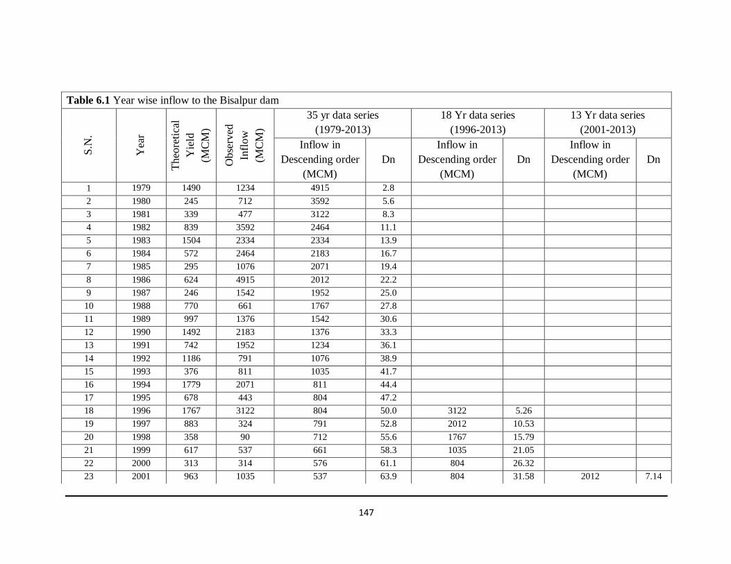
Study of Temporal Variation of Inflow to the Dams of Rajasthan State with Special Reference to Ramgarh and Bisalpur Dams.
147
Table 6.1 Year wise inflow to the Bisalpur dam
S.N
.
Yea
r
Theo
reti
cal
Yie
ld
(MC
M)
Obse
rved
Infl
ow
(MC
M)
35 yr data series
(1979-2013)
18 Yr data series
(1996-2013)
13 Yr data series
(2001-2013)
Inflow in
Descending order
(MCM)
Dn
Inflow in
Descending order
(MCM)
Dn
Inflow in
Descending order
(MCM)
Dn
1 1979 1490 1234 4915 2.8
2 1980 245 712 3592 5.6
3 1981 339 477 3122 8.3
4 1982 839 3592 2464 11.1
5 1983 1504 2334 2334 13.9
6 1984 572 2464 2183 16.7
7 1985 295 1076 2071 19.4
8 1986 624 4915 2012 22.2
9 1987 246 1542 1952 25.0
10 1988 770 661 1767 27.8
11 1989 997 1376 1542 30.6
12 1990 1492 2183 1376 33.3
13 1991 742 1952 1234 36.1
14 1992 1186 791 1076 38.9
15 1993 376 811 1035 41.7
16 1994 1779 2071 811 44.4
17 1995 678 443 804 47.2
18 1996 1767 3122 804 50.0 3122 5.26
19 1997 883 324 791 52.8 2012 10.53
20 1998 358 90 712 55.6 1767 15.79
21 1999 617 537 661 58.3 1035 21.05
22 2000 313 314 576 61.1 804 26.32
23 2001 963 1035 537 63.9 804 31.58 2012 7.14

Study of Temporal Variation of Inflow to the Dams of Rajasthan State with Special Reference to Ramgarh and Bisalpur Dams.
148
Rainfall-Inflow trends for different data series are shown in Fig. 6.2 (a). Inflow trend at different dependability’s for 35, 18,
and 13-year data series is shown in Fig. 6.2 (b). Inflow is showing a declining trend for all three dependability’s with longer
to shorter data series.
24 2002 195 17 477 66.7 576 36.84 1767 14.29
25 2003 741 177 443 69.4 537 42.11 1035 21.43
26 2004 1272 1767 324 72.2 324 47.37 804 28.57
27 2005 948 169 314 75.0 314 52.63 804 35.71
28 2006 1683 2012 235 77.8 235 57.89 576 42.86
29 2007 600 143 177 80.6 177 63.16 235 50.00
30 2008 778 161 169 83.3 169 68.42 177 57.14
31 2009 328 21 161 86.1 161 73.68 169 64.29
32 2010 950 235 143 88.9 143 78.95 161 71.43
33 2011 1244 804 90 91.7 90 84.21 143 78.57
34 2012 1224 576 21 94.4 21 89.47 21 85.71
35 2013 1465 804 17 97.2 17 94.74 17 92.86
Inflow Average =
1170.00 MCM 684.00 MCM 609.00 MCM
Inflow at 50% Dn =
803.88 MCM 318.89 MCM 234.67 MCM
Inflow at 75% Dn =
313.79 MCM 156.75 MCM 152.08 MCM
Inflow at 90% Dn =
121.67 MCM 20.81 MCM 18.69 MCM

Study of Temporal Variation of Inflow to the Dams of Rajasthan State with Special Reference to Ramgarh and Bisalpur Dams.
149
Graph of three-time segments 1979-2013, 1996-2013 and 2001-2013 (Fig. 6.2)
shows a reduction of inflow at the same quantum of monsoon rainfall. The figure can also
be used to predict the maximum probable inflow for a certain amount of monsoon rainfall
using trend line of 2001-2013.
(a) Rainfall-Inflow trend for different data series
(b) Inflow at different dependability for different data series
Fig. 6.2 Water Inflow trend for different time segment: Bisalpur
6.1 Formulation and Testing of hypothesis
(1) Z Test for 35 years data series (1979-2013):
0
1000
2000
3000
4000
5000
6000
300 400 500 600 700 800 900
Infl
ow
(M
CM
)
Rainfall (mm)
Rainfall-Inflow trend for different data series: Bisalpur
Trend 1979-2013 Trend 1996-2013 Trend 2001-2013
Linear (Trend 1979-2013) Linear (Trend 1996-2013) Linear (Trend 2001-2013)
804
319
235
314
157 152 122
21 19
0
100
200
300
400
500
600
700
800
900
35 yr data series (1979-2013) 18 Yr data series (1996-2013) 13 Yr data series (2001-2013)
Infl
ow
(M
CM
)
Dependable inflow for different data series: Bisalpur
50% dependability 75% dependability 90% dependability

Study of Temporal Variation of Inflow to the Dams of Rajasthan State with Special Reference to Ramgarh and Bisalpur Dams.
150
Ho (Null Hypothesis): 1095 MCM
H1 (Alternate Hypothesis): 1095 MCM
For n=35 (>30), z-test has been applied.
1170x ; S= 1130.22; SE= 191.04;
Z= 0.39;
Critical z value at 5% significance level= 1.96 (two tail) and 1.645 (one tail)
Z<zc; therefore null hypothesis is accepted, i.e. Bisalpur dam is getting the desired 1095
MCM inflow of water.
(1I) T-Test for 18 years data series (1996-2013):
Ho (Null Hypothesis): 1095 MCM
H1 (Alternate Hypothesis): 1095 MCM
For n=18 (<30), t-test has been applied.
684x ; S= 835.33; SE= 196.89;
t= -2.09;
Critical t value at 5% significance level= 1.74 (one tail) at df= 18-1= 17
t>tc; therefore null hypothesis is rejected and alternate hypothesis is accepted, i.e.
Bisalpur dam is receiving less than the desired 1095 MCM inflow of water.
(1II) T-Test for 13 year data series (2001-2013):
Ho (Null Hypothesis): 1095 MCM
H1 (Alternate Hypothesis): 1095 MCM
For n=13 (<30), test has been applied.
609x ; S= 658.48; SE= 182.63;
t= -2.66;
Critical t value at 5% significance level= 1.782 (one tail) at df= 13-1= 12
t>tc; therefore null hypothesis is rejected and alternate hypothesis is accepted, i.e.
Bisalpur dam is receiving less than the desired 1095 MCM inflow of water.
Hypotheses tested on three data series shows that water inflow in Bisalpur dam is
on decreasing trend

Study of Temporal Variation of Inflow to the Dams of Rajasthan State with Special Reference to Ramgarh and Bisalpur Dams.
151
6.2 Performance Study and Performance Statistics
By year wise inflow data (Table 6.1) hydrological performance of the dam regarding
reliability, resilience, vulnerability, maximum deficit and sustainability can be determined
for different data series, which is as shown below:
35 years data series
(1979-2013) 18 Year data series
(1996-2013) 13 Year data series
(2001-2013)
Reliability: 37.14% 16.67% 15.38%
Resilience:
31.82% 13.33% 18.18%
Vulnerability:
35.78% 55.90% 55.52%
Maximum Deficit(2002):
98.45% 98.45% 98.45%
Sustainability 42.34% 21.40% 23.17%
Inflow on dependability is plotted as shown in Fig. 6.3. The graph shows that
there was 17 MCM inflow at 97.20% reliability. As per code provisions, inflow at 100%
reliability is considered for drinking water projects (IS 5477 Part-3:2002). Danil’Yan et
al. (2006) recommends guarantee of 95% occurrence for water supply. The dam was
designed for 1095 MCM at 75% dependability, but it is yielding only 314 MCM as per 35
years data series. For 13 year or 18-year data series, it is yielding only half of this i.e.
around 152 MCM at 75 % dependability.
Fig. 6.3 Variations of inflow with dependability in Bisalpur Dam
Theoretical inflow computed by annual rainfall, and catchment area has been compared
with observed values. The performance of method of computing theoretical inflow is
shown in Table 6.2.
0
1000
2000
3000
4000
5000
6000
0.0 20.0 40.0 60.0 80.0 100.0 120.0
Infl
ow
(M
CM
)
Dependability (%)
Dependability-Inflow Curve
1979-2013 1996-2013 2001-2013

Study of Temporal Variation of Inflow to the Dams of Rajasthan State with Special Reference to Ramgarh and Bisalpur Dams.
152
Table 6.2 Performance Statistics: Bisalpur dam
Statistical
Parameter MAE MAPE (%) R R2 t33 NSE RMSE RSR NMBE
Value 713.57 170.51 0.36 0.13 2.22 0.05 1085.38 0.97 -25.49
Optimal
value
Lower
value
Lower
value Unity Unity 2.034 Unity
Lower
value Zero
Lower
Value
The value of the coefficient of correlation is 0.36, the corresponding t-value is
2.22, which is more than the critical value of tc = 2.034, at (35-2) =33 degree of freedom
at 5% level of significance. This shows that there is a marginal correlation between the
observed and computed values. Nash-Sutcliff Efficiency (NSE) is a low positive value,
which also shows a marginal correlation. RSR is far beyond the optimal value. MAE,
MAPE, and NMBE are very high. Therefore, it can be concluded that the method of
computation of theoretical values of inflow is not an accepTable method in this case.
6.3 Determination of Critical Year
Performance dependability of Bisalpur dam is only 36.45%, and water inflow trend to the
Bisalpur dam is declining. Therefore, it is essential to find out the critical year. Time
Series Analysis and Sequential Cluster Analysis have been carried out for the purpose.
Time series analysis gives us an idea about the possible critical years where trends are
broken, and abrupt changes have taken place. The Sequential cluster analysis gives us the
critical year out of the possible critical years, which divides the pre and post-disturbance
epochs.
6.3.1 Determination of Possible Critical Years: Time Series Analysis
To determine the critical year using sequential cluster analysis, we need to determine
possible critical years. Possible critical years have been identified with the help of time
series analysis by trend elimination using least square method. The results of the time
series analysis are as shown in Table 6.3. Time series of inflow for Bisalpur dam has been
shown in Fig. 6.4.

Study of Temporal Variation of Inflow to the Dams of Rajasthan State with Special Reference to Ramgarh and Bisalpur Dams.
153
Table 6.3. Time series analysis: Bisalpur Dam (Trend elimination using least square
method) S. N. Year
Inflow t t*I t*t Trend Elimination of
Trend
Possible
critical year
MCM
1 1979 1233.93 -17 -20977 289 2050 -816.18
2 1980 712.26 -16 -11396 256 1998 -1286.06
3 1981 476.64 -15 -7150 225 1947 -1469.9
4 1982 3592.47 -14 -50295 196 1895 1697.71 ***
5 1983 2333.9 -13 -30341 169 1843 490.92
6 1984 2464.46 -12 -29574 144 1791 673.27
7 1985 1075.62 -11 -11832 121 1739 -663.78
8 1986 4914.76 -10 -49148 100 1688 3227.14 ***
9 1987 1542.34 -9 -13881 81 1636 -93.49
10 1988 661.29 -8 -5290 64 1584 -922.75
11 1989 1375.81 -7 -9631 49 1532 -156.45
12 1990 2182.95 -6 -13098 36 1480 702.47
13 1991 1951.57 -5 -9758 25 1429 522.87
14 1992 791.28 -4 -3165 16 1377 -585.63
15 1993 810.82 -3 -2432 9 1325 -514.3
16 1994 2070.8 -2 -4142 4 1273 797.45
17 1995 442.93 -1 -442.9 1 1222 -778.62
18 1996 3122.34 0 0 0 1170 1952.56 ***
19 1997 323.99 1 323.99 1 1118 -793.99
20 1998 90.06 2 180.12 4 1066 -976.14
21 1999 537.24 3 1611.7 9 1014 -477.17
22 2000 313.79 4 1255.2 16 962.6 -648.84
23 2001 1034.55 5 5172.8 25 910.8 123.7
24 2002 16.99 6 101.94 36 859.1 -842.07
25 2003 176.72 7 1237 49 807.3 -630.55
26 2004 1767.49 8 14140 64 755.5 1011.99 ***
27 2005 168.51 9 1516.6 81 703.7 -535.19
28 2006 2011.89 10 20119 100 651.9 1359.96 ***
29 2007 142.74 11 1570.1 121 600.1 -457.39
30 2008 161.43 12 1937.2 144 548.4 -386.92
31 2009 21.23 13 275.99 169 496.6 -475.33
32 2010 234.67 14 3285.4 196 444.8 -210.11
33 2011 804.29 15 12064 225 393 411.29
34 2012 576.32 16 9221.1 256 341.2 235.1
35 2013 803.88 17 13666 289 289.4 514.45
Sum 40942 0 -184872 3570 40942
The Trend equation U = a + bt has been derived as
Inflow = (1169.77) + (-51.78) x Time
Where a = 1169.77 and b = -51.78

Study of Temporal Variation of Inflow to the Dams of Rajasthan State with Special Reference to Ramgarh and Bisalpur Dams.
154
Fig. 6.4 Time series inflow of Bisalpur dam
Exceptional periods are (possible critical years) marked as *** where there are
changes that can be attributed to climatic or anthropogenic changes.
6.3.2 Determination of Critical Year: Sequential Cluster Analysis
A critical year for the possible critical years is determined using sequential cluster
analysis as shown in Table 6.4. From section 6.1 it is evident that there is a declining
trend of water inflow to the Bisalpur Dam. It is essential to determine the critical year,
which divides two consecutive non-overlapping epochs- pre-disturbance and post-
disturbance. Determination of critical year will help in policy formulation for an effective
water resources planning and management of the area. Sequential Cluster Analysis has
been employed to determine the critical year.
y = -51.785x + 1169.8
0
1000
2000
3000
4000
5000
6000
-20 -10 0 10 20
Time series of inflow (Bisalpur)
Time series Bisalpur
Linear (Time series Bisalpur)

Study of Temporal Variation of Inflow to the Dams of Rajasthan State with Special Reference to Ramgarh and Bisalpur Dams.
155
Table 6.4. Sequential cluster analysis: Bisalpur Dam
S.
N. Year
Actual
Inflow
(MCM)
Possible Critical Year
1982 1986 1996 2001 2004 2006
1 1979 1234 72939 751814 280976 61045 22823 16919
2 1980 712 626848 1928591 1106151 590957 452575 424761
3 1981 477 1055478 2638560 1657307 1008748 825126 787416
4 1982 3592 4361693 2224473 3343291 4458292 4872909 4966064
5 1983 2334 1471126 54242 324786 727438 900411 940706
6 1984 2464 1804878 132101 490641 967189 1165229 1211007
7 1985 1076 2060 1051412 473873 164336 95718 83165
8 1986 4915 14392577 7917217 9927257 11790674 12459171 12607861
9 1987 1542 177527 420344 49133 3763 24756 31805
10 1988 661 211337 54156 1215979 671931 523762 493807
11 1989 1376 64930 232145 150688 11064 84 140
12 1990 2183 1127740 1661395 175520 492735 636726 670681
13 1991 1952 689850 1118458 35183 221438 321004 345241
14 1992 791 108717 10552 946190 475717 352507 328011
15 1993 811 96213 6919 908555 449143 329684 306010
16 1994 2071 902123 1384862 94127 347866 470324 499568
17 1995 443 459773 203461 1745215 1077581 887488 848363
18 1996 3122 4005382 4965521 1845101 2694013 3018367 3091777
19 1997 324 635229 324914 46661 1338678 1125747 1081626
20 1998 90 1062838 646320 202446 1934716 1676871 1622924
21 1999 537 340774 127277 8 890680 718694 683529
22 2000 314 651585 336641 51170 1362374 1147486 1102937
23 2001 1035 7473 19755 244581 199317 122814 108537
24 2002 17 1218833 769142 273537 310258 1871445 1814430
25 2003 177 891664 514490 131972 157831 1459939 1409633
26 2004 1767 417947 762981 1506727 1424414 146297 162803
27 2005 169 907242 526339 138007 164424 143257 1429202
28 2006 2012 793693 1249688 2166474 2067541 2145916 419767
29 2007 143 957001 564398 157819 185989 163430 62133
30 2008 161 920780 536663 143317 170216 148666 53164
31 2009 21 1209494 761727 269122 305555 276434 137470
32 2010 235 785581 434716 93226 115145 97550 24753
33 2011 804 100305 8048 69849 53033 66198 169983
34 2012 576 72939 751814 280976 61045 22823 16919
35 2013 804 626848 1928591 1106151 590957 452575 424761
Mean On= 1504 2101 1764 1481 1385 1364
Mean ON-n= 1121 894 540 574 547 392
Sum Vn+ VN-n= 42531629 34339324 30264890 36894099 38669410 37936191

Study of Temporal Variation of Inflow to the Dams of Rajasthan State with Special Reference to Ramgarh and Bisalpur Dams.
156
The minimum sum of squared deviations of hydrological series before and after the
possible critical year is corresponding to the year 1996 as shown in Table 6.4. Therefore,
the year 1996 is considered as the critical year for the hydrological behavior of the
Bisalpur Dam. This shows that some disturbances have taken place after 1996 which is
attributed to the low inflow to the dam.
6.4 Various Parameters and Their Trends
The declining trend of inflow to the Bisalpur dam has been observed. The critical year of
initiation of post-disturbance epoch is determined as 1996. The various factors which are
considered responsible for surface runoff are analyzed and discussed. Trends of various
factors are plotted and shown in Fig. 6.5 to 6.10. Climatic parameters such as average
daily minimum and maximum temperature, precipitation, wind speed, relative humidity
and solar radiation are studied, and graphs are plotted to determine the variation of these
parameters with time.
6.4.1 Rainfall and Other Climatic Factors
Eleven numbers RGS are situated within and nearby catchment area of Bisalpur dam.
Year wise rainfall has been computed using the Thiessen polygon technique and the
graph has been plotted (Fig. 6.5 a). Variation of rainy days during monsoon period has
been shown in Fig. 6.5 (b).
(a) Rainfall trend (1979-2013)
0
100
200
300
400
500
600
700
800
900
1975 1980 1985 1990 1995 2000 2005 2010 2015
Rain
fall
(m
m)
Rainfall trend-Bisalpur

Study of Temporal Variation of Inflow to the Dams of Rajasthan State with Special Reference to Ramgarh and Bisalpur Dams.
157
(b) Rainy days trend (1979-2013)
Fig. 6.5 Rainfall trend: Bisalpur
The rainfall trend over the catchment area of Bisalpur Dam varies significantly
over the years, showing the temporal variation of rainfall and the trend of variation is
increasing. Minimum and maximum weighted annual rainfall is 336 mm (2002) and 806
mm (1994) with an average value of 573 mm. This shows that there exists temporal
variation of rainfall over the catchment. During 2005, 2010, and 2013, even after more
than average rainfall, the inflow to the dam was less than design capacity. Trends of other
climatic parameters are shown in Fig. 6.6.
(a) Mean of daily maximum and daily minimum temperature
0
10
20
30
40
50
60
1975 1980 1985 1990 1995 2000 2005 2010 2015
Rain
y d
ays
Rainy days trend-Bisalpur
17.00
18.00
19.00
20.00
21.00
22.00
23.00
24.00
25.00
30.00
31.00
32.00
33.00
34.00
35.00
36.00
1975 1980 1985 1990 1995 2000 2005 2010 2015
Min
. te
mp
. (0
C)
Max. te
mp
. (0
C)
Mean of daily max. and daily min. temperature: Bisalpur
Mean of daily max. temp. Mean of daily min. temp.Linear (Mean of daily max. temp.) Linear (Mean of daily min. temp.)

Study of Temporal Variation of Inflow to the Dams of Rajasthan State with Special Reference to Ramgarh and Bisalpur Dams.
158
(b) Mean of daily wind speed
(c) Mean of daily relative humidity and solar radiation
Fig. 6.6 Trends of other climatic factors: Bisalpur
There is an increasing trend of mean of daily maximum and minimum
temperature, daily relative humidity and daily solar radiation while a slightly decreasing
trend of mean of daily wind speed. These trends are shown in Table 4.8.
2.00
2.20
2.40
2.60
2.80
3.00
3.20
3.40
1975 1980 1985 1990 1995 2000 2005 2010 2015
Win
d s
peed
(m
/s)
Mean of daily wind speed: Bisalpur
17.00
18.00
19.00
20.00
21.00
22.00
23.00
24.00
25.00
0.10
0.15
0.20
0.25
0.30
0.35
0.40
0.45
0.50
1975 1980 1985 1990 1995 2000 2005 2010 2015
Sola
r r
ad
iati
on
(M
J/m
^2
)
Rela
tive h
um
idit
y (
Fra
cti
on
) Mean of daily relative humidity and solar radiation: Bisalpur
Relative humidity Solar radiation
Linear (Relative humidity) Linear (Solar radiation)

Study of Temporal Variation of Inflow to the Dams of Rajasthan State with Special Reference to Ramgarh and Bisalpur Dams.
159
6.4.2 Land Use Land Cover Changes
Due to anthropogenic reasons, land use land cover is changing with time. Land use has
been divided in two category viz. land use having a contributing effect and reducing
effect. One of the major land use is increasing cultivated area. Land use trend
(Contributing area) is shown in Fig. 6.7. Various types of land use trends are shown in
Fig. 6.8. These figures show that land use having reducing effect viz. area sown, area
sown more than once are on an increasing trend.
Fig. 6.7 Land use (Contributing effect): Bisalpur
25.00
30.00
35.00
40.00
45.00
50.00
19
78
19
80
19
82
19
84
19
86
19
88
19
90
19
92
1994
19
96
19
98
20
00
20
02
20
04
20
06
20
08
20
10
20
12
La
nd
use
% (
Con
trib
uti
ng e
ffect)
LULC (Contributing effect): Bisalpur
0%
20%
40%
60%
80%
100%
1978
1980
1985
1992
1995
2000
2003
2007
2008
2009
2010
2012
Area
(%
)
Land use changes: Bisalpur dam catchment
Barren land Culturable waste Fallow land Non Ag. uses Forest and pasture Net area sown

Study of Temporal Variation of Inflow to the Dams of Rajasthan State with Special Reference to Ramgarh and Bisalpur Dams.
160
Fig. 6.8 Land use changes: Bisalpur
0
10
20
30
40
50
60
70
80
1978 1980 1985 1992 1995 2000 2003 2007 2008 2009 2010 2012
Area
(%
)
Contributing and reducing areas (%): Bisalpur dam catchment
Contributing effect Reducing effectLinear (Contributing effect) Linear (Reducing effect)
0
10
20
30
40
50
60
70
1978 1980 1985 1992 1995 2000 2003 2007 2008 2009 2010 2012
Area
(%
)
Cultivation area: Bisalpur dam catchment
Area sown more than once Net area sown
2.00
2.05
2.10
2.15
2.20
2.25
2.30
2.35
2.40
2.45
2.50
1978
1980
1982
1984
1986
1988
1990
1992
1994
1996
1998
2000
2002
2004
2006
2008
2010
2012
Average f
ield
siz
e (
ha)
Average size of field: Bisalpur dam catchment

Study of Temporal Variation of Inflow to the Dams of Rajasthan State with Special Reference to Ramgarh and Bisalpur Dams.
161
Agricultural area is increasing with time and population. It has increased from
5,691 sqkm to 6,916 sqkm from 1978 to 2012. The area sown more than once is also
increasing; it has increased from around 1,973 sqkm to 3,520 sqkm. Due to this increase
in agricultural areas, land use pattern changed at a very fast pace.
Due to continuous partitions of the fields, the average size of the field is
decreasing, and the total number of fields is increasing with time. The average size of the
land holding has decreased from 2.45 ha to 2.07 ha from 1980 to 2000. This reflects that
total number of fields are increasing because of partitions of large fields, thereby more
length of periphery boundaries increasing the surface roughness and decreasing the
resultant runoff to the reservoir.
6.4.3 Groundwater Level Changes
Year wise changes in pre monsoon and post monsoon groundwater level below ground
level in the catchment area of Bisalpur dam are shown in Fig. 6.9. Average river bed level
below ground level within the catchment area was measured at some random places and
found in between 12-15m. After the year 1996 the pre-monsoon ground water level went
down the average river bed level, and post monsoon water levels were also deeper than
the average river bed level in some years. No recorded data is available to mention the
contribution of groundwater to rivers. The local enquiry was conducted by the old people
of the area, and they told that earlier to 1995-1996, some deep rivers of the catchment
flowed during the post-monsoon period also. However, according to the literature
reviewed earlier, the declining water table reduces runoff due to baseflow and hence the
inflow to the wetland (Jain et al. 2008).

Study of Temporal Variation of Inflow to the Dams of Rajasthan State with Special Reference to Ramgarh and Bisalpur Dams.
162
Fig. 6.9 Pre-monsoon and Post-monsoon GWL below GL: Bisalpur
Pre-monsoon GWL below ground level of the catchment area of Bisalpur Dam
has increased from an average level of 10.0m to 17.0m during the observation period,
which depicts a lowering trend of GWL at the rate of 15 cm per year. The rise of
underground water level before and after the monsoon period ranges from approximately
0.5m to 8.0m, with an average rise of 4.9m. Development of lift facilities through pump
sets has resulted in a tremendous increase in irrigation from underground water using
wells and tube wells.
6.4.4 Population Growth
Land use and cultivation area are influenced by the population growth, which is plotted in
the graph and shown in Fig 6.10. As the population increases, cultivation and other
anthropogenic disturbances increases and fallow land decrease, therefore, reducing the
surface runoff.
0.0
2.0
4.0
6.0
8.0
10.0
12.0
14.0
16.0
18.0
20.0
1984
1985
1986
1987
1988
1989
1990
1991
1992
1993
1994
1995
1996
1997
1998
1999
2000
2001
2002
2003
2004
2005
2006
2007
2008
2009
2010
2011
2012
2013
GW
L(m
)
Temporal Variation of GWL below GL of Bisalpur Dam Catchment
Premonsoom GWL Postmonsson GWL Average river bed level

Study of Temporal Variation of Inflow to the Dams of Rajasthan State with Special Reference to Ramgarh and Bisalpur Dams.
163
Fig. 6.10 Population density and its growth: Bisalpur
Population growth in the catchment area of Bisalpur dam has been derived by
applying weights to the corresponding districts density. Population density has an
excellent negative correlation with LULC (contributing effect) at 1% level of significance
(Table 6.6)
6.4.5 Various Parameters, Trend Lines and their Rate of Changes
Trend lines plotted in section 6.4 give an idea about the various factors, whether they are
in increasing or decreasing trend and at what rate. The results are summarized in Table
6.5.
Table 6.5 Factors and their trends: Bisalpur
S.N. Factor Trend Rate of Change
1 Rainfall 1979-2013 (mm) Increasing 5 mm in 2 yrs.
2 Rainy days in a year (nos.) Increasing 1 day in 3 yrs.
3 Mean of daily max. temp. (0C) Increasing 1 deg. in 100 yrs.
4 Mean of daily min. temp. (0C) Increasing 1 deg. in 250 yrs.
5 Mean of daily wind speed (m/sec) Decreasing 1 m/sec in 300 yrs.
6 Mean of daily RH (fraction) Constant NA
7 Mean of daily solar radiation (MJ/m2) Decreasing 1MJ/m2 in yrs.
8 Land use (Contributing effect) (%) Decreasing 1% in 2.5 yrs.
9 Cultivation area (%) Increasing 1% in 2 yrs.
10 Groundwater level below GL(m) Increasing 0.15m in 1 yrs.
11 Population density Increasing 450 in 2021
12 State population density Increasing 254 in 2021
0
50
100
150
200
250
300
350
400
450
1975 1980 1985 1990 1995 2000 2005 2010 2015
Pop
ula
tion
den
sity
Population density: Bisalpur

Study of Temporal Variation of Inflow to the Dams of Rajasthan State with Special Reference to Ramgarh and Bisalpur Dams.
164
Rainfall and rainy days trends over the catchment area of Bisalpur dam are
increasing. Groundwater levels below GL and population density are on increasing trend.
6.4.6 Correlation Matrix: Bisalpur
A 14x14 correlation matrix has been developed. Mutual correlations of most of the
factors are insignificant, being quite low. But, some factors have significant mutual
correlations. Significant correlations at 2-tailed test at 1% and 5% level of significance
has been shown by * and **. However, the matrix has been derived to show the mutual
correlations of all the factors with each other (Table 6.6), for the sake of mutual
dependence. This matrix can be utilized for determining the sensitivity of each parameter
with other remaining parameters.
Table 6.6 Correlation Matrix: Bisalpur

Study of Temporal Variation of Inflow to the Dams of Rajasthan State with Special Reference to Ramgarh and Bisalpur Dams.
165
Correlations
1.000 -.469** -.943** .998** .810** .195 .327 .100 .048 -.319 .142 .342* .816** .265
. .004 .000 .000 .000 .262 .055 .566 .783 .062 .417 .045 .000 .124
35 35 35 35 35 35 35 35 35 35 35 35 35 35
-.469** 1.000 .362* -.473** -.337* .345* -.147 -.270 -.300 -.059 .063 -.194 -.308 .024
.004 . .033 .004 .048 .042 .398 .116 .080 .738 .721 .264 .071 .893
35 35 35 35 35 35 35 35 35 35 35 35 35 35
-.943** .362* 1.000 -.938** -.669** -.282 -.305 .034 .017 .451** -.231 -.182 -.907** -.528**
.000 .033 . .000 .000 .100 .075 .847 .921 .007 .182 .296 .000 .001
35 35 35 35 35 35 35 35 35 35 35 35 35 35
.998** -.473** -.938** 1.000 .804** .192 .320 .097 .043 -.330 .148 .361* .803** .255
.000 .004 .000 . .000 .268 .061 .580 .808 .053 .397 .033 .000 .140
35 35 35 35 35 35 35 35 35 35 35 35 35 35
.810** -.337* -.669** .804** 1.000 .190 .306 .341* .187 -.132 -.092 .407* .575** -.056
.000 .048 .000 .000 . .275 .074 .045 .283 .449 .598 .015 .000 .750
35 35 35 35 35 35 35 35 35 35 35 35 35 35
.195 .345* -.282 .192 .190 1.000 .506** -.573** -.359* -.593** .560** -.281 .252 .273
.262 .042 .100 .268 .275 . .002 .000 .034 .000 .000 .102 .144 .112
35 35 35 35 35 35 35 35 35 35 35 35 35 35
.327 -.147 -.305 .320 .306 .506** 1.000 -.588** -.170 -.377* .750** -.278 .319 .144
.055 .398 .075 .061 .074 .002 . .000 .329 .025 .000 .106 .062 .409
35 35 35 35 35 35 35 35 35 35 35 35 35 35
.100 -.270 .034 .097 .341* -.573** -.588** 1.000 .626** .528** -.853** .450** -.077 -.386*
.566 .116 .847 .580 .045 .000 .000 . .000 .001 .000 .007 .661 .022
35 35 35 35 35 35 35 35 35 35 35 35 35 35
.048 -.300 .017 .043 .187 -.359* -.170 .626** 1.000 .418* -.223 -.093 .027 -.175
.783 .080 .921 .808 .283 .034 .329 .000 . .013 .197 .594 .878 .315
35 35 35 35 35 35 35 35 35 35 35 35 35 35
-.319 -.059 .451** -.330 -.132 -.593** -.377* .528** .418* 1.000 -.538** .054 -.370* -.428*
.062 .738 .007 .053 .449 .000 .025 .001 .013 . .001 .760 .029 .010
35 35 35 35 35 35 35 35 35 35 35 35 35 35
.142 .063 -.231 .148 -.092 .560** .750** -.853** -.223 -.538** 1.000 -.456** .253 .355*
.417 .721 .182 .397 .598 .000 .000 .000 .197 .001 . .006 .143 .036
35 35 35 35 35 35 35 35 35 35 35 35 35 35
.342* -.194 -.182 .361* .407* -.281 -.278 .450** -.093 .054 -.456** 1.000 .056 -.276
.045 .264 .296 .033 .015 .102 .106 .007 .594 .760 .006 . .749 .108
35 35 35 35 35 35 35 35 35 35 35 35 35 35
.816** -.308 -.907** .803** .575** .252 .319 -.077 .027 -.370* .253 .056 1.000 .714**
.000 .071 .000 .000 .000 .144 .062 .661 .878 .029 .143 .749 . .000
35 35 35 35 35 35 35 35 35 35 35 35 35 35
.265 .024 -.528** .255 -.056 .273 .144 -.386* -.175 -.428* .355* -.276 .714** 1.000
.124 .893 .001 .140 .750 .112 .409 .022 .315 .010 .036 .108 .000 .
35 35 35 35 35 35 35 35 35 35 35 35 35 35
Pearson Correlation
Sig. (2-tailed)
N
Pearson Correlation
Sig. (2-tailed)
N
Pearson Correlation
Sig. (2-tailed)
N
Pearson Correlation
Sig. (2-tailed)
N
Pearson Correlation
Sig. (2-tailed)
N
Pearson Correlation
Sig. (2-tailed)
N
Pearson Correlation
Sig. (2-tailed)
N
Pearson Correlation
Sig. (2-tailed)
N
Pearson Correlation
Sig. (2-tailed)
N
Pearson Correlation
Sig. (2-tailed)
N
Pearson Correlation
Sig. (2-tailed)
N
Pearson Correlation
Sig. (2-tailed)
N
Pearson Correlation
Sig. (2-tailed)
N
Pearson Correlation
Sig. (2-tailed)
N
YEAR
INFLOW
LULC
POPDEN
WTRTBL
RAINFALL
RDAYS
MAXTMP
MINTMP
WINDSPD
RELHUM
SOLAR
NA
ASMO
YEAR INFLOW LULC POPDEN WTRTBL RAINFALL RDAYS MAXTMP MINTMP WINDSPD RELHUM SOLAR NA ASMO
Correlation is signif icant at the 0.01 level (2-tailed).**.
Correlation is signif icant at the 0.05 level (2-tailed).*.
Table 6.6 Correlation Matrix : Bisalpur dam

Study of Temporal Variation of Inflow to the Dams of Rajasthan State with Special Reference to Ramgarh and Bisalpur Dams.
166
6.5 Determination of Principal Components
In section 6.4, trend lines and directions of various parameters which influence to runoff
have been shown. Now it is essential to determine the principal components out of the
various components discussed earlier so that the same may be considered for further
planning and analysis.
6.5.1 Regression Analysis
Regression lines of various parameters (predictors) with inflow (dependent variable) have
been plotted as shown in Fig. 6.11. Coefficients of determination have also been
mentioned on graphs. By coefficient of correlations and corresponding t-values compared
with critical t-values at 5% and 1% level of significance, we can determine the
significance level of the parameters for inflow to the dam.
(a) Rainfall (b) Rainy days
(c) Land use (d) GWL below GL
y = 2.8004x - 434.67
R² = 0.1194
0
1000
2000
3000
4000
5000
6000
200 300 400 500 600 700 800 900
Infl
ow
(M
CM
)
Rainfall (mm)
Rainfall-Inflow
y = -13.939x + 1606.3
R² = 0.0203
0
1000
2000
3000
4000
5000
6000
0 20 40 60
Infl
ow
(M
CM
)
Rainy days
Rainy days-Inflow
y = 90.231x - 2265.8
R² = 0.1307
0
1000
2000
3000
4000
5000
6000
25 35 45 55
Infl
ow
(M
CM
)
Land use (Contributing effect)
Land use (Conctributing
effect)-Inflow
y = -180.82x + 3628
R² = 0.1135
0
1000
2000
3000
4000
5000
6000
10 12 14 16 18 20
Infl
ow
(M
CM
)
GWL below GL(m)
GWL below GL-Inflow

Study of Temporal Variation of Inflow to the Dams of Rajasthan State with Special Reference to Ramgarh and Bisalpur Dams.
167
(e) Mean daily max. Temp. (f)Mean daily min. temp.
(g) Wind speed (h) Relative humidity
(i)Solar radiation (j) Population density
Fig. 6.11 Cross plots: Between inflow and independent variables:Bisalpur
y = -365.4x + 13473 R² = 0.0731
0
1000
2000
3000
4000
5000
6000
31 32 33 34 35 36
Infl
ow
(M
CM
)
Mean daily max temp.
Mean daily max temp-Inflow
y = -640.84x + 13315
R² = 0.0898
0
1000
2000
3000
4000
5000
6000
17 18 19 20 21
Infl
ow
(M
CM
)
Mean daily min. temp.
Mean daily min. temp.-Inflow
y = -564.71x + 2808.1
R² = 0.004
0
1000
2000
3000
4000
5000
6000
2 2.5 3 3.5
Infl
ow
(M
CM
)
Wind speed
Wind speed-Inflow
y = 1629.6x + 540.54
R² = 0.0029
0
1000
2000
3000
4000
5000
6000
0.3 0.35 0.4 0.45 0.5
Infl
ow
(M
CM
)
Relative humidity
Relative humidity-Inflow
y = -488.83x + 10587
R² = 0.0372
0
1000
2000
3000
4000
5000
6000
18 19 20
Infl
ow
(M
CM
)
Solar radiation
Solar radiation-Inflow
y = -8.71x + 3872.8
R² = 0.2244
0
1000
2000
3000
4000
5000
6000
100 300 500
Infl
ow
(M
CM
)
Population density (nos.)
Population density-Inflow

Study of Temporal Variation of Inflow to the Dams of Rajasthan State with Special Reference to Ramgarh and Bisalpur Dams.
168
Regression analysis of inflow with various factors independently, as shown in Fig
6.11 is summarized in Table 6.7. Several cross plots showing the relationship between
independent variables and inflow may be generated to develop empirical relations for the
indirect estimation of the output. These relations are obtained using statistical methods
such as regression analysis. However, although empirical equations are cost- effective
and not too time-consuming, they include uncertainties relating to the limited data
available (Majdi et al. 2010). To determine the parameters affecting inflow more than
others, several cross plots showing the relationship between independent variables and
inflow have been generated from a total of 35 data (Fig. 6.11 and Table 6.7).
Table 6.7 Correlation and regression of inflow with various parameters: Bisalpur
S.N. Factor
Regression
equation
Type of
correlation
Coefficient of
correlation (R)
t-
value Significance
1 Rainfall y = 2.80x -434.6 Positive 0.34 2.11 S
2 Rainy days y = -13.93x+1606 Negative 0.14 0.82 NS
3 Land use (Cont. effect) y = 90.23x -2265 Positive 0.36 2.22 S
4 GWL below GL y = -180.8x + 3628 Negative 0.34 2.05 S
5 Population density y = -8.71x + 3872 Negative 0.47 3.09 HS
6 Mean of daily max. temp.
(0C)
y = -365.4x + 13473 Negative 0.27 1.61 NS
7 Mean of daily min. temp. (0C) y = -640.8x + 13315 Negative 0.30 1.80 NS
8 Mean of daily wind speed
(m/sec) y = -564.7x + 2808 Negative 0.06 0.36 NS
9 Mean of daily RH (fraction) y = 1629x –540.5 Positive 0.04 0.26 NS
10 Mean of daily solar radiation
(MJ/m2) y = -488.8x + 10587 Negative 0.19 1.13 NS
Here, NS=Not Significant, S= Significant, HS= Highly Significant
The critical value of tc for the n=35-2=33 degree of freedom at the 5% level of
significance is 2.034 and 1% level of significance is 2.735. Rainfall, land use
(contributing effect), groundwater level are having a significant correlation with the
inflow, and population density is highly significant while other climatic factors like mean
daily min. temp., wind speed, and solar radiation are having no correlation with inflow.
Population density, land use, rainfall, and GWL below GL are having correlations with
inflow and t-values are higher than the critical tc value. This concludes that population

Study of Temporal Variation of Inflow to the Dams of Rajasthan State with Special Reference to Ramgarh and Bisalpur Dams.
169
density; land use, rainfall, and GWL below GL are principal components for the inflow to
the Bisalpur dam.
6.5.2 Cosine Amplitude Method
Cosine Amplitude Method of sensitivity analysis is employed to find out the principal
components and their relative influence so that the MLR can be further simplified as per
availability of data. By relative influence value (Rij) computed by CAM (Annexure 8c),
the relative importance of the four factors is mentioned as below (Fig. 6.12):
(1) LULC (Contributing area %)= 0.75
(2) Rainfall= 0.74
(3) GWL= 0.47
(4) Population density= 0.43
Fig. 6.12 Relative influences of the factors responsible for inflow: CAM for Bisalpur
From the two analyses, it is found that four components viz. LULC, rainfall, GWL
below GL, and population density are the principal components for inflow to the Bisalpur
dam. Out of these four principal components, LULC and rainfall are most influencing
components to the inflow to Bisalpur dam. Sensitivity analysis shows less water inflow to
the Bisalpur dam due to the LULC is the main factor having 32% of the effect; rainfall is
responsible for 31% of the effect, GWL below GL is having 19% of the effect and
population density has 18% effect on the inflow.
0.43
0.75 0.74
0.47
0.00
0.10
0.20
0.30
0.40
0.50
0.60
0.70
0.80
0.90
1.00
Population density LULC (Contributing
area %)
Rainfall GWL
Rela
tive in
flu
en
ce
Factor
Relative influence (CAM): Bisalpur

Study of Temporal Variation of Inflow to the Dams of Rajasthan State with Special Reference to Ramgarh and Bisalpur Dams.
170
6.6 MLR for Generation of Inflow Equation
The inflow equation for Bisalpur dam may be formed with the help of Multiple Linear
Regression (MLR) considering the six principal components as derived in Section 6.5.
Table 6.8 MLR summary output: Inflow to the Bisalpur dam
Regression Statistics Multiple R 0.67 R Square 0.44 Adjusted R Square 0.37 Standard Error 896.65 Observations 35.00
ANOVA
df SS MS F Significance
F Regression 4 19312407 4828102 6.01 0.001 Residual 30 24119425 803980.8
Total 34 43431832
Coefficients Standard
Error t Stat. P-
value Lower 95% Upper 95%
Intercept 9280.76 6829.89 1.36 0.18 -4667.74 23229.26 LULC (Contributing effect) -123.43 115.30 -1.07 0.29 -358.90 112.03
Rainfall 3.17 1.21 2.63 0.01 0.71 5.64
Water table 108.26 137.80 0.79 0.44 -173.16 389.69
Population density -21.59 10.39 -2.08 0.05 -42.80 -0.38
Using the computed coefficients, inflow equation is developed as shown below:
443322110 **** xxxxInflow (6.1)
Where values of the coefficients are 9820.76, -123.43, 3.17, 108.26, -21.59 and
variables are LULC (Contributing effect), rainfall, GWL below GL and population
density respectively, and a minimum value of computed inflow is set to zero. The
correlation coefficient (multiple R) for the above relationship is 0.67.
From the developed equation, the inflow has been computed, and a graph is
plotted between observed inflow and computed inflow along with the goodness of fit as
shown in Fig.6.13. Between the two values, the coefficient of correlation (R) is 0.67, and
the corresponding t-value is 5.16, which is more than the critical value at 1% level of
significance (2.735), which infers that the inflow values computed from the developed
equation are highly significant.

Study of Temporal Variation of Inflow to the Dams of Rajasthan State with Special Reference to Ramgarh and Bisalpur Dams.
171
Fig. 6.13 Goodness of fit for the developed equation (MLR)
6.7 Regression Analysis and Determination of Factors Responsible for Principal
Components
As far as changes in land use are concerned, agricultural area (Total crop area) is
increasing with time and population. It has increased from 7664 sqkm to 10437 sqkm
from 1978 to 2012. The area sown more than once is also increasing; it has increased
from around 1973 sqkm to 3520 sqkm. Agricultural activities, land area sown, forest area,
land area put to non-agricultural uses like habitation, industries, mining, roads,
infrastructures, etc. are increasing at a very fast pace. Fig. 6.7 and 6.8 show that land
utilizations which are having a reducing effect on the surface runoff are increasing and
the land utilizations which are having a contributing effect on the surface runoff viz.
barren land, culturable waste, and fallow land are decreasing with the passage of time.
Due to continuous partitions of the fields, the average size of the field is decreasing, and
the number of total fields is increasing with time. The average size of the field has
decreased from 2.45 ha to 2.07 ha from 1980 to 2000. Population density has highly
significant correlations with LULC, crop area, GWL below GL, and average field size. T-
values for these correlations are 15.48, 7.73, 7.74, and 39.22 which is more than the
critical value of tc=2.735 at df=35-2=33 and 1% level of significance. T-value for
correlation of average field size with LULC is 11.67 which is highly significant. In these
analyses, it is inferred that inflow to the dam is influenced by the land use (contributing
y = 1.0417x - 69.083
R² = 0.4477
0.00
1000.00
2000.00
3000.00
4000.00
5000.00
6000.00
0 500 1000 1500 2000 2500 3000
Goodness of fit for developed equation (MLR): Bisalpur
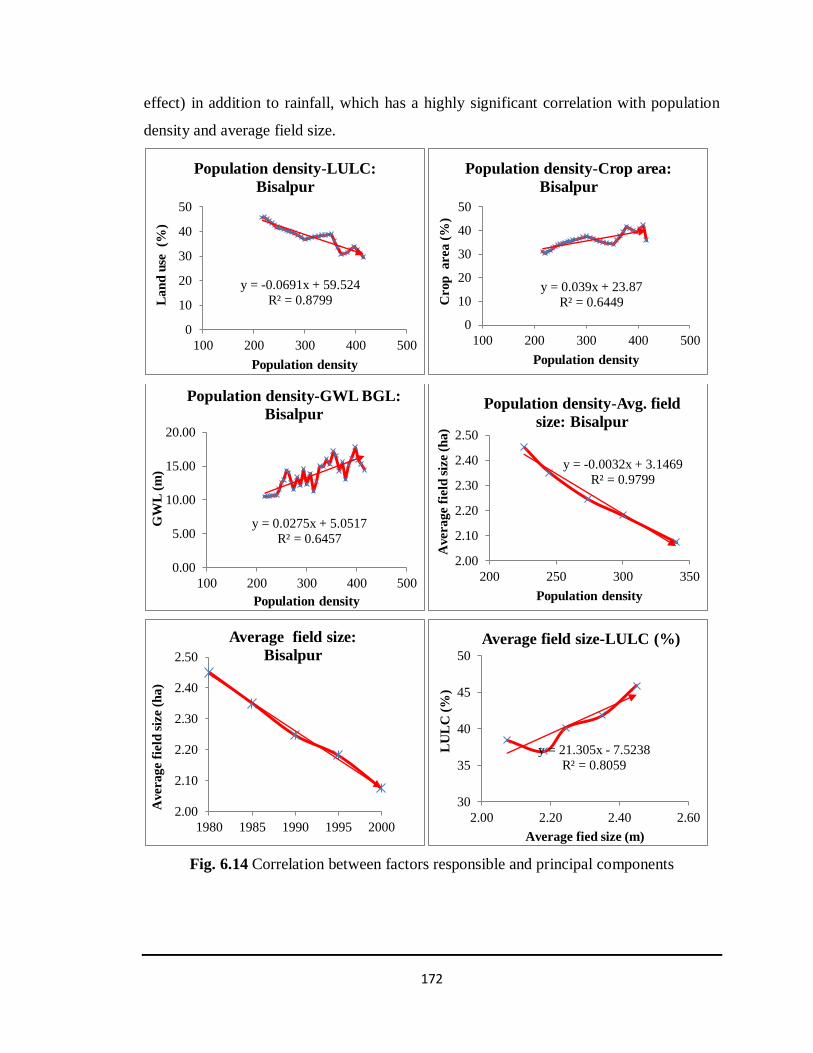
Study of Temporal Variation of Inflow to the Dams of Rajasthan State with Special Reference to Ramgarh and Bisalpur Dams.
172
effect) in addition to rainfall, which has a highly significant correlation with population
density and average field size.
Fig. 6.14 Correlation between factors responsible and principal components
y = -0.0691x + 59.524
R² = 0.8799
0
10
20
30
40
50
100 200 300 400 500
Lan
d u
se
(%)
Population density
Population density-LULC:
Bisalpur
y = 0.039x + 23.87
R² = 0.6449
0
10
20
30
40
50
100 200 300 400 500
Crop
area (
%)
Population density
Population density-Crop area:
Bisalpur
y = 0.0275x + 5.0517
R² = 0.6457
0.00
5.00
10.00
15.00
20.00
100 200 300 400 500
GW
L (
m)
Population density
Population density-GWL BGL:
Bisalpur
y = -0.0032x + 3.1469
R² = 0.9799
2.00
2.10
2.20
2.30
2.40
2.50
200 250 300 350
Avera
ge f
ield
siz
e (
ha
)
Population density
Population density-Avg. field
size: Bisalpur
2.00
2.10
2.20
2.30
2.40
2.50
1980 1985 1990 1995 2000
Average f
ield
siz
e (
ha
)
Average field size:
Bisalpur
y = 21.305x - 7.5238
R² = 0.8059
30
35
40
45
50
2.00 2.20 2.40 2.60
LU
LC
(%
)
Average fied size (m)
Average field size-LULC (%)

Study of Temporal Variation of Inflow to the Dams of Rajasthan State with Special Reference to Ramgarh and Bisalpur Dams.
173
7 CONCLUSIONS AND RECOMMENDATIONS
7.1 Conclusions
7.2 Recommendations
7.3 Major Contributions of Present Study
7.4 Limitations of Findings
7.5 Scope of Further Research

Study of Temporal Variation of Inflow to the Dams of Rajasthan State with Special Reference to Ramgarh and Bisalpur Dams.
174
CHAPTER-7
CONCLUSIONS AND RECOMMENDATIONS
7.1 The following conclusions are drawn based on the studies
I. The temporal variation of water inflow to the dams of Rajasthan State is declining.
It has slightly improved since the last couple of years (2010-2013). The inflow
trend has diminished in the Ramgarh dam while it is showing a declining trend in
the Bisalpur dam.
II. Performance dependability of the state surface water resources has reduced to
33.36% and 24.02% for 20 years data series and 10 year data series against the
50% expected dependability. This shows a sign of temporal variation of inflow to
the dams of Rajasthan State. Performance dependability of Ramgarh dam is zero.
Performance dependability of Bisalpur dam for 35 yrs, 18 yrs, and 13 yrs data
series is 36.45%, 16.23%, and 14.88% respectively. Therefore, the reliability of
the state surface water resources is very less and showing the declining trend.
Sustainability of the dams of Rajasthan state is 38.7%, and vulnerability is
15.52%. The two parameters for Ramgarh dam are 0% and 83.89%. Sustainability
of Bisalpur dam is 42.34%, 21.40% and 23.17% for 35 yrs, 18 yrs, and 13 yrs data
series respectively. The vulnerability of Bisalpur dam is 35.78%, 55.90%, and
55.52% for 35 yrs, 18 yrs, and 13 yrs data series respectively.
III. The year 2002 was the year of maximum deficit. In this year, dams of Rajasthan
State received only 30.9% water while Bisalpur dam received only 17 MCM of
water, which were the lowest inflow to the dams.
IV. Various performance statistical parameters reveal that method of computation of
theoretical inflow “Strange‟s Table Method” proved to be giving the less precise/
erroneous results.
V. Year 1994 is identified as critical year, which divides two consecutive non-
overlapping epochs- pre-disturbance and post-disturbance, for the dams of
Rajasthan State. Critical years for Ramgarh and Bisalpur dams are 1998 and 1996
respectively.
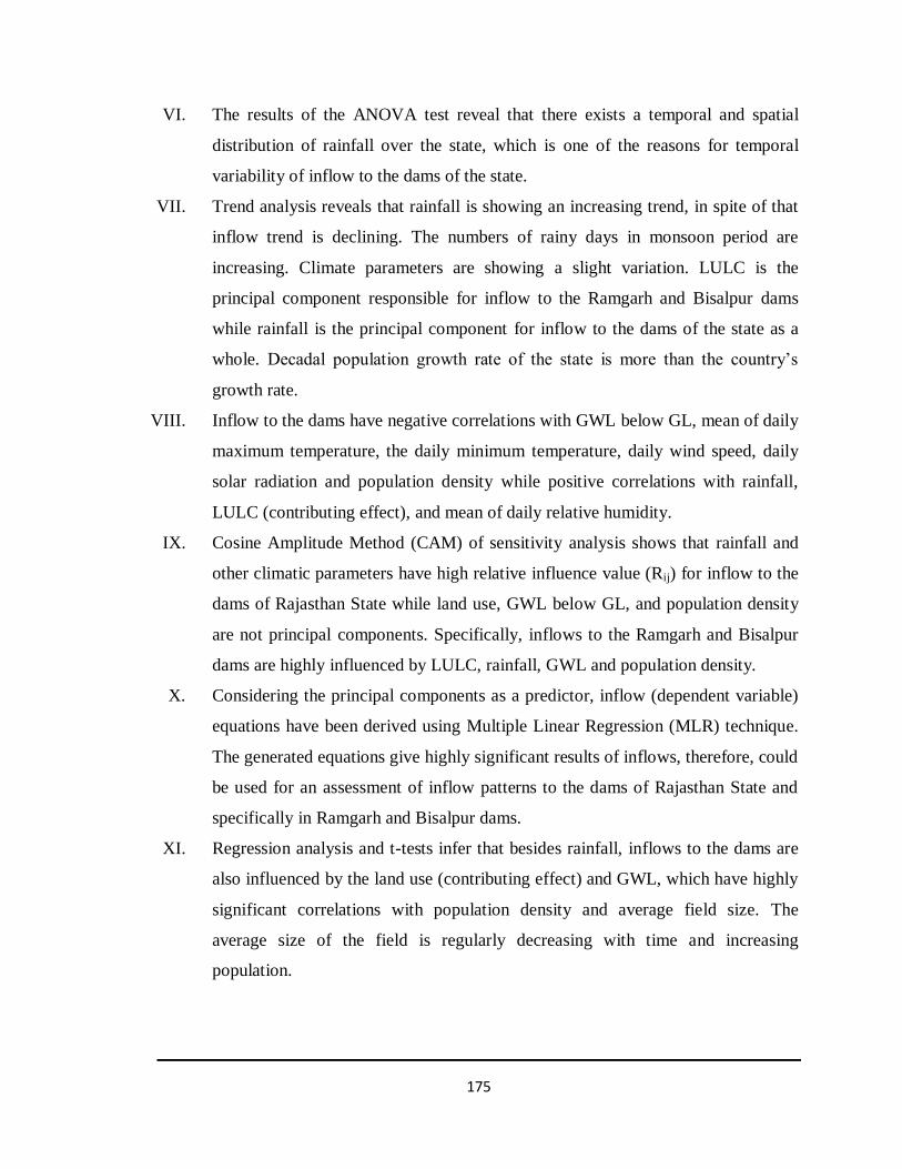
Study of Temporal Variation of Inflow to the Dams of Rajasthan State with Special Reference to Ramgarh and Bisalpur Dams.
175
VI. The results of the ANOVA test reveal that there exists a temporal and spatial
distribution of rainfall over the state, which is one of the reasons for temporal
variability of inflow to the dams of the state.
VII. Trend analysis reveals that rainfall is showing an increasing trend, in spite of that
inflow trend is declining. The numbers of rainy days in monsoon period are
increasing. Climate parameters are showing a slight variation. LULC is the
principal component responsible for inflow to the Ramgarh and Bisalpur dams
while rainfall is the principal component for inflow to the dams of the state as a
whole. Decadal population growth rate of the state is more than the country‟s
growth rate.
VIII. Inflow to the dams have negative correlations with GWL below GL, mean of daily
maximum temperature, the daily minimum temperature, daily wind speed, daily
solar radiation and population density while positive correlations with rainfall,
LULC (contributing effect), and mean of daily relative humidity.
IX. Cosine Amplitude Method (CAM) of sensitivity analysis shows that rainfall and
other climatic parameters have high relative influence value (Rij) for inflow to the
dams of Rajasthan State while land use, GWL below GL, and population density
are not principal components. Specifically, inflows to the Ramgarh and Bisalpur
dams are highly influenced by LULC, rainfall, GWL and population density.
X. Considering the principal components as a predictor, inflow (dependent variable)
equations have been derived using Multiple Linear Regression (MLR) technique.
The generated equations give highly significant results of inflows, therefore, could
be used for an assessment of inflow patterns to the dams of Rajasthan State and
specifically in Ramgarh and Bisalpur dams.
XI. Regression analysis and t-tests infer that besides rainfall, inflows to the dams are
also influenced by the land use (contributing effect) and GWL, which have highly
significant correlations with population density and average field size. The
average size of the field is regularly decreasing with time and increasing
population.

Study of Temporal Variation of Inflow to the Dams of Rajasthan State with Special Reference to Ramgarh and Bisalpur Dams.
176
7.2 The following recommendations are made based on the studies
Increase in population density is putting stress on quality and quantity (Q & Q) of water
and on the other hand it is affecting the land use (contributing effect) pattern and also
lowering the GWL below GL of the catchment area of the dams. This situation is leading
to the declining trend of inflow to the dams of Rajasthan State.
I. More scientific methods should be used to compute theoretical inflow to the dams
instead of using „Strange‟s table‟, which gives less precise/ erroneous results.
II. 1994-1998 are proved to be critical years, which divide the two consecutive non-
overlapping epochs- pre-disturbance and post-disturbance. This may be used to
analyze the changes occurred leading to declining trend of inflow to the dams. It is
recommended to review the policies adopted, LULC; agricultural practices etc.
after the respective critical years.
III. Population density is found to be one of the principal component responsible for
less water inflow to the Ramgarh and Bisalpur dams. It is recommended to adhere
with most efficient use of available water to cater the increasing population and
also to plan to stabilize/reduce the decadal growth rate of population. This will
lead to stabilization of the average size of the field; increase in LULC
(contributing effect), and improvement of GWL below GL. As concluded earlier,
these improvements will lead to augmentation of inflow pattern to the dams.
IV. IWRM, INRM, RWH, recycle and reuse of water, micro watershed planning,
benchmarking and water auditing, water pricing, water trading, water
privatization, interlinking of rivers/ transboundary water sharing,
infiltration/ground water recharge, conjunctive use of surface and subsurface
water, more crop per drop by adopting sprinkler/drip/shednet irrigation techniques
and other suitable water management techniques should be adhered to ensure
equitable and sustainable Q & Q of water to all stakeholders including
environment and river itself. Policies need to fulfill the slogan ‟some, for all,
forever. Dedicated pressure irrigation techniques like sprinkler/drip were
implemented in Narmada Canal Project (Jalore district) and selected canals of
Indira Gandhi Nahar Project (IGNP). This has resulted in 30% saving of water
along with around 20% increase in per acre production. Similarly, RWH has been

Study of Temporal Variation of Inflow to the Dams of Rajasthan State with Special Reference to Ramgarh and Bisalpur Dams.
177
made compulsory for residential houses of the area more than 300 sqm in Jaipur
city. These RWH (Tankas) and reuse techniques were being used in western
Rajasthan since long back for self-reliance for water. Recycle (Sewerage
Treatment Plant-STP) is being made compulsory for new housing and industrial
project. In housing effluents, STP recycles around 75-80% water. District wise
and village wise IWRM plans have been prepared, and micro-watershed planning
is being done in the state. This type of planning is enabling the water
administrators to supervise, monitor and plan the available water and demand at
micro-watershed level. The project of ATW (Any Time Water) and water cans are
ensuring availability of drinking water 24x7 at a very nominal price. These types
of case studies are making successful stories of proper allocation and planning of
available water and recommended to be encouraged.
V. 5-R principal (refuse, reduce, reuse, recycle, rationing) can help in facing the
consequences arising out of water scarcity situations. Resource saving is resource
generation. Iglesias et al. (2007) and Liu et al. (2005) emphasized that water
saving is the key strategy for overall reduction of societal vulnerability to
drought/water scarcity.
7.3 Major Contribution of Present Study
I. The present study attempts to address the existing gap in available scientific
literature to describe the temporal variation of inflow to the dams of Rajasthan
State.
II. This study is an attempt to draw conclusions regarding the direction and
variability of inflow to the dams of Rajasthan State with special reference to
Ramgarh and Bisalpur dams.
III. This study attempts to draw a conclusion regarding the correctness of inflow
assessment by „Strange‟s table‟ being used as per prevailing practice in the WRD.
It is concluded in the study that this method gives less precise/ erroneous results.
IV. Critical years have been determined in this study, which may help in the
determination of factors responsible for disturbances, which lead to the declining
trend of inflow to the dams.

Study of Temporal Variation of Inflow to the Dams of Rajasthan State with Special Reference to Ramgarh and Bisalpur Dams.
178
V. Direction and variability assessment of various parameters viz. Climatic, land use,
groundwater and population parameters which influence the inflow to the dams
have been made in this study.
VI. Correlation and relative influence of various parameters have been ascertained to
find out the principal components responsible for inflow to the dams so that it may
help in an efficient planning and management of surface water availability in the
state.
VII. Equations for inflow assessment of dams in the state, specifically for Ramgarh
and Bisalpur dams have been derived in this study, which may help for reliable
assessment of inflows to these dams.
VIII. Ramgarh dam was the source of drinking water supply of Jaipur city and Bisalpur
dam is a present source. Inflow to the Ramgarh dam has diminished to zero level,
and Bisalpur dam is showing a declining trend even after more than normal
rainfall. It is now being planned by the Government of Rajasthan to augment the
inflow to Bisalpur dam by the interlinking of rivers Banas (catchment area of
Bisalpur dam) and Chambal. Future of drinking water supply in Jaipur „the capital
city of the state‟ is dependent on surplus water availability in the Chambal River,
which is also uncertain looking to the inflow trend in the state. Therefore, this
study may help in an optimized and efficient planning and management of
storages, distribution and uses of available water and the various factors
influencing these aspects.
IX. In the future, the study can also be used by managers as a decision support system
(DSS) to manage the inflow to the dams.
7.4 Limitations of Findings
I. Theoretical inflow has been computed using Strange‟s table due to absence of
gauge-discharge data. However it is proved that this method gives less precise/
erroneous results. More scientific method is desired to be used for assessment of
theoretical inflow, specifically in Ramgarh dam.

Study of Temporal Variation of Inflow to the Dams of Rajasthan State with Special Reference to Ramgarh and Bisalpur Dams.
179
II. LULC is determined as principal component responsible for temporal variation of
inflow to the dams. LULC data has been collected from statistical department
instead of GIS.
III. Hydrological processes like water balance equations etc. have not been covered in
the thesis.
IV. There is little physics or science like soil moisture, evapotranspiration etc.
7.5 Scope of Further Research
I. Further research may be carried out to simulate the actual inflow to the Ramgarh
dam as there is further need for the development of water balance equation.
II. A similar study can be undertaken for other major/medium dams so that inflow
pattern, critical year, and principal components responsible for less water inflow
can be ascertained. This will help in reviewing the impact of policy formed earlier
and will also help in policy formation in future.
III. More scientific investigations of the impacts of anthropogenic changes and
climate change on inflow to the dams based on focused field study, systematic
experimental design, and long term programmes can be undertaken.
IV. Effect of soil moisture and GWL below GL on inflow to the dams can be
investigated further.

180
REFERENCES
1. www.waterresources.rajasthan.gov.in
2. www.swat.tamu.edu
3. www.envfor.nic.in
4. www.imdagrimat.gov.in
5. www.imd.rajasthan.gov.in
6. www.indiaweather.gov.in
7. www.bhuvan.nrsc.gov.in
8. www.glcf.com
9. www.fao.org/geonetwork/srv/en/metadata
10. www.iscgm.org
11. http://www.savethecolorado.org
12. http://www.ndtv.com dated 19.06.16
13. http://www.dnaindia.com/india/report-water-inflow-into-bhakra-pong-dams-
remains-low-1709536 dated 19.06.16
14. Acharya, A., Piechota, T. C., and Tootle, G. (2011). “Quantitative impacts of
climate change impacts on the hydrology of North Platte River watershed,
Wyoming.” J. of Hydrologic Engineering., doi: 10.1061/(ASCE)HE.1943-
5584.0000543
15. Akkuzu, E. (2011). “Usefulness of empirical equations in assessing canal losses
through seepage in concrete lined canal.” J. of Irrigation and Drainage
Engineering., doi: 10.1061/(ASCE)IR.1943-4774.0000414
16. Alfa, B., Hasholt, B., Jorgensen, N. O., and Yakubo, B. B. (2011). “Rainfall and
water resources of a coastal basin of Ghana.” J. of Hydrologic Engineering, 16(4),
316-323.
17. Andrew, M., Mayer, A., and Watkins, D. W.(2011). “Integrated Hydrologic-
Economic-Institutional Model of Environmental Flow Strategies for Rio Yaqui
Basin, Sonora, Mexico.”J. of Water Resour. Plann.and Manage., 137(2), 227-
237.
18. Baynes, T. M., Turner, G. M. and West, J. (2011). “Historical calibration of water
account system.” J. of Water Resour. Plann.and Manage., 137(1), 41-50.

181
19. Baynes, T. M., Turner, G. M. and West, J. (2011). “Historical calibration of water
account system.” J. of Water Resour. Plann.and Manage., 137(1), 41-50.
20. Bhandari, A., Liebe, J. (2012). “Cooperation in transboundary water sharing with
issue linkage: A game theoretical case study in Volta basin.” J. of Water Resour.
Plann. andManage.,doi: 10.1061/(ASCE)WR.1943-5252.0000252.
21. Bobba, A. G. (2012). “Groundwater surface water interface (GWSWI) modeling:
Recent advances and future challenges.”Water Resour. Manage. Published online:
14 September 2012.
22. Bolgov, M. V., Shtengelov, R. S., Maslov, A. A., and Filimonova, E. A. (2012).
“Assessing the efficiency of combined use of surface water and ground water for
process water supply to Kalininskaya NPP.” Water Res. Development: Economic
and Legal Aspects, Water Resources, Pleiades Publishing Ltd., 39(2), 229-236.
23. Cai, X., and Wang, D. (2006). “Calibrating holistic water resources-Economic
models.” J. of Water Resour. Plann. and Manage., 132(6), 414-423
24. Carrasco, F., Garrote, L., Iglesias, A., and Mediero, L. (2012). “Diagnosing causes
of water scarcity in complex water resources systems and identifying risk
management actions.” Water Resour, Manage., Springer, doi: 10.1007/s11269-
012-0081-6
25. CGWB (2014). “Groundwater scenario of Rajasthan.” Central Ground Water
Board Western Region, Jaipur publication December 2014, Table-4& 5, 22-23
26. Chahar, B. R., Graillot, D., and Gaur, S. (2012). “Storm-water management
through infiltration trenches” J. of Irrigation and Drainage Engineering, ASCE,
Technical note March 2012, 274-280
27. Chandwani, V., Agarwal, V., Nagar, R. (2015). “Modeling slump of ready mix
concrete using genetic algorithms assisted training of Artificial Neural Networks.”
Expert Systems with Applications, Elsevier, 42, 885-893.
28. Chang, L. C., Ho, C. C., Yeh, M. S., Yang, C. C. (2011). “An integrated approach
for the conjunctive-use planning of surface and subsurface water system.” Water
Resour Manage., Springer,25, 59-78.
29. Chen, H., Xu, C., and Guo, S. (2012). “Comparison and evaluation of multiple
GCM‟s, Statistical downscaling and hydrological models in the study of climate

182
change impacts on runoff.” Journal of Hydrology, 434–435, 36–45.
30. Chunale, G. I., Gorantiwar, S. D., and Satpute, G. U. (2014a). “Event and
continuous hydrological modeling using HEC-HMS.” Proceedings of
4th
International Conference on Hydrology and Watershed Management,
Hyderabad, India, 29th
October to 1st November 2014, 932-938.
31. Chunale, G. I., Gorantiwar, S. D., and Satpute, G. U. (2014b). “Optimization of
rainwater harvesting storage (RWHS) structure for the small agricultural
watershed based on simulated runoff.” Proceedings of 4th
International Conference
on Hydrology and Watershed Management, Hyderabad, India, 29th
October to 1st
November 2014, 939-947.
32. Comair, G. F., McKinney, D. C., Siegel, D. (2012). “Hydrology of the Jordan
river basin: Watershed delineation, precipitation, and evapotranspiration.” Water
Resour. Manage., DOI 10.1007/s11269-012-0144-8.
33. Cosgrove, M. D., and Johnson, G. S. (2005). “Aquifer management zone based on
simulated surface- Water response functions.” J. of Water Resour. Plann. And
Manage. 131(2). 89-100.
34. CWC (2000). “Water and related statistics.” Information Systems Organization,
Water Planning & Project Wing, Central Water Commission, New Delhi.
February 2000.
35. Dainik Bhaskar. (2014). “Kukas and Kanota will be history as Ramgarh.” Dainik
Bhaskar, July 16, 2014
36. Danil‟yan. V. I. D. (2005). “Freshwater Deficiency and the World Market.” Water
Resources, 32(5), 572-579.
37. Danil‟yan, V.I. D., Bolgov, M.V., and Dubinina, V.G. (2006). “Assessment of
Admissible Runoff Withdrawals in Small River Basins: Methodological
Principles.” Water Resources, 33(2), 205-218.
38. Demin, A. P. (2005). “The efficiency of water resources management in Volga
Basin.” Water Resources, 32(6), 594-604.
39. Demin, A. P. (2010). “Water management complex of Russia: Concept, state of
the art, and problems.” Water Res. Development: Economic and Legal Aspects,
Water Resources, Pleiades Publishing Ltd., 37(5), 711-726.

183
40. Directorate of Economics and Statistics (n.d.). “Agricultural Statistics of
Rajasthan-1991-92.” Directorate of Economics and Statistics, Government of
Rajasthan, Jaipur.
41. Directorate of Economics and Statistics (n.d.). “Agricultural Statistics of
Rajasthan-1994-95.” Directorate of Economics and Statistics, Government of
Rajasthan, Jaipur.
42. Directorate of Economics and Statistics (2009). “Agricultural Statistics of
Rajasthan-2007-08.” Directorate of Economics and Statistics, Government of
Rajasthan, Jaipur, November 2009.
43. Directorate of Economics and Statistics (2000). “Basic statistics, Rajasthan-1999.”
Directorate of Economics and Statistics, Government of Rajasthan, Jaipur, March
2000.
44. Directorate of Economics and Statistics (2002). “Basic statistics, Rajasthan-2002.”
Directorate of Economics and Statistics, Government of Rajasthan, Jaipur,
November 2002.
45. Directorate of Economics and Statistics (2006). “Basic statistics, Rajasthan-2005.”
Directorate of Economics and Statistics, Government of Rajasthan, Jaipur,
December 2006.
46. Directorate of Economics and Statistics (2008). “Basic statistics,Rajasthan-2007.”
Directorate of Economics and Statistics, Government of Rajasthan, Jaipur, August
2008.
47. Directorate of Economics and Statistics (2003). “Statistical abstract, Rajasthan-
2001.” Directorate of Economics and Statistics, Government of Rajasthan, Jaipur,
February 2003
48. Directorate of Economics and Statistics (2005). “Statistical abstract, Rajasthan-
2003.” Directorate of Economics and Statistics, Government of Rajasthan, Jaipur,
June 2005.
49. Directorate of Economics and Statistics (2010). “Statistical abstract, Rajasthan-
2010.” Directorate of Economics and Statistics, Government of Rajasthan, Jaipur,
August 2010.
50. Directorate of Economics and Statistics (2000). “Some development facts of

184
Rajasthan-1956-1999.” Directorate of Economics and Statistics, Government of
Rajasthan, Jaipur, August 2000.
51. Directorate of Economics and Statistics (2012). “Some facts of Rajasthan-2012.”
Directorate of Economics and Statistics, Government of Rajasthan, Jaipur,
September-2012.
52. Directorate of Economics and Statistics. “District statistical outlines of Jaipur,
Tonk, Bhilwara, Ajmer, and Udaipur districts for various years.” Directorate of
Economics and Statistics, Government of Rajasthan, Jaipur
53. Dourte, D., Shukla, S., Singh, P., and Haman, D. (2012). “Rainfall intensity-
duration-frequency relationships for Andhra Pradesh, India: changing rainfall
pattern and implications for runoff and groundwater recharge.” J. of Hydrological
Engineering, ASCE, doi: 10.1061/(ASCE)HE.1943-5584.0000625
54. Draper, S.E., and Kundell, J.E.(2007). “Impact of Climate Change on
Transboundary Water Sharing.” J. of Water Resour. Plann.andManage., 133(5),
405-415.
55. Draper, S.E. (2007a). “Introduction of transboundary water sharing.” J. of Water
Resour. Plann.and Manage., Introduction 2007, 377-381.
56. Draper, S.E. (2007b). “Administrative and institutional provisions of water
sharing agreements.” J. of Water Resour. Plann.and Manage., 133(5), 446-455.
57. Draper, S. E. (2008). “Limits to water privatization.” J. of Water Resour.
Plann.and Manage., 134(6), 493-503.
58. Eleftheriadou, E., and Mylopoulos, Y. (2005). “Game-theoretical approach to
conflict resolution in transboundary water resources management.” J. of Water
Resour. Plann. And Manage., 134(5), 466-473.
59. Erturk, A., Gurel, M., Baloch, M. A., Dikerler, T., Varol, E., Akbulut, N., and
Tanik, A. (2014). “Application of watershed modeling system (WMS) for
integrated management of a watershed in Turkey.” J. of Env. Science and Health,
Part A: Toxic/Hazardous Substances and Env. Engineering, Taylor & Francis,
41(9), 2045-2056.
60. Frevert, D., Fulp, T., Zagona, E., Leavesley, G., and Lins, H. (2006). “Watershed
and river systems management program: Overview of capabilities.” J. of

185
Irrigation and Drainage Engineering. 132(2), 92-97.
61. Gurjar, J. (2011). “Rejuvenation of Ruparail River.” Tarun Bharat Sangh. 1-159
62. Hakkim, V. M. A., Sajeena, S., and Nandkumar, V. (2014). “Effect of land use
change on runoff from small watersheds of Western Ghats of Kerala.”
Proceedings of 4th
International Conference on Hydrology and Watershed
Management, Hyderabad, India, 29th
October to 1st November 2014, 927-931.
63. Hen, M, Qingwang, R., Wang, Y., Du, J., Hao, Z., Fangling, S., Cheng, S, Qi, S.,
and Li, D. (2012). “Integrated approach to water allocation in river basins.” J. of
Water Resour. Plann. And Manage., ASCE, doi: 10.1061/(ASCE)WR. 1943-
5452.0000255,
64. Hayashi, S., Murakami, S., Kai-Qin, X., and Watanabe, M.(2008). “Daily Runoff
Simulation by an Integrated Catchment Model in the Middle and Lower Regions
of the Changjiang Basin, China.” J. of Hydrol. Engg., 13(9), 846-862.
65. Hassanzadeh, E., Zarghami, M, Hassanzadeh, Y. (2012). “Determining the main
factors in declining the Urmia lake level by using system dynamic modeling.”
Water Resources Management, Springer, 26, 129-145.
66. Hernandez, A. M., Mayer, A. S., and Watkins, D. W. (2011). “Integrated
hydrologic-economic-institutional model of environmental flow strategies for Rio
Yaqui Basin, Sonora, Mexico.” J. of Water Resour. Plann. And Manage.,ASEC,
137(2), 227-237.
67. Iglesias, A., Garrote, L., Flores, F. (2007). “Challenges to manage the risk of
water scarcity and climate change in the Mediterranean.” Water Resour. Manage.,
21, 775-788.
68. IS: 5477 (Part-3) (2002). “Fixing the capacities of reservoirs-Methods.” Bureau of
Indian Standards, New Delhi, India, 1-6.
69. Jain, S. K., Sarkar, A., and Garg, V. (2008). “Impact of declining trend of flow on
Harike wetland, India” Water Resour. Manage., 22, 409-421.
70. Kar, D. (2011). “Water Resources development- An Indian perspective.” Science
J. of Civil Engg. and Architecture, Science Journal Publication ISSN: 2276-6332,
2011(2011), Issue 2.
71. Karamouz, M., Mojahedi, S. A., and Ahmadi, A. (2010). “Interbasin water

186
transfer: Economic water quality-based model.” J. of Irrigation and Drainage
Engineering, 136(2), 90-98.
72. Keng, D., and Lancy, K. (2012). “Scenario-based robust optimization of regional
water and wastewater infrastructure.” J. of Water Resour. Plann.and Manage.,
doi: 10.1061/(ASCE)/WR.1943-5452.0000236
73. Khaustov, A. P., and Redina, M. M. (2010). “European Experience in
Environmental Regulation for Groundwater Use.” Water Resources, 36(6), 854-
861.
74. Kim, N. W., Lee, J. E., and Kim, J. T. (2012). “Assessment of flow regulation
effects by dams in the Han River, Korea, on the downstream flow regimes using
SWAT.” J. of Water Resour. Plann.and Manage., ASCE, 138(1), 24-35.
75. Kisi, A., Shiri, J., and Tombul, M. (2013). “Modeling rainfall-runoff process using
soft computing techniques.” Computers and Geosciences, 51, 108–117.
76. Kravtsova, V. I., Mikhailov, V. N., and Efremova, N. A. (2009). “Variations of
the hydrological regime, morphological structure, and landscapes of the Indus
river delta (Pakistan) under the effect of large-scale water management measures.”
Water Resources, Pleiades Publishing Ltd., 36(4), 365-379.
77. Krol, M. S., Vries, M. J., Oel, P. R., Araujo, J. C. (2011). “Sustainability of small
reservoirs and large scale water availability under current conditions and climate
change.” Water Resour. Manage., Springer, 25, 3017-3026.
78. Krysanova, V., Arnold, J. G. (208). “Advances in ecohydrological modeling with
SWAT- A review.” Hydrological Sciences Journal, 53(3), 939-947.
79. Kumar, M., Reddy, K. S., Kumar, N. R. (2014). “Spatial modeling of
evapotranspiration in real time using interpolation technique for efficient water
management at regional scale.” Proceedings of 4th International Conference on
Hydrology and Watershed Management, Centre for Water Resources, Institute of
Science and Technology, JNLU, Telangana State, India, 971-978.
80. Kumar, P. (2014). “Impact of technological advances on the environment.”
Proceedings of National Seminar on Technological Advances & their Impact on
Environment, Jaipur, India, April 22, 2014, NSTAIE-14/64.
81. Lany, P. H., Choudhury, F., Hepworth, N., and Akande, K. (2012). “Applying

187
optimization and uncertainty analysis to help develop and integrated water
resources plan for South East England.” Water Resour. Manage., Springer,
doi:10.1007/s11269-012-0121-2
82. Laxminarayana, P., Rao, B. V., and Neelima, M. (2014). “Rainfall trend and
variability investigation in Yerrakalava River Basin of Andhra Pradesh, India.”
Proceedings of 4th International Conference on Hydrology and Watershed
Management, Centre for Water Resources, Institute of Science and Technology,
JNLU, Telangana State, India, 964-970.
83. Lee, M. S., Chen, T. Y., Kao, C. M., Hung, J. L., and Chen, C.
Y.(2008).“Development of watershed management strategies for Chiang-Chun
river basin, Taiwan.” Practice Periodical of Hazardous, Toxic, and Radioactive
Waste Management, 12(2), 47-52.
84. Lemeshko, N.A. (2011). “Inflow to the Largest Reservoirs of Russia as a Factor of
Sustainable Development.” Int. J. of Earth Sci. and Engg., 6(Sp.), 1040-1042.
85. Liu, H., Cai, X., Geng, L., Zhong, H. (2005). “Restoration of pastureland
ecosystems: a Casestudy of Western Inner Mongolia.” Int. J. of Water Resour.
Plann. And Manage., ASCE, 131(6), 420-430.
86. Maheshwari, B. L., Simmons, B. L. and Singh, V. P. “(2012). “Role and
complexity of Integrated Water Resources Management in Periurban landscapes
in Australia.” Journal of Hydrologic Engineering, 10.1061/ (ASCE) HE.1943-
5584.0000471. 229-236.
87. Majdi, A., Morteza, B.“(2010). “Evolving neural network using a genetic
algorithm for predicting the deformation modulus of rock masses.” International
Journal of Rock Mechanics & Mining Sciences, 47(2010), 246-253.
88. Makropoulos, C. K., Butler, D. (2010). “Distributed water infrastructure for
sustainable communities.” Water Resour. Manage. 24(2010), 2795-2816.
89. Mantel, S.K., Hughes, D.A., and Muller, N.W.J. (2010). “Ecological Impacts of
Small dams on South African Rivers Part 1: Drivers of Change- Water Quality
and Quantity.” Water SA, 36(3), 351-360.
90. Mayaja, N. A., and Srinivasa, C. V. (2014). “Trend analysis of Tropical monsoon
rainfall at Pampa River Basin, Kerala, India.” Proceedings of 4th International

188
Conference on Hydrology and Watershed Management, Centre for Water
Resources, Institute of Science and Technology, JNLU, Telangana State, India,
979-984.
91. Migliaccio, K. W., and Srivastava, P. (2007). “Hydrologic components of
watersheds –Scale models.” Transactions of the American Society of Agricultural
and Biological Engineers, 50(5), 1695-1703.
92. Moriasi, D. N., Arnold, J. G., Van Liew, M. W., Bingner, R. L., Harmel, R. D.,
and Veith, T.L. (2007). “Model evaluation guidelines for systematic quantification
of accuracyin watershed simulations.” Transactions of the ASABE, 50(3), 885–
900.
93. Nash, J.E., and Sutcliffe, J.V. (1970).”River Flow Forecasting Through
Conceptual Models, I, A Discussion of Principles.” J. Hydrol., 10, 282-290.
94. Nayak, T. (2014). “Remote Sensing and GIS applications for estimation of runoff
in an ungauged watershed.” Proceedings of 4th International Conference on
Hydrology and Watershed Management, Centre for Water Resources, Institute of
Science and Technology, JNLU, Telangana State, India, 996-1002.
95. Oel. P. R. V., Krol, M. S., and Hoekstra, A. Y. (2011). “Downstreamness: A
concept to analyze basin closure.” Journal of Water Resour. Plann. And Manage.,
137(5), 404-411.
96. Parmar, H. V., and Subbaiah, R. (2014). “Estimation of runoff using the reverse of
SCS-curve number technique and Remote Sensing and GIS approach.”
Proceedings of 4th
International Conference on Hydrology and Watershed
Management, Hyderabad, India, 29th
October to 1st November 2014, 948-956.
97. Petrov, G. N., Normatov, I. Sh. (2010). ”Conflicts of interests between water users
in the Central Asian region and possible ways of its elimination.” Water Res.
Development: Economic and Legal Aspects, Water Resources, Pleiades Publishing
Ltd., 37(1), 113-120.
98. Piman, T., Babel, M. S. (2012). ”Predication of rainfall-runoff in an ungauged
basin: A case study in the mountainous region of Northern Thailand.” J. of Hyd.
Engineering, ASCE, doi: 10.1061/(ASCE)HE.1943-5584.0000573.
99. Pundik, A.D., Taley, S.M., and Kala, M.U. (2014). “Prediction of Runoff with

189
Limited Data.” Proceedings of 4th International Conference on Hydrology and
Watershed Management, Centre for Water Resources, Institute of Science and
Technology, JNLU, Telangana State, India, 957-963.
100. Punmia, B.C. et al. (n.d.). “Irrigation and water power engineering” Laxmi
Publications, New Delhi, pp-158.
101. Rajasthan High Court Decision (2003).“Abdul Rahman v/s State of Rajasthan &
Others.” 1536/2003 decision dated Aug. 2, 2004.
102. Rajasthan Patrika (2012). “Ramgarh Dead.” Rajasthan Patrika, June 10, 1012.
103. Rajasthan Patrika (2012). “Thirst due to carelessness about water.” Rajasthan
Patrika, June 10, 1012.
104. Rajasthan Patrika (2012). “Remove encroachments from Ramgarh dam
catchment.” Rajasthan Patrika, August 28, 1012.
105. Rajasthan Patrika (2012). “Engineers reached at Ramgarh to identify the reasons
of no water inflow in Ramgarh.” Rajasthan Patrika, November 23, 1012.
106. Rajasthan Patrika (2014). “Monsoon gone-Ramgarh dry.” Rajasthan Patrika,
August 10, 1014.
107. Rajasthan Patrika (2014). “Dam for drinking water is polluted.” Rajasthan Patrika,
April 6, 2014.
108. Reddy, P. J. R. (n.d.). “A textbook of hydrology” Laxmi Publications, 337-338.
109. Sadeghi, S. H. R, Gholami, L. Darvishan, A. K., and Saeidi, P. (2014). “A review
of the application of MUSLE model worldwide.” Hydrological Science Journal,
59(2). 365-375.
110. Saito, L., Louks, D.P., and Grayman, W.M. (2012). “Road to 2050: Vision for a
More Sustainable Future.” J. of Water Resour. Plann.and Manage., ASCE,
Jan/Feb 2012.
111. Sang, X., Zhou, Z., Wang, H., Qin, D., Zhai, Z., and Chen, Q. (2010).
“Development of Soil and Water Assessment Tool model on human water use and
application in the area of high human activities, Tianjin, China.” J. of Irr. And
Drainage Engg., 136(1), 23-30.
112. Satyanarayana M. C. (2006). “Water resources engineering: Principal and
Practices” New Age International (P) Ltd., pp-8.

190
113. Sayadi, A., Monjeji, M., Talebi, N., and Khandelwal, M. (2013). “A Comparative
Study on the Application of Various Artificial Neural Networks to Simultaneous
Prediction of Rock Fragmentation and Backbreak.” J. of Rock Mechanics and
Geotechnical Engineering, 5 (2013), 318-324.
114. Selyutin, V. V., Berdnikov, S. V., and Kulygin, V. V. (2009). “Comparative
analysis of water use scenario for lower don water management system.” Water
Res. Development: Economic and Legal Aspects, Water Resources, Pleiades
Publishing Ltd., 36(2), 225-237.
115. Shah, Z., and Kumar, M. D. (2008). “In the Midst of the large dam controversy:
Objectives, criteria for assessing large water storages in the developing world.”
Water Resources Manage., Springer, 22, 1799-1824.
116. Sharma, R. K., Sharma, T. K. (n.d.). “Irrigation Engineering” S. Chand &
Company Ltd., New Delhi, pp-397.
117. Shiklomanov, I.A., Babkin, V.I., and Balonishrukov, Z.A. (2011). “Water
resources, their use, and water availability in Russia: Current estimates and
forecasts.” Water Resources, 38 (2), 139-148.
118. Solis, S. S., McKinney, D. C., Teasley, R. L., Gomez, C. P. (2011). “Groundwater
banking in the Rio Grande basin.” J. of Water Resour. Plann.and Manage.,
ASCE, 137(1), 62-71.
119. Srinivasulu, S., and Jain, A. (2006).“A comparative analysis of training methods
forartificial neural network rainfall-runoff models.” Applied Soft Computing,
6,295–306.
120. State Water Policy of Rajasthan (2010). Issued by State Water Resources
Planning Department, Rajasthan, Jaipur in February 2010, pp-6
121. State Water Resources Planning Department. (2011). “Minutes of the meeting
held on 20.11.2002 regarding fixing of criteria for preparation of minor irrigation
projects.” Letter no. CE/IDR/DD/T-911(II)/490 dated 21.10.2011 by Chief
Engineer, SWRPD, Jaipur
122. Stefanovic, D., Radojevic, I., Comic, L., Ostojic, A., Topuzoviic, M., and Malisic,
A. K. (2012). “Management information system of lakes and reservoirs.” Water
Res. Development: Economic and Legal Aspects, Water Resources, Pleiades

191
Publishing Ltd., 39(4), 488-495.
123. Subramanya, K. (2013). “Engineering Hydrology” Tata McGraw Hill Education,
149-152.
124. Sun, Z., Huang, Q., Opp, C., Hennig, T., and Marold, U. (2012). “Impacts and
Implications of Major changes caused by the Three Gorges Dam in the middle
reach of the Yangtze River, China.” Water Resources Management, Springer,
26:3367-3378.
125. Tahal report (2013). ”Study on the planning of water resources of Rajasthan.”
Main Report-IN-24740-R13-065, 17 June 2013,
126. Takayanagi, N., Mizutani, Y., and Loucks, D.P. (2011). “Stakeholders consensus
building in multi-objective environment.” J. of Water Resour. Plann. and
Manage., 137(3), 293-303.
127. Tarun Bharat Sangh (2007). “Water Culture.” Jal Biradari, 1-88.
128. Times News Network (n.d.). “Dammed‟ Ramgarh still dry.” Times News
Network.
129. Technical Committee Report (2013). “Government of Rajasthan Report
09.01.2013.”
130. Uniyal, B., Jha, M. K., and Verma, A.K. (n.d.). “Modeling the impacts of climate
change on runoff in a river basin of Eastern India.”
131. Valazquez, M. P., Andreu, J., and Sahuquillo, A. (2006). “Economic optimization
of the conjunctive use of surface water and ground water at the basin scale.”
Journal of Water Resour. Plann. and Management, ASCE, 132(6) 454-467/
132. Walker, P. A. (2006). “Impact of politics on the Colorado river basin water
agreement: In-depth administrative analysis.” Leadership and Management in
Engineering, ASCE, April 2006, 75-80.
133. Wang, G.Q., Zang, J.Y., Pagano, T.C., and Liu, C.S. (2011). “Identifying
Contributions of Climate Change and Human Activity to Change in Runoff Using
Epoch Detection and Hydrologic Simulation.” J. of Hydrol. Engg., ASCE, 18(11),
1385-1392.
134. Wang, G., Zhang, J. Y., Pagano, T. C., Jin, J. L., and Liu, C. S. (2012).
“Identifying contributions of climate change and human activity to changes in

192
runoff using epoch detection and hydrologic simulation.” J. of Hydrol. Engg.,
ASCE, doi: 10.1061/(ASCE)HE. 1943-5584.0000559
135. Wang, L., Fang, L., and Hipel, K. W. (2008). “Integrated hydrologic-economic
modeling of a coalition of stakeholders for water allocation in the South
Saskatchewan river basin.” J. of Hydrol. Engg., ASCE, 13(9), 781-792.
136. Water Research Commission. (2012). “Practical methodology for assessing the
potential impacts of climate change on the yield characteristics of reservoirs.”
Technical Brief, January 2012, pp1-2
137. Water Resources Department. (2002). “Minutes of meeting held on 20.11.2002 at
11.00 A.M. regarding fixing of criteria for preparation of minor irrigation
projects.” Letter no. F.3(12)AS/I/Cell/96/422 dated 22.11.2002 by DS & TA to
Chief Engineer, Irrigation, Rajasthan, Jaipur
138. Williams, J. R., Arnold, J. G., Kiniry, J. R., Gassman, P. W., and Green, C. H.
(2008). “History of model development at Temple, Texas.” Hydrological Sciences
Journal, Taylor & Francis, 53(5), 948-960.
139. Wurbs, R. A., Muttiah, R., and Feldan, F. (2005). “Incorporation of climate
change in water availability modeling.” J. of Hyd. Engineering,10 (5), 375-385.
140. Yildirim, U., Erdogan, S., and Uysal, M., (2011). “Changes in the Coastline and
Water Level of the Akashir and Eber Lakes.” Water Resour. Manage.,(2011) 25,
941-962.
141. Yates, D., Purkey, D., Sieber, J., Huber-Lee, A., Galbraith, H., West, J., Herrod-
Julius, S., Young, C., Joyce, B., and Kaye, M. (2009). “Climate-Driven Water
Resource Model of the Sacramento Basin, California.” J. of Water Resour.
Plann.and Manage., 135(5), 303-313.
142. Zhao, Y., and Xu M. (2013). “Runoff and soil loss from revegetated grasslands in
the hilly loess plateau region, China: Influence of bio crust patches and plant
canopies.” J. of Hydrologic Engineering, ASCE, 18(4), 387-393.

193
APPENDICES
Appendix-1
Detail of 115 major and medium dams of Rajasthan State
S.N. Name of the
Dam Name of
Basin Name of District
Type of Dam
Capacity (MCM)
Actual Dn based on
Inflow
(20 years)
Actual Dn based on
Inflow
(10 years)
IF of the
district
(20 years)
IF of the
district
(10 years)
1 Udaisagar Banas Udaipur Medium 31.15 15.0% 9.1% 165.0 100.1
2 Vallabhnagar Banas Udaipur Medium 30.44 9.5% 9.1% 102.1 97.8
3 Bhagolia Banas Udaipur Medium 18.55 4.8% 9.1% 31.2 59.6
4 Badgaon Banas Udaipur Medium 31.49 33.0% 45.0% 367.0 500.4
5 Jaisamand Mahi Udaipur Major 414.90 19.1% 9.1% 2790.8 1333.2
6 Jakham Mahi Udaipur Major 142.03 38.1% 27.3% 1910.7 1367.6
7 Som kagdar Banas Udaipur Medium 36.19 81.0% 72.7% 1035.2 929.4
Udaipur District(Total)=
704.76
6402.0 4388.0
Wtd. Dn (%)= 25.7 17.6
8 Rajasmand Banas Rajasmand Major 98.73 0.0% 0.0% 0.0 0.0
9 Nandsamand Banas Rajasmand Medium 21.24 66.7% 45.5% 500.0 340.9
10 Mataji ka
khera Banas Rajasmand Medium 11.92 0.0% 0.0% 0.0 0.0
Rajasmand District(Total)=
131.89
500.0 340.9
Wtd. Dn (%)= 10.7 7.3
11 Bisalpur Banas Tonk Major 938.83 33.3% 27.3% 11048.
9 9040.0
12 Galwa Banas Tonk Major 48.74 28.6% 0.0% 491.7 0.0
13 Tordi sagar Banas Tonk Major 47.15 19.1% 0.0% 317.2 0.0
14 Mashi Banas Tonk Medium 48.15 33.3% 0.0% 566.6 0.0
15 Chandsen Banas Tonk Medium 14.70 14.3% 0.0% 74.2 0.0
16 Galwania Chambal Tonk Medium 12.55 38.1% 27.3% 168.8 120.8
17 Motisagar Banas Tonk Medium 12.89 38.1% 9.1% 173.4 41.4
Tonk District(Total)=
1123.00
12840.
7 9202.2
Wtd. Dn (%)= 32.4 23.2
18 Meja Banas Bhilwara Major 84.03 9.5% 9.1% 281.9 270.0
19 Matrakundia Banas Bhilwara Medium 50.67 0.0% 0.0% 0.0 0.0
20 Sareri Banas Bhilwara Medium 55.11 4.8% 0.0% 92.6 0.0
21 Arwar Banas Bhilwara Medium 47.81 4.8% 0.0% 80.3 0.0
22 Khari Dam Banas Bhilwara Medium 33.31 14.3% 0.0% 168.1 0.0
23 Naharsagar Banas Bhilwara Medium 24.53 23.8% 9.1% 206.2 78.8
24 Kothari Banas Bhilwara Medium 21.52 28.6% 18.2% 217.1 138.2
25 Jetpura Banas Bhilwara Medium 16.40 57.1% 36.4% 330.8 210.5
26 Umedsagar Banas Bhilwara Medium 17.79 14.3% 0.0% 89.7 0.0
27 Mandal Banas Bhilwara Medium 11.89 14.3% 18.2% 60.0 76.4
28 Chandrabhag
a Banas Bhilwara Medium 9.01 0.0% 0.0% 0.0 0.0
29 Jhadol Banas Bhilwara Medium 9.29 19.1% 18.2% 62.5 59.6
Bhilwara District(Total)=
381.34
1589.3 833.5
Wtd. Dn (%)= 11.8 6.2

194
30 Gosunda Banas Chittorgarh Major 0.00 D.N.A.
31 Bassi Banas Chittorgarh Medium 20.25 57.1% 45.5% 408.6 325.0
32 Bhopal Sagar Banas Chittorgarh Medium 18.55 9.5% 9.1% 62.4 59.6
33 Dhindoli Banas Chittorgarh Medium 7.53 5.9% 0.0% 15.7 0.0
34 Gambhiri Banas Chittorgarh Medium 55.03 33.3% 18.2% 647.6 353.2
35 Murlia Banas Chittorgarh Medium 9.63 14.3% 9.1% 48.6 30.9
36 Orai Banas Chittorgarh Medium 35.29 61.9% 27.3% 771.3 339.8
37 Rana Pratap
Sagar Chambal Chittorgarh Major 2899.07 28.6% 27.3% 29246.
0
27915.
2 38 Wagon Banas Chittorgarh Medium 37.58 28.6% 9.1% 379.1 120.8
Chhitorgarh District(Total)=
3082.92
31579.2
29144.5
Wtd. Dn (%)= 29.0 26.8
39 Buchara Sabi Jaipur Medium 16.65 16.7% 0.0% 98.0 0.0
40 Chhittoli Sabi Jaipur Medium 24.38 0.0% 0.0% 0.0 0.0
41 Ramgarh Banganga Jaipur Major 75.05 0.0% 0.0% 0.0 0.0
42 Chhaparwara Banas Jaipur Medium 35.00 4.8% 0.0% 58.8 0.0
43 Kalakh Sagar Banas Jaipur Medium 16.45 0.0% 0.0% 0.0 0.0
44 Kanota Banas Jaipur Medium 14.13 0.0% 0.0% 0.0 0.0
45 Hingoniya Banas Jaipur Medium 7.50 0.0% 0.0% 0.0 0.0
Jaipur District(Total)=
189.18
156.8 0.0
Wtd. Dn (%)= 2.3 0.0
46 Narayan
Sagar Banas Ajmer Medium 19.97 0.0% 0.0% 0.0 0.0
47 Phool Sagar Luni Ajmer Medium 0.00 D.N.A.
0.0 0.0
48 Lassariya Banas Ajmer Medium 11.50 38.1% 18.2% 154.7 73.8
Ajmer District(Total)=
31.46
154.7 73.8
Wtd. Dn (%)= 13.9 6.6
49 Mora Sagar Banas Sawai
Madhopur Medium
13.74 9.5% 9.1% 46.2 44.1
50 Dheel Banas Sawai
Madhopur Medium
27.75 42.9% 9.1% 420.0 89.2
51 Kalisil Banas Sawai
Madhopur Medium
41.77 42.9% 27.3% 632.2 402.2
52 Mansarovar Chambal Sawai
Madhopur Medium
15.32 33.3% 18.2% 180.3 98.4
53 Surwal Banas Sawai
Madhopur Medium
22.91 14.3% 0.0% 115.6 0.0
Sawai Madhopur District(Total)=
121.50
1394.3 633.9
Wtd. Dn (%)= 32.5 14.8
54 Raipur Patan Shekhawati Sikar Medium 9.18 4.8% 0.0% 4.8 0.0
Wtd. Dn (%)=
55 Harsora Sabi Alwar Medium 8.81 21.1% 9.1% 65.5 28.3
56 Jaisamand Ruparail Alwar Medium 26.96 4.8% 0.0% 45.3 0.0
57 Tasai Banganga Alwar Medium 0.00 D.N.A.
0.0 0.0
Alwar District(Total)=
35.77
110.8 28.3
Wtd. Dn (%)= 8.8 2.2
58 Bharetha gambhir Bharatpur Medium 52.68 19.1% 9.0% 354.3 167.6
59 Sikari Bund Ruparail Bharatpur Major 42.48 D.N.A.
0.0 0.0
60 Ajan Lower Banganga Bharatpur Medium 17.98 19.0% 0.0% 120.9 0.0
61 Bhatawali Banganga Bharatpur Medium 0.00 D.N.A.
0.0 0.0

195
62 Sarsera Banganga Bharatpur Medium 0.00 D.N.A.
0.0 0.0
63 Baretha Banganga Bharatpur Medium 0.00 D.N.A.
0.0 0.0
Bharatpur District(Total)=
113.14
475.2 167.6
Wtd. Dn (%)= 11.9 4.2
64 Morel Banas Dausa Major 76.66 19.1% 0.0% 515.7 0.0
65 Chandrana Banganga Dausa Medium 4.93 14.3% 0.0% 24.9 0.0
66 Kala Kho Banganga Dausa Medium 13.28 33.3% 0.0% 156.3 0.0
67 Rondh Banganga Dausa Medium 0.00 D.N.A.
0.0 0.0
68 Moroli Banganga Dausa Medium 0.00 D.N.A.
0.0 0.0
69 Sainthal Sagar
Banganga Dausa Medium 13.71 19.1% 0.0% 92.2 0.0
70 Madho Sagar Banganga Dausa Medium 22.60 0.0% 0.0% 0.0 0.0
Dausa District(Total)=
131.18
789.1 0.0
Wtd. Dn (%)= 17.0 0.0
71 Jugger gambhir Karauli Medium 35.00 24.5% 0.0% 302.8 0.0
72 Panchana gambhir Karauli Medium 59.47 0.0% 0.0% 0.0 0.0
Karauli District(Total)=
94.48
302.8 0.0
Wtd. Dn (%)= 9.1 0.0
73 Parbati Parbati Dholpur Major 113.85 22.2% 18.2% 893.2 730.8
74 Urmila Sagar Parbati Dholpur Medium 15.75 9.5% 0.0% 52.9 0.0
Dholpur District(Total)=
129.60
946.2 730.8
Wtd. Dn (%)= 20.7 16.0
75 Sawan Bhado Chambal Kota Medium 30.02 9.5% 18.2% 100.7 192.7
76 Alnia Chambal Kota Medium 43.73 23.8% 9.1% 367.5 140.5
77 Kota Barrage Chambal Kota Major 0.00 D.N.A.
78 Takli Chambal Kota Medium 0.00 D.N.A. Ongoing
Dholpur District(Total)=
73.75
468.2 333.2
Wtd. Dn (%)= 18.0 12.8
79 Jawahar Sagar
Chambal Bundi Major 0.00 D.N.A.
80 Burdha Chambal Bundi Medium 29.00 61.9% 36.4% 633.9 372.3
81 Bhimlet Chambal Bundi Medium 11.70 38.1% 45.5% 157.4 187.7
82 Bundi Ka Gothra
Chambal Bundi Medium 18.97 33.3% 18.2% 223.3 121.8
83 Dugari Chambal Bundi Medium 18.10 5.3% 0.0% 33.6 0.0
84 Gudha Chambal Bundi Major 95.58 61.9% 45.5% 2089.1 1533.9
85 Gararda Chambal Bundi Medium 0.00 D.N.A. Ongoing
Bundi District(Total)=
173.35
3137.3 2215.8
Wtd. Dn (%)= 51.3 36.2
86 Parwan Pickup
Chambal Baran Medium 0.00 D.N.A. Pickup/lift
87 Parwati
Pickup Chambal Baran Medium 0.00 D.N.A. Pickup/lif
t
88 Parwan Lift Chambal Baran Medium 0.00 D.N.A. Pickup/lif
t
89 Gopalpura Chambal Baran Medium 32.65 71.4% 36.4% 823.6 419.2
90 Bilas Chambal Baran Medium 29.17 66.7% 54.5% 686.6 561.8
91 Benthali Chambal Baran Medium 31.58 _ 22.2% 0.0 247.8
92 Umedsagar Chambal Baran Medium 18.61 66.7% 36.4% 438.0 238.9
93 Lhasi Chambal Baran Medium 0.00 D.N.A. Ongoing
Baran District(Total)=
112.01
1948.2 1467.6

196
Wtd. Dn (%)= 68.6 37.1
94 Chhapi Chambal Jhalawar Medium 82.64 0.0% 0.0% 0.0 0.0
95 Chauli Chambal Jhalawar Medium 53.44 _ 14.28%(6
yr) 0.0 269.5
96 Bhimsagar Chambal Jhalawar Medium 76.55 38.1% 18.2% 1029.8 491.4
97 Harishchand
Sagar Chambal Jhalawar Medium 0.00 D.N.A.
98 Piplad Chambal Jhalawar Medium 0.00 D.N.A. Ongoing
99 Gagrin Chambal Jhalawar Medium 0.00 D.N.A. Ongoing
Jhalawar District(Total)=
212.63
1029.8 760.9
Wtd. Dn (%)= 18.3 10.1
100 Mahi Mahi Basnwara Major 2061.48 57.1% 36.4% 0.6 0.4
101 Som Kamla
Amba Mahi Dungarpur Major 172.81 25.0% 27.3% 0.3 0.3
102 Sardarsamand Luni Pali Major 88.22 4.8% 0.0% 148.3 0.0
103 Jawai Dam Luni Pali Major 207.45 28.6% 18.2% 2092.8 1331.7
104 Hemawas Luni Pali Medium 62.53 33.3% 9.1% 735.9 200.9
105 Kharda Luni Pali Medium 18.80 28.6% 18.2% 189.7 120.7
106 Giroliya Luni Pali Medium 0.00 D.N.A.
0.0 0.0
107 Raipur Luni Luni Pali Medium 12.55 52.4% 27.3% 232.0 120.8
108 Rajsagar
Chopra Luni Pali Medium 7.59 23.5% 0.0% 63.1 0.0
Pali District(Total)=
397.14
3461.8 1774.1
Wtd. Dn (%)= 24.7 12.7
109 Jaswant Sagar Luni Jodhpur Medium 52.82 4.8% 9.1%
Jodhpur District(Total)=
Dn (%)= 4.8 9.1
110 Bankli Luni Jalore Medium 34.55 33.3% 9.1%
111 Bandi
Sandhara Luni Jalore Medium 0.00 D.N.A. Ongoing
112 Chittalwara Luni Jalore Medium 12.23 0.0% 0.0% 0.0 0.0
Jalore District(Total)=
46.79 Wtd.
24.6 6.7
113 Angore Luni Sirohi Medium 14.02 38.1% 36.4% 188.6 180.0
114 Ora Luni Sirohi Medium 22.66 9.5% 0.0% 76.2 0.0
115 West Banas West Banas Sirohi Medium 39.08 33.3% 18.2% 460.0 250.9
Sirohi District(Total)=
75.76
724.7 430.9
Wtd. Dn (%)= 18.3 16.1

197
Appendix-2
113-yea rrainfall data for ANOVA test (A3 Sheet attached)

198
Appendix-3 Weather Data of Ramgarh Dam Catchment Year Annual
mean Max
temp.
Annual
mean min.
temp.
Annual
Precipitation
Annual
mean Rainy
days<5.0mm
Annual
mean wind
speed
Annual
mean
relative
humidity
Annual
mean
solar
radiation
0C
0C mm days m/s fraction MJ/sqm
1979 32.99 17.85 363.58 20.00 2.70 0.39 18.92
1980 33.95 16.93 525.32 34.50 2.68 0.38 19.13
1981 32.80 17.72 697.74 37.50 2.66 0.42 18.43
1982 32.21 17.88 380.75 21.50 2.54 0.42 17.79
1983 31.98 16.93 654.00 39.50 2.44 0.44 18.55
1984 33.21 16.80 413.00 22.00 2.84 0.37 18.39
1985 33.45 17.22 566.00 26.50 2.80 0.40 19.02
1986 33.48 16.56 305.00 20.00 2.66 0.39 19.05
1987 34.83 17.38 210.00 10.50 2.58 0.34 18.26
1988 33.69 17.97 547.00 55.00 2.71 0.41 18.40
1989 33.30 16.51 454.00 23.00 2.69 0.37 18.89
1990 32.87 17.92 451.00 45.00 2.75 0.43 18.36
1991 33.52 17.35 302.00 20.50 2.56 0.39 18.19
1992 32.65 17.08 577.00 35.50 2.57 0.42 18.22
1993 33.51 18.16 606.00 34.50 2.69 0.39 18.31
1994 32.84 17.15 502.00 43.00 2.56 0.43 18.54
1995 32.83 17.57 856.00 44.00 2.55 0.42 18.39
1996 32.79 17.37 862.00 61.50 2.60 0.44 18.15
1997 31.39 16.91 541.00 37.50 2.58 0.46 17.32
1998 33.17 18.12 558.00 37.50 2.58 0.43 18.12
1999 35.77 18.75 446.00 19.00 2.75 0.34 19.14
2000 34.83 16.51 402.00 26.00 2.76 0.35 19.25
2001 34.49 16.89 364.00 24.50 2.53 0.36 19.10
2002 35.82 16.88 223.00 12.00 2.68 0.34 19.02
2003 33.22 17.18 922.00 58.00 2.46 0.42 19.03
2004 34.41 18.09 547.00 15.00 2.60 0.37 19.10
2005 33.60 16.69 856.00 18.50 2.55 0.38 18.51
2006 34.54 17.25 432.00 8.50 2.57 0.38 18.20
2007 34.09 17.84 412.00 22.50 2.60 0.39 17.74
2008 33.35 17.82 847.00 49.50 2.50 0.41 17.90
2009 34.46 18.48 361.00 26.50 2.68 0.38 18.59
2010 33.66 18.87 868.00 62.00 2.44 0.44 18.86
Averag
e 33.55 17.46 532.86 31.59 2.62 0.40 18.53
Min. 31.39 16.51 210.00 8.50 2.44 0.34 17.32
Max. 35.82 18.87 922.00 62.00 2.84 0.46 19.25

199
Appendix-4 Weather Data of Bisalpur Dam Catchment
Year Annual
mean Max
temp.
Annual
mean min.
temp.
Annual
Precipitation
Annual mean
Rainy
days<5.0mm
Annual
mean
wind
speed
Annual
mean
relative
humidity
Annual
mean
solar
radiation
0C
0C mm days m/s fraction MJ/sqm
1979 33.47 19.14 736.98 23 2.95 0.39 19.20
1980 34.07 19.19 360.22 22 2.95 0.36 19.50
1981 33.03 19.04 407.80 32 2.95 0.42 18.96
1982 32.87 19.05 585.20 24 2.87 0.42 18.63
1983 32.87 18.24 744.20 34 2.74 0.40 19.22
1984 33.27 18.12 497.50 18 3.03 0.36 19.55
1985 34.02 18.70 383.10 20 2.93 0.36 19.68
1986 33.55 18.45 516.20 21 3.01 0.37 19.68
1987 34.84 19.09 361.50 11 2.89 0.32 19.10
1988 33.82 19.35 564.10 52 2.92 0.40 18.89
1989 33.31 18.42 627.20 29 2.94 0.36 19.22
1990 33.02 19.17 740.50 46 2.99 0.42 18.47
1991 33.85 19.06 555.00 24 2.90 0.37 19.31
1992 33.15 18.67 675.30 33 2.80 0.40 19.02
1993 33.80 19.48 424.50 28 2.99 0.38 18.87
1994 32.66 18.88 805.80 44 2.78 0.43 18.41
1995 33.38 19.22 534.40 31 2.87 0.39 19.00
1996 33.04 18.70 803.40 46 2.90 0.41 19.02
1997 32.12 18.61 596.40 43 3.06 0.46 18.28
1998 33.98 19.41 416.60 30 2.87 0.40 18.98
1999 35.54 20.14 513.90 18 3.09 0.34 19.73
2000 34.87 18.74 394.10 25 3.08 0.32 19.73
2001 34.29 18.61 618.20 35 2.86 0.35 19.61
2002 35.45 19.56 335.60 20 3.19 0.31 20.00
2003 34.01 19.00 554.80 46 3.01 0.38 19.42
2004 34.63 19.22 696.00 19 2.88 0.35 19.50
2005 33.80 18.33 614.20 22 2.78 0.36 19.64
2006 34.10 19.26 786.30 23 2.74 0.39 18.90
2007 33.87 19.40 507.70 30 2.84 0.39 19.06
2008 33.69 18.94 566.80 40 2.89 0.38 18.90
2009 34.75 19.86 402.50 22 3.01 0.37 19.70
2010 33.89 19.86 614.60 48 2.84 0.43 19.80
2011 32.42 18.37 689.40 57 2.66 0.46 19.68
2012 32.73 17.84 684.60 34 2.76 0.41 19.95
2013 32.29 18.17 738.00 46 2.58 0.45 19.63
2014 34.40 19.33
3.08 0.36
Average 33.69 18.96 572.93 31 2.91 0.39 19.26
Min. 32.12 17.84 335.60 11 2.58 0.31 18.28
Max. 35.54 20.14 805.80 57 3.19 0.46 20.00

200
OUTPUT INPUT
S.
N. Year
Actual
Inflow
LULC
(Contributing
effect)
Population
density
Water
Table
Rain-
fall
Rainy
days >
5.0mm
Mean
of daily
max.
temp.
Mean
of
daily
min.
temp.
Wind
speed
Relative
Humidity
Solar
radiation
Net
area
sown
Area
sown
more
than
once
Total
Crop
area
MCM %
m mm days 0C 0C m/sec fraction MJ/m^2 % % %
1 1990 71.01 37.58 126 21.6 731 46 33.02 19.10 2.98 0.42 18.47 45.57 6.71 52.27
2 1991 78.53 35.32 129 20.3 476 23 33.83 18.97 2.88 0.37 19.25 47.81 8.76 56.58
3 1992 66.16 37.81 133 20.9 657 33 33.13 18.59 2.79 0.40 18.98 45.22 7.60 52.82
4 1993 62.60 33.52 136 19.9 539 28 33.79 19.41 2.97 0.38 18.84 49.46 9.43 58.88
5 1994 85.76 35.47 140 20.8 706 44 32.67 18.79 2.77 0.43 18.42 47.41 8.83 56.23
6 1995 77.60 33.11 143 19.9 648 31 33.35 19.13 2.85 0.40 18.97 49.71 9.81 59.52
7 1996 76.70 34.37 147 19.6 769 47 33.03 18.64 2.89 0.41 18.98 48.41 9.05 57.46
8 1997 71.09 33.70 151 18.8 713 43 32.09 18.53 3.04 0.46 18.23 49.04 11.40 60.44
9 1998 57.78 32.76 154 18.6 597 30 33.94 19.35 2.86 0.40 18.94 49.84 15.32 65.16
10 1999 43.58 35.60 158 19.7 508 18 35.55 20.07 3.08 0.34 19.70 46.91 15.55 62.46
11 2000 42.03 37.12 161 20.0 395 25 34.87 18.63 3.06 0.32 19.71 45.27 11.03 56.30
12 2001 58.40 35.99 165 21.3 561 34 34.30 18.53 2.84 0.35 19.58 46.30 9.82 56.13
13 2002 30.87 33.24 169 21.2 276 19 35.47 19.43 3.16 0.31 19.95 48.93 11.77 60.70
14 2003 58.08 50.57 173 23.5 607 47 33.97 18.91 2.98 0.39 19.40 31.54 7.03 38.57
15 2004 71.01 31.31 177 22.5 537 19 34.62 19.17 2.87 0.35 19.48 50.77 12.46 63.23
16 2005 71.00 33.73 181 22.1 515 22 33.79 18.25 2.77 0.36 19.58 48.30 13.17 61.47
17 2006 83.58 32.69 186 22.9 711 22 34.12 19.16 2.73 0.38 18.86 49.13 14.19 63.33
18 2007 69.72 32.81 190 21.9 582 29 33.88 19.32 2.82 0.39 19.00 48.92 13.92 62.85
19 2008 56.20 31.44 194 22.9 603 41 33.67 18.89 2.87 0.39 18.85 50.07 14.58 64.65
20 2009 41.27 30.07 198 23.4 438 22 34.74 19.79 3.00 0.38 19.64 51.22 15.23 66.45
21 2010 51.52 27.94 202 24.6 710 49 33.87 19.81 2.82 0.43 19.76 53.55 22.33 75.88
22 2011 73.35 28.85 206 23.01 726 55 32.45 18.35 2.67 0.46 19.64 53.09 20.61 73.70
23 2012 76.78 28.85 211 22.14 653 34 32.79 17.80 2.76 0.41 19.91 52.63 18.88 71.51
24 2013 76.71 28.81 216 21.84 580 46 32.32 18.14 2.58 0.45 19.57 52.17 19.69 71.86
Appendix-5 Various input and output data: Rajasthan

201
Appendix-6 Various input and output data: Ramgarh
OUTPUT INPUT
S.
N. Year
Theoretical
Yield
Actual
Inflow
LULC
(Contribu
ting
effect)
Populat
ion
density
Water
Table
Rainf
all
Rainy
days >
5.0mm
Mean of
daily max.
temp.
Mean of
daily min.
temp.
Wind
speed
Relative
Humidity
Solar
radiation
Net
area
sown
Area
sown
more
than once
MCM MCM %
m mm days 0C 0C m/sec fraction MJ/m^2 % %
1 1983 51.37 55.45 30.37 228 15.46 654 40 31.98 16.93 2.44 0.44 18.55 50.66 19.22
2 1984 16.39 8.38 28.70 234 16.95 413 22 33.21 16.80 2.84 0.37 18.39 51.76 21.98
3 1985 36.22 40.47 27.03 241 13.98 566 27 33.45 17.22 2.80 0.40 19.02 52.86 24.73
4 1986 6.83 20.56 26.96 248 19.11 305 20 33.48 16.56 2.66 0.39 19.05 53.80 23.45
5 1987 2.29 4.56 26.90 254 16.83 210 11 34.83 17.38 2.58 0.34 18.26 54.74 22.17
6 1988 33.47 20.25 26.83 261 18.07 547 55 33.69 17.97 2.71 0.41 18.40 55.68 20.89
7 1989 21.14 0.91 26.77 267 18.88 454 23 33.30 16.51 2.69 0.37 18.89 56.62 19.61
8 1990 20.74 1.39 26.70 274 18.47 451 45 32.87 17.92 2.75 0.43 18.36 57.56 18.33
9 1991 6.67 4.79 26.63 281 23.45 302 21 33.52 17.35 2.56 0.39 18.19 58.50 17.05
10 1992 37.91 29.00 26.57 292 21.07 577 36 32.65 17.08 2.57 0.42 18.22 59.45 15.78
11 1993 42.93 15.72 26.50 303 24.69 606 35 33.51 18.16 2.69 0.39 18.31 59.33 16.37
12 1994 27.30 5.89 26.44 314 23.90 502 43 32.84 17.15 2.56 0.43 18.54 59.22 16.96
13 1995 95.23 49.67 26.37 325 25.17 856 44 32.83 17.57 2.55 0.42 18.39 60.63 17.54
14 1996 96.59 53.10 26.30 337 24.09 862 62 32.79 17.37 2.60 0.44 18.15 60.85 19.75
15 1997 32.64 27.78 26.24 348 23.93 541 38 31.39 16.91 2.58 0.46 17.32 61.06 21.96
16 1998 35.02 14.22 26.17 359 23.58 558 38 33.17 18.12 2.58 0.43 18.12 61.28 24.17
17 1999 20.17 8.07 26.11 370 24.16 446 19 35.77 18.75 2.75 0.34 19.14 62.95 26.4
18 2000 15.30 3.54 26.04 381 23.08 402 26 34.83 16.51 2.76 0.35 19.25 60.27 23.66
19 2001 11.65 1.93 25.97 393 24.39 364 25 34.49 16.89 2.53 0.36 19.10 52.84 20.88
20 2002 2.72 0.06 25.91 405 24.62 223 12 35.82 16.88 2.68 0.34 19.02 56.29 23.23
21 2003 112.33 7.34 25.84 416 25.30 922 58 33.22 17.18 2.46 0.42 19.03 46.64 15.02
22 2004 33.54 1.73 24.02 428 27.19 547 15 34.41 18.09 2.60 0.37 19.10 51.45 18.35
23 2005 95.24 7.31 22.20 439 29.59 856 19 33.60 16.69 2.55 0.38 18.51 56.25 21.67
24 2006 18.44 1.87 21.21 451 28.29 432 9 34.54 17.25 2.57 0.38 18.20 56.25 21.97

202
25 2007 16.24 0.85 20.22 462 29.46 412 23 34.09 17.84 2.60 0.39 17.74 56.25 22.27
26 2008 92.95 0.76 19.23 474 30.72 847 50 33.35 17.82 2.50 0.41 17.90 57.66 25.14
27 2009 11.41 0.00 18.24 485 33.61 361 27 34.46 18.48 2.68 0.38 18.59 59.06 28.01
28 2010 98.21 1.08 17.25 497 36.68 868 62 33.66 18.87 2.44 0.44 18.86 59.09 25.41
29 2011 64.33 0.00 16.26 508 39.63 721 20 32.99 17.85 2.70 0.39 18.92 60.13 31.45
30 2012 47.40 0.00 15.27 519 43.64 632 35 33.95 16.93 2.68 0.38 19.13 61.17 37.49
31 2013 59.37 0.00 14.28 531 43.62 696 38 32.80 17.72 2.66 0.42 18.43 62.05 36.85
32 2014 26.60 0.00 13.29 542 44.50 497 22 32.21 17.88 2.54 0.42 17.79 62.75 35.43

203
Appendix-7 Various input and output data: Bisalpur
OUTPUT INPUT
S.N. Year Theoretical
Yield
Actual
Inflow
LULC
(Contri-
buting
effect)
Population
density
Water
Table Rainfall
Rainy
days >
5.0mm
Mean of
daily
max.
temp.
Mean
of daily
min.
temp.
Wind
speed
Relative
Humidity
Solar
radiation
Net
area
sown
Area
sown
more
than
once
MCM MCM %
m mm days 0C 0C m/sec fraction MJ/m^2 % %
1 1979 1489.79 1233.93 45.59 216 10.50 737 23 33.47 19.14 2.95 0.39 19.20 31.07 10.77
2 1980 244.95 712.26 45.9 221 10.54 360 22 34.07 19.19 2.95 0.36 19.50 30.48 9.2
3 1981 339.28 476.64 45.08 226 10.58 408 32 33.03 19.04 2.95 0.42 18.96 31.15 9.7
4 1982 838.86 3592.47 44.26 231 10.62 585 24 32.87 19.05 2.87 0.42 18.63 31.82 10.2
5 1983 1504.39 2333.90 43.44 236 10.66 744 34 32.87 18.24 2.74 0.40 19.22 32.49 10.7
6 1984 571.51 2464.46 42.62 240 10.71 498 18 33.27 18.12 3.03 0.36 19.55 33.16 11.2
7 1985 295.38 1075.62 41.8 245 11.60 383 20 34.02 18.70 2.93 0.36 19.68 33.85 12.7
8 1986 623.62 4914.76 41.464 250 12.52 516 21 33.55 18.45 3.01 0.37 19.68 34.2 12.83
9 1987 245.82 1542.34 41.128 255 12.92 362 11 34.84 19.09 2.89 0.32 19.10 34.55 12.96
10 1988 770.32 661.29 40.792 260 14.32 564 52 33.82 19.35 2.92 0.40 18.89 34.9 13.09
11 1989 996.88 1375.81 40.456 264 14.03 627 29 33.31 18.42 2.94 0.36 19.22 35.25 13.22
12 1990 1492.21 2182.95 40.12 269 12.54 741 46 33.02 19.17 2.99 0.42 18.47 35.6 13.35
13 1991 742.00 1951.57 39.784 274 11.56 555 24 33.85 19.06 2.90 0.37 19.31 35.95 13.47
14 1992 1186.07 791.28 39.45 281 13.38 675 33 33.15 18.67 2.80 0.40 19.02 36.3 13.6
15 1993 376.38 810.82 38.61 287 12.14 425 28 33.80 19.48 2.99 0.38 18.87 36.72
3 14.67
16 1994 1779.10 2070.80 37.77 294 14.52 806 44 32.66 18.88 2.78 0.43 18.41 37.14
6 15.74
17 1995 677.71 442.93 36.94 300 12.34 534 31 33.38 19.22 2.87 0.39 19.00 37.57 16.82
18 1996 1766.64 3122.34 37.24 307 13.89 803 46 33.04 18.70 2.90 0.41 19.02 37.04 15.04
19 1997 882.75 323.99 37.54 314 11.25 596 43 32.12 18.61 3.06 0.46 18.28 36.51 13.26
20 1998 357.97 90.06 37.84 320 12.66 417 30 33.98 19.41 2.87 0.40 18.98 35.98 11.48
21 1999 617.11 537.24 38.14 327 14.99 514 18 35.54 20.14 3.09 0.34 19.73 35.45 9.7
22 2000 312.94 313.79 38.43 333 14.93 394 25 34.87 18.74 3.08 0.32 19.73 34.91 7.92
23 2001 963.18 1034.55 38.62 340 16.05 618 35 34.29 18.61 2.86 0.35 19.61 34.61 6.95
24 2002 195.13 16.99 38.80 346 15.30 336 20 35.45 19.56 3.19 0.31 20.00 34.31 5.98
25 2003 741.15 176.72 38.99 353 17.21 555 46 34.01 19.00 3.01 0.38 19.42 34.01 5.00
26 2004 1271.88 1767.49 36.19 359 16.56 696 19 34.63 19.22 2.88 0.35 19.50 35.88 8.95
27 2005 948.46 168.51 33.39 365 14.27 614 22 33.80 18.33 2.78 0.36 19.64 37.75 12.90
28 2006 1683.09 2011.89 30.58 372 15.59 786 23 34.10 19.26 2.74 0.39 18.90 39.62 16.85

204
29 2007 599.83 142.74 30.94 378 13.00 508 30 33.87 19.40 2.84 0.39 19.06 41.68 20.8
30 2008 778.25 161.43 31.3 384 15.16 567 40 33.69 18.94 2.89 0.38 18.90 40.89 17.1
31 2009 327.95 21.23 32.6 390 16.15 403 22 34.75 19.86 3.01 0.37 19.70 39.92 15.68
32 2010 949.87 234.67 33.9 397 17.76 615 48 33.89 19.86 2.84 0.43 19.80 39.26 9.11
33 2011 1244.41 804.29 32.44 403 15.87 689 57 32.42 18.37 2.66 0.46 19.68 40.72 15.29
34 2012 1224.30 576.32 30.97 409 15.30 685 34 32.73 17.84 2.76 0.41 19.95 42.17 21.47
35 2013 1465.00 803.88 29.51 416 14.41 738 46 32.29 18.17 2.58 0.45 19.63 35.96 12.58

205
Appendix-8a Cosine Amplitude Method (CAM): Rajasthan
X-1 X-2 X-3 X-4
Year x1 x2 x3 x4 y Y2 xy x2 xy x2 xy x2 xy x2
1990 0.92 0.75 0.69 0.27 0.73 0.53 0.68 0.85 0.55 0.57 0.50 0.47 0.20 0.07
1991 0.41 0.36 0.52 0.50 0.87 0.75 0.35 0.17 0.31 0.13 0.45 0.27 0.44 0.25
1992 0.77 0.59 0.36 0.30 0.64 0.41 0.50 0.60 0.38 0.35 0.23 0.13 0.19 0.09
1993 0.53 0.47 0.68 0.49 0.58 0.33 0.31 0.28 0.27 0.22 0.39 0.46 0.28 0.24
1994 0.87 0.78 0.32 0.17 1.00 1.00 0.87 0.76 0.78 0.60 0.32 0.10 0.17 0.03
1995 0.75 0.55 0.47 0.37 0.85 0.72 0.64 0.57 0.47 0.31 0.40 0.22 0.31 0.13
1996 1.00 0.68 0.53 0.27 0.83 0.70 0.83 1.00 0.57 0.46 0.44 0.28 0.23 0.07
1997 0.89 1.00 0.78 0.00 0.73 0.54 0.65 0.78 0.73 1.00 0.57 0.62 0.00 0.00
1998 0.65 0.57 0.48 0.54 0.49 0.24 0.32 0.42 0.28 0.32 0.24 0.23 0.26 0.29
1999 0.47 0.15 0.86 1.00 0.23 0.05 0.11 0.22 0.03 0.02 0.20 0.73 0.23 1.00
2000 0.24 0.02 0.83 0.80 0.20 0.04 0.05 0.06 0.00 0.00 0.17 0.69 0.16 0.65
2001 0.58 0.26 0.45 0.64 0.50 0.25 0.29 0.34 0.13 0.07 0.22 0.20 0.32 0.41
2002 0.00 0.00 1.00 0.98 0.00 0.00 0.00 0.00 0.00 0.00 0.00 1.00 0.00 0.95
2003 0.67 0.48 0.69 0.54 0.50 0.25 0.33 0.45 0.24 0.23 0.34 0.48 0.27 0.29
2004 0.53 0.26 0.49 0.73 0.73 0.53 0.39 0.28 0.19 0.07 0.36 0.24 0.54 0.54
2005 0.48 0.31 0.32 0.49 0.73 0.53 0.35 0.23 0.22 0.09 0.24 0.11 0.36 0.24
2006 0.88 0.48 0.25 0.59 0.96 0.92 0.85 0.78 0.46 0.23 0.24 0.06 0.57 0.35
2007 0.62 0.48 0.42 0.52 0.71 0.50 0.44 0.39 0.34 0.23 0.30 0.18 0.37 0.27
2008 0.66 0.49 0.51 0.46 0.46 0.21 0.31 0.44 0.22 0.24 0.23 0.26 0.21 0.21
2009 0.33 0.41 0.72 0.77 0.19 0.04 0.06 0.11 0.08 0.17 0.14 0.52 0.15 0.59
2010 0.88 0.78 0.41 0.52 0.38 0.14 0.33 0.77 0.29 0.60 0.15 0.17 0.19 0.27
2011 0.91 0.98 0.15 0.10 0.77 0.60 0.71 0.83 0.76 0.96 0.11 0.02 0.08 0.01
2012 0.77 0.63 0.31 0.20 0.84 0.70 0.64 0.59 0.53 0.40 0.26 0.09 0.17 0.04
2013 0.62 0.93 0.00 0.07 0.84 0.70 0.51 0.38 0.77 0.86 0.00 0.00 0.06 0.00
Sum= 10.70 10.52 11.30 8.62 8.14 6.52 7.53 5.75 7.00
120.99 87.14 80.59 74.98
Cosine Amplitude Method (CAM): Relative Influence Value (Rij)= 0.96 0.92 0.73 0.66
Where X1= Rainfall, X2= = Mean of Relative Humidity, X3= Mean of daily wind speed, X4= Mean of daily max. temp., Y= Output (Inflow %)

206
Appendix-8b Cosine Amplitude Method (CAM): Ramgarh
X-1 X-2 X-3 X-4 X-5
Year x1 x2 x3 x4 x5 y Y2 xy x2 xy x2 xy x2 xy x2 xy x2
1983 1.00 0.62 0.00 0.05 0.13 1.00 1.00 1.00 1.00 0.62 0.39 0.00 0.00 0.05 0.00 0.13 0.02
1984 0.90 0.29 0.02 0.10 0.41 0.15 0.02 0.14 0.81 0.04 0.08 0.00 0.00 0.01 0.01 0.06 0.17
1985 0.80 0.50 0.04 0.00 0.46 0.73 0.53 0.59 0.65 0.36 0.25 0.03 0.00 0.00 0.00 0.34 0.22
1986 0.80 0.13 0.06 0.17 0.47 0.37 0.14 0.30 0.64 0.05 0.02 0.02 0.00 0.06 0.03 0.18 0.22
1987 0.80 0.00 0.08 0.09 0.78 0.08 0.01 0.07 0.63 0.00 0.00 0.01 0.01 0.01 0.01 0.06 0.60
1988 0.79 0.47 0.10 0.13 0.52 0.37 0.13 0.29 0.63 0.17 0.22 0.04 0.01 0.05 0.02 0.19 0.27
1989 0.79 0.34 0.13 0.16 0.43 0.02 0.00 0.01 0.62 0.01 0.12 0.00 0.02 0.00 0.03 0.01 0.19
1990 0.79 0.34 0.15 0.15 0.33 0.03 0.00 0.02 0.62 0.01 0.11 0.00 0.02 0.00 0.02 0.01 0.11
1991 0.78 0.13 0.17 0.31 0.48 0.09 0.01 0.07 0.61 0.01 0.02 0.01 0.03 0.03 0.10 0.04 0.23
1992 0.78 0.52 0.20 0.23 0.28 0.52 0.27 0.41 0.60 0.27 0.27 0.11 0.04 0.12 0.05 0.15 0.08
1993 0.77 0.56 0.24 0.35 0.48 0.28 0.08 0.22 0.60 0.16 0.31 0.07 0.06 0.10 0.12 0.14 0.23
1994 0.77 0.41 0.27 0.32 0.33 0.11 0.01 0.08 0.59 0.04 0.17 0.03 0.08 0.03 0.11 0.03 0.11
1995 0.77 0.91 0.31 0.37 0.32 0.90 0.80 0.69 0.59 0.81 0.82 0.28 0.10 0.33 0.13 0.29 0.11
1996 0.76 0.92 0.35 0.33 0.32 0.96 0.92 0.73 0.58 0.88 0.84 0.33 0.12 0.32 0.11 0.30 0.10
1997 0.76 0.46 0.38 0.33 0.00 0.50 0.25 0.38 0.57 0.23 0.22 0.19 0.15 0.16 0.11 0.00 0.00
1998 0.75 0.49 0.42 0.31 0.40 0.26 0.07 0.19 0.57 0.13 0.24 0.11 0.17 0.08 0.10 0.10 0.16
1999 0.75 0.33 0.45 0.33 0.99 0.15 0.02 0.11 0.56 0.05 0.11 0.07 0.21 0.05 0.11 0.14 0.98
2000 0.75 0.27 0.49 0.30 0.78 0.06 0.00 0.05 0.56 0.02 0.07 0.03 0.24 0.02 0.09 0.05 0.60
2001 0.74 0.22 0.53 0.34 0.70 0.03 0.00 0.03 0.55 0.01 0.05 0.02 0.28 0.01 0.12 0.02 0.49
2002 0.74 0.02 0.56 0.35 1.00 0.00 0.00 0.00 0.55 0.00 0.00 0.00 0.32 0.00 0.12 0.00 1.00
2003 0.73 1.00 0.60 0.37 0.41 0.13 0.02 0.10 0.54 0.13 1.00 0.08 0.36 0.05 0.14 0.05 0.17
2004 0.63 0.47 0.64 0.43 0.68 0.03 0.00 0.02 0.39 0.01 0.22 0.02 0.40 0.01 0.19 0.02 0.47
2005 0.52 0.91 0.67 0.51 0.50 0.13 0.02 0.07 0.27 0.12 0.82 0.09 0.45 0.07 0.26 0.07 0.25
2006 0.46 0.31 0.71 0.47 0.71 0.03 0.00 0.02 0.22 0.01 0.10 0.02 0.50 0.02 0.22 0.02 0.51
2007 0.41 0.28 0.75 0.51 0.61 0.02 0.00 0.01 0.16 0.00 0.08 0.01 0.56 0.01 0.26 0.01 0.37
2008 0.35 0.89 0.78 0.55 0.44 0.01 0.00 0.00 0.12 0.01 0.80 0.01 0.61 0.01 0.30 0.01 0.20
2009 0.29 0.21 0.82 0.64 0.69 0.00 0.00 0.00 0.08 0.00 0.04 0.00 0.67 0.00 0.41 0.00 0.48
2010 0.23 0.92 0.86 0.74 0.51 0.02 0.00 0.00 0.05 0.02 0.85 0.02 0.73 0.01 0.55 0.01 0.26
2011 0.17 0.72 0.89 0.84 0.36 0.00 0.00 0.00 0.03 0.00 0.52 0.00 0.79 0.00 0.71 0.00 0.13
2012 0.12 0.59 0.93 0.97 0.58 0.00 0.00 0.00 0.01 0.00 0.35 0.00 0.86 0.00 0.94 0.00 0.33
2013 0.06 0.68 0.96 0.97 0.32 0.00 0.00 0.00 0.00 0.00 0.47 0.00 0.93 0.00 0.94 0.00 0.10
2014 0.00 0.40 1.00 1.00 0.19 0.00 0.00 0.00 0.00 0.00 0.16 0.00 1.00 0.00 1.00 0.00 0.03
sum 4.31 5.57 14.43 4.18 9.72 1.60 9.71 1.62 7.31 2.45 9.20
62.15
41.86
41.82
31.47
39.60
Cosine Amplitude Method (CAM): Relative Importance Value (Rij)= 0.71
0.65
0.25
0.29
0.39
Where X1= LULC (Contributing area %), X2= = Rainfall, X3= Population density, X4= GWL below GL, X5= Mean of daily max. temp., Y= Output (Inflow, MCM)

207
Appendix-8c Cosine Amplitude Method (CAM): Bisalpur
X-1 X-2 X-3 X-4
Year x1 x2 x3 x4 y Y2 xy x2 xy x2 xy x2 xy x2 1979 0.00 0.98 0.85 0.00 0.25 0.06 0.00 0.00 0.24 0.96 0.21 0.73 0.00 0.00
1980 0.02 1.00 0.05 0.01 0.14 0.02 0.00 0.00 0.14 1.00 0.01 0.00 0.00 0.00
1981 0.05 0.95 0.15 0.01 0.09 0.01 0.00 0.00 0.09 0.90 0.01 0.02 0.00 0.00
1982 0.07 0.90 0.53 0.02 0.73 0.53 0.05 0.01 0.66 0.81 0.39 0.28 0.01 0.00
1983 0.10 0.85 0.87 0.02 0.47 0.22 0.05 0.01 0.40 0.72 0.41 0.76 0.01 0.00
1984 0.12 0.80 0.34 0.03 0.50 0.25 0.06 0.01 0.40 0.64 0.17 0.12 0.01 0.00
1985 0.14 0.75 0.10 0.15 0.22 0.05 0.03 0.02 0.16 0.56 0.02 0.01 0.03 0.02
1986 0.17 0.73 0.38 0.28 1.00 1.00 0.17 0.03 0.73 0.53 0.38 0.15 0.28 0.08
1987 0.19 0.71 0.06 0.33 0.31 0.10 0.06 0.04 0.22 0.50 0.02 0.00 0.10 0.11
1988 0.22 0.69 0.49 0.53 0.13 0.02 0.03 0.05 0.09 0.47 0.06 0.24 0.07 0.28
1989 0.24 0.67 0.62 0.49 0.28 0.08 0.07 0.06 0.19 0.45 0.17 0.38 0.13 0.24
1990 0.27 0.65 0.86 0.28 0.44 0.20 0.12 0.07 0.29 0.42 0.38 0.74 0.12 0.08
1991 0.29 0.63 0.47 0.15 0.39 0.16 0.11 0.08 0.25 0.39 0.18 0.22 0.06 0.02
1992 0.32 0.61 0.72 0.40 0.16 0.02 0.05 0.10 0.10 0.37 0.11 0.52 0.06 0.16
1993 0.36 0.56 0.19 0.23 0.16 0.03 0.06 0.13 0.09 0.31 0.03 0.04 0.04 0.05
1994 0.39 0.50 1.00 0.55 0.42 0.18 0.16 0.15 0.21 0.25 0.42 1.00 0.23 0.31
1995 0.42 0.45 0.42 0.25 0.09 0.01 0.04 0.18 0.04 0.21 0.04 0.18 0.02 0.06
1996 0.45 0.47 0.99 0.47 0.63 0.40 0.29 0.21 0.30 0.22 0.63 0.99 0.30 0.22
1997 0.49 0.49 0.55 0.10 0.06 0.00 0.03 0.24 0.03 0.24 0.03 0.31 0.01 0.01
1998 0.52 0.51 0.17 0.30 0.01 0.00 0.01 0.27 0.01 0.26 0.00 0.03 0.00 0.09
1999 0.55 0.53 0.38 0.62 0.11 0.01 0.06 0.31 0.06 0.28 0.04 0.14 0.07 0.38

208
2000 0.59 0.54 0.12 0.61 0.06 0.00 0.04 0.34 0.03 0.30 0.01 0.02 0.04 0.37
2001 0.62 0.56 0.60 0.76 0.21 0.04 0.13 0.38 0.12 0.31 0.12 0.36 0.16 0.58
2002 0.65 0.57 0.00 0.66 0.00 0.00 0.00 0.43 0.00 0.32 0.00 0.00 0.00 0.44
2003 0.68 0.58 0.47 0.92 0.03 0.00 0.02 0.47 0.02 0.33 0.02 0.22 0.03 0.85
2004 0.72 0.41 0.77 0.83 0.36 0.13 0.26 0.51 0.15 0.17 0.27 0.59 0.30 0.70
2005 0.75 0.24 0.59 0.52 0.03 0.00 0.02 0.56 0.01 0.06 0.02 0.35 0.02 0.27
2006 0.78 0.07 0.96 0.70 0.41 0.17 0.32 0.61 0.03 0.00 0.39 0.92 0.29 0.49
2007 0.81 0.09 0.37 0.34 0.03 0.00 0.02 0.66 0.00 0.01 0.01 0.13 0.01 0.12
2008 0.84 0.11 0.49 0.64 0.03 0.00 0.02 0.71 0.00 0.01 0.01 0.24 0.02 0.41
2009 0.87 0.19 0.14 0.78 0.00 0.00 0.00 0.76 0.00 0.04 0.00 0.02 0.00 0.61
2010 0.91 0.27 0.59 1.00 0.04 0.00 0.04 0.82 0.01 0.07 0.03 0.35 0.04 1.00
2011 0.94 0.18 0.75 0.74 0.16 0.03 0.15 0.88 0.03 0.03 0.12 0.57 0.12 0.55
2012 0.97 0.09 0.74 0.66 0.11 0.01 0.11 0.94 0.01 0.01 0.08 0.55 0.08 0.44
2013 1.00 0.00 0.86 0.54 0.16 0.03 0.16 1.00 0.00 0.00 0.14 0.73 0.09 0.29
sum 3.75 2.74 11.02 5.09 12.16 4.96 11.91 2.74 9.22
41.32
45.58
44.65
34.56
Cosine Amplitude Method (CAM): Relative Importance Value
(Rij)=
0.43
0.75
0.74
0.47
Where X1= Population density, X2= LULC (Contributing area %), X3= = Rainfall, X4= GWL below GL, X5= Mean of daily max. temp., Y= Output (Inflow, MCM)

209
Appendix-9: Weighted rainfall in the catchment of Ramgarh Dam
S.
No. Year
Shahpura Amer Jamwa Ramgarh Virat Nagar Weighted
Rainfall
( mm) Monsoon
RF
I. F. Monsoon
RF
I. F. Monsoon
RF
I. F. Monsoon
RF
I. F.
0.49 0.08 0.30 0.13 1.00
1 1983 - - 685.6 107.5 666.9 392.3 605.0 154.2 654.1
2 1984 - - 486.9 102.5 393.9 311.0 - - 413.5
3 1985 - - 588.3 92.3 564.7 332.2 554.0 141.2 565.7
4 1986 - - 373.3 58.6 291.7 171.6 293.0 74.7 304.8
5 1987 - - 295.4 46.3 192.8 113.4 196.1 50.0 209.7
6 1988 - - 376.1 59.0 505.9 297.6 747.1 190.4 547.0
7 1989 - - 651.5 102.2 405.8 238.7 444.0 113.2 454.1
8 1990 - - 587.5 92.2 430.0 252.9 415.0 105.8 450.9
9 1991 196.5 96.3 495.0 39.6 440.5 132.2 265.0 34.5 302.5
10 1992 457.2 224.0 857.0 68.6 653.0 195.9 681.0 88.5 577.0
11 1993 640.0 313.6 809.0 64.7 468.4 140.5 672.0 87.4 606.2
12 1994 485.0 237.7 676.0 54.1 447.0 134.1 588.5 76.5 502.3
13 1995 832.0 407.7 963.0 77.0 870.9 261.3 847.8 110.2 856.2
14 1996 781.0 382.7 840.0 67.2 993.0 297.9 875.6 113.8 861.6
15 1997 544.0 266.6 524.9 42.0 495.0 148.5 648.0 84.2 541.3
16 1998 507.4 248.6 685.4 54.8 568.0 170.4 643.5 83.7 557.5
17 1999 444.0 217.6 354.0 28.3 445.0 133.5 514.9 66.9 446.3
18 2000 361.0 176.9 264.0 21.1 505.0 151.5 407.0 52.9 402.4
19 2001 373.0 182.8 335.0 26.8 312.5 93.8 464.5 60.4 363.7
20 2002 211.0 103.4 182.0 14.6 269.0 80.7 183.5 23.9 222.5
21 2003 902.0 442.0 631.0 50.5 996.0 298.8 1005.0 130.7 921.9
22 2004 505.0 247.5 628.0 50.2 697.0 209.1 313.0 40.7 547.5
23 2005 851.0 417.0 453.0 36.2 959.0 287.7 887.0 115.3 856.2
24 2006 469.0 229.8 316.0 25.3 422.0 126.6 387.0 50.3 432.0
25 2007 309.2 151.5 434.0 34.7 596.5 179.0 360.0 46.8 412.0
26 2008 751.4 368.2 469.0 37.5 1118.0 335.4 814.5 105.9 847.0
27 2009 300.0 147.0 241.0 19.3 521.0 156.3 296.0 38.5 361.1
28 2010 868.0 425.3 656.0 52.5 945.0 283.5 821.0 106.7 868.0
29 2011 831.0 407.2 539.0 43.1 541.0 162.3 830.0 107.9 720.5
30 2012 636.0 311.6 786.0 62.9 599.0 179.7 599.0 77.9 632.1
31 2013 615.0 301.4 854.0 68.3 684.0 205.2 931.0 121.0 695.9
32 2014 398.0 195.0 568.0 45.4 679.0 203.7 405.0 52.7 496.8
Min.
196.5
182.0
192.8
183.5
209.7
Max.
902.0
963.0
1118.0
1005.0
921.9
Avg.
552.8
550.2
583.6
570.8
550.9

210
Appendix-10: Groundwater resources of Rajasthan state as on 31.03.2011 (CGWB 2014) OE=Over Exploited, C= Critical, SC= Semi-Critical
Sl.
No.
Assessment
Unit/
District
Area Potential
Area
Total
Annual
Replenish
able
Water
Recharge
Natural
Discharge
during
Non -
Monsoon
season
Net
Annual
Ground
Water
Availabi
lity
Existing
Gross
Ground
Water Draft
for
irrigation
Existing Gross
Ground Water
Draft for
domestic and
industrial water
supply
Existing
Gross
Ground
Water
Draft for
All Uses
Net
Groundwater
Availability
for future
Irrigation
Development
Groundwater
Allocation for
Domestic &
Industrial
Development
Stage of
G.W.
Develop-
ment.
Categor
y
Sq. km Sq. km MCM MCM MCM MCM MCM MCM MCM MCM %
1 Ajmer 8481 7467 355.11 33.05 322.06 415.47 46.91 462.38 0 46.91 143.57 OE
2 Alwar 8720 6825 795.51 63.82 731.69 1215.52 95.66 1311.18 3.99 95.95 179.20 OE
3 Banswara 4536 3980 257.62 26.96 230.66 92.31 19.61 111.92 166.87 28.53 48.52 SAFE
4 Baran 6955 6892 519.67 48.04 471.63 525.96 39.38 565.34 55.62 44.75 119.87 OE
5 Barmer 28387 12735 272.53 25.24 247.29 239.01 67.66 306.67 21.17 68.47 124.01 OE
6 Bharatpur 5044 3413 492.5 43.14 449.36 458.39 63.78 522.17 3.96 65.69 116.20 OE
7 Bhilwara 10455 9355 464.32 44.76 419.56 501.98 37.96 539.94 0 39.8 128.69 OE
8 Bikaner 30382 13603 252.65 12.63 240.02 258.67 83.74 342.41 40.11 90.33 142.66 OE
9 Bundi 5500 4240 422.65 59.7 362.95 336.69 27.11 363.8 53.28 34.72 100.23 OE
10 Chittorgarh 7880 6095 352.76 34.17 318.59 432.27 13.79 446.06 0 13.79 140.01 OE
11 Churu 13793 5192 141.01 7.05 133.96 94.45 24.08 118.53 30.96 43.98 88.48 SC
12 Dausa 3420 3086 263.73 26.2 237.53 378.86 24.87 403.73 0 24.87 169.97 OE
13 Dholpur 3009 2486 283.12 23.82 259.3 307.06 25.26 332.32 15.96 25.76 128.16 OE
14 Dungarpur 3770 2634 141.03 12.91 128.12 83.96 8.82 92.78 0 44.16 72.42 SC
15 Ganganagar 11604 1546 407.98 40.8 367.18 156.17 5.45 161.62 200.68 10.33 44.02 SAFE
16 Hanumnagarh 9580 1279 226.49 22.65 203.84 157.16 7.05 164.21 34.46 11.07 80.56 SAFE
17 Jaipur 11061 9995 712.38 66.85 645.53 1081.11 256.86 1337.97 9.79 257.33 207.27 OE
18 Jaiselmer 38401 12090 67.92 6.33 61.59 93.56 28.93 122.49 18.74 29.61 198.88 OE
19 Jalore 10640 8228 462.85 40.86 421.99 779.52 40.9 820.42 9.69 41.91 194.42 OE
20 Jhalawar 6219 6106 441.71 29.48 412.23 476.01 15.83 491.84 4.79 19.4 119.31 OE
21 Jhunjhunu 5928 5274 263.51 23.5 240.01 456.04 85.71 541.75 3.3 86.04 225.72 OE
22 Jodhpur 22250 18868 429.52 42.39 387.13 727 103.97 830.97 47.61 113.03 214.65 OE
23 Karauli 5039 3902 373.14 36.17 336.97 411.77 50.64 462.41 12.39 49.84 137.23 OE
24 Kota 5204 5123 566.89 53.59 513.3 420.97 48.91 469.88 77.76 62.51 91.54 C
25 Nagaur 17718 16379 580.75 56.49 524.26 811.86 178.93 990.79 41.2 189.53 188.99 OE
26 Pali 12357 7363 328.59 32.29 296.3 314.36 27.47 341.83 9.59 30.48 115.37 OE
27 Pratapgarh 4360 2950 155.21 14.36 140.85 168.84 5.97 174.81 3.99 9.82 124.11 OE
28 Rajasmand 4635 3540 118.72 11.87 106.85 102.7 15.25 117.95 0.63 15.25 110.39 OE
29 Sawaimadhop
ur 5021 7263 321.48 30.37 291.11 370.52 58.42 428.94 2.09 83.75 147.35 OE
30 Sikar 7881 4326 396.36 35.94 360.42 374.08 79.47 453.55 9.72 62.38 125.84 OE
31 Sirohi 5136 4076 303.38 28.54 274.84 299.52 11.08 310.6 11.26 14.84 113.01 OE
32 Tonk 7200 6525 483.53 44.59 438.94 357.45 76.35 433.8 18.41 91.04 98.83 C
33 Udaipur 11761 7771 286.85 33.94 252.91 229.31 31.95 261.26 4.5 39.46 103.30 OE
STATE 342327 220604 11941.5 1112.49 10829 13133.182 1709.8153 14843 912.5 1885.32 137.07 OE

211
Appendix-10 (b): Abstractions in the catchment area of existing dams
and resulting in nearly nil inflow to these dams
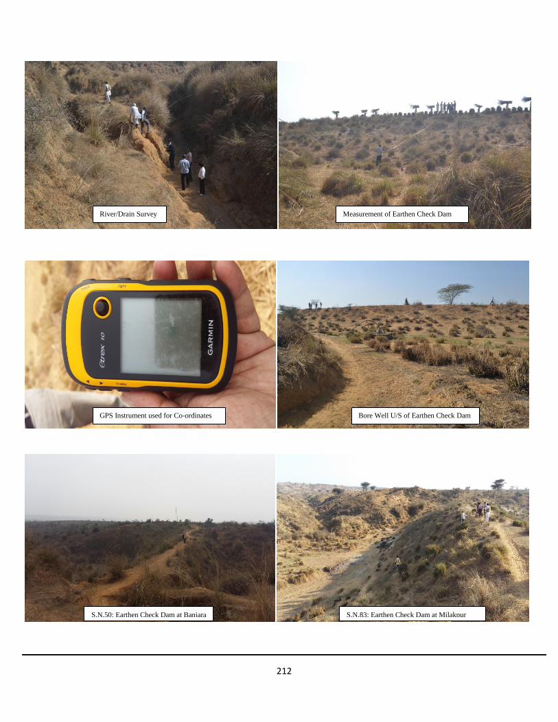
212
S.N.50: Earthen Check Dam at Banjara
River/Drain Survey Measurement of Earthen Check Dam
Bore Well U/S of Earthen Check Dam GPS Instrument used for Co-ordinates
S.N.83: Earthen Check Dam at Milakpur

213
S.N.52: Showing Measurement and Extensive
Agriculture along Earthen Check Dam at Banjara S.N.53: Stone Mine at Nimbahedi
S.N.30: River at Milakpur Turk S.N.37: Earthen Check Dam at Bhaleshwar
Agriculture in River Bed Agriculture U/S of Earthen Check
Dam

214
Detail of earthen check dams/other WHS in the catchment of existing dams
S.N. Location Detail
Co-ordinates Approximate Capacity
Latitude Longitude Nos. L W H Quantity
(CUM)
Quantity
(mcft) 1 Johad, Jhundpuri 28005'36.70" 76050'12.2" 1 50 35 2.25 3937.5 0.139
2 deep excavation mitiya was 28004'44.95" 76050'45.05" 1 40 150 3 18000 0.636
3 deep excavation mitiya was 28004'44.71" 76050'47.28" 1 60 25 2.25 3375 0.119
4 deep excavation mitiya was 28004'52.9" 76050'54.7" 1 70 20 2 2800 0.099
5 old johad bubkahera 28004'42" 76051'22.4" 1 25 25 2 1250 0.044
6 old johad dholi pahadi 28004'3.9" 76052'59.6" 1 110 90 1.5 14850 0.524
7 old johad bhalesar 28004'13.9" 76054'1.7" 1 40 40 3 4800 0.169
8 E.C.D. ubaraka 28004'26.3" 76053'19.1" 1 100 20 4 8000 0.282
2 200 10 1 4000 0.141
9 E.C.D. ubaraka 28004'35.9" 76053'40.4" 1 55 30 4 6600 0.233
11 E.C.D. 1 150 10 4 6000 0.212
10 E.C.D. bhalesar 28004'36.2" 76053'50.1" 1 60 30 1.75 3150 0.111
11 E.C.D. ubaraka 28004'54" 76053'52.5" 1 100 20 3 6000 0.212
12 E.C.D. ubaraka 28004'52" 76053'56.6" 1 80 80 3.5 22400 0.791
1 200 25 2 10000 0.353
13 E.C.D. bhalesar 28004'47.2" 76054'7.4" 1 200 20 2.5 10000 0.353
14 E.C.D. bhalesar 28004'52.2" 76054'6.8" 1 150 30 2 9000 0.318
15 E.C.D. bhalesar 28004'47.9" 76054'1" 1 200 10 1.5 3000 0.106
16 E.C.D. ubaraka 28004'57.7" 76053'48.4" 1 30 25 2 1500 0.053
17 old johad ubaraka 28004'49.2" 76053'45.2" 1 150 150 2 45000 1.589
18 E.C.D. ubaraka 28005'2.5" 76053'37.7" 2 100 10 2 4000 0.141
19 E.C.D. ubaraka 28005'4.3" 76053'38.4" 1 200 20 3 12000 0.424
20 E.C.D. ubaraka 28005'5.5" 76053'42.9" 1 300 30 1 9000 0.318
21 E.C.D. gwalda 28005'10.2" 76053'47.3" 1 100 20 2 4000 0.141
1 300 20 2 12000 0.424
22 E.C.D. gwalda 28005'12.8" 76053'39.4" 1 40 20 3 2400 0.085
1 100 10 2 2000 0.071
23 E.C.D. ubaraka 28005'1.1" 76053'52.6" 1 40 20 1.5 1200 0.042
24 E.C.D. bhalesar 28004'53.8" 76054'14.9" 1 250 20 3 15000 0.530
25 E.C.D. bhalesar 28005'4.8" 76054'12.2" 1 120 20 2 4800 0.169
1 150 10 2 3000 0.106
1 60 30 3 5400 0.191
26 E.C.D. bhalesar 28004'39.7" 76054'44.2" 1 300 40 2 24000 0.847
27 E.C.D. bhalesar 28004'29.5" 76054'54.7" 2 200 10 3 12000 0.424
28 E.C.D. bhalesar 28004'28.7" 76054'51.6" 1 50 10 1.5 750 0.026
29 E.C.D. milakpur turk 28004'28.7" 76054'50.4" 1 100 10 2 2000 0.071
30 E.C.D. milakpur turk 28004'24.3" 76054'48" 1 100 10 2 2000 0.071
31 E.C.D. milakpur turk 28004'20.5" 76054'54.3" 1 100 20 2 4000 0.141
32 E.C.D. milakpur turk 28004'19.7" 76054'55.6" 1 30 5 1 150 0.005
33 E.C.D. milakpur turk 28004'21.1" 76054'1.3" 1 100 10 3 3000 0.106
34 E.C.D. bhalesar 28004'33.2" 76055'2.5" 2 100 10 2 4000 0.141
35 E.C.D. gwalda 28005'31.7" 76053'44.8" 1 70 100 1.5 10500 0.371
36 old johad patla ki dhani gwalda 28005'49.3" 76053'9.1" 1 60 150 1 9000 0.318
37 E.C.D. gwalda patla ki dhani 28005'36.6" 76053'5.5" 1 60 30 3 5400 0.191
1 250 40 1 10000 0.353
38 E.C.D. gwalda 28005'27.2" 76053'6.4" 1 60 60 2.5 9000 0.318
1 150 20 1.5 4500 0.159

215
1 200 10 1.5 3000 0.106
39 E.C.D. gwalda 28005'29.3" 76053'13.4" 1 200 200 1.5 60000 2.119
40 E.C.D. gwalda supheda ki dhani 28005'17" 76054'16" 1 40 40 1 1600 0.056
41 E.C.D. gwalda supheda ki dhani 28005'12.1" 76054'15.5" 1 100 5 3 1500 0.053
1 40 30 3 3600 0.127
42 E.C.D. gwalda 28005'11.8" 76054'20.3" 1 100 10 4 4000 0.141
1 70 20 4 5600 0.198
43 E.C.D. gwalda ghamandi ki dhani 28005'9.2" 76054'26.6" 1 60 40 4 9600 0.339
1 150 20 3 9000 0.318
44 E.C.D. gwalda ghamandi ki dhani 28005'17.6" 76054'22.7" 1 30 10 3 900 0.032
1 20 10 3 600 0.021
45 E.C.D. banjhda 28005'24.9" 76054'35.9" 1 40 30 1.5 1800 0.064
1 150 10 1 1500 0.053
46 E.C.D. banjhda 28005'17.8" 76054'38.5" 1 60 30 4 7200 0.254
1 170 10 2 3400 0.120
47 E.C.D. banjhda 28005'13.7" 76054'44" 1 40 30 4 4800 0.169
1 200 20 3 12000 0.424
48 E.C.D. banjhda 28005'17.2" 76054'55.6" 1 50 30 4 6000 0.212
1 150 20 2 6000 0.212
1 200 20 2 8000 0.282
49 E.C.D. banjhda 28005'24.1" 76054'49.9" 1 60 10 3 1800 0.064
1 100 5 2 1000 0.035
1 20 10 2 400 0.014
50 deep excavated mines nimbahedi 28005'49.1" 76052'24" 1 200 100 15 300000 10.593
51 johad nakhnoal 28006'23.7" 76051'42.8" 1 60 40 1 2400 0.085
52 anicut nimbaheri 28006'0.1" 76051'53.1" 1 50 30 1.5 2250 0.079
53 Stone Mine nimbaheri 28005'59.8" 76052'3.4" 1 70 150 1.5 15750 0.556
54 E.C.D. nimbaheri 28005'59.4" 76052'11" 1 50 100 1.3 6500 0.230
55 anicut nimbaheri 28006'2.9" 76052'18.1" 1 80 20 1 1600 0.056
56 E.C.D. nimbaheri 28006'6.3" 76052'15.8" 1 50 10 1.5 750 0.026
2 100 10 1.5 3000 0.106
57 deep excavated mines, Nakh. 28005'57.3" 76052'0.6" 1 60 40 4 9600 0.339
58 johad milakpur turk 28003'35.4" 76053'38.9" 1 30 30 2 1800 0.064
59 E.C.D. bhalesar 28004'0.1" 76053'56.9" 1 50 5 1 250 0.009
60 E.C.D. bhalesar hyat ki dhani 28003'57.7" 76054'1.9" 1 40 10 2 800 0.028
1 50 5 1 250 0.009
61 E.C.D. Milakpur turk 28004'8.4" 76054'15.1" 1 150 40 2 12000 0.424
1 150 10 1 1500 0.053
62 E.C.D. milakpur turk chonchpuri 28004'8.7" 76054'41.5" 1 60 20 2 2400 0.085
63 E.C.D. milakpur turk chonchpuri 28004'6.6" 76054'53.9" 1 100 40 4 16000 0.565
1 200 15 2 6000 0.212
64 E.C.D. milakpur turk chonchpuri 28004'4" 76054'53.3" 1 100 10 2 2000 0.071
65 E.C.D. milakpur turk chonchpuri 28004'8.2" 76055'4.7" 2 100 10 1.5 3000 0.106
66 E.C.D. milakpur turk chonchpuri 28004'1.9" 76054'44.1" 2 50 5 1.5 750 0.026
67 E.C.D. milakpur turk chonchpuri 28004'0.1" 76054'52.9" 1 300 15 3 13500 0.477
1 50 5 2 500 0.018
68 E.C.D. milakpur turk chonchpuri 28004'4" 76054'30.4" 1 200 15 3 9000 0.318
69 E.C.D. milakpur turk 28003'33" 76053'55.3" 1 150 50 3.5 26250 0.927
1 300 40 2 24000 0.847
70 E.C.D. milakpur turk 28003'27.4" 76054'47.4" 1 40 20 3 2400 0.085

216
2 150 15 2 9000 0.318
71 E.C.D. milakpur turk 28003'33" 76054'42.5" 2 150 12 2 7200 0.254
72 E.C.D. milakpur turk 28003'30.8" 76054'40.2" 1 50 10 1.5 750 0.026
73 E.C.D. milakpur turk 28003'36.8" 76054'37.6" 1 150 30 3 13500 0.477
74 E.C.D. milakpur turk 28003'25.7" 76054'16.1" 1 50 30 1.5 2250 0.079
75 E.C.D. milakpur turk 28003'11.4" 76053'53.9" 1 70 20 2 2800 0.099
1 50 20 1.5 1500 0.053
76 E.C.D. milakpur turk 28003'10.7" 76054'24" 1 100 40 1.5 6000 0.212
77 E.C.D. milakpur turk 28003'11.4" 76054'37" 1 80 40 3 9600 0.339
1 150 20 2 6000 0.212
1 100 10 1 1000 0.035
78 E.C.D. milakpur turk 28003'3.4" 76055'1.4" 1 60 40 3 7200 0.254
2 100 5 1 1000 0.035
1 200 20 2 8000 0.282
79 E.C.D. milakpur turk 28002'57" 76054'37.5" 1 300 25 3 22500 0.794
80 E.C.D. milakpur turk 28002'53.9" 76054'34.9" 2 200 20 3 24000 0.847
2 100 5 2 2000 0.071
81 E.C.D. milakpur turk 28003'1.6" 76054'31.9" 2 150 10 2 6000 0.212
82 E.C.D. milakpur turk 28002'58.3" 76054'26" 1 100 10 2 2000 0.071
83 E.C.D. milakpur turk 28003'4.3" 76053'43.8" 1 40 80 1 3200 0.113
84 E.C.D. milakpur turk 28002'53.5" 76053'53.3" 1 500 40 2 40000 1.412
85 E.C.D. milakpur turk 28002'40.4" 76054'16.6" 2 150 10 2 6000 0.212
1 40 50 3 6000 0.212
86 E.C.D. milakpur turk 28002'45.8" 76054'28.2" 2 60 10 1 1200 0.042
1 300 50 1 15000 0.530
87 E.C.D. milakpur turk 28002'47.1" 76054'32.1" 1 30 30 1 900 0.032
88 E.C.D. milakpur turk 28002'49.1" 76054'38.4" 1 40 10 1 400 0.014
89 E.C.D. milakpur turk 28002'49.1" 76054'44.4" 2 75 5 1 750 0.026
90 E.C.D. milakpur turk 28002'45.5" 76054'45" 1 100 30 1 3000 0.106
91 E.C.D. milakpur turk 28002'35.5" 76054'27.2" 1 40 60 1 2400 0.085
92 E.C.D. milakpur turk 28002'32" 76054'15.1" 1 50 20 2 2000 0.071
93 E.C.D. milakpur turk 28002'32.5" 76054'11.2" 1 20 10 2 400 0.014
1 100 10 1 1000 0.035
94 E.C.D. milakpur turk 28002'39.7" 76054'0.4" 1 50 40 2 4000 0.141
1 200 25 1.5 7500 0.265
95 E.C.D. milakpur turk 28002'45.2" 76053'53" 1 100 50 2.5 12500 0.441
1 150 30 1 4500 0.159
2 100 10 1 2000 0.071
96 E.C.D. milakpur turk 28002'44.3" 76053'46.1" 1 30 20 1 600 0.021
1 50 5 1 250 0.009
97 E.C.D. milakpur turk 28002'44.9" 76053'45.3" 1 100 20 2.25 4500 0.159
98 E.C.D. milakpur turk 28002'56.9" 76053'36.3" 1 40 30 1.25 1500 0.053
1 50 5 1.25 312.5 0.011
99 E.C.D. dholi pahadi 28004'14.5" 76053'4.6" 1 40 20 1 800 0.028
100 E.C.D. dholi pahadi 28004'16.2" 76052'53.7" 1 45 20 1.5 1350 0.048
1 50 15 1 750 0.026
101 E.C.D. patan khurd 28003'31.9" 76052'42.8" 1 30 20 20 12000 0.424
102 E.C.D. patan khurd 28003'35.5" 76052'15.7" 1 100 40 0.75 3000 0.106
103 E.C.D. patan khurd 28003'32.9" 76052'17.1" 1 125 20 1.5 3750 0.132
104 E.C.D. dholi pahadi 28004'4.7" 76052'7.2" 1 300 50 2 30000 1.059
TOTAL 45.203
E.C.D.= Earthen Check Dam

217
Appendix-11 Some actual site photographs showing the changes in LULC in the
catchment areas of dams
„(a) (b)
„(c) (d)
„(e) (f)
Figure showing several of abstractions within the catchment of dams (a) Agricultural
activity (b) Infrastructural development: road (c) Poor drainage at developed area:
obstructing the flow of water to natural drainage (d & e) Forest development activities:
CVH & DCB (f) Small water harvesting structures within the catchment of dams.
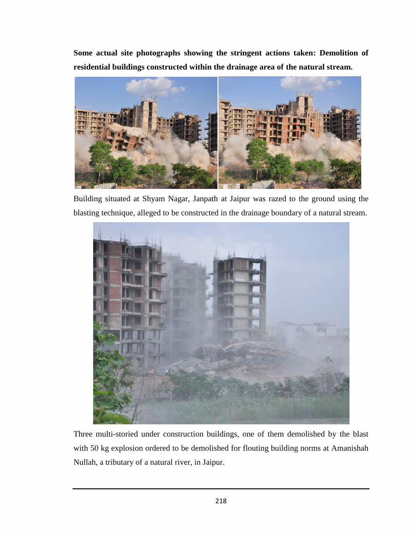
218
Some actual site photographs showing the stringent actions taken: Demolition of
residential buildings constructed within the drainage area of the natural stream.
Building situated at Shyam Nagar, Janpath at Jaipur was razed to the ground using the
blasting technique, alleged to be constructed in the drainage boundary of a natural stream.
Three multi-storied under construction buildings, one of them demolished by the blast
with 50 kg explosion ordered to be demolished for flouting building norms at Amanishah
Nullah, a tributary of a natural river, in Jaipur.

219
AUTHOR’S BIO-DATA
The author obtained his Bachelor‟s degree in Civil Engineering from MBM Engineering
College, Jodhpur in the year 1995 and Master‟s degree in Structural Engineering from
MNIT, Jaipur in 2011. Author has also obtained Master‟s degree in Business
Administration (MBA) from Indira Gandhi National Open University, New Delhi in the
year 2004. Author has been working as a water resources engineer since 1996. The author
has been designated as Chartered Engineer (India) by Institution of Engineers (India),
Kolkata. The author is presently working as Executive Engineer, Water Resources
Department of Government of Rajasthan. Previously, the author has worked as Assistant
Engineer and Junior Engineer in various engineering departments of Government of
Rajasthan. The author is also in the expert panel of Engineering Staff Training Institute,
Jaipur, which imparts training to the engineers of various government departments.
List of publications are as follows:
1. Gupta N.K., Jethoo A.S., and Gupta S.K. (2016). “Rainfall and Surface Water
Resources of Rajasthan State,” Water Policy Journal. IWA Publishing, Volume
18(2016), pp. 276-287.
2. Gupta, S.K., Sharma, G., Jethoo, A.S., Tyagi, J., Gupta, N.K. (2015). “A Critical
Review of Hydrological Models.” HYDRO 2015 International, IIT Roorkee, India,
17-19 December 2015, 20th International Conference on Hydraulics, Water
Resources and River Engineering
3. Gupta, S.K., Jethoo, A.S., Tyagi, J., Gupta, N.K., and Gautam, P.(2015).
“Application of Hydrological Models in Water Resources: A Review.”
International Journal of Computer &Mathematical Sciences, Vol. 4 (Sp.), March
2015, pp. 94-100.
4. Jethoo, A.S., Sharma, G., Gupta, N.K., and Gupta, S.K. (2015). “Temporal
Variation of Water Inflow to Bisalpur Dam- A threat to Water Management of
The Rajasthan State.” All India Symposium on Golden Jubilee, Civil Engineering
Department, MNIT, Jaipur
5. Gupta, N.K., and Jethoo, A.S. (2014). “Declining Trend of Water Inflow to the
dams of Rajasthan State.” International Journal of Technology, IJTech 2014 (1),
pp.14-21.
6. Gupta, N.K., Mathur, P., Jethoo, A.S. (2014). “Feasibility Analysis for
Construction of New Dams in Rajasthan State.” Proceedings of International
Symposium on Dams in Global Environmental Challenges, International
Commission on Large Dams (ICOLD), Bali, Indonesia, June 1th-6th, 2014.
7. Gupta, N.K., Jethoo, A.S., and Pandel, B., (2014). “Declining Trend of Water

220
Inflow in Bisalpur Dam: A Threat to Environmental Sustainability.” National
Seminar on Technological Advances & Their Impact on Environment, April 22,
2014 (NSTAIE-2014/36).
8. Gupta, N.K., Gupta, S.K., and Jethoo, A.S. (2014). “Hydrological Modeling of
Ramgarh Dam of Rajasthan State Using Soil and Water Assessment Tool
(SWAT).” Proceedings of 4th International Conference on Hydrology and
Watershed Management, Centre for Water Resources, Institute of Science and
Technology, JNTU, Telangana State, India, PP. 985-995.
9. Gupta, N.K., and Jethoo, A.S. (2013). “Helpline for Water Leakages- A Solution
to the Water Crisis.”Proceedings India Water Week-2013, Efficient Water
Management: Challenges and Opportunities Ministry of Water Resources,
Government of India, 8-12 April 2013, PP. 190
Research Papers under Review:
1. Gupta, N.K., and Jethoo, A.S. “Transboundary Management of Surplus Water in a
River Basin -A Case Study of Sabarmati River Basin in Rajasthan.” J. of
Institution of Engineers (India): Series A, Springer.
Copyright © 2022 FDOKUMEN