Temporal variability of a benthic food web: Patterns and processes in a low-diversity system

MARINE ECOLOGY PROGRESS SERIESMar Ecol Prog Ser

Vol. 378: 13–26, 2009doi: 10.3354/meps07872

Published March 12

INTRODUCTION

The food web remains a focal point in ecology as acentral part of the description of ecosystems and inter-actions between species within a community. Althoughoften portrayed as such, the links in a food web are farfrom static, but vary in time and space (McCann et al.2005). Temporal changes in food web interactions canbe prominent in aquatic systems due to variation in thebiotic and abiotic factors structuring the web (Polis etal. 1996, Riera & Richard 1997, Straile 2005). One of themajor challenges in food web studies is to incorporateand interpret variation in community and food webdynamics (McCann et al. 2005, Akin & Winemiller2006, Winemiller et al. 2007). In temperate environ-ments, a seasonal change in primary production is pro-nounced and the zoobenthic community consequently

shows succession patterns in structure and trophicinteractions along the production season (Möller et al.1985, Blomqvist & Bonsdorff 1986). Generalist con-sumers can switch between food sources as the preyspecies change in availability and profitability withinthe habitat, and may thereby stabilize trophic dynam-ics (McCann et al. 2005).

Stable isotope analysis has become an essential toolfor ecologists (Peterson & Fry 1987, Fry 2006), function-ing as ‘short, medium and long-term recorders forecological processes’ (West et al. 2006). Whereasstomach/gut content analysis provides a snapshot ofingested food objects, stable isotope analysis depictswhat has been digested and assimilated by the organ-ism and whether seasonal changes in diet are mani-fested on the tissue level of an organism. The use ofδ13C and δ15N in trophic interaction studies rely on the

© Inter-Research 2009 · www.int-res.com*Email: [email protected]

Temporal variability of a benthic food web:patterns and processes in a low-diversity system

Marie Nordström*, Katri Aarnio, Erik Bonsdorff

Environmental and Marine Biology, Åbo Akademi University, BioCity, Artillerigatan 6, 20520 Åbo, Finland

ABSTRACT: Trophic interactions are not static links, but are dynamic both in space and time. In tem-perate environments, seasonal patterns in primary production may be pronounced and, hence, thezoobenthic community and the trophic couplings within it change during the main production sea-son. We assessed temporal variability in a benthic food web using stable isotope ratios of C and N.Organisms belonging to 3 trophic levels, producers (e.g. macroalgae and vascular plants), primaryconsumers (macrozoobenthos) and secondary consumers (epibenthic fishes and Crangon crangon),were sampled monthly in a shallow soft-substrate habitat in the northern Baltic Sea. The studyfocused on intra-seasonal (main production period from June to September 2005) and inter-annual(comparing data collected in June of 2 consecutive years) variability of trophic interactions involvingphyto- and zoobenthos. Intra-seasonal changes in stable isotope ratios of food web componentsoccurred both on a horizontal (within a trophic level) and a vertical scale (between trophic levels).Generally, unimodal patterns were evident, with enrichment of 13C and depletion of 15N occurringduring the production period. The fluctuation in stable isotope values over the season decreased withincreasing trophic level. Predator stable isotope values are probably affected by changes at the baseof the food web and changes in consumer diet. The intra-seasonal pattern, together with limitedinterannual variability, indicates a temporally stable food web structure.

KEY WORDS: Epibenthic predators · Functional diversity · Benthic macrofauna · Trophicrelationships · Soft substrate · Stable isotopes · δ13C · δ15N

Resale or republication not permitted without written consent of the publisher

Mar Ecol Prog Ser 378: 13–26, 2009

assumption of specific fractionation of the isotopes.The δ13C value of an organism provides an estimate ofthe energy source through a miniscule enrichmentover trophic levels, 0 to 1‰, whereas δ15N indicates thetrophic position of an organism as its isotope value isenriched by 3 to 4‰ relative to that of the diet (Peter-son & Fry 1987). Thus, dual isotope analysis describesprocesses in the food web, as well as functions as atracer. The actual fractionation can vary between spe-cies and habitats (Vander Zanden & Rasmussen 2001),and nitrogen fractionation may, in fact, be closer to 2‰(McCutchan et al. 2003).

The isotopic composition of primary producers maychange several times during a year, e.g. plankton inthe Baltic Sea exhibit bimodal (δ13C) and trimodal(δ15N) distributions (Rolff 2000). Apart from speciesturnover, changes in temperature and inorganic nutri-ent concentrations affect plankton stable isotope val-ues within and between seasons (Goering et al. 1990,Sato et al. 2006). This kind of variation is not restrictedto autotrophs, but can, after an eventual time lag, bemirrored in higher trophic levels (Goering et al. 1990,Vizzini & Mazzola 2003). Stable isotope values of ani-mal tissues are influenced by tissue turnover time,temperature, individual size, and health condition orstarvation (Yokoyama et al. 2005, Guelinckx et al.2007). Changes in isotope values can also occur overan individual’s life span according to seasonal or onto-genetic shifts in diet. Temporal fluctuations in stableisotopes are easily detectable in small species withhigh tissue turnover. Large individuals and long-livedspecies show isotope values representative of a longertime (up to months or a year, Hesslein et al. 1993) and,thus, respond more slowly to fluctuations in the iso-topic signature of food items. Temporal variability instable isotope values has been reported for zooplank-ton (Rolff 2000), benthic invertebrates (Riera & Richard1997, Vizzini & Mazzola 2003) and fish (Sarà et al.2002, Vizzini & Mazzola 2003).

Whereas several studies have revealed differencesin δ13C and δ15N between seasons, only rarely has thevariation of stable isotope values within a season orover the main production period been assessed (butsee Goering et al. 1990, Riera & Richard 1997, Rolff2000). The literature regarding benthic primary andsecondary consumers is particularly scarce for this sub-ject. Although spatial variation in stable isotopes is rec-ognized (Deegan & Garritt 1997, Hansson et al. 1997,Norkko et al. 2007), we suggest that it is equally neces-sary to acknowledge temporal variability (Akin &Winemiller 2006) and its possible implications for theinterpolation and extrapolation power of results fromstable isotope studies that sample on a limited timescale (e.g. few sampling events, or even a singleevent).

The prime objective of our study was to evaluate thevariability in benthic food web structure over the mainproduction season. This was undertaken by assessingtemporal changes in the ratios of stable isotopes, 13C:12Cand 15N:14N, of organisms belonging to 3 trophic levels:producers, primary consumers and secondary con-sumers of a shallow, coastal, soft-bottom habitat in thenorthern Baltic Sea. We were particularly interested in(1) intra-seasonal variability (over the main productionperiod, June to September 2005) and (2) inter-annualvariability (comparing June 2005 with June 2006) ofphyto- and zoobenthos (focusing on benthic inverte-brates and fishes). The present study aimed to elucidatethe temporal variation of trophic interactions on both ahorizontal scale (within a trophic level) and a verticalscale (between trophic levels) in the food web.

MATERIALS AND METHODS

Study site and organisms. Our study site (60° 10’ N,19° 32’ E, Åland Islands, northern Baltic Sea) is a shal-low (mean depth, 2.5 m), exposed, sandy bay. Sub-strate organic content is low (0.1%, as determined byloss on ignition, 3 h at 500°C). Water temperature was12.0 to 12.5°C in June (both years) and September2005. In July and August 2005, the temperature was17.0 and 19.0°C, respectively. Salinity in this part of theBaltic Sea is 5 to 7.

The low species number in this area allows us tostudy most of the numerically or functionally importantspecies of this particular habitat; in all, 21 species areincluded in this study. This biotope, shallow sandy sub-strate, provides a suitable model system for studyingtemporal changes in marine coastal food webs. Theeastern part of the bay is characterized as bare sandwhile the western part is vegetated from 1 to 5 m depth(Boström & Bonsdorff 2000). The soft-bottom vegeta-tion consists of meadows of Zostera marina L. and Rup-pia maritima L. as well as Potamogeton spp. and Zan-nichellia spp. (Boström & Bonsdorff 2000). Apart fromthe sandy substrate dominating the bay, rocks are alsopresent, supplying substrate for the annual filamen-tous algae, Cladophora glomerata (L.) Kützing, Pylai-ella littoralis (L.) Kjellman/Ectocarpus siliculosus (Dill-wyn) Lyngbye and Ceramium tenuicorne (Kützing)Waern, and the perennial macroalga Fucus vesiculo-sus L. Drift algae are common in the bight during theproduction season. Drift algal assemblages vary inspecies composition during summer but are usuallyconglomerates of filamentous brown, red and greenalgal species (P. littoralis/E. siliculosus, C. tenuicorne,C. glomerata) (Holmström 1998).

Shallow sandy bottoms are important nursery andfeeding grounds for juvenile flatfishes, such as Pla-

14

Nordström et al.: Temporal variability of a benthic food web

tichthys flesus L. and Scophthalmus maximus L., andother epibenthic predators, e.g. Crangon crangon L.and Pomatoschistus minutus Pallas (Bonsdorff & Blom-qvist 1993, Aarnio et al. 1996) (see Table 1). Macomabalthica L., Nereis diversicolor (syn. Hediste diversi-color) Müller and Bathyporeia pilosa Lindström belongto the dominant infauna in this habitat, and constituteimportant food sources for epibenthic predators. SeeBoström & Bonsdorff (2000) for information on otherbenthic invertebrate fauna characteristic of the site.

Organism sampling. Sampling was conducted 4times during 2005 (June 14, July 28, August 22 andSeptember 26) and once in 2006 (June 29) to collectorganisms for analysis of the stable isotope ratios,13C:12C and 15N:14N. Infaunal invertebrates were sam-pled with a shovel and a bucket sieve (1 mm mesh) atabout 1 m depth. Macrophytes and sediment weresampled through snorkeling and SCUBA diving, whiledrift algae were collected with a net. Samples of sedi-ment organic matter (ca. 2 cm surface sediment) werecollected from 1 and 4 m depths using a core. Epiben-thic predators such as fish and Crangon crangon werecollected using a beach seine (4 mm mesh net with2 mm mesh bag) and a push net (2 mm mesh). Plank-tonic matter was collected from the water column with90 µm mesh and 10 µm mesh nets. Additionally,unsieved seawater was collected.

Stable isotope analyses. Macrophytes were rinsed infiltered (20 µm) seawater and cleared of any remainingassociated biota by hand under a stereomicroscope.Epiphytes were collected from Fucus vesiculosus.Infaunal macroinvertebrates were identified to speciesor group level and put in filtered seawater for aminimum of 12 h for clearance of gut contents. Thesizes of all individuals were measured, and in the caseof juvenile Platichthys flesus, 2 size groups were ana-lyzed separately (size limit, 46 mm at which P. flesusswitches from meiofaunal to macrofaunal diet). Allsamples were stored frozen (–20°C) until they wereoven-dried (60°C, 48 h) and ground to a fine powderusing a mortar and pestle. Aliquots were packed into6 × 8 mm tin capsules for subsequent analysis. All fau-nal samples consisted of several whole individuals,except fish and crustacean samples that consisted ofmuscle tissue alone. Mollusc samples were obtainedby removing the soft tissue from the shells. Planktonicmatter was filtered through pre-combusted (500°C,4 h) Whatman GF/C or GF/F glass fiber filters. Filterswere dried, quickly acidified with 1 M HCl and driedagain. We aimed at minimizing HCl treatment of theother samples to avoid a negative influence on stableisotope values. The effects of acidification of samplesare contentious; several studies have documented thatacid treatment affects δ13C but not δ15N, or affects both(Jacob et al. 2005, Søreide et al. 2006). C and N stable

isotope ratios were determined at the Stable IsotopeFacility (University of California, Davis, California),using a Europa Scientific Hydra 20/20 continuous flowisotope ratio mass spectrometer. Stable isotope signa-tures are reported in delta (δ) notation in units of permille (‰) according to:

δ13C or δ15N = [(Rsample/Rstandard – 1)] × 103 (1)

where R is 13C:12C or 15N:14N. The standards for C andN are Vienna-PDB and atmospheric N2, respectively(Fry 2006).

Trophic positioning. Trophic positioning relative toa common baseline allows for evaluation of trophicstructure using δ15N signatures (Cabana & Rasmussen1996, Vander Zanden & Rasmussen 1999, Post 2002).Unionid mussels are useful in providing baseline δ15Nvalues for limnic food web studies (Post 2002). We usedthe measured δ15N of the tellinid bivalve Macomabalthica as our reference value. The bivalve is a facul-tative active suspension feeder and surface depositfeeder (Ólafsson 1986), giving us a δ15N baseline inte-grating pelagic as well as benthic production. The δ15Nvalues of M. balthica were compared with those of theobligate filter feeder Mytilus edulis L. (monthly datafrom 3 simultaneous sampling events, M. Nordström,K. Aarnio, E. Bonsdorff unpubl. data) to test for poten-tial effects of facultative feeding or filter feeding onnitrogen isotopic ratio. No statistically significant dif-ference was found between the species (2-wayANOVA, main factor ‘Species’: df = 1, MS = 0.071, F =0.410, p = 0.530, error df = 18). The interactionbetween Species and Month was also non-significant(n = 4), and as M. balthica is a key species in our studyarea and constitutes an important food object withinthe benthic food web, we estimated the species to be asuitable reference for predator trophic positions in thisparticular study. Trophic position for consumers wascalculated as following:

Trophic position = λ + (δ15Nconsumer – δ15Nbase)/Δn (2)

where λ is the trophic level of the organism used toestablish δ15Nbase (in the present study the primaryconsumer, i.e. trophic level = 2), δ15Nconsumer is mea-sured directly, and Δn is the enrichment in δ15N pertrophic level (in this study, 3.6‰ according to the esti-mate based on our data).

Statistical analyses. Multivariate analyses were per-formed to reveal natural groupings in the data accord-ing to time. Non-metric multidimensional scaling(nMDS) and cluster analyses were performed usingBray-Curtis similarity coefficients based on means ofstable isotope values (δ13C or δ15N). One-way ANOVAs(factor ‘month’ or ‘species’) were performed to deter-

15


mine species-specific changes in stable isotope valuesduring the main production season and inter-specificdifferences for particular sampling occasions. Two-way mixed model ANOVAs (factors ‘Species’ and‘Year’, fixed and random, respectively) were per-formed groupwise (primary producers, primary con-sumers, secondary consumers) on stable isotope datato determine inter-annual changes in isotopes andinter-specific patterns. Linear regression with δ15N as afunction of predator length was performed to estimatethe effect of consumer body size on trophic position.Prior to analyses, the data were tested for normalityand homogeneity of variances and log transformed ifnot meeting the assumptions. Transformation was notsuccessful in all cases, and data subsequently wereanalyzed using the non-parametric Kruskal-Wallistest. All values are reported as mean ± SE unlessdefined otherwise.

Modeling. Using the IsoSource mass balance model(Phillips & Gregg 2003), we estimated intra-seasonalchanges in relative contribution of 3 abundant benthicinvertebrate species, Macoma balthica,Nereis diversicolor and Bathyporeiapilosa, to the diet of 2 epibenthic preda-tors, Platichthys flesus and Crangoncrangon. Based on species δ13C andδ15N values (mean for each month andmean for total season), IsoSource deliv-ered feasible proportions (0 to 100%) ofprey species accounting for the targetmixture (predator value). The sourceincrement was set to 1% and the lowestpossible mass balance tolerance (0.01 to1.10) supplying solutions was used. Noadditional constraints were used.IsoSource estimates based on δ13C val-ues only required somewhat lower tol-erance levels and the results from thisanalysis are compared with diet esti-mates based on dual isotope analysis.

RESULTS

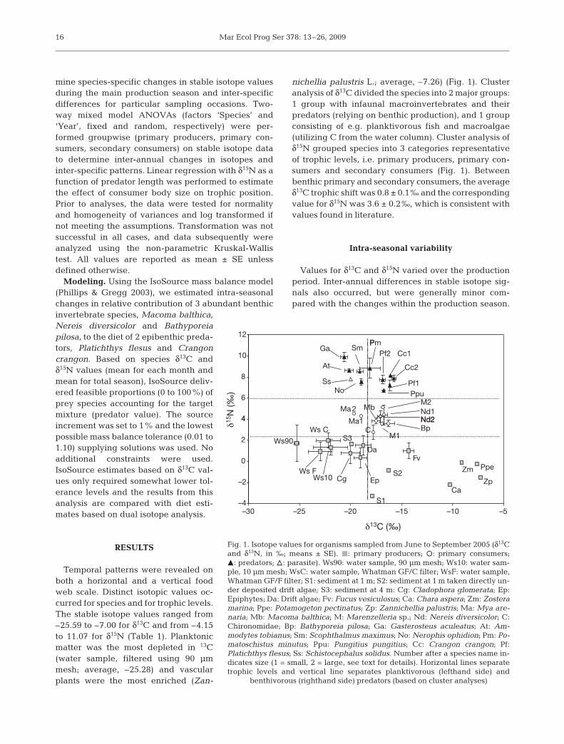
Temporal patterns were revealed onboth a horizontal and a vertical foodweb scale. Distinct isotopic values oc-curred for species and for trophic levels.The stable isotope values ranged from–25.59 to –7.00 for δ13C and from –4.15to 11.07 for δ15N (Table 1). Planktonicmatter was the most depleted in 13C(water sample, filtered using 90 µmmesh; average, –25.28) and vascularplants were the most enriched (Zan-

nichellia palustris L.; average, –7.26) (Fig. 1). Clusteranalysis of δ13C divided the species into 2 major groups:1 group with infaunal macroinvertebrates and theirpredators (relying on benthic production), and 1 groupconsisting of e.g. planktivorous fish and macroalgae(utilizing C from the water column). Cluster analysis ofδ15N grouped species into 3 categories representativeof trophic levels, i.e. primary producers, primary con-sumers and secondary consumers (Fig. 1). Betweenbenthic primary and secondary consumers, the averageδ13C trophic shift was 0.8 ± 0.1‰ and the correspondingvalue for δ15N was 3.6 ± 0.2‰, which is consistent withvalues found in literature.

Intra-seasonal variability

Values for δ13C and δ15N varied over the productionperiod. Inter-annual differences in stable isotope sig-nals also occurred, but were generally minor com-pared with the changes within the production season.

16

12P

4

6

8

10

At

Ga

Ppu

Pf1

Pf2

No

PmSm

Cc1

Cc2

Ma 2

Nd2Nd1

M2Mb

Ss

–2

0

2

4

Ws90

Cg

Fv

Ep

Da

PpeZm

Ws C

Ws F Ws10

S2

CaZp

S3

Ma1

M1BpC

Nd2

–4–30 –25 –20 –15 –10 –5

δ13C (‰)

δ15N

(‰

)

S1

Fig. 1. Isotope values for organisms sampled from June to September 2005 (δ13Cand δ15N, in ‰; means ± SE). j: primary producers; s: primary consumers;m: predators; n: parasite). Ws90: water sample, 90 µm mesh; Ws10: water sam-ple, 10 µm mesh; WsC: water sample, Whatman GF/C filter; WsF: water sample,Whatman GF/F filter; S1: sediment at 1 m; S2: sediment at 1 m taken directly un-der deposited drift algae; S3: sediment at 4 m: Cg: Cladophora glomerata; Ep:Epiphytes; Da: Drift algae; Fv: Fucus vesiculosus; Ca: Chara aspera; Zm: Zosteramarina; Ppe: Potamogeton pectinatus; Zp: Zannichellia palustris; Ma: Mya are-naria; Mb: Macoma balthica; M: Marenzelleria sp.; Nd: Nereis diversicolor; C:Chironomidae; Bp: Bathyporeia pilosa; Ga: Gasterosteus aculeatus; At: Am-modytes tobianus; Sm: Scophthalmus maximus; No: Nerophis ophidion; Pm: Po-matoschistus minutus; Ppu: Pungitius pungitius; Cc: Crangon crangon; Pf:Platichthys flesus; Ss: Schistocephalus solidus. Number after a species name in-dicates size (1 = small, 2 = large, see text for details). Horizontal lines separatetrophic levels and vertical line separates planktivorous (lefthand side) and

benthivorous (righthand side) predators (based on cluster analyses)


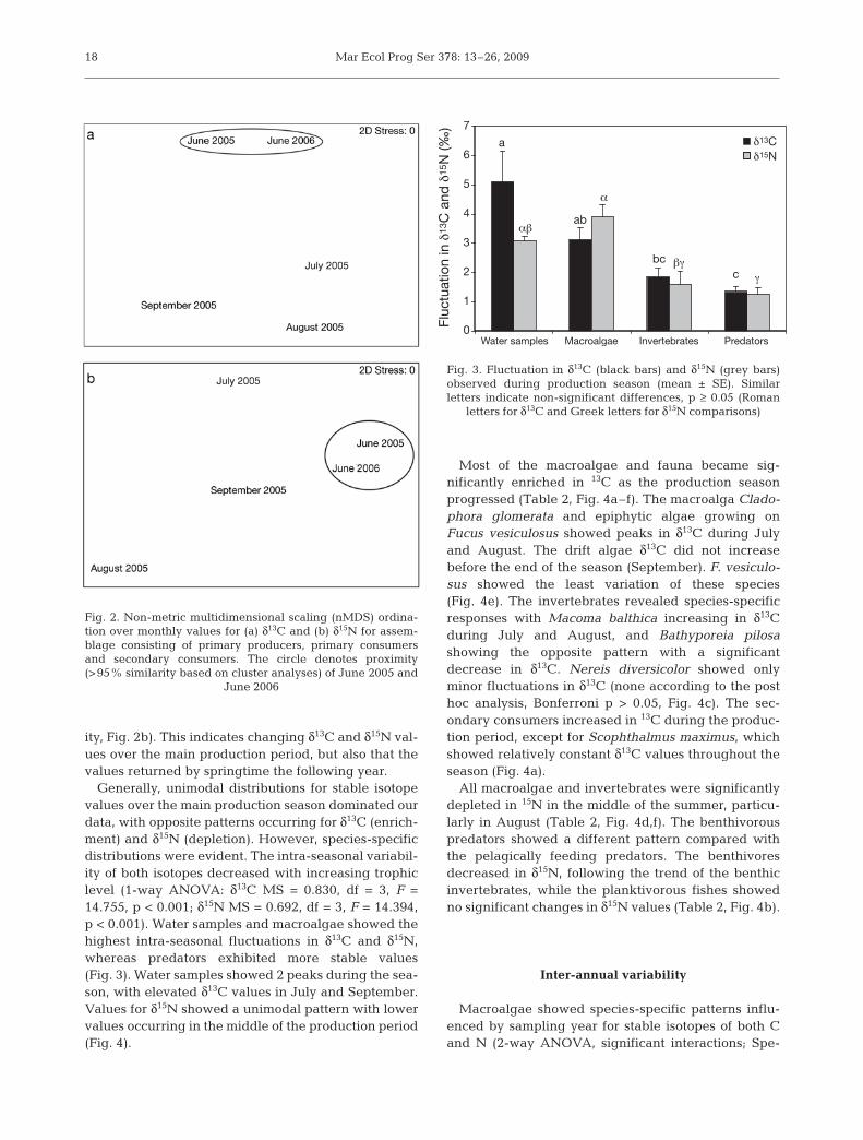
The δ13C values recorded in early summer differedfrom the other sampling dates (nMDS and clusteranalysis, in which June 2005 and June 2006 showedthe highest level of separation from other months; sim-

ilarity > 96%, Fig. 2a). Values for δ15N revealed a dif-fering temporal pattern as August was singled out fromthe other months. June 2005 and June 2006 stillshowed highest resemblance for δ15N (>95% similar-

17

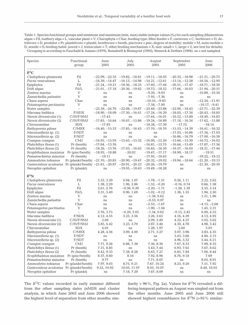
Table 1. Species functional groups and minimum and maximum (min, max) stable isotope values (‰) for each sampling (filamentousalgae = Fil, leathery alga = L, vascular plant = V, Charophyta = Char; feeding type: filter-feeder = F, carnivore = C, herbivore = H, de-tritivore = D, predator = Pr, planktivore = plankt, benthivore = benth, piscivore = pisc; degree of mobility: mobile = M, semi-mobile =D, sessile = S; feeding habit: jawed = J, tentaculate = T, other feeding mechanism = X; size: small = 1, large = 2, see text for details).

Grouping is according to Fauchald & Jumars (1979), Bonsdorff & Blomqvist (1993), Steneck & Dethier (1994). ns = not sampled

Species Functional June July August September June group 2005 2005 2005 2005 2006

δδ13CCladophora glomerata Fil –22.99, –22.35 –19.82, –18.81 –19.11, –18.05 –20.35, –18.98 –21.51, –20.75Fucus vesiculosus L –16.39, –14.47 –16.13, –14.98 –14.21, –12.61 –15.14, –12.28 –16.54, –12.95Epiphytes Fil –21.24, –19.21 –18.56, –18.33 –17.60, –17.46 –20.51, –17.47 –18.71, –18.50Drift algae Fil/L –21.01, –17.18 –20.36, –19.82 –19.73, –18.52 –17.66, –16.03 –21.94, –20.51Zostera marina V ns ns –9.20, –9.03 ns –10.89, –10.50Zannichellia palustris V ns ns –7.95, –7.36 ns nsChara aspera Char ns ns –10.55, –9.83 ns –12.34, –11.91Potamogeton pectinatus V ns ns –7.58, –7.00 ns –10.17, –9.41Water samples – –25.59, –24.70 –22.08, –19.87 –25.48, –23.88 –22.00, –18.45 –23.71, –22.39Macoma balthica F/SDX –18.90, –18.09 –17.30, –16.61 –17.24, –16.29 –18.05, –17.34 –20.43, –18.85Nereis diversicolor (1) C/H/F/SMJ –17.43 ns –17.44, –16.01 –16.52, –15.89 –18.49, –16.83Nereis diversicolor (2) C/H/F/SMJ –17.85, –16.64 –16.67, –15.86 –19.24, –16.89 –17.18, –16.34 –17.62, –15.88Chironomidae SDX –17.83 ns –18.28, –17.30 –17.72 –18.14Bathyporeia pilosa C/MSX –16.40, –15.33 –17.85, –16.43 –17.70, –16.70 –15.53, –14.39 –16.41, –16.32Marenzelleria sp. (1) F/SDT ns ns ns –17.03, –16.86 –17.34, –17.03Marenzelleria sp. (2) F/SDT ns ns ns –16.86, –16.79 –17.00, –16.58Crangon crangon CMJ –16.91, –15.93 –15.65, –15.32 –16.09, –15.20 –15.66, –15.30 –16.72, –16.02Platichthys flesus (1) Pr (benth) –17.64, –13.76 ns –16.81, –15.75 –16.64, –15.49 –17.87, –17.56Platichthys flesus (2) Pr (benth) –18.26, –13.76 –17.03, –16.62 –16.85, –16.50 –16.57, –16.05 –18.31, –17.44Scophthalmus maximus Pr (pisc/benth) –18.93, –18.88 –20.02 –19.47, –17.17 –18.99, –18.17 –19.51Pomatoschistus minutus Pr (benth) –19.11 ns –17.95, –16.65 ns –19.22, –19.12Ammodytes tobianus Pr (plankt/benth) –21.70, –20.85 –20.90, –19.47 –20.32, –19.02 –19.94, –18.64 –21.20, –19.13Gasterosteus aculeatus Pr (plankt/benth) –21.61, –20.87 –20.91, –20.23 –20.26, –19.79 ns –21.30, –20.50Nerophis ophidion Pr (plankt) ns –19.05, –18.63 –19.49, –18.28 ns ns

δδ15NCladophora glomerata Fil 2.55, 3.29 0.94, 1.07 –1.78, –1.51 0.26, 1.11 2.22, 2.62Fucus vesiculosus L 1.38, 2.29 1.96, 2.86 –1.52, –0.20 –0.16, 0.74 0.66, 1.58Epiphytes Fil 2.61, 2.76 –0.56, 0.39 –2.20, –1.71 –1.28, 1.39 2.55, 3.14Drift algae Fil/L 3.31, 5.49 0.96, 1.69 –1.02, –0.12 1.38, 1.55 1.94, 2.50Zostera marina V ns ns –1.38, 0.62 ns 1.51, 1.96Zannichellia palustris V ns ns –0.53, 0.07 ns nsChara aspera Char ns ns –2.53, –1.67 ns –4.15, –2.68Potamogeton pectinatus V ns ns –1.90, –1.04 ns 1.45, 2.31Water samples – 2.76, 3.75 –0.20, 3.05 –1.34, 0.62 –0.15, 2.42 0.00, 4.55Macoma balthica F/SDX 4.12, 4.55 3.23, 3.56 3.26, 3.65 4.16, 4.39 4.13, 4.93Nereis diversicolor (1) C/H/F/SMJ 5.69 ns 2.09, 3.49 4.32, 4.57 5.02, 5.62Nereis diversicolor (2) C/H/F/SMJ 5.85, 6.42 3.23, 3.70 2.87, 3.46 4.30, 4.78 4.98, 5.42Chironomidae SDX 4.05 ns 1.28, 1.97 2.60 3.03Bathyporeia pilosa C/MSX 4.28, 4.56 3.09, 4.00 2.71, 3.27 3.07, 3.96 3.83, 4.35Marenzelleria sp. (1) F/SDT ns ns ns 3.43, 3.66 4.84, 5.15Marenzelleria sp. (2) F/SDT ns ns ns 4.96, 5.32 5.44, 6.21Crangon crangon CMJ 7.71, 9.26 6.88, 7.38 7.56, 8.36 7.67, 8.33 7.09, 8.35Platichthys flesus (1) Pr (benth) 7.31, 8.85 ns 5.43, 7.44 6.93, 7.65 7.67, 8.62Platichthys flesus (2) Pr (benth) 8.42, 9.33 7.58, 8.28 6.63, 7.27 6.85, 7.84 7.06, 8.44Scophthalmus maximus Pr (pisc/benth) 8.37, 8.60 8.16 7.92, 8.96 8.76, 9.18 7.69Pomatoschistus minutus Pr (benth) 9.77 ns 7.71, 8.07 ns 8.05, 8.91Ammodytes tobianus Pr (plankt/benth) 7.97, 9.03 8.75, 9.21 7.67, 10.24 8.25, 9.20 7.51, 7.92Gasterosteus aculeatus Pr (plankt/benth) 9.52, 10.92 10.05, 11.07 8.05, 10.07 ns 8.48, 10.05Nerophis ophidion Pr (plankt) ns 7.18, 7.29 7.67, 8.09 ns ns


ity, Fig. 2b). This indicates changing δ13C and δ15N val-ues over the main production period, but also that thevalues returned by springtime the following year.

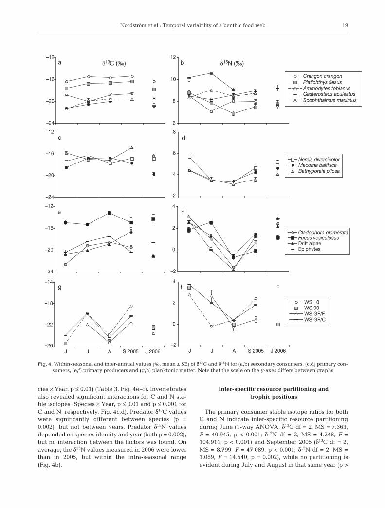
Generally, unimodal distributions for stable isotopevalues over the main production season dominated ourdata, with opposite patterns occurring for δ13C (enrich-ment) and δ15N (depletion). However, species-specificdistributions were evident. The intra-seasonal variabil-ity of both isotopes decreased with increasing trophiclevel (1-way ANOVA: δ13C MS = 0.830, df = 3, F =14.755, p < 0.001; δ15N MS = 0.692, df = 3, F = 14.394,p < 0.001). Water samples and macroalgae showed thehighest intra-seasonal fluctuations in δ13C and δ15N,whereas predators exhibited more stable values(Fig. 3). Water samples showed 2 peaks during the sea-son, with elevated δ13C values in July and September.Values for δ15N showed a unimodal pattern with lowervalues occurring in the middle of the production period(Fig. 4).

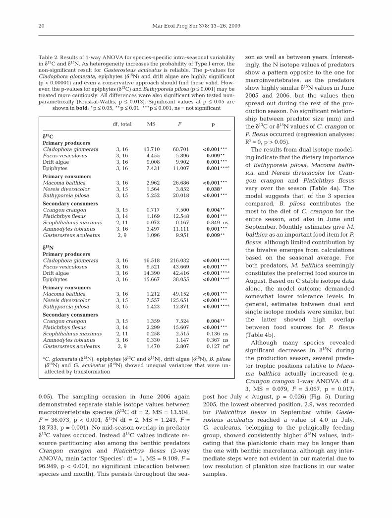
Most of the macroalgae and fauna became sig-nificantly enriched in 13C as the production seasonprogressed (Table 2, Fig. 4a–f). The macroalga Clado-phora glomerata and epiphytic algae growing onFucus vesiculosus showed peaks in δ13C during Julyand August. The drift algae δ13C did not increasebefore the end of the season (September). F. vesiculo-sus showed the least variation of these species(Fig. 4e). The invertebrates revealed species-specificresponses with Macoma balthica increasing in δ13Cduring July and August, and Bathyporeia pilosashowing the opposite pattern with a significantdecrease in δ13C. Nereis diversicolor showed onlyminor fluctuations in δ13C (none according to the posthoc analysis, Bonferroni p > 0.05, Fig. 4c). The sec-ondary consumers increased in 13C during the produc-tion period, except for Scophthalmus maximus, whichshowed relatively constant δ13C values throughout theseason (Fig. 4a).

All macroalgae and invertebrates were significantlydepleted in 15N in the middle of the summer, particu-larly in August (Table 2, Fig. 4d,f). The benthivorouspredators showed a different pattern compared withthe pelagically feeding predators. The benthivoresdecreased in δ15N, following the trend of the benthicinvertebrates, while the planktivorous fishes showedno significant changes in δ15N values (Table 2, Fig. 4b).

Inter-annual variability

Macroalgae showed species-specific patterns influ-enced by sampling year for stable isotopes of both Cand N (2-way ANOVA, significant interactions; Spe-

18

Fig. 2. Non-metric multidimensional scaling (nMDS) ordina-tion over monthly values for (a) δ13C and (b) δ15N for assem-blage consisting of primary producers, primary consumersand secondary consumers. The circle denotes proximity(>95% similarity based on cluster analyses) of June 2005 and

June 2006

0

1

2

3

4

5

6

7

Water samples Macroalgae Invertebrates Predators

a

αβ

βγγ

α

ab

bc

c

Flu

ctu

atio

n in δ

13C

and

δ1

5N

(‰

)

δ13C

δ15N

Fig. 3. Fluctuation in δ13C (black bars) and δ15N (grey bars)observed during production season (mean ± SE). Similarletters indicate non-significant differences, p ≥ 0.05 (Roman

letters for δ13C and Greek letters for δ15N comparisons)


cies × Year, p ≤ 0.01) (Table 3, Fig. 4e–f). Invertebratesalso revealed significant interactions for C and N sta-ble isotopes (Species × Year, p ≤ 0.01 and p ≤ 0.001 forC and N, respectively, Fig. 4c,d). Predator δ13C valueswere significantly different between species (p =0.002), but not between years. Predator δ15N valuesdepended on species identity and year (both p = 0.002),but no interaction between the factors was found. Onaverage, the δ15N values measured in 2006 were lowerthan in 2005, but within the intra-seasonal range(Fig. 4b).

Inter-specific resource partitioning and trophic positions

The primary consumer stable isotope ratios for bothC and N indicate inter-specific resource partitioningduring June (1-way ANOVA: δ13C df = 2, MS = 7.363,F = 40.945, p < 0.001; δ15N df = 2, MS = 4.248, F =104.911, p < 0.001) and September 2005 (δ13C df = 2,MS = 8.799, F = 47.089, p < 0.001; δ15N df = 2, MS =1.089, F = 14.540, p = 0.002), while no partitioning isevident during July and August in that same year (p >

19

–24

–20

–16

–12a δ13C (‰) δ15N (‰)

6

8

10

12

Crangon crangonPlatichthys flesusAmmodytes tobianusGasterosteus aculeatusScophthalmus maximus

b

–24

–20

–16

–12c

2

4

6

8

Nereis diversicolorMacoma balthicaBathyporeia pilosa

d

–24

–20

–16

–12e

–2

0

2

4

Cladophora glomerataFucus vesiculosusDrift algaeEpiphytes

f

–26

–22

–18

–14

J J A S 2005 J 2006

g

–2

0

2

4

J J A S 2005 J 2006

WS 10WS 90WS GF/FWS GF/C

h

Fig. 4. Within-seasonal and inter-annual values (‰, mean ± SE) of δ13C and δ15N for (a,b) secondary consumers, (c,d) primary con-sumers, (e,f) primary producers and (g,h) planktonic matter. Note that the scale on the y-axes differs between graphs


0.05). The sampling occasion in June 2006 againdemonstrated separate stable isotope values betweenmacroinvertebrate species (δ13C df = 2, MS = 13.504,F = 36.073, p < 0.001; δ15N df = 2, MS = 1.243, F =18.733, p = 0.001). No mid-season overlap in predatorδ13C values occured. Instead δ13C values indicate re-source partitioning also among the benthic predatorsCrangon crangon and Platichthys flesus (2-wayANOVA, main factor ‘Species’: df = 1, MS = 9.109, F =96.949, p < 0.001, no significant interaction betweenspecies and month). This persists throughout the sea-

son as well as between years. Interest-ingly, the N isotope values of predatorsshow a pattern opposite to the one formacroinvertebrates, as the predatorsshow highly similar δ15N values in June2005 and 2006, but the values thenspread out during the rest of the pro-duction season. No significant relation-ship between predator size (mm) andthe δ13C or δ15N values of C. crangon orP. flesus occurred (regression analyses:R2 ≈ 0, p > 0.05).

The results from dual isotope model-ing indicate that the dietary importanceof Bathyporeia pilosa, Macoma balth-ica, and Nereis diversicolor for Cran-gon crangon and Platichthys flesusvary over the season (Table 4a). Themodel suggests that, of the 3 speciescompared, B. pilosa contributes themost to the diet of C. crangon for theentire season, and also in June andSeptember. Monthly estimates give M.balthica as an important food item for P.flesus, although limited contribution bythe bivalve emerges from calculationsbased on the seasonal average. Forboth predators, M. balthica seeminglyconstitutes the preferred food source inAugust. Based on C stable isotope dataalone, the model outcome demandedsomewhat lower tolerance levels. Ingeneral, estimates between dual andsingle isotope models were similar, butthe latter showed high overlapbetween food sources for P. flesus(Table 4b).

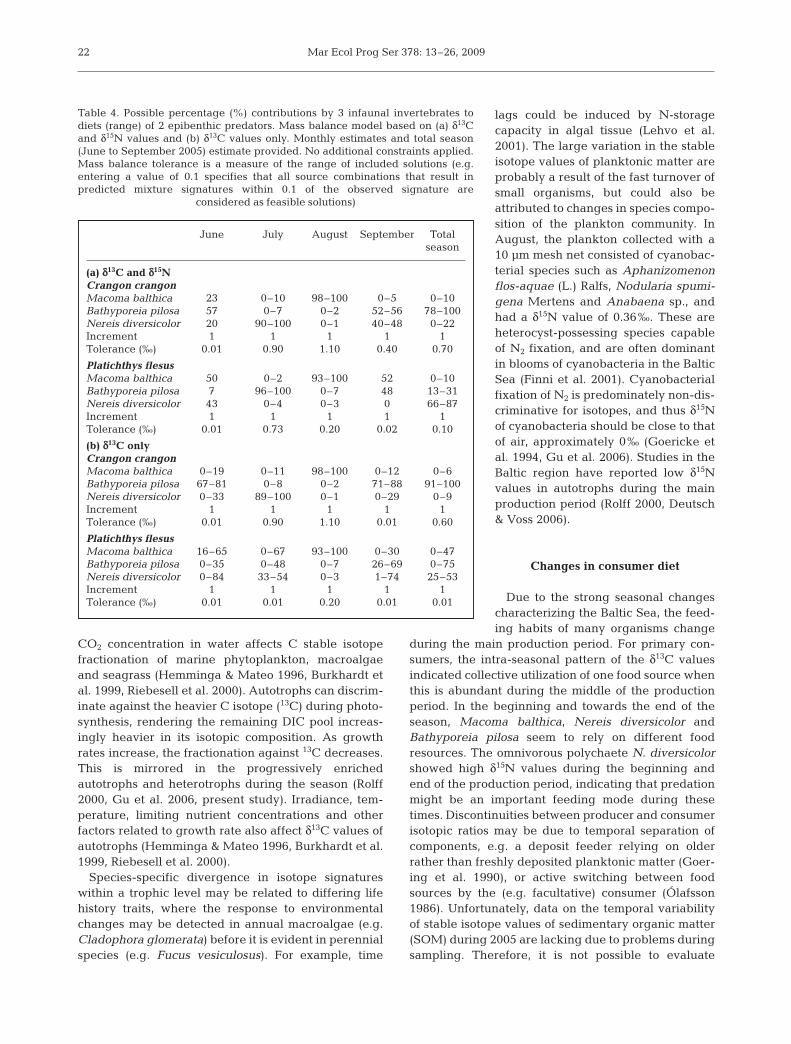
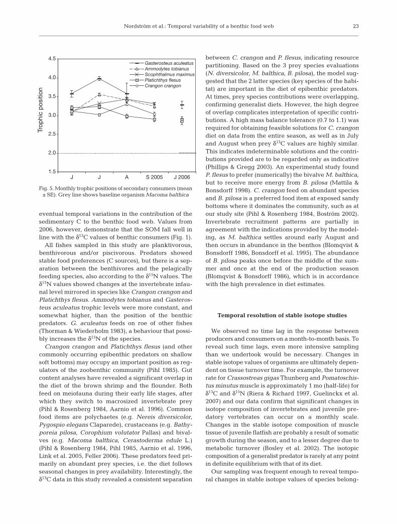
Although many species revealedsignificant decreases in δ15N duringthe production season, several preda-tor trophic positions relative to Maco-ma balthica actually increased (e.g.Crangon crangon 1-way ANOVA: df =3, MS = 0.079, F = 5.067, p = 0.017;

post hoc July < August, p = 0.026) (Fig. 5). During2005, the lowest observed position, 2.9, was recordedfor Platichthys flesus in September while Gaste-rosteus aculeatus reached a value of 4.0 in July.G. aculeatus, belonging to the pelagically feedinggroup, showed consistently higher δ15N values, indi-cating that the planktonic chain may be longer thanthe one with benthic macrofauna, although any inter-mediate steps were not evident in our material due tolow resolution of plankton size fractions in our watersamples.

20

Table 2. Results of 1-way ANOVA for species-specific intra-seasonal variabilityin δ13C and δ15N. As heterogeneity increases the probability of Type I error, thenon-significant result for Gasterosteus aculeatus is reliable. The p-values forCladophora glomerata, epiphytes (δ15N) and drift algae are highly significant(p < 0.00001) and even a conservative approach should find these valid. How-ever, the p-values for epiphytes (δ13C) and Bathyporeia pilosa (p ≤ 0.001) may betreated more cautiously. All differences were also significant when tested non-parametrically (Kruskal-Wallis, p ≤ 0.013). Significant values at p ≤ 0.05 are

shown in bold; *p ≤ 0.05, **p ≤ 0.01, ***p ≤ 0.001, ns = not significant

df, total MS F p

δδ13CPrimary producersCladophora glomerata 3, 16 13.710 60.701 <0.001***Fucus vesiculosus 3, 16 4.455 5.896 0.009**Drift algae 3, 16 9.008 9.902 0.001***Epiphytes 3, 16 7.431 11.007 0.001***a

Primary consumersMacoma balthica 3, 16 2.962 26.686 <0.001***Nereis diversicolor 3, 15 1.564 3.852 0.038*Bathyporeia pilosa 3, 15 5.252 20.018 <0.001***

Secondary consumersCrangon crangon 3, 15 0.717 7.500 0.004**Platichthys flesus 3, 14 1.169 12.548 0.001***Scophthalmus maximus 2, 11 0.073 0.167 0.849 nsAmmodytes tobianus 3, 16 3.497 11.111 0.001***Gasterosteus aculeatus 2, 9 1.096 9.951 0.009**

δδ15NPrimary producersCladophora glomerata 3, 16 16.518 216.032 <0.001***a

Fucus vesiculosus 3, 16 9.521 43.669 <0.001***Drift algae 3, 16 14.390 42.416 <0.001***a

Epiphytes 3, 16 15.667 38.055 <0.001***a

Primary consumersMacoma balthica 3, 16 1.212 49.152 <0.001***Nereis diversicolor 3, 15 7.557 125.651 <0.001***Bathyporeia pilosa 3, 15 1.423 12.871 <0.001***a

Secondary consumersCrangon crangon 3, 15 1.359 7.524 0.004**Platichthys flesus 3, 14 2.299 15.607 <0.001***Scophthalmus maximus 2, 11 0.258 2.515 0.136 nsAmmodytes tobianus 3, 16 0.330 1.147 0.367 nsGasterosteus aculeatus 2, 9 1.470 2.807 0.127 nsa

aC. glomerata (δ15N), epiphytes (δ13C and δ15N), drift algae (δ15N), B. pilosa(δ15N) and G. aculeatus (δ15N) showed unequal variances that were un-affected by transformation


DISCUSSION

Our study revealed that trophic interactions variedwithin season and that temporal patterns in isotopiccomposition were applicable to food web componentswithin, as well as across, trophic levels, even up to sec-ondary consumers. The indications of changes in inter-specific resource partitioning found in our study are ofinterest regarding species with similar function ortrophic flexibility.

Temporal variability of coastal food web components

The temporal patterns observed in our study are con-sistent with Rolff (2000), who found bimodal (δ13C) andtrimodal (δ15N) distributions in size-fractionated plank-ton sampled during a year, and the peaks and lows

reported by Rolff (2000) occurred at similar time inter-vals as those observed in our study. However, seasonalcomparisons in some other studies have revealed con-tradictory patterns. Higher δ13C values in summercompared with other seasons has been found formacrophytes and macroalgae, benthic invertebratesand fish (Hentschel 1998, Kang et al. 1999, Sarà et al.2002, Vizzini & Mazzola 2003), but depleted valueshave also been observed (Goering et al. 1990, Carlieret al. 2007). We found that δ15N values generallydecrease over the season, as Carlier et al. (2007) alsodiscovered, but Vizzini & Mazzola (2003) could notidentify any evident trend for nitrogen. Quarterly sam-pling occasions seldom provide unambiguous informa-tion on temporal changes in food web structure,whereas a more intense frequency of sampling sup-ports a more rigid description (e.g. Goering et al. 1990,Rolff 2000, the present study). The range observed byRolff (2000) for phytoplankton isotope values fromJune to September 1994 was about 7‰ for δ13C and5‰ for δ15N, whereas the corresponding fluctuationsin our study were approximately 5 and 3‰. Diurnalchanges in phytoplankton δ13C, e.g. coupled with lightconditions, are smaller (≤1.5‰, Burkhardt et al. 1999)than fluctuations occurring within a season. Differ-ences between winter and summer values for inverte-brate δ13C of roughly 3‰ have been reported (Vizzini& Mazzola 2003). In our study, maximum fluctuationsin macroinvertebrate δ13C were about 2‰. Thus, in-herent variability observable between or within sea-sons may be greater than the fractionation levels thatsupposedly define trophic structure (0 to 1‰ for δ13Cand 2 to 4‰ for δ15N), especially for C.

Our study revealed within-season changes on both ahorizontal and a vertical level in a coastal benthic foodweb. Possible mechanisms behind temporal variabilityin predator stable isotope values include (1) changesoccurring at the base of the food web that are mirroredin higher trophic levels, (2) changes occurring in con-sumer diet or (3) a combination of both (Wainright et al.1993).

Changes at the base of the food web

Short-lived autotrophs are affected by seasonalchanges in environmental factors to a greater extentthan are higher-level organisms (Cabana & Rasmussen1996). In our study, the variations observed over theseason were largest for primary producers. Thus, abi-otic factors are probably driving the patterns of enrich-ment of 13C (unimodal for macroalgae and bimodal forplanktonic matter) and a depletion of 15N (unimodal).Dissolved inorganic carbon (DIC) dynamics are impor-tant for the isotopic composition of producers, and the

21

Table 3. Two-factorial ANOVA for inter-annual changes(June 2005 and June 2006) in δ13C and δ15N of primary pro-ducers, primary consumers and secondary consumers. Sig-nificant values at p ≤ 0.05 are shown in bold; *p ≤ 0.05,

**p ≤ 0.01, ***p ≤ 0.001

Treatment df MS F p

Primary producersδδ13CSpecies 3 78.509 14.806 0.026*Year 1 2.398 0.452 0.549Species × Year 3 5.303 5.483 0.005**Error 24 0.967

δδ15NSpecies 3 3.826 3.029 0.194Year 1 3.962 3.136 0.175Species × Year 3 1.263 5.571 0.005**Error 24 0.227

Primary consumersδδ13CSpecies 2 19.375 11.998 0.077Year 1 1.017 0.631 0.510Species × Year 2 1.615 5.938 0.010**Error 19 0.272

δδ15NSpecies 2 4.591 6.923 0.126Year 1 0.808 1.220 0.384Species × Year 2 0.663 12.573 ≤≤0.001***Error 19 0.053

Secondary consumersδδ13CSpecies 3 42.870 98.248 0.002**Year 1 0.727 1.669 0.287Species × Year 3 0.436 1.74 0.187Error 23 0.251

δδ15NSpecies 3 4.810 81.666 0.002**Year 1 5.427 90.925 0.002**Species × Year 3 0.059 0.187 0.904Error 23 0.315


CO2 concentration in water affects C stable isotopefractionation of marine phytoplankton, macroalgaeand seagrass (Hemminga & Mateo 1996, Burkhardt etal. 1999, Riebesell et al. 2000). Autotrophs can discrim-inate against the heavier C isotope (13C) during photo-synthesis, rendering the remaining DIC pool increas-ingly heavier in its isotopic composition. As growthrates increase, the fractionation against 13C decreases.This is mirrored in the progressively enrichedautotrophs and heterotrophs during the season (Rolff2000, Gu et al. 2006, present study). Irradiance, tem-perature, limiting nutrient concentrations and otherfactors related to growth rate also affect δ13C values ofautotrophs (Hemminga & Mateo 1996, Burkhardt et al.1999, Riebesell et al. 2000).

Species-specific divergence in isotope signatureswithin a trophic level may be related to differing lifehistory traits, where the response to environmentalchanges may be detected in annual macroalgae (e.g.Cladophora glomerata) before it is evident in perennialspecies (e.g. Fucus vesiculosus). For example, time

lags could be induced by N-storagecapacity in algal tissue (Lehvo et al.2001). The large variation in the stableisotope values of planktonic matter areprobably a result of the fast turnover ofsmall organisms, but could also beattributed to changes in species compo-sition of the plankton community. InAugust, the plankton collected with a10 µm mesh net consisted of cyanobac-terial species such as Aphanizomenonflos-aquae (L.) Ralfs, Nodularia spumi-gena Mertens and Anabaena sp., andhad a δ15N value of 0.36‰. These areheterocyst-possessing species capableof N2 fixation, and are often dominantin blooms of cyanobacteria in the BalticSea (Finni et al. 2001). Cyanobacterialfixation of N2 is predominately non-dis-criminative for isotopes, and thus δ15Nof cyanobacteria should be close to thatof air, approximately 0‰ (Goericke etal. 1994, Gu et al. 2006). Studies in theBaltic region have reported low δ15Nvalues in autotrophs during the mainproduction period (Rolff 2000, Deutsch& Voss 2006).

Changes in consumer diet

Due to the strong seasonal changescharacterizing the Baltic Sea, the feed-ing habits of many organisms change

during the main production period. For primary con-sumers, the intra-seasonal pattern of the δ13C valuesindicated collective utilization of one food source whenthis is abundant during the middle of the productionperiod. In the beginning and towards the end of theseason, Macoma balthica, Nereis diversicolor andBathyporeia pilosa seem to rely on different foodresources. The omnivorous polychaete N. diversicolorshowed high δ15N values during the beginning andend of the production period, indicating that predationmight be an important feeding mode during thesetimes. Discontinuities between producer and consumerisotopic ratios may be due to temporal separation ofcomponents, e.g. a deposit feeder relying on olderrather than freshly deposited planktonic matter (Goer-ing et al. 1990), or active switching between foodsources by the (e.g. facultative) consumer (Ólafsson1986). Unfortunately, data on the temporal variabilityof stable isotope values of sedimentary organic matter(SOM) during 2005 are lacking due to problems duringsampling. Therefore, it is not possible to evaluate

22

Table 4. Possible percentage (%) contributions by 3 infaunal invertebrates todiets (range) of 2 epibenthic predators. Mass balance model based on (a) δ13Cand δ15N values and (b) δ13C values only. Monthly estimates and total season(June to September 2005) estimate provided. No additional constraints applied.Mass balance tolerance is a measure of the range of included solutions (e.g.entering a value of 0.1 specifies that all source combinations that result inpredicted mixture signatures within 0.1 of the observed signature are

considered as feasible solutions)

June July August September Total season

(a) δδ13C and δδ15NCrangon crangonMacoma balthica 23 0–10 98–100 0–5 0–10Bathyporeia pilosa 57 0–7 0–2 52–56 78–100Nereis diversicolor 20 90–100 0–1 40–48 0–22Increment 1 1 1 1 1Tolerance (‰) 0.01 0.90 1.10 0.40 0.70

Platichthys flesusMacoma balthica 50 0–2 93–100 52 0–10Bathyporeia pilosa 7 96–100 0–7 48 13–31Nereis diversicolor 43 0–4 0–3 0 66–87Increment 1 1 1 1 1Tolerance (‰) 0.01 0.73 0.20 0.02 0.10

(b) δδ13C onlyCrangon crangonMacoma balthica 0–19 0–11 98–100 0–12 0–6Bathyporeia pilosa 67–81 0–8 0–2 71–88 91–100Nereis diversicolor 0–33 89–100 0–1 0–29 0–9Increment 1 1 1 1 1Tolerance (‰) 0.01 0.90 1.10 0.01 0.60

Platichthys flesusMacoma balthica 16–65 0–67 93–100 0–30 0–47Bathyporeia pilosa 0–35 0–48 0–7 26–69 0–75Nereis diversicolor 0–84 33–54 0–3 1–74 25–53Increment 1 1 1 1 1Tolerance (‰) 0.01 0.01 0.20 0.01 0.01


eventual temporal variations in the contribution of thesedimentary C to the benthic food web. Values from2006, however, demonstrate that the SOM fall well inline with the δ13C values of benthic consumers (Fig. 1).

All fishes sampled in this study are planktivorous,benthivorous and/or piscivorous. Predators showedstable food preferences (C sources), but there is a sep-aration between the benthivores and the pelagicallyfeeding species, also according to the δ15N values. Theδ15N values showed changes at the invertebrate infau-nal level mirrored in species like Crangon crangon andPlatichthys flesus. Ammodytes tobianus and Gasteros-teus aculeatus trophic levels were more constant, andsomewhat higher, than the position of the benthicpredators. G. aculeatus feeds on roe of other fishes(Thorman & Wiederholm 1983), a behaviour that possi-bly increases the δ15N of the species.

Crangon crangon and Platichthys flesus (and othercommonly occurring epibenthic predators on shallowsoft bottoms) may occupy an important position as reg-ulators of the zoobenthic community (Pihl 1985). Gutcontent analyses have revealed a significant overlap inthe diet of the brown shrimp and the flounder. Bothfeed on meiofauna during their early life stages, afterwhich they switch to macrosized invertebrate prey(Pihl & Rosenberg 1984, Aarnio et al. 1996). Commonfood items are polychaetes (e.g. Nereis diversicolor,Pygospio elegans Claparede), crustaceans (e.g. Bathy-poreia pilosa, Corophium volutator Pallas) and bival-ves (e.g. Macoma balthica, Cerastoderma edule L.)(Pihl & Rosenberg 1984, Pihl 1985, Aarnio et al. 1996,Link et al. 2005, Feller 2006). These predators feed pri-marily on abundant prey species, i.e. the diet followsseasonal changes in prey availability. Interestingly, theδ13C data in this study revealed a consistent separation

between C. crangon and P. flesus, indicating resourcepartitioning. Based on the 3 prey species evaluations(N. diversicolor, M. balthica, B. pilosa), the model sug-gested that the 2 latter species (key species of the habi-tat) are important in the diet of epibenthic predators.At times, prey species contributions were overlapping,confirming generalist diets. However, the high degreeof overlap complicates interpretation of specific contri-butions. A high mass balance tolerance (0.7 to 1.1) wasrequired for obtaining feasible solutions for C. crangondiet on data from the entire season, as well as in Julyand August when prey δ13C values are highly similar.This indicates indeterminable solutions and the contri-butions provided are to be regarded only as indicative(Phillips & Gregg 2003). An experimental study foundP. flesus to prefer (numerically) the bivalve M. balthica,but to receive more energy from B. pilosa (Mattila &Bonsdorff 1998). C. crangon feed on abundant speciesand B. pilosa is a preferred food item at exposed sandybottoms where it dominates the community, such as atour study site (Pihl & Rosenberg 1984, Boström 2002).Invertebrate recruitment patterns are partially inagreement with the indications provided by the model-ing, as M. balthica settles around early August andthen occurs in abundance in the benthos (Blomqvist &Bonsdorff 1986, Bonsdorff et al. 1995). The abundanceof B. pilosa peaks once before the middle of the sum-mer and once at the end of the production season(Blomqvist & Bonsdorff 1986), which is in accordancewith the high prevalence in diet estimates.

Temporal resolution of stable isotope studies

We observed no time lag in the response betweenproducers and consumers on a month-to-month basis. Toreveal such time lags, even more intensive samplingthan we undertook would be necessary. Changes instable isotope values of organisms are ultimately depen-dent on tissue turnover time. For example, the turnoverrate for Crassostreas gigas Thunberg and Pomatoschis-tus minutus muscle is approximately 1 mo (half-life) forδ13C and δ15N (Riera & Richard 1997, Guelinckx et al.2007) and our data confirm that significant changes inisotope composition of invertebrates and juvenile pre-datory vertebrates can occur on a monthly scale.Changes in the stable isotope composition of muscletissue of juvenile flatfish are probably a result of somaticgrowth during the season, and to a lesser degree due tometabolic turnover (Bosley et al. 2002). The isotopiccomposition of a generalist predator is rarely at any pointin definite equilibrium with that of its diet.

Our sampling was frequent enough to reveal tempo-ral changes in stable isotope values of species belong-

23

1.5

2.0

2.5

3.0

3.5

4.0

4.5

J J A S 2005 J 2006

Tro

phic

po

sitio

n

Gasterosteus aculeatusAmmodytes tobianusScophthalmus maximusPlatichthys flesusCrangon crangon

Fig. 5. Monthly trophic positions of secondary consumers (mean ± SE). Grey line shows baseline organism Macoma balthica


ing to 3 trophic levels. One short sampling effort wouldprovide material depicting food web structure. Relyingon samples collected at different trophic levels at dif-ferent times during the main production period could,however, result in misinterpretation of relevant foodsources. Sample collection should be targeted accord-ing to the biology and ecology of the species. Also, asingle sampling event may leave temporal changes indiet unaccounted for, and the inclusion or exclusion oftemporal variability must be considered according tothe hypotheses in question. Stable isotope analysis is acomplement to, but not a replacement for, other foodweb study methods such as dietary data analysis andexperimental studies on trophic relationships (Wine-miller et al. 2007).

CONCLUSIONS

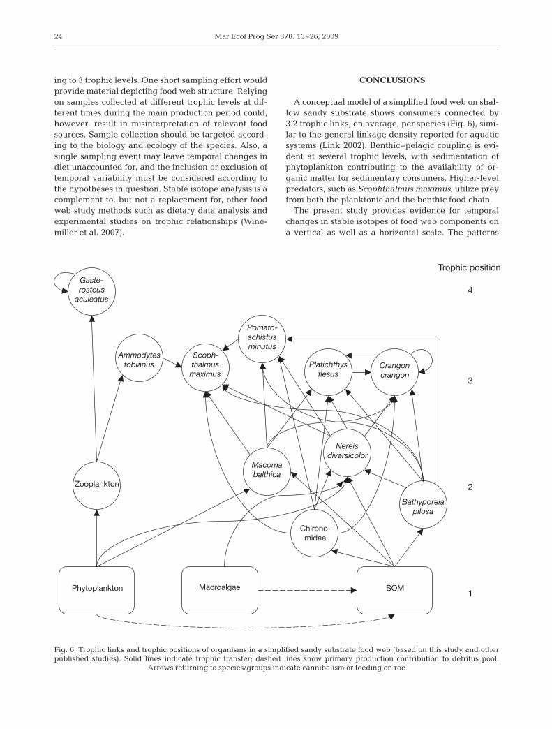
A conceptual model of a simplified food web on shal-low sandy substrate shows consumers connected by3.2 trophic links, on average, per species (Fig. 6), simi-lar to the general linkage density reported for aquaticsystems (Link 2002). Benthic–pelagic coupling is evi-dent at several trophic levels, with sedimentation ofphytoplankton contributing to the availability of or-ganic matter for sedimentary consumers. Higher-levelpredators, such as Scophthalmus maximus, utilize preyfrom both the planktonic and the benthic food chain.

The present study provides evidence for temporalchanges in stable isotopes of food web components ona vertical as well as a horizontal scale. The patterns

24

Trophic position

4

3

2

1Phytoplankton SOMMacroalgae

Chirono-midae

Bathyporeiapilosa

Zooplankton

Crangoncrangon

Nereisdiversicolor

Gaste-rosteus

aculeatus

Ammodytestobianus

Scoph-thalmusmaximus

Pomato-schistusminutus

Platichthysflesus

Macomabalthica

Fig. 6. Trophic links and trophic positions of organisms in a simplified sandy substrate food web (based on this study and otherpublished studies). Solid lines indicate trophic transfer; dashed lines show primary production contribution to detritus pool.

Arrows returning to species/groups indicate cannibalism or feeding on roe


indicate isotopic processes connected to the seasonal-ity of the abiotic factors driving production (Gu et al.2006). Changes in isotope ratios of higher-level organ-isms are probably due to changes occurring at the baseof the food web as well as changes in consumer diet.Benthic invertebrates showed a collective utilization ofone abundant food source, but inter-specific resourcepartitioning seems to occur otherwise (Fig. 4). Re-source partitioning was indicated also for epibenthicpredators. Generalist feeding is, however, characteris-tic for these species. Thus, there is a possibility foroverlaps in diet and trophic niche among benthicmacrofauna of the northern Baltic Sea, but the truewidth of feeding or functions may have remained hid-den during the conditions of this study.

Acknowledgements. The authors acknowledge the input pro-vided by R. I. Jones, A. Norkko and J. Norkko in stages ofplanning this study and writing the manuscript. We thank thereviewers, in particular B. T. Hentschel, whose input greatlyimproved this work. We are indebted to the staff and studentsat Husö Biological Station that helped with the fieldwork.J. Lindholm is thanked for his meticulous work in the labora-tory. Financial support was received from Stiftelsen för ÅboAkademi, Suomen Luonnonsuojelun Säätiö and Societas proFlora et Fauna Fennica.

LITERATURE CITED

Aarnio K, Bonsdorff E, Rosenback N (1996) Food and feedinghabits of juvenile flounder Platichthys flesus (L.), and tur-bot Scophthalmus maximus L. in the Åland archipelago,northern Baltic Sea. J Sea Res 36:311–320

Akin S, Winemiller KO (2006) Seasonal variation in food webcomposition and structure in a temperate tidal estuary.Estuar Coast 29:552–567

Blomqvist EM, Bonsdorff E (1986) Spatial and temporal varia-tions of benthic macrofauna in a sandbottom area onÅland, northern Baltic Sea. Ophelia Suppl 4:27–36

Bonsdorff E, Blomqvist EM (1993) Biotic couplings on shallowwater soft bottoms — examples from the northern BalticSea. Oceanogr Mar Biol Annu Rev 31:153–176

Bonsdorff E, Norkko A, Boström C (1995) Recruitment andpopulation maintenance of the bivalve Macoma balthica(L.) — factors affecting settling success and early survivalon shallow sandy bottoms. Proc 28th Eur Mar Biol Symp,Olsen and Olsen, Fredensborg, p 253–260

Bosley KL, Witting DA, Chambers C, Wainright SC (2002)Estimating turnover rates of carbon and nitrogen inrecently metamorphosed winter flounder Pseudopleu-ronectes americanus with stable isotopes. Mar Ecol ProgSer 236:233–240

Boström M (2002) Epibenthic predators and their prey —interactions in a coastal food web. PhD thesis, ÅboAkademi University

Boström C, Bonsdorff E (2000) Zoobenthic community estab-lishment and habitat complexity — the importance of sea-grass shoot-density, morphology and physical disturbancefor faunal recruitment. Mar Ecol Prog Ser 205:123–138

Burkhardt S, Riebesell U, Zondervan I (1999) Stable carbonisotope fractionation by marine phytoplankton in responseto daylength, growth rate and CO2 availability. Mar EcolProg Ser 184:31–41

Cabana G, Rasmussen JB (1996) Comparison of aquatic foodchains using nitrogen isotopes. Proc Natl Acad Sci USA93:10844–10847

Carlier A, Riera P, Amouroux JM, Bodiou JY and others (2007)A seasonal survey on the food web in the Lapalme Lagoon(northwestern Mediterranean) assessed by carbon andnitrogen stable isotope analysis. Estuar Coast Shelf Sci 73:299–315

Deegan LA, Garritt RH (1997) Evidence for spatial variabilityin estuarine food webs. Mar Ecol Prog Ser 147:31–47

Deutsch B, Voss M (2006) Anthropogenic nitrogen inputtraced by means of δ15N values in macroalgae: results fromin situ incubation experiments. Sci Total Environ 366:799–808

Fauchald K, Jumars P (1979) The diet of worms: a study ofpolychaete feeding guilds. Oceanogr Mar Biol Annu Rev17:193–284

Feller RJ (2006) Weak meiofaunal trophic linkages in Cran-gon crangon and Carcinus maenus. J Exp Mar Biol Ecol330:274–283

Finni T, Kononen K, Olsonen R, Wallström K (2001) Thehistory of cyanobacterial blooms in the Baltic Sea. Ambio30: 172–178

Fry B (2006) Stable isotope ecology. Springer, New YorkGoericke R, Montoya JP, Fry B (1994) Physiology of isotopic

fractionation in algae and cyanobacteria. In: Lajtha K,Mitchener RH (eds) Stable isotopes in ecology and environ-mental science. Blackwell Scientific, Oxford, p 187–221

Goering J, Alexander V, Haubenstock N (1990) Seasonal vari-ability of stable carbon and nitrogen isotope ratios oforganisms in a North Pacific bay. Estuar Coast Shelf Sci30:239–260

Gu B, Chapman A, Schelske C (2006) Factors controlling sea-sonal variations in stable isotope composition of particu-late organic matter in a soft water eutrophic lake. LimnolOceanogr 51:2837–2848

Guelinckx J, Maes J, Vand Den Driessche P, Geysen B,Dehairs F, Ollevier F (2007) Changes in δ13C and δ15N indifferent tissues of juvenile sand goby Pomatoschistusminutus: a laboratory diet-switch experiment. Mar EcolProg Ser 341:205–215

Hansson S, Hobbie JE, Elmgren R, Larsson U, Fry B, Johans-son S (1997) The stable nitrogen isotope ratio as a markerof food-web interactions and fish migration. Ecology 78:2249–2257

Hemminga MA, Mateo MA (1996) Stable carbon isotopes inseagrasses: variability in ratios and use in ecological stud-ies. Mar Ecol Prog Ser 140:285–298

Hentschel BT (1998) Intraspecific variations in δ13C indicateontogenetic diet changes in deposit-feeding polychaetes.Ecology 79:1357–1370

Hesslein RH, Hallard KA, Ramlal P (1993) Replacement of sul-fur, carbon, and nitrogen in tissue of growing broad white-fish (Coregonus nasus) in response to a change in diettraced by δ34S, δ13C, and δ15N. Can J Fish Aquat Sci 50:2071–2076

Holmström A (1998) Occurrence, species composition, bio-mass and decomposition of drifting algae in the north-western Åland archipelago, N. Baltic Sea. MSc thesis, ÅboAkademi University (in Swedish with English summary)

Jacob U, Mintenbeck K, Brey T, Knust R, Beyer K (2005) Sta-ble isotope food web studies: a case for standardized sam-ple treatment. Mar Ecol Prog Ser 287:251–253

Kang CK, Sauriau PG, Richard P, Blanchard GF (1999) Foodsources of an infaunal suspension-feeding bivalve Ceras-toderma edule in a muddy sandflat of Marennes-OléronBay, as determined by analyses of carbon and nitrogen

25


stable isotopes. Mar Ecol Prog Ser 187:147–158Lehvo A, Bäck S, Kiirikki M (2001) Growth of Fucus vesiculo-

sus L. (Phaeophyta) in the northern Baltic proper: energyand nitrogen storage in seasonal environment. Bot Mar44:345–350

Link J (2002) Does food web theory work for marine ecosys-tems? Mar Ecol Prog Ser 230:1–9

Link JS, Fogarty MJ, Langton RW (2005) The trophic ecologyof flatfishes. In: Gibson RN (ed) Flatfishes: biology andexploitation. Fish Aquat Resour Ser 9, Blackwell Publish-ing, Oxford, p 164–184

Mattila J, Bonsdorff E (1998) Predation by juvenile flounder(Platichthys flesus L.): a test of prey vulnerability, predatorpreference, switching behaviour and functional response.J Exp Mar Biol Ecol 227:221–236

McCann K, Rasmussen J, Umbanhowar J, Humphries M(2005) The role of space, time, and variability in food webdynamics. In: de Ruiter P, Wolters V, Moore JC (eds) Dyna-mic food webs: multispecies assemblages, ecosystem de-velopment, and environmental change. Academic Press,Boston, p 56–70

McCutchan JH Jr, Lewis WM Jr, Kendall C, McGrath CC(2003) Variation in trophic shift for stable isotope ratios ofcarbon, nitrogen, and sulfur. Oikos 102:378–390

Möller P, Pihl L, Rosenberg R (1985) Benthic faunal energyflow and biological interaction in some shallow marine softbottom habitats. Mar Ecol Prog Ser 27:109–121

Norkko A, Thrush SF, Cummings VJ, Gibbs MM, Andrew NL,Norkko J, Schwarz AM (2007) Trophic structure of coastalAntarctic food webs associated with changes in sea iceand food supply. Ecology 88:2810–2820

Ólafsson EB (1986) Density dependence in suspension-feedingand deposit-feeding populations of the bivalve Macomabalthica: a field experiment. J Anim Ecol 55:517–526

Peterson BJ, Fry B (1987) Stable isotopes in ecosystem stud-ies. Annu Rev Ecol Syst 18:293–320

Phillips DL, Gregg JW (2003) Source partitioning using stableisotopes: coping with too many sources. Oecologia 136:261–269

Pihl L (1985) Food selection and consumption of mobileepibenthic fauna in shallow marine areas. Mar Ecol ProgSer 22:169–179

Pihl L, Rosenberg R (1984) Food selection and consumption ofthe shrimp Crangon crangon in some shallow marineareas in western Sweden. Mar Ecol Prog Ser 15:159–168

Polis GA, Holt RD, Menge BA, Winemiller KO (1996) Time,space, and life history: influences on food webs. In: PolisGA, Winemiller KO (eds) Food webs. Integration of pat-terns and dynamics. Chapman & Hall, London, p 435–460

Post DM (2002) Using stable isotopes to estimate trophic posi-tion: models, methods, and assumptions. Ecology 83:703–718

Riebesell U, Burkhardt S, Dauelsberg A, Kroon B (2000) Car-bon isotope fractionation by a marine diatom: dependenceon the growth-rate-limiting resource. Mar Ecol Prog Ser193:295–303

Riera P, Richard P (1997) Temporal variation of δ13C in par-ticulate organic matter and oyster Crassostrea gigas in

Marennes-Oléron Bay (France): effect of freshwaterinflow. Mar Ecol Prog Ser 147:105–115

Rolff C (2000) Seasonal variation in δ13C and δ15N of size-frac-tionated plankton at a coastal station in the northern Balticproper. Mar Ecol Prog Ser 203:47–65

Sarà G, Vizzini S, Mazzola A (2002) The effect of temporalchanges and environmental trophic condition on the iso-topic composition (delta13C and delta15N) of Atherinaboyeri (Risso, 1810) and Gobius niger (L., 1758) in aMediterranean coastal lagoon (Lake of Sabaudia): impli-cations for food web structure. PSZN I: Mar Ecol 23:352–360

Sato T, Miyajima T, Ogawa H, Umezawa Y, Koike I (2006)Temporal variability of stable carbon and nitrogen isotopiccomposition of size-fractioned particulate organic matterin the hypertrophic Sumida River Estuary of Tokyo Bay,Japan. Estuar Coast Shelf Sci 68:245–258

Søreide JE, Tamelander T, Hop H, Hobson KA, Johansen I(2006) Sample preparation effects on stable C and N iso-tope values: a comparison of methods in Arctic marinefood web studies. Mar Ecol Prog Ser 328:17–28

Steneck RS, Dethier MN (1994) A functional group approachto the structure of algal-dominated communities. Oikos69:476–498

Straile D (2005) Food webs in lakes — seasonal dynamics andthe impact of climate variability. In: Belgrano A, ScharlerUM, Dunne J, Ulanowicz RE (eds) Aquatic food webs. Anecosystem approach. Oxford University Press, New York,p 41–50

Thorman S, Wiederholm AM (1983) Seasonal occurrence andfood resource use of an assemblage of nearshore fish spe-cies in the Bothnian Sea, Sweden. Mar Ecol Prog Ser10:223–229

Vander Zanden MJ, Rasmussen JB (1999) Primary consumerδ13C and δ15N and the trophic position of aquatic con-sumers. Ecology 80:1395–1404

Vander Zanden MJ, Rasmussen JB (2001) Variation in δ15Nand δ13C trophic fractionation: implications for aquaticfood web studies. Limnol Oceanogr 46:2061–2066

Vizzini S, Mazzola A (2003) Seasonal variations in the stablecarbon and nitrogen isotope ratios (13C/12C and 15N/14N) ofprimary producers and consumers in a western Mediter-ranean coastal lagoon. Mar Biol 142:1009–1018

Wainright SC, Fogarty MJ, Greenfield RC, Fry B (1993) Long-term changes in the Georges Bank food web: trends in sta-ble isotopic composition of fish scales. Mar Biol 115:481–493

West JB, Bowen GJ, Cerling TE, Ehleringer JR (2006) Stableisotopes as one of nature’s ecological recorders. TrendsEcol Evol 21:408–414

Winemiller KO, Akin S, Zeug SC (2007) Production sourcesand food web structure of a temperate tidal estuary: inte-gration of dietary and stable isotope data. Mar Ecol ProgSer 343:63–76

Yokoyama H, Tamaki A, Harada K, Shimoda K, Koyama K,Ishihi Y (2005) Variability of diet-tissue isotopic fractiona-tion in estuarine macrobenthos. Mar Ecol Prog Ser 296:115–128

26

Editorial responsibility: Otto Kinne, Oldendorf/Luhe, Germany

Submitted: June 2, 2008; Accepted: December 3, 2008Proofs received from author(s): February 23, 2009

Temporal variability of a benthic food web: Patterns and processes in a low-diversity system

Documents

Transcript of Temporal variability of a benthic food web: Patterns and processes in a low-diversity system