Spatial and Temporal Variability and Long-Term Trends in ...

ORIGINAL RESEARCHpublished: 21 March 2016

doi: 10.3389/fmars.2016.00029

Frontiers in Marine Science | www.frontiersin.org 1 March 2016 | Volume 3 | Article 29

Edited by:

Janine Nauw,

Royal Netherlands Institute for Sea

Research, Netherlands

Reviewed by:

Thomas Wahl,

University of South Florida, USA

Andreas Sterl,

Koninklijk Nederlands Meteorologisch

Instituut, Netherlands

Fernando Mendez,

Universidad de Cantabria, Spain

*Correspondence:

Robert J. Mawdsley

[email protected]

Specialty section:

This article was submitted to

Coastal Ocean Processes,

a section of the journal

Frontiers in Marine Science

Received: 08 December 2015

Accepted: 29 February 2016

Published: 21 March 2016

Citation:

Mawdsley RJ and Haigh ID (2016)

Spatial and Temporal Variability and

Long-Term Trends in Skew Surges

Globally. Front. Mar. Sci. 3:29.

doi: 10.3389/fmars.2016.00029

Spatial and Temporal Variability andLong-Term Trends in Skew SurgesGloballyRobert J. Mawdsley* and Ivan D. Haigh

Ocean and Earth Science, National Oceanography Centre Southampton, University of Southampton, Southampton, UK

Storm surges and the resulting extreme high sea levels are among the most dangerous

natural disasters and are responsible for widespread social, economic and environmental

consequences. Using a set of 220 tide gauges, this paper investigates the temporal

variations in storm surges around the world and the spatial coherence of its variability.

We compare results derived from two parameters used to represent storm surge: skew

surge and the more traditional, non-tidal residual. We determine the extent of tide-surge

interaction, at each study site, and find statistically significant (95% confidence) levels of

tide-surge interaction at 59% of sites based on tidal level and 81% of sites based on

tidal-phase. The tide-surge interaction was strongest in regions of shallow bathymetry

such as the North Sea, north Australia and the Malay Peninsula. At most sites the

trends in the skew surge time series were similar to those of non-tidal residuals, but

where there were large differences in trends, the sites tended to have a large tidal

range. Only 13% of sites had a statistically significant trend in skew surge, and of

these approximately equal numbers were positive and negative. However, for trends

in the non-tidal residual there were significantly more negative trends. We identified 8

regions where there were strong positive correlations in skew surge variability between

sites, which meant that a regional index could be created to represent these groups

of sites. Despite strong correlations between some regional skew surge indices, none

were significant at the 95% level, however, at the 80% level there was significant positive

correlation between the north-west Atlantic—south and the North Sea. Correlations

between the regional skew surge indices and climate indices only became significant at

the 80% level, where Nino 4 was positively correlated with the Gulf of Mexico skew surge

index and negatively correlated with the east Australia skew surge index. The inclusion

of autocorrelation in the calculation of correlation greatly reduced their significance,

especially in the short time-series used for the regional skew surge indices. Skew surge

improved the representation of storm surge magnitudes, and therefore allows a more

accurate detection of changes on secular and inter-annual time scales.

Keywords: storm surge, extreme sea level, tide-surge interaction, regional climate, skew surge

http://www.frontiersin.org/Marine_Science

http://www.frontiersin.org/Marine_Science/editorialboard




http://dx.doi.org/10.3389/fmars.2016.00029

http://crossmark.crossref.org/dialog/?doi=10.3389/fmars.2016.00029&domain=pdf&date_stamp=2016-03-21


http://www.frontiersin.org

http://www.frontiersin.org/Marine_Science/archive

https://creativecommons.org/licenses/by/4.0/

mailto:[email protected]

http://dx.doi.org/10.3389/fmars.2016.00029

http://journal.frontiersin.org/article/10.3389/fmars.2016.00029/abstract

http://loop.frontiersin.org/people/300739/overview

http://loop.frontiersin.org/people/194509/overview

Mawdsley and Haigh Variability in Global Skew Surge

INTRODUCTION

Storm surges and the resulting extreme high sea levels areamong the most dangerous events influencing the coastal zone(von Storch and Woth, 2008), and have been responsible formany devastating natural disasters, both in terms of loss of life(e.g., Typhoon Haiyan in November 2013) and economic losses(e.g., Hurricane Sandy in October 2012; Pugh and Woodworth,2014). The widespread social, economic, and environmentalimpacts associated with such events have driven research to betterunderstand their generating mechanisms and propagation intoshallow coastal areas. However, the large number of stochasticprocesses that influence storm surges over a range of timeand space scales, mean that they remain difficult to predictover periods longer than a few days. Understanding the risksassociated with storm surges and how these might change in thefuture is therefore essential to aid coastal zone management andsustainable developmental planning in coastal regions (Wonget al., 2014). Using a set of 220 tide gauges, this paper buildson previous studies (e.g., Woodworth and Blackman, 2004;Menéndez and Woodworth, 2010) and assesses the regionalspatial coherence of storm surges around the world and theirtemporal variations.

Storm surges are the response of the sea surface to forcingby the atmosphere. Several factors influence their generationand propagation into coastal waters, including: meteorologicalinfluences (i.e., wind speed, direction, persistence and spatialdistribution, and sea level pressure); oceanographic effects (i.e.,sea-surface temperature (SST), water density, and sea ice cover);and topographic features (i.e., water depth, width of continentalshelf, as well as sand bars and reefs; Pugh and Woodworth,2014). These characteristics are non-stationary, with variationsoccurring on scales from hourly to centennial, influenced by bothinternal natural variability and anthropogenic climate change.

Climate change could alter the frequency, intensity andtracks of storms thus influencing storm surges and extremesea levels (Church et al., 2013). An increase in the ambientpotential intensity, caused by high SST, that tropical cyclonesmove through should shift the distribution of intensitiesupwards (Seneviratne et al., 2012). However, this relationshipis complicated by uncertainties concerning the responseto warming (Vecchi and Soden, 2007), and the strength ofcounteracting mechanisms (Vecchi and Soden, 2007; Emanuelet al., 2008). As such, confidence remains low for centennialchanges in tropical cyclone activity, even after accounting forpast changes in observing capabilities (Hartmann et al., 2013).However, in the North Atlantic, it is virtually certain that thefrequency and intensity of the strongest cyclones has increasedsince the 1970’s (Kossin et al., 2007). Meanwhile, a net increase infrequency and intensity of extra-tropical storms, coupled with apoleward shift in storm tracks has been observed since the 1950sin both the North Atlantic and North Pacific (Trenberth et al.,2007).

The relatively short observational data set of meteorologicalconditions makes detecting long-term changes difficult, becauseof inter-annual variability (Hartmann et al., 2013). Therefore,sea level records have been often used as a proxy for storminess

(e.g., Zhang et al., 2000; Araújo and Pugh, 2008; Haigh et al.,2010;Menéndez andWoodworth, 2010; Dangendorf et al., 2014),since some hourly sea level records extend back over 100 years.These studies have generally investigated changes in the non-tidal residual (NTR; the component that remains once theastronomical tidal component has been removed), or extreme sealevels (ESL; which includes changes in all components of sea level,namely, storm surges, mean sea level (MSL) and astronomicaltide). The most comprehensive of these studies, by Woodworthand Blackman (2004) and Menéndez and Woodworth (2010),found that increases in ESL over the twentieth century weresimilar to the increases observed in MSL at most sites aroundthe world. Further regional studies of theMediterranean (Marcoset al., 2009), the English Channel (Araújo and Pugh, 2008; Haighet al., 2010), the Caribbean (Torres and Tsimplis, 2013), theU.S. East Coast (Zhang et al., 2000; Thompson et al., 2013), theSouth China Sea (Feng and Tsimplis, 2014), had similar findings.This suggests that changes in storm surges, and therefore themeteorological conditions that drive them, were not significantover the twentieth Century and early part of the twenty-firstCentury, at most locations.

However, Menéndez and Woodworth (2010) did observesignificant (at 95% confidence) secular trends in the NTR at a fewsites. These included: increases in the Caribbean and the Gulfof Mexico; and decreases around most of Australia and parts ofthe east coast of the USA north of Cape Hatteras. Grinsted et al.(2012) also observed decreases in storm surge activity along thenortheast US coast, but Talke et al. (2014) found evidence foran increase in annual maximum storm tide (which includes thetidal component) at New York. Significant differences betweenthe trends in ESL and MSL have been observed for several otherregions, including: the Mediterranean, at Camargue (Ullmannet al., 2007), Venice (Lionello et al., 2005), and Trieste (Raicich,2003); the German Bight (Müdersbach et al., 2013); and sitesalong the western coastline of North America (Bromirski et al.,2003; Abeysirigunawardena and Walker, 2008; Cayan et al.,2008).

Many of the studies mentioned above assessed changes inESL without separating out the tide and non-tidal components.Several recent studies have found significant trends in tidallevels and tidal constituents along the coasts of the USA orin the German Bight (e.g., Jay, 2009; Ray, 2009; Woodworth,2010; Müdersbach et al., 2013; Mawdsley et al., 2015), and thesechanges in the tide may have contributed toward the observedchanges in ESL at some sites. To determine changes in stormsurge activity accurately any non-meteorological influence, suchas non-meteorological MSL fluctuations, tidal variations andtide-surge interactions, should be removed.

Tide-surge interaction is an important component to considerand occurs for two main reasons (Horsburgh and Wilson, 2007).First, wind stress is more effective at generating storm surges atlow tide, compared to high tide, because of the reduced waterdepth at low tide. Second, the greater water depth present duringa positive surge increases the speed of tidal wave propagation,often resulting in the observed high water occurring beforepredicted high water (Wolf, 1981; Pugh and Woodworth, 2014).Tide-surge interaction has been most studied in the southern






North Sea, where the largest positive NTR are observed to occuron the rising tide (Horsburgh and Wilson, 2007). Tide-surgeinteractions have also been observed across other continentalshelf regions and in shallow water areas, including: the EnglishChannel (Haigh et al., 2009b; Idier et al., 2012); Canada (Bernierand Thompson, 2007); Australia (Haigh et al., 2014); the SouthChina Sea (Feng and Tsimplis, 2014); the Bay of Bengal (Antonyand Unnikrishnan, 2013); and was observed during HurricaneSandy off the USA east coast (Valle-Levinson et al., 2013).However, the extent to which tide-surge interactions occur hasnot been assessed for large stretches of the world’s coastline.

Recently, several studies have used the parameter “skew surge,”rather than the traditional NTR, to assess ESL in north-westEurope (Batstone et al., 2013; Dangendorf et al., 2014), and in theUSA (Wahl and Chambers, 2015). A skew surge is the differencebetween the maximum observed sea level and the maximumpredicted tidal level regardless of their timing during the tidalcycle. There is one skew surge value per tidal cycle. A skew surgeis thus an integrated and unambiguous measure of the stormsurge that represents the true meteorological component of sealevel (Haigh et al., 2015). For the UK, Batstone et al. (2013) foundthat variations in skew surge heights are independent of the tidallevel, and therefore by using them, one does not have to considerthe complications of non-linear tide-surge interactions.

Whatever parameter is used, understanding changes in stormsurge requires analysis of low frequency variability, which canhave a considerable effect on storm surge conditions. This is oftendone by comparing storm surge parameters to regional climaticvariations, by the use of simple indices, typically based on sealevel pressure (SLP) or SST and gives a simplified description ofthe regional climatic conditions.

The El Niño Southern Oscillation (ENSO) has one of the mostwidespread influences on climate variability, stretching acrossthe Pacific and into the Atlantic. For example, the number ofhurricanes in the Atlantic is known to reduce during strong ElNino events (Bell and Chelliah, 2006). However, Menéndez andWoodworth (2010) found a small positive correlation betweenthe Nino 3 index and the magnitude of the NTR at sites betweenCape Hatteras and Cape Cod. In the Caribbean, Torres andTsimplis (2013) found that 2 out of the 5 sites they studiedwere anti-correlated with ENSO, but Menéndez andWoodworth(2010) found no significant relationship. Woodworth andMenéndez (2015) found that ESL largely followed the patternof MSL response to ENSO. By contrast, the tropical west Pacificand the coast of Australia showed a negative correlation (Fengand Tsimplis, 2014). Positive correlation was observed betweenENSO, the number of storms that make landfall (Feng andTsimplis, 2014) and the magnitude of the NTR (Menéndez andWoodworth, 2010) in China, although Feng and Tsimplis (2014)found that neither ENSO nor the Pacific Decadal Oscillation(PDO) was an indicator of a change in magnitude of ESL.Elsewhere in the Pacific, increases in ESL at sites in BritishColumbia were attributed to a strong positive trend in the PDO(Abeysirigunawardena and Walker, 2008).

In the North Atlantic, the North Atlantic Oscillation (NAO) isthe most dominant regional climate signal. Marcos et al. (2009)found that the median and higher percentiles of sea level wereboth strongly correlated with NAO. However, the correlation

between NAO and the NTR was weaker. Haigh et al. (2010)showed that there was a weak negative correlation to the winterNAO throughout the English Channel and a stronger significantpositive correlation at the boundary with the southern North Sea.This latter finding is supported by Menéndez and Woodworth(2010) who found a positive correlation of the Arctic Oscillation(AO) and NAO, for most sites around the UK (but not theEnglish Channel) and Scandinavia. In the eastern Atlantic, Talkeet al. (2014) and Ezer and Atkinson (2014) both observed anti-correlation between NAO and their different measures of ESL.

In summary, although much research has been conductedto determine the temporal variability of storm surge activity ondecadal and longer time-scales, the majority of past studies havefocused on the NTR. Skew surges can quantify themeteorologicalcomponent of sea level better, by removing the impact of phaseoffsets and tide-surge interactions. However, until now (to ourknowledge) they have only been used to assess changes in stormsurge activity around north-west Europe andUSA. Little researchhas been conducted into tide-surge interaction in many regions,and therefore it would be prudent to identify further regionswhere this may have an important impact on the magnitudeof ESL. Furthermore, few studies have examined the spatialcoherence in storm surge variability along stretches of coastlinesand between regions. This is despite the fact that regional climaticvariability can account for much of the inter-annual and multi-decadal variability in storm surges (Marcos et al., 2015; Wahl andChambers, 2016).

Therefore, the overall aim of this paper is to assess the spatialand temporal variations in storm surge activity (and thus inferchanges in storminess) over the twentieth century and early partof the twenty-first century at a quasi-global scale, addressingthe issues highlighted above. We build on two comprehensiveglobal studies undertaken by Woodworth and Blackman (2004)and Menéndez and Woodworth (2010) and utilize an updatedversion of their Global Extreme Sea Level Analysis (GESLA) tidegauge dataset (Mawdsley et al., 2015). We have four specificobjectives. Our first objective is to determine the extent of tide-surge interaction, at each of our 220 study sites, as this determinesthe scale of the differences between skew surge and NTR values.Our second objective is to compare how the use of skew surgeor NTR, effects the assessment of storm surge activity. Our thirdobjective is to assess the extent to which there is spatial coherencein skew surge variability, both locally (i.e., between adjacenttide gauge sites) and regionally (i.e., across ocean basins). Ourfourth and final objective is to compare inter-annual and multi-decadal variations in skew surge with fluctuations in regionalclimate.

The format of the paper is as follows. The data andmethodology are described in Sections Data and Methodology,respectively. The results for each of the four objectives arepresented in Section Results in turn. Key findings are discussedin Section Discussion and conclusions are given in SectionConclusions.

DATA

High-resolution (i.e., at least hourly) sea level data is requiredto analyse storm surge characteristics. The most comprehensive






FIGURE 1 | Location map of 220 selected sites used in the analysis. Normalized frequency histograms are plotted along the x-axis for longitude and y-axis for

latitude.

high frequency sea level dataset available is the GESLAdatabase. This dataset was originally collated by staff fromthe National Oceanography Centre (NOC) in the UK and theAntarctic Climate and Ecosystems Cooperative Research Centre(ACECRC) in Australia. The GESLA dataset has primarily beenused to assess changes in ESL (e.g., Woodworth and Blackman,2004; Menéndez and Woodworth, 2010; Hunter, 2012; Hunteret al., 2013; Marcos et al., 2015) but has also been used toevaluate changes in the tides (Woodworth, 2010; Mawdsley et al.,2015).

We have extended the original GESLA dataset, to includeadditional sites and updated the records to the end of 2014 (seeMawdsley et al., 2015 for details). Many records in the GESLAdataset were excluded from this analysis by a number of criteriadesigned to ensure that data were of sufficient length and qualityfor robust analysis. These criteria are detailed in Mawdsley et al.(2015) and resulted in 220 eligible sites, the locations of whichare shown in Figure 1 (and documented in the SupplementaryMaterial). The sites used in this study were determined by theneeds of the previous study on change in tidal levels (Mawdsleyet al., 2015) and hence sites in the Mediterranean and Baltic seashave not been used, because the tide was too small to be analyzedon an annual basis in these areas. We conducted further qualitycontrol on all records to ensure any remaining spikes, or datumand phase offsets were flagged and excluded from the analysis.Data clearly affected by tsunamis were also removed, since theoccurrence of these non-climate related events are unpredictableand can affect results. Small tsunami signals are difficult toseparate from the NTR, and therefore some events remain inthe dataset. Tide gauge measurements are deemed acceptable ifthey have an accuracy of less than 1 cm, according to the Inter-governmental Oceanographic Commission (IOC; 2006). Manymodern day instruments are accurate to approximately 3 mm,

but all instruments used in this study will meet the minimumrequirements of the IOC.

We used 8 climate indices: the Atlantic Multi-decadalOscillation (AMO), AO, NAO, Nino 3, Nino 4, North Pacific(NP), PDO, Southern Oscillation Index (SOI). The NAOindex was downloaded from the Climate Research Unit of theUniversity of East Anglia (https://crudata.uea.ac.uk/cru/data/nao/nao.dat). The other indices were obtained from the NationalOceanic and Atmospheric Administration (NOAA) (http://www.cpc.ncep.noaa.gov).

METHODOLOGY

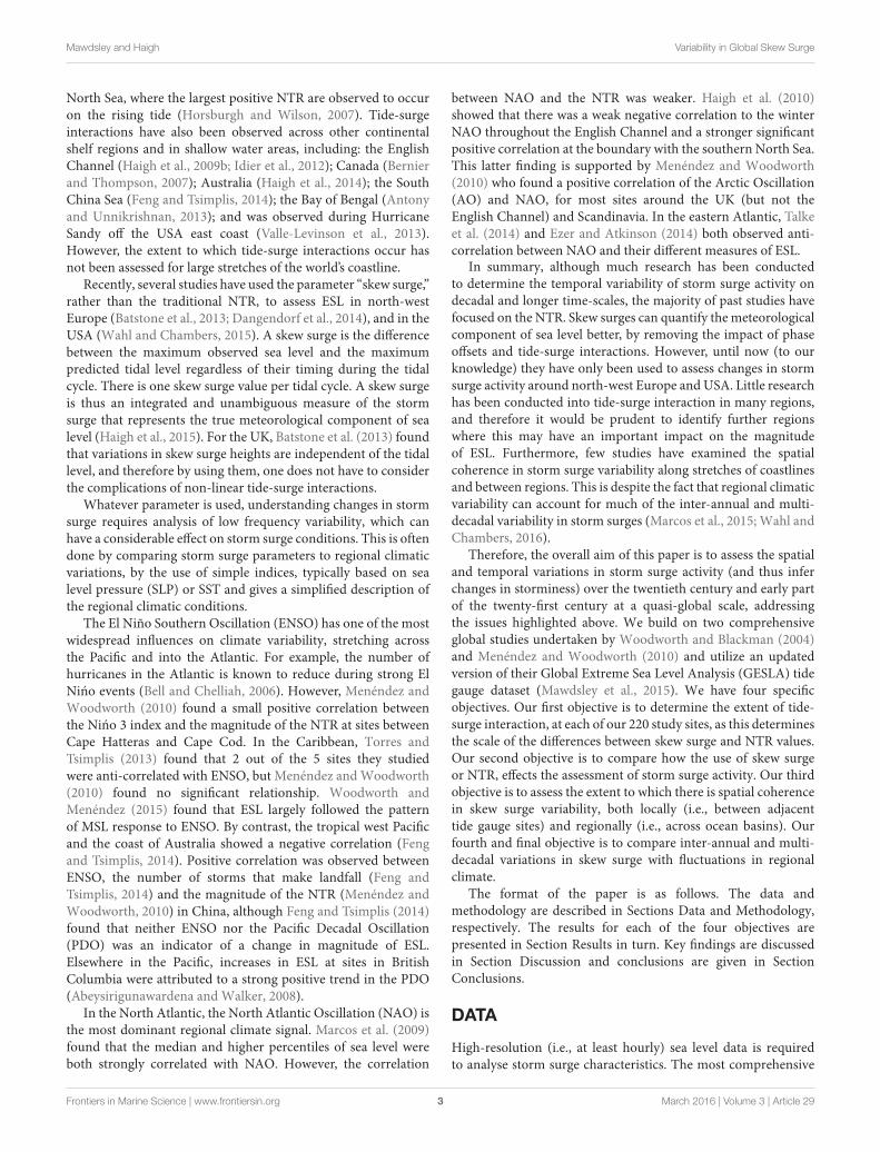
At each of the 220 study sites, the observed sea level record wasseparated into its three main component parts for each year:MSL, tide and NTR (Pugh and Woodworth, 2014). We followedthe same method as detailed in Mawdsley et al. (2015), and usedtheir technique for extracting the time and magnitude of tidalhigh waters (HW), from here on described as predicted HW. Forevery predicted HW at each site, we calculated a skew surge value.Batstone et al. (2013) used amethod that identified themaximumpredicted and observed water levels between successive lowwaters. However, we found this approach was not appropriatein mixed tidal regimes, and given the global nature of this studywe developed another method that works across all tidal regimes.We calculated skew surges by finding the largest local maximain the observed sea level, within a ±3 h window of the timeof each predicted HW (Figure 2). Most observed HW occurredwithin this window, but if no observed HW were found duringthis window we extended it to ±6 h. In a mixed tidal regime, thecoupling of each observed HW to each predicted HW is morecomplicated. Therefore, we introduced two criteria to ensure


https://crudata.uea.ac.uk/cru/data/nao/nao.dat

https://crudata.uea.ac.uk/cru/data/nao/nao.dat

http://www.cpc.ncep.noaa.gov

http://www.cpc.ncep.noaa.gov





FIGURE 2 | Schematic example of a storm surge event and the

different calculation methods for the NTR and skew surge.

that the observed HW is primarily caused by the predicted HWto which it is coupled. Firstly, if the predicted HW is betweendouble low tides we do not assign an observed HW. Secondly,if a second predicted HW is closer in time to an observed HWthan its coupled predicted HW, we remove the coupling betweenthat predicted and observed HW. These caveats mean that somepredicted HW did not have an associated observed HW, but thismethod captured a mean of 95% of observed HWs at all sites.Two sites (Bunbury andHoek vanHolland) had an observedHWassignment less than 80%, because many observed HWs occurredaround double low tides and were removed.

We then examined the differences between the skew surge andNTR time series, at each of our 220 study sites, and determinedthe extent of tide-surge interaction. Initially we compared themaximum values of skew surge and NTR from the entire timeseries, where concurrent values in both time series occur foran event at each site. For example, the maximum NTR atGalveston, USA was generated by Hurricane Ike in September2008, however, the tide gauge broke just before the predictedHW and no corresponding skew surge value for this particulartidal cycle could be calculated. We also compared the maximumskew surge value with the maximum NTR at high water (if tide-surge interaction is negligible you would expect these two valuesto be the same). We used the chi-squared (χ2) test, which wasfirst used for sea level studies by Dixon and Tawn (1994) but wasmodified by Haigh et al. (2010) to quantify the level of tide-surgeinteraction at each site. The χ

2 test calculates the probability thatthe observed dataset is different to an expected dataset. In thiscase, if the two are different then it demonstrates that tide-surgeinteraction is significant. Dixon and Tawn’s (1994) approach,from here on called the tidal-level method, involved splitting theastronomical tidal range into five equi-probable bands. If the tideand NTR were independent processes, the number of NTR pertidal band would be equal, but if interaction is significant thenumber of NTR per tidal bandwould differ. AsHaigh et al. (2010)pointed out, this method does not distinguish that interactiontends to be different on the ebb and flood phases of the tide

(Horsburgh and Wilson, 2007). Haigh et al. (2010) thereforemodified the method to compare the relative timing of the peakNTR to the predicted HW, and this method is from here on calledthe tidal-phase method. The tide was divided into 13 hourlybands between 6.5-h before and after high water. With no tide–surge interaction the expected number of occurrences in eachof the 13 bands would be the same. See Haigh et al. (2010) forthe mathematical details. We use the same 13 hourly bands toassess tide-surge interaction in the tidal-phase method, but use6 equi-probable bands for the tidal-level. The results from bothmethods are based on the largest 200 NTR events, where an eventis defined by a 72-h window centered on the peak NTR, to ensurethat each NTR peak is independent. Statistical significance for theχ2 test is given for a p <0.05.Next, we assessed the long-term trends in skew surge time-

series, at each site and compared these to trends calculated fromthe NTR time-series.We used the percentiles method (e.g., Haighet al., 2010; Menéndez and Woodworth, 2010), which ranksthe parameter values for each year. The 50th percentile of theNTR time-series (the median) approximates to zero, while the99.9th percentile is about the level of the 8th highest hourly sealevel value. For skew surges, the tidal regime at each site affectsthe annual number of HWs. In semi-diurnal regimes there areapproximately 705 skew surge values a year, whereas for a diurnalregime an average of 352 skew values would occur. Therefore, the99th percentile represents a value between the 4th and 7th highestvalues in the skew surge time series. Trends were calculated forthese percentiles, using linear regression, while standard errorswere estimated using a Lag-1 autocorrelation function to allowfor any serial autocorrelation in the time-series (Box et al., 1994).From here on, when we use the term “significant trends,” thissignifies that the trends are statistically (at 95% confidence level)different from zero.

We chose high percentiles because they represent the largestevents at each site, but the inter-annual variability present inthe higher percentile time-series can obscure the inter-decadalvariability and secular trends. To assess the extent to which thereis spatial coherence in skew surge variability, we calculated acorrelation coefficient between the skew surge percentile time-series for each pair of sites. We identified groups of sites, along astretch of coastline, where the correlation between themwas high,and designated them as coherent regions. We created regionalskew surge indices by calculating the mean of the de-trendedand normalized time-series of the 99th percentile of skew surgefor each site in that area. We only derived regional indices forthe period from 1970 to 2010, when there was sufficient overlapof data among sites in each region, but increase the temporalcomparison by comparing individual long-time series from eachregion. We filtered the regional skew surge indices using a locallyregressed least squares (Loess) approach (Cleveland and Devlin,1988), which through testing gave the lowest standard error. Thisnon-parametric method combines a multiple regression modelwith a nearest-neighbor model. Each point of the loess curve wasfitted using local regression, using a 2nd degree polynomial tothe points within a 10-year window centered on that point. Thesefiltered time-series are used to assess the temporal variationsin the regional skew surge indices and the correlation of those






indices between each other and against the regional climateindices, listed in Section Data. The significance of the correlationbetween the different regional skew surge indices and betweenthem and the climate indices, is determined by using the Lag-1autocorrelation function (Box et al., 1994).

RESULTS

Tide-Surge InteractionsOur first objective was to identify any tide-surge interaction, ateach of the 220 study sites, and we did this using the 4 methodsdetailed in Section Methodology. The difference between themaximum skew surge value and the maximum NTR over thewhole time series, is shown for each site in Figure 3A. Weexpect small differences at sites where tide-surge interaction isnegligible. Results shows that the difference is predominantlylargest in regions surrounded by shallow bathymetry, such asthe German Bight, Northern Australia, the Gulf of Panama andparts of the east coast of North America. However, there are othersites with large differences, including: sites in northern Australia(Port Hedland, Broome, Wyndham, Townsville and Bundaberg);Easter and Wake Islands in the Pacific Ocean; Funchal onMadeira, Portugal; and Yakutat in Alaska. At 120, 80, and 20 sites,the difference is larger than 10, 20, and 50 cm, respectively. Whenwe calculate the difference between themaximum skew surge andthe maximum NTR observed at the time of predicted HW wefind that 137 sites have a value of zero, as shown in Figure 3B.However, sites in the North Sea, the US east coast, north-west Australia and a few other individual locations have non-zero values which suggests that in these regions the tide-surgeinteraction shifts the peak in NTR away from predicted HW.

Figures 3C,D present the magnitude of the χ2 test statistic

as a colored dot (where p < 0.05) and a black dot whereno significant difference was found between the observed andexpected datasets. The results for the tidal-level method areshown in Figure 3C, and show that tide-surge interaction isstatistically significant (95% confidence) at 130 of the 220 sites(59%). These sites include those listed above, which are mainly inshallow regions, but also include sites on theMalay Peninsula andalong the coast of Washington and Oregon, USA. The results forthe tidal-phase method, are shown in Figure 3D, and show thattide-surge interaction is statistically significant at 175 of the 220sites (81%). As mentioned earlier, Haigh et al. (2010) modifiedDixon and Tawn’s (1994) original χ

2 test statistic as it did notdistinguish that interaction tends to be different on the ebb andflood phases of the tide. Interestingly, these results show thetidal-phase method identifies a greater number of sites at whichtide-surge interaction is statistically significant.

At several sites the differences between the maximum skewsurge and NTR values are large, but the χ

2 statistic values aresmall, and this is most often caused by the impact of one largestorm. For example, at Wake Island, Pacific, it is Typhoon Ioke in2006 (skew surge= 0.97m, NTR= 1.45m), at Broome, Australiait is Cyclone Rosito in 2000 (skew surge= 0.82m, NTR= 2.24m)and for Townsville, Australia it is Cyclone Yasi in 2011 (skewsurge= 0.93m, NTR= 2.10m). At Easter Island, Chile the eventin June 2006 is a high frequency signal, similar to seiching, but

further research is needed to determine its cause (skew surge =0.51m, NTR= 1.18m).

The difference between skew surges and NTRs at a site canvary considerably between individual events as a result of thetiming of the peak in the NTR relative to the predicted HW. Thisis illustrated in Figure 4, for 8 selected sites. The scatter sub-plotsshow themagnitude of the 200 largest NTR events plotted againstthe magnitude of the associated skew surge. The histogram sub-plots show the time of the peak in NTR for 200 events relativeto time of predicted HW. The colors on each plot display themaximum NTR (green), the top 10 NTRs (red), the top 25NTRs (blue), and the remainder of the top 200 NTR’s (black). AtAtlantic City, USA (Figure 4A), Galveston, USA (Figure 4D) andNaze in Japan (Figure 4F), the largest skew surge and largest NTRoccurred during the same event. However, at the other selectedsites, the timing of the peak NTR relative to the HW meansthat the largest skew surge and largest NTR are not coincident.For example, at Immingham, UK, the maximum NTR occurred6 h before predicted high water and because the mean tidalrange (MTR; as defined by Mawdsley et al., 2015) is 4.8m, themagnitude of the skew surge was only the 56th largest from thetop 200 NTR events (Figure 4E). The timing relative to predictedHW is less important where MTR is small. At Galveston, USA(MTR = 0.24m) for example, the largest NTR (with the valuescaused by Hurricane Ike removed) occurred during HurricaneCarla in 1961. The peak NTR occurred at the same time aspredicted HW, and 7 of the 10 largest events occur within 3 hof predicted HW (Figure 4D).

As mentioned earlier, tide-surge interaction has been moststudied in the southernNorth Sea, where the largest positive NTRtend to occur on the rising tide and not at high water. This patterncan be clearly observed in the results for Immingham shown onFigure 4E. However, these distributions vary around the world.For example, at Fremantle in Australia (Figure 4C) tide-surgeinteraction appears to lead to most peaks in NTR occurringnear the time of predicted HW. For Charleston (Figure 4B) andSeattle (Figure 4H) in USA, the majority of peaks in NTR occuron the ebb tide.

Skew Surge and Non-Tidal ResidualComparisonOur second objective was to determine if using skew surgeto assess changes in storm surge activity, gave different resultscompared to using the NTR. As we identified in the sectionabove, tide-surge interaction is evident at a large proportion ofthe study sites, suggesting that trends in skew surges and NTRmay also differ. The trends calculated for the 95th, 99th, and99.9th percentiles of the NTR are plotted in Figure 5, against thetrends in skew surge time-series for the same three percentiles.Given the differences in sampling of the two parameter, assummarized in Section Methodology, comparisons of trends indifferent percentiles gives an understanding of how to relate thepercentiles of the two parameters to each other. If the trendswere the same between skew surge and NTR, all points would liealong the 1:1 ratio line shown on each figure. Trend differencesbetween the skew surge and the NTR are generally small, withtrends of the same percentiles of skew surge and NTR showing






FIGURE 3 | Global maps of the 220 selected sites. (A) difference between the maximum NTR and the maximum skew surge value. (B) difference between the

maximum skew surge value and the maximum NTR occurring at the same time as predicted HW (C) χ2 values showing magnitude of tide at time of peak NTR for the

200 largest NTR. (D) χ2 values showing time of peak NTR relative to predicted HW for the 200 largest NTR event. Black dots (C,D) show non-significant values in the

chi-squared test (based on p-values larger than 0.05).

FIGURE 4 | For eight selected sites: (A) Atlantic City, USA; (B) Charleston, USA; (C) Fremantle, Australia; (D) Galveston, USA; (E) Immingham, UK; (F)

Naze, Japan; (G) Port Adelaide, Australia; (H) Seattle, USA. Left, scatter plot of 200 largest NTR and the associated skew surge value, right histogram of the

time of the peak NTR relative to predicted high water. Both plots are cultured according to magnitude with green showing the maximum NTR, red the top 10 NTR and

blue the top 25 NTR, black are the remainder of the top 200 NTR.






FIGURE 5 | Scatter plots comparing trends in the 95th, 99th and 99.9th percentiles and NTR (labeled along the x-axis), to the same percentiles of skew

surge (labeled along the y-axis). Each point is shaded according to the average mean tidal range at each site. The black line shows 1:1 ratio. The root mean

squared error value for each plot is the value for the best fit (red line).

the closest comparison (i.e., the closest 1:1 match occurs betweenthe 99th percentile of NTR and the 99th percentile of skewsurge). The color of each dot in Figure 5 represents the heightof MTR at that site. Sites with the largest difference betweentrends in skew surge and NTR typically have a large MTR. Thesesites include Broome, Australia, Ilfracombe, UK and Hoek vanHolland, Netherlands, and these sites also have a large tide-surgeinteraction as quantified by the χ

2 test statistics (Figures 3B,C).At three further sites, Calais, France, Darwin, Australia andEastport, USA, the trend in skew surge is significantly larger thanthe trend in NTR (i.e., the 95% confidence intervals of the twotrends do not overlap). The trends at Calais and Eastport changefrom significant negative trends (at the 95% level) to positivetrends that are significant at the 66% level. The rootmean squarederror (RMSE) between skew surge trends and NTR trends arelisted for each plot on Figure 5. The RMSEs are largest for the99.9th percentile, since trends in this percentile can be affected byindividual large events.

The time-series of the 99th (blue) and 99.9th (red) percentilesof skew surges are presented in Figure 6 for selected sites, alongwith the linear trends in these time-series and the corresponding95% confidence intervals. The variability around the 99.9thpercentile, which captures only the annual maximum of skewsurge, is large relative to the magnitude of the linear trend andtherefore very few significant trends can be detected. Thereforewe use the 99th percentile of skew surge throughout the rest of thepaper. Previous studies, including Menéndez and Woodworth

(2010), used the 99th percentile of NTR, so our choice allowsdirect comparison with the results of that study.

Linear trends calculated for the 99th percentile of skew surgeand NTR are shown for each site in Figures 7A,B respectively.Significant trends are shown with larger dots, with the colorrepresenting the magnitude of the trends. Overall there arefew significant trends in skew surge time-series, with significantnegative trends at 18 sites and significant positive trends at 11sites. For the NTR there are significant negative trends at 33sites and significant positive trends at only 5 sites. There are15 sites with negative trends in both parameters, and 4 siteswith positive trends in both. Trends were calculated at sites withenough years for the last 20, 40, 60, and 80 years, and comparedto the trend of the entire time series. These results are presentedin Supplementary Material and show that the number of positiveand negative trends are roughly similar, and low in relation to thenumber of sites. Despite the low numbers of sites with significanttrends there are some regions with consistent trends betweenneighboring stations, such as coherent decreases around northAustralia and the Atlantic coast of southern Europe.

Spatial Variability of Skew SurgeOur third objective is to assess the extent to which there isspatial coherence in skew surge variability, both locally (i.e.,between adjacent tide gauge sites) and regionally (i.e., acrossocean basins). For each site in turn, correlation coefficients werecalculated between the unfiltered 99th percentile time series at






FIGURE 6 | Time series plots of annual values of the 99th (blue) and 99.9th (red) percentile for skew surge at 8 selected sites. (A) Atlantic City, USA; (B)

Charleston, USA; (C) Fremantle, Australia; (D) Galveston, USA; (E) Immingham, UK; (F) Naze, Japan; (G) Port Adelaide, Australia; (H) Seattle, USA.

that site and each of the other 219 sites. The results are shownin Figure 8. There are distinct regions where strong positivecorrelations occur among neighboring sites. These include thenorth-east Pacific, north-west Atlantic and sites in northernEurope. Interestingly, sites on the west coast of the US are weaklyanti-correlated (at the 66% level) with several sites in northernEurope.

The strong correlation between groups of sites implies thatwe can create regional skew surge indices that represent the

average skew surge conditions for a particular region; similarto what other studies have done for MSL (e.g., Shennan andWoodworth, 1992; Woodworth et al., 1999, 2009; Haigh et al.,2009a; Wahl et al., 2013; Dangendorf et al., 2014; Thompsonand Mitchum, 2014). We identified 8 regions, where a largedensity of sites meant that strong positive correlations existedbetween them. These regions, and the sites of which they arecomprised, are detailed in Table 1 and include the: north-eastPacific (NEP), Gulf of Mexico (GOM), north-west Atlantic South






FIGURE 7 | Shows the magnitude of the trend in in the 99th percentile of (A) skew surge and (B) NTR, for the 220 sites analyzed. Large dots show that

the trend is significant at the 95% level.

FIGURE 8 | Correlation between each site. Each site is plotted along an imaginary coastline running from Alaska down the west and up the east coast of the

America, across to the Atlantic to Norway, down through Europe around Africa, around the Indian Ocean, up the western Pacific Ocean and then across the Pacific

Islands to the east. Sites with correlations at the 66% level are shown as bold color.






TABLE 1 | Details of sites included in each of the regional indices.

Regional index name (and abbreviation) Sites included in index

North East Pacific (NEP) Canada: Bella Bella, Port Hardy, Tofino, Campbell River, Point Atkinson, Vancouver, Bamfield, Victoria, Patricia Bay.

USA: Seattle, Neah Bay.

Gulf of Mexico (GOM) USA: Port Isabel, Galveston, Grand Isle, Pensacola, St. Petersburg, Key West.

North-west Atlantic—South (NWA-S) USA: Fernandina Beach, Mayport, Fort Pulaski, Charleston, Wilmington.

North-west Atlantic—North (NWA-N) USA: Duck Pier, Chesapeake Bay, Baltimore, Lewes, Cape May, Atlantic City, New York (Battery), New London,

Montauk, Newport, Boston, Woods Hole, Portland, Nantucket, Eastport.

North Sea (NS) Denmark: Esbjerg.

Netherlands: Delfzijl, Den Helder.

France: Calais.

UK: Dover, Sheerness, Lowestoft, Immingham, North Shields, Aberdeen, Wick.

Western Australia (WAUS) Australia: Darwin, Broome, Port Hedland, Carnarvon, Geraldton, Fremantle, Bunbury, Albany, Esperance

Eastern Australia (EAUS) Australia: Wyndham, Thevenard, Port Lincoln, Port Pirie, Port Adelaide, Port Lonsdale, Victor Harbor, Geelong,

Williamstown, Burnie, Spring Bay, Fort Denison, Newcastle, Brisbane, Bundaberg, Mackay, Townsville, Cairns.

Japan (JAP) Japan: Nishinoomote, Aburatsu, Kushimoto, Maisaka, Miyakejima, Mera, Ofunato, Hachinohe, Hakodate.

FIGURE 9 | Creation of regional skew surge index for the north-east Pacific. (A) The de-trended time series of the 99th percentile for each site from north to

south (see Table 1 for site ID), (B) All the time-series with the mean of all sites plotted in red, and (C) the sites that are in this region highlighted in red.

(NWA-S), north-west Atlantic North (NWA-N), North Sea (NS),west Australia (WAUS), east Australia (EAUS), and Japan (JAP).

An example of the creation of a regional index is shown inFigure 9 for the north-east Pacific. The de-trended, normalizedtime-series from each of the 11 selected sites in the regionare plotted in Figure 9A, with an arbitrary offset. These timeseries are overlaid in Figure 9B. The thicker red lines showsthe regional time-series that has been created by averaging thede-trended, normalized time-series for each of the 11 sites. Thelocations of the 11 sites used to calculate the regional index are

shown in Figure 9C, as red dots. Similar figures for the other 8regions are shown in the Supplementary Material.

There is considerable year-to-year variability in the 8 regionalindices. To better investigate the inter-decadal variability weapplied a Loess filter to each of the 8 regional skew surge indices,and the filtered time series are shown in Figure 10A. Concurrentpeaks in skew surge are observed in multiple regions, mostnotably in 1992–1993 in the north-west Atlantic (North andSouth indices) and the North Sea. Peaks in skew surge in thesouthern North Atlantic throughout the 1990s appear to lag






FIGURE 10 | Temporal variability of 8 selected regions as shown by the de-trended normalized and then filtered magnitude of skew surge for: (A)

regional indices; (B) selected long site from each region, which has a strong correlation with the regional index.

FIGURE 11 | (A) Stacked time series of filtered regional skew surge indices, with arbitrary offset applied, (B) Correlation of each filtered regional skew surge index

against the others.

peaks in the Gulf of Mexico by approximately 1 year. Stormseasons for these regions are summer and winter respectively andthe lag may be a result of this or a delay in the response to changesin regional scale climatology.

The 8 regional skew surge indices are plotted as stackedtime series in Figure 11A, with the correlations between themshown in Figure 11B. Between many regions, there is a strongcorrelation (r > 0.5), but at the 95% level these are notsignificant, due largely to the reduction in the number of effectiveobservations when autocorrelation is accounted for. Strongcorrelations exist between: the two north-west Atlantic indices

(r = 0.65, p = 0.02), the Gulf of Mexico and both two north-west Atlantic indices (South: r = 0.37, p = 0.33; North: r = 0.31,p= 0.4), the North Sea and north-west Atlantic—South (r= 0.65,p= 0.12). Therefore, only this last correlation is significant at the80% level.

The regional skew surge indices were only calculated for theperiod 1970–2010, because fewer sites with valid data outside ofthis period increases the variability in the indices. To allow longertemporal comparisons between regions, we selected individualsites within each region that were both long and highly correlatedwith the regional index. The 8 sites with long records, across the






8 regions, are shown in Figure 10B. Note, these time series havealso be subjected to the same Loess filter, applied to the regionaltime series. The simultaneous peak in the 1990s, mentionedabove, is also present in the individual sites. However, a peak inthe signal in the filtered time series at Charleston and AtlanticCity, USA in the 1960s is not clear at Immingham, UK. Thereverse is true in the late 1980s, where an increase at Imminghamis not present at Charleston or Atlantic City.

Comparison of Skew Surge to ClimateIndicesOur fourth objective is to compare inter-annual and multi-decadal variations in skew surge with fluctuations in regionalclimate. Correlation coefficients were calculated between the 8regional skew surge indices and each of the 8 regional climateindices. The results are shown in Figure 12.

There are no statistically significant correlations at the 95%level, again largely because of the large degree of autocorrelationin the filtered time-series. Strong positive correlations (r >

0.5) occur between: the North Sea and NAO (r = 0.60, p =

0.28), the Gulf of Mexico and Nino 4 (r = 0.52, p = 0.19) andwestern Australian and SOI (r = 0.59, p= 0.31). Strong negativecorrelations (r < −0.5) occur between the north-east Pacific andAO (r = −0.57, p = 0.28) and NAO (r = −0.50, p = 0.40), theGulf of Mexico and AO (r = −0.53, p = 0.32), western Australiaand NP (r = −0.56, p = 0.28), and eastern Australia and Nino4 (r = −0.52, p = 0.19). The correlations detailed above thatinvolve Nino 4 are the only correlations significant at the 80%level.

The peak observed in the north-east Pacific index in 1997–1998 (Figure 10A), corresponds to one of the strongest El Ninoevents in the time-series. The peak observed in both the Seattlerecord and the NEP index in 1982–1983 corresponds to anotherstrong El Nino event, however, the El Nino event of 1972 is notevident in the skew surge time series. Also, the typically positiveNino 3 values observed through the early 1990s coincide with atrough in the north-east Pacific index. The presence of a peakin north-east Pacific index during only the strongest El Ninoevents suggest a complex relationship between skew surge andthe magnitude of variability in regional climate.

DISCUSSION

One of the key goals of this paper was to determine if differentresults are obtained when using skew surge to assess changes instorm surge activity, compared to the more traditional NTR. AsHorsburgh and Wilson (2007) showed, while the NTR primarilycontains the meteorological contribution termed the surge, itmay also contain harmonic prediction errors or timing errors,and non-linear interactions, which can bias analysis of stormsurges. It is for this reason that we wanted to assess the alternativeuse of skew surges. The advantage of using skew surge is that itis an integrated and unambiguous measure of the storm surge(Haigh et al., 2015). Changes in skew surges have only previouslybeen assessed (to our knowledge) at sites around the north-westEurope (Batstone et al., 2013; Dangendorf et al., 2014) and

FIGURE 12 | Correlation of regional indices of skew surge against key

climatic indices.

the USA (Wahl and Chambers, 2015). Both of these regionsgenerally display semi-diurnal tidal behavior, but our methodworks well in all tidal regimes.

We found that significant tide-surge interaction occurs at130 of the 220 sites analyzed (59%) based on the tidal-levelmethod, and 175 sites (81%) based on tidal-phase approach.These sites include those previously reported, as well as regionsnot previously identified in the literature, such as the Gulf ofPanama and the Malay Peninsula. We also found that tide-surgeinteraction is not limited to locations with large adjacent areasof shallow bathymetry. Smaller but still statistically significantinteractions occur along the Pacific coast of North America, ona number of Pacific Islands and around the Iberian Peninsula.The topography of these sites is highly variable. Some sites arein shallow water such as Willapa Bay, USA, which is in a largebay, and Astoria, USA, which is influenced by the ColumbiaRiver. Other sites are on volcanic islands rising steeply from theocean floor, such as Papette, French Polynesia and Pohnpei, theFederated States of Micronesia. For both these island sites thereis an increased frequency of peaks in NTR around the time ofpredicted HW, a pattern that is also observed at Galveston, USA(Figure 4D).

In some regions the timing of the peak NTR relative to tidal-phase, and therefore the level of tide-surge interaction is sitespecific. For example, around the UK, peak NTR usually occursaway from predicted HW (Horsburgh and Wilson, 2007; Haighet al., 2010; Olbert et al., 2013), and in the North Sea HorsburghandWilson (2007) showed that the external surge component willalways peak away from predicted HW. However, at Larne andBangor in Northern Ireland, peak NTRmost frequently occurredat predicted HW (Olbert et al., 2013). These sites have similartidal conditions and are geographically close but highlight thatsmall changes in bathymetry and tidal range can influence theextent of tide-surge interaction.

Individual storm characteristics vary from the average pattern,and where these deviations occur in the largest storm surges thedifference in skew surge magnitude can be important. At WakeIsland in the Pacific, Typhoon Ioke generated a NTR of 1.5 m






but a skew surge of only 1.0 m, because the peak NTR for thisevent occurred 5 h before predicted HW (see Figure A3.10 inSupplementary Material, Site 434). However, no significant tide-surge interaction is observed at this site and the peak NTR foran event like Typhoon Ioke could have occurred at predictedHW. Conversely, at Brest, France, where significant tide-surgeinteraction meant that peaks in NTR usually occurred away frompredictedHW, themaximumNTR (caused by the so-called GreatStorm inOctober 1987) occurs at the same time as predictedHW.Therefore, although the skew surge is a more reliable indicatorof the average meteorological influence on sea level, individualstorm surges may have different characteristics. Parameterizationof any physical process aims to use one value to represent acomplex system, and this must be considered when we use skewsurge in ESL calculations. This is especially true in regions withsmall tidal ranges or those affected by tropical cyclones. The rapidpeak in storm surge associated with tropical cyclones reducesthe influence of storm surge on tidal propagation, and may leadto a more uniform distribution of peak NTR timing relative topredicted HW.

Although tide-surge interaction is evident at many sites, andthere are differences between skew surge and NTR values, wefound that at most sites, the trends in skew surge are very similarto those in NTR. The largest differences in trends are at sitesalong the north-coast of Australia or the French coast of theEnglish Channel, and this results in the reversal of trends atCalais and Darwin. Both locations have macro-tidal regimes withsignificant tide-surge interaction. The general similarity in trendsmeans we can compare our results to previous studies which usedNTR. Menéndez and Woodworth (2010) found more negativetrends in NTR than positive trends globally. We also find morenegative trends in NTR, but no statistically significant differencebetween the number of positive and negative trends in skewsurge time-series. Our findings are consistent with those of Wahland Chambers (2015) for the US, who found a greater numberof sites had significant trends in NTR compared to skew surge.The number of sites with significant trends in skew surge andNTRmay be generated from chance, but a formal assessment hasnot been made here, because of the spatially non-homogenousdataset. Methods such as that of Livezey and Chen (1983) couldbe adapted to assess whether the number of trends is statisticallysignificant. Even so, there are a greater number of negative trendsin NTR than skew surge and this may be caused by timingerrors or changes in the tide-surge interaction. Timing errorsare particular evident in early records that have been digitizedfrom paper charts and are often associated with issues withthe older mechanical tide gauges (Pugh and Woodworth, 2014).Therefore, timing errors are more prevalent in the early part ofthe tide gauge records, and if they are included in the analysisthey may introduce a negative bias into the NTR time-series. Bydefinition, time-series of skew surges are not influenced by suchtiming errors. Another possible reason for the difference in trendsis that the magnitude of the tide-surge interaction is changingthrough time, because of changes in the phase or magnitude ofthe tide (e.g., Mawdsley et al., 2015). Previous studies in theNorthSea (Horsburgh and Wilson, 2007) and English Channel (Haighet al., 2010) however, found no significant changes in tide-surgeinteraction over time.We have not investigated this, in this study.

We found little spatial coherence in the magnitude and signof trends among sites, mainly because the trends are insignificantat most sites. However, in northern Australia a number of sitesdisplay significant negative trends in skew surge (Figure 7) andin NTR, which is consistent with Menéndez and Woodworth(2010), while our findings also support their research showingpositive trends at sites in the Gulf of Mexico and along theAtlantic coast of Florida. However, most other findings vary fromthose of Menéndez and Woodworth (2010). We find a decreaseat sites in southern Europe, and an increase at a number ofsites in southern Australia. No coherent trend along the north-east coast of America is observed in this study, which agreeswith Zhang et al. (2000) but contradicts the increase foundin this region by both Menéndez and Woodworth (2010) andGrinsted et al. (2012). Differences between our findings andthose of Menéndez and Woodworth (2010) may be the result offurther quality control, or the inclusion of new data, which alongthe north-east coast of America included large storms surgesin 2010 and 2012, generated by Hurricanes Irene and Sandy,respectively. Figures A3.1–3.4, in the Supplementary Material,show that trends over the last 20–80 years change depending onthe period studied, and therefore extra data can change results.In other studies of ESL, changes may also be caused by theinclusion of tide, such as the increases in New York (Talkeet al., 2014), western Northern America (Bromirski et al., 2003;Abeysirigunawardena and Walker, 2008; Cayan et al., 2008) andthe German Bight (Müdersbach et al., 2013). Mawdsley et al.(2015) observed significant increases in tidal HW in all theseregions, and we speculate that this has contributed toward theobserved increase in ESL, in other studies, and the lack of trendsin skew surges identified by this paper in these areas. Withthe growing literature regarding changes in tide (e.g., Jay, 2009;Woodworth, 2010; Pickering et al., 2012; Pelling et al., 2013;Mawdsley et al., 2015), it is essential that studies of storm surgeuse parameters that just relate to meteorological changes andidentify other drivers of change, such as the tide or tide-surgeinteraction.

The number of statistically significant trends is low, inpart, because of the large inter-annual variability in the highpercentiles of skew surges. The creation of filtered regional skewsurge indices removed the high frequency variability and helpedto reveal underlying inter-decadal variability and the spatialcoherence between regional signals. However, despite strongcorrelations between some regions around the North Americancoastline and across the Atlantic to the North Sea, none ofthe correlations are significant at the 95% level. Just prior tocompleting our study, we learnt of a similar investigation byMarcos et al. (2015). Using the GESLA dataset, they showedthat the intensity and frequency of ESL unrelated to MSLdisplay a regional coherence on decadal time-scales. Their findingpoints toward large-scale climate drivers of decadal changes instorminess (Marcos et al., 2015). The string correlations betweenneighboring sites show that these large scale climatic driversare important, but there significance is difficult to assess inrelatively short datasets have a high degree of temporal auto-correlation.

Comparisons of regional storm surge time-series and climateindices have been undertaken in numerous past studies.






Menéndez and Woodworth (2010) found the Nino 3 index hada positive correlation with the magnitude of NTR in the easternPacific and a negative correlation in the western equatorialPacific. The magnitude of an El Nino appears to influence thenorth-east Pacific index, with peaks in the index associatedwith the largest El Nino events in 1982–1983 and 1997–1998,but a trough in the index during small but positive values ofthe Nino 3 index in the early 1990s. Also in the Pacific thePDO was previously shown to correlate positively with sites inthe northeast Pacific (Abeysirigunawardena and Walker, 2008),however we do not find any significant correlation. The findingsrelated to the North Sea index supports previous studies (e.g.,Haigh et al., 2010) that find a positive correlation with the NAO,although our correlation is not significant. Studies by Ezer andAtkinson (2014) and Talke et al. (2014) found anti-correlationbetween the NAO and sites on the US east coast, but we find veryweak (and non-significant) correlations. Our method of usingfiltered regional skew surge indices, means that although strongcorrelations (r > 0.5) are observed between some regional skewsurge indices and climate indices, they are not deemed significantat the 95% level. The effect of autocorrelation in the calculationreduces the degrees of freedom (effective observations) from40 to less than 8 for all correlation calculations, and thereforeincreases the size of the confidence intervals. The significance ofcorrelations may improve with increased data length or reducedfilter size, however, filters are a widely used and during thedevelopment of the methodology the 10 year Loess filter wasfound to give the lowest RMSE. In this study we have correlatedskew surge time-series against climate indices, but it would bemore appropriate to use wind and pressure datasets, as these arethe parameters that directly cause storm surges. In the future,we hope to do this using meteorological re-analysis datasets,like Bromirski et al. (2003), Calafat et al. (2013) and Wahl andChambers (2015) did to assess storm surge variability in theirregional studies.

One of the main limitations of this study (and other studies)remains the relatively small number of sites and the limitedlength of the time-series available. Although the GESLA datasetis probably the most comprehensive collection of hourly sealevel data, there are still many under-represented regions in thedatabase. The 8 regional indices we derived all cover data denseregions since this is where the strongest correlations are, buteven here the number of datasets longer than 40 years limitedthe length of the regional skew surge indices. The applicationof the filter, which is necessary to extract relationships betweenthe datasets, meant that the confidence intervals increased andthe significance of the correlations decreased. There is a need foreither more sites or better access to data in under-representedareas, especially areas that are prone to large storm surges,such as the Caribbean, the Bay of Bengal and countries aroundthe South China Sea. Conversely, the already global nature ofthe study does not allow for a detailed understanding of thefindings presented here. Further work conducted on a local toregional scale, should be undertaken to assess the mechanismsthat are driving the tide-surge interaction, and control its specificsignature. Such assessment could consider differences in thetide-surge interaction for tropical and extra-tropical storms, the

influence of slope angle or shelf width, or the effect of changes inbathymetry.

CONCLUSIONS

In this paper, we have used time series of skew surge to assesschanges in storm surges on a quasi-global scale for the first time.Past studies that have assessed changes in storm surges havetended to focus on the NTR, which includes contributions fromnon-meteorological generated factors, which may bias results.This study also assessed the spatial and temporal variability inthe skew surge, using regional indices.

First, we determined the extent of tide-surge interaction, ateach of the 220 study sites, as this determines the scale of thedifferences between skew surge and NTR values. Using χ

2 teststatistics we found statistically significant (95% confidence) levelsof tide-surge interaction at 130 of the 220 sites (59%) based ontidal-level and 175 sites (81%) based on tidal-phase. The tide-surge interaction is strongest in regions of shallow bathymetrysuch as the North Sea, north Australia and the Malay Peninsula.However, non-standard distributions are also observed at siteson open ocean islands, although at these sites the peak in NTRoften tended toward the time of predicted HW, rather thanaway from it as experienced in shallow water areas (such as theNorth Sea).

Second, we determined if different results are obtained whenusing skew surges to assess changes in storm surge activity,compared to the more traditional NTR. At most sites thetrends in skew surge are similar to those of NTRs. Where thedifferences in trends were large, the sites tended to have a largetidal range, such as those in northern Australia and northernFrance. Although at most sites the trends in skew surges werenot statistically significant, we observed approximately equalnumbers of positive and negative trends. However, there weremore negative trends in the NTR. This suggests that skew surgeimproves the calculation of trends, because phase offsets causedby time errors are not present in time series of skew surges.

Third, we examined the extent to which there is spatialcoherence in skew surge variability, both locally (i.e., amongadjacent tide gauge sites) and regionally (i.e., across oceanbasins). We identified 8 regions, where there were strongpositive correlations among neighboring sites, and hence deriveda regional index for each region. We observed a number ofstrong (r > 0.5) correlations between regions, including: positivecorrelation between the two regions on North American Atlanticcoast, positive correlation between the north-west Atlantic—south and the North Sea; and negative correlation betweenthe North Sea and north-east Pacific. However, these trendswere not significant at the 95% level, since the high degree ofautocorrelation in the filtered dataset increased the size of theconfidence intervals.

Finally, we compared multi-decadal variations in skew surgewith fluctuations in regional climate. Again strong correlationswere observed, but were not significant at the 95% level.Correlations significant at the 80% level included those betweenthe Gulf of Mexico and eastern Australia and the Nino 4index.






AUTHOR CONTRIBUTIONS

RM conducting the data quality control for all tide gauge sites,before developing and coding the method for extraction of theskew surge. Also was primarily involved in creation of Figuresand writing of text. IH developed and coded some of the methodfor skew surge extraction, as well as the chi-squared test to assesstide-surge interaction. Also heavily involved with editing of text.

ACKNOWLEDGMENTS

This study was funded by the University of Southampton, Schoolof Ocean and Earth Science and the National EnvironmentalResearch Council (NERC). Conversations and feedback fromPhillip Woodworth, Neil Wells and Francisco Calafat at theNational Oceanography Centre have been invaluable. Wethank the reviewers of the paper, whose excellent commentshave improved this paper. The GESLA data set was initially

collated by staff from the National Oceanography Centre(NOC), Liverpool in the UK and the Antarctic Climateand Ecosystems Cooperative Research Centre (ACE CRC)in Australia. Extensions to the dataset were provided by:University of Hawaii Sea Level Center (UHSLC), NationalOceanographic and Atmospheric Authority (NOAA), BritishOceanographic Data Centre (BODC), Norwegian MappingAuthority (NMA), Marine Environmental Data Service (MEDS);Bureau of Meteorology (BOM); and Norwegian MappingAuthority (NMA). This paper contributes to the Engineering andPhysical Science Research Council Flood Memory Project (grantnumber EP/K013513/1).

SUPPLEMENTARY MATERIAL

The Supplementary Material for this article can be foundonline at: http://journal.frontiersin.org/article/10.3389/fmars.2016.00029

REFERENCES

Abeysirigunawardena, D. S., and Walker, I. J. (2008). Sea level responses toclimatic variability and change in Northern British Columbia. Atmosp. Ocean

46, 277–296. doi: 10.3137/ao.460301Antony, C., and Unnikrishnan, A. S. (2013). Observed characteristics of tide-surge

interaction along the east coast of India and the head of Bay of Bengal. EstuarineCoast. Shelf Sci. 131, 6–11. doi: 10.1016/j.ecss.2013.08.004

Araújo, I. B., and Pugh, D. T. (2008). Sea levels at Newlyn 1915–2005: analysis oftrends for future flooding risks. J. Coastal Res. 24, 203–212. doi: 10.2112/06-0785.1

Batstone, C., Lawless, M., Tawn, J., Horsburgh, K., Blackman, D., McMillan,A., et al. (2013). A UK best-practice approach for extreme sea-levelanalysis along complex topographic coastlines. Ocean Eng. 71, 28–39. doi:10.1016/j.oceaneng.2013.02.003

Bell, G. D., and Chelliah, M. (2006). Leading tropical modes associated withinterannual and multidecadal fluctuations in North Atlantic hurricane activity.J. Clim. 19, 590–612. doi: 10.1175/JCLI3659.1

Bernier, N., and Thompson, K. (2007). Tide-surge interaction off the east coastof Canada and northeastern United States. J. Geophys. Res. 112, C06008. doi:10.1029/2006jc003793

Box, G. E. P., Jenkins, G. M., and Reinsel, G. C. (1994). Time Series Analysis:

Forecasting and Control. 3rd Edn. Upper Saddle River, NJ: Prentice-Hall.Bromirski, P. D., Flick, R. E., and Cayan, D. R. (2003). Storminess variability

along the California Coast: 1858–2000. J. Clim. 16, 982–993. doi: 10.1175/1520-0442(2003)016<0982:SVATCC>2.0.CO;2

Calafat, F. M., Chambers, D. P., and Tsimplis, M. N. (2013). Inter-annual todecadal sea-level variability in the coastal zones of the Norwegian and SiberianSeas: the role of atmospheric forcing. J. Geophys. Res. 118, 1287–1301. doi:10.1002/jgrc.20106

Cayan, D. R., Bromirski, P. D., Hayhoe, K., Tyree, M., Dettinger, M. D., andFlick, R. E. (2008). Climate change projections of sea level extremes along theCalifornia coast. Clim. Change 87, S57–S73. doi: 10.1007/s10584-007-9376-7

Church, J. A., Clark, P. U., Cazenave, A., Gregory, J. M., Jevrejeva, S., Levermann,A., et al. (2013). “Sea level change,” inClimate Change 2013: The Physical Science

Basis. Contribution of Working Group I to the Fifth Assessment Report of the

Intergovernmental Panel on Climate Change, eds T. F. Stocker, D. Qin, G.-K.Plattner, M. Tignor, S. K. Allen, J. Boschung, A. Nauels, Y. Xia, V. Bex, andP. M. Midgley (Cambridge, UK; New York, NY: Cambridge University Press),1137–1216.

Cleveland,W. S., and Devlin, S. J. (1988). Locally weighted regression: an approachto regression analysis by local fitting. J. Am. Stat. Assoc. 83, 596–610. doi:10.1080/01621459.1988.10478639

Dangendorf, S., Calafat, F. M., Arns, A., Wahl, T., Haigh, I. D., and Jensen, J.(2014). Mean sea level variability in the North Sea: processes and implications.J. Geophys. Res. 119, 6820–6841. doi: 10.1002/2014jc009901

Dixon, M. J., and Tawn, J. A. (1994). Extreme Sea-Levels at the UK A-Class

Sites: Site-by-Site Analyses. Proudman Oceanographic Laboratory, InternalDocument, No. 65, 229.

Emanuel, K. A., Sundararajan, R., and Williams, J. (2008). Hurricanes and globalwarming: results from downscaling IPCC AR4 simulations. Bull. Am. Meteorol.

Soc. 89, 346–367. doi: 10.1175/bams-89-3-347Ezer, T., and Atkinson, L. P. (2014). Accelerated flooding along the U.S. East Coast:

on the impact of sea-level rise, tides, storms, the Gulf Stream, and the NorthAtlantic Oscillations. Earth Fut. 2, 362–382. doi: 10.1002/2014EF000252

Feng, X., and Tsimplis, M. N. (2014). Sea level extremes at the coasts of China. J.Geophys. Res. 119, 1593–1608. doi: 10.1002/2013jc009607

Grinsted, A., Moore, J. C., and Jevrejeva, S. (2012). Homogeneous record ofAtlantic hurricane surge threat since 1923. Proc. Natl. Acad. Sci. U.S.A. 109,19601–19605. doi: 10.1073/pnas.1209542109

Haigh, I., Nicholls, R., and Wells, N. (2009a). Mean sea level trends around theEnglish Channel over the 20th century and their wider context. Cont. Shelf Res.29, 2083–2098. doi: 10.1016/j.csr.2009.07.013

Haigh, I., Nicholls, R., and Wells, N. (2009b). Twentieth-Century changes inextreme still sea levels in the English channel.Coast. Eng. 2008. 1–5, 1199–1209.doi: 10.1142/9789814277426_0100

Haigh, I., Nicholls, R., and Wells, N. (2010). Assessing changes in extreme sealevels: Application to the English Channel, 1900–2006. Cont. Shelf Res. 30,1042–1055. doi: 10.1016/j.csr.2010.02.002

Haigh, I., Wijeratne, E. M. S., MacPherson, L., Pattiaratchi, C., Mason, M.,Crompton, R., et al. (2014). Estimating present day extreme water levelexceedance probabilities around the coastline of Australia: tides, extra-tropical storm surges and mean sea level. Clim. Dynam. 42, 121–138. doi:10.1007/s00382-012-1652-1

Haigh, I. D., Wadey, M. P., Gallop, S. L., Loehr, H., Nicholls, R. J., Horsburgh,K., et al. (2015). A user-friendly database of coastal flooding in the UnitedKingdom from 1915–2014. [Data Descriptor]. Sci. Data 2, 150021. doi:10.1038/sdata.2015.21

Hartmann, D. L., Klein Tank, A., and Rusticucci, M. (2013). “Observations:ocean,” in Climate Chanage 2013: The Physical Scientific Basis. Working Group I

Contribution to the Intergovernmental Panel on Climate Change 5th Assessment

Report, eds J. Hurrell, J. Marengo, F. Tangang, and P. Viterbo (Cambridge, UK;New York, NY: Cambridge University Press), 159–254.

Horsburgh, K. J., and Wilson, C. (2007). Tide-surge interaction and its role in thedistribution of surge residuals in the North Sea. J. Geophys. Res. 112, C08003.doi: 10.1029/2006jc004033


http://journal.frontiersin.org/article/10.3389/fmars.2016.00029





Hunter, J. (2012). A simple technique for estimating an allowance for uncertainsea-level rise. Clim. Change 113, 239–252. doi: 10.1007/s10584-011-0332-1

Hunter, J. R., Church, J. A., White, N. J., and Zhang, X. (2013). Towards a globalregionally varying allowance for sea-level rise. Ocean Eng. 71, 17–27. doi:10.1016/j.oceaneng.2012.12.041

Idier, D., Dumas, F., and Muller, H. (2012). Tide-surge interaction in the EnglishChannel. Nat. Hazards Earth Syst. Sci. 12, 3709–3718. doi: 10.5194/nhess-12-3709-2012

Jay, D. A. (2009). Evolution of tidal amplitudes in the eastern Pacific Ocean.Geophys. Res. Lett. 36, L04603. doi: 10.1029/2008gl036185

Kossin, J. P., Knapp, K. R., Vimont, D. J., Murnane, R. J., and Harper, B. A. (2007).A globally consistent reanalysis of hurricane variability and trends. Geophys.Res. Lett. 34:L04815. doi: 10.1029/2006gl028836

Lionello, P., Mufato, R., and Tomasin, A. (2005). Sensitivity of free and forcedoscillations of the Adriatic Sea to sea level rise. Clim. Res. 29, 23–39. doi:10.3354/cr029023

Livezey, R. E., and Chen, W. Y. (1983). Statistical field significance and itsdetermination by monte carlo techniques. Mon. Weather Rev. 111, 46–59. doi:10.1175/1520-0493(1983)111<0046:sfsaid>2.0.co;2

Marcos, M., Calafat, F. M., Berihuete, Á., and Dangendorf, S. (2015). Long-termvariations in global sea level extremes. J. Geophys. Res. 120, 8115–8134. doi:10.1002/2015jc011173

Marcos, M., Tsimplis, M. N., and Shaw, A. G. P. (2009). Sea level extremes insouthern Europe. J. Geophys. Res. 114:C01007. doi: 10.1029/2008JC004912

Mawdsley, R. J., Haigh, I. D., and Wells, N. C. (2015). Global secular changes indifferent tidal high water, low water and range levels. Earth Fut. 3, 66–81. doi:10.1002/2014EF000282

Menéndez, M., andWoodworth, P. L. (2010). Changes in extreme high water levelsbased on a quasi-global tide-gauge data set. J. Geophys. Res. 115, C10011. doi:10.1029/2009JC005997

Müdersbach, C., Wahl, T., Haigh, I. D., and Jensen, J. (2013). Trends in highsea levels of German North Sea gauges compared to regional mean sea levelchanges. Cont. Shelf Res. 65, 111–120. doi: 10.1016/j.csr.2013.06.016

Olbert, A. I., Nash, S., Cunnane, C., and Hartnett, M. (2013). Tide–surgeinteractions and their effects on total sea levels in Irish coastal waters. [journalarticle]. Ocean Dynam. 63, 599–614. doi: 10.1007/s10236-013-0618-0

Pelling, H. E., Mattias Green, J. A., and Ward, S. L. (2013). Modelling tidesand sea-level rise: to flood or not to flood. Ocean Modell. 63, 21–29. doi:10.1016/j.ocemod.2012.12.004

Pickering, M. D., Wells, N. C., Horsburgh, K. J., and Green, J. A. M. (2012). Theimpact of future sea-level rise on the European Shelf tides. Cont. Shelf Res. 35,1–15. doi: 10.1016/j.csr.2011.11.011

Pugh, D., and Woodworth, P. (2014). Sea-level Science: Understanding Tides,

Surges, Tsunamis and Mean Sea-level Changes: Cambridge University Press.Raicich, F. (2003). Recent evolution of sea-level extremes at Trieste (Northern

Adriatic). Cont. Shelf Res. 23, 225–235. doi: 10.1016/S0278-4343(02)00224-8Ray, R. D. (2009). Secular changes in the solar semidiurnal tide of the

western North Atlantic Ocean. Geophys. Res. Lett., 36, L19601. doi:10.1029/2009gl040217

Seneviratne, S. I., Nicholls, N., Easterling, D., Goodess, C. M., Kanae, S., Kossin,J., et al. (2012). “Changes in climate extremes and their impacts on the naturalphysical environment,” in Managing the Risks of Extreme Events and Disasters

to Advance Climate Change Adaptation. A Special Report of Working Groups I

and II of the Intergovernmental Panel on Climate Change (IPCC), eds C. B. Field,V. Barros, T. F. Stocker, D. Qin, D. J. Dokken, K. L. Ebi, et al. (Cambridge; NewYork, NY: Cambridge University Press), 109–230.

Shennan, I., and Woodworth, P. L. (1992). A comparison of late Holocene andtwentieth-century sea-level trends from the UK and North Sea region.Geophys.J. Intern. 109, 96–105. doi: 10.1111/j.1365-246X.1992.tb00081.x

Talke, S. A., Orton, P., and Jay, D. A. (2014). Increasing storm tides inNew York Harbor, 1844–2013. Geophys. Res. Lett. 41, 3149–3155. doi:10.1002/2014GL059574

Thompson, P. R., and Mitchum, G. T. (2014). Coherent sea level variability onthe North Atlantic western boundary. J. Geophys. Res. 119, 5676–5689. doi:10.1002/2014jc009999

Thompson, P. R., Mitchum, G. T., Vonesch, C., and Li, J. (2013). Variability ofWinter Storminess in the Eastern United States during the Twentieth Centuryfrom Tide Gauges. J. Clim. 26, 9713–9726. doi: 10.1175/JCLI-D-12-00561.1

Torres, R. R., and Tsimplis, M. N. (2013). Sea-level trends and interannualvariability in the Caribbean Sea. J. Geophys. Res. 118, 2934–2947. doi:10.1002/jgrc.20229

Trenberth, K. E., Jones, P. D., Ambenje, P., Bojariu, R., Easterling, D., Klein Tank,A., et al. (2007). “Observations: surface and atmospheric climate change,” inClimate Change 2007: The Physical Science Basis. Contribution of Working

Group I to the Fourth Assessment Report of the Intergovernmental Panel

on Climate Change, eds S. Solomon, D. Qin, M. Manning, Z. Chen, M.Marquis, K.B. Averyt, M. Tignor, and H. L. Miller (Cambridge; New York, NY:Cambridge University Press), 235–336.

Ullmann, A., Pirazzoli, P. A., and Tomasin, A. (2007). Sea surges inCamargue: trends over the 20th century. Cont. Shelf Res. 27, 922–934. doi:10.1016/j.csr.2006.12.001

Valle-Levinson, A., Olabarrieta, M., and Valle, A. (2013). Semidiurnalperturbations to the surge of Hurricane Sandy. Geophys. Res. Lett. 40,2211–2217. doi: 10.1002/grl.50461

Vecchi, G. A., and Soden, B. J. (2007). Increased tropical Atlantic wind shearin model projections of global warming. Geophys. Res. Lett. 34:L08702. doi:10.1029/2006gl028905

von Storch, H., and Woth, K. (2008). Storm surges: perspectives and options.Sustainab. Sci. 3, 33–43. doi: 10.1007/s11625-008-0044-2

Wahl, T., and Chambers, D. P. (2015). Evidence for multidecadal variabilityin US extreme sea level records. J. Geophys. Res. 120, 1527–1544. doi:10.1002/2014jc010443

Wahl, T., and Chambers, D. P. (2016). Climate controls multidecadal variability inU. S. extreme sea level records. J. Geophys. Res. 121. doi: 10.1002/2015JC011057

Wahl, T., Haigh, I. D., Woodworth, P. L., Albrecht, F., Dillingh, D., Jensen, J.,et al. (2013). Observed mean sea level changes around the North Sea coastlinefrom 1800 to present. Earth Sci. Rev. 124, 51–67. doi: 10.1016/j.earscirev.2013.05.003

Wolf, J. (1981). “Surge-tide interaction in the North Sea and River Thames,” inFloods Due to High Winds and Tides, ed D. H. Peregrine (New York, NY:Elseiver), 75–94.

Wong, P. P., Losada, I. J., Gattuso, J. P., Hinkel, J., Khattabi, A.,McInnes, K. L., et al.(2014). “Coastal systems and low-lying areas,” inClimate Change 2014: Impacts,

Adaptation, and Vulnerability. Part A: Global and Sectoral Aspects. Contribution

of Working Group II to the Fifth Assessment Report of the Intergovernmental

Panel of Climate Change, eds C. B. Field, V. R. Barros, D. J. Dokken, K. J. Mach,M. D. Mastrandrea, T. E. Bilir, et al. (Cambridge; New York, NY: CambridgeUniversity Press), 361–409.

Woodworth, P. L. (2010). A survey of recent changes in the main components ofthe ocean tide. Cont. Shelf Res. 30, 1680–1691. doi: 10.1016/j.csr.2010.07.002

Woodworth, P. L., and Blackman, D. L. (2004). Evidence for systematic changesin extreme high waters since the mid-1970s. J. Clim. 17, 1190–1197. doi:10.1175/1520-0442(2004)017<1190:EFSCIE>2.0.CO;2

Woodworth, P. L., and Menéndez, M. (2015). Changes in the mesoscale variabilityand in extreme sea levels over two decades as observed by satellite altimetry. J.Geophys. Res. 120, 64–77. doi: 10.1002/2014jc010363

Woodworth, P. L., Teferle, F. N., Bingley, R. M., Shennan, I., and Williams, S. D.P. (2009). Trends in UKmean sea level revisited. Geophys. J. Intern. 176, 19–30.doi: 10.1111/j.1365-246X.2008.03942.x

Woodworth, P. L., Tsimplis, M. N., Flather, R. A., and Shennan, I. (1999). A reviewof the trends observed in British Isles mean sea level data measured by tidegauges.Geophys. J. Intern. 136, 651–670. doi: 10.1046/j.1365-246x.1999.00751.x

Zhang, K. Q., Douglas, B. C., and Leatherman, S. P. (2000). Twentieth-century storm activity along the US east coast. J. Clim. 13, 1748–1761. doi:10.1175/1520-0442(2000)013<1748:TCSAAT>2.0.CO;2

Conflict of Interest Statement: The authors declare that the research wasconducted in the absence of any commercial or financial relationships that couldbe construed as a potential conflict of interest.

Copyright © 2016 Mawdsley and Haigh. This is an open-access article distributed

under the terms of the Creative Commons Attribution License (CC BY). The use,

distribution or reproduction in other forums is permitted, provided the original

author(s) or licensor are credited and that the original publication in this journal

is cited, in accordance with accepted academic practice. No use, distribution or

reproduction is permitted which does not comply with these terms.


http://creativecommons.org/licenses/by/4.0/








Spatial and Temporal Variability and Long-Term Trends in ...

Documents

Transcript of Spatial and Temporal Variability and Long-Term Trends in ...