JOURNAL OF

Contaminant Hydrology

ELSEVIER Journal of Contaminant Hydrology 22 ( 1996) I - 17

Temporal discretisation errors in non-iterative split-operator approaches to solving chemical

reaction/groundwater transport models

D.A. Barry a,*, CT. Miller a, P.J. Culligan-Hensley b a Department of Environmentul Sciences and Engineering, University of North Carolinu, Chapel Hill, NC

27599.7400, USA b Department of Civil and Environmental Engineering, Massuchusetts Institute of Technology, Cnmhridge, MA

02139-4307. USA

Received 20 January 1995; accepted 18 May 1995

Abstract

Split-operator approaches are methods in widespread use for numerical solutions of reaction/transport problems. However, only a couple of analyses of truncation errors resulting from operator splitting have been published. A range of linear, single species models is analysed here, leading to generalisations of earlier findings, in addition to developing new results. Linear retardation, radioactive decay and interphase mass transfer are considered in detail. Operator-split- ting errors for both the standard two-step and alternating two-step methods are presented, the latter approach being popular as a way to reduce errors due to operator splitting. An ambiguity in implementing two-step methods is revealed. The truncation error analysis also shows that the application of the usual alternating split-operator method to an equilibrium reaction (linear retardation) actually increases the (first order in time) truncation error relative to the standard method. However, for homogeneous boundary conditions, the same reaction can he solved to second-order accuracy if the model derived from taking the limit of a nonequilibrium, interphase mass transfer process is used. For the linear reactions considered here, the alternating two-step method is always second-order accurate in the temporal discretisation.

* Corresponding author. Permanent address: Department of Environmental Engineering, University of Western Australia, Nedlands, W.A. 6907, Australia.

0169.7722/96/$15.00 6 1996 Elsevier Science B.V. All rights reserved SSDI 0 I69-7722(95)00062-3

2 D.A. Barry et ul./Journd oj’Contuminant Hydrology 22 (1996) 1-17

1. Introduction

The practice of splitting the reaction and transport steps in simulations of reactive chemical transport in groundwater is common (e.g., Herzer and Kinzelbach, 1989; Miller and Rabideau, 1993; Dougherty and Tompson, 1994; Zysset et al., 1994; Barry et al., 1996; Kaluarachchi and Morshed, 1995; Morshed and Kaluarachchi, 1995). There are two main reasons for implementing such approaches to reaction/transport problems: (1) existing transport codes can be coupled with chemical reaction models (Yeh and Tripathi, 1989, 1991; Barry, 1992) relatively easily; and (2) computational requirements are much reduced (Barry et al., 1996). Another attractive feature of operator splitting is that formal error control is possible within each phase of the numerical solution (Miller and Rabideau, 1993). For example, accurate ODE (ordinary differential equation) solvers can be employed to cope with the sometimes stiff systems of equations describing the chemical reactions.

The standard approach to operator splitting consists of first solving, within a time step, At, the transport equation(s), followed next by the reaction(s). Typically, an O( At) error is introduced as a result of the splitting, so small time steps are required to obtain accurate solutions. Herzer and Kinzelbach (1989) gave discretisation errors for the standard approach applied to the case of a single solute species undergoing instanta- neous sorption to the solid phase, where the sorption is modelled using a linear isotherm. It was shown that numerical diffusion, proportional to At, is induced by the operator splitting. Barry et al. (1996), in several numerical examples, observed O( At) splitting errors in other transport models, e.g., the two-region model with a linear interphase mass transfer rate (Coats and Smith, 1964).

Another analysis of the errors induced by operator splitting was based on the case of a radioactive decay process occurring simultaneously with advection and diffusion (Valocchi and Malmstead, 1992). In this case the operator splitting resulted in mass balance errors, again proportional to At. An alternating two-step method was proposed whereby the splitting error was reduced to 0(At2). As pointed out by Valocchi and Malmstead (19921, their splitting method is closely related to the method presented by Strang (1968) for spatial operators. However, formally at least, the analysis presented by Strang (1968) is not applicable to reaction/transport problems, as the chemical reactions involve temporal operators. Similarly, LeVeque and Oliger (1983) consider splitting methods for hyperbolic partial differential equations. Despite these different systems, it appears to be accepted (e.g., Dougherty and Tompson, 19941 that the discretisation error inherent in operator splitting can be removed by alternating the reaction and transport steps, i.e. instead of carrying out the sequence: time step one - transport over At, reaction over At; time step 2 - transport over At, reaction over At; etc., one carries out the sequence: time step one - transport over At, reaction over At; time step 2 - reaction over At, transport over At; etc. Our results suggest that some care is needed in implementing such approaches.

We will show in this paper that there is ambiguity in how split-operator methods are implemented. For the case of linear retardation, a straightforward extension of the standard method to the alternating scheme outlined above actually leads to worse results. However, by examining the interphase mass transfer model it is shown that an

D.A. Barry et al./Jourd of Contaminant Hydrology 22 (1996) 1-17 3

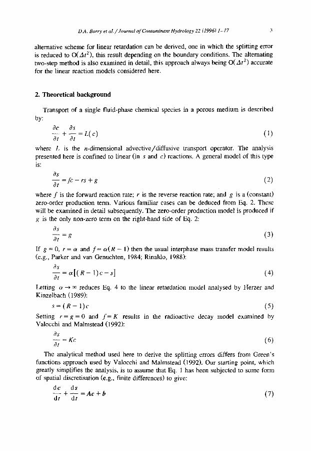
alternative scheme for linear retardation can be derived, one in which the splitting error is reduced to o( At*>, this result depending on the boundary conditions. The alternating two-step method is also examined in detail, this approach always being O(At*> accurate for the linear reaction models considered here.

2. Theoretical background

Transport of a single fluid-phase chemical species in a porous medium is described by:

where L is the n-dimensional advective/diffusive transport operator. The analysis presented here is confined to linear (in s and cl reactions. A general model of this type is:

as y$=fc-rs+g

where f is the forward reaction rate; r is the reverse reaction rate; and g is a (constant) zero-order production term. Various familiar cases can be deduced from Eq. 2. These will be examined in detail subsequently. The zero-order production model is produced if g is the only non-zero term on the right-hand side of Eq. 2:

as x=g (3)

If g = 0, r = a and f= a(R - 1) then the usual interphase mass transfer model results (e.g., Parker and van Genuchten, 1984; Rinaldo, 1988):

as z=a[(R-l)c-s]

Letting a + = reduces Eq. 4 to the linear retardation model analysed by Herzer and Kinzelbach ( 1989):

s=(R- 1)” (5) Setting r = g = 0 and f= K results in the radioactive decay model examined by Valocchi and Malmstead (1992):

as - = Kc at

The analytical method used here to derive the splitting errors differs from Green’s functions approach used by Valocchi and Malmstead (1992). Our starting point, which greatly simplifies the analysis, is to assume that Eq. 1 has been subjected to some form of spatial discretisation (e.g., finite differences) to give:

dc ds

dt+ -=Ac+b dr (7)

4 D.A. Barry et al./ Journal of Contaminant Hydrology 22 (1996) I -I 7

where c is a vector (length m) of concentrations; s is vector (length m) of sorbed solute concentrations; A is a (usually sparse) matrix (m X m) representing the discretisation of the spatial operator, L, in Eq. 1; and b is a vector (length m) resulting from the application of the boundary conditions together with the spatial discretisation scheme. Note that b = 0 for homogeneous boundary conditions. Most numerical schemes are constructed such that a Taylor series expansion of Eq. 7 about an arbitrary node in the spatial grid differs from Eq. 1 by a term with the coefficient Ax*, in which case the spatial discretisation is second-order, i.e. O( Ax2), accurate.

If the fully coupled transport/reaction problem was being solved then, similarly to the spatial discretisation, the temporal discretisation of Eq. 7 would usually be con- structed so that it is 0(At2) accurate. This is achieved using a Crank-Nicolson discretisation (e.g., Noye, 1982) of Eq. 7:

A,c(k+ 1) +s(k+ 1) =s(k) +A,c(k) + [Z&k+ 1) +b(k)];

where c(k) - meaning c(kAt) - is the numerical solution at the kth time step; A, = Z - A At/2; A, = Z + A At/2; and b is a given function of time. Solutions c and s computed using Eq. 8 are second-order accurate in space and time. Of course, the idea is not to solve Eq. 8 at all, as it represents the fully coupled problem. Rather, one wishes to approximate its solution in (at least) two, more simple steps, viz. operator splitting. However, this may introduce an O( At) error, so negating the effectiveness of the O(At2> numerical scheme given in Eq. 8. In this paper we will adopt the stance that any O(At2> operator-splitting method is “exact”, in the sense that its error term is of the same order as Eq. 8. Thus, below we present only the O( At) terms that arise due to operator splitting.

The standard two-step method consists of carrying out sequentially the following operations within each time step of the numerical solution (Barry et al., 1996):

Transport: c*(k+ 1) =A;’ A,c(k) + [b(k+ 1) +b(k)]G)

and

Reaction: c(k+ 1) +s(k+ 1) =s(k) +c*(k+ 1) (10)

where the superscripted asterisk indicates an intermediate estimate. The transport equation simply calculates the solution as though s = 0 in Eq. 8. The reaction step is a node-wise statement of mass balance, i.e. Eq. 10 is a discretised version of:

dC as at=-at’ kAt<t<(k+l)At, c(k)=c*(k+l), s(k)known (11)

EQ. 11 contains two unknowns, so a second equation is needed for its solution:

as - =h(c,s), at

kAt< ts (k+ 1)At (12)

where h is assumed to operate node-wise on c and s, i.e. only local reactions take place. Because the reaction step, Eq. 10, is a Crank-Nicolson discretisation of Eq. 11, it cannot

DA. Barry et al./Journal oj’Contaminunt Hydrology 22 (1996) 1-17 5

be solved until h in Eq. 12 is specified. If h is such that, upon Crank-Nicolson discretisation, an explicit equation for s(k + 1) results, then this variable can be eliminated in the reaction step above, leaving c(k + 1) as the only unknown. Otherwise, Eq. 10 and the discretised version of Eq. 12 are solved simultaneously to compute s(k + 1) and c(k + 1). However, in either case an ambiguity arises because the solution of Eq. 12 requires starting values. For s it is clear that one takes s(k), but for c there are two choices, either c(k) or c * (k + 1). Not surprisingly, each choice gives different results, as will become clear below.

3. Example applications of the standard two-step scheme

In this section we determine the splitting error for the various models listed above in Eqs. 3-6.

3. I, Zero-order production

Although this case is trivial, it is included for completeness. The standard two-step scheme consists of Eq. 9, followed by Eq. 10, where s(k + 1) is eliminated using a Crank-Nicolson discretisation of Eq. 3, i.e. Eq. 10 becomes:

c(k+ 1) =c*(k+ 1) -gAt (13)

The intermediate term, c * (k + 11, on the right-hand side of this equation can be eliminated using Eq. 9, so F!q. 13 relates c(k + 1) to c(k). We then calculate the Taylor series expansion in At for each side of Eq. 13, and ascertain the governing model that is actually being solved by the numerical scheme. This simple calculation shows that the governing model, Eq. 7, is recovered with o(At’) accuracy. We thus regard the standard two-step as being exact in this case.

3.2. Radioactive decay

It is instructive to treat the case of radioactive decay in some detail. Eq. 6 is taken as the governing reaction model. A Crank-Nicolson discretisation of this equation yields, in vector form:

s(k+ 1) =s(k) + YIc(k+ 1) +c] (14)

where the circumflex indicates that either c(k) or c* (k + 1) may be selected. With Eq. 14, the reaction step is written:

KAt I

c(k+ 1) = c’(k+l)-TC

KAt (15) lf-

2

6 D.A. Barry et al./Journal of Contaminant Hydrology 22 (1996) l-17

After calculation of Eq. 15, Eq. 14 can be solved to keep track of solute removal from the system. However, Eq. 14 need not be used if only the liquid-phase concentra- tion, c, is of interest. Taylor series expansions in Ar were determined for each side of Eq. 15 using the two available choices for c^, with the results:

dc KAt -=Ac+b-Kc+ dr

-AC, e=c(k) 2 ( 16)

and dc KAt -=Ac+b-Kc-- dt

2 b, c^=c*(k+l) (17)

To obtain Eqs. 16 and 17 (and similar expansions presented below) the Taylor series expansions were carried out at the midpoint of the time step, i.e. at t = (k + +)At. Some details are given in Appendix A to demonstrate the method by which these results are obtained. Eqs. 16 and 17 show the O( At) error involved in the standard two-step method. Recall that A is a matrix that results from discretisation of L. Conversely, A, after it acts upon c, can be considered an operator for which spatial Taylor series for the elements of c can be calculated. In Eq. 16, the error term shows that the magnitude of both the diffusive and advective terms is increased in proportion to At. Eq. 17, on the other hand, includes an additional sink term, again proportional to At. The additional term will lead to mass balance errors, as previously shown by Valocchi and Malmstead (1992). Note also that for b = 0 (homogeneous boundary conditions), the error term for Eq. 17 is O(At’>, i .e. O( At2) accuracy is available for homogeneous boundary conditions and an inhomogeneous initial condition. This general&s the findings of Valocchi and Malmstead (1992), who derived their results for the special case of a one-dimensional, semi-infinite spatial domain, with an inhomogeneous boundary condi- tion at the origin.

In Fig. 1, an example of the result given in Eq. 17 displayed. Two sets of boundary and initial conditions were considered. In the first case, Eqs. 1 and 6 were solved numerically in one dimension in the finite domain 0 < x < 1, with the following initial and boundary conditions:

X7T c( x,0) = cgcos - ) ( 1 O<x<l

21 (18) c(O,t)=c,, O<t (19)

and c(f,t)=O, O<t (20)

A Crank-Nicolson finite-difference scheme (e.g., Barry et al., 1983) was used to calculate the “exact” numerical results (grid-independent results are shown), repre- sented by the pluses. The corresponding two-step scheme predictions, Eq. 15 with c^ = c * (k + l), are shown as the solid circles. The O( At) error discussed by Valocchi and Malmstead (1992) is evident. To compare this with the case of homogeneous boundary conditions, we calculated identical numerical solutions for the same problem except that Eqs. 18 and 19 are replaced by:

c( x,0) = c0 sin( xm/l) , 0 < x < 1 (21)

D.A. Barry et al. / Journal of Contaminant Hydrology 22 (1996) 1 -I 7 7

Fig. 1. Comparison of “exact” and two-step numerical solutions. Exact solutions are given by the solid line (underlies the solid squares) and the plus signs. The corresponding two-step solutions are given by the solid squares and solid circles, respectively. Parameters used: ul/D = u2t/D = 10, u*/KD = 5. The solutions were all calculated with Ax/l= 10m3. The exact solutions used the time step KAt = 2. 10e4, while the two-step results were calculated using KAt = 2. IO- ‘.

and

c(O,t) = 0, 0 < I (22)

respectively. Using the same discretisation in the two-step scheme gives more accurate results, as is clear in Fig. 1 where the exact and two-step solutions are almost indistinguishable.

3.3. Interphase mass transfer

Interphase mass transfer is a widely used model for analysing transport experiments (e.g., van Genuchten et al., 1974, 1977; van Genuchten and Wierenga, 1976, 1977; Miller et al., 1990; Li et al., 1994a, b; Bajracharya and Barry, 1995). Eq. 4 is the specific reaction model analysed here. As in Sections 3.1 and 3.2, a Crank-Nicolson discretisation will be applied to this model, giving an explicit expression for s(k + 11, which is then used in the reaction portion of the two-step algorithm. The equations to be solved in each time step are:

(1) Begin: t=kAt [c(k) and s(k) areknown]

(a) Transport: Solve Eq. 9

(b) Reaction: c( k + 1) = (1 -+)8(k) +c*(k+ 1) -a,c^

1 +a, (23)

8 D.A. Barry et al./ Journul of Contumimnt Hydrology 22 (1996) I-I 7

and

s(k+ 1) =a,[c(k+ 1) i-21 fa,s(k)

where

aAt y(R-1)

a, = crdt 1+-

2

(24)

(25)

aAt l--

2 a2 = aAt (26) 1+-

2

(2) End of time step: t=(k+ 1)At [c(k+ 1) and s(k+ 1) areknown].

Eqs. 23 and 24 were expanded in Taylor series as before, the difference in this case being the additional variables s(k) and s(k + 1). The two resulting expressions were solved simultaneously for s and d c/d t. We treat c^ each case of separately.

For c^ = c(k), we find that the vector form of Eq. 4 is recovered with an O( At21 error term while for the transport equation we have:

dc ds At ds dt+dr=Ac+b+-A-

2 dt (27)

An explicit expression for the O( At) term in Eq. 27 is derived in Appendix B. Over the time step from k At to (k + 1) At the non-trivial part of this term is written:

A: = exp( -RaAt)Ae dt I f kAt

+ a( R - l)l(k+‘)Ar kAr

Xexp[-Ra{(k+l)At-r}]A*c(r)dr (28) By recursion, the first term on the right-hand side of this equation can be written in

terms of previous time steps. This expansion is not made as we assume for the purpose of the error calculation that the results from the k At time step are exact, i.e. we are interested in the error over a single time step. Eq. 28 is such that simple corrections to the standard two-step scheme are not readily available for interphase mass transfer. An exception is the case of very rapid transfer, cr -+ a. In this limit Eq. 28 reduces to:

(29)

Recall the A is a discretised version of L, the latter operator consisting of first- and second-order spatial derivatives, so second- through fourth-order spatial derivatives will occur on the right-hand side of Eq. 29. One generally assumes that the lowest-order derivative dominates error terms. Eq. 29 thus produces numerical diffusion of magnitude v2At(R - 1)/2R for the special case of steady, unidirectional flow, this result agreeing

D.A. Barry et al./ Journal of Contaminant Hydrology 22 (1996) I-17 9

with that presented by Herzer and Kinzelbach (1989). Eq. 28, however, is significantly more general as it applies for arbitrary (Y and A.

For c^ = c * (k + l), the analysis is a little more involved. After performing Taylor series on each of Eqs. 23 and 24, we obtain, again, Eq. 27. However, the expression for ds/dt is no longer o(At*> accurate:

ds aAt ;=a[(R- l)c-s] +$R- l)(Ac+b)

Because Eq. 30 contains an O( At) term, deriving an explicit expression O( At) term in Eq. 27 requires some care. Note that Eq. 30 is equivalent to:

ds

dt

(30)

for the

=aexp(-at)[(R-l)c(O)-s(O)] +a(R--l)/dexp[-a(t-r)]zdr

+ $(R- l)(exp(-ur)[Ac(O) +b(O)] +ktexp[-a(r-r)]

.(A;+g)dr) (31)

where, as in Appendix B, we have set k = 0 to avoid unnecessary cluttering of the expression. When the O( At) term in Eq. 31 is removed, it reduces to Eq. B-l, as it should. Now, substitute from Eq. 31 into Eq. 27 and simplify, to obtain (taking k + 0):

z +(~exp(-c~dt)[(R- I)c(kAt) -s(kAt)]

+a(~-l)~(‘t’)A’exp[-u{(k+l)At-r}]~dr kAr

aAt =Ac+b-- 2 exp( - aAt) [ As( kdt) + b( kdt)]

_ z$_ q-t exp[-a{(k+ I)Ar-Tj]gdT (32)

Eq. 32 thus has an O( At) error as its left-hand side is exact. Observe that in the limit of a (Y --) 00 the left-hand side reduces to R . dc/dr, and most of the terms on the right-hand side disappear. However, unless t, is constant, the final term on the right-hand side will always be non-zero, so that otherwise the scheme remains ddt) accurate for the linear retardation model, Eq. 5. In addition, unless b = 0 for all t, an O( At) error will be introduced as the imposition of a non-zero b means that there is a step change in concentration as t + 0. Thus, for homogeneous boundary conditions, the two-step scheme given by Eqs. 23 and 24 is o(At*) accurate for the case of linear retardation. Clearly, this scheme is not one that would be apparent if Eq. 5 was used as the starting point in place of Eq. 4. An example of this result is shown in Fig. 2. There

10 D.A. Barry et al./Journal of Contaminunt Hydrology 22 (1996) 1-17

Position, x/l

Fig. 2. Comparison of two-step schemes for linear retardation. The solid curue is the “exact” solution, the dashes were computed using Eqs. 23 and 24 with c^ = c * (k + 1). The solid circles were computed identically but with E = c(k). Parameters used: IA/D = u*t/D = 10, R = 2. The solutions were all calculated with Ax/l= 10e3. The exact solution (line) was computed using the time step u’At/D= 10m3, while the two-step results were calculated using v2At/D = 1.

we show simulations of the one-dimensional transport equation for the case of linear retardation solved subject to the conditions given by Eqs. 20-22. The “exact” numeri- cal solution was calculated as for Fig. 1. Both cases of c^ are considered, i.e. E=c*(k+l)and c^=c(k).Th e e b h aviour discussed above is evident, with the choice c^ = c * (k + 1) giving O( At*) accuracy.

4. The alternating two-step method

In this method the reaction step is sandwiched between two transport steps. As mentioned already, Valocchi and Malmstead (1992) showed that an O( At2> scheme results by taking this approach for the case of radioactive decay. Miller and Rabideau (1993) carried out a thorough numerical study of the approach. They considered that in many problems the reaction portion of the calculations would dominate the computa- tional load, so they used the Strang (1968) approach in each time step: transport over At/2, react over At, traqort over At/2. Generally the results of this approach were satisfactory, a finding that was echoed more recently by Zysset et al. (1994). This scheme differs slightly from that considered by Valocchi and Malmstead (19921, who used two reaction steps, each of duration At/2, in their alternating two-step scheme for

D.A. Barry et al./Journal of Contaminant Hydrology22 (1996) I-17 I1

radioactive decay. We consider in detail the Miller and Rabideau (1993) approach here. A Taylor series analysis for the radioactive decay model shows that either scheme is O( Ar2) accurate so long as we set c^ = c * (k + l), otherwise each scheme is only O( At) accurate. That both schemes give the same order of accuracy is hardly surprising as if the reaction step is carried out analytically using the solution to Eq. 6 then the schemes become identical. For the purposes of this section, we shall assume that the transport steps are carried out over a time interval of Ar/2, i.e. At in the definitions of A, and A, is replaced by At/2.

4.1. Linear retardation

Unlike the radioactive decay model for which the alternating two-step scheme works well, the linear retardation isotherm presents an interesting counter-example, and serves to show that some care is needed in applying the alternating two-step method to equilibrium reactions. The scheme consists of the following steps:

(1) For tfrom(k- l)Ar+kAt,

s(k) = (R- l)c*(k) 1

(2) For tfrom kAt-+(k+ l)At,

(a) Transport. Solve:

c*(k++)=A;l(a,c(k)+[b(ic;)+b(k)];} (34)

(33)

(b) Reaction. Solve Eq. 10 using Eq. 5:

c*(k+ t> = c*(k++)+s(k) R (35)

and

s(k+l)=(R-l)c*(k+l) (36) (c) Transport. Solve:

c(k+ 1) =a;‘ja,c*(t+ 1) + [b(k+ 1) +b(i+&) (37)

Eq. 33 is used only to relate s(k) to c(k). Note that there is no choice concerning c^. We cannot replace the definition of s(k) in Eq. 33 with s(k) = (R - l>c * (k + $1 in Eq. 35 as otherwise no reaction will take place. A Taylor series expansion of Eq. 37 yields the governing linear retardation transport equation with an O(At) error term. We do not write this term here as it is precisely the expression (multiplied by At/21 given on the right-hand side of Eq. 29, i.e. the error has doubled (recall that At is effectively halved

12 D.A. Barry er al./Journal of Conraminmt Hydrology 22 (1996) 1-17

here as two transport steps are being carried out). Clearly, the alternating two-step is not useful in this case.

4.2. Interphase mass transfer

We next consider the nonequilibrium interphase mass transfer model, Eq. 4, as our prototype. The specific steps that compose the alternating two-step method in this case are:

(1) Begin: r=kAt[c(k) and s(k) areknown].

(a) Transport. Solve Eq. 34, giving C* (k + 3).

(b) Reaction:

c*(k+l)= (1 -az)s(k) +(l -a,)c*(k++)

1 +a,

and

s(k+ 1) =a,[c*(k+ 1) +c*(k+i)] +a,s(k)

(c) Transport: Solve Eq. 37.

(38)

(39)

(2)Endoftimestep: t=(k+l)At[c(k+l)ands(k+l)areknown]

Note that the definitions of a, and a2 are precisely the same as given in Section 3.3, i.e. At is not replaced by At/2 in the reaction step. The Taylor series expansions of s(k + 1) and c(k + 1) reveal that this model is O(At’> accurate. Of course, taking the limit (Y -+ w gives a similarly accurate model for linear retardation.

As in Section 3.3, there are two choices available in the specification of c^. Only results for c^ = c * (k + i) are given here. The other choice, E = c(k), results in an O( At) accurate scheme, so it is of no interest.

5. Concluding remarks

We have developed a number of results on split-operator methods for popular linear models of single species “ reaction’ ’ . There is no spatial discretisation error induced by operator splitting of reaction/transport models and, hence, we have focused entirely on the temporal discretisation errors. By dealing with an arbitrary spatial operator, we are able to generalise and extend previous analyses. For convenience, a summary of the analyses carried out here is included in Table 1. This table shows the order of the various truncation errors derived for all the models examined.

Three main points come out of this paper: (1) There is some ambiguity in the initial condition for c in the chemical reaction

model, ds/d t. One can use c from the beginning of the time step, or from the most recent transport step. For the standard two-step method, the former case generally results in additional numerical diffusion, while the latter tends to give mass-balance errors, particularly for inhomogeneous boundary conditions.

D.A. Barry et al./Joumal of Contaminant Hydrology 22 (1996) I-17 13

Table 1 Summary of models and numerical solutions

Case Analytical Solution Numerical Accuracy Notes model scheme model

Zero-order production F.q. 3 TS a F.q. 13 o(Ar*) Radioactive decay Eq.6 TS F.q. 1.5 O(At) c = c(k)

o(At’> e^=c *(k+l)and b=O Interphase mass transfer Eq. 4 TS Eqs. 23 @At)

and 24

AS b Eqs. 37 and 39 dAt-9 i?=c ‘G+i) Linear retardation Eq.5 TS (I +m in Eqs. 23 O(At) ? = c(k)

and 24

o(At*) f=c *(k+l)and b=O AS Eqs. 36 and 37 ddt)

AS a --tee in Eqs. 37 O(Ar*)

and 39

a Standard two-step scheme.b Alternating two-step scheme.

(2) Rather than decreasing the truncation error, a direct application of the alternating split-operator method leads to increased error for the equilibrium reaction model considered here. We considered the simple case of linear retardation, but it is reasonable to expect that this finding will also hold for nonlinear models.

(3) Alternative equilibrium models can be derived as a limiting case of a nonequilib- rium model. In particular, the split-operator approach presented by Miller and Rabideau (1993) leads directly to an O( At21 accurate model for the case of linear retardation. Unlike the previous conclusion, it is likely that this result is not a general one, and relies on the linearity of the interphase transfer model used here. Miller and Rabideau (1993) found that for nonlinear models the numerical scheme error increased with reaction rate, apparently in proportion to At. More analysis of nonlinear models is needed before the findings presented here can be generalised to nonlinear isotherms.

6. Notation

List of symbols used in this paper

Symbol Description aI a2 A

variable defined by Eq. 25 variable defined by Eq. 26 matrix representing discretisation of the spatial operators matrices defined below Rq. 8 vector representing boundary conditions liquid-phase concentration solute concentration vector

AL, A, b C

c

Dimensions

[T-II

[ML3 T-‘1 [M L-3] [ML-3]

14

h Z k K 1 L m n P r R s

S

t

V

x

Greek

it Ax 7

D.A. Barry et al./Journal of Contaminant Hydrology 22 (1996) I-17

boundary concentration diffusion/dispersion coefficient

[M, L-3l

forward reaction rate [k- ;-‘I

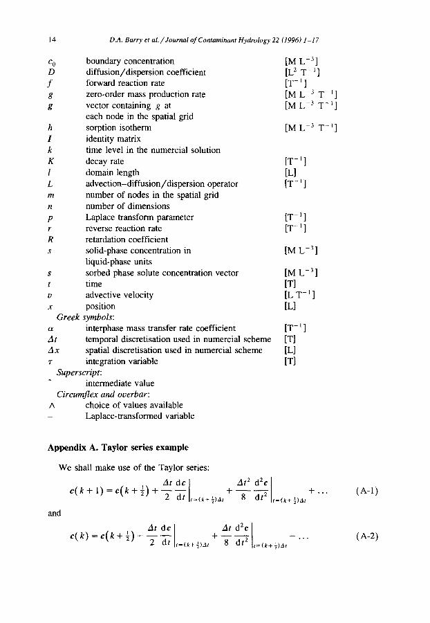
zero-order mass production rate [M L-3 T-‘1 vector containing g at [M L-3 T-‘1 each node in the spatial grid sorption isotherm [M L-3 T-l] identity matrix time level in the numercial solution decay rate domain length K” advection-diffusion/dispersion operator IT-‘] number of nodes in the spatial grid number of dimensions Laplace transform parameter IT-‘] reverse reaction rate [T-II retardation coefficient solid-phase concentration in [M L-3] liquid-phase units sorbed phase solute concentration vector time El L-33 advective velocity position kT-‘l

symbols: interphase mass transfer rate coefficient CT-‘1 temporal discretisation used in numercial scheme [T] spatial discretisation used in numercial scheme Ll integration variable [T]

Superscript: 1: intermediate value Circumflex and overbar:

A choice of values available _ Laplace-transformed variable

Appendix A. Taylor series example

We shall make use of the Taylor series:

E(kfl)=e(k++)+;~ = + $2 _ + . . . (A-1) f (k+$)Ar r-(k+ f)Ar

and

At d2c c(k)=c(k++)-;z = +8dt2 _ -...

I (k+f)Ar r-(k+f)Ar (A-2)

DA. Barry er ai./Journal of Contaminant Hydrology 22 (1996) l-17 1s

Similar expressions will be used for b(k) and b,(k + 1). In the following all derivatives will be assumed to be evaluated at r = (k + i)Ar. Expansion of Eq. 9 using these series gives:

c*(k+l)=c(k++)+Ar

At= +t A’c-A

( ;+;$ +0(At3)

1 (A-3)

This expression is then substituted into Eq. 15, and a further Taylor series is calculated for c(k + 1). Finally, the iatter expression is subtracted from the right-hand side of Eq. A-l, and an expression for dc/dt is obtained. Depending on the choice of c^ in Eq. 15, this sequence of steps gives either Eq. 16 or Eq. 17.

Appendix B. Calculation of A . d s/d t

As stated in the text, Eq. 4 agrees with the expression for ds/dr from the numerical scheme to O( At’), so we may take this as an exact expression for the purpose of calculating A * ds/dt. With this starting point, we note also that although s(k) and c(k) are the initial conditions, it is irrelevant what value of k is selected, so we take k = 0, as it simplifies slightly the expressions given below. First, note that Eq. 4 is equivalent to:

ds - =exp(-nt)? dt

dt = +a(R- l)/derp[-a(t-r)]zdr I 0

Laplace transformation of each side of Eq. B-l yields:

+a(R+ l)[Ac+&G+s(O)]

P-1)

(B-2)

where Eq. 27 has been used to arrive at the terms in brackets on the right-hand side. An explicit expression for ps^ - s(O) can be derived from Eq. B-2. The inverse Laplace transform of this equation is:

ds - =exp(-Rut); _ dt t-0

+a(R- l)/okXP[-R~l(f-T)][Ac(T) +b(r)]dr

P-3)

The required expression is derived by operating on each side of Eq. B-3 by A, i.e.:

A: = exp( -Rat)AdS dt = +a(R- l)[exp[-Ru(r--r)]A2c(r)dT I 0

(B-4)

where we have noted that, because A represents a spatial operator, Ab = 0.

16 D.A. Barry et al./ Journal oj’Contaminant Hydrology 22 (1996) I-l 7

References

Bajracharya, K. and Barry, D.A., 1995. MCMFIT: Efficient optimal fitting of a generalised nonlinear advection-dispersion model to experimental data. Comput. Geosci., 2 1: 6 1-76.

Barry, D.A., 1992. Modelling contaminant transport in the subsurface: Theory and computer programs. In: H. Ghadiri and C.W. Rose (Editors), Modelling Chemical Transport in Soil: Natural and Applied Contami- nants. Lewis, Boca Raton, FL, pp. 10.5- 144.

Barry, D.A., Starr, J.L., Parlange, J.-Y. and Braddock, R.D., 1983. Numerical analysis of the snow-plow effect. Soil Sci. Sot. Am. J., 47: 862-868.

Barry, D.A., Miller, CT. and Bajracharya, K., 1996. Alternative split-operator approach for solving chemical reaction/groundwater transport models. Adv. Water Resour. (submitted).

Coats, K.H. and Smith, B.D., 1%4. Dead end pore volume and dispersion in porous media. Sot. Pet. Eng. J., 4: 73-84.

Dougherty, D.E. and Tompson, A.F.B., 1994. Pass the trash. In: A. Peters, G. Wittum, B. Herrling, U. Meissner, C.A. Brebbia, W.G. Gray and G.F. Pinder (Editors), Computational Methods in Water Resources, X. Kluwer, Dordrecht, pp. 613-620.

Hetzer, J. and Kinzeibach, W., 1989. Coupling of transport and chemical processes in numerical transport models. Geoderma, 44: 115- 127.

Kaluarachchi, J.J. and Motshed, J., 1995. Critical assessment of the operator-splitting technique in solving the advection-dispersion-reaction equation, 1. First-order reaction. Adv. Water Resour., 18 89-100.

LeVeque, R. and Oliger, J., 1983. Numerical methods based on additive splittings for hyperbolic partial differential equations. Math. Comput., 40: 469-497.

Li, L., Barry, D.A. and Stone, K.J.L., 1994a. Centrifugal modelling of nonsorbing, nonequilibrium solute transport in a locally inhomogeneous soil. Can. Geotech. J., 31: 471-477.

Li, L., Barry, D.A., Culligan-Hensley, P.J. and Bajracharya, K., 1994b. Mass transfer in soils with local stratification of hydraulic conductivity. Water Resour. Res., 30: 2891-2900.

Miller, C.T. and Rabideau, A.J., 1993. Development of split-operator, Petrov-Galerkin methods to simulate transport and diffusion problems. Water Resour. Res., 29: 2227-2240.

Miller, C.T., Poirier-McNeill, M.M. and Mayer, AS., 19%. Dissolution of trapped nonaqueous phase liquids: Mass transfer characteristics. Water Resour. Res., 26: 2783-2796.

Morshed, J. and Kaluarachchi, J.J., 1995. Critical assessment of the operator-splitting technique in solving the advection-dispersion-reaction equation, 2. Monod kinetics and coupled transport. Adv. Water Resour., 18: 101-I 10.

Noye, J., 1982. Numerical solutions of partial differential equations. In: J. Noye (Editor), Proceedings of the 1981 Conference on the Numerical Solutions of Partial Differential Equations Held at Queen’s College, Melbourne University, Australia. North-Holland Publ. Co., Amsterdam, pp. 3-137.

Parker, J.C. and van Genuchten, M.Th., 1984. Determining transport parameters from laboratory and field tracer experiments, Va. Agric. Exp. Stn. Bull. 84-3, Va. Polytech. Inst. and State Univ., Blacksburg, VA.

Rinaldo, A., 1988. Solute lifetime distributions in soils and the two-component convection-dispersion equation. In: P.J. Wierenga and D. Bachelet (Editors), Validation of Flow and Transport Models for the Unsaturated Zone: Conference Proceedings, May 23-26, Ruidoso, New Mexico. Dep. Agron. Hart., New Mexico State Univ., Las Crimes, NM, pp. 340-345.

Stmng, G., 1968. On the construction and comparison of difference schemes. SIAM (Sot. Ind. Appl. Math.) J. Numer. Anal., 5: 506-517.

Valocchi, A.J. and Malmstead, M., 1992. Accuracy of operator splitting for advection-dispersion-reaction problems. Water Resour. Res., 28: 1471- 1476.

van Genuchten, M.Th. and Wierenga, P.J., 1976. Mass transfer studies in sorbing porous media, 1. Analytical solutions. Soil Sci. Sot. Am. J., 40: 473-480.

van Genuchten, M.Th. and Wierenga, P.J., 1977. Mass transfer studies in sorbing porous media, II. Experimental evaluation with tritium (‘H,O). Soil Sci. Sot. Am. J., 41: 272-278.

van Genuchten, M.Th., Davidson, J.M. and Wierenga, P.J., 1974. An evaluation of kinetic and equilibrium equations for the prediction of pesticide movement through porous media. Soil Sci. Sot. Am. J., 38: 29-35.

DA. Barry et al./ Journal of Contaminant Hydrology 22 (1996) I -I7 17

van Genuchten, M.Th., Wierenga, P.J. and O’Comter, G.A., 1977. Mass transfer studies in sorbing porous media, III. Experimental evaluation with 2,4,5-T. Soil Sci. Sot. Am. J., 41: 278-285.

Yeh, G.-T. and Tripathi, VS., 1989. A critical evaluation of recent developments of hydrogeochemical transport models of reactive multichemical components. Water Resour. Res., 25: 93- 108.

Yeh, G.-T. and Tripathi, V.S., 1991. A model for simulating transport of reactive multispecies components: Model development and demonstration. Water Resour. Res., 27: 3075-3094.

Zysset, A., Stauffer, F. and Dracos, T., 1994. Modeling of chemically reactive groundwater transport. Water Resour. Res., 30: 2217-2228.