Iterative Support Detection based Split Bregman Method for Wavelet Frame Based Image Inpainting

5470 IEEE TRANSACTIONS ON IMAGE PROCESSING, VOL. 23, NO. 12, DECEMBER 2014

Iterative Support Detection-Based Split BregmanMethod for Wavelet Frame-Based Image Inpainting

Liangtian He, Member, IEEE, and Yilun Wang, Member, IEEE

Abstract— The wavelet frame systems have been extensivelystudied due to their capability of sparsely approximating piece-wise smooth functions, such as images, and the correspondingwavelet frame-based image restoration models are mostly basedon the penalization of the �1 norm of wavelet frame coefficientsfor sparsity enforcement. In this paper, we focus on the imageinpainting problem based on the wavelet frame, propose aweighted sparse restoration model, and develop a correspondingefficient algorithm. The new algorithm combines the idea ofiterative support detection method, first proposed by Wang andYin for sparse signal reconstruction, and the split Bregmanmethod for wavelet frame �1 model of image inpainting, and moreimportant, naturally makes use of the specific multilevel structureof the wavelet frame coefficients to enhance the recovery quality.This new algorithm can be considered as the incorporation ofprior structural information of the wavelet frame coefficients intothe traditional �1 model. Our numerical experiments show thatthe proposed method is superior to the original split Bregmanmethod for wavelet frame-based �1 norm image inpainting modelas well as some typical � p(0 ≤ p < 1) norm-based nonconvexalgorithms such as mean doubly augmented Lagrangian method,in terms of better preservation of sharp edges, due to their failingto make use of the structure of the wavelet frame coefficients.

Index Terms— Image inpainting, iterative support detection,augmented Lagrangian, split Bregman, wavelet frames, sparseoptimization, nonconvex optimization.

I. INTRODUCTION

INPAINTING refers to problems of filling-in the missingparts in images, and it arises, for examples, from removing

scratches in photos, restoring ancient drawings, and fillingin the missing pixels of images transmitted through noisychannels. For the simplicity of notations, we denote the imageas vectors in R

n with n being equal to the number of totalpixels. Image inpainting is often formulated as a linear inverseproblem:

f = Au + η, (1)

where f is the observed image, η denotes the additiveGaussian white noise with mean being 0 and variance

Manuscript received November 5, 2013; revised May 2, 2014 andSeptember 16, 2014; accepted September 18, 2014. Date of publicationOctober 8, 2014; date of current version November 12, 2014. This work wassupported in part by the National Science Foundation of China underGrant 11201054 and Grant 91330201 and in part by the FundamentalResearch Funds for the Central Universities under Grant ZYGX2012J118 andGrant ZYGX2013Z005. The associate editor coordinating the review of thismanuscript and approving it for publication was Dr. Ali Bilgin.

The authors are with the School of Mathematical Sciences, University ofElectronic Science and Technology of China, Chengdu 611731, China (e-mail:[email protected]; [email protected]).

Color versions of one or more of the figures in this paper are availableonline at http://ieeexplore.ieee.org.

Digital Object Identifier 10.1109/TIP.2014.2362051

being σ 2, the linear operator A is a projection operator,or more precisely, a diagonal matrix with diagonals 1 if thecorresponding pixel is known, or 0 otherwise, and u is theunknown true image.

To restore u from f , one of the most natural choices issolving the following least square problem

minu∈Rn

||Au − f ||22 (2)

where ||.||2 denotes the �2 norm. However, the noise ηpossessed by f will be amplified greatly, since the matrix Ais usually ill-conditioned. Therefore, to suppress the effectof noise and also preserve the sharp attributes of images,e.g., edges and boundaries, various regularization based meth-ods have been proposed to obtain a reasonable approximatedsolution from (1). Among them, variational methods andwavelet frames based approaches are widely used and havebeen proven successful.

The trend of variational methods for image processingbegins with the refined Rudin-Osher-Fatemi (ROF) model [11]which penalized the total variation (TV) of u, due to its advan-tages in exploiting blocky image structures and preservingimage edges, and the ROF model is particularly effective onrestoring images that are piecewise constant. In the past fewyears, many corresponding efficient algorithms have been pro-posed to further promote the applicability of the ROF model,including our proposed operator splitting algorithm [55], andmany others [56], [57] and el al. In addition, many othertypes of variational models have been also proposed afterwardand we refer the interested readers to [12], [23]–[27], and thereferences therein for further studies.

Wavelet frame based methods are relatively new and theirbasic idea is that images can be sparsely approximatedby properly designed wavelet frames. Correspondingly, thecommonly regularization method for these models is the�1-norm of the wavelet frame coefficients due to its sparsityenforcement and convexity. Although the forms of waveletframe are similar to variational methods, they were consideredas different approaches, partially because the wavelet framemodels are defined for discrete data, while the variationalmethods assume continuity. While some studies in the liter-atures [54] indicated that there was a relationship betweenhaar wavelet and variational methods, it is still not clearwhether there exist general relations between wavelet framesand variational models in the context of image restoration,though a recent paper [30] shows that, for one of the waveletframe based models namely analysis based approach, it can beviewed as a finite difference approximation of a certain type of

1057-7149 © 2014 IEEE. Personal use is permitted, but republication/redistribution requires IEEE permission.See http://www.ieee.org/publications_standards/publications/rights/index.html for more information.

HE AND WANG: ITERATIVE SUPPORT DETECTION BASED-SPLIT BREGMAN METHOD 5471

general variational model, and the approximation will be exactif image resolution goes to infinity. In addition, it has beenshown in [1], [2], [6], and [28]–[30] that the wavelet framebased models are often superior than some variational modelssuch as ROF model because the multiresolution structure andredundancy property of wavelet frames allow to adaptivelychoose proper differential operators according to the order ofthe singularity of the underlying solutions for different regionsof a given image [30].

The main contributions of this paper are summarized asfollows. We propose a new wavelet frame based weighted�1 minimization model for image inpainting. While the newmodel is non-convex, we give an efficient multi-stage convexrelaxation algorithm based on the ideas of iterative supportdetection [13] and alternative optimization to find a reasonablegood solution, which is not necessarily the global solutionthough. More important, when performing the key compo-nent, i.e. support detection, we make use of the multi-levelstructure of wavelet frame coefficients to improve the supportdetection quality rather than the plain thresholding adopted inthe original implementation proposed in [13], and the betterperformance is achieved than the plan �1 model and the�p(0 ≤ p < 1) model which both fail to make use of thestructure information of the wavelet coefficients. Numericalexperiments empirically demonstrate the advantages of thisnew algorithm in terms of better preserving of image structuressuch as edges.

The rest of this paper is organized as follows. In the nextsection, we first introduce wavelet frames and a correspond-ing wavelet frame based �1 norm image inpainting model.An efficient algorithm proposed by [2], [30], and [41] is thenreviewed. In Section III, we introduced our new wavelet framebased weighted �1 image inpainting model and proposed acorresponding effective algorithm motivated by the idea ofthe iterative support detection. In Section IV, we comparethe performance of our new method with the �1 norm basedapproach proposed by [30] and �p(0 ≤ p < 1) norm basedapproach [7]. Section V is devoted to the conclusion of thispaper and discussions on some possible future research.

II. BACKGROUNDS

A. Wavelet Frame and Wavelet Frame Based Models

We first briefly introduce the concepts of tight frame andtight wavelet frame, then review some of the typical waveletrestoration models. Interested readers can consult [31], [32],and [5], [6], [33] for further detailed introduction of waveletframe and its applications.

A countable set X ⊂ L2(R) is called a tight frame ofL2(R) if

f =∑

h∈X

< f, h > h, ∀ f ∈ L2(R).

where < · > denotes the inner product of L2(R). Thetight frame X is called a tight wavelet frame if theelements of X are generated by dilations and translationsof finitely many functions called framelets. The construction

of framelets can be obtained according to the unitary exten-sion principle (UEP) [31]. Following the common experi-ment implementations, we will also use the piecewise linearB-spline framelets constructed by considering the balanceof the time and quality. Given a 1D framelet system forL2(R), the s-dimensional tight wavelet frame system forL2(R

s) can be easily constructed by using tensor products of1D framelets [6], [32].

In the discrete setting, we will use W ∈ Rm×n with m ≥ n

to denote fast tensor product framelet decomposition and useW T to denote the fast reconstruction. Then according to theunitary extension principle [31], we have W T W = I , and thenwe will have a perfect reconstruction i.e., u = W T Wu for anyimage u. We further denote an L-level framelet decompositionof u as

Wu = (. . . , Wl, j u, . . .) for 0 ≤ 1 ≤ L − 1, j ∈ Iwhere I denotes the index set of all framelet bands andWl, j u ∈ R

n is the wavelet frame coefficients of u in bands jat level l. We will also use α ∈ R

m to denote the framecoefficients, i.e., α = Wu , where

α = (. . . , αl, j , . . .), with αl, j = Wl, j u.

Since wavelet frame systems are redundant systems, it isclear that the mapping from the image u to its coefficientsis not one-to-one, i.e., the representation of u in the waveletdomain is not unique. There have existed several differentwavelet frame based models proposed in the literature utilizingthe sparseness of the wavelet frame coefficients, includingthe synthesis based approach [34]–[38], the analysis basedapproach [2]–[4], and the balanced approach [1], [39], [40].

In this paper, we will take the analysis based approach(shorten as ASBA) as the example to demonstrate our newidea, though it can also be applied to other wavelet frame basedsparse models. We first review the analysis based approach forsolving the image inpainting problem (1).

(ASBA) minu

1

2||Au − f ||22 + ||λ · Wu||1,q (3)

where q = 1 or q = 2 corresponding to anisotropic �1 normand isotropic �1 norm, respectively. The �1-norm can beextended to a generalized �1-norm defined as

||λ · Wu||1,q = ||L−1∑

l=0

⎛

⎝∑

j∈Iλl, j |Wl, j u|q

⎞

⎠1/q

||1 (4)

where |·|p and (·) 1p are entrywise operations. If we let α = Wu

and substitute it into (3), we can get the rewritten form of (3)as follows

minu,α

1

2||Au − f ||22 + ||λ · α||1,q s.t . α = Wu (5)

it is obvious that (3) and (5) are equivalent.In order to avoid confusion, it is necessary to explain the

parameter λ and wavelet frame transform Wu in more details.λ and Wu are 3-mode tensors. The first mode of λ and Wudenotes the level, e.g., framelet decomposition level to be 4(i.e., L = 4) in our numerical tests. The second mode of


λ and Wu denotes pixel location, i.e., the number of totalpixels is n. The third mode of λ and Wu denotes the bands,e.g, the number of bands in given level at a given pixel is9 if we use the piecewise linear B-spline framelets in thispaper. We denote the elements of λ and Wu as λl,i, j , Wl,i, j u,respectively, where 0 ≤ l ≤ L − 1, i ∈ {1, 2, . . . , n}, j ∈ I.Specifically, if the subscripts only contain two of (l, i, j),the elements of the omitting mode constitute a vector e.g.,Wl, j u ∈ R

n denotes a vector, where the elements of it are thewavelet frame coefficients of u in bands j at level l, λl, j ∈ R

n

denotes a vector. The elements of it are the λl,i, j in bands jat level l, λl,i ∈ R

|I| denotes a vector similarly, where theelements of it are the λl,i, j in level l at pixel i .

Note that if we choose q = 1 for the second term of (3), it isthe �1,1 norm usually used for earlier frame and wavelet basedimage restoration models, which is known as the anisotropic�1 norm of the frame coefficients. When we choose q = 2,the second term of (3) is called the isotropic �1 norm, whichcan be understood as an isotropic �1 of the frame coefficientsusing an �2 norm to combine different frame bands at agiven location and decomposition level. The isotropic �1 normproposed in [30] was shown to be superior than the anisotropic�1 norm, and therefore we select q = 2 to make a comparisonof the two algorithms in the section of numerical experimentsin this paper.

B. Review of the Split Bregman Algorithm for (3)

In this subsection, we mainly review the classical split breg-man [30] for the minimization problem (3) or equivalently (5).

The split bregman algorithm was first proposed in [41]and was shown to be powerful in [41] and [42] whenit is applied to solving various PDE based image restora-tion problems, e.g., ROF and nonlocal variational models.The initial idea of operator splitting, i.e. the transforma-tion from (3) to (5) was early proposed in our previouswork [55]. The split bregman algorithm has been recentlyproven to be equivalent to the alternating direction methodof multipliers (ADMM) [43]–[45] applied to the augmentedLagrangian [46]–[48] of the problem (3):

L(u, α, v) = 1

2||Au − f ||22 + ||λ · α||1,q

+ < v, Wu − α > +μ

2||Wu − α||22. (6)

The corresponding augmented Lagrangian(AL) method can bedescribed as the following two alternative minimization steps:

{(uk+1, αk+1) = arg minu,α L(u, a, vk) (step a)

vk+1 = vk + δ(Wuk+1 − αk+1) (step b)(7)

for some δ > 0. And one can approximates the solutions(uk+1, αk+1) of step a of (7) by the following alternative twosteps:

{uk+1 = arg minu L(u, αk , vk)

αk+1 = arg minL(uk+1, α, vk+1)

This way we get the split bregman algorithm for the opti-mization problem (5). Choosing δ = μ (see [6], [49], [50]),

Algorithm 1 The Split Bregman Algorithm [2], [40], [29]

we have the split bregman method in Algorithm 1, based onsome computations of the augment Lagrangian L(u, α, v).

The minimization with respect to u is a least square problemwith the normal equation

(AT A + μI )uk+1 = AT f + μW T (αk − vk) (8)

where A is a projection operator for image inpainting prob-lems, the coefficient matrix (AT A +μI ) is a diagonal matrix,and therefore this inverse problem can be solved efficiently.

The second subproblem of Algorithm 1 can also be solvedrather efficiently. For the case q = 1, αk+1 can be obtainedby soft-thresholding as follows (see [51], [52]):

αk+1 = τ 1λ/μ(Wuk+1 + vk) (9)

where the soft-thresholding operator τ 1τ (ξ) := ξ

|ξ |max{|ξ | −τ, 0} (note that this operator is an entry-wise operation). Thesuperscript 1 of τ 1

λ/μ indicates that it is the shrinkage operatorcorresponding to the �1,1-norm, and we call this case as theanisotropic shrinkage. For q = 2, it becomes a more com-plicated situation, and we will need some proper assumptionson the parameter λ in order to obtain neat analytical formulafor αk+1. Define Jl , for each 0 ≤ l ≤ L − 1, to be a subset ofthe index set of I, and denote J c

l := I\Jl . Assume that

λl, j ={

0, j ∈ Jl

τl , j ∈ J cl

(10)

where for each 0 ≤ l ≤ L − 1, τl ∈ Rn denotes a vector.

Due to the structure of the framelet decomposition Wu, thebands (0, 0) ∈ I of Wu corresponds to the low frequencycomponents of u , which is not sparse in general. So we shouldnot penalize the �1-norm of it (see [30] in details). Under thisassumption about λ, we obtain

α∗ = arg minα

||λ · α||2 + μ

2||α − ξ ||22 = τ 2

λ/μ(ξ) (11)

Here we have

(τ 2λ/μ(ξ))l, j =

{ξl, j , j ∈ Jlξl, jFl

max{Fl − τl/μ, 0}, j ∈ J cl

(12)

where Fl = (∑

j∈J cl|ξl, j |2) 1

2 . Similarly, the superscript 2 of

τ 2τ indicates that it is the shrinkage operator corresponding to

the �1,2-norm, and we call τ 2τ as the isotropic shrinkage. The


convergency analysis of the split bregman to solve the analysisbased approach (3) was given in [2].

Remarks for Algorithm 1: For the case q = 2 and λ

not satisfying the assumption (10), one can still obtain ananalytic form of the solution at least theoretically, for theoptimization problem (11). However, the analytic form israther complicated. So, in this paper, we will choose the λ thatsatisfies the condition of (10), and we will not go into details ofsolving (11) for general λ. Since the proof of convergence ofthe split bregman algorithm given by [2] is meant for generalcase, it directly indicates the convergence of the Algorithm 1.

III. OUR PROPOSED MODEL AND ALGORITHM

A. The Weighted ASBA

The original model (3) is based on the �1 norm, whichis a popular sparsity enforcement regularization due to itsconvexity. However, in general, the non-convex sparse regu-larization prefers an even more sparse solution and usuallyhas a better theoretical property, such as the widely used�p norm (0 ≤ p < 1) models [7], [8], [11], [65]. Whilethere have existed many works based on non-convex penal-ization for image processing, there have existed only fewspecific works for image inpainting based on wavelet frame,to our best knowledge. The major difficulties with the existingnonconvex algorithms are that the global optimal solutioncannot be efficiently computed for now, the behavior of alocal solution is also hard to analyze [58] and more seriouslythe prior structural information of the solution is hard to beincorporated. In this paper, we present a non-convex sparsemodel based on the convex model (3) and proposed a multi-stage convex relaxation scheme for solving it via our proposediterative support detection [13], which is able to incorporatethe structural information of the underlying solution and hasproved to be better than the pure �1 solution in theory in manycases [13]. We will also demonstrate its advantages over somenon-convex sparse regularization like �p norm (0 ≤ p < 1)based models, which also fail to make use of the structuralinformation of the wavelet frame coefficients.

We first rewrite the last term of (3) similar to the form ofvariational methods as follows:

(ASBA) min1

2||Au − f ||22 +

L−1∑

l=0

(n∑

i=1

||λl,i ◦ Wl,i u||q)

(13)

where Wl,i u, and λl,i ∈ R|I| are vectors, which are the sets

of Wl,i, j u, λl,i, j , j ∈ I, respectively. n equals to the numberof total pixels, and |I| denotes the total number of bands ingiven level at each pixel, e.g., |I| = 9 for the piecewise linearB-spline framelets. In order to better illustrate these notations,we use the total variation as an example. As we know thatthe total variation is summation of variation over all pixels,for each given pixel, the variation has two directions, whichare horizonal and vertical ones, respectively. Generalizing thisto the case of wavelet framelets, we can similarly think thatthe Wl,i has |I| directions in each level at given pixel. Here,

we use the following vector computation rule:

a ◦ b = (a1 × b1, a2 × b2, . . . , ap × bp),

a ◦ b ◦ c = (a1 × b1 × c1, a2 × b2 × c2, . . . , ap × bp × cp)

where vector a = (a1, a2, . . . , ap), b = (b1, b2, . . . , bp), andc = (c1, c2, . . . , cp) have the same dimensionality. Note thatthe output of this vector computation rule, is not a scalar, buta vector of the original dimensionality. For the complicatedcase q = 2, we choose the λl,i ∈ R

|I| in line with (10):

λl,i, j ={

0, j ∈ Jl

l , j ∈ J cl

(14)

where for each 0 ≤ l ≤ L − 1, i ∈ {1, 2, . . . , n}, and l is ascalar. Namely, in level l at given pixel i , when j ∈ Jl , thecorrespondent scaler value λl,i, j equals to 0. We should pointout that the necessity to introduce the equivalent form of themodel ASBA was just for the convenient introduction for ournew proposed model, and the better comparison between thesetwo models.

Now we introduce our new model and corresponding algo-rithm. The new model is named as Weighted ASBA and hasthe form as follows:

minu

1

2||Au − f ||22 +

L−1∑

l=0

(n∑

i=1

||Tl,i ◦ (λl,i ◦ Wl,i u)||q)

(15)

where Tl,i ∈ R|I| are the weights, which are related with u.

The only difference between the old model (13) and ourproposed new model, is the introduction of the weights Tl,i .With regard to the old model ASBA, traditionally, we justsolved a plain convex optimization minimization problem onetime and get the final result, and it has been generally acceptedthat the sparse penalization is uniform, i.e. the setting ofweights Tl,i ∈ R

|I| are always ones.While it is well known that by choosing proper weights Tl,i ,

the weighted model (15) should perform much better than theplain �1 model (13), how to choose the weights is not trivialand even very difficult. One difficulty is that we do not havea lot of information about the true image u beforehand andthe other is that once we have some information about thetrue solution, we need to find a good way to make use of itto calculate the weights Tl,i . In this paper, we proposed tomake use of the idea of the iterative support detection [13] toextract the reliable information about the true solution and setup correspondingly weights. The corresponding new algorithmis an alternating optimization procedure, which repeatedlyapplies the following two steps:

• Step 1: First we optimize u with Tl,i fixed (initially 1):this is a convex problem in u.

• Step 2: Second we determine the value of Tl,i accordingto the current u. The value of Tl,i will be used in theStep 1 of the next iteration.

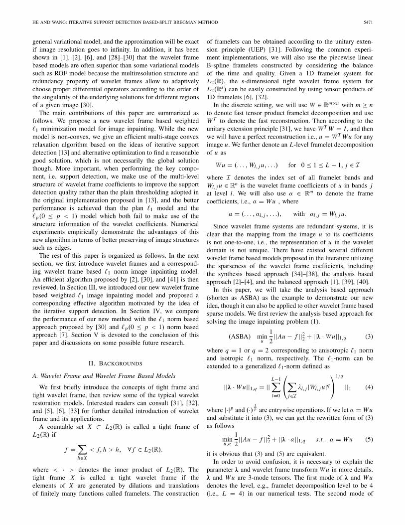
In order to achieve more direct comparison between the twodifferent kinds of algorithms, we show the flow chart ofSB method and our proposed method in Figure 1, we cansee that for our proposed method, the final result is obtainedfrom multi-stage process by solving a series of weightedASBA problems. The scheme of alternating optimization help


Fig. 1. The algorithm framework of single stage SB method (the first row)and our proposed multi-stage method ((JL)ISD-SB, see the second row).

decouple the original too complicated model (15) into tworeasonably easier sub-problems. We start from solving theplain �1 model (13), then improve the solution gradually viathe above multi-stage procedure. At each stage (iteration)in the process, the weights will change according to themost recently recovered image via adaptive learning. This fullprocedure and Step 2 will be introduced in more details in nextsection, where the iterative support detection is reviewed.

B. Step 1: Solving a Weighted ASBA Given Weights

Now we come to how to solve the weighted ASBA oncethe weights are given, i.e. how to realize Step 1. We transformthe problem (15) to

minα,u1

2||Au − f ||22 +

L−1∑

l=0

(n∑

i=1

||Tl,i ◦ (λl,i ◦ αl,i )||q)

,

s.t. αl,i = Wl,i u. (16)

Then the augment Lagrangian function of (15) can bewritten as

L(α, u) = 1

2||Au − f ||22

+L−1∑

l=0

(n∑

i=1

(||Tl,i ◦ (λl,i ◦ αl,i )||q)

)

+L−1∑

l=0

(n∑

i=1

(< vl,i , Wl,i u − αl,i >)

)

+L−1∑

l=0

(n∑

i=1

(μ

2||Wl,i u − αl,i ||22

)).

We note that α is the complete set of αl,i, j , where l ∈ 0 ≤l ≤ L −1, i ∈ {1, 2, . . . , n}, j ∈ I. The original split bregmanalgorithm can be applied here with some modifications due tothe existence of Tl,i as follows.

This joint minimization problem of (α, u) can be carriedin parallel. Specifically, the minimization with respect to u isattained by

(AT A + μI )u = AT f + μW T (α − v/μ) (17)

Note that similar to α, v is the complete set of vl,i, j , wherel ∈ 0 ≤ l ≤ L − 1, i ∈ {1, 2, . . . , n}, j ∈ I. The optimizationproblem with respect to αl,i is obtained by

minαl,i

||Tl,i ◦ (λl,i ◦ αl,i )||q+ < vl,i , Wl,i u − αl,i >

+μ

2||Wl,i u − αl,i ||22 (18)

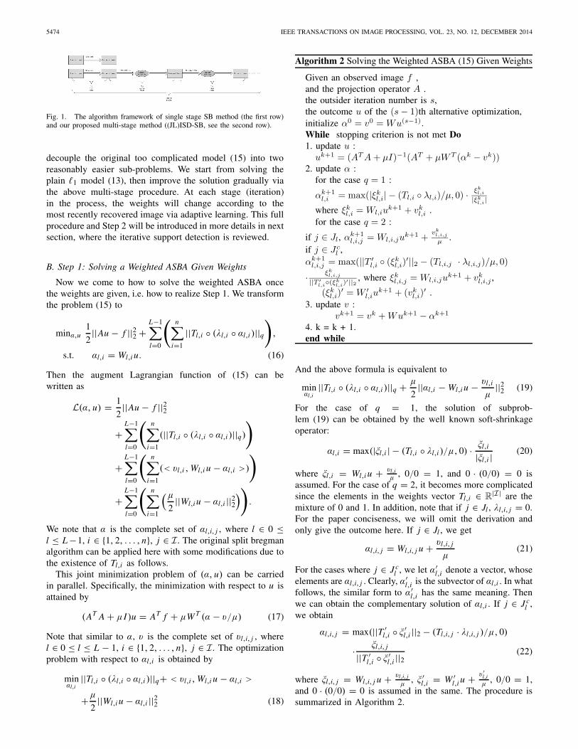
Algorithm 2 Solving the Weighted ASBA (15) Given Weights

And the above formula is equivalent to

minαl,i

||Tl,i ◦ (λl,i ◦ αl,i )||q + μ

2||αl,i − Wl,i u − vl,i

μ||22 (19)

For the case of q = 1, the solution of subprob-lem (19) can be obtained by the well known soft-shrinkageoperator:

αl,i = max(|ξl,i | − (Tl,i ◦ λl,i )/μ, 0) · ξl,i

|ξl,i | (20)

where ξl,i = Wl,i u + vl,iμ , 0/0 = 1, and 0 · (0/0) = 0 is

assumed. For the case of q = 2, it becomes more complicatedsince the elements in the weights vector Tl,i ∈ R

|I| are themixture of 0 and 1. In addition, note that if j ∈ Jl , λl,i, j = 0.For the paper conciseness, we will omit the derivation andonly give the outcome here. If j ∈ Jl , we get

αl,i, j = Wl,i, j u + vl,i, j

μ(21)

For the cases where j ∈ J cl , we let α′

l,i denote a vector, whoseelements are αl,i, j . Clearly, α′

l,i is the subvector of αl,i . In whatfollows, the similar form to α′

l,i has the same meaning. Thenwe can obtain the complementary solution of αl,i . If j ∈ J c

l ,we obtain

αl,i, j = max(||T ′l,i ◦ ξ ′

l,i ||2 − (Tl,i, j · λl,i, j )/μ, 0)

· ξl,i, j

||T ′l,i ◦ ξ ′

l,i ||2(22)

where ξl,i, j = Wl,i, j u + vl,i, jμ , ξ ′

l,i = W ′l,i u + v ′

l,iμ , 0/0 = 1,

and 0 · (0/0) = 0 is assumed in the same. The procedure issummarized in Algorithm 2.


Fig. 2. This is to show the joint level support detection. Specifically, wecombine the given frame bands of all levels at the given pixel as a vector(joint group), and calculate its �2 norm magnitude, and all its componentswill be set to have the same weights (either 0 or 1).

Notice that the above procedure is in fact a selectiveshrinkage procedure. The original �1 model obtains a sparsesolution via the soft shrinkage operator. However, this kindof shrinkage has a fatal disadvantage, i.e., it shrinks the truenonzero components as well, and reduces the sharpness of therecovered images. By using 0 − 1 weights, some componentswill not be shrunk if we believe that they are unlikely to bezero. In such cases, their corresponding weights are set as 0.This is a natural setting and the advantages of the 0−1 weightsover other kinds of weights have been demonstrated in eithertheoretic or practical point of view in [13] and will be reviewedin Part C.

Remarks for Algorithm 2: not that initializing α0 = v0 =Wu(s−1) in Algorithm 2 is actually a warm-starting in thewhole algorithmic framework based on alternative optimiza-tion. Since the proof of convergence of the split bregmanalgorithm given by [2] is very general, it directly indicatesthe convergence of the Algorithm 2.

C. Step 2: Weights Determination Basedon Iterative Support Detection

In this part, we explain the way of determining Tl,i ofStep 1. While the idea is originally coming from our pro-posed iterative support detection (ISD) in pure sparse signalrecovery [13], we propose a specific implementation to makeuse of the multi-level structures of the coefficients of waveletframe, when considering the image inpainting problem.

To make the paper self-contained, we first briefly reviewthe idea of ISD. While the idea of exploiting available partialsupport detection have arisen in several subsequent literatures,see [14]–[19], ISD also focus more on how to extractthis partial support information instead. Compressivesensing [21], [22] reconstructs a unknown sparse signal froma small set of linear projections. Let x denote a k-sparsesignal, and let b = Ax represent a set of m linear projectionsof x . The general reconstruction optimization problem isBasis Pursuit (BP) problem

(BP) minx

||x ||1 s.t . Ax = b. (23)

However, unlike the BP problem which is a one-stage convexrelaxation method, ISD is a multi-stage convex relaxation

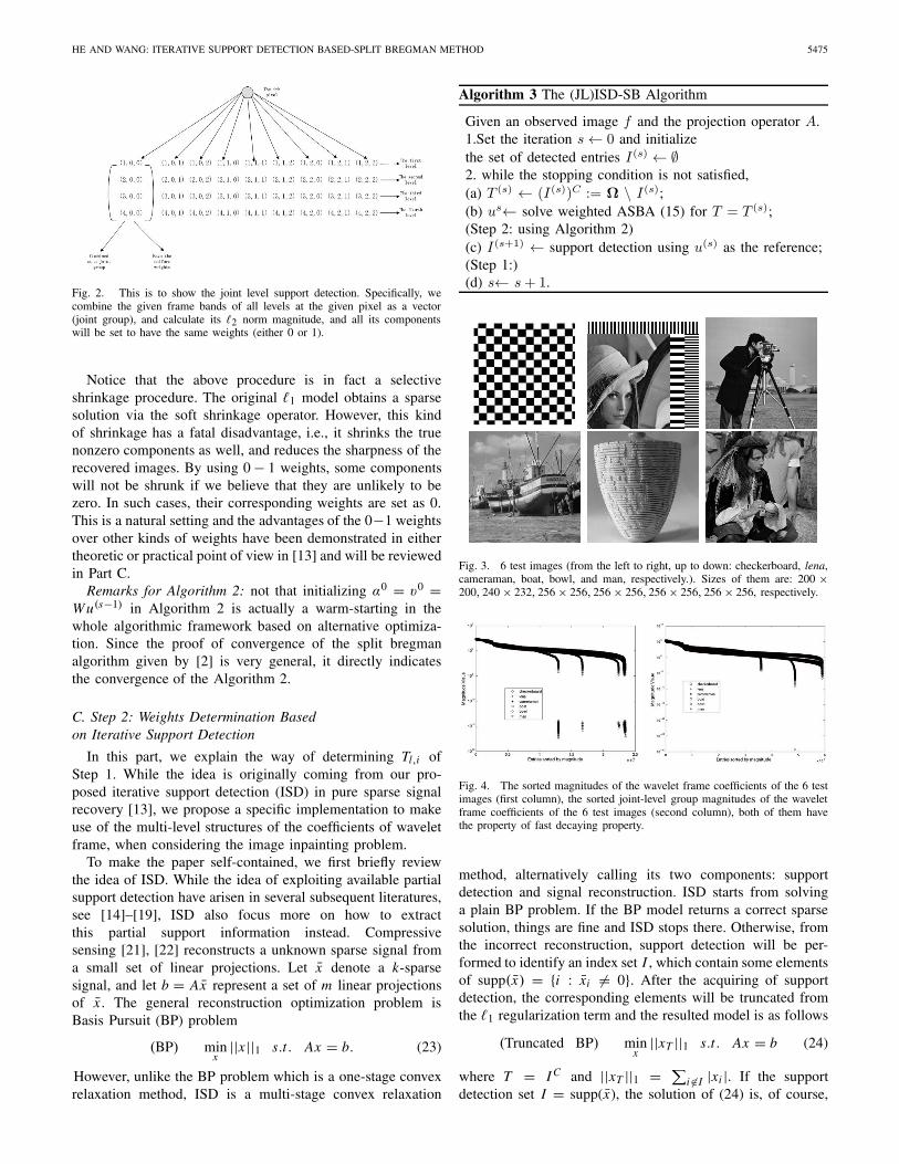
Algorithm 3 The (JL)ISD-SB Algorithm

Fig. 3. 6 test images (from the left to right, up to down: checkerboard, lena,cameraman, boat, bowl, and man, respectively.). Sizes of them are: 200 ×200, 240 × 232, 256 × 256, 256 × 256, 256 × 256, 256 × 256, respectively.

Fig. 4. The sorted magnitudes of the wavelet frame coefficients of the 6 testimages (first column), the sorted joint-level group magnitudes of the waveletframe coefficients of the 6 test images (second column), both of them havethe property of fast decaying property.

method, alternatively calling its two components: supportdetection and signal reconstruction. ISD starts from solvinga plain BP problem. If the BP model returns a correct sparsesolution, things are fine and ISD stops there. Otherwise, fromthe incorrect reconstruction, support detection will be per-formed to identify an index set I , which contain some elementsof supp(x) = {i : xi �= 0}. After the acquiring of supportdetection, the corresponding elements will be truncated fromthe �1 regularization term and the resulted model is as follows

(Truncated BP) minx

||xT ||1 s.t . Ax = b (24)

where T = I C and ||xT ||1 = ∑i �∈I |xi |. If the support

detection set I = supp(x), the solution of (24) is, of course,


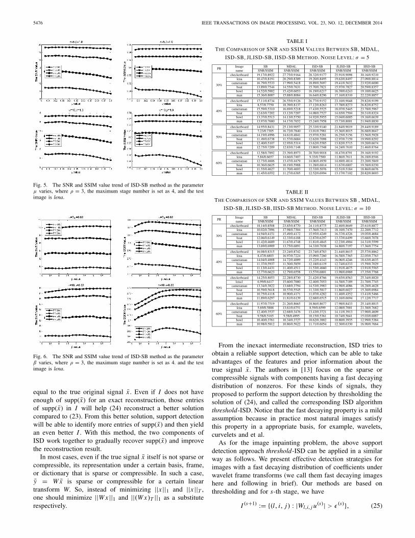
Fig. 5. The SNR and SSIM value trend of ISD-SB method as the parameterμ varies, where ρ = 3, the maximum stage number is set as 4, and the testimage is lena.

Fig. 6. The SNR and SSIM value trend of ISD-SB method as the parameterβ varies, where ρ = 3, the maximum stage number is set as 4. and the testimage is lena.

equal to the true original signal x . Even if I does not haveenough of supp(x) for an exact reconstruction, those entriesof supp(x) in I will help (24) reconstruct a better solutioncompared to (23). From this better solution, support detectionwill be able to identify more entries of supp(x) and then yieldan even better I . With this method, the two components ofISD work together to gradually recover supp(x) and improvethe reconstruction result.

In most cases, even if the true signal x itself is not sparse orcompressible, its representation under a certain basis, frame,or dictionary that is sparse or compressible. In such a case,y = W x is sparse or compressible for a certain lineartransform W. So, instead of minimizing ||x ||1 and ||x ||T ,one should minimize ||W x ||1 and ||(W x)T ||1 as a substituterespectively.

TABLE I

THE COMPARISON OF SNR AND SSIM VALUES BETWEEN SB, MDAL,

ISD-SB, JLISD-SB, IISD-SB METHOD. NOISE LEVEL: σ = 5

TABLE II

THE COMPARISON OF SNR AND SSIM VALUES BETWEEN SB , MDAL,

ISD-SB, JLISD-SB, IISD-SB METHOD. NOISE LEVEL: σ = 10

From the inexact intermediate reconstruction, ISD tries toobtain a reliable support detection, which can be able to takeadvantages of the features and prior information about thetrue signal x . The authors in [13] focus on the sparse orcompressible signals with components having a fast decayingdistribution of nonzeros. For these kinds of signals, theyproposed to perform the support detection by thresholding thesolution of (24), and called the corresponding ISD algorithmthreshold-ISD. Notice that the fast decaying property is a mildassumption because in practice most natural images satisfythis property in a appropriate basis, for example, wavelets,curvelets and et al.

As for the image inpainting problem, the above supportdetection approach threshold-ISD can be applied in a similarway as follows. We present effective detection strategies forimages with a fast decaying distribution of coefficients underwavelet frame transforms (we call them fast decaying imageshere and following in brief). Our methods are based onthresholding and for s-th stage, we have

I (s+1) := {(l, i, j) : |Wl,i, j u(s)| > ε(s)}, (25)


Fig. 7. The intermediate stage results of ISD-SB method are showed, where the second, third, fourth and fifth columns are corresponding to the results ofthe first stage, second stage and third stage and fourth stage, respectively. The first row, the second row, the third row and the fourth row correspond to theresults of different PR values from 30%, 40%, 50%, to 60%, respectively. Noise level: σ = 5. Test image: cameraman.

s = 0, 1, 2, . . ., The weights T (s)l,i, j equals 0 if the cor-

responding element belongs to the support detection I (s),or 1 otherwise. Before discussing the choice of ε(s), wepoint out that support detection sets I (s) are not necessarilyincreasing and nested, i.e., I (s) ⊂ I (s+1) may not hold for alls. This is very important because the support detection we getfrom the currently solution may contains wrong detections byε(s) thresholding. Not requiring I (s) to be monotonic leavesthe chance for support detection to remove previous wrongdetections, and this makes I (s) less sensitive to ε(s), thusmaking ε(s) easier to choose. In [13], we have proved thatISD can tolerate certain ratio of wrong detections and stillachieve a better recovery.

As for the threshold rule, we set

ε(s) := max{|Wl,i, j u(s)|}/ρ(s+1) (26)

with ρ > 0. The above is only a plain extension of the

original ISD to our problem and we can make the supportdetection even more effective by considering the structuresof the wavelet coefficients. It is known that the edges ofan image should correspond to large coefficients consistentlyfor all levels, in wavelet frames. Considering this specificcharacteristic, we propose a corresponding effective supportdetection strategy, which is shown in Figure 2. Specifically,for a given pixel, we combine the given frame bands of alllevels as a joint group, the magnitudes of these groups aremeasured as || · ||22, and the weights in each group are uniform(0 or 1), i.e., in given bands j at given pixel i , the weightsin each level (0 ≤ l ≤ L − 1) are same. In order to betterillustrate this strategy, we introduce a 2-mode tensor, denotedas �, whose elements are the aforementioned magnitudes ofthese groups taken over all pixels, denoted as �i, j , where thesubscript i denotes the ith pixel, and j denotes the specificframe bands of a given pixel. The cardinality of � is n × |I|,


where n is equal to the number of total pixels, and |I| is thetotal number of bands in given level at each pixel, e.g., |I| = 9if we use the piecewise linear B-spline framelets in this paper.It should be pointed out that the sorted magnitudes of tensor� still have the property of fast decaying, and the supportdetection method is based on thresholding:

I (s+1) := {(i, j) : |�i, j | > ε(s)}, (27)

s = 0, 1, 2, . . .. Similarly, we set the threshold value:

ε(s) := max{|�i, j |}/η(s+1). (28)

We named this support detection method as joint level iterativesupport detection method (JLISD method for short).

An excessively large ρ and η results in too many false detec-tions and lead to low solution quality, while an excessivelysmall ρ and η tends to cause a large number of iterations.ISD will be quite effective with an appropriate ρ and η,though the proper range of ρ and η might be case-dependent,due to the No Free Lunch theorem [59]. However, numericalexperiments have shown that the performance of ISD is notvery sensitive to the choice of ρ and η.

Now we would like to further explain the features ofISD, as a specific 0–1 weighting scheme, in an intuitiveway, compared to other similar multi-stage algorithms includ-ing the well known iterative reweighted �1 algorithm [60].Firstly, we emphasize the importance of the partial supportinformation as prior to better reconstruct the original sparsesignals (images), and inspire ones to develop new and effectiveimplementations in their own particular problems, for example,edge detection in the total variation regularized image recon-struction [20]. Secondly, its performance over the single stagepure �1 model has been proved rigorously in [13] once we candetect correct partial support information (by thresholding, forexample, in this paper), while most of the related alternativessuch as the reweighted �1 algorithm [60] do not have suchrigorous theoretical guarantees. Thirdly, for the reweighted�1 algorithm, the weights are usually set like θi = 1

|xi |+ε .In [13], we have pointed out that the tuning parameter ε > 0is the key parameter and should be determined carefully.Roughly, ε should not be a fixed value and should decreasefrom a large value to a small value. In an extreme case,if ε is always fixed to 0, then we would not get a bettersolution for the next stage, even there is no numerical troubleof dividing 0, because we just passively make use of the allthe information of the current solution without any filteringout the inaccurate information. From our analysis, the choiceof ε is like controlling the extraction of the useful informationand suppressing the distortion of the recovery noise. From thepoint of view, our 0 − 1 weights of ISD is a more explicit andstraightforward way to imply the idea of making use of thecorrect information (mainly about the locations of componentsof large magnitude and setting the corresponding weights as 0)and give up the rest too noisy information (for those compo-nents of small magnitudes, they are mostly overwhelmed bythe recovery noise and therefore there is very little meaningto set different weights according to their magnitudes. So it ismore reasonable to set the same weights as 1).

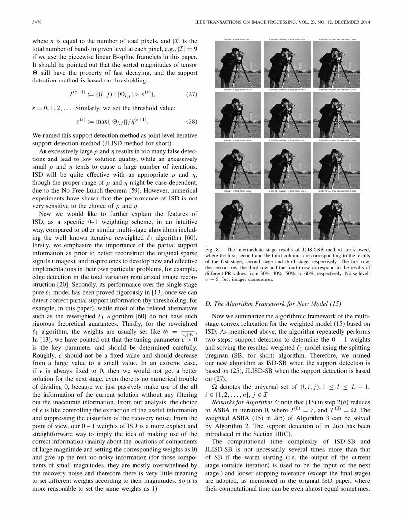
Fig. 8. The intermediate stage results of JLISD-SB method are showed,where the first, second and the third columns are corresponding to the resultsof the first stage, second stage and third stage, respectively. The first row,the second row, the third row and the fourth row correspond to the results ofdifferent PR values from 30%, 40%, 50%, to 60%, respectively. Noise level:σ = 5. Test image: cameraman.

D. The Algorithm Framework for New Model (15)

Now we summarize the algorithmic framework of the multi-stage convex relaxation for the weighted model (15) based onISD. As mentioned above, the algorithm repeatedly performstwo steps: support detection to determine the 0 − 1 weightsand solving the resulted weighted �1 model using the splittingbregman (SB, for short) algorithm. Therefore, we namedour new algorithm as ISD-SB when the support detection isbased on (25), JLISD-SB when the support detection is basedon (27).

� denotes the universal set of (l, i, j), 1 ≤ l ≤ L − 1,i ∈ {1, 2, . . . , n}, j ∈ I.

Remarks for Algorithm 3: note that (15) in step 2(b) reducesto ASBA in iteration 0, where I (0) = ∅, and T (0) = �. Theweighted ASBA (15) in 2(b) of Algorithm 3 can be solvedby Algorithm 2. The support detection of in 2(c) has beenintroduced in the Section III(C).

The computational time complexity of ISD-SB andJLISD-SB is not necessarily several times more than thatof SB if the warm starting (i.e. the output of the currentstage (outside iteration) is used to be the input of the nextstage.) and looser stopping tolerance (except the final stage)are adopted, as mentioned in the original ISD paper, wheretheir computational time can be even almost equal sometimes.


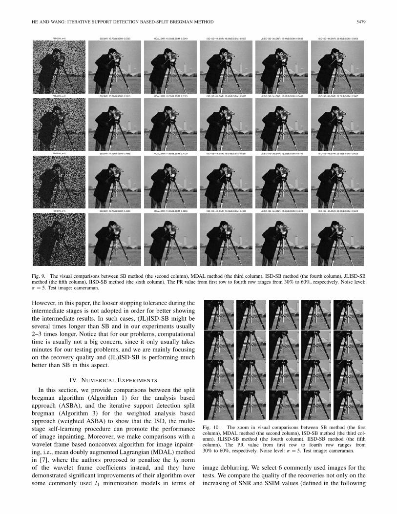
Fig. 9. The visual comparisons between SB method (the second column), MDAL method (the third column), ISD-SB method (the fourth column), JLISD-SBmethod (the fifth column), IISD-SB method (the sixth column). The PR value from first row to fourth row ranges from 30% to 60%, respectively. Noise level:σ = 5. Test image: cameraman.

However, in this paper, the looser stopping tolerance during theintermediate stages is not adopted in order for better showingthe intermediate results. In such cases, (JL)ISD-SB might beseveral times longer than SB and in our experiments usually2–3 times longer. Notice that for our problems, computationaltime is usually not a big concern, since it only usually takesminutes for our testing problems, and we are mainly focusingon the recovery quality and (JL)ISD-SB is performing muchbetter than SB in this aspect.

IV. NUMERICAL EXPERIMENTS

In this section, we provide comparisons between the splitbregman algorithm (Algorithm 1) for the analysis basedapproach (ASBA), and the iterative support detection splitbregman (Algorithm 3) for the weighted analysis basedapproach (weighted ASBA) to show that the ISD, the multi-stage self-learning procedure can promote the performanceof image inpainting. Moreover, we make comparisons with awavelet frame based nonconvex algorithm for image inpaint-ing, i.e., mean doubly augmented Lagrangian (MDAL) methodin [7], where the authors proposed to penalize the l0 normof the wavelet frame coefficients instead, and they havedemonstrated significant improvements of their algorithm oversome commonly used l1 minimization models in terms of

Fig. 10. The zoom in visual comparisons between SB method (the firstcolumn), MDAL method (the second column), ISD-SB method (the third col-umn), JLISD-SB method (the fourth column), IISD-SB method (the fifthcolumn). The PR value from first row to fourth row ranges from30% to 60%, respectively. Noise level: σ = 5. Test image: cameraman.

image deblurring. We select 6 commonly used images for thetests. We compare the quality of the recoveries not only on theincreasing of SNR and SSIM values (defined in the following


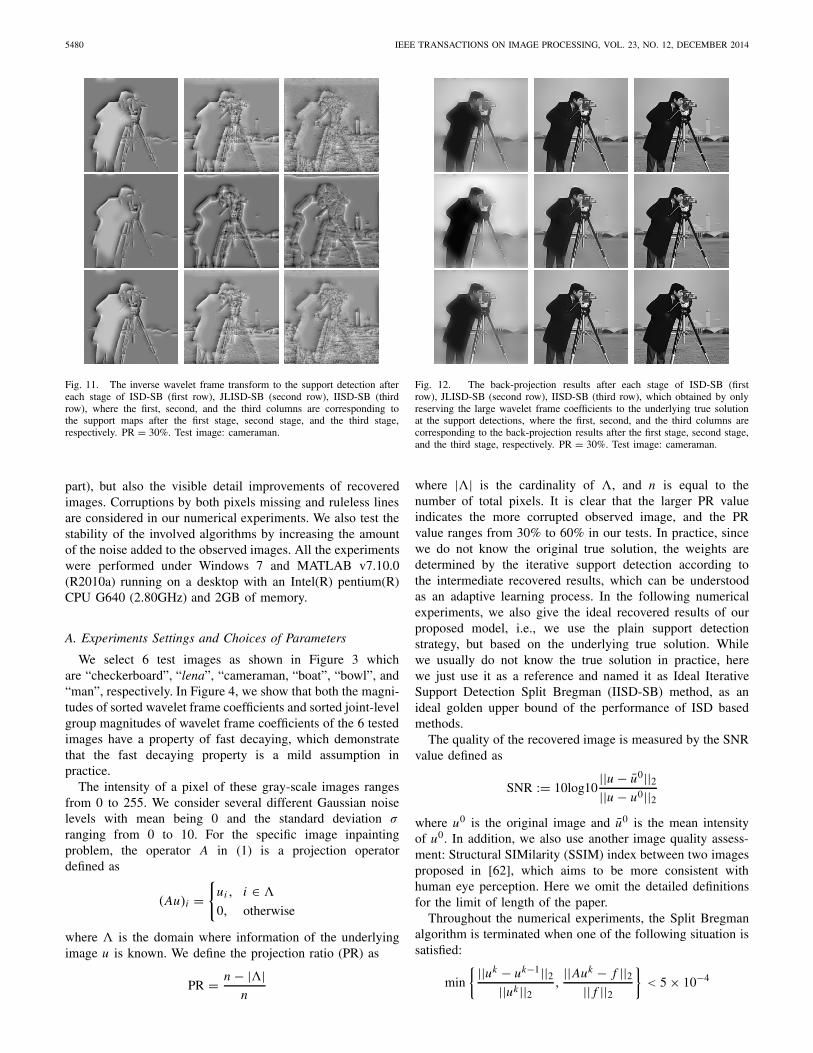
Fig. 11. The inverse wavelet frame transform to the support detection aftereach stage of ISD-SB (first row), JLISD-SB (second row), IISD-SB (thirdrow), where the first, second, and the third columns are corresponding tothe support maps after the first stage, second stage, and the third stage,respectively. PR = 30%. Test image: cameraman.

part), but also the visible detail improvements of recoveredimages. Corruptions by both pixels missing and ruleless linesare considered in our numerical experiments. We also test thestability of the involved algorithms by increasing the amountof the noise added to the observed images. All the experimentswere performed under Windows 7 and MATLAB v7.10.0(R2010a) running on a desktop with an Intel(R) pentium(R)CPU G640 (2.80GHz) and 2GB of memory.

A. Experiments Settings and Choices of Parameters

We select 6 test images as shown in Figure 3 whichare “checkerboard”, “lena”, “cameraman, “boat”, “bowl”, and“man”, respectively. In Figure 4, we show that both the magni-tudes of sorted wavelet frame coefficients and sorted joint-levelgroup magnitudes of wavelet frame coefficients of the 6 testedimages have a property of fast decaying, which demonstratethat the fast decaying property is a mild assumption inpractice.

The intensity of a pixel of these gray-scale images rangesfrom 0 to 255. We consider several different Gaussian noiselevels with mean being 0 and the standard deviation σranging from 0 to 10. For the specific image inpaintingproblem, the operator A in (1) is a projection operatordefined as

(Au)i ={

ui , i ∈ �

0, otherwise

where � is the domain where information of the underlyingimage u is known. We define the projection ratio (PR) as

PR = n − |�|n

Fig. 12. The back-projection results after each stage of ISD-SB (firstrow), JLISD-SB (second row), IISD-SB (third row), which obtained by onlyreserving the large wavelet frame coefficients to the underlying true solutionat the support detections, where the first, second, and the third columns arecorresponding to the back-projection results after the first stage, second stage,and the third stage, respectively. PR = 30%. Test image: cameraman.

where |�| is the cardinality of �, and n is equal to thenumber of total pixels. It is clear that the larger PR valueindicates the more corrupted observed image, and the PRvalue ranges from 30% to 60% in our tests. In practice, sincewe do not know the original true solution, the weights aredetermined by the iterative support detection according tothe intermediate recovered results, which can be understoodas an adaptive learning process. In the following numericalexperiments, we also give the ideal recovered results of ourproposed model, i.e., we use the plain support detectionstrategy, but based on the underlying true solution. Whilewe usually do not know the true solution in practice, herewe just use it as a reference and named it as Ideal IterativeSupport Detection Split Bregman (IISD-SB) method, as anideal golden upper bound of the performance of ISD basedmethods.

The quality of the recovered image is measured by the SNRvalue defined as

SNR := 10log10||u − u0||2||u − u0||2

where u0 is the original image and u0 is the mean intensityof u0. In addition, we also use another image quality assess-ment: Structural SIMilarity (SSIM) index between two imagesproposed in [62], which aims to be more consistent withhuman eye perception. Here we omit the detailed definitionsfor the limit of length of the paper.

Throughout the numerical experiments, the Split Bregmanalgorithm is terminated when one of the following situation issatisfied:

min

{ ||uk − uk−1||2||uk ||2 ,

||Auk − f ||2|| f ||2

}< 5 × 10−4


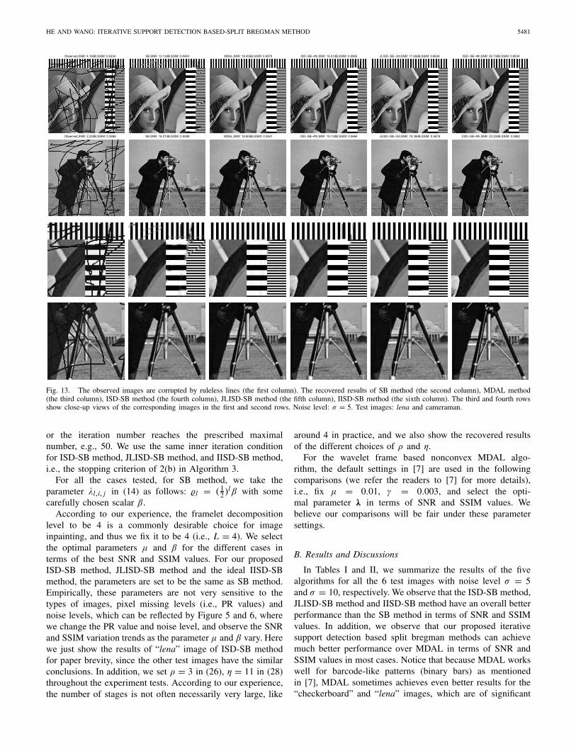
Fig. 13. The observed images are corrupted by ruleless lines (the first column). The recovered results of SB method (the second column), MDAL method(the third column), ISD-SB method (the fourth column), JLISD-SB method (the fifth column), IISD-SB method (the sixth column). The third and fourth rowsshow close-up views of the corresponding images in the first and second rows. Noise level: σ = 5. Test images: lena and cameraman.

or the iteration number reaches the prescribed maximalnumber, e.g., 50. We use the same inner iteration conditionfor ISD-SB method, JLISD-SB method, and IISD-SB method,i.e., the stopping criterion of 2(b) in Algorithm 3.

For all the cases tested, for SB method, we take theparameter λl,i, j in (14) as follows: l = ( 1

2 )lβ with somecarefully chosen scalar β.

According to our experience, the framelet decompositionlevel to be 4 is a commonly desirable choice for imageinpainting, and thus we fix it to be 4 (i.e., L = 4). We selectthe optimal parameters μ and β for the different cases interms of the best SNR and SSIM values. For our proposedISD-SB method, JLISD-SB method and the ideal IISD-SBmethod, the parameters are set to be the same as SB method.Empirically, these parameters are not very sensitive to thetypes of images, pixel missing levels (i.e., PR values) andnoise levels, which can be reflected by Figure 5 and 6, wherewe change the PR value and noise level, and observe the SNRand SSIM variation trends as the parameter μ and β vary. Herewe just show the results of “lena” image of ISD-SB methodfor paper brevity, since the other test images have the similarconclusions. In addition, we set ρ = 3 in (26), η = 11 in (28)throughout the experiment tests. According to our experience,the number of stages is not often necessarily very large, like

around 4 in practice, and we also show the recovered resultsof the different choices of ρ and η.

For the wavelet frame based nonconvex MDAL algo-rithm, the default settings in [7] are used in the followingcomparisons (we refer the readers to [7] for more details),i.e., fix μ = 0.01, γ = 0.003, and select the opti-mal parameter λ in terms of SNR and SSIM values. Webelieve our comparisons will be fair under these parametersettings.

B. Results and Discussions

In Tables I and II, we summarize the results of the fivealgorithms for all the 6 test images with noise level σ = 5and σ = 10, respectively. We observe that the ISD-SB method,JLISD-SB method and IISD-SB method have an overall betterperformance than the SB method in terms of SNR and SSIMvalues. In addition, we observe that our proposed iterativesupport detection based split bregman methods can achievemuch better performance over MDAL in terms of SNR andSSIM values in most cases. Notice that because MDAL workswell for barcode-like patterns (binary bars) as mentionedin [7], MDAL sometimes achieves even better results for the“checkerboard” and “lena” images, which are of significant


Fig. 14. Curves of SNR value v.s. noise level for the SB method,MDAL method, ISD-SB method, JLISD-SB method, and IISD-SB method.PR = 30%.

amount of barcode-like patterns. However, for other naturalimages, JLISD-SB mostly achieves significantly better results,partially due to the usage of the structure of the wavelet framecoefficients. In the following, we will give more plots to helpdemonstrate these points.

In Figures 7 and 8, we give the visual comparisonsbetween SB, ISD-SB and JLISD-SB recovered results, aswell as the intermediate results of each stage of ISD. Thetest image is “cameraman” here, the noise level is fixed asσ = 5, and the projection ratio (PR) ranges from 30%to 60%. Recall that the first stage of both ISD-SB andJLISD-SB method is to run the plain SB method, and wecan observe that our proposed algorithm can bring gradualimprovements as the ISD proceeds. Empirically, for mostcases, ISD-SB and JLISD-SB method achieves the best finalresults when the maximum stage number reaches 4 and 3,respectively.

Now we show the recovered images of the five algorithms,i.e. SB, MDAL, ISD-SB, JLISD-SB and IISD-SB, respec-tively. Due to the page limit, we just show the cases listedin Tabel 1 in Figure 9, where the test image is “cameraman”here, since the other cases have the similar conclusions.In addition, for better visual comparisons, in Figure 10,we give the close-up views (zoom-ins) of results. We canobserve that JLISD-SB brings significant visual enhance-ments in the sharp edges of the recovered images com-pared to SB method and MDAL method, as reflected by theSSIM values.

Fig. 15. Curves of SSIM value v.s. noise level for the SB method,MDAL method, ISD-SB method, JLISD-SB method, and IISD-SB method.PR = 30%.

To further study our proposed method, we also provide someintermediate detected support maps as ISD proceeds. We fixthe PR as 30% and choose the test image “cameraman” here.In Figure 11, we show the pictures of inverse wavelet frametransform to the support detection (binary 0-1 coefficients, thecoefficients on the support detections are 1, and the remainderare 0) after each stage of ISD-SB, JLISD-SB, and IISD-SB methods. In Figure 12, we provide the back-projectionresults after each stage of ISD-SB, JLISD-SB, and IISD-SBmethods, which obtained by only reserving the large waveletframe coefficients to the underlying true solution at the supportdetections. From the above observations, it is demonstratedagain that the we indeed obtain more reliable true supportdetection as the ISD proceeds.

In Figure 13, we also present the inpainting results ofthe images corrupted by ruleless lines, where we only use thetest images “lena” and “cameraman” as examples, since theother test images have the similar results. From the zoom-invisual comparisons, we can observe that ISD-SB, JLISD-SB,IISD-SB and MDAL methods achieve better inpainting perfor-mance compared to SB method in terms of better preservingthe edges of these two test images. We note that for the image“lena”, MDAL achieves a better SNR over ISD methods dueto a significant portion of barcode-like patterns which are idealfor MDAL (see [7] for details). However, JLISD-SB achievesa better SSIM value.

In Figures 14 and 15, we also test the stability ofthe five algorithms. As the noise level increases, the


Fig. 16. Curves of SNR value and SSIM value v.s. ρ choices for the ISD-SBmethod. Test image: lena.

Fig. 17. Curves of SNR value and SSIM value v.s. η choices for the JLISD-SB method. Test image: lena.

degradation of recovered image quality is linear and ISDbased methods have better performance in most cases,though the superiority of our proposed ISD-SB method, andJLISD-SB method over the SB method and MDAL methodshrinks, because reliable support detection becomes moredifficult to acquire as the noise level and/or the PR valueincreases.

In Figures 16 and 17, we present the different recoveryresults of ISD-SB method and JLISD-SB as the parametersρ and η change, respectively. For the paper conciseness, weonly choose the test image “lena” here, and fix the PR valueas 30%, since the other cases have the similar conclusions.For threshold-ISD strategy (0-1 weighting scheme) belongingto greedy methods, the different options of ρ and η reflectthe different greedy degree, showing the confident level thatwe detect the true supports. In particular, the more smaller theρ and η we choose, the more greedy we act and the more con-fidence we have. We observe that we can achieve different bestrecovered results at different stages as the parameters ρ and η

change. Moreover, when the stage number s becomes too big,the results become worse instead, because the threshold valuebecomes very small, resulting into too many wrong detections,according to the formulas (26) and (28). In such cases, we canset up a lower bound of threshold according to certain priorinformation to avoid excessive support detections.

V. CONCLUSIONS AND FUTURE WORK

In this paper, we propose the ISD-SB method and espe-cially the JLISD-SB method for wavelet frame based imageinpainting problems. The final result is obtained from amultistage process consisting of solving a series of weightedASBA model, where threshold-ISD strategy is applied to therough intermediate results to determine the adaptive binaryweights.

ISD-SB method and especially JLISD-SB method can bringsignificant enhancements at the sharp edges of the recoveredimages compared to SB method and MDAL method, becausethe large wavelet frame coefficients reflect the singulari-ties of the underlying true solution, and the threshold-ISDstrategy sharpens the edges of the approximate solution bynot thresholding the large coefficients and thus encouragingthe edges to form in the recovery. More important, JLISDmakes use of the joint sparsity property of the wavelet framecoefficients [63], [64] to further improve the recovery quality.Therefore future research includes studying specific imageclasses (including color images) and developing more effectivecorresponding support detection methods.

REFERENCES

[1] R. H. Ghan, T. F. Chan, L. Shen, and Z. Shen, “Wavelet algorithms forhigh-resolution image reconstruction,” SIAM J. Sci. Comput., vol. 24,no. 4, pp. 1408–1432, 2003.

[2] J.-F. Cai, S. Osher, and Z. Shen, “Split Bregman methods and framebased image restoration,” Multiscale Model. Simul., vol. 8, no. 2,pp. 337–367, 2009.

[3] M. Elad, J.-L. Starck, P. Querre, and D. L. Donoho, “Simultaneouscartoon and texture image inpainting using morphological componentanalysis (MCA), “Appl. Comput. Harmonic Anal., vol. 19, no. 3,pp. 340–358, 2005.

[4] J.-L. Starck, M. Elad, and D. L. Donoho, “Image decomposition via thecombination of sparse representations and a variational approach,” IEEETrans. Image Process., vol. 14, no. 10, pp. 1570–1582, Oct. 2005.

[5] Z. Shen, “Wavelet frames and image restorations,” in Proc. Int. Congr.Math., vol. 4. 2010, pp. 2834–2863.

[6] B. Dong and Z. Shen, “MRA-based wavelet frames and apllications,”in The Mathematics of Image Processing (IAS Lecture Notes Series).Salt Lake City, UT, USA: Park City Mathematics Institute, 2010.

[7] B. Dong and Y. Zhang, “An efficient algorithm for �0 minimizationin wavelet frame based image restoration,” J. Sci. Comput., vol. 54,nos. 2–3, pp. 350–368, 2013.

[8] Y. Zhang, B. Dong, and Z. Lu, “�0 minimization for waveletframe based image restoration,” Math. Comput., vol. 82, no. 282,pp. 995–1015, 2013.

[9] I. F. Gorodnitsky and B. D. Rao, “Sparse signal reconstruction fromlimited data using FOCUSS: A re-weighted minimum norm algorithm,”IEEE Trans. Signal Process., vol. 45, no. 3, pp. 600–616, Mar. 1997.

[10] H. Jung, K. Sung, K. S. Nayak, E. Y. Kim, and J. C. Ye, “k-t FOCUSS:A general compressed sensing framework for high resolution dynamicMRI,” Magn. Reson. Med., vol. 61, no. 1, pp. 103–116, 2009.

[11] L. I. Rudin, S. Osher, and E. Fatemi, “Nonlinear total variation basednoise removal algorithms,” Phys. D, Nonlinear Phenomena, vol. 60,nos. 1–4, pp. 259–268, 1992.

[12] A. Chambolle and P.-L. Lions, “Image recovery via total variationminimization and related problems,” Numer. Math., vol. 76, no. 2,pp. 167–188, 1997.


[13] Y. Wang and W. Yin, “Sparse signal reconstruction via iterative supportdetection,” SIAM J. Imag. Sci., vol. 3, no. 3, pp. 462–491, 2010.

[14] N. Vaswani and W. Lu, “Modified-CS: Modifying compressive sens-ing for problems with partially known support,” IEEE Trans. SignalProcess., vol. 58, no. 9, pp. 4595–4607, Sep. 2010.

[15] W. Lu and N. Vaswani, “Regularized modified BPDN for noisy sparsereconstruction with partial erroneous support and signal value knowl-edge,” IEEE Trans. Signal Process., vol. 60, no. 1, pp. 182–196,Jan. 2012.

[16] L. Jacques, “A short note on compressed sensing with partially knownsignal support,” Signal Process., vol. 90, no. 12, pp. 3308–3312, 2010.

[17] M. P. Friedlander, H. Mansour, R. Saab, and O. Yilmaz, “Recoveringcompressively sampled signals using partial support information,” IEEETrans. Inf. Theory, vol. 58, no. 2, pp. 1122–1134, Feb. 2012.

[18] R. E. Carrillo, L. F. Polania, and K. E. Barner, “Iterative algo-rithms for compressed sensing with partially known support,” in Proc.IEEE Int. Conf. Acoust. Speech Signal Process. (ICASSP), Mar. 2010,pp. 3654–3657.

[19] R. Carrillo, L. Polania, and K. Barner, “Iterative hard threshold-ing for compressed sensing with partially known support,” in Proc.IEEE Int. Conf. Acoust. Speech Signal Process. (ICASSP), May 2011,pp. 4028–4031.

[20] W. Guo and W. Yin, “Edge guided reconstruction for compressiveimaging,” SIAM J. Imag. Sci., vol. 5, no. 3, pp. 809–834, 2012.

[21] D. L. Donoho, “Compressed sensing,” IEEE Trans. Inf. Theory, vol. 52,no. 4, pp. 1289–1306, Apr. 2006.

[22] E. J. Candès, J. K. Romberg, and T. Tao, “Stable signal recovery fromincomplete and inaccurate measurements,” Commun. Pure Appl. Math.,vol. 59, no. 8, pp. 1207–1233, 2006.

[23] Y. Meyer, Oscillating Patterns in Image Processing and NonlinearEvolution Equations: The Fifteenth Dean Jacqueline B. Lewis MemorialLectures. Providence, RI, USA: AMS, 2001.

[24] G. Sapiro, Geometric Partial Differential Equations and Image Process-ing. Cambridge, U.K.: Cambridge Univ. Press, 2001.

[25] S. Osher and R. Fedkiw, Level Set Methods and Dynamic ImplicitSurfaces. New York, NY, USA: Springer-Verlag, 2003.

[26] T. Chan, S. Esedoglu, F. Park, and A. Yip, “Total variation image restora-tion: Overview and recent developments,” in Handbook of MathematicalModels in Computer Vision. New York, NY, USA: Springer-Verlag,2006, pp. 17–31.

[27] G. Aubert and P. Kornprobst, Mathematical Problems in Image Process-ing: Partial Differential Equations and the Calculus of Variations.New York, NY, USA: Springer-Verlag, 2006.

[28] R. Chan, L. Shen, and Z. Shen, “A framelet-based approach for imageinpainting,” Res. Rep., vol. 4, p. 325, 2005.

[29] J.-F. Cai, S. Osher, and Z. Shen, “Linearized Bregman iterations forframe-based image deblurring,” SIAM J. Imag. Sci, vol. 2, no. 1,pp. 226–252, 2009.

[30] J.-F. Cai, B. Dong, S. Osher, and Z. Shen, “Image restorations: Totalvariation, wavelet frames and beyond,” J. Amer. Math. Soc., vol. 25,no. 4, pp. 1033–1089, 2012.

[31] A. Ron and Z. Shen, “Affine systerms in L2(Rd ): The analysis of theanalysis operator,” J. Funct. Anal., vol. 148, no. 2, pp. 408–447, 1997.

[32] I. Daubechies, Ten Lectures on Wavelets (CBMS-NSF Regional Con-ference Series in Applied Mathematics). Philadelphia, PA, USA: SISM,1992.

[33] I. Daubechies, B. Han, A. Ron, and Z. Shen, “Framelets:MRA-based constructions of wavelet frames,” Appl. Comput. HarmonicAnal., vol. 14, no. 1, pp. 1–46, Jan. 2003.

[34] I. Daubechies, G. Teschke, and L. Vese, “Iteratively solving linearinverse problems under general convex constraints,” Inverse ProblemsImag., vol. 1, no. 1, p. 29, 2007.

[35] M. J. Fadili and J.-L. Starck, “Sparse representations and Bayesian imageinpainting,” in Proc. Int. Conf. SPARS, vol. 5. 2005.

[36] M. J. Fadili, J.-L. Starck, and F. Murtagh, “Inpainting and zooming usingsparse representations,” Comput. J., vol. 52, no. 1, pp. 64–79, 2009.

[37] M. A. T. Figuriredo and R. D. Nowak, “An EM algorithm for wavelet-based image restoration,” IEEE Trans. Image Process., vol. 12, no. 8,pp. 906–916, Aug. 2003.

[38] M. A. T. Figuriredo and R. D. Nowark, “A bound optimization approachto wavelet-based image deconvolution,” in Proc. IEEE Int. Conf. ImageProcess. (ICIP), vol. 2. Sep. 2005, pp. II-782–II-785.

[39] J. Cai, R. Chan, L. Shen, and Z. Shen, “Convergence analysis of tightframelet approach for missing data recovery,” Adv. Comput. Math.,vol. 31, nos. 1–3, pp. 87–113, Oct. 2009.

[40] J. Cai, R. Chan, and Z. Shen, “Simutaneous cartoon and textureinpainting,” Inverse Problems Imag., vol. 4, no. 3, pp. 379–395,2010.

[41] T. Goldtein and S. Osher, “The split Bregman algorithm for L1 reg-ularized problems,” SIAM J. Imag. Sci., vol. 2, no. 2, pp. 323–343,2009.

[42] X. Zhang, M. Burger, X. Bresson, and S. Osher, “Bregmanized nonlocalregularization for deconvolution and sparse reconstruction,” SIAM J.Imag. Sci., vol. 3, no. 3, pp. 253–276, 2010.

[43] D. Gabay and B. Mercier, “A dual algorithm for the solution of nonlinearvariational problems via finite element approximation,” Comput. Math.Appl., vol. 2, no. 1, pp. 17–40, 1976.

[44] D. P. Bertsekas and J. N. Tsitsiklis, Parallel and Distributed Compu-tation: Numerical Methods. Englewood Cliffs, NJ, USA: Prentice-Hall,1989.

[45] J. Eckstein and D. P. Bertsekas, “On the Douglas–Rachford splittingmethod and the proximal point algorithm for maximal monotone oper-ators,” Math. Program., vol. 55, nos. 1–3, pp. 293–318, 1992.

[46] M. R. Hestenes, “Multiplier and gradient methods,” J. Optim. TheoryAppl., vol. 4, no. 5, pp. 303–320, 1969.

[47] M. J. D. Powell, “A method for nonlinear constraints in minimizationproblems,” in Optimization, R. Fletcher, Ed. New York, NY, USA:Academic, 1969, pp. 283–298.

[48] R. Glowinski and P. Le Tallec, Augmented Lagrangian and Operator-Splitting Methods in Nonlinear Mechanics. Philadelphia, PA, USA:SIAM, 1989.

[49] E. Esser, “Applications of Lagrangian-based alternating directionmethods and connections to split Bregman,” Dept. Math., UCLA,Los Angeles, CA, USA, CAM Rep., 2009.

[50] X.-C. Tai and C. Wu, “Augmented Lagrangian method, dual methods andsplit Bregman iteration for ROF model,” Scale Space and VariationalMethods in Computer Vision. Berlin, Germany: Springer-Verlag, 2009,pp. 502–513.

[51] D. L. Donoho, “De-noising by soft-thresholding,” IEEE Trans. Inf.Theory, vol. 41, no. 3, pp. 613–627, May 1995.

[52] P. L. Combettes and V. R. Wajs, “Signal recovery by proximalforward-backward splitting,” Multiscale Model. Simul., vol. 4, no. 4,pp. 1168–1200, 2006.

[53] P. Mrázek and J. Weickert, “Rotationally invariant wavelet shrink-age,” in Pattern Recognition. Berlin, Germany: Springer-Verlag, 2003,pp. 156–163.

[54] G. Steidl, J. Weickert, T. Brox, P. Mrázek, and M. Welk, “On theequivalence of soft wavelet shrinkage, total variation diffusion, totalvariation regularization, and SIDEs,” SIAM J. Numer. Anal., vol. 42,no. 2, pp. 686–713, 2005.

[55] Y. Wang, J. Yang, W. Yin, and Y. Zhang, “A new alternating minimiza-tion algorithm for total variation image reconstruction,” SIAM J. Imag.Sci., vol. 1, no. 3, pp. 248–272, 2008.

[56] S. Becker, J. Bobin, and E. J. Candès, “NESTA: A fast and accuratefirst-order method for sparse recovery,” SIAM J. Imag. Sci., vol. 4, no. 1,pp. 1–39, 2011.

[57] X. Zhang, M. Burger, and S. Osher, “A unified primal-dual algorithmframework based on Bregman iteration,” J. Sci. Comput., vol. 46, no. 1,pp. 20–46, 2011.

[58] T. Zhang, “Analysis of multi-stage convex relaxation for sparse regular-ization,” J. Mach. Learn. Res., vol. 11, pp. 1081–1107, Mar. 2010.

[59] D. H. Wolpert and W. G. Macready, “No free lunch theorems foroptimization,” IEEE Trans. Evol. Comput., vol. 1, no. 1, pp. 67–82,Apr. 1997.

[60] E. J. Candès, M. B. Wakin, and S. P. Boyd, “Enhancing sparsity byreweighted �1 minimization,” J. Fourier Anal. Appl., vol. 14, no. 5,pp. 877–905, 2008.

[61] R. Chartrand and W. Yin, “Iteratively reweighted algorithms for com-pressive sensing,” in Proc. 33rd Int. Conf. Acoust., Speech, SignalProcess. (ICASSP), Mar./Apr. 2008, pp. 3869–3872.

[62] Z. Wang, A. C. Bovik, H. R. Sheikh, and E. P. Simoncelli, “Imagequality assessment: From error visibility to structural similarity,” IEEETrans. Image Process., vol. 13, no. 4, pp. 600–612, Apr. 2004.

[63] C. Chen and J. Huang, “Compressive sensing MRI with wavelettree sparsity,” in Advances in Neural Information Processing Systems.Red Hook, NY, USA: Curran & Associates Inc., 2012, pp. 1124–1132.

[64] C. Chen and J. Huang, “The benefit of tree sparsity in accelerated MRI,”Med. Image Anal., to be published.

[65] I. F. Gorodnitsky and B. D. Rao, “Sparse signal reconstruction fromlimited data using FOCUSS: A re-weighted minimum norm algorithm,”IEEE Trans. Signal Process., vol. 45, no. 3, pp. 600–616, Mar. 1997.


Liangtian He (M’–) is currently pursuing thePh.D. degree with School of Mathematical Science,University of Electronic Science and Technologyof China, Chengdu, China. His research interestsare in image and signal processing (in particular,restoration, compression, and compressive sensing),computer vision, pattern recognition, and machinelearning.

Yilun Wang received the B.S. degree from theDalian University of Technology, Dalian, China,in 2002, the M.S. degree from Fudan University,Shanghai, China, in 2005, and the Ph.D. degreefrom Rice University, Houston, TX, USA, in 2009,respectively, all in computational and applied math-ematics. From 2009 to 2012, he was a Post-DoctoralResearcher with Cornell University, Ithaca, NY,USA. Since 2012, he has been an AssociateProfessor with the School of Mathematical Sciences,University of Electronic Science and Technology of

China, Chengdu, China. He is working on developing fast algorithms tofind the optimal sparse representation, with applications in visual computing,machine learning, and data mining to deal with high-dimensionality. He hasauthored several papers in high-ranked journals, such as the SIAM Journalon Imaging Sciences, Information Sciences, and the Journal of Agricultural,Biological, and Environmental Statistics. One of his papers has been citedover 640 times according to the Google Scholar.

Iterative Support Detection based Split Bregman Method for Wavelet Frame Based Image Inpainting

Documents

Transcript of Iterative Support Detection based Split Bregman Method for Wavelet Frame Based Image Inpainting