RESEARCH ARTICLE10.1002/2014JC009791

Temporal and spatial variability of tidal-fluvial dynamics in theSt. Lawrence fluvial estuary: An application of nonstationarytidal harmonic analysisPascal Matte1, Yves Secretan1, and Jean Morin2

1Centre Eau Terre Environnement, Institut National de la Recherche Scientifique, Quebec, Canada, 2Hydrology andEcohydraulic Section, Environment Canada, Meteorological Service of Canada, Quebec, Canada

Abstract Predicting tides in upstream reaches of rivers is a challenge, because tides are highly nonlinearand nonstationary, and accurate short-time predictions of river flow are hard to obtain. In the St. Lawrencefluvial estuary, tide forecasts are produced using a one-dimensional model (ONE-D), forced downstreamwith harmonic constituents, and upstream with daily discharges using 30 day flow forecasts from LakeOntario and the Ottawa River. Although this operational forecast system serves its purpose of predictingwater levels, information about nonstationary tidal-fluvial processes that can be gained from it is limited,particularly the temporal changes in mean water level and tidal properties (i.e., constituent amplitudes andphases), which are function of river flow and ocean tidal range. In this paper, a harmonic model adapted tononstationary tides, NS_TIDE, was applied to the St. Lawrence fluvial estuary, where the time-varying exter-nal forcing is directly built into the tidal basis functions. Model coefficients from 13 analysis stations werespatially interpolated to allow tide predictions at arbitrary locations as well as to provide insights into thespatiotemporal evolution of tides. Model hindcasts showed substantial improvements compared to classicalharmonic analyses at upstream stations. The model was further validated by comparison with ONE-D pre-dictions at a total of 32 stations. The slightly lower accuracy obtained with NS_TIDE is compensated bymodel simplicity, efficiency, and capacity to represent stage and tidal variations in a very compact way andthus represents a new means for understanding tidal rivers.

1. Introduction

Tides in rivers are the result of nonlinear interactions of the oceanic tide with channel geometry, bottomfriction, and river flow. They are best represented by a diffusive phenomenon in which the tidal wave, origi-nating from tidal forces in the ocean, is increasingly distorted and damped as it propagates upriver [LeBlond,1978]. This results in asymmetries in the duration of ebb and flood, as well as in the timing and height ofhigh and low water [Godin, 1984, 1999; Nidzieko, 2010]. Fortnightly oscillations of mean water levels (MWL)following the neap-spring cycle also increase in strength upstream and eventually surpass the semidiurnaltidal amplitude, with mean low water progressively being lowered during neap tides rather than springtides [LeBlond, 1979, 1991; Gallo and Vinzon, 2005].

Classical harmonic analysis (HA) is possibly the most widely used approach to analyze and predict tides. Itperforms very well in semienclosed basins, coastal shelves, and seas, but usually fails in representing rivertides, as the assumptions of stationarity and independence of the tidal components are not fulfilled due tonontidal modulating processes [Jay and Flinchem, 1999]. As a consequence, no information on the evolutionof the tidal content in time as a function of the nontidal forcing (e.g., annual river flow cycle) can beextracted. Some authors [e.g., Godin, 1985; Jay and Flinchem, 1997; Godin, 1999] showed the potential ofsimple regression relations to predict the modification of the tide by variations in river flow, but most inves-tigators have turned to numerical modeling in order to get around the problem of nonstationary signals(i.e., tidal signals influenced by nonstationary external forcing). One and two-dimensional models are nota-bly used in estuaries to represent longitudinal variations in tidal properties and to produce cotidal charts,respectively. In these models, imposed discharges are generally kept constant at the upstream boundaries,with tidal components forced at the downstream entrance, and simulations are performed for a sufficientlylong period (typically 1 year) to extract tidal properties at the grid nodes using traditional HA methods [see,

Key Points:� River geometry sets the limit of

applicability of classical harmonicanalysis� Response to forcing in tidal rivers is

spatially and frequency dependent� Frictional damping eventually

overcomes the nonlinear generationof overtides

Correspondence to:P. Matte,pascal.matte@ete.inrs.ca

Citation:Matte, P., Y. Secretan, and J. Morin(2014), Temporal and spatial variabilityof tidal-fluvial dynamics in the St.Lawrence fluvial estuary: Anapplication of nonstationary tidalharmonic analysis, J. Geophys. Res.Oceans, 119, doi:10.1002/2014JC009791.

Received 6 JAN 2014

Accepted 11 AUG 2014

Accepted article online 14 AUG 2014

MATTE ET AL. VC 2014. American Geophysical Union. All Rights Reserved. 1

Journal of Geophysical Research: Oceans

PUBLICATIONS

e.g., El-Sabh and Murty, 1990; Parker, 1991]. Although these models provide a basis for understanding thenonlinear interactions of tides with friction and river flow, continuous functions of the response of tidalproperties (i.e., amplitudes and phases of tidal constituents) to river flow and ocean tidal forcing are gener-ally not incorporated in the analyses, thus limiting the predictive capabilities of the models.

Several methods or improvements to traditional harmonic methods have been developed to better repre-sent transient tidal processes (for an overview, see, e.g., Jay and Kukulka [2003] and Parker [2007]). Amongthe latest, an adaptation of classical HA to nonstationary tides, NS_TIDE, has been proposed and success-fully applied in the Columbia River to a tidal signal strongly altered by river flow [Matte et al., 2013]. InNS_TIDE, the nonstationary forcing is built directly into the HA basis functions using a functional representa-tion derived from river-tide propagation theory [Jay, 1991] and adapted from Kukulka and Jay [2003a,2003b] and Jay et al. [2011]. Tidal-fluvial interactions are decoupled, allowing stage and tidal properties tobe modeled separately as a function of time, in terms of time-varying external forcing by river flow andocean tides. Moreover, the independence of the tidal components is ensured through redefined constituentselection and error estimation procedures.

In the St. Lawrence River, tide tables are produced using HA for all ports in the gulf and estuary up to Saint-Joseph-de-la-Rive (Figure 1). Upstream of Saint-Joseph-de-la-Rive, the influence of river discharge isincluded in the prediction using a one-dimensional model (ONE-D) of the St. Lawrence River [Dailey andHarleman, 1972; Morse, 1990]. The ONE-D model solves the one-dimensional St. Venant equations. It isforced downstream with harmonic constituents at Saint-Joseph-de-la-Rive and upstream with daily dis-charges at the outlets of Lake Saint-Louis and Lake Des-Deux-Montagnes for a typical year, i.e., an averagespring freshet followed by low flows in summer and rising flows in fall. The model is run for the entire year,and hourly water levels, along with the times and heights of high and low tides, are extracted to producetide tables at the stations.

The model is also run in operational mode, fed by the freshwater outflows from Lake Ontario and theOttawa River. These outflows are forecast 30 days ahead and carefully regulated to prevent flooding in the

Figure 1. Map showing tide gauges in the St. Lawrence fluvial estuary: (red squares) analysis stations; (blue triangles) validation stations; (light blue diamonds) reference stations forocean tidal range (Sept-Iles) and river discharge (Lasalle). River kilometers are shown beside each station name.

Journal of Geophysical Research: Oceans 10.1002/2014JC009791

MATTE ET AL. VC 2014. American Geophysical Union. All Rights Reserved. 2

spring and to avoid low water conditions throughout the year, for navigation safety purposes. For the first48 h, the wind forecast of Environment Canada (Meteorological Service of Canada) for the St. LawrenceEstuary is used to calculate wind-induced storm surge at the downstream boundary. The effect of ice coveron the flow is also included in winter time, by restricting the flow on some sections [Lefaivre et al., 2009].

This operational forecast system meets the need for a water level prediction throughout the entire St. Law-rence system and has proven to be quite valuable to the Canadian Coast Guard, the Canadian Port Author-ities, ship owners, and in diverse applications from coastal flooding forecasts and ice cover management tohydrodynamic and climate change impact studies [Lefaivre et al., 2009]. However, a discrepancy remainsbetween the harmonic-based predictions made in the estuary and gulf and the hydrodynamic-based pre-dictions made upstream, which is strongly linked to the nature of the tides in both regions. Traditional har-monic methods assume that tides at a coastal station can be represented by a sum of sine waves withconstant amplitudes and phases, whose frequencies are derived from tidal potential and nonlinear shallow-water interactions. Hydrodynamic models, for their part, solve the shallow water equations for the conserva-tion of mass and momentum. They offer a spatially integrated representation of water levels and velocitiesin a system at the scale of the grid element size, whereas regression models such as HA or others offer tem-porally integrated views of a tidal signal measured at one or a few points in space, but usually over muchlarger periods of time [e.g., Jay et al., 2011], typically expressed in terms of its frequency content. Conse-quently, the dynamical understanding that can be gained in the upstream and downstream portions of theSt. Lawrence is inherently different due to drastically different methods used to represent the tides.

In this paper, a harmonic-based, nonstationary tidal propagation model of the St. Lawrence fluvial estuary isdeveloped through application of NS_TIDE to 13 tide gauges distributed between Saint-Joseph-de-la-Riveand Lanoraie (Figure 1). In order to represent tidal properties in a continuous manner throughout the sys-tem, model coefficients are spatially interpolated between the stations, thus yielding a spatial model of theevolution of stage and tidal properties as a function of upriver location and forcing conditions. To validatethe model, water level predictions are produced at 19 intermediate (mostly temporary) stations and com-pared to observations as well as to forecasts made by the operational ONE-D model. The objectives of thiswork are (1) to develop a spatial harmonic model capable of predicting variations in stage and tidal proper-ties as a function of nonstationary forcing variables, and (2) to improve current knowledge on tidal-fluvialprocesses in the St. Lawrence fluvial estuary. The goal is not to supplant the operational ONE-D forecastmodel, which serves its purpose of predicting water levels in the St. Lawrence River, but to complement itby exploring temporal changes in the frequency content of the tides, thereby bringing new insights intotidal-fluvial interactions. Such a treatment also guarantees continuity between predictions made in theupper and lower St. Lawrence by use of harmonic methods throughout.

2. Methods

2.1. Regression ModelsClassical HA was given a structure based on a modern understanding of the tidal potential by Doodson[1921]. Following a reformulation of Doodson’s work by Godin [1972], tidal heights h are typically modeledas:

hðtÞ5b0;01Xn

k51

½b1;k cos ðrk tÞ1b2;k sin ðrk tÞ�; (1)

where t is time, rk are a priori known frequencies, n is the number of constituents, and b0,0, b1,k, and b2,k areunknown coefficients determined by regression analysis to best fit the observations.

Improvements to traditional harmonic methods have been made in the recent years [e.g., Foreman et al.,2009; Leffler and Jay, 2009; Codiga, 2011]. Among those, Leffler and Jay [2009] incorporated robust statisticalfitting through iteratively reweighted least-squares (IRLS) analyses [Holland and Welsch, 1977; Huber, 1996]to increase the level of confidence in computed parameters. With these inclusions, the solution to equation(1) is obtained by minimizing the sum of weighted residuals:

E5Xm

j51

w2j ðhj2yjÞ2; (2)

Journal of Geophysical Research: Oceans 10.1002/2014JC009791

MATTE ET AL. VC 2014. American Geophysical Union. All Rights Reserved. 3

where y is the observations, m is the record length, and w is a weighting function. Setting all wj (j 5 1. . .m)values to 1 reduces the equation to the ordinary least-squares (OLS) solution, while introducing a weightingfunction allows one to penalize outliers with lower values of wj, thus downweighting observations thatincrease residual variance.

A generalization of traditional HA has also been proposed by Matte et al. [2013] for the study of nonstationarytides, more specifically, river tides, implemented through modifications of the T_TIDE toolbox in Matlab [Paw-lowicz et al., 2002]. To include contributions caused by external forcing (river flow and ocean tides) and nonlin-ear interactions, a functional representation, derived from a theory of river-tide propagation [Jay, 1991] byKukulka and Jay [2003a, 2003b] and Jay et al. [2011], was embedded directly in the HA basis functions imple-mented in NS_TIDE [Matte et al., 2013]. This formulation is based on the Tschebyschev decomposition of thebed stress sB5qCDjUjU of the one-dimensional St. Venant equations [Dronkers, 1964], which is the dominantsource of nonlinearities in shallow rivers; here, q is the water density, CD is the drag coefficient, and U is thevelocity. It is obtained for the critical convergence regime defined by Jay [1991], in which case tides can beconsidered as diffusive [LeBlond, 1978]. In this regime, tidal and fluvial flows are assumed to be of similar mag-nitude and channel convergence moderate. Conceptually, the constants b0,0, b1,k, and b2,k in equation (1) arereplaced by functions of river flow and greater diurnal tidal range (i.e., the difference between higher highwater and lower low water within a day) at a convenient station removed from fluvial influence:

bl;kðtÞ5a0;l;k1a1;l;k Qpl ðtÞ1a2;l;kRql ðtÞQrl ðtÞ ; (3)

where Q is the river flow (m3 s21); R is the greater diurnal tidal range (m); p, q, r are the exponents for eachstation and frequency band; a0,l,k, a1,l,k, a2,l,k are the model coefficients for each station and frequency; k isthe index for tidal constituents (k 5 1, n); l is the index for coefficients (l 5 0, 2).

The coefficient a0,l,k in equation (3) is primarily determined by the convergence or divergence of the chan-nel cross section. The second term represents the nonlinear response of tidal parameters to river flow,approximated in theory by a two-term function [Jay, 1991], but reduced in equation (3) to one dischargeterm with its associated coefficient and exponent. Also, the variable Q appearing in equation (3) is itself asimplification of U5Q=AðQÞ, where A(Q) is the cross-channel area. Variations in channel geometry andperipheral intertidal areas are thus absorbed into the model parameters. The last term in equation (3) repre-sents the effects of frictional interaction due to neap-spring variability, responsible for the tidal monthlychanges in MWL and tidal properties. In practice, deviations from theory, due to time-varying channel geo-metries and variations in the ratio of river flow to tidal currents as a function of upriver distance, can beaccounted for by tuning the exponents by station [e.g., Jay et al., 2011].

In the following application, exponents are set to the theoretical values of Kukulka and Jay [2003a, 2003b],rather than iteratively optimized, to allow comparisons between stations and development of a spatialmodel (see next section). Also, at each station, a time lag is applied to the forcing variables Q and R, repre-senting the average time of propagation of the waves to the station. The Q and R time series are lagged bycalculating the maximum correlation between Q or R and the observations y (either low-passed or range-fil-tered). More complex lag functions could be used to better capture the varying propagation times as afunction of river stage and improve synchronism between the input time series, although they are notapplied here. The final form of the model, with the exponents replaced by their theoretical values, isobtained by distributing equation (3) into equation (1):

hðtÞ5 c01c1Q2=3ðt2sQÞ1c2R2ðt2sRÞ

Q4=3ðt2sQÞ|fflfflfflfflfflfflfflfflfflfflfflfflfflfflfflfflfflfflfflfflfflfflfflfflfflfflfflfflffl{zfflfflfflfflfflfflfflfflfflfflfflfflfflfflfflfflfflfflfflfflfflfflfflfflfflfflfflfflffl}stage model or sðtÞ

1Xn

k51

dðcÞ0;k1dðcÞ1;k Qðt2sQÞ1dðcÞ2;k

R2ðt2sRÞQ1=2ðt2sQÞ

� �cos ðrk tÞ1 dðsÞ0;k1dðsÞ1;k Qðt2sQÞ1dðsÞ2;k

R2ðt2sRÞQ1=2ðt2sQÞ

� �sin ðrk tÞ

� �|fflfflfflfflfflfflfflfflfflfflfflfflfflfflfflfflfflfflfflfflfflfflfflfflfflfflfflfflfflfflfflfflfflfflfflfflfflfflfflfflfflfflfflfflfflfflfflfflfflfflfflfflfflfflfflfflfflfflfflfflfflfflfflfflfflfflfflfflfflfflfflfflfflfflfflfflfflfflfflfflfflfflfflfflfflfflfflfflfflfflfflfflfflfflfflfflfflffl{zfflfflfflfflfflfflfflfflfflfflfflfflfflfflfflfflfflfflfflfflfflfflfflfflfflfflfflfflfflfflfflfflfflfflfflfflfflfflfflfflfflfflfflfflfflfflfflfflfflfflfflfflfflfflfflfflfflfflfflfflfflfflfflfflfflfflfflfflfflfflfflfflfflfflfflfflfflfflfflfflfflfflfflfflfflfflfflfflfflfflfflfflfflfflfflfflfflffl}

tidal-fluvial model or f ðtÞ

;

(4)where s and f denote the stage and tidal-fluvial models, respectively; the superscripts (c) and (s) refer to thecosine and sine terms, respectively; ci (i 5 0, 2) are the model parameters for the stage model; di,k (i 5 0, 2)are the model parameters for the tidal-fluvial model; sQ and sR are the time lags applied to the Q and R time

Journal of Geophysical Research: Oceans 10.1002/2014JC009791

MATTE ET AL. VC 2014. American Geophysical Union. All Rights Reserved. 4

series, respectively. The regression coefficients (c0, c1, c2, d0,k, d1,k, and d2,k) in equation (4) are determinedby application of equation (2).

Each tidal component of the tidal-fluvial model can be represented in the form of a time series:

ZkðtÞ5zkðtÞeirk t1z2kðtÞe2irk t5jzkðtÞje2iukðtÞeirk t1jz2kðtÞjeiukðtÞe2irk t; (5)

with time-dependent amplitudes and phases respectively given by:

jZkðtÞj5jzkðtÞj1jz2kðtÞj (6a)

and

/kðtÞ5arctan Im z2kðtÞð Þ=Re z2kðtÞð Þ½ �: (6b)

In terms of the coefficients in equation (4), z2kðtÞ can be rewritten as:

z2kðtÞ5z�k ðtÞ512

Ak cos ak1Bk cos bk1Ck cos ckð Þ1i12

Ak sin ak1Bk sin bk1Ck sin ckð Þ; (7)

where the amplitudes Ak, Bk, and Ck, and phases ak, bk, and ck are defined as:

Ak5

ffiffiffiffiffiffiffiffiffiffiffiffiffiffiffiffiffiffiffiffiffiffiffiffiffiffiffiffiffiffiffiffiffiffidðcÞ0;k

� 21 dðsÞ0;k

� 2r

; (8a)

Bk5Qðt2sQÞffiffiffiffiffiffiffiffiffiffiffiffiffiffiffiffiffiffiffiffiffiffiffiffiffiffiffiffiffiffiffiffiffiffi

dðcÞ1;k

� 21 dðsÞ1;k

� 2r

; (8b)

Ck5R2ðt2sRÞ

Q1=2ðt2sQÞ

ffiffiffiffiffiffiffiffiffiffiffiffiffiffiffiffiffiffiffiffiffiffiffiffiffiffiffiffiffiffiffiffiffiffidðcÞ2;k

� 21 dðsÞ2;k

� 2r

; (8c)

ak5arctan dðsÞ0;k=dðcÞ0;k

� ; (9a)

bk5arctan dðsÞ1;k=dðcÞ1;k

� ; (9b)

ck5arctan dðsÞ2;k=dðcÞ2;k

� : (9c)

Hence, time series of MWL and tidal amplitudes and phases for each resolved frequency can be generatedfor any given forcing time series Q and R.

2.2. Spatial ModelUsing the regression models described in the previous section, stage and tidal properties were determinedat a finite number of stations located along the St. Lawrence. A spatial model is required to represent theseproperties in a continuous manner so that spatial interpretation of the physics becomes possible as well aspredictions at arbitrary locations. The criteria used in the selection of interpolating functions were thesmoothness properties and degree of approximation. Here interpolation of the coefficients in equation (4)is made between the stations using piecewise cubic Hermite interpolants [Fritsch and Carlson, 1980]. CubicHermite functions are exact interpolants. They are continuous up to the first derivatives only and do notgenerate extrema or oscillations. Furthermore, slopes between stations are determined in a way that theshape of the data (e.g., local extrema, convexity) is preserved and monotonicity is respected.

Spatial interpolation of tidal harmonic fields is more robust and accurate when performed in complex ampli-tude form, in this case using model coefficients, rather than interpolating amplitudes and phases directly.Large errors can otherwise be introduced; for example, the average of 350� and 10� is 0�, not 180� if inap-propriately interpolated [Martin et al., 2009; Park et al., 2012]. Hence, model coefficients in equation (4) werespatially interpolated, so that they become a function of the distance x, i.e., ci ) ciðxÞ and di;k ) di;kðxÞ. Forthe interpolation to be relevant, the analysis parameters (i.e., model exponents, tidal constituents, recordlength and analysis period, etc.) must be the same at all stations. They are detailed in the next section.

3. Application to the St. Lawrence Fluvial Estuary

3.1. SettingThe St. Lawrence River connects the Atlantic Ocean with the Great Lakes (Figure 1). It is the third largestriver in North America, with a catchment area of �1.6 3 106 km2 and an average freshwater discharge of

Journal of Geophysical Research: Oceans 10.1002/2014JC009791

MATTE ET AL. VC 2014. American Geophysical Union. All Rights Reserved. 5

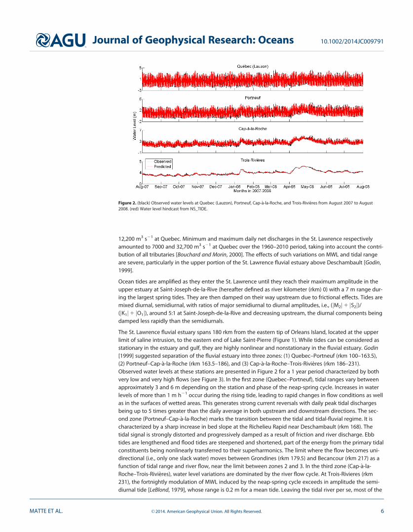
12,200 m3 s21 at Quebec. Minimum and maximum daily net discharges in the St. Lawrence respectivelyamounted to 7000 and 32,700 m3 s21 at Quebec over the 1960–2010 period, taking into account the contri-bution of all tributaries [Bouchard and Morin, 2000]. The effects of such variations on MWL and tidal rangeare severe, particularly in the upper portion of the St. Lawrence fluvial estuary above Deschambault [Godin,1999].

Ocean tides are amplified as they enter the St. Lawrence until they reach their maximum amplitude in theupper estuary at Saint-Joseph-de-la-Rive (hereafter defined as river kilometer (rkm) 0) with a 7 m range dur-ing the largest spring tides. They are then damped on their way upstream due to frictional effects. Tides aremixed diurnal, semidiurnal, with ratios of major semidiurnal to diurnal amplitudes, i.e., (jM2j1 jS2j)/(jK1j1 jO1j), around 5:1 at Saint-Joseph-de-la-Rive and decreasing upstream, the diurnal components beingdamped less rapidly than the semidiurnals.

The St. Lawrence fluvial estuary spans 180 rkm from the eastern tip of Orleans Island, located at the upperlimit of saline intrusion, to the eastern end of Lake Saint-Pierre (Figure 1). While tides can be considered asstationary in the estuary and gulf, they are highly nonlinear and nonstationary in the fluvial estuary. Godin[1999] suggested separation of the fluvial estuary into three zones: (1) Quebec–Portneuf (rkm 100–163.5),(2) Portneuf–Cap-�a-la-Roche (rkm 163.5–186), and (3) Cap-�a-la-Roche–Trois-Rivieres (rkm 186–231).Observed water levels at these stations are presented in Figure 2 for a 1 year period characterized by bothvery low and very high flows (see Figure 3). In the first zone (Quebec–Portneuf), tidal ranges vary betweenapproximately 3 and 6 m depending on the station and phase of the neap-spring cycle. Increases in waterlevels of more than 1 m h21 occur during the rising tide, leading to rapid changes in flow conditions as wellas in the surfaces of wetted areas. This generates strong current reversals with daily peak tidal dischargesbeing up to 5 times greater than the daily average in both upstream and downstream directions. The sec-ond zone (Portneuf–Cap-�a-la-Roche) marks the transition between the tidal and tidal-fluvial regime. It ischaracterized by a sharp increase in bed slope at the Richelieu Rapid near Deschambault (rkm 168). Thetidal signal is strongly distorted and progressively damped as a result of friction and river discharge. Ebbtides are lengthened and flood tides are steepened and shortened, part of the energy from the primary tidalconstituents being nonlinearly transferred to their superharmonics. The limit where the flow becomes uni-directional (i.e., only one slack water) moves between Grondines (rkm 179.5) and Becancour (rkm 217) as afunction of tidal range and river flow, near the limit between zones 2 and 3. In the third zone (Cap-�a-la-Roche–Trois-Rivieres), water level variations are dominated by the river flow cycle. At Trois-Rivieres (rkm231), the fortnightly modulation of MWL induced by the neap-spring cycle exceeds in amplitude the semi-diurnal tide [LeBlond, 1979], whose range is 0.2 m for a mean tide. Leaving the tidal river per se, most of the

Figure 2. (black) Observed water levels at Quebec (Lauzon), Portneuf, Cap-�a-la-Roche, and Trois-Rivieres from August 2007 to August2008. (red) Water level hindcast from NS_TIDE.

Journal of Geophysical Research: Oceans 10.1002/2014JC009791

MATTE ET AL. VC 2014. American Geophysical Union. All Rights Reserved. 6

short-period tide (i.e., diurnal, semidiurnal, etc.) is damped in Lake Saint-Pierre (rkm 264), but long-periodoscillations are still noticeable as far as Montreal (rkm 360).

3.2. Analysis ParametersNS_TIDE was applied to hourly water level data at 13 tide gauges, maintained by Canada’s Department ofFisheries and Oceans (DFO), distributed between Saint-Joseph-de-la-Rive and Lanoraie (Figure 1); they arelisted in Table 1. Time series composed of more than 90,000 good data points were selected for the analysis,for a reference period extending from 1999 to 2009 inclusively, the remaining 19 stations being used forvalidation (Table 2). Validation stations are a mix of temporary DFO’s tide gauges and pressure sensorsinstalled from May to October 2009 (Figure 1) [Matte et al., 2014]. The 11 year analysis period was chosenfor its wide range in river flow. Also, no major construction or dredging work was done after 1998 [Cot�e andMorin, 2007], so that stage and tidal properties are expected to be rather stable during that time period.Moreover, the proportion of fine materials is about 20% in the St. Lawrence, between Sorel and OrleansIsland, with an average sedimentation rate of 4 mm yr21 [Couillard, 1987]. Most of the silting-up is dredgedfor maintenance of the navigational channel or flushed in fall and spring [Gagnon, 1995; Robitaille, 1998b,1998a] and thus has a limited effect on tidal propagation.

Five daily discharge time series Q were used as forcing conditions, each of which is an estimate based uponcontinuous water level measurements at the station of Lasalle (Figure 1) and has been modified to account

Figure 3. Forcing discharges in the St. Lawrence River for the 1999–2009 period: (top) discharge time series at Trois-Rivieres, B�ecancour,Batiscan, Neuville, and Quebec; (bottom) empirical cumulative distribution function.

Table 1. Parameters of the NS_TIDE Analyses at the Tide Gauges for the 1999–2009 Period, Including the Number of Good Data Points,and Their Corresponding Discharge Time Series and Time Lags

rkm Station Good Data Q Time Series sQ (h) sR (h)

0 Saint-Joseph-de-la-Rive 93,149 Qu�ebec 214 566 Saint-Francois 95,418 Qu�ebec 214 5100 Lauzon 95,048 Qu�ebec 214 5104 Saint-Charles River 94,608 Qu�ebec 214 5138 Neuville 95,449 Neuville 26 6163.5 Portneuf 94,833 Neuville 26 6186 Cap-�a-la-Roche 95,301 Batiscan 16 7199 Batiscan 93,062 Batiscan 16 7217 B�ecancour 95,649 B�ecancour 26 9231 Trois-Rivieres 95,583 B�ecancour 26 9264 Lake Saint-Pierre 90,395 B�ecancour 26 9288 Sorel 95,718 Trois-Rivieres 28 10302 Lanoraie 96,119 Trois-Rivieres 28 10

Journal of Geophysical Research: Oceans 10.1002/2014JC009791

MATTE ET AL. VC 2014. American Geophysical Union. All Rights Reserved. 7

for flows from tributaries. The data were produced based on a stage-discharge relation at Lasalle. Fort-nightly variations of MWL due to low-frequency tides were considered as part of the noise. The flows fromtributaries were reconstructed by adding the discharge measured at an upstream station to the estimatedlateral inflow, consisting of surface water runoff and groundwater inflow. Virtually no data are available forgroundwater inflow, so that only surface water runoff was considered, based on gauged areas. For unga-uged areas, the inflow was estimated from the runoff coefficient of an adjoining gauged area. Relations foreach tributary to the St. Lawrence were developed by Morse [1990] and adapted by Bouchard and Morin[2000]. Since the drainage area in the St. Lawrence increases moving downstream, the contribution of tribu-taries was progressively added to the total discharge time series used at the stations. The reconstructed dis-charge time series used in the analyses are presented in Figure 3 and listed in Table 1 for each station.Discharge time series used at the validation stations are shown in Table 2. Differences in discharge betweenTrois-Rivieres and Quebec for the 1999–2009 period reached a maximum of 8700 m3 s21 in April 2008during the freshet (Figure 3). Minimum and maximum discharges at Quebec for that period were observedin September 2007 (7600 m3 s21) and April 2008 (26,400 m3 s21), respectively, which are fairly extremewhen compared to the most extreme flows that occurred in March 1965 (7000 m3 s21) and April 1976(32,700 m3 s21) for the 1960–2009 period. Empirical cumulative distribution functions are shown in Figure 3for each discharge time series and were used to define quantiles of river flow (see next section).

Sept-Iles was chosen as the reference station for ocean tidal forcing (Figure 1), similarly to Godin’s [1999]regression model, because it is removed from fluvial influence and sufficient data are available. Greater diur-nal tidal ranges R were extracted from hourly data at Sept-Iles. Water levels were high-pass filtered, then re-interpolated using (exact) cubic spline functions to a 6 min interval in order to capture the tidal extrema(data are smooth and regularly sampled so that no oscillations are generated during interpolation). Tidalranges were calculated as the difference between higher high water and lower low water using a 27 h mov-ing window with 1 h steps, then smoothed to eliminate discontinuities, similarly to Kukulka and Jay’s[2003a] tidal range filter. The time series of tidal range for the analysis period is presented in Figure 4, alongwith its corresponding empirical cumulative distribution function, used to define quantiles of tidal range.

Time lags sQ and sR for both Q and R time series are presented in Table 1. They were set to identical valuesfor stations sharing the same discharge time series, corresponding to the average lags for the stations con-cerned. For predictions made at arbitrary locations, e.g., at the validation stations, the same lags as the onesused at neighbouring stations were applied to the time series. It is noteworthy that for the Trois-Rivieres sta-tion, the discharge time series for B�ecancour was used instead of that of Trois-Rivieres, in order to include

Table 2. Validation Stations From DFO and Pressure Sensors, Along With Their Corresponding Discharge Time Series, Record Lengthsand Number of Good Data Points for the 1999–2009 Perioda

rkm Station Source Record Length (yr) Good Data Q Time Series

30 Islet-sur-Mer Pressure sensor 0.4 13,522 Quebec38 Rocher Neptune DFO 4.4 19,433 Quebec45 Ile-aux-Grues South Pressure sensor 0.3 9,780 Quebec46 Ile-aux-Grues North Pressure sensor 0.3 9,785 Quebec54 Banc du Cap Brul�e DFO 3.1 12,436 Quebec78 Saint-Jean DFO 3.5 16,988 Quebec97 Beauport Pressure sensor 0.4 13,410 Quebec106.5 L�evis Pressure sensor 0.4 13,415 Quebec106.5 Quebec Pressure sensor 0.4 12,769 Quebec115 Quebec Bridge Pressure sensor 0.4 13,617 Quebec124 Saint-Nicolas Pressure sensor 0.4 12,963 Quebec146 Sainte-Croix-Est Pressure sensor 0.4 13,052 Neuville157 Cap-Sant�e Pressure sensor 0.4 12,765 Neuville161 Pointe-Platon Pressure sensor 0.4 12,964 Neuville168 Deschambault Pressure sensor 0.4 11,243 Batiscan179.5 Leclercville Pressure sensor 0.4 11,966 Batiscan179.5 Grondines Pressure sensor 0.4 12,431 Batiscan213 Champlain Pressure sensor 0.4 11,452 B�ecancour241 Port Saint-Francois DFO 10.3 63,857 B�ecancour

aPressure sensor data are sampled at a 15 min interval, while DFO’s data are hourly. Stations in italics are not covered by the mainbranch of the ONE-D model.

Journal of Geophysical Research: Oceans 10.1002/2014JC009791

MATTE ET AL. VC 2014. American Geophysical Union. All Rights Reserved. 8

the backwater effects from the Saint-Maurice River, located 1 km downstream of the station. This effectpropagates up to the station of Lake Saint-Pierre.

In the development of a spatial model, identical analysis parameters must be applied to each station toensure that spatial variations in the coefficients are not the result of changes in model properties, but thatthey are attributable to tidal-fluvial processes. Preliminary tests on the model exponents in equation (3)showed that model performance was little sensitive to their value, as deviations from theoretical exponentswere compensated by changes in the regression coefficients. Similar conclusions were drawn from the sen-sitivity analysis performed by Matte et al. [2013]. Therefore, model exponents were set to the theoretical val-ues used by Kukulka and Jay [2003a, 2003b], as they appear in equation (4). The same tidal constituentswere imposed at all stations to allow interpolation of model coefficients throughout the system. As a conse-quence, errors for some constituents may grow upstream, while some other constituents become less sig-nificant downstream. The IRLS analyses (cf. equation (2)) were performed using a Cauchy weightingfunction with a default tuning constant of 2.385 [Leffler and Jay, 2009; MathWorks, R2010a MathWorks docu-mentation, http://www.mathworks.com/help/releases/R2010a/helpdesk.html].

The allowed frequency separation in NS_TIDE is dictated by a redefined Rayleigh criterion, which takes intoaccount the overlap between frequencies associated with their tidal cusps [Munk et al., 1965]. The width ofthese cusps reflects the intensity of modulation of the tidal components. Therefore, the inclusion of toomany constituents with overlapping cusps can lead to erroneous estimates of tidal properties [e.g., Godin,1999]. One typical symptom of an overdetermined solution (i.e., too many constituents) is that closelyspaced components take very large (unreal) amplitudes, their phases are almost 180� out of phase, so theycancel partially, and phase errors are very large (typically exceeding 100�). Conversely, not resolving enoughconstituents may result in oscillation of the tidal amplitudes as a compensation for modulations that wouldnormally occur between pairs of constituents not included in the analyses. In the most extreme case, onlyincluding one component per tidal band would yield similar results as continuous wavelet transform (CWT)[Flinchem and Jay, 2000]. Here tidal constituents were selected, partly based on rather permissive constitu-ent selection criteria (g 5 0.5 and mean signal-to-noise ratio (SNR)� 2; see Matte et al. [2013] for a definitionof the parameters). Constituent amplitudes and phases were then carefully inspected to detect artifacts aris-ing from the method. To ensure that included constituents have a physical meaning, comparisons of time-averaged tidal properties (especially the phases) with those given by standard HA were made, assumingthat HA accurately represents the average frequency content of the time series. Constituents presentingnonphysical characteristics were excluded from the analyses, while some others were progressively addedto reduce oscillations in the tidal amplitudes of principal components. In the end, the tidal-fluvial model

Figure 4. Forcing tidal range in the St. Lawrence River for the 1999–2009 period: (top) tidal range time series at Sept-Iles; (bottom) empiri-cal cumulative distribution function.

Journal of Geophysical Research: Oceans 10.1002/2014JC009791

MATTE ET AL. VC 2014. American Geophysical Union. All Rights Reserved. 9

was forced using the same 39 components at all sta-tions, listed in Table 3. At Saint-Joseph-de-la-Rive (rkm0), these 39 constituents explain 98% of the variance inwater levels, with classical HA. Low-frequency varia-tions in water levels, for their part, are represented bythe stage model (cf. equation (4)), rather than the usuallow-frequency harmonic constituents.

The time reference for the analyses was Eastern Stand-ard Time. Greenwich phases were computed, with nonodal corrections. The latter are performed in NS_TIDEin the same manner as T_TIDE [Pawlowicz et al., 2002]

and should be applied on overlapping 366 day periods. However, for the coefficients of the nonstationaryanalysis to be robust, a record length that covers the widest dynamic range of flow conditions is sought.The chosen 11 year period met this criterion. NS_TIDE does not currently embed the nodal corrections inthe least squares matrix, which would remove the need for assumptions that underlie usual postfit correc-tions and that may restrict the length of the analysis period [Foreman et al., 2009]. Nevertheless, modula-tions of the main tidal constituents by their satellites are small in rivers relative to the effects of stagevariations. Nodal modulations are also modified by fluvial modulations. In fact, deviations from the equilib-rium constants may occur due to friction and shallow-water effects, which may lead to systematic errors inthe estimation of tidal constituents [Amin, 1983, 1985, 1993; Shaw and Tsimplis, 2010]. In practice, it is virtu-ally impossible to separate the modulation effects on the main tidal constituents by river flow and tidalrange from those stemming from changes in lunar declination (see, e.g., Matte et al. [2013] for further dis-cussion). For these reasons, nodal corrections were not included in the analyses.

To assess model performance, water level hindcasts were compared to results from classical HA at the sta-tions. Standard HA [Pawlowicz et al., 2002; Leffler and Jay, 2009] were performed using a threshold SNR of 2for constituent rejection. The number of replicates for the error estimation was set to 300 and a correlatednoise model was used. The same weighting function and tuning constant as for the nonstationary analyseswere used. To further validate model predicting capabilities, water level forecasts were produced at all sta-tions for a period free of ice extending from 21 May to 21 October 2009, during which pressure sensorswere in place. Results were compared to simulations from the ONE-D model of the St. Lawrence withoutconsidering the effects of wind. The numerical scheme and formulation of the model are detailed in Hicks[1997], along with a thorough analysis of its performance.

3.3. Results3.3.1. Model PerformanceFigure 2 shows water level hindcasts from NS_TIDE compared to observations at four selected stations forthe 2007–2008 period, characterized by very low and very high flows (cf. Figure 3). Predicted signals followthe variations in tidal amplitude and in MWL with good accuracy at both upstream and downstreamstations.

Statistics obtained from classical HA and NS_TIDE at the analysis stations of Table 1 for the 1999–2009period are presented in Figure 5. They include the number of model coefficients solved for (different fromn, the number of tidal constituents; see equation (4)), the residual variance, root-mean-square errors (RMSE),and maximum absolute errors. The only criteria for constituent selection and rejection in HA are based onthe record length and error level in coefficients, respectively. As shown in Figure 5a, the total number ofmodel coefficients is higher with NS_TIDE, with nearly half the constituents of HA, due to the higher num-ber of terms composing the nonstationary model. The ability of classical HA to explain the signal variance iscomparable to NS_TIDE at downstream stations, from Saint-Joseph-de-la-Rive (rkm 0) to Portneuf (rkm163.5), landward of which the residual variance drastically increases for HA (Figure 5b). This coincides withthe presence of rapids near Deschambault (rkm 168) combined with a rapid increase of the bottom slope,marking the transition from tidal to tidal-fluvial regimes where the influence of discharge becomesprominent.

In Figure 5c, RMSE from both methods are plotted at the stations. The curves coincide in the first 100 rkm,but the RMSE associated with NS_TIDE sharply decrease upstream, while those of HA increase. On average,

Table 3. Tidal Constituents Included in the Analyses, forEach Tidal Band From Diurnal to Eight-Diurnal (D1–D8)

Tidal Bands Constituents

D1 r1, Q1, q1, O1, P1, K1, h1, J1, OO1

D2 e1, 2N2, l2, N2, m2, M2, k2, L2, S2, K2, MSN2

D3 MO3, SO3, MK3

D4 MN4, M4, SN4, MS4, MK4, S4, SK4

D5 2MK5

D6 2MN6, M6, 2MS6, 2MK6, 2SM6, MSK6

D7 3MK7

D8 M8

Journal of Geophysical Research: Oceans 10.1002/2014JC009791

MATTE ET AL. VC 2014. American Geophysical Union. All Rights Reserved. 10

the NS_TIDE analyses are far more representative of the tidal-fluvial dynamics than HA in upstream reachesof tidal rivers. At downstream stations, where the tidal signals are much more stationary (see Figure 2),NS_TIDE is comparable to HA, thus demonstrating the validity of the model under these conditions too.

Maximum absolute errors shown in Figure 5d are again comparable between the two methods up to Port-neuf (rkm 163.5), where they split. They then show a significant decrease with NS_TIDE, attributable to abetter representation of the physics by the nonstationary model. Note that both RMSE and maximum errorsare absolute values; their sharp decrease past Portneuf thus also follows the decrease in tidal range.

3.3.2. Spatial InterpolationsThe model coefficients in equation (4) were spatially interpolated using Hermite polynomials so that tidalproperties may be retrieved at any points in space. Figures 6a and 6b show an example of interpolatedcoefficients for the stage model and the M2 component of the tidal-fluvial model, respectively. For clarity,second and third coefficients were multiplied by the average discharge and tidal range for the 1999–2009period, as shown in the legends. In the stage model (Figure 6a), the coefficient c0 is primarily determined byriver geometry. In the first �160 rkm, its contribution to the MWL is partly balanced by the discharge termc1. From Portneuf (rkm 163.5) and upstream, the c0 term increases following the rapid rising of the bedslope. This may be due to a long-term water level setup caused by river-tide interaction that steepens thewater surface profile [e.g., Sassi and Hoitink, 2013]. The discharge coefficient c1 increases from downstreamto upstream; its effect is more pronounced past Portneuf, where changes in the tidal-fluvial regime occur.The range term c2 is responsible for fortnightly variations in MWL. The value of c2 increases gradually up toCap-�a-la-Roche (rkm 186), where the amplitude of the fortnightly wave reaches a maximum; it thendecreases upstream. This tendency is consistent with the variations in Mf, MSf, and Mm amplitudes (notshown) calculated from classical HA at the stations.

In Figure 6b, the coefficients of the M2 component of the tidal-fluvial model are presented, where the bluecurves represent the cosine part of equation (4) and the red curves represent the sine part. Both sine andcosine parts of the constant term d0 (solid lines), representing the astronomical tide, are strongly dampedmoving upstream. The discharge terms d1 (dashed lines) are in general opposite in sign with d0, each pairof curves of a given part (cosine or sine) intercepting around zero, so that they cancel each other once theyare summed. In other words, the sign difference between d1 and d0 means that an increase in discharge isreflected as a decrease in tidal amplitude. The range terms d2 are not consistently opposed in sign with d0,

Figure 5. Statistics on water level hindcasts from NS_TIDE and classical HA at the analysis stations of Table 1 for the 1999–2009 period:(a) number of model coefficients solved for; (b) residual variance; (c) root-mean-square errors (RMSE); (d) maximum absolute errors. RMSEand maximum errors are absolute values, thus decreasing with tidal range.

Journal of Geophysical Research: Oceans 10.1002/2014JC009791

MATTE ET AL. VC 2014. American Geophysical Union. All Rights Reserved. 11

so that their effect on M2 amplitudesvaries along the river. The amplitudesand phases can be retrieved for eachterm from equations (8) and (9) forfurther analysis (see next sections).

3.3.3. ValidationTo validate the model, water levelpredictions were generated at all 32stations from Tables 1 and 2 andcompared with observations, for theperiod extending from 21 May to 21October 2009. The same exercise wasdone for the ONE-D model for com-parison purposes. Results are pre-sented in Figure 7. Stations identifiedwith asterisks are not covered by themain branch of the ONE-D model andshould be interpreted with caution;they are either located on the southshore of the upper estuary (down-stream of Orleans Island) or in thenorth arm of Orleans Island. In gen-eral, residual variances, RMSE andmaximum errors are lower with theONE-D model than with NS_TIDE,with the exception of a few upstreamstations. This is not a surprising resultsince ONE-D has many more degreesof freedom than NS_TIDE. The ONE-Dmodel of the St. Lawrence is com-posed of 1241 sections, eachdescribed in terms of geometry andfriction. It solves the one-dimensionalSt. Venant equations at every timestep of the validation period. In com-parison, the NS_TIDE model is basedon an analytical solution of the St.Venant equations for the critical con-vergence regime [Jay, 1991]. It is

composed of 237 parameters per station or, equivalently, 237 Hermite polynomial functions for the spatialmodel which are invariant in time (i.e., no need for time integration). Although much simpler, the NS_TIDEmodel is capable of good accuracy, with RMSE lower than 0.3 m at all stations. This is quite low consideringthat tidal ranges often exceed 5 m in the downstream portion of the river. Furthermore, error at the valida-tion stations is not systematically higher than at the analysis stations, which is an indication that the stationnetwork is dense enough to allow accurate interpolation. It also shows that the interpolation functions arewell adapted to the variations in modeled parameters, and thereby to the physics of the river. Interpolationerrors are discussed in section 4. Higher residual variances were obtained at the station of Champlain (rkm213) due to a higher noise level in the observed data (Figure 7a).

To better characterize the model predicting capabilities, RMSE values were computed separately onMWL, tidal range, and height and time of high water (HW) and low water (LW). Results are shown inFigure 8. MWL are better reproduced by the ONE-D model at most stations except a few where thetwo models are comparable. With NS_TIDE, the highest errors in MWL occur between Neuville (rkm138) and Portneuf (rkm 163.5), possibly due to lateral gradients in water levels associated with channel

Figure 6. Spatially interpolated coefficients of the (a) stage model and (b) M2 com-ponent from the tidal-fluvial model. Second and third coefficients in Figures 6a and6b were multiplied by their average discharge and tidal range for the 1999–2009period.

Journal of Geophysical Research: Oceans 10.1002/2014JC009791

MATTE ET AL. VC 2014. American Geophysical Union. All Rights Reserved. 12

curvature. Errors in tidal range decreasewith upriver distance as tidal amplitudesare damped. They reach a maximumbetween Quebec Bridge (rkm 115) andSaint-Nicolas (rkm 124), which can beexplained by very large water depthsbetween Lauzon (rkm 100) and Saint-Nicolas, varying approximately from 30to 60 m. The tidal wave propagatesfaster with increased water depth and isless rapidly damped by bottom friction.Because the interpolation is madebetween Saint-Charles River estuary (rkm104) and Neuville (rkm 138) assumingsmooth variations in tidal properties, theresulting tidal ranges at intermediate sta-tions are less accurate. This is confirmedby errors in LW heights, which are signifi-cantly higher at Quebec Bridge andSaint-Nicolas, as LW are the most sensi-tive to depth variations. It is however alittle surprising to observe the samebehaviour with ONE-D considering thatwater depths are taken into account inthe model; this might be related to alack of stations for calibration betweenLauzon and Neuville. Furthermore, errorsin the heights and times of HW arerather stable downstream of Trois-Rivieres (rkm 231), while errors in thetimes of occurrence of LW graduallyincrease from downstream to upstream.They reach values of about 2 h at Trois-Rivieres. LW are more sensitive to frictionand river flow than HW [e.g., Godin,1999], thus explaining the higher andincreasing errors in the timing of LW.Timing errors of HW and LW upstream ofTrois-Rivieres were excluded, because

tide completely vanishes during high discharge events. Here the comparison of the times of occurrenceof HW and LW is an indirect evaluation of tidal asymmetry.

3.3.4. Tidal-Fluvial ProcessesTo demonstrate the ability of the model to improve current knowledge on tidal-fluvial processes, results inthe St. Lawrence fluvial estuary are presented in Figures 9–12. Because the objective is not to present athorough analysis of the dynamical processes in play, results are restricted to the stage model and to fivemajor constituents from the diurnal, semidiurnal, and quarter-diurnal bands of the tidal-fluvial model.

The harmonic representation of low frequencies in traditional HA, composed of semimonthly (Mf, MSf),monthly (Mm, MSm), semiannual (Ssa), and annual (Sa) constituents, is unable to adequately represent low-frequency river motions dominated by nonlinear interactions of tides with river flow [Parker, 2007]. In con-trast, these interactions are well accounted for in NS_TIDE because river flow and ocean tidal range areincluded directly in the basis functions. Longitudinal profiles of MWL are shown in Figure 9 for the 0.1, 0.5,and 0.9 quantiles of discharge and tidal range. The water surface slopes clearly exhibit three contrastingzones in the fluvial estuary, as suggested by Godin [1999], with marked changes in the slopes around

Figure 7. Statistics on water level predictions from NS_TIDE and ONE-D atthe stations of Tables 1 and 2 for the period from 21 May to 21 October2009. Stations identified with asterisks are not covered by the main branchof the ONE-D model.

Journal of Geophysical Research: Oceans 10.1002/2014JC009791

MATTE ET AL. VC 2014. American Geophysical Union. All Rights Reserved. 13

Portneuf (rkm 163.5) and Cap-�a-la-Roche (rkm 186). The region delimited by these two stations forms a tran-sition zone from the tidal to the tidal-fluvial regime, characterized by a rapid increase in bottom slope atthe Richelieu Rapid near Deschambault (rkm 168). This supports the idea that breaks in morphology areresponsible for splitting the system into river and tide-dominated parts, similarly to the results obtained bySassi et al. [2012]—in their case, however, they associated this separation with the point where the expo-nential width decrease stops. A jump in MWL also occurs around rkm 235, corresponding to the location ofLaviolette Bridge, which acts as a major restriction to the flow. A fourth region can therefore be definedfrom this point, located near the entrance of Lake Saint-Pierre, up to Lanoraie where the semidiurnal tidecompletely extinguishes during neap tides. The sensitivity of MWL to variations in discharge considerablyincreases in the upstream region of the fluvial estuary, while it is little affected at the most downstream sta-tions. Increases in tidal range are also reflected by increases in MWL, and vice versa, which is in accordancewith the fortnightly rise and fall of MWL during spring and neap tides, respectively [LeBlond, 1979]. Further

modulations of the MWL induced by fric-tional interactions between tidal constitu-ents are accounted for by the stage modelthrough the range term. Moreover, theresponse of the system to variations intidal range is greater at lower discharges.At downstream stations, MWL under con-ditions of low discharge and high tidalrange are similar to MWL observed duringhigh discharge and mean tidal range.

In Figures 10a and 10b, longitudinal pro-files of amplitudes and phases are shownfor the two dominant diurnal constituents,O1 and K1. In general, they suggest a simi-lar separation of the fluvial estuary intofour distinct regions. Tidal amplitudes are

Figure 8. Root-mean-square error (RMSE) on predicted mean water level (MWL), tidal range, and height and time of high water (HW) and low water (LW) from NS_TIDE and ONE-D atthe stations of Tables 1 and 2 for the period from 21 May 2009 to 21 October 2009. Stations identified with asterisks are not covered by the main branch of the ONE-D model.

Figure 9. Longitudinal profiles of mean water levels (MWL) for quantiles ofdischarge and tidal range. Blue, black, and red lines correspond to 0.1, 0.5,and 0.9 quantiles of discharge, respectively; dotted, solid, and dash-dottedlines correspond to 0.1, 0.5, and 0.9 quantiles of tidal range, respectively.

Journal of Geophysical Research: Oceans 10.1002/2014JC009791

MATTE ET AL. VC 2014. American Geophysical Union. All Rights Reserved. 14

characterized by a slow decrease downstream to Portneuf (rkm 163.5), followed by a sharp diminutionupstream. At downstream stations, tidal amplitudes increase with discharge, because of larger water depth.Although amplitudes are being damped considerably from Portneuf, it is only around Cap-�a-la-Roche (rkm186) that tidal amplitudes start to decrease with increases in discharge. From that point, amplitudes aremore severely damped by the discharge. Past the Laviolette Bridge (rkm 235), the decrease in tidal ampli-tudes slows as it approaches zero.

Figure 10. Same as Figure 9 for O1 and K1 amplitudes and phases.

Figure 11. Same as Figure 10 for M2 and S2 amplitudes and phases.

Journal of Geophysical Research: Oceans 10.1002/2014JC009791

MATTE ET AL. VC 2014. American Geophysical Union. All Rights Reserved. 15

K1 is the dominant diurnal constituent andhas higher amplitudes than O1 downstreamof Portneuf. However, the amplitudes of O1

and K1 reach similar values around Port-neuf, K1 being damped slightly more rap-idly than O1, possibly due to the higherfrequency of K1 [Godin, 1999]. According tothe development of the tidal potential[Doodson, 1921], O1 should consistently besmaller than K1. One possible explanationfor O1 and K1 being of similar amplitude isto attribute this discrepancy to the effect ofM2 on K1 and O1 in presence of strong bot-tom friction [Godin and Martinez, 1994].

O1 and K1 are responsible for the diurnalinequality associated with lunar declination.Their combined effect leads to a modula-tion with a period of 27.32 days, reaching aminimum every 13.66 days when the moonis over the equator. However, in presenceof friction, their summed amplitude is alsomodulated by tidal range. In fact, takenindividually, the amplitude of K1 is dampedduring spring tides (higher tidal range) andamplified during neap tides (lower tidalrange) due to nonlinear interactions, asobserved in Figure 10. As for O1, higher

amplitudes are obtained at spring tides downstream of Portneuf (rkm 163.5), while they are lower upstream.This effect reverses upstream of Laviolette Bridge (rkm 235) in the case of O1 and upstream of Cap-�a-la-Roche (rkm 186) for K1.

As for the phases of O1 and K1 in Figures 10c and 10d, they show a constant increase with distance up toPortneuf (rkm 163.5) where a change in slope occurs, meaning that tide propagation is delayed due to theincreasing influence of river flow (here a steeper slope means a slower propagation of the tidal wave). How-ever, for O1, phase lags are slightly larger at high discharges compared to low discharges, while the oppo-site is observed for K1. Although this may be an artifact of the method, the consequence is a modificationof their combined effect on a semimonthly basis. Finally, with larger tidal ranges the phases of both compo-nents are increased downstream while they are reduced upstream; this is another effect of the reversal ofmean low waters during spring and neap tides.

In Figure 11, longitudinal profiles of amplitudes and phases are shown for the two dominant semidiurnalconstituents, M2 and S2. Similar observations as in Figure 10 can be made with respect to the general aspectof the curves. Both M2 and S2 show little variations in amplitude with discharge throughout the system, rela-tive to their amplitude. Overall, slightly lower amplitudes are obtained at higher discharges with M2, wheredamping is more influenced by discharge upstream of Portneuf (rkm 163.5). With S2, higher amplitudes areobserved downstream of Portneuf at higher discharges, while damping occurs upstream. The effects of tidalrange on the amplitudes of M2 are little, except in the first �80 rkm, while the amplitudes of S2 are muchmore sensitive. In presence of larger tidal ranges, the amplitudes of S2 decrease, which might seem counter-intuitive. In fact, M2 and S2 interact together to produce neap-spring variations with a modulation period of14.77 days. When tidal ranges are large (at spring tides), M2 and S2 are in phase, their amplitude beingadded to each other. However, as shown in Figure 11b, the individual amplitude of S2 is smaller duringspring tide compared to neap tides, meaning that the summed amplitude of M2 and S2 is smaller than itwould be in absence of friction. In other words, M2 and S2 are responsible for the generation of the neap-spring cycle, but they may be, in turn, affected by these fortnightly variations through friction, by afeedback mechanism.

Figure 12. Same as Figure 10 for M4/M2 amplitude ratios and 2M2–M4

phase differences.

Journal of Geophysical Research: Oceans 10.1002/2014JC009791

MATTE ET AL. VC 2014. American Geophysical Union. All Rights Reserved. 16

As for the phases of M2 and S2, shown in Figures 11c and 11d, variations are more subtle. Increases in dis-charge lead to slightly higher phases of S2, while increases in tidal range lead to lower phases. Variations forM2 are almost imperceptible, but they show similar trends.

In upstream reaches of rivers, discharge has the effect of damping constituents of higher frequency moreeffectively [Godin, 1991; Godin and Martinez, 1994]. As a result, semidiurnal constituents are being dampedfaster than diurnal tides [see, e.g., Godin, 1999]. The decay profiles of the diurnal and semidiurnal compo-nents in Figures 10 and 11 between Saint-Joseph-de-la-Rive (rkm 0) and Lanoraie (rkm 302) are highly simi-lar, but damping ratios seem to confirm this trend. In fact, for an average discharge, approximately 3% ofthe original diurnal amplitude remains at Lanoraie, while only 0.7% of the semidiurnal amplitude measuredat Saint-Joseph-de-la-Rive is still observable at Lanoraie. While damping and phase speed may be frequencydependent, frictional nonlinearities also act as a generating mechanism for overtides and compound tides,hence contributing to the modification of the principal components.

In Figure 12 are shown the M4/M2 amplitude ratios and 2M2–M4 phase differences as a function of upriverdistance. The first 50 rkm were removed due to interpolation errors between the first two stations for fre-quencies higher or equal to that of M4 (see discussion in section 4). Other oscillations are most likely arti-facts of the interpolation functions. In general, an increase in M4/M2 amplitudes is observed up to PortSaint-Francois (rkm 241), indicating a transfer of energy from M2 to M4 through friction that is amplifiedupstream due to the increasing influence of discharge. The amplitude ratio then undergoes a rapiddecrease in Lake Saint-Pierre as most of the tidal signal is damped, M4 being attenuated more rapidly thanM2 due to its higher frequency. Similar observations can be made between scenarios of low and high dis-charge. Downstream of Cap-�a-la-Roche (rkm 186), the M4/M2 ratio increases with increasing discharges,while the reverse holds upstream. Past Cap-�a-la-Roche, M4 is damped more rapidly by discharge than it iscreated from M2, while downstream the energy transfer from M2 to M4 at higher discharge overcomes itsdamping effects.

As for tidal ranges, their effect on M4/M2 amplitude ratio is consistent throughout the domain: a larger tidalrange is expressed through smaller M4/M2 ratios, and vice versa. This is counterintuitive at first sight, asincreases in the M4/M2 ratio are generally expected at spring tide rather than neap tide. One possible expla-nation is that the relative decrease in amplitude of M4, even more pronounced than that of M2 duringspring tide, may be related to the lowering of low waters at neap tides rather than spring tides, with corre-spondingly stronger bottom friction.

The key to explain this unusual observation may lie in the tidal analysis approach used and in how rivertides are conceptualized. For example, CWT tidal analysis methods [Jay and Flinchem, 1997, 1999; Jay andKukulka, 2003; Buschman et al., 2009] are able to express time variations in the tidal content of a signal,although with no distinction between frequencies of a given tidal band. Ratios of D4/D2 amplitudes (whereD2 and D4 refer to the semidiurnal and quarter-diurnal species, respectively) thus represent the relativeenergy contained in the quarter-diurnal and semidiurnal bands, all frequencies combined. Similarly, theconcept of ‘‘reduced vector’’ introduced by George and Simon [1984], and notably applied by Godin [1999],yields daily averaged band estimates of the major tidal components, again with no possible separationbetween neighbouring frequencies. The amplitudes associated with M2 and M4 thus correspond to the totalenergy of their respective tidal band, much like CWT. Because NS_TIDE allows for the inclusion of multiplefrequencies within each tidal band, direct comparisons with conventional methods is not straightforward.In fact, to actually reproduce the variations in M4/M2 ratios as traditionally expected from conventionalmethods, the total contribution from quarter-diurnal and semidiurnal bands needs to be taken into account.For example, plots of the dominant semidiurnal and quarter-diurnal constituents (not shown) confirm thattheir summed amplitudes in each tidal band are synchronized with tidal range, and so are the amplituderatios. This is because both fortnightly and monthly modulations are induced by the interactions betweenpairs of frequencies. Taken individually, however, these constituents may respond differently to changes indischarge and ocean tidal range. Moreover, the energy transfer through friction from M2 to higher frequen-cies not only involves M4, but also MN4, MS4, and so on. As such, results are dependent on the number ofincluded constituents within each tidal band.

Finally, in Figure 12b, the 2M2–M4 phase differences show a gradual increase as a function of upriver dis-tance. The relative phase differences are below 180�, which indicates a flood tidal asymmetry [Friedrichs and

Journal of Geophysical Research: Oceans 10.1002/2014JC009791

MATTE ET AL. VC 2014. American Geophysical Union. All Rights Reserved. 17

Aubrey, 1988]. As these differences approach 180�, tidal asymmetry increases, with a signal characterized byshort and abrupt flood tides and slowly decreasing ebb tides. The phase differences tend to increase withdischarge, except for stations located between Neuville (rkm 138) and Cap-�a-la-Roche (rkm 186); this is notclear whether it is the result of interpolations or river-tide interactions. Moreover, in the first �250 rkm,flood tidal asymmetry is enhanced during neap tides compared to spring tides, which is coherent with thevariations in M4/M2 ratios. The other quarter-diurnal tides possibly play a role in reinforcing tidalasymmetry.

4. Discussion and Conclusion

The potential of NS_TIDE to predict tides in upstream reaches of tidal rivers has been demonstrated. Signalanalyses from 13 contrasting stations in terms of tidal-fluvial dynamics showed significantly better statisticsthan classical HA at upstream stations, while model performance at downstream stations was comparableto classical HA. Despite all assumptions made on the physics, the predicting capability of NS_TIDE was sur-prisingly high. In fact, many parameters such as the model exponents were set to constant values, while inreality they may be influenced by the river geometry, including the cross-sectional area, the wetted perime-ter, the convergence rate, or other factors. Furthermore, the model implemented in NS_TIDE was developedfor systems where tidal and fluvial flows are of similar magnitude. Knowing that tidal discharges can bemore than 5 times greater than the residual flow at downstream locations, the agreement between the pre-dicted and the observed water levels is remarkable. Even with these simplifications, tidal-fluvial processesthat are explained by the method are physically plausible. When time-averaged, the amplitudes and phasesresemble those obtained from HA, which confirms that the energy is well distributed between the constitu-ents. Furthermore, predicting water levels from hindcast results for a time period other than the analysisperiod [e.g., Matte et al., 2013], or equivalently, at intermediate stations if coefficients are spatially interpo-lated (like here), is a good way to test the validity of a model. Nonphysical variations (e.g., unreal amplitudesand phases), which sometimes improve the harmonic fits, are likely to degrade the predictions when trans-posed to other time periods or stations. Here the addition of constituents in the analysis was carried outuntil the point was reached where prediction accuracy decreased or artifacts started to appear (e.g., inco-herent phases compared to classical HA). While resolving for too few components could lead to oscillationsin the tidal amplitudes, some of the modulations observed in the results for the dominant frequencies werenot eliminated by adding more constituents. The remaining variations may be attributable to increasederrors under specific discharge and tidal range conditions, or they may be of physical origin. Further investi-gation may be needed to identify the sources of variation.

The model was validated with observations at a total of 32 stations and by comparison with the operationalONE-D model of the St. Lawrence River. Better statistics were obtained with the ONE-D model, but at theprice of a more complex and time-consuming modeling process (including the time devoted to developand calibrate the model). In contrast, NS_TIDE provided still very good accuracy from a simpler but moreinformative model in terms of tidal-fluvial dynamics. In fact, numerical models and tidal analysis tools havevery different strengths and weaknesses. Much can be learned from the existing operational model, espe-cially if all terms in the momentum balance can be stored. However, no information on the time-varying fre-quency content of water levels or velocities can be obtained if not combined with other tidal analysismethods. By contrast, NS_TIDE uses a functional representation of tides (i.e., constituent amplitudes andphases) expressed in terms of external nonstationary forcing, which can be used for prediction in a straight-forward manner. With an approach based on regression analysis, no field description is needed (topogra-phy, substrate friction, etc.), thus minimizing sensitivity to local topographic or frictional uncertainty.Instead, model parameters are optimized by stations to account for changes in these variables, as experi-enced by the water levels. NS_TIDE also preserves the compactness and efficiency of HA and ensures conti-nuity between analyses performed in the St. Lawrence fluvial estuary, marine estuary, and gulf.Furthermore, its capacity to distinguish frequencies within tidal species represents a considerable improve-ment compared to conventional tidal analysis methods that offers new possibilities for dynamical inquiry.

In NS_TIDE, the inclusion of river discharge in the basis function drastically improves the predictions atupstream stations, which had been demonstrated before, notably by Godin [1985, 1999] and Jay and Flin-chem [1997]. Similar adaptations of the models developed by Kukulka and Jay [2003a, 2003b] were made tohindcast lower low water (LLW) and higher high water (HHW) as a function of river flow and external tidal

Journal of Geophysical Research: Oceans 10.1002/2014JC009791

MATTE ET AL. VC 2014. American Geophysical Union. All Rights Reserved. 18

forcing in the Columbia River [Jay et al., 2011]. Likewise, an inverse model based on analysis of tidal statisticswas derived from Kukulka and Jay’s [2003a, 2003b] approach to produce monthly averaged tidal dischargeestimates in the San Francisco Bay [Moftakhari et al., 2013]; in their analysis, however, the tidal range termwas neglected, because of the 31.7 day averaging period used.

Buschman et al. [2009] presented a method to analyze subtidal water levels in tidal rivers. Unlike Kukulkaand Jay’s [2003a, 2003b] models, they used Godin’s approximation of the friction term [Godin, 1999], ratherthan the Tschebyschev polynomial approach [Dronkers, 1964], to derive a new expression for subtidalfriction, and successfully applied their model in the Berau River (Indonesia). They attribute subtidal motionto three sources, namely the river flow, river-tide interactions, and tides alone. The river-tide interactionwas mainly responsible for fortnightly variations in water levels at the station under study. By comparison,the stage model implemented in NS_TIDE, derived from Kukulka and Jay’s [2003b] model, decompose var-iations in MWL into contributions from river forcing, tides, atmospheric pressure (not included here), andtopographic offset. As shown in the present application, NS_TIDE is able to reproduce the nonlinearly gen-erated fortnightly variations in MWL, as well as seasonal variations associated with river discharge. The fre-quency content of the stage model contains energy at annual and semiannual periods due to seasonalcycles in discharge (c1 term), and at monthly and semimonthly periods due to the influence of the tidalrange (c2 term). These low frequencies are generated by tidal-fluvial interactions and nonlinear compoundtides, which are inadequately represented in tidal rivers by the usual harmonic apparatus [Parker, 2007;Matte et al., 2013]. The improved statistics in the upstream reach of the St. Lawrence fluvial estuary (cf.Figure 5) is directly related to the ability of the stage model to accurately represent subharmonics.

Part of the error in the spatial model is related to the position of the analysis stations, the distance that sep-arates them and the interpolation functions used. It was shown that Hermite polynomials are good interpo-lators in the present case, given the spatial variations in the coefficients in the St. Lawrence. However, asthe frequency of the constituents increases, the wavelength decreases, leading to more oscillations in thecoefficients due to a higher number of cycles. When the distance separating the stations approaches halfthe wavelength of the constituent, interpolation errors may increase drastically. In that case, components ofhigher frequencies should be neglected or more stations should be added to the available network. In thepresent application, the average distance between the stations is 25 km (cf. Table 1), which is less than halfthe wavelength of M8 (roughly �70 km). Between Saint-Joseph-de-la-Rive (rkm 0) and Saint-Francois (rkm66), however, the interpolation of M4 (wavelength �140 km) and higher frequencies is questionable due tothe distance separating the two stations, as mentioned above (cf. Figure 12). Using numerical models toimprove the interpolation, by taking advantage of a higher spatial resolution, may be an interesting avenueto explore.

NS_TIDE does not currently differentiate between the rising and falling limbs of a hydrograph, mainlybecause coefficients determined by regression are constant in time. This feature allows general applicabil-ity of the model, although it cannot account for hysteresis phenomena. For example, as shown by Sassiand Hoitink [2013], tides are damped faster during the rising limb of a discharge wave than inversely. Thefact that nonstationary (rather than constant) river discharges are built directly in the basis function matrixof NS_TIDE offers the possibility of analysing such mechanisms; they should be addressed in the future.Moreover, recent studies show that flow division in tidal branching systems is controlled by river flow,tides, and the interactions between the two [Buschman et al., 2010; Sassi et al., 2011]. Notably, the dis-charge asymmetry features fortnightly oscillations attributable to neap-spring variations in tidal range. Theuse of NS_TIDE to further examine these interactions would be interesting, especially at the junction ofOrleans Island in the St. Lawrence fluvial estuary.

The spatial, nonstationary harmonic model presented in this paper represents a new way to look at river tides.Applied to the St. Lawrence fluvial estuary, it successfully reproduced stage and tidal properties in an unprece-dented way, by expressing their variations in terms of nonstationary forcing variables, i.e., river discharge andocean tidal range, for a broad range of conditions. Several characteristics of the St. Lawrence and, by exten-sion, of tidal rivers in general were brought to light by the model. They can be summarized as follows:

1. The decrease in predictive skill of classical HA compared to NS_TIDE coincides with a break in river mor-phology, in the present case associated with the presence of rapids combined with a rapid increase ofthe bottom slope, which marks the transition from the tidal to tidal-fluvial regimes.

Journal of Geophysical Research: Oceans 10.1002/2014JC009791

MATTE ET AL. VC 2014. American Geophysical Union. All Rights Reserved. 19

2. A mean water level setup is observed, starting in the transition zone between the tidal and tidal-fluvialregimes (Portneuf; rkm 163.5).

3. The sensitivity of mean water levels to variations in discharge considerably increases upstream. Theresponse of the system to variations in tidal range is greater at lower discharges.

4. A fortnightly rise and fall of the mean water levels is observed during spring and neap tides, respec-tively. The amplitude of the fortnightly wave reaches a maximum as it enters into the tidal-fluvialregime (Cap-�a-la-Roche; rkm 186).

5. Tides are rapidly damped in the transition zone between the tidal and tidal-fluvial regimes, and tidepropagation is delayed.

6. The response of tidal constituents to external forcing by discharge and ocean tides is both spatially andfrequency dependent; it differs between constituents in different tidal species, but also between fre-quencies of a single species.

7. Frictional nonlinearities act as a generating mechanism for overtides, until they reach a point upstreamwhere they are damped more rapidly by friction than they are generated through nonlinear interactions.

Together with numerical modeling, nonstationary HA has the potential to improve current knowledge ontidal-fluvial processes in highly nonlinear environments such as tidal rivers, pushing the limits of conven-tional tidal prediction tools. Furthermore, it can be used to assess the temporal and spatial variability oftidal-fluvial dynamics in systems where the development of a numerical model is not possible.

ReferencesAmin, M. (1983), On perturbations of harmonic constants in the Thames Estuary, Geophys. J. R. Astron. Soc., 73(3), 587–603.Amin, M. (1985), Temporal variations of tides on the west coast of Great Britain, Geophys. J. R. Astron. Soc., 82(2), 279–299.Amin, M. (1993), The mutual influence of tidal constituents in the presence of bottom stress, Estuarine Coastal Shelf Sci., 37(6), 625–633.Bouchard, A., and J. Morin (2000), Reconstitution des d�ebits du fleuve Saint-Laurent entre 1932 et 1998, Rapp. Tech. RT-101, 71 p., Environ.

Can., Sainte-Foy.Buschman, F. A., A. J. F. Hoitink, M. van der Vegt, and P. Hoekstra (2009), Subtidal water level variation controlled by river flow and tides,

Water Resour. Res., 45, W10420, doi:10.1029/2009WR008167.Buschman, F. A., A. J. F. Hoitink, M. van der Vegt, and P. Hoekstra (2010), Subtidal flow division at a shallow tidal junction, Water Resour.

Res., 46, W12515, doi:10.1029/2010WR009266.Codiga, D. L. (2011), Unified tidal analysis and prediction using the UTide Matlab functions, Tech. Rep. 2011-01, 59 p., Grad. Sch. of Ocean-

ogr., Univ. of R. I., Narragansett.Cot�e, J.-P., and J. Morin (2007), Principales interventions humaines survenues dans le fleuve Saint-Laurent entre Montr�eal et Qu�ebec au

20e siecle: 1907–2005, Rapp. Tech. RT-141, 65 p., Environ. Can., Sainte-Foy.Couillard, D. (1987), Qualit�e des s�ediments en suspension et de fond du systeme Saint-Laurent (Canada), Hydrol. Sci. J., 32(4), 445–467.Dailey, J. E., and D. R. F. Harleman (1972), Numerical model for the prediction of transient water quality in estuary networks, RT72-72, Rep.

158, 226 pp., Hydrodyn. Lab., Mass. Inst. of Technol., Cambridge, Mass.Doodson, A. T. (1921), The harmonic development of the tide-generating potential, Proc. R. Soc. London, Ser. A, 100(704), 305–329.Dronkers, J. J. (1964), Tidal Computations in Rivers and Coastal Waters, 518 p., North-Holland, Amsterdam.El-Sabh, M. I., and T. S. Murty (1990), Mathematical modelling of tides in the St. Lawrence Estuary, in Oceanography of a Large-Scale Estua-

rine System: The St. Lawrence, edited by M. I. El-Sabh and N. Silverberg, pp. 10–50, Springer, N. Y.Flinchem, E. P., and D. A. Jay (2000), An introduction to wavelet transform tidal analysis methods, Estuarine Coastal Shelf Sci., 51(2), 177–

200.Foreman, M. G. G., J. Y. Cherniawsky, and V. A. Ballantyne (2009), Versatile harmonic tidal analysis: Improvements and applications, J. Atmos.

Oceanic Technol., 26(4), 806–817.Friedrichs, C. T., and D. G. Aubrey (1988), Non-linear tidal distortion in shallow well-mixed estuaries: A synthesis, Estuarine Coastal Shelf Sci.,

27(5), 521–545.Fritsch, F., and R. Carlson (1980), Monotone piecewise cubic interpolation, SIAM J. Numer. Anal., 17(2), 238–246.Gagnon, M. (1995), Bilan R�egional—Qu�ebec-L�evis. Zone d’Intervention Prioritaire 14, 65 p., Environ. Can-R�egion du Qu�ebec., Cent. Saint-Lau-

rent, Montr�eal, Qu�e., Canada.Gallo, M. N., and S. B. Vinzon (2005), Generation of overtides and compound tides in Amazon estuary, Ocean Dyn., 55(5–6), 441–448.George, K. J., and B. Simon (1984), The species concordance method of tide predictions in estuaries, Int. Hydrogr. Rev., 61(1), 121–145.Godin, G. (1972), The Analysis of Tides, 264 pp., Univ. of Toronto Press, Toronto, Ont., Canada.Godin, G. (1984), The tide in rivers, Int. Hydrogr. Rev., 61, 159–170.Godin, G. (1985), Modification of river tides by the discharge, J. Waterway Port Coastal Ocean Eng., 111(2), 257–274.Godin, G. (1991), Compact approximations to the bottom friction term, for the study of tides propagating in channels, Cont. Shelf Res.,

11(7), 579–589.Godin, G. (1999), The propagation of tides up rivers with special considerations on the Upper Saint Lawrence River, Estuarine Coastal Shelf

Sci., 48(3), 307–324.Godin, G., and A. Martinez (1994), Numerical experiments to investigate the effects of quadratic friction on the propagation of tides in a

channel, Cont. Shelf Res., 14(7–8), 723–748.Hicks, F. (1997), Accuracy and conservation characteristics of the numerical algorithm in Environment Canada’s ONE-D model, Can. J. Civ.

Eng., 24(4), 560–569.

AcknowledgmentsThis work was supported byscholarships from the Natural Sciencesand Engineering Research Council ofCanada and Fonds de recherche duQuebec–Nature et technologies. Theauthors wish to thank Denis Lefaivreand Alain D’Astous for providingsimulation results from the ONE-Dmodel, David A. Jay for discussionsregarding the analysis of tides in rivers,and two anonymous reviewers fortheir constructive comments on themanuscript.

Journal of Geophysical Research: Oceans 10.1002/2014JC009791

MATTE ET AL. VC 2014. American Geophysical Union. All Rights Reserved. 20

Holland, P. W., and R. E. Welsch (1977), Robust regression using iteratively reweighted least-squares, Commun. Stat. Theory Methods, 6(9),813–827.

Huber, P. J. (1996), Robust statistical procedures, in CBMS-NSF Regional Conference Series in Applied Mathematics, 67 p., Soc. of Ind. andAppl. Math., Bayreuth, Germany.

Jay, D. A. (1991), Green’s law revisited: Tidal long wave propagation in channels with strong topography, J. Geophys. Res., 96(20), 585–598.Jay, D. A., and E. P. Flinchem (1997), Interaction of fluctuating river flow with a barotropic tide: A demonstration of wavelet tidal analysis

methods, J. Geophys. Res., 102(C3), 5705–5720.Jay, D. A., and E. P. Flinchem (1999), A comparison of methods for analysis of tidal records containing multi-scale non-tidal background

energy, Cont. Shelf Res., 19(13), 1695–1732.Jay, D. A., and T. Kukulka (2003), Revising the paradigm of tidal analysis—The uses of non-stationary data, Ocean Dyn., 53(3), 110–125.Jay, D. A., K. Leffler, and S. Degens (2011), Long-term evolution of Columbia River tides, J. Waterway Port Coastal Ocean Eng., 137(4), 182–

191.Kukulka, T., and D. A. Jay (2003a), Impacts of Columbia River discharge on salmonid habitat: 1. A nonstationary fluvial tide model, J. Geo-

phys. Res., 108(C9), 3293, doi:10.1029/2002JC001382.Kukulka, T., and D. A. Jay (2003b), Impacts of Columbia River discharge on salmonid habitat: 2. Changes in shallow-water habitat, J. Geo-

phys. Res., 108(C9), 3294, doi:10.1029/2003JC001829.LeBlond, P. H. (1978), On tidal propagation in shallow rivers, J. Geophys. Res., 83(C9), 4717–4721.LeBlond, P. H. (1979), Forced fortnightly tides in shallow rivers, Atmos. Ocean, 17(3), 253–264.LeBlond, P. H. (1991), Tides and their interactions with other oceanographic phenomena in shallow water (Review), in Tidal Hydrodynamics,

edited by B. B. Parker, pp. 357–378, John Wiley, N. Y.Lefaivre, D., S. Hamdi, and B. Morse (2009), Statistical analysis of the 30-day water level forecasts in the St. Lawrence River, Mar. Geod.,

32(1), 30–41.Leffler, K. E., and D. A. Jay (2009), Enhancing tidal harmonic analysis: Robust (hybrid L1/L2) solutions, Cont. Shelf Res., 29(1), 78–88.Martin, P. J., S. R. Smith, P. G. Posey, G. M. Dawson, and S. H. Riedlinger (2009), Use of the Oregon State University tidal inversion software

(OTIS) to generate improved tidal prediction in the East-Asian Seas, Rep. NRL/MR/7320-09-9176, 29 p., Nav. Res. Lab., Stennis SpaceCent., Bay St. Louis, Miss.

Matte, P., D. A. Jay, and E. D. Zaron (2013), Adaptation of classical tidal harmonic analysis to nonstationary tides, with application to rivertides, J. Atmos. Oceanic Technol., 30(3), 569–589.

Matte, P., Y. Secretan, and J. Morin (2014), Quantifying lateral and intratidal variability in water level and velocity in a tide-dominated riverusing combined RTK GPS and ADCP measurements, Limnol. Oceanogr. Methods, 12, 279–300.

Moftakhari, H. R., D. A. Jay, S. A. Talke, T. Kukulka, and P. D. Bromirski (2013), A novel approach to flow estimation in tidal rivers, WaterResour. Res., 49, 4817–4832.

Morse, B. (1990), St-Lawrence River Water-Levels Study: Application of the ONE-D Hydrodynamic Model, Transp. Canada, Waterways Dev. Div.,Can. Coast Guard., Ottawa, Ont., Canada.

Munk, W. H., B. Zetler, and G. W. Groves (1965), Tidal cusps, Geophys. J. R. Astron. Soc., 10(2), 211–219.Nidzieko, N. J. (2010), Tidal asymmetry in estuaries with mixed semidiurnal/diurnal tides, J. Geophys. Res., 115, C08006, doi:10.1029/

2009JC005864.Park, S.-Y., D.-S. Byun, and D. Hart (2012), A solution for the correct interpolation of data across regions with abrupt changes in tidal phase-

lag, Ocean Sci. J., 47(3), 215–219.Parker, B. B. (1991), The relative importance of the various nonlinear mechanisms in a wide range of tidal interactions (Review), in Tidal

Hydrodynamics, edited by B. B. Parker, pp. 237–268, John Wiley, N. Y.Parker, B. B. (2007), Tidal analysis and prediction, Rep. NOS CO-OPS 3, 378 p., U.S. Dep. of Commer., Silver Spring, Md.Pawlowicz, R., B. Beardsley, and S. Lentz (2002), Classical tidal harmonic analysis including error estimates in MATLAB using T_TIDE, Com-

put. Geosci., 28(8), 929–937.Robitaille, J. (1998a), Bilan R�egional—Pointe-du-Lac-Deschambault. Zone d’Intervention Prioritaire 12, 90 p., Environ. Can.-R�egion du Qu�ebec,

Conserv. de l’environ., Cent. Saint-Laurent, Montr�eal, Qu�e., Canada.Robitaille, J. (1998b), Bilan R�egional—Portneuf-Saint-Nicolas. Zone d’Intervention Prioritaire 13, 78 p., Environ. Can.-R�egion du Qu�ebec, Con-

serv. de l’Environ., Cent. Saint-Laurent, Montr�eal, Qu�e., Canada.Sassi, M. G., and A. J. F. Hoitink (2013), River flow controls on tides and tide-mean water level profiles in a tidal freshwater river, J. Geophys.

Res. Oceans, 118, 4139–4151, doi:10.1002/jgrc.20297.Sassi, M. G., A. Hoitink, B. de Brye, B. Vermeulen, and E. Deleersnijder (2011), Tidal impact on the division of river discharge over distributary

channels in the Mahakam Delta, Ocean Dyn., 61(12), 2211–2228.Sassi, M. G., A. J. F. Hoitink, B. de Brye, and E. Deleersnijder (2012), Downstream hydraulic geometry of a tidally influenced river delta, J.

Geophys. Res., 117, F04022, doi:10.1029/2012JF002448.Shaw, A. G. P., and M. N. Tsimplis (2010), The 18.6 yr nodal modulation in the tides of Southern European coasts, Cont. Shelf Res., 30(2),

138–151.

Journal of Geophysical Research: Oceans 10.1002/2014JC009791

MATTE ET AL. VC 2014. American Geophysical Union. All Rights Reserved. 21