HYDROLOGICAL PROCESSESHydrol. Process. 18, 2515–2543 (2004)Published online 30 June 2004 in Wiley InterScience (www.interscience.wiley.com). DOI: 10.1002/hyp.1479

Techniques for assessing the climatic sensitivity of riverflow regimes

Donna Bower,* David M. Hannah and Glenn R. McGregorSchool of Geography, Earth and Environmental Sciences, University of Birmingham, Edgbaston, Birmingham B15 2TT, UK

Abstract:

Regimes are useful tools for characterizing the seasonal behaviour of river flow and other hydroclimatological variablesover an annual cycle (hydrological year). This paper develops and tests: (i) a regime classification method to identifyspatial and temporal patterns in intraannual hydroclimatological response; and (ii) a novel sensitivity index (SI ) toassess river flow regimes’ climatic sensitivity. The classification of regime shape (form) and magnitude considers thewhole annual cycle rather than isolating a single month or season for analysis, which has been the common approachof previous studies. The classification method is particularly useful for identifying large-scale patterns in regimesand their between-year stability, thus providing a context for short-term, small-scale process-based research. The SIprovides a means of assessing the often-complex linkages between climatic drivers and river flow, as it identifiesthe strength and direction of associations between classifications of climate and river flow regimes. The SI has thepotential for application to other problems where relationships between nominal classifications require to be found.These techniques are evaluated by application to a test data set of river flow, air temperature and rainfall time-series(1974–1999) for a sample of 35 UK river basins. The results support current knowledge about the hydroclimatologyof the UK. Although this research does not seek to yield new, detailed physical process understanding, it providesperspective at large spatial and temporal scales upon climate and flow regime patterns and quantifies linkages. Havingclearly demonstrated the regime classification and SI to be effective in an environment where the hydroclimatology isrelatively well known, there appears to be much to gain from applying these techniques in parts of the world wherepatterns and associations between climate and hydrology are poorly understood. Copyright 2004 John Wiley &Sons, Ltd.

KEY WORDS river flow; temperature; rainfall; regimes; hydroclimatology; climatic sensitivity; classification;regionalization

INTRODUCTION

Regimes describe seasonal behaviour in hydroclimatological variables over the annual cycle (hydrologicalyear). Most frequently, river flow regimes are constructed based upon mean monthly flows to characterizegeneral patterns rather than short-term fluctuations; and they have been regarded as static entities (Harris et al.,2000). The nature of this intraannual flow behaviour is attributed to climate (first-order control) and riverbasin characteristics (second-order control). Spatial variability in flow regimes has been examined in severalregionalization studies (below). However, given present concerns about climate change and human impactsupon water resources, it is important to understand the interannual dynamics (stability) of flow regimes. Inthis context, the flow regime provides a useful tool for identifying spatial and temporal variations in flowseasonality and magnitude and, in turn, for assessing current and future water stress. By relating flow andclimate regimes, it is possible to identify the climatic sensitivity of river flows and, thus, the catchmentsmost susceptible to climate change. Classification methods have been used to assess interannual variability in

* Correspondence to: Donna Bower, Department of Geography, King’s College London, Strand, London WC2R 2LS, UK.E-mail: donna.bower@kcl.ac.uk

Received 1 July 2002Copyright 2004 John Wiley & Sons, Ltd. Accepted 1 September 2003

2516 D. BOWER, D. M. HANNAH AND G. R. MCGREGOR

regimes (e.g. Krasovskaia and Gottschalk, 1992); but, once nominal classes of flow and climate are found,their associations are difficult to quantify.

World-wide, flow regimes have been used in regionalization studies to determine hydrologically similarareas (e.g. Mosley, 1981; Gottschalk, 1985; Arnell et al., 1993; Dettinger and Diaz, 2000). Spatial andinterannual variability in flow regime has been analysed in detail at the European- and Scandinavian-scales(Krasovskaia et al., 1994; Krasovskaia, 1995, 1996, 1997); but these studies concentrated upon the timingof flows and somewhat neglected magnitude. Krasovskaia (1995, 1997) used ‘entropy’ to quantify year-to-year variability (stability) in annual flow regime classes. Entropy (H) is based upon the probabilityof observing each regime class. It reaches a maximum (H D ln ny , where ny is the number of regimeclasses) when all regime classes occur with equal frequency (P1 D P2 D Ð Ð Ð Pn D 1/n) and tends towardzero when a single regime class dominates. This form of entropy is unconditional as it is calculatedacross all climatic conditions. Thus, Krasovskaia (1996) used ‘complete conditional entropy’ to assess flowregime variability with respect to air temperature classes. Although entropy is a useful index, it has severallimitations.

i. Unconditional entropy describes both the number and frequency of regime classes as a single value, whichlimits interpretability.

ii. Complete conditional entropy (H (YjX)) is heavily weighted by the number of climate classes.iii. Complete conditional entropy is difficult to interpret because a value tending toward zero can indicate that

either a single flow regime is observed for each climatic regime (sensitive) or all climate regimes yield asingle flow regime (insensitive).

A new index is needed that summarizes the strength and direction of climate-flow associations andovercomes these limitations.

At the UK-scale, different aspects of river flow have been researched: (i) floods (e.g. NERC, 1975; Robsonet al., 1998), (ii) low flows (e.g. Gustard et al., 1992; Young et al., 2000), (iii) seasonally averaged flows (e.g.Arnell et al., 1990), (iv) flow duration curves, which give percentage time a flow is exceeded or equalledbut no information about timing of flows (e.g. Ward, 1981), (v) long-term average annual regimes, which areconsidered static over time (e.g. Ward, 1968; 1981), and (vi) long-term annual flow averages (e.g. Arnell et al.,1990; Marsh et al., 2000). Consequently, broad patterns in flow across the UK are fairly well established andtraditionally attributed to geological factors, with the impermeable uplands in the north-west producing ‘flashy’flows and the permeable lowlands in the south-east yielding more attenuated flows (e.g. Ward, 1968, 1981;Arnell et al., 1990). In addition to spatial structuring, flow regimes are known to vary between years (e.g.Arnell et al., 1990; Harris et al., 2000; Bower and Hannah, 2002). However, UK studies of the interannualvariability in the whole flow regime (i.e. flows over the annual cycle) are limited, with the notable exceptionof the investigation by Arnell et al. (1990) of annual and seasonal runoff totals. Although Arnell et al.(1990) analyse the impact of climatic variability upon the magnitude of seasonal flows, intra- and interannualvariability are not considered simultaneously. Seasonally averaged values (i.e. a single value for a 3-monthwindow, e.g. winter: December, January, February) hide detail about variations in flow timing and changesin magnitude over time, particularly when seasons are considered in isolation.

This paper addresses the above research gaps as it aims to develop and test: (i) a regime classificationmethod to identify spatial and temporal patterns in intraannual hydroclimatological response; and (ii) a novelsensitivity index (SI ) to assess flow regimes’ climatic sensitivity. The classification of regime shape (form)and magnitude considers the whole annual cycle rather than isolating a single month or season for analysis,which has been the common approach of previous studies. The regime classes provide a basis for quantifyingthe temporal stability of flows at a station. The SI provides a means for assessing the often-complex linkagesbetween climatic drivers and river flow, as it identifies the strength and direction of associations betweenclassifications of climate and river flow regimes. These techniques are evaluated by application to a test dataset of flow, air temperature and rainfall time-series (1974–1999) for a sample of 35 UK river basins. Although

Copyright 2004 John Wiley & Sons, Ltd. Hydrol. Process. 18, 2515–2543 (2004)

TECHNIQUES FOR ASSESSING CLIMATIC SENSITIVITY OF FLOW REGIMES 2517

this research does not seek to yield new, detailed physical process understanding, it provides perspective atlarge spatial and temporal scales upon climate and flow regime patterns and quantifies linkages across theUK. The regime classification method and the SI are evaluated as analytical tools and in terms of widerapplicability in the final section of the paper.

DATA

River flow

Long-term (1974–1999; 25 hydrological years) daily flows were obtained for 35 UK hydrometric stations(Table I) from the Flow Regimes for International Experimental and Network Data-European Water Archive(FRIEND-EWA). Although records are available for >1300 UK stations (CEH, 2003a), a much smallernumber were required to provide a test data set for the regime classification and SI methods. Stations wereselected that gauge similar basin areas (100–500 km2) and provide coverage across the UK. Only basins withflows approximating natural conditions have been included within the FRIEND-EWA (Roald et al., 1993).Monthly averages of daily flows (mm month�1) were calculated to characterize annual regimes. As the monthof minimum flow was most frequently July, flow and climate time-series were divided into hydrological yearscommencing in August. Throughout the paper, station-years are referred to by the calendar year in whichthey begin.

Climate

Daily observations (0900 GMT; 1974–1999) of maximum and minimum air temperature and rainfall amountwere obtained for the 35 British Atmospheric Data Centre (BADC) climate stations closest to selected rivergauges (Table I). The use of a single climate station was deemed appropriate as this study is concerned withtesting methodologies, not detailing catchment-scale temperature–/rainfall–runoff relationships. Mean dailytemperatures were estimated as the average of daily extremes. Monthly averages of mean daily temperature(°C) and monthly rainfall totals (mm month�1) were calculated to characterize climate regimes.

METHOD

The analytical procedure is divided into four linked sections: (i) regionalization of long-term average(1974–1999) regimes for river flow, temperature and rainfall; (ii) classification of annual regimes for eachstation-year; (iii) quantification of interannual regime stability; and (iv) development and application of asensitivity index (SI ) to link annual climate and flow regimes. These techniques are detailed below.

Regime classification

As it is important to assess the timing (seasonality) and size of flows over the annual cycle, a method isadopted that uses multivariate techniques to separately classify regimes (river flow, air temperature and rainfall)according to their shape and magnitude. The classification procedure is similar to that devised by Hannah et al.(2000) and adapted by Harris et al. (2000). The shape classification identifies stations (for regionalization) orstation-years (to assess interannual regime variability) with similar regime forms, regardless of magnitude;whereas the magnitude classification is based upon four indices (i.e. the mean, minimum, maximum andstandard deviation) derived from long-term mean monthly values or monthly mean values for each station orstation-year, respectively, regardless of timing.

It is important to note that these methods (for both shape and magnitude) are applied to give two separatesets of regime classification results.

i. Regionalization groups stations based upon long-term average values to examine spatial patterns.

Copyright 2004 John Wiley & Sons, Ltd. Hydrol. Process. 18, 2515–2543 (2004)

2518 D. BOWER, D. M. HANNAH AND G. R. MCGREGOR

Table I. Paired river gauging and climate stations, distance between paired stations

River Gauging site Number Latitude(N)

Longitude(E)

Altitude(m)

Climatestation

Latitude(N)

Longitude(E)

Altitude(m)

Distance(km)

Thursco Halkirk 97 002 58Ð52 �3Ð49 30 Wick 58Ð45 �3Ð09 36 24Carron Sgodachail 3002 57Ð89 �4Ð55 71 Lairg 58Ð02 �4Ð41 91 17Ewe Poolewe 94 001 57Ð76 �5Ð60 5 Poolewe 57Ð77 �5Ð60 6 2Ugie Inverugie 10 002 57Ð53 �1Ð83 9 Culterty 57Ð33 �2Ð00 3 25Deveron Avochie 9001 57Ð51 �2Ð78 82 Fyvie Castle 57Ð44 �2Ð39 55 25Tromie Tromie Bridge 8008 57Ð07 �4Ð00 240 Faskally 56Ð72 �3Ð77 94 42Eden Kemback 14 001 56Ð33 �2Ð95 6 Cupar 56Ð32 �3Ð03 42 5Eye Water Eyemouth Mill 21 016 55Ð86 �2Ð09 3 Dunbar 56Ð00 �2Ð53 23 31Black Cart

WaterMilliken Park 84 017 55Ð82 �4Ð54 25 Paisley 55Ð85 �4Ð43 32 7

Tweed Kingledores 21 014 55Ð54 �3Ð41 214 Camps Reservoir 55Ð49 �3Ð59 295 13Bush Seneirl Bridge 204 001 55Ð17 �6Ð52 25 Coleraine Uni 55Ð15 �6Ð68 23 11Blyth Hartford Bridge 22 006 55Ð11 �1Ð62 25 Cockle Park 55Ð21 �1Ð69 95 12Six Mile

WaterAntrim 203 018 54Ð72 �6Ð22 13 Stormont Castle 54Ð60 �5Ð83 56 28

Derwent Ouse Bridge 75 003 54Ð68 �3Ð24 68 Newton Rigg 54Ð67 �2Ð79 169 29Tees Middleton-in- 25 018 54Ð62 �2Ð08 212 Durham 54Ð77 �1Ð58 102 36

TeesdaleSeven Normanby 27 057 54Ð23 �0Ð87 29 High Mowthorpe 54Ð10 �0Ð64 175 20Drumragh Campsie Bridge 201 006 54Ð06 �7Ð29 63 Banager 54Ð88 �6Ð97 216 38Wyre St Michaels 72 002 53Ð86 �2Ð82 4 Squires Gate 53Ð78 �3Ð04 10 17Dearne Barnsley Weir 27 023 53Ð56 �1Ð47 44 Sheffield 53Ð38 �1Ð50 131 20Bain Fulsby Lock 30 003 53Ð13 �0Ð14 10 Kirton 52Ð94 �0Ð07 4 22Alwen Druid 67 006 52Ð98 �3Ð43 146 Bala 52Ð91 �3Ð58 163 13Weaver Audlem 68 005 52Ð98 �2Ð52 45 Keele 53Ð00 �2Ð7 179 17Wensum Fakenham 34 011 52Ð83 0Ð85 34 Cromer 52Ð93 1Ð29 37 32Dovey Dovey Bridge 64 001 52Ð60 �3Ð85 6 Moel Cynnedd 52Ð47 �3Ð71 358 17Soar Littlethorpe 28 082 52Ð57 �1Ð20 61 Rugby 52Ð37 �1Ð26 117 23Lugg Byton 55 014 52Ð28 �2Ð93 124 Lyonshall 52Ð21 �2Ð97 155 8Deben Naunton Hall 35 002 52Ð13 1Ð39 6 East Bergholt 51Ð96 1Ð02 7 31Taf Clog-y-Fran 60 003 51Ð81 �4Ð56 7 Orielton 51Ð65 �4Ð96 60 33Upper Lee Water Hall 38 018 51Ð77 �0Ð12 44 Rothmansted 51Ð81 �0Ð36 128 17Frome Ebley Mill 54 027 51Ð74 �2Ð24 31 Cheltenham 51Ð89 �2Ð08 65 20Ogmore Bridgend 58 001 51Ð50 �3Ð58 14 Porthcawl 51Ð48 �3Ð70 6 8Great Stour Horton 40 011 51Ð26 1Ð03 13 Wye 51Ð18 0Ð95 56 10Itchen Highbridge 42 010 50Ð99 �1Ð33 17 Martyr Worthy 51Ð10 �1Ð26 85 13Axe Whitford 45 004 50Ð75 �3Ð05 7 Sidmouth 50Ð68 �3Ð24 10 15Camel Denby 49 001 50Ð48 �4Ð80 5 Bastreet 50Ð56 �4Ð48 233 24

ii. Annual regimes for each station-year (based upon monthly mean values) are grouped to identify temporal(between-year) variability.

The regionalization of long-term regimes provides a basis for structuring analyses of between- and within-region patterns in interannual regime variability. It is also important to note that: (i) regime classes arenot interchangeable between long-term and station-year regime classifications, as analyses are performedupon different input data matrices; and (ii) magnitude classes for regionalization identify absolute differencesbetween stations whereas magnitude classes for regime stability identify relative interannual variations at astation. Together, these classifications characterize spatial and temporal regime dynamics.

Regionalization. The long-term regime for a station was estimated from mean monthly values across allyears. To classify regime shape independently of magnitude, the 12 monthly observations for each station arestandardized separately using z -scores (mean D 0, standard deviation D 1). The four magnitude indices arederived for the long-term regime for each station; it is necessary to standardize (z -score) between indices tocontrol for differences in their relative values.

Copyright 2004 John Wiley & Sons, Ltd. Hydrol. Process. 18, 2515–2543 (2004)

TECHNIQUES FOR ASSESSING CLIMATIC SENSITIVITY OF FLOW REGIMES 2519

For both shape and magnitude, classification is achieved using a two-stage procedure: (i) hierarchical,agglomerative cluster analysis followed by (ii) non-hierarchical, k -means cluster analysis. The comparisonof solutions for seven hierarchical, agglomerative clustering algorithms (i.e. average linkage between andwithin groups, complete linkage, single linkage, centroid, median and Ward’s Method) revealed that differentalgorithms identify different groups. Ward’s Method produces the most robust clusters with fairly equalmembership. Once clusters are formed by hierarchical, agglomerative cluster analysis outliers cannot bereassigned to a more appropriate cluster; therefore, non-hierarchical k -means clustering is used to realigncluster boundaries around cluster centroids defined using Ward’s Method. The refinement achieved using thistwo-stage clustering procedure is assessed by comparing results with those from discriminant function analysis(DFA). The 35 stations are grouped by regime shape and magnitude; the spatial distribution of classes allowsidentification of regions. The two-stage clustering procedure and the use of DFA are extensions to the authors’classification approach as published previously (above).

Interannual regime classes. Regimes for individual station-years were characterized using monthly meanvalues. To standardize for absolute magnitude differences between stations, the 12 monthly observations foreach station-year are z -scored before shape classification. To classify the magnitude indices for all stationsjointly, it is necessary to control for between-station differences in the indices. This is achieved by expressingeach index as z -scores over the 25-year record for individual stations prior to amalgamating z -scores for allstations into the four indices. Regime shape and magnitude classes are identified for the 875 station-yearsusing the same statistical procedures as for regionalization.

Quantifying interannual regime stability

Interannual variability in both regime shape and magnitude is analysed for each station using: (i) numberand frequency of regime classes; (ii) equitability (E) of regime classes, as given by

E D�

n∑iD1

Pi ln Pi

ln n�1�

(iii) sequencing of regime classes, as given by the number and equitability of different regime couplets (twosuccessive years). Equation (1) is adapted from an ecological index (Kent and Coker, 1992), where n is thenumber of regime classes, and P is the probability of occurrence for each class i D 1 . . . n. Equitability rangesfrom 0 to 1; higher values indicate greater equitability (evenness).

Sensitivity index (SI )

A novel statistical approach was devised to determine the sensitivity of flow regimes to air temperatureand rainfall regimes. This sensitivity index (SI ) is calculated for each station (for both shape and magnitudeclasses) using a set of six equations, as detailed below. The approach provides an alternative to completeconditional entropy (Krasovskaia, 1996) or conditional probability, which exploratory analyses revealed areheavily influenced by number of classes. The SI is based upon the concept of equitability and considers theconditional probability, P(YjjXi) of observing a particular flow regime, Yj, under each climate regime, Xi,where n is the maximum number of regimes observed across all stations (ny for river flow, and nx for climate)and P is the probability of occurrence of each regime i�j� D 1 . . . n

E�YjX� D � 1

nx

ny∑jD1

(P�YjjXi� ln P�YjjXi�

ln ny

)�2�

Equation (2) considers sensitivity as the probability of observing a particular flow regime as conditionedby each climatic regime. However, if the same flow regime occurs under all climate regimes (insensitive),

Copyright 2004 John Wiley & Sons, Ltd. Hydrol. Process. 18, 2515–2543 (2004)

2520 D. BOWER, D. M. HANNAH AND G. R. MCGREGOR

this gives the same value as a single flow regime being associated with a single climatic regime (sensitive).To overcome this problem, Equation (3) assesses the association in the other direction (i.e. probability of aparticular climate regime prevailing for each flow regime). Multiplying by the factor in Equations (2) and (3)(1/nx and 1/ny , respectively, i.e. dividing by the maximum number of conditioning regimes observed acrossall stations) rescales solutions between 0 and 1, where 0 indicates that a single regime is observed for eachcondition and 1 indicates that regimes occur with equal frequency for each condition

E�XjY� D � 1

ny

nx∑iD1

(P�XijYj� ln P�XijYj�

ln nx

)�3�

Equations (4) and (5) calculate the equitability of regimes as the probability (P (Yj) and P( Xi)) of observinga particular river flow and climate regime (Yj and Xi), respectively

E�Y� D �ny∑

jD1

(P�Yj� ln P�Yj�

ln ny

)�4�

E�X� D �nx∑

iD1

(P�Xi� ln P�Xi�

ln nx

)�5�

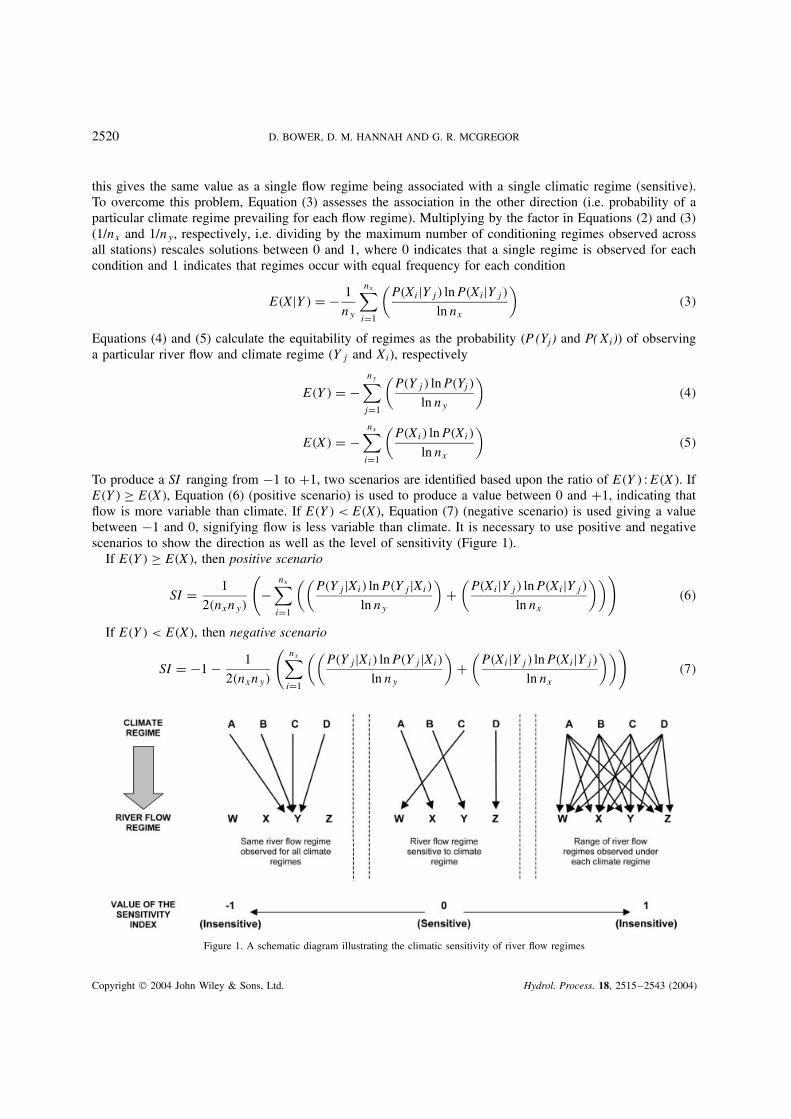
To produce a SI ranging from �1 to C1, two scenarios are identified based upon the ratio of E (Y ) : E (X ). IfE�Y� ½ E�X�, Equation (6) (positive scenario) is used to produce a value between 0 and C1, indicating thatflow is more variable than climate. If E�Y� < E�X�, Equation (7) (negative scenario) is used giving a valuebetween �1 and 0, signifying flow is less variable than climate. It is necessary to use positive and negativescenarios to show the direction as well as the level of sensitivity (Figure 1).

If E�Y� ½ E�X�, then positive scenario

SI D 1

2�nxny�

(�

nx∑iD1

((P�YjjXi� ln P�YjjXi�

ln ny

)C

(P�XijYj� ln P�XijYj�

ln nx

)))�6�

If E�Y� < E�X�, then negative scenario

SI D �1 � 1

2�nxny�

(nx∑

iD1

((P�YjjXi� ln P�YjjXi�

ln ny

)C

(P�XijYj� ln P�XijYj�

ln nx

)))�7�

Figure 1. A schematic diagram illustrating the climatic sensitivity of river flow regimes

Copyright 2004 John Wiley & Sons, Ltd. Hydrol. Process. 18, 2515–2543 (2004)

TECHNIQUES FOR ASSESSING CLIMATIC SENSITIVITY OF FLOW REGIMES 2521

Together, Equations (6) and (7) provide a measure of the overall (strength and direction) sensitivity of flow totemperature and rainfall. A value approaching �1 indicates that a single flow regime is observed regardlessof climatic regime (insensitive). A value nearing C1 indicates that a variety of flow regimes are observedunder each climatic regime (also insensitive but the SI identities a different direction of association). Avalue around zero indicates a highly sensitive situation, where a different flow regime is observed under eachclimatic regime (Figure 1).

REGIONALIZATION

Regime shape and magnitude are classified using long-term (1974–1999) mean monthly runoff, air temperatureand rainfall for 35 stations. Correspondence between flow and climate regions is explored. No attemptis made to spatially interpolate results or draw regional limits owing to likely differences in climate andterrestrial controls between neighbouring basins (Harvey, 2000). Instead, this application tests classificationresults against established UK-scale hydroclimatological patterns. Table II lists the improved group separationachieved using the two-stage clustering procedure.

Flow regimes

Four shape classes (Figure 2a) are identified and characterized by the timing of flow peak(s):

Class AF—December/January peak with secondary March peak (16 stations);Class BF—January peak with relatively steep rising and falling limbs (12 stations);Class CF—February peak with prolonged rising limb (4 stations);Class DF—double peak in December/January and March with intervening lower February flow (3 stations).

Three magnitude classes are found and arranged in ascending order with respect to the indices (Table IIIa):

Class 1F—low with the lowest values for all indices (16 stations);Class 2F—intermediate with values of all indices between Classes 1F and 3F (12 stations);Class 3F—high with the highest values of all indices (7 stations).

Table II. Cluster separations achieved using (a) Ward’s hierarchical cluster analysisand (b) the two-stage clustering procedure. The percentages show the classification

agreement for methods (a) and (b) with discriminant function analysis

Classification (a) Ward’s method (%) (b) Two stage (%)

Regime regionsFlow shape 100Ð0 100Ð0Flow magnitude 94Ð3 97Ð1Temperature magnitude 97Ð1 100Ð0Rainfall shape 100Ð0 97Ð1Rainfall magnitude 100Ð0 100Ð0Inter-annual regimesFlow shape 78Ð6 94Ð6Flow magnitude 90Ð7 96Ð2Temperature shape 98Ð1 97Ð6Temperature magnitude 91Ð0 95Ð9Rainfall shape 79Ð8 93Ð8Rainfall magnitude 86Ð9 96Ð7

Copyright 2004 John Wiley & Sons, Ltd. Hydrol. Process. 18, 2515–2543 (2004)

2522 D. BOWER, D. M. HANNAH AND G. R. MCGREGOR

CLA

SS

AF (

Dec

/Jan

pea

k, s

econ

dary

Mar

pea

k)

(a)

RIV

ER

FLO

W

Aug

Sep

Oct

Nov

Dec

Jan

Feb

Mar

Apr

May

Jun

Jul

3 2 1 0 -1 -2 -3

Mon

th

Aug

Sep

Oct

Nov

Dec

Jan

Feb

Mar

Apr

May

Jun

Jul

Mon

th

Aug

Sep

Oct

Nov

Dec

Jan

Feb

Mar

Apr

May

Jun

Jul

Mon

th

Aug

Sep

Oct

Nov

Dec

Jan

Feb

Mar

Apr

May

Jun

Jul

Mon

th

Aug

Sep

Oct

Nov

Dec

Jan

Feb

Mar

Apr

May

Jun

Jul

Mon

th

Aug

Sep

Oct

Nov

Dec

Jan

Feb

Mar

Apr

May

Jun

Jul

Mon

th

CLA

SS

CF (

Feb

pea

k)

3 2 1 0 -1 -2 -3

CLA

SS

BF

(Jan

pea

k)

3 2 1 0 -1 -2 -3

CLA

SS

DF (

Dou

ble

peak

: Dec

/Jan

and

Mar

)3 2 1 0 -1 -2 -3

CLA

SS

AR (

Sep

-Jan

pea

k, w

ith s

econ

dary

Mar

and

tert

iary

Jun

e pe

ak)

3 2 1 0 -1 -2 -3 CLA

SS

BR (

Aug

-Jan

pea

k,w

ith m

arke

d F

eb m

inim

uman

d se

cond

ary

June

pea

k)3 2 1 0 -1 -2 -3

(b)

RA

INFA

LL

Runoff (z-scores) Runoff (z-scores)

Runoff (z-scores) Runoff (z-scores)

Rainfall (z-scores) Rainfall (z-scores)

Figu

re2.

Stan

dard

ized

long

-ter

mre

gim

esfo

ral

lst

atio

nsw

ithin

each

ofth

esh

ape

regi

ons:

(a)

rive

rflo

wan

d(b

)ra

infa

ll

Copyright 2004 John Wiley & Sons, Ltd. Hydrol. Process. 18, 2515–2543 (2004)

TECHNIQUES FOR ASSESSING CLIMATIC SENSITIVITY OF FLOW REGIMES 2523

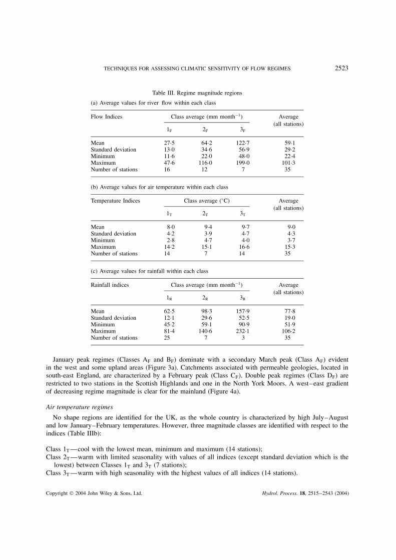
Table III. Regime magnitude regions

(a) Average values for river flow within each class

Flow Indices Class average (mm month�1) Average(all stations)

1F 2F 3F

Mean 27Ð5 64Ð2 122Ð7 59Ð1Standard deviation 13Ð0 34Ð6 56Ð9 29Ð2Minimum 11Ð6 22Ð0 48Ð0 22Ð4Maximum 47Ð6 116Ð0 199Ð0 101Ð3Number of stations 16 12 7 35

(b) Average values for air temperature within each class

Temperature Indices Class average (°C) Average(all stations)

1T 2T 3T

Mean 8Ð0 9Ð4 9Ð7 9Ð0Standard deviation 4Ð2 3Ð9 4Ð7 4Ð3Minimum 2Ð8 4Ð7 4Ð0 3Ð7Maximum 14Ð2 15Ð1 16Ð6 15Ð3Number of stations 14 7 14 35

(c) Average values for rainfall within each class

Rainfall indices Class average (mm month�1) Average(all stations)

1R 2R 3R

Mean 62Ð5 98Ð3 157Ð9 77Ð8Standard deviation 12Ð1 29Ð6 52Ð5 19Ð0Minimum 45Ð2 59Ð1 90Ð9 51Ð9Maximum 81Ð4 140Ð6 232Ð1 106Ð2Number of stations 25 7 3 35

January peak regimes (Classes AF and BF) dominate with a secondary March peak (Class AF) evidentin the west and some upland areas (Figure 3a). Catchments associated with permeable geologies, located insouth-east England, are characterized by a February peak (Class CF). Double peak regimes (Class DF) arerestricted to two stations in the Scottish Highlands and one in the North York Moors. A west–east gradientof decreasing regime magnitude is clear for the mainland (Figure 4a).

Air temperature regimes

No shape regions are identified for the UK, as the whole country is characterized by high July–Augustand low January–February temperatures. However, three magnitude classes are identified with respect to theindices (Table IIIb):

Class 1T—cool with the lowest mean, minimum and maximum (14 stations);Class 2T—warm with limited seasonality with values of all indices (except standard deviation which is the

lowest) between Classes 1T and 3T (7 stations);Class 3T—warm with high seasonality with the highest values of all indices (14 stations).

Copyright 2004 John Wiley & Sons, Ltd. Hydrol. Process. 18, 2515–2543 (2004)

2524 D. BOWER, D. M. HANNAH AND G. R. MCGREGOR

94001

970023002

8008

900110002

21016

14001

8401721014

22006

7500325018

270577200227023

30003

28082 34011

3801835002

400114201045004

49001

5402758001

6000355014

6400167006 68005

204001

203018

201006

Class AF (Dec/Janpeak with secondaryMar peak)

Class BF (Jan peak)

Class CF (Feb peak)

Class DF (Doublepeak Dec/Janand Mar)

Class AR (Sep-Janpeak, with secondaryMar and tertiary Junepeak)

Class BR (Aug-Janpeak, with markedFeb minimum andsecondary June peak)

Altitude >180 m

(a) RIVER FLOW (b) RAINFALL

0 200 km 0 200 km

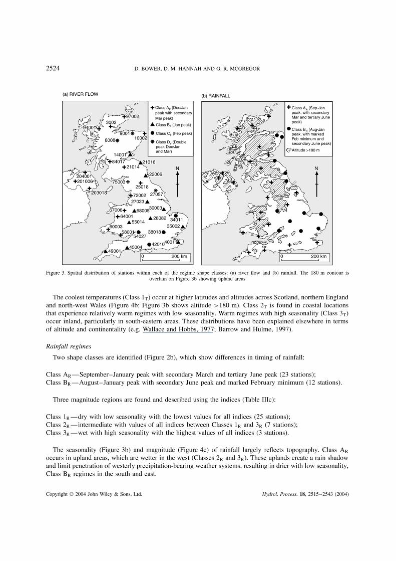
NN

Figure 3. Spatial distribution of stations within each of the regime shape classes: (a) river flow and (b) rainfall. The 180 m contour isoverlain on Figure 3b showing upland areas

The coolest temperatures (Class 1T) occur at higher latitudes and altitudes across Scotland, northern Englandand north-west Wales (Figure 4b; Figure 3b shows altitude >180 m). Class 2T is found in coastal locationsthat experience relatively warm regimes with low seasonality. Warm regimes with high seasonality (Class 3T)occur inland, particularly in south-eastern areas. These distributions have been explained elsewhere in termsof altitude and continentality (e.g. Wallace and Hobbs, 1977; Barrow and Hulme, 1997).

Rainfall regimes

Two shape classes are identified (Figure 2b), which show differences in timing of rainfall:

Class AR—September–January peak with secondary March and tertiary June peak (23 stations);Class BR—August–January peak with secondary June peak and marked February minimum (12 stations).

Three magnitude regions are found and described using the indices (Table IIIc):

Class 1R—dry with low seasonality with the lowest values for all indices (25 stations);Class 2R—intermediate with values of all indices between Classes 1R and 3R (7 stations);Class 3R—wet with high seasonality with the highest values of all indices (3 stations).

The seasonality (Figure 3b) and magnitude (Figure 4c) of rainfall largely reflects topography. Class AR

occurs in upland areas, which are wetter in the west (Classes 2R and 3R). These uplands create a rain shadowand limit penetration of westerly precipitation-bearing weather systems, resulting in drier with low seasonality,Class BR regimes in the south and east.

Copyright 2004 John Wiley & Sons, Ltd. Hydrol. Process. 18, 2515–2543 (2004)

TECHNIQUES FOR ASSESSING CLIMATIC SENSITIVITY OF FLOW REGIMES 2525

Class 1F (low)

Class 2F (intermediate)

Class 3F (high)

(a) RIVER FLOW

0 200 km 0 200 km

Class 1T (cool region)

Class 2T (warm regionwith limited seasonality)

Class 3T (warm regionwith high seasonality)

N N

(b) TEMPERATURE

0 200 km

N

(c) RAINFALL

Class 1R (dry regionwith low seasonality)

Class 3R (wet regionwith high seasonality)

Class 2R (intermediate)

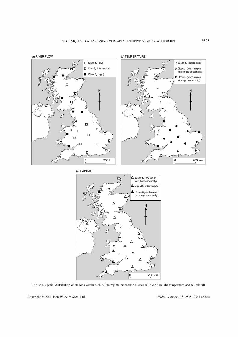
Figure 4. Spatial distribution of stations within each of the regime magnitude classes (a) river flow, (b) temperature and (c) rainfall

Copyright 2004 John Wiley & Sons, Ltd. Hydrol. Process. 18, 2515–2543 (2004)

2526 D. BOWER, D. M. HANNAH AND G. R. MCGREGOR

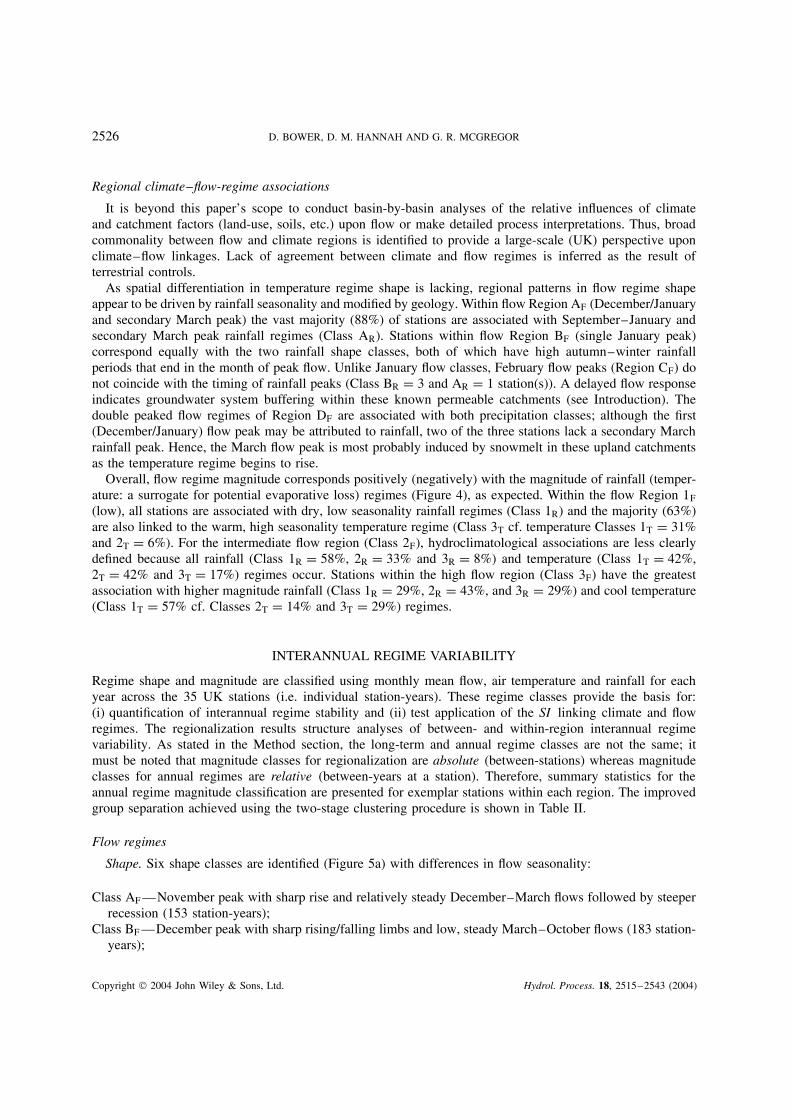
Regional climate–flow-regime associations

It is beyond this paper’s scope to conduct basin-by-basin analyses of the relative influences of climateand catchment factors (land-use, soils, etc.) upon flow or make detailed process interpretations. Thus, broadcommonality between flow and climate regions is identified to provide a large-scale (UK) perspective uponclimate–flow linkages. Lack of agreement between climate and flow regimes is inferred as the result ofterrestrial controls.

As spatial differentiation in temperature regime shape is lacking, regional patterns in flow regime shapeappear to be driven by rainfall seasonality and modified by geology. Within flow Region AF (December/Januaryand secondary March peak) the vast majority (88%) of stations are associated with September–January andsecondary March peak rainfall regimes (Class AR). Stations within flow Region BF (single January peak)correspond equally with the two rainfall shape classes, both of which have high autumn–winter rainfallperiods that end in the month of peak flow. Unlike January flow classes, February flow peaks (Region CF) donot coincide with the timing of rainfall peaks (Class BR D 3 and AR D 1 station(s)). A delayed flow responseindicates groundwater system buffering within these known permeable catchments (see Introduction). Thedouble peaked flow regimes of Region DF are associated with both precipitation classes; although the first(December/January) flow peak may be attributed to rainfall, two of the three stations lack a secondary Marchrainfall peak. Hence, the March flow peak is most probably induced by snowmelt in these upland catchmentsas the temperature regime begins to rise.

Overall, flow regime magnitude corresponds positively (negatively) with the magnitude of rainfall (temper-ature: a surrogate for potential evaporative loss) regimes (Figure 4), as expected. Within the flow Region 1F

(low), all stations are associated with dry, low seasonality rainfall regimes (Class 1R) and the majority (63%)are also linked to the warm, high seasonality temperature regime (Class 3T cf. temperature Classes 1T D 31%and 2T D 6%). For the intermediate flow region (Class 2F), hydroclimatological associations are less clearlydefined because all rainfall (Class 1R D 58%, 2R D 33% and 3R D 8%) and temperature (Class 1T D 42%,2T D 42% and 3T D 17%) regimes occur. Stations within the high flow region (Class 3F) have the greatestassociation with higher magnitude rainfall (Class 1R D 29%, 2R D 43%, and 3R D 29%) and cool temperature(Class 1T D 57% cf. Classes 2T D 14% and 3T D 29%) regimes.

INTERANNUAL REGIME VARIABILITY

Regime shape and magnitude are classified using monthly mean flow, air temperature and rainfall for eachyear across the 35 UK stations (i.e. individual station-years). These regime classes provide the basis for:(i) quantification of interannual regime stability and (ii) test application of the SI linking climate and flowregimes. The regionalization results structure analyses of between- and within-region interannual regimevariability. As stated in the Method section, the long-term and annual regime classes are not the same; itmust be noted that magnitude classes for regionalization are absolute (between-stations) whereas magnitudeclasses for annual regimes are relative (between-years at a station). Therefore, summary statistics for theannual regime magnitude classification are presented for exemplar stations within each region. The improvedgroup separation achieved using the two-stage clustering procedure is shown in Table II.

Flow regimes

Shape. Six shape classes are identified (Figure 5a) with differences in flow seasonality:

Class AF—November peak with sharp rise and relatively steady December–March flows followed by steeperrecession (153 station-years);

Class BF—December peak with sharp rising/falling limbs and low, steady March–October flows (183 station-years);

Copyright 2004 John Wiley & Sons, Ltd. Hydrol. Process. 18, 2515–2543 (2004)

TECHNIQUES FOR ASSESSING CLIMATIC SENSITIVITY OF FLOW REGIMES 2527

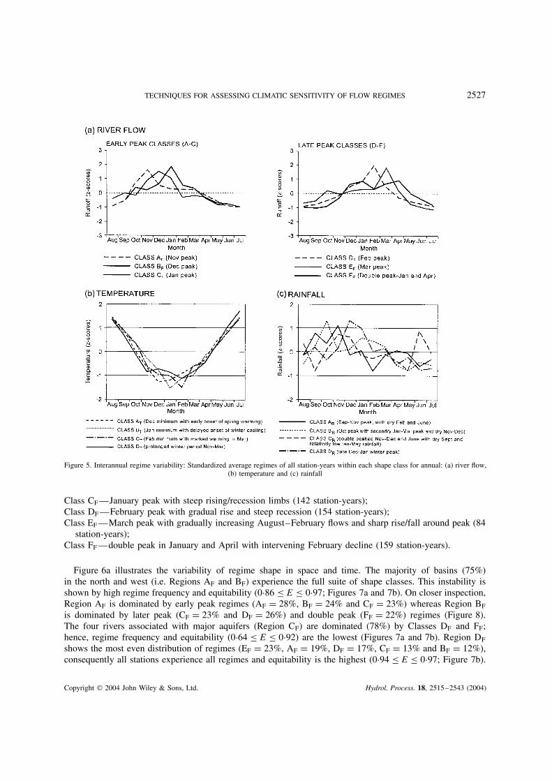
Figure 5. Interannual regime variability: Standardized average regimes of all station-years within each shape class for annual: (a) river flow,(b) temperature and (c) rainfall

Class CF—January peak with steep rising/recession limbs (142 station-years);Class DF—February peak with gradual rise and steep recession (154 station-years);Class EF —March peak with gradually increasing August–February flows and sharp rise/fall around peak (84

station-years);Class FF—double peak in January and April with intervening February decline (159 station-years).

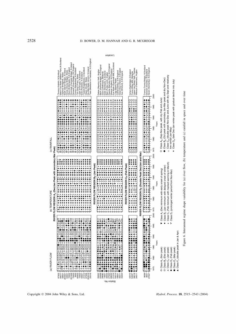
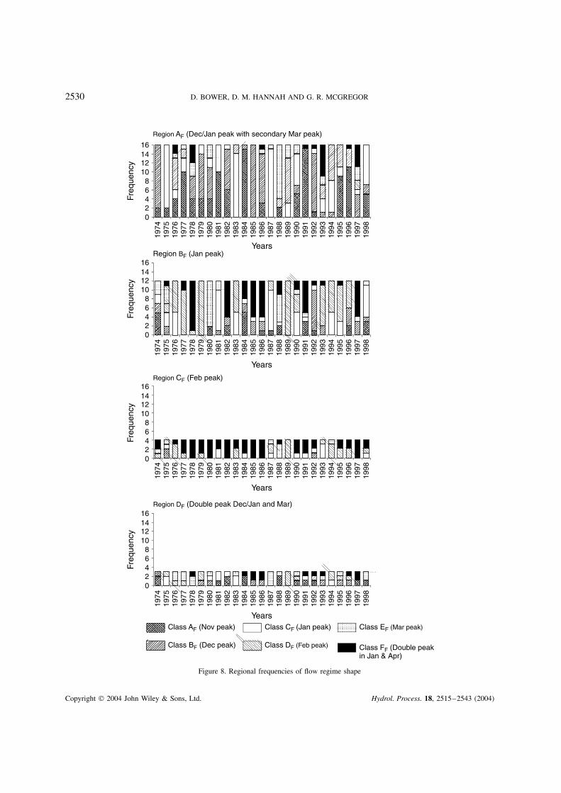
Figure 6a illustrates the variability of regime shape in space and time. The majority of basins (75%)in the north and west (i.e. Regions AF and BF) experience the full suite of shape classes. This instability isshown by high regime frequency and equitability (0Ð86 � E � 0Ð97; Figures 7a and 7b). On closer inspection,Region AF is dominated by early peak regimes (AF D 28%, BF D 24% and CF D 23%) whereas Region BF

is dominated by later peak (CF D 23% and DF D 26%) and double peak (FF D 22%) regimes (Figure 8).The four rivers associated with major aquifers (Region CF) are dominated (78%) by Classes DF and FF;hence, regime frequency and equitability (0Ð64 � E � 0Ð92) are the lowest (Figures 7a and 7b). Region DF

shows the most even distribution of regimes (EF D 23%, AF D 19%, DF D 17%, CF D 13% and BF D 12%),consequently all stations experience all regimes and equitability is the highest (0Ð94 � E � 0Ð97; Figure 7b).

Copyright 2004 John Wiley & Sons, Ltd. Hydrol. Process. 18, 2515–2543 (2004)

2528 D. BOWER, D. M. HANNAH AND G. R. MCGREGOR

1975

1980

1985

1990

1995

2000

9700

284

017

5800

120

4001

6400

172

002

2010

0675

003

3002

6000

310

002

9400

121

014

6700

620

3018

2501

8

3500

222

006

2808

214

001

3000

327

023

Station No.

Location

6800

521

016

5501

449

001

4001

145

004

4201

054

027

3801

834

011

8008

9001

2705

7

Thu

rsco

(Hal

kirk

), N

.Sco

tland

Car

ron

(Sgo

dach

ail),

N.S

cotla

ndT

af (

Clo

g-y-

Fra

n), W

ales

Ugi

e (I

nver

ugie

), N

.Sco

tland

Ew

e (P

oole

we)

, N.S

cotla

ndT

wee

d (K

ingl

edor

es),

E.S

cotla

ndA

lwen

(D

ruid

), W

ales

Six

Mile

Wat

er (

Ant

rim),

N.Ir

elan

dT

ees

(Mid

dlet

on-in

-Tee

sdal

e), N

.E.E

ngla

nd

Deb

en (

Nau

nton

Hal

l), A

nglia

n

Lugg

(B

yton

) W

ales

Cam

el (D

enby

), S

.W.E

ngla

nd

Fro

me

(Ebl

ey M

ill),

Mid

land

sU

pper

Lee

(Wat

er H

all),

Tha

mes

Tro

mie

(Tro

mie

Brid

ge),

N.S

cotla

ndD

ever

on (A

voch

ie),

N.S

cotla

ndS

even

(Nor

man

by),

N.E

.Eng

land

RIV

ER

FL

OW

RE

GIO

N B

F (

Jan

Pea

k)

RIV

ER

FL

OW

RE

GIO

N C

F (F

eb P

eak)

RIV

ER

FL

OW

RE

GIO

N D

F (

Do

ub

le P

eak

Dec

/Jan

an

d M

ar)

RIV

ER

FL

OW

RE

GIO

N A

F (

Dec

/Jan

Pea

k w

ith

sec

on

dar

y M

ar P

eak)

(a)

RIV

ER

FLO

W(c

) R

AIN

FA

LL(b

) T

EM

PE

RA

TU

RE

Yea

rs

1975

1980

1985

1990

1995

2000

Yea

rs

1975

1980

1985

1990

1995

2000

Yea

rs

Cla

ss A

R (

Sep

-Nov

pea

k, w

ith d

ry F

eb a

nd J

une)

Cla

ss B

R (

Oct

pea

k w

ith s

econ

dary

Jan

-Mar

pea

k an

d dr

y N

ov-D

ec)

Cla

ss C

R (

doub

le p

eak

Nov

-Dec

and

Jun

e w

ith d

ry S

ept

and

rela

tivel

ylo

w r

ainf

all J

an-M

ay)

Cla

ss D

R (

late

Dec

-Jan

win

ter

peak

with

gra

dual

dec

line

into

Jul

y)

+++

++++

+++

++++

+++

++++

++++

++++

+++++

+++++

+++

++++++++++++

+++++++++++

++++++++++++

++

++++++++++++

+++

++++++++++++

++++++++++++

++ + + + + + + + + + + + + + + +

+ + + + + + + + + +

+ + + + + + + + + + + + + + +

+ + + + + + + + + + + + + + + +++++++++++++++++

+++++++++++++++++

++

Cla

ss A

T (

Dec

min

imum

with

ear

ly o

nset

of s

prin

g)C

lass

BT (

Jan

min

imum

with

del

ayed

ons

et o

f w

inte

r)C

lass

CT (

Feb

min

imum

with

mar

ked

war

min

g in

Mar

ch)

Cla

ss D

T (

prol

onge

d w

inte

r pe

riod

from

Nov

-Mar

)+

Cla

ss A

F (

Nov

pea

k)C

lass

BF (

Dec

pea

k)C

lass

CF (

Jan

peak

)C

lass

DF (

Feb

pea

k)C

lass

EF (

Mar

pea

k)C

lass

FF (

doub

le p

eak

in J

an &

Apr

)

Wen

sum

(Fak

enha

m),

Ang

lian

Itche

n (H

ighb

ridge

), S

.Eng

land

Axe

(Whi

tford

), S

.W.E

ngla

ndG

reat

Sto

ur (H

orto

n), S

.Eng

land

Eye

Wat

er (E

yem

outh

Mill

), E

.Sco

tland

Wea

ver (

Aud

lem

), N

.E.E

ngla

ndD

earn

e (B

arns

ley

Wei

r), N

.E.E

ngla

ndB

ain

(Ful

sby

Lock

), A

nglia

nE

den

(Kem

back

), E

.Sco

tland

Soa

r (Li

ttlet

horp

e), M

idla

nds

Bly

th (H

artfo

rd B

ridge

), N

.E.E

ngla

nd

Der

wen

t (O

use

Brid

ge),

N.E

.Eng

land

Dru

mra

gh (

Cam

psie

Brid

ge),

N.Ir

elan

dW

yre

(St.M

icha

els)

, N.E

.Eng

land

Dov

ey (

Dov

ey B

ridge

), W

ales

Bus

h (S

enei

rl B

ridge

), N

.Irel

and

Ogm

ore

(Brid

gend

), W

ales

Bla

ck C

art W

ater

(M

illik

en P

ark)

,W.S

cotla

nd

Figu

re6.

Inte

rann

ualre

gim

esh

ape

variab

ility

for

(a)

rive

rflo

w,(b

)te

mpe

ratu

rean

d(c

)ra

infa

llin

spac

ean

dov

ertim

e

Copyright 2004 John Wiley & Sons, Ltd. Hydrol. Process. 18, 2515–2543 (2004)

TECHNIQUES FOR ASSESSING CLIMATIC SENSITIVITY OF FLOW REGIMES 2529

(d) Equitability of two - year regime couplets

1.0

0.9

0.8

0.7

0.6

(b) Equitability of regime classes

7

6

5

4

3

2DFCFBFAF

Region

DFCFBFAF

Region

DFCFBFAF

Region

DFCFBFAF

Region

(a) Number of regime classes

22

20

18

16

14

12

10

8

6

(c) Number of two - year regime couplets

Num

ber

Num

ber

Equ

itabi

lity

(E)

1.0

0.9

0.8

0.7

0.6

Equ

itabi

lity

(E)

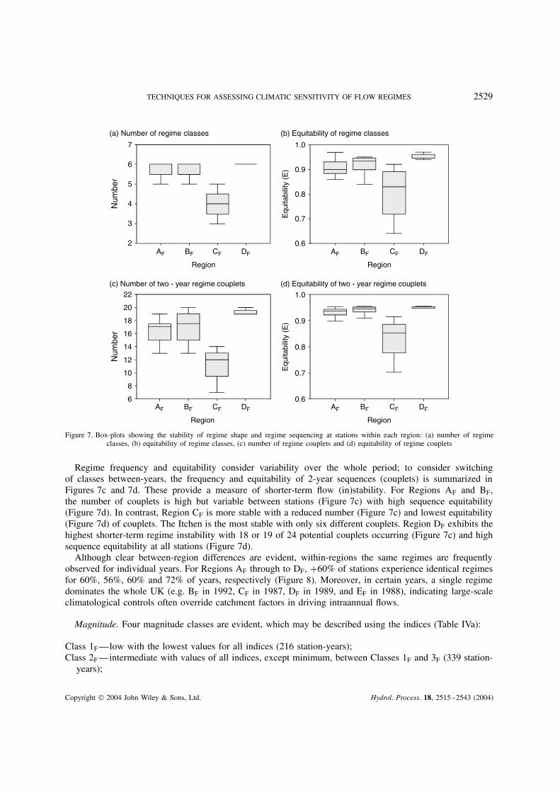
Figure 7. Box-plots showing the stability of regime shape and regime sequencing at stations within each region: (a) number of regimeclasses, (b) equitability of regime classes, (c) number of regime couplets and (d) equitability of regime couplets

Regime frequency and equitability consider variability over the whole period; to consider switchingof classes between-years, the frequency and equitability of 2-year sequences (couplets) is summarized inFigures 7c and 7d. These provide a measure of shorter-term flow (in)stability. For Regions AF and BF,the number of couplets is high but variable between stations (Figure 7c) with high sequence equitability(Figure 7d). In contrast, Region CF is more stable with a reduced number (Figure 7c) and lowest equitability(Figure 7d) of couplets. The Itchen is the most stable with only six different couplets. Region DF exhibits thehighest shorter-term regime instability with 18 or 19 of 24 potential couplets occurring (Figure 7c) and highsequence equitability at all stations (Figure 7d).

Although clear between-region differences are evident, within-regions the same regimes are frequentlyobserved for individual years. For Regions AF through to DF, C60% of stations experience identical regimesfor 60%, 56%, 60% and 72% of years, respectively (Figure 8). Moreover, in certain years, a single regimedominates the whole UK (e.g. BF in 1992, CF in 1987, DF in 1989, and EF in 1988), indicating large-scaleclimatological controls often override catchment factors in driving intraannual flows.

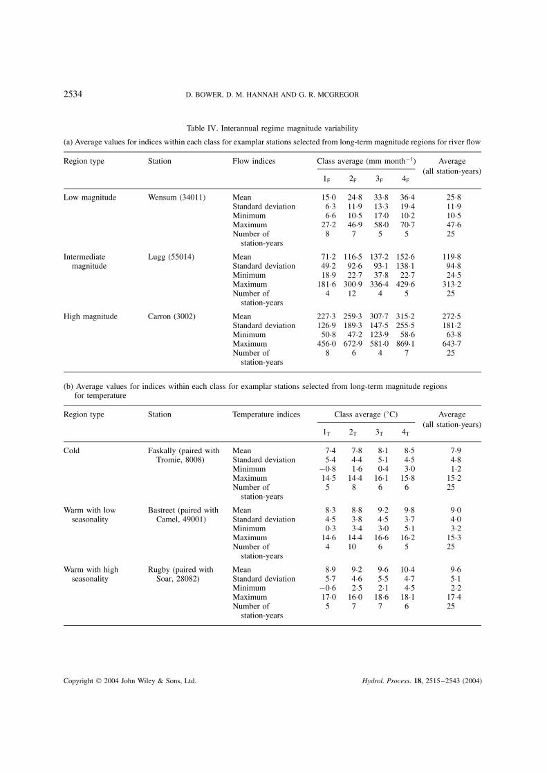
Magnitude. Four magnitude classes are evident, which may be described using the indices (Table IVa):

Class 1F—low with the lowest values for all indices (216 station-years);Class 2F —intermediate with values of all indices, except minimum, between Classes 1F and 3F (339 station-

years);

Copyright 2004 John Wiley & Sons, Ltd. Hydrol. Process. 18, 2515–2543 (2004)

2530 D. BOWER, D. M. HANNAH AND G. R. MCGREGOR

16141210

86420

1974

1975

1976

1977

1978

1979

1980

1981

1982

1983

1984

1985

1986

1987

1988

1989

1990

1991

1992

1993

1995

1996

1997

1998

1994

Region AF (Dec/Jan peak with secondary Mar peak)

Region CF (Feb peak)

Region BF (Jan peak)

Region DF (Double peak Dec/Jan and Mar)

Class CF (Jan peak)

Class DF (Feb peak)

Class EF (Mar peak)

Class FF (Double peakin Jan & Apr)

Class AF (Nov peak)

Class BF (Dec peak)

Years

1974

1975

1976

1977

1978

1979

1980

1981

1982

1983

1984

1985

1986

1987

1988

1989

1990

1991

1992

1993

1995

1996

1997

1998

1994

Years

1974

1975

1976

1977

1978

1979

1980

1981

1982

1983

1984

1985

1986

1987

1988

1989

1990

1991

1992

1993

1995

1996

1997

1998

1994

Years

1974

1975

1976

1977

1978

1979

1980

1981

1982

1983

1984

1985

1986

1987

1988

1989

1990

1991

1992

1993

1995

1996

1997

1998

1994

Years

Freq

uenc

y

16141210

86420

Freq

uenc

y

16141210

86420

Freq

uenc

y

16141210

86420

Freq

uenc

y

Figure 8. Regional frequencies of flow regime shape

Copyright 2004 John Wiley & Sons, Ltd. Hydrol. Process. 18, 2515–2543 (2004)

TECHNIQUES FOR ASSESSING CLIMATIC SENSITIVITY OF FLOW REGIMES 2531

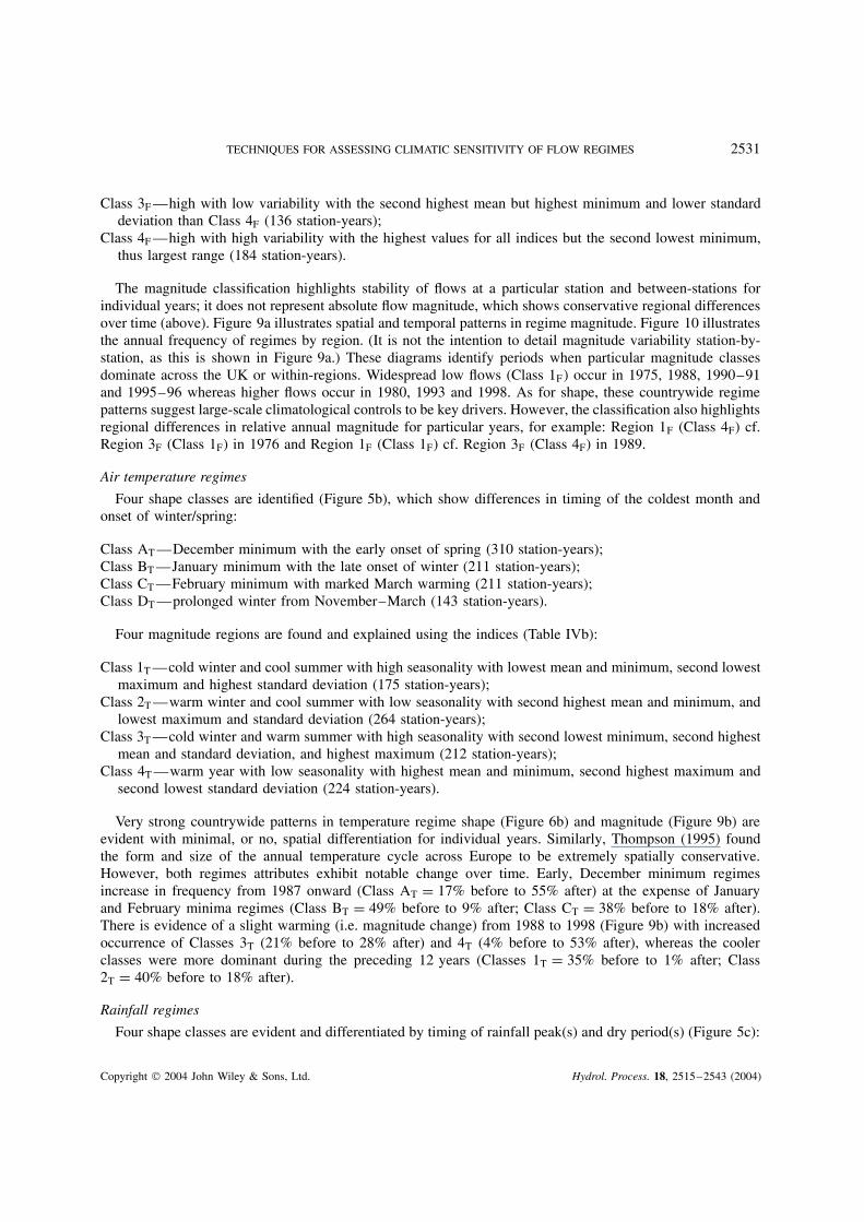
Class 3F —high with low variability with the second highest mean but highest minimum and lower standarddeviation than Class 4F (136 station-years);

Class 4F —high with high variability with the highest values for all indices but the second lowest minimum,thus largest range (184 station-years).

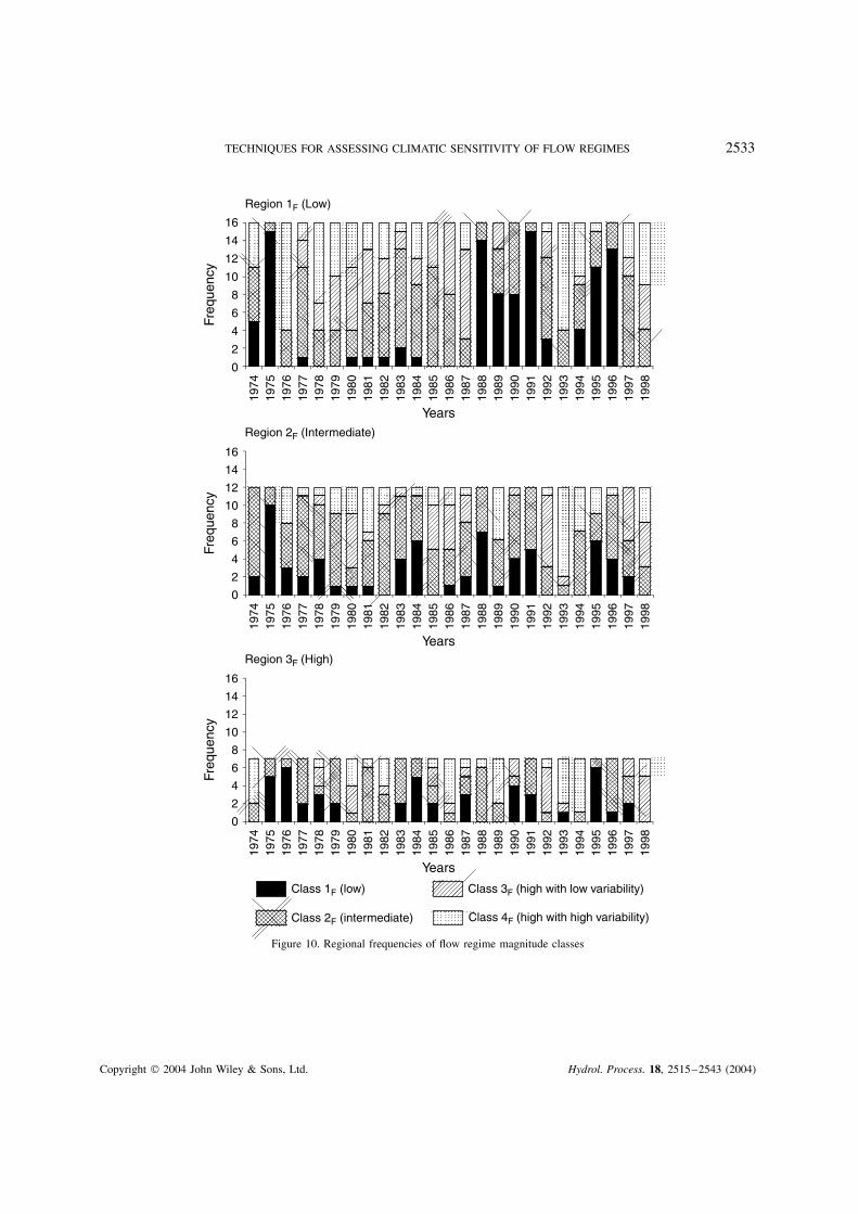
The magnitude classification highlights stability of flows at a particular station and between-stations forindividual years; it does not represent absolute flow magnitude, which shows conservative regional differencesover time (above). Figure 9a illustrates spatial and temporal patterns in regime magnitude. Figure 10 illustratesthe annual frequency of regimes by region. (It is not the intention to detail magnitude variability station-by-station, as this is shown in Figure 9a.) These diagrams identify periods when particular magnitude classesdominate across the UK or within-regions. Widespread low flows (Class 1F� occur in 1975, 1988, 1990–91and 1995–96 whereas higher flows occur in 1980, 1993 and 1998. As for shape, these countrywide regimepatterns suggest large-scale climatological controls to be key drivers. However, the classification also highlightsregional differences in relative annual magnitude for particular years, for example: Region 1F (Class 4F) cf.Region 3F (Class 1F) in 1976 and Region 1F (Class 1F) cf. Region 3F (Class 4F) in 1989.

Air temperature regimes

Four shape classes are identified (Figure 5b), which show differences in timing of the coldest month andonset of winter/spring:

Class AT—December minimum with the early onset of spring (310 station-years);Class BT—January minimum with the late onset of winter (211 station-years);Class CT—February minimum with marked March warming (211 station-years);Class DT—prolonged winter from November–March (143 station-years).

Four magnitude regions are found and explained using the indices (Table IVb):

Class 1T—cold winter and cool summer with high seasonality with lowest mean and minimum, second lowestmaximum and highest standard deviation (175 station-years);

Class 2T—warm winter and cool summer with low seasonality with second highest mean and minimum, andlowest maximum and standard deviation (264 station-years);

Class 3T—cold winter and warm summer with high seasonality with second lowest minimum, second highestmean and standard deviation, and highest maximum (212 station-years);

Class 4T—warm year with low seasonality with highest mean and minimum, second highest maximum andsecond lowest standard deviation (224 station-years).

Very strong countrywide patterns in temperature regime shape (Figure 6b) and magnitude (Figure 9b) areevident with minimal, or no, spatial differentiation for individual years. Similarly, Thompson (1995) foundthe form and size of the annual temperature cycle across Europe to be extremely spatially conservative.However, both regimes attributes exhibit notable change over time. Early, December minimum regimesincrease in frequency from 1987 onward (Class AT D 17% before to 55% after) at the expense of Januaryand February minima regimes (Class BT D 49% before to 9% after; Class CT D 38% before to 18% after).There is evidence of a slight warming (i.e. magnitude change) from 1988 to 1998 (Figure 9b) with increasedoccurrence of Classes 3T (21% before to 28% after) and 4T (4% before to 53% after), whereas the coolerclasses were more dominant during the preceding 12 years (Classes 1T D 35% before to 1% after; Class2T D 40% before to 18% after).

Rainfall regimes

Four shape classes are evident and differentiated by timing of rainfall peak(s) and dry period(s) (Figure 5c):

Copyright 2004 John Wiley & Sons, Ltd. Hydrol. Process. 18, 2515–2543 (2004)

2532 D. BOWER, D. M. HANNAH AND G. R. MCGREGOR

9700

284

017

5800

120

4001

6400

172

002

2010

0675

003

3002

6000

310

002

9400

121

014

6700

620

3018

2501

835

002

2200

628

082

1400

130

003

2702

3

Station No.

6800

521

016

5501

449

001

4001

145

004

4201

054

027

3801

834

011

8008

9001

2705

7

Location

Thu

rsco

(Hal

kirk

), N

.Sco

tland

Car

ron

(Sgo

dach

ail),

N.S

cotla

ndT

af (

Clo

g-y-

Fra

n), W

ales

Ugi

e (I

nver

ugie

), N

.Sco

tland

Ew

e (P

oole

we)

, N.S

cotla

ndT

wee

d (K

ingl

edor

es),

E.S

cotla

ndA

lwen

(D

ruid

), W

ales

Six

Mile

Wat

er (

Ant

rim),

N.Ir

elan

dT

ees

(Mid

dlet

on-in

-Tee

sdal

e), N

.E.E

ngla

ndD

eben

(N

aunt

on H

all),

Ang

lian

Lugg

(B

yton

) W

ales

Cam

el (D

enby

), S

.W.E

ngla

nd

Fro

me

(Ebl

ey M

ill),

Mid

land

sU

pper

Lee

(Wat

er H

all),

Tha

mes

Tro

mie

(Tro

mie

Brid

ge),

N.S

cotla

ndD

ever

on (A

voch

ie),

N.S

cotla

ndS

even

(Nor

man

by),

N.E

.Eng

land

Wen

sum

(Fak

enha

m),

Ang

lian

Itche

n (H

ighb

ridge

), S

.Eng

land

Axe

(Whi

tford

), S

.W.E

ngla

ndG

reat

Sto

ur (H

orto

n), S

.Eng

land

Eye

Wat

er (E

yem

outh

Mill

), E

.Sco

tland

Wea

ver (

Aud

lem

), N

.E.E

ngla

ndD

earn

e (B

arns

ley

Wei

r), N

.E.E

ngla

ndB

ain

(Ful

sby

Lock

), A

nglia

nE

den

(Kem

back

), E

.Sco

tland

Soa

r (Li

ttlet

horp

e), M

idla

nds

Bly

th (H

artfo

rd B

ridge

), N

.E.E

ngla

nd

Der

wen

t (O

use

Brid

ge),

N.E

.Eng

land

Dru

mra

gh (

Cam

psie

Brid

ge),

N.Ir

elan

dW

yre

(St.M

icha

els)

, N.E

.Eng

land

Dov

ey (

Dov

ey B

ridge

), W

ales

Bus

h (S

enei

rl B

ridge

), N

.Irel

and

Ogm

ore

(Brid

gend

), W

ales

Bla

ck C

art W

ater

(M

illik

en P

ark)

,W.S

cotla

nd

1975

1980

1985

1990

1995

2000

Yea

rs

1975

1980

1985

1990

1995

2000

Yea

rs

1975

1980

1985

1990

1995

2000

Yea

rs

Cla

ss 1

F (

low

)C

lass

2F (

inte

rmed

iate

)C

lass

3F (

high

with

low

var

iabi

lity)

Cla

ss 4

F (

high

with

hig

h va

riabi

lity)

Cla

ss 1

T (

cold

win

ter

and

cool

sum

mer

w

ith h

igh

seas

onal

ity)

Cla

ss 1

R (

mod

erat

ely

wet

win

ter

and

dry

sum

mer

)C

lass

2R (

dry

year

with

low

sea

sona

lity)

Cla

ss 3

R (

wet

yea

r w

ith lo

w s

easo

nalit

y)C

lass

4R (

wet

yea

r w

ith h

igh

seas

onal

ity)

Cla

ss 2

T (

war

m w

inte

r an

d co

ol s

umm

er

with

low

sea

sona

lity)

Cla

ss 3

T (

cold

win

ter

and

war

m s

umm

er

with

hig

h se

ason

ality

)

Cla

ss 4

T (

war

m y

ear

with

low

sea

sona

lity)

(a)

RIV

ER

FLO

W(c

) R

AIN

FA

LL(b

) T

EM

PE

RA

TU

RE

Figu

re9.

Inte

rann

ualre

gim

em

agni

tude

variab

ility

for

(a)

rive

rflo

w,(b

)te

mpe

ratu

rean

d(c

)ra

infa

llin

spac

ean

dov

ertim

e

Copyright 2004 John Wiley & Sons, Ltd. Hydrol. Process. 18, 2515–2543 (2004)

TECHNIQUES FOR ASSESSING CLIMATIC SENSITIVITY OF FLOW REGIMES 2533

Class 1F (low)

Class 2F (intermediate)

Class 3F (high with low variability)

Class 4F (high with high variability)

Region 3F (High)

Region 2F (Intermediate)

Region 1F (Low)

1974

1975

1976

1977

1978

1979

1980

1981

1982

1983

1984

1985

1986

1987

1988

1989

1990

1991

1992

1993

1995

1996

1997

1998

1994

Years

1974

1975

1976

1977

1978

1979

1980

1981

1982

1983

1984

1985

1986

1987

1988

1989

1990

1991

1992

1993

1995

1996

1997

1998

1994

Years

1974

1975

1976

1977

1978

1979

1980

1981

1982

1983

1984

1985

1986

1987

1988

1989

1990

1991

1992

1993

1995

1996

1997

1998

1994

Years

16

14

12

10

8

6

4

2

0

Freq

uenc

y

16

14

12

10

8

6

4

2

0

Freq

uenc

y

16

14

12

10

8

6

4

2

0

Freq

uenc

y

Figure 10. Regional frequencies of flow regime magnitude classes

Copyright 2004 John Wiley & Sons, Ltd. Hydrol. Process. 18, 2515–2543 (2004)

2534 D. BOWER, D. M. HANNAH AND G. R. MCGREGOR

Table IV. Interannual regime magnitude variability

(a) Average values for indices within each class for examplar stations selected from long-term magnitude regions for river flow

Region type Station Flow indices Class average (mm month�1) Average(all station-years)

1F 2F 3F 4F

Low magnitude Wensum (34011) Mean 15Ð0 24Ð8 33Ð8 36Ð4 25Ð8Standard deviation 6Ð3 11Ð9 13Ð3 19Ð4 11Ð9Minimum 6Ð6 10Ð5 17Ð0 10Ð2 10Ð5Maximum 27Ð2 46Ð9 58Ð0 70Ð7 47Ð6Number of

station-years8 7 5 5 25

Intermediate Lugg (55014) Mean 71Ð2 116Ð5 137Ð2 152Ð6 119Ð8magnitude Standard deviation 49Ð2 92Ð6 93Ð1 138Ð1 94Ð8

Minimum 18Ð9 22Ð7 37Ð8 22Ð7 24Ð5Maximum 181Ð6 300Ð9 336Ð4 429Ð6 313Ð2Number of

station-years4 12 4 5 25

High magnitude Carron (3002) Mean 227Ð3 259Ð3 307Ð7 315Ð2 272Ð5Standard deviation 126Ð9 189Ð3 147Ð5 255Ð5 181Ð2Minimum 50Ð8 47Ð2 123Ð9 58Ð6 63Ð8Maximum 456Ð0 672Ð9 581Ð0 869Ð1 643Ð7Number of

station-years8 6 4 7 25

(b) Average values for indices within each class for examplar stations selected from long-term magnitude regionsfor temperature

Region type Station Temperature indices Class average (°C) Average(all station-years)

1T 2T 3T 4T

Cold Faskally (paired with Mean 7Ð4 7Ð8 8Ð1 8Ð5 7Ð9Tromie, 8008) Standard deviation 5Ð4 4Ð4 5Ð1 4Ð5 4Ð8

Minimum �0Ð8 1Ð6 0Ð4 3Ð0 1Ð2Maximum 14Ð5 14Ð4 16Ð1 15Ð8 15Ð2Number of

station-years5 8 6 6 25

Warm with low Bastreet (paired with Mean 8Ð3 8Ð8 9Ð2 9Ð8 9Ð0seasonality Camel, 49001) Standard deviation 4Ð5 3Ð8 4Ð5 3Ð7 4Ð0

Minimum 0Ð3 3Ð4 3Ð0 5Ð1 3Ð2Maximum 14Ð6 14Ð4 16Ð6 16Ð2 15Ð3Number of

station-years4 10 6 5 25

Warm with high Rugby (paired with Mean 8Ð9 9Ð2 9Ð6 10Ð4 9Ð6seasonality Soar, 28082) Standard deviation 5Ð7 4Ð6 5Ð5 4Ð7 5Ð1

Minimum �0Ð6 2Ð5 2Ð1 4Ð5 2Ð2Maximum 17Ð0 16Ð0 18Ð6 18Ð1 17Ð4Number of

station-years5 7 7 6 25

Copyright 2004 John Wiley & Sons, Ltd. Hydrol. Process. 18, 2515–2543 (2004)

TECHNIQUES FOR ASSESSING CLIMATIC SENSITIVITY OF FLOW REGIMES 2535

Table IV. (Continued)

(c) Average values for indices within each class for examplar stations selected from long-term magnitude regions for rainfall

Region type Station Rainfall indices Class average (mm month�1) Average(all station-years)

1R 2R 3R 4R

Dry with low Sheffield (paired with Mean 70Ð5 55Ð7 73Ð8 74Ð0 67Ð3seasonality Dearne, 27023) Standard deviation 42Ð3 27Ð5 34Ð2 56Ð6 39Ð5

Minimum 12Ð6 14Ð3 28Ð4 16Ð2 15Ð5Maximum 147Ð1 107Ð2 140Ð2 215Ð0 145Ð9Number of

station-years11 7 3 4 67Ð3

Intermediate Camps Reservoir Mean 105Ð2 92Ð7 114Ð4 116Ð0 105Ð0(paired with Tweed, Standard deviation 62Ð8 46Ð0 47Ð2 93Ð5 59Ð421014) Minimum 20Ð9 25Ð9 57Ð3 31Ð1 28Ð6

Maximum 228Ð1 168Ð6 197Ð0 349Ð1 220Ð9Number of

station-years14 5 4 2 25

Wet with high Moel Cynnedd (paired Mean 195Ð1 153Ð1 202Ð1 218Ð3 192Ð6seasonality with Dovey, 64001) Standard deviation 122Ð1 78Ð3 98Ð8 139Ð5 112Ð5

Minimum 32Ð7 24Ð7 69Ð9 59Ð5 42Ð1Maximum 417Ð8 305Ð6 386Ð9 530Ð5 407Ð2Number of

station-years13 4 5 3 25

Class AR—September–November peak with dry February and June (245 station-years);Class BR—October peak with secondary January–March peak and dry November–December (253 station-

years);Class CR—double peak November–December and June with dry September and relatively low January–May

rainfall (176 station-years);Class DR—later (December–January) winter peak with gradual decline into July (201 station-years).

Four magnitude classes are found, which may be described using the indices (Table IVc):

Class 1R—moderately wet winter and dry summer with lowest minimum, second highest maximum andstandard deviation, and second lowest mean (321 station-years).

Class 2R—dry year with low seasonality with lowest mean, standard deviation and maximum and secondlowest minimum (232 station-years);

Class 3R—wet year with low seasonality with highest minimum, second highest mean and second lowestmaximum and standard deviation (189 station-years);

Class 4R—wet year with high seasonality with the highest values for all indices, except for second highestminimum (133 station-years).

Rainfall shape (Figure 6c) and magnitude (Figure 9c) regimes exhibit spatial and annual uniformity butto a lesser degree than temperature. Clear between-region (flow) differences, but within-region similarity,in rainfall regime shape are evident throughout the study period (e.g. 1977, 1982, 1983, 1989 and 1990).However, in individual years, a single regime shape class may dominate the whole UK, for example ClassesAR in 1984, 1991 and 1992; BR in 1976 and 1987; CR in 1979, 1986, 1996 and 1997; and DR in 1978, 1985and 1994. For magnitude, Class 2R dominates in 1975, 1988, 1990 and 1991. Notably, 1975 is the seconddriest summer on record for England and Wales (Jones and Conway, 1997). There is no discernible trend in

Copyright 2004 John Wiley & Sons, Ltd. Hydrol. Process. 18, 2515–2543 (2004)

2536 D. BOWER, D. M. HANNAH AND G. R. MCGREGOR

either regime attribute over the study period. Likewise, Thompson (1999) and Osborn et al. (2000) found nosignificant increase in annual precipitation, although both identified some evidence of a shift toward moreintense winter and less intense summer precipitation. The resolution of regime analysis is too coarse to pickout such finer-scale phenomena.

Interannual climate–flow-regime associations

Climate–flow-regime associations are explored at the annual time-scale; these results are cross-referencedwith the literature to test efficacy of the regime classification. As for regional analyses, basin-by-basin processinvestigations are not conducted (as justified above). Validation of the temperature regimes is not performedowing to a shortage of publications upon subseasonal variability. The discussion focuses upon a sample ofyears when single flow shape or magnitude regimes dominate the UK because these are well documented.

Shape. December peak flow regimes (BF) dominate in 1992 (hydrological year 1992–93) with 40% ofstations classified as high magnitude (4F). Rainfall shape Class AR (September–November peak with dryFebruary and June) and wet winter rainfall (1R and 4R) regimes occur at 83% and 74% of stations, respectively.Accordingly, Institute of Hydrology (UK) and British Geological Survey (IH–BGS, 1993) report high flowsand flooding during November–December 1992 with high autumn–winter rainfall, but the lowest observed2-month rainfall total for many English catchments in February–March 1993 (IH–BGS, 1993, 1994).

January peak flow regimes (CF; 71% of stations) dominate in 1987, corresponding with rainfall ClassBR (October peak with secondary January–March peak and dry November–December; 97%). TotalJanuary–March 1988 rainfall is the greatest recorded that century (IH–BGS, 1989a, b).

February peak flow regimes (DF) dominate (83% of all stations; 100% of stations in Regions BF, CF andDF) in 1989. Rainfall regimes are characterized by Class BR and late December–January peaks (DR) (51% and34%, respectively). The former rainfall class is most common within Region AF (75%) and the latter withinRegions BF and CF (63%). Low flows are identified across much of the UK until December 1989, followedby high mid-late winter precipitation and flows (IH–BGS, 1990, 1991). However, rainfall was significant inthe west and north in October 1989 (IH–BGS, 1990, 1991), which explains the high frequency of rainfallregime BR and possibly the occurrence of flow regimes CF and EF within Region AF, as both classes havehigh flows coinciding with the secondary rainfall peak.

March peak flow regimes (EF) dominate (63%) in 1988 with 69% of stations experiencing rainfall ClassBR and all stations experiencing a prolonged winter with respect to temperature (Class DT). Many rainfallregimes for Scotland and north-west England exhibit low seasonality in magnitude indices (Class 2R and 3R).The winter dry period and secondary January–March peak associated with rainfall regime BR may account forthe March peak, as onset of higher flows is delayed until unsettled weather in January–February (IH–BGS,1989b, 1990). Many river gauges recorded unprecedented high flows in spring 1989 (IH–BGS, 1989b).

November peak flow regimes (AF) do not dominate nationwide but account for 94% of Region AF

stations in 1991. This flow class is associated largely with rainfall regime AR (75%), which possesses aSeptember–November peak. For autumn 1991, IH–BGS (1992) report that upland rainfall and river flow washigh whereas the lowlands were particularly dry.

Magnitude. Three periods of low flow are evident during the study period, which affect many but not allstations: (i) 1975, (ii) 1988 and 1990–91, and (iii) 1995–96 (Figure 9a). The most widespread low flows(86%) occur in 1975 with four basins in north-west Scotland and the Deben (East Anglia) classified asintermediate (2F). Rainfall regimes are dominated (89%) by 2R (dry year with low seasonality) and airtemperature regimes by 3T (cold winter and warm summer with high seasonality; 63%) and 4T (warm yearwith low seasonality; 37%), which together explain reduced flows. Similarly, Doornkamp (1980) and Marshand Turton (1996) attribute the 1975 ‘drought’ to below average winter and summer precipitation and highsummer temperatures. A prolonged period of low flow occurs in 1988 and 1990–91 with 60%, 46% and 66%

Copyright 2004 John Wiley & Sons, Ltd. Hydrol. Process. 18, 2515–2543 (2004)

TECHNIQUES FOR ASSESSING CLIMATIC SENSITIVITY OF FLOW REGIMES 2537

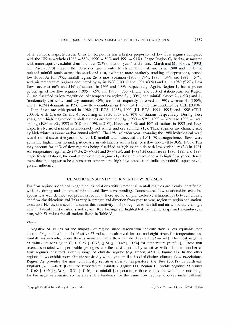
of all stations, respectively, in Class 1F. Region 1F has a higher proportion of low flow regimes comparedwith the UK as a whole (1988 D 88%, 1990 D 50% and 1991 D 94%). Shape Region CF basins, associatedwith major aquifers, exhibit clear low flow (83% of station-years) at this time. Marsh and Monkhouse (1993)and Price (1998) suggest that decreased groundwater levels in these catchments in 1988 and 1991 andreduced rainfall totals across the south and east, owing to more northerly tracking of depressions, causedlow flows. As for 1975, rainfall regime 2R is most common (1988 D 74%, 1990 D 54% and 1991 D 57%)with air temperature regimes dominated by 4T in 1988 (100%) and 1991 (86%) and 3T in 1989 (97%). Lowflows occur at 66% and 51% of stations in 1995 and 1996, respectively. Again, Region 1F has a greaterpercentage of low flow regimes (1995 D 69% and 1996 D 75% cf. UK) and 88% of station-years for RegionCF are classified as low magnitude. Air temperature regime 3T (100%) and rainfall classes 2R (49%) and 1R

(moderately wet winter and dry summer; 40%) are most frequently observed in 1995; whereas 4T (100%)and 1R (63%) dominate in 1996. Low flow conditions in 1995 and 1996 are also identified by CEH (2003b).

High flows are widespread in 1980 (IH–BGS, 1985), 1993 (IH–BGS, 1994, 1995) and 1998 (CEH,2003b), with Classes 3F and 4F occurring at 77%, 83% and 80% of stations, respectively. During theseyears, both high magnitude rainfall regimes are common: 3R (1980 D 57%, 1993 D 37% and 1998 D 14%)and 4R (1980 D 9%, 1993 D 20% and 1998 D 31%). However, 30% and 40% of stations in 1993 and 1998,respectively, are classified as moderately wet winter and dry summer (1R). These regimes are characterizedby high winter, summer and/or annual rainfall. The 1981 calendar year (spanning the 1980 hydrological year)was the third successive year in which UK rainfall totals exceeded the 1941–70 average; hence, flows weregenerally higher than normal, particularly in catchments with a high baseflow index (IH–BGS, 1985). Thismay account for 46% of flow regimes being classified as high magnitude with low variability (3F) in 1981.Air temperature regimes 2T (97%), 2T (40%) and 3T (49%), and 4T (94%) dominate in 1980, 1993 and 1998,respectively. Notably, the coolest temperature regime (1T) does not correspond with high flow years. Hence,there does not appear to be a consistent temperature–high-flow association, indicating rainfall inputs have agreater influence.

CLIMATIC SENSITIVITY OF RIVER FLOW REGIMES

For flow regime shape and magnitude, associations with interannual rainfall regimes are clearly identifiable,with the timing and amount of rainfall and flow corresponding. Temperature–flow relationships exist butappear less well defined (see previous section). There are no simple, exclusive relationships between climateand flow classifications and links vary in strength and direction from year-to-year, region-to-region and station-to-station. Hence, this section assesses this sensitivity of flow regimes to rainfall and air temperature using anew analytical tool (sensitivity index, SI ). Key findings are highlighted for regime shape and magnitude, inturn, with SI values for all stations listed in Table V.

Shape

Negative SI values for the majority of regime shape associations indicate flow is less equitable thanclimate (Figure 1, SI ! �1). Positive SI values are observed for one and eight rivers for temperature andrainfall, respectively, where flow is more equitable than climate (Figure 1, SI ! C1). The most negativeSI values are for Region CF (�0Ð69 [�0Ð73] � SI � �0Ð49 [�0Ð54] for temperature [rainfall]). These fourrivers, associated with permeable geologies, are the least climatically sensitive with a limited number offlow regimes observed under a range of climatic regime (e.g. Itchen, 42 010, Figure 11). In the otherregions, flows exhibit more climatic sensitivity with a greater likelihood of distinct climate–flow associations.Region AF provides the most climatically sensitive river to temperature: the Tees (25018) in north-eastEngland (SI D �0Ð26 [0Ð53] for temperature [rainfall]) (Figure 11). Region BF yields negative SI values(�0Ð68 [�0Ð60] � SI � �0Ð31 [�0Ð46] for rainfall [temperature]); these values are within the mid-rangefor the negative scenario so there is still a tendency for the same flow regime to occur under different

Copyright 2004 John Wiley & Sons, Ltd. Hydrol. Process. 18, 2515–2543 (2004)

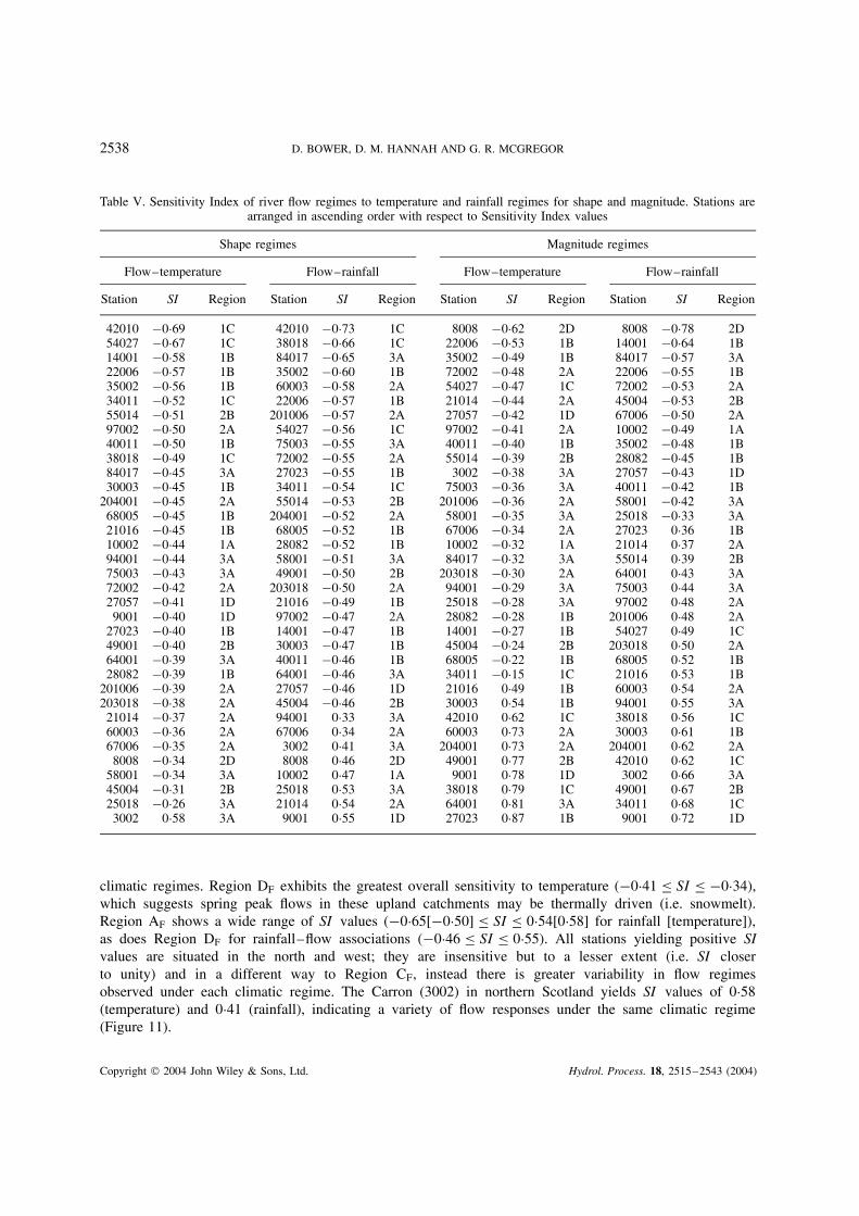
2538 D. BOWER, D. M. HANNAH AND G. R. MCGREGOR

Table V. Sensitivity Index of river flow regimes to temperature and rainfall regimes for shape and magnitude. Stations arearranged in ascending order with respect to Sensitivity Index values

Shape regimes Magnitude regimes

Flow–temperature Flow–rainfall Flow–temperature Flow–rainfall

Station SI Region Station SI Region Station SI Region Station SI Region

42010 �0Ð69 1C 42010 �0Ð73 1C 8008 �0Ð62 2D 8008 �0Ð78 2D54027 �0Ð67 1C 38018 �0Ð66 1C 22006 �0Ð53 1B 14001 �0Ð64 1B14001 �0Ð58 1B 84017 �0Ð65 3A 35002 �0Ð49 1B 84017 �0Ð57 3A22006 �0Ð57 1B 35002 �0Ð60 1B 72002 �0Ð48 2A 22006 �0Ð55 1B35002 �0Ð56 1B 60003 �0Ð58 2A 54027 �0Ð47 1C 72002 �0Ð53 2A34011 �0Ð52 1C 22006 �0Ð57 1B 21014 �0Ð44 2A 45004 �0Ð53 2B55014 �0Ð51 2B 201006 �0Ð57 2A 27057 �0Ð42 1D 67006 �0Ð50 2A97002 �0Ð50 2A 54027 �0Ð56 1C 97002 �0Ð41 2A 10002 �0Ð49 1A40011 �0Ð50 1B 75003 �0Ð55 3A 40011 �0Ð40 1B 35002 �0Ð48 1B38018 �0Ð49 1C 72002 �0Ð55 2A 55014 �0Ð39 2B 28082 �0Ð45 1B84017 �0Ð45 3A 27023 �0Ð55 1B 3002 �0Ð38 3A 27057 �0Ð43 1D30003 �0Ð45 1B 34011 �0Ð54 1C 75003 �0Ð36 3A 40011 �0Ð42 1B

204001 �0Ð45 2A 55014 �0Ð53 2B 201006 �0Ð36 2A 58001 �0Ð42 3A68005 �0Ð45 1B 204001 �0Ð52 2A 58001 �0Ð35 3A 25018 �0Ð33 3A21016 �0Ð45 1B 68005 �0Ð52 1B 67006 �0Ð34 2A 27023 0Ð36 1B10002 �0Ð44 1A 28082 �0Ð52 1B 10002 �0Ð32 1A 21014 0Ð37 2A94001 �0Ð44 3A 58001 �0Ð51 3A 84017 �0Ð32 3A 55014 0Ð39 2B75003 �0Ð43 3A 49001 �0Ð50 2B 203018 �0Ð30 2A 64001 0Ð43 3A72002 �0Ð42 2A 203018 �0Ð50 2A 94001 �0Ð29 3A 75003 0Ð44 3A27057 �0Ð41 1D 21016 �0Ð49 1B 25018 �0Ð28 3A 97002 0Ð48 2A9001 �0Ð40 1D 97002 �0Ð47 2A 28082 �0Ð28 1B 201006 0Ð48 2A

27023 �0Ð40 1B 14001 �0Ð47 1B 14001 �0Ð27 1B 54027 0Ð49 1C49001 �0Ð40 2B 30003 �0Ð47 1B 45004 �0Ð24 2B 203018 0Ð50 2A64001 �0Ð39 3A 40011 �0Ð46 1B 68005 �0Ð22 1B 68005 0Ð52 1B28082 �0Ð39 1B 64001 �0Ð46 3A 34011 �0Ð15 1C 21016 0Ð53 1B

201006 �0Ð39 2A 27057 �0Ð46 1D 21016 0Ð49 1B 60003 0Ð54 2A203018 �0Ð38 2A 45004 �0Ð46 2B 30003 0Ð54 1B 94001 0Ð55 3A21014 �0Ð37 2A 94001 0Ð33 3A 42010 0Ð62 1C 38018 0Ð56 1C60003 �0Ð36 2A 67006 0Ð34 2A 60003 0Ð73 2A 30003 0Ð61 1B67006 �0Ð35 2A 3002 0Ð41 3A 204001 0Ð73 2A 204001 0Ð62 2A8008 �0Ð34 2D 8008 0Ð46 2D 49001 0Ð77 2B 42010 0Ð62 1C

58001 �0Ð34 3A 10002 0Ð47 1A 9001 0Ð78 1D 3002 0Ð66 3A45004 �0Ð31 2B 25018 0Ð53 3A 38018 0Ð79 1C 49001 0Ð67 2B25018 �0Ð26 3A 21014 0Ð54 2A 64001 0Ð81 3A 34011 0Ð68 1C3002 0Ð58 3A 9001 0Ð55 1D 27023 0Ð87 1B 9001 0Ð72 1D

climatic regimes. Region DF exhibits the greatest overall sensitivity to temperature (�0Ð41 � SI � �0Ð34),which suggests spring peak flows in these upland catchments may be thermally driven (i.e. snowmelt).Region AF shows a wide range of SI values (�0Ð65[�0Ð50] � SI � 0Ð54[0Ð58] for rainfall [temperature]),as does Region DF for rainfall–flow associations (�0Ð46 � SI � 0Ð55). All stations yielding positive SIvalues are situated in the north and west; they are insensitive but to a lesser extent (i.e. SI closerto unity) and in a different way to Region CF, instead there is greater variability in flow regimesobserved under each climatic regime. The Carron (3002) in northern Scotland yields SI values of 0Ð58(temperature) and 0Ð41 (rainfall), indicating a variety of flow responses under the same climatic regime(Figure 11).

Copyright 2004 John Wiley & Sons, Ltd. Hydrol. Process. 18, 2515–2543 (2004)

TECHNIQUES FOR ASSESSING CLIMATIC SENSITIVITY OF FLOW REGIMES 2539

Figure 11. Examples of the climatic sensitivity of flow regimes (a) air temperature shape and (b) rainfall magnitude. The thickness andnumbers on arrows denote the frequency of associations

Magnitude

The sensitivity of flow regime magnitude to climate varies widely between stations, irrespective of region(Table V). All magnitude regions experience a range of SI values, both positive to negative, for flowassociations with temperature and rainfall. The absence of regional patterns may be expected, because theinterannual regime magnitude classification is relative at a station (see Method section). It is beyond the scopeof this section to provide a detailed discussion of the climatic sensitivity of individual rivers; therefore, threeexamples are selected to characterize the nature of associations identified across the UK. The Tromie in centralnorthern Scotland (8008) is stable in terms of flow magnitude, with Class 2F occurring for 64% of station-yearsregardless of the climatic regime. It follows that the Tromie is climatically insensitive (SI D �0Ð62 [�0Ð78]for temperature [rainfall], Figure 11). The nearby Deveron (9001) is also insensitive to climate but in theopposite direction, because a variety of flow regimes occur under each climatic regime (SI D 0Ð78[0Ð72] fortemperature [rainfall], Figure 11). Again, the Tees shows climatic sensitivity (Figure 11) with different flowregime magnitudes typically observed for each climate regime (SI D �0Ð28 [�0Ð33] for temperature [rainfall],Figure 11).

For regime shape and magnitude, climate-flow associations are insensitive where SI ! 1 with a range offlows observed under each climatic regime. Climatic insensitivity of flows also occurs where SI ! �1, butfor this scenario the flow response is arguably more predictable because a limited number of flow classesoccur under a range of climate regimes (e.g. Region CF). Stations where SI ! 0 are climatically sensitive;however, for the test data set SI values close to unity were generally lacking most probably owing to themoderating effect of terrestrial factors, which may vary over time. This highlights the importance of thecatchment in determining the sensitivity of climate–flow response.

EVALUATION OF REGIME CLASSIFICATION METHOD AND SENSITIVITY INDEX

This paper develops and tests: (i) a regime classification method to identify spatial and temporal patterns inintraannual hydroclimatological response, and (ii) a novel sensitivity index (SI ) to assess the sensitivity offlow regimes to climate. The application of these methods to a test data set generates results that support

Copyright 2004 John Wiley & Sons, Ltd. Hydrol. Process. 18, 2515–2543 (2004)

2540 D. BOWER, D. M. HANNAH AND G. R. MCGREGOR

current knowledge about the hydroclimatology of the UK. Although this research does not seek to yield new,detailed physical process understanding, it provides perspective at large spatial and temporal scales uponclimate and flow regime and quantifies linkages. In this final section, the regime classification method andthe SI are evaluated as analytical tools and in terms of wider applicability.

Regime classification

The classification of regime shape (form) and magnitude considers the whole annual cycle rather thanisolating a single month or season for analysis, which has been the common approach of previous studies.The method presented is a refinement of techniques published by Harris et al. (2000), based upon Hannah et al.(1999, 2000). The regime classification presented is arguably more statistically robust owing to incorporation ofa two-stage clustering procedure and discriminant function analysis (see Method section). The test applicationshows the method to be particularly useful for identifying large-scale patterns in regimes (i.e. regionalization:spatial mode) and their between-year stability (i.e. interannual variability: temporal mode) and, thus, providesa context for short-term, small-scale process-based research. Although in this instance monthly river flows,temperatures and rainfall are analysed, the classification approach may be applied to a range of environmentaldata, at different spatio-temporal resolution, where there is an underlying signal with a form and magnitudeof interest.

However, any method of simplification (including classification) has limitations. Wilby (1994) identifiesthree ‘problems’ with categorization: classification, scale and stability. Classification may result in: (i) lossof potentially useful information; (ii) identification of arbitrary classes; (iii) non-transferable results, and(iv) subjectivity introduced by different analysts. Each of these points has been carefully considered indevelopment of the regime classification (numbers below correspond with those points above).

i. The method enables description of regime shape and magnitude, which are the key attributes of interestfor academic and operational research. Although actual values are ‘lost’, a clearer understanding of datastructure is gained.

ii. Distinct classes are not arbitrary (i.e. random) but rather statistically informed and reflect specifichydrological and climatological features.

iii. It may not be possible to transfer information from one study to another but this is true for most empiricalresearch. However, nesting of classifications at different scales provides an understanding of patterningand variability at multiple resolutions.

iv. Exploratory analyses reveal the optimum cluster solution is yielded using a two-stage procedure: Ward’sagglomerative, hierarchical cluster analysis and non-hierarchical k -means cluster analysis (see Methodsection). Hence, the only subjective decision is the number of clusters retained (aided by agglomerationschedule and dendrogram plots), which determines classification detail.

Scale issues relate to the inability of categorization to represent continuous spatial and temporal variability.In this paper, regimes represent long-term average or interannual patterns for points (air temperature and pre-cipitation) or runoff integrated over catchment areas. The use of monthly values provides valuable informationon the intraannual variability, which is subsumed by seasonally- and annually-averaged (continuous) values.The classification scheme may be applied at a range of scales: single or few sites at diurnal (Hannah et al.,1999, 2000) to annual (Harris et al., 2000; Wood et al., 2001) time-scales but also multiple stations (Bowerand Hannah, 2002; Kansakar et al., 2002).

Stability refers to the assumption that the physical processes inferred to operate under each class are notconstant but vary spatially and temporally. For flow regionalization, this may be overcome, at least partially,by a basin-by-basin knowledge of climate and catchment controls. Non-stationarity is an inherent problemwith most climatological and hydrological time-series. Hence, it is the responsibility of the researcher to useappropriate statistical homogeneity tests, refer to metadata and review literature to place the study period incontext.

Copyright 2004 John Wiley & Sons, Ltd. Hydrol. Process. 18, 2515–2543 (2004)

TECHNIQUES FOR ASSESSING CLIMATIC SENSITIVITY OF FLOW REGIMES 2541

Sensitivity index (SI )

The SI provides a means of assessing the often-complex linkages between climatic drivers and river flow,as it identifies the strength and direction of associations between classifications of air temperature/rainfalland flow regimes. Thus, it provides a useful diagnostic hydroclimatological tool. The application of theSI to assess sensitivity of river flow regimes to seasonal climatic variations is novel, as previous workhas considered months or seasons in isolation. However, any method of summarizing associations has itslimitations, particularly when a single value determines both the strength and direction of the relationship.Conversely, this may be considered a benefit as it provides a concise measure that is readily comparablebetween different sites (and potentially time periods). Although the SI identifies stations where river flowsare climatically (in)sensitive, it does not indicate the reason behind (in)sensitivity, which can be gained onlyby knowledge of the river basin and physical process interactions.

Differences in the number of regime classes for climate and flow classifications can affect the SI, asequitability tends to decrease with the number of classes. The relative equitability of the two classificationsdetermines whether the SI is calculated using the positive or negative scenario, hence, the index sign. Forthe UK test data set, six flow and four climate shape regimes were identified, resulting in a shift toward thenegative scenario. Despite this cautionary note, the SI clearly indicates that the occurrence of flow regimesare more uneven than climate regimes and provides information about the strength of climatic controls uponflow.

The SI has potential for application to other problems where relationships between two nominal classifica-tions need to be quantified. For example, the SI may be applied to link classes for climate regime and landproductivity or snow cover, or hydrological regime and river channel engineering type or ecological status.Hence, the SI has potentially wide utility as an analytical tool.

Having demonstrated the regime classification and SI to be useful in an environment (UK) where thehydroclimatology is relatively well known, there appears to be much to gain by applying these techniquesto parts of the world where large-scale patterns and associations between climate and hydrology are poorlyunderstood (e.g. Hannah et al., submitted; Kansakar et al., in press) to advance scientific understanding andinform water resource management.

ACKNOWLEDGEMENTS

D. Bower is funded by NERC studentship GTNER/S/A/2000/03936. G. Rees and I. Akram at the Centre forEcology and Hydrology (CEH) Wallingford extracted daily river flow time-series from the FRIEND-EWA. TheBritish Atmospheric Data Centre (BADC) provided daily temperature and rainfall time-series. K. Burkhill andA. Ankcorn redrew diagrams. The authors thank the two anonymous referees for their constructive comments.

REFERENCES

Arnell NW, Brown RPC, Reynard NS. 1990. Impact of Climatic Variability and Change on River Flow Regimes in the UK. Report 107,Institute of Hydrology: Wallingford; 154.

Arnell NW, Krasovskaia I, Gottschalk L. 1993. River flow regimes in Europe. In Flow Regimes from International Experimental and NetworkData (FRIEND), Vol. 1, Gustard A (ed.). Institute of Hydrology: Wallingford; 112–121.

Barrow E, Hulme M. 1997. The surface climate of the British Isles. In Climates of the British Isles , Hulme M, Barrow E (eds). Routledge:London; 33–62.

Bower D, Hannah DM. 2002. Spatial and temporal variability of UK river flow regimes. In FRIEND 2002—Regional Hydrology: Bridgingthe Gap between Research and Practice (Proceedings of Cape Town Conference). IAHS Publication 274, International Association &Hydrological Sciences: Wallingford; 457–464.

CEH. 2003a. National River Flow Archive Data Retrieval Service. http://www.nwl.ac.uk/ih/nrfa/river flow data/nrfa retrievals.htm (accessed17 July 2003).

CEH. 2003b. Water watch. http://www.nwl.ac.uk/ih/nrfa/water watch/index.htm (accessed 17 July 2003).Dettinger MD, Diaz HF. 2000. Global characteristics of stream flow seasonality and variability. Journal of Hydrometeorology 1: 289–310.Doornkamp JC, Gregory KJ, Burn AS. 1980. Atlas of Drought in Great Britain: 1975/1976 . Institute of British Geographers: London; 82.

Copyright 2004 John Wiley & Sons, Ltd. Hydrol. Process. 18, 2515–2543 (2004)

2542 D. BOWER, D. M. HANNAH AND G. R. MCGREGOR

Gottschalk L. 1985. Hydrological regionalisation of Sweden. Hydrological Sciences Journal 30: 65–83.Gustard A, Bullock A, Dixon JM. 1992. Low Flow Estimation in the United Kingdom. Report 108, Institute of Hydrology: Wallingford; 195.Hannah DM, Gurnell AM, McGregor GR. 1999. A methodology for investigation of the seasonal evolution of proglacial hydrograph form.

Hydrological Processes 13: 2603–2621.Hannah DM, Kansakar SR, Gerrard AJ, Rees G. Flow regimes of Himalayan rivers of Nepal: nature and spatial patterns. Journal of Hydrology

(submitted).Hannah DM, Smith BPG, Gurnell AM, McGregor GR. 2000. An approach to hydrograph classification. Hydrological Processes 14:

317–338.Harris NM, Gurnell AM, Hannah DM, Petts GE. 2000. Classification of river regimes: a context for hydroecology. Hydrological Processes

14: 2831–2848.Harvey LDD. 2000. Upscaling in global change research. Climatic Change 44: 225–263.Institute of Hydrology, British Geological Survey. 1985. Hydrological Data UK 1981 Yearbook . Institute of Hydrology/British Geological

Survey: Wallingford; 168 pp.Institute of Hydrology, British Geological Survey. 1989a. Hydrological Data UK 1987 Yearbook . Institute of Hydrology/British Geological

Survey: Wallingford; 188 pp.Institute of Hydrology, British Geological Survey. 1989b. Hydrological Data UK 1988 Yearbook . Institute of Hydrology/British Geological

Survey: Wallingford; 192 pp.Institute of Hydrology, British Geological Survey. 1990. Hydrological Data UK 1989 Yearbook . Institute of Hydrology/British Geological

Survey: Wallingford; 200 pp.Institute of Hydrology, British Geological Survey. 1991. Hydrological Data UK 1990 Yearbook . Institute of Hydrology/British Geological

Survey: Wallingford; 193 pp.Institute of Hydrology, British Geological Survey. 1992. Hydrological Data UK 1991 Yearbook . Institute of Hydrology/British Geological

Survey: Wallingford; 175 pp.Institute of Hydrology, British Geological Survey. 1993. Hydrological Data UK 1992 Yearbook . Institute of Hydrology/British Geological

Survey: Wallingford; 176 pp.Institute of Hydrology, British Geological Survey. 1994. Hydrological Data UK 1993 Yearbook . Institute of Hydrology/British Geological

Survey: Wallingford; 174 pp.Institute of Hydrology, British Geological Survey. 1995. Hydrological Data UK 1994 Yearbook . Institute of Hydrology/British Geological

Survey: Wallingford; 176 pp.Jones PD, Conway D. 1997. Precipitation in the British Isles: an analysis of area-average data updated to 1995. International Journal of

Climatology 17: 427–438.Kansakar SR, Hannah DM, Gerrard J, Rees G. 2002. Flow regime characteristics of Himalayan river basins in Nepal. In FRIEND

2002—Regional Hydrology: Bridging the Gap between Research and Practice (Proceedings of Cape Town Conference). IAHS Publication274, International Association of Hydrological Sciences: Wallingford; 425–432.

Kansakar SR, Hannah DM, Gerrard AJ, Rees G. Spatial pattern in the precipitation regimes of Nepal. International Journal of Climatology(in press).

Kent M, Coker P. 1992. Vegetation Description and Analysis: a Practical Approach. Wiley: Chichester; 363.Krasovskaia I. 1995. Quantification of the stability of river flow regimes. Hydrological Sciences Journal 40: 587–597.Krasovskaia I. 1996. Sensitivity of the stability of river flow regimes to small fluctuations in temperature. Hydrological Science Journal 41:

251–264.Krasovskaia I. 1997. Entropy-based grouping of river flow regimes. Journal of Hydrology 202: 173–191.Krasovskaia I, Arnell NW, Gottschalk L. 1994. Flow regimes in northern and western Europe: development and application of procedures

for classifying flow regimes. In FRIEND: Flow Regimes from International Experimental and Network Data (Proceedings of BraunschweigConference). IAHS Publication 221, International Association of Hydrological Sciences: Wallingford; 185–192.

Krasovskaia I, Gottschalk L. 1992. Stability of river flow regimes. Nordic Hydrology 23: 137–154.Marsh T, Black A, Arcreman M, Elliott C. 2000. River flows. In The Hydrology of the UK , Acreman M (ed.). Routledge: London; 101–133.Marsh TJ, Monkhouse RA. 1993. Drought in the United Kingdom, 1988–92. Weather 48: 15–23.Marsh TJ, Turton PS. 1996. The 1995 drought—a water resources perspective. Weather 51: 46–53.Mosley MP. 1981. Delimitation of New Zealand hydrologic regions. Journal of Hydrology 49: 173–192.NERC. 1975. Flood Studies Report, Vol. 1. Natural Environment Research Council: London; 550 pp.Osborne TJ, Hulme M, Jones PD, Basnett TA. 2000. Observed trends in the daily intensity of United Kingdom precipitation. International

Journal of Climatology 20: 347–364.Price M. 1998. Water storage and climate change in Great Britain—the role of groundwater. Proceedings of the Institution of Civil Engineers,

Water, Materials and Energy 130: 42–50.Roald L, Wesselink AJ, Arnell NW, Dixon JM, Rees G, Andrews AJ. 1993. European Water Archive. In Flow Regimes from International

Experimental and Network Data (FRIEND), Vol. 1, Gustard A (ed.). Institute of Hydrology: Wallingford; 7–20.Robson AJ, Jones TK, Reed DW, Bayliss AC. 1998. A study of national trend and variation in UK floods. International Journal of

Climatology 18: 165–182.Thompson R. 1995. Complex demodulation and the estimation of the changing continentality of Europe climate. International Journal of

Climatology 15: 175–185.Thompson R. 1999. A time-series analysis of the changing seasonality of precipitation in the British Isles and neighbouring areas. Journal

of Hydrology 224: 169–183.Wallace JM, Hobbs PV. 1977. Atmospheric Science: an Introductory Survey . Academic Press: London; 467.Ward RC. 1968. Some runoff characteristics of British rivers. Journal of Hydrology 6: 358–372.Ward RC. 1981. River systems and river regimes. In British Rivers , Lewin J. (ed). Allen & Unwin: London; 1–33.

Copyright 2004 John Wiley & Sons, Ltd. Hydrol. Process. 18, 2515–2543 (2004)

TECHNIQUES FOR ASSESSING CLIMATIC SENSITIVITY OF FLOW REGIMES 2543

Wilby RL. 1994. Stochastic weather type simulation for regional climate change impact assessment. Water Resources Research 30:3395–3403.

Wood PJ, Hannah DM, Agnew MD, Petts GE. 2001. Scales of hydroecological variability within a groundwater-dominated stream. RegulatedRivers: Research and Management 17: 347–367.

Young AR, Round CE, Gustard A. 2000. Spatial and temporal variations in the occurrence of low flow events in the UK. Hydrology andEarth System Sciences 4: 35–45.

Copyright 2004 John Wiley & Sons, Ltd. Hydrol. Process. 18, 2515–2543 (2004)