
TECHNICAL DOCUMENTATION OF THE LATVIAN LABOUR ...
244
1 Eiropas Sociālā fonda programmas „Cilvēkresursi un nodarbinātība” papildinājuma 1.3.prioritātes „Nodarbinātības veicināšana un veselība darbā” apakšaktivitātes 1.3.1.7. „Darba tirgus pieprasījuma īstermiņa un ilgtermiņa prognozēšanas un uzraudzības sistēmas attīstība” projekta Nr.1DP//1.3.1.7.0/10/IPIA/NVA/001 „Darba tirgus pieprasījuma vidēja termiņa un ilgtermiņa prognozēšanas sistēmas attīstība” aktivitāte „Darba tirgus vidēja un ilgtermiņa prognozēšanas instrumentārija pilnveide” (30.03.2011. Iepirkuma līgums Nr. EM 2010/82/ESF) TECHNICAL DOCUMENTATION OF THE LATVIAN LABOUR MARKET MEDIUM AND LONG-TERM FORECASTING AND POLICY ANALYSIS MODEL RTU Riga, 2013
-
Upload
khangminh22 -
Category
Documents
-
view
5 -
download
0
Transcript of TECHNICAL DOCUMENTATION OF THE LATVIAN LABOUR ...

1
Eiropas Sociālā fonda programmas „Cilvēkresursi un nodarbinātība” papildinājuma 1.3.prioritātes
„Nodarbinātības veicināšana un veselība darbā” apakšaktivitātes 1.3.1.7. „Darba tirgus pieprasījuma
īstermiņa un ilgtermiņa prognozēšanas un uzraudzības sistēmas attīstība” projekta
Nr.1DP//1.3.1.7.0/10/IPIA/NVA/001 „Darba tirgus pieprasījuma vidēja termiņa un ilgtermiņa
prognozēšanas sistēmas attīstība” aktivitāte
„Darba tirgus vidēja un ilgtermiņa prognozēšanas instrumentārija pilnveide” (30.03.2011. Iepirkuma līgums Nr. EM 2010/82/ESF)
TECHNICAL DOCUMENTATION OF THE LATVIAN LABOUR MARKET
MEDIUM AND LONG-TERM FORECASTING AND POLICY ANALYSIS
MODEL
RTU
Riga, 2013
2
CONTENT
Introduction 4
1. General overview of the Latvian labour market medium and long-term forecasting and policy
analysis model 7
1.1. Methodological framework 7
1.2. Model blocks and logical structure 9
1.3. Data specification and sources 11
2. Mathematical description of the model 13
2.1. Labour demand module 13
2.1.1. Sector labour demand sub-model 13
2.1.2. Occupational labour demand sub-model 19
2.1.3. Modelling labour demand by education 28
2.1.4. Modelling labour demand by gender 36
2.2. Labour supply module 39
2.2.1. Demographic sub-model 39
2.2.2. Education attainment sub-model 51
2.2.3. Working-age population stock-taking sub-model 79
2.2.4. Labour force participation sub-model 92
2.2.5. International migration sub-model 99
2.3. Labour market module: balancing labour demand and supply 108
2.3.1. Labour market sub-model 108
2.3.1.1. Framework and structure of the labour demand and supply balancing sub-model
108
2.3.1.2. Calculation algorithm of vacancies 123
2.3.1.3. Liquidation algorithm of working places 126
2.3.1.4. Declining algorithm of vacancies and occupied working places 129
2.3.1.5. Employment and occupational mobility algorithm 134
2.3.1.6. Synchronization algorithm 164
2.3.2. Wage sub-model 168
3. Model user guide 178
3.1. Model interface 178
3.2. Data input and model update 181
3.3. Integrated constants in the model 182
3.4. Model output tables 182
4. Description of the results obtained with the model, interpretation and reliability of the results
186
5. The time frame of the forecasting process 198
References 199
Annex A. The annexes to the body text of the technical documentation 209
Annex A.1. Data specification and sources used in modelling 209
Annex A.2. Period of changes of productivity by sectors 214
Annex A.3. Conformance of the significance of the occupational groups (3-character level)
to criteria by sectors in 2010 214
Annex A.4. Dropout index values 215

3
Annex A.5. Privileged age structure index values 215
Annex A.6. Constants integrated in the model 216
Annex A.7. Technical description of SDM_IN.XLS fail 225
Annex A.8. Mathematical formula abbreviations 235
Annex A.9. Data recovery time 242
Annex A.10. Data recovery and forecasting time consumption 244
Annex B. Detailed description of the model in the form of the Powersim Studio programming
language (separate fail, only in Latvian version of technical documentation)

4
INTRODUCTION
Today, the globalization and information society influences the development of different
economic processes. The processes are developing with unprecedented speed and leave an impact
both at the regional and global levels. Latvia is the member of the European Union (EU), so it has
international, European and local features, including the advanced changes of the situation in
economics and labour market.
In the rapidly changing environment the traditional forecasting methods do not allow
providing the reasonable forecasts in the average and long-term periods. Time series forecasting
methods are intended for short-term forecasting; econometric methods are able to predict the longer
term, but only when the degree of impact of influencing factors and form of compliance are not
changing in the analysed period. Along with the economic processes the rapid changes and
development create a need for economists - practitioners throughout the world to search for new
strategic planning tools. In particular, they have been affected by the global economic crisis.
One solution is the broader application of the system dynamics method, including the
forecasting of economic processes and labour market processes.
The system dynamics method has been applied in the labour market forecasting in Latvia for
a long time. One of the most practicable researches in this field is the study of the University of
Latvia (LU) “Research of the long-term forecasting system of the labour market demand and
analysis of the improvement opportunities”, which has resulted in a dynamic optimization model
(DOM). For some time, the Ministry of Economics of the Republic of Latvia (MoE) has used the
model results, and then the DOM model has been improved in MoE. With the rapid changes of
environment, the previously developed models needs to be supplemented, improved. This document
describes the improved model, its principles and operation.
Detailed DOM structure is available in the research published by the University of Latvia
and the Ministry of Welfare of the Republic of Latvia.
It is being proposed in the improved model to use optimization theory methods, as well as
reduce the application of econometric index in the model, thus transforming the model and,
consequently, developing the system dynamics model (SDM) by the principles of system dynamics
method.
The first significant improvement of the model is the development of the international
labour migration sub-model. Detailed development of this sub-model is based on the passed and
ongoing processes in the Latvian labour market, as well as increasing labour migration to more
economically developed countries of EU.
In the improved model the decision to abandon environmental and resource module, as well
as not to use technology sub-model has been taken. These DOM parts have the low relation to the
predictive objects.
The third significant improvement in the model is that the SDM has changed the model-
building principles: not only in the demographic sub-model, but in all related labour supply sub-
models have been set the multi-dimensional system dynamics flows, which provide a more effective
reflection of the significant changes and labour amount, forecasting of structure and changes.
The main economic relation changes are related to the use of the production function and
changes in productivity. By analysing the new system dynamics researches, it is concluded that the
Cobb-Douglas production function almost cannot be applied in the practical researches in
macroeconomics. The invested and accumulated capital in the sectors in systems dynamics has been
divided into two groups: effective and speculative. Theoretically, system dynamics production
function is most often used in effective capital. There is almost no researches, statistics, separating
the speculative capital from the effective capital. The effective and speculative capital consolidation
and application is causing significant deviations in labour market forecasting, including the short-
term and medium-term periods of 3-5 years. Consequently, the SDM base is designed on the basis
of Leontief production function.

5
By improving the model, the number of analysed labour groups has been significantly
increased; the forecasting dimensions have been extended. Dimensional comparison of DOM and
SDM models are represented in Table 1.
Table 1
DOM and SDM dimensions
Dimension DOM SDM
Sectors
Representation of the economic structure
with the use of the first level of NACE 1.1.
classification
Statistical classification of economic
activities of NACE 2 red, the first
level of classification
Occupational
groups
Aggregation of 37 occupational groups
included in the occupational classification,
by combining the similar occupations by
experience and skills of the employees,
thus forming the labour supply at the
certain education system level and sector
Latvian Occupational Classification
(adapted according to the ISCO-08)
(3-digit occupation code level) of 127
occupational group units.
Education
groups No
Aggregation of levels of education in
8 units and 79 fields of education (on
the basis of the classification of the
Ministry of Education of the Republic
of Latvia, third, fourth and fifth groups
of the code).
Gender No Men, women
Age groups
15-19, 20-24, 25-34, 35-44, 45-54, 55-64;
65-74 (the combination of 7 groups by five
and ten year old age groups)
12 age groups by five years, aged from
15 to 74 years
Age No from 0 to 99 years and one group of
population of 100 years old and more
Economic
activity No
Economically active population,
economically inactive population
SDM model provides the forecasts of the following parameters:
labour demand in terms of economic sectors, skill groups, levels of education;
population, including the population long-term international migration, in terms of
gender, 1-year age groups, skill groups and levels of education;
economically active population in terms of gender, 5-year age groups, skill groups,
levels and fields of education;
the number of employed population in terms of 5-year age groups, skill groups,
levels and fields of education and economic sectors;
the number of unemployed in 5-year age groups, skills groups, levels of education
and sectors of the economy section;
the number of working places, including free vacancies according to the
requirements to gender, occupation, level and field of education determined to
employees.
SDM model evaluates the impact of the labour market policy changes on the labour market,
including the changes of immigration policy, the number of study places, etc.
In SDM the ergonomics of the model was advanced: one of the model improvement and
development principles is the model independence from the operation of the rest of the components
- the model in the autonomous mode (or, if needed, with the help of the user/operator) prepare the
necessary forecasts from the input data. Calculation of the indexes is not using the sub-model or
computer program beyond the system.

6
In the technical documentation of the Latvian labour market medium and long-term
forecasting and policy analysis model the system dynamics Latvian labour market medium and
long-term forecasting and policy analysis model is being described.
The first chapter gives a description of the used methodology, the model structure and the
logical structure, as well as the data required for modelling.
The second chapter describes the system dynamics model in the mathematical form,
indicating and justifying the interaction of the parameters included in the model.
The third chapter represents the detailed model user guide.
The fourth part reflects the description of the results derived from the model.
The fifth part reflects the time curve description of the forecasting process.
SDM model author is Riga Technical University’ leading researcher, associate professor
Dr.oec.V.Skribans, the project realized by the working group consisting of Dr. oec. V.Skribans
(leading expert), Dr. oec. A.Auziņa-Emsiņa, Dr. sc. ing. A.Lektauers.

7
1. GENERAL OVERVIEW OF THE LATVIAN LABOUR MARKET
MEDIUM AND LONG-TERM FORECASTING AND POLICY ANALYSIS
MODEL
1.1. Methodological framework
Modelling is one of the ways of problem solution in practice. Modelling is being used when
experimenting with the real system or its prototype is too expensive or not possible.
Most common types of analytical modelling are time series, econometric methods etc. These
methods provide relatively good forecasting results in the short periods of time when statistically
determined connections do not change. Modern economic processes can develop so quickly that
these methods could be inapplicable even for 2-3 years of forecasting. On the basis of the research
task - to carry out medium and long-term forecasting (up to 30 years) - the provided method groups
are considered to be invalid. So long forecasting period is most frequently the system dynamics
approach, which determines the choice of the method for model building. The choice of the system
dynamics approach is being determined by the compliance of the method with the examined
problem, method abstraction and precision level.
By definition, system dynamics analyses the system behaviour in time, depending on the
structure of the system elements and their mutual interaction, including cause - effect relationship,
feedback links, effects of reaction time etc. Key components of system dynamics are stocks, flows,
the system links of the elements that form feedback loops and time delays.
Stocks accumulate materials, non-material objects, represent stocks, stock increasing and
reduction potentials (limits). By developing the labour market forecasting model, the task of the
stock is to reflect the number of population (including labour, employment, etc.), working positions,
study places, etc. in time. The integral calculations are being used for this purpose (see formula 1):
T
t
0
0
dt )()(t (t) TMLMLM , (1)
where
LM - stock;
TM - flow.
As formula 1 shows, the value of the stock size in time t is, primarily, dependent on the
stock in the base period (time t0) and, secondly, on the change, determined by the flow in the
analysed period. Without the effect (change) of the flow, the stock maintains its initial condition.
Here the advantage of this method is evident: if the effect of the influence factors is not known or it
cannot be calculated, the stock as the parameter can still be available (it is possible to make
calculation on its basis).
By assessing the essence of the method, the main methodological assumption of the labour
market forecasting model has been established: the stock (reflecting the number of population
(including labour, employed people, etc.), working positions, and study places, etc.) remain
unchanged until they are not affected by the influence factors. In practice, it is being expressed as
follows: the number of employed (labour volume or the number of working positions, etc.) remains
unchanged until it is not being changed by the pre-defined (change) factors. The total influence
factors change the stock (repository) through a flow.
Graphically the system dynamic stocks are being marked as rectangle.
The flows reflect the rate of change of the stocks. By developing the labour market
forecasting model, the task of the flows is to reflect for how many people per year (or how many
8
places per year, etc.) the stocks (i.e., the number of population (including labour, employed people,
etc.), working positions, study places, etc.) are changing (increasing or decreasing). For calculation
of the flows the algebraic calculations are being used.
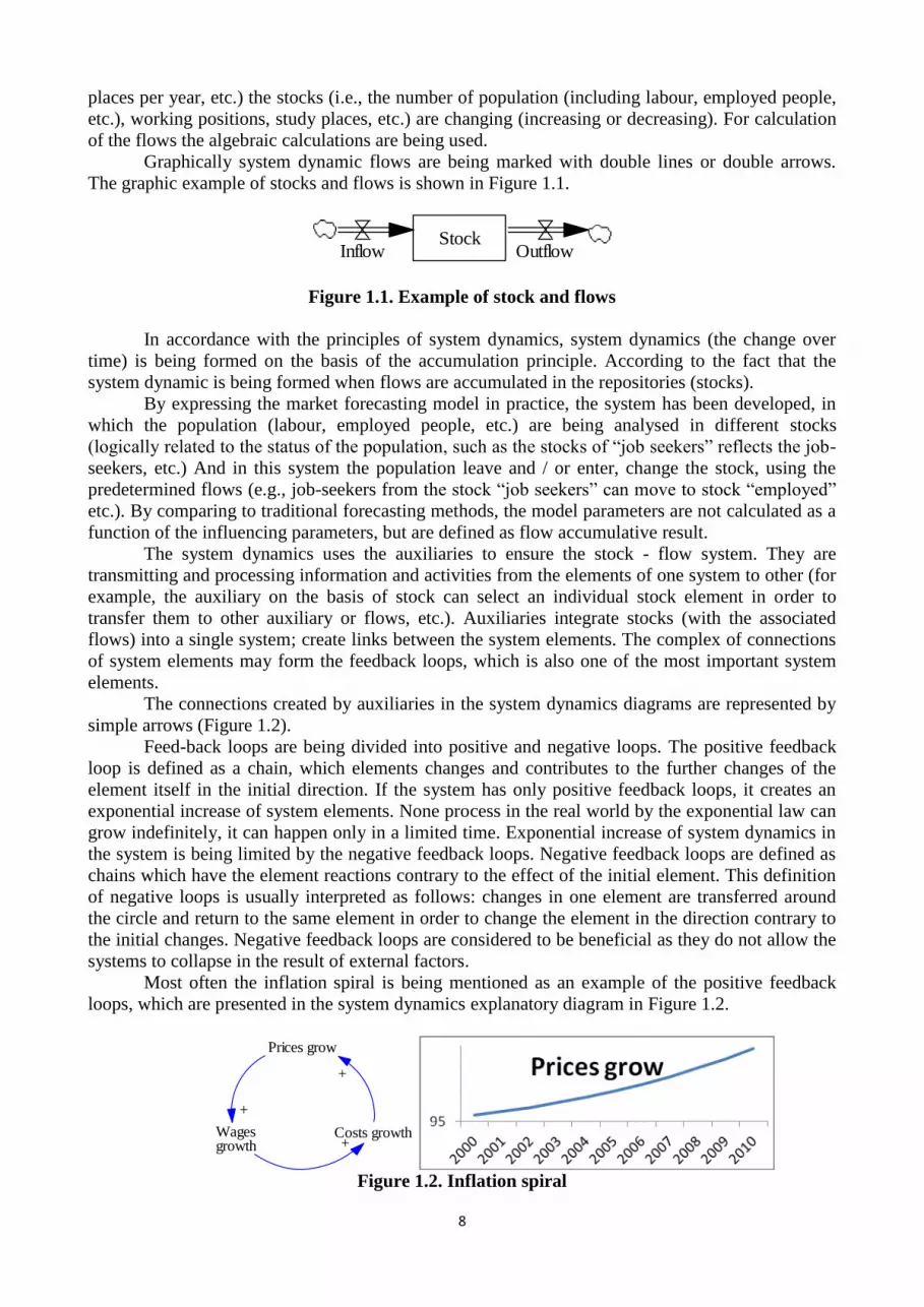
Graphically system dynamic flows are being marked with double lines or double arrows.
The graphic example of stocks and flows is shown in Figure 1.1.
StockInflow Outflow
Figure 1.1. Example of stock and flows
In accordance with the principles of system dynamics, system dynamics (the change over
time) is being formed on the basis of the accumulation principle. According to the fact that the
system dynamic is being formed when flows are accumulated in the repositories (stocks).
By expressing the market forecasting model in practice, the system has been developed, in
which the population (labour, employed people, etc.) are being analysed in different stocks
(logically related to the status of the population, such as the stocks of “job seekers” reflects the job-
seekers, etc.) And in this system the population leave and / or enter, change the stock, using the
predetermined flows (e.g., job-seekers from the stock “job seekers” can move to stock “employed”
etc.). By comparing to traditional forecasting methods, the model parameters are not calculated as a
function of the influencing parameters, but are defined as flow accumulative result.
The system dynamics uses the auxiliaries to ensure the stock - flow system. They are
transmitting and processing information and activities from the elements of one system to other (for
example, the auxiliary on the basis of stock can select an individual stock element in order to
transfer them to other auxiliary or flows, etc.). Auxiliaries integrate stocks (with the associated
flows) into a single system; create links between the system elements. The complex of connections
of system elements may form the feedback loops, which is also one of the most important system
elements.
The connections created by auxiliaries in the system dynamics diagrams are represented by
simple arrows (Figure 1.2).
Feed-back loops are being divided into positive and negative loops. The positive feedback
loop is defined as a chain, which elements changes and contributes to the further changes of the
element itself in the initial direction. If the system has only positive feedback loops, it creates an
exponential increase of system elements. None process in the real world by the exponential law can
grow indefinitely, it can happen only in a limited time. Exponential increase of system dynamics in
the system is being limited by the negative feedback loops. Negative feedback loops are defined as
chains which have the element reactions contrary to the effect of the initial element. This definition
of negative loops is usually interpreted as follows: changes in one element are transferred around
the circle and return to the same element in order to change the element in the direction contrary to
the initial changes. Negative feedback loops are considered to be beneficial as they do not allow the
systems to collapse in the result of external factors.
Most often the inflation spiral is being mentioned as an example of the positive feedback
loops, which are presented in the system dynamics explanatory diagram in Figure 1.2.
Prices grow
Wagesgrowth
Costs growth
+
+
+
Figure 1.2. Inflation spiral

9
As the example of the negative feedback loop the classic “Hare - wolf” system (it is
converted to “profit - entrepreneurs” system in entrepreneurship) is being mentioned. With the
growing number of hare in “Hare - wolf” system, the number of wolfs is also growing, which is
indicated by the positive loop. But the growth of the number of hares is being reduced by the
number of wolfs, as indicated by the negative loop. Explanatory scheme of the “Hare - wolf”
system is presented in Figure 1.3.
Hares
Wolfs
+
-
Hares and Wolfs
120120
00
0 5 10 15 20 25 30 35 40 45 50
Time (Month)Hares : Current
Wolfs : Current
Figure 1.3. „ Hare - wolf” system
As shown in Figure 1.3, the simple model represents a very complex dynamics of the system
elements. The number of wolves is being decreased in the model only when the wolves will not
have anything to eat; it is being determined by the ratio of hares and wolves. While the number of
hares corresponds to the number of wolves, the number of wolves is growing.
Models without feedback loops are not considered as system dynamics models, despite the
fact that the method elements can be used here. By forecasting the labour market development, the
market feedback loops are taken into account.
Time delays or the rate of exposure response is the next characteristic element of system
dynamics. Nowadays, there is an opinion among the system dynamics economists that the delay of
economic processes, decisions and response is the main cause of economic instability, including
accelerated growth (boom) and recession (crisis).
The real estate market is often mentioned as an example: with the growth in demand, the
supply cannot satisfy it momentarily, it takes time to do that, for example, to construct new
buildings. System dynamics defines that supply responds to the demand changes with the delay.
The consequences of such delays are the following: as long as there are no changes in supply, there
is a boom in the real estate market; when there is the change in supply and production surplus - the
prolonged crisis in the sector occurs. The delay is observed in various areas and fields: from
investment attraction to training of employees in the labour market, etc. Time delay elements are
included in the labour market forecasting model.
1.2. Model blocks and logical structure
The model provides multi-dimensional system dynamics stock and flow system, which
reflect the condition and dynamics of workplace, population and other important elements of labour
market. Stocks and flows are integrated into algorithms, sub-models and modules. The overall
diagram of sub-models and modules is presented in the Figure 1.4.
10
Labour market module
Labour market
sub-model
Wage sub-model
Labour demand module of SDM model
Sector labour demand sub-model
Occupational labour demand sub-model
Sub-model of
labour demand
by education
Sub-model of
labour demand
by gender
Labour supply module of SDM model
Demographic
sub-model
Education
attainment
sub-model
Working-age
population
stock-taking
sub-model
Labour force
participation
sub-model
International
migration
sub-model
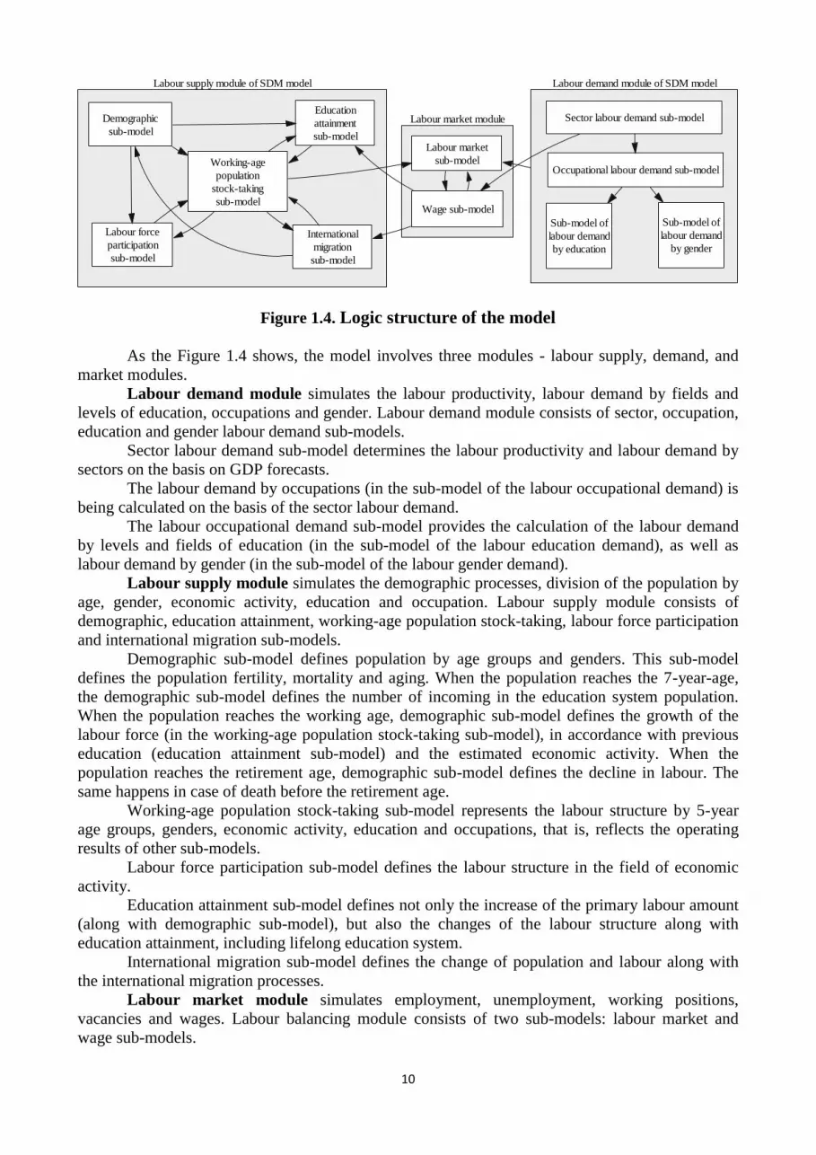
Figure 1.4. Logic structure of the model
As the Figure 1.4 shows, the model involves three modules - labour supply, demand, and
market modules.
Labour demand module simulates the labour productivity, labour demand by fields and
levels of education, occupations and gender. Labour demand module consists of sector, occupation,
education and gender labour demand sub-models.
Sector labour demand sub-model determines the labour productivity and labour demand by
sectors on the basis on GDP forecasts.
The labour demand by occupations (in the sub-model of the labour occupational demand) is
being calculated on the basis of the sector labour demand.
The labour occupational demand sub-model provides the calculation of the labour demand
by levels and fields of education (in the sub-model of the labour education demand), as well as
labour demand by gender (in the sub-model of the labour gender demand).
Labour supply module simulates the demographic processes, division of the population by
age, gender, economic activity, education and occupation. Labour supply module consists of
demographic, education attainment, working-age population stock-taking, labour force participation
and international migration sub-models.
Demographic sub-model defines population by age groups and genders. This sub-model
defines the population fertility, mortality and aging. When the population reaches the 7-year-age,
the demographic sub-model defines the number of incoming in the education system population.
When the population reaches the working age, demographic sub-model defines the growth of the
labour force (in the working-age population stock-taking sub-model), in accordance with previous
education (education attainment sub-model) and the estimated economic activity. When the
population reaches the retirement age, demographic sub-model defines the decline in labour. The
same happens in case of death before the retirement age.
Working-age population stock-taking sub-model represents the labour structure by 5-year
age groups, genders, economic activity, education and occupations, that is, reflects the operating
results of other sub-models.
Labour force participation sub-model defines the labour structure in the field of economic
activity.
Education attainment sub-model defines not only the increase of the primary labour amount
(along with demographic sub-model), but also the changes of the labour structure along with
education attainment, including lifelong education system.
International migration sub-model defines the change of population and labour along with
the international migration processes.
Labour market module simulates employment, unemployment, working positions,
vacancies and wages. Labour balancing module consists of two sub-models: labour market and
wage sub-models.

11
Labour market sub-model combines supply and demand, taking into account the working
positions, vacancies, the amount of labour and wages.
Wage sub-model analyses the most important processes in the national economy (change of
productivity) and labour demand and supply amounts, forming the labour salaries. Labour salaries
affect both labour market balance and labour supply formation, that is, affect the choice of
education and international migration.
1.3. Data specification and sources
In model implementation, the main data source is the Central Statistical Bureau (CSB). The
data required for the model is presented there, and the sources are indicated (surveys carried out by
CSB on the regular basis):
The first source is a REVIEW OF THE SALARY STRUCTURE (5-work) 1
.
Review will provide information on employees by gender, age structure, education,
occupations, load, type of agreements, number of years worked out in the work position,
calculated gross salary (with and without occasional payments), number of paid hours etc.
Next data source is the REPORT ON WORK PERFORMED (3-work)2.
This will provide statistics on occupied and free working positions by occupational groups and
sectors. The report also provides information on the salaries (by occupational groups and
sectors).
Similarly, CSB should provide data on the population and its structure, division by gender, one-
year age groups, (IS06. MEN AND WOMEN AGE STRUCTURE IN THE BEGINNING OF
THE YEAR), data on population mortality, which would be the basis for the calculation of the
population mortality indexes (IM01. AGE AND GENDER STRUCTURE OF DECEASED
PEOPLE), data on the population birth rate, which would be the basis for the calculation of the
population birth rate indexes (ID02. NUMBER OF BORN PEOPLE BY GENDER, ID03.
ALIVE BORN PEOPLE BY THE AGE OF MOTHER), data on long-term migration of the
population (IB04. LONG-TERM AGE AND GENDER STRUCTURE OF MIGRANTS).
In order to assess the economic development, as well as labour demand changes, data on the
sector development and productivity is necessary. It is provided by the gross domestic product
by sectors (IK04. GROSS DOMESTIC PRODUCT BY TYPES OF ACTIVITY).
Education statistics is being collected by the Ministry of Education and Science. According to
the reports, the following information is required: the number of students in general education
institutions, by classes and birth years, the graduates of 9 and 12 classes according to VS-1
GENERAL REPORT OF EDUCATIONAL INSTITUTION (DAY SCHOOL)3, and VV-1
GENERAL REPORT OF EDUCATIONAL INSTITUTION (EVENING (SHIFT) SCHOOL)4;
data on vocational training, number of students, number of dismissed and graduates by source
of financing (state-financed, financing from EU structural funds, paid services), by levels of
qualification, education programs, gender according to REPORTS OF VOCATIONAL
EDUCATIONAL INSTITUTION PROF-2 and PROF-2m 5
.
The data analysis required for the more detailed development of the model is presented in
Annex A.1.
1 According to the 06.11.2006 Regulations of the Cabinet of Ministers Nr.922 Annex No.186
2 According to the 06.11.2006 Regulations of the Cabinet of Ministers Nr.922 Annex No.32
3 Draft Regulations of the Cabinet of Ministers “Amendments in 25.08.2008. Regulations of the Cabinet of Ministers
No.695 „Regulations on Education State Statistics Survey Samples”” 1.Annex 4 Draft Regulations of the Cabinet of Ministers “Amendments in 25.08.2008. Regulations of the Cabinet of Ministers
No.695 „Regulations on Education State Statistics Survey Samples”” 2.Annex 5 Approved by the 20.07.2010 Order No.380 of the Ministry of Education and Science

12
By observing the requirements of the project while creating the model for average and long-
term periods (up to 30 years), the model requires annual data. If it is not possible to apply the period
data and MoE labour market forecasts to the certain data, due to non-compliance, in these cases the
model should be created on the basis of the previous year or last available year. Data delay will not
make problems while defining the basic trends in the average and long-term periods.
In order to make the forecasting scenario analysis, the MoE should prepare forecasts of the
long-term development of gross domestic product (added value) by sectors and forecasts of
population birth rate and mortality indexes.

13
2. MATHEMATICAL DESCRIPTION OF THE MODEL
2.1. Labour demand module
Labour demand module is responsible for modelling labour productivity, labour demand by
sectors, occupations, education and gender. The module consists of 4 sub-models: sector labour
demand sub-model, occupational labour demand sub-model, sub-model of labour demand by
education and sub-model of labour demand by gender. Module structure is presented in the figure
2.1.
Labour demand module of SDM model
Sector labour demand sub-model
Occupational labour demand sub-model
Sub-model of
labour demand
by education
Sub-model of
labour demand
by gender
Figure 2.1. Logical structure of the labour demand module
Figure 2.1 represents that the labour demand by occupations, and further - by education and
genders, have been calculated from the sector labour demand in the labour demand module. For the
calculation of labour demand in the mentioned dimensions the relevant sub-models have been
developed.
Sector labour demand sub-model from the GDP forecasts determines labour productivity
and labour demand by sectors.
Calculation of the labour demand by occupations is based on sector labour demand (in the
occupational labour demand sub-model).
On the basis of the occupational labour demand sub-model, the labour demand by levels and
fields of education has been calculated (in the sub-model of labour demand by education), as well
as labour demand by gender (in the sub-model of labour demand by gender).
The further sub-sections describe labour demand module sub-models.
2.1.1. Sector labour demand sub-model
The sub-model is based on Leontief production function, and GDP and employment in the
base period, as well as the production function coefficient (further - productivity index) have been
used in the calculations. Sub-model logical structure is represented in the Figure 2.2.

14
Labour demand
by sectors
Labour
productivity index
Changes of labour
demand by sectorsChanges of
productivity index
GDP forecasts
<Labour supply by
sectors>
Figure 2.2. Logical structure of the labour demand sub-model of national economy sectors
Figure 2.2 represents in a simplified form that the labour demand by sectors is calculated on
the basis of GDP forecasts and labour productivity index. Also, the labour productivity index is
calculated from GDP forecasting and labour supply by sectors (from the labour supply module),
which is necessary in order to ensure the forecasted GDP at the existing labour volume. Labour
demand calculation is discussed in detail below, but the calculation logic of the productivity index
is represented in the Fig. 2.3.
Necessary
productivity index
Necessary changes of
productivity index
Short-term expected
productivity index
Productivity
indexChanges of
productivity index
<Employment> <GDP forecasts>
<Time of the change
of productivity>
Figure 2.3. Calculation of productivity index
The necessary labour productivity index is being calculated from GDP forecasts and current
employment rate. The index represents the value of the productivity coefficient (Leontief
production function) in order to ensure the certain GDP volume at the existing level of employment.
Comparing the required productivity index with the actual productivity index, it is possible to
determine the changes in capacity, labour productivity (in the model - productivity index) that are
necessary to ensure in economics the forecasted GDP, the difference is reflected in the index
“necessary changes of productivity index” (the principle that the economy is being developed due to
the increasing productivity rather than the employment growth). Productivity cannot be changed
immediately, as soon as the need arises. The change of actual productivity index is going slower
than the change of required productivity index, as the delay is being affected by the time of
productivity changes. Short-term expected productivity index is being used while planning the
labour demand for the future period (short-term expected productivity index changes in the current
period, while productivity index - only in the future period).
Let us sequentially look at the formation of each sub-model element, starting from the basic
principles of calculation of labour productivity and its relation to the Leontief production function.
Leontief production function directly from the volume of output of the sector determines the
production factor (labour) demand. Accordingly, along with the changes (with development) in the
sector it is possible mathematically to calculate labour changes (development). At the same time,
Leontief production function reflects the fact that production factor (labour) demand depends on

15
both the volume of output and the productivity changes. Unifactor Leontief production function is
being determined by the following equation (formula 2):
iii RAY , (2)
where
Yt - volume of output of the sector;
Ai - productivity of the production factor i;
Ri - utilisation of the production factor i.
In order to assess the volume of resource demand, the inverse functions for production
functions are being used, i.e., the production resource consumption functions.
In order practically to apply the sub-model, the data of employment and GDP in the base
period, as well as the GDP development forecasts (exogenous data of the model) should be
available in the forecasting moment. GDP by sectors serves as a measure of sector output volume.
Additional exogenous factor is the time of the productivity change (which is constant throughout
the forecasting period).
On the ground of the employment in the base period and GDP in the base period, the labour
productivity index in the base period is being calculated (formula 3):
0
00
N
NN
N
GDPPK , (3)
where
PKN0 - labour productivity index by sectors in the base period;
GDPN0 - GDP by sectors in the base period;
NN0 - employment by sectors in the base period.
After the calculation of the index in the base period the key role belongs to GDP forecasts.
On the basis of actual employment and forecasted GDP (exogenous data), the productivity index
(formula 4) is being calculated:
Nt
NtNt
N
GDPNPK , (4)
where
NPKN - the necessary productivity index by sectors;
GDPN - GDP forecasts by sectors;
NN - employment by sectors.
The necessary productivity index determines, which productivity coefficient (Leontief
production function) is necessary in order to ensure the certain GDP volume at the current level of
employment. Comparing the required productivity index to the actual productivity index, it is
possible to determine which changes in labour productivity (in the model - productivity index) are
necessary to ensure in economics the forecasted GDP; its difference is presented in the index
“necessary changes of productivity index” (in the sub-model the principle that the economy is
expanding because of the employment growth, rather than increase in productivity, is observed)
(formula 5):

16
0 NtNtNt PKNPKNPKI , (5)
where
NPKIN - the necessary changes of productivity index by sectors;
NPKN - the necessary productivity index by sectors;
RKN - productivity index by sectors.
Formula 5 shows that the necessary changes of productivity index are always positive
(greater or equal to zero). This indicates that the productivity index (labour productivity) cannot be
reduced along with GDP reduction.
Productivity cannot be changed immediately, as soon as the need arises. The actual change
of productivity index is slower than the necessary change of productivity index; this delay is
affected by the time of productivity change. Calculation of the change of productivity index is
presented in formula 6:
N
NtNt
PIL
NPKIPKI , (6)
where
PKIN - changes of productivity index by sectors;
NPKIN - the necessary changes of productivity index by sectors;
PILN - time of the changes of productivity by sectors.
Time of productivity change is calculated on the basis of the historical data from 1996 to
2010, optimizing the time value so as the historical retrospective would minimize the root-mean-
square error of the employment forecast. Equation of root mean square error’s calculation is shown
in formula 7:
min
2
ni
ii
n
xxS , (7)
where
S - root mean square error;
xi - statistical employment;
ix - employment calculated in the model;
n - the number of observations.
Time of productivity change is taken as a constant index, which cannot change greatly
within 30 years. Justification for this assumption is related to the constancy of the productivity.
Productivity in short-term periods is considered to be constant. It is being changed insignificantly in
the medium and longer periods. Time of productivity change is the second degree derivative, which
changes more slowly, so even during the long-term forecasting it is possible to take it as a constant
value. Index values of the time of productivity change are presented in Annex A 2.
The economic meaning of the index “time of productivity change” indicates how quickly the
productivity is changing by sectors. If to estimate the national economy as a whole, this index value
is 1.205. Higher sector index value than in the overall national economy shows that in the sector the
change of the labour productivity is slower than in the national economy. But the smaller sector
index value than in the overall national economy shows that the change of the labour productivity is
happening faster than in the national economy.

17
The index shows the number of years required for full change of productivity in accordance
with GDP changes. An index value 1 means that the change of labour productivity is possible
within a year. The higher the value of this index, the more important is the role of the sector
employment in formation of GDP. For example, in the agriculture, in accordance with EU grants,
when the productivity significantly increases, the number of employees decreases - this index is the
lowest in the national economy. This indicates that the formation of agricultural GDP has a
secondary role for employment, but a key role belongs to productivity growth. However, in the
construction sector, where the index is very high, employment has a key role in formation of GDP
as the productivity is not changing as fast as it would be necessary. Connection of index with
employment is based on a model of logic - if productivity due to the time delay cannot provide the
required GDP growth, then this can be done by increasing the number of employees.
Change of productivity index determines the productivity index (formula 8), as well as the
expected short-term productivity index (formula 9) (expected productivity index changes in the
current period, while the productivity index - only in the future period):
T
t
0
0
dt )()(t (t) NNN PKIPKPK , (8)
where
PKN - productivity index by sectors;
RKIN - changes of productivity index by sectors.
Changes of productivity index reflect both the productivity response to changes of GDP and
supply effect on productivity:
NtNtNt PKIPKISPK , (9)
where
ISPKN - short-term expected productivity index by sectors;
PKN - productivity index by sectors;
PKIN - changes of productivity index by sectors.
It is important to emphasize once again that the sub-model involves the limit, after which
productivity cannot be reduced simultaneously with the decrease of GDP (i.e., it can only grow at
the same time with GDP) (formula 5). If GDP decreases, the productivity index according to this
assumption remains constant, but the labour demand will decrease.
Considering that the calculated changes of productivity index do not coincide with the
necessary changes of productivity index, changes of GDP cannot fully be ensured by changes of the
productivity. Changes of GDP partially make the changes of employment (but the changes that
cannot be implemented in the productivity), which make the basis of the changes of labour demand.
In order to model the labour demand, the scheme similar to productivity index is being
applied.
Labour demand modelling involves the data on employment in the base period (natively it is
being considered that the employment in the base year coincide with the labour demand in the base
year), GDP forecasts and short-term expected productivity index (from this sub-model). In addition
to an exogenous data - index of the time of employment change has a formal role - in all
calculations it is equal to 1, which indicates that during the year it is possible to change employment
in accordance with the demand (in this sub-model). Calculation logics of the labour demand
forecast is presented in the Figure 2.4.
18
Necessary labour
Short-term expected
productivity index
Necessary changes
of labour
Labour
demandChanges of labour
demand
<Time of the change
of employment>
<GDP forecasts>
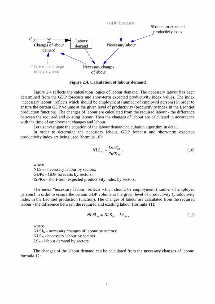
Figure 2.4. Calculation of labour demand
Figure 2.4 reflects the calculation logics of labour demand. The necessary labour has been
determined from the GDP forecasts and short-term expected productivity index values. The index
“necessary labour” reflects which should be employment (number of employed persons) in order to
ensure the certain GDP volume at the given level of productivity (productivity index in the Leontief
production function). The changes of labour are calculated from the required labour - the difference
between the required and existing labour. Then the changes of labour are calculated in accordance
with the time of employment changes and labour.
Let us investigate the equation of the labour demand calculation algorithm in detail.
In order to determine the necessary labour, GDP forecast and short-term expected
productivity index are being used (formula 10):
Nt
NtNt
ISPK
GDPNLS , (10)
where
NLSN - necessary labour by sectors;
GDPN - GDP forecasts by sectors;
ISPKN - short-term expected productivity index by sectors.
The index “necessary labour” reflects which should be employment (number of employed
persons) in order to ensure the certain GDP volume at the given level of productivity (productivity
index in the Leontief production function). The changes of labour are calculated from the required
labour - the difference between the required and existing labour (formula 11):
NtNtNt LSNLSNLSI , (11)
where
NLSIN - necessary changes of labour by sectors;
NLSN - necessary labour by sectors
LSN - labour demand by sectors.
The changes of the labour demand can be calculated from the necessary changes of labour,
formula 12:

19
NPIL
NLSILSI Nt
Nt , (12)
where
LSIN - changes of labour demand by sectors;
NLSIN - necessary changes of labour by sectors;
NPIL - time of the change of employment.
As mentioned above, the change of employment time in this sub-model is taken as constant
and equals to 1 (one year). This means that within a year it is possible to make the necessary
changes of labour in accordance with demand. In this case, the necessary changes of labour
coincide with changes of labour demand, but the additional element and additional equation
(formula 11) are introduced in order to forecast theoretically the situation when the necessary
changes of labour requires a longer period than one year.
Knowing the changes of labour demand, it is possible to calculate the labour demand,
formula 13:
T
t
0
0
dt )()(t (t) NNN LSILSLS , (13)
where
LSN - labour demand by sectors.
LSIN - changes of labour demand by sectors.
Changes of labour demand reflect both the labour demand response to changes of GDP and
supply effect on labour demand (which leads to changes of labour productivity and it, in turn, affect
the labour demand).
By combining the productivity index and calculation of labour demand, the sub-model of
sectorial labour demand has been developed.
2.1.2. Occupational labour demand sub-model
The sub-model is based on sub-model of labour demand by sectors, as well as on
occupations - sectorial statistical data, the ratio of occupations by sectors, and determines the
changes of labour demand by occupations - sectors, taking into account the changes of labour
demand in the sectors (in relation to changes of GDP in the sector), and structural changes of the
occupations on the basis of the target structure.
In order to ensure the operation of sub-model in the forecasting time the functional labour
demand sub-model of the sector (with all the incoming indexes and data) should be available, as
well as statistical data on occupations - the number of the employed persons in the base period and
the target structure of the labour demand by occupations - sectors in the end of the forecasting
period.
The sub-model logic of the labour demand by occupations is presented in the Figure 2.5.

20
Labour demand by
occupations and
sectorsChanges of labour
demand occupations andsectors
Changes of labour demand by
occupations and sectors in accordance
with the structural changes on the basis of
the target structure
Changes of labour demand by
occupations and sectors in accordance
with the sectoral changes of labour
demand
Figure 2.5. Sub-model logics of labour demand by occupations
As shown in Figure 2.5, the changes of labour demand by occupations and sectors are made
of two algorithms: on the basis of the target structure of the changes and on the basis of the demand.
The constituent algorithms of the changes are viewed below.
Sub-model has only one stock - “labour demand by occupations and sectors”. The
calculation equation is presented in formula 14:
T
t
0
0
dt )()(t (t) PNPNPN LSILSLS , (14)
where
LSPN - labour demand by occupations and sectors;
LSIPN - changes of labour demand by occupations and sectors.
Stock initial level is determined from statistical data. Stock changes are determined by the
flow of “changes of labour by occupations and sectors” which have been developed by summing
the changes associated with structural changes on the basis of the target structure and changes
associated with changes in volume of labour demand (formula 15):
PNtPNtPNt LSINLSILSIMStLSI , (15)
where
LSIPN - changes in labour demand by occupations and sectors;
LSIMStPN - changes of labour demand by occupations and sectors in accordance with the
structural changes on the basis of the target structure;
LSINLSIPN - changes of labour demand by occupations and sectors in accordance with the
sectorial changes of labour demand.
Calculation scheme of the changes of labour demand by sectors, in accordance with the
target structural changes are presented in the Figure 2.6.

21
Labour demand by occupationsand sectors on the basis of the
target structure
Target structure of the labourdemand by occupations and
sectors
Changes of labour demand by
occupations and sectors in accordance
with the structural changes on the basis of
the target structure
<Labour demand by
industries>
Labour demand by
occupations and sectors
Figure 2.6. Calculation of the changes of occupational labour demand by sectors in
accordance with the desired structural changes
The first index, affecting the sectorial - occupational separation, is the “changes of labour
demand by occupations and sectors in accordance with structural changes on the basis of the target
structure”. Its calculation algorithm is following: “labour demand by occupations and sectors on the
basis of the target structure” is being calculated from the target structure of labour demand by
occupations and sectors and labour demand by sectors (from the sub-model of sectorial labour
demand) (in formula 16), further, comparing the target and actual labour demand in occupation by
sectors, and taking into account the time provided for changes, the changes of labour demand in
occupation by sectors are being calculated, taking into account the structural changes on the basis of
the target structure (formula 17):
NtPNtPNt LSLSMStLSMSt , (16)
where
LSMStPN - labour demand by occupations and sectors on the basis of the target structure;
LMStPN - target structure of the labour demand by occupations and sectors;
LSN - labour demand by sectors.
tt
LSLSMStLSIMSt
b
PNtPNt
PNt
, (17)
where
LSIMStPN - changes of labour demand by occupations and sectors in accordance with the
structural changes on the basis of the target structure;
LSMStPN - labour demand by occupations and sectors on the basis of the target structure;
LSPN - labour demand by occupations and sectors;
tb - forecasting time horizon (forecasting last year);
t - forecasting time (forecasting current year).
It is seen that formula 16 does not require any additional explanations, i.e., a simple
multiplication of the target structure by labour demand by sectors. Formula 17 involves the time
elements. They help to split the time difference between the actual and target labour demand in the
occupation. The target labour demand in the occupation by sectors shows a target level; its
difference from the actual labour demand in the occupation, and the sector indicates, which should

22
be the structure changes throughout the forecasting period. By separating the target changes
throughout the whole forecasting period by forecasting period (which is calculated as forecasting
last year minus forecasting current year), the required changes by occupations are being calculated
within a year. Inclusion of time elements in formula 17 creates the dynamic changes. If there were
no other factors affecting the structure, developed algorithm would ensure gradual, smooth
transition from actual condition to the target level. If the system involves other factors, the rate of
structural changes will be changed.
The other index affecting sectors-occupations distribution is “change of labour demand by
occupations and sectors in accordance with sectorial changes of labour demand”. This calculation is
related to the uneven response to the sectorial changes of labour demand.
In one of the first works on system dynamics “Urban Dynamics”, which for the moment has
become a classic in this field, Jay Forrester in 1969 developed a separation of labour for workers,
specialists and managers. With the development of the economy, the changes of labour demand in
each of these groups are different. In the sub-model Forrester principles are taken into account by
developing the separation of labour from the three groups to the division of occupations in
accordance with Occupational classification of the Republic of Latvia (3-digit level of the
occupation code).
One of the modern management concepts considers the organizations as a hierarchical
structure, which higher-level elements are based on lower-level elements. This approach may be
also transmitted to the labour market, separating by basic occupations (which attract the largest
labour amount), specialised occupations (which are ensured by the work performance conditions for
workers with basic occupations), management occupations, etc. in the specialty distribution market.
The most common hierarchical systems are presented in the form of a pyramid, which is shown in
the Figure 2.7.
Simple professional occupations
Specialists
Senior specialists
Managers
Figure 2.7. The sample of hierarchical system in the labour market
Figure 2.7 represents the hierarchical sample of the traditional sector, which is based on the
elementary occupations, then the specialists, senior specialists and managers are coming. Some
sectors do not correspond to this sample, for example, the general staff in education or medicine are
specialists or senior specialists, but their work conditions may be ensured by the staff from simple
occupational groups. In the improved sub-model on the basis of the statistical data the establishment
of the hierarchy of occupations is being proposed, determining the basic occupations that are most
commonly found in a particular sector, but the higher level occupations are relatively rare in the
analysed sector.
The development of hierarchy of occupations by the staffing is associated with a different
response to the growth of the sector and growth of staff demand. The higher the occupation in the
hierarchical pyramid is, the smaller are the changes of its representatives (employees), by changing
the staff in the sector. And vice versa, the major changes in the sector staff are ensured by
occupations, which are most prevailing in the sector and form the basis for a hierarchical pyramid.
The increase of the number of employees in the hierarchy is schematically reflected in the Figure

23
2.8, using one sector as the example - fishing sector (B) in accordance with the NACE
classification.
Fishermen of inland waters and sea coast
Sailors, mechanics on the fishing ships
Electrical engineers
Ship drivers
Figure 2.8. Sample of the increase of the number of the sector hierarchy employees for the
fishing sector
Figure 2.8 shows by the example of the fishing sector that the growth of the number of the
employees is mainly ensured by increase of the lowest level of the hierarchy number of employees.
Management practices shows that not always the growth of the lower level of hierarchy
occupations causes an increase in higher groups. Management theory explains that with the means
of the administration scale. Every manager has his certain optimal number of subordinate
employees and boundaries. With the change in the number of subordinate employees within the
optimal boundaries, the number of the managers does not increase. When the number of subordinate
employees is beyond the optimal boundaries, the number of managers changes as well. This
management concept is also appropriate for labour market in order to forecast occupations.
Application of the given concept for forecasting of the occupations in the labour market will ensure
dynamism of occupational structure in the sectors.
The development of the changes of occupational labour demand by sectors, taking into
account the changes of the sectorial labour demand, is presented in the Figure 2.9.
Structure of labour demand
by occupations and sectors
Total changes of labour
demand by occupations
Changes of the majoroccupations of labour
demandMeasure of importance
of the occupation
The total ratio of the
major occupations
Changes of labour demand by
occupations and sectors in accordance
with the sectoral changes of the labour
demand
Estimation of theaccumulated changes of
labour demand
Estimation index of thestages of changes of labour
demand
Accumulated changes
of labour demand
<Labour demand
by sectors><Labour demand by
sectors in the base period>
<Changes of labour
demand by sectors>
Figure 2.9. Formation of changes of occupational labour demand by sectors in accordance
with the development of the sectors
Figure 2.9 shows that the starting point of the sub-model is the change of labour demand and
the structure of occupation in the sector. Changes of labour demand in the sectors are divided

24
according to the structure of the occupation, by using two algorithms, which are titled as “total
changes of labour demand by occupations” and “changes of the major occupations”. Changes of
occupational labour demand are using one or another algorithm, taking into account the rate of
growth of the labour demand.
According to the theoretical assumptions, depending on the sectorial growth of the labour
demand growth, the changes of occupational labour demand by sectors, taking into account the
changes of the sectorial labour demand, are composed of two affecting indexes: “the total changes
of labour demand by occupations” (under conditions of the accelerated growth (boom) of the
sectorial labour demand) and “changes of the major occupational labour demand” (under conditions
of moderate growth). The equation is presented in formula 18:
2 ,
2 ,
t
t
tPNt
PNt ULSINSLSI
ULSINKLSI
LSINLSI , (18)
where
LSINLSIPN - changes of labour demand by occupations and sectors in accordance with the
sectorial changes of labour demand.
ULSIN - estimation of the accumulated changes of labour demand;
KLSIPN - total changes of labour demand by occupations and sectors;
SLSI - changes of the major occupations of the labour demand 6
.
The main point demonstrated by formula 18 is how the algorithms of occupational labour
demand and structural changes modify due to the growth of labour demand. The index “estimation
of the accumulated changes of labour demand” divides the changes of the labour demand in the
stages: “paired” and “unpaired”. The determination of the stage nature is associated with the
belonging of the half of the index “estimation of the accumulated changes of labour demand” to the
group of integers. If the index divided by two is an integer, the stage is paired, and vice versa - if the
index divided by two is not an integer, the stage is unpaired. The first unpaired stage starts from
zero.
The economic and system dynamical essence of this mathematical equation is the following.
When the growth level is close to zero the sector extension (growth of labour demand) is associated
with the increase in primary occupations: the number of vendors is growing in trade, the number of
workers - in the sector, the number of different categories of staff (cleaners, drivers) is not growing,
but the existing reserves are being used instead. In the sub-model explanation this stage is denoted
as “unpaired”. In the further development the reserves disappear. At the stage when the system has
no reserves, there is total growth of occupational demand. In the sub-model explanation this stage is
denoted as “paired”. Then the reserves are created at the paired stage, leading to the end of the
paired stage and the start of the unpaired stage. This algorithm can be continued indefinitely, it is
possible to be applied both for the labour growth and decreases. Schematically, the development of
this process is presented in Figure 2.10.
6 Term is defined in the 23rd formula.
25
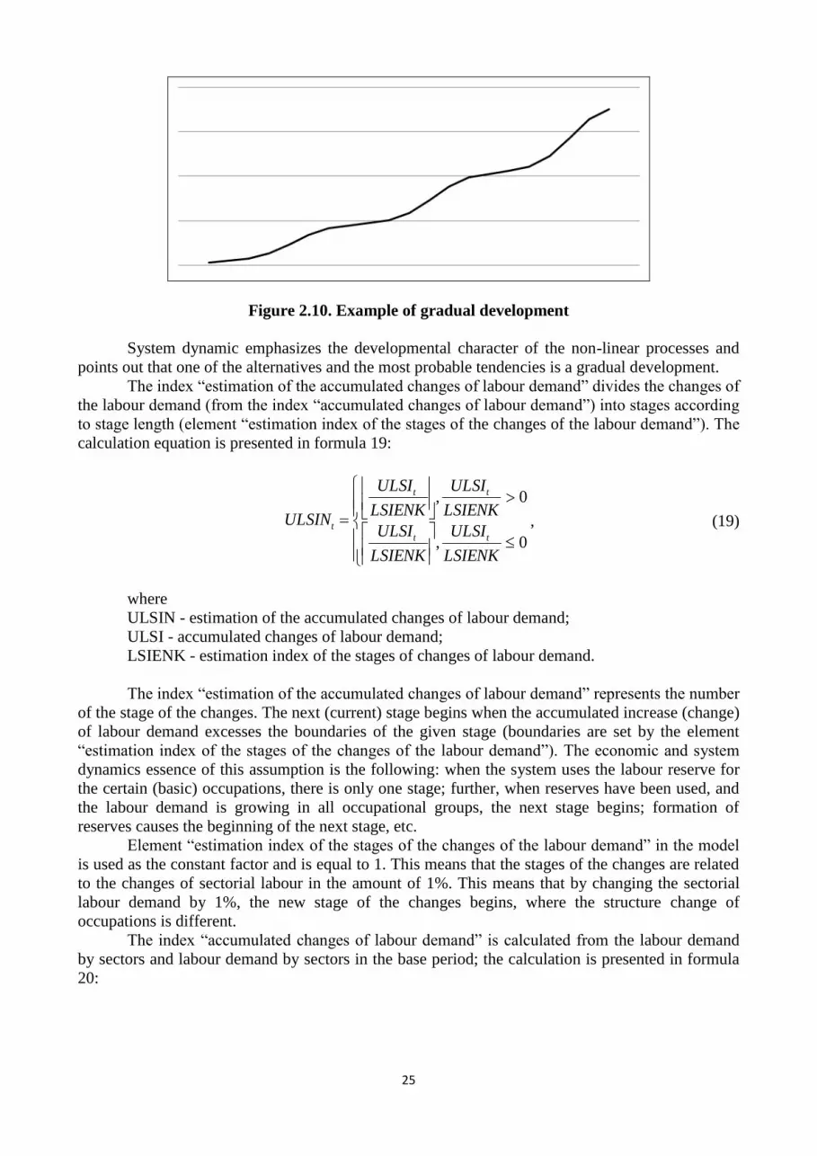
Figure 2.10. Example of gradual development
System dynamic emphasizes the developmental character of the non-linear processes and
points out that one of the alternatives and the most probable tendencies is a gradual development.
The index “estimation of the accumulated changes of labour demand” divides the changes of
the labour demand (from the index “accumulated changes of labour demand”) into stages according
to stage length (element “estimation index of the stages of the changes of the labour demand”). The
calculation equation is presented in formula 19:
0,
0,
LSIENK
ULSI
LSIENK
ULSI
LSIENK
ULSI
LSIENK
ULSI
ULSINtt
tt
t , (19)
where
ULSIN - estimation of the accumulated changes of labour demand;
ULSI - accumulated changes of labour demand;
LSIENK - estimation index of the stages of changes of labour demand.
The index “estimation of the accumulated changes of labour demand” represents the number
of the stage of the changes. The next (current) stage begins when the accumulated increase (change)
of labour demand excesses the boundaries of the given stage (boundaries are set by the element
“estimation index of the stages of the changes of the labour demand”). The economic and system
dynamics essence of this assumption is the following: when the system uses the labour reserve for
the certain (basic) occupations, there is only one stage; further, when reserves have been used, and
the labour demand is growing in all occupational groups, the next stage begins; formation of
reserves causes the beginning of the next stage, etc.
Element “estimation index of the stages of the changes of the labour demand” in the model
is used as the constant factor and is equal to 1. This means that the stages of the changes are related
to the changes of sectorial labour in the amount of 1%. This means that by changing the sectorial
labour demand by 1%, the new stage of the changes begins, where the structure change of
occupations is different.
The index “accumulated changes of labour demand” is calculated from the labour demand
by sectors and labour demand by sectors in the base period; the calculation is presented in formula
20:

26
1001 0
N
Nt
tLS
LSULSI , (20)
where
ULSI - accumulated changes of labour demand;
LSN - labour demand by sectors.
LSN0 - labour demand by sectors in the base period.
Accumulated changes of labour demand reflect the changes of labour demand from the
beginning of forecasting in the base period. Labour demand and labour demand in the base period
are defined in the sub-model of the sectorial labour demand.
The first element affecting the changes of occupational labour demand and occupational
structure (from formula 18), i.e., the index “total changes of labour demand by occupations” is
calculated in formula 21:
NtPNtPNt LSILSStKLSI , (21)
where
KLSIPN - total changes of labour demand by occupations and sectors;
LSStPN - structure of labour demand by occupations and sectors;
LSIN - changes of labour demand by sectors.
The index “total changes of labour demand by occupations” divided changes of labour
demand in accordance with the existing occupational structure. This index does not provide
structural changes.
Structure of labour demand by occupations in the sector is calculated as the labour demand
by occupations and sectors, divided by labour demand in the sector (formula 22):
Nt
PNtPNt
LS
LSLSSt , (22)
where
LSStPN - structure of labour demand by occupations and sectors;
LSPN - labour demand by occupations and sectors;
LSN - labour demand by sectors.
The second element affecting the changes of occupational labour demand and occupational
structure (from formula 18), i.e., the index “changes of the major occupations of the labour
demand” is calculated in formula 23:
PSKLSSt
PSKLSStSPKI
LSILSSt
SPKI
KLSI
SLSI
Pt
Pt
Nt
NtPNt
Nt
PNt
t
,0
, (23)
where
SLSI - the changes of the major occupations of the labour demand;
LSStPN - structure of labour demand by occupations and sectors;
PSK - measure of importance of the occupations;
KLSIPN - total changes of labour demand by occupations and sectors;
SPKIN - the total ratio of the major occupations by sectors;
LSIN - changes of labour demand by sectors.

27
The index “the changes of the major occupations of the labour demand” for the major
occupational groups (for those occupational groups, which ratio in the sector is larger than defined
in the element “measure of importance of the occupations”) determines from the index “total
changes of labour demand by occupations” the total changes of the groups of the major occupations
by sectors. At the same time, other occupational groups (which do not meet the ‘significance”
criteria) will not be changed. Instead of the index “total changes of labour demand by occupations”
the constituent elements from formula 21 may be used, as presented in formula 23.
The economic essence of the mathematical calculation of the index “the changes of the
major occupations of the labour demand” is the following: it determines the changes of the sectorial
labour demand only for major occupational groups.
The calculation of the total ratio of the major occupations is presented in formula 24:
Pi
PSR
PNtNtiLSStSPKI
ii
PNt
ii
PNt
i
PtPSR
PNtPSKLSSt
PSKLSStLSStLSSt i
,0
, , (24)
where
SPKIN - the total ratio of the major occupations by sectors;
LSStPN - structure of labour demand by occupations and sectors;
PSK - measure of importance of the occupations;
P - occupation.
In the index “the total ratio of the major occupations by sectors” are summed up by sector
only those occupations whose ratio exceeds the criterion of the significance of the occupational
group.
The criterion of the significance of the occupational group is taken as a constant index for all
sectors and equals to 3%. This means that the occupations, whose ratio is more than 3%, should be
considered as important or primary occupations. The choice of the index is based on Pareto
principle and is reasoned by statistical data and analysis (see Annex A3). Despite the low level of
the boundary of significance criterion, only a small number of groups of occupations does not
confirm to it. But the same occupational groups are employing the highest number of employees in
the sectors, which is indicated by the total ratio of the sector (see Annex A3).
In the sub-model the element “labour demand by occupations” has reduced number of
dimensions, summing up the labour demand in the occupations by sectors, see formula 25:
Ni
i
PNtPt LSLS , (25)
where
LSP - labour demand by occupations;
LSPN - labour demand by occupations and sectors;
N - sector.
Calculation of the labour demand by occupations in the sub-model has a technical function;
this index is not being used in the sub-model.

28
2.1.3. Modelling labour demand by education
The sub-model of labour demand by education is based on labour demand by occupations,
as well as educational - occupational statistical data, educational - occupational compliance matrix,
and determines the labour demand by levels and fields of education.
In order to ensure the operation of sub-model in the forecasting time the functional sub-
model of the sectorial labour demand, sub-model of the occupational labour demand (with all
incoming indexes and data) should be available, as well as the following statistical data should be
available: 1) data on the number of employees by levels and fields of education of the base year and
2) educational - occupational compliance matrix.
The logic of sub-model is the following: changes of labour demand by occupations are
divided into positive (growth) and negative (decrease) changes. The reduction of labour demand by
occupation leads to reduction of labour demand in proportion to the existing educational structure
(by fields and levels of education). But the increase of the labour demand by occupations leads to
the formation of labour demand with an appropriate education. The correspondence of the education
to the occupation is being determined by the compliance matrix of the occupation (hereinafter
referred to as matrix, educational compliance matrix). Sub-model involves a three-stage algorithm,
which, in accordance with the matrix, determines the formation of the labour demand by fields and
levels of education. At the first stage the labour demand is being calculated according to the matrix
and structure of labour demand by fields and levels of education, at the second stage - in accordance
with the matrix and the structure of labour demand by levels of education, and the at the third stage
- according to a matrix structure, it is being visually presented in figure 2.11.
Labour demand by
education fields, levels
and occupations
Decrease of labour demand byeducation fields, levels and
occupations
Growth of labour demand byeducation fields, levels and
occupations
Labour demand in accordance withthe matrix and structure of labour
demand by education fields and levels
Labour demand in accordance withthe matrix and the structure of labour
demand by education levels
Labour demand inaccordance with the matrix
structure
<Changes of labour
demand by occupations>
Figure 2.11.Logics of the sub-model of labour demand by education
The first mathematical step of the sub-model creating is associated with the division of the
changes of labour demand by occupations into positive (greater than zero) and negative (less than
zero) changes. The negative changes create the reduction of labour demand by field, levels of
education and occupations, but the positive changes create growth. Division of changes into two

29
parts is associated with an application of different algorithm for every part. Division of changes is
presented in figure 2.12.
Changes of labour
demand by occupations
Growth of labour
demand by occupationsDecrease of labour
demand by occupations
<Changes of labourdemand by occupations and
sectors>
Figure 2.12. Transition from the sub-model of occupational labour demand to sub-model of
labour demand by education
Figure 2.12 presents that the index “changes of labour demand by occupations and sectors”
from the sub-model of occupational labour demand is divided into in the indexes of growth and
reduction of labour demand, which will later be used in the sub-model of the educational labour
demand.
Equations of division of changes are shown in formulas 26 and 27:
0,0
0,
Pt
PtPt
PtLSI
LSILSILSS , (26)
0,0
0,
Pt
PtPt
PtLSI
LSILSILSP , (27)
where
LSSP - decrease of labour demand by occupations;
LSPP - growth of labour demand by occupations;
LSIP - changes of labour demand by occupations.
It is important to note that the sub-model of occupational demand does not determine the
index “changes of labour demand by occupations”. This is a simple summing up of the changes of
labour demand by occupations and sectors. The calculation equation is presented in formula 28:
Ni
i
PNtPt LSILSI , (28)
where
LSIP - changes of labour demand by occupations;
LSIPN - changes of labour demand by occupations and sectors;
N - sector.
Formulas 26 – 28 create the transition from the sub-model of occupational labour demand to
sub-model of labour demand by education. These formulas have a support function in the model,
but it is not practicable to create a special sub-model.

30
The sub-model of labour demand by education has only one stock - “labour demand by
fields, levels of education and occupations”. The calculation equation is presented in formula 29:
T
t
0
0
dt )()(t (t) JLPJLPJLPJLP LSSLSPLSLS , (29)
where
LSJLP - labour demand by fields, levels of education and occupations;
LSPJLP - growth of labour demand by fields, levels of education and occupations;
LSSJLP - decrease of labour demand by fields, levels of education and occupations.
The initial level of stock is determined on the basis of statistical data, by the means of
Latvian Occupational Classification (3-digit level of occupation code) of 127 occupational group
units, aggregation of levels of education of 5 units and 79 fields of education (on the basis of the
classification of the Ministry of Education and Science of the Republic of Latvia, third, fourth and
fifth groups). Stock changes are determined by the flows “growth of labour demand by fields, levels
of education and occupations” and “decrease of labour demand by fields, levels of education and
occupations” that divide the changes of labour demand in occupations by levels and fields of
education. This calculation equations are presented in formulas 30 and 31:
tJLPPttJLP LSStLSSLSS , (30)
JLPtJLPtJLPtJLPt LSPMLSPLNLSPALSP , (31)
where
LSSJLP - decrease of labour demand by fields, levels of education and occupations;
LSSP - decrease of labour demand by occupations;
LSStJLP - structure of labour demand by fields, levels of education and occupations;
LSPJLP - growth of labour demand by fields, levels of education and occupations;
LSPAJLP - growth of labour demand by fields, levels of education and occupations in
accordance with the compliance of education to occupation;
LSPLJLP - growth of labour demand by fields, levels of education and occupations in
accordance with the structure of labour demand by educational levels;
LSPMJLP - growth of labour demand by fields, levels of education and occupations in
accordance with the structure of educational compliance matrix.
As seen in formulas 30 and 31, changes of labour demand by fields, levels of education of
education and occupations are also divided into two parts: growth and reduction. Division of
changes into two parts is associated with the application of different algorithms in every part.
Calculation of reduction is simpler, but the growth has the more difficult calculation and consists of
three elements.
At first, the algorithm is being analysed in details and this algorithm is used in the
calculations of reduction of labour demand by fields, levels of education and occupations. Formula
30 shows that it is related to the reduction in labour demand by occupations and structure of labour
demand by fields, levels of education and occupations.
The general scheme of the calculation algorithm of reduction of labour demand by fields,
levels of education and occupations is presented in Figure 2.13.

31
Labour demand byeducation fields, levels and
occupations
Decrease of labour demand byeducation fields, levels and
occupations
Decrease of labour
demand by occupationsStructure of labour demand by
education fields, levels andoccupations
Figure 2.13.The general scheme of the calculation algorithm of reduction of labour demand
by fields, levels of education and occupations
Figure 2.13 shows that the decrease of labour demand by occupations according to the
structure of labour demand by fields, levels of education and occupations is divided into fields,
levels of education and occupations. As a result, it leads to changes of labour demand in the
mentioned dimensions. The economic essence of this algorithm is simple: by reducing the labour
demand in occupation, the labour demand in occupation by education groups decreases in
proportion to labour demand in education groups. The reduction of labour demand by occupations
is analysed in formula 26, but the calculation of the structure of labour demand by fields, levels of
education and occupations is presented in formula 32:
0,0
0,
Lk Ji
ki
JLPt
Lk Ji
ki
JLPt
Lk Ji
ki
JLPt
JLPt
JLPt
LS
LSLS
LS
LSSt , (32)
where
LSStJLP - structure of labour demand by fields, levels of education and occupations;
LSJLP - labour demand by fields, levels of education and occupations;
L - level of education;
J - field of education;
Formula 32 presents that the structure of labour demand by fields, levels of education and
occupations is being calculated by dividing the labour demand by fields, levels of education and
occupations (matrix) by the total labour demand in the occupation by fields and levels of education
(vector).
Additionally, formula 32 shows that under specific conditions (when there is not employed
any person in the occupation and /or there is no labour demand in the occupation) it is not
mathematically possible to calculate the structure of labour demand. Under these conditions,
formula 32 assigns 0 value (no structure) for all elements related to occupations.
The growth of labour demand by fields, levels of education and occupations (formula 31) is
divided into three parts:
1) in accordance with the education-occupational compliance, including the ratio of fields
and levels of education;
2) in accordance with the education-occupational compliance, including the ratio of levels of
education;
3) in accordance with the education-occupational compliance.

32
Each of these three algorithms divides the growth of labour demand in occupation by fields
and levels of education, and is forming a single three-step algorithm. The general scheme of
algorithm calculation of the growth of labour demand by fields, levels of education and occupations
is presented in the Figure 2.14.
Growth of labour
demand by occupations
Growth of labour demand by the education
fields, levels and occupations, in
accordance with the compliance of
education to the occupation
Growth of labour demand by the education
fields, levels and occupations, in accordance
with the structure of labour demand by
education levels
Growth of labour demand by the education
fields, levels and occupations, in accordance
with the structure of the educational
compliance matrix
Growth of labour demand bythe education fields, levels and
occupations
Growth of labour demand by
occupations, without regard to the
compliance of education to the
requirements of occupation
Growth of labour demand by occupations,
without regard to the compliance of education to
the requirements of occupation and structure of
labour demand by education levels
Figure 2.14 The general scheme of algorithm calculation of the growth of labour demand by
fields, levels of education and occupation
With the growth of labour demand in occupations, only the specialists with the appropriate
education should be employed, taking into account the level and field of education, which is the
first priority of the model (or division of the growth of labour demand by fields and levels of
education at the first stage of the algorithm). It is not always possible to employ the specialists with
appropriate education. In this case, the growth of labour demand in occupations, which were not
previously divided by educational groups, is being divided in accordance with the structure of levels
of education (only those specialists are being employed, whose level of education meets the
occupational requirements), which the second priority of the model. Theoretically, there is one more
algorithm of growth of labour demand by education groups and occupations: when the new
occupations are being created, or the occupation has new educational requirements and / or no
employee does not correspond to the occupation. In this case there may not be occupational and
educational structure, and employees should be recruited directly in accordance with the
requirements for their education. This is the third model priority, which analyses only the undivided
growth of labour demand in the first two priorities. Each of these algorithms of growth of labour
demand will be analysed separately - the first is the growth of labour demand by the levels of
education and occupations, taking into account the compliance of education to the requirements of
the occupation, whose calculation equation is presented in formula 33:
PtJLPtJLPt LSPLSStALSPA , (33)
where
LSPAJLP - growth of labour demand by fields, levels of education of education and
occupations, in accordance with the compliance of education to requirements of occupation;
LSStAJLP - structure of labour demand in the occupation with the appropriate education by
fields and levels of education;
LSPP - growth of labour demand by occupations.
Formula 33 shows that the growth of labour demand by occupations is divided into fields,
levels of education in accordance with the structure of labour demand in the occupation with the
appropriate education. The compliance of the occupations and education is determined by the

33
educational compliance matrix. Calculation of the structure of labour demand with the appropriate
education is presented in formula 34:
0,0
0,
Lk Ji
ki
JLPt
Lk Ji
ki
JLPt
Lk Ji
ki
JLPt
JLPt
JLPt
LSA
LSADSPA
LSA
LSStA , (34)
where
LSStAJLP - structure of labour demand in the occupation with the appropriate education by
fields and levels of education;
LSAJLP - labour demand in the occupation with the appropriate education by fields and
levels of education.
Structure of labour demand in the occupation with the appropriate division of education by
fields and levels of education is being calculated by dividing the labour demand in the occupation
by the appropriate education by fields and levels of education (matrix) with a total labour demand in
the occupation with the appropriate education (vector).
Additionally, formula 34 shows that under specific conditions (when the occupation does
not employ any person and/or there is no labour demand in the occupation) it is not mathematically
possible to calculate the structure of labour demand. Under these conditions, formula 34 assigns 0
value (no structure) for all elements related to occupations.
Calculation of labour demand in occupation with the appropriate education by fields and
levels of education is presented in formula 35:
IAMLSLSA JLPtJLPt , (35)
where
LSAJLP - labour demand in the occupation with the appropriate education by fields and
levels of education;
LSJLP - labour demand by fields, levels of education and occupations;
IAM - educational compliance matrix.
Labour demand in the occupation with the appropriate education by fields and levels of
education is being calculated by multiplying the labour demand by fields, levels of education and
occupations by educational compliance matrix. In this way, the labour demand is being selected
from the total demand, which refers to the occupations with the appropriate education. Beforehand
it is presented (formula 34) how their structure, according to which the growth of labour demand is
divided into educational fields and levels (formula 33), is calculated.
Theoretically, this algorithm should fully support the growth of labour demand in
occupations by fields and levels of education. In practice, the quality of the educational compliance
matrix as well as the quality of statistical data has a huge impact. If the educational compliance
matrix determines that a specific education is necessary for the occupational performance, but
statistics shows that there are no employed persons with the appropriate education in the
occupation, the algorithm will never ensure the growth of labour demand in the analysed
occupations with the appropriate education. In order to close this, the algorithm of the growth of
labour demand by fields and levels of education is complemented with two other parts (sub-
algorithms). It is described in more detail below.

34
As stated above, the sub-algorithm does not fully ensure the division of occupational labour
demand by fields and levels of education. The division level is being calculated in the model
(formula 36):
Lk Ji
ki
JLPtPt LSPALSPA , (36)
where
LSPAP - growth of labour demand by occupations, in accordance with the compliance of
education to the requirements of occupation;
LSPAJLP - growth of labour demand by fields, levels of education of education and
occupations, in accordance with the compliance of education to occupation;
L - level of education;
J - field of education.
In fact, formula 36 presents the return path: the growth of labour demand by fields, levels of
education and occupations has the reduced aggregation to occupational level. It allows analysing the
divided labour demand in terms of occupation by fields and levels of education, as well as to
compare it to the growth of labour demand by occupations, which are presented in formula 37:
PtPtPt LSPALSPLSPnA , (37)
where
LSPnAP - growth of labour demand by occupations, without regard to the compliance of
education to the requirements of occupation;
LSPP - growth of labour demand by occupations;
LSPAP - growth of labour demand by occupations, in accordance with the compliance of
education to the requirements of occupation.
By subtracting the divided growth of labour demand in terms of occupation from the growth
of labour demand by occupations, the “undivided balance” is being calculated, which needs to be
divided later. In the model it is marked as “growth of labour demand by occupations, without regard
to compliance of education to the requirements of occupation”.
The second stage sub-algorithm of the growth of labour demand by occupations is related to
the structure of labour demand levels of education. This sub-algorithm divided previously
undivided growth of labour demand by educational levels. This algorithm is simple, and the essence
is the following: in accordance with the structure of labour demand by educational levels,
previously undivided growth of labour demand by occupations and structure of educational
compliance matrix the growth of labour demand by fields, levels of education and occupations is
being calculated (formula 38):
JLPtLPtPtJLPt IAMSLLSStLSPnALSPL , (38)
where
LSPLJLP - growth of labour demand by fields, levels of education and occupations, in
accordance with the structure of labour demand by levels of education;
LSPnAP - growth of labour demand by occupations, without regard to the compliance of
education to the occupation;
LSStLP - structure of labour demand by levels of education and occupations;
IAMSLJLP - structure of educational compliance matrix by levels of education.
35
The elements, presented in formula 38, define only the growth of labour demand by
occupations, without regard to the compliance of the education to the occupation. Structure of
labour demand by levels of education and occupations is calculated in formula 39, but the
calculation of the structure of educational compliance matrix is presented in formula 40:
Jk Li Pn
kin
JLPt
Ji
i
JLPt
LPtLS
LS
LSSt , (39)
where
LSStLP - structure of labour demand by levels of education and occupations;
LSJLP - labour demand by fields, levels of education and occupations;
L - level of education;
J - field of education;
P - occupation.
0,0
0,
Jk
k
Jk
k
Jk
k
JLPt
IAM
IAMIAM
IAM
IAMSL , (40)
where
IAMSLJLP - structure of educational compliance matrix by levels of education;
IAM - educational compliance matrix;
J - field of education.
At the second stage the observation of three components in formula 38 divides the demand
on occupations of labour by educational levels in accordance with existing structure of labour
demand educational levels, and further, without the regard to the current labour demand and its
structure, according to the educational compliance matrix structure, divides into fields of education.
This action allows reducing the effect of the lack of statistical data and educational compliance
matrix, and changes the structure of labour demand under specific circumstances, for example,
when the new educational requirements arise.
However, the second stage sub-algorithm does not ensure an adequate functioning of the
model for new occupations or occupations that have not previously employed any people. The
growth of labour demand by occupations will not be divided by fields and levels of education. In
order to avoid the possible problem, the division of the growth of occupational labour demand at the
third stage is being offered. But before the examination it is necessary to determine the level of
labour demand, which is not divided into occupations and education groups at the first two stages.
Second stage level is calculated in a similar way to first stage level, i.e., by determining the divided
volume in the sub-algorithm, and calculating the difference between divided and undivided labour
demand (formulas 41 and 42):

36
Lk Ji
ki
JLPtPt LSPLLSPL , (41)
PtPtPt LSPLLSPnALSPnAL , (42)
where
LSPLP - growth of labour demand by occupations, in accordance with the structure of labour
demand by levels of education;
LSPLJLP - growth of labour demand by fields, levels of education and occupations, in
accordance with the structure of labour demand by levels of education;
L - level of education;
J - field of education;
LSPnALP - growth of labour demand by occupations, without regard to the compliance of
education to the requirements of occupation and structure of labour demand by levels of education;
LSPnAP - growth of labour demand by occupations, without regard to the compliance of
education to the requirements of occupation.
The calculated growth of labour demand by occupations, without regard to the compliance
with the requirements of the occupation and structure of labour demand by levels of education,
further, at the third stage, is divided in direct ratio to educational compliance matrix. This means
that if the occupation required the single-field and single-level education, the entire growth of
labour demand in the occupation causes the demand only in a single education group, if the
education is required in two groups, this causes the demand in two education groups in the same
proportion, etc.
This sub-algorithm defines the structure of educational matrix (formula 43) and in
accordance to this, the growth of labour demand by fields, levels of education and occupations, in
accordance with the structure of educational compliance matrix, is being calculated (formula 44):
0,0
0,
Lk Ji
ki
Lk Ji
ki
Lk Ji
ki
JLP
IAM
IAMIAM
IAM
IAMSM , (43)
JLPPtJLPt IAMSMLSPnALLSPM , (44)
where
IAMSMJLP - structure of educational compliance matrix;
IAM - educational compliance matrix;
LSPMJLP - growth of labour demand by fields, levels of education and occupations, in
accordance with the structure of the educational compliance matrix;
LSPnALP - growth of labour demand by occupations, without regard to the compliance of
education to the requirements of occupation and structure of labour demand by levels of education.
The analysed three-step algorithm allows adequate division of the growth of labour demand
by fields and levels of education.
2.1.4. Modelling labour demand by gender
The sub-model of labour demand by gender is being based on the sub-model of the labour
demand by occupations, as well statistical data on gender and occupations, and determines the
labour demand by gender.

37
In order to ensure the operation of the sub-model at the forecasting time, the sub-model of
sectorial labour demand, sub-model of occupational labour demand (with all those incoming
indexes and data), as well as statistical data on the number of employees by occupations and gender
in the base year should be available.
Some elements are taken from the sub-model of labour demand by education, but they are
calculated in the sub-model of labour demand by education on the basis of the other sub-models.
They have input data functions in the sub-model of labour demand by education; the given sub-
model has no effect on them. They can be calculated in other sub-models, so that would indicate
that the sub-model of labour demand by gender technically (functionally) is related to the sub-
model of labour demand by education. But there is no full functional relationship between these two
sub-models.
The sub-model of labour demand by gender has only one stock - “labour demand by fields,
levels of education, occupations and gender”. The calculation equation is presented in formula 45:
T
t
0
0
dt )()(t (t) JLDPJLDPJLDPJLDP LSSLSPLSLS , (45)
where
LSJLDP - labour demand by fields, levels of education, occupations and gender;
LSPJLDP - growth of labour demand by fields, levels of education, occupations and gender;
LSSJLDP - decrease of labour demand by fields, levels of education, occupations and gender;
Stock level in the base period is determined from statistical data. Stock changes determine
the flow of “growth of labour demand by occupations and gender” and “decrease of labour demand
by occupations and gender”. These calculation equations are presented in formulas 46 and 47:
DPtJLPtJLDPt LSStLSPLSP , (46)
DPtJLPtJLDPt LSStLSSLSS , (47)
where
LSPJLDP - growth of labour demand by fields, levels of education, occupations and gender;
LSSJLDP - decrease of labour demand by fields, levels of education, occupations and gender;
LSPJLP - growth of labour demand by fields, levels of education and occupations;
LSSJLP - decrease of labour demand by fields, levels of education and occupations;
LSStDP - structure of labour demand by occupations and gender.
By analysing the equations of changes of labour demand by occupations and gender, it is
evident that the changes by gender are associated with changes in the occupations and observe the
structure of labour demand by occupations and gender. The similar equations are used for the
growth and decrease of labour demand by occupations and gender, as well as a single algorithm is
being used. This is done in order to facilitate the further model development: the further
perspective, by combining the sub-models of gender supply and demand, decrease of the number of
employees by gender would be associated with the decrease of gender demand, but the growth
would be corrected in accordance with the supply structure.
The calculation equation of the structures of labour demand by occupations and gender are
presented in formula 48:
38
0,0
0,
Jk Ln Di
kni
JLDPt
Jk Ln Di
kni
JLDPt
Jk Ln Di
kni
JLDPt
Jk Ln
kn
JLDPt
DPt
LS
LSLS
LS
LSSt , (48)
where
LSStDP - structure of labour demand by the occupations and gender;
LSJLDP - labour demand by fields, levels of education, occupations and gender;
D - gender.
Structure of labour demand by occupations and is calculated by dividing the labour demand
by occupations and gender (matrix) with the labour demand by gender (vector).
Additionally, formula 47 shows that under specific conditions (when the occupation does
not employ any person and/or there is no labour demand in the occupation) it is not mathematically
possible to calculate the structure of labour demand. Under these conditions, formula 47 assigns 0
value (no structure) for all elements related to occupations.
In order to ensure the observance of the requirements of MoE for the obtained results, labour
demand by occupations and gender has the reduced the number of dimensions, by summing up the
labour demand for gender by occupations, formula 49:
Jk Ln Pi
kni
JLDPtDt LSLS , (49)
where
LSD - labour demand by gender;
LSDP - labour demand by occupations and gender;
P - occupations.
The calculation of the labour demand by gender in the sub-model has largely a technical
function; this index is not being used in the sub-model.

39
2.2. Labour supply module
Labour supply module simulates the demographic processes, division of the population by
ages, gender, economic activity, education and occupation. Labour supply module consists of sub-
models of demography, education attainment, working-age population stock-taking, labour force
participation and international migration. Module structure is being presented in the Figure 2.15.
Labour supply module of SDM model
Demographic
sub-model
Education
attainment
sub-model
Working-age
population
stock-taking
sub-model
Labour force
participation
sub-model
International
migration
sub-model
Figure 2.15. Logical structure of labour supply module
In the demographic sub-model of labour supply module the population is defined by age for
one-year groups and gender. This sub-model defines the birth rate, mortality and aging of
population. By reaching the age of seven years, the demographic sub-model defines the incoming
population of education system. By reaching working age, the demographic sub-model defines the
labour growth (in working-age population stock-taking sub-model), in accordance with prior
education (education attainment sub-model) and the anticipated economic activity (labour force
participation sub-model). By reaching retirement age, demographic sub-model defines the labour
decrease. The same happens in case of death before retirement age.
Working-age population stock-taking sub-model represents the labour structure by 5-year
age groups, gender, economic activity, education and occupations, that is, represent the operating
results of other sub-models.
Labour force participation sub-model defines the labour structure in the field of economic
activity.
Education attainment sub-model defines not only the increase of the primary labour volume
(along with demographic sub-model), but also the changes of the labour along with education
attainment, including lifelong education.
International migration sub-model defines the change of population and labour along with
international migration processes.
The sub-models of labour demand module are examined in the following subsections.
2.2.1. Demographic sub-model
For the demographic modelling in SDM model the classical scheme is being applied: the
central place belongs to population stock; it can be complemented by incoming flows (e.g., birth

40
rate), devastated by outgoing flows (such as mortality), as well as the age structure can be changed
by the means of aging algorithm.
Before the identification of the SDM demographic sub-model structure, the connection with
other sub-models is being examined.
Birth rate should be dependent on the economic situation in the country, i.e. GDP per capita.
For this purpose, the new element of “GDP per capita” is being created in the model. In order to
make the model more user friendly, this element is calculated automatically from the existing model
parameters.
The elements related to GDP per capita and the calculation of its changes is presented in
Figure 2.16.
Total GDP per
capitaTotal GDP per capita in
the previous period
Growth rate of the total
GDP per capita
<Population>
<GDP>
Figure 2.16. GDP per capita and the calculation of its changes
Figure 2.16 represents that the algorithm consists of three elements: GDP per capita, the
established GDP per capita in the previous period, and the GDP growth rate. Total GDP per capita
is being calculated by summing up GDP by sectors and dividing it by the total population; its
calculation equation is presented in formula 50:
Vi Dj
ij
DVt
Nk
k
Nt
tI
GDP
GDPI , (50)
where
GDPI - total GDP per capita;
GDPN - GDP forecasts by sectors;
IVD - population;
V - age;
D - gender.
For calculation of total GDP per capita the used GDP is derived from the labour demand
module and has been considered above, but the population will be analysed further.
Total GDP per capita is being delayed by one year, thus, calculating the total GDP per capita
in the previous period (see formula 51):
1 tt IKPIIPIKPI , (51)
where
IPIKPI - total GDP per capita in the previous period;
GDPI - total GDP per capita.
It is possible to calculate the GDP growth rate from the total GDP per capita and total GDP
per capita in the previous period (see formula 52):
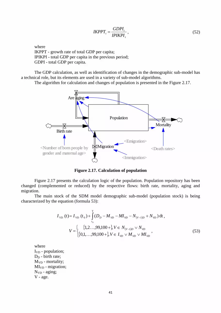
41
t
tt
IPIKPI
GDPIIKPPT , (52)
where
IKPPT - growth rate of total GDP per capita;
IPIKPI - total GDP per capita in the previous period;
GDPI - total GDP per capita.
The GDP calculation, as well as identification of changes in the demographic sub-model has
a technical role, but its elements are used in a variety of sub-model algorithms.
The algorithm for calculation and changes of population is presented in the Figure 2.17.
Population
Are aging
Birth rate
Mortality
Migration<Number of born people by
gender and maternal age><Death rates>
<Emigration>
<Immigration>
Figure 2.17. Calculation of population
Figure 2.17 presents the calculation logic of the population. Population repository has been
changed (complemented or reduced) by the respective flows: birth rate, mortality, aging and
migration.
The main stock of the SDM model demographic sub-model (population stock) is being
characterized by the equation (formula 53):
T
t
10VDVD
0
dt )()(t (t) VDDVVDVDD NNMIMDII ,
VDVDVD
VDDV
MIMIV
NNVV
,100,99,,1,0
,100,99,2,1
1
, (53)
where
IVD - population;
DD - birth rate;
MVD - mortality;
MIVD - migration;
NVD - aging;
V - age.

42
By analysing formula 53, it is evident that the population is dependent on the initial level
and changes, consisting of birth rate, mortality, migration and aging. Aging is increasing the
population of certain ages and at the same time reducing the population of younger ages. The aging
dimension is being reduced by one group (0 years old), as it not possible to calculate the population
that is one year younger than this age.
Aging is the only element in formula 53, which calculation does not involve a special
algorithm; its calculation is simple and is described in one equation. Therefore, the further
explanation of the model is being started from this element. Aging calculation equation is presented
in formula 54:
1-tD1-V1-tD1-V1-tD1-VVDt MIMIN ,
100,99,,2,1 V , (54)
where
NVD - aging;
IVD - population;
MVD - mortality;
MIVD - migration;
V - age.
By analysing the 54 equation, it is visible that the change of population (aging) in the
current period, for the relevant age depends on the previous period's population that is one year
younger, and from the mortality and migration of this group. Aging determines decrease of
population of 0 age, and both decrease and increase of other ages.
Formula 55 presents the birth rate flow:
Vi
i
DVtDt DD , (55)
where
DD - birth rate;
DDV - the number of born people by gender and maternal age;
V - age.
Birth rate equation sums up the number of born people by maternal age, preserving a
separation by gender. The number of new-borns by gender and maternal age is the result of the birth
rate calculation algorithm, which will be considered further.
Formula 56 presents the mortality flow:
VDtVDtVDt MKIM , (56)
where
MVD - mortality;
IVD - population;
MKVD - death rates.
The mortality is being calculated by multiplying the mortality index for one-year age groups
and by gender by a population in the corresponding groups. Mortality index reflects the result of the
mortality index calculation algorithm, which will be considered further.
Calculation of migration is presented in formula 57:

43
VDtVDtVDt IMEMMI , (57)
where
MIVD - migration;
EMVD - emigration;
IMVD - immigration.
Migration flow represents the balance of emigration and immigration.
Then the flow-forming algorithms will be analysed, the first of which is related to birth rate.
Birth rate algorithm is a complex, which can be explained in two stages: changes of birth
rate index in accordance with the changes in GDP and changes of birth rate in accordance with birth
rate index and demographic changes. It is visually represented in Figure 18.2.
Algorithm of changes
of birth rate indexAlgorithm of changes
of birth rate
<GDP> <Population>
Figure 2.18. Birth rate calculation algorithm
The description of birth rate calculation algorithm starts from the change of birth rate index
algorithm.
Considering GDP per capita, there are two calculation sub-algorithms of birth rate index:
one - for reduction of GDP per capita, and the other - for growth of GDP per capita. Algorithms
reflect GDP impact on the birth rate indexes: by growing GDP increases birth rate index, by
reducing GDP, decreases birth rate index. Decrease of birth rate index in case of reducing GDP is
being characterized by formula 58:
ttt IKPPTDKSDKSSA , (58)
where
DKSSA - total birth rate per woman of reproductive age in case of GDP reduction;
IKPPT - total growth rate of GDP per capita;
DKS - birth rate per woman of reproductive age.
As we can see in formula 58, the total birth rate per woman of reproductive age in case of
GDP reduction (i.e., birth rate index) is directly dependent on changes of GDP per capita. The
decrease of GDP per capita causes the same decrease of the birth rate index. This model equation
has been composed on the basis of available statistics of decrease of GDP. The next formula 59
analyses the birth rate index in case of GDP growth:
tt IPIKPIDKRKDKNDDKSPA , (59)
where
DKSPA - total birth rate per woman of reproductive age in case of GDP growth;
DKND - independent part of birth rate index;
DKRK - regression index of birth rate index;
IPIKPI - total GDP per capita in the previous period.
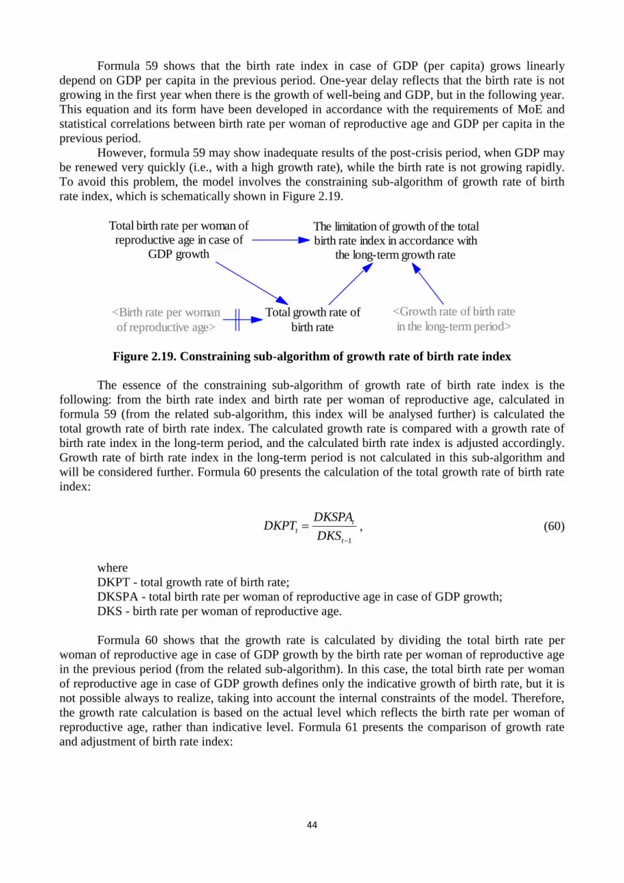
44
Formula 59 shows that the birth rate index in case of GDP (per capita) grows linearly
depend on GDP per capita in the previous period. One-year delay reflects that the birth rate is not
growing in the first year when there is the growth of well-being and GDP, but in the following year.
This equation and its form have been developed in accordance with the requirements of MoE and
statistical correlations between birth rate per woman of reproductive age and GDP per capita in the
previous period.
However, formula 59 may show inadequate results of the post-crisis period, when GDP may
be renewed very quickly (i.e., with a high growth rate), while the birth rate is not growing rapidly.
To avoid this problem, the model involves the constraining sub-algorithm of growth rate of birth
rate index, which is schematically shown in Figure 2.19.
Total birth rate per woman ofreproductive age in case of
GDP growth
Total growth rate of
birth rate
The limitation of growth of the totalbirth rate index in accordance with
the long-term growth rate
<Growth rate of birth rate
in the long-term period><Birth rate per woman
of reproductive age>
Figure 2.19. Constraining sub-algorithm of growth rate of birth rate index
The essence of the constraining sub-algorithm of growth rate of birth rate index is the
following: from the birth rate index and birth rate per woman of reproductive age, calculated in
formula 59 (from the related sub-algorithm, this index will be analysed further) is calculated the
total growth rate of birth rate index. The calculated growth rate is compared with a growth rate of
birth rate index in the long-term period, and the calculated birth rate index is adjusted accordingly.
Growth rate of birth rate index in the long-term period is not calculated in this sub-algorithm and
will be considered further. Formula 60 presents the calculation of the total growth rate of birth rate
index:
1
t
t
tDKS
DKSPADKPT , (60)
where
DKPT - total growth rate of birth rate;
DKSPA - total birth rate per woman of reproductive age in case of GDP growth;
DKS - birth rate per woman of reproductive age.
Formula 60 shows that the growth rate is calculated by dividing the total birth rate per
woman of reproductive age in case of GDP growth by the birth rate per woman of reproductive age
in the previous period (from the related sub-algorithm). In this case, the total birth rate per woman
of reproductive age in case of GDP growth defines only the indicative growth of birth rate, but it is
not possible always to realize, taking into account the internal constraints of the model. Therefore,
the growth rate calculation is based on the actual level which reflects the birth rate per woman of
reproductive age, rather than indicative level. Formula 61 presents the comparison of growth rate
and adjustment of birth rate index:

45
tttt
tt
ttt
t DKPTDKPTIPDKSPADKSDKPTDKPTIP
DKPTDKPTIPDKSPA
DKPTiIPT,
2
,
, (61)
where
DKPTiIPT - limitation of total birth rate index growth in accordance with the long-time
growth rate;
DKSPA - total birth rate per woman of reproductive age in case of GDP growth;
DKPTIP - growth rate of birth rate in the long-term period;
DKPT - total growth rate of birth rate;
DKS - birth rate per woman of reproductive age.
Formula 61 shows that, if the growth rate of the birth rate index in the long-term period is
greater than in the current period, the birth rate index is not being changed, however, if the growth
rate of the birth rate in the current period is greater than the changes in the long-term period, the
birth rate is adjusted. The average growth rate in the current and long-term period are being
calculated for the adjustment, and the average annual growth rate is being multiplied by the birth
rate per woman of reproductive age (i.e., the birth rate index), the resulting element being compared
to the index “total birth rate per woman of reproductive age in case of GDP growth” and the
minimal index is being selected to prevent the exceed of the constrained index over the limitable
index. In the result this equation provides a gradual increase of birth rate without the “acceleration”
after of GDP crises.
The regression equation, applied in formula 59, has the disadvantage that it has a linear
form. However, having examined the statistical data, this form reflects the reality of the last decade
better than other forms. The linear regression equation indicates an infinite growth in case of
infinite GDP growth, but this does not correspond to statistics or theoretical assumptions. Upon
achievement of certain level, GDP growth does not cause the growth of birth rate. So the constraint
should be introduced into the equation, which causes the stop of the growth of birth rate. This
constraint is being analysed in formula 62:
ttt
ttt
tDKPTiIPTDKSMDKSM
DKPTiIPTDKSMDKPTiIPTDKPTiMR
,
, , (62)
where
DKPTiMR - limitation of total birth rate index growth in accordance with the maximum
threshold;
DKPTiIPT - limitation of total birth rate index growth in accordance with the long-time
growth rate;
DKSM - maximum total birth rate per woman.
Formula 62 shows that until the birth rate is less than the set constraint, it is not being
adjusted, but above this constraint the birth rate is being replaced by the maximum birth rate. The
maximum birth rate constraint in the model is set at the average EU level.
So, it was investigated the calculation of the birth rate index in case of GDP reduction
(formula 58) and GDP growth (formulas 59 - 62). The next equation (formula 63) presents the
choice of index, depending on the changes of GDP:
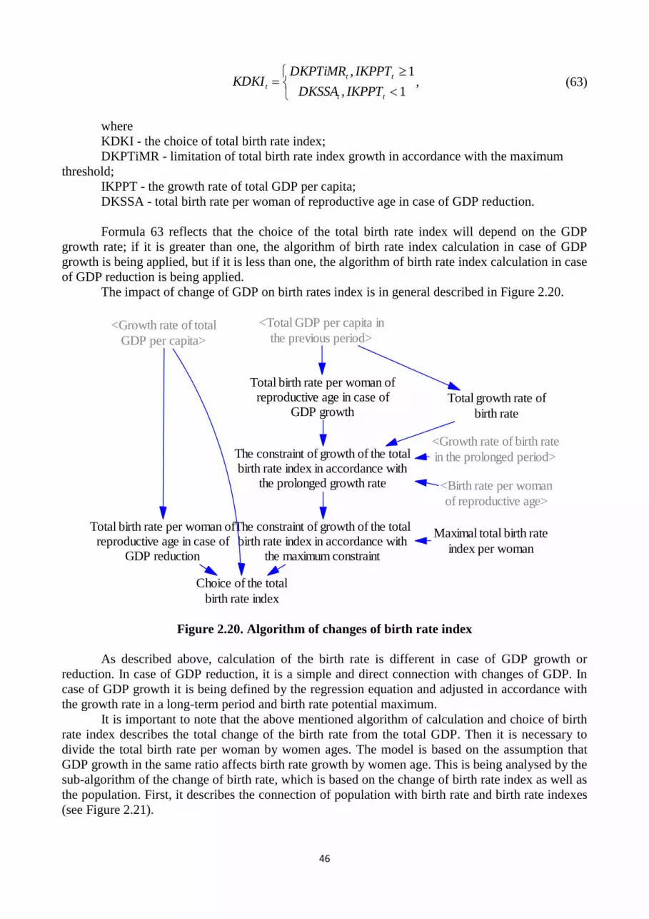
46
1,
1,
tt
tt
tIKPPTDKSSA
IKPPTDKPTiMRKDKI , (63)
where
KDKI - the choice of total birth rate index;
DKPTiMR - limitation of total birth rate index growth in accordance with the maximum
threshold;
IKPPT - the growth rate of total GDP per capita;
DKSSA - total birth rate per woman of reproductive age in case of GDP reduction.
Formula 63 reflects that the choice of the total birth rate index will depend on the GDP
growth rate; if it is greater than one, the algorithm of birth rate index calculation in case of GDP
growth is being applied, but if it is less than one, the algorithm of birth rate index calculation in case
of GDP reduction is being applied.
The impact of change of GDP on birth rates index is in general described in Figure 2.20.
<Total GDP per capita in
the previous period><Growth rate of total
GDP per capita>
Total birth rate per woman ofreproductive age in case of
GDP reduction
Total birth rate per woman ofreproductive age in case of
GDP growthTotal growth rate of
birth rate
<Growth rate of birth rate
in the prolonged period>
<Birth rate per woman
of reproductive age>
The constraint of growth of the totalbirth rate index in accordance with
the prolonged growth rate
The constraint of growth of the totalbirth rate index in accordance with
the maximum constraint
Maximal total birth rate
index per woman
Choice of the total
birth rate index
Figure 2.20. Algorithm of changes of birth rate index
As described above, calculation of the birth rate is different in case of GDP growth or
reduction. In case of GDP reduction, it is a simple and direct connection with changes of GDP. In
case of GDP growth it is being defined by the regression equation and adjusted in accordance with
the growth rate in a long-term period and birth rate potential maximum.
It is important to note that the above mentioned algorithm of calculation and choice of birth
rate index describes the total change of the birth rate from the total GDP. Then it is necessary to
divide the total birth rate per woman by women ages. The model is based on the assumption that
GDP growth in the same ratio affects birth rate growth by women age. This is being analysed by the
sub-algorithm of the change of birth rate, which is based on the change of birth rate index as well as
the population. First, it describes the connection of population with birth rate and birth rate indexes
(see Figure 2.21).

47
PopulationBirth rate
Number of born people by
gender and maternal ageNumber of women
<Birth rate
indexes>
Figure 2.21. Connection of birth rate, birth rate index and population
Population and birth rates have been analysed previously (in formulas 53 and 55, Figures
2.17 and 2.18). The main thing, reflected by Figure 2.21 is that the women are being selected, while
maintaining the age structure and the selected number is being multiplied by the birth rate, thus
obtaining the number of born people by gender and maternal age.
Calculation of the number of women is presented in formula 64, but the number of born
people by gender and maternal age - in formula 65:
SDIS VDtVt , , (64)
where
SV - number of women;
IVD - population;
D - gender;
S - female gender.
VtDSVtDVt SDKD , (65)
where
DDV - number of born people by gender and maternal age;
SV - number of women;
DKDSV - birth rate index.
In the previous equations (formulas 58 - 63) the total birth rate (per woman of reproductive
age) has been analysed. Formula 65 shows the birth rate indexes by gender and maternal age. In
order to combine the total birth rate index (scalar) and birth rate (matrix which reflects indexes by
gender and maternal age), the model involves sub-algorithm of changes of birth rate, presented in
Figure 2.22.

48
Calculated birth
rate indexes
<Choice of the total
birth rate index>Birth rate per woman of
reproductive age
<Number of born people
by age and maternal age>
<Number of
women>Number of women of
reproductive age
Birth rate
indexes Changes of birth
rate indexes
Figure 2.22. Algorithm of changes of birth rate index
Figure 2.22 presents that the women of reproductive age have been selected from the total
number of women. The birth rate per woman of reproductive age (ie overall index, scalar value) is
being calculated form the number of born people by gender and maternal age. This index represents
the total birth rate, taking into account the population. This can be compared to the “choice of total
birth rate index”, which shows, which should be the birth rate index, considering the changes of
GDP. As the birth rate per woman of reproductive age is being expressed in the birth rate, it can be
called as the total actual birth rate.
By dividing the index of “choice of total birth rate” by birth rate per woman of reproductive
age (or actual total birth rate index), it is possible to determine which changes should take place in
the birth rate in accordance with the changes of GDP and population. By multiplying the expected
changes of the birth rate, the “calculated birth rate indexes” are being calculated, i.e., which should
be the birth rate indexes in accordance with the changes of GDP and population.
Birth rates indexes are being changed in accordance with the difference between the birth
rate indexes and calculated birth rate indexes, i.e. the change of birth rate indexes.
The main part in this algorithm belongs to the birth rate stock, which is presented in formula
66:
T
t
0DSVDSV
0
dt)(t (t) DSVDKIDKDK , (66)
where
DKDSV - birth rate indexes;
DKIDSV - change of birth rate indexes.
Calculation of the change of birth rate indexes is presented in formula 67:
DSVtDSVtDSVt ADKDKDKI , (67)
where
DKIDSV - change of birth rate indexes;
DKDSV - birth rate indexes;
ADKDSV - calculated birth rate indexes.
Determination of the calculated birth rate indexes is presented in formula 68:

49
t
t
DKS
KDKIDKADK DSVtDSVt , (68)
where
ADKDSV - calculated birth rate indexes;
DKDSV - birth rate indexes;
KDKI - choice of the total birth rate index;
DKS - birth rate per woman of reproductive age.
Calculation of birth rate per woman of reproductive age is presented in formula 69, but the
calculation of the number of women of reproductive age is presented in formula 70:
Vi
i
Vt
Vi Dj
ij
DVt
SR
D
DKSt , (69)
where
DKS - birth rate per woman of reproductive age;
SRV - number of women of reproductive age;
DDV - number of born people by gender and maternal age;
D - gender;
V - age.
}45,44,,16,15{,Vt VSSR Vt , (70)
where
SRV - number of women of reproductive age;
SV - number of women;
V - age.
By explaining the birth rate algorithm, another index should be considered - the growth rate
of birth rate in the long-term period, which has been used in formula 60. The growth rate of birth
rate in the long-term period has been analysed in formula 71:
1
it
itt
tDKS
i
DKSDKS
DKPTIP , (71)
where
DKPTIP - growth rate of birth rate in the long-term period;
DKS - birth rate per woman of reproductive age;
i -birth rate distribution time.
Formula 71 shows that at first the difference between the birth rate in the beginning and in
the end of the period is being determined, then the difference is being divided by the number of
years in the long-term period, obtaining the average annual changes; the average annual changes are
divided by the initial birth rate index, i.e., obtaining relative index. This sub-section will be
continued with the mortality algorithm interpretation. Figure 2.23 represents the mortality index
creating algorithm.

50
Balanced death rates in
the prolonged period
Change of death rate inaccordance with GDP
growthMortality response of
changes in GDP
<Growth rate of total
GDP per capita>Death rate
Death rate
variance
Figure 2.23. Death rate creating algorithm
Death rates creating algorithm as an exogenous index is using GDP growth rate. By
multiplying it by the regression index “mortality response to changes of GDP” the changes of death
rates are being calculated, taking into account GDP growth. Death rates are calculated in
accordance with the death rates variance, caused by the change of GDP and constrained by long-
term balanced death rates. Death rate variance is being visually characterized by the Figure 2.24.
0,00
0,05
0,10
0,15
0,20
0,25
0,30
0,35
50 52 54 56 58 60 62 64 66 68 70 72 74 76 78 80 82 84 86 88 90 92
Dea
th r
ate
Age
rate variance
Figure 2.24. Death rate variance
Figure 2.24. reflects by the abstract example that in the result of the death rate variance the
death rate of one age becomes the death rate of the next older age, death rates of all ages are being
reduced (with GDP growth).
Balanced death rates in the long-term period constraint the death rate reduction, the same
element can be used in the planning of the target population life. The index “change of death rate in
accordance with GDP growth” defines speed of variance of the death rates.
The calculation of the index “change of death rate in accordance with GDP growth” is
presented in formula 72. Calculation of death rate variance is presented in formula 73:
MRIKPPTMKI tt 1 , (72)
where
MKI - change of death rate in accordance with GDP growth;
IKPPT - growth rate of total GDP per capita;
MR - mortality response to changes of GDP.

51
1,
,0
,
1,0
1-tD1-V1-tD1-V1-tD1-V
1-tD1-V1-tD1-V1-tD1-VVDt
V
ILMKMKMKMKI
ILMKMKMKMKI
V
MKN ,
100,99,,2,1 V , (73)
where
MKNVD - death rate variance;
MKI - change of death rate in accordance with GDP growth;
MKVD - death rates;
ILMKVD - balanced death rates in the long-term period;
V - age.
Formula 73 reflects the death rate variance is being applied only for the death rates of the
age above one year. This part of the equation is based on the assumption that the infant mortality is
independent of changes of GDP. Then, for the age above one year, if death rate is higher than the
balanced death rates in the long-term period (relevant group), then the variance is formed as the
multiplication of the index “change of death rate in accordance with GDP growth”. This helps to
reduce and increase the mortality index variance along with a decrease and increase of GDP (when
the death rates are above the long-term balanced indexes, i.e. less than the target or a reasonable
minimum level). When the death rates are lower than the balanced death rates in the long-term
period, death rates during the crisis of GDP can be only increased (as well as mortality).
Death rates meet the set changes, their calculation is presented in formula 74:
T
t
10VDVD
0
dt )()(t (t) VDDV MKNMKNMKMK ,
VD
VDDV
MKV
MKNMKNVV
,100,99,,1,0
,100,99,2,1
1
, (74)
where
MKVD - death rates;
MKNVD - death rate variance;
V - age.
Formula 74 shows that the death rate is based on the value in the previous period, but the
changes cause the rate variance. In the result of the rate variance, the relevant age the death rates
will be reduced, as well as the mortality.
2.2.2 Education attainment sub-model
Education attainment sub-model consists of two parts: a sub-model of education attainment
and sub-model of lifelong education system. The structure of the sub-model of the education
attainment is presented in the Figure 2.25.

52
Algorithm ofmastering ofbasic generaleducation orvocational
education withgeneral
education
Algorithm of
mastering of
basic vocational
education or
vocational
secondary
education
Algorithm of
mastering of
first level higher
professional
education
Algorithm of
mastering of
academic
education and
2nd level higher
professional
education
Algorithmof
masteringof
doctoralstudies
Algorithm of calculation of education
continuation index from the basic general
education in the vocational education and
vocational secondary education
Algorithm of calculation of education
continuation index from the basic general
education in the general secondary
education
Algorithm of calculation of education
continuation index from the basic general
education in the first level higher
professional education
Algorithm of calculation of educationcontinuation index from the first level
higher professional education
Algorithm of calculation of education
continuation index from the academic
education in the second level higher
professional education
Continuation of
education
Continuation of
education 2Continuation of
education 4
Continuation of
education 5
Continuation of
education 3
Figure 2.25. Education attainment sub-model structure
Model of education attainment is based on a unified algorithm. All levels of education involve
one and the same algorithm, but the provided constants and initial levels (input data) for each level
are different. Education attainment and lifelong education sub-models are based on a unified
algorithm, with the difference that the education attainment sub-model involves a continuous flow
from the primary to doctoral education, but in the lifelong education sub-model the number of
people, continuing studies of the highest level does not depend on the number of lower-level
graduates, but on the population with the lowest level of education (i.e., it the principle of the
continuation of lifelong education is being ensured).
So the education attainment sub-model (Figure 2.25) reflects the Latvian education system,
which begins with primary education, the secondary education follows (or vocational education),
then it is possible to get the higher education or vocational education (up to bachelor's degree level),
after the bachelor’s degree is possible to obtain a master's degree and then - the degree of doctor.
Continuation of education is being defined by the unified algorithm, which is identical at all
levels of education, but the input data is different at each level. Algorithm of continuation of
education considers the labour demand and supply volumes in different education groups.
Then the education acquisition and continuation unified algorithms are considered.
Education acquisition unified algorithms
The general scheme of the unified education acquisition algorithm is presented in Figure
2.26.
Mastering of
education
Learning process
Beginning of mastering
of education
Aquisition of
educationInterruption of
education
Figure 2.26. Structure of the education acquisition model

53
Education stock includes students (pupils or students, depending on the level of education),
which are getting education. Flow “learning process” moves the student (pupil or student) to the
next class (the course); the other incoming and outgoing flows in the stock are intuitively
understandable: students (pupils or students) start their education, entering the stock and leave it,
stopping the studies or getting the education. The calculation of the education acquisition stock is
being described by the following equation (formula 75):
T
t
10GJDGJD
0
dt )A()(t (t) GJDJDGGJDGJDGJD APAPSPIISIAIA ,
VJDVJDVJD
VJDJDV
SPIIIAGii
APAPGiiG
,,1,,2,1
,,1,,3,2
1
, (75)
where
IAGJD - mastering of education;
SAGJD - beginning of education mastering;
IIGJD - acquisition of education;
SPGJD - interruption of education;
APGJD - learning process;
G - academic year.
As stated above, the flow “learning process” moves the student (pupil or student) to the next
class (the course). Everybody, who have not stopped their studies or have not received education in
the analysed year, move to the next class (course). So the flow is being defined by the number of
the students (pupils or students), (which is analysed in the model in the stock “mastering of
education”), acquisition of education or interruption of the education. The calculation of the flow
“learning process” is presented in formula 76:
1...1, iGSPIIIAAP GJDtGJDtGJDtGJDt , (76)
where
APGJD - learning process;
IAGJD - mastering of education;
IIGJD - acquisition of education;
SPGJD - interruption of education;
G - academic year.
Formula 76 shows that the students of the last academic year (pupils or students) are not
reflected in the flow “learning process”, they leave educational institution in this year.
Education acquisition is dependent on the learning time, which is constant for each level of
education and each field of education, and on the number of students (pupil or student), who have
studied the appropriate number of years. The calculation formula of the education acquisition is
shown in formula 77:
J
JGJDt
GJDtAIG
AIGAIII
,0
, , (77)
where
IIGJD - acquisition of education;
IAGJD - mastering of education;
AIJ - learning time;
G - academic year.

54
Formula 77 shows that students (pupils or students) acquire education, if they have studied
the appropriate number of years. It is important to note that the model operates with a whole
number of years, and the input data of the learning time should consist of whole numbers in order to
obtain the adequate results.
Calculation of the interruption of the studies is slightly more complicated. The interruption
of studies may have two reasons: natural population change (mortality or migration) or dropout. It is
being described by formula 78:
GJDtGJDtGJDtGJDt
GJDtGJDtGJDtGJDtGJDt
GJDtSPmmATIAIA
SPmmATIASPmmATSP
,
, , (78)
where
SPGJD - interruption of education;
ATGJD - dropout;
SPmmGJD - interruption of education due to mortality and migration;
IAGJD - mastering of education.
Interruption of the studies is being defined by the mortality (along with migration) and
dropouts, but it cannot exceed the number of students that is reasonably understandable. This
logical constraint is being represented by equation 78.
Dropouts, which are calculated from the number of students (pupils or students) and the
index of dropouts, the calculation equation is presented in formula 79:
W omenDAI
AKsAKIA
DAI
AKsAKIA
AT
J
GJDt
J
GJDt
GJDt
,
Men,1
, (79)
ATGJD - dropout;
IAGJD - mastering of education;
AKs - women dropout index;
AK - level of education dropout index;
AIJ - learning time.
Formula 79 shows that the fixed part is being dismissed from the students, and the part
differs by gender. Dropout is being evenly distributed by academic years. Dropout indexes are
calculated from the statistical data, as the average indexes for levels of education and gender.
Dropout indexes are not changing depending on the field of education. Women's dropout index is
constant at all levels of education, and is equal to 0.377726. This means that women make around
37.8% of the total number of dismissed. Dropout indexes by educational levels are presented in
Annex A4.
The index “interruption of studies due to mortality and migration” connects the learning
process with demographic processes, i.e., regulates the number of students in accordance with
demographic changes. This index divides the mortality and migration of the population of the
corresponding age by the students, in accordance with the education structure. The calculation of
the index “interruption of studies due to mortality and migration” is presented in formula 80:

55
GDtJtDJDt SMMSSSPmm , (80)
where
SPmmGJD - interruption of education due to mortality and migration;
SSJ - structure of students by fields of education;
SMMGD - mortality and migration of students.
Student structure by fields of education is calculated on the basis of the number of students,
see formula 81:
Gi Dl Jk
ilk
GJDt
Gi Dl
il
GJDt
JtIA
IA
SS , (81)
where
SSJ - structure of students by fields of education;
IAGJD - mastering of education;
G - academic year;
D - gender;
J - field of education.
Mortality and migration of students is calculated from mortality and emigration of the
population of the corresponding age, see formula 82:
Gi
i
: V
V
VV
GDt VDtVDtEMIMSMM , (82)
SMMGD - mortality and migration of students.
MVD - mortality;
EMVD - emigration;
V - age;
G - academic year.
Formula 82 reflects that for the mortality and emigration from the appropriate age of the
beginning of education (V=i) to the age of completion of education (V=i+G) the dimension is being
converted into the dimension of the academic year, thus providing the synchronization of
demographic and educational sub-models (in the demographic sub-model the population is being
analysed by one-year age groups, but in the education sub-model - by learning (academic) years)).
Mortality and emigration of the population are being calculated in the related sub-models. Formula
82 reflects the emigration index rather than migration, taking into account that if the people are
leaving the country, they leave the education system, but arriving people do not automatically add
the number of students.
In general, unified sub-model of the education attainment is presented in the figure 2.27.

56
Mastering of
education
Learning process
Beginning of mastering
of education
Reception of
educationInterruption of
studies
Learning time
Education level
dropout index
Dropout
Women dropout
index
Interruption of studies due
to mortality and migration
Student structure by
education fields
Mortality and
migration for students <Migration>
<Mortality>
Figure 2.27. Unified sub-model of the education attainment
From the unified sub-model elements all elements have been previously explained, except
the flow “beginning of mastering of education”. This flow connects the previous level of education.
Visually, this connection at bachelor and master levels is being characterized, as an example, by
Figure 2.28.
Acquisition of education atthe level of bachelor’s
studies
Beginning of mastering ofeducation at the level of
master’s studies
Sub-algorithm of
continuation of education
Figure 2.28. Unified connection of sub-model of education attainment by the example of the
levels of bachelor’s and master’s studies
Figure 2.28 shows that the sub-models of two levels of education attainment are connected
with the education continuation sub-algorithm, which is also unified, and similarly connects all
levels of education. Algorithm of continuation of education at the level of bachelor’s and master’s
studies is presented in Figure 2.29.

57
Acquisition of education atthe level of bachelor’s
studies
Beginning of mastering ofeducation at the level of
master’s studies
Acquisition ofeducation by age
groups
Bachelor degree or
qualification
Decision making of
continuation of studies
Structure of alumni’gender and education
fields
Occupation of vacant
study places
Number of alumni bygenders and education
fields
<Structure ofeducation field
demand>
<Vacant study
places>
<Acceptation in the
base period>
<Education
continuation index>
Figure 2.29. Algorithm of continuation of education at the level of bachelor’s and master’s
studies
Figure 2.29 reflects that after the completion of the level of studies the alumni are moved
from the course dimension to the age dimension. Then the test of the obtained qualification follows
(this is necessary as at the certain levels of education a variety of qualifications can be obtained,
including insufficient to continue the education at the next level). The part of the number of
graduates decide to continue further studies, this choice is being defined by the education
continuation index. For the determination of the education continuation index the unique unified
sub-model has been developed, which is discussed below. The model provides that the beginning of
education acquisition defines the wish to continue studies, but in the base period this is a statistic
value. After the decision to continue studies, according to the field of education demand structure,
the field of education, in which the decision maker continues studies, is being defined. The next
step is the filling of the vacant study places. If the number of graduates is less than the number of
vacancies, all graduates occupy vacant places and begin the studies. Otherwise, all vacant places are
occupied, but graduates are accepted in proportion to the structure of graduates.
Formula 83 demonstrates the movement of the course dimension of graduates from the level
of studies to the age dimension:
GJDtVJDt IIII : , (83)
where
IIVJD - education acquisition by age groups;
IIGJD - acquisition of education.
Most often, in order to obtain the qualification, required for the further continuation of
studies, it is necessary to study more than in other programs (laws and regulations determine a
minimal learning time). On this basis, it can be assumed, that the number of persons, who have
obtained qualification, may be selected by age, which is being described in formula 84 for
bachelor’s studies:
nVIIB VJDtVJDt , , (84)
where
BVJD - bachelor degree or qualification;
IIVJD - education acquisition by age groups.

58
By multiplying the number of people with the qualification by index of continuation of the
studies, the number of people, who decide to continue studies at the next level, is being calculated.
The example of the bachelor's degree recipients is presented in formula 85:
tVJDtVJDt ITKBNTM , (85)
where
NTMVJD - decide to continue the studies;
BVJD - bachelor degree or qualification;
ITK - education continuation index.
Upon taking the decision the alumni at one level of education become the graduates of the
next level of education. Number of graduates by gender and education is being calculated by
multiplying the demand structure of the fields of education by the number of alumni at the previous
level of education, thus defining the division of graduates by fields of education, formula 86:
0,
0,
tIPNTM
tBABS
JtDt
GJD
JDt , (86)
where
ABSJD - number of graduates by gender and fields of education;
BGJD - admission in the base period;
NTMD - decide to continue the studies;
IPJ - structure of field of education demand;
t - period of time.
Formula 86 equation provides that the education acquisition is not being started in the base
period by the number of students (pupils or students), but the number, which is taken from the
statistical data. Also, regardless of the age of admission, all graduates are admitted to the first year
(class), i.e., starting the first study year.
In accordance with the number of graduates by gender and fields of education is being
calculated the gender and education structure of the graduates, formula 87:
0,0
0,
Dk
i
JDt
Dk
i
JDt
Dk
i
JDt
JDt
JDt
ABS
ABSABS
ABS
ABSt , (87)
where
ABStJD - structure of graduates’ gender and fields of education;
ABSJD - number of graduates by gender and fields of education.
When the gender and education structure of the graduates is being calculated, the number of
graduates is being compared to a number of vacant places and the vacant places are being occupied,
formula 88:

59
Jt
Di
i
JDtJtJDt
Jt
Di
i
JDtJDt
JDtVSVABSVSVABSt
VSVABSABS
VSVA,
,
, (88)
where
VSVAJD - occupation of vacant study places;
ABSJD - number of graduates by gender and fields of education;
VSVJ - vacant study places;
ABStJD - structure of gender and field of education of the graduates.
Formula 88 demonstrates that if the number of graduates is less than the number of vacant
places, all graduates occupy the vacant places and begin the studies. Otherwise, all vacant places are
being occupied, but graduates are admitted in proportion to the structure of graduates.
When graduates occupy the study places, they begin their studies in the first year. The
dimension of the study year change is being represented in formula 89:
1,: GVSVASA JDtGJDt , (89)
where
SAGJD - beginning of education acquisition;
VSVAJD - occupation of vacant study places.
The parameters of the figure 2.29 do not explain the formation of the index of continuation
of studies. For the index formation the unified sub-model is being used, which is analytically shown
in Figure 2.30.
Changes of educationcontinuation index in accordance
with the level of wages
Changes of educationcontinuation index in accordance
with the level of employment
Changes of educationcontinuation index in accordance
with the long-term trends
Balanced educationcontinuation index in the
prolonged period
Period of changes ofeducation continuation
index
Changes of demandededucation continuation
index
<Total active
population><Number of employed
people by education levels>
Education continuation
index
Changes of education
continuation index
<Average wages at the
education levels>
Figure 2.30. Calculation sub-model of the education continuation index
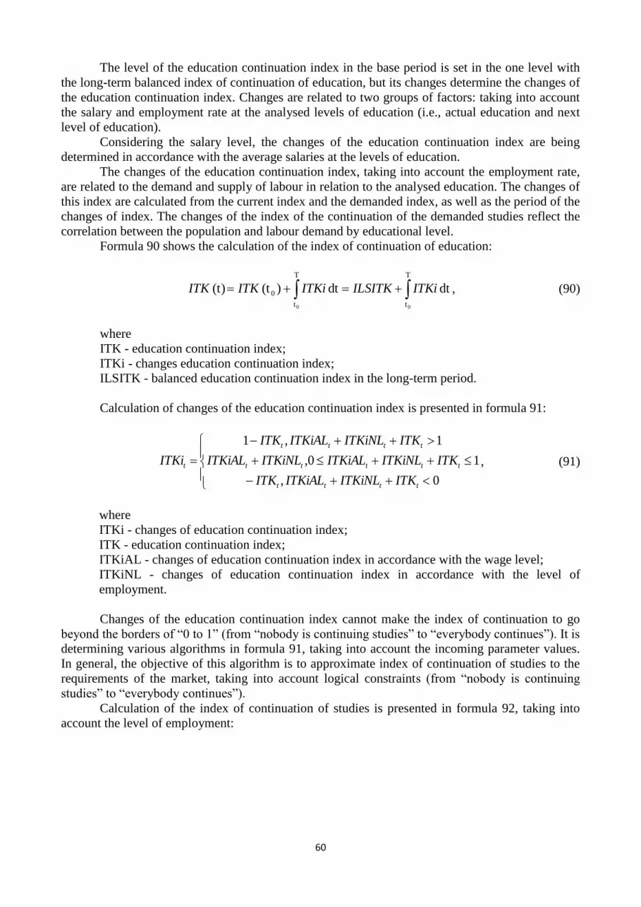
60
The level of the education continuation index in the base period is set in the one level with
the long-term balanced index of continuation of education, but its changes determine the changes of
the education continuation index. Changes are related to two groups of factors: taking into account
the salary and employment rate at the analysed levels of education (i.e., actual education and next
level of education).
Considering the salary level, the changes of the education continuation index are being
determined in accordance with the average salaries at the levels of education.
The changes of the education continuation index, taking into account the employment rate,
are related to the demand and supply of labour in relation to the analysed education. The changes of
this index are calculated from the current index and the demanded index, as well as the period of the
changes of index. The changes of the index of the continuation of the demanded studies reflect the
correlation between the population and labour demand by educational level.
Formula 90 shows the calculation of the index of continuation of education:
T
t
T
t
0
00
dt dt )(t (t) ITKiILSITKITKiITKITK , (90)
where
ITK - education continuation index;
ITKi - changes education continuation index;
ILSITK - balanced education continuation index in the long-term period.
Calculation of changes of the education continuation index is presented in formula 91:
0,
10,
1,1
tttt
ttttt
tttt
t
ITKITKiNLITKiALITK
ITKITKiNLITKiALITKiNLITKiAL
ITKITKiNLITKiALITK
ITKi , (91)
where
ITKi - changes of education continuation index;
ITK - education continuation index;
ITKiAL - changes of education continuation index in accordance with the wage level;
ITKiNL - changes of education continuation index in accordance with the level of
employment.
Changes of the education continuation index cannot make the index of continuation to go
beyond the borders of “0 to 1” (from “nobody is continuing studies” to “everybody continues”). It is
determining various algorithms in formula 91, taking into account the incoming parameter values.
In general, the objective of this algorithm is to approximate index of continuation of studies to the
requirements of the market, taking into account logical constraints (from “nobody is continuing
studies” to “everybody continues”).
Calculation of the index of continuation of studies is presented in formula 92, taking into
account the level of employment:

61
JTK
ttt
t
PITKiNLITKITKiNL
1 , (92)
where
ITKiNL - changes of education continuation index in accordance with the level of
employment;
ITK - education continuation index;
PITKiNL - changes of demanded education continuation index studies in accordance with
the level of employment;
tITK - period of changes of education continuation index.
Formula 91 shows that in accordance with the level of employment the index of
continuation of studies adjusts the index of continuation of studies in accordance with the index
demand. The index demand changes immediately with the changes of labour demand and supply.
But in reality, to understand that the education demand has been established, people need time.
Therefore, the changes of the education continuation index, demanded in formula 91, are divided
into time of changes of the education continuation index, thus ensuring the process delay in time.
The example of calculation of the demanded education continuation index, taking into
account the level of employment, from the general secondary and vocational education to the first
level vocational higher education is presented in formula 93:
0
0
0
0
vvpvi_
plpai_
plpai_
vvpvi_
vvpvi_
plpai_
plpai_
vvpvi_
tl
tl
ta
ta
tl
tl
ta
ta
t
N
N
I
I
N
N
I
I
PITKiNL
, (93)
where
PITKiNL - changes of demanded education continuation index studies in accordance with
the level of employment;
Ia_i - active population with i level of education;
Nl_i - number of employed people with i level of education.
Formula 93 evaluates the supply and demand changes of labour with the general, vocational
and first level vocational higher education. This equation is unified and is used for various levels of
education. Each of the evaluations uses the supply and demand factors of the previous education.
But the calculation of each level of education has the specifics of the highest levels. Usually the
demand of higher levels influences the education demand at the certain level. For example,
education demand at the doctoral level consists of master's, bachelor's (etc.) levels of education
demand. The incoming parameters of education demand of higher levels are presented in the table
2.2.
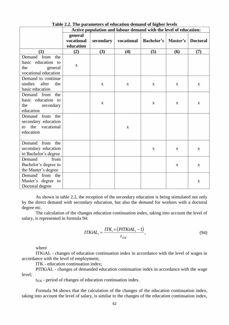
62
Table 2.2. The parameters of education demand of higher levels
Active population and labour demand with the level of education:
general
vocational
education
secondary vocational Bachelor’s Master’s Doctoral
(1) (2) (3) (4) (5) (6) (7)
Demand from the
basic education to
the general
vocational education
x
Demand to continue
studies after the
basic education
x x x x x
Demand from the
basic education to
the secondary
education
x x x x
Demand from the
secondary education
to the vocational
education
x
Demand from the
secondary education
to Bachelor’s degree
x x x
Demand from
Bachelor’s degree to
the Master’s degree
x x
Demand from the
Master’s degree to
Doctoral degree
x
As shown in table 2.2, the reception of the secondary education is being stimulated not only
by the direct demand with secondary education, but also the demand for workers with a doctoral
degree etc.
The calculation of the changes education continuation index, taking into account the level of
salary, is represented in formula 94:
JTK
ttt
t
PITKiALITKITKiAL
1 , (94)
where
ITKiAL - changes of education continuation index in accordance with the level of wages in
accordance with the level of employment;
ITK - education continuation index;
PITKiAL - changes of demanded education continuation index in accordance with the wage
level;
tITK - period of changes of education continuation index.
Formula 94 shows that the calculation of the changes of the education continuation index,
taking into account the level of salary, is similar to the changes of the education continuation index,

63
taking into account the level of employment. The example of calculation of demanded education
continuation index, taking into account the level of salary, from the general secondary and
vocational education to the first level vocational higher education is presented in formula 95:
0
0
vvpvi
plpai
vvpvi
plpai
t
t
t
t
t
A
A
A
A
PITKiAL , (95)
where
PITKiAL - changes of demanded education continuation index in accordance with the wage
level;
AL - average salaries at the levels of education.
Formula 95 evaluates the salary in the groups with the general, vocational and first level
vocational higher education. This equation is unified and is used for various levels of education.
Formula 95 represents that the decision to continue the studies is being affected only by salaries of
two levels of education: salary of the last education (current level) and the salary of the next level of
education.
Figure 2.29 represents the element “structure of fields of education demand”. Demand
structure of fields of education is determined by the existing vacancies in the labour market at the
certain level of education. The more vacancies in the field of education, the greater the education
demand in this field. The calculation of the demand structure of fields of education is presented in
formula 96:
0,0
0,
_
_
_
_
Dk Pn Jl
knl
itDPJ
Dk Pn Jl
knl
itDPJ
Dk Pn Jl
knl
itDPJ
Dk Pn
kn
itDPJ
Jt
VS
VSVS
VS
IP , (96)
where
IPJ - structure of fields of education demand;
VSDPJ_i - number of vacancies at the education level i.
Formula 96 is being applied to vocational education, vocational secondary education,
vocational education after the secondary education and higher education, i.e., where there is an
urgent question of the choice of field of education. This equation is not completely unified, as the
model provides that the populations continue to receive highest level of education (higher
education) in accordance with the already received education, i.e., doctoral and master's levels
coincides with the bachelor’s level of education.
Unified algorithm of state-financed study places
Education sub-model involves one more unified algorithm, which is not related to the
education attainment by the population, but to the state policy planning in the field of education.
The objective of the unified algorithm is to determine the optimal number for the labour market of
the state-financed places by levels and fields of education.
The developed model provides the application of exogenously specified number of study
places for the education system, as well as modelling of the number of the study places in

64
accordance with the market situation. The type of determination of study places used in the model
depends on the choice and activities of the model operator in the developed interface. The essence
of the algorithm of determination of study places is being described in the Figure 2.31.
Vacant study
places
Types of study
placesType of determination
of study places<Optimized vacant
study places>
<Provided vacant
study places>
Figure 2.31. The essence of the algorithm of determination of study places
As the Figure 2.31 shows, there are two types of study places: provided vacant study places
and optimized vacant study places. Depending on the interface parameter “type of determination of
study places”, status element “vacant study places” accepts one of these values. The data in the
determination algorithm of the study places is not modified or processed, this algorithm represents
the logical choice of the operator and it has a technical support function of the model, so that the
technical code of the algorithm is not described in the form of mathematical equation.
Figure 2.31 shows the parameter “vacant study places” (which has already been occurring,
for example in formula 88). This is a key indicator, which determines the number of vacant study
places in the model. If it is equal to “provided number of vacant study places”, the model reflects
the effect of the exogenously provided number of study places on the education system and the
labour market. In this case, the model does not apply any algorithms for determination of the study
places.
If the parameter “vacant study places” accepts the values of the parameter “optimized vacant
study places”, the model is based on the optimization algorithm of the study places, which is
presented in Figure 2.32.
Optimizedvacant study
placesChanges of study
places
<Decide to continue
the studies>
Number of
applications
Ratio of labour demand andactive population by
education fields
<Population>
<Labour demand byeducation fields, levels and
occupations>
Average ratio of labourdemand and active population
by education fields
Critical education
fields
Opening of study
places in the new fieldsAdvanced study
places
<Constraint of the
changes of study places><Initial number of study
places in the new fields>
Summed up advanced
study places
Total ratio of number ofapplications and study
places
Number of optimized
study places
Figure 2.32. Optimization algorithm of the study places

65
Optimization algorithm of the study places is complex and complicated. On the one hand,
there is the effect of the labour market demand and supply on the study places, but on the other
hand - the opportunities and the desire of the population to participate in educational processes. Let
us gradually review it.
The ration of labour demand and supply (ratio of labour demand and active population by
fields of education) is being calculated on the basis of the labour demand distributed by fields and
levels of education (defined in subchapter 2.1) and the active population (defined in subchapter
2.2.3) (this equation is unified, and will be applied to all levels of education). The average ratio in
the fields of education is being calculated on the basis of the ratio of the labour demand and supply.
The fields of education, which have the ratio of labour demand and population lower than average
(critical fields of education) are being determined on the basis of the ratio by fields of education and
average ratio. If these fields do not have state-funded study places, the new study places (the
number of study places is being defined by the index “initial number of study places in the new
fields”) are being opened. If there are state-financed study places, its number is being “advanced”,
taking into account the constraints of changes of study places (increased for critical fields,
decreased for other fields). By summing up the advanced study places and study places in the new
fields, the summed up advances study places are being obtained. It reflects the effect of labour
market supply and demand on the study places. Its objective is to help students to go in the fields
with the greatest shortage of labour.
The second part of the algorithm compares summed up advanced study places and the
number of applicants (applications). Summed up advanced study places are optimized in
accordance with the number of applicants, that is, if the number of summed up advanced study
places exceeds the number of applications, the inefficient places are being liquidated. Thus, the
number of study places comes after the number of applications (which is also a function of the
population). However, with an increase in applications, the number of study places does not grow,
as the maximum number of study places is being determined by the labour supply and demand, but
the minimum number - by the population.
To ensure the functionality of the model “number of optimized study places” is compared
with the existing optimized vacant study places, the flow “changes of study places” is being created,
which determines the stock “optimized vacant study places”.
Upon explanation of the essence of algorithm of optimization of study places let us look at
the forming equations. The first forming equation is the ratio of labour demand and active
population by fields of education, formula 97:
activeE
I
II
LS
LSIA
Vgk Dn Pl
knlVgDPJEt
Vgk Dn Pl
knlVgDPJEt
Vgk Dn Pl
knlVgDPJEt
Lk Pn
knLJPt
Jt
,
0,1
0,
, (97)
where
LSIAJ - ratio of labour demand and active population by fields of education;
LSJLP - labour demand by fields, levels of education and occupations;
IVgDPJE - population.
Formula 97 uses the existing parameters in the model, sums them up to the necessary
dimension - by fields of education, selecting from the population only the economically active
population (i.e., only labour power). If the labour power of the certain field of education does not
have any representative in order to ensure the functionality of the model, the value of -1 is being
assigned to the ratio. Later it will also allow dividing situations when there is no labour demand
from those cases when there is no labour.

66
Upon the calculation of the ratio of labour demand and population, the average ratio of
labour demand and population is being determined, formula 98:
Jk
k
Jk
Jt
tx
LSIA
LSIA
0
, (98)
where
00,0
00,1
Jk
Jkk
LSIA
LSIAx
;
LSIA - average ratio of labour demand and active population;
LSIAJ - ratio of labour demand and active population by fields of education.
As formula 98 shows, the average calculation involves only the fields of education with
labour, i.e. ratio of labour demand and active population by fields of education is greater than zero.
The critical fields of education are being determined on the basis of the ratio of labour
demand of active population, formula 99:
0,
1,0
1,1
0,0
1,1
Jt
t
Jt
t
Jt
Jt
Jt
Jt
LSIA
LSIA
LSIA
LSIA
LSIA
LSIA
LSIA
KIJ , (99)
where
KIJJ - critical fields of education;
LSIA - average ratio of labour demand and active population;
LSIAJ - ratio of labour demand and active population by fields of education.
Formula 99 shows that the parameter assigns the value 1 to the critical fields of education;
the other fields are being assigned the value of 0. Formula 99 indicates that the critical fields of
education are those without labour, as well as the ratio of labour demand and active population by
fields of education is greater than or equal to the average ratio. If there is no labour demand or ratio
of active population by fields of education is less than the average ratio, the fields are not critical.
By comparing the critical fields of education with the study places by fields, the decision on
the opening of study places in the new fields (formula 100) or advancement of current number of
places (formula 101) is being taken:

67
0
00 JJVSKIJOVSVJSVA
JtJt
Jt , (100)
where
JSVAJ - opening of study places in the new fields;
OVSVJ - optimized vacant study places;
KIJJ - critical fields of education;
JJVS - initial number of study places in the new fields.
Formula 100 shows that, if the field of education does not have optimized vacant study
places, but at the same time, this is critical, the new study places are being opened in the field (the
number is being defined by the index “the initial number of the study places in the new fields”). In
all other cases, the opening of new study places in the field is not taking place:
0,
1,
JtJt
JtJt
Jt KIJSVIR
OVSV
KIJSVIROVSV
USV , (101)
where
USVJ - advanced study places;
OVSVJ - optimized vacant study places;
SVIR - constraint of the changes of study places;
KIJJ - critical fields of education.
Formula 101 shows that if the number of study places in the critical fields of education is
being increased according to the index “constraint of the changes of study places”. The number of
study places in all other fields is being reduced.
Upon the opening of study places in the new fields and advancement of the existing study
places, it is necessary to determine its total effect on the study places (see formula 102):
JtJtJt USVJSVASUSV , (102)
where
SUSVJ - summed up advanced study places;
JSVAJ - opening of study places in the new fields;
USVJ - advanced study places.
Summed up advanced study places compose the overall result of the opening of new study
places in the fields and advancement of the existing study places.
Summed up advanced study places reflect the labour market demands for the study places.
The situation, when the population may be incompatible with the market demands, is possible; in
this case, the market may demand more population than can be trained. In this case, it is necessary
to reduce the inefficient places. To achieve this, the summarized advanced study places are being
compared and optimized according to the number of applications at the level of education.
Formula 103 reflects the calculation of the number of applications at the level of education:

68
Dk
k
Dtt NTMPS , (103)
where
PS - number of applications;
NTMD - decide to continue studies.
The number of applications at the level of education is the total number of people who
decide to continue studies at the next level of education, their total sum. Formula 104compares it
with the summed up advances study places:
1
Jk
k
Jt
tt
SUSV
PSPSSVA , (104)
where
PSSVA - total ratio of number of applications and study places;
PS - number of applications;
SUSVJ - summed up advanced study places.
Formula 104 calculates the ratio of the total number of applications and the summed up
advanced study places. In accordance with the equation, this ratio is constrained and cannot exceed
1. This constraint is being used in formula 105 in order to reduce the number of study places if the
number of applications is less than the number of study places:
tJtJt PSSVASUSVOSV , (105)
where
OSVJ - number of optimized study places;
SUSVJ - summed up advanced study places;
PSSVA - total ratio of number of applications and study places.
Formula 105 shows that the optimized number of study places is being calculated on the
basis of the summed up advanced study places, by adjusting them and taking into account number
of applications for studies.
Optimized number of study places by levels of education is integrated into a single matrix
and compared with optimized vacant study places, by determining the changes of study places,
formula 106:
JLtiitJitiJtJtJJLt OVSVOSVOSVOSVOSVOSVI _11_22_11_ ... , (106)
where
OSVIJL - changes of study places;
OSVJ_i - number of optimized study places at the education level i;
OVSVJL - optimized vacant study places.
The changes of study places is a flow that determines the changes of the stock of optimized
vacant study places, see formula 107:

69
T
t
0
0
dt )()(t (t) JLJLJL OSVIOVSVOVSV , (107)
where
OVSVJL - optimized vacant study places;
OSVIJL - changes of study places.
Optimized vacant study places are used for the needs of the model (for example, by
selecting the level of education in formula 111), and it is an important element while planning the
state policy in the field of education.
The above presented unified sub-models are being applied to all levels of education.
Individual educational levels are using the specific elements of the sub-models, which are
considered below.
The specifics of the algorithm of the basic education, vocational education with basic
education
The first specific element of the sub-model is related to basic education and vocational
education with basic education. This is the initial level of education. The model provides that there
is no education prior to initial level. Accordingly, the sub-model cannot realize the unified
algorithm of continuation of education. The model provides that the general basic education is
being started by all people who reach the age of 7. This is the first specific sub-model’s element.
The sub-algorithm of the basic education, vocational education with the basic education is
being implemented not only in the formation of the basic education, but also in the formation of
vocational education with the basic education. People, who fail to complete the basic education,
start vocational education, so the sub-model should provide a possibility of changing of basic
education to vocational education with basic education. It is the second specific sub-model’s
element. It is being described by Figure 2.33.
Mastering of basic
education, vocational
education with basic
education
Learning process
Beginning of mastering
of education
Acquisition of
education
Interruption of
studies
Change of basic education tovocational education with basic
education Abandon basic
education
Mastering of vocationaleducation with basic
education
<Population of 7
years old>
Figure 2.33. Features of the sub-model of the basic education, vocational education with basic
education

70
As the Figure 2.33 shows, the sub-model of the basic education, vocational education with
basic education has the specific start of the education acquisition, equal to 7-year-old population,
and the additional flow “change of basic education to the vocational education with basic
education” with the determinant factors.
The additional flow changes the calculation equation of the stock, the new look is presented
in formula 108:
T
t
1GJD0GJDGJD1
0
dt )AvpNapA()(t (t) GJDJDGGJDGJDGJD APAPSPIISIAIA
,
GJD
1
AvpNap ,,1,,2,1
,,1,,3,2
VJDVJDVJD
VJDJDV
SPIIIAGii
APAPGiiG
, (108)
where
IAGJD1 - mastering of basic education or vocational education with basic education;
AvpNapGJD - change of basic education to the vocational education with basic education;
SAGJD - beginning of mastering of education;
IIGJD - acquisition of education;
SPGJD - interruption of education;
APGJD - learning process;
G - academic year.
The calculation equation of the additional flow “change of basic education to the vocational
education with basic education” is presented in formula 109:
GJDtGJDt IapPvp GJDtAvpNap , (109)
where
AvpNapGJD - change of basic education to the vocational education with basic education;
PvpGJD - abandon basic education;
IapGJD - mastering of vocational education with basic education.
The key role of the additional flow is to change the general basic education to vocational
education with basic education. The number of students, who leave studies, is being deprived from
the total number of students, and the same number of people is being added to the number of
students receiving vocational education, which is generally specified in formulas 108 and 109.
Specifics of the algorithm of continuation of studies after the basic education
Upon acquisition of the basic education there is a choice - to continue the general secondary
education or vocational education (vocational secondary education). This choice is not provided by
the unified model. To realize this principle in the sub-model, the following algorithm has been
developed: the demand for continuation of basic education is being calculated, and then the demand
for continuation of secondary education is being calculated. The demand for continuation of
vocational education (vocational secondary education) is being calculated as the difference between
the demand for continuation of education after basic education and secondary education. Visually,
this algorithm is being reflected in Figure 2.34.
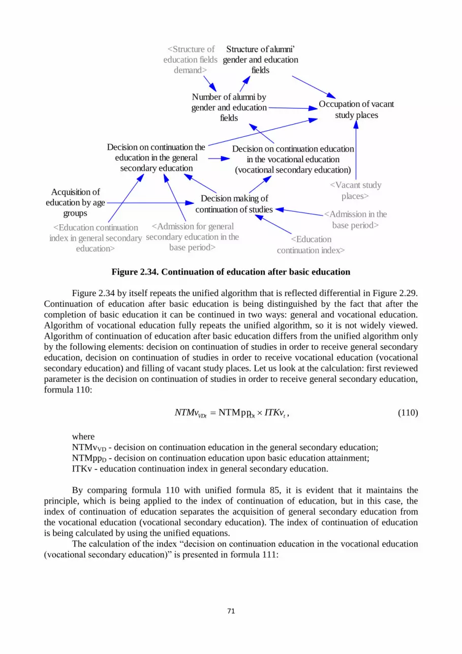
71
Acquisition ofeducation by age
groups
Decision making of
continuation of studies
Structure of alumni’gender and education
fields
Occupation of vacant
study places
Number of alumni bygender and education
fields
<Structure ofeducation fields
demand>
<Vacant study
places>
<Admission in the
base period>
<Education
continuation index>
Decision on continuation theeducation in the general
secondary education
Decision on continuation educationin the vocational education
(vocational secondary education)
<Education continuationindex in general secondary
education>
<Admission for generalsecondary education in the
base period>
Figure 2.34. Continuation of education after basic education
Figure 2.34 by itself repeats the unified algorithm that is reflected differential in Figure 2.29.
Continuation of education after basic education is being distinguished by the fact that after the
completion of basic education it can be continued in two ways: general and vocational education.
Algorithm of vocational education fully repeats the unified algorithm, so it is not widely viewed.
Algorithm of continuation of education after basic education differs from the unified algorithm only
by the following elements: decision on continuation of studies in order to receive general secondary
education, decision on continuation of studies in order to receive vocational education (vocational
secondary education) and filling of vacant study places. Let us look at the calculation: first reviewed
parameter is the decision on continuation of studies in order to receive general secondary education,
formula 110:
tVDt ITKvNTMv DtNTMpp , (110)
where
NTMvVD - decision on continuation education in the general secondary education;
NTMppD - decision on continuation education upon basic education attainment;
ITKv - education continuation index in general secondary education.
By comparing formula 110 with unified formula 85, it is evident that it maintains the
principle, which is being applied to the index of continuation of education, but in this case, the
index of continuation of education separates the acquisition of general secondary education from
the vocational education (vocational secondary education). The index of continuation of education
is being calculated by using the unified equations.
The calculation of the index “decision on continuation education in the vocational education
(vocational secondary education)” is presented in formula 111:

72
}863,862,...,211,142,141{,NTMvNTMppNTMa DtDtJDt JIPaJt , (111)
where
NTMaJD - decision on continuation education in the vocational education (vocational
secondary education);
NTMppD - decision on continuation education upon basic education attainment;
NTMvD - decision on continuation education in general secondary education;
IPaJ - demand of fields of education for vocational education and vocational secondary
education.
Formula 111 shows that vocational education (vocational secondary education) fields end
with the penultimate education code. Later, by summing up the vocational education (vocational
secondary education) and general secondary education, one flow combines all fields of education
(formula 63).
According to algorithms presented in Figure 2.34, the parameter “Occupation of vacant
study places” is being changed, its calculation is presented in formula 112:
Jt
Di
i
JDtJtJDt
Jt
Di
i
JDtJDt
JDtVSVABSVSVABSt
VSVABSABS
VSVA,NTMv
,NTMv
Dt
Dt
, (112)
where
VSVAJD - occupation of vacant study places;
ABSJD - number of alumni by gender and fields of education;
NTMvD - decision on continuation education in general secondary education;
VSVJ - vacant study places;
ABStJD - structure of alumni’ gender and fields of education.
As shown in formula 111, by comparing with the unified formula 88, instead of one
direction in education the two-direction combination of education is being used. Additionally,
formula 111 shows that, regardless of the number of study places, everybody who decides to study
is admitted for general secondary education.
The optimization algorithm of the general secondary vocational education and secondary
vocational education also has its own specifics. The number of study places in vocational education
(vocational secondary education) is being calculated according to unified algorithm, but its number
in general secondary education is equal to the number of graduates (everybody who decides to
study is admitted for general secondary education). Thus, the algorithm of general secondary
vocational education and secondary vocational education contains only one equation, which differs
from the unified algorithm. And this equation combines the optimized number of study places in
vocational education (vocational secondary education) and general secondary education, formula
113:
Jt
Di
i
JttJt OSVaOSVaOSVvOSVva
DtNTMv , (113)
where
OSVvaJ - optimized number of study places in the secondary, vocational and secondary
vocational education;
OSVv - optimized number of study places in the general secondary education;
OSVaJ - optimized number of study places in the vocational and secondary vocational
education;
NTMvD - decision on continuation education in general secondary education.

73
As formula 113 shows, the optimized number of study places in general secondary
vocational education and secondary vocational education is a combination of study places in
general secondary and vocational education (vocational secondary education). The number of study
places in vocational education is being calculated by the means of unified algorithm, while in
general secondary education it is equal to the number of graduates (everybody who decides to study
is admitted for general secondary education) by summing up the number of graduates (by summing
up, eliminating the gender dimension).
Specifics of the algorithm of acquisition of the higher education
The unified algorithms are being used for acquisition of higher education (academic
education and second-level vocational education), as well as other levels of education. Acquisition
of higher education has its own specifics. First of all, higher education is divided into two parts:
Bachelor's and Master's studies. Both parts use unified algorithms, wherefore only the
corresponding specific calculations are being presented here, including the division of study places
between bachelor’s and master’s levels and private funding of the studies.
The algorithm of division of study places between bachelor’s and master’s levels is based on
the principle that the bachelor‘s and master’s study places are related in the fixed proportion.
Accordingly, by multiplying the total number of study places by constant index, it is possible to
determine the number of bachelor’s and master’s study places. This index in the model is named as
“Bachelor’s index”, and reflects the ratio of the number of the places of bachelor’s level in the total
number of study places in higher education.
Bachelor’s index is used in the unified algorithm, where the calculations are related to study
places: opening of study places in new fields, advanced study places and filling of vacant study
places (they are defined in the unified equations, formulas 100, 101 and 88). Calculation of opening
of study places in new fields and advanced study places for the bachelor’s level is presented in
formulas 114 and 115:
0
00 BKJJVSKIJOVSVJSVA
JtJt
Jt , (114)
where
JSVAJ - opening of study places of the new field;
OVSVJ - optimized vacant study places;
KIJJ - critical fields of education;
JJVS - initial number of study places of the new field;
BK - bachelor’s index.
0,
1
1,1
JtJt
JtJt
Jt KIJSVIR
BKOVSV
KIJBKSVIROVSV
USV , (115)
where
USVJ - advanced study places;
OVSVJ - optimized vacant study places;
SVIR - limit of changes of study places;
KIJJ - critical fields of education;
BK - bachelor’s index.

74
By comparing the equations (formulas 100 and 101) in the unified algorithm with the
equations of the bachelor’s level (formulas 114 and 115), it is evident that they differ only by the
fact that the bachelor’s level values are being multiplied by the bachelor’s index.
The calculation of opening of study places in new fields and advanced study places for the
master’s level is presented in formulas 116 and 117:
0
100 BKJJVSKIJOVSVJSVA
JtJt
Jt , (116)
where
JSVAJ - opening of study places of the new field;
OVSVJ - optimized vacant study places;
KIJJ - critical fields of education;
JJVS - initial number of study places of the new field;
BK - bachelor’s index.
0,
1
1,1
JtJt
JtJt
Jt KIJSVIR
BKOVSV
KIJBKSVIROVSV
USV , (117)
where
USVJ - advances study places;
OVSVJ - optimized vacant study places;
SVIR - limit of changes of study places;
KIJJ - critical fields of education;
BK - bachelor’s index.
The same formula is being used for the master’s level, but instead of the bachelor’s index
the ratio of places in the master's studies is being used, which is being calculated by subtracting
from 1 the bachelor’s index.
Filling of vacant study places at the bachelor's and master's levels is accordingly presented
in formulas 118 and 119:
JJt
Di
i
JDtJJtJDt
JJt
Di
i
JDtJDt
JDtSVPBKVSVABSSVPBKVSVABSt
SVPBKVSVABSABS
VSVA,
,
, (118)
where
VSVAJD - occupation of vacant study places;
ABSJD - number of graduates by gender and fields of education;
VSVJ - vacant study places;
ABStJD - structure of alumni’ gender and fields of education;
BK - bachelor’s index;
SVPJ - private financing of the study places.
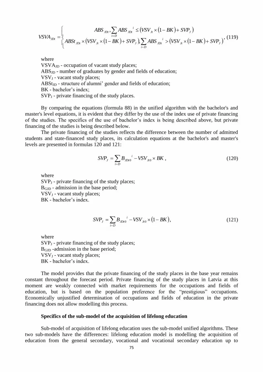
75
JJt
Di
i
JDtJJtJDt
JJt
Di
i
JDtJDt
JDtSVPBKVSVABSSVPBKVSVABSt
SVPBKVSVABSABS
VSVA1,1
1,
, (119)
where
VSVAJD - occupation of vacant study places;
ABSJD - number of graduates by gender and fields of education;
VSVJ - vacant study places;
ABStJD - structure of alumni’ gender and fields of education;
BK - bachelor’s index;
SVPJ - private financing of the study places.
By comparing the equations (formula 88) in the unified algorithm with the bachelor's and
master's level equations, it is evident that they differ by the use of the index use of private financing
of the studies. The specifics of the use of bachelor’s index is being described above, but private
financing of the studies is being described below.
The private financing of the studies reflects the difference between the number of admitted
students and state-financed study places, its calculation equations at the bachelor's and master's
levels are presented in formulas 120 and 121:
BKVSVBSVP Jt
Di
i
JDtJ
00 , (120)
where
SVPJ - private financing of the study places;
BGJD - admission in the base period;
VSVJ - vacant study places;
BK - bachelor’s index.
BKVSVBSVP Jt
Di
i
JDtJ
100 , (121)
where
SVPJ - private financing of the study places;
BGJD -admission in the base period;
VSVJ - vacant study places;
BK - bachelor’s index.
The model provides that the private financing of the study places in the base year remains
constant throughout the forecast period. Private financing of the study places in Latvia at this
moment are weakly connected with market requirements for the occupations and fields of
education, but is based on the population preference for the “prestigious” occupations.
Economically unjustified determination of occupations and fields of education in the private
financing does not allow modelling this process.
Specifics of the sub-model of the acquisition of lifelong education
Sub-model of acquisition of lifelong education uses the sub-model unified algorithms. These
two sub-models have the differences: lifelong education model is modelling the acquisition of
education from the general secondary, vocational and vocational secondary education up to

76
bachelor’s level; indexes of continuation of education in the lifelong education are more stable than
in the acquisition of the basic education: the basis of graduates in the lifelong education is not being
formed by the graduates of the previous level of education, but by the population with previous
level of education.
Limitation of the lifelong education sub-model functionality is related to the specifics of the
levels of education: for example, the doctoral education is not a mass education, so it does not make
sense to include this level of education in the lifelong education. The higher education in the labour
market is not statistically distributed in the bachelor’s and master’s fields of education, so the
continuation of education at Master's level is not included in the lifelong education, as the graduates
and applicants at this level are analysed in one group both in the model and in the labour market. It
is also useless to build a system of continuation of education for persons who have not attained the
basic education. These persons usually continue working by simple occupations that do not require
specific knowledge.
Indexes of continuation of education in the lifelong education are more stable than in the
acquisition of the basic education. The pupils and students with the prior education are actively
responding to market requirements, so the indexes of continuation of education due to the demand
can vary significantly. The situation is the opposite in the lifelong education system: the elderly
person should have the great motivation to begin mastering a new occupation. By conducting the
lifelong education system research, it is being determined that a certain part of the population is still
participating in lifelong education system. By dividing the population, participating in lifelong
education system, by the total population, the index of continuation of education balanced in a long-
term period is being determined. This index supplements the calculation algorithm of the education
of continuation index in the lifelong education.
The equation of changes of the index of continuation of education is being modified in the
lifelong education algorithm, formula 122:
02
,
12
0,2
12
,1
tt
tt
t
tt
tt
t
tt
tt
tt
t
t
ITKITKiITITKiNLITKiAL
ITK
ITKITKiITITKiNLITKiAL
ITKiITITKiNLITKiAL
ITKITKiITITKiNLITKiAL
ITK
ITKi , (122)
where
ITKi - changes of education continuation index;
ITK - education continuation index;
ITKiAL - changes of education continuation index, in accordance with the wage level;
ITKiNL - changes of education continuation index, in accordance with the level of
employment;
ITKiIT - changes education continuation index, in accordance with long-term trends.
By comparing the equation of changes of education continuation index in the lifelong
education (formula 122) with the unified equation (formula 91), it is evident that lifelong education
equation is supplemented by the changes of the index of continuation of education, taking into
account the long-term trends. In addition, the ratio of the changes of the index, taking into account
the salaries and employment rates, has been reduced twice, it has an average level of impact.
On the basis of the unified equations, reflected in formula 122, all elements, except changes
of the index of continuation of education have been calculated, taking into account the long-term
trends, which calculation equation has not previously been described, but is presented in formula
123:

77
JTK
t
tt
ITKILSITKITKiIT
, (123)
where
ITKiIT - changes of index of continuation of studies, in accordance with long-term trends;
ILSITK -education continuation index in the long-term period;
ITK - index of continuation of studies;
tITK - period of changes of education continuation index.
As formula 123 shows, the changes of education continuation index in accordance with the
long-term trends are moving closer the education continuation index in the long-term period to the
balanced education continuation index.
The basis of the graduates in the lifelong education is not being formed by the alumni of the
previous level, but the population with previous level of education, which is presented in formula
124:
tVgDPJEtVgDPJEt ITKINTM , (124)
where
NTMVgDPJE - decide to continue the studies;
IVgDPJE - population;
ITK - education continuation index.
In comparison with formula 85, formula 124 shows that the decision to continue education
is not taken by the alumni of the previous level of education graduates, but population, analysed in
the corresponding educational group. Population analysis group, its formation and calculation are
investigates in the next subsection (2.2.3 subsection, labour analysis sub-model).
Formula 124 shows that the population is being analysed in the wider dimensions, in order
to move to the unified equations, it is necessary to reduce the number of dimensions, which is
performed in formula 125:
Jt
Vgk Pi Jl En
ki
VgDPJEtJDt IPNTMABS
ln, (125)
where
ABSJD - number of applicants by gender and fields of education;
NTMD - decide to continue the studies;
IPJ - structure of the field of education demand;
t - time period.
Formula 125 shows that the wide groups of population are summed up to the necessary
gender dimension. Then the equation repeats the unified formula 86 by its form and substance, i.e.
graduates have the determined field of education.
Due to the fact that the lifelong education sub-model is associated, it is being added to the
basic education sub-model, they together provide the filling of study places. Filling of study places
in basic education is presented in formula 88. Lifelong education system is filling the unfilled study
places in the basic education. Equation of filling of vacant study places in lifelong education is
presented in formula 126:

78
Di
i
JDtJt
Di
i
JDt
Di
i
JDtJtJDt
Di
i
JDtJt
Di
i
JDtJDt
JDt
VSVAVSVABSMVSVAVSVABStM
VSVAVSVABSMABSM
VSVAM
,
,
, (126)
where
VSVAMJD - occupation of vacant study places in the lifelong education;
ABSMJD - number of applicants by gender and fields of education in the lifelong education;
VSVJ - vacant study places;
VSVAJD - occupation of vacant study places;
ABStMJD - structure of alumni’ gender and fields of education in the lifelong education.
By comparing the equation of filling of vacant study places in lifelong education (formula
126) with the unified equation (formula 88), it is evident that the system of lifelong education
provides the study places, which have not been filled in the basic education.
In comparison with the basic education system, the specifics of the lifelong education
system is that the lifelong education system does not contain dominant age group. Accordingly, it is
not possible to determine the average age of alumni on the basis of the duration of the studies (as is
done in the basic education system). The age of graduates in the lifelong education system is being
determined in accordance with the age of alumni. The acquisition of education by age groups in the
lifelong education systems is presented in formula 127:
Vgt
Gk
k
GJDtVgJDt AbsVStIIII
, (127)
where
IIVgJD - acquisition of education by age groups;
IIGJD - acquisition of education;
AbsVStVg - age structure of alumni.
Acquisition of education by age groups in the lifelong education is the multiplication of the
number of educated people by the age structure of alumni. The number of educated people is being
calculated on the basis of the unified equation (formula 79), but the calculation of age structure is
presented in formula 128:
59_55..19_15,:1 vgvgVgAbiVStAbsVSt VgttVg , (128)
where
AbsVStVg - age structure of alumni;
AbiVStVg - age structure of graduates.
As shown in formula 128, upon the acquisition of education the alumni change the age
groups, i.e., move to the next group, the older group of five-years old. This equation reflects that the
studies require time and the graduates enter the educational institution at one age (age group), but
graduate the older age (next age group).
The age structure of graduates is being calculated on the basis of graduates, formula 129:

79
Dk Pi Jl En Vgm
kinlm
VgDPJEt
Dk Pi Jl En
kinl
VgDPJEt
VgtNTM
NTM
AbiVSt , (129)
where
AbiVStVg - age structure of graduates;
NTMD - decide to continue the studies.
As formula 129 shows, the age structure of graduates is being calculated on the basis of the
population who have decided to continue education in the lifelong education system, by summing
up the population by age groups and dividing it by the total population.
The calculation equation of age structure of the graduates is the final specific equation in the
education system. All other model calculations in the education system are realised in accordance
with the unified equations (formulas 77 - 97).
2.2.3. Working-age population stock-taking sub-model
Working-age population stock-taking sub-model structure is presented in Figure 2.35.
<Mortality>
Algorithm of mortalitydistribution of working agepopulation by education
levels
Algorithm of analysis of
the population with
doctoral degree
Algorithm of analysis of
the population with
academic education
Algorithm of analysis ofthe population with firstlevel higher vocational
education
Algorithm of analysis ofthe population with
general secondary andvocational education
Algorithm of analysis of
the population with lower
than secondary education
Algorithm of choosing ofoccupation upon the
acquisition of educationfor the population with
doctoral degree
Algorithm of choosing ofoccupation upon the
acquisition of educationfor the population with
academic degree
Algorithm of choosing ofoccupation upon the
acquisition of educationfor the population with
first level highervocational education
Algorithm of choosing ofoccupation upon the
acquisition of educationfor the population withgeneral secondary andvocational education
Algorithm of choosing ofoccupation upon the
acquisition of educationfor the population withlower than secondary
education
Technical algorithm
of acquisition of
doctoral degree
Technical algorithm
of acquisition of
academic education
Technical algorithmof acquisition of first
level highervocational education
Technical algorithmof acquisition of
general secondaryand vocational
education
<Acquisition of
education>
International migration
algorithm for population
with doctoral degree
International migration
algorithm for population
with academic education
International migrationalgorithm for population
with first level highervocational education
International migrationalgorithm for populationwith general secondary
and vocational education
International migrationalgorithm for population
with lower thansecondary education
Algorithm of economic
activity for population
with doctoral degree
Algorithm of economic
activity for population
with academic education
Algorithm of economicactivity for populationwith first level highervocational education
Algorithm of economicactivity for populationwith general secondary
and vocational education
Algorithm of economicactivity for population
with lower thansecondary education
Algorithm of agingdistribution of working age
population by educationlevels
<Aging>
Figure 2.35. Working-age population stock-taking sub-model structure

80
Figure 2.35 reflects that the working-age population stock-taking sub-model structure
consists of various algorithms. The essence of the sub-model is the following: the working-age
population is divided into five groups according to the level of attained education: each of which
includes a unified population and structural analysis sub-model. All groups of population reduce
beyond working age, or due to natural mortality. Natural mortality amounts are determined by
demographic sub-model, but their division by the population analysis groups is determined by the
algorithm of the mortality division of the working-age population by levels of education.
Changes of the population age structure are determined by the algorithm of the aging
division of the working-age population, which synchronizes the demographic sub-model and
working-age population stock-taking sub-model. The integral part of the aging algorithm is the
retirement algorithm, which characterizes the population aging up to the age when they leave the
labour market, i.e. retire. Retirement algorithm is the specific part of the aging algorithm, so it is not
split into a separate algorithm, but is investigated by other algorithms.
The acquisition of education causes the changes of population in the analysis groups.
Education attainment increases the population in the group according to the obtained education and
reduces the population in the group in accordance with the previous education. This is determined
by education technical algorithms. They have a technical function - to shift population from one
group to another, as the education attainment is analysed in the education attainment sub-model.
Upon acquisition of education the population can change or choose the occupation. Choice
of occupation upon the acquisition of education algorithm determines the change or choice of
occupation.
Working-age population stock-taking sub-model also reflects the operation of international
migration and labour force participation algorithms. International migration algorithms can both
increase and reduce the population. Labour force participation algorithms change the economic
activity status of the population, i.e., change the population structure.
These algorithms have a unified nature, they are applicable to all population groups. Further
the operation of the unified algorithm is investigated.
Population analysis algorithm
The overall scheme of the population analysis algorithm is presented in Figure 2.36.
Population
Aging
Admission for
analysis
Removal from
analysis
Changes of population
and structure<Algorithm of acquisition ofeducation and choosing of
occupation>
<Algorithm of
mortality division>
<Emigration
algorithm><Immigration
algorithm>
<Acquisition of the
education of higher level>
<Algorithm of
economic activity>
Change of occupation in
the market module
<Aging
algorithm>
<Algorithm of removal
from analysis>
<Change of the group ofeconomic activity with the
change of age group>
Figure 2.36. Population analysis sub-model

81
As the Figure 2.36 shows, by acquiring education and occupation, the population is admitted
for analysis in the unified algorithm in accordance with the level of education. Population age
structure is changed when the flow “aging” indicates it. Beyond the retirement age, the population
is taken away from the analysis. The changes of population and structural changes are possible,
taking into account the migration processes, mortality, and acquisition of higher levels of education.
The change of occupation is analysed in the separate flow, which is related to the change of
occupation model in the market equilibrium module
The calculation of the stock of the population analysis is presented in formula 130:
T
t
DPJEDPJE1VgDPJEVgDPJEVgDPJEVgDPJE0VgDPJEVgDPJE
0
dt )(t (t) VgVg NOVNOVPMTBISSIUNUPII
,
VgDPJEVgDPJEVgDPJEVgDPJEVgDPJE
DPJEDPJE1
,74_70,,24_20,19_15
,74_70,69_65,,24_20
PMTBISSIUNUPIVg
NOVNOVVgVg
VgVg
,(130)
where
IVgDPJE - population;
UPVgDPJE - admission for analysis;
UNVgDPJE - removal from analysis;
ISSIVgDPJE - change of population and structure;
PMTBVgDPJE - change of occupation in the market module;
NOVVgDPJE - aging;
Vg - age group.
Formula 130 reflects the essence of the Figure 2.36. It is important to note that the 130
formula indicates that aging is possible in age groups from 15 to 69 years. Then people simply leave
the analysis system (are removed from the analysis).
Constituent elements of formula 130 are based on the algorithms of the investigated sub-
model. The exception is the element “the change of occupation in the market module”, which is
based on the defined elements in the market equilibrium module. Therefore, the description of this
element does not have the allocated thematic paragraph, the element formation is investigated in
one equation, formula 131:
activenonE
activeENPMPMDMPMNPMTB
,0
,VgDPJEtVgDPJEtVgDPJtVgDPJEt , (131)
where
PMTBVgDPJE - change of occupation in the market module;
PMNVgDPJ - employment after the change of occupation;
PMDMVgDPJ - change of occupation in order to get a job;
NPMVgDPJ - change of occupation of the employed.
Formula 131 shows that the occupation is changed only by economically active population.
The change of analysis group of occupation in the labour analysis sub-model is caused by the
change of occupation in order to get a job (the population is increased in groups with new
occupations and, at the same time, is reduced in groups with old occupations, which is indicated by
the difference between the elements “placement after change of occupation” and “change of
occupation in order to obtain employment”), as well as the change of occupation by the employees

82
(which is summarily the change of occupation for employees). These elements are described more
in the market equilibrium module. But the algorithms of labour analysis sub-model are described
further.
The algorithms of admission for analysis and changes of population and structure are
interrelated. Admission for analysis in a single population group causes the decline in population in
other groups (except for the first-time admission, which is described below). Therefore, these two
sub-algorithms are to be considered as a whole. At first the algorithms that are not related to the
admission for the analysis (i.e., algorithms of mortality division, aging and removal from the
analysis) are investigated, then the related algorithms are investigated and, finally, the algorithm
related to the admission for analysis (algorithm of occupational supply).
Algorithm of mortality division of working-age population by levels of education
Algorithm of mortality division of working-age population by levels of education is
presented in Figure 2.37.
Population
Population by age
groups and gender
Population
structure
Population ratio of the totalpopulation by age groups and
gender
Total population by age
groups and gender<Mortality by age groups
and gender a.g.15 70>
Mortality
<Population by age groups andgender in the group of i
education level>
Figure 2.37. Algorithm of mortality division of working-age population by levels of education
The Figure 2.37 shows that in order to calculate the mortality in the group of levels of
education, the population in the group is aggregated by age groups and gender dimensions. All
groups of levels of education allow calculating the ratio of a particular group in the population. The
ratio of the group in the population determines the ratio of mortality of the group in the total
mortality (along with overall mortality, it allows to calculate how many people die in the group).
The division of mortality people by occupations, fields of education and groups of economic
activities is determined by the population structure.
The calculation of the population by age groups and gender is presented in formula 132:
Pi Jk El
iklII VgDPJEtVgDt , (132)
where
IVgD - population by age groups and gender;
IVgDPJE - population;
P - occupation;
J – field of education;
E - group of economic activity.
Calculation of population structure is presented in formula 133:

83
VgDt
VgDPJEt
VgDPJEtI
IISt , (133)
where
IStVgDPJE - population structure;
IVgDPJE - population;
IVgD - population by age groups and gender.
Calculation of total population by age groups and gender is presented in formula 134:
Li
iIKI VgDtVgDt , (134)
where
KIVgD - total population by age groups and gender;
IVgD - population by age groups and gender;
L - group of level of education.
Calculation of the ratio of population by age groups and gender is presented in formula 135:
VgDt
VgDt
VgDtKI
IISI , (135)
where
ISIVgD - population ratio of the total population by age groups and gender;
IVgD - population by age groups and gender;
KIVgD - total population by age groups and gender.
Mortality calculation is presented in formula 136:
VgDPJEtVgDtVgDtVgDPJEt IStISIMM , (136)
where
MVgDPJE - mortality;
MVgD - mortality by age groups and gender in 15-70-year-old groups;
ISIVgD - population ratio of the total population by age groups and gender;
IStVgDPJE - population structure.
Formula 136 provides the mortality calculation by age groups, gender, occupations, fields of
education and groups of economic activity. One equation includes the total mortality, group ratio of
the total population and the internal structure of the population.
Working-age population aging and removal from the analysis (retirement) algorithms
divided by educational levels.
Working-age population aging algorithm divided by educational levels is largely repeating
the mortality division of the population algorithm. They have the same function: to synchronize
demographics and labour analysis sub-models. The algorithms use the same principle - calculation
of the population structure and ratio, but differ by their application object (in the algorithm of
mortality, i.e. mortality, but in the aging algorithm - aging). On the basis of this fact, the aging
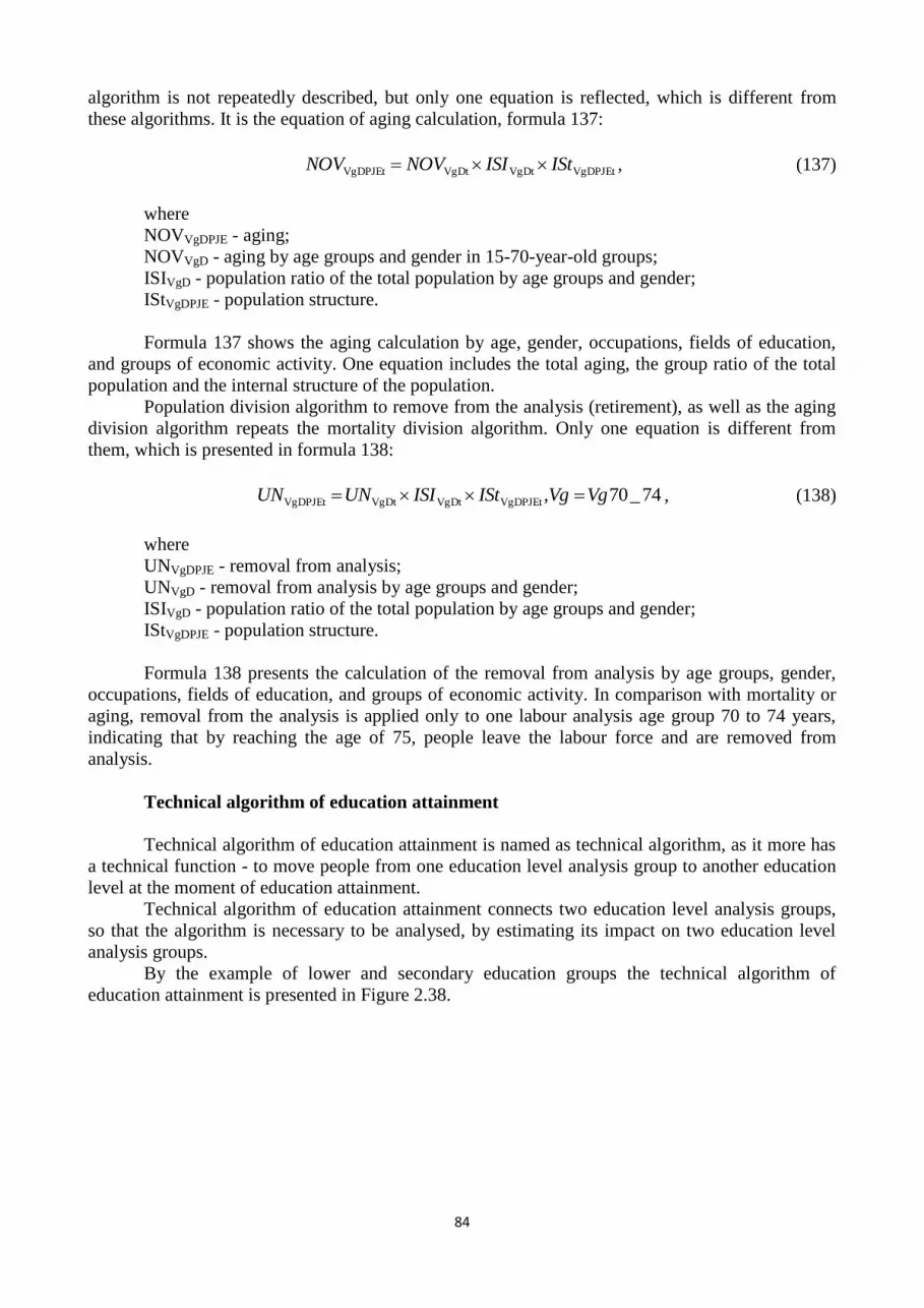
84
algorithm is not repeatedly described, but only one equation is reflected, which is different from
these algorithms. It is the equation of aging calculation, formula 137:
VgDPJEtVgDtVgDtVgDPJEt IStISINOVNOV , (137)
where
NOVVgDPJE - aging;
NOVVgD - aging by age groups and gender in 15-70-year-old groups;
ISIVgD - population ratio of the total population by age groups and gender;
IStVgDPJE - population structure.
Formula 137 shows the aging calculation by age, gender, occupations, fields of education,
and groups of economic activity. One equation includes the total aging, the group ratio of the total
population and the internal structure of the population.
Population division algorithm to remove from the analysis (retirement), as well as the aging
division algorithm repeats the mortality division algorithm. Only one equation is different from
them, which is presented in formula 138:
74_70,VgDPJEtVgDtVgDtVgDPJEt VgVgIStISIUNUN , (138)
where
UNVgDPJE - removal from analysis;
UNVgD - removal from analysis by age groups and gender;
ISIVgD - population ratio of the total population by age groups and gender;
IStVgDPJE - population structure.
Formula 138 presents the calculation of the removal from analysis by age groups, gender,
occupations, fields of education, and groups of economic activity. In comparison with mortality or
aging, removal from the analysis is applied only to one labour analysis age group 70 to 74 years,
indicating that by reaching the age of 75, people leave the labour force and are removed from
analysis.
Technical algorithm of education attainment
Technical algorithm of education attainment is named as technical algorithm, as it more has
a technical function - to move people from one education level analysis group to another education
level at the moment of education attainment.
Technical algorithm of education attainment connects two education level analysis groups,
so that the algorithm is necessary to be analysed, by estimating its impact on two education level
analysis groups.
By the example of lower and secondary education groups the technical algorithm of
education attainment is presented in Figure 2.38.

85
Population withgeneral secondary
and vocationaleducation
Population withlower thansecondaryeducation
Admission for
analysis
Changes of population
and structure
<Acquisition of education at thegeneral secondary and vocational
education levels>
Sub-model of choiceof occupation upon theeducation attainment
Maximum of
changes
Structure of
maximum of changes
Leaving of the old
analysis group
Figure 2.38. Technical algorithm of education attainment by the example of lower and
secondary education groups
Figure 2.38 shows that by attaining education the population is admitted for analysis in the
group according to the attained education. By acquiring education, the population obtains the
occupation, which is indicated by the choice of occupation algorithm upon the education
attainment. Admission of the population to the education level analysis group reduces the
population in the analysis group of the previous educational level to the same extent by age groups
and gender. But they have different (or may be different) occupations, fields of education, economic
activity. The population of the certain age and gender is reduced in the analysis group of the
previous educational level, but its occupations, fields of education, economic activity are
determined, taking into account the existing population in the group (selecting by the element
“maximum of changes”, as well as calculating its structure).
The calculation of the equation of admission for analysis is presented in formula 139:
VgDtPJtVJDtVgDPJEt ULLPPSIIUP , (139)
where
UPVgDPJE - admission for analysis;
IIVJD - mastering of education at the level of general secondary and vocational studies;
PPSPJ - structure of occupation demand in accordance with ECM for population with general
secondary and vocational education;
ULLVgD - present level of participation.
Formula 139 shows that the equation of admission for analysis adapts the education
mastering and choice of occupation for the working age analysis algorithm. In accordance with
formula 139, all people, acquiring new education, regardless of previous economic status, are
divided by groups of economic activity, taking into account the provided level of participation by
age groups and gender (participation level for the model is provided exogenously, it is described in
details in the sub-model of labour economic activity). According to the attained education, the
graduates obtain the occupation by entering the labour market. The occupation is obtained in
accordance with the structure of the demand for occupations (from labour demand sub-model) and
education compliance matrix (ECM).
By determining the decline in population in the group of previous level of education, the
population selection is carried out for the calculation of the structure. The population selection is
denoted in the model as a maximum of changes. The maximum of changes, i.e., the population
forms the analysed age group and does not leave it at the next forecasting stage (year). Maximum
change is necessary to prevent the developed algorithms simultaneously to modify the same

86
population groups more than it is allowed by the condition of analysis group. The calculation of the
maximum of changes equation is presented in formula 140:
74_70,
69_65...19_15,
VgDPJEt
VgDPJEtVgDPJEtVgDPJEt
VgDPJEt VgI
VgNOVMIIZM , (140)
where
IZMVgDPJE - maximum of changes;
IVgDPJE - population;
MVgDPJE - mortality;
NOVVgDPJE - aging;
Vg - age group.
Formula 140 shows that the maximum of changes for age groups from 15 to 69 years is
calculated as the difference between the population and the summed up mortality and aging. The
maximum of changes of the older groups coincide with the population.
Maximum of changes structure is calculated in formula 141:
0
1,0
0,0
0,
DPJEt
VgDPJEt
DPJEt
VgDPJEt
DPJEt
VgDPJEt
VgDPJEt
Pk Jn Em
knm
Vg
Pk Jn Em
knm
Vg
Pk Jn Em
knm
Vg
IZM
IZM
IZM
IZM
IZM
IZM
IZMSt , (141)
where
IZMStVgDPJE - maximum of changes structure;
IZMVgDPJE - maximum of changes.
The maximum of changes structure is calculated by dividing the array elements by the total
amount of these elements. In addition, formula 141 shows that the calculation of the maximum of
changes structure is protected from situations, when there are no people in the array (i.e., it is not
possible to calculate the structure). In this case, a value of zero is assigned to the corresponding
structural elements. Population which abandon the previous education analysis group due to
attainment of new education is calculated in formula 142:
Pk Jn Em
knm
VgUPIZMStVAGA DPJEtVgDPJEtVgDPJEt , (142)
where
VAGAVgDPJE - old analysis group abandonment;
IZMStVgDPJE - maximum of changes structure;
UPVgDPJE - admission for analysis.
Formula 142 reflects that the analysis group of the previous educational level is abandoned
by the population of certain age and gender (the number coincides with the educated people by age
and gender in the next level of education), but their occupations, fields of education, economic
activity are determined in accordance with the population in the group and its structure.

87
Abandonment of the old analysis group along with the results of other algorithms form the
population and structural changes in the analysed education level group, formula 143:
VgDPJEtVgDPJEtVgDPJEtVgDPJEtVgDPJEtVgDPJEtVgDPJEt AMVGMIMEMVAGAAMMISSI ,(143)
where
ISSIVgDPJE - change of population and structure;
MVgDPJE - mortality;
AMVgDPJE - change of the economic activity group of the population;
VAGAVgDPJE - old analysis group abandonment;
EMVgDPJE - emigration;
IMVgDPJE - immigration;
MIVgDPJE - maximum of changes;
AMVGMVgDPJE - change of the economic activity group along with the change of age.
Formula 143 reflects all parameters affecting the population and structural changes. Formula
143 reflects the last equation, which connects the various analysis groups of the education levels.
Further the algorithm of occupational supply is described, which is related only to technical
algorithm of education attainment.
Algorithm of occupational supply
Algorithm of occupational supply provides obtainment of occupation upon education
attainment, by entering the labour analysis group of the corresponding level. In the algorithm the
occupation is given according to the attained education, occupation - according to education
compliance matrix (ECM) and occupational demand. The algorithm of occupational supply is
presented in Figure 2.39.
Demand for occupations
in accordance with ECM
Demand structure ofoccupations in accordance
with ECM
<Education
compliance matrix>
<Demand for
occupations>
Figure 2.39. occupational supply development algorithm
Occupational supply structure is formed in accordance with the occupational demand
structure. Occupational demand is determined in the occupational demand sub-model (formula 29).
Multiplying the occupational demand by integrated educational compliance matrix (AECM, the
development is analysed in formula 296), the occupational demand is determined according to the
ECM. This indicates the required number of employees, whose occupation corresponds to the
education. Then the structure of occupational demand according to ECM is determined.
The calculation of the occupational demand according to ECM is presented in formula 144:
0,
0,
PJtPJtPJtPJt
PJtPJtPJt
PJtLSAIAMLSAIAM
LSAIAMAIAMPP , (144)
where
PPPJ - demand for occupation in accordance with ECM;
LSPJ - labour demand by fields of education and occupations at the level of education;
AIAMPJ - integrated education compliance matrix.

88
Occupational demand according to ECM is developed multiplying ECM by the occupational
demand. In some cases the certain occupations may not be demanded. In this case, ECM determines
the occupational demand. It is an artificial activity that allows to assign occupation to the education,
which does not have a demand from the market side (model provides that the graduates begin their
studies for the demanded occupations, but the demand during the study time may fall to zero, so the
alumni acquire a non-demanded education and a non-demanded occupation).
Calculation of the occupational demand structure according to ECM is presented in formula
145:
0
1,0
0,0
0,
Pl
PJt
Pl
PJt
Pl
PJt
PJt
PJt
PJtPJt
l
ll
PP
PP
PP
PP
PP
PP
PPS , (145)
where
PPSPJ -demand structure of occupations in accordance with ECM;
PPPJ - demand for occupation in accordance with ECM;
P - occupation;
J - field of education.
In the equation of the occupational demand structure not only the structure is calculated, but
the model is also protected from the situation when there is no demand in the specific field. In this
case, a certain element of structure obtains the value of zero.
Change of the economic activity group together with the change of age group
In statistical records the age groups differ in economic activity. In order to reflect the
changes of economic activity in the model, along with the age changes, the labour analysis sub-
model provides the algorithm of the economic activity group change along with the change of age
group. This is presented in Figure 2.40.
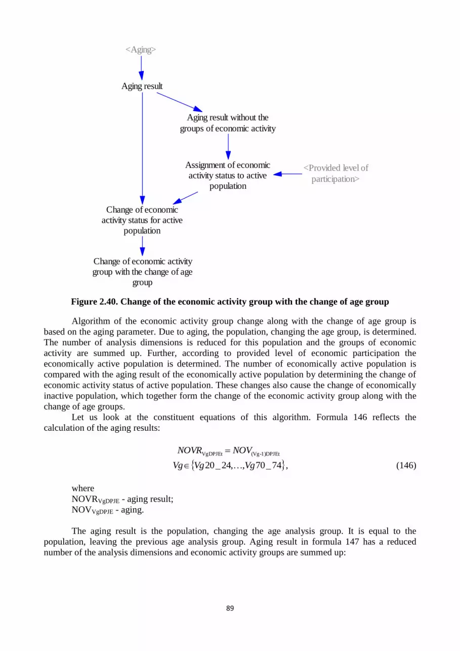
89
<Aging>
Aging result
Aging result without the
groups of economic activity
Assignment of economicactivity status to active
population
Change of economicactivity status for active
population
Change of economic activitygroup with the change of age
group
<Provided level of
participation>
Figure 2.40. Change of the economic activity group with the change of age group
Algorithm of the economic activity group change along with the change of age group is
based on the aging parameter. Due to aging, the population, changing the age group, is determined.
The number of analysis dimensions is reduced for this population and the groups of economic
activity are summed up. Further, according to provided level of economic participation the
economically active population is determined. The number of economically active population is
compared with the aging result of the economically active population by determining the change of
economic activity status of active population. These changes also cause the change of economically
inactive population, which together form the change of the economic activity group along with the
change of age groups.
Let us look at the constituent equations of this algorithm. Formula 146 reflects the
calculation of the aging results:
1)DPJEt-(VgVgDPJEt NOVNOVR
74_70,,24_20 VgVgVg , (146)
where
NOVRVgDPJE - aging result;
NOVVgDPJE - aging.
The aging result is the population, changing the age analysis group. It is equal to the
population, leaving the previous age analysis group. Aging result in formula 147 has a reduced
number of the analysis dimensions and economic activity groups are summed up:

90
VgDPJEtVgDPJt
Ei
iNOVRNOVRb , (147)
where
NOVRbVgDPJ - aging result without the economic activity in the groups;
NOVRVgDPJE - aging result.
The active population is calculated on the basis of the aging results without the groups of
economic activity and provided participation level, formula 148:
VgDtVgDPJtVgDPJt ULLNOVRbASP , (148)
where
ASPVgDPJ - assignment of economic activity status to active population;
NOVRbVgDPJ - aging result without the economic activity in the groups;
ULLVgD - determined level of participation.
The calculated active population is compared with the aging results (the active population);
the difference indicates to the change of the active population along with the change of age group,
formula 149:
activeEASPNOVRASM ,VgDPJtVgDPJEtVgDPJt , (149)
where
ASMVgDPJ - change of economic activity status for active population;
NOVRVgDPJE - aging result;
ASPVgDPJ - assignment of economic activity status to active population.
Changes in one group of economic activity cause the opposite changes in the second group
of economic activity (i.e., by increasing the economically active population, the economically
inactive population should be reduced). The summed up changes in the active and inactive
population form the change of the economic activity group, formula 150:
activenonEASM
activeEASMAMVGM
,
,
VgDPJt
VgDPJtVgDPJEt , (150)
where
AMVGMVgDPJE - change of the economic activity group along with the change of age;
ASMVgDPJ - change of economic activity status for active population.
Formula 150 shows that the change of one economic activity group is inseparable from the
other.
The unified algorithms reflected above form the base model. The features of certain
algorithms are described below.
Features of unified algorithms in the labour analysis sub-model
The first feature of the algorithm is related to the initial admission for analysis of the
population in the level of education groups. Unified models determine that the admission for
analysis is possible by acquiring education. So, by acquiring basic education and at the same time
reaching the age of 15, people are admitted for analysis. Unified algorithms do not provide that any
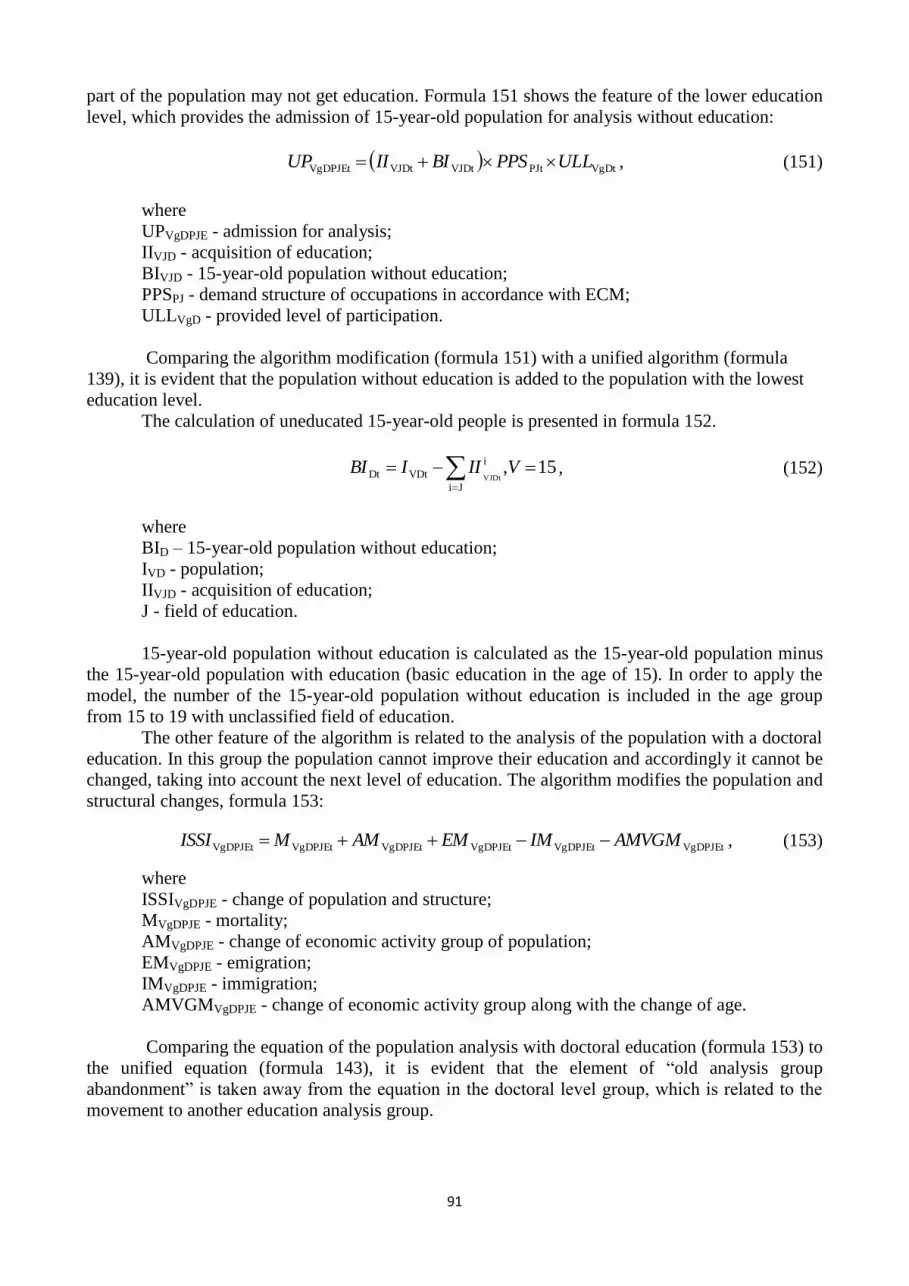
91
part of the population may not get education. Formula 151 shows the feature of the lower education
level, which provides the admission of 15-year-old population for analysis without education:
VgDtPJtVJDtVJDtVgDPJEt ULLPPSBIIIUP , (151)
where
UPVgDPJE - admission for analysis;
IIVJD - acquisition of education;
BIVJD - 15-year-old population without education;
PPSPJ - demand structure of occupations in accordance with ECM;
ULLVgD - provided level of participation.
Comparing the algorithm modification (formula 151) with a unified algorithm (formula
139), it is evident that the population without education is added to the population with the lowest
education level.
The calculation of uneducated 15-year-old people is presented in formula 152.
15,Ji
i
VDtDt VJDt
VIIIBI , (152)
where
BID – 15-year-old population without education;
IVD - population;
IIVJD - acquisition of education;
J - field of education.
15-year-old population without education is calculated as the 15-year-old population minus
the 15-year-old population with education (basic education in the age of 15). In order to apply the
model, the number of the 15-year-old population without education is included in the age group
from 15 to 19 with unclassified field of education.
The other feature of the algorithm is related to the analysis of the population with a doctoral
education. In this group the population cannot improve their education and accordingly it cannot be
changed, taking into account the next level of education. The algorithm modifies the population and
structural changes, formula 153:
VgDPJEtVgDPJEtVgDPJEtVgDPJEtVgDPJEtVgDPJEt AMVGMIMEMAMMISSI , (153)
where
ISSIVgDPJE - change of population and structure;
MVgDPJE - mortality;
AMVgDPJE - change of economic activity group of population;
EMVgDPJE - emigration;
IMVgDPJE - immigration;
AMVGMVgDPJE - change of economic activity group along with the change of age.
Comparing the equation of the population analysis with doctoral education (formula 153) to
the unified equation (formula 143), it is evident that the element of “old analysis group
abandonment” is taken away from the equation in the doctoral level group, which is related to the
movement to another education analysis group.

92
2.2.4. Labour force participation sub-model
Labour force participation sub-model is based on the assumption that at the forecasting
moment the labour economic activity is known, i.e., the labour participation in the labour market by
age group and gender is known, which is an exogenously provided parameter. According to this
assumption, the task of labour force participation sub-model is to simulate labour economic activity
by levels, fields of education, gender, occupations and age groups from exogenously provided
labour economic activity by age groups and gender.
In order to implement this, the model provides two algorithms: the first divides the
population by economic activity in accordance with educational levels, and, the second, which is
unified and used at every level of education, divides the population by economic activity in
accordance with fields of education and occupations. Visually it is presented in Figure 2.41.
<Provided
participation level>
Algorithm of distribution
of targeted economically
active population by
education levels
Algorithm of change of
targeted economic activity
group
Figure 2.41. Algorithms of labour force participation sub-model
The Figure 2.41 shows that the labour in economic activity sub-model consists of two
algorithms. They will be examined in more detail further.
Algorithm of division of target economically active population by levels of education
This algorithm is not unified and is used only once, dividing the economically active
population by levels of education. The nature of the algorithm is described in Figure 2.42.

93
Provided economically
active population
<Provided
participation level><Total population by age
groups and gender>
Number of economically activepopulation by education levels,
age groups and gender
Structure of economically activepopulation by education levels,
age groups and gender
<Population>
Targeted economically activepopulation by education levels,
age groups and gender
Targeted economically activepopulation by age groups and
gender in i education level group
Targeted economically active
population by age groups and gender
in the 1st education level group
Targeted economically activepopulation by age groups and
gender in i+1 education level group
Figure 2.42. Algorithm of division of target economically active population by levels of
education
The algorithm consists of two parts: primarily, the provided participation level (ratio of
economically active population by age and gender) and, secondly, the population. Multiplying the
provided participation level (exogenous parameter) by the labour amount (total population by age
groups and gender (working age), from the demographic sub-model), the provided (target) number
of economically active population (by age groups and gender) is obtained.
At the same time, knowing the economically active population by levels of education, age
groups and gender, it is possible to calculate the structure. This structure is not the target structure,
but it is the structure of real condition. On this basis, the target division by educational levels
(assuming that the structure of economic activity at the levels of education in the future will remain
the same) is calculated.
The target economically active population by educational levels, age groups and gender is
calculated in accordance with the provided economically active population by age groups and
gender, and the real structure by educational levels. According to their calculation, for each level of
education appropriate target economically active population is selected (by age groups and gender).
Let us investigate the forming equations of the algorithm.
Provided economically active population is calculated in formula 154:
VgDtVgDVgDt KIULLUEAI , (154)
where
UEAIVgD - provided economically active population by age groups and gender;
ULLVgD - provided level of participation;
KIVgD - total population by age groups and gender.

94
On the basis of the provided economically active population (by age groups and gender) the
number of target economically active population by educational levels, age groups and gender is
calculated (formula 155):
VgDLtVgDtVgDLt EAIStUEAIMEAI , (155)
where
MEAIVgDL - target economically active population by levels of education, age groups and
gender;
UEAIVgD - provided economically active population by age groups and gender;
EAIStVgDL - structure of economically active population by levels of education, age groups
and gender.
For calculation of the target economically active population the provided economically
active population (from formula 154) and the structure of the economically active population,
presented in formula 156, are used:
0
1,0
0,0
0,
Li
LiLi
i
VgDLt
VgDLt
i
VgDLt
VgDLt
i
VgDLt
VgDLt
VgDLtEAI
EAI
EAI
EAI
EAI
EAI
EAISt , (156)
where
EAIStVgDL - structure of economically active population by levels of education, age groups
and gender;
EAIVgDL - number of economically active population by levels of education, age groups and
gender.
In addition to the calculation of structure, formula 156 presents the model and data technical
features: the structure is calculated only if mathematically possible, but if it is impossible to
calculate the structure, all elements are assigned the value of zero.
The economically active population, presented in formula 156, is calculated on the basis of
labour analysis algorithm, but its forming equation is included in economic activity sub-model, as it
is not used anywhere else. The calculation of economically active population is presented in
formula 157:
activeEIIIIEAI
iPi Jk
nkitVgDPJE
iPi Jk
nktiVgDPJE
Pi Jk
nktVgDPJE
Pn Jk
nktVgDPJEVgDLt
,... _
1
)1_(
2
2_
1
1_ UUUU , (157)
where
EAIVgDL - number of economically active population by levels of education, age groups and
gender;
IVgDPJE - population.

95
Formula 157 shows that the economically active population by educational level is
calculated by aggregating the economically active population of all educational levels, reducing the
number of analysis dimensions, i.e., summing up the field of education and occupation groups.
Formula 157 describes the last equation of the analysed algorithm. Further the algorithm of
change of economic activity group of the population is described.
Algorithm of change of target economic activity group of the population
Algorithm of change of economic activity group of population is unified, which can be used
for each level of education. The nature of the algorithm is described in Figure 2.43.
<Targeted economically activepopulation by age groups and
gender>
<Population>
Structure ofeconomically active
population
Targeted economically
active population
Change of economic activitygroup of the population inaccordance with the target
Growth of active
populationGrowth of inactive
population
Change of economicactivity group of the
population
Positive change of economicactivity group in accordance
with the target
Negative change of economicactivity group in accordance
with the target
Figure 2.43. Algorithm of change of target economic activity group of the population
Algorithm of change of economic activity group of the population in the beginning reminds
the algorithm of division of economic activity by educational levels: the target economically active
population is calculated from provided population and the actual economic population structure.
The difference is in dimensions: if previously the level of education was analysed, now the structure
involves the fields of education and occupations.
Upon determination of the target economically active population, it is necessary to calculate
the changes of the population to achieve the target level. Changes are calculated in such a way that

96
the difference between the current and target participation level is included in the parameter
“change of the economic activity groups of the population in accordance with the target”.
If it is necessary to increase the economically active population, this parameter is positive
(greater than zero), and this part is reflected by the parameter “positive change of the economic
activity groups of the population in accordance with the target”. If it is necessary to reduce the
economically active population, this parameter is negative (less than zero), and this part is reflected
by the parameter “negative change of the economic activity groups of the population in accordance
with the target”, as indicated by Figure 2.37.
Changes in one economic activity group (in our case, the active population) give rise to the
opposite changes in the second economic activity group (i.e., by increasing the economically active
population, it is necessary to reduce the economically inactive population). Therefore, the positive
change of economic activity group affects both the growth of the active population and the growth
of inactive population (but in this case it would be a minus sign, i.e. decline). The same can be
related to the negative change of economic activity group.
By summing up the growth (or decline) of active and inactive population, the total change of
economic activity of population is calculated.
Let us investigate the forming equations of the algorithm.
Primarily, the unified algorithm for level of education begins selecting the economically
active population of the relevant level from the target economically active population by
educational levels, formula 158:
iLMEAIMEAI VgDLtVgDt , , (158)
where
MEAIVgD - target economically active population by age groups and gender at i level of
education;
MEAIVgDL - target economically active population by level of education, age groups and
gender;
L - level of education.
The target economically active population by age groups and gender is further divided by
occupation and education groups, formula 159.
Ek
k
VgDPJtVgDtVgDPJt VgDPJEtIEAIStMEAIMEAI , (159)
where
MEAIVgDPJ - target economically active population;
MEAIVgD - target economically active population by age groups and gender;
EAIStVgDPJ - structure of economically active population by age groups, gender, occupations
and fields of education;
IVgDPJE - population.
Calculation of the target economically active population involves the target economically
active population by age groups and gender, and the population structure by age groups, gender,
occupations and fields of education. In addition to formula 159, each target economically active
population group is compared to the total population (by summing up the economically active and
inactive population); in the result the lowest index is selected to prevent exceeding of the target
economically active population over the total population. Population is calculated in the labour
analysis algorithm, but the structure of the economically active population is calculated in formula
160.
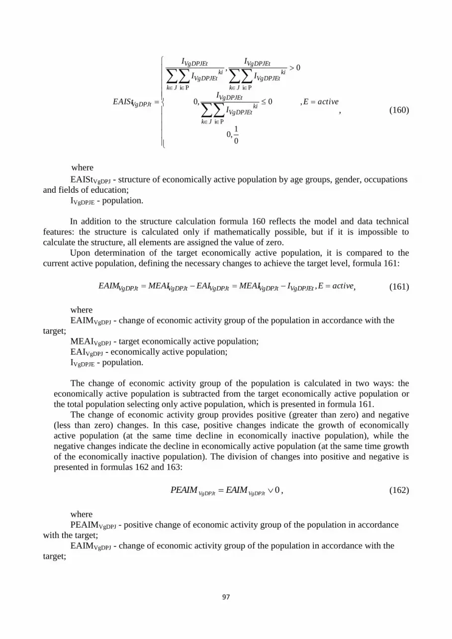
97
activeE
I
I
I
I
I
I
EAISt
Jk
kiVgDPJEt
VgDPJEt
Jk
kiVgDPJEt
VgDPJEt
Jk
kiVgDPJEt
VgDPJEt
VgDPJt
,
0
1,0
0,0
0,
Pi
PiPi
, (160)
where
EAIStVgDPJ - structure of economically active population by age groups, gender, occupations
and fields of education;
IVgDPJE - population.
In addition to the structure calculation formula 160 reflects the model and data technical
features: the structure is calculated only if mathematically possible, but if it is impossible to
calculate the structure, all elements are assigned the value of zero.
Upon determination of the target economically active population, it is compared to the
current active population, defining the necessary changes to achieve the target level, formula 161:
activeEIMEAIEAIMEAIEAIM VgDPJEtVgDPJtVgDPJtVgDPJtVgDPJt , , (161)
where
EAIMVgDPJ - change of economic activity group of the population in accordance with the
target;
MEAIVgDPJ - target economically active population;
EAIVgDPJ - economically active population;
IVgDPJE - population.
The change of economic activity group of the population is calculated in two ways: the
economically active population is subtracted from the target economically active population or
the total population selecting only active population, which is presented in formula 161.
The change of economic activity group provides positive (greater than zero) and negative
(less than zero) changes. In this case, positive changes indicate the growth of economically
active population (at the same time decline in economically inactive population), while the
negative changes indicate the decline in economically active population (at the same time growth
of the economically inactive population). The division of changes into positive and negative is
presented in formulas 162 and 163:
0 VgDPJtVgDPJt EAIMPEAIM , (162)
where
PEAIMVgDPJ - positive change of economic activity group of the population in accordance
with the target;
EAIMVgDPJ - change of economic activity group of the population in accordance with the
target;

98
0 VgDPJtVgDPJt EAIMNEAIM , (163)
where
NEAIMVgDPJ - negative change of economic activity group of the population in accordance
with the target;
EAIMVgDPJ - change of economic activity group of the population in accordance with the
target;
Positive and negative changes of the economic activity group are calculated comparing the
change of the group to zero. In addition, the negative change of economic group receives another
sign, i.e. negative (less than zero) number receives the positive (greater than zero) number. In the
result the further calculated index “growth of inactive population” is positive.
Growth of economically active and inactive population is presented in formulas 164 and
165:
VgDPJtVgDPJtVgDPJt NEAIMPEAIMEAIP . (164)
where
EAIPVgDPJ - growth of active population;
PEAIMVgDPJ - positive change of economic activity group of the population in accordance
with the target;
NEAIMVgDPJ - negative change of economic activity group of the population in accordance
with the target.
VgDPJtVgDPJtVgDPJt PEAIMNEAIMENIP . (165)
where
ENIPVgDPJ - growth of inactive population;
NEAIMVgDPJ - negative change of economic activity group of the population in accordance
with the target;
PEAIMVgDPJ - positive change of economic activity group of the population in accordance
with the target.
Calculating the growth of economically active and inactive population, positive and
negative changes of economic activity groups are taken into account twice: primarily, they increase
the relevant population group, secondly - reduce the population of the opposite group (i.e., with the
growth of economically active population, economically inactive population declines, and vice
versa). Taking into account the equation specifics, the growth of economically active and inactive
population can be both positive and negative, that is, they reflect both population growth and
decline in the groups.
Knowing the economically active and inactive population growth, it is possible to calculate
the resulting change of economic activity group of population, formula 166:
VgDPJtVgDPJtVgDPJEt ENIPEAIPAM . (166)
where
AMVgDPJE - change of economic activity group of the population;
EAIPVgDPJ - growth of active population;
ENIPVgDPJ - growth of inactive population.

99
The change of economic activity group of population integrates the growth of economically
active and inactive population into a single matrix, giving the status of the economic activity group
to the elements of the group.
2.2.5. International migration sub-model
International migration sub-model uses unified algorithms according to analysis groups of
the population education level. Overall scheme of the unified algorithm of the international
migration is presented in Figure 2.44.
<Wages
correlation index>
<Population>
<Longstandingunoccupied working
places>
Labour emigration inaccordance with the current
structure
Time to take
emigration decision
Emigration
propensity
Economic emigration
formation index
Economic immigration
formation index
Target wage ratio
Changes of longstanding
unoccupied working places
Total emigration
Return immigration
Economic
immigration
Total immigration
Readiness to invite the
foreign employees
Time to get integrated
into Latvian society
Longstanding unoccupiedworking places, which are
forming immigration
Check of longstanding
unoccupied working places
Demanded
immigration
Age structure of
immigrants
Provided
participation level
Immigration ratio forsolution of the laborshortage problem
Method of definition of
the migration types
Labour emigration inaccordance with theprovided structure
Labour immigration inaccordance with the current
structure
Figure 2.44. Overall scheme of the unified algorithm of the international migration
Figure 2.44 shows that the international migration algorithm of the population is divided
into two parts: emigration and immigration. Two different algorithms are applied to those parts.
Economic migration for both algorithms is formed by the salary ratio. Two pairs of salaries
are used to compare the salary: “target salary ratio”, which evaluates the relationship of the salary
100
level between two highly developed countries, at which the economic migration has a random
nature, and “salary ratio”, which compares the Latvian and EU average salaries. The closer these
indexes are and the less the difference is, the less the economic migration cause is. This is presented
by economic migration (emigration and immigration) formation indexes in Figure 2.44.
Emigration is determined by the economic emigration formation index, emigration
propensity (which is a fixed factor) and the population in the analysis group, it is represented by the
element “labour emigration according to the current structure”. While forecasting the labour market
development, emigration amount is partly simulated and partly controllable parameter, so the labour
emigration does not take place in accordance with the current labour structure. The emigration in
the model takes place according to the provided economic activity level. This means that the
element “labour emigration according to the current structure” determines labour emigration
amounts by occupations, gender, age and education groups, while the next element “labour
emigration according to the provided structure” determines the labour migration by economic
activity levels. The element “total emigration” compares emigration and population if necessary,
reducing the emigration in order to prevent the emigration amounts to exceed the population.
Immigration in sub-model is formed of three aspects: return immigration, economic
migration and demanded immigration.
The significant proportion of immigration is formed by returned emigrants, called as the
“return migration” in algorithm. It depends on the improvement of economic situation in the
country, in particular - on the changes of long-term vacant working places (i.e., growth). With the
increase of the number of long term vacant working places, the return immigration increases and
may be equal to emigration amounts.
Economic immigration consists of long-term vacant working places in the country,
economic immigration index (as a measure of the salary level), but it is limited by the readiness of
the local employers to invite the employees from abroad, as well as the time required for foreigners
to integrate into Latvian society.
Additionally, immigration covers potential long-term labour shortage in the country. If the
GDP growth is projected, which cannot be ensured by the increase in productivity, and there are no
labour reserves in the country, the immigration can solve labour shortage problem. This
immigration is called as the demanded immigration in algorithm. It mainly depends on the long-
term vacant working places and their dynamics. The developed algorithm allows determining the
level of the demanded immigration impact on the labour market, i.e. modelling of the state
migration policy outcomes (the elements “immigration ratio for solution of the labour shortage
problem” and “method of definition of migration types” are integrated in the user interface and
allow modelling different scenarios).
Summing up economic return and the demanded immigration, the labour immigration is
obtained according to the current structure. Forecasting labour market development, immigration
amount is partly simulated and partly controllable parameter, so that labour migration does not take
place in accordance with the current immigration structure determined by the market. The
immigration in the model takes place according to the provided economic activity level. It means
that the element “labour immigration in accordance with the current structure” determines the
labour immigration levels by occupation, gender, age and education groups, but the next element
“total immigration” determines the labour migration by economic activity levels. Unlike
emigration, immigration amounts are not dependent on the population in the analysed group.
Investigation of the constituent equations of the international migration sub-model begins
with the investigation of the emigration equations. Formula 167 presents the investigation of the
economic emigration formation index:

101
0 tt AAKMAAKEEVK , (167)
where
EEVK - economic emigration formation index;
MAAK - target salary ratio;
AAK - salary ratio.
Economic emigration formation index compares two pairs of salaries “target salary ratio”,
which evaluates the relationship of the salary level between two highly developed countries, at
which the economic migration has the random nature, and “salary ratio”, which compares the
Latvian and EU average salaries. The closer these indexes are and the less the difference is, the less
the economic migration cause is. Economic emigration formation index is always greater than zero,
i.e., with the increase of the salary level in the country up to EU level or more, the index decreases
only to zero, and emigration does not become an immigration.
Economic emigration formation index allows calculating the labour emigration amounts
according to current labour structure, which is presented in formula 168:
tEEVKTML
ETIEMES
VgDPJEt
VgDPJEt , (168)
where
EMESVgDPJE - labour emigration in accordance with the current structure;
IVgDPJE - population;
ET - emigration propensity;
TML - time to take the emigration decision;
EEVK - economic migration formation index.
Formula 168 shows that emigration depends on the population in the group, emigration
propensity, time of decision making on emigration and economic emigration formation index.
In accordance with the structure in formula 169, the labour emigration has been changed
according to the provided economic activity level:
activenonEULL
activeEULLEMESEMUS
Ei
i
,1
,
VgDt
VgDtVgDPJEtVgDPJEt , (169)
where
EMUSVgDPJE - labour emigration in accordance with the provided structure;
EMESVgDPJE - labour emigration in accordance with the current structure;
ULLVgD - provided participation level.
Formula 169 shows that according to the current structure, the economic activity groups are
summed up for the labour emigration, and then the new economic activity groups are assigned
according to the provided participation level.
On the basis of the labour emigration the total emigration is calculated according to the
current structure, formula 170:

102
VgDPJEtVgDPJEt
l
VgDPJEt IEMUSEM , (170)
where
EMVgDPJEl - total emigrations at the education level 1;
EMUSVgDPJE - labour emigration in accordance with the provided structure;
IVgDPJE - population.
The resulting emigration is calculated as the minimum number of people in the calculated
labour emigration according to the provided structure and in the analysed labour group. This
prevents more people to emigrate than there are in the system.
Unlike emigration, immigration has several causes. Model analyses three causes of
immigration: return immigration, economic immigration and demanded immigration. The return
immigration is analysed first.
Return immigration is related to the return of emigrants. It depends on the improvement of
economic situation in the country, in particular - with the changes of long-term vacant working
places (i.e., growth). Return immigration is calculated in formula 171:
101 VgDPJEtVgDPJEt tINDVIEMAIM , (171)
where
AIMVgDPJE - return immigration;
EMVgDPJE - emigration;
INDVI - changes of long-term vacant working places.
Formula 171 shows that the return of emigrants is dependent on the changes of long-term
vacant working places, which determine the ratio of the return of emigrants. As formula 170 shows,
the ratio of the return of emigrants is limited from 0 to 1, as required by the technical realization of
the model. Model predicts - if the economic situation gets worse, the return immigration may be
reduced up to zero.
The changes of long-term vacant working places from formula 171 are calculated in formula
172:
0;0
0,
0;0
0,
t
t
t
tt
1-t
1-t
1-t
t1-t
t
IINDV
IINDVIINDV
INDVIINDV
INDV
INDVINDV
INDVINDV
INDVI , (172)
where
INDVI - changes of long-term vacant working places;
INDV - long-term vacant working places;
IINDV - long-term vacant working places of the previous period.
The changes of long-term vacant working places can be calculated in two ways: directly
from long-term vacant working places and by introducing the intermediate parameter - long-term
vacant working places in the previous period. Regardless of the type of calculation, the parameter
reflects the relative changes of long-term vacant working places. This calculation requires the long-
term vacant working places, described in formula 173:

103
INDVD
VS
INDV Pk Di Jm
kim
DPJt t
, (173)
where
INDV - long-term vacant working places;
VSDPJ - number of vacancies;
INDVD - definition of long-term vacant working places.
In the calculation of the long-term vacant working places the number of vacancies and ratio
index of the long-term vacant working places (definition) have been used, which present the time
when the vacancies become long-term vacancies. Balancing module subchapter describes creation
of vacancies in detail.
The second type of migration is economic immigration. Calculation of economic
immigration is similar to the calculation of economic emigration. It is based on the economic
immigration formation index, which evaluates salaries in several countries. The calculation of the
economic immigration formation index is presented in formula 174:
0 tt MAAKAAKEIVK , (174)
where
EIVK - economic migration formation index;
AAK - salary ratio;
MAAK - target salary ratio.
The calculation of the economic immigration formation index (formula 174) is similar to the
calculation of the economic emigration formation index (formula 167). Comparing these indexes
we can see that in one case the difference in salaries is used to evaluate the economic benefits for
emigration, but in the second case - for immigration.
The calculation of the economic immigration is presented in formula 175:
ActiveEINDVStIMStTILS
EIVKGAADINDVEIM t
, DPJtVg
tVgDPJEt , (175)
where
EIMVgDPJE - economic immigration;
INDV - long-term vacant working places;
GAAD - readiness to invite the foreign employees;
EIVK - economic migration formation index;
TILS - time to get integrated into Latvian society;
IMStVg - age structure of immigrants;
INDVStDPJ - structure of long-term vacant working places;
E - economic activity group.
Economic immigration amounts determine the long-term vacant working places, but they
reduce the index “readiness to invite the foreign employees”, economic immigration formation
index and the time necessary for integration into Latvian society. The economic immigration
structure is determined by the age structure and the structure of longstanding unoccupied working
places, as indicated by formula 175. The calculation of the economic immigration uses constant
indexes that can be changed when planning the national policy on immigration.
In formula 175 all elements have been examined apart from the element “structure of long-
term vacant working places”, which is calculated in formula 176:

104
0,0
0,
t
ttt
INDV
INDVD
VS
INDV
INDVD
VS
INDV
INDVD
VS
INDVStDPJt
DPJtDPJt
, (176)
where
INDVStDPJ - structure of long-term vacant working places;
VSDPJ - number of vacancies;
INDVD - definition of long-term vacant working places;
INDV - long-term vacant working places.
The structure of long-term vacant working places is determined by dividing the long-term
vacant working places by gender, occupations and fields of education by total number of long-term
vacant working places. The number of long-term vacant working places by gender, occupations and
fields of education are calculated from the number of vacancies and definition of long-term vacant
working places (this is explained in formula 173). Additionally, formula 176 reflects that when it is
not possible to calculate the structure of long-term vacant working places, the relevant structure
elements are given the value of zero.
Further the required immigration has been investigated. It should be determined, based on
the state global and long-term labour shortage.
In the demanded immigration the formation of vacancies (long-term vacancies) does not
immediately create the immigration flow. These vacancies may be terminated by changing the
occupations of the employees or by means of education systems. It means that the required
immigration is caused by vacancies, which have a status of vacant working places for a long time,
as marked in the model “long-term vacant working places, which form immigration”. This
calculation is presented in formula 177:
IMITPROIINDVINDVIMITPRINDVINDVINDVM ttTVSM-ttt , (177)
where
INDVM - long-term vacant working places, which are forming immigration;
INDV - long-term vacant working places;
TVSM - time for occupation of vacancies for migration;
OIINDV - long-term vacant working places of the second level in the previous period;
IMITPR - immigration ratio in the solution of the labour shortage problem.
The long-term vacant working places, which form immigration, can be calculated in two
ways: directly from long-term vacant working places and by introducing the intermediate parameter
- long-term vacant working places of the second level in the previous period. Formula 177 shows
that the migration consists of a number of vacancies which have not been reduced in a certain time
(time for occupation of vacancies for migration). In addition, formula 177 specifies the national
policy planning element - immigration ratio in the solution of the labour shortage problem, which is
dependent on the choice of the model user and is integrated into the user management interface of
the model.
The demanded immigration calculation is based on the migration forming working places,
formula 178:

105
ActiveEIMVNVINDVStIMStINDVMPIM , DPJtVgtVgDPJEt , (178)
where
PIMVgDPJE - demanded immigration;
INDVM - long-term vacant working places, which form immigration;
IMStVg - age structure of immigrants;
INDVStDPJ - structure of long-term vacant working places;
IMVNV - method to define the immigration types;
E - economic activity group.
The requested immigration amount is determined by long-term vacant working places,
which are forming immigration. The structure of the required immigration is determined by the age
structure of immigrants and structure of long-term vacant working places. Additionally, formula
178 reflects the national policy planning element “method to define immigration type”, which
excludes or switches off the required immigration calculation, depending on the user management
interface of the model.
Summing up the return, economic and required immigration, labour immigration is
calculated in accordance with the current structure, formula 179:
VgDPJEtVgDPJEtVgDPJEtVgDPJEt PIMEIMAIMIMES , (179)
where
IMESVgDPJE - labour immigration in accordance with the current structure;
AIMVgDPJE - return immigration;
EIMVgDPJE - economic immigration;
PIMVgDPJE - demanded immigration.
Labour immigration in accordance with the current structure does not ensure the sufficient
controllability of the model results. To ensure the controllability options of the model results, the
immigration according to the current structure is converted according to the provided structure, by
calculating the resulting immigration, formula 180:
activenonEULL
activeEULLIMESIM
Ei
i
,1
,
VgDt
VgDtVgDPJEt
lVgDPJEt , (180)
where
IMVgDPJEl - total immigrations at the education level 1;
IMESVgDPJE - labour immigration in accordance with the current structure;
ULLVgD - provided participation level.
Formula 180 shows that for the labour immigration, according to the current structure, the
economic activity groups are summed up, and the new economic activity groups are defined
according to the provided participation level, obtaining the resulting immigration.
Formula 180 presents the last equation of international migration sub-model unified
algorithm of the educational levels. Sub-model also contains non-unified equations. They ensure
international migration, labour analysis and demographic sub-model synchronization. This is
presented in Figure 2.45.

106
<Total emigration at the
1st education level><Total emigration at the
i education level>
<Total immigration at the
1st education level><Total immigration at
the i education level>... ...
Total emigration Total immigration
Emigration by age
groups and gender
Immigration by age
groups and gender
Figure 2.45. International migration, labour analysis and demographic sub-model
synchronization
The unified algorithms of the international migration sub-model calculate emigration and
immigration by educational levels, which directly without processing are used in labour analysis
sub-model in the unified algorithms by educational levels. To synchronize demography and
international migration sub-models from unified algorithms, the total emigration and immigration
are calculated by levels of education. Further, provided that the international migration sub-model
operates with 5-year age groups, but the demographic sub-model analyses the population by one-
year age groups, migrants from 5-year age groups are divided by one-year age groups.
Summed up emigration and immigration calculation is reflected in formulas 181 and 182:
Li
EMEMli
VgDPJEtVgDPJEt , (181)
where
EMVgDPJE - total emigration;
EMVgDPJEl - total emigration at the education level 1.
Li
IMIMli
VgDPJEtVgDPJEt , (182)
where
IMVgDPJE - total immigration;
IMVgDPJEl - total immigration at the education level 1.
The total migration is calculated as the sum of the migration by educational levels.
Migration conversion from five-year age groups by one-year age groups is presented in
formulas 183 and 184:
74_70,7470,5
...
19_15,1915,5
nki
VgDPJEt
nki
VgDPJEt
VDt
VgVgV
EM
VgVgV
EM
EM
En Jk Pi
En Jk Pi
, (183)
where
EMVD - emigration by age groups and gender;
EMVgDPJE - summed up emigration.

107
74_70,7470,5
...
19_15,1915,5
nki
VgDPJEt
nki
VgDPJEt
VDt
VgVgV
IM
VgVgV
IM
IM
En Jk Pi
En Jk Pi
, (184)
where
IMVD - immigration by age groups and gender;
IMVgDPJE - summed up immigration.
Formulas 183 and 184 reflect the fact that the international migration and demographic sub-
model synchronization requires the reduction of the number of migration dimensions (population is
summed up by occupations, fields of education and economic activity groups), and the population is
divided from the five-year age groups in the equal proportion by the relevant one-year age groups.

108
2.3. Labour market module: balancing labour demand and supply
Structure of labour market module is presented in Figure 2.46.
Labour market module
Labour market
sub-model
Wage sub-model
Labour demand module of SDM model
Sector labour demand sub-model
Occupational labour demand sub-model
Sub-model of
labour demand
by education
Sub-model of
labour demand
by gender
Labour supply module of SDM model
Demographic
sub-model
Education
attainment
sub-model
Working-age
population
stock-taking
sub-model
Labour force
participation
sub-model
International
migration
sub-model
Figure 2.46. Structure of labour market module and relation to other model modules
The Figure 2.46 shows that the labour market module consists of two sub-models: labour
market and wage sub-models. Labour market sub-model combines labour demand and supply,
taking into account the labour amounts and wages. Formation of labour supply and demand has
been analysed above. Wage sub-model analyses the most important processes (changes of
productivity) in the national economy and labour demand and supply amounts, resulting in the
wages. Labour wages affect both labour market balance and labour supply formation, that is, the
choice of education and international migration.
2.3.1. Labour market sub-model
SDM model in the labour market sub-model combines the labour supply and demand by
determining labour employment, number of jobseekers, number of working places and number of
occupied working places. On the basis of these key elements such important parameters as the
number of vacancies, etc. are calculated. The scheme of the labour market sub-model algorithms is
presented in Figure 2.47 (next page).
Figure 2.47 presents the labour market sub-model stocks, flows, key elements and
algorithms scheme. Figure 2.74 reflects all stocks and flows, the impact of the algorithm on them,
but it does not present the impact of the stocks and flows on key elements of the algorithms in
detail. Figure 2.47 provides presentation of the operation logic and stock - flow system of the
module. The logical structure of the sub-model is analysed in detail in the next subsection.
2.3.1.1. Framework and structure of the labour demand and supply
balancing sub-model
SDM model provides analysis of the labour market by educational levels, each of the
educational levels uses the unified labour balancing sub-model, which is presented in Figure 2.47.
Combining labour balancing sub-models by levels of education, the overall labour market sub-
model is presented in the following way, Figure 2.48 (next page).

109
Jobseekers Employed
Move fromemployment to job
search
Move from job search
to employment
Increase of the
number of jobseekers
Decline in the number
of jobseekers
Decline in the number ofemployed due to the change of
age structure
Employment after the
change of occupation
Change of occupation in
order to get a job
Change of the age
structure of jobseekers
Number ofworkingplaces
Occupiedworkingplaces
The working place is
being released
The working place is
being occupied
Number of
vacancies
Decline in the number
of working places
Creation of new
working places
<Algorithm of liquidation
of working places>
<Algorithm of decline in thenumber of vacancies and
occupied working places>
Change of occupation
of employed
Change of the age
structure of employed
Decline in the number
of employed
<Algorithm of changes
of labor amount>
<Employment andprofessional mobility
algorithm>
Correction
<Algorithm ofcalculation of the
vacancies>
<Algorithm of
sinhronization>
Correction of the
structure of employed
Figure 2.47. Scheme of the algorithm of the labour market sub-model
Basic general education,
vocational education with
basic education
Darba
meklētājiStrādājošie
Pariet no nodarbinātības
uz darba meklēšanu
Pariet no darbameklēšanas uznodarbinātību
Darba meklētāju
skaita pieaugums
Darba meklētāju
skaita samazinājums
Nodarbināto skaitasamazinājums vecumastruktūras izmaiņas dēļ
Iekārtošana darbā pēc
profesijas nomaiņas
Profesijas nomaiņa ar
mērķi iegūt darbu
Darba meklētājuvecuma struktūras
izmaiņas
Darba vietu
skaitsAizņemtas
darba vietas
Tiek atbrīvota
darba vieta
Tiek aizņemta
darba vieta
Vakančuskaits
Darba vietu
samazināšana
Jaunu darba vietu
izveidošana
<Darba vietusamazināšanas
algoritms>
<Vakanču un Aizņemtodarba vietu samazināšanas
algoritms>
Nodarbināto
profesijas nomaiņa
Nodarbināto vecuma
struktūras izmaiņas
Nodarbināto skaita
samazinājums
<Darbaspēka apjomaizmaiņu algoritms>
<Iekārtošana darbā unprofesionālās mobilitātes
algoritms>
General secondary,
vocational and secondary
vocational education
Darba
meklētājiStrādājošie
Pariet no nodarbinātības
uz darba meklēšanu
Pariet no darbameklēšanas uznodarbinātību
Darba meklētāju
skaita pieaugums
Darba meklētāju
skaita samazinājums
Nodarbināto skaitasamazinājums vecumastruktūras izmaiņas dēļ
Iekārtošana darbā pēc
profesijas nomaiņas
Profesijas nomaiņa ar
mērķi iegūt darbu
Darba meklētājuvecuma struktūras
izmaiņas
Darba vietu
skaitsAizņemtas
darba vietas
Tiek atbrīvota
darba vieta
Tiek aizņemta
darba vieta
Vakančuskaits
Darba vietu
samazināšana
Jaunu darba vietu
izveidošana
<Darba vietusamazināšanas
algoritms>
<Vakanču un Aizņemtodarba vietu samazināšanas
algoritms>
Nodarbināto
profesijas nomaiņa
Nodarbināto vecuma
struktūras izmaiņas
Nodarbināto skaita
samazinājums
<Darbaspēka apjomaizmaiņu algoritms>
<Iekārtošana darbā unprofesionālās mobilitātes
algoritms>
First level vocational higher
education
Darba
meklētājiStrādājošie
Pariet no nodarbinātības
uz darba meklēšanu
Pariet no darbameklēšanas uznodarbinātību
Darba meklētāju
skaita pieaugums
Darba meklētāju
skaita samazinājums
Nodarbināto skaitasamazinājums vecumastruktūras izmaiņas dēļ
Iekārtošana darbā pēc
profesijas nomaiņas
Profesijas nomaiņa ar
mērķi iegūt darbu
Darba meklētājuvecuma struktūras
izmaiņas
Darba vietu
skaitsAizņemtas
darba vietas
Tiek atbrīvota
darba vieta
Tiek aizņemta
darba vieta
Vakančuskaits
Darba vietu
samazināšana
Jaunu darba vietu
izveidošana
<Darba vietusamazināšanas
algoritms>
<Vakanču un Aizņemtodarba vietu samazināšanas
algoritms>
Nodarbināto
profesijas nomaiņa
Nodarbināto vecuma
struktūras izmaiņas
Nodarbināto skaita
samazinājums
<Darbaspēka apjomaizmaiņu algoritms>
<Iekārtošana darbā unprofesionālās mobilitātes
algoritms>
Academic education and
second level vocational
higher education
Darba
meklētājiStrādājošie
Pariet no nodarbinātības
uz darba meklēšanu
Pariet no darbameklēšanas uznodarbinātību
Darba meklētāju
skaita pieaugums
Darba meklētāju
skaita samazinājums
Nodarbināto skaitasamazinājums vecumastruktūras izmaiņas dēļ
Iekārtošana darbā pēc
profesijas nomaiņas
Profesijas nomaiņa ar
mērķi iegūt darbu
Darba meklētājuvecuma struktūras
izmaiņas
Darba vietu
skaitsAizņemtas
darba vietas
Tiek atbrīvota
darba vieta
Tiek aizņemta
darba vieta
Vakančuskaits
Darba vietu
samazināšana
Jaunu darba vietu
izveidošana
<Darba vietusamazināšanas
algoritms>
<Vakanču un Aizņemtodarba vietu samazināšanas
algoritms>
Nodarbināto
profesijas nomaiņa
Nodarbināto vecuma
struktūras izmaiņas
Nodarbināto skaita
samazinājums
<Darbaspēka apjomaizmaiņu algoritms>
<Iekārtošana darbā unprofesionālās mobilitātes
algoritms>
Doctoral education
Darba
meklētājiStrādājošie
Pariet no nodarbinātības
uz darba meklēšanu
Pariet no darbameklēšanas uznodarbinātību
Darba meklētāju
skaita pieaugums
Darba meklētāju
skaita samazinājums
Nodarbināto skaitasamazinājums vecumastruktūras izmaiņas dēļ
Iekārtošana darbā pēc
profesijas nomaiņas
Profesijas nomaiņa ar
mērķi iegūt darbu
Darba meklētājuvecuma struktūras
izmaiņas
Darba vietu
skaitsAizņemtas
darba vietas
Tiek atbrīvota
darba vieta
Tiek aizņemta
darba vieta
Vakančuskaits
Darba vietu
samazināšana
Jaunu darba vietu
izveidošana
<Darba vietusamazināšanas
algoritms>
<Vakanču un Aizņemtodarba vietu samazināšanas
algoritms>
Nodarbināto
profesijas nomaiņa
Nodarbināto vecuma
struktūras izmaiņas
Nodarbināto skaita
samazinājums
<Darbaspēka apjomaizmaiņu algoritms>
<Iekārtošana darbā unprofesionālās mobilitātes
algoritms>
Total number of jobseekers Total number of employed Total number of vacancies
Figure 2.48. Labour market sub-model

110
Summing up the results of unified labour market sub-models by educational levels, the key
model elements have been calculated: total number of jobseekers, total number of employed, total
number of vacancies. On this basis, the key labour market indicators have been calculated: the
number of jobseekers by educational levels, the number of jobseekers by gender, jobseekers by
occupations, the number of employed by age groups and gender, the number of employed by
occupations, the number of employed by levels and fields of education; the number of vacancies by
gender, the number of vacancies by occupations, the number of vacancies by educational levels.
185 - 188 formulas reflect the summation equations of the results of the unified labour
market sub-models by levels of education.
Formula 185 reflects the calculation of the total number of jobseekers:
iVgk
k
itVgDPJ
iVgk
k
tiVgDPJ
Vgk
k
tVgDPJ
Vgk
k
tVgDPJDPJLt DMDMDMDMKDM _
1
)1_(
2
2_
1
1_ ... ,(185)
where
KDMDPJL - total number of jobseekers;
DMVgDPJ_i - number of jobseekers at the education level i;
Vg - age group;
D - gender;
P - occupation;
J - field of education;
L - level of education.
Formula 186 reflects the calculation of the total number of employed:
iVgk
k
itVgDPJ
iVgk
k
tiVgDPJ
Vgk
k
tVgDPJ
Vgk
k
tVgDPJDPJLt NNNNKN _
1
)1_(
2
2_
1
1_ ... , (186)
where
KNDPJL - total number of employed;
NVgDPJ_i - number of employed at the education level i;
Vg - age group;
D - gender;
P - occupation;
J - field of education;
L - level of education.
Formula 187 reflects the calculation of the total number of vacancies:
iitDPJitiDPJtDPJtDPJDPJLt VSVSVSVSKVS _1)1_(22_11_ ...
, (187)
where
KVSDPJL - total number of vacancies;
VSDPJ_i - number of vacancies at the education level i;
Vg - age group;
D - gender;
P - occupation;
J - field of education;
L - level of education.
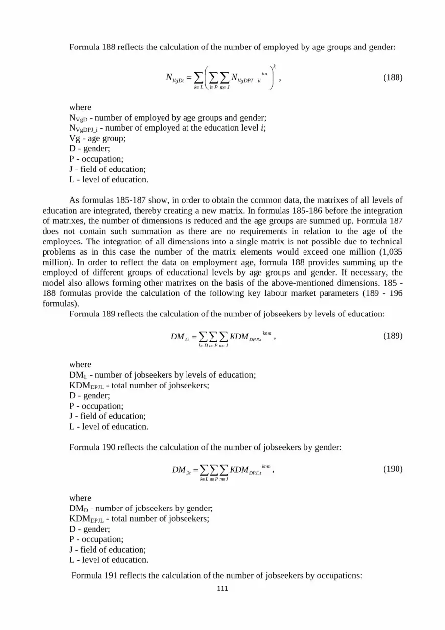
111
Formula 188 reflects the calculation of the number of employed by age groups and gender:
Lk
k
Pi Jm
im
itVgDPJVgDt NN _ , (188)
where
NVgD - number of employed by age groups and gender;
NVgDPJ_i - number of employed at the education level i;
Vg - age group;
D - gender;
P - occupation;
J - field of education;
L - level of education.
As formulas 185-187 show, in order to obtain the common data, the matrixes of all levels of
education are integrated, thereby creating a new matrix. In formulas 185-186 before the integration
of matrixes, the number of dimensions is reduced and the age groups are summed up. Formula 187
does not contain such summation as there are no requirements in relation to the age of the
employees. The integration of all dimensions into a single matrix is not possible due to technical
problems as in this case the number of the matrix elements would exceed one million (1,035
million). In order to reflect the data on employment age, formula 188 provides summing up the
employed of different groups of educational levels by age groups and gender. If necessary, the
model also allows forming other matrixes on the basis of the above-mentioned dimensions. 185 -
188 formulas provide the calculation of the following key labour market parameters (189 - 196
formulas).
Formula 189 reflects the calculation of the number of jobseekers by levels of education:
Dk Pn Jm
knm
DPJLtLt KDMDM , (189)
where
DML - number of jobseekers by levels of education;
KDMDPJL - total number of jobseekers;
D - gender;
P - occupation;
J - field of education;
L - level of education.
Formula 190 reflects the calculation of the number of jobseekers by gender:
Lk Pn Jm
knm
DPJLtDt KDMDM , (190)
where
DMD - number of jobseekers by gender;
KDMDPJL - total number of jobseekers;
D - gender;
P - occupation;
J - field of education;
L - level of education.
Formula 191 reflects the calculation of the number of jobseekers by occupations:

112
Lk Dn Jm
knm
DPJLtPt KDMDM , (191)
where
DMP - number of jobseekers by occupations;
KDMDPJL - total number of jobseekers;
D - gender;
P - occupation;
J - field of education;
L - level of education.
Formula 192 reflects the calculation of the number of employed by occupations:
Lk Di Jm
kim
DPJLtPt KNN , (192)
where
NP - number of employed by occupations;
KNDPJL - total number of employed;
D - gender;
P - occupation;
J - field of education;
L - level of education.
Formula 193 reflects the calculation of the number of employed by levels and fields of
education:
Dk Jm
km
DPJLtLJt KNN , (193)
where
NLJ - number of employed by levels and fields of education;
KNDPJL - total number of employed;
D - gender;
P - occupation;
J - field of education;
L - level of education.
Formula 194 reflects the calculation of vacancies by gender:
Lk Pi Jm
kim
DPJLtDt KVSVS , (194)
where
VSD - number of vacancies by gender;
KVSDPJL - total number of vacancies;
D - gender;
P - occupation;
J - field of education;
L - level of education.

113
Formula 195 reflects the calculation of vacancies by occupations:
Lk Di Jm
kim
DPJLtPt KVSVS , (195)
where
VSP - number of vacancies by occupations;
KVSDPJL - total number of vacancies;
D - gender;
P - occupation;
J - field of education;
L - level of education.
Formula 196 reflects the calculation of vacancies by levels of education:
Pk Di Jm
kim
DPJLtLt KVSVS , (196)
where
VSL - number of vacancies by levels of education;
KVSDPJL - total number of vacancies;
D - gender;
P - occupation;
J - field of education;
L - level of education.
As the 189 - 196 formulas show, the key labour market parameters have been calculated
from the technical elements of the model (185 - 188 formulas), simply by reducing the number of
dimensions and summing up the indexes in the selected dimension.
The investigation of the labour market sub-model equation is followed by explanation of the
labour market sub-model unified algorithm (Figure 2.47). Calculation equations of the unified
algorithm levels are presented in the 197 - 200 formulas.
Formula 197 reflects the calculation equation of the stock of the number of jobseeker:
dt )
()(t (t)
DPJDPJDPJ1VgDPJVgDPJ
T
t
VgDPJVgDPJVgDPJ0VgDPJVgDPJ
0
VgVgVg KORDMvSDMvSDMSNDM
DMNPMDMDMPDMDM
,
VgDPJVgDPJVgDPJVgDPJVgDPJ
DPJDPJ1
,74_70,69_65,,24_20,19_15
,74_70,69_65,,24_20
DMSNDMDMNPMDMDMPVg
DMvSNDMvSVgVg
VgVg
, (197)
where
DMVgDPJ - number of jobseekers;
DMPVgDPJ - increase of the number of jobseekers;
PMDMVgDPJ - change of occupations in order to get a job;
DMNVgDPJ - move from job search to employment;
NDMVgDPJ - move from employment to job search;
DMSVgDPJ - decline in the number of jobseekers;
DMvSVgDPJ - change of the age structure of jobseekers;
KORVgDPJ - correction;
Vg - age group;
D - gender;

114
P - occupation;
J - field of education.
Formula 198 reflects the calculation equation of the stock of the number of employed:
dt )
()(t (t)
DPJDPJDPJDPJ1VgDPJVgDPJVgDPJ
T
t
VgDPJVgDPJVgDPJ0VgDPJVgDPJ
0
VgVgVgVg NKORKORNvSNvSNSNPPMN
NDMNPMDMNNN
,
DPJDPJVgDPJVgDPJVgDPJ
VgDPJVgDPJ
DPJDPJ1
,74_70,69_65,,24_20,19_15
,74_70,69_65,,24_20
VgVg
VgVg
NKORKORNSPMNNDM
NPMDMNVg
NvSNvSVg
Vg
, (198)
where
NVgDPJ - number of employed;
DMNVgDPJ - move from job search to employment;
NPMVgDPJ - change of occupation of employed;
NDMVgDPJ - move from employment to job search;
PMNVgDPJ - employment after the change of occupation;
NSVgDPJ - decline in the number of employed due to the change of age structure;
NPVgDPJ - decline in the number of employed;
NvSVgDPJ - change of the age structure of employed;
KORVgDPJ - correction;
NKORVgDPJ - correction of the structure of employed;
Vg - age group;
D - gender;
P - occupation;
J - field of education.
Formula 199 reflects the calculation equation of the stock of the number of occupied
working places:
T
t
DPJDPJDPJ0DPJDPJ
0
dt )()(t (t) ADVKDVTDVIADVADV , (199)
where
ADVDPJ - occupied working places;
DVIDPJ - the working place is being occupied;
DVTDPJ - the working place is being released;
ADVKDPJ - correction of occupied working places;
D - gender;
P - occupation;
J - field of education.
Formula 200 reflects the calculation equation of the stock of the number of working places:
115
T
t
DPJDPJ0DPJDPJ
0
dt )()(t (t) DVLDVJDVDV , (200)
where
DVDPJ - number of working places;
DVJDPJ - creation of new working places;
DVLDPJ - decline in the number of working places;
D - gender;
P - occupation;
J - field of education.
As formulas 197 - 200 show, the stock levels of the algorithms are formed by the inflows
and outflows. Nature of levels is described below.
The stock of number of jobseekers, i.e., the number of jobseeker is calculated (formula 197)
by adding the increase of the number of jobseekers to the initial number of jobseekers (this flow can
be positive, i.e., may reflect the direct increase, and can also be negative, indicating the labour
reduction), as well as adding unemployed , who move from employment to job search (i.e.,
employees who have lost their jobs), and subtracting unemployed , who move from job search to
employment (have found a job), subtracting the decline in the number of unemployed , who change
occupations in order to get a job (have found a job in another occupation), subtracting the decline in
number of unemployed due to aging, as well as changing the age structure of the jobseekers and
making the correction of the jobseekers in accordance with the synchronization algorithm.
The stock of the number of jobseekers with three flows (move from job search to
employment, move from employment to job search and correction) is directly related to the level of
the number of employed.
The stock of the number of employed, i.e. the number of employed is calculated (formula
198) by adding the unemployed , who move from job search to employment (have found a job) to
the initial number of employed, adding the persons who found a job after the change of occupation,
adding the decline in number of employed (this flow can be positive, i.e., may reflect the direct
increase, and can also be negative, indicating the labour reduction), and subtracting the number of
employed, who changed their occupations (on one hand, this flow subtracts the number of
employed, who changed their occupations from the stock of the number of employed, while, on the
other hand, adds the number of employed with new occupations, thus, the flow in some groups may
be both positive and negative), subtracting the decline in number of unemployed due to aging, as
well as changing the age structure of the jobseekers and making the correction of the jobseekers in
accordance with the synchronization algorithm.
In total, the stock of the number of jobseekers and employed, and their binding flows model
the labour (active population) movement in the labour market: transition from employment to job
search and backward, the changes of occupational and age structure, as well as labour growth and
reduction.
Figure 2.47 presents two other stocks, namely occupied working places (formula 199) and
the number of working places (formula 200). The stock of the number of working places reflects the
number of the proposed working places in the national economy, but the stock of the occupied
working places reflects how many working places are occupied. Occupied working places result
from the initially occupied working places and their affecting changes, i.e., vacation, occupation
and correction of occupied working places (appropriate flows). Working places result from the
initial working places and affecting changes, i.e., creation and liquidation of working places
(appropriate flows).
All flows presented in Figure 2.47 are interrelated. Algorithms presented in Figure 2.47
ensure synchronization of the flows. Employment depends on two factors: labour supply and
demand, or, in other words, working places and labour (employed and jobseekers). By

116
synchronizing working places, occupied working places and the number of employed, the biggest
problem is related to the fact that the certain working places can be occupied by partially
appropriate staff, that is, for example, the working place can be occupied by an employee with an
appropriate occupation, but with nonconforming gender and education. In this case, the structures of
working places, occupied working places and employed do not match. The number of vacancies
cannot be calculated by subtracting the number of occupied working places from the number of
working places. There is a need to include corrections and synchronization algorithms, which are
described below along with the flow characterizing equations, in the algorithms scheme (Figure
2.47).
The flows in Figure 2.47 present the results of the algorithms, which combine sub-model
algorithms with the most important (central) model parameters. The input data for the flows in
Figure 2.47 are mostly related to the sub-model algorithms. The flow constituent equations,
showing their relation to the algorithms are presented below (formulas 201, 203 - 216, 219 and
220).
Formula 201 presents the calculation equations of the flow “changes of the age structure of
jobseekers”:
VgDPJtVgDPJEtVgDPJt DMIsNOVDMvS ,
,69_65,,24_20,19_15 Vg E = active, (201)
where
DMvSVgDPJ - change of the age structure of jobseekers;
NOVVgDPJE - aging;
DMIsVgDPJ - ratio of jobseekers in active population;
E - economic activity group;
Vg - age group;
D - gender;
P - occupation;
J - field of education.
As formula 201 shows, changes of the age structure of jobseekers are synchronized with the
labour supply module (element “aging”), as well as the ratio of jobseekers in the active population
is observed. This formula shows that the active population, from the population labour supply
module, is partially aging in the group of jobseekers (the second part is aging in the group of
employed, and this distribution by groups determines the ratio of jobseekers in active population).
In order to calculate the changes of the age structure of jobseekers, it is necessary to know
the ratio of jobseekers in active population. Its calculation is presented in formula 202:
000,0
000,00
0
VgDPJtVgDPJt
VgDPJtVgDPJt
VgDPJtVgDPJt
VgDPJt
VgDPJt
NDM
NDMNDM
DM
DMIs
,
(202)
where
DMIsVgDPJ - ratio of jobseekers in active population;
DMVgDPJ - number of jobseekers;
NVgDPJ - number of employed;
Vg - age group;
D - gender;
P - occupation;
J - field of education.

117
The calculation of the group ratio is based on the total calculation principle: the group is
divided by the total sum of the group. Formula 202 shows technological specifics of the SDM
model. The model analyses various groups, for example, by occupation and age, etc. If the sum of
the groups is equal to zero (for example, the certain occupation has no labour, employed and
jobseekers), it is not possible automatically to calculate the ratio of the group (it is not possible to
divide by zero). In this case, all group elements and the results of the formula are equal to zero.
Similarly, formula 202 includes protection against negative numbers among the number of
jobseekers and employed people.
The changes of the age structure of employed are related to the changes of the age structure
of jobseekers. The calculation of the age structure of the employed is presented in formula 203:
VgDPJtVgDPJEtVgDPJt DMvSNOVNvS ,
,69_65,,24_20,19_15 Vg E = active, (203)
where
NvSVgDPJ - change of the age structure of employed;
NOVVgDPJE - aging;
DMvSVgDPJ - change of the age structure of jobseekers;
E - economic activity group;
Vg - age group;
D - gender;
P - occupation;
J - field of education.
Formula 203 reflects that the people who have not changed the age group in the group of
jobseekers, but have changed in the labour supply module among the active population, change the
age group also in the group of employed. Thus, the model provides demographic, labour analysis
sub-model synchronization with the labour market sub-model in accordance with the changes of the
age structure.
Similarly, the retirement possibilities are ensured, i.e. abandonment of the labour market by
reaching the retirement age. Formula 204 presents the calculation of the decline in the number of
jobseekers in accordance with the reach of retirement age:
VgDPJtVgDPJEtVgDPJt DMIsUNDMS , E = active, (204)
where
DMSVgDPJ - decline in number of employed;
UNVgDPJE - removal from analysis;
E - economic activity group;
Vg - age group;
D - gender;
P - occupation;
J - field of education.
As formula 204 shows, the decline in the number of jobseekers is synchronized with the
element “removal from analysis”, which is in the labour supply module. Labour market
abandonment by labour force is calculated in formula 205:

118
VgDPJtVgDPJEtVgDPJt DMSUNNS , E = active, (205)
where
NSVgDPJ - decline in the number of employed due to the change of age structure;
UNVgDPJE - removal from analysis;
DMSVgDPJ - decline in the number of employed;
E - economic activity group;
Vg - age group;
D - gender;
P - occupation;
J - field of education.
Formula 205 shows that the people who do not leave the labour market in the group of
jobseekers, but leave it in the labour supply module among the active population, also leave it in the
group of employed.
Formula 206 presents the flow, which provides the employment of jobseekers according to
the current occupation, but formulas 207 and 208 represent the flows that are related to the change
of occupation by the population in order to receive a job:
B
Ai
VgDPJtDMNDMN3
1
i
VgDPJt , (206)
where
DMNVgDPJ - move from job search to employment;
DMNiVgDPJ - occupation of vacancies in the i priority;
Vg - age group;
D - gender;
P - occupation;
J - field of education.
E
Ai
VgDPJtPMDMPMDM5
4
i
VgDPJt , (207)
where
PMDMVgDPJ - change of occupation in order to get a job;
PMDMiVgDPJ - change of occupation in i priority;
Vg - age group;
D - gender;
P - occupation;
J - field of education.
E
Ai
VgDPJtPMNPMN5
4
i
VgDPJt , (208)
where
PMNVgDPJ - employment after the change of occupation;
PMNiVgDPJ - occupation of vacancies in i priority;
Vg - age group;
D - gender;
P - occupation;
J - field of education.

119
Formulas 206-208 reflect the summing up of the results of employment multi-level
algorithm. The algorithm will be investigated later. Levels of the algorithm are numbered with
number and letter symbols and formulas show that the first three groups of the algorithm are related
to the employment according to the current occupation, but the other two - with the change of
occupation of the population in order to receive a job.
Formula 209 reflects the results of the algorithm of the employed occupational mobility
operations:
VgDPJtVgDPJtVgDPJt NPMVNPMANPM , (209)
where
NPMVgDPJ - change of occupation of employed;
NPMAVgDPJ - change of occupation;
NPMVVgDPJ - occupation of vacancies of employed;
Vg - age group;
D - gender;
P - occupation;
J - field of education.
Formula 209 reflects that in the result of the occupational mobility the same persons, on one
hand, leave certain occupations, but on the other hand, fill vacancies in other occupations.
Formula 210 and 211 reflect the flows of the increase of the number of jobseekers and
decline in the number of employed. These flows connect jobseekers and employed with labour
supply module, labour analysis sub-model; transfer the demographic changes to the labour
structure, economic activity, etc. changes to the labour market sub-model.
00 VgDPJEtVgDPJEtVgDPJtVgDPJEtVgDPJt ISSIISSIDMIsUPDMP , E = active, (210)
where
DMPVgDPJ - increase of the number of jobseekers;
UPVgDPJE - admission for analysis;
DMIsVgDPJ - ratio of jobseekers in active population;
ISSIVgDPJE - change of population and structure;
Vg - age group;
D - gender;
P - occupation;
J - field of education.
01 VgDPJEtVgDPJtVgDPJt ISSIDMIsNP , E = active, (211)
where
NPVgDPJ - decline in the number of jobseekers;
DMIsVgDPJ - ratio of jobseekers in active population;
ISSIVgDPJE - change of population and structure;
E - economic activity group;
Vg - age group;
D - gender;
P - occupation;
J - field of education.

120
The result of formula 210 can be either positive (there is an increase of the number of
jobseekers in the appropriate flow) or negative (decline). Formula 211 reflects the decline in
employment. This difference is related to the fact that along with the growth of labour, the new
labour supplements only the group of jobseekers, but the decline (e.g., mortality) affects both
jobseekers and employed. Decline in the number of jobseekers is calculated from the ratio of
jobseekers in the active population and positive changes of population and structure in formula 211.
The selection of positive changes from the change of population and structure indicates only the
decline in population in the analysis group, and is based on the decline in the number of employed.
The part which is not observed in the decline process of employed, is observed in the increase of the
number of jobseekers (formula 210). In addition, formula 210 shows that the jobseekers in the level
of education analysis group are supplemented by persons, who have attained this level of education
(admission for analysis), and all negative changes of population and structure. Negative changes of
population and structure reflect the increase of the population in the analysis group of the level of
education (taking into account the change of emigration or economic activity group). With the
growing population in the group, people are included in the circle of jobseekers (if the economic
activity status is active), as indicated by formula 210.
According to the algorithm of changes of labour amount, formulas 210 and 211 divide the
changes of active population in education, economic activity and demography among jobseekers
and employed.
Formula 212 reflects the flow, which makes employed people lose their jobs and move to
jobseekers:
VgDPJtVgDPJt ATSATSNDM 21VgDPJt , (212)
where
NDMVgDPJ - move from employment to job search;
ATS1VgDPJ - dismissal in the 1st priority;
ATS2VgDPJ - dismissal in the 2nd priority;
Vg - age group;
D - gender;
P - occupation;
J - field of education.
Formula 212 shows that employed people move from employment to job search in two
stages (priorities). The transfer from employment to job search is viewed in detail in the description
of the algorithm of decline in the number of vacancies and occupied working places, formula 212
reflects the overall result.
Formula 213 reflects the correction flow of the jobseekers and employed:
VgDPJtVgDPJt DMNKORKOR , (213)
where
KORVgDPJ - correction;
DMNKORVgDPJ - correction of the number of jobseekers and employed;
Vg - age group;
D - gender;
P - occupation;
J - field of education.
Formula 213 shows that the correction directly forms (without interference) and follows the
synchronization algorithm results.

121
Formula 214 reflects the correction flow of the structure of employed:
VgDPJtVgDPJtVgDPJtVgDPJtVgDPJt 21 NKORVNNKORNKORVNNKORNKOR , (214)
where
NKORVgDPJ - correction of the structure of employed;
NNKORVgDPJ - required correction of the structure of employed;
V1NKORVgDPJ - age group correction 1;
PNNKORVgDPJ - additionally required correction of employed structure;
V2NKORVgDPJ - age group correction 2;
Vg - age group;
D - gender;
P - occupation;
J - field of education.
Formula 214 processes synchronization algorithm results. Synchronization algorithm
defines the correction of the structure of employed so that the number of employed is not negative,
which is presented in formula 214. Further formula 212 shows that the age group correction is
subtracted from the correction of the employment structure (which is calculated according to the
required correction of employment structure). The logical nature of these activities is the following:
if the negative number of employed is provided, the age structure is corrected by changing the age
group to the previous or next, in order to provide a positive number of employed people. The
synchronization algorithm is in detail described in the synchronization algorithm sub-section.
Formula 215 reflects equation of the flow of occupation of working places:
Jk Di
DVINAVSADVIXDVI ik
DPJtDPJtDPJtDPJt , (215)
where
DVIDPJ - the working place is being occupied;
DVIXDPJ - the working place is being occupied in accordance with vacancies;
AVSADPJ - the structure of remaining vacancies;
DVINDPJ - the working place is being occupied in accordance with occupation of vacancies;
D - gender;
P - occupation;
J - field of education.
Formula 215, along with formulas 216 and 218 provide analysis of occupied working
places. The flow in formula 215 increases the number of occupied working places, the flow in
formula 216 reduces the number of the occupied working places, but formula 217 changes
(corrects) the employment structure, taking into account the fact that the employment structure does
not comply to the vacancy structure (for example, by gender or educational fields). Formula 216
reflects the flow equation of the released working places:
Vgi Vgi Vgi
NPMNDMNPNSDVT i
VgDPJt
i
VgDPJt
i
VgDPJtDPJtDPJt , (216)
where
DVTDPJ - the working place is being released;
NSDPJ - decline in the number of employed due to the change of age structure by occupation,
fields of education and gender;

122
NPVgDPJ - decline in the number of employed;
NDMVgDPJ - move from employment to job search;
NPMVgDPJ - change of occupation of employed;
Vg - age group;
D - gender;
P - occupation;
J - field of education.
Formula 215 operates with the elements of the algorithm of decline in the vacancies and
occupied working places, this algorithm is described below. Formula 216 is directly related to the
sub-model flows. The only interparameter, which is not covered by the flows or algorithms is the
“decline in the number of employed due to the change of age structure by occupation, fields of
education and gender” which is derived from “decline in the number of employed due to the change
of age structure” by reducing the number of element dimensions (aggregating by age groups)
formula 217:
Vgi
NSNS i
VgDPJtDPJt , (217)
where
NSDPJ - decline in the number of employed due to the change of age structure by
occupations, fields of education and gender;
NSVgDPJ - decline in the number of employed due to the change of age structure;
Vg - age group;
D - gender;
P - occupation;
J - field of education.
Transferring from the labour analysis to the analysis of the working places, it is necessary
to reduce the number of element dimensions in the model, as the labour (supply) requires the
analysis by age groups, but the working places (demand) do not have such a requirement. This
activity is presented in formula 218. Formula 218 shows the correction calculation equation.
0,
0,0)( DPJtDPJtDPJt
DVTADVADVK
Jk Di
ik
Pl Jk Di
iklDVTADV )0)(( DPJtDPJt
,
DPJtDPJtDPJt DVTDVIADV , (218)
where
ADVKDPJ - correction of occupied working places;
ADVDPJ - occupied working places;
DVTDPJ - working place is being released;
DVIDPJ - working place is being occupied.
The calculation of the correction of occupied working places reflects the results of vacancies
calculation algorithm, which are analysed in the next subsections.
The number of working places in the system is dependent on development of the national
economy: with the development of the national economy, the number of working places increases,
but during the crisis, as well as with the growth of the labour productivity, the number of working

123
places decreases. The equation of the flow of the creation of new working places is presented in
formula 219, but the equation of the liquidation flow of the working places is presented in formula
220:
iLLSPLSPDVJ ,DPJLtDPJtDPJt , (219)
where
DVJDPJ - creation of new working places;
LSPDPJ - growth of labour demand by occupation and gender at the level of education;
LSPJLDP - growth of labour demand by fields of education, levels, occupations and gender;
D - gender;
P - occupation;
J - field of education;
L - i group of level of education.
DPJtDPJtDPJt DVLaDDVLaBDVL , (220)
where
DVLDPJ - decrease in the number of working places;
DVLaBDPJ - appropriate decrease in the number of working places;
DVLaDDPJ - adapted decrease in the number of working places;
D - gender;
P - occupation;
J - field of education.
As formula 219 shows, the creation of new working places at the educational level fully
conforms to the increase of labour demand at the educational level. But in order to reflect the
elimination of working places, the elimination of working places algorithm has been developed,
whose results of performance are reflected in formula 220. Elimination of working places algorithm
is analysed in the next subsections.
2.3.1.2. Calculation algorithm of vacancies
The model provides the elements of “occupied working places” and “number of working
places” The simplest way of calculation of the number of vacancies would be subtraction of the
occupied working places from the total working places. However, it is not practically possible,
taking into account that the occupied working places represent the education, gender and
occupational structure of the employed, but the working places reflect the demand structure. They
may be inconsistent, as some working places may be occupied by people with an inappropriate
gender or education. This potential difference defines the need to develop the calculation algorithm
of vacancies, which is described in this subsection.
The overall scheme of the calculation algorithm of vacancies is presented in Figure 2.49.

124
Occupiedworkingplaces
Number ofworkingplaces
Number of
appropriate vacancies
Surplus of occupied
working places
Structure of
appropriate vacancies
Adapted number of
vacancies
Figure 2.49. The overall scheme of the calculation algorithm of vacancies
The essence of the calculation algorithm of vacancies is the following: the number of
appropriate vacancies is calculated from the working places and occupied working places, which is
a positive difference of these elements. The number of appropriate vacancies reflects vacancies that
are not occupied. At the same time, the negative difference between the working places and
occupied working places creates the surplus, which consists of occupied working places that do not
have appropriate vacancies (or appropriate working places). In order to calculate the number of
vacancies, the surplus of the occupied working places is subtracted from appropriate vacancies, by
changing their structure.
The calculation of the surplus of the number of appropriate vacancies and occupied working
places is presented in formulas 221 and 222:
0DPJtDPJtDPJt ADVDVATVS , (221)
where
ATVSDPJ - number of appropriate vacancies;
DVDPJ - number of working places;
ADVDPJ - occupied working places;
D - gender;
P - occupation;
J - field of education.
Di Jk
ikADVDVNAVS 0DPJtDPJtPt , (222)
where
NAVSP - surplus of occupied working places;
DVDPJ - number of working places;
ADVDPJ - occupied working places;
D - gender;
P - occupation;
J - field of education.
For the calculation of the appropriate number of vacancies and surplus of occupied working
places the difference between the working places and occupied working places is used, in the first
case it is a positive value, while in the second - negative. In the calculation of the surplus of

125
occupied working places the obtained surplus has a decreased number of dimensions - surplus
reflects only occupations.
The calculation of the appropriate vacancy structure is presented formula 223:
0,0
0,
DPJt
DPJt
DPJt
DPJt
DPJt
Di Jk
ik
Di Jk
ik
Di Jk
ik
ATVS
ATVSATVS
ATVS
ATVSSt , (223)
where
ATVSStDPJ - structure of appropriate vacancies;
ATVSDPJ - number of appropriate vacancies;
D - gender;
P - occupation;
J - field of education.
Structure calculation (formula 223) reflects also the protection against situations when it is
not possible to calculate the structure (it is not possible to divide by zero); in this case all structural
elements are assigned the value of zero.
Calculation of the adapted number of vacancies is presented in formula 224
PtDPJtDPJtDPJt NAVSATVSStATVSADAVS , (224)
where
ADAVSDPJ - adapted number of vacancies;
ATVSDPJ - number of appropriate vacancies;
ATVSStDPJ - structure of appropriate vacancies;
NAVSP - surplus of occupied working places;
D - gender;
P - occupation;
J - field of education.
Adapted number of vacancies consists of the appropriate number of vacancies and the
surplus of occupied working places, which structure is modified in accordance with the appropriate
number of vacancies.
Adapted number of vacancies reflects the number of vacancies. Technically, the number of
vacancies is the prescribed value in the model, in the base period. Accordingly, the technical
calculation equation of the number of vacancies is the following, formula 225:
0,
0,
DPJt
DPJt0
DPJttADAVS
tVSVS , (225)
where
VSDPJ - number of vacancies;
ADAVSDPJ - adapted number of vacancies;
D - gender;
P - occupation;
J - field of education;
t - time.

126
Formula 225 reflects that the number of vacancies is not calculated in the base period, but it
is the prescribed index.
2.3.1.3. Liquidation algorithm of working places
Liquidation of working places is associated with the slowdown of the economy,
restructuring of the national economy and labour productivity growth. If there is a working place in
the labour market, and it needs to be liquidated, then it is immediately liquidated. The model
requires the algorithm of liquidation of working places, as the model does not analyse working
places, but working places with occupations, fields of education, gender of potential or actual
employees at the level of education. According to the shrinkage of the economy, restructuring of the
national economy or productivity growth may indicate the need to liquidate working places by
occupations, but the liquidation of working places in accordance with gender and education of the
potential or actual employees may be associated with uncertain factors. This uncertainty can be
resolved by the algorithm of liquidation of working places, the overall scheme is presented in
Figure 2.50.
Decrease of labour demand byoccupation and gender at the
education level
Appropriate decrease of
number of working places
Adapted decrease of
number of working places
Number ofworkingplaces
Decrease of number of
working places
Surplus
Number of remainingworking places by
occupations
Structure of remaining
working places
Number of remaining
working places
Figure 2.50. Overall scheme of the algorithm of liquidation of working places
The beginning of the algorithm of liquidation of working places is related to the element
“decline in labour demand by occupations and gender at the levels of education”. This element is
calculated in the labour demand module. Decrease of labour demand is compared with the actual
working places, the working places that correspond to the decline in the labour demand, are
determined. In the model they are denoted as “appropriate liquidation of working places”, i.e. the
working places that correspond to the requested decline in the working places are immediately
liquidated. Then the difference between the requested decline in the working places and appropriate
liquidation of working places is calculated in the model - “surplus”. This means working places that
are required to be liquidated, but do not exist in the labour market. The formation of this difference
or surplus is related to the changes of labour market in accordance with the work requirements of
the occupations by gender and education of employees. However, in order to reduce the number of
working places according to the requested decline, the number of the remaining working places and
their structure are taken into account.

127
The number of remaining working places is calculated as the difference between the number
of working places and appropriate liquidation of the working places. From this index the technical
element of “the number of remaining working places by occupations” is calculated, which provides
the calculation of the structure of remaining working places. By multiplying the structure of
remaining working places (by gender and fields of education) by “surplus” (i.e., the requested for
reduction and still non-reduced number of working places) (by occupations), the adapted liquidation
of working places is obtained. Adapted liquidation of working places provides decline in working
places according to the initially requested decline in working places by occupations, but by adapting
the decline, in accordance with the current market structure of the gender and fields of education of
the working places.
The calculation of the appropriate liquidation of working places is presented in formula 226:
DPJtDPJtDPJt
DPJtDPJtDPJt
DPJt,
,
LSSDVDV
LSSDVLSSDVLaB , (226)
where
DVLaBDPJ - appropriate decrease of number of working places;
LSSDPJ - decrease of labour demand by occupation and gender at the level of education;
DVDPJ - number of working places;
D - gender;
P - occupation;
J - field of education.
Appropriate liquidation of working places is equal to the low value from the decline in
labour demand and number of working places.
Formula 227 reflects the calculation of the element „surplus”:
DPJtDPJtDPJt DVLaBLSSATL , (227)
where
ATLDPJ - surplus;
LSSDPJ - decrease of labour demand by occupation and gender at the level of education;
DVLaBDPJ - appropriate decrease of number of working places;
D - gender;
P - occupation;
J - field of education.
Element “surplus” reflects the number of working places that cannot be immediately
automatically liquidated, taking into account the difference between working places and requested
decline in the gender and education dimensions.
Formula 228 reflects the calculation of the number of remaining working places:
DPJtDPJtDPJt DVLaBDVAtDV , (228)
where
AtDVDPJ - number of remaining working places;
DVDPJ - number of working places;
DVLaBDPJ - appropriate decrease of number of working places;
D - gender;
P - occupation;
J - field of education.
128
The number of the remaining working places reflects the working places remaining after the
appropriate liquidation of working places, i.e. how many working places can be liquidated during
the operation of algorithm. On its basis the number by occupations (formula 229) and the structure
of the remaining working places (formula 230) is calculated:
Jk Di
AtDVAtDV ik
DPJtPt , (229)
where
AtDVP - number of remaining working places by occupations;
AtDVDPJ - number of remaining working places;
D - gender;
P - occupation;
J - field of education.
0,0
0,
Pt
Pt
Pt
DPJt
DPJt
AtDV
AtDVAtDV
AtDV
AtDVS , (230)
where
AtDVSDPJ - structure of remaining working places;
AtDVDPJ - number of remaining working places;
AtDVP - number of remaining working places by occupations;
D - gender;
P - occupation;
J - field of education.
Formula 230 presents the calculation of the structure of the remaining working places, as
well as the model is protected from situations when it is not possible to calculate the structure of the
remaining working places (not possible to divide by zero), in this case all structural elements are
assigned the value of zero.
The calculation of the adapted liquidation of working places is presented in formula 231:
DPJtDPJtDPJt AtDVSATLDVLaD , (231)
where
DVLaDDPJ - adapted decrease of number of working places;
ATLDPJ - surplus;
AtDVSDPJ - structure of the remaining working places;
D - gender;
P - occupation;
J - field of education.
Algorithm of liquidation of working places eliminates non-compliance of the decline in the
demand and the market structure for working places by gender and level of education, as well as
liquidates working places by occupations according to decline in the demand for working places.

129
2.3.1.4. Declining algorithm of vacancies and occupied working
places
With the decline in the number of working places the model observes the principle that
primarily the number of vacancies is reduced. If the number of vacancies is insufficient to cover the
decline in the number of working places, the occupied working places are decreased, the employees
move from employment to job search. Algorithm of decline in the number of vacancies and
working places divides the decline of working places in the vacancies and occupied working places,
as well as determines the release of employees from their working places, taking into account the
liquidation of working places. The overall scheme of the algorithm of decline in the number of
vacancies and occupied working places is presented in Figure 2.51.
Number of
vacancies Decline in the number
of working placesThe working place is
being released
Decline in the number
of vacancies
Decline in the number of
remaining working places
Decline in the number ofoccupied working places in the
second priority
Release from work in
the first priority
Maximum possible
changes of employed
Number of employed in the
second priority of the release
Age structure ofemployed in the second
priority
Release from work in
the second priority
Release from work inaccordance with the decline inthe number of working places
Privileged age structure of
the release from work
Move fromemployment to job
search
Figure 2.51. The overall scheme of the algorithm of decline in the number of vacancies and
occupied working places
Algorithm of decline in the number of vacancies and occupied working places is based on
decline in working places, which was investigated in the previous subsection. In the algorithm the
decline in working places is compared with the number of vacancies, vacancies cover the decline in
the number of working places as far as possible. Then the decline in the number of vacancies is
subtracted from the decline in working places, thus obtaining the necessary decline in occupied
working places. According to these indexes, the decline in the number of occupied working places,
the release of employed from their work take place, taking into account the decline in the number of
working places.
release from work in this algorithm takes place in two phases - in the first phase (the first
release priority) the release takes place in accordance with the privileged age structure, i.e., from the
market point of view, less required and/or less secured employees (by age structure) are released in
the first priority. If the first release priority is not enough sufficient to cover the decline in working
places, the proportional (by age structure) release of employed takes place in the second priority.
Release from work in the 1st priority is calculated by multiplying the decline in the number
of working places by the privileged age structure value of the release from work; this multiplication
is compared to the maximum possible changes of employed. The decline in working places in this
operation changes to the decline in the number of employed, i.e., it is extended by the dimension
characteristic to employees - age group. The appliance of release privileged age structure does not
guarantee that the number of employed will be sufficient by age groups, so it is necessary to
compare to the maximum possible changes of employed.

130
After the release from work in the 1st priority, the decline in the number of occupied
working places is calculated in the second priority, i.e. the difference between the decline in the
number of occupied working places and release from work in the 1st priority. Simultaneously with
the release from work in the 1st priority and the maximum possible changes of employed, the
number of employed in the 2nd priority of release is calculated; this is the difference between the
constituent elements. The number of employed in the 2nd priority of release ensures the calculation
of the age structure of employed for the 2nd priority. By multiplying the age structure of employed
in the 2nd priority by the decline in the working places in the 2nd priority, the release from work in
the 2nd priority is calculated.
Release from work in accordance with the decline in the number of working places is the
summary result of two release levels.
The calculation of the decline in the number of vacancies is presented in formula 232:
DPJtDPJtDPJt VSDVLVSS , (232)
where
VSSDPJ - decline in the number of vacancies;
DVLDPJ - liquidation of working places;
VSDPJ - number of vacancies;
D - gender;
P - occupation;
J - field of education.
Decline in the number of working places provides e less value of the number of vacancies
and liquidation of working places.
Formula 233 reflects the calculation of the decrease of occupied working places.
DPJtDPJtDPJt VSSDVLADVS , (233)
where
ADVSDPJ - decline in the number of remaining working places;
DVLDPJ - liquidation of working places;
VSSDPJ - decline in the number of vacancies;
D - gender;
P - occupation;
J - field of education.
Formula 234 reflects the calculation of the release from work in the 1 priority:
VgDPJtVgDPJtVgDPJt NMIATSSADVSATS 1 , (234)
where
ATS1VgDPJ - release from work in the 1st priority;
ADVSDPJ - decline in the number of remaining working places;
ATSSVg - privileged age structure of the release from work;
NMIVgDPJ - maximum possible changes of employed;
Vg - age group;
D - gender;
P - occupation;
J - field of education.
131
Release from work in the 1st priority is calculated by multiplying the decline in the number
of working places by the age structure of the release from work, this multiplication is compared
with the maximum possible changes in employment, and the minimum index is selected.
Formula 235 presents the calculation of decline in number of occupied working places in
the 2nd priority:
Vgi
DPJtDPJt ATSADVSADVS i
VgDPJt1 2 , (235)
where
ADVS2DPJ - decline in the number of occupied working places in the 2nd priority;
ADVSDPJ - decline in the number of remaining working places;
ATS1VgDPJ - release from work in the 1st priority;
Vg - age group;
D - gender;
P - occupation;
J - field of education.
The number of occupied working places in the 2nd priority is calculated as the difference
between the decline in the number of occupied working places and release from work in the 1st
priority. Release from work in the 1st priority has the reduced number dimensions, taking into
account that the working places, in contrast to employed persons, are not analysed by age groups.
Formula 236 reflects the calculation of the number of employed in the 2nd priority of
release from work:
VgDPJtVgDPJtVgDPJt ATSNMINMI 1 2 , (236)
where
NMI2VgDPJ - number of employed in the 2nd priority of release from work;
NMIVgDPJ - maximum possible changes of employed;
ATS1VgDPJ - release from work in the 1st priority;
Vg - age group;
D - gender;
P - occupation;
J - field of education.
Release of employed in the 2nd priority is based on the calculation of the age structure of
employed in the 2nd priority, formula 237:
02,0
02,2
2
2Vgt
Vgi Dk Pn Jm
iknm
VgDPJt
Vgi Dk Pn Jm
iknm
VgDPJt
Vgi Dk Pn Jm
iknm
VgDPJt
Dk Pn Jm
knm
VgDPJt
NMI
NMINMI
NMI
NvS , (237)
where
NvS2Vg - age structure of employed in the 2nd priority;
NMI2VgDPJ - number of employed in the 2nd priority of release from work;
Vg - age group;
D - gender;

132
P - occupation;
J - field of education.
Formula 238 reflects the release from work in the 2nd priority:
VgtDPJtVgDPJt NvSADVSATS 22 2 , (238)
where
ATS2VgDPJ - release from work in the 2nd priority;
ADVS2DPJ - decrease in the number of occupied working places for the 2nd priority;
NvS2Vg - age structure of employed in the 2nd priority;
Vg - age group;
D - gender;
P - occupation;
J - field of education.
Release from work in the 2nd priority along with the release from work in the 1st priority
form the total release from work, which is investigated in formula 212.
Algorithm of decline in the number of vacancies and occupied working places has been
examined, but the elements, which link it to the rest of the model algorithms, are not reflected -
among them the privileged age structure of the release from work (formula 239) and the maximum
possible changes of employed (formula 240):
Vgii
Vg
Vg
Vg
PSt
PStATSS
1
1
, (239)
where
ATSSVg - privileged age structure of the release from work;
PStVg - preferential age structure;
Vg - age group;
The element “privileged age structure of the release from work” reflects the view of
employers on the privileged age structure of employees, releasing the employees from work. This
Element is associated with an element (and its opposite at the same time) “privileged age structure”,
which determines the privileges of employees by getting a job. Both these elements are not
dependent on time, and despite the fact that one element in the model is expressed through the
other, they are constant values. Their values are presented in annex A5.
The indexes of privileged age structure determine that, primarily, the employees of average
age get a job, and employees above and below the average age are released from work.
Formula 240 presents the calculation of the element “maximum possible changes of
employed”:

133
74_70,
69_65,...,19_15{
,
2
VgDPJtVgDPJtVgDPJtVgDPJtVgDPJtVgDPJt
VgDPJtVgDPJtVgDPJtVgDPJtVgDPJtVgDPJtVgDPJt
VgDPJtVgDPJt
vgVgNPNSNPMPMNDMNN
vgvgVg
DMvSvNPNSNPMPMNDMNN
NMINMI ,
74_70,,19_15 vgvgVg , (240)
where
NMIVgDPJ - maximum possible changes of employed;
NMI2VgDPJ - maximum possible changes of employed from LS;
NVgDPJ - number of employed at the level of education;
DMNVgDPJ - move from job search to employment;
PMNVgDPJ - employment after the change of occupation;
NPMVgDPJ - change of occupation of employed;
NSVgDPJ - decrease in the number of jobseekers due to the change of age structure;
NPVgDPJ - decline in the number of jobseekers;
NvSVgDPJ - changes of the age structure of employed;
Vg - age group;
D - gender;
P - occupation;
J - field of education.
The task of the element of maximum possible changes of employed is to provide the
sequential changes of the stocks variables.
As formula 240 shows, the maximum possible changes of employed are related to the
appropriate stock variable “number of employed at the level of education” and the related flows,
including the decline in the number of employed, transfer from job search to employment, change
of occupations and age structures. The maximum possible changes of employed are calculated in
two age groups: up to the age of 69 years and after the age of 70 years. This division has a technical
nature of the model. The model for the group after the age of 70 years does not analyse the changes
of the age structure as the largest number of population, having reached this age group, leaves the
labour market. This is the only reason why the equation is different in the two age groups; the other
elements of the equation are equal.
Additionally, formula 240 represents that the maximum possible changes of employed are
limited (cannot be larger, exceed) by the element of “maximum possible changes of employed from
LS”. This element does not represent the maximum possible changes from the stock and flows of
the employed, but from the perspective of the labour supply. It is understood that the changes of
employed people cannot exceed labour changes. The calculation of the element of “maximum
possible changes of employed from LS” is presented in formula 241:
VgDPJEtVgDPJtVgDPJt 12 IZMDMIsNMI , E = active, (241)
where
NMI2VgDPJ - maximum possible changes of employed from LS;
DMIsVgDPJ - ratio of jobseekers in active population;
IZMVgDPJE - maximum of changes;
E - economic activity group;
Vg - age group;
D - gender;
P - occupation;
J - field of education.

134
Maximum possible changes of employed from LS reflect the maximum potential changes of
the active labour that are related to employed population (the remaining part is related to the
jobseekers).
The algorithm of decline in the number of vacancies and occupied working places regulates
the labour market balance with the decline in the labour demand.
2.3.1.5. Employment and occupational mobility algorithm
Algorithm of employment and occupational mobility is complex, it consists of several sub-
algorithms. The overall scheme of the algorithm of employment and occupational mobility is
presented in Figure 2.52.
Occupational mobility of employed. Employed people by changing their occupations occupy vacancies;
the new vacancies are being organized at that moment.
Vacancies in demanded occupations can be replaced by occupations of the jobseekers.
Occupations for jobseekers are changed according to the PC matrix. Fields of education
and gender structures are determined from the perspective of the supply.
Fields of education of jobseekers correspond to vacancies. Gender structure is
determined from the perspective of supply. Occupations for jobseekers are
changed according to education.
Occupations of the jobseekers correspond to vacancies. Fields of
education and gender structures are determined from the
perspective of supply.
Fields of education and occupations of jobseekers
correspond to vacancies. Gender structure is
determined from the perspective of supply.
Gender, occupations and fields of
education of jobseekers correspond to
vacancies.
1st priority 2nd priority 3rd priority 4 priority 5 priority 6 priority
Are accepted for employment
Figure 2.52. The overall scheme of the algorithm of employment and occupational mobility
As Figure 2.52 shows, employment (including recruitment) is carried out in several stages.
First of all, the jobseekers, whose gender, occupation and education correspond to vacancies, are
employed in the first priority. It is important to note that each stage, reflected in Figure 2.52, is
divided into two sub-stages, where the employment by age is analysed: initially, in the first sub-
stage is the employment according to privileged age structure (see Annex A5), and afterwards, in
the second sub-stage - according to the age structure of the market supply. Model explanation sub-
stages are designated by letters A and B. In total with the priorities presented in Figure 2.52, they
create the 8 sub-stage (from 1A to 4B, the further stages are used only in the absence of staff,
accordingly at the fifth and sixth stages the employers do not have the opportunity to choose
employees by age).
If the first priority does not cover all vacancies, then those jobseekers are accepted for
employment in the second priority, whose occupations and fields of education correspond to their
vacancies, in this case the employers will not have any possibility to choose employees by gender.
In the third priority those jobseekers are accepted for employment, whose occupations (and
appropriate experience) correspond to their vacancies, in this case gender and field of education are
not important.
Va
can
cies

135
In the fourth priority those jobseekers are accepted for employment, whose fields of
education correspond to the field of education of the vacancy, and, therefore, the attained education
corresponds to the vacancy of occupation. In this case, considering that it is possible to work by
occupation with the certain education, the previous occupation of the employees is not taken into
account. Similarly, the gender is not taken into account as well.
In the fifth priority the jobseekers occupy vacancies in similar occupations, i.e., there is a
change of occupation in order to get a job. The field of education, gender and age of employees are
not taken into account.
The sixth priority determines the occupational mobility of employees. If certain occupations
have better work conditions, there are vacancies and lack of employees, as well as it is also possible
to change the occupation, the employees can change their occupations, occupying better
occupations and releasing working places in unattractive occupations.
Employment and algorithm of occupational mobility analyses not only the employment
procedure, but also regulates the ability of new employees to keep their job and determines the
decline in the number of vacancies after employment.
In the employment sub-models (stages) the unified scheme is used, which is reflected in
Figure 2.53.
Occupation of vacancies
in the i priority
Preferential age
structure
Number of jobseekers
in the i priorityNumber of vacancies
in the i priority
Structure of jobseekers
in the i+1 priority
Number of jobseekers
in the i+1 priorityNumber of vacancies
in the i+1 priority
Occupation ofvacancies in the i+1
priority
<Compliance coefficient ofdemand and supply wage in
the i priority>
<Compliance coefficient ofdemand and supply wage in the
i+1 priority>
<Geografical compliancecoefficient of demand and
supply in the i priority>
<Geografical compliancecoefficient of demand andsupply in the i+1 priority>
Figure 2.53. The unified scheme of the employment sub-algorithms (stages)
The unified algorithm starts with the number of jobseekers and vacancies in the given
priority. By distributing the number of vacancies according to the privileged age structure,
vacancies are compared with the number of jobseekers, and the lowest index is selected. The
resulting figure is adjusted according to wage correlation index of the supply and demand and
geographical compliance index of the supply and demand, resulting in vacancy occupation rate
(certain priority). It is important to note that the geographical correlation indexes are constant and
equal to 1 in the model, i.e., the supplied geography in the labour market corresponds to the demand
geography.
From the total number of jobseekers and occupation of vacancies in the priority the number
of jobseekers for the next priority is calculated (i.e. the number of jobseeker who have not found
jobs in the current priority). By analogy, from the number of vacancies in the priority and
occupation of vacancies in the priority the number of vacancies for your next priority is calculated.
The privileged age structure is not used for the employment in the next priority; instead the
age structure of jobseekers is calculated. Next, by analogy to the first stage, on the basis of the
number of vacancies, structure and number of jobseekers, the occupation of vacancies is calculated.
Two-stage scheme is repeated n times.

136
Figure 2.53 reflects the unified algorithm scheme, but each priority has a slight deviation
from it. Deviations are related to the need to establish a variety of jobseeker structures, i.e., by
gender, fields of education, and occupations. The scheme presented in figure 2.53 fully reflects the
first stage of employment; the equations are presented in formulas 242 -246.
VgDPJtDPJtDPJt
VgDPJtDPJtVgDPJtA1A11A
DPJt ,
,
DMPSVSPSVS
DMPSVSDMPPGAKPPAAKDMN
VgVg
Vg
Vg , (242)
where
DMN1A
VgDPJ - occupation of vacancies in the 1A priority;
PPAAK1A
- wages compliance coefficient of demand and supply in the 1A priority;
PPGAK1A
- geographical compliance coefficient of demand and supply in the 1A priority;
DMVgDPJ - number of jobseekers at the level of education;
VSDPJ - number of vacancies at the level of education;
PSVg - preferential age structure;
Vg - age group;
D - gender;
P - occupation;
J - field of education.
Vgi
i
VgDMNVSVS 1A
DPJtDPJt
1A
DPJt , (243)
where
VS1B
DPJ - number of vacancies in the 1B priority;
VSDPJ - number of vacancies at the level of education;
DMN1A
VgDPJ - occupation of vacancies in the 1A priority;
Vg - age group;
D - gender;
P - occupation;
J - field of education.
1A
DPJtDPJt
1B
DPJt VgVgVg DMNDMDM , (244)
where
DM1B
VgDPJ - number of jobseekers in the 1B priority;
DMVgDPJ - number of jobseekers at the level of education;
DMN1A
VgDPJ - occupation of vacancies in the 1A priority;
Vg - age group;
D - gender;
P - occupation;
J - field of education.

137
0,0
0,
1B
DPJt
1B
DPJt1B
DPJt
1B
DPJt
1B
t
Vgi Dk Pn Jm
iknm
Vg
Vgi Dk Pn Jm
iknm
Vg
Vgi Dk Pn Jm
iknm
Vg
Dk Pn Jm
knm
Vg
Vg
DM
DMDM
DM
DMvS , (245)
where
DMvS1B
Vg - age structure of employed in the 1B priority;
DM1B
VgDPJ - number of jobseekers in the 1B priority;
Vg - age group;
D - gender;
P - occupation;
J - field of education.
1B
DPJt
1B
tDPJt
1B
t
1B
DPJt
1B
DPJt
1B
t
1B
DPJt
1B
DPJtB1B11B
DPJt,
,
VgVgVg
VgVgVg
VgDMDMvSVSDMvSVS
DMDMvSVSDMPPGAKPPAAKDMN , (246)
where
DMN1B
VgDPJ - occupation of vacancies in the 1B priority;
PPAAK1B
- wages compliance coefficient of demand and supply in the 1B priority;
PPGAK1B
- geographical compliance coefficient of demand and supply in the 1B priority;
DM1B
VgDPJ - number of jobseekers in the 1B priority;
VS1B
DPJ - number of vacancies in the 1B priority;
DMvS1B
Vg - age structure of jobseekers in the 1B priority;
Vg - age group;
D - gender;
P - occupation;
J - field of education.
The equations of the first stage employment (formulas 242 - 246) are simple and do not
require further explanation. By using the number of jobseekers and vacancies, they determine the
correspondence of the number of jobseekers and vacancies, appropriate employment, as well as the
remaining number of jobseekers and vacancies for the subsequent stages.
Figure 2.54 presents the second priority sub-model of employment, where the market
requirements for employees (of certain gender) are not provided, but are implemented in accordance
with the supply.

138
Occupation ofvacancies of the i
priority
Preferential age
structure
Number of jobseekers
in the i priorityNumber of vacancies
in the i priority
Number of jobseekers
in the i+1 priority
Number of vacancies
in the i+1 priority
<Wage compliance index ofsupply and demand in the i
priority>
<Geographical complianceindex of supply and demand in
the i priority>
Gender structure of
jobseekers in the i priority
Number of vacancies in the ipriority without the gender
requirements
Gender structure of
vacancies in the i priority
Occupation of vacancies of thei priority without the gender
requirements
Occupation of vacancies ofthe i priority by gender
demand
Noncompliance of genders ofoccupation of vacancies of i
priority
Noncompliance of genderdemand of occupation of
vacancies in i priority for men
Noncompliance of genderdemand of occupation of
vacancies in i priority for women
Changes of gender demand ofthe occupation of vacancies of
i priority
Figure 2.54. Sub-model of the employment of the second priority
Comparing the second priority sub-model of employment (Figure 2.54) with the unified
scheme (Figure 2.53), the following differences are evident: from jobseekers the gender structure is
calculated; vacancies are analysed without the gender requirements; in the occupation of vacancies
the number of jobseekers, the number of vacancies, gender structure of jobseekers are considered
and, by analogy with the unified scheme - age structure, wage and geographical compliance
indexes.
In this scheme vacancies may be occupied by inappropriate employees, that is, instead of
men women can be employed. After occupation of vacancies it is necessary to calculate the number
of vacancies for the next priority, i.e. the number of vacancies. Considering the fact that vacancies
may be occupied by inappropriate employees, it is not possible to obtain the number of vacancies
by subtracting the number of occupied vacancies from the initial number of vacancies in the
priority. In order to determine the number of vacancies adequately for the next priority, the sub-
models determine inappropriately occupied vacancies, which are adjusted according to the initial
demand, which allows determining the number of vacancies adequately.
To explore inappropriately occupied vacancies, it is determined, which vacancies should be
occupied in accordance with the initial gender structure of vacancies (or gender demand) at the
actual vacancy occupation level. comparing the occupation of vacancies by gender demand with the
initial number of vacancies, the nonconformity is determined. Nonconformity is divided by gender -
women and men. Then the gender of employees is changed for inappropriately occupied vacancies
in the model, i.e. if the vacancy has been designed for men, but occupied by a woman, it is
considered that it is still occupied by a man (i.e., a woman has been replaced by a man) (the gender
remains constant only for the registration of employed and jobseekers). This procedure allows
reducing the number of vacancies of the same gender, if they are occupied by jobseekers of the
other gender; at the same time the number of vacancies of the other gender remains unchanged.
Equations of employment in the second stage are presented in formulas 247 - 259.
139
1B
DPJt
1B
DPJt
2A
DPJt VgVgVg DMNDMDM , (247)
where
DM2A
VgDPJ - number of jobseekers in the 2A priority;
DM1B
VgDPJ - number of jobseekers in the 1B priority;
DMN1B
VgDPJ - occupation of vacancies in the 1B priority;
Vg - age group;
D - gender;
P - occupation;
J - field of education.
0,0
0,
2A
DPJt
2A
DPJt2A
DPJt
2A
DPJt
2A
t
Di Vgk Pn Jm
iknm
Vg
Di Vgk Pn Jm
iknm
Vg
Di Vgk Pn Jm
iknm
Vg
Vgk Pn Jm
knm
Vg
D
DM
DMDM
DM
DMdS , (248)
where
DMdS2A
D - gender structure of jobseekers in the 2A priority;
DM2A
VgDPJ - number of jobseekers in the 2A priority;
Vg - age group;
D - gender;
P - occupation;
J - field of education.
Vgi
i
VgDMNVSVS 1B
DPJt
1B
DPJt
2A
DPJt , (249)
where
VS2A
DPJ - number of vacancies in the 2A priority;
VS1B
DPJ - number of vacancies in the 1B priority;
DMN1B
VgDPJ - occupation of vacancies in the 1B priority;
Vg - age group;
D - gender;
P - occupation;
J - field of education.
Di
iVSVSbD 2A
DPJt
2A
PJt , (250)
where
VSbD2A
PJ - number of vacancies in the 2A priority without gender requirements;
VS2A
DPJ - number of vacancies in the 2A priority;
D - gender;
P - occupation;
J - field of education.

140
2A
DPJt
2A
ttPJt
2A
t
2A
t
2A
PJt
2A
DPJt
2A
tt
2A
PJt
2A
DPJt
2A2A2A
DPJt
,
,
VgDVgDVg
VgDVgVg
Vg
DMDMdSPSVSbDDMdSDMvSVSbD
DMDMdSPSVSbDDM
PPGAKPPAAKDMN
, (251)
where
DMN2A
VgDPJ - occupation of vacancies in the 2A priority;
PPAAK2A
- wages compliance coefficient of demand and supply in the 2A priority;
PPGAK2A
- geographical compliance coefficient of demand and supply in the 2A priority;
DM2A
VgDPJ - number of jobseekers in the 2A priority;
VSbD2A
PJ - number of vacancies in the 2A priority without gender requirements;
PSVg - preferential age structure;
DMdS2A
D - gender structure of jobseekers in the 2A priority;
Vg - age group;
D - gender;
P - occupation;
J - field of education.
As formulas 247 - 251 show, the second priority sub-model of employment is essentially
repeating the first priority sub-model of employment. Existing differences are related to the
observance of the age structure of jobseekers. Then the gender nonconformity balancing equations
are presented (formulas 252 - 259).
0,0
0,
2A
DPJt
2A
DPJt2A
DPJt
2A
DPJt
2A
t
Di Pn Jm
inm
Di Pn Jm
inm
Di Pn Jm
inmPn Jm
nm
D
DM
DMDM
DM
VSdS , (252)
where
VSdS2A
D - gender structure of vacancies in the 2A priority;
VS2A
DPJ - number of vacancies in the 2A priority;
D - gender;
P - occupation;
J - field of education.
Dm Vgi
im
VgDMNDMNbD 2A
DPJt
2A
PJt , (253)
where
DMNbD2A
PJ - occupation of vacancies in the 2A priority without the gender requirements;
DMN2A
VgDPJ - occupation of vacancies in the 2A priority;
Vg - age group;
D - gender;
P - occupation;
J - field of education.

141
2A
PJt
2A
t
2A
DPJt DMNbDVSdSDMNpD D , (254)
where
DMNpD2A
DPJ - occupation of vacancies in the 2A priority by gender demand;
VSdS2A
D - gender structure of vacancies in the 2A priority;
DMNbD2A
PJ - occupation of vacancies in the 2A priority without the gender requirements;
D - gender;
P - occupation;
J - field of education.
0 2A
DPJt
2A
DPJt
2A
DPJt DMNpDVSDPN , (255)
where
DPN2A
DPJ - noncompliance of gender of occupation of vacancies in the 2A priority;
VS2A
DPJ - number of vacancies in the 2A priority;
DMNpD2A
DPJ - occupation of vacancies in the 2A priority by gender demand;
D - gender;
P - occupation;
J - field of education.
The element “Noncompliance of gender of occupation of vacancies of the 2A” reflects the
difference between the initial and calculated number of vacancies. This element is negative, i.e.,
less than zero. In the following two equations (formulas 256 -257) it is divided by gender.
2A
DPJt
2A
PJt DPNDPNv , D = men, (256)
where
DPNv2A
PJ - noncompliance of gender of occupation of vacancies in the 2A priority for men;
DPN2A
DPJ - noncompliance of gender of occupation of vacancies in the 2A priority;
D - gender;
P - occupation;
J - field of education.
2A
DPJt
2A
PJt DPNDPNs , D = women, (257)
where
DPNs2A
PJ - noncompliance of gender of occupation of vacancies in 2A priority for women;
DPN2A
DPJ - noncompliance of gender of occupation of vacancies in 2A priority;
D - gender;
P - occupation;
J - field of education.
men D,
women= D,
2APJt
2APJt
2ADPJt
DPNs
DPNv
DMNI U , (258)
where
DMNI2A
DPJ - changes of gender demand of occupation of vacancies in the 2A priority;
DPNv2A
PJ - noncompliance of gender of occupation of vacancies in the 2A priority for men;

142
DPNs2A
PJ - noncompliance of gender of occupation of vacancies in the 2A priority for
women;
D - gender;
P - occupation;
J - field of education.
Formula 258 reflects the formation of new matrixes by changing the gender for the
inappropriately occupied vacancies. It is important to note that the element values of 255 - 257
formulas are negative, i.e., less than zero. This indicates the lack of vacancies of certain gender. In
formula 258 the minus sign has been changed to plus sign, as the inappropriate gender has been
changed to the appropriate, i.e., the lack is liquidated.
2A
DPJt
2A
DPJt
2A
DPJt
2B
DPJt 0 DMNIDMNpDVSVS , (259)
where
VS2B
DPJ - number of vacancies in the 2B priority;
VS2A
DPJ - number of vacancies in the 2A priority;
DMNpD2A
DPJ - occupation of vacancies in the 2A priority by gender demand;
DMNI2A
DPJ - changes of gender demand of occupation of vacancies in the 2A priority;
D - gender;
P - occupation;
J - field of education.
Number of vacancies for the next 2B priority is calculated by subtracting the changes of the
gender vacancies from the positive (larger than zero value) initial and calculated difference of the
number of vacancies. Formula 259 reflects the positive part of the difference between initial and
calculated number of vacancies. The negative part of this difference is selected in formula 255, and
the gender changes of vacancies are calculated. Thus, formula 259 reflects the remaining vacancies
of the second stage after employment, taking into account the changes of gender structure.
2B priority sub-model equations repeat the 2A priority equations (247 - 259 formulas),
except for the fact that instead of the privileged age structure in the 2B priority the age structure of
jobseekers is used (the calculation is represented by formula 245). Considering the equation
duplication, they are not repeatedly reflected here.
Figure 2.55 reflects the third priority sub-model of the sub-model, where the market
demands by gender and education of employees are not provided, but implemented in accordance
with the supply.
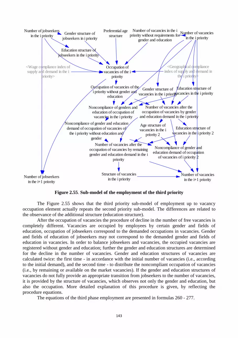
143
Occupation ofvacancies of the i
priority
Preferential age
structure
Number of jobseekers
in the i priorityNumber of vacancies
in the i priority
Number of jobseekers
in the i+1 priority
Number of vacancies
in the i+1 priority
<Wage compliance index ofsupply and demand in the i
priority>
<Geographical complianceindex of supply and demand in
the i priority>
Gender structure of
jobseekers in i priority
Number of vacancies in the ipriority without requirements for
gender and education
Gender structure of
vacancies in the i priority
Occupation of vacancies of thei priority without gender and
education
Education structure of
jobseekers in the i priority
Education structure of
vacancies in the i priority
Noncompliance of genders andeducation of occupation ofvacancies in the i priority
Number of vacancies after theoccupation of vacancies by gender
and education demand in the i priority
Noncompliance of gender and education
demand of occupation of vacancies of
the i priority without education and
gender
Education structure of
vacancies in the i priority 2
Age structure ofvacancies in the i
priority 2
Noncompliance of gender andeducation demand of occupation
of vacancies of i priority 2
Number of vacancies after the
occupation of vacancies by remaining
gender and education demand in the i
priority
Structure of vacancies
in the i priority
Figure 2.55. Sub-model of the employment of the third priority
The Figure 2.55 shows that the third priority sub-model of employment up to vacancy
occupation element actually repeats the second priority sub-model. The differences are related to
the observance of the additional structure (education structure).
After the occupation of vacancies the procedure of decline in the number of free vacancies is
completely different. Vacancies are occupied by employees by certain gender and fields of
education, occupation of jobseekers correspond to the demanded occupations in vacancies. Gender
and fields of education of jobseekers may not correspond to the demanded gender and fields of
education in vacancies. In order to balance jobseekers and vacancies, the occupied vacancies are
registered without gender and education; further the gender and education structures are determined
for the decline in the number of vacancies. Gender and education structures of vacancies are
calculated twice: the first time - in accordance with the initial number of vacancies (i.e., according
to the initial demand), and the second time - to distribute the noncompliant occupation of vacancies
(i.e., by remaining or available on the market vacancies). If the gender and education structures of
vacancies do not fully provide an appropriate transition from jobseekers to the number of vacancies,
it is provided by the structure of vacancies, which observes not only the gender and education, but
also the occupation. More detailed explanation of this procedure is given, by reflecting the
procedure equations.
The equations of the third phase employment are presented in formulas 260 - 277.

144
2B
DPJt
2B
DPJt
3A
DPJt VgVgVg DMNDMDM , (260)
where
DM3A
VgDPJ - number of jobseekers in the 3A priority;
DM2B
VgDPJ - number of jobseekers in the 2B priority;
DMN2B
VgDPJ - occupation of vacancies in the 2B priority;
Vg - age group;
D - gender;
P - occupation;
J - field of education.
Di Vgk Pn Jm
iknm
Vg
Vgk Pn Jm
knm
Vg
D
DM
DM
DMdS3A
DPJt
3A
DPJt
3A
t
1, (261)
where
DMdS3A
D - gender structure of jobseekers in the 3A priority;
DM3A
VgDPJ - number of jobseekers in the 3A priority;
Vg - age group;
D - gender;
P - occupation;
J - field of education.
Di Vgk Pn Jm
iknm
Vg
Vgk Pn Dm
knm
Vg
DM
DM
DMizS3A
DPJt
3A
DPJt
3A
Jt
1, (262)
where
DMizS3A
J - education structure of jobseekers in the 3A priority;
DM3A
VgDPJ - number of jobseekers in the 3A priority;
Vg - age group;
D - gender;
P - occupation;
J - field of education.
The calculation of the structure of jobseekers in comparison with the calculation of the
second priority structure (248 formula) uses a new element - technical overall minimum of
jobseekers (1 person), in formulas 261 and 262. This minimum is necessary as at certain levels of
education (such as doctoral education) in the third employment priority may not be unemployed. In
the absence of jobseekers, it is impossible to calculate the structure, without this technical
supplement the model may not work.
2B
DPJt
2B
DPJt
2B
DPJt
3A
DPJt 0 DMNIDMNpDVSVS , (263)
where
VS3A
DPJ - number of vacancies in the 3A priority;
VS2B
DPJ - number of vacancies in the 2B priority;
DMNpD2B
DPJ - occupation of vacancies in the 2B priority by gender demand;

145
DMNI2B
DPJ - changes of gender demand of the occupation of vacancies in the 2B priority;
D - gender;
P - occupation;
J - field of education.
Jn Di
inVSVSbD 3A
DPJt
3A
Pt , (264)
where
VSbDI3A
P - number of vacancies in the 3A priority without requirements for gender and
education;
VS3A
DPJ - number of vacancies in the 3A priority;
D - gender;
P - occupation;
J - field of education.
3A
DPJt
3A
t
3A
tt
3A
PJt
3A
tt
3A
PJt
3A
DPJt
3A
t
3A
tt
3A
PJt
3A
DPJt
3A3A3A
DPJt
,
,
VgJDVgDVg
VgJDVgVg
Vg
DMDMizSDMdSPSVSbDIDMdSPSVSbDI
DMDMizSDMdSPSVSbDIDM
PPGAKPPAAKDMN
, (265)
where
DMN3A
VgDPJ - occupation of vacancies in the 3A priority;
PPAAK3A
- wages compliance coefficient of demand and supply in the 3A priority;
PPGAK3A
- geographical compliance coefficient of demand and supply in the 3A priority;
DM3A
VgDPJ - number of jobseekers in the 3A priority;
VSbDI3A
P - number of vacancies in the 3A priority without requirements for gender and
education;
PSVg - preferential age structure;
DMdS3A
D - gender structure of jobseekers in the 3A priority;
DMizS3A
D - education structure of jobseekers in the 3A priority;
Vg - age group;
D - gender;
P - occupation;
J - field of education.
Formulas 260 -265 show that the third priority sub-model of employment largely repeats the
second priority sub-model of employment. The difference between them is related to observance of
the education structure of jobseekers. Further the gender and education non-conformity balancing
equations (266 - 277 formulas) are reflected.
Di Pn Jm
inm
Pn Jm
nm
D
VS
VS
VSdS3A
DPJt
3A
DPJt3A
t , (266)
where
VSdS3A
D - gender structure of vacancies in the 3A priority;
VS3A
DPJ - number of vacancies in the 3A priority;
D - gender;
P - occupation;
J - field of education.

146
Di Pn Jm
inm
Pn Dm
nm
J
VS
VS
VSizS3A
DPJt
3A
DPJt3A
t , (267)
where
VSizS3A
J - education structure of vacancies in the 3A priority;
VS3A
DPJ - number of vacancies in the 3A priority;
D - gender;
P - occupation;
J - field of education.
The equations of determination of the structure of vacancies (266 and 267 formulas) are
analogical to the unified sub-models.
Jn Dm Vgi
imn
VgDMNDMNbD 3A
DPJt
3A
Pt , (268)
where
DMNbDI3A
P - occupation of vacancies in the 3A priority without gender and education;
DMN3A
VgDPJ - occupation of vacancies in the 3A priority;
Vg - age group;
D - gender;
P - occupation;
J - field of education.
Formula 268 presents the calculation of the number of occupied vacancies, not reflecting the
education and gender requirements. Then formula 269 presents the calculation of the number of
occupied vacancies, which corresponds to the demand (by education and gender), and at the same
time, it is subtracted from the initial number of vacancies, thus obtaining the number of vacancies
for occupation of vacancies in accordance with the demand. In turn, formula 270 calculates the
number of occupied vacancies, where the gender and education of employees do not correspond to
the demand.
0 3A
Jt
3A
Dt
3A
Pt
3A
DPJt
3A
DPJt VSizSVSdSDMNbDIVSVSpA , (269)
where
VSpA3A
DPJ - number of vacancies after occupation of vacancies by gender and education
demand in the 3A priority;
VS3A
DPJ - number of vacancies in the 3A priority;
DMNbDI3A
P - occupation of vacancies in the 3A priority without gender and education
requirements;
VSdS3A
D - gender structure of vacancies in the 3A priority;
VSizS3A
J - education structure of vacancies in the 3A priority;
D - gender;
P - occupation;
J - field of education.
Calculating the number of vacancies after occupation of vacancies in accordance with the
demand, the occupied vacancies (by occupations), multiplying them by the demanded gender and
education structures, are subtracted from the initial number of vacancies. If the structures develop
unallowable non-conformance of the demand and occupation, i.e., the occupation is larger than the
demand, then in order to avoid negative (less than zero) number of vacancies, formula 269
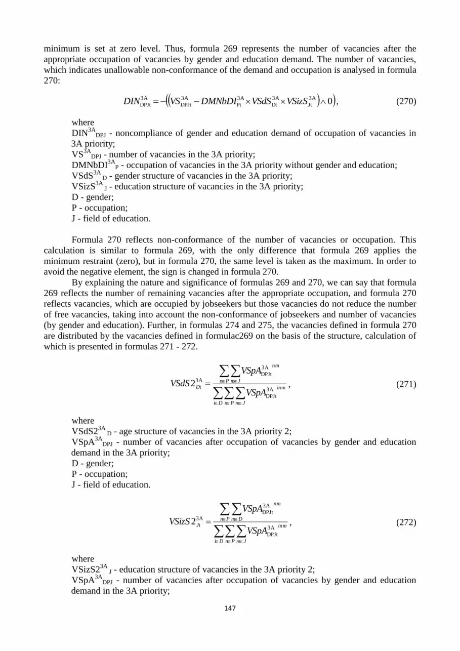
147
minimum is set at zero level. Thus, formula 269 represents the number of vacancies after the
appropriate occupation of vacancies by gender and education demand. The number of vacancies,
which indicates unallowable non-conformance of the demand and occupation is analysed in formula
270:
0 3A
Jt
3A
Dt
3A
Pt
3A
DPJt
3A
DPJt VSizSVSdSDMNbDIVSDIN , (270)
where
DIN3A
DPJ - noncompliance of gender and education demand of occupation of vacancies in
3A priority;
VS3A
DPJ - number of vacancies in the 3A priority;
DMNbDI3A
P - occupation of vacancies in the 3A priority without gender and education;
VSdS3A
D - gender structure of vacancies in the 3A priority;
VSizS3A
J - education structure of vacancies in the 3A priority;
D - gender;
P - occupation;
J - field of education.
Formula 270 reflects non-conformance of the number of vacancies or occupation. This
calculation is similar to formula 269, with the only difference that formula 269 applies the
minimum restraint (zero), but in formula 270, the same level is taken as the maximum. In order to
avoid the negative element, the sign is changed in formula 270.
By explaining the nature and significance of formulas 269 and 270, we can say that formula
269 reflects the number of remaining vacancies after the appropriate occupation, and formula 270
reflects vacancies, which are occupied by jobseekers but those vacancies do not reduce the number
of free vacancies, taking into account the non-conformance of jobseekers and number of vacancies
(by gender and education). Further, in formulas 274 and 275, the vacancies defined in formula 270
are distributed by the vacancies defined in formulac269 on the basis of the structure, calculation of
which is presented in formulas 271 - 272.
Di Pn Jm
inm
Pn Jm
nm
D
VSpA
VSpA
VSdS3A
DPJt
3A
DPJt3A
t2 , (271)
where
VSdS23A
D - age structure of vacancies in the 3A priority 2;
VSpA3A
DPJ - number of vacancies after occupation of vacancies by gender and education
demand in the 3A priority;
D - gender;
P - occupation;
J - field of education.
Di Pn Jm
inm
Pn Dm
nm
J
VSpA
VSpA
VSizS3A
DPJt
3A
DPJt3A
t2 , (272)
where
VSizS23A
J - education structure of vacancies in the 3A priority 2;
VSpA3A
DPJ - number of vacancies after occupation of vacancies by gender and education
demand in the 3A priority;

148
D - gender;
P - occupation;
J - field of education.
Jn Dm
mnDINDMNbD 3A
DPJt
3A
Pt 2 , (273)
where
DMNbDI23A
P - noncompliance of gender and education demand of occupation of vacancies
in the 3A priority without education and gender;
DIN3A
DPJ - noncompliance of gender and education demand of occupation of vacancies in
the 3A priority;
D - gender;
P - occupation;
J - field of education.
0222 2 3AJt
3ADt
3APt
3ADPJt
3ADPJt VSizSVSdSDMNbDIVSpAVSpA , (274)
where
VSpA23A
DPJ - number of vacancies after the occupation of vacancies by remaining gender
and education structure in the 3A priority;
VSpA3A
DPJ - number of vacancies after occupation of vacancies by gender and education
demand in 3A priority;
DMNbDI23A
DPJ - noncompliance of gender and education demand of occupation of
vacancies in 3A priority;
VSdS23A
D - gender structure of vacancies in the 3A priority;
VSizS23A
J - education structure of vacancies in the 3A priority;
D - gender;
P - occupation;
J - field of education.
022DMNbDI2 2 3AJt
3ADt
3APt
3ADPJt
3ADPJt VSizSVSdSVSpADIN , (275)
where
DIN23A
DPJ - noncompliance of gender and education demand of occupation of vacancies in
the 3A priority 2;
VSpA3A
DPJ - number of vacancies after occupation of vacancies by gender and education
demand in the 3A priority;
DMNbDI23A
DPJ - noncompliance of gender and education demand of occupation of
vacancies in the 3A priority;
VSdS23A
D - gender structure of vacancies in the 3A priority;
VSizS23A
J - education structure of vacancies in the 3A priority;
D - gender;
P - occupation;
J - field of education.
Analysing formulas 271 -275, it is evident that they largely repeat formulas 266 - 270. These
two groups provide the transition from job seekers to the number of vacancies and form the cycle,
where jobseekers during employment reduce the number of free vacancies.
In the end of the cycle, if the model preserves the unallowable non-conformities of the
labour demand and occupation of vacancies, they are divided in proportion to vacancies (the

149
proportion observes the gender, education and occupation). This division, as well as the calculation
of vacancies for the next priority are reflected by formulas 276 and 277.
Di Pn Jm
inmDPJ
VSpA
VSpAAVSA
3A
DPJt
3A
DPJt3A
t
2
2, (276)
where
AVSA3A
DPJ - structure of vacancies in the 3A priority;
VSpA23A
DPJ - number of vacancies after occupation of vacancies by remaining gender and
education structure in the 3A priority;
D - gender;
P - occupation;
J - field of education.
Formula 276 reflects the structure of vacancies, then formula 277 presents the proportional
division of unallowable non-conformities of the occupation of vacancies:
022 3A
DPJt
3A
t
3A
t
3B
t
Di Pn Jm
inm
DPJDPJDPJ DINAVSAVSpAVS , (277)
where
VS3B
DPJ - number of vacancies in 3B priority;
VSpA23A
DPJ - number of vacancies after occupation of vacancies by remaining gender and
education structure in 3A priority;
AVSA3A
DPJ - structure of vacancies in 3A priority;
DIN23A
DPJ - noncompliance of gender and education demand of occupation of vacancies in
3A priority 2;
D - gender;
P - occupation;
J - field of education.
Formula 277 reflects the number of vacancies for the next priority.
Figure 2.56 reflects the fourth priority sub-model of employment, in which jobseekers
change their occupations in accordance with the market requirements, observing the education of
jobseekers.

150
Change of occupation
in the i priority
Preferential age
structure
Number of jobseekers
in the i priorityNumber of vacancies
in the i priority
Number of jobseekers
in the i+1 priority
Number of vacancies
in the i+1 priority
<Wage compliance coefficientof supply and demand in the i
priority>
<Geographical compliancecoefficient of supply anddemand in the i priority>
Structure ofjobseekers in the i
priority
Number of vacancies in the ipriority without gender andoccupations requirements
Gender structure ofvacancies in the i
priority
Occupation of vacancies of the ipriority without gender andprofessional occupations
Occupation ofvacancies of the i
priority
Occupationalstructure of vacancies
in i priority
Non-conformance of gender andprofessional occupation demand of
occupation of vacancies of the i priority
Number of vacancies after theoccupation of vacancies by genderand education demand in i priority
Non-conformance of gender and
professional occupation demand of
occupation of vacancies of the i priority
without education and gender
Occupational structure of
vacancies in the i priority 2Gender structure of
vacancies in the i priority 2
Non-conformance of gender andoccupational demand of occupation
of vacancies of the i priority 2
Number of vacancies after the occupation
of vacancies by the remaining gender and
professional occupation structure in i
priority
Structure of vacancies
in the i priority
Occupation of vacancies of thei priority without professional
occupations
Figure 2.56. Sub-model of the employment of the fourth priority
Comparing the fourth priority sub-model (Figure 2.56) with the third priority sub-model
(Figure 2.55), it is evident that they differ mainly just prior to occupation of vacancies. After
occupation of vacancies the existing differences can be related only to the application of the
different structure: in the third priority sub-model the gender and education structures are applied,
but in the fourth priority sub-model - gender and occupation structures. The part of the model after
the occupation of the vacancies is explained in detail in formulas 266 - 277, therefore, it is not
described again.
The feature of the fourth priority sub-model is related to the fact that jobseekers change
occupation in order to get a job. Change of occupation is restrained by the attained education, i.e.,
with the certain education it is possible to work in different occupations and, when it is necessary,
to change occupation according to the attained education.
By implementing this principle in the model, Figure 2.56 shows that the number of
jobseekers who have changed occupations (in the previous priorities it is the occupation of
vacancies) are calculated in the beginning. This index reflects the number of jobseekers, which will
occupy the vacant working places. In this phase jobseekers retain their previous occupations. This
index is also important to calculate the number of jobseekers in accordance with the priority in the
end of algorithm. Then the jobseekers are assigned occupations and they occupy vacancies in the
demanded occupations (i.e., considering the occupational structure of vacancies). The equations of

151
the part of the fourth priority sub-model (before occupation of the vacancies) of employment are
presented in formulas 278 - 283.
Di Vgk Pn Jm
iknm
Vg
Vgk
k
Vg
DM
DM
DMkS4A
DPJt
4A
DPJt
4A
DPJt
1, (278)
where
DMkS4A
DPJ - structure of jobseekers in the 4A priority;
DM4A
VgDPJ - number of jobseekers in the 4A priority;
Vg - age group;
D - gender;
P - occupation;
J - field of education.
Formula 278 reflects the structure of jobseekers in the 4A priority.
Pn Di
inVSVSbDP 4A
DPJt
4A
Jt , (279)
where
VSbDP4A
J - number of vacancies in the 4A priority without gender and occupational
requirements;
VS4A
DPJ - number of vacancies in the 4A priority;
D - gender;
P - occupation;
J - field of education.
Formula 279 presents the calculation of the number of vacancies by educational levels
without gender and occupational requirements.
4A
DPJt
4A
tt
4A
PJt
4A
tt
4A
PJt
4A
DPJt
4A
tt
4A
PJt
4A
DPJt
4A4A4A
DPJt
,
,
VgDVgDVg
VgDVgVg
Vg
DMDMkSPSVSbDPDMkSPSVSbDP
DMDMkSPSVSbDPDM
PPGAKPPAAKPMDM
, (280)
where
PMDM4A
VgDPJ - change of occupation in the 4A priority;
PPAAK4A
- wage compliance coefficient of demand and supply in the 4A priority;
PPGAK4A
- geographical compliance coefficient of demand and supply wage in the 4A
priority;
DM4A
VgDPJ - number of jobseekers in the 4A priority;
VSbDP4A
J - number of vacancies in the 4A priority without gender and occupational
requirements;
PSVg - preferential age structure;
DMkS4A
DPJ - structure of jobseekers in the 4A priority;
Vg - age group;
D - gender;
P - occupation;
J - field of education.

152
Formula 280 presents the calculation of the number of jobseekers, which changed the
occupation. Formula 280 is analogous to formulas 246, 251 and 265 that calculate the occupation of
vacancies. However, formula 280 does not immediately reflect the occupation of vacancies, but
reflect the number of jobseekers that occupy the vacancies with the previous occupations. Formula
281 analyses the number of jobseekers without previous occupations:
Pn
n
VgVg PMDMDMNbP 4A
DPJt
4A
DJt , (281)
where
DMNbP4A
VgDJ - occupation of vacancies in the 4A priority without occupations;
PMDM4A
VgDPJ - change of occupation in the 4A priority;
Vg - age group;
D - gender;
P - occupation;
J - field of education.
Di Pn Jm
inm
Jn Dm
nm
P
VS
VS
VSpS4A
DPJt
4A
DPJt4A
t2 , (282)
where
VSpS4A
P - occupational structure of the vacancies in the 4A priority;
VS4A
DPJ - number of vacancies in the 4A priority;
D - gender;
P - occupation;
J - field of education.
Formula 282 reflects the occupational structure of vacancies.
4A
t
4A
DJt
4A
DPJt PVgVg VSpSDMNbPDMN , (283)
where
DMN4A
VgDPJ - occupation of vacancies in the 4A priority;
DMNbP4A
VgDJ - occupation of vacancies in the 4A priority without occupations;
VSpS4A
P - occupational structure of the vacancies in the 4A priority;
Vg - age group;
D - gender;
P - occupation;
J - field of education.
Formula 283 defines the occupation of vacancies, which is based on the occupational
structure of vacancies and occupation of vacancies without occupations.
Figure 2.57 presents the fifth priority sub-model of employment, in which jobseekers change
their occupations in accordance with the market requirements, observing the previous experience of
jobseekers.

153
Number of jobseekers
in the i priorityNumber of vacancies
in the i priority
Number of jobseekers
in the i+1 priority
Number of vacancies
in the i+1 priority
<Wage compliance coefficientof supply and demand in the i
priority>
<Geographical compliancecoefficient of supply anddemand in the i priority>
Structure ofjobseekers in the i
priority
Number of vacancies in the ipriority without gender and
education requirements
Occupation ofvacancies of the i
priority
Matrix of potential newoccupations for the number of
jobseekers in the i priority
Change of occupation
in the i priority
Structure of jobseekers
in the i priority 2
Structure of vacancies
in the i priority
Matrix of potential newoccupations for vacancies in
the i priority
Restraint of the number of
vacancies in the i priority
Division structure of vacanciesby related occupations in the i
priority
Matrix of possible newoccupations for vacancies in
the i priority
Comparison ofoccupational matrixes in
the i priority
Occupations before thechange of occupation in the i
priority
Occupations after thechange of occupation in the
i priority
Occupation of vacancies
of the i priority without age
Figure 2.57. Sub-model of the employment of the fifth priority
Fifth priority sub-model (Figure 2.57) essentially differs from all previous models. It is
based on the comparison of potential occupations of vacancies and jobseekers. It means that the
vacant places by occupations are replaced by vacant places in occupations requiring the same (or
similar) skills (similar occupations). At the same time, jobseekers by occupational groups move to
similar occupations. If the “similar” vacancies coincide with similar occupations of job seekers and
jobseekers occupy working places, the number of vacancies and jobseekers declines.
By implementing this principle, the fifth priority sub-model calculates the matrix of
potentially new occupations for vacancies (on the basis of the compliance matrix of occupations),
adjusts this matrix, taking into account the restraint of the number of vacancies, thus creating a new
matrix of potentially new occupations. The matrix of potentially new occupations for vacancies
reflects the occupations that can replace the requirements of the occupations of vacancies. On the
basis of the number of jobseekers and matrix structure of vacancies the matrix of potentially new
occupations for jobseekers is developed, which reflects occupations that can be changed by
jobseekers while looking for a job. The structure of the change of occupation of jobseekers is
defined by free vacancies.
The comparison of the occupational matrix is made in order to calculate the correspondence
of jobseekers to the vacancies. The comparison also observes other factors, such as conformity of
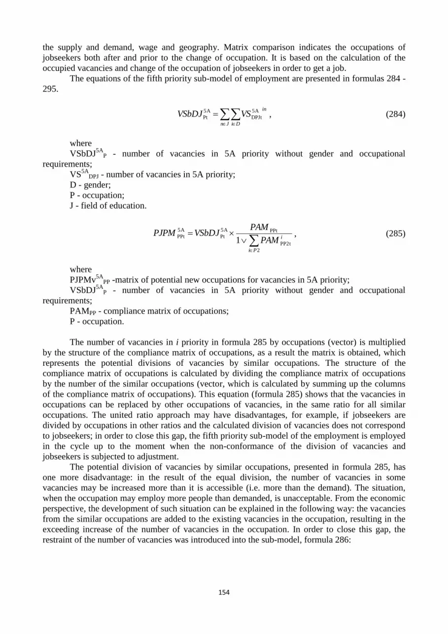
154
the supply and demand, wage and geography. Matrix comparison indicates the occupations of
jobseekers both after and prior to the change of occupation. It is based on the calculation of the
occupied vacancies and change of the occupation of jobseekers in order to get a job.
The equations of the fifth priority sub-model of employment are presented in formulas 284 -
295.
Jn Di
inVSVSbDJ 5A
DPJt
5A
Pt , (284)
where
VSbDJ5A
P - number of vacancies in 5A priority without gender and occupational
requirements;
VS5A
DPJ - number of vacancies in 5A priority;
D - gender;
P - occupation;
J - field of education.
2
PP2t
PPt5A
Pt
5A
PPt1
Pi
iPAM
PAMVSbDJPJPM , (285)
where
PJPMv5A
PP -matrix of potential new occupations for vacancies in 5A priority;
VSbDJ5A
P - number of vacancies in 5A priority without gender and occupational
requirements;
PAMPP - compliance matrix of occupations;
P - occupation.
The number of vacancies in i priority in formula 285 by occupations (vector) is multiplied
by the structure of the compliance matrix of occupations, as a result the matrix is obtained, which
represents the potential divisions of vacancies by similar occupations. The structure of the
compliance matrix of occupations is calculated by dividing the compliance matrix of occupations
by the number of the similar occupations (vector, which is calculated by summing up the columns
of the compliance matrix of occupations). This equation (formula 285) shows that the vacancies in
occupations can be replaced by other occupations of vacancies, in the same ratio for all similar
occupations. The united ratio approach may have disadvantages, for example, if jobseekers are
divided by occupations in other ratios and the calculated division of vacancies does not correspond
to jobseekers; in order to close this gap, the fifth priority sub-model of the employment is employed
in the cycle up to the moment when the non-conformance of the division of vacancies and
jobseekers is subjected to adjustment.
The potential division of vacancies by similar occupations, presented in formula 285, has
one more disadvantage: in the result of the equal division, the number of vacancies in some
vacancies may be increased more than it is accessible (i.e. more than the demand). The situation,
when the occupation may employ more people than demanded, is unacceptable. From the economic
perspective, the development of such situation can be explained in the following way: the vacancies
from the similar occupations are added to the existing vacancies in the occupation, resulting in the
exceeding increase of the number of vacancies in the occupation. In order to close this gap, the
restraint of the number of vacancies was introduced into the sub-model, formula 286:

155
5A
Pt
1
5A
P1Pt
1
5A
P1Pt
5A
Pt
1
5A
P1Pt
5A
Pt5A
Pt
,
,
VSbDJPJPMPJPM
VSbDJPJPMVSbDJ
VSR
Pi
i
Pi
iPi
i
, (286)
where
VSR5A
P - restraint of the number of vacancies in 5A priority;
VSbDJ5A
P - number of vacancies in 5A priority without gender and education requirements;
PJPMv5A
PP - matrix of potential new occupations for vacancies in 5A priority;
P - occupation.
Restraint of the number of vacancies sums up the lines of the compliance matrix of
occupation and compares them with the number of vacancies by occupations (equal to the sum of
column of the compliance matrix of occupation); from these elements the smaller is chosen. This
ensures that the occupation will not employ more employees than demanded.
The index “restraint of the number of vacancies” represents the number of vacancies by
occupations, which can be occupied by jobseekers in the model. This index may be less than the
number of vacancies in i priority. Not to lose the vacancies, the fifth priority sub-model of the
employment is repeated in the cycle while regulating the non-conformance of the division of
vacancies and jobseekers.
The restraint structure of the number of vacancies or the division structure of vacancies by
related occupations is calculated in formula 287:
0
1,0
0,0
0,
1
5A
P1Pt
5A
PPt
1
5A
P1Pt
5A
PPt
1
5A
P1Pt
5A
PPt
5A
PPt
T
Pi
i
T
Pi
i
T
Pi
i
PJPM
PJPM
PJPM
PJPM
PJPM
PJPM
VSSS , (287)
where
VSSS5A
PP - division structure of vacancies by related occupations in 5A priority;
PJPMv5A
PP - matrix of potential new occupations for vacancies in 5A priority;
P - occupation.
Division structure of vacancies is calculated on the basis of the matrix of potential new
occupations. The specific type of equation (formula 287) is related to the technical characteristics of
the model, and shows that if it is not possible to calculate the structure (the resulting number of
vacancies in the occupation is equal to zero) or the calculation is not logical (less than zero), all
structural elements are assigned the value of zero, otherwise the structure is calculated in a classical
way. Matrix transposition is related to the calculation of the structure by the matrix lines, but then
the matrix structure of the column section is required.
On the basis of the division structure of vacancies and restraint of the number of vacancies,
the matrix of the potential new occupations is calculated for the vacancies, formula 288:

156
5A
Pt
5A
PPt
5A
PPt VSRVSSSJPMv , (288)
where
JPMv5A
PP - matrix of potential new occupations for vacancies in 5A priority;
VSSS5A
PP - division structure of vacancies by related occupations in 5A priority;
VSR5A
P - restraint of the number of vacancies in 5A priority;
P - occupation.
Matrix of potential new occupations for vacancies reflects the occupations that may have the
changed occupational demands of the vacancies. The sum of this matrix by lines reflects initial
requirements of the occupations of vacancies, but the sum by columns reflects the equivalent
potential requirements, while observing the interdependence of occupations.
After the calculation of the matrix of potential new occupations of vacancies, the matrix of
potential new occupations for jobseekers is calculated, formula 289:
2
5A
PP2t
5A
PPt5A
DPJt
5A
PPt
Pi
iDi Vgk Jm
ikm
Vg
JPM
JPMvDMJPMdm , (289)
where
JPMdm5A
PP - matrix of possible new occupations for the number of jobseekers in 5A
priority;
DM5A
VgDPJ - number of jobseekers in 5A priority;
JPMv5A
PP - matrix of possible new occupations for vacancies in 5A priority;
Vg - age group;
D - gender;
P - occupation;
J - field of education.
In the calculation of the matrix of potential new occupations of jobseekers (formula 289),
the jobseekers are summed up to the occupational level (vector), the matrix is formed by the
correlation structure, which is based on the occupational structure of vacancies, i.e., the structure of
the change of occupation of jobseekers is defined by free vacancies.
The developed matrixes of potential new occupations are compared in formula 290:
5A
PPt
5A
PPt
5A
PPt
5A
PPt
5A
PPt
5A
PPt5A5A5A
PPt,
,
JPMdmJPMvJPMv
JPMdmJPMvJPMdmPPGAKPPAAKPMS , (290)
where
PMS5A
P - comparison of occupations matrixes in the 5A priority;
PPAAK5A
- wage compliance coefficient of demand and supply in the 5A priority;
PPGAK5A
- geographical compliance coefficient of demand and supply in the 5A priority;
JPMv5A
PP - matrix of possible new occupations for vacancies in the 5A priority;
JPMdm5A
PP - matrix of potential new occupations for the number of jobseekers in the 5A
priority;
P - occupation.
The comparison of the occupational matrix is made in order to calculate the correspondence
of jobseekers to vacancies. Formula 290 shows that it also observes other factors, such as wage and
geographical conformance of supply and demand. The resulting matrix reflects which occupations
are replaced by jobseekers in order to get a job. These indexes in formulas 290 and 291 are

157
distinguished separately, and then they are used for decline in the number of free vacancies and
jobseekers.
2
5A
PP2t
5A
Pt
Pi
iPMSPMSpe , (291)
where
PMSpe5A
P - occupations of jobseekers after the change of occupation in the 5A priority;
PMS5A
PP - comparison of occupations matrixes in the 5A priority;
P - occupation.
2
5A
PP2t
5A
Pt
Pi
iPMSPMSpi , (292)
where
PMSpi5A
P - occupations of jobseekers before the change of occupation in the 5A priority;
PMS5A
PP - comparison of occupations matrixes in the 5A priority;
P - occupation.
As formulas 291 and 292 show, they differ by summing up the matrix elements by rows and
columns.
The occupations of jobseekers after the change of occupation, i.e. the occupations of
occupied vacancies. The vacancies are analysed in details in the sub-model, including the
requirements of vacancies for the education and gender. The requirements of occupied vacancies in
relation to the education and gender are calculated according to the structure of vacancies, formula
293:
5A
t
5A
t
5A
t DPJPDPJ AVSAPMSpeDMNbV , (293)
where
DMNbV5A
DPJ - occupation of vacancies in the 5A priority without age;
PMSpe5A
P - occupations of jobseekers after the change of occupation in the 5A priority;
AVSA5A
DPJ - structure of vacancies in the 5A priority;
D - gender;
P - occupation;
J - field of education.
The index “occupation of vacancies in i priority without age” reflects the quantity and types
of vacancies that are occupied in the current priority. Then this index is used by calculating the
number of free vacancies in the next priority. The structure of vacancies is calculated by the unified
equation (formula 276), so it is not re-presented again.
Formula 294 reflects the calculation of the parameter „change of occupation”:
5A
DPJt
5A
Pt
5A
DPJt VgVg DMkSPMSpiPMDM , (294)
where
PMDM5A
VgDPJ - change of occupation in the 5A priority;
PMSpi5A
P - occupations of jobseekers before the change of occupation in the 5A priority;
DMkS5A
VgDPJ - structure of jobseekers in the 5A priority;
Vg - age group;
D - gender;
P - occupation;
J - field of education.

158
The index “change of occupation in i priority” reflects the quantity and types of jobseekers
(including by the occupations) which have found jobs and have been employed. On the basis of this
index the “structure of jobseekers in i priority 2” has been calculated, which reflects the age and
education structure of jobseekers (i.e. new employees). Structures of jobseekers are calculated on
the basis of the unified equations, therefore, are not reflected here again. The calculation of the
second structure is related to the fact that in new working places the structure of employees should
not correspond to the structure of jobseekers, but to the structure, which is characteristic to
jobseekers with new occupation. The index “change of occupation in i priority” is used, by reducing
the number of jobseekers.
The number of jobseekers who occupy working places is calculated on the basis of the
structures of new employees and jobseekers (after the change of occupation), formula 295:
5A
DPJt
5A
Pt
5A
DPJt 2 VgVg DMkSPMSpeDMN , (295)
where
DMN5A
VgDPJ - occupation of vacancies in the 5A priority;
PMSpe5A
P - occupations of jobseekers after the change of occupation in the 5A priority;
DMkS25A
VgDPJ - structure of jobseekers in the 5A priority 2;
Vg - age group;
D - gender;
P - occupation;
J - field of education.
The index “occupation of vacancies in i priority” is used by increasing the number of
employed.
The fifth priority sub-model of employment is repeated in the cycle until the moment, when
non-compliance of vacancies distribution and jobseekers is subject of regulations.
In the explanation of the fifth priority sub-model of employment the occupational
compliance matrix was mentioned. The calculation of the occupational compliance matrix is not
related to the sub-model. Considering that it consists of three equations, it is not appropriate to
distinguish a separate subsection for it. The essence of the calculation of the occupational
compliance matrix is presented below.
The occupational compliance matrix is based on the education compliance matrix and
reflects the interchangeable occupations. In order to obtain the occupational compliance matrix
from the education compliance matrix, in the first step the integrated education compliance matrix
of the levels of education is developed, formula 296:
Li
IAMAIAM i
PJtPJt 1 , (296)
where
AIAMPJ - integrated education compliance matrix;
IAMiPJ - education compliance matrix of i level of education;
P - occupation;
J - field of education;
L - level of education.
As formula 296 shows, one matrix reflects all connections of the occupational-educational
field of all levels of education. The maximum constraint 1 of formula 296 has been introduced in
order to avoid duplication connections of the occupational-educational field from the different
levels of education in the integrated matrix.

159
At the next stage the integrated education compliance matrix is transposed, formula 297:
TAIAMTAIAM PJtJPt , (297)
where
TAIAMJP - transposition of integrated education compliance matrix;
AIAMPJ - integrated education compliance matrix;
P - occupation;
J - field of education.
multiplying the transposed education compliance matrix with the integrated education
compliance matrix, the occupational compliance matrix is obtained, formula 298:
PJtJPtPPt 1 AIAMTAIAMPAM , (298)
where
PAMPP - occupational compliance matrix;
TAIAMJP - transposition of integrated education compliance matrix;
AIAMPJ - integrated education compliance matrix;
P - occupation;
J - field of education.
The maximum restraint is also applied to occupational compliance matrix.
After employment, all the fifth priority sub-model vacancies that may be occupied by
jobseekers are occupied. As stated above, there is an increase of the number of employed (formulas
198 and 208) and decline in the number of jobseekers (formulas 197 and 207). Simultaneously,
there is a decline in the number of free vacancies, which has not been previously described. Figure
2.58 reflects a decline in the number of free vacancies in the conceptual form.
<Number of
vacancies><Number of vacancies
in the 6th priority>
Working place is beingoccupied in accordance with
the vacancies
Working place is being occupiedin accordance with the
occupation of the vacancy
Remaining
vacancies
Structure of
remaining vacancies
Figure 2.58. Algorithm of decline in the number of vacancies
After the employment the five priorities in the sub-model have the element of the number of
free vacancies that is marked as “number of vacancies in the 6 priority”. comparing it to the initial
number of vacancies (before the employment priorities), the number of occupied vacancies can be
determined. Considering that vacancies may be occupied in accordance with the demand and
without regard to the demand requirements in relation to gender or education, the occupation of

160
vacancies (occupation of working places) is divided into two parts: occupation of working places
according to vacancies and occupation of working places according to occupation of vacancies.
Both of these indexes are used for decline in the number of vacancies along with the occupation of
working places (see 215 formula). Occupation of working places in accordance with the vacancies
directly reduces the number of vacancies. Occupation of working places in accordance with the
occupation of vacancies (with the non-conformity to gender or education) may lead to inappropriate
decline in the number of vacancies, including the formation of a negative number of vacancies. To
solve this problem, an algorithm of decline in the number of vacancies has calculated the index
“remaining vacancies”, which reflects the vacancies that remained after the occupation of working
places according to vacancies. On the basis of the remaining vacancies, the structure of remaining
vacancies is calculated, which ensures the appropriate division of the occupation of working places
by fields of education and gender in accordance with occupations.
The equations of the decline in the number of vacancies are presented in formulas 299 - 302.
0,
0,
6
DPJtDPJtDPJt
6
DPJtDPJt
6
DPJtDPJt
DPJtVSVSVS
VSVSVSVSDVIX , (299)
where
DVIXDPJ - the working place is being occupied in accordance with vacancies;
VSDPJ - number of vacancies;
VS6
DPJ - number of vacancies in the 6 priority;
D - gender;
P - occupation;
J - field of education.
Comparing the number of vacancies before employment priorities with the number of
vacancies after the fifth priority, in formula 299 the occupation of working places (occupation of
vacancies) is determined. Mathematically, it is positive (greater than zero) difference of constituent
elements. Negative difference (less than zero) of these elements makes up an inappropriate
occupation of vacancies, formula 300.
6
DPJtDPJtDPJt 0 VSVSDVIN , (300)
where
DVINDPJ - the working place is occupied in accordance with occupation of vacancy;
VSDPJ - number of vacancies;
VS6
DPJ - number of vacancies in the 6 priority;
D - gender;
P - occupation;
J - field of education.
The gender and fields of education do not correspond to the requirements of vacancies in the
inappropriate occupation of vacancies, while observing the constructing logics of the model. But the
requirements by occupations are observed. Considering that mathematically, this index is negative
(less than zero), the sign has been changed in formula 300.
DPJtDPJtDPJt DVIXVSAVS , (301)
where
AVSDPJ - remaining vacancies;
VSDPJ - number of vacancies;
DVIXDPJ - the working place is occupied in accordance with vacancies;

161
D - gender;
P - occupation;
J - field of education.
The remaining vacancies are calculated in order to obtain the structure of remaining
vacancies, which provides the occupation of working places by occupations in accordance with an
appropriate division by fields of education and gender.
Dk Jm
kmAVS
AVSAVSA
DPJt
DPJtDPJt
1
, (302)
where
AVSADPJ - structure of remaining vacancies;
AVSDPJ - remaining vacancies;
D - gender;
P - occupation;
J - field of education.
the standard equation is used for the calculation of structure of remaining vacancies, formula
302.
Figure 2.59 reflects the sixth priority sub-model of employment, in which the employed
change their occupations in order to improve their financial situation (increase the amount of
salaries), observing the available free working places (vacancies) in the labour market.
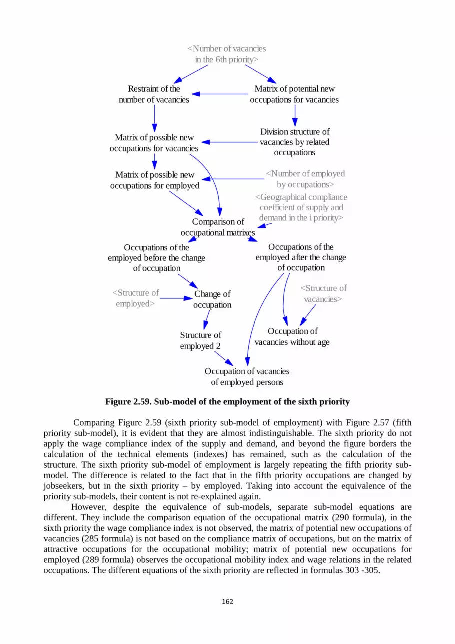
162
<Number of employed
by occupations>
<Structure of
employed>
<Number of vacancies
in the 6th priority>
Matrix of possible new
occupations for employed
Restraint of the
number of vacancies
Matrix of potential new
occupations for vacancies
Division structure ofvacancies by related
occupations
Matrix of possible new
occupations for vacancies
Comparison of
occupational matrixes
Occupations of theemployed before the change
of occupation
Occupations of theemployed after the change
of occupation
Occupation of
vacancies without age
Change of
occupation
Structure of
employed 2
Occupation of vacancies
of employed persons
<Structure of
vacancies>
<Geographical compliancecoefficient of supply anddemand in the i priority>
Figure 2.59. Sub-model of the employment of the sixth priority
Comparing Figure 2.59 (sixth priority sub-model of employment) with Figure 2.57 (fifth
priority sub-model), it is evident that they are almost indistinguishable. The sixth priority do not
apply the wage compliance index of the supply and demand, and beyond the figure borders the
calculation of the technical elements (indexes) has remained, such as the calculation of the
structure. The sixth priority sub-model of employment is largely repeating the fifth priority sub-
model. The difference is related to the fact that in the fifth priority occupations are changed by
jobseekers, but in the sixth priority – by employed. Taking into account the equivalence of the
priority sub-models, their content is not re-explained again.
However, despite the equivalence of sub-models, separate sub-model equations are
different. They include the comparison equation of the occupational matrix (290 formula), in the
sixth priority the wage compliance index is not observed, the matrix of potential new occupations of
vacancies (285 formula) is not based on the compliance matrix of occupations, but on the matrix of
attractive occupations for the occupational mobility; matrix of potential new occupations for
employed (289 formula) observes the occupational mobility index and wage relations in the related
occupations. The different equations of the sixth priority are reflected in formulas 303 -305.
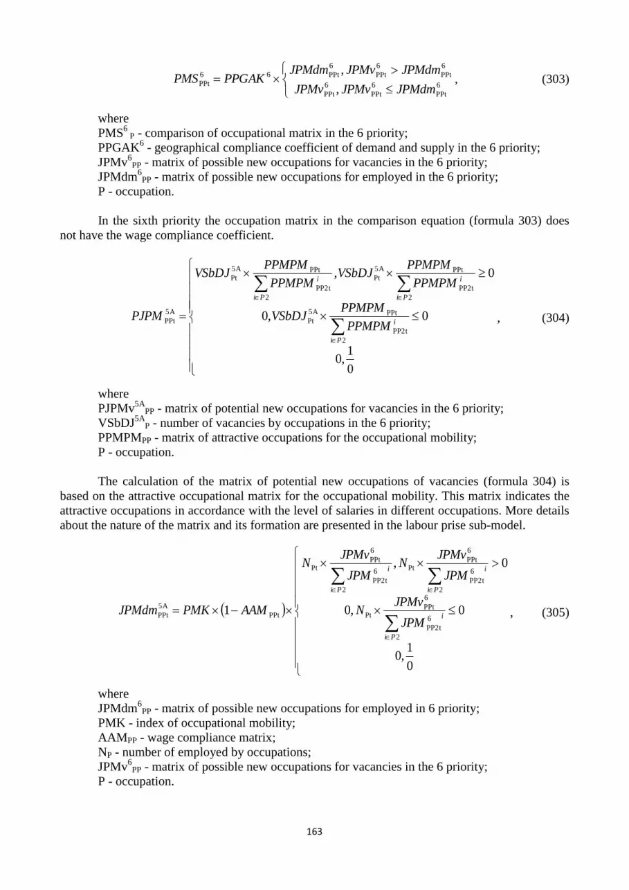
163
6
PPt
6
PPt
6
PPt
6
PPt
6
PPt
6
PPt66
PPt,
,
JPMdmJPMvJPMv
JPMdmJPMvJPMdmPPGAKPMS , (303)
where
PMS6
P - comparison of occupational matrix in the 6 priority;
PPGAK6 - geographical compliance coefficient of demand and supply in the 6 priority;
JPMv6
PP - matrix of possible new occupations for vacancies in the 6 priority;
JPMdm6
PP - matrix of possible new occupations for employed in the 6 priority;
P - occupation.
In the sixth priority the occupation matrix in the comparison equation (formula 303) does
not have the wage compliance coefficient.
0
1,0
0,0
0,
2
PP2t
PPt5A
Pt
2
PP2t
PPt5A
Pt
2
PP2t
PPt5A
Pt
5A
PPt
Pi
i
Pi
i
Pi
i
PPMPM
PPMPMVSbDJ
PPMPM
PPMPMVSbDJ
PPMPM
PPMPMVSbDJ
PJPM , (304)
where
PJPMv5A
PP - matrix of potential new occupations for vacancies in the 6 priority;
VSbDJ5A
P - number of vacancies by occupations in the 6 priority;
PPMPMPP - matrix of attractive occupations for the occupational mobility;
P - occupation.
The calculation of the matrix of potential new occupations of vacancies (formula 304) is
based on the attractive occupational matrix for the occupational mobility. This matrix indicates the
attractive occupations in accordance with the level of salaries in different occupations. More details
about the nature of the matrix and its formation are presented in the labour prise sub-model.
0
1,0
0,0
0,
1
2
6
PP2t
6
PPtPt
2
6
PP2t
6
PPtPt
2
6
PP2t
6
PPtPt
PPt
5A
PPt
Pi
i
Pi
i
Pi
i
JPM
JPMvN
JPM
JPMvN
JPM
JPMvN
AAMPMKJPMdm , (305)
where
JPMdm6
PP - matrix of possible new occupations for employed in 6 priority;
PMK - index of occupational mobility;
AAMPP - wage compliance matrix;
NP - number of employed by occupations;
JPMv6
PP - matrix of possible new occupations for vacancies in the 6 priority;
P - occupation.
164
The matrix of the potential new occupations of employed additionally observes the
occupational mobility index (i.e. the certain proportion of employees is ready to change occupation
in order to get a better job), and the wage compliance matrix, which nature and formation are
explained in the labour price sub-model.
The sixth priority sub-model of employment is the last part of the labour market sub-model,
after which the synchronization algorithm and wage formation sub-models are investigated.
2.3.1.6. Synchronization algorithm
The need for the synchronization algorithm is based on the simulated object specifics:
labour can change the age, level and field of education, occupation and economic activity status at
the same time. These changes are divided into two groups for the economically active population:
job seekers and employed, who are additionally interacting with one another and can change their
employment status. Analytically it is not possible to predict the total result of the impact of several
factors on the simulated index. But, on the other hand, impossible results can be determined
analytically and which contravene to common sense. Such results may include the negative number
(less than zero) of jobseekers or employed. Accordingly, the impact of influencing factors is
required to be restrained in order to prevent excess of the bounds of common sense by total result. It
is ensured by the flow synchronization algorithm, or, simpler, - synchronization algorithm.
It is important to explain why the model can develop illogical results, i.e., the number of
people can be negative. The flows are based on the structure of the index of the current period. But
the flows act in the end of the current period. If the simple model, with one flow, is analysed, then
the situation does not cause any problems. In case of multiple flows, pre-formed flows change the
index structure, which causes the disparities of the index and flow, and can lead to logically
unreasonable results.
Implementing the model in practice, this theoretical situation is the following: with the
decline in the number of working places in a certain occupational and educational filed, the
situation may arise that there is no employed with a combination of such occupation and education.
This situation may arise due to the non-conformance of the model assumptions and statistics: the
model provides that it is possible to obtain an occupation and find an appropriate job only with a
certain education (or education groups), but the statistics sometimes shows that occupations are not
related to education. But, despite this fact, it is necessary to reduce the number of employed. In
order to avoid logically unreasonable results in such situations, the synchronization algorithm
complements the existing flows.
In the labour analysis sub-model of the labour supply module this situation is solved by
introducing the element “maximum of changes”, and regulating the flows in accordance with the
structure of the maximum of changes. The synchronization algorithm is based on different
principles in this sub-section. First of all, the index number of employed is predicted in the next
period, and, further, while predicting the non-conformance (negative number of employees); a
negative number is applied to the correction, i.e., not changing the values and structure of the flows.
Synchronization algorithm is presented in Figure 2.60.

165
Forecast of the
number of employed
Forecast of the
number of jobseekers
<Move from job
search to employment>
<Move fromemployment to job
search>
<Employment after the
change of occupation>
<Change ofoccupation ofemployed>
<Decline in the
number of employed>
<Decline in the number ofemployed due to the change of
age structure>
<Number of
employed>
<Change of the age
structure of employed>
<Number of
jobseekers>
<Increase of the
number of jobseekers><Decline in the number
of jobseekers>
<Change of the age
structure of jobseekers>
<Change of occupation
in order to get a job>
Correction of the number of
jobseekers and employed
Required correction of
employed structure
Age group
correction 1
Additionally requiredcorrection of employed
structure
Age group
correction 2
Figure 2.60. Synchronization algorithm
Synchronization algorithm is based on the forecasts of the number of jobseekers and
employed. They are calculated by taking into account the appropriate stocks (jobseekers or
employed), as well as all flows.
The forecasts of the number of jobseekers and employed determine the forecasted non-
conformities (negative value). Forecasts are compared in the element “correction of the number of
jobseekers and employed”, in case of non-conformity; the inappropriate result is transferred from
one group to another, provided that this will not cause an inappropriate result in the second group.
This reflects that, if the required employees lose their jobs after planning of the flows, then the
provided action is not carried out in the group of employees (as was expected), but in the group of
jobseekers.
If the correction of the number of jobseekers and employed does not ensure the prevention
of non-conformity (it is checked in the element “required correction of employed structure”), the
age group correction of the employed is carried out. The age group correction of employed includes
two stages, looking for appropriate employees in the younger and older age groups. This points out
that in case after the flow planning the required employed persons may change the age group, the
algorithm with the provided actions transmits into another age group.
Synchronization algorithm equations are presented in formulas 306 - 312.
Formulas 306 and307 reflect the forecasts of the number of jobseekers and employed.

166
DPJtDPJtDPJt1VgDPJtVgDPJt
VgDPJtVgDPJtVgDPJtVgDPJtVgDPJt
VgVgVg KORDMvSDMvSDMSNDM
DMNPMDMDMPDMDMSP
,
VgDPJVgDPJVgDPJVgDPJVgDPJ
DPJDPJ1
,74_70,69_65,,24_20,19_15
,74_70,69_65,,24_20
DMSNDMDMNPMDMDMPVg
DMvSNDMvSVgVg
VgVg
, (306)
where
DMSPVgDPJ - forecast of the number of jobseekers;
DMVgDPJ - number of jobseekers;
DMPVgDPJ - increase of the number of jobseekers;
PMDMVgDPJ - change of occupations in order to get a job;
DMNVgDPJ - move from job search to employment;
NDMVgDPJ - move from employment to job search;
DMSVgDPJ - decline in the number of jobseekers;
DMvSVgDPJ - change of age structure of jobseekers;
Vg - age group;
D - gender;
P - occupation;
J - field of education.
DPJtDPJt1VgDPJtVgDPJtVgDPJt
VgDPJtVgDPJtVgDPJtVgDPJtVgDPJt
VgVg NvSNvSNSNPPMN
NDMNPMDMNNNSP
,
VgDPJVgDPJVgDPJ
VgDPJVgDPJ
DPJDPJ1
,74_70,69_65,,24_20,19_15
,74_70,69_65,,24_20
NSPMNNDM
NPMDMNVg
NvSNvSVg
Vg
VgVg
, (307)
where
NSPVgDPJ - forecast of the number of employed;
NVgDPJ - number of employed;
DMNVgDPJ - move from job search to employment;
NPMVgDPJ - change of occupation of employed;
NDMVgDPJ - move from employment to job search;
PMNVgDPJ - employment after the change of occupation;
NSVgDPJ - decline in the number of jobseekers due to the change of age structure;
NPVgDPJ - decline in the number of jobseekers;
NvSVgDPJ - change of age structure of employed;
Vg - age group;
D - gender;
P - occupation;
J - field of education.
The forecasts of the number of jobseekers and employed reflect related stocks and flow
amounts for the current period. Specifics of the system dynamics method, shows that the stocks
reflect the current state of the period, but the flows - the changes of the period, allowing to calculate
in the current period the condition of repository for the next period, which is realized in formulas
306 and 307.
On the basis of the forecasts of the number of jobseekers and employed, the correction of
the number of jobseekers and employed is carried out, formula 308:

167
0 00
0 00
VgDPJtVgDPJtVgDPJtVgDPJt
VgDPJtVgDPJtVgDPJtVgDPJt
VgDPJt
DMSPNSPDMSPDMSP
NSPDMSPNSPNSPDMNKOR , (308)
where
DMNKORVgDPJ - correction of the number of jobseekers and employed;
NSPVgDPJ - forecast of the number of employed;
DMSPVgDPJ - forecast of the number of jobseekers;
Vg - age group;
D - gender;
P - occupation;
J - field of education.
The calculation of the correction of the number of jobseekers and employed consists of two
parts: the correction of the number of jobseekers is subtracted from the correction of the number of
employed. Both parts of correction are calculated in a similar manner: if the negative value is
forecasted, and, at the same time, the total amount of jobseekers and employed is greater or equals
to zero, then the correction, which coincides with the expected negative value, is possible.
After the calculation of the correction of the number of jobseekers and employed it is
checked whether this correction ensures the elimination of non-conformance, formula 309:
0 VgDPJtVgDPJtVgDPJt DMNKORNSPNNKOR , (309)
where
NNKORVgDPJ - required correction of the structure of employed;
NSPVgDPJ - forecast of the number of employed;
DMNKORVgDPJ - correction of the number of jobseekers and employed;
Vg - age group;
D - gender;
P - occupation;
J - field of education.
The required correction of employed structure adjustment is calculated as a negative value,
by subtracting the correction of the number of jobseekers and employed from the forecast of the
number of employed. If the correction of the number of jobseekers and employed ensures the
prevention of non-conformance, the result is equal to zero, and the further correction is not required.
However, when the further correction is required, the correction of the age group of employed is
made, formula 310:
DPJt1-VgVgDPJt1 NNKORNKORV , (310)
where
V1NKORVgDPJ - age group correction 1;
NNKORVgDPJ - required correction of the structure of employed;
Vg - age group;
D - gender;
P - occupation;
J - field of education.
In the correction of the first age group for the required correction of employed structure the
age group is changed, assigning the new group to the previous age group, which is one stage

168
younger than in the analysed group. This reflects the fact that the employed can become older at the
forecasting stage, but in order to provide a positive number of employed, it will be returned in
accordance with the flow synchronization.
After the first age group correction it is checked whether there is a need for further
correction formula 311:
01 VgDPJtVgDPJtVgDPJtVgDPJtVgDPJt NNKORNKORVDMNKORNSPPNNKOR , (311)
where
PNNKORVgDPJ - additionally required correction of employed structure;
NSPVgDPJ - forecast of the number of employed;
DMNKORVgDPJ - correction of the number of jobseekers and employed;
V1NKORVgDPJ - age group correction1;
NNKORVgDPJ - required correction of employment structure;
Vg - age group;
D - gender;
P - occupation;
J - field of education.
By calculating the additionally required correction of the employed structure, the first
correction of the number of jobseekers and employed, as well as employed age group is observed. If
at this stage the non-conformities are detected, they are liquidated in the second age group
correction, formula 312:
DPJt2VgVgDPJt2 PNNKORNKORV , (312)
where
V2NKORVgDPJ - age group correction 2;
PNNKORVgDPJ - additionally required correction of employed structure;
Vg - age group;
D - gender;
P - occupation;
J - field of education.
In the second age group correction the age group is changed, by assigning a new group to
the former age group, which is one step older than the initial group (up to age group correction).
This reflects the fact that the flows may become older at the forecasting stage, but to provide a
positive number of employed, it should be returned in accordance with the number of employed.
The existing flows on the basis of the synchronization algorithm are investigated along with
all the other sub-model flows. Then the wage sub-model is investigated.
2.3.2. Wage sub-model
The calculation of wages in SDM model is based on the productivity growth considering the
mutual relations of vacancies and the number of jobseekers. Wage sub-model is presented in Figure
2.61.

169
Wages
Balanced wagesin the prolonged
period
Wage growth inaccordance with theproductivity growth
Index of the change
of wage
Wage reduction index inaccordance with number of
unemployed in the occupations
Wage growth index inaccordance with the shortage of
employees in occupations
Minimum wageLabour demand and
supply impact limits
<Relation algorithm ofwage and industry
productivity>
Wages by
occupationsWages by
education levels
Figure 2.61. Wage sub-model
Wage sub-model reflects that the labour price (wages) is formed by balanced wages in long-
term period, as well as it changes the modification index, which reflects the labour surplus or
shortage and minimum wage. Wages can be analysed by occupational groups, levels of education
and sectors (algorithm of relation of wage and sector productivity). Relation algorithm of wage and
sector links the productivity of balanced wage and sectors in a long-term period.
The labour price sub-model equations are presented in formulas 312 - 333.
PtPt
PtPt
1
DMN
VSAPT
, (313)
where
APTP - wage growth index in accordance with the shortage of employees in occupations;
VSP - number of vacancies by occupations;
NP - number of employed by occupations;
DMP - number of jobseekers by occupations;
P - occupation.
Wage growth index in accordance with the shortage of employees in occupations reflects the
relation of the number of vacancies and the economically active population by occupations. The
more vacancies exist, the more wages in the occupations grow. 312 formula calculates the
economically active population by summing the number of employed and jobseekers. A minimum
has been applied to economically active population by occupations - 1 person, this minimum is
necessary to ensure the functionality of the model, taking into account that the statistical data
reflects the fact that not all occupations involve economically active population.
PtPt
PtPt
1
DMN
DMASB
, (314)
where
ASBP - wage reduction index in accordance with a number of unemployed in occupations;
DMP - number of jobseekers by occupations;
NP - number of employed by occupations;
P - occupation.
Wage reduction index in accordance with the number of unemployed in occupations reflects
the ratio of the total number of unemployed and the economically active population by occupations.
The more the jobseekers there are, the less wages in the occupations are reduced. The technical
calculation of the wage reduction index in accordance with the number of unemployed in the

170
occupations (formula 314) is identical to the calculation of the wage growth index in accordance
with the shortage of employees in occupations (formula 313), so it is not explained again. In total,
these indexes form the index of the change of the wage, formula 315:
0,
0,
PtPtPtPt
PtPtPtPt
PtASBAPTASBAPTDSR
ASBAPTASBAPTDSRAIK , (315)
where
AIKP - index of the change of wage;
DSR - labour demand and supply impact limits;
APTP - wage growth index in accordance with the shortage of employees in occupations;
ASBP - wage reduction index in accordance with a number of unemployed in occupations;
NP - number of employed by occupations;
P - occupation.
Index of the change of wage is based on the difference between wage growth index (in
accordance with the shortage of employees in occupations) and wage reduction index (in
accordance with the number of unemployed in occupations). By analysing the behaviour of the
model, it is established that theoretically there are circumstances, when at the relatively small
number of economically active population in occupation; this wage can be changed too quickly with
the negligible change in employment or the number of vacancies. In order to prevent this
shortcoming, the model assumes that the labour shortage or surplus cannot change wages more than
intended within the bounds of the impact in comparison to the wages, balanced in the long-term
period. These bounds are titled in the model as labour demand and supply impact limits. These
limits determine the percentage of the change of the wage from the wages, balanced in the long-
term period, in accordance with the market conditions, i.e. labour supply and demand. Labour
demand and supply impact bounds limit the difference between wage growth and reduction indexes
in formula 315. Formula 316 presents the calculation of the wages:
PtPtPt 1 AIKIAMAA , (316)
where
AP - wages;
MA - minimum wage;
IAP - balanced wages in the long-term period;
AIKP - index of the change of wage;
P - occupation.
As formula 316 shows, the wage calculation is based on the multiplication of the wages,
balanced in the long-term period, by the index of the change of the wages. This multiplication
cannot be lower than the minimum wage in the country.
T
t
P0PP
0
dt )()(t (t) IAPIAIA , (317)
where
IAP - balanced wages in the long-term period;
IAPP - wage growth in accordance with the productivity growth;
P - occupation.

171
The changes of the wages, balanced in a long-term period, are determined by the wage
growth in accordance with the productivity growth, formula 318.
0,
0,0
PtPtPtPt
PtPt
PtIAAPPIAAPP
IAAPPIAP , (318)
where
IAPP - wage growth in accordance with the productivity growth;
APPP - wages by occupations in accordance with the productivity growth;
IAP - balanced wages in a long-term period;
P - occupation.
Wage growth in accordance with the productivity growth is related to the relation algorithm
of wage and sector productivity, and reflect the difference of the wage and wages, balanced in a
long-term period (under growth conditions), determined in the algorithm. This means that the
balanced wages (in a long-term period) in the model are inflexible on the reduction side.
The relation algorithm of wage and sector productivity is presented in Figure 2.62.
Wage fund of the
industries
Wages
Average wagesin the sectors inthe base period
Average wages inthe sectors in the
occupations
Structure of the average wage inthe sectors by occupations in the
base period
Average wages in
the sectors
Average wages in the sectors byoccupations in accordance with
the productivity growth
Wage fund of the sectors inaccordance with theproductivity growth
Wages by occupations inaccordance with theproductivity growth
Figure 2.62. Algorithm of relation of wage and sector productivity
Algorithm of relation of wage and sector productivity in the base period calculates the
average wages in sectors and average wage structure in the sectors by occupations (in order to
calculate these indexes, the algorithm calculates inter-indexes “wage fund of the sectors” and
“average wages in the sectors by occupations”). Multiplying the average wages in the base period
by the productivity growth, the average wages in the sectors are obtained. This assumption is based

172
on the principle that the wages and productivity growth should be similar in a longer period. On the
basis of the average wages in the sectors and the wage structures by occupations in the base period,
the average wages in the sectors by occupations are calculated in accordance with productivity
growth. The base period structure indicates that, throughout the forecasting period the occupational
input structure in the formation of GDP remains unchanged, accordingly, the wage structure
remains unchanged as well (e.g. drivers’ wages are higher than workers' wages, in a fixed constant
ratio). Next, on the basis of the average wages in the sectors by occupations (according to
productivity growth), by the means of the inter-index “wage fund of the sectors in accordance with
the productivity growth”, the wages by occupations are obtained (according to productivity growth).
The nature and appliance of this index has already been investigated (formula 318).
The equations of the correlation algorithm of wage and sector productivity are presented in
formulas 319 - 326.
PtPNtPNt ANNAF , (319)
where
NAFPN - wage fund of the sectors;
NPN - number of employed in the occupation by sectors;
AP - wages;
P - occupation;
N - sector.
Wage fund of the sectors is calculated by multiplying the wages (by occupations) by the
number of employed in the sector (formula 319). The index is calculated for the entire forecasting
period, but is only used in the base period (t0).
PNt
PNtPNt
1 N
NAFA
, (320)
where
APN - average wages in the sectors by occupations;
NAFPN - wage fund of the sectors;
NPN - number of employed in the occupation by sectors;
P - occupation;
N - sector.
Taking into account the statistical data shortage, formula 320 reflects the assumption that in
all sectors the certain occupation wages do not differ. This means that the wages (vector)
determined in formula 316 can be applied in any sector. Formula 320 extends vector up to matrix,
taking into account a number of sectors. This index is calculated for the entire forecasting period,
but is only used for the base period (t0).
Pi
Pi
N
NAF
Ai
PNt
i
PNt
Nt
0
0
0, (321)
where
ANt0 - average wages in the sectors in the base period;
NAFPN - wage fund of the sectors;
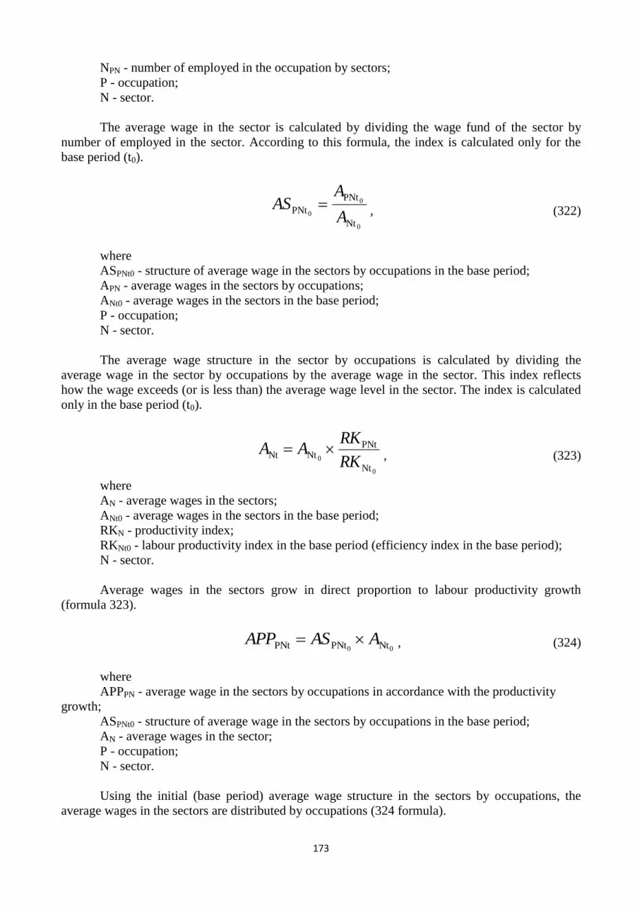
173
NPN - number of employed in the occupation by sectors;
P - occupation;
N - sector.
The average wage in the sector is calculated by dividing the wage fund of the sector by
number of employed in the sector. According to this formula, the index is calculated only for the
base period (t0).
0
0
0
Nt
PNt
PNtA
AAS , (322)
where
ASPNt0 - structure of average wage in the sectors by occupations in the base period;
APN - average wages in the sectors by occupations;
ANt0 - average wages in the sectors in the base period;
P - occupation;
N - sector.
The average wage structure in the sector by occupations is calculated by dividing the
average wage in the sector by occupations by the average wage in the sector. This index reflects
how the wage exceeds (or is less than) the average wage level in the sector. The index is calculated
only in the base period (t0).
0
0
Nt
PNtNtNt
RK
RKAA , (323)
where
AN - average wages in the sectors;
ANt0 - average wages in the sectors in the base period;
RKN - productivity index;
RKNt0 - labour productivity index in the base period (efficiency index in the base period);
N - sector.
Average wages in the sectors grow in direct proportion to labour productivity growth
(formula 323).
00 NtPNtPNt AASAPP , (324)
where
APPPN - average wage in the sectors by occupations in accordance with the productivity
growth;
ASPNt0 - structure of average wage in the sectors by occupations in the base period;
AN - average wages in the sector;
P - occupation;
N - sector.
Using the initial (base period) average wage structure in the sectors by occupations, the
average wages in the sectors are distributed by occupations (324 formula).
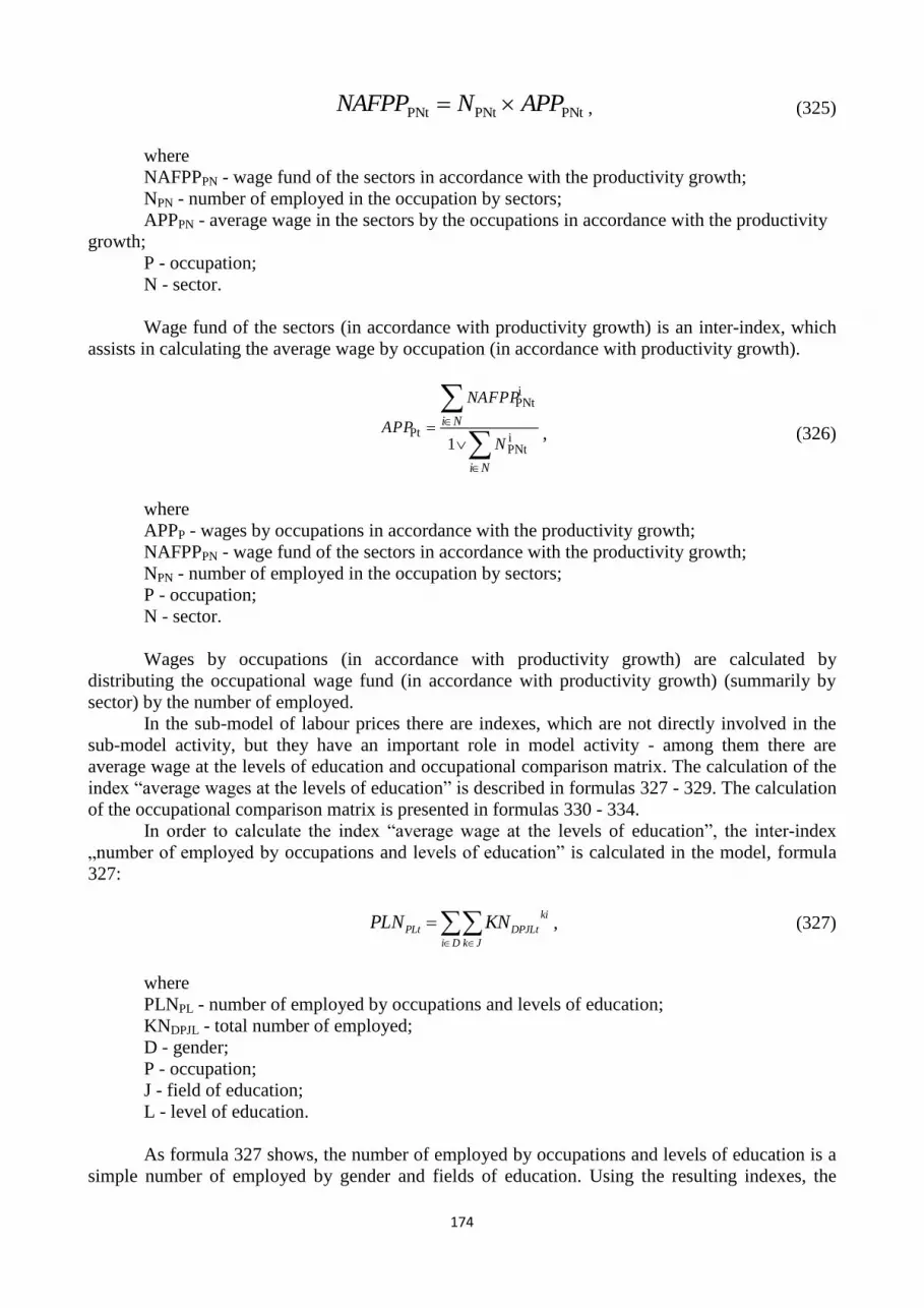
174
PNtPNtPNt APPNNAFPP , (325)
where
NAFPPPN - wage fund of the sectors in accordance with the productivity growth;
NPN - number of employed in the occupation by sectors;
APPPN - average wage in the sectors by the occupations in accordance with the productivity
growth;
P - occupation;
N - sector.
Wage fund of the sectors (in accordance with productivity growth) is an inter-index, which
assists in calculating the average wage by occupation (in accordance with productivity growth).
Ni
Ni
N
NAFPP
APPiPNt
iPNt
Pt1
, (326)
where
APPP - wages by occupations in accordance with the productivity growth;
NAFPPPN - wage fund of the sectors in accordance with the productivity growth;
NPN - number of employed in the occupation by sectors;
P - occupation;
N - sector.
Wages by occupations (in accordance with productivity growth) are calculated by
distributing the occupational wage fund (in accordance with productivity growth) (summarily by
sector) by the number of employed.
In the sub-model of labour prices there are indexes, which are not directly involved in the
sub-model activity, but they have an important role in model activity - among them there are
average wage at the levels of education and occupational comparison matrix. The calculation of the
index “average wages at the levels of education” is described in formulas 327 - 329. The calculation
of the occupational comparison matrix is presented in formulas 330 - 334.
In order to calculate the index “average wage at the levels of education”, the inter-index
„number of employed by occupations and levels of education” is calculated in the model, formula
327:
Di Jk
ki
DPJLtPLt KNPLN , (327)
where
PLNPL - number of employed by occupations and levels of education;
KNDPJL - total number of employed;
D - gender;
P - occupation;
J - field of education;
L - level of education.
As formula 327 shows, the number of employed by occupations and levels of education is a
simple number of employed by gender and fields of education. Using the resulting indexes, the

175
whole amount of wages of all workers by levels of education and occupations are calculated,
formula 328:
PtPLtPLt APLNLPAF , (328)
where
LPAFPL - wage fund by levels of education and occupations;
PLNPL - number of employed by occupations and levels of education;
AP - wages;
P - occupation;
L - level of education.
The average wages at the levels of education have been calculated from the wage fund by
levels of education and occupations and the number of employed at the levels of education, formula
329:
Pi
Pi
PLN
LPAF
Ai
PLt
i
PLt
Lt1
, (329)
where
AL - average wages at the levels of education;
LPAFPL - wage fund by levels of education and occupations;
PLNPL - number of employed by occupations and levels of education;
P - occupation;
L - level of education.
Average wages bythe levels of education, the relative difference of the levels is one of the
indexes, which makes the population to continue their education.
Wage level affects not only the choice of the level of education, but also the wish of the
employed to change occupation. Labour price sub-model determines the privileged occupations
along with the other indexes, i.e. occupations with the higher wage level than in other occupations;
as well as the opportunities to change occupation are determined, taking into account higher wage
level, formulas 330 - 334.
T
AAA PtPtPPt , (330)
where
APP - wage vector transformation to matrix;
AP - wages;
P - occupation.
The wage vector (column) in formula 330 is multiplied by the transposed vector (vector -
row). The square root has been taken from the multiplication. In the result of the mathematical
operations the matrix has been obtained, whose rows represent wages by occupations. This inter-
index does not have any economic sense, but it provides a mathematically technical implementation
of the model. It allows calculating the wage correlation matrix, formula 331:
176
MPA
AAAM
Pt
PPt
PPt1
, (331)
where
AAMPP - wage correlation matrix;
APP - wage vector transformation to matrix;
AP - wages;
MP - permutation matrix;
P - occupation.
Wage correlation matrix represents that the wage in a particular occupation is lower in
comparison with other occupations. In accordance with the low quality of the available data (wages
are not known for certain occupations, or they contain a zero level), 331 formula determines the
lowest wage level (1 LVL); it provides the functionality of the model, regardless of the quality of
the available data. Permutation matrix function in formula 330 is related to the conversion of the
wage correlation matrix to the triangular matrix form, so the condition is fulfilled aij = 0, if i>j.
Triangular matrix compares the wage of the particular occupation with other wages only once (once
for each), it is the economic advantage of this type of matrix. Permutation matrix is an upper
triangular matrix (aij = 1, if i≤j and aij = 0, if i>j.).
The privileged occupations have been calculated from the wage correlation matrix, formula
332:
1,0
1,
PPt
PPtPPt
PPtAAM
AAMAAMPAAM , (332)
where
PAAMPP - privileged occupations;
AAMPP - wage correlation matrix;
P - occupation.
As the wage correlation matrix represents how many times the wage of a particular
occupation is lower in comparison with the other occupations, this index in the privileged
occupations is less than one, i.e., the wages in the privileged occupations are higher. Indexes of
privileged occupations reflect how many times the wage in a particular occupation is more
attractive in comparison with other occupations (the smaller this index is, the higher the wage is).
The calculation of privileged occupational matrix is based on the privileged occupations,
formula 332:
0,0
0,12
PPt
PPt
PPtPAAM
PAAMPAAM , (333)
where
PAAM2PP - matrix of privileged occupations;
PAAMPP - privileged occupations;
P - occupation.
Privileged occupational matrix forms the permutation matrix based on the privileged
occupations, i.e., indicates that the occupations are economically related, not indicating the degree
of the relation.

177
Privileged occupational matrix is used to calculate matrix of privileged occupations for
occupational mobility, formula 334:
PPtPPtPPt 2 PAMPAAMPPMPM , (334)
where
PPMPMPP - matrix of privileged occupations for occupational mobility;
PAAM2PP - matrix of privileged occupations;
PAMPP - occupational compliance matrix;
P - occupation.
Privileged occupational matrix cannot be used directly. Despite the attractiveness of the
occupations, it is not always possible to change one occupation to another; it is determined by the
specifics of an occupation. The occupational compliance matrix has previously specified the
occupations that can be changed to other occupations. Privileged occupational matrix observes the
specifics of these occupations for the occupational mobility (formula 334).
Matrix of privileged occupations for the occupational mobility is the last labour price sub-
model index.

178
3. MODEL USER GUIDE
SDM has been developed by Powersim Studio 9 (service release 2) software, the created file
is adapted to the earlier versions of the program, starting with Powersim Studio 7 Feature Pack 2
(Service Release 5 (Studio 7)). Model application possibilities are related to Powersim software
requirements: Microsoft Windows, as well as Powersim hardware requirements. The developed
model (along with Powersim software) is using in the performance process up to 1.90 GB of RAM.
Model optimal performance is largely dependent on the Powersim software version and specificity.
Powersim software, according to the available versions, determines the model simulation process
speed. 30 step simulation (from 2010 to 2040 year, one step per year) takes 5 minutes on the
average. Hardware capacity increase over the requirements specified in the Powersim version
specification, does not increase the model simulation speed.
The model has been designed for the staff with basic Powersim knowledge. In order to
improve the model application possibilities for the staff, the model contains the model graphical
user interface. Despite the fact that the model can be used by the staff with basic Powersim
knowledge, it is not recommended to change the model connections without any solid experience in
Powersim. Application of the model is related to the offered opportunities in the model control
interface, preparation of data (MS Excel environment) and start of the simulation. Model
automatically ensures the data exchange from the external environment (MS Excel) to the model
and vice versa.
3.1. Model interface
The model consists of three files: Powersim file with SDM.sip model and two MS Excel
files - SDM_in.xls and SDM_out.xls. SDM_in.xls - file that automatically ensures the data
exchange from the external environment to the model. The model results are automatically
integrated into SDM_out.xls file.
To start the work with the model, SDM.sip file should be opened. By opening SDM.sip file,
the model is displaying on the first page the model control interface, Figure 3.1.
Darba tirgus vidēja un ilgtermiņa prognozēšanasun politikas analīzes sistēmdinamikas modelis
Imigrācijas īpatsvars darbaspēka
trūkuma problēmas risināšanā
0,0 0,2 0,4 0,6 0,8 1,0 1,2
�
Studiju vietu pielietošana
Uzdotās studiju vietas
Modelētās studiju vietas
Migrācijas pielietošana
Uzdotā migrācija
Modelētā migrācija
Konstanšulabošana
Ģenerētaissākotnējais
vakančuskaits
Paplašinātādatu
eksportēšana
Figure 3.1. Model control interface
Model control interface is designed to control the policy analysis options (education and
migration fields) to change the integrated constants in the model in order to obtain the number of
calculated vacancies, as well as to ensure additional data export.

179
Model control interface provides the following policy analysis options: firstly, the model
user is being offered to choose the application type of study places: the provided study places in the
external environment (from MS Excel) or the modelled study places in the model. Secondly, it is
being offered to choose the international migration application type: the provided migration in the
external environment (from MS Excel) or the modelled migration in the model. By choosing the
modelled migration in the model, it is possible to determine the significance of the impact of the
modelled migration on the labour market, i.e., it is possible to change the index of “migrant ratio in
labour shortage problem solution” (in Latvian: „imigrācijas īpatsvars darbaspēka trūkuma
problēmas risināšanā”). This index reflects the part of the labour shortage covered by the
international migration (the other part is being covered by the education system). By determining
the index value greater than 1, the situation is being modelled, in which international migration
exceeds over labour shortage.
Model control interface allows changing the constants integrated into the model. To start the
constant correction, it is necessary to go to the constant correction (using the URL “constant
correction” (in Latvian: „konstanšu labošana”)), Figure 3.2.
Galvenas un ārpus apakšmodeļu konstantes
Prognozēšanas horizonts 2041,00 Nosaka prognozēšanas pēdējo gadu (neieskaitot).
Nodarbinātības izmaiņu laiks 1,00 yr Atspoguļo laiku, kurā ir iespējams veikt nodarbinātības izmaiņas atbilstoši IKP izmaiņām.
Profesijas svarīguma kritērijs 0,03 Nosaka nozarei svarīgo profesiju minimālo īpatsvaru no visiem nozarē nodarbinātajiem.
Nodarbinātības izmaiņu etapu novērtēšanas koeficients 1,00 Atspoguļo, kā mainoties nozaru nodarbinātībai par i (%), iestājas jauns izmaiņu posms, kurā profesiju izmaiņu struktūra ir citāda.
Darba atrašanas cerību zuduma laiks 1,50 Darba atrašanas cerību zuduma laiks.
Profesionālās mobilitātes koeficients 1,00 Atspoguļo nodarbināto daļu, kuri mainītu darba vietu, ja būtu pieejams izdevīgāks piedāvājums.
Priekšrocīga vecuma struktūra [vg15_19] 6,93e-3 Atspoguļo no darba devēju skatījuma darbinieku prekšrocīgo vecumu (pa 5 gadīgām grupām).
Priekšrocīga vecuma struktūra [vg20_24] 0,10 Priekšrocīga vecuma struktūras daļa vecuma grupai no 20 gadiem līdz 24 gadiem.
Priekšrocīga vecuma struktūra [vg25_29] 0,13
Priekšrocīga vecuma struktūra [vg30_34] 0,12
Priekšrocīga vecuma struktūra [vg35_39] 0,13
Priekšrocīga vecuma struktūra [vg40_44] 0,12
Priekšrocīga vecuma struktūra [vg45_49] 0,13
Priekšrocīga vecuma struktūra [vg50_54] 0,12
Priekšrocīga vecuma struktūra [vg55_59] 0,09
Priekšrocīga vecuma struktūra [vg60_64] 0,03
Priekšrocīga vecuma struktūra [vg65_69] 0,01
Priekšrocīga vecuma struktūra [vg70_74] 7,63e-3
Darbaspēka pieprasījuma un piedāvājuma ietekmes robežas 0,03 Atspoguļo, cik būtiski darbaspēka trūkums vai pārpalikums var ietekmēt algas (daļa).
Minimālā alga 200,00 Ls Minimālā alga.
Non-commercial use only!
Figure 3.2. Fragment of the constant correction tables
The fragment of the second page, table of constants correction, is shown in Figure 3.2. The
constants integrated into the model are grouped by sub-models in the separate tables, and the logical
relationship of constants is underlined by the colours (e.g., single equation/algorithm constants or
structure constants (where the table is successively reflecting each structure element)). The
constants integrated into the model are described in subsection 3.3.
Simultaneously with the constant regulation, the model is necessary to be ensured by the
data, i.e. to fill SDM_in.xls file. SDM_in.xls file data description is available in Annex A.1, but the
technical description of the file is available in Annex A.7.
By calculating the designed labour reduction and changes of labour demand in the first
forecasting year, the model determines the vacancies, created in the base year. The vacancies in the
base year is a specific parameter, which can be provided on the basis of both statistic and model
calculations for the base year. If this parameter has been provided on the basis of the statistics, its
completion is standard (as all other SDM_in.xls file tables). If the model calculations are required, it
is necessary to perform the following procedure:
1. Model control interface goes to the link “Generated number of initial vacancies” (in
Latvian: „Ģenerētais sākotnējais vakanču skaits”).
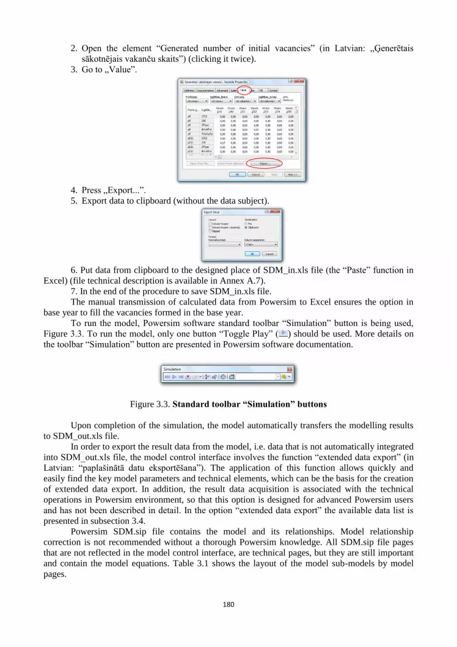
180
2. Open the element “Generated number of initial vacancies” (in Latvian: „Ģenerētais
sākotnējais vakanču skaits”) (clicking it twice).
3. Go to „Value”.
4. Press „Export...”.
5. Export data to clipboard (without the data subject).
6. Put data from clipboard to the designed place of SDM_in.xls file (the “Paste” function in
Excel) (file technical description is available in Annex A.7).
7. In the end of the procedure to save SDM_in.xls file.
The manual transmission of calculated data from Powersim to Excel ensures the option in
base year to fill the vacancies formed in the base year.
To run the model, Powersim software standard toolbar “Simulation” button is being used,
Figure 3.3. To run the model, only one button “Toggle Play” ( ) should be used. More details on
the toolbar “Simulation” button are presented in Powersim software documentation.
Figure 3.3. Standard toolbar “Simulation” buttons
Upon completion of the simulation, the model automatically transfers the modelling results
to SDM_out.xls file.
In order to export the result data from the model, i.e. data that is not automatically integrated
into SDM_out.xls file, the model control interface involves the function “extended data export” (in
Latvian: “paplašinātā datu eksportēšana”). The application of this function allows quickly and
easily find the key model parameters and technical elements, which can be the basis for the creation
of extended data export. In addition, the result data acquisition is associated with the technical
operations in Powersim environment, so that this option is designed for advanced Powersim users
and has not been described in detail. In the option “extended data export” the available data list is
presented in subsection 3.4.
Powersim SDM.sip file contains the model and its relationships. Model relationship
correction is not recommended without a thorough Powersim knowledge. All SDM.sip file pages
that are not reflected in the model control interface, are technical pages, but they are still important
and contain the model equations. Table 3.1 shows the layout of the model sub-models by model
pages.

181
Table 3.1. SDM.sip file description
No. Name of the page Brief description
1. Home
(Sakums)
Reflects the model control interface; home, first page of the model.
2. Tables
(Tabulas)
Reflects the model control interface; tables of constant corrections.
3. Start_vac
(Sak_vak)
Reflects the model control interface; number of generated initial
vacancies.
4. Output
(Izvadei)
Reflects the model control interface; copies of the significant
parameters and technical elements, which are provided for the
formation of the additional output.
5. Sectors_dem
(Nozares_piep)
Reflects the sub-model for the formation of the labour demand by
sectors
6. Occupation_dem
(Profesijas_piep)
Reflects the sub-model for the formation of the labour demand by
sectors and occupations.
7. Education_dem
(Izglītības_piep)
Reflects the sub-model for the formation of the labour demand by
occupations and education.
8. Education_dem _ind
(Izglītības_piep_Noz)
Reflects the sub-model for the formation of the labour demand by
sectors, occupations and education.
9. Gender_dem
(Dzimums_piep)
Reflects the sub-model for the formation of the labour demand by
occupations and gender.
10. Education_supp
(Izglītība_pied)
Reflects the education attainment sub-model.
11. Lifelong
educationl_supp
(Mūžizgl_pied)
Reflects the lifelong education attainment sub-model.
12. Population_supp
(Iedzīvotāji_pied)
Consists of demography and employable population analysis sub-
models.
13. Ec_activity_supp
(Ek_aktivitāte_pied)
Reflects the population economic activity sub-model.
14. Migration_supp
(Migrācija_pied)
Reflects the population international migration sub-model.
15. Market
(Tirgus)
Reflects the labour market sub-model.
16. Sectors_employm
(Nozaru_nodarb)
Reflects the sub-model for employed population division by
occupations and sectors.
17. Wage
(Alga)
Reflects the wage definition sub-model.
3.2. Data input and model update
SDM_in.xls - file that automatically ensures the data exchange from the external
environment to the model. By updating SDM_in.xls file, the model can be used over a longer period
of time. The file has multiple pages that contain different types of data. More detailed relative
analysis of the file pages and data is presented in Annex A.1.
SDM_in.xls file pages, the included technical format and technical data requirements are
described in detail in Annex A.7.

182
3.3. Integrated constants in the model
In order to make the model function adequately, it is necessary to set the forecasting start
and end time in the modelling settings (Simulation/Simulation settings in the Powersim computer
program).
Figure 3.4. Powersim software program „Simulation/Simulation settings” window
Along with the “Simulation/Simulation settings”, it is important to restore the element
“Forecasting horizon” (in Latvian: “Prognozēšanas horizonts”) (which is explained in Annex A.6).
Upon determination of the values for the constants, it is not required to change them.
In model pages constants are marked as Powersim constants, and additionally are filled in
yellow colour (apart from “Forecasting horizon”, which is filled in red). The integrated constants
into model are described in Annex A.6.
Mostly the integrated constants into the model are to be determined by means of survey of
the experts. The majority of the constants does not change in the short and medium time period
(periods less than 10 years).
3.4. Model output tables
The model results are automatically integrated into SDM_out.xls file. The list of
SDM_out.xls file pages and tables is presented in Figure 3.2.
Table 3.2. SDM_out.xls fail description
No. Name of the page List of tables / description
1. Employment
(Nodarbinātība)
Employment demand structure by sectors (people)
2. OccupationsD
(ProfesijasD)
Employment demand structure by occupations (people);
Replacing demand structure by occupations (people);
Expansion demand structure by occupations (people)
3. Occupations
(ProfesijasS)
Population structure by occupations (people)
4. OccupationsA
(ProfesijasA)
Active population structure by occupations (people)
5. OccupationsN
(ProfesijasN)
Employment structure by occupations (people)
6. PG_LS_LN Technical page, can be excluded form file
7. Ratio of occupations
(Profesiju_īpatsv)
Employment demand division by sectors and occupations (structure
of sectors-occupations) (%)
8. EducationD
(IzglītībaD)
Employment demand structure by levels, fields of education (people)
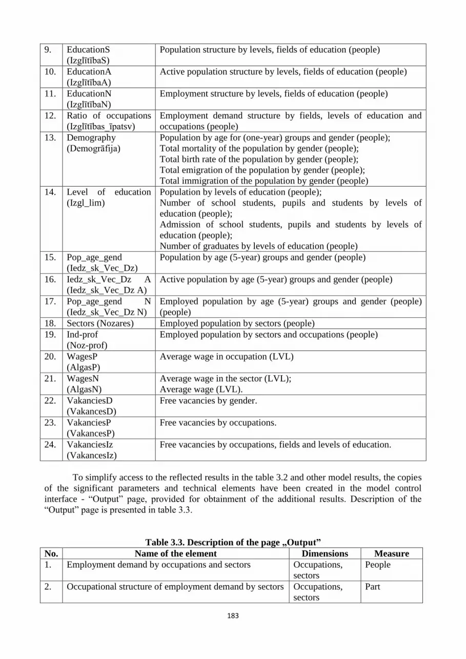
183
9. EducationS
(IzglītībaS)
Population structure by levels, fields of education (people)
10. EducationA
(IzglītībaA)
Active population structure by levels, fields of education (people)
11. EducationN
(IzglītībaN)
Employment structure by levels, fields of education (people)
12. Ratio of occupations
(Izglītības_īpatsv)
Employment demand structure by fields, levels of education and
occupations (people)
13. Demography
(Demogrāfija)
Population by age for (one-year) groups and gender (people);
Total mortality of the population by gender (people);
Total birth rate of the population by gender (people);
Total emigration of the population by gender (people);
Total immigration of the population by gender (people)
14. Level of education
(Izgl_lim)
Population by levels of education (people);
Number of school students, pupils and students by levels of
education (people);
Admission of school students, pupils and students by levels of
education (people);
Number of graduates by levels of education (people)
15. Pop_age_gend
(Iedz_sk_Vec_Dz)
Population by age (5-year) groups and gender (people)
16. Iedz_sk_Vec_Dz A
(Iedz_sk_Vec_Dz A)
Active population by age (5-year) groups and gender (people)
17. Pop_age_gend N
(Iedz_sk_Vec_Dz N)
Employed population by age (5-year) groups and gender (people)
(people)
18. Sectors (Nozares) Employed population by sectors (people)
19. Ind-prof
(Noz-prof)
Employed population by sectors and occupations (people)
20. WagesP
(AlgasP)
Average wage in occupation (LVL)
21. WagesN
(AlgasN)
Average wage in the sector (LVL);
Average wage (LVL).
22. VakanciesD
(VakancesD)
Free vacancies by gender.
23. VakanciesP
(VakancesP)
Free vacancies by occupations.
24. VakanciesIz
(VakancesIz)
Free vacancies by occupations, fields and levels of education.
To simplify access to the reflected results in the table 3.2 and other model results, the copies
of the significant parameters and technical elements have been created in the model control
interface - “Output” page, provided for obtainment of the additional results. Description of the
“Output” page is presented in table 3.3.
Table 3.3. Description of the page „Output”
No. Name of the element Dimensions Measure
1. Employment demand by occupations and sectors Occupations,
sectors
People
2. Occupational structure of employment demand by sectors Occupations,
sectors
Part

184
3. Employment demand by occupations, fields, levels of
education and gender
Levels of
education, fields
of education,
occupations,
gender
People
4. Occupational structure of employment demand by fields
and levels of education
Levels of
education, fields
of education,
occupations
Part
5. Employment demand by occupations, fields, levels of
education and sectors A..J
Levels of
education, fields
of education,
occupations,
sectors A..J
People
6. Employment demand by occupations, fields, levels of
education and sectors K..R
Levels of
education, fields
of education,
occupations,
sectors K..R
People
7. Admission of students by fields and levels of education Levels of
education, fields
of education
People per
year
8. Number of graduates by fields and levels of education Levels of
education, fields
of education
People per
year
9. Number of students by fields and levels of education Levels of
education, fields
of education
People
10. Number of optimized study places by fields and levels of
education
Levels of
education, fields
of education
People per
year
11. Population Age, gender People
12. Birth rate by gender Gender People per
year
13. Mortality Age, gender People per
year
14. Emigration by age groups and gender Age, gender People per
year
15. Immigration by age groups and gender Age, gender People per
year
16. Emigration Age groups,
gender,
occupations,
fields of
education,
economic
activity groups
People per
year

185
17. Immigration Age groups,
gender,
occupations,
fields of
education,
economic
activity groups
People per
year
18. Population by levels, fields of education occupations and
economic activity groups
Age groups,
gender,
occupations,
fields of
education,
economic
activity groups
People
19. Population by age groups, gender and economic activity
groups
Age groups,
gender,
economic
activity groups
People
20. Total number of vacancies Gender,
occupations,
fields of
education, levels
of education
People
21. Total number of employed Gender,
occupations,
fields of
education, levels
of education
People
22. Number of employed by age groups and gender Age groups,
gender
People
23. Total number of jobseekers Gender,
occupations,
fields of
education, levels
of education
People
24. Replacing demand Gender,
occupations,
fields of
education, levels
of education
People per
year
25. Number of employed in the occupation by sectors Occupations,
sectors
People
26. Salaries by occupations Occupations LVL
27. Average salaries in the sector Sectors LVL
28. Average wage - LVL

186
4. DESCRIPTION OF THE RESULTS OBTAINED WITH THE MODEL,
INTERPRETATION AND RELIABILITY OF THE RESULTS
Model result evaluation is based on the experiment (simulation) series result analysis. Series
of experiments includes several simulations based on the model, labour market and the national
economy real statistical data, by changing the exogenous forecasting data in the experiments, as
well as switching on and off the provided functions in the model. Table 4.1 visually describes the
experiments.
Table 4.1. Description of experiments
No GDP
forecast
Study places Migration policy Name of
experiment
1.
GDP
without
changes
Study places without
changes in accordance
with the base year
The closed system has been
modelled, no migration, it is not
affecting the labour market
GDP without
changes, scenario
without impact
2. Study places has been
modelled by
optimizing the
national policy in
education
The closed system has been
modelled, no migration, it is not
affecting the labour market
GDP without
changes,
optimization
scenario of the
study places
3. Study places without
changes in accordance
with the base year
Emigration and immigration has
been defined in the model in
accordance with the market
demand
GDP without
changes,
migration impact
scenario
4.
GDP is
growing
regularly in
all sectors
throughout
the whole
forecasting
period, 3%
per year
Study places without
changes in accordance
with the base year
The closed system has been
modelled, no migration, it is not
affecting the labour market
GDP growth
impact, scenario
without impact
5. Study places has been
modelled by
optimizing the
national policy in
education
The closed system has been
modelled, no migration, it is not
affecting the labour market
GDP growth
impact,
optimization
scenario of the
study places
6. Study places without
changes in accordance
with the base year
Emigration and immigration has
been defined in the model in
accordance with the market
demand
GDP growth
impact, migration
impact scenario
7.
GDP is
decreasing
regularly in
all sectors
throughout
the whole
forecasting
period, 3%
per year
Study places without
changes in accordance
with the base year
The closed system has been
modelled, no migration, it is not
affecting the labour market
GDP decrease
impact, scenario
without impact
8. Study places has been
modelled by
optimizing the
national policy in
education
The closed system has been
modelled, no migration, it is not
affecting the labour market
GDP decrease
impact,
optimization
scenario of the
study places
9. Study places without
changes in accordance
with the base year
Emigration and immigration has
been defined in the model in
accordance with the market
demand
GDP decrease
impact, migration
impact scenario

187
The table 4.1 shows that the experiments have been grouped into 3 groups, depending on the
GDP forecasting conditions, and the scenarios without impact and the changes of study places and
migration impacts are analysed in each group.
Results of the experiments are presented in table 4.2. They are analysed in more detail after
the table.

188
Table 4.2. Modelled scenario analysis table
Parameter Without GDP changes GDP growth impact GDP decrease impact
GDP No changes Growth in all sectors is always 3% Decrease in all sectors is always 3%
Labour demand (scenario without
impact), thous.
places
Labour demand (optimization
scenario of the
study places),
thous. places
Labour demand (migration
impact scenario),
thous. places

189
Population,
thous. people
Population of
active age, thous.
people
Birth rate,
children per
thous. women of
15-49.
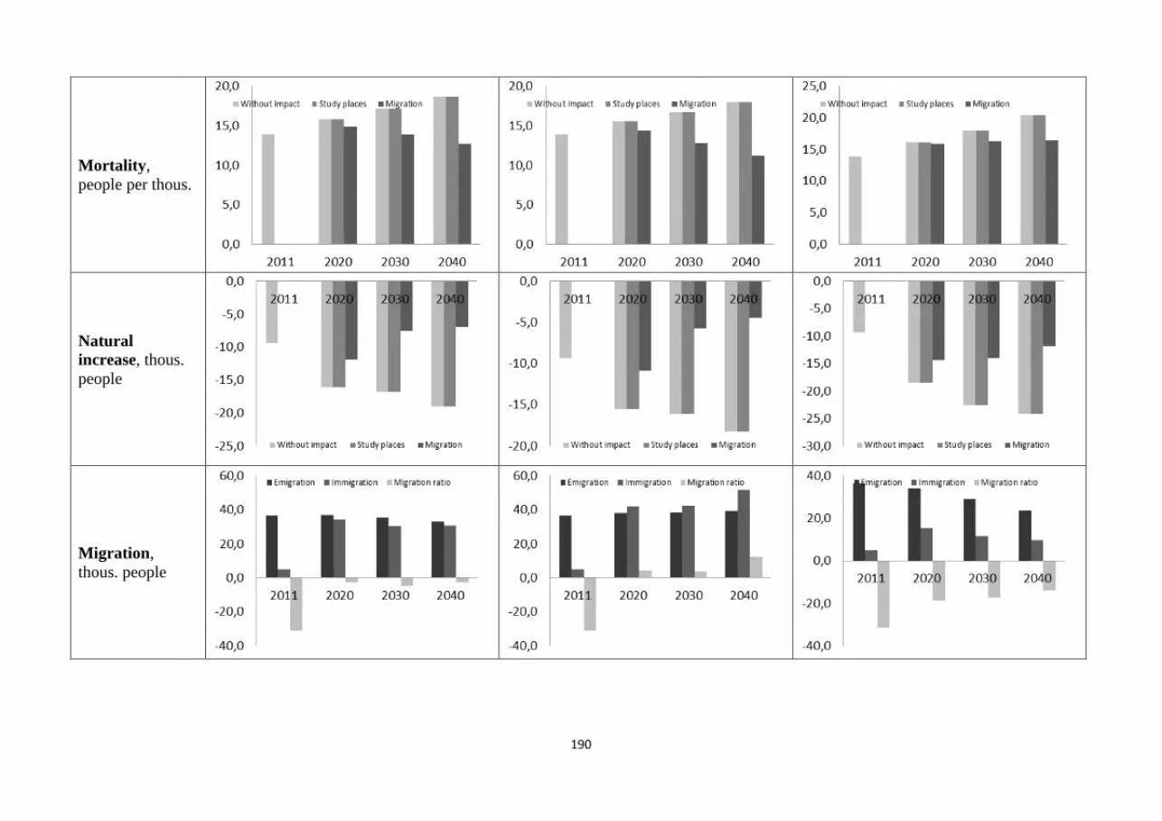
190
Mortality,
people per thous.
Natural
increase, thous.
people
Migration,
thous. people

191
Economically
active
population,
thous. people.
Participation
level
Number of
employed, thous.
people.
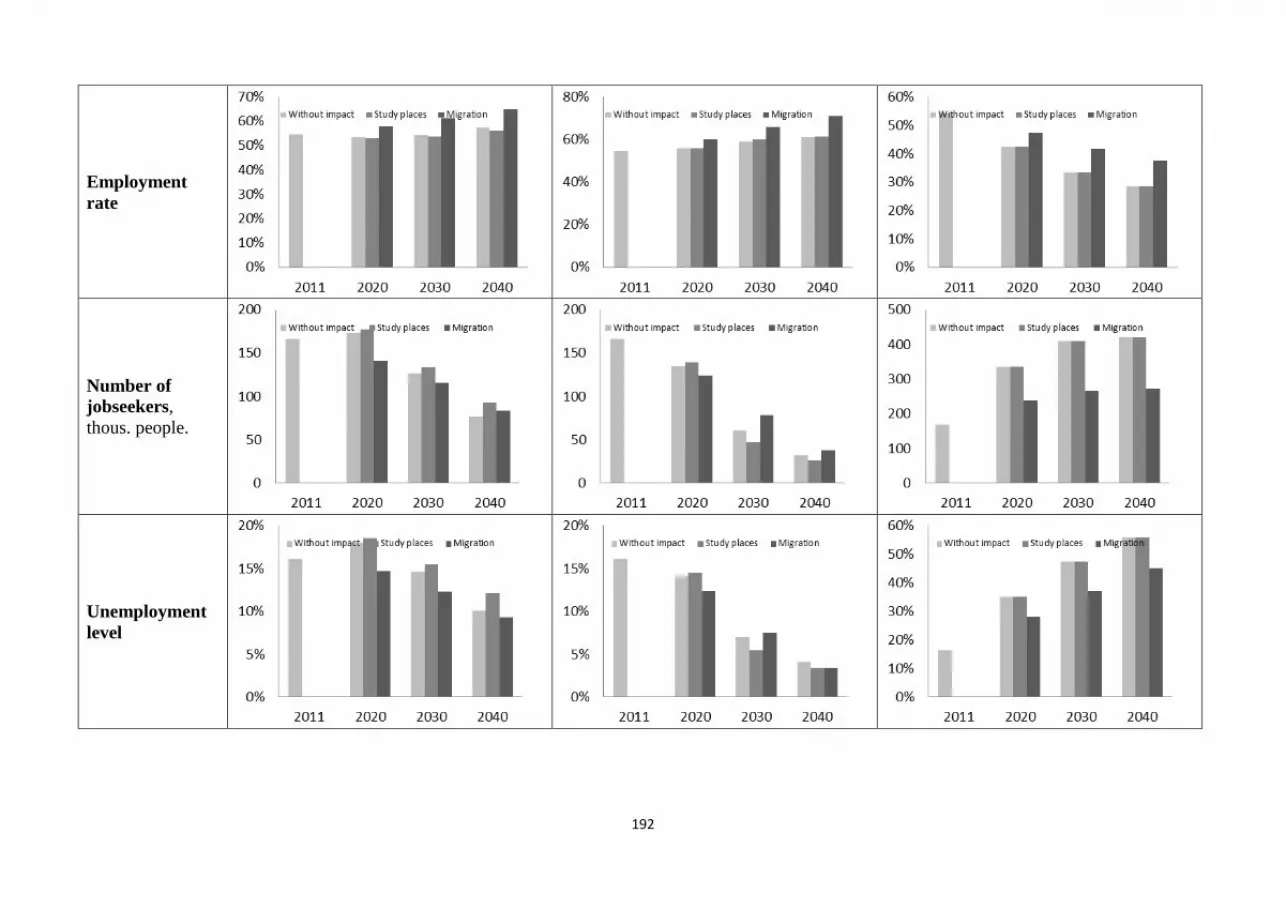
192
Employment
rate
Number of
jobseekers,
thous. people.
Unemployment
level
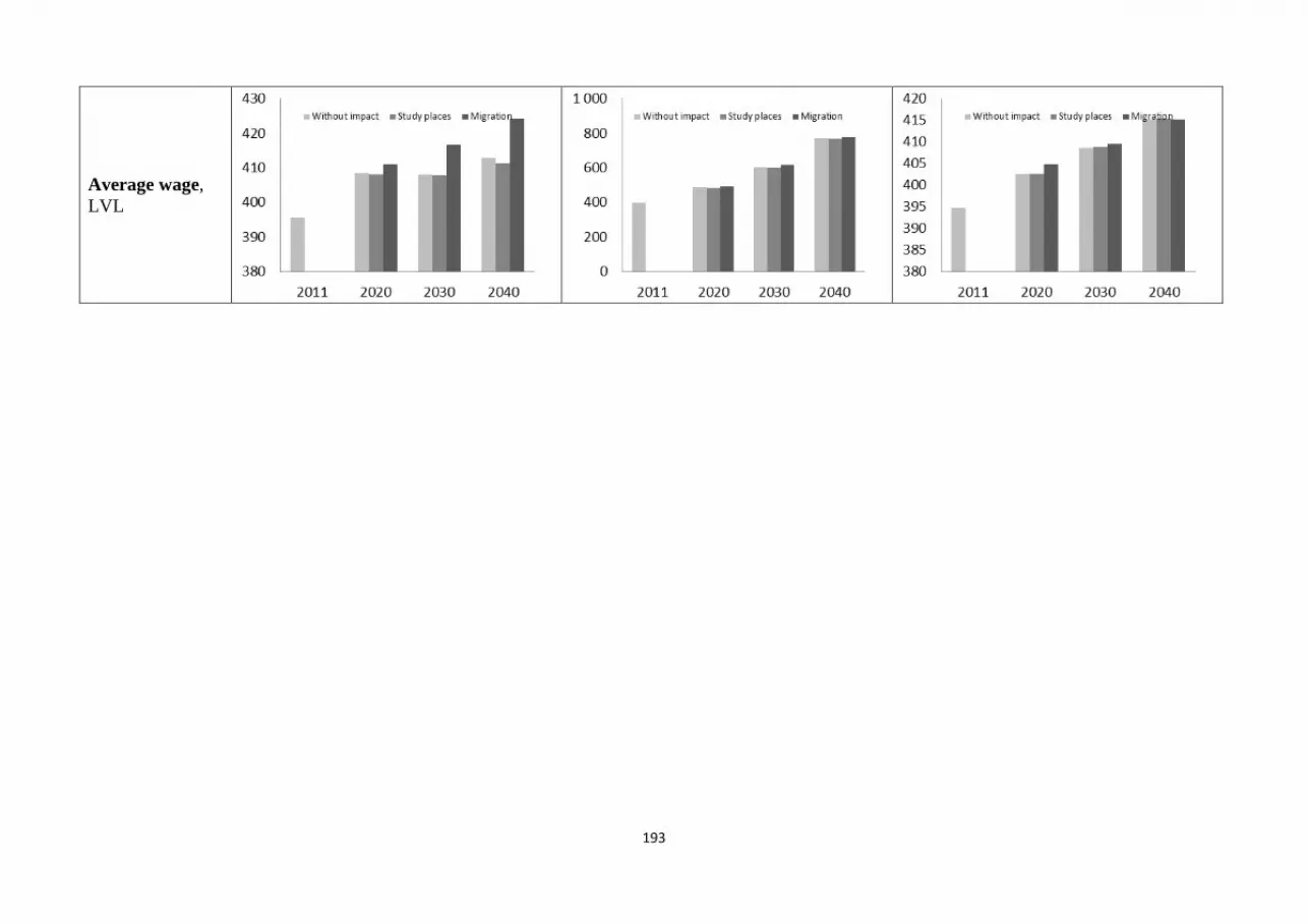
193
Average wage,
LVL

194
The first parameter analysed in the model is the labour demand. Labour demand is
analysed separately for each scenario. Each scenario evaluates the expansion and replacing labour
demand, comparing to the initial (base period) labour demand.
Expansion labour demand indicates the changes of the labour demand (expansion) in case of
change (growth) of GDP. Model results indicate the connection between the changes of the labour
and GDP: the growing GDP causes the growth of labour demand; decline in GDP causes the decline
in labour demand; in case of constant GDP, the labour demand remains unchanged.
By summing up the initial (base) labour demand and expansion labour demand, the total
labour demand is being obtained, which dynamics depends on GDP development forecasts.
The replacing labour demand indicates the labour demand, which is being formed due to the
need to replace the employed population, who was die, as well as population, leaving their working
places due to the retirement age. Replacing demand is significant, taking into account that more
than 55% of the Latvian employed is older than 40 years and are going to leave the labour market in
the coming 30 years (forecast period). The replacing labour demand for labour is mainly related to
the population and employed initial (base) age structure, and this parameter does not differ
significantly by the scenarios.
The analysed table is visually showing that before 2040 the replacing labour demand
exceeds the half of the initial (base) labour demand, which means that most of the current
specialists in the market should meet the deputies.
The next analysed parameter in the model is the population. Population in all developed
scenarios in the country has declined.
By analysing the change of population, it is determined that GDP growth is almost not
affecting the population (excluding migration scenario), but the decline in GDP significantly
accelerates the decline in population (compared to scenarios without changes of GDP).
Migration policy impact on the population is different. Over the first ten years, following the
initial large negative balance of migration, migration always reduces the population. The following
situation is not so simple: depending on the changes of GDP, the labour demand changes as well,
and then the population follows. With the growth of GDP, the labour demand also grows, migration
covers missing labour demand, the population in the country grows as well, which is evident in the
GDP growth scenario from 2030 year. Without changes of GDP, in the scenario the shortage of
labour due to decline in population will appear only in 2040, and migration is to cover it. In case of
decline in GDP there is no labour shortage, while there is a labour surplus, which is being reduced
by migration. In this case, there is a decline in population.
By summarizing the above mentioned, it can be concluded that the model reflects the fact
that in case of GDP growth the migration increases the population, but in case of decline in GDP
the migration reduces the population.
Part of the population is the population of working age. These two parameters are mutually
correlating, so the dynamics will not be re-examined.
The birth rate is significantly dependent on the population and structures. In the coming
decade the birth rate decline by 15% is expected. This is related to the fact that during the same
period, the population and the number of women of reproductive age will decrease by the same
amount. It is important to note that GDP growth is mostly not affecting the changes of the birth rate,
but the decline in GDP accelerates the decline in birth rate.
The growth of the birth rate is predicted till the 2030, which is related to the age structure of
the population: by assessing the population by 5-year old groups, now the 5-year-old to 9-year-old
population exceeds 10-year-old to 14-year-old population, but 0-year-old to 4-year-old population
exceeds 5-year-old to 9-year-old population. This will ensure the growth of the population and the
number of women of reproductive age from 2020 to 2030th, which will accordingly increase the
birth rate. However, in case of decline of GDP, the present growth of birth fails to overcome
another influencing factor - GDP reduction, and in these scenarios the growth of birth rate is not
expected.

195
Significant impact on the birth rate has the migration processes. Model indicates that
migration always increases the birth rate. It reflects that the emigration structure depends on the
current structure of the population, but immigrants are mostly of reproductive age and are able to
raise the birth rate.
The next parameter analysed in the model is mortality. Mortality significantly depends on
the population and structure. Despite this fact, the growth of GDP reduces mortality, but the
decrease in GDP increases mortality. Besides the impact and optimization of study places the
scenarios provide a sustained increase of mortality. However, migration reduces mortality. This is
explained by the fact that the emigration structure is based on the current structure of population,
but immigrants are generally relatively young people, who reduce the mortality rate.
Birth rate and mortality form the natural growth rate, which is analysed below. Natural
growth is negative in all scenarios. Natural growth is dependent on changes of GDP - with the
growth of GDP, the natural growth increases; with the decrease of GDP, the natural growth
decreases. Considering that migration increases birth rate and reduces mortality, it is evident that
migration significantly increases the natural growth.
By analysing the migration in the model, instead of nine simulations, only three are being
investigated, which were included in the migration modelling and these three simulations are
analysing three parameters: emigration, immigration and balance of migration.
In the analysed scenarios emigration initially significantly exceeds immigration. Emigration
amounts are not changing significantly in all scenarios. Its gradual reduction is being explained by
the gradual decline in population.
According to the included relations, immigration covers the labour shortage, which explains
the rapid increase in immigration until 2020th. In subsequent years, immigration is dependent on
changes of GDP: with the growth of GDP, immigration increases, with the decrease of GDP,
immigration decreases. This is related to the changes of labour demand and arising of labour
shortage.
Balance of migration reflects the difference between immigration and emigration.
The economically active population is related to the working age population. These two
parameters are mutually correlating; the model assumes that the economically active population is
directly proportional to the population by 5-year-old groups and gender according to externally
provided indexes (for the provided participation level). This explains why a whole economically
active population is proportional to the population of working age.
However, taking into account the changes of age structure, it leads to the overall
participation level fluctuations. Participation level will increase slightly by 2020th, by 2030 it will
decrease by 2 percentage points, and by 2040 will increase (in scenarios without impact and
optimization of study places). The population age structure in immigration scenarios is different: the
population is younger. In the younger groups the participation level is higher. With the increase of
population in younger groups, the overall participation level increases as well.
Number of employed persons is a complex index, which affects both the economically
active population, from the perspective of the supply, and the labour demand from the perspective
of the demand. To simplify the interpretation of the parameter, it is analysed along with the next
parameter - employment rate.
Dynamics of the number of employed persons and employment is different in all scenarios.
In addition to the changes of GDP, the major impact on the employment in the scenario
group has the decline in the number of employees, as indicated by the decline in the number of
employed along with the preservation of the employment rate. The scenario does not provide the
growth of GDP, and, accordingly, the increase of living standard and the rapid demand expansion in
occupations. In such circumstances occurs the short-term satisfaction of the occupational demand,
education attainment, but then it remains non-demanded. In order to slightly increase the number of
employed and employment rate in this scenario, the significant investments in the education system
(through continuous re-qualification) are required. In the present results the employment in the
scenario of optimization of study places is slightly lower than in the scenario without impact. This

196
is related to the fact that the model optimizes the study places in accordance with the population,
but in the scenario without impact 1.35 places will be financed per one applicant by 2040th. Model
reflects the by increasing the number of study places, employment may be increased. And to
increase the number of employed, the number of study places should never be reduced. The
migration policy in the same scenario group can solve the labour problem - increase both
employment and employment rate.
The decline in the number of employed in the GDP growth scenario group is slower, at the
same time there is a growth of employment rate. This indicates the fact that the main role in
employment in this scenario group belongs to the growth of GDP and the resultant increase of
labour demand. In case of the growth of labour demand, the incentive to attain education also
increases, and in this scenario group the optimization of study places increases both the number of
employed and the employment rate (the number of study places, comparing to the base year, is
being significantly reduced). However, the education system is not able to completely solve all
problems of labour market due to lack of population. But migration policy can solve labour
problems, by increasing both employment and employment rate.
The decline in the number of employed and decrease of employment rate in GDP reduction
scenario group is being significantly affected by the decline in GDP and the resultant decline in
labour demand. None of the influencing factors can increase the number of employed. But the
migration policy may result in faster decrease of the number of employed; there is also decline in
the total population, which leads to slower decrease of the employment rate.
The next analysed parameter is the number of jobseekers. The number of jobseekers is a
complicated parameter, which is being affected by the economically active population and the
number of employed. To simplify the explanation of the parameter, it is being analysed along with
the unemployment rate.
Dynamics of the number of jobseekers and unemployment is different in all scenarios.
In the scenario group without changes of GDP the number of jobseekers and the
unemployment rate is declining in accordance with the decline in population (over the first
forecasting years the unemployment rate remains stable high, considering that the new study places
are not created, and the replacing demand is minimal). This scenario group shows the fiasco of
education system, in the case of absence of GDP growth - occurs the short-term satisfaction of the
occupational demand, education attainment, but then it remains non-demanded. Therefore, the
optimization of study places (mainly the decline in accordance with the population) causes the
increase of the number of jobseekers and unemployment rate. Migration policy in this scenario
group reduces both the number of jobseekers and the unemployment rate.
In the GDP growth scenario group, the number of jobseekers and the unemployment rate are
decreasing, taking into account the decline in the number of population and increase of the number
of employed (due to the growth of GDP and increase of labour demand). This scenario group
represents that the education system optimization is acting over the medium term. This is related to
the objective reasons: in order to prepare specialists with higher education, at least 4 years are
necessary, additionally the time is required from the formation of the shortage of occupations to the
problem identification and opening of new study places, etc. Education policy in this scenario group
allows reducing the number of employed and the unemployment rate prior to other affecting
elements. However, its effectiveness is being also reduced, with the unemployment rate reaching 2-
3%. In this scenario group migration reduces the speed of decline in the number of jobseekers. This
is related to the fact that migration increases the population. Migration policy options are also
limited, when the unemployment rate is on 2-3% level.
The number of jobseekers and the unemployment rate in GDP reduction scenario group are
steadily increasing. This indicates the fact that in case of decline in GDP, neither the education, nor
the immigration policy can reduce unemployment. However, the migration policy reduces the
population, which is not creating so rapid increase of the number of jobseekers and unemployment
rate, as in the other scenarios.

197
The next analysed parameter is the average wage. Model provides long-term increase of the
wage along with the increase of the labour productivity, the steady increase of the wage is evident
in GDP growth scenario group. This parameter is also affected by other factors, such as labour
supply and demand ratio, occupational structure. In total, these factors lead to a small increase of
the wage in other scenario groups. In migration scenarios, compared to other scenarios, the wage
increase is slightly faster. It is based on the changes of the occupational: the shortage of specialists
is being formed in country, which is being filled by immigrants. Increase of the number of qualified
specialists changes the labour market structure, by increasing the number of highly paid specialists,
raising the average wage in the country.

198
5. DESCRIPTION OF THE TIME CURVE OF THE DETAILED
FORECASTING PROCESS
SDM model uses a number of statistical data types prepared by CSB as the input data. This
determines the necessity for the regular data update. Table 5.1 presents data update time schedule.
Table 5.1 presents data update and updating time by months. Data update detailed information (for
each parameter with an accuracy to the day) is presented in Annex A.9.
Table 5.1. Data update time schedule Month
Data group .
I II III IV V VI VII VIII IX X XI XII
Demography data (population)
Demography data (birth rate, mortality)
Education data (school)
Education data (other)
Labour data
GDP data
Wage data
Forecasting data of the MoE
SDM model operates with the annual data. Accordingly, the annual data is being prepared
by CSB once a year. The only data that can be updated on a quarterly basis in order to increase the
quality of forecasts is data on wage.
Along with the CSB statistical data update, it is necessary to revise the forecasts, i.e.
assumption data. Among them are the GDP forecast, target labour sector-occupational structure,
forecast of the economically active part of the population. Depending on the simulation target, the
update of the parameter “number of the new state-financed study places” may be needed.
With the global change of national economy, labour market or education system may need
to update the following elements: period of the studies, occupation compliance matrix, time indexes
of sectorial labour productivity. It is not necessary to annually update these elements.
SDM model data update and forecasting time consumption is presented in table 5.2. Table
5.2 visually reflects the activity groups and the required time. More detailed information of data
update and forecasting time is presented in Annex A.10.
Table 5.2. Data update and forecasting time consumption
No. Activity group Total time of the group
1. Data update 13 hours
2. Assumption data review 2 hours
3. Special data review (option) 10 hours
4. Implementation of the procedure before modelling 0,2 hours
5. Modelling process (one simulation) 0,2 hours
6. Full calibration of the model (option) 48 hours
7. Examination of results 0,2 hours
Table 5.2 shows that the data update, development of one scenario, modelling and
obtainment of the results require about 2 days. If the changes of global national economy, labour
market and education system have been observed, the model adjustment can take longer time. This
is largely related to the special data review and model calibration. The developed model contains
updated data, which is the latest available at the moment of the model transfer; the model contains a
full calibration. Review of the optional opportunity is not required in the next 3-year period.

199
6. REFERENCES
1. Astra Auziņa 2007 Apstrādes rūpniecības apakšnozaru attīstības prognozēšana, izmantojot
Latvijas multisektorālo makroekonomisko modeli. RTU zinātniskie raksti, 3.sērija,
Ekonomika un uzņēmējdarbība, Tautsaimniecība: teorija un prakse, 14.sējums. RTU. Rīga.
18-25.
2. Astra Auziņa 2010 Latvijas tautsaimniecības nozaru attīstības un konkurētspējas analīze un
prognozēšana. RTU zinātniskie raksti, 3. sēr., Ekonomika un uzņēmējdarbība,
Tautsaimniecība: teorija un prakse, 18.sējums. RTU. Rīga. 9-18.
3. Astra Auziņa 2008 Latvijas tekoša konta deficīts globālā kontekstā. LU Raksti, "Vadības
zinātne", 721.sēj. LU. Rīga. 10-20.
4. Astra Auziņa; Remigijs Počs 2005 Multisektorālā makroekonomiskā modeļa izstrādāšanas
problēmas Latvijā un to risinājumi. RTU zinātniskie raksti, 3.sērija, Ekonomika un
uzņēmējdarbība, Tautsaimniecība: teorija un prakse, 11.sējums. RTU. Rīga. 9-15.
5. Juris Roberts Kalniņš; Valerijs Skribans; Gints Ozoliņš 2009 Lauksaimniecības nozares
stratēģiskās attīstības sistēmdinamikas modelēšana. LU raksti No 743 sējums. 320-332.
6. Arnis Lektauers; Jekabs Trušiņš; Inese Trušiņa 2011 Kuldīgas novada ilgtspējīgas attīstības
sistēmdinamiskais modelis. Rīgas Tehniskās universitātes zinātniskie raksti, 14.sēr.,
Ilgtspējīga telpiskā attīstība. RTU Izdevniecība. Rīga. 23-29.
7. Remigijs Počs; Astra Auziņa; Velga Ozoliņa; Valērijs Skribans; Jekaterina Komkova.
Latvijas tautsaimniecības nozaru attīstības un konkurētspējas prognozēšana, izmantojot
modelēšanas instrumentāriju. LZP Ekonomikas, juridiskās un vēstures zinātnes galvenie
pētījumi virzieni 2009. gadā. LZP. Rīga. 111-118.
8. Valerijs Skribans 2000 Būvmateriālu ražošanas un būvniecību ietekmējošie faktori Latvijā.
RTU Zinātniskie raksti. 110-116.
9. Valerijs Skribans 2001 Jaunā ekonomika un jaunie tirgi: pamatprincipi un veidošanās
problēmas. Konferences materiāli 21. gadsimta universitāte. 121-127.
10. Valerijs Skribans 2002 Prognozēšanas metodes uzņēmējdarbībā. Konferences materiāli
Inženierekonomikas nozīme uzņēmējdarbības attīstībā. 37-43.
11. Valerijs Skribans; Remigijs Počs 2008 Latvijas būvniecības nozares attīstības prognozēšanas
modelis.
12. Valerijs Skribans 2001 Būvniecības tirgus novērtēšana jaunās ekonomikas apstākļos.
Konferences materiāli Izglītota sabiedrība un jaunā ekonomika kvalitatīvā mijiedarbībā.
234-240.
13. Valerijs Skribans 2002 Būvnozares prognozēšanas modelis un tā izstrādāšanas metodika.
Konferences materiāli Tradicionālais un novatoriskais sabiedrības ilgtspējīgā attīstībā. 356-
364.
14. Valerijs Skribans 2007 Ekonomisko un vadības profesiju darba apmaksas tirgus konjuktūra
Latvijā. LU raksti, Vol. Ekonomika, No. 718. sējums.
15. Valerijs Skribans 2008 Jauna produkta ievešanas tirgū modelēšana, izmantojot
sistēmdinamikas metodi. RTU Zinātniskie raksti, Vol. ECONOM, No. ECONOMICS AND
BUSINESS. 99-105.
16. Valerijs Skribans 2009 Būvniecības nozares prognozēšanas modelis. RTU zinātniskie raksti,
Vol. 18, No. 3. 68-82.
17. Valerijs Skribans 2009 Krīzes un 2009. gada nodokļu politikas izmaiņu ietekme uz Latvijas
ekonomiku. LU raksti No. 743. Sējums. 189-200.
18. Valerijs Skribans 2009 Latvijas būvniecības industrijas resursu problēmas vienotā Eiropā.
RTU zinātniskie raksti, Vol. 6, No. 11. 93-106.
19. Valerijs Skribans 2009 Latvijas būvniecības nozares uzņēmumu finansiālās stabilitātes
novērtēšana. 50 International Scientific Conference of Riga Technical University: RTU
FEEM Scientific Conference on Economics and Entrepreneurship (SCEE’2009) Conference
Proceedings. 344-356.

200
20. Valerijs Skribans 2009 Nodokļu ieņēmumu modelēšana, izmantojot sistēmdinamikas
metodi. 50 International Scientific Conference of Riga Technical University: RTU FEEM
Scientific Conference on Economics and Entrepreneurship (SCEE’2009) Conference
Proceedings. 474-481.
21. Valerijs Skribans 2010 Darbaspēka migrācijas ietekme uz darba tirgu Latvijā. LU raksti,
Vol. 758. 189-200.
22. Valerijs Skribans 2010 Latvijas energosektora sistēmdinamikas prognozēšanas modeļa
izstrāde. RTU zinātniskie raksti, Vol. 26, No. 4. 34-40.
23. Valerijs Skribans 2010 Latvijas iestāšanās Eiropas Savienībā ekonomiskā efekta
novērtēšana. RTU zinātniskie raksti, Vol. 20, No. 3: Ekonomika un uzņēmējdarbība. 108-
116.
24. Valerijs Skribans 2011 Makroekonomiskā aprites modeļa izstrādāšana izmantojot
sistēmdinamikas metodi. RTU Zinātniskie raksti, Vol. 2, No. 14. 46-55.
25. Adolfo Crespo-Morquez; James Gavigan 2000 Modelling Social & Demographics Trends
Using System Dynamics. Proceedings of the 18 International Conference of the System
Dynamics Society. System Dynamics Society, Bergen, Norway August 6-10.
26. Agata Sawicka; Agnieszka Ziomek 2003 The Work Seeking Motivation: Where It Comes
From? A Study Based on the Polish Case. Proceedings of the 21st International Conference
of the System Dynamics Society. The System Dynamics Society, New York City, USA July
20-24.
27. Agnieszka Ziomek 2002 The Performance of the Relationship Between Domestic Product
and Unemployment. Proceedings of the 20 International Conference of the System
Dynamics Society. The System Dynamics Society, Palermo, Italy July 28 - August 1.
28. Agnieszka Ziomek 2005 Foreign Direct Investment Impact on Polish Labour Market: The
Case of Employment Fluctuation in GSK Pharmaceuticals in Poznan. Proceedings of the
23rd International Conference of the System Dynamics Society. The System Dynamics
Society, Boston 157.
29. Alan K. Gaynor; Jr. Karl H. Clauset 1983 Implementing Effective School Improvement
Policies: A System Dynamics Policy Analysis. Proceedings of the 1983 International
System Dynamics Conference. Chestnut Hill, MA 307-314.
30. Alexander Ryzhenkov 2007 Controlling Employment, Profitability and Proved Non-
Renewable Reserves in a Theoretical Model of the U.S. Economy. Proceedings of the 2007
International Conference of the System Dynamics Society. The System Dynamics Society,
Boston, MA.
31. Alexander V. Ryzhenkov 1994 Bargaining Delays in a Macroeconomic Context.
Proceedings of the 1994 International System Dynamics Conference. System Dynamics
Society, Sterling, Scotland 93.
32. Alexander V. Ryzhenkov 1998 The Puzzle of Unemployment: Retrospecting Kaldor, Lipsey
and Phillips on Wage, Employment and Profitability. Proceedings of the 16 International
Conference of the System Dynamics Society, Quebec '98. System Dynamics Society,
Quebec City, Canada 75.
33. Alexander V. Ryzhenkov 2003 Why Slower Growth of the Labour Force Complicates the
US Transition to Sustainable Development. Proceedings of the 21st International
Conference of the System Dynamics Society. The System Dynamics Society, New York
City, USA July 20-24.
34. Alexander V. Ryzhenkov 2004 Profitability, Productivity and Employment in a Model of
the US Long Waves. Proceedings of the 22nd International Conference of the System
Dynamics Society. The System Dynamics Society, Oxford, England July 25-29.
35. Alexander V. Ryzhenkov 2005 Supposing a Control Law of Primary Income Distribution
for the Modern US Economy. Proceedings of the 23rd International Conference of the
System Dynamics Society. The System Dynamics Society, Boston 129.

201
36. Alexander V. Ryzhenkov 2006 Controlling primary income distribution and employment
under increasing returns. Proceedings of the 24 International Conference of the System
Dynamics Society. The System Dynamics Society, Nijmegen, The Netherlands 108.
37. Alphonse Toussea-Oulai 1991 Supply and Demand of Computer Personnel in African
Developing Countries: A System Dynamics Model. Proceedings of the 1991 International
System Dynamics Conference: System Dynamics 91. International System Dynamics
Society, Bangkok 598.
38. Andreas Gregoriades 2001 Manpower Planning with System Dynamics and Business
Objects Proceedings of the19 International Conference of the System Dynamics Society.
System Dynamics Society, Atlanta, Georgia July 23-27.
39. Andrej Skraba; Miroljub Kljajic; Davorin Kofjac; Andrej Knaflic; Iztok Podbregar 2007
Development of a Human Resources Transition Simulation Model in Slovenian Armed
Forces. Proceedings of the 2007 International Conference of the System Dynamics Society.
The System Dynamics Society, Boston, MA.
40. Andres E. Breiter 1990 Dynamics of Company Excellence Through Motivation of
Employees. Proceedings of the 1990 International System Dynamics Conference: System
Dynamics 90. International System Dynamics Society, Chestnut Hill, Mass. 141.
41. Anwar M. Shaikh 2003 Labour Market Dynamics within Rival Macroeconomic
Frameworks. Proceedings of the 21st International Conference of the System Dynamics
Society. The System Dynamics Society, New York City, USA July 20-24.
42. Astra Auzina 2007 INFORUM model development in Latvia: problems and solutions.
Recent Development in INFORUM-type Modelling. Lodz University Press, Lodz. 7-16.
43. Astra Auzina; Remigijs Počs 2010 Impact of income changes on private consumption
expenditure and its structure. 6 International Scientific Conference "Business and
Management-2010" Selected papers. Vilnius, Lithuania. 579-585.
44. Astra Auziņa 2008 Base-Scenario Forecasts Using the Latvian Multisectoral
Macroeconomic Model: Theoretical Structure and Results. University of Florence. Florence.
43-61.
45. Astra Auziņa 2011 Evaluation of Manufacturing Dynamics and Structural Changes of the
EU in 2008-2011. Mykolas Romeris University 1st International Scientific Conference
"Whither Our Economies": Conference Proceedings. Lietuva, Vilnius, November 16-17
November. 240-249.
46. Astra Auziņa 2011 Export Dependency of Latvia'a Manufacturing. 52nd International
Scientific Conference of Riga Technical University: RTU FEEM Scientific Conference on
Economics and Entrepreneurship (SCEE'2011): Conference Abstract Proceedings. Latvia,
Rīga. 23-24.
47. Astra Auziņa 2011 Export Dependency of Latvia's Manufacturing Sector. RTU zinātniskie
raksti, 3. sēr., Ekonomika un uzņēmējdarbība, Series 21. 7-12.
48. Astra Auziņa 2008 Households' consumption expenditure long-term forecasting by purpose.
49 International Scientific Conference of RTU: The Problems of Development of National
Economy and Entrepreneurship (SCEE' 2008): Conference Proceedings, 49 International
Scientific Conference of RTU: The Problems of Development of National Economy and
Entrepreneurship (SCEE' 2008). LATVIJA, Riga. 16-18.
49. Astra Auziņa 2008 Long-Term Forecasting of Household's Consumption Expenditures.
Humanities and Social Sciences: Modelling Latvian Economy. University of Latvia,
Institute of Economics, Latvian Academy of Sciences. Rīga, LATVIJA. 92-113.
50. Astra Auziņa; Velga Ozoliņa; Remigijs Počs 2010 Productivity and current trends and
options of the Latvian INFORUM model. Development and applications of multisectoral
macroeconomic models. RTU Publishing House. Riga. 99-105.
51. Astra Auziņa; Remigijs Počs 2007 Latvian multisectoral macroeconomic model. 4 Nordic
Econometric meeting conference proceedings. University of Tartu. Tartu.
202
52. Astra Auziņa; Remigijs Počs 2008 Overall macroeconomic environment impact on business
demography. 5 International Scientific Conference "Business and Managment'2008" Full
Papers Conference Proceedings CD. Technika. Vilnius. 490 - 494.
53. Astra Auziņa-Emsiņa; Velga Ozoliņa 2012 Export, Industrial Productivity and International
Competitiveness: the Case of Latvia. International Scientific Conference 53rd Riga
Technical University Conference SCEE'2012 "Scientific Conference on Economics and
Entrepreneurship": Proceedings. Latvia, Rīga. 1-8.
54. Bent Erik Bakken; Pal R. Ostby; Arne Raksund 2005 Transforming a Military Personnel
Policy - Learning from a Model Supported Intervention. Proceedings of the 23rd
International Conference of the System Dynamics Society. The System Dynamics Society,
Boston 46.
55. Bo Hu; Hans-Rolf Vetter 2008 System Dynamical Analysis for Interdisciplinary Research
on Human Resource Development. Proceedings of the 2008 International Conference of the
System Dynamics Society. The System Dynamics Society, Athens, Greece July 20-24,
2008.
56. Bo Hu; Hans-Rolf Vetter 2010 A System Dynamics Model of Individual Patterns and
Strategies for Labour Market Reintegration. Proceedings of the 28 International Conference
of the System Dynamics Society. System Dynamics Society, Seoul, Korea.
57. Brian C. Dangerfield; Lazaros V. Petrides 2000 The Economic Consequences Of The
Introduction Of A National Minimum Wage Scheme: A Systems Perspective. Proceedings
of the 18 International Conference of the System Dynamics Society. System Dynamics
Society, Bergen, Norway 55-56 August 6-10.
58. Chet Labedz; George Stalker 2005 Addressing Methodological Issues in Simulating a
Human Resources Problem across Multiple Levels of Observation. Proceedings of the 23rd
International Conference of the System Dynamics Society. The System Dynamics Society,
Boston 96.
59. Christopher Roe; Kathryn Sullivan 2009 STEM Education and Workforce Challenges: How
Can System Dynamics Improve Key Outcomes? Proceedings of the 27 International
Conference of the System Dynamics Society. System Dynamics Society, Albuquerque, New
Mexico.
60. D. R. Davies; R. E. H. M. Smits; R. Tweehuysen; Wilbert Wils 1981 Staff Strategic Survey
TNO-Mobility of Researchers in the Netherlands. Proceedings of the 1981 System
Dynamics Research Conference. International System Dynamics Society, Rensselaerville,
NY 9p.
61. Dale Runge 1976 A Dynamic Model of Worker Mobility and Wage Determination:
Structure and Behaviour. Proceedings of the Summer Computer Simulation Conference.
Simulation Councils, Inc. Washington, DC.
62. Dale Runge 1976 Labour Market Dynamics. Proceedings of the 1976 International
Conference on System Dynamics. The System Dynamics Society, Geilo, Norway.
63. Dale Runge 1976 Labour Market Dynamics: An Analysis of Mobility and Wages M. I. T.
64. Dale Runge 1976 Understanding Job Vacancy-Workforce Dynamics M.I.T. System
Dynamics Group.
65. Daniel H. Kim; Colleen Lannon-Kim 1994 Stewardship: A New Employment Covenant The
Systems Thinker.
66. Daniel J. W. Arthur; Jonathan D. Moizer 2000 Macro Regional Economic Development
From Micro-Level Partnerships Between The Higher Education And Business Sectors.
Proceedings of the 18 International Conference of the System Dynamics Society. System
Dynamics Society, Bergen, Norway 30-31 August 6-10, 2000.
67. David C. Lane 2000 LSE Influences Employment Practices LSE News & Views 1.
68. David F. Andersen; Terrence A. Maxwell; George P. Richardson; Thomas R. Stewart 1994
Mental Models and Dynamic Decision Making in a Simulation of Welfare Reform.

203
Proceedings of the 1994 International System Dynamics Conference. System Dynamics
Society, Sterling, Scotland 11.
69. Donald L. Koch; Nathaniel J. Mass 1981 The Florida Economy-Elements of a System
Dynamics Approach Business Economics 21-25.
70. Donald R Mack 1973 A Model of the Supply and Demand for Engineers. Proceedings of the
Summer Computer Simulation Conference. Simulation Councils Inc., Montreal.
71. Edward G. Anderson, Jr. 1998 Managing Skilled-Employee Productivity in Cyclical
Markets. Proceedings of the 16 International Conference of the System Dynamics Society,
Quebec '98. System Dynamics Society, Quebec City, Canada 15.
72. Gonenc Yucel 2003 Modelling the Differences and Conflicts between North and South in
the Context of Global Sustainability. Proceedings of the 21st International Conference of the
System Dynamics Society. The System Dynamics Society, New York City, USA July 20-
24.
73. George Edward Blakeslee 1984 Science And Mathematics Teacher Supply And Demand In
The Competitive Professional Labour Market: A System Dynamics Policy Study Boston
University.
74. Gerard Pfann;Martin J. Beckmann;W. Krelle 1990 Dynamic Modelling of Stochastic
Demand for Manufacturing Employment Lecture Notes in Economics and Mathematical
Systems Series Springer-Verlag New York, Inc. New York iv, 158p. ill.
75. Gloria E. Peaa Zapata; Isaac Dyner; Luis Fernando Moreno Velosquez; Francisco Diaz
Serna; Nelson Armando Agudelo Vanegas; Carlos Eduardo Montoya Rojas 2003 Policy
Assessment for Unemployment Abatement in Colombia. Proceedings of the 21st
International Conference of the System Dynamics Society. The System Dynamics Society,
New York City, USA July 20-24.
76. Graham W. Winch 1998 The Skills Paradox in Times of Change. Proceedings of the 1998
International System Dynamics Conference. System Dynamics Society, Quebec City,
Canada 87.
77. H. H. E. W. Eijdems; Desmond J. Sweeny; B. J. Brouwer; W. R. Snel; J. M. den Breeje
1986 Industrial Site Planning as a Tool to Control Regional Employment - A Dynamo
Model. Proceedings of the 1986 International System Dynamics Conference: System
Dynamics: On the Move. International System Dynamics Society, Sevilla, Spain 1127.
78. H. William Lorber 1979 Coping with Fluctuating Demand for Professional Staff: A
Prescription and Examples Interfaces.
79. Habib Sedehi 1984 A Dynamic Model for the Planning of Human Resources. Proceedings
of the 1984 International System Dynamics Conference. The System Dynamics Society,
Oslo.
80. Herry Purnomo;Agung Prasetyo 2006 Future of Forestry Employment in Indonesia.
Proceedings of the 24 International Conference of the System Dynamics Society. The
System Dynamics Society, Nijmegen, The Netherlands 103.
81. Izidean Aburawi 2008 Analysing Grading and Promotion using System Dynamics
Modelling. Proceedings of the 2008 International Conference of the System Dynamics
Society. The System Dynamics Society, Athens, Greece July 20 - 24, 2008.
82. Jason E. Bartolomei, 1Lt, USAF, AFIT 2000 The Generation of a System Dynamic Model
of a Government Acquisition Integrated Product Team to Determine Manpower
Requirements. (Working paper).
83. Jay Wright Forrester 1981 Inflation and Unemployment. Proceedings of the 6 International
Conference on System Dynamics, University of Paris-Dauphine, November, 1980 North-
Holland New York 111-135.
84. Jay Wright Forrester; Gilbert W. Low; Nathaniel J. Mass 1978 Employment, Labour
Productivity and Wage Change. Sloan School of Management, M.I.T.
204
85. Jeff Trailer 2007 The Problem of Delayed Discharge in Labour and Delivery. Proceedings
of the 2007 International Conference of the System Dynamics Society. The System
Dynamics Society, Boston, MA.
86. Jiang Xiaodong 1990 Challenge and Opportunity, The View of Management on the
Employment Problem in China. Proceedings of the 1990 International System Dynamics
Conference: System Dynamics 90. International System Dynamics Society, Chestnut Hill,
Mass. 522.
87. Pablo Alvarez de Toledo Saavedra; Fernando Nunez Hernandez; Adolfo Crespo Marquez;
Carlos Usabiaga Ibanez; Yolanda Rebollo Sanz 2002 Autoregressive Models and System
Dynamics: A Case Study for the Labour Market in Spain. Proceedings of the 20
International Conference of the System Dynamics Society. The System Dynamics Society,
Palermo, Italy July 28 - August 1.
88. John F. Runcie 1980 Dynamic Systems and the Quality of Work Life Personnel. 13-24
89. Jose Edgar S. Mutuc 1994 Investigating the Dynamics of Employee Participation.
Proceedings of the 1994 International System Dynamics Conference. System Dynamics
Society, Sterling, Scotland 161.
90. Karumanchi Vizayakumar 2005 Human Resource Development for the Agricultural Sector
in India: A Dynamic Analysis. Proceedings of the 23rd International Conference of the
System Dynamics Society. The System Dynamics Society, Boston 147.
91. Keith T. Linard; Mark Blake; David Paterson 1999 Optimising Workforce Structure the
System Dynamics of Employment Planning. Proceedings of the 17 International Conference
of the System Dynamics Society and 5 Australian & New Zealand Systems Conference
System Dynamics Society. Wellington, New Zealand 12p.
92. Kenneth S Foster 1976 The Supply and Demand for Teachers in Minnesota. U. of
Minnesota, Dept. of Education Administration.
93. Khaled Wahba; Walid El Gebaly 2006 The Dynamics of Egyptian Information Technology
Employees Turnover Intention. Proceedings of the 24 International Conference of the
System Dynamics Society. The System Dynamics Society, Nijmegen, The Netherlands 130.
94. Khalid Saeed 1981 Rural Poverty and Development Policy in Pakistan: The Case of a
Resilient Income Distribution System. Proceedings of the 1981 System Dynamics Research
Conf.. Rensselaerville, NY 44.
95. Khalid Saeed 1981 Worker Compensation and Income Distribution in a Dual Agrarian
Economy. IE & M Division, Asian Institute of Technology.
96. Khalid Saeed 1986 Limits to National Development: Resources or Resource Allocation
Processes. Proceedings of the 1986 International System Dynamics Conference: System
Dynamics. On the Move Seville, Spain 28.
97. Khalid Saeed; N. L. Bach 1992 Chaos out of Stiff Models. Proceedings of the 1992
International System Dynamics Conference. The System Dynamics Society, Utrecht, the
Netherlands 629-638.
98. Lasse Franck; Christoph Endress; Per Axel Prydz 1979 Tanker Fleet Employment in an
Uncertain Future - Long Term Stagnation or Continued Growth? Norwegian Shipping
News.
99. Lazaros V. Petrides; Brian C. Dangerfield 2002 The Economics of a Biting Minimum Wage.
Proceedings of the 20 International Conference of the System Dynamics Society. The
System Dynamics Society, Palermo, Italy July 28 - August 1.
100. Arnis Lektauers, Jekabs Trusins, Inese Trusina 2010 A Conceptual Framework for Dynamic
Modelling of Sustainable Development for Local Government in Latvia. Proceedings of the
28 International Conference of the System Dynamics Society. Seoul, Korea.
101. Lilia Nayibe Gelvez; Mercedes Andrade; Adolfo Hernandez; Jairo Osorio; Nubia Rodriguez
2002 System Dynamics in Research Processes About Sustainable Human Development of
the Colombian Agricultural Sector. Proceedings of the 20 International Conference of the

205
System Dynamics Society. The System Dynamics Society, Palermo, Italy July 28 - August
1.
102. Liu Jiaoliang; Yin Liuying; Liu Yongkang 1985 An Analysis of the Impact of the
Population Control on Chinese Economic Development. Proceedings of the 1985
International System Dynamics Conference. International System Dynamics Society,
Keystone, Colorado 422.
103. Sakari T. Jutila 1982 Social Development as a Reflection of the Evolution and Use of
Human Resources Dependence and Inequality: A Systems Approach to the Problems of
Mexico and Other Developing Countries. Pergamon Press.
104. Lucia Diawati; Hironao Kawashima; Yoshio Hayashi 1994 Skill Formation and its Impact
on the Adaptation Process of New Production Systems. System Dynamics Review 29-47.
105. M. Dolores Soto Torres 1993 A System Dynamics Approach to Kalecki's Model.
Proceedings of the 1993 International System Dynamics Conference. System Dynamics
Society, Cancun, Mexico 505.
106. M. Dolores Soto Torres; J. J. Garcillan-Garcia 2000 Real Exchange Rate And Labour
Market: A System Dynamic Approach. Proceedings of the 18 International Conference of
the System Dynamics Society. System Dynamics Society, Bergen, Norway 197 August 6-
10.
107. M. Dolores Soto Torres; R. Fernandez Lechon 1995 A Dynamic Model of Labour Market.
Proceedings of the 1995 International System Dynamics Conference: System Dynamics '95.
International System Dynamics Society, Tokyo 878-887.
108. M. Dolores Soto Torres; Ramon Fernandez-Lechon 1986 Employment Policy and
Expectations. Proceedings of the 1986 International Conference of the Systems Dynamics
Society: System Dynamics: On the Move. International System Dynamics Society. Sevilla,
Spain 721.
109. M. Dolores Soto-Torres; Ramon Fernandez-Lechon 2006 Feedback Processes in Economic
Growth: Relations between Hours Worked and Labour Productivity. Proceedings of the 24
International Conference of the System Dynamics Society. The System Dynamics Society,
Nijmegen, The Netherlands 117-118.
110. M. J. Mogridge 1973 Dynamic Equilibrium Characteristics of Economic Systems: the
Labour Market as an Example IFAC/IFORS. International Conference on Dynamic
Modelling and Control of National Economies. Institution of Electrical Engineers, U. of
Warwick.
111. Margaret Ann Fulenwider; Philip Helmes; Mohammad T. Mojtahedzadeh; Roderick H.
MacDonald 2004 Operational Labour Productivity Model. Proceedings of the 22nd
International Conference of the System Dynamics Society. The System Dynamics Society,
Oxford, England July 25-29.
112. Margarita Vazquez; Miguel A. Quintanilla; Bruno Maltras 1992 The Spanish Research and
Development System: a model for the equilibrium conditions between the offer and the
demand of new researchers. Proceedings of the 1992 International System Dynamics
Conference. The System Dynamics Society, Utrecht, the Netherlands 735-744.
113. Mark Blake 2000 Optimisation Of Employment Dynamic Model: Comparative Analysis Of
Optimisation Approaches. Proceedings of the 18 International Conference of the System
Dynamics Society. System Dynamics Society, Bergen, Norway August 6-10.
114. Matthew Byrne; Andrew N. Davis 1991 STELLA Modelling Process for a Manpower
Strategy. Proceedings of the 1991 International System Dynamics Conference: System
Dynamics 91. International System Dynamics Society, Bangkok 73-81.
115. Matthew S. Mendis; Joseph I. Rosenburg; Douglas M. Medville 1979 An Economic
Assessment of Labour Supply and Demand in the Coal Mining Sector through 2000.
Proceedings of the Second Miami International Conference on Alternative Energy Sources.
U. of Miami, Miami.

206
116. Michael J. Radzicki 1985 The Impact of an Increased Level of Vocational and Technical
Education On Employment and Population Growth in The Indiana Economy University of
Notre Dame.
117. Michael Montagna; John P. Davulis 2002 Growing Vacationland by Retaining and
Attracting Knowledge Workers. Proceedings of the 20 International Conference of the
System Dynamics Society. The System Dynamics Society, Palermo, Italy July 28 - August
1.
118. Michael R. Goodman 1974 Aggregation and Definition: The Underemployed, a Case Study
Readings in Urban Dynamics Productivity Press Cambridge MA 59-64.
119. Michael R. Goodman; Peter M. Senge 1974 Issues of Empirical Support for the Migration
Formulation in Urban Dynamics Readings in Urban Dynamics Productivity Press
Cambridge MA 87-102.
120. Michael S. Garet 1973 Occupational Life in Massachusetts: A System Dynamics Study of
Poverty and Underemployment. Management and Information System for Occupational
Education, Winchester, Mass.
121. Michael S. Garet 1973 The Growth of an Occupational Education Program. Management
and Information System for Occupational Education, Winchester, Mass.
122. Mirmojtaba Gharibi 2009 Dynamics of Workforce in Iranian National Petrochemical
Company. Proceedings of the 27 International Conference of the System Dynamics Society.
System Dynamics Society, Albuquerque, New Mexico.
123. Muhammad Tasrif 1995 Developing Countries Dilemma: Labour Intensive Technology or
Capital Intensive Technology?. Proceedings of the 1995 International System Dynamics
Conference: System Dynamics '95. International System Dynamics Society, Tokyo 868-877.
124. Nancy H. Roberts; David F. Andersen; Ralph M. Deal; Michael S. Garet; William A.
Shaffer 1983 Introduction to Computer Simulation: The System Dynamics Modelling
Approach. Addison-Wesley Reading, MA 562.
125. Nancy Sue Malcolm 1985 Computer Simulation of Nursing Education Policy in Minnesota:
Impact of the Baccalaureate Degree Requirement for Professional Nursing Practice
University of Minnesota.
126. Nathaniel J Mass 1974 A Dynamic Model of Managerial Recruitment and Attrition M.I.T.
System Dynamics Group.
127. Nathaniel J. Mass 1978 Managerial Recruitment and Attrition: A Policy Analysis Model
Behavioural Science Behavioural Science 49-60.
128. Nurse Training Act of 1975: Second Report to the Congress, March 15, 1979 (Revised)
Health Resources Administration (DHEW/PHS), Bureau of Health Manpower.
129. Velga Ozoliņa; Astra Auziņa-Emsiņa 2012 Inbound Tourism and Sectoral Development in
Latvia. International Scientific Conference 53rd Riga Technical University Conference
SCEE'2012 "Scientific Conference on Economics and Entrepreneurship": Proceedings.
Latvia, Rīga.
130. P. J. Grandstaff; R. E. Markland 1975 Modelling Demographic-Employment Interactions in
an Urbanized Economy Simulation 113-125.
131. Peter L. Fekke, MAJ, USAF 1978 Systems dynamics modelling approach to analysis of the
USAF pilot production/allocation system. Air Force Institute of Technology Wright-
Patterson AFB, OH. (GPO Report Number: ADA065692). 342.
132. Peter M Senge 1975 Workforce Skill Composition and Higher Education in the National
Socio-Economic Model. Proceedings of the Summer Computer Simulation Conference.
Simulation Councils Inc., San Francisco.
133. Peter M. Milling 1971 A Simple Analysis of Labour Displacement and Absorption in a
Two-Sector Economy. MIT System Dynamics Group.
134. Remigijs Počs; Astra Auziņa; Velga Ozoliņa; Gunta Piņķe 2009 The competitiveness of
manufacturing branches in Latvia; and international comparison with analysis and forecasts.
Energy Policy and International Competitiveness. University of Florence. Florence.
207
135. Purnendu Mandal; Ashok Jain; Pratap K. J. Mohapatra; V.K.C. Sanghi 1990 Dynamics of
Flow of Scientist in Government Research Establishments. Proceedings of the 1990
International System Dynamics Conference: System Dynamics 90. International System
Dynamics Society, Chestnut Hill, Mass. 714.
136. Ronald J. Zaraza; Diana M. Fisher 1996 Experiences in Developing Single-Discipline and
Cross-Curricular Models for Classroom Use. Proceedings of the 1996 International System
Dynamics Conference. System Dynamics Society, Cambridge, Massachusetts 621-624.
137. Sakari T. Jutila 1982 International Comparisons of the Development and Utilization of
Human Resources. Academy of Intl Business, Chicago.
138. Saroj Koul; K.R. Divakar Roy 2009 Human Resource Planning in a Shore-based Integrated
Steel Plant: A SD Model. Proceedings of the 27 International Conference of the System
Dynamics Society. System Dynamics Society, Albuquerque, New Mexico.
139. Sibel Guven; Erol Sayin; Mustafa Akmaz 1999 Strategic Analysis of and Scenario Planning
for the Turkish Public Social Security System. Proceedings of the 17 International
Conference of the System Dynamics Society and 5 Australian & New Zealand Systems
Conference. The System Dynamics Society, Wellington, New Zealand 13p.
140. Valerijs Skribans 2002 Construction sector forecasting model. RTU Zinātniskie raksti. 72-
80.
141. Valerijs Skribans 2003 Construction demand: a model of research and forecast for Latvia
from 2002 to 2025. LU raksti. 90-105.
142. Valerijs Skribans 2009 Influence Of Labour Migration On Latvia’s Labour Market. The 27
International System Dynamics Conference materials.
143. Valerijs Skribans 2009 Latvian and Europe construction comparison: stability and reasons of
crisis. Conference material No. Economies of Central and Eastern Europe: Convergence,
Opportunities and Challenges.
144. Valerijs Skribans 2009 Modelling crediting volume by using the system dynamic method.
Humanities and social sciences: Latvia No. 4(57)/2008. 114-123.
145. Valerijs Skribans 2010 Construction sector forecasting system dynamic model. Proceedings
of the 28 International Conference of the System Dynamics Society.
146. Valerijs Skribans 2010 Development of the Latvian energy sector system dynamic model.
Proceedings of the 7 EUROSIM Congress on Modelling and Simulation, Vol.2.
147. Valerijs Skribans 2010 Investments model development with the system dynamic method.
Social Research, Economics and Management: Current Issues and Perspectives, Vol. 2 (18).
104-114.
148. Valerijs Skribans 2010 Latvia’s incoming in European Union economic effect estimation.
BUSINESS, MANAGEMENT AND EDUCATION 2010 No. Contemporary Regional
Issues Conference Proceedings.
149. Valerijs Skribans 2011 Development of System Dynamic Model of Latvia’s Economic
Integration in the EU. Proceedings of the 29 International Conference of the System
Dynamics Society. 1-16.
150. Sy-Feng Wang 2000 Human Resource Planning In The Knowledge Society: A Dynamic
Experimental Simulation Approach. Proceedings of the 18 International Conference of the
System Dynamics Society. System Dynamics Society, Bergen, Norway 211 August 6-10.
151. Tao Jianhua; Tang Ming; Zhang Xing; Chen Jinfang 1987 The Mechanism and Program of
Demand and Supply of Talent in ESE (Education-Society-Economy). Proceedings of the
1987 International System Dynamics Conference. International System Dynamics Society,
Shanghai 519-532.
152. Th. J. B. M. Posmta; M. T. Smits; S. Terpstra; Cees A. Th. Takkenberg 1992 Personnel
planning in health care: an example in the field of rheumatology. Proceedings of the 1992
International System Dynamics Conference. The System Dynamics Society, Utrecht, the
Netherlands 515-524.

208
153. Trevor E Gambling 1974 A System Dynamics Approach to Human Resource Accounting
Accounting Review 538-546.
154. Ulrich D. Zietemann 1989 The dynamics of shortening working hours, System Dynamics
Review 114-129.
155. Ulrich La Roche 1994 Is there a Cause-Effect Relationship Between Unemployment and
Taxation Level?. Proceedings of the 1994 International System Dynamics Conference.
System Dynamics Society, Sterling, Scotland 35.
156. Vincenzo Di Giulio; Marco Grasso; Alessandro Vaglio; Luciano Canova; Stefano Pareglio;
Sara Lelli 2004 MISS: A Model of Sustainable Human Development. Proceedings of the
22nd International Conference of the System Dynamics Society. The System Dynamics
Society, Oxford, England July 25-29.
157. Walter W. Schroeder, III; Robert E. Sweeney 1975 Fluctuations in College Career Track
Enrollments. Sixth Annual Pittsburgh Modelling and Simulation Conference. Instrument
Society of America, Pittsburgh, PA.
158. William Ammentorp; Paul Gunderson; Jon Morris 1976 A Dynamic Simulation Model of
the Articulation Between A Regional Occupational Training System and an Occupational
Work Force. Regional Science Perspectives 28-39.
159. Yucun Hu; Qiping Shen 2000 System Thinking In The Study Of Housing Development In
Hong Kong New Towns. Proceedings of the 18 International Conference of the System
Dynamics Society. System Dynamics Society, Bergen, Norway 103-104 August 6-10.
160. Valerijs Skribans 2009 Влияние Трудовой Эмиграции на Рынок Труда в Латвии.
Economics and Management: Current Issues and Perspectives, Vol. 15, No. 2. 250-258.
161. Valerijs Skribans 2010 Модель жилищного строительства в постсоциалистических
странах на примере Латвии. Экономика, оценка и управление недвижимостью и
природными ресурсами: материалы Междунар. науч.-практ. конф.. 58-66.
162. Valerijs Skribans 2010 Разработка модели макроэкономического равновесия с
использованием метода системной динамики. Государственное управление в ХХI
веке: традиции и инновации: Материалы 8-ой международной конференции
факультета государственного управления, Vol. 2. 31-44.
163. Valerijs Skribans 2011 Разработка модели системной динамики для энергетического
сектора в Латвии. Материалы 9-ой международной конференции Государственное
управление в XXI веке: Традиции и инновации, Vol. 1. 540-552.

209
Annex A.
The annexes to the body text of the technical documentation
Annex A.1.
Data specification and sources used in modelling
Data
No.
SDM_in file
sheet name
Included data
Data name Data source Dimensions Classification Absolute /
relative
Measure Brief description
1. Employment /
Nodarbinātība
Employment by
sectors in the
base year
CSB OVERVIEW OF
WAGE STRUCTURE
(5-work); OVERVIEW
OF WORK (3-work)
Sectors At NACE 2 red.
branch (letter)
level
Absolute people Reflects the employment by
sectors in the base year.
2. GDP / IKP GDP forecast MoE Sectors At NACE 2 red.
branch (letter)
level
Absolute Actual prices,
thous. lats
Reflects GDP forecasts by
sectors.
3. GDP in the base
year
CSB overview table
IK04. GROSS
DOMESTIC PRODUCT
BY TYPE OF
ACTIVITY
Reflects GDP by sectors in the
base year.
4. Indexes /
Koeficienti
Time index of
changes of
labour
productivity of
the sectors
Experts Sectors At NACE 2 red.
branch (letter)
level
Absolute - Reflects the time indexes of
changes of labour productivity of
the sectors.
5. Occupations /
Profesijas
Division of
employed by
sectors and
occupations in
the base year
CSB OVERVIEW OF
WAGE STRUCTURE
(5-work); OVERVIEW
OF WORK (3-work)
Sectors,
occupations
Classifier of the
occupations of the
Republic of
Latvia,
occupations at the
3-character level;
At NACE 2 red.
branch (letter)
level
Absolute people Reflects the division of employed
by sectors and occupations in the
base year.
6. Target labour
sectorial-
occupational
structure
MoE Relative part Reflects the target labour
sectorial-occupational structure
7. Education /
Izglītība
Division of
employed by
levels of
CSB OVERVIEW OF
WAGE STRUCTURE
(5-work); OVERVIEW
Level of
education,
Field of
First four levels of
the Latvian
education
Absolute people Reflects division of employed by
levels, fields of education
occupations.

210
education,
fields,
occupations
OF WORK (3-work) education,
occupations
classification
code; Classifier of
the occupations of
the Republic of
Latvia,
occupations at the
3-character level
8. Occupational
compliance
matrix
MoE - Reflects the correspondence of
occupations to the education
(occupational compliance matrix)
9. Demography /
Demogrāfija
Population by
age and gender
in the base year
CSB overview table
IS06. AGE
STRUCTURE OF MEN
AND WOMEN AT THE
BEGINNING OF THE
YEAR
One-year age
groups, gender
- Absolute people Reflects the population by age
and gender in the base year.
10. Population
mortality by age
and gender
CSB overview table
IM01. DEATHS BY
AGE AND SEX
- people Reflects the population mortality
by age and gender.
11. Alive born
people by age of
the mother
CSB overview table
ID02. NUMBER OF
BORN BY GENDER
and ID03. ALIVE BORN
PEOPLE BY AGE OF
MOTHER
CSB data in
Excel file by
5-year-old
groups are
automatically
regularly
divided by
one-year-old
age groups.
- people Reflects the number of alive born
people by age of the mother.
12. Dem_Dr Population by
levels of
education in the
base year
CSB OVERVIEW OF
WAGE STRUCTURE
(5-work); OVERVIEW
OF WORK (3-work)
5-year-old age
groups,
gender, field
of education,
occupation,
economic
activity
First four levels of
the Latvian
education
classification
code; Classifier of
the occupations of
the Republic of
Latvia,
occupations at the
3-character level
Absolute people Reflects the population by levels
of education in the base year.
Each sheet reflects only one level
of education (Dr - doctor’s
degree; Ai - academic education
and second level vocational
education; Plpai - first level
higher vocational education;
VvAPvi - general secondary,
vocational and vocational
secondary education; VpApZp -
basic general education,
vocational educations with basic
education and primary education).
13. Dem_Ai
14. Dem_Plpai
15. Dem_VvAPvi
16. Dem_VpApZp
17. Primary_pupils /
Sak_skoln
Number of
pupils in the
CSB overview table
IZG09. NUMBER OF
Study year
(class), gender
- Absolute people Reflects the number of pupils by
classes and gender in the base

211
base year EDUCATED IN
GENERAL ACADEMIC
SCHOOLS BY
CLASSES (at the
beginning of the school
year)
year.
18. Students /
Studējošie
Mastering of
vocational
education with
the basic
education
OVERVIEWS PROF-2
and PROF-2m OF
VOCATIONAL
EDUCATIONAL
INSTITUTIONS
Study year,
field of
education,
gender
First three levels
of the Latvian
education
classification
code.
Absolute people Reflects the number of students in
the base year. Each table reflects
only one study level.
19. Mastering of
vocational
education and
vocational
secondary
education
20. Mastering of
first level higher
vocational
education
21. Earning of
bachelor’s
degree
22. Earning of
master’s degree
23. Earning of
doctor’s degree
24. Admission /
Uzņemšana
Mastering of
vocational
education and
vocational
secondary
education
OVERVIEWS PROF-2
and PROF-2m OF
VOCATIONAL
EDUCATIONAL
INSTITUTIONS
Fields of
education,
gender
First three levels
of the Latvian
education
classification
code.
Absolute people Reflects the number of enrolled
pupils and students in the base
year. Each table reflects only one
study level.
25. First level
higher
vocational
education
26. Bachelor’s
degree
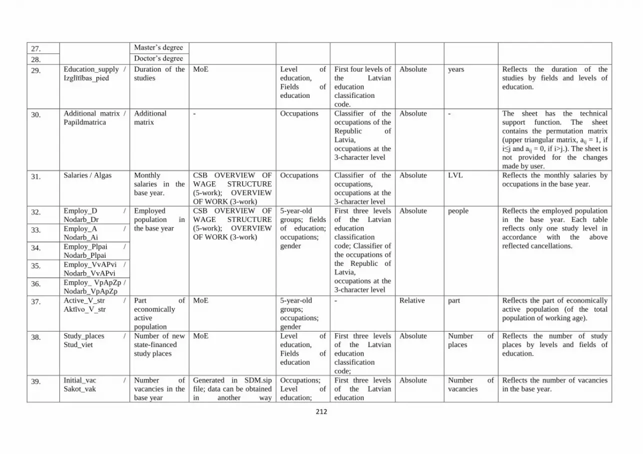
212
27. Master’s degree
28. Doctor’s degree
29. Education_supply /
Izglītības_pied
Duration of the
studies
MoE Level of
education,
Fields of
education
First four levels of
the Latvian
education
classification
code.
Absolute years Reflects the duration of the
studies by fields and levels of
education.
30. Additional matrix /
Papildmatrica
Additional
matrix
- Occupations Classifier of the
occupations of the
Republic of
Latvia,
occupations at the
3-character level
Absolute - The sheet has the technical
support function. The sheet
contains the permutation matrix
(upper triangular matrix, aij = 1, if
i≤j and aij = 0, if i>j.). The sheet is
not provided for the changes
made by user.
31. Salaries / Algas Monthly
salaries in the
base year.
CSB OVERVIEW OF
WAGE STRUCTURE
(5-work); OVERVIEW
OF WORK (3-work)
Occupations Classifier of the
occupations,
occupations at the
3-character level
Absolute LVL Reflects the monthly salaries by
occupations in the base year.
32. Employ_D /
Nodarb_Dr
Employed
population in
the base year
CSB OVERVIEW OF
WAGE STRUCTURE
(5-work); OVERVIEW
OF WORK (3-work)
5-year-old
groups; fields
of education;
occupations;
gender
First three levels
of the Latvian
education
classification
code; Classifier of
the occupations of
the Republic of
Latvia,
occupations at the
3-character level
Absolute people Reflects the employed population
in the base year. Each table
reflects only one study level in
accordance with the above
reflected cancellations.
33. Employ_A /
Nodarb_Ai
34. Employ_Plpai /
Nodarb_Plpai
35. Employ_VvAPvi /
Nodarb_VvAPvi
36. Employ_ VpApZp /
Nodarb_VpApZp
37. Active_V_str /
Aktīvo_V_str
Part of
economically
active
population
MoE 5-year-old
groups;
occupations;
gender
- Relative part Reflects the part of economically
active population (of the total
population of working age).
38. Study_places /
Stud_viet
Number of new
state-financed
study places
MoE Level of
education,
Fields of
education
First three levels
of the Latvian
education
classification
code;
Absolute Number of
places
Reflects the number of study
places by levels and fields of
education.
39. Initial_vac /
Sakot_vak
Number of
vacancies in the
base year
Generated in SDM.sip
file; data can be obtained
in another way
Occupations;
Level of
education;
First three levels
of the Latvian
education
Absolute Number of
vacancies
Reflects the number of vacancies
in the base year.

213
(statistically or from
experts).
fields of
education;
gender
classification
code; Classifier of
the occupations of
the Republic of
Latvia,
occupations at the
3-character level
40. Educ_sector /
Izgl_noz
Division of
employed by
levels of
education,
fields,
occupations and
sectors in the
base year.
CSB OVERVIEW OF
WAGE STRUCTURE
(5-work); OVERVIEW
OF WORK (3-work)
Sectors; Level
of education;
fields of
education;
occupations
Sector at the
section (leer)
level; First three
levels of the
Latvian education
classification
code; Classifier of
the occupations of
the Republic of
Latvia,
occupations at the
3-character level
Absolute people Reflects the division of employed
by levels of education, fields,
occupations and sectors in the
base year.

214
Annex A.2.
Period of changes of productivity by sectors
Sectors (according to the grouping of MoE) Index
Agriculture, Forestry and Fishing (A) 0,78
Mining and quarrying (B); Electricity, gas, steam and air conditioning supply
(D); Water supply, sewerage, waste management and remediation activities (E)
2,40
Manufacturing (C) 0,96
Construction (F) 2,67
Wholesale and retail trade; repair of motor vehicles and motorcycles (G) 1,485
Transportation and storage (H) 1,47
Accommodation and food service activities (I) 3,00
Information and communication (J) 2,50
Financial and insurance activities (K) 2,30
Real estate activities (L) 2,80
Professional, scientific and technical activities (M); Administrative and support
service activities (N); Other service activities (S);
Activities of households as employers; undifferentiated goods- and services-
producing activities of households for own use (T)
5,00
Public administration and defence; compulsory social security (O); Activities of
extra territorial organizations and bodies (U)
8,00
Education (P) 0,74
Human health and social work activities (Q) 0,79
Arts, entertainment and recreation (R) 1,205
Annex A.3.
Compliance of the significance of occupational groups (3-character level) to the criteria by
sectors in 2010
Sectors
Number
of
occupatio
nal
groups
Total
ratio in
the sector
Agriculture, hunting and forestry (A) 8 75%
Fishing (B) 6 91%
Mining and quarrying (C) 10 90%
Manufacturing (D) 7 42%
Electricity, gas and water supply (E) 7 67%
Construction (F) 12 81%
Wholesale and retail trade; repair of motor vehicles, motorcycles and
personal and household goods (G) 8 69%
Hotels and restaurants (H) 4 81%
Transport, storage and communication (I) 8 52%
Financial intermediation (J) 10 86%
Real estate, renting and business activities (K) 10 62%
Public administration and defence, compulsory social security (L) 10 70%
Education (M) 7 69%
Health and social care (N) 8 80%
Other utility, social and personal services (O) 7 55%

215
Annex A.4.
Dropout index values
Basic general
education,
vocational
education with
basic
education
General
secondary
vocational
education
and
vocational
secondary
education
Vocational
education
First level
higher
vocational
education
Academic
education
and second
level
vocational
education
Doctor’s
degree
Dropout
indexes 0% 13,4% 19,4% 17,2% 4,0% 19,9%
Annex A.5.
Privileged age structures index values
Age group Privileged age structure Privileged age structure of
the release from work
vg15_19 0,7% 30,6%
vg20_24 10,0% 2,1%
vg25_29 13,3% 1,6%
vg30_34 12,1% 1,8%
vg35_39 12,6% 1,7%
vg40_44 12,0% 1,8%
vg45_49 13,0% 1,6%
vg50_54 12,4% 1,7%
vg55_59 9,0% 2,3%
vg60_64 3,2% 6,6%
vg65_69 1,0% 20,4%
vg70_74 0,8% 27,8%
Total 100% 100%

216
Annex A.6.
Constants integrated in the model
No
.
Name Sub-model Value Measu
re
Recommended
constraints
Description Role in the model
1. Time of change of
employment
Sector
demand
1 year 1 Reflects the time, when it is
possible to make employment
changes in accordance with
GDP changes.
Ensures the changes of the
labour demand in accordance
with GDP changes. The time
defines the extent of
synchronization of GDP and
changes of labour demand (at
index 1 - changes are
synchronized).
2. Forecasting
horizon
Occupational
demand
2041 year Forecasting last
year (excluding)
Determines the forecasting last
year.
Ensures uniform changes of
labour occupational structure
from the beginning to the end
of the forecasting.
3. Measure of
importance of
occupations
Occupational
demand
0,03 part 0,03
(determined
statistically)
Determines the minimum ratio
of the occupation from all,
which is important to sector.
Occupations, which ratio in the
sector exceeds their value, are
considered to be the sector
primary occupations; the
labour demand in these
occupations varies in
proportion to GDP
4. Estimation index of
the stages of the
change of
employment
Occupational
demand
1 % 1 Reflects the new stage of
changes coming along with the
change of employment in the
sector by i (%), which has the
different structure of changes
of occupation.
Under conditions of long-term
growth the demand is being
increasing not only for primary
occupations, but also for other
occupations. The index
determines the growth limits,
which cause the demand
changes for “supplementary
occupations”.
5. General secondary
education dropout
Education
supply
0 part determined
statistically
Dropout index in the basic
general education.
Determines the dropout part of
the students.

217
ratio
6. General secondary
vocational
education dropout
index
Education
supply
0,134 part determined
statistically
Dropout index.
7. First level higher
vocational
education dropout
index
Education
supply
0,194 part determined
statistically
Dropout index.
8. Bachelor’s degree
dropout index
Education
supply
0,172 part determined
statistically
Dropout index.
9. Master’s degree
dropout index
Education
supply
0,04 part determined
statistically
Dropout index.
10. Doctor’s degree
dropout index
Education
supply
0,2 part determined
statistically
Dropout index.
11. Women dropout
index
Education
supply
0,378 part determined
statistically
Dropout index.
12. Bachelor’s index Education
supply
0,715 part determined
statistically
Reflects the bachelor’s degree
ratio in the vacant study places
in the academic and second
level vocational education.
Divides the academic and
second level occupation in
bachelor’s and master’s
degrees (study places).
13. Longstanding
balanced education
continuation index
from VP AP
Education
supply
0,98 part determined
statistically
Reflects longstanding
education continuation ratio
after GBE (general basic
education) into VE (vocational
education).
Determines the initial part of
the graduates, which continues
the education at the higher
level. (Index is being used only
in the base period, afterwards it
is being recalculated).
14. Time of change of
education
continuation index
Education
supply
2 years 1≤x≤7 Time of change of education
continuation index.
Determines the time of change
of education continuation
index

218
VP AP
15. Longstanding
balanced education
continuation index
from VP AP VV
Education
supply
0,619 part determined
statistically
Reflects longstanding
education continuation ratio.
Determines the initial part of
the graduates, which continues
the education at the higher
level. (Index is being used only
in the base period, afterwards it
is being recalculated).
16. Time of change of
education
continuation index
VP AP VV
Education
supply
2 part 1≤x≤7 Time of change of education
continuation index.
Determines the time of change
of education continuation
index
17. Longstanding
balanced education
continuation index
from VP AP Arod
Education
supply
0,35 part determined
statistically
Reflects longstanding
education continuation ratio.
Determines the initial part of
the graduates, which continues
the education at the higher
level. (Index is being used only
in the base period, afterwards it
is being recalculated).
18. Time of change of
education
continuation index
VP Arod
Education
supply
2 years 1≤x≤7 Time of change of education
continuation index.
Determines the time of change
of education continuation
index
19. Longstanding
balanced education
continuation index
from PLPaI BLI
Education
supply
0,53 part determined
statistically
Reflects longstanding
education continuation ratio.
Determines the initial part of
the graduates, which continues
the education at the higher
level. (Index is being used only
in the base period, afterwards it
is being recalculated).
20. Time of change of
education
continuation index
PLPaI BLI
Education
supply
2 years 1≤x≤7 Time of change of education
continuation index.
Determines the time of change
of education continuation
index
21. Longstanding
balanced education
continuation index
Education
supply
0,1 part determined
statistically
Reflects longstanding
education continuation ratio.
Determines the initial part of
the graduates, which continues
the education at the higher
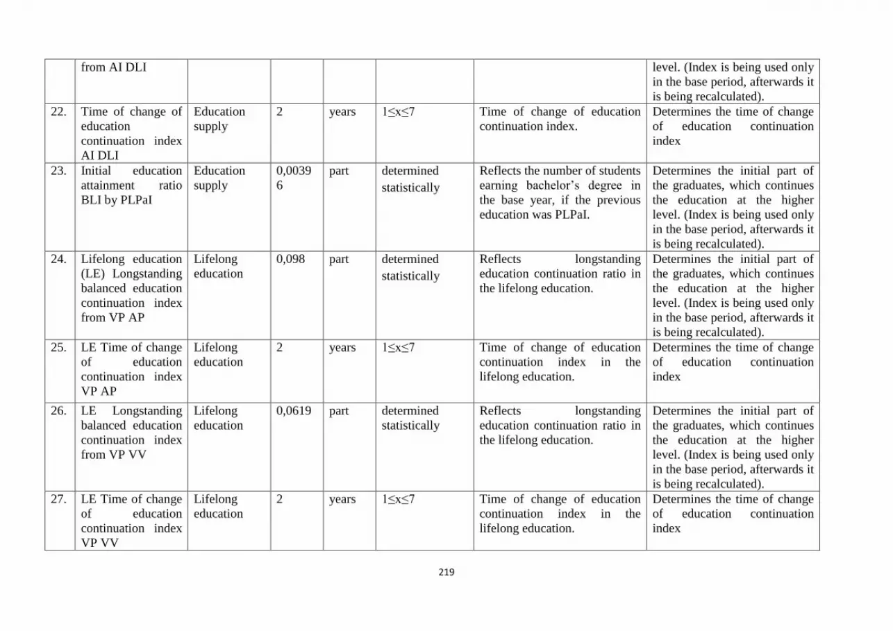
219
from AI DLI level. (Index is being used only
in the base period, afterwards it
is being recalculated).
22. Time of change of
education
continuation index
AI DLI
Education
supply
2 years 1≤x≤7 Time of change of education
continuation index.
Determines the time of change
of education continuation
index
23. Initial education
attainment ratio
BLI by PLPaI
Education
supply
0,0039
6
part determined
statistically
Reflects the number of students
earning bachelor’s degree in
the base year, if the previous
education was PLPaI.
Determines the initial part of
the graduates, which continues
the education at the higher
level. (Index is being used only
in the base period, afterwards it
is being recalculated).
24. Lifelong education
(LE) Longstanding
balanced education
continuation index
from VP AP
Lifelong
education
0,098 part determined
statistically
Reflects longstanding
education continuation ratio in
the lifelong education.
Determines the initial part of
the graduates, which continues
the education at the higher
level. (Index is being used only
in the base period, afterwards it
is being recalculated).
25. LE Time of change
of education
continuation index
VP AP
Lifelong
education
2 years 1≤x≤7 Time of change of education
continuation index in the
lifelong education.
Determines the time of change
of education continuation
index
26. LE Longstanding
balanced education
continuation index
from VP VV
Lifelong
education
0,0619 part determined
statistically
Reflects longstanding
education continuation ratio in
the lifelong education.
Determines the initial part of
the graduates, which continues
the education at the higher
level. (Index is being used only
in the base period, afterwards it
is being recalculated).
27. LE Time of change
of education
continuation index
VP VV
Lifelong
education
2 years 1≤x≤7 Time of change of education
continuation index in the
lifelong education.
Determines the time of change
of education continuation
index

220
28. LE Longstanding
balanced education
continuation index
from VP Arod
Lifelong
education
0,0035 part determined
statistically
Reflects longstanding
education continuation ratio in
the lifelong education.
Determines the initial part of
the graduates, which continues
the education at the higher
level. (Index is being used only
in the base period, afterwards it
is being recalculated).
29. LE Time of change
of education
continuation index
VP Arod
Lifelong
education
2 years 1≤x≤7 Time of change of education
continuation index in the
lifelong education.
Determines the time of change
of education continuation
index
30. LE Longstanding
balanced education
continuation index
from PLPaI BLI
Lifelong
education
0,0106 part determined
statistically
Reflects longstanding
education continuation ratio in
the lifelong education.
Determines the initial part of
the graduates, which continues
the education at the higher
level. (Index is being used only
in the base period, afterwards it
is being recalculated).
31. LE Time of change
of education
continuation index
PLPaI BLI
Lifelong
education
2 years 1≤x≤7 Time of change of education
continuation index in the
lifelong education.
Determines the time of change
of education continuation
index
32. Birth rate ratio of
boys
Population
supply
0,511
part determined
statistically
Birth rate ratio of boys. Reflects the birth rate ratio of
boys
33. Independent part of
birth rate index
Population
supply
0,0396 part determined
statistically
Provided to reflect the birth
rate changes along with GDP
changes.
Reflects that the birth rate
depends not only on GDP, but
also on other extrasystemic
factors. Determines the total
impact of extrasystemic factors
on birth rate index.
34. Birth rate index
regression index
Population
supply
5,21e-6 part determined
statistically
Provided to reflect the birth
rate changes along with GDP
changes.
Reflects that birth rate changes
along with the changes of
GDP.
35. Maximum total
birth rate index per
Population
supply
0,0535 part determined The maximum birth rate index
limit is reflected in the model
Reflects the number of children
being born per ann. Per one

221
woman statistically at the average EU level. woman of reproductive age.
36. Birth rate matching
time
Population
supply
10 years 1≤x≤15 Determines, how fast the birth
rate can change in the longer
period.
Determines the time of change
of birth rate in the longer
period.
37. Mortality reaction
to GDP changes
Population
supply
1 - Not defined Provided to reflect the
mortality changes along with
GDP changes.
By multiplying the growth rate
of total GDP per capita by this
index, the changes of mortality
index are being calculated,
taking into account the GDP
growth.
38. Correction of
longstanding
balanced mortality
indexes
Population
supply
0,9 part 0≤x≤1 Provided to reflect the global
prolongation of life.
Reflects that the mortality
index balanced in the longer
period is X from the mortality
index in the base year.
39. Definition of
longstanding
unoccupied
working places
Migration
supply
1,5 years 1≤x≤3 Definition of longstanding
unoccupied working places.
Defines the time, after which
the vacancy is being
considered as the longstanding
vacancy. The longstanding
vacancies promote
immigration.
40. Time to take
migration decision
Migration
supply
3 years 1≤x≤5 Time to take migration
decision.
The index reduces the
emigration (or slows it in the
longstanding unfavourable
economic conditions).
Emigration in the given period
is X times smaller than the
initial conditions, taking into
account that emigration
decision is not being taken
immediately.
41. Unemployed
emigration
propensity
Migration
supply
0,05 part 0≤x≤0,1 Unemployed emigration
propensity.
Reflects the part of the
unemployed and economically
inactive population, which can

222
potentially emigrate under
certain circumstances.
42. Employed
emigration
propensity
Migration
supply
0,01 part 0≤x≤0,05 Employed emigration
propensity.
Reflects the part of the
employed, which can
potentially emigrate under
certain circumstances.
43. Readiness to call
foreign workers
Migration
supply
0 0≤x≤1 Readiness to call foreign
workers.
Reflects the privileges of the
“local” employees in the labour
market. At the index value 1
the “local” employees does not
have benefits, at the index
value “0” the “foreign”
workers do not get jobs,
economic migration does not
take place.
44. Time to get
integrated in the
Latvian society
Migration
supply
1 years 1≤x≤2 Time to get integrated in the
Latvian society.
Time to meet labour market
legislation formal requirements
in order to get a job.
45. Immigrant age
structure
Migration
supply
{0,05;
0,4;
0,3;
0,15;
0,05;
0,05; 0;
0; 0; 0;
0; 0}
part - Age structure of immigrants
reflects that most of
immigrants are 25 - 40 years
old, i.e. active working age.
The assumption reflects that
immigration flow is mostly
related to the economically
active population migration.
46. Time of coverage
of vacancies for
migration
Migration
supply
2 years 1≤x≤10 Time, after which the current
vacancies cause immigration.
If the longstanding vacancy
occurs, it may have random
character. This index
determines the time, after
which the immigration takes
place if the vacancy is still
relevant.
47. Immigration ratio Migration Change part 0≤x Labour shortage may be Political leadership toolbar

223
in labour shortage
problem solution
supply s by
scenari
os
covered by education system or
immigration. The ratio reflects
the labour shortage problem,
which can be resolved by the
means of the immigration.
part.
48. Target wage ratio
index
Migration
supply
0,87 - 0≤x≤1 Wage ratio index (in Latvia
and largest EU countries),
which does not provide
economic emigration.
By determining the size of this
index, the salaries in Sweden -
Norway and Sweden - Finland
are being compared. Along
with the “Wage ratio index”
the economic migration is
being determined.
49. Wage ratio index
5VpApZp
Migration
supply
0,4362 - 0≤x≤1 Wage ratio index (in Latvia
and largest EU countries) at the
level of education VpApZp.
Wage ratio index by levels of
education. If the index is
smaller than the “Target wage
ratio index”, the economic
emigration is taking place.
50. Wage ratio index
4VvAPvI
Migration
supply
0,4362 - 0≤x≤1 Wage ratio index (in Latvia
and largest EU countries) at the
level of education.
51. Wage ratio index
3PLPaI
Migration
supply
0,4362 - 0≤x≤1 Wage ratio index (in Latvia
and largest EU countries) at the
level of education.
52. Wage ratio index
2AI
Migration
supply
0,4362 - 0≤x≤1 Wage ratio index (in Latvia
and largest EU countries) at the
level of education.
53. Wage ratio index
1DLI
Migration
supply
0,4362 - 0≤x≤1 Wage ratio index (in Latvia
and largest EU countries) at the
level of education.
54. Privileged age
structure
Market {0,007;
0,1;
0,133;
0,121;
0,126;
part Definition is
based on the
number of
employed by
age groups.
Reflects the privileged age
structure of the employees
from the perspective of the
employers (by 5-year-old
groups).
Indexes reflect the probability
that the vacancy may be
occupied by a certain employee
of a certain age group (ranging
from 15-year-old group to 74-
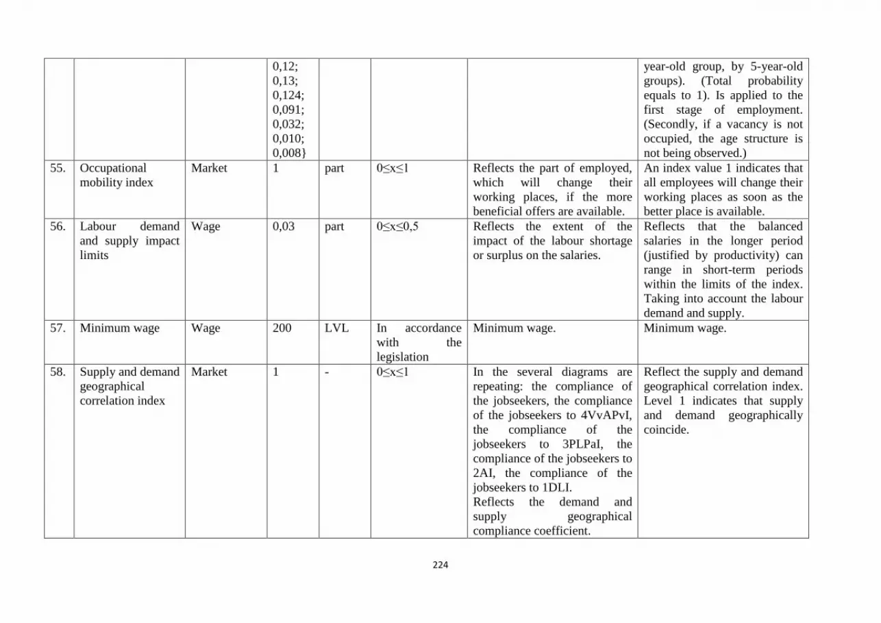
224
0,12;
0,13;
0,124;
0,091;
0,032;
0,010;
0,008}
year-old group, by 5-year-old
groups). (Total probability
equals to 1). Is applied to the
first stage of employment.
(Secondly, if a vacancy is not
occupied, the age structure is
not being observed.)
55. Occupational
mobility index
Market 1 part 0≤x≤1 Reflects the part of employed,
which will change their
working places, if the more
beneficial offers are available.
An index value 1 indicates that
all employees will change their
working places as soon as the
better place is available.
56. Labour demand
and supply impact
limits
Wage 0,03 part 0≤x≤0,5 Reflects the extent of the
impact of the labour shortage
or surplus on the salaries.
Reflects that the balanced
salaries in the longer period
(justified by productivity) can
range in short-term periods
within the limits of the index.
Taking into account the labour
demand and supply.
57. Minimum wage Wage 200 LVL In accordance
with the
legislation
Minimum wage. Minimum wage.
58. Supply and demand
geographical
correlation index
Market 1 - 0≤x≤1 In the several diagrams are
repeating: the compliance of
the jobseekers, the compliance
of the jobseekers to 4VvAPvI,
the compliance of the
jobseekers to 3PLPaI, the
compliance of the jobseekers to
2AI, the compliance of the
jobseekers to 1DLI.
Reflects the demand and
supply geographical
compliance coefficient.
Reflect the supply and demand
geographical correlation index.
Level 1 indicates that supply
and demand geographically
coincide.

225
Annex A.7.
Technical description of SDM_IN.XLS file.
Employment (nodarbinātība) sheet format:
The sheet contains a table that reflects employment by sectors in the base year (people), the
table starts in A1 cell, the data has been entered, starting from B3 cell. The table has a vertical
orientation. A column is designed to reflect the names of the sectors. B column should include the
data. B2 cell sums up the number of employed by sectors. Figure 2.1 reflects the visual appearance
of the table (Print Screen).
Figure 2.1. Employment sheet data format
GDP (IKP) sheet format:
The sheet contains two tables: GDP forecasts by sectors and GDP by sectors in the base year
(in current prices, thous. LVL).
The table “GDP forecasts by sectors” starts in A1 cell, the data has been entered, starting
from B3 cell. Sectors in the table are reflected vertically, but GDP forecasts by years - horizontally.
A column is designed to reflect the names of the sectors, starting from B column the data should be
entered. First row represents forecasting year; second row sums up the number of employed by
sectors. Figure 2.2 reflects the visual appearance of the table (Print Screen).
Figure 2.2. GDP sheet data format
Index (koeficienti) sheet format:

226
The sheet contains a table that reflects the time indexes of the changes of sectorial labour
productivity, the table starts in A1 cell, the data has been entered, starting from B2 cell. The table
has a vertical orientation. A column is designed to reflect the names of the sectors. B column should
contain the data. Figure 3.2 reflects the visual appearance of the table (Print Screen).
Figure 2.3. Index sheet data format
Occupation (profesijas) sheet format:
The sheet contains two tables: division of employed by sectors and occupations in the base
year (people) and the target labour sectorial-occupational structure (%).
The table of division of employed by sectors and occupations in the base year (people) starts
in A1 cell, the data has been entered, starting from B2 cell. The occupations in the table are
reflected vertically, but the sectors - horizontally. A column is designed to reflect the names of the
occupations, starting from B column the data should be entered. First row reflects the names of the
sectors.
The format of the table “Target labour sectorial-occupational structure (%)” is identical to
the format of the table “division of employed by sectors and occupations in the base year” (people).
Table “Target labour sectorial-occupational structure (%)” starts in Y1 cell, the data has been
entered, starting from Z2 cells. Figure 2.4 reflects the visual appearance of the tables (Print Screen).
Figure 2.4. Occupation sheet data format
Education (izglītība) sheet format:
The sheet contains two tables: “Division of employed by education levels, fields,
occupations (people)” and “Occupational compliance matrix”.
The division of employed by education levels, fields, occupations starts in A1 cell, the data
has been entered, starting from D3 cell.
Occupational compliance matrix begins in A1001 cell, the data has been entered, starting
from D1003 cell.
Education sheet data format and visual appearance (Print Screen) are presented in Figure
2.5.

227
A B C D
1 Title of occupation ... Title of occupation P
2
Occupation code (in
growing sequence, starting
from a smaller) ... Occupation code P
3
Education level (starting
from doctoral level
education to the lowest
education)
Education field code
(in growing sequence,
starting with a smaler)
Title of education
field
... ... ... Data fields
Education level L Education field code J
Title of education
field J
Figure 2.5. Education sheet data format
Education sheet format is unified for two sheet tables.
Demography (demogrāfija) sheet format:
The page contains the following tables: “Population by age and gender (people). “Mortality
of the population (people) by age and gender”, “Alive born people by age of the mother (people)”,
(by alive born people by age of the mother by 5 year-old groups); as well as the tables providing
choice of the index of division of born people by gender (which are not related to the model).
The table of the population by age and gender (people) starts in A1 cell, the data has been
entered, starting from B3 cell. The one-year age groups are presented in the tables vertically, but the
gender of the population - horizontally. A column is designed to reflect the name of the one-year-
old group, starting from B column the data should be entered. Second row reflects the names of the
gender.
The format of the table “Mortality of the population by age and gender (people) is identical
to the format of the table “Population by age and gender (people). Table “Mortality by age and
gender (population)” starts in E1 cell, the data has been entered, starting from F3 cell.
The table of alive born people by age of the mother (people) starts from M5 cell, the data
has been entered, starting from N7 cell. The table has a horizontal orientation. 6 row (N6) is
designed to reflect the name of the one-year-old group, 7 row (from N7 cell) the data has been
entered. The table fields are being filled automatically from the related table “Alive born people by
age of the mother by 5 year-old groups”. Related table “Alive born people by age of the mother by
5 year-old groups” starts in M1 cell, the data has been entered, starting from N3 cell. These tables
have identical format.
Figure 2.6 reflects the visual appearance of the table (Print Screen).

228
Figure 2.6. Demography sheet data format
Dem_Dr, Dem_Ai, Dem_Plpai, Dem_VvAPvi, Dem_VpApZp sheet’s format:
All sheets have a unified format. Each sheet is reflecting one level of education according to
its shortened name. (Dr. - PhD, Ai - academic education and second-level vocational education;
Plpai - first level vocational higher education; VvAPvi - secondary general, vocational and
vocational secondary education; VpApZp - basic general education, vocational education with the
basic education and primary education).
Each sheet contains a table that reflects the population by age (5-year-old), groups, gender,
fields of education, occupations, economic activity (people) in the base year. Table starts in A4 cell,
the data has been entered, starting from D6 cell.
“Dem” group sheet data format and visual appearance (Print Screen) are presented in Figure
2.7.
A B C D
4
Occupation code (in
growing sequence, starting
from a smaller) ...
Occupation code
P
5
Economically active
population (starting from
active, till non-active) ...
Economically
active population
Ek
6
Age group (in
growing sequence,
starting with a
younger)
Gender (starting
from men, till
women)
Education field code (in
growing sequence,
starting from a smaler)
... ... ... Data fields
Age group Vg Gender D Education field code J
Figure 2.7. “Dem” group sheet data format
Grade (Sak_skoln) sheet format:
The sheet contains a single table, which reflects the number of students by classes and
gender (people). The table starts in A1 cell, the data has been entered, starting from B2 cell. The
learning classes in the table are presented vertically, but the gender of the students - horizontally.
The table has a vertical orientation. A column is designed to reflect the names of the classes, B and
C columns should contain data. The following table fields are filled automatically from the
transposed table (i.e., table, in which the rows and columns are interchanged). Transposed table
starts in G1 cell, the data has been entered, starting from H2 cell. Model does not take the data from
the transposed table.
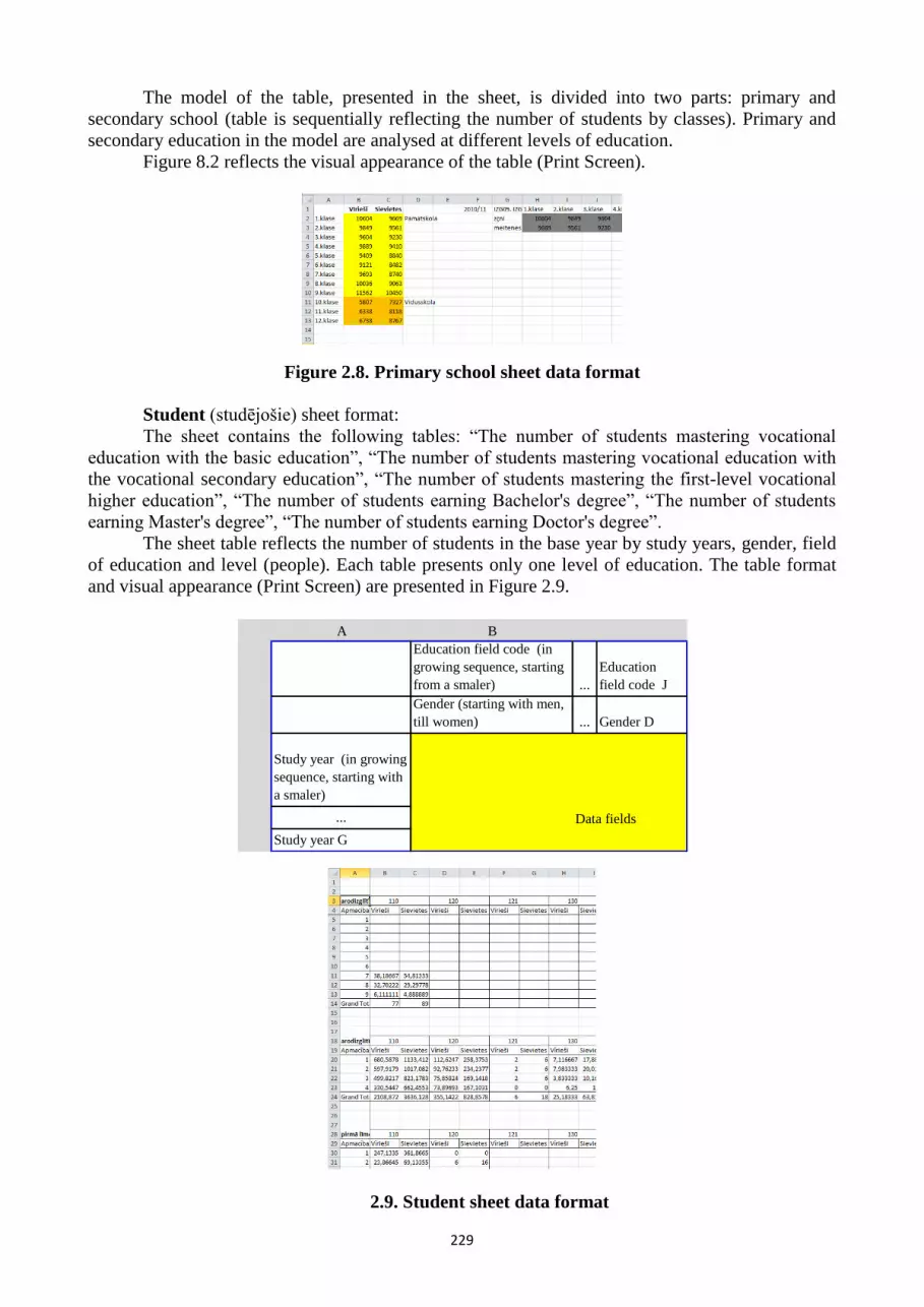
229
The model of the table, presented in the sheet, is divided into two parts: primary and
secondary school (table is sequentially reflecting the number of students by classes). Primary and
secondary education in the model are analysed at different levels of education.
Figure 8.2 reflects the visual appearance of the table (Print Screen).
Figure 2.8. Primary school sheet data format
Student (studējošie) sheet format:
The sheet contains the following tables: “The number of students mastering vocational
education with the basic education”, “The number of students mastering vocational education with
the vocational secondary education”, “The number of students mastering the first-level vocational
higher education”, “The number of students earning Bachelor's degree”, “The number of students
earning Master's degree”, “The number of students earning Doctor's degree”.
The sheet table reflects the number of students in the base year by study years, gender, field
of education and level (people). Each table presents only one level of education. The table format
and visual appearance (Print Screen) are presented in Figure 2.9.
A B
Education field code (in
growing sequence, starting
from a smaler) ...
Education
field code J
Gender (starting with men,
till women) ... Gender D
Study year (in growing
sequence, starting with
a smaler)
... Data fields
Study year G
2.9. Student sheet data format

230
The tables in the sheet are unified, use the same format. Tables start in different locations, it
is reflected by Table 2.1.
Table 2.1. Arrangement of the table of „Student” sheet
Name of the table Beginning of
the table (cell)
First cell of
data entry
Number of vocational education with the basic education
mastering students
A3 B5
Number of vocational education and the vocational secondary
education mastering students
A18 B20
Number of first level vocational higher education mastering
students
A28 B30
Number of students earning the Bachelor’s degree A39 B41
Number of students earning the Master’s degree A51 B53
Number of students earning the Doctor’s degree A63 B65
By preparing the data in the student sheets, it is important to note that study year may not
exceed the duration of the studies (see Education_supply description of the page).
Admission (uzņemšana) sheet format:
The page contains the following tables: “Number of enrolled in vocational education and
vocational secondary education”, “Number of enrolled in first level vocational higher education”,
“Number of enrolled for Bachelor’s degree”, “Number of enrolled for Master’s degree”, “Number
of enrolled for Doctor’s degree”.
The table reflects the enrolled students and the number of students in the base year by
gender, fields and levels of education (people). Each table reflects only one level of education.
Figure 2.10 reflects the visual appearance of the table (Print Screen).
Figure 2.10. Admission sheet data format
Table has the following format: vertically, in ascending sequence, starting from the lowest,
is reflected the code of the field of education, but horizontally - gender (first - men, second -
women). Accordingly the data has been entered. The tables in the sheet are unified, use the same
format. Tables start in different locations, it is reflected by Table 2.2.
Table 2.2. Arrangement of the table of „Admission” sheet
Name of the table Beginning of
the table (cell)
First cell of
data entry
Number of enrolled in vocational education and vocational
secondary education
A1 B3
Number of enrolled in first level vocational higher education F1 G3
Number of enrolled for Bachelor’s degree K1 L3
Number of enrolled for Master’s degree P1 Q3
Number of enrolled for Doctor’s degree U1 V3

231
Education_supply (izlgītības_pied) sheet format:
The page contains a table that reflects the duration of the studies by fields and levels of
education (years), the table starts in A1 cell, the data has been entered, starting from D2 cell. The
table has a vertical orientation. A column is designed to reflect the name of the level of education
(from Doctor’s degree to lower-level studies), B column - the code of the field of education (in
ascending sequence, starting from the lowest), C column - name of the education, D column should
contain the data.
The model of the table, presented in the sheet, is divided into five parts in accordance with
the levels of education (table successively reflects the duration of the studies). The levels of
education in the model are analysed separately.
Figure 2.11 reflects the visual appearance of the table (Print Screen).
Figure 2.11. Education supply sheet data format
The model requires the duration of the studies as the whole numbers. The maximum
duration of the studies at each level of education is limited in the following way: basic education,
vocational education with basic education and primary education - 9 years, general secondary,
vocational and vocational secondary education - 4 years, first level vocational higher education,
academic education and second level vocational education, Doctor’s degree - 6 years (for each
level).
Wage (algas) sheet format:
The page contains one table, which reflects the monthly income by occupations (LVL) in the
base year, as well as technical information for the calculation of these salaries. The table starts in
D1 cell, the data has been entered, starting from E2 cell. The table has a vertical orientation. D
column is designed to reflect the name of the occupational code (in ascending sequence, starting
from the lowest), E column should contain the data.
Taking into account that the data on the wage income would be available only in annual
terms, as well as in detail at the two-digit level, in order to fill the required table for the table the
data contains the algorithm that transforms the annual wage income (two-digit level in occupations)
up to monthly wage income at the three-digit level. In order to use this algorithm in the additional
table, which starts in A1 cell, the data should be entered (starting from B2 cell).
Figure 2.12 reflects the visual appearance of the table (Print Screen).
Figure 2.12. Wage sheet data format
Employ_Dr, Employ _Ai, Employ _Plpai, Employ _VvAPvi, Employ _VpApZp
(Nodarb_Dr, Nodarb_Ai, Nodarb_Plpai, Nodarb_VvAPvi, Nodarb_VpApZp) sheet format:

232
All these sheets have a unified format. Each sheet presents only one level of education
according to the above reflected abbreviations.
Each sheet contains a table that reflects the employed population by age (5 year-old) groups,
gender, fields of education, occupations (people). Table starts in B3 cell, the data has been entered,
starting from D5 cell.
“Employment” group sheet data format and visual appearance (Print Screen) are presented
in Figure 2.13.
B C D
3
Occupation code (in
growing sequence, starting
from a smaller) ...
Occupation
code P
4
Gender (starting from men,
till women) ... Gender D
5
Age group (in
growing sequence,
starting from a
younger)
Education field code
(in a growing sequence,
starting from a smaler)
... ... Data fields
Age group Vg Education field code J
Figure 2.13. “Employment” group sheet data format
Active_V_str (Aktīvo_V_str) sheet format:
The sheet contains a table that reflects the part of economically active population (of total
population) by age (5-year-old) groups and gender. The table starts in A1 cell, the data has been
entered, starting from C2 cell. The table has a vertical orientation. A column is designed to reflect
the age group (in ascending sequence starting from the youngest), B column is designed to reflect
the gender (starting from men to women), starting from C column, the data should be entered. First
line represents forecasting year.
Figure 2.14 reflects the visual appearance of the table (Print Screen).
Figure 2.14. Active_V_str sheet data format
Study_place (Stud_viet) sheet format:
The sheet contains a table that reflects the number of vacant study places by levels and fields
of education. The table starts in A1 cell, the data has been entered, starting from C2 cell. The table
has a vertical orientation. A column is designed to reflect the name of level of education (starting
from Doctor’s degree to lower level studies), B column - code of the field of education (in

233
ascending sequence, starting from the lowest), starting from C column, the data should be entered.
First line represents forecasting year.
Figure 2.15 reflects the visual appearance of the table (Print Screen).
Figure 2.15. Study_place sheet data format
Initial_vac (sakot_vak) sheet format:
The sheet contains a table that reflects the number of vacant study places by occupations,
education levels, fields and gender. The table starts in A1 cell, the data has been entered, starting
from C3 cell.
Initial_vac sheet data format and visual appearance (Print Screen) are presented in Figure
2.16.
A B C
1
Gender (starting from men,
till women) ... Gender D
2
Education field code (in
growing sequence, starting
from a smaler) ...
Education
field code J
3
Occupation code (in
growing sequence,
starting from a smaler)
Education level
(starting from the
doctoral level
education, till a lower
education)
... ... Data fields
Occupation code P Education level L
Figure 2.16. Initial_vac sheet data format
The table of initial number of vacancies can be filled, using statistical data, or exporting
from the original SDM model the calculated number of vacancies (the element “Generated initial
number of vacancies” from the Market sheet).
Educ_ind (Izgl_noz) sheet format:
The sheet contains a table: “The division of employed by educational levels, fields,
occupations by sectors” (people). The table starts in A1 cell, the data has been entered, starting from
E3 cell.
Educ_ind sheet data format and visual appearance (Print Screen) is presented in Figure 2.17.

234
A B C D E
1 Title of occupation ...
Title of
occupation P
2
Occupation code (in
growing sequence, starting
with a smaller ...
Occupation
code P
3
Industry code (in
alfabetical order
starting from A
to R)
Education level (starting
from doctoral level
studies, till a lower
education)
Education field code
(in a growing
sequence, starting
from a smaller)
Title of education
field
... ... ... ... Data
Industry code N Education level L
Education field code
J
Title of education
field J
Figure 2.17. Education sheet data format
Educ_ind sheet is a logically organized table. The size of the table (matrix) exceeds the
Powersim software restrictions in relation to the matrix sizes. SDM model takes the data from this
table, virtually dividing the table into two parts: the sectors with codes from A to J, and from K to
R.

235
Annex A.8.
Mathematical formula abbreviations
AAK - wage ratio;
ABSJD - number of applicants by gender and fields of education;
ABSMJD - number of applicants by gender and fields of education in lifelong education;
ABSSJD - structure of applicants and fields of education of graduates;
ABStMJD - structure of alumni’s and fields of education of graduates in lifelong education;
AbsVStVg - age structure of alumni;
ADAVSDPJ - adapted number of vacancies;
ADVDPJ - occupied working places;
ADVKDPJ -correction of occupied working places;
ADVS2DPJ - decrease in the number of occupied working places in the 2nd priority;
ADVSDPJ - decrease in the number of occupied working places;
AIAMPJ - integrated education compliance matrix.
AIJ - learning time;
AIMVgDPJE - return immigration;
AK - level of education dropout index;
AKs - women dropout index;
AL - average wages at the levels of education;
AMVgDPJE - change of the group of the economic activity of the population;
AMVGMVgDPJE - change of the economic activity group along with the change of age;
APGJD - learning process;
ASMVgDPJ - change of economic activity status for active population;
ASPVgDPJe - assignment of the status of economic activity for the active population;
AtDVDPJ - number of remaining working places;
AtDVSDPJ - structure of remaining working places;
ATGJD - dropout;
ATLDPJ - surplus;
ATS1VgDPJ - release from work in the 1st priority;
ATS2VgDPJ - release from work in the 2nd priority;
ATSSVg - privileged age structure of the release from work;
ATVSDPJ - number of appropriate vacancies;
ATVSStDPJ - structure of appropriate vacancies;
AvpNapGJD - change of general secondary education to the vocational education with the basic
education;
AVSADPJ - structure of remaining vacancies;
BGJD - admission in the base period;
BIVJD -15-year-old population without education;
BK - bachelor’s index;
BVJD - bachelor degree or qualification;
D - gender;
DD - birth rate;
DDV - the number of born people by gender and maternal age;
DKDSV - birth rate index;
DKIDSV - change of birth rate index;
DKND - independent part of birth rate index;
DKPT - total growth rate of birth rate;
DKPTiIPT - limitation of total birth rate index growth in accordance with the long-time growth
rate;
DKPTiMR - limitation of total birth rate index growth in accordance with the maximum threshold;
DKPTIP - growth rate of birth rate in the long-term period;
236
DKRK - regression index of the birth rate index;
DKS - birth rate per woman of reproductive age;
DKSM - maximum total birth rate per woman;
DKSPA - total birth rate per woman of reproductive age in case of GDP growth;
DKSSA - total birth rate per woman of reproductive age in case of GDP reduction;
DMD - number of jobseekers by gender;
DMIsVgDPJ - ratio of jobseekers in active population;
DML - number of jobseekers by levels of education;
DMNiVgDPJ - occupation of vacancies in the i priority;
DMNKORVgDPJ - correction of the number of jobseekers and employed;
DMNVgDPJ - move from job search to employment;
DMP - number of jobseekers by occupations;
DMPVgDPJ - increase of the number of jobseekers;
DMSPVgDPJ - forecast of the number of jobseekers;
DMSVgDPJ - decline in the number of jobseekers;
DMVgDPJ - number of jobseekers;
DMVgDPJ_i - number of jobseekers at i level of education;
DMvSVgDPJ - change of the age structure of jobseekers;
DVDPJ - number of working places;
DVIDPJ - working place is being occupied;
DVINDPJ - working place is being occupied in accordance with the occupation of the vacancy;
DVIXDPJ - working place is being occupied in accordance with the vacancies;
DVJDPJ - creation of new working places;
DVLaBDPJ - appropriate decrease of number of working places;
DVLaDDPJ - adapted decrease of number of working places;
DVLDPJ - liquidation of working places;
DVTDPJ - working place is being released;
E - economic activity group;
EAIMVgDPJ - change of economic activity group of the population in accordance with the target;
EAIPVgDPJ - growth of active population;
EAIStVgDL - structure of economically active population by levels of education, age groups and
gender.
EAIStVgDPJ - structure of economically active population by age groups, gender, occupations and
fields of education;
EAIVgDL - economically active population by levels of education, age groups and gender;
EAIVgDPJ - economically active population;
EEVK - economic migration formation index;
EIMVgDPJE - economic immigration;
EIVK - economic immigration formation index;
EMESVgDPJE - labour immigration in accordance with the current structure;
EMUSVgDPJE - labour immigration in accordance with the provided structure;
EMVD - emigration;
ENIPVgDPJ - growth of inactive population;
ET - emigration propensity;
G - learning year;
GAAD - readiness to invite the foreign employees;
i - birth rate distribution time;
IAGJD - mastering of education;
IAGJD1 - mastering of basic general education or vocational education with general education;
IAM - education compliance matrix;
IAMSLJLP - structure of education compliance matrix by levels of education;
IAMSMJLP - structure of education correlation matrix;

237
IapGJD - mastering of vocational education with general education;
IIGJD - acquisition of education;
IINDV - longstanding vacant working places of the previous period;
IIVJD - education attainment by age groups;
IKPI - total GDP per capita;
IKPN - GDP forecasts by sectors;
IKPN0 - GDP by sectors in the base period;
IKPPT - growth rate of total GDP per capita;
ILMKVD - balanced death rates in the long-term period;
ILSITK - balanced education continuation index in the long-term period;
IMESVgDPJE - labour immigration in accordance with the current structure;
IMITPR - immigration ratio for solution of the labour shortage problem;
IMStVg - age structure of immigrants;
IMVD - immigration;
IMVNV - method of definition of immigration types;
INDV - longstanding vacant working places;
INDVD - definition of longstanding vacant working places;
INDVI - changes of longstanding vacant working places;
INDVM - longstanding vacant working places, which are forming immigration;
INDVStDPJ - structure of longstanding vacant working places;
IPaJ - demand of fields of education for the vocational education and vocational secondary
education;
IPIKPI - total GDP per capita in the previous period;
IPJ - structure of field of education demand;
ISIVgD - population ratio of the total population by age groups and gender;
ISPKN - short-term expected productivity index by sectors;
ISSIVgDPJE -change of population and structure;
IStVgDPJE - population structure;
ITK - education continuation index;
ITKi - change of education continuation index;
ITKiAL - change of education continuation index, in accordance with the wage level;
ITKiIT - change of education continuation index, in accordance with the long-term trends;
ITKiNL - change of education continuation index, in accordance with the employment rate;
IVD - population;
IVgD - population by age groups and gender;
IVgDPJE - population;
IZMStVgDPJE - structure of maximum of changes;
IZMVgDPJE - maximum of changes;
J - field of education;
JJVSJ - initial number of study places in the new fields;
JSVAJ - opening of study places in the new fields;
KDKI - choice of the total birth rate index;
KDMDPJL - total number of jobseekers;
KIJJ - critical fields of education;
KIVgD - total population by age groups and gender;
KLSIPN - changes of total labour demand by occupations and sectors;
KNDPJL - total number of employed;
KORVgDPJ - correction;
KVSDPJL - total number of vacancies;
L - level of education (group);
LMStPN - target structure of the labour demand by occupations and sectors;

238
LSAJLP - labour demand in the occupation with the appropriate education by fields and levels of
education;
LSD - labour demand by gender;
LSIA - average ratio of labour demand and active population;
LSIAJ - average ratio of labour demand and active population by fields of education;
LSIENK - estimation index of the stages of changes of labour demand;
LSIMStPN - changes of labour demand by occupations and sectors in accordance with the sectorial
changes on the basis of the target structure;
LSIN - changes of labour demand by sectors.
LSINLSIPN - changes of labour demand by occupations and sectors in accordance with the sectorial
changes of labour demand.
LSIP - changes of labour demand by occupations.
LSIPN - changes of labour demand by occupations and sectors;
LSJLDP - labour demand by fields of education, levels, occupations and gender;
LSJLP - labour demand by fields, levels of education and occupations;
LSMStPN - labour demand by occupations and sectors on the basis of the target structure;
LSN - labour demand by sectors;
LSN0 - labour demand by sectors in the base period;
LSP - labour demand by occupations;
LSPAJLP - growth of labour demand by fields, levels of education and occupations, in accordance
with the compliance of education to occupation;
LSPAP - growth of labour demand by occupations, in accordance with the compliance of education
to the requirements of occupation;
LSPDPJ - growth of labour demand by occupations and gender at the level of education;
LSPJLDP - growth of labour demand by fields, levels of education and occupations and gender;
LSPJLP - growth of labour demand by fields, levels of education and occupations;
LSPLJLP - growth of labour demand by fields, levels of education and occupations, in accordance
with the structure of labour demand by levels of education;
LSPLP - growth of labour demand by occupations, in accordance with the structure of labour
demand by levels of education;
LSPMJLP - growth of labour demand by fields, levels of education and occupations, in accordance
with the structure of the educational compliance matrix;
LSPN - growth of labour demand by occupations and sectors;
LSPnALP - growth of labour demand by occupations, without regard to the compliance of education
to the requirements of occupation and structure of labour demand by levels of education;
LSPnAP - growth of labour demand by occupations, without regard to the compliance of education
to the occupation;
LSPP - growth of labour demand by occupations;
LSSJLDP - decrease of labour demand by fields, levels, of education occupations and gender;
LSSJLP - decrease of labour demand by fields, levels of education and occupations;
LSSP - decrease of labour demand by occupations;
LSStAJLP - structure of labour demand in the occupation with the appropriate education by fields
and levels of education;
LSStDP - structure of labour demand by occupations and gender;
LSStJLP - structure of labour demand by fields, levels of education and occupations;
LSStLP - structure of labour demand by levels of education and occupations;
LSStPN - structure of labour demand by occupations and sectors;
MAAK - target wage ratio;
MEAIVgD - target economically active population by age groups and gender at i level of education;
MEAIVgDL - target economically active population by levels of education, age groups and gender;
MEAIVgDPJ - target economically active population;
MIVD - migration;

239
MKI - change of death rate in accordance with GDP growth;
MKNVD - death rate variance;
MKVD - death rate.
MR - mortality response to changes of GDP;
MVD - mortality;
MVgD - mortality by age groups and gender in 15-70-year-old groups;
MVgDPJE - mortality;
N - sector;
NAVSP - surplus of occupied working places;
NDMVgDPJ - move from employment to job search;
NEAIMVgDPJ - negative change of economic activity group of the population in accordance with the
target;
NKORVgDPJ -correction of the structure of employed;
NLJ - number of employed by levels and fields of education;
NLSIN - necessary labour changes by sectors;
NLSN - necessary labour by sectors;
NMI2VgDPJ - maximum possible changes of employed from LS;
NMI2VgDPJ - number of employed in the 2nd priority of release from work;
NMIVgDPJ - maximum possible changes of employed;
NN0 - employment by sectors in the base period;
NNKORVgDPJ - required correction of the structure of employed;
NOVRbVgDPJE - aging result without the economic activity groups;
NOVRVgDPJE - aging result;
NOVVD - aging;
NOVVgD - aging by age groups and gender in 15-70-year-old groups;
NOVVgDPJE - aging;
NP - number of employed by occupations;
NPIL - time of the change of employment;
NPKIN - the necessary changes of productivity index by sectors;
NPKN - necessary productivity index by sectors;
NPMAVgDPJ - change of occupation;
NPMVgDPJ - change of occupation of employed;
NPMVVgDPJ - occupation of vacancies of employed;
NPVgDPJ - decrease in the number of employed;
NSDPJ - decrease in the number of employed due to the change of age structure by occupations,
fields of education and gender;
NSPVgDPJ - forecast of the number of employed;
NSVgDPJ - decline in the number of employed due to the change of age structure;
NTMaGJD - decide to continue the studies in vocational education (vocational secondary education);
NTMppGJD - decide to continue the studies after basic education;
NTMvGJD - decide to continue the studies in general secondary education;
NTMVJD - decide to continue the studies;
NVgD - number of employed by age groups and gender;
NVgDPJ_i - number of employed at i level of education;
NvS2Vg - age structure of employed in the 2nd priority;
NvSVgDPJ - change of the age structure of employed;
OIINDV - longstanding vacant working places of the second level in the previous period;
OSVIJL - change of study places;
OSVJ - number of optimized study places;
OVSVJ - optimized vacant study places;
P - occupation;
PEAIMVgDPJ - positive change of economic activity group in accordance with the target;
240
PILN - time of the change of productivity by sectors;
PIMVgDPJE - demanded immigration;
PITKiAL - changes of demanded education continuation index in accordance with the wage level;
PITKiNL - changes of demanded education continuation index in accordance with the level of
employment;
PKIN - changes of productivity index by sectors;
PKN0 - labour productivity index by sectors in the base period;
PMDMVgDPJ - change of occupation in order to get a job;
PMNVgDPJ - employment after the change of occupation;
PMTBVgDPJE - change of occupation in the market module;
PNNKORVgDPJ - additionally required correction of employed structure;
PPPJ - occupational demand in accordance with IAM;
PPSPJ - demand structure of occupation in accordance with IAM for the population with general
secondary and vocational education;
PPSPJ - structure of occupational demand in accordance with IAM;
PS - number of applications;
PSK - measure of importance of occupation;
PSSVA - total ratio of number of applications and study places;
PStVg - preferential age structure;
PvpGJD - abandon basic education;
RKN - productivity index by sectors;
SAGJD - beginning of education mastering;
SLSI - the changes of the major occupations of the labour demand;
SMMGD - mortality and migration of students;
SPGJD - interruption of education;
SPKIN - total ratio of major occupations by sectors;
SPmmGJD - interruption of education due to mortality or migration;
SRV - number of women of reproductive age;
SSJ - student structure by fields of education;
SUSVJ - summed up advanced study places;
SVIR - limit of changes of study places;
SVPJ - private financing of study places;
t - forecasting time (forecasting current year);
tb - forecasting time horizon (forecasting last year);
TILS - time to get integrated into Latvian society;
tITK - period of change of education continuation index;
TML - time to take the emigration decision;
TVSM - time for occupation of vacancies for migration;
UEAIVgD - provided economically active population;
ULLVgD - provided participation level;
ULSI - accumulated changes of labour demand;
ULSIN - estimation of the accumulated changes of labour demand;
UNVgD - removal from analysis by age groups and gender;
UNVgDPJE - removal from analysis;
UPVgDPJE - admission for analysis;
USVJ - advanced study places;
V1NKORVgDPJ - age group correction 1;
V2NKORVgDPJ - age group correction 2;
VAGAVgDPJE - leaving the old analysis group;
Vg - age group;
VSD - number of vacancies by gender;
VSDPJ - number of vacancies;

241
VSDPJ_i - number of vacancies at the education level i;
VSL - number of vacancies by levels of education;
VSP - number of vacancies by occupations;
VSSDPJ - decline in the number of vacancies;
VSVAJD - occupation of vacant study places;
VSVAMJD - occupation of vacant study places in the lifelong education;
VSVJ - vacant study places.

242
Annex A.9.
Data recovery time.
No. SDM_in file
sheet name
Data name Data source Update
1. Employment /
Nodarbinātība
Employment by sectors in
the base year
CSB OVERVIEW OF WAGE
STRUCTURE (5-work); OVERVIEW OF
WORK (3-work)
75days after the end of
the year of account
2. GDP / IKP GDP forecast MoE Upon preparedness of
the forecast
3. GDP in the base year CSB overview table IK04. GROSS
DOMESTIC PRODUCT BY TYPE OF
ACTIVITY
70 after the end of the
year of account
4. Indexes /
Koeficienti
Time index of changes of
labour productivity of the
sectors
Experts Over the period of
GDP base year update
the examination should
be carried out, whether
it is required to update.
If necessary, it should
be updated along with
GDP.
5. Occupations /
Profesijas
Division of employed by
sectors and occupations in
the base year
CSB OVERVIEW OF WAGE
STRUCTURE (5-work); OVERVIEW OF
WORK (3-work)
75days after the end of
the year of account
6. Target labour sectorial-
occupational structure
MoE Upon completion
7. Education /
Izglītība
Division of employed by
levels of education, fields,
occupations
CSB OVERVIEW OF WAGE
STRUCTURE (5-work); OVERVIEW OF
WORK (3-work)
75days after the end of
the year of account
8. Occupational compliance
matrix
MoE Does not require
regular updates. Should
be reviewed once in 5-
10 years.
9. Demography /
Demogrāfija
Population by age and
gender in the base year.
CSB overview table IS06. AGE
STRUCTURE OF MEN AND WOMEN
AT THE BEGINNING OF THE YEAR
13.06.2013.
10. Population mortality by age
and gender
CSB overview table IM01. DEATHS BY
AGE AND SEX
03.07.2013.
11. Alive born people by age of
the mother
CSB overview table ID02. NUMBER OF
BORN BY GENDER and ID03. ALIVE
BORN PEOPLE BY AGE OF MOTHER
03.07.2013.
12. Dem_Dr Population by levels of
education in the base year
CSB OVERVIEW OF WAGE
STRUCTURE (5-work); OVERVIEW OF
WORK (3-work)
75days after the end of
the year of account 13. Dem_Ai
14. Dem_Plpai
15. Dem_VvAPvi
16. Dem_VpApZp
17. Primary_pupil
s / Sak_skoln
Number of pupils in the base
year
CSB overview table IZG09. NUMBER OF
EDUCATED IN GENERAL ACADEMIC
SCHOOLS BY CLASSES (at the
beginning of the school year)
01.03.2013.
18. Students /
Studējošie
Mastering of vocational
education with the basic
education
OVERVIEWS PROF-2 and PROF-2m OF
VOCATIONAL EDUCATIONAL
INSTITUTIONS
21.06.2013.
19. Mastering of vocational
education and vocational
secondary education
21.06.2013.
20. Mastering of first level
higher vocational education
21.06.2013.

243
21. Mastering of bachelor’s
degree
21.06.2013.
22. Mastering of master’s
degree
21.06.2013.
23. Mastering of doctor’s degree 21.06.2013.
24. Admission /
Uzņemšana
Vocational education and
vocational secondary
education
OVERVIEWS PROF-2 and PROF-2m OF
VOCATIONAL EDUCATIONAL
INSTITUTIONS
21.06.2013.
25. First level higher vocational
education
21.06.2013.
26. Bachelor’s degree 21.06.2013.
27. Master’s degree 21.06.2013.
28. Doctor’s degree 21.06.2013.
29. Education_sup
ply /
Izglītības_pied
Duration of the studies MoE Does not require
regular updates. Should
be reviewed once in 3-
7 years.
30. Additional
matrix /
Papildmatrica
Additional matrix - Does not require
updates
31. Salaries /
Algas
Monthly salaries in the base
year
CSB OVERVIEW OF WAGE
STRUCTURE (5-work); OVERVIEW OF
WORK (3-work)
65 day after the end of
the quarter of account
32. Employ_D /
Nodarb_D
Employed population in the
base year
CSB OVERVIEW OF WAGE
STRUCTURE (5-work); OVERVIEW OF
WORK (3-work)
75days after the end of
the year of account
33. Employ_Ai /
Nodarb_Ai
34. Employ_Plpai
/
Nodarb_Plpai
35. Employ_VvA
Pvi /
Nodarb_VvAP
vi
36. Employ_
VpApZp /
Nodarb_VpAp
Zp
37. Active_V_str /
Aktīvo_V_str
Part of economically active
population
MoE Upon completion
38. Study_places /
Stud_viet
Number of new state-
financed study places
MoE Dependence on the
simulation target. May
not be used or use
previous simulation
results
39. Initial_vac /
Sakot_vak
Number of vacancies in the
base year
Generated in SDM.sip file; data can be
obtained in another way (statistically or
from experts).
Generated in SDM.sip
file, it is recommended
to be updated before
each simulation
40. Educ_sector /
Izgl_noz
Division of employed by
levels of education, fields,
occupations and sectors in
the base year.
CSB OVERVIEW OF WAGE
STRUCTURE (5-work); OVERVIEW OF
WORK (3-work)
75days after the end of
the year of account

244
Annex A.10.
Data recovery and forecasting time consumption.
No
.
Activity group Activity Time Total
group
time
1.
Data update
Update of the table “Employment by sectors in the base
year” 10 min
13
hours
2. Update of the table “GDP in the base year” 10 min
3. Update of the table „Division of employed by sectors and
occupations in the base year” 15 min
4. Update of the table „ Division of employed by education
levels, fields and occupations” 20 min
5. Update of the table „ Population by age and gender in the
base year” 10 min
6. Update of the t]
able „ Population mortality by age and gender” 10 min
7. Update of the table „ Alive born people by age of the
mother” 15 min
8. Update of the tables „Population by levels of education in
the base year” for the five levels of education together 240 min
9. Update of the table „ Number of pupils in the base year” 10 min
10. Update of the tables „Mastering of education” for the five
levels of education together 60 min
11. Update of the tables „Admission by levels of education”
for the five levels of education s together 60 min
12. Update of the table „Monthly salaries in the base year” 30 min
13. Update of the tables „Employed population in the base
year” for the five levels of education together 240 min
14. Update of the table „Division of employed by education
levels, fields, occupations and sectors in the base year” 30 min
15.
Assumption data
review
Review of the GDP forecast 5 min
2
hours
16. Review of the target labour sectorial-occupational
structure 30 min
17. Review of the part of the economically active population 30 min
18. Review of the number of state-financed new study places 30 min
19.
Special data
review (option)
Review of the duration of the studies 30 min
10
hours
20. Review of the occupational compliance matrix 480 min
21. Review of the time indexes of the sectorial labour
productivity 30 min
22. Implementation
of pre-modelling
procedure
Modelling mode setup 5 min 0,2
hours 23. Occupation of number of vacancies in the base year
5 min
24. Modelling
process
Modelling process (one simulation) 10 min
0,2
hours
25. Model full
fitting (option)
5 simulations for fitting of each constant (number of
constants 58) 10 min
48
hours
26. Result
examination
Result examination 10 min
0,2
hours