A Analytical Details

A.1 Households

Cost Minimization Households decide the composition of the consumption basket

to minimize expenditures

min{Ck

it}i

∫ 1

0PitC

kitdi

s.t.

(∫ 1

0

(Ckit − θCit−1

) η−1

ηdi

) η

η−1

≥ Xkt

The demand for individual goods i is

Ckit =

(Pit

Pt

)−η

Xkt + θCit−1,

where Pt is the overall price level, expressed as an aggregate of the good i prices, Pt =(∫ 10 P

1−ηit di

) 1

1−η.

Utility Maximization The solution to the utility maximization problem is ob-

tained by solving the Lagrangian function,

L = E0

∞∑t=0

βt[u(Xk

t , Nkt

)− λkt

(PtX

kt + Ptϑt +Qt,t+1D

kt+1 −WtN

kt (1− τ)−Dk

t − Φt − Tt

)].

32

In the budget constraint, we have re-expressed the total spending on the consumption

basket,∫ 10 PitC

kitdi, in terms of quantities that affect the household’s utility,∫ 1

0PitC

kitdi = PtX

kt + Ptϑt,

where under deep habits ϑt is given as ϑt ≡ θ∫ 10

(Pit

Pt

)Cit−1di, while under superficial

habits it takes the simpler form, ϑt ≡ θCt−1. Households take ϑt as given when maximiz-

ing utility.

The first order conditions are then,(Xk

t

): uX(t) = λkt Pt(

Nkt

): −uN (t) = uX(t) Wt

Pt(1− τ)

(Dk

t

): 1 = βEt

[uX(t+1)uX(t)

Pt

Pt+1

]Rt

where Rt =1

Et[Qt,t+1]is the one-period gross return on nominal riskless bonds.

With utility given by u (X,N) = X1−σ

1−σ − N1+υ

1+υ , the first derivatives are

uX (·) = X−σ and uN (·) = −Nυ.

33

A.2 Firms

The cost minimization involves the choice of labor input Nit subject to the available

production technology

minNit

WtNit

s.t. AtNit = Yit

The minimization problem implies a labor demand, Nit =Yit

At, and a nominal marginal

cost which is the same across all brand producing firms, MCt = (1− κ) Wt

At. Profits are

defined as:

Φit ≡ PitYit −WtNit −ϕ

2

(Pit

πPit−1− 1

)2

PtYt

= (Pit −MCt)Yit −ϕ

2

(Pit

πPit−1− 1

)2

PtYt

where the last term represents the nominal costs of adjusting prices, as in Rotemberg

(1982), and π is the steady state inflation.

Each firm then chooses processes for Pit and Yit to maximize the present discounted

value of profits, under the restriction that all demand be satisfied at the chosen price

(Cit = Yit):

max{Pit, Yit}

Et

∞∑s=0

Qt,t+sΦit+s = Et

∞∑s=0

Qt,t+s

[(Pit+s −MCt+s)Yit+s −

ϕ

2

(Pit+s

πPit+s−1− 1

)2

Pt+sYt+s

]

s.t.Yit+s =

(Pit+s

Pt+s

)−η

Xt+s + θYit+s−1

Qt,t+s = βs

(Xt+s

Xt

)−σ Pt

Pt+s

The first order conditions are:

vit = (Pit −MCt) + θEt [Qt,t+1vit+1]

and

Yit = vit

[η

(Pit

Pt

)−η−1 Xt

Pt

]+

[ϕ

(Pit

πPit−1− 1

)PtYtπPit−1

− ϕEtQt,t+1

(Pit+1

πPit− 1

)Pit+1

π (Pit)2Pt+1Yt+1

]

where vit is the Lagrange multiplier on the dynamic demand constraint and represents

the shadow price of producing good i.

34

B Equilibrium Conditions

B.1 Aggregation and Symmetry

Aggregate output: In this setup, all firms and all households are symmetric. This

implies that aggregate output is given by

Yt = AtNt

Aggregate resource constraint: Aggregate profits are

Φt = PtYt −WtNt −ϕ

2

(πtπ

− 1)2PtYt

and the household budget constraint becomes in equilibrium (note: PtXt + Ptϑt reduces

to PtCt)

PtCt =WtNt(1− τ) + Φt + Tt

Combine the household budget constraint with the government budget constraint (τWtNt = Tt)

and the definition of profits to obtain the aggregate resource constraint

Ct +ϕ

2

(πtπ

− 1)2Yt = Yt

B.2 System of Non-linear Equations

Xt = Ct − θCt−1 (32)

Nυt X

σt =

Wt

Pt≡ wt(1− τ) (33)

X−σt = βEt

[X−σ

t+1 Rtπ−1t+1

](34)

Yt = ηωtXt + ϕ(πtπ

− 1) πtπYt − ϕβEt

[(Xt+1

Xt

)−σ (πt+1

π− 1) πt+1

πYt+1

](35)

ωt =

(1−

1

μt

)+ θβEt

[(Xt+1

Xt

)−σ

ωt+1

](36)

Yt = AtNt (37)

Yt = Ct +ϕ

2

(πtπ

− 1)2Yt (38)

mct =wt

At(39)

μt =1

mct(40)

lnAt = ρ lnAt−1 + εt (41)

35

B.3 The Deterministic Steady State

The non-stochastic long-run equilibrium is characterized by constant real variables and

nominal variables growing at a constant rate. The equilibrium conditions (32) - (41)

reduce to:

X = (1− θ)C (42)

NυXσ = w(1 − τ ) (43)

1 = β(Rπ−1

)= βr (44)

Y = ηωX (45)

μ = [1− (1− θβ)ω]−1 (46)

Y = AN (47)

Y = C (48)

mc =w

A(49)

μ =1

mc

A = 1

Table 1 contains the imposed calibration restrictions. We assume values for the real

interest rate, the Frisch labor supply elasticity, steady state inflation, and the parameters

σ, η, ϕ, and θ. The discount factor β matches the assumed real rate of interest, β = r−1,

while the nominal interest rate is R = rπ. Given the specification of the utility function,

υ is the inverse of the Frisch labor supply elasticity, εNw = 1υ .

With no price adjustment costs in the deterministic steady state, C = Y. Then, using

equations (42) and (45), the steady state value of the shadow price ω is

ω = [η (1− θ)]−1 ,

while the markup μ is given by equation (46) and the marginal cost is its inverse, mc =

μ−1.

To determine the steady state value of labor, we substitute for X in terms of Y in (43)

and then, using the aggregate production function, we obtain the following expression,

Nσ+υ [(1− θ)A]σ = w(1− τ), (50)

which can be solved for N . Note that this expression depends on the real wage w, which

can be obtained from equation (49). However, in order to assess the level of taxation

needed to make the long-run equilibrium efficient, we substitute for real wages using the

36

steady-state condition for marginal costs, mc = w/A = 1/μ

Nσ+υ [(1− θ)A]σ =A

μ(1− τ), (51)

In order for this condition to match the social planner’s allocation (65) it must be the

case that τ = 1 − μ (1− θβ). See Appendix E for the social planner’s problem. Finally,

equations (47) and (42) can be solved for aggregate output Y (or consumption C) and

habit-adjusted consumption X.

B.4 System of Log-linear Equations

Log-linearizing the equilibrium conditions (32) - (41) around the efficient deterministic

steady state gives the following set of equations:

Xt = (1− θ)−1(Ct − θCt−1

)σXt + υNt = wt

Xt = EtXt+1 −1

σ

(Rt − Etπt+1

)Yt = ωt + Xt + ϕ (πt − βEtπt+1) (52)

ωt =1

μωμt + θβEtωt+1 + θβσ

(Xt − EtXt+1

)(53)

Yt = At + Nt

Yt = Ct

mct = wt − At

μt = −mct

At = ρAt−1 + εt

The New Keynesian Phillips Curve is given by the pricing equation (52)

πt = βEtπt+1 +1

ϕ

(Yt − ωt − Xt

)where the evolution of the shadow value ωt is given by equation (53).

37

C The Case of Superficial External Habits

C.1 Households

Habits are “superficial” when they are formed at the level of the aggregate consumption

good. Households derive utility from the habit-adjusted composite good Xkt ,

Xkt = Ck

t − θCt−1,

where household k’s consumption, Ckt , is an aggregate of a continuum of final goods,

indexed by i ∈ [0, 1] ,

Ckt =

(∫ 1

0

(Ckit

) η−1

ηdi

) η

η−1

,

with η > 1 the elasticity of substitution between them and Ct−1 ≡∫ 10 C

kt−1dk the cross-

sectional average of consumption.

Cost Minimization Households decide the composition of the consumption basket

to minimize expenditures

min{Ck

it}i

∫ 1

0PitC

kitdi

s.t.

(∫ 1

0

(Ckit

) η−1

ηdi

) η

η−1

≥ Ckt .

The demand for individual goods i is

Ckit =

(Pit

Pt

)−η

Ckt ,

where Pt ≡(∫ 1

0 P1−ηit di

) 1

1−ηis the consumer price index. The overall demand for good i

is obtained by aggregating across all households

Cit =

∫ 1

0Ckitdk =

(Pit

Pt

)−η

Ct. (54)

Unlike in the case of deep habits, this demand is not dynamic.

C.2 Firms

The firms’ cost minimization problem is unchanged, while the profit maximization is still

dynamic (due to the nature of price inertia) but subject to the static demand (54). The

38

price is set optimally to satisfy the following relationship:[1− η

(1−

1

μt

)]Yt = ϕ

(πtπ

− 1) πtπYt − ϕβEt

[(Xt+1

Xt

)−σ (πt+1

π− 1) πt+1

πYt+1

].

(55)

C.3 Equilibrium

In this setup, we obtain the familiar looking New Keynesian Phillips Curve,

πt = βEtπt+1 +η − 1

ϕmct (56)

to which we add the IS curve,

Xt = EtXt+1 −1

σRt +

1

σEtπt+1, (57)

and two equations defining the habit-adjusted consumption and the real marginal cost,

Xt =1

1− θ

(Yt − θYt−1

)(58)

mct = σXt + υYt − (1 + υ) At. (59)

39

D The Case of Internal Habits

D.1 Households

Habits are internal and superficial when they are formed at the level of the aggregate

consumption bundle but households endogenize the effects of their current consumption

choices on future utility. Each household k derives utility from a habit-adjusted composite

good Xkt ,

Xkt = Ck

t − θCkt−1

where Ckt is the time-t aggregate of a continuum of goods, indexed by i ∈ [0, 1] ,

Ckt =

(∫ 1

0

(Ckit

) η−1

ηdi

) ηη−1

with η > 0 the elasticity of substitution between them, and Ckt−1 is the previous period

consumption of household k. Since households are symmetric and, in this case, we also

do not need to distinguish between individual and aggregate variables, in what follows we

drop the k superscript.

Cost Minimization The households’ cost minimization problem yields a typical

static demand for each good i,

Cit =

(Pit

Pt

)−η

Ct

where Pt ≡(∫ 1

0 P1−ηit di

) 1

1−η.

Utility maximization The Lagrangian function is

L = E0

∞∑t=0

βt

[((Ct − θCt−1)

1−σ

1− σ−N1+υ

t

1 + υ

)− λt (PtCt +EtQt,t+1Dt+1 −WtNt(1− τ)−Dt − Φt − Tt)

]

where Rt =1

Et[Qt,t+1]is the one-period gross return on nominal riskless bonds. Anticipat-

ing that current consumption decisions affect the stock of habits entering into the future,

the consumption Euler equation is given by,

X−σt − θβEtX

−σt+1 = βEt

[(X−σ

t+1 − θβEt+1X−σt+2

) Rt

πt+1

]and the labor supply condition by,

(Nt)υ(

X−σt − θβEtX

−σt+1

) = wt(1− τ )

40

In log-linear form, the first order condition for labor and the Euler equation become

υNt = wt −σ

1− θβ

(Xt − θβEtXt+1

)(60)

and

Xt − θβEtXt+1 = Et

(Xt+1 − θβEt+1Xt+2

)−

1− θβ

σ

(Rt − Etπt+1

)(61)

D.2 Firms

The firms’ behavior is unchanged, except that the stochastic discount factor in their profit

maximization problem is given by,

Qt,t+s = βs(λt+s

λt

)= βs

(X−σ

t+s − θβEt+sX−σt+s+1

X−σt − θβEtX

−σt+1

)Pt

Pt+s

and the firms’ FOC for price is then

[1− η (1−mct)] Yt = ϕ(πtπ

− 1) πtπYt−ϕβEt

[(X−σ

t+1 − θβEt+1X−σt+2

X−σt − θβEtX

−σt+1

)(πt+1

π− 1) πt+1

πYt+1

]

In a deterministic steady state, this relationship still reduces to 1 = η (1−mc) , and

the log-linearized equation, which is essentially the NKPC, is the same as under external

superficial habits.

The marginal cost relationship is slightly modified due to the different marginal rate

of substitution between consumption and labor:

mct = wt − At

=

[σ

1− θβ

(Xt − θβEtXt+1

)+ υNt

]− At

=σ

1− θβ

(Xt − θβEtXt+1

)+ υYt − (1 + υ) At (62)

Hence, the system of relevant equations includes the IS curve (61), the NKPC (56), the

marginal cost relationship (62), and the usual definition of the habit-adjusted consumption

(58).

In gap form

In the case of internal habits, it is easy to write these relationships in ‘gap’ form. Let

Y gt ≡ Yt− Y

∗t and Xg

t ≡ Xt− X∗t denote the relevant ‘gap’ variables. Using the equations

describing the social planner’s allocation below, the marginal cost equation can be written

41

as

mct =σ

1− θβ

(Xt − θβEtXt+1

)+ υYt − (1 + υ) At

=σ

1− θβ

(Xt − θβEtXt+1

)+ υYt −

σ

1− θβ

(X∗

t − θβEtX∗t+1

)− υY ∗

t

=σ

1− θβ

[(Xt − X∗

t

)− θβEt

(Xt+1 − X∗

t+1

)]+ υ

(Yt − Y ∗

t

)

=σ

1− θβ

(Xg

t − θβEtXgt+1

)+ υY g

t

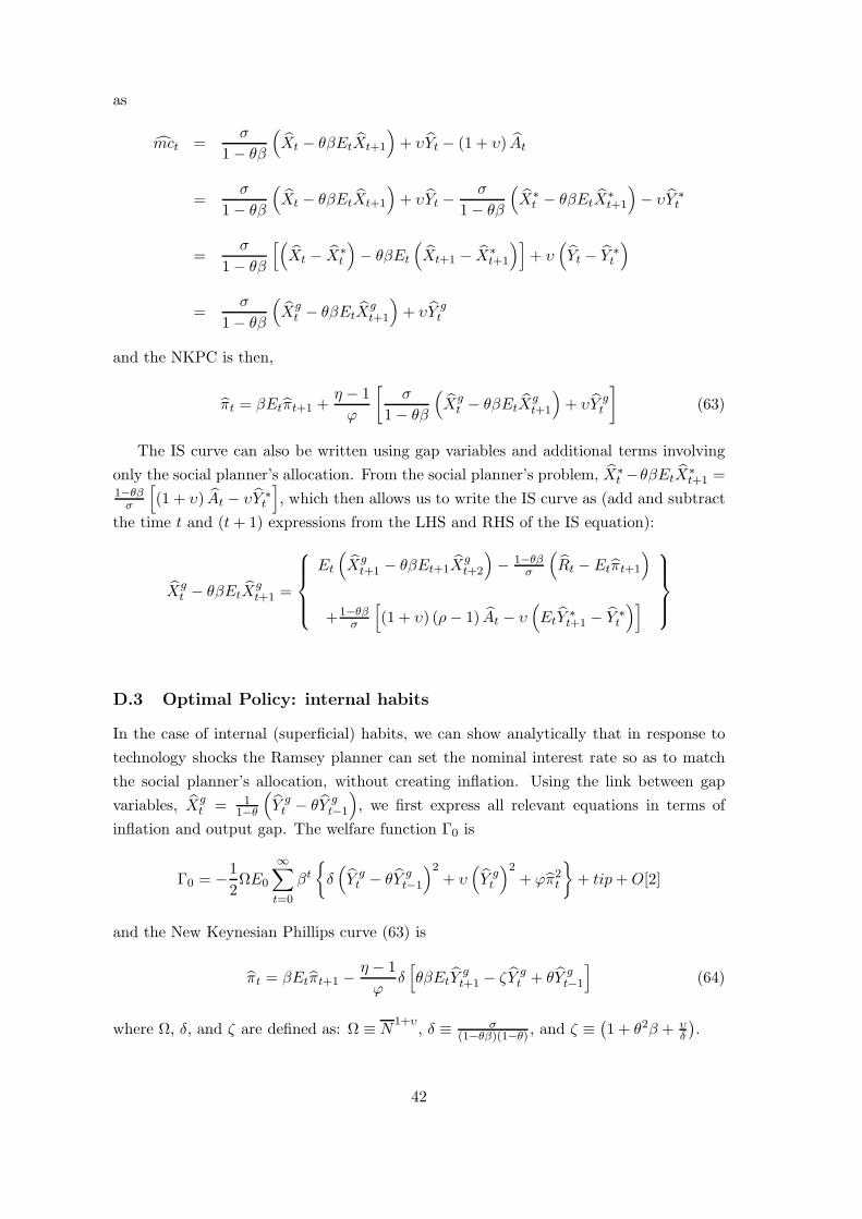
and the NKPC is then,

πt = βEtπt+1 +η − 1

ϕ

[σ

1− θβ

(Xg

t − θβEtXgt+1

)+ υY g

t

](63)

The IS curve can also be written using gap variables and additional terms involving

only the social planner’s allocation. From the social planner’s problem, X∗t −θβEtX

∗t+1 =

1−θβσ

[(1 + υ) At − υY ∗

t

], which then allows us to write the IS curve as (add and subtract

the time t and (t+ 1) expressions from the LHS and RHS of the IS equation):

Xgt − θβEtX

gt+1 =

⎧⎪⎪⎨⎪⎪⎩Et

(Xg

t+1 − θβEt+1Xgt+2

)− 1−θβ

σ

(Rt − Etπt+1

)+1−θβ

σ

[(1 + υ) (ρ− 1) At − υ

(EtY

∗t+1 − Y ∗

t

)]⎫⎪⎪⎬⎪⎪⎭

D.3 Optimal Policy: internal habits

In the case of internal (superficial) habits, we can show analytically that in response to

technology shocks the Ramsey planner can set the nominal interest rate so as to match

the social planner’s allocation, without creating inflation. Using the link between gap

variables, Xgt = 1

1−θ

(Y gt − θY g

t−1

), we first express all relevant equations in terms of

inflation and output gap. The welfare function Γ0 is

Γ0 = −1

2ΩE0

∞∑t=0

βt

{δ(Y gt − θY g

t−1

)2+ υ

(Y gt

)2+ ϕπ2t

}+ tip+O[2]

and the New Keynesian Phillips curve (63) is

πt = βEtπt+1 −η − 1

ϕδ[θβEtY

gt+1 − ζY g

t + θY gt−1

](64)

where Ω, δ, and ζ are defined as: Ω ≡ N1+υ

, δ ≡ σ(1−θβ)(1−θ) , and ζ ≡

(1 + θ2β + υ

δ

).

42

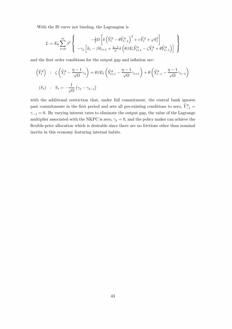
With the IS curve not binding, the Lagrangian is

L = E0

∞∑t=0

βt

⎧⎪⎨⎪⎩ −12Ω

[δ(Y gt − θY g

t−1

)2+ υY g

t + ϕπ2t

]−γt

[πt − βπt+1 +

η−1ϕ δ

(θβEtY

gt+1 − ζY g

t + θY gt−1

)]⎫⎪⎬⎪⎭

and the first order conditions for the output gap and inflation are:(Y gt

): ζ

(Y gt −

η − 1

ϕΩγt

)= θβEt

(Y gt+1 −

η − 1

ϕΩγt+1

)+ θ

(Y gt−1 −

η − 1

ϕΩγt−1

)

(πt) : πt = −1

ϕΩ

(γt − γt−1

)with the additional restriction that, under full commitment, the central bank ignores

past commitments in the first period and sets all pre-existing conditions to zero, Y g−1 =

γ−1 = 0. By varying interest rates to eliminate the output gap, the value of the Lagrange

multiplier associated with the NKPC is zero, γt = 0, and the policy maker can achieve the

flexible-price allocation which is desirable since there are no frictions other than nominal

inertia in this economy featuring internal habits.

43

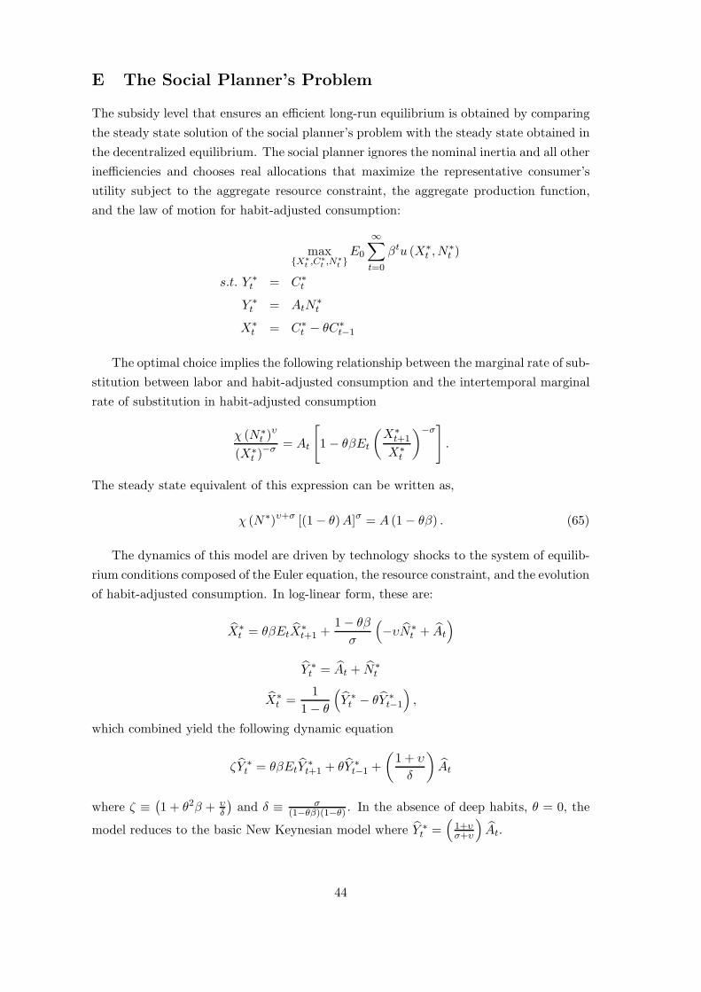
E The Social Planner’s Problem

The subsidy level that ensures an efficient long-run equilibrium is obtained by comparing

the steady state solution of the social planner’s problem with the steady state obtained in

the decentralized equilibrium. The social planner ignores the nominal inertia and all other

inefficiencies and chooses real allocations that maximize the representative consumer’s

utility subject to the aggregate resource constraint, the aggregate production function,

and the law of motion for habit-adjusted consumption:

max{X∗

t ,C∗

t ,N∗

t }E0

∞∑t=0

βtu (X∗t , N

∗t )

s.t. Y ∗t = C∗

t

Y ∗t = AtN

∗t

X∗t = C∗

t − θC∗t−1

The optimal choice implies the following relationship between the marginal rate of sub-

stitution between labor and habit-adjusted consumption and the intertemporal marginal

rate of substitution in habit-adjusted consumption

χ (N∗t )

υ

(X∗t )

−σ = At

[1− θβEt

(X∗

t+1

X∗t

)−σ].

The steady state equivalent of this expression can be written as,

χ (N∗)υ+σ [(1− θ)A]σ = A (1− θβ) . (65)

The dynamics of this model are driven by technology shocks to the system of equilib-

rium conditions composed of the Euler equation, the resource constraint, and the evolution

of habit-adjusted consumption. In log-linear form, these are:

X∗t = θβEtX

∗t+1 +

1− θβ

σ

(−υN∗

t + At

)Y ∗t = At + N∗

t

X∗t =

1

1− θ

(Y ∗t − θY ∗

t−1

),

which combined yield the following dynamic equation

ζY ∗t = θβEtY

∗t+1 + θY ∗

t−1 +

(1 + υ

δ

)At

where ζ ≡(1 + θ2β + υ

δ

)and δ ≡ σ

(1−θβ)(1−θ) . In the absence of deep habits, θ = 0, the

model reduces to the basic New Keynesian model where Y ∗t =

(1+υσ+υ

)At.

44

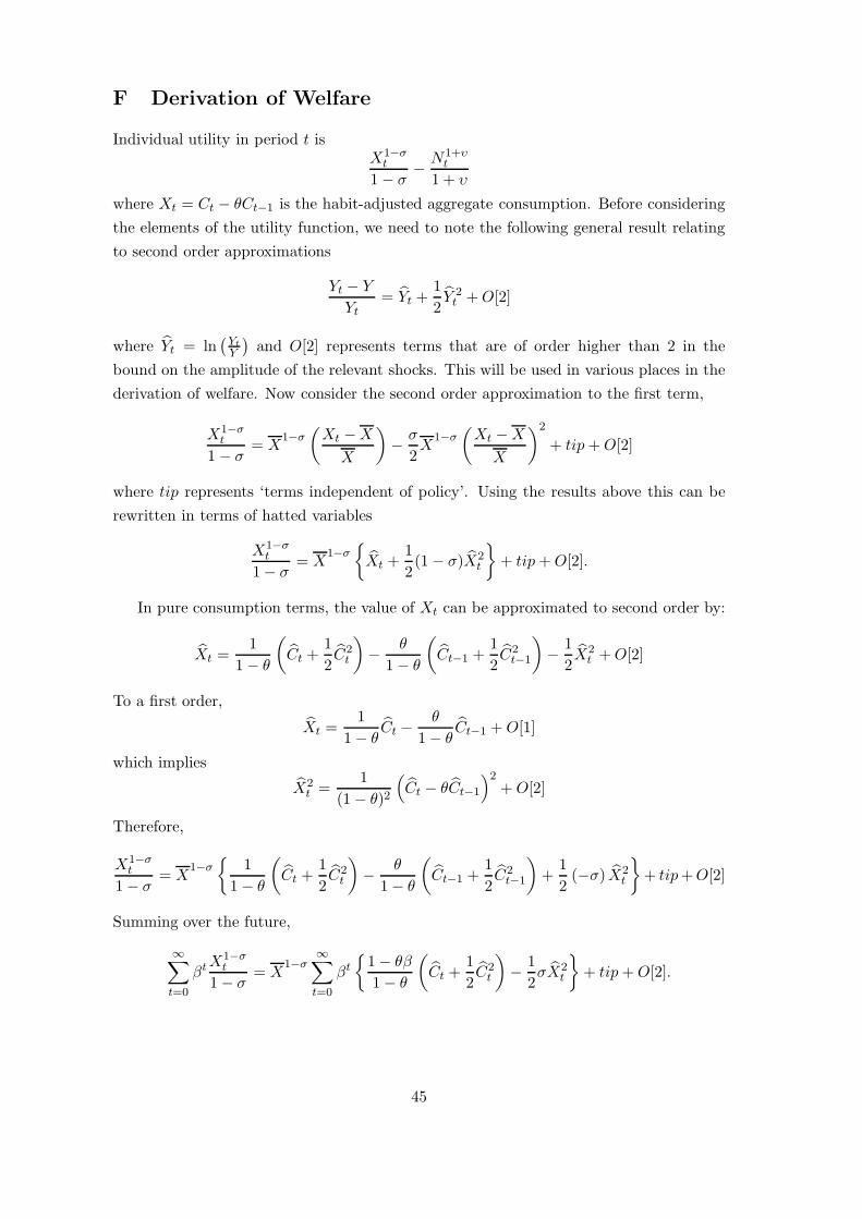
F Derivation of Welfare

Individual utility in period t isX1−σ

t

1− σ−N1+υ

t

1 + υ

where Xt = Ct − θCt−1 is the habit-adjusted aggregate consumption. Before considering

the elements of the utility function, we need to note the following general result relating

to second order approximations

Yt − Y

Yt= Yt +

1

2Y 2t +O[2]

where Yt = ln(Yt

Y

)and O[2] represents terms that are of order higher than 2 in the

bound on the amplitude of the relevant shocks. This will be used in various places in the

derivation of welfare. Now consider the second order approximation to the first term,

X1−σt

1− σ= X

1−σ(Xt −X

X

)−σ

2X

1−σ(Xt −X

X

)2

+ tip+O[2]

where tip represents ‘terms independent of policy’. Using the results above this can be

rewritten in terms of hatted variables

X1−σt

1− σ= X

1−σ{Xt +

1

2(1− σ)X2

t

}+ tip+O[2].

In pure consumption terms, the value of Xt can be approximated to second order by:

Xt =1

1− θ

(Ct +

1

2C2t

)−

θ

1− θ

(Ct−1 +

1

2C2t−1

)−

1

2X2

t +O[2]

To a first order,

Xt =1

1− θCt −

θ

1− θCt−1 +O[1]

which implies

X2t =

1

(1− θ)2

(Ct − θCt−1

)2+O[2]

Therefore,

X1−σt

1− σ= X

1−σ{

1

1− θ

(Ct +

1

2C2t

)−

θ

1− θ

(Ct−1 +

1

2C2t−1

)+

1

2(−σ) X2

t

}+ tip+O[2]

Summing over the future,

∞∑t=0

βtX1−σ

t

1− σ= X

1−σ∞∑t=0

βt{1− θβ

1− θ

(Ct +

1

2C2t

)−

1

2σX2

t

}+ tip+O[2].

45

The term in labour supply can be written as

N1+υt

1 + υ= N

1+υ{Nt +

1

2(1 + υ) N2

t

}+ tip +O[2]

Now we need to relate the labor input to output which, in this case without price

dispersion, is simply,

Nt =YtAt

and can be approximated to first order,

Nt = Yt − At

which implies

N2t =

(Yt − At

)2so we can then write

N1+υt

1 + υ= N

1+υ{Yt +

1

2(1 + υ) Y 2

t − (1 + υ) YtAt

}+ tip +O[2]

Welfare is then given by

Γ0 = X1−σ

E0

∞∑t=0

βt{1− θβ

1− θ

(Ct +

1

2C2t

)−

1

2σX2

t

}

−N1+υ

E0

∞∑t=0

βt{Yt +

1

2(1 + υ) Y 2

t − (1 + υ) YtAt

}

+tip+O[2]

From the social planner’s problem we know, X−σ

(1−θβ) = Nυsuch that X

1−σ(1−θβ) =

(1 − θ)N1+υ

. If we use the appropriate subsidy to render the steady-state efficient and

also use the second order approximation to the national accounting identity,

Ct +1

2C2t = Yt +

1

2Y 2t −

ϕ

2π2t +O[2],

we can eliminate the level terms and write the sum of discounted utilities as:

Γ0 = −1

2N

1+υE0

∞∑t=0

βt

{σ (1− θ)

1− θβX2

t + υ

(Yt −

1 + υ

υAt

)2

+ ϕπ2t

}+ tip+O[2] (66)

The welfare function can be also expressed in the usual “gap” form. To do so, we

employ the social planner’s solution in log-linear form to re-write the output term in the

46

welfare function as,

υ

(Yt −

1 + υ

υAt

)2

= υ(Yt − Y ∗

t

)2+ 2

σ

1− θβYt

(X∗

t − θβEtX∗t+1

)+ tip

Summing across time periods, we have

E0

∞∑t=0

βtυ

(Yt −

1 + υ

υAt

)2

= E0

∞∑t=0

βt

[υ(Yt − Y ∗

t

)2− 2

σ

1− θβYt

(X∗

t − θβEtX∗t+1

)]+tip+O [2]

Then note that we can write

X2t =

(Xt − X∗

t

)2+ 2XtX

∗t −

(X∗

t

)2and, keeping only the terms relevant for policy, the welfare function becomes,

Γ0 = −1

2N

1+υE0

∞∑t=0

βt

⎧⎪⎪⎪⎨⎪⎪⎪⎩σ(1−θ)1−θβ

(Xt − X∗

t

)2+ 2σ(1−θ)

1−θβ XtX∗t + υ

(Yt − Y ∗

t

)2−2 σ

1−θβ Yt

(X∗

t − θβEtX∗t+1

)+ ϕπ2t

⎫⎪⎪⎪⎬⎪⎪⎪⎭+tip+O[2]

Finally, we can show that

E0

∞∑t=0

βt σ

1− θβYt

(X∗

t − θβEtX∗t+1

)=

[E0

∞∑t=0

βtσ (1− θ)

1− θβXtX

∗t

]+ tip

which allows to write the welfare function in gap form as follows

Γ0 = −1

2N

1+υE0

∞∑t=0

βt{σ (1− θ)

1− θβ

(Xt − X∗

t

)2+ υ

(Yt − Y ∗

t

)2+ ϕπ2t

}+ tip+O[2]

F.1 Welfare Measure

We measure welfare as the unconditional expectation of lifetime utility, approximated as

W = E∞∑t=0

βtu (Xt, Nt)

=1

1− β

{u+

1

2

[(ΛC + ΛC−1

)var

(Yt

)+ 2ΛCC−1

cov(Yt, Yt−1

)+ ΛNvar

(Nt

)+ Λπvar (πt)

]}

47

with u the steady-state level of the momentary utility and the Λ coefficients defined as⎧⎪⎪⎪⎪⎪⎪⎪⎪⎨⎪⎪⎪⎪⎪⎪⎪⎪⎩

ΛC ≡ 11−θ

(1− σ

1−θ

)X

1−σ

ΛC−1≡ − θ

1−θ

(1 + σθ

1−θ

)X

1−σ

ΛCC−1≡ σθ

(1−θ)2X

1−σ

and

⎧⎪⎨⎪⎩ΛN ≡ − (1 + υ)N

1+υ

Λπ ≡ −ϕX1−σ

The welfare terms associated with the Ramsey policy that are involved in computing

the welfare costs of alternative policies, as in expression (28) in the text, are given by,

WRX = E

∞∑t=0

βt(XR

t

)1−σ

1− σ

=1

1− β

{(X)1−σ

1− σ+

1

2

[(ΛC + ΛC−1

)var

(Y Rt

)+ 2ΛCC−1

cov(Y Rt , Y

Rt−1

)+ Λπvar

(πRt

)]}

and

WRN = −E

∞∑t=0

βt(NR

t

)1+υ

1 + υ=

1

1− β

{−

(N)1+υ

1 + υ+

1

2ΛNvar

(NR

t

)}

48

G Optimal Policy: Commitment

Upon substitution of the habit-adjusted consumption term, the central bank’s objective

function becomes

1

2ΩE0

∞∑t=0

βt[(δ + υ) Y 2

t − 2θδYtYt−1 + θ2δY 2t−1 − 2 (1 + υ) YtAt + ϕπ2t

]

where Ω ≡ N1+υ

and δ ≡ σ(1−θβ)(1−θ) and we re-write the constraints as,

(1 + θ

1− θ

)Yt =

1

1− θEtYt+1 +

1

σEtπt+1 +

θ

1− θYt−1 −

1

σRt

πt = βEtπt+1 − κ2Yt + κ2Yt−1 − κ1ωt

μωωt = μωθβEtωt+1 − γ1βEtYt+1 + γ2Yt + γ3Yt−1 + (1 + υ) At

where

⎧⎪⎨⎪⎩κ1 ≡

1ϕ

κ2 ≡ κ1θ

1−θ

and

⎧⎪⎪⎪⎪⎪⎪⎪⎨⎪⎪⎪⎪⎪⎪⎪⎩

γ1 ≡ μω σθ1−θ

γ2 ≡ γ1β (1 + θ)−(

σ1−θ + υ

)γ3 ≡

σθ1−θ (1− μωθβ)

L = E0

∞∑t=0

βt

⎧⎪⎪⎪⎪⎪⎪⎨⎪⎪⎪⎪⎪⎪⎩

12Ω[− (δ + υ) Y 2

t + 2θδYtYt−1 − θ2δY 2t−1 + 2 (1 + υ) YtAt − ϕπ2t

]−χt

[(1+θ1−θ

)Yt −

11−θ Yt+1 −

1σ πt+1 −

θ1−θ Yt−1 +

1σ Rt

]−ψt

[πt − βπt+1 + κ2Yt − κ2Yt−1 + κ1ωt

]−ςt

[μωωt − μωθβEtωt+1 + γ1βEtYt+1 − γ2Yt − γ3Yt−1 − (1 + υ) At

]

⎫⎪⎪⎪⎪⎪⎪⎬⎪⎪⎪⎪⎪⎪⎭The government chooses paths for Rt, Yt, πt, and ωt. The first order condition with

respect to the nominal interest rate gives:

−σ−1E0βtχt = 0, ∀t ≥ 0 (67)

which implies that the IS curve is not binding and it can therefore be excluded from the

optimization problem. Once the optimal rules for the other variables have been obtained,

we use the IS curve to determine the path of the nominal interest rate. So, the central

bank now chooses{Yt, πt, ωt

}. The Lagrangian takes the form:

L = E0

∞∑t=0

βt

⎧⎪⎪⎪⎨⎪⎪⎪⎩12Ω[− (δ + υ) Y 2

t + 2θδYtYt−1 − θ2δY 2t−1 + 2 (1 + υ) YtAt − ϕπ2t

]−ψt

[πt − βπt+1 + κ2Yt − κ2Yt−1 + κ1ωt

]−ςt

[μωωt − μωθβEtωt+1 + γ1βEtYt+1 − γ2Yt − γ3Yt−1 − (1 + υ) At

]⎫⎪⎪⎪⎬⎪⎪⎪⎭ .

49

The first order condition for the shadow value ωt gives the relationship between the two

Lagrange multipliers,

κ1ψt = −μω (ςt − θςt−1)

while for inflation we have the rather usual expression

πt = −1

ϕΩ

(ψt − ψt−1

).

The first order condition for output gives

−ΩδζYt+ΩδθYt−1+Ω(1 + υ) At−κ2ψt+γ2ςt−γ1ς t−1+βEt

[ΩδθYt+1 + κ2ψt+1 + γ3ςt+1

]= 0

where, as defined before, ζ ≡(1 + θ2β + υ

δ

).

Under full commitment, the central bank ignores past commitments in the first period

by setting all pre-existing conditions to zero, Y−1 = 0 and ψ−1 = ς−1 = 0. To find the

solution, solve the system of equations composed of the first order conditions, the three

constraints, and the technology process.

G.1 Optimal Policy: Discretion

In order to solve the time-consistent policy problem we employ the iterative algorithm of

Soderlind (1999), which follows Currie and Levine (1993) in solving the Bellman equation.

The per-period objective function can be written in matrix form as Z ′tQZt, where Zt+1 =[

At+1 Yt EtYt+1 Etωt+1 Etπt+1

]′and

Q =1

2Ω

⎡⎢⎢⎢⎢⎢⎢⎣0 0 − (1 + υ) 0 0

0 θ2δ −θδ 0 0

− (1 + υ) −θδ (δ + υ) 0 0

0 0 0 0 0

0 0 0 0 ϕ

⎤⎥⎥⎥⎥⎥⎥⎦and the structural description of the economy is given by,

Zt+1 = AZt +But + ξt+1,

where ut =[Rt

], ξt+1 =

[εAt+1 0 0 0 0

]′, A ≡ A−1

0 A1, B ≡ A−10 B0,

A0 =

⎡⎢⎢⎢⎢⎢⎢⎣1 0 0 0 0

0 1 0 0 0

0 0 γ1β 0 0

0 0 11−θ 0 σ−1

0 0 0 0 β

⎤⎥⎥⎥⎥⎥⎥⎦ , A1 =

⎡⎢⎢⎢⎢⎢⎢⎣ρ 0 0 0 0

0 0 1 0 0

1 + υ γ3 γ2 −μω 0

0 − θ1−θ

1+θ1−θ 0 0

0 −κ2 κ2 κ1 1

⎤⎥⎥⎥⎥⎥⎥⎦

50

and

B0 =[0 0 0 σ−1 0

]′.

This completes the description of the required inputs for Soderlind (1999)’s Matlab code

which computes optimal discretionary policy.

51

−10 0 10−10

010

θ =0 and φR

=0

φπ

φ y

−10 0 10−10

010

θ =0.4 and φR

=0

φπ

φ y

−10 0 10−10

010

θ =0.7 and φR

=0

φπ

φ y

−10 0 10−10

010

θ =0.8 and φR

=0

φπ

φ y

−10 0 10−10

010

θ =0.9 and φR

=0

φπ

φ y−10 0 10

−100

10

θ =0 and φR

=0.5

φπ

φ y

−10 0 10−10

010

θ =0.4 and φR

=0.5

φπ

φ y−10 0 10

−100

10

θ =0.7 and φR

=0.5

φπ

φ y

−10 0 10−10

010

θ =0.8 and φR

=0.5

φπ

φ y

−10 0 10−10

010

θ =0.9 and φR

=0.5

φπ

φ y

−10 0 10−10

010

θ =0 and φR

=0.9

φπ

φ y

−10 0 10−10

010

θ =0.4 and φR

=0.9

φπ

φ y

−10 0 10−10

010

θ =0.7 and φR

=0.9

φπ

φ y

−10 0 10−10

010

θ =0.8 and φR

=0.9

φπ

φ y

−10 0 10−10

010

θ =0.9 and φR

=0.9

φπ

φ y

−10 0 10−10

010

θ =0 and φR

=1.1

φπ

φ y

−10 0 10−10

010

θ =0.4 and φR

=1.1

φπ

φ y

−10 0 10−10

010

θ =0.7 and φR

=1.1

φπ

φ y

−10 0 10−10

010

θ =0.8 and φR

=1.1

φπ

φ y

−10 0 10−10

010

θ =0.9 and φR

=1.1

φπ

φ y

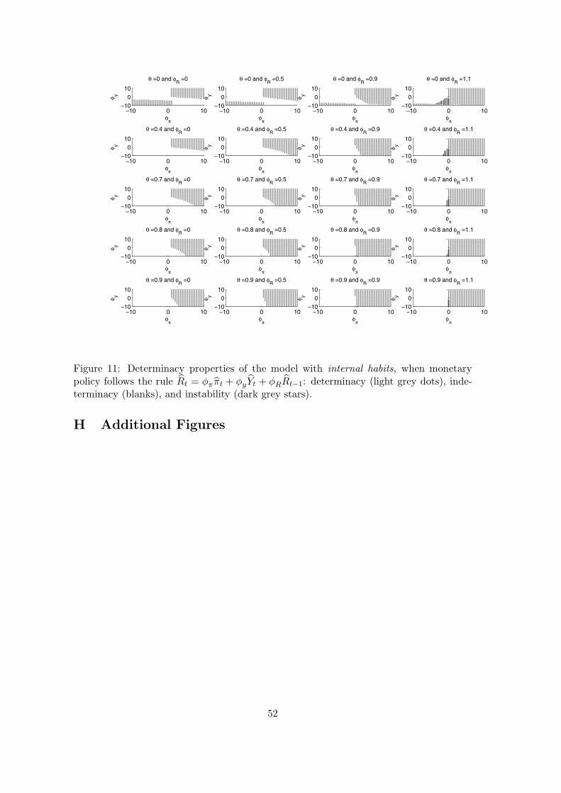
Figure 11: Determinacy properties of the model with internal habits, when monetarypolicy follows the rule Rt = φππt + φyYt + φRRt−1: determinacy (light grey dots), inde-terminacy (blanks), and instability (dark grey stars).

H Additional Figures

52

0.1 0.2 0.3 0.4 0.5 0.6 0.7 0.8 0.95

10

15

20

25

30

35

θ

φ π

0.1 0.2 0.3 0.4 0.5 0.6 0.7 0.8 0.9−0.6

−0.4

−0.2

0

0.2

0.4

0.6

0.8

1

1.2

φ y and

φR

φπ

φy

φR

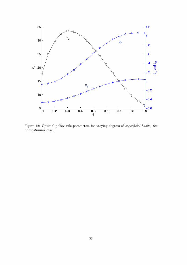
Figure 12: Optimal policy rule parameters for varying degrees of superficial habits, theunconstrained case.

53

0.1 0.2 0.3 0.4 0.5 0.6 0.7 0.8 0.90

5

10

15

20

25

30

35

40

45

50

θ

φ π

0.1 0.2 0.3 0.4 0.5 0.6 0.7 0.8 0.9−0.5

0

0.5

1

1.5

2

2.5

3

3.5

4

φ y and

φR

φπ

φy

φR

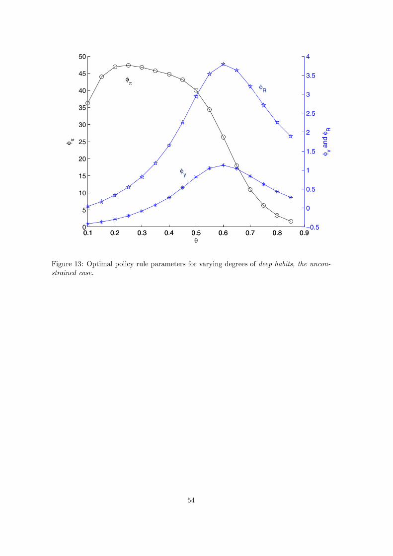
Figure 13: Optimal policy rule parameters for varying degrees of deep habits, the uncon-

strained case.

54

0 2 4 6−0.05

0

0.05Inflation

%

0 2 4 60

0.05

0.1Output gap

0 2 4 6−0.2

−0.1

0Nominal interest rate

%

0 2 4 6−0.2

−0.1

0Real interest rate

0 2 4 60

0.2

0.4Output

years

%

0 2 4 6−0.5

0

0.5Markup

years

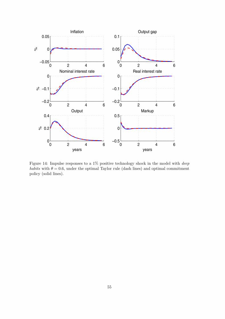
Figure 14: Impulse responses to a 1% positive technology shock in the model with deep

habits with θ = 0.6, under the optimal Taylor rule (dash lines) and optimal commitmentpolicy (solid lines).

55