Optimal Monetary Policy in a New Keynesian Model with

Habits in Consumption∗

Campbell Leith Ioana Moldovan Raffaele RossiUniversity of Glasgow

December 15, 2008

Abstract

While consumption habits have been utilised as a means of generating a hump-

shaped output response to monetary policy shocks in sticky-price New Keynesian

economies, there is relatively little analysis of the impact of habits (particularly,

external habits) on optimal policy. In this paper we consider the implications of ex-

ternal habits for optimal monetary policy, when those habits either exist at the level

of the aggregate basket of consumption goods (‘superficial’ habits) or at the level of

individual goods (‘deep’ habits: see Ravn, Schmitt-Grohe, and Uribe (2006)). Ex-

ternal habits generate an additional distortion in the economy, which implies that

the flex-price equilibrium will no longer be efficient and that policy faces interest-

ing new trade-offs and potential stabilisation biases. Furthermore, the endogenous

mark-up behaviour, which emerges when habits are deep, can also significantly af-

fect the optimal policy response to shocks, as well as dramatically affecting the

stabilising properties of standard simple rules.

• JEL Codes: E30, E57 and E61

• Key Words: consumption habits, nominal inertia, optimal monetary policy

1 Introduction

Within the benchmark New Keynesian analysis of monetary policy (see, for example,

Woodford (2003)), monetary policy typically influences the economy through the impact

of interest rates on a representative household’s intertemporal consumption decision. It

has often been felt that the purely forward-looking consumption dynamics that such ba-

sic intertemporal consumption decisions imply, are unable to capture the hump-shaped

output response to changes in monetary policy one typically finds in the data. As a∗Address for correspondence: Department of Economics, Adam Smith Building, University

of Glasgow, Glasgow G12 8RT, e-mail: c.b.leith@lbss.gla.ac.uk, i.moldovan@lbss.gla.ac.uk andr.rossi.1@research.gla.ac.uk. Raffaele Rossi would like to thank the Monetary Policy Strategy Divi-sion at the European Central Bank where part of this paper was completed. Campbell Leith would liketo thank the ESRC (Grant No. RES-156-25-003) for financial assistance.

1

means of accounting for such patterns, some authors have augmented the benchmark

model with various forms of habits effects in consumption. The habits effects can either

be internal (see for example, Fuhrer (2000), Christiano, Eichenbaum, and Evans (2005),

Leith and Malley (2005)) or external (see, for example, Smets and Wouters (2007))

the latter reflecting a catching up with the Joneses effect whereby households fail to

internalise the externality their own consumption causes on the utility of other house-

holds. Both forms of habits behaviour can help the New Keynesian monetary policy

model capture the persistence found in the data (see, for example Kozicki and Tinsley

(2002)), although the policy implications are likely to be different. More recently, Ravn,

Schmitt-Grohe, and Uribe (2006) offer an alternative form of habits behaviour, which

they label ‘deep’. Deep habits occur at the level of individual goods rather than at the

level of an aggregate consumption basket (‘superficial’ habits). While this distinction

does not affect the dynamic description of aggregate consumption behaviour relative

to the case of superficial habits, it does render the individual firms’ pricing decisions

intertemporal and, in the flexible price economy considered by Ravn, Schmitt-Grohe,

and Uribe (2006), can produce a counter-cyclical mark-up which significantly affects the

responses of key aggregates to shocks.

While the focus of the papers listed above is on the dynamic response of economies

which feature some form of habits, they do not consider the implications for optimal

policy of such an extension. In contrast, Amato and Laubach (2004) consider optimal

monetary policy in a sticky-price New Keynesian economy which has been augmented to

include internal (but superficial) habits. Since the form of habits is internal (households

care about their consumption relative to their own past consumption, rather than the

consumption of other households), there is no additional externality associated with

consumption habits themselves, and, given an efficient steady-state, the flexible price

equilibrium in the neighbourhood of that steady-state remains efficient. Accordingly, as

in the benchmark New Keynesian model, there is no trade-off between output gap and

inflation stabilisation in the face of technology shocks and interesting policy trade-offs

require the introduction of additional inefficiencies (such as mark-up shocks or a desire

for interest rate smoothing).

In this paper we extend the benchmark sticky-price New Keynesian economy to

include external habits in consumption, where these habits can be either superficial or

deep. The focus on external habits implies that there is an externality associated with

fluctuations in consumption which implies that the flexible price equilibrium will not

usually be efficient, thereby creating an additional trade-off for policy makers, which may

give rise to additional stabilisation biases if policy is constrained to be time consistent.

Such trade-offs will occur whether or not habits are superficial or deep. We also consider

the implications for optimal policy of assuming habits are of the deep kind. Here the

ability of policy to influence the time profile of endogenously determined mark-ups

can significantly affect the monetary policy stance and how it differs across discretion

2

and commitment. In addition to examining optimal policy, we also consider how the

introduction of habits affects the conduct of policy through simple rules. We find that

the introduction of deep habits can induce problems of indeterminacy, as the tightening

of monetary policy can induce inflation through variations in mark-up behaviour, such

that an interest rate rule which satisfies the Taylor principle (where nominal interest

rates rise more than one for one with increases in inflation above target) may not be

sufficient to ensure determinacy of the local equilibrium. We also consider whether or

not there is a significant role for the output gap in an optimal simple rule given that our

economy contains a major additional externality beyond that associated with nominal

inertia.

The plan of the paper is as follows: in the next section we outline our model with deep

and superficial habits. In section 3 we consider optimal policy under both commitment

and discretion, where the policy-maker’s objective function is derived from a second

order approximation to households’ utility. In section 4 we turn to our analysis of

simple rules, considering both their determinacy properties and, for rules which can

ensure determinacy, their ability to mimic optimal policy. Section 5 concludes.

2 The Model

The economy is comprised of households, two monopolistically competitive production

sectors, and the government. There is a continuum of final goods that enter the house-

holds’ consumption basket, each final good being produced as an aggregate of a contin-

uum of intermediate goods. Households can either form external consumption habits at

the level of each final good in their basket, Ravn, Schmitt-Grohe, and Uribe (2006) call

this type of habits ‘deep’, or they can form habits at the level of the consumption basket

- ‘superficial’ habits. Throughout the paper, we use the same terminology. Furthermore,

we assume price inertia at the level of intermediate goods producers. We shall derive a

general model, and note when assuming superficial or deep habits alters the behavioural

equations.

2.1 Households

The economy is populated by a continuum of households, indexed by k and of measure

1. Households derive utility from consumption of a composite good and disutility from

hours spent working.

Deep Habits When habits are of the deep kind, each household’s consumption basket,

Xkt , is an aggregate of a continuum of habit-adjusted final goods, indexed by i and of

measure 1,

Xkt =

µZ 1

0

³Ckit − θCit−1

´ η−1η

di

¶ ηη−1

,

3

where Ckit is household k’s consumption of good i and Cit ≡

R 10 C

kitdk denotes the cross-

sectional average consumption of this good. η is the elasticity of substitution between

habit-adjusted final goods (η > 1), while the parameter θ measures the degree of external

habit formation in the consumption of each individual good i. Setting θ to 0 returns us

to the usual case of no habits.

The composition of the consumption basket is chosen in order to minimize expendi-

tures, and the demand for final goods is

Ckit =

µPitPt

¶−ηXkt + θCit−1, ∀i

where Pt represents the overall price index (or CPI), defined as an average of final goods

prices, Pt ≡³R 10 P

1−ηit di

´1/(1−η). Aggregating across households yields the total demand

for good i, i ∈ [0, 1] ,

Cit =

µPitPt

¶−ηXt + θCit−1. (1)

Due to the presence of habits, this demand is dynamic in nature, as it depends not

only on current period elements but also on the lagged value of consumption. This, in

turn, will make the pricing/output decisions of the firms producing these final goods,

intertemporal.

Superficial Habits Habits are superficial when they are formed at the level of the ag-

gregate consumption good. Households derive utility from the habit-adjusted composite

good Xkt ,

Xkt = Ck

t − θCt−1

where household k’s consumption, Ckt , is an aggregate of a continuum of final goods

indexed by i ∈ [0, 1] ,

Ckt =

µZ 1

0

³Ckit

´η−1η

di

¶ ηη−1

with η the elasticity of substitution between them and Ct−1 ≡R 10 C

kt−1dk the cross-

sectional average of consumption.

Households decide the composition of the consumption basket to minimize expendi-

tures and the demand for individual good i is

Ckit =

µPitPt

¶−ηCkt =

µPitPt

¶−η ³Xkt + θCt−1

´

where Pt ≡³R 10 P

1−ηit di

´ 11−η is the consumer price index. The overall demand for good

4

i is obtained by aggregating across all households,

Cit =

Z 1

0Ckitdk

=

µPitPt

¶−ηCt. (2)

Unlike the case of deep habits, this demand is not dynamic and the final goods producing

firms will face a static pricing/output decision.

Remainder of the Household’s Problem The remainder of the household’s prob-

lem is the same irrespective of whether or not habits are deep or superficial. Specifically,

households choose the habit-adjusted consumption aggregate, Xkt , hours worked, N

kt ,

and the portfolio allocation, Dkt+1, to maximize expected lifetime utility

E0

∞Xt=0

βt

"¡Xkt

¢1−σ1− σ

− χ

¡Nkt

¢1+υ1 + υ

#

subject to the budget constraintZ 1

0PitC

kitdi+EtQt,t+1D

kt+1 =WtN

kt +Dk

t +Φkt − T k

t (3)

and the usual transversality condition. Et is the mathematical expectation conditional

on information available at time t, β is the discount factor (0 < β < 1) , χ the relative

weight on disutility from time spent working, and σ and υ are the inverses of the in-

tertemporal elasticities of habit-adjusted consumption and work (σ, υ > 0; σ 6= 1). Thehousehold’s period-t income includes: wage income from providing labour services to

intermediate goods producing firms WtNkt , dividends from the monopolistically com-

petitive firms Φkt , and payments on the portfolio of assets Dkt . Financial markets are

complete and Qt,t+1 is the one-period stochastic discount factor for nominal payoffs. T kt

are lump-sum taxes collected by the government. In the maximization problem, house-

holds take as given the processes for Ct−1, Wt, Φkt , and T kt , as well as the initial asset

position Dk−1.

The first order conditions for labour and habit-adjusted consumption are:

−χ¡Nkt

¢υ¡Xkt

¢−σ = wt

and

Qt,t+1 = β

ÃXkt+1

Xkt

!−σPtPt+1

(4)

where wt ≡ WtPtis the real wage (see Appendix A for further details). The Euler equation

5

for consumption can be written as

1 = βEt

"ÃXkt+1

Xkt

!−σPtPt+1

#Rt

where R−1t = Et [Qt,t+1] denotes the inverse of the risk-free gross nominal interest rate

between periods t and t+ 1.

2.2 Firms

In this subsection we consider the behaviour of firms. These are split into two kinds:

final and intermediate goods producing firms, respectively. In the case of the former,

their behaviour depends upon the form of demand curve they face, which is dynamic in

the case of deep habits, and static under superficial habits. Intermediate goods firms

produce a differentiated intermediate good and are subject to nominal inertia in the form

of Calvo (1983) contracts. This structure is adopted for reasons of tractability, allowing

us to easily switch between superficial and deep habits. Additionally, combining optimal

price setting under both Calvo contracts and dynamic demand curves would undermine

the desirable aggregation properties of the Calvo model as each firm given the signal to

re-set prices would set a different price dependent on the level of consumption habits

their product enjoyed relative to other firms’. By separating the two pricing decisions we

avoid reintroducing the history-dependence in price setting the Calvo set-up is designed

to avoid.

2.2.1 Final Goods Producers

We assume that final goods are produced by monopolistically competitive firms as an

aggregate of a set of intermediate goods (indexed by j), according to the function

Yit =

µZ 1

0(Yjit)

ε−1ε dj

¶ εε−1

, (5)

where ε is the constant elasticity of substitution between inputs in production (ε > 1).

Taking as given intermediate goods prices Pjitj and subject to the available tech-nology (5), firms first choose the amount of intermediate inputs Yjitj that minimizeproduction costs

R 10 PjitYjitdj. The first order conditions yield the demand functions

Yjit =

µPjitPmit

¶−εYit, ∀j, ∀i, (6)

where Pmit ≡

³R 10 P

1−εjit dj

´ 11−ε

is the aggregate of intermediate goods prices in sector i

and represents the nominal marginal cost of producing an additional unit of the final

good i. Nominal profits are given by Φit = (Pit − Pmit )Yit. It is important to note

6

that this cost-minimisation problem takes the same form whether firms are faced with

consumers whose habits are deep or superficial. However, their pricing decisions will

differ across this dimension. We now examine the pricing decision of final goods firms,

dependent upon whether habits are deep or superficial.

Deep Habits When habits are deep, firms face the dynamic demand from households,

given by expression (1), and their profit maximization problem becomes intertemporal:

the choice of price affects market share and future profits. Therefore, firms choose

processes for Yit and Pit to maximize the present discounted value of expected profits,

Et

∞Xs=0

Qt,t+sΦit+s, subject to this dynamic demand and the constraint that Cit = Yit.

Qt,t+s is s-step ahead equivalent of the one-period stochastic discount factor in (4). The

first order conditions for Yit and Pit are:

vit = (Pit − Pmit ) + θEt [Qt,t+1vit+1] (7)

and

Yit = vit

"η

µPitPt

¶−η−1 Xt

Pt

#, (8)

where the Lagrange multiplier vit represents the shadow price of producing an addi-

tional unit of the final good i. This shadow value equals the marginal benefit of addi-

tional profits, (Pit − Pmit ), plus the discounted expected payoff from higher future sales,

θEt [Qt,t+1vit+1]. Due to the presence of habits in consumption, increasing output by

one unit in the current period leads to an increase in sales of θ in the next period. In

the absence of habits, when θ = 0, the intertemporal effects of higher output disappear

and the shadow price simply equals time-t profits. The other first order condition in

equation (8) says that an increase in price brings additional revenues, Yit, while simul-

taneously causing a decline in demand, given by the term in square brackets and valued

at the shadow value vit.

Superficial Habits Under superficial habits the profit maximization problem of the

final goods firms is the typical static problem whereby firms choose the price to maximize

current profits, Φit = (Pit − Pmit )Yit, subject to the demand for their good (2) and under

the restriction that all demand be satisfied at the chosen price, Cit = Yit. The optimal

price is set at a constant markup, μ = ηη−1 , over the marginal cost,

Pit = μPmit .

7

2.2.2 Intermediate Goods Producers

The intermediate goods sectors consist of a continuum of monopolistically competitive

firms indexed by j and of measure 1. Each firm j produces a unique good using only

labour as input in the production process

Yjit = AtNjit. (9)

Total factor productivity, At, affects all firms symmetrically and follows an exogenous

stationary process, lnAt = ρ lnAt−1 + εt, with persistence parameter ρ ∈ (0, 1) andrandom shocks εt ∼ iidN

¡0, σ2A

¢.

Firms choose the amount of labour that minimizes production costs, (1− κ)WtNjit.

The subsidy κ, financed by lump-sum taxes, is designed to ensure that the long-run

equilibrium is efficient.1 The minimization problem gives a demand for labour Njit =YjitAjit

and a nominal marginal costMCt = (1− κ) WtAt, which is the same across firms. (See

Appendix A for more details.) Nominal profits are expressed as Φjit ≡ (Pjit −MCt)Yjit.

We further assume that intermediate goods producers are subject to the constraints

of Calvo (1983)-contracts such that, with fixed probability (1− α) in each period, a

firm can reset its price and with probability α the firm retains the price of the previous

period. When a firm can set the price, it does so in order to maximize the present

discounted value of profits, Et

∞Xs=0

αsQt,t+sΦjit+s, and subject to the demand for its own

good (6) and the constraint that all demand be satisfied at the chosen price. Profits are

discounted by the s-step ahead stochastic discount factor Qt,t+s and by the probability

of not being able to set prices in future periods.

Optimally, the relative price satisfies the following relationship:

P ∗jitPt

=

µε

ε− 1

¶ Et

∞Xs=0

(αβ)s (Xt+s)−σmct+s

¡Pmit+s

¢εYit+s

Et

∞Xs=0

(αβ)s (Xt+s)−σ³Pt+sPt

´−1 ¡Pmit+s

¢εYit+s

where mct =MCtPt

is the real marginal cost.

Pmit represents the price at the level of sector i and is an average of intermediate

goods prices within that sector. With α of firms keeping last period’s price and (1− α)

of firms setting a new price, the law of motion of this price index is:

(Pmit )

1−ε = α¡Pmit−1

¢1−ε+ (1− α)

¡P ∗jit

¢1−ε.

This description of intermediate goods firms is the same irrespective of the nature of

1 In this model, all firms are monopolistically competitive but only intermediate goods producingfirms are subsidized. Still, in steady-state the subsidy level is such that all production inefficiencies areeliminated.

8

habits formation.

2.3 The Government

The government collects lump-sum taxes which it rebates to intermediate goods pro-

ducing firms as subsidies, which ensure an efficient long-run level of output. There is no

government spending per se. The government budget constraint is given by

κWtNt = Tt. (10)

In this cashless economy, monetary policy is conducted in optimal fashion, with

the nominal interest rate being the central bank’s policy instrument. However, we also

consider the consequences of the central bank adopting more simple forms of policy,

such as Taylor-type interest rate rules, and explore how closely these simple policy rules

come to the optimal.

2.4 Equilibrium

In the absence of sector-specific shocks or other forms of heterogeneity, final goods

producers are symmetric and so are households. However, symmetry does not apply

to intermediate goods producers who face randomness in price setting. There is a

distribution of intermediate goods prices and aggregate output is therefore determined

as (see Appendix B for details on aggregation)

Yt = AtNt

∆t. (11)

∆t ≡Z 1

0

³PjtPmt

´−εdj is the measure of price dispersion, which can be shown (see Wood-

ford (2003), Chapter 6) to follow an AR(1) process given by

∆t = (1− α)

µP ∗tPmt

¶−ε+ α (πmt )

ε∆t−1. (12)

Note that we have two measures of aggregate prices, a producer price index Pmt

and the usual consumer price index Pt, and consequently, there will be two measures of

inflation. We define: πmt ≡Pmt

Pmt−1

and πt ≡ PtPt−1

. Furthermore, the two inflation variables

are related according to the following relationship

πt = πmtμtμt−1

, (13)

where μt ≡ PtPmtis the markup of final goods producers. In the presence of deep habits,

this markup is time-varying. The overall markup in the economy is given by the product

9

of markups in the intermediate goods and final goods sectors and equals the inverse of

the real marginal cost,mc−1t = PtMCt

. It should be noted that when habits are superficial,

the mark-up in the final goods sectors is constant, μt = μ, and there is no longer any

wedge between consumer price and producer price inflation.

Finally, the aggregate version of the household’s budget constraint (3) combines with

the government budget constraint (10) and the definition of aggregate profits (Φt =

PtYt − (1− κ)WtNt) to obtain the usual aggregate resource constraint,

Yt = Ct. (14)

The equilibrium is then characterized by equations (11) - (14), to which we add

the monetary policy specification (to be detailed in Sections 3 and 4 below) and the

following set of equations:

Consumers:

Xt = Ct − θCt−1 (15)

−χNυt

X−σt

= wt (16)

X−σt = βEt

∙X−σt+1

PtPt+1

¸Rt (17)

Government:

κWtNt = Tt (18)

Intermediate goods producers:

(Pmt )

1−ε = α¡Pmt−1¢1−ε

+ (1− α)¡P ∗jt¢1−ε (19)

P ∗jtPt

=

µε

ε− 1

¶K1t

K2t(20)

where : K1t = X−σt mctμ

−εt Yt + αβEt

£K1t+1π

εt+1

¤(21)

: K2t = X−σt μ−εt Yt + αβEt

£K2t+1π

ε−1t+1

¤(22)

mct = (1− κ)wt

At(23)

lnAt = ρ lnAt−1 + εt (24)

Final goods firms:

The differences in the two economies when habits are deep rather than superficial

emerges in the behaviour of the final goods firms. As noted above, when habits are

superficial they simply adopt a constant mark-up over the price of the bundle of inter-

10

mediate goods,

μt = μ. (25)

In contrast, when habits are deep and final goods firms face a dynamic demand curve

for their product, the endogenous time varying mark-up is described by the following

two equations (note that we have written the shadow price of producing final goods in

real terms, i.e. ωt ≡ vtPt),

ωt =

µ1− 1

μt

¶+ θβEt

"µXt+1

Xt

¶−σωt+1

#(26)

Yt = ηωtXt. (27)

2.5 Solution Method and Model Calibration

In the absence of a closed-form solution, the model’s equilibrium conditions are log-

linearized around the efficient deterministic steady state. The efficiency of the steady

state, obtained through the subsidy allocated to intermediate goods producers, allows

us to obtain an accurate expression for welfare involving only second-order terms.

In order to solve the model, we must select numerical values for some key structural

parameters. Table 1 reports our choices, which are similar to those of other studies

using a New Keynesian economy with habits in consumption. The model is calibrated

to a quarterly frequency. We assume zero average inflation (π = 1) and an annual real

rate of interest of 4%, which together imply a discount factor β of 0.9902. The risk

aversion parameter σ is set at 2.0, while υ equals 0.252, and the relative weight on

labour in the utility function χ is assumed to be 3.0. Consistent with the empirical

evidence, the level of price inertia α is set at 0.75 and the degree of market power is

1.21, split approximately equally between the two monopolistically competitive sectors

of our economy. The steady state value of the markup in the final goods sector is given

as, μ =h1− (1−θβ)

(1−θ)η

i−1, and depends on both the elasticity of substitution between final

goods η and the degree of habit formation θ. However, the impact of θ on the markup

μ is minimal and we therefore set η = ε = 11. For the habit formation parameter θ, we

use a benchmark value of 0.65, which falls within the range of estimates identified in the

literature3. However, we allow θ to vary in the [0, 1) interval as we conduct sensitivity

analyses of our results. Technology shocks are assumed persistent with persistence

parameter ρ = 0.9 and standard deviation σA = 0.009. Finally, we set the subsidy rate

κ so as to ensure an efficient steady state, κ = 1− 11−θβ

³1με−1ε

´.

2υ is the inverse of the Frisch labour supply elasticity. While micro estimates of this elasticity arerather small, they tend not to fit well in macro models. Here, we follow the macroeconomic literatureand choose a larger value of 4.0.

3Macro-based estimates of habit formation of the superficial type range from 0.59 as in Smets andWouters (2003) to very high values of 0.98 as reported by Bouakez, Cardia, and Ruge-Murcia (2005).For the deep type of habits, Ravn, Schmitt-Grohe, and Uribe (2006) give a value of 0.86. Micro-basedestimates (see, for example, Ravina (2007)) are substantially lower, with a range of 0.29-0.5.

11

2.6 Log-linear Representation

Upon log-linearizing and combining the relevant equilibrium conditions, we obtain a

system of equations which characterize the dynamics of the economy in the neighborhood

of the efficient steady state. Firstly, we have the IS curve in terms of habit-adjusted

consumption, bXt = EtbXt+1 −

1

σbRt +

1

σEtbπt+1, (28)

and the New Keynesian Phillips Curve (NKPC) written in terms of producer price

inflation bπmt = βEtbπmt+1 + κ (cmct + bμt) (29)

where κ ≡ (1−αβ)(1−α)α and it should be remembered that the markup, μt, is constant

under superficial habits such that, bμt = 0. In contrast, when habits are deep, the

dynamic equation describing changes in the markup can be written as,

bμt = μω (bωt − θβEtbωt+1)− μωθβσ³ bXt −Et

bXt+1

´, (30)

where the shadow value of producing another unit of a final good subject to deep habits

is given by, bωt = bYt − bXt. (31)

And finally, we have the following expressions defining habit-adjusted consumption bXt,

CPI inflation bπt (when habits are deep), and the real marginal cost cmct:

bXt =1

1− θ

³bYt − θbYt−1´ (32)

bπt = bπmt + bμt − bμt−1 (33)

cmct = σ bXt + υbYt − (1 + υ) bAt. (34)

3 Optimal Policy

In this section we consider the nature of optimal monetary policy in response to technol-

ogy shocks, under both cases of commitment and discretion by the monetary authority.

The central bank’s objective function is given by a second order approximation to the

representative households’ utility (see Appendix E for details),

Γ0 = −12χN

1+υE0

∞Xt=0

βt

("σ

µ1− θ

1− θβ

¶ bX2t + υ

µbYt − 1 + υ

υbAt

¶2#+

ε

κ(bπmt )2

)+ tip+O[2].

= −12χN

1+υE0

∞Xt=0

βtnh(δ + υ) bY 2t − 2θδbYt bYt−1 + θ2δbY 2t−1 − 2 (1 + υ) bYt bAt

i+

ε

κ(bπmt )2o

+tip+O[2]

12

where δ ≡ σ(1−θβ)(1−θ) . The last line was obtained by replacing

bXt with its expression

in terms of output. The weights given to the various elements in the objective function

are derived from basic preference parameters, and the presence of the term in inflation

reflects the costs of price dispersion due to nominal inertia. It should be noted that this

objective function applies whether or not habits are deep or superficial.

While this welfare measure has the same basic components (output and inflation) as

the benchmark New Keynesian model (without externalities due to consumption habits),

this welfare measure looks different, in that it does not contain a single “output gap”,

defined as the difference between output and the flex-price level of output. However,

the more complex term in the current set-up is conceptually similar. The output gap

term in the standard analysis captures the extent to which output deviates from its

efficient level (typically because of nominal inertia, rather than any other distortion).

In a model with external habits, there is an additional externality which means that the

flexible price equilibrium is unlikely to be efficient, such that it is not possible to rewrite

output in gap form. Nevertheless, it is possible to show that minimisation of the terms

in square brackets is equivalent to implementing the social planner’s allocation. In other

words, we are still trading off inflation control against minimising the deviation of the

decentralised equilibrium to that which would be implemented by a benevolent social

planner (see appendix D for the social planner’s problem).

We measure the welfare cost of a particular policy as the fraction of permanent

consumption that must be given up in order to equal welfare in the stochastic economy to

that of the efficient steady state, E∞Pt=0

βtu (Xt, Nt) = (1− β)−1 u¡(1− θ) (1− ξ)C,N

¢.

Given the utility function adopted, the expression for ξ in percentage terms is

ξ =

"1− [(1− σ)Υ]

11−σ

(1− θ)C

#× 100,

where Υ ≡ (1− β)W +χN1+υ

1+υ and W ≡ E∞Pt=0

βtu (Xt, Nt) represents the unconditional

expectation of lifetime utility in the stochastic equilibrium.

3.1 Optimal Policy under Commitment

If the monetary authority can credibly commit to following its policy plans, it then

chooses the policy that maximizes households’ welfare subject to the private sector’s

optimal behaviour, as summarized in equations (28) - (34), and given the exogenous

process for technology (see Appendix F for details of the policy problem under com-

mitment). We analyze the implications of this policy in terms of impulse responses to

exogenous technology shocks.

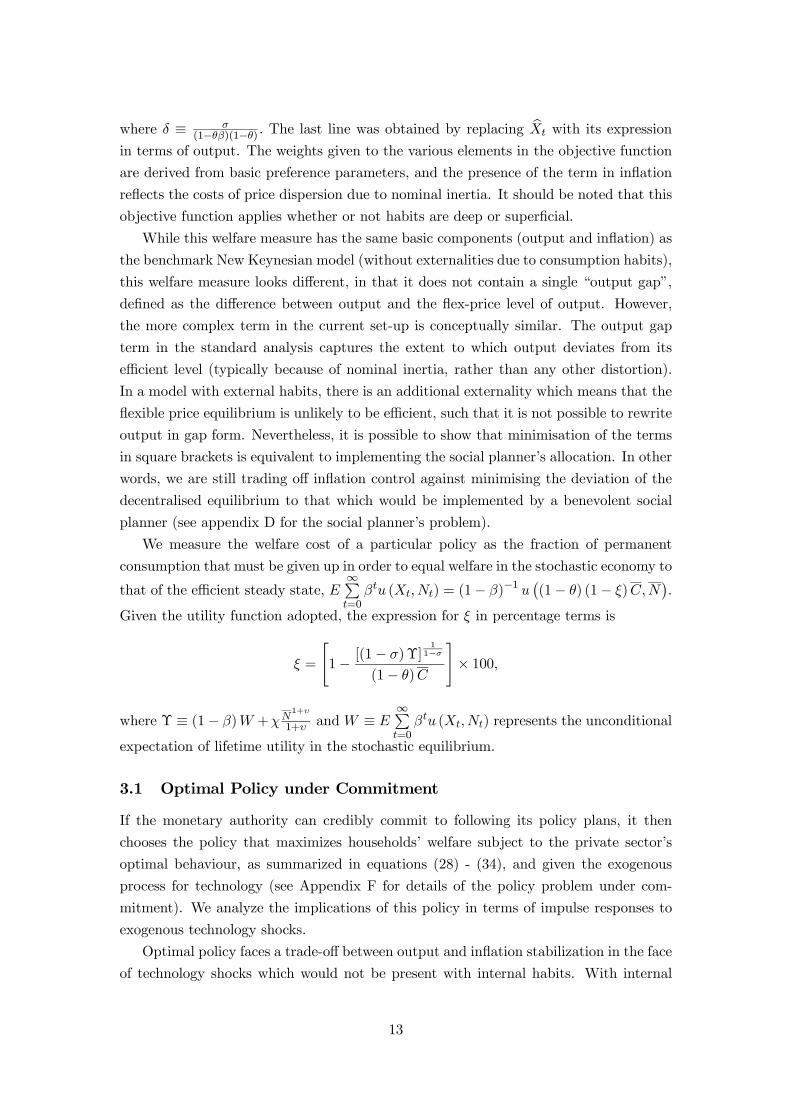
Optimal policy faces a trade-off between output and inflation stabilization in the face

of technology shocks which would not be present with internal habits. With internal

13

habits, policy would be loosened to ensure the flexible price equilibrium was recreated

without generating any inflation (see Amato and Laubach (2004)).4 However, when

habits are external, such that one household does not take account of the impact their

increased consumption has on the utility of others, then with one policy instrument

available, the monetary authority cannot simultaneously ensure output is at its efficient

level and inflation is eliminated. Instead, while nominal inertia points to a relaxation of

policy in the face of a positive technology shock to boost output, the consumption exter-

nality suggests that the higher consumption this entails need not be desirable.5 Figure

1 shows that the optimal response of the economy to a positive persistent technology

shock is a positive output gap and an initial decline followed by an increase in inflation

(pluses indicate the benchmark calibration with θ = 0.65) when habits are superficial.

To achieve this outcome, the monetary authority reduces the nominal interest rate

to boost demand to the socially optimal level. Because the policy is expansionary,

we can implicitly say that the inefficiency due to price stickiness is dominating in this

case. As the degree of importance of habits increases, inflation stabilisation remains the

primary goal and the policy maker suffers a widening output gap due to the consumption

externality.

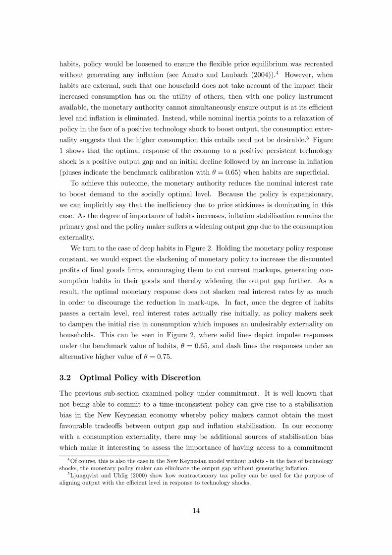
We turn to the case of deep habits in Figure 2. Holding the monetary policy response

constant, we would expect the slackening of monetary policy to increase the discounted

profits of final goods firms, encouraging them to cut current markups, generating con-

sumption habits in their goods and thereby widening the output gap further. As a

result, the optimal monetary response does not slacken real interest rates by as much

in order to discourage the reduction in mark-ups. In fact, once the degree of habits

passes a certain level, real interest rates actually rise initially, as policy makers seek

to dampen the initial rise in consumption which imposes an undesirably externality on

households. This can be seen in Figure 2, where solid lines depict impulse responses

under the benchmark value of habits, θ = 0.65, and dash lines the responses under an

alternative higher value of θ = 0.75.

3.2 Optimal Policy with Discretion

The previous sub-section examined policy under commitment. It is well known that

not being able to commit to a time-inconsistent policy can give rise to a stabilisation

bias in the New Keynesian economy whereby policy makers cannot obtain the most

favourable tradeoffs between output gap and inflation stabilisation. In our economy

with a consumption externality, there may be additional sources of stabilisation bias

which make it interesting to assess the importance of having access to a commitment

4Of course, this is also the case in the New Keynesian model without habits - in the face of technologyshocks, the monetary policy maker can eliminate the output gap without generating inflation.

5Ljungqvist and Uhlig (2000) show how contractionary tax policy can be used for the purpose ofaligning output with the efficient level in response to technology shocks.

14

technology. Appendix F defines the inputs to the iterative algorithm used to compute

time-consistent policy in Soderlind (1999).

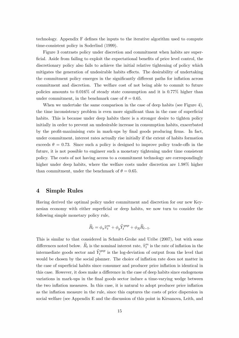
Figure 3 contrasts policy under discretion and commitment when habits are super-

ficial. Aside from failing to exploit the expectational benefits of price level control, the

discretionary policy also fails to achieve the initial relative tightening of policy which

mitigates the generation of undesirable habits effects. The desirability of undertaking

the commitment policy emerges in the significantly different paths for inflation across

commitment and discretion. The welfare cost of not being able to commit to future

policies amounts to 0.016% of steady state consumption and it is 0.77% higher than

under commitment, in the benchmark case of θ = 0.65.

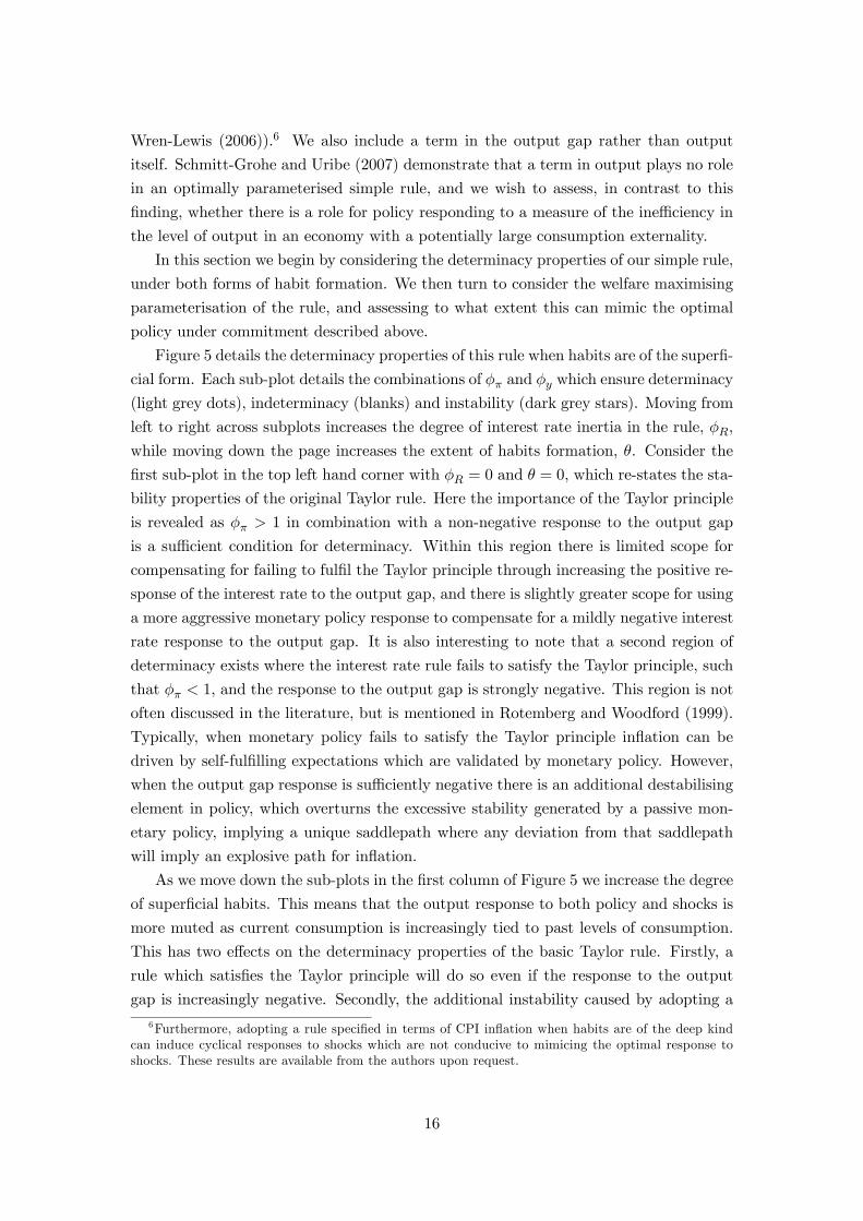
When we undertake the same comparison in the case of deep habits (see Figure 4),

the time inconsistency problem is even more significant than in the case of superficial

habits. This is because under deep habits there is a stronger desire to tighten policy

initially in order to prevent an undesirable increase in consumption habits, exacerbated

by the profit-maximising cuts in mark-ups by final goods producing firms. In fact,

under commitment, interest rates actually rise initially if the extent of habits formation

exceeds θ = 0.73. Since such a policy is designed to improve policy trade-offs in the

future, it is not possible to engineer such a monetary tightening under time consistent

policy. The costs of not having access to a commitment technology are correspondingly

higher under deep habits, where the welfare costs under discretion are 1.98% higher

than commitment, under the benchmark of θ = 0.65.

4 Simple Rules

Having derived the optimal policy under commitment and discretion for our new Key-

nesian economy with either superficial or deep habits, we now turn to consider the

following simple monetary policy rule,

bRt = φπbπmt + φy bY gapt + φR bRt−1.

This is similar to that considered in Schmitt-Grohe and Uribe (2007), but with some

differences noted below. bRt is the nominal interest rate, bπmt is the rate of inflation in theintermediate goods sector and bY gap

t is the log-deviation of output from the level that

would be chosen by the social planner. The choice of inflation rate does not matter in

the case of superficial habits since consumer and producer price inflation is identical in

this case. However, it does make a difference in the case of deep habits since endogenous

variations in mark-ups in the final goods sector induce a time-varying wedge between

the two inflation measures. In this case, it is natural to adopt producer price inflation

as the inflation measure in the rule, since this captures the costs of price dispersion in

social welfare (see Appendix E and the discussion of this point in Kirsanova, Leith, and

15

Wren-Lewis (2006)).6 We also include a term in the output gap rather than output

itself. Schmitt-Grohe and Uribe (2007) demonstrate that a term in output plays no role

in an optimally parameterised simple rule, and we wish to assess, in contrast to this

finding, whether there is a role for policy responding to a measure of the inefficiency in

the level of output in an economy with a potentially large consumption externality.

In this section we begin by considering the determinacy properties of our simple rule,

under both forms of habit formation. We then turn to consider the welfare maximising

parameterisation of the rule, and assessing to what extent this can mimic the optimal

policy under commitment described above.

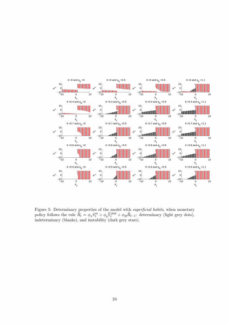
Figure 5 details the determinacy properties of this rule when habits are of the superfi-

cial form. Each sub-plot details the combinations of φπ and φy which ensure determinacy

(light grey dots), indeterminacy (blanks) and instability (dark grey stars). Moving from

left to right across subplots increases the degree of interest rate inertia in the rule, φR,

while moving down the page increases the extent of habits formation, θ. Consider the

first sub-plot in the top left hand corner with φR = 0 and θ = 0, which re-states the sta-

bility properties of the original Taylor rule. Here the importance of the Taylor principle

is revealed as φπ > 1 in combination with a non-negative response to the output gap

is a sufficient condition for determinacy. Within this region there is limited scope for

compensating for failing to fulfil the Taylor principle through increasing the positive re-

sponse of the interest rate to the output gap, and there is slightly greater scope for using

a more aggressive monetary policy response to compensate for a mildly negative interest

rate response to the output gap. It is also interesting to note that a second region of

determinacy exists where the interest rate rule fails to satisfy the Taylor principle, such

that φπ < 1, and the response to the output gap is strongly negative. This region is not

often discussed in the literature, but is mentioned in Rotemberg and Woodford (1999).

Typically, when monetary policy fails to satisfy the Taylor principle inflation can be

driven by self-fulfilling expectations which are validated by monetary policy. However,

when the output gap response is sufficiently negative there is an additional destabilising

element in policy, which overturns the excessive stability generated by a passive mon-

etary policy, implying a unique saddlepath where any deviation from that saddlepath

will imply an explosive path for inflation.

As we move down the sub-plots in the first column of Figure 5 we increase the degree

of superficial habits. This means that the output response to both policy and shocks is

more muted as current consumption is increasingly tied to past levels of consumption.

This has two effects on the determinacy properties of the basic Taylor rule. Firstly, a

rule which satisfies the Taylor principle will do so even if the response to the output

gap is increasingly negative. Secondly, the additional instability caused by adopting a

6Furthermore, adopting a rule specified in terms of CPI inflation when habits are of the deep kindcan induce cyclical responses to shocks which are not conducive to mimicing the optimal response toshocks. These results are available from the authors upon request.

16

negative interest rate response to the output gap becomes insufficient to move a passive

interest rate rule to a position of determinacy. Accordingly, the importance of the Taylor

principle is enhanced when consumption is subject to superficial habits effects.

As we move across the page from left to right we increase the extent of interest rate

inertia in the rule. In this case, as Woodford (2001) shows, the Taylor principle needs to

be rewritten in terms of the long-run interest rate response to excess inflation, φπ1−φR

> 1.

As a result, the determinacy region in the positive quadrant spreads further into the

adjacent quadrants since a given level of instantaneous policy response to inflation φπ

has a far greater long-run effect.

Finally, when we combine superficial habits effects with interest rate inertia, it be-

comes possible to induce instability in our economy when the rule is passive, φπ1−φR

< 1,

and the interest rate response to the output gap is negative, φy < 0. Essentially, the

slow evolution of consumption under habits combined with interest rate inertia and a

perverse policy response to output gaps and inflation serves to induce a cumulative

instability in the model.

Figure 6 constructs a similar set of sub-plots when habits are of the deep, rather

than superficial, kind. If the extent of habits formation is relatively low, the deter-

minacy properties of the model are similar to those observed under superficial habits.

However, when the degree of habits formation exceeds θ > 0.77, then there are some

significant differences. Firstly, the usual determinacy region in the positive quadrant

disappears and becomes indeterminant. This indeterminacy is linked to the additional

dynamics displayed in the final goods sectors, where the markup is time-varying under

deep habits formation. Suppose economic agents expect an increase in inflation. Given

an active interest rate rule, φπ > 1, this will give rise to a tightening of monetary policy.

Typically, such a policy would lead to a contraction in aggregate demand, invalidating

the inflation expectations. However, in the presence of deep habits, the higher real

interest rates will encourage final goods firms to raise current mark-ups as they dis-

count the lost future sales such price increases would imply more heavily. If the size of

habits effects is sufficiently large, then this increase in mark-ups can validate the initial

increase in inflationary expectations, leading to self-fulfilling inflationary episodes and

indeterminacy.

Furthermore, the region of instability identified under superficial habits, becomes

determinate when combined with the excessive stability implied by endogenous mark-

up behaviour, such that the only determinant rule in the presence of a large deep habits

effect is where the rule is passive, φπ1−φR

< 1, and the policy response to the output gap

is sufficiently strongly negative.

Optimal Rules Having explored the determinacy properties of the simple rule

described above when embedded in our economy featuring either superficial or deep

17

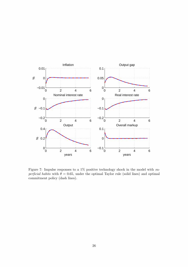
habits, we now turn to consider the optimal parameterisation of the rule in each case.7

In the case of superficial habits and under the benchmark value of θ = 0.65, the optimal

rule implies a lot of interest rate smoothing, with a strong positive response to inflation

but a negative response to the output gap (φπ = 18.47, φy = −0.09, and φR = 0.93).

With this type of optimal monetary policy rule, the economy’s response to a technology

shock essentially replicates the responses obtained under a full commitment policy, as

shown in Figure 7. To explore the intuition underpinning this result, Figure 8 explores

how the optimal policy rule parameters vary with the degree of habits formation, θ.

In the absence of habits effects, in a New Keynesian economy, a positive technology

shock leads to a decrease in inflation and, due to the nominal inertia, an insufficiently

large increase in output. Optimally, a decrease in the nominal interest rate stimulates

demand by reducing the real interest rate. This can be achieved by having a very large

coefficient on inflation relative to all other parameters, which essentially allows the simple

policy rule to achieve the flex-price equilibrium with zero inflation and a zero output

gap. As we introduce superficial habits effects, in the face of the same shock households

overconsume and the output gap becomes positive suggesting that policy be tightened

rather than relaxed. This trade-off, which is not present in the model without external

habits, affects the optimal parameterisation of the simple policy rule. Specifically, as

we increase the degree of habits formation, the optimal parameter on inflation in the

simple rule falls and the extent of interest rate inertia increases. Furthermore, the

negative coefficient on the output gap also falls, eventually turning positive.

A key feature of optimal policy under commitment is price level control where the

optimal policy achieves expectational benefits in seeking to ensure that price level returns

to base following any shock. As the degree of superficial habits formation is increased,

this price level control can be achieved most effectively through a combination of interest

rate inertia and output gap response. Consider the impact of the positive technology

shock depicted in Figure 7. Essentially, the rule is able to maintain a cut in real interest

rates, even when inflation is slightly positive (to undo the price level effects of the initial

fall in inflation), by responding negatively to the persistent positive output gap and

maintaining that stance for longer by increasing the amount of interest rate inertia.

When the degree of habits formation becomes sufficiently large, the coefficient on the

output gap becomes positive in order to reduce the initial relaxation of policy, and the

degree of interest rate inertia is increased to ensure price level control.

Figure 9 plots the optimal parameters of the simple rule, when the economy features

an increasing level of deep habits formation. When habits are deep there is less of a

desire to cut interest rates initially, to prevent final goods firms’ cutting their mark-

ups and generating even greater consumption externalities. For relatively low levels

7We search across the rule parameter space using the Simplex method employed by the Fminsearchalgorithm in Matlab (see, Lagarias, Reeds, Wright, and Wright (1998)) in order to minimise the uncon-ditional welfare losses associated with the rule.

18

of habits, this implies a more muted response to inflation and output gaps. However,

there is a surprising ‘blip’ in the optimal parameters for intermediate levels of the deep

habits effect. At intermediate levels of deep habits this desire to tighten policy is finely

balanced against the need to avoid falls in intermediate goods inflation which induces

undesirable increases in price dispersion. Despite the large rule parameters this implies,

the rule still successfully mimics optimal policy under commitment, and the simple rule

in all cases comes close to achieving the welfare levels observed under commitment - see

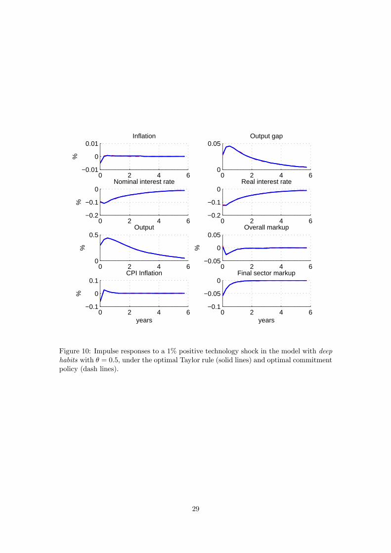
Figure 10 for an illustration of impulse responses to a technology shock in the case of

θ = 0.5.

5 Conclusion

In this paper we considered the optimal policy response to technology shocks in a New

Keynesian economy subject to habits effects in consumption. These effects were as-

sumed to be external, such that one household fails to take account of the impact their

consumption behaviour has on other households as each household seeks to ‘catch up

with the Joneses’. This consumption externality needs to be traded-off against the mon-

etary policy maker’s usual desire to stabilise inflation (a trade-off which would not exist

if habits were internal) and generates a new form of stabilisation bias as time consistent

policy is unable to mimic the initial policy response under commitment. This framework

is further enriched by allowing the habits effects to be either superficial (at the level of

household’s total consumption) or deep (at the level of individual consumption goods).

Under deep habits, firms face dynamic demand curves which imply an intertemporal

dimension to price setting and endogenous mark-up behaviour. This, in turn, further

modifies the optimal policy response to technology shocks when habits are deep.

In addition to considering optimal policy, we also consider the stabilising proper-

ties of simple rules. We investigate the determinacy properties of such rules and find

that superficial habits effects tend to increase the range of parameters consistent with

determinacy, provided the Taylor principle is satisfied. However, for sufficiently large

measures of deep habits (which fall within the range of econometric estimates) the Tay-

lor principle ceases to be either a necessary or sufficient condition for determinacy. We

demonstrate that optimally parameterised determinate simple rules can typically come

close to achieving the welfare levels observed under optimal commitment policy. Overall

our work suggests that the choice of internal or external habits effects will have non

trivial implications for optimal policy, even if the implied dynamics of the model when

policy is described by an ad hoc rule could be similar (Kozicki and Tinsley (2002)).

19

0 2 4 6−0.01

0

0.01Inflation

%

0 2 4 60

0.05

0.1Output gap

0 2 4 6−0.2

−0.1

0Nominal interest rate

%

0 2 4 6−0.2

−0.1

0Real interest rate

0 2 4 60

0.5Output

years

%

0 2 4 6−0.1

0

0.1Overall markup

years

Figure 1: Impulse responses to a 1% positive technology shock under optimal commit-ment policy, in the case of superficial habits: θ = 0.4 (dash lines), θ = 0.65 (benchmarkvalue, pluses), θ = 0.75 (solid lines).

20

0 2 4 6−0.02

0

0.02Producer price inflation

%

0 2 4 60

0.05

0.1Output gap

0 2 4 6−0.2

−0.1

0Nominal interest rate

%

0 2 4 6−0.2

0

0.2Real interest rate

0 2 4 60

0.2

0.4Output

%

0 2 4 6−0.1

0

0.1Overall markup

0 2 4 6−0.1

0

0.1CPI Inflation

years

%

0 2 4 6−0.2

0

0.2Final sector markup

years

Figure 2: Impulse responses to a 1% positive technology shock under optimal commit-ment policy, in the case of deep habits for θ = 0.65 (benchmark value, solid lines) andθ = 0.75 (dash lines).

21

0 2 4 6−0.01

0

0.01Inflation

%

0 2 4 60

0.05

0.1Output gap

0 2 4 6−0.2

−0.1

0Nominal interest rate

%

0 2 4 6−0.2

−0.1

0Real interest rate

0 2 4 60

0.2

0.4Output

years

%

0 2 4 6−0.1

0

0.1Overall markup

years

Figure 3: Impulse responses to a 1% positive technology shock in the case of superficialhabits under optimal policy with commitment (solid lines) and with discretion (dashlines).

22

0 2 4 6−0.02

0

0.02Producer price inflation

%

0 2 4 60

0.05

0.1Output gap

0 2 4 6−0.2

−0.1

0Nominal interest rate

%

0 2 4 6−0.2

−0.1

0Real interest rate

0 2 4 60

0.2

0.4Output

%

0 2 4 6−0.1

0

0.1Overall markup

0 2 4 6−0.2

0

0.2CPI Inflation

years

%

0 2 4 6−0.2

−0.1

0Final sector markup

years

Figure 4: Impulse responses to a 1% positive technology shock in the case of deep habitsunder optimal policy with commitment (solid lines) and with discretion (dash lines).

23

−10 0 10−10

0

10

θ =0 and φR

=1.1

φπ

φ y

−10 0 10−10

0

10

θ =0.4 and φR

=1.1

φπ

φ y

−10 0 10−10

0

10

θ =0.7 and φR

=1.1

φπ

φ y

−10 0 10−10

0

10

θ =0.8 and φR

=1.1

φπ

φ y

−10 0 10−10

0

10

θ =0.9 and φR

=1.1

φπ

φ y

−10 0 10−10

0

10

θ =0 and φR

=0.9

φπ

φ y

−10 0 10−10

0

10

θ =0.4 and φR

=0.9

φπ

φ y

−10 0 10−10

0

10

θ =0.7 and φR

=0.9

φπ

φ y

−10 0 10−10

0

10

θ =0.8 and φR

=0.9

φπ

φ y

−10 0 10−10

0

10

θ =0.9 and φR

=0.9

φπ

φ y

−10 0 10−10

0

10

θ =0 and φR

=0.5

φπ

φ y

−10 0 10−10

0

10

θ =0.4 and φR

=0.5

φπ

φ y

−10 0 10−10

0

10

θ =0.7 and φR

=0.5

φπ

φ y

−10 0 10−10

0

10

θ =0.8 and φR

=0.5

φπ

φ y

−10 0 10−10

0

10

θ =0.9 and φR

=0.5

φπ

φ y−10 0 10

−10

0

10

θ =0 and φR

=0

φπ

φ y

−10 0 10−10

0

10

θ =0.4 and φR

=0

φπ

φ y

−10 0 10−10

0

10

θ =0.7 and φR

=0

φπ

φ y

−10 0 10−10

0

10

θ =0.8 and φR

=0

φπ

φ y

−10 0 10−10

0

10

θ =0.9 and φR

=0

φπ

φ y

Figure 5: Determinacy properties of the model with superficial habits, when monetarypolicy follows the rule bRt = φπbπmt + φy bY gap

t + φR bRt−1: determinacy (light grey dots),indeterminacy (blanks), and instability (dark grey stars).

24

−10 0 10−10

0

10

θ =0 and φR

=0

φπ

φ y

−10 0 10−10

0

10

θ =0.4 and φR

=0

φπ

φ y

−10 0 10−10

0

10

θ =0.7 and φR

=0

φπ

φ y

−10 0 10−10

0

10

θ =0.8 and φR

=0

φπ

φ y

−10 0 10−10

0

10

θ =0.9 and φR

=0

φπ

φ y

−10 0 10−10

0

10

θ =0 and φR

=0.5

φπ

φ y

−10 0 10−10

0

10

θ =0.4 and φR

=0.5

φπ

φ y

−10 0 10−10

0

10

θ =0.7 and φR

=0.5

φπ

φ y

−10 0 10−10

0

10

θ =0.8 and φR

=0.5

φπ

φ y

−10 0 10−10

0

10

θ =0.9 and φR

=0.5

φπ

φ y−10 0 10

−10

0

10

θ =0 and φR

=0.9

φπ

φ y

−10 0 10−10

0

10

θ =0.4 and φR

=0.9

φπ

φ y

−10 0 10−10

0

10

θ =0.7 and φR

=0.9

φπ

φ y

−10 0 10−10

0

10

θ =0.8 and φR

=0.9

φπ

φ y

−10 0 10−10

0

10

θ =0.9 and φR

=0.9

φπ

φ y

−10 0 10−10

0

10

θ =0 and φR

=1.1

φπ

φ y

−10 0 10−10

0

10

θ =0.4 and φR

=1.1

φπ

φ y

−10 0 10−10

0

10

θ =0.7 and φR

=1.1

φπ

φ y

−10 0 10−10

0

10

θ =0.8 and φR

=1.1

φπ

φ y

−10 0 10−10

0

10

θ =0.9 and φR

=1.1

φπ

φ y

Figure 6: Determinacy properties of the model with deep habits, when monetary pol-icy follows the rule bRt = φπbπmt + φy bY gap

t + φR bRt−1: determinacy (light grey dots),indeterminacy (blanks), and instability (dark grey stars).

25

0 2 4 6−0.01

0

0.01Inflation

%

0 2 4 60

0.05

0.1Output gap

0 2 4 6−0.2

−0.1

0Nominal interest rate

%

0 2 4 6−0.2

−0.1

0Real interest rate

0 2 4 60

0.2

0.4Output

years

%

0 2 4 6−0.1

0

0.1Overall markup

years

Figure 7: Impulse responses to a 1% positive technology shock in the model with su-perficial habits with θ = 0.65, under the optimal Taylor rule (solid lines) and optimalcommitment policy (dash lines).

26

0.1 0.2 0.3 0.4 0.5 0.6 0.7 0.8 0.9−40

−20

0

20

40

60

80

100

120

140

θ

φ π and

φy

0.1 0.2 0.3 0.4 0.5 0.6 0.7 0.8 0.90

0.2

0.4

0.6

0.8

1

1.2

1.4

φ R

φR

φπ

φy

Figure 8: Optimal policy rule parameters for varying degrees of superficial habits.

27

0.1 0.2 0.3 0.4 0.5 0.6 0.7 0.8 0.9−100

0

100

200

300

400

500

600

θ

φ π and

φy

0.1 0.2 0.3 0.4 0.5 0.6 0.7 0.8 0.90

5

10

15

20

25

30

35

40

45

φ R

φπ

φy

φR

Figure 9: Optimal policy rule parameters for varying degrees of deep habits.

28

0 2 4 6−0.01

0

0.01Inflation

%

0 2 4 60

0.05Output gap

0 2 4 6−0.2

−0.1

0Nominal interest rate

%

0 2 4 6−0.2

−0.1

0Real interest rate

0 2 4 60

0.5Output

%

0 2 4 6−0.05

0

0.05Overall markup

%

0 2 4 6−0.1

0

0.1CPI Inflation

years

%

0 2 4 6−0.1

−0.05

0Final sector markup

years

Figure 10: Impulse responses to a 1% positive technology shock in the model with deephabits with θ = 0.5, under the optimal Taylor rule (solid lines) and optimal commitmentpolicy (dash lines).

29

A Analytical Details

A.1 Households

Cost Minimization Households decide the composition of the consumption bas-

ket to minimize expenditures

minCk

iti

Z 1

0PitC

kitdi

s.t.

µZ 1

0

³Ckit − θCit−1

´ η−1η

di

¶ ηη−1≥ X

kt

The demand for individual goods i is

Ckit =

µPitPt

¶−ηXkt + θCit−1,

where Pt is the overall price level, expressed as an aggregate of the good i prices, Pt =³R 10 P

1−ηit di

´ 11−η

.

Utility Maximization The solution to the utility maximization problem is ob-

tained by solving the Lagrangian function,

L = E0

∞Xt=0

βthu³Xkt , N

kt

´− λkt

³PtX

kt + Ptϑt +EtQt,t+1D

kt+1 −WtN

kt −Dk

t −Φkt + T kt

´i.

In the budget constraint, we have re-expressed the total spending on the consumption

basket,R 10 PitC

kitdi, in terms of quantities that affect the household’s utility,Z 1

0PitC

kitdi = PtX

kt + Ptϑt

where under deep habits ϑt is given as ϑt ≡ θR 10

³PitPt

´Cit−1di, while under superfi-

cial habits it takes the simpler form, ϑt ≡ θCt−1. Households take ϑt as given when

maximising utility.

The first order conditions are then,¡Xkt

¢: uX(t) = λktPt¡

Nkt

¢: −uN (t) = uX(t)

WtPt¡

Dkt

¢: 1 = βEt

huX(t+1)uX(t)

PtPt+1

iRt

where Rt =1

Et[Qt,t+1]is the one-period gross return on nominal riskless bonds.

30

With utility given by u (X,N) = X1−σ

1−σ − χN1+υ

1+υ , the first derivatives are

uX (·) = X−σ and uN (·) = −χNυ.

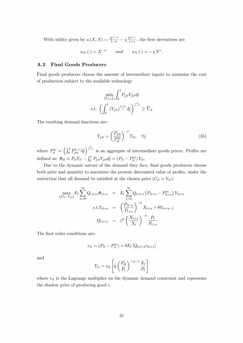
A.2 Final Goods Producers

Final goods producers choose the amount of intermediate inputs to minimize the cost

of production subject to the available technology

minYjitj

Z 1

0PjitYjitdj

s.t.

µZ 1

0(Yjit)

ε−1ε dj

¶ εε−1≥ Y it

The resulting demand functions are:

Yjit =

µPjitPmit

¶−εYit, ∀j (35)

where Pmit =

³R 10 P

1−εjit dj

´ 11−ε is an aggregate of intermediate goods prices. Profits are

defined as: Φit ≡ PitYit −R 10 PjitYjitdj = (Pit − Pm

it )Yit.

Due to the dynamic nature of the demand they face, final goods producers choose

both price and quantity to maximize the present discounted value of profits, under the

restriction that all demand be satisfied at the chosen price (Cit = Yit):

maxPit, Yit

Et

∞Xs=0

Qt,t+sΦit+s = Et

∞Xs=0

Qt,t+s

¡Pit+s − Pm

it+s

¢Yit+s

s.t.Yit+s =

µPit+sPt+s

¶−ηXt+s + θYit+s−1

Qt,t+s = βsµXt+s

Xt

¶−σ PtPt+s

The first order conditions are:

vit = (Pit − Pmit ) + θEt [Qt,t+1vit+1]

and

Yit = vit

"η

µPitPt

¶−η−1 Xt

Pt

#where vit is the Lagrange multiplier on the dynamic demand constraint and represents

the shadow price of producing good i.

31

A.3 Intermediate Goods Producers

The cost minimization of brand producers involves the choice of labour inputNjit subject

to the available production technology

minNjit

(1− κ)WtNjit

s.t. AtNjit = Yjit

Costs are subsidized at rate κ, which is determined to ensure that the long-run equilib-rium of the economy is efficient. The minimization problem implies a labour demand,

Njit =YjitAt, and a nominal marginal cost which is the same across all brand producing

firms MCt = (1− κ) WtAt. Profits are defined as:

Φjit ≡ PjitYjit − (1− κ)WtNjit = PjitYjit − (1− κ)WtYjitAt

= (Pjit −MCt)Yjit

The profit maximization is subject to the Calvo-style of price setting behavior where,

with fixed probability (1− α) each period, a firm can set its price and with probability α

the firm keeps the price from the previous period. When a firm can set the price it does

so in order to maximize the present discounted value of profits, subject to the demand

for its own goods. Profits are discounted by the stochastic discount factor, adjusted for

the probability of not being able to set prices in future periods:

maxP∗jit

Et

∞Xs=0

αsQt,t+sΦjit+s = Et

∞Xs=0

αsQt,t+s

£¡P ∗jit −MCt+s

¢Yjit+s

¤s.t.Yjit+s =

µP ∗jitPmit+s

¶−εYit+s

Qt,t+s = βsµXt+s

Xt

¶−σ PtPt+s

Optimally, the relative price is set at

P ∗jitPt

=

µε

ε− 1

¶ Et

∞Xs=0

(αβ)s (Xt+s)−σmct+s

¡Pmit+s

¢εYit+s

Et

∞Xs=0

(αβ)s (Xt+s)−σ³Pt+sPt

´−1 ¡Pmit+s

¢εYit+s

where mct =MCtPt

is the real marginal cost. The relative price can also be expressed as

P ∗jitPt

=

µε

ε− 1

¶K1t

K2t

32

where K1t and K2t have a recursive representation:

K1t ≡ Et

∞Xs=0

(αβ)s (Xt+s)−σmct+s

¡Pmit+s

¢εYit+s

= X−σt mct μ

−εt Yt + αβEt

£K1t+1π

εt+1

¤and

K2t ≡ Et

∞Xs=0

(αβ)s (Xt+s)−σµPt+sPt

¶−1 ¡Pmit+s

¢εYit+s

= X−σt μ−εt Yt + αβEt

£K2t+1π

ε−1t+1

¤

B Equilibrium Conditions

B.1 Aggregation and Symmetry

Aggregate Output: The market clearing condition at the level of intermediate

goods is µPjitPmit

¶−εYit = AtNjit, ∀j, ∀i

which, upon aggregation across the j firms, becomes:

Yit∆it = AtNit, ∀i

where ∆it ≡Z 1

0

³PjitPmit

´−εdj represents intermediate goods price dispersion in sector i.

With final goods producing sectors being symmetric, we can drop the i subscript and

write the aggregate production function as

Yt = AtNt

∆t.

Aggregate Profits: The economy wide profits are given by the aggregate profits

from final goods producers and intermediate goods producers:

Φt =

Z 1

0Φitdi+

Z 1

0

Z 1

0Φjitdjdi

=

Z 1

0PitYitdi− (1− κ)WtNt

= PtYt − (1− κ)WtNt

where we have used the assumption of symmetric final goods sectors to obtain the final

result.

33

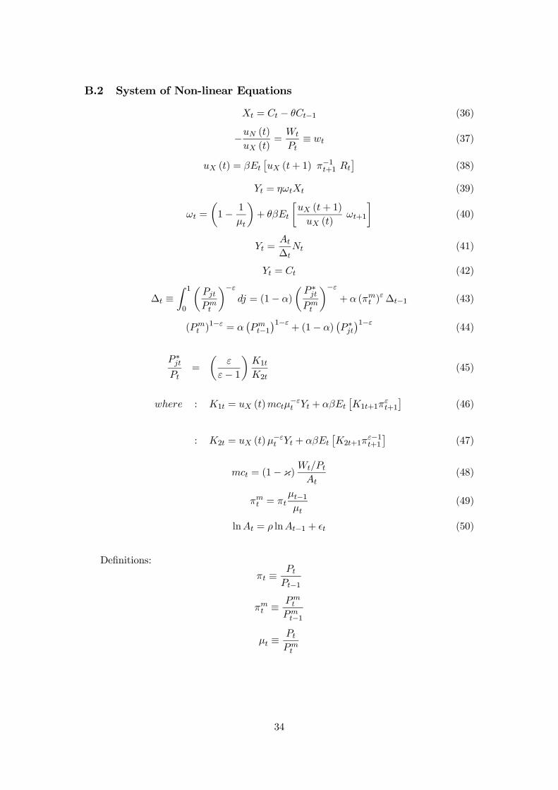
B.2 System of Non-linear Equations

Xt = Ct − θCt−1 (36)

−uN (t)uX (t)

=Wt

Pt≡ wt (37)

uX (t) = βEt

£uX (t+ 1) π−1t+1 Rt

¤(38)

Yt = ηωtXt (39)

ωt =

µ1− 1

μt

¶+ θβEt

∙uX (t+ 1)

uX (t)ωt+1

¸(40)

Yt =At

∆tNt (41)

Yt = Ct (42)

∆t ≡Z 1

0

µPjtPmt

¶−εdj = (1− α)

µP ∗jtPmt

¶−ε+ α (πmt )

ε∆t−1 (43)

(Pmt )

1−ε = α¡Pmt−1¢1−ε

+ (1− α)¡P ∗jt¢1−ε (44)

P ∗jtPt

=

µε

ε− 1

¶K1t

K2t(45)

where : K1t = uX (t)mctμ−εt Yt + αβEt

£K1t+1π

εt+1

¤(46)

: K2t = uX (t)μ−εt Yt + αβEt

£K2t+1π

ε−1t+1

¤(47)

mct = (1− κ)Wt/PtAt

(48)

πmt = πtμt−1μt

(49)

lnAt = ρ lnAt−1 + t (50)

Definitions:

πt ≡PtPt−1

πmt ≡Pmt

Pmt−1

μt ≡PtPmt

34

B.3 The Deterministic Steady State

The non-stochastic long-run equilibrium is characterized by constant real variables and

nominal variables growing at a constant rate. The equilibrium conditions (36) - (50)

reduce to:

X = (1− θ)C (51)

χNυXσ = w (52)

1 = β¡Rπ−1

¢= βr (53)

ω = [(1− θ) η]−1 (54)

μ = [1− (1− θβ)ω]−1 (55)

Y = AN

∆(56)

Y = C (57)

∆ =1− α

1− α (πm)ε

µP ∗

P

¶−εμ−ε (58)

1 = α (πm)ε−1 + (1− α)

µP ∗

P

¶1−εμ1−ε (59)

P ∗

P=

ε

ε− 1K1

K2=

∙ε

ε− 11− αβπε−1

1− αβπε

¸mc (60)

K1 =uX mc μ−εY

1− αβπε(61)

K2 =uX μ−εY

1− αβπε−1(62)

mc = (1− κ) wA

(63)

πm = π

A = 1

Table 1 contains the imposed calibration restrictions. We assume values for the

real interest rate, the Frisch labour supply elasticity, the steady state inflation, and the

following parameters, σ, η, ε, α, θ, and χ. The discount factor β matches the assumed

real rate of interest, β = r−1, while, given the specification of the utility function, υ is

the inverse of the Frisch labour supply elasticity, Nw =1υ .

The steady state values of the shadow price ω and the markup μ are given by

equations (54) and (55). The relative price P∗

P can then be obtained from equation (59)

35

as,P ∗

P=

∙1

1− α

³1− α (πm)ε−1

´¸ 11−ε

μ−1.

while equation (58) gives the steady state value of price dispersion ∆ and, from equation

(60), the marginal cost is

mc =

µP ∗

P

¶ ∙ε

ε− 11− αβπε−1

1− αβπε

¸−1.

Under the assumption of zero steady state inflation (π = πm = 1), the following long-run

equilibrium expressions simplify to:

P ∗

P=1

μ

∆ = 1

mc =1

μ

µε− 1ε

¶.

To determine the steady state value of labour, we substitute for X in terms of

Y in (52) and then, using the aggregate production function, we obtain the following

expression,

χNσ+υ [(1− θ)A]σ = w, (64)

which can be solved for N . Note that this expression depends on the real wage w, which

can be obtained from equation (63). However, in order to make the long-run equilibrium

efficient, we impose the condition

w = 1− θβ.

This condition is equivalent to setting the cost subsidy κ so as to ensure that the allo-cation under the decentralized equilibrium (64) matches the social planner’s allocation

(75), i.e. κ = 1− 11−θβ

³1με−1ε

´. See Appendix D for the social planner’s problem.

Finally, equations (56), (57), and (51) can be solved for aggregate output Y , con-

sumption C and habit-adjusted consumption X.

36

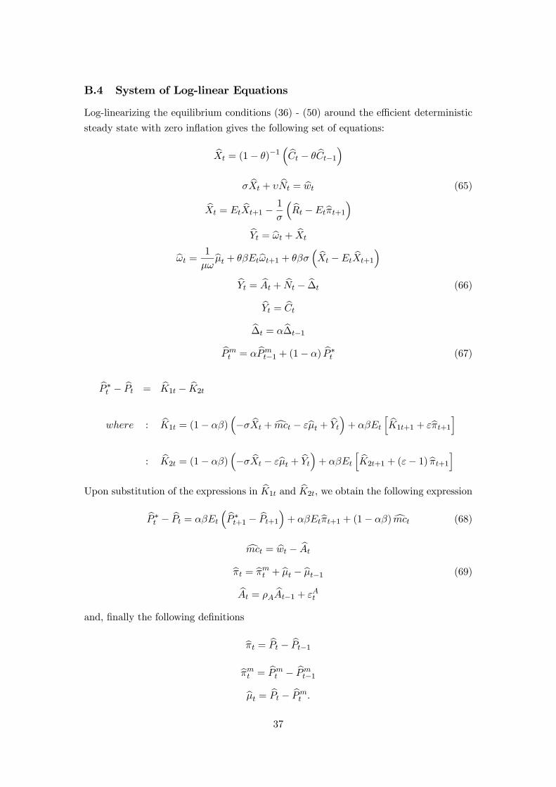
B.4 System of Log-linear Equations

Log-linearizing the equilibrium conditions (36) - (50) around the efficient deterministic

steady state with zero inflation gives the following set of equations:

bXt = (1− θ)−1³ bCt − θ bCt−1

´σ bXt + υ bNt = bwt (65)

bXt = EtbXt+1 −

1

σ

³ bRt −Etbπt+1´bYt = bωt + bXt

bωt = 1

μωbμt + θβEtbωt+1 + θβσ

³ bXt −EtbXt+1

´bYt = bAt + bNt − b∆t (66)

bYt = bCtb∆t = αb∆t−1bPmt = α bPm

t−1 + (1− α) bP ∗t (67)

bP ∗t − bPt = bK1t − bK2t

where : bK1t = (1− αβ)³−σ bXt + cmct − εbμt + bYt´+ αβEt

h bK1t+1 + εbπt+1i: bK2t = (1− αβ)

³−σ bXt − εbμt + bYt´+ αβEt

h bK2t+1 + (ε− 1) bπt+1iUpon substitution of the expressions in bK1t and bK2t, we obtain the following expression

bP ∗t − bPt = αβEt

³ bP ∗t+1 − bPt+1´+ αβEtbπt+1 + (1− αβ) cmct (68)

cmct = bwt − bAt

bπt = bπmt + bμt − bμt−1 (69)

bAt = ρA bAt−1 + εAt

and, finally the following definitions

bπt = bPt − bPt−1bπmt = bPm

t − bPmt−1

bμt = bPt − bPmt .

37

Combine equations (68), (67), (69), together with the definitions of producer price

inflation and markup to obtain a New Keynesian Phillips Curve in terms of producer

inflation bπmt = βEtbπmt+1 + ∙(1− αβ) (1− α)

α

¸(cmct + bμt) ,

while the real marginal cost can be re-written as

cmct = σ bXt + υbYt − (1 + υ) bAt,

where we have used the first order conditions (65) to substitute for the real wage bwt,

and the production function (66) and the fact that price dispersion in the linear model

is deterministic to write bNt = bYt − bAt.

38

C Model with Superficial Habits

C.1 Households

Habits are “superficial” when they are formed at the level of the aggregate consumption

good. Households derive utility from the habit-adjusted composite good Xkt ,

Xkt = Ck

t − θCt−1

where household k’s consumption, Ckt , is an aggregate of a continuum of final goods,

indexed by i ∈ [0, 1] ,

Ckt =

µZ 1

0

³Ckit

´η−1η

di

¶ ηη−1

with η > 1 the elasticity of substitution between them and Ct−1 ≡R 10 C

kt−1dk the cross-

sectional average of consumption.

Cost Minimization Households decide the composition of the consumption bas-

ket to minimize expenditures

minCk

iti

Z 1

0PitC

kitdi

s.t.

µZ 1

0

³Ckit

´ η−1η

di

¶ ηη−1≥ C

kt

The demand for individual goods i is

Ckit =

µPitPt

¶−ηCkt

where Pt ≡³R 10 P

1−ηit di

´ 11−η

is the consumer price index. The overall demand for good

i is obtained by aggregating across all households

Cit =

Z 1

0Ckitdk =

µPitPt

¶−ηCt. (70)

Unlike in the case of deep habits, this demand is not dynamic.

C.2 Final Goods Producers

Final goods producers’ cost minimization problem is unchanged. However, the profit

maximization is the typical static problem whereby firms choose the price to maximize

current profits, Φit = (Pit − Pmit )Yit, subject to the demand for their good (70) and

under the restriction that all demand be satisfied at the chosen price (Cit = Yit). The

39

optimal price is set at a constant markup, μ = ηη−1 , over the marginal cost,

Pit = μPmit .

C.3 Equilibrium

With a constant markup in the final goods sectors, the system of equilibrium conditions

(36) - (50) in appendix B changes along the following dimensions: in a symmetric

equilibrium, producer price inflation equals CPI inflation, πt = πmt . We impose a

constant markup, μt = μ, in the pricing equation of intermediate goods firms and we

exclude equations (39) and (40), which are no longer valid under constant markup at

the level of final goods producers.

In this setup, we obtain the familiar looking New Keynesian Phillips Curve,

bπt = βEtbπt+1 + κcmct, κ ≡ (1− αβ) (1− α)

α, (71)

to which we add the IS curve

bXt = EtbXt+1 −

1

σbRt +

1

σEtbπt+1 (72)

and two equations defining real marginal cost and habit-adjusted consumption,

bXt =1

1− θ

³bYt − θbYt−1´ (73)

cmct = σ bXt + υbYt − (1 + υ) bAt. (74)

40

D The Social Planner’s Problem

The subsidy level that ensures an efficient long-run equilibrium is obtained by comparing

the steady state solution of the social planner’s problem with the steady state obtained

in the decentralized equilibrium. The social planner ignores the nominal inertia and

all other inefficiencies and chooses real allocations that maximize the representative

consumer’s utility subject to the aggregate resource constraint, the aggregate production

function, and the law of motion for habit-adjusted consumption:

maxX∗t ,C∗t ,N∗t

E0

∞Xt=0

βtu (X∗t , N

∗t )

s.t. Y ∗t = C∗t

Y ∗t = AtN∗t

X∗t = C∗t − θC∗t−1

The optimal choice implies the following relationship between the marginal rate

of substitution between labour and habit-adjusted consumption and the intertemporal

marginal rate of substitution in habit-adjusted consumption

χ (N∗t )

υ

(X∗t )−σ = At

"1− θβEt

µX∗t+1

X∗t

¶−σ#.

The steady state equivalent of this expression can be written as,

χ (N∗)υ+σ [(1− θ)A]σ = A (1− θβ) . (75)

The dynamics of this model are driven by technology shocks to the system of equilib-

rium conditions composed of the Euler equation, the resource contraint and the evolution

of habit-adjusted consumption. In log-linear form, these are:

bX∗t = θβEt

bX∗t+1 +

1− θβ

σ

³−υ bN∗

t + bAt

´bY ∗t = bAt + bN∗

t

bX∗t =

1

1− θ

³bY ∗t − θbY ∗t−1´ ,which combined yield the following dynamic equation

bY ∗t = θβζEtbY ∗t+1 + θζ bY ∗t−1 +µ1 + υ

δ

¶ζ bAt

where ζ ≡¡1 + θ2β + υ

δ

¢−1and δ ≡ σ

(1−θβ)(1−θ) . In the absence of deep habits, θ = 0,

the model reduces to the basic New Keynesian model where bY ∗t = ³ 1+υσ+υ

´ bAt.

41

E Derivation of Welfare

Individual utility in period t isX1−σt

1− σ− χ

N1+υt

1 + υ

where Xt = Ct−θCt−1 is the habit-adjusted aggregate consumption. Before considering

the elements of the utility function, we need to note the following general result relating

to second order approximations

Yt − Y

Yt= bYt + 1

2bY 2t +O[2]

where bYt = ln¡YtY

¢and O[2] represents terms that are of order higher than 2 in the

bound on the amplitude of the relevant shocks. This will be used in various places in

the derivation of welfare. Now consider the second order approximation to the first

term,X1−σt

1− σ= X

1−σµXt −X

X

¶− σ

2X1−σ

µXt −X

X

¶2+ tip+O[2]

where tip represents ‘terms independent of policy’. Using the results above this can be

rewritten in terms of hatted variables

X1−σt

1− σ= X

1−σ½ bXt +

1

2(1− σ) bX2

t

¾+ tip+O[2].

In pure consumption terms, the value of Xt can be approximated to second order

by: bXt =1

1− θ

µbCt +1

2bC2t¶− θ

1− θ

µbCt−1 +1

2bC2t−1¶− 12 bX2

t +O[2]

To a first order, bXt =1

1− θbCt −

θ

1− θbCt−1 +O[1]

which implies bX2t =

1

(1− θ)2

³ bCt − θ bCt−1´2+O[2]

Therefore,

X1−σt

1− σ= X

1−σ½

1

1− θ

µbCt +1

2bC2t¶− θ

1− θ

µbCt−1 +1

2bC2t−1¶+ 12 (−σ) bX2

t

¾+tip+O[2]

Summing over the future,

∞Xt=0

βtX1−σt

1− σ= X

1−σ∞Xt=0

βt½1− θβ

1− θ

µbCt +1

2bC2t ¶− 12σ bX2

t

¾+ tip+O[2].

42

The term in labour supply can be written as

χN1+υt

1 + υ= χN

1+υ½ bNt +

1

2(1 + υ) bN2

t

¾+ tip+O[2]

Now we need to relate the labour input to output and a measure of price dispersion.

Aggregating the individual firms’ demand for labour yields

Nt =

Z 1

0

µYitAt

¶Z 1

0

µPjitPmit

¶−εdjdi.

Note that in the absence of any sector specific shocks or heterogeneity, Yit = Yt. It can

be shown (see Woodford (2003), Chapter 6) that

bNt = bYt − bAt + ln

"Z 1

0

µPjitPmit

¶−εdi

#= bYt − bAt +

ε

2varjpjit+O[2]

so we can write

χN1+υt

1 + υ= χN

1+υ½bYt + 1

2(1 + υ) bY 2t − (1 + υ) bYt bAt +

ε

2varjpjit

¾+ tip+O[2]

Welfare is then given by

Γ0 = X1−σ

E0

∞Xt=0

βt½1− θβ

1− θ

µbCt +1

2bC2t ¶− 12σX2

t

¾

−χN1+υE0

∞Xt=0

βt½bYt + 1

2(1 + υ) bY 2t − (1 + υ) bYt bAt +

ε

2varjpjit

¾

+tip+O[2]

From the social planner’s problem we know, X−σ(1− θβ) = χN

υsuch that X

1−σ(1−

θβ) = (1 − θ)χN1+υ. If we use the appropriate subsidy to render the steady-state

efficient and the second order approximation to the national accounting identity,

bCt = bYt − 12bC2t + 12 bY 2t +O[2],

43

we can eliminate the level terms and rewrite the loss function as

Γ0 = χN1+υ

E0

∞Xt=0

βt½−12σ

µ1− θ

1− θβ

¶ bX2t

¾

−χN1+υE0

∞Xt=0

βt½1

2υbY 2t − (1 + υ)bYt bAt +

ε

2varjpjit

¾

+tip+O[2]

Using the result from Woodford (2003) that

∞Xt=0

βtvarjpjit =α

(1− α)(1− αβ)

∞Xt=0

βt (bπmt )2 + tip+O[2]

we can write the discounted sum of utility as,

Γ0 = −12χN

1+υE0

∞Xt=0

βt

(σ

µ1− θ

1− θβ

¶ bX2t + υ

µbYt − 1 + υ

υbAt

¶2+

αε

(1− α)(1− αβ)(bπmt )2

)

+tip+O[2]

Note that due to the dynamic nature of the social planner’s problem it is not as straight-

forward to rewrite the welfare function in the usual “gap” form.

E.1 Welfare Measure

We measure welfare as the unconditional expectation of lifetime utility in the stochastic

equilibrium,

W = E∞Xt=0

βtu (Xt, Nt)

=1

1− β

⎧⎨⎩u− 12χN

1+υ

⎡⎣ ¡δ + υ + θ2δ¢var

³bYt´− 2θδcov ³bYt, bYt−1´− 2 (1 + υ) cov³bYt, bAt

´+(1 + υ) var

³ bAt

´+ ε

κvar(bπmt )⎤⎦⎫⎬⎭

with κ ≡ (1−αβ)(1−α)α , δ ≡ σ

(1−θβ)(1−θ) , and u the steady-state level of the momentary

utility. To obtain the above expression we have used the second order approximation

of utility derived above (inclusive of tip terms) and also imposed the condition that

var³bYt´ = var

³bYt−1´.

44

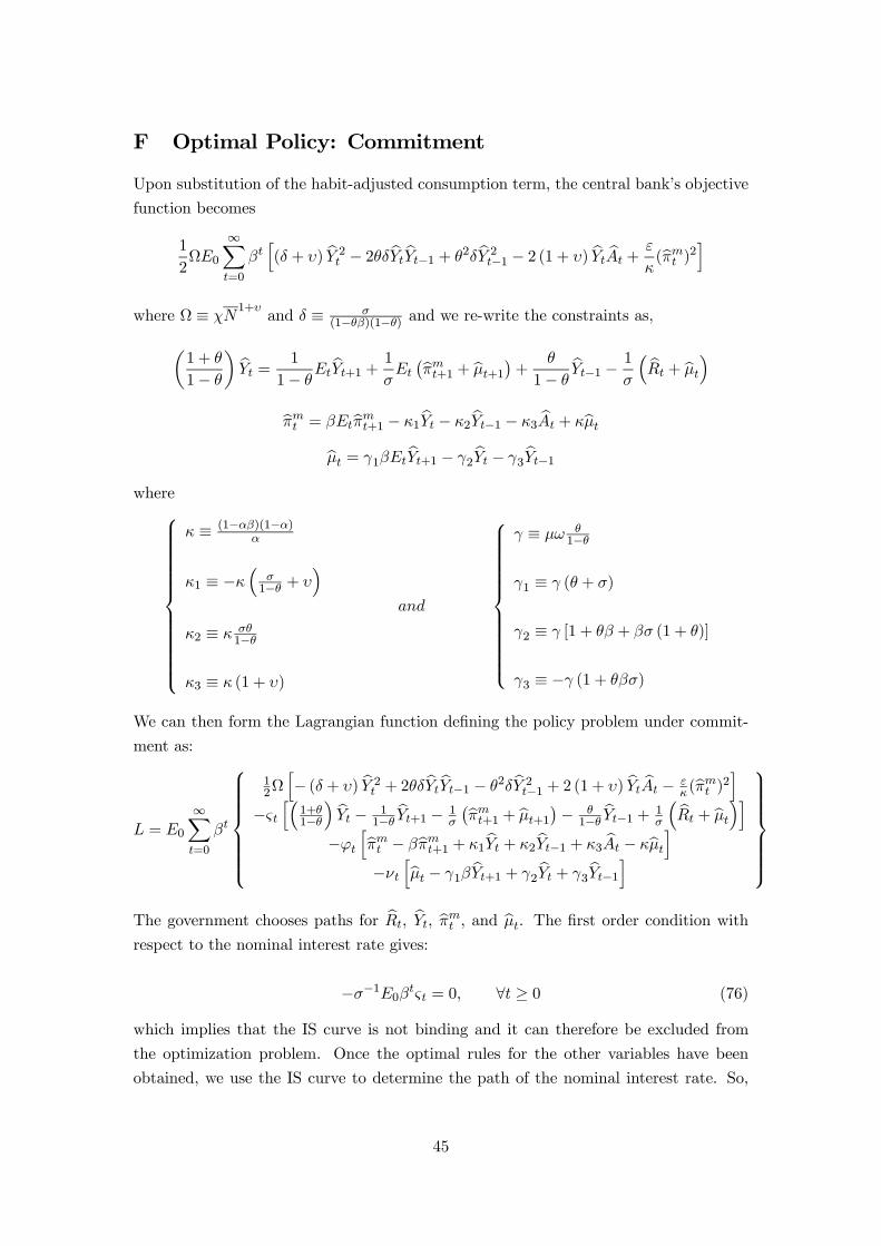
F Optimal Policy: Commitment

Upon substitution of the habit-adjusted consumption term, the central bank’s objective

function becomes

1

2ΩE0

∞Xt=0

βth(δ + υ) bY 2t − 2θδbYt bYt−1 + θ2δbY 2t−1 − 2 (1 + υ) bYt bAt +

ε

κ(bπmt )2i

where Ω ≡ χN1+υ

and δ ≡ σ(1−θβ)(1−θ) and we re-write the constraints as,µ

1 + θ

1− θ

¶ bYt = 1

1− θEtbYt+1 + 1

σEt

¡bπmt+1 + bμt+1¢+ θ

1− θbYt−1 − 1

σ

³ bRt + bμt´bπmt = βEtbπmt+1 − κ1bYt − κ2bYt−1 − κ3 bAt + κbμt

bμt = γ1βEtbYt+1 − γ2 bYt − γ3bYt−1

where⎧⎪⎪⎪⎪⎪⎪⎪⎪⎪⎪⎪⎪⎨⎪⎪⎪⎪⎪⎪⎪⎪⎪⎪⎪⎪⎩

κ ≡ (1−αβ)(1−α)α

κ1 ≡ −κ³

σ1−θ + υ

´κ2 ≡ κ σθ

1−θ

κ3 ≡ κ (1 + υ)

and

⎧⎪⎪⎪⎪⎪⎪⎪⎪⎪⎪⎪⎨⎪⎪⎪⎪⎪⎪⎪⎪⎪⎪⎪⎩

γ ≡ μω θ1−θ

γ1 ≡ γ (θ + σ)

γ2 ≡ γ [1 + θβ + βσ (1 + θ)]

γ3 ≡ −γ (1 + θβσ)

We can then form the Lagrangian function defining the policy problem under commit-

ment as:

L = E0

∞Xt=0

βt

⎧⎪⎪⎪⎪⎪⎪⎨⎪⎪⎪⎪⎪⎪⎩

12Ωh− (δ + υ) bY 2t + 2θδbYt bYt−1 − θ2δbY 2t−1 + 2 (1 + υ) bYt bAt − ε

κ(bπmt )2i−ςt

h³1+θ1−θ

´ bYt − 11−θ

bYt+1 − 1σ

¡bπmt+1 + bμt+1¢− θ1−θ

bYt−1 + 1σ

³ bRt + bμt´i−ϕt

hbπmt − βbπmt+1 + κ1bYt + κ2bYt−1 + κ3 bAt − κbμti−νt

hbμt − γ1β bYt+1 + γ2bYt + γ3bYt−1i

⎫⎪⎪⎪⎪⎪⎪⎬⎪⎪⎪⎪⎪⎪⎭The government chooses paths for bRt, bYt, bπmt , and bμt. The first order condition withrespect to the nominal interest rate gives:

−σ−1E0βtςt = 0, ∀t ≥ 0 (76)

which implies that the IS curve is not binding and it can therefore be excluded from

the optimization problem. Once the optimal rules for the other variables have been

obtained, we use the IS curve to determine the path of the nominal interest rate. So,

45

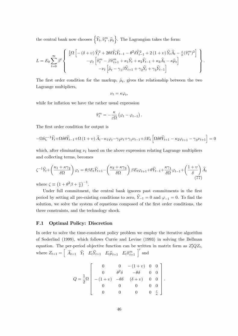
the central bank now choosesnbYt, bπmt , bμto. The Lagrangian takes the form:

L = E0

∞Xt=0

βt

⎧⎪⎪⎪⎨⎪⎪⎪⎩12Ωh− (δ + υ) bY 2t + 2θδbYtbYt−1 − θ2δbY 2t−1 + 2 (1 + υ) bYt bAt − ε

κ(bπmt )2i−ϕt

hbπmt − βbπmt+1 + κ1bYt + κ2bYt−1 + κ3 bAt − κbμti−νt

hbμt − γ1β bYt+1 + γ2bYt + γ3bYt−1i⎫⎪⎪⎪⎬⎪⎪⎪⎭ .

The first order condition for the markup, μt, gives the relationship between the two

Lagrange multipliers,

νt = κϕt,

while for inflation we have the rather usual expression

bπmt = − κ

εΩ

¡ϕt − ϕt−1

¢.

The first order condition for output is

−Ωδζ−1bYt+ΩδθbYt−1+Ω (1 + υ) bAt−κ1ϕt−γ2νt+γ1νt−1+βEt

hΩδθbYt+1 − κ2ϕt+1 − γ3νt+1

i= 0

which, after eliminating νt based on the above expression relating Lagrange multipliers

and collecting terms, becomes

ζ−1bYt+µκ1 + κγ2δΩ

¶ϕt = θβEt

bYt+1−µκ2 + κγ3δΩ

¶βEtϕt+1+θbYt−1+κγ1

δΩϕt−1+

µ1 + υ

δ

¶ bAt

(77)

where ζ ≡¡1 + θ2β + υ

δ

¢−1.

Under full commitment, the central bank ignores past commitments in the first

period by setting all pre-existing conditions to zero, bY−1 = 0 and ϕ−1 = 0. To find the

solution, we solve the system of equations composed of the first order conditions, the

three constraints, and the technology shock.

F.1 Optimal Policy: Discretion

In order to solve the time-consistent policy problem we employ the iterative algorithm

of Soderlind (1999), which follows Currie and Levine (1993) in solving the Bellman

equation. The per-period objective function can be written in matrix form as Z 0tQZt,

where Zt+1 =h bAt+1

bYt EtbYt+1 Etbμt+1 Etbπmt+1 i0 and

Q =1

2Ω

⎡⎢⎢⎢⎢⎢⎢⎣0 0 − (1 + υ) 0 0

0 θ2δ −θδ 0 0

− (1 + υ) −θδ (δ + υ) 0 0

0 0 0 0 0

0 0 0 0 εκ

⎤⎥⎥⎥⎥⎥⎥⎦ .

46

and the structural description of the economy is given by,

Zt+1 = AZt +But + ξt+1,

where ut =h bRt

i, ξt+1 =

hεAt+1 0 0 0 0

i0, A ≡ A−10 A1, B ≡ A−10 B0,

A0 =

⎡⎢⎢⎢⎢⎢⎢⎣1 0 0 0 0

0 1 0 0 0

0 0 βγ1 0 0

0 0 11−θ σ−1 σ−1

0 0 0 0 β

⎤⎥⎥⎥⎥⎥⎥⎦ , A1 =

⎡⎢⎢⎢⎢⎢⎢⎣ρ 0 0 0 0

0 0 1 0 0

0 γ3 γ2 1 0

0 − θ1−θ

1+θ1−θ σ−1 0

κ3 κ2 κ1 −κ 1

⎤⎥⎥⎥⎥⎥⎥⎦and

B0 =h0 0 0 σ−1 0

i0.

This completes the description of the required inputs for Soderlind (1999)’s Matlab code

which computes optimal discretionary policy.

47

Parameter Value Descriptionr (1.04)1/4 Real interest rateσ 2 Inverse of intertemporal elasticity of substitutionη 11.0 Elasticity of substitution across final goodsε 11.0 Elasticity of substitution across intermediate goodsα 0.75 Degree of price stickinessθ 0.65 Degree of habit formationNw 4.0 Frisch labour supply elasticityχ 3.0 Relative weight on labour in the utility functionπ 1 Gross CPI inflation rate in steady-stateρ 0.9 Persistence of exogenous shocksσA 0.009 Standard deviation of exogenous shocks

Table 1: Parameter values used in simulations

References

Amato, J. D., and T. Laubach (2004): “Implications of Habit Formation for Optimal

Monetary Policy,” Journal of Monetary Economics, 51, 305—325.

Bouakez, H., E. Cardia, and F. J. Ruge-Murcia (2005): “Habit Formation and

the Persistence of Monetary Shocks,” Journal of Monetary Economics, 52, 1073—1088.

Calvo, G. (1983): “Staggered Prices in a Utility Maximising Framework,” Journal of

Monetary Economics, 12(3), 383—398.

Christiano, L. J., M. Eichenbaum, and C. L. Evans (2005): “Nominal Rigidi-

ties and the Dynamic Effects of a Shock to Monetary Policy,” Journal of Political

Economy, 113(1), 1—45.

Currie, D., and P. Levine (1993): Rules, Reputation and Macroeconomic Policy

Coordination. Cambridge University Press, Cambridge.

Fuhrer, J. C. (2000): “Habit Formation in Consumption and Its Implications for

Monetary-Policy Models,” The American Economic Review, 90(June), 367—390.

Kirsanova, T., C. Leith, and S. Wren-Lewis (2006): “Should Central Banks Target

Consumer Prices or the Exchange Rate?,” Economic Journal, 116(June), F208—F231.

Kozicki, S., and P. Tinsley (2002): “Dynamic Specifications in Optimizing Trend-

deviation Macro Models,” Journal of Economic Dynamics and Control, 26, 1585—1611.

Lagarias, J. C., J. A. Reeds, M. H. Wright, and P. E. Wright (1998): “Con-

vergence Properties of the Nelder-Mead Simplex Method in Low Dimensions,” SIAM

Journal of Optimization, 9(1), 112—147.

48

Leith, C., and J. Malley (2005): “Estimated General Equilibrium Models for the

Analysis of Monetary Policy in the US and Europe,” European Economic Review,

49(8), 2137—2159.

Ljungqvist, L., and H. Uhlig (2000): “Tax Policy and Aggregate Demand Manage-

ment under Catching up with the Joneses,” The American Economic Review, 90(3),

356—366.

Ravina, E. (2007): “Habit Persistence and Keeping Up with the Joneses: Evidence

from Micro Data,” mimeo.

Ravn, M., S. Schmitt-Grohe, and M. Uribe (2006): “Deep Habits,” Review of

Economic Studies, 73, 195—218.

Rotemberg, J. J., and M. Woodford (1999): “Interest Rate Rules in an Estimated

Sticky Price Model,” in Monetary Policy Rules, ed. by J. B. Taylor, vol. 31, pp.

57—119. The National Bureau of Economic Research - Business Cycle Series, Chicago.

Schmitt-Grohe, S., and M. Uribe (2007): “Optimal, Simple, and Implementable

Monetary and Fiscal Rules,” Journal of Monetary Economics, 54(Sep), 1702—1725.

Smets, F., and R. Wouters (2003): “An Estimated Dynamic Stochastic General

Equilibrium Model of the Euro Area,” Journal of the European Economic Association,

1(5), 1123—1175.

(2007): “Shocks and Frictions in US Business Cycles: A Bayesian DSGE

Approach,” The American Economic Review, 97(3), 586—606.

Soderlind, P. (1999): “Solution and Estimation of Rational Expectations Macro Mod-

els with Optimal Policy,” European Economic Review, 43, 813—823.

Woodford, M. (2001): “The Taylor Rule and Optimal Monetary Policy,” American

Economic Review, 91(2), 232—237.

(2003): Interest and Prices: Foundations of a Theory of Monetary Policy.

Princeton University Press, Princeton, NJ.

49