Teaching Tools For Data Analysis - Clute Journals

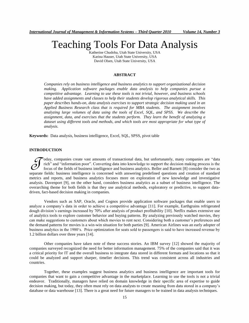
International Journal of Management & Information Systems – Third Quarter 2010 Volume 14, Number 3

15

Teaching Tools For Data Analysis Katherine Chudoba, Utah State University, USA

Karina Hauser, Utah State University, USA

David Olsen, Utah State University, USA

ABSTRACT

Companies rely on business intelligence and business analytics to support organizational decision

making. Application software packages enable data analysis to help companies pursue a

competitive advantage. Learning to use these tools is not trivial, however, and business schools

have added assignments and classes to help their students develop rigorous analytical skills. This

paper describes hands-on, data analysis exercises to support strategic decision making used in an

Applied Business Research class that is required for MBA students. The assignment involves

analyzing large volumes of data using the tools of Excel, SQL, and SPSS. We describe the

assignment, data, and exercises that the students perform. They learn the benefit of analyzing a

dataset using different tools and methods, and which tools are most appropriate for what type of

analysis.

Keywords: Data analysis, business intelligence, Excel, SQL, SPSS, pivot table

INTRODUCTION

oday, companies create vast amounts of transactional data, but unfortunately, many companies are “data

rich” and “information poor”. Converting data into knowledge to support the decision making process is the

focus of the fields of business intelligence and business analytics. Beller and Barnett [8] consider the two as

separate fields: business intelligence is concerned with answering predefined questions and creation of standard

metrics and reports, and business analytics focuses more on exploration of new knowledge and investigative

analysis. Davenport [9], on the other hand, considers business analytics as a subset of business intelligence. The

overarching theme for both fields is that they use analytical methods, exploratory or predictive, to support data-

driven, fact-based decision making in companies.

Vendors such as SAP, Oracle, and Cognos provide application software packages that enable users to

analyze a company‟s data in order to achieve a competitive advantage [11]. For example, Earthgrains refrigerated

dough division‟s earnings increased by 70% after analysis of product profitability [10]. Netflix makes extensive use

of analytics tools to explore customer behavior and buying patterns. By analyzing previously watched movies, they

can make suggestions to customers about which movies to rent next. Considering both a customer‟s preferences and

the demand patterns for movies is a win-win situation for both parties [9]. American Airlines was an early adopter of

business analytics in the 1980„s. Price optimization for seats sold to passengers is said to have increased revenue by

1.2 billion dollars over three years [14].

Other companies have taken note of these success stories. An IBM survey [12] showed the majority of

companies surveyed recognized the need for better information management. 75% of the companies said that it was

a critical priority for IT and the overall business to integrate data stored in different formats and locations so that it

could be analyzed and support sharper, timelier decisions. This trend was consistent across all industries and

countries.

Together, these examples suggest business analytics and business intelligence are important tools for

companies that want to gain a competitive advantage in the marketplace. Learning to use the tools is not a trivial

endeavor. Traditionally, managers have relied on domain knowledge in their specific area of expertise to guide

decision making, but today, they often must rely on data analysts to create meaning from data stored in a company‟s

database or data warehouse [13]. There is a great need for future managers to be trained in data analysis techniques.

T


16

Universities have recognized that need. Some MBA programs [4, 5, 7] have created specializations in

Business Intelligence, and a few offer degrees in Masters in Business Intelligence [1, 3] or Business Analytics [2, 6].

The vast majority of programs incorporate data analysis into one or more of their MBA courses. The exercises

described in this paper are an integral part of an Applied Business Research that is required for MBAs at Utah State

University. The class introduces students to the scientific method, including how to articulate a research question

and hypotheses, design a study and use appropriate methods to evaluate the hypotheses, and analyze results and

discuss the implications of the research findings. Students learn to apply the scientific method to address problems

in marketing research, lean manufacturing process optimization, financial analysis, and fraud detection in

accounting data.

This paper describes hands-on, data analysis exercises to support strategic decision making used in the

Applied Business Research class. Students complete the exercises using three commonly available software tools:

Excel, SQL and SPSS. The objective is for them to become familiar with multiple tools. The first section describes

the assignment and data that serve as a basis for all the exercises. The next three sections give detailed insight into

the Excel exercises, SQL exercises and SPSS exercises, followed by the conclusion.

DESCRIPTION OF STUDENT ASSIGNMENT AND DATA USED

Students are provided a dataset with almost 30,000 records and a series of questions to prime their

exploration of the data. For example, they are asked to identify the salespeople who had the highest and lowest sales

over a ten year period, and to perform various statistical analyses using the data. They are encouraged to go beyond

answers to the set of questions and to perform a thorough analysis of the data. Students submit a ten-page paper that

describes their review and includes a set of recommendations for management. They submit their statistical analyses

and work papers (e.g., audit trail) in Appendices. Emphasis is placed on presenting the data in an appropriate

manner (numbers vs. graphs) and clear written communication. The instructor seeds the data differently each

semester. The assignment is worth ten percent of a student‟s overall grade.

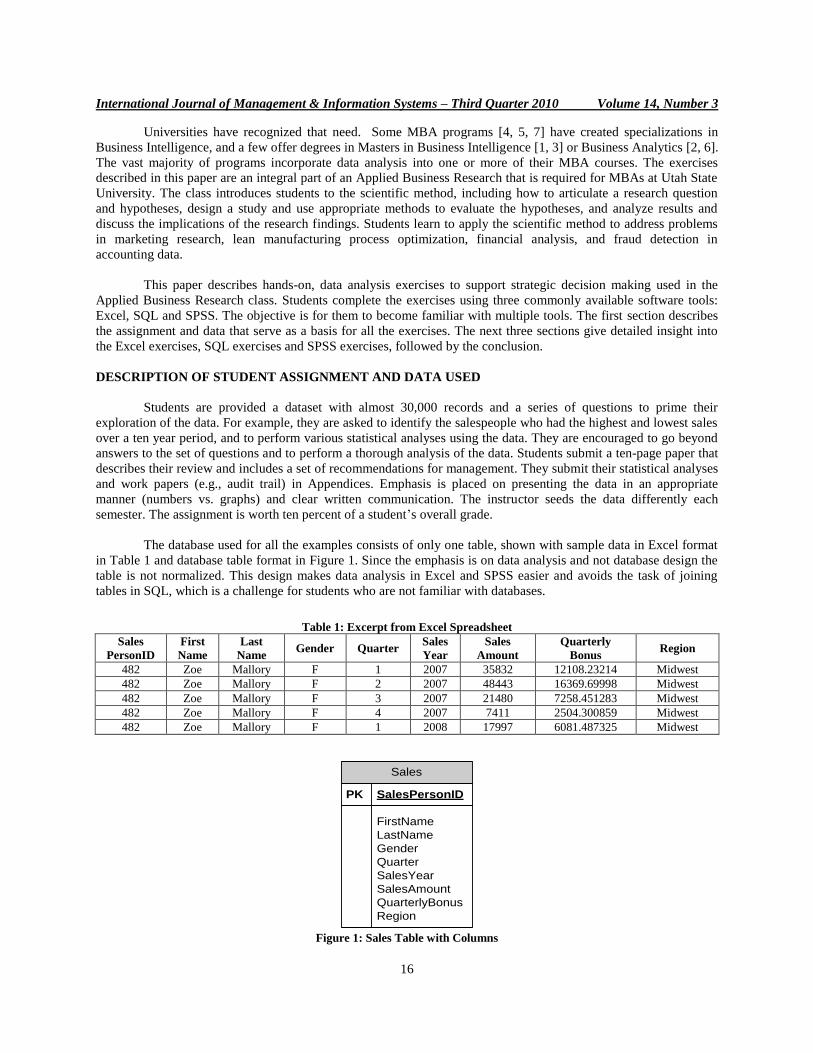
The database used for all the examples consists of only one table, shown with sample data in Excel format

in Table 1 and database table format in Figure 1. Since the emphasis is on data analysis and not database design the

table is not normalized. This design makes data analysis in Excel and SPSS easier and avoids the task of joining

tables in SQL, which is a challenge for students who are not familiar with databases.

Table 1: Excerpt from Excel Spreadsheet

Sales

PersonID

First

Name

Last

Name Gender Quarter

Sales

Year

Sales

Amount

Quarterly

Bonus Region

482 Zoe Mallory F 1 2007 35832 12108.23214 Midwest





Sales

PK SalesPersonID

FirstName

LastName

Gender

Quarter

SalesYear

SalesAmount

QuarterlyBonus

Region

Figure 1: Sales Table with Columns


17

The original data is generated through a series of SQL statements and then exported to Excel. The SQL

statements for creation of the table, filling the Year and Quarter column and two examples for filling in the personal

data are shown in Listing 1.

The data is provided to the students in an Excel spreadsheet. Part of the student‟s SQL assignment is to

import the Excel file into Microsoft SQL Server. An earlier lesson discusses different data formats and how to

convert data from one format to another.

DATA ANALYSIS USING EXCEL

Analysis in Excel requires that students use both basic functions and more advanced methods. The

functions and approaches described below are only one way to achieve the desired results.

Data students report

Overall sales amount (using the SUM function)

Overall bonus amount (using the SUM function)

Sales amount and bonus amount by gender (using the SUMIF function)

Sales amount and bonus amount by region (using the SUMIF function)

Sales amount and bonus amount by quarter (using the SUMIF function)

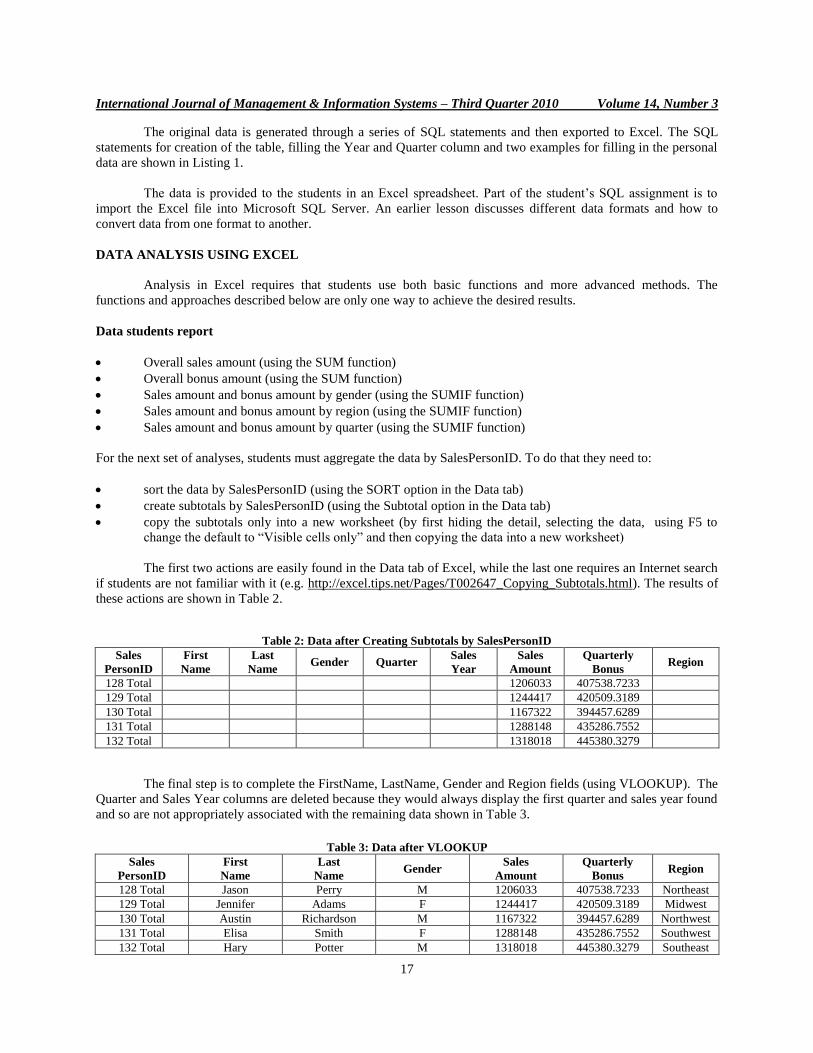
For the next set of analyses, students must aggregate the data by SalesPersonID. To do that they need to:

sort the data by SalesPersonID (using the SORT option in the Data tab)

create subtotals by SalesPersonID (using the Subtotal option in the Data tab)

copy the subtotals only into a new worksheet (by first hiding the detail, selecting the data, using F5 to

change the default to “Visible cells only” and then copying the data into a new worksheet)

The first two actions are easily found in the Data tab of Excel, while the last one requires an Internet search

if students are not familiar with it (e.g. http://excel.tips.net/Pages/T002647_Copying_Subtotals.html). The results of

these actions are shown in Table 2.

Table 2: Data after Creating Subtotals by SalesPersonID

Sales

PersonID

First

Name

Last

Name Gender Quarter

Sales

Year

Sales

Amount

Quarterly

Bonus Region

128 Total 1206033 407538.7233

129 Total 1244417 420509.3189

130 Total 1167322 394457.6289

131 Total 1288148 435286.7552

132 Total 1318018 445380.3279

The final step is to complete the FirstName, LastName, Gender and Region fields (using VLOOKUP). The

Quarter and Sales Year columns are deleted because they would always display the first quarter and sales year found

and so are not appropriately associated with the remaining data shown in Table 3.

Table 3: Data after VLOOKUP

Sales

PersonID

First

Name

Last

Name Gender

Sales

Amount

Quarterly

Bonus Region

128 Total Jason Perry M 1206033 407538.7233 Northeast

129 Total Jennifer Adams F 1244417 420509.3189 Midwest

130 Total Austin Richardson M 1167322 394457.6289 Northwest

131 Total Elisa Smith F 1288148 435286.7552 Southwest

132 Total Hary Potter M 1318018 445380.3279 Southeast

http://excel.tips.net/Pages/T002647_Copying_Subtotals.html


18

Listing 1: SQL Statements To Create Data

After these analyses, students are able to report the following information:

Overall number of sales persons

Number of female/male sales persons (using the COUNTIF function)

CREATE TABLE Sales

(SalesPersonID INT NOT NULL,

FirstName CHAR(15) NULL,

LastName CHAR(15) NULL,

Gender CHAR(1) NULL CHECK (Gender IN ('M','F')),

Quarter INT NULL,

SalesYear INT NULL,

SalesAmount DECIMAL(21,13) NULL,

QuarterlyBonus DECIMAL(21,13) NULL,

Region CHAR(15) NULL CHECK (Region IN('Northwest',

'Southwest','Southeast','Northeast','Midwest')),)

GO

SET NOCOUNT ON

DECLARE @salesid AS int, @yr AS int, @qu AS int, @reg AS char(15)

SET @salesid = 100

WHILE @salesID < 1001

BEGIN

SET @yr = 1999

WHILE @yr < 2011

BEGIN

SET @qu = 1

WHILE @qu < 5

BEGIN

INSERT INTO Sales

VALUES(@salesid,NULL,NULL,NULL,@qu,@yr,

CAST(RAND() * 50001 AS DECIMAL(21,0)),

NULL,NULL)

SET @qu = @qu + 1

END

SET @yr = @yr + 1

END

SET @salesid = @salesid + 1

END

GO

UPDATE Sales SET QuarterlyBonus = SalesAmount * (RAND() *1 )

UPDATE Sales

SET FirstName = 'Jason', LastName = 'Perry',Gender = 'M', Region = 'Northeast'

WHERE SalesPersonID = 128

GO

UPDATE Sales

SET FirstName = 'Jennifer', LastName = 'Adams',Gender = 'F', Region = 'Midwest'

WHERE SalesPersonID = 129

GO


19

Number of sales persons per region (using the COUNTIF function)

Determine the sales person with the highest/lowest sales amount and bonus amount (using the MAX/MIN

function)

Average sales amount and bonus amount

Number of sales persons below/above average

Average sales amount and bonus amount by gender

Average sales mount and bonus amount per region per sales person

Students create a subtotal by year to provide the following data:

Yearly sales amount and bonus amount

Trend line, regression equation and R2 of regression analysis

Adding region as another subtotal within the year will create

Sales amount and bonus amount by region by year

Table 4: Excerpt of Pivot Table, Filtered by Region and Gender

Region Midwest

Sum of SalesAmount SalesYear

Gender SalesPersonID 1999 2000 2001 2002 2003 2004 2005 2006 2007 Grand Total

F 103 181,825.51 65,857.39 64,892.04 122,695.26 120,267.26 86,563.45 116,258.06 113,529.02 104,806.36 976,694.35

104 123,794.32 133,828.60 100,409.84 127,040.37 87,743.89 75,290.58 31,532.97 133,907.90 119,500.35 933,048.82

121 72,681.30 124,655.86 146,097.83 142,868.62 105,056.37 133,028.82 132,300.23 98,848.75 95,747.20 1,051,284.99

125 122,957.88 112,858.69 155,965.00 117,468.82 142,790.27 123,102.91 54,923.83 100,410.71 112,707.20 1,043,185.32

129 120,141.20 105,978.65 45,352.55 57,325.13 103,110.50 61,311.08 59,315.12 91,708.05 157,066.52 801,308.80

137 37,395.06 125,588.28 211,792.03 102,563.82 67,922.00 140,029.09 110,825.46 60,514.42 59,654.91 916,285.08

139 130,833.23 105,896.43 90,504.31 49,569.61 127,777.08 84,622.18 111,515.62 88,786.80 97,754.95 887,260.21

148 62,863.66 154,594.50 152,605.19 133,549.13 84,213.21 129,109.80 111,161.58 134,363.53 134,715.58 1,097,176.18

221 131,135.57 88,325.83 104,400.82 60,221.73 113,171.57 120,760.30 146,064.38 77,534.01 121,347.47 962,961.68

281 116,904.61 126,188.56 127,105.78 118,334.45 140,748.05 69,268.68 101,590.29 85,755.01 107,568.66 993,464.09

321 135,149.01 124,982.30 146,085.58 128,825.83 100,950.34 87,268.73 83,178.46 141,067.95 85,391.58 1,032,899.78

331 130,739.61 96,688.27 159,618.08 141,771.22 54,133.00 119,527.72 113,420.22 120,117.35 76,737.59 1,012,753.07

335 109,416.39 111,932.33 141,997.94 91,547.26 35,835.63 77,247.68 137,664.57 101,499.01 125,645.76 932,786.57

360 100,840.97 64,673.87 54,479.55 117,036.24 60,425.68 141,231.02 100,088.01 94,473.12 146,668.59 879,917.05

393 143,719.93 95,126.71 81,590.33 134,871.21 90,006.24 144,894.00 85,045.98 57,114.96 77,489.58 909,858.94

417 76,038.78 131,331.48 87,566.41 93,748.57 87,453.95 99,947.35 98,708.53 110,768.53 164,351.63 949,915.23

429 82,060.80 76,431.52 112,574.85 124,760.44 92,380.75 103,278.11 74,909.25 109,455.41 100,072.53 875,923.65

461 147,356.63 77,369.86 183,409.96 106,627.16 161,391.46 79,644.57 91,423.37 125,017.84 46,472.43 1,018,713.29

467 65,505.23 130,079.37 121,008.73 63,090.51 71,010.21 150,315.89 109,961.76 103,586.95 131,392.84 945,951.49

482 96,094.61 84,342.78 88,910.69 179,630.67 132,598.26 149,606.44 129,408.73 99,563.55 58,137.44 1,018,293.18

492 89,700.91 169,543.96 198,086.12 123,951.99 95,821.81 119,564.53 73,667.21 105,135.75 79,455.92 1,054,928.21

499 57,560.82 84,004.42 134,272.51 95,234.00 73,328.70 64,092.12 134,973.43 77,438.61 94,081.51 814,986.13

504 106,416.39 86,428.82 135,716.12 138,254.38 112,420.29 63,709.62 125,862.80 153,189.15 115,098.08 1,037,095.64

506 91,984.73 91,493.84 104,139.34 89,132.52 53,196.84 112,124.62 61,637.55 86,220.87 134,543.73 824,474.03

511 103,619.88 69,105.52 211,170.02 139,812.53 152,677.69 105,761.25 97,388.70 72,166.28 64,551.81 1,016,253.66

515 104,386.07 60,519.44 147,631.73 124,252.49 64,306.20 86,836.54 110,403.00 82,557.52 75,417.46 856,310.43

526 81,780.87 131,113.68 128,988.69 86,454.90 83,921.43 111,786.78 71,660.73 153,836.62 89,562.31 939,106.00

529 65,189.82 106,385.59 109,075.94 150,130.17 106,025.20 90,748.99 145,671.97 98,191.78 65,055.31 936,474.76

535 137,072.81 65,905.26 141,156.62 120,232.48 91,488.84 83,916.12 46,107.92 134,560.07 84,709.79 905,149.89

540 89,299.96 111,425.11 102,636.98 58,710.67 96,574.29 121,574.88 135,961.05 79,797.92 142,817.62 938,798.46

553 151,556.12 160,528.18 106,138.66 87,254.00 122,661.59 93,590.50 73,757.11 137,755.03 146,659.64 1,079,900.84

558 132,713.36 51,532.23 136,265.96 126,074.79 69,792.22 93,516.83 95,791.54 88,500.36 113,695.19 907,882.49

560 105,467.62 102,237.66 101,637.53 114,660.79 13,889.02 126,299.21 126,709.45 107,736.15 92,136.16 890,773.59

566 138,710.59 92,537.39 149,009.81 80,166.95 63,660.03 106,891.30 76,695.63 85,259.17 106,746.96 899,677.84

570 120,407.52 125,522.24 85,789.17 99,156.18 119,716.13 173,033.24 122,046.60 98,311.68 92,288.37 1,036,271.13

589 67,926.85 65,523.39 123,361.11 71,903.53 131,609.26 101,886.67 124,960.67 96,697.41 92,967.32 876,836.20

604 76,520.14 92,142.91 141,136.89 79,491.84 152,534.21 178,015.34 127,281.83 114,124.32 89,022.34 1,050,269.81

606 79,053.38 75,359.30 141,974.88 55,762.16 14,630.60 59,319.62 121,291.52 86,355.92 93,991.53 727,738.89

636 114,243.99 128,037.86 134,172.20 123,436.06 135,443.93 21,316.30 121,117.40 124,302.52 160,110.81 1,062,181.06

687 104,446.02 119,842.82 90,495.65 103,987.07 132,962.58 91,963.43 63,280.62 95,411.01 104,809.14 907,198.35

692 101,400.71 97,743.86 79,014.71 155,755.17 142,194.73 131,635.32 95,425.47 66,490.23 138,484.72 1,008,144.91

F Total 4,306,912.82 4,223,664.75 5,078,238.18 4,437,360.72 4,007,841.33 4,313,631.58 4,150,988.59 4,192,061.28 4,299,434.87 39,010,134.11


20

DATA ANALYSIS USING EXCEL PIVOT TABLES

In addition to analyzing the data using formulas and scenario tools, students must demonstrate mastery of

the pivot table function in Excel. Once students have created a pivot table (using Insert/Pivot table), they can explore

different ways of manipulating the data by adding attributes to the column (e.g., year), row (e.g., region), and values

(e.g., sales) section of the pivot table report. Assignment questions lead students to apply filters to fields (e.g.,

gender, region), add report totals, and add formulas or calculated fields. Once students identify an interesting

relationship or trend in aggregated data, they quickly learn how easy it is to drill down into the data to explore and

understand the reasons behind the relationships. They learn that aggregating data by variables such as sales person

ID and gender are trivial tasks when done using a pivot table, and that pivot tables make it much easier to

dynamically manipulate data and search for the explanation behind interesting relationships.

Graphs students create

One objective of the assignment is for students to make judgments about what data is best represented in

tables and what data is best represented in charts and graphs. For example, they should realize that it is best to

display regional data in a pie or column chart and yearly data in a trend chart. Of course, Excel makes it easy for

students to create visual representations of their analyses, as shown in Figure 2.

Figure 2: Sample Charts and Graphs Created in Excel


21

DATA ANALYSIS USING SQL

As mentioned earlier, students are required to import the data into a SQL database and change the data

types to be appropriate for analysis. For example, they must ensure that all fields that contain numbers are

represented as numerical fields and have the right amount of decimals. Since most students have only limited or no

experience with SQL, a variety of SQL statements with descriptions about their functions are provided by the

instructor. Some examples are included in Listing 2. Most students are able to adjust the queries for the analyses

they need to create.

Listing 2: SQL Statements Provided to the Students

In the SQL portion of the assignment, students discover that they can get answers to the same questions

they answered using Excel, but with less time and effort involved. The grouping by salesperson that required several

steps in Excel is done with a single SQL statement. For example, the overall number and the number of female/male

sales persons can be easily determined with the SQL statements in Listing 3: Example SQL StatementsListing 3.

Listing 3: Example SQL Statements

The inclusion of an example of stored procedures shows students that the user is not required to input the

statements every time and also that the SQL statement could be prepared by somebody with extensive database

knowledge and then simply executed by the person who needs the results. Students also discover that some of the

statistical analysis options, included in Excel, are not available in standard SQL and so they must perform these

analyses using SPSS.

Overall number of sales persons

SELECT COUNT(DISTINCT SalesPersonID) FROM Sales;

Number of female/male sales persons

SELECT Gender, COUNT(DISTINCT SalesPersonID) from Sales

GROUP BY Gender;

List all attributes of the sales table as well as all tuples/

SELECT * FROM Sales;

Find the average quarterly sales amount. Name this new column AverageSalesAmount.

SELECT AVG(SalesAmount) AS AverageSalesAmount FROM Sales;

List the total amount of sales for each quarter for each sales year. Put your answer in order of year and then quarter in

ascending order.

SELECT SalesYear, Quarter, SUM(SalesAmount) AS TotAmt FROM Sales

GROUP BY SalesYear, Quarter

ORDER BY SalesYear, Quarter;

Write a stored procedure that lists the sales person‟s id, first name and name for the person whose id is input as a

parameter.

CREAT E PROCEDURE ChooseSalesPerson (@ID INT) AS

SELECT SalesPersonID, FirstName, LastName

FROM Sales WHERE SalesPersonID = @ID;

To run the stored procedure:

EXEC ChooseSalesPerson 305


22

DATA ANALYSIS USING SPSS

SPSS Statistics is a commonly used statistical analysis program that is installed in all computer labs at Utah

State University. It allows user to import different data formats, Excel being one of them.

SPSS has an option to aggregate data which makes tasks that required sorting and creating subtotals in

Excel very easy. For example, using SalesPersonID, FirstName, LastName, Gender, and Region as the Break

Variables and SalesAmount, QuarterlyBonus as aggregate variables, user can create a wide variety of aggregate

function as shown in Figure 3.

Figure 3: SPSS Aggregate Functions

SPSS also offers a user-friendly Chart Builder that includes some unique graphs, such as a histogram split

by gender, illustrated in Figure 4.

Figure 4: SPSS Graph, Split Histogram


23

Conducting a T-test or ANOVA can be done by simply entering the Test Variable and Grouping Variable.

The sophistication of the SPSS analyses the students are able to complete depend largely on their statistical

knowledge and creativity.

INSIGHTS STUDENTS SHOULD GLEAN FROM THEIR ANALYSES

As mentioned earlier, the instructor can reseed the dataset every semester, so the results discussed below

will vary. They point, however, to the kinds of analyses students are expected to complete above and beyond

answering the explicit questions that they are asked to answer using Excel, SQL, or SPSS.

The overall sales amount and bonus amount is higher for the male salesperson but the average is nearly the

same. This initial finding should be supported by a t-test showing that there is no statistically significant

difference between the groups.

There is a large difference (>100%) between the best performing region and the lowest one.

The yearly sales amount by region is stable, with no up/downward trends.

The difference between the highest performing salesperson and the lowest one is nearly 100%.

Only 11 salespersons sold less than 1 million dollars

Nearly half of all salespersons are below average and half above (e.g., mean and median are almost

identical).

The total sales amount fluctuates by quarter. Students need to perform an ANOVA test to reveal that there

is no statistically significant difference between the groups.

Whereas the trend line shows an upward trend the regression analysis reveals that the fit is not very good.

In the example shown only 6.32% of the total variance can be "explained" by the linear regression model.

That leaves the rest of the variance (~94% of the total) as variability of the data from the model.

CONCLUSIONS

The data analysis assignment that our MBA students complete gives them experience in managing and

analyzing large volumes of data using the tools of Excel, SQL, and SPSS. For example, it is somewhat cumbersome

to create subtotals in Excel, but straightforward to do so in SQL and SPSS. Performing an ANOVA in Excel is a

lengthy process because the data need to be rearranged so that each quarter appears in a separate column. Students

learn the benefits of being able to analyze data and get the same results using different tools and methods, and which

tools are most appropriate for what type of analysis. They also gain an appreciation of the amount and level of data

needed to make informed decisions in business. A company‟s competitive advantage will depend on how data is

used to support these decisions.

AUTHOR INFORMATION

Katherine M. Chudoba is Associate Professor of MIS in the Jon M. Huntsman School of Business at Utah State

University. Her research focuses on the nature of work in distributed environments, and how Information and

Communication Technologies (ICTs) are used and integrated into work practices. She has published in journals

such as MIS Quarterly, Organization Science, and Information Systems Journal. She earned her Ph.D. at the

University of Arizona, and her bachelor's degree and MBA at the College of William and Mary. Before joining

academe, she worked as an analyst and manager with IBM.

Karina Hauser is an associate professor in the Management Information Systems department at Utah State

University. She received her PhD in Decision Science and Information Technology at the University of Kentucky on

a Toyota Fellowship. Her research interests are in Web Development, Web Design and Lean Manufacturing. Before

going into academia, Karina spent 16 years in industry, first as a programmer and later as a consultant and project

manager for Enterprise Resource Planning systems, mainly in the automotive sector. Her research appeared in

journals such as the Journal of Information Systems Education, Journal of Computer Information Systems, and

International Journal of Production Research.


24

David Olsen received his Ph.D. in Management Information Systems from The University of Arizona in 1993 and

taught at The University of Akron accounting department in accounting information systems for five years. Dr.

Olsen joined the MIS department at Utah State University in 1998 and teaches primarily in the database area as well

as the MBA strategy and management course. His research interests include database concurrency control,

accounting information systems, the integration of SQL, XML and XBRL, and database modeling. His research has

been published in journals such as Communications of the ACM, Issues in Accounting Education, and the Journal of

Database Management. Dr. Olsen is happiest with regards to the teaching awards he has received.

REFERENCES

1. Master's Degree in Business Intelligence vs. MBA: Which is More Relevant to Today's Workplace? [cited

11/15/2009]; Available from: http://www.sju-online.com/articles/masters-business-intelligence.asp.

2. Master in Business Analytics. [cited; Available from: http://soms.utk.edu/analytics/index.htm.

3. Master of Science Business Intelligence. [cited; Available from: http://www.americansentinel.edu/online-

degree/online-masters-degree/masters-business-intelligence.php.

4. MBA in Business Intelligence. [cited; Available from:

http://www.lsbf.org.uk/programmes/masters/mba/intelligence.html.

5. MBA with Business Intelligence Concentration. [cited; Available from:

http://spears.okstate.edu/management/degrees/mba/concentrations/intel.

6. Msc in Business Analytics. [cited; Available from:

http://www.smurfitschool.ie/specialistmasters/technology/mscinbusinessanalytics/.

7. Specialize in Business Intelligence. [cited 2009/11/17]; Available from:

http://business.cudenver.edu/Graduate/ProMBA/Track_BusinessIntelligence.htm.

8. Beller, M. and A. Barnett. Next Generation Business Analytics Technology Trends. 2009 [cited

11/23/2009]; Available from: http://www.scribd.com/full/16588686?access_key=key-

14sahazncp852mcpammn.

9. Davenport, T.H. and J.G. Harris, Competing on Analytics.Boston, MA: Harvard Business School Press.

10. Davenport, T.H., et al., Data to Knowledge to Results: Building An Analytic Capability. California

Management Review, 2001. 43(2): p. 117-138. 2001

11. Gnatovich, R. Business Intelligence Versus Business Analytics -- What's the Difference? 2006 [cited

11/23/2009]; Available from:

http://www.cio.com/article/18095/Business_Intelligence_Versus_Business_Analytics_What_s_the_Differe

nce_?page=1.

12. IBM, Inside the midmarket: A 2009 Perspective, I.W. Study, Editor. 2009.

13. Kohavi, R., N.J. Rothleder, and E. Simoudis, Emerging trends in business analytics. Commun. ACM, 2002.

45(8): p. 45-48. 2002

14. Smith, B.C., et al., E-Commerce and Operations Research in Airline Planning, Marketing, and Distribution.

Interfaces, 2001. 31(2): p. 38-55. 2001

http://www.sju-online.com/articles/masters-business-intelligence.asp

http://soms.utk.edu/analytics/index.htm

http://www.americansentinel.edu/online-degree/online-masters-degree/masters-business-intelligence.php

http://www.americansentinel.edu/online-degree/online-masters-degree/masters-business-intelligence.php

http://www.lsbf.org.uk/programmes/masters/mba/intelligence.html

http://spears.okstate.edu/management/degrees/mba/concentrations/intel

http://www.smurfitschool.ie/specialistmasters/technology/mscinbusinessanalytics/

http://business.cudenver.edu/Graduate/ProMBA/Track_BusinessIntelligence.htm

http://www.scribd.com/full/16588686?access_key=key-14sahazncp852mcpammn

http://www.scribd.com/full/16588686?access_key=key-14sahazncp852mcpammn

http://www.cio.com/article/18095/Business_Intelligence_Versus_Business_Analytics_What_s_the_Difference_?page=1

http://www.cio.com/article/18095/Business_Intelligence_Versus_Business_Analytics_What_s_the_Difference_?page=1

Teaching Tools For Data Analysis - Clute Journals

Documents

Transcript of Teaching Tools For Data Analysis - Clute Journals