1

Teaching Non-Ideal Reactors with CFD Tools

Luis M. Madeira, Manuel A. Alves and Alírio E. Rodrigues

Departamento de Engenharia Química, Faculdade de Engenharia, Universidade do Porto

R. Dr. Roberto Frias, 4200-465 Porto, Portugal

Abstract

In this paper, a computational fluid dynamics (CFD) code (Fluent) was used to illustrate

important concepts regarding residence time distribution (RTD) theory. The case study adopted

considers isothermal laminar flow through 2-D reservoirs of different geometries (various

length/height, L/H, ratios), and a tracer step input is simulated for RTD determination. From the

steady-state solution, quasi-stagnant zones are easily identified, particularly for high flow rates

(or, more rigorously, high Reynolds numbers) and for low L/H ratios. In some cases, the fraction

of dead volumes amounts to values as high as 70%. For high L/H ratios one approaches the

theoretical RTD for laminar flow between parallel plates. Transient simulations are also very

useful because they allow ‘visualization’ of the evolution of tracer concentration fronts, which

animation is available in our web site. The RTD obtained allows students to predict reactor’s

performance, either in steady-state or transient regime. Such information can also be obtained

directly from Fluent by simulating the injection of a reactive feed stream. The use of a

commercially available CFD tool is illustrated to be advantageous, as it allows students to easily

‘visualize’ and understand the involved concepts, namely flow pattern and behavior/diagnosis of

non-ideal reactors.

Keywords: RTD, CFD, Fluent, non-ideal reactors.

2

Introduction

Behavior of non-ideal reactors and their flow pattern characterization are issues taught in

the majority of chemical reaction engineering (CRE) courses [1-4] (usually at undergraduate

level, but this depends on the structure of the ChE curriculum), and therefore addressed in most

CRE textbooks [e.g., 5-8]. In this respect, the classical stimulus-response tracer experiments [9]

are essential to obtain theoretical functions like the residence time distribution (RTD), which are

crucial for diagnosis of equipment operation, reactor modeling and prediction of conversion.

Comprehension of the involved concepts, which are not easily grasped by students, can be

improved with laboratory sessions, but this is not always feasible. However, this disadvantage

can be overcome by implementing computer simulation of tracer experiments [10], particularly

with a commercial computational fluid dynamics (CFD) tool [11-13].

CFD codes have been widely used for simulating flow pattern in real systems and its use in

a chemical engineering undergraduate course has several advantages, as mentioned by Sinclair

[14]. Among them, we can mention the following: first, the use of color in CFD plots allows

students to visualize the flow behavior, and this visualization of the flow phenomenon can

significantly facilitate and enhance the learning process. Secondly, students can explore the

effects of change in system geometry, system properties or operating conditions. All these

advantages, apart from the fact that students like to experience software tools used in industry,

which are usually user-friendly, justifies implementation of CFD codes in CRE courses,

particularly when teaching RTD theory.

However, such tools also have some disadvantages and/or limitations. Codes commercially

available may be extremely powerful, but their operation still requires a high level of skill and

understanding from the operator to obtain meaningful results. In addition, CFD cannot be

adequately used without continued reference to experimental and/or analytical validation of

numerical results [13].

3

The case study described here can be implemented, for instance, as homework for students

taking a CRE course dealing with non-ideal reactors. Simulations can be performed using a

commercial package such as Fluent, but it is advisable that a brief tutorial is provided so that

students can quickly familiarize with the program. In this tutorial, the essential steps that must be

followed for any simulation should be outlined. Different reservoir/reactor geometries can be

provided for different groups of two to three students, but each one should perform its own

parametric study (e.g., evaluate the effect of space-time, or Reynolds number, in flow pattern

characterization, or Damköhler number in reaction simulations). They should finally compile the

results obtained by other colleagues and discuss it in the final written report.

Using 2-D reservoirs/reactors with laminar flow, described in detail in the next section,

students should perform the following tasks, which are also the objectives of the present paper:

(i) characterize the hydrodynamics in the vessel(s); (ii) determine the RTD from tracer

experiments, which includes diagnosis of reservoir/reactor operation; and (iii) predict the

conversion in the continuous-flow system.

Case Study Formulation and Simulation with Fluent

It is well known that the mean residence time ( rt ) has an important effect in the

performance of some large natural conversion systems such as biological lagoons, as it affects

the biological conversion of biodegradable matter. Moreover, the geometry of the reservoirs

seems to affect the RTD, and thus rt . It is therefore very important to perform tracer

experiments in these systems (or try to estimate the RTD function) in order to better design such

wastewater treatment plants. However, the mean residence times in these large reservoirs or

lagoons are extremely high (ranging from one day up to several months [15,16]), so that tracer

experiments are impracticable. Possible strategies to overcome this problem are: i) obtain the

RTD on pilot-scale set-ups with various geometries, where tracer experiments are easily

4

conducted, and perform a scale-up analysis, and (ii) derive the RTD by solving the Navier-

Stokes and diffusion-convection equations which students learned in fluid mechanics curricula

[e.g., 16]. Commercially available CFD packages (e.g., Fluent, CFX, Fidap, Phoenics, STAR-

CD, FLOW3D, etc.) can readily solve the balance equations for reactor operation coupled with

the Navier-Stokes equations, and thus the second approach was herein adopted.

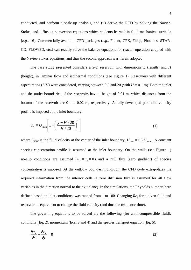
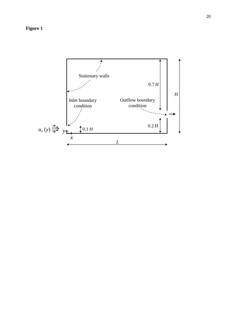
The case study presented considers a 2-D reservoir with dimensions L (length) and H

(height), in laminar flow and isothermal conditions (see Figure 1). Reservoirs with different

aspect ratios (L/H) were considered, varying between 0.5 and 20 (with H = 0.1 m). Both the inlet

and the outlet boundaries of the reservoirs have a height of 0.01 m, which distances from the

bottom of the reservoir are 0 and 0.02 m, respectively. A fully developed parabolic velocity

profile is imposed at the inlet boundary:

−−=2

max 20/20/1

HHyUux (1)

where Umax is the fluid velocity at the center of the inlet boundary, max mean1.5 U U= . A constant

species concentration profile is assumed at the inlet boundary. On the walls (see Figure 1)

no-slip conditions are assumed ( 0x yu u= = ) and a null flux (zero gradient) of species

concentration is imposed. At the outflow boundary condition, the CFD code extrapolates the

required information from the interior cells (a zero diffusion flux is assumed for all flow

variables in the direction normal to the exit plane). In the simulations, the Reynolds number, here

defined based on inlet conditions, was ranged from 1 to 100. Changing Re, for a given fluid and

reservoir, is equivalent to change the fluid velocity (and thus the residence-time).

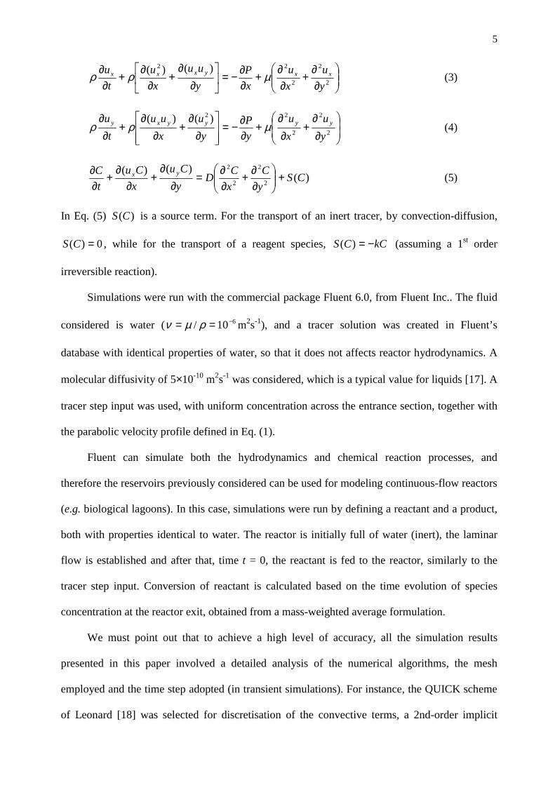
The governing equations to be solved are the following (for an incompressible fluid):

continuity (Eq. 2), momentum (Eqs. 3 and 4) and the species transport equation (Eq. 5).

0=∂∂

+∂∂

yu

xu yx (2)

5

∂∂

+∂∂

+∂∂−=

∂∂

+∂

∂+

∂∂

2

2

2

22 )()(yu

xu

xP

yuu

xu

tu xxyxxx µρρ (3)

∂∂

+∂∂

+∂∂−=

∂∂

+∂

∂+

∂∂

2

2

2

22 )()(yu

xu

yP

yu

xuu

tu yyyyxy µρρ (4)

)()()(

2

2

2

2

CSyC

xCD

yCu

xCu

tC yx +

∂∂+

∂∂=

∂∂

+∂

∂+

∂∂ (5)

In Eq. (5) )(CS is a source term. For the transport of an inert tracer, by convection-diffusion,

0)( =CS , while for the transport of a reagent species, kCCS −=)( (assuming a 1st order

irreversible reaction).

Simulations were run with the commercial package Fluent 6.0, from Fluent Inc.. The fluid

considered is water ( 610/ −== ρµν m2s-1), and a tracer solution was created in Fluent’s

database with identical properties of water, so that it does not affects reactor hydrodynamics. A

molecular diffusivity of 5×10-10 m2s-1 was considered, which is a typical value for liquids [17]. A

tracer step input was used, with uniform concentration across the entrance section, together with

the parabolic velocity profile defined in Eq. (1).

Fluent can simulate both the hydrodynamics and chemical reaction processes, and

therefore the reservoirs previously considered can be used for modeling continuous-flow reactors

(e.g. biological lagoons). In this case, simulations were run by defining a reactant and a product,

both with properties identical to water. The reactor is initially full of water (inert), the laminar

flow is established and after that, time t = 0, the reactant is fed to the reactor, similarly to the

tracer step input. Conversion of reactant is calculated based on the time evolution of species

concentration at the reactor exit, obtained from a mass-weighted average formulation.

We must point out that to achieve a high level of accuracy, all the simulation results

presented in this paper involved a detailed analysis of the numerical algorithms, the mesh

employed and the time step adopted (in transient simulations). For instance, the QUICK scheme

of Leonard [18] was selected for discretisation of the convective terms, a 2nd-order implicit

6

formulation was used during unsteady simulation and the computational grid contained typically

100 × 100 elements (note that for reservoirs with L/H >> 1, it is convenient to use a larger

number of cells in the x-direction). It is always a good practice to perform the calculations on

several meshes with different levels of refinement, in order to obtain mesh-independent results.

A similar procedure should be adopted regarding the time step used in transient calculations. A

control-volume approach is used by Fluent to numerically solve the governing equations [11].

Results and Discussion

i) Hydrodynamic characterization

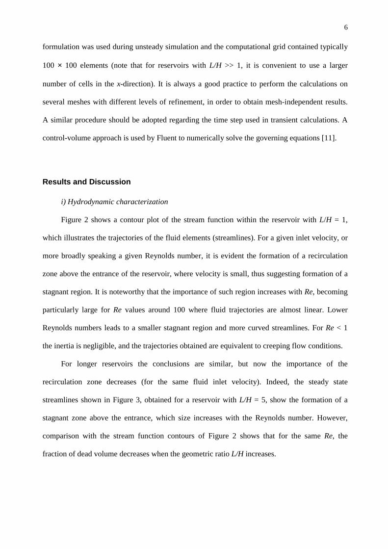
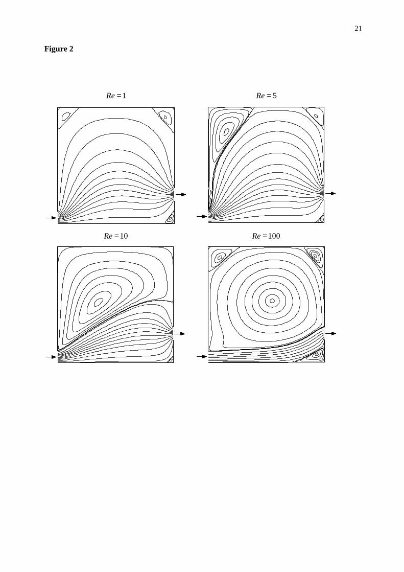
Figure 2 shows a contour plot of the stream function within the reservoir with L/H = 1,

which illustrates the trajectories of the fluid elements (streamlines). For a given inlet velocity, or

more broadly speaking a given Reynolds number, it is evident the formation of a recirculation

zone above the entrance of the reservoir, where velocity is small, thus suggesting formation of a

stagnant region. It is noteworthy that the importance of such region increases with Re, becoming

particularly large for Re values around 100 where fluid trajectories are almost linear. Lower

Reynolds numbers leads to a smaller stagnant region and more curved streamlines. For Re < 1

the inertia is negligible, and the trajectories obtained are equivalent to creeping flow conditions.

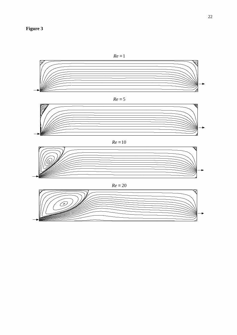
For longer reservoirs the conclusions are similar, but now the importance of the

recirculation zone decreases (for the same fluid inlet velocity). Indeed, the steady state

streamlines shown in Figure 3, obtained for a reservoir with L/H = 5, show the formation of a

stagnant zone above the entrance, which size increases with the Reynolds number. However,

comparison with the stream function contours of Figure 2 shows that for the same Re, the

fraction of dead volume decreases when the geometric ratio L/H increases.

7

ii) RTD determination from tracer experiments

After performing steady state simulations, students may proceed to transient runs.

However, they must first define a tracer step input at the inlet boundary condition. They must

also be aware that for t = 0 no tracer exists within the reservoir and that the laminar flow is

already established. So, they must first initialize the entire domain with a null tracer

concentration, and wait until the laminar regime is established before introducing the tracer step

change at inlet. After that, the CFD code solves the convection-diffusion equation that describes

the tracer transport in the reservoir, and one obtains the concentration field of tracer under

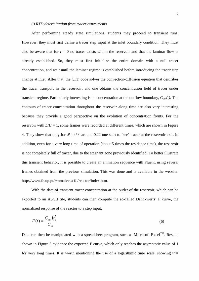
transient regime. Particularly interesting is its concentration at the outflow boundary, Cout(t). The

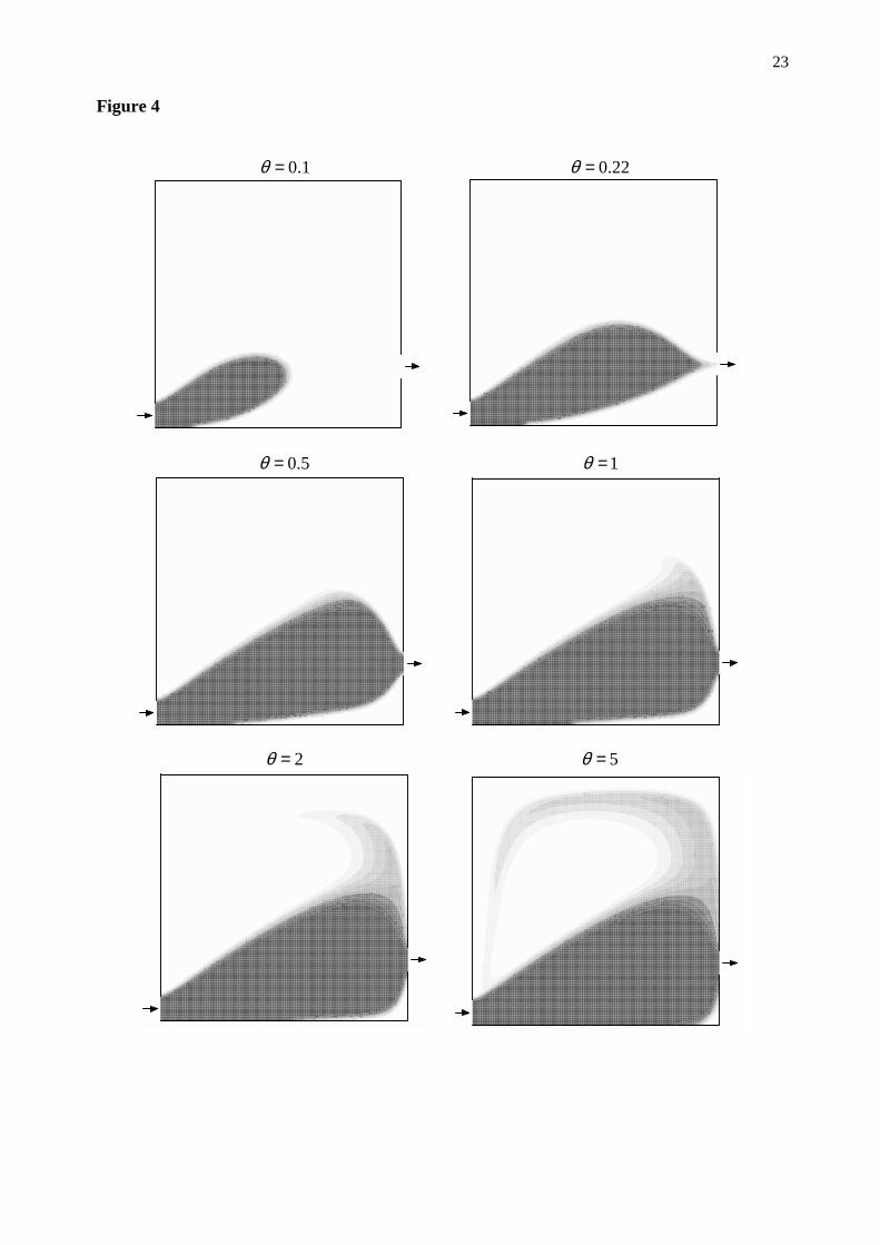
contours of tracer concentration throughout the reservoir along time are also very interesting

because they provide a good perspective on the evolution of concentration fronts. For the

reservoir with L/H = 1, some frames were recorded at different times, which are shown in Figure

4. They show that only for /tθ τ= around 0.22 one start to ‘see’ tracer at the reservoir exit. In

addition, even for a very long time of operation (about 5 times the residence time), the reservoir

is not completely full of tracer, due to the stagnant zone previously identified. To better illustrate

this transient behavior, it is possible to create an animation sequence with Fluent, using several

frames obtained from the previous simulation. This was done and is available in the website:

http://www.fe.up.pt/~mmalves/cfd/reactor/index.htm.

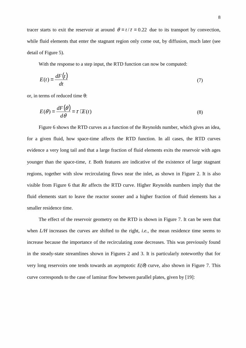
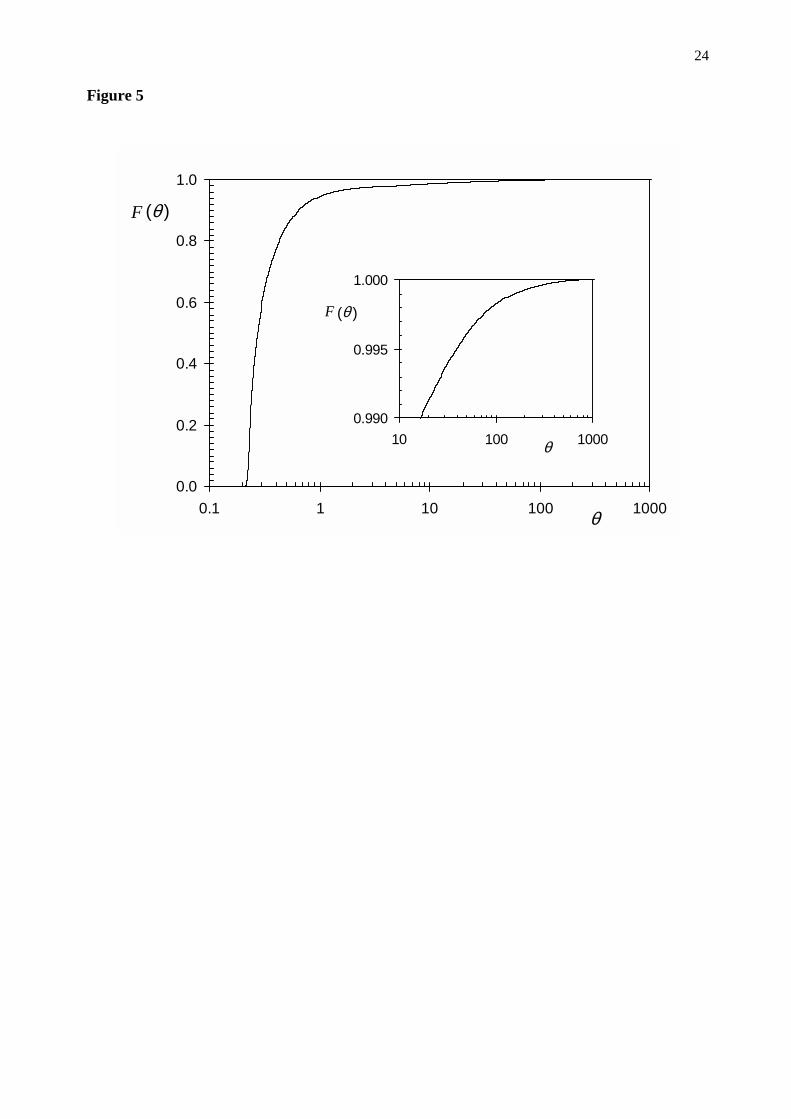
With the data of transient tracer concentration at the outlet of the reservoir, which can be

exported to an ASCII file, students can then compute the so-called Danckwerts’ F curve, the

normalized response of the reactor to a step input:

( )in

out

CtCtF =)( (6)

Data can then be manipulated with a spreadsheet program, such as Microsoft ExcelTM. Results

shown in Figure 5 evidence the expected F curve, which only reaches the asymptotic value of 1

for very long times. It is worth mentioning the use of a logarithmic time scale, showing that

8

tracer starts to exit the reservoir at around 22.0/ == τθ t due to its transport by convection,

while fluid elements that enter the stagnant region only come out, by diffusion, much later (see

detail of Figure 5).

With the response to a step input, the RTD function can now be computed:

( )dt

tdFtE =)( (7)

or, in terms of reduced time θ:

( ) )()( tEd

dFE ⋅== τθθθ (8)

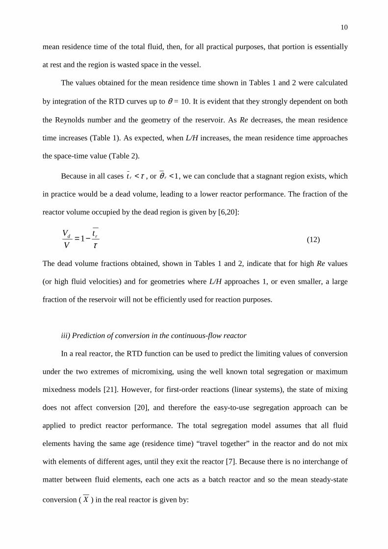
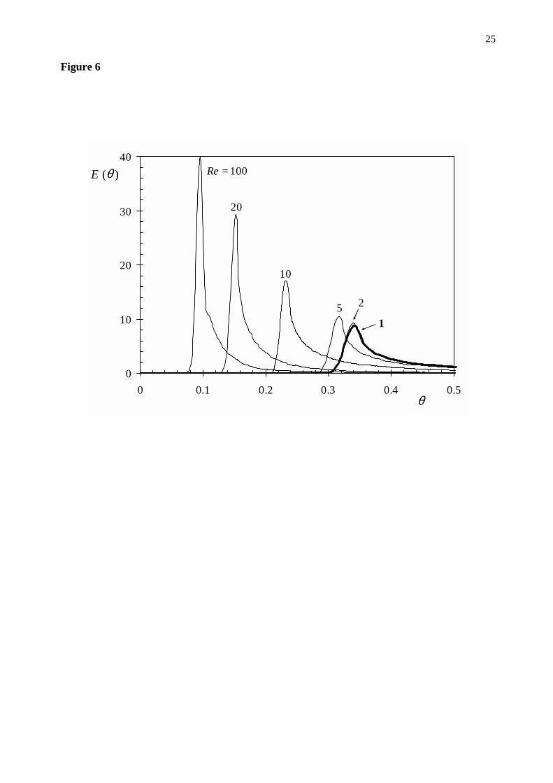
Figure 6 shows the RTD curves as a function of the Reynolds number, which gives an idea,

for a given fluid, how space-time affects the RTD function. In all cases, the RTD curves

evidence a very long tail and that a large fraction of fluid elements exits the reservoir with ages

younger than the space-time, τ. Both features are indicative of the existence of large stagnant

regions, together with slow recirculating flows near the inlet, as shown in Figure 2. It is also

visible from Figure 6 that Re affects the RTD curve. Higher Reynolds numbers imply that the

fluid elements start to leave the reactor sooner and a higher fraction of fluid elements has a

smaller residence time.

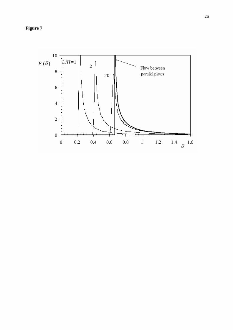
The effect of the reservoir geometry on the RTD is shown in Figure 7. It can be seen that

when L/H increases the curves are shifted to the right, i.e., the mean residence time seems to

increase because the importance of the recirculating zone decreases. This was previously found

in the steady-state streamlines shown in Figures 2 and 3. It is particularly noteworthy that for

very long reservoirs one tends towards an asymptotic E(θ) curve, also shown in Figure 7. This

curve corresponds to the case of laminar flow between parallel plates, given by [19]:

9

( )

<

≥−=

320

32

3213

1

3

θ

θ

θθθ

E (9)

It must be stressed that for this situation, i.e., laminar flow between parallel plates, the parabolic

profile is characterized by a maximum velocity, at the center, which is 1.5 times the average

velocity, while for flow in pipes this ratio is 2.

The RTD functions can then be used to calculate the mean residence time, defined as:

( )∫∞

⋅=0

dttEttr (10)

or,

( )∫∞

⋅==0

θθθτ

θ dEtrr (11)

For a closed-closed system (i.e., with no dispersion), and if no bypass or stagnant regions exists,

it is well known that the mean residence time and space-time are equal [7,20]. However, due to

the very long tail of the RTD function, this is only verified if simulations are run up to very high

times (typically θ of O (103)). Otherwise, the normalization condition ( ) ( ) 100

== ∫∫∞∞

θθ dEdttE is

not satisfied, and the computed mean residence time is smaller than the real space-time.

Calculation of the mean residence time is very important for evaluation of malfunctions

during reactor’s operation. Indeed, a straightforward way to diagnose the reactor’s flow

performance consists in comparing the computed value of the mean residence time from Eq. (10)

with the space-time (τ = V / Q, where V is the total volume of reactor and Q the volumetric flow

rate), which is equivalent to compare rθ with 1. Disagreement between these two values may

indicate the existence of bypasses, dead volumes, etc. For instance, as indicated by Froment [5],

if a region of the vessel retains a portion of the fluid for an order of magnitude greater than the

10

mean residence time of the total fluid, then, for all practical purposes, that portion is essentially

at rest and the region is wasted space in the vessel.

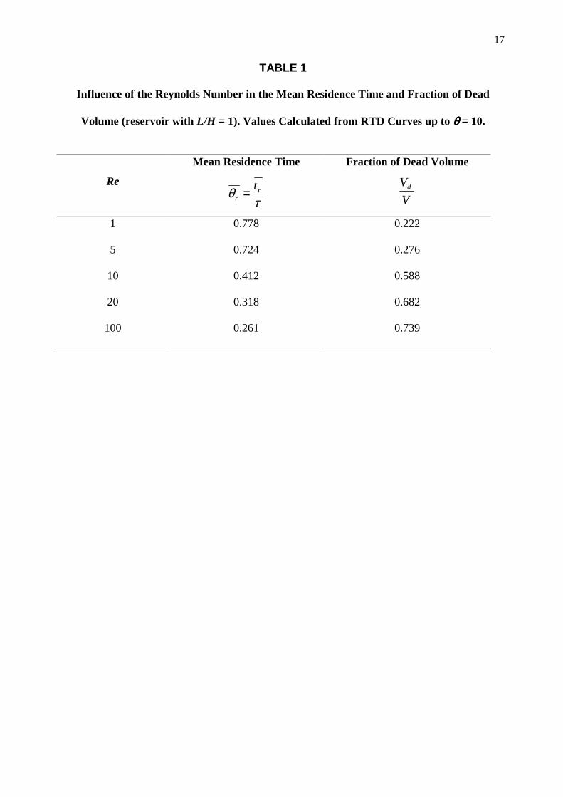
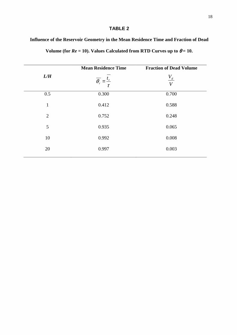
The values obtained for the mean residence time shown in Tables 1 and 2 were calculated

by integration of the RTD curves up to θ = 10. It is evident that they strongly dependent on both

the Reynolds number and the geometry of the reservoir. As Re decreases, the mean residence

time increases (Table 1). As expected, when L/H increases, the mean residence time approaches

the space-time value (Table 2).

Because in all cases τ<rt , or 1<rθ , we can conclude that a stagnant region exists, which

in practice would be a dead volume, leading to a lower reactor performance. The fraction of the

reactor volume occupied by the dead region is given by [6,20]:

τrd t

VV −=1 (12)

The dead volume fractions obtained, shown in Tables 1 and 2, indicate that for high Re values

(or high fluid velocities) and for geometries where L/H approaches 1, or even smaller, a large

fraction of the reservoir will not be efficiently used for reaction purposes.

iii) Prediction of conversion in the continuous-flow reactor

In a real reactor, the RTD function can be used to predict the limiting values of conversion

under the two extremes of micromixing, using the well known total segregation or maximum

mixedness models [21]. However, for first-order reactions (linear systems), the state of mixing

does not affect conversion [20], and therefore the easy-to-use segregation approach can be

applied to predict reactor performance. The total segregation model assumes that all fluid

elements having the same age (residence time) “travel together” in the reactor and do not mix

with elements of different ages, until they exit the reactor [7]. Because there is no interchange of

matter between fluid elements, each one acts as a batch reactor and so the mean steady-state

conversion ( X ) in the real reactor is given by:

11

∫∫∞∞

⋅=⋅=o

batcho

batch dEXdttEtXX θθθ )()()()( (13)

where Xbatch(t), for a first-order reaction, is given by:

( ) ( )θ⋅−⋅− −=−= Datkbatch eeX 11 (14)

and τkDa = is the Damköhler number.

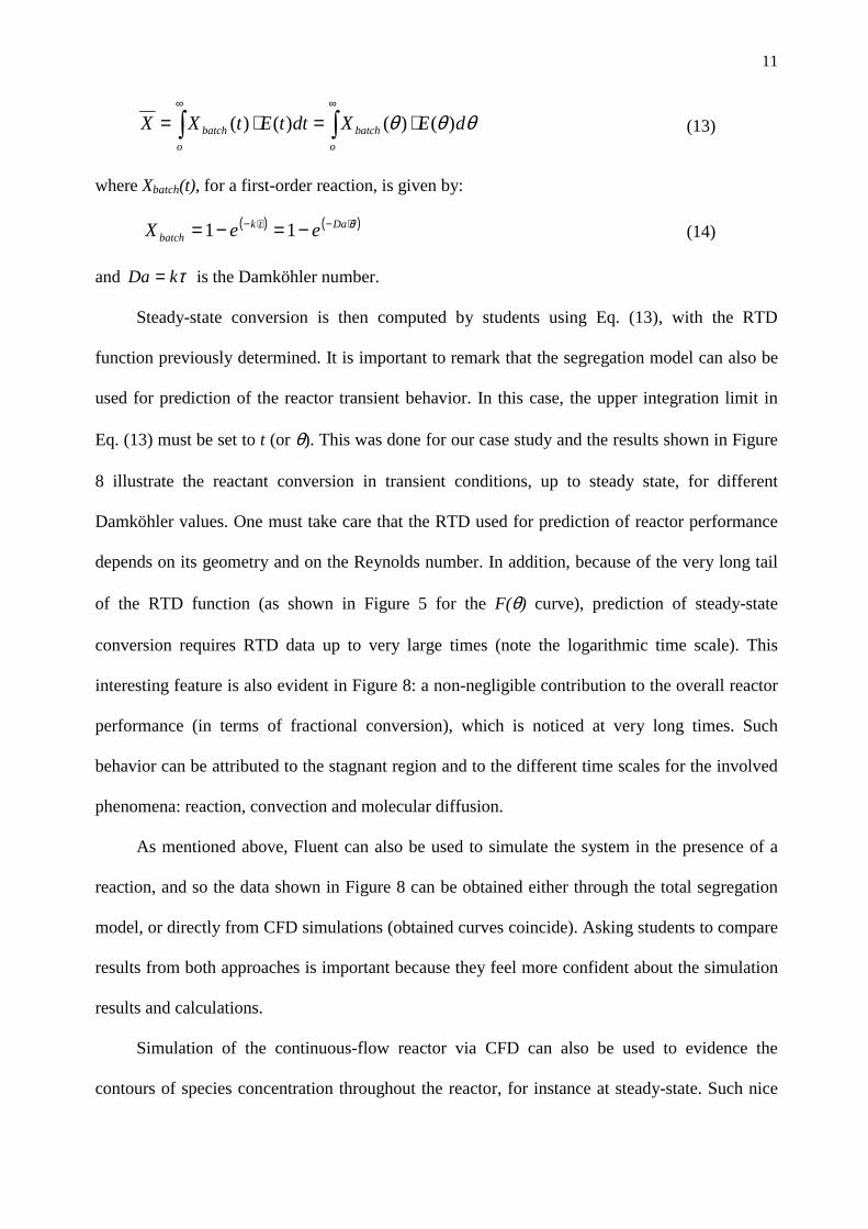
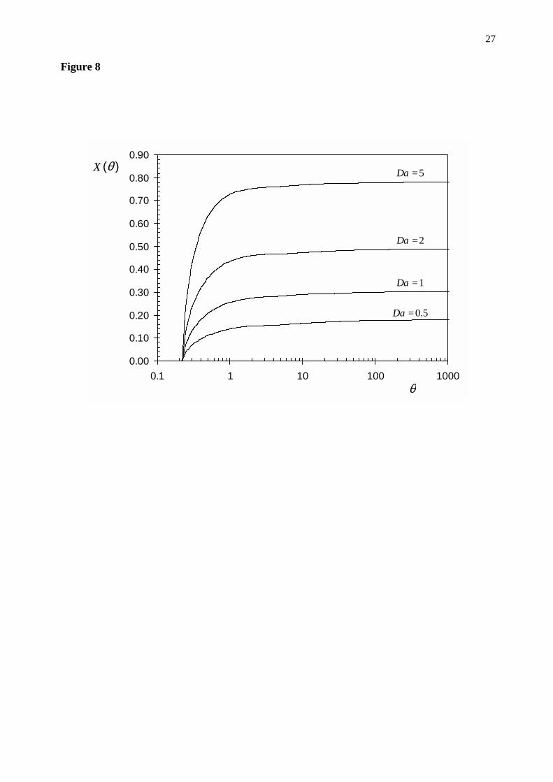
Steady-state conversion is then computed by students using Eq. (13), with the RTD

function previously determined. It is important to remark that the segregation model can also be

used for prediction of the reactor transient behavior. In this case, the upper integration limit in

Eq. (13) must be set to t (or θ). This was done for our case study and the results shown in Figure

8 illustrate the reactant conversion in transient conditions, up to steady state, for different

Damköhler values. One must take care that the RTD used for prediction of reactor performance

depends on its geometry and on the Reynolds number. In addition, because of the very long tail

of the RTD function (as shown in Figure 5 for the F(θ) curve), prediction of steady-state

conversion requires RTD data up to very large times (note the logarithmic time scale). This

interesting feature is also evident in Figure 8: a non-negligible contribution to the overall reactor

performance (in terms of fractional conversion), which is noticed at very long times. Such

behavior can be attributed to the stagnant region and to the different time scales for the involved

phenomena: reaction, convection and molecular diffusion.

As mentioned above, Fluent can also be used to simulate the system in the presence of a

reaction, and so the data shown in Figure 8 can be obtained either through the total segregation

model, or directly from CFD simulations (obtained curves coincide). Asking students to compare

results from both approaches is important because they feel more confident about the simulation

results and calculations.

Simulation of the continuous-flow reactor via CFD can also be used to evidence the

contours of species concentration throughout the reactor, for instance at steady-state. Such nice

12

color pictures can also be seen in our web site:

http://www.fe.up.pt/~mmalves/cfd/reactor/index.htm. The color gradient inside the reactor is

particularly interesting to observe.

Finally, it is convenient to ask students to compare the steady-state conversion attained in

the real reactor with those achieved with the ideal reactors that they learned in previous CRE

courses: continuous stirred tank and plug flow reactors. For a first-order reaction, performance

achieved by these reactors is given by [e.g., 7,8]:

DaDaX CSTR +

=1

(15)

( )DaPFR eX −−=1 (16)

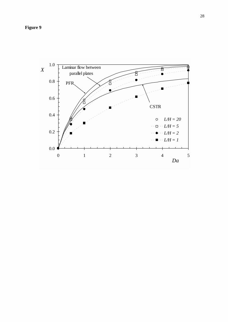
Data shown in Figure 9 indicate that when dead regions or stagnant zones are negligible,

i.e. for geometries where L/H is higher than about 5 (for Re = 10), the performance of the real

reactor lies between that of the CSTR and PFR. When L/H is close to 1, or even smaller, such

anomaly (dead volume) leads to a much lower performance of the non-ideal reactor, even lower

than that achieved with a perfectly mixed reactor. It is also noteworthy that for very long reactors

(i.e. high L/H ratios), one approaches the theoretical behavior of a laminar flow reactor (flow

between parallel plates), computed using the RTD function given in Eq. (9) and the segregation

model.

Concluding Remarks

Concepts dealing with the RTD theory and non-ideal reactors are not very familiar to

undergraduate students, and thus it is not an easy task to teach these matters in CRE courses.

Explanation of how stimulus-response tracer experiments provide the theoretical functions which

are crucial for reactor’s diagnosis, prediction of conversion, etc., becomes clearer through

experimentation, which is not always feasible. For such purpose, the use of CFD packages has

13

been particularly advantageous. Besides, CFD tools provide a graphical portrait of flow

throughout the reservoir/reactor, thus allowing going beyond simply predicting what will come

out of the reactor to predicting all of the properties of interest within the reactor. Some of the

concepts involved are more easily understood, like the progression of the tracer concentration

front, the formation of dead volumes or the existence of a concentration profile along the reactor.

Therefore, implementation of a CFD code has a considerable pedagogical content.

The case study herein described, a 2-D lagoon with laminar flow, was solved with the

commercial package Fluent. Using reservoirs/reactors with different geometries and/or different

operating conditions, students are asked to: (i) characterize the hydrodynamics; (ii) determine the

residence time distribution from tracer experiment, which provides diagnosis of reactor

operation; and (iii) predict conversion in a continuous-flow reactor (both steady-state and

transient behavior). Our experience shows that the use of the CFD code allows students to more

easily understand some of the basic concepts taught in CRE curricula. Finally, comparison of

numerical with analytical solutions known for laminar flow between parallel plates (i.e., for

geometries with high L/H ratios), improves their self-reliance regarding CFD results.

In a survey performed a few years ago to several chemical engineering departments spread

all over the world, some of the main points addressed by the departments to a question relating to

the future of CRE courses were [2]: i) the increasing importance of computer applications and

software packages and ii) put more emphasis on non-ideal reactors. With the case study herein

proposed, both issues are dealt with, therefore meeting current trends in CRE instruction. In

addition, students face the potential of CFD codes, which have been successfully used in practice

to design commercial-size reactors, usually with complex flow processes [22].

Nomenclature

C = concentration of tracer, reactant or product (mol.m-3 or kg.m-3);

D = coefficient of diffusivity (m2.s);

14

Da = Damköhler number, dimensionless;

E(t) = residence-time distribution function (s-1);

E(θ) = normalized RTD function, dimensionless;

F(t) = Danckwerts’ F curve, dimensionless;

H = height of the reservoir/reactor (m);

k = reaction rate constant of the first-order reaction (s-1);

L = length of the reservoir/reactor (m);

P = pressure (Pa);

S = source term (mol m-3 s-1 or kg m-3 s-1);

Q = volumetric flow rate (m3s-1);

Re = Reynolds number, dimensionless;

t = time (s);

rt = mean residence time (s);

Umax = fluid velocity at the center of the inlet boundary (m.s-1);

Umean = mean fluid velocity at the inlet boundary (m.s-1);

xu = x-velocity (m.s-1);

yu = y-velocity (m.s-1);

V = volume of reservoir/reactor (m3);

Vd = dead volume in the reservoir/reactor (m3);

X = conversion, dimensionless;

x = horizontal co-ordinate (m);

y = vertical co-ordinate (m);

Subscripts

batch = refers to batch reactor;

CSTR = continuous stirred tank reactor;

in = inlet conditions;

PFR = plug flow reactor;

out = outflow conditions;

Greek Symbols

θ = t/τ = reduced time, dimensionless;

τθ /rr t= = reduced mean residence time, dimensionless;

15

µ = viscosity of the fluid (kg m-1s-1);

ν = kinematic viscosity of the fluid (m2s-1);

ρ = density of the fluid (kg m-3);

τ = space-time (s);

References 1. Fogler, H.S., “An Appetizing Structure of Chemical Reaction Engineering for

Undergraduates”, Chem. Eng. Ed., 27, 110 (1993)

2. Shalabi, M., M. Al-Saleh, J. Beltramini, and D. Al-Harbi, “Current Trends in Chemical

Reaction Engineering Education”, Chem. Eng. Ed., 30, 146 (1996)

3. Falconer J.L., and G.S. Huvard, “Important Concepts in Undergraduate Kinetics and Reactor

Design Courses”, Chem. Eng. Ed. 38, 138 (1999)

4. Conesa, J.A., and I. Martín-Gullón, “Courses in Fluid Mechanics and Chemical Reaction

Engineering in Europe”, Chem. Eng. Ed. 34, 284 (2000)

5. Froment, G.F., and K.B. Bischoff, Chemical Reactor Analysis and Design, 2nd ed., John

Wiley & Sons, New York, NY (1990)

6. Villermaux, J., Génie de la Réaction Chimique – Conception et Fonctionnement des

Réacteurs, Tec & Doc – Lavoisier, Paris (1993).

7. Fogler, H.S., Elements of Chemical Reaction Engineering, 3rd ed., Prentice Hall, New

Jersey (1999)

8. Levenspiel, O., Chemical Reaction Engineering, 3rd ed., John Wiley & Sons, New York,

NY (1999)

9. Danckwerts, P.V., “Continuous Flow Systems. Distribution of Residence Times”, Chem.

Eng. Sci., 2, 1 (1953)

10. Conesa, J.A., J. González-García, and J. Iniesta, “Computer Simulations of Tracer Input

Experiments”, Chem. Eng. Ed. 33, 300 (1999)

11. Versteeg, H.K., and W. Malalasekera, An Introduction to Computational Fluid Dynamics.

The Finite Volume Method, Prentice Hall (1995)

12. Roache, P.J., Fundamentals of Computational Fluid Dynamics, Hermosa Publishers,

Albuquerque, New Mexico, USA (1998)

13. Roache, P.J., Verification and Validation in Computational Science and Engineering,

Hermosa Publishers, Albuquerque, New Mexico, USA (1998)

14. Sinclair, J.L., “CFD Case Studies in Fluid-Particle Flow”, Chem. Eng. Ed. 32, 108 (1998)

16

15. Metcalf & Eddy Inc., Wastewater Engineering: Treatment, Disposal, and Reuse, revised by

G. Tchobanoglous and F.L. Burton, 3rd ed., McGraw-Hill, New York, NY (1991)

16. Brunier, E., A. Zoulalian, G. Antonini, and A. Rodrigues, “Residence Time Distributions in

Laminar Flow Through Reservoirs from Momentum and Mass Transport Equations”, in

ISCRE8 – The 8th International Symposium on Chemical Reaction Engineering, IChemE

Symposium Series, Nº 87, 439 (1984)

17. Bird, R.B., W.E. Stewart, and E.N. Lightfoot, Transport Phenomena, 1st ed., John Wiley &

Sons, New York, NY (1960)

18. Leonard, B.P., “A Stable and Accurate Convective Modelling Procedure Based on Quadratic

Upstream Interpolation”, Comput. Meth. Appl. Mech. Eng., 19, 59 (1979)

19. Levenspiel, O., The Chemical Reactor Omnibook, OSU Book Stores, Corvallis, OR 97330

(1979)

20. Rodrigues, A.E., “Theory of Residence Time Distributions”, in Multiphase Chemical

Reactors, Rodrigues, A.E., J.M. Calo, and N.H. Sweed (Eds.), NATO ASI Series, Sijthoff

Noordhoff, No. 51, Vol. I, 225 (1981)

21. Zwietering, Th.N., “The Degree of Mixing in Continuous Flow Systems”, Chem. Eng. Sci.,

11, 1 (1959)

22. Bakker, A., A.H. Haidari, and E.M. Marshall, “Design Reactors via CFD”, Chem. Eng.

Progress 97, 30 (2001)

17

TABLE 1

Influence of the Reynolds Number in the Mean Residence Time and Fraction of Dead

Volume (reservoir with L/H = 1). Values Calculated from RTD Curves up to θθθθ = 10.

Mean Residence Time Fraction of Dead Volume

Re

τθ r

rt= V

Vd

1 0.778 0.222

5 0.724 0.276

10 0.412 0.588

20 0.318 0.682

100 0.261 0.739

18

TABLE 2

Influence of the Reservoir Geometry in the Mean Residence Time and Fraction of Dead

Volume (for Re = 10). Values Calculated from RTD Curves up to θθθθ = 10.

Mean Residence Time Fraction of Dead Volume

L/H

τθ r

rt= V

Vd

0.5 0.300 0.700

1 0.412 0.588

2 0.752 0.248

5 0.935 0.065

10 0.992 0.008

20 0.997 0.003

19

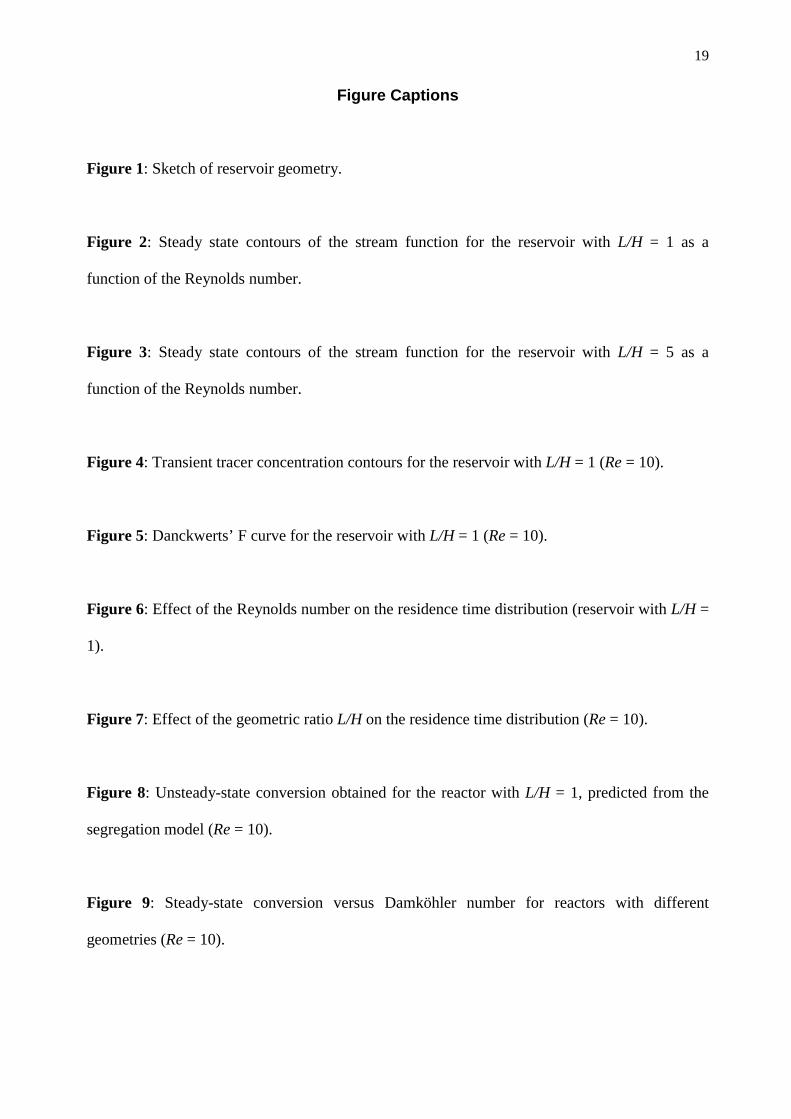
Figure Captions

Figure 1: Sketch of reservoir geometry.

Figure 2: Steady state contours of the stream function for the reservoir with L/H = 1 as a

function of the Reynolds number.

Figure 3: Steady state contours of the stream function for the reservoir with L/H = 5 as a

function of the Reynolds number.

Figure 4: Transient tracer concentration contours for the reservoir with L/H = 1 (Re = 10).

Figure 5: Danckwerts’ F curve for the reservoir with L/H = 1 (Re = 10).

Figure 6: Effect of the Reynolds number on the residence time distribution (reservoir with L/H =

1).

Figure 7: Effect of the geometric ratio L/H on the residence time distribution (Re = 10).

Figure 8: Unsteady-state conversion obtained for the reactor with L/H = 1, predicted from the

segregation model (Re = 10).

Figure 9: Steady-state conversion versus Damköhler number for reactors with different

geometries (Re = 10).

20

Figure 1

Inlet boundary condition

Stationary walls

Outflow boundary condition

ux (y)

L

0.1 H 0.2 H

0.7 H

H

x y

21

Figure 2

1Re = 5Re =

10Re =

100Re =

22

Figure 3

1Re =

5Re =

10Re =

20Re =

23

Figure 4

0.1θ =

0.22θ =

0.5θ =

1θ =

2θ =

5θ =

24

Figure 5

0.0

0.2

0.4

0.6

0.8

1.0

0.1 1 10 100 1000θ

F (θ )

0.990

0.995

1.000

10 100 1000θ

F (θ )

25

Figure 6

0

10

20

30

40

0 0.1 0.2 0.3 0.4 0.5θ

E (θ ) Re = 100

10

20

5 2

1

26

Figure 7

0

2

4

6

8

10

0 0.2 0.4 0.6 0.8 1 1.2 1.4 1.6θ

E (θ ) L /H =12

20Flow between parallel plates

27

Figure 8

0.00

0.10

0.20

0.30

0.40

0.50

0.60

0.70

0.80

0.90

0.1 1 10 100 1000θ

X (θ ) Da = 5

Da = 2

Da = 1

Da = 0.5

28

Figure 9

0.0

0.2

0.4

0.6

0.8

1.0

0 1 2 3 4 5Da

X

L/H = 20L/H = 5L/H = 2L/H = 1

PFR

CSTR

Laminar flow between parallel plates

29

Luis M. Madeira is Assistant Professor of Chemical Engineering at the Faculty of Engineering – University of Porto, Portugal. He graduated in Chemical Engineering (1993) and received his PhD (1998) from the Technical University of Lisbon, Portugal. He teaches Chemical Engineering Laboratories and Chemical Reaction Engineering. His main research interests are in catalytic membrane reactors, heterogeneous catalysis (including environmental catalysis) and fuel cells.

Manuel A. Alves is a Teaching Assistant in the Chemical Engineering Department at the Faculty of Engineering – University of Porto, Portugal. He graduated in Chemical Engineering at University of Porto, Portugal, in 1995. His main research interests are in the simulation of viscoelastic flows and the development of numerical algorithms for computational fluid dynamics. These are the main topics of his PhD research that is currently under conclusion.

Alírio E. Rodrigues is Professor of Chemical Engineering at the Faculty of Engineering – University of Porto, Portugal. He graduated in Chemical Engineering at University of Porto, Portugal (1968) and received his Docteur-Ingenieur degree at the University of Nancy (France) in 1973. He is Director of the Laboratory of Separation and Reaction Engineering - LSRE (www.fe.up.pt/lsre). His main research interests are in Cyclic Separation/Reaction Processes (Simulated Moving Bed, Pressure Swing Adsorption and Parametric Pumping technologies) and Chemical Reaction Engineering.