Tax Rates and Corporate Decision Making

John R. Graham Duke University

john.graham@duke.edu

Michelle Hanlon Massachusetts Institute of Technology

mhanlon@mit.edu

Terry Shevlin University of California, Irvine

tshevlin@uci.edu

Nemit Shroff Massachusetts Institute of Technology

shroff@mit.edu

July 2016 Abstract: We survey companies and find that many use incorrect tax rate inputs into important corporate decisions. Specifically, many companies use an average tax rate (the GAAP effective tax rate, ETR) to evaluate incremental decisions, rather than using the theoretically correct marginal tax rate. We find evidence consistent with behavioral biases (heuristics, salience) and managers’ educational backgrounds affecting these choices. We estimate the economic consequences of using the theoretically incorrect tax rate and find that using the ETR for capital structure decisions leads to suboptimal leverage choices and using the ETR in investment decisions makes firms less responsive to investment opportunities. This paper is the winner of the American Accounting Association 2015 FARS Midyear Meeting Best Paper Award. We thank John Barrios for sharing data on the LinkedIn profiles of our survey respondents. We appreciate helpful comments from Robin Greenwood (the editor), two anonymous referees, Mary Barth, James Chyz, Bryan Cloyd, Russ Lundholm, Lil Mills (discussant), Richard Sansing, Joel Slemrod (discussant), seminar participants at the Baruch College, Columbia Law School, INSEAD conference, International Institute for Public Finance (IIPF) Annual Congress (Dublin), MaTax Conference in Germany, Stanford Summer Camp, University of California, Davis, University of Tennessee, and Virginia Tech University. Thanks to the following people for helpful comments on the development of survey questions: Jennifer Blouin, Merle Erickson, Ken Klassen, Ed Maydew, Peter Merrill, Lil Mills, Sonja Rego, Richard Sansing, Stephanie Sikes, Joel Slemrod, and Ryan Wilson. We also appreciate the support of PricewaterhouseCoopers (especially Peter Merrill) and the Tax Executives Institute (especially Tim McCormally) in asking firms to participate and in reviewing the survey document. We are grateful for the discussions with several tax executives about their role in their company. Finally, each author is grateful for the financial support of the Fuqua School of Business, Paton Accounting Fund at the University of Michigan, MIT Junior Faculty Research Assistance Program, and the Paul Merage School of Business at the University of California-Irvine. All errors are our own.

1

Taxes represent a significant cost for most profitable corporations and, thus, are an

important input into many corporate decisions (see Shackelford and Shevlin (2001), Graham

(2003), and Hanlon and Heitzman (2010) for reviews). According to theory, the marginal tax rate

(MTR), defined as the present value of additional taxes paid on an additional dollar of income

earned today (Scholes et al., 2014), is the appropriate rate to use to evaluate incremental

corporate decisions (MacKie-Mason, 1990; Graham, 1996a, b; Brealey, Myers, and Allen, 2014;

and Scholes et al., 2014). Consistent with this theory, prior research finds that the MTR is

correlated with firms’ capital structure decisions (e.g., Graham, 1996a; Heider and Ljungqvist,

2015). However, prior research also finds that some firms appear to follow conservative debt

policies given their MTRs (e.g., Graham, 2000; Strebulaev and Yang, 2013), raising the question

of whether managers use the appropriate tax input when making corporate decisions.

In this paper, we use a survey to directly ask tax executives, for the first time, which tax

rate their firms use when making corporate financing and investment decisions. Survey data are

particularly useful to address this question because the rate employed cannot be directly

observed. Indeed, archival-based tests designed to identify which tax rates managers incorporate

into decision making are necessarily joint tests of what measure of taxes (if any) is used to make

the decision and whether the researchers’ empirical proxy of the rate is correct.1 We combine the

survey data with Compustat data to explore the determinants of managers’ tax rate choices and

the economic consequences of deviating from the theoretically preferred tax rate.

We directly ask tax executives of both public and private firms which tax rates their

companies employ in a number of decision-contexts, such as capital structure and capital

investment among others. We find that fewer than 13% of our sample firms use the MTR in any

decision-making context. Rather, survey responses indicate that most firms use either the U.S.

statutory tax rate (STR) or the ‘average’ tax rate computed in financial statements (the Generally

Accepted Accounting Principles effective tax rate [GAAP ETR] defined as income tax expense 1 Survey data are, of course, subject to many of their own concerns, which we acknowledge and attempt to mitigate. Our goal is to use survey data to complement the evidence in prior empirical-archival studies.

2

scaled by pretax book income, both of which are found on financial statements, not tax returns)

for evaluating incremental decisions. For example, 30% (26%) of the respondents indicate that

they use the GAAP ETR (STR) for making capital structure decisions.

Although these findings are seemingly inconsistent with corporate finance theory, they

are potentially consistent with theories and evidence from psychology. For example, prior

research finds that agents often use simple heuristics in many decision-making contexts rather

than more complex and fully rational approaches; further, employing heuristics often leads to

acceptable solutions that are “efficient” when considering the high cognitive cost of employing

the more complex fully rational approach (e.g., Tversky and Kahneman, 1974; Simon, 1979).

Computing the MTR is complicated due to unique features of the tax code (e.g., the treatment of

net operating losses, alternative minimum tax, etc.) coupled with the need to forecast taxable

income many years into the future. It is precisely in such complicated situations that managers

are likely to make decisions based on heuristics such as the STR. Further, consistent with the

idea that reliance on heuristics often serves as an efficient approximation for the purely rational

decision rule, we find that the difference between the MTR and STR (which we assume to be

35% throughout) is less than two percentage points for 4-out-of-5 firms that use the STR as the

tax rate input for decision making.2 Thus, our data are consistent with the STR being a simple

heuristic used by managers to approximate the MTR.

Prior research in psychology also finds that individuals are more likely to use a tax rate as

an input into decision making if that rate is more salient or noticeable to the individual (e.g., de

Bartolome, 1995; Chetty, Looney, and Kroft, 2009; Finkelstein, 2009).3 For publicly traded

firms, GAAP based financial accounting earnings reported to investors is indeed the focus of

2 We estimate MTRs using the approaches developed by Graham (1996a) and Blouin, Core, and Guay (2010). 3 Much of the related behavioral literature focuses on individuals rather than managers because, as DellaVigna (2009) states, “firms can specialize, hire consultants, and obtain feedback from capital markets. Firms are also subject to competition…therefore, firms are less likely to be affected by biases (except for principal–agent problems)…” (p. 361). However, Camerer and Malmendier (2007) suggest that managers make mistakes or inefficient decisions that markets do not fully correct when the decisions are infrequent and/or lacking clear feedback (e.g., capital structure).

3

much managerial attention (Healy, 1985; Degeorge, Patel, and Zeckhauser, 1999; Graham,

Harvey, and Rajgopal, 2005; Graham, Hanlon, Shevlin, and Shroff, 2014). Further, such a focus

on externally reported earnings is even more pronounced among firms that face more capital

market pressures (such as firms with large analyst following). As a result, the numbers reported

on financial statements, including the GAAP ETR, are arguably more salient to managers of

publicly traded firms. Our data reveal that public firms (relative to private firms) and firms with

high analyst following (relative to firms with low analyst following) are more likely to use the

GAAP ETR as the tax input in their decisions. We interpret these results as being consistent with

the idea that a capital market focus increases the salience of the GAAP ETR (henceforth, referred

to as ETR for expositional ease) and thus leads to its use in decisions. In addition, we obtain data

on managers’ educational backgrounds and find that more educated managers and managers with

a degree in accounting are less likely to use the ETR for decision making.

Because there is little economic or theoretical justification for using an average rate such

as the ETR as the tax rate input when making incremental decisions (see Brealey et al., 2014, p.

449), we next explore whether there are negative economic consequences to using the ETR in

corporate decisions. We focus on capital structure and investment outcomes to limit the scope of

the paper and because these are important decisions with empirical proxies in prior research. We

use proxies from Graham (2000) and van Binsbergen, Graham, and Yang (2010) to evaluate

firms’ capital structure decisions; we use the sensitivity of investment to investment

opportunities following Bloom, Bond, and Van Reenen (2007) and Asker, Farre-Mensa, and

Ljungqvist (2015) among others as well as the difference between firms’ actual and optimal

investment (predicted by our model) to evaluate firms’ capital investment decisions.

To facilitate empirical identification, we focus on firms that use the ETR for decision

making and exploit time-series variation in the difference between their MTRs and ETRs; we

predict decision-making errors from using the ETR to be greater when the difference between the

MTR and ETR is larger. We gather ETR and estimated MTR measures for the years 1997 to

2006 and associate the MTR vs. ETR difference with outcomes of corporate decisions. We also

4

conduct analyses that benchmark the association between the MTR vs. ETR difference and

decision-making efficiency for firms that use the ETR to that observed for a matched sample of

firms that use the MTR or STR. Essentially, this research design is akin to a difference-in-

differences design where firms using the ETR for decision making serve as “treatment” firms

and firms using the MTR or STR for decision making serve as “control” firms.4

We find that firms using ETRs as the tax rate input for capital structure decisions adopt a

suboptimal debt policy when the ETR differs from their estimated MTR. Similarly, we find that

firms using ETRs as the tax rate input for investment decisions are less responsive to investment

opportunities when the ETR differs from their estimated MTR. Our results are robust to

controlling for variables typically associated with debt and investment policy decisions,

including firm fixed effects, using various estimates of MTRs and investment opportunities, and

employing different research designs (see Section 5.3. for details). To our knowledge, this is the

first evidence of incorrect corporate decision making tied directly to the use of incorrect inputs.

In terms of estimates of economic magnitude, we use the van Binsbergen et al. (2010)

approach and find that the average firm that uses the ETR for capital structure decisions incurs a

loss of $16 million (in 2006 dollars) or 0.25% of the firm’s book value of assets from making

suboptimal capital structure decisions. van Binbergen et al. (2010) report that having the optimal

capital structure on average increases firm value by 3.5% of its book value of assets (relative to a

firm that is entirely equity financed). Our estimates suggest that using the correct tax rate

explains approximately 7% (=0.25/3.5) of value creation from having the optimal capital

structure. For the investment responsiveness tests, we estimate that, when the ETR is ten

percentage points different than the MTR, a one standard deviation increase in Tobin’s Q is

associated with an investment response that is 3.7% or $20 million (in 2006 dollars) lower, on

4 Benchmarking the outcome efficiency of firms that use the ETR for decision making with those that use the STR/MTR for decision making mitigates concerns that our results are spurious and that measurement error in our proxies induces our results. For example, it is plausible that MTR vs. ETR wedge picks up other firm characteristics (e.g., economic conditions, the presence of NOLs, permanently reinvested foreign earnings, etc.) that are correlated with the decision outcomes we examine, thereby affecting our inferences. However, as long as such correlated omitted firm characteristics affect firms using the ETR and MTR/STR similarly, they will get differenced away.

5

average, than when the ETR and MTR are equal. Our estimates of the dollar cost of using the

ETR for decision making is likely smaller than the total loss to the firm from using the ETR

because it only accounts for suboptimal capital structure choices and investment choices. To the

extent firms use the ETR for other recurring decisions such as M&A, R&D, and compensation

(which our survey suggests firms indeed do), the total loss in value from using ETRs is

potentially much larger.

Our paper contributes to the literature in psychology and behavioral economics that finds

that agents often deviate from decision rules predicted by standard models, which assume agents

optimize perfectly. The distinction between the “marginal” and “average” concepts is perhaps

one of the most basic ideas in economics and yet it is easy to get wrong; the evidence from many

recent studies suggests that agents often do not distinguish between marginal and average

concepts as standard theory predicts. For example, many surveys find that individuals often do

not distinguish between the marginal and average rate in cases of nonlinear price, subsidy, and

tax (e.g., see Liebman (1998) who studies taxes; Brown, Hoffman, and Baxter (1975) study

electricity price; and Carter and Milon (2005) test water prices). Similarly, subjects in laboratory

experiments show cognitive difficulty in understanding nonlinear price/tax systems and respond

to the average price/tax instead of the marginal (e.g., de Bartolome, 1995). This literature

predominantly focuses on decision making by individuals in non-corporate settings. We

contribute by showing that biases that affect individuals also affect managers, as predicted by

Camerer and Malmendier (2007), with respect to their choice of tax inputs for decision making.5

Our paper also contributes to the literature by providing further evidence that there is an

association between taxes and corporate decisions, such as leverage and investment; associations

that have drawn skepticism at times (e.g., Li, Whited, and Wu 2015). Finally, our paper responds

to Baker and Wurgler’s (2013) call for research to examine whether behavioral biases help

explain why managers do not more aggressively pursue the tax benefits of debt: We show and 5 Camerer and Malmendier (2007) and Baker and Wurgler (2013) summarize research documenting that managers are affected by biases other than those documented here, such as overconfidence and corporate socialism.

6

provide a lower bound estimate of the negative economic effects from managers using the ETR

in their decisions. If our hypothesis is descriptive that the decision to use the ETR is due to

salience, our estimates can be interpreted as the costs of such biases.

1. Survey methodology and sample6

We developed an initial survey instrument to investigate how taxes affect key corporate

decisions. We solicited feedback from several academic researchers, Tax Executives Institute

(TEI), and PricewaterhouseCoopers (PwC) on the survey content and design.7 Survey Sciences

Group (SSG), a survey research consulting firm, assisted with survey formatting and

programmed an online version. Two executives beta tested the survey and we made revisions

based on their suggestions. The final survey contained 64 questions, most with subparts. There

were many branching questions and thus, many firms answered only a portion of the questions.

An initial email invitation was sent on August 9, 2007 to the highest ranking tax

executive who is a member of TEI at 2,794 firms (only one invitation was sent to each

company); three were returned as undeliverable.8 We also sent a letter via two-day express mail

to fifteen companies for which we did not have email addresses. Thus, a total of 2,806

companies received invitations to complete the survey. SSG sent three email reminders in

August and September. For those who had not responded, we sent a paper version of the survey,

along with instructions of how to complete the survey online, in September and October. We

closed the survey on November 9, 2007.

A total of 804 firms accessed the survey. Sixty of these companies entered no more than

two responses and thus we delete them from our sample, leaving 744 usable responses. The 6 Our survey has four parts and the data from different parts of this survey are used in Graham, Hanlon, and Shevlin (2010, 2011), and Graham et al. (2014). Thus, the discussion in this section is similar to that in those papers. However, the research questions addressed in these papers are very different. Specifically, Graham et al. (2010) focus on the 2004 American Jobs Creation Act and repatriation decisions in response to that Act. Graham et al. (2011) explore questions concerning the location, reinvestment, and repatriation of foreign earnings. In particular, they examine the effect of an accounting rule, APB 23, on these decisions. Finally, Graham et al. (2014) examine the effects of reputational and accounting concerns on tax planning decisions. 7 TEI is an association whose members are executives responsible for the tax affairs of U.S. and foreign businesses. 8 Table OA1 in the online appendix provides a frequency distribution of the title held by the surveyed tax executive: 43.5% hold the title “Director,” 28.9% hold the title “Vice President,” and 13.3% hold the title “Manager.”

7

response rate for our survey is 26%, which compares favorably to many prior survey studies.9

We eliminate 11 firms that indicate they are not subject to the U.S. corporate income tax (i.e.,

businesses not taxed at the entity level, such as S corporations and other flow-through entities).

We also eliminate 29 companies that indicate that they did not file a corporate income tax

return—Form 1120 (we assume that these companies are also not taxed at the entity level). We

restrict the sample further by eliminating firms that are subsidiaries of foreign parents since their

corporate decisions and tax planning incentives are likely to be affected by the tax rules in the

parent’s home country. Finally, we lose 95 firms that did not respond to the section concerning

tax rates and decision making, the subject of our study. This leaves 500 remaining firms on

which we conduct our analyses. The sample size varies across the individual decisions (e.g.,

capital investment, capital structure) because of occasional missing responses.

There are caveats and limitations to survey research. First, firms that decide to answer the

survey may systematically differ from those that do not answer the survey. We address this

concern by comparing our survey respondents to the average Compustat firm to get a sense of

the characteristics of our sample firms relative to the typical sample of firms studied in the extant

literature.10 In addition, we compare firms that responded to the survey with firms that did not

respond. These data are tabulated and discussed below (see Section 3).

Another concern with survey-based research is that it is plausible that survey respondents

do not tell the complete truth in their responses. In addition, we may not have asked the

questions clearly, the respondent may not have understood some questions, or perhaps the

respondent just answered questions randomly. There is no way to completely eliminate these

possibilities; however, we attempted to mitigate these concerns by having academics,

practitioners, a professional survey consulting firm, and a set of beta firms carefully review the

survey and provide advice on how to best ask the questions before it was distributed. Finally,

9 For example, Trahan and Gitman (1995), Slemrod and Blumenthal (1996), Graham and Harvey (2001), Slemrod and Venkatesh (2002), and Graham et al. (2005) report response rates between 10.4% and 21.8%. 10 Unlike much research based on surveys, we know the identities of the firms that responded (and that did not respond), allowing tests for potential non-response bias.

8

most of our inferences are based on associations between our survey data and Compustat data,

which helps mitigate concerns related to biases in the survey data.

2. The role of tax executives in organizations

Our survey participants are corporate tax executives and thus it is important to understand

the role they play in their organizations. To better understand the functional role of a tax

executive, we interviewed three respondents to the survey and consulted several resources

including a recent article about tax directors, the tax function, and the tax environment11 and the

TEI 2011-2012 Corporate Tax Department Survey.12

The chief tax executive’s role generally manages three to four broad primary functions:

(i) tax planning, (ii) tax compliance (including audits), (iii) advising and aiding the C-suite and

operational functions of the firm and, (iv) for the roughly largest 20 to 50 companies, work on

tax policy. The complexity of the job varies with firm size, range of businesses within the firm,

and whether the firm is a multinational. For example, tax directors at the very largest firms spend

a significant amount of time on tax policy, meaning educating and lobbying policymakers and

staff in Washington, D.C., the European Union, the OECD (Organization for Economic

Cooperation and Development), and the state and territory governments that are important to

their business, as well as meeting with government affairs offices. In terms of education, many of

the heads of tax and high-level tax department personnel are lawyers or accountants and some

are both. In addition, tax directors today need to be comprehensive business people aware of

public relations, reputational concerns, and risk management.

The TEI 2011-2012 Corporate Tax Department Survey includes responses of 514

companies (67% are publicly traded). The survey was conducted in 2011 and had a 19%

response rate. The data show that the head of tax most often has the title of Director of

11 The article is entitled “A Conversation on the Current Tax Environment with George Forster” by Yoder and Fowler (2015) published in the International Tax Journal (September-October 2015, pp. 7-11). George Forster was a partner at PwC and was the V.P. – Taxes and Assistant Treasurer of IBM Corporation for five years. 12 The TEI survey is available for purchase at the TEI website at https://www.tei.org/news/Pages/Corporate-Tax-Department-Survey.aspx.

9

Tax/Corporate Tax Director (39%) or Vice President (39%), which is similar to the evidence

from our survey (see Table OA1 in the online appendix). Most companies report having a CPA

or licensed accountant among their tax department personnel (92%), more than any other

credential. The TEI survey also reveals that 67% of the senior tax executives report to the CFO,

12% to the company’s controller, 9% to the Chief Accounting Officer, and 5% report to the

Treasurer. Finally, the TEI survey indicates that senior tax executives met with the following

individuals (at least five times per year) to discuss tax risk: 71% with the CFO, 32% with

General Counsel, 15% with Internal Audit, 12% with the CEO, 4% with the Audit Committee,

and 2% with the Board of Directors.

Evidence from other surveys (e.g., Ernst and Young 1997, 2004) suggests that tax

executives are often involved in operating decisions. A 2013 survey of senior finance executives

conducted by CFO.com finds that the majority indicate that tax considerations should be

accounted for when “committing to major transactions.”13 Thus, it is quite likely that tax

executives are involved in corporate decision making, and are at a minimum, consulted about the

tax rates to use as inputs into decision making. Notwithstanding, if the tax executives are

unaware of the tax rates used for decision making then their responses to our survey should be

just noise and we would not see a consistent relation between their survey responses and

decision-making outcomes, working against our ability to document such a relation.

3. Descriptive statistics and non-response bias tests

We obtain demographic information from both survey data and, for publicly-traded firms,

from Compustat. Table 1 presents the descriptive statistics of our sample firms for 2006, which

was the most recent fiscal year at the time the survey was conducted. Nearly 78% of our sample

firms are publicly listed. The average firm has $5.6 billion in assets (Assets), with the average

public (private) firm having $6.5 ($2.4) billion in assets (untabulated). The average firm has

13 see: http://www.cfo.com/research/index.cfm/displayresearch/14710054

10

18.2% of its assets in foreign locations (Foreign Assets) and a GAAP ETR of 30.8%.14 Finally,

46.2% of our sample firms have a U.S. net operating loss carryforward (US NOL).

Additional data from Compustat indicate that the average public firm in our sample has

$4.7 billion in sales (Sales), a market capitalization (MVE) of $6 billion and earns a 5.9% return

on assets (i.e., net income scaled by assets; ROA). In terms of tax rate proxies, we find that the

average public firm in our sample has a marginal tax rate before accounting for debt interest

deductions (MTR) of 31% based on Graham’s methodology and 33.5% based on Blouin, Core,

and Guay’s (2010; BCG henceforth).15 Similarly, the average after-interest marginal tax rates

(MTR A.I.) are 21.4% and 31.8%, respectively, and the average GAAP ETR is 31.3%.16 The

average unsigned difference between the MTR and GAAP ETR (|MTR – GAAP ETR|) is 10.6%

(8.3%) using Graham’s (BCG’s) MTR methodology and is 16% (8.8%) between the MTR A.I.

and GAAP ETR (|MTR A.I. – GAAP ETR|). All variable are defined in the Variable Appendix.

Table 2 compares public survey firms with Compustat firms. We present means of

descriptive variables for (i) Compustat firms, (ii) firms we sent the survey to, (iii) firms that

responded to the survey and, (iv) firms that did not respond to the survey. The average survey

firm is larger than the average Compustat firm (measured by Assets, MVE, and Sales) and

different than Compustat firms in liquidity/profitability (Cash and ROA), growth (MB, Sales

Growth, and Asset Growth), investment intensity, and tax rates (GAAP ETR and MTR). To

further examine the source of the differences between our survey firms and Compustat firms, we

match each survey firm with Compustat firms based on size (i.e., Assets, MVE, and Sales) and

re-examine the differences in firm characteristics. We find that the average survey firm is

14 We asked tax executives to state their GAAP ETR in our survey instrument even though we can compute this number using Compustat. The correlation between the GAAP ETR listed in the survey response and that computed from Compustat is 0.99. This high correlation suggests that managers were careful when responding to the survey. 15 The two methodologies differ in their approaches for forecasting future taxable income. Graham’s methodology assumes that future taxable income follows a random walk with drift while BCG use a nonparametric approach to forecast taxable income. 16 The before-interest MTR computes taxable income prior to the deduction for interest expense (i.e., before financing). The after-interest MTR computes taxable income after subtracting the interest deduction. See Graham, Lemmon, and Schallheim (1998) for a discussion of when to use before- and after-interest MTRs.

11

statistically indistinguishable from the average Compustat firm once we control for size

(untabulated). Specifically, the survey firms and size-matched Compustat firms have similar

Leverage, MB, ROA, Asset Growth, Sales Growth, investment intensity, NOL, 3-Yr Cash ETR,

and MTR. Therefore, once one controls for size (which we do in our analyses below), the survey

sample appears representative of Compustat.

More importantly, we compare respondents to non-respondents (with Compustat data) to

test for non-response bias. We find that the average respondent is statistically no different than

the average non-respondent in terms of size (i.e., Assets, MVE and Sales), Leverage, Cash,

growth (MB, Asset Growth, Sales Growth), investment intensity, acquisition intensity, R&D

intensity, NOL, GAAP ETR, 3-Yr Cash ETR, and MTR. The only statistical difference is that the

respondent firms have, on average, a higher ROA than non-respondent firms. Overall, there is

little evidence of non-response bias in our sample.

4. How do managers incorporate taxes into their decisions?

Finance theory suggests that managers should use the MTR to evaluate incremental

decisions because it is the rate paid on an incremental dollar of income. For example, Graham

(1996a, p. 42) states that, “Financial theory is clear that the marginal tax rate is relevant when

analyzing incremental financing [and investing] choices.” In a similar vein, the popular corporate

finance text Brealey, Myers, and Allen (2014, p. 449) explicitly prescribes that managers should

“Always use the marginal corporate tax rate, not the average rate.” Despite the widely held belief

that managers should evaluate incremental corporate decisions using the MTR, there is little

direct evidence that managers indeed do so.17

In our survey, we ask executives ‘What is the primary tax rate your company uses to

incorporate taxes into each of the following forecasts or decision-making processes?’ The tax

17 The idea that MTRs should be used to evaluate incremental financing/investing decisions is generally well accepted. That said, some textbooks such as Damodaran (2014) propose using the ETR as the tax rate for equity valuation purposes. Using an average tax rate (such as the ETR) to value the entire firm essentially captures the varying marginal rates for different income levels. For whole-firm valuation, the ETR can be thought of as a proxy for the average MTR.

12

executive is allowed to choose from the following options (or write in an answer if the options

given are not sufficient): (i) U.S. statutory tax rate, (ii) GAAP effective tax rate, (iii) jurisdiction-

specific statutory tax rate, (iv) jurisdiction-specific effective tax rate, (v) marginal tax rate, and

(vi) other. The respondent then chooses which is the primary tax rate input in the following

decision contexts : (i) mergers and acquisitions, (ii) capital structure (debt versus equity), (iii)

investment decisions (property, equip., etc.), (iv) the decision to purchase versus lease, (v)

weighted average cost of capital, (vi) new facility location and, (vii) compensation. The

respondent could choose one tax rate for each decision context. Because we were not certain that

tax executives would hold the same definition of MTRs that exists in academia, we defined in

parenthesis the MTR as “an estimation of the change in the present value of taxes from earning a

marginal dollar of income, where the present value computation takes into account net operating

loss carrybacks and carryforwards.” We acknowledge that defining the MTR and no other rate

may induce response biases. Particularly, it is plausible that by defining MTRs, we heightened

respondents’ awareness to MTRs over the other tax rates, thereby increasing the number of

executives choosing the MTR.18 Therefore, our results might possibly represent an upper bound

estimate of the number of firms using the MTR as their tax rate input for decision making.19

Figure 1 and Table 3, Panel A present the survey responses to the above question. The

most popular tax rate managers claim to incorporate into their decision making is the GAAP

ETR and the second most popular is the STR. For example, with respect to capital structure

18 It is also plausible that defining the rate made it seem complicated and the executive did not choose it as a result. This alternative seems unlikely because respondents that use MTRs for decision-making should not be confused by its definition. 19 The definition of MTR provided in our survey follows from the Scholes-Wolfson framework (see Scholes et al., 2014). It is plausible that managers use a tax rate that incorporates the Scholes-Wolfson intuition without explicitly computing MTRs per that definition (e.g., a company might have separate tax rates for different economic scenarios – high, medium, and low – and these scenarios might include the effect of NOLs, etc.). If so, the number of firms saying they use the MTR might be understated. We created a provision for such an outcome in our survey by allowing respondents to choose the “other” option and by providing space for them to write-in an answer. Depending on the decision, 11 to 20 firms listed a response in this “other” space. From these we see that one firm indicated that it uses an “Employees’ marginal tax rate average” for its compensation decisions, and other firms stated they use “Business plan ETR,” “A standard 41%,” “Effective cash tax rate,” and “cash tax rate.” No firm suggested using something that we could interpret as equivalent or similar to the MTR in concept.

13

decisions, survey responses indicate that 30% of firms use the GAAP ETR, 26% use the U.S.

STR, 15% use the jurisdiction-specific STR, 15% use the jurisdiction-specific ETR, and 12% use

the MTR. Averaging across all decision contexts, 25.8% use GAAP ETRs, 23.1% use STRs,

19.6% use jurisdiction-specific STRs, 17.0% use jurisdiction-specific ETRs, 11.2% use MTRs,

and 3.2% use some other rate.

That very few firms use the MTR may seem surprising. However, the STR closely

approximates the MTR for firms that generate high taxable income and foresee themselves

continuing to do so. Indeed, in untabulated analyses, we find that over 80% of the firms that

indicate they use the STR for capital structure decisions have a simulated MTR that is within two

percentage points of the STR (35%). Thus, for the majority of firms that say they use the STR,

this choice is unlikely to induce costly errors. To the extent the STR and the jurisdiction-specific

STR closely approximate the MTR of a given firm, our results suggest that over 50% of

respondents use tax rates that are consistent with standard finance theory (e.g., Graham, 2003;

Brealey et al., 2014; Scholes et al., 2014).

Another noteworthy observation is that when making location-specific decisions, most

managers indicate that they use jurisdiction-specific rates (statutory and effective) as tax input.

For example, 55% of respondents indicate they use a jurisdiction-specific rate for the location of

new facilities. In contrast, only 30% and 26% say that they use a jurisdiction-specific rate for

capital structure decisions and weighted average cost of capital computations, respectively. This

change in responses across the factors suggests that the respondents carefully considered the

questions and varied their answers when appropriate (i.e., the respondents did not provide the

same response for each factor without thought).

Table 3, Panel B shows that tax rate choices are highly correlated across different

decision contexts (ranging from 0.66 to 0.93). Given the high correlations, for the remainder of

our analyses, we focus on firms’ capital structure and investment decisions for brevity and

because these are important decisions. Also in the interest of brevity, we combine firms that use

14

the jurisdiction-specific STR (ETR) with those using the U.S. STR (ETR) in our analyses of the

determinants of managers’ tax rate choices (in the next section).

5. Determinants of tax rate choices

To better understand tax rate choices, we examine the association between survey

responses, firm characteristics, and the executives’ educational backgrounds. We draw from

psychology and behavioral economics theories to guide the choice of independent variables to

include and to interpret the results. We conjecture that managers’ tax rate choices are affected by

the following: (i) the complexity of calculating the tax rate and the availability of simple

heuristics that approximate expected tax costs, (ii) the salience of different tax rates to managers,

(iii) operations that are conducive to corporate tax planning, (iv) the existence of mechanisms to

monitor managers and increase their efficiency (such as institutional investors and competitive

forces), and (v) the tax executive’s education. We recognize that these factors do not comprise a

complete list of factors that affect a tax rate choice; we view our analyses in this section as an

initial step to understanding managers’ tax rate choices. Importantly, the analyses in this section

are largely exploratory and descriptive in nature, without any causal inference.

We estimate three probit regressions where the dependent variable is an indicator variable

for the manager’s tax rate choice (ETR, STR or MTR). Specifically, the indicator variable Use

STR equals one for firms that use the STR or jurisdiction-specific STR for both capital structure

and investment decisions; and equals zero otherwise. Use MTR and Use ETR are indicator

variables defined analogously.20 The independent variables are measured in 2006 (the most

recent fiscal year at the time of the survey).

5.1. Firm characteristics and the tax rate choice

We begin by examining both public and private firms, with the independent variables in

these initial regressions are limited to firm characteristics obtained from the survey. Table 4,

20 We combine capital structure and investment decisions for brevity. Our inferences are unchanged if we estimate separate regressions for each decision context (i.e., capital structure and investment) and define Use STR (Use ETR; Use MTR) to equal one firms that use the STR (ETR; MTR) for the individual decision context.

15

Panel A presents the marginal effects from probit regressions; the standard errors are clustered

by industry.21 The main result from the table is that public firms are 9.6 percentage points more

likely to use the ETR (relative to the STR/MTR) for decision making. In contrast, private firms

are 12 percentage points more likely to use the STR (relative to the ETR/MTR). We interpret this

as being consistent with tax rate salience affecting managers’ tax rate choices. Our inference is

based on prior research that finds that top management of public firms view GAAP earnings as

the most important performance metric of a firm (Graham et al., 2005). In a tax setting, prior

research finds that public firm tax executives are incrementally compensated for lowering ETRs

and often view the ETR as a more important metric than cash taxes paid (Armstrong, Blouin, and

Larcker, 2012; Graham et al., 2014). The focus on GAAP earnings and by extension GAAP

ETRs is likely to make the ETR more salient to the decision-makers in public firms. In contrast,

prior research finds that private firms are less focused on GAAP-based numbers than public

firms (Cloyd, Pratt, and Stock, 1996; Graham et al., 2005), making them less likely to use the

ETR. For private firms, the STR is the most salient tax rate compared to the MTR and ETR. As a

result, we interpret the association between ownership and managers’ tax rate choices as

evidence consistent with salience.22

In Table 4, Panel B we include additional independent variables that we obtain from

databases such as Compustat. We drop private firms from the analyses due to the lack of data

availability in Compustat. The main results in Table 4, Panel B are as follows. First, we find that

larger firms are more likely to use the STR and MTR for decision making while smaller firms

are more likely to use the ETR (consistent with Panel A). For example, a 10% increase in total

assets increases the likelihood of using the STR (MTR) by 0.5 (0.3) percentage points and

reduces the likelihood of using the ETR by one percentage point. We also find that R&D-

21 We do not include industry fixed effects in the main regressions because our sample size is small. However, Table OA2 in the online appendix shows that inferences are unchanged when we control for industry fixed effects. 22 Although managers are compensated for lowering the ETR, which leads them to consider the effect of their decisions on ETR, we do not see any reason why it is efficient or correct for them to use the ETR in estimating after-tax cash flows or the after-tax cost of debt. We discuss this point in more detail and provide supporting empirical evidence in Section 6.3.

16

intensive firms are more likely to use the MTR and less likely to use the ETR for decision

making. Specifically, a ten percentage point increase in R&D intensity increases the likelihood

of using the MTR by 7.4 percentage points and reduces the likelihood of using the ETR by 17.7

percentage points. Our interpretation is that larger firms and high-R&D-intensity firms are likely

to have greater tax compliance activities and/or greater tax planning opportunities, which leads

them to employ well-trained tax personnel. Consequently, such firms are more likely to

accurately compute MTR estimates and use the MTR (or STR when appropriate) rather than the

ETR for decision making. Our interpretation is based on prior research that finds that (i) larger

firms benefit from economies of scale in tax planning, and thus are more likely to hire well-

trained/sophisticated tax personnel (Mills, Erickson, and Maydew, 1998; Rego, 2003); and (ii)

R&D activities create additional opportunities for tax planning because they generate tax credits

that can be offset against current/future income, as well as intellectual capital that can be

transferred to low tax jurisdictions to save taxes (Grubert and Slemrod, 1998). Thus, large firms

and firms with high R&D are more likely to have a sophisticated tax team that promotes using

the MTR (rather than the ETR) for decision making within the firm.

Second, we find that firms are less likely to use the STR for decision making when the

difference between the MTR and STR is larger. Specifically, a ten percentage point increase in

the difference between the MTR and STR reduces the likelihood of using the STR by 2.6

percentage points. Further, firms with a large proportion of their assets in foreign locations are

significantly more likely to use the STR (in this case often a jurisdiction-specific STR) and less

likely to use the MTR as their tax rate input. For example, a ten percentage point increase in

foreign assets increases the likelihood of using the STR by 2.2 percentage points and reduces the

likelihood of using the MTR by 1.9 percentage points. Our interpretation of these patterns is that

firms use the STR as a heuristic in place of the MTR (i) when the STR closely approximates the

MTR and (ii) when computing the MTR is very complex. Specifically, the evidence that firms

are less likely to use the STR as the difference between the STR and MTR increases is consistent

with Kahneman et al. (1982) and Pitz and Sachs (1984), who indicate that heuristics are typically

17

used to approximate the fully rational solution while saving on cognitive costs.23 Similarly, the

association between foreign operations and tax rate choices is consistent with firms relying on

heuristics when the rational decision rule is more complex. Foreign operations increase the

complexity and uncertainty of computing MTR estimates because of differences in the likelihood

and timing of foreign earnings repatriations, and cross-country differences in the tax

rates/schedules, transfer pricing rules, tax policy uncertainty, etc. Given the complexity of

estimating MTRs at firms with foreign operations, theory suggests that such firms are more

likely rely on heuristics to approximate the rational decision rule.

Third, we find that firms with larger analyst following are more likely to use the ETR and

less likely to use the STR and MTR for decision making. Our estimates imply that firms with one

additional analyst following them are 1.5 percentage points more likely to use the ETR and 1.2

(0.6) percentage points less likely to use the STR (MTR). To the extent financial analysts

increase capital market pressure as suggested by prior research (e.g., Fuller and Jensen, 2002; He

and Tian, 2013), an increase in analyst following is likely to increase managerial focus on

financial accounting earnings. As discussed previously, an increased focus on accounting

earnings potentially increases the salience of the GAAP ETR. Thus, we interpret the association

between analyst following and ETR usage as consistent with a salience hypothesis.

Finally, we find that firms with high institutional ownership and firms operating in

environments with greater product market competition are more likely to use the MTR and less

likely to use the ETR for decision making, respectively.24 Our estimates imply that a ten

percentage point increase in institutional ownership increases the likelihood of using the MTR by 23 A noteworthy observation in Table 4, Panel B is that the magnitude of the differences between the MTR and GAAP ETR is not negatively associated with ETR usage (in contrast to the association between the MTR-STR difference and STR usage). This result suggests that firms using the ETR do not seem to treat the ETR as an easy-to-compute heuristic to approximate the MTR as it converges with the MTR. Rather, this result is more consistent with the idea that the decision to use the ETR is a result of other factors/biases but not heuristics, at least as described by Hogarth (1981), Kahneman et al. (1982) and Pitz and Sachs (1984), among others. 24 We measure a firm’s competitive environment using the approaches in Li, Lundholm, and Minnis (2013) and Hoberg and Phillips (2015). Specifically, we classify firms as operating in competitive environments if (i) they operate in an industry with below median concentration measured using the Hoberg and Phillips (2015) text-based industry concentration index, and (ii) the Li et al. (2013) index measuring competitive intensity based on the firm’s discussion of competition in its 10-K filing is greater than the sample median.

18

1.2 percentage points; and firms are 15.4 percentage points less likely to use the ETR when they

operate in more competitive environments. Our interpretation of these results is that companies

are more likely to use the MTR and less likely to use the ETR when external monitoring

mechanisms discipline managers and curb agency problems. A large body of evidence finds that

institutional ownership is associated with more efficient outcomes (see e.g., McConnell and

Servaes, 1990; Bushee, 1998; and Aghion, Van Reenen, and Zingales, 2013). Similarly, prior

research finds that competition increases managerial focus on firm value and reduces the

incentive and ability to slack off (or to lead a “quiet life”). The intuition is that competition

makes it costlier for firms to forgo long-run value since such actions decrease the likelihood of

survival (see e.g., Nickell, 1996; Shleifer and Vishny, 1997).

5.2. Executive educational background and tax rate choice

Next, we examine whether the educational background of tax executive is associated with

the tax rate inputs used by their companies. Prior research finds that managers’ education

backgrounds are associated with their decision-making behavior (e.g., Hambrick and Mason

1984; Chevalier and Ellison 1999; Barker and Muller 2002). Thus, it is plausible that tax

executives with more education or education in a field that exposes them to the “marginal vs.

average” concept are less likely to use the ETR (or more likely to use the MTR for decision

making). To test the relation between education and managers’ tax rate choice, we obtain

educational background data from the executives’ LinkedIn profiles, matched by the manager’s

name and place of employment (and hand checked to ensure accuracy). This yields the LinkedIn

profiles of 210 of the tax executives that responded to our survey.25 Using the LinkedIn data, we

identify each tax executive’s degree and major. The data (tabulated in Table 5, Panel A) reveal

that 66% of tax executives have at least one accounting degree such as a Masters or Bachelor of

Accounting; 43% have a tax specialization such as Master of Taxation or Master of Business

Taxation (MBT); 16% have a law degree such as a Master of Laws (LLM) or Juris Doctor (JD); 25 We appreciate John Barrios sharing the LinkedIn data with us. Barrios (2016) discusses these data in detail.

19

and 16% have a business or economics degree such as an MBA or BA in economics. Table 5,

Panel A shows that tax executives average 1.9 degrees. Using these data, we estimate three

probit regressions where the dependent variables are Use STR, Use MTR, or Use ETR (as defined

previously) and the independent variables are the tax executives’ major and the number of

degrees. Table 5, Panel B presents initial results that do not control for firm characteristics and

Panel C presents results in which we control for firm characteristics obtained from our survey.

The analysis reveals two patterns: First, tax executives with at least one accounting

degree are more likely to use the MTR and less likely to use the ETR (see Table 5, Panel B).

This result is robust to controlling for firm characteristics such as public vs. private ownership,

firm size, NOLs, complexity, and foreign operations (see Table 5, Panel C). Second, more

educated tax executives, proxied by number of degrees, are less likely to use the ETR for

decision making (see Table 5, Panels B and C).26 The economic magnitude of the effect of

education on managers’ tax rate choices is large. Having an accounting major increases the

likelihood of using the MTR by 11.1 percentage points in the regression without controls, and by

7.4 percentage points in the regression with controls. Further, having an accounting degree

reduces the likelihood of using the ETR by 16.4 (14.2) percentage points in the regression

without (with) controls. Finally, having one additional degree lowers the likelihood of using the

ETR by 9.4 (11.2) percentage points in the regression without (with) controls. These results

provide additional insights into the determinants of managers’ tax rate choices and suggest that

educational background affects the choices that managers make.

5.3. Summary and caveats

To briefly summarize, our results so far are consistent with (i) managers relying on

heuristics, such as the STR, for decision making when doing so approximates the MTR and

26 Panel C shows that the coefficient on Public is insignificantly associated with Use ETR even though the magnitude of the coefficient estimate is similar to that in Table 4, Panel A. This is likely because of the sample size drops from 449 in Table 4, Panel A to 189 observations in Table 5, Panel B. Consistent with a ‘low power’ explanation for the loss of significance on Public in Table 5, we find that re-estimating the Table 4, Panel A regression using the Table 5 sample of 189 observations produces an insignificant coefficient on Public.

20

MTR calculations are complex, (ii) managers of public firms and firms with high analyst

following being more likely to use ETRs for decision making, which we interpret as consistent

with a salience bias, and (iii) managers of larger firms and R&D intensive firms being more

likely to use the MTR and/or less likely to use the ETR, which we interpret as consistent with

firms with greater tax planning opportunities hiring sophisticated tax personnel, who promote

using the theoretically correct tax rate,27 (iv) firms with high institutional ownership and firms

operating in more competitive environments being more likely to use the MTR and/or not the

ETR, which we interpret as consistent with external monitoring mechanisms leading firms to use

the theoretically correct tax rate and (v) firms with more educated managers and managers with

an accounting background being more likely to use the MTR and/or not the ETR, which we

interpret as consistent with knowledge-based explanations for tax rate choice.

Due to data limitations, we are not able to entirely distinguish between these explanations

of tax rate choice, nor rank them by relative importance. We also recognize that our analyses on

determinants documents associations, not causal evidence, and could have alternative

interpretations to those we offer. We hope future research provides more definitive, and perhaps

causal, evidence on determinants of managers’ tax choices.

6. Economic consequences of tax rate choices

In this section, we examine whether using the ETR as the tax rate input leads to

inefficient corporate decisions. We employ two research designs. Our first design focuses on

firms that use the ETR as the tax rate input for decision making and exploits time series variation

in the difference between their MTRs and ETRs. We predict that firms using the ETR are likely

to make better decisions when their ETR is close to their MTR. However, as the difference

between the MTR and ETR becomes larger, these firms’ decisions are likely to become more

inefficient. This research design provides two important benefits: First and perhaps foremost,

27 Although these findings are descriptive in nature, future research can perhaps use them to infer and measure differences in “tax sophistication” across firms.

21

inferences based on this research design are unaffected by (potential) response biases induced by

our survey because we restrict our sample to just those firms that use the ETR. Second, because

we only exploit time-series variation in the difference between a firm’s MTR and its ETR (both

of which vary over time), our inferences are less likely to be affected by any unaccounted for

relation between a firm’s tax rate choices and its characteristics.

Nonetheless, one limitation of the research design is that the difference between the MTR

and ETR might be correlated with other factors (besides firm characteristics potentially

correlated with tax rate choices) that also affect the dependent variable. In other words, within-

firm changes in the MTR vs. ETR difference could pick up non-tax factors that affect corporate

decision-making efficiency (or even measurement error).28 To address this concern, we perform

a second research design: we benchmark the association between the MTR vs. ETR wedge and

decision-making efficiency for firms that use the ETR for decision making with that for a

matched sample that uses the STR or MTR. Essentially, this design (henceforth referred to as the

“benchmark sample” research design) is akin to a difference-in-difference design that compares

the effect of the MTR vs. ETR wedge on the decision-making efficiency of ETR firms (i.e.,

treatment firms) to the effect of the MTR vs. ETR wedge on the decision-making efficiency of

MTR and STR firms (i.e., control firms).

The intuition for the benchmark sample research design is that if firms use the MTR or

STR as the tax rate input for their decisions, then the difference between the MTR and ETR

should be unrelated to their capital structure and investment outcomes because the MTR and

STR are theoretically appropriate tax rate inputs for decision making. In contrast, if the

difference between the MTR and ETR captures confounding factors that have a direct relation

with corporate decisions, then we would (spuriously) find that this difference is related to the

28 For example, highly profitable firms that have foreign operations in low tax jurisdictions often have a lower ETR (due to their permanently reinvested earnings) and high MTRs as measured by MTR proxies, leading to a large wedge between the MTR and ETR. Further, evidence in prior research suggests that multinational firms tend to make different capital structure choices due to the presence of internal capital markets and greater agency problems from having geographic dispersed operations (e.g., Desai, Foley, and Hines 2004, Giroud 2013, and Shroff, Verdi, and Yu 2014), thereby creating a potential correlated omitted variable problem.

22

corporate outcomes even for firms that use the MTR/STR for decision making. As a result, any

non-tax factors that induce a relation between the MTR vs. ETR wedge and the decision

outcomes should get differenced away in our benchmark sample tests.29

We merge the survey data with Compustat data from 1997 to 2006, thereby creating a

ten-year panel.30 We measure ETRs for each firm-year as total income tax expense scaled by

pre-tax book income and we estimate MTRs for each firm-year using the approaches developed

by (i) Shevlin (1987, 1990) and Graham (1996a) and (ii) BCG. We use propensity score

matching to identify a sample of control firms that use MTR/STR for decision making but are

similar to our treatment firms in terms of their likelihood of using the ETR for decision making.

Based on the evidence from our determinants analyses presented in Table 4, we match firms on

their total assets, foreign income, analyst following, and R&D intensity.

6.1. Capital structure consequences of tax rate choices

We begin by examining whether firms that use the ETR in capital structure decisions

make suboptimal choices. We conjecture that firms using the ETR for capital structure decisions

misestimate the tax benefits of debt when their ETR differs from their MTR. As a result, the

MTR vs. ETR wedge should be related to the suboptimality in capital structure policy.

Optimal leverage occurs where the marginal benefit equals the marginal cost of debt.

Graham (2000) simulates tax benefit functions for debt. These functions are downward sloping,

reflecting declining marginal benefit (MB) of using debt; Graham (2000) infers how aggressive a

firm is in using debt by where its debt choice lies relative to the downward sloping portion of the 29 One other way to test for decision-making inefficiencies from using the ETR (that we implement in Table OA3 in the online appendix and discuss in Section 6.3) is to directly compare the outcomes of corporate decisions of companies that use the ETR for decision making with those of companies that use the MTR or STR (henceforth, the cross-sectional approach). However, testing the direct relation between managers’ tax rate choices and the outcomes of their corporate decisions has two important weaknesses. First, it is possible that the manner in which we present or phrase our survey questions (e.g., defining MTRs) leads to response biases that are systematically correlated with the manner in which managers make corporate decisions. Second, it is possible that responses to survey questions reflect certain firm characteristics that are correlated with corporate decisions. For example, the availability of tax planning opportunities is likely to affect survey responses and is also likely to affect corporate decisions. Both limitations make the cross sectional approach vulnerable to a correlated omitted variable bias. 30 Tables OA4 and OA5 in the online appendix present results from tests where we (i) shorten the time-series to a five-year panel from 2001 to 2006, and (ii) examine the years after the survey was conducted (i.e., 2007 onwards).

23

MB function. Alternatively, van Binsbergen et al. (2010) use variation in debt benefit functions

to identify marginal cost (MC) function of using debt. In this approach, a firm’s optimal capital

structure occurs where MB intersects MC, and the aggressiveness of a firm’s capital structure is

determined by where its debt choice lies relative to the MB, MC intersection.31 We use both

measures in our tests.

Figure 2 and the discussion below provide some intuition for the approaches we use to

measure the optimal leverage ratio; we refer readers to the original papers for more detailed

descriptions of the methods. Graham (2000) computes firm-level estimates of the point at which

the marginal tax benefits of debt begin to decline – the “kink” in Figure 2. Firms with leverage

ratios to the left of this “kink” are inferred to have conservative debt polices in the sense that

large tax benefits are left on the table. In the van Binsbergen et al. (2010) approach, a firm’s

‘optimal’ or ‘equilibrium’ leverage ratio is at the intersection of the marginal benefit and cost

curves (point “x*” in Figure 2).

Our empirical proxy constructed using Graham’s method, Leverage Conservatism, is

defined such that larger values of the variable imply that the firm uses debt conservatively. For

example, a value of 2.0 implies the firm could increase the amount of interest paid on its debt by

a factor of 2.0 before reaching the downward sloping portion of the MB curve. We compute

Leverage Conservatism using the MTR proxies from both Graham (1996a) and BCG. Our

31 van Binsbergen et al. (2010) assume that some firms make optimal capital structure decisions to trace out the marginal cost and benefit functions, which may seem contradictory to the assumption/evidence in our paper that managers do not make optimal capital structure choices. Here, it is important to note that van Binsbergen et al. (2010) estimate their ‘optimal’ capital structure decision rules on their Sample B, which is about one-sixth of their total sample (their Sample A). Sample B in van Binsbergen et al. is designed in an attempt to focus on firms that are making optimal (or close to optimal) capital structure decisions by deleting more than 5/6 of observations and retaining only the observations that do not appear to be financially constrained or distressed. Then, van Binsbergen et al. apply the coefficients from a capital structure model estimated on Sample B to other firms, including those in Sample A but not in Sample B. The nuanced way to interpret the van Binsbergen et al. exercise is that some firms in Sample A appear to be suboptimally levered relative to the capital structure choices made by similar firms in Sample B (i.e., using the coefficients from a capital structure model estimated on Sample B). That is, van Binsbergen et al. assume that Sample B firms are (close to) optimal but they allow as much as 5/6 of the sample to have varying degrees of suboptimality relative to leverage choices firms similar to Sample B firms would make. Therefore, in this sense, our experiment is not inconsistent with the spirit of the van Binsbergen et al. approach since both papers “allow” some firms to be optimal (MTR/STR firms in our case) and others to be suboptimal (ETR firms in our case).

24

empirical proxy constructed using the van Binsbergen et al. method, Equilibrium Factor, is the

model-predicted-optimal-leverage ratio divided by the firm’s observed leverage. Thus, an

Equilibrium Factor of one implies that the firm’s optimal leverage ratio equals its actual. An

Equilibrium Factor of 1.2 (0.8) implies that the firm’s optimal leverage ratio is 20% larger

(smaller) than its actual leverage ratio and the firm is underlevered (overlevered). We estimate

the following regressions to test our prediction:

Leverage Conservatism (or Equilibrium Factor)i, t = αsic + αt + β1 (MTR – GAAP ETR)i, t-1 + ɤ′X + ϵi, t (1)

Leverage Conservatism (or Equilibrium Factor)i, t = αsic + αt + β1 (MTR – GAAP ETR)i, t-1 + β2 Use GAAP ETRi + β3 Use GAAP ETRi × (MTR – GAAP ETR)i, t-1 + ɤ′X + ϵi, t (2)

In the regressions above, i indexes firms, t indexes years, αsic and αt are industry and year fixed

effects, X is a vector of control variables that includes a number of nontax factors that affect debt

policy. The standard errors are clustered by firm. Equation 1 is estimated on the sample of firms

that use ETR in their capital structure decisions and thus the signed difference between firms’

before-interest MTRs and their ETRs (MTR – GAAP ETR) is the primary explanatory variable of

interest. Equation 2 is estimated on the sample of firms that use ETR in their capital structure

decisions and a matched sample of firms that use the MTR/STR in their capital structure

decisions, and thus the primary variable of interest is the interaction between Use GAAP ETR

(the indicator variable for firms using the GAAP ETR for decision making) and MTR – GAAP

ETR. We use before-interest MTRs in these analyses because the dependent variables, Leverage

Conservatism and Equilibrium Factor, are based on the cumulative financial policy of all

financing decisions rather than just the marginal financing decision. Before-interest MTRs

remove the effect of past financing decisions (that are still part of existing capital structure) and

are appropriate to use when the dependent variable is a stock measure of capital structure.32

32 In contrast, after-interest MTRs are based on income after interest is deducted and are the appropriate MTRs in many settings, including those in which the dependent variable measures future incremental investing and financing choices (see Graham, Lemmon, and Schallheim, 1998; Graham and Mills, 2008).

25

β1 is predicted to be positive in equation 1: larger values of MTR – GAAP ETR lead firms

that use the ETR to underestimate the tax benefit of debt, and thus lead such firms to use debt too

conservatively (as captured by larger values for Leverage Conservatism/Equilibrium Factor).

Conversely, smaller values of MTR – GAAP ETR lead firms that use the ETR to overestimate the

tax benefit of debt, and thus lead such firms to use debt too aggressively (as captured by smaller

values for Leverage Conservatism/Equilibrium Factor). In equation 2, β3 is predicted to be

positive since it captures the incremental effect of the MTR vs. ETR wedge on the capital

structure decisions of firms that use the ETR for decision making, relative to those that use the

MTR and STR for decision making estimated by β1.

Table 6, Panel A presents the descriptive statistics for the variables used in our analyses

of Leverage Conservatism for the sample of firms that use the ETR and the matched sample of

firms that use the MTR/STR for decision making. Panel B presents the regression results with

Leverage Conservatism as the dependent variable. Specifically, we present a base-line, reduced

form model without control variables, a second model with control variables but without the

control sample, and a third model that uses the benchmark sample design; each model is

presented using both MTR proxies, Graham/Shevlin and BCG. Panel B shows that the

coefficient for MTR – GAAP ETR is positive and statistically significant at the 5% level or better

in all four regressions using equation 1. These coefficients suggest that as the difference between

a firm’s MTR and ETR widens such that the firm’s ETR is higher (lower) than its MTR, the firm

adopts a relatively aggressive (conservative) debt policy, consistent with our prediction.

Similarly, the coefficient for MTR – GAAP ETR × Use GAAP ETR is positive and

statistically significant at the 1% level in both regressions using equation 2, but (as would be

expected in a placebo test) the coefficients for Use GAAP ETR and MTR – GAAP ETR are

statistically insignificant in those regressions. These estimates suggest that the MTR vs. ETR

wedge is associated with the debt policy of firms that use the ETR for decision making but there

is no such association between the MTR vs. ETR wedge and debt policy of firms that use the

STR and MTR. Further, firms using the ETR for decision making make capital structures

26

decisions similar to firms using the STR/MTR for decision making when MTR–GAAP ETR is

zero. These results are entirely consistent with our predictions and inconsistent with alternative

explanations related to a correlated omitted variable.

Table 7, Panel A presents the descriptive statistics for the variables used in the

Equilibrium Factor regression. In Panel B, we tabulate the mean and median Equilibrium Factor

by quartile of MTR – GAAP ETR. This panel confirms that there is a relation between MTR –

GAAP ETR and Equilibrium Factor and also shows whether the mean/median firm in each

quartile is overlevered or underlevered (Equilibrium Factor smaller (larger) than one implies that

the firm is overlevered (underlevered)). We find a near monotonic increase in Equilibrium

Factor as we move from the first to the fourth quartile of MTR – GAAP ETR. Further, the median

firm in the 1st quartile of the MTR – GAAP ETR distribution is overlevered but the median firm

in the remaining three quartiles is underlevered. These relations indicate that firms using the

ETR for capital structure decisions become more underlevered as MTR becomes larger than the

ETR, consistent with our prediction.33

Table 7, Panel C presents the results from regressing Equilibrium Factor on MTR –

GAAP ETR, Use GAAP ETR and the interaction of the two. Consistent with the univariate results

in Panel B, we find that the coefficient for MTR – GAAP ETR is positive and statistically

significant at the 5% level or better in first two specifications (i.e., without controls and with

controls), and the coefficient for MTR – GAAP ETR × Use GAAP ETR is positive and significant

at the 5% level in the benchmark sample specification. The coefficient estimate for MTR – GAAP

ETR × Use GAAP ETR in the benchmark sample specification is 2.25, indicating that a one

percentage point increase in the difference between the MTR and ETR increases Equilibrium

Factor by 0.0225 for firms that use the ETR for decision making. Given that the average firm

that uses the ETR has an Equilibrium Factor of 1.43 and a MTR vs. ETR wedge of 7.7%, our

33 That many firms are conservatively levered is also consistent with prior research (van Binsbergen et al., 2010; Korteweg, 2010) and the observation that the cost of being overlevered is asymmetrically higher than the cost of being underlevered (Leary and Roberts, 2005; van Binsbergen et al., 2010).

27

regression coefficient suggests that by using the ETR for capital structure decisions, this firm’s

leverage ratio is 12.1% further away from its optimal (relative to firms using the MTR/STR).34

To our knowledge, the results thus far document, for the first time, that (i) some firms use the

wrong (tax rate) inputs in their decisions and (ii) the use of an incorrect (tax) input leads to

suboptimal corporate decision making in the direction one would expect.

To get a better sense of the magnitude of the loss in firm value from using ETR instead of

MTR, in Panel D we change the dependent variable in our regression to the total value loss of

being suboptimally levered. Total Value Loss is measured using the area between the cost and

benefit curves when a firm has more/less debt than that recommended by our model (see the

striped region in Figure 2), calculated as a percentage of the book value of assets. We use the

absolute value of the difference between MTRs and ETRs in this regression because the

dependent variable combines the loss from being underlevered for some firms with the loss from

being overlevered for others.35 The average Total Value Loss for our sample firms is 1.1%

(Table 7, Panel A), consistent with these firms being off equilibrium, on average.

In Table 7, Panel D we find that the coefficient for |MTR – GAAP ETR| is positive and

significant at the 1% level in the two regressions without the benchmark sample and the

coefficient for |MTR – GAAP ETR| × Use GAAP ETR is positive and significant at the 1% level

in the benchmark sample specification (as expected). The coefficient for |MTR – GAAP ETR| ×

Use GAAP ETR suggests that a one percentage point increase in the MTR vs. ETR wedge

increases Total Value Loss by 0.032 percentage points. Considering that the average firm that

uses the ETR has a MTR vs. ETR wedge of 7.7%, our regression coefficient implies that a firm

that uses the ETR for capital structure decisions incurs a loss of 0.25% of its book value of

34 This magnitude is obtained by taking the product of the MTR vs. ETR wedge (=7.7%) and the regression coefficient for MTR – GAAP ETR × Use GAAP ETR (=2.25) scaled by the average Equilibrium Factor (=1.43). 35 If we drop the absolute value operation, in untabulated analyses, we find that the signed difference between the MTR and ETR is positively (negatively) associated with the value loss of being overlevered (underlevered), consistent with our expectation. Interestingly, the coefficient for MTR – GAAP ETR is larger in magnitude when the dependent variable is the value loss from being overlevered. This result is consistent with the asymmetrically higher loss of overleverage relative to underleverage (Leary and Roberts, 2005).

28

assets, which amounts to $16 million (in terms of 2006 dollars) from making suboptimal capital

structure decisions.36 To provide further context in which to evaluate this economic magnitude,

consider that van Binsbergen et al. (2010) document that having the optimal capital structure on

average increases firm value by 3.5% of its book value of assets. Thus, our estimates suggest that

the value lost from using the ETR (instead of the MTR) for capital structure decisions is

approximately 7% (=0.25/3.5) of the potential value created by optimal capital structure.

The economic magnitude of the value loss from using ETR is modest given the size of

the firms in our sample (average book value of equity (assets) of $2.0 ($6.5) billion). To interpret

the economic magnitude of the loss from using the ETR for decision making, the following three

points are important. First, the above test documents the economic value loss of using the ETR

only for capital structure decisions. While the cost of using the ETR for any one decision may

seem small, when aggregated across all managerial decisions that require a tax rate input, the

total cost of using the ETR is certainly larger and likely non-trivial. For example, in the

following section, we document that using the ETR reduces the sensitivity of firms’ capital

expenditures to their investment opportunities.

Second, our sample firms are (i) much larger and (ii) more closely monitored by

institutional investors than the average public firm. Thus our sample firms are relatively less

likely to suffer from large losses that result from using the ETR as a tax rate input (or any other

such bias) because institutional investors (and other market forces) discipline suboptimal

behavior in these firms. To the extent that suboptimal decisions are more likely to go unchecked

in smaller firms with fewer monitoring mechanisms in place, our results should be thought of as

a lower bound estimate of the cost of using an incorrect tax rate.

Finally, theory predicts that firms (unlike individuals) are less likely to be affected by

behavioral biases because there are governance mechanisms to discipline them (DellaVigna,

2009). Our evidence can be interpreted as suggesting that using the ETR leads to a value loss but 36 The dollar magnitude is the product of average book value of assets ($6.5 billion as reported in Table 1) and the change in the Total Value Loss (7.7 x 0.032 = 0.25%) from a 7.7 percentage point increase in |MTR – GAAP ETR|.

29

the cost of doing so is within transaction cost bounds, such as the costs outside investors would

incur if they attempted to force the firm to change its policies.

6.2. Capital investment consequences of tax rate choices

We examine whether firms that use ETR as the tax rate input for capital spending

decisions make inefficient choices. The intuition is that differences between the MTR and ETR

can lead firms to incorrectly forecast after-tax cash flows from their current and potential

investments. Incorrect cash flow forecasts are likely to create errors in firms’ evaluations of their

existing investments as well as that of their investment opportunities. We predict that such errors

in forecasting cash flows lead to too little investment in high NPV projects and/or too much

investment in low (or negative) NPV projects.

To test the relation between tax input and optimal investment, we rely on prior literature

that interprets the association between investment and investment opportunities as an outcome of

efficient behavior (Bekaert, Harvey, Lundblad, and Siegel, 2007; Bloom et al. 2007; Badertscher,

Shroff, and White, 2013; Asker et al., 2015 among others).37 We predict that if a firm’s ETR is

higher (lower) than its MTR and the ETR is used for decision making, such a firm is likely to

underestimate (overestimate) the after-tax cash flows from investing and thus underinvest

(overinvest). Overall, therefore, this tax distortion will make the firm less responsive to

investment opportunities, relative to the efficient response. We estimate the following

regressions in the tradition of the q theory of investment (the first is estimated over firms that use

the ETR and the second is estimated over firms that use the ETR and a matched sample of firms

that use the MTR/STR):

CAPEXi, t = αsic + αt + β1 INV OPPi, t-1 + β2 |MTR A.I. – GAAP ETR|i, t-1 + β3 INV OPP × |MTR A.I. – GAAP ETR|i, t-1 + β4 CFO i, t + ϵi, t (3)

37 According to neoclassical q theory, firms should invest more as their investment opportunities improve, up to the point at which their marginal q equals one. However, the vast majority of studies find that the sensitivity of investment to investment opportunities is well below one, an empirical fact that is often assumed to be the result of investment distortions, measurement error, and adjustment costs (see Bond and Van Reenen 2007 for a review).

30

CAPEXi, t = αsic + αt + β1 INV OPPi, t-1 + β2 |MTR A.I. – GAAP ETR|i, t-1 + β3 INV OPP × |MTR A.I. – GAAP ETR|i, t-1 + β4 Use GAAP ETRi × INV OPPi, t-1 + β5 Use GAAP ETRi × |MTR A.I. – GAAP ETR|i, t-1 + β6 Use GAAP ETRi × INV OPP × |MTR A.I. – GAAP ETR|i, t-1 + β7 CFO i, t + ϵi, t (4)

where CAPEX is capital expenditures scaled by lagged total assets, INV OPP is our proxy for

investment opportunities (discussed below), |MTR A.I. – GAAP ETR| is the unsigned difference

between firms’ simulated after-interest MTRs and their ETRs, Use GAAP ETR is an indicator

variable for firms using the GAAP ETR for investment decisions, CFO is cash flows from

operations scaled by total assets, and 𝛼𝛼𝑠𝑠𝑠𝑠𝑠𝑠 (𝛼𝛼𝑡𝑡) are industry (year) fixed effects. Investment

efficiency is estimated by the β1 coefficient on INV OPP, which is predicted to be positive. The

coefficient of interest in the first equation is β3, which captures the incremental sensitivity of

investment to investment opportunities for firm-years when MTR differs from ETR. The

coefficient of interest in the second equation is β6, which captures the incremental sensitivity of

investment to investment opportunities for firms that use the ETR for decision making when

MTR differs from ETR. As any under- or over-investment is captured by a smaller coefficient

for INV OPP, our prediction is that β3 (β6) will be negative in equation (3) ((4)).

We use the absolute value of the difference between MTR A.I. and GAAP ETR in this

analysis because both over- and under-investment reduce the sensitivity of a firm’s investment to

its investment opportunities. For example, firms that increase investment when their growth

opportunities are declining (overinvestment firms) are likely to have lower investment-growth

opportunity sensitivities; and firms that decrease investment when their growth opportunities are

increasing (underinvestment firms) are also likely to have lower investment-growth opportunity

sensitivities. Also note that we use an after-interest estimate of MTR in the above regression

because cash flows for the marginal investment decision are subject to the firm’s marginal tax

rate given existing capital structure effects (Graham et al., 1998; Graham and Mills, 2008).

Following a long list of prior studies (Whited, 2006; Bloom et al., 2007; Badertscher et

al., 2013; Shroff et al., 2014; Asker et al., 2015), we proxy for investment opportunities using

31

Tobin’s Q and Sales Growth.38 While these proxies are measured with error (as in prior

research), our inferences are only affected to the extent that measurement error in these proxies is

correlated with time-series variation in |MTR A.I. – GAAP ETR|. We have no reason to expect

such a correlation. Moreover, to the extent measurement error does affect the relation between

|MTR A.I. – GAAP ETR| and CAPEX–INV OPP sensitivity, our benchmark sample test should

mitigate any biases as long as the predicted bias similarly affects firms using the ETR, MTR and

STR for decision making.

Table 8, Panel A presents descriptive statistics for the variables in the regressions, and

Panels B and C present the results. Consistent with our prediction, we find that the estimated

coefficients for |MTR A.I. – GAAP ETR| × INV OPP and Use GAAP ETR × |MTR A.I. – GAAP

ETR| × INV OPP are negative and significant in 6 of 8 specifications (these coefficients are not

significant for the BCG tax variable in the specifications with Sales Growth as the proxy for

investment opportunities). The negative coefficients suggest that as the gap between a firm’s

MTR and ETR widens, firms that use the ETR as the tax rate input for investment decisions

become less responsive to their growth opportunities. This result can be interpreted as indicating

that, among firms that use the ETR as the tax rate input for investment decisions, the efficiency

of investment choices deteriorates with the magnitude of the wedge between ETRs and MTRs.

The table also shows that the coefficients for INV OPP and CFO are positive and statistically

significant in all the specifications, consistent with prior research.

To evaluate economic magnitudes, we focus on the first regression in Panel B where the

coefficient for Tobin’s Q is 0.005 and the coefficient for |MTR A.I. – GAAP ETR| × Tobin’s Q is

-0.003. These coefficients suggest that a one standard deviation increase in Q is associated with a

0.51 percentage point increase in investment when the MTR and ETR are equal and a 0.20

percentage point increase in investment when the MTR vs. ETR wedge is ten percentage points. 38 A potential limitation to using Tobin’s Q to proxy for investment opportunities is that the numerator in Q includes the market value of equity. To the extent investors anticipate and identify firms that use the GAAP ETR as their tax rate for decision making and incorporate this information into the firm’s stock price, our inferences could be confounded by an endogeneity bias. However, this concern does not affect the Sales Growth proxy.

32

Average capital spending is 8.1% of assets annually (see Panel A). Thus, a one standard

deviation increase in Q would increase capital spending to 8.6% for a firm basing decisions on

the MTR but only to 8.3% for a firm basing decisions on the ETR (when the ETR is ten

percentage points different than the MTR is absolute value). For the average firm that responded

to our survey, this 0.3% difference amounts to a 3.7% (i.e., 0.3/8.1) lower annual investment rate

or $20 million (in 2006 dollars) in reduced investment spending annually.

We conduct an additional test using an alternative measure of optimal investment that

does not rely on investment sensitivity. Specifically, we estimate regressions of capital

expenditure on Tobin’s Q and cash flows (i.e., the typical q theory investment model) for the

entire sample of financially unconstrained firms in Compustat by industry-year. We use the

Hadlock and Pierce (2010) size-age index to sort firms based on financial constraint, and classify

firms in the bottom tercile of the index each year as unconstrained. We obtain coefficient

estimates for Tobin’s Q and cash flows for each industry-year combination. We multiply these

coefficient estimates by Tobin’s Q and cash flows of our sample firms to obtain an estimate of

predicted investment for each firm-year observation in our sample (Predicted Capital

Expenditure). We interpret Predicted Capital Expenditure for each firm-year as a proxy for

optimal investment, assuming that financially unconstrained firms make optimal investment

decisions on average. The difference between a firm’s actual Capital Expenditures and Predicted

Capital Expenditures serves as a proxy for deviations from optimal investment. To test whether

firms that use the ETR suboptimally invest, we estimate the following regressions (the first is

estimated over firms that use the ETR and the second is estimated over firms that use the ETR

and a matched sample of firms that use the MTR/STR):

Capital Expenditure–Predicted Capital Expenditurei, t = αsic + αt + β1 MTR A.I. – GAAP ETRi, t-1 + ϵi, t (5)

Capital Expenditure–Predicted Capital Expenditurei, t = αsic + αt + β1 MTR A.I. – GAAP ETRi, t-1 + β2 Use GAAP ETRi + β3 Use GAAP ETRi × MTR A.I. – GAAP ETRi, t-1 + ϵi, t

(6)

33

The coefficient of interest in the first equation, β1, captures the relation between suboptimal

investment and the MTR vs. ETR wedge. The coefficient of interest in the second equation, β3,

captures the incremental effect of the MTR vs. ETR wedge on suboptimal investment for firms

that use the ETR to make investment decisions (relative to matched firms that use MTR/STR as

input). Our prediction is that β1 (β3) will be positive in the first (second) regression. Consistent

with our prediction, Table 8, Panel D shows that the coefficients for MTR A.I. – GAAP ETR and

Use GAAP ETR × MTR A.I. – GAAP ETR are positive in all regressions and statistically

significant in 2 of 4 regressions (these coefficients are not significant when MTRs are measured

using the BCG approach). These results support our inference that the efficiency of investment

decreases with the MTR vs. ETR wedge for firms that use the ETR as tax input.

6.3. Additional analyses and discussion

In this section, we discuss potential alternative interpretations of our results and

additional robustness tests tabulated in the online appendix. First, we explore the idea that

managers may use the GAAP ETR as the tax rate for decision making because the ETR impacts

their personal utility. Prior research finds that tax managers are compensated for reducing ETRs

(e.g., Armstrong et al., 2012) and that CEOs/CFOs have a preference for high accounting

earnings (e.g., Graham et al., 2005, 2014). Thus, it is conceivable that managers use the ETR for

decision making because the ETR affects earnings and managers are compensated based on

earnings. To explore this alternative explanation, we identify firms in which managers are more

likely to be compensated for lowering the ETR and then examine whether these firms are also

more likely to use the ETR for decision making. Under the proposed alternative interpretation of

our results, we would expect to see that the importance of the ETR for manager compensation is

a first-order determinant of its use as an input for decision making. Empirically, a question from

our survey asks tax executives “Which metric is more important to top management at your

company?” The available responses include: (i) GAAP ETR, (ii) cash taxes paid, and (iii) GAAP

ETR and cash taxes paid are equally important. If firms responded to the above question by

saying that the ETR is more or equally important as cash taxes paid, we assume the tax managers

34

of such firms are more likely to be compensated for reducing ETR and thus may be more likely

to use the ETR for decision making under the alternative/agency view. However, the results in

Table 4, Panels A and B suggest that there is not a significant association between the

importance of the ETR metric to top management and its use for decision making. This result

provides some evidence that agency considerations do not appear to lead firms to use the ETR

for decision making.

Second, a potential concern with our analyses is that our survey was conducted in 2007

and yet we analyze data from 1997 to 2006 (in Section 6). As a result, it is plausible that (i) there

is a look-ahead bias that results from using the survey data to explain past decisions, and (ii) it is

plausible that a firm’s tax rate choice in 2007 is not representative of its tax rate choice as far

back as 1997. We conduct three tests to mitigate these concerns. First, we avoid this timing of

variables issue altogether by studying a cross-sectional design that focuses on just 2007 data and

compare firms using ETR for decision making to those using STR/MTR. Second, we restrict our

analyses to the years 2001 to 2006 rather than 1997 to 2006. Third, we examine the post-survey

years (i.e., 2007 onwards). In all these tests, our inferences are similar albeit statistically weaker

in a few cases (see Tables OA3 to OA5 in the online appendix).

Third, we recognize that both simulated MTR proxies, Graham/Shevlin and BCG, have

measurement error when firms have non-debt tax shields such as foreign income in low tax

jurisdictions, among other things. If measurement error in the MTR proxy is correlated with the

corporate outcomes we examine, then our results could be spurious. We rerun our tests for the

subsample of domestic firms (i.e., firms with no foreign income), to at least partially mitigate

this concern. Tables OA6 in the online appendix show that our inferences are unchanged.

Fourth, we recognize that the sample sizes employed in our tests are small, which raises

the possibility that small sample biases (e.g., extreme observations, multicollinearity, etc.) affect

our inferences. In our main tests, we try to mitigate this concern by (i) winsorizing all our

variables at the 5% level to reduce the influence of outliers, and (ii) tabulating base-line

regressions without control variables. In Table OA7 in the online appendix, we present

35

additional results where we use median regressions to further mitigate these concerns; our

inferences continue to hold when we employ median regressions instead of OLS.

Finally, we conduct a placebo test to provide additional comfort that our results are not

spurious. Specifically, we re-estimate our tests examining the relation between the MTR vs. ETR

wedge and decision-making outcomes for firms that use the MTR or STR for decision making.

The intuition is that if firms use MTR/STR as the tax rate input for their decisions, then the

difference between the MTR and ETR should not matter for such firms’ capital structure and

investment decisions. However, if the difference between the MTR and ETR captures

confounding factors that have a direct relation with corporate decisions, then we would

(spuriously) find that this difference is related to the corporate outcomes even for firms that use

MTR/STR for decision making. Consistent with our prediction, we find that the MTR vs. ETR

wedge is unrelated to the decision-making outcomes for firms that use MTR/STR as the tax rate

input. These results are tabulated in Table OA8 in the online appendix.

7. Conclusion

We survey corporate tax executives to examine the manner in which their companies

incorporate taxes into their decisions. We find that many firms use the GAAP effective tax rate

and the U.S. statutory tax rate as tax rate input and few firms use the marginal tax rate. We

perform descriptive analysis in an attempt to explain the survey responses. We find that the

difference between the STR (assumed to be 35%) and MTR is less than two percentage points

for the vast majority of firms that use STR as the tax rate input for decision making. This result is

consistent with managers relying on simple heuristics that approximate theoretically correct

constructs in their decision-making process, as predicted in the psychology literature. We also

find evidence consistent with a behavioral salience effect. Companies that are more focused on

external reporting (e.g., public firms and firms with high analyst following) are significantly

more likely to use the GAAP ETR as tax rate input. In contrast, private firms that are less

focused on external reporting are significantly less likely to use GAAP ETRs and more likely to

36

use STRs in their decisions. These results are consistent with managers exhibiting a salience bias

with respect to the tax rate used for decision making. Lastly, we find that more educated

managers and managers with an accounting degree are less likely to use the ETR for decision

making, consistent with knowledge-based explanations.

We tie the use of incorrect tax-rate inputs to suboptimal corporate decision making. We

find that firms using ETRs as the tax rate input for capital structure decisions adopt an aggressive

(conservative) debt policy when their ETR is greater (less) than their MTR. We also find that the

firms that use the ETR as the tax rate input for investment decisions are less responsive to

investment opportunities when the difference between their firm’s MTR and ETR is large. To

our knowledge, this is the first evidence directly tying the use of incorrect inputs into suboptimal

corporate decisions. We estimate that capital structure inefficiency alone costs the average firm

$16 million (in 2006 dollars) in forgone value. While this dollar magnitude is small considering

the average size of our sample firms, this value represents a lower bound because it is based on

just one decision-context in which tax considerations matter.

Our paper answers a call for research from Shackelford and Shevlin (2001) and Baker

and Wurgler (2013) to find out what tax rate managers actually use in decision-making settings

and whether behavioral factors contribute to some of the puzzles documented in prior research

(e.g., the underleverage puzzle in Graham (2000)). Our results suggest that some managers

behave in an inefficient manner (i.e., use an average tax rate for making incremental decisions),

leading to a loss in firm value. As Camerer and Malmendier (2007) explain, these inefficiencies

likely persist because there is not a clear feedback mechanism that helps managers learn from

their past mistakes from using improper tax rate inputs for decision making. Our hope is that our

analysis can be the start of providing such feedback.

37

References

Aghion, P., Van Reenen, J., and Zingales, L., 2013. Innovation and Institutional Ownership. American Economic Review 103, 277-304.

Altman, E., 1968. Financial ratios, Discriminant Analysis and the Prediction of Corporate Bankruptcy. Journal of Finance 23,589–609.

Armstrong, C., Blouin, J., and Larcker, D., 2012. The Incentives for Tax Planning. Journal of Accounting and Economics 53: 391-411.

Asker, J., Farre-Mensa, J., and Ljungqvist, A., 2015. Corporate Investment and Stock Market Listing: A Puzzle? Review of Financial Studies 28(2), 342-390.

Badertscher, B., Shroff, N., and White, H., 2013. Externalities of Public Firm Presence: Evidence from Private Firms’ Investment Decisions. Journal of Financial Economics 109 (3): 682–706.

Baker, M., and Wurgler, J., 2013. Behavioral Corporate Finance : An Updated Survey. Handbook of the Economics of Finance: Volume 2, Part A, ed. G. M. Constantinides, M. Harris, and R. M. Stulz, pp. 357–424.

Barker, V.L. and G.C. Mueller (2002) “CEO Characteristics and Firm R&D Spending,” Management Science, vol. 48(6, June) p. 782-801.

Barrios, J. 2016. Occupational Licensing and Accountant Quality: Evidence from LinkedIn. University of Chicago working paper.

de Bartolome, C. A. M., 1995. Which Tax Rate Do People Use: Average or Marginal? Journal of Public Economics, 56(1): 79–96.

Bekaert, G., Harvey, C., Lundblad, C., and Siegel, S., 2007. Global Growth Opportunities and Market Integration. Journal of Finance 62: 1081–1137.

van Binsbergen, J. H., Graham, J.R., and Yang, J., 2010. The Cost of Debt, Journal of Finance 65, 2089-2136.

Bloom, N., Bond, S., Van Reenen, J., 2007. Uncertainty and investment dynamics. Review of Economic Studies 74, 391–415.

Blouin, J., Core, J., and Guay, W., 2010. Have the Tax Benefits of Debt Been Overestimated. Journal of Financial Economics 98, 195-213.

Bond, S., and J. van Reenen. 2007. Microeconometric models of investment and employment. In Handbook of econometrics, vol. 6. Eds. J. Heckman, and E. Leamer. Amsterdam: Elsevier.

Brealey, R., Myers, S., and Allen, F., 2014, Principles of Corporate Finance (11th ed.), McGraw-Hill.

Brown, Lee F., Lou Hoffman, and Jerry D. Baxter. 1975. New Way to Measure Price Elasticity. Electrical World 184: 52–4.

Bushee, B. J., 1998. The Influence of Institutional Investors on Myopic R&D Investment Behavior. The Accounting Review 73 (3), 305–33.

38

Camerer, C., and Malmendier, U., 2007. Behavioral Economics of Organizations. In: P. Diamond and H. Vartiainen (eds.), Behavioral Economics and Its Applications, Princeton University Press.

Carter, David W., and J. Walter Milon. 2005. Price Knowledge in Household Demand for Utility Services. Land Economics 81 (2): 265–83.

Chetty, R., Looney, A., and Kroft, K., 2009. Salience and Taxation: Theory and Evidence. American Economic Review, Vol. 99, No. 4 (September), pages 1145-1177.

Chevalier J. and G. Ellison (1999) “Are Some Mutual Fund Managers Better than Others? Cross Sectional Patterns in Behavior and Performance,” Journal of Finance, vol. 54, p. 875-899.

Cloyd, C.B., Pratt, J., Stock, T., 1996. The use of financial accounting choice to support aggressive tax position: public and private firms. Journal of Accounting Research 34, 23–43.

Damodaran, A., 2014. Applied Corporate Finance, 4th ed John Wiley & Sons, Hoboken/NJ

Degeorge, F., Patel, J., Zeckhauser, R., 1999. Earnings Manipulation to Exceed Thresholds. Journal of Business 72, 1–33.

DellaVigna, S., 2009. Psychology and Economics: Evidence from the Field. Journal of Economic Literature, 47(2): 315–72.

Desai, Mihir A., C. Fritz Foley, and James R. Hines Jr., 2004, A multinational perspective on capital structure choice and internal capital markets, Journal of Finance 59, 2451-2487.

Ernst & Young. 2004. Tax risk management: The evolving role of tax directors. Available at: http://www.ey.com/global/download.nsf/International/EY_-_Tax_-_Tax_Risk_Management/$file/EY_Tax_Risk_Survey_Report.pdf.

Finkelstein, A., 2009. E-ZTAX: Tax Salience and Tax Rates. Quarterly Journal of Economics, 124(3), 969-1010.

Fuller, J., Jensen, M., 2002. Just say no to Wall Street: Putting a stop to the earnings game. Journal of Applied Corporate Finance 22, 59-63.

Giroud, Xavier, 2013, Proximity and investment: Evidence from plant-level data, Quarterly Journal of Economics, 128, 861–915.

Graham, J.R., 1996a. Debt and the Marginal Tax Rate, Journal of Financial Economics 41, 41-73.

Graham, J.R., 1996b. Proxies for the Corporate Marginal Tax Rate, Journal of Financial Economics 42, 187-221.

Graham, J.R., 2000. How Big are the Tax Benefits of Debt? Journal of Finance 55, 1901-1941.

Graham, J.R., 2003. Taxes and corporate finance: A review. Review of Financial Studies 16, 1074–1128.

Graham, J.R., and Harvey, C., 2001. The Theory and Practice of Corporate Finance: Evidence from the Field. Journal of Financial Economics 60: 187-243.

Graham, J.R., Harvey, C., and Rajgopal, S., 2005. The Economic Implications of Corporate Financial Reporting. Journal of Accounting and Economics 40: 3-73.

39

Graham, J.R., Hanlon, M., and Shevlin. T., 2010. Barriers to Mobility: the Lockout Effect of U.S. Taxation of Worldwide Corporate Profits. National Tax Journal 63: 1111-1144.

Graham, J.R., Hanlon, M., and Shevlin. T., 2011. Real Effects of Accounting Rules: Evidence from Multinational Firms’ Investment Location and Profit Repatriation Decisions. Journal of Accounting Research 49: 137-185.

Graham, J.R., Hanlon, M., Shevlin, T., and Shroff, N., 2014. Incentives for Tax Planning and Avoidance: Evidence from the Field. The Accounting Review 89, 991-1023.

Graham, J., Lemmon, M., and Schallheim, J., 1998. Debt, Leases, Taxes, and the Endogeneity of Corporate Tax Status. Journal of Finance 53, 131–162.

Graham, J.R., and Mills, L., 2008. Simulating Marginal Tax Rates Using Tax Return Data. Journal of Accounting and Economics 46, 366-388.

Grubert, H., and Slemrod, J., 1998. The Effect of Taxes on Investment Shifting and Income Shifting to Puerto Rico. The Review of Economics and Statistics 80: 365-373.

Hadlock, J.H., and Pierce, J. R., 2010. New Evidence on Measuring Financial Constraints: Moving Beyond the KZ Index. Review of Financial Studies, 23(5): 1909-1940.

Hanlon, M., and Heitzman, S. 2010. A Review of Tax Research. Journal of Accounting and Economics 50: 127-178.

Hambrick, D.C. and P.P. Mason (1984) “Upper Echelons: The Organization as a Reflection of its Top Managers,” Academy of Management Review, vol. 2, p. 193-206.

He, J. and Tian, X., 2013. The Dark Side of Analyst Coverage: The Case of Innovation. Journal of Financial Economics 109 (3): 856–878.

Healy, P. M., 1985. The Effect of Bonus Schemes on Accounting Decisions. Journal of Accounting and Economics 7 (1-3): 85–107.

Heider, F., and Ljungqvist, A., 2015, As Certain as Debt and Taxes: Estimating the Tax Sensitivity of Leverage from State Tax Changes. Journal of Financial Economics 118(3), 684-712.

Hoberg, G., Phillips, G., 2015. Text-based Network Industries and Endogenous Product Differentiation. Journal of Political Economy, forthcoming.

Hogarth, R. M., 1981. Beyond Discrete Biases: Functional and Dysfunctional Aspects of Judgmental Heuristics. Psychological Bulletin. 90:2 197-217.

Kahneman, D., Slovic, P., and Tversky, A., 1982. Judgment under Uncertainty: Heuristics and Biases. New York: Cambridge University Press.

Korteweg, A., 2010, The Net Benefits to Leverage. Journal of Finance 65, 2137–2170.

Leary, M. T., and Roberts, M.R., 2005, Do Firms Rebalance their Capital Structures? Journal of Finance 60, 2575–2619.

Li, F., Lundholm, R., Minnis, M., 2013. A new measure of competition based on 10-K filings. Journal of Accounting Research, 51: 399–436.

40

Li, Shaojin, Toni M. Whited, and Yufeng Wu, 2015, “Collateral, Taxes, and Leverage,” Review of Financial Studies, forthcoming.

Liebman, Jeffrey B. 1998. The Impact of the Earned Income Tax Credit on Incentives and Income Distribution. In Tax Policy and the Economy. Vol. 12, edited by James M. Poterba, 83–120. Cambridge, MA: MIT Press.

MacKie-Mason, J.K., 1990. Do Taxes Affect Capital Structure Decisions? Journal of Finance 45, 1471-1493.

McConnell, J., Servaes, H., 1990. Additional Evidence on Equity Ownership and Corporate Value. Journal of Financial Economics 27, 595–613.

Mills, L., Erickson, M., Maydew, E., 1998. Investments in Tax Planning. Journal of American Taxation Association 20, 1–20.

Nickell, S., 1996. Competition and Corporate Performance. Journal of Political Economy 104, 724-746.

Pitz, G.F. and Sachs, N.J., 1984. Judgment and Decision: Theory and Application. Annual Review of Psychology 35:139–164.

Rego, S., 2003. Tax Avoidance Activities of U.S. Multinational Corporations. Contemporary Accounting Research 20, 805–833.

Scholes, M., Wolfson, M., Erickson, M., Hanlon, M., Maydew, E., and Shevlin, T., 2014. Taxes and Business Strategy: A Planning Approach. 5th edition, Prentice-Hall, Upper Saddle River, NJ.

Shackelford, D., and Shevlin, T., 2001. Empirical Research in Accounting. Journal of Accounting and Economics 31: 321-387.

Shevlin, T., 1987, Taxes and Off-balance Sheet Financing: Research and Development Limited Partnerships, The Accounting Review 62, 480–509.

Shevlin, T., 1990. Estimating Corporate Marginal Tax Rates with Asymmetric Tax Treatment of Gains and Losses, Journal of the American Taxation Association 12, 51–67.

Shleifer A., and Vishny, R.W., 1997. A Survey of Corporate Governance. Journal of Finance 52: 737-784.

Shroff, N., Verdi, R., and Yu, G., 2014. Information Environment and the Investment Decisions of Multinational Corporations. The Accounting Review 89, 759-790.

Simon, H. A., 1979. Information Processing Models of Cognition. Annual Review of Psychology 30: 363-396.

Slemrod, J. and Blumenthal, M., 1996. The Income Tax Compliance Cost of Big Business. Public Finance Quarterly (October) 24: 411-438.

Slemrod, J. and Venkatesh, V., 2002. The Income Tax Compliance Cost of Large and Midsize Businesses. A Report to the IRS LMSB Division.

Strebulaev, I.A., Yang, B., 2013. The Mystery of Zero-leverage Firms. Journal of Financial Economics 109, 1–23.

41

Trahan, E.A., and Gitman, L.J., 1995. Bridging the Theory-practice Gap in Corporate Finance: a Survey of Chief Financial Officers. Quarterly Review of Economics and Finance 35: 73-87.

Tversky, A., and Kahneman, D., 1974. Judgment Under Uncertainty: Heuristics and Biases. Science 185:1124-1131.

Whited, T. M., 2006. External Finance Constraints and the Intertemporal Pattern of Intermittent Investment. Journal of Financial Economics 81, 467-502.

Yoder, L. and Fowler, T. 2015. A Conversation on the Current Tax Environment with George Forster, The International Tax Journal, September-October, pages 7-11.

42

VARIABLE APPENDIX Variable Definitions

This table provides a detailed description of the procedure used to compute each variable used in our analyses. Our data are obtained through (i) survey questions, (ii) Compustat, (iii) I/B/E/S, (iv) Thomson Reuters, (v) John Graham’s website (JG Website), (vi) the Hoberg-Phillips Data Library (H-P Website) (vii) Feng Li’s website, (viii) courtesy of Jie Yang, and (ix) LinkedIn (courtesy of John Barrios). The cross-sectional variables are constructed using data from fiscal year 2006. All continuous variables are winsorized at 5% and 95% of the distribution and all dollar amounts are in millions. The variables are listed in alphabetical order.

Variable Definition

3-Yr Cash ETR 3-Yr Cash ETR is computed as the ratio of the sum of cash taxes paid (data TXPD) for the preceding three years to the sum of pre-tax accounting income (data PI) for the preceding three years.

Accounting Major

An indicator equal to one if the tax executive’s LinkedIn profile shows that the executive has any one of the following degrees: Bachelor of Arts/Science majoring in Accounting, Bachelor of Business Administration majoring in Accounting, Master of Accounting, Master of Arts/Science majoring in Accounting, or if the executive has a CPA.

Analyst Following The number of analysts following a firm in I/B/E/S. We assume that analyst following is zero for public firms not covered by I/B/E/S.

Assets Worldwide assets (in millions) and corresponds with Compustat data item AT. Asset Growth Changes in total assets scaled by lag total assets (data AT).

BGY Fin. Constraints Indicator

Indicator variable for firm-years in the bottom two terciles of all of the following variables: long-term debt issuance (data DLTIS), long-term debt reduction (data DLTR), equity issuance (data SSTK), and equity reduction (data PRSTKC). This proxy is developed by van Binsbergen, Graham and Yang (2010).

Capital Expenditures Capital expenditures (data CAPX) scaled by lag total assets (data AT).

Capital Expenditures – Predicted Capital Expenditures

Capital Expenditures is as defined above. Predicted Capital Expenditures is computed using the following steps: First, we estimate the following regression at the industry-year level on a sample of all financially unconstrained firms using the Hadlock and Pierce (2010) index. Capital Expendituresit=α0 + α1 Tobin’s Qit-1 + α2 CFOit/Assetsit-1 + εit

Second, we multiply the estimate coefficients α1 and α2, computed for each industry-year, by the Tobin’s Q and CFO of our sample firm-years and then add α0 to obtain values for Predicted Capital Expenditure for each firm-year observation in our sample.

CFO Cash flow from operations (data OANCF) scaled by lag total assets (data AT).

Competition This is an indicator variable that equals one for firms with below median values of the Text-Based HHI (defined below) and above median values of the Li, Lundholm and Minnis (2013) competition index.

Credit Rating Dummy Indicator variable equal to one if the firm has an S&P credit rating (non-missing Compustat data item SPLTICRM).

Dividend Dummy Indicator variable equal to one if the firm pays a dividend in a given year.

Economics or Business Major

An indicator equal to one if the tax executive’s LinkedIn profile shows that the executive has any one of the following degrees: Bachelor of Arts/Science majoring in Business or Economics, Bachelor of Business Administration without any listed major, MBA, and Master of Arts/Science majoring in Economics.

Equilibrium Factor

Equilibrium Factor is defined as the intersection of the marginal benefit of debt and marginal cost of debt curves. The marginal benefit curve is computed following Graham (2000) and the marginal cost curve is computed following van Binsbergen, Graham, and Yang (2010). If Equilibrium Factor = 1, the firm’s equilibrium leverage is 100% of its actual (i.e., firm is at equilibrium). If Equilibrium Factor = 1.2, the firm should have 120% of its actual leverage (i.e., firm is underlevered). If Equilibrium Factor = 0.8, the firm should have 80% of its actual leverage (firm is overlevered). We thank Jie Yang for sharing this variable with us.

43

Foreign Assets Proportion of assets owned in foreign locations. Foreign Income Foreign pre-tax income (data PIFO) divided by total assets (data AT).

GAAP ETR GAAP ETR is the GAAP effective tax rate defined as total tax expense (data TXT) divided by pretax accounting income (data PI). The GAAP ETR is set to missing of PI is less than or equal to zero.

GAAP ETR Importance

This variable is computed using the survey responses to the question “Which metric is more important to the top management at your company?” The respondents could pick one of the following answers: (i) GAAP ETR, (ii) Cash Taxes Paid, or (iii) Both are equally important. GAAP ETR Importance is an indicator variable that takes on the value of one for firms indicating that the GAAP ETR is the most important metric to top management or both cash taxes and the GAAP ETR are equally important to top management.

HP Fin. Constraints Indicator

Indicator variable for firms in the top tercile of the yearly size-age index developed by Hadlock and Pierce (2010). The size-age index is (−0.737 × Size) + (0.043 × Size2) − (0.040 × Age), where size equals the log of inflation-adjusted book assets, and age is the number of years the firm is listed with a non-missing stock price on Compustat. In calculating this index, size is winsorized at $4.5 billion, and age is winsorized at 37 years.

Intangible Intensity The ratio of intangible assets (data INTAN) scaled by total assets (data AT). Missing data are coded as zero.

Institutional Ownership (%)

The percentage of the firm’s equity held by institutional investors in year t. Calculated from data provided in the Thomson-Reuter’s Institutional Holdings (13F) Database. Set equal to zero if the data are missing.

Law Major An indicator equal to one if the tax executive’s LinkedIn profile shows that the executive has a Juris Doctor (JD), Master of Laws (LLM), or a Bachelors of Arts/Science majoring in Law.

Leverage Ratio of long-term debt (data DLTT) plus the debt included in current liabilities (data DLC) to total assets (data AT).

Leverage Conservatism

Ratio of the amount of interest required to make the tax rate function slope downward to actual interest expense (this is the “kink” used in Graham (2000) and follow-on papers). The tax rate function is computed using the MTRs from Graham (1996a) or Blouin, Core, and Guay (2010). See Graham (2000) for more details.

MB Market-to-book ratio (MVE/data CEQ).

MTR MTR is the simulated marginal tax rate (before financing) obtained from John Graham’s website (https://faculty.fuqua.duke.edu/~jgraham/taxform.html) or from WRDS for the Blouin, Core, and Guay (2010) procedure.

MTR After Interest (MTR A.I.)

MTR A.I. is the simulated marginal tax rate (after financing) obtained from John Graham’s website (https://faculty.fuqua.duke.edu/~jgraham/taxform.html) or from WRDS for the Blouin, Core, and Guay (2010) procedure.

MVE MVE is the market value of equity (data PRCC_F multiplied by data CSHO).

NOL An indicator variable that equals one if the firm has a positive tax loss carry-forward (TLCF) on Compustat.

Non-Distress Indicator

Indicator variable for firm-years in the top tercile of the z-score distribution (following van Binsbergen, Graham, and Yang (2010)). Z-score is a bankruptcy score that is computed as follows: 1.2 × working capital + 1.4 × retained earnings + 3.3 × earnings before interest and taxes + 1.0 × sales.

Number of Degrees A count of the number of unique degrees or diplomas listed in the tax executive’s LinkedIn profile. We count a CPA certification as a degree.

Organization Tax Complexity

Sum of (i) the number entities in the consolidated IRS Form 1120, (ii) the number of IRS Form 1120s filed, (iii) the number of IRS Form 5471s filed, and (iv) the number of flow through entities in which the firm has ownership interest.

PPE Book value of Net Property, Plant, and Equipment (data PPENT) scaled by lag total assets (data AT).

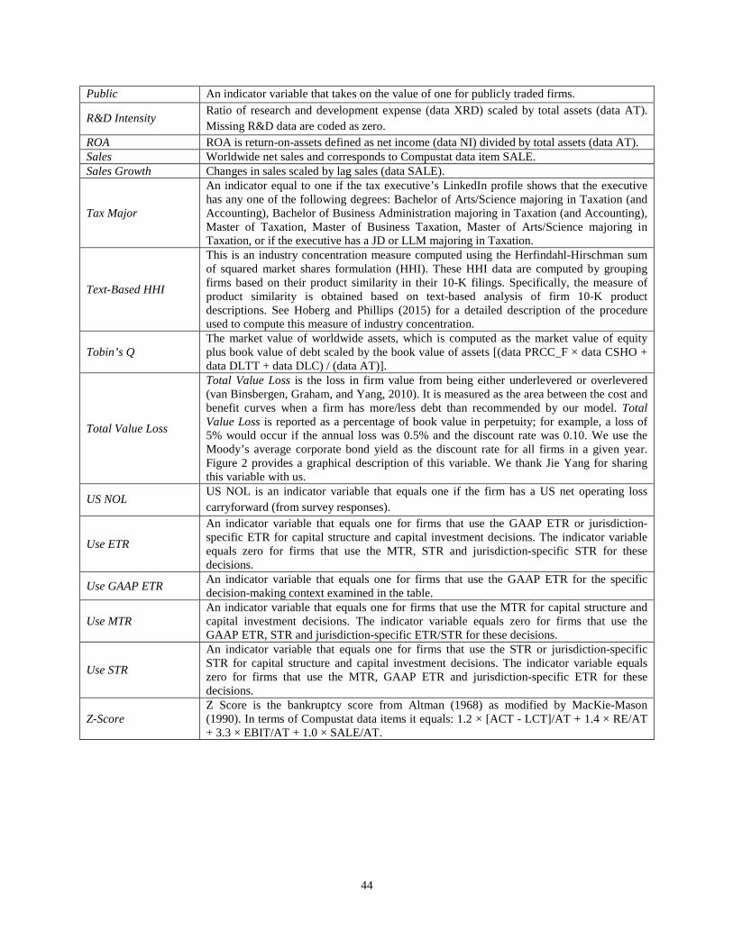
44

Public An indicator variable that takes on the value of one for publicly traded firms.

R&D Intensity Ratio of research and development expense (data XRD) scaled by total assets (data AT). Missing R&D data are coded as zero.

ROA ROA is return-on-assets defined as net income (data NI) divided by total assets (data AT). Sales Worldwide net sales and corresponds to Compustat data item SALE. Sales Growth Changes in sales scaled by lag sales (data SALE).

Tax Major

An indicator equal to one if the tax executive’s LinkedIn profile shows that the executive has any one of the following degrees: Bachelor of Arts/Science majoring in Taxation (and Accounting), Bachelor of Business Administration majoring in Taxation (and Accounting), Master of Taxation, Master of Business Taxation, Master of Arts/Science majoring in Taxation, or if the executive has a JD or LLM majoring in Taxation.

Text-Based HHI

This is an industry concentration measure computed using the Herfindahl-Hirschman sum of squared market shares formulation (HHI). These HHI data are computed by grouping firms based on their product similarity in their 10-K filings. Specifically, the measure of product similarity is obtained based on text-based analysis of firm 10-K product descriptions. See Hoberg and Phillips (2015) for a detailed description of the procedure used to compute this measure of industry concentration.

Tobin’s Q The market value of worldwide assets, which is computed as the market value of equity plus book value of debt scaled by the book value of assets [(data PRCC_F × data CSHO + data DLTT + data DLC) / (data AT)].

Total Value Loss

Total Value Loss is the loss in firm value from being either underlevered or overlevered (van Binsbergen, Graham, and Yang, 2010). It is measured as the area between the cost and benefit curves when a firm has more/less debt than recommended by our model. Total Value Loss is reported as a percentage of book value in perpetuity; for example, a loss of 5% would occur if the annual loss was 0.5% and the discount rate was 0.10. We use the Moody’s average corporate bond yield as the discount rate for all firms in a given year. Figure 2 provides a graphical description of this variable. We thank Jie Yang for sharing this variable with us.

US NOL US NOL is an indicator variable that equals one if the firm has a US net operating loss carryforward (from survey responses).

Use ETR

An indicator variable that equals one for firms that use the GAAP ETR or jurisdiction-specific ETR for capital structure and capital investment decisions. The indicator variable equals zero for firms that use the MTR, STR and jurisdiction-specific STR for these decisions.

Use GAAP ETR An indicator variable that equals one for firms that use the GAAP ETR for the specific decision-making context examined in the table.

Use MTR An indicator variable that equals one for firms that use the MTR for capital structure and capital investment decisions. The indicator variable equals zero for firms that use the GAAP ETR, STR and jurisdiction-specific ETR/STR for these decisions.

Use STR

An indicator variable that equals one for firms that use the STR or jurisdiction-specific STR for capital structure and capital investment decisions. The indicator variable equals zero for firms that use the MTR, GAAP ETR and jurisdiction-specific ETR for these decisions.

Z-Score Z Score is the bankruptcy score from Altman (1968) as modified by MacKie-Mason (1990). In terms of Compustat data items it equals: 1.2 × [ACT - LCT]/AT + 1.4 × RE/AT + 3.3 × EBIT/AT + 1.0 × SALE/AT.

45

Figure 1 Survey Responses Describing the Tax Rates used by Firms for Corporate Decision Making Averaged Across all

Decisions Examined in the Survey

This figure presents the responses to the survey question “What is the primary tax rate your company uses to incorporate taxes into each of the following forecasts or decision-making processes?” The survey respondent is allowed to choose from the following options (or, write in an answer if the options given are not sufficient): (i) U.S. statutory tax rate, (ii) GAAP effective tax rate, (iii) jurisdiction-specific statutory tax rate, (iv) jurisdiction-specific effective tax rate, (v) marginal tax rate, and (vi) other. The question then listed a number of decisions and settings for the respondent to indicate the primary tax rate used in that decision: (i) mergers and acquisitions, (ii) capital structure (debt versus equity), (iii) investment decisions (property, equip., etc), (iv) decision to purchase versus lease (property, equip., etc.), (v) weighted average cost of capital, (vi) where to locate new facilities, and (vii) compensation decisions. The figure provides the percentage of firms using each tax rate averaged across all seven decision contexts. The results are shown separately for public and private firms. The corresponding data in table form are in Table 3, Panel A.

46

Figure 2 Measure of Total Value Loss from Being Overlevered and Underlevered

This figure shows the marginal benefit of debt curve, MB(x), the marginal cost of debt curve, MC(x), and the equilibrium level of debt, x*, that occurs where the marginal cost and benefit curves intersect. The cost of being underlevered is depicted by the shaded area between the MC and MB curves from the actual debt, x0, to the equilibrium, x*, in the case in which the actual level of debt is less than the equilibrium level of debt. For example, a firm with an ETR smaller than its MTR that uses ETR in capital structure choices might choose debt level x0 and incur the shaded costs of being underlevered. Similarly, the cost of been overlevered is depicted by the shaded area between the MC and MB curves from the equilibrium, x*, to the observed debt, x1, in the case in which the actual level of debt is greater than the equilibrium level of debt.

47

Table 1 Descriptive Statistics

Our data are obtained through (i) survey questions, (ii) Compustat, (iii) I/B/E/S, (iv) Thomson Reuters, (v) John Graham’s website (JG Website: https://faculty.fuqua.duke.edu/~jgraham/taxform.html) (iv) the Hoberg-Phillips Data Library (H-P Website: http://alex2.umd.edu/industrydata/industryconcen.htm) or (v) Feng Li’s Website (http://webuser.bus.umich.edu/feng/). The variables are measured as of the fiscal year ending in 2006, which is the more recent fiscal year at the time the survey was conducted. All continuous variables are winsorized at 5% and 95% of the distribution and all dollar amounts are in millions. All variables are defined in the Variable Appendix.

Variable Source N Mean SD P25 P50 P75Public Survey 500 0.778 0.416 1.000 1.000 1.000Assets (in millions) Survey 493 5,647 9,712 473 1,313 4,895Assets (in millions for public firms) Compustat 389 6,515 10,361 611 1,574 6,632

MVE (in millions) Compustat 354 5,989 8,857 703 1,936 6,164Sales (in millions) Compustat 356 4,673 7,244 575 1,474 5,260Tobin's Q Compustat 354 1.931 0.897 1.271 1.594 2.359

ROA Compustat 356 0.059 0.055 0.024 0.059 0.096Foreign Assets (% of assets) Survey 488 0.182 0.202 0.000 0.100 0.305Organization Tax Complexity Survey 488 101.859 382.934 17.000 36.000 77.000Leverage Compustat 356 0.204 0.175 0.048 0.174 0.320Sales Growth Compustat 353 0.139 0.178 0.039 0.098 0.193Asset Growth Compustat 354 0.124 0.189 0.003 0.071 0.189US NOL Survey 478 0.462 0.499 0.000 0.000 1.000R&D Intensity Compustat 356 0.022 0.037 0.000 0.000 0.032Intangible Intensity Compustat 351 0.184 0.172 0.030 0.137 0.307Analyst Following I/B/E/S 356 9.576 7.698 3.000 8.000 15.000Institutional Ownership (%) Thomson Reuters 357 0.533 0.397 0.000 0.688 0.869Text-Based HHI H-P Website 340 0.202 0.201 0.059 0.121 0.26210K Competition Score Feng Li's Website 232 0.264 0.147 0.147 0.231 0.370GAAP ETR (survey response) Survey 398 0.308 0.119 0.273 0.340 0.377GAAP ETR Compustat 311 0.313 0.105 0.278 0.336 0.375MTR JG Website 203 0.310 0.096 0.350 0.350 0.350MTR After Interest (MTR A.I.) JG Website 234 0.214 0.156 0.029 0.347 0.350MTR WRDS-Blouin/Core/Guay 334 0.335 0.029 0.337 0.345 0.350MTR After Interest (MTR A.I.) WRDS-Blouin/Core/Guay 334 0.318 0.052 0.317 0.341 0.348|MTR - GAAP ETR| JG Website & Compustat 187 0.106 0.131 0.024 0.050 0.118|MTR A.I. - GAAP ETR| JG Website & Compustat 210 0.160 0.146 0.029 0.096 0.306|MTR - GAAP ETR| Blouin/Core/Guay & Comp 291 0.083 0.096 0.023 0.044 0.099|MTR A.I. - GAAP ETR| Blouin/Core/Guay & Comp 291 0.088 0.100 0.026 0.048 0.1073-Yr Cash ETR Compustat 297 0.267 0.151 0.171 0.254 0.356

48

Table 2 Non-Response Bias Test

All dollar amounts are in millions. All Compustat variables are measured in the fiscal year ending in 2006 and are winsorized at 1% and 99% of the distribution. Column (1) consists of all the firms on Compustat except for firms with a negative book value, firms whose names indicate they are limited partnerships, and firms incorporated outside the United States. Column (2) includes all the firms that were sent a survey (as described in Section 2 in the paper) that we could match to and retrieve the data from Compustat. Column (3) includes the survey responders with data available on Compustat. Column (4) consists of the group of firms that are on Compustat and that we sent a survey to but did not receive a response. All variables are defined in the Variable Appendix.

N Mean N Mean N Mean N Mean 1 vs. 2 1 vs. 3 2 vs. 3 3 vs. 4 Assets 5,938 3,580.2 1356 9,075.2 414 10,173.8 942 8,592.3 0.00 0.00 0.45 0.28MVE 5,443 2,369.1 1288 7,206.3 396 8,283.1 892 6,728.2 0.00 0.00 0.33 0.15Sales 5,911 1,719.4 1342 5,049.7 400 5,717.8 942 4,766.1 0.00 0.00 0.29 0.13Leverage 5,921 0.19 1341 0.22 400 0.21 941 0.22 0.00 0.21 0.25 0.12Cash 5,937 0.20 1337 0.14 396 0.15 941 0.13 0.00 0.00 0.30 0.16MB 5,443 4.35 1279 3.30 387 3.32 892 3.30 0.00 0.00 0.95 0.93ROA 5,911 -0.04 1338 0.05 396 0.07 942 0.04 0.00 0.00 0.00 0.00Asset Growth 5,692 0.36 1326 0.15 396 0.14 930 0.15 0.00 0.00 0.55 0.42Sales Growth 5,499 0.25 1323 0.14 395 0.14 928 0.14 0.00 0.00 0.75 0.66Capital Exp. 5,877 0.04 1334 0.05 396 0.05 938 0.05 0.00 0.01 0.27 0.12Acquisition Exp. 5,938 0.02 1338 0.03 396 0.03 942 0.03 0.00 0.02 0.46 0.32R&D Exp. 5,938 0.05 1338 0.02 396 0.02 942 0.02 0.00 0.00 0.80 0.74NOL 5,938 0.37 1338 0.42 396 0.39 942 0.43 0.00 0.28 0.33 0.18GAAP ETR 4,239 0.26 1172 0.29 349 0.31 823 0.29 0.00 0.00 0.18 0.093-Yr Cash ETR 4,052 0.27 1165 0.27 354 0.27 811 0.28 0.72 0.67 0.55 0.42MTR 2,097 0.27 756 0.31 227 0.31 529 0.31 0.00 0.00 0.91 0.88

All Compustat (1)

All Public Firms we Contacted with Available Data

(2)

Survey Responders (Public Firms) with

Available Data (3)

Survey Nonresponders (Public Firms) with

Available Data (4)

p-Value

49

Table 3 Survey Responses Describing the Tax Rates used by Firms for Corporate Decision Making

Panel A in this table summarizes the responses to our survey question and Panel B presents the correlations among the survey responses in Panel A. The correlations are computed by first creating indicated variables for the firm’s chosen tax rate for each decision-context and then computing the Pearson correlations among these indicator variables. All the correlation coefficients in Panel B are statistically significant at the 1% level. Panel A: What is the primary tax rate your company uses to incorporate taxes into each of the following forecasts or decision-making processes?

U.S. Statutory

Tax Rate (STR) GAAP ETR Jurisdiction Specific STR

Jurisdiction Specific ETR

Marginal Tax Rate Other N

Merger &Acquisition Decisions 21.1% 24.9% 20.3% 20.1% 10.1% 3.4% 497 Capital Structure 25.9% 29.7% 14.5% 15.3% 12.0% 2.7% 491 Investment Decisions 22.9% 24.5% 21.1% 16.0% 12.5% 3.1% 489 Decision to Purchase vs. Lease 23.9% 23.7% 20.3% 16.4% 12.3% 3.5% 489 Weighted Average Cost of Capital 25.4% 34.3% 13.4% 12.6% 11.8% 2.5% 484 Where to Locate New Facilities 17.0% 16.6% 28.8% 25.9% 8.8% 2.9% 487 Compensation 25.7% 27.2% 19.1% 12.9% 10.6% 4.6% 482

Panel B: Pearson Correlation

1 2 3 4 5 6 7

1 Merger &Acquisition Decisions 1 2 Capital Structure 0.78 1 3 Investment Decisions 0.80 0.80 1 4 Decision to Purchase vs. Lease 0.76 0.80 0.93 1 5 Weighted Average Cost of Capital 0.72 0.78 0.81 0.82 1 6 Where to Locate New Facilities 0.76 0.74 0.82 0.78 0.71 1 7 Compensation 0.66 0.71 0.77 0.77 0.76 0.70 1

50

Table 4 Probit Analyses of the Determinants of Firms’ Responses to Survey Questions

This table presents the marginal effects from probit regressions where managers’ tax rate choices are the dependent variables and their firm characteristics are the independent variables. Panel A presents data from our entire sample of firms (both private and public) where the independent variables constructed from our survey instrument. Panel B presents data from our sample of public firms where the independent variables are constructed from our survey instrument and archival sources such as Compustat. The sample in both panels comprise of data for the fiscal year ending in 2006. The regressions standard errors are clustered at the industry-level. ***, **, * signifies statistical significance at the two-tailed 1%, 5%, and 10% levels. All variables are defined in the Variable Appendix. Panel A: Determinants of Public and Private Firms Survey Responses (Sample period: Fiscal year 2006)

Dependent Variable: Use STR Use MTR Use ETR

Public Firm -0.120*** 0.013 0.096***(-3.19) (0.64) (3.17)

Log(Assets) 0.028** 0.009 -0.036**(2.46) (1.23) (-2.46)

US NOL -0.021 -0.018 0.023(-0.39) (-0.68) (0.51)

GAAP ETR Importance 0.001 -0.039 0.064(0.02) (-1.23) (1.40)

Log(Org. Tax Complexity) -0.021 0.006 0.008(-1.09) (0.42) (0.32)

Foreign Assets 0.084 -0.114 -0.174(0.78) (-1.47) (-1.57)

N 449 449 449Pseudo R-Squared 1.1% 1.7% 2.1%S.E. Clustered by Industry Yes Yes Yes

51

Table 4 (continued) Probit Analyses of the Determinants of Firms’ Responses to Survey Questions

Panel B: Determinants of Public Firms’ Survey Responses (Sample period: Fiscal year 2006)

Dependent Variable: Use STR Use MTR Use ETR

Log(Assets) 0.050* 0.027* -0.097***(1.94) (1.81) (-3.16)

US NOL 0.030 0.012 -0.026(0.48) (0.36) (-0.37)

GAAP ETR Importance -0.016 -0.048 0.081(-0.18) (-0.90) (1.05)

Log(Org. Tax Complexity) -0.019 0.008 0.025(-0.63) (0.41) (0.68)

Foreign Assets 0.221* -0.184** -0.262(1.65) (-2.49) (-1.63)

R&D Intensity 0.876 0.742** -1.772***(1.41) (2.22) (-2.85)

Leverage -0.156 -0.068 0.201(-0.94) (-0.92) (1.05)

ROA 0.484 0.332 -0.818(1.01) (1.42) (-1.64)

Intangible Intensity 0.081 -0.004 0.070(0.48) (-0.05) (0.39)

Analyst Following -0.012*** -0.006** 0.015***(-2.65) (-2.36) (3.07)

Institutional Ownership 0.072 0.115*** -0.087(0.92) (2.63) (-1.08)

Sales Growth -0.043 -0.085 0.104(-0.37) (-1.34) (0.75)

Competition -0.033 0.062 -0.154**(-0.42) (1.10) (-2.09)

|MTR - GAAP ETR| -0.315 -0.077 0.441(-1.04) (-1.08) (1.54)

|MTR - STR| -0.264* 0.294 -0.294(-1.95) (1.03) (-1.03)

N 303 303 303Pseudo R-Squared 4.6% 13.0% 9.2%S.E. Clustered by Industry Yes Yes Yes

52

Table 5 Probit Analyses of the Relation between Executive Education and their Survey Responses

This table presents the marginal effects from probit regressions where managers’ tax rate choices are the dependent variables and their educational background and firm characteristics are the independent variables. We obtain managers’ educational backgrounds from their LinkedIn profiles. Panel A presents the descriptive statistics of our survey respondents’ educational background. Panel B presents the results from regressions of firms (both private and public) tax rate choices on managers’ educational backgrounds. Panel C presents the results from regressions of firms’ tax rate choices on managers’ educational backgrounds and firms characteristics constructed from our survey instrument. The sample in both panels comprise of data for the fiscal year ending in 2006. The regressions standard errors are clustered at the industry-level. ***, **, * signifies statistical significance at the two-tailed 1%, 5%, and 10% levels. All variables are defined in the Variable Appendix. Panel A: Descriptive Statistics of the Educational Backgrounds of our Survey Respondents

Panel B: Regression of Survey Responses on Tax Executives’ Educational Background

Variable N Mean SD P25 P50 P75Law Major 210 0.157 0.365 0.000 0.000 0.000Tax Major 210 0.429 0.496 0.000 0.000 1.000

Accounting Major 210 0.662 0.474 0.000 1.000 1.000

Economics or Business Major 210 0.157 0.365 0.000 0.000 0.000Number of Degrees 210 1.857 0.769 1.000 2.000 2.000

Dependent Variable: Use STR Use MTR Use ETR

Law Major 0.089 -0.011 -0.100(0.60) (-0.16) (-0.80)

Tax Major -0.070 -0.014 0.039(-0.84) (-0.33) (0.52)

Accounting Major 0.053 0.111*** -0.164**(0.80) (3.04) (-2.24)

Economics or Business Major 0.059 -0.021 -0.067(0.52) (-0.35) (-0.59)

Number of Degrees 0.079 -0.047 -0.094*(1.50) (-1.20) (-1.85)

N 210 210 210Pseudo R-Squared 2.9% 7.1% 4.4%S.E. Clustered by Industry Yes Yes Yes

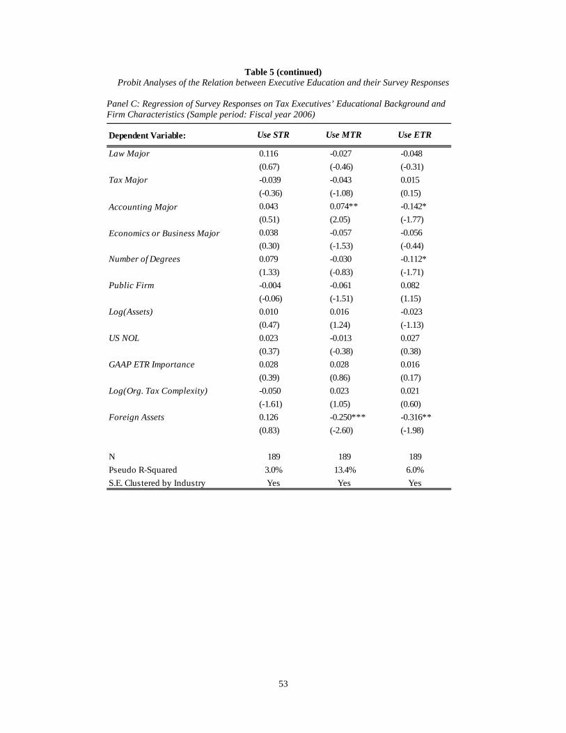
53

Table 5 (continued) Probit Analyses of the Relation between Executive Education and their Survey Responses

Panel C: Regression of Survey Responses on Tax Executives’ Educational Background and Firm Characteristics (Sample period: Fiscal year 2006)

Dependent Variable: Use STR Use MTR Use ETR

Law Major 0.116 -0.027 -0.048(0.67) (-0.46) (-0.31)

Tax Major -0.039 -0.043 0.015(-0.36) (-1.08) (0.15)

Accounting Major 0.043 0.074** -0.142*(0.51) (2.05) (-1.77)

Economics or Business Major 0.038 -0.057 -0.056(0.30) (-1.53) (-0.44)

Number of Degrees 0.079 -0.030 -0.112*(1.33) (-0.83) (-1.71)

Public Firm -0.004 -0.061 0.082(-0.06) (-1.51) (1.15)

Log(Assets) 0.010 0.016 -0.023(0.47) (1.24) (-1.13)

US NOL 0.023 -0.013 0.027(0.37) (-0.38) (0.38)

GAAP ETR Importance 0.028 0.028 0.016(0.39) (0.86) (0.17)

Log(Org. Tax Complexity) -0.050 0.023 0.021(-1.61) (1.05) (0.60)

Foreign Assets 0.126 -0.250*** -0.316**(0.83) (-2.60) (-1.98)

N 189 189 189Pseudo R-Squared 3.0% 13.4% 6.0%S.E. Clustered by Industry Yes Yes Yes

54

Table 6 Analyses of Capital Structure Decisions

Panel A in this table presents the descriptive statistics of the variables used in a regression of Leverage Conservatism, which measures the conservativeness of a firm’s debt policy, on the difference firm’s MTR and its GAAP ETR, and control variables. Panel B presents the regression results. Firms using the GAAP ETRs as the tax rate input for capital structure decisions serve as the treatment sample. The control sample (used in columns 3 and 6 in Panel B) is comprised of a propensity scored matched sample of firms that use the MTR or STR as the tax rate input for capital structure decisions. The sample period ranges from 1997 to 2006. The regressions include both year and industry fixed effects and the standard errors are clustered at the firm-level. ***, **, * signifies statistical significance at the two-tailed (one-tailed) 1%, 5%, and 10% levels (for the coefficients of interest in the highlighted row). All the variables are defined in the Variable Appendix.

Panel A: Descriptive Statistics of the Variables Used in the Regression (Sample period: 1997 to 2006)

N Mean SD P25 P50 P75 Mean SD P25 P50 P75Leverage Conservatism (Graham/Shevlin) 450 3.856 3.257 1.200 3.000 6.000 4.081 3.477 1.200 3.000 7.000Leverage Conservatism (BCG) 450 2.071 2.343 0.400 1.200 3.000 2.108 2.498 0.400 1.200 3.000MTR - GAAP ETR (Graham/Shevlin) 450 -0.021 0.108 -0.051 -0.023 0.019 -0.022 0.105 -0.056 -0.023 0.020MTR - GAAP ETR (BCG) 450 -0.011 0.085 -0.056 -0.030 0.010 -0.014 0.086 -0.061 -0.028 0.019

Log(Assets) 450 7.115 1.364 6.088 6.983 7.930 7.008 1.517 5.800 6.769 7.892

Tobin's Q 450 1.767 1.317 0.912 1.356 2.290 1.721 1.386 0.896 1.277 1.961Sales Growth 450 0.136 0.156 0.037 0.108 0.194 0.149 0.184 0.022 0.109 0.232CFO 450 0.029 0.016 0.017 0.028 0.039 0.030 0.017 0.017 0.030 0.042

PPE 450 0.291 0.192 0.143 0.241 0.392 0.309 0.206 0.149 0.241 0.450Capital Expenditures 450 0.016 0.010 0.008 0.013 0.021 0.014 0.010 0.007 0.011 0.017R&D Expenditures 450 0.003 0.007 0.000 0.000 0.002 0.004 0.007 0.000 0.000 0.004Acquisition Expenditures 450 0.009 0.016 0.000 0.001 0.011 0.009 0.017 0.000 0.000 0.010Credit Rating Dummy 450 0.456 0.499 0.000 0.000 1.000 0.502 0.501 0.000 1.000 1.000Z-Score 450 2.036 0.931 1.367 1.943 2.752 1.624 0.736 1.056 1.648 2.149Dividend Dummy 450 0.556 0.497 0.000 1.000 1.000 0.498 0.501 0.000 0.000 1.000Foreign Income 450 0.013 0.026 0.000 0.000 0.014 0.015 0.029 0.000 0.000 0.016NOL Dummy 450 0.287 0.453 0.000 0.000 1.000 0.282 0.451 0.000 0.000 1.000

VariableFirms using GAAP ETRs Matched firms using MTRs/STRs

55

Table 6 (continued) Analyses of Capital Structure Decisions

Panel B: Regression Results (Sample period: 1997 to 2006)

Dependent Variable:Method of Simulating MTRs: Pr. SignMTR - GAAP ETR +, +, 0 2.468** 2.104** -0.972 4.721*** 3.013*** -1.845

(1.97) (1.96) (-0.82) (3.76) (2.34) (-1.59)MTR - GAAP ETR × Use GAAP ETR + 3.943*** 5.668***

(2.42) (3.55)Use GAAP ETR 0.181 -0.292

(0.55) (-1.16)Log(Assets) 0.842*** 0.522*** 0.615*** 0.186*

(3.88) (3.83) (3.25) (1.79)Tobin's Q 0.377** 0.339*** 0.219 0.437***

(2.34) (3.24) (1.56) (5.48)Sales Growth 0.351 -0.506 0.068 -0.005

(0.45) (-0.91) (0.10) (-0.01)CFO 37.949*** 39.998*** 15.297** 17.101***

(4.68) (6.06) (2.15) (3.40)PPE 0.080 -1.730 -1.443 1.119

(0.04) (-1.28) (-0.74) (1.09)Capital Expenditures 48.258** 19.578 43.198*** 10.815

(2.57) (1.31) (2.64) (0.95)R&D Expenditures -101.951** -12.560 -16.216 0.724

(-2.37) (-0.46) (-0.43) (0.03)Acquisition Expenditures 17.916*** 9.580* 2.232 3.862

(2.66) (1.76) (0.38) (0.93)Credit Rating Dummy -0.539 -0.474 -0.694 0.034

(-1.11) (-1.46) (-1.64) (0.14)Z-Score 0.323 0.362* 0.674*** 0.435***

(1.15) (1.78) (2.74) (2.81)Dividend Dummy -0.729 0.785** 0.299 0.799***

(-1.56) (2.56) (0.74) (3.43)Foreign Income 2.257 5.783 18.025** 10.541***

(0.28) (1.21) (2.54) (2.90)NOL Dummy -0.419 -0.675*** -0.159 -0.471**

(-1.38) (-2.72) (-0.60) (-2.50)N 450 450 900 450 450 900Adjusted R-Squared 43.0% 68.7% 59.6% 33.5% 54.0% 54.7%S.E. Clustered by Firm Yes Yes Yes Yes Yes YesYear & Industry Fixed Effects Yes Yes Yes Yes Yes Yes

Leverage ConservatismGraham/Shevlin Blouin, Core, and Guay (2010)

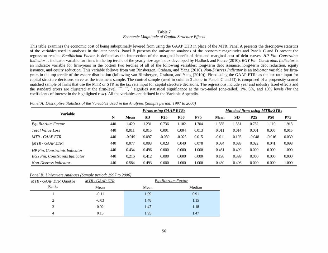
56

Table 7 Economic Magnitude of Capital Structure Effects

This table examines the economic cost of being suboptimally levered from using the GAAP ETR in place of the MTR. Panel A presents the descriptive statistics of the variables used in analyses in the later panels. Panel B presents the univariate analyses of the economic magnitudes and Panels C and D present the regression results. Equilibrium Factor is defined as the intersection of the marginal benefit of debt and marginal cost of debt curves. HP Fin. Constraints Indicator is indicator variable for firms in the top tercile of the yearly size-age index developed by Hadlock and Pierce (2010). BGY Fin. Constraints Indicator is an indicator variable for firm-years in the bottom two terciles of all of the following variables: long-term debt issuance, long-term debt reduction, equity issuance, and equity reduction. This variable follows from van Binsbergen, Graham, and Yang (2010). Non-Distress Indicator is an indicator variable for firm-years in the top tercile of the zscore distribution (following van Binsbergen, Graham, and Yang (2010)). Firms using the GAAP ETRs as the tax rate input for capital structure decisions serve as the treatment sample. The control sample (used in column 3 alone in Panels C and D) is comprised of a propensity scored matched sample of firms that use the MTR or STR as the tax rate input for capital structure decisions. The regressions include year and industry fixed effects and the standard errors are clustered at the firm-level. ***, **, * signifies statistical significance at the two-tailed (one-tailed) 1%, 5%, and 10% levels (for the coefficients of interest in the highlighted row). All the variables are defined in the Variable Appendix. Panel A: Descriptive Statistics of the Variables Used in the Analyses (Sample period: 1997 to 2006)

Panel B: Univariate Analyses (Sample period: 1997 to 2006)

N Mean SD P25 P50 P75 Mean SD P25 P50 P75Equilibrium Factor 440 1.429 1.231 0.736 1.102 1.704 1.555 1.381 0.732 1.110 1.913Total Value Loss 440 0.011 0.015 0.001 0.004 0.013 0.011 0.014 0.001 0.005 0.015MTR - GAAP ETR 440 -0.019 0.097 -0.050 -0.025 0.015 -0.011 0.103 -0.048 -0.016 0.030|MTR - GAAP ETR| 440 0.077 0.093 0.023 0.040 0.078 0.084 0.099 0.022 0.041 0.098

HP Fin. Constraints Indicator 440 0.434 0.496 0.000 0.000 1.000 0.461 0.499 0.000 0.000 1.000BGY Fin. Constraints Indicator 440 0.216 0.412 0.000 0.000 0.000 0.198 0.399 0.000 0.000 0.000Non-Distress Indicator 440 0.584 0.493 0.000 1.000 1.000 0.430 0.496 0.000 0.000 1.000

VariableFirms using GAAP ETRs Matched firms using MTRs/STRs

MTR - GAAP ETRMean Mean Median

1 -0.11 1.09 0.912 -0.03 1.48 1.153 0.02 1.47 1.184 0.15 1.95 1.47

MTR - GAAP ETR Quartile Ranks

Equilibrium Factor

57

Table 7 (continued) Economic Magnitude of Capital Structure Effects

Panel C: Regression Results with Equilibrium Factor as Dependent Variable (Sample period: 1997 to 2006)

Panel D: Regression Results with Total Value Loss of Being Under- or Over-Levered as Dependent Variable (Sample period: 1997 to 2006)

Dependent Variable: Pr. SignMTR - GAAP ETR +, +, 0 1.437** 1.787** 0.314

(1.80) (2.21) (0.46)MTR - GAAP ETR × Use GAAP ETR + 2.246**

(2.08)Use GAAP ETR -0.440

(-1.06)HP Fin. Constraints Indicator -0.415 -0.562*

(-1.26) (-1.96)BGY Fin. Constraints Indicator 0.295* 0.264**

(1.91) (2.59)Non-Distress Indicator 0.116 0.020

(0.57) (0.13)N 440 440 880Adjusted R-Squared 48.7% 50.3% 44.6%S.E. Clustered by Firm Yes Yes YesYear & Industry Fixed Effects Yes Yes Yes

Equilibrium Factor

Dependent Variable: Pr. Sign|MTR - GAAP ETR| +, +, 0 0.037*** 0.038*** 0.000

(3.43) (3.39) (0.02)|MTR - GAAP ETR| × Use GAAP ETR + 0.032***

(2.61)Use GAAP ETR 0.002

(0.41)HP Fin. Constraints Indicator -0.001 -0.004

(-0.26) (-1.36)BGY Fin. Constraints Indicator 0.001 0.000

(0.71) (0.34)Non-Distress Indicator 0.002 0.001

(0.99) (0.61)N 440 440 880Adjusted R-Squared 51.7% 51.7% 32.4%S.E. Clustered by Firm Yes Yes YesYear & Industry Fixed Effects Yes Yes Yes

Total Value Loss

58

Table 8 Analyses of Capital Investment Decisions

Panel A in this table presents the descriptive statistics of the variables used in our investment regressions. Panels B and C present the regression results using Tobin’s Q and Sales Growth as proxies for investment opportunities, respectively. Panel D presents regression results with suboptimal investment measured as the difference between firms’ actual investment and predicted investment. Firms using the GAAP ETRs as the tax rate input for capital investment decisions serve as the treatment sample. The control sample (used in columns 2 and 4 alone in Panels B, C and D) is comprised of a propensity scored matched sample of firms that use the MTR or STR as the tax rate input for capital investment decisions. The regressions include both year and industry fixed effects and the standard errors are clustered at the firm-level. ***, **, * signifies statistical significance at the two-tailed (one-tailed) 1%, 5%, and 10% levels (for the coefficients of interest in the highlighted row). All the variables are defined in the Variable Appendix. Panel A: Descriptive Statistics of the Variables Used in the Regression (Sample period: 1997 to 2006)

N Mean SD P25 P50 P75 Mean SD P25 P50 P75Capital Expenditures 461 0.081 0.083 0.025 0.054 0.105 0.071 0.075 0.029 0.047 0.078

Capital Expenditures - Predicted Capital Expenditures 461 0.004 0.052 -0.017 0.001 0.026 -0.001 0.059 -0.024 -0.001 0.020

|MTR A.I. - GAAP ETR| (Graham/Shevlin) 461 0.135 0.147 0.028 0.052 0.255 0.137 0.149 0.025 0.050 0.269|MTR A.I. - GAAP ETR| (BCG) 461 0.086 0.091 0.031 0.054 0.097 0.081 0.090 0.027 0.050 0.092MTR A.I. - GAAP ETR (Graham/Shevlin) 461 -0.086 0.159 -0.155 -0.036 -0.007 -0.091 0.163 -0.230 -0.037 0.005MTR A.I. - GAAP ETR (BCG) 461 -0.031 0.095 -0.073 -0.041 -0.003 -0.021 0.097 -0.065 -0.030 0.014

Tobin's Q 461 1.692 1.012 0.937 1.352 2.224 1.814 1.208 0.952 1.407 2.194Sales Growth 461 0.171 0.177 0.040 0.141 0.259 0.179 0.209 0.035 0.124 0.274CFO 461 0.129 0.086 0.066 0.119 0.186 0.131 0.084 0.068 0.121 0.179

VariableFirms using GAAP ETRs Matched firms using MTRs/STRs

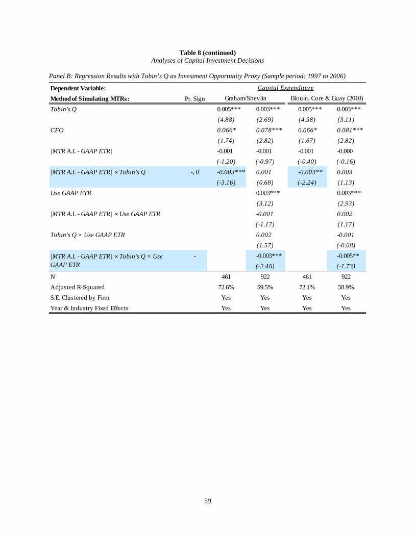
59

Table 8 (continued) Analyses of Capital Investment Decisions

Panel B: Regression Results with Tobin’s Q as Investment Opportunity Proxy (Sample period: 1997 to 2006)

Dependent Variable:Method of Simulating MTRs: Pr. SignTobin's Q 0.005*** 0.003*** 0.005*** 0.003***

(4.88) (2.69) (4.58) (3.11)CFO 0.066* 0.078*** 0.066* 0.081***

(1.74) (2.82) (1.67) (2.82)|MTR A.I. - GAAP ETR| -0.001 -0.001 -0.001 -0.000

(-1.20) (-0.97) (-0.40) (-0.16)|MTR A.I. - GAAP ETR| × Tobin's Q -, 0 -0.003*** 0.001 -0.003** 0.003

(-3.16) (0.68) (-2.24) (1.13)Use GAAP ETR 0.003*** 0.003***

(3.12) (2.93)|MTR A.I. - GAAP ETR| × Use GAAP ETR -0.001 0.002

(-1.17) (1.17)Tobin's Q × Use GAAP ETR 0.002 -0.001

(1.57) (-0.68)- -0.003*** -0.005**

(-2.46) (-1.73)N 461 922 461 922Adjusted R-Squared 72.6% 59.5% 72.1% 58.9%S.E. Clustered by Firm Yes Yes Yes YesYear & Industry Fixed Effects Yes Yes Yes Yes

Graham/Shevlin Blouin, Core & Guay (2010)Capital Expenditure

|MTR A.I. - GAAP ETR| × Tobin's Q × Use GAAP ETR

60

Table 8 (continued) Analyses of Capital Investment Decisions

Panel C: Regression Results with Sales Growth as Investment Opportunity Proxy (Sample period: 1997 to 2006)

Panel D: Regression Results using Alternative Measure for Optimal Investment (Sample period: 1997 to 2006)

Dependent Variable:Method of Simulating MTRs: Pr. SignSales Growth 0.021*** 0.018*** 0.023*** 0.018***

(2.94) (2.69) (3.19) (2.65)CFO 0.881*** 0.825*** 0.923*** 0.860***

(2.94) (4.96) (2.95) (4.88)|MTR A.I. - GAAP ETR| -0.007 -0.005 0.002 -0.008

(-1.64) (-0.95) (0.17) (-1.15)|MTR A.I. - GAAP ETR| × Sales Growth -, 0 -0.018** 0.000 -0.001 0.001

(-2.02) (0.05) (-0.07) (0.06)Use GAAP ETR 0.017*** 0.018***

(2.86) (2.90)|MTR A.I. - GAAP ETR| × Use GAAP ETR -0.012* 0.001

(-1.77) (0.14)Sales Growth × Use GAAP ETR 0.006 0.007

(0.57) (0.68)- -0.019** -0.004

(-1.67) (-0.27)N 461 922 461 922Adjusted R-Squared 65.8% 61.2% 65.2% 60.4%S.E. Clustered by Firm Yes Yes Yes YesYear & Industry Fixed Effects Yes Yes Yes Yes

|MTR A.I. - GAAP ETR| × Sales Growth × Use GAAP ETR

Capital ExpenditureGraham/Shevlin Blouin, Core & Guay (2010)

Dependent Variable:Method of Simulating MTRs: Pr. SignMTR A.I. - GAAP ETR +, 0 0.006** -0.003 0.001 -0.002

(2.30) (-0.94) (0.49) (-0.76)Use GAAP ETR 0.009 0.009

(1.19) (1.19)MTR A.I. - GAAP ETR × Use GAAP ETR + 0.007* 0.001

(1.85) (0.24)N 461 922 461 922Adjusted R-Squared 31.8% 13.1% 31.1% 12.9%S.E. Clustered by Firm Yes Yes Yes YesYear & Industry Fixed Effects Yes Yes Yes Yes

Capital Expenditure - Predicted Capital ExpenditureGraham/Shevlin Blouin, Core & Guay (2010)