qt4z70t80r.pdf - eScholarship.org

UC BerkeleyUC Berkeley Electronic Theses and Dissertations

TitleEssays in Energy and Development Economics

Permalinkhttps://escholarship.org/uc/item/4z70t80r

AuthorBurlig, Fiona Elizabeth Wilkes

Publication Date2017 Peer reviewed|Thesis/dissertation

eScholarship.org Powered by the California Digital LibraryUniversity of California

https://escholarship.org/uc/item/4z70t80r

https://escholarship.org

http://www.cdlib.org/

Essays in Energy and Development Economics

by

Fiona Elizabeth Wilkes Burlig

A dissertation submitted in partial satisfaction of the

requirements for the degree of

Doctor of Philosophy

in

Agricultural and Resource Economics

in the

Graduate Division

of the

University of California, Berkeley

Committee in charge:

Professor Catherine Wolfram, Co-chairAssociate Professor Jeremy Magruder, Co-chair

Professor Maximilian AuffhammerProfessor Edward Miguel

Spring 2017

Abstract


by


Doctor of Philosophy in Agricultural and Resource Economics

University of California, Berkeley

Professor Catherine Wolfram, Co-chair

Associate Professor Jeremy Magruder, Co-chair

As demand for electricity grows around the world, so does the need for rigorous eval-uation of energy policy interventions. In this dissertation, I use large datasets andmodern econometric methods to study two such policies at scale - rural electrificationin India and energy efficiency subsidies in California. I find that the benefits asso-ciated with these interventions are substantially smaller than previously thought,highlighting the importance of using new techniques for causal inference in thesesettings. In Chapter 1, I study the impacts of grid-scale rural electrification in India,using a regression discontinuity framework. In Chapter 2, I evaluate energy efficiencyupgrades in K-12 schools in California using high-frequency data and novel machinelearning methods. In Chapter 3, I develop methods to guide experimental design inthe presence of panel data.

In the first chapter, coauthored with Louis Preonas, we study the impacts ofenergy access in the developing world. Over 1 billion people still lack electricityaccess. Developing countries are investing billions of dollars in rural electrification,targeting economic growth and poverty reduction, despite limited empirical evidence.We estimate the effects of rural electrification on economic development in the contextof India’s national electrification program, which reached over 400,000 villages. Weuse a regression discontinuity design and high-resolution geospatial data to identifymedium-run economic impacts of electrification. We find a substantial increase inelectricity use, but reject effects larger than 0.26 standard deviations across numerousmeasures of economic development, suggesting that rural electrification may be lessbeneficial than previously thought.

In the second chapter, coauthored with Christopher R. Knittel, David Rapson,Mar Reguant, and Catherine Wolfram, we study the impacts of energy efficiency

1

investments at public K-12 schools in California. We leverage high frequency data– electricity use every 15 minutes – to develop several approaches to estimatingcounterfactual energy consumption in the absence of the efficiency investments. Inparticular, We use difference-in-differences approaches with rich sets of fixed effects.We show, however, that these estimates are sensitive to the set of fixed effects in-cluded and to the set of schools included as controls. To address these concerns, Wedevelop and implement a novel machine learning approach to predict counterfactualenergy consumption at treated schools and validate the approach with non-treatedschools. We find that the energy efficiency projects in our sample reduce electricityconsumption between 2 to 5% on average, which can result in substantial savings toschools. We also compare our estimates of the energy savings to ex ante engineeringestimates. Realized savings are generally less than 50% of ex ante forecasts and quitelow for measures other than heating and air-conditioning systems or lighting.

In the third chapter, coauthored with Louis Preonas and Matt Woerman, we seekto answer: How should researchers design experiments with panel data? We deriveanalytical expressions for the variance of panel estimators under non-i.i.d. error struc-tures, which inform power calculations in panel data settings. Using Monte Carlosimulation, data from a randomized experiment in China, and high-frequency U.S.electricity consumption data, we demonstrate that traditional methods produce ex-periments that are incorrectly powered with proper inference. Failing to account forserial correlation yields overpowered experiments in short panels and underpoweredexperiments in long panels. Our theoretical results enable us to achieve correctlypowered experiments in both simulated and real data.

2

Contents

Contents i

List of Figures ii

List of Tables iv

Acknowledgements vii

1 Out of the Darkness and Into the Light? Development Effects ofRural Electrification 11.1 Introduction . . . . . . . . . . . . . . . . . . . . . . . . . . . . . . . . 11.2 RGGVY . . . . . . . . . . . . . . . . . . . . . . . . . . . . . . . . . . 31.3 Empirical approach . . . . . . . . . . . . . . . . . . . . . . . . . . . . 71.4 Data . . . . . . . . . . . . . . . . . . . . . . . . . . . . . . . . . . . . 91.5 Regression discontinuity results . . . . . . . . . . . . . . . . . . . . . 201.6 Interpretations and Extensions . . . . . . . . . . . . . . . . . . . . . . 371.7 Conclusion . . . . . . . . . . . . . . . . . . . . . . . . . . . . . . . . . 45

2 Machine Learning from Schools About Energy Efficiency 472.1 Introduction . . . . . . . . . . . . . . . . . . . . . . . . . . . . . . . . 472.2 Context and Data . . . . . . . . . . . . . . . . . . . . . . . . . . . . . 502.3 Regression Analysis . . . . . . . . . . . . . . . . . . . . . . . . . . . . 552.4 Machine Learning Analysis . . . . . . . . . . . . . . . . . . . . . . . . 662.5 Realized versus Ex-Ante Predicted Energy Savings . . . . . . . . . . 902.6 Conclusions . . . . . . . . . . . . . . . . . . . . . . . . . . . . . . . . 96

3 Panel Data and Experimental Design 973.1 Introduction . . . . . . . . . . . . . . . . . . . . . . . . . . . . . . . . 973.2 Background . . . . . . . . . . . . . . . . . . . . . . . . . . . . . . . . 993.3 Theory . . . . . . . . . . . . . . . . . . . . . . . . . . . . . . . . . . . 104

i

3.4 Applications to real-world data . . . . . . . . . . . . . . . . . . . . . 1133.5 Discussion . . . . . . . . . . . . . . . . . . . . . . . . . . . . . . . . . 1213.6 Power calculations in practice . . . . . . . . . . . . . . . . . . . . . . 1283.7 Conclusion . . . . . . . . . . . . . . . . . . . . . . . . . . . . . . . . . 130

References 131

A Out of the Darkness and Into the Light? Development Effects ofRural Electrification – Appendix 139A.1 Data . . . . . . . . . . . . . . . . . . . . . . . . . . . . . . . . . . . . 139A.2 Empirics . . . . . . . . . . . . . . . . . . . . . . . . . . . . . . . . . . 176A.3 Electrification in India: A (More) Detailed History . . . . . . . . . . 246

B Panel Data and Experimental Design – Appendix 252B.1 Derivations and proofs . . . . . . . . . . . . . . . . . . . . . . . . . . 252B.2 Figures in main text . . . . . . . . . . . . . . . . . . . . . . . . . . . 281B.3 Additional results . . . . . . . . . . . . . . . . . . . . . . . . . . . . . 290B.4 A practical guide to power calculations . . . . . . . . . . . . . . . . . 295B.5 Estimation-related proofs . . . . . . . . . . . . . . . . . . . . . . . . . 309

List of Figures

1.2.1 Indian Districts by RGGVY Implementation Phase . . . . . . . . . . 61.4.2 Nighttime Lights in India, 2001 and 2011 . . . . . . . . . . . . . . . . 111.4.3 Density of RD Running Variable . . . . . . . . . . . . . . . . . . . . . 161.5.4 RD – 2011 Nighttime Brightness . . . . . . . . . . . . . . . . . . . . . 221.5.5 Nighttime Brightness – Validity Tests . . . . . . . . . . . . . . . . . . 251.5.6 Nighttime Brightness – Falsification Tests . . . . . . . . . . . . . . . . 261.5.7 RD – Labor Outcomes . . . . . . . . . . . . . . . . . . . . . . . . . . 301.5.8 RD – Housing and Asset Ownership . . . . . . . . . . . . . . . . . . . 311.5.9 RD – SECC Village-Level Outcomes . . . . . . . . . . . . . . . . . . . 341.5.10 RD – School Enrollment . . . . . . . . . . . . . . . . . . . . . . . . . 361.6.11 Difference-in-Differences Results . . . . . . . . . . . . . . . . . . . . . 42

ii

2.2.1 Locations of Treated and Untreated Schools . . . . . . . . . . . . . . 552.3.2 Energy efficiency upgrades: Event study . . . . . . . . . . . . . . . . . 572.3.3 Placebo Treatment Effects – Difference-in-Difference . . . . . . . . . . 632.4.4 Number of LASSO coefficients by school . . . . . . . . . . . . . . . . 772.4.5 Holiday Effects in LASSO models . . . . . . . . . . . . . . . . . . . . 782.4.6 Placebo Treatment Effects – Machine Learning . . . . . . . . . . . . . 892.5.7 Estimated realization rates . . . . . . . . . . . . . . . . . . . . . . . . 922.5.8 Ex-ante energy savings . . . . . . . . . . . . . . . . . . . . . . . . . . 942.5.9 Realization rates: sensitivity to outliers . . . . . . . . . . . . . . . . . 95

3.2.1 Hypothesis testing framework . . . . . . . . . . . . . . . . . . . . . . 1013.3.2 Traditional methods result in improperly powered experiments in AR(1)

data . . . . . . . . . . . . . . . . . . . . . . . . . . . . . . . . . . . . 1123.4.3 Power simulations for Bloom et al. (2015) data . . . . . . . . . . . . . 1153.4.4 Pecan Street data – Varying levels of aggregation . . . . . . . . . . . 1183.4.5 Power simulations for Pecan Street data . . . . . . . . . . . . . . . . . 1193.4.6 Analytical power calculations – daily Pecan Street dataset . . . . . . 1213.5.7 The benefits of ANCOVA are limited with serial correlation . . . . . . 1243.5.8 Analytical power calculations with increasing panel length . . . . . . . 127

A.1.1 Rajasthani Village Boundaries . . . . . . . . . . . . . . . . . . . . . . 145A.1.2 Example of Nighttime Lights with Village Boundaries . . . . . . . . . 149A.1.3 Habitation Merge Results, by 2001 Village Population . . . . . . . . . 159A.1.4 SECC Merge Results, by 2001 Village Population . . . . . . . . . . . 164A.1.5 Sample DISE data, 2012–2013 . . . . . . . . . . . . . . . . . . . . . . 170A.1.6 School Merge Results, by 2001 Village Population . . . . . . . . . . . 173A.2.1 RD Sensitivity – Nighttime Brightness, Bandwidth . . . . . . . . . . . 181A.2.2 RD Sensitivity – Nighttime Brightness, Higher Order Polynomials . . 183A.2.3 RD Sensitivity – Pre-RGGVY Brightness . . . . . . . . . . . . . . . . 189A.2.4 RD on Nighttime Brightness Over Time . . . . . . . . . . . . . . . . . 194A.2.5 RD Reduced Form – 2011 Village Population . . . . . . . . . . . . . . 197A.2.6 RD Sensitivity – Census Outcomes, Bandwidths . . . . . . . . . . . . 199A.2.7 RD Sensitivity – Census Outcomes, Second-Order Polynomials . . . . 201A.2.8 RD Sensitivity – Census Outcomes, No Fixed Effects . . . . . . . . . 206A.2.9 RD Sensitivity – Census Outcomes, District Fixed Effects . . . . . . . 208A.2.10 RD Sensitivity – Census Outcomes, No 2001 Controls . . . . . . . . . 210A.2.11 RD Sensitivity – Census Outcomes, 2001 Covariate Smoothness . . . 212A.2.12 RD Results – Share of “Main” Workers by Sector . . . . . . . . . . . . 215A.2.13 Male Labor Shares – Placebo and Randomization Tests . . . . . . . . 217

iii

A.2.14 Male Agricultural Labor – Falsification Tests . . . . . . . . . . . . . . 218A.2.15 Male Other Labor – Falsification Tests . . . . . . . . . . . . . . . . . 219A.2.16 RD Results – SECC Village-Level Outcomes . . . . . . . . . . . . . . 225A.2.17 RD Sensitivity – SECC, Bandwidths . . . . . . . . . . . . . . . . . . 226A.2.18 RD Results – School Enrollment . . . . . . . . . . . . . . . . . . . . . 229A.2.19 RD Sensitivity – School-Level Enrollment Regressions . . . . . . . . . 230A.2.20 RD Sensitivity – School Enrollment, Bandwidths . . . . . . . . . . . . 231A.2.21 RD Sensitivity – Selected Regressions, Low-Deficit States . . . . . . . 242A.2.22 Difference-in-Differences Results . . . . . . . . . . . . . . . . . . . . . 244A.3.1 RGGVY Implementation Timeline . . . . . . . . . . . . . . . . . . . . 251

B.3.1 Power in short panels – AR(1) data . . . . . . . . . . . . . . . . . . . 292B.3.2 Power in short panels – Real data . . . . . . . . . . . . . . . . . . . . 293B.3.3 Traditional ANCOVA methods fail to achieve desired power . . . . . . 294B.4.1 Actual vs. estimated parameters – AR(1) data . . . . . . . . . . . . . 301B.4.2 Estimated parameters - Bloom et al. (2015) data . . . . . . . . . . . . 302B.4.3 Estimated parameters - Pecan Street data . . . . . . . . . . . . . . . 303

List of Tables

1.4.1 Summary Statistics – Villages with Populations Between 150 and 450 181.5.2 RD – Nighttime Brightness . . . . . . . . . . . . . . . . . . . . . . . . 271.5.3 RD – Census Outcomes . . . . . . . . . . . . . . . . . . . . . . . . . . 321.5.4 RD – SECC Village-Level Outcomes . . . . . . . . . . . . . . . . . . . 331.5.5 RD – School Enrollment . . . . . . . . . . . . . . . . . . . . . . . . . 37

2.2.1 Average characteristics of schools in the sample . . . . . . . . . . . . . 542.3.2 Difference-in-Difference Results by Hour-Block . . . . . . . . . . . . . 592.3.3 Difference-in-Difference Results by Type of Intervention . . . . . . . . 612.3.4 Matching Results . . . . . . . . . . . . . . . . . . . . . . . . . . . . . 652.4.5 Monte Carlo Results, Percent Deviations from “True” Effect . . . . . . 752.4.6 Prediction Results - Average prediction errors . . . . . . . . . . . . . . 802.4.7 Prediction Results by Hour-Block . . . . . . . . . . . . . . . . . . . . 81

iv

2.4.8 Prediction Results by Type of Intervention . . . . . . . . . . . . . . . 832.4.9 Prediction Results: Pre- vs. Post-Period Training . . . . . . . . . . . 852.4.10 Double Selection Prediction Results . . . . . . . . . . . . . . . . . . . 872.5.11 Ex-Post vs. Ex-Ante Savings . . . . . . . . . . . . . . . . . . . . . . . 91

3.4.1 Summary statistics – Bloom et al. (2015) . . . . . . . . . . . . . . . 1143.4.2 Summary statistics – Pecan Street . . . . . . . . . . . . . . . . . . . 117

A.1.1 RGGVY Microdata Irregularities . . . . . . . . . . . . . . . . . . . . 140A.1.2 Summary Statistics – RGGVY Implementation and Scope . . . . . . 142A.1.3 Correlation of Shapefiles with Village Areas . . . . . . . . . . . . . . . 144A.1.4 Summary Statistics – Primary Census Abstract . . . . . . . . . . . . 153A.1.5 Summary Statistics – Houselisting Primary Census Abstract . . . . . 154A.1.6 Summary Statistics – Village Directory . . . . . . . . . . . . . . . . . 155A.1.7 Summary of Habitation Census Merge Results . . . . . . . . . . . . . 158A.1.8 Summary Statistics – SECC Village-Level Dataset . . . . . . . . . . 165A.1.9 Summary Statistics – SECC Village-Level Dataset (Cont’d) . . . . . 166A.1.10 Summary Statistics – DISE Schools Dataset . . . . . . . . . . . . . . 171A.1.11 Summary of School Merge Results . . . . . . . . . . . . . . . . . . . 172A.1.12 Count of Villages by Merged Dataset . . . . . . . . . . . . . . . . . . 175A.2.1 RD Sensitivity – Raw vs. Projected Lights . . . . . . . . . . . . . . . 177A.2.2 RD Sensitivity – Alternative Lights Variables . . . . . . . . . . . . . . 178A.2.3 RD Sensitivity – NOAA DMSP–OLS Datasets . . . . . . . . . . . . . 179A.2.4 RD Sensitivity – Higher Order Polynomials . . . . . . . . . . . . . . . 182A.2.5 RD Sensitivity – Fixed Effects and 2001 Control . . . . . . . . . . . . 185A.2.6 Nighttime Brightness by State . . . . . . . . . . . . . . . . . . . . . . 186A.2.7 RD Sensitivity – 2001 Village Controls . . . . . . . . . . . . . . . . . 187A.2.8 RD Sensitivity – Pre-RGGVY Brightness . . . . . . . . . . . . . . . . 188A.2.9 RD Sensitivity – Alternative Standard Errors . . . . . . . . . . . . . . 190A.2.10 RD Sensitivity – Falsification Tests . . . . . . . . . . . . . . . . . . . 192A.2.11 RD Sensitivity – Brightness by Year . . . . . . . . . . . . . . . . . . . 193A.2.12 RD Sensitivity – Census Outcomes, No Forced Population Match . . . 196A.2.13 RD Sensitivity – Census Outcomes, Quadratic in Population . . . . . 200A.2.14 RD Sensitivity – Census Outcomes, Weighting Inverse Distance from

Cutoff . . . . . . . . . . . . . . . . . . . . . . . . . . . . . . . . . . . 202A.2.15 RD Sensitivity – Census Outcomes, No Fixed Effects . . . . . . . . . 205A.2.16 RD Sensitivity – Census Outcomes, District Fixed Effects . . . . . . . 207A.2.17 RD Sensitivity – Census Outcomes, No 2001 Controls . . . . . . . . . 209A.2.18 RD Sensitivity – Census Outcomes, 2001 Covariate Smoothness . . . 211

v

A.2.19 RD Results – Share of “Main” Workers by Sector . . . . . . . . . . . . 214A.2.20 RD Sensitivity – Falsification Tests . . . . . . . . . . . . . . . . . . . 220A.2.21 RD Sensitivity – SECC Village-Level Outcomes . . . . . . . . . . . . 223A.2.22 RD Results – Additional SECC Village-Level Employment Outcomes 224A.2.23 RD Sensitivity – School Enrollment, School-Level Regressions . . . . . 228A.2.24 RD Sensitivity – Total Grade 1–8 Enrollment, Village-Level Regressions232A.2.25 Spatial Spillovers to Adjacent Villages . . . . . . . . . . . . . . . . . . 234A.2.26 Subsample – Districts Receiving Early RGGVY Funding . . . . . . . 237A.2.27 Subsample – States with Low Power Deficits (Lights and Labor) . . . 238A.2.28 Subsample – States with Low Power Deficits (Assets, Housing, Public

Goods) . . . . . . . . . . . . . . . . . . . . . . . . . . . . . . . . . . . 239A.2.29 Subsample – States with Low Power Deficits (SECC Outcomes) . . . 240A.2.30 Subsample – States with Low Power Deficits (DISE Outcomes) . . . . 241A.2.31 RD vs. Difference-in-Differences Results . . . . . . . . . . . . . . . . . 245

B.2.1 Pecan Street Simulation Parameters . . . . . . . . . . . . . . . . . . . 288

vi

Acknowledgments

I am deeply grateful to many people for their guidance and support. My advisors,Catherine Wolfram and Jeremy Magruder, have been invaluable. Catherine is a rolemodel and an inspiration, and I am lucky to call myself her student. Jeremy hasdevoted countless hours to teaching me to think rigorously about difficult problems.Both Catherine and Jeremy simultaneously hold me to an incredibly high standardand teach me how I can make that standard attainable.

I would also like to thank Maximilian Auffhammer, Severin Borenstein, MeredithFowlie, and Lucas Davis for taking in, putting up with, and striving to improve thiswayward development economist, both professionally and personally. I am so luckyto be a part of the Energy Institute family. Aprajit Mahajan, Betty Sadoulet, andTed Miguel broaden and simultaneously sharpen my thinking.

I have been lucky to work with and learn from a number of other faculty membersat Berkeley and elsewhere. Dave Rapson, Chris Knittel, and Mar Reguant, mycoauthors on the third chapter of this dissertation, have helped me appreciate theresearch process. Solomon Hsiang inspires me to ask big questions. Alain de Janvry,Ethan Ligon, Jim Sallee, and Reed Walker provide endless constructive criticism,and have made me a better economist.

I am indebted to Andy Campbell, Casey Hennig, Carmen Karahalios, KarenNotsund, Paula Pedro, and Maggie Smith for their support at Berkeley. I am alsograteful to the National Science Foundation for generously funding this work.

Patrick Baylis, Ceren Baysan, Kenny Bell, Susanna Berkouwer, Josh Blonz,Tamma Carleton, Aluma Dembo, Sylvan Herskowitz, Erin Kelley, Dave McLaughlin,Kate Pennington, Louis Preonas, Andrew Stevens, Becca Taylor, and Matt Woer-man have allowed me to ask hard questions, learn, fail, succeed, and not take myselftoo seriously. I could not ask for a better group of friends and compatriots.

Finally, I thank my family, who are and remain an endless source of generosity,support, and love.

vii

Chapter 1

Out of the Darkness and Into theLight? Development Effects of RuralElectrification1

1.1 IntroductionApproximately 1.1 billion people around the world still lack access to electricity.These people are overwhelmingly rural, and live almost exclusively in Sub-SaharanAfrica and Asia. In recent years, developing countries have made large investmentsto extend the electricity grid to the rural poor. The International Energy Agencyestimates that approximately $9 billion was spent on electrification in 2009, which itexpects to rise to $14 billion per year by 2030 (International Energy Agency (2011)).This is not surprising, given that electrification is widely touted as an essential toolto help alleviate poverty and spur economic progress; universal energy access is oneof the UN’s Sustainable Development Goals (UNDP (2015), World Bank (2015)).While access to electricity is highly correlated with GDP at the national level, thereexists limited evidence on the causal effects of electricity access on rural economies.

Recovering causal estimates of the effects of electrification is challenging, sinceenergy infrastructure projects target relatively wealthy or quickly-growing regions.Selection of this kind would bias econometric estimates of treatment effects towardfinding large economic impacts. Previous work has relied on instrumental variablesstrategies to circumvent this problem, and has tended to find large positive effects of

1The material in this chapter is from Energy Institute at Haas Working Paper #268, coauthoredwith Louis Preonas. The original version can be found online at https://ei.haas.berkeley.edu/research/papers/WP268.pdf.

1

https://ei.haas.berkeley.edu/research/papers/WP268.pdf


electrification. Posited mechanisms for these gains include structural transformation,which in turn changes employment opportunities (Rud (2012)); female empowerment(Dinkelman (2011)); increased agricultural productivity (Chakravorty, Emerick, andRavago (2016)); health improvements as households switch from kerosene and coalto electricity (Barron and Torero (2016)); and greater educational attainment (Lip-scomb, Mobarak, and Barham (2013)).

This paper documents that while large-scale rural electrification causes a substan-tial increase in energy access and power consumption, it leads at best to small changesin economic outcomes in the medium term. We exploit quasi-experimental variationin electrification generated by a population-based eligibility cutoff in India’s massivenational rural electrification program, Rajiv Gandhi Grameen Vidyutikaran Yojana(RGGVY). The “Prime Minister’s Rural Electrification Program” was launched in2005 to expand electricity access in over 400,000 rural Indian villages across 27 states.In order to cap program costs, the Central Government introduced a population-based eligibility cutoff based on the size of village neighborhoods (“habitations”).2When the program was introduced, only villages with constituent habitations largerthan 300 people were eligible for electrification under RGGVY.

We pair detailed geospatial information with rich administrative data on the uni-verse of Indian villages and use a regression discontinuity (RD) design to test for thevillage-level effects of RGGVY eligibility on employment, asset ownership, householdwealth, village-wide outcomes, and education. This design relies on relatively weakidentifying assumptions, and we provide evidence that these assumptions are satis-fied below. We estimate effects using a main sample of nearly 30,000 villages across22 states. We demonstrate that RGGVY led to statistically significant and eco-nomically meaningful increases in electric power availability and consumption thatis visible from space. We then show that despite these gains, electrification led toat most modest changes in economic outcomes. More specifically, we are able to re-ject even small changes, of 0.26 of a standard deviation, across a range of outcomes,including employment, asset ownership, the housing stock, village-wide outcomes,household wealth, and school enrollment. Taken together, these results suggest thatthe causal impact of large-scale rural electrification on economic development maybe substantially smaller than previously thought.

We show that these small effects do not simply reflect issues with the timing orquality of RGGVY project implementation. Our results are quantitatively similar forvillages electrified near the beginning and near the end of our sample period, meaning

2In the 2001 Indian Census, the village was the lowest-level administrative unit. Villages arecomposed of habitations (or “hamlets”), which correspond to the inhabited areas of a village. SouthAsian villages typically have one or more inhabited regions surrounded by agricultural land. India’s600,000 villages contain approximately 1.6 million unique habitations.

2

that any confounding rollout effects are unlikely. Likewise, we find quantitativelysimilar results for the subset of states with above-average power supply reliability,which suggests that even in places with relatively infrequent power outages, theeconomic impacts remain quite small. We also employ an alternative identificationstrategy, difference-in-differences (DD), which reveals that our RD results appearto generalize to villages far from our 300-person population cutoff. Using this DDapproach, we find treatment effects that are broadly consistent with our RD strategy,across the full support of Indian village populations. Our main RD results also standup to a battery of placebo tests, falsification exercises, and robustness checks.

This paper makes three key contributions to the existing literature. First, ourresults contrast starkly with the large economic impacts of electrification found inearlier work. They apply directly to rural villages across 27 states in India, represent-ing the world’s largest unelectrified population. Perhaps more importantly, we usea regression discontinuity design to quantify the effects of electrification; this neces-sitates substantially weaker identifying assumptions than the instrumental variablesapproaches of the prior literature. Second, we add to the knowledge on the economiceffects of infrastructure in developing countries. Existing work in this area has tendedto find large positive impacts of infrastructure investments.3 We provide evidencethat electricity infrastructure may not necessarily spur large-scale economic growth.Third, our results contribute to a small but growing literature on energy use in thedeveloping world.4 We demonstrate that while electrified villages are consumingpower, this energy use does not appear to be transforming rural economies.

The remainder of the paper proceeds as follows: Sections 1.2, 1.3, and 1.4 describerural electrification in India, our empirical strategy, and the data used in our analysis.Section 1.5 presents our main empirical results, which we discuss and interpret inSection 1.6. Section 3.7 concludes.

1.2 RGGVYAt the time of its independence in 1947, only 1,500 of India’s villages had accessto electricity (Tsujita (2014)). By March 2014, that number had risen to 576,554out of 597,464 total villages. This massive technological achievement is largely at-tributable to a series of national electrification programs, the first of which beganin the 1950s. The flagship program of India’s modern electrification efforts was Ra-

3See, for example, Donaldson (forthcoming) on the effects of railroads on trade costs and welfarein India and Banerjee, Duflo, and Qian (2012) and Faber (2014) on roads in China.

4See Gertler et al. (2016) on income growth and energy demand, Allcott, Collard-Wexler, andO’Connell (2016) on power outages, and McRae (2015) on energy infrastructure.

3

jiv Gandhi Grameen Vidyutikaran Yojana (RGGVY), or the Prime Minister’s RuralElectrification Plan. Prior to RGGVY, over 125,000 (21 percent) of rural villages hadno access to power whatsoever. Many of the remaining villages had extremely lim-ited power access; 57 percent of all rural households lacked access to electricity, withthe majority of unelectrified households falling below the poverty line. Substantialopportunities remained to expand electricity access in rural communities.

RGGVY was launched in 2005 with the goal of extending power access to over100,000 unelectrified rural villages in 27 Indian states. The program also set outto provide more intensive electrification to over 300,000 “under-electrified” villages.RGGVY’s primary mandate was to install and upgrade electricity infrastructure —specifically transmission lines, distribution lines, and transformers — in order to sup-port electric irrigation pumps, small-to-medium industries, cold chains, healthcare,schooling, and information technology applications. Such infrastructure investmentsaimed to “facilitate overall rural development, employment generation, and povertyalleviation” (Ministry of Power (2005)). RGGVY also extended electric connectionsto public places, including schools, health clinics, and local government offices. Whilethe program focused on providing electricity infrastructure to support growing villageeconomies, RGGVY was also charged with extending household electricity access byoffering free grid connections to all households below the poverty line.5 RGGVYinvestments occurred primarily on the intensive margin, upgrading existing infras-tructure to have the capability to power growing rural economies. The majorityof RGGVY works, including new grid connections, occurred in villages with somedegree of household electrification prior to 2005.

In order for a village to be electrified under RGGVY, its state government had tosubmit an implementation proposal to the Rural Electrification Corporation (REC),a public-private financial institution overseen by the national government’s Ministryof Power. These district-specific proposals, or Detailed Project Reports (DPRs),were based on village-level surveys carried out by local electric utilities, coveringboth unelectrified villages and partially electrified villages in need of “intensive elec-trification.” Each DPR proposed a village-by-village implementation plan, whichincluded details on new electricity infrastructure to be installed and the number ofhouseholds and public places to be connected. The REC reviewed DPR proposals,approved projects, and disbursed funds to states.

5Above poverty line households were able to purchase connections. All households were requiredto pay for their own power consumption. The program did not subsidize the consumption ofelectricity for any household, but Indian retail electricity tariffs are heavily subsidized, and average2.4 rupees (4 U.S. cents) per kilowatt-hour.

4

Funding for RGGVY came from India’s 10th (2002–2007) and 11th (2007–2012)Five-Year Plans.6 Districts were sorted into Plans on a first-come, first-serve basis:the first group of approved DPRs were allocated funding under the 10th Plan, andthe next group were allocated funding under the 11th Plan. Under the 10th Plan,all villages with habitation populations above 300 were eligible for RGGVY electri-fication. Under the 11th Plan, this threshold was decreased to 100. Approximately164,000 (267,000) villages in 229 (331) districts in 25 (25) states were slated for elec-trification under the 10th (11th) Plan, which also targeted 7.5 million (14.6 million)below-poverty-line households for free connections. Funding for the 10th Plan wasdisbursed between 2005 and 2010, with over 95 percent of funds released before 2008.The 11th Plan distributed funds between 2008 and 2011.7

Figure 1.2.1 shows the spatial distribution of RGGVY districts covered by the10th and 11th Plans, highlighting the program’s broad scope. The vast majority ofeligible districts received RGGVY funding under exactly one Five-Year Plan, and23 out of 27 states contain both 10th- and 11th-Plan districts. We focus our em-pirical analysis on the districts that received RGGVY funding under the 10th Plan,because electrification in these districts was completed earlier, giving us a longerpost-electrification sample period.

6Midway through the 12th Plan, RGGVY was subsumed into Deendayal Upadhyaya Gram JyotiYojana (DDUGJY); the remaining projects are slated to be finished by the end of the 13th Plan.As of 2016, all villages are eligible for electrification under DDUGJY, regardless of size.

7We downloaded data on RGGVY implementation from http://www.rggvy.gov.in, since re-placed with http://www.ddugjy.gov.in. Appendix A.3 describes the RGGVY program in greaterdetail, along with additional background on the history of rural electrification in India.

5

http://www.rggvy.gov.in

http://www.ddugjy.gov.in

Figure 1.2.1: Indian Districts by RGGVY Implementation Phase

Note. — This map shows 2001 district boundaries, shaded by RGGVY coverage status. Navydistricts are covered under the 10th Plan, light blue districts are covered under the 11th Plan,cross-hatched districts were covered under both the 10th and 11th Plans, and white districtsare not covered by RGGVY. As of 2001, India had 584 districts across its 28 states and 7Union Territories. RGGVY covered 530 total districts in 27 states (neither Goa nor the UnionTerritories were eligible), with 30 districts split between the 10th and 11th Plans.

6

1.3 Empirical approach

1.3.1 Regression discontinuity design

In this paper, we aim to estimate the causal effect of rural electrification on devel-opment. Because energy infrastructure programs are large-scale investments, andbecause governments allocate funds to specific regions or groups of people in waysthat are likely correlated with economic outcomes of interest, it can be challeng-ing to disentangle the impact of electrification from other observed and unobservedfactors that affect development. Furthermore, since the electricity grid is spatiallyintegrated, a national-scale rollout of electrification is likely to have different effectsthan can be observed by a randomized controlled trial that impacts a few hundred ru-ral villages.8 To overcome these challenges, we implement a regression discontinuitydesign, allowing us to identify the causal effect of electrification at scale.

Under the RGGVY program rules, villages in 10th-Plan districts were eligible fortreatment if they contained habitations with populations of 300 or above. Our RDanalysis includes only villages whose districts received funding under the 10th Plan,and we restrict our sample to villages with exactly one habitation. This allows usto use an RD to estimate local average treatment effects for villages with habitationpopulations close to this 300-person cutoff. In this sharp RD design, eligibility fortreatment changes discontinuously from 0 to 1 as village population (our runningvariable) crosses the 300-person threshold, allowing us to identify the effects of eli-gibility for RGGVY on both observed changes in electrification and on village-leveleconomic outcomes.9

This design necessitates two main identifying assumptions. First, we must as-sume continuity across the RD threshold for all village covariates and unobservablesthat might be correlated with our outcome variables. While this assumption isfundamentally untestable, we support it with evidence from several key village char-acteristics.10 We know of no other Indian social program with a 300-person eligibilitythreshold. Second, we assume that our running variable, 2001 Census population, isnot manipulable around the threshold. Because our running variable predates theannouncement of RGGVY in 2005, we are confident that our population data were

8Lee, Miguel, and Wolfram (2016) are implementing a randomized controlled trial of householdelectrification in 150 rural communities in Western Kenya.

9See Imbens and Lemieux (2008) and Lee and Lemieux (2010) for further detail about theformal assumptions underlying RD analysis, and practical issues in applying RD designs.

10We find no evidence to suggest that pre-period covariates change discontinuously across the300-person cutoff. These results are available in Appendix A.2.4.5, as well as in Figure 1.5.5 below.

7

not influenced by the future existence of RGGVY. Figure 1.4.3 shows no evidence ofbunching of villages around this 300-person population cutoff.

Given these assumptions, our RD design provides a consistent estimate of the ef-fect of eligibility for treatment on outcomes of interest for the set of single-habitationvillages located in districts that received RGGVY funding under the 10th Plan. For-mally, we estimate:

Y 2011vs = β0 + β1Zvs + β2(Pvs − 300) + β3(Pvs − 300) · Zvs + β4Y

2001vs + ηs + εvs

(1.1)

for 300− h ≤ Pvs ≤ 300 + h , where Zvs ≡ 1[Pvs ≥ 300] .

Y 2011vs represents the outcome of interest in village v in state s in 2011, Pvs is the 2001

village population, Zvs is the RD indicator equal to one for villages above the cutoff,h is the RD bandwidth, Y 2001

vs is the 2001 value of the outcome variable, ηs is a statefixed effect, and εvs is an idiosyncratic error term.11 We cluster our standard errorsat the district level to allow for arbitrary dependence between the errors of villageswithin the same district. This accommodates both implementer-specific correlationswithin a district’s DPR (RGGVY’s unit of project implementation) and naturalspatial autocorrelation between nearby villages. We use a preferred RD bandwidthof 150 people on either side of the 300-person cutoff; this allows us to include a largesample of villages, while remaining confident that villages away from the discontinuityare similar to those at the 300-person cutoff.12

1.3.2 Economic Outcomes

Economic theory suggests that electrification could impact village economies throughseveral channels. First, as electricity becomes available, we should expect small firmsto invest in new capital equipment that uses power. This in turn would raise themarginal product of labor in the non-agricultural sector, drawing workers to newemployment opportunities (Rud (2012)). On the other hand, electrification couldspur agricultural mechanization, which would improve farm productivity (Chakra-vorty, Emerick, and Ravago (2016)).13 This could either increase or decrease em-ployment in agriculture.14 However, because the marginal product of labor would

11Neither the 2001 value of the outcome variable nor the fixed effects are necessary for identifi-cation, but they improve the precision of our estimates (see Lee and Lemieux (2010)).

12We perform bandwidth sensitivity checks in Appendix A.2.1.2, including calculating the Imbensand Kalyanaraman (2012) optimal bandwidth; our results are not sensitive to bandwidth choice.

13In the Indian context, one potential use of electricity in agricultural production is to powerirrigation tubewells.

14The potential for changes in agricultural employment depends on several factors, including theexcess supply of labor, the excess supply of farmland, the degree to which farm mechanization and

8

unambiguously increase in both the agricultural and non-agricultural sectors, thisshould increase wages, incomes, and expenditures.

Next, electricity access may lead to gains for women. New employment op-portunities, like those described above, could enable more women to work outsidethe home. Alternatively, newly-electrified households could invest in labor-savingdevices, which could decrease the time required for women to complete householdduties. This could also lead to increased female employment, either outside the homeor in microenterprises. Dinkelman (2011) uses an instrumental variables approach inSouth Africa, and finds that electrification substantially raises female employmentthrough this latter channel.

Rural electrification may also bring substantial health benefits. Kerosene is widelyused throughout the developing world as a fuel for both lighting and cooking, andIndian households also commonly cook with coal and biomass. Combustion of thesefuels produces harmful indoor air pollution, which is especially detrimental to youngchildren and infants in utero. Access to electricity may foster investment in electriclights and electric cookstoves, which would likely reduce indoor air pollution andimprove child health outcomes (Barron and Torero (2016)). Electrification may alsoindirectly improve health outcomes, through higher incomes and improved access tohealth care.

Finally, electrification could impact educational attainment through several chan-nels. On the extensive margin, total school enrollment may increase if electrificationleads to income gains, making households less reliant on child labor earnings. On theother hand, rising wages may draw students out of school and into the labor force.Alternatively, we might expect electricity access to change the education productionfunction. Lighting or computing facilities in schools may improve learning in theclassroom, and children in homes with electric lighting will likely develop more ef-fective study habits. If electrification improves student performance, it could affectthe intensive margin of schooling as students tend to stay in school longer, caus-ing enrollment in upper grades to increase. Using instrumental variables strategies,Lipscomb, Mobarak, and Barham (2013) find that rural electrification increases thenumber of years that students attend school.

1.4 DataOur empirical analysis uses data from four main sources. First, we link satelliteimages of nighttime brightness to village boundary shapefiles, yielding a panel of

agricultural labor are complements or substitutes, and the effect of electricity access on agriculturalcommodity prices.

9

village brightness. Next, we use several large administrative datasets published bythree different Indian government entities, which contain village populations and abroad set of economic indicators. Armed with a wealth of data on Indian villages,we can test the channels through which we expect electrification under RGGVY toimpact economic development.

1.4.1 Nighttime lights data

In order to understand the economic effects of electrification resulting from RGGVY,we must first demonstrate that RGGVY led to a meaningful increase in electricityaccess and consumption in rural Indian villages. A binary indicator of the presenceof electricity infrastructure would be insufficient, since it would mask heterogeneityin power quality, electricity consumption, and connection density. There exists nocomprehensive dataset of power consumption at the village level across India, butwe are able to construct a measure of electricity consumption using remotely-senseddata.

As an indicator of electrification under RGGVY, we use changes in nighttimebrightness as observed from space. The National Oceanic and Atmospheric Admin-istration’s Defense Meteorological Satellite Program–Operational Line Scan (DMSP-OLS) program collects images from U.S. Air Force satellites, which photograph theearth daily between 8:30pm and 10:00pm local time. After cleaning and processingthese images, NOAA averages them across each year and distributes annual compos-ite images online.15 Each yearly dataset reports light intensity for each 30 arc-secondpixel (approximately 1 km2 at the equator) on a 0–63 scale, which is proportional toaverage observed luminosity.16 Figure 1.4.2 shows nighttime brightness in India in2001 and 2011.

Economists frequently use these nighttime lights data as proxies for economic ac-tivity, as popularized by Chen and Nordhaus (2011) and Henderson, Storeygard, andWeil (2012). Existing work demonstrates that nighttime brightness can also be usedto detect electrification, even at small spatial scales: Min et al. (2013) find evidence

15This cleaning removes any sunlit hours, glare, cloud cover, forest fires, the aurora phe-nomena, and other irregularities. Nighttime lights data are available for download at http://ngdc.noaa.gov/eog/dmsp/downloadV4composites.html. We use the average lights productin our main analysis. See Appendix A.1.3 for further discussion.

16Chen and Nordhaus (2011) detail the relationship between physical luminosity and brightnessin the nighttime lights images.

10

http://ngdc.noaa.gov/eog/dmsp/downloadV4composites.html


Figure 1.4.2: Nighttime Lights in India, 2001 and 2011

Note. — This figure shows the DMSP-OLS nighttime brightness data for India. The top panel showsnighttime lights in 2001, and the bottom panel shows nighttime lights for 2011. The ≈1km2 pixels in thisimage range in brightness from 0 to 63, covering the full range of the DMSP-OLS data.

11

of a statistically detectable relationship between NOAA DMSP-OLS brightness andthe electrification status of rural villages in Senegal and Mali. Min and Gaba (2014)show that a similar correlation between electrification and nighttime brightness alsoexists in rural Vietnam. Chand et al. (2009) show a direct relationship betweennighttime lights and electric power consumption in India, while Min (2011) finds astrong correlation between brightness and district-level electricity consumption inUttar Pradesh. We build on this research by using nighttime brightness to demon-strate that RGGVY successfully increased village electricity access, where nighttimelights serve an objective measure of realized energy consumption in these villages.

Importantly, these satellite images represent a lower bound on electricity con-sumption. While nighttime brightness data record light output (including lightingfrom houses, public spaces, and outdoor streetlights), they do not directly measureelectricity consumed for other purposes. Because all electricity end-uses rely on thesame power grid, we treat increases in nighttime brightness as necessary indicatorsof investments in electricity infrastructure. Likewise, if total electricity consumptionincreases, we should expect nighttime brightness to increase as well, as more powerreaches rural villages. A potential concern with using nighttime lights to proxy fortotal electricity consumption is that we could mistake new sources of outdoor light-ing for increases in electricity access. However, RGGVY’s primary mandate was toexpand and improve electricity infrastructure, and there is no mention of streetlightinstallation in 10th-Plan program documentation.17 Hence, an observed increase innighttime brightness as a result of RGGVY would very likely be driven not by newstreetlights alone, but rather by village-wide increases in access to energy services.

We construct a village-level panel of nighttime brightness by overlaying annualNOAA DMSP-OLS images with 2001 village shapefiles.18 Our preferred measure ofa village’s lighting is the maximum brightness of any pixel whose centroid lies withinits borders.19

We use the brightest pixel because Indian villages are typically organized suchthat there are centralized populated areas surrounded by fields. This targets ourelectrification measure at the populated parts of villages, while avoiding measure-

17RGGVY 11th-Plan documentation did discuss streetlights in the context of a small carve-outfor microgrids targeted at extremely remote villages. Because this carve-out did not exist underthe 10th Plan, the 300-person eligibility cutoff did not apply for these villages.

18Indian villages have official boundaries, which are recorded by the Census Organization ofIndia. Every square meter in India (excluding bodies of water and forests) is contained in a city,town, or village. We use shapefiles of village boundaries published by ML InfoMap, Ltd.

19We calculate this level in ArcGIS, using the standard Zonal Statistics as Table operation.For villages too small to contain a pixel’s centroid, we assign the brightness value of the pixel atthe village centroid.

12

ment error from brightness averaged across unlit agricultural land.20 In performingthis calculation, we are forced to drop 10 states from our sample. We are missingshapefiles for five states, which represent fewer than 3 percent of the total villagescovered by RGGVY. We also exclude five states because we believe these shapefilesto be of extremely low quality: the correlation between the village area implied bythe shapefiles and village area recorded by the Indian Census, the entity in charge ofdefining village boundaries, is below 0.35.21 We are left with a nighttime lights sam-ple of 370,689 villages across 15 states. We do not impose these sample restrictionsfor any other outcome variables.

1.4.2 Census of India

We combine several village-level datasets published by the Census of India from the2001 and 2011 decennial Censuses.22 The Primary Census Abstract (PCA) containsvillage population data, and a detailed breakdown of labor allocation by gender andjob type. In particular, the PCA reports the number of men and women that areworking in agriculture; “household industry workers” (engaged in informal produc-tion of goods within the home); and “other workers” that engage in all other types ofwork.23 Examples of “other workers” include government servants, municipal employ-ees, teachers, factory workers, and those engaged in trade, commerce, or business.These data allow us to test for sectoral shifts in employment due to RGGVY electri-fication, either away from agriculture (consistent with structural transformation) orinto agriculture (consistent with increased agricultural productivity). We also testfor effects on female employment. Because we observe the share of women engagedin economic activity both outside and within the home, these data are well-suited tocapture potential impacts of electrification on female labor.

20Our results remain largely unchanged if we use the mean lights value rather than the maximumvalue. We also undertake a procedure to remove measurement error from the nightlights data vialinear projection. See Appendix A.1.3 for details.

21The five states with missing shapefiles are Arunachal Pradesh, Meghalaya, Mizoram, Nagaland,and Sikkim. The five states with low-quality shapefiles and village areas are Assam, HimachalPradesh, Jammu and Kashmir, Uttar Pradesh, and Uttarakhand. The remaining states in thesample all have correlations between datasets above 0.6. See Appendix A.1.2 for further discussion.

22These data are all publicly available at http://www.censusindia.gov.in. Because our re-search design relies on observing a large number of villages with populations around 300, we areunable to use additional Indian survey datasets such as the NSS or ASI. These datasets do notinclude a sufficient number of small villages to support our RD analysis, and are not designed tobe representative below the district level.

23The agriculture category is decomposed further into “cultivators” (on their own land) and“agricultural laborers” (on others’ land).

13

http://www.censusindia.gov.in

The Houselisting Primary Census Abstract (HPCA) provides extensive data onliving conditions, household size, physical household characteristics, and asset own-ership. These data report the fraction of households that own a variety of assets,including radios, mobile phones, bicycles, motorcycles, and televisions. RGGVYmay have contributed both directly and indirectly to asset ownership, if householdspurchased electric appliances to take advantage of improved power availability, orif potential income games from electrification enabled increased household expen-ditures on durable goods. Physical housing characteristics such as floor and roofmaterials are indicators of household wealth. If RGGVY spurred increases in house-hold expenditures, we expect to observe medium-run investments to improve thehousing stock. The HPCA also allows us to examine the health channel, as thisdataset reports the fraction of households that cook with electricity and that usekerosene as a main source of lighting.

Finally, the Village Directory (VD), another Census dataset, contains detailedinformation on village amenities.24 In particular, the VD includes data on the pres-ence of education and medical facilities; banking facilities and agricultural creditsocieties; the existence and quality of road network connections and the presenceof bus services; and communications access, including postal services and mobilephone networks. We use these data to test for the effects of RGGVY on villageamenities. The VD also includes information on village electrification, in the formof binary indicators of electric power availability in each village, separately for theagricultural, domestic, and commercial sectors. These indicators are coded as “1”if any electric power was available for a given end use anywhere in the village, andas “0” otherwise. Two-thirds of RGGVY 10th-Plan villages met this criterion atbaseline (i.e. were coded as “1” for electric power availability), making these vari-ables particularly poorly suited to analyze the effects of RGGVY. The main goalsof RGGVY were to upgrade energy infrastructure and increase the penetration ofelectricity access within each village. The VD data contain no information on theintensity of electrification within a village, and therefore do not reflect the vast ma-jority of RGGVY works.25 We instead turn to the nighttime lights data, which allowus to track intensive-margin changes in energy consumption.

We combine the PCA, HPCA, and VD data into a two-wave village-level panel.The 2001 PCA also reports the official 2001 population of each village, which was thepopulation of record for the RGGVY program, and which we use as our RD running

24In 2001, the VD was a separate Census product. In 2011, it was bundled into the DistrictCensus Handbook (DCHB).

25The 2011 Village Directory also reports the average hours of electricity available per day,by sector. Because electricity is distributed over an integrated grid, it is unlikely that RGGVY’sinfrastructure upgrades would have any effect on these measures of electricity access.

14

variable.26 However, RGGVY implementing agencies were instructed to determineeligibility based on 2001 habitation (sub-village neighborhood) populations. To thebest of our knowledge, the only nation-wide habitation census in existence was con-ducted by the National Rural Drinking Water Program.27 We use a fuzzy matchingalgorithm, modified from Asher and Novosad (2016), to link this habitation census toour village panel and identify the 50 percent of villages with exactly one habitation.28

For these single-habitation villages, habitation populations are equivalent to villagepopulations—meaning that 2001 village population should exactly correspond to thepopulation that determined RGGVY eligibility for these villages.

The main dataset for our analysis contains the 2001–2011 Census, nighttimebrightness, RGGVY program implementation details, and the number of habitationsin each village. The subsample of single-habitation, 10th-Plan villages comprises 20percent of Indian villages.29 After restricting this 20 percent sample to our preferredRD bandwidth of 150 people above and below the 300-person threshold, we are leftwith 29,765 10th-Plan single-habitation villages from 22 states.30 The left panel ofFigure 1.4.3 displays a histogram of village populations, showing that the modalvillage lies within our RD window of 150–450 people. The right panel demonstrateshow our two sample restrictions reduce the size of our RD sample, and shows thatour running variable, 2001 village population, is smooth across the RD threshold.

26RGGVY ledgers we observed in Rajasthan were pre-printed with 2001 Census populations.27Administered by the Ministry of Drinking Water and Sanitation, this census of habitations

was collected in 2003 and 2009, and is available at http://indiawater.gov.in.28We thank the authors for sharing their code. Appendix A.1.5 details our matching algorithm.2950 percent of villages are in districts eligible under RGGVY’s 10th Plan, 86 percent of villages

match to the habitation census, and 52 percent of matched villages in 10th-Plan districts have onehabitation. Our analysis excludes villages that match to the habitation census but have populationsthat disagree by over 20 percent across datasets, as these matches are likely erroneous. In AppendixA.2, we show that including these villages slightly attenuates our RD point estimates as expected,yet they remain statistically significant.

30Three small states with 10th-Plan districts (Manipur, Kerala, and Tripura) are excluded fromour final regression because they have no villages that meet these criteria.

15

http://indiawater.gov.in

Figure 1.4.3: Density of RD Running Variable

Bandwidth

0

10

20

30

40

50T

ho

usa

nd

Vill

ag

es

0 1000 2000 3000 4000 5000Village Population

2001 Census

2011 Census

0

1000

2000

Vill

ag

es

150 200 250 300 350 400 4502001 Village Population

All villages

Villages in 10th−Plan districts

Single−habitation, 10th−Plan districts

Note. — This figure summarizes the distribution of Indian village populations. The top panel shows thepopulation distribution of villages in India in 2001 (solid navy) and 2011 (hollow blue). The bottom panelzooms in on the set of villages used in our RD analysis, within a 150–450 population window around the300-person cutoff. Our RD sample of single-habitation 10th-Plan villages is shown in navy, relative to allIndian villages (white) and all villages in 10th-Plan districts (light blue).

16

Table 1.4.1 reports 2001 summary statistics for three sets of villages with popula-tions between 150 and 450: all Indian villages, all villages in 10th-Plan districts, andall villages in 10th-Plan districts that have only one habitation. On average, villagesin 10th-Plan districts are geographically smaller and less electrified than the nationalaverage, but similar across a range of other covariates. 10th-Plan villages with onlyone habitation are very similar on observables to average 10th-Plan villages.

17

Table 1.4.1: Summary Statistics – Villages with Populations Between 150 and 450

2001 Village Characteristics All Districts 10th-PlanDistricts

10th-Plan DistrictsSingle-Habitation

Village area (hectares) 199.74 177.98 173.53(462.39) (561.29) (661.57)

Share of area irrigated 0.23 0.30 0.35(0.30) (0.33) (0.34)

Agricultural workers / all workers 0.39 0.37 0.37(0.16) (0.16) (0.15)

Other workers / all workers 0.06 0.06 0.06(0.08) (0.08) (0.08)

Employment rate 0.46 0.44 0.44(0.14) (0.14) (0.14)

Literacy rate 0.45 0.44 0.45(0.18) (0.17) (0.17)

Education facilities (0/1) 0.66 0.58 0.58(0.47) (0.49) (0.49)

Medical facilities (0/1) 0.13 0.12 0.12(0.34) (0.32) (0.32)

Banking facilities (0/1) 0.01 0.01 0.01(0.11) (0.11) (0.10)

Agricultural credit societies (0/1) 0.03 0.03 0.03(0.18) (0.16) (0.16)

Electric power (0/1) 0.68 0.62 0.64(0.46) (0.49) (0.48)

Share households with indoor water 0.21 0.21 0.25(0.17) (0.17) (0.19)

Share households with thatched roofs 0.27 0.27 0.28(0.27) (0.24) (0.24)

Share households with mud floors 0.78 0.79 0.77(0.17) (0.16) (0.17)

Average household size 5.36 5.53 5.56(0.58) (0.61) (0.60)

Number of villages 129, 438 62, 638 29, 765

Note. — This table shows village-level summary statistics from the 2001 Census, for three sets of villageswith 2001 populations between 150 and 450: all villages, villages in 10th-Plan districts, and single-habitationvillages in 10th-Plan districts. This third group corresponds to the sample of villages used in our RDanalysis. We present workers by sector as the share of total workers in the village; “other” workers areclassified as non-agricultural, non-household workers. The employment rate divides the number of workersby village population. Binary variables are labeled (0/1). Standard deviations in parentheses.

18

1.4.3 Socioeconomic and Caste Census

We draw on individual-level microdata from the Socioeconomic and Caste Census(SECC) for measures of income and alternative employment data. The SECC wascollected between 2011 and 2012, with the goal of enumerating the full populationof India. We obtained a subset of these data from the Ministry of Petroleum andNatural Gas, whose liquid petroleum gas subsidy program, Pradhan Mantri UjjwalaYojana, uses SECC data to determine eligibility.31 As a result, we observe theuniverse of rural individuals that are eligible for this fuel subsidy program. Thisincludes all individuals living in households that satisfied at least one of seven povertyindicators, and that did not meet any of fourteen affluence criteria.32 This yields adataset of data of 332 million individuals from 81 million households, representingroughly half of all households in rural India.

For this selected sample, we observe individual-level data on age, gender, em-ployment, caste, and marital status; and household-level data on the housing stock,land ownership, asset ownership, and income sources. We use the SECC to test forthe effects of RGGVY on wealth, using three main indicators. First, we test for thefraction of households with at least one poverty indicator (and no affluence indica-tors), as measured by the fraction of 2011 Census households that appear in ourSECC dataset. Next, the SECC contains an indicator for whether the main incomeearner in each household earns at least 5,000 rupees per month.33 This representsthe highest-resolution measure of household income in a large-scale Indian dataset,enabling us to directly, albeit coarsely, test the effect of electrification on income. Wealso use SECC data to test for the effects of RGGVY on the fraction of householdsthat own land or have at least one salaried laborer, two additional wealth indicators.Finally, we construct SECC employment variables that are analogous to the Cen-sus’s village-wide measures, allowing us to test for distributional employment effectsamong the subset of households with poverty indicators.

31The Ministry of Rural Development, who collected the SECC, are in the process of makingthe full dataset publicly available. As of now, only district-level aggregates are posted at http://secc.gov.in/welcome. We downloaded our data in Excel format from http://lpgdedupe.nic.in/secc/secc_data.html.

32The sample also excludes the less than 1 percent of the population that met one of five desti-tution indicators. See Appendix A.1.6 for more details on the inclusion and exclusion criteria. Weare missing data from six rural districts, which represent less than 1 percent of Indian villages.

33All households whose primary earner made over 10,000 rupees per month were ineligible forthe fuel subsidy program, and are not included in our SECC dataset.

19

http://secc.gov.in/welcome


http://lpgdedupe.nic.in/secc/secc_data.html


1.4.4 District Information System on Education

In order to estimate the effects of electrification on education, we include data onthe universe of Indian primary and upper primary schools from the 2005–2006 schoolyear through the 2014–2015 school year.34 These data come from the District Infor-mation System on Education (DISE), which reports annual school-level snapshotson a variety of student, teacher, and school building characteristics. We collectedthese data at the school level and construct a 10-year panel dataset containing infor-mation from 1.68 million unique schools.35 This panel is strongly unbalanced, andthe average school appears in 7 out of a possible 10 years. Given that the reportingof school characteristics varies considerably across years, we focus our analysis onvillage-wide enrollment counts, which are consistently reported by gender and gradelevel. We test for effects of RGGVY on total enrollment, enrollment by gender, andenrollment by grade level, which allows us to measure how electrification impactedboth the extensive and intensive margins of schooling.

1.5 Regression discontinuity results

1.5.1 Electrification

In order to demonstrate that RGGVY had a meaningful effect on electrificationin eligible villages, we examine the effects of eligibility for RGGVY on nighttimebrightness. Specifically, we use Equation (1.1) to estimate the effect of having a2001 population above the RGGVY cutoff on village brightness in 2011. After re-moving states with low-quality or missing shapefiles, we are left with a sample of18,686 single-habitation villages, in RGGVY 10th-Plan districts across 12 states,with populations in our RD bandwidth of 150–450 people.

Figure 1.5.4 presents the results from our preferred RD specification graphically,while Table 1.5.2 reports the corresponding numerical results. We find that 2011nighttime brightness increased discontinuously at the 300-person threshold by 0.15units of brightness. This jump is statistically significant at the 5 percent level, with

34While we use the full time series to match DISE schools to Census villages, we restrict ouranalysis to the 2010–11 school year, for consistency with our other outcome variables.

35We downloaded these data from http://schoolreportcards.in/SRC-New/. See AppendixA.1.7 for details.

20

http://schoolreportcards.in/SRC-New/

a p-value of 0.015.36 Appendix A.2.1 demonstrates that this is robust to a range ofalternative bandwidths, functional forms, and specifications.

Though this point estimate might seem small, these results in fact demonstratethat RGGVY eligibility led to a substantial increase in brightness for barely-eligiblevillages as compared to barely-ineligible villages. To interpret these effects, we turn tothe remote sensing literature. The magnitude of the effect we observe is consistentwith ground-truthed estimates by Min et al. (2013), who find that electrificationis associated with a 0.36-unit increase in nighttime brightness in rural villages inSenegal.37 Our point estimate of 0.15 is on the same order of magnitude but smaller,which is to be expected, given that villages in our RD bandwidth are significantlysmaller than the villages studied in Senegal. In a similar exercise, Min and Gaba(2014) find that a 1-unit increase in brightness corresponds to 60 public streetlightsor 240–270 electrified homes in Vietnamese villages.38

Extrapolating these results to the Indian context, our estimated 0.15-unit in-crease translates to roughly 9 additional streetlights per village. This represents asubstantial increase in nighttime luminosity, especially considering that RGGVY didnot install streetlights. Alternatively, if we extrapolate the (weaker) household re-lationship to our setting, a 0.15-unit increase would translate to roughly 38 newlyelectrified homes, or 68 percent of households in the average village in our RD sam-ple. These estimates from Senegal and Vietnam suggest that our effect size in Indiais consistent with a substantial increase in village electrification under RGGVY, es-pecially given that many electricity end-uses that RGGVY sought to enable are notcaptured by the nighttime brightness proxy.39

36These results include a control for 2001 nighttime brightness. Due to substantial cross-sectionalheterogeneity, conditioning on the pre-period level dramatically improves the signal-to-noise ratio.This is common practice with remote sensing data (see also Jayachandran et al. (2016)). If werestrict the RD sample to include only villages that had electric power availability, according to the2001 Census, we recover a nearly identical result (β1 = 0.16 with a p-value of 0.046). This suggeststhat the Census’s 1/0 indicator variable for electric power availability masks substantial changes inelectricity access under RGGVY, which we are able to detect using nighttime lights.

37This result uses the same average annual DMSP–OLS product that we use, unlike many ofthe other results reported in the paper, which rely on monthly composites that are not publiclyavailable. We exclude the Mali results described in Min et al. (2013) because the authors excludethem from their main regression estimates.

38The relationship between nighttime brightness and streetlights is predictably stronger thanthe relationship between nighttime brightness and electrified homes.

39While many factors could cause the relationship between household electrification and night-time brightness to differ between India and West Africa or Vietnam, Min et al. (2013) and Min

21

Figure 1.5.4: RD – 2011 Nighttime Brightness

−.15

−.1

−.05

0

.05

.1

.15

20

11

brig

htn

ess,

resid

ua

ls

150 200 250 300 350 400 4502001 village population

Note. — This figure shows RD results using maximum 2011 nighttimebrightness as a dependent variable, as reported in Table 1.5.2. Blue dotsshow average residuals from regressing the 2011 maximum nighttime bright-ness on 2001 maximum nighttime brightness and state fixed effects. Eachdot contains approximately 1,600 villages, averaged in 25-person popula-tion bins. Lines are estimated separately on each side of the 300-personthreshold, for 18,686 single-habitation villages between 150–450 people, in10th-Plan districts. The point estimate on the level shift is 0.149, witha p-value of 0.015. Neither slope coefficient is significant at conventionallevels.

22

We perform a series of validity tests in order to demonstrate that this increasein brightness is, in fact, attributable to the RGGVY program. First, we estimateEquation (1.1) using 2005 nighttime brightness as the dependent variable. BecauseRGGVY was announced in 2005 and nearly all project implementation began in sub-sequent years, we should not expect to find an immediate effect of program eligibilityon brightness. The left panel of Figure 1.5.5 shows no visual evidence of a discon-tinuity in 2005 brightness at the 300-person threshold. The point estimate in thisregression is 0.031, with a standard error of 0.020, and is not statistically significantat conventional level. This demonstrates that nighttime brightness was smooth atthe 300-person cutoff prior to RGGVY.40

Next, we conduct a placebo test using 801 placebo RD “thresholds” between 151and 1000.41 For each threshold, we re-estimate Equation (1.1) and save β1. Weplot the distribution of these placebo coefficients in the center panel of Figure 1.5.5.We also perform a randomization inference exercise, by scrambling the relationshipbetween nighttime brightness and village population 10,000 times.42 For each it-eration, we estimate Equation (1.1), and the right panel of Figure 1.5.5 shows theresulting distribution of RD point estimates. The red lines indicate our estimate ofβ1, which falls above the 99th percentile of the placebo distribution and above the98th percentile of the randomization distribution. This provides evidence that ourRD estimates do not simply reflect spurious volatility in the relationship betweennighttime lights and village population data.

We also perform a falsification exercise based on the implementation details ofthe RGGVY program. Our RD sample includes only villages that were eligiblefor RGGVY under the 10th Plan, for which the relevant eligibility cutoff was 300people. It also includes only those villages confirmed to have exactly one habitation,for which 2001 village population is the appropriate running variable. We should notfind effects at the 300-person cutoff on nighttime brightness for villages eligible underthe 11th Plan, for which the relevant eligibility cutoff was moved from 300 to 100people. Similarly, we should not find any RD effects for villages comprising multiplehabitations, because these villages’ populations do not correspond to the habitation

and Gaba (2014) provide evidence that the magnitude of our RD point estimate is consistent withwhat we might expect from a substantial increase in electricity access in these small villages.

40We perform a variety of additional pre-period covariate smoothness checks in Appendix A.2.4.5,and find no evidence of discontinuities prior to RGGVY. Appendix A.2.3 demonstrates that thediscontinuity in brightness steadily increases from 2006 onward.

41We test all 801 integer values in [151, 275] ∪ [325, 1000], which is asymptotically equivalent tosimulating placebo draws across this discrete support. We omit thresholds between 275 and 325 toavoid possible contamination of the placebo results with the real threshold. We also avoid placebothresholds below 151, to ensure positive values across the full 300-person RD window.

42We assign lights values to each village by sampling Y 2001v , Y 2011

v pairs without replacement.

23

populations that determined RGGVY eligibility. Figure 1.5.6 presents RD resultsestimated using these alternative samples: as expected, none exhibits evidence of adiscontinuity at the 300-person cutoff. This provides strong evidence that RGGVY,rather than spurious effects or other programs, is causing these effects.

24

Figure 1.5.5: Nighttime Brightness – Validity Tests

−.15

−.1

−.05

0

.05

.1

.15

20

05

brig

htn

ess,

resid

ua

ls


2005 Nighttime Brightness

0

20

40

60

80

Co

un

t

−.3 −.2 −.1 0 .1 .2

Placebo RD coefficients

Placebo Test

0

200

400

600

800

Co

un

t

−.2 −.1 0 .1 .2

RD coefficients with randomized outcomes

Randomization Test

Note. — This figure presents results from three RD validity checks. The left panel displays results fromestimating our main specification using 2005 brightness as the dependent variable; the point estimate is0.031 with a standard error of 0.020. The center panel was generated by estimating Equation (1.1) on 801placebo RD thresholds, representing all integer values in [151, 275]∪ [325, 1000]. We omit placebo thresholdswithin 25 people of the true 300-person threshold to ensure that placebo RDs do not detect the true effectsof RGGVY eligibility, and we exclude thresholds below 151 due to our 150-person bandwidth. The rightpanel was generated by scrambling village brightness 10,000 times and re-estimating Equation (1.1). Thered lines represent the RD coefficient from the actual data at the correct 300-person threshold. Our RDpoint estimate falls above the 99th percentile of the placebo distribution and above the 98th percentile ofthe randomization distribution. 25

Figure 1.5.6: Nighttime Brightness – Falsification Tests

−.15

−.1

−.05

0

.05

.1

.15

20

11

brig

htn

ess,

resid

ua

ls


10th−Plan, Multi−Habitation Villages

−.15

−.1

−.05

0

.05

.1

.15

20

11

brig

htn

ess,

resid

ua

ls


11th−Plan, Single−Habitation Villages

−.15

−.1

−.05

0

.05

.1

.15

20

11

brig

htn

ess,

resid

ua

ls



Note. — This figure presents three falsification tests for our RD on nighttime brightness. The top and rightpanels include only villages with multiple habitations, for which the running variable of village populationdid not determine village eligibility. The center and bottom panels include only villages in districts thatbecame eligible for RGGVY under the 11th Plan, for which the appropriate eligibility cutoff was loweredfrom 300 to 100 people. Blue dots show average residuals from regressing 2011 nighttime brightness on2001 brightness and state fixed effects. Each dot contains approximately 900–1,600 villages, averaged in 25-person population bins. Lines are estimated separately on each side of the 300-person threshold, for villageswithin the 150–450 population bandwidth. Supplementary Table A.2.10 reports the regression results thatcorrespond to these figures.

26

Table 1.5.2: RD – Nighttime Brightness

2011 village brightness1[2001 pop ≥ 300] 0.1493∗∗

(0.0603)

2001 population −0.0008(0.0007)

1[2001 pop ≥ 300] × 2001 pop 0.0008(0.0008)

2001 Control YesState FEs YesRD bandwidth 150Number of observations 18,686Number of districts 130Mean of dependent variable 6.370R2 0.766

Note. — This table shows results from estimating Equation (1.1), which corresponds to Figure 1.5.4.We define village brightness based on the brightest pixel contained within the village boundary. Thisregression includes all single-habitation villages in 10th-Plan districts with 2001 populations in theRD bandwidth (a 150-person bandwidth includes villages with 2001 populations between 150 and450), for the 12 states with available village shapefiles that match to Census village areas witha correlation above 0.35. Standard errors are clustered at the district level. Significance: ***p < 0.01, ** p < 0.05, * p < 0.10.

27

1.5.2 Economic outcomes

We now turn to the effects of RGGVY eligibility on village economies, and testfor impacts of electrification via each of the potential channels discussed in Section1.3.2. We estimate Equation (1.1) using outcome variables from six broad categories:employment, asset ownership, housing stock characteristics, village-wide outcomes,household income, and education. Each RD regression uses a dependent variablefrom 2011, while controlling for 2001 population as the running variable, state fixedeffects, and the 2001 level of the dependent variable (unless otherwise noted).

First, we test for employment effects by estimating Equation (1.1) using thetotal number of male (female) workers in a given category divided by the total male(female) population of a village as the dependent variable.43 Figure 1.5.7 summarizesthese workforce results graphically for each gender and sector, and Panel B of Table1.5.3 reports them numerically. We find that eligibility for RGGVY caused a 0.7percentage point decrease in the share of men working in agriculture, on a mean of 42percent. In contrast, the percentage of men in non-agricultural, non-household laborincreased by 0.5 percentage points, on a mean of 10 percent. While these sectoralshifts are statistically significant and in a direction consistent with the structuraltransformation hypothesis, these effect sizes are very small: we can reject changesin male labor allocation larger than 1.3 percentage points. We find no statisticallysignificant effects of electrification on the share of women working in any sector, andsimilarly narrow confidence intervals allow us to reject changes in female employmentlarger than 1.3 percentage points.44

We next test for effects of RGGVY eligibility on the share of households witha variety of different assets and housing stock characteristics. Figure 1.5.8 depictsRD results for the percent of households that own a telephone, own a television,own a motorcycle, have kerosene lighting, have mud floors, and are categorized as“dilapidated” by the Census. We see no strong graphical evidence of discontinuouschanges in any of these dependent variables at the 300-person cutoff. Table 3 presentsthese results numerically in Panels C and D, while also reporting on the share ofhouseholds with radios, bicycles, and without assets; the share of households cookingwith electricity or gas; and the share of households with thatched roofs. Consistentwith the graphical evidence in Figure 1.5.8, these results show that RGGVY did

432011 population does not change discontinuously at the 300-person threshold. See Panel A ofTable 1.5.3, where we find that RGGVY caused no meaningful changes in village demographics.

44These results focus on the extensive margin of employment (i.e., number of workers). We alsotest for effects the intensive margin of employment in Appendix A.2.5 (i.e., share of workers workingat least six months of the year). We find no evidence of statistically significant or economicallymeaningful changes on the intensive margin.

28

not lead to economically meaningful investments in electricity-using assets, non-electricity-using assets, or the housing stock in the medium term. We can rejectincreases larger than 1 percentage point in all cases. This suggests that RGGVY isunlikely to have contributed to significant increases in household expenditures. Theprogram is also unlikely to have led to meaningful reductions in indoor air pollution,since we see no effects on the share of households with kerosene lighting or electric/gascooking.

In Panel E of Table 1.5.3, we present RD results for village-level outcomes, in-cluding mobile phone coverage, the presence of agricultural credit societies, and thepresence of irrigation tubewells, and the share of village area planted and irrigated.45

These results are not statistically significant, and even the upper bounds on the95 percent confidence intervals represent economically insignificant changes (smallerthan 2 percentage points) in these outcomes. Taken together, these result imply thatif RGGVY did lead to increases in agricultural productivity, farmers did not respondby increasing either the scale of irrigation or total farmland.

Next, we test for effects of RGGVY eligibility on economic outcomes amonghouseholds with at least one poverty indicator. We estimate Equation (1.1) usingthe fraction of households with at least one poverty indicator (and zero affluenceindicators) as the dependent variable. We also test for effects on the fraction of thissubset of households for which the main income earner earns at least 5,000 rupeesper month. The top row of Figure 1.5.9 presents these results graphically, revealingno evidence that RGGVY led to changes in these outcomes. Panel A of Table 1.5.4reports the corresponding regression results, along with RD estimates for the fractionof households that report salaried employment and that own land. For each outcome,we can reject increases larger than 1.6 percentage points, at 95 percent confidence,suggesting that eligibility for RGGVY did not have economically meaningful effectson household poverty or wealth.

Using the SECC dataset, we also can test whether RGGVY eligibility had dif-ferent employment impacts among individuals of lower socioeconomic status. Weconstruct sector-specific labor shares that are analogous to Panel B of Table 1.5.3,except that they include only adults living in households with at least one povertyindicator.46 We report these results graphically in the bottom row of Figure 1.5.9 and

45Tubewells are deep wells used for groundwater extraction, which are a common means ofirrigation throughout rural India. Electric pumps improve the efficiency of tubewells.

46See Appendix A.1.6 for further information on how we constructed these categories from theSECC data.

29

Figure 1.5.7: RD – Labor Outcomes

−.01

−.005

0

.005

.01

Sh

are

of

Ma

le P

op

ula

tio

n,

resid

ua

ls


Male Agricultural Workers

−.01

−.005

0

.005

.01

Sh

are

of

Fe

ma

le P

op

ula

tio

n,

resid

ua

ls


Female Agricultural Workers

−.01

−.005

0

.005

.01

Sh

are

of

Ma

le P

op

ula

tio

n,

resid

ua

ls


Male Household Workers

−.01

−.005

0

.005

.01

Sh

are

of

Fe

ma

le P

op

ula

tio

n,

resid

ua

ls


Female Household Workers

−.01

−.005

0

.005

.01

Sh

are

of

Ma

le P

op

ula

tio

n,

resid

ua

ls


Male Other Workers

−.01

−.005

0

.005

.01

Sh

are

of

Fe

ma

le P

op

ula

tio

n,

resid

ua

ls


Female Other Workers

Note. — This figure shows the results from our preferred RD specification (Equation (1.1)), as reportednumerically in Table 1.5.3. Blue dots show average residuals from regressing the 2011 percentage of themale/female population classified in each labor category on the corresponding 2001 percentage and statefixed effects. Each dot contains approximately 1,500 villages, averaged in 15-person population bins. Linesare estimated separately on each side of the 300-person threshold, for all 29,765 single-habitation villagesbetween 150 and 450 people, in 10th-Plan districts.

30

Figure 1.5.8: RD – Housing and Asset Ownership

−.02

−.01

0

.01

.02

Sh

are

of

Ho

use

ho

lds,

resid

ua

ls


Telephone Ownership

−.02

−.01

0

.01

.02

Sh

are

of

Ho

use

ho

lds,

resid

ua

ls


TV Ownership

−.02

−.01

0

.01

.02

Sh

are

of

Ho

use

ho

lds,

resid

ua

ls


Motorcycle Ownership

−.02

−.01

0

.01

.02

Sh

are

of

Ho

use

ho

lds,

resid

ua

ls


Kerosene Lighting

−.02

−.01

0

.01

.02

Sh

are

of

Ho

use

ho

lds,

resid

ua

ls


Mud Floors

−.02

−.01

0

.01

.02

Sh

are

of

Ho

use

ho

lds,

resid

ua

ls


Dilapidated Households

Note. — This figure shows the results from our preferred RD specification (Equation (1.1)), as reported nu-merically in Table 1.5.3. Blue dots show average residuals from regressing the 2011 percentage of householdsowning each asset (or with each characteristic) on the corresponding 2001 percentage and state fixed effects.Each dot contains approximately 1,500 villages, averaged in 15-person population bins. Lines are estimatedseparately on each side of the 300-person threshold, for all 29,765 single-habitation villages between 150and 450 people, in 10th-Plan districts.

31

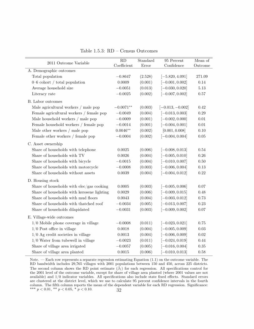
Table 1.5.3: RD – Census Outcomes

2011 Outcome Variable RDCoefficient

StandardError

95 PercentConfidence

Mean ofOutcome

A. Demographic outcomesTotal population −0.8647 (2.528) [−5.820, 4.091] 271.090–6 cohort / total population 0.0009 (0.001) [−0.001, 0.002] 0.14Average household size −0.0051 (0.013) [−0.030, 0.020] 5.13Literacy rate −0.0025 (0.002) [−0.007, 0.002] 0.57

B. Labor outcomesMale agricultural workers / male pop −0.0071∗∗ (0.003) [−0.013,−0.002] 0.42Female agricultural workers / female pop −0.0049 (0.004) [−0.013, 0.003] 0.29Male household workers / male pop −0.0009 (0.001) [−0.002, 0.000] 0.01Female household workers / female pop −0.0014 (0.001) [−0.004, 0.001] 0.01Male other workers / male pop 0.0046∗∗ (0.002) [0.001, 0.008] 0.10Female other workers / female pop −0.0004 (0.002) [−0.004, 0.004] 0.05

C. Asset ownershipShare of households with telephone 0.0025 (0.006) [−0.008, 0.013] 0.54Share of households with TV 0.0026 (0.004) [−0.005, 0.010] 0.26Share of households with bicycle −0.0015 (0.004) [−0.010, 0.007] 0.50Share of households with motorcycle −0.0008 (0.003) [−0.006, 0.004] 0.13Share of households without assets 0.0039 (0.004) [−0.004, 0.012] 0.22

D. Housing stockShare of households with elec/gas cooking 0.0005 (0.003) [−0.005, 0.006] 0.07Share of households with kerosene lighting 0.0029 (0.006) [−0.009, 0.015] 0.48Share of households with mud floors 0.0043 (0.004) [−0.003, 0.012] 0.73Share of households with thatched roof −0.0034 (0.005) [−0.013, 0.007] 0.23Share of households dilapidated −0.0031 (0.003) [−0.009, 0.002] 0.07

E. Village-wide outcomes1/0 Mobile phone coverage in village −0.0008 (0.011) [−0.023, 0.021] 0.751/0 Post office in village 0.0018 (0.004) [−0.005, 0.009] 0.031/0 Ag credit societies in village 0.0013 (0.004) [−0.006, 0.009] 0.021/0 Water from tubewell in village −0.0023 (0.011) [−0.024, 0.019] 0.44Share of village area irrigated −0.0057 (0.005) [−0.016, 0.004] 0.35Share of village area planted 0.0015 (0.006) [−0.010, 0.013] 0.58

Note. — Each row represents a separate regression estimating Equation (1.1) on the outcome variable. TheRD bandwidth includes 29,765 villages with 2001 populations between 150 and 450, across 225 districts.The second column shows the RD point estimate (β1) for each regression. All specifications control forthe 2001 level of the outcome variable, except for share of village area planted (where 2001 values are notavailable) and 1/0 indicator variables. All specifications also include state fixed effects. Standard errorsare clustered at the district level, which we use to calculate 95 percent confidence intervals in the fourthcolumn. The fifth column reports the mean of the dependent variable for each RD regression. Significance:*** p < 0.01, ** p < 0.05, * p < 0.10. 32

numerically in Panel B of Table 1.5.4. While the SECC sample differs notably fromthe village averages in the PCA, these results are broadly consistent with our mainlabor results, and visual evidence suggests a small decrease (increase) in agricultural(other) employment for adult men. We can reject 2 percentage point shifts across allsix labor categories, which suggests that the average employment effects of RGGVYwere similar to the effects on less wealthy households.

Table 1.5.4: RD – SECC Village-Level Outcomes

2011 Outcome RDCoefficient

StandardError


Mean ofOutcome

A. Share of householdsAt least one poverty indicator 0.0006 (0.006) [−0.011, 0.012] 0.48Monthly income greater than Rs 5,000 0.0043 (0.004) [−0.004, 0.013] 0.08One member holding salaried job 0.0030 (0.002) [−0.002, 0.008] 0.02Owning any land −0.0005 (0.008) [−0.017, 0.016] 0.44

B. Adult employmentMale agricultural workers / adult men −0.0091∗ (0.005) [−0.019, 0.001] 0.29Female agricultural workers / adult women −0.0039 (0.005) [−0.013, 0.006] 0.08Male household workers / adult men 0.0008 (0.001) [−0.002, 0.004] 0.01Female household workers / adult women −0.0015 (0.008) [−0.016, 0.013] 0.51Male other workers / adult men 0.0052 (0.006) [−0.007, 0.017] 0.42Female other workers / adult women 0.0054 (0.005) [−0.005, 0.016] 0.16

Note. — Each row represents a separate regression estimating Equation (1.1) on a different SECC village-level outcome. The first row of Panel A is coded as the share of total households in the village with atleast one poverty indicator. Other outcomes in Panel A are coded as the proportion of this subset ofhouseholds (with poverty indicators) that meet each criterion. Panel B outcomes are coded as the share ofadult men (women) with an occupation in each subcategory, for the sample of adults in households with atleast one poverty indicator. (We treat all invididuals over 16 years of age as adults.) The second columnshows the RD point estimate (β1) for each regression. All specifications include state fixed effects, butthey do not include any additional baseline control variables. The RD bandwidth includes 25,942 villageswith 2001 populations between 150 and 450. These regressions contain fewer villages than regressions inTable 1.5.3 because only 87 percent of 10th-Plan, single-habitation, 150–450 villages match to the SECCdataset. Standard errors are clustered at the district level with 222 clusters, which we use to calculate 95percent confidence intervals in the fourth column. The fifth column reports the mean of the dependentvariable for each RD regression. Significance: *** p < 0.01, ** p < 0.05, * p < 0.10.

Finally, we test for the effects of RGGVY eligibility on education. We estimateEquation (1.1) using village-wide enrollment for grades 1–8, both pooled and sep-arately by gender, as the dependent variable. We also test for separate effects for

33

Figure 1.5.9: RD – SECC Village-Level Outcomes

−.02

−.01

0

.01

.02

Sh

are

of

Ho

use

ho

lds,

resid

ua

ls


At Least 1 Poverty Indicator

−.02

−.01

0

.01

.02

Sh

are

of

Ho

use

ho

lds,

resid

ua

ls


Monthly Income Over Rs 5,000

−.02

−.01

0

.01

.02

Sh

are

of

Ad

ult M

en

, re

sid

ua

ls


Adult Men Working in Agriculture

−.02

−.01

0

.01

.02

Sh

are

of

Ad

ult M

en

, re

sid

ua

ls


Adult Men Working in Other Jobs

Note. — This figure shows the results from our preferred RD specification (Equation (1.1)), as reportednumerically in Table 1.5.4. The upper-left panel reports the proportion of total village households with atleast one poverty indicator in 2011, while the upper-right panel reports the proportion of households witha poverty indicator that had a maximum monthly income over Rs 5,000 in 2011. The lower panels reportthe share of adult men in households with a poverty indicator with occupations in each category. Blue dotsshow average residuals from regressing the 2011 share of households on state fixed effects. Each dot containsapproximately 1,600 villages, averaged in 20-person population bins. Lines are estimated separately on eachside of the 300-person threshold for 25,942 villages, i.e. all 10th-Plan single-habitation villages within our150–450 population RD bandwidth, that match to the SECC dataset.

34

primary (grades 1–5) and upper primary (grades 6–8) enrollment, where the latterreflects changes on the intensive margin of schooling. We report these results inFigure 1.5.10 and Table 1.5.5, which show no statistically significant changes in en-rollment at the 300-person threshold.47 As with our other results, our 95 percentconfidence intervals can reject even moderate changes in enrollment on either theintensive or extensive margins.

47These regressions control for the 2005 level of the outcome variable, which is the earliest yearof enrollment data available. Also, we not that because these village-level enrollment regressionsaggregate enrollment across all schools in each village, they might confound changes in within-school attendance with changes in enrollment due to new school construction over time. AppendixA.2.8 repeats these same regressions using school-level enrollment observations, while conductingadditional sensitivity analysis.

35

Figure 1.5.10: RD – School Enrollment

−10

−5

0

5

10

20

11

En

rollm

en

t, r

esid

ua

ls


2011 Total Enrollment, Grades 1−8

−10

−5

0

5

10

20

11

Up

pe

r P

rim

ary

En

rollm

en

t, r

esid

ua

ls



Note. — This figure shows the results from our preferred RD specification (Equation (1.1)), as reportednumerically in the first and last rows of Table 1.5.5. Blue dots show average residuals from regressingthe 2011 number of (total, grades 6–8 only) students on the corresponding 2005 enrollment counts andstate fixed effects. Each dot contains approximately 1,000 villages, averaged in 25-person population bins.Lines are estimated separately on each side of the 300-person threshold, for 12,251 single-habitation villagesbetween 150 and 450 people, in 10th-Plan districts, with school-village matches and nonmissing 2005 and2011 enrollment data.

36

Table 1.5.5: RD – School Enrollment


StandardError


Mean ofOutcome

Total enrollment, grades 1–8 −0.472 (3.93) [−8.18, 7.24] 74.05Male enrollment, grades 1–8 0.197 (2.00) [−3.72, 4.11] 37.60Female enrollment, grades 1–8 −0.650 (2.02) [−4.61, 3.31] 36.45Total enrollment, grades 1–5 −0.408 (2.95) [−6.19, 5.37] 60.58Total enrollment, grades 6–8 0.051 (1.50) [−2.89, 2.99] 13.47

Note. — Each row represents a separate regression estimating Equation (1.1) on a different enrollmentcount, aggregating schools enrollment up to village-level observations. The second column shows the RDpoint estimate (β1) for each regression. All specifications control for the 2005 level of the outcome variableand state fixed effects. The RD bandwidth includes 12,251 village observations with 2001 populationsbetween 150 and 450, with a single habitation, in RGGVY 10th-Plan districts. These regressions containfewer villages than regressions in Table 1.5.3 because only 51 percent of 10th-Plan, single-habitation, 150–450 person villages match to a school, and only 76 percent of these matched villages contain schools thatreport nonmissing enrollment values for 2011 and 2005. Standard errors are clustered at the district level,with 215 clusters, which we use to calculate 95 percent confidence intervals in the fourth column. The fifthcolumn reports the mean of the dependent variable for each RD regression. Significance: *** p < 0.01, **p < 0.05, * p < 0.10.

Taking these results together, we conclude that while the provision and consump-tion of electricity substantially increased as a result of RGGVY eligibility, we detectno economically meaningful changes in labor outcomes, asset ownership, the hous-ing stock, village-level outcomes, household income, or school attendance. Our RDresults are precisely estimated, enabling us to rule out even modest effect sizes forthese outcomes. This suggests that eligibility for RGGVY did not lead to structuraltransformation, increased agricultural productivity, female empowerment, reductionsin indoor air pollution, improved education, or poverty reductions.

1.6 Interpretations and Extensions

1.6.1 Scaling

The above regressions recover intent-to-treat estimates: they show the effect of be-ing eligible for RGGVY on our outcomes of interest. In order to compute averagetreatment effects, we need to scale these estimates such that we recover the effect ofelectrification on development.48

48We do not scale via two-stage least squares because we do not have access to a binary “RGGVYelectrification” variable, nor would this variable capture different levels of energy access and con-sumption across villages treated under RGGVY, as discussed above.

37

We propose several methods of scaling our estimates. First, we consider inflat-ing our outcomes based on the proportion of villages within our bandwidth thatRGGVY claims to have treated. This is akin to the scale factor we would applywith a traditional instrumental variables estimator. RGGVY’s district-level aggre-gate data suggest that between 56 and 82 percent of eligible villages were treated bythe program.49 This implies that our estimates should be inflated by approximatelya factor of 1.5 in order to recover the causal effects of treatment under RGGVY.

Alternatively, we can calibrate a scaling factor to the magnitude of the increasein nighttime brightness, which we estimate to be 0.15 units of brightness. Minet al. (2013) suggest that when villages in Senegal were electrified, they experiencedincreases of approximately 0.4 nighttime brightness points. If, alternatively, we applyMin and Gaba (2014)’s estimates of a 1-unit increase in brightness corresponding to240–270 electrified households, then full electrification of the average village in ourRD sample with 56 households would imply an increase of 0.2 brightness points.50

This suggests that our RD estimates should be inflated by a factor of between 1.3and 3 to recover the average effect of RGGVY electrification.51

Scaling the point estimates reported in Tables 1.5.3–1.5.5 by a factor of 3 doesnot yield adjusted estimates that are economically meaningful. For the vast majorityof outcomes, we see no visual evidence of a discontinuity, suggesting that these upperbounds are quite conservative. Even after inflating the 95 percent confidence intervalsby these factors, we can still reject 4 percentage point changes in labor outcomes,4 percentage point changes in asset ownership, 5 percentage point changes in thehousing stock, and 8 percentage point changes in village-level outcomes. We can alsoreject 6 percentage point changes in outcomes in Table 1.5.4, as well as 21 student(30 percent) increases in total school enrollment. Scaling by a factor of 3, we canrule out effects larger than 0.26 of one standard deviation in all outcomes presentedin Tables 1.5.3–1.5.5.

Even if we were to scale our estimates by an extremely conservative factor of 10,we can still reject effect sizes consistent with the previous literature.52 Dinkelman

49RGGVY’s aggregate village counts in 10th-Plan districts sum to 56 percent of the total numberof villages in these districts, and 82 percent of villages with 2001 populations over 300.

50These increases of 0.4 and 0.2 are internally consistent; the average villages in Min et al. (2013)and Min and Gaba (2014) are larger than the villages in our RD bandwidth.

51We do not propose a scale factor based on Min and Gaba (2014)’s streetlights estimate, sincewe do not have data on the number of streetlights per village, and because RGGVY did not installstreetlights.

52In order to arrive at factor of 10, which we believe to be the most conservative interpretation ofour results, we assume that RGGVY only impacted household electricity end-uses. Our nighttimebrightness effect of 0.15 is comparable to the change in brightness associated with a 10 percentagepoint increase in the share of households with electric lighting, a proxy for household power con-

38

(2011) finds that electrification caused 9–9.5 percentage point increases in female em-ployment; we can reject 2 percentage point increases in total female employment.53

Lipscomb, Mobarak, and Barham (2013) likewise find large effects of electrification ontotal employment rates; we can reject 1 percentage point increases in the village-wideemployment rate even after applying a conservative scaling factor of 10.54 Chakra-vorty, Emerick, and Ravago (2016) find that rural electrification leads to a 56 percentdecrease in a deprivation index, and a 38 percent increase in household expenditures;scaling our Table 1.5.4 results by 10, we can reject an 11 percentage point decreasein the share of households with at least one poverty indicator, and a 13 percentagepoint increase in the share of households (with at least one poverty indicator) withmonthly incomes greater than 5,000 rupees.

1.6.2 Heterogeneous effects

It is possible that our results mask heterogeneity in the quality of energy servicesexperienced by RGGVY villages. In particular, India faces major electricity short-ages, which vary across locations (Allcott, Collard-Wexler, and O’Connell (2016)).If half of the villages in our sample experienced frequent power outages while theother half received consistent power, our average intent-to-treat estimate across bothgroups would be small even if RGGVY led to large economic effects in places withhigh-quality energy supply. We test for this by re-estimating all of our RD resultsusing the subset of states with above-average power availability (Central ElectricityAuthority (2011)).55 In this subsample, our estimated RD coefficient on nighttimebrightness increases from 0.15 to 0.25, statistically significant at the 1 percent level.However, the results for labor, asset ownership, the housing stock, village-level out-comes, and household wealth are quantitatively similar to those estimated using thefull RD sample.56

sumption, at the mean of our RD sample. This suggests a scaling factor of 10 to translate this intoan increase from 0 to 100 percent of households.

53We estimate Equation (1) pooling female employment across all three sectors, resulting inan RD point estimate of −0.0067 with the upper end of our 95 percent confidence interval of0.0015, which we multiply by 10. We can similarly reject increases of 3 percentage points in femaleagricultural employment, 1 percentage point in female household employment, and 4 percentagepoints in female other employment.

54If we pool all six labor outcomes in Panel B of Table 1.5.3, the resulting RD point estimate is−0.0053 with an upper 95 percent confidence interval of 0.0002.

55These seven states are (in decreasing order of 2011 power quality): Chhattisgarh, Orissa,Karnataka, West Bengal, Gujarat, Haryana, and Rajasthan.

56Appendix A.2.10 reports regression results for both split-sample exercises discussed in thissection. The schooling results are qualitatively similar, but somewhat less robust.

39

This suggests that poor power quality in a subset of states is not attenuating ourestimate of the average effect across the full sample. Moreover, our main RD resultsreflect the realized implementation of a large-scale national rural electrification pro-gram in the developing world. Even if we had found substantial positive effects fora subset of states, the overall treatment effect would be indicative of the degree towhich future rural electrification programs might be limited by the supply reliability.

It is also possible that we do not detect large effects because the benefits ofelectrification take many years to accrue. While we cannot rule this possibilityout completely, our 2011 outcome data were collected between three and five yearsafter 95 percent of villages in our sample received RGGVY funding.57 Even if therewere significant delays in implementation, this is much longer than the time spanover which development interventions are typically studied. Nevertheless, we recoverquantitatively similar RD point estimates when we restrict our RD sample to districtswith early RGGVY funding. Therefore, it is unlikely that our small results are drivenby villages that failed to take advantage of the full set of possible medium-run benefitsof electric power before being surveyed by the 2011 Census.

1.6.3 Difference-in-differences

Finally, we might be concerned that villages close to the 300-person RD thresholdstand little to gain from electrification. Perhaps these small villages are simply toopoor, too credit-constrained, or too economically isolated to translate increased elec-tricity access into new employment or income-generating opportunities. We employa second identification strategy, difference-in-differences (DD), to test for the effectsof RGGVY eligibility on larger villages far from our RD threshold. Recall that therewere two major phases of RGGVY implementation: the 10th-Plan phase and the11th-Plan phase. The majority of 11th-Plan electrification projects had not beencompleted before the 2011 Census. We can therefore use 10th-Plan districts as a“treated” group and 11th-Plan districts as a “control” group in a DD framework.58

We estimate the following fixed effects specification on our two-decade village panel:

Yvst = γ0 +∑b

γb11 [10th× Post]vt × 1 [Pv ∈ Binb] + δt + ηv + εvt(1.2)

where 1 [10th× Post]vt is an indicator equal to one if village v was eligible forRGGVY under the 10th Plan and the year t is 2011, 1 [Pv ∈ Binb] are 2001 vil-

57Over 70 percent of villages in our RD sample are in districts that received RGGVY fundingbefore the end of 2006. See Appendix Table A.2.26.

58Selection into the different plans was non-random. It is plausible that 10th-Plan districts weremore administratively capable than 11th-Plan districts, likely biasing our DD estimates upward.

40

lage population bins along the full support of populations (shown in Figure 1.4.3),δt are year fixed effects, and ηv are village fixed effects. This necessitates strongeridentifying assumptions than our RD specification, namely that villages in 10th-Plandistricts were trending in parallel to 11th-Plan villages prior to RGGVY. Village-leveldata are not available for the 1991 Census, therefore we are unable to directly testthis assumption.59

Figure 1.6.11 compares our main RD results with DD results from estimatingEquation (1.2) with 300-person population bins, for nighttime brightness and maleagricultural workers. For both outcomes, the RD point estimates lie within the DDconfidence intervals. Moreover, the DD effect of RGGVY on nighttime lights in-creases nearly monotonically in population, while the DD effect for male agriculturallabor is close to constant as population increases. This suggests that our small RDresults for male agricultural employment are likely to be externally valid outside ofour RD bandwidth. Other economic outcome variables show similarly constant DDcoefficients across small and large villages.60

These DD results are broadly consistent with our RD results, despite using amuch larger population of villages (from 10th- and 11th-Plan districts, includingmulti-habitation villages) and using 11th-Plan villages as counterfactuals (as op-posed to barely ineligible 10th-Plan villages). Beyond allowing us to extend ourRD results to larger villages, the DD results are encouragingly similar to the RD.Relying on alternative identifying assumptions on a different sample of villages, weagain demonstrate that RGGVY caused nighttime brightness to increase, but hasnot meaningfully improved the economic outcomes that we observe.

59In Appendix A.2.11, we test for differential pre-trends using district-level data. These trendsare not statistically zero, suggesting that our DD results should be interpreted with some caution.

60We report additional DD results in Appendix A.2.11.

41

Figure 1.6.11: Difference-in-Differences Results

−1

0

1

2

DD

co

eff

icie

nt

(95

% C

I)

300 900 1500 2100 27002001 village population

Nighttime Brightness

−.03

−.02

−.01

0

.01

DD

co

eff

icie

nt

(95

% C

I)


Male Agricultural Workers

Note. — This figure compares the reduced form effects from our preferred RD specification (Equation(1.1)) to the results from our DD specification (Equation (1.2)), using 300-person population bins. Navyblue dots show the RD coefficients, with whiskers indicating 95 percent confidence intervals. Light bluedots and dashed lines show the binned DD point estimates and 95 percent confidence intervals. The toppanel shows the effects for nighttime lights, as measured by maximum village brightness. The bottom panelshows the effects for male agricultural workers. The RD results are statistically significant at the 5 percentlevel and the 1 percent level, respectively. The pooled DD point estimates are 0.45 and −0.008; both arestatistically significant at the 10 percent level (Appendix A.2.11 reports these results in a regression table).DD regressions for lights and labor include 629,778 and 994,802 village-year observations, respectively.

42

1.6.4 Costs and benefits

We do not have direct estimates of village-level program costs, incomes, or expendi-tures.61 However, we perform several back-of-the-envelope calculations based on ourRD results. This enables us to better understand the overall economics of RGGVY,while also quantifying the costs and benefits of electrification.

First, we consider the per-village costs of RGGVY implementation. In 2005,RGGVY was expected to cost 634.2 billion rupees, or approximately $17.2 billion.62

Given the stated scope of the program detailed in Section 1.2, this suggests a costper village of approximately 1,470,000 rupees, or $36,000 in 2015 USD.63

We can apply average Indian rural wage rates to estimate the income differen-tial that might have resulted from the (small) sectoral shift from agricultural tonon-agricultural employment we observe under RGGVY. According to India’s Na-tional Sample Survey Office, the average 2011 wage for male (female) non-agriculturalworkers was 196 (116) rupees per day, which was 26 (0.9) percent higher than theaverage agricultural wage of 155 (115) rupees per day. To compute the average in-crease in village-level income, we scale the lower bound of our confidence interval formale (female) agricultural labor from Table 1.5.3, −0.013 (−0.013), by a factor of3. This converts our intent-to-treat estimate into an average treatment effect, andit implies a maximum shift out of male and female agricultural employment of 3.9percentage points.64 If all of these men (women) shifted from agriculture into non-agriculture employment, then total daily male (female) village wage earnings wouldhave increased by approximately 293 (7) rupees. If each employed person worked365 days per year, this would translate into a total annual village income increase ofapproximately 109,000 rupees, or an upper bound of 1.4 percent.

Alternatively, we can use our RD estimates on household asset ownership to inferchanges in expenditures resulting from electrification. Scaling the upper confidenceintervals in Panel C of Table 1.5.3 by 3, we can reject increases in asset ownershipof greater than 3.9 percent for mobile phones, 3.0 percent for televisions, 2.1 percentfor bicycles, and 1.2 percent for motorcycles. Monetizing these upper bounds usingasset prices from ICRISAT’s Village Dynamics in South Asia dataset, this implies a

61The SECC income data indicate whether households’ main income earners earned more or lessthan 5,000 rupees per month, and comes from a selected subset of households. Hence, we excludethese data from the subsequent cost-benefit analysis.

62We use the 2005 exchange rate of 44 rupees per dollar, and convert to 2015 USD.63This is comparable to Chakravorty, Emerick, and Ravago (2016), who report average electri-

fication costs of $42,000 per village in the Philippines.64In keeping with Section 1.6.1, we apply a scaling factor of 3 throughout this section.

43

maximum average household expenditure of 572 rupees.65 Supposing that only 10percent of RGGVY-driven expenditure increases were spent on these four durablegoods implies a maximum increase in per-household expenditure of 5,720 rupees,or a total village-wide increase of around 398,000 rupees. These asset purchasesoccurred during the 3–6 year period after electrification; if we conservatively assumethat they all occurred within 3 years of electrification, this would represent at besta 2.1 percent increase in annual village expenditures.66

Our back-of-the-envelope estimates suggest that annual village income increasedby a maximum of 109,000 rupees, that annual village expenditures increased by amaximum of 133,000 rupees, and that RGGVY electrification came at a cost ofapproximately 1,470,000 rupees per village. These results are quite conservative:though we do not measure all possible benefits from electrification, the benefits wedo use in performing this calculation come almost entirely from regression estimateswhere we cannot reject zero; our assumptions in performing this calculation alsomake it biased towards finding large effects. Using the larger expenditure estimateand applying a conservative 3 percent discount rate, this translates into a paybackperiod of approximately 12 years.67

At best, we find that RGGVY increased annual incomes by 1.4 percent and an-nual expenditure by 2.1 percent, despite causing a substantial shift in nighttimelights. This suggests exercising caution when using nighttime brightness as a proxyfor income or expenditures. The DMSP-OLS dataset measures light emissions. Be-cause brightness relates directly to energy consumption through lighting, it servesas a useful indicator of electrification. Since electrification should lead to increasedbrightness even absent a corresponding increase in incomes, we do not use the DMSP-OLS data as a proxy for income/expenditures, and caution others against doing sowhen evaluating programs that directly increase light emissions.

Importantly, our results do not speak directly to the effects of RGGVY on wel-fare. It is quite possible that electrification has dramatically increased average qual-ity of life for rural Indians. Indeed, since villagers are using more power as a resultof RGGVY, revealed preference suggests that they benefit from the program. Eventhough we measure a wide range of outcome variables which are typical of large-scaleadministrative datasets, there may be important utility benefits that we cannot mea-

65The average prices for durables commonly purchased after electrification are: Rs 2,796 for cellphones, Rs 4,166 for televisions, Rs 1,259 for bicycles, and Rs 25,922 for motorcycles.

66India’s average rural monthly per capita expenditures were 1,430 rupees for 2011–2012.67This starkly contrasts with Chakravorty, Emerick, and Ravago (2016), who find a payback

period of approximately 1 year; however, it is corroborated by evidence from Lee, Miguel, andWolfram (2016), who use revealed preference results to suggest that the costs of electrification aremuch larger than the benefits.

44

sure. Our results highlight the need to incorporate additional non-market measuresinto future administrative data collection efforts.

1.7 ConclusionIn this paper, we evaluate the medium-run effects of electrification on developmentusing a regression discontinuity (RD) design which exploits a population eligibilitythreshold in India’s national rural electrification program, RGGVY. We find thateligibility for RGGVY led to substantial changes in nighttime brightness and poweravailability. Despite this increase in energy access, we find that electrification didnot have economically meaningful impacts on a range of development outcomes.

These results hold when we rescale our reduced form estimates to account for theproportion of eligible villages that underwent treatment. We see similar effects ondevelopment among states with high and low average reliability of electricity supply.We also find similar effects when we restrict our analysis to the earliest districts to ob-tain RGGVY funding, suggesting that our results do not depend on the timing of ourpost-intervention data. Finally, we apply a difference-in-differences strategy, whichrelies on alternative identifying assumptions and includes a larger sample of villageswell outside our RD bandwidth. These results support the main conclusions fromour RD analysis that while nighttime lights, and therefore power consumption, in-creased substantially with RGGVY electrification, other development outcomes thatwe observe did not. Our cost-benefit calculations suggests a much longer paybackperiod than previously estimated.

These results are the first to suggest that electrifying rural villages may not causesizable economic gains in the medium term. Our regression discontinuity strategyrelies on much less stringent identifying assumptions than the instrumental variablesapproaches of previous work, allowing us to measure effects of a natural rollout ofrural electrification, at scale. In contrast to the existing literature, we find that elec-trification did not yield even modest changes in labor, income, household wealth,asset ownership and expenditures, village-level outcomes, and education. These nullresults come from the world’s largest unelectrified population, and appear to gener-alize to over 400,000 villages across rural India.

Nevertheless, electrification may lead to large economic benefits in certain con-texts, and may have important positive effects on human well-being that we areunable to quantify. An important direction for future work will be to understandwhen, where, and after how long electricity access and power availability have thegreatest economic impact. For example, electrification may lead to substantial gainsin economic productivity in urban settings, or in regions with budding local indus-

45

tries. There may also be substantial long-run effects of electrification, and moreresearch is necessary to identify these benefits. Finally, we encourage future researchon quantifying the non-market benefits from electrification that frequently go un-measured.

46

Chapter 2

Machine Learning from SchoolsAbout Energy Efficiency1

2.1 IntroductionEnergy efficiency is a cornerstone of global greenhouse gas (GHG) abatement efforts.For example, worldwide proposed climate mitigation plans rely on energy efficiencyto deliver 42 percent of emissions reductions (IEA (2015)). The appeal of energyefficiency investments is straightforward: they may pay for themselves by loweringfuture energy bills. At the same time, lower energy consumption reduces reliance onfossil fuel energy sources, providing the desired GHG reductions. A number of pub-lic policies – including efficiency standards, utility-sponsored rebate programs, andinformation provision requirements – aim to encourage more investment in energyefficiency.

Policymakers are likely drawn to energy efficiency because a number of analy-ses point to substantial unexploited opportunities for cost-effective investments (see,e.g., McKinsey & Company (2009)). These analyses are almost universally basedon engineering estimates of the potential energy savings over time rather than fieldevidence of actual savings. One strand of the economics literature has attemptedto explain why consumers might fail to avail themselves of profitable investment op-portunities (see, e.g., Allcott and Greenstone (2012), Gillingham and Palmer (2014),and Gerarden, Newell, and Stavins (2015)). The most popular explanations haveemphasized the possibility of market failures, such as imperfect information, capitalmarket failures, split incentive problems, and behavioral biases, including myopia,

1The material in this chapter is from an unpublished working paper, coauthored with Christo-pher R. Knittel, David Rapson, Mar Reguant, and Catherine Wolfram.

47

inattentiveness, prospect theory and reference-point phenomena. The literature alsopoints to the possibility that engineering estimates understate the costs consumersface.

Economists have also pointed out that accurately measuring the returns to energyefficiency investments is difficult as it requires constructing a counterfactual energyconsumption path from which reductions caused by the efficiency investments can bemeasured (Joskow and Marron (1992)). Recent studies use both experimental (e.g.,Fowlie, Greenstone, and Wolfram (2015a)) and quasiexperimental (e.g., Levinson(2016), Myers (2014), Davis, Fuchs, and Gertler (2014)) approaches to developingthis counterfactual. Many of these papers suggest that the energy savings fromefficiency investments are lower than expected, and the results cast doubt on theextent to which emissions reductions can be achieved through energy efficiency. Atthe same time, energy efficiency proponents have criticized these findings as onlypertaining to specific contexts (Kushler (2015)), and are skeptical that experimentaland quasi-experimental estimation approaches can be applied broadly. In general,there is a clear need for techniques to estimate returns to energy efficiency programsthat can be applied in a wide set of contexts.

The proliferation of high-frequency data in electricity markets provides a promis-ing opportunity to estimate treatment effects associated with energy efficiency in-vestments wherever advanced metering infrastructure (AMI, or “smart metering”) isinstalled. In this paper, we use high-frequency data to implement several approachesto estimating counterfactual energy consumption absent the energy efficiency invest-ments. We begin with difference-in-difference approaches that employ rich sets offixed effects. We show, however, that the resulting estimates are sensitive to theset of observations included as controls as well as to the fixed effects included in thespecification. To address these concerns, we develop and implement a novel machine-learning approach to predict counterfactual energy consumption at treated schoolsand validate the approach with non-treated schools.

Specifically, we match hourly electricity consumption data from public K-12schools in California to energy efficiency installation records, and exploit tempo-ral and cross-sectional variation to estimate the causal effect of the energy efficiencyinvestments on energy use. Our data span 2008 to 2014, although only 20 per-cent of schools had smart meter data in 2008 and half have entered our data setby 2011. Our methodology includes traditional regression-based approaches, whichallow us to non-parametrically control for a wide array of potential confounders.We implement a novel machine learning approach, using model selection and fore-casting methods to construct school-specific counterfactual electricity usage usingonly pre-treatment data. We compare the results of this approach to the traditional

48

difference-in-difference methods, and find, consistent with Monte Carlo simulations,that our machine learning approach yields slightly larger treatment effects.

Our contributions to the literature are both policy-relevant and methodological.From a policy perspective, this paper departs from much of the previous academicliterature on energy efficiency by examining energy efficiency outside the residen-tial sector. 37 percent of electricity use in the United States in 2014 was residential,and over half is attributable to commercial and industrial uses (EIA (2015)). A morecomplete view of what energy efficiency opportunities are cost-effective requires moreevidence from a variety of settings, which, in turn, requires an informed understand-ing of the costs and benefits of investment in settings that have traditionally beendifficult to study.

Our results demonstrate that energy efficiency investments can lead to substantialenergy savings in schools. Across all types of investments, energy efficiency appearsto deliver between 2 and 5 percent reductions in electricity use. We also look at thetwo most prevalent upgrade categories in our sample, lighting, which makes up 22percent of upgrades; and heating, ventilation, and air conditioning (HVAC), whichmakes up 51 percent of upgrades. During daytime hours, investments in energyefficient lighting lead to 3 to 7 percent reductions in electricity use and smallerreductions at night. Investments in energy efficient HVAC systems produce a 2-4 percent reduction in the daytime hours, when temperatures are highest. Theseresults translate into a significant amount of overall energy savings, representingabout 60 kWh in daily electricity savings per school, which we estimate using bothregression and machine learning techniques. When we compare these ex post effectsto ex ante savings, however, we find that these ex-post saving estimates appear todeliver less than 50 percent of expected ex-ante savings.

From a methodological perspective, high frequency data provides large benefits,but also presents new challenges. Using 15-minute interval electricity consumptiondata allows us to incorporate a rich set of controls and fixed effects in order to non-parametrically separate the causal effect of energy efficiency upgrades from otherconfounding factors. However, over-saturation is a concern; fixed effects estimatorsthat absorb too much identifying variation can spuriously detect “treatment effects”that are simply artifacts of measurement problems in the data (Fisher et al. (2012)).The machine learning method that we develop in this paper uses LASSO, a form ofregularized regression, to generate a model of counterfactual electricity consumptionthat leverages our high-frequency data while avoiding overfitting. This allows us tooptimally saturate the regression (trading off precision with bias). Furthermore, weonly use pre-treatment data to train the LASSO model, meaning that the school-specific prediction models we generate do not risk absorbing part of the treatment,which is not present in the data used to build the model.

49

To our knowledge, this is the first paper in economics to incorporate machinelearning methods into a selection-on-unobservables design in order to conduct causalinference.2 We validate the machine learning predictions at our control schools,finding tightly-estimated zero effects for non-treated schools. We further embed ourmachine learning predictions into a difference-in-difference framework to account forthe possibility of systematic trends in the prediction errors. Using a series of MonteCarlo simulations, we demonstrate that the machine learning approach performs asexpected relatively to the regressions. We believe our methodology may be of interestto empiricists in a broad class of settings.

The remainder of the study proceeds by describing our empirical setting anddatasets (Section 2.2). We then describe the baseline difference-in-differences method-ology and estimate results using these standard tools (Section 2.3). Section 2.4 in-troduces our machine learning methodology, and presents the results. In Section 2.5,we compare our savings estimates to the ex ante engineering projections to calculaterealization rates. Section 2.6 concludes.

2.2 Context and DataExisting ex ante estimates suggest that commercial buildings, including schools, maypresent important opportunities to increase energy efficiency. For example, McKinsey& Company, who developed the iconic global abatement cost curve (see McKinsey &Company (2009)), note that buildings account for 18 percent of global emissions andas much as 30 percent in many developed countries. In turn, commercial buildingsaccount for 32 percent of building emissions, with residential buildings making up thebalance. Opportunities to improve commercial building efficiency primarily revolvearound lighting, office equipment, and HVAC systems.

Commercial buildings such as schools, which are not operated by profit-maximizingagents, may be less likely to take advantage of cost-effective investments in energyefficiency, so they may yield particularly high returns to targeted programs that en-courage energy efficiency investments. On the other hand, schools are open fewerhours than many commercial buildings, so the returns may be lower. Energy ef-ficiency retrofits for schools gained prominence in California with Proposition 39,which voters passed in November 2012. The proposition closed a corporate tax loop-hole and devoted half of the revenues to reducing the amount public schools spend onenergy, largely through energy-efficiency retrofits. Over the first three fiscal years ofthe program, the California legislature appropriated $1 billion to the program (CEC

2In a recent NBER working paper, Cicala (2017) implements a variant on this methodology,using random forests rather than LASSO, in the context of electricity market integration.

50

(2017)). To put this in perspective, it represents about one-third of what Californiais currently spending on all utility-funded energy efficiency programs (ranging fromlow-interest financing to light bulb subsidies to complex industrial programs) andabout 5 percent of what utilities nationwide spend on energy efficiency (Barboseet al. (2013)). Though our time period precedes most investments financed throughProposition 39, our results are relevant to expected energy savings from this largepublic program.

Methodologically, schools provide a convenient laboratory to isolate the impactsof energy efficiency. School buildings are all engaged in nearly the same activities,subject to relatively similar trends in education, and are clustered within distinctneighborhoods and towns. Other commercial buildings, by contrast, can house any-thing from an energy intensive data center that operates around the clock to a churchthat operates very few hours per week. Finally, given the public nature of schools,we are able to assemble relatively detailed data on building characteristics and recentinvestments.

Most of the existing empirical work on energy efficiency focuses on the residentialsector. There is little existing work on energy efficiency in commercial buildings.Kahn, Kok, and Quigley (2014) provide descriptive evidence on differences in en-ergy consumption across one utility’s commercial buildings as a function of variousobservables, including incentives embedded in the occupants’ leases, age and otherphysical attributes of the buildings. In other work, Kok and co-authors analyze thefinancial returns to energy efficiency attributes, though many of the attributes werepart of the building’s original construction and not part of deliberate retrofits, whichare the focus of our work (Kok and Jennen (2012) and Eichholtz, Kok, and Quigley(2013)).

2.2.1 Data Sources

This project merges data from several sources. We combine high-frequency electricityconsumption and account information with data on energy efficiency upgrades, schoolcharacteristics, community demographics, and weather.

We obtained 15-minute interval electricity metering data for the universe of publicK-12 schools in Northern California served by Pacific Gas and Electric Company(PG&E). The data begin in January 2008, or the first month after the school’ssmart meter was installed, whichever comes later. 20 percent of the schools in thesample appear in 2008; the median year schools enter the sample is 2011. The data

51

series runs through 2014. To speed computation time, we aggregate these 15-minuteobservations to three-hourly “blocks.”3

In general, PG&E’s databases link meters to customers for billing purposes. Forschools, this creates a unique challenge: in general, school bills are paid at the dis-trict, rather than individual school site, level. In order to estimate the effect ofenergy efficiency investments on electricity consumption, we required a concordancebetween meters and school sites. We developed a meter matching process in parallelwith PG&E. The final algorithm that was used to match meters to schools was im-plemented as follows: first, PG&E retrieved all meters associated with “education”customers.4 Next, they used GPS coordinates attached to each meter to match me-ters from this universe to school sites, using school location data from the CaliforniaDepartment of Education. This results in a good but imperfect match between me-ters and schools. In some cases, multiple school sites match to one or more meters.This can often be resolved by hand, and was wherever possible, but several “clus-ters” remain. We use only school-meter matches that did not need to be aggregated.Robustness tests suggest that the results presented here do not change substantivelywhen we include these “clusters.” Our final sample includes 2,094 schools.

The PG&E data also describe energy efficiency upgrades at the schools as long asthe school applied for rebates from the utility.5 A total of 6,971 upgrades occurred at1,039 schools between January 2008 and December 2014. For each energy efficiencymeasure installed, our data include the measure code, the measure description6, atechnology family (e.g., “HVAC”, “Lighting”, “Food service technology"), the numberof units installed, the installation date, the expected lifetime of the project, theengineering-estimate-based expected annual kWh savings, the incremental measurecost, and the PG&E upgrade incentive received by the school.7

Many schools undertake multiple upgrades, either within or across categories. Weinclude all upgrades in our analysis, and break out results for the two most commonupgrade categories: HVAC and lighting. Together these two categories make up over70 percent of the total upgrades, and over 60 percent of the total projected savings.

3Robustness checks suggest that our results are similar if we aggregate to hourly blocks.4PG&E records a NAICS code for most customers in its system; this list of education customers

was based on the customer NAICS code.5Anecdotally, the upgrades in our database are likely to make up a large share of energy efficiency

upgrades undertaken by schools. PG&E reports making concerted marketing efforts to reach outto schools to induce them to make these investments; schools often lack funds to devote to energyefficiency upgrades in the absence of such rebates.

6One example lighting measure description from our data: “PREMIUM T-8/T-5 28W ELECBALLAST REPLACE T12 40W MAGN BALLAST-4 FT 2 LAMP”

7We have opted not to use the cost data as we were unable to obtain a consistent definition ofthe variables.

52

We obtained school and school-by-year information from the California Depart-ment of Education on academic performance, number of students, the demographiccomposition of each school’s students, the type of school (i.e., elementary, middleschool, high school or other) and location. We also matched schools and school dis-tricts to Census blocks in order to incorporate additional neighborhood demographicinformation, such as racial composition and income. Finally, we obtained informa-tion on whether school district voters had approved facilities bonds in the two to fiveyears before retrofits began at treated schools.8

We obtained hourly temperature data from 2008 to 2014 from over 4,500 weatherstations across California from MesoWest, a weather data aggregation project hostedby the University of Utah.9 We matched school GPS coordinates provided by theDepartment of Education with weather station locations from MesoWest to pair eachschool with its closest weather station to create a school-specific hourly temperaturerecord.

2.2.2 Summary Statistics

Table 2.2.1 displays summary statistics for the data described above, across schoolswith and without energy efficiency projects. Of the 2,094 schools in the sample, 1,039received some type of energy efficiency upgrade. 628 received only HVAC upgradesand 493 received only lighting upgrades. There are 1,055 schools that received noupgrade. Our main variable of interest is electricity consumption, which we observeevery 15 minutes but summarize in Table 2.2.1 at the 3-hourly “block” level forpractical purposes. We observe electricity consumption data for the average schoolfor a three-year period.

For schools that are treated, expected energy savings are almost 30,000 kWh,which is approximately 5 percent of average electricity consumption. Savings are aslightly larger share of consumption for schools with lighting interventions.10

The first three columns of Table 2.2.1 highlight measurable differences betweentreated and non-treated schools. Treated schools use over 50 percent more elec-tricity, have 30 percent more enrolled students, different student demographics and

8Bond data are from EdSource (edsource.org).9We performed our own sample cleaning procedure on the data from these stations, dropping

observations with unreasonably large fluctuations in temperature, and dropping stations with morethan 10% missing or bad observations.

10We do not summarize projected savings since it is zero for the control schools.

53

http://mesowest.utah.edu/

Table2.2.1:

Averagecharacteristics

ofschoolsin

thesam

ple

Untreated

Any

InterventionHVAC

InterventionsLighting

InterventionsCategory

Treated

T-U

Treated

T-U

Treated

T-U

Hourly

energycons.

(kWh)

34.257.1

22.963.5

29.461.6

27.5[15.3,39.1]

[24.7,59.5](2.5)

[28.7,63.9](2.9)

[27.3,60.8](3.1)

First

yearin

sample

20122009.9

-2.02009.5

-2.32009.8

-2.1[2011.0,2013.0]

[2008.0,2012.0](0.1)

[2008.0,2011.0](0.1)

[2008.0,2011.0](0.1)

Totalenrollm

ent553.5

722.3168.8

765.9212.4

747.7194.2

[355.4,658.9][462.5,808.3]

(19.9)[496.8,832.0]

(22.8)[479.8,812.4]

(24.5)API

789.4793.7

4.3792.8

3.4786.5

-2.9[734.8,855.3]

[737.9,854.6](4.2)

[734.0,856.0](4.9)

[736.5,836.0](5.1)

Bond

passed–2yrs

0.30.3

0.00.3

-0.00.3

-0.1[0.0,1.0]

[0.0,1.0](0.0)

[0.0,1.0](0.0)

[0.0,1.0](0.0)

Bond

passed–5yrs

0.40.4

0.00.4

-0.00.4

-0.1[0.0,1.0]

[0.0,1.0](0.0)

[0.0,1.0](0.0)

[0.0,1.0](0.0)

High

SchoolGraduates

23.523.3

-0.223.7

0.124.1

0.6[14.4,32.0]

[15.3,31.8](0.5)

[15.3,32.5](0.6)

[17.5,31.5](0.7)

College

Graduates

20.120.3

0.219.4

-0.619.7

-0.4[9.5,29.8]

[9.8,29.4](0.5)

[9.0,28.8](0.6)

[9.3,28.5](0.7)

Percent

singlemothers

20.119.4

-0.720.0

-0.119.9

-0.2[4.8,30.4]

[4.9,28.8](0.9)

[4.9,30.4](1.0)

[4.8,31.1](1.1)

Percent

African-A

merican

5.76.2

0.55.5

-0.35.9

0.1[1.0,6.3]

[1.3,7.8](0.4)

[1.3,7.3](0.4)

[1.3,8.1](0.5)

Percent

White

34.330.7

-3.629.8

-4.529.7

-4.6[8.5,56.5]

[8.8,51.9](1.1)

[8.3,49.3](1.3)

[8.5,48.0](1.4)

Percent

2+races

2.42.0

-0.41.6

-0.81.9

-0.5[0.3,3.5]

[0.3,2.8](0.1)

[0.0,2.0](0.1)

[0.3,2.8](0.2)

Tem

perature(F

)60.2

60.70.5

61.21.0

60.90.7

[57.5,62.6][58.1,63.0]

(0.2)[58.4,63.7]

(0.2)[58.2,63.2]

(0.2)Latitude

37.737.5

-0.237.4

-0.337.4

-0.2[37.2,38.2]

[36.9,38.0](0.0)

[36.8,38.0](0.1)

[36.8,38.0](0.1)

Longitude

-121.6-121.3

0.4-121.0

0.6-121.2

0.4[-122.2,-121.1]

[-122.0,-120.4](0.0)

[-122.0,-119.8](0.1)

[-122.0,-120.0](0.1)

Num

berof

schools1055

1039628

493N

otes:This

tabledisplays

characteristicsof

thetreated

anduntreated

schoolsin

oursam

ple,bytype

ofintervention.

Interquantilerange

inbrackets;p-value

ondifferences

between

treatedand

untreatedschools

inparentheses.

54

Figure 2.2.1: Locations of Treated and Untreated Schools

Notes: This figure displays the locations of schools in our sample. The left panel shows “untreated” schoolsthat did not undertake any energy efficiency upgrades during our sample period, and the right panel shows“treated” schools that had at least one upgrade during our sample. There is substantial overlap in thelocations of treated and untreated schools. The light gray outline shows the PG&E service territory.

are generally further south and further east. Figure 2.2.1 shows the spatial distribu-tion of treatment and control schools. Schools that received HVAC and/or lightingupgrades look different across an array of observable characteristics from schools thatdid not receive these upgrades. Schools receiving lighting upgrades perform less wellacademically than non-upgrading schools, but this difference disappears when com-paring schools that did and did not receive HVAC upgrades. Because these schoolsare different on a range of observable characteristics, and because these indicatorsmay be correlated with electricity usage, it is important that we consider selectioninto treatment as a possible threat to econometric identification in this setting.

2.3 Regression AnalysisWe first present regression results that estimate the treatment effect of the energyefficiency interventions using a difference-in-difference framework. Specifically, we

55

compare schools with and without energy efficiency interventions, using data thatspans the period before and after schools invested.

2.3.1 Difference-in-Difference Approach

In order for a difference-in-difference analysis to be valid, the identifying assumptionthat treated and untreated schools were trending similarly prior to the treatmentmust hold. While this assumption is fundamentally untestable, we provide evidencein support of the assumption by using an event study framework. In this event study,we compare treated and untreated schools in event time (i.e., in the years prior toand after treatment), and demonstrate that these groups of schools were not trendingdifferently before the treated schools installed energy efficiency upgrades. Becausewe observe upgrades, including HVAC investments, that may be expected to deliversavings during some parts of the year and not others, we estimate our event studiesat the annual level. Figure 2.3.2 displays the results of this event study using aparsimonious specification, including only school and block fixed effects.11

In the years prior to treatment, we are unable to statistically distinguish the differ-ence between treated group and untreated group outcomes from zero. However, aftertreatment, we observe a statistically significant reduction in electricity consumption.This suggests that the difference-in-difference design is likely to be valid in this con-text.

Moving into the full difference-in-difference design, as our base specifications, weestimate regressions similar to the following:

(2.1) Yith = βhDit + αi + κh + γt + εith,

where Yith represents the log of electricity consumption in kWh at school i on datet during hour-block h. Dit is a treatment variable equal to the cumulative fractionof upgrades installed in school i by date t, as measured by ex ante expected kWhsavings.12 Therefore, this coefficient can be interpreted as the effect of going from

11To generate the coefficients displayed in Figure 2.3.2, we randomly assign a treatment date tountreated schools, and regress the log of energy consumption on a set of years-to-treatment dummies(excluding the year before treatment), a set of years-to-treatment × treated-school dummies, schoolfixed effects, and block fixed effects. Figure 2.3.2 reports the coefficients on the years-to-treat ×treated-school dummies.

12Specifically, an untreated school will have Dit = 0 in all periods. At a treated school thatundergoes two upgrades with projected savings of 10 kWh each, Dit will be zero prior to the firstupgrade; after the first upgrade, Dit will be 0.5; and after the second upgrade, Dit will be 1.

56

Figure 2.3.2: Energy efficiency upgrades: Event study

-.05

0

.05

Ene

rgy

cons

umpt

ion

(log

kWh)

-2 0 2 4

Years to upgrade

Notes: This event study figure displays the effects of installing any energy efficiency upgrade overtime, having residualized school and block fixed effects. In order to leverage untreated observations,we randomly assign the untreated schools in our sample a treatment date. The point estimatespresented here are the incremental changes in electricity consumption for treated units, relative tountreated units, in each time period. We find no statistically significant impact of energy efficiencyupgrades prior to treatment, but a sharp decline in electricity consumption in the years followingtreatment. Because our panel is strongly unbalanced, we pool two or more years before treatmentinto a single coefficient, and four or more years after treatment into a single coefficient. We do notfind a strong contemporaneous effect of energy efficiency upgrades, but given that many upgradestake place during the summer, we would not expect to see large effects during year zero.

57

no upgrades to 100% of a school’s upgrades. This parameterization allows us to esti-mate treatment effects in a setting where schools undergo multiple energy efficiencyupgrades. We allow the coefficient on the treatment, βh, to be different for eachblock, as we expect upgrades to have heterogeneous effects on energy consumptionthroughout the day. We also include school fixed effects, αi, to absorb school-specificaverage energy consumption, for instance related to its physical characteristics oraverage enrollment. We include hour-block fixed effects, κh, to absorb variation overthe daily cycle in energy use, and γt, date or month-of-sample fixed effects, to capturecommon shocks across the sample. εith is an idiosyncratic error term. We cluster ourstandard errors at the school level, allowing for arbitrary dependence between anytwo observations within the same school. In all estimates that follow, we trim oursample to remove the 1st and 99th percentile observations of the dependent variable,in order to prevent extreme outliers from affecting the results.

We present results for several specifications, each with a different combinationof fixed effects, which range from fairly parsimonious specifications, including onlyschool and block fixed effects, to much more flexible ones, allowing for, for instance,school-specific hour-block by month-of-year effects. Under the assumption that, con-ditional on fixed effects, treatment is as good as randomly assigned, or, that con-ditional on fixed effects, there are no remaining time-varying differences betweentreated and untreated schools, we can use this approach to identify the causal effectsof energy efficiency upgrades on electricity consumption.

2.3.2 Difference-in-Difference Results

Table 2.3.2 reports the results from a series of difference-in-difference specifications.As we move across columns, we progressively include richer fixed effects and controls.The top panel reports estimates of the aggregate treatment effect of the retrofitsacross all hours. Below it, we report differential treatment effects for each three-hourblock.

Looking at the aggregate effects, we find that the average project implemented atthe schools in our sample delivered a reduction in electricity consumption between 2and 5%. The estimated effect is sensitive to the presence of month-of-sample fixedeffects and controls, which are included in columns (4) and (5), respectively. Thiscould reflect common trends across schools. Examining the block patterns, we findthat the largest reductions accrue during the hours of school operation, which seemsintuitive. Note that consumption of electricity (in levels) is larger in those hours

58

Table 2.3.2: Difference-in-Difference Results by Hour-Block

(1) (2) (3) (4) (5)

Any Intervention: (aggregate) -0.0454 -0.0450 -0.0488 -0.0191 -0.0174(0.0068) (0.0068) (0.0068) (0.0082) (0.0082)

Midn. to 3 AM x Treat -0.0560 -0.0505 -0.0538 -0.0242 -0.0222(0.0096) (0.0081) (0.0082) (0.0092) (0.0092)

3 AM to 6 AM x Treat -0.0571 -0.0487 -0.0519 -0.0223 -0.0204(0.0093) (0.0082) (0.0083) (0.0092) (0.0093)

6 AM to 9 AM x Treat -0.0229 -0.0264 -0.0306 -0.0007 0.0008(0.0079) (0.0066) (0.0064) (0.0084) (0.0082)

9 AM to Noon x Treat -0.0416 -0.0490 -0.0518 -0.0237 -0.0205(0.0084) (0.0061) (0.0062) (0.0082) (0.0081)

Noon to 3 PM x Treat -0.0362 -0.0454 -0.0481 -0.0201 -0.0167(0.0088) (0.0067) (0.0068) (0.0085) (0.0084)

3 PM to 6 PM x Treat -0.0454 -0.0438 -0.0503 -0.0180 -0.0188(0.0090) (0.0082) (0.0082) (0.0092) (0.0092)

6 PM to 9 PM x Treat -0.0514 -0.0453 -0.0506 -0.0192 -0.0191(0.0089) (0.0080) (0.0081) (0.0091) (0.0091)

9 PM to Midn. x Treat -0.0524 -0.0511 -0.0535 -0.0247 -0.0220(0.0089) (0.0078) (0.0079) (0.0089) (0.0089)

Observations 19,253,018 19,252,986 19,251,960 19,252,986 19,251,960

School FE, Block FE Yes Yes Yes Yes YesSchool-Block FE No Yes Yes Yes YesSchool-Block-Month FE No No Yes No YesMonth of Sample FE No No No Yes NoMonth of Sample Ctrl. No No No No Yes

Notes: Standard errors clustered at the school level. Dependent variable is log hourly electricityconsumption, averaged by blocks of three hours.

59

(often twice as high), so the difference in electricity savings in levels across hours issubstantial.13

Table 2.3.3 presents the results for two subsample: treated schools that installedHVAC upgrades and treated schools that installed lighting upgrades (both comparedto untreated schools that installed no upgrades over our sample period). The resultsfor HVAC and lighting differ substantially. We estimate reductions of between 2 and5 % for HVAC interventions, but the HVAC estimates are relatively noisy. Lightinginterventions appear to drive larger reductions in electricity consumption: between 4and 7 %. Furthermore, the HVAC effects appear to be relatively consistent through-out the day, while the lighting effects are stronger during the main school hours.

One potential explanation for this difference is that the effects of lighting inter-ventions are relatively homogeneous across schools, while the effects of HVAC inter-ventions are much more sensitive to the local climate, current weather conditions,and other factors. Therefore, it might be harder to control for all confounding factorsin a parsimonious way. For example, the inclusion of school-specific month effectsappears to affect some of the estimates for the HVAC specifications (e.g., columns(3) and (5)), whereas they are much less important for the lighting interventions.14

13Boomhower and Davis (2016) measure the benefits of efficiency investments by time of dayand show that reductions in the middle of the day are worth significantly more in California.

14In ongoing work, we are exploring heterogeneity in more detail.

60

Table 2.3.3: Difference-in-Difference Results by Type of Intervention(1) (2) (3) (4) (5)

HVAC Interventions: (aggregate) -0.0489 -0.0484 -0.0523 -0.0238 -0.0213(0.0089) (0.0089) (0.0089) (0.0108) (0.0103)

Midn. to 3 AM x Treat -0.0654 -0.0538 -0.0582 -0.0304 -0.0293(0.0120) (0.0100) (0.0101) (0.0111) (0.0108)

3 AM to 6 AM x Treat -0.0671 -0.0521 -0.0560 -0.0286 -0.0271(0.0115) (0.0100) (0.0101) (0.0111) (0.0109)

6 AM to 9 AM x Treat -0.0193 -0.0195 -0.0271 0.0034 0.0018(0.0100) (0.0082) (0.0080) (0.0098) (0.0093)

9 AM to Noon x Treat -0.0408 -0.0457 -0.0496 -0.0230 -0.0209(0.0103) (0.0076) (0.0075) (0.0094) (0.0090)

Noon to 3 PM x Treat -0.0302 -0.0416 -0.0444 -0.0190 -0.0157(0.0107) (0.0083) (0.0082) (0.0100) (0.0095)

3 PM to 6 PM x Treat -0.0320 -0.0406 -0.0477 -0.0177 -0.0188(0.0110) (0.0103) (0.0102) (0.0113) (0.0108)

6 PM to 9 PM x Treat -0.0526 -0.0498 -0.0561 -0.0265 -0.0273(0.0112) (0.0101) (0.0102) (0.0111) (0.0108)

9 PM to Midn. x Treat -0.0526 -0.0557 -0.0591 -0.0323 -0.0302(0.0111) (0.0094) (0.0094) (0.0105) (0.0102)

Observations 14,939,790 14,939,760 14,938,895 14,939,760 14,938,895

Light Interventions: (aggregate) -0.0674 -0.0669 -0.0705 -0.0421 -0.0427(0.0095) (0.0095) (0.0097) (0.0124) (0.0121)

Midn. to 3 AM x Treat -0.0575 -0.0486 -0.0510 -0.0223 -0.0196(0.0128) (0.0110) (0.0112) (0.0122) (0.0122)

3 AM to 6 AM x Treat -0.0593 -0.0489 -0.0537 -0.0227 -0.0223(0.0126) (0.0111) (0.0113) (0.0122) (0.0124)

6 AM to 9 AM x Treat -0.0274 -0.0370 -0.0443 -0.0112 -0.0131(0.0105) (0.0084) (0.0083) (0.0105) (0.0103)

9 AM to Noon x Treat -0.0515 -0.0629 -0.0668 -0.0376 -0.0356(0.0110) (0.0080) (0.0081) (0.0103) (0.0105)

Noon to 3 PM x Treat -0.0416 -0.0606 -0.0622 -0.0354 -0.0311(0.0114) (0.0089) (0.0089) (0.0109) (0.0110)

3 PM to 6 PM x Treat -0.0582 -0.0559 -0.0608 -0.0303 -0.0295(0.0116) (0.0109) (0.0110) (0.0122) (0.0123)

6 PM to 9 PM x Treat -0.0647 -0.0531 -0.0581 -0.0271 -0.0268(0.0116) (0.0104) (0.0106) (0.0116) (0.0118)

9 PM to Midn. x Treat -0.0659 -0.0553 -0.0561 -0.0290 -0.0247(0.0119) (0.0108) (0.0110) (0.0120) (0.0121)

Observations 12,940,064 12,940,036 12,939,239 12,940,036 12,939,239


Notes: Standard errors clustered at the school level. Dependent variable is log hourly electricity consump-tion, averaged by blocks of three hours. Only schools that experienced either an HVAC or light upgradeare included in the treated sample, respectively. 61

2.3.3 Robustness

Despite the promising event study shown above, several features of our data suggestthat the treatment effects estimated using the difference-in-difference approach maybe biased. For one, the coefficient estimates appear sensitive to the sets of fixedeffects we include. Also, the number and composition of schools in the sample (andthe treatment group) changes over time, which means it is important to flexiblycontrol for time-varying, confounding factors. Since electricity consumption followsseasonal, weekly and diurnal patterns, controlling for all potential changes can bedifficult.

Here, we present two sets of robustness checks on the difference-in-difference ap-proach. First, we show a placebo exercise, in which we randomly assign “treatments”to schools in the period prior to actual treatment, to test the robustness of our fixedeffects approaches. We observe patterns in these placebo estimates that suggest thatour specifications do not adequately control for time-varying unobservable character-istics that may bias our difference-in-difference results. We next present results froma series of nearest-neighbor matching estimators, in an effort to avoid issues withselection bias that may arise given the differences between treated and untreatedschools in our sample. We find that these results are highly unstable, and sensitiveto different matching specifications.

2.3.3.1 Placebo Tests

We first conduct a series of placebo tests using the same specifications summarizedin Tables 2.3.2 and 2.3.3 to gauge the extent to which our difference-in-differenceapproach is appropriately controlling for time-varying unobservable characteristicswhich may threaten our identification strategy. To do this, we drop all post-treatmentobservations and randomly assign approximately 50% of schools into a placebo“treated” group, to match the proportion of schools actually in treatment in thereal sample. We then randomly assign these “treated” schools a “treatment date” bytaking a uniform date draw between their first appearance in the sample and theirlast appearance in the sample.15 We then estimate specifications (1) through (5) andstore the block-wise coefficients. We repeat this process 25 times.

Figure 2.3.3 reports the results of this exercise. Panels 1 to 5 match the speci-fications in columns (1) to (5) of Tables 2.3.2 and 2.3.3. We plot treatment effectsfor each placebo run in gray, and overlay our estimated treatment effects for anyupgrades, HVAC upgrades and lighting upgrades in shades of blue. We also plotthe average coefficient across all placebo estimates (solid thick gray line). Notably,

15We do not allow schools to be “treated” in either their first or last month in the sample.

62

Figure 2.3.3: Placebo Treatment Effects – Difference-in-Difference

1

-.06

-.03

0

.03

.06

Ene

rgy

cons

umpt

ion

(log

kWh)

Midn

. to

3 AM

3 AM

to 6

AM

6 AM

to 9

AM

9 AM

to N

oon

Noon

to 3

PM

3 PM

to 6

PM

6 PM

to 9

PM

9 PM

to M

idn.

2

-.06

-.03

0

.03

.06

Ene

rgy

cons

umpt

ion

(log

kWh)

Midn

. to

3 AM

3 AM

to 6

AM

6 AM

to 9

AM

9 AM

to N

oon

Noon

to 3

PM

3 PM

to 6

PM

6 PM

to 9

PM

9 PM

to M

idn.

3

-.06

-.03

0

.03

.06

Ene

rgy

cons

umpt

ion

(log

kWh)

Midn

. to

3 AM

3 AM

to 6

AM

6 AM

to 9

AM

9 AM

to N

oon

Noon

to 3

PM

3 PM

to 6

PM

6 PM

to 9

PM

9 PM

to M

idn.

4

-.06

-.03

0

.03

.06E

nerg

y co

nsum

ptio

n (lo

g kW

h)

Midn

. to

3 AM

3 AM

to 6

AM

6 AM

to 9

AM

9 AM

to N

oon

Noon

to 3

PM

3 PM

to 6

PM

6 PM

to 9

PM

9 PM

to M

idn.

5

-.06

-.03

0

.03

.06

Ene

rgy

cons

umpt

ion

(log

kWh)

Midn

. to

3 AM

3 AM

to 6

AM

6 AM

to 9

AM

9 AM

to N

oon

Noon

to 3

PM

3 PM

to 6

PM

6 PM

to 9

PM

9 PM

to M

idn.

Notes: This figure presents difference-in-difference treatment effects using real and placebo data. Eachpanel corresponds to the column of the same number from Tables 2.3.2 and 2.3.3. The light gray linespresent the placebo effects, with the solid gray line showing the average placebo effect. Placebo effects aregenerated using pre-treatment data only, and randomly assigning treatment status and timing accordingto the distribution present in real data. The solid blue line shows treatment effects from any upgrade;the dashed aqua line shows treatment effects for HVAC upgrades; and the dash-dotted navy line showstreatment effects from lighting upgrades, all using real data. Even with the most flexible specifications,which include school-by-hour-block fixed effects, we see marked hourly patterns in the placebos.

63

the placebo coefficient estimates display a systematic pattern by block across all ofthe simulations. Specifically, estimates appear negative in the early part of the dayand positive after noon. These results suggest changes in the temporal pattern ofconsumption over time that are not captured by the rich fixed effects we include.This calls into question the validity of these difference-in-difference specifications.

2.3.3.2 Matching

Given the systematic differences between treated and untreated schools summarizedin Table 2.2.1, we also explore the sensitivity of the coefficient estimates to the setof untreated schools included in the estimation sample. In particular, we implementnearest neighbor matching based on several candidate choice sets, with the goal ofchoosing matches that are most closely aligned on observable characteristics, in orderto reduce selection bias.

Matching presents a challenge in the school setting. An unrestricted nearestneighbor match will tend to select untreated schools from the same district as thetreated schools, since schools within the same district tend to be demographicallysimilar and have similar weather and electricity consumption. However, school in-frastructure decisions are often made at the district level, meaning that unrestrictedmatches and matches that are restricted to be within the same school district maybe problematic. In particular, if a district selects one of its schools to receive anenergy efficiency upgrade and not others for reasons that are unobservable to theeconometrician, this type of nearest-neighbor matching strategy may induce selec-tion bias. On the other hand, restricting matches to schools that are in differentdistricts makes it more difficult to find untreated schools that are comparable onobservable characteristics.

We present results from three types of matches: unrestricted, restricted to schoolsin the same district, and restricted to schools in other districts. Our treatment effectestimates exhibit strong sensitivity to the matching criteria that we choose. Table2.3.4 presents aggregate treatment effect estimates, analogous to the top row of Table2.3.2.

In each panel, matches are drawn from an unrestricted set in the first row, theset of schools in the same district in the second row and the set of schools in outsidedistricts in the third row.16 Examining the top panel (“Any interventions”), it isclear that estimates are sensitive to modeling choices. Matching on “Any district”yields larger estimates than when candidate matches are restricted, although the

16The matching variables are summarized in the table notes and include both demographicvariables and electricity usage patterns. Results using other sets of matching variables are similarlysensitive to the specification and match issues summarized in Table 2.3.4.

64

Table 2.3.4: Matching Results

(1) (2) (3) (4) (5)

Any Intervention:Any district -0.0504 -0.0506 -0.0541 -0.0289 -0.0304

(0.0124) (0.0124) (0.0131) (0.0123) (0.0130)Same district -0.0149 -0.0147 -0.0096 0.0008 0.0100

(0.0141) (0.0141) (0.0149) (0.0143) (0.0147)Opposite district -0.0471 -0.0471 -0.0506 -0.0215 -0.0258

(0.0119) (0.0120) (0.0127) (0.0123) (0.0130)Observations 4,828,122 4,828,108 4,826,977 4,828,108 4,826,977

HVAC Interventions:Any district -0.0098 -0.0100 -0.0054 -0.0113 -0.0068

(0.0263) (0.0263) (0.0273) (0.0265) (0.0265)Same district 0.0079 0.0081 0.0132 0.0136 0.0157


(0.0151) (0.0151) (0.0156) (0.0155) (0.0166)Observations 2,379,037 2,379,033 2,378,466 2,379,033 2,378,466

Lighting Interventions:Any district -0.0602 -0.0599 -0.0562 -0.0339 -0.0251

(0.0212) (0.0212) (0.0220) (0.0205) (0.0235)Same district -0.0459 -0.0455 -0.0451 -0.0270 -0.0287


(0.0122) (0.0122) (0.0128) (0.0190) (0.0203)Observations 1,914,567 1,914,563 1,914,147 1,914,563 1,914,147


Notes: This table displays regression results where the untreated group is chosen via nearest-neighbormatching. We match one untreated school to each treatment school. Each row in the table employs adifferent restriction on which schools are allowed to be matched to any given treatment school. “Anydistrict” matches allow any control school to be matched to a treatment school; “same district” matches arerestricted to untreated schools in the same school district, and “opposite district” matches are restricted tountreated schools from different districts. In each case, the matching variables are the mean, maximum,and standard deviation of electricity consumption in each three-hour block (e.g. 9 AM-Noon) from thepre-treatment period; demographic indicators at the census block level, including the poverty rate, logof per capita income, school-level indicators (enrollment; age of the school; grades taught; an academicperformance index; and climate).

65

differences are greater when matches are drawn from the same district. Lookingacross panels, which isolate HVAC and lighting interventions, a similar narrativeholds. The sensitivity to matching criteria and specification reflects a tension betweenquality of candidate matches and selection bias on imperfect matches. These resultssuggest that it is difficult to use matching methods to construct an appropriatecounterfactual in this setting.

2.4 Machine Learning AnalysisOur machine learning approach deploys forecasting methods to predict electricityconsumption at each school and uses this prediction as a counterfactual to estimateenergy savings. Broadly, these methods use algorithms to construct prediction mod-els that are designed to perform well out of sample. The researcher provides themachine learning tool with a dataset and the candidate variables for model selection.The machine learning algorithm will then subset the data into “training” and “test”subsamples, fit models using the training data only, and test the out-of-sample fit ofthese models using the test data.17 These methods are designed to trade off bias andvariance, and penalize overfitting, such that the resulting model provides the bestout-of-sample fit. There are a variety of machine learning algorithms that can usedto do this, including LASSO, trees, random trees, a combination of models (bagging),and others. Ultimately, these methods return a forecasting model, which we use togenerate a counterfactual data series.

2.4.1 Machine Learning Approach

The goal of the predictive model in our setting is to provide a counterfactual duringthe treated period that describes what would have happened to energy consumptionat treated schools if they had not implemented an energy efficiency project. Machinelearning tools are particularly well-suited to constructing counterfactuals, since thegoal of building the counterfactual is not to individually isolate the effect of anyparticular variable, but rather to provide a good overall prediction fit. With thegoal of achieving best predictive power, machine learning techniques give substantialflexibility to the algorithms to build a statistical model that considers many potentialregressors. Machine learning models tend to out-perform models that are chosen bythe researcher in a more idiosyncratic fashion when it comes to predictive power,since they use an algorithm and penalty rule that trades off fit and variance. This

17Often, this subsampling procedure is repeated several times to improve the performance ofpredictions.

66

enables the econometrician to select models from a much wider space than would bepossible with trial-and-error. Importantly, in our empirical setting, we generate aprediction model separately for each school This allows for a great deal of flexibilityin the control variables used to create our counterfactual and makes it feasible toretrieve estimates of heterogeneous treatment effects.

Relative to the difference-in-differences estimators, a key difference in our machinelearning approach is that we only use pre-treatment data to generate the counterfac-tual model. By providing only pre-treatment data to the algorithm, we generates apredictive model that is a function of co-variates and, by construction, is uncontam-inated by the treatment effect itself.18

2.4.1.1 Methodological Contribution

Until now, the intersection of machine learning and causal inference has focusedon two applications: randomized controlled trials and selection-on-observables de-signs. Our approach combines machine learning with selection on unobservables.We leverage high-frequency data to construct unit-specific counterfactuals in a panelfixed-effects framework.

The first strand of the existing literature to combine machine learning and causalinference focuses on randomized trials. Under random (or as good as random) as-signment, there is little need for machine learning to identify average treatmenteffects. In many randomized settings, however, researchers are often also interestedin retrieving heterogeneous effects while minimizing concerns about “cherry-picking”.Athey and Imbens 2015 propose a recursive partitioning methodology which usesrandom forests to estimate heterogeneous treatment effects with proper inference.While these methods are useful when units are randomly assigned to treatment, thenon-random selection present in our setting makes this method undesirable, as thepartitioning itself may introduce greater selection bias.

Machine learning methods have also been developed for settings without randomassignment into treatment. The existing work in this area focuses on identifyingaverage treatment effects in selection-on-observables designs, where, conditional onobservable characteristics, the identifying assumption is that the outcome of inter-est would be equal across groups in the absence of treatment (i.e., no selection onunobservables). Three broad classes of methods have arisen to use machine learningto improve selection on observables methods. The first approach is akin to existingpropensity score methods (cross-sectional units are assigned PS weights according to

18Note that the pre-treatment data is further subsetted by the algorithm into a “training” and“test” sample, as described above. None of the post-treatment data is used to “test” the predictivemodel. The method is described in detail below.

67

their ability to predict treatment status), but uses machine learning tools for modelselection (McCaffrey, Ridgeway, and Morral 2004). A closely-related method forcescovariate “balance” by directly including a covariate balancing constraints in the ma-chine learning algorithm (e.g., Wyss et al. 2014). Finally, Belloni, Chernozhukov,and Hansen (2014) proposes a “double selection” approach, using machine learningin the form of LASSO, to both predict selection into treatment as well as to predictan outcome, using both the covariates that predict treatment assignment and theoutcome in the final step.

These double selection methods improve upon existing selection-on-observablesmachine learning designs, but all three methods are subject to the same identifyingassumptions as traditional selection-on-observables methods. Furthermore, thesemethods perform best with large N, and when the degree of heterogeneity is smallrelative to the sample size (i.e., it is possible to find control units that are suitablematches on observable characteristics). In our setting, it is challenging to find goodmatches across the treated and untreated groups, as we observe a limited number ofunits and the nature of selection in our setting makes matching difficult. In partic-ular, it seems attractive to match treated schools to untreated schools in the samedistrict, but it is likely that selection into treatment occurs within district. Alterna-tively, restricting our matches to occur across districts means that our matches willoften remain relatively different on observables.

Though our setting features non-random assignment to treatment and small N,we have large T: our electricity consumption data consists of tens- or hundreds-of-thousands of observations per cross-sectional unit. As a result, we propose a newmethod for combining machine learning and causal inference. Rather than usingmachine learning to predict selection into treatment, we use untreated time periodsto create unit-specific predictions of the outcome in the absence of treatment. Foreach school, we generate a LASSO-based counterfactual electricity consumption timeseries for the treated periods. We can then use these data in conjunction with awithin estimator to recover the causal effect of treatment. While our method hassome particular data requirements that limit its suitability to settings with large-Tsamples, it also offers many benefits. There is an intuitive appeal to using untreatedobservations within a subsequently treated unit as a counterfactual. Machine learningallows the researcher to take an agnostic approach to model selection, where outcomesof different cross-sectional units may be optimally predicted using different variables.Furthermore, the machine learning approach protects against oversaturation. Ourmethod also provides benefits when some features of the data-generating process areexposed to measurement error, as we will demonstrate.

Our method proceeds in two steps. In a first step, we build a statistical model thatexplains electricity consumption at a given school, as a function of a set of observable

68

variables, only using pre-treatment data. We repeat this step for each school sepa-rately, generating an individual prediction model tailored to match past consumptionpatterns. In a second step, we compare actual energy consumption to the predictionfrom the model during the treatment period. Exploiting the same structure as inthe difference-in-difference specifications, we take advantage of untreated schools bycomparing prediction errors both for treated and untreated schools.

2.4.1.2 Step 1

We begin by forecasting electricity consumption for each school using machine learn-ing. The machine learning algorithms pick and/or create explanatory variables andgenerate a prediction model based on a LASSO regression.

A key feature of our approach is that we only use data from the pre-period to“train” and “test” the model. For treated schools, the pre-period is defined as theperiod before any intervention occurs. For untreated schools, we select a subset ofthe data to be the pre-treatment period by randomly assigning a treatment datebetween the 20th percentile and 80th percentile calendar dates available.19 Dataafter the treatment or pseudo-treatment date is set aside and not used for the pur-poses of estimating the model.20 Once the pre-treatment period is defined, we use across-validation method for each school separately to algorithmically select the bestpredictive model.

The resulting output of this first step is a school-specific prediction model forelectricity consumption that we apply to each observation in our sample. Usingthe coefficients from the prediction model in this first step, and observations on thecovariates during our entire sample, we predict energy consumption for the wholesample period for each school.

2.4.1.3 Step 2

Armed with this prediction, we can apply a variety of estimators. The simplest treat-ment effect estimate is to take the difference between actual electricity consumptionat treatment schools and our prediction from the machine learning model result-ing from the first step in the post-treatment period. The resulting estimator of the

19We set the threshold to be between the 20th and 80th percentile to have a more balancednumber of observations in the pre- and post-sample.

20Imagine an untreated school that we observe between 2009 and 2013. We randomly select acutoff date for this particular school, e.g., March 3, 2011, and only use data prior to this cutoff datewhen generating our prediction model.

69

average effect across treated schools becomes

βT = E[Y Ti,post − Y T

i,post],

where Y Ti,post represents actual average consumption of electricity during the treat-

ment period, and Y Ti,post is the predicted electricity consumption during the same

treatment period, based on the predictive model built using pre-treatment data only.If an energy efficiency project achieved savings, we would expect βT to be negative,as the prediction Y T

i,post would overstate expected electricity consumption.To account for any systematic biases in the prediction, we also use pre-treatment

data in a differenced framework, and obtain,

βTD = E[Y Ti,post − Y T

i,post]− E[Y Ti,pre − Y T

i,pre],

where Y Ti,pre and Y T

i,pre are actual and predicted log electricity consumption duringthe pre-period, respectively. In the context of prediction models, this correction willtend to be very minor on average, as by construction the average prediction in thepre-treatment period should be close to average actual consumption. For example,these two averages cancel each other by construction if the prediction is based onOLS.21

These estimators do not leverage the presence of untreated schools. As withany case study, a before-and-after comparison can suffer from substantial pitfalls.Whereas a richer predictive model can help control for nonlinear effects of observablevariables, there is still the concern that there might be trends and other shocks thatare not properly captured by the model.

To partially address these concerns, we can use untreated schools as in the previ-ous section, as long as trends are common across schools. We can check the perfor-mance of the prediction during the treatment period by examining prediction errorsat untreated schools, i.e.,

βU = E[Y Ui,post − Y U

i,post].

If the model has good performance out of sample, βUi should be zero in expectation.In practice, however, the predictive model might fail at capturing behavioral changesover time or other trends in unobservables, leading to some systematic differencesthat would imply βU 6= 0.

21When using more sophisticated prediction methods that trade-off overfitting, or when allowingfor heterogeneous treatment effects within a school (e.g., across hours, for different temperatureranges, etc.), the average prediction might not exactly match average actual consumption at agiven cell, making this correction potentially more relevant.

70

We can also test the model’s performance in a differenced approach similar toestimating βTD, where we examine the differences between real and predicted con-sumption in the post and pre period for untreated schools only, and obtain,

βUD = E[Y Ui,post − Y U

i,post]− E[Y Ui,pre − Y U

i,pre],

Again, βUD should be zero in expectation if the model is successful.To the extent that there are systematic differences between the prediction and

the observed outcomes for untreated schools, and to the extent that these differencesreflect trends and biases in the predictive model that are common across schools, wecan use these differences as a bias correction for the treated schools. We have,

βPD = E[Y Ti,post − Y T

i,post]− E[Y Ui,post − Y U

i,post]

= βT − βU ,

which will provide a corrected treatment effect estimate under the assumption ofcommon trends and shocks between treated and untreated schools. As before, wecan also rely on a triple difference that exploits the differences in predictions betweentreated and untreated schools during the pre- and post-period,

βDD =(E[Y T

i,post − Y Ti,post]− E[Y T

i,pre − Y Ti,pre]

)−(E[Y U

i,post − Y Ui,post]− E[(Y U

i,pre − Y Ui,pre]

)= βTD − βUD.

As mentioned above, this triple difference will tend to provide very similar resultsto those only using post data when looking at average effects. Note that this tripledifference relies on the same identifying assumptions as the difference-in-differenceestimator described in the regression methodology section above, namely, that con-ditional on covariates, treatment and control schools are trending similarly.

Additionally, we consider embedding our machine learning predictions into a re-gression framework to account for potential additional confounding factors, such asthe composition of schools over time. In particular, we consider a regression in whichwe regress the differences between actual energy consumption and the prediction onthe treatment dummy, school-hour fixed effects, month-of-sample fixed effects, andother controls. The approach parallels a standard difference-in-differences method-ology, with the major difference that the dependent variable is the error from theprediction model, instead of electricity consumption itself. The only difference withthe regression approach is that we include an additional control, “post-period”, which

71

is a dummy to account for the fact that there is a break between the predictions in-and out-of-sample. Including this control is an additional way to take into accountthat predictions are not as accurate during the post-period, which could introducean artificial structural break in the data.

2.4.2 Methods Comparison: Monte Carlo

The regression and machine learning methodologies use different sources of variationto generate their respective counterfactuals, and as a result they may retrieve dif-ferent estimates of the average treatment effect (ATE). Without ex ante knowledgeof the true ATE and the true underlying data generating process (DGP), it is notpossible to evaluate the relative performance of the estimators as they are appliedto our observational data. Monte Carlo simulations, on the other hand, providea way to control the DGP and thereby compare the relative merits of various ap-proaches against a known benchmark. In this subsection, we describe a series ofMonte Carlo simulations, which allow us to understand how well the regression andmachine learning approaches perform when applied to settings with known potentialconfounders.

The baseline DGP is chosen to reflect the main features of our observational dataon school energy use. Cross-sectional units (call them “schools”) arrive in the datasetat different dates and are observed at high frequency for different durations. Theoutcome variable of interest at these schools (“energy use”) varies according to schoolsize and temperature, which in turn varies by geographic location (inland versuscoastal), season, and hour-of-day. At some schools, a treatment of known magnitudeand timing is superimposed on this DGP; the remaining schools are untreated.

There are many potential confounders that one may want to consider. The onesthat we highlight in this Monte Carlo exercise are motivated by actual uncertaintythat we encounter when attempting to correctly specify our regression approaches inthe context of school energy efficiency investments: 1) the treatment effect may benonlinear with respect to temperature; and, 2) the treatment date may be observedwith error.

There are several intuitive reasons why the machine learning approach describedabove can offer benefits relative to a regression approach that seeks to retrieve theATE. In order to recover a consistent estimate of the ATE, the regression model mustbe correctly specified. In a setting with a complex DGP, properly selecting controlscan be extremely difficult, and there are often not clear rules governing variableselection. In contrast, machine learning uses an algorithm, including cross-validation,to select control variables, imposing discipline on variable selection. Furthermore,because we can implement school-specific machine learning predictions, we are able

72

to much more flexibly specify the counterfactual-generating model than would becomputationally feasible in a regression context. Regression models are also subjectto over-fitting. While omitting variables from a regression may lead to bias, includingvariables that are correlated with treatment can also introduce bias, causing controlsto soak up some of the treatment effect. Because our machine learning predictionsare constructed using pre-treatment data only, the counterfactual model will notsuffer from these problems.

Such overfitting would not occur with the machine learning approach. The pre-diction model is tested and trained on pre-treatment data only, and will capture thetrue relationship between Yith and covariates in the absence of the intervention. Thisallows the researcher to retrieve the correct ATE by comparing the prediction tothe true data. There is an important potential benefit, therefore, from using onlypre-intervention data to estimate control parameters. This is potentially feasible ina regression approach as well, but it is rarely the way regressions are implemented.In addition, measurement error in the timing of treatment may cause bias in a re-gression model, as mistakenly attributing post-treatment data to the pre-treatmentperiod and vice versa will attenuate estimated treatment effects. Machine learningwill be subject to less bias than regression if the treatment date is perceived to beearlier than it actually is, since the counterfactual will remain uncontaminated. Inthe case where the treatment date is thought to be later than it actually is, we mayhave concerns that the testing and training dataset used to build the model includestreated observations, but in cross-validating the model, these observations should begiven less weight, as they will appear to be outliers.

Ultimately, the machine learning algorithm results in a parsimonious predictionmodel that allows the researcher to remain more agnostic about variable selection,prevents model overfitting, and reduces concerns about measurement error. OurMonte Carlo results provide evidence that there are real benefits to implementingsuch an approach.

Table 2.4.5 presents summary statistics from the Monte Carlo simulations. Wetest three DGPs, each of which includes a treatment effect that is nonlinearly in-creasing in temperature. The first DGP (“No Measurement Error”) assumes that theeffective treatment date used by the researcher is accurate. Two alternate DGPs as-sume that the researcher is using a mismeasured treatment date that is either before(“early”) or after (“late”) the true date. We attempt to retrieve the true treatmenteffect using the regression and machine learning approaches under four different lev-els of controls. Specification 0 is reported only for the machine learning method,and it controls for nothing in the second stage. Specifications 1-3 deploy controls

73

that sequentially increase saturation.22 The table reports the percentage distancebetween the estimated ATE and the truth, and the standard error.

Several qualitative conclusions emerge. The regression estimates are systemati-cally attenuated (i.e., the statistics in Table 2.4.5 are negative), and appear to besensitive to the specification. When there is no measurement error in the treatmentdate, the fully-specified regression retrieves the true ATE and is precise. This isconsistent with the efficiency of OLS (best linear unbiased estimator). Regressionalso performs well when slightly underspecified (Specification 2), although this fea-ture may not be generalizable since correlations between observed and unobservedvariables may be stronger in the real world. Machine learning without controls (Spec-ification 0) performs significantly better than regression under Specification 1, whenthe regression model is poorly specified. Including additional controls with the ma-chine learning model seems to have little effect on its overall performance under thisscenario. This suggests, as expected, that machine learning may have substantialbenefits relative to a misspecified regression.

Measurement error in the treatment date introduces significant attenuation biasinto the regression estimates. While machine learning does not solve these problemsentirely, it appears to yield results with superior properties relative to the regressionestimates. First, machine learning estimates are less sensitive to the presence ofcontrols in the second stage. This is a direct result of the prediction itself havingbeen generated using LASSO-selected variables at the school level, which alreadyembody the most important sources of variation. This can be seen most clearly inSpecification 0, which performs remarkably well in the absence of any second-stagecontrol variables.

Second, while regression estimates are attenuated across the board, machinelearning estimates are far less so. This is particularly true in the presence of measure-ment error. When the treatment date is mismeasured “early”, the counterfactual willbe uncontaminated but the “treatment period” will include untreated periods, lead-ing to attenuation. One might be concerned when mismeasurement of the treatmentdate is late, since this may expose the training/testing procedure to some contami-nation of the treatment effect. However, the LASSO procedure may perceive theseas outliers. Recall that it penalizes the inclusion of additional variables, and thustrades off parsimony against goodness of fit. The large reduction in bias that weobserve from machine learning is encouraging, and aligns with our intuition aboutthe channels of potential bias.

22Specification 1 includes school fixed effects. Specification 2 adds month of year and yearfixed effects. Finally, specification 3 include month-of-sample fixed effects, school interacted withtime-of-day fixed effects, and school-specific temperature controls.

74

Table 2.4.5: Monte Carlo Results, Percent Deviations from “True” Effect

DGP Specification Regression Machine Learning

No Measurement Error 0 0.0213(0.0200)

1 -0.1656 -0.0029(0.0071) (0.0107)

2 -0.0032 0.0057(0.0027) (0.0068)

3 0.0005 0.0130(0.0014) (0.0018)

Wrong treatment date (Early) 0 -0.1870(0.0212)

1 -0.4259 -0.2301(0.0107) (0.0149)

2 -0.3002 -0.2216(0.0089) (0.0094)

3 -0.3102 -0.2113(0.0106) (0.0093)

Wrong treatment date (Late) 0 0.0050(0.0197)

1 -0.3538 -0.1569(0.0148) (0.0111)

2 -0.2818 -0.1516(0.0133) (0.0090)

3 -0.2827 -0.1438(0.0126) (0.0083)

Notes: This table reports percentage deviations from the “true” treatment effect using regressionand machine learning approaches under different data generating processes. “No MeasurementError” indicates that the reported date of treatment is accurate. “Wrong treatment date (Early)”and “Wrong treatment date (Late)” refer to reported treatment dates (used by the researcher)that are before and after the true treatment date, respectively. Specification 0 has no second-stage control variables, Specification 1 includes school FEs, Specification 2 includes school, month,and year FEs, and Specification 3 includes school-by-block, month-of-sample, and school-specifictemperature controls. Standard errors, clustered by school, in parentheses.

75

There is some question as to the necessity of implementing the second stage at all.A clear tradeoff exists between bias and precision, which can be seen most clearly in“Wrong treatment date (Late)”. In that case, the second stage biases the estimates,presumably due to measurement error; but there are clear gains in precision. Theextent to which this trade-off favors implementing the second stage or not will dependon the true DGP, and it is impossible to draw a general conclusion from the singleDGP that we simulate here.

In summary, machine learning appears to offer some meaningful advantages overthe regression approach. While we have tested it on a limited class of potential con-founding factors, our intuition is that some of the benefits will extend to a broad classof DGPs. Parsimonious variable selection, robustness to second-stage (researcher)control variable selection, and training/testing on pre-treatment period data all haveappealing features in a general sense.

2.4.3 Machine Learning Results

2.4.3.1 Step 1

We use a LASSO estimator with pre-treatment data to estimate each school-specificelectricity consumption model. We are flexible in the allowed regressors that areconsidered by the estimator, including: block fixed effects, day of the week, a holidaydummy, a seasonal spline, a temperature spline, and several multiple combinationsof these variables (e.g., day of the week interacted with holiday, the seasonal splineinteracted with temperature and the blocks, etc). In total, this generates over 3,000candidate variables.23

The machine learning estimator tries to balance the number of explanatory vari-ables and the prediction errors of the model, using cross-validation. Naturally, giventhat we are estimating these coefficients for each school separately, the optimal mod-els do not include all regressors. In fact, we find that the optimal models usuallyinclude between 50 and 100 variables. Importantly, however, the variables are notthe same for each school. In fact, we find that the joint set of variables across allschools covers all of the more than 3,000 candidate variables that we consider.

The richness of the selected model depends substantially on the available data.Figure 2.4.4 shows the relationship between the amount of data available to “train”the model and the number of non-zero coefficients in the prediction model. One cansee that when data availability is limited, the LASSO coefficient will try to avoidoverfitting and limit the number of coefficients that produce the predictive model.

23Note that if we were to run all schools together, we would have over 6,000,000 candidatevariables, as each variable is allowed to have a school-specific coefficient!

76

Figure 2.4.4: Number of LASSO coefficients by school

0

50

100

150

200

Num

ber

of L

AS

SO

coe

ffici

ents

0 500 1000 1500 2000 2500

Observations in training sample

Notes: This figure shows the relationship between the number of observations for a school in thepre-treatment (“training”) dataset and the number of variables the LASSO selects to include in theprediction model for that school, across every school in the sample. As expected, the more dataavailable to the LASSO, the more variables it chooses to include. This provides evidence that theLASSO is not overfitting.

One can also see that, even with larger data sets, at some point the inclusion ofadditional variables is limited.

The variables related to the holiday dummy provide a good example to under-stand the power of the machine learning approach applied to each school individu-ally.24 Holidays dramatically affect electricity consumption in general, and certainly

24We define holiday to include major national holidays, as well as the Thanksgiving and Winterbreak common to most schools. Unfortunately, we do not have school-level data for the summerbreak, although the seasonal splines should help account for long spells of inactivity at the schools.

77

Figure 2.4.5: Holiday Effects in LASSO models

0

.5

1

1.5

Den

sity

-2 -1.5 -1 -.5 0 .5Coefficient on holiday variable

Notes: This figure displays the marginal effect of holidays on predicted energy consumption fromthe school-specific LASSOs.

at K-12 schools. Indeed, almost all the school-specific models pick up at least onevariable containing the holiday dummy, potentially interacted with other regressors(e.g., interacted with the time of day or the day of week). We allow for over fifty suchinteractions. The median model picks up eight of them, but some school models pickup over twenty holiday variables, depending on data availability and the importanceof holidays to that school. The LASSO methodology tries to avoid including toomany variables that could lead to collinearity issues and poor performance out ofsample. The coefficient estimates on those variables are mostly negative, and we donot observe many large outliers, as seen in Figure 2.4.5.

78

2.4.3.2 Step 2

Table 2.4.6 presents the baseline estimates comparing prediction errors across schools.In column (1), one can see that the average prediction error for untreated schoolsduring the post-treatment period (i.e., out of sample) is zero. The algorithm appearsto predict average consumption well on average, although the prediction errors arenot zero at the block level, suggesting that the prediction model performs less wellwhen predicting particular times of the day. This is because the prediction method-ology was built to minimize average errors, but was not stratified to also balanceerrors across hours.25

Column (2) also reports average prediction errors, but in this case for treatedschools. One can see that the differences for this set of schools are more systematic,as implied by the average effect. At the block level, all of the estimates are negative,implying energy consumption reductions during the treatment period for most blocksof hours. Overall, one can see that the prediction errors for treated and untreatedschools are systematically different, with prediction errors for untreated schools pre-cisely estimated around zero, and prediction errors for treated schools significantlynegative, i.e., implying energy savings.

Column (3) presents the difference between prediction errors for treated and un-treated schools. To the extent that both predictive models have common biases,βDD should provide a better estimate of the treatment effect. One can see thatthe estimated effects between column (2) and (3) are not very different on average,although the effects by block appear to be more balanced after performing the cor-rection. Columns (4) and (5) exploit the pre-treatment data to correct for potentialprediction biases already present in the baseline. The results are very similar tocolumn (3), suggesting that the estimated treatment effect is not an artifact of thepredictive model performing poorly for treated schools in-sample.

The previous results present differences-in-differences across treated and untreatedschools, without controlling for any other factors such as school fixed-effects or sea-sonality and time trends. However, the prediction model has limitations, and it isthus important to further control for confounding factors. Table 2.4.7 presents post-period average effects including additional controls, which parallels Table 2.3.2 inthe difference-in-differences results. In column (1), one can see that the effects for

25We also consider a predictive model for each school-block, to correct some of these biases. Wefind that the main findings in this section remain, with most of the biases at the block level thatwe observe being corrected even without controls.

79

Table 2.4.6: Prediction Results - Average prediction errors

(1) (2) (3) (4) (5) (6)βU βT βPD βUD βTD βDD

Aggregate -0.0042 -0.0465 -0.0423 -0.0113 -0.0529 -0.0501(0.0050) (0.0061) (0.0079) (0.0050) (0.0060) (0.0063)

Midn. to 3 AM -0.0149 -0.0510 -0.0361 -0.0165 -0.0513 -0.0361(0.0073) (0.0081) (0.0109) (0.0074) (0.0081) (0.0109)

3 AM to 6 AM -0.0146 -0.0467 -0.0321 -0.0169 -0.0472 -0.0321(0.0074) (0.0081) (0.0110) (0.0074) (0.0081) (0.0110)

6 AM to 9 AM -0.0051 -0.0272 -0.0221 -0.0126 -0.0335 -0.0221(0.0055) (0.0058) (0.0080) (0.0054) (0.0057) (0.0080)

9 AM to Noon 0.0024 -0.0360 -0.0384 -0.0164 -0.0558 -0.0384(0.0050) (0.0053) (0.0073) (0.0051) (0.0053) (0.0073)

Noon to 3 PM 0.0087 -0.0402 -0.0489 -0.0092 -0.0596 -0.0489(0.0051) (0.0057) (0.0076) (0.0050) (0.0056) (0.0076)

3 PM to 6 PM 0.0075 -0.0572 -0.0647 0.0024 -0.0617 -0.0647(0.0065) (0.0073) (0.0097) (0.0065) (0.0073) (0.0097)

6 PM to 9 PM -0.0055 -0.0582 -0.0527 -0.0083 -0.0586 -0.0527(0.0066) (0.0075) (0.0100) (0.0066) (0.0075) (0.0100)

9 PM to Midn. -0.0111 -0.0547 -0.0437 -0.0126 -0.0554 -0.0437(0.0071) (0.0077) (0.0105) (0.0071) (0.0076) (0.0105)

Observations 3,434,982 7,341,034 10,776,016 6,916,585 12,331,889 19,248,474

Notes: Standard errors clustered at the school level. Dependent variable is the prediction error inlog electricity consumption consumption by blocks of three hours.

treated schools remain negative and significant, albeit smaller, as we include schoolfixed effects that take away some persistent heterogeneity. We obtain similar resultsif we also include school-specific block effects, as seen in column (2). Column (3)includes school-specific block times month effects, to control for seasonality. One cansee that the results are not very different. As in the regression section, to controlfor trends, we include month-of-sample fixed effects in column (4), and a month-ofsample time trend in column (5). We find that controlling for seasonality, trends,and changes in the composition of the panel is important and reduces the treatmenteffect, but the main patterns remain.

80

Table 2.4.7: Prediction Results by Hour-Block

(1) (2) (3) (4) (5)

Treatment (aggregate) -0.0400 -0.0403 -0.0417 -0.0266 -0.0237(0.0068) (0.0068) (0.0071) (0.0076) (0.0076)

Midn. to 3 AM x Treat -0.0375 -0.0411 -0.0426 -0.0273 -0.0245(0.0087) (0.0082) (0.0085) (0.0087) (0.0088)

3 AM to 6 AM x Treat -0.0315 -0.0368 -0.0386 -0.0230 -0.0205(0.0088) (0.0083) (0.0086) (0.0088) (0.0089)

6 AM to 9 AM x Treat -0.0205 -0.0201 -0.0213 -0.0064 -0.0033(0.0068) (0.0064) (0.0066) (0.0074) (0.0074)

9 AM to Noon x Treat -0.0422 -0.0457 -0.0469 -0.0321 -0.0289(0.0064) (0.0061) (0.0065) (0.0074) (0.0074)

Noon to 3 PM x Treat -0.0457 -0.0457 -0.0457 -0.0321 -0.0277(0.0067) (0.0064) (0.0068) (0.0075) (0.0076)

3 PM to 6 PM x Treat -0.0528 -0.0475 -0.0500 -0.0339 -0.0320(0.0081) (0.0078) (0.0081) (0.0084) (0.0085)

6 PM to 9 PM x Treat -0.0480 -0.0430 -0.0444 -0.0291 -0.0264(0.0083) (0.0081) (0.0084) (0.0086) (0.0087)

9 PM to Midn. x Treat -0.0421 -0.0430 -0.0445 -0.0292 -0.0264(0.0084) (0.0080) (0.0083) (0.0085) (0.0086)

Observations 19,253,016 19,252,988 19,251,882 19,252,988 19,251,882


Notes: Standard errors clustered at the school level. Dependent variable is the prediction error inlog electricity consumption consumption by blocks of three hours.

81

As shown in the regression results, our data include both HVAC and lightinginterventions. Using the alternative machine learning approach, we also explorewhether the treatment effects across interventions appear to be different. Table 2.4.8presents the results for schools with only HVAC interventions and those with onlylighting interventions. We find results that are broadly consistent with the findingsin Table 2.3.3, although substantially larger in some specifications.

For HVAC, we find that there is no effect at night, and most of the effects arehighest during sunlight hours, between 9am and 3pm, and are statistically significantbetween 3pm and 6pm. We also find some positive (not significant) results in theearly hours of the morning, which can be explained by potential ramping up of newHVAC systems, since these ramps tend to be better timed in newer systems. Theresults appear to be less sensitive across specifications than in the case of regression.For lighting, we find that there is a treatment effect both during the day and atnight, although the effect is largest during the day and only significant during schoolhours, suggesting that the interventions appear to be most useful during active hoursof operation. The results appear to be stable and large, in the order of 3-7% duringthe day.

82

Table 2.4.8: Prediction Results by Type of Intervention(1) (2) (3) (4) (5)

HVAC Interventions: (aggregate) -0.0444 -0.0447 -0.0464 -0.0319 -0.0292(0.0081) (0.0081) (0.0083) (0.0092) (0.0091)

Midn. to 3 AM x Treat -0.0451 -0.0457 -0.0471 -0.0332 -0.0315(0.0102) (0.0094) (0.0096) (0.0099) (0.0099)

3 AM to 6 AM x Treat -0.0387 -0.0407 -0.0421 -0.0282 -0.0265(0.0102) (0.0094) (0.0097) (0.0099) (0.0100)

6 AM to 9 AM x Treat -0.0175 -0.0139 -0.0166 -0.0016 -0.0010(0.0075) (0.0070) (0.0072) (0.0080) (0.0079)

9 AM to Noon x Treat -0.0355 -0.0401 -0.0430 -0.0278 -0.0273(0.0070) (0.0066) (0.0068) (0.0077) (0.0076)

Noon to 3 PM x Treat -0.0393 -0.0412 -0.0426 -0.0289 -0.0271(0.0073) (0.0070) (0.0073) (0.0080) (0.0079)

3 PM to 6 PM x Treat -0.0438 -0.0441 -0.0471 -0.0318 -0.0315(0.0094) (0.0091) (0.0094) (0.0096) (0.0096)

6 PM to 9 PM x Treat -0.0514 -0.0472 -0.0494 -0.0346 -0.0338(0.0098) (0.0095) (0.0098) (0.0100) (0.0100)

9 PM to Midn. x Treat -0.0487 -0.0488 -0.0502 -0.0364 -0.0345(0.0098) (0.0090) (0.0093) (0.0095) (0.0095)

Observations 14,939,789 14,939,763 14,938,822 14,939,763 14,938,822

Light Interventions: (aggregate) -0.0620 -0.0626 -0.0638 -0.0510 -0.0478(0.0093) (0.0092) (0.0096) (0.0105) (0.0105)

Midn. to 3 AM x Treat -0.0277 -0.0352 -0.0358 -0.0237 -0.0192(0.0108) (0.0106) (0.0108) (0.0110) (0.0112)

3 AM to 6 AM x Treat -0.0240 -0.0355 -0.0370 -0.0241 -0.0205(0.0112) (0.0107) (0.0110) (0.0111) (0.0113)

6 AM to 9 AM x Treat -0.0269 -0.0311 -0.0329 -0.0198 -0.0163(0.0085) (0.0077) (0.0078) (0.0088) (0.0089)

9 AM to Noon x Treat -0.0596 -0.0610 -0.0617 -0.0498 -0.0452(0.0078) (0.0072) (0.0076) (0.0087) (0.0089)

Noon to 3 PM x Treat -0.0641 -0.0587 -0.0572 -0.0476 -0.0408(0.0081) (0.0076) (0.0080) (0.0090) (0.0092)

3 PM to 6 PM x Treat -0.0675 -0.0561 -0.0567 -0.0450 -0.0402(0.0102) (0.0097) (0.0101) (0.0104) (0.0107)

6 PM to 9 PM x Treat -0.0565 -0.0475 -0.0481 -0.0361 -0.0316(0.0103) (0.0100) (0.0103) (0.0106) (0.0107)

9 PM to Midn. x Treat -0.0425 -0.0436 -0.0439 -0.0321 -0.0273(0.0106) (0.0105) (0.0107) (0.0109) (0.0111)

Observations 12,940,115 12,940,089 12,939,223 12,940,089 12,939,223


Notes: Standard errors clustered at the school level. Dependent variable is the prediction error in logelectricity consumption consumption by blocks of three hours. Only treated schools that experienced eitheran HVAC or light upgrade are included. 83

2.4.4 Machine Learning Robustness

In order to demonstrate that these machine learning results are robust, we providetwo tests in this section. We first demonstrate that we recover similar estimatesto our main results when we “predict backwards in time.” That is, in our mainresults, we use only pre-treatment data to train the machine learning model, and usethis model to generate predictions about counterfactual electricity use in the post-treatment period.26 As demonstrated above, we find that energy efficiency upgradescause a reduction in consumption of between 2 and 4 percent.

In this exercise, we instead train the model on the post-treatment data, and gen-erate predictions about counterfactual electricity consumption in the pre-treatmentperiod to create this “trained-on-post” model (as opposed to our original “trained-on-pre” version). We now expect to see an increase in electricity consumption whenwe move from the training sample to the testing sample, because the training samplenow includes the treatment effect, and the testing sample does not. In our anal-ysis, we scale the treatment effects generated by this trained-on-post model by -1,such that the magnitudes of the changes generated by the two models are directlycomparable. This exercise provides evidence about the validity of the identifying as-sumption that the treated and untreated groups are not trending differently; if thesegroups were exhibiting similar trends, the main analysis and this trained-on-postanalysis would differ. Table 2.4.9 presents the results of this exercise.

The first panel of Table 2.4.9 displays results that are analogous to our mainregressions, where we use the pre-treatment data to forecast into the post-treatmentperiod. The dependent variable is the log of the prediction error. Note here thatthe explanatory variable of interest is a post-treatment dummy variable, which willallow us to make a clean comparison between this regression and the model wherewe forecast from the post-treatment period into the pre-treatment period.27 Whenwe implement this model, as expected, we find similar results to Table 2.4.7 above.The next panel presents the results of using the trained-on-post model. We findsimilar results to the trained-on-pre model across all specifications. If anything,

26As described above, we assign untreated schools a randomized “treatment” date.27The reason that we implement this regression rather than a regression with treatment fractions

on the right-hand side is that this would require that we split the sample into training and testsets at different points across the two models - in the normal model, splitting at the point whereany treatment is implemented; in the trained-on-post model at the point where all treatments havebeen implemented. We intend to do this in the future, but re-implementing the machine learningprocedure is computationally intensive.

84

Table 2.4.9: Prediction Results: Pre- vs. Post-Period Training

(1) (2) (3) (4) (5)

Trained on pre -0.0451 -0.0465 -0.0498 -0.0251 -0.0397(0.0077) (0.0077) (0.0082) (0.0082) (0.0082)

Observations 19,253,016 19,252,988 19,251,882 19,252,988 19,251,882

Trained on post -0.0461 -0.0485 -0.0531 -0.0309 -0.0486(0.0078) (0.0078) (0.0083) (0.0082) (0.0085)

Observations 19,103,288 19,101,250 19,100,030 19,101,250 19,100,030

Pooled -0.0393 -0.0412 -0.0420 -0.0413 -0.0420(0.0074) (0.0074) (0.0075) (0.0074) (0.0075)

Observations 38,350,824 38,343,320 38,343,004 38,343,320 38,343,004


Notes: Standard errors clustered at the school level. Dependent variable is the prediction errorin log electricity consumption consumption by blocks of three hours. Independent variable is anindicator, equal to zero in the training period and equal to one in the post-training period. Thetraining period in the “Trained on pre” panel is the pre-treatment period; the training period inthe “Trained on post” panel is the post-treatment period. In the “Trained on post” and “pooled”panels, the dependent variable is normalized such that the sign of the effect matches the “Trainedon pre” panel.

the estimates from this trained-on-post model are slightly larger. Finally, we showthe results from a model where we pool both trained-on-pre and trained-on-postobservations. Here, we find again find nearly identical results. These results provideconfidence in our machine learning estimates.

For a second robustness check, we implement a variant on the double selectionprocedure described by Belloni, Chernozhukov, and Hansen (2014). In the standardversion of this procedure (typically used in cross-sectional models), the econometri-cian fits a first LASSO to predict selection into treatment, and stores the variableswith non-zero coefficients. Next, she fits a second LASSO to predict the outcomeof interest, again storing the non-zero-coefficient variables. Finally, she regresses theoutcome variable on the treatment indicator, as well as the non-zero-coefficient re-

85

gressors from both LASSOs. This procedure allows for proper inference after modelselection.

In our panel data setting, school fixed effects preclude us from including timeinvariant predictors of selection into treatment in our regressions. We modify thedouble selection procedure to fit our context. We first estimate a LASSO to predictthe timing of treatment, next estimate a second LASSO to predict electricity con-sumption, and finally estimate a third LASSO with time as the dependent variable,in order to handle trends. Similar to the standard double selection procedure, wethen regress energy consumption on treatment timing and the union of the non-zero-coefficient variables from all three LASSOs.28 This procedure allows us to control forselection into treatment timing, which is potentially endogenous in our context, andalso allows us to do proper inference in a context where we have used LASSO formodel selection. Table 2.4.10 displays the results of this exercise for any intervention,HVAC interventions, and lighting interventions.

Note that because we are predicting the timing of treatment, the double selectionprocedure is designed to work for one specification only. In particular, Table 2.4.10presents the results of the double selection procedure in a model with school-blockfixed effects and a month of sample control. There are two noteworthy features ofTable 2.4.10. First, the effects of energy efficiency upgrades on electricity consump-tion estimated via double-selection are remarkably similar to specifications (4) and(5) of our main estimates, which are the closest comparisons. This suggests thatselection into the timing of treatment is not substantially biasing our main effects.Second, the standard errors from the double selection procedure are substantiallysmaller than those from our main estimates. This is consistent with results fromBelloni, Chernozhukov, and Hansen (2014), and, since the double selection proce-dure is designed in part to enable proper inference, suggests that the standard errorsin our main estimates are quite conservative.

28To make this computationally tractable, we residualize each dependent variable by the full setof controls, and implement the final step by regressing residualized prediction errors on residualizedtreatment date error and residualized time error. These procedures are mathematically equivalent,via Frisch-Waugh-Lovell.

86

Table 2.4.10: Double Selection Prediction Results

(1) (2) (3)Any HVAC Lighting

Intervention Interventions Interventions

Treatment (aggregate): -0.0265 -0.0271 -0.0341(0.0065) (0.0076) (0.0089)

Midn. to 3 AM x Treat -0.0211 -0.0264 -0.0171(0.0079) (0.0092) (0.0108)

3 AM to 6 AM x Treat -0.0189 -0.0239 -0.0201(0.0080) (0.0094) (0.0109)

6 AM to 9 AM x Treat -0.0095 -0.0049 -0.0228(0.0062) (0.0072) (0.0084)

9 AM to Noon x Treat -0.0345 -0.0292 -0.0522(0.0062) (0.0068) (0.0082)

Noon to 3 PM x Treat -0.0374 -0.0328 -0.0518(0.0064) (0.0071) (0.0085)

3 PM to 6 PM x Treat -0.0369 -0.0335 -0.0490(0.0073) (0.0088) (0.0100)

6 PM to 9 PM x Treat -0.0283 -0.0335 -0.0350(0.0076) (0.0092) (0.0103)

9 PM to Midn. x Treat -0.0258 -0.0322 -0.0266(0.0077) (0.0089) (0.0107)

Observations 18,955,082 14,739,263 12,676,858

School FE, Block FE Yes Yes YesSchool-Block FE Yes Yes YesSchool-Block-Month FE No No NoMonth of Sample FE No No NoMonth of Sample Ctrl. Yes Yes Yes

Notes: Standard errors clustered at the school level. Dependent variable is the prediction error in logelectricity consumption consumption by blocks of three hours. This table displays the results of estimatinga model with school-by-hour-block fixed effects where prediction models are generated via the doubleselection approach.

87

2.4.5 Methods Comparison: Results

The results from the machine learning approach are broadly consistent with ourfindings using the difference-in-differences approach. However, there are some differ-ences. One major difference is that the traditional regressions are more sensitive tothe inclusion of fixed effects and controls. An extreme version of this difference is thefact that regression results without including school fixed effects are severely biased,whereas the school-specific predictions inherent to the machine learning method al-ready removes substantial differences across schools. This means that fixed effectsin the prediction model do not need to absorb as many remaining differences acrossschools. It is clear that that estimates from the machine learning approach appearto be larger, which is consistent with our initial hypothesis and Monte Carlo results,and could be due to the presence of measurement error and/or specification bias.

One way to see the power of the machine learning methodology is by running aseries of placebo simulations akin to the ones we implemented for the difference-in-differences methodology. As above, we drop all post-treatment observations, therebyeliminating usage data that are exposed to treatment, and randomly assign approx-imately 40 percent of schools to be “treated”. For the prediction placebos, and forcomputational reasons, we keep the same random treatment date that we used togenerate the prediction.

Figure 2.4.6 presents a series of placebo tests with 25 placebo realizations for theprediction regressions. As was the case for the difference-in-differences placebos, theaverage placebo effects are centered around zero for all the simulations. Comparingthe two sets of placebo results (Figures 2.3.3 and Figures 2.4.6), one can see thatthe hourly patterns that previously emerged in the difference-in-differences placebosare no longer as systematic for the machine learning estimates. Thus, the machinelearning methodology appears to more successfully control for compositional changesover time.

88

Figure 2.4.6: Placebo Treatment Effects – Machine Learning

1

-.06

-.03

0

.03

.06

Pre

dict

ion

erro

r (lo

g kW

h)

Midn

. to

3 AM

3 AM

to 6

AM

6 AM

to 9

AM

9 AM

to N

oon

Noon

to 3

PM

3 PM

to 6

PM

6 PM

to 9

PM

9 PM

to M

idn.

2

-.06

-.03

0

.03

.06

Pre

dict

ion

erro

r (lo

g kW

h)

Midn

. to

3 AM

3 AM

to 6

AM

6 AM

to 9

AM

9 AM

to N

oon

Noon

to 3

PM

3 PM

to 6

PM

6 PM

to 9

PM

9 PM

to M

idn.

3

-.06

-.03

0

.03

.06

Pre

dict

ion

erro

r (lo

g kW

h)

Midn

. to

3 AM

3 AM

to 6

AM

6 AM

to 9

AM

9 AM

to N

oon

Noon

to 3

PM

3 PM

to 6

PM

6 PM

to 9

PM

9 PM

to M

idn.

4

-.06

-.03

0

.03

.06P

redi

ctio

n er

ror

(log

kWh)

Midn

. to

3 AM

3 AM

to 6

AM

6 AM

to 9

AM

9 AM

to N

oon

Noon

to 3

PM

3 PM

to 6

PM

6 PM

to 9

PM

9 PM

to M

idn.

5

-.06

-.03

0

.03

.06

Pre

dict

ion

erro

r (lo

g kW

h)

Midn

. to

3 AM

3 AM

to 6

AM

6 AM

to 9

AM

9 AM

to N

oon

Noon

to 3

PM

3 PM

to 6

PM

6 PM

to 9

PM

9 PM

to M

idn.

Notes: This figure presents machine learning treatment effects using real and placebo data. Each panelcorresponds to the column of the same number from Tables 2.4.7 and 2.4.8. The light gray lines present theplacebo effects, with the solid gray line showing the average placebo effect. Placebo effects are generatedusing pre-treatment data only, and randomly assigning treatment status and timing according to the distri-bution present in real data. The solid blue line shows treatment effects from any upgrade; the dashed aqualine shows treatment effects for HVAC upgrades; and the dash-dotted navy line shows treatment effectsfrom lighting upgrades, all using real data. Unlike when we use a difference-in-difference method (as inFigure 2.3.3), we see little to no hourly patterns in the placebo treatment effects with machine learning.

89

2.5 Realized versus Ex-Ante Predicted EnergySavings

Both the regression and machine learning approach provide estimates that suggestaverage energy savings at schools that range between 2 to 5%, depending on thespecification. While these effects provide an average sense of the treatment effect,the interventions across schools can be quite different, ranging from replacing a fewfixtures, to upgrading a whole HVAC system. Therefore, it might be difficult tointerpret such measures in terms of success or failure of these interventions.

In this section, we take advantage of the fact that each intervention has an engi-neering estimate of expected savings as a first step to understand the effectiveness ofthese heterogeneous measures. We estimate a treatment effect that is proportionalto these measures of expected savings, so that interventions that are quite differentin scope can be easily compared.

2.5.1 Assessing realized vs. expected savings

To estimate the effectiveness of the interventions when compared to ex-ante expectedsavings, we consider the following set of regressions (and variants):

Yith = −βSit + αi + κh + γt + εith,

where Y represents electricity consumption for the difference-in-differences approach,and prediction error for the machine learning methodology. The variable Si repre-sents expected ex-ante energy savings for a given intervention, which are estimatedat the annual level. In particular, we define the expected energy savings at any pointin time to only include the energy savings that belong to efficiency projects that havealready taken place.

The main coefficient of interest is β. Note that these regressions are in levels, asopposed to logs, so that a coefficient of one can be interpreted as ex-post expectedsavings matching on average ex-ante energy savings. A coefficient larger than onewould suggest that the observed energy savings are larger than those estimated ex-ante. On the contrary, an estimate smaller than one would suggest that the ex-postrealized savings are not as large as anticipated.

Table 2.5.11 presents the results for all interventions, HVAC interventions, andlighting interventions across specifications. In each panel, we present the estimates

90

Table 2.5.11: Ex-Post vs. Ex-Ante Savings

(1) (2) (3) (4) (5)

Any Intervention:

Energy consumption (kWh) 0.3008 0.3031 0.3167 0.2411 0.2470(0.0531) (0.0536) (0.0561) (0.0531) (0.0533)

Prediction error (kWh) 0.2517 0.2522 0.2534 0.2043 0.2098(0.0657) (0.0663) (0.0683) (0.0650) (0.0656)

Observations 19,249,960 19,249,932 19,248,920 19,249,932 19,248,920

HVAC Interventions:



Observations 14,939,791 14,939,764 14,938,902 14,939,764 14,938,902

Light Interventions:



Observations 12,940,115 12,940,088 12,939,300 12,940,088 12,939,300


Notes: Standard errors clustered at the school level. Estimates report the coefficient on expectedsavings, scaled over time as projects get implemented. A coefficient of one implies that ex-postsavings were realized as expected on average.

91

Figure 2.5.7: Estimated realization rates

AnyIntervention

HVACInterventions

LightingInterventions

0

.2

.4

.6

.8

1

Engineering estimate Realized savings (DD) Realized savings (ML)

Notes: This figure displays the realization rates from various energy efficiency upgrades, estimatedfrom a specification with school-by-block-by-month fixed effects and a month of sample control(Column (5) in Table 2.5.11). Difference in difference (DD) estimates use the log of electricity con-sumption as the dependent variable; machine learning (ML) estimates use the log of the predictionerror as the dependent variable. Standard errors are clustered at the school level.

for the regression approach, in which the dependent variable is electricity consump-tion followed by estimates based on the machine learning approach, in which thedependent variable is prediction error from the machine learning model. Figure 2.5.7displays these same results in graphical form, using the regression specification inColumn (5) of Table 2.5.11.

The results suggest that realized savings are consistently lower than predictedex ante. None of the estimated coefficients, which are akin to realization rates, areabove 50 percent and some are closer to 20 percent. Across interventions, the resultssuggest that expected energy savings from HVAC and lighting interventions matchex ante expected savings more closely than other interventions. These highlights

92

some of the difficulties in assessing energy efficiency investment in the presence ofvery heterogeneous measures.

Energy efficiency policy discussions sometimes distinguish between “net” and“gross” savings, where the former subtracts energy efficiency investments customerswould make absent a utility program. Because the machine learning approach pro-vides school-specific counterfactuals, it allows us to disentangle the extent to whichuntreated schools (i.e., schools who are not receiving rebates from the utility) arealso reducing their consumption over the time period. For example, comparing esti-mates of βU and βT in Table 2.4.6 suggests that untreated schools are not reducingconsumption over time. This suggests that the low realized savings are not drivenby unmeasured efficiency upgrades at untreated schools, and are more likely drivenby overly optimistic ex ante predictions or rebound.

2.5.2 Sensitivity to outliers

When evaluating the effectiveness of energy efficiency upgrades, measurement erroris a substantial concern. There are many ways in which energy efficiency upgradedata can fail to reflect on-the-ground realities. One plausible dimension of mismea-surement is in upgrade dates: schools may differ in whether they report the date anupgrade was initiated vs. completed vs. paid for; or installations may occur overmultiple days; or there may simply be enumeration error. As shown in the MonteCarlo exercise in Section 2.4.2, mismeasured treatment dates can drive large wedgesbetween real and estimated treatment effects. We demonstrate that our machinelearning procedure is less biased than a standard regression model in the presence ofthis type of measurement error.

A second important dimension of measurement error is in expected savings. Ourown estimates, as well as other recent work (e.g. Fowlie, Greenstone, and Wolfram2015a) suggest that ex ante engineering estimates do not accurately reflect real-worldsavings. One potential reason for this discrepancy in our context is expected savingsestimates that are implausibly large. Figure 2.5.8 shows the distribution of expectedsavings in the population of schools that implement energy efficiency upgrades. Mostinterventions represents savings of less than 10% of a school’s average electricityconsumption. However, there is a long tail of interventions that represent muchlarger savings.

There is vast heterogeneity across measures, which highlights challenges in esti-mating the effectiveness of these energy efficiency interventions. Futhermore, Figure

93

Figure 2.5.8: Ex-ante energy savings

0

5

10

15

Den

sity

0 .2 .4 .6 .8 1

Expected Savings (as percent of average electricity consumption)

Notes: This figure displays the distributions of ex-ante expected savings as a percent over aver-age electricity consumption. Only schools with interventions (i.e., non-zero expected savings arereported). The figure excludes schools for which expected savings are above 100%.

2.5.8 highlights measurement issues in the data. For example, we find that someschools have reported expected energy savings that exceed their average electricityconsumption in our data, which cannot be possibly true. The measurement issuescould be due to some measurement error in expected savings, or due to a mismatchbetween schools and interventions. The clear mismeasurement in expected savingsdisplayed in Figure 2.5.8 has real consequences for policy, as ex ante expected savingsestimates are being used to determine whether measures pass a cost-benefit test.

Furthermore, this type of measurement error will lead our ex post analysis toestimate small realization rates: if a school installs an upgrade that, ex ante, isprojected to save 100% of its energy consumption, but in fact this upgrade only saves5% of consumption, we will estimate a 5% realization rate. If this same upgrade wereex ante estimated to reduce consumption by 10%, we would instead estimate a 50%

94

Figure 2.5.9: Realization rates: sensitivity to outliers

AnyIntervention

HVACInterventions

LightingInterventions

0

.2

.4

.6

Est

imat

ed r

ealiz

atio

n ra

te

Notes: This figure displays estimated realization rates for any intervention, HVAC interventions,and lighting interventions across a range of samples, estimated estimated from a specification withschool-by-block-by-month fixed effects and a month of sample control. Blue markers indicate pointestimates and gray lines indicate 95% confidence intervals from the machine learning method; graymarkers indicate point estimates from the regression method. Each symbol shape represents adifferent sample. Diamonds display results using the full sample. Circles display results trimming1st and 99th percentile outliers in prediction errors across the full sample – this is the main trimperformed throughout the paper. Squares trim 1st and 99th percentile outliers in prediction errorswithin each school. Triangles trim 1st and 99th percentile schools by average electricity consump-tion. Xs trim 1st and 99th percentile schools by total expected savings. +s trim 1st and 99thpercentile schools by total expected savings divided by consumption. There is a large range ofestimates, but the point estimates never exceed 0.65.

realization rate. In order to check the sensitivity of our estimates to outliers, were-estimate our main results under a variety of sample trimming exercises.

95

Figure 2.5.9 displays the results of this exercise. Using a specification with school-by-block-by-month fixed effects and a month of sample control, the machine learningmethod estimates realization rates for any intervention ranging from 0.091 (trimmingthe 1st and 99th percentile of prediction errors within school) to 0.432 (trimming atthe 1st and 99th percentile of expected savings). In general, removing the smallestand largest schools from the sample yields the largest realization rates - but acrossupgrade types, these rates never exceed 0.601 (estimated using HVAC, trimmingschools by average electricity consumption). This range of results highlights thechallenges inherent in measuring the returns to energy efficiency upgrades when acentral parameter, the expected savings, is measured with substantial error. De-spite these difficulties, however, nearly all of the estimates fall within the confidenceinterval of our main estimate (trimming the 1st and 99th percentile of predictionerrors within school, displayed with circles). We can reject realization rates of 1 inall cases, but cannot always reject realization rates of 0. This suggests that while ourrealization rate estimates do vary with our choice of sample, even our most favorableestimates imply that energy efficiency investments undertaken in schools fall shortof delivering the expected energy savings.

2.6 ConclusionsWe study the incidence and impacts of energy efficiency investments at public K-12 schools in California. Using high-frequency hourly electricity data, we estimatethe treatment effect of energy efficiency projects at treated schools, leveraging thepresence of control schools that did not participate in these programs. We exploretwo complementary methodologies: a regression approach and a machine learningapproach. We find that results are comparable across methodologies and a battery ofcontrols, although machine learning estimates are systematically larger. We discussin the methodological section how these differences can be explained by potentialmeasurement error and specification bias.

Focusing on HVAC and lighting interventions, we find that these energy efficiencyinvestments delivered about 2 to 4% electricity consumption savings on average,when compared to control schools. These energy savings appear to be a substantialshare of ex-ante expected savings for the lighting and HVAC interventions, withactual savings predicted to be around 70-90% of projected savings. However, realizedsavings appear to be noisily measured and small when we consider a wider battery ofmeasures, with estimates of at most 15% of ex-ante expected savings. Heterogeneityin how expected savings are defined, as well as other sources of measurement error(e.g., in treatment date), could be driving some of these results.

96

Chapter 3

Panel Data and Experimental Design1

3.1 IntroductionRandomized controlled trials (RCTs) are an extremely valuable and increasinglypopular tool for causal inference. The number of RCTs published in the top fiveeconomics journals has risen substantially over time (Card, DellaVigna, and Mal-mendier (2011)). As researchers embark on RCTs, they face many challenges indesigning experiments: they must choose a sampling frame and sample size, designan intervention, and collect data, all subject to budget constraints. Experimentsmust have large enough sample sizes to be sufficiently powered, or to be able tostatistically distinguish between true and false null hypotheses. At the same time,their sample sizes must be small enough to keep costs down.

Power calculations represent an important tool for calibrating the sample sizeand design of RCTs. By applying either analytical formulas or simulation-basedalgorithms, power calculations enable researchers to trade off sample size with thesmallest effect an experiment can empirically detect. Bloom (1995) provides anearly overview of the power calculation framework.2 Duflo, Glennerster, and Kremer(2007) and Glennerster and Takavarashi (2013) describe the basics of power calcu-lations and discuss practical considerations. The existing literature on statisticalpower in economics focuses on single-wave experiments, where units are randomizedinto a treatment group or a control group, and researchers observe each unit once.3

1The material in this chapter is from Energy Institute at Haas Working Paper #277, coauthoredwith Louis Preonas and Matt Woerman. The original version can be found online at https://ei.haas.berkeley.edu/research/papers/WP277.pdf.

2Cohen (1977) and Murphy, Myors, and Wolach (2014) are classic references.3In economics, researchers often collect two waves of data, but estimate treatment effects using

post-treatment data only and controlling for the baseline level of the outcome variable (following

97



In a widely cited paper based on results from Frison and Pocock (1992), McKen-zie (2012) recommends considering experimental designs that involve panel data,using multiple observations per unit to increase statistical power. This is especiallyattractive in settings where collecting additional waves of data for one individual ismore cost-effective than collecting data on more individuals. In recent years, severalprominent papers have employed RCT designs with panel data.4 As data collectionbecomes cheaper and easier, panel RCTs are becoming increasingly common, allow-ing researchers to answer new questions using more flexible empirical strategies.

Panel data also poses challenges in terms of statistical inference. Bertrand, Duflo,and Mullainathan (2004) highlights the notion that units in panel data generallyexhibit serial correlation, and that failing to account for this error structure willyield standard errors that are biased towards zero. This dramatically raises theprobability of a Type I error. In order to achieve correct false rejection rates, appliedeconometricians using panel data in quasi-experimental settings generally implementthe cluster-robust variance estimator (CRVE), or use “clustered standard errors”.5

In a panel RCT, it is likewise important to account for serially correlated errorsboth during ex post analysis and in ex ante experimental design. If researchersassume that errors are independent and identically distributed (i.i.d.) in ex antepower calculations, and then do not adjust their standard errors ex post, they willover-reject true null hypotheses if their errors are in fact serially correlated. On theother hand, if researchers adjust their standard errors ex post but do not adjusttheir power calculations ex ante, they introduce a fundamental mismatch betweenex ante and ex post assumptions that will yield incorrectly powered experiments inthe presence of serial correlation. To the best of our knowledge, there is no existingeconomics literature on power calculations in panel data that accounts for arbitraryserial correlation.

In this paper, we derive analytical expressions for the variance of panel estimatorsunder non-i.i.d. error structures. We use these expressions to formalize a power cal-culation formula for difference-in-differences estimators that is robust to serial corre-lation in panel data settings. We conduct Monte Carlo analysis using both simulatedand real data, and demonstrate that standard methods for experimental design yieldexperiments that are incorrectly powered in the presence of serially correlated er-

McKenzie (2012)). Baird et al. (2014) extends the classic cross-sectional setup to randomizedsaturation designs, capable of measuring spillover and general equilibrium effects. Athey and Imbens(2016a) discusses statistical power using a randomization inference approach.

4These include Bloom et al. (2013), Blattman, Fiala, and Martinez (2014), Jessoe and Rapson(2014), Bloom et al. (2015), Fowlie, Greenstone, and Wolfram (2015b), and Fowlie et al. (2016).

5See Cameron and Miller (2015) for a practical guide to CRVE standard errors, which were firstproposed by White (1984), and popularized by Arellano (1987).

98

rors, even with proper ex post inference. Our theoretical results enable us to correctthis mismatch between ex ante and ex post assumptions on the error structure, andour serial-correlation-robust power calculation technique achieves the desired powerin both simulated and real data. Ultimately, we provide researchers with both thetheoretical insights and practical tools to design well-powered experiments in paneldata settings.

We make three main contributions to the literature on experimental design ineconomics. First, we show that existing power calculation methods for panel datain economics, discussed in McKenzie (2012), fail in the presence of arbitrary serialcorrelation. We demonstrate this both analytically and via Monte Carlo using realand simulated data. Second, we derive a new expression for the variance of thedifference-in-differences estimator under arbitrary serial correlation, which enables usto calibrate panel RCTs to the desired power. Finally, we address practical challengesinvolved in performing power calculations on panel data real experimental settings.

The paper proceeds as follows. Section 3.2 provides background on power calcu-lations. Section 3.3 presents analytical power calculations expressions for panel data,and demonstrates their importance in Monte Carlo simulations with serially corre-lated errors. Section 3.4 applies these results to real experimental data. Section 3.5discusses a few alternative estimation strategies and extensions. Section 3.6 dis-cusses issues in designing panel RCTs and conducting power calculations in practice.Section 3.7 concludes.

3.2 BackgroundRandomized controlled trials allow researchers to overcome the fundamental chal-lenge of causal inference highlighted by Rubin (1974): we can never observe theoutcome for the same unit i under treatment and control conditions simultaneously.RCTs solve this problem in expectation, by randomly assigning treatment to a subsetof a population. Comparing the average outcomes of treated and untreated (“con-trol”) populations, researchers can identify the average causal effect of treatment.RCTs, and quasi-experimental research designs that attempt to mimic them, havebeen an important part of the ongoing empirical “credibility revolution” in economics(Angrist and Pischke (2010)).

Designing randomized experiments is challenging, in part because researchershave many degrees of freedom when doing so. They must choose a study location andsampling frame, select a sample size, implement an intervention, and collect data, allsubject to partnerships with implementing agencies and to financial constraints. Thechoice of sample size is of particular importance, as it forces researchers to balance

99

implementation costs and statistical power. Because recruitment and implementationof subjects is costly, an experiment should avoid excessively large samples. At thesame time, an experiment that is too small will not be able to statistically distinguishbetween true and false null hypotheses.

A power calculation computes the smallest effect size that an experiment, with agiven sample size and experimental design, will statistically be able to detect. Themost general power calculation equation is:

(3.1) MDE =(td1−κ + tdα/2

)√Var (τ | X)

where Var(τ | X) is the exact finite sample variance of the treatment effect estimator,conditional on independent variables X; tdα/2 is the critical value of a t distributionwith d degrees of freedom associated with the probability of a Type I error, α, ina two-sided test against a null hypothesis of τ = 0; and td1−κ is the critical valueassociated with the probability of correctly rejecting a false null, κ.6 These parame-ters determine the minimum detectable effect (MDE), the smallest value |τ |> 0 forwhich the experiment will (correctly) reject the null τ = 0 with probability κ at thesignificance level α.

Figure 3.2.1 illustrates these concepts graphically. The black curve representsthe distribution of τ if the null hypothesis is true, and the blue curve representsthe distribution of τ if the null hypothesis is false, where τ is instead equal to somevalue τ 6= 0. Note that the variances of these distributions decrease with the samplesize of the experiment. The dashed gray line is the critical value tdα/2. The shadedgray areas represent the likelihood that the researcher will reject a true null, andthe blue-shaded area represents the statistical power of the test, or the probabilitythat the experiment will correctly reject a false null. Figure 3.2.1 displays the casein which τ = MDE, the minimum detectable effect size calibrated to the varianceof τ , Type I error tolerance α, and desired power κ.

While α and κ are conventionally set to 0.05 and 0.80, respectively, researcherchoices govern the estimator τ . The variance of τ depends jointly on the experimentaldesign, the sample size, the model used to estimate τ , and the underlying propertiesof the data. To illustrate this, we first follow Bloom (1995) and Duflo, Glennerster,and Kremer (2007) in considering perhaps the simplest experimental design: a cross-sectional RCT. In this setup, J units are randomly assigned a treatment status Di,with proportion P in treatment (Di = 1) and proportion (1−P ) in control (Di = 0).We make standard assumptions for randomized trials:

6For one-sided tests, tdα/2 can be replaced with tdα. 1−κ gives the probability of a false rejection,or a Type II error. The degrees of freedom, d, will depend on the dimensions of X and the treatmenteffect estimator in question.

100

Figure 3.2.1: Hypothesis testing framework

τ = MDEτ = 0

α/2

κ

Notes: This figure displays the theoretical underpinnings of statistical power calculations. Theblack curve represents the distribution of the treatment effect estimator τ under the null hypothesisof a zero effect. For a chosen significance level α, we will reject this null if τ lies above (below)the 1 − α/2 (α/2) percentile of the distribution. The gray-shaded area represents the likelihoodof a Type I error. The blue curve is the distribution of τ under the hypothesis that τ is equal tosome other value, where this value is the minimum detectable effect (MDE) that yields a statisticalpower of κ. Given that τ = MDE and given the sample size J , the shaded blue area is the powerof this test. The unshaded area to the left of the critical value (the dashed gray line) and underthe blue distribution represents the likelihood of committing a Type II error.

Assumption 1 (Data generating process). The data are generated according to thefollowing model:

Yi = β + τDi + εi

where εi is distributed i.i.d. N (0, σ2ε); and the treatment effect, τ , is homogeneous

across all units.

Assumption 2 (Strict exogeneity). E[εi | X] = 0, where X = [β D]. In practice,this follows from random assignment of Di.

101

Define the OLS estimator of τ to be τ = (X′X)−1X′Y . Under Assumptions 1–2:7

E[τ − τ | X] = 0

Var(τ | X) =σ2ε

P (1− P )J

MDE =(tJ−21−κ + tJ−2

α/2

)√ σ2ε

P (1− P )J(3.2)

Intuitively, the MDE decreases with sample size J , increases with error variance,σ2ε , and is minimized at P = 0.5. Given α and κ, larger experiments with less noisy

data can statistically reject the null of zero for smaller true treatment effects.Researchers are not limited to this simple cross-sectional RCT design, however.

Alternative designs and estimators may yield similarMDEs at lower cost. McKenzie(2012) highlights the possibility of using multiple waves of data in conjunction witha difference-in-difference (DD) estimator to decrease the number of units requiredto achieve a given MDE. In this model, P proportion of the J units are againrandomized into treatment. The researcher collects the outcome Yit for each unit i,across m pre-treatment time periods and r post-treatment time periods. For units inthe treatment group, Dit = 0 in pre-treatment periods and Dit = 1 in post-treatmentperiods; for units in the control group, Dit = 0 in all (m+ r) periods.


Yit = β + τDit + υi + δt + ωit

where υi is a unit-specific disturbance distributed i.i.d. N (0, σ2υ); δt is a time-specific

disturbance distributed i.i.d. N (0, σ2δ ); ωit is an idiosyncratic error term distributed

i.i.d. N (0, σ2ω); and the treatment effect, τ , is homogeneous across all units and all

time periods.8

Assumption 4 (Strict exogeneity). E[ωit | X] = 0, where X is a full rank matrix ofregressors, including a constant, the treatment indicator D, J − 1 unit fixed effects,and (m + r) − 1 time fixed effects. This again follows from random assignment ofDit.

Assumption 5 (Balanced panel). The number of pre-treatment observations, m, andpost-treatment observations, r, is the same for each unit, and all units are observedin every time period.

7See Appendix B.1.1.1 for a full derivation of the variance of τ in this model.8This is the standard model used in panel RCTs. We assume here that these models are properly

specified.

102

The OLS estimator of τ with unit and time fixed effects is τ = (D′D)−1D′Y , where:9

Yit = Yit −1

m+ r

∑t

Yit −1

J

∑i

Yit +1

J(m+ r)

∑i

∑t

Yit

Dit = Dit −1

m+ r

∑t

Dit −1

J

∑i

Dit +1

J(m+ r)

∑i

∑t

Dit

Under Assumptions 3–5:

E[τ − τ | X] = 0

Var(τ | X) =

(σ2ω

P (1− P )J

)(m+ r

mr

)MDE =

(tJ1−κ + tJα/2

)√( σ2ω

P (1− P )J

)(m+ r

mr

)(3.3)

This is the power calculation equation originally derived by Frison and Pocock (1992)(henceforth FP).10 The experiment’s MDE decreases symmetrically in m and r,because, holding the error variance constant, longer panels decrease the variance ofthe DD estimator. Note that researchers can potentially trade off J for m and/or rto decrease both MDE and implementation costs.

Importantly, σ2ω ≤ σ2

ε by construction, since ωit represents only the idiosyncraticcomponent of the error term. Empirically, the inclusion of fixed effects reduces theerror variance to the extent that underlying within-unit and within-time correlationsexplain Yit. To see this, we can rewrite Equation (3.3) in terms of σ2

ε . Let ρυ andρδ denote the proportion of the composite variance σ2

ε contributed by σ2υ and σ2

δ ,respectively:

ρυ ≡σ2υ

σ2υ + σ2

δ + σ2ω

=σ2υ

σ2ε

ρδ ≡σ2δ

σ2υ + σ2

δ + σ2ω

=σ2δ

σ2ε

Then, (3.3) can be rewritten as:

(3.4) MDE =(tJ1−κ + tJα/2

)√( σ2ε

P (1− P )J

)(m+ r

mr

)(1− ρυ − ρδ)

9Under the assumption that the researcher knows the true model, random effects is more efficientthan fixed effects. In practice, however, this is rarely the case, and researchers use fixed effectsinstead of random effects. Hence, we consider the fixed effects estimator here.

10See Appendix B.1.2.1 for a full derivation. Here, we use critical values with J degrees offreedom, which is consistent with the assumptions of the CRVE with J clusters. By contrast, theOLS variance estimator would use J(m+ r)− (J +m+ r) degrees of freedom.

103

In this formula, larger unit-level intracluster correlations (i.e., ρυ closer to 1) orstronger temporal shocks (i.e., ρδ closer to 1) yield smaller MDEs.11 Notice that,although Equation (3.4) includes intracluster correlation coefficient terms, the id-iosyncratic component of the error term (ωit) is still assumed to be i.i.d. This high-lights an important point: accounting for intracluster correlation is not the same asallowing for arbitrary serial correlation. Indeed, Bertrand, Duflo, and Mullainathan(2004) (henceforth BDM) demonstrate that panel data are likely to exhibit serialcorrelation within units, meaning that the assumption of i.i.d. errors is unlikely tohold in practice.

3.3 Theory

3.3.1 Correlated errors in panel models

Power calculation formulas such as the standard cross-sectional model (Equation(3.2)) and the FP model (Equation (3.3)) assume that the error structure in dataresults from an i.i.d. process. Real data rarely exhibit i.i.d. errors, and researchersfrequently apply the CRVE to allow for correlated errors. In cases where treatment israndomly assigned across cross-sectional units, however, the OLS variance estimatoris an unbiased estimator of the true variance, even in the presence of cross-sectionalerror correlations:

Lemma 1. In a cross-sectional model with random assignment to treatment, σ2ε

P (1−P )J

is an unbiased estimator of Var(τ | X) even if E[εiεj | X] 6= 0 for some i 6= j. SeeAppendix B.1.3 for a proof.12

This means that in single-wave RCTs, researchers need not adjust standard errorsto account for correlation across experimental units.

11Replacing ρδ = 0, P = 0.5, and J = 2n, Equation (3.4) is equivalent to the power calculationformula for difference-in-differences derived by FP and discussed in McKenzie (2012). See AppendixB.1.2.1 for complete derivations. Equation (3.3) is not identical to the model in FP or McKenzie(2012), because these authors assume that the time disturbance δt is deterministic and has novariance. Our model allows for σ2

δ > 0, in keeping with assumptions economists typically makeabout data generating processes. Hence, Equation (3.3) represents a more general version of theFP formula.

12Campbell (1977) provides the first version of this proof, which is cited by Moulton (1986),and which imposes a grouped error structure. In Appendix B.1.3, we provide a proof which allowsfor arbitrary cross-sectional error dependence. Athey and Imbens (2016a, 2016b) still recommendusing Eicker-Huber-White standard errors in this case, to allow for heteroskedasticity. We do notknow of a paper that discusses power calculations in the presence of heteroskedastic disturbances.

104

Cross-sectional randomization does not obviate the need to account for seriallycorrelated errors in panel datasets. When an experimenter collects data from thesame cross-sectional units over multiple time periods, each unit’s error terms arelikely correlated across time.13 In most DD research designs, once treatment be-gins, it persists for the remainder of the study, so both a unit’s error terms and itstreatment status are serially correlated. Hence, researchers still need to account forserial correlation when randomizing treatment at the unit level.14 BDM demonstratethat serial correlation in DD designs can severely bias conventional standard errorstowards zero. This means that failing to account for serially correlated errors canlead to high Type I error rates and substantial over-rejection of true null hypotheses.

Given that a panel DD analysis should account for potential serial correlation expost, what does this imply for the ex ante statistical power of such an experiment?BDM find that while applying the CRVE on a serially correlated panel dataset canreduce the Type I error rate to the desired level, this has the effect of increasing theType II error rate. In other words, correctly accounting for serial correlation willtend to inflate standard errors, which in turn will reduce the rejection rates of bothfalse and true null hypotheses. If a researcher designs a DD experiment using theFP power calculation formula, and then applies the CRVE ex post, this suggests thather experiment will likely be underpowered.

3.3.2 Power calculations with serial correlation

We derive a more general version of the FP DD power calculation formula in order toaccommodate the non-i.i.d. error structures, including arbitrary correlations withincross-sectional units over time, which are present in real-world data.15 Just as in theFP model, there are J units, P proportion of which are randomized into treatment.The researcher again collects outcome data Yit for each unit i, acrossm pre-treatmenttime periods and r post-treatment time periods. For treated units, Dit = 0 in pre-

13This is true even in a model with unit and time period fixed effects. These fixed effectscontrol for the average outcome of each unit across all time periods, and the average outcomeacross all units in each time period. However, if each unit’s demeaned outcome realizations evolvenon-independently across time, then the resulting “idiosyncratic” error terms (i.e., ωit in Equation(3.3)) will exhibit some form of correlation that violates the i.i.d. assumption.

14As with single-wave RCTs, cross-sectional randomization in panel RCTs eliminates the need toadjust for cross-sectional correlations. Randomizing the timing and duration of treatment withintreated units would make the OLS variance estimator unbiased, but would be logistically prohibitivein most settings.

15We do not consider cross-sectional correlation, because we consider a treatment that is ran-domized at the unit level. For a full version of this model incorporating both arbitrary serial andcross-sectional correlations, see Appendix B.1.2.3.

105

treatment periods, and Dit = 1 in post-treatment periods; for control units, Dit = 0in all periods.



where υi is a unit-specific disturbance distributed i.i.d. N (0, σ2υ); δt is a time-specific

disturbance distributed i.i.d. N (0, σ2δ ); ωit is an idiosyncratic error term distributed

(not necessarily i.i.d.) N (0, σ2ω); and the treatment effect, τ , is homogeneous across

all units and all time periods.

Assumption 7 (Strict exogeneity). E[ωit | X] = 0, where X is a full rank matrix ofregressors, including a constant, the treatment indicator D, J − 1 unit fixed effects,and (m + r) − 1 time fixed effects. This again follows from random assignment ofDit.

Assumption 8 (Balanced panel). The number of pre-treatment observations, m, andpost-treatment observations, r, is the same for each unit, and all units are observedin every time period.

Assumption 9 (Independence across units). E[ωitωjs | X] = 0, ∀ i 6= j, ∀ t, s.

Assumption 10 (Symmetric covariance structures). Define:

ψBT ≡2

PJm(m− 1)

PJ∑i=1

−1∑t=−m+1

0∑s=t+1

Cov (ωit, ωis | X)

ψAT ≡2

PJr(r − 1)

PJ∑i=1

r−1∑t=1

r∑s=t+1


ψXT ≡1

PJmr

PJ∑i=1

0∑t=−m+1

r∑s=1


to be the average pre-treatment, post-treatment, and across-period covariance betweendifferent error terms of the same treated unit, respectively. Define ψBC , ψAC , and ψXCanalogously, where we consider the (1− P )J control units instead of the PJ treatedunits. Using these definitions, assume that ψB = ψBT = ψBC ; ψA = ψAT = ψAC ; andψX = ψXT = ψXC .16

16We choose the letters “B” to indicate the Before-treatment period, and “A” to indicate the After-treatment period. We index them pre-treatment periods −m+1, . . . , 0, and the r post-treatment

106

The OLS estimator with unit and time fixed effects remains τ = (D′D)−1D′Y andagain, E[τ − τ | X] = 0. However, Assumptions 21–10 extend FP to a more generalpower calculation formula that incorporates arbitrary within-unit correlations:17

Var(τ | X) =

(1

P (1− P )J

)[(m+ r

mr

)σ2ω +

(m− 1

m

)ψB +

(r − 1

r

)ψA − 2ψX

]

MDE = (tJ1−κ + tJα/2)

√(1

P (1− P )J

)[(m+ r

mr

)σ2ω

(3.5)

+

(m− 1

m

)ψB +

(r − 1

r

)ψA − 2ψX

](3.6)

Throughout the remainder of the paper, we refer to Equation (3.6) as the “serial-correlation-robust” (SCR) power calculation formula. Note that under cross-sectionalrandomization, this expression for the variance of τ still holds in expectation, evenin the presence of within-period error correlations across units:

Lemma 2. In a panel difference-in-differences model with treatment randomly as-signed at the unit level,

(1

P (1−P )J

) [ (m+rmr

)σ2ω+(m−1m

)ψB+

(r−1r

)ψA−2ψX

]is an un-

biased estimator of Var(τ | X), even in the presence of arbitrary within-period cross-sectional correlations. See Appendix B.1.3 for a proof, and see Appendix B.1.2.3 fora more general model that relaxes Assumptions 9–10.

To illustrate the difference between the FP and SCR models, consider two cross-sectional units (indexed i, j) and four time periods (indexed 0, 1, 2, 3). Thevector of errors, ~ω, and the corresponding variance-covariance matrix, Ω, can be

periods 1, . . . , r. In a randomized setting, E[ψBT]

= E[ψBC], E[ψAT]

= E[ψAC], and E

[ψXT]

=

E[ψXC], making this a reasonable assumption ex ante. However, it is possible for treatment to alter

the covariance structure of treated units only.17We present the formal derivation of this formula in Appendix B.1.2.2. Note that if m = 1 (or

r = 1), ψB (or ψA) is not defined and is multiplied by 0 in Equation (3.6).

107

represented as follows:18

~ω =

ωi0ωi1ωi2ωi3ωj0ωj1ωj2ωj3

Ω =

σ2i0

σi0,i1 σ2i1

σi0,i2 σi1,i2 σ2i2

σi0,i3 σi1,i3 σi2,i3 σ2i3

σ2j0

σj0,j1 σ2j1

σj0,j2 σj1,j2 σ2j2

σj0,j3 σj1,j3 σj2,j3 σ2j3

Serial correlation within each unit is represented by the (potentially non-zero) co-variance terms σit,is and σjt,js, for all t 6= s. In contrast, the FP model assumes thatthese off-diagonal covariance elements are all zero.

The magnitudes of these off-diagonal covariance terms directly affect the vari-ance of the DD estimator. The three ψ terms defined above, along with the errorvariance and experimental design parameters, are sufficient to fully characterize thetrue variance of the treatment effect estimator in this model. To fix ideas, usingthe four-period model above, and supposing treatment is administered beginning att = 2, these three covariance parameters are:

ψB =σi0,i1 + σj0,j1

2

ψA =σi2,i3 + σj2,j3

2

ψX =σi0,i2 + σi1,i2 + σi0,i3 + σi1,i3 + σj0,j2 + σj1,j2 + σj0,j3 + σj1,j3

8

Alternatively, if treatment is administered beginning at t = 1, these covariance termsbecome:

ψB = (not defined for only 1 pre-treatment period)

ψA =σi1,i2 + σi1,i3 + σi2,i3 + σj1,j2 + σj1,j3 + σj2,j3

6

ψX =σi0,i1 + σi0,i2 + σi0,i3 + σj0,j1 + σj0,j2 + σj0,j3

6

The SCR power calculation formula above generalizes this structure to a modelwith J units across m pre-treatment periods and r post-treatment periods. In this

18We show only the lower diagonal of the variance-covariance matrix because the full matrixis symmetric. Note further that we do not show the cross-unit covariance terms for notationalconvenience, as these terms are assumed to be zero.

108

model, greater average covariance in the pre- or post-treatment periods (ψB or ψA)increases the MDE. Intuitively, as errors for treated and control units are moreserially correlated, the benefits of collecting multiple waves of pre- and post-treatmentdata are eroded. However, cross-period covariance (ψX) enters the MDE formulanegatively. This highlights a key property of the DD estimator — because DDidentifies the treatment effect off of differences between post- and pre-treatmentoutcomes, greater serial correlation between pre- and post-treatment observationsmakes differences caused by treatment easier to detect.

Assuming that the within-unit correlation structure does not vary systematicallyacross time periods, positively correlated errors will imply positive ψB, ψA, and ψX .Because ψB and ψA enter the SCR power calculation formula positively, while ψXenters negatively, serial correlation may either increase or decrease theMDE relativeto the i.i.d. case. Specifically, serial correlation will increase the MDE if and onlyif:

(3.7)(m− 1

m

)ψB +

(r − 1

r

)ψA > 2ψX

This inequality is more likely to hold in longer panels, for two reasons. First, as thenumber of pre- and post-treatment periods increases,

(m−1m

)and

(r−1r

)approach one.

Second, the covariance terms contributing to ψX lie farther away from the diagonalof the variance-covariance matrix than the covariance terms contributing to ψB andψA. Because errors from non-adjacent time periods are likely to be less correlatedthan errors from adjacent time periods, and because the number of far-off-diagonalcovariances increases relatively more quickly for ψX as the panel becomes longer, ψXis increasingly likely to be smaller than ψB and ψA in longer panels. Together, thesetwo effects imply that for longer panels, the FP model is increasingly likely to yieldunderpowered experiments. At the same time, using FP with short panels is likelyto yield overpowered experiments.

3.3.3 Monte Carlo simulations

If a randomized experiment relies on a power calculation that fails to account forserial correlation ex ante, its realized power may be different from the desired κ. Tounderstand the extent to which this matters in practice, we conduct a series of MonteCarlo simulations comparing the FP model and the SCR model over a range of panellengths and error correlations. We simulate three cases and compute the Type Ierror rate and the statistical power for each: (i) experiments that fail to account forserial correlation both ex ante and ex post ; (ii) experiments that fail to account forserial correlation ex ante but apply the CRVE to account for serial correlation ex

109

post ; and (iii) experiments that both account for serial correlation ex ante and applythe CRVE ex post.

For each set of parameter values characterizing both a data generating processand an experimental design, we first calculate two treatment effect sizes: τFP equalto the MDE from the FP formula, and τSCR equal to the MDE from our SCRformula. Second, we use these parameter values to create a panel dataset from thefollowing data generating process:

Yit = β + υi + δt + ωit(3.8)

where ωit follows an AR(1) process:

ωit = γωi(t−1) + ξit(3.9)

Third, we randomly assign treatment, with effect sizes τFP , τSCR, and τ 0 = 0 atthe unit level, to create three separate outcome variables. Fourth, we regress each ofthese outcome variables on their respective treatment indicators, unit fixed effects,and time fixed effects. Fifth, we compute both OLS standard errors and CRVEstandard errors clustered at the unit level, for all three regressions. We repeat stepstwo through five 10,000 times for each set of parameters, calculating rejection ratesof the null hypothesis τ = 0 across all simulations. For τFP and τSCR, this raterepresents the realized power of the experiment. For the placebo τ 0, it representsthe realized false rejection rate.

We test five levels of the AR(1) parameter: γ ∈ 0, 0.3, 0.5, 0.7, 0.9. For eachγ, we simulate symmetric panels with an equal number of pre-treatment and post-treatment periods, with panel lengths ranging from 2 periods (m = r = 1) to 40periods (m = r = 20). We hold J , P , β, σ2

υ, σ2δ , α, and κ fixed across all simulations,

and we adjust the variance of the white noise term σ2ξ such that every simulation

has a fixed idiosyncratic variance σ2ω. This allows γ to govern the proportion of σ2

ω

that is serially correlated.19 The covariance terms ψB, ψA, and ψX have closed-formexpressions under the AR(1) structure, and we use these expressions to calculateτSCR.20 This causes τSCR to vary both with the degree of serial correlation andpanel length, whereas τFP varies only with panel length.

Figure 3.3.2 displays the results of this exercise. The left column shows rejectionrates under the FP formula using OLS standard errors, which assumes zero serial

19In an AR(1) model, the relationship between the variance of the AR(1) process and the variance

of the white noise disturbance depends on γ, with σ2ω =

σ2ξ

1−γ2 .20We provide these formal derivations in Appendix B.2.1, along with further details on these

Monte Carlo simulations. We also provide additional simulation results that separately vary m andr in Appendix B.3.

110

correlation both ex ante and ex post. The middle column shows rejection rates underthe FP formula using CRVE standard errors, which accounts for serial correlationex post only. The right column show rejection rates under our SCR formula usingCRVE standard errors, which allows for serial correlation both ex ante and ex post.The top row plots realized power as a function of the number of pre/post-treatmentperiods, which should equal κ = 0.80 in a properly designed experiment. The bottomrow plots the corresponding realized false rejection rates, which should equal thedesired α = 0.05. Only the SCR formula, in conjunction with CRVE standard errors,achieves the desired 0.80 and 0.05 across all panel lengths and AR(1) parameters.

The left column confirms the BDM result that failing to account for serial cor-relation leads to false rejection rates dramatically higher than α = 0.05. Even amodest serial correlation parameter of γ = 0.5 yields a 20 percent probability ofa Type I error, for panels with m = r > 5. This underscores the fact that ran-domization cannot correct serial correlation in panel settings, and experiments thatcollect multiple waves of data from the same cross-sectional units should account forwithin-unit correlation over time. By contrast, the middle and right columns applythe CRVE and reject placebo effects at the desired rate of α = 0.05.

The middle column shows how failing to account for serial correlation ex antecan yield dramatically overpowered or underpowered experiments. Particularly forlonger panels with m = r > 5, performing power calculations via Equation (3.3)may actually produce experiments with less than 50 percent power, even thoughresearchers intended to achieve power of 80 percent (i.e., κ = 0.80). For a relativelyhigh serial correlation of γ = 0.7, simulations based on the conventional power cal-culation formula yield power less than 32 percent, for m = r > 10. This is broadlyconsistent with the BDM finding that applying the CRVE reduces statistical power,even though doing so achieves the desired Type I error rate. By contrast, the rightcolumn applies both the SCR power calculation formula and the CRVE, and thesesimulations achieve the desired power of κ = 0.80 for each γ.

The middle column also highlights how failing to account for serial correlationex ante may either increase or decrease statistical power, as shown in Equation(3.7). For shorter panels, using the FP formula instead of our SCR formula yieldsdramatically overpowered experiments. While this may seem counterintuitive, (3.7)is increasingly unlikely to hold as m and r decrease to 1. In the extreme case wherem = r = 1, ψB and ψA do not enter, and the only covariance term in the SCRformula is ψX , which enters negatively. These simulations reveal that just as higher

111

Figure 3.3.2: Traditional methods result in improperly powered experiments in AR(1)data

.2

.4

.6

.8

1

Pow

er

0 5 10 15 20

Pre/post periods

OLS SE

Frison and Pocock

.2

.4

.6

.8

1

Pow

er

0 5 10 15 20

Pre/post periods

Clustered SE

Frison and Pocock

.2

.4

.6

.8

1

Pow

er

0 5 10 15 20

Pre/post periods

Clustered SE

Serial−Correlation−Robust

0

.2

.4

.6

Fals

e r

eje

ction r

ate

0 5 10 15 20

Pre/post periods

0

.2

.4

.6

Fals

e r

eje

ction r

ate

0 5 10 15 20

Pre/post periods

0

.2

.4

.6

Fals

e r

eje

ction r

ate

0 5 10 15 20

Pre/post periods

0 0.3 0.5 0.7 0.9

AR(1) γ

Notes: This figure displays power and rejection rates from performing power calculations withthree different sets of assumptions on data generated with AR(1) processes with differing levels ofserial correlation and differing panel lengths (ranging from 2, m = r = 1, to 40, m = r = 20). Inthe left column, we apply the formula of Frison and Pocock (1992) (Equation (3.3)), and use OLSstandard errors ex post, in line with the assumptions of this formula. In the middle column, we againapply calibrate power calculations using Frison and Pocock (1992)’s formula, but cluster standarderrors ex post — which is inconsistent with the ex ante formula, but corrects for within-unit serialcorrelation following Bertrand, Duflo, and Mullainathan (2004). In the right column, we apply theserial-correlation-robust power calculation formula to account for non-i.i.d. errors ex ante, and wecluster standard errors at the individual level ex post. As expected, this third set of simulationsachieves the desired 80 percent power and 5 percent false rejection rate.

γ yields more dramatically underpowered experiments for longer panels, higher γyields more dramatically overpowered experiments for shorter panels.21

21Intuitively, serial correlation has two opposite effects on the statistical power of a DD estimator.It decreases power by reducing the effective number of observations for each cross-sectional unit,

112

These results are striking. For even a modest degree of serial correlation, applyingthe FP power calculation formula will not yield experiments of the desired statisticalpower. By contrast, the SCR formula achieves the desired 80 percent power for allpanel lengths and AR(1) parameters. While AR(1) is a relatively simple correlationstructure, it serves as a reasonable first-approximation for more complex forms ofserial correlation. This exercise suggests that, in theory, researchers must account forserial correlation in experimental design. Given that real-world panel datasets exhibitenough serial correlation to produce high Type I error rates, it stands to reason thatsuch serial correlation can similarly impact the statistical power of experiments ifnot accounted for ex ante.

3.4 Applications to real-world data

3.4.1 Bloom et al. (2015) data

In order to understand whether the differences in power demonstrated in the MonteCarlo simulations above are meaningful in practice, we conduct an analogous simula-tion exercise using a real dataset from an experiment in a developing-country setting.We use data from Bloom et al. (2015), in which Chinese call center employees wererandomly assigned to work either from home or from the office for a nine-month pe-riod. The authors estimate the following equation to derive the central result, whichis found in Table 2 in the original paper:

Performanceit = αTreati × Experimentt + βt + γi + εit(3.10)

This is a standard DD estimating equation with fixed effects for individual i and weekt. The paper’s dataset consists of weekly performance measures for the 249 workersenrolled in the experiment between January 2010 and August 2011. We performsimulations using data from the pre-treatment period only, to avoid contaminationfrom the Bloom et al. (2015) intervention. We keep only those individuals who havenon-missing performance data for the entire pre-treatment period, leaving us witha balanced panel of 79 individuals over 48 pre-treatment weeks.22 Table 3.4.1 pro-vides summary statistics, including the AR(1) γ parameter recovered by estimating

and it increases power by increasing the signal in estimating treatment effects off of a post−predifference. In shorter panels, this second effect tends to dominate. See Appendix B.3 for additionalshort-panel results.

22This leaves us with a very different sample from Bloom et al. (2015). Our purpose with thisexercise is not to comment on the statistical power of the original paper, but rather to investigatethe importance of accounting for serial correlation ex ante in real experimental data.

113

Equation (3.9) on residuals from this dataset. Our estimate of γ = 0.233 is highlystatistically significant, which indicates that these worker performance data exhibitweak serial correlation.

Table 3.4.1: Summary statistics – Bloom et al. (2015)

Mean Std. Dev. Min Max AR(1) γ Individuals Periods Observations

0.153 0.943 −2.766 3.665 0.233 79 48 3, 792

Notes: This table shows summary statistics for worker productivity in the Bloom et al.(2015) data. The data are weekly job performance z-scores, constructed by taking theaverage of normalized performance measures, where each measure is standardized to havea mean of 0 and standard deviation of 1 across the sample. Our sample consists only ofindividuals that had no missing observations throughout the entire pre-treatment period,January 1, 2010 through November 28, 2010. We compute γ by estimating Equation (3.9)on residuals from this dataset. In doing so, we cluster standard errors at the individuallevel. The 95% confidence interval is [0.165, 0.300]. For more details on the standardizedjob performance measures and the actual experimental design, see Bloom et al. (2015).

We perform Monte Carlo simulations on this dataset which are analogous tothose presented above. We subset consecutive periods of the Bloom et al. (2015)dataset to create panels ranging in length from 2 periods (m = r = 1) to 40 periods(m = r = 20). For each panel length, we randomly assign three treatment effectsizes, τFP , τAR(1), and τSCR, at the individual level and estimate Equation (3.10)separately for each treatment effect size. We calibrate τFP using the FP formula,assuming zero serial correlation and estimating σ2

ω using residuals from these data.We calibrate τAR(1) using the SCR formula, deriving the ψ parameters analytically byassuming an AR(1) error structure with γ = 0.233. We calibrate τSCR using the SCRformula, where we non-parametrically estimate ψBω , ψAω , and ψXω from residuals.23

Figure 3.4.3 reports the results of this exercise, demonstrating that only the SCRformula achieves the desired statistical power in the Bloom et al. (2015) data. Incontrast, failing to account for serial correlation leads to experiments that deviatedramatically from the desired 80 percent power, even in the presence of relativelyweak serial correlation. For an experiment with 12 pre/post-treatment periods, ap-plying the FP formula with κ = 0.80 yields an experiment with only 35 percentpower.

23We define σ2ω, ψ

Bω , ψ

Aω and ψXω to be the estimated analogues of σ2

ω, ψB , ψA, and ψX , wherethe subscript ω denotes the variance/covariance of residuals rather than errors. Appendix B.4.1outlines how to estimate these parameters, and Appendix B.2.2 provides further details on thissimulations.

114

Figure 3.4.3: Power simulations for Bloom et al. (2015) data

.2

.4

.6

.8

1

Pow

er

0 5 10

Pre/post periods

Frison and Pocock AR(1) imposed Serial−Correlation−Robust

Notes: This figure shows results from Monte Carlo simulations using Bloomet al. (2015) data. Each curve displays the relationship between realized powerand the number of pre/post periods used, applying different ex ante assump-tions. The long-dashed line uses the Frison and Pocock (1992) formula. Theshort-dashed line uses the serial-correlation-robust formula, under the assump-tion that the error structure is AR(1). We estimate the AR(1) parameter viaEquation (3.9). The solid line applies the serial-correlation-robust formula, wherewe non-parametrically generate estimates of ψBω , ψ

Aω , and ψXω terms using the

Bloom et al. (2015) dataset. All three sets of simulations apply the CRVE expost, clustering at the individual level. Only the serial-correlation-robust powercalculation formula achieves the desired power of 80 percent, even though theBloom et al. (2015) data exhibit relatively weak serial correlation.

This confirms our previous finding from simulated data: in a panel data settingwith serial correlation, the FP equation does not yield the desired power. By contrast,simulations calibrated with the SCR formula yield 80 percent power, even using realexperimental data. These results show that it is possible to design a panel RCT toachieve 80 percent power, so long as the ex ante formula properly accounts for thewithin-unit correlation structure of the data.

115

3.4.2 Pecan Street data

Having demonstrated the importance of properly accounting for serial correlation us-ing data from an actual RCT in a developing country setting, we now turn to a muchhigher-frequency dataset on residential electricity consumption in the United States.Electricity data are particularly well-suited for studying power calculations for panelRCTs. Hourly electricity data exhibit high within-household autocorrelation, so weshould expect to have to adjust our standard errors, and also our power calculations,accordingly. Furthermore, we can aggregate the hourly data by averaging hourlyelectricity consumption over different time spans, each of which exhibits a distinctcorrelation structure.

We use publicly available household electricity data from Pecan Street (2016),a research organization based at the University of Texas at Austin, which makeshigh-resolution energy usage data available to academic researchers. We downloadeda dataset of hourly electricity consumption, measured in kilowatt hours (kWh), from699 households over 26,888 hours.24 We restrict the sample to households that appearin every hour between January 1, 2013 and December 31, 2014 in order to constructa balanced panel, and we drop any household that ever reports zero consumption.25

We are left with a final sample of 97 households over 17,520 hours. We create threeadditional datasets by collapsing these hourly data into daily, weekly, and monthlyaverages for each household.

Table 3.4.2 presents basic summary statistics, and Figure 3.4.4 displays the timeseries of data for one randomly selected household in our sample at varying levels ofaggregation. Unsurprisingly, while mean electricity use is consistent across differentcollapses of the data, the standard deviation decreases as we move from higher- tolower-frequency datasets.

As observation frequency decreases, the number of observations declines from1,699,440 total observations over 17,520 periods in the hourly data to 2,328 obser-vations over 24 periods in the monthly dataset. Taken together, this suggests thatdifferent frequencies will shed light on the performance of different power calculationapproaches, since the hourly data likely has a different correlation structure than themonthly data. Finally, RCTs using energy consumption data are becoming increas-

24The raw data are available with a login from https://dataport.pecanstreet.org/data/interactive.

25These observations are likely to be errors.

116

https://dataport.pecanstreet.org/data/interactive


ingly common in economics, making our Pecan Street application relevant to thisgrowing literature.26

Table 3.4.2: Summary statistics – Pecan Street

Dataset Mean Std. Dev. Min Max AR(1) γ Households Periods ObservationsHourly 1.200 1.164 0.019 13.501 0.628 97 17, 520 1, 699, 440

Daily 1.200 0.789 0.082 6.013 0.651 97 730 70, 810

Weekly 1.198 0.739 0.105 5.175 0.713 97 106 10, 282

Monthly 1.197 0.712 0.169 4.296 0.654 97 24 2, 328

Notes: This table shows summary statistics for electricity consumption in the Pecan Street data.All values are in average kW of electricity consumed. The raw data are at the hourly level, in kWh.To construct the daily, weekly, and monthly dataset, we average hourly kWh consumption dataacross the relevant time period. We compute γ by estimating Equation (3.9) on residuals fromthis dataset. In doing so, we cluster standard errors at the household level. All are statisticallysignificant at less than the 1% level.

We conduct Monte Carlo simulations on all four versions of the Pecan Streetdata to assess the performance of alternative power calculation assumptions. Thesefollow the exact same procedure as the Bloom et al. (2015) simulations, performedseparately for the hourly, daily, weekly, and monthly datasets. We subset consec-utive periods to create panels of differing lengths, and we calibrate τFP using theFP formula, τAR(1) using the SCR formula assuming AR(1) errors, and τSCR usingthe SCR formula, non-parametrically estimating the ψω terms to leverage the fullcorrelation structure of each subsetted dataset.27 Again, the realized power for eachset of simulations is the rejection rate of the null hypothesis, τ = 0, across 10,000iterations.

Figure 3.4.5 shows that in all four versions of the Pecan Street data, improperlyaccounting for serial correlation ex ante yields realized power that sharply deviatesfrom the desired 80 percent. Neither the FP assumption of i.i.d. errors nor an as-sumed AR(1) structure ex ante manages to account for the serial correlation presentin electricity consumption data. As with the Bloom et al. (2015) simulations, weachieve correctly powered experimental designs only by applying the SCR methodand accounting for the full covariance structure of the Pecan Street data. This resultholds at both high and low temporal frequencies.

26For example, see Allcott (2011), Jessoe and Rapson (2014), Ito, Ida, and Tanaka (2015), Fowlie,Greenstone, and Wolfram (2015b), and Fowlie et al. (2016). There is also a large quasi-experimentalliterature that uses energy consumption data.

27See Appendix B.2.3 for details on the Pecan Street simulations.

117

Figure 3.4.4: Pecan Street data – Varying levels of aggregation

0

2

4

6

Ele

ctr

icity c

onsum

ption (

avg k

W)

Jan 2013 Jan 2014 Jan 2015

Time

Hourly

0

2

4

6

Ele

ctr

icity c

onsum

ption (

avg k

W)

Jan 2013 Jan 2014 Jan 2015

Time

Daily

0

2

4

6

Ele

ctr

icity c

onsum

ption (

avg k

W)

Jan 2013 Jan 2014 Jan 2015

Time

Weekly

0

2

4

6

Ele

ctr

icity c

onsum

ption (

avg k

W)

Jan 2013 Jan 2014 Jan 2015

Time

Monthly

Notes: This figure shows the time series of Pecan Street electricity consumption data for onerandomly selected household in our sample. Each panel displays the data at a different level ofaggregation. The data are in units of average kW. These data are highly serially correlated: whenwe estimate an AR(1) model, Equation (3.9), on residuals from these datasets, we recover theAR(1) parameters of 0.628, 0.651, 0.713, and 0.654 for the hourly, daily, weekly, and monthly data,respectively.

118

Figure 3.4.5: Power simulations for Pecan Street data

.2

.4

.6

.8

1

Pow

er

0 4 8 12

Pre/post periods

Hourly

.2

.4

.6

.8

1

Pow

er

0 4 8 12

Pre/post periods

Daily

.2

.4

.6

.8

1

Pow

er

0 4 8 12

Pre/post periods

Weekly

.2

.4

.6

.8

1P

ow

er

0 4 8 12

Pre/post periods

Monthly

Frison and Pocock AR(1) imposed Serial−Correlation−Robust

Notes: This figure shows results from Monte Carlo simulations using the Pecan Street electricitydata, collapsed to different levels of aggregation. Each curve displays the relationship betweenpower and the number of pre/post periods used, applying different ex ante assumptions. The long-dashed lines use the Frison and Pocock (1992) formula (Equation (3.3)). The short-dashed linesuse Equation (3.6) assuming an AR(1) error structure, where we estimate the AR(1) parametersby estimating Equation (3.9) separately for each dataset. The solid lines apply Equation (3.6), byestimating separate covariance components of ψBω , ψ

Aω , and ψXω terms using residuals from each

Pecan Street dataset. All simulations apply the CRVE ex post, clustering at the household level.For each temporal resolution, only the serial-correlation-robust power calculation formula achievesdesired power of 80 percent.

119

3.4.3 Power calculations in real data

We can use the SCR formula to perform power calculations, which quantify thetradeoff betweenMDE and J over different panel lengths. In order to operationalizethe SCR formula, researchers must assume values for σ2

ω, ψB, ψA, and ψX that reflectthe error structure likely to be present in their (future) experimental datasets. Inthe best case scenario, researchers will have access to data that are representative ofwhat will be collected in the field, and they can simply calculate these variance andcovariance terms from this pre-existing dataset.28 Plugging these estimates into theSCR formula, researchers can evaluate the tradeoffs between different experimentaldesign elements, such as the desired power of the experiment, the number of units torecruit, the number of observations to collect for each unit, and the expected effectsize of the intervention.

We perform this procedure on the daily Pecan Street dataset to imitate the designof an experiment that affects household electricity consumption. We do so both underthe assumption of uncorrelated errors and also allowing for arbitrary correlationsamong the error terms of a household using the FP formula and the SCR formula,respectively. For simplicity, we consider only balanced panels of households withthe same number of observations before and after the experimental intervention (i.e.m = r). For each experiment length, we estimate the average σ2

ω and ψω terms fromthe daily Pecan Street dataset, and we assume constant values for the remainingparameters.29

We plot the results of this exercise in Figure 3.4.6. The left panel depicts powercalculations using the FP formula, which assumes an i.i.d. error structure. The rightpanel applies the SCR formula to compute the number of units required for the sameset of MDEs, using our non-parametric estimates of ψBω , ψAω , and ψXω to reflect thereal error structure of the data. Each curve corresponds to an experiment of a par-ticular length, ranging from m = r = 1 to m = r = 12; the curves plot the numberof households required to achieve 80 percent power as a function of the MDE. Foreach MDE, fewer households are required as the length of the experiment increases.However, the “naive” power calculation always implies a smaller number of house-holds than the SCR power calculation. Hence, if an researcher in this setting applies

28Appendix B.4.1 provides details on how to estimate σ2ω, ψ

Bω , ψ

Aω , and ψXω from pre-existing

data, and Appendix B.5 proves that power calculations using estimated parameters recover thesame MDE in expectation as those using true parameters. Whether estimating these parametersis plausible will vary across settings. Researchers with implementing partners that have access tolarge amounts of historical data may use these data to estimate σ2

ω, ψBω , ψ

Aω , and ψ

Xω . On the other

hand, this may not be possible for experiments in completely unstudied settings. See Section 3.6for more details on how to overcome a lack of pre-experimental data.

29See Appendix B.2.4 for details.

120

the CRVE ex post but assumes i.i.d. errors ex ante, he will likely include too fewhouseholds to achieve the desired statistical power.

Figure 3.4.6: Analytical power calculations – daily Pecan Street dataset

0

5

10

15

Min

imu

m d

ete

cta

ble

eff

ect

(%)

0 500 1000

Number of households required

Frison and Pocock

0

5

10

15

Min

imu

m d

ete

cta

ble

eff

ect

(%)

0 500 1000

Number of households required

Serial−Correlation−Robust

1 2 3 4 5 6 7 8 9 10 11 12

Pre/post periods

Notes: This figure shows the result of analytic power calculations on Pecan Street electricity data,collapsed to the daily level. Each curve displays the number of units required to detect a givenminimum detectable effect with 80 percent power. The individual lines are 80 percent power curvesfor datasets with varying panel lengths, with the shortest panel (1 pre-period, 1 post-period) in lightblue, and the longest panel (12 pre-periods, 12 post-periods) in navy. The left panel shows a powercalculation using the Frison and Pocock (1992) formula, which assumes an i.i.d. error structure. Theright panel applies the serial-correlation-robust formula, which accounts for the real error structureof the data. Note that, as discussed above, failing to account for the full covariance structure willlead a researcher to dramatically underestimate the sample size required to detect a given effect.

3.5 Discussion

3.5.1 Collapsing data

Above, we demonstrate the importance of considering serial correlation when per-forming power calculations. Applying the SCR power calculation formula will appro-priately account for within-unit correlation, yielding correctly powered experiments.This is analogous to using CRVE standard errors to recover the correct false rejectionrate. BDM suggest an alternative way of achieving the correct false rejection ratesin the presence of serial correlation: ignore the time-series structure of the data byaveraging the pre-treatment and post-treatment data for each unit, then estimate a

121

two-period panel DD regression on this collapsed dataset and apply the OLS varianceestimator.

While this approach does recover the desired false rejection rate, simply applyingthe FP formula to a collapsed dataset will not yield correctly powered experiments.The FP formula for collapsed data is:


α/2

)√( 2

P (1− P )J

)σ2ωC(3.11)

where σ2ωC is the variance of ωCit , the error terms in the collapsed data. In contrast,

the SCR formula with data collapsed to one pre- and one post-treatment period is:


α/2

)√( 2

P (1− P )J

)(σ2ωC − ψX

)(3.12)

where ψX is the same average covariance term for the uncollapsed data.30 Evenwhen using a collapsed dataset, the FP formula fails to account for the cross-periodcovariance represented by ψX , and will therefore yield an incorrect MDE. Whilethis may seem to contradict the BDM result, the two results are in fact consistent.

Intuitively, to achieve the desired false rejection rate using the OLS varianceestimator on collapsed data, it need only be the case that this estimator producean unbiased estimate of the true variance. Because the collapsed model is a two-period panel, it is isomorphic to a (cross-sectional) first-difference model. Since thismodel has only one observation per unit, it cannot exhibit within-unit correlationover time. This means that the OLS variance estimator is unbiased, and so too is theOLS variance estimator from the equivalent two-period panel model. A researcheraiming to achieve the correct false rejection rate can be agnostic to the actual valueof Var(τ); she simply needs to know that the estimator of Var(τ) will be unbiased.

In contrast, for a power calculation, the researcher must know (or have an esti-mate of) Var (τ | X). Applying the first-difference model to the collapsed two-period

30The collapsed model begins with Assumptions 21–10, and then averages all m pre-treatmentobservations and r post-treatment observations for each unit, in order to estimate a two-periodpre/post panel with 2J observations. We can express the idiosyncratic error variance of this col-lapsed model, σ2

ωC , in terms of uncollapsed parameters, where σ2ωC = 1

2

[ (m+rmr

)σ2ω +

(m−1m

)ψB +(

r−1r

)ψA]. This shows that Equation (3.12) is identical to the uncollapsed SCR formula in Equa-

tion (3.6). By contrast, Equation (3.11) differs from the uncollapsed FP formula in Equation (3.3),because σ2

ωC captures a portion of the serial correlation (represented by ψB and ψA). We providethis proof in Appendix B.1.2.4.

122

panel, the resulting expression for the variance of the errors of the collapsed-and-first-differenced data is σ2

∆ωC = 2(σ2ωC − ψX

). That is, we can represent the variance of

the collapsed data with a single term, which incorporates both the idiosyncratic vari-ance and serial correlation.31 To accurately perform power calculations for a collapsedDD model, a researcher may either plug σ2

∆ωC into the cross-sectional power calcula-tion formula (Equation (3.2)), or apply the SCR formula which directly incorporatesboth σ2

ωC and ψX . In both cases, generating appropriately powered experiments re-quires accounting for ψX , and therefore accounting for serial correlation — simplyplugging σ2

ωC into FP will not yield the desired result.

3.5.2 ANCOVA

The vast majority of experiments that have been published in top economics journals,and of ongoing experiments that have been pre-registered at the American EconomicsAssociation’s RCT registry, estimate treatment effects using analysis of covariance(ANCOVA) methods. These regression specifications include only post-treatmentobservations, and control for the average pre-treatment level of the outcome variableY i,pre = 1

m

∑t∈m Yit, and post-period fixed effects δt:32

(3.13) Yit = β + τDi + θY i,pre + δt +$it

In a randomized setting, where unit fixed effects are not needed for identification,this method may be preferred to DD because it more efficiently estimates τ (Frisonand Pocock (1992)). McKenzie (2012) comments that, with i.i.d. error structures,ANCOVA is always more efficient than the DD model with the same number ofperiods, but that these gains are eroded as the intracluster correlation coefficientincreases.

We examine the relative benefits of ANCOVA in settings with serial correlation,by conducting an analogous simulation exercise to that in Section 3.3. As above,we generate data with an AR(1) parameter governing the error structure. We usethe SCR power calculation formula to calibrate τMDE, such that τMDE equals the

31For example, when compared to data with no serial correlation, a collapsed dataset withpositive serial correlation will exhibit smaller first-difference error terms, and hence a smaller errorvariance.

32This model again follows Assumptions 21–10, and then averages all m pre-treatment obser-vations for each unit, in order to estimate a model with Jr post-treatment observations only.Note that in most cases, researchers collect one pre-treatment (“baseline”) wave of data, and onepost-treatment (“follow-up”) wave of data. This yields the cross-sectional ANCOVA specification:Yi,post = β + τDi + θYi,pre +$i.

123

minimum detectable effect for a panel fixed effects model, and randomly assign treat-ment at the unit level. Whereas above we estimate τ using a panel DD model, herewe estimate τ using Equation (3.13). We again record whether we reject the nullof τ = 0, and repeat 10,000 times. We do this twice: once, as above, for varyinglevels of the AR(1) parameter γ; and also for varying levels of intracluster correlationcoefficient ρυ.33 Figure 3.5.7 presents the results of this exercise, on the same scaleas Figure 3.3.2.

Figure 3.5.7: The benefits of ANCOVA are limited with serial correlation

.2

.4

.6

.8

1

Po

we

r

0 5 10 15 20

Pre/post periods

0 0.3 0.5 0.7 0.9

AR(1) γ

.2

.4

.6

.8

1

Po

we

r

0 5 10 15 20

Pre/post periods

0.1 0.3 0.5 0.7 0.9

ICC (ρυ)

Notes: This figure displays realized power from performing power calculations on data generatedwith AR(1) processes, where we calibrate the treatment effect size using the serial-correlation-robust power calculation formula from a panel DD model, but estimate the treatment effect usingthe ANCOVA specification of Equation (3.13). A realized power of 0.80 indicates that the ANCOVAestimator is exactly as efficient as the DD estimator; power above 0.80 indicates that ANCOVA ismore efficient; power below 0.80 indicates that ANCOVA is less efficient. In left panel, we displayrealized rejections rates for different panel lengths, while varying the level of serial correlation γ(setting m = r, with ρυ = 0.5). In the right panel, we alternatively vary the intracluster correlationcoefficient ρυ for different panel lengths (keeping m = r, with γ = 0.5). We apply the cluster-robustvariance estimator in all cases. While the ANCOVA estimator is generally more efficient than theDD estimator, these gains are relatively small in the presence of serial correlation. As expected,the gains decay as ρυ increases.

Across the range of AR(1) γ values, intracluster correlations, and panel lengths,estimation using ANCOVA provides realized power greater than 80 percent. Thismeans that ANCOVA is indeed more efficient than a panel DD estimator, even inthe presence of serial correlation. However, the magnitude of these power gains

33We adjust ρυ by varying σ2υ. See Appendix B.2.1 for further detail on these ANCOVA simu-

lations.

124

from ANCOVA is quite modest, especially for moderate levels of γ and moderate-to-large ρυ. It is intuitive that introducing serial correlation and proper inference willerode the relative efficiency gains of ANCOVA. In a world with i.i.d. errors, muchof ANCOVA’s efficiency advantage relative to DD results from its use of just onedegree of freedom in predicting the post-treatment outcome with pre-treatment data(i.e. in estimating θ), as opposed to J degrees of freedom for J unit fixed effects ina DD model. In settings with serial correlation, however, both ANCOVA and DDrequire the CRVE with J degrees of freedom, thereby eroding the degrees-of-freedomadvantage of ANCOVA. Our results suggest that ANCOVA only marginally improvesthe efficiency of DD in the presence of serial correlation.

3.5.3 Trading off J for m and r

Recruiting participants, administering treatment, and collecting data are all costly.Implementation costs are often the limiting factor in study size. Power calculationsenable researchers to calibrate experimental design parameters to a particularMDE.We can use the power calculation framework to conceptualize the optimal design ofa panel RCT given a budget, by couching it in a simple constrained optimizationproblem of the following form:

minP,J,m,r

MDE(P, J,m, r) s.t. pTPJ + pC(1− P )J + pmJm+ prJr ≤ B(3.14)

Here, pT and pC are the costs of including each treated and control unit in theexperiment, respectively; pm and pr are the costs of collecting one pre- and post-treatment observation, respectively; and B is the experiment’s budget.

The budget constraint creates a fundamental tradeoff between including addi-tional units and including additional time periods in the experiment, since eachcomes at a cost. This tradeoff arises not only from differences in these costs, but alsofrom differences in the marginal effects of additional units and time periods on theMDE. These marginal effects can be calculated by taking the partial derivative ofthe MDE formula with respect to each of these design parameters. Using the SCRpower calculation formula, the “elasticities” of the MDE with respect to number ofunits and number of time periods are:

125

∂MDE/MDE

∂J/J= −1

2

∂MDE/MDE

∂m/m= −1

2

[σ2ω

m− ψB

m− (m− 1)∂ψ

B

∂m+ 2m∂ψX

∂m(m+rmr

)σ2ω +

(m−1m

)ψB +

(r−1r

)ψA − 2ψX

]∂MDE/MDE

∂r/r= −1

2

[σ2ω

r− ψA

r− (r − 1)∂ψ

A

∂r+ 2r ∂ψ

X

∂r(m+rmr

)σ2ω +

(m−1m

)ψB +

(r−1r

)ψA − 2ψX

]

There is a constant elasticity of MDE with respect to J of −0.5, meaning that a1 percent increase in the number of units always yields a 0.5 percent reduction in theMDE. However, the elasticity of MDE with respect to m and r varies as a functionof the error structure and the number of time periods.34 For some parameter values,this elasticity can be positive, such that increasing the length of the experimentwould actually increase the MDE. This may seem counter-intuitive, but addingtime periods can reduce the average covariance between pre- and post-treatmentobservations, ψX , which introduces more noise in the estimation of pre- vs. post-treatment difference. For relatively short panels with errors that exhibit strong serialcorrelation, this effect can dominate the benefits of collecting more time periods.35

Figure 3.5.8 illustrates the fact that additional time periods may either increaseor decrease statistical power. The left panel plots the MDE of an experiment as afunction of the number of pre- and post-treatment waves, holding the number of unitsJ constant. We normalize the MDE to be in units of σω. The right panel depictsthe tradeoff between additional units and additional time periods, by plotting thecombinations of J and m = r that yield an MDE equal to σω. To analytically

34Note that J , m, and r must all be integer-valued, hence these derivatives serve as continuousapproximations of discrete changes in these parameters. Likewise, the partial derivatives of ψB , ψA,and ψX with respect to m and r are not technically defined, as these covariance terms are averagedover discrete numbers of periods (as shown in Equations (B.39)–(B.41) of Appendix B.1.1.1).

35Researchers may also adjust P to make an experimental design more cost effective. An RCTwill have the lowest MDE at P = 0.5, but if control units are cheap compared to treatmentunits, the same power may be achieved at lower cost by decreasing P and increasing J . See Duflo,Glennerster, and Kremer (2007) for more details. We also typically consider α and κ to be fixed“by convention.” While α is the product of research norms, and therefore relatively inflexible,researchers may want to adjust κ. 1 − κ is the probability of being unable to distinguish a trueeffect from 0. In lab experiments which are cheaply replicated, researchers may accept κ < 0.80,whereas in large, expensive field experiments that can only be conducted once, researchers mayinstead wish to set κ > 0.80. Researchers may also choose to size their experiments such that theyachieve a power of 80 percent for the smallest economically meaningful effect, even if they expectthe true MDE to be larger.

126

Figure 3.5.8: Analytical power calculations with increasing panel length

0

.2

.4

.6

.8

Min

imum

dete

cta

ble

effect (S

D o

f ω

)

0 20 40 60 80 100

Pre/post periods

0

50

100

150

Num

ber

of units r

equired

0 20 40 60 80 100

Pre/post periods

0 0.3 0.5 0.7 0.9

AR(1) γ

Notes: This figure displays the results of analytical power calculations using the serial-correlation-robust formula for varying AR(1) parameters. The left panel shows the tradeoff between theminimum detectable effect (MDE) and the number of time periods (m = r) for varying levelsof serial correlation, holding the number of units fixed at J = 100 and normalizing MDE by thestandard deviation of ωit. At low levels of γ, theMDE declines monotonically inm and r. However,for higher γ, increasing m and r actually increases the MDE when m = r is relatively small anddecreases theMDE when m = r is relatively large. The right panel shows the relationship betweenthe number of units (J) and number of pre/post periods (m = r) required to detect anMDE equalto one standard deviation of ωit. Similarly, for low levels of serial correlation, the trade-off betweenJ and m = r is monotonic. However, as γ increases, adding periods in short panels necessitates agreater number of units to achieve the same MDE, while adding periods in longer panels meansthat fewer units are required to achieve the same MDE.

construct these curves, we use the SCR formula and assume that the error structureis AR(1) with varying γ values.

At low to moderate levels of serial correlation, increasing the panel length alwaysreduces the MDE for a given J , and likewise reduces the J required to achieve agiven MDE. However, at higher levels of serial correlation, this relationship is nolonger monotonic. In fact, for γ ≥ 0.6, marginally increasing m or r in a relativelyshort panel actually increases the MDE for a given J , and likewise increases theJ required to achieve a given MDE. While such non-monotonicities only occurin settings with a high degree of serial correlation, we recover γ > 0.6 for all fourversions of the Pecan Street dataset. This suggests that for experiments using highlycorrelated data, additional periods of data might decrease statistical power if thepanel is not sufficiently long.

127

3.6 Power calculations in practice

3.6.1 A simulation-based approach

In this paper, we develop an analytical framework for performing power calculationsin a DD model with panel data that have a non-i.i.d. error structure. Shifting fromthe i.i.d. model to a non-i.i.d. model increases the number of parameters required tocalibrate a DD power calculation formula. This reveals a fundamental challenge ofanalytical power calculations: more complex experimental designs and DGPs requiremore complex treatment effect estimators, which in turn have analytic variance ex-pressions that are increasingly difficult to derive and parameterize. For example, ifwe relax the assumption of randomization and instead consider a quasi-experimentalDD design, where cross-sectional correlations remain important, the expression forVar(τ) includes 13 separate ψ parameters — each of which would need to be non-parametrically estimated to fully characterize the error structure of the data andconduct an analytical power calculation.36

In light of these challenges, we recommend performing power calculations viasimulation rather than by using analytic formulas in cases where researchers haveaccess to a pre-existing dataset that is representative of their future experimentaldata. Simulation-based power calculations follow a straightforward Monte Carloprocess, where each simulation implements the proposed estimating equation over arange of assumed treatment effect sizes (τ), numbers of units (J), proportion of unitstreated (P ), and panel lengths (m and r).37 Calculating the average rejection ratesof the null hypothesis τ = 0 over all simulations will reveal the statistical power ofeach parameterization, and researchers can compare power across parameterizationsto find their preferred values of P , J , m, and r.

Importantly, simulation-based power calculations do not require researchers toestimate Var(τ) as a function of the underlying error structure in the data. Thisallows for greater flexibility in selecting research designs, and easily facilitates com-parisons across alternative estimating equations. For example, a simulation-basedpower calculation for a proposed experiment using hourly electricity consumptiondata could compare the standard DD specification with individual and time fixedeffects to an alternative specification that also includes group-specific time trends,without needing to formally derive an expression for Var(τ) under this alternativemodel.

36See Appendix B.1.2.3 for the full derivation and resulting power calculation equation.37For each simulation, the researcher re-randomizes PJ units into treatment, adds τ to treated

units’ outcomes for all post-treatment periods, and estimates τ using her preferred variance esti-mator. We provide further guidance on simulation-based power calculations in Appendix B.4.2.

128

Simulation-based power calculations allow researchers to leverage any representa-tive pre-existing data that may exist, and our analytical results provide key intuitionfor interpreting this simulation output. Given that power calculations via simulationare computationally intensive and necessitate a grid search over the full space ofcandidate design parameters, researchers may begin by using analytical power cal-culation formulas to narrow the range of plausible parameter values. In the absenceof representative data ex ante, researchers may apply analytical techniques (withappropriate sensitivity analyses) to inform experimental design. It may still be pos-sible to calibrate the variance-covariance parameters in the serial-correlation-robustpower calculation formula, even if the ideal pre-existing dataset is not available.

3.6.2 Practical challenges

All power calculations are a combination of art and science (Duflo, Glennerster,and Kremer (2007)). Even in cases where researchers are able to simulate powercalculations using a large pre-existing dataset, they must assume that these data arerepresentative of the underlying DGP governing their future experiment.38 Imperfectpre-existing datasets can be used to inform ex ante experimental design, even ifthey are less representative than desired, and especially if they are smaller thanthe expected size of the experiment. For example, if a pre-existing dataset has toofew cross-sectional units, researchers can bootstrap these units to construct a largerdataset for the purposes of simulating power calculations. Likewise, if a pre-existingdataset has too few time periods, it may be possible to estimate the error structurein this short panel in order to bound estimates of the ψB, ψA, and ψX covarianceparameters and apply the analytical formula.39

In some settings, researchers may have no pre-existing data whatsoever, meaningthat power calculations will require substantial guesswork. In this scenario, we rec-ommend that researchers apply our SCR formula analytically, assuming a range ofreasonable parameters. It may be possible to benchmark these “reasonable” param-eter values to previous research, coupled with appropriate sensitivity analyses.

While accounting for non-i.i.d. errors increases the number of parameters neededto perform power calculations, ignoring the potential for serially correlated errors cansignificantly undermine an experiment’s chances of success. Hence, it is importantto consider the error structure ex ante, even in the absence of pre-existing data. In

38It is always possible that experimental data will differ systematically from a seemingly repre-sentative pre-existing dataset, due to either cross-sectional sampling differences or exogenous timetrends affecting the outcome of interest.

39See Appendix B.4.3 for further detail on strategies to overcome shortcomings in pre-existingdata.

129

any case, we recommend that researchers perform power calculations under a rangeof assumed parameter values, in order to test the sensitivity of their experiment’sMDE to different assumptions about the data generating process and to experimen-tal design parameters.

3.7 ConclusionRandomized experiments are costly, and it is important that researchers avoid under-powered experiments that are not informative, as well as dramatically overpoweredexperiments that waste resources. Statistical power calculations help researchers tocalibrate the sample size of experiments ex ante, such that they are likely to col-lect enough data to detect treatment effects of a meaningful size, while also unlikelyto collect excessive amounts of costly data. As data collection becomes easier andcheaper, panel data are becoming increasingly common in randomized experiments.Temporally disaggregated data allow researchers to ask new questions, and to applya wider range of empirical methods to answer these questions (McKenzie (2012)).

In this paper, we identify a fundamental mismatch between existing ex ante powercalculation techniques and ex post inference in panel data settings. We develop newtools to incorporate serial correlation into the design of panel RCTs. We derive thevariance of a panel difference-in-differences estimator allowing for arbitrary within-unit correlation, which we use to update the conventional differences-in-differencespower calculation formula derived by Frison and Pocock (1992). This new “serial-correlation-robust” formula is consistent with the CRVE variance estimator, whichhas become standard practice in ex post analysis of panel RCTs. We use MonteCarlo analyses to demonstrate that our updated power calculation formula achievesthe desired statistical power, whereas the conventional formula is likely to produceeither dramatically underpowered or overpowered experiments in the presence ofserially correlated errors. These results hold in real data from a panel RCT inChina, and for household electricity consumption data similar to that used in panelRCTs in the energy economics literature.

Our work highlights the need to carefully consider the assumptions that willenter ex post analysis when calibrating the design of experiments ex ante. Theserial-correlation-robust power calculation framework allows researchers to conductpower calculations that correctly account for within-unit correlation, and providesintuition about these calculations under non-i.i.d. errors. We extend the main resultsby demonstrating that serial correlation matters, even when collapsing data or imple-menting ANCOVA methods; providing researchers with a framework for trading offunits for effect sizes that takes cost into account; and discussing implementation of

130

power calculations in practice.40 Ultimately, we provide researchers with new toolsfor experimental design that properly account for serial correlation in panel datasettings, which enable the development of well-powered experiments with multiplewaves of data.

40We have an accompanying software package, pcpanel, which makes our power calculationmethod easily accessible and user-friendly. The Stata package pcpanel is currently is availablefrom ssc, with an R version to follow shortly, which will be available from CRAN.

131

References

Allcott, Hunt. 2011. “Social Norms and Energy Conservation.” Journal of PublicEconomics 95 (9): 1082–1095.

Allcott, Hunt, Allan Collard-Wexler, and Stephen D. O’Connell. 2016. “How Do Elec-tricity Shortages Affect Industry? Evidence from India.” American EconomicReview 106 (3): 587–624.

Allcott, Hunt, and Michael Greenstone. 2012. “Is there an energy efficiency gap?”The Journal of Economic Perspectives 6 (1): 3–28.

Angrist, Joshua D., and Jorn-Steffen Pischke. 2010. “The Credibility Revolution inEmpirical Economics: How Better Research Design is Taking the Con out ofEconometrics.” Journal of Economic Perspectives 24 (2): 3–30.

Arellano, Manuel. 1987. “Computing Robust Standard Errors for Within-Group Es-timators.” Oxford Bulletin of Economics and Statistics 49 (4): 431–34.

Asher, Sam, and Paul Novosad. 2016. “Market Access and Structural Transformation:Evidence from Rural Roads in India.” http://www.dartmouth.edu/~novosad/asher-novosad-roads.pdf.

Athey, Susan, and Guido Imbens. 2015. “Recursive Partitioning for HeterogeneousCausal Effects.” Proceedings of the National Academy of Science 113 (27): 7353–7360.

Athey, Susan, and Guido W. Imbens. 2016a. “The Econometrics of RandomizedExperiments.” Working Paper.

. 2016b. “The State of Applied Econometrics – Causality and Policy Evalua-tion.” Working Paper.

Baird, Sarah, J. Aislinn Bohren, Craig McIntosh, and Berk Ozler. 2014. “DesigningExperiments to Measure Spillover Effects.” World Bank Policy Research Work-ing Paper WPS 6824.

132

http://www.dartmouth.edu/~novosad/asher-novosad-roads.pdf

http://www.dartmouth.edu/~novosad/asher-novosad-roads.pdf

Banerjee, Abhijit, Esther Duflo, and Nancy Qian. 2012. “On the Road: Access toTransportation Infrastructure and Economic Growth in China.” NBER WorkingPaper 17897.

Barbose, Galen L., Charles A. Goldman, Ian M. Hoffman, and Megan A. Billings-ley. 2013. “The future of utility customer-funded energy efficiency programs inthe United States: projected spending and savings to 2025.” Energy EfficiencyJournal 6, no. 3 (January): 475–493.

Barron, Manuel, and Maximo Torero. 2016. “Household Electrification and IndoorAir Pollution.” https://ideas.repec.org/p/pra/mprapa/61424.html.

Belloni, Alexandre, Victor Chernozhukov, and Christian Hansen. 2014. “Inference onTreatment Effects After Selection Amongst High-Dimensional Controls.” TheReview of Economic Studies 81 (2): 608–650.

Bertrand, Marianne, Esther Duflo, and Sendhil Mullainathan. 2004. “How MuchShould We Trust Differences-In-Differences Estimates?” The Quarterly Journalof Economics 119 (1): 249–275.

Blattman, Christopher, Nathan Fiala, and Sebastian Martinez. 2014. “GeneratingSkilled Self-Employment in Developing Countries: Experimental Evidence fromUganda.” The Quarterly Journal of Economics 129 (2): 697–752.

Bloom, Howard S. 1995. “Minimum Detectable Effects: A Simple Way to Report theStatistical Power of Experimental Designs.” Evaluation Review 19 (5): 547–556.

Bloom, Nicholas, Benn Eifert, Aprajit Mahajan, David McKenzie, and John Roberts.2013. “Does Management Matter? Evidence from India.” The Quarterly Journalof Economics 128 (1): 1–51.

Bloom, Nicholas, James Liang, John Roberts, and Zhichun Jenny Ying. 2015. “DoesWorking from Home Work? Evidence from a Chinese Experiment.” The Quar-terly Journal of Economics 130 (1): 165–218.

Boomhower, Judson, and Lucas Davis. 2016. “Do Energy Efficiency Investments De-liver at the Right Time?” Energy Institute at Haas Working Paper, no. WP271.

Cameron, A. Colin, and Douglas L. Miller. 2015. “A Practitioner’s Guide to Cluster-Robust Inference.” Journal of Human Resources 50 (2): 317–372.

133

https://ideas.repec.org/p/pra/mprapa/61424.html

Campbell, Cathy. 1977. “Properties of Ordinary and Weighted Least Square Estima-tors of Regression Coefficients for Two-Stage Samples.” Proceedings of the SocialStatistics Section, American Statistical Association: 800–805.

Card, David, Stefano DellaVigna, and Ulrike Malmendier. 2011. “The Role of Theoryin Field Experiments.” Journal of Economic Perspectives 25 (3): 39–62.

CEC. 2017. Proposition 39: California Clean Energy Jobs Act, K-12 Program andEnergy Conservation Assistance Act 2015-2016 Progress Report. Technical re-port. California Energy Commission.

Central Electricity Authority. 2011. Load Generation Balance Report: 2011-12.

Chakravorty, Ujjayant, Kyle Emerick, and Majah-Leah Ravago. 2016. “Lighting upthe last mile: The benefits and costs of extending electricity to the rural poor.”https://works.bepress.com/chakravorty/45/download/.

Chand, T. R. Kiran, K. V. S. Badarinath, Christopher D. Elvidge, and B. T. Tuttle.2009. “Spatial characterization of electrical power consumption patterns over In-dia using temporal DMSP–OLS night–time satellite data.” International Journalof Remote Sensing 30 (3): 647–661.

Chen, Xi, and William D. Nordhaus. 2011. “Using luminosity data as a proxy foreconomic statistics.” Proceedings of the National Academy of Sciences 108 (21):8589–8594.

Cicala, Steve. 2017. “Imperfect Markets versus Imperfect Regulation in U.S. Elec-tricity Generation.” NBER Working Paper.

Cohen, Jacob. 1977. Statistical Power Analysis for the Behavioral Sciences. NewYork, NY: Academic Press.

Davis, Lucas, Alan Fuchs, and Paul Gertler. 2014. “Cash for coolers: evaluatinga large-scale appliance replacement program in Mexico.” American EconomicJournal: Economic Policy 6 (4): 207–238.

Dinkelman, Taryn. 2011. “The Effects of Rural Electrification on Employment: NewEvidence from South Africa.” American Economic Review 101 (7): 3078–3108.

Donaldson, Dave. Forthcoming. “Railroads of the Raj: Estimating the Impact ofTransportation Infrastructure.” American Economic Review.

134

https://works.bepress.com/chakravorty/45/download/

Duflo, Esther, Rachel Glennerster, and Michael Kremer. 2007. “Using Randomiza-tion in Development Economics Research: A Toolkit.” Chap. 61 in Handbook ofDevelopment Economics, edited by Paul T. Schultz and John A. Strauss, 3895–3962. Volume 4. Oxford, UK: Elsevier.

EIA. 2015. Electric Power Monthly. Technical report. Energy Information Adminis-tration, November.

Eichholtz, Piet, Nils Kok, and John M. Quigley. 2013. “The Economics of GreenBuilding.” Review of Economics and Statistics 95 (1): 50–63.

Faber, Benjamin. 2014. “Trade Integration, Market Size, and Industrialization: Evi-dence from China’s National Trunk Highway System.” The Review of EconomicStudies 83 (2): 1046–1070.

Fisher, Anthony, Michael Haneman, Michael Roberts, and Wolfram Schlenker. 2012.“The Economic Impacts of Climate Change: Evidence from Agricultural Outputand Random Fluctuations in Weather: Comment.” American Economic Review102 (7): 1749–1760.

Fowlie, Meredith, Michael Greenstone, and Catherine Wolfram. 2015a. “Do EnergyEfficiency Investments Deliver? Evidence from the Weatherization AssistanceProgram.” Mimeograph.

. 2015b. “Do Energy Efficiency Investments Deliver? Evidence from theWeath-erization Assistance Program.” NBER Working Paper 21331.

Fowlie, Meredith, Catherine Wolfram, C. Anna Spurlock, Annika Todd, PatrickBaylis, and Peter Cappers. 2016. “Default Effects, Follow-on Behavior and Wel-fare in Residential Electricity Pricing Programs.” Working Paper.

Frison, L., and S. J. Pocock. 1992. “Repeated Measures in Clinical Trials: AnalysisUsing Mean Summary Statistics and its Implications for Design.” Statistics inMedicine 11 (13): 1685–1704.

Gerarden, Todd D, Richard G Newell, and Robert N Stavins. 2015. Assessing theEnergy-Efficiency Gap. Technical report. Harvard Environmental EconomicsProgram, January.

Gertler, Paul, Orie Shelef, Catherine Wolfram, and Alan Fuchs. 2016. “The Demandfor Energy-Using Assets among the World’s Rising Middle Classes.” AmericanEconomic Review 106 (6): 1366–1401.

135

Gillingham, Kenneth, and Karen Palmer. 2014. “Bridging the energy efficiency gap:policy insights from economic theory and empirical evidence.” Review of Envi-ronmental Economics and Policy 8, no. 1 (January): 18–38.

Glennerster, Rachel, and Kudzai Takavarashi. 2013. Running Randomized Evalua-tions: A Practical Guide. Princeton, NJ: Princeton University Press.

Henderson, J. Vernon, Adam Storeygard, and David N. Weil. 2012. “Measuring Eco-nomic Growth from Outer Space.” American Economic Review 102 (2): 994–1028.

IEA. 2015. World Energy Outlook. Technical report. International Energy Agency,June.

Imbens, Guido W., and Thomas Lemieux. 2008. “Regression discontinuity designs:A guide to practice.” Journal of Econometrics 142 (2): 615–635.

Imbens, Guido, and Karthik Kalyanaraman. 2012. “Optimal Bandwidth Choice forthe Regression Discontinuity Estimator.” Review of Economic Studies 79 (3):933–959.

International Energy Agency. 2011. World Energy Outlook 2011: Energy for All.

Ito, Koichiro, Takanori Ida, and Makoto Tanaka. 2015. “The Persistence of MoralSuasion and Economic Incentives: Field Experimental Evidence from EnergyDemand.” NBER Working Paper 20910.

Jayachandran, Seema, Joost de Laat, Eric Lambin, and Charlotte Stanton. 2016.“Cash for Carbon: A Randomized Controlled Trial of Payments for EcosystemServices to Reduce Deforestation.” http://faculty.wcas.northwestern.edu/~sjv340/jayachandran_etal_pes_rct.pdf.

Jessoe, Katrina, and David Rapson. 2014. “Knowledge Is (Less) Power: ExperimentalEvidence from Residential Energy Use.” American Economic Review 104 (4):1417–1438.

Joskow, Paul L, and Donald B Marron. 1992. “What does a negawatt really cost?Evidence from utility conservation programs.” The Energy Journal 13 (4): 41–74.

Kahn, Matthew, Nils Kok, and John Quigley. 2014. “Carbon emissions from thecommercial building sector: The role of climate, quality, and incentives.” Journalof Public Economics 113:1–12.

136

http://faculty.wcas.northwestern.edu/~sjv340/jayachandran_etal_pes_rct.pdf

http://faculty.wcas.northwestern.edu/~sjv340/jayachandran_etal_pes_rct.pdf

Kok, Nils, and Maarten Jennen. 2012. “The impact of energy labels and accessibilityon office rents.” Energy Policy 46 (C): 489–497.

Kushler, Martin. 2015. “Residential energy efficiency works: Don’t make a mountainout of the E2e molehill.” American Council for an Energy-Efficient EconomyBlog (June).

Lee, David S., and Thomas Lemieux. 2010. “Regression Discontinuity Designs inEconomics.” Journal of Economic Literature 48 (2): 281–355.

Lee, Kenneth, Edward Miguel, and Catherine Wolfram. 2016. “Experimental Evi-dence on the Demands for and Costs of Rural Electrification.” NBER WorkingPaper 22292.

Levinson, Arik. 2016. “How Much Energy Do Building Energy Codes Save? Evidencefrom California Houses.” American Economic Review 106, no. 10 (October):2867–2894.

Lipscomb, Molly, A. Mushfiq Mobarak, and Tania Barham. 2013. “DevelopmentEffects of Electrification: Evidence from the Topographic Placement of Hy-dropower Plants in Brazil.” American Economic Journal: Applied Economics5 (2): 200–231.

McCaffrey, Daniel, Greg Ridgeway, and Andrew Morral. 2004. “Propensity Score Es-timation with Boosted Regression for Evaluating Causal Effects in ObservationalStudies.” RAND Journal of Economics 9 (4): 403–425.

McKenzie, David. 2012. “Beyond Baseline and Follow-up: The Case for More T inExperiments.” Journal of Development Economics 99 (2): 210–221.

McKinsey & Company. 2009. Unlocking energy efficiency in the U.S. economy. Tech-nical report. McKinsey Global Energy and Materials.

McRae, Shaun. 2015. “Infrastructure Quality and the Subsidy Trap.” American Eco-nomic Review 105 (1): 35–66.

Min, Brian. 2011. “Electrifying the Poor: Distributing Power in India.” https://courses.cit.cornell.edu/patel/psac/Min_PSAC_4_6.pdf.

Min, Brian, and Kwawu Mensan Gaba. 2014. “Tracking Electrification in VietnamUsing Nighttime Lights.” Remote Sensing 6 (10): 9511–9529.

Min, Brian, Kwawu Mensan Gaba, Ousmane Fall Sarr, and Alassane Agalassou.2013. “Detection of rural electrification in Africa using DMSP-OLS night lightsimagery.” International Journal of Remote Sensing 34 (22): 8118–8141.

137

https://courses.cit.cornell.edu/patel/psac/Min_PSAC_4_6.pdf

https://courses.cit.cornell.edu/patel/psac/Min_PSAC_4_6.pdf

Ministry of Power. 2005. Rajiv Gandhi Grameen Vidyutikaran Yojna Scheme of RuralElectricity Infrastructure and Household Electrification.

Moulton, Brent. 1986. “Random group effects and the precision of regression esti-mates.” Journal of Econometrics 32 (3): 385–397.

Murphy, Kevin, Brett Myors, and Allen Wolach. 2014. Statistical Power Analysis: ASimple and General Model for Traditional and Modern Hypothesis Tests. 4th ed.New York, NY: Routledge.

Myers, Erica. 2014. “Asymmetric information in residential rental markets: implica-tions for the energy efficiency gap.” Job Market Paper.

Pecan Street. 2016. “Dataport.” https://dataport.pecanstreet.org/.

Rubin, Donald B. 1974. “Estimating Causal Effects of Treatments in Randomizedand Nonrandomized Studies.” Journal of Educational Psychology 66 (5): 688–701.

Rud, Juan Pablo. 2012. “Electricity provision and industrial development: Evidencefrom India.” Journal of Development Economics 97 (2): 352–367.

Tsujita, Yuko, ed. 2014. Inclusive Growth and Development in India: Challenges forUnderdeveloped Regions and the Underclass. United Kingdom: Palgrave Macmil-lan.

UNDP. 2015. “Energy access.” http : / / www . undp . org / content / undp / en / home /ourwork / climate - and - disaster - resilience / sustainable - energy / energy -access.html.

White, Halbert. 1984. Asymptotic Theory for Econometricians. 1st ed. San Diego,CA: Academic Press.

World Bank. 2015. “Energy Overview.” http : / / www . worldbank . org / en / topic /energy/overview.

Wyss, Richard, Alan Ellis, Alan Brookhart, Cynthia Girman, Michele Funk, RobertLoCasale, and Til Sturmer. 2014. “The Role of Prediction Modeling in Propen-sity Score Estimation: An Evaluation of Logistic Regression, bCART, and theCovariate-Balancing Propensity Score.” American Journal of Epidemiology 180(6): 645–655.

138

https://dataport.pecanstreet.org/

http://www.undp.org/content/undp/en/home/ourwork/climate-and-disaster-resilience/sustainable-energy/energy-access.html



http://www.worldbank.org/en/topic/energy/overview

http://www.worldbank.org/en/topic/energy/overview

Appendix A

Out of the Darkness and Into theLight? Development Effects of RuralElectrification – Appendix

A.1 Data

A.1.1 RGGVY program data

The Rural Electrification Corporation maintains an online database of RGGVY im-plementation status, and also hosts two separate portals for “Villages Covered” and“Villages Completed” under the 10th and 11th Plans of RGGVY.1 Each village-specific page within these portals reported that village’s pre-program electrificationstatus, proposed RGGVY implementation details (e.g. number of households to beelectrified, new transformer capacity to be installed), actual progress of RGGVY im-plementation (e.g. number of household connections completed, new transformer ca-pacity installed), and implementation status (e.g. whether work has been completedin this village).2 Unfortunately, these village-level data are of very poor quality, withrampant missing information, internal inconsistencies, and program outcomes that

1We downloaded these data from the RGGVY home page, http://rggvy.gov.in, which hassince been deactivated as RGGVY has ben subsumed into DDUGJY. The new program website ishttp://www.ddugjy.in/.

2Notably, neither portal recorded the date on which a village was sanctioned for electrification,nor the date on which works were begun or completed. The only timing recorded in either set ofwebpages describes, to the best of our knowledge, was the latest upload of data to the internet. Eachof these datasets had a separate tab on the RGGVY homepage, respectively: “Villages Covered (X& XI Plan DPR)” and “Villages Completed (X & XI Plan)”. We scraped these datasets betweenAugust and October 2014.

139

http://rggvy.gov.in

http://www.ddugjy.in/

conflict with village-level Census data.3 As detailed in Table A.1.1, RGGVY pro-grams outcomes are missing for 65 percent of villages that were eligible under the10th Plan (our analysis focuses on this earlier wave of the RGGVY program). Thesedata also report a greater number of covered habitations than exist for 32 percent ofvillages.4

Table A.1.1: RGGVY Microdata Irregularities

Type of Irregularity Percent ofVillages

Percent of10th-Plan Villages

RGGVY outcomes disagree across Covered and Completed datasets 26.8 32.7Outcomes missing from either Covered or Completed dataset 77.9 65.3Outcomes missing from both Covered and Completed datasets 74.4 59.9All outcomes missing from both Covered and Completed datasets 33.4 22.3Completed dataset reports status not energised 24.4 14.1RGGVY covers more habitations than exist in village 32.2 31.7

Note. — This table shows data irregularities across the RGGVY Covered and Completed villagedatasets, which we do not use in our analysis. The right two columns shows the percent of allvillages and the percent of 10th-Plan villages that satisfy each irregularity criterion, where thedenominator excludes missing and unmatched villages. Program outcomes considered in the firstfour rows include the count of household connections, aggregate transformer capacity installed, andaggregate transmission capacity installed. (The first three rows count villages where any outcomedisagrees or is missing; the fourth row counts only villages for which all of these outcomes aremissing.)

Even if these village-level program data were of better quality, we might worryabout using them for our analysis. We would expect the RGGVY microdata toidentify precisely which villages were treated under the program. However, we wouldstill need to construct a control group from the subset of villages not represented inthe RGGVY microdata. Because the RGGVY datasets do not include informationon villages left out of the program, we would need to merge the RGGVY microdatainto village-level Census data and denote villages included in the RGGVY datasetas “treated” and all other villages as “control.” Any imperfect merge or missingRGGVY microdata would cause us to incorrectly categorize a village. We mightalso worry about manipulation of RGGVY village-level outcomes, if implementing

3The Census data seems to be of relatively high quality, with no evidence of population ma-nipulation. Asher and Novosad (2016) shows that PCA data has a high correlation with anotherIndian dataset, the Socioeconomic and Caste Census; we also find high correlations between Censusdata and National Rural Drinking Water Programme’s census of habitations (described further inSection A.1.5). For these reasons, we are inclined to trust the Census data over the RGGVY data.

4We base this total number of habitations on our merge of the Habitation Census to the village-level Census panel, considering only those RGGVY villages that match to a matched village fromthe habitation census merge (described below).

140

agencies (or data tabulators) had an incentive to overstate the extent of electrificationattributable to RGGVY.5

For these reasons, we have chosen to exclude the RGGVY village-level data fromour analysis entirely. Instead, we rely on district-level RGGVY summary reports todetermine the Five-Year Plan under which each electrification project was sanctioned,the implementing agency responsible for implementation, and the approximate tim-ing of electrification. Since the program was implemented based on Detailed ProjectReports (DPR) at the district level, we can use these aggregate data to link villagesto DPRs, and, importantly, to the 10th or 11th Plan.6 Our analysis only relies onthese district-level reports to assign districts to Five-Year Plans. As this is a matterof public record and involves large transfers of public funds from the Rural Elec-trification Corporation to decentralized implementing agencies, we are much moreconfident in the accuracy of this aggregate information.

Table A.1.2 summarizes these district-level progress reports.7 We see that underboth the 10th and 11th Plans, the majority of district-level DPRs were implementedby local electricity distribution companies. However, there were also many districtswhose implementing agencies included large public sector undertakings, state depart-ments of power, and state electricity boards. This table also shows that the majorityof villages covered under both Plans were categorized as “electrified” villages, mean-ing that there was a minimum of power access prior to RGGVY.8 For these villages,RGGVY sought to provide “more intensive electrification,” including bringing energyaccess to below-poverty-line households that still lacked connections. In early 2015,the program reported that over 97 percent of 10th-Plan projects had been completed,and that over 90 percent of 11th-Plan projects had been completed.

5We are not the only researchers to find inconsistencies in microdata from Indian programs.Asher and Novosad (2016) document striking irregularities in PMGSY population data.

6These reports were available at http://rggvy.gov.in under the “Progress Reports” menu,and can now be found at http://ddugjy.gov.in. Most districts were appear in exactly one DPR.For districts with multiple DPRs, we have aggregated DPRs up to the district-level, in order tocreate a one-to-one mapping between districts and DPRs. Of the 530 RGGVY districts, only 30districts had DPRs aggregated across both the 10th and 11th Plans.

7The state of Goa was excluded from RGGVY along with all 7 union territories, because 100percent of their villages were electrified prior to 2005 (Ministry of Power (2012)). We treat Telan-gana as part of Andhra Pradesh, since its 2014 split from Andhra Pradesh occurred after our periodof analysis.

8The definition of “electrification” has changed over time in India, but as long as “one bulb wasburning” anywhere in the village, a village was considered electrified.

141

http://rggvy.gov.in

http://ddugjy.gov.in

Table A.1.2: Summary Statistics – RGGVY Implementation and ScopeType of

Implementing Agency States Districts AwardDates

UnelectrifiedVillages

ElectrifiedVillages

BPLConnections

A. 10th PlanPublic Sector 11 57 2005–2007 32,638 20,126 2,386,042State Departments 5 10 2007–2010 542 1,088 45,921State Electricity Boards 3 6 2006–2007 4,482 2,604 441,639Distribution Companies 14 156 2005–2008 26,429 76,495 4,649,733Total 25 229 64,091 100,313 7,523,335

B. 11th PlanPublic Sector 9 78 2008–2011 30,298 62,705 6,768,765State Departments 5 33 2008–2010 2,710 3,850 212,887State Electricity Boards 3 34 2008–2011 80 18,166 149,882Distribution Companies 15 183 2008–2010 13,118 135,038 7,363,814Rural Electricity Coops 2 5 2008–2011 0 755 79,220Total 25 331 46,206 220,514 14,574,568

Note. — Data summarize district-level progress reports, previously available at http://rggvy.gov.in. Public sector undertakings include government-owned generating companies, such as Power GridCorporation of India and National Hydroelectric Power Corporation. The right three columns show thenumber of previously unelectrified and previously electrified villages covered by the program, as well asthe the number of below poverty line households to receive electric connections. Villages classified aselectrified had basic electricity infrastructure with at least 10 percent of households electrified prior toRGGVY implementation. 23 (of 27) states contain both 10th and 11th Plan districts, while 30 (of 530)individual districts were targeted under both Plans. For a few districts, we correct financial award datesreported to have occurred before their respective project sanction dates or before the official announcementof the program.

A.1.2 Geospatial data

Our main source of geospatial information is ML Infomap’s VillageMap.9 Thisdataset includes village boundary shapefiles for nearly every village in India, as de-fined by the 2001 village-level Census. We take the 2001 boundaries as fixed, whichis consistent with our decision to use the 2001 village as our unit of analysis.10 Everysquare meter in India belongs to a village or city/town; the only “blank spaces” inthe village maps are forests, bodies of water, and “towns” (urban areas). Villageboundaries are set by the Census Organization of India (Census of India (2011)).Figure A.1.1 shows an example of the level of detail included in the village boundarydataset.

We were unable to acquire village shapefiles for Arunachal Pradesh, Meghalaya,Mizoram, Nagaland, and Sikkim. This forces us to drop these 5 states from our

9These data are also used by Min (2011) and Asher and Novosad (2015), among others, to mapvillages in India.

10In the 2 percent of cases where a 2001 village matches to multiple 2011 villages in the 2001/2011Census concordance, we aggregate 2011 data up to the 2001 village definition.

142

http://rggvy.gov.in

http://rggvy.gov.in

geospatial dataset (and, subsequently, from our analysis of nighttime lights), thoughwe are still able to include them for the remainder of our analysis. Fortunately, thesesmall states comprise only 2 percent of all Indian villages and less than 1 percent ofIndia’s rural population. They also represent less 3 percent of villages covered underRGGVY, and only 1 percent of villages covered by the 10th Plan.

We also exclude Assam, Himachal Pradesh, Jammu and Kashmir, Uttar Pradesh,and Uttarakhand from our geospatial dataset, because we believe that the shapefilesfor these states are extremely poor quality. For these 5 states, the correlation betweenthe village area measurement implied by the shapefiles and the village area reportedin the Indian Census (the official body in charge of defining village boundaries) isbelow 0.35. Table A.1.3 shows these correlations by state, demonstrating a cleargap between the 12 correlated and 5 uncorrelated states. These uncorrelated statesrepresent 39 percent of villages in RGGVY 10th-Plan districts, most of which are inUttar Pradesh. While we restrict our analysis of nighttime brightness to these 12correlated states, our analysis of Census outcomes includes villages in all 22 statesin Table A.1.3.

Our full geospatial dataset includes village boundaries for 172,013 villages acrossthe 12 RGGVY states remaining after the sample restrictions detailed above.11 Eachboundary shapefile is identified by its 2001 Census code, as well as village attributesfrom the 2001 Primary Census Abstract. We use this identifying information to linkgeospatial information into our administrative datasets.

11This number excludes village with null or missing populations, which appear to have beenmiscoded.

143

Table A.1.3: Correlation of Shapefiles with Village Areas

State AreaCorrelation

Percent ofTotal Villages

Percent of10th-Plan Villages

Jharkhand 0.978 5.0 5.9West Bengal 0.954 6.4 10.8Bihar 0.932 6.6 9.8Gujarat 0.896 3.1 0.8Haryana 0.873 1.1 0.4Karnataka 0.806 4.6 6.5Maharashtra 0.781 7.0 1.5Andhra Pradesh 0.772 4.5 7.2Rajasthan 0.714 6.8 9.9Orissa 0.680 8.1 2.5Madhya Pradesh 0.638 8.9 3.4Chhattisgarh 0.605 3.3 1.2

Uttarakhand 0.326 2.7 5.3Uttar Pradesh 0.281 16.6 31.8Himachal Pradesh 0.138 3.0 0.4Assam 0.106 4.1 1.0Jammu and Kashmir 0.002 1.1 0.5

Arunachal Pradesh missing 0.6 0.3Meghalaya missing 0.9 0.3Mizoram missing 0.1 0.1Nagaland missing 0.2 0.1Sikkim missing 0.1 0.1

States with correlation > 0.35 68.3 59.9States with correlation < 0.35 28.8 39.0States with missing shapefiles 2.9 1.0

Note. — This table shows the correlation between areas calculated from village shapefiles andvillage areas reported in the Census’s 2001 Village Directory. Our spatial dataset includes onlythe 12 states for which this correlation is at least 0.35. We omit the 5 states with shapefile areasthat are uncorrelated with reported village areas, as we take this as a sign of low quality shapefiles.The middle column reports the percent of Indian villages contained in each state, while the rightcolumn shows the percent of villages in districts eligible for RGGVY under the 10th Plan. Omittedfrom this table are 3 states which were not eligible under RGGVY’s 10th Plan (Goa, Punjab, andTamil Nadu), as well as 2 states which were eligible under RGGVY’s 10th Plan but contain nosingle-habitation 10th-Plan villages in our RD bandwidth (Kerala and Tripura).

144

Figure A.1.1: Rajasthani Village Boundaries

Note. — This figure shows the approximately 41,575villages in Rajasthan. The 1st and 99th percentiles ofRajasthani village area are 0.2 km2 and 29.5 km2,respectively.

145

A.1.3 Nighttime lights

In order to credibly measure electrification, we use the National Oceanic and Atmo-spheric Administration (NOAA)’s Defense Meteorological Satellite Program - Oper-ational Line Scan (DMSP-OLS) Nighttime Lights data12. Descriptions of these datacan be found in Elvidge et al. (1997) and Doll (2008).13 Data are publicly availablefrom 1992 to 2013; we use images from 1999 to 2013 in this paper. These images arecompiled from nightly satellite photographs taken between 8:30 and 10:00 PM localtime, and they are extremely high resolution: pixels are 30 arc-second squares.14 TheIndian subcontinent alone contains 417,876 pixels. Each pixel is assigned a digitalnumber (DN) indicating brightness, ranging from 0 to 63. This DN is approximatelyproportional to average luminosity.15 While the images often top-code very brightlocations such as urban centers (Henderson, Storeygard, and Weil (2012)), we focusour attention on rural areas with very low risk of top-coding.

We might instead worry that the DMSP-OLS sensors are not sensitive enoughto detect the subtle changes in brightness associated with rural electrification. How-ever, a substantial body of evidence suggests otherwise. Elvidge et al. (1997) andElvidge et al. (2001) use DMSP-OLS data to estimate electrification rates aroundthe world at the national level. A variety of papers have also mapped nighttimelights to electrification rates at the sub-national level, including Ebener et al. (2005),Doll, Muller, and Morley (2006), Chand et al. (2009), and Townsend and Bruce(2010). Three studies are particularly relevant to our work: Min et al. (2013) useoriginal survey data from Senegal and Mali to show that electrified rural villages aresignificantly brighter in the DMSP-OLS data than their unelectrified counterparts.Min and Gaba (2014) find a strong correlation between village-level ground-basedelectricity usage survey data and DMSP-OLS nighttime lights imagery in rural Viet-nam, showing that both streetlights and electrified homes are correlated with higherDMSP-OLS DN readings. Finally, Min (2011) shows a strong correlation betweenpower distribution and nighttime lights and administrative data on electrification

12The data are available for download here: http://ngdc.noaa.gov/eog/dmsp/downloadV4composites.html

13Researchers have also used these nighttime lights data as proxies for economic activity, includ-ing Noor et al. (2008), Bleakley and Lin (2012), Henderson, Storeygard, and Weil (2012), Li, Ge,and Chen (2013), Michalopoulos and Papaioannou (2013), and Michalopoulos and Papaioannou(2014). Given that we are studying electrification directly, we refrain from using nighttime lightingas a proxy for GDP.

14These pixels are squares with approximately 500 meter sides at the equator.15See Chen and Nordhaus (2011) for details.

146



and nighttime lights in the Indian state of Uttar Pradesh.16 Based on these findings,we are confident that the DMSP-OLS data are capable of accurately measuring ruralelectrification — any activity in rural India bright enough to be visible from space islikely to require electricity.17 Furthermore, any bottom coding in our data will leadus to underestimate the effects of RGGVY on nighttime brightness.18

NOAA releases three different DMSP-OLS lights products: average visible lights;stable lights; and average visible × percent lights. The average visible lights datasetcontains the average DN over the year’s observations for each pixel. The stable lightsdataset is a more heavily processed version of the average visible lights: it containsthe lighting from persistently lit places, and does not include the light from fires andother sporadic events. Finally, the average visible × percent lights takes the averagevisible DN in a pixel and multiplies it by the frequency with which it is observed.19

Our analysis focuses on the average visible lights data, which are best equipped todetect the low levels of lighting associated with electrification of rural villages (Minet al. (2013)). Section A.2.1 performs a robustness check using the stable lightsdataset.

We construct village-level nighttime lights values by combining village shapefileswith the nighttime brightness data in ArcGIS, overlaying the 2001 village boundarieson top of lights images for each year. Figure A.1.2 shows an example of this overlayfrom a region of Andhra Pradesh. For each village, we calculate the maximum DNvalue over all pixels whose centroids are contained within a village boundary. In otherwords, a village’s brightness for a given year is equal to the brightness of its brightest

16Note that this analysis was done at the district level, obviating the need for village-levelshapefiles.

17There are two obvious exceptions: the first is agricultural fires; the second is car headlamps.Because of the yearly nature of the DMSP-OLS data, ephemeral fires do not appear in the finalstable lights averaged datasets (details can be found in NOAA’s DMSP-OLS data description).Roads are sparse in the villages we are looking at; it is extremely unlikely that there is enough roadtraffic to appear in the DMSP-OLS dataset. Even if there were enough road traffic to be detectedin any given flyover of the satellite, this road traffic is likely to be erratic enough, and the satelliteimages are taken at variable enough times of night, that it is unlikely that we mistake vehicle trafficfor consistent village electrification (Min and Gaba (2014)).

18Suppose, for example, that the satellite can detect brightnesses of λ or greater only, and thatat baseline, villages A and B both have brightness of λ− 5. These are both coded as λ. Village Bis electrified under RGGVY, and now has brightness of λ+ 5. We observe a difference of 5 betweenA and B, when in fact, the true difference was 10.

19These lights have been used by Alam (2013) to examine power quality in India, but they aremuch less frequently used in the economics literature.

147

pixel.20 For villages too small to contain a pixel’s centroid, we assign the value of thepixel at the village centroid as the maximum lights value.21 Between 1999 and 2007,NOAA had two satellites operating DMSP-OLS equipment.22 For these years, wecalculate the mean and maximum lights values for each satellite separately, and thenwe take an unweighted average across satellites to obtain village-year DN statistics.

One concern about the DMSP-OLS dataset is that the sensors used to calculatethe DN tend to degrade and become dirty over time. The satellites do not con-tain on-board calibration equipment, and the sensors are only adjusted before beingloaded onto the satellite platform. NOAA’s Earth Observation Group, which man-ages DMSP-OLS data, has done some ex-post calibration in order to bring differentsatellite-years in line with one another. However, this algorithm must assume thatbrightness in one region (usually the island of Sicily is used) remains fixed over time,thereby calibrating the sensors to that region’s DN values. This process is imperfectand not fully transparent. Most economists who use these data in a panel settinginclude satellite or year fixed effects to control for inconsistencies in sensors over time(e.g. Henderson, Storeygard, and Weil (2012)). In our empirical analysis of nighttimebrightness, we use an estimator that relies primarily on cross-sectional variation inbrightness, which should assuage these concerns.

We undertake an additional procedure to remove measurement error from thelights data. After constructing a village-year panel of the maximum nighttime bright-ness, we linearly project lights values from 2001 and 2011 on the values of the twoyears before and after. We run the following OLS regressions, weighting by villagearea23:

L2001v = α0 + α1L

1999v + α2L

2000v + α3L

2002v + α4L

2003v + εv(A.1)

L2011v = κ0 + κ1L

2009v + κ2L

2010v + κ3L

2012v + κ4L

2013v + υv ,

where Lyv is the maximum brightness of village v in year y. We use the estimated αisand κis (for i = 0, 1, 2, 3, 4) to construct the nighttime lights outcome variables weuse in our regressions, L2001

v and L2011v . This removes random year-to-year noise in

20We also conduct sensitivity analysis on assigning each village the average brightness across allits pixels. We use the the standard Zonal Statistics as Table operation in ArcGIS to calculateboth the maximum and mean brightness.

21All of the villages that did not contain a pixel centroid only overlapped with one pixel, so thisis the correct operation for these very small villages.

22In 1999, F12 and F14 were active; from 2000 to 2003, F14 and F15 were active; from 2004 to2007, F15 and F16 were active; from 2008 to 2009, only F16 was active; and from 2010 to 2013,only F18 was active.

23The results are not sensitive to the decision to weight. Unweighted regressions produce nearlyidentical results.

148

Figure A.1.2: Example of Nighttime Lights with Village Boundaries

Note. — This image shows a close-up of averge visible nighttime brightnessoverlaid with village boundaries, for an area in Rajasthan. The ≈1km2 pixelsin this image range in brightness values from 3 to 38.

the 2001 and 2011 lights data that cannot be explained by the brightness observedin adjacent years. It also isolates the more stable year-to-year changes in brightnessthat we would associate with new electricity infrastructure. In Section A.2.1, weinclude a sensitivity analysis that varies the number of adjacent years in these linearprojections, while also considering simple unweighted averages of adjacent years.

A.1.4 Census data

We construct a village-level panel dataset using three datasets from the Census of In-dia’s 2001 and 2011 decennial Censuses. These datasets are all available for download

149

from the Census of India’s website.24 Below, we describe each dataset separately,along with the process we used to construct our 2001–2011 village panel.

A.1.4.1 Primary Census Abstract

The Primary Census Abstract (PCA) reports village population and employmentinformation for all geographic units across India’s 28 states and 8 union territories.25

This dataset includes the total number of households in each village, along withvillage population broken down by gender, the 0–6 age cohort, scheduled caste, andscheduled tribe.26 Village-level literacy rates are also included. The 2001 PCAdataset contains 593,643 villages, while the 2011 dataset contains 597,483 villages.

The PCA reports employment counts by gender, for three disjoint subsets of thevillage population: “main workers” who participate in any economically productiveactivity (with or without compensation) for at least 6 months of the year; “marginalworkers” who do so for less than 6 months of the year; and “non-workers” who donot participate in economically productive activity. Within each of these groups,workers of each gender are separately categorized as either cultivators, agriculturallaborers, household industry workers, or other. The distinction between cultivatorsand agricultural laborers is that agricultural laborers work for wages, while taking onno risk in cultivation and owning no right to cultivate land. “Other” workers includeall workers not covered by the other three categories, such as government workers,teachers, doctors, and factory workers, and includes all non-farm, non-householdemployment.

A.1.4.2 Houselisting Primary Census Abstract

The Houselisting Primary Census Abstract (HPCA) reports on a variety of house-hold attributes and amenities at the village level. These include physical housingstock characteristics such as type of floor/wall/roof and number of rooms; drink-ing water source; type of latrine; primary cooking fuel; and main source of in-homelighting (e.g., electricity vs. kerosene). This dataset also includes information onhousehold inhabitants, including the number of members; number of married cou-ples; and whether houses are owned or rented. Finally, the HPCA includes data on

24http://censusindia.gov.in. We downloaded these data between September 2014 and Au-gust 2015.

25India currently has 29 states, but the Andhra Pradesh-Telangana split occurred in 2014, afterthe 2011 data were collected and published.

26Scheduled castes (SC) and scheduled tribes (ST) are official designations for castes and ethnicgroups that have been historically disadvantaged. Since its independence, India has targeted SCand ST communities for affirmative action in social programs and political representation.

150

http://censusindia.gov.in

household asset ownership, including whether houses own mobile phones, televisions,motorcycles, radios, and other durable goods.

For each of the above categories, the HPCA reports the proportion of householdswithin each administrative unit that satisfy each respective criterion. This allowsus to treat each variable as continuous, with considerable variation across villages.The 2011 HPCA is publicly available at the village level, and it reports on 597,502villages. The 2001 HPCA is only available at the Census block level (i.e. the admin-istrative unit between district and village), and it reports block-specific values formost variables across all 5,415 blocks. However, a few variables are only reported atthe district level, including indicators of physical upkeep, ownership status, numberof rooms, and number of married couples per household.

A.1.4.3 Village Directory

The Village Directory (VD) provides detailed village-level information on a variety ofamenities.27 These data are analogous to a community survey that is often includedwith household survey data. Unlike the amenities featured in the HPCA, the VDreports public, community-level characteristics that are not specific to individualhouseholds. These include the number of primary/middle/secondary schools andother educational facilities; the number of hospitals, community health centers, andother health facilities; community drinking water sources; phone, post office, andother communication services; bus/rail service and road quality; and the presence ofbanking facilities and credit societies. The dataset also includes 1/0 indicators forthe availability of electric power services, broken out by agricultural, domestic, andcommercial end-use sectors; the 2011 VD additionally reports average hours per dayof electric power received by each sector. For most villages, the VD lists the mostimportant manufacturing and agricultural commodities (the latter in 2011 only).Finally, the VD contains several geographic variables, including village area, areaof cropland irrigated (by water source), distance to the nearest road and navigablewaterway, and distance to the nearest town. After removing villages with populationsthat are either zero or missing, the 2001 and 2011 VD datasets contain 593,643 and596,615 villages, respectively.

A.1.4.4 Census panel dataset

We are able to match villages across the above six datasets using their official censuscodes. Within each Census year (2001 and 2011), state, district, and village codes are

27The 2001 VD was a standalone product, while the 2011 VD was distributed as part of theDistrict Census Handbook (DCHB).

151

coded consistently across PCA, HPCA, and VD datasets, so merging these data isstraightforward.28 In order to link villages across Census years, we take advantage ofthe Census’s 2001–2011 concordance. We treat the 2001 PCA village as our mastercross-sectional unit, re-aggregating any 2001 villages that split into multiple villagesby 2011.29 Our final panel includes only those villages that match to all 5 villagelevel datasets – 2001/2011 PCA, 2011 HPCA, and 2001/2011 VD. Since village-leveldata do not exist for the 2001 HPCA, we instead assign each village the values fromits parent block (or district, when block-level data is unavailable).30

In many cases, the variables reported in the 2011 Census datasets differ fromthose published in the corresponding 2001 datasets. This is especially true for theVD and certain sections of the HPCA. Because our preferred specification includesa control for the 2001 level of the outcome variable wherever possible, we combineand redefine variables such that our final panel contains only consistent variables.31

The full panel dataset contains 580,643 villages, with over 200 matching pre/postvariables. Tables A.1.4, A.1.5, and A.1.6 provide summary statistics for our Censuspanel dataset, for three subsets of variables originating from PCA, HPCA, and VD,respectively.

28Subdistrict, tehsil, and block codes are not consistently coded across datasets, which reflectsdifferent administrative conventions across states. For example, while the PCA and HPCA assignsa single tehsil code to each village, the VD assigns separate tehsil and block codes. In our merges,we match on only state, district, and village code, ignoring block code. Because village code isvirtually unique within each district, this does not affect the accuracy of this merge.

29There are many 2001 villages that match to more than one 2011 village, based on the 2001–2011concordance. We interpret these as administrative splits, and re-aggregation of all 2011 variablesaffords us a consistent comparison across years. We drop the very few cases (i.e. < 0.01 percent)where multiple 2001 villages appear to have merged into a single 2011 village.

30While this is imperfect, the alternative would be to ignore any block-level information on the2001 levels of 2011 HPCA variables. Our RD analysis of 2011 village-level outcomes greatly benefitsfrom the use of 2001 controls to increase precision.

31For example, the 2001 VD lists multiple types of tubewells, while the 2011 VD lists only asingle tubewell indicator. We construct a single tubewell indicator from the 2001 VD, such thatthis indicator is coded identically across VD years.

152

Table A.1.4: Summary Statistics – Primary Census Abstract

VillageCharacteristics All Districts 10th-Plan Districts 10th-Plan Districts

150–450 Population2001 2011 2001 2011 2001 2011

Village population 1222.19 1416.42 1234.40 1442.17 297.60 359.46(1713.62) (1963.73) (1607.80) (1879.55) (86.60) (154.96)

Number of HH 226.02 286.50 218.46 277.65 54.08 70.55(337.69) (418.29) (303.64) (382.86) (18.50) (31.10)

Share of pop. SC or ST 0.36 0.37 0.33 0.33 0.39 0.40(0.32) (0.32) (0.30) (0.30) (0.36) (0.36)

Literacy rate 0.46 0.57 0.44 0.56 0.44 0.55(0.17) (0.15) (0.16) (0.13) (0.17) (0.15)

Employment rate 0.44 0.45 0.42 0.42 0.44 0.45(0.13) (0.14) (0.13) (0.14) (0.14) (0.15)

Male employment rate 0.53 0.54 0.52 0.52 0.52 0.53(0.09) (0.10) (0.10) (0.10) (0.10) (0.11)

Female employment rate 0.35 0.35 0.32 0.32 0.36 0.36(0.21) (0.22) (0.21) (0.22) (0.23) (0.23)

% Male ag workers 0.41 0.40 0.40 0.40 0.42 0.42(0.14) (0.15) (0.14) (0.15) (0.15) (0.16)

% Male household workers 0.01 0.01 0.01 0.01 0.01 0.01(0.03) (0.03) (0.03) (0.03) (0.03) (0.03)

% Male other workers 0.11 0.12 0.10 0.11 0.09 0.10(0.11) (0.12) (0.10) (0.11) (0.10) (0.12)

% Female ag workers 0.30 0.28 0.27 0.25 0.32 0.30(0.22) (0.22) (0.21) (0.21) (0.23) (0.23)

% Female household workers 0.01 0.01 0.01 0.01 0.01 0.01(0.05) (0.05) (0.05) (0.05) (0.06) (0.05)

% Female other workers 0.04 0.05 0.03 0.05 0.03 0.05(0.08) (0.08) (0.07) (0.08) (0.07) (0.09)

% Male main workers 0.44 0.41 0.43 0.38 0.42 0.37(0.13) (0.16) (0.13) (0.17) (0.15) (0.19)

% Female main workers 0.18 0.18 0.16 0.16 0.17 0.17(0.19) (0.19) (0.18) (0.18) (0.20) (0.20)

% Male marginal workers 0.09 0.13 0.09 0.14 0.10 0.16(0.11) (0.14) (0.10) (0.14) (0.12) (0.17)

% Female marginal workers 0.17 0.17 0.16 0.16 0.19 0.19(0.18) (0.19) (0.17) (0.18) (0.20) (0.21)

Number of villages 580, 643 580, 643 290, 067 290, 067 62, 647 62, 647

Note. — This table reports means and standard deviations from the 2001 and 2011 Primary CensusAbstract. The left two columns include all villages that match across Census datasets, for all 27 RGGVYstates. The middle two columns include the subset of those villages located in districts eligible for RGGVYunder the 10th Plan. The right two columns include only 10th-Plan villages with 2001 populations between150 and 450 (i.e. our RD bandwidth). Worker by sector is presented as the fraction of total workers in thevillage (main + marginal for each gender, respectively). Agricultural workers include both cultivators andagricultural laborers; other workers are classified as non-agricultural, non-household workers. By definition,main workers work at least 6 months per year, while marginal worker work less than 6 months per year.The employment rate (by gender) divides the sum of main and marginal workers by the village population(of that gender). SC and ST refer to Schedule Caste and Scheduled Tribe designations.

153

Table A.1.5: Summary Statistics – Houselisting Primary Census Abstract

HouseholdCharacteristics All Districts 10th-Plan Districts 10th-Plan Districts

150–450 Population2001 2011 2001 2011 2001 2011

Average household size 5.42 5.03 5.60 5.24 5.53 5.16(0.61)‡ (0.82) (0.64)‡ (0.86) (0.61)‡ (0.86)

Average number of rooms 2.11 2.03 2.18 2.04 2.20 2.06(0.52)‡ (0.73) (0.54)‡ (0.73) (0.54)‡ (0.81)

% Good condition 0.43 0.43 0.42 0.43 0.43 0.43(0.14)‡ (0.31) (0.11)‡ (0.30) (0.12)‡ (0.35)

% Livable condition 0.51 0.50 0.51 0.51 0.50 0.51(0.12)‡ (0.29) (0.10)‡ (0.28) (0.11)‡ (0.33)

% Dilapidated condition 0.06 0.06 0.06 0.07 0.06 0.07(0.04)‡ (0.10) (0.03)‡ (0.11) (0.03)‡ (0.12)

% Owns phone 0.03 0.51 0.02 0.54 0.02 0.51(0.04)† (0.27) (0.02)† (0.26) (0.02)† (0.29)

% Owns TV 0.17 0.28 0.15 0.24 0.14 0.23(0.14)† (0.25) (0.10)† (0.21) (0.10)† (0.22)

% Owns bicycle 0.43 0.47 0.48 0.51 0.45 0.50(0.23)† (0.29) (0.25)† (0.30) (0.26)† (0.33)

% Owns motorcycle/scooter 0.06 0.13 0.05 0.12 0.05 0.11(0.05)† (0.13) (0.03)† (0.12) (0.03)† (0.13)

% Owns car 0.01 0.02 0.01 0.02 0.01 0.02(0.01)† (0.04) (0.01)† (0.04) (0.01)† (0.04)

% Electric/gas cooking 0.05 0.08 0.04 0.06 0.05 0.06(0.07)† (0.16) (0.06)† (0.13) (0.07)† (0.13)

% Non-elec/gas cooking 0.94 0.92 0.96 0.93 0.95 0.94(0.08)† (0.16) (0.06)† (0.13) (0.07)† (0.14)

% Thatched roof 0.27 0.21 0.30 0.23 0.27 0.22(0.26)† (0.26) (0.24)† (0.25) (0.24)† (0.27)

% Mud floor 0.76 0.70 0.78 0.73 0.79 0.76(0.18)† (0.29) (0.17)† (0.28) (0.16)† (0.28)

% Electric/solar lighting 0.40 0.52 0.31 0.45 0.32 0.49(0.29)† (0.37) (0.25)† (0.36) (0.26)† (0.38)

% Non-electric/solar lighting 0.59 0.48 0.68 0.54 0.68 0.51(0.30)† (0.37) (0.25)† (0.36) (0.26)† (0.38)

% Indoor water 0.25 0.29 0.25 0.29 0.21 0.23(0.19)† (0.30) (0.19)† (0.29) (0.17)† (0.28)

Number of villages 580, 643 290, 067 62, 647

Note. — This table reports means and SDs from the 2001 and 2011 Houselisting Primary Census Abstract.The left two columns include all villages that match across Census datasets, for all 27 RGGVY states.The middle two columns include the subset of those villages located in districts eligible for RGGVY underthe 10th Plan. The right two columns include only 10th-Plan villages with 2001 populations between150 and 450 (our RD bandwidth). The 2001 HPCA reports at either the block or district level, so 2001columns report these means. A ‡ indicates district SDs, while a † indicates block SDs. Share variables arereported in the HPCA as the share of households satisfying each condition. Households are categorizedas good, livable, or dilapidated based on their physical structure. Phone ownership includes both landlineand mobile phones; non-electric/gas cooking includes households that cook with kerosene, charcoal, cropresidue, cowdung, and firewood; non-electric/solar lighting sources include kerosene and other oil.

154

Table A.1.6: Summary Statistics – Village DirectoryVillage

Characteristics All Districts 10th-Plan Districts 10th-Plan Districts150–450 Population

2001 2011 2001 2011 2001 2011Village area (ha) 432.89 413.25 402.66 378.37 178.09 185.39

(1369.13) (972.28) (1721.84) (1163.87) (562.11) (1664.20)

% of area irrigated 0.43 0.40 0.63 0.56 0.51 0.45(10.28) (14.46) (14.48) (20.28) (6.77) (9.32)

Drinking water facilities 0.99 0.99 0.99 0.99 0.99 0.99(0.07) (0.08) (0.08) (0.08) (0.08) (0.09)

Educational facilities 0.80 0.84 0.76 0.80 0.58 0.64(0.40) (0.36) (0.43) (0.40) (0.49) (0.48)

# of primary schools 1.12 1.41 1.05 1.31 0.59 0.71(1.19) (1.50) (1.18) (1.51) (0.56) (0.63)

# of secondary schools 0.12 0.24 0.09 0.22 0.01 0.05(0.37) (0.60) (0.33) (0.60) (0.13) (0.24)

Medical facilities 0.32 0.43 0.29 0.45 0.12 0.28(0.47) (0.50) (0.45) (0.50) (0.32) (0.45)

# of health ctrs 0.03 0.10 0.03 0.16 0.00 0.01(0.18) (39.55) (0.17) (55.95) (0.07) (0.11)

Number of dispensaries 0.08 0.07 0.07 0.04 0.01 0.01(0.50) (8.48) (0.48) (1.24) (0.14) (0.14)

Agricultural credit societies 0.14 0.14 0.11 0.10 0.03 0.03(0.34) (0.34) (0.31) (0.30) (0.16) (0.16)

Banking facilities 0.06 0.07 0.06 0.07 0.01 0.02(0.24) (0.26) (0.23) (0.25) (0.11) (0.13)

Electric power 0.77 0.90 0.70 0.91 0.62 0.88(0.42) (0.31) (0.46) (0.29) (0.49) (0.33)

Elec. power for ag. 0.60 0.68 0.52 0.67 0.41 0.59(0.49) (0.47) (0.50) (0.47) (0.49) (0.49)

Elec. power for dom. use 0.75 0.89 0.68 0.90 0.59 0.88(0.43) (0.31) (0.47) (0.30) (0.49) (0.33)

Elec. power for all uses 0.49 0.55 0.38 0.52 0.29 0.43(0.50) (0.50) (0.49) (0.50) (0.46) (0.49)

Post office 0.23 0.11 0.20 0.10 0.04 0.03(0.42) (0.32) (0.40) (0.30) (0.20) (0.18)

Bus service 0.75 0.45 0.63 0.35 0.43 0.22(0.43) (0.50) (0.48) (0.48) (0.49) (0.41)

Rail service 0.05 0.02 0.04 0.03 0.01 0.01(0.21) (0.15) (0.19) (0.16) (0.11) (0.11)

# of villages 580, 643 580, 643 290, 067 290, 067 62, 647 62, 647

Note. — This table reports means and standard deviations from the 2001 and 2011 Village Directory.The left two columns include all villages that match across Census datasets, for all 27 RGGVY states.The middle two columns include the subset of those villages located in districts eligible for RGGVY underthe 10th Plan. The right two columns include only 10th-Plan villages with 2001 populations between 150and 450 (i.e. our RD bandwidth). Educational facilities include schools and adult training centers. Medicalfacilities include hospitals, family or maternity welfare centers, clincs, and dispensaries (i.e. small outpatientfacilities). Electric power end uses include agriculture, domestic use, and commercial use (the latter is notreported separately in the 2001 Village Directory). All variables are 1/0 when not otherwise noted.

155

A.1.5 Habitation merge

Because the RGGVY program determines eligibility based on habitation population(only villages with constituent habitations of at least 300 people were eligible forelectrification under the 10th Plan), the 2001 village population as reported in thePCA provides an imperfect indicator of eligibility status.32 Any village with a pop-ulation below 300 cannot contain a habitation that is eligible under the 10th Plan.However, a village with a population above 300 may or may not be eligible, depend-ing on the number and size of its constituent habitations. In order to accuratelyassign eligibility status, we supplement our Census panel dataset with informationabout the habitations within each village.

To the best our knowledge, there exists only one comprehensive nationwidehabitation-level data source: the National Rural Drinking Water Programme con-ducted a census of habitations in 2003 and 2009 with the purpose of assessing thedrinking water availability for all rural habitations in India.33 The two waves of thecensus list the habitation names and populations for 483,510 and 567,406 villages,respectively, and include over 1.3 and 1.6 million individual habitations, respectively.Together, these datasets cover over 95 percent of India’s villages. Unlike the Censusproducts described above, the habitation census datasets do not include village cen-sus codes, meaning that the only village identifier present is the village name. Linkingthese datasets to our master Census village panel is therefore not straightforward.

We apply a multi-step string matching algorithm in order to merge the 2003 and2009 habitation census data into our Census panel. First, for each village censuscode, we construct a list of the various transliterations of that village’s name thatappear in each of our datasets.34 Second, we search for exact string matches betweenvillages with census codes and village names that appear in the Water HabitationCensus. We repeat this procedure for each version of the village name. Becausetransliterations of names from Hindi, Bengali, and other Indian languages into En-glish are not standardized from Hindi, Bengali, and other Indian languages, mergingon multiple spellings increases the likelihood of an exact string match. We save the

32Recall that a habitation is a sub-village administrative unit, similar to a neighborhood. Habi-tations are not official census administrative units, but are frequently used in making policy thataffects rural village in India.

33The data, along with more information on the National Rural Drinking Water Programme areavailable from http://indiawater.gov.in/imisreports/nrdwpmain.aspx. In fact, the RGGVYprogram documentation lists this habitation census as a reference to be used by implementingagencies (Ministry of Power (2014b)).

34These include the 2001 and 2011 PCA, the 2001 VD, the Census 2001–2011 village concordance,and the RGGVY microdata. The latter simply provide another set of variant spellings, in order toincrease the chances of an exact string match.

156

http://indiawater.gov.in/imisreports/nrdwpmain.aspx

matches in a separate file, and then remove them from subsequent steps. Third, werepeat this process using the reclink fuzzy string match function in Stata. Finally, forthe remaining unmatched villages, we apply the Masala merge fuzzy match routinedeveloped by Asher and Novosad (2016). This algorithm computes the Levenstheindistance between strings, while accounting for letter substitutions and interpolationscommon to Hindi transliterations, and produces a set of village name matches.35

After completing this matching procedure separately for the 2003 and 2009 habi-tation datasets, we combine the results into a single village-level dataset to mergewith the Census panel. This dataset includes indicators for villages having matchedto the 2003 and/or 2009 habitation census; the 2003 and 2009 counts of the numberof habitations per village; the 2003 and 2009 populations of the largest habitation ineach village; and the 2003 and 2009 populations summed over all constituent habi-tations. Overall, 86.1 percent of villages match to either the 2003 or 2009 habitationcensus, and 50.6 percent of matched villages have exactly 1 habitation.36

Table A.1.7 reports match rates after each step in this fuzzy merge process. For91.3 percent of matches (and 88.6 percent of matches with 2001 village populationsbetween 150 and 450), the village population implied by the habitation census (i.e.the sum of all habitation populations in a village) deviates from the village populationreported by the Census by less than 20 percent.37 We suspect large population dis-parities to indicate erroneous matches, hence we exclude the 11.4 percent of matchedvillages with disparities greater than 20 percent from all RD specifications.38 FigureA.1.3 shows habitation matches across the support of 2001 village populations, withlower match rates for smaller villages closer to our RD bandwidth.

35Masala merge is more accurate and flexible than standard fuzzy merging routines, such asreclink. However we use reclink to remove close matches before applying Masala merge, as thissignificantly reduces the time required to execute the computationally intensive Masala merge pro-gram. We thank the authors for sharing this algorithm with us. A longer description of Masalamerge, as well as the code, can be found here: http://www.dartmouth.edu/~novosad/code.html.

36These match rates are very close to those achieved by Asher and Novosad (2016). For villagesthat match to both the 2003 and 2009 habitation census, there is a correlation of 0.98 between 2003and 2009 habitation counts.

37Since the habitation censuses were conducted two years after the 2001 Census and two yearsbefore the 2011 Census, we should not expect 2003/2009 habitation population to correspondexactly with 2001/2011 village populations — even with 100 percent match accuracy.

38Mismatched villages would lead to measurement error in our RD threshold, which relies oncorrectly identifying villages with a single habitation. Tables A.2.3 and A.2.12 include these villagesas sensitivity analysis.

157

http://www.dartmouth.edu/~novosad/code.html

Table A.1.7: Summary of Habitation Census Merge ResultsHabitation census match 2003 and 2009 2003 only 2009 only Unmatched

A. Match rates (all villages)Exact matches 0.486 0.065 0.132 0.317+ reclink 0.639 0.050 0.126 0.185+ Masala merge 0.651 0.085 0.125 0.139

B. Match rates (150–450 population)Exact matches 0.471 0.046 0.140 0.343+ reclink 0.627 0.048 0.139 0.186+ Masala merge 0.641 0.069 0.137 0.153

C. Summary statistics (all villages)Average habitations per village 2.672 2.397 3.352Share single-habitation villages 0.571 0.402 0.517Share with population mismatch > 20% 0.087 0.478 0.095

D. Summary statistics (150–450 population)Average habitations per village 1.875 1.776 2.057Share single-habitation villages 0.654 0.517 0.607Share with population mismatch > 20% 0.114 0.545 0.106

Note. — This table shows results from the habitation merge algorithm described above. Panels A and Breport the share of villages that have merged after each step of the algorithm. Panels C and D calculatesummary statistics on the subset of Census panel villages that successfully merge to the habitation dataset.Panels A and C report match counts and summary statistics for all 580,643 villages, while Panels B andD report only the 129,453 villages with 2001 populations between 150 and 450. We define a populationmismatch over 20 percent to be a matched village for which the sum of constituent habitation populationsdeviates from both 2001 and 2011 Census populations by at least 20 percent.

158

Figure A.1.3: Habitation Merge Results, by 2001 Village Population

Bandwidth

0

10

20

30

40

50

Thousand V

illages

0 1000 2000 3000 4000 5000

All villages

Villages matched with habitation census

Villages matched with habitation census, no population mismatch

Note. — This figure shows a histogram of Indian villages by 2001 population (solidnavy), and the subset of villages that we successfully matched with the habitationcensus (hollow blue). The solid light blue bars show the subset of matched villageswith population disparities of less than 20 percent, which we include in our RDanalysis. Match rates are lower for smaller villages, yet we still match 84.7 percentof villages with 2001 populations between 150 and 450. Exclude villages with popu-lation disparities, this leaves us with 69.6 percent of villages with 2001 populationsbetween 150 and 450.

159

A.1.6 Socio-Economic Caste Census dataset

We use microdata from the Socioeconomic and Caste Census (SECC) to examinethe effects of RGGVY on income. These data were collected between 2011 and 2012,with the intention of recording data on the socioeconomic status of every single In-dian.39 The SECC is a follow-up to the 2002 Below Poverty Line Census, which onlyincluded households that were likely to be below the poverty line.40 The 2011 SECCwas expanded to the entire population, and while it used the Enumeration Blocksfrom the 2011 Census, it was collected separately, using an electronic tablet-baseddata collection platform. We obtained a subset of these data from the Ministry ofPetroleum and Natural Gas, whose liquid petroleum gas subsidy program, PradhanMantri Ujjwala Yojana, uses SECC data to determine eligibility.41 As a result, weobserve the universe of rural individuals that are eligible for this fuel subsidy pro-gram. This includes “households having one of the Deprivations [in the SECC]”42,where a “deprivation” is a household poverty indicator. In the SECC, to be consid-ered for poverty status, a household must not be automatically deemed either toowealthy or too destitute. After removing these affluent and destitute households, theremaining households are considered for poverty status. That is, only the subset ofhouseholds without one (or more) affluence indicator(s) and without one (or more)destitution indicator(s) were tested for poverty indicators. Among the tested house-holds, the households found to display at least one poverty indicator were eligible forthe program, and therefore included in our dataset.

Specifically, our sample of fuel-subsidy-eligible households was constructed byfirst removing all households that satisfied at least one affluence indicator, or “ex-clusion.”43 In particular, households with motorized 2/3/4 wheelers or fishing boats;with mechanized 3-4 wheeler agricultural equipment; with a Kisan credit card (issuedby the government to assist farmers) with a credit limit over Rs. 50,000; with a gov-ernment employee member; operating a non-agricultural enterprise registered withthe government; with a member earning more than Rs. 10,000 per month; payingincome tax; paying professional tax; with 3 or more rooms with “pucca” (essentiallypermanent) walls and roof; with a refrigerator; with a landline phone; with more

39See http://www.secc.gov.in/aboutusReport for further details.40We do not use the 2002 data in our analysis. It does not comprehensively survey the entire

population, and we have been unable to gain access to the data.41The Ministry of Rural Development, who collected the SECC, are in the process of making

the full dataset publicly available. As of now, only district-level aggregates are posted at http://secc.gov.in/welcome. We downloaded our data in Excel format from http://lpgdedupe.nic.in/secc/secc_data.html.

42http://www.pmujjwalayojana.com/faq.html43See http://secc.gov.in/reportlistContent.

160

http://www.secc.gov.in/aboutusReport





http://www.pmujjwalayojana.com/faq.html

http://secc.gov.in/reportlistContent

than 2.5 acres of irrigated land and irrigation equipment; with 5 or more acres ofirrigated land for two or more crop seasons; or owning at least 7.5 acres of landand irrigation equipment were all excluded from our SECC dataset. Next, destitutehouseholds were “automatically” included if they were without shelter; were destituteor living on alms; earned income from manually scavenging; belonged to a primitivetribal group; or were engaged in legally released bonded labor.

Our SECC dataset includes all remaining households that satisfy at least onepoverty (or “deprivation”) critertion. These criteria are: households with one or fewerrooms, “kuccha” (non-pucca) walls and roof; households with no adult members be-tween the age of 18 and 59; female-headed households with no adult male memberbetween 16 and 59; households with a “differently-able” member with no other able-bodied member; scheduled caste and scheduled tribe households; households withno literate adults above age 25; or landless households deriving a majority of theirincome from manual labor. These households yield a dataset the 332 million indi-viduals from 81 million households with no affluence indicators (auto-exclusions), nodestitution indicators (auto-inclusions), and at least one poverty indicator (depriva-tion).44 This represents roughly half of all households in rural India.

This SECC datset contains individual-level data on age, gender, employment,caste, and marital status; and household-level data on the housing stock, land own-ership, asset ownership, income sources, and the household head. Importantly forour analysis, the SECC includes data on income, in the form of an indicator forwhether the main income earner in each household receives less than 5,000 rupeesper month, or between 5,000 and 10,000 rupees per month.45 Ideally, we would liketo have a continuous measure of income, yet we believe this to be the best mea-surement of income available in any Indian Census product. We cannot use incomedata included in other surveys, such as the more comprehensive NSS or ICRISAT’sVDSA, because these datasets do not contain a large enough sample of villages nearthe 300-person RGGVY cutoff to be useful for our identification strategy. The SECCalso contains information on the main source of household income, and whether atleast one household member has a salaried job. We use these variables to test for

44We were unable to download SECC data from several districts. While most of these are urbandistricts with virtually no rural villages, six of these districts contain a nontrivial number of ruralvillages. These missing districts are: Chamoli, Uttarakhand (1,246 villages); Jalor, Rajasthan (802villages); Jalpaiguri, West Bengal (768 villages); Dhanbad, Jharkhand (1,760 vilages); Dindigul,Tamil Nadu (481 villages); and Thanjavur, Tamil Nadu (516 villages). Together, these districtscontain 5,573 villages, representing less than 1 percent of the total number of villages in our Censusdataset.

45As described above, households whose primary income earner earns above 10,000 rupees permonth were automatically excluded from our sample.

161

the effects of RGGVY on incomes. The SECC also contains information on land andasset ownership and household head characteristics. Because the SECC containsrecords at the individual level, we can also use it to corroborate overall employmentresults from the PCA, and to test for heterogeneity by age group.

In particular, we use data each individual supplies on occupation to test for theeffects of RGGVY on sectoral changes. Unlike the other data in the SECC, theoccupation field in the SECC was not implemented via a drop-down menu in thesurvey program, but rather was left open-ended. This results in a large number ofemployment categories, rampant misspellings, and transliterations from Indian lan-guages to English. We attempt to consolidate these to sectors that match the PCA:“agriculture,” “household,” and “other” labor. To do this, for each district, we use thestrgroup command in Stata to group similar words. We then replace each group ofwords with the word in the group that appears in the largest number of entries, underthe assumption that it is most likely the correct spelling. From this cleaned subsetof words, we use regular expressions to categorize agriculture, students, dependents,shopkeepers, retirees, drivers, household laborers, children, and generic workers. Wedeploy this grouping algorithm a second time, again keeping the most-representedword in each group. Finally, we sort the remaining occupations into three mutually-exclusive worker categories: “agriculture,” “household,” and “other” (which are asconsistent as possible with the PCA coding of these variables). We also create threemutually exclusive non-labor categories: “students,” “dependents,” and “none” (thelatter includes both unemployed individuals and individuals that do not report anoccupation).

We merge these SECC data with our village-level Census dataset using a fuzzymatch algorithm similar to that described in Section A.1.5. While the SECC datainclude Census codes for state, district, and block, they do not include the samevillage codes that are used by the Census. However, upon inspection we discoveredthat in nearly all districts, SECC village codes simply reindex Census village codesand largely preserve the relative order of village codes within a block. Hence, thefirst step of our algorithm searches for exact matches on (reindexed) villages codes,allowing for discrepancies between village names of up to 2 characters. Second, for theremaining unmatched villages, we search for exact matches on villages name. Third,for the few remaining unmatched villages, we apply the Masala merge algorithmdiscussed above. Ultimately, we are able to match 94.2 percent of SECC villages toa village in our Census dataset, with very few (i.e., less than 5 percent) of matchesrelying on the fuzzy Masala merge algorithm.46 However, because our subset of SECC

46This excludes the 2.7 percent of SECC-Census matches for which the SECC data include eithera village population or a village household count over 10 percent larger than those reported by the

162

data does not include the full population of Indian villages, only 89.7 percent ofvillages in our Census dataset match to an SECC village. Figure A.1.4 summarizesthe proportion of total villages that match to our SECC dataset in a histogram bypopulation.

Table A.1.8 displays summary statistics from our SECC dataset. The first col-umn includes all villages in our raw subset of the SECC data, while the remainingcolumns report on SECC villages that match to the Census. They reveal no system-atic differences induced by our matching algorithm. The bottom row reveals thatproportion of village households included in our SECC dataset (i.e. the proportionof households with at least one poverty indicator) is very similar after restricting thematched sample to only villages in RGGVY 10th-Plan districts and within our 150–450 RD bandwidth. Consistent with Table 1.4.1, villages in our main RD analysissample are slightly more agricultural, and households in these villages are more likelyto own land, more likely to rely on cultivation as a source of income, and less likelyto earn income from manual labor. Panel B reports employment rates separately bygender and age, and we see that both male and female youth unemployment ratesare quite low across all subsets of the SECC data.

2011 Census. We also omit this 2.7 of villages from our analysis, as these population and householdcount discrepancies make these SECC-Census matches suspect.

163

Figure A.1.4: SECC Merge Results, by 2001 Village Population

Bandwidth

0

10

20

30

40

50

Thousand V

illages

0 1000 2000 3000 4000 5000

All villages

Villages matched with SECC dataset

Note. — This figure shows a histogram of Indian villages by 2001 population, and thesubset of villages that we successfully matched with a village in the SECC dataset (hol-low blue). Overall, we match 88.9 percent of Census villages to the SECC dataset, andfor 94.1 percent of these matches, at least 10 percent of total households are includedin our SECC dataset (because they have at least one poverty indicator). Withinour 150–450 population bandwidth, we match 88.7 percent of Census villages to theSECC dataset, and for 91.9 percent of these matches, our SECC dataset includes atleast 10 percent of total village households.

164

Table A.1.8: Summary Statistics – SECC Village-Level Dataset

2011 VillageCharacteristics

All Districts All Districts 10th-PlanDistricts

10th-Plan Districts150–450 Population

Raw Data Matched Matched MatchedA. Share of householdsMonthly income >Rs 5,000 0.08 0.08 0.09 0.08

(0.17) (0.16) (0.17) (0.19)

Main income: cultivation 0.27 0.27 0.28 0.34(0.31) (0.30) (0.30) (0.35)

Main income: non-farm enterprise 0.01 0.01 0.01 0.01(0.05) (0.05) (0.04) (0.05)

Main income: manual/casual labor 0.64 0.65 0.63 0.57(0.33) (0.33) (0.33) (0.37)

Main income: domestic service 0.02 0.02 0.02 0.02(0.07) (0.07) (0.07) (0.08)

Main income: other sources 0.06 0.06 0.06 0.06(0.16) (0.16) (0.16) (0.18)

> 1 HH member w/ salaried job 0.02 0.02 0.02 0.02(0.09) (0.09) (0.09) (0.10)

Owning any land 0.36 0.37 0.39 0.47(0.32) (0.31) (0.31) (0.35)

Owning irrigation equipment 0.03 0.03 0.04 0.04(0.09) (0.09) (0.10) (0.11)

HH head is female 0.16 0.16 0.16 0.18(0.14) (0.14) (0.15) (0.18)

HH head is literate 0.45 0.45 0.43 0.43(0.24) (0.23) (0.23) (0.26)

HH head w/ middle school educ. 0.19 0.19 0.18 0.18(0.16) (0.16) (0.16) (0.18)

Note. — This table reports means and standard deviations from the SECC village-level dataset, whichincludes all individuals residing in households with at least one poverty indicator in 2011. Variables inPanel A are coded as the share of households in each village, while variables in Panel B are calculated byaggregating up from the individual level. For all summary statistics, the denominator is the total numberof households (individuals of a given subpopulation) included in this SECC dataset for each village. Theleft column reports raw means and standard deviations for all villages in the SECC dataset, while theremaining columns include only SECC villages that match to villages in our Census dataset. We define“adult” to include all individuals at least 16 years old. The last row reports the average fraction of eachvillage’s total number of households (per the 2011 Census) that is reported in the SECC dataset, withstandard deviations in parentheses.

165

Table A.1.9: Summary Statistics – SECC Village-Level Dataset (Cont’d)

2011 Village Characteristics All Districts All Districts 10th-PlanDistricts

10th-Plan Districts150–450 Population

Raw Data Matched Matched MatchedB. Share of each subpopulationMale adult employment rate 0.73 0.73 0.71 0.71

(0.20) (0.19) (0.20) (0.23)

Female adult employment rate 0.75 0.76 0.73 0.74(0.20) (0.19) (0.20) (0.22)

Male youth employment rate 0.09 0.09 0.08 0.09(0.15) (0.15) (0.16) (0.18)

Female youth employment rate 0.09 0.09 0.09 0.09(0.16) (0.15) (0.16) (0.18)

Adult literacy rate 0.50 0.50 0.48 0.49(0.22) (0.21) (0.21) (0.23)

Number of villages 548, 489 516, 456 255, 989 54, 481

Number of households 80.6M 74.6M 36.6M 2MNumber of individuals 331.8M 308.5M 158.7M 8.5MShare of village households included 0.51 0.49 0.50

(0.26) (0.25) (0.28)

Note. — This table reports means and standard deviations from the SECC village-level dataset, whichincludes all individuals residing in households with at least one poverty indicator in 2011. Variables inPanel A are coded as the share of households in each village, while variables in Panel B are calculated byaggregating up from the individual level. For all summary statistics, the denominator is the total numberof households (individuals of a given subpopulation) included in this SECC dataset for each village. Theleft column reports raw means and standard deviations for all villages in the SECC dataset, while theremaining columns include only SECC villages that match to villages in our Census dataset. We define“adult” to include all individuals at least 16 years old. The last row reports the average fraction of eachvillage’s total number of households (per the 2011 Census) that is reported in the SECC dataset, withstandard deviations in parentheses.

166

A.1.7 DISE schools dataset

In order to include educational outcomes in our analysis, we construct a panel datasetcontaining the universe of primary (grades 1–5) and upper primary (grades 6–8)schools in India for the 2005–2006 through 2014–2015 school years. These dataare publicly available online through the District Information System for Education(DISE)’s School Report Cards website.47 In total, these data cover 1.68 millionschools across over 600,000 villages. However, this yearly school panel is quite un-balanced, with the average school appearing in only 7 out of 10 total years.48

The DISE data were originally intended to inform policymakers about the effec-tiveness of the District Primary Education Programme (DPEP), and data collectionfor DPEP districts began in 1995. In the early 2000s, DISE was extended to coverthe rest of the country in the early 2000s. The information in this dataset is collectedby school headmasters or head teachers, and submitted to district- and subsequentlystate-level authorities before entering the official national system. Quality control isperformed by the cluster resource coordinator, and again at the district level.

This dataset includes a large number of variables, although all variables do notappear in every year of the data. We restrict our analysis to student enrollmentcounts, which appear consistently throughout the full panel. DISE records the num-ber of students, broken down by grade and gender, for each school-year pair.49 TableA.1.10 summarizes enrollment counts from this dataset at the village level. AcrossIndia, there are approximately 200 children in primary school (grades 1–5) and ap-proximately 70 children in upper primary school (grades 6–8) on average per village.There are slightly more boys on average than girls in primary school, and this gapgrows among upper primary students. On average, we observe between 1.9 and 2.3schools per village in the DISE data; we observe between 536,330 and and 559,442unique villages in each year, reflecting the unbalanced panel nature of these data.

DISE also reports information on various school facility characteristics. TheDISE dataset includes, for example, what building materials each school is made outof, whether a school has toilets, whether a school is private or public, the fundingreceived by the school, and the number of teachers employed by each school. FigureA.1.5 provides an example of the data included in the 2012–2013 school year’s DISE

47These data can be found here: http://schoolreportcards.in/SRC-New/.48While this partly reflects new school construction between 2005 and 2014, we encountered a

number of errors when downloading data from the DISE website that contributed to the unbalancednature of this panel. This means that 7 percent of schools in our DISE panel are missing data forat least 1 year between their first and last reporting years. We have no reason to believe that theseerrors are anything other than random.

49In some years, these variables are also broken down by students who belong to ScheduledCastes and Scheduled Tribes, as well as students with special needs.

167

http://schoolreportcards.in/SRC-New/

dataset for a randomly selected school, Government Private School Gujro Ka Jhoprain Rajasthan.

In constructing our DISE panel dataset, we link schools across years based ontheir unique numerical school codes. DISE also reports the state, district, block, andvillage name of each school. We use this information to match schools to villages inour main analysis dataset. DISE does not report village census codes, so we are forcedto undertake a fuzzy match procedure similar to that used to merge habitations intoour village dataset (see Section A.1.5). We begin by building a concordance betweenschool codes and village names as reported in the DISE dataset. In many cases, oneschool will be associated with multiple village names in different years — this canoccur both when villages are split or combined, and when single villages are spelleddifferently across datasets.50 We conservatively allow for multiple village spellingsfor a single school, in order to maximize our chances of matching to a village namein the census.

We search for exact string matches between villages with census codes and villagenames that appear in the DISE data, following the exact string match, reclink,and Masala merge algorithm described in Section A.1.5. After establishing a listof census villages matched to DISE villages, we remove duplicates by reintroducingthe school code data. In cases where one school code matches to multiple censusvillages, we select the match which occurs most frequently.51 We use the resultsof this matching procedure to construct two datasets: first, a dataset of schoolsmatched to census villages, which we use to generate our school-level RD results inthe main text and in Appendix A.2.8; and second, a village-level dataset that sumsenrollment across schools in a village to a single village-level observation, which weuse for sensitivity analysis below.

Table A.1.11 reports the proportion of census villages that we successfully matchto the DISE dataset, after each stage of the matching algorithm. We achieve anoverall match rate of 67 percent across all villages, and 58 percent for villages withpopulations within our main RD bandwidth of 150–450 people. Note that unlike thehabitation match described above, we should not expect to be able to match 100percent of villages ex ante: not every village in India is home to a school. Accordingto the Village Directory, only 84 percent of villages actually had schools in 2011. Ofthese villages, we are able to successfully match 74 percent of villages to schools, and66 percent of villages with populations between 150 and 450.

50We only observe each school once per school year. These different linkages occur when weobserve schools across different years.

51For example: if school A matches to village 1 in 2005, village 1 in 2006, and village 2 in 2007,we keep the match that links school A with village 1.

168

Figure A.1.6 displays our match results graphically, demonstrating both thatsmall villages are less likely to have schools than large villages, and that our match-ing algorithm is more successful in larger villages than in smaller villages. Ourfinal match rates for villages containing schools (according to the Village Directory)within our preferred RD bandwidth are comparable to those achieved with habitationmerges. Our RD analysis on school enrollment ultimately includes only 41 percentof the villages in our RD regressions for Census outcomes, because only 51 percentof single-habitation villages in our main RD sample match to the DISE data. Wealso must exclude the 10 percent of school-village matches with missing enrollmentdata in either 2011–2012 or 2005–2006, as our main RD specification uses 2011–2012enrollment as an outcome and 2005–2006 enrollment as a control variable.52

52In many cases, these data appears “missing” because schools likely did not exist during the2005–2006 school year. We perform sensitivities on the choice of school years in Section A.2.8.

169

Figure A.1.5: Sample DISE data, 2012–2013

Change Language Hindi, Marathi, Kannada, Malayalam, Tamil, Telugu, Gujarati, Punjabi

Click to print this page Previous year report card 201112, 201011, 200910, 200809 Click Here to see Detailed Report Click here to see RTE Report Card

SCHOOL REPORT CARD:201213*

State RAJASTHAN District Name BUNDI Grade*

6/10School Code 08230302902 School Name GOVT. PS GUJRO KA JHOPRABlock Name NAINWA Cluster Name BAMANGAON, GGUPSVillage Name BAMANGAON Name of Head Master KAMLESH (Post Graduate)General Information (PINCODE:323801)

Rural / Urban Rural Distance from BRC (Km.) 17 Distance From CRC (Km.) 0

Type of Residential School NA Residential School No Approachable by all weather roads Yes

School Category Primary only Lowest Class in school 1 Highest class in school 5

Preprimary Section No Total Students (Preprimary) 0 Total Teachers (Preprimary) 0Year of Establishment 2001 Year of recognition 2001 Year of Upgradation from Pri. to U.Pri.

Management Local Body Academic Inspections 13 School Funds (In Rs.) Recd. Expd.

Type of School CoEducational Shift School No Teaching Learning Material fund 500 500

Special School for CWSN No No.of visits by Resource teacher for CWSN 0 School Development Fund 5000 5000

No. of Visits by BRC Coordinator 10 No. of Visits by CRC Coordinator 3 Collection from Students 0 0

Staff Category (Primary & Upper Primary only)Teaching Staff Pri. U.Pri. Teacher(s) Male 1 Teacher(s) Female 0Sanctioned 2 0 Parttime instructor (Upper Primary only) 0 Nonteaching Staff 0In Position 1 0 Teachers Involved in Nonteaching assignments 0 Head Master/Head Teacher YesContract Teachers 0 0 Avg. working days spent on Nontch assignments 0 Teachers Received in service Training 1Graduate & Above 1 Teachers with Professional Qualification 1 Teachers Aged above 55School Building, Equipment & FacilitiesNumber of Building Blocks Pucca 1 Partially Pucca 0 Kuccha 0 Tent 0Classrooms Require Major Repairs 0 # of Classrooms for Teaching 2 Number of Other Rooms 1Classrooms Require Minor Repairs 0 Status of School Building Government Separate Room for Head Master No

# of Classrooms in Good Condition 2 Playground No Land available for playground No

Ramp for Disabled Children Needed Yes Ramps for Disabled Children Available Yes Hand rails for Ramp No

Medical checkup of Students Yes Electricity No Computer Aided Learning Lab No

Furniture for Students No # of Computers Available 0 # of Computers Functional 0Toilets Boys Girls Library Yes # of Books in School Library 158Total 0 1 Drinking Water Facility Handpump Drinking Water Functional NoFunctional 0 1 Measured campus plan prepared Yes Boundary Wall NoEnrolment & RepeatersEnrolment 201112 Total SC ST OBC Repeaters CWSN MuslimGrade All All Boys Girls Boys Girls Boys Girls Boys Girls Boys Girls Boys GirlsI 5 10 5 5 0 0 0 0 3 4 0 0 0 0 0

II 8 7 3 4 0 0 0 0 1 4 0 0 0 0 0

III 5 6 2 4 0 0 0 0 1 4 0 0 0 0 0

IV 1 5 1 4 0 0 0 0 1 4 0 0 0 0 0

V 2 2 1 1 0 0 0 0 1 0 0 0 0 0 0

VI 0 0 0 0 0 0 0 0 0 0 0 0 0 0 0

VII 0 0 0 0 0 0 0 0 0 0 0 0 0 0 0

VIII 0 0 0 0 0 0 0 0 0 0 0 0 0 0 0

Total 21 30 12 18 0 0 0 0 7 16 0 0 0 0 0

Incentives (Previous Academic Year )Primary only Upper Primary only

General SC Students ST Students OBC Students MuslimMinority General SC Students ST Students OBC Students Muslim

MinorityBoys Girls Boys Girls Boys Girls Boys Girls Boys Girls Boys Girls Boys Girls Boys Girls Boys Girls Boys Girls

Textbooks 1 0 0 1 0 0 5 14 0 0 NA NA NA NA NA NA NA NA NA NAStationary 0 0 0 0 0 0 0 0 0 0 NA NA NA NA NA NA NA NA NA NAUniform 0 0 0 0 0 0 0 0 0 0 NA NA NA NA NA NA NA NA NA NAScholarship 0 0 0 0 0 0 0 0 0 0 NA NA NA NA NA NA NA NA NA NATransport Facility 0 0 0 0 0 0 0 0 0 0 NA NA NA NA NA NA NA NA NA NAResidential Facility 0 0 0 0 0 0 0 0 0 0 NA NA NA NA NA NA NA NA NA NA

Key Indicators

Pupil : Teacher Ratio 30 Student : Classroom Ratio 15 % Change in Enr. Over Prev. Year 42.86

% SC Students 0.00 %SC Girls to SC Enrolment 0.00 % Girls Enrolment 60.00

% ST Students 0.00 %ST Girls to ST Enrolment 0.00 % CWSN Enrolment 0.00

%Muslim Students 0.00 % Muslim Girls to Muslim Enrolment 0.00 %Classrooms Require Major Repair 0.00

% OBC Enrolment 76.67 % Repeaters to Total Enrolment 0.00 Teachers with Prof. Qualification 100.00* Based on availability of Ramp, Playground, Boundary Wall, Drinking Water, Boys Toilet, Girls Toilet, Library, PTR≤30 at Primary Schools, PTR ≤35 at Upper Primary Level,SCR≤30 at Primary Schools, SCR ≤35 at Upper Primary Level and ClassroomTeacher Ratio≥1.

CWSN : Children with Special Needs, BRC : Block Resource Center, CRC : Cluster Resource Center , NA : Not Applicable, na : Not Available

© 2013, NUEPA, New Delhi, India *As on 30th September 2012

Note. — This figure displays the variables available in the 2012–2013 DISE dataset, fromthe Government Private School Gujro Ka Jhopra in Rajasthan.

170

TableA.1.10:

Summary

Statistics–DISE

SchoolsDataset

Schoolyearbeginning

in2005

20062007

20082009

20102011

20122013

2014

A.Students

enrolledper

villageGrades

1–5,male

100.3

104.8

104.2103.3

100.8

101.0

100.9

97.569.0

72.8(1

44.6

)(152.2)

(154.5)(1

53.8

)(1

57.7

)(1

58.6

)(1

62.9)

(163.7)(149.3)

(142.4)

Grades

1–5,female

91.8

97.3

97.397.3

95.4

95.6

95.3

92.264.4

68.4(12

9.1)

(136.7)

(139.6)(1

37.8

)(1

42.5

)(1

42.4

)(1

45.9)

(146.6)(131.2)

(127.7)

Grades

6–8,male

33.7

36.337.5

38.2

39.0

41.0

43.2

44.033.7

37.5(8

5.7)(8

8.6)(90.9)

(89.9

)(9

3.4)

(94.7

)(9

7.9)(101.8)

(94.2)(93.7)

Grades

6–8,female

27.8

31.132.9

34.5

36.3

38.8

41.4

42.631.9

35.8(7

4.0)(7

8.5)(81.8)

(82.5

)(8

7.2)

(89.4

)(9

2.1)(96.7)

(87.1)(89.2)

Total

253.6

269.4

271.9273.4

271.5

276.4

280.9

276.3198.9

214.6(3

91.3

)(4

12.4)(424.5)

(421.8

)(4

40.2

)(4

45.9

)(4

60.4)

(469.8)(431.6)

(425.1)

B.O

bservationsper

yearNum

berof

villages536

,330

542,135

552,028

526,7

65

558,7

08

562,0

35

564,904

567,565568,382

559,442

Num

berof

schools0.99M

1.06M

1.11M

1.0

9M1.1

6M1.2

1M1.2

4M1.26M

1.32M

1.28M

Schoolsper

village1.9

1.92.0

2.12.1

2.12.2

2.22.3

2.3(1.8)

(2.0)(2.1)

(2.1)

(2.1)

(2.2)

(2.3)(2.3)

(2.5)(2.4)

Unique

villagesYears

pervillage

Unique

schoolsYears

perschool

C.O

bservationcounts

667,514

8.30

1,678,5

45

6.98(2.8

6)

(3.32)

Note.

—This

tablereports

means

andstandard

deviationsfor

schoolenrollment,by

villageby

year.PanelA

sumsenrollm

entacross

allschoolswithin

avillage,for

boys/girlsand

forprim

ary/upperprim

arylevels.

PanelB

reportsthe

number

ofuniquevillages

andschools

ineach

annualcross-section

ofthis

unbalancedpanel.

Panel

Ccounts

thenum

berof

uniquevillages

andschools

presentacross

allten

years,as

well

asthe

averagenum

berof

observationsper

cross-sectionalunit.

Note

thata“village”

inthese

datais

definedby

DISE

schoolcodeidentifiers,and

thisdoes

notexactly

correspondto

theCensus

definitionof

avillage.

171

Table A.1.11: Summary of School Merge Results

All Villages 150–450 Population

A. Match ratesExact matches 0.371 0.324+ reclink 0.624 0.541+ Masala merge 0.667 0.578

B. Summary statisticsAverage number of schools per matched village 3.594 1.972Share of villages with school in 2011 0.844 0.741Match rates for villages with school in 2011 0.734 0.654

Note. — This table shows results from the school merge algorithm described above, and it is analogous toTable A.1.7. Panel A reports the share of villages that have merged after each step of the algorithm. PanelB calculates summary statistics on the subset of Census panel villages that successfully merge to the DISEschools dataset. The first column reports match counts and summary statistics for all 580,643 villages,while the second column considers only the 129,453 villages with 2001 populations between 150 and 450.Our merge algorithm does not restrict matches to only the subset of villages reported to have schools inthe 2011 Census.

172

Figure A.1.6: School Merge Results, by 2001 Village Population

Bandwidth

0

10

20

30

40

50

Thousand V

illages

0 1000 2000 3000 4000 5000

All villages

Villages with schools in 2011

Villages matched with schools in DISE dataset

Note. — This figure shows a histogram of Indian villages by 2001 population (hollowwhite), the subset of villages with schools 2011 (as reported by the 2011 VillageDirectory; solid navy), and the subset of villages that we successfully matched with aschool in the the DISE dataset (hollow blue). After adjusting for the relatively shareof small villages without schools, we achieve match rates closer to those shown inFigure A.1.3.

173

A.1.8 Village counts by dataset

Our master dataset includes RGGVY district-level implementation details, villagecharacteristics from the 2001 and 2011 Census, and a count of habitations per vil-lage as determined by the fuzzy merge to the habitation census. Each merge betweendifferent data sources is imperfect, and Table A.1.12 shows the number of villagespresent after each step in this merging process. We focus on single-habitation villagesin RGGVY 10th-Plan districts (in the middle and right columns), in order to ensurethe internal validity of our RD design. Our analysis of nighttime brightness requiresan additional merge between this panel dataset and village-specific brightness forthe restricted 12-state geospatial sample (as indicated by the fourth row of TableA.1.12).53 Likewise, our analyses of SECC outcomes and school enrollment eachrequire an additional (fuzzy) merge with the SECC and DISE datasets, respectively(as indicated by rows 4 and 6 of Table A.1.12). We do not enforce the lights matchwhen running regressions on non-spatial outcomes, nor we do not enforce SECC orschools matches when running regressions on non-SECC/non-enrolllment outcomes.

53Village shapefiles include attribute tables with 2001 Census codes, allowing a straightforwardmerge between Census datasets and shapefiles.

174

TableA.1.12:

Count

ofVillages

byMerged

Dataset

Num

berof

Villages

Total

RGGVY

10th-Plan

RGGVY

10th-Plan

Single-Hab.

RGGVY

10th-Plan

Single-Hab.

150–450

Raw

Census

datasets(village-level)

>593,000

2001–2011Census

panel580,643

290,0672001–2011

Census

panel+habitations

499,799218,841

115,44429,765

2001–2011Census

panel+habitations

+SE

CC

380,528193,493

100,82725,942

2001–2011Census

panel+habitations

+lights

309,105137,519

70,79018,686

2001–2011Census

panel+habitations

+schools

297,330140,196

68,87215,215†

Note.

—Allvillage

countsexclude

Goa

andthe

7Union

Territories,

which

were

notcovered

underRGGVY.Row

slabeled

“habitations”count

onlyvillages

thatwecan

successfullymatch

tothe

2003or

2009census

ofhabitations,

with

populationdisparities

oflessthan

20percent.

The

rowlabeled

“SECC”includes

onlyvillages

thatwesuccessfully

linkto

ourSE

CCdataset.

The

rowlabeled

“lights”counts

onlyvillages

thatwesuccessfully

match

villageshapefiles.

This

excludes5states

forwhich

wedo

nothave

shapefiles(A

runachalPradesh,

Meghalaya,

Mizoram

,Nagaland,

Sikkim)and

5states

forwhich

theshapefiles

arenot

correlatedwith

reportedvillage

areas(A

ssam,H

imachalP

radesh,Jammuand

Kashm

ir,Uttar

Pradesh,U

ttarakhand).The

rowlabeled

“schools”includes

onlyvillages

thatwesuccessfully

linkto

aschoolin

theDISE

dataset.Weconduct

ourRD

analysison

villagesin

theright-m

ostcolum

n,which

restrictsthe

middle

columnto

villageswith

2001populations

between

150and

450.†Only

81percent

ofvillage-school

matches

reportnonm

issingenrollm

entdata

forboth

2011and

2005,further

reducingour

sample

sizefor

regressionson

enrollment

outcomes.

175

A.2 EmpiricsIn this appendix, we provide a variety of robustness and falsification exercises tocomplement the results in the main text. We first discuss sensitivity of our nighttimebrightness results, and then move to the economic outcomes of interest.

A.2.1 Nighttime brightness: RD robustness

A.2.1.1 Sample and outcome variable definition

As discussed above in Section A.1.2, because of missing or low-quality shapefiles, weare forced to drop ten states from our nighttime lighting analysis sample. This leavesus with twelve states with 10th-Plan RGGVY districts, which contain over 18,000single-habitation villages within our RD bandwidth. Our main specification assignsvillage brightness based on each village’s brightest pixel. We focus on the brightestpixel due to the typical organizational structure of South Asian villages, which haveconcentrated inhabited regions surrounded by agricultural lands. Since RGGVY istargeted at electrifying public places and homes, the brightest pixel will best reflectbrightness that is attributable to RGGVY infrastructure upgrades.

We also linearly project village brightness on the values in adjacent years in orderto remove year-to-year measurement error and focus on more permanent year-to-year changes in electricity use (see Equation (A.1) in Appendix A.1.3). Table A.2.1demonstrates the degree to which this cross-year calibration refines our estimates,while Table A.2.2 compares these weight-averaged linear projections to unweighted 3-and 5-year averages. These unweighted averages yield very similar point estimates,however we see that the linear projections provide greater precision. In addition,Table A.2.2 shows that our results are almost identical when we average villagebrightness across all pixels (i.e., Columns (2), (4), and (6)), as opposed to using themaximum brightness.

We have chosen to use NOAA’s average lights product, as opposed to the moreprocessed stable nighttime lights. While the latter images exclude fires and othersporadic lights, they are also less likely to detect the low levels of lighting we mightexpect from small recently electrified villages. Table A.2.3 compares RD estimatesusing each data product, and we see that the stable lights actually yield larger RDcoefficients than the (preferred) average visible lights. Columns (2) and (4) of TableA.2.3 display the results of an additional sensitivity test, by including 2,373 single-

176

Table A.2.1: RD Sensitivity – Raw vs. Projected Lights

2011 village brightness RawLights

Projected(2010–2012)

Projected(2009–2013)

(1) (2) (3)1[2001 pop ≥ 300] 0.0788 0.1408∗∗ 0.1493∗∗

(0.0698) (0.0680) (0.0603)

2001 population −0.0002 −0.0006 −0.0008(0.0009) (0.0007) (0.0007)

1[2001 pop ≥ 300] × 2001 pop 0.0012 0.0007 0.0008(0.0011) (0.0009) (0.0008)

2001 Control Yes Yes YesState FEs Yes Yes YesRD bandwidth 150 150 150Number of observations 18,686 18,686 18,686Number of districts 130 130 130Mean of dependent variable 6.244 6.368 6.370R2 0.673 0.746 0.766

Note. — This table shows results from estimating Equation (1.1), using raw and projected 2011brightness. Column (1) uses raw 2011 lights as the dependent variable. Column (2) uses a linearprojection of 2011 lights on 2010 and 2012 values. Column (3) reproduces our preferred specificatonfrom Table 1.5.2, using a linear projection of 2011 lights on 2009, 2010, 2012, and 2013 values. Foreach column, the 2001 lights control uses the analogous projection, for consistency within eachregression. Each regression includes all single-habitation villages in 10th-Plan districts with 2001populations in the RD bandwidth (a 150-person bandwidth includes villages with 2001 populationsbetween 150 and 450), for the 12 states with available village shapefiles that match to Census villageareas with a correlation above 0.35. Standard errors are clustered at the district level. Significance:*** p < 0.01, ** p < 0.05, * p < 0.10.

habitation villages whose official village Census populations differ from their matchedhabitation populations by over 20 percent. Such substantial population disparitiessuggest that these Census villages may be wrongly matched to single-habitationvillages, hence we have excluded them from all other specifications. As expected, in-cluding these potentially erroneous matches attenuates our RD estimates, by havingintroduced measurement error in the RD indicator variable.

177

Table A.2.2: RD Sensitivity – Alternative Lights Variables

2011 village brightness Projected 3-Year Average 5-Year AverageMax Mean Max Mean Max Mean(1) (2) (3) (4) (5) (6)

1[2001 pop ≥ 300] 0.1493∗∗ 0.1386∗∗ 0.1163∗ 0.1146∗ 0.1219∗ 0.1188∗∗

(0.0603) (0.0556) (0.0671) (0.0622) (0.0631) (0.0592)

2001 population −0.0008 −0.0008 −0.0004 −0.0004 −0.0004 −0.0004(0.0007) (0.0007) (0.0008) (0.0008) (0.0008) (0.0007)

1[2001 pop ≥ 300] × 2001 pop 0.0008 0.0006 0.0007 0.0004 0.0006 0.0004(0.0008) (0.0007) (0.0009) (0.0009) (0.0009) (0.0008)

2001 Control Yes Yes Yes Yes Yes YesState FEs Yes Yes Yes Yes Yes YesRD bandwidth 150 150 150 150 150 150Number of observations 18,686 18,686 18,686 18,686 18,686 18,686Number of districts 130 130 130 130 130 130Mean of dependent variable 6.370 6.077 7.047 6.711 6.735 6.411R2 0.766 0.762 0.753 0.751 0.761 0.760

Note. — This table shows results from estimating Equation (1.1), using alternative definitions of2011 brightness as the outcome variable. Columns (1)–(2) use a linear projection of 2011 lights on2009, 2010, 2012, and 2013 values, with Column (1) reproduces our preferred specification fromTable 1.5.2. Columns (3)–(4) use unweighted averages of 2010–2012 values, while Columns (5)–(6)use unweighted averages of 2009–2013 values. Columns (1), (3), and (5) assign village brightnessbased on the brightest pixel, whereas Columns (2), (4), and (6) average village brightness acrossall pixels contained in the village boundary. We construct 2001 lights controls to be analogous totheir respective outcome variables, for consistency within each regression. Each regression includesall single-habitation villages in 10th-Plan districts with 2001 populations in the RD bandwidth (a150-person bandwidth includes villages with 2001 populations between 150 and 450), for the 12states with available village shapefiles that match to Census village areas with a correlation above0.35. Standard errors are clustered at the district level. Significance: *** p < 0.01, ** p < 0.05, *p < 0.10.

178

Table A.2.3: RD Sensitivity – NOAA DMSP–OLS Datasets

2011 village brightness Average Visible Lights Stable Lights(1) (2) (3) (4)

1[2001 pop ≥ 300] 0.1493∗∗ 0.1170∗∗ 0.1810∗∗ 0.1419∗∗

(0.0603) (0.0530) (0.0726) (0.0680)

2001 population −0.0008 −0.0004 −0.0012 −0.0008(0.0007) (0.0006) (0.0008) (0.0007)

1[2001 pop ≥ 300] × 2001 pop 0.0008 0.0004 0.0008 0.0005(0.0008) (0.0007) (0.0010) (0.0009)

Forced population match Yes No Yes No2001 Control Yes Yes Yes YesState FEs Yes Yes Yes YesRD bandwidth 150 150 150 150Number of observations 18,686 21,059 18,686 21,059Number of districts 130 130 130 130Mean of dependent variable 6.370 6.333 4.873 4.825R2 0.766 0.775 0.782 0.789

Note. — This table shows results from estimating Equation (1.1), using alternative NOAA DMSP–OLS lights data. Columns (1)–(2) show the average visible lights data, which is our preferredmeasure of nighttime brightness (Column (1) is reproduced from Table 1.5.2). Columns (3)–(4)show results for NOAA’s more processed stable lights product. Columns (2) and (4) include villagesthat match to the 2003 and/or 2009 habitation census datasets, but have population disparities ofgreater than 20 percent (indicating potentially erroneous matches). For each specification, 2011 and2001 brightness values are constructed using a linear projection on the brightness values of adjacentyears, using their respective NOAA data products. Each regression includes all single-habitationvillages in 10th-Plan districts with 2001 populations in the RD bandwidth (a 150-person bandwidthincludes villages with 2001 populations between 150 and 450), for the 12 states with available villageshapefiles that match to Census village areas with a correlation above 0.35. Standard errors areclustered at the district level. Significance: *** p < 0.01, ** p < 0.05, * p < 0.10.

179

A.2.1.2 Bandwidths

Because RD designs rely on data close to the threshold to estimate a local averagetreatment effect (LATE) at the threshold, any sensitivity of RD estimates to band-width selection could undermine their internal validity. Our preferred specificationuses a 150-person bandwidth on either side of the 300-person cutoff, including vil-lages of between 150 and 450 people. Figure A.2.1 estimates Equation (1.1) usingbandwidths ranging from 50 to 300 people. This demonstrates that our RD pointestimate is not sensitive to bandwidth selection, as our point estimates are quite sta-ble. At the same time, they lose significance at narrower bandwidths, which reducethe RD sample size.

We choose a 150-person bandwidth for two primary reasons. First, we want toensure that our estimation window does not overlap with two other program eligibilitycutoffs — the 100-person cutoff implemented under the 11th Plan of RGGVY, andthe 500-person cutoff used in the PMGSY road-building program. Both thresholdsmay have led to increases in nighttime brightness with the potential to confound ourestimates at the 300-person cutoff, either directly through electrification or indirectlydue to the economic benefits of road infrastructure. Second, we want to exclude verysmall villages (i.e. population less than 50) in our RD sample. These villages arelikely quite different than villages of 200–400 inhabitants.

As an alternative strategy, we implement on the optimal RD bandwidth pro-cedure formalized by Imbens and Kalyanaraman (2012). Using this technique, wederive an optimal bandwidth of 137 using a uniform kernel, 162 using an Epanech-nikov kernel, and 174 using a triangular kernel. Figure A.2.1 shows that had wechosen any of these three bandwidths, our results would have be nearly identical.

180

Figure A.2.1: RD Sensitivity – Nighttime Brightness,Bandwidth

−.2

0

.2

.4

RD

co

eff

icie

nt

(95

% C

I)

50 100 150 200 250 300RD bandwidth

Note. — This figure presents our bandwidth sensitivity analysis forEquation (1.1), estimated separately on bandwidths ranging from 50(i.e., 250–350 people) to 300 (i.e., 0–600 people). Each dot repre-sents the point estimate on the RD discontinuity at a given band-width around the 300-person cutoff, with 95 percent confidence in-tervals clustered at the district level. Our chosen bandwidth of 150includes villages with populations between 150 and 450. The optimalbandwidth, calculated using the algorithm proposed by Imbens andKalyanaraman (2012), is 137 using a uniform kernel, 162 using anEpanechnikov kernel, and 174 using a triangular kernel.

A.2.1.3 Functional form

Our preferred RD specification excludes higher-order polynomials, following Gelmanand Imbens (2014). We control for only a linear function of the running variable,allowing the slope to differ on either side of the RD threshold. While this has becomestandard practice for implementing RD designs, we also test for sensitivity of ourestimates to higher-order polynomials. Table A.2.4 compares our preferred speci-

181

fication (in Column (1)) to specifications with 2nd- and 3rd-order terms. Our RDestimate is robust to the inclusion of a quadratic function of the running variable, butwe lose precision when we include higher-order terms. Figure A.2.2 presents theseresults graphically, and we see that the 3rd-order polynomial appears to be affectedby observations far from the RD threshold (as Gelman and Imbens (2014) warnmight occur with higher-order polynomials). The right-hand panels of Figure A.2.2present the same three specifications using a 174-person bandwidth, also reported inColumns (2), (4), and (6) of Table A.2.4. This is our largest Imbens-Kalyanaramanoptimal bandwidth (which we calculated using uniform, Epanechnikov, and trian-gular kernels). We see that extending the bandwidth affects the curvature of the3rd-order polynomial estimates, while the fitted linear and quadratic curves appearmostly unchanged.

Table A.2.4: RD Sensitivity – Higher Order Polynomials2011 village brightness Linear Quadratic Cubic

(1) (2) (3) (4) (5) (6)1[2001 pop ≥ 300] 0.1493∗∗ 0.1337∗∗ 0.1497∗∗ 0.1372∗∗ 0.0742 0.1261

(0.0603) (0.0549) (0.0607) (0.0550) (0.0987) (0.0864)

2001 population −0.0008 −0.0002 −0.0011 −0.0021 0.0001 −0.0019(0.0007) (0.0005) (0.0016) (0.0013) (0.0016) (0.0015)

1[2001 pop ≥ 300] × 2001 pop 0.0008 −0.0001 0.0014 0.0036 0.0014 0.0036(0.0008) (0.0006) (0.0029) (0.0023) (0.0029) (0.0024)

(2001 population)2 −0.0000 −0.0000 −0.0000 −0.0000(0.0000) (0.0000) (0.0000) (0.0000)

(2001 population)3 −0.0000 −0.0000(0.0000) (0.0000)


Note. — This table compares our main RD specification to two specificaions with higher-order polynomials,as presented graphically in Figure A.2.2. Columns (1)–(2) estimate our main specification using a linearfunction of the running variable, 2001 population. Columns (3)–(4) use a quadratic function of population,while Columns (5)–(6) use a cubic function of population. Each regression includes all villages meetingthe above sample criteria with 2001 populations in the RD bandwidth (either our preferred bandwidth of150 or our largest optimal bandwidth of 174), for the 12 states with available village shapefiles that matchto Census village areas with a correlation above 0.35. Standard errors are clustered at the district level.Significance: *** p < 0.01, ** p < 0.05, * p < 0.10.

182

Figure A.2.2: RD Sensitivity – Nighttime Brightness, Higher Order Polynomials

−.15

−.1

−.05

0

.05

.1

.15

20

11

brig

htn

ess,

resid

ua

ls


1st−Order Polynomial

−.15

−.1

−.05

0

.05

.1

.15

20

11

brig

htn

ess,

resid

ua

ls


1st−Order Polynomial (Optimal Bandwidth)

−.15

−.1

−.05

0

.05

.1

.15

20

11

brig

htn

ess,

resid

ua

ls


2nd−Order Polynomial

−.15

−.1

−.05

0

.05

.1

.15

20

11

brig

htn

ess,

resid

ua

ls


2nd−Order Polynomial (Optimal Bandwidth)

−.15

−.1

−.05

0

.05

.1

.15

20

11

brig

htn

ess,

resid

ua

ls


3rd−Order Polynomial

−.15

−.1

−.05

0

.05

.1

.15

20

11

brig

htn

ess,

resid

ua

ls


3rd−Order Polynomial (Optimal Bandwidth)

Note. — This figure presents our RD for 2011 nighttime brightness, estimated using 1st-, 2nd-, and3rd-order polynomials. The three figures in the left-hand column correspond to the regressions in TableA.2.4, and the top-left panel reproduces Figure 1.5.4. The three figures in the right-hand column usethe Imbens-Kalyanaraman optimal bandwidth of 174 (which contains 21,551 villages). Blue dots showaverage residuals from regressing 2011 nighttime brightness on 2001 nighttime brightness and state fixedeffects. Each dot contains approximately 1,600 villages, averaged in 25-person population bins. Linearterms are estimated separately on each side of the threshold, and higher-order terms are restricted to bethe same on each side of the threshold. Plots include all within-bandwidth, single-habitation, 10th-Planvillages, for the 12 states with available village shapefiles that correspond to Census village areas (witha correlation above 0.35). 183

A.2.1.4 Fixed effects and 2001 controls

RD designs do not rely on fixed effects or controls for identification, but their inclu-sion can greatly improve efficiency (Lee and Lemieux (2010)). Our main specificationcontrols for both state fixed effects and the 2001 level of nighttime brightness. TableA.2.5 estimates this specification with and without this 2001 control, as well as withno fixed effects, state fixed effects, and district fixed effects. We see that the RDestimates without the 2001 control are noisy and imprecise, meaning that our RDrequires this baseline control to find a statistically detectable effect. Stated differ-ently, we find that RGGVY eligibility has led to a statistically significant increase inbrightness conditional on 2001 levels of brightness, but we are unable to statisticallydetect the unconditional effect of RGGVY eligibility on 2011 brightness. This makessense: nighttime brightness prior to RGGVY is very heterogeneous; conditioning onthe pre-period level dramatically improves the signal-to-noise ratio. This is not anuncommon practice in papers using remotely sensed data, as Jayachandran et al.(2016) also rely on pre-period controls in order to detect treatment effects. TableA.2.5 also reveals that our estimates are not sensitive to the inclusion of fixed effects.We have chosen to include state fixed effects in our main specification, in order tocontrol for large differences in nighttime brightness across our 12 sample states (seeTable A.2.6).

Table A.2.7 introduces additional 2001 village controls to our main RD specifica-tion. Our RD point estimates are not affected by the inclusion of these pre-RGGVYcontrols, even though two (literacy rate and presence of road) have statistically signif-icant associations with 2011 nighttime brightness. Interestingly, 2001 electric powerindicator variables are poor predictors of 2011 brightness. This is not surprising,considering that these Census variables do not capture the intensity of electrificationwithin the village.

184

Table A.2.5: RD Sensitivity – Fixed Effects and 2001 Control2011 village brightness

(1) (2) (3) (4) (5) (6)1[2001 pop ≥ 300] 0.1002 0.0836 0.0745 0.1451∗∗ 0.1493∗∗ 0.1292∗∗

(0.1201) (0.1149) (0.1144) (0.0635) (0.0603) (0.0568)

2001 population 0.0006 0.0007 0.0009 −0.0012∗ −0.0008 −0.0005(0.0013) (0.0013) (0.0012) (0.0007) (0.0007) (0.0006)

1[2001 pop ≥ 300] × 2001 pop 0.0008 0.0005 −0.0001 0.0012 0.0008 0.0005(0.0017) (0.0016) (0.0015) (0.0008) (0.0008) (0.0008)

2001 Control No No No Yes Yes YesState FEs No Yes No No Yes NoDistrict FEs No No Yes No No YesRD bandwidth 150 150 150 150 150 150Number of observations 18,686 18,686 18,686 18,686 18,686 18,686Number of districts 130 130 130 130 130 130Mean of dependent variable 6.370 6.370 6.370 6.370 6.370 6.370R2 0.001 0.062 0.169 0.748 0.766 0.791

Note. — This table shows results from estimating Equation (1.1), using with and without fixed effectsand the 2001 control. For each regression, the dependent variable is the maximum village brightness for2011. Column (5) reproduces our preferred specification from Table 1.5.2. Each regression includes allsingle-habitation villages in 10th-Plan districts with 2001 populations in the RD bandwidth (a 150-personbandwidth includes villages with 2001 populations between 150 and 450), for the 12 states with availablevillage shapefiles that match to Census village areas with a correlation above 0.35. Standard errors areclustered at the district level. Significance: *** p < 0.01, ** p < 0.05, * p < 0.10.

185

Table A.2.6: Nighttime Brightness by State

RD Sample State 2001 AverageVillage Brightness

2011 AverageVillage Brightness

Villages inRD Sample

Andhra Pradesh 5.021 7.049 1,020Bihar 3.347 4.559 2,555Chhattisgarh 3.999 6.807 364Gujarat 5.111 6.007 333Haryana 12.329 17.625 31Jharkhand 4.211 6.537 549Karnataka 5.495 8.002 2,747Madhya Pradesh 4.774 5.191 1,568Maharashtra 4.946 5.563 315Orissa 4.258 5.681 471Rajasthan 4.757 7.039 4,138West Bengal 4.413 6.568 4,595

Total 4.583 6.492 18,686

Note. — This table shows the average 2001 and 2011 brightness by state, for villages in our main RDsample. The 2001 and 2011 brightness variables used in this table are the same linear projectionsused in our main specification.

186

Table A.2.7: RD Sensitivity – 2001 Village Controls2011 village brightness

(1) (2) (3) (4) (5) (6)1[2001 pop ≥ 300] 0.1489∗∗ 0.1484∗∗ 0.1510∗∗ 0.1431∗∗ 0.1468∗∗ 0.1808∗∗∗

(0.0603) (0.0605) (0.0606) (0.0615) (0.0604) (0.0573)

2001 population −0.0009 −0.0008 −0.0008 −0.0008 −0.0008 −0.0013∗∗(0.0007) (0.0007) (0.0007) (0.0007) (0.0007) (0.0006)

1[2001 pop ≥ 300] × 2001 pop 0.0009 0.0008 0.0008 0.0009 0.0009 0.0016∗∗

(0.0008) (0.0008) (0.0008) (0.0008) (0.0008) (0.0007)

2001 literacy rate 0.9232∗∗∗

(0.2937)

2001 share SC/ST −0.1558(0.1181)

2001 share of area irrigated 0.2959(0.2699)

2001 presence of road (0/1) 0.2690∗∗∗

(0.0630)

2001 electricity, any use (0/1) 0.0072(0.1343)

2001 electricity, all uses (0/1) 0.1593(0.1333)

2001 Brightness Yes Yes Yes Yes Yes YesState FEs Yes Yes Yes Yes Yes YesRD bandwidth 150 150 150 150 150 150Number of observations 18,686 18,686 18,669 18,358 18,647 16,907Number of districts 130 130 130 130 130 130Mean of dependent variable 6.370 6.370 6.370 6.398 6.365 6.451R2 0.767 0.766 0.766 0.766 0.766 0.773

Note. — This table introduces 2001 village controls to our main RD specification. SC/ST refer to officialScheduled Caste and Scheduled Tribe designations, while the 2001 presence of a road indicator includesboth paved and mud roads. 2001 electric power indicators consider three distinct end uses: domestic,agricultural, and commercial. Electricity for any use (all uses) indicates whether any one (all) of thesethree end-use sectors had electric power in 2001. Each regression includes all villages meeting the abovesample criteria with 2001 populations in the RD bandwidth (a 150-person bandwidth includes villageswith 2001 populations between 150 and 450), for the 12 states with available village shapefiles that matchto Census village areas with a correlation above 0.35. Standard errors are clustered at the district level.Significance: *** p < 0.01, ** p < 0.05, * p < 0.10.

187

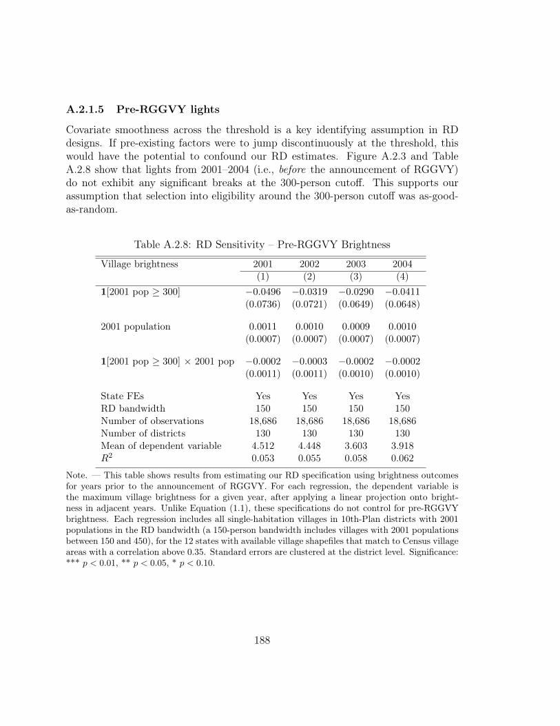
A.2.1.5 Pre-RGGVY lights

Covariate smoothness across the threshold is a key identifying assumption in RDdesigns. If pre-existing factors were to jump discontinuously at the threshold, thiswould have the potential to confound our RD estimates. Figure A.2.3 and TableA.2.8 show that lights from 2001–2004 (i.e., before the announcement of RGGVY)do not exhibit any significant breaks at the 300-person cutoff. This supports ourassumption that selection into eligibility around the 300-person cutoff was as-good-as-random.

Table A.2.8: RD Sensitivity – Pre-RGGVY Brightness

Village brightness 2001 2002 2003 2004(1) (2) (3) (4)

1[2001 pop ≥ 300] −0.0496 −0.0319 −0.0290 −0.0411(0.0736) (0.0721) (0.0649) (0.0648)

2001 population 0.0011 0.0010 0.0009 0.0010(0.0007) (0.0007) (0.0007) (0.0007)

1[2001 pop ≥ 300] × 2001 pop −0.0002 −0.0003 −0.0002 −0.0002(0.0011) (0.0011) (0.0010) (0.0010)

State FEs Yes Yes Yes YesRD bandwidth 150 150 150 150Number of observations 18,686 18,686 18,686 18,686Number of districts 130 130 130 130Mean of dependent variable 4.512 4.448 3.603 3.918R2 0.053 0.055 0.058 0.062

Note. — This table shows results from estimating our RD specification using brightness outcomesfor years prior to the announcement of RGGVY. For each regression, the dependent variable isthe maximum village brightness for a given year, after applying a linear projection onto bright-ness in adjacent years. Unlike Equation (1.1), these specifications do not control for pre-RGGVYbrightness. Each regression includes all single-habitation villages in 10th-Plan districts with 2001populations in the RD bandwidth (a 150-person bandwidth includes villages with 2001 populationsbetween 150 and 450), for the 12 states with available village shapefiles that match to Census villageareas with a correlation above 0.35. Standard errors are clustered at the district level. Significance:*** p < 0.01, ** p < 0.05, * p < 0.10.

188

Figure A.2.3: RD Sensitivity – Pre-RGGVY Brightness

−.15

−.1

−.05

0

.05

.1

.15

20

01

brig

htn

ess,

resid

ua

ls



−.15

−.1

−.05

0

.05

.1

.15

20

02

brig

htn

ess,

resid

ua

ls



−.15

−.1

−.05

0

.05

.1

.15

20

03

brig

htn

ess,

resid

ua

ls



−.15

−.1

−.05

0

.05

.1

.15

20

04

brig

htn

ess,

resid

ua

ls



Note. — These four figures estimate our preferred RD specification using nighttime brightnessfor 2001–2004, corresponding to the regressions in Table A.2.8. Each graph uses a different year’snighttime brightness as the dependent variable, after having linearly projected these values onadjacent years. Blue dots show average residuals from regressing that year’s nighttime brightnesson state fixed effects (without any other controls). Each dot contains approximately 1,600villages, averaged in 25-person population bins. Lines are estimated separately on each side ofthe 300-person threshold, for all 18,686 single-habitation villages between 150–450 people, in10th-Plan districts, for the 12 states with available village shapefiles that correspond to Censusvillage areas (with a correlation above 0.35).

189

A.2.1.6 Standard errors

Finally, our main specification clusters standard errors at the district level. Thisallows for arbitrary dependence in the error structure between any two villages inthe same district. Because RGGVY projects were approved based on district-specificimplementation plans (or DPRs), and funds were awarded to district implementingagencies, we allow for within-district dependence to control for any unobserved fac-tors affecting RGGVY implementation. Since districts are geographically contiguousarea, this also accounts for spatial correlations between nearby villages.

Table A.2.9 reports standard errors on our RD point estimate for alternative as-sumptions about the error structure. We see that clustering by census block yieldsslightly larger standard errors than clustering by district.54 We also calculate Conley“spatial HAC” standard errors, which are robust to spatial dependencies betweenvillages within a given geographic radius, as well as heteroscedasticity and autocor-relation.55 Table A.2.9 shows that spatial standard errors estimated with a 50-kmand 250-km bandwidth are smaller than our preferred standard error estimates.

Table A.2.9: RD Sensitivity – Alternative Standard Errors

Clusteredby Block

Clusteredby District

Spatial HAC(50 km)

Spatial HAC(250 km)

Standard Erroron RD coefficient (0.0680)∗∗ (0.0603)∗∗ (0.0602)∗∗ (0.0542)∗∗∗

Note. — This table shows robustness of our RD point estimate (β1 from Table 1.5.2) to alternativestandard error assumptions. Column (1) clusters standard errors by census block, which is theadministrative unit between district and village. Column (2) clusters by district, which is ourpreferred method. Columns (3)–(4) apply standard errors that are robust to heteroscedasticity andspatial correlation, with bandwidths of 50 and 250 km. Significance: *** p < 0.01, ** p < 0.05, *p < 0.10.

54Census block is the administrative unit that is smaller than district but larger than village.The only administrative unit larger than district is state. Because our nightlights regressions onlyinclude 12 states, we do not cluster at the state level for fear of bias resulting from having too fewclusters (Cameron and Miller (2015)).

55We use code from Fetzer (2014) to implement this Conley HAC procedure. This code can befound online: http://www.trfetzer.com/conley-spatial-hac-errors-with-fixed-effects/.It is in turn based on code from Hsiang (2010), itself based on theory from Conley (1999) and Conley(2008). Because our RD regression is cross-sectional and does not include multiple observations foreach village, the autocorrelation (“AC”) component of the spatial HAC estimator is not relevantfor our purposes. Our spatial standard errors apply a uniform kernel, which yields very similarestimates to those generated using a linear Bartlett kernel.

190

http://www.trfetzer.com/conley-spatial-hac-errors-with-fixed-effects/

A.2.2 Nighttime brightness: validity tests

In addition to the robustness checks above, we also conduct placebo, randomization,and falsification tests to corroborate our results for nighttime brightness. Section 1.5in the main text discuss our placebo test and randomization inference procedures,and Figure 1.5.5 reveals that our observed increase in nighttime brightness is veryunlikely to result from spurious correlations in the relationship between brightnessand village populations.

Section 1.5 describes an additional falsification exercise, where we demonstratethat nighttime brightness only increased for the subset of villages within 10th-Plan el-igible districts containing a single habitation. We find no increase in brightness at the300-person threshold for villages in 11th-Plan districts (for which the eligibility cutoffwas reduced from 300 to 100 people) or for villages with more than one habitation(for which the total village population does not correspond to the population usedto determine eligibility). Figure 1.5.6 graphically compares our main RD results tothree “falsification” samples: multi-habitation villages in 10th-Plan districts, single-habitation villages in 11th-Plan districts, and multi-habitation villages in 11th-Plandistricts. Table A.2.10 presents the same results in regression format. As expected,none of these alternative samples exhibits evidence of a positive discontinuity atthe 300-person cutoff. This provides further evidence that the RGGVY program iswhat is driving the increase in nighttime brightness for 10th-Plan, single-habitationvillages.

191

Table A.2.10: RD Sensitivity – Falsification Tests

2011 village brightness 10th-PlanSingle-Hab.

10th-PlanMulti-Hab.

11th-PlanSingle-Hab.

11th-PlanMulti-Hab.

(1) (2) (3) (4)1[2001 pop ≥ 300] 0.1493∗∗ −0.0326 −0.0109 −0.0781

(0.0603) (0.0751) (0.0595) (0.0986)

2001 population −0.0008 −0.0001 −0.0001 0.0007(0.0007) (0.0007) (0.0005) (0.0009)

1[2001 pop ≥ 300] × 2001 pop 0.0008 0.0011 0.0005 −0.0005(0.0008) (0.0008) (0.0008) (0.0008)

2001 Control Yes Yes Yes YesState FEs Yes Yes Yes YesRD bandwidth 150 150 150 150Number of observations 18,686 10,304 17,385 11,382Number of districts 130 116 174 149Mean of dependent variable 6.370 5.398 5.587 5.010R2 0.766 0.793 0.756 0.611

Note. — This table compares our main RD specification in Column (1) to three separate samplesfor which RGGVY’s 300-person eligibility threshold should not be relevant. Columns (2) and (4)estimate Equation (1.1) using villages with multiple habitations, for which the running variable(village population) does not correspond to the habitation populations that determined villageeligibility. Columns (3) and (4) estimate Equation (1.1) using villages that were eligibile for RGGVYunder the 11th Plan, which moved the eligibility cutoff from 300 to 100 people. Figure 1.5.6presents these three falsification tests graphically. Each regression includes all villages meetingthe above sample criteria with 2001 populations in the RD bandwidth (a 150-person bandwidthincludes villages with 2001 populations between 150 and 450), for the 12 states with available villageshapefiles that match to Census village areas with a correlation above 0.35. Standard errors areclustered at the district level. Significance: *** p < 0.01, ** p < 0.05, * p < 0.10.

A.2.3 Nighttime brightness: timing

As a final validity test, we look at changes in nighttime brightness over time. Sincewe are attributing the increase in nighttime brightness to RGGVY eligibility, year-on-year changes in differential brightness at the RD cutoff should be consistent withthe rollout of the RGGVY program. We should expect our RD estimates to increaseincrementally over time, for two reasons. First, RGGVY project funds under the10th Plan were disbursed gradually between 2005 and 2010. Because we estimate

192

the average effect on brightness across 128 eligible districts, our RD estimate shouldincrease in magnitude as more districts received RGGVY funding. (There is an addi-tional lag between the date that a district received RGGVY funding and the rolloutof project implementation across its constituent villages). Second, the effects of in-frastructure improvements on observed brightness are likely not immediate. For avillage that received transformer upgrades and additional household electric connec-tions in 2009, we might expect observed brightness to increase incrementally between2010–2011, as villages invest in appliances that use electricity and emit light.

We test for these gradual rollout and investment effects in Figure A.2.4 and TableA.2.11. As expected, we see that the RD point estimate increases monotonically from2006 to 2011. Hence, the RD effect that we detect from NOAA’s satellite imagesis consistent with the incremental rollout and takeup of electricity use due to theRGGVY program.

Table A.2.11: RD Sensitivity – Brightness by Year

Village brightness 2006 2007 2008 2009 2010 2011(1) (2) (3) (4) (5) (6)

1[2001 pop ≥ 300] 0.0377 0.0649∗∗ 0.0900∗∗ 0.0999∗∗ 0.1175∗ 0.1493∗∗

(0.0251) (0.0321) (0.0352) (0.0427) (0.0632) (0.0603)

2001 population −0.0000 −0.0001 −0.0003 −0.0004 −0.0005 −0.0008(0.0002) (0.0003) (0.0003) (0.0005) (0.0008) (0.0007)

1[2001 pop ≥ 300] × 2001 pop −0.0000 −0.0002 0.0002 0.0004 0.0007 0.0008(0.0003) (0.0003) (0.0004) (0.0006) (0.0009) (0.0008)


Note. — This table shows results from estimating Equation (1.1), using brightness outcomes fromvarying years. For each regression, the dependent variable is the maximum village brightness fora given year, after applying a linear projection onto brightness in adjacent years. Each regressionincludes all single-habitation villages in 10th-Plan districts with 2001 populations in the RD band-width (a 150-person bandwidth includes villages with 2001 populations between 150 and 450), forthe 12 states with available village shapefiles that match to Census village areas with a correlationabove 0.35. Standard errors are clustered at the district level. Significance: *** p < 0.01, **p < 0.05, * p < 0.10.

193

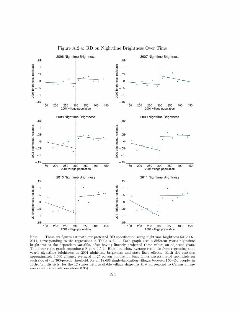
Figure A.2.4: RD on Nighttime Brightness Over Time

−.15

−.1

−.05

0

.05

.1

.15

20

06

brig

htn

ess,

resid

ua

ls



−.15

−.1

−.05

0

.05

.1

.15

20

07

brig

htn

ess,

resid

ua

ls



−.15

−.1

−.05

0

.05

.1

.15

20

08

brig

htn

ess,

resid

ua

ls



−.15

−.1

−.05

0

.05

.1

.15

20

09

brig

htn

ess,

resid

ua

ls



−.15

−.1

−.05

0

.05

.1

.15

20

10

brig

htn

ess,

resid

ua

ls



−.15

−.1

−.05

0

.05

.1

.15

20

11

brig

htn

ess,

resid

ua

ls



Note. — These six figures estimate our preferred RD specification using nighttime brightness for 2006–2011, corresponding to the regressions in Table A.2.11. Each graph uses a different year’s nighttimebrightness as the dependent variable, after having linearly projected these values on adjacent years.The lower-right graph reproduces Figure 1.5.4. Blue dots show average residuals from regressing thatyear’s nighttime brightness on 2001 nighttime brightness and state fixed effects. Each dot containsapproximately 1,600 villages, averaged in 25-person population bins. Lines are estimated separately oneach side of the 300-person threshold, for all 18,686 single-habitation villages between 150–450 people, in10th-Plan districts, for the 12 states with available village shapefiles that correspond to Census villageareas (with a correlation above 0.35).

194

A.2.4 Census outcome results: RD robustness

Next, we run a series of analogous RD robustness tests for the range of Censusoutcomes results that we report in the main text.

A.2.4.1 Sample and outcome variables

We normalize our main village-level results in Table 1.5.3 by either village population(by gender) or by the share of village households. This is because our RD specifica-tion is cross-sectional, and most village-level outcomes will vary mechanically withthe running variable (e.g., number of 2011 female agricultural workers will increasemechanically in 2001 village population). However, this normalization relies on theassumption that village-level demographics were unaffected by RGGVY program el-igibility. Figure A.2.5 shows RD plots for 2011 village population and the size ofthe 0–6 age cohort, as reported in Panel A of Table 1.5.3. We see no evidence thatRGGVY eligibility changed either the total village population or the fertility rate.

As an additional sensitivity, Table A.2.12 reproduces our main RD results fromTable 1.5.3, including villages with population disparities in the habitation census ofover 20 percent. After adding nearly 3,962 villages that were potentially miscatego-rized as having a single habitation, our RD estimates are nearly identical, althoughslightly more precise due to a greater sample size. In contrast, including villages withpopulation disparities attenuates our nighttime brightness results (see Table A.2.3).As we see no corresponding attenuation in Table A.2.12, this underscores the lackof evidence of any economically meaningful impacts of RGGVY electrification forvillages close to the cutoff.

195

Table A.2.12: RD Sensitivity – Census Outcomes, No Forced Population Match


StandardError


Mean ofOutcome


B. Labor outcomesMale agricultural workers / male pop −0.0069∗∗∗ (0.002) [−0.012,−0.002] 0.42Female agricultural workers / female pop −0.0055 (0.004) [−0.013, 0.002] 0.29Male household workers / male pop −0.0008 (0.001) [−0.002, 0.000] 0.01Female household workers / female pop −0.0015 (0.001) [−0.003, 0.001] 0.01Male other workers / male pop 0.0035∗ (0.002) [−0.000, 0.007] 0.10Female other workers / female pop −0.0016 (0.002) [−0.005, 0.002] 0.05

C. Asset ownershipShare of households with telephone 0.0025 (0.005) [−0.007, 0.012] 0.53Share of households with TV 0.0015 (0.004) [−0.006, 0.009] 0.25Share of households with bicycle 0.0007 (0.004) [−0.007, 0.008] 0.49Share of households with motorcycle −0.0008 (0.003) [−0.006, 0.004] 0.13Share of households without assets 0.0016 (0.004) [−0.006, 0.009] 0.23


E. Village-wide outcomes1/0 Mobile phone coverage in village 0.0051 (0.010) [−0.015, 0.025] 0.741/0 Post office in village 0.0017 (0.003) [−0.005, 0.008] 0.031/0 Ag credit societies in village 0.0005 (0.003) [−0.006, 0.007] 0.021/0 Water from tubewell in village −0.0033 (0.011) [−0.024, 0.017] 0.45Share of village area irrigated −0.0075∗ (0.005) [−0.016, 0.001] 0.35Share of village area planted 0.0018 (0.006) [−0.009, 0.013] 0.58

Note. — This table includes the identical set of regressions in Table 1.5.3, including villages with largepopulation disparaties with the Habitation Census (i.e., villages whose matched habitation populationsdisagree with official Census populations by over 20 percent). The RD bandwidth now includes 33,727villages with 2001 populations between 150 and 450, across 225 districts. The second column shows theRD point estimate (β1) for each regression. All specifications control for the 2001 level of the outcomevariable, except for share of village area planted (where 2001 values are not available) and 1/0 indicatorvariables. All specifications also include state fixed effects. Standard errors are clustered at the districtlevel, which we use to calculate 95 percent confidence intervals in the fourth column. The fifth columnreports the mean of the dependent variable for each RD regression. Significance: *** p < 0.01, **p < 0.05, * p < 0.10.

196

Figure A.2.5: RD Reduced Form – 2011 Village Population

−200

−100

0

100

200

20

11

Po

pu

latio

n,

resid

ua

ls


2011 Population

−.01

−.005

0

.005

.01

Sh

are

of

Po

p.

Ag

es 0

−6

, re

sid

ua

ls


Population Cohort 0−6 Years Old

Note. — This figure presents results for RD regressions of 2011 village population (left) and theshare of the 2011 population less than 7 years old (right). These correspond to the first two rowsof Table 1.5.3. Blue dots show average residuals from regressing the 2011 outcome on and statefixed effects and the 2001 level of the outcome (except for the left panel, where 2001 populationis the running variable and hence not an additional control). Each dot contains approximately1,500 villages, averaged in 15-person population bins. Lines are estimated separately on eachside of the 300-person threshold, for all 29,765 single-habitation villages between 150 and 450people, in 10th-Plan districts.

A.2.4.2 Bandwidths

Section A.2.1.2 discusses our choice of a 150-person RD bandwidth around RGGVY’s300-person 10th-Plan cutoff, which avoids overlapping with the 100-person 11th-Plancutoff and the 500-person PMGSY eligibility cutoff. However, we also demonstratethat our RD results for nighttime brightness are not sensitive to our choice of band-width (see Figure A.2.1). We present analogous bandwidth sensitivities in FigureA.2.6, for eight census outcomes reported in Table 1.5.3. This demonstrates that ourRD results for these Census outcomes (male and female labor shares; mud floors;asset ownership; share of village area planted and irrigated) are not overly sensitiveto our choice of bandwidth, for bandwidths between 100 and 250 (above which in-cludes very small villages). Figure A.2.6 shows the range of feasible symmetric RDbandwidths, which stops at 300 due to our 300-person RD threshold. The optimalbandwidth calculations (following Imbens and Kalyanaraman (2012)) vary acrosseach outcome, ranging from 130 to 353.

197

A.2.4.3 Functional form

Section A.2.1.3 discusses our choice to exclude higher-order polynomials from ourpreferred RD specification (following Gelman and Imbens (2014)). Table A.2.13tests for sensitivity of our RD regressions on village-level census outcomes to theinclusion of a quadratic function of the running variable. This yields point estimatesand confidence intervals that are very close to the linear RD specification in Table1.5.3. Figure A.2.7 presents a subset of these results graphically, where the shareof male agricultural workers remains the census outcome that is most obviouslydiscontinuous at the 300-person threshold.

Table A.2.14 re-estimates Equation (1.1) using weighted least squares, weightingobservations by their distance from the RD threshold. We define village weights aswv ≡ 1 − |Pv−300|

150, where Pv is the 2001 village population. These results confirm

that upweighting villages close to the RD threshold does not significantly change ourresults.

198

Figure A.2.6: RD Sensitivity – Census Outcomes, Bandwidths

−.02

−.01

0

.01

RD

co

eff

icie

nt

(95

% C

I)

50 100 150 200 250 300RD bandwidth

Male other workers Male ag workers

Bandwidth Sensitivities, Male Workers

−.03

−.02

−.01

0

.01

RD

co

eff

icie

nt

(95

% C

I)

50 100 150 200 250 300RD bandwidth

Female other workers Female ag workers

Bandwidth Sensitivities, Female Workers

−.01

0

.01

.02

.03

RD

co

eff

icie

nt

(95

% C

I)

50 100 150 200 250 300RD bandwidth

Mud floors No household assets

Bandwidth Sensitivities, Household Assets

−.02

−.01

0

.01

.02

RD

co

eff

icie

nt

(95

% C

I)

50 100 150 200 250 300RD bandwidth

Village area planted VIllage area irrigated

Bandwidth Sensitivities, Area Planted & Irrigated

Note. — This figure presents our bandwidth sensitivity analysis for eight separate outcomes inTable 1.5.3. For each outcome, we estimate Equation (1.1) separately on bandwidths rangingfrom 50 (i.e., 250–350 people) to 300 (i.e., 0–600 people). Each dot represents the point estimateon the RD discontinuity at a given bandwidth around the 300-person cutoff, with 95 percentconfidence intervals clustered at the district level. Our chosen bandwidth of 150 includes villageswith populations between 150 and 450. The optimal RD bandwidth varies for each outcome,ranging from 130 to 354 for the eight outcomes shown here (calculated using the algorithmproposed by Imbens and Kalyanaraman (2012), using uniform, Epanechnikov, and triangularkernels).

199

Table A.2.13: RD Sensitivity – Census Outcomes, Quadratic in Population


StandardError


Mean ofOutcome





E. Village-wide outcomes1/0 Mobile phone coverage in village −0.0002 (0.011) [−0.022, 0.022] 0.751/0 Post office in village 0.0015 (0.004) [−0.006, 0.009] 0.031/0 Ag credit societies in village 0.0015 (0.004) [−0.006, 0.009] 0.021/0 Water from tubewell in village −0.0025 (0.011) [−0.024, 0.019] 0.44Share of village area irrigated −0.0056 (0.005) [−0.015, 0.004] 0.34Share of village area planted 0.0019 (0.006) [−0.009, 0.013] 0.58

Note. — This table includes the identical set of regressions in Table 1.5.3, except controlling for aquadratic function of 2001 village population. The RD bandwidth includes 29,765 villages with 2001populations between 150 and 450, across 225 districts. The second column shows the RD point estimate(β1) for each regression. All specifications control for a 2nd-order polynomial in the running variable andstate fixed effects. All specifications also control for the 2001 level of the outcome variable, except forshare of village area planted (where 2001 values are not available) and 1/0 indicator variables. Standarderrors are clustered at the district level, which we use to calculate 95 percent confidence intervals in thefourth column. The fifth column reports the mean of the dependent variable for each RD regression.Significance: *** p < 0.01, ** p < 0.05, * p < 0.10.

200

Figure A.2.7: RD Sensitivity – Census Outcomes, Second-Order Polynomials

−.01

−.005

0

.005

.01

Share

of M

ale

Pop

ula

tion,

resid

uals


Male Agricultural Workers (Quadratic)

−.01

−.005

0

.005

.01

Share

of M

ale

Pop

ula

tion,

resid

uals


Male Household Workers (Quadratic)

−.01

−.005

0

.005

.01

Share

of M

ale

Pop

ula

tion,

resid

uals


Male Other Workers (Quadratic)

−.01

−.005

0

.005

.01

Sha

re o

f F

em

ale

Po

pu

latio

n, re

sid

ua

ls


Female Agricultural Workers (Quadratic)

−.01

−.005

0

.005

.01

Sha

re o

f F

em

ale

Po

pu

latio

n, re

sid

ua

ls


Female Household Workers (Quadratic)

−.01

−.005

0

.005

.01

Sha

re o

f F

em

ale

Po

pu

latio

n, re

sid

ua

ls


Female Other Workers (Quadratic)

−.02

−.01

0

.01

.02

Sha

re o

f H

ou

se

hold

s, re

sid

ua

ls


Telephone Ownership (Quadratic)

−.02

−.01

0

.01

.02

Sha

re o

f H

ou

se

hold

s, re

sid

ua

ls


TV Ownership (Quadratic)

−.02

−.01

0

.01

.02

Sha

re o

f H

ou

se

hold

s, re

sid

ua

ls


Motorcycle Ownership (Quadratic)

−.02

−.01

0

.01

.02

Sha

re o

f H

ou

se

hold

s,

resid

ua

ls


Kerosene Lighting (Quadratic)

−.02

−.01

0

.01

.02

Sha

re o

f H

ou

se

hold

s,

resid

ua

ls


Mud Floors (Quadratic)

−.02

−.01

0

.01

.02

Sha

re o

f H

ou

se

hold

s,

resid

ua

ls


Dilapidated Households (Quadratic)

Note. — This figure shows reduced form results estimating Equation (1.1) including a second-order polynomial in population, as reported in Table A.2.13. Blue dots show average residualsform regressing the 2011 outcomes on the 2001 control and state fixed effects. Each dot containsapproximately 1,500 villages, averaged in 15-person population bins, including all 29,765 single-habitation villages between 150 and 450 people, in 10th-Plan districts.

201

Table A.2.14: RD Sensitivity – Census Outcomes, Weighting Inverse Distancefrom Cutoff


StandardError


Mean ofOutcome


B. Labor outcomesMale agricultural workers / male pop −0.0075∗∗∗ (0.003) [−0.013,−0.002] 0.43Female agricultural workers / female pop −0.0063 (0.004) [−0.015, 0.002] 0.28Male household workers / male pop −0.0008 (0.001) [−0.002, 0.000] 0.01Female household workers / female pop −0.0010 (0.001) [−0.003, 0.001] 0.01Male other workers / male pop 0.0044∗∗ (0.002) [0.000, 0.009] 0.10Female other workers / female pop 0.0010 (0.002) [−0.003, 0.005] 0.05

C. Asset ownershipShare of households with telephone 0.0037 (0.006) [−0.008, 0.016] 0.54Share of households with TV 0.0050 (0.004) [−0.003, 0.013] 0.25Share of households with bicycle 0.0007 (0.004) [−0.008, 0.009] 0.51Share of households with motorcycle 0.0016 (0.003) [−0.004, 0.007] 0.13Share of households without assets 0.0030 (0.004) [−0.005, 0.011] 0.22


E. Village-wide outcomes1/0 Mobile phone coverage in village 0.0088 (0.013) [−0.017, 0.035] 0.751/0 Post office in village 0.0056 (0.004) [−0.002, 0.013] 0.031/0 Ag credit societies in village 0.0053 (0.004) [−0.002, 0.013] 0.021/0 Water from tubewell in village 0.0040 (0.012) [−0.019, 0.028] 0.46Share of village area irrigated −0.0063 (0.006) [−0.018, 0.005] 0.36Share of village area planted 0.0034 (0.006) [−0.008, 0.015] 0.59

Note. — This table includes the same regressions as in Table 1.5.3, but running weighted least squares.We weight villages by their absolute distance from the 300-person cutoff, such that a wv ≡ 1− |Pv−300|

150.

The RD bandwidth includes 29,573 villages with 2001 populations between 150 and 450, across 225districts. The second column shows the RD point estimate (β1) for each regression. All specificationscontrol for the 2001 level of the outcome variable, except for share of village area planted (where 2001values are not available) and 1/0 indicator variables. All specifications also include state fixed effects.Standard errors are clustered at the district level, which we use to calculate 95 percent confidenceintervals in the fourth column. The fifth column reports the mean of the dependent variable for eachRD regression. Significance: *** p < 0.01, ** p < 0.05, * p < 0.10.

202

A.2.4.4 Fixed effects and controls

As mentioned above, while RD designs do not require fixed effects or controls foridentification, they can greatly improve precision of RD point estimates. SectionA.2.1.4 demonstrates that the RD results for nighttime brightness are robust todifferent fixed effects specifications, and our results for census outcomes are also notsensitive to cross-sectional fixed effects. Table A.2.15 and Figure A.2.8 present RDresults estimating Equation (1.1) without fixed effects, while Table A.2.16 and FigureA.2.9 include more granular fixed effects at the district level. These results are quitesimilar to our preferred specification (with state fixed effects), with slight differencesin precision.

Section A.2.1.4 also shows that our RD results for nighttime brightness depend onthe inclusion of 2001 brightness as a village-level control. This reveals that there isenough cross-sectional variation in brightness levels (even within districts) to obscurewithin-village changes in brightness due to RGGVY electrification. In contrast, TableA.2.17 and Figure A.2.10 show that our RD results for census outcomes are muchless sensitive to the exclusion of 2001 controls. The decrease in male agriculturalemployment at the 300-person cutoff remains small but precisely estimated, and theconfidence intervals on other labor outcomes in Panel B are very similar to those inTable 1.5.3.

Comparing Tables 1.5.3 and A.2.17 highlights two key features of our censusoutcome data. First, Panels C and D report on outcomes from the HouselistingPrimary Census Abstract (HPCA), which is not available at the village level for2001 (see Section A.1.4.2). This means that for Table 1.5.3 regressions in PanelsC and D, 2001 controls are at the block level.56 Because these regressions cannotcontrol for within-block baseline heterogeneity, it is unsurprising that removing these2001 block-level controls does not affect their precision.

Second, our regressions in Panel E of Table 3 already do not include 2001 con-trols for 1/0 indicator variables. Since these outcomes are not continuous, includingbaseline controls would not greatly increase the precision of our RD point estimates.Moreover, including 2001 controls for 1/0 indicator variables would effectively removeobservations for villages that did not change status (i.e. from 0 to 1) between 2001and 2011. This illustrates why we strongly prefer nighttime brightness as a measureof electricity access: nighttime brightness is a more continuous measure of electricityaccess (a 0–63 scale, compared to a binary indicator); nighttime brightness measuresluminosity, a better proxy for electricity consumption than binary indicators of elec-tricity access (the latter does not account for variation in reliability or usage); the

56The only exception is share of households dilapidated, which was only available in 2001 at thedistrict level.

203

majority of RGGVY villages were targeted for “more intensive electrification”, whilealready meeting the government’s official definition of being “electrified” (we wouldnot expect binary indicators to reflect more intensive electrification); and the officialdefinition of “electrified” changed in 2004, meaning that 2001 and 2011 VD variablesmight not be apples-to-apples comparisons (see Section A.3 for further detail). TableA.2.17 reports RD results for end-use-specific 1/0 electric power indicators, and wesee the RGGVY led to statistically significant increases in electricity access for thecommercial sector. We do not see corresponding increases for electricity access inthe domestic or agricultural sectors, which reflects the fact that most treated vil-lages already had low levels of electrification prior to RGGVY — meaning that the1/0 indicators were coded as 1 in the baseline, and RGGVY did not cause them toincrease.

A.2.4.5 2001 covariate smoothness

A key RD identifying assumption is smoothness of covariates across the RD cutoff.Section A.2.1.5 demonstrates that nighttime brightness is not discontinuous at the300-person threshold prior to the 2005 announcement of RGGVY. Table A.2.18 showsthat 2001 village-level covariates are also smooth across the 300-person cutoff in 2001population. This includes all 2001 covariates corresponding to 2011 census outcomesreported in Table 1.5.3, which are available in 2001 at the village level. Figure A.2.11presents a subset of these results graphically.

204

Table A.2.15: RD Sensitivity – Census Outcomes, No Fixed Effects


StandardError


Mean ofOutcome



C. Asset ownershipShare of households with telephone 0.0026 (0.006) [−0.009, 0.015] 0.54Share of households with TV 0.0039 (0.004) [−0.004, 0.012] 0.26Share of households with bicycle −0.0007 (0.004) [−0.009, 0.008] 0.50Share of households with motorcycle 0.0001 (0.003) [−0.005, 0.005] 0.13Share of households without assets 0.0034 (0.004) [−0.005, 0.011] 0.22


E. Village-wide outcomes1/0 Mobile phone coverage in village −0.0035 (0.012) [−0.027, 0.020] 0.751/0 Post office in village 0.0020 (0.004) [−0.005, 0.009] 0.031/0 Ag credit societies in village 0.0010 (0.004) [−0.006, 0.008] 0.021/0 Water from tubewell in village 0.0006 (0.011) [−0.022, 0.023] 0.44Share of village area irrigated −0.0068 (0.006) [−0.019, 0.005] 0.34Share of village area planted 0.0059 (0.006) [−0.006, 0.018] 0.58

Note. — This table includes the identical set of regressions in Table 1.5.3, without controlling forstate fixed effects. The RD bandwidth includes 29,765 villages with 2001 populations between150 and 450, across 225 districts. The second column shows the RD point estimate (β1) foreach regression. All specifications control for the 2001 level of the outcome variable, except forshare of village area planted (where 2001 values are not available) and 1/0 indicator variables.Standard errors are clustered at the district level, which we use to calculate 95 percent confidenceintervals in the fourth column. The fifth column reports the mean of the dependent variable foreach RD regression. Significance: *** p < 0.01, ** p < 0.05, * p < 0.10.

205

Figure A.2.8: RD Sensitivity – Census Outcomes, No Fixed Effects

−.01

−.005

0

.005

.01

Share

of M

ale

Pop

ula

tion,

resid

uals


Male Agricultural Workers (No FEs)

−.01

−.005

0

.005

.01

Share

of M

ale

Pop

ula

tion,

resid

uals


Male Household Workers (No FEs)

−.01

−.005

0

.005

.01

Share

of M

ale

Pop

ula

tion,

resid

uals


Male Other Workers (No FEs)

−.02

−.01

0

.01

.02

Sha

re o

f F

em

ale

Po

pu

latio

n, re

sid

ua

ls


Female Agricultural Workers (No FEs)

−.01

−.005

0

.005

.01

Sha

re o

f F

em

ale

Po

pu

latio

n, re

sid

ua

ls


Female Household Workers (No FEs)

−.01

−.005

0

.005

.01

Sha

re o

f F

em

ale

Po

pu

latio

n, re

sid

ua

ls


Female Other Workers (No FEs)

−.02

−.01

0

.01

.02

Sha

re o

f H

ou

se

hold

s, re

sid

ua

ls


Telephone Ownership (No FEs)

−.02

−.01

0

.01

.02

Sha

re o

f H

ou

se

hold

s, re

sid

ua

ls


TV Ownership (No FEs)

−.02

−.01

0

.01

.02

Sha

re o

f H

ou

se

hold

s, re

sid

ua

ls


Motorcycle Ownership (No FEs)

−.04

−.02

0

.02

.04

Sha

re o

f H

ou

se

hold

s,

resid

ua

ls


Kerosene Lighting (No FEs)

−.02

−.01

0

.01

.02

Sha

re o

f H

ou

se

hold

s,

resid

ua

ls


Mud Floors (No FEs)

−.02

−.01

0

.01

.02

Sha

re o

f H

ou

se

hold

s,

resid

ua

ls


Dilapidated Households (No FEs)

Note. — This figure shows reduced form results estimating Equation (1.1) without fixed effects, asreported in Table A.2.15. Blue dots show average residuals form regressing the 2011 outcomes onthe 2001 control. Each dot contains approximately 1,500 villages, averaged in 15-person populationbins, including all 29,765 single-habitation villages between 150 and 450 people, in 10th-Plandistricts.

206

Table A.2.16: RD Sensitivity – Census Outcomes, District Fixed Effects


StandardError


Mean ofOutcome



C. Asset ownershipShare of households with telephone −0.0003 (0.005) [−0.011, 0.010] 0.54Share of households with TV 0.0014 (0.004) [−0.006, 0.009] 0.26Share of households with bicycle −0.0016 (0.004) [−0.010, 0.006] 0.50Share of households with motorcycle −0.0012 (0.002) [−0.006, 0.004] 0.13Share of households without assets 0.0041 (0.004) [−0.004, 0.012] 0.22

D. Housing stockShare of households with elec/gas cooking −0.0005 (0.003) [−0.006, 0.005] 0.07Share of households with kerosene lighting 0.0018 (0.006) [−0.010, 0.014] 0.48Share of households with mud floors 0.0038 (0.004) [−0.003, 0.011] 0.73Share of households with thatched roof −0.0018 (0.005) [−0.011, 0.008] 0.23Share of households dilapidated −0.0033 (0.003) [−0.009, 0.002] 0.07

E. Village-wide outcomes1/0 Mobile phone coverage in village 0.0022 (0.011) [−0.019, 0.024] 0.751/0 Post office in village 0.0010 (0.004) [−0.006, 0.008] 0.031/0 Ag credit societies in village 0.0013 (0.004) [−0.006, 0.008] 0.021/0 Water from tubewell in village −0.0013 (0.010) [−0.021, 0.018] 0.44Share of village area irrigated −0.0059 (0.005) [−0.015, 0.004] 0.34Share of village area planted 0.0016 (0.005) [−0.007, 0.011] 0.58

Note. — This table includes the identical set of regressions in Table 1.5.3, except controlling for districtfixed effects (instead of state fixed effects). The RD bandwidth includes 29,765 villages with 2001populations between 150 and 450, across 225 districts. The second column shows the RD point estimate(β1) for each regression. All specifications control for the 2001 level of the outcome variable, except forshare of village area planted (where 2001 values are not available) and 1/0 indicator variables. Standarderrors are clustered at the district level, which we use to calculate 95 percent confidence intervals in thefourth column. The fifth column reports the mean of the dependent variable for each RD regression.Significance: *** p < 0.01, ** p < 0.05, * p < 0.10.

207

Figure A.2.9: RD Sensitivity – Census Outcomes, District Fixed Effects

−.01

−.005

0

.005

.01

Share

of M

ale

Pop

ula

tion,

resid

uals


Male Agricultural Workers (District FEs)

−.01

−.005

0

.005

.01

Share

of M

ale

Pop

ula

tion,

resid

uals


Male Household Workers (District FEs)

−.01

−.005

0

.005

.01

Share

of M

ale

Pop

ula

tion,

resid

uals


Male Other Workers (District FEs)

−.01

−.005

0

.005

.01

Sha

re o

f F

em

ale

Po

pu

latio

n, re

sid

ua

ls


Female Agricultural Workers (District FEs)

−.01

−.005

0

.005

.01

Sha

re o

f F

em

ale

Po

pu

latio

n, re

sid

ua

ls


Female Household Workers (District FEs)

−.01

−.005

0

.005

.01

Sha

re o

f F

em

ale

Po

pu

latio

n, re

sid

ua

ls


Female Other Workers (District FEs)

−.02

−.01

0

.01

.02

Sha

re o

f H

ou

se

hold

s, re

sid

ua

ls


Telephone Ownership (District FEs)

−.02

−.01

0

.01

.02

Sha

re o

f H

ou

se

hold

s, re

sid

ua

ls


TV Ownership (District FEs)

−.02

−.01

0

.01

.02

Sha

re o

f H

ou

se

hold

s, re

sid

ua

ls


Motorcycle Ownership (District FEs)

−.02

−.01

0

.01

.02

Sha

re o

f H

ou

se

hold

s,

resid

ua

ls


Kerosene Lighting (District FEs)

−.02

−.01

0

.01

.02

Sha

re o

f H

ou

se

hold

s,

resid

ua

ls


Mud Floors (District FEs)

−.02

−.01

0

.01

.02

Sha

re o

f H

ou

se

hold

s,

resid

ua

ls


Dilapidated Households (District FEs)

Note. — This figure shows reduced form results estimating Equation (1.1) including districtfixed effects, as reported in Table A.2.16. Blue dots show average residuals form regressing the2011 outcomes on the 2001 control and district fixed effects. Each dot contains approximately1,500 villages, averaged in 15-person population bins, including all 29,765 single-habitation villagesbetween 150 and 450 people, in 10th-Plan districts.

208

Table A.2.17: RD Sensitivity – Census Outcomes, No 2001 Controls


StandardError


Mean ofOutcome

A. Demographic outcomesTotal population −0.8647 (2.528) [−5.820, 4.091] 271.090–6 cohort / total population 0.0007 (0.001) [−0.001, 0.002] 0.14Average household size 0.0022 (0.014) [−0.026, 0.031] 5.13Literacy rate −0.0016 (0.003) [−0.007, 0.004] 0.57

B. Labor outcomesMale agricultural workers / male pop −0.0084∗∗∗ (0.003) [−0.014,−0.003] 0.42Female agricultural workers / female pop −0.0055 (0.004) [−0.013, 0.003] 0.29Male household workers / male pop −0.0007 (0.001) [−0.002, 0.001] 0.01Female household workers / female pop −0.0018 (0.001) [−0.004, 0.000] 0.01Male other workers / male pop 0.0047∗∗ (0.002) [0.000, 0.009] 0.10Female other workers / female pop −0.0005 (0.002) [−0.004, 0.003] 0.05


D. Housing stockShare of households with elec/gas cooking −0.0006 (0.003) [−0.006, 0.005] 0.07Share of households with kerosene lighting 0.0031 (0.006) [−0.009, 0.015] 0.48Share of households with mud floors 0.0075 (0.005) [−0.003, 0.018] 0.73Share of households with thatched roof −0.0022 (0.006) [−0.013, 0.009] 0.23Share of households dilapidated −0.0028 (0.003) [−0.009, 0.003] 0.07

E. Village-wide outcomes1/0 Electricity (domestic use) −0.0086 (0.006) [−0.021, 0.004] 0.901/0 Electricity (agricultural use) −0.0098 (0.010) [−0.030, 0.010] 0.611/0 Electricity (commercial use) 0.0243∗∗ (0.011) [0.003, 0.046] 0.441/0 Electricity (all end uses) 0.0240∗∗ (0.011) [0.002, 0.046] 0.43Share of village area irrigated −0.0021 (0.006) [−0.013, 0.009] 0.35

Note. — Panels A–D of this table included the same sets of regressions in Table 1.5.3. Panel E includessector-specific 1/0 indicator variables for electricity availability at the village level, while omiting 4regressions from Table 1.5.3 that already did not include 2001 controls. All RD regressions in this tablecontrol only for state fixed effects, not for the 2001 level of the outcome variable. The RD bandwidthincludes 29,765 villages with 2001 populations between 150 and 450, across 225 districts. The secondcolumn shows the RD point estimate (β1) for each regression. Standard errors are clustered at thedistrict level, which we use to calculate 95 percent confidence intervals in the fourth column. The fifthcolumn reports the mean of the dependent variable for each RD regression. Significance: *** p < 0.01,** p < 0.05, * p < 0.10.

209

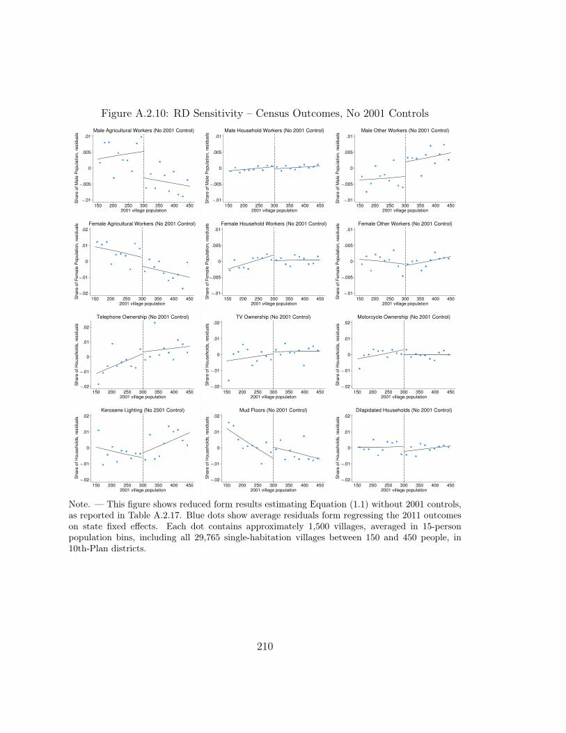
Figure A.2.10: RD Sensitivity – Census Outcomes, No 2001 Controls

−.01

−.005

0

.005

.01

Share

of M

ale

Pop

ula

tion,

resid

uals


Male Agricultural Workers (No 2001 Control)

−.01

−.005

0

.005

.01

Share

of M

ale

Pop

ula

tion,

resid

uals


Male Household Workers (No 2001 Control)

−.01

−.005

0

.005

.01

Share

of M

ale

Pop

ula

tion,

resid

uals


Male Other Workers (No 2001 Control)

−.02

−.01

0

.01

.02

Sha

re o

f F

em

ale

Po

pu

latio

n, re

sid

ua

ls


Female Agricultural Workers (No 2001 Control)

−.01

−.005

0

.005

.01

Sha

re o

f F

em

ale

Po

pu

latio

n, re

sid

ua

ls


Female Household Workers (No 2001 Control)

−.01

−.005

0

.005

.01

Sha

re o

f F

em

ale

Po

pu

latio

n, re

sid

ua

ls


Female Other Workers (No 2001 Control)

−.02

−.01

0

.01

.02

Sha

re o

f H

ou

se

hold

s, re

sid

ua

ls


Telephone Ownership (No 2001 Control)

−.02

−.01

0

.01

.02

Sha

re o

f H

ou

se

hold

s, re

sid

ua

ls


TV Ownership (No 2001 Control)

−.02

−.01

0

.01

.02

Sha

re o

f H

ou

se

hold

s, re

sid

ua

ls


Motorcycle Ownership (No 2001 Control)

−.02

−.01

0

.01

.02

Sha

re o

f H

ou

se

hold

s,

resid

ua

ls


Kerosene Lighting (No 2001 Control)

−.02

−.01

0

.01

.02

Sha

re o

f H

ou

se

hold

s,

resid

ua

ls


Mud Floors (No 2001 Control)

−.02

−.01

0

.01

.02

Sha

re o

f H

ou

se

hold

s,

resid

ua

ls


Dilapidated Households (No 2001 Control)

Note. — This figure shows reduced form results estimating Equation (1.1) without 2001 controls,as reported in Table A.2.17. Blue dots show average residuals form regressing the 2011 outcomeson state fixed effects. Each dot contains approximately 1,500 villages, averaged in 15-personpopulation bins, including all 29,765 single-habitation villages between 150 and 450 people, in10th-Plan districts.

210

Table A.2.18: RD Sensitivity – Census Outcomes, 2001 Covariate Smoothness


StandardError


Mean ofOutcome

A. Demographic indicators0–6 cohort / total population −0.0009 (0.001) [−0.003, 0.001] 0.18Share or population SC or ST −0.0080 (0.007) [−0.021, 0.005] 0.33Literacy rate 0.0015 (0.003) [−0.005, 0.008] 0.45

B. Labor indicatorsMale agricultural workers / male pop −0.0027 (0.003) [−0.008, 0.003] 0.43Female agricultural workers / female pop −0.0017 (0.005) [−0.011, 0.007] 0.31Male household workers / male pop 0.0010 (0.001) [−0.000, 0.002] 0.01Female household workers / female pop −0.0014 (0.001) [−0.004, 0.001] 0.01Male other workers / male pop 0.0001 (0.002) [−0.004, 0.004] 0.09Female other workers / female pop −0.0007 (0.002) [−0.004, 0.003] 0.03Male main workers / male pop −0.0017 (0.004) [−0.009, 0.005] 0.43Female main workers / female pop −0.0047 (0.004) [−0.013, 0.004] 0.17Male marginal workers / male pop 0.0002 (0.003) [−0.005, 0.006] 0.09Female marginal workers / female pop 0.0008 (0.004) [−0.007, 0.009] 0.18

C. Village-wide indicators1/0 Electricity (all end uses) 0.0038 (0.007) [−0.009, 0.017] 0.291/0 Electricity (domestic use) 0.0018 (0.010) [−0.018, 0.021] 0.591/0 Electricity (agricultural use) −0.0014 (0.009) [−0.020, 0.017] 0.411/0 Water from tubewell in village −0.0188∗ (0.010) [−0.039, 0.001] 0.51Share of village area irrigated 0.0079 (0.007) [−0.006, 0.022] 0.331/0 Educational facilities −0.0081 (0.010) [−0.028, 0.012] 0.50Number of primary schools −0.0093 (0.012) [−0.032, 0.014] 0.49Number of secondary schools 0.0039 (0.003) [−0.001, 0.009] 0.011/0 Medical facilities 0.0036 (0.007) [−0.010, 0.018] 0.101/0 Banking facilities 0.0012 (0.002) [−0.003, 0.006] 0.011/0 Agricultural credit societies 0.0002 (0.004) [−0.008, 0.009] 0.021/0 Post office 0.0006 (0.004) [−0.007, 0.008] 0.031/0 Bus service 0.0058 (0.014) [−0.022, 0.033] 0.41

Note. — This table regresses 2001 village covariates on the RD variables in Equation 1.1 and statefixed effects. Each row represents a separate regression, with the second column reporting the RDpoint estimate (β1). This table includes all available 2001 village-level covariates that correspond to a2011 outcome reported in Table 1.5.3. SC and ST refer to official scheduled caste and scheduled tribedesignations. “Main” workers work at least six months of the year, while “marginal” workers work lessthan six months. The RD bandwidth includes 29,765 villages with 2001 populations between 150 and450, across 225 districts. Standard errors are clustered at the district level, which we use to calculate 95percent confidence intervals in the fourth column. The fifth column reports the mean of the dependentvariable for each RD regression. Significance: *** p < 0.01, ** p < 0.05, * p < 0.10.

211

Figure A.2.11: RD Sensitivity – Census Outcomes, 2001 Covariate Smoothness

−.015

−.01

−.005

0

.005

.01

.015

Share

of M

ale

Pop

ula

tion,

resid

uals


2001 Male Agricultural Workers

−.01

−.005

0

.005

.01

Share

of M

ale

Pop

ula

tion,

resid

uals


2001 Male Household Workers

−.01

−.005

0

.005

.01

Share

of M

ale

Pop

ula

tion,

resid

uals


2001 Male Other Workers

−.015

−.01

−.005

0

.005

.01

.015

Sha

re o

f F

em

ale

Po

pu

latio

n, re

sid

ua

ls


2001 Female Agricultural Workers

−.01

−.005

0

.005

.01

Sha

re o

f F

em

ale

Po

pu

latio

n, re

sid

ua

ls


2001 Female Household Workers

−.01

−.005

0

.005

.01

Sha

re o

f F

em

ale

Po

pu

latio

n, re

sid

ua

ls


2001 Female Other Workers

−.1

−.05

0

.05

.1

1/0

Ele

ctr

icity (

All)

, re

sid

ua

ls


2001 Electricity for All Uses

−.04

−.02

0

.02

.04

1/0

Wa

ter

fro

m T

ub

ew

ell,

re

sid

ua

ls


2001 Drinking Water from Tubewell

−.03

−.02

−.01

0

.01

.02

.03

Sh

are

of

Vill

age

Are

a,

resid

uals


2001 Share of Land Irrigated

−.2

−.1

0

.1

.2

Nu

mb

er

of S

ch

ools

, re

sid

uals


2001 Number of Primary Schools

−.04

−.02

0

.02

.04

1/0

Me

dic

al F

acili

tie

s,

resid

uals


2001 Medical Facilities in Village

−.02

−.01

0

.01

.02

1/0

Cre

dit S

ocie

tie

s, re

sid

ua

ls


2001 Agricultural Credit Societies

Note. — This figure shows reduced form results estimating Equation (1.1) without 2001 controls,as reported in Table A.2.17. Blue dots show average residuals form regressing the 2011 outcomeson state fixed effects. Each dot contains approximately 1,500 villages, averaged in 15-personpopulation bins, including all 29,765 single-habitation villages between 150 and 450 people, in10th-Plan districts.

212

A.2.5 Census outcome results: intensive margin of labor

Our main results examine the effects of electrification on extensive-margin employ-ment. Thus far, we have presented results on the fraction of men and women workingin agriculture, in the home, and in other sectors (see Table 1.5.3). We find evidencethat eligibility for RGGVY shifts a small number of men out of agriculture and intothe more formal sector, and we find a small but not statistically significant impact ofRGGVY eligibility on female employment. However, it is also possible that electrifi-cation changes employment on the intensive margin, by causing previously employedworkers to either increase of decrease the amount they work.

We test for effects on this intensive margin using data from the PCA, whichreports separately employment counts for workers are “main”, working 6 or moremonths out of the year, or “marginal”, working fewer than 6 months.57 We conductan analogous employment analysis using the number of main workers divided bythe number of total (main plus marginal) workers for each gender and sector as thedependent variable. In doing this, we drop villages with no workers in a particulargender-sector group, where this fraction is undefined. (This essentially amountsto dropping cases where this intensive margin does not exist.) Our results shouldtherefore be interpreted as the effects of eligibility for electrification on the share ofworkers working at least 6 months per year, conditional on each village employingpeople of a given category.

Table A.2.19 and Figure A.2.12 display the results of this exercise. We find noevidence of a discontinuity in the intensive margin of labor at the 300-person RDthreshold across any gender-sector category. Our point estimates across all categoriesare negative, with the exception of female agricultural workers. This demonstratesthat RGGVY eligibility did not increase labor on the intensive margin. None of ourresults are statistically significant, but our confidence intervals are relatively tight,and we can reject small effects.

57For all employment results in Table 1.5.3 and Appendix A.2.4, we sum main and marginalworkers into a single pooled employment metric for each subcategory.

213

TableA.2.19:

RD

Results

–Share

of“Main”

Workers

bySector

2011Outcom

eVariable

RD

Coeffi

cientStandardError

95Percent

Confidence

Mean

ofOutcom

eTotal

Villages

Shareofm

ainmale

agriculturalworkers

−0.0029

(0.007)[−

0.016,0.011]0.72

29,572Share

ofmain

female

agriculturalworkers

0.0023(0.010)

[−0.017,0.022]

0.5126,487

Shareofm

ainmale

householdworkers

−0.0333

(0.023)[−

0.079,0.013]0.65

5,324Share

ofmain

female

householdworkers

−0.0161

(0.035)[−

0.084,0.052]0.42

2,807Share

ofmain

male

otherworkers

−0.0018

(0.008)[−

0.017,0.013]0.79

24,855Share

ofmain

female

otherworkers

−0.0010

(0.013)[−

0.027,0.025]0.69

14,389Note.

—This

tableestim

atesEquation

(1.1)on

theshare

of“main”

workers

foreach

sector/gender.Bydefinition,“m

ain”workers

work

forat

least6months

ofthe

year,while

“marginal”

workers

work

forless

than6months

ofthe

year.Our

main

resultsin

Table

1.5.3pooled

main

andmarginal

workers,

therebytesting

foreffects

onthe

extensivemargin

oflabor.

Inthis

table,we

testthe

intensivemargin

usingoutcom

evariables

thatdivide

thenum

berof

main

workers

bythe

number

of(m

ain+

marginal)

workers

ineach

category.Each

rowrepresents

aseparate

regression,with

thesecond

columnreporting

theRD

pointestim

ate(β

1 ).Allspecifications

controlforstate

fixedeffects

andthe

2001levelof

theoutcom

evariable.

Standarderrors

areclustered

atthe

districtlevel,

which

weuse

tocalculate

95percent

confidenceintervals

inthe

fourthcolum

n.The

fifthcolum

nreports

themean

ofthedependent

variablefor

eachRD

regression.The

sixthcolum

nshow

sthe

number

ofvillagesin

eachregression,w

hichvaries

sincethe

2011outcom

eand

the2001

controldivideby

totalworkers

andmany

villagesreport

zerototalw

orkersfor

agiven

category.Significance:

***p<

0.01,**

p<

0.05,*

p<

0.10.

214

Figure A.2.12: RD Results – Share of “Main” Workers by Sector

−.03

−.02

−.01

0

.01

.02

.03

Sh

are

Ma

in W

ork

ers

, re

sid

ua

ls


Share of Main Male Ag Workers

−.15

−.1

−.05

0

.05

.1

.15

Sh

are

Ma

in W

ork

ers

, re

sid

ua

ls


Share of Main Male Household Workers

−.03

−.02

−.01

0

.01

.02

.03

Sh

are

Ma

in W

ork

ers

, re

sid

ua

ls


Share of Main Male Other Workers

−.03

−.02

−.01

0

.01

.02

.03

Sh

are

Ma

in W

ork

ers

, re

sid

ua

ls


Share of Main Female Ag Workers

−.15

−.1

−.05

0

.05

.1

.15

Sh

are

Ma

in W

ork

ers

, re

sid

ua

ls


Share of Main Female Household Workers

−.03

−.02

−.01

0

.01

.02

.03

Sh

are

Ma

in W

ork

ers

, re

sid

ua

ls


Share of Main Female Other Workers

Note. — This figure shows RD results estimating Equation (1.1) on the share of workers in eachcategory that work at least 6 months of the year, as reported in Table A.2.19. Blue dots showaverage residuals form regressing the 2011 outcomes on the 2001 control and state fixed effects.Each dot contains between 150–1,500 villages, averaged in 15-person population bins, including all29,765 single-habitation villages between 150 and 450 people, in 10th-Plan districts, with nonzerototal workers for both 2001 and 2011.

215

A.2.6 Census outcome results: validity tests

Section 1.5 in the main text supports the validity of the nighttime brightness RDresults using a placebo test, a randomization test, and three falsification tests. Below,we conduct the analogous validity tests on the two census outcomes with the strongestnon-zero results — the share of male agricultural workers, and the share of male“other” workers. While even these RD results are small in magnitude, they arestatistically significant and have RD plots that display a level shift at the 300-personeligibility cutoff.58 This implies that these validity tests can support our use of RDinference to test the effects of RGGVY program eligibility on these labor outcomes.

Figure A.2.13 reports the results of placebo and randomization tests for 2011 malelabor outcomes. We implement these tests separately on each outcome, exactly asdescribed in Section 1.5 in the main text. The decrease in the share of men workingin agriculture falls below the 3rd percentile of the placebo distribution and below the1st percentile of the randomization distribution. This indicates that that this RDresult is very unlikely to reflect spurious volatility in the relationship between maleagricultural labor and village population data. The increase in the share of male“other” labor also passes the placebo and randomization tests (above the 99th and97th percentiles, respectively).

Table A.2.20, Figure A.2.14, and Figure A.2.15 conduct three falsification tests,by estimating Equation (1.1) on subsets of villages for which the 300-person cutoffin village population was not the relevant criterion determining RGGVY eligibility(because these villages contain multiple habitations and/or faced a 100-person eligi-bility cutoff). As expected, none of the three alternative samples shows statisticallysignificant discontinuities at the 300-person cutoff. This provides further evidencethat the RGGVY program has driven the small-but-statistically-significant shift ofmale labor out of the agricultural sector.

58Male agricultural labor is statistically significant at the 5 percent level in every set of sensitivityresults we present. Male other labor is mostly significant at the 5 percent level, and quite robustto different RD specifications.

216

Figure A.2.13: Male Labor Shares – Placebo and Randomization Tests

0

20

40

60

80

Co

un

t

−.01 −.005 0 .005 .01Placebo RD coefficients

Placebo Test − Male Ag Labor

0

200

400

600

800

1000

Co

un

t

−.01 −.005 0 .005 .01RD coefficients with randomized outcomes

Randomization Test − Male Ag Labor

0

20

40

60

80

Co

un

t

−.005 0 .005

Placebo RD coefficients

Placebo Test − Male Other Labor

0

200

400

600

800

1000

Co

un

t

−.01 −.005 0 .005 .01

RD coefficients with randomized outcomes

Randomization Test − Male Other Labor

Note. — This figure presents the distributions of placebo RD coefficients and randomized RDcoefficients. The left panels were generated by estimating Equation (1.1) using 801 placebo RDthresholds, representing all integer values in [151, 275]∪ [325, 1000]. We omit placebo thresholdswithin 25 people of the true 300-person threshold to ensure that placebo RDs do not detect thetrue effects of RGGVY eligibility, and we exclude thresholds below 151 due to our 150-personbandwidth. The right panel was generated by scrambling village brightness 10,000 times and re-estimating Equation (1.1) each time. The red lines represent our estimates of the RD coefficientsfrom Table 1.5.3, using the correct 300-person threshold with unscrambled lights data. The RDpoint estimate for the share of male agricultural workers falls below the 3nd percentile of theplacebo distribution and below the 1st percentile of the randomization distribution. The RDpoint estimate for the share of male other workers falls above the 99th percentile of the placebodistribution and above the 97th percentile of the randomization distribution.

217

Figure A.2.14: Male Agricultural Labor – Falsification Tests

−.01

−.005

0

.005

.01

Sh

are

of

Ma

le P

op

ula

tio

n,

resid

ua

ls



−.01

−.005

0

.005

.01

Sh

are

of

Ma

le P

op

ula

tio

n,

resid

ua

ls



−.01

−.005

0

.005

.01

Sh

are

of

Ma

le P

op

ula

tio

n,

resid

ua

ls



Note. — This figure presents three falsification tests for our RD on male agricultural labor, correspond-ing to the first row of Table A.2.20. The top and bottom panels include only villages with multiplehabitations, for which the running variable of village population did not determine RGGVY eligibility.The middle and bottom panels include only villages in districts that became eligible for RGGVY underthe 11th Plan, for which the appropriate eligibility cutoff was lowered from 300 to 100 people. Blue dotsshow average residuals form regressing the 2011 outcomes on 2001 male agricultural employment andstate fixed effects. Each dot contains approximately 800–1,500 villages, averaged in 15-person popula-tion bins. Lines are estimated separately on each side of the 300-person threshold, for villages withinthe 150–450 population RD bandwidth.

218

Figure A.2.15: Male Other Labor – Falsification Tests

−.01

−.005

0

.005

.01

Sh

are

of

Ma

le P

op

ula

tio

n,

resid

ua

ls



−.01

−.005

0

.005

.01

Sh

are

of

Ma

le P

op

ula

tio

n,

resid

ua

ls



−.01

−.005

0

.005

.01

Sh

are

of

Ma

le P

op

ula

tio

n,

resid

ua

ls



Note. — This figure presents three falsification tests for our RD on male other labor, correspondingto the second row of Table A.2.20. The top and bottom panels include only villages with multiplehabitations, for which the running variable of village population did not determine RGGVY eligibility.The middle and bottom panels include only villages in districts that became eligible for RGGVY underthe 11th Plan, for which the appropriate eligibility cutoff was lowered from 300 to 100 people. Blue dotsshow average residuals form regressing the 2011 outcomes on 2001 male other employment and statefixed effects. Each dot contains approximately 800–1,500 villages, averaged in 15-person population bins.Lines are estimated separately on each side of the 300-person threshold, for villages within the 150–450population RD bandwidth.

219

Table A.2.20: RD Sensitivity – Falsification Tests

2011 Outcome Variable 10th PlanSingle-Hab.

10th PlanMulti-Hab.

11th PlanSingle-Hab.

11th PlanMulti-Hab.

(1) (2) (3) (4)Male ag workers / male pop. −0.0071∗∗ 0.0009 −0.0034 0.0024

(0.0028) (0.0039) (0.0033) (0.0042)

Male other workers / male pop. 0.0046∗∗ 0.0032 0.0027 −0.0003(0.0019) (0.0033) (0.0027) (0.0033)

RD bandwidth 150 150 150 150Number of observations 29,765 16,481 24,104 16,164Number of districts 225 202 261 219

Note. — This table reports results from 8 separate RD regressions, estimating Equation (1.1) on fourdisjoint subsets of Indian villages. Column (1) reproduces results from Table 1.5.3, using our RD sampleof single-habitation villages in 10th-Plan RGGVY districts. Columns (2) and (4) include villages withmultiple habitations, for which the the running variable (village population) does not correspond to thehabitation populations that determined village eligibility. Columns (3) and (4) includes villages thatwere eligibile for RGGVY under the 11th Plan, after the cutoff had moved from 300 to 100 people.Figures A.2.14 and A.2.15 present these falsification tests graphically. All specifications control for the2001 level of the outcome variable and state fixed effects. Standard errors are clustered at the districtlevel. Significance: *** p < 0.01, ** p < 0.05, * p < 0.10.

220

A.2.7 Socio-Economic Caste Census results: RD robustness

Table 1.5.4 presents in the main text results from ten SECC outcomes relating tohousehold wealth and adult employment. Figure 1.5.9 displays RD plots for fourof these ten outcomes, and we report the remaining six RD plots below in FigureA.2.16. The two household figures show no visual evidence of discontinuities at the300-person threshold, confirming our results from Table 1.5.4 that reject economicallysignificant effect as a result of RGGVY electrification. The four employment figuresare qualitatively similar to those in Figure 1.5.7, except for suggestive evidence of anincrease in the share of adult women working on other jobs.

Figure A.2.17 conducts RD bandwidth sensitivities on two SECC outcomes re-ported in the main text: the share of total households with at least one povertyindicator, and the share of these households earning a monthly income greater thanRs 5,000. We see that for bandwidths above 80 people, our RD estimates are notsensitive to the choice of bandwidth.59

We might be concerned that when we average SECC outcomes to the village levelfor villages containing very few households with a poverty indicator in 2011, theseaverages are noisy and sensitive to outliers. Table A.2.21 tests for this possibility, bydropping villages with fewer than 10 percent of households in our SECC dataset inPanel A, and fewer than 20 percent of households in Panel B. In Panel C, we introduce2001 controls to the SECC RD specifications, by selecting the 2001 Census variablesthat most closely align with each 2011 village level outcome. These sensitivities havevery little effect on our results from Table 1.5.4.

Table A.2.22 presents results for additional village-level employment outcomes.In Panel A, we report results for the main source of household income earned bythe household’s main income earner. These income categories (“cultivation”, “man-ual/casual labor”, “non-farm enterprise”) were recorded directly by SECC enumera-tors, and they do not map to the employment sectors used in other SECC outcomes.By contrast, the string-parsed employment categories for heads of household produceresults very close to the adult male employment regressions in Panel B of Table 1.5.4.This is not surprising, as 83 precent household heads in our RD sample are adultmen. Panel B of Table A.2.22 reports analogous results for youth (i.e. ages 0–16)employment, for the subset of households with at least 1 poverty indicator. We seethat non-farm, non-household youth employment may increase slightly as a result ofRGGVY eligibility, but we can reject effects larger than 1.6 percentage points.

We construct the employment categories “agricultural”, “household”, and “other”by string parsing occupations reported at the individual level and aggregating up to

59The Imbens and Kalyanaraman (2012) optimal bandwidths range from 102 to 141 for theseoutcomes).

221

the household/village. While we try to recreate the three labor sectors reported inthe Primary Census Abstract as closely as possible (in order to best facilitate apples-to-apples comparisons between Census and SECC outcomes), the “other” categorycontains an extremely wide range of occupations. In Panel C of Table A.2.22, werestrict this “other” category to exclude occupations containing strings closely asso-ciated with manual labor: “labor” and “worker”. This yields larger point estimateswith larger t-stats, across all four gender/age combinations. Hence, this suggeststhat the (small) increases in “other” employment caused by RGGVY may representa (small) shift towards relatively higher paying jobs outside of agriculture.

222

Table A.2.21: RD Sensitivity – SECC Village-Level Outcomes


StandardError


Mean ofOutcome

A. Minimum 10 percent households with poverty indicatorMonthly income greater than Rs 5,000 0.0017 (0.004) [−0.006, 0.010] 0.08One member holding salaried job 0.0030 (0.002) [−0.001, 0.007] 0.02Owning any land 0.0044 (0.009) [−0.012, 0.021] 0.44

Male agricultural workers / adult men −0.0108∗∗ (0.005) [−0.021,−0.000] 0.29Female agricultural workers / adult women −0.0021 (0.005) [−0.011, 0.007] 0.08Male household workers / adult men 0.0013 (0.001) [−0.001, 0.004] 0.01Female household workers / adult women −0.0035 (0.007) [−0.018, 0.010] 0.51Male other workers / adult men 0.0056 (0.006) [−0.007, 0.018] 0.42Female other workers / adult women 0.0063 (0.005) [−0.004, 0.016] 0.16

B. Minimum 20 percent households with poverty indicatorMonthly income greater than Rs 5,000 0.0029 (0.004) [−0.006, 0.011] 0.07One member holding salaried job 0.0018 (0.002) [−0.003, 0.006] 0.02Owning any land 0.0049 (0.008) [−0.011, 0.020] 0.43

Male agricultural workers / adult men −0.0114∗∗ (0.006) [−0.022,−0.001] 0.29Female agricultural workers / adult women −0.0015 (0.005) [−0.011, 0.008] 0.08Male household workers / adult men 0.0011 (0.001) [−0.002, 0.004] 0.01Female household workers / adult women −0.0044 (0.007) [−0.018, 0.009] 0.51Male other workers / adult men 0.0056 (0.007) [−0.008, 0.019] 0.43Female other workers / adult women 0.0064 (0.006) [−0.004, 0.017] 0.17

C. Adding 2001 village controlsAt least one poverty indicator 0.0001 (0.006) [−0.012, 0.013] 0.48Monthly income greater than Rs 5,000 0.0053 (0.004) [−0.003, 0.014] 0.08One member holding salaried job 0.0030 (0.002) [−0.002, 0.008] 0.02Owning any land −0.0005 (0.008) [−0.017, 0.016] 0.44

Male agricultural workers / adult men −0.0072 (0.005) [−0.017, 0.003] 0.29Female agricultural workers / adult women −0.0036 (0.005) [−0.013, 0.006] 0.08Male household workers / adult men 0.0007 (0.001) [−0.002, 0.004] 0.01Female household workers / adult women −0.0016 (0.008) [−0.016, 0.013] 0.51Male other workers / adult men 0.0044 (0.006) [−0.008, 0.017] 0.42Female other workers / adult women 0.0054 (0.005) [−0.005, 0.016] 0.16

Note. — This table reports results of three sensitivity analyses on regressions reported in Table 1.5.4.Household-level outcomes are coded as the proportion of households with at least one poverty indicator, whileadult employment outcomes are coded as the share of men (women) over 16 in households with a povertyindicator with an occupation in each sector. Each row represents a separate RD regression. Panel A includesvillages where at least 10 percent of total households are included in our subset of the SECC data, resultingin 23,711 village observations. Panel B includes only villages where at least 20 percent of total households areincluded in our subset of the SECC data, restricting the analysis to only 21,072 village observations. Panel Cincludes all 25,942 SECC villages within our RD bandwidth, and also includes 2001 controls from the Censusdataset. All regressions include a corresponding 2001 control. The second column shows the RD point esti-mate (β1) for each regression. All specifications include state fixed effects. Standard errors are clustered at thedistrict level, which we use to calculate 95 percent confidence intervals in the fourth column. The fifth columnreports the mean of the dependent variable for each RD regression. Significance: *** p < 0.01, ** p < 0.05, *p < 0.10.

223

Table A.2.22: RD Results – Additional SECC Village-Level Employment Outcomes


StandardError


Mean ofOutcome

A. Share of householdsMain source of income: cultivation 0.0046 (0.007) [−0.010, 0.019] 0.33Main source of income: manual/casual labor −0.0081 (0.007) [−0.022, 0.006] 0.58Main source of income: non-farm enterprise −0.0006 (0.001) [−0.002, 0.001] 0.01

Head of household occupation: agriculture −0.0119∗ (0.007) [−0.025, 0.001] 0.34Head of household occupation: household work 0.0026 (0.003) [−0.003, 0.008] 0.06Head of household occupation: other work 0.0060 (0.007) [−0.008, 0.020] 0.46

B. Youth employmentMale youth ag workers / male youth 0.0006 (0.001) [−0.001, 0.003] 0.01Female youth ag workers / female youth −0.0009 (0.001) [−0.003, 0.001] 0.01Male youth household workers / male youth −0.0006 (0.001) [−0.003, 0.002] 0.01Female youth household workers / female youth −0.0007 (0.001) [−0.004, 0.002] 0.02Male youth other workers / male youth 0.0070 (0.005) [−0.002, 0.016] 0.07Female youth other workers / female youth 0.0067 (0.004) [−0.001, 0.015] 0.07

C. Excluding manual laborAdult male other workers / adult men 0.0107∗∗∗ (0.004) [0.003, 0.019] 0.15Adult female other workers / adult women 0.0104∗∗∗ (0.004) [0.003, 0.018] 0.08Male youth other workers / male youth 0.0086∗ (0.005) [−0.000, 0.017] 0.06Female youth other workers / female youth 0.0080∗ (0.004) [−0.000, 0.016] 0.06

Note. — Each row represents a separate regression estimating Equation (1.1) on a different SECC village-level outcome. Outcomes are coded as the proportion of households (individuals) in each village, conditionalon the (individual belonging to a) household having at least one poverty indicator in 2011. In Panel A,we report household income by source, based on categories coded in the SECC data; household headoccupations are coded via string parsing each individual’s reported occupation. Panel B presents youthemployment results analogous to the adults labor results presented in Panel B of Table 1.5.4, defining allindividuals less than 16 years old as “youth”. Panel C reports adult and youth employment results wherewe narrow the definition of “other” to exclude occupations with “labor” or “worker” in their description.The second column shows the RD point estimate (β1) for each regression. All specifications include statefixed effects, but they do not include any additional baseline control variables. The RD bandwidth includes25,942 villages with 2001 populations between 150 and 450. These regressions contain fewer villages thanregressions in Table 1.5.3 because only 87 percent of 10th-Plan, single-habitation, 150–450 villages matchto the SECC dataset. Standard errors are clustered at the district level with 222 clusters, which we use tocalculate 95 percent confidence intervals in the fourth column. The fifth column reports the mean of thedependent variable for each RD regression. Significance: *** p < 0.01, ** p < 0.05, * p < 0.10.

224

Figure A.2.16: RD Results – SECC Village-Level Outcomes

−.02

−.01

0

.01

.02

Sh

are

of

Ho

use

ho

lds,

resid

ua

ls


Household Member has Salaried Job

−.02

−.01

0

.01

.02

Sh

are

of

Ho

use

ho

lds,

resid

ua

ls


Household Owns Land

−.02

−.01

0

.01

.02

Sh

are

of

Ad

ult W

om

en

, re

sid

ua

ls


Adult Women Working in Agriculture

−.02

−.01

0

.01

.02

Sh

are

of

Ad

ult M

en

, re

sid

ua

ls


Adult Men with Household Jobs

−.02

−.01

0

.01

.02

Sh

are

of

Ad

ult W

om

en

, re

sid

ua

ls


Adult Women with Household Jobs

−.02

−.01

0

.01

.02

Sh

are

of

Ad

ult W

om

en

, re

sid

ua

ls


Adult Women Working in Other Jobs

Note. — This figure presents RD results for SECC outcomes for our preferred specification, asa complement to Figure 1.5.9. They correspond to results reported in Table 1.5.4. Blue dotsshow average residuals from regressing the 2011 SECC village-level outcome (coded as the shareof households in the village with at least one poverty indicator) on state fixed effects. Each dotcontains approximately 1,600 villages, averaged in 20-person population bins. Lines are estimatedseparately on each side of the 300-person threshold, for all 10th-Plan single-habitation villageswithin our 150–450 population RD bandwidth, which match to the SECC dataset.

225

Figure A.2.17: RD Sensitivity – SECC, Bandwidths

−.02

−.01

0

.01

.02

RD

coeffic

ient (9

5%

CI)

50 100 150 200 250RD bandwidth

Household has at least 1 poverty indicator

Household monthly income over Rs 5,000

Bandwidth Sensitivities, SECC Village−Level Outcomes

Note. — This figure presents our bandwidth sensitivity analysis for two SECC outcomes(represented in the first two rows of Table 1.5.4). For each outcome, we estimate Equation(1.1) separately on bandwidths ranging from 50 (i.e., 250–350 people) to 250 (i.e., 50–550 people). Each dot represents the point estimate on the RD discontinuity at a givenbandwidth around the 300-person cutoff, with 95 percent confidence intervals clusteredat the district level. Our chosen bandwidth of 150 includes villages with populationsbetween 150 and 450. The optimal RD bandwidth for these RD specifications rangesfrom 102 to 141 (calculated using the algorithm proposed by Imbens and Kalyanaraman(2012), using uniform, Epanechnikov, and triangular kernels).

226

A.2.8 School enrollment results: RD robustness

Table 1.5.5 reports results for five measures of village-level school enrollment, usingour preferred RD specification. Figure 1.5.10 includes RD plots for two of these fiveoutcomes, and we report the remaining three RD plots below in Figure A.2.18. Wesee no visual evidence of a discontinuity at the RD threshold, confirming our resultsin Table 1.5.5 that reject economically significant increases in school enrollment as aresult of RGGVY electrification.

As an alternative RD specification, we re-estimate these enrollment regressionsat the school level. Instead of aggregating enrollment counts across all schools ina village up to a single village-level observation, these regressions treat each schoolas a separate observation.60 Table A.2.23 reports results for these school-level RDregressions, while Figure A.2.19 shows the analogous RD graphs. These estimatesare very similar to the village-level results, with confidence intervals that reject 10percent changes in enrollment as a result of RGGVY eligibility. The school-level RDplots in Figure A.2.19 likewise show no evidence of a discontinuity at the 300-personthreshold.

Figure A.2.20 conducts RD bandwidth sensitivities using the total enrollmentoutcome, for both the village-level and school-level specifications. This demonstratesthat these RD results are not sensitive to bandwidths above 100 people, which isbelow the smallest optimal bandwidth calculation for these outcomes (Imbens andKalyanaraman (2012) optimal bandwidths range from 138 to 179). This providesfurther evidence in support of the assumptions underpinning our RD design. TableA.2.24 conducts additional specification sensitivities for our village-level enrollmentRD. This shows that our RD point estimates are not sensitive to our choice ofoutcome year (i.e. total enrollment for the school year beginning in 2010, 2011, or2012), control year (i.e. pre-RGGVY enrollment for the school year beginning in 2005or 2006), or sample restriction (i.e. removing village-school matches most likely to beinaccurate). Across all sensitivities, we can reject even moderate increases to schoolenrollment around our 300-person RD threshold.

6025 percent of the 15,215 RD bandwidth villages that matched to the DISE schools dataset(via the fuzzy matching algorithm detailed in Section A.1.7) matched to multiple schools reportingenrollment counts in 2005 and 2011.

227

Table A.2.23: RD Sensitivity – School Enrollment, School-LevelRegressions


StandardError


Mean ofOutcome

Total enrollment, grades 1–8 −0.742 (2.30) [−5.25, 3.77] 61.19Male enrollment, grades 1–8 −0.189 (1.13) [−2.39, 2.02] 31.07Female enrollment, grades 1–8 −0.556 (1.22) [−2.95, 1.84] 30.12Total enrollment, grades 1–5 −1.205 (1.98) [−5.08, 2.67] 50.06Total enrollment, grades 6–8 0.499 (0.75) [−0.97, 1.97] 11.13

Note. — Each row represents a separate regression estimating Equation (1.1) at the school level, on adifferent enrollment count. The second column shows the RD point estimate (β1) for each regression. Allspecifications control for the 2005 level of the outcome variable and state fixed effects. The RD bandwidthincludes 13,150 school-level observations, across 11,578 villages with 2001 populations between 150 and450. These regressions contain fewer villages than regressions in Table 1.5.5 because some villages havenonmissing enrollment counts for for 2011 and 2005 only after summing across multiple schools (even thoughno single school in these villages has nonmissing data for both years). Standard errors are clustered at thedistrict level, with 215 clusters, which we use to calculate 95 percent confidence intervals in the fourthcolumn. The fifth column reports the mean of the dependent variable for each RD regression. Significance:*** p < 0.01, ** p < 0.05, * p < 0.10.

228

Figure A.2.18: RD Results – School Enrollment

−10

−5

0

5

10

20

11

Ma

le E

nro

llme

nt,

re

sid

ua

ls


2011 Male Enrollment, Grades 1−8

−10

−5

0

5

10

20

11

Fe

ma

le E

nro

llme

nt,

re

sid

ua

ls


2011 Female Enrollment, Grades 1−8

−10

−5

0

5

10

20

11

Prim

ary

En

rollm

en

t, r

esid

ua

ls



Note. — This figure presents RD results for school enrollment counts for our preferred specifica-tion, as a complement to Figure 1.5.10. They correspond to results reported in Table 1.5.5. Bluedots show average residuals form regressing the 2011 village-level enrollment on 2005 village-levelenrollment and state fixed effects. Each dot contains approximately 1,000 villages, averaged in25-person population bins. Lines are estimated separately on each side of the 300-person thresh-old, for all 10th-Plan single-habitation villages within our 150–450 population RD bandwidth,with school-village matches and nonmissing enrollment counts for both 2005 and 2011.

229

Figure A.2.19: RD Sensitivity – School-Level Enrollment Regressions

−10

−5

0

5

10

20

11

To

tal E

nro

llme

nt,

re

sid

ua

ls



−10

−5

0

5

10

20

11

Ma

le E

nro

llme

nt,

re

sid

ua

ls



−10

−5

0

5

10

20

11

Fe

ma

le E

nro

llme

nt,

re

sid

ua

ls



−10

−5

0

5

10

20

11

Prim

ary

En

rollm

en

t, r

esid

ua

ls



−10

−5

0

5

10

20

11

Up

pe

r P

rim

ary

En

rollm

en

t, r

esid

ua

ls



Note. — This figure presents RD results for school-level enrollment, corresponding to resultsreported in Table A.2.23. Blue dots show average residuals form regressing the 2011 schoolenrollment on 2005 enrollment and state fixed effects. Each dot contains approximately 1,000schools, averaged in 25-person population bins. Lines are estimated separately on each side of the300-person threshold, for all 10th-Plan single-habitation villages within our 150–450 populationRD bandwidth, with schools reporting nonmissing enrollment data for both 2011 and 2005.

230

Figure A.2.20: RD Sensitivity – School Enrollment, Bandwidths

−10

−5

0

5

10

RD

co

eff

icie

nt

(95

% C

I)

50 100 150 200 250 300RD bandwidth

Village−level regressions School−level regressions

Bandwidth Sensitivities, Total School Enrollment

Note. — This figure presents our bandwidth sensitivity analysis for total school enrollment (grades1–8), at the village level (represented in the first row of Table 1.5.5) and at the school level (repre-sented in the first row of Table A.2.23). For each outcome, we estimate Equation (1.1) separatelyon bandwidths ranging from 50 (i.e., 250–350 people) to 300 (i.e., 0–600 people). Each dot rep-resents the point estimate on the RD discontinuity at a given bandwidth around the 300-personcutoff, with 95 percent confidence intervals clustered at the district level. Our chosen bandwidth of150 includes villages with populations between 150 and 450. The optimal RD bandwidth for theseRD specifications ranges from 138 to 179 (calculated using the algorithm proposed by Imbens andKalyanaraman (2012), using uniform, Epanechnikov, and triangular kernels).

231

Table A.2.24: RD Sensitivity – Total Grade 1–8 Enrollment, Village-Level Re-gressions

OutcomeYear

ControlYear Subsample RD

CoeffStandardError


Mean ofOutcome

VillageObservations

2011 2005 −0.472 (3.93) [−8.18, 7.24] 74.05 12,2512011 2006 2.196 (3.31) [−4.30, 8.69] 74.05 12,6512010 2005 −1.242 (3.66) [−8.42, 5.94] 75.96 12,2902012 2005 −2.952 (4.97) [−12.69, 6.78] 69.94 12,205

2010–12 2005–06 0.528 (3.19) [−5.73, 6.79] 73.30 12,8012011 2005 VD school 0.825 (3.48) [−6.00, 7.65] 66.21 8,8372011 2005 PIN code −1.449 (4.49) [−10.25, 7.35] 73.81 9,560

Note. — This table conducts sensitivity analysis on the RD results for total school enrollment,at the village level. The first row reproduces our preferred specification from the top row ofTable 1.5.5. The next three rows report results for the same regression, using outcomes andcontrols from adjacent years. Due to the unbalanced nature of DISE school panel dataset,nonmissing village observation counts are sensitive to the choice of outcome/control year. Thefifth row averages village enrollment across 2010–2012 nonmissing values and controls across2005–2006 nonmissing enrollment, which allows us to include 4 percent more schools than ourpreferred specification. The bottom two rows restrict our sample of village-schools matches toinclude only villages reported to have schools in the 2011 Village Directory; and only villageswith Pincodes that match those reported in the DISE dataset. The fourth column shows theRD point estimate (β1) for each regression. All specifications control for total enrollment from2005 (or 2006) and state fixed effects. The RD bandwidth includes single-habitation villages in10th-Plan districts with 2001 populations between 150 and 450. Standard errors are clusteredat the district level. Significance: *** p < 0.01, ** p < 0.05, * p < 0.10.

232

A.2.9 Spatial spillovers

Villages economies do not exist in isolation, and it is important to consider potentialspillover effects of electrification on neighboring villages. Below, we test for spatialspillovers by modifying Equation (1.1) such that the dependent variable is the averageof each 2011 outcome across villages within 10-, 20-, and 50-km radii of each villagein our RD sample. These regressions still treat single-habitation 10th-Plan villageswith 2001 populations between 150–450 as the unit of analysis; they simply test foreffects on RGGVY eligible on outcomes in other surrounding villages.61

Table A.2.25 reports these results, where we find little evidence of spatial spillovers.Compared to our main specification (labeled “0 km”), spillover results attenuate at10 km. Weakly significant effects within a 10km radius would not necessarily provideevidence of spillovers, given the measurement error inherent to assigning villages toshapefiles and calculating spatial averages in GIS. As we have no reason to suspectdifferent degrees of measurement error across outcomes, we conclude that economi-cally meaningful spatial spillovers are unlikely.

61We exclude RD-sample villages when taking these spatial averages, in order to ensure thatno village is simultaneously represented on the left-hand side and the right-hand side of theseregressions.

233

Table A.2.25: Spatial Spillovers to Adjacent Villages

Radius around within-bandwidth village2011 Outcome Variable 0 km 10 km 20 km 50 km

2011 nighttime brightness 0.1493∗∗ 0.0529 0.0475∗∗ 0.0178(0.0603) (0.0360) (0.0241) (0.0189)

Male agricultural workers / male population −0.0065∗∗ −0.0004 −0.0004 0.0001(0.0033) (0.0009) (0.0007) (0.0004)

Female agricultural workers / female population −0.0051 −0.0012 −0.0004 −0.0002(0.0049) (0.0015) (0.0011) (0.0006)

Male other workers / male population 0.0056∗∗ 0.0009 0.0007 0.0003(0.0023) (0.0007) (0.0005) (0.0003)

Female other workers / female population −0.0006 0.0010 0.0007 0.0002(0.0026) (0.0009) (0.0007) (0.0004)

Note. — This table estimates Equation (1.1) on main RD samples, using the average 2011 outcomesof adjacent villages. For each single-habitation, 10th-Plan district within our 150–450 bandwidth,we calculate the average level of each outcome varaible for all adjacent villages not in the RDsample, within a 10-, 20-, and 50-kilometer radius of the village centroid. In each row, we presentRD point estimates (β1) from four separate regressions — three regressions of the average outcomefor adjacent villages within a given radius, and the main specification (i.e. 0 km) in the first column.Both nighttime brightness and labor regressions include 18,686 village observations, restrictingthe RD sample to the 12 states with available shapefiles that correlate with village areas. Allspecifications control for the 2001 level of the outcome variable and state fixed effects. Standarderrors are clustered at the district level. Significance: *** p < 0.01, ** p < 0.05, * p < 0.10.

A.2.10 Heterogeneous RGGVY implementation

One possible explanation for the small magnitudes of our RD results could be thatRGGVY only impacted a subset of villages/districts/states in our sample. If this iswere the case, and our RD estimates pooled villages with strong treatment effectsand villages with no treatment effects, this would produce small average treatmenteffects. Below, we employ two strategies of subsampling our RD sample, by isolatingdistricts and states most likely to demonstrate economically significant impacts fromRGGVY.

First, we exploit the gradual rollout of RGGVY implementation under the 10thPlan. As shown in Table A.1.2, 10th-Plan districts received RGGVY funding as earlyas 2005 and as late as 2010. Even though the latest 10th-Plan funding predates our2011 outcome data, it is quite possible that these 2011 data do not reflect the fullimpacts of electrification in districts where RGGVY implementation began in 2009

234

or 2010. This is especially likely to be true for medium-run economic outcomes.Table A.2.26 estimates Equation (1.1) on subsamples of RGGVY 10th-Plan districtsthat received RGGVY funds before 2007, 2008, 2009, and 2010. We see that whileover half of 10th-Plan districts received funding in 2005 or 2006 (i.e. before 2007),this subsample yields RD point estimates very close to the full-sample averages.Variation in the timing of RGGVY rollout is unlikely to be obscuring large effects ofelectrification in districts with early RGGVY implementation.

Second, we consider heterogeneous power quality across states. Poor power qual-ity could help to explain the small magnitudes of our economic results — newlyelectrified villages can only benefit from electricity infrastructure if power reliablyflows through the grid. As a proxy for power quality at the state level, we use electric-ity demand surpluses/deficits as reported in the 2011–2012 Load Generation BalanceReport (Central Electricity Authority (2011)). This defines demand surplus/deficitas the percentage of required electricity load that is available to the state. For the 12states in our RD sample for nighttime brightness, this measure ranged from a 17.3percent surplus in Chhattisgarh to a 19.4 percent deficit in Madhya Pradesh, with a2011 national average shortfall of 10.3 percent of total load.

To test for heterogeneous effects in power quality, we estimate Equation (1.1) onthe 7 states in our 12-state RD sample with 2011–2012 shortfalls that were betterthan the national average. These states are, in order of lowest-to-highest deficit(i.e. negative surplus): Chhattisgarh (−17.3 percent), Orissa (−15.4), Karnataka(−4.8), West Bengal (0.0), Gujarat (1.6), Haryana (6.0), and Rajasthan (7.0). TableA.2.27 shows that restricting the RD sample to these 7 states increases our RD pointestimate for nighttime brightness by a factor of 1.7, without sacrificing precision.However, applying the same restriction to RD regressions on labor outcomes if any-thing attenuates our point estimates while barely affecting their confidence intervals.This demonstrates that even in states where RGGVY investments were likely cou-pled with above-average power availability, we can still reject economically significantchanges in employment. Table A.2.28 presents analogous results for asset ownership,housing outcomes, and village-wide outcomes, while Tables A.2.29 and A.2.30 do sofor the outcomes in Tables 1.5.4 and 1.5.5, respectively. The confidence intervalsfor the low-deficit sample remain broadly similar to those of both full 22-state RDsample and the 12-state lights sample, even at 32 percent smaller sample size.62

62For simplicity, A.2.27–A.2.30 use the 12-state RD lights sample for all outcome regressions.This excludes 11,079 villages in 10 states with low-quality or missing shapefiles, which are includedin all other RD regressions on Census outcomes. 93 percent of these excluded villages are in UttarPradesh and Uttarakhand, two states with deficits well above the national average. Hence, the 12vs. 22 state distinction is unimportant in this split-sample exercise, because the excluded stateswith below-average deficits are all very small.

235

There are three exceptions. First, the share of households owning bicycles inTable A.2.28 is negative and statistically significant in the low-deficit sample. Thisresult appears to be spurious, as it is not robust across other assets that requireelectricity. Second, the adult male other employment result in Table A.2.29 is largerand statistically significant in the low-deficit sample. While the 0.034 upper bound ofthe 95 percent confidence interval is twice as large as with the full sample of 22 states,0.034 still represents a relatively small change in the share of adult male workers.63

Third, the five school enrollment results in Table A.2.30 are negative and statisticallysignificant for low-deficit states, suggesting that RGGVY led to decreases in studentenrollment. We report six corresponding RD pictures in Figure A.2.21, and only theSECC adult male other employment result reveals visual evidence of a discontinuityat the 300-person threshold.

RGGVY implementation may have been heterogeneous in other ways that lim-ited its effectiveness. Given that district-specific RGGVY projects were often car-ried out by decentralized implementing agencies (i.e. state electricity boards, localdistribution companies), the efficacy of project implementation might have variedwidely across states/districts.64 Even if all implementation efforts were identical, en-forcement of the 300-person eligibility cutoff might have varied across implementers,which could reduce the power of our RD design. However, we lack a strong prior asto which states/districts are likely to have most strongly enforced the 300-person ruleand most effectively implemented RGGVY projects. Interestingly, if we cherry-pickthe 7 states with the largest RD point estimates for 2011 nighttime brightness, 6 ofthe 7 cherry-picked states also had below-average electricity deficits in 2011. Thissuggests that if poor implementation prevented barely eligible RGGVY villages incertain states from exhibiting increased nighttime brightness, these states were likelyto have been states with above-average power shortfalls.

63Our labor share results from Table 1.5.3 use the village’s full male population as the denomi-nator. For comparison, a 3.4 percentage point increase in adult men in households with at least onepoverty indicator translates to less than a 1 percentage point increase in the full male population.This is because for the average village in our sample, 67 percent of the male population is 16 orolder, and only 44 percent of the male population is included in our SECC dataset.

64Apart from implementer-specific effects, this could reflect socioeconomic or political differencesacross states. For example, newspaper stories have cited ethnic conflict as having caused RGGVYimplementation delays in the northeastern states of Bihar, Assam, and Jharkhand.

236

Table A.2.26: Subsample – Districts Receiving Early RGGVY Funding

Received RGGVY funding before2011 Outcome Variable 2007 2008 2009 2010

2011 nighttime brightness 0.1414 0.1172∗ 0.1172∗ 0.1493∗∗

(0.0977) (0.0609) (0.0609) (0.0603)

Number of villages 10,833 17,960 17,960 18,686Number of districts 90 126 126 130Number of states 10 12 12 12

Male agricultural workers / male pop. −0.0081∗∗ −0.0063∗∗ −0.0070∗∗ −0.0073∗∗∗

(0.0035) (0.0029) (0.0028) (0.0028)

Female agricultural workers / female pop. −0.0056 −0.0036 −0.0042 −0.0050(0.0049) (0.0041) (0.0041) (0.0041)

Male other workers / male pop. 0.0047∗∗ 0.0041∗∗ 0.0046∗∗ 0.0046∗∗

(0.0024) (0.0020) (0.0020) (0.0019)

Female other workers / female pop. 0.0016 −0.0004 −0.0003 −0.0004(0.0022) (0.0021) (0.0020) (0.0020)

Number of villages 20,958 28,489 28,973 29,703Number of districts 167 211 217 223Number of states 12 18 20 21

Note. — This table estimates Equation (1.1) on subsamples of villages, in districts that receivedRGGVY 10th-Plan funding before a given year. All 10th-Plan districts received funding beforethe end of 2010, and only 2 districts in Nagaland received funding after January 1, 2010 (andare not included in the rightmost column above). In each row, we present RD point estimates(β1) from four separate regressions on subsamples of single-habitation, 10th-Plan villages withinour RD bandwith. The number of villages/districts/states differ across nighttime brightness andlabor regressions, because our nighttime lights sample includes only the 12 states with availableshapefiles that correlate with village areas. All specifications control for the 2001 level of theoutcome variable and state fixed effects. Standard errors are clustered at the district level.Significance: *** p < 0.01, ** p < 0.05, * p < 0.10.

237

Table A.2.27: Subsample – States with Low Power Deficits (Lights and Labor)

2011 Outcome Variable Full RDSample

Full LightsSample

Low-DeficitStates

2011 nighttime brightness 0.1493∗∗ 0.2481∗∗∗

(0.0603) (0.0737)[0.031, 0.268] [0.104, 0.393]

Number of villages 18,686 12,679Number of districts 130 67Number of states 12 7

Male agricultural workers / male pop. −0.0071∗∗ −0.0065∗∗ −0.0043(0.0028) (0.0033) (0.0039)

[−0.013,−0.002] [−0.013,−0.000] [−0.012, 0.003]

Female agricultural workers / female pop. −0.0049 −0.0051 −0.0040(0.0040) (0.0049) (0.0061)

[−0.013, 0.003] [−0.015, 0.005] [−0.016, 0.008]

Male other workers / male pop. 0.0046∗∗ 0.0056∗∗ 0.0054∗∗

(0.0019) (0.0023) (0.0025)[0.001, 0.008] [0.001, 0.010] [0.000, 0.010]

Female other workers / female pop. −0.0004 −0.0006 −0.0006(0.0020) (0.0026) (0.0036)

[−0.004, 0.004] [−0.006, 0.005] [−0.008, 0.006]

Number of villages 29,765 18,686 12,679Number of districts 225 130 67Number of states 22 12 7

Note. — This table estimates Equation (1.1) on our full RD sample (in the first column), our 12-statelights RD sample (in the second column), and a subsample of 7 states with the lowest reported electricitydemand shortfalls for 2011 (in the third column). We define this demand shortfall as the percent of totalelectricity demand not met by each state (Central Electricity Authority (2011)). These 7 states are (inorder of increasing demand shortfall) Chhattisgarh, Orissa, Karnataka, West Bengal, Gujarat, Haryana,and Rajasthan. In each row, we present RD point estimates (β1) from three separate regressions, includeall villages in the full RD sample, the nighttime lights RD sample or the 7-state subset of the nighttimelights RD sample (the latter two samples exclude states with shapefiles that are either unavailable oruncorrelated with village areas). All specifications control for the 2001 level of the outcome variable andstate fixed effects. We report 95 percent confidence intervals in brackets. Standard errors (in parentheses)are clustered at the district level. Significance: *** p < 0.01, ** p < 0.05, * p < 0.10.

238

Table A.2.28: Subsample – States with Low Power Deficits (Assets, Housing, PublicGoods)


Full LightsSample

Low-DeficitStates

C. Asset ownershipShare of households with telephone 0.0025 −0.0007 −0.0010

[−0.008, 0.013] [−0.014, 0.013] [−0.018, 0.016]Share of households with TV 0.0026 0.0041 0.0016

[−0.005, 0.010] [−0.004, 0.013] [−0.008, 0.011]Share of households with bicycle −0.0015 −0.0048 −0.0116∗∗

[−0.010, 0.007] [−0.016, 0.006] [−0.023,−0.000]Share of households with motorcycle −0.0008 −0.0008 −0.0020

[−0.006, 0.004] [−0.007, 0.005] [−0.010, 0.006]Share of households without assets 0.0039 0.0060 0.0098

[−0.004, 0.012] [−0.005, 0.017] [−0.003, 0.022]

D. Housing stockShare of households with elec/gas cooking 0.0005 −0.0013 −0.0045

[−0.005, 0.006] [−0.006, 0.003] [−0.010, 0.001]Share of households with kerosene lighting 0.0029 −0.0047 0.0027

[−0.009, 0.015] [−0.020, 0.011] [−0.009, 0.014]Share of households with mud floors 0.0043 0.0046 0.0040

[−0.003, 0.012] [−0.004, 0.013] [−0.007, 0.015]Share of households with thatched roof −0.0034 −0.0045 0.0037

[−0.013, 0.007] [−0.016, 0.007] [−0.008, 0.015]Share of households dilapidated −0.0031 −0.0060∗ −0.0060

[−0.009, 0.002] [−0.013, 0.001] [−0.014, 0.003]

E. Village-wide outcomes1/0 Mobile phone coverage in village −0.0008 −0.0006 −0.0193

[−0.023, 0.021] [−0.030, 0.029] [−0.049, 0.011]1/0 Post office in village 0.0017 0.0002 0.0001

[−0.005, 0.009] [−0.008, 0.008] [−0.009, 0.009]1/0 Ag credit societies in village 0.0013 −0.0032 −0.0035

[−0.006, 0.008] [−0.011, 0.005] [−0.011, 0.004]1/0 Water from tubewell in village −0.0075 −0.0170 −0.0290

[−0.036, 0.021] [−0.050, 0.016] [−0.065, 0.007]Share of village area irrigated −0.0057 −0.0033 −0.0051

[−0.016, 0.004] [−0.011, 0.004] [−0.014, 0.003]Share of village area planted 0.0015 0.0064 0.0036

[−0.010, 0.013] [−0.008, 0.021] [−0.014, 0.022]

Note. — This table is exactly analogous to Table A.2.27, except that it reports full sample, lights sample,and low-deficit-states results for outcomes in Panels C, D, and E of Table 1.5.3. Standard errors are omittedfor brevity, but 95 percent confidence intervals are still presented in brackets. Please refer to the notes belowTable A.2.27.

239

Table A.2.29: Subsample – States with Low Power Deficits (SECC Outcomes)


Full LightsSample

Low-DeficitStates

A. Share of householdsAt least one poverty indicator 0.0006 −0.0034 −0.0021

[−0.011, 0.012] [−0.019, 0.012] [−0.022, 0.018]Monthly income greater than Rs 5,000 0.0043 0.0069 0.0059

[−0.004, 0.013] [−0.003, 0.017] [−0.006, 0.018]One member holding salaried job 0.0030 0.0046∗∗ 0.0029

[−0.002, 0.008] [0.000, 0.009] [−0.002, 0.008]Owning any land −0.0005 −0.0007 0.0068

[−0.017, 0.016] [−0.015, 0.014] [−0.011, 0.024]

B. Adult employmentMale agricultural workers / adult men −0.0091∗ −0.0078 −0.0047

[−0.019, 0.001] [−0.021, 0.005] [−0.022, 0.013]Female agricultural workers / adult women −0.0039 −0.0002 −0.0001

[−0.013, 0.006] [−0.012, 0.012] [−0.017, 0.017]Male household workers / adult men 0.0008 0.0013 0.0014

[−0.002, 0.004] [−0.002, 0.005] [−0.004, 0.007]Female household workers / adult women −0.0015 0.0065 0.0111

[−0.016, 0.013] [−0.014, 0.027] [−0.019, 0.041]Male other workers / adult men 0.0052 0.0124∗ 0.0177∗∗

[−0.007, 0.017] [−0.002, 0.027] [0.001, 0.034]Female other workers / adult women 0.0054 0.0017 0.0033

[−0.005, 0.016] [−0.011, 0.014] [−0.010, 0.017]

Note. — This table is exactly analogous to Table A.2.27, except that it reports full RD sample, lights RDsample, and low-deficit-state results for outcomes in Table 1.5.4. Regressions in the first column contain25,942 village observations (as in Table 1.5.4), while regressions in the second and third columns contain16,240 and 11,027 village observations, respectively. All regressions control for state fixed effects, but donot include any additional controls. Standard errors are omitted for brevity, but 95 percent confidenceintervals are still presented in brackets. Please refer to the notes below Table A.2.27.

240

Table A.2.30: Subsample – States with Low Power Deficits (DISE Outcomes)


Full LightsSample

Low-DeficitStates

Total enrollment, grades 1–8 −0.4725 −2.7663 −7.4681∗∗

[−8.182, 7.237] [−8.174, 2.642] [−13.325,−1.611]

Male enrollment, grades 1–8 0.1966 −1.5136 −3.6321∗∗

[−3.715, 4.108] [−4.304, 1.277] [−6.737,−0.527]

Female enrollment, grades 1–8 −0.6504 −1.1691 −3.7973∗∗∗

[−4.612, 3.311] [−3.910, 1.572] [−6.678,−0.917]

Total enrollment, grades 1–5 −0.4080 −0.8513 −4.3510∗∗

[−6.191, 5.375] [−4.848, 3.146] [−8.133,−0.569]

Total enrollment, grades 6–8 0.0513 −1.4067 −2.6964∗

[−2.892, 2.994] [−4.083, 1.270] [−5.815, 0.423]

Note. — This table is exactly analogous to Table A.2.27, except that it reports full RD sample, lightsRD sample, and low-deficit-state results for outcomes in Table 1.5.5. We report the correspondingRD figures in A.2.21. Regressions in the first column contain 12,251 village observations (as inTable 1.5.5), while regressions in the second and third columns contain 8,569 and 5,482 villageobservations, respectively. All regressions control for state fixed effects and the 2005 level of theoutcome variable. Standard errors are omitted for brevity, but 95 percent confidence intervals arestill presented in brackets. Please refer to the notes below Table A.2.27.

241

Figure A.2.21: RD Sensitivity – Selected Regressions, Low-Deficit States

−.03

−.02

−.01

0

.01

.02

.03

Sh

are

of

Ad

ult M

en

, re

sid

ua

ls


Adult Men Working in Other Jobs

−15

−10

−5

0

5

10

15

20

11

En

rollm

en

t, r

esid

ua

ls



−10

−5

0

5

10

20

11

Ma

le E

nro

llme

nt,

re

sid

ua

ls



−10

−5

0

5

10

20

11

Fe

ma

le E

nro

llme

nt,

re

sid

ua

ls



−10

−5

0

5

10

20

11

Prim

ary

En

rollm

en

t, r

esid

ua

ls



−10

−5

0

5

10

20

11

Up

pe

r P

rim

ary

En

rollm

en

t, r

esid

ua

ls



Note. — This figure presents RD results for the subset of states with above-average power quality (i.e.,below-average deficits). They correspond to the adult male other workers regression in Table A.2.29, andall five village-level enrollment regressions in Table A.2.30. Only the upper-left RD plot for the share ofadult men working in “other” job reveals visual evidence of a discontinuity, even though all six RD pointestimates are statistically significant. Blue dots show average residuals form regressing the 2011 outcomeon state fixed effects and the 2005 level of the outcome (for enrollment variables only). Each dot in theupper-left plot contains approximately 700 villages, averaged in 20-person population bins. For the fiveenrollment plots, each dot contains approximately 450, averaged in 25-person population bins.

242

A.2.11 Difference-in-differences results

We estimate a two-period difference-in-differences (DD) model in Section 1.6.3, asan alternative to our RD strategy. While invoking much stronger identifying as-sumptions (i.e. parallel trends, no time-varying unobservables, as-good-as-randomselection into 10th-Plan treatment), this model allows us to include larger villagesthat are far from our 300-person RD cutoff.65 Despite estimating treatment effectson a larger sample with a different counterfactuals (comparing 10th- vs. 11th-Planvillages, as opposed to barely eligible 10th-Plan vs. barely ineligible 10th-Plan vil-lages), our DD estimates for nighttime brightness and male agricultural employmentare quite comparable to our (preferred) RD estimates (see Figure 1.6.11).

Figure A.2.22 reports the analogous DD results for female agricultural, maleother, and female other employment. We see that the DD point estimates are quiteclose to our RD estimates, except for female other employment.66 This DD figure alsoshows relatively constant treatment effects for labor outcomes across the populationsupport, which is consistent with the DD results for male agricultural employmentin Figure 1.6.11. By contrast, DD treatment effects for nighttime brightness arepositive and increase monotonically in village population.

Together, these results suggest that the small magnitude of our RD labor resultsis not simply an artifact of restricting our sample to villages smaller than 450 peo-ple. Even though the effects of electrification on nighttime brightness are increasingin population, labor effects are constant. This corroborates our RD evidence thatelectrification does not transform labor markets.

Table A.2.31 compares our preferred RD point estimates to DD estimates esti-mated using a pooled version of Equation (1.2):

Yvst = γ0 + γ11[10th× Post]vt + δt + ηv + εvt(A.2)

Taken at face value, the pooled DD point estimates (in the second column) arefairly consistent with the RD point estimates, except for female other employment.Importantly, for all four labor outcomes, 95 percent confidence intervals reject effectslarger than 2.2 percent for both RD and DD models. The third column of Table

65Our difference-in-differences analysis also allows us to incorporate multi-habitation villagesand villages we could not match to the habitation dataset, since these restrictions are not necessaryfor identification in the DD context.

66Our 300-person DD bins estimate separate treatments for villages with 2001 populations be-tween 0–300 and 300–600. Because our 150–450 RD window spans two bins, the RD estimate liesbetween these two DD binned estimates. We construct population bins this way in order to allowfor heterogeneous DD effects on either side of the 300-person cutoff.

243

Figure A.2.22: Difference-in-Differences Results

−.02

−.01

0

.01

DD

co

eff

icie

nt

(95

% C

I)


Female Agricultural Workers

−.01

−.005

0

.005

.01

DD

co

eff

icie

nt

(95

% C

I)


Male Other Workers

−.005

0

.005

.01

.015

DD

co

eff

icie

nt

(95

% C

I)


Female Other Workers

Note. — This figure compares the reduced form effects from our preferred RD specification (Equa-tion (1.1)) to the results from our DD specification (Equation (1.2)), using 300-person populationbins. Navy blue dots show the RD coefficients, and whiskers the RD 95 percent confidence interval.Light blue dots and dashed lines show the DD point estimates and 95 percent confidence intervals.From left to right, the three panels show effects for female agricultural, male other, and femaleother employment. Only the RD results for male employment is statistically significant at the 10percent level. Table A.2.31 reports pooled DD results. DD regressions include 994,802 village-yearobservations.

244

A.2.31 tests the parallel trends assumption by estimating a district-level model onpre-RGGVY employment:

Ydt = ζ0 + ζ11[10th× 2001]dt + δt + ηd + εdt , for t ∈ 1991, 2001(A.3)

The parallel trends assumption necessary to identify Equations (1.2) and (A.2) re-quires that ζ1 = 0. However, Table A.2.31 reveals that we can reject parallel trendsfor three out of four labor outcomes, as ζ1 is statistically different from zero. Hence,we interpret our DD results with caution.

Table A.2.31: RD vs. Difference-in-Differences Results

Outcome Variable RD PointEstimate

DD PointEstimate

1991–2001 DistrictPre-Trend

Nighttime brightness 0.1493∗∗ 0.4540∗

(0.0603) (0.2659)[0.031, 0.268] [−0.067, 0.975]

Number of villages 18,686 314,889Number of districts 130 307

Male ag workers / male pop. −0.0071∗∗ −0.0136∗∗∗ −0.0112∗∗(0.0028) (0.0042) (0.0049)

[−0.013,−0.002] [−0.022,−0.005] [−0.021,−0.002]

Female ag workers / female pop. −0.0049 −0.0069 0.0024(0.0040) (0.0059) (0.0101)

[−0.013, 0.003] [−0.019, 0.005] [−0.017, 0.022]

Male other workers / male pop. 0.0046∗∗ 0.0013 −0.0076∗∗(0.0019) (0.0028) (0.0033)

[0.001, 0.008] [−0.004, 0.007] [−0.014,−0.001]

Female other workers / female pop. −0.0004 0.0086∗∗∗ −0.0130∗∗∗(0.0020) (0.0028) (0.0039)

[−0.004, 0.004] [0.003, 0.014] [−0.021,−0.005]

Number of villages 29,765 497,401Number of districts 225 499 499

Note. — This table compares our main RD regression results (from estimating Equation (1.1)) to resultsfrom a difference-in-differences model. The first column reproduces the RD results from Tables 1.5.2 and1.5.3. The second column reports γ1 from separate regressions of Equation (A.2) on each outcome. Thethird column reports ζ1 from separate district-level regressions of Equation (A.3) on each outcome. (weightdistricts by their 2001 rural populations). The number of villages and districts differs across nighttimebrightness and labor regressions, because our nighttime lights sample includes only states with availableshapefiles that correlate with village areas. We report 95 percent confidence intervals in brackets. Allstandard errors (in parentheses) are clustered at the district level. Significance: *** p < 0.01, ** p < 0.05,* p < 0.10.

245

A.3 Electrification in India: A (More) DetailedHistory

A.3.1 Before RGGVY

India has a long history of rural electrification programs.67 Upon Independence in1947, rural electricity access was virtually nonexistent; by 2012, 92 percent of India’svillages were electrified, based on the government’s official definition. This dramaticincrease is attributable to a series of rural electrification schemes. Each of India’sFive Year Plans has funded some sort of rural electrification program, beginning withthe 1st Plan (1951–1956) and continuing through the current 12th Plan (2012–2017).

The 1st Plan (1951–1956) focused its electrification efforts on agricultural pro-duction and irrigation. A village was legally considered electrified if any electricitywas used within its boundaries for any purpose. During these early years, the gov-ernment’s goal was to provide electricity in every 200th village. Ultimately, 4,231villages were electrified. Under the 2nd Plan (1956–1961), the government’s goalsshifted towards providing electricity as a “social amenity.” This accelerated electri-fication efforts, bringing 14,458 villages and 350 towns online by the end of the 2ndPlan. The 3rd Plan (1961–1966) motivated electrification as an anti-poverty tactic,with an additional 25,955 villages receiving access to electricity.

With rural electrification becoming increasingly expensive, the All India RuralCredit Review Committee recommended forming a financing agency focused on en-ergy access. At the start of the 4th Plan in 1969, the Rural Electrification Corpo-ration (REC) opened its doors. As a Public Sector Undertaking with a significantdegree of fiscal autonomy, the REC funded rural electrification with the joint goalsof reducing poverty and promoting productive activity. During that period, India’sGreen Revolution was increasing the economic returns to electricity in rural areas:electrified pumps enabled the irrigation systems necessary to support new high yieldvariety grains. The REC had a mandate to promote electrified pumpsets, and ittargeted villages with populations of at least 5,000. In 1974, the beginning of the5th Plan, the Minimum Needs Programme was begun in order to improve stan-dards of living and provide for basic needs. This scheme targeted states with villageelectrification rates below than the national average and subsidized short distanceconnections between villages and the existing grid. Broader access to electricity, be-yond for agriculture alone, was a key component of this legislation. As a result, over200,000 villages gained access to electricity between 1969 and 1979.

67The information from this section comes from a combination of Rural Electrification Corpo-ration (2010) and Banerjee et al. (2014).

246

Between 1980 and 1990, the 6th and 7th Plans funded a variety of schemes topromote access to electricity, including the Integrated Rural Energy Program andKutir Jyoti Yojana.68 These programs had strong distributional motivations, andwere designed to decrease energy poverty amongst India’s poorest households. The1980s saw 237,371 newly electrified villages.

Under the 8th Plan (1992–1997), the government created both the Ministry ofPower and the Ministry of New and Renewable Energy. However, funding challengesforced rural electrification efforts to slow dramatically, with only 11,666 villages elec-trified in this five year period. The 9th Plan (1997–2002) once again sought topromote electrification as an economic development program. In keeping with thisgoal, the Ministry of Power released a new definition of electrification in 1997. Vil-lages were now only considered electrified if electricity was being used in the inhabitedareas of the village. This exemplified the shift away from electrification solely foragriculture’s sake. At the same time, new government programs, including PradhanMantri Gramodaya Yojana, began providing subsidies for electricity services. Newprovisions in the Minimum Needs Programme, as well as the launch of the Accel-erated Rural Electrification Program, helped to provide individuals and states withthe financing necessary to increase rural energy access. During the 9th Plan, 13,317villages were electrified. By 2001, 86 percent of all villages were deemed electrified.

The 10th Plan (2002–2007) spanned several major changes to India’s rural elec-trification efforts. The Electricity Act, 2003, codified the government’s commitmentto rural electrification, stating that “The Central Government shall ... formulate anational policy...for rural electrification and for bulk purchase of power and manage-ment of local distribution in rural areas.” The Act also requires the government to“endeavour to supply electricity to all areas including villages and hamlets” (Ministryof Law and Justice (2003)). In 2004, the Ministry of Power created a new, stricterdefinition of electrification, which is still in use today. A village is now officiallyconsidered electrified only if basic infrastructure, including transformers and distri-bution lines exist in that village and in its constituent habitations; if public locationssuch as schools, government offices, health centers, and others have electricity; andif at least 10 percent of the village’s households are electrified.

In 2004’s National Electricity Policy, the Ministry of Power laid the groundworkfor the future of rural electrification in India. Invoking the 2003 Electricity Act,the National Electricity Policy states that “The key development objective of thepower sector is supply of electricity to all areas including rural areas...governmentswould jointly endeavour to achieve this objective at the earliest” (Ministry of Power

68Kutir Jyoti Yojana provided 100 percent subsidies for single point connections to BPL house-holds.

247

(2005a)). In particular, subsequent rural electrification programs are supposed tocreate a “Rural Electrification Distribution Backbone” (REDB) of at a minimumone 33/11 kV or 66/11 kV substation in each Census block, with higher-load regionssupplied with additional substations. These substations are to be connected to thestate transmission grid. In addition, each village should have supply feeders andat least one distribution transformer, such that every household may be connectedon demand to the grid via that transformer. Every household should be connectedon demand to the village’s transformer.69 In keeping with the theme of electrifica-tion as a tool for development, the Policy requires that electricity infrastructure beable to support the load from agriculture, textiles and other industries, small andmedium enterprises, cold-chain (refrigeration) services, and other public services suchas health and education. The Policy also stipulates that priority be given to electrifi-cation in “economically backwards” regions. Finally, the Policy makes the REC (nowa division of the Ministry of Power) the nodal agency in charge of implementing thecountry’s rural electrification goals.

A.3.2 RGGVY

In 2005, the REC initiated Rajiv Gandhi Grameen Vidyutikaran Yojana (RGGVY),the Prime Minister’s Rural Electrification Plan. RGGVY was the flagship Indian ru-ral electrification program, created with the National Common Minimum Programmegoal of universal electricity access in mind.70 Upon launch, RGGVY enveloped theremaining ongoing electrification schemes, including the Accelerated Electrification ofOne Lakh Villages and One Crore Households and the Minimum Needs Programme.71

The RGGVY scheme was detailed in a Ministry of Power Office Memorandum fromMarch of 2005 (Ministry of Power (2005b)), and its rules followed directly from theNational Electricity Policy.

Under RGGVY, states were required to “make adequate arrangements for supplyof electricity,” and to serve rural and urban customers equally. As stipulated bythe National Electricity Policy, RGGVY was mandated to create the Rural Electric-ity Distribution Backbone, to electrify unelectrified habitations and villages, and toprovide adequate distribution infrastructure in these newly electrified areas. This in-

69Rural Indian households typically pay for their own electricity connections, unless they arespecifically subsidized through an electrification program.

70The program was designed to cover the entire country, but one state (Goa) and all of the unionterritories have been left out, since they had already achieved 100 percent village electrification by2005.

71These other schemes had, by this point, been discontinued for financial reasons. In the SouthAsian numbering system, 1 lakh = 100,000 and 1 crore = 10,000,000.

248

frastructure was supposed to be able to support household load, as well as load fromirrigation pumpsets, various industrial activity, cold chains, health care, education,and information technology. A small Decentralized Distributed Generation (DDG)provision was put in place for villages where grid connection would be infeasible orprohibitively expensive. RGGVY was specifically intended to “facilitate overall ruraldevelopment, employment generation and poverty alleviation,” and the policy specif-ically supported the poor by providing 100 percent subsidies for grid connections forbelow-poverty line (BPL) households.72 As part of India’s national anti-corruptionefforts, details of proposed and completed electrification under RGGVY are availableonline.73

The Rural Electrification Corporation, serving as a nodal agency to the Ministryof Power, has been the main implementing agency for RGGVY, providing 90 per-cent of the capital needs as direct grants to states and loaning them the remaining10 percent. The REC was responsible for providing detailed program guidelines,including requirements and standards for materials, equipment, and construction.Within each state that was eligible for RGGVY, the state government power utili-ties designated implementing agencies. These implementing agencies could be statepower distribution companies, state electricity boards, state government power de-partments, central power sector undertakings (appointed by the state government),or co-operative societies.74 These implementing agencies prepared Detailed ProjectReports (DPRs) for each district under their jurisdiction, by carrying out surveysin every village. A DPR listed each village’s electrification status, population, num-ber of households (above/below the poverty line, and with/without electricity), andnumber of public places (with/without electricity). These reports proposed village-by-village RGGVY implementation plans for eligible villages, which included detailson new electricity infrastructure and household connections to be installed (Ministryof Power (2014b)). These DPRs were then submitted to the REC after approvalfrom the state government. After the REC conducted a comprehensive review ofeach DPR, it passed them on to the Ministry of Power for final approval. Once the

72Note that this does not include free power - RGGVY only provides free connections to BPLhouseholds. Above-poverty line households pay their own connection charges.

73The new program website with these details is http://www.ddugjy.in/.74The choice of implementing agency was left to the states, and depended on the administrative

structure and relative capacity amongst different state agencies. Importantly, these were not localagencies: the REC specifically prohibited Gram Panchayats (local governments) from implementingRGGVY projects.

249

http://www.ddugjy.in/

Ministry of Power approved a DPR, it sanctioned that district’s RGGVY project,and the REC disbursed funds to the implementing agency in charge of the project.75

Under the 10th Plan, RGGVY limited program eligibility to villages with con-stituent habitations of 300 people or above. It justified this population cutoff onthe grounds of keeping program costs low. In all, the REC reports that RGGVYelectrified 64,091 villages under the 10th Plan. This number included both “unelec-trified” villages that did not meet the 2004 definition of electrification, as well as“de-electrified” that had previously been deemed electrified but no longer meet theofficial definition of electrification.76

In 2008, the Ministry of Power ordered the continuation of RGGVY in the 11thplan (2007–2012).77 This second wave of RGGVY continued to target electrificationfor all, with the goal electrifying 115,000 un-electrified villages and providing freeconnections to 23.4 million BPL households. The REC continued as the nodal agency,with the same the 90/10 percent subsidy/loan capital split. Under the 11th Plan,RGGVY provided the same infrastructure as under the 10th Plan. However, stateswere now required to guarantee a minimum 6–8 hours of power supply for RGGVYvillages before the REC would approved a given DPR proposal. The 11th Planalso included guidelines for electrifying villages where grid extensions would be cost-prohibitive with microgrids, under the small Decentralized Distributed Generation(DDG) carve-out.78

A three-tier quality monitoring mechanism was also put in place with the 11thplan. First, the state or sub-state level implementing agencies would conduct inspec-tions to ensure that workmanship on RGGVY projects was up to standards. Theseagencies were mandated to randomly inspect 50 percent of RGGVY villages. Next,the REC was instructed to inspect materials before shipment to RGGVY sites, aswell as a random subsample 10 percent of villages. Finally, the Ministry of Powerhired National Quality Monitors to inspect 1 percent of villages. Amid complaintsfrom state and local governments, the 300-person constraint was relaxed in the 11thplan. All villages with habitations of 100 people or more were supposed to be coveredin RGGVY during this period. Between 2007 and 2012, the REC reports that anadditional 46,206 villages were electrified.

75All implementing agencies were required to bring their own teams to villages for RGGVYelectrification; no hiring of local labor was permitted.

76These “de-electrified” village either had access to electricity and then lost this access due toinfrastructure breakdown, or moved out of official electrified status when the definition becamemore stringent in 2004.

77A new Office Memorandum contains the details (Ministry of Power (2008)).78For more details on this DDG carve-out, see: http://powermin.nic.in/sites/default/

files/uploads/Guidelines_for_Village_Electrification_DDG_under_RGGVY_0.pdf

250

http://powermin.nic.in/sites/default/files/uploads/Guidelines_for_Village_Electrification_DDG_under_RGGVY_0.pdf

http://powermin.nic.in/sites/default/files/uploads/Guidelines_for_Village_Electrification_DDG_under_RGGVY_0.pdf

India is currently in its 12th Five-Year Plan (2012-2017). In September 2013,the Ministry of Power again extended RGGVY, this time to be covered under boththe 12th and 13th Plans (forthcoming in 2017–2022).79 This time, the scheme wassanctioned to complete unfinished projects from the 10th and 11th Plans and to coverall remaining habitations and villages with populations above 100. The third waveof RGGVY also continues to subsidize BPL connections. As of 2012, 92 percent ofvillages in India were officially classified as electrified.

Rural electrification work continues in India. In 2014, RGGVY was subsumedinto a new program, Deendayal Upadhyaya Gram Jyoti Yojana (DDUGJY), theDeendayal Upadhyaya Village Light Plan.80 This program is slated to carry outRGGVY’s works as under the 2013 continuation document. Under DDUGJY, how-ever, all villages and habitations are now eligible for rural electrification, regardlessof population (Ministry of Power (2015)). DDUGJY also provides for the creation ofnew feeder lines to separate agricultural and non-agricultural consumers. It aims tostrengthen sub-transmission and distribution infrastructure in the rural areas, witha particular focus on metering.

Figure A.3.1: RGGVY Implementation Timeline

Note. — This figure shows the timing of the Indian decennial census, the 10th and 11th Five-YearPlans, and RGGVY under these Plans. Our RD analysis uses data from the 2001 and 2011 Censusyears, described in detail in Section 1.4.

79Once again, an Office Memorandum marked the occasion (Ministry of Power (2013)).80The Ministry of Power announced this decision in an Office Memorandum in December (Min-

istry of Power (2014a)).

251

Appendix B

Panel Data and Experimental Design– Appendix

B.1 Derivations and proofsWe are the first to derive analytic power calculation formulas for panel data modelsunder non-i.i.d. error structures. In this section, we derive power calculation analyt-ics for cross-sectional, difference-in-differences, and collapsed data estimators. Wepresent the resulting equations in Sections 3.2 and 3.3 of the main text.

We first re-derive well-known power calculation formulas, for both a cross-sectionalexperiment and a panel experiment that applies the difference-in-differences estima-tor, under the assumption that error terms are uncorrelated. We then relax thisassumption to consider the difference-in-differences estimator applied to a panel ex-periment in which the error structure of the data exhibits an arbitrary form of serialcorrelation. We show that the previously reported power calculation formula is in-correct in this case, and we derive the first power calculation formula that correctlyincorporates arbitrary serial correlation in a panel data setting. We then considera collapsed data research design, and we again show that the previously reportedpower calculation formula is incorrect in the presence of serial correlation, whereasour new power calculation formula gives the correct analytic results.

We then provide the proofs to the lemmas presented in the main text. Theselemmas show that the above power calculation formulas can be applied even in thepresence of cross-sectional correlations, so long as treatment is randomly assignedat the unit level. In particular, Lemma 2 states that the variance estimator wederive, which accounts for serial correlation, gives an unbiased estimate of the truevariance under unit-level randomization, even when cross-sectional correlations exist.

252

In other words, our newly derived power calculation formula can be applied to anypanel experiment setting, regardless of the true error structure of the data, so longas treatment is randomly assigned to units.

B.1.1 Cross section

B.1.1.1 Independent error structure

Model There are J units randomly assigned a treatment statusDi, with proportionP in treatment (Di = 1) and proportion (1− P ) in control (Di = 0). The units areindexed so i ∈ [1, PJ ] is treated and j ∈ [PJ + 1, J ] is a control. We make standardassumptions for randomized trials:


Yi = β + τDi + εi(B.1)

where Yi is the outcome of interest for unit i; β is the expected outcome of non-treated units; τ is the treatment effect which is homogenous across all units; Di is atreatment indicator; and εi is an idiosyncratic error term distributed i.i.d. N (0, σ2

ε).

Assumption 12 (Strict exogeneity). E[εi | X] = 0, where X = [β D]. In practice,this follows from random assignment of Di.

Coefficient estimate The coefficient estimates from an OLS regression are(βτ

)= (X′X)−1X′Y

=

(J PJPJ PJ

)−1( ∑J

i=1 Yi∑Ji=1DiYi

)

=1

P (1− P )J2

PJ (∑Ji=1 Yi −

∑Ji=1DiYi

)J(∑J

i=1DiYi − P∑Ji=1 Yi

)=

(1

(1−P )J

∑Ji=1 (1−Di)Yi

1PJ

∑Ji=1DiYi − 1

(1−P )J

∑Ji=1 (1−Di)Yi

)

=

(1

(1−P )J

∑Ji=PJ+1 Yi

1PJ

∑PJi=1 Yi −

1(1−P )J

∑Ji=PJ+1 Yi

)Defining the mean outcome in the treatment and control groups, respectively, as

Y T =1

PJ

PJ∑i=1

Yi

253

Y C =1

(1− P )J

J∑i=PJ+1

Yi

gives coefficient estimates of

β = Y C

τ = Y T − Y C

Variance of coefficient estimate The variance of the estimate of the treatmenteffect, τ , is

Var (τ | X) = Var(Y T | X

)+ Var

(Y C | X

)− 2 Cov

(Y T , Y C | X

)= Var

(Y T | X

)+ Var

(Y C | X

)(B.2)

The first term of Equation (B.2) is

Var(Y T | X

)= Var

(1

PJ

PJ∑i=1

Yi | X

)

=1

(PJ)2

PJ∑i=1

Var(Yi | X)

=σ2ε

PJ(B.3)

Similarly, the second term of Equation (B.2) is

Var(Y C | X

)=

σ2ε

(1− P )J(B.4)

Substituting Equations (B.3) and (B.4) into Equation (B.2) gives

Var(τ | X) =σ2ε

PJ+

σ2ε

(1− P )J

=σ2ε

P (1− P )J(B.5)

This is equal to the variance estimator produced by an OLS regression of Equation(B.1).

Minimum detectable effect The minimum detectable effect (MDE), or thesmallest treatment effect we have the power to detect, is


α/2

)√Var (τ | X)

254

=(tJ−21−κ + tJ−2

α/2

)√ σ2ε

P (1− P )J(B.6)

where κ is the power of the hypothesis test, α is the significance level, and the criticalvalues are drawn from t-distributions with J−2 degrees of freedom. We present thiswell-known result as Equation (3.2) in the main text.

B.1.2 Difference-in-differences

B.1.2.1 Independent error structure

Model In this model, P proportion of the J units are again randomized into treat-ment. The researcher collects the outcome Yit for each unit i, across m pre-treatmenttime periods and r post-treatment time periods. For units in the treatment group,Dit = 0 in pre-treatment periods and Dit = 1 in post-treatment periods; for units inthe control group, Dit = 0 in all (m+ r) periods.


Yit = β + τDit + εit

= β + τDit + υi + δt + ωit(B.7)

where Yit is the outcome of interest for unit i at time t; β is the expected outcome ofnon-treated observations; τ is the treatment effect that is homogenous across all unitsand all time periods; Dit is a time-varying treatment indicator; υi is a time-invariantunit effect distributed i.i.d. N (0, σ2

υ); δt is a common time effect distributed i.i.d.N (0, σ2

δ ); and ωit is an idiosyncratic error term distributed i.i.d. N (0, σ2ω).

Assumption 14 (Strict exogeneity). E[ωit | X] = 0, where X is a full rank matrixof regressors, including a constant, the treatment indicator D, J−1 unit fixed effects,and (m + r) − 1 time fixed effects. This again follows from random assignment ofDit.

Assumption 15 (Balanced panel). The number of pre-treatment observations, m,and post-treatment observations, r, is the same for each unit, and all units are ob-served in every time period.

Coefficient estimate The treatment effect, τ , can be estimated by OLS with unitand time fixed effects. In a balanced panel, this is equivalent to de-meaning at boththe unit and time levels. Define

Yit = Yit − Y i − Y t + Y(B.8)

255

Dit = Dit −Di −Dt +D(B.9)ωit = ωit − ωi − ωt + ω(B.10)

where

Y i =1

m+ r

r∑t=−m+1

Yit

Y t =1

J

J∑i=1

Yit

Y =1

J(m+ r)

r∑t=−m+1

J∑i=1

Yit

with Di, Dt, D, ωi, ωt, and ω defined analogously. Substituting Equations (B.8)–(B.10) into Equation (B.7) and simplifying gives the de-meaned DGP,

Yit = τDit + ωit

The estimate of the treatment effect is

τ = (D′D)−1D′Y

=

(J∑i=1

r∑t=−m+1

D2it

)−1 J∑i=1

r∑t=−m+1

DitYit

=m+ r

P (1− P )Jmr

[J∑i=1

r∑t=−m+1

DitYit −J∑i=1

Y i

r∑t=−m+1

Dit

−r∑

t=−m+1

Y t

J∑i=1

Dit + Y

J∑i=1

r∑t=−m+1

Dit

]

=m+ r

P (1− P )Jmr

J∑i=1

r∑t=−m+1

DitYit

=m+ r

P (1− P )Jmr

[PJ∑i=1

(−(1− P )r

m+ r

0∑t=−m+1

Yit +(1− P )m

m+ r

r∑t=1

Yit

)

+

J∑i=PJ+1

(Pr

m+ r

0∑t=−m+1

Yit +−Pmm+ r

r∑t=1

Yit

)]

=1

PJ

PJ∑i=1

[−1

m

0∑t=−m+1

Yit +1

r

r∑t=1

Yit

]

− 1

(1− P )J

J∑i=PJ+1

[−1

m

0∑t=−m+1

Yit +1

r

r∑t=1

Yit

]

256

Var(YA

C | X)

=1

(1− P )Jr

(rσ2υ + (1− P )Jσ2

δ + σ2ω

)(B.15)

Var(YB

C | X)

=1

(1− P )Jm

(mσ2

υ + (1− P )Jσ2δ + σ2

ω

)(B.16)

The first covariance component of Equation (B.11) is

Cov(YA

T , YB

T | X)

= E[YA

T YB

T | X]− E

[YA

T | X]

E[YB

T | X]

= E

[(1

PJr

PJ∑i=1

r∑t=1

(β + τ + υi + δt + ωit)

)

×

(1

PJm

PJ∑i=1

0∑t=−m+1

(β + υi + δt + ωit)

)| X

]

− E

[1

PJr

PJ∑i=1

r∑t=1

(β + τ + υi + δt + ωit) | X

]

× E

[1

PJm

PJ∑i=1

0∑t=−m+1

(β + υi + δt + ωit) | X

]

=

[β(β + τ) +

1

PJE[υ2i | X

]]− β(β + τ)

=1

PJ

(Var(υi)− E [υi | X]

2)

=σ2υ

PJ(B.17)

Similarly, the remaining covariance terms of Equation (B.11) are

Cov(YA

T , YA

C | X)

=σ2δ

r(B.18)

Cov(YB

T , YB

C | X)

=σ2δ

m(B.19)

Cov(YA

C , YB

C | X)

=σ2υ

(1− P )J(B.20)

Substituting Equations (B.13)–(B.20) into Equation (B.11) gives

Var (τ | X) = 2σ2υ

P (1− P )J+ 2

(m+ r)σ2δ

mr+

(m+ r)σ2ω

P (1− P )Jmr(B.21)

− 2

[σ2υ

P (1− P )J+

(m+ r)σ2δ

mr

]=

(σ2ω

P (1− P )J

)(m+ r

mr

)(B.22)

This is equal to the variance estimator produced by an OLS regression of Equation(B.7), except that it is scaled by σ2

ω instead of σ2ε .

258

Minimum detectable effect The MDE is

MDE =(tJ1−κ + tJα/2

)√Var (τ | X)

=(tJ1−κ + tJα/2

)√( σ2ω

P (1− P )J

)(m+ r

mr

)This is the standard Frison and Pocock (1992) result, also referenced by McKenzie(2012), and is shown as Equation (3.3) in the main text. We assume J degrees offreedom to be consistent with the assumptions of the CRVE; alternatively, J(m +r)− (J+m+r) degrees of freedom would be consistent with the assumptions of OLSstandard errors. Note that this model is, in fact, an extension of the result in thesepapers, as both Frison and Pocock (1992) and McKenzie (2012) assume σ2

δ = 0.

B.1.2.2 Serially correlated error structure

Model There are J units, P proportion of which are randomized into treatment.The researcher again collects outcome data Yit for each unit i, acrossm pre-treatmenttime periods and r post-treatment time periods. For treated units, Dit = 0 in pre-treatment periods, and Dit = 1 in post-treatment periods; for control units, Dit = 0in all periods.


Yit = β + τDit + υi + δt + ωit(B.23)

where Yit is the outcome of interest for unit i at time t; β is the expected outcome ofnon-treated observations; τ is the treatment effect that is homogenous across all unitsand all time periods; Dit is a time-varying treatment indicator; υi is a unit-specificdisturbance distributed i.i.d. N (0, σ2

υ); δt is a time-specific disturbance distributedi.i.d. N (0, σ2

δ ); and ωit is an idiosyncratic error term distributed (not necessarilyi.i.d.) N (0, σ2

ω).



259

Assumption 19 (Independence across units). E[ωitωjs | X] = 0, ∀ i 6= j, ∀ t, s.

Assumption 20 (Symmetric covariance structures). Define:

ψBT ≡2

PJm(m− 1)

PJ∑i=1

−1∑t=−m+1

0∑s=t+1


ψAT ≡2

PJr(r − 1)

PJ∑i=1

r−1∑t=1

r∑s=t+1


ψXT ≡1

PJmr

PJ∑i=1

0∑t=−m+1

r∑s=1



Coefficient estimate The deterministic portion of this model is the same as thatin Equation (B.7), so the estimate of the treatment effect is again

τ =(YA

T − YB

T

)−(YA

C − YB

C

)Variance of coefficient estimate With a serially correlated error structure,Equation (B.11) is still correct because of independence between observations thatdo not correspond to the same unit, but Equations (B.13)–(B.20) no longer hold.With serially correlated errors, the first term of Equation (B.11) is

Var(YA

T | X)

= Var

(1

PJr

PJ∑i=1

r∑t=1

Yit | X

)

=1

(PJr)2Var

(PJ∑i=1

r∑t=1

Yit | X

)

=1

(PJr)2[PJrVar(Yit | X) + (PJ − 1)rCov(Yit, Yjt | X)(B.24)

1We choose the letters “B” to indicate the Before-treatment period, and “A” to indicate the After-treatment period. We index them pre-treatment periods −m+1, . . . , 0, and the r post-treatmentperiods 1, . . . , r. In a randomized setting, E[ψBT ] = E[ψBC ], E[ψAT ] = E[ψAC ], and E[ψXT ] = E[ψXC ],making this a reasonable assumption ex ante. However, it is possible for treatment to alter thecovariance structure of treated units only.

260

+2

PJ∑i=1

r−1∑t=1

r∑s=t+1

Cov(Yit, Yis | X)

]

=σ2ε

PJr+

(PJ − 1)σ2δ

(PJ)2r+

2

(PJr)2

PJ∑i=1

r−1∑t=1

r∑s=t+1

(σ2υ + Cov(ωit, ωis | X)

)=

1

PJr

(rσ2υ + PJσ2

δ + σ2ω

)+

2

(PJr)2

PJ∑i=1

r−1∑t=1

r∑s=t+1

Cov(ωit, ωis | X)

=1

PJr

(rσ2υ + PJσ2

δ + σ2ω + (r − 1)ψAT

)(B.25)

Similarly, with serial correlation, the remaining variance terms of Equation (B.11)are

Var(YB

T | X)

=1

PJm

(mσ2

υ + PJσ2δ + σ2

ω + (m− 1)ψBT)

(B.26)

Var(YA

C | X)

=1

(1− P )Jr

(rσ2υ + (1− P )Jσ2

δ + σ2ω + (r − 1)ψAC

)(B.27)

Var(YB

C | X)

=1

(1− P )Jm

(mσ2

υ + (1− P )Jσ2δ + σ2

ω + (m− 1)ψBC)

(B.28)

With serial correlation, the first covariance component of Equation (B.11) is

Cov(YA

T , YB

T | X)

= E[YA

T YB

T | X]− E

[YA

T | X]

E[YB

T | X]

=

[β(β + τ) +

1

PJE[υ2i | X

](B.29)

+1

(PJ)2mr

PJ∑i=1

0∑t=−m+1

r∑s=1

E[ωitωis | X]

]− β(β + τ)

=σ2υ

PJ+

1

(PJ)2mr

PJ∑i=1

0∑t=−m+1

r∑s=1

Cov(ωit, ωis | X)

=1

PJ

(σ2υ + ψXT

)(B.30)

Similarly, with serial correlation, the remaining covariance terms of Equation (B.11)are

Cov(YA

T , YA

C | X)

=σ2δ

r(B.31)

Cov(YB

T , YB

C | X)

=σ2δ

m(B.32)

Cov(YA

C , YB

C | X)

=1

(1− P )J

(σ2υ + ψXC

)(B.33)

Substituting Equations (B.25)–(B.33) into Equation (B.11) and simplifying gives

Var (τ | X) =1

PJr

(rσ2υ + PJσ2

δ + σ2ω + (r − 1)ψAT

)261

+1

PJm

(mσ2

υ + PJσ2δ + σ2

ω + (m− 1)ψBT)

+1

(1− P )Jr

(rσ2υ + (1− P )Jσ2

δ + σ2ω + (r − 1)ψAC

)+

1

(1− P )Jm

(mσ2

υ + (1− P )Jσ2δ + σ2

ω + (m− 1)ψBC)

− 2

[1

PJ

(σ2υ + ψXT

)+σ2δ

r+σ2δ

m+

1

(1− P )J

(σ2υ + ψXC

)]=

(m+ r

P (1− P )Jmr

)σ2ω +

(m− 1

PJm

)ψBT(B.34)

+

(r − 1

PJr

)ψAT +

(m− 1

(1− P )Jm

)ψBC

+

(r − 1

(1− P )Jr

)ψAC −

2

PJψXT −

2

(1− P )JψXC(B.35)

To further simplify, we set ψB = ψBT = ψBC , ψA = ψAT = ψAC , and ψX = ψXT = ψXC .This follows from Assumption 20 above, whereby the average covariance term of thetreated group is equal to the comparable covariance term of the control group.2

Then the variance of the estimate of the treatment effect is

Var (τ | X) =

(1

P (1− P )J

)[(m+ r

mr

)σ2ω +

(m− 1

m

)ψB +

(r − 1

r

)ψA − 2ψX

](B.36)

Neither Equation (B.35) nor Equation (B.36) is equal to Equation (B.22), the vari-ance of τ that is estimated by an OLS regression. Instead, the serially correlatederror structure alters the true variance of the estimator such that the OLS estimatorof the variance is not correct. The cluster-robust variance estimator must be usedfor correct inference.

Minimum detectable effect With serial correlation, the MDE is


)√Var (τ | X)

=(tJ1−κ + tJα/2

)[( m+ r

P (1− P )Jmr

)σ2ω +

(m− 1

PJm

)ψBT +

(r − 1

PJr

)ψAT

+

(m− 1

(1− P )Jm

)ψBC +

(r − 1

(1− P )Jr

)ψAC

− 2

PJψXT −

2

(1− P )JψXC

]1/2

2Under random assignment into treatment, this will hold in expectation, as shown in SectionB.1.3.

262

Following the same assumption as in Equation (B.36), the MDE simplifies to


√(1

P (1− P )J

)[(m+ r

mr

)σ2ω(B.37)

+

(m− 1

m

)ψB +

(r − 1

r

)ψA − 2ψX

](B.38)

where

ψB ≡ 2

Jm(m− 1)

J∑i=1

−1∑t=−m+1

0∑s=t+1

Cov (ωit, ωis | X)(B.39)

ψA ≡ 2

Jr(r − 1)

J∑i=1

r−1∑t=0

r∑s=t+1


ψX ≡ 1

Jmr

J∑i=1

0∑t=−m+1

r∑s=1


This is the serial-correlation-robust (SCR) power calculation formula, found in Equa-tion (3.6) in the main text. Note that ψB, ψA, and ψX are likely to depend on thelength of the pre- and post- treatment periods, m and r; serial correlation oftendiminishes as time periods become further apart, so larger values of m and r willresult in less correlation on average and smaller parameter values. These parametersdo not depend in a systematic way on the number of experimental units, J , however.

B.1.2.3 Serially and cross-sectionally correlated error structure

While randomization at the unit level eliminates cross-sectional correlation fromEquation (B.36) in expectation, we can also characterize the full variance without thisrandom assignment assumption. This highlights the type of correlation structuresthat someone wanting to perform a power calculation for a quasi-experimental designmight face.

Model There are J units, P proportion of which are randomized into treatment.The researcher again collects outcome data Yit for each unit i, acrossm pre-treatmenttime periods and r post-treatment time periods. For treated units, Dit = 0 in pre-treatment periods, and Dit = 1 in post-treatment periods; for control units, Dit = 0in all periods.



263




ω).



Assumption 24 (Independence across units at different times). E[ωitωjs | X] =0, ∀ i 6= j, t 6= s.

Define ψi to be the average serial correlation parameters previously defined in SectionB.1.2.2, with the subscript i denoting the correlation is within unit i. Also defineψt to be the comparable parameters characterizing cross-sectional correlations, withthe subscript t denoting the correlation is within time t. For example, the averagecross-sectional covariance among the treated group post-treatment is

ψAt,T =2

PJ(PJ − 1)r

PJ−1∑i=1

PJ∑j=i+1

r∑t=1

Cov(ωit, ωjt | X)

Coefficient estimate The deterministic portion of this model is the same as thatin Equation (B.7), so the estimate of the treatment effect is again

τ =(YA

T − YB

T

)−(YA

C − YB

C

)Variance of coefficient estimate As with the serially correlated error structurein Section B.1.2.2, Equation (B.11) is still correct because of independence betweenobservations that do not correspond to the same unit or time period, but Equations(B.13)–(B.20) no longer hold. With these arbitrary correlations, the first term ofEquation (B.11) is

Var(YA

T | X)

= Var

(1

PJr

PJ∑i=1

r∑t=1

Yit | X

)

264

=1

(PJr)2Var

(PJ∑i=1

r∑t=1

Yit | X

)

=1

(PJr)2

[PJrVar(Yit | X) + 2

PJ∑i=1

r−1∑t=1

r∑s=t+1

Cov(Yit, Yis | X)(B.42)

+2

r∑t=1

PJ−1∑i=1

PJ∑j=i+1

Cov(Yit, Yjt | X)

=

σ2ε

PJr+

2

(PJr)2

PJ∑i=1

r−1∑t=1

r∑s=t+1


)+

2

(PJr)2

r∑t=1

PJ−1∑i=1

PJ∑j=i+1

(σ2δ + Cov(ωit, ωjt | X)

)=

1

PJr

(rσ2υ + PJσ2

δ + σ2ω

)+

2

(PJr)2

PJ∑i=1

r−1∑t=1

r∑s=t+1

Cov(ωit, ωis | X)

+2

(PJr)2

r∑t=1

PJ−1∑i=1

PJ∑j=i+1

Cov(ωit, ωjt | X)

=1

PJr

(rσ2υ + PJσ2

δ + σ2ω + (r − 1)ψAi,T + (PJ − 1)ψAt,T

)(B.43)

Similarly, with arbitrary correlations, the remaining variance terms of Equation(B.11) are

Var(YB

T | X)

=1

PJm

(mσ2

υ + PJσ2δ + σ2

ω + (m− 1)ψBi,T + (PJ − 1)ψBt,T)

(B.44)

Var(YA

C | X)

=1

(1− P )Jr

(rσ2υ + (1− P )Jσ2

δ

+σ2ω + (r − 1)ψAi,C + ((1− P )J − 1)ψAt,C

)(B.45)

Var(YA

C | X)

=1

(1− P )Jm

(mσ2

υ + (1− P )Jσ2δ

+σ2ω + (m− 1)ψBi,C + ((1− P )J − 1)ψBt,C

)(B.46)

With arbitrary correlations, the first covariance component of Equation (B.11) is

Cov(YA

T , YB

T | X)

= E[YA

T YB

T | X]− E

[YA

T | X]

E[YB

T | X]

=

[β(β + τ) +

1

PJE[υ2i | X

](B.47)

+1

(PJ)2mr

PJ∑i=1

0∑t=−m+1

r∑s=1

E[ωitωis | X]

]− β(β + τ)

=σ2υ

PJ+

1

(PJ)2mr

PJ∑i=1

0∑t=−m+1

r∑s=1

Cov(ωit, ωis | X)

265

=1

PJ

(σ2υ + ψXi,T

)(B.48)

Similarly, with arbitrary correlations, the remaining covariance terms of Equation(B.11) are

Cov(YA

T , YA

C | X)

=1

r

(σ2δ + ψAt,X

)(B.49)

Cov(YB

T , YB

C | X)

=1

m

(σ2δ + ψBt,X

)(B.50)

Cov(YA

C , YB

C | X)

=1

(1− P )J

(σ2υ + ψXi,C

)(B.51)


Var (τ | X) =1

PJr

(rσ2υ + PJσ2

δ + σ2ω + (r − 1)ψAi,T + (PJ − 1)ψAt,T

)+

1

PJm

(mσ2

υ + PJσ2δ + σ2

ω + (m− 1)ψBi,T + (PJ − 1)ψBt,T)

+1

(1− P )Jr

(rσ2υ + (1− P )Jσ2

δ + σ2ω + (r − 1)ψAi,C + ((1− P )J − 1)ψAt,C

)+

1

(1− P )Jm

(mσ2

υ + (1− P )Jσ2δ + σ2

ω + (m− 1)ψBi,C + ((1− P )J − 1)ψBt,C)

− 2

[1

PJ

(σ2υ + ψXi,T

)+

1

r

(σ2δ + ψAt,X

)+

1

m

(σ2δ + ψBt,X

)+

1

(1− P )J

(σ2υ + ψXi,C

)]=

(m+ r

P (1− P )Jmr

)σ2ω +

(m− 1

PJm

)ψBi,T +

(PJ − 1

PJm

)ψBt,T

+

(r − 1

PJr

)ψAi,T +

(PJ − 1

PJr

)ψAt,T +

(m− 1

(1− P )Jm

)ψBi,C

+

((1− P )J − 1

(1− P )Jm

)ψBt,C +

(r − 1

(1− P )Jr

)ψAi,C +

((1− P )J − 1

(1− P )Jr

)ψAt,C

− 2

PJψXi,T −

2

mψBt,X −

2

rψAt,X −

2

(1− P )JψXi,C

Minimum detectable effect With arbitrary correlations, the MDE is


)√Var (τ | X)

=(tJ1−κ + tJα/2

)[( m+ r

P (1− P )Jmr

)σ2ω +

(m− 1

PJm

)ψBi,T +

(PJ − 1

PJm

)ψBt,T

+

(r − 1

PJr

)ψAi,T +

(PJ − 1

PJr

)ψAt,T +

(m− 1

(1− P )Jm

)ψBi,C

+

((1− P )J − 1

(1− P )Jm

)ψBt,C +

(r − 1

(1− P )Jr

)ψAi,C +

((1− P )J − 1

(1− P )Jr

)ψAt,C

− 2

PJψXi,T −

2

mψBt,X −

2

rψAt,X −

2

(1− P )JψXi,C

]1/2

(B.52)

266

We show in Section B.1.3 that Equation (B.52) collapses (in expectation) tothe serial-correlation-robust power calculation formula when treatment is randomlyassigned.

B.1.2.4 Collapsed dataset

Bertrand, Duflo, and Mullainathan (2004) (henceforth BDM) suggest an alternativeto the CRVE in order to achieve the correct false rejection rates in the presenceof serial correlation: ignore the time-series structure of the data by averaging thepre-treatment data and the post-treatment data for each unit, then estimate a panelDD regression on this two-period collapsed dataset and apply the OLS varianceestimator. While this does yield the desired false rejection rate, simply applying theFP formula to a collapsed dataset will not yield the desired power.

Consider again the model presented in Section B.1.2.2 under Assumptions 16–20,but now consider the case in which, prior to estimation, the data are collapsed toone pre- and one post-treatment observation per unit (to eliminate serial correlation,as suggested in BDM). The resulting DGP for the collapsed dataset is

Y Cip = β + τDCip + υi + δCp + ωCip(B.53)

where Y Cip is the average outcome for unit i for collapsed period p and the other

variables are as defined in Section B.1.2.2 or are the collapsed analogs. Note that theτ in Equation (B.53) is equivalent to that in Equation (B.7). These models will yieldthe same estimate of the treatment effect, τ , but different estimates of its variancein the presence of a (pre-collapsed) serially correlated error structure.

Equivalence of first-difference model BDM show that applying the OLS vari-ance estimator to Equation (B.53) achieves the correct false rejection rate. To seewhy this is the case, note that this collapsed model can alternatively be expressedas a first-difference model by subtracting each unit’s collapsed pre-treatment datafrom its collapsed post-treatment data. Let ∆Y C

i be this difference for the outcomeof interest, which gives

∆Y Ci = Y CiA − Y CiB=(β + τDC

iA + υi + δCA + ωCiA)−(β + τDC

iB + υi + δCB + ωCiB)

= τ(DCiA −DC

iB

)+(δCA − δCB

)+(ωCiA − ωCiB

)Defining the other differences variables similarly gives the first-difference DGP of

∆Y Ci = τ∆DCi + ∆δC + ∆ωCi(B.54)

267

Equations (B.53) and (B.54) are equivalent, so estimating these models yields notonly the same estimate of the treatment effect, τ , but also the same estimate of itsvariance. Note that the first-difference model, Equation (B.54), is cross-sectional, sothe error terms are i.i.d.3 and the model meets the assumptions of OLS. As a result,the OLS variance estimator is unbiased for the first-difference model, as well as theequivalent collapsed model of Equation (B.53).

Power Although using a collapsed dataset yields the correct false rejection rate,experiments will not be correctly powered if the FP formula is applied to a collapseddataset. To see this, first consider the MDE of an experiment based on the first-difference model of Equation (B.54). This is a cross-sectional model, so applyingEquation (B.6) yields:

Var (τ | X) =σ2

∆ωC

P (1− P )J(B.55)


α/2

)√ σ2∆ωC

P (1− P )J(B.56)

where σ2∆ωC is the variance of the error term in the collapsed, first-difference model.

This variance can be expressed as a function of the parameters that define the errorstructure of the collapsed data

σ2∆ωC = Var

(ωCiA − ωCiB | X

)= Var

(ωCiA | X

)+ Var

(ωCiB | X

)− 2 Cov

(ωCiA, ω

CiB | X

)= 2 Var

(ωCip | X

)− 2 Cov

(ωCiA, ω

CiB | X

)= 2

(σ2ωC − ψ

CX)

(B.57)

where σ2ωC is the variance of the error term of the collapsed model, and ψCX is the

average covariance between error terms for the same unit in the collapsed model.Substituting Equation (B.57) into Equation (B.55) gives the variance of τ in termsof parameters of the collapsed data:

Var (τ | X) =

(2

P (1− P )J

)(σ2ωC − ψ

CX)

(B.58)

This formula is equal to the variance of τ from the SCR formula applied to collapseddata, where m = r = 1. Applying the FP formula to collapsed data, however, givesthe incorrect variance:

Var (τ | X) =

(2

P (1− P )J

)σ2ωC(B.59)

3here are no cross-sectional error correlations due to Assumption B.5.2, because randomizationobviates the need to account for this kind of correlation.

268

Equations (B.58) and (B.59) differ by the ψCX term that characterizes the covariancebetween the pre- and post-treatment error terms in the collapsed data. This term isomitted from the FP formula that (incorrectly) assumes no serial correlation in theerror structure.

The error structure parameters of the collapsed data in Equation (B.58) can alsobe expressed as functions of the parameters that define the error structure of theoriginal, uncollapsed data

σ2ωC =

1

2Var

(ωCiA | X

)+

1

2Var

(ωCiB | X

)=

1

2Var

(1

r

r∑t=1

ωit | X

)+

1

2Var

(1

m

0∑s=−m+1

ωis | X

)

=1

2r

[σ2ω + (r − 1)ψA

]+

1

2m

[σ2ω + (m− 1)ψB

]=

1

2

[(m+ r

mr

)σ2ω +

(r − 1

r

)ψA +

(m− 1

m

)ψB]

(B.60)

ψCX =1

J

J∑i=1

Cov(ωCiA, ω

CiB | X

)=

1

J

J∑i=1

Cov

(1

r

r∑t=1

ωit,1

m

0∑s=−m+1

ωis | X

)

=1

Jmr

J∑i=1

r∑t=1

0∑s=−m+1

Cov(ωit, ωis | X)

= ψX(B.61)

Substituting Equations (B.60) and (B.61) into Equation (B.58) gives

Var (τ | X) =

(1

P (1− P )J

)[(m+ r

mr

)σ2ω +

(m− 1

m

)ψB +

(r − 1

r

)ψA − 2ψX

]which is equivalent to the variance of τ given in Equation (B.36). Hence, the un-collapsed, collapsed, and first-difference models yield (virtually) equivalent MDEswhen using the appropriate power calculation formula.4 By contrast, applying theFP formula ignores the across-period serial correlation that remains after collapsingserially correlated data.

4The only difference between these three MDE calculations is the critical values td1−κ and tdα/2.The uncollapsed model will apply the CRVE ex post, which implies d = J degrees of freedom ex ante.The collapsed model will apply the OLS variance estimator ex post to a panel with 2J observationsand J+2 regressors, which implies d = J−2 degrees of freedom ex ante. The first-difference modelwill apply the OLS variance estimator ex post to a cross-sectional specification with J observationsand 2 regressors, which implies d = J − 2 degrees of freedom ex ante.

269

B.1.3 Arbitrary cross-sectional correlations

In this section, we provide proofs of Lemma 1 and Lemma 2.

Lemma 3. In a cross-sectional model with random assignment to treatment, σ2ε

P (1−P )J

is an unbiased estimator of Var(τ | X) even if E[εiεj | X] 6= 0 for some i 6= j.

Proof We wish to demonstrate that the OLS variance estimator, which assumesthat errors are independent across units, is an unbiased estimator of the true varianceunder non-i.i.d. errors when units are randomly assigned to treatment. To do this,consider the following setup:

There are J units, indexed by i. P fraction of these units is randomized into treat-ment, and (1 − P ) fraction remain in the control group, such that i ∈ [i, PJ ] aretreated, and i ∈ [PJ + 1, J ] are control. We observe each unit only once. This yieldsa DGP of:

Yi = β + τDi + ωi

where Yi is the outcome of interest for unit i, β is the expected outcome for controlobservations, τ is a treatment effect that is constant across all units, and ωi is an id-iosyncratic error term distributed N (0, σ2

ω). These errors need not be independentlydrawn.

Coefficient estimate The coefficient estimates from an OLS regression are(βτ

)= (X′X)−1X′Y

=

(J PJPJ PJ

)−1( ∑J

i=1 Yi∑Ji=1DiYi

)

=1

P (1− P )J2

PJ (∑Ji=1 Yi −

∑Ji=1DiYi

)J(∑J

i=1DiYi − P∑Ji=1 Yi

)=

(1

(1−P )J

∑Ji=1 (1−Di)Yi

1PJ

∑Ji=1DiYi − 1

(1−P )J

∑Ji=1 (1−Di)Yi

)

=

(1

(1−P )J

∑Ji=PJ+1 Yi

1PJ

∑PJi=1 Yi −

1(1−P )J

∑Ji=PJ+1 Yi

)

270

Defining the mean outcome in the treatment and control groups, respectively, as

Y T =1

PJ

PJ∑i=1

Yi

Y C =1

(1− P )J

J∑i=PJ+1

Yi

gives coefficient estimates of

β = Y C

τ = Y T − Y C

Variance of coefficient estimate Note first that the OLS variance estimator is:

VarOLS (τ | X) =σ2ω

P (1− P )J

The variance of the estimate of the treatment effect, τ , is:

Var (τ | X) = Var(Y T | X

)+ Var

(Y C | X

)− 2 Cov

(Y T , Y C | X

)(B.62)

where the first term of Equation (B.62) is:

Var(Y T | X

)= Var

(1

PJ

PJ∑i=1

Yi | X

)

=1

(PJ)2Var

(PJ∑i=1

Yi | X

)

=1

(PJ)2

PJ∑i=1

Var(Yi | X) +2

(PJ)2

PJ−1∑i=1

PJ∑j=i+1

Cov(Yi, Yj | X)

=1

(PJ)2

PJ∑i=1

Var(ωi | X) +2

(PJ)2

PJ−1∑i=1

PJ∑j=i+1

Cov(ωi, ωj | X)

=σ2ω

PJ+PJ − 1

PJψT(B.63)

where

ψT ≡2

PJ(PJ − 1)

PJ−1∑i=1

PJ∑j=i+1

Cov (ωi, ωj | X)

is the average covariance between treated units. The second term of Equation (B.62) is:

Var(Y C | X

)=

σ2ω

(1− P )J+

(1− P )J − 1

(1− P )JψC(B.64)

271

where

ψC ≡2

(1− P )J((1− P )J − 1)

J−1∑i=PJ+1

J∑j=i+1

Cov (ωi, ωj | X)

is the average covariance between control units. The third term of Equation (B.62) is:

−2 Cov(Y T , Y C | X

)= −2 Cov

1

PJ

PJ∑i=1

Yi,1

(1− P )J

J∑j=PJ+1

Yj | X

= −2

PJ∑i=1

J∑j=PJ+1

Cov

(1

PJYi,

1

(1− P )JYj | X

)

=−2

P (1− P )J2

PJ∑i=1

J∑j=PJ+1

Cov(ωi, ωj | X)

= −2ψTC(B.65)

where

ψTC ≡1

P (1− P )J2

PJ∑i=1

J∑j=PJ+1

Cov (ωi, ωj | X)

is the average covariance between treatment and control units. Substituting Equations (B.63)–(B.65) into Equation (B.62) yields:

Var (τ | X) =

[σ2ω

PJ+PJ − 1

PJψT

]+

[σ2ω

(1− P )J+

(1− P )J − 1

(1− P )JψC

]− 2ψTC

=σ2ω

P (1− P )J+PJ − 1

PJψT +

(1− P )J − 1

(1− P )JψC − 2ψTC

Note that σ2ω, P , and J are constant population or design parameters. With this in mind, taking

expectations yields:

E [Var (τ | X)] =σ2ω

P (1− P )J+PJ − 1

PJE [ψT | X]

+(1− P )J − 1

(1− P )JE [ψC | X]− 2 E [ψTC | X](B.66)

where, by random assignment to treatment

E [ψT | X] =2

PJ(PJ − 1)E

PJ−1∑i=1

PJ∑j=i+1

Cov (ωi, ωj | X)

=

2

PJ(PJ − 1)E

J−1∑i=1

J∑j=i+1

Cov (ωi, ωj | X) 1i ∈ T, j ∈ T

272

=2

PJ(PJ − 1)

J−1∑i=1

J∑j=i+1

Cov (ωi, ωj | X) E [1i ∈ T, j ∈ T]

=2

PJ(PJ − 1)

J−1∑i=1

J∑j=i+1

Cov (ωi, ωj | X)P 2

=2P

J(PJ − 1)

J−1∑i=1

J∑j=i+1

Cov (ωi, ωj | X)(B.67)

E [ψC | X] =2(1− P )

J((1− P )J − 1)

J−1∑i=1

J∑j=i+1


E [ψTC | X] =2

J2

J−1∑i=1

J∑j=i+1


Substituting Equations (B.67)–(B.69) into Equation (B.66) yields:

E [Var (τ | X)] =σ2ω

P (1− P )J+

2

J2

J−1∑i=1

J∑j=i+1

Cov (ωi, ωj | X)

+2

J2

J−1∑i=1

J∑j=i+1

Cov (ωi, ωj | X)− 4

J2

J−1∑i=1

J∑j=i+1

Cov (ωi, ωj | X)

=σ2ω

P (1− P )J

= VarOLS (τ | X)

Therefore, the OLS variance estimator is an unbiased estimate of the true varianceunder random assignment to treatment, even under non-i.i.d. errors.

Lemma 4. In a panel difference-in-differences model with treatment randomly as-signed at the unit level,

(1

P (1−P )J

) [ (m+rmr

)σ2ω +

(m−1m

)ψB +

(r−1r

)ψA − 2ψX

]is an

unbiased estimator of Var(τ | X), even in the presence of arbitrary within-periodcross-sectional correlations.

Proof We wish to demonstrate that the serial-correlation-robust variance, whichassumes that errors are independent across units, is an unbiased estimator of thetrue variance under arbitrary within-period correlations, when units are randomlyassigned to treatment. To do this, consider the following setup:

273

There are J units, indexed by i. P fraction of these units is randomized into treat-ment, and (1 − P ) fraction remain in the control group, such that i ∈ [i, PJ ] aretreated, and i ∈ [PJ + 1, J ] are control. We observe each unit m times in the pre-treatment period, and r times in the post-treatment period, such that time periodst ∈ [−m + 1, 0] are in the pre-treatment period, and time periods s ∈ [1, r] are inthe post-treatment period. Treatment begins at the same time for all treated units.There are unit-specific shocks that affect all time periods, as well as time-varyingshocks that are common across units. Treatment begins at the same time for alltreated units. This yields a DGP of:

Yit = β + τDit + εit

= β + τDit + υi + δt + ωit

where Yit is the outcome of interest for unit i at time t; β is the expected outcomeof non-treated observations; τ is a treatment effect that is constant across all unitsand time periods; Dit is a time-varying treatment indicator, equal to one if and onlyif a unit is in the treatment group and t ≥ 1; υi is a time-invariant unit-specificeffect distributed i.i.d. N (0, σ2

υ); δt is a time-specific effect distributed i.i.d. N (0, σ2δ );

and ωit is an idiosyncratic error term distributed N (0, σ2ω). These errors need not

be independently drawn, such that ωit may exhibit arbitrary within-unit and within-period correlations. However, this still assumes E [ωit, ωjt | X] = 0 in all cases wherei 6= j and t 6= s.

Coefficient estimate Under this model, the estimate of the treatment effect is

τ =(YA

T − YB

T

)−(YA

C − YB

C

)where

YA

T =1

PJr

PJ∑i=1

r∑t=1

Yit

YB

T =1

PJm

PJ∑i=1

0∑t=−m+1

Yit

YA

C =1

(1− P )Jr

J∑i=PJ+1

r∑t=1

Yit

YB

C =1

(1− P )Jm

J∑i=PJ+1

0∑t=−m+1

Yit

274

Variance of coefficient estimate Note first that the serial-correlation-robustvariance estimator is

VarSCR (τ | X) =

(1

P (1− P )J

)[(m+ r

mr

)σ2ω

+

(m− 1

m

)ψB +

(r − 1

r

)ψA − 2ψX

]We wish to demonstrate that this is an unbiased estimator of the variance of τ whenunits have been randomly assigned to treatment but may exhibit between-unit errorcorrelations with a given time period.

The variance of the treatment effect estimator is:

Var (τ | X) = Var(YA

T | X)

+ Var(YB

T | X)

+ Var(YA

C | X)

+ Var(YB

C | X)

(B.70)

− 2

[Cov

(YA

T , YB

T | X)

+ Cov(YA

T , YA

C | X)

+ Cov(YB

T , YB

C | X)

+ Cov(YA

C , YB

C | X)]

(B.71)

This equation can be broken up into components, such that:

Var(YA

T | X)

= Var

(1

PJr

PJ∑i=1

r∑t=1

Yit | X

)

=1

(PJr)2Var

(PJ∑i=1

r∑t=1

Yit | X

)

=1

(PJr)2

[PJrVar(Yit | X) + 2

PJ∑i=1

r−1∑t=1

r∑s=t+1

Cov(Yit, Yis | X)(B.72)

+2

r∑t=1

PJ−1∑i=1

PJ∑j=i+1

Cov(Yit, Yjt | X)

=

σ2ε

PJr+

2

(PJr)2

PJ∑i=1

r−1∑t=1

r∑s=t+1


)+

2

(PJr)2

r∑t=1

PJ−1∑i=1

PJ∑j=i+1

(σ2δ + Cov(ωit, ωjt | X)

)=

1

PJr

(rσ2υ + PJσ2

δ + σ2ω

)+

2

(PJr)2

PJ∑i=1

r−1∑t=1

r∑s=t+1

Cov(ωit, ωis | X)

+2

(PJr)2

r∑t=1

PJ−1∑i=1

PJ∑j=i+1

Cov(ωit, ωjt | X)

275

=1

PJr

(rσ2υ + PJσ2

δ + σ2ω + (r − 1)ψAi,T + (PJ − 1)ψAt,T

)(B.73)

where

ψAi,T ≡2

PJr(r − 1)

PJ∑i=1

r−1∑t=1

r∑s=t+1


ψAt,T ≡2

PJ(PJ − 1)r

PJ−1∑i=1

PJ∑j=i+1

r∑t=1

Cov (ωit, ωjt | X)

Similarly, with arbitrary correlations, the remaining variance terms of Equation (B.71) are

Var(YB

T | X)

=1

PJm

(mσ2

υ + PJσ2δ + σ2

ω + (m− 1)ψBi,T + (PJ − 1)ψBt,T)(B.74)

where

ψBi,T ≡2

PJm(m− 1)

PJ∑i=1

−1∑t=−m+1

0∑s=t+1


ψBt,T ≡2

PJ(PJ − 1)m

PJ−1∑i=1

PJ∑j=i+1

0∑t=−m+1


Var(YA

C | X)

=1

(1− P )Jr

(rσ2υ + (1− P )Jσ2

δ + σ2ω + (r − 1)ψAi,C + ((1− P )J − 1)ψAt,C

)(B.75)

where

ψAi,C ≡2

(1− P )Jr(r − 1)

J∑i=PJ+1

r−1∑t=1

r∑s=t+1


ψAt,C ≡2

(1− P )J((1− P )J − 1)r

J−1∑i=PJ+1

J∑j=i+1

r∑t=1


Var(YB

C | X)

=1

(1− P )Jm

(mσ2

υ + (1− P )Jσ2δ + σ2

ω + (m− 1)ψBi,C + ((1− P )J − 1)ψBt,C)(B.76)

where

ψBi,C ≡2

(1− P )Jm(m− 1)

J∑i=PJ+1

−1∑t=−m+1

0∑s=t+1


ψBt,C ≡2

(1− P )J((1− P )J − 1)m

J−1∑i=PJ+1

J∑j=i+1

0∑t=−m+1


276

(B.77)

With arbitrary correlations, the first covariance component of Equation (B.71) is

Cov(YA

T , YB

T | X)

= E[YA

T YB

T | X]− E

[YA

T | X]

E[YB

T | X]

=

[β(β + τ) +

1

PJE[υ2i | X

](B.78)

+1

(PJ)2mr

PJ∑i=1

0∑t=−m+1

r∑s=1

E[ωitωis | X]

]− β(β + τ)

=σ2υ

PJ+

1

(PJ)2mr

PJ∑i=1

0∑t=−m+1

r∑s=1

Cov(ωit, ωis | X)

=1

PJ

(σ2υ + ψXi,T

)(B.79)

where

ψXi,T ≡1

PJmr

PJ∑i=1

0∑t=−m+1

r∑s=1


(B.80)

Similarly, with arbitrary correlations, the remaining covariance terms of Equation(B.71) are

Cov(YA

T , YA

C | X)

=1

r

(σ2δ + ψAt,TC

)(B.81)

where

ψAt,TC ≡1

P (1− P )J2r

PJ∑i=1

J∑j=PJ+1

r∑t=1


Cov(YB

T , YB

C | X)

=1

m

(σ2δ + ψBt,TC

)(B.82)

where

ψBt,TC ≡1

P (1− P )J2m

PJ∑i=1

J∑j=PJ+1

0∑t=−m+1


Cov(YA

C , YB

C | X)

=1

(1− P )J

(σ2υ + ψXi,C

)(B.83)

where

ψXi,C ≡1

(1− P )Jmr

J∑i=PJ+1

0∑t=−m+1

r∑s=1


277

(B.84)


Var (τ | X) =1

PJr

(rσ2υ + PJσ2

δ + σ2ω + (r − 1)ψAi,T + (PJ − 1)ψAt,T

)+

1

PJm

(mσ2

υ + PJσ2δ + σ2

ω + (m− 1)ψBi,T + (PJ − 1)ψBt,T)

+1

(1− P )Jr

(rσ2υ + (1− P )Jσ2

δ + σ2ω + (r − 1)ψAi,C + ((1− P )J − 1)ψAt,C

)+

1

(1− P )Jm

(mσ2

υ + (1− P )Jσ2δ + σ2

ω + (m− 1)ψBi,C + ((1− P )J − 1)ψBt,C)

− 2

[1

PJ

(σ2υ + ψXi,T

)+

1

r

(σ2δ + ψAt,X

)+

1

m

(σ2δ + ψBt,X

)+

1

(1− P )J

(σ2υ + ψXi,C

)]=

(m+ r

P (1− P )Jmr

)σ2ω +

(m− 1

PJm

)ψBi,T +

(PJ − 1

PJm

)ψBt,T

+

(r − 1

PJr

)ψAi,T +

(PJ − 1

PJr

)ψAt,T +

(m− 1

(1− P )Jm

)ψBi,C

+

((1− P )J − 1

(1− P )Jm

)ψBt,C +

(r − 1

(1− P )Jr

)ψAi,C +

((1− P )J − 1

(1− P )Jr

)ψAt,C

− 2

PJψXi,T −

2

mψBt,X −

2

rψAt,X −

2

(1− P )JψXi,C

Next, we show that, in expectation, this is equal to VarSCR (τ | X). We begin bytaking expectations:

E [Var (τ | X)] =

(m+ r

P (1− P )Jmr

)σ2ω +

(m− 1

PJm

)E[ψBi,T | X

]+

(PJ − 1

PJm

)E[ψBt,T | X

]+

(r − 1

PJr

)E[ψAi,T | X

]+

(PJ − 1

PJr

)E[ψAt,T | X

]+

(m− 1

(1− P )Jm

)E[ψBi,C | X

]+

((1− P )J − 1

(1− P )Jm

)E[ψBt,C | X

]+

(r − 1

(1− P )Jr

)E[ψAi,C | X

]+

+

((1− P )J − 1

(1− P )Jr

)E[ψAt,C | X

]− 2

PJE[ψXi,T | X

]− 2

mE[ψBt,X | X

]− 2

rE[ψAt,X | X

]− 2

(1− P )JE[ψXi,C | X

]where

E[ψBi,T | X

]=

2

Jm(m− 1)

J∑i=1

−1∑t=−m+1

0∑s=t+1


E[ψBt,T | X

]=

2P

J(PJ − 1)m

J−1∑i=1

J∑j=i+1

0∑t=−m+1


278

E[ψAi,T | X

]=

2

Jr(r − 1)

J∑i=1

r−1∑t=1

r∑s=t+1


E[ψAt,T | X

]=

2P

J(PJ − 1)r

J−1∑i=1

J∑j=i+1

r∑t=1


E[ψBi,C | X

]=

2

Jm(m− 1)

J∑i=1

−1∑t=−m+1

0∑s=t+1


E[ψBt,C | X

]=

2(1− P )

J((1− P )J − 1)m

J−1∑i=1

J∑j=i+1

0∑t=−m+1


E[ψAi,C | X

]=

2

Jr(r − 1)

J∑i=1

r−1∑t=1

r∑s=t+1


E[ψAt,C | X

]=

2(1− P )

J((1− P )J − 1)r

J−1∑i=1

J∑j=i+1

r∑t=1


E[ψXi,T | X

]=

1

Jmr

J∑i=1

0∑t=−m+1

r∑s=1


E[ψBt,TC | X

]=

2

J2m

J−1∑i=1

J∑j=i+1

0∑t=−m+1


E[ψAt,TC | X

]=

2

J2r

J−1∑i=1

J∑j=i+1

r∑t=1


E[ψXi,C | X

]=

1

Jmr

J∑i=1

0∑t=−m+1

r∑s=1


Furthermore, define

ψB ≡ 2

Jm(m− 1)

J∑i=1

−1∑t=−m+1

0∑s=t+1


ψA ≡ 2

Jr(r − 1)

J∑i=1

r−1∑t=1

r∑s=t+1


ψX ≡ 1

Jmr

J∑i=1

0∑t=−m+1

r∑s=1


Using these terms, we can rewrite:

E [Var (τ | X)] =

(m+ r

P (1− P )Jmr

)σ2ω +

(m− 1

PJm

)ψB

279

+

(pJ − 1

PJm

)(2P

J(PJ − 1)m

) J−1∑i=1

J∑j=i+1

0∑t=−m+1


+

(r − 1

PJr

)ψA +

(PJ − 1

PJr

)(2P

J(PJ − 1)r

) J−1∑i=1

J∑j=i+1

r∑t=1


+

(m− 1

(1− P )Jm

)ψB

+

((1− P )J − 1

(1− P )Jm

)(2(1− P )

J((1− P )J − 1)m

) J−1∑i=1

J∑j=i+1

0∑t=−m+1


+

(r − 1

(1− P )Jr

)ψA

+

((1− P )J − 1

(1− P )Jr

)(2(1− P )

J((1− P )J − 1)r

) J−1∑i=1

J∑j=i+1

r∑t=1


−(

2

PJ

)ψX −

(2

m

)(2

J2m

) J−1∑i=1

J∑j=i+1

0∑t=−m+1


−(

2

(1− P )J

)ψX −

(2

r

)(2

J2r

) J−1∑i=1

J∑j=i+1

r∑t=1


=

(m+ r

P (1− P )Jmr

)σ2ω +

[m− 1

PJm+

m− 1

(1− P )Jm

]ψB +

[r − 1

PJr+

r − 1

(1− P )Jr

]ψA

+

[−2

PJ− 2

(1− P )J

]ψX

+

[2

J2m2+

2

J2m2− 4

J2m2

] J−1∑i=1

J∑j=i+1

0∑t=−m+1


+

[2

J2r2+

2

J2r2− 4

J2r2

] J−1∑i=1

J∑j=i+1

r∑t=1


=

(m+ r

P (1− P )Jmr

)σ2ω +

(m− 1

P (1− P )Jm

)ψB

+

(r − 1

P (1− P )Jr

)ψA − 2

P (1− P )JψX

=1

P (1− P )J

[(m+ r

mr

)σ2ω +

(m− 1

m

)ψB +

(r − 1

r

)ψA2ψX

]= VarSCR (τ | X)

And therefore the SCR variance estimator is an unbiased estimate of the true varianceunder random assignment to treatment, even under non-i.i.d. errors.

280

B.2 Figures in main textThis section provides further detail on the simulations and power calculations refer-enced in the main text. We discuss the algorithms and assumptions behind each ofthe simulation plots, as well as the two analytical power calculation figures.

B.2.1 Simulated AR(1) data

In Figure 3.3.2, we run Monte Carlo simulations where each iteration generates a newsimulated dataset with an idiosyncratic error term (ωit) that evolves via an AR(1)process. We vary the following three parameters across sets of 10,000 simulations:the number of pre-treatment periods (m), the number of post-treatment periods (r),and the AR(1) dependece parameter (γ). The remaining parameters (J , P , α, κ, β,µυ, σ2

υ, µδ, σ2δ , σ2

ω) are fixed across all simulations.

Step 1: We calculate τFP and τSCR for each set of simulations, given a set of parame-ters values form, r, and γ. These values are functions of the number of pre-treatmentperiods m, the number of post-treatment periods r, the number of units J , the pro-portion of units randomized into treatment P , the desired Type-I error rate α, thedesired power κ, and the idiosyncratic variance σ2

ω:

τFP =(tJ1−κ + tJα/2

)√( σ2ω

P (1− P )J

)(m+ r

mr

)(B.1)

τSCR = (tJ1−κ + tJα/2)

√(1

P (1− P )J

)[(m+ r

mr

)σ2ω +

(m− 1

m

)ψB +

(r − 1

r

)ψA − 2ψX

](B.2)

Note that for both τFP and τSCR, we calculate the critical values tJ1−κ and tJα/2assuming J degrees of freedom, which is consistent with applying the CRVE ex post,clustering at the unit level with J units. Note also that ψB, ψA, and ψX depend onthe correlation structure of the errors, and the AR(1) process enables us to deriveclosed form expressions for these covariances in terms of γ, σ2

ω, m, and r. Becausewe set m = r across all simulations, we can write ψB, ψA, and ψX as:

ψB =2σ2

ω

(m− 1)m

m−1∑z=1

(m− z)γz(B.3)

ψA = ψB(B.4)

ψX =σ2ω

m2

[m∑z=1

zγz +

2m−1∑z=m+1

(2m− z)γz]

(B.5)

281

Step 2: For each simulation, we generate a dataset as specified by the data generatingprocess:

Yit = β + υi + δt + ωit(B.6)

To do this, we draw J independent values of υi from the distribution N(µυ, σ2υ), and

draw m+ r independent values of δt from the distribution N(µδ, σ2δ ). We create the

idiosyncratic error ωit = γωi(t−1) + ξit by simulating an AR(1) process with serialcorrelation γ and a white noise term ξit drawn from the distribution N(0, σ2

ξ ), whereσ2ξ = σ2

ω(1− γ2).5

Step 3: We randomly assign treatment to PJ units. This involves randomly scram-bling a vector of PJ ones and (1 − P )J zeros and assigning each unit i either a 1indicating treatment or a 0 indicating control.6 This allows us to construct a time-varying treatment indicator Dit, where Dit = 1 for all treated units in post-treatmentperiods only, and Dit = 0 otherwise. We then create three outcome variables byadding treatment effects to the data generated in the previous step:

Y FPit ≡ Yit + τFPDit(B.7)

Y SCRit ≡ Yit + τSCRDit(B.8)

Y 0it ≡ Yit + τ0Dit,(B.9)

where τ 0 = 0 is a placebo treatment effect.

Step 4: We estimate the following three OLS-fixed effects regressions:

Y FPit = β + τFPDit + υi + δt + ωit(B.10)

Y SCRit = β + τSCRDit + υi + δt + ωit(B.11)

Y 0it = β + τ0Dit + υi + δt + ωit(B.12)

Step 5: For each estimated τFP , τSCR, and τ 0, we compute both OLS standarderrors and CRVE standard errors, clustered at the unit level.

We repeat Steps 2–5 10,000 times, for values of m = r ∈ 1, . . . , 20 and forvalues of γ ∈ 0, 0.3, 0.5, 0.7, 0.9.7 After each set of 10,000 simulations, we calculate

5We allow for a sufficiently long “burn-in period” in this AR(1) process, so that the processstarts to evolve many periods before the first period of simulated data.

6Our code rounds PJ to the nearest integer value, however PJ is already an integer in ourmain parameterization. Note that for the τFP and τSCR to be precisely calibrated, round(PJ)/Jneeds to equal the parameter value P .

7We set m = r only for simplicity. However, the results are very similar if fix m = 3 and varyr ∈ 1, . . . , 20, or vice versa. In Appendix B.3, we present results that vary m and r separately.

282

the percent of simulations where τFP , τSCR, and τ 0 reject null hypothesis of τ = 0at significance level α, under both OLS and CRVE standard errors.

Figure 3.3.2 reports these rejection rates on the vertical axes, with the numberof pre- and post-treatment periods (m = r) on the horizontal axes, for each valueof γ. Reading the top row left to right, we report the rejection rates for τFP underOLS standard errors, for τFP under CRVE standard errors, and for τSCR underCRVE standard errors, respectively. Because these are rejection rates of true effects,we interpret these curves as realized statistical power. Reading the bottom rowleft to right, we report the rejection rates for τ 0 under OLS standard errors, for τ 0

under CRVE standard errors, and for τ 0 under CRVE standard errors, respectively.Because these are rejection rates of placebo effects, we report these curves as realizedfalse rejection rates. (The bottom-center and bottom-right panels report identicalrejection rates, because the center and right columns have the same test for falserejection rates.)

We fix α = 0.05 and κ = 0.80 across all simulations, as these are the criticalvalues commonly used in practice. However, they are essentially arbitrary, and oursimulation results would look identical if we had chosen alternative tolerances forType I vs. Type II errors. (The only difference would be that the vertical axeswould change to reflect these alternative values.) All other fixed parameter valuesare arbitrary. We have set J = 50, P = 0.5, β = 0, µυ = 100, σ2

υ = 80, µδ =20, σ2

δ = 10, and σ2ω = 10. These values of σ2

υ, σ2δ , and σ2

ω imply an intraclustercorrelation coefficient of ρυ = 0.8 and within-period correlation coefficient of ρδ = 0.1.Importantly, our simulation results do not depend on any particular combination ofthese parameters values, because they rely on the internal consistency of the ex antetreatment effect calibration and the ex post estimation, conditional on a given set ofparameter values. The only exceptions are for J and P : J must be larger enough toallow us to use the CRVE estimator (i.e., at least 40 clusters), and P must be withina reasonable range (i.e., between 0.1 and 0.9) such that there are a sufficient numberof both treated clusters and control clusters.

The ANCOVA simulations in Figure 3.5.7 follow the exact same algorithm asthose in Figure 3.3.2, except that after Step 3, we collapse all pre-treatment obser-vations into a unit-specific unweighted average:

YFP

i,pre ≡∑t∈pre

Y FPit YSCR

i,pre ≡∑t∈pre

Y SCRit Y0

i,pre ≡∑t∈pre

Y 0it

Step 4 then becomes a set of ANCOVA regressions with time fixed effects, butreplacing unit fixed effects with a unit-specific pre-period control:

Y FPit = β + τFPDi + θYFP

i,pre + δt + ωit(B.13)

283

Y SCRit = β + τSCRDi + θYSCR


Y 0it = β + τ0Di + θY

0


We estimate these ANCOVA specifications on post-treatment observations only,meaning that the treatment indicator Di is now time-invariant. In Step 5, we collectonly CRVE standard errors, and Figure 3.5.7 reports the resulting rejection ratesof the ANCOVA estimator. We do not report the false rejection rates from the Y 0

i

regression for the sake of brevity, and they do achieve the desired α = 0.05 rejectionrate in all cases.

An additional nuance with the ANCOVA simulations is that our simulation re-sults are now sensitive to the intracluster correlation coefficient ρυ. This is becausethe proportion of variance that is unit-specific now affects the precision of the τestimator, because we have replaced the unit fixed effect (which directly controlledfor this variance) with a linear control in the average pre-treatment level of the out-come variable. For a low ρυ, removing the unit fixed effect sacrifices little in termsof efficiency, because the between-unit differences are relatively small; for a high ρυ,removing the unit fixed effect can substantially reduce efficiency — enough to al-most fully erode the efficiency gains of ANCOVA relative to DD. For this reason, ourANCOVA simulations in Figure 3.5.7 simulate over m = r, γ, and now ρυ. The leftpanel shows results for γ ∈ 0, 0.3, 0.5, 0.7, 0.9 with ρυ = 0.5; the right panel showsresults for ρυ ∈ 0.1, 0.3, 0.5, 0.7, 0.9 with γ = 0.5.8

B.2.2 Bloom et al. (2015) data

In Figure 3.4.3, we run Monte Carlo simulations using data from Bloom et al. (2015).These simulations are analogous to those described above, except that rather thansimulating data, we use an actual dataset from a published panel RCT. We down-loaded the paper’s dataset from the Quarterly Journal of Economics website, andfocused on the data used to estimate the paper’s main results, reported in Column(1) of Table II of the paper. Consistent with the regression model that produced thisresult, we base our Monte Carlo analysis on the following DD specification:

Performanceit = αTreati × Experimentt + βt + γi + εit

Converting the original paper’s notation to our notation, and substituting the outcome variableand fixed effects with the names of the variables in the Bloom et al. (2015) dataset, we have:

perform1it︸︷︷︸Yit

= τDit + year_weekt︸︷︷︸δt

+ personidi︸︷︷︸υi

+ωit

8Mechanically, we vary ρυ by varying σ2υ only, and leaving σ2

δ and σ2ω unchanged. The values

σ2υ ∈ 20

9 ,607 , 20, 140

3 , 180 translate to the values ρυ ∈ 0.1, 0.3, 0.5, 0.7, 0.9.

284

We keep only units in the main sample (i.e. expgroup ∈ 0, 1), only pre-treatmentweeks of data (i.e. year_week < 201049), and only individuals with non-missingperform1it values for all weeks of pre-treatment data. This leaves us with a balancedpanel of J = 79 individuals across 48 weeks.

We conduct simulations on this dataset by varying the number of pre-treatmentperiods (m) and the number of post-treatment periods (r). As with the simulationsdescribed above, we vary the panel length for values m = r ∈ 1, . . . , 20, iterating10,000 simulations for each value of m = r. We set the parameter values σ2

ω = 0.507and γ = 0.233 by regressing Yit on person and week fixed effects, calculating thevariance of the resulting residuals ωit, and then estimating γ by estimating

ωit = γωi(t−1) + ξit(B.16)

Step 1: We calculate τFP and τAR(1) for each set of simulations, given m = r:

τFP =(tJ1−κ + tJα/2

)√( σ2ω

P (1− P )J

)(m+ r

mr

)(B.17)

τAR(1) = (tJ1−κ + tJα/2)

√(1

P (1− P )J

)[(m+ r

mr

)σ2ω +

(m− 1

m

)ψB +

(r − 1

r

)ψA − 2ψX

](B.18)

where

ψB =2σ2

ω

(m− 1)m

m−1∑z=1

(m− z)γz

(B.19)

ψA = ψB(B.20)

ψX =σ2ω

m2

[m∑z=1

zγz +2m−1∑z=m+1

(2m− z)γz](B.21)

We denote the covariance terms as ψB, ψA, and ψX to indicate that the AR(1) errorassumption is a (poor) representation of the more complex covariance structure ofthis dataset. For both τFP and τAR(1), we calculate the critical values tJ1−κ and tJα/2assuming J degrees of freedom, which is consistent with applying the CRVE ex post,clustering at the individual level with J individuals.

Step 2: We calculate τSCR given m = r, by non-parametrically estimating σ2ω, ψBω ,

ψAω , and ψXω from residuals. Appendix B.4.1 provides step-by-step details of this esti-mation algorithm. Rather than impose an AR(1) structure on the serial correlation,

285

this method enables us to flexibly characterize the covariance structure of the Bloomet al. (2015) dataset with just three averaged parameters. This allows us to calculateτSCR as:

τSCR =(tJ1−κ + tJα/2

)( 1

P (1− P )J

)[(m+ r

mr

)kσσ

2ω +

(m− 1

m

)kBψ

Bω

+

(r − 1

r

)kAψ

Aω − 2kXψ

Xω

]1/2

(B.22)

where

kσ =I(m+ r)2

2(I − 1)mr

kB =I(m+ r)2

2(I − 1)r2

kA =I(m+ r)2

2(I − 1)m2

kX = 0

Appendix B.5 provides a derivation of the coefficients kσ, kB, kA, and kX , and itproves that this expression for τSCR as a function of estimated variance-covarianceparameters is equal (in expectation) to the MDE as a function of the true variance-covariance parameters.9

Step 3: For each simulation, we randomly select a range ofm+r consecutive weeks inthe dataset. This subset of weeks will become the (m+ r)-period panel dataset usedin this particular simulation. We randomly assign treatment to PJ individuals. Thisinvolves randomly scrambling a vector of PJ ones and (1− P )J zeros and assigningeach individual i either a 1 indicating treatment or a 0 indicating control.10 Thisallows us to construct a time-varying treatment indicator Dit, where Dit = 1 for alltreated units in post-treatment periods only, and Dit = 0 otherwise. We then createthree outcome variables by adding treatment effects to the data generated in theprevious step:

Y FPit ≡ Yit + τFPDit(B.23)

YAR(1)it ≡ Yit + τAR(1)Dit(B.24)

9I denotes the number of units used to estimate σ2ω, ψ

Bω , ψ

Aω and ψXω . This is distinct from the

sample size of the experiment J , however these simuations set I = J = 79 to include all units inthe Bloom et al. (2015) dataset.

10Our code rounds PJ to the nearest integer value, even though PJ is already an integer in ourmain parameterization. Note that for the τFP , τAR(1), and τSCR to be precisely calibrated, theeffective P (where P = round(PJ)/J) needs to equal the actual parameter value P .

286

Y SCRit ≡ Yit + τSCRDit(B.25)

Step 4: We estimate the following three OLS-fixed effects regressions:

Y FPit = β + τFPDit + υi + δt + ωit(B.26)

YAR(1)it = β + τAR(1)Dit + υi + δt + ωit(B.27)

Y SCRit = β + τSCRDit + υi + δt + ωit(B.28)

Step 5: For each estimated τFP , τAR(1), and τSCR, we compute CRVE standarderrors, clustered at the individual level.

As with the AR(1) simulations above, we repeat Steps 3–5 10,000 times, forvalues of m = r ∈ 1, . . . , 20.11 After each set of 10,000 simulations, we calculatethe percent of simulations where τFP , τAR(1), and τSCR reject null hypothesis ofτ = 0 at significance level α, under CRVE standard errors. Figure 3.4.3 reportsthese three rejection rates on the vertical axes, with the number of pre- and post-treatment periods (m = r) on the horizontal axes. We can interpret these curves asrealized statistical power, just as in the top row of Figure 3.3.2. We fix α = 0.05and κ = 0.80 across all simulations, for the reasons discussed above. Besides ourarbitrary choices of P = 0.5, all other parameters are determined by the Bloomet al. (2015) dataset: J = I = 79, σ2

υ = 0.243, σ2δ = 0.146, and σ2

ω = 0.507, implyingρυ = 0.271 and ρδ = 0.163. We do not estimate β, µυ, or µδ, as these parameters areno longer relevant when simulating on top of an existing dataset.

B.2.3 Pecan Street data

In Figure 3.4.4, we present analogous Monte Carlo results for simulations using thePecan Street dataset of household electricity consumption (Pecan Street (2016)).These data are publicly available (with a researcher login) at https://dataport.pecanstreet.org/data/interactive, and they include 699 households over 26,888hours. As with the Bloom et al. (2015) simulations, we construct a balanced panelof households and hours, by restricting the full Pecan Street dataset to a sample ofhouseholds that report non-missing, non-zero electricity consumption for every hourbetween January 1, 2013 and December 31, 2014. This results in a balanced panelof J = 97 households over 17,520 hours, which we collapse to create daily, weekly,and monthly datasets.

These Pecan Street simulations follow an algorithm identical to the Bloom et al.(2015) simulations, and we describe this algorithm in detail above. We repeat the

11As with the AR(1) simulations, we set m = r only for simplicity. However, the results are verysimilar if fix m = 3 and vary r ∈ 1, . . . , 20, or vice versa.

287



same set of simulations four times, estimating separate rejection rates for τFP , τAR(1),and τSCR, for each of the hourly, daily, weekly, and monthly datasets. We again setα = 0.05, κ = 0.80, and P = 0.5. The other relevant parameters for each datasetare:

Table B.2.1: Pecan Street Simulation Parameters

Dataset J σ2υ σ2

δ σ2ω γ ρυ ρδ

Hourly 97 0.257 0.458 0.642 0.623 0.189 0.337Daily 97 0.257 0.234 0.135 0.651 0.411 0.373Weekly 97 0.256 0.211 0.083 0.713 0.465 0.384Monthly 97 0.256 0.203 0.058 0.654 0.495 0.392

These values are estimated separately from each dataset used in the simulations.

B.2.4 Analytic Power Calculations

Figure 3.4.6 displays the results of analytic power calculations performed using thedaily Pecan Street dataset. In other words, we calculate the number of units neededby applying the FP and SCR power calculation formulas by using the data to estimateσ2ω, ψBω , ψAω , and ψXω . For each experiment of lengthm = r ∈ 1, . . . , 12, we estimate

the average values of σ2ω, ψBω , ψAω , and ψXω over all possible panels of that length.12

We assign half of the households to treatment (P = 0.5), allow for a 5 percent TypeI error rate (α = 0.05), and calibrate to 80 percent power (κ = 0.80). Finally, werearrange Equations (3.3) and (B.2) to calculate the number of households requiredto detectMDEs that range from 0 to 15 percent of baseline electricity consumption.

Figure 3.5.8 also shows the results of analytic power calculations using the SCRformula. However, instead of parameterizing Equation (3.6) using estimates from adataset, we now normalize σ2

ω = 1 and assume an AR(1) correlation structure withγ ∈ 0, 0.3, 0.5, 0.7, 0.9. For panel lengths m = r ∈ 1, . . . , 100, we analytically

12We follow the algorithm outlined in Section B.4.1 below. For a given value of m = r, weconsider each (consecutive) subset S of the daily Pecan Street data with length 2r. We firstresidualize this subset of the data with household and day fixed effects, and we calculate σ2

ω,S fromthese residuals. We then assign the first m residuals for each household to the pre-treatment periodand the remaining r residuals to the post-treatment period, thereby estimating ψBωS , ψ

AωS , and ψ

XωS

(by averaging all pairwise covariances for subset S. Averaging σ2ωS , ψ

BωS , ψ

AωS , and ψXωS over all

subsets S, we arrive at estimates for σ2ω, ψ

Bω , ψ

Aω , and ψ

Xω .

288

derive ψB, ψA, and ψX using the formulas from Equations (B.3)–(B.5). In the leftpanel, we fixe P = 0.5, α = 0.05, κ = 0.80, and J = 100, and use Equation (3.6) tosolve for MDE as a function of m = r and γ. In the right panel, we fix P = 0.5,α = 0.05, κ = 0.80, and MDE = 1, and rearrange Equation (3.6) to solve for J as afunction of m = r and γ.

289

B.3 Additional resultsIn this section, we present extensions of our simulation results from the main text.Here, we focus on short panels, as many existing randomized trials in economicscontain few waves of data. We also allow m and r to vary separately in this section,to demonstrate the robustness of our results in contexts where m and r are unequal.

We begin by extending the realized power results from the middle column ofFigure 3.3.2 in the main text, allowing the number of pre- and post-treatment periodsto vary separately. We simulate data with serially correlated errors of varying AR(1)parameters γ, for different panel lengths, and we calibrate treatment effect sizes usingthe Frison and Pocock power calculation formula (Equation (3.3)). Figure B.3.1displays the results for panels with m ∈ 1, . . . , 6 and r ∈ 1, . . . , 6.

Notably, across all levels of non-zero serial correlation (γ > 0), the “naive” FPpower calculation formula yields over-powered experiments for panels with either onepre-treatment or one post-treatment period. This is striking, given the number ofexisting experiments in economics that follow a traditional “one baseline, one follow-up” model. Given that panel data typically exhibit serial correlation, it follows that,had they relied on the FP formula to conduct ex ante power calculations (and hadthe assumed MDE been equal to the true effect), most existing experiments arelikely to have been overpowered.13 In line with the results in Figure 3.3.2, realizedpower decreases monotonically as panel length increases, and the FP formula becomesincreasingly likely to yield underpowered experiments.

In Figure B.3.2, we perform an analogous exercise using the Bloom et al. (2015)and Pecan Street datasets. These figures present results from the same algorithmused to produce Figures 3.4.3 and 3.4.4, except that we vary m and r separately,for m ∈ 1, . . . , 6 and r ∈ 1, . . . , 6. As with the simulated data, we find thatthe “naive” FP power calculation yields over-powered experiments with either onepre-treatment or one post-treatment period.

Next, rather than estimating a standard panel fixed effects model, we insteadfollow McKenzie (2012) and estimate treatment effects using ANCOVA methods.According to McKenzie (2012) and Frison and Pocock (1992), the analogous powercalculation formula for an ANCOVA model with i.i.d. errors is:

MDE =(t1−κ + tα/2

)√( σ2ε

P (1− P )J

)[1 + (r − 1)ρ

r− mρ2

1 + (m− 1)ρ

](B.1)

13Technically, this also assumes that these ex ante power calculations parameterized the FPformula with a residual variance either calculated over a long time series, or inflated to correct forthe downward bias from estimating residual variance in a short time series.

290

Converting this expression to our notation:


)√( 1

P (1− P )J

)[(1− θ)2σ2

υ +m+ θ2r

mrσ2ω

](B.2)

where θ =mσ2

υ

mσ2υ + σ2

δ + σ2ω

(B.3)

As in Figure 3.5.7, we simulate data with varying levels of AR(1) serial correlationand estimate Equation (3.13). We vary the number of pre-treatment and post-treatment periods separately, for values of m ∈ 1, . . . , 5 and r ∈ 1, . . . , 5. Wealso vary the intracluster correlation coefficient ρυ ∈ 0.1, 0.5, 0.9. We calibratetreatment effect sizes equal to MDE in Equation (B.2), and apply CRVE standarderrors ex post (clustered by unit). Figure B.3.3 displays the results of this exercise.

In the presence of non-zero serial correlation (γ > 0), the “naive” FP ANCOVApower calculation formula yields overpowered experiments in shorter panels, andunderpowered experiments in longer panels. This is consistent with the panel DDresults from Figure B.3.1, and demonstrates that simply implementing an ANCOVAdesign under the i.i.d. assumption will not ensure a correctly powered experiment.

291

Figure B.3.1: Power in short panels – AR(1) data

1

.21 3 5

1 pre period1

.21 3 5

2 pre periods1

.21 3 5

3 pre periods

1

.21 3 5

4 pre periods1

.21 3 5

5 pre periods1

.21 3 5

6 pre periods

Pow

er

Post periods

0 0.3 0.5 0.7 0.9 FP SCR

AR(1) γ

Notes: This figure displays realized power from performing power calculations using Frison andPocock (1992)’s formula (Equation (3.3)) and the serial-correlation-robust formula (Equation (3.6))to calibrate the treatment effect size. We cluster standard errors ex post in all cases, followingBertrand, Duflo, and Mullainathan (2004). We separately vary the number of the pre-treatmentand post-treatment periods, where differing pre-period lengths are shown in different panels, anddiffering post-period lengths are shown along each panel’s horizontal axis. For all cases with eitherone pre-treatment period or one post-treatment period, the FP formula yields over-powered exper-iments across the full range of positive AR(1) parameters. Experiments that follow the traditional“one baseline, one follow-up” structure will be overpowered, having calibrated an excessively largesample size. As the number of pre-treatment periods increases, power decreases monotonically forall γ > 0. At the same time, the serial-correlation-robust formula is properly powered in all cases.

292

Figure B.3.2: Power in short panels – Real data

1

.21 3 5

1 pre period1

.21 3 5

2 pre periods1

.21 3 5

3 pre periods

1

.21 3 5

4 pre periods1

.21 3 5

5 pre periods1

.21 3 5

6 pre periods

Pow

er

Post periods

Bloom PS Monthly PS Weekly PS Daily PS Hourly FP SCR

Dataset

Notes: This figure displays realized power from performing power calculations using Frison andPocock (1992)’s formula (Equation (3.3)) and the serial-correlation-robust formula (Equation (3.6))to calibrate the treatment effect size. We cluster standard errors ex post in all cases, followingBertrand, Duflo, and Mullainathan (2004). We separately vary the number of the pre-treatmentand post-treatment periods, where differing pre-period lengths are shown in different panels, anddiffering post-period lengths are shown along each panel’s horizontal axis. We show results forfive different datasets: the Bloom et al. (2015) data, as well as monthly, weekly, daily, and hourlyPecan Street data. For nearly all cases with either one pre-treatment period or one post-treatmentperiod, the FP formula yields over-powered experiments. Experiments that follow the traditional“one baseline, one follow-up” structure will be overpowered, having calibrated an excessively largesample size. As the number of pre-treatment periods increases, power decreases monotonically foreach dataset. By contrast, the serial-correlation-robust formula is properly powered in all cases.

293

Figure B.3.3: Traditional ANCOVA methods fail to achieve desired power

.2

1

1 3 5

1 pre, ρυ 0.1

.2

1

1 3 5

2 pre, ρυ 0.1

.2

1

1 3 5

3 pre, ρυ 0.1

.2

1

1 3 5

4 pre, ρυ 0.1

.2

1

1 3 5

5 pre, ρυ 0.1

.2

1

1 3 5

1 pre, ρυ 0.5

.2

1

1 3 5

2 pre, ρυ 0.5

.2

1

1 3 5

3 pre, ρυ 0.5

.2

1

1 3 5

4 pre, ρυ 0.5

.2

1

1 3 5

5 pre, ρυ 0.5

.2

1

1 3 5

1 pre, ρυ 0.9

.2

1

1 3 5

2 pre, ρυ 0.9

.2

1

1 3 5

3 pre, ρυ 0.9

.2

1

1 3 5

4 pre, ρυ 0.9

.2

1

1 3 5

5 pre, ρυ 0.9

Pow

er

Post periods

0 0.3 0.5 0.7 0.9

AR(1) γ

Notes: This figure displays realized power from performing power calculations using Frison andPocock (1992)’s ANCOVA formula (Equation (B.2)) to calibrate the treatment effect size. Wecluster standard errors ex post in all cases, following Bertrand, Duflo, and Mullainathan (2004),and estimate treatment effects using the ANCOVA estimating Equation (3.13). We separately varythe number of pre-treatment periods (by column), the number of post-treatment periods (alongeach panel’s horizontal axis), and the intra-cluster correlation of the pre-period, the length of thepost-period, and the intracluster correlation coefficient (by by row). As with Figure B.3.1, applyingthe FP ANCOVA formula in the presence of serial correlation will lead to incorrectly experiments,and experiments with either one pre- or one post-treatment period will be overpowered.

294

B.4 A practical guide to power calculationsIn this section, we address several practical considerations when conducting powercalculations. Most of these challenges involve variance and covariance parametersthat must be either estimated or assumed in order to operationalize a power calcula-tion formula. We also outline steps for estimating power calculations via simulation,which is our preferred method but requires a representative pre-existing dataset.

B.4.1 Analytical power calculations

The most challenging aspect of analytical power calculations is parameterizing thevariance and (if applicable) covariance terms that characterize the data’s error struc-ture. In the absence of a representative pre-existing dataset, researchers may strug-gle to even guess the order of magnitude of the error variance, let alone generatea precise estimate of this key parameter. Our theoretical results demonstrate thatthe error covariance structure is likewise key to determining the statistical power ofpanel RCTs. As in the paper, we denote the true parameters governing the datagenerating process as σ2

ω, ψB, ψA, and ψX . We define σ2ω, ψBω , ψAω , and ψXω to be the

parameters that characterize the residuals (rather than real errors). If researchers dohave access to a representative dataset when performing ex ante power calculations,they can directly estimate σ2

ω, ψBω , ψAω , and ψXω , and use these values to parameterizepower calculations. Section B.5.2 proves that researchers can recover the true MDEusing these residual-based parameters. Nevertheless, this process is not trivial, forseveral reasons.

First, while the idiosyncratic variance σ2ω is a population parameter, the three

ψ parameters are functions of both the full covariance structure of the populationand the specific values of m and r.14 For a given population and serially correlatedoutcome variable, experiments with small m and r are likely to exhibit larger ψB,ψA, and ψX parameters than experiments with large m and r. This is because asthe number of pre-treatment (post-treatment) periods increases, ψB (ψA) averagesacross covariances of time periods that are farther apart. For example, compare ψBwith m = 3 vs. m = 30, for an outcome with a covariance structure where adjacentperiods are more positively correlated than distant periods. For m = 3, ψB averagesm(m−1)/2 = 3 pairwise covariances, 2 of which are for adjacent periods; form = 30,ψB averagesm(m−1)/2 = 435 pairwise covariances, only 29 of which are for adjacent

14Deriving the residual-based parameters σ2ω, ψ

Bω , ψ

Aω , and ψXω introduces an additional com-

plexity, as these residual-based parameters are defined by the number of pre-treatment periods (m),post-treatment periods (r) and cross-sectional units (I) used to produce these residuals.

295

periods. Because ψX expands with both m and r, it attenuates relatively faster thanψB and ψA as panel length grows.

Second, estimating Cov(ωit, ωis) using residuals from an existing dataset is funda-mentally impossible, given that each dataset contains only one realization of (Yit, Yis).However, researchers may treat the (I × 1) vectors of residuals (~ωt, ~ωs) as I drawsfrom the distributions of residuals for periods (t,s) and estimate these distributions’covariance. The resulting estimates, which we denote σ2

ω, ψBω , ψAω , and ψXω , areunbiased estimators of σ2

ω, ψBω , ψAω , and ψXω .15

Third, if the representative dataset contains a long time series, the residual vari-ance and covariance structure may change throughout the time series. This meansif researchers estimate σ2

ω, ψBω , ψAω , and ψXω by averaging across the full time series,these estimated parameters may be less representative than if they were estimatedfrom just the end of the time series.16 Furthermore, because the residual varianceis not a function of panel length, it may be tempting to estimate σ2

ω using a longvector of residuals, while estimating ψBω , ψAω , and ψXω using only residuals within an(m + r)-period range. In a time series where the variance-covariance structure ischanging, this would produce ψω estimates that are inconsistent with σ2

ω.Fourth, while σ2

ω, ψBω , ψAω , and ψXω are unbiased estimators of σ2ω, ψBω , ψAω , and

ψXω , they are not unbiased estimators of σ2ω, ψB, ψA, and ψX . This is because the

residuals from the regression Yit = υi + δt +ωit will have a variance less than the pa-rameter σ2

ω from the data generating process, by the properties of linear projection.In addition, when they are estimated using residuals from shorter panels, σ2

ω, ψBω ,ψAω , and ψXω have a more severe bias, but these estimates converge to their true values(i.e., σ2

ω, ψB, ψA, and ψX) as the panel length used to the estimate these residualsincreases.17 Importantly, for the purposes of power calculations using the SCR for-mula, we can recover an unbiased estimate of the minimum detectable effect with thetrue parameters using our parameter estimates. That is, MDEest(σ2

ω, ψBω , ψ

Aω , ψ

Xω ) =

MDE(σ2ω, ψ

B, ψA, ψX). As Section B.5.1 shows, E[σ2ω | X] = σ2

ω, E[ψBω | X] = ψBω ,E[ψAω | X] = ψAω , and E[ψXω | X] = ψXω . Combining these two proofs suggests that

15Appendix B.5.1 proves that E[σ2ω | X] = σ2

ω, E[ψBω | X] = ψBω , E[ψAω | X] = ψAω , andE[ψXω | X] = ψXω .

16Of course, if the researcher knows that certain parts of her data are more likely to representthe experimental timeframe and data, it would be wise to perform power calculations on this subsetalone.

17The estimated residuals include both the true idiosyncratic error, ωit, and (attenuating) fixed-effect estimation error. Although both sets fixed effects, υi and δt, are unbiased and consistent in Tand I, respectively, error in estimating these parameters will always yield residuals that are smalleron average, biasing the estimation of these parameters. The estimation error and resulting biasesdecrease in T and I.

296

MDEest(E[σ2ω | X],E[ψBω | X],E[ψAω | X],E[ψXω | X]) = MDE(σ2

ω, ψB, ψA, ψX).

Therefore, for values of σ2ω, ψBω , ψAω , and ψXω estimated from a pre-existing dataset

with I cross-sectional units:

MDEest =(tJ1−κ + tJα/2

)( 1

P (1− P )J

)[(m+ r

mr

)kσ E

[σ2ω | X

]+

(m− 1

m

)kB E

[ψBω | X

]+

(r − 1

r

)kA E

[ψAω | X

]− 2kX E

[ψXω | X

]]1/2

(B.1)

=(tJ1−κ + tJα/2

)( 1

P (1− P )J

)[(m+ r

mr

)kσσ

2ω +

(m− 1

m

)kBψ

Bω

+

(r − 1

r

)kAψ

Aω − 2kXψ

Xω

]1/2

(B.2)

where

kσ =I(m+ r)2

2(I − 1)mr

kB =I(m+ r)2

2(I − 1)r2

kA =I(m+ r)2

2(I − 1)m2

kX = 0

and the expectation of parameters are taken over subsets of the dataset, as describedin the next point. Appendix B.5.2 proves that Equations (B.1) and (B.2) are equiv-alent, and we derive the above expressions for the coefficients kσ, kB, kA, and kX inAppendix B.5.2.

Fifth, because the estimated variance-covariance terms enter the power calcula-tion under a radical, researchers must be conscious of Jensen’s Inequality. If theresearcher is estimating σ2

ω, ψBω , ψAω , and ψXω by taking the expectation of σ2ω, ψBω ,

ψAω , and ψXω across a range of (m+ r)-period subsets, then the correct calculation is:

MDEest(

E[σ2ω | X

],E[ψBω | X

],E[ψAω | X

],E[ψXω | X

]),

notE[MDEest

(σ2ω, ψ

Bω , ψ

Aω , ψ

Xω

)| X].

Similarly, if Equation (3.6) is rearranged as a function of κ, it becomes convex in thevariance-covariance parameters, and the correct calculation is:

κ(

E[σ2ω | X

],E[ψBω | X

],E[ψAω | X

],E[ψXω | X

]),

297

notE[κ(σ2ω, ψ

Bω , ψ

Aω , ψ

Xω

)| X].

When solving for sample size J , Equation (3.6) becomes linear in variance-covarianceparameters, meaning that Jensen’s Inequality does not affect the estimate of

J(σ2ω, ψ

Bω , ψ

Aω , ψ

Xω

).

In light of each of these issues, we recommend the following algorithm for esti-mating the MDE using a pre-existing panel dataset:18

1. Determine all feasible ranges of experiments with (m + r) periods, given thenumber of time periods in the pre-existing dataset. For example, if this datasetcontains 100 time periods indexed t = 1, . . . , 100, and m = 5 and r = 6, thenthere are 90 feasible ranges for an experiment with (m+ r) = 11 periods (i.e.,beginning in periods t = 1, . . . , 90).

2. For each feasible range S:

a) Regress the outcome variable on unit and time-period fixed effects, Yit =υi+δt+ωit, and store the residuals. (This regression includes all I availablecross-sectional units, but only time periods with the specific range S.19)

b) Calculate the variance of the stored residuals, and save as σ2ω,S.

c) For each pair of pre-treatment periods (i.e., the first m periods in rangeS), calculate the covariance between these periods’ residuals. Take anunweighted average of these m(m− 1)/2 covariances, and save as ψBω,S.For example, if m = 4, r = 2, and range S begins in period t = 1, sumCov(ωi1, ωi2), Cov(ωi1, ωi3), Cov(ωi1, ωi4), Cov(ωi2, ωi3),Cov(ωi2, ωi4), and Cov(ωi3, ωi4), and divide by m(m− 1)/2 = 6.

d) For each pair of post-treatment periods (i.e., the last r periods in rangeS), calculate the covariance between these periods’ residuals. Take anunweighted average of these r(r − 1)/2 covariances, and save as ψAω,S.For example, if m = 4, r = 2, and range S begins in period t = 1, ψAω,S isthe average of a single post-period covariance, Cov(ωi5, ωi6).

18Our accompanying software packages implement this algorithm using the programspc_dd_covar (in Stata) and PCDDCovar (in R).

19This bears no relationship to the sample size J units to be included in the power calculation.Assuming that all I units in the pre-existing dataset represent the population to be included in therandomization, estimating the variance and covariances using all available units will provide thebest estimates of σ2

ω, ψBω , ψ

Aω , and ψ

Xω (by the weak law of large numbers).

298

e) For each pair of pre- and post-treatment periods (i.e. the first m and thelast r periods in range S), calculate the covariance between these periods’residuals. Take an unweighted average of these mr covariances, and saveas ψXω,S.For example, if m = 4, r = 2, and range S begins in period t = 1, sumCov(ωi1, ωi5), Cov(ωi1, ωi6), Cov(ωi2, ωi5), Cov(ωi2, ωi6), Cov(ωi3, ωi5),Cov(ωi3, ωi6), Cov(ωi4, ωi5), and Cov(ωi4, ωi6), and divide by mr = 8.

3. Calculate the average of σ2ω,S, ψBω,S, ψAω,S, and ψXω,S across all ranges S, deflating

σ2ω,S by IT−1

IT, and ψBω,S, ψAω,S, and ψXω,S by I−1

I. These averages are equal in

expectation to σ2ω, ψBω , ψAω , and ψXω .

4. Plug these values into Equation (B.2) to produce MDEest.

Figure B.4.1 shows the difference between true and estimated variance-covarianceparameters in AR(1) data. In particular, we show true parameter values of σ2

ω, ψB, ψA,

and ψX alongside estimated values of these same parameters, calculated according tothe procedure outlined above. As expected, σ2

ω is biased downwards relative to σ2ω,

but converges towards this value as the panel length increases. This convergence isslower for larger AR(1) parameters, as highly serially correlated errors make it harderto identify the unit fixed effects. Similarly, while the true ψX is positive across allpanel lengths, ψXω is negative everywhere, and ψB and ψA also differ from their esti-mated counterparts. Despite the differences between the true parameters and theirestimated values, Section B.5.2 proves that we can recover the MDE based on trueunderlying parameters using residual-based parameters. In conjunction with the factthat we can estimate the residual-based parameters from real data, this confirms thatresearchers can use estimated parameters to calibrate power calculations.

Figure B.4.2 uses the Bloom et al. (2015) dataset to present an analogous com-parison between actual vs. estimated σ2

ω, ψB,A, and ψX parameters. Here, as inFigure B.4.1, the dotted lines estimate σ2

ω, ψB,Aω , and ψXω using the above algorithm.

However, unlike with simulated AR(1) datasets, the “true” parameters of the Bloomet al. (2015) data generating process are unknown. We estimate these “true” valuesusing residuals from the full 48-period time series, which minimizes the fixed effectestimation error that biases σ2

ω, ψBω , ψAω , and ψXω in short panels.20 This reveals avery similar pattern: “subsetted” σ2

ω, ψBω , ψAω , and ψXω estimates are systematically20These σ2

ω, ψBω , ψ

Aω , and ψ

Xω estimates (represented by solid lines in Figure B.4.2) result from

the same algorithm as detailed above, except omitting Step 2(a) and estimating a single 48-periodset of residuals in Step 1. This provides the closest possible approximation to the “true” variance-covariance structure of these data, and hence the most apples-to-apples comparison to Figure B.4.1.

299

biased downward, but converge to their “full time-series” (i.e. closer to “true”) valuesas panel length increases. As in Figure B.4.1, we show that both sets of estimatedvariance-covariance parameters yield (virtually) identical MDEs, as long as Equa-tion (3.6) uses estimated parameters that are internally consistent.

Figure B.4.3 replicates Figure B.4.2 for all four Pecan Street datasets. We seethat while the estimated values σ2

ω, ψBω , ψAω , and ψXω differ across different levelsof aggregation, they follow the same pattern. The subsetted estimates are biaseddownward, but appear to converge to the full time series estimates (i.e. closer totruth) as panel length increases. In all four cases, the MDE is (virtually) identicalwhen calculated using either all full time series estimates or all subsetted estimates.

Two additional nuances that arise during analytical power calculations are worthnoting. First, the critical values td1−κ and tdα/2 should be drawn from an inverse t-distribution with the same degrees of freedom as the ex post regression model. Thismeans that if researchers plan to use CRVE standard errors clustered by experimentalunit, they should draw these critical values from an inverse t-distribution with Jdegrees of freedom. To be precise, these critical values should be sensitive to changesin the number of unit/clusters J , although the t degrees of freedom has a very smalleffect on MDE, relative to other parameters in Equation (3.6).

Finally, in panel RCTs with CRVE standard errors clustered by unit, the pro-portion of units treated P cannot be too large or too small. Our simulations havedemonstrated that the Equation (3.6) performs poorly is P < 0.1 or P > 0.9, be-cause the CRVE requires a sufficient number of clusters that are both treated andcontrol.

This paper’s accompanying software packages allow researchers to conduct ana-lytical power calculations for difference-in-differences RCTs, via the functionspc_dd_analytic in Stata and PCDDAnalytic in R.21 These programs implement theestimation version of the serial-correlation-robust power calculation formula, Equa-tion (B.2), allowing researchers to solve for effect size MDE, sample size J , orpower κ, as functions of all other parameters. Users may provide assumed variance-covariance parameters, or alternatively our software will estimate these parametersdirectly by applying the above procedure to a dataset stored in memory.

21See Section B.4.4 for details on acquiring this software.

300

Figure B.4.1: Actual vs. estimated parameters – AR(1) data

0

2

4

0 5 10 15 20Pre/post periods

MDE

0

5

10


σω2

-5

0

5

10


ψB,A

-5

0

5

10


ψX

0 0.3 0.5 0.7 0.9Truth Est

AR(1) γ

Notes: This figure displays the difference between the true residual variance (σ2ω), average pre

(post)-period covariance (ψB,A), and average cross-period covariance (ψX), and their estimatedcounterparts over varying panel lengths. This figure also shows the resulting minimum detectableeffect (MDE), calculated using the serial-correlation-robust power calculation formula (Equation(3.6)). These parameters and estimates come from a simulated datasets with AR(1) errors, gen-erated identically to those presented in Figure 3.3.2. True parameters are displayed with solidlines (with ψ terms derived analytical using Equations (B.3)–(B.5)), and estimates are displayedwith dashed lines (estimated according to the algorithm described above). As expected, the trueσ2ω is constant across panel lengths, while ψB,A declines with the number of pre (post) periods,

and ψX declines more quickly than ψB,A as the panel length increases. The higher the AR(1)parameter, the larger are the ψ terms. The estimated parameters behave quite differently fromtheir true counterparts. In short panels, σ2

ω is biased downwards, because the regression model’sindividual fixed effects are inconsistently estimated, and capture more of the true error variancethan they should explain in expectation. This has the effect of reducing the estimated covariancesψB,Aω , which scale with σ2

ω. At the same time, ψXω is mechanically negative, as the estimated fixedeffects yield residuals that are negatively correlated within individuals across pre/post-treatmenttime periods (and some of the variation that should be captured by σ2

ω is instead loaded on to theψω terms). Note that as the panel length increases, the ψω terms converge to the true ψ values.Importantly, despite the fact that the estimated parameters are different from the true parameters,these differences offset such that both estimated and real parameters result in the same MDEs, asdemonstrated by the top left panel. 301

Figure B.4.2: Estimated parameters - Bloom et al. (2015) data

.2

.4

.6

0 4 8 12Pre/post periods

MDE

.2

.4

.6


σω2

-.2

0

.2


ψωB,A

-.2

0

.2


ψωX

Full time series estimate Subsetted estimate

Notes: This figure shows two different methods for estimating variance parameters, applied to theBloom et al. (2015) data, and also depicts the resulting minimum detectable effect (MDE) resultingfrom both methods. The solid lines show parameters calculated by running a regression of theoutcome variable on unit and time period fixed effects, estimated on the entire time series of data,and then using the residuals from this regression to calculate σ2

ω, ψBω , ψ

Aω , and ψ

Xω for the average

panel of length m+ r. We then plug these estimates into Equation (3.6) to calculate the minimumdetectable effect. The dashed lines show parameters estimated using the procedure described above,where rather than use residuals from the full time series, we subset the dataset into shorter panelsof length m+ r, calculate the parameters using residuals only from this subset, and average acrossall possible subsets to arrive at σ2

ω, ψBω , ψ

Aω , and ψ

Xω . We calculate the MDE by plugging these

estimates into Equation (B.2). Note that these variance-covariance estimates converge as the panellength increases. Both procedures yield (virtually) identical MDEs, even though the underlyingparameter estimates differ substantially.

302

Figure B.4.3: Estimated parameters - Pecan Street data

0

.2

0 4 8 12

MDE

0

.2

0 4 8 12

σω2

0

.2

0 4 8 12

ψωB,A

0

.2

0 4 8 12

ψωX

Monthly

0

.2

0 4 8 12

MDE

0

.2

0 4 8 12

σω2

0

.2

0 4 8 12

ψωB,A

0

.2

0 4 8 12

ψωX

Weekly

0

.2

0 4 8 12

MDE

0

.2

0 4 8 12

σω2

0

.2

0 4 8 12

ψωB,A

0

.2

0 4 8 12

ψωX

Daily

0

1

0 4 8 12

MDE

0

1

0 4 8 12

σω2

0

1

0 4 8 12

ψωB,A

0

1

0 4 8 12

ψωX

Hourly

Para

met

er v

alue

Pre/post periods

Full time series estimate Subsetted estimate

Notes: This figure shows two different methods for estimating variance parameters, applied to thePecan Street data at the four levels of aggregation presented in the main text, and also depictsthe resulting minimum detectable effect (MDE) resulting from both methods. Note that the yaxis scale differs between the hourly data and the other three datasets; this is because the degreeof residual variation left in the hourly data after removing time and individual fixed effects ismuch greater than in the other datasets, which is to be expected. The solid lines show parameterscalculated by running a regression of the outcome variable on unit and time period fixed effects,estimated on the entire time series of data, and then using the residuals from this regression tocalculate σ2

ω, ψBω , ψ

Aω , and ψ

Xω for the average panel of length m+ r. We then plug these estimates

into Equation (3.6) to calculate the minimum detectable effect. By contrast, the dashed lines showparameters estimated using the procedure described above, where rather than use residuals from thefull time series, we subset the dataset into shorter panels of length m+ r, calculate the parametersusing residuals only from this subset, and average across all possible subsets to arrive at σ2

ω, ψBω ,

ψAω , and ψXω . We calculate the MDE by plugging these estimates into Equation (B.2). Note that

these variance-covariance estimates converge as the panel length increases. Both procedures yield(virtually) identicalMDEs, even though the two procedures’ method for estimating the underlyingparameters differ substantially.

303

B.4.2 Simulation-based power calculations

In cases where researchers have access to a representative pre-existing dataset, werecommend that they perform power calculations via simulation. This obviates theneed to estimate ex ante variance-covariance parameters, and it ensures that exante power calculations assume the same experimental design, regression model,and variance estimator expected to be used in ex post analysis. Our accompanyingsoftware packages perform simulation-based power calculations, using the programspc_simulate in Stata and PCSimulate in R. These programs implement the followingalgorithm:

1. Choose the following candidate parameters: sample size J , pre-treatment peri-ods m, and post-treatment periods r, treatment ratio P , minimum detectableeffect MDE, and significance level α. Let Xit denote the outcome variable ofinterest in the pre-existing dataset.

2. Randomly select J units from the representative dataset, and randomly selecta range of (m + r) consecutive time periods. This will serve as a simulatedexperimental dataset, with sample size J , m pre-treatment periods, and r post-treatment periods.

3. Randomly scramble a [J×1] vector of PJ ones and (1−P )J zeros, rounding PJto the nearest integer. Assign each of the J units to either treatment (D = 1)or control (D = 0), based on the order of this scrambled vector.

4. Construct an experimental outcome variable Yit, where Yit = Xit + MDE fortreated units in post-treatment periods, and Yit = Xit otherwise.

5. Using this simulated experimental dataset and the simulated outcome variableYit, implement the exact regression specification and variance estimator to beused in ex post analysis. Record whether this model rejects the null hypothesesof zero treatment effects with significance level α (i.e. H0 : τ = 0).

6. Repeat Steps 2–5 many times, and calculate the rejection rate across all simu-lations. This is the experiment’s statistical power as a function of J , m, r, P ,MDE, and α.

7. Repeat Steps 1–6 for a range of MDEs and design parameters, increasing thenumber of simulations after narrowing down this range of parameters to moreprecisely calibrate power.

304

This algorithm allows users to test alternative regression specifications and al-ternative standard error assumptions, without needing to formally derive a powercalculation expression for each model. If the pre-existing dataset contains fewercross-sectional units than the desired sample size J , our software allows users tosimulate additional units by bootstrapping units with replacement from the existingdataset (using the functions pc_bootstrap_units in Stata and PCBootstrapUnitsin R). Unfortunately, if the pre-existing dataset contains fewer time periods than thedesired panel length (m+ r), an analogous bootstrapping procedure would be muchless straightforward (because unlike cross-sectional units, time periods are orderedand have a ordered covariance structure that is not orthogonal to the treatmentvector D).

Importantly, this simulation-based algorithm can only calibrate statistical powerκ. Rather than rely on the critical value td1−κ, the algorithm simply estimates real-ized power as the proportion of simulations where the treatment effect is statisticallydistinguishable from zero. (By contrast, users may algebraically rearrange (or in-vert) an analytical power calculation formula to solve for any one of its parameters.)Calibrating simulation-based power calculations for a parameter other than κ neces-sitates a grid search over candidate parameter values, as described in Step 7 above.For example, to calibrate sample size J by simulation, users may repeat Step 1–6 overa range of candidate J values, narrowing this range (while simultaneously increasingthe number of simulations) to calibrate to the desired power.

B.4.3 Lack of (representative) pre-existing data

To perform accurate ex ante power calculations, researchers must either have accessto data that is representative (in expectation) of their future experimental data, orbe able to parameterize an analytical power calculation with accurate estimates ofthe variance and covariance of the error structure. We recommend that researchersconduct power calculations via simulation (as described above), in cases where theyhave a representative pre-existing dataset with (i) data for the desired outcome (andrelevant control variables); (ii) at least as many unique cross-sectional units as thedesired experimental sample size; and (iii) a time series at least as long the desiredexperimental panel length. Many candidate experiments likely satisfy these crite-ria, such as when researchers partner with organizations that maintain historicaldatabases on the desired population of experimental subjects.

At the same time, there are many cases where researchers cannot obtain repre-sentative data ex ante. This problem is not unique to panel data, as even the simplecross-sectional power calculation formula hinges on (an estimate of) the variance σ2

ε .However, power calculations for panel RCT designs require four variance-covariance

305

parameters: σ2ω, ψB, ψA, and ψX . While σ2

ω is fixed in the population, the ψ (andψω) terms are endogenous to the panel length of the experiment, which underscoresthe importance of estimating ψBω , ψAω , and ψXω from a representative time series.

In the absence of representative data, we generally recommend using analyticalformulas in conjunction with appropriate sensitivity analyses.22 Depending on thetype of data that is available, approximating the parameters σ2

ω, ψB, ψA, and ψX

may be possible. We consider three cases:

1. Too few units: If researchers have access to a representative pre-existing datasetwith too few cross-sectional units, they may still estimate σ2

ω, ψBω , ψAω , and ψXω ,and apply these values to the (estimation-specific) analytic formula.23 Thesevariance-covariance parameters do not depend on sample size J in the SCRpower calculation formula, and estimates of σ2

ω, ψBω , ψAω , and ψXω derived fromresiduals are not sensitive in expectation to the number of panel units J tobe used in the experiment.24 Alternatively, we recommend that researchersbootstrap units by sampling existing units with replacement, and use this ex-panded dataset (including simulated units) to conduct power calculations bysimulation, as described above.25

2. Too few time periods: If the pre-existing dataset contains too few time periods,researchers may still estimate σ2

ω using residuals from a regression with fewerthan m + r periods (because σ2

ω does not depend on panel length). However,the ψ terms do depend on panel length, and they cannot be estimated directlyfrom a dataset with fewer than m + r periods. One strategy is to simplyestimate ψBω , ψAω , and ψXω using the longest possible panel (i.e., all availabletime periods in the pre-existing dataset), even if it is shorter thanm+r periods.

22The alternative would be to impose assumptions on some existing data to construct a simulatedrepresentative dataset, which could then be used to conduct power calculations by simulation.(This may involve structural assumptions on the data generating process and/or assumptions onthe representativeness of the best available pre-existing dataset.) However, this process will bemuch more computationally intensive than simply applying an analytical formula with appropriateparameter sensitivities. The exception is the case where users simulate additional cross-sectionalunits by bootstrapping an existing dataset (Case 1 here), which facilitates simulation-based powercalculations using both real and simulated experiment units.

23It is important that researchers using estimated parameters use Equation (B.2) rather thanEquation (3.6).

24Estimates of σ2ω, ψ

Bω , ψ

Aω , and ψ

Xω are sensitive to the number of cross-sectional units I used

to estimate ωit, but this is not related to the sample size parameter J . In Equation (B.2), thecomparative static dψω/dJ = 0.

25Our accompanying software packages allow users to perform this bootstrapping algorithm usingthe functions pc_bootstrap_units in Stata and PCBootstrapUnits in R.

306

The resulting ψω estimates are likely to be upper bounds (in absolute value) onthe ψω estimates for longer panels, because as the panel length increases, theψ terms incorporate more covariances between time periods that are furtherapart (which tend to become less correlated in distance). Another strategy isto attempt to extend the time series for each unit, analogous to the approachof bootstrapping units. As a rule of thumb, researchers often approximatetime series data as an AR(k) process with k ≥ 3

√T , where T is the full time

series length. To extend short panels, researchers may estimate this AR(k)process using (residuals from) the existing dataset, and then simulate forwardfor each unit’s outcome realization. Neither of these strategies is perfect, andwe recommend conducting appropriate sensitivity analyses in either case.

3. No data: In the complete absence of data, power calculations will be challeng-ing. At the very least, we recommend that researchers search for estimates ofthe residual variance in the existing literature, noting that panel fixed effectsmodels are likely to yield lower residual variances than cross-sectional modelswith similar outcome data. If this is not possible, researchers may iterate ana-lytical power calculations over a range of parameter choices. If researchers areable to guess a reasonable value of σ2

ω, they my test a range of AR(1) param-eters for plausible values of ψB,A,X . As a rule of thumb, ψB,A,X are likely tobe positive in the absence of a strong prior of negative serial correlation. Inabsolute value, ψB,A,X should not exceed σ2

ω, and they should decrease mono-tonically in panel length. To provide a sense of what plausible values of ψB, ψA,and ψX (and their residual-based counterparts) may be, we plot estimates froma range of panel lengths using simulated AR(1) data, the Bloom et al. (2015)data, and Pecan Street data, in Figures B.4.1, B.4.2, and B.4.3, respectively.

B.4.4 Software packages

To facilitate user implementation of the methods described above, we are releasingaccompanying software packages in Stata and in R. These packages each contain thefollowing four programs:

pc_simulate (Stata), PCSimulate (R): Performs simulation-based power calcula-tions using a pre-existing dataset. Accomodates four types of RCTs:

• one-shot (one wave of post-treatment data)

• post-only (multiple waves of post-treatment data)

• difference-in-difference (pre-treatment and post-treatment data)

307

• ANCOVA (post-treatment data, conditioning on pre-treatment data)

Calculates realized power over a set of user-provided design parameters. Allowsfor arbitrary linear regression specifications, linear controls, stratified random-ization, and estimation of collapsed models.

pc_bootstrap_units (Stata), PCBootstrapUnits (R): Bootstraps additional unitsfrom an existing dataset, to allow for simulation-based power calculations usermore cross-sectional units than are included in the pre-existing dataset.

pc_dd_analytic (Stata), PCDDAnalytic (R): Performs analytical power calcula-tions using the serial-correlation-robust power calculation formula (Equation(3.6)). Solves for either sample size J , minimum detectable effect MDE, orpower κ, as a function of all other parameter values. Users may either inputassumed values for variance-covariance parameters, or allow the program toestimate variance-covariance parameters from data stored in memory.

pc_dd_covar (Stata), PCDDCovar (R): Estimates σ2ω, ψBω , ψAω , and ψXω from an ex-

isting dataset, for a given number of pre-treatment and post-treatment periods.Serves as subprogram within pc_dd_analytic/PCDDAnalytic.

All of these programs are available for download. The Stata packages are availablevia -ssc install pcpanel-. The R packages remain in development, but will beposted shortly.

308

B.5 Estimation-related proofsIn this section, we prove that researchers may calculate unbiased power calculationsby estimating the variance-covariance parameters from a real dataset, where theparameters governing the data generating process is unknown.

B.5.1 Recovering estimated parameters

Here, we demonstrate that the procedure described in Appendix B.4.1 recovers unbi-ased estimates of the variance and covariance parameters governing the residuals ωitfrom a regression of Yit on unit and time fixed effects, σ2

ω, ψBω , ψAω , and ψXω (thoughthese do not represent unbiased estimates of the true parameters σ2

ω, ψB, ψA, andψX). We denote our procedure for computing these parameters with a ∼. Note thatthroughout this section, we are considering I units in the sample used to estimateωit, which may be distinct from the sample size J units used in the ensuing powercalculations. Note also that because we are estimating the variance and covarianceof a population of residuals, we use the population variance/covariance estimators asopposed to the (unbiased) sample variance/covariance estimators.26

In order to estimate the variance of the residuals, σ2ω, we simply calculate:

σ2ω = Var (ωit | X)

=1

IT

I∑i=1

r∑t=−m+1

(ωit − ¯ω

)2

where ¯ω =1

IT

I∑i=1

r∑t=−m+1

ωit = 0. Taking expectations of both sides:

E[σ2ω | X

]=

1

IT

I∑i=1

r∑t=−m+1

E[ω2it | X

]= σ2

ω

To estimate ψBω , ψAω , and ψ

Xω , we define the [I×1] vector of residuals for period t as ~ωt. This allows

us to calculate:

ψBω =2

m(m− 1)

−1∑t=−m+1

0∑s=t+1

Cov(~ωt, ~ωs | X

)26This means that to calculate σ2

ω, we deflate the sample variance estimate by IT−1IT , and to

calculate the ψω terms, we deflate the sample covariance estimates by I−1I . This distinction is

ultimately innocuous, and the following derivations simply rely on a consistent decision to useeither the population or sample variance/covariance estimators.

309

=2

Im(m− 1)

−1∑t=−m+1

0∑s=t+1

I∑i=1

(ωitωis − ωit ¯ωs − ωis ¯ωt + ¯ωt ¯ωs

)

where ¯ωt =1

I

I∑i=1

ωit = 0. Taking expectations yields:

E[ψBω | X

]=

2

Im(m− 1)

−1∑t=−m+1

0∑s=t+1

I∑i=1

E [ωitωis | X]

=2

Im(m− 1)

−1∑t=−m+1

0∑s=t+1

I∑i=1

Cov(ωit, ωis | X)

= ψBω

Similarly:

ψAω =2

r(r − 1)

r−1∑t=1

r∑s=t+1

Cov(~ωt, ~ωs | X

)

=2

Ir(r − 1)

r−1∑t=1

r∑s=t+1

I∑i=1


)and therefore:

E[ψAω | X

]= ψAω

Applying the same steps to ψXω :

ψXω =1

mr

0∑t=−m+1

r∑s=1

Cov(~ωt, ~ωs | X

)

=1

Imr

0∑t=−m+1

r∑s=1

I∑i=1


)Taking expectations of both sides:

E[ψXω | X

]=

1

Imr

0∑t=−m+1

r∑s=1

I∑i=1

E [ωitωis | X]

=1

Imr

0∑t=−m+1

r∑s=1

I∑i=1


= ψXω

Hence, we can recover unbiased estimates of the parameters σ2ω, ψBω , ψAω , and ψXω

(defined over residuals ωit, rather than errors ωit) by calculating the averages of theestimated σ2

ω, ψBω , ψAω , and ψXω , respectively.

310

B.5.2 Estimating MDE from residual-based parameters

To calculate the MDE using the SCR formula, we must know the true parametersthat characterize the variance and covariance of the error structure, σ2

ω, ψB, ψA, andψX . We cannot calculate these these parameters directly from a real dataset, how-ever, because we do not observe the true error structure or data generating process.Instead, we estimate a residual for each observation and calculate the residual-basedanalogs of these parameters, σ2

ω, ψBω , ψAω , and ψXω . In this section, we derive anexpression for MDEest in terms of these residual-based parameters that is equiva-lent to MDE from the SCR formula as defined in terms of true variance-covarianceparameters:

MDEest(σ2ω, ψ

Bω , ψ

Aω , ψ

Xω

)= MDE

(σ2ω, ψ

B, ψA, ψX)

Model While estimating the variance and covariance parameters of a dataset doesnot require a treatment, we assume that all other features of this model are identicalto the model that generates the serial-correlation-robust power calculation formula,Equation (3.6).

That is, there are J units, P proportion of which are randomized into treatment.The researcher again collects outcome data Yit for each unit i, acrossm pre-treatmenttime periods and r post-treatment time periods. For treated units, Dit = 0 in pre-treatment periods, and Dit = 1 in post-treatment periods; for control units, Dit = 0in all periods. We restate the remaining assumptions from Section B.1.2.2 here forconvenience:

Assumption (Data generating process). The data are generated according to thefollowing model:

Yit = β + τDit + υi + δt + ωit(B.3)




ω).

Assumption (Strict exogeneity). E[ωit | X] = 0, where X is a full rank matrix ofregressors, including a constant, the treatment indicator D, J − 1 unit fixed effects,and (m + r) − 1 time fixed effects. This again follows from random assignment ofDit.

311

Assumption (Balanced panel). The number of pre-treatment observations, m, andpost-treatment observations, r, is the same for each unit, and all units are observedin every time period.

Assumption (Independence across units). E[ωitωjs | X] = 0, ∀ i 6= j, ∀ t, s.

Assumption (Symmetric covariance structures). Define:

ψBT ≡2

PJm(m− 1)

PJ∑i=1

−1∑t=−m+1

0∑s=t+1


ψAT ≡2

PJr(r − 1)

PJ∑i=1

r−1∑t=1

r∑s=t+1


ψXT ≡1

PJmr

PJ∑i=1

0∑t=−m+1

r∑s=1



Estimates We first need to estimate the residuals of this model. To do this, weregress Yit on a constant and fixed effects at the unit and time levels. For a balancedpanel, the estimated coefficients are

β =1

IT

I∑i=1

r∑t=−m+1

Yit

υi =1

T

r∑t=−m+1

TYit −1

IT

I∑i=1

r∑t=−m+1

Yit

δt =1

I

I∑i=1

Yit −1

IT

I∑i=1

r∑t=−m+1

Yit

Then the residual is defined as

ωit = Yit − Yit27We choose the letters “B” to indicate the Before-treatment period, and “A” to indicate the After-

treatment period. We index them pre-treatment periods −m+1, . . . , 0, and the r post-treatmentperiods 1, . . . , r. In a randomized setting, E[ψBT ] = E[ψBC ], E[ψAT ] = E[ψAC ], and E[ψXT ] = E[ψXC ],making this a reasonable assumption ex ante. However, it is possible for treatment to alter thecovariance structure of treated units only.

312

= (β + υi + δt + ωit)−(β + υi + δt

)= ωit − ωi − ωt + ¯ω

where

ωi =1

T

r∑s=−m+1

ωis

ωt =1

I

I∑j=1

ωjt

¯ω =1

IT

I∑j=1

r∑s=−m+1

ωjs

We can now use this definition of residuals to derive expressions for σ2ω, ψBω , ψAω , and

ψXω . We first derive an expression for σ2ω, the average variance of a residual.

σ2ω =

1

IT

I∑i=1

r∑t=−m+1

Var(ωit | X)

=1

IT

I∑i=1

r∑t=−m+1

Var (ωit − ωi − ωt + ¯ω | X)

=1

IT

I∑i=1

r∑t=−m+1

[Var(ωit | X) + Var (ωi | X) + Var (ωt | X) + Var (¯ω | X)

− 2 Cov (ωit, ωi | X)− 2 Cov (ωit, ωt | X) + 2 Cov (ωit, ¯ω | X)

+2 Cov (ωi, ωt | X)− 2 Cov (ωi, ¯ω | X)− 2 Cov (ωt, ¯ω | X)]

Calculating each of these terms, in turn, gives

1

IT

I∑i=1

r∑t=−m+1

Var(ωit | X) = σ2ω

1

IT

I∑i=1

r∑t=−m+1

Var (ωi | X) =1

IT

I∑i=1

r∑t=−m+1

Var

(1

T

r∑s=−m+1

ωis | X

)

=1

IT 3

I∑i=1

r∑t=−m+1

r∑s=−m+1

Var (ωis | X)

+2

IT 3

I∑i=1

0∑t=−m+1

r−1∑s=−m+1

r∑p=s+1

Cov(ωis, ωip | X)

=1

Tσ2ω +

m(m− 1)

T 2ψB +

r(r − 1)

T 2ψA +

2mr

T 2ψX

1

IT

I∑i=1

r∑t=−m+1

Var (ωt | X) =1

IT

I∑i=1

r∑t=−m+1

Var

1

I

I∑j=1

ωjt | X

313

=1

Iσ2ω

1

IT

I∑i=1

r∑t=−m+1

Var (¯ω | X) =1

IT

I∑i=1

r∑t=−m+1

Var

1

IT

I∑j=1

r∑s=−m+1

ωjs | X

=

1

ITσ2ω +

m(m− 1)

IT 2ψB +

r(r − 1)

IT 2ψA +

2mr

IT 2ψX

1

IT

I∑i=1

r∑t=−m+1

2 Cov (ωit, ωi | X) =2

IT

I∑i=1

r∑t=−m+1

Cov

(ωit,

1

T

r∑s=−m+1

ωis | X

)

=2

Tσ2ω +

2m(m− 1)

T 2ψB +

2r(r − 1)

T 2ψA +

4mr

T 2ψX

1

IT

I∑i=1

r∑t=−m+1

2 Cov (ωit, ωt | X) =2

IT

I∑i=1

r∑t=−m+1

Cov

ωit, 1

I

I∑j=1

ωjt | X

=

2

Iσ2ω

1

IT

I∑i=1

r∑t=−m+1

2 Cov (ωit, ¯ω | X) =2

IT

I∑i=1

r∑t=−m+1

Cov

ωit, 1

IT

I∑j=1

r∑s=−m+1

ωjs | X

=

2

ITσ2ω +

2m(m− 1)

IT 2ψB +

2r(r − 1)

IT 2ψA +

4mr

IT 2ψX

1

IT

I∑i=1

r∑t=−m+1

2 Cov (ωi, ωt | X) =2

IT

I∑i=1

r∑t=−m+1

Cov

1

T

r∑s=−m+1

ωis,1

I

I∑j=1

ωjt | X

=

2

ITσ2ω +

2m(m− 1)

IT 2ψB +

2r(r − 1)

IT 2ψA +

4mr

IT 2ψX

1

IT

I∑i=1

r∑t=−m+1

2 Cov (ωi, ¯ω | X) =2

IT

I∑i=1

r∑t=−m+1

Cov

1

T

r∑s=−m+1

ωis,1

IT

I∑j=1

r∑p=−m+1

ωjp | X

=

2

ITσ2ω +

2m(m− 1)

IT 2ψB +

2r(r − 1)

IT 2ψA +

4mr

IT 2ψX

1

IT

I∑i=1

r∑t=−m+1

2 Cov (ωt, ¯ω | X) =2

IT

I∑i=1

r∑t=−m+1

Cov

1

I

I∑j=1

ωjt,1

IT

I∑k=1

r∑s=−m+1

ωks | X

=

2

ITσ2ω +

2m(m− 1)

IT 2ψB +

2r(r − 1)

IT 2ψA +

4mr

IT 2ψX

Combining these terms yields

σ2ω = σ2

ω +

[1

Tσ2ω +

m(m− 1)

T 2ψB +

r(r − 1)

T 2ψA +

2mr

T 2ψX]

+1

Iσ2ω

+

[1

ITσ2ω +

m(m− 1)

IT 2ψB +

r(r − 1)

IT 2ψA +

2mr

IT 2ψX]

314

−[

2

Tσ2ω +

2m(m− 1)

T 2ψB +

2r(r − 1)

T 2ψA +

4mr

T 2ψX]− 2

Iσ2ω

+

[2

ITσ2ω +

2m(m− 1)

IT 2ψB +

2r(r − 1)

IT 2ψA +

4mr

IT 2ψX]

+

[2

ITσ2ω +

2m(m− 1)

IT 2ψB +

2r(r − 1)

IT 2ψA +

4mr

IT 2ψX]

−[

2

ITσ2ω +

2m(m− 1)

IT 2ψB +

2r(r − 1)

IT 2ψA +

4mr

IT 2ψX]

−[

2

ITσ2ω +

2m(m− 1)

IT 2ψB +

2r(r − 1)

IT 2ψA +

4mr

IT 2ψX]

= σ2ω +

[1

Tσ2ω +

m(m− 1)

T 2ψB +

r(r − 1)

T 2ψA +

2mr

T 2ψX]

+1

Iσ2ω

+

[1

ITσ2ω +

m(m− 1)

IT 2ψB +

r(r − 1)

IT 2ψA +

2mr

IT 2ψX]

−[

2

Tσ2ω +

2m(m− 1)

T 2ψB +

2r(r − 1)

T 2ψA +

4mr

T 2ψX]− 2

Iσ2ω

=

[1 +

1

T+

1

I+

1

IT− 2

T

]σ2ω +

[m(m− 1)

T 2+m(m− 1)

IT 2− 2m(m− 1)

T 2

]ψB

+

[r(r − 1)

T 2+r(r − 1)

IT 2− 2r(r − 1)

T 2

]ψA +

[2mr

T 2+

2mr

IT 2− 4mr

T 2

]ψX

=

((I − 1)(T − 1)

IT

)σ2ω −

((I − 1)m(m− 1)

IT 2

)ψB −

((I − 1)r(r − 1)

IT 2

)ψA

−(

2(I − 1)mr

IT 2

)ψX

We next derive an expression for ψAω .

ψAω =2

r(r − 1)I

I∑i=1

r−1∑t=1

r∑s=t+1

Cov(ωit, ωis | X)

=2

r(r − 1)I

I∑i=1

r−1∑t=1

r∑s=t+1

Cov(ωit − ωi − ωt + ¯ω, ωis − ωi − ωs + ¯ω | X)

=2

r(r − 1)I

I∑i=1

r−1∑t=1

r∑s=t+1

[Cov(ωit, ωis | X)− Cov(ωit, ωi | X)

−Cov(ωit, ωs | X) + Cov(ωit, ¯ω | X)

− Cov(ωi, ωis | X) + Cov(ωi, ωi | X) + Cov(ωi, ωs | X)− Cov(ωi, ¯ω | X)

− Cov(ωt, ωis | X) + Cov(ωt, ωi | X) + Cov(ωt, ωs | X)− Cov(ωt, ¯ω | X)

+ Cov(¯ω, ωis | X)− Cov(¯ω, ωi | X)− Cov(¯ω, ωs | X) + Cov(¯ω, ¯ω | X)]

315

We again calculate each term.

2

r(r − 1)I

I∑i=1

r−1∑t=1

r∑s=t+1

Cov(ωit, ωis | X) = ψA

2

r(r − 1)I

I∑i=1

r−1∑t=1

r∑s=t+1

Cov(ωit, ωi | X) =2

r(r − 1)IT

I∑i=1

r∑t=1

r∑p=−m+1

(r − t) Cov(ωit, ωip | X)

2

r(r − 1)I

I∑i=1

r−1∑t=1

r∑s=t+1

Cov(ωit, ωs | X) =1

IψA

2

r(r − 1)I

I∑i=1

r−1∑t=1

r∑s=t+1

Cov(ωit, ¯ω | X)

=2

r(r − 1)I2T

I∑i=1

r∑t=1

r∑p=−m+1


2

r(r − 1)I

I∑i=1

r−1∑t=1

r∑s=t+1

Cov(ωi, ωis | X) =2

r(r − 1)IT

I∑i=1

r∑t=1

r∑p=−m+1

(t− 1) Cov (ωit, ωip | X)

2

r(r − 1)I

I∑i=1

r−1∑t=1

r∑s=t+1

Cov(ωi, ωi | X) =1

Tσ2ω +

m(m− 1)

T 2ψB +

r(r − 1)

T 2ψA +

2mr

T 2ψX

2

r(r − 1)I

I∑i=1

r−1∑t=1

r∑s=t+1

Cov(ωi, ωs | X) =2

r(r − 1)I2T

I∑i=1

r∑t=1

r∑p=−m+1

(t− 1) Cov(ωit, ωip | X)

2

r(r − 1)I

I∑i=1

r−1∑t=1

r∑s=t+1

Cov(ωi, ¯ω | X) =1

ITσ2ω +

m(m− 1)

IT 2ψB +

r(r − 1)

IT 2ψA +

2mr

IT 2ψX

2

r(r − 1)I

I∑i=1

r−1∑t=1

r∑s=t+1

Cov(ωt, ωis | X) =1

IψA

2

r(r − 1)I

I∑i=1

r−1∑t=1

r∑s=t+1

Cov(ωt, ωi | X) =2

r(r − 1)I2T

I∑i=1

r∑t=1

r∑p=−m+1


2

r(r − 1)I

I∑i=1

r−1∑t=1

r∑s=t+1

Cov(ωt, ωs | X) =1

IψA

2

r(r − 1)I

I∑i=1

r−1∑t=1

r∑s=t+1

Cov(ωt, ¯ω | X) =2

r(r − 1)I2T

I∑i=1

r∑t=1

r∑p=−m+1


2

r(r − 1)I

I∑i=1

r−1∑t=1

r∑s=t+1

Cov(¯ω, ωis | X) =2

r(r − 1)I2T

I∑i=1

r∑t=1

r∑p=−m+1


2

r(r − 1)I

I∑i=1

r−1∑t=1

r∑s=t+1

Cov(¯ω, ωi | X) =1

ITσ2ω +

m(m− 1)

IT 2ψB +

r(r − 1)

IT 2ψA +

2mr

IT 2ψX

316

2

r(r − 1)I

I∑i=1

r−1∑t=1

r∑s=t+1

Cov(¯ω, ωs | X) =2

r(r − 1)I2T

I∑i=1

r∑t=1

r∑p=−m+1


2

r(r − 1)I

I∑i=1

r−1∑t=1

r∑s=t+1

Cov(¯ω, ¯ω | X) =1

ITσ2ω +

m(m− 1)

IT 2ψB +

r(r − 1)

IT 2ψA +

2mr

IT 2ψX


ψAω = ψA − 2

r(r − 1)IT

I∑i=1

r∑t=1

r∑p=−m+1

(r − t) Cov(ωit, ωip | X)− 1

IψA

+2

r(r − 1)I2T

I∑i=1

r∑t=1

r∑p=−m+1


− 2

r(r − 1)IT

I∑i=1

r∑t=1

r∑p=−m+1

(t− 1) Cov (ωit, ωip | X)

+

[1

Tσ2ω +

m(m− 1)

T 2ψB +

r(r − 1)

T 2ψA +

2mr

T 2ψX]

+2

r(r − 1)I2T

I∑i=1

r∑t=1

r∑p=−m+1


−[

1

ITσ2ω +

m(m− 1)

IT 2ψB +

r(r − 1)

IT 2ψA +

2mr

IT 2ψX]− 1

IψA

+2

r(r − 1)I2T

I∑i=1

r∑t=1

r∑p=−m+1

(r − t) Cov(ωit, ωip | X) +1

IψA

− 2

r(r − 1)I2T

I∑i=1

r∑t=1

r∑p=−m+1


+2

r(r − 1)I2T

I∑i=1

r∑t=1

r∑p=−m+1


−[

1

ITσ2ω +

m(m− 1)

IT 2ψB +

r(r − 1)

IT 2ψA +

2mr

IT 2ψX]

− 2

r(r − 1)I2T

I∑i=1

r∑t=1

r∑p=−m+1


+

[1

ITσ2ω +

m(m− 1)

IT 2ψB +

r(r − 1)

IT 2ψA +

2mr

IT 2ψX]

= ψA − 2

r(r − 1)IT

I∑i=1

r∑t=1

r∑p=−m+1

(r − 1) Cov(ωit, ωip | X)− 1

IψA

317

+2

r(r − 1)I2T

I∑i=1

r∑t=1

r∑p=−m+1

(r − 1) Cov(ωit, ωip | X)

+

[1

Tσ2ω +

m(m− 1)

T 2ψB +

r(r − 1)

T 2ψA +

2mr

T 2ψX]

−[

1

ITσ2ω +

m(m− 1)

IT 2ψB +

r(r − 1)

IT 2ψA +

2mr

IT 2ψX]

=

(I − 1

I

)ψA +

(I − 1

I

)[1

Tσ2ω +

m(m− 1)

T 2ψB +

r(r − 1)

T 2ψA +

2mr

T 2ψX]

− 2(I − 1)

rI2T

I∑i=1

r∑t=1

r∑p=−m+1

Cov(ωit, ωip | X)

=

(I − 1

I

)ψA +

(I − 1

I

)[1

Tσ2ω +

m(m− 1)

T 2ψB +

r(r − 1)

T 2ψA +

2mr

T 2ψX]

− 2(I − 1)

rI2T

[I∑i=1

r∑t=1

Var(ωit | X) + 2

I∑i=1

r−1∑t=1

r∑p=t+1

Cov(ωit, ωip | X)

+

I∑i=1

r∑t=1

0∑p=−m+1

Cov(ωit, ωip | X)

]

=

(I − 1

I

)ψA +

(I − 1

I

)[1

Tσ2ω +

m(m− 1)

T 2ψB +

r(r − 1)

T 2ψA +

2mr

T 2ψX]

−(I − 1

I|)[

2

Tσ2ω +

2(r − 1)

TψA +

2m

TψX]

=

(I − 1

I

)[1

T− 2

T

]σ2ω +

(I − 1

I

)[m(m− 1)

T 2

]ψB

+

(I − 1

I

)[1 +

r(r − 1)

T 2− 2(r − 2)

T

]ψA +

(I − 1

I

)[2mr

T 2+

2m

T

]ψX

= −(I − 1

IT

)σ2ω +

((I − 1)m(m− 1)

IT 2

)ψB

+

((I − 1)(m2 + 2m+ r)

IT 2

)ψA −

(2(I − 1)m2

IT 2

)ψX

By symmetry, the expression for ψBω is

ψBω = −(I − 1

IT

)σ2ω +

((I − 1)(r2 + 2r +m)

IT 2

)ψB

+

((I − 1)r(r − 1)

IT 2

)ψA −

(2(I − 1)r2

IT 2

)ψX

318

We finally derive an expression for ψXω .

ψXω =1

Imr

I∑i=1

0∑t=−m+1

r∑s=1

Cov(ωit, ωis | X)

=1

Imr

I∑i=1

0∑t=−m+1

r∑s=1

Cov(ωit − ωi − ωt + ¯ω, ωis − ωi − ωs + ¯ω | X)

=1

Imr

I∑i=1

0∑t=−m+1

r∑s=1

[Cov(ωit, ωis | X)− Cov(ωit, ωi | X)

−Cov(ωit, ωs | X) + Cov(ωit, ¯ω | X)]

− Cov(ωi, ωis | X) + Cov(ωi, ωi | X)

+ Cov(ωi, ωs | X)− Cov(ωi, ¯ω | X)

− Cov(ωt, ωis | X) + Cov(ωt, ωi | X)

+ Cov(ωt, ωs | X)− Cov(ωt, ¯ω | X)

+ Cov(¯ω, ωis | X)− Cov(¯ω, ωi | X)− Cov(¯ω, ωs | X)

+ Cov(¯ω, ¯ω | X)]

We again calculate each term.

1

Imr

I∑i=1

0∑t=−m+1

r∑s=1

Cov(ωis, ωit | X) = ψX

1

Imr

I∑i=1

0∑t=−m+1

r∑s=1

Cov(ωit, ωi | X) =1

Tσ2ω +

m− 1

TψB +

r

TψX

1

Imr

I∑i=1

0∑t=−m+1

r∑s=1

Cov(ωit, ωs | X) =1

IψX

1

Imr

I∑i=1

0∑t=−m+1

r∑s=1

Cov(ωit, ¯ω | X) =1

ITσ2ω +

m− 1

ITψB +

r

ITψX

1

Imr

I∑i=1

0∑t=−m+1

r∑s=1

Cov(ωi, ωis | X) =1

Tσ2ω +

r − 1

TψA +

m

TψX

1

Imr

I∑i=1

0∑t=−m+1

r∑s=1

Cov(ωi, ωi | X) =1

Tσ2ω +

m(m− 1)

T 2ψB +

r(r − 1)

T 2ψA +

2mr

T 2ψX

1

Imr

I∑i=1

0∑t=−m+1

r∑s=1

Cov(ωi, ωs | X) =1

ITσ2ω +

r − 1

ITψA +

m

ITψX

1

Imr

I∑i=1

0∑t=−m+1

r∑s=1

Cov(ωi, ¯ω | X) =1

ITσ2ω +

m(m− 1)

IT 2ψB +

r(r − 1)

IT 2ψA +

2mr

IT 2ψX

319

1

Imr

I∑i=1

0∑t=−m+1

r∑s=1

Cov(ωt, ωis | X) =1

IψX

1

Imr

I∑i=1

0∑t=−m+1

r∑s=1

Cov(ωt, ωi | X) =1

ITσ2ω +

m− 1

ITψB +

r

ITψX

1

Imr

I∑i=1

0∑t=−m+1

r∑s=1

Cov(ωt, ωs | X) =1

IψX

1

Imr

I∑i=1

0∑t=−m+1

r∑s=1

Cov(ωt, ¯ω | X) =1

ITσ2ω +

m− 1

ITψB +

r

ITψX

1

Imr

I∑i=1

0∑t=−m+1

r∑s=1

Cov(¯ω, ωis | X) =1

ITσ2ω +

r − 1

ITψA +

m

ITψX

1

Imr

I∑i=1

0∑t=−m+1

r∑s=1

Cov(¯ω, ωi | X) =1

ITσ2ω +

m(m− 1)

IT 2ψB +

r(r − 1)

IT 2ψA +

2mr

IT 2ψX

1

Imr

I∑i=1

0∑t=−m+1

r∑s=1

Cov(¯ω, ωs | X) =1

ITσ2ω +

r − 1

ITψA +

m

ITψX

1

Imr

I∑i=1

0∑t=−m+1

r∑s=1

Cov(¯ω, ¯ω | X) =1

ITσ2ω +

m(m− 1)

IT 2ψB +

r(r − 1)

IT 2ψA +

2mr

IT 2ψX


ψXω = ψX −[

1

Tσ2ω +

m− 1

TψB +

r

TψX]− 1

IψX +

[1

ITσ2ω +

m− 1

ITψB +

r

ITψX]

−[

1

Tσ2ω +

r − 1

TψA +

m

TψX]

+

[1

Tσ2ω +

m(m− 1)

T 2ψB +

r(r − 1)

T 2ψA +

2mr

T 2ψX]

+

[1

ITσ2ω +

r − 1

ITψA +

m

ITψX]−[

1

ITσ2ω +

m(m− 1)

IT 2ψB +

r(r − 1)

IT 2ψA +

2mr

IT 2ψX]

− 1

IψX +

[1

ITσ2ω +

m− 1

ITψB +

r

ITψX]

+1

IψX −

[1

ITσ2ω +

m− 1

ITψB +

r

ITψX]

+

[1

ITσ2ω +

r − 1

ITψA +

m

ITψX]−[

1

ITσ2ω +

m(m− 1)

IT 2ψB +

r(r − 1)

IT 2ψA +

2mr

IT 2ψX]

−[

1

ITσ2ω +

r − 1

ITψA +

m

ITψX]

+

[1

ITσ2ω +

m(m− 1)

IT 2ψB +

r(r − 1)

IT 2ψA +

2mr

IT 2ψX]

= ψX −[

1

Tσ2ω +

m− 1

TψB +

r

TψX]− 1

IψX +

[1

ITσ2ω +

m− 1

ITψB +

r

ITψX]

−[

1

Tσ2ω +

r − 1

TψA +

m

TψX]

+

[1

Tσ2ω +

m(m− 1)

T 2ψB +

r(r − 1)

T 2ψA +

2mr

T 2ψX]

+

[1

ITσ2ω +

r − 1

ITψA +

m

ITψX]−[

1

ITσ2ω +

m(m− 1)

IT 2ψB +

r(r − 1)

IT 2ψA +

2mr

IT 2ψX]

320

=

[− 1

T+

1

IT− 1

T+

1

T+

1

IT− 1

IT

]σ2ω

+

[−m− 1

T+m− 1

IT+m(m− 1)

T 2− m(m− 1)

IT 2

]ψB

+

[−r − 1

T+r(r − 1)

T 2+r − 1

IT+r(r − 1)

IT 2

]ψA

+

[1− r

T− 1

I+

r

IT− m

T+

2mr

T 2+m

IT− 2mr

IT 2

]ψX

= −(I − 1

IT

)σ2ω −

((I − 1)r(m− 1)

IT 2

)ψB

−(

(I − 1)m(r − 1)

IT 2

)ψA +

(2(I − 1)mr

IT 2

)ψX

To summarize, the residual-based variance and covariance parameters can be ex-pressed as functions of the variance and covariance parameters that define the errorstructure.

σ2ω =

((I − 1)(T − 1)

IT

)σ2ω −

((I − 1)m(m− 1)

IT 2

)ψB −

((I − 1)r(r − 1)

IT 2

)ψA

−(

2(I − 1)mr

IT 2

)ψX

ψBω = −(I − 1

IT

)σ2ω +

((I − 1)(r2 + 2r +m)

IT 2

)ψB

+

((I − 1)r(r − 1)

IT 2

)ψA −

(2(I − 1)r2

IT 2

)ψX

ψAω = −(I − 1

IT

)σ2ω +

((I − 1)m(m− 1)

IT 2

)ψB

+

((I − 1)(m2 + 2m+ r)

IT 2

)ψA −

(2(I − 1)m2

IT 2

)ψX

ψXω = −(I − 1

IT

)σ2ω −

((I − 1)r(m− 1)

IT 2

)ψB

−(

(I − 1)m(r − 1)

IT 2

)ψA +

(2(I − 1)mr

IT 2

)ψX

Factoring I−1IT 2 from each term, we have:

σ2ω =

(I − 1

IT 2

)(T (T − 1)σ2

ω −m(m− 1)ψB − r(r − 1)ψA − 2mrψX)

ψBω =

(I − 1

IT 2

)(− Tσ2

ω + (r2 + 2r +m)ψB + r(r − 1)ψA − 2r2ψX)

321

ψAω =

(I − 1

IT 2

)(− Tσ2

ω +m(m− 1)ψB + (m2 + 2m+ r)ψA − 2m2ψX)

ψXω =

(I − 1

IT 2

)(− Tσ2

ω − r(m− 1)ψB −m(r − 1)ψA + 2mrψX)

In matrix notation: σ2ω

ψBωψAωψXω

= Γ

σ2ω

ψB

ψA

ψX

where

Γ =I − 1

IT 2

T (T − 1) −m(m− 1) −r(r − 1) −2mr−T r2 + 2r +m r(r − 1) −2r2

−T m(m− 1) m2 + 2m+ r −2m2

−T −r(m− 1) −m(r − 1) 2mr

Minimum detectable effect We are ultimately interested in deriving an expres-sion for the MDE of an experiment as a function of the residual-based parameters,σ2ω, ψBω , ψAω , and ψXω , rather than the true parameters, σ2

ω, ψB, ψA, and ψX . Recallthat:


√(1

P (1− P )J

)[(m+ r

mr

)σ2ω

+

(m− 1

m

)ψB +

(r − 1

r

)ψA − 2ψX

]Having solved for σ2

ω, ψBω , ψAω , and ψXω as linear functions of the true parameters σ2ω,

ψB, ψA, and ψX , we can define kσ, kB, kA, and kX as coefficients on the residual-basedparameters σ2

ω, ψBω , ψAω , and ψXω . These coefficients will allow us to use residual-basedparameters in the SCR formula in place of the true parameters. In other words, kσ,kB, kA, and kX must satisfy the following equation:28

(tJ1−κ + tJα/2

)√( 1

P (1− P )J

)[(m+ r

mr

)kσσ2

ω +

(m− 1

m

)kBψBω +

(r − 1

r

)kAψAω − 2kXψXω

]

=(tJ1−κ + tJα/2

)√( 1

P (1− P )J

)[(m+ r

mr

)σ2ω +

(m− 1

m

)ψB +

(r − 1

r

)ψA − 2ψX

]28This assumes kσ, kB , kA, and kX are functions of m, r, and I only, and do not themselves

depend on σ2ω, ψB , ψA, or ψX . We show this to be true below.

322

or more simply (m+ r

mr

)kσσ

2ω +

(m− 1

m

)kBψ

Bω +

(r − 1

r

)kAψ

Aω − 2kXψ

Xω

=

(m+ r

mr

)σ2ω +

(m− 1

m

)ψB +

(r − 1

r

)ψA − 2ψX

We can express this equality in matrix form as29

[m+rmr

m−1m

r−1r −2

] σ2ω

ψB

ψA

ψX

=[(m+rmr

)kσ

(m−1m

)kB

(r−1r

)kA −2kX

] σ2ω

ψBωψAωψXω

=[(m+rmr

)kσ

(m−1m

)kB

(r−1r

)kA −2kX

]Γ

σ2ω

ψB

ψA

ψX

where Γ is defined as above:

Γ =I − 1

IT 2

T (T − 1) −m(m− 1) −r(r − 1) −2mr−T r2 + 2r +m r(r − 1) −2r2

−T m(m− 1) m2 + 2m+ r −2m2

−T −r(m− 1) −m(r − 1) 2mr

Γ is a singular matrix and cannot be inverted. However, we can show that, ratherthan having no solutions, this system is instead overdetermined and there are aninfinite number of solutions. We are simply interested in one such solution. To findone set of kσ, kB, kA, and kX coefficients that solve this system, we iteratively solvefor each k coefficient as a function of the remaining k coefficients and then substituteinto the subsequent equations. That is, we use the first equation of this system tosolve for kσ as a function of kB, kA, and kX and substitute this expression in placeof kσ in the subsequent equations in the system, and we repeat for the remainingcoefficients and equations. This iterative procedure yields:

kσ =I(m+ r)2 + (I − 1)[r(m− 1)kB +m(r − 1)kA − 2mrkX ]

(I − 1)(m+ r)(m+ r − 1)

kB =I(m+ r)2(m− r +mr + r2) + (I − 1)[m2(r − 1)(2−m− r)kA + 2mr(r −m−mr − r2)kX ]

(I − 1)r2(3m+ r +mr + r2 − 2)

kA =I(m+ r)2 − 2(I − 1)mrkX

2(I − 1)m2

29Note that if m = 1 (or r = 1), the corresponding ψB and ψBω (or ψA and ψAω ) parameters areundefined and no longer enter the system. Similarly, the corresponding row(s) and column(s) areremoved from Γ.

323

kX = 0

We iteratively substitute each coefficient into the expressions for the remainingcoefficients. That is, we first substitute this value of kX into the expressions for theother three coefficients, then substitute kA, and so on. This yields expressions forkσ, kB, kA, and kX in terms of m, r, and I.

kσ =I(m+ r)2

2(I − 1)mr

kB =I(m+ r)2

2(I − 1)r2

kA =I(m+ r)2

2(I − 1)m2

kX = 0

We can now express the MDE of an experiment as a function of the residual-basedparameters:

MDEest =(tJ1−κ + tJα/2

)( 1

P (1− P )J

)[(m+ r

mr

)(I(m+ r)2

2(I − 1)mr

)σ2ω

+

(m− 1

m

)(I(m+ r)2

2(I − 1)r2

)ψBω +

(r − 1

r

)(I(m+ r)2

2(I − 1)m2

)ψAω

]1/2

324

qt4z70t80r.pdf - eScholarship.org

Documents

Transcript of qt4z70t80r.pdf - eScholarship.org