
Swap Curve Construction and Optimization of Tension Parameter (Working Draft)
24
Spring2013 • Financial Engineering • FE800 Swap Curve Construction and Optimization of Tension Parameter Ashutosh Sinha * Stevens Institute of Technology [email protected] Abstract Polynomial splines have been is use for construction of swap curves. They however suffer from limitations such as excessive convexity and lack of locality in situations when input rates are perturbed. In this paper we examine the tension splines as a strategy to construct rate curves. Furthermore, we model a swap curve as a series of interconnected elastic beams. Using this analogy we compute the potential energy for the whole curve and then use that as norm to find optimum value of tension parameter by identifying right balance of smoothness and beam energy. I. Introduction R isk free term structure is fundamental to pricing of fixed income securities as well as for risk management for the same. The term structure is also required to be a continous function of time with additional requirements on continuity of it’s first and second order differential. Given these complexities, computational procedures are required to estimate the term struc- ture. For these computational procedures using just the treasury rates is not enough. In order to reflect the reality of market a combination of various financial products such as cash rates, eurodollars, swap rates, basis swaps are used to estimate the curve. Finding the right set of instruments to construct a curve is only half the problem. The curve should also be smooth and should reflect the market reality while also providing best behavior for risk calculations as much as possible. As articulated by Hagan[10] there is no single best way to construct a term structure using a set of rates. However, it is commonaly desired that the derived curve is smooth, the interpolation method is local and the forwards are not just smooth but also stable. Also the hedges should be as local as possible. The smoothness requirement generally means that the curve should not display any kinks or wiggliness. Reflection of market reality requires that the rates predicted by the curve should match the rates already known in the market. For if it does not, then it will create significant mispricing. The requiremnet for risk calculation and hedging usually means that curve should localize the perturabation as much as possible. This is usually required to properly hedge a fixed income portfolio. The importance of the term structure of interest rates can not be overstated. It is used by praction- ers for valuation and by central banks for forcasting purposes[Pienaar & Choudhary 9]. Therefore * The author gratefully acknowledges Prof. David Starer of Stevens Institute of Technology for his valuable helps during the coursework, author’s coleagues & author’s employer - RBC Capital Markets, New York 1
Transcript of Swap Curve Construction and Optimization of Tension Parameter (Working Draft)
Spring2013 • Financial Engineering • FE800
Swap Curve Construction andOptimization of Tension Parameter
Ashutosh Sinha∗
Stevens Institute of [email protected]
Abstract
Polynomial splines have been is use for construction of swap curves. They however suffer from limitationssuch as excessive convexity and lack of locality in situations when input rates are perturbed. In this paperwe examine the tension splines as a strategy to construct rate curves. Furthermore, we model a swapcurve as a series of interconnected elastic beams. Using this analogy we compute the potential energy forthe whole curve and then use that as norm to find optimum value of tension parameter by identifyingright balance of smoothness and beam energy.
I. Introduction
Risk free term structure is fundamental to pricing of fixed income securities as well as for riskmanagement for the same. The term structure is also required to be a continous function oftime with additional requirements on continuity of it’s first and second order differential.
Given these complexities, computational procedures are required to estimate the term struc-ture. For these computational procedures using just the treasury rates is not enough. In orderto reflect the reality of market a combination of various financial products such as cash rates,eurodollars, swap rates, basis swaps are used to estimate the curve.
Finding the right set of instruments to construct a curve is only half the problem. The curveshould also be smooth and should reflect the market reality while also providing best behavior forrisk calculations as much as possible. As articulated by Hagan[10] there is no single best way toconstruct a term structure using a set of rates. However, it is commonaly desired that the derivedcurve is smooth, the interpolation method is local and the forwards are not just smooth but alsostable. Also the hedges should be as local as possible.
The smoothness requirement generally means that the curve should not display any kinks orwiggliness. Reflection of market reality requires that the rates predicted by the curve should matchthe rates already known in the market. For if it does not, then it will create significant mispricing.The requiremnet for risk calculation and hedging usually means that curve should localize theperturabation as much as possible. This is usually required to properly hedge a fixed incomeportfolio.The importance of the term structure of interest rates can not be overstated. It is used by praction-ers for valuation and by central banks for forcasting purposes[Pienaar & Choudhary 9]. Therefore
∗The author gratefully acknowledges Prof. David Starer of Stevens Institute of Technology for his valuable helps duringthe coursework, author’s coleagues & author’s employer - RBC Capital Markets, New York
1
Spring2013 • Financial Engineering • FE800
accurate fiting of interest rate curve is vital for proper functioning of the market [9]. As an approx-imation theory problem curve fitting always presents the issue of having ease of computationalimplementation while maintaining accuracy of the fit. While practioners prefer the former it iscritically important the the curve is smooth and accurate enough. Parametric methods - whichattempt to fit a parameter function to rates data - such as Nelson Siegal have been shown toproduce an overall good shape of the curve however they leave much to be desired so far asaccuracy of the fit is concerned. Cubic spline - on the other hand - provide no such problem andthey have been shown to be at least as satisfactory as other methods[17].
Polynomial splines (cubic C2 splines in particular) [5,9,14,16] have been very popular among aca-demicians and practioners alike for term structure modeling. The cubic spline is a very powerfulmathematical technique and it gives smoothest possible curve. Cubic regression splines were firstused for term structure estimation by McCulloch [17] his was first article to use splines of any typeon the term structure problem. Tanggaard[16] presented a novel idea of using non parametricsmoothing of the yield curve.He used a natural cubic spline smoothing estimator derived from ageneralization of the traditional penalized least squares approach to nonparametric regression.This concept was further expanded by Anderson[1]. Anderson[1] modified the penalty term andused the hyperbolic tension splines instead.
The cubic splines, however, are not perfect. Significant issues such as their inability to guar-antee the convexity and montonicity properties of origial data [1] as well as lack of locality [1] aresystematic problem in cubic spline. These issues can create significant pricing and hedging issuesand also may open arbitrage opportunities.Kamada and Rentsen [20] provide additional insight to tension spline as a generalization of linearand cubic splines.A cubic spline gives the interpolation of data that minimizes the square integralof its second derivative and is regarded as the smoothest interpolation. On the other hand alinear spline gives the piecewise linear interpolation and is characterized as minimizing the squareintegral of its first derivative. Tension splines provide us a convinient middle ground while alsoproviding an ability to preserve the shape of the interpolating data[8].
Hyperbolic tension splines [1,6,10,11,15] have been studied widely [6,8] to solve curve fittingissues. Tension spline provides one additional parameter which mimics the linear tensile forcein beam theory. This parameter is used to bring the curve to a desired shape. By varying thetension parameter one essentially enforces a departure from standard cubic spline based curve.Usually this departure results in a better curve. Costantini, Kvasov and Manni [8] have addressedthe hyperbolic tension splines in detail as a solution of differential multipoint boundary valueproblem (DMBVP). As a solution of DMBVP with an extra parameter to tweak the shape of curve -the tension spline emerge as a very good candidate for shape preserving spline. They, however,are not always easy to work with a very large or very small value of tension parameter for theydepend on hyperbolic sine and cosine (or exponential) function [8]. Constantini provides a naturaldiscretization of the DMBVP replacing, in the given interval [a, b], the differential operator by itsdifference approximation. This provides a linear system with a pentadiagonal matrix which canbe solved to obtain a mesh solution. In that sense this method appear to be very similar to finitedifference method of solving differential equations with extra conditions applied for continuity upto second order derivatives. The mesh method - however - may be of limited use for interest ratedata since it is not always possible to obtain knots at regular intervals so far as rates are concerned.
Renka[11] provides a novel approach of automating the selection of tension parameter. For
2
Spring2013 • Financial Engineering • FE800
every shape preserving interpolation it is important to maintain the constraints with minimumtension, monotonicity and convexity. These constraints ensure that the curve is visually appealing.Additional requirements on continuity of first and second derivatives ensure the smoothness of thecurve. Renka [11] provided an algorithm to obtain minimum required tension for a curve. Renkageneralizes the tension splines to piecewise exponential or cubic functions with C2 splines as anoption corresponding to appropriate choice of derivatives at the abscissae. Using this approach heprovides a basis for automatic selection of tension factors. To this end following three constraintsare imposed on the curve (i) bounds on function value, (ii) bounds on first derivative values withmonotonicity as a special case and (iii) bounds on the second derivative (convexity or concavity).Furthermore each of the constaints are satisfied for τ = 0 i.e. cubic interpolation. Also a τ > 0 issufficient to satisfy the boundary conditions. He further provides algorithm which converges veryfast towards an optimum tension factor. While very novel in concept, the automated selectionof tension factor - in author’s view - may not be the most desired solution for a practioner. Inreality one always needs to tweak the curve and it’s shape to make it better match with economicreality and also with risk and hedging preferences. Therefore any method that attempts to findan appropriate tension factor should take into account the factors like risk and hedging preferences.
In this paper we explore the similarity between a swap curve and an elastic beam. Further-more we argue that a swap curve can be viewed as a series of small cantilevers. By following thismodel we calculate the energy that these cantilevers develop as one makes the curve to deviatefrom cubic spline structure. We propose a way to estimate an optimum value for the tensionparameter by comparing the beam ebergy and the overall smoothness of the curve. Our approachis similar to the one adopted by Anderson[1] except that we add one extra parameter representingthe beam energy in the norm minimization equation for the spline.
The rest of this paper is organized as follows. In section II we disscuss basics of fixed incomepricing, espcially in relation with pricing of vanilla swaps. In section III we discuss fundamentalsof cubic splines and hyperbolic tension splines. We also dicuss numerical implemeentation ofboth in this section. In section IV we discuss our algorithm in which we formulate the energyfunction for the curve by utilizing it’s similarity with an elastic beam. We also illustrate the resultsof numerical implementation of our algorithm in this section. In section V we discuss the results.
II. Fixed Income Pricing Basics
A Money market Account evolves with time according to following equations:
dB(t) = rtdt (1)
B(t) = e∫ t
0 rsds (2)
D(t, T) = e−∫ T
t rsds (3)
Where rt is the instantaneous spot rate also known as short rate and D(t,T) is stochastic discountfactor.P(t,T) is a zero coupon bond’s present value at time t < T. It is is expectation of D(t,T) under riskneutral measure. P(t,T) will be equal to D(t,T) if the rate process is deterministic.The continously compounded spot interest rate - also known as continously compounded zerocoupon rate - at time t for Maturity T is a constant rate at which an investment of P(t,T) at time t
3

Spring2013 • Financial Engineering • FE800
accrues continously to yield $1 at time T. It is expressed as R(t,T).Therefore
P(t, T)eR(t,T)τ(t,T) = 1 (4)
P(t, T) = e−R(t,T)τ(t,T)))
(5)
R(t, T) = − ln(P(t, T))τ(t, T)
(6)
Where τ(t, T) is year fraction represnting the time to maturity.The market LIBOR rates are simple compounded spot artes and they use Act/360 day countconvention. It is given by
L(t, T) =1− P(t, T)
τ(t, T)P(t, T)(7)
Forward rate for time t, expiry T1 and maturity T2 with t ≤ T1 ≤ T2 is defined as the rate locked attime t for an investment in a future time period. It is given by the following equation for continouscompounding.
F(t, T1, T2) =1
τ(T1, T2)ln
P(t, T1)
P(t, T2)(8)
For simple compounding it is defined as
F(t, T1, T2) =1
τ(T2, T2)(
P(t, T1)
P(t, T2)− 1) (9)
When the maturity of forward rate is infinitesimally close to it’s expiry then the forward rate isexpressed as instantaneous forward rate and it is given by the following quation.
f (t, T) = limT2→T1
F(t, T1, T2) = −∂lnP(t, T))
∂T(10)
Therefore we can writeP(t, T) = e−
∫ Tt f (t,u)du (11)
Consequently the forward rate F(t, T1, T2) or simply r(t, T) can also be expressed as time weightedaverage of the instaneous forward rate i.e.
F(t, T1, T2) = r(T1, T2) =1
T2 − T1
∫ T2
T1
f (t, u)du (12)
We now turn our attention to the simple vanilla swaps. The rest of this paper is about the curveconstructed for the rates implied by vanilla interest rate swaps.
A payer interest rate swap is a contract to exchange the payment between two parties usingtwo differently indexed legs, starting from a future time. A vanilla interest rate swap has followingattributes:Notional - It is generally set to $1,000,000. All fixed and floating coupon payments are calculated byusing notional as the principal amount. Notional is never exchanged as part of swap transaction,it is used only for cashflow calculations.
4
Spring2013 • Financial Engineering • FE800
Fixed Rate - This is the coupon rate that is used to calculate fixed rate cashflow.Coupon Frequency - It is usually set as annual (also known as annual money), semi-annual orquarterly. In the simplest form the coupon frequency is same for both fixed and float cashflows.Business Day Convention - Because of holidays, month ends the business day count may needadjustments. Business day convention specifies the rule for this adjustment.Floating Index - Floating index is used to set the floating coupons. For example a 3M libor indexmay be used for floating payments.Daycount conventions - These are usually set to Act/365 or Act/360 which mean actual day countwith year being 365 days or 360 days. Daycount convention is used to calculate the time fractionfor coupon payments.Effective Date - Start date of the swap contract, the interests accruing on the effective date. Usuallyit is set as 2b i.e. two business days.Maturity Date - On this day the contract ends and all coupon payment obligations are cancelled.Although no actual cash exchange takes place for notional on this date - it can be said that bothfloating and fixed legs pay each other the notional amount on this date.A swap must have a PV of zero when the contract is signed. From that point on since the floatinginterest rate will move the swap contract will generally have a non zero PV. It is important toconstruct the coupon payment schedules in order to value a swap. To do that it is often useful tostart from the maturity date using steps that match the coupon frequency. The dates so obtainedare then adjusted for the business day convention and the holiday schedules. These adjustmentsusually result in slight changes in the number of days between different coupons and thereforethe cashflows will vary acordingly as well.Swap fixed coupons are then calculated by using the simple interest rate calculation for the numberof days between payments. For floating leg payment a similar calculation is done by using theforward rate. The difference of the two payments is then used to calculate the PV.A swap rate is the fixed rate which makes the PV of a swap contract zero at the time whne swapcontract is initiated. It is important to note that swap rates will generally be different for differentmaturity periods. A plot of swap rates against different tenor gives us the swap curve. Cash depositrates along with eurodollars alongwith the swap rates calculated by using treasury yields andswap spreads are generally used to bootstrap a swap curve. A swap curve can then be used toobtain swap rates for any standard or non standard tenor.We use deposit rates, eurodollars and swap rates to construct a simple libor curve. The datapresented in this section will be used throughout this paper. The deposit rates upto 3 months areused on the short end of the curve. We use following equation to find the continous compoundingspot rates using these rates:
fsl =1
θslln(
1 + rlθl1 + rsθs
)(13)
On the middle part of the curve eurodollars are used and w euse following equation to find thecontinous compounding spot rates for the period represented by the eurodollars. The spot ratesare calculated from rates so obtained.
(1 + FθF) = e f θ f (14)
The swap rates have more complex relationship with the forward rates via the discount factorsupto the tenor of the swap rates. Hagan uses following equation to outline a procedure to obtainthe forward rates corresponding to a swap rate.
rn = − 1τn
ln
(1− Rn ∑n−1
j=1 θjB(t, tj)
1 + Rnθn
)(15)
5

Spring2013 • Financial Engineering • FE800
Type Tenor Quoted Price Start Tenor End Tenor Tenor Spot Rate Forward RateDeposits O/N 0.0028250 01-Apr-13 02-Apr-13 0.002740 0.2825% 0.2825%
T/N 0.0028250 02-Apr-13 03-Apr-13 0.005479 0.2825% 0.2825%1W/3M 0.0028250 01-Apr-13 08-Apr-13 0.019178 0.2825% 0.2825%1M/3M 0.0028250 01-Apr-13 01-May-13 0.082192 0.2825% 0.2825%2M/3M 0.0028438 01-Apr-13 03-Jun-13 0.172603 0.2844% 0.2860%3M/3M 0.0028875 01-Apr-13 19-Jun-13 0.216438 0.2888% 0.3058%
Futures Jun-2013 99.6775000 19-Jun-13 18-Sep-13 0.465753 0.3069% 0.3224%Sep-2013 99.6376000 18-Sep-13 18-Dec-13 0.715068 0.3366% 0.3622%Dec-2013 99.6077000 18-Dec-13 19-Mar-14 0.964384 0.3704% 0.3921%Mar-2014 99.5880000 19-Mar-14 18-Jun-14 1.213699 0.3967% 0.4118%Jun-2014 99.5586000 18-Jun-14 17-Sep-14 1.463014 0.4174% 0.4412%Sep-2014 99.5195000 17-Sep-14 17-Dec-14 1.712329 0.4475% 0.4802%Dec-2014 99.4609000 17-Dec-14 18-Mar-15 1.961644 0.4885% 0.5387%Mar-2015 99.3934000 18-Mar-15 17-Jun-15 2.210959 0.5474% 0.6061%Jun-2015 99.3112000 17-Jun-15 16-Sep-15 2.460274 0.6159% 0.6882%Sep-2015 99.2153000 16-Sep-15 16-Dec-15 2.709589 0.6988% 0.7839%Dec-2015 99.1010000 16-Dec-15 16-Mar-16 2.958904 0.7959% 0.8980%Mar-2016 98.9727000 16-Mar-16 15-Jun-16 3.208219 0.9111% 1.0260%
Swaps 5Y 0.0096526 01-Apr-13 03-Apr-18 5.008219 0.9653% 1.0621%7Y 0.0146297 01-Apr-13 01-Apr-20 7.005479 1.4630% 1.5859%10Y 0.0203215 01-Apr-13 03-Apr-23 10.010959 2.0321% 2.1941%30Y 0.0301812 01-Apr-13 01-Apr-43 30.019178 3.0181% 3.3943%
Table 1: 3M Curve 01-Apr-2013
The value 1 in the numerator should actually be replaced by the discount factor for the effectivedate of the swap which is typically 2 business days. For simplicity of calculations we have ignoredthat and are using 1.0 instead.The spot rate for unknown tenors are obtained by simple linear interpolation and then the euqua-tion above can be used to bootstrap the curve for all tenors.Using the approach outlined above we have used the data shown in table to calculate the forwardand spot rate 3M curves on 01-April-2013 using modified following business daye conventionand by using NY and London as holiday calendars. This curve data will be used throughout thispaper for interpolation. We are using zero business days as effective date for the swaps.
III. Cubic Spline Basics
1 We now turn our attention to approximation theory and polynomial interpolation techniques ingeneral and to natural cubic spline interpolation and tension spline interpolation in particular.A polynomial p of a given degree n is said to interpolate the given data yi if for (0 ≤ i ≤ n)it satifies p(xi) = yi. As a matter of fact for a set of real numbers x0, x1, x2, ......, xn and a set ofarbitrary values y0, y1, y2, ......, yn there is always a unique polynomial of degree n which satisfies
1This section is based on analysis of cubic and tension splines in [19]
6
Spring2013 • Financial Engineering • FE800
the above equation.Newton’s form of interpolating polynomial is expressed by the following equation.
pk(x) =k
∑i=0
ci
i−1
∏j=0
(x− xj) (16)
The coefficients ci can be computed easily. An efficient method to compute these coefficients usesdivided differences.Lagrange ’s form of interpolating polynomial is given by following equation.
pk(x) =n
∑k=0
ykłk(x) (17)
Where łi(x) are defined as cardinal functions for (0 ≤ i ≤ n) and are given as
łi(x) =n
∏j=0,j 6=i
x− xj
xi − xj(18)
The lagrange’s polynomial equations for the set of nodes x0, x1, x2, ......, xn and set of known val-ues y0, y1, y2, ......, yn can be expressed as system of n simultaneous linear equations as shown below.
ł0(x0) ł1(x0) . . . łn(x0)ł0(x1) ł1(x1) . . . łn(x1)
.... . .
ł0(xn) ł1(xn) . . . łn(xn)
y0
y1...yn
=
p(x0)p(x1)...p(xn)
(19)
The coefficient matrix of these equations is known as Vandermonde matrix. The Vandermondematrix is always non singualr a unique polynomial always exists for (x,y).
Theorem on Polynomial Interpolation Error: Let f be a function in Cn+1[a, b], and let p bethe polynomial of degree of at most n that interpolates the function f at n+1 distinct points in theinterval [a,b] there corresponds a point ζx in (a,b) such that
f (x)− p(x) =1
(n + 1)!f n+1(ζx)
n
∏i=0
(x− xi) (20)
A spline interpolation uses multiple polynomial interpolations. Each known point is calleda knot and a polynomial is defined for each interval. For n + 1 knots points x0 < x1...... < xn aspline function of degree k is defined as a function f such that f is a polynomial of degree < k oninterval [xi−1, xi) and f (k−1) derivative is continous on interval [xi−1, xi].A cubic spline uses cubic polynomials to represent the functions f. Furthermore f
′′and f
′are
continous. Since the polynomials fi interpolate the same value at the knot points, the function f iscontinous at the knots. A cubic spline satisfies the following equation
f (iv) = 0 (21)
The equation above implies that f′′
are piecewise linear functions.
7
Spring2013 • Financial Engineering • FE800
Therefore for known values yi, i ∈ (0, n) at knot points xi, i ∈ (0, n) one must have
fxi−1 = yi = fxi (22)
limx↑yi
f′′(x) = yi = lim
x↓yif′′(x) (23)
limx↑yi
f′(x) = yi = lim
x↓yif′(x) (24)
f′′i (x) =
f′′i (xi)
xi+1 − xi(xi+1 − x) +
f′′i+1(xi+1)
xi − xi+1(x− xi+1) (25)
The last equation can be rewritten as
f′′=
zihi(xi+1 − x) +
zi+1
hi(x− xi) (26)
Where hi = (xi+1 − xi) and zi = f′′i (xi)
By integrating the second differential twice and applying continuity conditions we find
fi(x) =zi
6hi(xi+1− x)3 +
zi+1
6hi(x− xi)
3 +
(yi+1
hi− zi+1hi
6
)(x− xi)+
(yihi− zihi
6
)(xi+1− x) (27)
This equation can be simplified to
fi(x) = yi + (x− xi) [Ci + (x− xi) [Bi + (x− xi)Ai]] (28)
f′i (x) = Ci + 2Bi(x− xi) + 3Ai(x− xi)
2 (29)
WhereAi =
16hi
(zi+1 − zi) (30)
Bi =zi2
(31)
Ci = −hi6
zi+1 −hi3
zi +1hi(yy+1 − yi) (32)
We can summarize the equations for i ∈ (1..n− 1) in following matrix form.
u1 h1h1 u2 h2
h2 u3 h3h3 u4 h4
h4 u5 h5. . . . . . . . .
hn−3 un−2 hn−2un−1 hn−1
z1z2z3z4z5...
zn−2zn−1
=
v1v2v3v4v5...
vn−2vn−1
(33)
Wherehi = xi+1 − xi (34)
8

Spring2013 • Financial Engineering • FE800
ui = 2(hi + hi−1 (35)
bi =6hi(yi+1 − yi) (36)
vi = bi − bi−1 (37)
This matrix is diagonally dominant and can be solved very easily. Equation for fi(x) is then usedto find interpolated value for any arbitrary value of x. The values for z0 and zn are taken as zero.This approximation is known as natural cubic spline.The curve resulting from cubic spline is very smooth. The cubic spline minimizes the quantity∫ b
a dx[
f′′(x)]2
. Since curvature a curve is defined as∣∣∣ f ′′(x)
∣∣∣ [1 + { f′(x)}2
]−32 , by ignoring the
bracketed term we can conclude that cubic spline interpolation finds the curve with minimumcurvature.Following chart shows plot of both linear and cubic splines for the forward rates data discussedearlier. The cubic plot is visibly smooth.
Figure 1: Plot for cubic and Linear splines
9
Spring2013 • Financial Engineering • FE800
IV. Tension Spline Basics
2 As stated in the introduction, the cubic splines are not good enough in many situations.Particularly for rates curve they can even produce negative forward rates because of oscillationsin the spline itself. Therefore there is a need to control the shape of the interpolated curve. Theresulting curve may not have best curvature but it will fit the economic reality better than thecubic spline curve. Tension splines address this requirement.In tension spline an additional parameter called tension ( σ ) is introduced. In limiting case whenσ approaches 0 the tension spline approaches the cubic spline interpolation. On the other handwhen σ approaches ∞ the tension spline approaches the piecewise linear interpolation. Thereforeby controlling the value of σ we find out a curve which is somewhere between a cubic spline andpiecewise linear interpolation and at the same time which fits real economic data better.A tension spline satisfies the following equation
S(iv) − σ2S′′= 0 (38)
This implies that the the function S′′ − σ2S is piecewise linear in tension spline. This condition
is different from cubic spline in which S′′
is required to be piecewise linear. All other boundaryconditions are similar to those in cubic spline, we define the symbols simlilar to cubic spline asshown below
f (iv) − σ2 f′′= 0 (39)
f (xi) = yi (40)
f (xi+1) = yi+1 (41)
f′′(xi) = zi (42)
f′′(xi+1) = zi+1 (43)
Similar to cubic spline, the first derivative of f is continous at the interior knot points. This ensuresglobal C2 smoothness of f.The linearity of S
′′ − σ2S results into following equation for each of the intervals [xi, xi+1] wherei ∈ (0, ....n− 1) and like before hi = xi+1 − xi.
f′′(x)− σ2 f (x) = ( f
′′(xi)− σ2yi)
xi+1 − xhi
+ ( f′′(xi+1)− σ2yi+1)
x− xihi
(44)
Which has following solution for x ∈ [xi, xi+1]
f (x) =zisinh(σ(xi+1 − x)) + zi+1sinh(σ(x− xi))
σ2sinh(σhi)+(
yi −ziσ2
)( xi+1 − xhi
)+(
yi+1 −zi+1
σ2
)( x− xihi
)(45)
Differentiating we get
f′(x) =
−σzicosh(σ(xi+1 − x)) + zi+1σsinh(σ(x− xi))
σ2sinh(σhi)+(
yi −ziσ2
)(−1hi
)+(
yi+1 −zi+1
σ2
)( 1hi
)(46)
2This section is based on analysis of tension splines in [Cline]
10
Spring2013 • Financial Engineering • FE800
By applying continuity of f′
we obtain the following for i ∈ (1, n− 2)
αi−1zi−1 + (βi−1 + βi)zi + αizi+1 = γi − γi−1 (47)
Where we have defined the folllowing
αi =1hi− σ
sinh(σhi)(48)
βi =σcosh(σhi)
sinh(σhi)− 1
hi(49)
γi =σ2(yi+1 − yi)
hi(50)
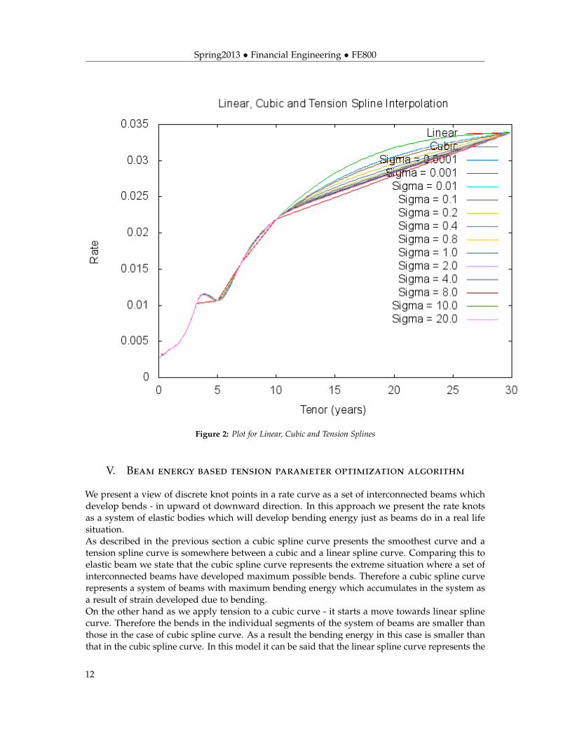
This defines a system of diagonally dominant equations which can be solved easily using GaussJordan elimination technique.These equations are similar to those for cubic spline. Like before wetake z0 and zn−1 as zero.The computational implementation of tension spline is similar to that of cubic spline with addedcomplexity of hyperbolic sine and cosine related calculations.It is important to note that we are taking tension parameter σ as constant for the entire duration ofthe term structure. By using similar mathematical derivation one can find the tridiagonal systemof equations for non uniform tension as well. The mathematical derivation is included in theappendix.For simplicity of calculations for we proceed with uniform tension model.Following chart shows plot of linear, cubic and tension splines for the forward rates data discussedearlier. Please note that gfor smaller tension the curve is closer to the cubic spline whereas astension is increased the curve approaches the linear spline shape.
11
Spring2013 • Financial Engineering • FE800
Figure 2: Plot for Linear, Cubic and Tension Splines
V. Beam energy based tension parameter optimization algorithm
We present a view of discrete knot points in a rate curve as a set of interconnected beams whichdevelop bends - in upward ot downward direction. In this approach we present the rate knotsas a system of elastic bodies which will develop bending energy just as beams do in a real lifesituation.As described in the previous section a cubic spline curve presents the smoothest curve and atension spline curve is somewhere between a cubic and a linear spline curve. Comparing this toelastic beam we state that the cubic spline curve represents the extreme situation where a set ofinterconnected beams have developed maximum possible bends. Therefore a cubic spline curverepresents a system of beams with maximum bending energy which accumulates in the system asa result of strain developed due to bending.On the other hand as we apply tension to a cubic curve - it starts a move towards linear splinecurve. Therefore the bends in the individual segments of the system of beams are smaller thanthose in the case of cubic spline curve. As a result the bending energy in this case is smaller thanthat in the cubic spline curve. In this model it can be said that the linear spline curve represents the
12
Spring2013 • Financial Engineering • FE800
curve with minimum bending energy and therefore it is "most" stable in elastic sense of meaning.Since we can not associate a linearly distributed weight with the pieces of rate curve the only waythe linear curve can develop a bend is because of some kind of force that is applied onto it. Weuse the beam theory equations to find out this force.Let us take a section of knot point (xi, yi), (xi+1, yi+1), it is essentially a straight line with a slope(
yi−yi+1xi−xi+1
). Now we imagine a force P acting at a distance a from xi, due to this force the straight
line will develop a deflection.Let us assume that a fictious force of magnitude P is acting at a distance a from (xi, yi). Wedefine b as distance of this point from (xi+1, yi+1). Clearly a + b gives the linear length of the knotsegment. Let us define this length as L defined as below.
L =√(yi+1 − yi)2 + (xi+1 − xi)2 (51)
The bending moment of the beam for (0 ≤ x ≤ a) is defined as under -
M = EId2ν
dx2 =Pbx
L(52)
While for (a ≤ x ≤ L) it is given by
M = EId2ν
dx2 =Pbx
L− P(x− a) (53)
E is the elastic constant of the beam and I is geometric moment of intertia. The product EI is theflextural rigidity of the beam.ν represents the deflction of the beam.The differential equation defined above can be used to find the deflection curve by using followingboundary conditions.
ν(0) = ν(L) = 0 (54)
ν(a + 0) = ν(a− 0) (55)
ν′(a + 0) = ν
′(a− 0) (56)
By solving the differential equation described above we obtain - For (0 ≤ x ≤ a) -
ν(x) =Pbx
6LEI(L2 − b2 − x2) (57)
For (a ≤ x ≤ L)
ν(x) =Pbx
6LEI(L2 − b2 − x2)− P(x− a)3
6EI(58)
The maximum deflection can be obtained by equating first differential of ν to zero. If a > b then
13
Spring2013 • Financial Engineering • FE800
maximum deflection will occur at a point x < a.The maximum deflection is given by
δmax = −ν(x1) =Pb(L2 − b2)
32
9√
3LEI(59)
The maximum deflection happens at
x =
√L2 − b2
3(60)
And the potential energy that is saved in the system is given by
U = P.δmax.cos(θ) (61)
Therefore in order to calculate the point "a" where concentrated force is acting, we need to findout the point of maximum deflection. Once we have "a" we can back calculate P in units of (EI)and then the potential energy can be calculated. We differntiate the equation for interpolationcurve set it to zero to find out point of maximum deflection i.e. x = x1. Using this value of x1we calculate value of b which is then used to obtain value of a and P. The resulting equation asshown below can be solved by using numerical technniques.We define the following three norms which we need to carefully analyze for the optimum tension.
Smoothness =∫ T
0y′′(t)2dt (62)
Smoothness term penalizes the high second order fluctuations. As the tension is increased thesmoothness of the curve will decrease.
Length =∫ T
0σ2y
′(t)2dt (63)
The length of the curve penalizes the first order perturbations which may cause lack of locality orexcessive convexity in the curve. This too will decrease as the tension is increased.
Energy =N−1
∑i=1
U(i− 1, i) (64)
The total beam energy of the curve is essentially equal to the work done on the curve by externallyapplied forces on individual segments. This term may not be a monotonically increasing ordecreasing function of the tension. Simulations done by the author reveal a irregular behaviorwhich is hard to fit any standard mathematical function. A careful look at the beam energy revealsthat this term actually penalizes the curve for the maximum deflection as well as position ofmaximum deflection in knot segments.It is easy to observe that beam enrgy will penalize the curve more if there are sharp bulges insmaller knot segments. That makes sense for financial data since a large deflection in a smallerknot segment essentially means very sharp change in rate in small duration of time and therebyindicating very sharp fluctuation.
14

Spring2013 • Financial Engineering • FE800
A careful observation reveals that these three norms are of different scale. therefore an absolutecomparison of these parameters will be of very limited use. Instead we normalize these forcomparison and analysis purposes.We hypothesize that a curve which satisfies following equation in a given range of tensionparameter will have right balance of beam energy as well as smoothness and length.
Smoothness(σ) + Length(σ) = BeamEnergy(σ) (65)
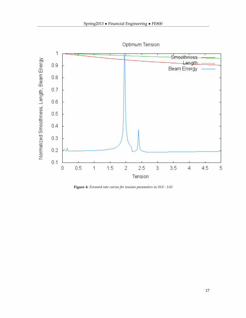
Where RHS and LHS are normalized by using their respective maximum values in a given rangeof σ.We now define our algorithm in the form of following computational steps / pseudocode1. Compute the curve for given range of σ.2. For each value of σ calculate the smoothness, length and beam energy.3. Normalize sum of smoothness and length by dividing the individual sum by the maximumvalue in the range of sigma.4. Normalize the beam energy by dividing individual values by the maximum value of the beamenergy.5. Iteratively find out the value of the σ which makes the normalized sum of smoothness andlength equal to the normalized beam energy.6. The σ so obtained is the optimum value of tension.Following chart shows output of simulation done over a wide range of tension parameters.
15

Spring2013 • Financial Engineering • FE800
Figure 3: Forward rate curves for tension parameters in (0.0 - 1.5)
16
Spring2013 • Financial Engineering • FE800
Figure 4: Forward rate curves for tension parameters in (0.0 - 5.0)
17
Spring2013 • Financial Engineering • FE800
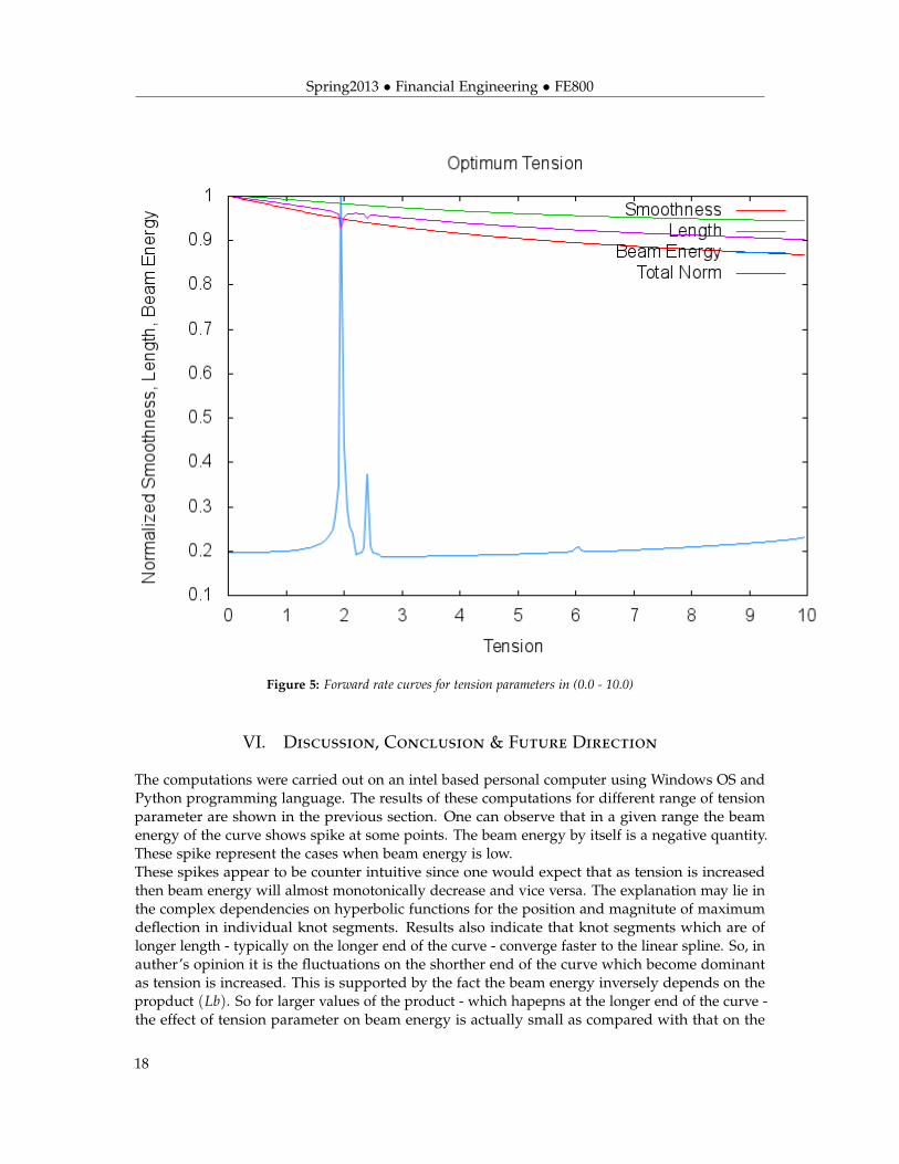
Figure 5: Forward rate curves for tension parameters in (0.0 - 10.0)
VI. Discussion, Conclusion & Future Direction
The computations were carried out on an intel based personal computer using Windows OS andPython programming language. The results of these computations for different range of tensionparameter are shown in the previous section. One can observe that in a given range the beamenergy of the curve shows spike at some points. The beam energy by itself is a negative quantity.These spike represent the cases when beam energy is low.These spikes appear to be counter intuitive since one would expect that as tension is increasedthen beam energy will almost monotonically decrease and vice versa. The explanation may lie inthe complex dependencies on hyperbolic functions for the position and magnitute of maximumdeflection in individual knot segments. Results also indicate that knot segments which are oflonger length - typically on the longer end of the curve - converge faster to the linear spline. So, inauther’s opinion it is the fluctuations on the shorther end of the curve which become dominantas tension is increased. This is supported by the fact the beam energy inversely depends on thepropduct (Lb). So for larger values of the product - which hapepns at the longer end of the curve -the effect of tension parameter on beam energy is actually small as compared with that on the
18
Spring2013 • Financial Engineering • FE800
shorter end of the curve.Another noteworthy observation is that there are minima of beam energy in different range oftension parameter. This suggests that - from a user point of view - one will first need to identifya possible range of tension parameter and then try to find out it’s optimum value using thealgorithm described in this paper.One should be advised that this work deals with the curve optimization problem in a very sim-plistic way. We have computed the energy of individual beams and simply added them. thereforewe have not really considered the interaction that the beam segments may have with each other.Literature on structural mechanics define mathematical techniques where the effect on bendingmoment is done by taking account of interaction with adajecnt beam. The multiple momentsmethod is one such technique. In author’s opinion use of such methods will definitely give betterresults.In this work we have also ignored - for simplicity of analysis and computation - effects that maybe caused by different angular orientation of individual beams. Including that will certainlyimprove the results. Also, we have approximated each beam to be having same elastic constantand geometric inertia. use of this approximation is justified by the fact that we are using sametension parameter for entire length of the curve. For better control on the curve behavior one maywant to use a non uniform tension model. A mathematical derivation for the same is outlined inappendix. use of such model will probably require us to have a non uniform constant of elasticityand geometric moment of inertia as well.In our view, much needs to be explored so far as construction of an ideal curve is concerned.Modeling of the curves by mimicking real world physical objects - such as elastic beam - can be agood tool to analyze behavior of the curve on the whole. The work presented in this paper is onesuch attempt and there is much more that needs to be done.
19
Spring2013 • Financial Engineering • FE800
A.Non uniform Tension Spline
We define the spline function as following equations in terms of hyperbolic sine and cosine. Likecubic spline, these functions are individually applicable in ranges (xi, xi+1) for i ∈ (0, n− 1). Thereare a total of n observations of (xi, yi) and there therefore there are (n-1) intervals (knot pointpairs) for which these equations will be individually valied.
fi(x) = ai + bi(x− xi) + cisinh(σi(x− xi)) + dicosh(σi(x− xi)) (66)
f′i (x) = bi + σicicosh(σi(x− xi)) + σidisinh(σi(x− xi)) (67)
f′′i (x) = σ2
i cisinh(σi(x− xi)) + σ2i dicosh(σi(x− xi)) (68)
Using symmetry we have
fi+1(x) = ai+1 + bi+1(x− xi+1) + ci+1sinh(σi+1(x− xi+1)) + di+1cosh(σi(x− xi+1)) (69)
f′i+1(x) = bi+1 + σi+1ci+1cosh(σi+1(x− xi+1)) + σi+1di+1sinh(σi+1(x− xi+1)) (70)
f′′i+1(x) = σ2
i+1ci+1sinh(σi+1(x− xi+1)) + σ2i+1di+1cosh(σi+1(x− xi+1)) (71)
Definehi = xi+1 − xi (72)
hi+1 = xi+2 − xi+1 (73)
α(i, j) = sinh(hiσj) (74)
β(i, j) = cosh(hiσj) (75)
zi = f′′i (xi) = σ2
i di (76)
di =zi
σ2i
(77)
di+1 =zi+1
σ2i+1
(78)
yi = fi(xi) = ai + di (79)
ai = yi −zi
σ2i
(80)
ai+1 = yi+1 −zi+1
σ2i+1
(81)
20
Spring2013 • Financial Engineering • FE800
Continuity of second derivative at x = xi, For n ∈ (1...n− 2)
zi = σ2i+1ci+1sinh(σi+1(xi − xi+1)) + σ2
i+1di+1cosh(σi+1(xi − xi+1)) (82)
zi = σ2i+1ci+1sinh(σi+1(−hi)) + σ2
i+1di+1cosh(σi+1(−hi)) (83)
zi = −σ2i+1ci+1sinh(σi+1hi) + σ2
i+1zi+1
σ2i+1
cosh(σi+1hi) (84)
σ2i+1ci+1sinh(σi+1hi) = zi+1cosh(σi+1hi)− zi (85)
ci+1 =zi+1cosh(σi+1hi)− zi
σ2i+1sinh(σi+1hi)
(86)
ci =zicosh(σihi−1)− zi−1
σ2i sinh(σihi−1)
(87)
Now we work on continuity of f (xi)
yi = fi(xi) = fi+1(xi) (88)
yi = ai+1 + bi+1(xi − xi+1) + ci+1sinh(σi+1(xi − xi+1)) + di+1cosh(σi(xi − xi+1)) (89)
yi = ai+1 + bi+1(−hi) + ci+1sinh(σi+1(−hi)) + di+1cosh(σi(−hi)) (90)
bi+1hi = ai+1 + ci+1sinh(σi+1(−hi)) + di+1cosh(σi(−hi))− yi (91)
bi+1hi = ai+1 − ci+1sinh(σi+1hi) + di+1cosh(σihi)− yi (92)
bi+1hi = yi+1 −zi+1
σ2i+1− ci+1sinh(σi+1hi) + di+1cosh(σihi)− yi (93)
bi+1hi =
[yi+1 −
zi+1
σ2i+1
]−[
zi+1cosh(σi+1hi)− zi
σ2i+1sinh(σi+1hi)
]sinh(σi+1hi) +
[zi+1
σ2i+1
]cosh(σihi)− yi (94)
bi+1hi =
[yi+1 −
zi+1
σ2i+1
]−[
zi+1cosh(σi+1hi)− zi
σ2i+1
]+
[zi+1
σ2i+1
]cosh(σihi)− yi (95)
bi+1hi = yi+1 − yi −zi+1
σ2i+1
+zi+1
σ2i+1
(−cosh(σi+1hi) + cosh(σihi)) +zi
σ2i+1
(96)
bi+1hi = yi+1 − yi +zi+1
σ2i+1
(cosh(σihi)− cosh(σi+1hi)− 1) +zi
σ2i+1
(97)
bi+1 =yi+1 − yi +
zi+1σ2
i+1(cosh(σihi)− cosh(σi+1hi)− 1) + zi
σ2i+1
hi(98)
bi =yi − yi−1 +
ziσ2
i(cosh(σi−1hi−1)− cosh(σihi−1)− 1) + zi−1
σ2i
hi−1(99)
bi =yi − yi−1
hi−1+
zi
hi−1σ2i(cosh(σi−1hi−1)− cosh(σihi−1)− 1) +
zi−1
hi−1σ2i
(100)
21
Spring2013 • Financial Engineering • FE800
bi+1 =yi+1 − yi
hi+
zi+1
hiσ2i+1
(cosh(σihi)− cosh(σi+1hi)− 1) +zi
hiσ2i+1
(101)
Now apply continuity of f′
bi + σici = bi+1 + σi+1ci+1cosh(σi+1(xi − xi+1)) + σi+1di+1sinh(σi+1(xi − xi+1)) (102)
bi + σici = bi+1 + σi+1ci+1cosh(σi+1(−hi)) + σi+1di+1sinh(σi+1(−hi)) (103)
bi + σici = bi+1 + σi+1ci+1cosh(σi+1hi)− σi+1di+1sinh(σi+1hi) (104)
After simplification we get the following result -
zi−1 Ai−1 + zi Ai + zi+1 Ai+1 =yi − yi−1
hi− yi−1 − yi−2
hi−1(105)
where
Ai−1 =
[−1
σisinh(σihi−1)
](106)
Ai =
[cosh(σihi−1)
σisinh(σihi−1)+
cosh(σi+1hi)
σi+1sinh(σi+1hi)
](107)
Ai+1 =
[sinh(σi+1hi)
σi+1− cosh(σi+1hi)
σi+1sinh(σi + 1hi)
](108)
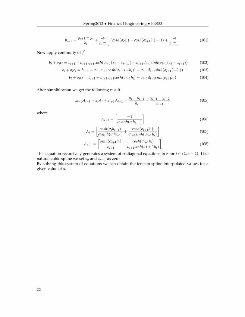
This equation recursively generates a system of tridiagonal equations in z for i ∈ (2, n− 2). Likenatural cubic spline we set z0 and zn−1 as zero.By solving this system of equations we can obtain the tension spline interpolated values for agiven value of x.
22

Spring2013 • Financial Engineering • FE800
References
[1] Leif Anderson (2007). Discount curve construction with tesnsion splines. Review of DerivativesResearch, ISSN 1380-6645, 12/2007, Volume 10, Issue 3, pp. 227 - 267.
[2] Mladen Rogina, Sanja Singer (2007). Conditions of matrices in discrete tension splineapproximations of DMBVP. Ann Univ Ferrara (2007), 53:393âAS404 DOI 10.1007/s11565-007-0019-8.
[3] Andrew Lesniewski (January 26, 2012). Interest Rates and FX Models (LIBOR and OIS).Courant Institute of Mathemetical Sciences, new York university, New yorl (2012).
[4] Uri Ron. A Practical Guide to Swap Curve Construction. Bank of Canada, Working paper2000-17.
[5] Dale J. Poirier (1973). Piecewise Regression Using Cubic Spline. Journal of the AmericanStatistical Association (1973), Vol. 68, No. 343 (Sep., 1973), pp. 515-524.
[6] Boris Kvasov (2011). Parallel mesh methods for tension splines. Journal Computational andApplied Mathematics, 236 (2011) 843-859.
[6] Jalil Rashidnia, Reza Mohammadi (2011). Tension Spline solution of nonlinear Sine-Gordanequation. Numer Algorithms (2011), 56:129-142 DOI 10.1007/s11075-010-9377-x.
[7] Jonathan Kinlay, Xu Bai Yield Curve Construction Models - Tools and Techniques.
[8] Paolo Costantini, Boris I. Kvasov and Carla Manni c. On Discrete Hyperbolic Tension Splines.Advances in Computational Mathematics (1999), , ISSN 1019-7168, 12/1999, Volume 11, Issue 4,pp. 331 - 354.
[9] Rod Pienaar, Moorad Choudhry. Fitting the term structure of interest rates: the practicalimplementation of cubic spline methodology. Centre for Mathematical Trading and Finance CityUniversity Business School, London.
[10] Patrick S. Hagan, Graeme West. Interpolation Methods for Curve Construction. AppliedMathematical Finance, Vol. 13, No. 2, 89âAS129, June 2006.
[11] R. J. Renka. Interpolatory Tension Splines With Automatic Selection Of Tension Factors.Society for Industrial and Applied Mathematics, SIAM J. ScI. STAT. COMPUT., Vol. 8, No. 3, May1987.
[12] Parviz Moin. Fundamentals Of Engineering Numerical Analysis. Cambridge University Press(2001) , ISBN-10: 0521801400 ISBN-13: 978-0521801409.
[13] Carl de Boor. A Practical Guide to Splines (Applied Mathematical Sciences) [Paperback].Springer (August 26, 1994) , ISBN-10: 0387903569 ISBN-13: 978-0387903569.
[14] F. N. Fritsch, R. E. Carlson. Monotone Piecewise Cubic Interpolation. Society for Industrial andApplied Mathematics, SIAM J. ScI. STAT. COMPUT., Vol. 8, No. 3, May 1987.
[15] A. K. Cline. Scalar- and planar-valued curve fitting using splines under tension (1974).Communications of the ACM., 17, 218âAS223.
[16] Carsten Tanggaard. Nonparametric Smoothing of Yield Curves. Review of Quantitative Financeand Accounting, 9 (1997): 251âAS267.
23

Spring2013 • Financial Engineering • FE800
[17] McCullach. The tax adjusted yield curve. Review of Quantitative Finance and Accounting, 9(1997): 251âAS267.
[18] Iraj Kani. Interest Rate Fundamentals (Lecture 1 - Part II). Topics in Quantitative Finance:Inflation Derivatives, http://www.columbia.edu/ ik2133/E4728/Lectures/Lecture%201%20-%20Part%20II.pdf.
[19] David Kincaid, Ward Cheney. Numerical Analysis - Mathematics of Scientific Computing,Third Edition. American Mathematical Society
[20] Masaru Kamada and Rentsen Enkhbat Spline Interpolation in Piecewise Constant Tension.Author manuscript, published in "SAMPTA’09, Marseille : France (2009)".
24