SUTRA: An Approach to Modelling Pandemics with ... - arXiv

SUTRA: An Approach to Modelling Pandemics with

Undetected Patients, and Applications to COVID-19

Manindra Agrawal, Madhuri Kanitkar, Deepu Phillip,Tanima Hajra, Arti Singh, Avaneesh Singh,

Prabal Pratap Singh and Mathukumalli Vidyasagar ∗

May 6, 2022

Abstract

Covid-19 pandemic has two characteristics: (i) asymptomatic cases (both detected and un-detected) that could result in fresh infections, and (ii) time-varying characteristics due to newvariants, NPIs etc. We developed a model ‘SUTRA’ (Susceptible, Undetected, Tested positive,and Removed, Analysis) for predicting the course of COVID-19.

All parameters in the SUTRA model can be robustly estimated purely from data and canbe re-estimated at any time in the pandemic. The model also indicates when recalibration isneeded. SUTRA can also estimate the number of undetected cases. To the best of our knowledgethis is the only model with all these capabilities.

The SUTRA approach can be applied at various levels of granularity, from national todistrict, and to any country with data on daily new cases and recoveries. The approach hasbeen validated on the pandemic in India during all three waves, and also on many other countries.A broad conclusion is that the best way to handle the pandemic is to allow the disease to spreadslowly in society, and a “zero-COVID” policy is not sustainable.

COVID-19 needs a dynamic model like SUTRA which can help plan logistics and interven-tions by policy makers.

1 Introduction

The COVID-19 pandemic caused by the SARS-CoV-2 virus has by now led to more than 500million cases and more than six million deaths worldwide, as of April 23rd, 2022 [1]. By way ofcomparison, the infuenza epidemic of 1957 led to 20,000 deaths in the UK and 80,000 deaths in theUSA, while the 1968 influenza pandemic led to 30,000 deaths in the UK and 100,000 deaths in theUSA [2]. In contrast, the COVID-19 pandemic has already led to more than one million deaths inthe USA and more than 170,000 deaths in the UK [2]. Therefore the COVID-19 pandemic is themost deadly since the Spanish Flu pandemic which started in 1918. In the USA, 675,000 people,or 0.64% of the population, died in that pandemic [3], compared to 0.33% of the population in thecurrent pandemic. Among large economies, the USA, UK, Italy, and Spain, have all registered morethan 2,200 deaths per million population [1]. In these countries, the pandemic has gone through

∗MA, DP, TH, ArS, AvS, PPS are at Indian Institute of Technology Kanpur, Kanpur, UP 208016; MK is theVice Chancellor of Maharashtra University of Health Sciences, Nashik, MH 422004; MV is with the Department ofArtificial Intelligence, Indian Institute of Technology Hyderabad, Kandi, TS 502284; MV is the corresponding author.Email: [email protected].

1

arX

iv:2

101.

0915

8v5

[q-

bio.

PE]

5 M

ay 2

022

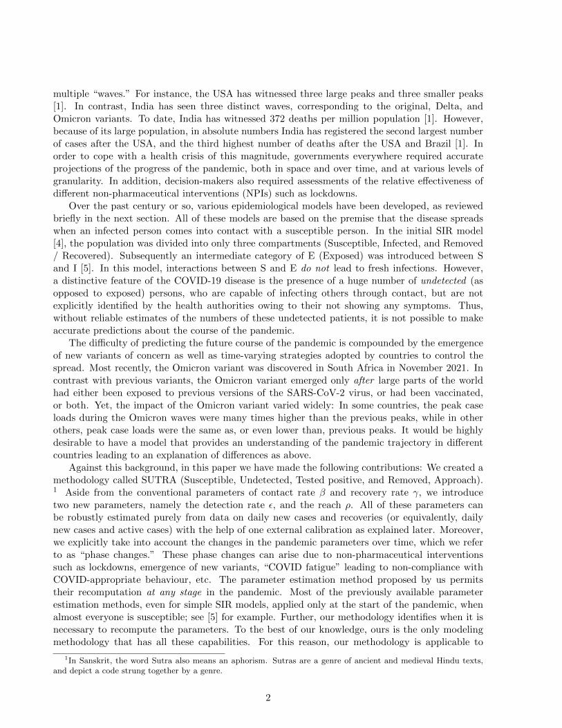
multiple “waves.” For instance, the USA has witnessed three large peaks and three smaller peaks[1]. In contrast, India has seen three distinct waves, corresponding to the original, Delta, andOmicron variants. To date, India has witnessed 372 deaths per million population [1]. However,because of its large population, in absolute numbers India has registered the second largest numberof cases after the USA, and the third highest number of deaths after the USA and Brazil [1]. Inorder to cope with a health crisis of this magnitude, governments everywhere required accurateprojections of the progress of the pandemic, both in space and over time, and at various levels ofgranularity. In addition, decision-makers also required assessments of the relative effectiveness ofdifferent non-pharmaceutical interventions (NPIs) such as lockdowns.

Over the past century or so, various epidemiological models have been developed, as reviewedbriefly in the next section. All of these models are based on the premise that the disease spreadswhen an infected person comes into contact with a susceptible person. In the initial SIR model[4], the population was divided into only three compartments (Susceptible, Infected, and Removed/ Recovered). Subsequently an intermediate category of E (Exposed) was introduced between Sand I [5]. In this model, interactions between S and E do not lead to fresh infections. However,a distinctive feature of the COVID-19 disease is the presence of a huge number of undetected (asopposed to exposed) persons, who are capable of infecting others through contact, but are notexplicitly identified by the health authorities owing to their not showing any symptoms. Thus,without reliable estimates of the numbers of these undetected patients, it is not possible to makeaccurate predictions about the course of the pandemic.

The difficulty of predicting the future course of the pandemic is compounded by the emergenceof new variants of concern as well as time-varying strategies adopted by countries to control thespread. Most recently, the Omicron variant was discovered in South Africa in November 2021. Incontrast with previous variants, the Omicron variant emerged only after large parts of the worldhad either been exposed to previous versions of the SARS-CoV-2 virus, or had been vaccinated,or both. Yet, the impact of the Omicron variant varied widely: In some countries, the peak caseloads during the Omicron waves were many times higher than the previous peaks, while in otherothers, peak case loads were the same as, or even lower than, previous peaks. It would be highlydesirable to have a model that provides an understanding of the pandemic trajectory in differentcountries leading to an explanation of differences as above.

Against this background, in this paper we have made the following contributions: We created amethodology called SUTRA (Susceptible, Undetected, Tested positive, and Removed, Approach).1 Aside from the conventional parameters of contact rate β and recovery rate γ, we introducetwo new parameters, namely the detection rate ε, and the reach ρ. All of these parameters canbe robustly estimated purely from data on daily new cases and recoveries (or equivalently, dailynew cases and active cases) with the help of one external calibration as explained later. Moreover,we explicitly take into account the changes in the pandemic parameters over time, which we referto as “phase changes.” These phase changes can arise due to non-pharmaceutical interventionssuch as lockdowns, emergence of new variants, “COVID fatigue” leading to non-compliance withCOVID-appropriate behaviour, etc. The parameter estimation method proposed by us permitstheir recomputation at any stage in the pandemic. Most of the previously available parameterestimation methods, even for simple SIR models, applied only at the start of the pandemic, whenalmost everyone is susceptible; see [5] for example. Further, our methodology identifies when it isnecessary to recompute the parameters. To the best of our knowledge, ours is the only modelingmethodology that has all these capabilities. For this reason, our methodology is applicable to

1In Sanskrit, the word Sutra also means an aphorism. Sutras are a genre of ancient and medieval Hindu texts,and depict a code strung together by a genre.

2

multiple countries, and at various levels of granularity, from nationwide to district and in-between.Moreover, by estimating changes in various parameters, we are able to quantify the waning ofimmunity over time or due to the emergence of new variants.

The past two years have witnessed different countries adopting different approaches to com-bating the pandemic. Our methodology has allowed us to compare and contrast these differentapproaches. At one extreme is the “zero COVID” strategy, in which the government imposes quitedrastic policies regarding quarantines, lockdowns, shutting down schools and colleges etc., whilein parallel vaccinating the population. In this approach, the authorities are counting solely onvaccine-induced immunity to protect the population from multiple variants of the SARS-CoV-2virus. Such countries are characterized by high vaccine penetration, but low sero-prevalence. Atthe other extreme lies an approach that allows the pandemic to run through the population with-out relying much on vaccination. This approach relies solely on natural immunity (due to priorexposure to the virus) for protection. Countries that adopt this approach are characterized by lowvaccine penetration, but high sero-prevalence. In between the two, lies an approach that might becalled “controlled spread,” in which the pandemic is allowed to work its way through the country ina controlled manner, while also vaccinating the population as quickly as possible. In this approach,the population is protected through a combination of both natural immunity and vaccination.Countries that adopt this approach have both high vaccine penetration and high sero-prevalence.As a part of our studies, we have analyzed thirty six countries, out of which detailed analyses arepresented for six countries, and ondensed analyses are presented for the rest: These six countriesare:

Australia and Singapore. Followed zero COVID approach until recently.

South Africa. Relied on natural immunity.

India and UK. Followed controlled spread approach.

US. Controlled spread approach but comparatively lower levels of vaccination and natural immu-nity.

The efficacy of each approach can be quantified by applying the SUTRA methodology to variouscountries. Our analysis shows that a “zero COVID strategy” does not succeed in the long run.Eventually the virus breaks through leading to massive increases in the number of cases. The bestapproach appears to be to permit the pandemic to work its way through the population, whileachieving full vaccination, as India and UK have done. More details can be found in the Resultsand the Discussion sections.

By using the SUTRA methodology, we are also able to quantify the waning of immunity overtime in thirty six countries, spread over all continents representing more than half the populationof the world. Our conclusions are very clear: Natural immunity conferred by prior exposure toany variant of SARS-CoV-2 confers good protection against infection by the Omicron variant,while vaccine-induced protection is bypassed almost totally. This reinforces the point made above,namely that a zero COVID policy is not sustainable in the long run.

2 Material and Methods

2.1 Model Formulation

Perhaps the earliest paper to propose a pandemic model incorporating asymptomatic patients is[6]. In this paper, the population is divided into four categories: S, A (for Asymptomatic), I (for

3

Infected) and R. Interactions between members of S and A, as well as between members of S andI, can lead to fresh infections. In that paper, it is assumed that almost all persons in A escapedetection, while almost all persons in I are detected by the health authorities. While the SAIRmodel of [6] is a good starting point for modelling diseases with asymptomatic patients, it does notdirectly apply to COVID-19, for the following reasons: Due to contact tracing, some fraction of A doget detected. In fact, detected asymptomatic cases are often comparable to detected symptomaticones. However, daily reported cases data typically does not provide this division and hence itbecomes difficult to estimate number of symptomatic cases even assuming that all symptomaticcases get detected.

Therefore, in the present paper we propose a different grouping, namely: S = SusceptiblePopulation, U = Undetected cases in the population, T = Tested Positive, either asymptomaticor symptomatic, and R = Removed, either through recovery or death. This leads to the SUTRAmodel, where the last A in SUTRA stands for “approach.” For discussion purposes, the categoryR of removed can be further subdivided into RU denoting those who are removed from U , andRT denoting those who are removed from T . As in the conventional SAIR model [6], interactionsbetween members of S on the and members of U or T , can lead to the person in S getting infectedwith a certain likelihood.

A compartmental diagram of the SUTRA model is shown in Figure 1. The term εβUS representsthe assumptions that (i) recent cases have higher chances of getting detected, and (ii) number of newcases do not change dramatically over a few days and so number of detected cases are proportionalto βUS, number of most recent cases. A few additional assumptions have been made that do notaffect the dynamics significantly, but greatly simplify parameter estimation. Specifically,

• It is assumed that the removal rate for both compartments T and U is the same. This canbe justified because, due to contact tracing, an overwhelming majority of patients in T areasymptomatic, and those people recover at the same rate as the asymptomatic people in U .Even for the small fraction in T who develop complications and pass away, the time durationis very close to that of those who recover.

• There is no interaction shown between the T and S compartments. In most countries, thosewho test positive (whether symptomatic or not) are either kept in institutional quarantine,or told to self-quarantine. In reality, there might still be a small amount of contact betweenT and S. However, neglecting this does not significantly change the dynamics of the model,and greatly simplifies the parameter estimation.

With these considerations, the governing equations for the SUTRA model are:

dS

dt= −βSU, dU

dt= βSU − εβSU − γU, dT

dt= εβSU − γT, dRU

dt= γU,

dRTdt

= γT, (1)

As is customary, these quantities denote the fraction of the population within each compartment,so that

S + U + T +RU +RT = 1.

There are four parameters in this model, namely β, γ, ε, ρ, and a constant of integration c. Theinterpretation of these parameters is as follows:

• β = The likelihood that contact between a susceptible person and an asymptomatic or symp-tomatic person leads to an infection of the susceptible person; it is called the “contact rate.”

• γ = Removal rate, including both recoveries and deaths.

4

• ε = Governs the rate at which infected patients in U move over to T . As shown later, it alsoequals the ratio T/(U + T ) and is thus called the “detection rate.”

• ρ = The ratio between the “effective” population P within reach of the pandemic, and thetotal population P0.

This last bullet requires a little elaboration, because the symbol ρ does not appear in the equa-tions (1). Recall that the various symbols in (1) denote the fraction of the population in eachcompartment. However, the actual data available to the modeller consists of raw numbers of someof these quantities. To arrive at the fractions, one must divide the raw numbers by the effectivepopulation of the group under study. This effective population P equals ρP0, where P0 is the totalpopulation (for example, about 1.4 billion for India), and ρ is the “reach” of the pandemic. Whenthe pandemic starts, the reach is very small, and increases as the pandemic spreads. Eventually itreaches a value very close to 1. However, as the pandemic progresses still further, and the immu-nity conferred via prior exposure begins to wane, the reach ρ can go beyond 1, denoting that somepersons who were previously exposed and immune to the infection, lose their immunity and arevulnerable to become infected again. Similarly, vaccination of susceptible persons can move themoutside the reach, thereby causing a reduction in ρ. This point is brought more clearly when weanalyze individual countries.

In addition to the four parameters mentioned above, there is also a constant of integration c,which is chosen to ensure continuity of the trajectories when there is a phase change.

2.2 Parameter Estimation and Forward Prediction

One of the distinctive features of our approach is a methodology for estimating the values of allthe parameters in the pandemic model from reported raw data on the number of daily new casesNT , the total number of active cases T , and the number of daily removals RT (including bothrecoveries as well as deaths). It is shown in the Supplementary Material that these quantitiessatisfy the following fundamental relationship:

T =1

βNT +

1

ρP0(T +RT )T , (2)

where P0 denotes the population of the underlying society (e.g., 1.4 billion for India), and

β = β(1− ε)(1− c), ρ = ερ(1− c). (3)

In this equation, c is a constant of integration, which is adjusted to ensure that the trajectories arecontinuous when phase changes occur.

In order to apply this fundamental relationship to estimating the parameters, we first discretizethe fundamental relationship by averaging all quantities over some fixed number of days ∆. Inevery country, the data has a very pronounced weekly periodicity, due to various intrinsic factors.Hence we chose ∆ = 7. However, in principle, any integer could be used. Once ∆ is chosen, definevectors as follows

u(t) =1

∆

t∑s=t−D+1

T (s),

v(t) =1

∆

t+1∑t−∆+2

NT (s),

5

w(t) =1

∆P0

t∑s=t−∆+1

(T (s) +RT (s))T (s).

In these equations, the index t varies over the duration of the current phase. Then the followinglinear regression problem is solved:

minβ,ρ||u− 1

βv − 1

ρw||2.

Once the linear regression problem is solved, the quality of the fit parameter, usually denoted byR2, is computed, as follows:

R2 =||u− 1

βv − 1

ρw||2

||u||2,

with the optimal parameter choices. The closer R2 is to one, the better is the quality of the fit.Once the quantities β, ρ are estimated as above, the following forward projection method is

used:

NT (t+ 1) = βT (t)− β

ρP0(T (t) +RT (t))T (t). (4)

The above methodology is implemented in the following manner: The linear regression problemis solved on a daily basis with new data. When the quality of fitR2 falls below an accepted threshold,denoting a significant change in one or more parameter values, a new “phase” is started. For sometime in the new phase, the parameter values may continue to change before stabilizing. This timeis called “drift period” of the new phase. The methods for computing the phase boundaries, driftperiods, and for interpolating the values of the parameters during the drift period, are spelled outin detail in the Supplementary Material.

After computing β and ρ values for current phase, the values of ε and c can be computed withthe help of parameter values of the previous phase (the details are given in the SupplementaryMaterial). Then β = β/(1− ε)(1− c) and ρ = ρ/ε(1− c) can be easily computed.

Once the parameters in the SUTRA model are estimated, it is possible to estimate the numberof undetected cases, and the fraction of population under the reach of the pandemic, thereby leadingto accurate projections about its temporal and spatial evolution.

2.3 Calibrating the Model

Previous subsection shows how to estimate parameter values for all phases, provided the followingtwo values are known: ε and c for the first phase. Note that there is no previous phase for whichwe know the parameter values. We may set c = 0 for the first phase since there is no requirementof continuity from previous phase. The value of ε for the first phase, say ε1, needs to be providedas an input to the model, and is called calibrating the model. We can calibrate the model in twoways:

• A sero-survey at time t provides a good estimate of fraction of population infected until timet − δ, where δ equals the time taken for antibodies to develop. Once we set ε1, the modelcan compute fraction of infected population at all times. So we can choose a suitable ε1 thatensures that model computation matches with the sero-survey result at time t− δ.

• When the pandemic has been active long enough in a region without major, long-term re-strictions, we may assume that it has reached all sections of society, making ρ close to 1.

6

Again, we can choose ε1 that ensures that the reach of the pandemic is close to 1 at suitabletime.

One more point needs to be made about using serosurveys to calibrate the SUTRA model.Many serosurveys suffer from significant sampling biases. For example, if survey is done usingresidual sera from a period of high infection numbers, it is likely to significantly overestimate theseroprevalence because a large fraction of uninfected persons would not venture to give blood samplein such a period. In order to minimize sampling biases, therefore, one should use serosurveys doneduring a period of low infection numbers. Even then, some uninfected people may not participatemaking the estimates higher than actual. To further reduce bias, one should ideally be able to usemultiple serosurveys as well as use the fact that reach is close to 1 by a given time.

However, there are regions where neither an accurate sero-survey is available, and it is evidentthat reach is nowhere close to 1. For such regions, calibration cannot be done with any confidence,and so estimation of all parameter values is not possible. Even for such regions, the model canstill compute values of ρ = ρε(1 − c) and β = β(1 − ε)(1 − c) for all phases. This ensures thattrajectories of T and NT , detected active and new cases respectively, can be simulated well.

The real time data for India and other countries was sourced from [7, 1]. We downloadedan extensive list of serosurveys, carried out in various countries, and maintained by the site [8],eliminated surveys that were not done at national level, or had small sample sizes, or had high riskof bias. Nineteen countries remained after this pruning. These sero-surveys were used togetherwith the SUTRA model to capture the pandemic trajectories in these countries. We also carriedout simulations for seventeen more countries based on following criteria:

1. All continents are represented well (4 from Africa, 2 from North America, 4 from SouthAmerica, 13 from Asia, 12 from Europe, and one from Australia)

2. Populous countries are simulated (except China for which it is not possible to calibrate themodel). More than half the world’s population lives in these countries.

3. It is likely that reach was close to maximum in these countries at the time of Omicron’sarrival, allowing us to calibrate the model.

2.4 Analysis of the Loss of Immunity Against the Omicron Variant

The percentage of population that has natural immunity in a country at the time of onset of theOmicron wave can be determined from the SUTRA simulation of the country after calibration.The percentage of the population in a country that has received at least one dose of vaccination atthe onset of Omicron wave is taken from the site [9]. To estimate the extent of hybrid immunity(that is, the percentage of the population that has both vaccine and natural immunity), we assumethat the two types of immunity are independent random variables, implying that the fraction withhybrid immunity is the product of vaccine immunity and natural immunity fractions. Withoutthe independence assumption, it is not possible to estimate the extent of hybrid immunity orvaccine-only immunity.

A property of the SUTRA model is that the vaccination induced immunity in a susceptiblepopulation results in reduction of the reach parameter ρ. This is because a susceptible personbecoming immune is equivalent to the person moving outside the reach of the pandemic. Therefore,a gain of vaccine immunity among a fraction f of the susceptible population results in a reductionin ρ by an additive factor of f .

7

Similarly, a loss of vaccine immunity or natural immunity (both can be viewed as people thatmoved outside the reach and have now come back within the reach) among a fraction g of thepopulation results in an increase in ρ by an additive factor of g. This implies that a change in thevalue of ρ is due to a change in the spread of the infection in the population, gain of immunitydue to vaccination, as well as loss of immunity. Therefore, ρ may not be close to 1 even when thepandemic has spread over entire population. To capture this, we define ρactual to denote the actualreach of pandemic, so ρ equals ρactual plus change in immunity levels.

The countries chosen have the property that ρactual is close to maximum at the onset of Omicronwave, and so increase in ρ during Omicron wave can be taken to be mostly due to loss of immunity.This allows us to obtain a good estimate of loss of immunity for the countries. In order to reducethe impact of the calibration value and method chosen, we use the relative increase in reach, definedas

1− reach before Omicron

reach after Omicron,

to estimate the immunity loss.

3 Results

3.1 Estimation of Pandemic Parameters and Forward Predictions

The SUTRA methodology was applied to thirty six countries, using publicly available data. Due tospace limitations, complete results are presented for six countries, namely (in alphabetical order):Australia, India, Singapore, South Africa, the UK, and the USA. For each country, the total numberof phases, duration of each phase, and the parameter values during each phase, are included in theSupplementary Material. Using these estimated values, forward predictions were made regardingthe number of daily new cases in each of these six countries. These predicted trajectories were thencompared with the actual. These results are presented here, in the main body of the paper.


The results of the immunity loss analysis are shown in Table 1. Figure 8 plots 1 − ρ againstvaccination percentage before the arrival of Omicron to ascertain whether reach has maximized inthe countries studied. Also, relative increase in the reach ρ, which captures the loss of immunity,is plotted as a function of the percentage of the population having natural immunity before thearrival of the Omicron variant (Figure 9) and vaccination-only immunity (Figure 10).

4 Discussion

4.1 Prediction of the Progression of the Pandemic

We have presented predicted and actual trajectories for six different countries, spanning the entireduration of the COVID-19 pandemic, starting from 2020 until now. During this period, thereemerged several “variants of concern” of the SARS-CoV-2 virus. In India for example, there werethree distinct waves, which corresponded to the original virus, the Delta variant, and the Omicronvariant. Despite so many varying factors, the fit between the predicted and the actual trajectorieswas excellent, in all countries, and throughout the entire duraction of the pandemic. Some notablesuccesses were predicting the timing and height of the peak of second wave of India ten days inadvance [10], predicting timing of the peak of third wave in India as well as many states of the

8

country [11], predicting height and timing of the peak of Delta-wave in UK ten days in advance [12],and predicting height and timing of the peak of Delta-wave in US more than a month in advance [13].The predictions for India and its states were extremely useful to the policy-makers in planning therequired capacity for providing health care, and scheduling nonpharmaceutical interventions suchas school reopenings.

4.2 Understanding the Trajectory of the Pandemic

The parameter table of a country enables us to quantify the impacts of various events like thearrival of a new mutant, or a lockdown. Moreover, through the reach parameter, we can alsoexplain the somewhat mysterious phenomenon of multiple peaks occurring in rapid succession thatwas observed in many countries. Below, we discuss in detail the progression of the pandemic in sixcountries.

4.2.1 India

The calibration for India was done using sero survey done in December 2020 [14], a period oflow infection. Estimates of seropositivity computed by the model were matched with two otherserosurveys [15, 16], and very good agreement was found. Further, our model showed that thereach was close to maximum by December 2021, a very likely scenario. Interestingly, the detectionrate ε stayed almost unchanged at 1/32 throughout the course of the pandemic. The parametertable for India (Supplementary Material) shows the following for each wave.

First wave (March to October 2020): The strict lockdown imposed at the send of March 2020brought down the contact rate β by a factor of two. The reach was very small until May(≈ 0.04) but increased to 0.38 between the end of June and the end of August. Reversemigration of workers, followed by a partial lifting of lockdown, occurred during this period.

Second wave (February to July 2021): The arrival of the Delta variant caused the value ofβ to rise to 0.4 in February 2021. As the variant began to spread in different parts of thecountry, most states imposed restrictions, which reduced the nationwide β to 0.28 by April.In the same month, ρ increased sharply to 0.83. The removal of all restrictions by Augustcaused β to increase to 0.6. This suggests that the Delta variant was more infectious by afactor of ≈ 2 compared to original variant.

Third wave (December 2021 to February 2022): The arrival of the Omicron variant causedβ to increase sharply to 1.54 and ρ to increase to 1.05 (from 0.93) by the end of December. InJanuary, mild restrictions were imposed across the country, causing β to drop to 1.22. Thesewere lifted in February, and β went back up to 1.66.

4.2.2 UK

Calibration for UK was done using two of the three serosurveys reported in [17]. During the periodof serosurveys, the infection numbers were going up and down, which made calibration a littletricky. We used the numbers from the last two surveys as well as the observation that reach hasremained stationary from November 2021 (suggesting that ρactual has been around 1 since then)for calibration. The detection rate started at 1/9.3 and over time increased to almost one in threecases. The parameter table for UK (Supplementary Material) shows the following for each wave.

9

First wave (March to July 2020): The strict lockdown imposed in March 2020 brought downthe contact rate β by about 40% in mid-April. However, almost simultaneously, ρ increasedthree-fold causing another peak. By July, β was back up to 0.24 after removal of restrictions.

Second wave (September 2020 to January 2021): This wave was primarily caused by in-crease in value of ρ from 0.08 to 0.6 (there was a new mutant as well that caused β toincrease slightly). It had two peaks: first in October-end when ρ increased to 0.3 and second(a bigger one) in January 2021 when ρ further increased to 0.6.

Third wave (February 2021 to October 2021): Although the numbers started increasing inJuly, the Delta variant appears to have arrived by February as indicated by a jump in valueof β from 0.36 to 0.77 by March. This jump did not cause an increase in numbers becausereach stayed around 0.6 and more than 85% of population within reach had natural immunity.There were three peaks in quick succession: The first caused by increase in ρ to 0.76 in July,the second caused by further increase in ρ to 0.92 in August ( when β came down to 0.44during this period, likely caused by precautions taken by people due to high numbers), andthe third caused by increase in β to 0.6 in addition to a slight increase in ρ.

Fourth wave (November 2021 to April 2022): In November the Omicron variant arrived caus-ing β to increase further. The wave had three peaks (although the second one got a bit messedup due to reporting of very large numbers on 31st January of backlog cases). These peakswere all caused by increase in β – to 0.98 in December, to 1.2 in January-end, and then to1.37 in March.

4.2.3 US

Calibration for US was done using the serosurvey [18]. The samples were taken from life insuranceapplications. The calibration was further supported by the fact that ρ has not changed sinceDecember, suggesting that ρactual was close to 1 at the time. The detection rate has slowly decreasedfrom 1/3.5 to 1/4.3 during the course of the pandemic. The parameter table for US (SupplementaryMaterial) shows the following for each wave.

First wave (March to August 2020): Restrictions imposed in March and April 2020 broughtdown the contact rate β by about 40% in mid-April. However, almost simultaneously, ρincreased to 0.04 causing a flat trajectory. In June, ρ increased further to 0.11 causing a peakin July-end.

Second wave (September 2020 to February 2021): This wave was caused by an increase invalues of both β and ρ. While β increased to 0.33 due to relaxations of restrictions, ρ increasedin three steps to cause three successive peaks.

Third wave (March 2021 to November 2021): There were two peaks separated by more thanfour months. The Delta variant appeared to have arrived in March causing β to increase to0.62. However, it caused only a small peak since ρ more or less stayed unchanged untilAugust. The reach started increasing in August to eventually become 0.7 by mid-Septembercausing another peak.

Fourth wave (December 2021 to April 2022): The Omicron variant started spreading in De-cember, but the numbers did not increase much by December-end, since ρ did not change bymuch. Then the reach increased substantially to 1.08 which led to a very high peak.

10

4.2.4 South Africa

Calibration for South Africa was done using the serosurvey [19]. The calibration was furthersupported by the fact that ρ has not changed since November suggesting that ρactual has been closeto 1 since then. The detection rate has remained almost unchanged at 1/17 during the course ofthe pandemic. The parameter table for South Africa (Supplementary Material) shows the followingfor each wave.

First wave (April to August 2020): Restrictions imposed in March and April 2020 broughtdown the contact rate β to around 0.2. A significant increase in ρ to 0.29 caused the firstwave.

Second wave (September 2020 to February 2021): This wave was primarily caused by theBeta variant that caused increases in the values of both β and ρ. While β increased to 0.49due to relaxations of restrictions, ρ increased to 0.5.

Third wave (March 2021 to July 2021): This wave was caused by the Delta variant that in-creased β to 0.68 before restrictions brought it down. The reach started increasing in mid-April to eventually become 0.93 by mid-August resulting in the third peak.

Fourth wave (August 2021 to February 2022): The model detected a sharp rise in β in Au-gust to 1.05. It caused an uptick in numbers that did not last long because ρ did not increase.Was this due to onset of Omicron? Possibly. In November, Omicron caused β to further in-crease to 1.68 and ρ to 1.04 resulting in a sharp peak. The reach has remained stationarysince then.

4.2.5 Australia

The only nationwide serosurvey available for Australia [20] has a wide error band, indicating thatthe value of ε lies between 1/18 and 1 in June 2020. This is not useful for calibrating the model.Moreover, the case load until August 2021 was extremely low – due to adopiting a zero-COVIDpolicy – that the model was unable to estimate the parameter values with any certainty. Thenumbers started increasing from August and the model was successful in capturing the trajectoryafter that. After some experimentation, we fixed the initial value of ε = 1/3.2 to calibrate themodel. This choice leads to current reach becoming close to 1, but it is difficult to state this withconfidence. The parameter table for Australia (Supplementary Material) shows a major wave withtwo peaks caused by increase in ρ: to 0.36 in December and then to 1.12 in March. The value ofβ does not show much variation.

4.2.6 Singapore

Similarly to Australia, the only serosurvey covering the general population available for Singa-pore [21] has a wide error band, indicating values of ε between 1/17 and 1 in November 2020. Also,the case load until September 2021 was not large enough for the model to capture the trajectorywell. We have set an initial value of ε = 1/3.3, which leads to the current reach becoming close to1. The parameter table (Supplementary Material) shows two waves with first in October caused byρ increasing to 0.22. The contact rate β jumped in January 2022 to 0.98, clearly indicating arrivalof Omicron variant. While β reduced in February to 0.32, the reach jumped to 0.98 to cause thesecond wave.

11


After the South African authorities announced the emergence of a new variant of concern (VOC),later named Omicron, the epidemiology community started analysing the ability of the Omicronvariant to bypass immunity provided by vaccination, or prior exposure, or both. Our objective inthis paper is to provide a quantitative analysis using the SUTRA model. But before that, we give abrief summary of the vast literature based on laboratory (as opposed to population-level) studies.

Everywhere in the world where it was discovered, the Omicron VOC soon replaced all othervariants and was responsible for a massive increase in cases. This was due to high transmissibilityconferred by the mutation, ensuring a tight binding to the ACE 2 receptor facilitating immuneescape [22]. The immune escape phenomenon was reported by many groups studying the neutral-ization activity of sera from both infected and vaccinated individuals; see [23, 24, 25, 26, 27]. Theimmunity conferred by complete vaccination decreased from 80% for the Delta variant to about30% for the Omicron variant. People infected with the Delta were better off than those infectedwith the initial Beta variant. There was a complete loss of neutralizing antibodies in over 50%of the vaccinated individuals and the decrease in titres varied from 43-122 fold between vaccines[28]. A booster Pfizer dose could generate an anti-Omicron neutralizing response, but titres were6-23 fold lower than those for Delta variant. Sera from vaccinated individual of the Pfizer or As-tra Zeneca vaccine barely inhibited the Omicron variant five months after complete vaccination[29]. In addition, Omicron was completely or partially resistant to neutralization by all mono-clonal antibodies tested [22]. Overall, most studies confirmed that sera from convalescent as wellas fully vaccinated individuals irrespective of the vaccine (BNT162b2, mRNA-1273, Ad26.COV2.5or ChAdOx1-nCoV19, Sputnik V or BBIBP-CorV) contained very low to undetectable levels ofnAbs against Omicron. A booster with a third dose of mRNA vaccine appeared to restore neu-tralizing activity but the duration over which this effect may last has not been confirmed. Doublevaccination followed by Delta breakthrough infection, or prior infection followed by mRNA vaccinedouble vaccination, appear to generate increased protective levels of neutralizing antibodies [30].Viral escape from neutralising antibodies can facilitate breakthrough infections in vaccinated andconvalescent individuals; however, pre-existing cellular and innate immunity could protect fromsevere disease [30, 31]. Mutations in Omicron can knock out or substantially reduce neutraliza-tion by most of the large panel of potent monoclonal antibodies and antibodies under commercialdevelopment. Studies also showed that neutralizing antibody titers against BA.2 were similar tothose against the BA.1 variant. A third dose of the vaccine was needed for induction of consistentneutralizing antibody titers against either the BA.1 or BA.2.3,4 variants, suggesting a substantialdegree of cross-reactive natural immunity [32].

Now we present our own analysis. One of the criteria we used for shortlisting countries wasthat ρactual should be close to maximum before the arrival of Omicron. We verify his condition byplotting 1 − ρ against the percentage of susceptible population that was vaccinated before arrivalof the Omicron variant. Since vaccination of the susceptible population reduces reach, the twoquantities would be proportional if ρactual was close to 1. Indeed, Figure 8 shows a very strongcorrelation between the two, providing more evidence that the increase in reach after arrival of theOmicron variant in these countries is primarily due to a loss of immunity.

Figure 10 shows a strong correlation between levels of vaccine-only immunity and loss of immu-nity during Omicron wave. In contrast, Figure 9 shows a strong inverse correlation between levelsof natural immunity and loss of immunity.

The R2 values of the straight-line fits in these figures are quite close to one, considering thatthe data sources are inherently noisy.

12

S

T

U

RT

RUβγ

γ

εβSU

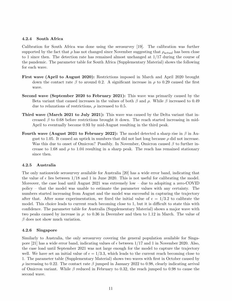
Figure 1: SUTRA Compartmental Diagram: S = Susceptible, U = Undetected, T = Testedpositive, RU = Removed from U , RT = Removed from T . β = contact rate, γ =removal rate(common to both T and U), ε = undetection ratio.

Taken together, these plots show that Omicron bypassed vaccine-only immunity almost com-pletely, but natural immunity provided very good protection. A clear conclusion is that countriesfollowing zero-COVID strategy – strictly control the spread and vaccinate entire population – suf-fered maximum during Omicron wave. Indeed, a perusal of Table 1 shows that in countries wherethe reach was very low before the arrival of the Omicron variant saw very large percentage in-creases in reach thereafter. Hence we conclude that a zero-COVID strategy does not work in thelong run, while the controlled spread strategy is far superior. The country-wise case load historyalso supports this conclusion.

Acknowledgments

The work of MA, DP, TH, Arti S, Avaneesh S, & Prabal S was supported by grants from CII andInfosys Foundation, and MV was supported by the Science and Engineering Research Board, India.

5 Figures and Tables

6 Supplementary Material

7 Derivation of the Fundamental Relationship

We first construct a model for the evolution of the pandemic. It is a mean-field model, thatanalyzes the average values of various quantities at a societal level. This approach is in contrast toagent-based models that adopt a much more fine-grained analysis.

The members of the group under study are divided into five nonoverlapping compartments,namely S (Susceptible), U (Undetected), T (Tested positive), RU (Recovered from the U compart-ment), and RT (Recovered from the T compartment). As is the convention, we use letters S, U , T ,RU , and RT to these symbols denote the fraction of population in the corresponding compartment.

At present, in most countries, persons in the group T (whether symptomatic or not) are mostlyquarantined, and it can be assumed that for the most part, they do not come into contact withthe susceptible population S. Therefore persons in group S get infected mostly through contactwith group U of undetected infected patients, with a likelihood of β. Finally, it is obvious that allinfected persons are initially undetected, and thus enter group U . In turn some part of U , call it

13

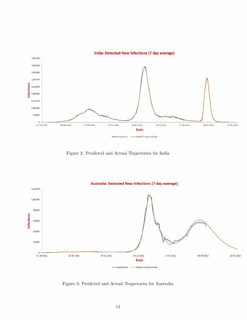
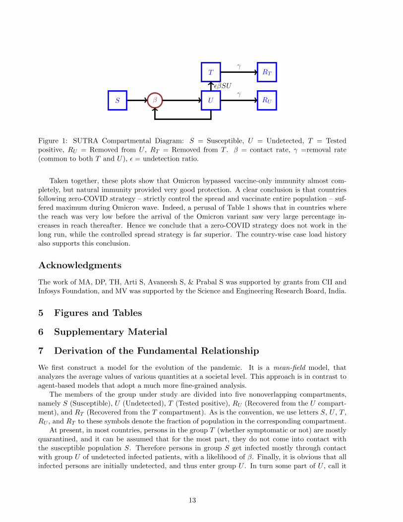
Figure 2: Predicted and Actual Trajectories for India

Figure 3: Predicted and Actual Trajectories for Australia

14

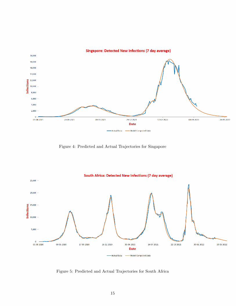
Figure 4: Predicted and Actual Trajectories for Singapore

Figure 5: Predicted and Actual Trajectories for South Africa

15

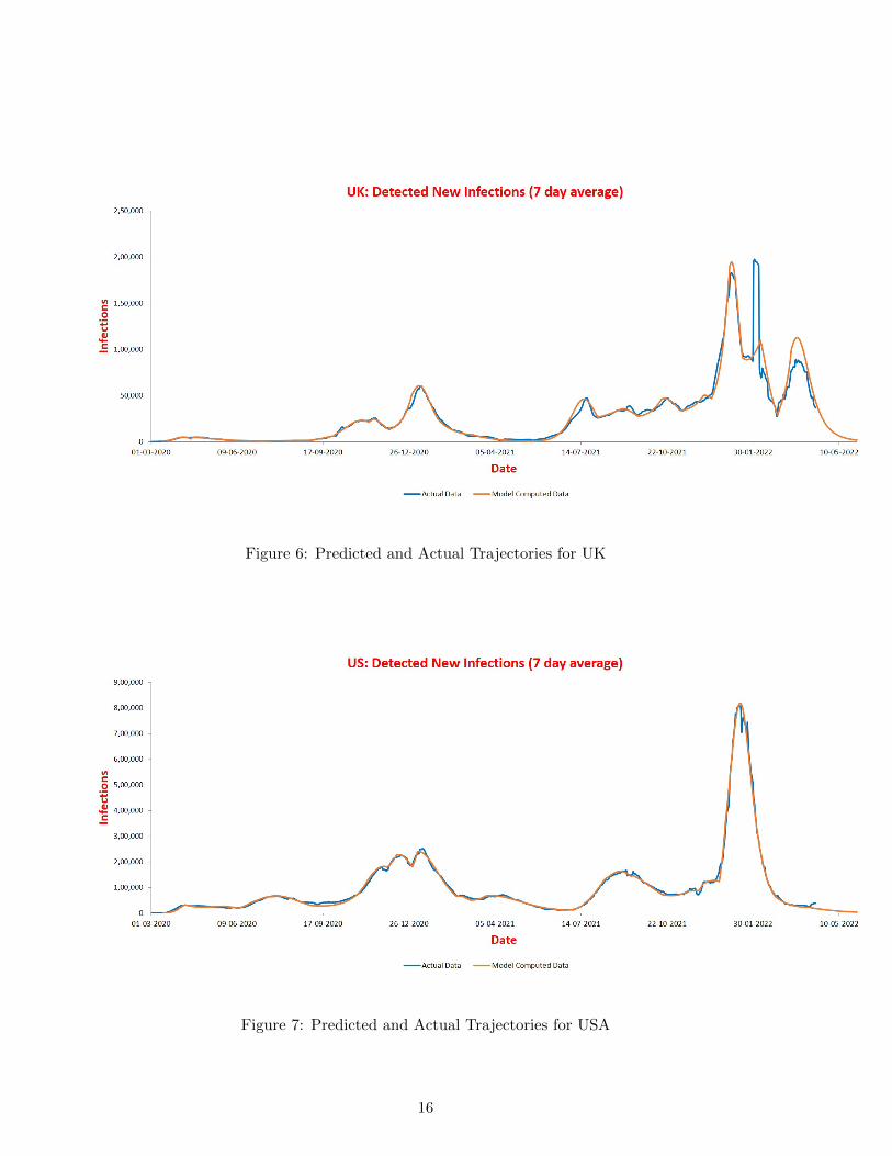
Figure 6: Predicted and Actual Trajectories for UK

Figure 7: Predicted and Actual Trajectories for USA

16

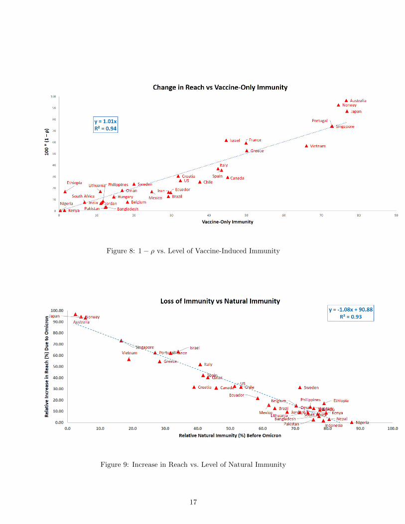
Figure 8: 1− ρ vs. Level of Vaccine-Induced Immunity

Figure 9: Increase in Reach vs. Level of Natural Immunity

17

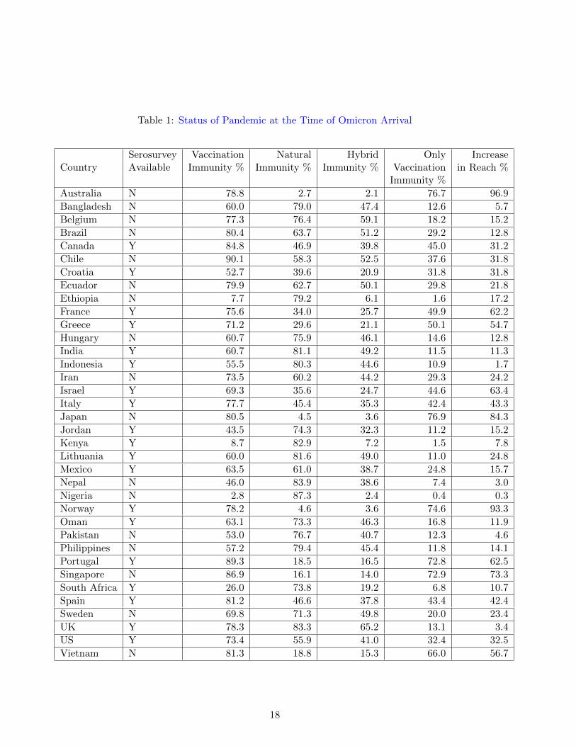
Table 1: Status of Pandemic at the Time of Omicron Arrival

Serosurvey Vaccination Natural Hybrid Only IncreaseCountry Available Immunity % Immunity % Immunity % Vaccination in Reach %

Immunity %

Australia N 78.8 2.7 2.1 76.7 96.9

Bangladesh N 60.0 79.0 47.4 12.6 5.7

Belgium N 77.3 76.4 59.1 18.2 15.2

Brazil N 80.4 63.7 51.2 29.2 12.8

Canada Y 84.8 46.9 39.8 45.0 31.2

Chile N 90.1 58.3 52.5 37.6 31.8

Croatia Y 52.7 39.6 20.9 31.8 31.8

Ecuador N 79.9 62.7 50.1 29.8 21.8

Ethiopia N 7.7 79.2 6.1 1.6 17.2

France Y 75.6 34.0 25.7 49.9 62.2

Greece Y 71.2 29.6 21.1 50.1 54.7

Hungary N 60.7 75.9 46.1 14.6 12.8

India Y 60.7 81.1 49.2 11.5 11.3

Indonesia Y 55.5 80.3 44.6 10.9 1.7

Iran N 73.5 60.2 44.2 29.3 24.2

Israel Y 69.3 35.6 24.7 44.6 63.4

Italy Y 77.7 45.4 35.3 42.4 43.3

Japan N 80.5 4.5 3.6 76.9 84.3

Jordan Y 43.5 74.3 32.3 11.2 15.2

Kenya Y 8.7 82.9 7.2 1.5 7.8

Lithuania Y 60.0 81.6 49.0 11.0 24.8

Mexico Y 63.5 61.0 38.7 24.8 15.7

Nepal N 46.0 83.9 38.6 7.4 3.0

Nigeria N 2.8 87.3 2.4 0.4 0.3

Norway Y 78.2 4.6 3.6 74.6 93.3

Oman Y 63.1 73.3 46.3 16.8 11.9

Pakistan N 53.0 76.7 40.7 12.3 4.6

Philippines N 57.2 79.4 45.4 11.8 14.1

Portugal Y 89.3 18.5 16.5 72.8 62.5

Singapore N 86.9 16.1 14.0 72.9 73.3

South Africa Y 26.0 73.8 19.2 6.8 10.7

Spain Y 81.2 46.6 37.8 43.4 42.4

Sweden N 69.8 71.3 49.8 20.0 23.4

UK Y 78.3 83.3 65.2 13.1 3.4

US Y 73.4 55.9 41.0 32.4 32.5

Vietnam N 81.3 18.8 15.3 66.0 56.7

18

Figure 10: Increase in Reach vs. Level of Vaccine-Induced Immunity

NT , gets tested positive and moves to T , while another part moves towards recovery. This leads to

S = −βSU, U = βSU −NT − γUUT = NT − γTT, RU = γUU, RT = γTT.

where γU is the rate of removal from U , and γT is the rate of removal from T .Although removal rates for symptomatic (= γI) and asymptomatic (= γA) groups are reported

to differ by a few days [33], removal rates for U (= γU ) and T (= γT ) groups are much closer:

Lemma 1. Let f be the fraction of symptomatic cases in T and g be the fraction of symptomaticcases in U . Then,

γT − γU = (f − g) · (γI − γA).

Proof. We have γT = fγI + (1 − f)γA and γU = gγI + (1 − g)γA. Therefore, γT − γU = (f − g) ·(γI − γA).

We can assume that f > g since symptomatic patients are more likely to get tested. In case fand g do not differ by much (in US [34], f − g < 1/8) or f is significantly smaller than 1 (in India[35], f < 1/10), γT ≈ γU since gI − gA is not more than five days [33, 36].

Above justifies the following simplification:

γU = γT = γ.

The equations then simplify to:

S = −βSU, U = βSU −NT − γUT = NT − γT, RU = γU, RT = γT.

19

Thus the model formulation is complete once we specify NT , the fraction tested positive at time t.One possibility is to assume that everyone in U is equally likely to get detected, so that NT = δU ,for some δ > 0. This would lead to

U = βSU − δU − γU, T = δU − γT.

This is the conventional approach, used in earlier models like SAIR and SEIR. However, detectionof COVID-19 cases is biased towards more recently infected due to contact tracing. Divide T intotwo subgroups: TC containing those that are detected through contact tracing and TNC are therest.

Lemma 2. Suppose an infected person infects R0 other persons. Further, suppose that upon de-tection of a positive case, all who came in contact with the infected person are also tested. Then,the expected number of days a person in T stays in U is R0+2

2(R0+1)k, where k is the average numberof days a person in TNC stays in U .

Proof. Observe that |TC | = 1R0+1 |T | since for every initiating case, contact tracing will find R0

additional cases on average. The cases detected via contact tracing would be infected after theinitiating case, and therefore, between 1 and k − 1 days ago. These are expected to be uniformlydistributed in the range [1, k − 1] and therefore, the expected number of days a person in T staysin U equals:

pk +k−1∑i=1

1− pk − 1

i = pk +1− p

2k

=1 + p

2k

=R0 + 2

2(R0 + 1)k

The mean duration for which a symptomatic case remained infected was estimated to be around13.4 in [33]. However, the movement from T to RT is likely to happen more quickly, since a personmay stop infecting others while still being RTPCR positive. (This number is lestimated to be lessthan 10 days for symptomatic cases in [36]). The average duration of stay in U for a person inTC is likely to be less than half of above duration, so k is less than 5. For Covid-19, the values ofR0 has been estimated to be in the range [3, 6] depending on the mutant. Therefore, the expectednumber of days a person in T stays in U is less than 4.

The above analysis shows that the cases that move from U to T are significantly biased towardsrecently infected ones, and therefore, it is better to set NT to be proportional to a fraction ofrecently infected cases. This number can be taken to be proportional to βSU , the fraction ofpersons who got infected most recently, as the number of cases do not change significantly overa window of few days. Therefore we choose NT = εβSU , with ε being another parameter of themodel. With this assumption, the full SUTRA model becomes

S = −βSU, (5)

U = βSU − εβSU − γU, T = εβSU − γT, (6)

RU = γU, RT = γT. (7)

20

S U T RβSU NT = εβSU γT

γU

Figure 11: Flowchart of the SUTRA model

A compartmental diagram depicting the SUTRA model is given in Figure 11.The acronym SUTRA stands for Susceptible, Undetected, Tested (positive), and Removed

(recovered or dead) Approach. Susceptible, The word Sutra also means an aphorism. Sutras are agenre of ancient and medieval Hindu texts, and depict a code strung together by a genre.

It is possible to introduce another parameter D denoting deaths, and write it as D = ηT .However, it is quite easy to estimate η as the ratio between the incremental death totals and theincrease in cumulative positive test cases. Hence that relationship is not shown as a part of theSUTRA model.

8 Analyzing the Model Equations

Defining M = U + T , R = RU +RT , we get from equations (6) and (7) that

M + R = βSU =1

ε(T + RT ), (8)

resulting in

M +R =1

ε(T +RT ) + c (9)

for an appropriate constant of integration c. Adding equations (6) gives

M = βSU − γM =1

ε(T + γT )− γM,

ord(Meγt)

dt=

1

ε

d(Teγt)

dt, (10)

resulting in

M =1

εT + de−γt (11)

for some constant d. Since e−γt is a decaying exponential, it follows that, except for an initialtransient period, the relationship M = (1/ε)I holds. This in turn implies that

U = M − T =1− εε

T.

How long is the transient period? Observe that the constant d equals M(0) − (1/ε)T (0) which isclose to zero since fraction of infected cases at the start of pandemic is very small. Therefore thetransient period will not last more than a few days. As we will see later, such transient periodswill recur at various stages of pandemic and all of them remain small.

21

These simplifications allow us to rewrite equation (8) as:

NT = εβSU = β(1− ε)ST= β(1− ε)(1− (M +R))T

= β(1− ε)(1− 1

ε(T +RT )− c)T

= β(1− ε)(1− c)T − β(1− ε)ε

(T +RT )T

(12)

Rearrange (12) as

T =1

βNT +

1

ε(1− c)(T +RT )T, (13)

whereβ = β(1− ε)(1− c).

9 Discretization of the Model Relationships

The progression of a pandemic is typically reported via two daily statistics: The number of peoplewho test positive, and the number of people who are removed (including both recoveries anddeaths). However, there is a difficulty with the second statistic: there is no consensus on when toclassify an infected person as removed. Some do it when RTPCR test is negative, some do it whensymptoms are absent after a predefined period, and some others do it after a fixed period of timeirrespective of symptoms. For the purpose of modeling, a person should be classified as recoveredat the time when that person is no longer capable of infecting others. This is difficult to ascertain,for which reason this criterion is almost never used. Further, some countries (UK for example) donot report this statistic at all. In such a situation, we do not rely on reported data, and insteadcompute RT by fixing γ to an appropriate value as discussed in section on parameter estimation.

Let T (t) denote the number of detected cases who are capable of infecting others on day t,RT (t) denote the number of detected cases that are removed on or before day t, and NT (t) denotethe number of cases detected on day t. Note that, in this notation, all three are integers, and t isalso a discrete counter. In contrast, in the SUTRA model, T , RT and NT are fractions in [0, 1],while t is a continuum. In order to infer these fractions from the case numbers, we observe that

T =TP,RT =

RTP,NT =

NTP

where P is the effective population that is potentially affected by the pandemic. Now we introducethe parameter measuring the spread of the pandemic. We define a number ρ, called the “reach,”which equals P/P0, where P is the effective population and P0 is the total population of the groupunder study, e.g., the entire country, or an individual state, or a district (this parameter is alsointroduced and studied in [37]). The reach parameter ρ is usually nondecreasing, starts at 0,and increases towards 1 over time (situations where it decreases are discussed later). While theunderlying population P0 is known, the reach ρ is not known and must be inferred from the data.

Substituting P = ρP0,

T = PT = ρP0T,RT = PRT = ρP0RT ,NT = PNT = ρP0NT

22

into (13) gives a relationship that involves only measurable and computable quantities T , RT andNT , and the parameters of the model, namely

T =1

βNT +

1

ρP0(T +RT )T , (14)

whereρ = ερ(1− c).

Eq. (14) is the fundamental equation governing the pandemic. It establishes a relationship betweenNT , T , and (T +RT )T , first of which is directly measurable and the remaining two are computableonce γ is fixed.

Finally, we integrate (14) over seven days because reported daily case numbers usually have aweekly periodicity to them. The integration will be a summation since T , RT and NT are availableat only discrete time instants. This gives

t∑s=t−6

T (s) =1

β

t+1∑s=t−5

NT (s) +1

ρP0

t∑s=t−6

[T (s) +RT (s)]T (s). (15)

Note that sum for NT is shifted forward by one day since new infections reported on day t+ 1 aredetermined by active infections and susceptible population on day t.

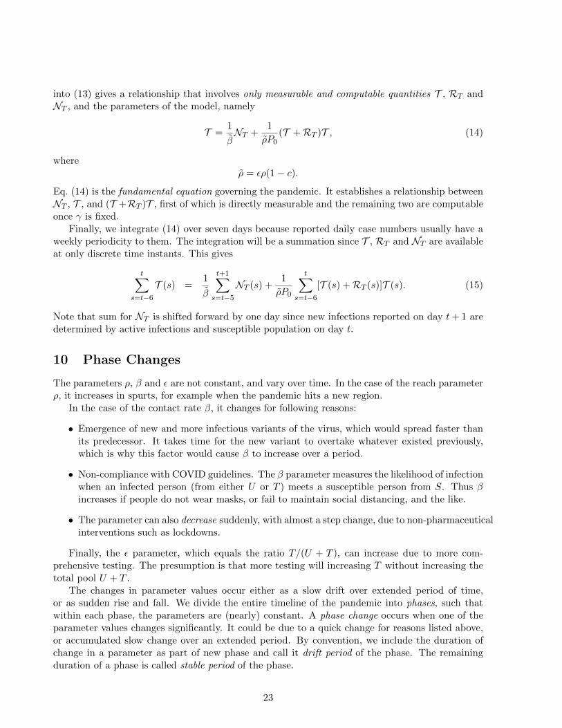
10 Phase Changes

The parameters ρ, β and ε are not constant, and vary over time. In the case of the reach parameterρ, it increases in spurts, for example when the pandemic hits a new region.

In the case of the contact rate β, it changes for following reasons:

• Emergence of new and more infectious variants of the virus, which would spread faster thanits predecessor. It takes time for the new variant to overtake whatever existed previously,which is why this factor would cause β to increase over a period.

• Non-compliance with COVID guidelines. The β parameter measures the likelihood of infectionwhen an infected person (from either U or T ) meets a susceptible person from S. Thus βincreases if people do not wear masks, or fail to maintain social distancing, and the like.

• The parameter can also decrease suddenly, with almost a step change, due to non-pharmaceuticalinterventions such as lockdowns.

Finally, the ε parameter, which equals the ratio T/(U + T ), can increase due to more com-prehensive testing. The presumption is that more testing will increasing T without increasing thetotal pool U + T .

The changes in parameter values occur either as a slow drift over extended period of time,or as sudden rise and fall. We divide the entire timeline of the pandemic into phases, such thatwithin each phase, the parameters are (nearly) constant. A phase change occurs when one of theparameter values changes significantly. It could be due to a quick change for reasons listed above,or accumulated slow change over an extended period. By convention, we include the duration ofchange in a parameter as part of new phase and call it drift period of the phase. The remainingduration of a phase is called stable period of the phase.

23

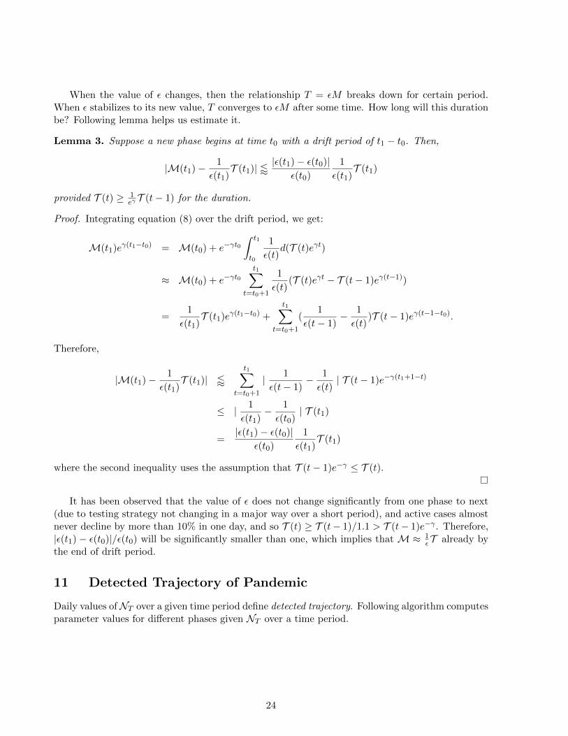
When the value of ε changes, then the relationship T = εM breaks down for certain period.When ε stabilizes to its new value, T converges to εM after some time. How long will this durationbe? Following lemma helps us estimate it.

Lemma 3. Suppose a new phase begins at time t0 with a drift period of t1 − t0. Then,

|M(t1)− 1

ε(t1)T (t1)| / |ε(t1)− ε(t0)|

ε(t0)

1

ε(t1)T (t1)

provided T (t) ≥ 1eγ T (t− 1) for the duration.

Proof. Integrating equation (8) over the drift period, we get:

M(t1)eγ(t1−t0) = M(t0) + e−γt0∫ t1

t0

1

ε(t)d(T (t)eγt)

≈ M(t0) + e−γt0t1∑

t=t0+1

1

ε(t)(T (t)eγt − T (t− 1)eγ(t−1))

=1

ε(t1)T (t1)eγ(t1−t0) +

t1∑t=t0+1

(1

ε(t− 1)− 1

ε(t))T (t− 1)eγ(t−1−t0).

Therefore,

|M(t1)− 1

ε(t1)T (t1)| /

t1∑t=t0+1

| 1

ε(t− 1)− 1

ε(t)| T (t− 1)e−γ(t1+1−t)

≤ | 1

ε(t1)− 1

ε(t0)| T (t1)

=|ε(t1)− ε(t0)|

ε(t0)

1

ε(t1)T (t1)

where the second inequality uses the assumption that T (t− 1)e−γ ≤ T (t).

It has been observed that the value of ε does not change significantly from one phase to next(due to testing strategy not changing in a major way over a short period), and active cases almostnever decline by more than 10% in one day, and so T (t) ≥ T (t− 1)/1.1 > T (t− 1)e−γ . Therefore,|ε(t1) − ε(t0)|/ε(t0) will be significantly smaller than one, which implies that M ≈ 1

εT already bythe end of drift period.

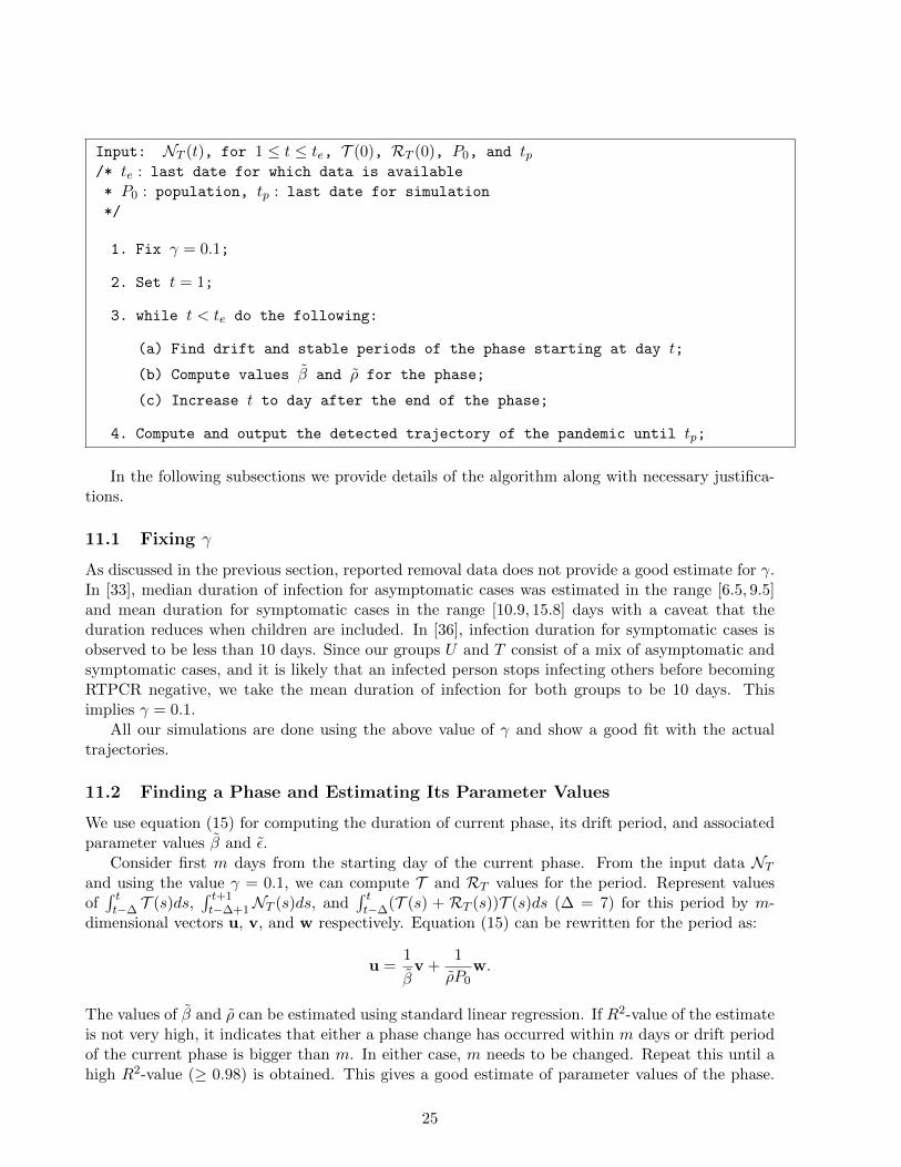
11 Detected Trajectory of Pandemic

Daily values ofNT over a given time period define detected trajectory. Following algorithm computesparameter values for different phases given NT over a time period.

24

Input: NT (t), for 1 ≤ t ≤ te, T (0), RT (0), P0, and tp/* te : last date for which data is available

* P0 : population, tp : last date for simulation

*/

1. Fix γ = 0.1;

2. Set t = 1;

3. while t < te do the following:

(a) Find drift and stable periods of the phase starting at day t;

(b) Compute values β and ρ for the phase;

(c) Increase t to day after the end of the phase;

4. Compute and output the detected trajectory of the pandemic until tp;

In the following subsections we provide details of the algorithm along with necessary justifica-tions.

11.1 Fixing γ

As discussed in the previous section, reported removal data does not provide a good estimate for γ.In [33], median duration of infection for asymptomatic cases was estimated in the range [6.5, 9.5]and mean duration for symptomatic cases in the range [10.9, 15.8] days with a caveat that theduration reduces when children are included. In [36], infection duration for symptomatic cases isobserved to be less than 10 days. Since our groups U and T consist of a mix of asymptomatic andsymptomatic cases, and it is likely that an infected person stops infecting others before becomingRTPCR negative, we take the mean duration of infection for both groups to be 10 days. Thisimplies γ = 0.1.

All our simulations are done using the above value of γ and show a good fit with the actualtrajectories.

11.2 Finding a Phase and Estimating Its Parameter Values

We use equation (15) for computing the duration of current phase, its drift period, and associatedparameter values β and ε.

Consider first m days from the starting day of the current phase. From the input data NTand using the value γ = 0.1, we can compute T and RT values for the period. Represent valuesof∫ tt−∆ T (s)ds,

∫ t+1t−∆+1NT (s)ds, and

∫ tt−∆(T (s) + RT (s))T (s)ds (∆ = 7) for this period by m-

dimensional vectors u, v, and w respectively. Equation (15) can be rewritten for the period as:

u =1

βv +

1

ρP0w.

The values of β and ρ can be estimated using standard linear regression. If R2-value of the estimateis not very high, it indicates that either a phase change has occurred within m days or drift periodof the current phase is bigger than m. In either case, m needs to be changed. Repeat this until ahigh R2-value (≥ 0.98) is obtained. This gives a good estimate of parameter values of the phase.

25

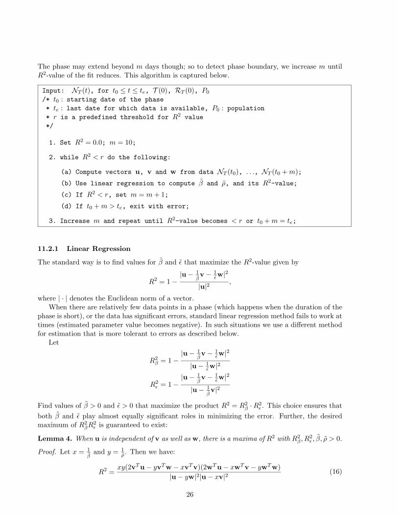
The phase may extend beyond m days though; so to detect phase boundary, we increase m untilR2-value of the fit reduces. This algorithm is captured below.

Input: NT (t), for t0 ≤ t ≤ te, T (0), RT (0), P0

/* t0 : starting date of the phase

* te : last date for which data is available, P0 : population

* r is a predefined threshold for R2 value

*/

1. Set R2 = 0.0; m = 10;

2. while R2 < r do the following:

(a) Compute vectors u, v and w from data NT (t0), . . ., NT (t0 +m);

(b) Use linear regression to compute β and ρ, and its R2-value;

(c) If R2 < r, set m = m+ 1;

(d) If t0 +m > te, exit with error;

3. Increase m and repeat until R2-value becomes < r or t0 +m = te;

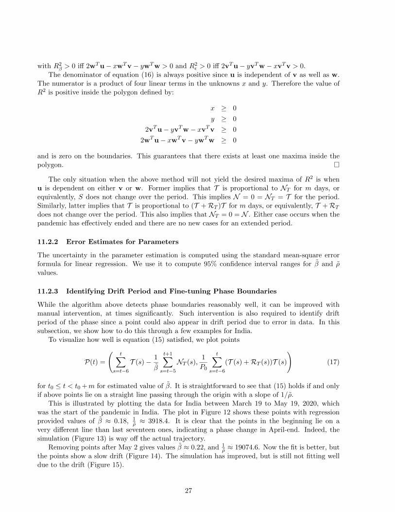
11.2.1 Linear Regression

The standard way is to find values for β and ε that maximize the R2-value given by

R2 = 1−|u− 1

βv − 1

εw|2

|u|2,

where | · | denotes the Euclidean norm of a vector.When there are relatively few data points in a phase (which happens when the duration of the

phase is short), or the data has significant errors, standard linear regression method fails to work attimes (estimated parameter value becomes negative). In such situations we use a different methodfor estimation that is more tolerant to errors as described below.

Let

R2β = 1−

|u− 1βv − 1

εw|2

|u− 1εw|2

R2ε = 1−

|u− 1βv − 1

εw|2

|u− 1βv|2

Find values of β > 0 and ε > 0 that maximize the product R2 = R2β ·R2

ε . This choice ensures that

both β and ε play almost equally significant roles in minimizing the error. Further, the desiredmaximum of R2

βR2ε is guaranteed to exist:

Lemma 4. When u is independent of v as well as w, there is a maxima of R2 with R2β, R

2ε , β, ρ > 0.

Proof. Let x = 1β

and y = 1ρ . Then we have:

R2 =xy(2vTu− yvTw − xvTv)(2wTu− xwTv − ywTw)

|u− yw|2|u− xv|2(16)

26

with R2β > 0 iff 2wTu− xwTv − ywTw > 0 and R2

ε > 0 iff 2vTu− yvTw − xvTv > 0.The denominator of equation (16) is always positive since u is independent of v as well as w.

The numerator is a product of four linear terms in the unknowns x and y. Therefore the value ofR2 is positive inside the polygon defined by:

x ≥ 0

y ≥ 0

2vTu− yvTw − xvTv ≥ 0

2wTu− xwTv − ywTw ≥ 0

and is zero on the boundaries. This guarantees that there exists at least one maxima inside thepolygon.

The only situation when the above method will not yield the desired maxima of R2 is whenu is dependent on either v or w. Former implies that T is proportional to NT for m days, orequivalently, S does not change over the period. This implies N = 0 = NT = T for the period.Similarly, latter implies that T is proportional to (T +RT )T for m days, or equivalently, T +RTdoes not change over the period. This also implies that NT = 0 = N . Either case occurs when thepandemic has effectively ended and there are no new cases for an extended period.

11.2.2 Error Estimates for Parameters

The uncertainty in the parameter estimation is computed using the standard mean-square errorformula for linear regression. We use it to compute 95% confidence interval ranges for β and ρvalues.

11.2.3 Identifying Drift Period and Fine-tuning Phase Boundaries

While the algorithm above detects phase boundaries reasonably well, it can be improved withmanual intervention, at times significantly. Such intervention is also required to identify driftperiod of the phase since a point could also appear in drift period due to error in data. In thissubsection, we show how to do this through a few examples for India.

To visualize how well is equation (15) satisfied, we plot points

P(t) =

(t∑

s=t−6

T (s)− 1

β

t+1∑s=t−5

NT (s),1

P0

t∑s=t−6

(T (s) +RT (s))T (s)

)(17)

for t0 ≤ t < t0 +m for estimated value of β. It is straightforward to see that (15) holds if and onlyif above points lie on a straight line passing through the origin with a slope of 1/ρ.

This is illustrated by plotting the data for India between March 19 to May 19, 2020, whichwas the start of the pandemic in India. The plot in Figure 12 shows these points with regressionprovided values of β ≈ 0.18, 1

ρ ≈ 3918.4. It is clear that the points in the beginning lie on avery different line than last seventeen ones, indicating a phase change in April-end. Indeed, thesimulation (Figure 13) is way off the actual trajectory.

Removing points after May 2 gives values β ≈ 0.22, and 1ρ ≈ 19074.6. Now the fit is better, but

the points show a slow drift (Figure 14). The simulation has improved, but is still not fitting welldue to the drift (Figure 15).

27

Figure 12: India Phase Plot Figure 13: India Trajectory



Removing twenty more points reduces the drift (Figure 16), with β ≈ 0.33, 1ρ ≈ 99741.5. R2

value of the fit is greater than 0.999. The simulation shows an excellent fit (Figure 17).We start a new phase from April 12th and plot the points up to June 30th. Last ten points show

a clear deviation from the trajectory of the previous points in Figure 18 (β ≈ 0.14, 1ρ ≈ 348.2), and

simulation confirms the incorrect identification of phase in Figure 19.


28

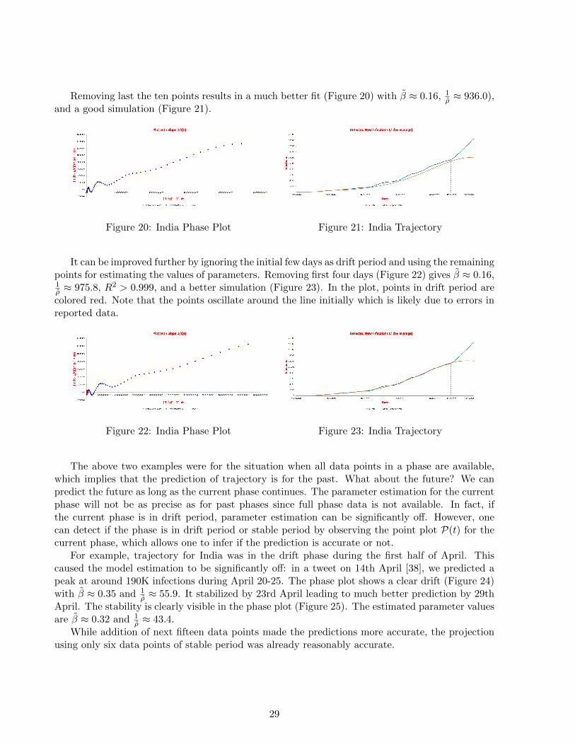
Removing last the ten points results in a much better fit (Figure 20) with β ≈ 0.16, 1ρ ≈ 936.0),

and a good simulation (Figure 21).


It can be improved further by ignoring the initial few days as drift period and using the remainingpoints for estimating the values of parameters. Removing first four days (Figure 22) gives β ≈ 0.16,1ρ ≈ 975.8, R2 > 0.999, and a better simulation (Figure 23). In the plot, points in drift period arecolored red. Note that the points oscillate around the line initially which is likely due to errors inreported data.


The above two examples were for the situation when all data points in a phase are available,which implies that the prediction of trajectory is for the past. What about the future? We canpredict the future as long as the current phase continues. The parameter estimation for the currentphase will not be as precise as for past phases since full phase data is not available. In fact, ifthe current phase is in drift period, parameter estimation can be significantly off. However, onecan detect if the phase is in drift period or stable period by observing the point plot P(t) for thecurrent phase, which allows one to infer if the prediction is accurate or not.

For example, trajectory for India was in the drift phase during the first half of April. Thiscaused the model estimation to be significantly off: in a tweet on 14th April [38], we predicted apeak at around 190K infections during April 20-25. The phase plot shows a clear drift (Figure 24)with β ≈ 0.35 and 1

ρ ≈ 55.9. It stabilized by 23rd April leading to much better prediction by 29thApril. The stability is clearly visible in the phase plot (Figure 25). The estimated parameter valuesare β ≈ 0.32 and 1

ρ ≈ 43.4.While addition of next fifteen data points made the predictions more accurate, the projection

using only six data points of stable period was already reasonably accurate.

29

Figure 24: India Phase Plot Figure 25: India Phase Plot

11.3 Parameter values during drift period

The above calculations give us values of parameters β and ρ post the drift period of every phase.However, in order to simulate the course of the pandemic, it is necessary to have the values of theparameters during the drift period as well.

Suppose d is the number of days in drift period, and b0 and b1 are the computed values of aparameter in the previous and the current phases. Then its value will move from b0 to b1 duringthe drift period. A natural way of fixing its value during the period is to use either arithmetic orgeometric progression. That is, on ith day in the drift period the value is set to b0 + i

d · (b1 − b0)

or b0 · ( b1b0 )i/d respectively.Among these, geometric progression captures the way parameters change better:

• When a new, more infectious, mutant spreads in a population, its infections grow exponen-tially initially. This corresponds to a multiplicative increase in β.

• Similarly, a new virus spreads in a region exponentially at the beginning. This correspondsto a multiplicative increase in ρ.

• A lockdown typically restricts movement sharply causing a multiplicative decrease in β.

• A change in testing strategy typically gets implement fast in a region, causing a multiplicativechange in ε.

For these reasons, we assume that changes in parameters β, ρ, and ε are multiplicative. Further,terms 1− ε and 1− c do not change much during drift period since, as has been observed in actualsimulations, both ε and c remain close to 0. Therefore, multiplicative changes in ε and c almostcoincide with multiplicative changes in 1−ε and 1−c, and so we can assume that these also changegeometrically. This leads to the nice conclusion that changes in β and ρ are also multiplicative.

11.4 Computing the Detected Trajectory

Once we have duration, drift periods, and parameter values for all phases, the trajectory of thepandemic can be computed easily.

Lemma 5. Given T (0), RT (0), γ, P0, Di, di, βi, and ρi for 1 ≤ i ≤ k, where

• P0 is population of the region,

• Di and di are respectively duration and drift period of ith phase,

• βi and ρi are respectively estimated values of parameters for ith phase,

30

the trajectory of detected cases can be computed for the period∑k

i=1Di.

Proof. Proof is by induction on t. Base case of t = 0 is given as input. Suppose T (t), and RT (t)are computed. Then, from (14):

NT (t+ 1) = βtT (t)− βtρtP0

(T (t) +RT (t))T (t).

And

RT (t+ 1) = RT (t) + γT (t)

T (t+ 1) = T (t) +RT (t) +NT (t+ 1)−RT (t+ 1).

where βt and ρt are values of parameters on day t.

Detected trajectory thus is captured by the (4k + 4)-tuple

D = (T (0),RT (0), P0, γ,D1, d1, β1, ρ1, . . . , Dk, dk, βk, ρk).

This shows that detected trajectory can be specified much more compactly than via∑k

i=1Di pointsNT (t).

12 Actual Trajectory of the Pandemic

Similar to quantities associated with detected trajectory, define U = ρP0U ,M = U+T , R = ρP0R,andN = ρP0N . The actual trajectory of the pandemic is given by the daily values ofN (t). There isno way to measure it directly. Is it possible to compute this trajectory given a detected trajectory?It appears unlikely since detected trajectory only provides β and ρ values while actual trajectoryis determined by four parameter β, ρ, ε and c. Given β and ρ, one needs two more parameters εand c for each phase to compute the entire trajectory:

Lemma 6. Given a detected trajectory D, along with M(0), R(0), εi, and ci for 1 ≤ i ≤ k, whereεi and ci are respectively values of parameters ε and c for ith phase, the trajectory of actual casescan be computed for the period

∑ki=1Di.

Proof. Proof is by induction on t. Base case of t = 0 is given as input. Suppose M(t), and R(t)are computed. Then, from SUTRA equations:

βt =βt

(1− εt)(1− ct)

ρt =ρt

εt(1− ct)

N (t+ 1) = βt(1− εt)(

1− 1

ρtP0(M(t) +R(t))

)M(t).

And

R(t+ 1) = R(t) + γM(t)

M(t+ 1) = M(t) +R(t) +N (t+ 1)−R(t+ 1).

where βt, ρt, εt and ct are values of parameters on day t.

31

Potentially, there may be infinitely many different actual trajectories for a given detected tra-jectory. We now prove that, given a detected trajectory and initial values M(0) and R(0), thereare only finitely many actual trajectories. Further, we give a canonical way to identify a uniquetrajectory from them and show how to compute it.

Theorem 1. Given a detected trajectory

D = (T (0),RT (0), P0, γ,D1, d1, β1, ρ1, . . . , Dk, dk, βk, ρk)

along with M(0) and R(0), there exist at most 24∑kj=1 dj actual trajectories satisfying the SUTRA

model that agree with the given detected trajectory and initial values.

Proof. Proof is by induction on the number of phases. In the base case we have only one phase. Forthis phase, d1 = 0 since there are no previous values of parameters. Therefore, parameter valuesstay the same throughout the phase duration of D1 days. Let β1, ρ1, ε1 and c1 be the parametersgoverning the actual trajectory for this phase. From equations (9) and (11):[

M(0)R(0)

]≈[T (0) 0RT (0) P0

]·[ 1

ε1c1ρ1

]giving us excellent approximations of ε1 and c1ρ1. From this, we can compute

ρ1 = ρ1/ε1 + ρ1c1

c1 = c1r1/r1

β1 = β1/(1− ε1)(1− c1)

giving values of all parameters for first phase, using which the trajectory can be computed for thefirst phase uniquely.

Suppose there are at most 22∑i−1j=1 dj trajectories up to phase i− 1. Fix any one trajectory with

values of four parameters in phase i − 1 being βi−1, ρi−1, εi−1 and ci−1. Let t0 =∑i−1

j=1Dj . Wehave: [

M(t0)R(t0)

]=

1

εi−1

[T (t0)RT (t0)

]+ ci−1ρi−1

[0P0

].

Phase i has a drift period of di days and, as we have argued, the parameter values changemultiplicatively during the period. Let εi,j = εi−1x

j , and 1 − ci,j = (1 − ci−1)/yj for 1 ≤ j ≤ di,where x and y are unknown multipliers by which the two parameters change every day. The finalvalue of the parameters will be εi = εi−1x

di and 1− ci = (1− ci−1)/ydi .

Let βi,j = βi−1( βiβi−1

)j/di and ρi,j = ρi−1( ρiρi−1

)j/di , for 1 ≤ j ≤ di. These numbers can be

computed since βi−1, βi, ρi−1, and ρi are known.

Let βi,j =βi,j

(1−εi,j)(1−ci,j) and ρi,j =ρi,j

εi,j(1−ci,j) for 1 ≤ j ≤ di. Then we can write:[M(t0 + j)R(t0 + j)

]=

[gj 0γ 1

]·[M(t0 + j − 1)R(t0 + j − 1)

]

32

where

gj = βi,j−1(1− εi,j−1)(1− M(t0 + j − 1) +R(t0 + j − 1)

ρi,j−1P0)− γ + 1

= βi,j−1(1

1− ci,j−1− εi,j−1

ρi,j−1

M(t0 + j − 1) +R(t0 + j − 1)

P0)− γ + 1

= βi,j−1(yj−1

1− ci−1− εi−1x

j−1

ρi,j−1

M(t0 + j − 1) +R(t0 + j − 1)

P0)− γ + 1

Therefore, bothM(t0 + j) and R(t0 + j) are polynomials in x and y. It is straightforward to showthat the degrees of M(t0 + j) and R(t0 + j) equal 2j − j − 1 and 2j−1 − j − 2 respectively.

At the end of drift period, we have:[M(t0 + di)R(t0 + di)

]=

1

εi

[T (t0 + di)RT (t0 + di)

]+ ciρi

[0P0

]=

1

εi

[T (t0 + di)RT (t0 + di)

]+ ci

ρiεi(1− ci)

[0P0

]=

1

εi−1xdi

[T (t0 + di)RT (t0 + di)

]+

ρiεi−1xdi

(ydi

1− ci−1− 1)

[0P0

](18)

For t0 + di < t ≤ t0 +Di, it inductively follows that:[M(t)R(t)

]=

[βi(1− εi)S(t− 1)− γ + 1 0

γ 1

]·[M(t− 1)R(t− 1)

]=

[βi(1− εi)S(t− 1)− γ + 1 0

γ 1

]·(

1

εi

[T (t− 1)RT (t− 1)

]+ ciρi

[0P0

])=

1

εi

[T (t)RT (t)

]+ ciρi

[0P0

](19)

Therefore, once the relationship is satisfied between actual and detected cases after drift period, itremains valid for rest of the phase.

For what values of unknown multipliers x and y is the relationship satified? Equation (18)provides two polynomials in x and y:[

QM (x, y)QR(x, y)

]= xdi

[M(t0 + di)R(t0 + di)

]− 1

εi−1

[T (t0 + di)RT (t0 + di)

]− ρiεi−1

(ydi

1− ci−1− 1)

[0P0

].

with QM (x, y) of degree 2di−1 and QR(x, y) of degree 2di−1−2, such that the actual multipliers aretheir common roots. Lemma 7 shows that the number of common roots of these two polynomialsthat correspond to a valid solution is at most 24di . Therefore, the number of possible trajectories

after i phases is bounded by 22∑ij=1 dj .

Lemma 7. The number of common roots of polynomials QM (x, y) and QR(x, y) that correspondto a valid solution is at most 24di.

Proof. A valid solution of the equations QM (x, y) = 0 = QR(x, y) needs to be tolerant of errorsin reported data NT (t): one should get a neighboring point as solution if there are small errors indata. Errors in NT (t) for t ≥ t0 + di will cause values of βi and ρi to change. These changes wouldbe small if perturbations of NT (t), t ≥ t0 + di, are small.

33

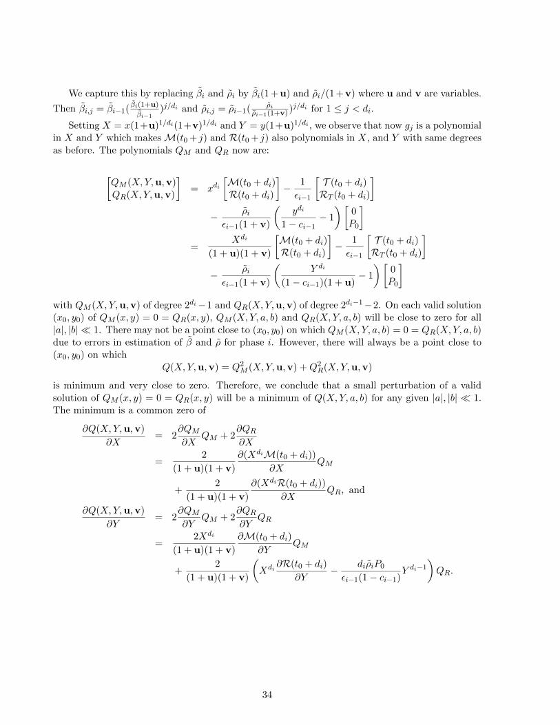
We capture this by replacing βi and ρi by βi(1 +u) and ρi/(1 +v) where u and v are variables.

Then βi,j = βi−1( βi(1+u)

βi−1)j/di and ρi,j = ρi−1( ρi

ρi−1(1+v))j/di for 1 ≤ j < di.

Setting X = x(1+u)1/di(1+v)1/di and Y = y(1+u)1/di , we observe that now gj is a polynomialin X and Y which makesM(t0 + j) and R(t0 + j) also polynomials in X, and Y with same degreesas before. The polynomials QM and QR now are:

[QM (X,Y,u,v)QR(X,Y,u,v)

]= xdi

[M(t0 + di)R(t0 + di)

]− 1

εi−1

[T (t0 + di)RT (t0 + di)

]− ρiεi−1(1 + v)

(ydi

1− ci−1− 1

)[0P0

]=

Xdi

(1 + u)(1 + v)

[M(t0 + di)R(t0 + di)

]− 1

εi−1

[T (t0 + di)RT (t0 + di)

]− ρiεi−1(1 + v)

(Y di

(1− ci−1)(1 + u)− 1

)[0P0

]with QM (X,Y,u,v) of degree 2di−1 and QR(X,Y,u,v) of degree 2di−1−2. On each valid solution(x0, y0) of QM (x, y) = 0 = QR(x, y), QM (X,Y, a, b) and QR(X,Y, a, b) will be close to zero for all|a|, |b| � 1. There may not be a point close to (x0, y0) on which QM (X,Y, a, b) = 0 = QR(X,Y, a, b)due to errors in estimation of β and ρ for phase i. However, there will always be a point close to(x0, y0) on which

Q(X,Y,u,v) = Q2M (X,Y,u,v) +Q2

R(X,Y,u,v)

is minimum and very close to zero. Therefore, we conclude that a small perturbation of a validsolution of QM (x, y) = 0 = QR(x, y) will be a minimum of Q(X,Y, a, b) for any given |a|, |b| � 1.The minimum is a common zero of

∂Q(X,Y,u,v)

∂X= 2

∂QM∂X

QM + 2∂QR∂X

=2

(1 + u)(1 + v)

∂(XdiM(t0 + di))

∂XQM

+2

(1 + u)(1 + v)

∂(XdiR(t0 + di))

∂XQR, and

∂Q(X,Y,u,v)

∂Y= 2

∂QM∂Y

QM + 2∂QR∂Y

QR

=2Xdi

(1 + u)(1 + v)

∂M(t0 + di)

∂YQM

+2

(1 + u)(1 + v)

(Xdi

∂R(t0 + di)

∂Y− diρiP0

εi−1(1− ci−1)Y di−1

)QR.

34

Define,

P1(X,Y,u,v) =(1 + u)2(1 + v)2

2

∂Q

∂X

=∂(XdiM(t0 + di))

∂X

(XdiM(t0 + di)− (1 + u)(1 + v)

T (t0 + di)

εi−1

)+∂(XdiR(t0 + di))

∂X

∗(XdiR(t0 + di)− (1 + u)(1 + v)

RT (t0 + di)

εi−1

−Y diρiP0

εi−1(1− ci−1)+ (1 + u)

ρiP0

εi−1

), and

P2(X,Y,u,v) =(1 + u)2(1 + v)2

2

∂Q

∂Y

= Xdi∂M(t0 + di)

∂Y

(XdiM(t0 + di)− (1 + u)(1 + v)

T (t0 + di)

εi−1

)+

(Xdi

∂(R(t0 + di))

∂Y− diρiP0

εi−1(1− ci−1)Y di−1

)∗(XdiR(t0 + di)− (1 + u)(1 + v)

RT (t0 + di)

εi−1

−Y diρiP0

εi−1(1− ci−1)+ (1 + u)

ρiP0

εi−1

).

Although the upper bound on the number is trajectories is quite large, in practice, most of thecommon roots of the polynomials QM and QR would not satisfy one or more of following conditionsthat should be satisfied by any actual trajectory:

0 < β < 1, 0 < ε < 1, 0 < ρ < 2, −1 < c < 1.

Therefore, most can be eliminated. Further, the value of parameter ε is unlikely to change sig-nificantly from one phase to next since testing strategies do not change dramatically in a shortperiod. This leads to following definition: Given an actual trajectory up to phase i− 1, its canon-ical extension to phase i is the actual trajectory for phase i such that |εi − εi−1| is minimum. Thecanonical actual trajectory is the trajectory obtained by taking the unique trajectory of phase 1and canonically extending it for subsequent phases.

In practice, we have observed that for most of the phases, there is only one actual trajectorycorresponding to the computed detected trajectory that satisfies the above-mentioned range forparameters, which then becomes the canonical actual trajectory.

12.1 Computing the Canonical Trajectory

Given canonical trajectory up to phase i− 1, its canonical extension for phase i can be computedusing standard gradient descent method for each phase provided there is no error in data. However,if data has errors, polynomials QM and QR may not have any common root that corresponds to afeasible trajectory. In such a situation, which is almost always true in practice, we use the methodused in proof of Lemma 7.

35

Observe that when data has errors, even the relationships of equation (19) will not hold. Definepolynomials:

QM,t(x, y) = xdi(M(t) +R(t))− 1

εi−1(T (t) +RT (t) +

βiP0

1− ci−1ydi − βiP0)

QR,t(x, y) = xdi(R(t))− 1

εi−1(RT (t) +

βiP0

1− ci−1ydi − βiP0)

And combine them as:

P (x, y) = Q2M (x, y) +Q2

R(x, y) +

t0+Di∑t=t0+di+1

(Q2M,t(x, y) +Q2

R,t(x, y)).

Instead of finding zeroes of all the polynomials, we find minima of P . Since εi is likely to be closeto εi−1 and the same would be true for 1− ci and 1− ci−1, we choose (x, y) = (1, 1) as the startingpoint. This results in following algorithm:

1. Let Px = ∂P∂x and Py = ∂P

∂y ;

2. Find a common root of polynomials Px and Py using Newton’s gradient descent

method, starting from point (1, 1);

Note that the common root in the above algorithm can be found quickly even though thedegree of polynomials Px and Py is exponential, since evaluation of the polynomials and theirpartial derivatives at any point can be done efficiently.

The above algorithm computes canonical trajectory for all phase except the first one. Thetrajectory of the first phase cannot be computed since M(0) and R(0) values are not known andtherefore, neither are ε1 and c1. We can estimate c1 by observing that at time t = 0, the pandemicis in its initial stages and so R(0) ≈ 0. This, in turn implies that 1

ε1RT (0) ≈ 0 and so c1 ≈ 0.

This only leaves ε1 as unknown. We can get a good estimate of ε1 if a serosurvey of the regionunder consideration is done at any point of time, say at ts. The survey provides an estimate ofR(ts). Varying ε1, we can compute different canonical trajectories and find the one for which thetrajectory-computed value of R(ts) comes close to the serosurvey result. Alternately, if a regionhas not imposed lockdown or restrictions for extended periods and has allowed normal life, wemay assume that the ρ is close to 1 after 18-20 months. By varying ε1, we can compute differentcanonical trajectories and find the one for which value of ρ is close to 1 after 18-20 months. We callthis step calibrating the model. More than one serosurveys allow fine-tuning of ε1, and thus bettercalibration.

The above analysis leads to the following corollary of Theorem 1:

Corollary 1. For a detected trajectory D, its canonical actual trajectory is given by A = (ε1,D).

12.2 Error Estimates for the Parameters

Error estimates for all the parameters can be derived using the estimates for β and ρ in the followingway: use upper and lower bounds of parameters β and ρ (for their 95% CI values) in the polynomialP (x, y) and compute the values ε and c that minimize P . These provide upper and lower boundsfor ε and c respectively. Using these, compute upper and lower bounds for other two parameters βand ρ. Thus we get 95% CI range of values for all the parameters.

36

13 SUTRA and SIR Trajectories

Both detected and actual trajectories of SUTRA model are a concatenation of multiple SIR tra-jectories, one for each phase.

Theorem 2. For stable period of phase i:

• The detected trajectory is the trajectory of an SIR model with contact parameter βi andpopulation ρiP0.

• The actual trajectory is the trajectory of an SIR model with contact parameter βi(1− εi) andpopulation ρiP0.

Proof. We have

S

1− ci= −βi

S

1− ciU = −βi(1− εi)

εi

S

1− ciT = −βi

S

1− ciTρiP0

TρiP0

=1

εi(1− ci)T =

1

εi(1− ci)(βi(1− εi)ST − γT ) = βi

S

1− ciTρiP0

− γ TρiP0

RTρiP0

=1

εi(1− ci)RT =

1

εi(1− ci)γT = γ

TρiP0

Therefore, S = S1−ci , T = T

ρiP0, and RT = RT

ρiP0follow SIR trajectory with contact rate βi, removal

rate γ, and population ρiP0.For the actual trajectory, we have

S = −βiSU = βi(1− εi)SM = −βi(1− εi)SMρiP0

MρiP0

= βi(1− εi)SMεiP0

− γ MρiP0

RρiP0

= γMρiP0

Therefore, S, M = MρiP0

, and R = RρiP0

follow SIR trajectory with contact rate βi(1− εi), removalrate γ, and population ρiP0.

During the drift period of a phase, SUTRA trajectory transitions from one SIR trajectory toanother. The above theorem explains why Covid-19 trajectories for short periods could be capturedwell by SIR models or their variants. The theorem also allows us to estimate the peak of activeinfections, both for detected and actual trajectories.

13.1 Peak of Active Infections

If active infections in detected trajectory peak in phase i, S = γ

βiat the peak. Since

S = 1− (M + R)

= 1− T +RTρiP0

37

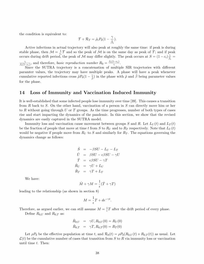
the condition is equivalent to:

T +RT = ρiP0(1− γ

βi).

Active infections in actual trajectory will also peak at roughly the same time: if peak is duringstable phase, then M = 1

εiT and so the peak of M is on the same day as peak of T ; and if peak

occurs during drift period, the peak ofM may differ slightly. The peak occurs at S = (1− ci) γβi =

γβi(1−εi) , and therefore, basic reproduction number R0 = βi(1−εi)

γ .Since the SUTRA trajectory is a concatenation of multiple SIR trajectories with different

paramter values, the trajectory may have multiple peaks. A phase will have a peak whenevercumulative reported infections cross ρP0(1− γ

β) in the phase with ρ and β being parameter values

for the phase.

14 Loss of Immunity and Vaccination Induced Immunity

It is well-established that some infected people lose immunity over time [39]. This causes a transitionfrom R back to S. On the other hand, vaccination of a person in S can directly move him or herto R without going through U or T groups. As the time progresses, number of both types of casesrise and start impacting the dynamics of the pandemic. In this section, we show that the reviseddynamics are easily captured in the SUTRA model.

Immunity loss and vaccination cause movement between groups S and R. Let LU (t) and LT (t)be the fraction of people that move at time t from S to RU and to RT respectively. Note that LU (t)would be negative if people move from RU to S and similarly for RT . The equations governing thedynamics change as follows:

S = −βSU − LU − LTU = βSU − εβSU − γUT = εβSU − γT

RU = γU + LU

RT = γT + LT

We have:

M + γM =1

ε(T + γT )

leading to the relationship (as shown in section 8)

M =1

εT + de−γt.

Therefore, as argued earlier, we can still assume M = 1εT after the drift period of every phase.

Define R0,U and R0,T as:

R0,U = γU,R0,U (0) = RU (0)

R0,T = γT,R0,T (0) = RT (0)

Let ρP0 be the effective population at time t, and R0(t) = ρP0(R0,U (t) +R0,T (t)) as usual. LetL(t) be the cumulative number of cases that transition from S to R via immunity loss or vaccinationuntil time t. Then:

38

Lemma 8. R(t) = R0(t) + L(t).

Proof. Follows immediately from the observation that R− R0 = LU + LT .

Let N(t) be the fraction of population infected at time t as usual. The following lemma iscrucial:

Lemma 9.

N = β(1− ε)(1− LρP0

)(1− M+R0

ρ(1− LρP0

)P0

)M.

Proof. We have:

N = βSU

= β(1− ε)SM= β(1− ε)(1− (M +R))M

= β(1− ε)(1− M+R0 + LρP0

)M

= β(1− ε)(1− LρP0− M+R0

ρP0)M

= β(1− ε)(1− LρP0

)(1− M+R0

ρ(1− LρP0

)P0

)M.

The above lemma shows that:

Corollary 2. The trajectory N (t) of the modified model equals the SUTRA trajectory with both βand ρ multiplied by 1− L

ρP0.

Therefore, ones does not need to modify the model in order to capture the effect of immunityloss and vaccination on the trajectory. The computed detected trajectory from the reported dataNT (t) provides the values

β = β(1− ε)(1− c)(1− LρP0

), ρ = ερ(1− c)(1− LρP0

),

incorporating their impact and thus the model still captures the detected trajectory well. Comput-ing actual trajectory from these parameter values provides values β(1− L

ρP0), ρ(1− L

ρP0), ε amd c for

every phase. While this means that we do not get the real values of β and ρ unless L is estimated,we can use the computed values to predict the near future well.

A byproduct of adjustment in parameter ρ is that it may decrease over time: this will happenwhen the change in L is positive during the drift period of a phase. This is best viewed as reductionin effective population due to vaccination.

15 Estimated Parameters for Various Countries

The set of pandemic parameters were estimated for each phase within each country. These estimatedparameters were used to perform forward prediction of the trajectories. These are reported in themain body of the paper for six countries. The actual parameter values for these six countries are

39

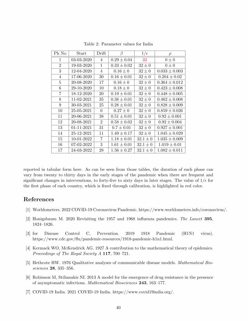
Table 2: Parameter values for India

Ph No Start Drift β 1/ε ρ

1 03-03-2020 4 0.29± 0.04 32 0± 0

2 19-03-2020 1 0.33± 0.02 32± 0 0± 0

3 12-04-2020 4 0.16± 0 32± 0 0.033± 0.003

4 17-06-2020 30 0.16± 0.01 32± 0 0.204± 0.02

5 20-08-2020 17 0.16± 0 32± 0 0.364± 0.012

6 29-10-2020 10 0.18± 0 32± 0 0.423± 0.008

7 18-12-2020 20 0.19± 0.01 32± 0 0.448± 0.005

8 11-02-2021 35 0.38± 0.01 32± 0 0.462± 0.008

9 30-03-2021 25 0.28± 0.01 32± 0 0.828± 0.009

10 25-05-2021 0 0.27± 0 32± 0 0.859± 0.026

11 20-06-2021 38 0.51± 0.01 32± 0 0.92± 0.001

12 20-08-2021 2 0.58± 0.02 32± 0 0.92± 0.004

13 01-11-2021 31 0.7± 0.01 32± 0 0.927± 0.001

14 25-12-2021 11 1.49± 0.17 32± 0 1.045± 0.029

15 10-01-2022 7 1.18± 0.01 32.1± 0 1.035± 0.009

16 07-02-2022 3 1.61± 0.01 32.1± 0 1.019± 0.01

17 24-03-2022 28 1.56± 0.27 32.1± 0 1.082± 0.011

reported in tabular form here. As can be seen from those tables, the duration of each phase canvary from twenty to thirty days in the early stages of the pandemic when there are frequent andsignificant changes in interventions, to forty-five to sixty days in later stages. The value of 1/ε forthe first phase of each country, which is fixed through calibration, is highlighted in red color.

References

[1] Worldometers. 2022 COVID-19 Coronavirus Pandemic. https://www.worldometers.info/coronavirus/.

[2] Honigsbaum M. 2020 Revisiting the 1957 and 1968 influenza pandemics. The Lancet 395,1824–1826.

[3] for Disease Control C, Prevention. 2019 1918 Pandemic (H1N1 virus).https://www.cdc.gov/flu/pandemic-resources/1918-pandemic-h1n1.html.

[4] Kermack WO, McKendrick AG. 1927 A contribution to the mathematical theory of epidemics.Proceedings of The Royal Society A 117, 700–721.

[5] Hethcote HW. 1976 Qualitative analyses of communicable disease models. Mathematical Bio-sciences 28, 335–356.

[6] Robinson M, Stilianakis NI. 2013 A model for the emergence of drug resistance in the presenceof asymptomatic infections. Mathematical Biosciences 243, 163–177.

[7] COVID-19 India. 2021 COVID-19 India. https://www.covid19india.org/.

40

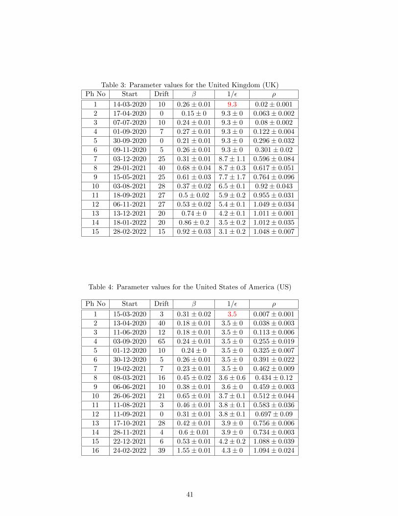
Table 3: Parameter values for the United Kingdom (UK)Ph No Start Drift β 1/ε ρ

1 14-03-2020 10 0.26± 0.01 9.3 0.02± 0.001

2 17-04-2020 0 0.15± 0 9.3± 0 0.063± 0.002

3 07-07-2020 10 0.24± 0.01 9.3± 0 0.08± 0.002

4 01-09-2020 7 0.27± 0.01 9.3± 0 0.122± 0.004

5 30-09-2020 0 0.21± 0.01 9.3± 0 0.296± 0.032

6 09-11-2020 5 0.26± 0.01 9.3± 0 0.301± 0.02

7 03-12-2020 25 0.31± 0.01 8.7± 1.1 0.596± 0.084

8 29-01-2021 40 0.68± 0.04 8.7± 0.3 0.617± 0.051

9 15-05-2021 25 0.61± 0.03 7.7± 1.7 0.764± 0.096

10 03-08-2021 28 0.37± 0.02 6.5± 0.1 0.92± 0.043

11 18-09-2021 27 0.5± 0.02 5.9± 0.2 0.955± 0.031

12 06-11-2021 27 0.53± 0.02 5.4± 0.1 1.049± 0.034

13 13-12-2021 20 0.74± 0 4.2± 0.1 1.011± 0.001

14 18-01-2022 20 0.86± 0.2 3.5± 0.2 1.012± 0.035

15 28-02-2022 15 0.92± 0.03 3.1± 0.2 1.048± 0.007

Table 4: Parameter values for the United States of America (US)


1 15-03-2020 3 0.31± 0.02 3.5 0.007± 0.001

2 13-04-2020 40 0.18± 0.01 3.5± 0 0.038± 0.003

3 11-06-2020 12 0.18± 0.01 3.5± 0 0.113± 0.006

4 03-09-2020 65 0.24± 0.01 3.5± 0 0.255± 0.019

5 01-12-2020 10 0.24± 0 3.5± 0 0.325± 0.007

6 30-12-2020 5 0.26± 0.01 3.5± 0 0.391± 0.022

7 19-02-2021 7 0.23± 0.01 3.5± 0 0.462± 0.009

8 08-03-2021 16 0.45± 0.02 3.6± 0.6 0.434± 0.12

9 06-06-2021 10 0.38± 0.01 3.6± 0 0.459± 0.003

10 26-06-2021 21 0.65± 0.01 3.7± 0.1 0.512± 0.044

11 11-08-2021 3 0.46± 0.01 3.8± 0.1 0.583± 0.036

12 11-09-2021 0 0.31± 0.01 3.8± 0.1 0.697± 0.09

13 17-10-2021 28 0.42± 0.01 3.9± 0 0.756± 0.006

14 28-11-2021 4 0.6± 0.01 3.9± 0 0.734± 0.003

15 22-12-2021 6 0.53± 0.01 4.2± 0.2 1.088± 0.039

16 24-02-2022 39 1.55± 0.01 4.3± 0 1.094± 0.024

41

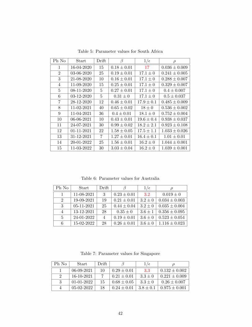
Table 5: Parameter values for South Africa


1 16-04-2020 15 0.18± 0.01 17 0.036± 0.009

2 03-06-2020 25 0.19± 0.01 17.1± 0 0.241± 0.005

3 21-08-2020 10 0.16± 0.01 17.1± 0 0.288± 0.007

4 11-09-2020 15 0.25± 0.01 17.1± 0 0.329± 0.007

5 08-11-2020 5 0.27± 0.01 17.1± 0 0.4± 0.007

6 03-12-2020 5 0.31± 0 17.1± 0 0.5± 0.037

7 28-12-2020 12 0.46± 0.01 17.9± 0.1 0.485± 0.009

8 11-02-2021 40 0.65± 0.02 18± 0 0.536± 0.002

9 11-04-2021 36 0.4± 0.01 18.1± 0 0.752± 0.004

10 06-06-2021 10 0.43± 0.01 19.6± 0.4 0.938± 0.037

11 24-07-2021 30 0.99± 0.02 18.2± 2.1 0.923± 0.108

12 01-11-2021 22 1.58± 0.05 17.5± 1.1 1.033± 0.026

13 31-12-2021 7 1.27± 0.01 16.4± 0.1 1.01± 0.01

14 20-01-2022 25 1.56± 0.01 16.2± 0 1.044± 0.001

15 11-03-2022 30 3.03± 0.04 16.2± 0 1.039± 0.001

Table 6: Parameter values for Australia


1 11-08-2021 3 0.23± 0.01 3.2 0.019± 0

2 19-09-2021 19 0.21± 0.01 3.2± 0 0.034± 0.003

3 05-11-2021 25 0.44± 0.04 3.2± 0 0.035± 0.004

4 13-12-2021 28 0.35± 0 3.6± 1 0.356± 0.095

5 24-01-2022 4 0.19± 0.01 3.6± 0 0.523± 0.054

6 15-02-2022 28 0.26± 0.01 3.6± 0 1.116± 0.023

Table 7: Parameter values for Singapore


1 06-09-2021 10 0.29± 0.01 3.3 0.132± 0.002

2 16-10-2021 7 0.21± 0.01 3.3± 0 0.221± 0.009

3 01-01-2022 15 0.68± 0.05 3.3± 0 0.26± 0.007

4 05-02-2022 18 0.24± 0.01 3.8± 0.1 0.975± 0.001

42

[8] Arora RK, Joseph A, Wyk JV et al.. 2022 Serotracker. https://serotracker.com/en.

[9] Our World in Data. 2022 Vaccination Statistics. https://ourworldindata.org/covid-vaccinations.

[10] Manindra Agrawal. 2021 Tweet on 29th April. https://twitter.com/agrawalmanindra/

status/1387734516807073792?s=20.

[11] Manindra Agrawal. 2022 Tweet on 13th February. https://twitter.com/agrawalmanindra/status/1492569073783570432?s=20&t=ULH1TMDIArosjgjZLvvRXw.

[12] Manindra Agrawal. 2021a Tweet on 10th July. https://twitter.com/agrawalmanindra/

status/1413762687213789185?s=20&t=ULH1TMDIArosjgjZLvvRXw.

[13] Manindra Agrawal. 2021b Tweet on 25th July. https://twitter.com/agrawalmanindra/

status/1419176814954500096?s=20.

[14] Manoj V Murhekar, Jeromie Wesley Vivian Thangaraj T et al.. 2021a SARS-CoV-2 seropreva-lence among the general population and healthcare workers in India. Int J Infect Dis.

[15] Manoj V Murhekar, Tarun Bhatnagar, Sriram Selvaraju, V Saravanakumar, Jeromie Wes-ley Vivian Thangaraj et al.. 2021b SARS-CoV-2 antibody seroprevalence in India, Au-gust–September, 2020: findings from the second nationwide household serosurvey. LANCETGlobal Health 9, E257–E266.

[16] Manoj V Murhekar, Tarun Bhatnagar, Jeromie Wesley Vivian Thangaraj et al.. 2021c Sero-prevalence of IgG antibodies against SARS-CoV-2 among the general population and health-care workers in India, June–July 2021: A population-based cross-sectional study. PLOSMedicine.

[17] Ward H, Cooke G, Atchison C, Whitaker M et al.. 2021 Prevalence of antibody positivity toSARS-CoV-2 following the first peak of infection in England: Serial cross-sectional studies of365,000 adults. LANCET Regional Health.

[18] Robert Stout and Steven Rigatti. 2021 Seroprevalence of SARS-CoV-2 Antibodies in the USAdult Asymptomatic Population as of September 30, 2020. JAMA Newwork Open.

[19] Nicole Wolter, Stefano Tempia, Anne von Gottberg, Jinal Bhiman et al.. 2022 Seroprevalenceof SARS-CoV-2 after the second wave in South Africa in HIV-infected and uninfected persons:a cross-sectional household survey. Clinical Infectious Diseases.

[20] Kaitlyn Vette and Dorothy Machalek and Heather Gidding and Suellen Nicholson et al.. 2022Seroprevalence of Severe Acute Respiratory Syndrome Coronavirus 2-Specific Antibodies inAustralia After the First Epidemic Wave in 2020: A National Survey. Open Forum InfectiousDiseases.

[21] Hannah Clapham and Wan Chia and Linda Tan and Vishakha Kumar and others. 2022 Con-trasting SARS-CoV-2 Epidemics in Singapore: Cohort Studies in Migrant Workers and theGeneral Population. International Journal of Infectious Diseases.

[22] Dejnirattisai W, Huo J, Zhou D et al.. 2022 SARS-CoV-2 Omicron-B.1.1.529 leads towidespread escape from neutralizing antibody responses. Cell 185, 467–484.e15.

43

https://twitter.com/agrawalmanindra/status/1387734516807073792?s=20


https://twitter.com/agrawalmanindra/status/1492569073783570432?s=20&t=ULH1TMDIArosjgjZLvvRXw






[23] Zhang L, Li Q, Liang Z et al.. 2022 The significant immune escape of pseudotyped SARS-CoV-2variant Omicron. Emerging Microbes & Infections 11, 1–5.

[24] Ren SY, Wang WB, Gao RD, Zhou AM. 2022 Omicron variant (B.1.1.529) of SARS-CoV-2:Mutation, infectivity, transmission, and vaccine resistance. World Journal of Clinical Cases10, 1–11.

[25] Cele S, Jackson L, Khoury DS et al.. 2021 SARS-CoV-2 Omicron has extensive but incompleteescape of Pfizer BNT162b2 elicited neutralization and requires ACE2 for infection. Nature.

[26] Zeng C, Evans JP, Qu P et al.. 2021 Neutralization and Stability of SARS-CoV-2 OmicronVariant. bioRxiv.

[27] Ai J, Zhang H, Zhang Y et al.. 2022 Omicron variant showed lower neutralizing sensitivitythan other SARS-CoV-2 variants to immune sera elicited by vaccines after boost. EmergingMicrobes & Infections 11, 337–343.

[28] St. Denis WFGBKJ, Hoelzemer A et al.. 2022 mRNA-based COVID-19 vaccine boosters induceneutralizing immunity against SARS-CoV-2 Omicron variant. Cell 185, 457–466.e4.

[29] Planas D, Saunders N, Maes P et al.. 2022 Considerable escape of SARS-CoV-2 Omicron toantibody neutralization. Nature 602, 671–675.

[30] Flemming A. 2022 Omicron, the great escape artist. Nature Reviews Immunology 22, 75.

[31] no JMC, Alshammary H, Tcheou J et al.. 2022 Activity of convalescent and vaccine serumagainst SARS-CoV-2 Omicron. Nature 602, 682–688.

[32] Yu J, Collier AY, Rowe M et al.. 2022 Neutralization of the SARS-CoV-2 Omicron BA.1 andBA.2 Variants. New England Journal of Medicine 386, 1579–1580.

[33] Byrne AW, McEvoy D, Collins AB, et al. 2020 Inferred duration of infectious period of SARS-CoV-2: rapid scoping review and analysis of available evidence for asymptomatic and symp-tomatic COVID-19 cases. BMJ Open 10.

[34] CDC, USA. 2021 Estimated COVID-19 Burden. https://www.cdc.gov/coronavirus/2019-ncov/cases-updates/burden.html.

[35] Narendra Kumar, Shafeeq K. Shahul Hameed, Giridhara R. Babu et al. 2021 Descriptive epi-demiology of SARS-CoV-2 infection in Karnataka state, South India: Transmission dynamicsof symptomatic vs. asymptomatic infections. EClinicalMedicine.

[36] Daniel Owusu, Mary A Pomeroy, Nathaniel M Lewis et al. 2021 Persistent SARS-CoV-2 RNAShedding Without Evidence of Infectiousness: A Cohort Study of Individuals With COVID-19.The Journal of Infectious Diseases.

[37] G. Calafiore, C. Novara and C. Possieri. 2020 A time-varying SIRD model for the Covid-19contagion in Italy. Annual Reviews in Control.

[38] Manindra Agrawal. 2021 Tweet on 14th April. https://twitter.com/agrawalmanindra/

status/1382264866874880002?s=20.

44



[39] Christian Holm Hansen, Daniela Michlmayr, Sophie Madeleine Gubbels et al. 2021 Assessmentof protection against reinfection with SARS-CoV-2 among 4 million PCR-tested individualsin Denmark in 2020: a population-level observational study. The Lancet 397.

45

SUTRA: An Approach to Modelling Pandemics with ... - arXiv

Documents

Transcript of SUTRA: An Approach to Modelling Pandemics with ... - arXiv