Sustainable Fiscal Strategies under Changing Demographics*

1

Sustainable Fiscal Strategies under Changing Demographics*

By

Andrew Hughes Hallett

School of Public Policy, George Mason University 3351 N. Fairfax Drive Arlington, VA 22201, USA

[email protected]

Svend E. Hougaard Jensen Department of Economics, Copenhagen Business School Porcelaenshaven 16A, DK-2000 Frederiksberg, Denmark

[email protected]

Thorsteinn Sigurdur Sveinsson Economics and Monetary Policy, Central Bank of Iceland

Kalkofnsvegur 1, 150 Reykjavik, Iceland [email protected]

and

Filipe Vieira Department of Economics, Copenhagen Business School Porcelaenshaven 16A, DK-2000 Frederiksberg, Denmark

[email protected]

Abstract: This paper develops an overlapping generations model to evaluate, first, the steady state growth-maximizing level of public debt around which the economy needs to stabilise; second, how the optimal level of public debt varies as a function of key population parameters; third, how fiscal rules designed to stabilise the economy around that debt level need to vary with the population parameters; and, fourth, how the model performs as a reasonable and plausible representation of the economies that we might be concerned with. Finally, following the diminished fiscal space and flexibility that is created by deteriorating population parameters, some political economy perspectives are offered.

Keywords: Fiscal rules, public debt, economic growth, demographic changes JEL Codes: E62, H63, J11

October 2017

*An earlier version of this paper was presented at the conference on “Fiscal Frameworks in Europe: Background and Perspectives”, Copenhagen, June 1-2, 2017. We gratefully acknowledge comments from the conference participants. Remaining errors and shortcomings are exclusively the responsibility of the authors.

2

1. Introduction

General fiscal rules are legislative agreements intended to mitigate the deficit bias usually

associated with fiscal policy and typically due to myopia by governments. Recent empirical

research suggests that national fiscal rules are helpful in achieving greater budgetary discipline

(Debrun et al., 2008; Nerlich and Reuter, 2013; Foremny, 2014). The issue about which specific

rule is most effective in promoting fiscal discipline has recently attracted scholarly attention.

For example, Bergman et al. (2016) find that a combination of an expenditure rule and a

balanced budget rule, or a combination of an expenditure rule, balanced budget rule and debt

rule, give significant positive effects on the primary balance for virtually all levels of

government efficiency.

In this paper, we take a different route. Rather than formulating generic rules designed to

reduce the deficit bias, we set up specific rules aimed at maximising economic growth.1 This

enables us to condition those rules on population parameters and age-related spending to show

the impact of population change on fiscal balances and debt. We ask: first, whether, and in

what circumstances, changing demographics will affect the net fiscal position; and, second,

whether it is acceptable to allow larger debt burdens, or whether tax or spending austerity is

always needed when demographic change leads to pressure on public finances.

Then, rather than evaluating alternative forms of fiscal rules, we restrict attention to a rule for

public debt. This is in line with previous work which argued that debt targets are generally

superior to deficit targets for both theoretical and practical reasons (Hughes Hallett and Jensen,

2012).2 But choosing a debt target is not a trivial task. A key issue is how to account for (the

discounted value of) future spending liabilities. If the implicit liabilities created by ageing

populations are ignored, the debt criterion will ignore the future revenues required to avoid

default despite the obvious need to cover the benefits promised to existing and future

beneficiaries.

This is the case for extending debt targeting rules to account for predictable demographic

changes. Put differently, forward looking fiscal rules are needed to allow for future liabilities

created by adverse demographics. The implication is that governments facing demographic

change or the need for higher social spending, will have to adjust (most likely restrict) their

1 Existing models in the literature with the aim of determining optimal levels of debt include Aschauer (2000),

Aiyagari and McGrattan (1998) and Checherita et al. (2013). 2 If debt targeting is preferred, the question is: what debt or debt-to-GDP ratio should be targeted (Auerbach, 2009)? Deriving optimal levels of public debt may involve several complicated trade-offs. For example, how should intergenerational equity be balanced against economic performance and long term fiscal sustainability?

3

fiscal plans to accommodate those changes. Hence, a key theme here is to make debt control

forward looking by designing a rule where fiscal policy reacts, not only to changes in existing

levels of debt, but also to anticipated changes in future liabilities.

This study provides a comparative static analysis. Within that framework, the paper makes

several contributions.3 First, we offer a formal evaluation of the optimal debt level around

which the economy needs to stabilise.4 Second, we study how the optimal level of debt varies

with key population parameters. Third, we show how fiscal rules designed to stabilise the

economy around that debt level need to vary with the population age, life expectancy, birth rate

and rising welfare expenditures.

While general fiscal rules primarily address the deficit bias, in this paper we also look at

specific policies to deal with ageing and lack of growth in the work force. Such policies imply

at least three roles for public policy: i) to improve the incentives to raise children, to maintain

the number of taxpayers and the ability to sustain a certain level of public debt; ii) to improve

the volume and effectiveness of public capital, to boost productivity and growth; iii) to smooth

the distributional implications of demographic shocks, to dampen concerns about increased

income inequality within and across generations and to mitigate the negative effects of rising

inequalities on growth. In this paper, we focus on all three factors because they explain why

we can reach a benign steady state and fiscal position despite adverse demographics, an

explanation missing in the literature so far, but is perhaps our key contribution here.

How and whether the government should incentivize child-rearing is a highly political

question. Since the children of today are the workers of tomorrow, we consider the relationship

between demographics and sustainable government finances. We analyze this topic by

allowing social spending aimed at alleviating the private cost of child-rearing. We include the

fiscal policy since growing populations have a feedback that can help maintain a certain level

of public debt. More specifically, we model government expenditures related to child-rearing.

We then analyze how these expenditures influence the economy.

3 In a companion piece, Hughes Hallett et al. (2017), we focus on the dynamics of how different economies might reach their new steady state. Here we focus on establishing that a feasible (from a political economy perspective) steady state exists before analysing how to reach it. It makes little sense to study the transition before we can show that an acceptable/sustainable steady state exists. 4 The optimal debt level depends on the marginal productivity of public capital, defined as public spending on investment projects which are (a) productive, (b) have an identifiable rate of return and (c) have a longer horizon than consumption expenditures. Conceptually, this is clear-cut. But in practice there are often problems in separating public investment from public consumption in the data (Checherita et al., 2013).

4

We also consider public and private capital as a labour productivity-enhancing factor in

production. Public capital can be interpreted as education, R&D and the social infrastructure

that underpins human capital formation and leads to a more skilled workforce. Private capital,

however, can also provide incentives for innovation and competition. The ratio of public to

private capital is therefore key to economic prosperity. The government seeks to improve the

volume and effectiveness of public infrastructure, helping to raise productivity and the

economy’s growth rate. Having a government with this mandate enables this study to present

an optimal public debt policy which allows for demographic factors.

Lastly, we study the income distribution implications: how they relate to economic growth

and debt levels. The underlying distribution issues are, first, capital and labour income shares;

and then, the quality, and way in which public capital is deployed as a productivity enhancing

device. The political economy trade-offs are then a matter of tracing how policies under

demographic change impact growth rates and debt levels under different distributions of

income and wealth.

The roadmap of the paper is as follows. In Section 2 we set out our analytical framework: an

OLG model extended to allow for public debt. Section 3 derives the optimal debt-to-GDP ratio;

section 4 outlines policies to manage demographic change, and in so doing introduces the

political economy forces that underlie the main issue: intergenerational equity and transfers.

Sections 5 and 6 provide a simulation treatment of the effects of population change on optimal

debt. Section 7 then illustrates the policy and political economy trade-offs that underlie

problems of this type. Section 8 concludes and offers suggestions for future research.

2. The model

We set out a model featuring overlapping generations, changing demographics, welfare

spending, and productive public and private capital accumulation (Yakita, 2008; Bokan et al.,

2016). The economy contains homogenous individuals and firms operating in perfectly

competitive markets. Individuals have two periods in their lives, first as a worker and then as

a retiree. To introduce population ageing and entitlement spending, people face a risk of dying

in the transition from worker to retirement, so that not every worker will live a full two-period

life. In each time interval, working people form the young cohort and surviving retirees the old

cohort. Public investment decisions are made by a government that issues debt and levies taxes

in order to fulfil its objectives.

5

2.1 Firms

The economy is composed of a large number of identical firms which produce a homo-genous

product by utilizing the services of private capital and labour. The production technology for

each firm � is characterized by constant returns to scale and labour augmenting productivity:

��,� = ��,�� ℎ��,��

��; 0 < � < 1 (1)

where ��,�, ��,� and ��,� denote, respectively, the output level, the private capital stock, and

labour input in firm � for period �. Total factor productivity (TFP) is captured by a standard

scale factor, � (which may be time dependent), labour augmenting productivity (not firm

specific) is described by ℎ�, and � is the output elasticity with respect to private capital.

Given the assumption of perfectly competitive markets for production goods and inputs, the

equilibrium rental rate of capital, ��, and wage rate, ��, can be found in the usual way as the

solutions to the firm’s profit maximization problem:

�� = �� ,�

��,��

(ℎ�)�� (2)

�� = �(1 − �)��,�

��,��

(ℎ�)�� (3)

Equations (2) and (3) reflect a perfectly competitive environment, where the marginal product

of an input equals its price.

The labour augmenting productivity factor, ℎ�, taken as given by the private sector, is

specified along the lines of Kalaitzidakis and Kalyvitis (2004):

ℎ� =��

��; 0 < � < 1 (4)

where �� is the public capital stock and β is the productivity elasticity of private capital. The

aggregate private capital stock and the aggregate labour input are, respectively, defined as �� =

∑ ��,�� and �� = ∑ ��,�� . Expression (4) reveals that both private and public capital have

productivity augmenting effects, with � establishing the strength of the augmenting effect of

private versus public capital.

Moreover, given the symmetry of firms, the equilibrium pricing expressions (2) and (3) imply

that all firms share the same optimal solution, such that the ratio of input choices of each firm

is the same in equilibrium: ��,� ��,�⁄ = �� ⁄ . This allows us to rewrite expression (1) in terms

of aggregate output at time �:

6

�� = ��(ℎ��)

�� = ��(��)

��(��)(��)

= ��

�� (5)

where �� = ∑ ��,�� and � ≡ � + �(1 − �). The firm specific optimality conditions can then be

rewritten in aggregate terms as:

�� = ��

��

(6)

�� = �(1 − �)��

��

�� (7)

Finally, for the purpose of simplification, this model assumes that neither private nor public

capital depreciates over time. We define the ratio of public-to-private capital, �� ⁄ , as ��.

2.2 Households

The economy is populated by homogeneous individuals. The lives of individuals are divided

into working and retirement periods. The working period is of fixed length. Individuals in the

working period form the young cohort; those in retirement the old cohort. At the end of the

working period, a fraction of the young agents die while the rest move into retirement. The

probability of dying by the end of the working period is given by the hazard rate �; the same

for all agents. So the probability of being alive at the beginning of the retirement period is 1 −

�. As there is no third period, the size of the retired cohort is (1 − �) times the size of the

working cohort in the previous period. With �� being the population of working-age people,

the total population of the economy at � is equal to �� + (1 − �)��.

Young individuals work, consume, save and raise children. The retirees do not have children

but they consume based on the return on savings from the previous period. The representative

individual's decisions in both periods are based on the maximization of life-time utility which

is given by the following function in period t:

ln�� + (1 − �)�ln�� + � ln�� (8)

where �� (��) is consumption in the working (retirement) period, �� is the number of children

the individual has, � is the priority/weight of having children in a person’s life-time utility, and

� denotes the usual time discount factor, being a value between 0 and 1.

The time endowment for a young individual is normalized to 1. The model does not include

leisure explicitly, but rather includes the child rearing time during which the young individual

7

receives no wages.5 Labour income is then allocated between current consumption, savings

and tax payments. However, the individual receives a subsidy for child rearing which is also

subject to taxation. This subsidy, denoted by ��, is a fixed ratio of the wage rate, ��. The tax

rate is the same for wages and the child-rearing subsidy6.

The budget constraint of the representative young agent at time � therefore reads:

(1 − ��)[��(1 − ��)+ ��]= �� + �� (9)

where � > 0 is the rearing time per child, and �� denotes the flat tax rate. Savings are denoted

by �� and are exclusively invested in purchasing annuity assets. In what follows we assume

that not all of the individual's time endowment can go towards child rearing: (1 − ��)> 0.7

As in Blanchard (1985), we assume the existence of an actuarially fair insurance company

operating in a perfectly competitive market for insurance. This insurance company collects

savings from agents and invests them in private capital and/or government bonds. We assume

that government bond purchases can crowd out private capital. The insurance company pays a

return on the savings to the agents that survive into retirement. The retirees therefore receive a

rate of return of ��

(��) on their savings. The returns (not the principal) on savings are taxed at a

rate equal to that on labour income. Thus, the second period budget constraint reads as follows:

��(��)��

(��)�� = �� (10)

The maximization problem of young individuals consists of choosing the optimal amount of

savings and number of children to maximize life-time utility subject to the budget constraints

for the working and retirement periods. The amount of savings directly influences the amount

consumed in both periods. Meanwhile labour income not saved in the working period goes to

5 Hence the desire to have children crowds out the time spent working. A more general approach might allow saving more to leave bequests or invest in education. But to do that, workers have to have the children and pay carers to rear the children while they are working extra hours to make the extra savings. The result is little or no net effect on incomes, savings or the fiscal position. So we treat these cases in a simpler way in Section 3 below. 6 We can think of the child-rearing subsidy as costs that are covered by the government. As such, the subsidy accounts for the amount of income that would be spent by the individual on child-rearing. The subsidy is indeed set-up as a labour income augmenting subsidy. Because it is income that ends up not being spent on child-rearing, then this subsidy should be taxed, and taxed at the same rate as labour income. This interpretation forces us to to see the subsidy as something that diminishes out-of-pocket costs with child-rearing. 7 (1 − ��)> 0 is guaranteed if the interval between the lower bound on � in (15), and the upper bound on � when (1 − ��)= 0, is nonempty. That interval is always nonempty if � < 1, a restriction that has to hold since not all agents can spend all of their allotted life time rearing children and still survive. The parameter restrictions in this model therefore guarantee (1 − ��)> 0.

8

current consumption, ��; while that saved goes towards consumption in retirement, ��. The

overall maximization problem now is:

max��,��,��

ln�� + (1 − �)�ln�� + � ln��

�.�. (�) �� + �� = (1 − ��)[��(1 − ��)+ ��]

(��) �� =1 + (1 − ��)��

(1 − �)��

By rearranging the first order conditions for this maximization, the following relationships

are obtained:

��

��= �[1 + (1 − ��)��] (11)

��

��=

�

(��)(��)�� (12)

From these two conditions we find optimal solutions for savings, ��, and number of children

per individual, ��:

�� =(��)�

��(��)��(1 − ��)�� (13)

�� =�

�(��)[��(��)��]≡ � > 0 (14)

Two insights follow from this. First, we see the fraction in equation (13) is solely composed

of demographic related factors, meaning that savings are a fixed share of after-tax income only

if population parameters do not change. Second, the same is true for the fraction in equation

(14), except that it includes �� which is determined by the government. Moreover, � is

increasing in ��. This should not be a surprise since increasing �� lowers the financial burden

of raising children, which gives individuals an incentive to have more children. The economy

will continue to survive so long as �� ≥ 1, which holds true as long as:

� ≥�(��)[��(��)�]

��(��) (15)

This model is not designed to deal with cases of shrinking populations since it could not then

produce a non-trivial steady state. For the sustainability of the steady state we assume that the

condition in equation (15) holds. In fact, to ensure such a steady state exists, we do not restrict

� to be greater than any particular replacement rate of the population, but impose a restraint on

the preferences of agents for children such that it does. The reality is that, with immigration,

population growth is positive (if small in some places) almost everywhere – as data from the

World Development Indicators show. Revealed preference therefore justifies (15) as the

9

appropriate restriction. Population growth may also be improved by changes in mortality (�)

as well as by fertility decisions (�, �).

2.3 Government

The government collects taxes from income of the working population (through wages), the

child-rearing subsidy, and from the returns on savings of the retired population. The tax rate is

denoted by �� and is fixed regardless of income type. The government also issues public debt,

��, and invests the proceeds in public capital, ��. In addition, the government pays the child-

rearing subsidy as specified above. The government budget constraint is therefore:

�� = (1 + ��)�� + (�� − ��)+ ��

− ��(�� + �� + ��) (16)

We assume interest payments and public consumption are financed via taxes on wages,

subsidies and returns on savings, as captured by the period-by-period budget constraint:

�� + �� = ��(�� + �� + ��) (17)

Public debt is then issued to finance public capital formation, that is:

�� = �� (18)

The model is thus stated in terms of the “golden rule” for public finance, so the government

only borrows to invest, not to finance its consumption or transfer payments.8 The question

becomes: what is the optimal level of public debt and how is it determined?

3. The optimal level of public debt

3.1 Growth maximising public debt

The representative insurance company, and hence the young generation, can invest in both

private and public capital. Equilibrium in capital markets requires that

�� = �� + �� (19)

We can use conditions (17), (18) and (19), and combine them with capital rents and wages,

(6) and (7), as well as the fact that �� = (1 − ��)�� (labour supply equals the time endowment

less child rearing time), to derive an expression for the income tax rate, ��, needed to satisfy

current public spending:

8 The rationale for this golden rule is given in Blanchard and Givazzi (2002) and Fatas et al. (2003). It is practiced in Germany, the UK and several other economies.

10

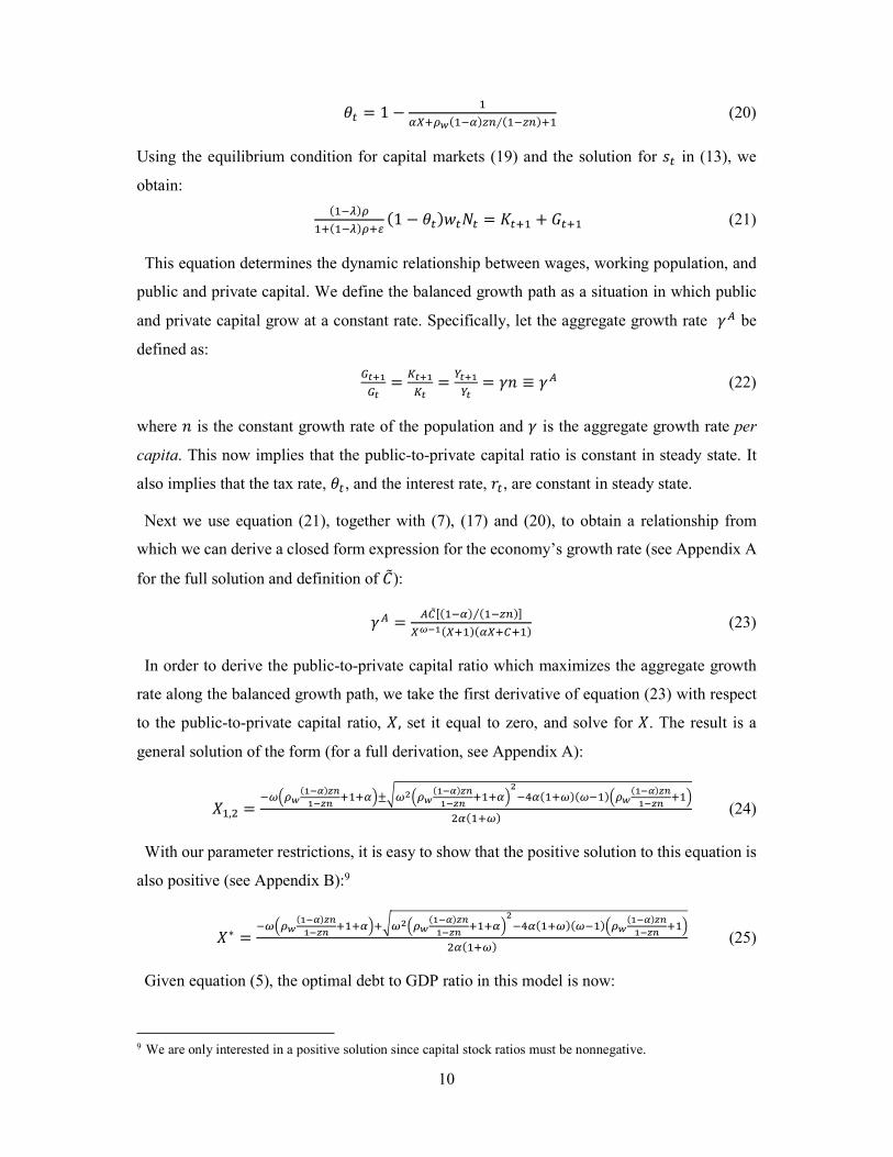
�� = 1 −�

��(��)��∕(��)�� (20)

Using the equilibrium condition for capital markets (19) and the solution for �� in (13), we

obtain:

(��)�

��(��)��(1 − ��)�� = �� + �� (21)

This equation determines the dynamic relationship between wages, working population, and

public and private capital. We define the balanced growth path as a situation in which public

and private capital grow at a constant rate. Specifically, let the aggregate growth rate �� be

defined as:

��

��=

��

��=

��

��= �� ≡ �� (22)

where � is the constant growth rate of the population and � is the aggregate growth rate per

capita. This now implies that the public-to-private capital ratio is constant in steady state. It

also implies that the tax rate, ��, and the interest rate, ��, are constant in steady state.

Next we use equation (21), together with (7), (17) and (20), to obtain a relationship from

which we can derive a closed form expression for the economy’s growth rate (see Appendix A

for the full solution and definition of ��):

�� =��[(��) (��)⁄ ]

��(��)(��) (23)

In order to derive the public-to-private capital ratio which maximizes the aggregate growth

rate along the balanced growth path, we take the first derivative of equation (23) with respect

to the public-to-private capital ratio, �, set it equal to zero, and solve for �. The result is a

general solution of the form (for a full derivation, see Appendix A):

��,� =��

(��)��

��±��

(��)��

��

��(��)(��)��

(��)��

��

��(��) (24)

With our parameter restrictions, it is easy to show that the positive solution to this equation is

also positive (see Appendix B):9

�∗ =��

(��)��

��

(��)��

��

��(��)(��)��

(��)��

��

��(��) (25)

Given equation (5), the optimal debt to GDP ratio in this model is now:

9 We are only interested in a positive solution since capital stock ratios must be nonnegative.

11

�∗ =�

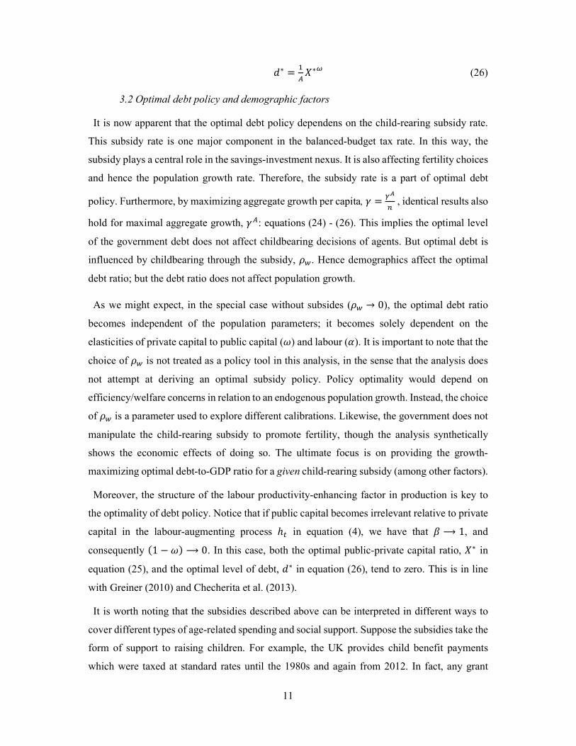
��∗� (26)

3.2 Optimal debt policy and demographic factors

It is now apparent that the optimal debt policy dependens on the child-rearing subsidy rate.

This subsidy rate is one major component in the balanced-budget tax rate. In this way, the

subsidy plays a central role in the savings-investment nexus. It is also affecting fertility choices

and hence the population growth rate. Therefore, the subsidy rate is a part of optimal debt

policy. Furthermore, by maximizing aggregate growth per capita, � =��

� , identical results also

hold for maximal aggregate growth, ��: equations (24) - (26). This implies the optimal level

of the government debt does not affect childbearing decisions of agents. But optimal debt is

influenced by childbearing through the subsidy, ��. Hence demographics affect the optimal

debt ratio; but the debt ratio does not affect population growth.

As we might expect, in the special case without subsides (�� → 0), the optimal debt ratio

becomes independent of the population parameters; it becomes solely dependent on the

elasticities of private capital to public capital (�) and labour (�). It is important to note that the

choice of �� is not treated as a policy tool in this analysis, in the sense that the analysis does

not attempt at deriving an optimal subsidy policy. Policy optimality would depend on

efficiency/welfare concerns in relation to an endogenous population growth. Instead, the choice

of �� is a parameter used to explore different calibrations. Likewise, the government does not

manipulate the child-rearing subsidy to promote fertility, though the analysis synthetically

shows the economic effects of doing so. The ultimate focus is on providing the growth-

maximizing optimal debt-to-GDP ratio for a given child-rearing subsidy (among other factors).

Moreover, the structure of the labour productivity-enhancing factor in production is key to

the optimality of debt policy. Notice that if public capital becomes irrelevant relative to private

capital in the labour-augmenting process ℎ� in equation (4), we have that � ⟶ 1, and

consequently (1 − �)⟶ 0. In this case, both the optimal public-private capital ratio, �∗ in

equation (25), and the optimal level of debt, �∗ in equation (26), tend to zero. This is in line

with Greiner (2010) and Checherita et al. (2013).

It is worth noting that the subsidies described above can be interpreted in different ways to

cover different types of age-related spending and social support. Suppose the subsidies take the

form of support to raising children. For example, the UK provides child benefit payments

which were taxed at standard rates until the 1980s and again from 2012. In fact, any grant

12

which is either taxed or means tested can be written as equation (9) under uniform grant or

means test rates. Most tax codes, including those in the US, offer a tax free element per-child

equivalent to a net income supplement of ��(1 − ��)�� , which is then taxed at the standard

rate (where �� is set to make this expression equal to the tax saving).

Subsidies could also be in the form of support to higher education. The US, for example, taxes

certain training grants and fee waivers. Subsidised loans or means tested tax reductions on fees

operate like child benefits, except that � now refers to time spent in education (child rearing by

society, rather than by parents). Subsidies could also support education in general, where state

spending per pupil is related to the average wage and taxes (levied at standard rates on steady

state earnings) that fund that spending. In this case, � is the proportion of the young population

in state funded schools.

Moreover, subsidies could be regarded as health care costs, where care givers are paid through

a state subsidy; or where, as in the US, those costs contain hidden subsidies. Another possibility

is sick pay. For example, most EU countries pay a fraction of the wage for time off sick, but

tax it as income. Similarly, care givers may be paid through a state subsidy, but taxed at

standard rates.

4. Policies to manage demographic change

This section examines how two major demographic trends, reduced mortality and reduced

fertility, affect fiscal policy and optimal levels of public debt. These two trends lead to ageing

populations. In addition, we study the debt responses to an increase in preferences for current

consumption over future consumption, as has been observed for the baby-boomer generation

throughout the OECD area. The final analysis considers changes to public support of child-

rearing.

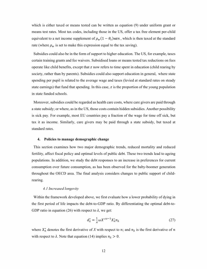
4.1 Increased longevity

Within the framework developed above, we first evaluate how a lower probability of dying in

the first period of life impacts the debt-to-GDP ratio. By differentiating the optimal debt-to-

GDP ratio in equation (26) with respect to �, we get:

��∗ =

�

��∗��

∗�� (27)

where ��∗ denotes the first derivative of X with respect to �; and �� is the first derivative of �

with respect to �. Note that equation (14) implies �� > 0.

13

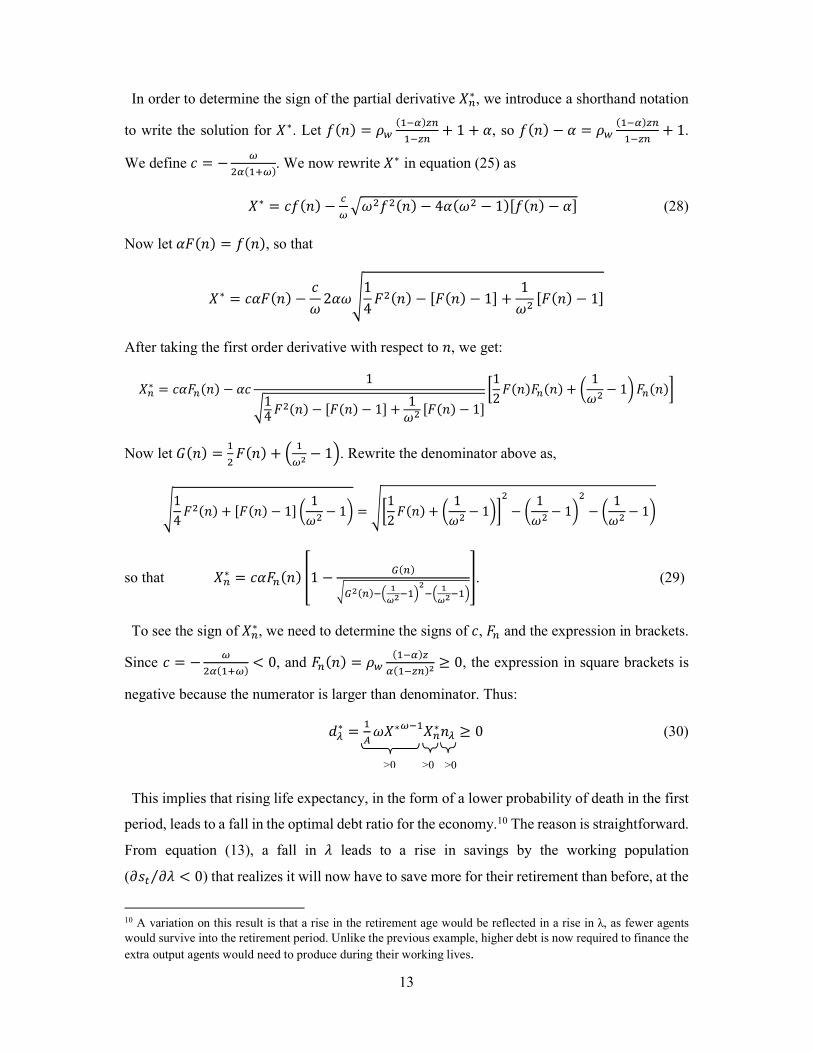
In order to determine the sign of the partial derivative ��∗ , we introduce a shorthand notation

to write the solution for �∗. Let �(�)= ��(��)��

��+ 1 + �, so �(�)− � = ��

(��)��

��+ 1.

We define � = −�

��(��). We now rewrite �∗ in equation (25) as

�∗ = ��(�)−�

��(�)− 4�(�� − 1)[�(�)− �] (28)

Now let ��(�)= �(�), so that

�∗ = ��(�)−�

�2��

1

4��(�)− [�(�)− 1]+

1

��[�(�)− 1]

After taking the first order derivative with respect to �, we get:

��∗ = ��(�)− ��

1

�14��(�)− [�(�)− 1]+

1�� [�(�)− 1]

�1

2�(�)��(�)+ �

1

��− 1��(�)�

Now let �(�)=�

��(�)+ �

�

��− 1�. Rewrite the denominator above as,

�1

4��(�)+ [�(�)− 1]�

1

��− 1�= ��

1

2�(�)+ �

1

��− 1��

�

− �1

��− 1�

�

− �1

��− 1�

so that ��∗ = ��(�)�1 −

�(�)

��(�)��

��

�

��

�. (29)

To see the sign of ��∗, we need to determine the signs of �, �� and the expression in brackets.

Since � = −�

��(��)< 0, and ��(�)= ��

(��)�

�(��)�≥ 0, the expression in square brackets is

negative because the numerator is larger than denominator. Thus:

��∗ =

�

��∗��

∗�� ≥ 0 (30)

This implies that rising life expectancy, in the form of a lower probability of death in the first

period, leads to a fall in the optimal debt ratio for the economy.10 The reason is straightforward.

From equation (13), a fall in � leads to a rise in savings by the working population

(�� < 0⁄ ) that realizes it will now have to save more for their retirement than before, at the

10 A variation on this result is that a rise in the retirement age would be reflected in a rise in λ, as fewer agents would survive into the retirement period. Unlike the previous example, higher debt is now required to finance the

extra output agents would need to produce during their working lives.

>0 >0 >0

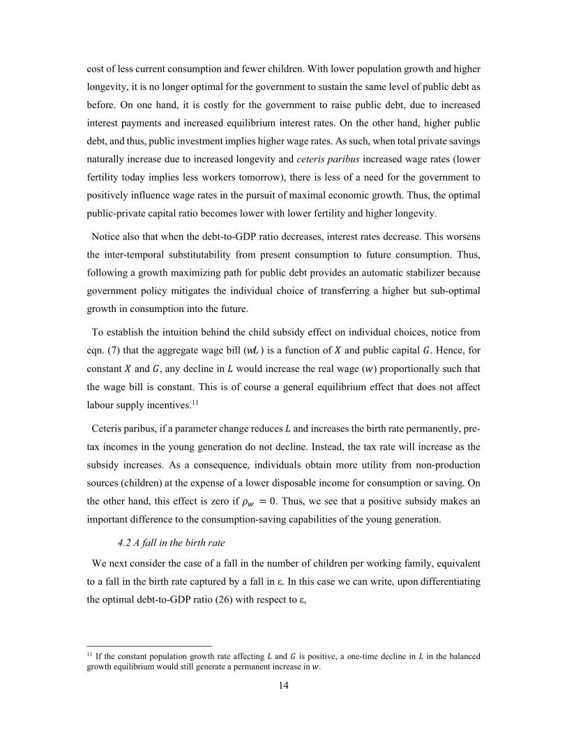
14

cost of less current consumption and fewer children. With lower population growth and higher

longevity, it is no longer optimal for the government to sustain the same level of public debt as

before. On one hand, it is costly for the government to raise public debt, due to increased

interest payments and increased equilibrium interest rates. On the other hand, higher public

debt, and thus, public investment implies higher wage rates. As such, when total private savings

naturally increase due to increased longevity and ceteris paribus increased wage rates (lower

fertility today implies less workers tomorrow), there is less of a need for the government to

positively influence wage rates in the pursuit of maximal economic growth. Thus, the optimal

public-private capital ratio becomes lower with lower fertility and higher longevity.

Notice also that when the debt-to-GDP ratio decreases, interest rates decrease. This worsens

the inter-temporal substitutability from present consumption to future consumption. Thus,

following a growth maximizing path for public debt provides an automatic stabilizer because

government policy mitigates the individual choice of transferring a higher but sub-optimal

growth in consumption into the future.

To establish the intuition behind the child subsidy effect on individual choices, notice from

eqn. (7) that the aggregate wage bill (�� ) is a function of � and public capital � . Hence, for

constant � and � , any decline in � would increase the real wage (� ) proportionally such that

the wage bill is constant. This is of course a general equilibrium effect that does not affect

labour supply incentives.11

Ceteris paribus, if a parameter change reduces � and increases the birth rate permanently, pre-

tax incomes in the young generation do not decline. Instead, the tax rate will increase as the

subsidy increases. As a consequence, individuals obtain more utility from non-production

sources (children) at the expense of a lower disposable income for consumption or saving. On

the other hand, this effect is zero if �� = 0. Thus, we see that a positive subsidy makes an

important difference to the consumption-saving capabilities of the young generation.

4.2 A fall in the birth rate

We next consider the case of a fall in the number of children per working family, equivalent

to a fall in the birth rate captured by a fall in ε. In this case we can write, upon differentiating

the optimal debt-to-GDP ratio (26) with respect to ε,

11 If the constant population growth rate affecting � and � is positive, a one-time decline in � in the balanced growth equilibrium would still generate a permanent increase in � .

15

��∗ =

�

��∗��

∗�� (31)

where ��∗ denotes the derivative of � with respect to �; and where

�� =��(��)�

�(��)[��(��)��]�> 0 (32)

which confirms that a fall in the preference for children leads to a fall in the birth rate. We may

therefore work with change in either � or �. It follows that

��∗ =

�

��∗��

∗�� > 0 (33)

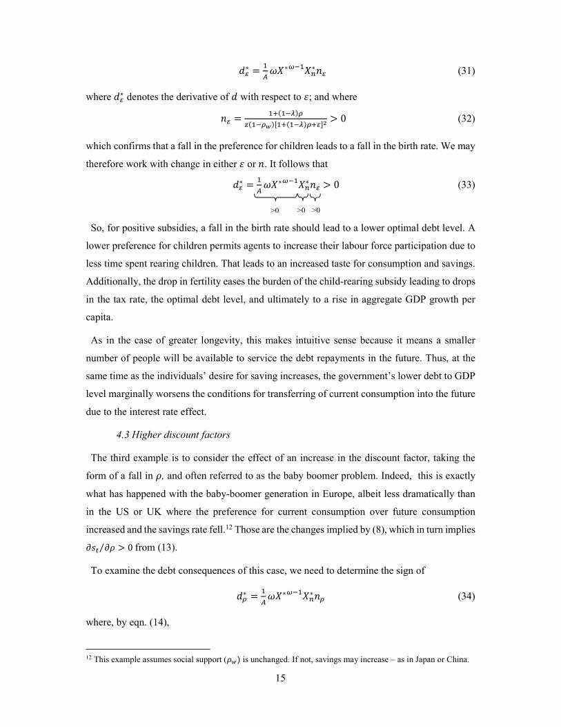
So, for positive subsidies, a fall in the birth rate should lead to a lower optimal debt level. A

lower preference for children permits agents to increase their labour force participation due to

less time spent rearing children. That leads to an increased taste for consumption and savings.

Additionally, the drop in fertility eases the burden of the child-rearing subsidy leading to drops

in the tax rate, the optimal debt level, and ultimately to a rise in aggregate GDP growth per

capita.

As in the case of greater longevity, this makes intuitive sense because it means a smaller

number of people will be available to service the debt repayments in the future. Thus, at the

same time as the individuals’ desire for saving increases, the government’s lower debt to GDP

level marginally worsens the conditions for transferring of current consumption into the future

due to the interest rate effect.

4.3 Higher discount factors

The third example is to consider the effect of an increase in the discount factor, taking the

form of a fall in �, and often referred to as the baby boomer problem. Indeed, this is exactly

what has happened with the baby-boomer generation in Europe, albeit less dramatically than

in the US or UK where the preference for current consumption over future consumption

increased and the savings rate fell.12 Those are the changes implied by (8), which in turn implies

�� > 0⁄ from (13).

To examine the debt consequences of this case, we need to determine the sign of

��∗ =

�

��∗��

∗�� (34)

where, by eqn. (14),

12 This example assumes social support (��) is unchanged. If not, savings may increase – as in Japan or China.

>0 >0 >0

16

�� =��(��)

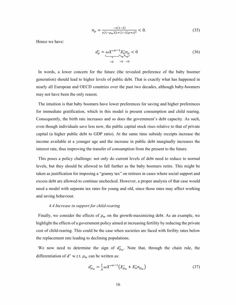
�(��)[��(��)��]�< 0. (35)

Hence we have:

��∗ = ��∗��

∗�� < 0 (36)

In words, a lower concern for the future (the revealed preference of the baby boomer

generation) should lead to higher levels of public debt. That is exactly what has happened in

nearly all European and OECD countries over the past two decades, although baby-boomers

may not have been the only reason.

The intuition is that baby boomers have lower preferences for saving and higher preferences

for immediate gratification, which in this model is present consumption and child rearing.

Consequently, the birth rate increases and so does the government’s debt capacity. As such,

even though individuals save less now, the public capital stock rises relative to that of private

capital (a higher public debt to GDP ratio). At the same time subsidy receipts increase the

income available at a younger age and the increase in public debt marginally increases the

interest rate, thus improving the transfer of consumption from the present to the future.

This poses a policy challenge: not only do current levels of debt need to reduce to normal

levels, but they should be allowed to fall further as the baby boomers retire. This might be

taken as justification for imposing a “granny tax” on retirees in cases where social support and

excess debt are allowed to continue unchecked. However, a proper analysis of that case would

need a model with separate tax rates for young and old, since those rates may affect working

and saving behaviour.

4.4 Increase in support for child-rearing

Finally, we consider the effects of �� on the growth-maximizing debt. As an example, we

highlight the effects of a government policy aimed at increasing fertility by reducing the private

cost of child-rearing. This could be the case when societies are faced with ferility rates below

the replacement rate leading to declining populations.

We now need to determine the sign of ��∗ . Note that, through the chain rule, the

differentiation of �∗ w.r.t. �� can be written as:

��∗ =

�

��∗��

∗ + ��∗�� (37)

>0 >0 <0

17

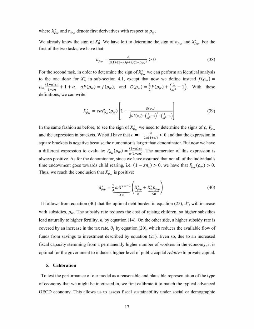
where ��∗ and �� denote first derivatives with respect to ��.

We already know the sign of ��∗. We have left to determine the sign of �� and ��

∗ . For the

first of the two tasks, we have that:

�� =�

�(��(��)��)(��)�> 0 (38)

For the second task, in order to determine the sign of ��∗ we can perform an identical analysis

to the one done for ��∗ in sub-section 4.1, except that now we define instead �(��)=

��(��)��

��+ 1 + �, ��(��)= �(��), and �(��)=

�

��(��)+ �

�

��− 1�. With these

definitions, we can write:

��∗ = ��(��)�1 −

�(��)

��(��)��

��

�

��

� (39)

In the same fashion as before, to see the sign of ��∗ we need to determine the signs of �, ��

and the expression in brackets. We still have that � = −�

��(��)< 0 and that the expression in

square brackets is negative because the numerator is larger than denominator. But now we have

a different expression to evaluate: ��(��)=(��)��

�(��). The numerator of this expression is

always positive. As for the denominator, since we have assumed that not all of the individual's

time endowment goes towards child rearing, i.e. (1 − ��)> 0, we have that ��(��)> 0.

Thus, we reach the conclusion that ��∗ is positive:

��∗ =

�

��∗��

��

��∗

��

+ ��∗��

� (40)

It follows from equation (40) that the optimal debt burden in equation (25), �∗, will increase

with subsidies, ��. The subsidy rate reduces the cost of raising children, so higher subsidies

lead naturally to higher fertility, n, by equation (14). On the other side, a higher subsidy rate is

covered by an increase in the tax rate, �� by equation (20), which reduces the available flow of

funds from savings to investment described by equation (21). Even so, due to an increased

fiscal capacity stemming from a permanently higher number of workers in the economy, it is

optimal for the government to induce a higher level of public capital relative to private capital.

5. Calibration

To test the performance of our model as a reasonable and plausible representation of the type

of economy that we might be interested in, we first calibrate it to match the typical advanced

OECD economy. This allows us to assess fiscal sustainability under social or demographic

18

changes of different sorts; how that compares to the fiscal position and growth rates in OECD

economies in their current or pre-financial crisis state; and whether these economies would find

it easy or feasible to transition to the corresponding steady state.13

5.1 Production parameters

To gain some insight into the current state of OECD economies facing demographic change,

we perform a baseline calibration of the model as set out in section 2. The calibration is based

on the period length of 45 years. This assumes that agents in the model start working at age 20,

work for 45 years and retire at age 65. Child rearing can be shared by any working adult pair.

In terms of income foregone, child rearing time per child is therefore z=0.2=9/45 (the age of

majority is reached at 18) and corresponds to 9 years of each parent’s working life.

We choose the remaining parameters with several key factors in mind. Primarily, we seek to

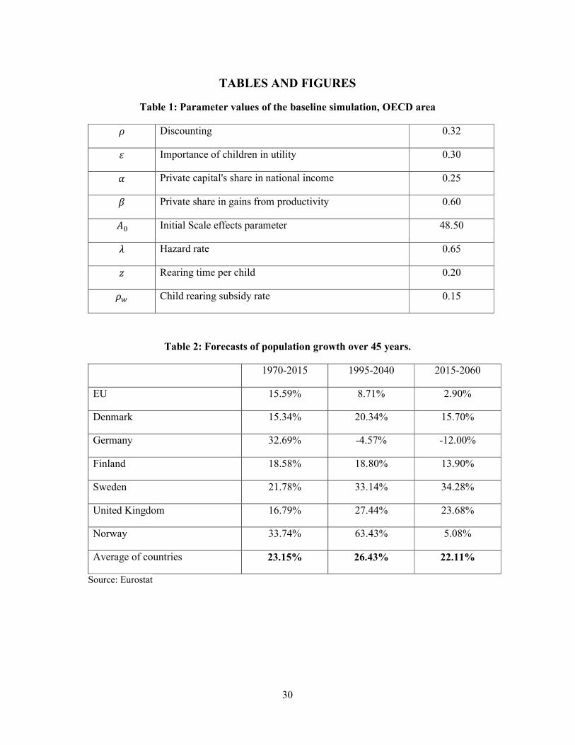
emulate a realistic demographic structure for the typical OECD economy. Table 1 sets out the

parameter values, while the motivation for each value follows below.

---Table 1 about here---

We focus first on production. The value of the output elasticity of private capital, �, should

be around 0.25. This is in line with results presented elsewhere (e.g., Felipe and Adams, 2005).

� captures the private sector share in productivity gains: that is, the share of any income gains

that come from productivity increases due to private capital as opposed to public capital. In

this calibration, the parameter � is set at 0.6. The TFP scale effect � is subject to interpretation.

Several authors (e.g., Hviding and Merette (1998) and Fehr et al. (2013)) argue that it should

reflect (TFP) productivity effects; and those operating with calibrated models proceed in two

steps as we do here: first to establish a steady state solution, and then examine the features of

the transition path to that steady state. In that case, A would be time varying: �� = ��(1.01)�,

where �� is the value of A at the start of generation t; TFP growth is set at 1% per year; and

s={0, 1, 2 …..45} denotes the year within generation t. The initial parameter �� must then be

normalised to align the model with historical data. In our case, this is the debt-to-GDP ratio at

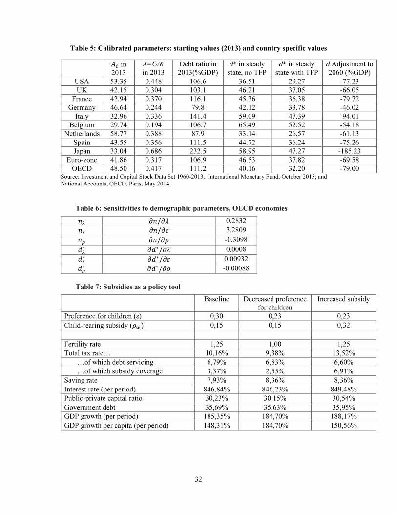
the start of the calibration period. For the OECD, this yields �� = 48.5 (see Table 5) and is

calculated as follows. First, the model generates a debt ratio, eqn. (26), from the stock of public

13 In later work, we can go on to look at the steady states implied in particular economies, including: (1) the “Anglo-Saxon economies” (US, Canada, UK); (2) countries where the process of population ageing is particularly strong (Japan, Italy, Germany); (3) Nordic welfare states with flexible markets and strong social provision (Denmark, Sweden); (4) economies with slow population growth and limited social support (Russia, China); and

(5) those with young and fast growing populations (India, Mexico or the Philippines).

19

capital/debt and output accumulated over a single generation (45 years). We need to convert

that to a steady state debt ratio for a single year (the stock of public debt outstanding at s,

relative to output in year s). We estimate the latter as the average annual output in a generation,

(�� = ��/45), and apply ��(1.01)��.�/45 to the denominator of eqn. (26) to get the final year

estimate. This is a crude estimate, but it is all that can be done within the confines of an OLG

model.

5.2 Preference and demographic parameters

Parameter � is designed to capture the value an agent puts on future consumption relative to

present consumption; that is, the discount to be applied at the start of the working period to the

decisions made in the retirement period 45 years later. A constant compounded annual discount

rate of 0.975 implies �=0.32 for a planning period spanning four and a half decades.

The values of 0.2 and 0.15 for � and ��, respectively, imply a net loss of close to 17% in life-

time earnings per child born. According to the United States Department of Agriculture, the

net expenditure per child in a middle income household (from birth until age 18) is estimated

to be $245340, or $13630 annually for children born in 2013; while, according to the Current

Population Survey of the US Census Bureau, the mean household total money income in the

year in 2014 was $72641.14 This implies that the direct cost of each child is approximately 17%

of lifetime income, suggesting a subsidy rate of �� = 0.15.

Next � and λ are the key demographic parameters; both influence the age structure of the

population. Regarding �: we set this equal to 0.3, so that the number of children born per adult

comes out at n=1.25, by eqn. (14), implying the number of children per woman is 2.5. This

implies a slow growing (native) population, growing at 0.5% per year (24.9% over 45 years).

These figures then match the experience of the average EU economy rather closely, see Table

2.


Regarding �: the number of people aged 65+ relative to the population of working age (20-

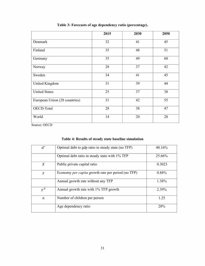
64) in the average OECD economy is 28%, see table 3. In the context of our model, this implies

that the probability of surviving into the retired cohort of 65+ is about 0.35. This yields an age-

dependency ratio of 28%, as in table 2, for the average OECD economy.

14 See Lino (2014) and DeNavas-Walt and Procter (2014) respectively.

20


Notice that � = 0.3 ensures that a steady state exists; the lowest permissible value, by (15),

is � ≈ 0.23. We make an important distinction between reality and the model here. The model

does not recognise that not every woman is able or willing to have children. The rule of thumb

is that 10% of adults do not have children which means that, to sustain a constant population,

each woman needs to have 2.2 children. What we are doing in this paragraph is checking that

our calibration not only produces a steady state in the model (� ≥ 0.23), but also a realistic

steady state population growth of 0.49% per year (� = 0.3).

6. Steady state characterisation

6.1 A first look at the results

Table 4 summarizes the output of the baseline simulation. We see that the demographic

parameters, viz. the number of children per agent and the age dependency ratio, are in line with

that expected in a typical OECD economy, as represented in Tables 2 and 3. The optimal debt

to GDP ratio, �∗, is at 40.16% which is a reasonable value for the current state of typical OECD

economies. The ratio of public-to-private capital is roughly 30%, while the growth rate of

output is only 85.35% per working period (45 years). This per period growth implies an

annual growth rate of 1.38% on average in steady state. However, this model does not include

any growth in total factor productivity TFP as such. So the average growth in output per head

of 0.88% or less is driven by accumulated savings, matching the zero long term per capita

growth rates predicted by almost all standard growth models, thus confirming that we are at or

close to steady state after one generation. Allowing exogenous annual growth of 1% in TFP in

addition, we arrive at a conventional figure of 2.39% for overall growth per year.


What are the lessons from these simulation results? First: a steady state solution, and hence

a sensible and sustainable set of fiscal policies for economies facing significant demographic

change, is both feasible and available. Second: based on reasonable parameter values for the

average OECD economy, the steady state solution demonstrates very reasonable properties

given the post financial crisis experience in the OECD. It suggests growth around the 2%-3%

mark as the “new normal”, rather than the 4%-5% observed in the 1990 to 2005 era.

21

It also suggests that a public debt level of 40% of GDP is a reasonable debt level to aim at.15

This accords well with the Maastricht Treaty/Fiscal Compact upper limit of 60% to create a

debt target with a safe zone to accommodate shocks. Moreover, it also accords well with the

pre-crisis experience of non-Eurozone economies (the US or UK) where debt was held in the

35%-45% range. Finally, it suggests a mixed economy with a public sector component of 30%,

lower than in Scandinavia or the Eurozone (France, Italy, Germany or the Netherlands), but

similar to that in the US, Canada or the UK in the pre-crisis era. The growth in population is

close to that projected for the OECD (Table 2, last column).16

A first impression of these results is that the demographic situation is perhaps not as bad as

some commentators fear. But it is no easy task for most OECD countries to get themselves

down to this optimal steady state level of debt (40%; or 70% off current debt ratios, see Table

5) and also to maintain this steady state rate of growth in productivity, which currently is a

matter of considerable concern to the OECD. In addition, endogenous growth under this

demographic burden is slow (≈1.4%); a larger share of the growth comes from TFP.

These results seem to reflect the current OECD experience pretty well, suggesting that the

slow growth problem is chiefly due to low productivity rather than poor market performance.

Interestingly, our results are consistent with the standard growth models showing that GDP

growth ultimately comes from either growth in productivity or growth in the workforce. Since

we have little of the latter (n=1.25 or 2.50 per woman, is only a little above the constant

population replacement rate), GDP growth has to come from productivity growth. Ultimately,

demographics should not affect that: the population growth is simply too slow to make up the

difference. However, the transition to steady state growth could become more difficult for

economies that currently find themselves a long way from that steady state.

6.2 Changes in the population parameters

To provide insight into the effect of demographic change on the steady state we evaluate the

partial derivatives in Section 4, using baseline simulation results from Table 4. The results are

presented in Table 6.


15 With a range of 44%-60% in the Euro Area without TFP (30%-50% with TFP), or 36%-60% in the OECD. 16 The calibration also yields an old-age dependency ratio of 28%, see Table 3 for 2015. This is very low and suggests a new a risk: if migrants arrive but then adopt the mores of the domestic population, as assumed by our model, then age-dependency ratios will rise without an increase in the long term population growth rate.

22

A general finding is that the changes in outcomes are all rather small with respect to �∗. Even

doubling the largest of them, the importance of having children (�), would add only 0.5

percentage points to the optimal debt ratio. This illustrates the scope of age-related transfers.

Both � and � influence the optimal debt ratio through � and the child-rearing subsidy. By

introducing more age related government expenditure the results are expected to be more

pronounced.17

Thus, we conclude that not only is the optimal steady state under the new demographics

relatively benign, but the likely future demographic and social changes will make little

difference to that steady state once the economy gets there. In the long term, there is no great

sensitivity to demographic or economic shocks. Instead, for most OECD economies, the real

difficulty will be how best to manage the transition from where they are now to their optimal

steady state.

6.3 Change in child-rearing subsidy

Changing the child-rearing subsidy rate also has an impact on the equilibrium steady state. As

an example, we consider a case where the government uses the child-rearing subsidy to reverse

an adverse demographic shock. Specifically, suppose a preference shift, such that agents have

lower propensity to raise children, thereby directing their income towards consumption. In

general, this could be problematic for society if the fertility rate drops below the replacement

rate. When faced with this problem, the government might step in and raise the child-rearing

subsidy. Indeed, we know from Section 4 that (a) a drop in the preference towards having

children leads to a drop in the optimal debt-GDP ratio and (b) a higher subsidy rate leads to an

increase in the optimal debt-GDP ratio.

To study this in further detail, we produce a calibration exercise where we look at the steady

state effects of a composite shock where, first, there is a severe drop in the preference for

children, leading to the fertility rate reaching the population replacement rate, and, second, a

rise in the child-rearing subsidy as the government seeks to maintain a growing population,

ultimately matching the fertility rate to its baseline value.

- Table 7 around here -

The results are summarized in Table 7. All parameters are the same as in the baseline

calibration presented in Table 1, except for the explicit changes made to ε and ��. For clarity,

17 Some generalisations of the model may also be useful: removing the assumption of no capital depreciation, of equal taxes on wages and subsidies, or of subsidies as a fixed ratio to wages.

23

the tax rate has been unraveled into taxes associated with servicing the public debt and taxes levied for

the coverage of subsidies. From the calibration results we see that a drop in preference for

children decreases the total tax rate, since there is less strain on the government’s budget, and

increases savings as agents divert income away from child-rearing. The tax rate associated with

debt servicing increases when the preference for children decreases. There are two opposing

forces at play here. On one hand, optimal public debt decreases. On the other hand, the tax base

decreases due to the fact that the subsidy payments are subject to taxation. Ultimately, the tax

base effect is stronger resulting in an increase in the tax rate necessary for debt servicing.

Economic growth per capita increases, even though economic output decreases because of

fewer children.

When we account for the government’s response of increasing the subsidy to reach the

baseline value of fertility a different picture is drawn. The added government expenditure of

the raised subsidy is covered by taxation, increasing the tax rate well above the baseline. This

is solely due to the higher subsidy rate, since the tax rate associated with debt servicing actually

decreases as a result of the broader tax base. The saving rate of after-tax income remains the

same. The public-private capital ratio and thus optimal government debt is above the baseline.

Interestingly, both per capita GDP growth and GDP growth are greater than in the baseline

case. Per capita growth has, however, decreased compared to the case with an unchanged

subsidy, which reveals a trade-off in fertility-promoting policies: Changes to the child-rearing

subsidy have opposite effects on economic growth and economic growth per capita.18

In sum, the government’s budget would be eased as the preference for children dropped but

tightened, and tighter than before the preference shift, when implementing subsidy rates that

raises fertility to its former level. This example demonstrates the trade-off between population

growth and economic growth when determining the extent of the child-rearing subsidy. Finally,

note that this analysis does not address the issues of an optimal value for the child-rearing

subsidy. The analysis merely evaluates steady state policy effects.

7. Policy and the political economy trade-offs under demographic change

In order to evaluate the political economy implications of our fiscal imbalances, figure 1

provides isoquant lines for different values of growth and debt. The isoquants are determined

by considering a different mix of values for � and �. In this sense income/wealth inequalities,

18 More generally, one can show that, ceteris paribus, changes to the child-rearing subsidy always have opposing effects on economic growth and economic growth pe capita.

24

and who benefits from productivity gains, can be discussed in the wider context of economic

performance and debt sustainability.

--- Figure 1 about here ---

The polical economy implications here are dependent on specific interpretations of � and �.

As the value of � increases, the importance of private capital in labour augmenting product-

ivity rises – as seen from equation (4). By contrast, a fall in � implies greater importance for

public capital. At the same time, a rise in � increases the productivity of private capital and

diminishes the share of labour in the production function, see expression (1). Hence higher

values of � and � imply an economic system increasingly based on private capital, leading to

a more unequal society. Lower values of � and �, by contrast, imply a society with stronger

public infrastructure or higher social support, with publicly financed education and universal

healthcare as classic examples.

Figure 1 can be interpreted as follows: If we go northeast up the diagram we get lower debt,

but little additional growth, and none at all if the movement is mostly east, plus an increasing

degree of income or wealth inequality. But the potential variations in growth are small. By

contrast, moving northwest up the diagram brings higher growth more rapidly, with greater

income and wealth equality and also lower debt ratios, although the debt reductions will

become increasingly elusive (and may not materialize at all if there is too much movement

west). In both cases, the income gains from higher productivity would increasingly accrue to

the owners of capital, and necessarily so because to get any reductions in debt ratios we have

to persuade the private sector to invest in productivity improving capital and production tech-

niques, rather than public investment funded by public debt.

The implication of these steady state results is that public sector productivity is crucial and

matters a great deal for economic performance. But more than that, it also matters how public

capital is deployed. Second, there are a series of complicated and unwelcome trade-offs to be

resolved. Greater income inequality clearly inhibits growth. But promoting productivity and

growth through the public sector or infrastructure investment increases debt. Thus, an

appropriately designed productivity policy can allow higher growth, or possibly lower debt,

and with or without incurring greater inequality of incomes. But whichever route is chosen,

that policy has to allow a greater share of the income gains made possible by higher product-

ivity to go to the owners of private capital if higher debt ratios are to be avoided or the burden

25

of public debt is to be reduced. These are the political economy trade-offs which arise when

fiscal balances come under threat from deteriorating population dynamics.

Similarly, we can see that higher productivity can also be used to lower public debt, with or

without increasing income inequalities. But it again comes at the cost of weaker/lower growth

rates if income inequalities are allowed to increase too sharply. And a greater share of gains

from this higher level of productivity will go to the owners of capital if we try to maintain or

increase growth rates and employment at the same time. On the other hand, reversing this

argument, policies designed to increase public participation in raising productivity will reduce

growth but increase debt; whereas those designed to reduce income inequality directly usually

increases both growth and debt.

Again the political economy trade-offs, in terms of economic performance and fiscal

imbalances, are laid out in uncompromising reality once we take account of changing

demographics and how the gains from productivity are distributed. It would appear that

productivity plays a key role, perhaps more than we thought before. But the way productivity

gains are used is at least as important as increased levels of productivity. And productivity only

assumes this role because demo-graphic changes mean that we have to diminish their impact

on fiscal imbalances without scaling back on entitlement spending – as shown in the model we

have used.

8. Concluding remarks

The model and calibrated simulations in this paper show that the steady state outcomes for an

advanced economy facing today’s demographic and social trends are relatively benign and

resemble those of the OECD economies a few decades back. Similarly, plausible changes to

population parameters and social conditions in the future would make rather little difference to

steady state outcomes. Instead the steady state is largely driven by economic fundamentals:

productivity, the production structure, income generation, income inequality and distribution

of productivity gains. The main problem is to get to the chosen steady state without undue

strain or fiscal collapse on the way (Hughes Hallett et al., 2017).

Hence, our results suggest that demographic change is not necessarily a problem, if properly

handled, compared to the kind of fiscal laxity we have seen over the past 20-30 years.19 This is

19 This result is however sensitive to the chosen calibration. For the average OECD economy, our results hold true. But an economy with other characteristics might face a more challenging situation than the average OECD economy. Specifically, our results are sensitive to the size of child-rearing subsidy, and, to some extent, to the

26

contrary to a conventional reading of the IMF’s earlier advice. But it is still consistent with the

IMF view if we reinterpret that to mean "this shows that ageing and social change is not a

problem in itself, in steady state, so long as reliable fiscal rules or credible fiscal restraints are

set up in advance to manage the rest of fiscal policy". In that sense, our work re-inforces the

need for forward-looking fiscal rules that explicitly allow for the cost of demographic change.

But to imply that ageing and changing demographics are not a problem in steady state is not

to say that all OECD economies will be able to get used to living in an era of slower growth

and lower debt than they enjoyed for three or four decades past. In fact, the real problem is

likely to be how to create and then safeguard the transition to that steady state. In short, the

challenge is to find and maintain durable dynamic adjustment paths.

In future work, a focus on modeling the dynamics of transition and risks in adjusting from the

current fiscally-weak-slow-growth of most OECD economies to the slow growth but fiscally

sustainable steady state predicted by our model is warranted. Finally, income inequalities play

a crucial role in determining the growth rates and debt reductions that are achievable under

demographic and social change. This is a new aspect of the problem that deserves a more

detailed investigation.

References:

Aiyagari, S. Rao and Ellen R. McGrattan (1998), “The Optimum Quantity of Debt”, Journal of Monetary Economics 42: 447-69.

Aschauer, David A. (2000), “Do States Optimise? Public Capital and Economic Growth”, Annals of Regional Science 34: 343-63.

Auerbach, Alan (2009), “Long-term Objectives for Government Debt”, FinanzArchiv 65: 472-501.

Bergman, U. Michael, Michael M. Hutchison and Svend E. Hougaard Jensen (2016), “Promoting Sustainable Public Finances in the European Union: The Role of Fiscal Rules and Government Efficiency”, European Journal of Political Economy, DOI: 10.1016/j.ejpoleco.2016.04.005.

Blanchard, Olivier (1985), “Debt, Deficits, and Finite Horizons”, Journal of Political Economy 93: 223-47.

Blanchard, O. and F. Giavazzi (2002) “Reforms that can be Done: Improving the SGP through a better accounting of public investment”, Dept. of Economics, MIT, Cambridge, MA (November)

Bokan, Nikola, Andrew Hughes Hallett and Svend E. Hougaard Jensen (2016), “Growth-Maximizing Debt under Changing Demographics”, Macroeconomic Dynamics 20: 1640-51.

values of � and �. The higher the subsidy rate, the more impact demographics have on optimal steady state. The lower are � and � (greater income equality), the more sensitive is the steady state to demographic change.

27

Checherita, Christina, Andrew Hughes Hallett and Philipp Rother (2013), “Fiscal Sustainability Using Growth-maximising Debt Targets”, Applied Economics 46: 638-47.

Debrun, X., L. Moulin, A. Turrini, J. Ayuso-i-Casals and M.S. Kumar (2008), “Tied to the Mast? National Fiscal Rules in the European Union”, Economic Policy 23: 297-362.

DeNavas-Walt, C. and B.D. Proctor (2014), “Income and Poverty in the United States: 2013”, U.S. Government Printing Office, Washington, DC, U.S. Census Bureau, Current Population Reports, P60-249.

Fatas, A, J. von Hagen, A. Hughes Hallett, R. Strauch and A. Siebert (2003), “Stability and Growth in Europe: Towards a better pact” Monitoring European Integration 13, Centre for Economic Policy, London.

Felipe, J. and F.G. Adams (2005), “A Theory of Production, The Estimation of the Cobb-Douglas Function: A Retrospective View”, Eastern Journal of Economics 31: 427-445.

Fehr, H., S. Jokisch, M. Kallweit, F. Kindermann, L Kotlikoff (2013), “Generational Policy and Aging in Closed and Open Dynamic Equilibrium Models” in Handbook of Computable General Equilibrium Models, Vol. 1, chapter 27, Elsevier, Amsterdam.

Foremny, D. (2014), “Sub-national Deficits in European Countries: The Impact of Fiscal Rules and Tax Autonomy”, Journal of European Political Economy 34: 86-110.

Greiner, A. (2010), “Economic Growth, Public Debt and Welfare: Comparing Three Budgetary Rules”, German Economic Review 12: 205-22.

Hughes Hallett, Andrew and Svend E. Hougaard Jensen (2012), “Fiscal Governance in the Eurozone: Institutions vs. Rules”, Journal of European Public Policy 19: 646-664.

Hughes Hallett, A., S.E. Hougaard Jensen, T.S. Sveinsson and F. Vieira (2017), “From Here to There: Transition Paths From High Debt to Sustainable Fiscal Strategies Under Adverse Demographics”, mimeo.

Hviding, K. and M. Merette (1998), “Macroeconomic Effects of Pension Reforms in the Context of Aging Populations: OLG model simulations for 7 OECD countries”, Economics Working Paper 201, Economics Department, OECD, Paris

Kalaitzidakis, Pantelis and Sarantis Kalyvitis (2004), “On the Macroeconomic Implications of Maintenance in Public Capital”, Journal of Public Economics 88: 695-712.

Lino, M. (2014), “Expenditures on Children by Families, 2013”, U.S. Department of Agriculture, Center for Nutrition Policy and Promotion, Miscellaneous Publication No. 1528-2013.

Nerlich, C. and W.H. Reuter (2013), “The Design of National Fiscal Frameworks and their Budgetary Impact”, ECB Working Paper Series No. 1588.

Yakita, Akira (2008), “Ageing and Public Capital Accumulation”, International Tax and Public Finance 15: 582

28

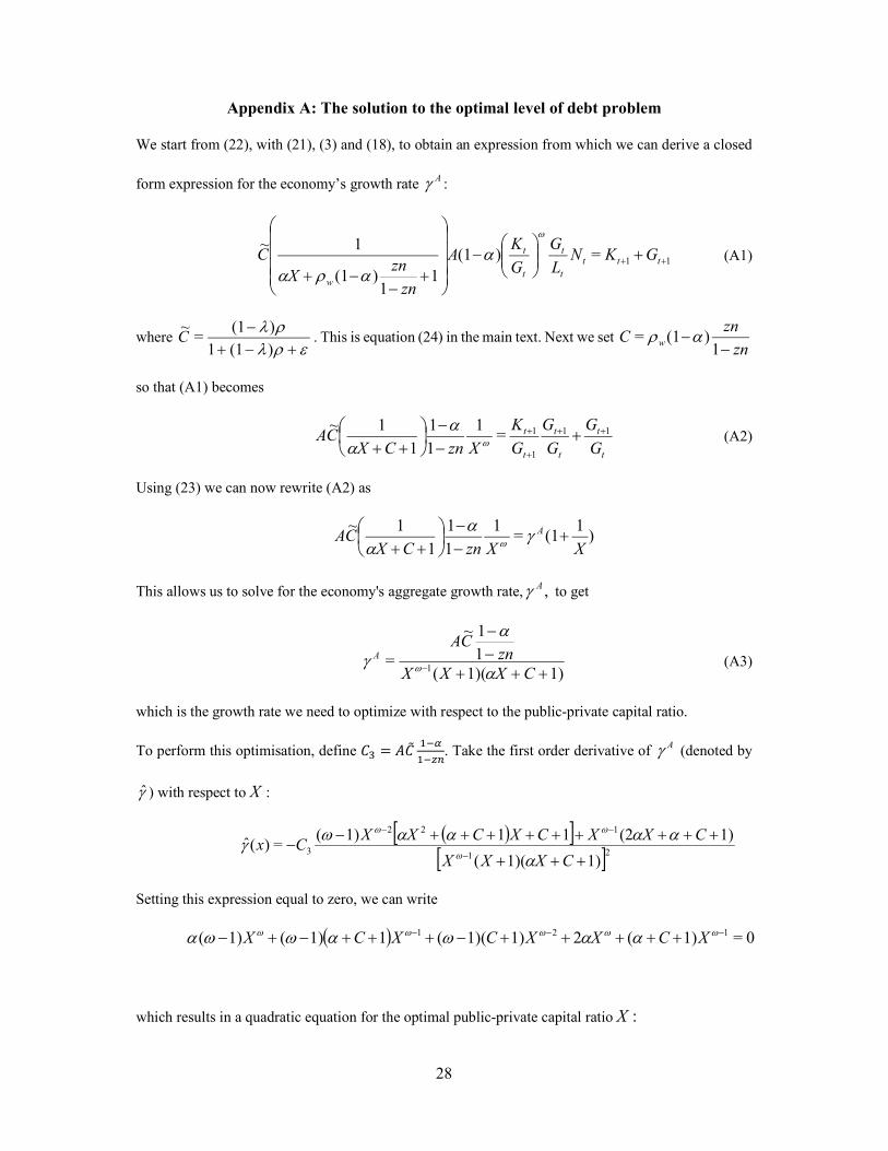
Appendix A: The solution to the optimal level of debt problem

We start from (22), with (21), (3) and (18), to obtain an expression from which we can derive a closed

form expression for the economy’s growth rate A :

11=)(1

11

)(1

1~

ttt

t

t

t

t

w

GKNL

G

G

KA

zn

znX

C

(A1)

where

)(11

)(1=

~C . This is equation (24) in the main text. Next we set

zn

znC w

1)(1=

so that (A1) becomes

t

t

t

t

t

t

G

G

G

G

G

K

XznCXCA 11

1

1=1

1

1

1

1~

(A2)

Using (23) we can now rewrite (A2) as

)1

(1=1

1

1

1

1~

XXznCXCA A

This allows us to solve for the economy's aggregate growth rate, ,A to get

1)1)((

1

1~

=1

CXXXzn

CAA

(A3)

which is the growth rate we need to optimize with respect to the public-private capital ratio.

To perform this optimisation, define �� = ��

��. Take the first order derivative of A (denoted by

) with respect to X :

21

122

31)1)((

1)(2111)(=)(ˆ

CXXX

CXXCXCXXCx

Setting this expression equal to zero, we can write

0=1)(21)1)((11)(1)( 121 XCXXCXCX

which results in a quadratic equation for the optimal public-private capital ratio :X

29

0=1)1)((11)( 2 CXCX

The required solution is therefore:

)(12

11

)(11))((141

1

)(11

1

)(1

=

2

2

1,2

zn

zn

zn

zn

zn

zn

Xwww

which is (26) in the main text.

Appendix B: The positive root

We now demonstrate that our solution for X* is in fact postive. We start from (27) in the text. Since

1<1,01,<0,0> nz , it follows that 0>11

)(1

zn

znw and 0.>)(12

Therefore to get a positive solution, ,0* X we need the numerator of (27) to be positive. It will be

positive if and only if

0>11

)(11))((141

1

)(11

1

)(12

2

zn

zn

zn

zn

zn

znwww

.

We therefore need to check if this condition is in fact satisfied for the parameter constraints that we

have imposed. We require

1

1

)(1>1

1

)(11))((141

1

)(12

2

zn

zn

zn

zn

zn

znwww ;

or

2

2

2

2 11

)(1>1

1

)(11))((141

1

)(1

zn

zn

zn

zn

zn

znwww ;

or 0>11

)(11))((14

zn

znw

which is true since 0>1)(4=1))((14 2 and 0>11

)(1

zn

znw

necessarily

hold. Hence X* in (27) is positive.

30

TABLES AND FIGURES

Table 1: Parameter values of the baseline simulation, OECD area

� Discounting 0.32

� Importance of children in utility 0.30

� Private capital's share in national income 0.25

� Private share in gains from productivity 0.60

�� Initial Scale effects parameter 48.50

� Hazard rate 0.65

� Rearing time per child 0.20

�� Child rearing subsidy rate 0.15

Table 2: Forecasts of population growth over 45 years.

1970-2015 1995-2040 2015-2060

EU 15.59% 8.71% 2.90%

Denmark 15.34% 20.34% 15.70%

Germany 32.69% -4.57% -12.00%

Finland 18.58% 18.80% 13.90%

Sweden 21.78% 33.14% 34.28%

United Kingdom 16.79% 27.44% 23.68%

Norway 33.74% 63.43% 5.08%

Average of countries 23.15% 26.43% 22.11%

Source: Eurostat

31

Table 3: Forecasts of age dependency ratio (percentage).

2015 2030 2050

Denmark 32 41 45

Finland 35 48 51

Germany 35 49 60

Norway 28 37 42

Sweden 34 41 45

United Kingdom 31 39 44

United States 25 37 38

European Union (28 countries) 31 42 55

OECD-Total 28 38 47

World 14 20 28

Source: OECD

Table 4: Results of steady state baseline simulation

�∗ Optimal debt to gdp ratio in steady state (no TFP) 40.16%

Optimal debt ratio in steady state with 1% TFP 25.66%

� Public private capital ratio 0.3023

� Economy per capita growth rate per period (no TFP) 0.88%

Annual growth rate without any TFP 1.38%

�� Annual growth rate with 1% TFP growth 2.39%

� Number of children per person 1.25

Age dependency ratio 28%

32

Table 5: Calibrated parameters: starting values (2013) and country specific values

�� in 2013

X=G/K in 2013

Debt ratio in 2013(%GDP)

d* in steady state, no TFP

d* in steady state with TFP

d Adjustment to 2060 (%GDP)

USA 53.35 0.448 106.6 36.51 29.27 -77.23 UK 42.15 0.304 103.1 46.21 37.05 -66.05

France 42.94 0.370 116.1 45.36 36.38 -79.72 Germany 46.64 0.244 79.8 42.12 33.78 -46.02

Italy 32.96 0.336 141.4 59.09 47.39 -94.01 Belgium 29.74 0.194 106.7 65.49 52.52 -54.18

Netherlands 58.77 0.388 87.9 33.14 26.57 -61.13 Spain 43.55 0.356 111.5 44.72 36.24 -75.26 Japan 33.04 0.686 232.5 58.95 47.27 -185.23

Euro-zone 41.86 0.317 106.9 46.53 37.82 -69.58 OECD 48.50 0.417 111.2 40.16 32.20 -79.00

Source: Investment and Capital Stock Data Set 1960-2013, International Monetary Fund, October 2015; and National Accounts, OECD, Paris, May 2014

Table 6: Sensitivities to demographic parameters, OECD economies

�� /�� 0.2832

�� /�� 3.2809

�� /�� -0.3098

��∗ ��∗/�� 0.0008

��∗ ��∗/�� 0.00932

��∗ ��∗/�� -0.00088

Table 7: Subsidies as a policy tool

Baseline Decreased preference

for children Increased subsidy

Preference for children (ε) 0,30 0,23 0,23

Child-rearing subsidy (��) 0,15 0,15 0,32

Fertility rate 1,25 1,00 1,25 Total tax rate… 10,16% 9,38% 13,52% …of which debt servicing 6,79% 6,83% 6,60% …of which subsidy coverage 3,37% 2,55% 6,91% Saving rate 7,93% 8,36% 8,36% Interest rate (per period) 846,84% 846,23% 849,48% Public-private capital ratio 30,23% 30,15% 30,54% Government debt 35,69% 35,63% 35,95% GDP growth (per period) 185,35% 184,70% 188,17% GDP growth per capita (per period) 148,31% 184,70% 150,56%

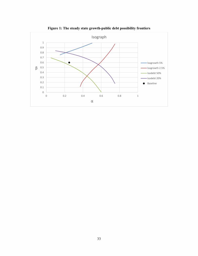
33

Figure 1: The steady state growth-public debt possibility frontiers

0

0.1

0.2

0.3

0.4

0.5

0.6

0.7

0.8

0.9

1

0 0.2 0.4 0.6 0.8 1

β

α

Isograph

Isogrowth 5%

Isogrowth 2.5%

Isodebt 50%

Isodebt 20%

Baseline

Sustainable Fiscal Strategies under Changing Demographics*

Documents

Transcript of Sustainable Fiscal Strategies under Changing Demographics*