SURFACE RECONSTRUCTIONUSING

ADAPTIVE CLUSTERING METHODS

Bjoern Heckel1,Antonio E. Uva2,

Bernd Hamann3, andKenneth I. Joy4

Center for Image Processing and Integrated Computing (CIPIC)Department of Computer Science

University of CaliforniaDavis, CA 95616-8562

Abstract

We present an automatic method for the generation of surface triangulations from sets of scattered

points. Given a set of scattered points in three-dimensional space, without connectivity information,

our method reconstructs a triangulated surface model in a two-step procedure. First, we apply an

adaptive clustering technique to the given set of points, identifying point subsets in regions that are

nearly planar. The output of this clustering step is a set of two-manifold “tiles” that locally approxi-

mate the underlying, unknown surface. Second, we construct a surface triangulation by triangulating

the data within the individual tiles and the gaps between the tiles. This algorithm can generate mul-

tiresolution representations by applying the triangulation step to various resolution levels resulting

from the hierarchical clustering step. We compute deviation measures for each cluster, and thus we

can produce reconstructions with prescribed error bounds.

Keywords: Surface reconstruction; reverse engineering; clustering; multiresolution representation;

triangulation; hierarchical reconstruction.

1PurpleYogi.com, Inc., 201 Ravendale, Mountain View, CA 94043, USA; e-mail:heckel@PurpleYogi.com2Dipartimento di Progettazione e Produzione Industriale, Politecnico di Bari, Viale Japigia, 182, 70126 Bari, Italy; email:

uva@dppi.poliba.it3Department of Computer Science, University of California, Davis, CA 95616-8562, USA; e-mail:

hamann@cs.ucdavis.edu4Corresponding Author; Department of Computer Science, University of California, Davis, CA 95616-8562, USA; e-

mail: joy@cs.ucdavis.edu

(a) (b) (c)

(d) (e)

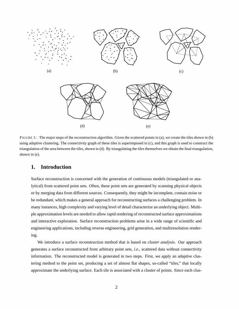
FIGURE 1: The major steps of the reconstruction algorithm. Given the scattered points in (a), we create the tiles shown in (b)

using adaptive clustering. The connectivity graph of these tiles is superimposed in (c), and this graph is used to construct the

triangulation of the area between the tiles, shown in (d). By triangulating the tiles themselves we obtain the final triangulation,

shown in (e).

1. Introduction

Surface reconstruction is concerned with the generation of continuous models (triangulated or ana-

lytical) from scattered point sets. Often, these point sets are generated by scanning physical objects

or by merging data from different sources. Consequently, they might be incomplete, contain noise or

be redundant, which makes a general approach for reconstructing surfaces a challenging problem. In

many instances, high complexity and varying level of detail characterize an underlying object. Multi-

ple approximation levels are needed to allow rapid rendering of reconstructed surface approximations

and interactive exploration. Surface reconstruction problems arise in a wide range of scientific and

engineering applications, including reverse engineering, grid generation, and multiresolution render-

ing.

We introduce a surface reconstruction method that is based oncluster analysis. Our approach

generates a surface reconstructed from arbitrary point sets,i.e., scattered data without connectivity

information. The reconstructed model is generated in two steps. First, we apply an adaptive clus-

tering method to the point set, producing a set of almost flat shapes, so-called “tiles,” that locally

approximate the underlying surface. Each tile is associated with a cluster of points. Since each clus-

2

ter is “nearly planar” we can assume that the data within a cluster can be represented as a height

field with respect to the best-fit plane defined by the tile. We can either triangulate all data points

in the tile to produce a high-resolution mesh locally representing the surface or we can choose to

only triangulate the boundary points defining the polygon of the tile to create a low-resolution local

surface approximation.

Second, we triangulate the gaps between the tiles by using aconstrained Delaunay triangulation,

producing a valid geometrical and topological model. We compute distance estimate for each cluster,

which allows us to calculate an error measure for the resulting triangulated models. By considering a

set of error tolerances, we can construct a hierarchy of reconstructions. Figure 1 illustrates the steps

of the algorithm.

In Section 2, we review algorithms related to surface reconstruction that apply to our work. In

Section 3, we discuss the mathematics of clustering based onprincipal component analysis(PCA)

and the generation of tiles. In Section 4, we describe the triangulation procedure that uses tiles as

input and produces a triangulation as output. This Section discusses the triangulation of the tiles

themselves as well as the method for triangulating the space between the tiles. Results of our algo-

rithm are provided in Section 5. Conclusions and ideas for future work are provided in Section 6.

2. Related Work

Given a set of points{pi = (xi, yi, zi)T , i = 1, ..., n

}assumed to originate from a surface in three-

dimensional space, the goal of surface reconstruction is to generate a triangulated model approxi-

mating the unknown surface. The representation and reconstruction of three-dimensional shapes has

been a significant problem in the computer graphics, computer vision, and mechanical engineering

communities for several years. Most research has focused on providing a known data structure along

with a set of heuristics that enable an approximating mesh to be constructed from the set of sample

points.

Boissonnat [8] was one of the first to address the problem of surface reconstruction from a

scattered point set. He uses a nearest neighbor criterion to produce an advancing front along the

surface. From an initial pointp0, an edge is generated betweenp0 and its nearest neighborp1.

An initial “contour” is generated by considering the two edgesp0p1 andp1p0. This contour is

then propagated by selecting a pointp2 in the neighborhood of the edge (considering thek nearest

neighbors ofp0 andp1) such that the projection ofp2 in the tangent planeT , generated by a least-

squares method using the neighborhood about the edge, “sees” the projected edge under the largest

angle. The pointp2 is added to the contour, creating a triangle, and the algorithm continues with each

edge of the contour. Under certain restrictive, non-folding conditions this algorithm is guaranteed to

3

work.

Hoppeet al. [17] and Curless and Levoy [10] utilize a regular grid and produce a signed distance

function on this grid. Hoppeet al.’s method [17] is based on azero-setapproach for reconstruction,

using the given points to create a signed distance functiond, and then triangulating the isosurface

d = 0. They determine an approximate tangent plane at each pointp, using a least-squares ap-

proximation based on thek nearest neighbors ofp. Using adjacent points and tangent planes, they

determine the normal to the tangent plane, which is then used to determine the signed distance func-

tion. The triangulation is then generated using the marching cubes algorithm of Lorensenet al. [23].

This algorithm produces an approximating triangulation. The approximation is treated as a global

optimization problem with an energy function that directly measures deviation of the approximation

from the original surface.

Curless and Levoy [10] present an approach to merge several range images by scan-converting

each image to a weighted signed distance function in a regular three-dimensional grid. The zero-

contour of this distance function, is then triangulated using a marching cubes algorithm [23]. This

algorithm also produces an approximating mesh to the data points. The closeness of the approxima-

tion is determined by the size of the grid elements.

Boissonnat [8], Attali [3] and Amentaet al. [2] utilize the properties of theDelaunay triangula-

tion [30] to assist in generating an interpolating mesh for a set of sample points. Boissonnat’s second

algorithm [8] first generates aDelaunay tetrahedrizationT of the points as an intermediate structure.

The boundary of this tetrahedral mesh defines the convex hull of the data points. The algorithm then

progressively removes tetrahedra fromT , such that the boundary of the resulting set of tetrahedra

remains a polyhedron. A drawback of this approach is that no change of the topology is allowed,

and consequently, it is impossible to create a surface formed of several connected components and

having holes.

Attali [3] utilizes a normalized mesh, a subset of the Delaunay triangulation, to approximate a

surface represented by a set of scattered data points. When applied to “r-regular shapes” in two

dimensions, this method is provably convergent. Unfortunately, in three dimensions, heuristics must

be applied to complete a surface. The general idea is to construct the Delaunay mesh in two dimen-

sions and remove those triangles that do not contribute to the normalized mesh. The boundary of the

remaining triangles forms the boundary of the surface.

Amentaet al. [2] use a three-dimensional “Voronoi diagram” and an associated (dual) Delaunay

triangulation to generate certain “crust triangles” on the surface that are used in the final triangulation.

The output of their algorithm is guaranteed to be topologically correct and converges to the original

surface as the sampling density increases.

The alpha shapesof Edelsbrunneret al. [12], which define a simplicial complex for an unor-

4

ganized set of points, have been used by a number of researchers for surface reconstruction. Guo

[14] describes a method for reconstructing an unknown surface of arbitrary topology, possibly with

boundaries, from a set of scattered points. He uses three-dimensional alpha shapes to construct a

simplified surface that captures the “topological structure” of a scattered data set and then computes

a curvature-continuous surface based on this structure. Teichmann and Capps [33] also utilize alpha

shapes to reconstruct a surface. They use a local density scaling of the alpha parameter, depending

on the sampling density of the mesh. This algorithm requires the normal to the surface to be known

at each point.

Bajaj et al. [4] use alpha shapes to compute a domain surface from which a signed distance

function can be approximated. After decomposing a set of scattered points into tetrahedra, they fit

algebraic surfaces to the scattered data. Bernardini and Bajaj [5] also utilize alpha shapes to con-

struct the surface. This approach provides a formal characterization of the reconstruction problem

and allows them to prove that the alpha shape is homeomorphic to the original object and that ap-

proximation within a specific error bound is possible. The method can produce artifacts and requires

a local “sculpting step” to approximate sharp edges well.

The ball-pivoting algorithm of Bernardiniet al. [6] utilizes a ball of a specified radius that pivots

around an edge of a seed triangle. If it touches another point another triangle is formed, and the

process continues. The algorithm continues until all reachable edges have been considered, and then

it re-starts with another seed triangle. This algorithm is closely related to one using alpha shapes,

but it computes a subset of the 2-faces of the alpha shape of the surface. This method has provable

reconstruction guarantees under certain sampling assumptions, and it is a simply implemented.

Mencl [25] and Mencl and Muller [26] use a different approach. They use an algorithm that

first generates aEuclidean minimum spanning treefor the point set. This spanning tree is a tree

connecting all sample points with line segments so that the sum of the edge lengths is minimized.

The authors extend and prune this tree depending on a set of heuristics that enable the algorithm to

detect features, connected components and loops in the surface. The graph is then used as a guide to

generate a set of triangles that approximate the surface.

The idea of generating clusters on surfaces is similar to the generation of “superfaces” as done

by Kalvin and Taylor [21, 22]. This algorithm uses random seed faces, and develops “islands”

on the surface that grow through an advancing front. Faces on the current superface boundary are

merged into the evolving superface when they satisfy the required merging criteria. A superface

stops growing when there are no more faces on the boundary that can be merged. These superfaces

form islands that partition the surface and can be triangulated to form a low-resolution triangulation

of the surface. Hinker and Hansen [16] have developed a similar algorithm.

The idea of stitching surfaces together has been used by Soucy and Laurendeau [32], who have

5

designed a stitching algorithm to integrate a set of range views. They utilize “canonical subset

triangulations” that are separated by a minimal parametric distance. They generate a parametric grid

for the empty space between the non-redundant triangulations and utilize a constrained Delaunay

triangulation, computed in parameter space, to fill empty spaces. Connecting these pieces allows

them to get an integrated, connected surface model.

The algorithm we present is based on a new approach. We utilize an adaptive clustering method

[24] to generate a set of “tiles” that represent the scattered data locally. The resulting disjoint tiles,

together with the space between the tiles, can be triangulated. Several steps are necessary to imple-

ment this method. First, the tiles must be generated. We utilize principal component analysis (PCA)

to determine clusters of points that are nearly coplanar. Each tile is generated from the boundary

polygon of the convex hull of a cluster of points that have been projected into the best-fit plane. We

use a hierarchical clustering scheme that splits clusters where their errors are too large. We determine

a connectivity graph for the tiles by generating a Delaunay-like triangulation of the tile centers. Fi-

nally, we triangulate the tiles and the space between them by using a localized constrained Delaunay

triangulation. By triangulating the original points within the tiles we can obtain a locally high-fidelity

and high-resolution representation of the data. By triangulating only the boundary polygons of the

tiles, we can also generate a low-fidelity and low-resolution representation of the data.

3. Hierarchical Clustering

Suppose we are given a set of distinct points

P = {pi = (xi, yi, zi)T , i = 1, ..., n},

where the points lie on or close to an unknown surface. We recursively partition this point set by

separating it into subsets, or clusters, where each subset consists of nearly coplanar points. In this

section, we describe a hierarchical clustering algorithm that utilizes PCA, see Hotelling [19], Jackson

[20] or Manly [24], to establish best-fit planes for each cluster. These planes enable us to measure

the distance between the original points in the clusters and the best-fit planes, and to establish the

splitting conditions for the clusters.

3.1. Principal Component Analysis

Given a set ofn points in three-dimensional space, the covariance matrixS of the point set is

S =1

n− 1(DTD

),

6

whereD is the matrix

D =

x1 − x y1 − y z1 − z

......

...

xn − x yn − y zn − z

(1)

and

c = (x, y, z)T =

(1n

n∑i=1

xi,1n

n∑i=1

yi,1n

n∑i=1

zi

)T(2)

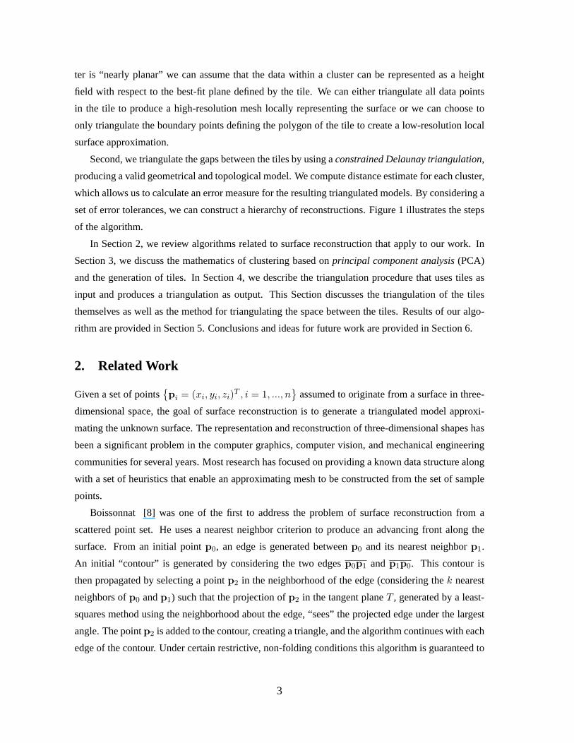
is the geometric mean of then points.

The 3 × 3 matrix S can be factored asUTLU , whereL is diagonal andU is an orthonormal

matrix. The diagonal elements ofL are the eigenvaluesλmax, λmid, andλmin of S (ordered by

decreasing absolute values), and the columns ofU are the corresponding normalized eigenvectors

~emax, ~emid, and~emin. These mutually perpendicular eigenvectors define the three axis directions of a

local coordinate frame with centerc.

We use the values ofλmax, λmid, andλmin to determine the “degree of coplanarity” of a point set.

Three cases are possible:

• Two eigenvalues –λmid andλmin – are zero, and one eigenvalue –λmax – has a finite, non-zero

absolute value. This implies that then points are collinear.

• One eigenvalue –λmin – is zero, and the other two eigenvalues –λmax andλmid – have finite,

non-zero absolute values. This implies that then points are coplanar.

• All three eigenvalues have finite, non-zero absolute values.

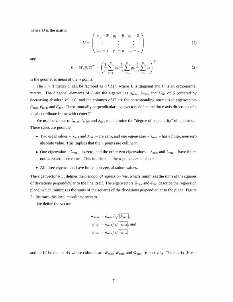
The eigenvector~emaxdefines theorthogonal regression line, which minimizes the sums of the squares

of deviations perpendicular to the line itself. The eigenvectors~emax and~emid describe the regression

plane, which minimizes the sums of the squares of the deviations perpendicular to the plane. Figure

2 illustrates this local coordinate system.

We define the vectors

~wmax = ~emax/√|λmax|,

~wmid = ~emid/√|λmid|, and

~wmin = ~emin/√|λmin|

and letW be the matrix whose columns are~wmax, ~wmid, and~wmin, respectively. The matrixW can

7

��

min

�

��

max

��

mid

FIGURE 2: Principal component analysis (PCA) of a set of points in three-dimensional space. PCA yields three eigenvectors

that form a local coordinate system with the geometric meanc of the points as its local origin. The two eigenvectors~emax

and~emid, corresponding to the two largest eigenvalues, define a plane that represents the best-fit plane for the points. The

eigenvector~emin represents the direction in which we measure the error.

be written asW = UL−12 , where

L−12 =

1√|λmax|

0 0

0 1√|λmid|

0

0 0 1√|λmin|

and

WW T = UL−12L−

12UT = UL−1UT = S−1.

There is another way to look at this coordinate frame. Given a pointp = (x, y, z)T , one can show

that

pTS−1p = pTWW Tp

= (W Tp)T (W Tp)

= qTq.

The quadratic formpTS−1p defines a norm in three-dimensional space. This affine-invariant norm,

which we denote by|| · ||, defines the square of the length of a vectorv = (x, y, z)T as

||v||2 = vTS−1v, (3)

see [28, 29]. The “unit sphere” in this norm is the ellipsoid defined by the set of pointsp satisfying

the quadratic equationpTS−1p = 1. This ellipsoid has its major axis in the direction of~emax. The

8

length of the major axis is√|λmax|. The other two axes of this ellipsoid are in the directions of~emid

and~emin, respectively, with corresponding lengths√|λmid| and

√|λmin|. We utilize this ellipsoid in

the clustering step.

We consider a point set as “nearly coplanar” when√|λmin| is small compared to

√|λmid| and√

|λmax|. If our planarity condition is not satisfied, we recursively subdivide the point set and con-

tinue this subdivision process until all point subsets meet the required planarity condition. We define

theerror of a cluster as√|λmin|, which is the maximum distance from the least-squares plane.1

The PCA calculation is linear in the number of points in the point set. The essential cost of

the operation is the calculation of the covariance matrix. The calculation of the eigenvalues and

eigenvectors is a fixed-cost operation, as it is performed for a3× 3 matrix.

3.2. Splitting Clusters

We use PCA to construct a set of clusters for a given point setP. In general, the eigenvalues implied

by the original point setP are non-zero and finite, unless the given points are collinear or coplanar.

The eigenvalueλmin measures, in some sense, the deviation of the point set from the plane that passes

throughc and is spanned by the two eigenvectors~emax and~emid.

If the error of a clusterC is greater than a certain threshold, we split the cluster into two subsets

along the plane passing throughc and containing the two vectors~emid and~emin. This bisecting plane

splits the data set into two subsets. The general idea is to perform the splitting of point subsets

recursively until the maximum of all clusters errors has a value less than a prescribed threshold,i.e.,

a planarity condition holds for all the clusters generated. For any given error tolerance, the splitting

of subsets always terminates when each cluster consists of less than four points.

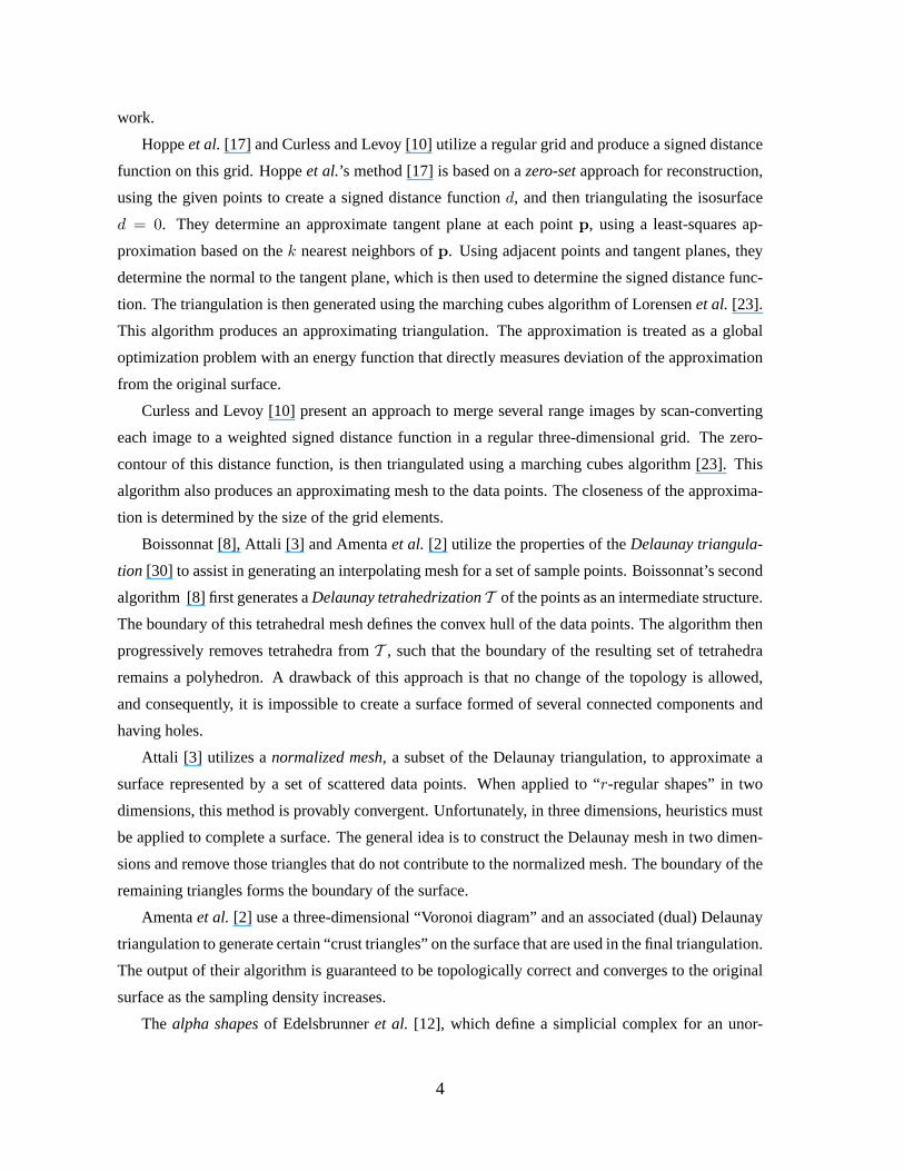
This method can fail to orient clusters correctly if the density of the surface samples is not suffi-

cient. For example, in areas where two components of a surface are separated by a small distance, the

algorithm may produce one cluster consisting of points from both components, see Figure 3. This

fact causes the algorithm to produce an incorrect triangulation. However, if the sample density is

high in these areas, the splitting algorithm will eventually define correctly oriented clusters.

This method is also useful when the density of sample points is highly varying. In these regions,

the algorithm correctly builds large clusters with low error. The triangulation step can thus create a

triangulation correctly in areas that have few or no samples, see [32].

1Potential outliers in a data set are removed in the scanning process. If outliers exist in the data, an “average” error of√|λmin|n , wheren is the number of points in the cluster, produces better results.

9

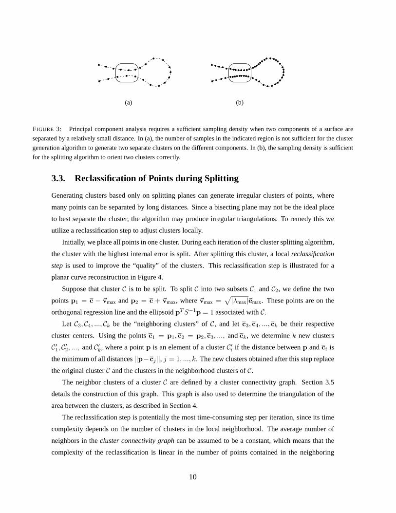
(a) (b)

FIGURE 3: Principal component analysis requires a sufficient sampling density when two components of a surface are

separated by a relatively small distance. In (a), the number of samples in the indicated region is not sufficient for the cluster

generation algorithm to generate two separate clusters on the different components. In (b), the sampling density is sufficient

for the splitting algorithm to orient two clusters correctly.

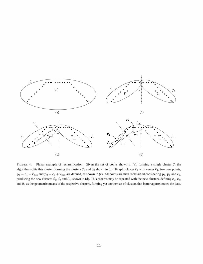
3.3. Reclassification of Points during Splitting

Generating clusters based only on splitting planes can generate irregular clusters of points, where

many points can be separated by long distances. Since a bisecting plane may not be the ideal place

to best separate the cluster, the algorithm may produce irregular triangulations. To remedy this we

utilize a reclassification step to adjust clusters locally.

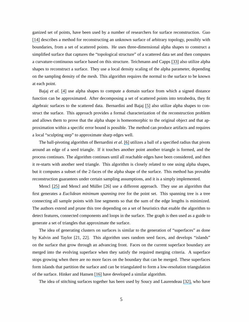
Initially, we place all points in one cluster. During each iteration of the cluster splitting algorithm,

the cluster with the highest internal error is split. After splitting this cluster, a localreclassification

step is used to improve the “quality” of the clusters. This reclassification step is illustrated for a

planar curve reconstruction in Figure 4.

Suppose that clusterC is to be split. To splitC into two subsetsC1 andC2, we define the two

pointsp1 = c − ~vmax andp2 = c + ~vmax, where~vmax =√|λmax|~emax. These points are on the

orthogonal regression line and the ellipsoidpTS−1p = 1 associated withC.Let C3, C4, ..., Ck be the “neighboring clusters” ofC, and letc3, c4, ..., ck be their respective

cluster centers. Using the pointsc1 = p1, c2 = p2, c3, ..., andck, we determinek new clusters

C′1, C′2, ..., andC′k, where a pointp is an element of a clusterC′i if the distance betweenp andci is

the minimum of all distances||p−cj ||, j = 1, ..., k. The new clusters obtained after this step replace

the original clusterC and the clusters in the neighborhood clusters ofC.The neighbor clusters of a clusterC are defined by a cluster connectivity graph. Section 3.5

details the construction of this graph. This graph is also used to determine the triangulation of the

area between the clusters, as described in Section 4.

The reclassification step is potentially the most time-consuming step per iteration, since its time

complexity depends on the number of clusters in the local neighborhood. The average number of

neighbors in thecluster connectivity graphcan be assumed to be a constant, which means that the

complexity of the reclassification is linear in the number of points contained in the neighboring

10

���� ���

��� �

(b)

(c) (d)

��max

(a)

���

��� ���

���

���

���

���

�!

"�#$�%

&!'

(

)+*

,+-

FIGURE 4: Planar example of reclassification. Given the set of points shown in (a), forming a single clusterC, the

algorithm splits this cluster, forming the clustersC1 andC2 shown in (b). To split clusterC1 with centerc1, two new points,

p1 = c1 − ~vmax andp2 = c1 + ~vmax are defined, as shown in (c). All points are then reclassified consideringp1, p2 andc2,

producing the new clustersC2, C3 andC4, shown in (d). This process may be repeated with the new clusters, definingc2, c3,

andc4 as the geometric means of the respective clusters, forming yet another set of clusters that better approximates the data.

11

�

�

�

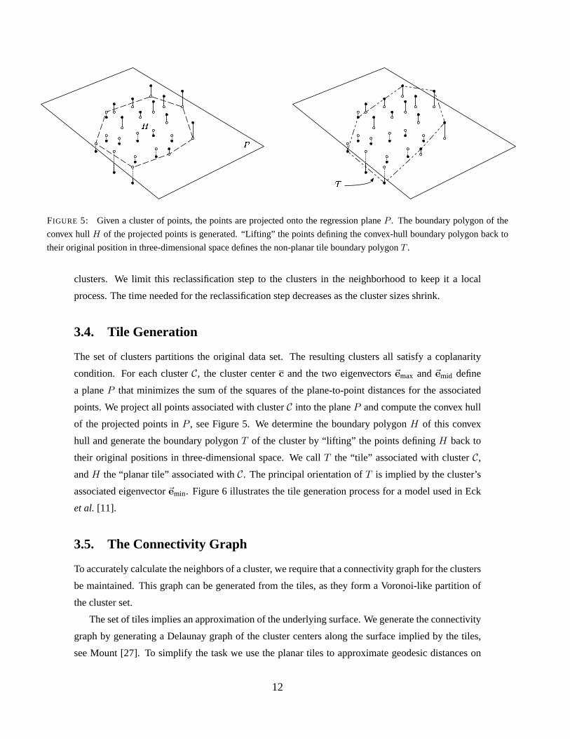
FIGURE 5: Given a cluster of points, the points are projected onto the regression planeP . The boundary polygon of the

convex hullH of the projected points is generated. “Lifting” the points defining the convex-hull boundary polygon back to

their original position in three-dimensional space defines the non-planar tile boundary polygonT .

clusters. We limit this reclassification step to the clusters in the neighborhood to keep it a local

process. The time needed for the reclassification step decreases as the cluster sizes shrink.

3.4. Tile Generation

The set of clusters partitions the original data set. The resulting clusters all satisfy a coplanarity

condition. For each clusterC, the cluster centerc and the two eigenvectors~emax and~emid define

a planeP that minimizes the sum of the squares of the plane-to-point distances for the associated

points. We project all points associated with clusterC into the planeP and compute the convex hull

of the projected points inP , see Figure 5. We determine the boundary polygonH of this convex

hull and generate the boundary polygonT of the cluster by “lifting” the points definingH back to

their original positions in three-dimensional space. We callT the “tile” associated with clusterC,andH the “planar tile” associated withC. The principal orientation ofT is implied by the cluster’s

associated eigenvector~emin. Figure 6 illustrates the tile generation process for a model used in Eck

et al. [11].

3.5. The Connectivity Graph

To accurately calculate the neighbors of a cluster, we require that a connectivity graph for the clusters

be maintained. This graph can be generated from the tiles, as they form a Voronoi-like partition of

the cluster set.

The set of tiles implies an approximation of the underlying surface. We generate the connectivity

graph by generating a Delaunay graph of the cluster centers along the surface implied by the tiles,

see Mount [27]. To simplify the task we use the planar tiles to approximate geodesic distances on

12

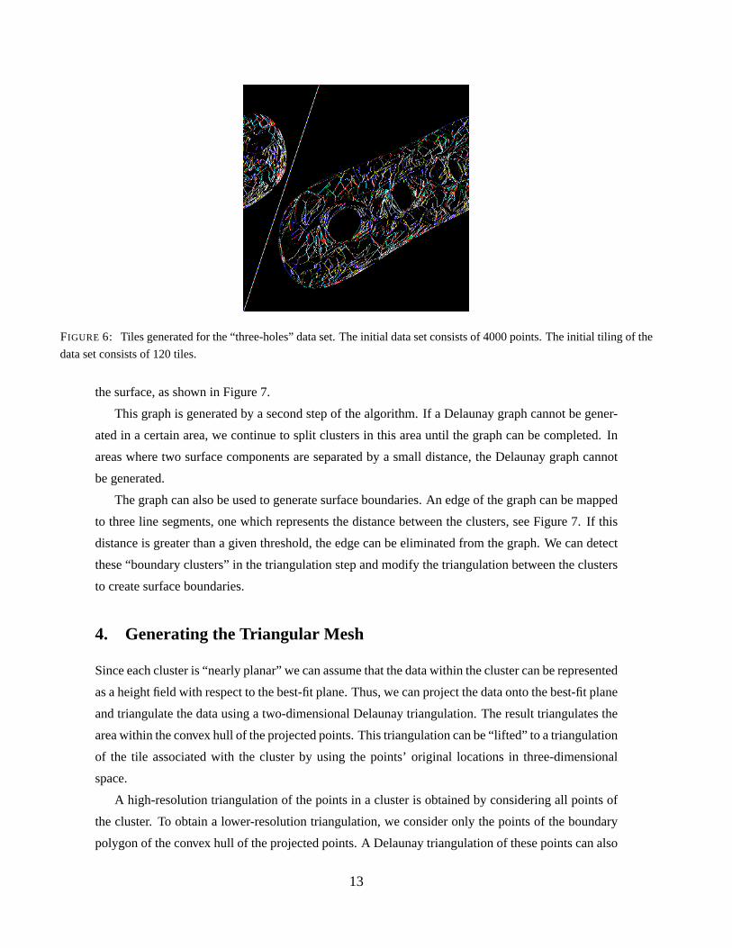
FIGURE 6: Tiles generated for the “three-holes” data set. The initial data set consists of 4000 points. The initial tiling of the

data set consists of 120 tiles.

the surface, as shown in Figure 7.

This graph is generated by a second step of the algorithm. If a Delaunay graph cannot be gener-

ated in a certain area, we continue to split clusters in this area until the graph can be completed. In

areas where two surface components are separated by a small distance, the Delaunay graph cannot

be generated.

The graph can also be used to generate surface boundaries. An edge of the graph can be mapped

to three line segments, one which represents the distance between the clusters, see Figure 7. If this

distance is greater than a given threshold, the edge can be eliminated from the graph. We can detect

these “boundary clusters” in the triangulation step and modify the triangulation between the clusters

to create surface boundaries.

4. Generating the Triangular Mesh

Since each cluster is “nearly planar” we can assume that the data within the cluster can be represented

as a height field with respect to the best-fit plane. Thus, we can project the data onto the best-fit plane

and triangulate the data using a two-dimensional Delaunay triangulation. The result triangulates the

area within the convex hull of the projected points. This triangulation can be “lifted” to a triangulation

of the tile associated with the cluster by using the points’ original locations in three-dimensional

space.

A high-resolution triangulation of the points in a cluster is obtained by considering all points of

the cluster. To obtain a lower-resolution triangulation, we consider only the points of the boundary

polygon of the convex hull of the projected points. A Delaunay triangulation of these points can also

13

���

���

���

�

�� ���

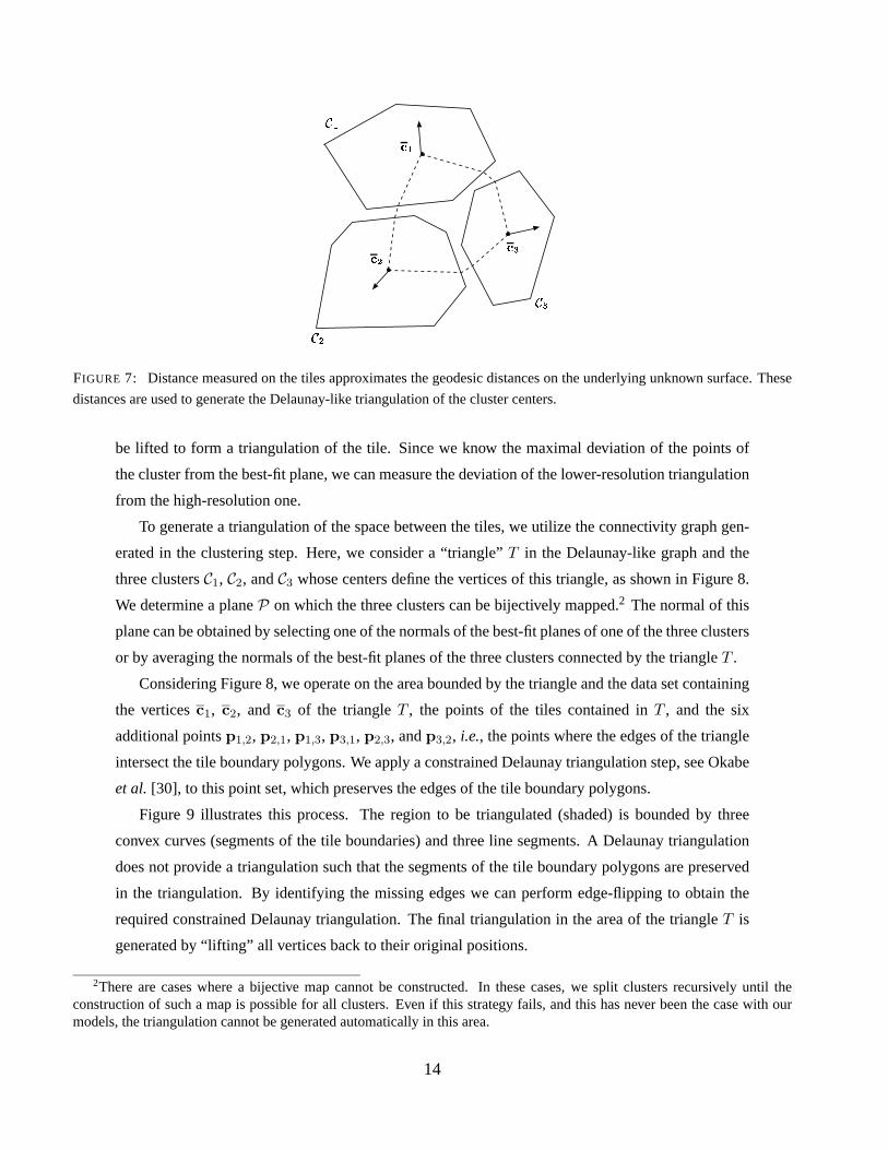
FIGURE 7: Distance measured on the tiles approximates the geodesic distances on the underlying unknown surface. These

distances are used to generate the Delaunay-like triangulation of the cluster centers.

be lifted to form a triangulation of the tile. Since we know the maximal deviation of the points of

the cluster from the best-fit plane, we can measure the deviation of the lower-resolution triangulation

from the high-resolution one.

To generate a triangulation of the space between the tiles, we utilize the connectivity graph gen-

erated in the clustering step. Here, we consider a “triangle”T in the Delaunay-like graph and the

three clustersC1, C2, andC3 whose centers define the vertices of this triangle, as shown in Figure 8.

We determine a planeP on which the three clusters can be bijectively mapped.2 The normal of this

plane can be obtained by selecting one of the normals of the best-fit planes of one of the three clusters

or by averaging the normals of the best-fit planes of the three clusters connected by the triangleT .

Considering Figure 8, we operate on the area bounded by the triangle and the data set containing

the verticesc1, c2, andc3 of the triangleT , the points of the tiles contained inT , and the six

additional pointsp1,2, p2,1, p1,3, p3,1, p2,3, andp3,2, i.e., the points where the edges of the triangle

intersect the tile boundary polygons. We apply a constrained Delaunay triangulation step, see Okabe

et al. [30], to this point set, which preserves the edges of the tile boundary polygons.

Figure 9 illustrates this process. The region to be triangulated (shaded) is bounded by three

convex curves (segments of the tile boundaries) and three line segments. A Delaunay triangulation

does not provide a triangulation such that the segments of the tile boundary polygons are preserved

in the triangulation. By identifying the missing edges we can perform edge-flipping to obtain the

required constrained Delaunay triangulation. The final triangulation in the area of the triangleT is

generated by “lifting” all vertices back to their original positions.

2There are cases where a bijective map cannot be constructed. In these cases, we split clusters recursively until theconstruction of such a map is possible for all clusters. Even if this strategy fails, and this has never been the case with ourmodels, the triangulation cannot be generated automatically in this area.

14

triangulatethis region

��� ���

���

� � � ���� �

��� � �

����� � ���! "#�$�% &

')( *,+

-/.

0

FIGURE 8: Three tiles projected onto a plane. The intersection pointspi,j between the edges of the tilesCi and the edges

of the triangleT are added to the set of tile boundary vertices. This enables us to triangulate the area of the triangle using a

constrained two-dimensional Delaunay triangulation that preserves the boundaries of the tiles.

invalidtriangulation

invalidtriangulation

(a) (b) (c)

FIGURE 9: Triangulating the region inside a triangleT . The points to be triangulated are shown as circles in (a); in

(b), a Delaunay triangulation has been generated; and in (c), edge-flipping operations have been used to construct a correct

triangulation. By removing the triangles that lie within the tiles, we obtain a triangulation of the shaded area.

15

(a) (b)

FIGURE 10: Eliminating unnecessary intersections points on tile boundaries. By considering those triangles that have

additional points (shown as circles) among their vertices, shown in (a), we can ignore those points and locally apply a

constrained Delaunay triangulation to this area, creating the desired triangulation in (b).

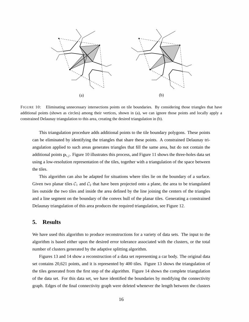
This triangulation procedure adds additional points to the tile boundary polygons. These points

can be eliminated by identifying the triangles that share these points. A constrained Delaunay tri-

angulation applied to such areas generates triangles that fill the same area, but do not contain the

additional pointspi,j . Figure 10 illustrates this process, and Figure 11 shows the three-holes data set

using a low-resolution representation of the tiles, together with a triangulation of the space between

the tiles.

This algorithm can also be adapted for situations where tiles lie on the boundary of a surface.

Given two planar tilesC1 andC2 that have been projected onto a plane, the area to be triangulated

lies outside the two tiles and inside the area defined by the line joining the centers of the triangles

and a line segment on the boundary of the convex hull of the planar tiles. Generating a constrained

Delaunay triangulation of this area produces the required triangulation, see Figure 12.

5. Results

We have used this algorithm to produce reconstructions for a variety of data sets. The input to the

algorithm is based either upon the desired error tolerance associated with the clusters, or the total

number of clusters generated by the adaptive splitting algorithm.

Figures 13 and 14 show a reconstruction of a data set representing a car body. The original data

set contains 20,621 points, and it is represented by 400 tiles. Figure 13 shows the triangulation of

the tiles generated from the first step of the algorithm. Figure 14 shows the complete triangulation

of the data set. For this data set, we have identified the boundaries by modifying the connectivity

graph. Edges of the final connectivity graph were deleted whenever the length between the clusters

16

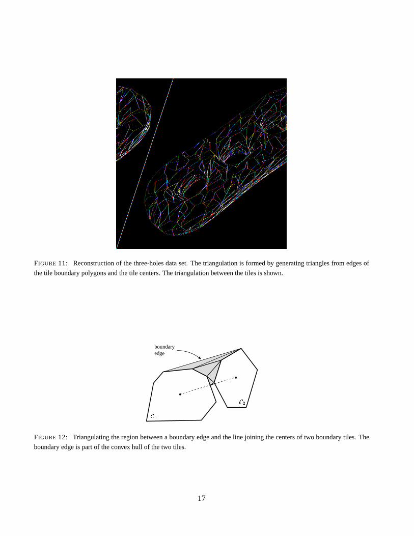
FIGURE 11: Reconstruction of the three-holes data set. The triangulation is formed by generating triangles from edges of

the tile boundary polygons and the tile centers. The triangulation between the tiles is shown.

boundaryedge

���

���

FIGURE 12: Triangulating the region between a boundary edge and the line joining the centers of two boundary tiles. The

boundary edge is part of the convex hull of the two tiles.

17

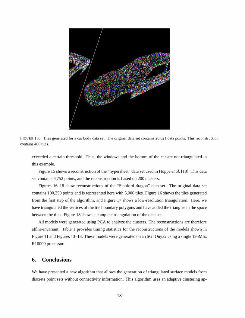
FIGURE 13: Tiles generated for a car body data set. The original data set contains 20,621 data points. This reconstruction

contains 400 tiles.

exceeded a certain threshold. Thus, the windows and the bottom of the car are not triangulated in

this example.

Figure 15 shows a reconstruction of the “hypersheet” data set used in Hoppeet al.[18]. This data

set contains 6,752 points, and the reconstruction is based on 200 clusters.

Figures 16–18 show reconstructions of the “Stanford dragon” data set. The original data set

contains 100,250 points and is represented here with 5,000 tiles. Figure 16 shows the tiles generated

from the first step of the algorithm, and Figure 17 shows a low-resolution triangulation. Here, we

have triangulated the vertices of the tile boundary polygons and have added the triangles in the space

between the tiles. Figure 18 shows a complete triangulation of the data set.

All models were generated using PCA to analyze the clusters. The reconstructions are therefore

affine-invariant. Table 1 provides timing statistics for the reconstructions of the models shown in

Figure 11 and Figures 13–18. These models were generated on an SGI Onyx2 using a single 195Mhz

R10000 processor.

6. Conclusions

We have presented a new algorithm that allows the generation of triangulated surface models from

discrete point sets without connectivity information. This algorithm uses an adaptive clustering ap-

18

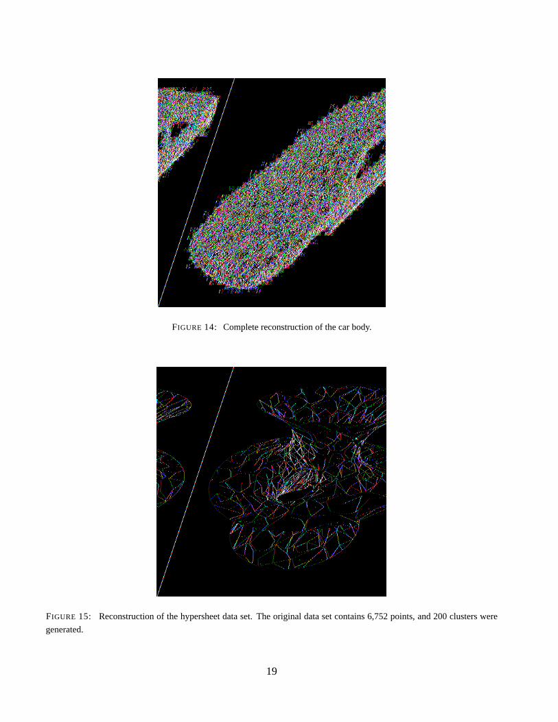
FIGURE 14: Complete reconstruction of the car body.

FIGURE 15: Reconstruction of the hypersheet data set. The original data set contains 6,752 points, and 200 clusters were

generated.

19

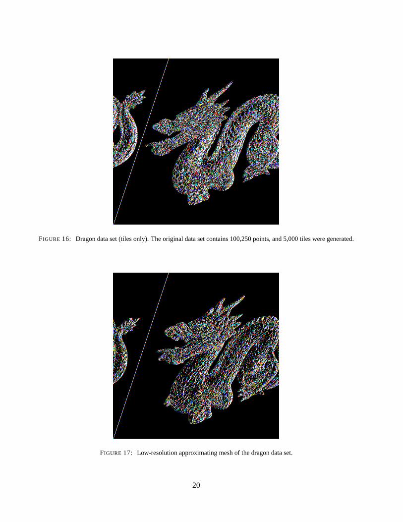
FIGURE 16: Dragon data set (tiles only). The original data set contains 100,250 points, and 5,000 tiles were generated.

FIGURE 17: Low-resolution approximating mesh of the dragon data set.

20

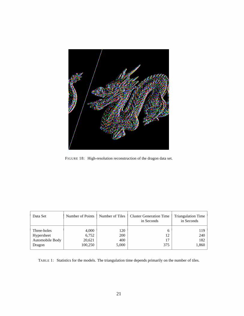
FIGURE 18: High-resolution reconstruction of the dragon data set.

Data Set Number of Points Number of Tiles Cluster Generation Time Triangulation Timein Seconds in Seconds

Three-holes 4,000 120 6 119Hypersheet 6,752 200 12 240Automobile Body 20,621 400 17 182Dragon 100,250 5,000 375 1,860

TABLE 1: Statistics for the models. The triangulation time depends primarily on the number of tiles.

21

proach to generate a set of two-manifold tiles that locally approximate the underlying unknown sur-

face. We construct a triangulation of the surface by triangulating the data within the individual tiles

and triangulating the gaps between the tiles. Approximating meshes can be generated by directly

triangulating the boundary polygons of the tiles. Since the deviation from the point set is known for

each cluster, we can produce approximate reconstructions with prescribed error bounds.

If a given data set has connectivity information, then our algorithm can be viewed as a general-

ization of the vertex-removal algorithm of Schroederet al. [31]. Instead of removing a vertex and

re-triangulating the resulting hole, we remove clusters of nearly coplanar points and re-triangulate

the hole generated by removing the cluster. This is an immediate extension of our approach. We also

plan to extend our algorithm to reconstruct surfaces with sharp edges and vertices.

We plan to extend our approach to the clustering of more general scattered data sets represent-

ing scalar and vector fields, defined over two-dimensional and three-dimensional domains. These

are challenging problems as faster algorithms for the generation of data hierarchies for scientific

visualization are becoming increasingly important due to our ability to generate ever larger data sets.

7. Acknowledgments

This work was supported by the National Science Foundation under contracts ACI 9624034 and

ACI 9983641 (CAREER Awards), through the Large Scientific and Software Data Set Visualiza-

tion (LSSDSV) program under contract ACI 9982251, and through the National Partnership for Ad-

vanced Computational Infrastructure (NPACI); the Office of Naval Research under contract N00014-

97-1-0222; the Army Research Office under contract ARO 36598-MA-RIP; the NASA Ames Re-

search Center through an NRA award under contract NAG2-1216; the Lawrence Livermore Na-

tional Laboratory under ASCI ASAP Level-2 Memorandum Agreement B347878 and under Mem-

orandum Agreement B503159; and the North Atlantic Treaty Organization (NATO) under contract

CRG.971628 awarded to the University of California, Davis. We also acknowledge the support of

ALSTOM Schilling Robotics, Chevron, General Atomics, Silicon Graphics, and ST Microelectron-

ics, Inc. We thank the members of the Visualization Group at the Center for Image Processing and

Integrated Computing (CIPIC) at the University of California, Davis.

We would like to thank the reviewers of the initial version of this paper. Their comments have

improved the paper greatly.

22

References

[1] A LGORRI, M.-E., AND SCHMITT, F. Surface reconstruction from unstructured 3D data.Com-

puter Graphics Forum 15, 1 (Mar. 1996), 47–60.

[2] A MENTA , N., BERN, M., AND KAMVYSSELIS, M. A new Voronoi-based surface reconstruc-

tion algorithm. InSIGGRAPH 98 Conference Proceedings(July 1998), M. Cohen, Ed., Annual

Conference Series, ACM SIGGRAPH, Addison Wesley, pp. 415–422.

[3] ATTALI , D. r-regular shape reconstruction from unorganized points.Computational Geometry.

Theory and Applications 10, 4 (July 1998), 239–247.

[4] BAJAJ, C. L., BERNARDINI, F., AND XU, G. Automatic reconstruction of surfaces and scalar

fields from 3D scans.Computer Graphics 29, Annual Conference Series (1995), 109–118.

[5] BERNARDINI, F., AND BAJAJ, C. L. Sampling and reconstructing manifolds using alpha-

shapes. InProc. 9th Canadian Conf. Computational Geometry(Aug. 1997), pp. 193–198.

[6] BERNARDINI, F., MITTLEMAN , J., RUSHMEIER, H., SILVA , C., AND TAUBIN , G. The

ball-pivoting algorithm for surface reconstruction.IEEE Transactions on Visualization and

Computer Graphics 5, 4 (1999), 145–161.

[7] B ITTAR , E., TSINGOS, N., AND GASCUEL, M.-P. Automatic reconstruction of unstructured

3D data: Combining medial axis and implicit surfaces.Computer Graphics Forum 14, 3 (Sept.

1995), C/457–C/468.

[8] BOISSONNAT, J.-D. Geometric structures for three-dimensional shape representation.ACM

Transactions on Graphics 3, 4 (Oct. 1984), 266–286.

[9] BOLLE, R. M., AND VEMURI, B. C. On three-dimensional surface reconstruction methods.

IEEE Transactions on Pattern Analysis and Machine Intelligence PAMI-13, 1 (Jan. 1991), 1–

13.

[10] CURLESS, B., AND LEVOY, M. A volumetric method for building complex models from range

images.Computer Graphics 30, Annual Conference Series (1996), 303–312.

[11] ECK, M., DEROSE, T., DUCHAMP, T., HOPPE, H., LOUNSBERY, M., AND STUETZLE, W.

Multiresolution analysis of arbitrary meshes. InSIGGRAPH 95 Conference Proceedings(Aug.

1995), R. Cook, Ed., Annual Conference Series, ACM SIGGRAPH, Addison Wesley, pp. 173–

182.

[12] EDELSBRUNNER, H., AND M UCKE, E. P. Three-dimensional alpha shapes.ACM Transactions

on Graphics 13, 1 (Jan. 1994), pp. 43–72. ISSN 0730-0301.

23

[13] GORDON, A. D. Hierarchical classification. InClustering and Classification, R. Arabie,

L. Hubert, and G. DeSoete, Eds. World Scientific Publishers, River Edge, NJ, 1996, pp. 65–

105.

[14] GUO, B. Surface reconstruction: from points to splines.Computer-Aided Design 29, 4 (1997),

pp. 269–277.

[15] HECKEL, B., UVA , A., AND HAMANN , B. Clustering-based generation of hierarchical surface

models. InProceedings of Visualization 1998 (Late Breaking Hot Topics)(Oct. 1998), C. Wit-

tenbrink and A. Varshney, Eds., IEEE Computer Society Press, Los Alamitos, CA, pp. 50–55.

[16] HINKER, P., AND HANSEN, C. Geometric optimization. InProceedings of the Visualiza-

tion ’93 Conference(San Jose, CA, Oct. 1993), G. M. Nielson and D. Bergeron, Eds., IEEE

Computer Society Press, Los Alamitos, CA, pp. 189–195.

[17] HOPPE, H., DEROSE, T., DUCHAMP, T., MCDONALD , J., AND STUETZLE, W. Surface

reconstruction from unorganized points. InComputer Graphics (SIGGRAPH ’92 Proceedings)

(July 1992), E. E. Catmull, Ed., vol. 26, pp. 71–78.

[18] HOPPE, H., DEROSE, T., DUCHAMP, T., MCDONALD , J., AND STUETZLE, W. Mesh opti-

mization. InComputer Graphics (SIGGRAPH ’93 Proceedings)(Aug. 1993), J. T. Kajiya, Ed.,

vol. 27, pp. 19–26.

[19] HOTELLING, H. Analysis of a complex of statistical variables into principal components.

Journal of Educational Psychology 24(1933), pp. 417–441 and 498–520.

[20] JACKSON, J. E.A User’s Guide to Principal Components. Wiley, New York, 1991.

[21] KALVIN , A. D., AND TAYLOR , R. H. Superfaces: Polyhedral approximation with bounded

error. InMedical Imaging: Image Capture, Formatting, and Display(Feb. 1994), vol. 2164,

SPIE, pp. 2–13.

[22] KALVIN , A. D., AND TAYLOR , R. H. Superfaces: Polygonal mesh simplification with

bounded error.IEEE Computer Graphics and Appl. 16, 3 (May 1996).

[23] LORENSEN, W. E., AND CLINE , H. E. Marching cubes: a high resolution 3D surface con-

struction algorithm. InComputer Graphics (SIGGRAPH ’87 Proceedings)(July 1987), M. C.

Stone, Ed., vol. 21, pp. 163–170.

[24] MANLY, B. Multivariate Statistical Methods, A Primer. Chapman & Hall, New York, New

York, 1994.

[25] MENCL, R. A graph-based approach to surface reconstruction.Computer Graphics Forum 14,

3 (Sept. 1995), C/445–C/456.

24

[26] MENCL, R., AND M ULLER, H. Graph-based surface reconstruction using structures in scat-

tered point sets. InProceedings of the Conference on Computer Graphics International 1998

(CGI-98) (Los Alamitos, California, June 22–26 1998), F.-E. Wolter and N. M. Patrikalakis,

Eds., IEEE Computer Society, pp. 298–311.

[27] MOUNT, D. M. Voronoi diagrams on the surface of a polyhedron. Technical Report CAR-TR-

121, CS-TR-1496, Department of Computer Science, University of Maryland, College Park,

MD, May 1985.

[28] NIELSON, G. M. Coordinate-free scattered data interpolation. InTopics in Multivariate Ap-

proximation, L. Schumaker, C. Chui, and F. Utreras, Eds. Academic Press, Inc., New York,

New York, 1987, pp. 175–184.

[29] NIELSON, G. M., AND FOLEY, T. A survey of applications of an affine invariant norm. In

Mathematical Methods in Computer Aided Geometric Design, T. Lyche and L. Schumaker,

Eds. Academic Press, Inc., San Diego, California, 1989, pp. 445–467.

[30] OKABE , A., BOOTS, B., AND SUGIHARA , K. Spatial Tesselations — Concepts and Applica-

tions of Voronoi Diagrams. Wiley, Chichester, 1992.

[31] SCHROEDER, W. J., ZARGE, J. A., AND LORENSEN, W. E. Decimation of triangle meshes.

In Computer Graphics (SIGGRAPH ’92 Proceedings)(July 1992), E. E. Catmull, Ed., vol. 26,

pp. 65–70.

[32] SOUCY, M., AND LAURENDEAU, D. A general surface approach to the integration of a set of

range views.IEEE Transactions on Pattern Analysis and Machine Intelligence 17, 4 (1995),

344–358.

[33] TEICHMANN , M., AND CAPPS, M. Surface reconstruction with anisotropic density-scaled al-

pha shapes. InProceedings of Visualization 98(Oct. 1998), D. Ebert, H. Hagen, and H. Rush-

meier, Eds., IEEE Computer Society Press, Los Alamitos, CA, pp. 67–72.

25