Support Vector Machines Applied to Handwritten Numerals Recognition

Shuonan Dong dongs@mit.edu

Introduction A good classifier must accurately and efficiently separate patterns from one another, given a set of training data. By maximizing the minimal distance from the training data to the decision boundary, support vector machines (SVMs) can achieve an errorless separation of the training data if one exists and a relatively low error separation if the data is inseparable. Maximizing the minimum margin takes SVMs one step forward from earlier perceptron algorithms [Hastie 2001, p. 107-111]. One advantage of SVMs is the ability to ignore outliers that may cause problems in other classifiers such as those that minimize mean squared errors. In addition, since SVMs are formulated as quadratic programming problems, they do not suffer from the complicated local minima issues of multilayer neural network classifiers.

1. Support Vector Machines I will first address SVMs used in two class problems, and then cover SVMs used in multiple class problems.

1.1 Two Class Problem Formulation In the most basic setup, the training data is drawn from an m-dimensional universe with just two classes. Each training datum is represented by an m-dimensional vector x that belongs to either class A or B, where the union of A and B is the universe. Much of the two class SVM derivations are referenced from [Boser 1992] and [Abe 2005]. The training data consists of a set of vectors ; we label each either +1 or –1 to associate it with a class: e.g. +1 for class A and –1 for class B. A training set containing p training points of vectors and labels l

pk xxxx KK ,,, 21 kx

kx k would look like:

( ) ( ) ( ) ( )ppkk llll ,,,,,,,,, 2211 xxxx KK , where (1) ⎩⎨⎧

∈−=∈=

B class if1A class if1

kk

kk

ll

xx

1.1.1 Decision Function Given the training data, the algorithm must derive a decision function (i.e. classifier)

to divide the two classes. The decision function may or may not be linear in x depending on the properties of the corpus and which kernel is chosen. For a classification scheme shown in Equation 1, a decision value of

( )xD

( ) 0=xD would be on the boundary

1

between the classes. Any new, unknown vector x can be classified by determining its decision value: a positive decision value places x in class A, and a negative value places x in class B. The decision function is a multidimensional surface that optimally divides the different classes. In our simple pedagogical example, D is some linear function of x = (x, y) that divides the two classes by maximizing the distance between itself and the nearest points in the corpus, as shown in Figure 1.

Figure 1: Decision function for the pedagogical example

The decision function of an unknown input vector x can be described in either direct space or dual space. In direct space, the representation of the decision function is:

, (2) ( ) ( ) bwDp

kkk += ∑

=1xx ϕ

where the iϕ are previously defined functions of x, and and b are adjustable weight parameters of D. Here, b is the bias, i.e. offset of D. In dual space, the decision function is represented by:

iw

, (3) ( ) ( ) bKDp

kkk += ∑

=1

, xxx α

where the and b are adjustable parameters, and xka k are the training patterns. The direct space and dual space representations of D, i.e. Equations 2 and 3, are related to each other via the following relation:

. (3) ( )∑=

=p

kkikiw

1

xϕα

K is a predefined kernel function of the form

max d max d

max d

),( yxfD =

2

( ) ( ) ( )xxxx ′=′ ∑ i

iiK ϕϕ, . (4)

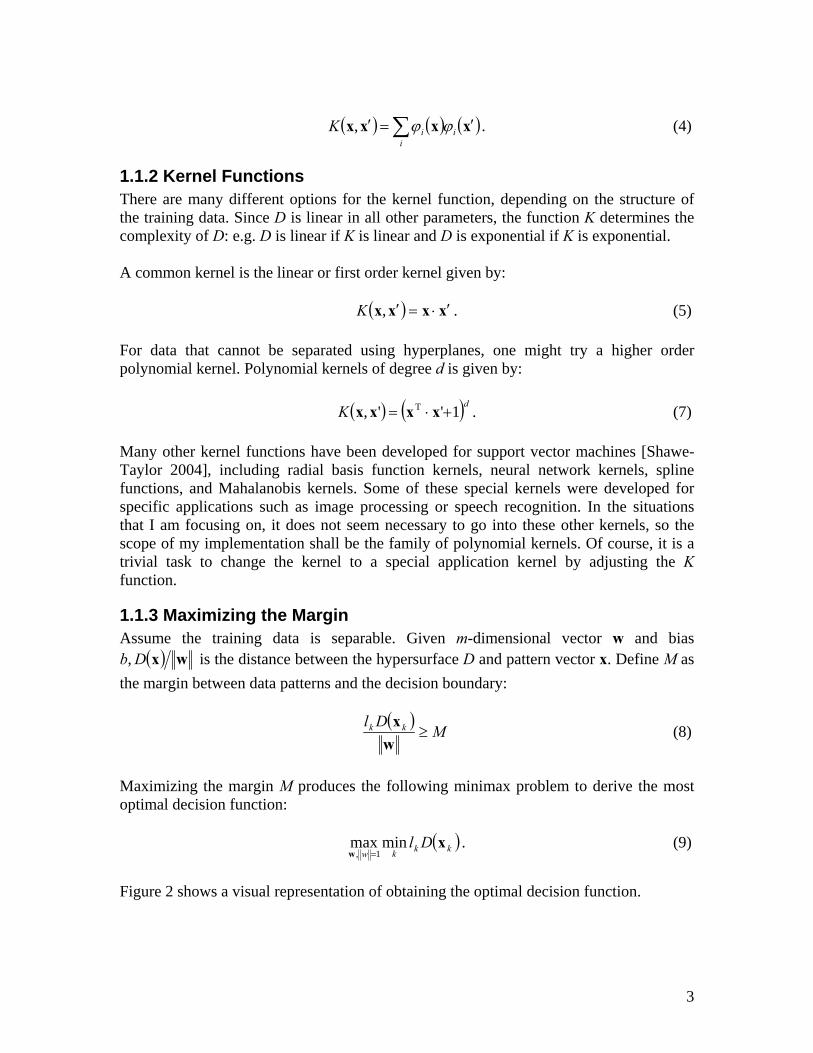
1.1.2 Kernel Functions There are many different options for the kernel function, depending on the structure of the training data. Since D is linear in all other parameters, the function K determines the complexity of D: e.g. D is linear if K is linear and D is exponential if K is exponential. A common kernel is the linear or first order kernel given by: ( ) xxxx ′⋅=′,K . (5) For data that cannot be separated using hyperplanes, one might try a higher order polynomial kernel. Polynomial kernels of degree d is given by: ( ) ( )dK 1'', T +⋅= xxxx . (7) Many other kernel functions have been developed for support vector machines [Shawe-Taylor 2004], including radial basis function kernels, neural network kernels, spline functions, and Mahalanobis kernels. Some of these special kernels were developed for specific applications such as image processing or speech recognition. In the situations that I am focusing on, it does not seem necessary to go into these other kernels, so the scope of my implementation shall be the family of polynomial kernels. Of course, it is a trivial task to change the kernel to a special application kernel by adjusting the K function.

1.1.3 Maximizing the Margin Assume the training data is separable. Given m-dimensional vector w and bias b, ( ) wxD is the distance between the hypersurface D and pattern vector x. Define M as the margin between data patterns and the decision boundary:

( )

MDl kk ≥w

x (8)

Maximizing the margin M produces the following minimax problem to derive the most optimal decision function: ( )kkkw

Dl xw

minmax1, =

. (9)

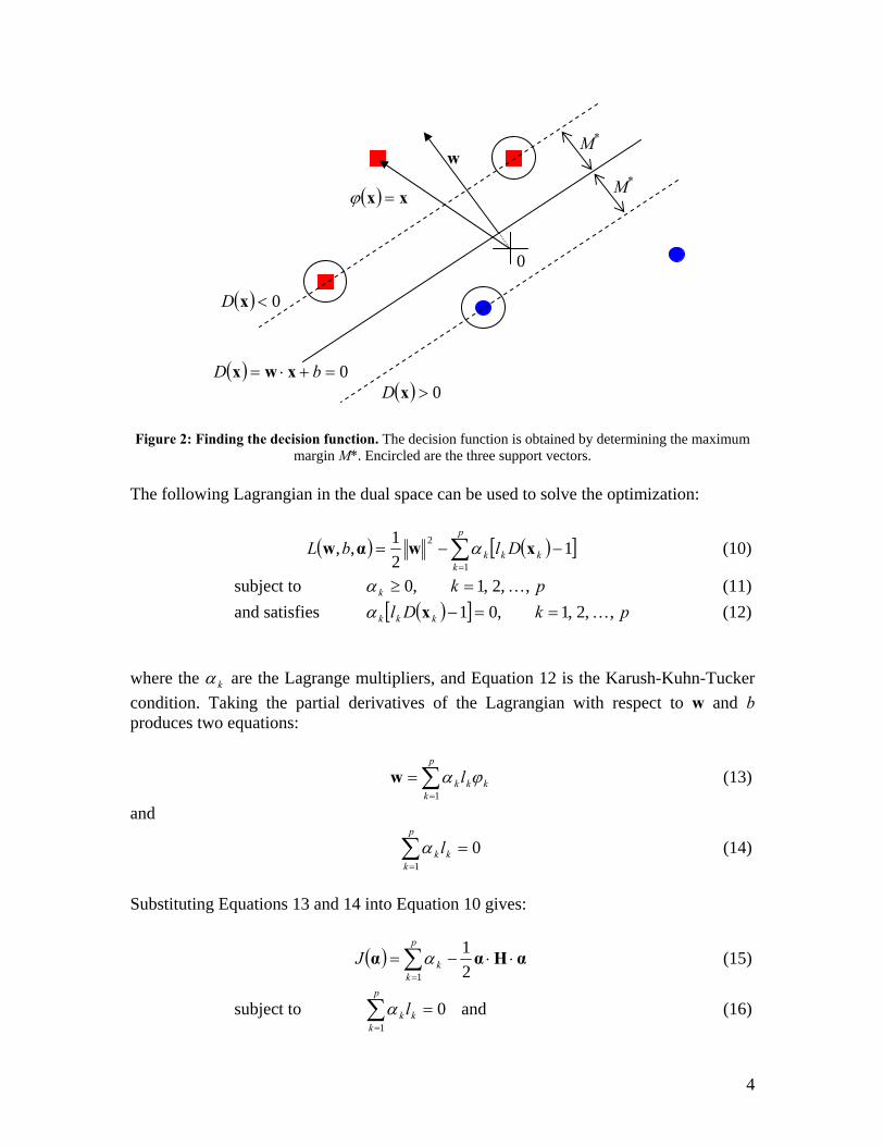
Figure 2 shows a visual representation of obtaining the optimal decision function.

3

M*

M*

( ) 0=+⋅= bD xwx

w

( ) xx =ϕ

0

Figure 2: Finding the decision function. The decision function is obtained by determining the maximum

margin M*. Encircled are the three support vectors. The following Lagrangian in the dual space can be used to solve the optimization:

( ) ( )[∑=

−−=p

kkkk DlbL

1

2 121,, xwαw α ] (10)

subject to pkk ,,2,1,0 K=≥α (11) and satisfies ( )[ ] pkDl kkk ,,2,1,01 K==−xα (12)

where the kα are the Lagrange multipliers, and Equation 12 is the Karush-Kuhn-Tucker condition. Taking the partial derivatives of the Lagrangian with respect to w and b produces two equations:

(13) ∑=

=p

kkkk l

1ϕαw

and

(14) 01

=∑=

p

kkk lα

Substituting Equations 13 and 14 into Equation 10 gives:

( ) αHαα ⋅⋅−= ∑= 2

11

p

kkJ α (15)

subject to and (16) 01

=∑=

p

kkk lα

( ) 0>xD

( ) 0<xD

4

pkk ,,2,1,0 K=≥α . (17) The kernel function K is contained in the pp× matrix H, which is defined by ( )mkmkkm KllH xx ,= (18) The optimal parameters α* can be found by maximizing the Lagrangian using quadratic programming. The training data that corresponds to non-zero values in α* are the support vectors. There are usually fewer support vectors than the total number of data points. The constraint in Equation 16 requires at least one support vector in each class. Assuming two arbitrary support vectors and Aclass∈Ax Bclass∈Bx , the bias b can be found:

( ) ([∑=

∗∗ +−=p

kkBkAkk KKlb

1,,

21 xxxxα )]. (19)

The decision function is therefore:

. (20) ( ) ( ) ∗

=

∗ += ∑ bKlDp

kkkk

1,xxx α

Each datum x is classified according to ( )[ ]xDsgn . (21)

1.1.4 Soft Margin Classifier When the data is not completely separable, slack variables are needed to allow some level of error. Define a set of slack variables pkk ...1, =ξ so that ( ) kkk Dl ξ−≥ 1x , (22) as illustrated in Figure 3.

10 >> kξ1>jξ

Figure 3. Examples of slack variables for soft margin classifiers.

5

There are two architectures for soft margin classifiers. One penalizes the linear sum of the slack variables, and the other penalizes the square sum. I will be using the first architecture. More information on least squares SVMs can be found in [Suykens 2003, Ch. 8]. The soft margin Lagrangian can be reduced to the form:

( ) αHαα ⋅⋅−= ∑= 2

11

p

kkJ α (23)

subject to and (24) 01

=∑=

p

kkk lα

pkC k ,,1,0 K=≥≥ α , (25) which is identical to that of the hard margin Lagrangian (Equation 15) except for the constraint 0≥≥ kC α , where C is some sufficiently large number. Now the optimal parameters can have three possible range of values: 0=kα , 0>> kC α , or Ck=α . Data corresponding to 0>> kC α are unbounded support vectors, for which the corresponding slack variables equal zero. Data corresponding to Ck=α are bounded support vectors. Like the example shown in Figure 3, if the corresponding slack variable is between 0 and 1, then the datum is classified correctly; if the slack variable is greater than 1, then the datum is misclassified. Once the optimal parameters α* are found, the bias and decision function is determined in the same way as discussed in Section 1.1.3.

1.2 Multiple Class Problem Formulation Since SVMs were originally designed for two class problems [Vapnik 1996], when there are more than two classes in the universe, the problem is formulated a little differently. The four main types of SVMs that handle multi-class problems as discussed in [Abe 2005] are:

1. One-against-all SVMs, 2. Pairwise SVMs [Li 2002], 3. Error-correcting output code SVMs, 4. All-at-once SVMs.

There are advantages and disadvantages to each kind of method. One-against-all and pairwise SVMs often have regions in the space that are not classifiable. Figures 4 and 5 show examples of unclassifiable regions by the one-against-all and pairwise SVMs in 2-D environments having three classes using first order kernels. These unclassifiable regions can be reduced or eliminated by using more involved architectures such as decision trees, directed acyclic graphs, fuzzy SVMs, or cluster-based SVMs. The advantage of the all-at-once SVM is the resolution of unclassifiable regions in the other methods without using any fancy architectures. The implementation is quite clean

6

and can be built directly upon the two class problem structure. The only difference in the problem formulations is the structure of the class labels.

Of the two formulations mentioned in [Abe 2005, p. 118-122] for all-at-once SVMs, I choose to represent the class labels as a cp× dimensional matrix, where c is the number of classes, and for each label:

(26) ⎩⎨⎧−

∈−=

otherwise.1classfor 1 jn

l kjk

x

The advantage of this formulation is the relatively small number of changes that need to be made to the two class quadratic programming optimizer in order to handle multiple classes.

1.2.1 Multi-Class All-At-Once Optimizer The all-at-once SVM optimizer follows the same derivation steps as those shown for the two class classifier in Section 1.1.3. The resulting soft margin Lagrangian is very similar:

( ) αHαα ⋅⋅−= ∑= 2

11

p

kkJ α (27)

subject to and (28) cjlp

k

jkk ,,1,0

1K==∑

=

α

( ) pkcC k ,,1,01 K=≥−≥ α . (29) The matrix H, is now defined by:

Class A

Class C

Class B

DAB(x) = 0

DBC(x) = 0

DAC(x) = 0

0 x1

x2 Class A

Class B

Class C

DA(x) = 0

DC(x) = 0

DB(x) = 0

0 x1

x2

Figure 4. Unclassifiable regions by one-against-all SVM. [Abe 2005, p. 85]

Figure 5 Unclassifiable regions by pairwise SVM. [Abe 2005, p. 97]

7

(30) (∑=

=c

jmk

jm

jkkm KllH

1,xx )

The decision function for each class is now given by:

. (31) ( ) ( ) ∗

=

∗ += ∑ j

p

kkk

jkj bKlD

1,xxx α

And the datum x is classified into class ( )xj

cjD

K1maxarg

=. (32)

2 Implementation I first implemented two class support vector machines and tried the algorithm on a simple 2-D toy problem, which is discussed in Section 3. I then adjusted the kernel functions, which produced different decision functions, as expected. To apply the algorithm to a real problem, I chose to use a set of hand drawn circle-line data (i.e. 0, 1 digits) on which to apply the SVM classifier. I also developed an error computation function to judge the performance of the classifier. The next step was to expand the two class SVM to multi-class SVM. Again, the algorithm was first applied to the 2-D toy problem and then to the 0-9 handwritten digits problem. The SVM implementation was developed in MATLAB 7.0.4.

2.1 Two Class There are several primary components to the SVM implementation: the decision function, the soft margin optimizer Lagrangian J, and the kernel function, in addition to some secondary components: an input data script, a helper function to extract the supports, an output script for 2-D data, and a run script. The input data script defines a mp× matrix called xTrain, which is the set of all the training data, and a matrix called labels, which contains the values +1 and –1 depending on the corresponding class of the training data.

1×p

The optimizer is of the form [alpha, b] = J(xTrain, labels). It uses the training data and labels to first find the H matrix via Equation 18, and then uses quadratic programming (MATLAB’s quadprog function) to find the optimal alpha vector via Equations 23-25. It calls the function supports to obtain one support from each class, and uses them to calculate the bias b via Equation 19.

8

The helper function supports extracts the unbounded support vectors given a set of alpha by testing that each element in alpha is >0 and <C. It also returns another matrix containing one arbitrary support from each class, which is used for finding the bias b in the optimizer. The kernel function is of the form K = Kernel(x1, x2). For this function, I have simply implemented Equation 7 with variable d. The decision function is of the form D = Decision(alpha, b, x, xTrain, labels) and follows Equations 20 and 21. The output2D script plots the training data for each class, and then plots the line or curve for which the decision function is zero. The RunSVM script calls the input data script, the optimizer, and the output script (for 2-D data only).

2.2 Multiple Class The implementation for multi-class SVM can be built upon the two class SVM with a few changes to the input data script, the optimizer, and the decision function. The input data script either defines the labels directly according to Equation 26 or converts existing labels from a different format. In the optimizer function, the H matrix is calculated with another summation over the classes, as dictated in Equation 30, and the quadratic programming requires a whole set of equality constraints found in Equation 28. The decision function computes one decision value for each class, and returns the index of the maximum decision value via Equations 31 and 32. The indices correspond to the class into which the datum x is classified. The output script for 2-D data plots the training data for each class using different sized markers, and also shades the regions determined by the decision function using different shades of color.

2.3 Error To generate some metric which can be used to judge the performance of the algorithm, I implemented an error function of the form loss0_1 = error0_1(alpha, b, xTrain, labels, xTest, labTest). This function runs the decision function on all of the test data xTest using a set of alpha and b values which had been trained from xTrain and labels. For every instance that the decision function output does not match the test data labels labTest (i.e. the test datum is misclassified), then a loss of 1 is incurred. In the end, the rate of error is given as a decimal by dividing the accumulated loss by the total number of test data.

9

2.4 Cross Validation For a limited set of data, the error of the classifier can be estimated using cross validation. Usually it is sufficient and computationally advantageous to use k-fold cross validation, but in the case of support vector machines, the leave-one-out (LOO) method is not too computationally poor. This is because the LOO only needs to be applied to support vectors (bounded and unbounded) and not all data points [Abe 2005, p. 74], since any datum that is not a support vector can be eliminated and the same classifier will be generated, ensuring that the datum that had been left out will definitely be classified correctly when being tested against. Cross validation is implemented in the form cvErr = crossValidation (xTrain, labels). It first generates a set of alpha and b values by training all of the data. Then it calls the supports helper function to find all support vectors. Iterating through the support vectors, the optimizer function is called with the training data leaving out the current support vector and accumulates an error by calling the error0_1 function on the LOO data. In the end, the cumulative error is normalized by the total number of data points.

3 Performance Demonstration on 2-D Example Problem A randomly generated 2-D toy problem is used to visually observe the results of the classifier. Although the actual values of the example data are not important, I include it in the figures of this section just for reference. The labels can be changed for demonstrating different data configurations.

3.1 Two Class Classifier The first thing to do is to run the two class SVM on the data shown in Figure 6 using a linear decision function. The resulting divider uses three support vectors, as expected.

x1 x2 l α 3 5 +1 0 4 6 +1 0 2 2 +1 0.065 7 4 +1 0 9 8 +1 0 -5 -2 –1 0 -8 2 –1 0.015 -2 -9 –1 0 1 -4 –1 0.05

Figure 6. Linear decision function for example data. Encircled are the support vectors. The data point

values, labels, and optimal parameters α are shown on the right.

10

Notice that there are three support vectors in the example problem shown in Figure 6. It may seem that the number of support vectors must be at least the Vapnik-Chervonenkis (VC) dimension (i.e. ) of the data, but this is not necessarily true. Figure 7 shows an example of data in 2-D that is classifiable using only two support vectors.

1+p

x1 x2 l α 3 5 –1 1 4 6 –1 1 2 2 +1 0 7 4 +1 0 9 8 +1 0 -5 -2 –1 0 -8 2 –1 0 -2 -9 –1 0 1 -4 –1 0

Figure 7. Example of 2-D data that only has two support vectors

Not all training data situations may be completely separable. In these cases, the soft margin classifier should minimize the error of misclassified points while also maximizing the minimum margin of the unbounded support vectors. In Figure 8, there are two bounded support vectors and three unbounded support vectors. Of the two bounded support vectors, one of them is misclassified.

x1 x2 l α 3 5 –1 100 4 6 +1 30.58 2 2 +1 100 7 4 +1 0 9 8 +1 0 -5 -2 –1 0 -8 2 –1 0.93 -2 -9 –1 0 1 -4 –1 29.64

Figure 8. Example data which is linearly inseparable. Encircled are the unbounded support vectors. The

arbitrary bound C is set to 100. In order to better separate the data, one might try a higher order kernel function. Figure 9 shows the same data that is separable by a hyperbola.

11

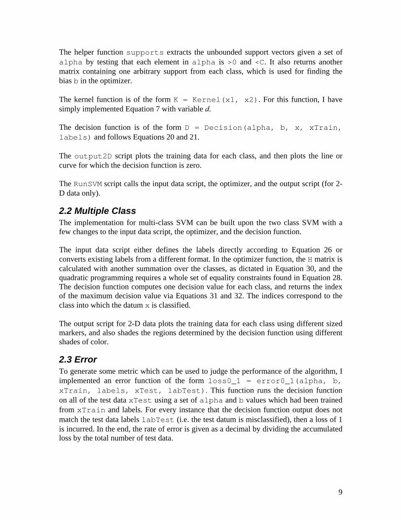
x1 x2 l α 3 5 –1 0.4918 4 6 +1 0.3061 2 2 +1 0.2423 7 4 +1 0 9 8 +1 0 -5 -2 –1 0.0565 -8 2 –1 0 -2 -9 –1 0 1 -4 –1 0

Figure 9. A quadratic decision function cleanly separates the example data.

The second order decision function may separate the data without misclassifications, however it may not be the best choice for the example data in general. To check this, I found the LOO cross validation errors for both the linear and second order decision functions. It turns out that the cross validation error for the linear classifier is 0.33 and for the second order classifier is 0.44. Thus I can conclude that a linear classifier is probably the better choice for the example data in Figures 8 and 9, even though the data are not linearly separable.

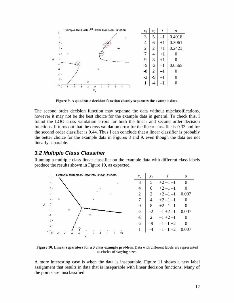
3.2 Multiple Class Classifier Running a multiple class linear classifier on the example data with different class labels produce the results shown in Figure 10, as expected.

x1 x2 l α 3 5 +2 –1 –1 0 4 6 +2 –1 –1 0 2 2 +2 –1 –1 0.007 7 4 +2 –1 –1 0 9 8 +2 –1 –1 0 -5 -2 –1 +2 –1 0.007 -8 2 –1 +2 –1 0 -2 -9 –1 –1 +2 0 1 -4 –1 –1 +2 0.007

Figure 10. Linear separators for a 3 class example problem. Data with different labels are represented

as circles of varying sizes. A more interesting case is when the data is inseparable. Figure 11 shows a new label assignment that results in data that is inseparable with linear decision functions. Many of the points are misclassified.

12

x1 x2 l α 3 5 +2 –1 –1 0 4 6 +2 –1 –1 0 2 2 +2 –1 –1 0.01577 4 –1 +2 –1 0.00739 8 –1 +2 –1 0 -5 -2 –1 +2 –1 0.0084-8 2 –1 +2 –1 0 -2 -9 –1 –1 +2 0 1 -4 –1 –1 +2 0.0157

Figure 11. Linear separators for an inseparable example problem

Now trying a second order divider in Figure 12 produces a much better result in which only one point is misclassified. The divider looks disconnected due to the resolution of the graphing function.

x1 x2 l α 3 5 +2 –1 –1 0 4 6 +2 –1 –1 0.000052 2 +2 –1 –1 0.000427 4 –1 +2 –1 0 9 8 –1 +2 –1 0 -5 -2 –1 +2 –1 0.00047-8 2 –1 +2 –1 0 -2 -9 –1 –1 +2 0 1 -4 –1 –1 +2 0.00047

Figure 12. Second order separators greatly improve the performance.

Trying a third order divider in Figure 13 worsens the result. In fact, one of the regions contains no training data. The poor performance is likely because the optimizer does not find the optimal curves which are of third order.

13

x1 x2 l α 3 5 +2 –1 –1 0 4 6 +2 –1 –1 0 2 2 +2 –1 –1 0.000047 4 –1 +2 –1 0.000019 8 –1 +2 –1 0 -5 -2 –1 +2 –1 0.00004-8 2 –1 +2 –1 0 -2 -9 –1 –1 +2 0 1 -4 –1 –1 +2 0.00005

Figure 13. Third order separators perform quite poorly.

Therefore, for this particular setup of training data, the best classifier is most likely of second order.

4 Pen Digits Problem Handwritten numerals classification is a useful real-world application for support vector machines. It is also the fortunate case that an abundance of data already exists for this problem.

4.1 Training and Testing Data The handwritten numerals data can be obtained from the UCI Repository of machine learning databases [Newman 1998], under the “pendigits” directory. E.Alpaydin and F. Alimoglu of Bogazici University in Istanbul, Turkey provided the database, which contains a total of 10992 data points. Such a large collection of data, while theoretically able to reach very accurate results, is too much for most personal computers to handle—either it takes an unreasonable amount of time to solve the optimization or the machine runs out of memory. Moreover, very reasonable classifiers can be achieved with far fewer data. Therefore, I generally use one or two hundred data points for training, and a few more hundred for testing. Each data holds the (x, y) position information of 8 sample points within a handwritten numeral, so the dimension of the data is 16. All of the data are normalized to be within {0, 0} and (100, 100).

4.2 Zero-One Classification To demonstrate the performance of the two class SVM, I used only the 0 and 1 digits from the database. One hundred data points were used for training and 627 other data points were used for testing. I used fewer training data to save time during optimization and cross validation.

14

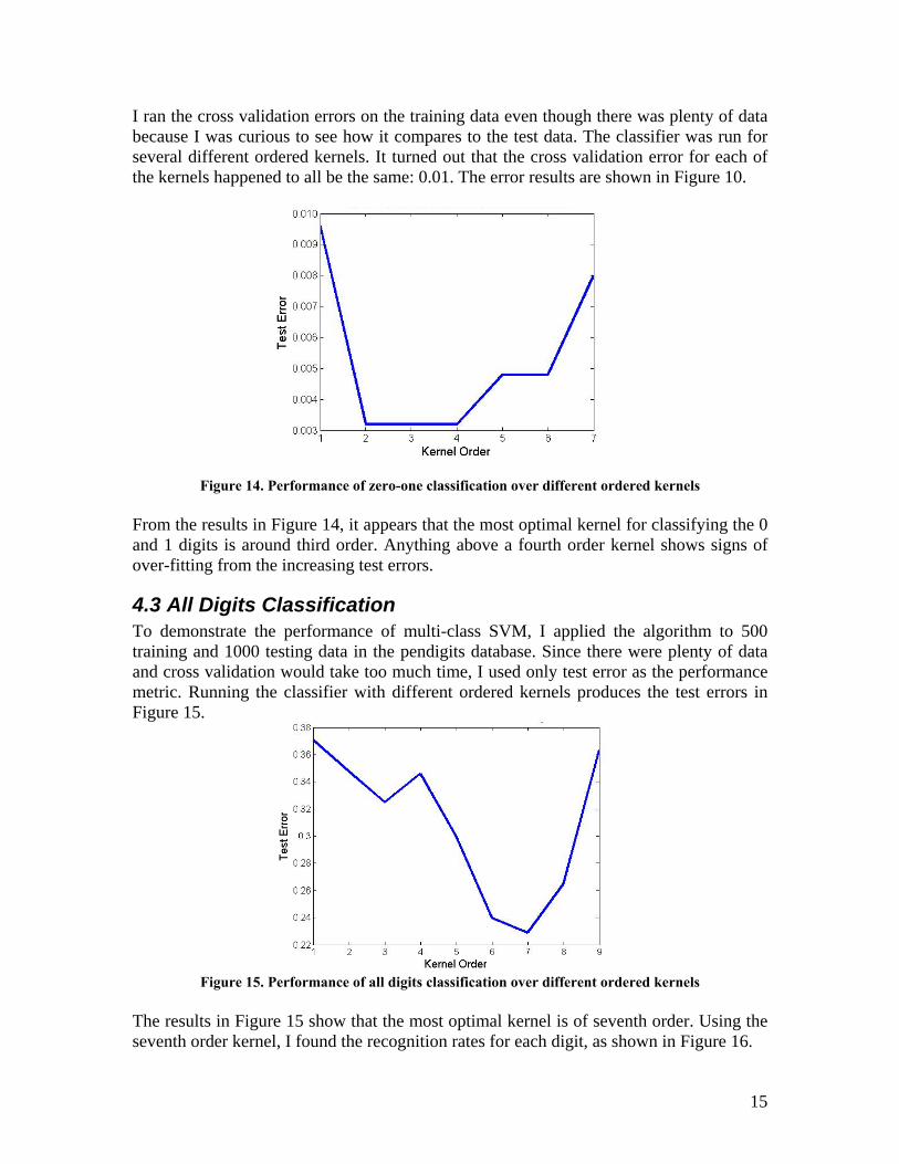
I ran the cross validation errors on the training data even though there was plenty of data because I was curious to see how it compares to the test data. The classifier was run for several different ordered kernels. It turned out that the cross validation error for each of the kernels happened to all be the same: 0.01. The error results are shown in Figure 10.

Figure 14. Performance of zero-one classification over different ordered kernels From the results in Figure 14, it appears that the most optimal kernel for classifying the 0 and 1 digits is around third order. Anything above a fourth order kernel shows signs of over-fitting from the increasing test errors.

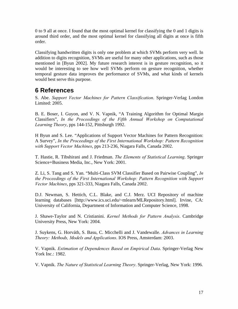
4.3 All Digits Classification To demonstrate the performance of multi-class SVM, I applied the algorithm to 500 training and 1000 testing data in the pendigits database. Since there were plenty of data and cross validation would take too much time, I used only test error as the performance metric. Running the classifier with different ordered kernels produces the test errors in Figure 15.

Figure 15. Performance of all digits classification over different ordered kernels

The results in Figure 15 show that the most optimal kernel is of seventh order. Using the seventh order kernel, I found the recognition rates for each digit, as shown in Figure 16.

15

0

0.1

0.2

0.3

0.4

0.5

0.6

0.7

0.8

0.9

1

0 1 2 3 4 5 6 7 8 9

Digit

Rec

ogni

tion

Rat

e

Figure 16. Recognition rate for each digit

From the results in Figure 16, it appears that SVMs have a difficult time recognizing a 1 or a 7. This may be the downfall of using only 8 sample points from a handwritten numeral to represent the numeral. Often, the data for 1 and 7 are extremely similar. For example, here are two typical pieces of data:

x label59 65 91 100 84 96 72 50 51 8 0 0 45 1 100 0 1 0 78 29 100 94 86 70 48 42 11 32 0 25 36 100 40 7 For the most part, many of the corresponding elements in each x vector are similar. Also, because the data is sampled over time, the horizontal piece on the 7 digit tends to only have 1 point associated with it, since most people tend to spend more time writing the vertical portion of the 7 than the horizontal portion. This may be contributing to much of the problem with distinguishing the 1 digit from the 7 digit.

5 Conclusions and Future Research In this paper, I have discussed the derivations of support vector machines for two class hard margin classification, soft margin classification, classification using different kernel functions, and multi-class classification. After implementing all of these SVM capabilities into MATLAB, I used a 2-D example data set to illustrate the performance of the SVMs through visual output for both two class and multi-class examples. I then applied SVMs to the handwritten numerals recognition problem, starting with distinguishing between 0 and 1 digits, and concluding with classifying all the digits from

16

0 to 9 all at once. I found that the most optimal kernel for classifying the 0 and 1 digits is around third order, and the most optimal kernel for classifying all digits at once is fifth order. Classifying handwritten digits is only one problem at which SVMs perform very well. In addition to digits recognition, SVMs are useful for many other applications, such as those mentioned in [Byun 2002]. My future research interest is in gesture recognition, so it would be interesting to see how well SVMs perform on gesture recognition, whether temporal gesture data improves the performance of SVMs, and what kinds of kernels would best serve this purpose.

6 References S. Abe. Support Vector Machines for Pattern Classification. Springer-Verlag London Limited: 2005. B. E. Boser, I. Guyon, and V. N. Vapnik, “A Training Algorithm for Optimal Margin Classifiers”, In the Proceedings of the Fifth Annual Workshop on Computational Learning Theory, pps 144-152, Pittsburgh 1992. H Byun and S. Lee. “Applications of Support Vector Machines for Pattern Recognition: A Survey”, In the Proceedings of the First International Workshop: Pattern Recognition with Support Vector Machines, pps 213-236, Niagara Falls, Canada 2002. T. Hastie, R. Tibshirani and J. Friedman. The Elements of Statistical Learning. Springer Science+Business Media, Inc., New York: 2001. Z. Li, S. Tang and S. Yan. “Multi-Class SVM Classifier Based on Pairwise Coupling”, In the Proceedings of the First International Workshop: Pattern Recognition with Support Vector Machines, pps 321-333, Niagara Falls, Canada 2002. D.J. Newman, S. Hettich, C.L. Blake, and C.J. Merz. UCI Repository of machine learning databases [http://www.ics.uci.edu/~mlearn/MLRepository.html]. Irvine, CA: University of California, Department of Information and Computer Science, 1998. J. Shawe-Taylor and N. Cristianini. Kernel Methods for Pattern Analysis. Cambridge University Press, New York: 2004. J. Suykens, G. Horváth, S. Basu, C. Micchelli and J. Vandewalle. Advances in Learning Theory: Methods, Models and Applications. IOS Press, Amsterdam: 2003. V. Vapnik. Estimation of Dependences Based on Empirical Data. Springer-Verlag New York Inc.: 1982. V. Vapnik. The Nature of Statistical Learning Theory. Springer-Verlag, New York: 1996.

17