SUPERCRITICAL WATER GASIFICATION OF WET BIOMASS
281
SUPERCRITICAL WATER GASIFICATION OF WET BIOMASS: MODELING AND EXPERIMENTS ONURSAL YAKABOYLU Process and Energy Department 3ME Faculty Delft University of Technology
-
Upload
khangminh22 -
Category
Documents
-
view
2 -
download
0
Transcript of SUPERCRITICAL WATER GASIFICATION OF WET BIOMASS
SUPERCRITICAL WATER GASIFICATION OF WET BIOMASS:
MODELING AND EXPERIMENTS
ONURSAL YAKABOYLU
Process and Energy Department
3ME Faculty
Delft University of Technology

iii
Supercritical Water Gasification of Wet Biomass:
Modeling and Experiments
Proefschrift
ter verkrijging van de graad van doctor
aan de Technische Universiteit Delft,
op gezag van de Rector Magnificus prof.ir. K.C.A.M. Luyben;
voorzitter van het College voor Promoties,
in het openbaar te verdedigen op
donderdag 17 maart 2016 om 10:00 uur
door
Onursal YAKABOYLU
Kimya Yu ksek Mu hendisi, I stanbul Teknik U niversitesi
Geboren te Eskişehir, Turkey

iv
This dissertation has been approved by the promotor:
Prof. dr. ir. B.J. Boersma
and the copromotor:
Dr. ir. W. de Jong
Composition of the doctoral committee:
Rector Magnificus chairman
Prof. dr. ir. B.J. Boersma Delft University of Technology, promotor
Dr. ir. W. de Jong Delft University of Technology, copromotor
Independent members:
Prof.dr.ir. W. Prins Ghent University, Belgium
Prof.dr. P. Koukkari VTT Techn. Res. Centre, Finland
Prof.dr.ir. G. Brem University of Twente
Prof.dr.ir. J.B. van Lier Delft University of Technology
Prof.dr. D.J.E.M. Roekaerts Delft University of Technology, reserved
Other member:
Prof.dr. H.J. Heeres University of Groningen
This research project is carried out within the Agentschap NL funded project “Superkritische vergassing van natte reststromen” (contract EOSLT10051).
Cover photo from pixabay.com, design and layout by Didem Sag lam.
ISBN: 978-94-6233-248-5
Copyright © 2016 by Onursal Yakaboylu. All rights reserved.

v
“[T]he supreme mystery of despotism, its prop and stay, is to keep men in a state of de-ception, and with the specious title of religion to cloak the fear by which they must be held in check, so that they will fight for their servitude as if for salvation, and count it no shame, but the highest honour, to spend their blood and their lives for the glorification of one man”1. However, “a fundamental element of human nature is the need for creative work, for creative inquiry, for free creation without the arbitrary limiting effect of coer-cive institutions”2. So, “a decent society should maximise the possibilities for this funda-mental human characteristic to be realised. That means trying to overcome the elements of repression and oppression and destruction and coercion that exist in any existing soci-ety” 2, and the “ultimate purpose [of the state should not be] to exercise dominion nor to restrain men by fear and deprive them of independence, but on the contrary to free every man from fear so that he may live in security as far as is possible, that is, so that he may best preserve his own natural right to exist and to act, without harm to himself and to others” 3. In addition, “[i]n a free commonwealth every man may think as he pleases, and say what he thinks”3.
1: Baruch Spinoza, Tractatus Theologico-Politicus, Preface, 1670. 2: Noam Chomsky, Human Nature: Justice versus Power. Noam Chomsky debates with Michel Foucault, 1971. 3: Baruch Spinoza, Tractatus Theologico-Politicus, Ch 20, 1670.

vi

vii
To all great people who not only interpreted the world, but also changed it…

viii

ix
SUMMARY
In the following decades, biomass will play an important role among the other renewable energy sources globally as it is already the fourth largest energy re-source after coal, oil and natural gas. It is possible to obtain gaseous, liquid or solid biofuels from biomass via thermochemical or biochemical conversion routes. Among them, gasification is one of the most favorable options as the products can serve all types of energy markets: heat, electricity and transportation. Convention-al gasification is an excellent method for dry ligno-cellulosic biomass feedstocks. However, in case of wet biomass with a high moisture content, it results in a nega-tive impact on the energy efficiency of the gasification process due to the fact that drying costs more energy than the energy content of the product for some very wet biomass types. An alternative method applied for the conversion of wet bio-mass such as sewage sludge, cattle manure and food industry waste is anaerobic digestion. This process is however characterized by a slow reaction rate and typi-cal residence times are almost 2–4 weeks. Besides, the fermentation sludge and wastewater from the reactors should further be treated.
The supercritical water gasification (SCWG) process is an alternative to both conventional gasification as well as the anaerobic digestion processes for conver-sion of wet biomass. This process does not require drying and the process takes place at much shorter residence times; a few minutes at most. Supercritical water gasification is therefore considered to be a promising technology for the efficient conversion of wet biomass into a product gas that after upgrading can be used as substitute natural gas. The main reason why supercritical water gasification is a promising technology is due to the favorable thermo-physical properties of water and the way they change in the supercritical region which causes water to act as a solvent as well as a catalyst. Furthermore, through hydrolysis reactions, water also acts as a reactant. Gasification of biomass is mainly influenced by the density, vis-cosity and dielectric constant of water. Above the critical point, physical properties of water drastically change and water behaves as a homogeneous fluid phase. In its supercritical state, water has a gas-like viscosity and liquid-like density, two properties which enhance mass transfer and solvation properties, respectively. Be-sides, when water enters its supercritical phase, the dielectric constant drastically decreases. Water thus starts to behave like an organic, non-polar solvent which re-sults in poor solubility for inorganics, and complete miscibility with gases and many hydrocarbons. Due to its miscibility, phase boundaries do not exist any-more. This absence leads to fast and complete homogeneous reactions of water with organic compounds.

x
This dissertation focuses on the three aspects of SCWG of biomass systems: i) thermodynamic equilibrium modeling, ii) experimental approaches and iii) pro-cess modeling.
In Chapter 2, the state of the art of the supercritical water gasification technolo-gy starting from the thermophysical properties of water and the chemistry of reac-tions to previous studies on modeling and experimental approaches, and the pro-cess challenges of such a biomass based supercritical water gasification plant is presented.
In Chapter 3, the thermodynamic equilibrium modeling of SCWG of biomass is presented in two sub-chapters. In the first sub-chapter, commercial software pack-ages are dealt with to model the gasification process of a pig–cow manure mixture in supercritical water. The phase and compound behavior of elements, behavior of gas products and water are investigated. Besides, the influence of pressure and dry biomass concentration on the gas yields are reported. In the second sub-chapter, a multi–phase thermodynamic equilibrium model is described. The model is vali-dated by comparing the predictions with the various experimental results. A case study concerning microalgae gasification in supercritical water was performed. The phase and compound behavior of elements and behavior of gas products are investigated. Additionally, the influence of pressure and dry biomass concentra-tion on the gas yields as well as the phase behavior of elements are studied and reported.
In Chapter 4, constrained equilibrium model is tested for SCWG of biomass systems in order to model systems which do not reach to their thermodynamic equilibrium state. Additional constraints are introduced into the developed multi–phase thermodynamic equilibrium model, which is described in Chapter 3, and the importance of the additional constraints are tested by comparing the predic-tions of the model with the experimental results available in the literature.
In Chapter 5, the experimental methods used in this work are described. A new and novel type of experimental setup which incorporates a fluidized bed reactor is designed with and manufactured by Gensos B.V. The setup has a capacity of 50 l/h and allows for clogging-free conditions for the experiments.
In Chapter 6, the results of the experiments for starch are given. The influence of reactor temperature and feed flow rate are investigated. The results include not only the gas composition but also the temperature profile along different process units and the velocity profile along the reactor for different process conditions. The observed process challenges are also reported in this chapter.
In Chapter 7, process modeling of SCWG of biomass is presented in two sub-chapters. In the first sub-chapter, SCWG of biomass process is modeled with an assumption of partial conversion in the pre-heater and a thermodynamic equilib-rium in the reactor. Constrained equilibrium modeling, described in Chapter 4, is used to model pre-heater and the multi-phase thermodynamic equilibrium model described in Chapter 3, was used to model the reactor. The influence of the inor-
xi
ganic content of the biomass on the final products and thermal behavior of the process is investigated and the results are reported in detail. In the second sub-chapter, based on the existing literature data, an integrated kinetic model consist-ing of decomposition and gasification reactions of cellulose, hemi-cellulose, lignin and protein is developed for the modeling of pre-heater and reactor of such a SCWG of biomass plant. The influence of biomass feedstock type, temperature and reactor residence time is investigated and the results are reported in detail.
Finally, in Chapter 8 main concluding remarks are provided, as well as recom-mendations for future research.
Onursal YAKABOYLU

xii

xiii
SAMENVATTING
In de komende decades zal biomassa wereldwijd een belangrijke rol spelen te-zamen met andere duurzame energiebronnen, aangezien het nu al de vierde plaats inneemt na de grootste energiebronnen kolen, olie en aardgas. Het is mogelijk om biobrandstoffen te produceren in de vorm van gas, vloeistof en vaste stof uit bio-massa via thermochemische en biochemische conversieroutes. Vergassing is een van de meest aantrekkelijke opties, omdat de producten hiervan alle energie-marktsegmenten kunnen bedienen: warmte, elektriciteit en transport. Conventio-nele vergassing is een voortreffelijke conversie technologie voor droge ligno-cellulose biomassavoedingen. Echter, in het geval van natte biomassa met een hoog vochtgehalte resulteert dit in een negatieve invloed op de energetische effici ëntie van het vergassingsproces vanwege het feit dat droging meer energie kost dan de energie-inhoud bedraagt van de voeding voor sommige erg natte biomassa soorten. Een alternatieve technologie die wordt toegepast voor conversie van natte biomassa, zoals rioolslib, dierlijke mest en residuen uit de voedingsmiddelenin-dustrie, is anaerobische vergisting. Dit proces, echter, wordt gekarakteriseerd door een lage reactiesnelheid en de typische verblijftijd in een vergister is bijna 2–4 we-ken. Daarnaast moet ook nog het digestaat van de fermentatie en afvalwater van de reactoren verder worden behandeld.
Het superkritisch water vergassingsproces vormt een alternatief voor zowel conventionele vergassing alsmede voor de anaerobische vergistingsprocessen van natte biomassa. Dit proces vergt geen droging en het vindt plaats bij veel kortere verblijftijden; hooguit een paar minuten. Superkritisch water vergassing wordt daarom beschouwd als een veelbelovende technologie voor de efficiënte conversie van natte biomassa in een productgas dat na verdere bewerking kan worden ge-bruikt als substituut aardgas. De belangrijkste reden waarom superkritisch water vergassing een veelbelovende technologie is, is vanwege de gunstige thermofysi-sche eigenschappen van water en hoe deze veranderen in het (nabij) superkritische gebied, wat ervoor zorgt dat water zich gaat gedragen als zowel oplosmiddel als katalysator. Voorts gedraagt water zich door hydrolyse reacties ook nog eens als reactant. Vergassing van biomassa in superkritisch water wordt hoofdzakelijk be-invloed door de dichtheid, viscositeit en de diëlectrische constante van water. Bo-ven het kritieke punt veranderen de fysische eigenschappen van water drastisch en gedraagt water zich als een homogeen fluïdum. In superkritische toestand heeft water een gasachtige viscositeit en een vloeistofachtige dichtheid, twee eigen-schappen die respectievelijk stoftransport en solvatatie eigenschappen bevorderen. Tevens neemt de waarde van de diëlectrische constante drastisch af wanneer wa-ter in superkritische toestand wordt gebracht. Water begint zich dan te gedragen als een organisch, niet-polair oplosmiddel, hetgeen resulteert in slechte oplosbaar-

xiv
heid voor anorganische componenten en complete menging met gassen en veel koolwaterstoffen. Dankzij dit menggedrag bestaan er geen fasengrenzen meer. Deze afwezigheid daarvan leidt tot snelle en totale homogene reacties van water met organische verbindingen.
Dit proefschrift is gericht op de drie volgende aspecten van superkritisch water vergassingssystemen voor biomassa: i) modellering van thermodynamisch even-wicht, ii) experimenteel onderzoek en iii) procesmodelering.
In Hoofdstuk 2 wordt de status van superkritisch water vergassingstechnologie gepresenteerd, beginnend bij de thermofysische eigenschappen van water en de chemie van de reacties tot voorgaande studies betreffende modellering, experi-menteel onderzoek en uitdagingen betreffende processen van een productieplant op basis van superkritisch water vergassing.
In Hoofdstuk 3 wordt de thermodynamische evenwichtsmodellering van su-perkritisch water vergassing van biomassa gepresenteerd in twee paragrafen. In de eerste paragraaf worden commerciële software pakketten behandeld voor de modellering van het vergassingsproces van een mengsel van varkens- en runder-mest in superkritisch water. Het fasengedrag alsmede het partitiegedrag van de elementen over verbindingen en het gedrag van gasvormige producten en water worden hierin bestudeerd. Tevens wordt de invloed van druk en droge biomassa concentratie op de gas productopbrengst gerapporteerd. In de tweede paragraaf wordt een meerfasen thermodynamisch evenwichtsmodel beschreven. Het model wordt gevalideerd door vergelijking van de voorspellingen met de diverse be-schikbare experimentele resultaten. Een casus betreffende de vergassing van mi-croalgen in superkritisch water wordt hierin gepresenteerd. Het fasengedrag en het partitiegedrag van de elementen over verbindingen, alsmede het gedrag van gasvormige producten wordt hierin bestudeerd. Tevens worden de invloed van druk en droge biomassaconcentratie op de gas productopbrengsten bestudeerd en gerapporteerd.
In Hoofdstuk 4 wordt een evenwichtsmodel met beperkende randvoorwaarden getest voor wat betreft systemen van superkritisch water vergassing van biomassa aangaande die modelsystemen die niet de staat van thermodynamisch evenwicht bereiken. Additionele beperkende randvoorwaarden worden geïntroduceerd in het ontwikkelde multifasen thermodynamisch evenwichtsmodel welke is be-schreven in Hoofdstuk 3, en het belang van de additionele beperkende randvoor-waarden wordt getest door de voorspellingen van het model te vergelijken met de experimentele resultaten die beschikbaar zijn in de literatuur.
In Hoofdstuk 5 worden de experimentele methodes, die in dit werk zijn ge-bruikt, beschreven. Een nieuw innovatief type experimentele opstelling is ontwor-pen, waarin een wervelbed reactor is geïntegreerd; deze is opgeleverd door het bedrijf Gensos BV. De opstelling heeft een capaciteit van 50 l/h en is veelbelovend voor wat betreft het realiseren van verstoppingsvrije experimentele condities.
xv
In Hoofdstuk 6 worden de resultaten van de experimenten op basis van zet-meel gegeven. De invloed van de reactortemperatuur en het debiet van de voeding worden hierin bestudeerd. De resultaten omvatten niet alleen de gassamenstelling, maar ook het gemeten temperatuurprofiel over de verschillende procescomponen-ten en het snelheidsprofiel over de reactor voor verschillende procescondities. De waargenomen uitdagingen van het proces worden in dit hoofdstuk ook gerappor-teerd.
In Hoofdstuk 7 wordt de procesmodellering van superkritisch water vergas-sing van biomassa gepresenteerd in twee paragrafen. In de eerste paragraaf wordt het op biomassa gebaseerde superkritisch water vergassingsproces gemodelleerd gebaseerd op een aanname van partiële conversie in de voorverhitter en thermo-dynamisch evenwicht in de reactor. Evenwichtsmodellering met beperkende randvoorwaarden, zoals beschreven in Hoofdstuk 4, wordt toegepast om de voor-verhitter te modelleren en het multifasen thermodynamisch evenwichtsmodel, be-schreven in Hoofdstuk 3, wordt gebruikt om de reactor te modelleren. De invloed van anorganische bestanddelen van de biomassa op de eindproducten en het thermische gedrag van het proces wordt bestudeerd en de resultaten worden in detail beschreven. In de tweede paragraaf wordt, gebaseerd op bestaande litera-tuurdata, een geïntegreerd kinetisch model ontwikkeld, dat bestaat uit decomposi-tie- en vergassingsreacties van cellulose, hemicellulose, lignine en eiwit, voor de modellering van de voorverhitter en reactor van een dergelijke procesinstallatie gebaseerd op superkritisch water vergassing van biomassa. De invloed van de biomassavoeding, temperatuur en verblijftijd in de reactor wordt onderzocht en de resultaten worden in detail gerapporteerd.
Tenslotte worden in Hoofdstuk 8 de belangrijkste conclusies getrokken en worden ook aanbevelingen gegeven voor toekomstig onderzoek.
Onursal YAKABOYLU

xvi

xvii
Contents
List of Figures ................................................................................................................ xxi List of Tables ................................................................................................................ xxxi Nomenclature ............................................................................................................ xxxiii 1. INTRODUCTION........................................................................................................ 1
1.1. Background Information ..................................................................................... 2 1.2. Motivation and Scope .......................................................................................... 3 1.3. Outline .................................................................................................................. 3
2. SUPERCRITICAL WATER GASIFICATION OF BIOMASS: A LITERATURE AND TECHNOLOGY OVERVIEW ................................................ 5 2.1. Properties of Near-Critical and Supercritical Water ........................................ 6 2.2. Hydrothermal Conversion of Organic Feedstocks ......................................... 10
2.2.1. Carbonization ............................................................................................. 10 2.2.2. Oxidation .................................................................................................... 11 2.2.3. Liquefaction ................................................................................................ 11 2.2.4. Gasification ................................................................................................. 11
2.3. Supercritical Water Gasification of Biomass: Experimental Approaches ........................................................................................................ 12
2.3.1. Understanding the chemistry ................................................................... 12 2.3.2. Real biomass experiments ......................................................................... 20
2.4. Supercritical Water Gasification of Biomass: Modeling Approaches........... 24 2.4.1. Kinetic modeling ........................................................................................ 24 2.4.2. Computational fluid dynamics modeling ............................................... 25 2.4.3. Thermodynamic equilibrium modeling .................................................. 28 2.4.4. Process modeling ....................................................................................... 30
2.5. Process Challenges and Reactor Technology Aspects for Industrial Applications ....................................................................................................... 31
2.6. Conclusions ......................................................................................................... 35 3. PREDICTION OF PRODUCT COMPOUNDS WITH A
THERMODYNAMIC EQUILIBRIUM APPROACH ............................................ 37 3.1 Predictions Using Commercial Software Packages ......................................... 38
3.1.1. Introduction ................................................................................................ 38 3.1.2. Thermodynamic model ............................................................................. 38 3.1.3. Results and discussion .............................................................................. 43 3.1.4. Conclusions................................................................................................. 55
3.2. Development of a Thermodynamic Model for the Predictions of Products at Equilibrium State .......................................................................... 56
3.2.1. Introduction ................................................................................................ 56 3.2.2. Thermodynamic model ............................................................................. 56

xviii
3.2.3. Gibbs free energy minimization ............................................................... 64 3.2.4. Model validation ........................................................................................ 64 3.2.5. A case study: microalgae gasification in supercritical water ................ 71 3.2.6. Discussions ................................................................................................. 79 3.2.7. Conclusions................................................................................................. 81
4. TESTING THE CONSTRAINED EQUILIBRIUM METHOD FOR THE MODELING OF SUPERCRITICAL WATER GASIFICATION OF BIOMASS ............................................................................................................. 83 4.1. Introduction ........................................................................................................ 84 4.2. Model ................................................................................................................... 85
4.2.1. The thermodynamic background for the unconstrained equilibrium ........................................................................................................... 85 4.2.2. Additional constraints ............................................................................... 85 4.2.3. Two approaches ......................................................................................... 87 4.2.4. Minimization procedure ........................................................................... 88
4.3. Results .................................................................................................................. 88 4.3.1. Comparison of two approaches ............................................................... 88 4.3.2. Testing of additional constraints .............................................................. 91 4.3.3. Algae case ................................................................................................... 94
4.4. Discussion ............................................................................................................ 99 4.5. Conclusions ....................................................................................................... 100
5. EXPERIMENTAL METHODS ............................................................................... 103 5.1. Materials ............................................................................................................ 104 5.2. Experimental Setup and Procedure ................................................................ 104 5.3. Analytical Methods .......................................................................................... 106
5.3.1. Analysis of the materials ......................................................................... 106 5.3.2. Analysis of the gas products ................................................................... 106
5.4. Residence Time and Velocity Profile Calculations ....................................... 107 6. EXPERIMENTAL RESULTS .................................................................................. 109
6.1. Introduction ...................................................................................................... 110 6.2. Results and Discussions ................................................................................... 110
6.2.1. The influence of reactor temperature .................................................... 110 6.2.2. The influence of feed flow rate ............................................................... 114
6.3. Observed Experimental Challenges and Possible Improvements .............. 116 6.4. Conclusions ....................................................................................................... 119
7. PROCESS MODELING ANALYSIS OF SUPERCRITICAL WATER GASIFICATION OF BIOMASS .............................................................. 121 7.1. Process Modeling Analysis of a SCWG of a Microalgae Plant.................... 122
7.1.1. Introduction .............................................................................................. 122 7.1.2. Methodology ............................................................................................ 123 7.1.3. Results and discussions ........................................................................... 128 7.1.4. Conclusions............................................................................................... 143

xix
7.2. An Integrated Kinetic Model for the Prediction of Product Compounds ..................................................................................................... 144
7.2.1. Introduction .............................................................................................. 144 7.2.2. Kinetic model............................................................................................ 144 7.2.3. Validation of the model ........................................................................... 153 7.2.4. Case studies: SCWG of microalgae, manure and paper pulp ............ 161 7.2.5. Conclusions............................................................................................... 164
8. CONCLUDING REMARKS ................................................................................... 167 8.1. Conclusions ....................................................................................................... 168 8.2. Recommendations for Future Research ......................................................... 169
8.2.1 Modeling study ......................................................................................... 169 8.2.2. Experimental study .................................................................................. 170
REFERENCES ................................................................................................................ 173 APPENDIX .................................................................................................................... 193 CURRICULUM VITAE ................................................................................................ 243

xx

xxi
List of Figures
Figure 2.1: Schematic phase diagram of water; data taken from [12]. ........................ 6 Figure 2.2: Dielectric constant of water at various temperatures and
pressures; calculated from the equation given in [15]. ............................. 7 Figure 2.3: Density of water at various temperatures and pressures; data
taken from [12]. .............................................................................................. 7 Figure 2.4: The solubility of limits of various salts at 25 MPa. Reprinted from
[9], original data is from [17]. ....................................................................... 8 Figure 2.5: Benzene solubility in high-pressure water. Reprinted from [9],
original data is from [19]. Please note that at 300 °C and above, the phases become completely miscible between 17 and 47 MPa ........... 9
Figure 2.6: Ionic product of water at various temperatures and pressures; data taken from [16] ...................................................................................... 9
Figure 2.7: Isobaric heat capacity of water at various temperatures and pressures; data taken from [12]. ................................................................. 10
Figure 2.8: Total efficiency of heat utilization processes versus biomass moisture content; data taken from [30]. The total efficiency is defined as the energy content of the product divided by the energy content of all energy inputs to the process. ................................. 12
Figure 2.9: Proposed reaction pathway for glucose to gas conversion at temperatures between 300 – 400 °C. From the work of [44]. Reprinted. Please note that TOC refers to total organic compounds in liquid phase such as acids. ............................................... 14
Figure 2.10: The reaction mechanism of xylose in supercritical water at a temperature interval of 450 and 650 °C proposed by Goodwin and Rorrer [47]. Reprinted. WSHS refers to water soluble humic substances. .................................................................................................... 15
Figure 2.11: Lignin conversion and guaiacol reaction mechanism at supercritical water at temperatures between 390 – 450 °C proposed by Yong and Matsumura [35]. Reprinted. Yong and Matsumura [34] further proposed that aromatic hydrocarbons can be directly formed from lignin within the temperature range of 300 – 370 °C. ............................................................................................. 15
Figure 2.12: The reaction mechanism of amino acids alanine and glycine in supercritical water at 250 – 450 °C proposed by Klingler et al. [51]. Reprinted. ............................................................................................ 16
xxii
Figure 2.13: The influence of catalyst on the reaction pathway of wood gasification under supercritical conditions proposed by Waldner and Vogel [78]. Reprinted. The term “cat.” designates reaction pathways influenced by the presence of a catalyst, whereas the term “cat.?” denotes pathways that are only assumed to be promoted by a catalyst. ............................................................................... 19
Figure 2.14: The process flow diagram of VERENA pilot plant. Reprinted from [135]. .................................................................................................... 34
Figure 3.1: Comparison of the experimental results of Taylor et al. [176] and the software prediction. Experiments have been carried out with a 15% feed concentration, at 700 °C and at 27.6 MPa. ............................. 42
Figure 3.2: Comparison of the experimental results of Byrd et al. [76] and the software prediction for the SCW gasification of glycerol. Experiments have been carried at 24.1 MPa............................................. 43
Figure 3.3: Mole fractions of carbon compounds during SCW gasification of manure at 24 MPa with a water weight fraction of 80% at different temperatures. The results for the subcritical region are based on the aforementioned Henrian model. ........................................ 46
Figure 3.4: Mole fractions of calcium compounds during SCW gasification of manure at 24 MPa with a water weight fraction of 80% at different temperatures. The results for the subcritical region are based on the aforementioned Henrian model. ........................................ 46
Figure 3.5: Mole fractions of chloride compounds during SCW gasification of manure at 24 MPa with a water weight fraction of 80% at different temperatures. The results for the subcritical region are based on the aforementioned Henrian model. ........................................ 47
Figure 3.6: Mole fractions of potassium compounds during SCW gasification of manure at 24 MPa with a water weight fraction of 80% at different temperatures. The results for the subcritical region are based on the aforementioned Henrian model. ........................................ 47
Figure 3.7: Mole fractions of magnesium compounds during SCW gasification of manure at 24 MPa with a water weight fraction of 80% at different temperatures. The results for the subcritical region are based on the aforementioned Henrian model. ...................... 48
Figure 3.8: Mole fractions of nitrogen compounds during SCW gasification of manure at 24 MPa with a water weight fraction of 80% at different temperatures. The results for the subcritical region are based on the aforementioned Henrian model. ........................................ 48
Figure 3.9: Mole fractions of sodium compounds during SCW gasification of manure at 24 MPa with a water weight fraction of 80% at different temperatures. The results for the subcritical region are based on the aforementioned Henrian model. ........................................ 49

xxiii
Figure 3.10: Mole fractions of phosphorus compounds during SCW gasification of manure at 24 MPa with a water weight fraction of 80% at different temperatures. The results for the subcritical region are based on the aforementioned Henrian model. ...................... 49
Figure 3.11: Mole fractions of sulphur compounds during SCW gasification of manure at 24 MPa with a water weight fraction of 80% at different temperatures. The results for the subcritical region are based on the aforementioned Henrian model. ........................................ 50
Figure 3.12: Mole fractions of silicon compounds during SCW gasification of manure at 24 MPa with a water weight fraction of 80% at different temperatures. The results for the subcritical region are based on the aforementioned Henrian model. ........................................ 50
Figure 3.13: Behavior of gases during SCW gasification of manure at 24 MPa with a water weight fraction of 80% at different temperatures. ............ 51
Figure 3.14: Mole amount of liquid and gas state water during SCW gasification of manure at 24 MPa with a water weight fraction of 80% at different temperatures .................................................................... 53
Figure 3.15: The effect of pressure on main product gases during SCW gasification of manure with a water weight fraction of 80% at different temperatures. ............................................................................... 54
Figure 3.16: The effect of water fraction on main product gases during SCW gasification of manure at a pressure of 24 MPa and at different temperatures with different water weight fractions. .............................. 54
Figure 3.17: Comparison of the experimental results of Taylor et al.[176] and the model prediction. Experiments have been carried out with a 15% wt. feed concentration, at 700 °C and at 27.6 MPa. ......................... 65
Figure 3.18: Comparison of the experimental results of Byrd et al.[76] and the model prediction for the SCW gasification of glycerol. Experiments have been carried out at 24.1 MPa. ..................................... 66
Figure 3.19: Comparison of the experimental results of Goodwin and Rorrer [47] and the model prediction for the SCW gasification of 4.0 wt.% xylose. Experiments have been carried out at a pressure of 25 MPa and a temperature of 650 °C. ........................................................ 66
Figure 3.20: Comparison of the experimental results of Guan et al.[85] and the model prediction for the SCW gasification of a 4.7 wt.% microalgae sample. Experiments have been carried out at a water density of 0.087 g∙cm-3 and at a temperature of 500 °C. ............... 67
Figure 3.21: Comparison of the experimental results of Waldner [13] and the model predictions for the SCW gasification of a 9.6 wt.% wood sample. Experiments have been carried out at a pressure of 31 MPa and at a temperature of 404 °C in the presence of Raney Ni 2800 catalyst. ................................................................................................ 68

xxiv
Figure 3.22: Comparison of the experimental results of Chakinala et al. [94] and the model predictions for the SCW gasification of a 7.3 wt.% microalgae sample. Experiments have been carried out at a pressure of 24 MPa and at a temperature of 600 °C in the presence of Ru/TiO2 catalyst. .................................................................... 68
Figure 3.23: Comparison of the experimental results with the model predictions for the solubility of mixture of sodium carbonate and sodium sulphate in supercritical water. The experimental data are from ref.[193] and the model predictions are the results of the approach defined in Section 2.4 at 25 MPa. .............................................. 69
Figure 3.24: Solubility of CO2 in a 6% wt. NaCl solution at 30 MPa. Comparison with the data of ref. [194] ..................................................... 70
Figure 3.25: Solubility of CaCO3 in a 1 molal NaCl + 0.01 molal CO2 solution at 25 MPa. Comparison with the model of ref.[195] ................................ 70
Figure 3.26: Phase distribution of carbon compounds at different conditions. ....... 73 Figure 3.27: Phase distribution of chlorine compounds at different
conditions. .................................................................................................... 73 Figure 3.28: Phase distribution of potassium compounds at different
conditions. .................................................................................................... 74 Figure 3.29: Phase distribution of nitrogen compounds at different
conditions. .................................................................................................... 74 Figure 3.30: Phase distribution of sodium compounds at different
conditions. .................................................................................................... 75 Figure 3.31: Phase distribution of phosphorus compounds at different
conditions. .................................................................................................... 75 Figure 3.32: Phase distribution of sulphur compounds at different
conditions. .................................................................................................... 76 Figure 3.33: Phase distribution of silicon compounds at different conditions. ....... 76 Figure 3.34: Equilibrium amounts of chlorine compounds at different
temperatures, at 25 MPa and at 20% dry matter concentration. ............ 77 Figure 3.35: The effect of temperature and pressure on the supercritical
gasification of microalgae. .......................................................................... 78 Figure 3.36: The effect of temperature and dry matter content on the
supercritical gasification of microalgae. ................................................... 79 Figure 4.1: Comparison of the model predictions with the results of
supercritical water gasification of 10 wt. % wood at a pressure of 34.1 MPa and at a temperature of 409 °C. Experimental data is taken from ref. [13]. Experiments have been conducted in the presence of Raney Ni 2800 catalyst in a batch reactor with a total residence time of 29 minutes. CGE is 0.46 and DCC is 0.991. ................ 88
Figure 4.2: Comparison of the model predictions with the results of supercritical water gasification of 9.7 wt. % wood at a pressure of 29.3 MPa and at a temperature of 400 °C. Experimental data is

xxv
taken from ref. [13]. Experiments have been conducted in the presence of Raney Ni 2800 catalyst in a batch reactor with a total residence time of 66 minutes. CGE is 0.80 and DCC is 0.951. ................ 89
Figure 4.3: Comparison of the model predictions with the results of supercritical water gasification of 29.9 wt. % wood at a pressure of 32 MPa and at a temperature of 403 °C. Experimental data is taken from ref. [13]. Experiments have been conducted in the presence of Raney Ni 2800 catalyst in a batch reactor with a total residence time of 93 minutes. CGE is 0.89 and DCC is 0.995. ................ 89
Figure 4.4: Comparison of the model predictions with the results of supercritical water gasification of 13.2 wt. % swine manure at a pressure of 30.1 MPa and at a temperature of 405 °C. Experimental data is taken from ref. [13]. Experiments have been conducted in the presence of Raney Ni 2800 catalyst in a batch reactor with a total residence time of 36 minutes. CGE is 0.813 and DCC is 0.935. ........................................................................................ 90
Figure 4.5: Comparison of the model predictions with the experimental results for the liquid phase organic compounds a) on compounds basis b) on compounds’ total number of carbon basis. The experimental conditions are the same as in Figure 4.2. ........ 92
Figure 4.6: Comparison of the model predictions with the results of supercritical water gasification of 0.6 M glucose at a pressure of 28 MPa and at a temperature of 600 °C. Experimental data is taken from ref. [37]. Experiments have been conducted in a flow reactor at a residence time of 50s. Constraints for i) Case 1: CGE, ii) Case 2: CGE, HGE and constant amount of hydrogen, iii) Case 3: CGE, HGE and constant amount of methane. ..................................... 93
Figure 4.7: Comparison of the experimental results of Goodwin and Rorrer [47] and the model predictions for the gas composition for the SCW gasification of 4.0 wt.% xylose at different temperatures. Experiments have been carried out at a pressure of 25 MPa in micro-tubular reactor. Constraints for i) Case 1: CGE, ii) Case 2: CGE and constant amount of hydrogen, iii) Case 3: CGE and constant amount of methane. ..................................................................... 95
Figure 4.8: Comparison of the experimental results of Goodwin and Rorrer [47] and the model predictions for the H2 production for the SCW gasification of 4.0 wt.% xylose at different temperatures. Experiments have been carried out at a pressure of 25 MPa in micro-tubular reactor. Constraints for i) Case 1: CGE, ii) Case 2: CGE and constant amount of hydrogen, iii) Case 3: CGE and constant amount of methane. ..................................................................... 96
Figure 4.9: Comparison between the experimental results and the kinetic modeling approach given by the Guan et al. [85] and the

xxvi
constrained equilibrium results for an algae sample (Nannochloropsis sp.) gasification in SCW. The experiments have been conducted in a stainless steel mini-batch reactor [95] at a water density of 0.087 g·cm-3. The dry mass concentration of the algae is 4.7 wt. % [85]. Constraints for i) Case 1: CGE, H2, CH4 and CO2 ii) Case 2: CGE, H2, CO2 and C2H6. ............................................ 98
Figure 5.1: The process flow diagram of the experimental setup............................ 105 Figure 6.1: The influence of reactor temperature on gas composition,
gasification efficiency and carbon gasification efficiency results for a 4.4 wt. % starch gasification in supercritical water. The feed flow rate is 35 kg/h and the pressure is ~ 24 MPa. ............................... 110
Figure 6.2: Temperature profile and residence time in heat exchanger, heater and reactor for a 4.4 wt. % starch gasification in supercritical water at different reactor temperatures. The feed flow rate is 35 kg/h and the pressure is ~24 MPa. ......................................................... 112
Figure 6.3: The influence of SCWG reactor temperature on velocity profiles along the reactor for a 4.4 wt. % starch gasification in supercritical water. The feed flow rate is 35 kg/h and the pressure is ~ 24 MPa. ................................................................................ 113
Figure 6.4: The influence of feed flow rate on gas composition, gasification efficiency and carbon gasification efficiency results for a 4.4 wt. % starch gasification in supercritical water. The reactor temperature is 600 °C and the pressure is ~ 24 MPa. ............................ 114
Figure 6.5: Temperature profile and residence time in heat exchanger, heater and reactor for a 4.4 wt. % starch gasification in supercritical water at different flow rates. The reactor temperature is 600 °C and the pressure is ~24 MPa. ................................................................... 115
Figure 6.6: The influence of feed flow rate on velocity profiles along the reactor for a 4.4 wt. % starch gasification in supercritical water. The reactor temperature is 600 °C and the pressure is ~ 24 MPa. ....... 116
Figure 6.7: The temperature and gas production rate over a run time of 250 minutes for a 4.4 wt. % starch gasification in supercritical water at a flow rate of 11 kg/h. The reactor set temperature was 500 °C and the pressure is ~ 23.5 MPa. ............................................................... 117
Figure 6.8: The velocity profiles along the reactor for a 4.4 wt. % starch gasification in supercritical water at a flow rate of 11 kg/h at a pressure of 23.5 MPa. ................................................................................ 117
Figure 6.9: The change of pressure before the back pressure valve over the experiment run time for a 4.4 wt. % starch + 0.5 wt. % NaCl + 0.5 wt. % K2CO3 solution at a feed flow rate of 24.5 kg/h. The reactor temperature was 600 °C. .............................................................. 119
Figure 7.1: The conceptual process design for the SCWG of biomass. ................... 124
xxvii
Figure 7.2: Schematic concept of the experimental work of Yanagida et al. [79]. .............................................................................................................. 126
Figure 7.3: Comparison of the modeling approach with the experimental work of Yanagida et al. [79] for the partitioning behavior of inorganic content of the biomass in SCWG process to liquid and solid phases. Please see Figure 7.2 and the reference [79] for the experimental conditions. .......................................................................... 127
Figure 7.4: The enthalpy of the Stream 6 at different temperatures and pressures for Case II. The reactor temperature is 500 °C and the dry microalgae concentration in the feed is 20 wt. %............................ 129
Figure 7.5: The amount of the gases that leave the HP Gas/Liquid Gas Separator (first flash column) for different conditions for Case II. The results represent Stream 7. Please note that the lowest amount for the gases corresponds to the highest pressure and the highest amount for the gases corresponds to the lowest pressure. ..... 129
Figure 7.6: The amount of gases that leave the reactor (R), HP Gas/Liquid Separator (F1) and LP Gas/Liquid Separator (F2) at different process conditions for Cases I and II. Please look at the right axis for H2S. The temperatures indicate the reactor operating temperature and the wt. % indicates the dry microalgae concentration in the feed. ......................................................................... 131
Figure 7.7: The mole fractions of Cl, K and Na separated in salt separator in Case I for different process conditions. The temperatures indicate the operating temperature of the reactor and filter and the wt. % indicates the dry microalgae concentration in the feed. ...... 132
Figure 7.8: The mole fractions of Ca, K, Mg, P and Si separated in Filter-1 (1) and Filter-2 (2) in Case II for different process conditions. The temperatures indicate the reactor operating temperature and the wt. % indicates the dry microalgae concentration in the feed. ............ 134
Figure 7.9: Thermal energy characteristics of the process for different conditions for Case II. The temperatures indicate the reactor operating temperature and the wt. % indicates the dry microalgae concentration in the feed. Please look at to the right axis for T. .................................................................................................... 137
Figure 7.10: Energetic performance of the process. a) The net thermal energy requirement of the process for different conditions for Case II. The temperatures indicate the reactor operating temperature and the wt. % indicates the dry microalgae concentration in the feed. Please look at to the right axis for S (Percentage %) and T (Temperature). b) The amount of CH4 and H2 that is fed to the network (Stream 16 in Figure 7.1). The temperatures indicate the reactor operating temperature and the wt. % indicates the dry microalgae concentration in the feed. ..................................................... 138

xxviii
Figure 7.11: The amount of gases that leaves the reactor (R), HP Gas/Liquid Separator (F1) and LP Gas/Liquid Separator (F2) at different mass fractions of the inorganic content of microalgae for Case II at 500 °C and 20 wt. % dry microalgae in the feed conditions. Please look at to the right axis for H2S. The wt. % indicates the mass fraction of the inorganic content of dry microalgae. ................... 139
Figure 7.12: The amount of gases that leaves the reactor (R), HP Gas/Liquid Separator (F1) and LP Gas/Liquid Separator (F2) at different mass fractions of the inorganic content of microalgae for Case II at 500 °C and 20 wt. % dry microalgae in the feed conditions with respect to 1 kg of organic content (C, H, O, N, S) of microalgae basis. Please look at to the right axis for H2S. The wt. % indicates the mass fraction of the inorganic content of dry microalgae. ................................................................................................. 140
Figure 7.13: The effect of the mass fraction of the inorganic content of the biomass on the mole fractions of the inorganic elements separated in Filter-1 (1) and Filter-2 (2) at a reactor temperature of 500 °C with a 20 wt. % dry microalgae concentration in the feed for Case II. The wt. % indicates the mass fraction of the inorganic content of dry microalgae. ...................................................... 141
Figure 7.14: The effect of the mass fraction of the inorganic content of the biomass on the thermal energy behavior of the process at a reactor temperature of 500 °C with a 20 wt. % dry microalgae concentration in the feed for Case II. The wt. % indicates the mass fraction of the inorganic content of dry microalgae. ................... 142
Figure 7.15: The effect of the mass fraction of the inorganic content of the biomass on the net thermal energy behavior of the process at a reactor temperature of 500 °C with a 20 wt. % dry microalgae concentration in the feed for Case II. The wt. % indicates the mass fraction of the inorganic content of dry microalgae. ................... 142
Figure 7.16: Decomposition reaction pathway for cellobiose in sub– and supercritical water: k1, k2, k3, kge.g, kgg.g from [116]; kg.e, kg.a, kg.gly, kg.f, kf.e, kf.gly from [42]; kgly.dih, kdih.gly, kgly.p, kdih.p from [231]; kg.5, kf.5 from [232]. ............................................................................................ 145
Figure 7.17: Decomposition reaction pathway for glucose-fructose derived products in sub– and supercritical water: kf.acid, kp.acid, ka.acid, ke.acid
from [233]; k5.lf, k5.ff from [235,236]. Please note that kglyo.acid is an assumed reaction and due to its similar structure the Arrhenius parameters of the erythrose conversion are used for that reaction. ...................................................................................................... 146
Figure 7.18: Decomposition reaction pathways for D-xylose in subcritical water. All of the reaction pathways are from [237]. .............................. 147
xxix
Figure 7.19: D-xylose decomposition and gasification reaction pathways in supercritical water. kxy.fu,kxy.wshs,kfu.wshs,kaa.ga are from [47] and kfu.ch is from [232]. ...................................................................................... 148
Figure 7.20: ecomposition reaction pathways for guaiacol in subcritical water. All of the reaction pathways are from [241]. .............................. 149
Figure 7.21: Decomposition and gasification reaction pathways for guaiacol in supercritical water. kgu.ch, kgu.ga, kgu.oc, kgu.c, kgu.t, kc.oc, kt.p kt.ch, kt.ga from [241]; kc.t, kp.c, kp.t, kp,ga, kp.ch, kb.t, kb.p, kb.ga, kb.na, kna.ch, kb.ch from [239]............................................................................................ 149
Figure 7.22: Decomposition pathway for aspartic acid in subcritical water. kas.a, kas.g from [240]; kal.et, kg.met from [51]. .............................................. 150
Figure 7.23: Decomposition and gasification reaction pathways for aspartic acid derived compounds in supercritical water. kal.et, kg.met from [51]; kal.gas, kg.gas from [242]. Please note that ket.gas and kmet.gas are assumed reactions and their Arrhenius parameters are assumed to be the same with kal.gas and kg.gas, respectively. ................................. 151
Figure 7.24: Organic acid and other intermediate compounds decomposition and gasification reaction pathways in sub and supercritical water. kfa.ga1, kfa.ga2 from [243]; kaa.ga from [244]; kpa.ga, kmf.aa from [47]; lactic acid reactions from [245]. Please note that kfal.ga, kglyco.ga and klevu.lacet are assumed reactions and the Arrhenius parameters of kf.ga1, kaa.ga, and kp.acid are used for these reactions, respectively. ............................................................................................... 152
Figure 7.25: The experimental setup of Lu et al. [178] (a), and the way it was modeled in AspenPlusTM for the simulations (b). (a) is reprinted from [178]. .................................................................................................. 154
Figure 7.26: The effect of residence time on carbon gasification efficiency (CGE) and gasification efficiency (GE) of wood sawdust gasification ( 2 wt.% wood sawdust + 2 wt.% CMC) in SCW at a pressure of 25 MPa and at a temperature of 650 °C. Solid lines are model predictions and dashed lines are experimental results. The experimental results are from Lu et al. [178]. ................................. 155
Figure 7.27: The effect of residence time on gas composition of wood sawdust gasification ( 2 wt.% wood sawdust + 2 wt.% CMC) in SCW at a pressure of 25 MPa and at a temperature of 650 °C. Solid lines are model predictions and dashed lines are experimental results. The experimental results are from Lu et al. [178]. ............................................................................................................ 155
Figure 7.28: The effect of pressure on carbon gasification efficiency (CGE) and gasification efficiency (GE) of wood sawdust gasification ( 2 wt.% wood sawdust + 2 wt.% CMC) in SCW at a residence time 27s and at a temperature of 650 °C. Solid lines are model

xxx
predictions and dashed lines are experimental results. The experimental results are from Lu et al. [178]. ......................................... 156
Figure 7.29: The effect of the type of biomass feedstock on carbon gasification efficiency (CGE) and gasification efficiency (GE) (2 wt.% biomass + 2 wt.% CMC) in SCW at a residence time of 27s, at 25 MPa and at a temperature of 650 °C. Solid filled bars (CGE and GE) are model predictions and pattern filled bars (CGE* and GE*) are experimental results. The experimental results are from Lu et al. [178]. ............................................................................................. 157
Figure 7.30: The experimental setup of Nakamura et al. [77] (a), and the way it was modeled in AspenPlusTM for the simulations (b). (a) is reprinted from [77]. ................................................................................... 160
Figure 7.31: Comparison of the model predictions with the experimental results for a 1.97 wt.% chicken manure gasification in SCW. The experimental results are from Nakamura et al. [77]. The residence times in the liquefaction and gasification reactors are 27 and 1.7 minutes, respectively. The liquefaction reactor operates at 180 °C at 1.2 MPa and the gasification reactor operates at 600 °C and 25 MPa................................................................. 161
Figure 7.32: The process scheme that was used throughout the SCWG simulations of microalgae, pig-cow manure and paper pulp. ............. 162
Figure 7.33: The effect of residence time on the gas yields and CGE at the exit of the reactor for microalgae, pig-cow manure mixture and paper pulp at reactor temperatures of 500 and 600 °C. The pressure is 25 MPa and dry biomass concentration in the feed is 10 wt.%........................................................................................................ 163
xxxi
List of Tables
Table 2.1: An overview of the real biomass experiments. .......................................... 23 Table 2.2: An overview of the kinetic parameters determined for selected
conversion pathways of biomass constituent compounds during supercritical water gasification. Please note that TOC refers to water-soluble organic species such as 1,2,4-benzenetriol, 1,4-benzenediol, 5-methyl-2-furaldehyde, levulinic acid, and formic acid. ............................................................................................................... 26
Table 2.3: An overview of the thermodynamic equilibrium modeling of supercritical water gasification of biomass papers. ................................. 29
Table 3.1: Elemental compositions of the mixed pig-cow manure obtained from Phyllis database [165] and the mole input for the calculations. .................................................................................................. 39
Table 3.2: Equilibrium constants of WGS and methanation reactions calculated by Aspen Plus. ........................................................................... 52
Table 3.3: The value and the units of the parameters given in the Eqs. (3.40) through (3.42). [185] .................................................................................... 61
Table 3.4: Elemental compositions of the microalgae from Phyllis database [165] and the mole input for the calculations. .......................................... 72
Table 4.1: Fitted functions and the parameters for the algae case based on the experimental results given in Guan et al. [85]. .................................. 97
Table 5.1: The analysis results of starch. ..................................................................... 106 Table 6.1: The influence of feed flow rate on the heating rates along the heat
exchanger for different temperature regions. ........................................ 116 Table 7.1: The compounds that are formed from the elements for Case I at
different process conditions. Liquid form represents the final liquid effluent (stream 10). The temperatures indicate the reactor operating temperature and the wt. % indicates the dry microalgae concentration in the feed. ..................................................... 133
Table 7.2: The compounds that are formed from the elements for Case II at different process conditions. Liquid form represents the final liquid effluent (stream 10). The temperatures indicate the reactor operating temperature and the wt. % indicates the dry microalgae concentration in the feed. ..................................................... 135
Table 7.3: The comparison of the composition of the liquid effluent that leaves the process (stream 10) for Cases I and II at a reactor
xxxii
temperature of 500 °C and at 20 wt. % dry microalgae concentration in the feed. ......................................................................... 136
Table 7.4: Input values for the SCWG of ligno-cellulosic biomass samples used in the kinetic model. The dry composition of the biomass feedstocks are obtained from Phyllis database [246]. ........................... 158
Table 7.5: Biochemical composition of dry chicken manure sample used in the kinetic model. The composition of the chicken manure is obtained from Phyllis database [246]. ..................................................... 159
Table 7.6: Biochemical compositions of dry microalgae, pig-cow manure and paper pulp samples used for the case studies. The compositions are obtained from Phyllis database [246]................................................ 161

xxxiii
Nomenclature
Abbreviations
5–HMF Hydroxymethylfurfural
CGE Carbon gasification efficiency
DCC Dissolved carbon conversion
EoS Equation of state
GC Gas chromatography
GE Gasification efficiency
GFEM Gibbs free energy minimization
GTE Global thermodynamic equilibrium
HEX, HX Heat exchanger
HGE Hydrogen gasification efficiency
HKF Helgeson–Kirkham–Flowers
HP High pressure
LP Low pressure
PLC Programmable logic controller
RCCE Rate–controlled constrained–equilibrium
SCC Solid carbon conversion
SCW Supercritical water
SCWG Supercritical water gasification
TOC Total organic carbon
WSHS Water soluble humic substances
wt Weight
Symbols
a Peng-Robinson EoS parameter (N∙m4∙mol-2), activity (–), number
of ions in the salt molecule (–)
a Ion size parameter (Angström)
ag Fitting parameter for calculating effective electrostatic radius (–)

xxxiv
A Peng-Robinson EoS parameter (–), fitting parameter for solid sol-
ubility in fluid (–), pro-exponential factor (s-1)
Aγ Electrostatic Debye-Hückel parameter (kg0.5∙mol-0.5)
Å Angström (=10-10 m)
Ar Archimedes number
b Peng-Robinson EoS parameter (m3∙mol-1), Number of ions in the
salt molecule (–)
bg Fitting parameter for calculating effective electrostatic radius (–)
bil, bni, bnl Short range interaction terms for calculating activity coefficients
(–)
bk Electrostatic parameter for calculating activity coefficients (–)
ˆkb Electrostatic parameter for calculating bk (–)
B Peng-Robinson EoS parameter (–), Fitting parameter for solid sol-
ubility in fluid (–)
Bγ Electrostatic Debye-Hückel parameter (kg0.5∙mol-1∙cm-1)
C Concentration (kg∙mol-1) (in Equation 3.58)
Cp Specific heat at constant pressure (kj∙mol-1∙K-1)
D Diameter (m)
Dn Discrimination number (–)
Ea Activation energy (kj∙mol-1)
f Fugacity (Pa), Fitting parameter for calculating effective electro-
static radius (–), Fluid
g Gibbs free energy (kj∙mol-1), Fitting parameter for calculating ef-
fective electrostatic radius, Gravitational acceleration (m∙s-2)
G Gibbs free energy (kj∙mol-1)
H Enthalpy (kJ∙mol-1)
I Ionic strength (–)
Keq Equilibrium constant (–)
m Molality (mol∙kg-1), Mass (kg)
Me Salt cation (–)
n Molar amount of a compound (mol)
N Total molar amount of a phase (mol)
p Pressure (Pa)

xxxv
R Universal gas constant (J∙mol-1∙K-1)
Re Reynolds number (–)
re,j Effective electrostatic radius of the jth aqueous species (Angström)
re,j,Pr,Tr Effective electrostatic radius of the jth aqueous species under the
condition of Pr = 1 bar, Tr = 298.15 K (Angström)
S Entropy (kj∙mol-1∙K-1)
s Solid (–)
T Temperature (K)
t Total (–)
u Velocity (m∙s-1)
x Mole fraction (–)
X Salt anion (–)
yk Stoichiometric ionic strength fraction (–)
V Volume (m3)
Z Compressibility factor (–), Charge of an aqueous species (–)
Greek symbols
ϵ Dielectric constant of pure water (–)
φ Phase index (–)
γ Mole fraction based activity coefficient (–)
Γγ Mole fraction to molality based conversion factor (–)
ρ Density of water (g∙ml-1) (in Equation 3.43)
Dimensionless density parameter (–)
μ Chemical potential (kj∙mol-1), visocity (Pa∙s)
ϕ Fugacity coefficient (–), osmotic coefficient of water (–)
η Electrostatic parameter (Å∙cal∙mol-1)
τ Residence time
ν Molar volume (m3∙mol-1)
kv Stoichiometric number of moles of ions in one mole of the kth
thermodynamic component of an electrolyte solution (–)
,j kv Stoichiometric number of moles of the jth ion (mole of the kth
component of an electrolyte solution)-1 (–)

xxxvi
ω Acentric factor (–), Born parameter (cal∙mol-1)
δ Critical volume parameter (m3∙mol-1)
ψ Ionic charge parameter (–)
Subscripts
0 Standard/reference
f Fluid
i Compound i, anion i
j Aqueous compound j
k Compound k of an electrolyte solution
l Cation l
q Aqueous complex q
c Critical property
m Molar based
mf Minimum fluidization
n Neutral aqueous compound
p Particle
t Terminal
w Water
Superscripts
0 Standard/Reference
* Sum
t Total
Over scripts
~ Molality based
– True
^ Component in a mixture
. Flow rate

1
1. INTRODUCTION

INTRODUCTION
2
1.1. BACKGROUND INFORMATION
Ever since the industrial revolution, global energy demand and consumption have increased drastically and it is predicted to increase even more in the near fu-ture. U.S. Energy Information Administration [1] foresees a 56% increase in the world energy consumption as well as in the natural gas demand in the following 30 years. In OECD Europe, natural gas consumption will increase from 540 to 680 billion cubic meters from 2015 to 2040. In contrast, the natural gas production in OECD Europe will increase only from 254 to 280 billion cubic meters. It is a fact that with such consumption rates, the fossil fuel reserves will deplete eventually.
It is not only the depletion problem that the fossil fuels face. More importantly, fossil fuels are associated with environmental problems. CO2 emissions have al-ready increased from 21.5 to 33.5 billion metric tons from 1990 to 2014, and in 2040 it is expected to reach 45.5 billion metric tons of which 10 billion metric tons origi-nate from natural gas [1].
Fortunately, the interest in renewable energy is also increasing. Consumption of renewable energy will double and the share of the renewables in the world’s energy consumption is expected to increase from 11% in 2010 to 15% in 2040 [1].
Biomass will play an important role among the other renewable energy sources globally as it is already the fourth largest energy resource after coal, oil and natural gas [2]. Furthermore, in particular non-food ligno-cellulosics are among the most sustainable energy sources which have the potential to decrease the fossil fuel con-sumption. It is possible to obtain gaseous, liquid or solid biofuels from biomass via thermochemical or biochemical conversion routes [3]. Thermochemical conversion consists of pyrolysis, liquefaction, gasification and combustion, whereas biochemi-cal conversion consists of fermentation and digestion [4]. Among them, gasifica-tion is one of the most favorable options as the products can serve all types of en-ergy markets: heat, electricity and transportation [3].
However, in case of wet biomass with a high moisture content, it results in a negative impact on the energy efficiency of the gasification process due to the fact that drying costs more energy than the energy content of the product for some very wet biomass types. An alternative method applied for the conversion of wet biomass such as sewage sludge, cattle manure and food industry waste is anaero-bic digestion. This process is however characterized by a slow reaction rate and typical residence times are almost 2 – 4 weeks. Besides, the fermentation sludge and wastewater from the reactors should further be treated [5].
The supercritical water gasification (SCWG) process is an alternative to both conventional gasification as well as the anaerobic digestion processes for conver-sion of wet biomass. This process does not require drying and the process takes place at much shorter residence times; a few minutes at most [3,5]. Supercritical water gasification is therefore considered to be a promising technology for the effi-cient conversion of wet biomass into a product gas that after upgrading can be used as substitute natural gas or hydrogen rich gas. The earliest research goes back

1.2. Motivation and Scope
3
as far as the 1970s [6] and since then, supercritical water has been the subject of many research works regarding the thermochemical conversion of wet biomass [7–9].
1.2. MOTIVATION AND SCOPE
There are many research works in the literature concerning the prediction of the product compounds during the supercritical water gasification of a biomass process. These works focus either on the reactor modeling or the process modeling aspects both of which incorporate a thermodynamic equilibrium approach and as-sume only the gas phase compounds as the products. However, it is known that the suitable wet biomass feedstocks for the SCWG process contain significant amounts of inorganic compounds as well. Besides, most of the real SCWG systems do not reach to their equilibrium state due to the natural constraints such as short residence times, low temperatures, char and tar formations. Therefore, the influ-ence of the inorganic content of the biomass on both reactor modeling and process modeling aspects as well as the non-equilibrium state behaviour of the SCWG of biomass systems should be investigated. In addition, even though a fluidized bed reactor theoretically offers a clogging free operation as well as higher heat and mass transfer rates which enhances the gasification efficiency during SCWG of bi-omass, it has never been tested at large scales. Thus, an experimental setup that in-corporates fluidized bed should be designed and tested. The objective of this re-search may be summarized as follows:
1. Prediction of the product compounds (minerals, aqueous species and gases) with a thermodynamic equilibrium approach and investigating the influence of inorganic content of the biomass on the gas phase com-pounds under equilibrium conditions: a) testing commercial software packages and b) developing a thermochemical model.
2. Investigating the non-equilibrium state conditions of the process. 3. With the research collaborator, Gensos B.V., designing and performing
experiments concerning a novel experimental setup which incorporates a fluidized bed reactor.
4. Developing process models to investigate: a) the influence of the inor-ganic content of the biomass on the final products and thermal behavior, and b) the formation behavior of intermediates and gas phase products with a kinetic modeling approach.
1.3. OUTLINE
This dissertation is divided into 8 chapters and is organized in the following way:
Chapter 2 presents the literature and technology overview of SCWG of biomass process.
INTRODUCTION
4
Chapter 3 concerns the modeling results of the SCWG process with a thermo-dynamic equilibrium approach. It consists of two sub-chapters: i) the results with commercial software packages and ii) the results with a developed model.
Chapter 4 describes the application of the constrained equilibrium model for SCWG of biomass system.
Chapter 5 depicts the experimental setup that was designed with and manufac-tured by the research collaborator, Gensos B.V., and the measurement techniques used for the analysis of the results.
Chapter 6 presents the experimental results for the SCWG of starch in that new-ly manufactured setup.
Chapter 7 investigates the process modeling analysis of such a SCWG of bio-mass plant and consists of two sub-chapters: i) a process model based on thermo-dynamic equilibrium and ii) a process model with an integrated kinetic model.
Finally in Chapter 8, an overview of the main conclusions, as well as recom-mendations and future research are described.

5
2. SUPERCRITICAL WATER GASIFICATION OF
BIOMASS: A LITERATURE AND TECHNOLOGY
OVERVIEW
In this chapter, the state of the art of the supercritical water gasification technology starting from the thermophysical properties of water and the chemistry of reactions to the process challenges of such a biomass based supercritical water gasification plant is present-ed.
The contents of this chapter have been adapted from:
O. Yakaboylu, J. Harinck, K.G. Smit, W. de Jong, Supercritical Water Gasification of Biomass: A Litera-ture and Technology Overview, Energies. 8 (2015) 859–894. doi:10.3390/en8020859.

SUPERCRITICAL WATER GASIFICATION OF BIOMASS: A LITERATURE AND TECHNOLOGY OVERVIEW
6
2.1. PROPERTIES OF NEAR-CRITICAL AND SUPERCRITICAL WATER
The main reason for the interest in research on supercritical water concerns the favorable physical properties of water and the way they change in the supercritical region which causes water to act as a solvent as well as a catalyst. Furthermore, through hydrolysis reactions, water also acts as a reactant [10].
The critical point for pure water is 374 °C and 22.1 MPa [11]. Above this tem-perature and pressure, water is in its supercritical phase as shown in Figure 2.1.
Figure 2.1: Schematic phase diagram of water; data taken from [12].
Gasification of biomass is mainly influenced by the density, viscosity and die-lectric constant of water. Above the critical point, physical properties of water drastically change and water behaves as a homogeneous fluid phase. In its super-critical state, water has a gas-like viscosity and liquid-like density, two properties which enhance mass transfer and solvation properties, respectively [3,13]. Figure 2.2 shows the dielectric constant and Figure 2.3 shows the density of water at vari-ous pressures and temperatures.
Liquid water at standard conditions (25 °C and 0.1 MPa) is an excellent polar solvent due to its high dielectric constant. It has a high solubility for many com-pounds and electrolytes, however, it is poorly miscible with hydrocarbons and gases. When water enters its supercritical phase, the dielectric constant drastically decreases. Water thus starts to behave like an organic, non-polar solvent which re-sults in poor solubility for inorganics, and complete miscibility with gases and many hydrocarbons. Due to its miscibility, phase boundaries do not exist any-more. This absence leads to fast and complete homogeneous reactions of water with organic compounds [10,14]. Figure 2.4 shows the solubility of some salts and Figure 2.5 shows the solubility of benzene in supercritical water.

2.1. Properties of Near-Critical and Supercritical Water
7
Figure 2.2: Dielectric constant of water at various temperatures and pressures; cal-culated from the equation given in [15].
Figure 2.3: Density of water at various temperatures and pressures; data taken from [12].
Figure 2.6 shows the ionic product of water at different conditions. The ionic product of water increases with an increase in the pressure, however, the tempera-ture shows a more complicated effect. At 25 MPa, the ionic product of water in-creases with temperature and reaches its highest value of 10-11 at a temperature of around 250 °C. Starting from 250 °C, it decreases slightly till the critical tempera-ture, then having a value of 10-13 and it subsequently decreases drastically with the increase in temperature reaching a value of 10-23 at 600 °C [16]. When the ionic product of water is relatively high, water acts as an acid or base catalyst due to the high concentration of H3O+ and OH- ions. At these conditions (liquid water, high

SUPERCRITICAL WATER GASIFICATION OF BIOMASS: A LITERATURE AND TECHNOLOGY OVERVIEW
8
pressure supercritical water and probably the dense gas phase), the main reaction pathways are ionic.
Figure 2.4: The solubility of limits of various salts at 25 MPa. Reprinted from [9], original data is from [17].
However, as it can be seen from Figure 2.6, when the ionic product of water is low (steam and less dense supercritical water), the main reactions are radical. Around the critical point of water, both ionic and radical reactions take place and compete with each other. It is concluded that when the ionic product is higher than 10-14, aqueous phase ionic reactions preferably take place and when the ionic product is much lower than 10-14, free radical gas phase reactions become domi-nant. Below the critical temperature, the rate of ionic reactions generally increases with an increase in temperature until the critical temperature is reached. Near the critical point, the reaction rate decreases drastically and shows a strong and char-acteristic non-Arrhenius behavior. At the critical point, the reaction rates can de-crease or increase drastically depending on the chemistry [10,14,18].

2.1. Properties of Near-Critical and Supercritical Water
9
Figure 2.5: Benzene solubility in high-pressure water. Reprinted from [9], original data is from [19]. Please note that at 300 °C and above, the phases become com-pletely miscible between 17 and 47 MPa
Figure 2.6: Ionic product of water (in log10 scale) at various temperatures and pres-sures; data taken from [16]
Another interesting phenomenon that is observed concerning the thermophysi-cal property of supercritical water is its change of the isobaric heat capacity, denot-ed with Cp. Figure 2.7 shows the isobaric heat capacity of water at various temper-atures and pressures. Please note that at the critical point, Cp of water tends to ap-proach infinity and becomes not measurable (the highest value of Cp given by [12] is at 373.91 °C with a value of 2.4355x10⁵J·mol-1·K-1). When the water shifts to its

SUPERCRITICAL WATER GASIFICATION OF BIOMASS: A LITERATURE AND TECHNOLOGY OVERVIEW
10
supercritical phase from liquid phase, its latent heat tends to zero. Instead, there is a high Cp value which mimics the high energy demand for the phase change. However, the increase in the pressure results in a decrease of the Cp value.
Figure 2.7: Isobaric heat capacity of water at various temperatures and pressures; data taken from [12].
The changes in the thermophysical properties of water, especially the disap-pearance of the phase boundaries and non-polar like solvent behavior, gives the opportunity for salt separation and tar-free gasification of biomass due to the salt precipitation, and dissolution and conversion of tar-precursors in a hydrothermal medium. The term hydrothermal refers to an aqueous system at temperatures and pressures near or above the critical point of water [13].
2.2. HYDROTHERMAL CONVERSION OF ORGANIC FEEDSTOCKS
Hydrothermal conversion of biomass can be classified as carbonization, oxida-tion, liquefaction and gasification depending on the process parameters. Each of these routes results in different products varying from biochar to hydrogen rich gas [20–24]. Hereafter they are briefly summarized.
2.2.1. Carbonization
Hydrothermal carbonization (HTC) is the (pre)treatment of lignocellulosic bi-omass in hot (180 – 280 °C) compressed water at residence times varying from minutes to hours. The solid product is hydrophobic and reported to be similar to lignite by means of ultimate analysis. Besides, it can be easily pelletized. By-products include aqueous sugars, acids, carbon dioxide and water [21].

2.2. Hydrothermal Conversion of Organic Feedstocks
11
2.2.2. Oxidation
Supercritical water oxidation (SCWO) has been the main research topic in the 1990s regarding the hydrothermal conversion of biomass. It is an effective technol-ogy for the treatment of organic compounds resulting in CO2 and H2O as the main products as well as N2 when nitrogen containing compounds are treated. The pro-cess takes place at very short residence times (less than 50s at around 650 °C). The main application of SCWO is the destruction of wastewaters and sludges [25,26].
2.2.3. Liquefaction
Hydrothermal liquefaction (HTL) is a technology which enables the conversion of biomass into clean liquid fuels (so called “biocrude” or “biooil”). The process takes place in the presence of water or water-containing solvent/co-solvent. The most efficient conversion can be obtained in the presence of a catalyst (mostly al-kaline based) at a temperature of 200 – 400 °C and at a pressure 5 – 25 MPa. The process’ oily product can be defined as a viscous crude oil replacement. However, it has been reported to show important differences as compared to conventional crude such as having a significantly higher oxygen content which (may) require an upgrading process [9,24].
2.2.4. Gasification
Gasification of organic feedstocks in a hydrothermal medium can be performed at different temperatures and pressures, or in the presence of a catalyst. It can be a catalytic gasification process at subcritical conditions (225 – 265 °C and 2.9 – 5.6 MPa) [27], a low temperature catalytic gasification process at supercritical condi-tions (near critical temperatures to ~500 °C) and a high temperature non-catalytic gasification process (at temperatures higher than 500 °C) [9]. It has significant ad-vantages over the other biomass conversion routes by means of heat utilization when the moisture content of the feedstocks exceeds 30 wt.%. Figure 2.8 shows the comparison of supercritical water gasification (SCWG) with the other biomass conversion routes on heat utilization efficiency basis. Another comparison be-tween conventional gasification and SCWG can be made based on the works of Gassner et al. [28] and van der Meijden et al. [29]. Here, both of the authors inves-tigated the energy efficiencies of wood gasification processes. The results of Gassner et al. [28] showed that the overall energy efficiency for a wood gasification process targeting the production of synthetic natural gas (SNG) in SCWG is 70 %. The overall energy efficiency is given in Equation 2.1 as
0
0
,
SNG SNG
biomass biomass daf
h m E Q
h m E
(2.1)
where 0
SNGh refers to the lower heating value (LHV), m refers to the mass flow, E
refers to the mechanical or electrical power, Q refers to the heat flow and daf refers

SUPERCRITICAL WATER GASIFICATION OF BIOMASS: A LITERATURE AND TECHNOLOGY OVERVIEW
12
to the dry ash free basis. The superscripts – and + refers to the flows leaving the system and flows entering the system, respectively. The same net efficiency for a SNG production process from wood were found to be 54.3 % for an entrained flow gasifier operating at 3 MPa, 58.1 % for a circulating fluidized bed operating at 1 MPa and 66.8 % for an allothermal gasifier operating at 0.1 MPa on LHV basis [29].
Figure 2.8: Total efficiency of heat utilization processes versus biomass moisture content; data taken from [30]. The total efficiency is defined as the energy content of the product divided by the energy content of all energy inputs to the process.
Supercritical water gasification of biomass can be performed under different process conditions with different feedstocks. The feedstock can be varied from simple model biomass compounds to complex real biomass feedstocks with or without the presence of catalyst at batch or continuous conditions. The experi-mental and modelling approaches of supercritical water gasification (SCWG) of biomass are described in detail in the next sections.
2.3. SUPERCRITICAL WATER GASIFICATION OF BIOMASS: EXPERIMENTAL AP-
PROACHES
2.3.1. Understanding the chemistry
Understanding the gasification reaction pathways of a real biomass is quite challenging due to the complex nature of a real biomass feedstock. However, per-forming experiments with representative model biomass compounds gives the opportunity to understand how the main ingredients of a real biomass could be-have under the same process conditions. Cellulose, hemicellulose and lignin con-tent of the biomass is generally represented by their monomers such as glucose, xylose and guaiacol, whereas the protein content of the biomass is represented by

2.3. Supercritical Water Gasification of Biomass: Experimental Approaches
13
some major amino acids. Effects of inorganic content of the biomass are tested by performing model biomass experiments in the presence of some salt solutions.
Biopolymers: Cellulose conversion in supercritical water has been the subject of studies presented by Sasaki et al. [31,32] and Resende et al. [33]. The results show that cellulose undergoes a rapid hydrolysis and decomposes to its monomer glucose at very short residence times as short as 3 s at 400 °C. At higher tempera-tures, intermediate species formation starts and from these intermediates further gaseous compounds are formed. Real biomass derived hemicellulose conversion has not been investigated so far, however lignin conversion has been investigated by Yong and Matsumura [34,35] and Resende et al. [36]. The results show that lig-nin is mainly decomposed to guaiacol which further decomposes to other inter-mediates. These intermediates then form permanent gas products at higher tem-peratures. Char can be formed directly from lignin or through these intermediates.
Monomers: Glucose has been the main research focus among the other model biomass derived sugar compounds. The earliest research has been conducted by Amin et al. [6] in 1975. Lee et al. [37], Hao et al. [38], Williams and Onwudili [39], Goodwin and Rorrer [40], and Güngören Madenoğlu et al. [41] have all performed parametric studies on the gasification of glucose in supercritical water. As ex-pected, the increase in the temperature and residence time resulted in increased glucose conversion to gaseous products enhancing hydrogen production at higher temperatures.
Kabyemela et al. [42] and Matsumura et al. [43] have examined the glucose de-composition pathways in supercritical water. They have proposed reaction path-ways and determined the reaction rate constants for various temperatures. Ka-byemela et al. [42] proposed that glucose undergoes an isomerization reaction to form fructose and then forms intermediates such as acids and 5-Hydroxymethylfurfural (5-HMF) at a temperature interval of 300 – 400 °C in which the decomposition reactions are proposed to be first order reactions. The in-termediate products are proposed to be further converted to gas products at high-er temperatures or longer residence times by different authors such as Goodwin and Rorrer [40] and Chuntanapum and Matsumura [44]. The latter research group proposed a general reaction mechanism for glucose to gas conversion. The reaction pathway is given in Figure 2.9. Similar to these researchers, Kruse and Gawlik [45] proposed that decomposition of glucose or fructose to furfurals is preferred under ionic conditions (characterized by a temperature lower than 374 °C), whereas a re-action pathway to acids or aldehydes is preferred at free radical conditions (char-acterized by temperatures higher than 374 °C).

SUPERCRITICAL WATER GASIFICATION OF BIOMASS: A LITERATURE AND TECHNOLOGY OVERVIEW
14
Figure 2.9: Proposed reaction pathway for glucose to gas conversion at tempera-tures between 300 – 400 °C. From the work of [44]. Reprinted. Please note that TOC refers to total organic compounds in liquid phase such as acids.
Unlike glucose, there are only limited research works on the xylose reactions in supercritical water. Aida et al. [46] have examined the xylose decomposition reac-tions at temperatures between 350 and 400 °C and Goodwin and Rorrer [47] have examined its conversion at temperatures in the range of 450 – 650 °C. Similar to glucose reactions, xylose undergoes isomerization and decomposition reactions. The smaller organic compounds then further decompose to produce gas com-pounds at temperatures higher than 400 °C. Figure 2.10 shows the reaction mecha-nism of xylose in supercritical water within a temperature interval of 450 and 650 °C proposed by Goodwin and Rorrer [47].
As a lignin model component, guaiacol conversion in supercritical water has been examined by Wahyudiono et al. [48,49] and Dileo et al. [50]. In addition, Yong and Matsumura [34,35] have investigated the lignin decomposition pathway through guaiacol. The results indicate that guaiacol first decomposes to o-cresol, catechol, phenol and other liquid products. These intermediates further decom-pose to smaller compounds which then subsequently decomposes to form gases. Figure 2.11 shows the lignin and guaiacol reaction mechanism at supercritical wa-ter at temperatures between 390 – 450 °C. The reaction rates are assumed to be first order.

2.3. Supercritical Water Gasification of Biomass: Experimental Approaches
15
Figure 2.10: The reaction mechanism of xylose in supercritical water at a tempera-ture interval of 450 and 650 °C proposed by Goodwin and Rorrer [47]. Reprinted. WSHS refers to water soluble humic substances.
Figure 2.11: Lignin conversion and guaiacol reaction mechanism at supercritical water at temperatures between 390 – 450 °C proposed by Yong and Matsumura [35]. Reprinted. Yong and Matsumura [34] further proposed that aromatic hydro-carbons can be directly formed from lignin within the temperature range of 300 – 370 °C.

SUPERCRITICAL WATER GASIFICATION OF BIOMASS: A LITERATURE AND TECHNOLOGY OVERVIEW
16
Amino acids: Klingler et al. [51] have examined the decomposition of two ami-no acids in sub- and supercritical water: alanine and glycine. The investigated temperature range was between 250 and 450 °C. The results indicate that both of the amino acids hydrolyze and release NH3 to form acid intermediates as well amine compounds. The acid compounds further decompose to produce smaller in-termediates and gases. Figure 2.12 shows the reaction mechanism of amino acids in supercritical water proposed by the group. However, Dileo et al. [52] also ob-served solid, black product in addition to liquids and gases at 500 °C.
Figure 2.12: The reaction mechanism of amino acids alanine and glycine in super-critical water at 250 – 450 °C proposed by Klingler et al. [51]. Reprinted.
Intermediates: The conversion of intermediates in supercritical water has also been investigated by many researchers. Zhang et al. [53] and Shin et al. [54] have examined the decomposition of formic acid in supercritical water. The results point to a mechanism in which formic acid undergoes dehydration and decarboxy-lation reactions to form carbon monoxide and carbon dioxide. Aida et al. [55] and Mok et al. [56] have studied the decomposition of lactic acid in supercritical water. The results are similar to formic acid reactions: lactic acid also undergoes dehydra-tion and decarboxylation reactions and forms smaller intermediates such as acet-
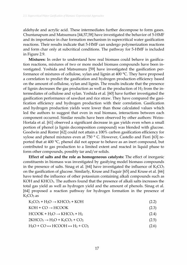
2.3. Supercritical Water Gasification of Biomass: Experimental Approaches
17
aldehyde and acrylic acid. These intermediates further decompose to form gases. Chuntanapum and Matsumura [44,57,58] have investigated the behavior of 5-HMF and its importance in char formation mechanism in supercritical water gasification reactions. Their results indicate that 5-HMF can undergo polymerization reactions and form char only at subcritical conditions. The pathway for 5-HMF is included in Figure 2.9.
Mixtures: In order to understand how real biomass could behave in gasifica-tion reactions, mixtures of two or more model biomass compounds have been in-vestigated. Yoshida and Matsumura [59] have investigated the gasification per-formance of mixtures of cellulose, xylan and lignin at 400 °C. They have proposed a correlation to predict the gasification and hydrogen production efficiency based on the amount of cellulose, xylan and lignin. The results indicate that the presence of lignin decreases the gas production as well as the production of H2 from the in-termediates of cellulose and xylan. Yoshida et al. [60] have further investigated the gasification performance of sawdust and rice straw. They have compared the gasi-fication efficiency and hydrogen production with their correlation. Gasification and hydrogen production yields were lower than those calculated values which led the authors to suggest that even in real biomass, interactions between each component occurred. Similar results have been observed by other authors: Weiss-Hortala et al. [61] observed a significant decrease in gas yields even when a small portion of phenol (a lignin decomposition compound) was blended with glucose. Goodwin and Rorrer [62] could not attain a 100% carbon gasification efficiency for xylose and phenol mixtures even at 750 ° C. However, Castello and Fiori [63] re-ported that at 400 °C, phenol did not appear to behave as an inert compound, but contributed to gas production to a limited extent and reacted in liquid phase to form other compounds, possibly tar and/or solids.
Effect of salts and the role as homogeneous catalysts: The effect of inorganic constituents in biomass was investigated by gasifying model biomass compounds in the presence of salts. Sinag et al. [64] have investigated the influence of K2CO3 on the gasification of glucose. Similarly, Kruse and Faquir [65] and Kruse et al. [66] have tested the influence of other potassium containing alkali compounds such as KOH and KHCO3. The authors found that the presence of alkali salts increases the total gas yield as well as hydrogen yield and the amount of phenols. Sinag et al. [64] proposed a reaction pathway for hydrogen formation in the presence of K2CO3 as
K2CO3 + H2O → KHCO3 + KOH (2.2)
KOH + CO → HCOOK (2.3)
HCOOK + H2O → KHCO3 + H2 (2.4)
2KHCO3 → H2O + K2CO3 + CO2 (2.5)
H2O + CO ↔ HCOOH ↔ H2 + CO2 (2.6)
SUPERCRITICAL WATER GASIFICATION OF BIOMASS: A LITERATURE AND TECHNOLOGY OVERVIEW
18
The positive effects of other (earth) alkali salts such as (NaOH, Ca(OH)2, Na2CO3, NaHCO3) on the gasification yield have also been reported by other au-thors [67–71] for different kinds of biomass feedstocks. Yildiz Bircan et al. [72] have investigated the addition of Ca(OH)2 on the gasification performance of an amino acid, L-cysteine. The results showed that the addition of Ca(OH)2 enhanced the H2 formation, but most importantly, it was observed that Ca(OH)2 was con-sumed throughout the reactions and reacted with CO2 to form CaCO3.
Effect of heterogeneous catalysts: Catalysts are used in order to achieve higher conversion at lower temperatures (< 500°C), especially when the desired product is methane [73,74]. The presence of a catalyst changes the reaction pathway of the biomass, resulting in the reduction of tar and coke production and an increase in the gas yields. Figure 2.13 shows the influence of catalyst on the reaction pathway of wood gasification under supercritical conditions. Ruthenium, nickel and acti-vated carbon based heterogeneous catalysts have been widely used in the litera-ture [75–79] for both model and real biomass experiments enabling to obtain full carbon gasification efficiency even at temperatures around 400 °C.
Yanik et al. [80] have investigated natural minerals like red mud (a by-product from alumina production plant containing Fe2O3 (37.7%), Al2O3 (17.3%), SiO2 (17.1%), TiO2 (4.8%), Na2O (7.1%) and CaO (4.5%) by wt.) and trona (Na-HCO3∙Na2CO3∙2H2O). Both of these minerals have been found to significantly in-crease the H2 yield and slightly promote the total gas yield for different kinds of carbohydrate based feedstocks.
It has been reported that the reactor wall material may also behave like a heter-ogeneous catalyst. Boukis et al. [81] have studied the methanol reforming in a nickel-based alloy Inconel 625. They have concluded that the conversion rate as well as the product gas composition are influenced by the presence of heavy met-als on the inner surface of the reactor and the catalytic effect remained high even after more than a thousand operation hours. Similarly, Gadhe and Gupta [82] ob-served a catalytic effect of the wall material from Inconel 600, which is an alloy of Ni, Cr and Fe, for methanol reforming. Lee et al. [37] have performed glucose gasi-fication in a reactor made of Hastelloy C-276 and noted a catalytic effect and en-hancement in the hydrogen yields. Similar results were observed by Yu et al. [83]; these authors tested Inconel, new Hastelloy and corroded Hastelloy for glucose hydrothermal gasification. Their results indicated that corroded Hastelloy signifi-cantly increased the hydrogen and total gas yields. Castello et al. [84] have investi-gated the effect of wall material for stainless steel and Inconel 625 for both glucose and sawdust gasification in micro-autoclaves without the presence of catalyst at temperatures of 350 °C and 400 °C. They have observed that stainless steel favored hydrogen production, whereas Inconel 625 enhanced CO consuming methanation and light hydrocarbon formation under supercritical conditions. Under subcritical conditions, the two reactors gave similar results.

2.3. Supercritical Water Gasification of Biomass: Experimental Approaches
19
Figure 2.13: The influence of catalyst on the reaction pathway of wood gasification under supercritical conditions proposed by Waldner and Vogel [78]. Reprinted. The term “cat.” designates reaction pathways influenced by the presence of a cata-lyst, whereas the term “cat.?” denotes pathways that are only assumed to be pro-moted by a catalyst.
Behavior of heteroatoms: Yildiz Bircan et al. [72] have investigated the behav-ior of heteroatoms such as S, N and P in supercritical water gasification using L-cysteine containing hetero-atoms S and N, and O-phospho-DL-serine containing P as feedstocks. They have performed experiments in an oven which was kept at 400 °C and at 26 – 27 MPa. After a residence time of 50 minutes, the oven was cooled to 30 °C and the components were analyzed. The results showed that sulphur par-titioned to SO2 and H2S in the gas phase, and SO3
2-, SO42- and S2- ions in the liquid
phase. When Ca(OH)2 was used as an additive, the gas phase sulphur compounds concentrations decreased by about one tenth and partitioned to the liquid phase sulphur. However, for both of the cases more than 90% of the sulphur partitioned to the solid phase. For nitrogen compounds, NO and NO2 were detected in trace levels and NH3 was not detectable. 95.7% percent of nitrogen was converted to NH4
+ in the liquid phase. This ratio decreased to 82% when Ca(OH)2 was used as an additive. When it comes to phosphorus compounds, 93.3% of the phosphorus partitioned to ionic compounds in the liquid phase. When Ca(OH)2 was used as an additive, more than 90% of the phosphorus precipitated as a solid phase.
Gas phase reactions: In has been reported by many authors (such as [47,85,86]), that water gas shift and methanation reactions have been assumed to be the main gas phase reactions which may result in equilibrium. Eqs. 2.7 and 2.8 show the wa-ter gas shift reaction and methanation reactions, respectively.
CO + H2O ↔ CO2 + H2 (2.7)
CO + 3H2 ↔ CH4 + H2O (2.8)
SUPERCRITICAL WATER GASIFICATION OF BIOMASS: A LITERATURE AND TECHNOLOGY OVERVIEW
20
In the water gas shift reaction, carbon monoxide and water form formic acid which further decomposes to carbon dioxide and hydrogen through the reactions 2.9 and 2.10 [87,88].
CO + H2O ↔ HCOOH (2.9)
HCOOH ↔ CO2 + H2 (2.10)
Savage’s group [85,86] has performed sensitivity analyses on the reaction rates for noncatalytic supercritical water gasification of biomass processes. It can be concluded from the results that the main reactions which determine the hydrogen and methane formation are not the water gas shift and methanation reactions in the gas phase, but the reactions which directly result in the gas formation from the feedstock and/or intermediates. It has also been reported in the literature [87–90] that the rates of noncatalytic water gas shift and methanation reactions in super-critical water are quite slow, resulting in only 5% conversion even after several minutes.
2.3.2. Real biomass experiments
Antal et al. [75] state that the first real biomass experiments in supercritical wa-ter have been performed by Modell et al. [91] in 1985 using maple wood sawdust as a feedstock. The results indicated that the sawdust quickly decomposed to tars and gases without the formation of char. Since the first experiments in 1985, real biomass has also been the subject of supercritical water gasification.
Carbohydrates: In their work, Antal et al. [75] have examined gasification per-formance of different biomass feedstocks such as corn- and potato-starch gels, wood sawdust suspended in a cornstarch gel, and potato wastes in 3 different tubular reactor which had activated carbon as a catalyst. They have performed ex-periments at temperatures higher than 650 °C and at a pressure of 28 MPa. Their results were in a good agreement with the equilibrium calculations resulting in an extraordinary gas yield higher than 2 L/g (liters of gas under 25 °C and 0.1 MPa per gram of organic matter in the feed) with a high yield of hydrogen (57%). Irre-spective of the reactor geometry and method of heating, they have observed plug-ging problems after 1 – 2 h of operation time with feedstocks that contained ap-proximately 15 wt. % of organic material.
D’Jesús et al. [92] have gasified corn starch, clover grass and corn silage in su-percritical water. They have investigated the influence of pressure, temperature, residence time and alkali addition on gasification performance. They have report-ed that the change in the pressure did not alter the gasification yield, however, the increase in the temperature significantly increased the gasification yield. Longer residence time resulted in higher gasification yields till the system attained a max-imum. Potassium addition (in the form of KHCO3) was found to increase the car-bon gasification efficiency for corn starch, however, no significant difference was observed for clover grass and corn silage as they naturally contained potassium.

2.3. Supercritical Water Gasification of Biomass: Experimental Approaches
21
Algae: Stucki et al. [93] have gasified a microalgae species, Spirulina platensis, in the presence of different catalysts. 100% of the carbon content of the microalgae was gasified using a Ru/C catalysts at a temperature of around 400 °C and at a pressure around 32 MPa. Their results were in a very good agreement with the equilibrium predictions. They proposed that 60 – 70% of the heating value of the algae can be recovered in the form of methane.
Chakinala et al. [94] have gasified Chlorella Vulgaris in supercritical water. They have observed more than 80% carbon gasification efficiency at 700 °C with a 7.3 wt.% dry mass concentration at a pressure of 24 MPa with a residence time of 2 minutes. As expected, gasification efficiency decreased with a decrease in tempera-ture and residence time. The increase in the dry mass concentration had a negative impact on the carbon gasification efficiency. They have also tested the effect of dif-ferent catalysts on the carbon gasification efficiency. The results indicated that the presence of a catalyst increased the carbon gasification efficiency, reaching even a 100% with a Ru/TiO2 catalyst at 600 °C with a residence time of 2 minutes.
Guan et al. [95] have gasified another microalgae sample, Nannochloropsis sp. in supercritical water at 450 – 550 °C at around 25 MPa. They have concluded that higher gas yields were obtained by higher temperatures, longer reaction times (> 20 minutes), higher water densities, and lower algae loadings. Their findings also show that when the biomass loading reduced from 15 wt.% to 1 wt.%, H2 yield more than tripled.
Onwudili et al. [71] have gasified three different types of microalgae samples (Chlorella vulgaris, Spirulina platensis and Saccharina latissima) at 500 °C and 36 MPa in an Inconel batch reactor for 30 minutes. They have also tested the influence of NaOH and/or Ni-Al2O3 on the gasification performance. Their results indicated that the presence of NaOH more than doubled the hydrogen yield and decreased the tar yield up to 71%. Presence of the nickel catalyst had also decreased the tar formation. A similar study has been performed by Bagnoud-Velásquez et al. [96] on the effluent recycling and the catalytic gasification of a microalgae sample, Phaeodactylum tricornutum. In a continuous reactor, for a 6.5 wt.% algae concentra-tion, they were able to obtain 31% carbon gasification efficiency at 420 °C and 32.3 MPa in the presence of a Ru/C catalysts. They have observed rapid deactivation of the catalyst due to sulphur poisoning and coke formation.
Sludge: Xu and Antal [97] have gasified digested sewage sludge, corn starch and poplar wood sawdust in the presence of coconut shell activated carbon cata-lyst. They have mixed sewage sludge (up to 7.69 wt. %) with corn starch gel (up to 7.69 wt. %) in order to form a viscous gel. They have performed experiments at 650 °C and at 28 MPa. Even with a lower sewage sludge loading (2.1 dry wt.% digest-ed sewage sludge with dry 5.1 wt.% corn starch), the reactor had plugging prob-lems after 1 – 2 h of operation time due to high ash content of sewage sludge.
Chen et al. [98] have used a fluidized bed to overcome reactor plugging prob-lems in sewage sludge gasification. They have also tested the effect of operating

SUPERCRITICAL WATER GASIFICATION OF BIOMASS: A LITERATURE AND TECHNOLOGY OVERVIEW
22
parameters as temperature, concentration of the feedstock, alkali catalysts and cat-alyst loading on gaseous products and carbon distribution. The authors have per-formed experiments at a pressure of 25 MPa and at a temperature range of 480 – 540 °C with a biomass concentration varying from 4 – 12 wt.%. As expected, the increase in temperature and decrease in feed concentration increased the carbon gasification efficiency. Addition of alkali catalyst was found to enhance the hydro-gen production.
Zhai et al. [99] have gasified digested sewage sludge in a batch reactor at tem-peratures up to 425 °C at a pressure varying from 25 to 35 MPa, with a residence time from 10 to 15 minutes and a dry matter content ranging from 5 to 25 wt.%. In the best case, they were able to obtain 3.5% carbon gasification efficiency where the presence of K2CO3 increased this value up to 26 %.
Manure: Waldner [13] has gasified real biomass samples such as wood and swine manure in a batch reactor in the presence of different catalysts. Using a Raney Ni 2800 catalyst, 100% carbon gasification efficiency was obtained at a tem-perature around 400 °C and at a pressure of 31 MPa for wood. The gas composi-tion was in agreement with the equilibrium predictions. Similar conditions result-ed in more than 75% carbon gasification efficiency for swine manure.
Nakamura et al. [77] have investigated the gasification of chicken manure in the presence of suspended fine activated carbon catalysts in an experimental pilot plant. At 600 °C and 25 MPa with a residence time of 1.7 minutes, they were able to completely gasify 2 wt.% and 10 wt.% chicken manure in the presence of 0.4 wt.% and 5 wt.% activated carbon, respectively. However, when there was no catalyst present, 80% carbon gasification efficiency was observed with a 2 wt.% feed concentration. Their setup included a liquefaction process with a residence time of 26.7 minutes of which the temperature was 180 °C and pressure was 1.2 MPa.
Yong and Matsumura [100] have investigated the gasification behavior of poul-try manure and eucalyptus wood in a flow reactor and the effect of activated car-bon on the gasification performance. Their results indicate that addition of 0.1 wt.% wood to 0.5 wt.% manure increased the carbon gasification efficiency (CGE) at temperatures between 550 and 650 °C and at a pressure of 25 MPa. However, the effect of wood decreased at 0.2 wt.% and became almost insignificant at 0.3 wt.%. They stated that cellulose and hemicellulose containing wood biomass, are more easily decomposed in SCW than poultry manure. The increase in the loading of wood in the mixture resulted in the deceleration of the gas producing pathways in the overall reactions. It was also found that the usage of activated carbon in the feedstock mixture improved the gasification efficiency. An overview of the real bi-omass experiments is presented in Table 2.1.

2.3. Supercritical Water Gasification of Biomass: Experimental Approaches
23
Table 2.1: An overview of the real biomass experiments.
Feedstock Wt. % Tempera-ture (°C)
Pressure (MPa)
Reactor Type Residence
Time
CGE (%)
Mole Fraction of Gas Products
(%)
Refer-ence
CH4 CO2 H2 CO
Corn Starch 10.4 ~ 700 28 Tubular with a carbon catalyst
2.18 h 91 22 38 37 2 [75]
Microalgae (Chlorella Vul-garis)
7.3 600 24 Quartz Capil-lary
2 min 53 25 26 7 22 [94]
Sewage Sludge
10 540 25 Fluidized Bed N/A 32 13 43 26 13.5 [98]
Swine Manure 13.2 405 30.1 Batch reactor with nickel cat-alyst
36 min 75.8 46 43 10.7 0.1 [13]
Chicken Ma-nure
10 600 25 Flow reactor with carbon catalyst
1.7 min 90 21.2 45.4 28.7 0 [77]

SUPERCRITICAL WATER GASIFICATION OF BIOMASS: A LITERATURE AND TECHNOLOGY OVERVIEW
24
2.4. SUPERCRITICAL WATER GASIFICATION OF BIOMASS: MODELING AP-
PROACHES
Modeling enables to simulate real cases in order to predict products and equipment performances and overcome possible challenges for different process conditions.
2.4.1. Kinetic modeling
Studies aimed at elucidating the reaction kinetics under hydrothermal gasifica-tion conditions have started with simple sugar compounds and have been extend-ed later to real biomass feedstocks. Matsumura’s group [43,44,57,58] and Kabye-mela et al. [42] have studied the glucose, fructose and glucose derived intermedia-te decompositions in sub- and supercritical water. Aida et al. [46] and Goodwin and Rorrer [47] have investigated the reactions of D-xylose in sub- and supercriti-cal water. Wahyudiono et al. [49] have studied the thermal decomposition kinetics of guaiacol as a lignin derived material. Sasaki et al. [31,101] have further studied the kinetics of cellulose and cellobiose conversion in sub- and supercritical water. Regarding modelling, Resende and Savage [86] have developed a kinetic model for noncatalytic supercritical water gasification of cellulose and lignin at high tem-peratures, and Guan et al. [85] proposed a reaction mechanism for the supercritical water gasification of a real biomass feedstock; microalgae. However, these kinetic models and parameters have limited applicability as
in most of these works, all of the reactions are assumed to be first order reactions;
the temperature effect on the rate constants has not been sufficiently inves-tigated;
most of these works only incorporate the decomposition rates and the formation of intermediates, but do not show the whole gasification routes;
the models which include entire gasification routes incorporate the lumped kinetic model, which neglects the composition of intermediates.
Another interesting approach to kinetic modeling is the detailed kinetic model-ing. Here, the whole reaction mechanisms consist of hundreds of elementary reac-tions. Most of these attempts have been made for SCWO of simple compounds such as methanol, carbon monoxide, methane and hydrogen [18,102–106]. Detailed kinetic modeling has also been applied for supercritical water gasification systems. Ederer et al. [107] have investigated the pyrolysis of tert-butylbenzene in super-critical water, Bühler et al. [108] have investigated the glycerol decomposition in supercritical water and Castello and Fiori [109] have used the detailed kinetic models for the supercritical water oxidation of methanol to model the gasification of methanol in supercritical water. Even though the results are promising, the ap-plication of detailed kinetic modeling for real biomass is not viable yet due to the complex nature of real biomass feedstocks. Table 2.2 shows an overview of the ki-

2.4. Supercritical Water Gasification of Biomass: Modeling Approaches
25
netic parameters for the selected conversion pathways of biomass constituent compounds during supercritical water gasification.
2.4.2. Computational fluid dynamics modeling
Computational fluid dynamics (CFD) modeling helps to simulate and design a reactor [110]. Yoshida and Matsumura [110] were the first researchers who per-formed CFD analysis for a SCWG reactor. The authors have used Fluent 6.3® soft-ware to perform simulations for 4.9 wt.% glucose conversion in the presence of hydrogen peroxide as oxidation agent in supercritical water at 400 °C and 25.4 MPa. However, the authors ignored all the reactions and calculated only the flow of water and inert particles as virtual char products.
Goodwin and Rorrer [111] have performed CFD simulations for xylose gasifica-tion in a Hastelloy micro-channel reactor at 650 °C and 25 MPa. The authors have used Fluent 6.3.26® for the simulations and the fluid was modeled by the Navier-Stokes equations for laminar flow. They have performed simulations using a 6 re-action based kinetic model which was developed in a previous paper [47] by them. The authors have used Peng-Robinson EoS for the pure gas species for the calcula-tion of the fugacities, however the mixing interactions in the reacting fluid have not been taken into account. The authors found that CFD simulations accurately predicted the gas yields. Besides, it was found that the endothermic xylose gasifi-cation reactions had a little influence on the reaction temperature thus not affect-ing the gas yield or H2 selectivity.
Wei et al. [112] have performed CFD simulations with a Eulerian model which incorporates the mechanical kinetic theory for solid particles to predict the solid distribution and the residence time distribution of the feeding materials for a fluid-ized bed reactor. Based on the simulation results, they have proposed a feeding pipe with an angle of 45° to enable a uniform solid distribution and long residence time among the reactor.
A different approach using CFD has been performed by Withag et al. [113,114]. Here the authors performed CFD simulations to calculate heat transfer characteris-tics of supercritical water to a flow reactor for both 1D and 2D cases. Further, Withag [115] also performed simulations for a reacting flow of methanol in super-critical water for a 2D case. Based on the simulations, it was concluded that meth-anol is mainly converted near the wall due to the high fluid temperatures resulting in high local reaction rates.

SUPERCRITICAL WATER GASIFICATION OF BIOMASS: A LITERATURE AND TECHNOLOGY OVERVIEW
26
Table 2.2: An overview of the kinetic parameters determined for selected conversion pathways of biomass constituent com-pounds during supercritical water gasification. Please note that TOC refers to water-soluble organic species such as 1,2,4-benzenetriol, 1,4-benzenediol, 5-methyl-2-furaldehyde, levulinic acid, and formic acid.
Compound Type of Reac-
tion
Activation Energy
(kJ·mol-1)
Pre-exp. Factor (s-1) Temperature
Range (°C)
Pressure (Mpa) Reference
Cellulose Conversion 145.9 1x1011.9 320-370 25 [31]
Cellulose Conversion 547.9 1x1044.6 370-400 25 [31]
Cellobiose Conversion 96.4 1.28x10⁸ 300-350 25 [116]
Cellobiose Conversion 96.4 1.48x10⁸ 350-400 30 [116]
Cellobiose Hydrolysis 108.6 1.10x10⁹ 300-350 25 [116]
Cellobiose Hydrolysis 108.6 1.15x10⁹ 350-400 30 [116]
Cellobiose Pyrolysis to glucosyl-eryhtrose and glycoaldehyde
30.4 17.68 300-350 25 [116]
Cellobiose Pyrolysis to glucosyl-eryhtrose and glycoaldehyde
30.4 57.13 350-400 30 [116]
Cellobiose Pyrolysis to glucosyl- gly-coaldehyde and eryhtrose
69.3 82730.74 300-350 25 [116]
Glucose Decomposition 121 1.33x10¹⁰ 175-400 25 [43]
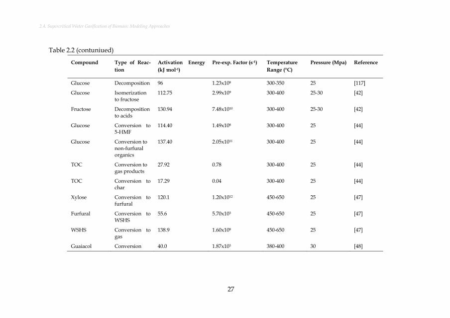
2.4. Supercritical Water Gasification of Biomass: Modeling Approaches
27
Table 2.2 (contuniued)
Compound Type of Reac-
tion
Activation Energy
(kJ·mol-1)
Pre-exp. Factor (s-1) Temperature
Range (°C)
Pressure (Mpa) Reference
Glucose Decomposition 96 1.23x10⁸ 300-350 25 [117]
Glucose Isomerization to fructose
112.75 2.99x10⁹ 300-400 25-30 [42]
Fructose Decomposition to acids
130.94 7.48x10¹⁰ 300-400 25-30 [42]
Glucose Conversion to 5-HMF
114.40 1.49x10⁸ 300-400 25 [44]
Glucose Conversion to non-furfural organics
137.40 2.05x10¹¹ 300-400 25 [44]
TOC Conversion to gas products
27.92 0.78 300-400 25 [44]
TOC Conversion to char
17.29 0.04 300-400 25 [44]
Xylose Conversion to furfural
120.1 1.20x10¹² 450-650 25 [47]
Furfural Conversion to WSHS
55.6 5.70x10³ 450-650 25 [47]
WSHS Conversion to gas
138.9 1.60x10⁸ 450-650 25 [47]
Guaiacol Conversion 40.0 1.87x10³ 380-400 30 [48]

SUPERCRITICAL WATER GASIFICATION OF BIOMASS: A LITERATURE AND TECHNOLOGY OVERVIEW
28
2.4.3. Thermodynamic equilibrium modeling
In addition to the kinetic models, supercritical water gasification of biomass compounds has also been modelled following a thermodynamic equilibrium mod-elling approach. Antal et al. [75] were the first researchers who used the thermo-dynamic equilibrium approach. They have compared the experimental results with the thermodynamic equilibrium predictions using STANJAN and HYSIM of which the first one uses ideal gas assumption as an equation of state (EoS) and the latter one Peng – Robinson EoS. Tang and Kitagawa [118] have performed ther-modynamic analysis for various model and real biomass compounds using Peng – Robinson EoS describing the non-ideal properties of the compounds. The authors used a Gibbs free energy minimization method (also known as the non-stoichiometric method) in order to predict the equilibrium amounts of gases. More authors followed the same approach [119–124]. All of these works have been de-veloped for the supercritical region and take only the gas phase compounds into account. Castello and Fiori [125] have extended the gas phase products and intro-duced graphitic carbon as an additional compound, and investigated the applica-tion of thermodynamic constraints such as solid carbon formation and process heat duty.
An alternative to Gibbs free energy minimization was given in the works of Letellier et al. [126] and Marias et al. [127]. Here the authors used the discrete reac-tion equilibria method (also known as stoichiometric approach) to predict the equilibrium composition of the gas phase compounds. Furthermore, they have al-so modeled the flash column for the separation of product gases from water and other organic compounds.
The aforementioned developed models do not cover the subcritical region of the process and the behavior of inorganics, and the partitioning behavior of ele-ments. However, Yanagida et al. [79] have investigated the equilibrium behavior of inorganic elements in poultry manure during supercritical water gasification us-ing a software; HSC Chemistry 6.12. Seven inorganic elements, namely N, Ca, K, P, S, Cl and Si, as well as C, H, O content of manure and possible compounds that could be formed by these elements have been taken into account for the thermo-dynamic equilibrium calculations. The simulation was run first at 32 MPa and 600 °C and after subtracting the amount of gases formed, the simulation then was run at room temperature conditions to observe the phase and compound behavior of the elements. The results have been compared with experimental works and found to be in agreement. Table 2.3 shows an overview of the thermodynamic equilibri-um modeling papers. There are other research works in the literature which use commercial software packages for the prediction of product compounds following a thermodynamic equilibrium calculation approach. However, most of these works concentrate on process modeling which is discussed in details in the follow-ing section.

2.4. Supercritical Water Gasification of Biomass: Modeling Approaches
29
Table 2.3: An overview of the thermodynamic equilibrium modeling of supercriti-cal water gasification of biomass papers.
Investigated
Compounds
Type of ap-
proach
Type of EoS or
Software used
for the calcula-
tions
Considered
Phases
Significant Contribu-
tion
Refer-
ence
Methanol,
Glucose,
Cellulose,
Starch, Saw-
dust
Gibbs free
energy min-
imization
(GFEM)
Peng-Robinson
EoS
Only Gas
Phase
The first paper with a
thermodynamic model
[118]
Glucose GFEM Duan EoS Only Gas
Phase
The introduction of
additional constraints
[124]
Wood saw-
dust
GFEM Duan EoS Gas Phase and
Solid Carbon
The introduction of sol-
id carbon
[122]
Poultry Ma-
nure
GFEM HSC Chemistry
6.12
Multi-Phase The first paper which
took the inorganic ele-
ments into account
[79]
Methanol,
Ethanol,
Glycerol,
Glucose and
Cellulose
GFEM Ideal Gas Gas Phase and
Solid Carbon
No need for initial
guesses for the mole
amount of product
species
[123]
Methanol,
Glucose,
Sewage
Sludge
Reaction
equilibria
Peng-Robinson
EoS
Gas Phase and
Solid Carbon
The first paper which
used the reaction equi-
libria method
[126]
Glycerol and
Microalgae
GFEM Peng-Robinson
EoS
Gas Phase and
Solid Carbon
Char formation condi-
tions have been exam-
ined
[125]
Glucose and
Cellulose
GFEM Virial EoS and
Ideal Gas
Only Gas
Phase
Introduction of the en-
tropy maximization
[120]
It is a fact that an arbitrary multi-component multi-phase system at a given temperature, pressure and chemical composition will always tend to minimize its total Gibbs free energy till it reaches the global minimum state. However, the pre-dicted compounds at that minimum state are the “unconstrained” equilibrium state compounds. Most of the real conversion systems do not reach that state due to the natural constraints (such as slow kinetics or reaction barrier conditions) that could keep the system away from it [128]. In that sense, for most of the cases, pre-dictions using a thermodynamic equilibrium approach will not show the real case

SUPERCRITICAL WATER GASIFICATION OF BIOMASS: A LITERATURE AND TECHNOLOGY OVERVIEW
30
results but will give an insight in the process limits as well as the formation behav-ior of the compounds.
2.4.4. Process modeling
Even though thermodynamic equilibrium models predict the (major) product compounds formed in reactors, one needs to model the performance of the other equipment in such a biomass based supercritical water gasification processing plant in order to gain insight into the whole process performance. Feng et al. [129] were the first researchers who have performed a thermodynamic analysis of a su-percritical water biomass gasification plant. They have analyzed the phase behav-ior and phase equilibria in the reactor and separators; in addition, they designed an optimized heat exchange network and performed a system exergy analysis. The authors have used the statistical association fluids theory (SAFT) EoS for the ther-modynamic calculations. Their results indicated that a cellulose gasification plant with reactor operating conditions of 600 °C and 35 MPa has an exergy efficiency of 40.6%. The exergy efficiency in this work is defined as the ratio of the exergy flows of the inlet (cellulose as being the feedstock, providing heat and electricity for the process) and outlet (hydrogen-rich) products.
Luterbacher et al. [130] have performed process simulations and life cycle as-sessment (LCA) for wood and manure as a feedstock in supercritical water gasifi-cation plant targeting to produce SNG. Using AspenPlusTM 2004.1 software for the process simulations, their results showed that 62% of the manure’s lower heating value (LHV) is converted to SNG and 71% of wood’s LHV is converted to SNG. Similarly, Gassner et al. [28,131] offered optimal process design for polygeneration of SNG, power and heat from various biomass sources varying from a typical lig-nocellulosic material (modeled as CH1.35O0.63) to manure and sewage sludge. The authors have made an extensive analysis from both thermo-economic and optimi-zation points of view concerning the processes. The results indicate that the SNG conversion efficiency of wood process was found to reach up to 70%. The same value was found to reach up to 75% for microalgae, 70% for manure and 60% for undigested sewage sludge where the SNG conversion efficiency is given in Equa-tion 2.11 as
0
0
,
SNG SNG
biomass biomass daf
h m
h m
(2.11)
where 0h refers to the LHV, m refers to the mass flow and daf refers to the dry
ash free basis. The superscripts – and + refers to the flows leaving the system and flows entering the system, respectively.
Gutiérrez Ortiz et al. [132] have performed process simulations using As-penPlusTM for gasification of glycerol in supercritical water. They have investigat-ed the effect of process conditions on the hydrogen yield. Using predictive Soave-Redlich-Kwong EoS for Gibbs free energy minimization in the reactor to predict the equilibrium composition, the authors concluded that the highest yield for hy-

2.5. Process Challenges and Reactor Technology Aspects for Industrial Applications
31
drogen could be obtained at 900 °C with 1 mol % glycerol in the feed. The authors reported that the pressure did not have an influence on the results.
A similar research has been conducted by Fiori et al. [133]. The authors per-formed process simulations using AspenPlusTM aiming at hydrogen production and energetic self-sustainability of different biomass feedstocks of glycerol, phe-nol, microalgae Spirulina, sewage sludge and grape marc. Their results indicated that biomass feed share should be at a minimum of 15–25 wt. % in order to estab-lish an energetic self-sustainable process (11.4 wt.% for phenol and 22.9 wt.% for Spirulina for a reactor operating at 700 °C and 30 MPa). The results also indicate that the thermal energy required for the microalgae process is around 0.6 MJ·(kg-total-feed)-1 for a reactor operating at 500 °C and 30 MPa when the dry biomass concentration in the feed is 10 wt.%. This value is around 1.5 MJ· (kg-total-feed)-1
for a reactor operating at 700 °C with the same process conditions.
Another process simulation concerning a system model based on methanol gas-ification has been performed by Withag et al. [134]. Here the authors also used As-penPlusTM and tested the validity of different EoS concluding that the property methods based on the Peng–Robinson and Soave Redlich–Kwong EoS all give a prediction of the H2 mole fraction within a bandwidth of 3.5% compared to exper-imental results. They have also performed simulations for different cases to predict the thermal efficiencies for methanol, glucose and cellulose conversion. Similar to the findings of Fiori et al. [133], the authors concluded that the dry mass concentra-tion of the feed should be at least 14.5 wt.% for methanol and ~25 wt.% for cellu-lose and glucose to have a thermal efficiency of 60% for a reactor operating at 600 °C and 30 MPa.
2.5. PROCESS CHALLENGES AND REACTOR TECHNOLOGY ASPECTS FOR INDUS-
TRIAL APPLICATIONS
Most of the experiments have been conducted in batch reactors which are not suitable for industrial applications. In contrast, industry rather demands continu-ous processes. However, continuous experimental approaches have some chal-lenges which need to be overcome in order to scale up the process and be applica-ble in industry.
Pumpability of the biomass slurry is a problem in continuous processes. The dry matter content of the biomass slurry should not exceed the pumpability limits due to possible clogging problems. On the other hand, a high dry matter content results in higher gas production which increases the energy efficiency and the profitability of the plant. Yet, the pumpability of the biomass slurry depends on the nature of the biomass [135]. Antal et al. [75] have used a cement pump to be able to pump a suspension of 4 wt.% starch gel mixed with wood sawdust and other particulate biomass. On the other hand, sewage sludge containing 40% dry matter can be successfully pumped [136]. A pretreatment of reducing the particle

SUPERCRITICAL WATER GASIFICATION OF BIOMASS: A LITERATURE AND TECHNOLOGY OVERVIEW
32
size of the biomass [135] and obtaining a suspended feed [75] can be used to over-come the possible pumpability problems.
Corrosion is another problem for industrial scale applications. The process takes place at harsh conditions which lead to corrosion of the reactor construction material. In addition, gases and minerals which are formed during the gasification lead to corrosion as well [135]. Marrone and Hong [137] propose some corrosion control approaches which are i) vortex/circulating flow reactor to prevent corro-sive species from reaching a solid surface, ii) use of high corrosion resistant mate-rials such as nickel based alloys or stainless steel or iii) reducing the temperature to 400 °C instead of 600 °C to improve the energy balance which would enable using other types of corrosion control methods such as using liners or coatings that de-crease the heat transfer.
Working at low temperatures might have a positive effect on solving corrosion and energy efficiency problems, however, carbon gasification efficiency decreases due to the slower reaction rates. One way to overcome such problems is to use cat-alysts to enhance the reaction rates. Waldner and Vogel [78] have already obtained a full carbon gasification for wood samples and sufficiently high carbon efficiency (> 80%) for swine manure experiments at low temperatures (~400 °C) using cata-lysts. Similar results have been observed by other researchers [93] as well. Howev-er, – in addition to increasing the process costs – catalysts are often reported to prone to deactivation problems [73,138–140] caused by i) the poisoning of the ac-tive surface of the catalyst by sulfur, ii) fouling of the catalyst surface by precipi-tated salts and other minerals and iii) coke formation and deposition on the cata-lyst surface [141]. Coke formation may also cause plugging problems in flow reac-tors [142].
Zöhrer et al. [143] state that mixing the unheated, relatively concentrated or-ganic solution with the preheated water avoids unwanted reactions and coke for-mation caused by the slow heating of the organic feed. However, this option could be feasible only for model biomass compounds as the concentrated biomass slurry would not be suitable for pumping as discussed earlier. For real biomass process-es, rapid heating of the feed can overcome such coke and tar formation behavior as the positive effect of rapid heating on less tar production and higher gas yields are reported by other researchers [144,145] as well. Another possible solution to coke and tar formation was given by Kruse and Faquir [65]. The authors proposed a re-action process in which a continuously stirred tank reactor (CSTR) is followed by a tubular reactor in order to benefit from the “active hydrogen” formation in the CSTR due to its backmixing. “Active hydrogen”, which is referred as the in statu nascendi hydrogen formed through the intermediate stages of the water gas shift reaction or by hydrogen, is reported to suppress tar and coke formation reactions. Furthermore, the gas yields increases when the CSTR is combined with a tubular reactor.
2.5. Process Challenges and Reactor Technology Aspects for Industrial Applications
33
Obtaining sufficient process thermal efficiency is another challenge for super-critical water gasification of biomass systems. Thermal efficiency should be high enough to make the process viable for industrial applications. The efficiency be-comes more important when the desired reactor temperature increases [135]. Pro-posed process demonstration units [73] as well as the VERENA pilot plant in Karlsruhe Institute of Technology [146,147] benefit from the high temperature of the product stream leaving from the reactor in order to preheat the feed using a heat exchanger. However, as reported earlier, if the heating rate of the heat ex-changer is low, coke and tar formation will take place. To overcome such prob-lems, VERENA pilot plant mixes the concentrated biomass, which was heated up to the critical temperature, with high temperature pure water [146]. The process flow diagram of VERENA pilot plant is given in Figure 2.14. Another approach was given by researchers in State Key Laboratory of Multiphase Flow in Power Engineering (SKLMF) of China [148–151]. Here, the researchers proposed solar en-ergy based heating for the reactor and successfully applied this energy source for supercritical water gasification of biomass compounds. The Dutch company Gen-sos B.V. has patented a process that incorporates extensive heat recovery which enables a high process thermal efficiency [152].
The most important challenge in supercritical water gasification of biomass processes remains the salt precipitation due to the rapid decrease in the solubility of salts in the supercritical region (see Figure 2.4). The precipitated salts may lead to plugging problems if the tube diameters are small, crystals are large or sticky, heterogeneous catalysts are used, and the velocity of the flow is low [135]. The ear-liest possible solutions to salt precipitation problem have been offered in the 1980s [153] and 1990s [154,155] as the salt precipitation was also a major problem for su-percritical water oxidation processes. Hong et al. [153] have patented a reverse flow reactor (known as MODAR reactor) in which the feedstock is fed from the top of the reactor and the cold water from the bottom. The upper part of the reactor is kept at supercritical temperatures, whereas the bottom part is kept at subcritical temperatures. Supercritical fluid leaves the reactor from the top and a brine efflu-ent leaves from the bottom. Daman [154,155] has patented a transpiring wall reac-tor in which solute-free water flows through a porous reactor liner in order to keep salt deposition as well as corrosion problems away from the reactor wall [156]. Xu et al. [157] have combined these two approaches for a sewage sludge supercritical water oxidation process which is expected to prevent reactor plugging and corro-sion problem. However, Marrone and Hong [137] stated that the transpiring wall reactor has limited usefulness for gasification systems due to adverse effect of dilu-tion on the system’s energy balance. On the other hand, Schubert et al. [158] have used a salt separation vessel which the design is similar to MODAR’s reverse flow reactor. The feed inlet and effluent to the reactor are from the top, whereas the brine effluent is from bottom. The top of the reactor is at supercritical and the bot-tom part is at subcritical temperatures. In contrast to MODAR reactor which acts as both salt separator and reactor, salt separation vessel proposed by Schubert et

SUPERCRITICAL WATER GASIFICATION OF BIOMASS: A LITERATURE AND TECHNOLOGY OVERVIEW
34
al. [158] is a kind of pretreatment unit before the reactor. Zöhrer et al. [140] have used this salt separator to perform catalytic gasification and liquefaction of fer-mentation residue samples. They have observed almost no salt separation at 430 °C. At 450 °C, the salt separation efficiency was higher. However, at 470 °C mas-sive tar formation which led to blockage in the rig was observed. Similar to MO-DAR reactor, Boukis et al. [146,147] have used a reactor in the VERENA pilot plant which acts as both reactor and salt separator. The lower part of the reactor has a cooler [159] that enables the brines and solids leaving the reactor via a third output from the lower part of the reactor.
Figure 2.14: The process flow diagram of VERENA pilot plant. Reprinted from [135].
Another possible solution for plugging problems in the reactor was proposed by Matsumura and Minowa [5]. The authors speculated on the potential benefits of applying a fluidized bed reactor to the supercritical water gasification process. They investigated the fundamental design parameters of such a fluidized bed. Potic et al. [160] have performed fluidization experiments for supercritical water in micro cylindrical quartz reactor with an internal diameter of 1 mm. Lu et al. [161] were the first researchers who performed supercritical water gasification experi-ments in a fluidized bed reactor at SKLMF. The reactor material was constructed from 316 stainless steel. The bed diameter was 30 mm, freeboard diameter was 40 mm, and the total length was 915mm. The authors stated that no reactor plugging was observed. Other researchers in SKLMF [98,162] continued to perform gasifica-tion experiments in the same fluidized bed reactor. Real biomass experiments (2 wt.% sewage sludge + 2 wt.% sodium carboxymethyl cellulose) resulted in more

2.6. Conclusions
35
than 40% carbon gasification efficiency at a temperature of 540 °C and at a pres-sure of 25 MPa. Gensos B.V. has patented a process and apparatus that incorpo-rates a fluidized bed reactor [163,164].
2.6. CONCLUSIONS
Supercritical water gasification is a promising technology for the efficient con-version of wet biomass into a product gas that after upgrading can be used as sub-stitute natural gas or hydrogen rich gas. The gasification behavior and the chemis-try of the decomposition reactions of the model biomass compounds have been well examined throughout the decades; this chapter made a survey of mechanisms proposed and associated reaction kinetics. Thermodynamic modeling has been performed by several groups with quite some success and an overview of these at-tempts was given in this chapter. Attempts have also been made for real biomass feedstocks varying from manure to sewage sludge. The results show the great po-tential of using supercritical water for gasification purposes. However, the process still faces some challenges which need to be overcome in order to enter the market. The main challenges seem to be thermal efficiency, plugging and corrosion prob-lems. Fortunately, new reactor technologies and process concepts are being devel-oped for the aforementioned problems.

SUPERCRITICAL WATER GASIFICATION OF BIOMASS: A LITERATURE AND TECHNOLOGY OVERVIEW
36

37
3. PREDICTION OF PRODUCT COMPOUNDS WITH
A THERMODYNAMIC EQUILIBRIUM APPROACH
This chapter deals with one of the most fundamental questions in SCWG systems: pre-diction of the product compounds. Even though there are various research studies in the literature on the prediction of the gas phase compunds using a thermodynamic equilibrium approach, practically no work had been done to predict the fate of the inorganic content of the biomass during the SCWG process. Two cases are investigated in this chapter: in the first part, commercial software packages (FactSage 5.4.1 and SimuSage 1.12) have been used to predict the behaviour of the product compounds over a wide range of process condi-tions. In the second part, a multi-phase thermodynamic equilibrium model is developed and validated to predict the product compounds’ behaviour during the SCWG of biomass.
The contents of this chapter have been adapted from:
Section 3.1: O. Yakaboylu, J. Harinck, K.G. Gerton Smit, W. de Jong, Supercritical water gasification of manure: A thermodynamic equilibrium modeling approach, Biomass Bioenergy. 59 (2013) 253–263. doi:10.1016/j.biombioe.2013.07.011.
Section 3.2: O. Yakaboylu, J. Harinck, K.G. Smit, W. de Jong, Supercritical Water Gasification of Bio-mass: A Thermodynamic Model for the Prediction of Product Compounds at Equilibrium State, Energy Fuels. 28 (2014) 2506–2522. doi:10.1021/ef5003342.

PREDICTION OF PRODUCT COMPOUNDS WITH A THERMODYNAMIC EQUILIBRIUM APPROACH
38
3.1 PREDICTIONS USING COMMERCIAL SOFTWARE PACKAGES
3.1.1. Introduction
Although supercritical water gasification can be an efficient way for the con-version of wet biomass, the precipitation of the mineral content of the real biomass might cause operational problems such as reactor plugging during the process. For a good design and the optimization of a reactor, development of knowledge con-cerning the behavior of compounds during the process is essential. This sub-chapter study aims to investigate for the equilibrium partitioning of elements on the basis of compounds and phases in the supercritical water gasification of mixed pig-cow manure for a relatively wide temperature interval of 100 – 580 °C and at a pressure of 24 MPa. The effects of pressure and water fraction on main product gases in the presence of inorganic compounds have also been investigated.
3.1.2. Thermodynamic model
3.1.2.1 Background for the calculations
For the equilibrium calculations, mixed pig-cow manure has been used as the input. The weight percentages have been chosen as 50% for each. The elemental composition of the mixed manure has been obtained from the Phyllis database which the results are the mean values of fresh, aged, dried and composted manure samples [165]. 9 inorganic elements, namely N, S, Cl, Ca, K, Mg, Na, P and Si, as well as C, H, O have been taken into account for the calculations. Table 3.1 shows the elemental compositions acquired from Phyllis database and the final mole amounts that have been used as the input for the calculations. Although the mean value for the weight fraction of water is 51.60%, throughout the simulations this value has been taken as 80% as the SCW gasification of biomass systems work with higher water fractions [73]. The elemental composition of manure has been calculated based on dry basis, and the difference between the ash fraction and in-organic elements have been assumed to be inorganic oxygen [13] and added to to-tal oxygen content for the calculations. Simulations have been run for a 125 kg of input of which the 20% was dry manure and the rest was water.
3.1.2.2 The software and the equilibrium calculations
The equilibrium state of a closed system can be defined as the state in which the total Gibbs free energy is at a minimum with respect to all possible changes at constant temperature and pressure [166].
The definition is given by Equation 3.1.
,( ) 0t
T PdG (3.1)

3.1 Predictions Using Commercial Software Packages
39
Table 3.1: Elemental compositions of the mixed pig-cow manure obtained from Phyllis database [165] and the mole input for the calculations.
Component Analysis Basis Mean Value Mole input
H2O % (wet) 51.60 5550.84
C % (daf*) 46.20 632.65
H % (daf) 6.70 1093.28
O % (daf) 35.30 837.22
N % (daf) 4.05 47.56
S % (daf) 0.77 3.95
Cl % (daf) 1.53 7.07
Ca g∙kg-1dry 11.4325 7.13
K g∙kg-1dry 31.125 19.90
Mg g∙kg-1dry 5.65 5.81
Na g∙kg-1dry 11.00 11.96
P g∙kg-1 dry 6.2833 5.07
Si g∙kg-1dry 6.30 5.61
*: dry ash free
For the equilibrium calculations, the software programs FactSage 5.4.1 and Si-muSage 1.12 have been used. FactSage is an integrated thermochemical databank system consisting of calculation modules and databases. It enables the user to ac-cess and manipulate pure substance and solution databases and perform thermo-chemical calculations such as multiphase chemical equilibria. The “Equilib” mod-ule of the program can be used to perform complex equilibrium calculations for multicomponent, multiphase systems using the elementary amounts, temperature and pressure as an input. The module uses the direct Gibbs free energy minimiza-tion method [167]. For a given temperature, pressure and composition, the total Gibbs free energy of the system which has to be minimized to reach the equilibri-um can be defined as
mG N G
(3.2)
where φ is a phase index and where Nφ is the amount and Gmφ is the integral
mole based Gibbs free energy of phase φ [168]. For a given multiphase system, the total Gibbs free energy is defined as
( ln )o o
i i i i i
ig pcp
G n g RT P n g
1
( ln ln )o
i i i i
s
n g RT x RT
2
( ln ln ) ... ...o
i i i i
s
n g RT x RT
(3.3)

PREDICTION OF PRODUCT COMPOUNDS WITH A THERMODYNAMIC EQUILIBRIUM APPROACH
40
where ig refers to ideal gas, pcp to pure condensed phases and s to solution phases, and ni is the mole amount of compound i, Pi is the compound i’s gas par-tial pressure divided by P0 (0.1 MPa for this study), xi is compound i’s mole frac-tion, γi is the activity coefficient and gi
o is standard mole based Gibbs energy of compound i. The “Equilib” module of the software determines the combination of ni, Pi and xi to minimize the total Gibbs free energy of the system for the selected compounds at a given pressure and temperature. The partial pressure term in Eq. 3.3 is multiplied by the fugacity coefficient of the gases calculated by the Virial EoS when the “real” option is selected for the gases [167,169]. The exact algorithm of the Gibbs free energy minimizer of the software is described elsewhere [168]. Due to the temperature limitations of the Henrian aqueous model in FactSage 5.4.1, Si-muSage 1.12 has been used for these calculations which uses the same Gibbs free energy minimizer and database. The calculations have been performed at a pres-sure of 24 MPa.
3.1.2.3 Calculations in the subcritical region
For the calculations in subcritical region, a solution model based on Henrian ac-tivity coefficients involving unity activity coefficients was used. In addition, Kohler-Toop solution model and solution model based on Helgeson equations of state (EOS) were also tested. However, the results of the latter two solution models are presented in Appendix A.
The equilibrium calculations involving unity activity coefficients with an as-sumption of ideal solution behavior for the aqueous (aq) phase have been per-formed with a temperature interval of 100 – 389.6 °C. After performing numerous simulations with SimuSage, it has been found that 389.6 °C is the temperature at which the phase transition of water is completed. Below this temperature, both liquid and vapor phase for water exist in an equilibrium, however, above this temperature only vapor phase exists. Thus, it can be stated that at 24 MPa the presence of solutes and gases increases the pseudo-critical point of water from 381.2 °C [12] to 389.6 °C. The pseudo-critical point refers to the temperature where the isobaric heat capacity of water is at its maximum point at the corresponding pressure [26].
For the subcritical region 44 real gases, 112 pure liquids, 238 pure solids, 113 aqueous compounds and 17 solution compounds in 3 different databases have been selected and the selected compunds are given in Appendix A. The selection has been made based on the activity and fugacity of compounds obtained from prior simulations which include all compounds defined in the database. Thermo-dynamic data of pure water has been modified to make it consistent with the real phase behavior. To use the new water database, another new aqueous database for 113 compounds has been created. The thermodynamic data required for this new solution model has been acquired from the FACT53 database of the software. Up-on the results of initial simulations, as the software returned an error, thermody-namic data of methane in aqueous form has been modified using the results of the

3.1 Predictions Using Commercial Software Packages
41
revised Helgeson-Kirkham-Flowers (HKF) EoS at 24 MPa provided by SUPCRT92 software [170]. In general, the databases that have been used for the simulations of this temperature region are: FTsalt-ACL_C database for calculations of solid solu-tion (ss) of NaCl, NH4Cl and KCl; FTsalt-CSOB database for calculations of solid solution of Na2CO3, Na2SO4, K2CO3 and K2SO4; FTsalt-SALTF database for calcula-tions of liquid solution of Na2CO3, NaNO3, NaCl, NaOH, Na2SO4, KCl, KOH, KNO3, K2CO3 and K2SO4; FToxid-SLAGC database for calculations of slag liquid solution of MgO, Na2O, SiO2, CaO, Na3(PO4)2, Ca3(PO4)2, Mg3(PO4)2; FACT53 data-base for pure liquids, real gases and solids; FToxid database for oxides and solu-tions; FTsalt database for salts and solutions; a new water database and a new aqueous database generated from FACT53.
3.1.2.4. Calculations in the supercritical region
The temperature interval for calculations in the supercritical region was 390 - 580 °C. As stated above, it is assumed that water exists only in its vapor phase above 389.6 °C. For this reason, the aqueous database has been excluded in the cal-culations. Instead of an aqueous phase, a new solution database which can be de-fined as aqueous hydrates has been created based on the works given in Leusbrock [171] and Shin et al. [172]. The new database has been created by using the Kohler-Toop model feature of FactSage which allows to see the phase equilibrium be-tween the solution and the solid under multi-component systems. A trial and error method has been used to generate the Gibbs free energies of the aqueous hydrates to make the simulations in agreement with the experimental results given in Leusbrock [171] and Shin et al. [172]. The compounds which have been defined with the new database are: NaCl, KCl, NaNO3, MgCl2, KH2PO4, MgSO4, CaCl2, Na2SO4, Na2CO3, SiO2, KOH. Please note that, the latter 2 are retrieved from Shin et al. [172] and the others from Leusbrock [171]. As FactSage did not take into ac-count the temperature dependence of Gibbs free energy of liquids, liquid water data has been changed so that it could represent the real Gibbs free energy data at 24 MPa. For the calculations in this region, it has been accepted that phase equilib-rium of solids exists in the form of hydrates as
2 2( ) ( )
a b a bMe X s n H O Me X n H O f (3.4)
where Me represents the salt cation, while X represent the salt anion, n is the num-ber of water molecules needed for solvation for the salt, while s and f refer to the phases solid and fluid [171,173].
The calculations for this temperature region have been performed twice; the first calculation is performed to observe the behavior of aqueous hydrates, solids and liquids and the second calculation is performed to observe the behavior of gases. In the first case, water is selected as a part of the solution for the aqueous hydrates and in the second case water is selected as gas without the selection of aqueous hydrates. Although the solubility of the solids in the supercritical region has been taken into account by introducing aqueous hydrates into the model, it is

PREDICTION OF PRODUCT COMPOUNDS WITH A THERMODYNAMIC EQUILIBRIUM APPROACH
42
likely for some of the solids to show a similar solvation phenomenon for the tem-perature region of 300 – 389.6 °C due to the high amount of water vapor. The data in the literature is limited to a couple of compounds such as sodium chloride [174] and quartz [175]. Furthermore, due to the presence of both liquid and gas state wa-ter at the same time, it is not possible to add these compounds as separate solu-tions to the software.
3.1.2.5. Validation of the software for the supercritical region
The validity of the software has been tested by comparing the experimental re-sults [76,176] of some model compounds with the results of the software. Taylor et al [176] have gasified methanol, ethanol and ethylene glycol at 27.6 MPa and at dif-ferent temperatures, whereas Byrd et al [76] carried out their SCW gasification of glycerol experiments in the presence of Ru/Al2O3 catalyst at 24.1 MPa and at dif-ferent temperatures. As the model compounds only consist of C, H and O ele-ments, only the gases and graphitic carbon have been selected for the calculations in the software. The comparisons of the results are given in Figure 3.1 and Figure 3.2. The software results are in a good agreement with the experimental results of Byrd et al. [76], and the ethanol results of Taylor et al [176]. The results of the soft-ware for methanol and ethylene glycol predict less hydrogen and carbon monox-ide, and more methane and carbon dioxide than the results of the experiments. The difference is most likely due to the short residence times, as the authors [176] indicate that longer residence time results in more carbon dioxide and less carbon monoxide as the software predicts.
Figure 3.1: Comparison of the experimental results of Taylor et al. [176] and the software prediction. Experiments have been carried out with a 15% feed concen-tration, at 700 °C and at 27.6 MPa.
0
0.1
0.2
0.3
0.4
0.5
0.6
0.7
0.8
0.9
1
H₂ CH₄ CO CO₂ C₂H₄ H₂ CH₄ CO CO₂ C₂H₄ H₂ CH₄ CO CO₂ C₂H₄
Methanol Ethanol Ethylene Glycol
Mo
le F
racti
on
Experimental results Software prediction

3.1 Predictions Using Commercial Software Packages
43
Figure 3.2: Comparison of the experimental results of Byrd et al. [76] and the soft-ware prediction for the SCW gasification of glycerol. Experiments have been car-ried at 24.1 MPa.
Unlike the gas compounds, the equilibrium behavior of inorganics by means of compound basis during the SCW gasification of biomass systems has not been ex-perimentally studied. However, the prediction and validation of the equilibrium composition of inorganic elements during the conventional gasification of biomass and/or coal have been extensively studied using FactSage. The list of publications of these studies can be accessed through the FactSage website [177].
3.1.3. Results and discussion
Behavior of elements: The results are given in Figure 3.3 to Figure 3.12 which represent the results for 10 elements on a compound and phase basis for the tem-perature region of 100 – 580 °C. Please note that for the temperature region of 100-389.6 °C, the calculations have been performed based on the aforementioned sub-critical region model and for the temperature region of 390-580 °C, the calculations have been performed based on the aforementioned supercritical region model. The results do not include the elements H and O as the great majority of these two el-ements form H2O either in liquid or gas state.
Figure 3.3 shows the mole fractions of carbon compounds. It can be stated that two different trends exist for carbon: the trend in temperature region of 100 – 340 °C and the trend in the temperature region of 340 – 580 °C. In the first region, solid carbon and the gaseous CO2 are the most formed compounds. Small amounts of aqueous compounds such as CO2, CH4, NaHCO3 and HCO3
- and another solid compound MgCO3 also exist. In the second region, the solid carbon is decomposed into the gas CO2 and CH4. While the amounts of these gases are almost the same
0
0.1
0.2
0.3
0.4
0.5
0.6
0.7
0.8
0.9
1
H₂ CH₄ CO CO₂ H₂ CH₄ CO CO₂ H₂ CH₄ CO CO₂
5% feed conc. 15% feed conc. 30% feed conc.
Mo
le F
racti
on
Experimental results (750 °C) Software prediction (750 °C)
Experimental results (800 °C) Software prediction (800 °C)
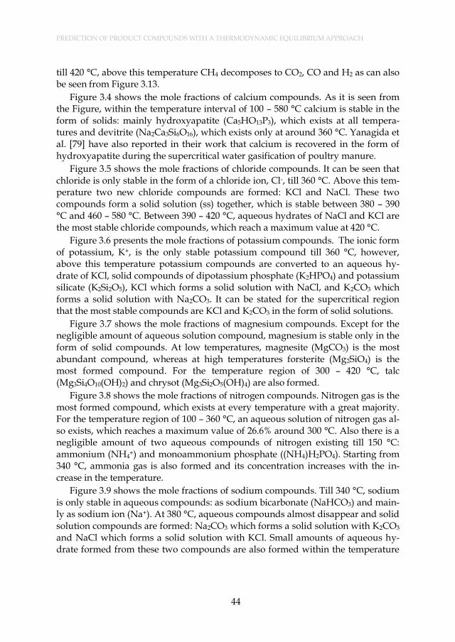
PREDICTION OF PRODUCT COMPOUNDS WITH A THERMODYNAMIC EQUILIBRIUM APPROACH
44
till 420 °C, above this temperature CH4 decomposes to CO2, CO and H2 as can also be seen from Figure 3.13.
Figure 3.4 shows the mole fractions of calcium compounds. As it is seen from the Figure, within the temperature interval of 100 – 580 °C calcium is stable in the form of solids: mainly hydroxyapatite (Ca5HO13P3), which exists at all tempera-tures and devitrite (Na2Ca3Si6O16), which exists only at around 360 °C. Yanagida et al. [79] have also reported in their work that calcium is recovered in the form of hydroxyapatite during the supercritical water gasification of poultry manure.
Figure 3.5 shows the mole fractions of chloride compounds. It can be seen that chloride is only stable in the form of a chloride ion, Cl-, till 360 °C. Above this tem-perature two new chloride compounds are formed: KCl and NaCl. These two compounds form a solid solution (ss) together, which is stable between 380 – 390 °C and 460 – 580 °C. Between 390 – 420 °C, aqueous hydrates of NaCl and KCl are the most stable chloride compounds, which reach a maximum value at 420 °C.
Figure 3.6 presents the mole fractions of potassium compounds. The ionic form of potassium, K+, is the only stable potassium compound till 360 °C, however, above this temperature potassium compounds are converted to an aqueous hy-drate of KCl, solid compounds of dipotassium phosphate (K2HPO4) and potassium silicate (K2Si2O5), KCl which forms a solid solution with NaCl, and K2CO3 which forms a solid solution with Na2CO3. It can be stated for the supercritical region that the most stable compounds are KCl and K2CO3 in the form of solid solutions.
Figure 3.7 shows the mole fractions of magnesium compounds. Except for the negligible amount of aqueous solution compound, magnesium is stable only in the form of solid compounds. At low temperatures, magnesite (MgCO3) is the most abundant compound, whereas at high temperatures forsterite (Mg2SiO4) is the most formed compound. For the temperature region of 300 – 420 °C, talc (Mg3Si4O10(OH)2) and chrysot (Mg3Si2O5(OH)4) are also formed.
Figure 3.8 shows the mole fractions of nitrogen compounds. Nitrogen gas is the most formed compound, which exists at every temperature with a great majority. For the temperature region of 100 – 360 °C, an aqueous solution of nitrogen gas al-so exists, which reaches a maximum value of 26.6% around 300 °C. Also there is a negligible amount of two aqueous compounds of nitrogen existing till 150 °C: ammonium (NH4
+) and monoammonium phosphate ((NH4)H2PO4). Starting from 340 °C, ammonia gas is also formed and its concentration increases with the in-crease in the temperature.
Figure 3.9 shows the mole fractions of sodium compounds. Till 340 °C, sodium is only stable in aqueous compounds: as sodium bicarbonate (NaHCO3) and main-ly as sodium ion (Na+). At 380 °C, aqueous compounds almost disappear and solid solution compounds are formed: Na2CO3 which forms a solid solution with K2CO3 and NaCl which forms a solid solution with KCl. Small amounts of aqueous hy-drate formed from these two compounds are also formed within the temperature

3.1 Predictions Using Commercial Software Packages
45
region of 390 – 500 °C. At 580 °C, a different compound, trisodium phosphate (Na3PO4), is formed with a mole fraction of 12.1%.
Figure 3.10 shows the mole fractions of phosphorus compounds. Hydroxyap-atite is the most formed compound at all temperatures. In the subcritical region, aqueous phosphate compounds are also formed: HPO4
2-, NH4H2PO4, HP2O73-,
MgP2O72- and H2P2O7
2-. The latter one is the most formed among the others and reaches a maximum value of 25% at 360 °C. In the supercritical region, two other solid compounds are formed: potassium phosphate for the temperature region of 390 – 580°C and trisodium phosphate at only 580 °C. The mole fraction of hydrox-yapatite is constant at 84.3% in the supercritical region. The reason for this stability originates from the mole ratio of phosphorus and calcium content in the manure and how much of them is consumed when they are forming hydroxyapatite. One can consider adding calcium compounds to the reaction to obtain all calcium and phosphate fractions in hydroxyapatite form.
Figure 3.11 shows the mole fractions of sulphur compounds. Till 200 °C, sul-phuric acid hexahydrate (H2SO4(H2O)6) is the only sulphur compound. Starting from 250 °C, it decomposes to aqueous compounds of the hydrogen sulfide ion (HS-), ionic sulphur (S2-) and aqueous form of hydrogen sulfide (H2S), and hydro-gen sulfide gas. In the supercritical region, hydrogen sulfide gas is the only sul-phur compound.
Figure 3.12 shows the mole fractions of silicon compounds. Among all of these elements silicon is the most diverted element showing a partitioning into 9 differ-ent compounds. Till 250 °C, aqueous silicic (H4SiO4) and metasilicic acid (H2SiO3), and quartz (SiO2) are stable compounds of which the latter one is the most formed one among them. Aqueous acidic compounds of silicon disappear at temperatures exceeding 300 °C and different solid compounds of silicon are formed. Talc is sta-ble within the temperature region of 300 – 360 °C and 390 – 420 °C. Chrysot only appears between 360 and 380 °C, whereas devitrite is stable only at 360 °C. In the supercritical region, a small amount of aqueous hydrate of quartz exists in equilib-rium with the other solid compounds mainly forsterite and potassium silicate.
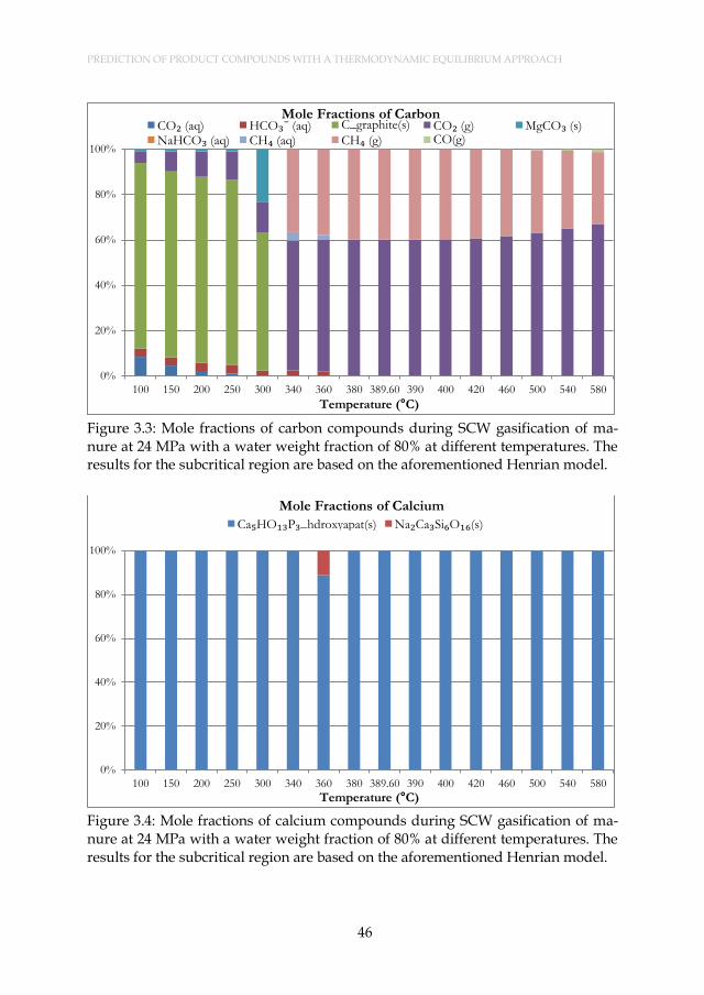
PREDICTION OF PRODUCT COMPOUNDS WITH A THERMODYNAMIC EQUILIBRIUM APPROACH
46
Figure 3.3: Mole fractions of carbon compounds during SCW gasification of ma-nure at 24 MPa with a water weight fraction of 80% at different temperatures. The results for the subcritical region are based on the aforementioned Henrian model.
Figure 3.4: Mole fractions of calcium compounds during SCW gasification of ma-nure at 24 MPa with a water weight fraction of 80% at different temperatures. The results for the subcritical region are based on the aforementioned Henrian model.
0%
20%
40%
60%
80%
100%
100 150 200 250 300 340 360 380 389.60 390 400 420 460 500 540 580
Temperature (°C)
Mole Fractions of Carbon CO₂ (aq) HCO₃⁻ (aq) C_graphite(s) CO₂ (g) MgCO₃ (s) NaHCO₃ (aq) CH₄ (aq) CH₄ (g) CO(g)
0%
20%
40%
60%
80%
100%
100 150 200 250 300 340 360 380 389.60 390 400 420 460 500 540 580
Temperature (°C)
Mole Fractions of Calcium
Ca₅HO₁₃P₃_hdroxyapat(s) Na₂Ca₃Si₆O₁₆(s)

3.1 Predictions Using Commercial Software Packages
47
Figure 3.5: Mole fractions of chloride compounds during SCW gasification of ma-nure at 24 MPa with a water weight fraction of 80% at different temperatures. The results for the subcritical region are based on the aforementioned Henrian model.
Figure 3.6: Mole fractions of potassium compounds during SCW gasification of manure at 24 MPa with a water weight fraction of 80% at different temperatures. The results for the subcritical region are based on the aforementioned Henrian model.
0%
20%
40%
60%
80%
100%
100 150 200 250 300 340 360 380 389.60 390 400 420 460 500 540 580Temperature (°C)
Mole Fractions of Chloride
Cl⁻ (aq) NaCl (ss with KCl) KCl (ss with NaCl)
0%
20%
40%
60%
80%
100%
100 150 200 250 300 340 360 380 389.60 390 400 420 460 500 540 580
Temperature (°C)
Mole Fractions of Potassium K⁺ (aq) K₂CO₃ (ss with Na₂CO₃) KCl (ss with NaCl)
K₂Si₂O₅(s) K₂HPO₄(s) KCl (Aqueous Hydrate)
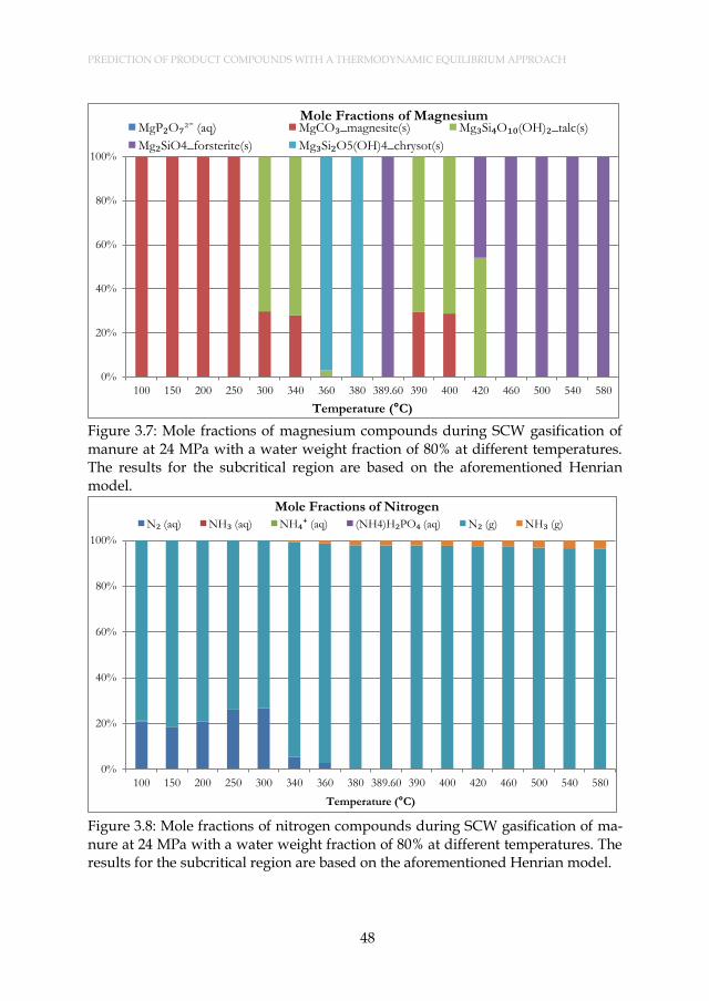
PREDICTION OF PRODUCT COMPOUNDS WITH A THERMODYNAMIC EQUILIBRIUM APPROACH
48
Figure 3.7: Mole fractions of magnesium compounds during SCW gasification of manure at 24 MPa with a water weight fraction of 80% at different temperatures. The results for the subcritical region are based on the aforementioned Henrian model.
Figure 3.8: Mole fractions of nitrogen compounds during SCW gasification of ma-nure at 24 MPa with a water weight fraction of 80% at different temperatures. The results for the subcritical region are based on the aforementioned Henrian model.
0%
20%
40%
60%
80%
100%
100 150 200 250 300 340 360 380 389.60 390 400 420 460 500 540 580
Temperature (°C)
Mole Fractions of Magnesium MgP₂O₇²⁻ (aq) MgCO₃_magnesite(s) Mg₃Si₄O₁₀(OH)₂_talc(s)
Mg₂SiO4_forsterite(s) Mg₃Si₂O5(OH)4_chrysot(s)
0%
20%
40%
60%
80%
100%
100 150 200 250 300 340 360 380 389.60 390 400 420 460 500 540 580
Temperature (°C)
Mole Fractions of Nitrogen
N₂ (aq) NH₃ (aq) NH₄⁺ (aq) (NH4)H₂PO₄ (aq) N₂ (g) NH₃ (g)

3.1 Predictions Using Commercial Software Packages
49
Figure 3.9: Mole fractions of sodium compounds during SCW gasification of ma-nure at 24 MPa with a water weight fraction of 80% at different temperatures. The results for the subcritical region are based on the aforementioned Henrian model.
Figure 3.10: Mole fractions of phosphorus compounds during SCW gasification of manure at 24 MPa with a water weight fraction of 80% at different temperatures. The results for the subcritical region are based on the aforementioned Henrian model.
0%
20%
40%
60%
80%
100%
100 150 200 250 300 340 360 380 389.60 390 400 420 460 500 540 580
Temperature (°C)
Mole Fractions of Sodium Na⁺ (aq) NaHCO₃ (aq) Na₂Ca₃Si₆O₁₆(s) Na₂CO₃(s) Na₂CO₃ (ss with K₂CO₃) NaCl (ss with KCl)
0%
20%
40%
60%
80%
100%
100 150 200 250 300 340 360 380 389.60 390 400 420 460 500 540 580
Temperature (°C)
Mole Fractions of Phosporus HPO₄²⁻(aq) HP₂O₇³⁻ (aq) H₂P₂O₇²⁻ (aq)
(NH₄)H₂PO₄ (aq) MgP₂O₇²⁻ (aq) Ca₅HO₁₃P₃_hdroxyapat(s)
K₂HPO₄(s) Na₃(PO₄)(s)

PREDICTION OF PRODUCT COMPOUNDS WITH A THERMODYNAMIC EQUILIBRIUM APPROACH
50
Figure 3.11: Mole fractions of sulphur compounds during SCW gasification of ma-nure at 24 MPa with a water weight fraction of 80% at different temperatures. The results for the subcritical region are based on the aforementioned Henrian model.
Figure 3.12: Mole fractions of silicon compounds during SCW gasification of ma-nure at 24 MPa with a water weight fraction of 80% at different temperatures. The results for the subcritical region are based on the aforementioned Henrian model.
0%
20%
40%
60%
80%
100%
100 150 200 250 300 340 360 380 389.60 390 400 420 460 500 540 580
Temperature (°C)
Mole Fractions of Sulphur H₂SO₄(H₂O)₆(liq) HS⁻ (aq) H₂S (g) S²⁻ (aq) H₂S (aq)
0%
20%
40%
60%
80%
100%
100 150 200 250 300 340 360 380 389.60 390 400 420 460 500 540 580
Temperature (°C)
Mole Fractions of Silicon H₂SiO₃ (aq) H₄SiO₄ (aq) SiO₂_quartz(s)
Mg₃Si₄O₁₀(OH)₂_talc(s) Mg₃Si₂O5(OH)4_chrysot(s) Na₂Ca₃Si₆O₁₆(s)
K₂Si₂O₅(s) Mg₂SiO4_forsterite(s) SiO₂ (aqueous hydrate)

3.1 Predictions Using Commercial Software Packages
51
3.1.3.4. Behavior of gases
Figure 3.13 shows the gas composition during the hydrothermal conversion at 24 MPa and different temperatures. In addition to water vapor, CO2, CH4, N2, H2 and negligible amounts of CO, NH3 and H2S are formed. While the amount of CO2, CH4 and H2 increases with the increase in temperature, the amount of N2 is almost stable in the region of 900 mmol∙kg-1 of dry manure during the subcritical region. As stated above, solid carbon drastically decreases starting from 300 °C and is converted into CO2 and CH4. Above 340 °C, the rate of increase of CO2 and CH4 decreases as the solid carbon completely disappears above that temperature. Above 340 °C, the increase in the amounts of CO2 and CH4 is due to the decrease of carbon content in aqueous phase.
CO and H2 amounts are at least one order of magnitude lower than those of CO2 and CH4 in the subcritical region. This can be explained based on water gas shift (WGS) and methanation reactions and the equilibrium constants of these re-actions. Equations 3.5 and 3.6 show the WGS and methanation reactions, respec-tively, and Table 3.2 shows the equilibrium constants calculated using Aspen Plus software.
CO + H2O ↔ CO2 + H2 (3.5)
CO + 3H2 ↔ CH4 + H2O (3.6)
Figure 3.13: Behavior of gases during SCW gasification of manure at 24 MPa with a water weight fraction of 80% at different temperatures.

PREDICTION OF PRODUCT COMPOUNDS WITH A THERMODYNAMIC EQUILIBRIUM APPROACH
52
Table 3.2: Equilibrium constants of WGS and methanation reactions calculated by Aspen Plus.
Equilibrium Constant Equilibrium Constant
Temperature (°C) WGS Methanation
Temperature (°C) WGS Methanation
100 3730 3.66E+17 389.6 13.7 31079.4
150 794 1.22E+14 390 13.6 30342
200 237 2.07E+11 400 12.28 16801
250 90 1.14E+09 420 10.1 5411
300 40 1.50E+07 460 7.06 671
340 24 7.69E+05 500 5.14 102.56
360 18.9 1.99E+05 540 3.88 18.74
380 15.1 55758 580 3.01 3.99
As seen from Table 3.2, the equilibrium constants of the aforementioned reac-tions are so high that they enhance the forward reactions which results in high amounts of CH4 and CO2 as seen in Figure 3.13. Although H2 is produced in the WGS reaction, it is largely consumed in the methanation reaction to form CH4. Starting from 380 °C, the amount of methane decreases and the amount of hydro-gen increases. This can be explained by the backward methanation reaction in which methane and water decomposes to hydrogen and carbon monoxide. As it can be seen from Figure 3.14, the amount of water also decreases in the supercriti-cal region. The results indicate that one should work at temperatures higher than 600 °C to obtain hydrogen rich gas.
3.1.3.5. Behavior of water
Figure 3.14 shows the behavior of water. Till 300 °C, water is mainly in liquid phase and above this temperature the amount of water vapour drastically increas-es. For the temperature region of 100-300 °C, the amount of liquid water is higher than the initial water content and the maximum amount of water vapour at high temperatures is lower than the initial water content. This indicates that hydrogen and oxygen atoms of manure contribute to water formation in the subcritical re-gion and then water is consumed in the reactions to form gases: mainly carbon di-oxide, methane and hydrogen.

3.1 Predictions Using Commercial Software Packages
53
Figure 3.14: Mole amount of liquid and gas state water during SCW gasification of manure at 24 MPa with a water weight fraction of 80% at different temperatures
3.1.3.6. The effect of pressure and water fraction on main product gases
Figure 3.15 shows the effect of pressure on the main product gases for the re-gion of 24-30 MPa with a water weight fraction of 80%. The simulations have been performed based on the aforementioned supercritical region model. It can be seen from Figure 3.15 that the pressure is not a main factor for the yield of the main product gases. H2 and CO2 yields decrease and CH4 yield increases with an in-crease in pressure, however, the change is almost insignificant for CO2 and CH4. Castello and Fiori [125] and Yan et al. [124] have also shown the same trend in their works. On the other hand, Basu and Mettanant [3] have stated that the effect of pressure shows a complex behavior as it has different effects on the subcritical and supercritical region where ionic and free radical mechanisms take place, re-spectively.
Figure 3.16 shows the effect of the water fraction on the main product gases for the region of 80-95% water weight fraction and at a pressure of 24 MPa. The simu-lations have been performed based on the aforementioned supercritical region model. The increase in the water fraction significantly increases the yields of H2 and CO2, whereas it decreases the yield of CH4. The results are in agreement with the results of Lu et al. [178] and Yan et al. [124]. This effect can be explained by Le Chateleir’s principle for the WGS and methanation reactions. The increased frac-tion of water enhances the forward WGS and backward methanation reactions which result in higher yields of H2 and CO2 and a lower yield of CH4.

PREDICTION OF PRODUCT COMPOUNDS WITH A THERMODYNAMIC EQUILIBRIUM APPROACH
54
Figure 3.15: The effect of pressure on main product gases during SCW gasification of manure with a water weight fraction of 80% at different temperatures.
Figure 3.16: The effect of water fraction on main product gases during SCW gasifi-cation of manure at a pressure of 24 MPa and at different temperatures with dif-ferent water weight fractions.

3.1 Predictions Using Commercial Software Packages
55
3.1.4. Conclusions
The equilibrium behavior of elements on compound and phase basis during the hydrothermal conversion of mixed pig-cow manure up to 580 °C and at 24 MPa, as well as the effect of pressure and water weight fraction on main product gases, have been investigated with using direct Gibbs free energy minimization method. It is found that the presence of solutes and gases increases the pseudo critical point of water and in the subcritical region calcium, magnesium, phosphorus and silicon are stable in the form of solid compounds, whereas chlorine, potassium and sodi-um are stable in the form of aqueous compounds. In the supercritical region, backward methanation reaction takes place and CH4 decomposes and forms H2. While the water fraction has a significant effect on the amount of main product gases, pressure was found to be less significant for the region of 24 – 30 MPa.

PREDICTION OF PRODUCT COMPOUNDS WITH A THERMODYNAMIC EQUILIBRIUM APPROACH
56
3.2. DEVELOPMENT OF A THERMODYNAMIC MODEL FOR THE PREDICTIONS OF
PRODUCTS AT EQUILIBRIUM STATE
3.2.1. Introduction
Most of research works in the literature regarding the prediction of product compounds with a thermodynamic equilibrium approach have been developed for the supercritical region and take only the gas phase compounds into account [118,120,123,124] or the graphitic carbon as the only solid product [125] as given in Table 2.3. The behavior of inorganics and the aqueous phase, on the other hand, have been investigated only by using software programs for only one type of bio-mass: animal manure [79]. In the previous sub-chapter, the equilibrium partition-ing of elements with respect to compounds and phases in the supercritical water gasification of a particular manure feedstock is investigated with the help of com-mercial software packages. However in industrial applications, the use of different biomass feedstocks in supercritical water gasification will result in a different par-titioning behavior. In addition, the solution phase models available in such soft-ware packages may not be suitable and adequate for the analysis of supercritical water gasification of different type of biomass feedstocks at different process con-ditions. For this reason, a model capable of predicting compound formation over a wider range of biomass types as well as using a more updated thermodynamic da-ta for the solute species is valuable. This sub-chapter deals with the development of such a multi-phase thermodynamic model to predict the formation of com-pounds at equilibrium state during the supercritical water gasification of biomass for both the subcritical and supercritical region.
3.2.2. Thermodynamic model
3.2.2.1 Equations for the gases
The pressure and temperature of supercritical water gasification systems result in a non-ideal thermodynamic behavior for the gaseous compounds. This leads to the introduction of the fugacity coefficient into the Eq (3.3). The Peng-Robinson equation of state (EoS) has been chosen for the calculations as the previous works that based their studies of supercritical water gasification of biomass on this EoS [118,123,125] showed good agreement with the experimental results.
With the introduction of the fugacity coefficients, the first term of the Eq. (3.3) becomes:
1
N
i i
i
n
(3.7)
where μi is the chemical potential under specific temperature and pressure con-
ditions, and can be defined as
3.2. Development of a Thermodynamic Model for the Predictions of Products at Equilibrium State
57
0,
0,
( , ) ( ) ln i
i i
i
fT P T RT
f (3.8)
where μ0,i is the chemical potential under standard pressure and can be defined as
,0 0
0, , , ,
298 298
( )( ) ( )
T T
p i
i f i p i f i
C TT H C T dT T S T dT
T (3.9)
Throughout this sub-chapter, the values for calculation of μ0,i have been ac-
quired from the FACT53 database of the FactSage software. The f0,i term in the (3.8) is P0, and fi term is the fugacity of component i and can be defined as
ˆ ˆi i i
f x P (3.10)
where ˆi is the fugacity coefficient and can be calculated by Peng-Robinson
EoS. Peng-Robinson EoS has been developed based on Van der Waals’ EoS using a and b parameters derived from critical properties of substances and defined as [179]
( ) ( )
RT aP
b b b b
(3.11)
and 3 2 2 2 3
(1 ) ( 3 2 ) ( ) 0Z B Z A B B Z AB B B (3.12)
where
2 2
aPA
R T (3.13)
bPB
RT (3.14)
PZ
RT
(3.15)
2 2
0.45724 c
c
R Ta
P (3.16)
0.07780 c
c
RTb
P (3.17)
1 (1 )
c
T
T (3.18)
20.37464 1.54226 0.26992 (3.19)
The subscript c refers to the critical point and ω is the acentric factor of the sub-stance. Solving the Eq. (3.12) will result in three roots and the maximum of the real roots refers to the gas phase and the minimum refers to the liquid phase in the two-phase region. For the supercritical region, only one real root exists [125,179].

PREDICTION OF PRODUCT COMPOUNDS WITH A THERMODYNAMIC EQUILIBRIUM APPROACH
58
The original Peng-Robinson EoS uses the Van der Waals mixing rule for mix-tures where the mixing parameters are determined using the following mixing rule [179]:
m i j ij
i j
a x x a (3.20)
m i i
j
b x b (3.21)
(1 )ij ij i j
a a a (3.22)
where δ can be calculated using the critical volume parameters of the substanc-es [180] as
, ,
33 3
, ,
1 8( )
c i c j
ij
c i c j
(3.23)
For mixtures, the values A and B in Eqs. (13) and (14) are calculated using the results of the Eqs. (20) and (21). Finally, the equation that enables to calculate the fugacity coefficients of the compounds in a mixture becomes:
,
ˆln ( 1) ln( )
22.414
( ) ln( )0.4142 2
i
i m
m
i i j
jm i m
m m m m
bZ Z B
b
x aA b Z B
a b Z BB
(3.24)
where the subscript m refers to the mixture parameters.
3.2.2.2 Equations for the pure condensed phases
It can be stated that pressure does not have an influence on the thermodynamic properties of pure solids. In addition, as no data are given, the effect of pressure on thermodynamic properties of selected pure liquids is assumed to be insignificant. Throughout this sub-chapter, the required thermodynamic data for these pure condensed phases has been acquired from FACT53 database of FactSage. No solu-tions nor postulated slags of these pure condensed phases have been taken into ac-count throughout the calculations.
Equations for the aqueous solution in subcritical region: The total Gibbs free energy of the aqueous phase is given in Eq. (3.3) as
( ln ln )
j
t o
Aqueous j j j j
Aqueous
G n g RT x RT (3.25)
which can be rewritten in terms of water and other solute species as

3.2. Development of a Thermodynamic Model for the Predictions of Products at Equilibrium State
59
( ln ln )
( ln ln )
i
t o
Aqueous w w w w
o
i i i i
Aqueous
G n g RT x RT
n g RT x RT
(3.26)
where the subscript w refers to the solvent, water.
3.2.2.3 Calculation of the thermodynamic properties of solute species
The second term of Eq. (3.26) gives an expression for the total Gibbs free energy of the aqueous solutes on a mole fraction basis. In contrast to the water properties in the aqueous phase, it is better to use the molality based equation for the solute species. The second term in Eq. (3.26) can be rewritten in terms of chemical poten-tials as: [181]
,
i
t
Aqueous solutes i i
Aqueous
G n (3.27)
and the chemical potential can be expressed as
( , ) ln( )i i
i i
mT P RT
m
(3.28)
so the second term in the Eq. (3.26) can be rewritten in terms of molality based terms as
,( ln ln )
i
t o i
Aqueous solute i i i
Aqueous
mG n g RT RT
m (3.29)
Where o
ig is the molality based standard Gibbs free energy, m is the species mo-
lality and i is the molality based activity coefficient and m is the molality conver-
sion factor with a value of 1 mol/kg. Throughout this sub-chapter, the thermody-
namic data required for o
ig values of solutes have been acquired from the SUP-
CRT92 software using the slop07.DAT database developed by Shock et al. [182] The software uses the revised Helgeson-Kirkham-Flower (HKF) EoS [183]. Molali-ty based activity coefficients for high pressure and high temperature aqueous sys-tems have been given by Helgeson et al. [184] and derived from Debye-Hückel equation as
2 1/2
1/2log ( / )
1
i abs
i i k k il l l
k l
A Z Ib y I b y I
aB I
(3.30)
2 1/2
1/2log ( / )
1
l abs
l l k k il i i
k l
A Z Ib y I b y I
aB I
(3.31)
log ( / ) ( / )n n k k ni i i nl l l
k i l
b y I b y I b y I
(3.32)

PREDICTION OF PRODUCT COMPOUNDS WITH A THERMODYNAMIC EQUILIBRIUM APPROACH
60
where the subscripts i, l and n represent anion, cation and neutral species, re-spectively. The first term of the Eqs. (3.30) and (3.31) is the long-range interaction term (extended Debye-Hückel equation) and the second term is the mole fraction to molality conversion factor. The third term can be expressed as the effect of the difference between the electrostatic effects of pure water and solution and the last term is the short-range interaction term. The last term has been assumed to be in-significant for the supercritical water gasification of biomass as the water content of the systems is quite high so that it can be assumed as a dilute system.
The equations of the parameters are as follows [184,185]: 6 1/2
3/2
1.824829238 10
( )A
T
(3.33)
8 1/2
1/2
50.29158649 10
( )B
T
(3.34)
2 21( )
2j j q q
j q
I Z m Z m (3.35)
, ,2 /
j k e j k
k j
a v r v (3.36)
,k j k
j
v v (3.37)
, , ,Pr,e j e j Tr jr r Z g (3.38)
ˆ(1 ) gb
gg a f (3.39)
2
,1 ,2 ,3g g g ga a a T a T (3.40)
2
,1 ,2 ,3g g g gb b b T b T (3.41)
4.8 16 3 4
,1 ,2 ,3
155 155[( ) ( ) ] [ (1000 ) (1000 ) ]
300 300f f f
T Tf a a P a P
(3.42)
3ˆ / (1 / )g cm (3.43)
,Pr,2 1
, ,Pr,( )
3.082
j Tr j
e j Tr j
Zr Z
(3.44)
2
,
jabs
j
e j
Z
r
(3.45)
2
,3.082
j j
j
e j
Z Z
r g
(3.46)
51.66027 10 Å∙cal∙mol-1 (3.47)

3.2. Development of a Thermodynamic Model for the Predictions of Products at Equilibrium State
61
*log(1 0.0180153 )m
(3.48)
2
,( )
2
j
j k k
j
k
Zv m
yI
(3.49)
21
2j j
j
I Z m (3.50)
ˆ
2.303
k
k
bb
RT (3.51)
The subscript k in Eqs. (3.30) through (3.32) refers to the kth component of an electrolyte solution. In the original paper, Helgeson et al. [184] treat an electrolyte solution as a mixture of dissolved neutral solutes or ion pairs formed from dissolu-tion of various particular components such as mixtures of salts and oxides. How-ever, for all the calculations in this sub-chapter, the feedstock has been considered as one single component and individual solute species (either in the form of ions or neutral solutes) have been taken into account instead of ion pairs. This led to the
reduction of ky to 1 and I to I. The parameter a has been accepted to be 2,e jr
for the calculations. The parameters for Eqs. (37) through (39) are given in Table
3.3 [185] with their units. ,Pr,j Tr values are acquired from SUPCRT92 software
[170,182], the dielectric constant of water has been calculated from Uematsu and Franck [15], and the properties of water have been acquired from SUPCRT92 soft-
ware [170]. For neutral species, ,Pr,j Tr has the same value of
j [170]. The ˆkb term
in Eq.(3.51) has been given for many neutral species at 25 °C and 0.1 MPa by Helgeson et al. [184] and for the species which have not been given in Helgeson et al. [184] the values are assumed to be 2x10⁻³ kg∙mol-1 as given values are very close to this number.
Table 3.3: The value and the units of the parameters given in the Eqs. (3.40) through (3.42). [185]
i ,g ia units
,g ib units
,f ia units
1 -0.2037662x101 Å 0.6107361x101 - 0.3666666x10⁻¹⁵ °C-16
2 0.5747000x10⁻² Å/°C -0.1074377x10⁻¹ °C-1 -0.1504956x10⁻⁹ Å/bar3
3 -0.6557892x10⁻⁵ Å /°C2 0.1268348x10⁻⁴ °C-2 0.5017997x10⁻¹³ Å/bar4
3.2.2.4 Calculation of the activity of water
For the calculation of the activity of water in the aqueous phase, the following equations given by Helgeson et al. [184] have been used:

PREDICTION OF PRODUCT COMPOUNDS WITH A THERMODYNAMIC EQUILIBRIUM APPROACH
62
*
ln55.51
w
ma
(3.52)
where wa is the activity of water, *m is the total molality of the solute species
and is the osmotic coefficient of water, which is given as
2 1/2 1/2
,* *
( )2.303[
3 0.0180153
1( )]
2
i
t j
j
j k k ij i jl il
k i i
A Z I aB Im
m m
b y I b m b m
(3.53)
The last two terms in Eq. (3.53) are the short-range interaction term and these are assumed to be insignificant for the supercritical water gasification of biomass systems studied in this work as explained above. So the Eq. (53) reduces to
2 1/2 1/2
,* *
( )2.303 1[ ( )]
3 0.0180153 2
i
t j j k k
j k
A Z I aB Im b y I
m m
(3.54)
where
1/2
3 3 3/2
3 1( ) ( 2ln )aB I
a B I
(3.55)
1/21 aB I
(3.56)
The fundamentals and details of the equations used for the aqueous phase in the subcritical region calculations can be found in the cited references (see ref. [170,184,185])
3.2.2.5. Equations for the aqueous solution in supercritical region
Solubility of solids in supercritical water has been investigated by many au-thors and several models have been developed. These vary from reaction equilib-rium to implementation of Flory-Huggins and lattice gas models theory in super-critical medium [171–173,186–191]. Based on the agreement with the experimental results, it can be stated that the most successful model is the reaction equilibrium model [171,173,186,188,191] which is mainly based on the assumption that the equilibrium exists in a way that the molecules of a solute associate with the mole-cules of a gas and form an aqueous hydrate complex [186]. This part is similar to section “3.1.2.4. Calculations in the supercritical region” and revisited here.
The model presented section “3.1.2.4. Calculations in the supercritical region” also presumes that the solvation occurs not in the form of dissociated ions but in the form of neutral ion pairs [171,173,186,188,191].Although it has been found that ion clustering could take place in supercritical water to form multiple associated ions (such as Na3Cl2
+), this presumption can be stated as valid within the investi-gated temperature, pressure and molality (< 0.1) region of the current work. [171,192]
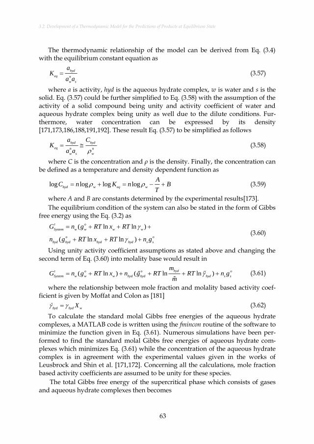
3.2. Development of a Thermodynamic Model for the Predictions of Products at Equilibrium State
63
The thermodynamic relationship of the model can be derived from Eq. (3.4) with the equilibrium constant equation as
hyd
eq n
w s
aK
a a (3.57)
where a is activity, hyd is the aqueous hydrate complex, w is water and s is the solid. Eq. (3.57) could be further simplified to Eq. (3.58) with the assumption of the activity of a solid compound being unity and activity coefficient of water and aqueous hydrate complex being unity as well due to the dilute conditions. Fur-thermore, water concentration can be expressed by its density [171,173,186,188,191,192]. These result Eq. (3.57) to be simplified as follows
hyd hyd
eq n n
w s w
a CK
a a (3.58)
where C is the concentration and ρ is the density. Finally, the concentration can be defined as a temperature and density dependent function as
log log log loghyd w eq w
AC n K n B
T (3.59)
where A and B are constants determined by the experimental results[173].
The equilibrium condition of the system can also be stated in the form of Gibbs free energy using the Eq. (3.2) as
( ln ln )
( ln ln )
t o
System w w w w
o o
hyd hyd hyd hyd s s
G n g RT x RT
n g RT x RT n g
(3.60)
Using unity activity coefficient assumptions as stated above and changing the second term of Eq. (3.60) into molality base would result in
( ln ) ( ln ln )hydt o o o
System w w w hyd hyd hyd s s
mG n g RT x n g RT RT n g
m (3.61)
where the relationship between mole fraction and molality based activity coef-ficient is given by Moffat and Colon as [181]
hyd hyd wX (3.62)
To calculate the standard molal Gibbs free energies of the aqueous hydrate complexes, a MATLAB code is written using the fmincon routine of the software to minimize the function given in Eq. (3.61). Numerous simulations have been per-formed to find the standard molal Gibbs free energies of aqueous hydrate com-plexes which minimizes Eq. (3.61) while the concentration of the aqueous hydrate complex is in agreement with the experimental values given in the works of Leusbrock and Shin et al. [171,172]. Concerning all the calculations, mole fraction based activity coefficients are assumed to be unity for these species.
The total Gibbs free energy of the supercritical phase which consists of gases and aqueous hydrate complexes then becomes

PREDICTION OF PRODUCT COMPOUNDS WITH A THERMODYNAMIC EQUILIBRIUM APPROACH
64
0,
0,
ˆ( ( ) ln ) ( ln ln )
hydt oi
fluid i hyd hyd hyd
gas hydi
i
mfG n T RT n g RT RT
f m (3.63)
It is assumed that the presence of aqueous hydrate complexes does not have an effect on the fugacity coefficient of the other species in the supercritical phase. Eq. (3.63) is the final equation which is the replacement for the ideal gas term in the Eq. (3.3) for the calculations in the supercritical region.
3.2.3. Gibbs free energy minimization
To determine the species and their amounts in the equilibrium state at a specif-ic temperature and pressure, one has to minimize Eq. (3.2). This is indeed an opti-mization problem with the constraints of mole and charge balance, and non-negativity of the amount of species. A MATLAB® code using its fmincon routine is written for the minimization of Eq. (3.2) with the aforementioned constraints. The code has been run for both subcritical and supercritical conditions. Due to the temperature limitation of Eq. (3.42), the minimum temperature for the equilibrium calculations was 155 °C. Within the pressure range investigated in this work, the SUPCRT92 software does not calculate the thermodynamic properties of ionic spe-cies for temperatures higher than 350 °C. One may also consider extrapolating the data for the ionic species beyond that region, but throughout this sub-chapter, to be consistent within the available databases existing in literature, only the neutral aqueous solutes have been taken into account for the subcritical region where the temperature is higher than 350 °C.
Keeping the pressure constant, the temperature is increased until the gas or aqueous phase disappears. This temperature is assumed to be the phase transition point for the corresponding pressure and above this temperature, the system’s state is referred to as being in the supercritical region. Instead of aqueous species, aqueous hydrate complexes have been chosen for this region.
3.2.4. Model validation
The model has been validated by comparing with experimental results and model predictions already published. The validity of the model has been tested for the supercritical region and the subcritical region separately. The supercritical re-gion simulations take the aqueous hydrate complexes and the solid and the gas phase compounds into account for all the simulations. However, the subcritical re-gion simulations take solid, aqueous and gaseous compounds into account as well as the inorganic species.
3.2.4.1. Validation of the model for the supercritical region
Seven experimental results for different process conditions as well as different feedstocks from different authors [76,176,47,85,13,193,94] have been investigated in this region. The experimental work includes the results from both model biomass compounds and real biomass samples as well as solubilities of inorganics in super-

3.2. Development of a Thermodynamic Model for the Predictions of Products at Equilibrium State
65
critical water. The comparisons of the results are given in Figure 3.17 to Figure 3.23. For all simulations, graphitic carbon and gaseous compounds consisting of C, H and O elements have been selected. However, for the cases shown in Figure 3.21 and Figure 3.22, additional compounds have been selected. The details of this se-lection are described below. For the validity of the solubilities of salt mixtures in supercritical water, aqueous hydrate complexes and their solid forms have been selected.
Taylor et al. [176] have performed methanol, ethanol and ethylene glycol gasifi-cation at a pressure of 27.6 MPa and at different temperatures, whereas Byrd et al.[76] gasified glycerol in supercritical water medium in the presence of Ru/Al2O3
catalyst at a pressure of 24.1 MPa and at different temperatures. The model predic-tions are in a good agreement with the experimental results of Byrd et al.[76] and the ethanol results of Taylor et al. [176]. The difference in gas fractions between the model predictions, and methanol and ethylene glycol experimental results in Fig-ure 3.17 are believed to be due to the short residence times, as the authors’ [176] longer residence time experiments result in more carbon dioxide and methane, and less carbon monoxide and hydrogen. The model predictions are in agreement with that result of the authors [176]. The predictions of these two cases are also in agreement and very close to the predictions of previous works [118,125] and the results shown in Figure 3.1 and Figure 3.2. This is an indication that i) the model is in agreement with the models of others, and as expected ii) at high temperatures, due to the fugacity coefficients approaching unity, the difference in predictions arising from using a different EoS in the calculations decreases and becomes al-most negligible.
Figure 3.17: Comparison of the experimental results of Taylor et al.[176] and the model prediction. Experiments have been carried out with a 15% wt. feed concen-tration, at 700 °C and at 27.6 MPa.
0
0.2
0.4
0.6
0.8
1
H₂
CH₄
CO
CO₂
C₂H
₄
H₂
CH₄
CO
CO₂
C₂H
₄
H₂
CH₄
CO
CO₂
C₂H
₄
Methanol Ethanol Ethylene Glycol
Mo
le F
racti
on
Experimental results Model prediction
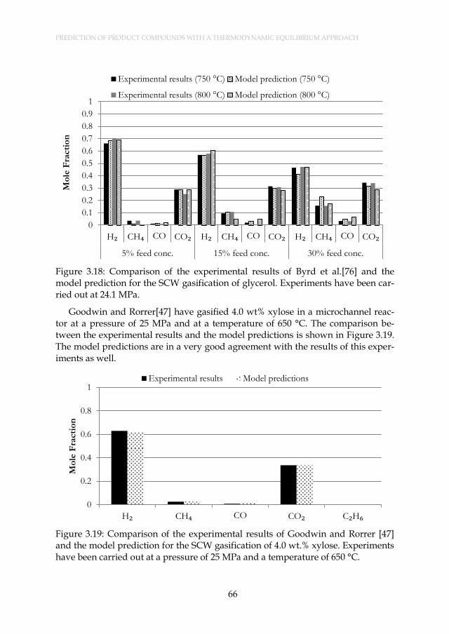
PREDICTION OF PRODUCT COMPOUNDS WITH A THERMODYNAMIC EQUILIBRIUM APPROACH
66
Figure 3.18: Comparison of the experimental results of Byrd et al.[76] and the model prediction for the SCW gasification of glycerol. Experiments have been car-ried out at 24.1 MPa.
Goodwin and Rorrer[47] have gasified 4.0 wt% xylose in a microchannel reac-tor at a pressure of 25 MPa and at a temperature of 650 °C. The comparison be-tween the experimental results and the model predictions is shown in Figure 3.19. The model predictions are in a very good agreement with the results of this exper-iments as well.
Figure 3.19: Comparison of the experimental results of Goodwin and Rorrer [47] and the model prediction for the SCW gasification of 4.0 wt.% xylose. Experiments have been carried out at a pressure of 25 MPa and a temperature of 650 °C.
0
0.1
0.2
0.3
0.4
0.5
0.6
0.7
0.8
0.9
1
H₂ CH₄ CO CO₂ H₂ CH₄ CO CO₂ H₂ CH₄ CO CO₂
5% feed conc. 15% feed conc. 30% feed conc.
Mo
le F
racti
on
Experimental results (750 °C) Model prediction (750 °C)
Experimental results (800 °C) Model prediction (800 °C)
0
0.2
0.4
0.6
0.8
1
H₂ CH₄ CO CO₂ C₂H₆
Mo
le F
racti
on
Experimental results Model predictions

3.2. Development of a Thermodynamic Model for the Predictions of Products at Equilibrium State
67
Guan et al. [85] have gasified microalgae (modeled as C7H12O3), whereas Wald-ner [13] has catalytically gasified wood as real biomass compounds in supercritical water. The comparison between the experimental results and the model predic-tions are shown in Figure 3.20 and Figure 3.21, respectively. Please note that the results of Guan et al.[85] are their predictions for the equilibrium state amounts based on the kinetic model developed within the original paper. In Figure 3.21, two cases are shown: i) the model predictions when the wood is modeled just as CH1.490O0.677 without taking other elements into account and ii) the model predic-tions when the wood is modeled not only as a CH1.490O0.677 but also taking nitrogen (0.00139 mol), sulphur (0.00015 mol), calcium (0.000303 mol), chlorine (0.00033 mol), potassium (0.00029 mol), magnesium (0.00011 mol), sodium (0.0006 mol) and phosphorus (4.23x10⁻⁵ mol) into account based on the elemental analysis results of Waldner [13]. The presence of aqueous hydrate complexes and solid phase com-pounds have been taken into account for that case. The model shows a good agreement between the experimental results of real biomass gasification systems as well. As it can be seen from Figure 3.21, taking the inorganic part of the biomass into account in the thermodynamic equilibrium analysis has a negligible effect on the gas composition. This phenomenon can be explained by the phase behavior of carbon at these process conditions. Almost all of it is stable only in the gas phase as the amount of inorganic elements are orders of magnitude less than carbon which limits the formation of carbon containing solid compounds (such as sodium car-bonate, potassium carbonate). Nonetheless, the predictions show that except for the chlorine salts, the formed solids are carbonates which explains the negligible difference for two cases.
Figure 3.20: Comparison of the experimental results of Guan et al.[85] and the model prediction for the SCW gasification of a 4.7 wt.% microalgae sample. Exper-iments have been carried out at a water density of 0.087 g∙cm-3 and at a tempera-ture of 500 °C.
0
0.1
0.2
0.3
0.4
0.5
0.6
0.7
0.8
0.9
1
H₂ CH₄ CO CO₂
Mo
le F
racti
on
Experimental results Model predictions

PREDICTION OF PRODUCT COMPOUNDS WITH A THERMODYNAMIC EQUILIBRIUM APPROACH
68
Figure 3.21: Comparison of the experimental results of Waldner [13] and the model predictions for the SCW gasification of a 9.6 wt.% wood sample. Experiments have been carried out at a pressure of 31 MPa and at a temperature of 404 °C in the presence of Raney Ni 2800 catalyst.
Chakinala et al. [94] have also catalytically gasified a microalgae sample, Chlo-rella Wulgaris, as a real biomass. The comparison between the experimental results and the model predictions are shown in Figure 3.22. Similar to the previous case, the presence of inorganics has been taken into account for all the simulations based on the analysis results given in the original paper. Please note that the sul-phur and the chlorine content of the microalgae has been assumed as 0.46 wt.% and 0.15 wt.%, respectively. The model predictions are in a very good agreement with the experimental results.
Figure 3.22: Comparison of the experimental results of Chakinala et al. [94] and the model predictions for the SCW gasification of a 7.3 wt.% microalgae sample. Ex-periments have been carried out at a pressure of 24 MPa and at a temperature of 600 °C in the presence of Ru/TiO2 catalyst.
0
0.2
0.4
0.6
0.8
1
H₂ CH₄ CO CO₂ g-CH₄ ∙ g-wood⁻¹
Mo
le F
racti
on
Experimental results Model predictions without inorganicsModel predictions with inorganics
0
0.2
0.4
0.6
0.8
1
H₂ CH₄ CO CO₂ C₂-C₃
Mo
le F
racti
on
Experimental results Model predictions

3.2. Development of a Thermodynamic Model for the Predictions of Products at Equilibrium State
69
The validity of the model in the supercritical region for the inorganics has been tested by comparing the experimental results of Khan and Rogak [193] for the sol-ubilities of Na2CO3 – Na2SO4 salt mixtures in supercritical water. The comparison of the model predictions with the experimental results are shown in Figure 3.23. The model predictions show a very good agreement with the experimental results within the uncertainty of the experiments.
Figure 3.23: Comparison of the experimental results with the model predictions for the solubility of mixture of sodium carbonate and sodium sulphate in supercritical water. The experimental data are from ref.[193] and the model predictions are the results of the approach defined in Section 3.2.2.5 at 25 MPa.
3.2.4.2. Validation of the model for the subcritical region
Validation of the model for the subcritical region has been performed by com-paring the solubilities of various compounds in a hydrothermal medium. Takenouchi and Kennedy [194] have investigated the CO2 solubility under various process conditions in a NaCl solution, whereas Duan and Li [195] have investigat-ed the phase and aqueous species equilibrium of the H2O – CO2 – NaCl – CaCO3
system at high pressures and temperatures, and developed a model for the predic-tion of the species.
Figure 3.24 shows the comparison between the model predictions and the ex-perimental results of CO2 solubility in a 6% wt. NaCl solution at a pressure of 30 MPa and Figure 3.25 shows the CaCO3 solubility comparison between the Duan and Li model predictions and the model developed within this sub-chapter in a 1 molal NaCl + 0.01 molal CO2 solution at pressure of 25 MPa.

PREDICTION OF PRODUCT COMPOUNDS WITH A THERMODYNAMIC EQUILIBRIUM APPROACH
70
Figure 3.24: Solubility of CO2 in a 6% wt. NaCl solution at 30 MPa. Comparison with the data of ref. [194]
Figure 3.25: Solubility of CaCO3 in a 1 molal NaCl + 0.01 molal CO2 solution at 25 MPa. Comparison with the model of ref.[195]
For both of the works, the model predictions show a similar trend as the com-pared data. The agreement between the experimental results of CO2 solubility is better than the Duan and Li model predictions of CaCO3, and very close to the ex-perimental results. The difference between the Duan and Li model and the model in this sub-chapter is acceptable and is most likely due to the different thermody-namic property values that have been used for some of the species and/or a dif-ferent activity coefficient model that Duan and Li have used. Another explanation

3.2. Development of a Thermodynamic Model for the Predictions of Products at Equilibrium State
71
could be the use of a different method for the prediction of the equilibrium state. Duan and Li have used the reaction equilibrium constant method instead of a Gibbs free energy minimization. The original paper of Duan and Li have also compared the predictions of their model with a model based on SUPCRT92 soft-ware for the calcite solubility. The relative differences between these two models are almost the same as the relative difference between the model in this sub-chapter and the Duan and Li model. This is an indication that i) the model in this sub-chapter is in agreement with the other models that use the SUPCRT92 data-base, and ii) the effect of thermodynamic data is more important than the effect of the selected activity coefficient model and equilibrium approach method on pre-dicting the equilibrium state amounts. From Figure 3.24 and Figure 3.25, one can also interpret that the neglected short range interactions might play a remarkable role for the solutions which have an ionic strength much higher than 1. Nonethe-less, the assumption of neglecting the short range interactions in the calculation of activity coefficients can still be considered to be valid, as the supercritical water gasification of biomass is carried out with a high water weight fraction which would result in an ionic strength substantially lower than 1 in the subcritical re-gion.
3.2.5. A case study: microalgae gasification in supercritical water
3.2.5.1. Simulation conditions
A case study has been performed to observe the effect of pressure, temperature and dry matter content on the phase behavior of elements and the main gas prod-uct yields during the supercritical water gasification of microalgae. The elemental analysis results of a microalgae sample (sample number #1921) of the Phyllis data-base [165] has been used for the input of the simulations. The sum of the results of the inorganics has been normalized to the total ash content of the sample. The analysis results and the input values for 1 kg of dry microalgae used in the simula-tions are given in Table 3.4.
The simulations have been performed at temperatures between 200 – 600 °C, pressures between 25 – 30 MPa and dry matter content between 10 – 20%. Regard-ing all the calculations in the subcritical region 13 gas compounds (water, hydro-gen, oxygen, methane, carbon dioxide, carbon monoxide, nitrogen, ammonia, hy-drogen sulfide, ethylene, ethane, cyclopropane and propane), 86 aqueous species (57 ionic and 28 neutral) including liquid water (all possible compounds from slop07.dat database except from the high molecular weight organic compounds) and 216 pure condensed phases (all possible 210 solid and 6 liquid compounds from the databases of FactSage software) have been taken into account. In the su-percritical region, 12 aqueous hydrate complexes (sodium chloride, potassium chloride, sodium nitrate, potassium nitrate, magnesium chloride, calcium chloride, monopotassium phosphate, magnesium sulfate, sodium sulfate, sodium car-

PREDICTION OF PRODUCT COMPOUNDS WITH A THERMODYNAMIC EQUILIBRIUM APPROACH
72
bonate, silicon dioxide and potassium hydroxide) have been taken into account in-stead of the aqueous species. The selected compounds are given in Appendix A.
Table 3.4: Elemental compositions of the microalgae from Phyllis database [165] and the mole input for the calculations.
Component Analysis Basis Value Mole input
C % (daf*) 52.73 43.9
H % (daf) 7.22 71.63
O % (daf) 28.85 18.03
N % (daf) 8.01 5.72
S % (daf) 0.49 0.15
Cl mg∙kg-1dry 1770.00 0.095
Ca mg∙kg-1dry 725.00 0.0345
K mg∙kg-1dry 6400.00 0.314
Mg mg∙kg-1dry 1390.00 0.11
Na mg∙kg-1dry 980.00 0.082
P mg∙kg-1 dry 2700.00 0.167
Si mg∙kg-1dry 125.00 0.009
Ash % dry 2.52 –
*: dry ash free
3.2.5.2. Simulation results
Phase behavior of elements: The simulations have been performed for 6 differ-ent temperatures, 3 different pressures and 3 different dry matter concentrations. Instead of showing the simulation results for the amounts of the equilibrium com-pounds for the 12 elements at 30 different conditions, phase behavior of elements and a typical result for the equilibrium amount of chlorine compounds are given within this sub-chapter to show the capability of the model. Figure 3.26 – Figure 3.33 show the phase behavior of elements at different temperatures, pressures and dry matter contents. The results do not include the elements H and O as the great majority of these two elements form H2O either in liquid or gas state. In addition, as calcium and magnesium compounds are only formed in solid phase, the results are not given for these elements. Calcium is stable in the form of hydroxyapatite (Ca5HO13P3) which is in agreement with the results of other works in the literature [79]. On the other hand, magnesium forms a variety of solid compounds, includ-ing silicon, phosphorus and carbonate in their composition. The term “fluid phase” refers to gas phase in the subcritical region and the aqueous phase does not exist in the supercritical region. Figure 3.34 shows the equilibrium amount of the chlorine compounds at different temperatures, at 25 MPa and at 20% dry matter concentra-tion.

3.2. Development of a Thermodynamic Model for the Predictions of Products at Equilibrium State
73
Figure 3.26: Phase distribution of carbon compounds at different conditions.
Figure 3.27: Phase distribution of chlorine compounds at different conditions.
0%
20%
40%
60%
80%
100%So
lid P
has
e
Aqueo
us
Ph
ase
Flu
id P
has
e
So
lid P
has
e
Aqueo
us
Ph
ase
Flu
id P
has
e
So
lid P
has
e
Aqueo
us
Ph
ase
Flu
id P
has
e
So
lid P
has
e
Aqueo
us
Ph
ase
Flu
id P
has
e
So
lid P
has
e
Aqueo
us
Ph
ase
Flu
id P
has
e
30 MPa - 20% dry 27.5 MPa - 20% dry 25 MPa - 20% dry 25 MPa - 10% dry 25 MPa - 30% dry
Dis
tru
bit
ion
Rati
o
Phase Distrubition of Carbon Compounds
200 300 350 400 500 600
Temperature (°C)
0%
20%
40%
60%
80%
100%
So
lid P
has
e
Aqueo
us
Ph
ase
Flu
id P
has
e
So
lid P
has
e
Aqueo
us
Ph
ase
Flu
id P
has
e
So
lid P
has
e
Aqueo
us
Ph
ase
Flu
id P
has
e
So
lid P
has
e
Aqueo
us
Ph
ase
Flu
id P
has
e
So
lid P
has
e
Aqueo
us
Ph
ase
Flu
id P
has
e
30 MPa - 20% dry 27.5 MPa - 20% dry 25 MPa - 20% dry 25 MPa - 10% dry 25 MPa - 30% dry
Dis
tru
bit
ion
Rati
o
Phase Distrubition of Chlorine Compounds
200 300 350 400 500 600
Temperature (°C)

PREDICTION OF PRODUCT COMPOUNDS WITH A THERMODYNAMIC EQUILIBRIUM APPROACH
74
Figure 3.28: Phase distribution of potassium compounds at different conditions.
Figure 3.29: Phase distribution of nitrogen compounds at different conditions.
0%
20%
40%
60%
80%
100%So
lid P
has
e
Aqueo
us
Ph
ase
Flu
id P
has
e
So
lid P
has
e
Aqueo
us
Ph
ase
Flu
id P
has
e
So
lid P
has
e
Aqueo
us
Ph
ase
Flu
id P
has
e
So
lid P
has
e
Aqueo
us
Ph
ase
Flu
id P
has
e
So
lid P
has
e
Aqueo
us
Ph
ase
Flu
id P
has
e
30 MPa - 20% dry 27.5 MPa - 20% dry 25 MPa - 20% dry 25 MPa - 10% dry 25 MPa - 30% dry
Dis
tru
bit
ion
Rati
o
Phase Distrubition of Potassium Compounds
200 300 350 400 500 600
Temperature (°C)
0%
20%
40%
60%
80%
100%
So
lid P
has
e
Aqueo
us
Ph
ase
Flu
id P
has
e
So
lid P
has
e
Aqueo
us
Ph
ase
Flu
id P
has
e
So
lid P
has
e
Aqueo
us
Ph
ase
Flu
id P
has
e
So
lid P
has
e
Aqueo
us
Ph
ase
Flu
id P
has
e
So
lid P
has
e
Aqueo
us
Ph
ase
Flu
id P
has
e
30 MPa - 20% dry 27.5 MPa - 20% dry 25 MPa - 20% dry 25 MPa - 10% dry 25 MPa - 30% dry
Dis
tru
bit
ion
Rati
o
Phase Distrubition of Nitrogen Compounds
200 300 350 400 500 600Temperature (°C)

3.2. Development of a Thermodynamic Model for the Predictions of Products at Equilibrium State
75
Figure 3.30: Phase distribution of sodium compounds at different conditions.
Figure 3.31: Phase distribution of phosphorus compounds at different conditions.
0%
20%
40%
60%
80%
100%So
lid P
has
e
Aqueo
us
Ph
ase
Flu
id P
has
e
So
lid P
has
e
Aqueo
us
Ph
ase
Flu
id P
has
e
So
lid P
has
e
Aqueo
us
Ph
ase
Flu
id P
has
e
So
lid P
has
e
Aqueo
us
Ph
ase
Flu
id P
has
e
So
lid P
has
e
Aqueo
us
Ph
ase
Flu
id P
has
e
30 MPa - 20% dry 27.5 MPa - 20% dry 25 MPa - 20% dry 25 MPa - 10% dry 25 MPa - 30% dry
Dis
tru
bit
ion
Rati
o
Phase Distrubition of Sodium Compounds
200 300 350 400 500 600
Temperature (°C)
0%
20%
40%
60%
80%
100%
So
lid P
has
e
Aqueo
us
Ph
ase
Flu
id P
has
e
So
lid P
has
e
Aqueo
us
Ph
ase
Flu
id P
has
e
So
lid P
has
e
Aqueo
us
Ph
ase
Flu
id P
has
e
So
lid P
has
e
Aqueo
us
Ph
ase
Flu
id P
has
e
So
lid P
has
e
Aqueo
us
Ph
ase
Flu
id P
has
e
30 MPa - 20% dry 27.5 MPa - 20% dry 25 MPa - 20% dry 25 MPa - 10% dry 25 MPa - 30% dry
Dis
tru
bit
ion
Rati
o
Phase Distrubition of Phosphorus Compounds
200 300 350 400 500 600Temperature (°C)

PREDICTION OF PRODUCT COMPOUNDS WITH A THERMODYNAMIC EQUILIBRIUM APPROACH
76
Figure 3.32: Phase distribution of sulphur compounds at different conditions.
Figure 3.33: Phase distribution of silicon compounds at different conditions.
0%
20%
40%
60%
80%
100%So
lid P
has
e
Aqueo
us
Ph
ase
Flu
id P
has
e
So
lid P
has
e
Aqueo
us
Ph
ase
Flu
id P
has
e
So
lid P
has
e
Aqueo
us
Ph
ase
Flu
id P
has
e
So
lid P
has
e
Aqueo
us
Ph
ase
Flu
id P
has
e
So
lid P
has
e
Aqueo
us
Ph
ase
Flu
id P
has
e
30 MPa - 20% dry 27.5 MPa - 20% dry 25 MPa - 20% dry 25 MPa - 10% dry 25 MPa - 30% dry
Dis
tru
bit
ion
Rati
o
Phase Distrubition of Sulphur Compounds
200 300 350 400 500 600
Temperature (°C)
0%
20%
40%
60%
80%
100%
So
lid P
has
e
Aqueo
us
Ph
ase
Flu
id P
has
e
So
lid P
has
e
Aqueo
us
Ph
ase
Flu
id P
has
e
So
lid P
has
e
Aqueo
us
Ph
ase
Flu
id P
has
e
So
lid P
has
e
Aqueo
us
Ph
ase
Flu
id P
has
e
So
lid P
has
e
Aqueo
us
Ph
ase
Flu
id P
has
e
30 MPa - 20% dry 27.5 MPa - 20% dry 25 MPa - 20% dry 25 MPa - 10% dry 25 MPa - 30% dry
Dis
tru
bit
ion
Rati
o
Phase Distrubition of Silicon Compounds
200 300 350 400 500 600Temperature (°C)

3.2. Development of a Thermodynamic Model for the Predictions of Products at Equilibrium State
77
Figure 3.34: Equilibrium amounts of chlorine compounds at different tempera-tures, at 25 MPa and at 20% dry matter concentration.
It can be stated that carbon compounds exist in all phases in the subcritical re-gion of which the majority is stable in the solid phase in the form of graphitic car-bon. In all cases, carbon gasification efficiency is already 100% at temperatures higher than 350 °C. Chlorine, potassium and sodium compounds have a similar trend: they are stable in the aqueous phase in the subcritical region, however the solubility in the fluid phase in the supercritical region is dependent on the process conditions. Higher pressures as well as higher water concentrations provide a higher solubility. On the other hand, the increase in the temperature has a negative effect on the solubility resulting in a precipitation in the supercritical region, espe-cially at temperatures higher than 400 °C. Nitrogen compounds have low solubili-ties in the aqueous phase in the subcritical region. In all of the cases, the solubility is less than 30% and shift to the gas phase even at a temperature of 350 °C of which the majority is in the form of N2. Phosphorus compounds are almost equally dis-tributed to aqueous and solid phases in the subcritical region and the dissolved compounds start precipitating in the supercritical region in all of the cases. Sul-phur compounds are mainly dissolved in the aqueous phase in the subcritical re-gion and they shift to the fluid phase in the supercritical region of which the ma-jority is in the form of H2S. Silicon compounds exist in both aqueous and solid phases in the subcritical region where the solubility ratio depends on the process conditions. While the solubility might even attain a value of 100% in the subcritical region, it is quite low in the supercritical region, attaining a value of 3% at most of which the remaining is stable in the form of magnesium silicate (Mg2SiO4).
The results indicate that pressure does not play a significant role on the phase behavior of elements, however, it does slightly increase the solubility of elements
0
0.2
0.4
0.6
0.8
1
200 300 350 400 500 600
Mo
le F
racti
on
Temperature (° C)
Cl⁻ (aq) NaCl(aq) KCl(aq) KCl(s) KCl(aq-hyd) NaCl(aq-hyd)

PREDICTION OF PRODUCT COMPOUNDS WITH A THERMODYNAMIC EQUILIBRIUM APPROACH
78
in the aqueous phase. This behavior is expected as the increase in the pressure in-creases the dielectric constant and density of water which results in an increase in the solvation properties of water. This effect is also valid in the supercritical region and results in an increase in the solubilities of aqueous hydrate complexes. Dry matter content plays a more significant role than the pressure. As expected, higher water content results in higher solubilities both in subcritical and supercritical re-gion. The temperature plays the most significant role in the supercritical gasifica-tion of microalgae. Not only the distribution of the elements into the phases change, but also the stable compounds in each of the phases change with the change of the temperature. The results also show that elements that have a high solubility in the subcritical region, also have a high solubility at the lower tempera-tures of the supercritical region. This is due to the higher dielectric constant and density properties of water at lower temperatures which provides better solvation properties as explained above.
Main gas products: Figure 3.35 and Figure 3.36 show the effect of temperature, pressure and dry matter content on the main product gases. It can be observed that pressure has almost an insignificant effect on the yield of the main product gases as well. On the other hand, dry matter content has a significant effect on the yields of the main product gases. The results are in agreement with the results of others [124,125,178]. The effect of dry matter content on the main gas products is lower in the subcritical region, however, it becomes more significant in the supercritical re-gion as both pressure and dry matter content parameters have more influence on the solid – aqueous phase equilibria in the subcritical region. The results do not in-clude carbon monoxide as the amount is quite low within the investigated temper-ature region of this sub-chapter. The behavior of carbon monoxide is in agreement with the experimental results shown in Figure 3.17 – Figure 3.22.
Figure 3.35: The effect of temperature and pressure on the supercritical gasification of microalgae.

3.2. Development of a Thermodynamic Model for the Predictions of Products at Equilibrium State
79
Figure 3.36: The effect of temperature and dry matter content on the supercritical gasification of microalgae.
The results also indicate that methane yield reaches its maximum at higher pressures and at higher dry matter conditions. In contrast, hydrogen yield reaches its maximum at lower pressures and at lower dry matter conditions. In all of the cases, with an increase in the temperature, the yield of methane decreases, where-as carbon dioxide and hydrogen yields increase. These observed predictions are explained by the equilibrium constants of the water gas shift and methanation re-actions (see section “3.1.3.4. Behavior of gases”).
3.2.6. Discussions
The developed model is capable of predicting the equilibrium state compounds for a given temperature, pressure and initial elemental composition. No limitations exist for pressure, however, temperature should be higher than 155 °C because of Eq. (3.42). Depending on the inorganic content of the biomass, dry matter content could be as high as 40% or as low as 10% if one does not want to take into account the short range interactions term in the subcritical region in Eqs. (3.30) – (3.32) and (3.53) within the ionic strength and solute molality limitations (<1) of the model.
In addition to the activity coefficient models for the aqueous species, the ther-modynamic data also plays a significant role in the validity of the model. Alt-hough there had been attempts to improve the revised HKF EoS in the literature (see ref. [196]), or the thermodynamic properties of some of the compounds were found to be inconsistent with the experimental data (see ref. [195]), the revised HKF EoS is still the most fundamental, common and reliable method to predict the thermodynamic properties of aqueous species at high pressures and temperatures, and it is widely used in the literature and by common thermochemical software packages such as FactSage and OLIAnalyzer. The inability of the revised HKF EoS

PREDICTION OF PRODUCT COMPOUNDS WITH A THERMODYNAMIC EQUILIBRIUM APPROACH
80
to predict the thermodynamic properties of ionic aqueous species at temperatures higher than 350 °C may be stated as a drawback. However, this could be consid-ered to be not that significant as it is known that the increase in the temperature strongly increases the tendency for ion pairing [197]. The model showed the same phenomena as well: the amount of neutral ion pairs (such as NaCl and KOH) sig-nificantly increased with the increase in the temperature, whereas the ionic forms of these species (Na+, Cl-, K+) decreased starting from 300 °C (see Figure 3.34 as well).
Concerning all the simulations presented in this sub-chapter, well-known and reliable databases of FactSage software have been used for the required thermo-dynamic properties of pure condensed phases and gases. There are free databases in the literature (NIST web database, JANAF tables, SUPCRT92 software etc.) from which one may benefit to make a freeware model.
For the simulations in the temperature range of 300 – 350 °C and dry matter content of 30%, it has been observed that the success of the optimization routine used in the model is strongly dependent on the initial guesses of the amounts of compounds. Changing the initial conditions with respect to the results of the con-ditions having a temperature of lower or higher than the aforementioned region as well as changing the constraint tolerances would overcome the possible nonrealis-tic results. One might also consider developing a specific optimizer or using a well-known optimizer – such as ChemSage (see ref. [168]) – to overcome any such problems. This is however, beyond the scope of this work as the focus of this sub-chapter is developing a thermochemical model rather than the optimizer.
The model also has the flexibility to add more phases such as liquid or solid so-lutions of salts, or slag phases into the calculations. Throughout this sub-chapter, these additional phases have not been taken into account as these phases start formation at higher temperatures than the studied temperatures of this work.
Obtaining the chemical equilibrium species at a constant pressure and tempera-ture via the minimization of free energy or maximization of entropy method – which are the same depending on the constraints used within the system [198] – has an important advantage over the method of equilibrium constants of chemical reactions: it does not require the information about the reactions taking place with-in the system which allow it to reach to its equilibrium state, in contrast, only the knowledge of the thermodynamic properties of selected species is needed. There-fore, the method is independent of any reaction mechanism to reach the equilibri-um state [199]. This equilibrium state of the system can be referred to as uncon-strained equilibrium or full thermodynamic equilibrium. Practically, the system might face various natural phenomena that would keep it from reaching that state [128]. However, the model can be improved with the introduction of additional physical constraints (in the form of linear/nonlinear equations) as well as taking less compounds into account to have a better prediction of the real experimental results. A similar approach has already been followed by Yan et al. [124] They

3.2. Development of a Thermodynamic Model for the Predictions of Products at Equilibrium State
81
have introduced gasification efficiency as a modified constraint in the minimiza-tion procedure to obtain a better prediction of the system. The testing of adding additional constraints is investigated in Chapter 4.
3.2.7. Conclusions
A multiphase thermodynamic equilibrium model based on the fundamentals of the Gibbs free energy minimization method has been developed to predict the equilibrium state compounds for the supercritical water gasification based bio-mass conversion systems. The model is capable of performing calculations for var-ious temperature, pressure and dry matter conditions for both subcritical and su-percritical regions. The validation of the model by comparing the results of others has been performed and the results of the model were found to be in agreement with the results of others. The model shows a very good performance in predicting the amount of gases in real biomass gasification processes and the solubility of salts mixtures in supercritical water.
The case study results for microalgae gasification in supercritical water under different process conditions show that pressure is the least significant parameter on the formation of compounds, whereas, temperature and dry matter content are found to have a significant effect on the compound formation behavior.
The current state of the model will still give adequate information on the be-havior of the elements and gases. Nonetheless, developing the model into a more reliable version by means of adding more constraints and selecting less com-pounds depending on the experimental results is presented in the next chapter.

PREDICTION OF PRODUCT COMPOUNDS WITH A THERMODYNAMIC EQUILIBRIUM APPROACH
82
83
4. TESTING THE CONSTRAINED EQUILIBRIUM
METHOD FOR THE MODELING OF SUPERCRITICAL
WATER GASIFICATION OF BIOMASS
In this chapter, constrained equilibrium method is tested for the modeling of supercriti-cal water gasification (SCWG) of biomass. In the previous chapter, SCWG of biomass has been modeled using a global thermodynamic equilibrium approach. However, it is known that most of the SCWG of biomass systems do not reach to its global thermodynamic equi-librium state.
Constrained equilibrium method can be a useful tool for the modeling of SCWG of bio-mass processes for local equilibrium conditions. The additional constraints for the Gibbs free energy minimization method and testing the constrained equilibrium method for the modeling of supercritical water gasification of biomass are reported in this chapter.
The contents of this chapter have been adapted from:
O. Yakaboylu, J. Harinck, K.G. Smit, W. de Jong, Testing the constrained equilibrium method for the modeling of supercritical water gasification of biomass, Fuel Process. Technol. 138 (2015) 74–85. doi:10.1016/j.fuproc.2015.05.009.
TESTING THE CONSTRAINED EQUILIBRIUM METHOD FOR THE MODELING OF SUPERCRITICAL WATER
GASIFICATION OF BIOMASS
84
4.1. INTRODUCTION
In the previous chapter, a global thermodynamic equilibrium approach using the Gibbs free energy minimization method is shown to be successful for the pre-diction of product compounds for different kinds of biomass feedstocks under dif-ferent process conditions. However, the predicted compounds are the “uncon-strained” equilibrium state compounds. Most of the real conversion systems do not reach that state due to the natural constraints that could keep the system away from it [128]. Nevertheless, adding more constraints into the Gibbs free energy minimization method has the potential to predict the local equilibrium state com-pounds more accurately. Keck and Gillespie [200] successfully applied a similar method for combustion systems as an alternative to detailed kinetic modeling. They introduced the rate-controlled constrained-equilibrium (RCCE) method; the basis of this model was to combine Gibbs free energy minimization with the reac-tion rates of slow reactions as well as introducing extra constraints throughout the minimization routine which significantly decreased the number of kinetic equa-tions needed to predict the gas composition for reacting gas mixtures. Keck [199] further improved and tested this model for different systems. Validity of con-strained equilibrium method in combustion systems has been tested by many oth-er researchers [201–204] as well. Unfortunately, this method is not viable for the systems of which the detailed kinetic mechanisms and reaction pathways are not known. However, the relationship between reaction kinetics and thermodynamic equilibrium as well as the use of both of them in calculating the multicomponent chemical reaction mixtures were investigated by Alberty [205] and Koukkari [206]. Koukkari and his co-workers [207–212] later improved their approach and extend-ed the applicability of the constrained equilibrium method for different systems. Recently, Kangas et al. [213,214] have successfully applied the constrained equilib-rium method for the conventional biomass gasification and conversion systems. Here, Kangas et al. [213] have introduced process dependent values (such as the amounts of carbon conversion, tar, ammonia, hydrogen, methane and other hy-drocarbons) as additional constraints in modeling the conventional biomass gasifi-cation. The physical values of the additional constraints were acquired from exper-imental data that exist in literature. The authors concluded that the accuracy of the model increases with the formulation of additional constraints, however, the use of the additional constraints requires at least partly process specific experimental information which might need to be adapted in order to use in different gasifica-tion setups and conditions. Nevertheless, the model was found to be promising as the chemical reactions, product streams’ enthalpy and the states of the system can be estimated concurrently.
The use of such a constrained equilibrium method in SCWG of biomass sys-tems has not been investigated so far. Unfortunately, the method of Keck and Gil-lespie [200] is not viable for SCWG of biomass systems as the detailed reaction ex-pressions and the pathway for complex real biomass are not known yet. Besides,
4.2. Model
85
there is not any thermodynamic data available in literature for complex biomass constituent compounds at high temperatures and pressures or in a hydrothermal medium. However, like the work of Kangas et al. [213] that involves conventional biomass gasification systems, with the introduction of additional physical con-straints in the minimization routine, supercritical water gasification of biomass products can also be better predicted. Yan et al. [124] have introduced carbon con-version efficiency as a constraint into their model which resulted in a better predic-tion of the gas products. This chapter aims to determine the additional constraints for the Gibbs free energy minimization method and to test the constrained equilib-rium method for the modeling of SCWG of biomass.
4.2. MODEL
The model proposed within this chapter is composed of two parts: i) the “un-constrained” equilibrium which directly uses the Gibbs free energy minimization method and ii) the additional “constraints” added into the minimization algorithm to obtain a better prediction of the real system.
4.2.1. The thermodynamic background for the unconstrained equilib-
rium
The basis of the methodology used within this chapter is the same as the model defined in the section “3.2.2. Thermodynamic model”.
4.2.2. Additional constraints
Additional constraints can be introduced into the minimization routine similar to the approach defined above. The constraints can be in the form of linear and/or nonlinear equations/inequalities. The proposed constraints within this chapter are described below.
Carbon/Hydrogen asification efficiency: One of the main criteria for the equi-librium for a biomass based SCWG system is the carbon gasification efficiency. Carbon or hydrogen gasification efficiency (C/HGE) can be expressed as the ratio of the total amount carbon or hydrogen in the gas phase to total amount of carbon or hydrogen in the feedstock and can be formulated as
,
,
, ,
il gas
l gas i
l
l feed l feed
nn
GEn n
(4.1)
where l refers to carbon or hydrogen and i refers to CH4, CO2, CO, H2, CxHy. It has been reported for many cases that thermodynamic equilibrium analysis for a typical biomass gasification system predicts complete (100%) CGE [125]. There-fore, it can be stated that the CGE is an indication for how far the system is from equilibrium. Even though it is not a main criterion, hydrogen gasification efficien-cy might also play a role in the indication of the equilibrium state of the system. The expression can be introduced into the minimization routine as
TESTING THE CONSTRAINED EQUILIBRIUM METHOD FOR THE MODELING OF SUPERCRITICAL WATER
GASIFICATION OF BIOMASS
86
, , ,
1
i
g
l l feed l gas i gas
i
GE n a n
(4.2)
Dissolved carbon conversion: Dissolved carbon conversion (DCC) is the amount of carbon that is dissolved in the water throughout the process. In other words, it is the difference between the amount of carbon in the feedstock and in the solid phase that is formed during the gasification process. When it is used to-gether with CGE, it shows how the carbon content of the feedstock will be parti-tioned to each phase. DCC can be formulated as
,
, ,
, , ,
1 1solid
C i
C gas liquid C solid i
C feed C feed C feed
nn n
DCCn n n
(4.3)
where i,solid is generally graphitic carbon. The expression can be introduced into the minimization routine in the form of solid carbon conversion (SCC) as
, , ,
1
i
s
C feed C solid i solid
i
SCC n a n
(4.4)
Constrained amounts for specific compounds: When there is a set of complex reactions in a system, there is a substantial possibility that the formation of a spe-cific compound might be significantly slower than the other ones due to some of the slower reactions. Thus, it can be stated that these reactions are rate limiting. Determining a fixed amount for that specific compound will take the slow reac-tions into account throughout the minimization of the Gibbs free energy of the sys-tem and can be introduced into the minimization routine as
in A (4.5)
where A is a specific mole amount of the compound i. Similarly, the fixed amount can be related to another compound. For that case, the relation becomes
i jn Bn (4.6)
where A and B can be either a ratio function or a constant number defining the relation between the amount of compounds. In order to take kinetics of the com-pound formation into account throughout the minimization procedure, the pa-rameters A and B in Eqs. (4.5) and (4.6) can be introduced as a function which takes the change in compound amounts in time into account. A similar approach has been used by Kangas et al. [213] for a conventional gasification process. Here, the authors used constant amounts or temperature dependent functions as addi-tional physical constraints for different compounds varying from char amount to molar quantity of benzene formed.
One can also include the fact that some of the compounds are more abundant than the others. For example, at low temperatures methane formation is more dominant, whereas at high temperatures hydrogen formation is more dominant during the supercritical water gasification. For these cases, the constraints can be in the form of inequalities such as

4.2. Model
87
i jn Bn (4.7)
where is an inequality sign.
Reaction equilibria: There is a possibility that the amount of compounds is de-pendent on the equilibrium of specific reactions. In some of the previous model-ling papers (such as [47,85,86]), water gas shift and methanation reactions have been assumed to be the main gas phase reactions which may result in equilibrium. So, for such a case, suppose that specific reactions are in equilibrium during the gasification process and the reactions are in the form of a reversible reaction as
xX + yY + … ↔ pP+ rR + … (4.8)
The reaction equilibrium constant can written in terms of activities as
...
...
p r
P R
x y
X Y
a aKeq
a a
(4.9)
where Keq is the equilibrium constant and ai is the activity of the compound i. The equilibrium constant of a reaction can be calculated using the well-known re-action Gibbs free energy method
0ln
fG RT K (4.10)
Activities of the species can be calculated via the EoS that are used in calculat-ing the Eqs. (3.8) and (3.29).
4.2.3. Two approaches
The model with the presence of additional constraints is referred to as the “con-strained equilibrium model”. Two different approaches have been tested for the constrained equilibrium model: i) treating the fluid phase as it is composed of one “pseudo” gas phase and one “pseudo” aqueous solution phase (approach I) and ii) treating the fluid phase as one single phase (approach II). In approach I, gas com-pounds and organic compounds have been treated as if they are separate phases. In approach II, only one single fluid phase has been assumed to exist in supercriti-cal phase for the gas compounds (such as H2, CH4, CO2, CO and CxHy) and organic compounds (such as acids and phenols) as it is reported in many papers that the thermophysical properties of water in its supercritical state results in a complete miscibility with gases and organic compounds [10,14,215]. In approach I, Eq. 3.8 has been used for the gases and Eqs. 3.25, 3.26, 3.29 and 3.52 have been used for the organic compounds, and in approach II, Eqs. 3.25, 3.26, 3.29 and 3.52 have been taken into account for all of the fluid phase compounds.
Throughout this chapter, the thermodynamic data required to calculate μ0,i val-ues for the gases and gi
0 values for the pure condensed phases have been acquired from the FACT53 database of the FactSage software, and the thermodynamic data
required for o
ig values of aqueous solutes have been acquired from the SUPCRT92
software using the slop07.DAT database developed by Shock et al. [170,182]. The software uses the revised Helgeson-Kirkham-Flower (HKF) EoS [183].

TESTING THE CONSTRAINED EQUILIBRIUM METHOD FOR THE MODELING OF SUPERCRITICAL WATER
GASIFICATION OF BIOMASS
88
4.2.4. Minimization procedure
A Gibbs free energy minimization code has been run in MATLAB using its fmincon routine. Gases, aqueous species and solids have been taken into account using the aforementioned equations. The constraints defined in section “3.2.3. Gibbs free energy minimization” were the basic constraints for all of the simula-tions. The effect of additional constraints on the prediction efficiency has been test-ed by comparing the results of the predictions with the experimental results of others.
4.3. RESULTS
4.3.1. Comparison of two approaches
Figure 4.1 – Figure 4.4 show the comparison of the model predictions with the results of supercritical water gasification of real biomass feedstocks (wood and swine manure). The model predictions include the two approaches defined in sec-tion “4.2.3. Two approaches”. To make a comparison, the results of the global thermodynamic equilibrium (GTE) predictions are also shown.
Figure 4.1: Comparison of the model predictions with the results of supercritical water gasification of 10 wt. % wood at a pressure of 34.1 MPa and at a temperature of 409 °C. Experimental data is taken from ref. [13]. Experiments have been con-ducted in the presence of Raney Ni 2800 catalyst in a batch reactor with a total res-idence time of 29 minutes. CGE is 0.46 and DCC is 0.991.
0
0.1
0.2
0.3
0.4
0.5
0.6
0.7
0.8
0.9
1
CO₂(g) CH₄(g) H₂(g) CO(g)
Mo
le F
ract
ion
Experimental Results Model Predictions with Approach I
Model Predictions with Approach II Model Predictions with GTE
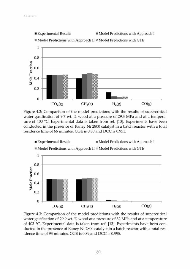
4.3. Results
89
Figure 4.2: Comparison of the model predictions with the results of supercritical water gasification of 9.7 wt. % wood at a pressure of 29.3 MPa and at a tempera-ture of 400 °C. Experimental data is taken from ref. [13]. Experiments have been conducted in the presence of Raney Ni 2800 catalyst in a batch reactor with a total residence time of 66 minutes. CGE is 0.80 and DCC is 0.951.
Figure 4.3: Comparison of the model predictions with the results of supercritical water gasification of 29.9 wt. % wood at a pressure of 32 MPa and at a temperature of 403 °C. Experimental data is taken from ref. [13]. Experiments have been con-ducted in the presence of Raney Ni 2800 catalyst in a batch reactor with a total res-idence time of 93 minutes. CGE is 0.89 and DCC is 0.995.
0
0.2
0.4
0.6
0.8
1
CO₂(g) CH₄(g) H₂(g) CO(g)
Mo
le F
ract
ion
Experimental Results Model Predictions with Approach I
Model Predictions with Approach II Model Predictions with GTE
0
0.2
0.4
0.6
0.8
1
CO₂(g) CH₄(g) H₂(g) CO(g)
Mo
le F
ract
ion
Experimental Results Model Predictions with Approach I
Model Predictions with Approach II Model Predictions with GTE

TESTING THE CONSTRAINED EQUILIBRIUM METHOD FOR THE MODELING OF SUPERCRITICAL WATER
GASIFICATION OF BIOMASS
90
Figure 4.4: Comparison of the model predictions with the results of supercritical water gasification of 13.2 wt. % swine manure at a pressure of 30.1 MPa and at a temperature of 405 °C. Experimental data is taken from ref. [13]. Experiments have been conducted in the presence of Raney Ni 2800 catalyst in a batch reactor with a total residence time of 36 minutes. CGE is 0.813 and DCC is 0.935.
For the cases shown in Figure 4.1 – Figure 4.4 only two additional constrains have been used: carbon gasification efficiency (CGE) and dissolved carbon conver-sion (DCC). The results show that the two approaches are in a very good agree-ment with the experimental results. Even for the complex biomass feedstocks such as wood and swine manure, and at high dry mass concentrations, the approaches predict reliable results that are in close agreements with experimental observa-tions. However, the agreement in Figure 4.3 and Figure 4.4 is better than the Fig-ure 4.1 and Figure 4.2. The reason for such a difference is due to the difference in the carbon gasification efficiency. Even though the global thermodynamic equilib-rium seems to show still a good agreement with the experimental results in pre-dicting the mole fraction of the gases, it should be noted that the absolute mole amount of these gases can be approximately twice as high as the experimental re-sults as the global thermodynamic equilibrium approach predicts a full CGE.
It can also be stated that the accuracy of the model significantly increases with the increase in the carbon gasification efficiency of the experiments. This is ex-pected as the higher carbon gasification efficiency indicates that the system is clos-er to its global thermodynamic equilibrium state. The effect of introducing the dis-solved carbon efficiency into the model plays a role in predicting the liquid phase carbon containing compounds. Figure 4.5a and Figure 4.5b shows the comparison of two approaches and experimental results for the liquid phase organic products. Figure 4.5a shows the analysis on compound basis and Figure 4.5b shows the same
0
0.2
0.4
0.6
0.8
1
CO₂(g) CH₄(g) H₂(g) CO(g)
Mo
le F
ract
ion
Experimental Results Model Predictions with Approach I
Model Predictions with Approach II Model Predictions with GTE

4.3. Results
91
analysis based on the total number of carbon atoms of the compounds. The select-ed organic compounds for the calculations were acetic acid, formic acid, phenol, acetaldehyde, ethanol, methanol, formaldehyde, lactic acid, glucose, oxalic acid. The results of Figure 4.5 show that the constrained equilibrium model is capable of predicting the organic compounds in the liquid phase quite well based on the total number of carbon atoms of the compounds. Unfortunately, slop07.dat database does not include all of the organic compounds that could be formed from the hy-drothermal treatment of biomass such as furfural, guaiacol, 5-HMF, catechol, and naphthalene. However, it is being updated regularly and the results indicate that it has a great potential in predicting the liquid phase organic compounds.
Approach I is more successful than approach II. There are two reasons for the better agreement of approach I; i) Peng-Robinson EoS with Van der Waals’ mixing rule is used for calculating the non-ideal properties behavior for the gases and ii) experiments based thermodynamic data is used for the calculation of Gibbs free energies of the gas phase compounds. In approach II, the activity coefficient model for calculating the non-ideal behavior of compounds incorporates some assump-tions which may affect the non-ideal behavior and the thermodynamic data used for the calculation of the standard molal Gibbs free energies of the compounds are performed with a theoretical approach for which the details are given in the works of Helgeson et al. [170,183,184]. However, the relative difference is almost negligi-ble at higher CGE and it performs even better for some cases (see Figure 4.4). If better activity coefficient models are developed for the neutral aqueous solutes (both for gas compounds and organic compounds) for hydrothermal conditions, approach II has the potential to replace the approach I, as it is physically more ac-curate in treating the miscibility of compounds in supercritical water. Neverthe-less, approach I has been selected for the testing of the other additional constraints due to its better agreement with the experimental results.
4.3.2. Testing of additional constraints
Figure 4.6 – Figure 4.8 show the performance of the prediction when additional constraints are used. In Figure 4.6, 3 different cases have been investigated. In Case 1, only the carbon gasification efficiency has been taken into account as an addi-tional constraint throughout the simulations. The reported experimental value for CGE is 0.673 [37]. In Case 2, in addition to CGE, hydrogen gasification efficiency and a constant amount for hydrogen have been taken into account. The reported experimental value for HGE is 0.913 and the mole amount of hydrogen is 2.63. In Case 3, instead of a constant amount of hydrogen, a constant amount of methane has been taken into account. The reported experimental value for the mole amount of methane is 0.71. In order to enable a comparison, the results of the global ther-modynamic equilibrium (GTE) is also shown.

TESTING THE CONSTRAINED EQUILIBRIUM METHOD FOR THE MODELING OF SUPERCRITICAL WATER
GASIFICATION OF BIOMASS
92
Figure 4.5: Comparison of the model predictions with the experimental results for the liquid phase organic compounds a) on compounds basis b) on compounds’ to-tal number of carbon basis. The experimental conditions are the same as in Figure 4.2.
0
20
40
60
80
100
wt.
%
Experimental Results Model Predictions with Approach I
Model Predictions with Approach II
a)
0
20
40
60
80
100
C2 organic compounds C1 organic compounds Phenol
wt.
%
Experimental Results Model Predictions with Approach I
Model Predictions with Approach II
b)

4.3. Results
93
Figure 4.6: Comparison of the model predictions with the results of supercritical water gasification of 0.6 M glucose at a pressure of 28 MPa and at a temperature of 600 °C. Experimental data is taken from ref. [37]. Experiments have been conduct-ed in a flow reactor at a residence time of 50s. Constraints for i) Case 1: CGE, ii) Case 2: CGE, HGE and constant amount of hydrogen, iii) Case 3: CGE, HGE and constant amount of methane.
The results of the Cases 1 and 2 are not in a good agreement with the experi-mental results. However, the predictions of Case 3 are in a very good agreement with the experimental results. It is expected to have a better agreement when more additional constraints are used. On the other hand, the model gives an insight into the reactions that take place inside the reactor. Based on the comparison of Case1 and the experimental results, the decomposition of C2 and C3 gases to CH4 and H2 as well as the formation of CO2 from CO via water gas shift reaction are expected when the residence time increases. Furthermore, the model predictions in Case 2 and Case 3 imply –based on the constraints imposed– that methane formation is slower compared to the hydrogen formation which indicates that the methane re-actions are rate limiting at 600 °C. Besides, the comparison of the three cases with the results of GTE shows that adding constraints results in a better prediction of the real systems.
In Figure 4.7 and Figure 4.8, a more detailed comparison has been made with the kinetic analysis of xylose gasification in a micro-tubular reactor based on the work of Goodwin and Rorrer [47]. Similar to Figure 4.6, three different cases have been investigated. In Case 1, only the carbon gasification efficiency has been taken into account as an additional constraint throughout the simulations. In Case 2, in addition to CGE, a constant amount for hydrogen have been taken into account
0
0.5
1
1.5
2
2.5
3
3.5
4
4.5
CO₂(g) CH₄(g) H₂(g) CO(g) C₂H₄(g) C₂H₆(g) C₃H₈(g) C₃H₆(g)
Mo
le g
as∙
(mo
le g
luco
se)⁻
¹ Experimental Results Case 1 Case 2 Case 3 GTE

TESTING THE CONSTRAINED EQUILIBRIUM METHOD FOR THE MODELING OF SUPERCRITICAL WATER
GASIFICATION OF BIOMASS
94
based on the experimental results given in Figure 4.8. In Case 3, instead of a con-stant amount of hydrogen, a constant amount of methane has been taken into ac-count. In all of the results, Case 2 shows the best performance. It indicates that at that temperature interval, the behaviour of hydrogen strongly determines the amount of the other gases. As expected, the model predictions have a better agreement when the gasification efficiency is closer to 100%. Another interesting result shown in Figure 4.7 is the behavior of carbon monoxide. Lower residence times result in a decreased CGE value and higher carbon monoxide yields. How-ever, at longer residence times, CGE increases and the yield of carbon monoxide decreases. This is an expected phenomenon as the higher CGE indicates that the system is closer to its global thermodynamic equilibrium state in which the CO concentration is negligibly low (see the GTE predictions of Figure 4.1 – Figure 4.4 and Figure 4.6).
It can be concluded from the constraints that were imposed and from the re-sults that at lower temperatures (400 – 550 °C), the behavior of hydrogen deter-mines the behavior of the other gas products. However, at higher temperatures (>550 °C), it is the methane behavior which determines the behavior of other gas products. The case 1 results of the Figure 4.6 and Figure 4.8 indicate that for non-catalytic supercritical water gasification of biomass processes, the main reactions which determine the hydrogen and methane formation are not the water gas shift and methanation reactions in the gas phase, but the reactions which directly result in the gas formation from the feedstock and/or intermediates. The same results are also reported by Savage’s group [85,86] using a sensitivity analysis on the reac-tion rates. It is also been reported in the literature that the rates of noncatalytic wa-ter gas shift and methanation reactions in supercritical water are quite slow result-ing only 5 % conversion even after several minutes [87–90]. The results of Figure 4.6 – Figure 4.8 also indicate that the lower CGE of the experimental results require a higher the number of additional constraints for the model in order to have a good agreement between the experimental results. This is expected; as stated earli-er, CGE is an indication for how far the system is away from global thermodynam-ic equilibrium. The lower CGE indicates that the system is further away from its global thermodynamic equilibrium state, thus, more additional constraints are re-quired to have an acceptable agreement with the experimental results.
4.3.3. Algae case
In order to make a comparison between the kinetic modeling approach and the constrained equilibrium approach, experimental results as well as the lumped ki-netic modeling predictions of an algae sample (Nannochloropsis sp.) gasification in SCW [85] are compared with the predictions of the constrained equilibrium model. Here, the authors [85] developed a lumped kinetic model for the SCWG of an al-gae sample based on 18 reactions and fitted the experimental results [95] to calcu-late the Arrhenius parameters of the reaction rate constants, namely activation en-ergy and the pre-exponential factor.
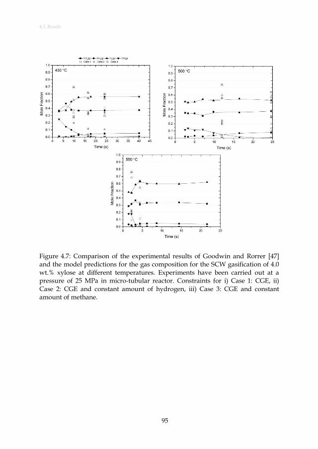
4.3. Results
95
Figure 4.7: Comparison of the experimental results of Goodwin and Rorrer [47] and the model predictions for the gas composition for the SCW gasification of 4.0 wt.% xylose at different temperatures. Experiments have been carried out at a pressure of 25 MPa in micro-tubular reactor. Constraints for i) Case 1: CGE, ii) Case 2: CGE and constant amount of hydrogen, iii) Case 3: CGE and constant amount of methane.
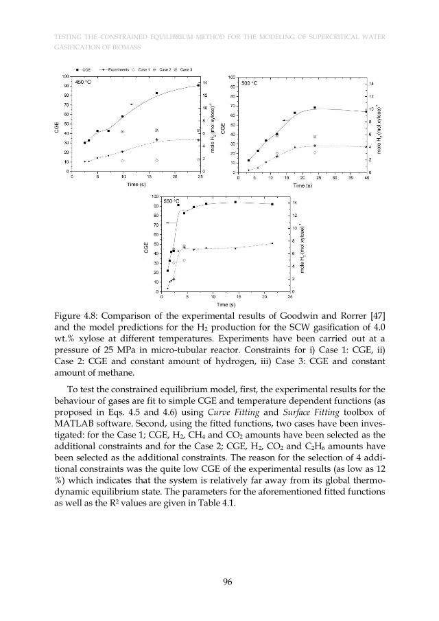
TESTING THE CONSTRAINED EQUILIBRIUM METHOD FOR THE MODELING OF SUPERCRITICAL WATER
GASIFICATION OF BIOMASS
96
Figure 4.8: Comparison of the experimental results of Goodwin and Rorrer [47] and the model predictions for the H2 production for the SCW gasification of 4.0 wt.% xylose at different temperatures. Experiments have been carried out at a pressure of 25 MPa in micro-tubular reactor. Constraints for i) Case 1: CGE, ii) Case 2: CGE and constant amount of hydrogen, iii) Case 3: CGE and constant amount of methane.
To test the constrained equilibrium model, first, the experimental results for the behaviour of gases are fit to simple CGE and temperature dependent functions (as proposed in Eqs. 4.5 and 4.6) using Curve Fitting and Surface Fitting toolbox of MATLAB software. Second, using the fitted functions, two cases have been inves-tigated: for the Case 1; CGE, H2, CH4 and CO2 amounts have been selected as the additional constraints and for the Case 2; CGE, H2, CO2 and C2H6 amounts have been selected as the additional constraints. The reason for the selection of 4 addi-tional constraints was the quite low CGE of the experimental results (as low as 12 %) which indicates that the system is relatively far away from its global thermo-dynamic equilibrium state. The parameters for the aforementioned fitted functions as well as the R2 values are given in Table 4.1.

4.3. Results
97
Table 4.1: Fitted functions and the parameters for the algae case based on the ex-perimental results given in Guan et al. [85].
Fitted function Fitting parameters R2
a b c
H2/CH4* 116.02 100124.11 -899.51 0.93
4
lga ae
CH
C
n
n**
0.151700
-478.50
-0.02892
0.97
2 6
lga ae
C H
C
n
n **
0.014560 40.23 -0.016360 0.97
2
lga ae
CO
C
n
n**
-0.045310
479.90
0.053970 0.91
*: ln( ) /a T b T c
**: ln( ) /a T CGE b T CGE c where T is in Kelvin.
Figure 4.9 shows the comparison between the experimental results and the ki-netic modeling approach given in the work of Guan et al. [85] and the constrained equilibrium results. The results show that the predictions of the constrained equi-librium approach show a better agreement with the experimental results than the kinetic modeling approach predictions of the authors [85]. Case 1 predictions are in a slightly better agreement with the experimental results than Case 2 predic-tions. This is due to the selection of CH4 as an additional constraint in Case 1 com-pared to C2H6 in Case 2 as CH4 is a more dominant gas product compared to C2H6 in SCWG of biomass process. Due to the success of Case 1, the results at other temperatures are given only for Case 1. It can be stated that the predictions of Case 1 for all of the process conditions have a very good agreement with the experi-mental results within the ± 10% interval of the experimental results.

TESTING THE CONSTRAINED EQUILIBRIUM METHOD FOR THE MODELING OF SUPERCRITICAL WATER GASIFICATION OF BIOMASS
98
Figure 4.9: Comparison between the experimental results and the kinetic modeling approach given by the Guan et al. [85] and the constrained equilibrium results for an algae sample (Nannochloropsis sp.) gasification in SCW. The experiments have been conducted in a stainless steel mini-batch reactor [95] at a water density of 0.087 g·cm-3. The dry mass concentration of the algae is 4.7 wt. % [85]. Constraints for i) Case 1: CGE, H2, CH4 and CO2 ii) Case 2: CGE, H2, CO2 and C2H6.

4.4. Discussion
99
Compared to the 18 reaction based lumped kinetic model, constrained equilib-rium model does not require any knowledge on the reactions. Yet, even at CGEs as low as 12 %, constrained equilibrium model for Case 1 resulted in a better agree-ment with only 4 additional constraints, namely CGE, CH4, CO2 and H2, which were based on simple functions. Besides, even without any constraints on C2H6 and CO (or CH4 and CO for Case 2) the amounts of these compounds were pre-dicted accurately as the reactions are taken into account concurrently in con-strained equilibrium model.
The model also predicts the behavior of nitrogen containing gases: global ther-modynamic equilibrium predictions result in mainly N2 as the nitrogen containing gas. However, it is known that the amino acids releases the nitrogen content in the form of NH3 gas and amine compounds. The predictions of the constrained equi-librium model are in agreement with the experimental results with respect to ni-trogen containing species: the model predicts NH3 as the main nitrogen containing gas and also amine compounds such as ethylamine and methylamine in the liquid phase. The model predicts almost no N2 formation which is also in agreement with the experimental results of Guan et al. [95]. Furthermore, constrained equilibrium model also predicts tar compounds and ethylbenzene in the liquid phase as well as char formation which these compounds were also reported by the authors [95] in their experimental study. The selected compounds for the simulations and the re-sults of the nitrogen compounds as well as the liquid phase compounds of some selected cases are given in Appendix B.
4.4. DISCUSSION
Additional constraints in Gibbs free energy minimization approach have been formulated in order to test the constrained equilibrium method for SCWG of bio-mass systems. The method is a promising technique to be used in the modeling of SCWG of biomass systems and similar conclusions with Kangas et al. [213] can be stated: i) the increase in the number of the additional constraints increases the ac-curacy of the model, ii) it requires less experimental data compared to the kinetic modeling approach, iii) different process dependent constraints may be required in different processes and iv) chemical reactions, enthalpy of the products and states of the system can be estimated concurrently.
One big drawback of the constrained equilibrium model could be stated as the requirement of the process specific experimental data. However, experimental da-ta is required to build any kind of model that predicts the multi-component chem-ical reacting mixtures: in kinetic modeling, one needs to experimentally investigate the reaction pathways and the rate constant parameters or use the available litera-ture data, and in equilibrium modeling one needs to use the experimentally de-termined thermo-physical properties of the compounds. On the other hand, the constrained equilibrium method can benefit from both of these two fundamental approaches. Any kind of time and/or temperature dependent function can be in-

TESTING THE CONSTRAINED EQUILIBRIUM METHOD FOR THE MODELING OF SUPERCRITICAL WATER
GASIFICATION OF BIOMASS
100
troduced as an additional constraint in Gibbs free energy minimization method as Kangas et al. [213,214] have successfully applied for a conventional biomass gasifi-cation system and as we have tested in Section 3.3. Adding more constraints is similar to adding more reactions in a kinetic model or adding more parameters to a data fit regression. However, the constrained equilibrium method requires sig-nificantly less experimental data –of a relatively simply to measure nature- com-pared to the kinetic approach: knowing the CGE and the amount of CH4 and/or H2 (based on the process conditions) would be enough to determine the behaviour of other gases –and even the intermediates to some extent if the CGE is higher than 60 %. One more additional constraint may be required for systems which have CGEs as low as 10 %. However, in order to build a kinetic model, one would need the behaviour of every gas phase compound as well as the possible reaction mech-anisms that could lead the formation/consumption of these compounds.
The concept of the model enables to extension of the number of additional con-straints used in the minimization procedure. If the nature of the chemical reactions occurring in SCWG of specific biomass types for specific type of reactor concepts is better known in the future, the additional constraints can be optimized for these systems. Possible additional constraints could be the tar conversion efficiency, to-tal amount of C/H bonds in each phase, the amount of C2-C3 gases and nitrogen to ammonia conversion efficiency.
The use of constrained equilibrium model may not seem to satisfy the needs to predict the behavior of a system other than the operating conditions, however, it still has significant advantages. The most beneficial use of the constrained equilib-rium method in SCWG of biomass systems would be predicting the behaviour of inorganic elements. So far, the behaviour of inorganic content of the biomass in SCWG systems was investigated only with the unconstrained equilibrium model-ing approaches [79] which assume a global thermodynamic equilibrium (see Chapter 3 as well). However, from the results of the tested cases shown in Figure 4.6 – Figure 4.9, it can be concluded that the more additional constraints are used in model the more process results can be accurately predicted. Therefore, for a sys-tem which is not in its global thermodynamic equilibrium state, one may also pre-dict the behavior of the inorganic content of the biomass conversion process on a compound and phase basis: the results of a SCWG of biomass process (either from complex kinetic modeling approaches or from experimental data) such as CGE and the amounts of the formed gases and intermediates can be introduced as addi-tional physical constraints in Gibbs free energy minimization for a multi-phase thermodynamic equilibrium model.
4.5. CONCLUSIONS
Determination of additional constraints in Gibbs free energy minimization and testing the constrained equilibrium method for the modeling of supercritical water gasification of biomass have been investigated in this chapter. The model benefits

4.5. Conclusions
101
from the natural phenomenon that every closed system will decrease its Gibbs free energy throughout the time domain. Two different approaches have been tested. Like the kinetic approach and RCCE method, the constrained equilibrium method benefits from the experimental results and may require process dependent values as additional constraints. The predictions of the model indicate that the con-strained equilibrium method requires fewer experimental results compared to ki-netic modeling approach and shows good performance for both real biomass and model biomass compounds as well as for catalytic and noncatalytic conditions. The results also indicate that carbon gasification efficiency appears to be the most important additional constraint. The accuracy of the model increases with an in-crease in the carbon gasification efficiency as the system gets closer to its global thermodynamic equilibrium state. Setting a constrained amount for a specific compound (either in the form of a constant or a linear/non-linear time dependent function) as another constraint improves the accuracy of the model as the reactions are taken into account concurrently. The model not only predicts the gas formation behaviour, but also gives an insight for the process and the reactions taking place inside the reactor.

TESTING THE CONSTRAINED EQUILIBRIUM METHOD FOR THE MODELING OF SUPERCRITICAL WATER
GASIFICATION OF BIOMASS
102

103
5. EXPERIMENTAL METHODS
This chapter describes the experimental setup, experimental methods and analytical techniques that were used throughout the experimental campaign of this dissertation. Be-sides, the relevant equations which were used to calculate residence time and velocity pro-files along different process units are also given.
The experimental setup used for the experimental campaign of this dissertation was de-signed with and manufactured by the project partner company, Gensos B.V. The setup has a capacity of 50 l/h and was designed to reflect a real industrial scale which has not only the reaction unit but also the thermal integration, heating and phase separation units. The experiences gained from the experimental setup has also provided valuable information for scaling up such a SCWG of biomass process to industrial scales.

EXPERIMENTAL METHODS
104
5.1. MATERIALS
To test the performance of the setup, starch was selected as it is relatively a simple biomass compound. To make starch representative of a real biomass feed-stock, the setup was run with salt solutions as well. Wheat starch (purchased from Tereos Syral, France), demi-water, NaCl (Sigma-Aldrich, 99%), K2CO3 (Sigma-Aldrich, 99%) and ethanol (Richter Chemie GmbH, Germany, commercial grade bioethanol 100 %) were used in the experiments.
5.2. EXPERIMENTAL SETUP AND PROCEDURE
The experimental setup consists of a feeding section, a pre-heating section, a heating section, a reactor and a gas/liquid separator. The setup is fully controlled with a PLC unit. The process flow diagram of the experimental setup is given in Figure 5.1.
The feeding section consists of a high pressure pump (displacement type, man-ufactured by Cat Pumps, model 5CP3120), a demi-water tank and a biomass slurry tank which has an in-house design mixer in order to ensure a homogeneous con-centration in the feed. The total flow rate of the feeding section can reach up to 50 l/h and the actual mass flow rate is calculated with a weighing scale that is located below the biomass slurry tank.
The pre-heating section consists of a double pipe heat exchanger. It is a coun-ter-current flow heat exchanger in which the inner flow is the cold stream (the feed stream) and the outer flow is the hot stream (the reactor exit –the return– stream). It is constructed from stainless steel with a total length of 55 meters. Here, the feed stream is pre-heated while the stream that leaves reactor is cooled down to ambi-ent temperatures. Once in every 5 meters, thermocouples (K type) are located at the outer wall of the inner and outer tubes of the heat exchanger in order to ob-serve the temperature profile along the heat-exchanger.
The heating section consists of a burner and a gas to fluid type of heat ex-changer. The total length of the heater is 4 meters and it is made of stainless steel. Here, the feed stream is heated up to the desired reactor temperatures using an ex-ternal gas supply (propane) as the fuel.
The reactor is a fluidized bed type of reactor of which the bed material (aver-age particle diameter of 0.5 mm) and the reactor are made of SS 316. It has an outer diameter of 25 mm with a wall thickness of 4 mm. The total length of the reactor is 1.1 m. The reactor has 3 sampling points which are located at 25 cm distance from each other. Every sampling point has a SwagelokTM filter to collect solid samples of which the filter size is 0.5 μm. The sampling points are then connected with expan-sion valves and a sampling gas/liquid separator which operates at ambient condi-tions. The reason to have 3 sampling points along the reactor is to enable observ-ing the influence of reactor length and the cooling residence time along the pre-heating section on the conversion efficiency. The reactor is coupled with 10 electri-
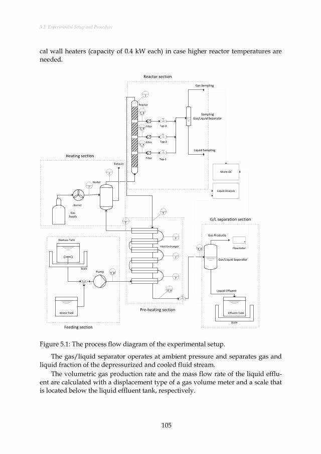
5.2. Experimental Setup and Procedure
105
cal wall heaters (capacity of 0.4 kW each) in case higher reactor temperatures are needed.
Pump
SamplingGas/Liquid Separator
Gas Sampling
Liquid Sampling
Gas/Liquid Separator
Gas Products
Liquid Effluent
Filter
Heat Exchanger
Biomass Tank
Heater
Reactor
Filter
Filter
Effluent Tank
Tap-1
Tap-2
Tap-3
Micro-GC
Liquid Analysis
Gas Supply
Burner
Scale
Scale
Exhaust
F
Flowmeter
T, P
T
T
T, P
T
T
T
T
T, P
T, P
T, P
T, P
Water Tank
T
T
Feeding section
Pre-heating section
Heating section
Reactor section
G/L separation section
Figure 5.1: The process flow diagram of the experimental setup.
The gas/liquid separator operates at ambient pressure and separates gas and liquid fraction of the depressurized and cooled fluid stream.
The volumetric gas production rate and the mass flow rate of the liquid efflu-ent are calculated with a displacement type of a gas volume meter and a scale that is located below the liquid effluent tank, respectively.

EXPERIMENTAL METHODS
106
Before every experiment, first demi-water was pumped into the setup with a desired pressure (~ 24 MPa) to clean and heat up the setup. The pressure was ad-justed with the back pressure valve which was located before the gas/liquid sepa-rator. Once the desired reactor temperature was reached, the feedstock was switched to model biomass feedstock of which the dry matter concentration is known. The change in the scale indication of the feed tank and the gas volume me-ter over time were noted. Once the gas production rate reached a constant value, it was assumed that the steady state was reached. Generally it took an hour to reach the steady state. Then, for a period of another hour, the gas products were filled in a gas sampling bag and then were analyzed via a micro GC.
At the end of each experiment, the setup is cleaned up with demi-water at su-percritical temperatures and then with ethanol at ambient conditions for several hours.
5.3. ANALYTICAL METHODS
5.3.1. Analysis of the materials
Wheat starch was analyzed for its water content and elemental analysis. Water content was analyzed with a thermogravimetric analyzer (Thermal Advantage SDT Q600) and the elemental analysis for the organic content were performed by Università degli Studi di L’Aquila, Italy. The analysis results of wheat starch giv-en in Table 5.1.
Table 5.1: The analysis results of starch.
unit Starch
moisture wt. % ara 11.4
ash content wt. % dbb -
C wt. % db 39.67
H wt. % db 6.83
O* wt. % db 52.45
N wt. % db -
S wt. % db 1.05
volatile matter wt. % db 85.2
fixed carbon wt. % db 14.8
a: ar: as received, b: db: dry basis, *: by difference
5.3.2. Analysis of the gas products
Analyses of the gas products were performed using a gas chromatograph (Var-ian Micro-GC CP-4900, column 1: 1m CP COX and column 2: 4m CP-Sil 5 CB). The remaining unanalysed percentage from the first column are assumed as a mixture of C2 – C3 gases in this dissertation.
5.4. Residence Time and Velocity Profile Calculations
107
5.4. RESIDENCE TIME AND VELOCITY PROFILE CALCULATIONS
It is quite important from reaction kinetics, heat transfer and hydrodynamics point of view to determine residence time and velocity profile of each process unit.
The residence time (τ) can be calculated by means of equation 5.1. as
.V
V
(5.1)
where V is the internal volume of the process unit (heat exchanger, heater or reac-
tor) and .
V is the volumetric flow rate of the feed. The volume of the process unit
in equation 5.1 can be rewritten in terms of length (L) and cross-sectional area (A) of the process unit, and the volumetric flow rate can be rewritten in terms of mass
flow rate (.m ) and density (ρ) of feed. Equation 5.1 then becomes
.AL
m
(5.2)
Taking into account the fact that the density of the feed stream will change throughout the length of the process unit due to the change of the temperature profile, the equation 5.2 will be as follows
0
.
LA
dL
m
(5.3)
where the density (ρ) of the feed stream is a function of the process unit length (L) as a result of the temperature profile along the length of the process unit.
Similar to the residence time, average velocity (u) of the fluid can be written in terms of mass flowrate and density as
.m
uA
(5.4)
As the reactor is a fluidized bed reactor, it is important to mention the mini-mum fluidization and terminal velocity concepts for the reactor. Matsumura and Minowa [5] were the first researchers who gave the fundamental design ap-proaches for the fluidization for a supercritical water gasification of biomass reac-tor. Here, the authors express the minimum fluidization velocity as:
Remf
mf
p f
uD
(5.5)
where Dp refers to the diameter of the bed particle (which is 0.5 mm for the ex-periments performed throughout this dissertation), ρf refers to density of the fluid

EXPERIMENTAL METHODS
108
(which is assumed as water in this dissertation) and Remf refers to the Reynolds number at minimum fluidization conditions and given as
2 1/2Re [(33.7) 0.0408 ] ) 33.7mf Ar (5.6)
where Ar is the Archimedes number and expressed as 3
2
( )p f p fD gAr
(5.7)
where ρp refers to the density of the particle, g refers to the gravitational accel-eration and μ refers to viscosity of the fluid.
The terminal velocity can be calculated using equation 5.8 as
3.03 ( )p f p
t
f
g Du
, when
5500 Re 10p t f
t
D u
(5.8)
The authors [5] also define the discrimination number, Dn, as
( )( )Re
p f
mf f
ArDn
(5.9)
in order to define the fluidization type. A discrimination number lower than 104 results a particulate bed and a discrimination number higher than 106 results in a bubbling bed. If the discrimination number is between 104 and 106, the fluidization starts as a homogeneous (particulate) bed and shifts to bubbling bed when the first bubbling takes place [5].
Throughout this dissertation, the measured wall temperatures were assumed as the fluid’s temperature inside the heat exchanger and heater, and for the reac-tor, the fluid’s measured temperature from the top of the reactor was used. The thermophysical properties of water at corresponding temperatures and pressures have been assumed for the fluid’s thermophysical properties which the data are acquired from NIST database [12]. Superficial velocities are assumed for the actual velocity of the fluid for the calculation of the residence time of the reactor. In addi-tion, linear temperature profiles are assumed for the heater and reactor as only the inlet and outlet temperatures are measured experimentally.
109
6. EXPERIMENTAL RESULTS
This chapter reports the results obtained from the preliminary experiments with starch gasification in supercritical water. The influence of reactor temperature and feed flow rate on gas composition were investigated. The results not only include the conversion efficien-cy and gas composition, but also the temperature profile along different process units and velocity profile along the reactor. In addition, the experiences that were gained and chal-lenges that were come across during performing experiments are also reported.

EXPERIMENTAL RESULTS
110
6.1. INTRODUCTION
Even though there had been various works [75,77,92–94,97,98,100,141,216,217] on the continuous supercritical water gasification of biomass compounds, there are only few works which involve high feed flow rates (> 20 kg/h) [77,146,147] or flu-idized bed reactors [98,161,162]. Operating at high flow rates gives the opportunity to observe process challenges similar to industrial scales and fluidized bed reactors have the potential to overcome plugging problems that might happen due to the mineral precipitation under supercritical conditions [5], and clogging free experi-ments were already achieved by some researchers [161] using a fluidized bed reac-tor. In this chapter, experimental results are reported for the supercritical water gasification of starch in a fluidized bed reactor at high flow rates.
6.2. RESULTS AND DISCUSSIONS
6.2.1. The influence of reactor temperature
The influence of SCWG reactor temperatures on the gas composition, carbon gasification efficiency (CGE) and gasification efficiency (GE) is given in Figure 6.1 for a 4.4 wt. % starch gasification in supercritical water at a pressure of ~ 24 MPa and at a flow rate of 35 kg/h. The definition of CGE is given in Equation 4.1, whereas GE refers to the ratio of total mass flow rate of the produced gases to the mass flow rate of the organic feed in dry basis.
Figure 6.1: The influence of reactor temperature on gas composition, gasification efficiency and carbon gasification efficiency results for a 4.4 wt. % starch gasifica-tion in supercritical water. The feed flow rate is 35 kg/h and the pressure is ~ 24 MPa.
It can be seen from Figure 6.1 that the increase in reactor temperature increases CGE and GE, as expected. However, the gas composition results follow a more complex trend: the fraction CO2 and C2 – C3 gases decrease with the increase in re-actor temperature, whereas CH4 and H2 slightly increase. CO has a different be-
500 550 600
0
10
20
30
40
50
500 550 600
0
10
20
30
40
50
mo
l fr
action
(%
)
Reactor Temperature (C)
CO2 CH
4
H2 CO
C2- C
3 gases
5
10
15
total gas production
mo
l(k
g-d
ry-b
iom
ass)-1
4.4 wt.% Starch; 35 kg/h Feed flow; Pressure:~24 MPa
Co
nve
rsio
n (
%)
Reactor Temperature (C)
CGE GE

6.2. Results and Discussions
111
havior: the concentration increased from 500 °C to 550 °C and then slightly de-creases at 600 °C. Lee et al. [37] also found in their glucose experiments that the CO composition increased from 510 °C to 550 °C and then slightly decreased with the increase in temperature till 600 °C. The authors [37] state that some of the glucose carbon might be directly converted to CO via a kind of pyrolysis reaction. Howev-er, Chuntanapum and Matsumura [44] propose that the gas formation from glu-cose takes place via intermediates, not directly from glucose. Another interesting result that can be seen from Figure 6.1 is that the dominant gases are CO and CO2. Similar trends in gas composition and conversion behavior were also reported by other researchers [37,216] at low temperatures and/or at low residence times. These phenomena cannot be just explained with the reactor temperature behavior, as the heating profile of the feed also influences the gas composition behavior and conversion efficiency. The heating profile of the heat exchanger, heater and reactor with their residence time are given in Figure 6.2. Another reason for the high con-centration of CO, might be due to a relatively slow rate of the water gas shift reac-tion at low temperatures (< 500 °C). Sato et al. [89] show that the water gas shift reaction can be so slow at temperatures lower than 500 °C that the reaction is al-most not taking place at all. As it can be seen from Figure 6.2, the fluid spends less than 5 seconds at temperatures higher than 500 °C and several minutes at tempera-tures lower than 500 °C for all of the cases. The temperature profile and the resi-dence time of the fluid at temperatures lower than 500 °C are the main reason for the high CO composition: i) the direct gasification of CO from glucose intermedi-ates via hydro-pyrolysis reactions and ii) lack of water gas shift reaction. It can be concluded that the formed CO from glucose intermediates via direct pyrolysis re-actions at temperatures lower than 500 °C did not have sufficient residence time to be converted to H2 via the water gas shift reaction.
Another interesting result that can be interpreted from Figure 6.2 is how the temperature profile shifts in the heat exchanger with a change in the reactor tem-perature. The higher reactor temperatures causes the fluid to reach 350 °C at short-er residence times for which the fast heating profile during the pre-heating section is known to be in favor of preventing coke and tar formation [143,145]. This could be another reason for having improved conversion efficiencies at higher reactor temperatures.
Figure 6.3 shows the velocity profile of the fluid in the reactor along with the terminal velocity, minimum fluidization velocity and discrimination number. For all of the cases, the superficial velocity of the fluid stays in between the minimum fluidization velocity and the terminal velocity which implies that the fluidization took place. From the discrimination number, it can be concluded that first the flu-idization started as a homogeneous bed and then changed to stable bubbling when the bubbling started.
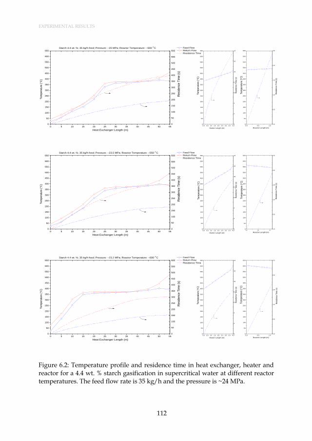
EXPERIMENTAL RESULTS
112
Figure 6.2: Temperature profile and residence time in heat exchanger, heater and reactor for a 4.4 wt. % starch gasification in supercritical water at different reactor temperatures. The feed flow rate is 35 kg/h and the pressure is ~24 MPa.
0 5 10 15 20 25 30 35 40 45 50 55
0
50
100
150
200
250
300
350
400
450
500
550
600
650
0.0 0.5 1.0 1.5 2.0 2.5 3.0 3.5 4.00
50
100
150
200
250
300
350
400
450
500
550
600
650
0.0 0.5 1.00
50
100
150
200
250
300
350
400
450
500
550
600
650
Tem
pera
ture
(C
)
Tem
pera
ture
(C
)
Te
mp
era
ture
(C
)
Heat Exchanger Length (m)
Feed Flow
Return Flow
Residence Time
0
50
100
150
200
250
300
350
400
450
500
550
600
Heater Length (m)
0
2
4
6
8
10
12
14
Reactor Length (m)
Starch 4.4 wt. %; 35 kg/h feed; Pressure: ~25 MPa; Reactor Temperature: ~500 C
0.0
0.5
1.0
1.5
2.0
2.5
Re
sid
en
ce T
ime
(s)
Re
sid
en
ce T
ime
(s)
Re
sid
en
ce T
ime
(s)
0 5 10 15 20 25 30 35 40 45 50 55
0
50
100
150
200
250
300
350
400
450
500
550
600
650
0.0 0.5 1.0 1.5 2.0 2.5 3.0 3.5 4.00
50
100
150
200
250
300
350
400
450
500
550
600
650
0.0 0.5 1.00
50
100
150
200
250
300
350
400
450
500
550
600
650
Tem
pera
ture
(C
)
Tem
pera
ture
(C
)
Te
mp
era
ture
(C
)
Heat Exchanger Length (m)
Feed Flow
Return Flow
Residence Time
0
50
100
150
200
250
300
350
400
450
500
550
600
Heater Length (m)
0
2
4
6
8
10
12
14
Reactor Length (m)
Starch 4.4 wt. %; 35 kg/h feed; Pressure: ~23.5 MPa; Reactor Temperature: ~550 C
0.0
0.5
1.0
1.5
2.0
2.5
Re
sid
en
ce T
ime
(s)
Re
sid
en
ce T
ime
(s)
Re
sid
en
ce T
ime
(s)
0 5 10 15 20 25 30 35 40 45 50 55
0
50
100
150
200
250
300
350
400
450
500
550
600
650
0.0 0.5 1.0 1.5 2.0 2.5 3.0 3.5 4.00
50
100
150
200
250
300
350
400
450
500
550
600
650
0.0 0.5 1.00
50
100
150
200
250
300
350
400
450
500
550
600
650
Tem
pera
ture
(C
)
Tem
pera
ture
(C
)
Te
mp
era
ture
(C
)
Heat Exchanger Length (m)
Feed Flow
Return Flow
Residence Time
0
50
100
150
200
250
300
350
400
450
500
550
600
Heater Length (m)
0
2
4
6
8
10
12
14
Reactor Length (m)
Starch 4.4 wt. %; 35 kg/h feed; Pressure: ~23.2 MPa; Reactor Temperature: ~600 C
0.0
0.5
1.0
1.5
2.0
2.5
Re
sid
en
ce T
ime
(s)
Re
sid
en
ce T
ime
(s)
Re
sid
en
ce T
ime
(s)

6.2. Results and Discussions
113
Figure 6.3: The influence of SCWG reactor temperature on velocity profiles along the reactor for a 4.4 wt. % starch gasifica-tion in supercritical water. The feed flow rate is 35 kg/h and the pressure is ~ 24 MPa.
0.0 0.2 0.4 0.6 0.8 1.0
0
100
200
300
400
500
600
Temperature
Te
mp
era
ture
(C
)
Reactor Length (m)
Starch 4.4 wt. %; 35 kg/h feed; Pressure ~25 MPa
0.0
0.2
0.4
0.6
0.8
1.0
1.2
1.4
1.6
1.8
2.0
Fluid Velocity
Minimum Fluidization Velocity
Terminal Velocity
Flu
id V
elo
city (
m/s
)
0.0
0.2
0.4
0.6
0.8
1.0
Discrimination number
Dis
crim
ina
tio
n n
um
be
r (x
10
6)
0.0 0.2 0.4 0.6 0.8 1.0
0
100
200
300
400
500
600
Temperature
Te
mp
era
ture
(C
)
Reactor Length (m)
Starch 4.4 wt. %; 35 kg/h feed; Pressure ~23.5 MPa
0.0
0.2
0.4
0.6
0.8
1.0
1.2
1.4
1.6
1.8
2.0
Fluid Velocity
Minimum Fluidization Velocity
Terminal Velocity
Flu
id V
elo
city (
m/s
)
0.0
0.2
0.4
0.6
0.8
1.0
Discrimination number
Dis
crim
ina
tio
n n
um
be
r (x
10
6)
0.0 0.2 0.4 0.6 0.8 1.0
0
100
200
300
400
500
600
Temperature
Te
mp
era
ture
(C
)
Reactor Length (m)
Starch 4.4 wt. %; 35 kg/h feed; Pressure ~23.2 MPa
0.0
0.2
0.4
0.6
0.8
1.0
1.2
1.4
1.6
1.8
2.0
Fluid Velocity
Minimum Fluidization Velocity
Terminal Velocity
Flu
id V
elo
city (
m/s
)
0.0
0.2
0.4
0.6
0.8
1.0
Discrimination number
Dis
crim
ina
tio
n n
um
be
r (x
10
6)
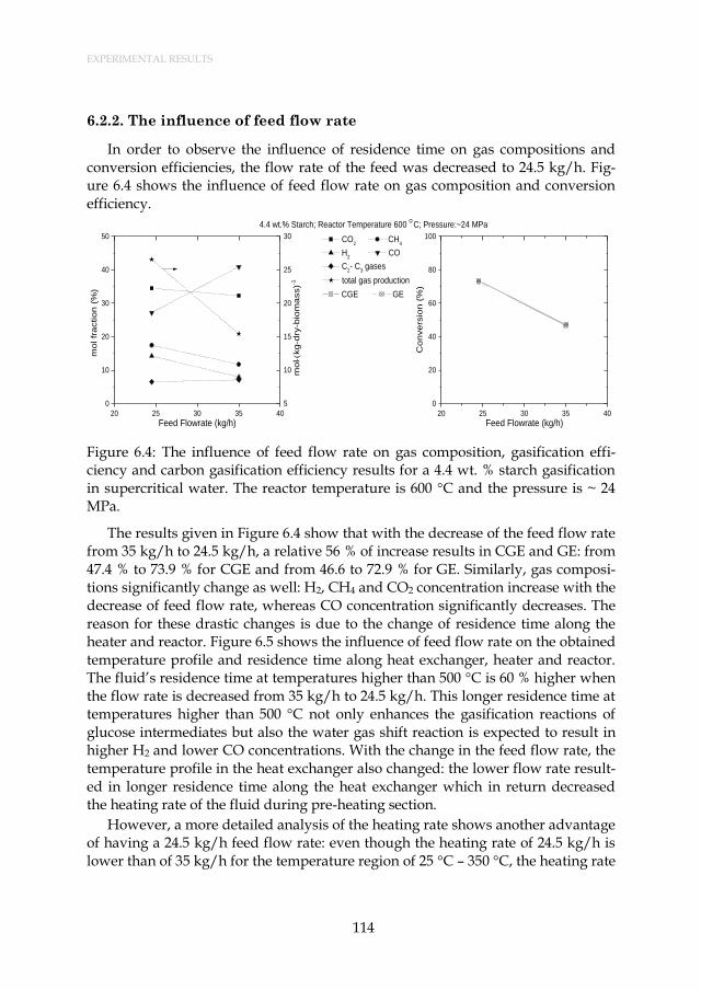
EXPERIMENTAL RESULTS
114
6.2.2. The influence of feed flow rate
In order to observe the influence of residence time on gas compositions and conversion efficiencies, the flow rate of the feed was decreased to 24.5 kg/h. Fig-ure 6.4 shows the influence of feed flow rate on gas composition and conversion efficiency.
Figure 6.4: The influence of feed flow rate on gas composition, gasification effi-ciency and carbon gasification efficiency results for a 4.4 wt. % starch gasification in supercritical water. The reactor temperature is 600 °C and the pressure is ~ 24 MPa.
The results given in Figure 6.4 show that with the decrease of the feed flow rate from 35 kg/h to 24.5 kg/h, a relative 56 % of increase results in CGE and GE: from 47.4 % to 73.9 % for CGE and from 46.6 to 72.9 % for GE. Similarly, gas composi-tions significantly change as well: H2, CH4 and CO2 concentration increase with the decrease of feed flow rate, whereas CO concentration significantly decreases. The reason for these drastic changes is due to the change of residence time along the heater and reactor. Figure 6.5 shows the influence of feed flow rate on the obtained temperature profile and residence time along heat exchanger, heater and reactor. The fluid’s residence time at temperatures higher than 500 °C is 60 % higher when the flow rate is decreased from 35 kg/h to 24.5 kg/h. This longer residence time at temperatures higher than 500 °C not only enhances the gasification reactions of glucose intermediates but also the water gas shift reaction is expected to result in higher H2 and lower CO concentrations. With the change in the feed flow rate, the temperature profile in the heat exchanger also changed: the lower flow rate result-ed in longer residence time along the heat exchanger which in return decreased the heating rate of the fluid during pre-heating section.
However, a more detailed analysis of the heating rate shows another advantage of having a 24.5 kg/h feed flow rate: even though the heating rate of 24.5 kg/h is lower than of 35 kg/h for the temperature region of 25 °C – 350 °C, the heating rate
20 25 30 35 40
0
10
20
30
40
50
20 25 30 35 40
0
20
40
60
80
100
mo
l fr
actio
n (
%)
Feed Flowrate (kg/h)
CO2 CH
4
H2 CO
C2- C
3 gases
5
10
15
20
25
30
total gas production
mo
l(k
g-d
ry-b
iom
ass)-1
4.4 wt.% Starch; Reactor Temperature 600 C; Pressure:~24 MPa
Co
nve
rsio
n (
%)
Feed Flowrate (kg/h)
CGE GE

6.2. Results and Discussions
115
for 24.5 kg/h is higher than of 35 kg/h for the temperature region of 350 °C – 375 °C. The latter temperature region is known to be a favorable temperature region for the hydrothermal liquefaction of biomass [218]. The influence of feed flow rate on the heating rates along the heat exchanger for different temperature regions is given in Table 6.1.
It can be concluded that with 24.5 kg/h feed flow rate, not only the residence time at temperatures higher than 500 °C increases, but also –due to the tempera-ture profile along the heat exchanger– the fluid spends less residence time at tem-peratures between 350 °C and 375 °C so that less bio-oil production at that temper-ature range takes place.
Figure 6.5: Temperature profile and residence time in heat exchanger, heater and reactor for a 4.4 wt. % starch gasification in supercritical water at different flow rates. The reactor temperature is 600 °C and the pressure is ~24 MPa.
0 5 10 15 20 25 30 35 40 45 50 55
0
50
100
150
200
250
300
350
400
450
500
550
600
650
0.0 0.5 1.0 1.5 2.0 2.5 3.0 3.5 4.00
50
100
150
200
250
300
350
400
450
500
550
600
650
0.0 0.5 1.00
50
100
150
200
250
300
350
400
450
500
550
600
650
Tem
pera
ture
(C
)
Tem
pera
ture
(C
)
Te
mp
era
ture
(C
)
Heat Exchanger Length (m)
Feed Flow
Return Flow
Residence Time
0
50
100
150
200
250
300
350
400
450
500
550
600
Heater Length (m)
0
2
4
6
8
10
12
14
Reactor Length (m)
Starch 4.4 wt. %; 35 kg/h feed; Pressure: ~23.2 MPa; Reactor Temperature: ~600 C
0.0
0.5
1.0
1.5
2.0
2.5
3.0
3.5
4.0
4.5
5.0
Re
sid
en
ce T
ime
(s)
Re
sid
en
ce T
ime
(s)
Re
sid
en
ce T
ime
(s)
0 5 10 15 20 25 30 35 40 45 50 55
0
50
100
150
200
250
300
350
400
450
500
550
600
650
0.0 0.5 1.0 1.5 2.0 2.5 3.0 3.5 4.00
50
100
150
200
250
300
350
400
450
500
550
600
650
0.0 0.5 1.00
50
100
150
200
250
300
350
400
450
500
550
600
650
Tem
pera
ture
(C
)
Tem
pera
ture
(C
)
Te
mp
era
ture
(C
)
Heat Exchanger Length (m)
Feed Flow
Return Flow
Residence Time
0
50
100
150
200
250
300
350
400
450
500
550
600
Heater Length (m)
0
2
4
6
8
10
12
14
Reactor Length (m)
Starch 4.4 wt. %; 24.5 kg/h feed; Pressure: ~24.2 MPa; Reactor Temperature: ~600 C
0.0
0.5
1.0
1.5
2.0
2.5
3.0
3.5
4.0
4.5
5.0
Re
sid
en
ce T
ime
(s)
Re
sid
en
ce T
ime
(s)
Re
sid
en
ce T
ime
(s)

EXPERIMENTAL RESULTS
116
Table 6.1: The influence of feed flow rate on the heating rates along the heat ex-changer for different temperature regions.
Feed flow rate (kg/h) Heating rate
(°C/s)
25 °C – 350 °C 350 °C – 375 °C
35 4.85 0.35
24.5 2 0.4
Figure 6.6 shows the influence of feed flow rate on velocity profiles along the reactor. Due to the decrease of the feed flow rate, the superficial velocity decrease, however, it is still higher than the minimum fluidization velocity and enabling the fluidization.
Figure 6.6: The influence of feed flow rate on velocity profiles along the reactor for a 4.4 wt. % starch gasification in supercritical water. The reactor temperature is 600 °C and the pressure is ~ 24 MPa.
In addition to 24.5 kg/h and 35 kg/h, the feed flow rates of 11 kg/h and 45 kg/h were also tested. However, the experiments failed which the reasons are ex-plained in the next section.
6.3. OBSERVED EXPERIMENTAL CHALLENGES AND POSSIBLE IMPROVEMENTS
Throughout the experimental campaign of this dissertation, various experi-mental challenges were observed.
To observe the influence of feed flow rate on CGE and GE at different condi-tions, feed flow rates of 11 kg/h and 45 kg/h were also tested. However, both ex-periments failed. The experiments performed at 11 kg/h did not reach the steady state. The reactor temperature and gas production rate showed significant fluctua-
0.0 0.2 0.4 0.6 0.8 1.0
0
100
200
300
400
500
600
Temperature
Te
mp
era
ture
(C
)
Reactor Length (m)
Starch 4.4 wt. %; 35 kg/h feed; Pressure ~23.2 MPa
0.0
0.2
0.4
0.6
0.8
1.0
1.2
1.4
1.6
1.8
2.0
Fluid Velocity
Minimum Fluidization Velocity
Terminal Velocity
Flu
id V
elo
city (
m/s
)
0.0
0.2
0.4
0.6
0.8
1.0
Discrimination number
Dis
crim
ina
tio
n n
um
be
r (x
10
6)
0.0 0.2 0.4 0.6 0.8 1.0
0
100
200
300
400
500
600
Temperature
Te
mp
era
ture
(C
)
Reactor Length (m)
Starch 4.4 wt. %; 24.5 kg/h feed; Pressure ~24.2 MPa
0.0
0.2
0.4
0.6
0.8
1.0
1.2
1.4
1.6
1.8
2.0
Fluid Velocity
Minimum Fluidization Velocity
Terminal Velocity
Flu
id V
elo
city (
m/s
)
0.0
0.2
0.4
0.6
0.8
1.0
Discrimination number
Dis
crim
ina
tio
n n
um
be
r (x
10
6)

6.3. Observed Experimental Challenges and Possible Improvements
117
tions throughout the run time of experiments. The temperature and gas produc-tion rate over a run time of 250 minutes are given in Figure 6.7. It can be stated that the reactor temperature fluctuated between 462 °C and 514 °C. On the other hand, the gas production rate fluctuated between 0.03 m3/h and 0.09 m3/h which result-ed in an average GE of 10 %.
Figure 6.7: The temperature and gas production rate over a run time of 250 minutes for a 4.4 wt. % starch gasification in supercritical water at a flow rate of 11 kg/h. The reactor set temperature was 500 °C and the pressure is ~ 23.5 MPa.
The reason behind the fluctuation and failing to reach the steady state can be explained by the low feed flow rates and how it influenced the fluidization inside the reactor. Figure 6.8 shows the velocity profiles along the reactor for a 4.4 wt. % starch gasification in supercritical water at a flow rate of 11 kg/h.
Figure 6.8: The velocity profiles along the reactor for a 4.4 wt. % starch gasification in supercritical water at a flow rate of 11 kg/h at a pressure of 23.5 MPa.
0 50 100 150 200 250
450
500
550
4.4 wt.% Starch; 11 kg/h Feed flow; Pressure:~23.5 MPa
R
ea
cto
r T
em
pe
ratu
re (C
)
Run time (min)
Reactor Temperature
0.00
0.05
0.10
Gas Production Rate
Ga
s P
rod
uctio
n R
ate
(m
3h
-1)
0.0 0.2 0.4 0.6 0.8 1.0
0
100
200
300
400
500
600
Temperature
Te
mp
era
ture
(C
)
Reactor Length (m)
Starch 4.4 wt. %; 11 kg/h feed; Pressure ~23.5 MPa
0.0
0.2
0.4
0.6
0.8
1.0
1.2
1.4
1.6
1.8
2.0
Fluid Velocity
Minimum Fluidization Velocity
Terminal Velocity
Flu
id V
elo
city (
m/s
)
0.0
0.2
0.4
0.6
0.8
1.0
Discrimination number
Dis
crim
ina
tio
n n
um
be
r (x
10
6)
EXPERIMENTAL RESULTS
118
The results show that at a feed flow rate of 11 kg/h, the calculated superficial velocity is barely higher than the calculated minimum fluidization velocity which, in reality, might have resulted in the lack of fluidization inside the reactor. The lack of fluidization results in poor mixing inside the reactor which also decreases the heat and mass transfer as it is known that the fluidization significantly increas-es the heat and mass transfer inside the reactor [219]. The decrease in heat transfer might have caused the fluctuations in reactor temperature and gas production rate. In addition, the decrease in mass transfer might have caused the low GE even the residence time was significantly higher than of the 500 °C experiment at 35 kg/h.
After observing the temperature fluctuations and low gas production rate at 11 kg/h feed flow rate, an experiment at 45 kg/h at a temperature of 600 °C was also performed. The setup ran without any plugging problem for several hours. Due to higher feed flow rate at a higher reactor temperature, a higher gas production rate was also visually observed. However, the gas/liquid separator did not operate as expected: the high gas production rate ended up building pressure inside the gas/liquid separator and some of the produced gases left the gas/liquid separator with the liquid effluent. Therefore, the exact gas production rate was not quanti-fied. The poor separation of the produced gases from the liquid effluent is most likely due to the design of the gas/liquid separator itself: i) the volume of the gas/liquid separator was not sufficient and/or ii) the cross sectional area of the tube from which the produced gases are leaving the gas/liquid separator was not sufficient.
During the experiments, small amounts of char and oil formation were ob-served in the liquid effluent. However, the amounts were not quantified.
To observe the influence of salts on CGE, GE and gas composition, another ex-periment was performed with a 4.4 wt. % starch + 0.5 wt. % NaCl + 0.5 wt. % K2CO3 solution at a feed flow rate of 24.5 kg/h and at a reactor temperature of 600 °C. The setup ran without any plugging or clogging problem for 2 hours. Howev-er, after the second hour of the run, the pressure of the setup started increasing drastically: more than 4 MPa in less than 10 minutes. The pressure of the system was lowered by opening the back pressure valve. The rapid increase of the pres-sure of the setup can be explained by the salt precipitation phenomenon under su-percritical conditions: the dissolved salts started precipitating when the fluid tem-perature reached supercritical conditions, but could not find sufficient residence time to be dissolved again inside the heat exchanger during the cooling period and clogged the back pressure valve causing an increase in the pressure. It can be stat-ed that the clogging due to the salt precipitation took place during the cooling of the fluid inside the heat exchanger as the pressure increased simultaneously both after the pump and before the back pressure valve. The pressure before the back pressure valve over the experiment run time is given in Figure 6.9.

6.4. Conclusions
119
It seems that the back pressure valve is a crucial process instrument in order to keep the pressure of the system at supercritical conditions. However, clogging of it causes problems to keep the pressure of the system at desired values. Not only the precipitated salts, but also the char that is formed during the pre-heating section are the main problems for the dysfunctioning of the back pressure valve. When the back pressure valve was dismantled for investigations, some amounts of char was found inside of it. To overcome the clogging of the back pressure valve, a filter can be placed before the back pressure valve in order to collect precipitated salts as well as the formed char.
Figure 6.9: The change of pressure before the back pressure valve over the experi-ment run time for a 4.4 wt. % starch + 0.5 wt. % NaCl + 0.5 wt. % K2CO3 solution at a feed flow rate of 24.5 kg/h. The reactor temperature was 600 °C.
6.4. CONCLUSIONS
The performance of a newly constructed experimental setup which incorpo-rated a fluidized bed reactor was tested under different process conditions with a 4.4 wt. % starch solution. The results show that the increase in reactor temperature results in higher CGE and GE values. This is an expected phenomena as the reac-tion rates increase with an increase of temperature. However, the relation between the reactor temperature and the gasification yield is also affected by the change of the temperature profile along the heat exchanger. Feed flow rate results in a more complex behavior: even though a low feed flow rate results in higher gasification efficiency due to a higher residence time, a too low feed flow rate causes a lack of fluidization inside the reactor resulting in a very low gasification efficiency. A flu-idized bed reactor not only has the potential to overcome possible plugging prob-lems, but also increases heat and mass transfer. A particle filter before the back pressure valve is required to prevent the clogging of back pressure valve from pre-
0 20 40 60 80 100 120 140
20
25
30
4.4 wt.% Starch + 0.5 wt. % NaCl + 0.5 wt. % K2CO
3; 24.5 kg/h Feed flow; Reactor Temperature 600 C
Pre
ssu
re b
efo
re th
e b
ack p
ressu
re v
alv
e (
MP
a)
Run time (min)

EXPERIMENTAL RESULTS
120
cipitated solids and formed char. In order to achieve higher gasification efficien-cies, higher residence times as well as higher reactor temperatures are needed. The influence of reactor temperatures and higher residence times are discussed with the kinetic model developed in the next chapter.

121
7. PROCESS MODELING ANALYSIS OF SUPER-
CRITICAL WATER GASIFICATION OF BIOMASS
In this chapter, process modeling analysis of a SCWG of a biomass plant has been per-formed in order to investigate the energy efficiency of the process and the performance of the process equipment.
This chapter is composed of two sub-chapters: in the first sub-chapter, the product com-pounds at the exit of the pre-heater and the reactor were predicted using constrained equi-librium (described in Chapter 4) and global thermodynamic equilibrium (described in Sec-tion “3.2. Development of a Thermodynamic Model for the Predictions of Products at Equilibrium State”) methods, respectively. In the second sub-chapter, kinetic modeling ap-proach involving 55 reactions for the pre-heater and 74 reactions for the reactor has been used.
The contents of this chapter have been adapted from:
Section 7.1: O. Yakaboylu, J. Harinck, K.G. Smit, W. de Jong, Supercritical Water Gasification of Bio-mass: A Detailed Process Modeling Analysis for a Microalgae Gasification Process, Ind. Eng. Chem. Res. 54 (21) (2015) 5550–5562. doi:10.1021/acs.iecr.5b00942.
Section 7.2: O. Yakaboylu, G. Yapar, M. Recalde, J. Harinck, K.G. Smit, E. Martelli, W. de Jong, Super-critical Water Gasification of Biomass: An Integrated Kinetic Model for the Prediction of Product Com-pounds, Ind. Eng. Chem. Res. 54 (33) (2015) 8100–8112. doi: 10.1021/acs.iecr.5b02019.

PROCESS MODELING ANALYSIS OF SUPERCRITICAL WATER GASIFICATION OF BIOMASS
122
7.1. PROCESS MODELING ANALYSIS OF A SCWG OF A MICROALGAE PLANT
7.1.1. Introduction
To obtain an insight in the whole process performance such as the thermal effi-ciency and the composition of each stream in the whole process, one needs to model the other process equipment of such a SCWG of biomass process. Feng et al. [129] were the first researchers who have investigated the phase behavior and phase equilibria in the reactor and gas/liquid separators. Besides, an optimized heat exchange network has been designed and exergy analysis has been per-formed. New studies have followed the work of Feng et al. [129] in the last decade: Luterbacher et al. [130] have performed process simulations and life cycle assess-ment (LCA) for synthetic natural gas (SNG) production using wood and manure as possible feedstocks, and Gassner et al. [28,131] have performed optimization studies for a process design which targets the polygeneration of SNG, power and heat from different biomass sources, varying from a typical lignocellulosic material (modeled as CH1.35O0.63) to manure and sewage sludge. Detailed analysis for the performance of such a SCWG of biomass plant have been performed using As-penPlusTM software by other researchers. Gutiérrez Ortiz et al. [132], Fiori et al. [133], Withag et al. [134] and Louw et al. [220] have investigated the energetic per-formance of the plant and the behavior of the gases in the reactor and separators for different types of feedstocks varying from glycerol to sewage sludge.
However, none of the aforementioned process modeling works include the presence of inorganic content of the biomass and the possible effects on the gas composition behavior in the reactor and separator as well as the thermal efficiency of the process. Also, an indication on how the inorganic content of the biomass will behave throughout the different equipment of the process is needed to deter-mine the possible pathways for the recovery of them as byproducts or fertilizers.
This study therefore aims to investigate the energetic behavior as well as the behavior of formed compounds in all reaction and separation processes of a SCWG plant, taking into account the inorganic content of the biomass. The bio-mass feedstock was chosen as microalgae. Different process conditions including varying inorganic content have been studied. In addition, the behavior of inorgan-ic elements in different process equipment by means of phase partitioning and compound formation has also been investigated. Throughout this sub-chapter, the enthalpy of the biomass slurry has been calculated by the constrained equilibrium model described in Chapter 4 and the reactor has been modeled by the multiphase thermodynamic equilibrium model described in Section “3.2. Development of a Thermodynamic Model for the Predictions of Products at Equilibrium State”. The gas/liquid separators have been modeled using OLI Analyzer Studio 9.1 which can perform phase behaviour calculations for highly concentrated complex aque-ous systems (ionic strengths up to 30) up to 300 °C and 152 MPa [221]. The furnace has been modeled using Aspen Plus 7.3.

7.1. Process Modeling Analysis of a SCWG of a Microalgae Plant
123
7.1.2. Methodology
Conceptual Process Design and Feedstock: The conceptual process design given in Figure 7.1 is based on the designs of Feng et al. [129] and the process demonstration unit (PDU) which was built by Biomass Technology Group (BTG) for University of Twente [73].
In the conceptual process design, biomass slurry is first pumped to the desired reactor pressure and then heated up in Heat Exchanger-1 (HX-1). The heated stream then enters the externally heated reactor which operates at desired temper-ature and pressure. The exit stream of the reactor is first cooled down in HX-1 to preheat the inlet feed and further cooled down in Heat Exchanger-2 (HX-2) to the operating temperature of the high pressure (HP) gas/liquid separator. The gas fraction (stream 7) is then depressurized to the operating pressure of HP mem-brane in which the separation of H2S and CO2 from CH4, H2, CO and H2O takes place. The HP combustible gases (stream 11) stream is further split into two streams one of which (stream 15) is first depressurized and fed to the furnace to generate sufficient heat required for the reactor. The other stream of the splitter (stream 16) is the final product gases which can be fed to the gas network or be uti-lized in other processes. The liquid fraction of the HP gas/liquid separator (stream Liquid Effluent-1) is depressurized to 1 bar and the separation of the remaining dissolved gases takes place in the low pressure (LP) gas/liquid separator. The gas fraction of the LP gas/liquid separator is fed to an LP membrane in which the sep-aration of H2S and CO2 from CH4, H2 and H2O takes place. The LP combustible gases stream (stream 13) is mixed with HP combustible gases (stream 15) and fed to the furnace. The flue gas of the furnace is used in Heat Exchanger-3 (HX-3) to preheat the air which is required for the combustion in the furnace. Two different options of salt separation have been investigated: Case I is the option in which the precipitated salts are removed only at the exit of the reactor with a high tempera-ture filter (Filter) and Case II is the option in which the salt separation takes place with filters only at the exit of the HP and LP gas/liquid separators (Filter-1 and Filter-2).

PROCESS MODELING ANALYSIS OF SUPERCRITICAL WATER GASIFICATION OF BIOMASS
124
Pump
Reactor
Biomass Slurry
LP Gas/Liquid Separator
Gas Products-2
Liquid Effluent-2
HP Gas/Liquid Separator
Gas Products-1
Liquid Effluent-1
1 2 3
4
8
7
10
9
Heat Exchanger-1
Heat Exchanger-2
3
6
Filter-1(only in Case II)
High Pressure Membrane
Low Pressure Membrane
CH4, H2, CO, H2O
CO2, H2S
CO2, H2S
SplitterTo Network
Flue gas
Heat Exchanger-3
Salts-F1
Salts-F2 )
Air
Filter (only in Case I)
Flue gas-2
5
Filter-2(only in Case II)
11
13
12
14
16
To Furnace15
Furnace
Air-2
CH4, H2, H2O
Salts
Figure 7.1: The conceptual process design for the SCWG of biomass.

7.1. Process Modeling Analysis of a SCWG of a Microalgae Plant
125
Throughout the simulations, some assumptions and design criteria have been used. These are listed below:
- The pressure of the reactor is at 25 MPa and the effect of the change of reac-tor pressure has not been investigated as it is known that the pressure does not have any significant effect on the gas composition for equilibrium calcu-lations within the investigated range of temperatures of this work
- Pressure losses in pipes and other process equipment are neglected.
- The temperature of the stream 3 is at 370 °C for all of the simulations. This temperature selection was made in order not to have plugging problems in-side the heat exchangers as observed in the earlier works (see Chapter 3), we have found that the most of the elements are still dissolved at 370 °C.
- Like the other process design works in the literature [132–134,220], the products in the reactor are predicted with a thermodynamic equilibrium as-sumption using the multiphase thermodynamic equilibrium model de-scribed in section “3.2. Development of a Thermodynamic Model for the Predictions of Products at Equilibrium State”.
- The filter for Case I separates the precipitated salts with a 100 % efficiency.
- Filter-1 and Filter-2 for Case II separate the precipitated salts with a 100 % efficiency.
- The enthalpy of stream 3 has been calculated by the constrained equilibrium model which was described in Chapter 4.
- The option of adopting a turbine for the depressurization of stream 7 has been ruled out due to the possible corrosive effects of sulphur gases.
- LP Gas/Liquid separator operates at a temperature of 25 °C and at a pres-sure of 1 bar.
- HP and LP membranes separate H2S and CO2 from the other product gases with a 100 % efficiency. This assumption is based on the works of Marzouk et al. [222] and Luis et al. [223].
- The furnace is modeled as a Gibbs reactor in Aspen Plus with an assump-tion of 10 % heat loss and 6 vol. % O2 in the flue gas composition. The tem-perature of the flue gas at the exit of the furnace (stream Flue gas) is as-sumed to be 50 °C higher than the reactor operating temperature.
- The temperature difference between the hot stream inlet (stream Flue gas) and cold stream outlet (stream Air-2) in HX-3 is 10 °C.
The simulations have been performed for three different reactor temperatures (400 °C, 500 °C and 600 °C) and three different dry biomass concentrations (10 wt.%, 20 wt.% and 30 wt.%) for two different abovementioned salt separation cas-es. In addition, the effect of the mass fraction of the inorganic content of the bio-mass (5 wt.%, 10 wt.% and 20 wt.%) on the product gases and process energetic behavior have also been investigated. As feedstock, the same microalgae sample was used (sample number #1921 from the Phyllis database [165] with composition

PROCESS MODELING ANALYSIS OF SUPERCRITICAL WATER GASIFICATION OF BIOMASS
126
given in Table 3.4) as was used in section “3.2. Development of a Thermodynamic Model for the Predictions of Products at Equilibrium State”.
Throughout this sub-chapter, all of the aforementioned microalgae simulations have been performed and presented based on 1 kg of dry biomass basis. The pres-ence of CO is taken into account in all of the calculations, however, it is not shown in the corresponding figures as the amount is negligibly low.
Validation of the Modeling Approach: The validation of the approach for the behavior of the inorganic content of the biomass has been done by comparing the simulation results with the experimental results of Yanagida et al. [79]. Here, the authors gasified a poultry manure sample in water (8.24 wt.% dry poultry ma-nure) in an autoclave at a pressure of 32 MPa and at a temperature of 600 °C in the presence of activated carbon as a catalyst. After reaching complete gasification, they cooled down and depressurized the autoclave to room conditions and ana-lyzed the partitioning behavior of each element of the poultry manure sample to solid and liquid phases with respect to the analyzed initial mole amounts of each element of the manure sample. The schematic concept of their experimental work is depicted in Figure 7.2.
Autoclave
Poultry manure
Water
Activated carbon
Heating to600 oC at 32
MPa
Cooling and depressurizing
to room conditions
Gases
Solids Liquid phase
Filtration
SCWG
Figure 7.2: Schematic concept of the experimental work of Yanagida et al. [79].
The experimental work has been simulated as follows; first the developed mul-tiphase thermodynamic equilibrium model (given in section “3.2. Development of a Thermodynamic Model for the Predictions of Products at Equilibrium State”.), the gasification step has been simulated at the same process conditions as the ex-perimental work and then the equilibrium composition outputs of that simulation were used as the input for the OLI Analyzer Studio 9.1 calculation which was per-formed at 25 °C and 1 bar conditions. The comparison between the experimental results and the modeling approach is given in Figure 7.3.

7.1. Process Modeling Analysis of a SCWG of a Microalgae Plant
127
Figure 7.3: Comparison of the modeling approach with the experimental work of Yanagida et al. [79] for the partitioning behavior of inorganic content of the bio-mass in SCWG process to liquid and solid phases. Please see Figure 7.2 and the reference [79] for the experimental conditions.
Experimental results are in a very good agreement with the modeling approach results except for sulphur, nitrogen and silicon behavior. Thermodynamic equilib-rium calculations predict the formation of N2 as the dominant nitrogen containing compound [133] and NH3 which is almost one order of magnitude less than N2
(see Chapter 3). N2 is almost insoluble in water for room temperature conditions, however NH3 is dissolved mainly in the form NH4
+ ion. The difference between the experimental and modeling results for nitrogen in Figure 7.3 indicates that during the gasification process, nitrogen content of biomass is released in the form of NH3 instead of N2. This observation is supported by the experimental works of Yildiz Bircan et al. [72] and Klingler et al. [51] who investigated the behavior of amino acids under hydrothermal conditions. Klingler et al. [51] proposed that when amino acids react with water under hydrothermal conditions, they form NH3 and Yildiz Bircan et al. [72] found out that 95 % of the nitrogen content of the amino acid is converted to NH4
+. Based on these results of Yildiz Bircan et al. [72] and Klingler et al. [51], the aforementioned gasification step was re-simulated with selecting NH3 as the only possible nitrogen containing gas compound and the out-puts of this new simulation were used as the new input for the OLI Analyzer Stu-dio 9.1 calculation. The new results were in a full agreement with the experimental results of nitrogen behavior shown in Figure 7.3. Hence, NH3 has been selected as the only nitrogen containing gas compound for all of the following microalgae gasification calculations in this work.
The inconsistency in the sulphur results is believed to be due to the activated carbon presence in the autoclave, as it is known that H2S is adsorbed on the acti-vated carbon [224–226]. A part of the formed gas phase sulphur containing com-
0
0.2
0.4
0.6
0.8
1
1.2
1.4
N Ca K P S Cl Si
Mo
le F
ract
ion
Solid phase
Experimental Model
0
0.2
0.4
0.6
0.8
1
1.2
1.4
N Ca K P S Cl Si
Mo
le F
ract
ion
Liquid phase
Experimental Model

PROCESS MODELING ANALYSIS OF SUPERCRITICAL WATER GASIFICATION OF BIOMASS
128
pound – equilibrium calculations predict this to be in the form of H2S (see Chapter 3) – was most likely adsorbed on the surface of the activated carbon which then re-sulted in solid phase sulphur. The solid phase analyzed after the experiment is re-ferred to as both ash and activated carbon by the researchers [79].
The inconsistency in the silicon results might be due to a specific limitation of the OLI Analyzer Studio 9.1 software. The gasification simulation resulted in the formation of K2Si2O5 as the silicon containing compound. However, this com-pound is not available in OLI Analyzer Studio 9.1 database. To close the mole bal-ances and to choose the most appropriate form of silicon, it has been modeled as K2O + 2SiO2, which may have influenced the solubility behavior of silicon contain-ing compounds. The inconsistency in silicon behavior could also be due to the in-organic elements in the biomass (such as Na and Mg); these had not been analyzed in the experimental study but could change the possible formation of silicon com-pounds, thus changing the solubility. Another possibility could be the form of SiO2; SiO2 can be in different forms which have different solubilities in water. However, OLI Analyzer Studio 9.1 only offers the amorphous silica as the SiO2 compound in the database. One final possibility could be the adsorption of some CO2 on the activated carbon surface in the experiment which could lead to less solubility of CO2 in water, thus decreasing the H+ ion concentration which could result in the insolubility behavior of silica. Nevertheless, throughout the aforemen-tioned microalgae simulations using OLI Analyzer Studio 9.1, complex solid com-pounds formed in the gasification step have been modeled as simpler forms ac-cording to their mole balance and amorphous silica has been selected in OLI Ana-lyzer Studio 9.1 to represent the SiO2 compound as it was the only option.
7.1.3. Results and discussions
Selection of the Operating Conditions for the HP Gas/Liquid Separator: The criterion for the selection of the operating temperature and pressure of the HP Gas/Liquid Separator were i) the thermal energy that could be recovered in HX-2, ii) the solubility of the gases in the HP Gas/Liquid separator and iii) the separation performance of the HP membrane separator. As a base case, 20 wt.% dry biomass concentration at a reactor temperature of 500 °C was selected. The composition of the product compounds leaving the reactor was calculated by the multiphase thermodynamic equilibrium model developed in section “3.2. Development of a Thermodynamic Model for the Predictions of Products at Equilibrium State”. The predicted compositions by the model were then used as the inputs for the OLI An-alyzer Studio 9.1 calculations. The enthalpy of the stream 6 and the amount of the gases that leaves the HP Gas/Liquid separator (first flash column) for Case II have been calculated for different pressures and temperatures. The results are presented in Figure 7.4 and Figure 7.5, respectively.

7.1. Process Modeling Analysis of a SCWG of a Microalgae Plant
129
Figure 7.4: The enthalpy of the Stream 6 at different temperatures and pressures for Case II. The reactor temperature is 500 °C and the dry microalgae concentration in the feed is 20 wt. %.
Figure 7.5: The amount of the gases that leave the HP Gas/Liquid Gas Separator (first flash column) for different conditions for Case II. The results represent Stream 7. Please note that the lowest amount for the gases corresponds to the highest pressure and the highest amount for the gases corresponds to the lowest pressure.
PROCESS MODELING ANALYSIS OF SUPERCRITICAL WATER GASIFICATION OF BIOMASS
130
The results in Figure 7.4 show that more enthalpy can be gained from Stream 6 in HX-2 when the pressure is higher and temperature is lower. From Figure 7.5, it can be seen that CO2 and NH3 have a higher solubility at higher pressures and lower temperatures, whereas CH4 and H2 are almost insoluble in water within the investigated temperature and pressure region. H2S has a different behavior; the highest solubility is at 25 MPa and at 140 °C. Given the fact that high pressure membranes operate at a temperature between 30 – 40 °C [227–229], a pressure of 25 MPa for a temperature of 35 °C has been selected to gain more thermal energy in HX-2, and to have a lower CO2 and NH3 content in the gas phase in order to have a more efficient separation of the remaining CO2 and H2S in the HP mem-brane.
Gas Behavior Results: Figure 7.6 shows the amount of gases that leave the re-actor (R), HP Gas/Liquid Separator (first flash column – F1) and LP Gas/Liquid Separator (second flash column – F2) at different process conditions (400 °C, 500 °C and 600 °C for the reactor temperature and 10 wt.%, 20 wt.% and 30 wt.% for dry microalgae concentration in the feed) for Cases I and II. Please note that there is a negligible difference between the results of Case I and Case II. Hence, regard-ing Case I, only the results for the 30 wt.% dry microalgae concentration in the feed are depicted in Figure 7.6.
The results show that around 20 % of H2S and all of NH3 leave the process in the aqueous phase (stream 10), however this value is around 30 % for CO2. NH3 is dissolved in water almost only in its ionic form (NH4
+), whereas CO2 and H2S are dissolved mainly in their ionic form (such as HS-, HCO3
- and CO3-2) and to a small
extent in their neutral form (CO2 and H2S). CH4 and H2 are almost not soluble in water and leave the process in their gas form at the top of HP and LP Gas/Liquid Separator (streams 7 and 9).
The results of Case I and Case II indicate that not removing the salts after the reactor results in the presence of ionic compounds in the HP and LP Gas/Liquid separator which influences the solubility of CO2 and H2S. This difference is de-pendent on the inorganic content of the biomass and/or the dry biomass concen-tration in the feed. The results also indicate that one needs to take into account the effect of ions on the gas/liquid separator performance instead of using only the Henry constants of gases if the inorganic content of the biomass (≥ 10 wt.%) and/or the dry biomass concentration in the feed (≥ 20 wt.%) are high.
For all of the cases at 600 °C and 10 wt.% dry algae feed, H2 is the most domi-nant gas product. One may consider implementing a H2 separation mem-brane/filter as proposed by Feng et al. [129] and Fiori et al. [133] at the outlets of streams 11 and 13 in order to have a clean H2 stream for a fuel cell application as proposed also by Toonssen et al. [230].
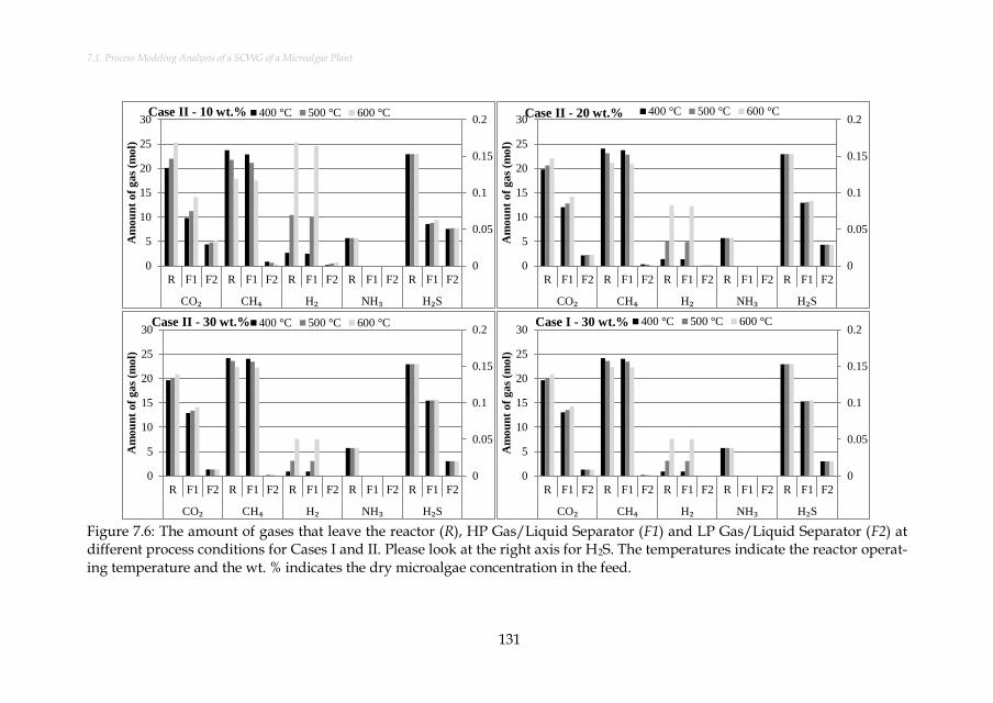
7.1. Process Modeling Analysis of a SCWG of a Microalgae Plant
131
Figure 7.6: The amount of gases that leave the reactor (R), HP Gas/Liquid Separator (F1) and LP Gas/Liquid Separator (F2) at different process conditions for Cases I and II. Please look at the right axis for H2S. The temperatures indicate the reactor operat-ing temperature and the wt. % indicates the dry microalgae concentration in the feed.
0
0.05
0.1
0.15
0.2
0
5
10
15
20
25
30
R F1 F2 R F1 F2 R F1 F2 R F1 F2 R F1 F2
CO₂ CH₄ H₂ NH₃ H₂S
Am
ou
nt
of
ga
s (m
ol)
Case II - 10 wt.% 400 °C 500 °C 600 °C
0
0.05
0.1
0.15
0.2
0
5
10
15
20
25
30
R F1 F2 R F1 F2 R F1 F2 R F1 F2 R F1 F2
CO₂ CH₄ H₂ NH₃ H₂S
Am
ou
nt
of
ga
s (m
ol)
Case II - 20 wt.% 400 °C 500 °C 600 °C
0
0.05
0.1
0.15
0.2
0
5
10
15
20
25
30
R F1 F2 R F1 F2 R F1 F2 R F1 F2 R F1 F2
CO₂ CH₄ H₂ NH₃ H₂S
Am
ou
nt
of
ga
s (m
ol)
Case II - 30 wt.% 400 °C 500 °C 600 °C
0
0.05
0.1
0.15
0.2
0
5
10
15
20
25
30
R F1 F2 R F1 F2 R F1 F2 R F1 F2 R F1 F2
CO₂ CH₄ H₂ NH₃ H₂S A
mo
un
t o
f g
as
(mo
l)
Case I - 30 wt.% 400 °C 500 °C 600 °C

PROCESS MODELING ANALYSIS OF SUPERCRITICAL WATER GASIFICATION OF BIOMASS
132
Inorganic Element Behavior Results: Figure 7.7 shows the mole fractions of Cl, K and Na separated in the filter in Case I for different process conditions. The sim-ulations indicate that Ca, Mg, P and Si are totally separated in the filter for all of the investigated process conditions, hence it is not shown in Figure 7.7.
Figure 7.7: The mole fractions of Cl, K and Na separated in salt separator in Case I for different process conditions. The temperatures indicate the operating tempera-ture of the reactor and filter and the wt. % indicates the dry microalgae concentra-tion in the feed.
The results show that higher reactor temperatures and higher dry microalgae concentrations result in more separation of Cl, K and Na elements. This is due to the decrease of the solubilities of Cl, K and Na compounds in supercritical water. The non-separated fraction of Cl, K and Na are dissolved in their ionic form in the LP Gas/Liquid Separator and leave the process in the liquid effluent (stream 10). The remaining elements can form different compounds at different process condi-tions. Table 7.1 shows the formed compounds for every element at different condi-tions. It can be stated that Ca forms Ca5(OH)(PO4)3, Cl forms KCl and Si forms Mg2SiO4. However, K, Mg and P form different kinds of compounds at different conditions.
0
0.2
0.4
0.6
0.8
1
10
wt.
%
20
wt.
%
30
wt.
%
10
wt.
%
20
wt.
%
30
wt.
%
10
wt.
%
20
wt.
%
30
wt.
%
10
wt.
%
20
wt.
%
30
wt.
%
10
wt.
%
20
wt.
%
30
wt.
%
10
wt.
%
20
wt.
%
30
wt.
%
10
wt.
%
20
wt.
%
30
wt.
%
10
wt.
%
20
wt.
%
30
wt.
%
10
wt.
%
20
wt.
%
30
wt.
%
400 °C 500 °C 600 °C 400 °C 500 °C 600 °C 400 °C 500 °C 600 °C
Cl K Na
Mo
le F
ra
cti
on
Case I Mole Fraction of Elements Separated in the Salt Separator
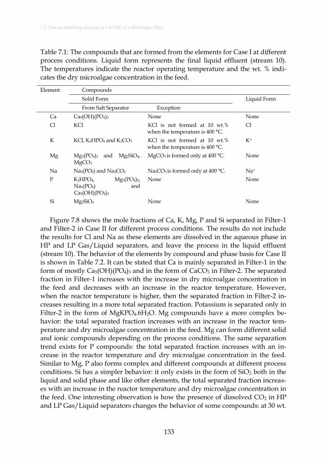
7.1. Process Modeling Analysis of a SCWG of a Microalgae Plant
133
Table 7.1: The compounds that are formed from the elements for Case I at different process conditions. Liquid form represents the final liquid effluent (stream 10). The temperatures indicate the reactor operating temperature and the wt. % indi-cates the dry microalgae concentration in the feed.
Element Compounds
Solid Form Liquid Form
From Salt Separator Exception
Ca Ca5(OH)(PO4)3 None None
Cl KCl KCl is not formed at 10 wt.% when the temperature is 400 °C.
Cl-
K KCl, K2HPO4 and K2CO3 KCl is not formed at 10 wt.% when the temperature is 400 °C.
K+
Mg Mg3(PO4)2 and Mg2SiO4, MgCO3
MgCO3 is formed only at 400 °C. None
Na Na3(PO4) and Na2CO3 Na2CO3 is formed only at 400 °C. Na+
P K2HPO4, Mg3(PO4)2, Na3(PO4) and Ca5(OH)(PO4)3
None None
Si Mg2SiO4 None None
Figure 7.8 shows the mole fractions of Ca, K, Mg, P and Si separated in Filter-1 and Filter-2 in Case II for different process conditions. The results do not include the results for Cl and Na as these elements are dissolved in the aqueous phase in HP and LP Gas/Liquid separators, and leave the process in the liquid effluent (stream 10). The behavior of the elements by compound and phase basis for Case II is shown in Table 7.2. It can be stated that Ca is mainly separated in Filter-1 in the form of mostly Ca5(OH)(PO4)3 and in the form of CaCO3 in Filter-2. The separated fraction in Filter-1 increases with the increase in dry microalgae concentration in the feed and decreases with an increase in the reactor temperature. However, when the reactor temperature is higher, then the separated fraction in Filter-2 in-creases resulting in a more total separated fraction. Potassium is separated only in Filter-2 in the form of MgKPO4.6H2O. Mg compounds have a more complex be-havior: the total separated fraction increases with an increase in the reactor tem-perature and dry microalgae concentration in the feed. Mg can form different solid and ionic compounds depending on the process conditions. The same separation trend exists for P compounds: the total separated fraction increases with an in-crease in the reactor temperature and dry microalgae concentration in the feed. Similar to Mg, P also forms complex and different compounds at different process conditions. Si has a simpler behavior: it only exists in the form of SiO2 both in the liquid and solid phase and like other elements, the total separated fraction increas-es with an increase in the reactor temperature and dry microalgae concentration in the feed. One interesting observation is how the presence of dissolved CO2 in HP and LP Gas/Liquid separators changes the behavior of some compounds: at 30 wt.

PROCESS MODELING ANALYSIS OF SUPERCRITICAL WATER GASIFICATION OF BIOMASS
134
% dry microalgae concentrations in the feed conditions, the dissolved CO2 is more concentrated in the Gas/Liquid separators and CaCO3 is formed instead of Ca5(OH)(PO4)3. A similar effect is the shifting of Na+ ion to NaHCO3
formation in the liquid phase at higher dry microalgae concentrations.
Figure 7.8: The mole fractions of Ca, K, Mg, P and Si separated in Filter-1 (1) and Filter-2 (2) in Case II for different process conditions. The temperatures indicate the reactor operating temperature and the wt. % indicates the dry microalgae con-centration in the feed.
Table 7.3 shows the comparison of the composition of the liquid effluent that leaves the process (stream 10) for Cases I and II at a reactor temperature of 500 °C for a 20 wt. % dry microalgae concentration in the feed. The results indicate that
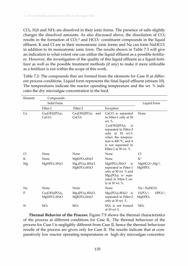
7.1. Process Modeling Analysis of a SCWG of a Microalgae Plant
135
CO2, H2S and NH3 are dissolved in their ionic forms. The presence of salts slightly changes the dissolved amounts. As also discussed above, the dissolution of CO2 results in the formation of CO3
-2 and HCO3- constituent compounds in the liquid
effluent. K and Cl are in their monoatomic ionic forms and Na can form NaHCO3 in addition to its monoatomic ionic form. The results shown in Table 7.3 will give an indication to what extent one can utilize the liquid effluent as a possible fertiliz-er. However, the investigation of the quality of this liquid effluent as a liquid ferti-lizer as well as the possible treatment methods (if any) to make it more utilizable as a fertilizer is not within the scope of this work.
Table 7.2: The compounds that are formed from the elements for Case II at differ-ent process conditions. Liquid form represents the final liquid effluent (stream 10). The temperatures indicate the reactor operating temperature and the wt. % indi-cates the dry microalgae concentration in the feed.
Element Compounds
Solid Form Liquid Form
Filter-1 Filter-2 Exception
Ca Ca5(OH)(PO4)3, CaCO3
Ca5(OH)(PO4)3 and CaCO3
CaCO3 is separated in Filter-1 only at 30 wt. %.
Ca5(OH)(PO4)3 is separated in Filter-2 only at 10 wt.% when the tempera-ture is 400 °C, and it is not separated in Filter-1 at 30 wt. %.
None
Cl None None None Cl-
K None MgKPO4.6H2O None K+
Mg MgHPO4.3H2O Mg3(PO4)2.8H2O, MgKPO4.6H2O
MgHPO4.3H2O is separated in Filter-1 only at 30 wt. % and Mg3(PO4)2 is sepa-rated in Filter-2 on-ly at 10 wt. %.
MgHCO3+,Mg+2, MgHPO4
Na None None None Na+, NaHCO3
P Ca5(OH)(PO4)3, MgHPO4.3H2O
Mg3(PO4)2.8H2O, MgKPO4.6H2O
Mg3(PO4)2.8H2O is separated in Filter-2 only at 10 wt. %.
H2PO4-1, HPO4-2, MgHPO4
Si SiO2 SiO2 SiO2 is not formed at 10 wt.%.
SiO2
Thermal Behavior of the Process: Figure 7.9 shows the thermal characteristics of the process at different conditions for Case II,. The thermal behaviour of the process for Case I is negligibly different from Case II, hence the thermal behaviour results of the process are given only for Case II. The results indicate that at com-paratively low reactor operating temperatures or high dry microalgae concentra-

PROCESS MODELING ANALYSIS OF SUPERCRITICAL WATER GASIFICATION OF BIOMASS
136
tions in the feed, the thermal energy required for the reactor (E-H) and available in HX-2 (E-C) are lower. However, the relative change in E-C with respect to the same amount of biomass slurry feed at different dry microalgae concentrations in the feed has an opposite behavior: at lower dry microalgae concentrations in the feed, the required thermal energy that could be gained in HX-2 (E-C) is higher. Lower dry microalgae concentrations result in higher fraction of water in the feed, which dissolves more compounds and thus leads to lower specific enthalpy values for stream 6.
Table 7.3: The comparison of the composition of the liquid effluent that leaves the process (stream 10) for Cases I and II at a reactor temperature of 500 °C and at 20 wt. % dry microalgae concentration in the feed.
Compound Mole Amount
Case I Case II
H2O 192.516 192.066
NH4+ 5.48224 5.48456
HCO3- 5.14635 5.24796
NH2CO2- 0.173496 0.173064
CO2 0.083252 0.082203
CO3-2 0.065123 0.067171
NH3 0.062055 0.060156
HS-1 0.032388 0.032022
H2S 5.00×10⁻³ 4.86×10⁻³
Cl- 2.38×10⁻³ 0.095657
K+ 2.18×10⁻³ 0.255479
Na+ 0.058874
NaHCO3 0.022467
HPO4-2 0.084023
MgHCO3+ 0.039831
Mg+2 8.21×10⁻³
SiO2 5.77×10⁻³
H2PO4- 3.03×10⁻³
MgCO3 1.46×10⁻³
MgHPO4 1.32×10⁻³
The thermal energy required for the reactor (E-H in Figure 7.9) may seem high-er (1 – 2 MJ·(kg-total-feed) -1). On the one hand, part of this thermal energy (50 – 80 %) can be recovered in HX-2 (E-C in Figure 7.9). On the other hand, the low tem-perature of stream 5 (T in Figure 7.9) limits the use of that heat source in the pro-cess. Nevertheless, that heat source can be used to heat up other utilities in a dif-ferent process and/or for the cultivation of microalgae.
Figure 7.10a shows the net thermal energy requirement of the process at differ-ent conditions for Case II and Figure 7.10b shows the remaining amount of CH4

7.1. Process Modeling Analysis of a SCWG of a Microalgae Plant
137
and H2 that are fed to the network (Stream 16 in Figure 7.1) after being used in the furnace in order to provide sufficient heat for the reactor. The results show that the process is thermally self-sufficient except for one condition: at a temperature of 600 °C when the dry microalgae concentration in the feed is 10 wt. %. As it can be seen from the splitting percentage (the ratio of stream 15 to stream 11 in %, “S” in Fig-ure 7.10a) results, all of the formed gases need to be used in order to provide suffi-cient heat to the reactor. Besides, additional thermal energy is required to supply sufficient heat for the reactor for this operating conditions. The required thermal energy can be supplied from a natural gas network in which the required amount of methane is 1.00 and 0.98 mol CH4∙(kg-dry-microalgae)-1 for Cases I and II, re-spectively.
The process is thermally more efficient when the reactor temperature is lower and when the dry micro algae concentration in the feed is higher. This behavior is expected since at lower reactor temperatures, less thermal energy is required to heat the feed to the reactor temperature and at higher dry microalgae concentra-tions more product gases are formed for the same amount of total feed. The most thermally efficient conditions are when the reactor operating temperature is at 400 °C with a dry microalgae concentration of 30 wt. %. However, in real cases such high dry biomass concentrations at 400 °C will unlikely lead to the full conversion of the biomass that is assumed in this study, but rather lead to an unconverted waste stream and lower gas production. There is still some thermal energy (E-F in Figure 7.10a) that could be gained in HX-3 (stream Flue gas-2). However, like the case of stream 5, the temperature of the stream Flue gas-2 (T in Figure 7.10a) limits the use of that heat source in the process, but can be utilized in other processes.
Figure 7.9: Thermal energy characteristics of the process for different conditions for Case II. The temperatures indicate the reactor operating temperature and the wt. % indicates the dry microalgae concentration in the feed. Please look at to the right axis for T.
0
50
100
150
200
250
300
350
0
4
8
12
16
20
E-H E-C T E-H E-C T E-H E-C T
10 % wt. 20 % wt. 30 % wt.
Tem
pera
ture (
° C
)
En
tha
py
(1
x1
06 J
)
Case II Reactor Temperature 400 °C 500 °C 600 °C

PROCESS MODELING ANALYSIS OF SUPERCRITICAL WATER GASIFICATION OF BIOMASS
138
Figure 7.10: Energetic performance of the process. a) The net thermal energy re-quirement of the process for different conditions for Case II. The temperatures in-dicate the reactor operating temperature and the wt. % indicates the dry microal-gae concentration in the feed. Please look at to the right axis for S (Percentage %) and T (Temperature). b) The amount of CH4 and H2 that is fed to the network (Stream 16 in Figure 7.1). The temperatures indicate the reactor operating tempera-ture and the wt. % indicates the dry microalgae concentration in the feed.
The Effect of the Mass Fraction of the Inorganic Content of Microalgae: Fig-ure 7.11 shows the effect of the mass fraction of the inorganic content of the bio-mass on the gas behavior in the reactor (R), HP Gas/Liquid Separator (first flash column – F1) and LP Gas/Liquid Separator (second flash column – F2) at a reactor temperature of 500 °C with a 20 wt. % dry microalgae in the feed for Case II. Fig-ure 7.12 is the reproduction of the results shown in Figure 7.11 with respect to 1 kg organic content (C, H, O, N, S) of microalgae: the amount of the gas compounds
0
20
40
60
80
100
120
140
0
1
2
3
4
E-F S T E-F S T E-F S T
10 % wt. 20 % wt. 30 % wt.
Percen
tag
e (
%)
Tem
pera
ture (
° C
)
En
tha
py
(1
x1
06
J)
Case II Reactor Temperature 400 °C 500 °C 600 °C
a)
0
5
10
15
20
10 wt.% 20 wt.% 30 wt.% 10 wt.% 20 wt.% 30 wt.%
CH₄ H₂
Am
ou
nt
of
ga
s (m
ol)
Case II 400 °C 500 °C 600 °C
b)

7.1. Process Modeling Analysis of a SCWG of a Microalgae Plant
139
given in Figure 7.11 were divided by the mass fraction of the organic content of the dry biomass.
Figure 7.11: The amount of gases that leaves the reactor (R), HP Gas/Liquid Sepa-rator (F1) and LP Gas/Liquid Separator (F2) at different mass fractions of the inor-ganic content of microalgae for Case II at 500 °C and 20 wt. % dry microalgae in the feed conditions. Please look at to the right axis for H2S. The wt. % indicates the mass fraction of the inorganic content of dry microalgae.
The results show that the amount of the formed gases decreases with an in-crease in the mass fraction of the inorganic content of microalgae. This is an ex-pected phenomena as the amount of organic elements (C, H, O, N, S) in the feed decreases with an increase in the mass fraction of the inorganic content of microal-gae resulting in lower gas formation.
The results need more attention when it comes to the Figure 7.12. The relative change of CO2 and H2S behavior in gas/liquid separators with respect to the change of the mass fraction of the inorganic content of microalgae is more signifi-cant than the other gases. The presence of salts slightly increases the solubility of CO2 and H2S. However, what is more noteworthy is the formation behavior of the gases in the reactor. While the amount of CO2 decreases, the amounts of CH4 and H2 increases with an increase in the mass fraction of the inorganic content of mi-croalgae. Some part of the decrease in the amount of CO2 can be attributed to for-mation of more carbonate salts with an increase in the mass fraction of the inor-ganic content of microalgae. However, the remaining decrease of CO2 and the in-crease in CH4 and H2 is due to the inorganic content of microalgae. It can be con-cluded that the increase in the mass fraction of the inorganic content of microalgae
0
0.05
0.1
0.15
0.2
0
5
10
15
20
25
R F1 F2 R F1 F2 R F1 F2 R F1 F2 R F1 F2
CO₂ CH₄ H₂ NH₃ H₂S
Am
ou
nt
of
ga
s (m
ol)
Case II - 500 °C 5 wt. % 10 wt. % 20 wt. %

PROCESS MODELING ANALYSIS OF SUPERCRITICAL WATER GASIFICATION OF BIOMASS
140
enhances the formation of CH4 and H2. This phenomena is most likely due to the increase in the total alkali content of the feed. Some part of CO2 forms carbonate salts with Na and K resulting in a decrease in the gas phase CO2 which further in-creases the amount of CH4 and H2 throughout the gas phase reactions. It has also been reported in the literature by many researchers [64–66] that the presence of al-kali salts increases the H2 yields.
Figure 7.12: The amount of gases that leaves the reactor (R), HP Gas/Liquid Sepa-rator (F1) and LP Gas/Liquid Separator (F2) at different mass fractions of the inor-ganic content of microalgae for Case II at 500 °C and 20 wt. % dry microalgae in the feed conditions with respect to 1 kg of organic content (C, H, O, N, S) of micro-algae basis. Please look at to the right axis for H2S. The wt. % indicates the mass fraction of the inorganic content of dry microalgae.
Figure 7.13 shows the effect of the mass fraction of the inorganic content of the biomass on the mole fractions of the inorganic elements separated in Filter-1 (1) and Filter-2 (2) at a reactor temperature of 500 °C with a 20 wt. % dry microalgae concentration in the feed for Case II. It can be concluded that the separated fraction of the elements increases with an increase in the mass fraction of the inorganic con-tent of microalgae except for K. K has an opposite behavior due to the formation of MgKPO4.6H2O in Filter-2: the more Mg and P are separated in Filter-1 the less K is separated in Filter-2.
0
0.05
0.1
0.15
0.2
0
5
10
15
20
25
R F1 F2 R F1 F2 R F1 F2 R F1 F2 R F1 F2
CO₂ CH₄ H₂ NH₃ H₂S
Am
ou
nt
of
ga
s (m
ol)
Case II - 500 °C 5 wt. % 10 wt. % 20 wt. %
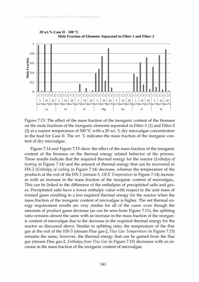
7.1. Process Modeling Analysis of a SCWG of a Microalgae Plant
141
Figure 7.13: The effect of the mass fraction of the inorganic content of the biomass on the mole fractions of the inorganic elements separated in Filter-1 (1) and Filter-2 (2) at a reactor temperature of 500 °C with a 20 wt. % dry microalgae concentration in the feed for Case II. The wt. % indicates the mass fraction of the inorganic con-tent of dry microalgae.
Figure 7.14 and Figure 7.15 show the effect of the mass fraction of the inorganic content of the biomass on the thermal energy related behavior of the process. These results indicate that the required thermal energy for the reactor (Enthalpy of heating in Figure 7.14) and the amount of thermal energy that can be recovered in HX-2 (Enthalpy of cooling in Figure 7.14) decrease, whereas the temperature of the products at the exit of the HX-1 (stream 5, HEX Temperature in Figure 7.14) increas-es with an increase in the mass fraction of the inorganic content of microalgae,. This can be linked to the difference of the enthalpies of precipitated salts and gas-es. Precipitated salts have a lower enthalpy value with respect to the unit mass of formed gases resulting in a less required thermal energy for the reactor when the mass fraction of the inorganic content of microalgae is higher. The net thermal en-ergy requirement results are very similar for all of the cases: even though the amounts of product gases decrease (as can be seen from Figure 7.11), the splitting ratio remains almost the same with an increase in the mass fraction of the inorgan-ic content of microalgae due to the decrease in the required thermal energy for the reactor as discussed above. Similar to splitting ratio, the temperature of the flue gas at the exit of the HX-3 (stream Flue gas-2, Flue Gas Temperature in Figure 7.15) remains the same, however, the thermal energy that can be gained from the flue gas (stream Flue gas-2, Enthalpy from Flue Gas in Figure 7.15) decreases with an in-crease in the mass fraction of the inorganic content of microalgae.
0
0.2
0.4
0.6
0.8
1
1 2 1 2 1 2 1 2 1 2 1 2 1 2 1 2 1 2 1 2 1 2 1 2 1 2 1 2 1 2 1 2 1 2 1 2 1 2 1 2 1 2
5
wt.%
10
wt.%
20
wt.%
5
wt.%
10
wt.%
20
wt.%
5
wt.%
10
wt.%
20
wt.%
5
wt.%
10
wt.%
20
wt.%
5
wt.%
10
wt.%
20
wt.%
5
wt.%
10
wt.%
20
wt.%
5
wt.%
10
wt.%
20
wt.%
Ca Cl K Mg Na P Si
Mo
le F
ra
cti
on
20 wt.% Case II - 500 °C
Mole Fraction of Elements Separated in Filter-1 and Filter-2

PROCESS MODELING ANALYSIS OF SUPERCRITICAL WATER GASIFICATION OF BIOMASS
142
Figure 7.14: The effect of the mass fraction of the inorganic content of the biomass on the thermal energy behavior of the process at a reactor temperature of 500 °C with a 20 wt. % dry microalgae concentration in the feed for Case II. The wt. % in-dicates the mass fraction of the inorganic content of dry microalgae.
Figure 7.15: The effect of the mass fraction of the inorganic content of the biomass on the net thermal energy behavior of the process at a reactor temperature of 500 °C with a 20 wt. % dry microalgae concentration in the feed for Case II. The wt. % indicates the mass fraction of the inorganic content of dry microalgae.

143
7.1.4. Conclusions
Based on a conceptual process design, the energetic behavior as well as the be-havior of gases of a SCWG of microalgae process in the presence of the inorganic content of microalgae have been investigated for two different salt separation cas-es. The effects of various process conditions including varying inorganic content have been studied. In addition, the behavior of inorganic elements in different process equipment by means of phase partitioning and compound formation has also been investigated. The results indicate that the presence of electrolytes influ-ences the solubility of gases in gas/liquid separators. Hence, one needs to account for the effect of ions on the gas/liquid separators instead of using only the Henry constants of gases if the inorganic content of the biomass (≥ 10 wt.%) and/or the dry biomass concentration in the feed (≥ 20 wt.%) are high. The process is thermal-ly more efficient when the reactor temperature is lower and when the dry microal-gae concentration in the feed is higher. The thermal energy required for the reactor may seem higher, however, some part of this thermal energy (50 – 80 %) can be re-covered as a heat source in other processes such as the cultivation of microalgae. The increase in the mass fraction of the inorganic content of microalgae enhances the formation of CH4 and H2 and decreases the required thermal energy for the re-actor. The results also show how sensitive the process outcomes are with respect to process conditions. Changing the pressure and temperature in the reactor and gas/liquid separators, and dry biomass concentration in the feed result in signifi-cant changes in process outcomes (thermal behavior, gas and salt composition) which make it hard to define the most critical parameters of the process.

PROCESS MODELING ANALYSIS OF SUPERCRITICAL WATER GASIFICATION OF BIOMASS
144
7.2. AN INTEGRATED KINETIC MODEL FOR THE PREDICTION OF PRODUCT COM-
POUNDS
7.2.1. Introduction
Even though there have been many research works on determining the decom-position and/or gasification reaction pathways for the main biomass constituents or on developing a lumped reaction mechanism for real biomass samples (see ref. [85] for a lumped kinetic model for algae), a comprehensive and detailed reaction network for a real biomass has not been proposed so far. However, proposing an integrated decomposition pathway and using kinetic parameters from the pub-lished reaction rates enables to investigate the compositional analysis of the deg-radation products of real biomass feedstocks at different process conditions. In addition, unlike a thermodynamic equilibrium approach, kinetic modeling enables the sizing of process equipment and observing the effect of residence time on the product compounds’ yields. Based on the already published literature data, this sub-chapter aims to develop and validate an integrated decomposition and gasifi-cation kinetic model using Aspen PlusTM software for cellulose, hemicellulose, lig-nin and protein model compounds in supercritical water.
7.2.2. Kinetic model
Integration of the available kinetic studies in the literature was established re-garding both sub- and supercritical reactions for given model compounds. Addi-tionally, experimental conditions under which the data were gathered were worked on carefully by grouping the data according to the operating conditions. The reaction pathways for the model compounds which were reported to show differences in the sub– and supercritical regions were separately implemented into the model for sub– and supercritical regions.
7.2.2.1. Cellulose reaction pathways in sub– and supercritical water
To model the cellulose decomposition and gasification reaction pathways, cel-lobiose has been chosen as the model compound as it has similar glycosidic bonds as cellulose [116].
Decomposition of cellobiose: In the proposed reaction network, cellobiose as a model compound of cellulose, undergoes reactions occurring in series and in par-allel to form simpler organic compounds under sub– and near-critical conditions. Cellobiose initially depolymerizes in three distinct ways: via pyrolysis to glucosyl-erythrose + glycolaldehyde, glucosyl-glycolaldehyde + erythrose and via hydroly-sis to glucose [116]. Glucose isomerizes to fructose, but fructose to glucose isomer-ization is not significant [42]. Glucose decomposes to erythrose, glyceraldehyde, 5-hydroxymethylfurfural (5-HMF) and also dehydrates to 1,6 anhydroglucose under hydrothermal conditions [42]. Dihydroxyacetone takes place in a 2-way isomeriza-tion reaction with glyceraldehyde. Pyruvaldehyde is a dehydration product of the
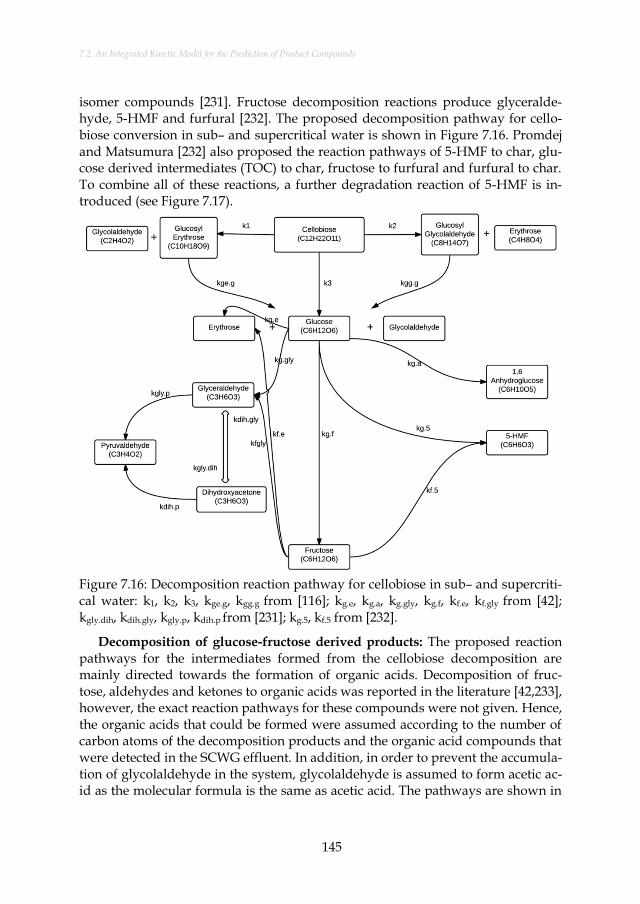
7.2. An Integrated Kinetic Model for the Prediction of Product Compounds
145
isomer compounds [231]. Fructose decomposition reactions produce glyceralde-hyde, 5-HMF and furfural [232]. The proposed decomposition pathway for cello-biose conversion in sub– and supercritical water is shown in Figure 7.16. Promdej and Matsumura [232] also proposed the reaction pathways of 5-HMF to char, glu-cose derived intermediates (TOC) to char, fructose to furfural and furfural to char. To combine all of these reactions, a further degradation reaction of 5-HMF is in-troduced (see Figure 7.17).
Figure 7.16: Decomposition reaction pathway for cellobiose in sub– and supercriti-cal water: k1, k2, k3, kge.g, kgg.g from [116]; kg.e, kg.a, kg.gly, kg.f, kf.e, kf.gly from [42]; kgly.dih, kdih.gly, kgly.p, kdih.p from [231]; kg.5, kf.5 from [232].
Decomposition of glucose-fructose derived products: The proposed reaction pathways for the intermediates formed from the cellobiose decomposition are mainly directed towards the formation of organic acids. Decomposition of fruc-tose, aldehydes and ketones to organic acids was reported in the literature [42,233], however, the exact reaction pathways for these compounds were not given. Hence, the organic acids that could be formed were assumed according to the number of carbon atoms of the decomposition products and the organic acid compounds that were detected in the SCWG effluent. In addition, in order to prevent the accumula-tion of glycolaldehyde in the system, glycolaldehyde is assumed to form acetic ac-id as the molecular formula is the same as acetic acid. The pathways are shown in

PROCESS MODELING ANALYSIS OF SUPERCRITICAL WATER GASIFICATION OF BIOMASS
146
Figure 7.17. The general reaction mechanism of glucose under sub- and supercriti-cal water conditions postulated in this work (combination of Figure 7.16 and Fig-ure 7.17) is also in agreement with the glucose decomposition pathway proposed by Castello et al. [234]
Figure 7.17: Decomposition reaction pathway for glucose-fructose derived prod-ucts in sub– and supercritical water: kf.acid, kp.acid, ka.acid, ke.acid from [233]; k5.lf, k5.ff from [235,236]. Please note that kglyo.acid is an assumed reaction and due to its simi-lar structure the Arrhenius parameters of the erythrose conversion are used for that reaction.
7.2.2.2. Hemicellulose reaction pathways in sub– and supercritical water
To model the hemicellulose decomposition and gasification reaction pathways, D-xylose has been chosen as the model compound as it is the major hydrolysis prod-uct of hemicellulose [237]. As the reaction pathways are not the same in sub– and supercritical water, the decomposition pathway for D-xylose has been developed for sub– and supercritical regions separately.

7.2. An Integrated Kinetic Model for the Prediction of Product Compounds
147
Decomposition of D-xylose in subcritical water: Unfortunately, there are not many studies dedicated to the decomposition of D-xylose under sub– or near-critical conditions. Hence, the decomposition reaction network for D-xylose under subcritical conditions is obtained from the research performed under rather mild temperatures and pressures (180 C- 220 oC, 10 MPa) [237]. In the proposed reaction network, D-xylose primarily decomposes to glyceraldehyde and methyl formate or forms furfural under subcritical conditions. Furfural further decomposes into a mixture of acetic acid and acrylic acid [237]. The proposed decomposition reaction pathways for D-xylose is given in Figure 7.18.
Figure 7.18: Decomposition reaction pathways for D-xylose in subcritical water. All of the reaction pathways are from [237].
Decomposition and gasification of D-xylose in supercritical water: In the su-percritical region, D-xylose decomposes to furfural or to an acetic acid and acrylic acid mixture. Furfural further undergoes a parallel reaction to form either char via a polymerization reaction or to form water soluble humic substance (WSHS) [47]. WSHS was assumed to be a mixture of acetic acid and acrylic acid as Goodwin and Rorrer [62] identified in their experimental work. The acetic acid and acrylic acid mixture further gasifies to form CO and H2 in the supercritical region. Figure 7.19 shows the proposed scheme for the decomposition reaction pathway for D-xylose in the supercritical region.
7.2.2.3. Lignin reaction pathways in sub– and supercritical water
To model the lignin decomposition and gasification reaction pathways, guaiacol has been chosen as the model compound due to its chemical structure and similar attached groups [34]. As the reaction pathways are again not the same in sub– and supercritical water, the decomposition pathway for guaiacol has also been devel-oped for sub– and supercritical regions separately.

PROCESS MODELING ANALYSIS OF SUPERCRITICAL WATER GASIFICATION OF BIOMASS
148
Figure 7.19: D-xylose decomposition and gasification reaction pathways in super-critical water. kxy.fu,kxy.wshs,kfu.wshs,kaa.ga are from [47] and kfu.ch is from [232].
Decomposition of guaiacol in subcritical water: In the proposed reaction net-work for the guaiacol decomposition in subcritical water, guaiacol decomposes to single ring structures such as o-cresol and benzene or it directly gasifies. Crosslink-ing between decomposition products produces heavier compounds, such as di-phenyl, which was assumed as a model compound for total organic carbon (TOC) [238]. Diphenyl and benzene further crosslink the active sites of the ring structure, which results in char formation. Diphenyl is then converted via direct gasification in a parallel reaction [34]. The reaction network of guaiacol in subcritical water is given in Figure 7.20.
Decomposition and gasification of guaiacol in supercritical water: The de-composition and gasification reaction pathways of guaiacol in supercritical water have been developed based on the integration of the reaction pathways given in the works of Yong et al. [34,239]. The proposed reaction pathway is given in Figure 7.21. In the supercritical region, guaiacol behaves similarly as in the behavior in subcritical region, however, further reactions of guaiacol derived compounds in supercritical water are also taken into account.
7.2.2.4. Protein reaction pathways in sub– and supercritical water
The decomposition products of a protein sample (albumin) to amino acids and other intermediate products as well as the Arrhenius parameters were given in Brunner [240]. However, as it was not possible to model raw protein in Aspen PlusTM, aspartic acid has been chosen as the model compound as it contains a higher number of carbon atoms in its molecular structure than alanine and glycine, which are the most investigated amino acids under hydrothermal conditions.

7.2. An Integrated Kinetic Model for the Prediction of Product Compounds
149
Figure 7.20: ecomposition reaction pathways for guaiacol in subcritical water. All of the reaction pathways are from [241].
Figure 7.21: Decomposition and gasification reaction pathways for guaiacol in su-percritical water. kgu.ch, kgu.ga, kgu.oc, kgu.c, kgu.t, kc.oc, kt.p kt.ch, kt.ga from [241]; kc.t, kp.c, kp.t, kp,ga, kp.ch, kb.t, kb.p, kb.ga, kb.na, kna.ch, kb.ch from [239].

PROCESS MODELING ANALYSIS OF SUPERCRITICAL WATER GASIFICATION OF BIOMASS
150
Decomposition of aspartic acid in subcritical water: In the proposed reaction network, aspartic acid first decomposes to alanine, glycine and other organic acids as well as char [240]. Glycine and alanine then further decomposes to form amine compounds, organic acids, and NH3 as well as CO2 [51]. The proposed reaction network is given in Figure 7.22.
Figure 7.22: Decomposition pathway for aspartic acid in subcritical water. kas.a, kas.g from [240]; kal.et, kg.met from [51].
Decomposition and gasification of aspartic acid derived compounds in su-percritical water: In the proposed reaction network, alanine and glycine decompo-sition also takes place in supercritical water [51]. However, alanine and glycine are reported to produce gases in supercritical water [242]. Besides, the carbon gasifica-tion efficiency for amino acids can reach more than 80 % in less than 120 s at 650 °C [242] which indicates that the intermediate compounds from amino acids’ de-composition produce gaseous compounds as well. Hence, ethylamine and methyl-amine are also assumed to produce gas compounds in supercritical water. The proposed reaction network is given in Figure 7.23.
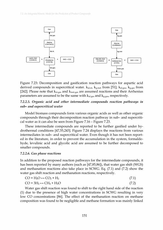
7.2. An Integrated Kinetic Model for the Prediction of Product Compounds
151
Figure 7.23: Decomposition and gasification reaction pathways for aspartic acid derived compounds in supercritical water. kal.et, kg.met from [51]; kal.gas, kg.gas from [242]. Please note that ket.gas and kmet.gas are assumed reactions and their Arrhenius parameters are assumed to be the same with kal.gas and kg.gas, respectively.
7.2.2.5. Organic acid and other intermediate compounds reaction pathways in
sub– and supercritical water
Model biomass compounds form various organic acids as well as other organic compounds through their decomposition reaction pathway in sub– and supercriti-cal water as it can also be seen from Figure 7.16 – Figure 7.23.
These intermediate compounds are reported to be further gasified under hy-drothermal conditions [47,55,243]. Figure 7.24 displays the reactions from various intermediates in sub– and supercritical water. Even though it has not been report-ed in the literature, in order to prevent the accumulation in the system, formalde-hyde, levulinic acid and glycolic acid are assumed to be further decomposed to smaller compounds.
7.2.2.6. Gas phase reactions
In addition to the proposed reaction pathways for the intermediate compounds, it has been reported by many authors (such as [47,85,86]), that water gas shift (WGS) and methanation reactions also take place in SCWG. Eq. (7.1) and (7.2) show the water gas shift reaction and methanation reactions, respectively.
CO + H2O ↔ CO2 + H2 (7.1)
CO + 3H2 ↔ CH4 + H2O (7.2)
Water gas shift reaction was found to shift to the right hand side of the reaction (1) due to the presence of high water concentrations in SCWG resulting in very low CO concentrations [86]. The effect of the methanation reaction on methane composition was found to be negligible and methane formation was mainly linked
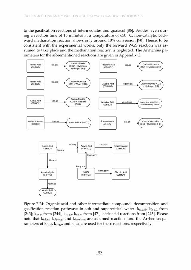
PROCESS MODELING ANALYSIS OF SUPERCRITICAL WATER GASIFICATION OF BIOMASS
152
to the gasification reactions of intermediates and guaiacol [86]. Besides, even dur-ing a reaction time of 15 minutes at a temperature of 650 °C, non-catalytic back-ward methanation reaction shows only around 10% conversion [90]. Hence, to be consistent with the experimental works, only the forward WGS reaction was as-sumed to take place and the methanation reaction is neglected. The Arrhenius pa-rameters for the aforementioned reactions are given in Appendix C.
Figure 7.24: Organic acid and other intermediate compounds decomposition and gasification reaction pathways in sub and supercritical water. kfa.ga1, kfa.ga2 from [243]; kaa.ga from [244]; kpa.ga, kmf.aa from [47]; lactic acid reactions from [245]. Please note that kfal.ga, kglyco.ga and klevu.lacet are assumed reactions and the Arrhenius pa-rameters of kf.ga1, kaa.ga, and kp.acid are used for these reactions, respectively.
7.2. An Integrated Kinetic Model for the Prediction of Product Compounds
153
7.2.3. Validation of the model
Validation of the model has been performed by comparing the model predictions with the experimental results of SCWG of ligno-cellulosic and protein containing biomass feedstocks.
7.2.3.1. Validation for ligno-cellulosic biomass
Validation of the proposed kinetic model for ligno-cellulosic containing biomass has been performed by comparing the model predictions with the experimental work of Lu et al. [178]. In addition, the comparison between the experimental re-sults reported in Chapter 6 and the predictions of the model is given in Appendix C.
Lu et al. [178] performed a substantial number of SCWG experiments of ligno-cellulosic biomass feedstocks under different process conditions in the presence of carboxymethylcellulose (CMC) in a heated tubular reactor. To model the tubular reactor of the experimental setup in AspenPlusTM, two plug flow reactors (RPlug type reactor) in series have been used: the first one was to model the reactions that take place under subcritical conditions (from 25 °C to 370 °C) and the second was to model the reactions that take place under supercritical conditions (from 370 °C to 650 °C). Figure 7.25 shows the experimental setup of Lu et al. [178] and the way it was modeled in AspenPlusTM for the simulations. Even though the authors [178] have given the sizing details of their setup, the temperature profile of their setup has not been given in their paper. As the authors’ experiments result in high gasi-fication efficiencies (> 90 %) at short residence times (14 – 47s), it can be stated that rapid heating of the reacting medium is achieved. Thus, for the kinetic model sim-ulations in AspenPlusTM, it was assumed that the residence time for the reacting medium from 25 °C to 370 °C is 5 seconds and that it is 3 seconds from 370 °C to 650 °C. Throughout the simulations, CMC has been modeled as cellobiose. This approximation is not expected to lead to appreciable inconsistencies as the struc-tures of the two compounds are similar. Figure 7.26 – Figure 7.28 show the com-parison of the model predictions with the experimental results for carbon gasifica-tion efficiency (CGE), gasification efficiency (GE) and gas yields of wood sawdust gasification in SCW at a temperature of 650 °C for different residence times and at different pressures. GE refers to the mass percentage of the gaseous phase outlet to the dry biomass inlet. CGE stands for the percentage of the number of moles of the carbon in the gaseous outlet to the biomass inlet.
It can be concluded that CGE and GE tend to increase with the residence time, which is simply explained by the enhanced production of gas compounds by al-lowance of more time to the gasification reactions to proceed. Average relative er-rors for the GE and CGE are found to be 15% and 10%, respectively. Besides these quantitative findings, the trend of the efficiencies also show quite good agreement as it can also be seen from Figure 7.26. Hydrogen, methane, carbon dioxide, and

PROCESS MODELING ANALYSIS OF SUPERCRITICAL WATER GASIFICATION OF BIOMASS
154
carbon monoxide formation show a similar trend as a function of residence time as the experimental result of Lu et al. [178].
Figure 7.25: The experimental setup of Lu et al. [178] (a), and the way it was mod-eled in AspenPlusTM for the simulations (b). (a) is reprinted from [178].

7.2. An Integrated Kinetic Model for the Prediction of Product Compounds
155
Figure 7.26: The effect of residence time on carbon gasification efficiency (CGE) and gasification efficiency (GE) of wood sawdust gasification ( 2 wt.% wood saw-dust + 2 wt.% CMC) in SCW at a pressure of 25 MPa and at a temperature of 650 °C. Solid lines are model predictions and dashed lines are experimental results. The experimental results are from Lu et al. [178].
Figure 7.27: The effect of residence time on gas composition of wood sawdust gasi-fication ( 2 wt.% wood sawdust + 2 wt.% CMC) in SCW at a pressure of 25 MPa and at a temperature of 650 °C. Solid lines are model predictions and dashed lines are experimental results. The experimental results are from Lu et al. [178].

PROCESS MODELING ANALYSIS OF SUPERCRITICAL WATER GASIFICATION OF BIOMASS
156
Figure 7.28: The effect of pressure on carbon gasification efficiency (CGE) and gasi-fication efficiency (GE) of wood sawdust gasification ( 2 wt.% wood sawdust + 2 wt.% CMC) in SCW at a residence time 27s and at a temperature of 650 °C. Solid lines are model predictions and dashed lines are experimental results. The experi-mental results are from Lu et al. [178].
In addition, the yields of carbon dioxide and carbon monoxide are also in a rel-atively good agreement as it can also be seen from Figure 7.27. Methane yield, on the other hand, is higher than the experimental study, whereas hydrogen yield is lower. Quite good agreements with the experimental results in CGE and GE can be seen, but disagreement in methane and hydrogen yields indicate that the gas form-ing reaction rates of the proposed kinetic model are quite accurate, however, the stoichiometry of gas forming reactions are less accurate. The difference in hydro-gen and methane yields might be due to the stoichiometry of the gas products in the lignin gasification pathway (see Figure 7.20 and Figure 7.21). The stoichiome-try of the gas products was not reported in the cited references [239,241], hence the stoichiometric coefficients of the gas products in the lignin gasification pathway were derived by performing calculations using the RGibbs reactor of AspenPlusTM software at the temperature of the reactor (for this case 650 °C) assuming a direct gasification of the corresponding compounds with supercritical water. CO2, CH4, CO, H2 and C2H6 were selected as the only possible gas phase compounds in the RGibbs reactor and determined the stoichiometric coefficients of CO2, CH4, CO, H2 and C2H6 for the direct gasification reactions in the lignin gasification pathway. It is also noteworthy that hydrogen, carbon dioxide and methane yields increase

7.2. An Integrated Kinetic Model for the Prediction of Product Compounds
157
with an increase in residence time, whilst the carbon monoxide concentration re-duces by following a similar trend as the experimental results. This observation can be explained by the water gas shift reaction. The proposed kinetic model is al-so in a quite good agreement with the experimental results in predicting the effect of pressure on CGE and GE at pressures between 25 and 30 MPa as it can be seen from Figure 7.28. However, the agreement is quite low at lower pressures. This is expected as the great majority of the kinetic data used in the proposed kinetic model is derived at pressures between 25 and 30 MPa.
Figure 7.29 shows the effect of feedstock type on CGE and GE and the compari-son between the model predictions with the experimental results. The composi-tions of the biomass feedstocks are obtained from Phyllis database [246] and the samples of which the biochemical composition result in the most similar elemental composition with as the experimental results of the authors [178] were selected. It should be noted that 2% CMC was added to the biomass cellulose content for the overall feed composition. Furthermore, for the samples with less than 100% bio-chemical and ash content, the remaining part was normalized to the biochemical content. Biochemical composition of the feedstocks that has been used as the input values throughout the simulations is given in Table 7.4.
Figure 7.29: The effect of the type of biomass feedstock on carbon gasification effi-ciency (CGE) and gasification efficiency (GE) (2 wt.% biomass + 2 wt.% CMC) in SCW at a residence time of 27s, at 25 MPa and at a temperature of 650 °C. Solid filled bars (CGE and GE) are model predictions and pattern filled bars (CGE* and GE*) are experimental results. The experimental results are from Lu et al. [178].
0
20
40
60
80
100
120
Rice Straw Peanut Shell Corn Stalk Corn Cob
Eff
icie
ncy (
%)
GE
GE*
CGE
CGE*
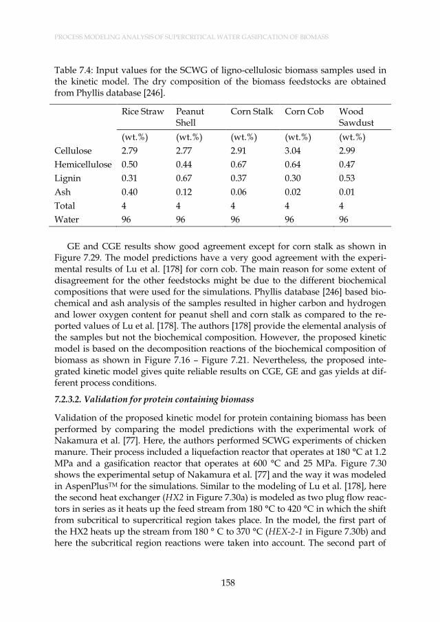
PROCESS MODELING ANALYSIS OF SUPERCRITICAL WATER GASIFICATION OF BIOMASS
158
Table 7.4: Input values for the SCWG of ligno-cellulosic biomass samples used in the kinetic model. The dry composition of the biomass feedstocks are obtained from Phyllis database [246].
Rice Straw Peanut Shell
Corn Stalk Corn Cob Wood Sawdust
(wt.%) (wt.%) (wt.%) (wt.%) (wt.%)
Cellulose 2.79 2.77 2.91 3.04 2.99
Hemicellulose 0.50 0.44 0.67 0.64 0.47
Lignin 0.31 0.67 0.37 0.30 0.53
Ash 0.40 0.12 0.06 0.02 0.01
Total 4 4 4 4 4
Water 96 96 96 96 96
GE and CGE results show good agreement except for corn stalk as shown in Figure 7.29. The model predictions have a very good agreement with the experi-mental results of Lu et al. [178] for corn cob. The main reason for some extent of disagreement for the other feedstocks might be due to the different biochemical compositions that were used for the simulations. Phyllis database [246] based bio-chemical and ash analysis of the samples resulted in higher carbon and hydrogen and lower oxygen content for peanut shell and corn stalk as compared to the re-ported values of Lu et al. [178]. The authors [178] provide the elemental analysis of the samples but not the biochemical composition. However, the proposed kinetic model is based on the decomposition reactions of the biochemical composition of biomass as shown in Figure 7.16 – Figure 7.21. Nevertheless, the proposed inte-grated kinetic model gives quite reliable results on CGE, GE and gas yields at dif-ferent process conditions.
7.2.3.2. Validation for protein containing biomass
Validation of the proposed kinetic model for protein containing biomass has been performed by comparing the model predictions with the experimental work of Nakamura et al. [77]. Here, the authors performed SCWG experiments of chicken manure. Their process included a liquefaction reactor that operates at 180 °C at 1.2 MPa and a gasification reactor that operates at 600 °C and 25 MPa. Figure 7.30 shows the experimental setup of Nakamura et al. [77] and the way it was modeled in AspenPlusTM for the simulations. Similar to the modeling of Lu et al. [178], here the second heat exchanger (HX2 in Figure 7.30a) is modeled as two plug flow reac-tors in series as it heats up the feed stream from 180 °C to 420 °C in which the shift from subcritical to supercritical region takes place. In the model, the first part of the HX2 heats up the stream from 180 ° C to 370 °C (HEX-2-1 in Figure 7.30b) and here the subcritical region reactions were taken into account. The second part of
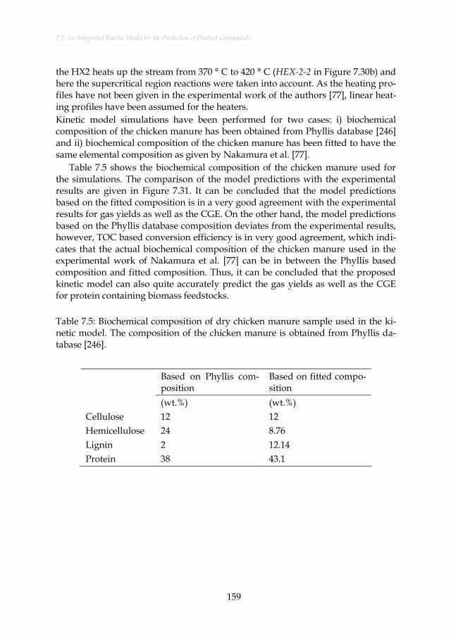
7.2. An Integrated Kinetic Model for the Prediction of Product Compounds
159
the HX2 heats up the stream from 370 ° C to 420 ° C (HEX-2-2 in Figure 7.30b) and here the supercritical region reactions were taken into account. As the heating pro-files have not been given in the experimental work of the authors [77], linear heat-ing profiles have been assumed for the heaters.
Kinetic model simulations have been performed for two cases: i) biochemical composition of the chicken manure has been obtained from Phyllis database [246] and ii) biochemical composition of the chicken manure has been fitted to have the same elemental composition as given by Nakamura et al. [77].
Table 7.5 shows the biochemical composition of the chicken manure used for the simulations. The comparison of the model predictions with the experimental results are given in Figure 7.31. It can be concluded that the model predictions based on the fitted composition is in a very good agreement with the experimental results for gas yields as well as the CGE. On the other hand, the model predictions based on the Phyllis database composition deviates from the experimental results, however, TOC based conversion efficiency is in very good agreement, which indi-cates that the actual biochemical composition of the chicken manure used in the experimental work of Nakamura et al. [77] can be in between the Phyllis based composition and fitted composition. Thus, it can be concluded that the proposed kinetic model can also quite accurately predict the gas yields as well as the CGE for protein containing biomass feedstocks.
Table 7.5: Biochemical composition of dry chicken manure sample used in the ki-netic model. The composition of the chicken manure is obtained from Phyllis da-tabase [246].
Based on Phyllis com-position
Based on fitted compo-sition
(wt.%) (wt.%)
Cellulose 12 12
Hemicellulose 24 8.76
Lignin 2 12.14
Protein 38 43.1

PROCESS MODELING ANALYSIS OF SUPERCRITICAL WATER GASIFICATION OF BIOMASS
160
Figure 7.30: The experimental setup of Nakamura et al. [77] (a), and the way it was modeled in AspenPlusTM for the simulations (b). (a) is reprinted from [77].

7.2. An Integrated Kinetic Model for the Prediction of Product Compounds
161
Figure 7.31: Comparison of the model predictions with the experimental results for a 1.97 wt.% chicken manure gasification in SCW. The experimental results are from Nakamura et al. [77]. The residence times in the liquefaction and gasification reactors are 27 and 1.7 minutes, respectively. The liquefaction reactor operates at 180 °C at 1.2 MPa and the gasification reactor operates at 600 °C and 25 MPa.
7.2.4. Case studies: SCWG of microalgae, manure and paper pulp
Using the proposed kinetic model, case studies have also been performed for the SCWG of microalgae, pig-cow manure mixture and paper pulp samples. The effect of residence time on the gas yields at the exit of the reactor has been investi-gated. Reactor temperatures were chosen as 500 °C and 600 °C. The pressure was kept constant at 25 MPa and the dry biomass concentration in the feed was 10 wt.%. Biochemical compositions of the biomass samples were obtained from Phyl-lis database [246] and these are given in Table 7.6.
Three tubular reactors were used in AspenPlusTM 8.2 software in order to simu-late a real SCWG process: a heat exchanger, a heater and a reactor. Figure 7.32 shows the process scheme that was used throughout the simulations.
Table 7.6: Biochemical compositions of dry microalgae, pig-cow manure and paper pulp samples used for the case studies. The compositions are obtained from Phyllis database [246].
Microalgae Pig-Cow Ma-nure
Paper Pulp
(wt.%) (wt.%) (wt.%)
Cellulose 13.93 31.28 68.36
Hemicellulose 31.98 34.05 19.08
Lignin 2.98 16.64 12.55
Protein 51.1 18.02 0
0
0.2
0.4
0.6
0.8
1
0
0.2
0.4
0.6
0.8
1
H₂ CO₂ CH₄ CO C₂H₆ C₂H₄ CGE → 1-TOC →
Co
nve
rsio
n
Mo
le F
racti
on
Experimental Results Based on Fitted Composition Based on Phyllis Composition

PROCESS MODELING ANALYSIS OF SUPERCRITICAL WATER GASIFICATION OF BIOMASS
162
Figure 7.32: The process scheme that was used throughout the SCWG simulations of microalgae, pig-cow manure and paper pulp.
The first tubular reactor was to simulate the heat exchanger (pre-heater) that heats up the feed stream from 25 °C to 370 °C. A linear temperature profile was as-sumed among the heat exchanger length. All of the aforementioned reaction pathways for the subcritical region (55 reactions) were taken into account. The to-tal residence time for the heat exchanger was assumed as 5 minutes and this was not varied. The second reactor was to simulate the heater that heats up the feed stream from 370 °C to the reactor operating temperature (500 or 600 °C). A linear temperature profile was assumed among the heater length. The total residence time in the heat exchanger was 20 s. The third reactor was to simulate the reactor in which the main reactions and conversion of biomass to gases took place. A con-stant temperature profile was assumed along reactor length (500 or 600 °C). By changing the reactor length, the total residence time was varied from 5 to 60 sec-onds. The results of the simulations are given in Figure 7.33.
The results show that the trends for gas yields as well as the CGE are similar for all of the investigated biomass samples: CGE and total gas yields increase with an increase in temperature and residence time. These are expected phenomena as it is known that both of these parameters significantly enhance the gasification ef-ficiency. On the other hand, the absolute values for CGE and total gas yields are different for all of the feedstocks as the biochemical composition of the investigat-ed biomass samples are different from each other which results in different gasifi-cation behavior in supercritical water.
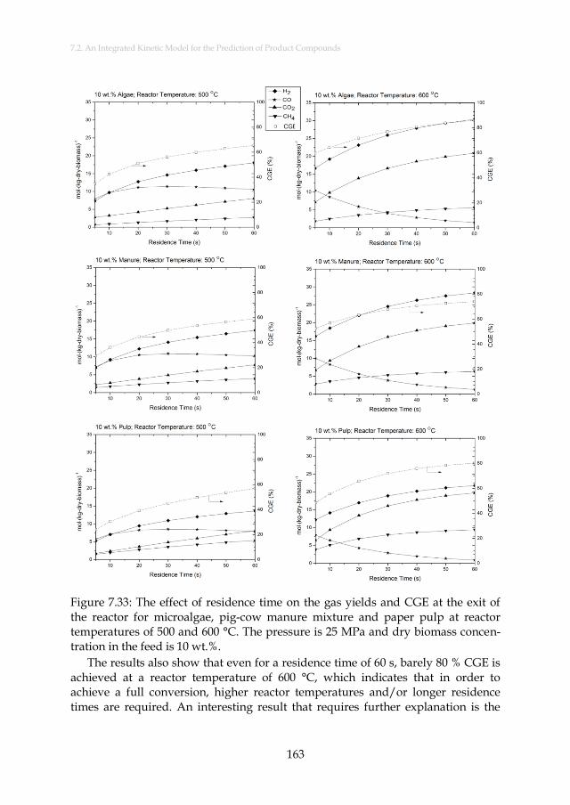
7.2. An Integrated Kinetic Model for the Prediction of Product Compounds
163
Figure 7.33: The effect of residence time on the gas yields and CGE at the exit of the reactor for microalgae, pig-cow manure mixture and paper pulp at reactor temperatures of 500 and 600 °C. The pressure is 25 MPa and dry biomass concen-tration in the feed is 10 wt.%.
The results also show that even for a residence time of 60 s, barely 80 % CGE is achieved at a reactor temperature of 600 °C, which indicates that in order to achieve a full conversion, higher reactor temperatures and/or longer residence times are required. An interesting result that requires further explanation is the
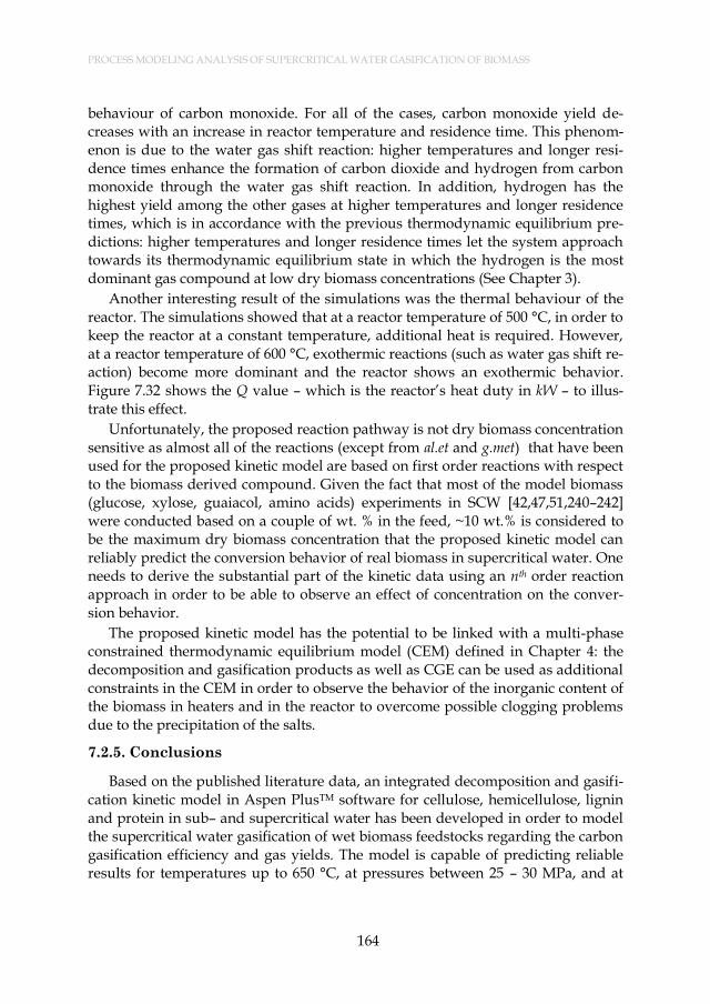
PROCESS MODELING ANALYSIS OF SUPERCRITICAL WATER GASIFICATION OF BIOMASS
164
behaviour of carbon monoxide. For all of the cases, carbon monoxide yield de-creases with an increase in reactor temperature and residence time. This phenom-enon is due to the water gas shift reaction: higher temperatures and longer resi-dence times enhance the formation of carbon dioxide and hydrogen from carbon monoxide through the water gas shift reaction. In addition, hydrogen has the highest yield among the other gases at higher temperatures and longer residence times, which is in accordance with the previous thermodynamic equilibrium pre-dictions: higher temperatures and longer residence times let the system approach towards its thermodynamic equilibrium state in which the hydrogen is the most dominant gas compound at low dry biomass concentrations (See Chapter 3).
Another interesting result of the simulations was the thermal behaviour of the reactor. The simulations showed that at a reactor temperature of 500 °C, in order to keep the reactor at a constant temperature, additional heat is required. However, at a reactor temperature of 600 °C, exothermic reactions (such as water gas shift re-action) become more dominant and the reactor shows an exothermic behavior. Figure 7.32 shows the Q value – which is the reactor’s heat duty in kW – to illus-trate this effect.
Unfortunately, the proposed reaction pathway is not dry biomass concentration sensitive as almost all of the reactions (except from al.et and g.met) that have been used for the proposed kinetic model are based on first order reactions with respect to the biomass derived compound. Given the fact that most of the model biomass (glucose, xylose, guaiacol, amino acids) experiments in SCW [42,47,51,240–242] were conducted based on a couple of wt. % in the feed, ~10 wt.% is considered to be the maximum dry biomass concentration that the proposed kinetic model can reliably predict the conversion behavior of real biomass in supercritical water. One needs to derive the substantial part of the kinetic data using an nth order reaction approach in order to be able to observe an effect of concentration on the conver-sion behavior.
The proposed kinetic model has the potential to be linked with a multi-phase constrained thermodynamic equilibrium model (CEM) defined in Chapter 4: the decomposition and gasification products as well as CGE can be used as additional constraints in the CEM in order to observe the behavior of the inorganic content of the biomass in heaters and in the reactor to overcome possible clogging problems due to the precipitation of the salts.
7.2.5. Conclusions
Based on the published literature data, an integrated decomposition and gasifi-cation kinetic model in Aspen PlusTM software for cellulose, hemicellulose, lignin and protein in sub– and supercritical water has been developed in order to model the supercritical water gasification of wet biomass feedstocks regarding the carbon gasification efficiency and gas yields. The model is capable of predicting reliable results for temperatures up to 650 °C, at pressures between 25 – 30 MPa, and at

7.2. An Integrated Kinetic Model for the Prediction of Product Compounds
165
dry matter concentrations up to 10 wt.% in the feed. The model involves 55 reac-tions in the subcritical region and 74 reactions in the supercritical region. The vali-dation of the model by comparing the experimental results of others has been per-formed, and the results of the model were found to be in quite good agreement.
The case studies for microalgae, pig-cow manure mixture and paper pulp show that the main trend for the gas yields and carbon gasification efficiency values are similar, however, the absolute values differ from each other due to the variability of the biochemical compositions. The results also show that even for a residence time of 60 s, barely 80 % CGE is achieved, which indicates that in order to achieve a full conversion, higher reactor temperatures and/or longer residence times are required.
The current state of the model results in quite accurate predictions regarding the CGE and gas yields for SCWG of biomass samples, nevertheless, it can be im-proved by introducing more detailed reaction pathways for some of the interme-diates (such as glycolaldehyde, glycolic acid, levulinic acid, methylamine and ethylamine) and model compounds (such as D-xylose under subcritical conditions and amino acids other than glycine and alanine).

PROCESS MODELING ANALYSIS OF SUPERCRITICAL WATER GASIFICATION OF BIOMASS
166

167
8. CONCLUDING REMARKS
This final chapter summarizes the conclusions drawn in this dissertation in view of the
scopes of the research stated in Chapter 1. Furthermore, suggestions and recommendations are given for future research.
CONCLUDING REMARKS
168
8.1. CONCLUSIONS
In line with the scope of this research as stated in Chapter 1:
1. Thermodynamic equilibrium modeling can be a useful tool to obtain in-sight into the SCWG of biomass systems as it shows the theoretical limits. Commercial software packages can be adequate for the modeling of most of the systems. Yet, a user defined thermochemical model has significant advantages over software packages: using more relevant EoS with updat-ed thermodynamic databases for supercritical water conditions and the ability to introduce additional constraints. The gas phase composition as well as the solubility of the salts in supercritical water can be accurately predicted. However, in real experimental cases, most of the systems do not reach to their equilibrium state. This limits the application of thermo-dynamic equilibrium approaches. The results show that lower reactor temperatures (~400 °C) and higher dry biomass concentrations (> 20 wt.%) in the feed enhances the CH4 yield. On the other hand, higher reactor temperatures (>600 °C) and lower dry biomass concentrations (~ 10 wt.%) in the feed enhance the H2 yield. The inorganic content of the biomass starts precipitating and forms various salts during the SCWG of biomass. Pressure appear to have an insignificant effect on the product yields.
2. Constrained equilibrium approach takes into account the limiting effects that keep the system away from reaching equilibrium: partial conversions, low temperatures, char and tar formations, and short residence times. It is an alternative to kinetic modeling but can be coupled with it. Like kinetic modeling, a constrained equilibrium approach also requires process de-pendent experimental results, however, the required data is significantly less than for the kinetic modeling approach. Carbon gasification efficiency appears to be the most important additional constraint as it indicates how far the system is away from its equilibrium state. Setting a constrained amount for a specific compound (either in the form of a constant or a line-ar/non-linear time dependent function) as another constraint improves the accuracy of the model as the reactions are taken into account concur-rently. Constrained equilibrium approach not only predicts the gas for-mation behaviour, but also gives an insight into the process and the reac-tions taking place inside the reactor.
3. Experimental results show that the increase in reactor temperature results in higher carbon gasification efficiency and gasification efficiency values. These are expected observations as the reaction rates increase with an in-crease of temperature. However, the relation between the reactor tempera-ture and the gasification yield is also affected by the change of the temper-ature profile along the preheating. Varying the feed flow rate shows a more complex behavior: even though a low feed flow rate results in higher gasification efficiency due to an increase residence time, a too low feed

169
flow rate causes a lack of fluidization inside the SCWG reactor resulting in a very low gasification efficiency and problems to reach steady state. The achieved highest carbon gasification efficiency for a 4.4 wt.% starch solu-tion was 69 % at a feed flow rate of 24.5 kg/h and at a reactor temperature of 600 °C.
4. Process modeling shows that the inorganic content of the biomass has an influence on both thermal behavior of the system as well as the final products. Low reactor temperatures (< 500 °C) and high dry biomass con-centrations in the feed (> 20 wt.%) result in better thermal behavior when thermodynamic equilibrium is assumed, however, the integrated kinetic model shows that even for a reactor residence time of 60 s, barely 80 % CGE is achieved, which indicates that in order to achieve a full conversion, higher reactor temperatures and/or longer residence times are required. The results indicate that the presence of electrolytes influences the solubili-ty of gases in gas/liquid separators. The increase in the mass fraction of the inorganic content of microalgae enhances the formation of CH4 and H2 and decreases the required thermal energy for the reactor. The proposed integrated kinetic model is capable of predicting reliable results for tem-peratures up to 650 °C, at pressures between 25 – 30 MPa, and at dry mat-ter concentrations up to 10 wt.% in the feed. The kinetic model shows that the carbon gasification efficiency is very much dependent on the biochem-ical composition of the biomass feedstock. Yet, for any type of biomass, carbon monoxide yield decreases with an increase in reactor temperature and residence time due to the water gas shift reaction. Another interesting result of the kinetic simulations was the thermal behaviour of the reactor. The simulations showed that at a reactor temperature of 500 °C, in order to keep the reactor at a constant temperature, additional heat is required. However, at a reactor temperature of 600 °C, exothermic reactions (such as water gas shift reaction) become more dominant and the reactor shows an exothermic behavior.
8.2. RECOMMENDATIONS FOR FUTURE RESEARCH
The research work described in this dissertation left many open issues of inter-est for future research.
8.2.1 Modeling study
Thermodynamic equilibrium modeling: Throughout this dissertation, a cubic EoS, Peng-Robinson, was used in order to model the gas phase compounds. Alt-hough the predictions are in a good agreement with the experimental results, dif-ferent types of EoS can also be tested, such as PC-SAFT. In addition, the activity coefficient equation that was used for the neutral organic compounds predicts al-most an ideality, however, it is known that the supercritical water conditions can

CONCLUDING REMARKS
170
cause highly non-ideal behavior. Thus, a different activity coefficient model can be tested and the results can be compared.
Constrained equilibrium modeling: The nature of the constrained equilibrium model leaves space for the introduction of even more constraints. These con-straints can be nitrogen to NH3 conversion and tar formation efficiency. However, these constraints will then be based on the experimental results.
Kinetic modeling: The kinetic modeling in this dissertation has been per-formed under steady-state conditions. However, it is worthwhile to investigate the dynamic behavior of such a SCWG plant. In addition, new kinetic parameters are being constantly developed in the literature for the intermediates and these new parameters can be coupled with the integrated model. One can also use the de-tailed kinetic modeling approach with unimolecular, bimolecular and third body reactions in order to determine the global kinetic parameters of water gas shift and methanation reactions under supercritical water conditions.
8.2.2. Experimental study
Due to the lack of time in the project, only a limited number of experiments were performed in order to test the performance of the newly constructed experi-mental setup. Therefore, many new research works can be performed with the setup.
The setup can be tested with known concentrations of starch and various salts in order to observe the behaviour of salt precipitation and the influence of gasifica-tion efficiency. The formed salts can be separated from the exit of the reactor with a high temperature filter and characterized with an X-Ray diffraction method. Us-ing the analysed gas composition and carbon gasification efficiency results as ad-ditional constraints, the developed constrained equilibrium model can be tested for the prediction of inorganic elements. If the constrained equilibrium model ac-curately predicts the formed solids, then it will enable to observe the salt precipita-tion phenomenon in a more detailed way.
During the experiments performed throughout this dissertation, only a 4.4 wt. % starch concentration in the feed was used. However, it is shown in Chapter 7 that dry biomass concentrations higher than 10 wt. % are required for an auto-thermal process. The setup can be tested at starch concentrations of 10 wt. % and higher. The experiments can be repeated using real biomass feedstocks as well. In-vestigation of the gasification efficiencies, gas compositions and thermal behavior of the process for different kind of real biomass feedstocks under different process conditions would enable the optimization of supercritical water gasification pro-cess for industrial scales. The analysis of the liquid effluent by means of compound and total organic carbon content characterization is also crucial for the waste treatment aspect of the supercritical water gasification process and would influ-ence the optimum conditions.
171
Fluidization under supercritical conditions is an interesting physical phenome-non to be investigated. However, the supercritical conditions make it hard to ena-ble visual observation. One option can be the replacement of some section of the reactor with a tube made from sapphire. This would enable the visual observation of fluidization. In addition to the fluidization, also the salt formation phenomenon as well as the in situ analysis of the compounds with a Raman spectrophotometer can be observed visually with a reactor which has a section made from sapphire.

CONCLUDING REMARKS
172

173
REFERENCES
[1] U.S. Energy Information Administration, International Energy Outlook 2013, Report Number: DOE/EIA-0484(2013), 2013.
[2] Process: The potential for biomass in the energy mix, Filtr. Sep. 43 (2006) 28–30. doi:10.1016/S0015-1882(06)71007-2.
[3] P. Basu, V. Mettanant, Biomass Gasification in Supercritical Water – A Re-view, Int. J. Chem. React. Eng. 7 (2009) 1–61.
[4] European Commission, Biomass - Green energy for Europe, Report Num-ber: EUR21350, 2005.
[5] Y. Matsumura, T. Minowa, Fundamental design of a continuous biomass gasification process using a supercritical water fluidized bed, Int. J. Hy-drog. Energy. 29 (2004) 701–707. doi:10.1016/j.ijhydene.2003.09.005.
[6] S. Amin, R. Reid, M. Modell, Reforming and decomposition of glucose in an aqueous phase. In “Intersociety Conference on Environmental Systems”, San Francisco, 1975.
[7] H.E. Barner, C.Y. Huang, T. Johnson, G. Jacobs, M. a. Martch, W.R. Killilea, Supercritical water oxidation: An emerging technology, J. Hazard. Mater. 31 (1992) 1–17. doi:10.1016/0304-3894(92)87035-E.
[8] G. Brunner, Near critical and supercritical water. Part I. Hydrolytic and hy-drothermal processes, J. Supercrit. Fluids. 47 (2009) 373–381. doi:10.1016/j.supflu.2008.09.002.
[9] A.A. Peterson, F. Vogel, R.P. Lachance, M. Fröling, M.J.J. Antal, J.W. Tester, Thermochemical biofuel production in hydrothermal media: A review of sub- and supercritical water technologies, Energy Environ. Sci. 1 (2008) 32–65. doi:10.1039/B810100K.
[10] A. Kruse, E. Dinjus, Hot compressed water as reaction medium and reac-tant: Properties and synthesis reactions, J. Supercrit. Fluids. 39 (2007) 362–380. doi:10.1016/j.supflu.2006.03.016.
[11] W. Wagner, A. Pruß, The IAPWS formulation 1995 for the thermodynamic properties of ordinary water substance for general and scientific use, J. Phys. Chem. Ref. Data. 31 (2002) 387–535. doi:10.1063/1.1461829.
[12] Thermophysical Properties of Fluid Systems, (n.d.). http://webbook.nist.gov/chemistry/fluid/ (accessed June 6, 2014).
[13] M.H. Waldner, Catalytic hydrothermal gasification of biomass for the pro-duction of synthetic natural gas, PhD Thesis, ETH/PSI, 2007. http://e-collection.library.ethz.ch/view/eth:29520.

REFERENCES
174
[14] M. Watanabe, T. Sato, H. Inomata, Richard Lee Smith, K. Arai, A. Kruse, et al., Chemical Reactions of C1 Compounds in Near-Critical and Supercritical Water, Chem. Rev. 104 (2004) 5803–5822. doi:10.1021/cr020415y.
[15] M. Uematsu, E.U. Frank, Static Dielectric Constant of Water and Steam, J. Phys. Chem. Ref. Data. 9 (1980) 1291–1306. doi:10.1063/1.555632.
[16] W.L. Marshall, E.U. Franck, Ion product of water substance, 0–1000 °C, 1–10,000 bars New International Formulation and its background, J. Phys. Chem. Ref. Data. 10 (1981) 295. doi:10.1063/1.555643.
[17] F.J. Armellini, Phase equilibria and precipitation phenomena of sodium chloride and sodium sulfate in sub- and supercritical water, PhD Thesis, Massachusetts Institute of Technology, 1993. http://dspace.mit.edu/handle/1721.1/12552 (accessed July 2, 2014).
[18] P.A. Webley, J.W. Tester, Fundamental Kinetics of Methane Oxidation in Supercritical Water, Energy Fuels. (1991) 411–419.
[19] J.F. Connolly, Solubility of Hydrocarbons in Water Near the Critical Solu-tion Temperatures., J. Chem. Eng. Data. 11 (1966) 13–16. doi:10.1021/je60028a003.
[20] D. Castello, Supercritical Water Gasification of Biomass, PhD Thesis, Uni-versity of Trento, 2013.
[21] C.J. Coronella, J.G. Lynam, M.T. Reza, M.H. Uddin, Hydrothermal Carbon-ization of Lignocellulosic Biomass, in: F. Jin (Ed.), Appl. Hydrothermal Re-act. Biomass Convers., Springer Berlin Heidelberg, 2014: pp. 275–311. http://link.springer.com/chapter/10.1007/978-3-642-54458-3_12 (accessed July 4, 2014).
[22] J.A. Onwudili, Hydrothermal Gasification of Biomass for Hydrogen Pro-duction, in: F. Jin (Ed.), Appl. Hydrothermal React. Biomass Convers., Springer Berlin Heidelberg, 2014: pp. 219–246. http://link.springer.com/chapter/10.1007/978-3-642-54458-3_10 (accessed July 4, 2014).
[23] S.S. Toor, L.A. Rosendahl, J. Hoffmann, T.H. Pedersen, R.P. Nielsen, E.G. Søgaard, Hydrothermal Liquefaction of Biomass, in: F. Jin (Ed.), Appl. Hy-drothermal React. Biomass Convers., Springer Berlin Heidelberg, 2014: pp. 189–217. http://link.springer.com/chapter/10.1007/978-3-642-54458-3_9 (accessed July 4, 2014).
[24] C.C. Xu, Y. Shao, Z. Yuan, S. Cheng, S. Feng, L. Nazari, et al., Hydrothermal Liquefaction of Biomass in Hot-Compressed Water, Alcohols, and Alcohol-Water Co-solvents for Biocrude Production, in: F. Jin (Ed.), Appl. Hydro-thermal React. Biomass Convers., Springer Berlin Heidelberg, 2014: pp. 171–187. http://link.springer.com/chapter/10.1007/978-3-642-54458-3_8 (accessed July 4, 2014).
[25] M.D. Bermejo, M.J. Cocero, Supercritical Water Oxidation : A Technical Re-view, AIChE J. 52 (2006) 3933–3951.

175
[26] M. Hodes, P.A. Marrone, G.T. Hong, K.A. Smith, J.W. Tester, Salt precipita-tion and scale control in supercritical water oxidation - Part A: Fundamen-tals and research, J. Supercrit. Fluids. 29 (2004) 265–288. doi:10.1016/S0896-8446(03)00093-7.
[27] R.D. Cortright, R.R. Davda, J.A. Dumesic, Hydrogen from catalytic reform-ing of biomass-derived hydrocarbons in liquid water, Nature. 418 (2002) 964–967. doi:10.1038/nature01009.
[28] M. Gassner, F. Vogel, G. Heyen, F. Maréchal, Optimal process design for the polygeneration of SNG, power and heat by hydrothermal gasification of waste biomass: Process optimisation for selected substrates, Energy Envi-ron. Sci. 4 (2011) 1742–1758. doi:10.1039/C0EE00634C.
[29] C.M. van der Meijden, H.J. Veringa, L.P.L.M. Rabou, The production of synthetic natural gas (SNG): A comparison of three wood gasification sys-tems for energy balance and overall efficiency, Biomass Bioenergy. 34 (2010) 302–311. doi:10.1016/j.biombioe.2009.11.001.
[30] Y. Yoshida, K. Dowaki, Y. Matsumura, R. Matsuhashi, D. Li, H. Ishitani, et al., Comprehensive comparison of efficiency and CO2 emissions between biomass energy conversion technologies—position of supercritical water gasification in biomass technologies, Biomass Bioenergy. 25 (2003) 257–272. doi:10.1016/S0961-9534(03)00016-3.
[31] M. Sasaki, T. Adschiri, K. Arai, Kinetics of cellulose conversion at 25 MPa in sub- and supercritical water, AIChE J. 50 (2004) 192–202. doi:10.1002/aic.10018.
[32] M. Sasaki, B. Kabyemela, R. Malaluan, S. Hirose, N. Takeda, T. Adschiri, et al., Cellulose hydrolysis in subcritical and supercritical water, J. Supercrit. Fluids. 13 (1998) 261–268. doi:10.1016/S0896-8446(98)00060-6.
[33] F.L.P. Resende, M.E. Neff, P.E. Savage, Noncatalytic Gasification of Cellu-lose in Supercritical Water, Energy Fuels. 21 (2007) 3637–3643.
[34] T.L.-K. Yong, Y. Matsumura, Kinetic Analysis of Lignin Hydrothermal Conversion in Sub- and Supercritical Water, Ind. Eng. Chem. Res. 52 (2013) 5626–5639. doi:10.1021/ie400600x.
[35] T.L.-K. Yong, Y. Matsumura, Reaction Kinetics of the Lignin Conversion in Supercritical Water, Ind. Eng. Chem. Res. 51 (2012) 11975–11988. doi:10.1021/ie300921d.
[36] F.L.P. Resende, S.A. Fraley, M.J. Berger, P.E. Savage, Noncatalytic Gasifica-tion of Lignin in Supercritical Water, Energy Fuels. 22 (2008) 1328–1334. doi:10.1021/ef700574k.
[37] I.-G. Lee, M.-S. Kim, S.-K. Ihm, Gasification of Glucose in Supercritical Wa-ter, Ind. Eng. Chem. Res. 41 (2002) 1182–1188. doi:10.1021/ie010066i.
[38] X.H. Hao, L.J. Guo, X. Mao, X.M. Zhang, X.J. Chen, Hydrogen production from glucose used as a model compound of biomass gasified in supercriti-cal water, Int. J. Hydrog. Energy. 28 (2003) 55–64.
REFERENCES
176
[39] P.T. Williams, J. Onwudili, Composition of Products from the Supercritical Water Gasification of Glucose: A Model Biomass Compound, Ind. Eng. Chem. Res. 44 (2005) 8739–8749. doi:10.1021/ie050733y.
[40] A.K. Goodwin, G.L. Rorrer, Conversion of glucose to hydrogen-rich gas by supercritical water in a microchannel reactor, Ind. Eng. Chem. Res. 47 (2008) 4106–4114. doi:10.1021/ie701725p.
[41] T. Güngören Madenoğlu, M. Sağlam, M. Yüksel, L. Ballice, Simultaneous effect of temperature and pressure on catalytic hydrothermal gasification of glucose, J. Supercrit. Fluids. 73 (2013) 151–160. doi:10.1016/j.supflu.2012.10.004.
[42] B.M. Kabyemela, T. Adschiri, R.M. Malaluan, K. Arai, Glucose and Fructose Decomposition in Subcritical and Supercritical Water: Detailed Reaction Pathway, Mechanisms, and Kinetics, Ind. Eng. Chem. Res. 38 (1999) 2888–2895. doi:10.1021/ie9806390.
[43] Y. Matsumura, S. Yanachi, T. Yoshida, Glucose Decomposition Kinetics in Water at 25 MPa in the Temperature Range of 448 - 673 K, Ind. Eng. Chem. Res. 45 (2006) 1875–1879.
[44] A. Chuntanapum, Y. Matsumura, Char Formation Mechanism in Super-critical Water Gasification Process: A Study of Model Compounds, Ind. Eng. Chem. Res. 49 (2010) 4055–4062. doi:10.1021/ie901346h.
[45] A. Kruse, A. Gawlik, Biomass Conversion in Water at 330 - 410 ° C and 30 - 50 MPa . Identification of Key Compounds for Indicating Different Chemi-cal Reaction Pathways, Ind. Eng. Chem. Res. 42 (2003) 267–279.
[46] T.M. Aida, N. Shiraishi, M. Kubo, M. Watanabe, R.L. Smith Jr., Reaction ki-netics of d-xylose in sub- and supercritical water, J. Supercrit. Fluids. 55 (2010) 208–216. doi:10.1016/j.supflu.2010.08.013.
[47] A.K. Goodwin, G.L. Rorrer, Reaction rates for supercritical water gasifica-tion of xylose in a micro-tubular reactor, Chem. Eng. J. 163 (2010) 10–21. doi:10.1016/j.cej.2010.07.013.
[48] Wahyudiono, T. Kanetake, M. Sasaki, M. Goto, Decomposition of a Lignin Model Compound under Hydrothermal Conditions, Chem. Eng. Technol. 30 (2007) 1113–1122. doi:10.1002/ceat.200700066.
[49] Wahyudiono, M. Sasaki, M. Goto, Thermal decomposition of guaiacol in sub- and supercritical water and its kinetic analysis, J. Mater. Cycles Waste Manag. 13 (2011) 68–79. doi:10.1007/s10163-010-0309-6.
[50] G.J. Dileo, M.E. Neff, P.E. Savage, Gasification of Guaiacol and Phenol in Supercritical Water, Energy Fuels. 21 (2007) 2340–2345.
[51] D. Klingler, J. Berg, H. Vogel, Hydrothermal reactions of alanine and gly-cine in sub- and supercritical water, J. Supercrit. Fluids. 43 (2007) 112–119. doi:10.1016/j.supflu.2007.04.008.
[52] G.J. Dileo, M.E. Neff, S. Kim, P.E. Savage, Supercritical Water Gasification of Phenol and Glycine as Models for Plant and Protein Biomass, Energy Fuels. 22 (2008) 871–877.

177
[53] Y. Zhang, J. Zhang, L. Zhao, C. Sheng, Decomposition of Formic Acid in Supercritical Water, Energy Fuels. 24 (2010) 95–99. doi:10.1021/ef9005093.
[54] K.S. Shin, H.Y. Cho, Y.W. Nam, D.S. Lee, Hydrothermal Decomposition of Formic Acid in Sub- and Supercritical Water, Environ. Eng. Res. 3 (1998) 61–66.
[55] T.M. Aida, A. Ikarashi, Y. Saito, M. Watanabe, R.L. Smith, K. Arai, Dehy-dration of lactic acid to acrylic acid in high temperature water at high pres-sures, J. Supercrit. Fluids. 50 (2009) 257–264. doi:10.1016/j.supflu.2009.06.006.
[56] W.S. Mok, M.J. Antal, M. Jones, Formation of Acrylic Acid from Lactic Acid in Supercritical Water, J. Org. Chem. 54 (1989) 4596–4602.
[57] A. Chuntanapum, Y. Matsumura, Formation of Tarry Material from 5-HMF in Subcritical and Supercritical Water, Ind. Eng. Chem. Res. 48 (2009) 9837–9846. doi:10.1021/ie900423g.
[58] A. Chuntanapum, T.L.-K. Yong, S. Miyake, Y. Matsumura, Behavior of 5-HMF in Subcritical and Supercritical Water, Ind. Eng. Chem. Res. 47 (2008) 2956–2962. doi:10.1021/ie0715658.
[59] T. Yoshida, Y. Matsumura, Gasification of Cellulose, Xylan, and Lignin Mixtures in Supercritical Water, Ind. Eng. Chem. Res. 40 (2001) 5469–5474. doi:10.1021/ie0101590.
[60] T. Yoshida, Y. Oshima, Y. Matsumura, Gasification of biomass model com-pounds and real biomass in supercritical water, Biomass Bioenergy. 26 (2004) 71–78. doi:10.1016/S0961-9534(03)00063-1.
[61] E. Weiss-Hortala, A. Kruse, C. Ceccarelli, R. Barna, Influence of phenol on glucose degradation during supercritical water gasification, J. Supercrit. Fluids. 53 (2010) 42–47. doi:10.1016/j.supflu.2010.01.004.
[62] A.K. Goodwin, G.L. Rorrer, Conversion of Xylose and Xylose - Phenol Mix-tures to Hydrogen-Rich Gas by Supercritical Water in an Isothermal Micro-tube Flow Reactor, Energy Fuels. 23 (2009) 3818–3825.
[63] D. Castello, A. Kruse, L. Fiori, Supercritical water gasification of glu-cose/phenol mixtures as model compounds for ligno-cellulosic biomass, Chem. Eng. Trans. 37 (2014) 193–198. doi:10.3303/CET1437033.
[64] A. Sınaǧ, A. Kruse, V. Schwarzkopf, Key Compounds of the Hydropyroly-sis of Glucose in Supercritical Water in the Presence of K2CO3, Ind. Eng. Chem. Res. 42 (2003) 3516–3521. doi:10.1021/ie030079r.
[65] A. Kruse, M. Faquir, Hydrothermal Biomass Gasification – Effects of Salts, Backmixing and Their Interaction, Chem. Eng. Technol. 30 (2007) 749–754. doi:10.1002/ceat.200600409.
[66] A. Kruse, D. Meier, P. Rimbrecht, M. Schacht, Gasification of Pyrocatechol in Supercritical Water in the Presence of Potassium Hydroxide, Ind. Eng. Chem. Res. 39 (2000) 4842–4848. doi:10.1021/ie0001570.
[67] Y. Guo, S. Wang, Y. Wang, J. Zhang, D. Xu, Y. Gong, Gasification of two and three-components mixture in supercritical water: Influence of NaOH

REFERENCES
178
and initial reactants of acetic acid and phenol, Int. J. Hydrog. Energy. 37 (2012) 2278–2286. doi:10.1016/j.ijhydene.2011.10.074.
[68] T. Minowa, F. Zhen, T. Ogi, Cellulose decomposition in hot-compressed water with alkali or nickel catalyst, J. Supercrit. Fluids. 13 (1998) 253–259. doi:10.1016/S0896-8446(98)00059-X.
[69] R. Muangrat, J.A. Onwudili, P.T. Williams, Influence of alkali catalysts on the production of hydrogen-rich gas from the hydrothermal gasification of food processing waste, Appl. Catal. B Environ. 100 (2010) 440–449. doi:10.1016/j.apcatb.2010.08.019.
[70] R. Muangrat, J.A. Onwudili, P.T. Williams, Alkali-promoted hydrothermal gasification of biomass food processing waste: A parametric study, Int. J. Hydrog. Energy. 35 (2010) 7405–7415. doi:10.1016/j.ijhydene.2010.04.179.
[71] J.A. Onwudili, A.R. Lea-Langton, A.B. Ross, P.T. Williams, Catalytic hydro-thermal gasification of algae for hydrogen production: Composition of re-action products and potential for nutrient recycling, Bioresour. Technol. 127 (2013) 72–80. doi:10.1016/j.biortech.2012.10.020.
[72] S. Yildiz Bircan, H. Kamoshita, R. Kanamori, Y. Ishida, K. Matsumoto, Y. Hasegawa, et al., Behavior of heteroatom compounds in hydrothermal gasi-fication of biowaste for hydrogen production, Appl. Energy. 88 (2011) 4874–4878. doi:10.1016/j.apenergy.2011.06.031.
[73] Y. Matsumura, T. Minowa, B. Potic, S. Kersten, W. Prins, W. Van Swaaij, et al., Biomass gasification in near- and super-critical water: Status and pro-spects, Biomass Bioenergy. 29 (2005) 269–292. doi:10.1016/j.biombioe.2005.04.006.
[74] H. Zöhrer, Hydrothermal gasification of fermentation residues for SNG-production, PhD Thesis, ETH Zurich, 2013. http://e-collection.library.ethz.ch/view/eth:7587?q=hemma.
[75] M.J. Antal, S.G. Allen, D. Schulman, X. Xu, R.J. Divilio, Biomass Gasifica-tion in Supercritical Water, Ind. Eng. Chem. Res. 39 (2000) 4040–4053. doi:10.1021/ie0003436.
[76] A.J. Byrd, K.K. Pant, R.B. Gupta, Hydrogen production from glycerol by re-forming in supercritical water over Ru/Al2O3 catalyst, Fuel. 87 (2008) 2956–2960. doi:10.1016/j.fuel.2008.04.024.
[77] A. Nakamura, E. Kiyonaga, Y. Yamamura, Y. Shimizu, T. Minowa, Y. Noda, et al., Gasification of Catalyst-Suspended Chicken Manure in Super-critical Water, J. Chem. Eng. Jpn. 41 (2008) 433–440. doi:10.1252/jcej.07WE289.
[78] M.H. Waldner, F. Vogel, Renewable Production of Methane from Woody Biomass by Catalytic Hydrothermal Gasification, Ind. Eng. Chem. Res. 44 (2005) 4543–4551. doi:10.1021/ie050161h.
[79] T. Yanagida, T. Minowa, A. Nakamura, Y. Matsumura, Y. Noda, Behavior of Inorganic Elements in Poultry Manure during Supercritical Water Gasifi-cation, J. Jpn. Inst. Energy. 87 (2008) 731–736.

179
[80] J. Yanik, S. Ebale, A. Kruse, M. Saglam, M. Yüksel, Biomass gasification in supercritical water: II. Effect of catalyst, Int. J. Hydrog. Energy. 33 (2008) 4520–4526. doi:10.1016/j.ijhydene.2008.06.024.
[81] N. Boukis, V. Diem, W. Habicht, E. Dinjus, Methanol Reforming in Super-critical Water, Ind. Eng. Chem. Res. 42 (2003) 728–735. doi:10.1021/ie020557i.
[82] J.B. Gadhe, R.B. Gupta, Hydrogen Production by Methanol Reforming in Supercritical Water: Suppression of Methane Formation, Ind. Eng. Chem. Res. 44 (2005) 4577–4585. doi:10.1021/ie049268f.
[83] D. Yu, M. Aihara, M.J. Antal, Hydrogen production by steam reforming glucose in supercritical water, Energy Fuels. 7 (1993) 574–577. doi:10.1021/ef00041a002.
[84] D. Castello, A. Kruse, L. Fiori, Biomass gasification in supercritical and sub-critical water: The effect of the reactor material, Chem. Eng. J. 228 (2013) 535–544. doi:10.1016/j.cej.2013.04.119.
[85] Q. Guan, C. Wei, P.E. Savage, Kinetic model for supercritical water gasifica-tion of algae, Phys. Chem. Chem. Phys. 14 (2012) 3140–3147. doi:10.1039/C2CP23792J.
[86] F.L.P. Resende, P.E. Savage, Kinetic model for noncatalytic supercritical water gasification of cellulose and lignin, AIChE J. 56 (2010) 2412–2420. doi:10.1002/aic.12165.
[87] K. Araki, H. Fujiwara, K. Sugimoto, Y. Oshima, S. Koda, Kinetics of Water-Gas Shift Reaction in Supercritical Water, J. Chem. Eng. Jpn. 37 (2004) 443–448. doi:10.1252/jcej.37.443.
[88] S.F. Rice, R.R. Steeper, J.D. Aiken, Water Density Effects on Homogeneous Water-Gas Shift Reaction Kinetics, J. Phys. Chem. A. 102 (1998) 2673–2678. doi:10.1021/jp972368x.
[89] T. Sato, S. Kurosawa, R.L. Smith Jr., T. Adschiri, K. Arai, Water gas shift re-action kinetics under noncatalytic conditions in supercritical water, J. Su-percrit. Fluids. 29 (2004) 113–119. doi:10.1016/S0896-8446(03)00049-4.
[90] A. Kruse, E. Dinjus, Hydrogen from Methane and Supercritical Water, An-gew. Chem. Int. Ed. 42 (2003) 909–911. doi:10.1002/anie.200390240.
[91] M. Modell, Gasification and liquefaction of forest products in supercritical water, in: R. Overend, T. Milne, L. Mudge (Eds.), Fundam. Thermochem. Biomass Convers., Elsevier, 1985: pp. 95–119.
[92] P. D’Jesús, N. Boukis, B. Kraushaar-Czarnetzki, E. Dinjus, Gasification of corn and clover grass in supercritical water, Fuel. 85 (2006) 1032–1038. doi:10.1016/j.fuel.2005.10.022.
[93] S. Stucki, F. Vogel, C. Ludwig, A.G. Haiduc, M. Brandenberger, Catalytic gasification of algae in supercritical water for biofuel production and car-bon capture, Energy Environ. Sci. 2 (2009) 535–541. doi:10.1039/b819874h.
REFERENCES
180
[94] A.G. Chakinala, D.W.F. Brilman, W.P.M. van Swaaij, S.R.A. Kersten, Cata-lytic and Non-catalytic Supercritical Water Gasification of Microalgae and Glycerol, Ind. Eng. Chem. Res. 49 (2010) 1113–1122. doi:10.1021/ie9008293.
[95] Q. Guan, P.E. Savage, C. Wei, Gasification of alga Nannochloropsis sp. in supercritical water, J. Supercrit. Fluids. 61 (2012) 139–145. doi:10.1016/j.supflu.2011.09.007.
[96] M. Bagnoud-Velásquez, M. Brandenberger, F. Vogel, C. Ludwig, Continu-ous catalytic hydrothermal gasification of algal biomass and case study on toxicity of aluminum as a step toward effluents recycling, Catal. Today. 223 (2014) 35–43. doi:10.1016/j.cattod.2013.12.001.
[97] X. Xu, M.J. Antal, Gasification of sewage sludge and other biomass for hy-drogen production in supercritical water, Environ. Prog. 17 (1998) 215–220. doi:10.1002/ep.670170411.
[98] Y. Chen, L. Guo, W. Cao, H. Jin, S. Guo, X. Zhang, Hydrogen production by sewage sludge gasification in supercritical water with a fluidized bed reac-tor, Int. J. Hydrog. Energy. 38 (2013) 12991–12999. doi:10.1016/j.ijhydene.2013.03.165.
[99] Y. Zhai, C. Wang, H. Chen, C. Li, G. Zeng, D. Pang, et al., Digested sewage sludge gasification in supercritical water, Waste Manag. Res. 31 (2013) 393–400. doi:10.1177/0734242X12471097.
[100] T.L.-K. Yong, Y. Matsumura, Catalytic Gasification of Poultry Manure and Eucalyptus Wood Mixture in Supercritical Water, Ind. Eng. Chem. Res. 51 (2012) 5685–5690. doi:10.1021/ie202385s.
[101] M. Sasaki, M. Furukawa, K. Minami, T. Adschiri, K. Arai, Kinetics and Mechanism of Cellobiose Hydrolysis and Retro-Aldol Condensation in Subcritical and Supercritical Water, Ind. Eng. Chem. Res. 41 (2002) 6642–6649. doi:10.1021/ie020326b.
[102] E.E. Brock, P.E. Savage, Detailed chemical kinetics model for supercritical water oxidation of C1 compounds and H2, AIChE J. 41 (1995) 1874–1888. doi:10.1002/aic.690410806.
[103] E.E. Brock, P.E. Savage, J.R. Barker, A reduced mechanism for methanol ox-idation in supercritical water, Chem. Eng. Sci. 53 (1998) 857–867. doi:10.1016/S0009-2509(97)00387-4.
[104] E.E. Brock, Y. Oshima, P.E. Savage, J.R. Barker, Kinetics and mechanism of methanol oxidation in supercritical water, J. Phys. Chem. 100 (1996) 15834–15842.
[105] R.K. Helling, J.W. Tester, Oxidation kinetics of carbon monoxide in super-critical water, Energy Fuels. 1 (1987) 417–423.
[106] J.W. Tester, P.A. Webley, H.R. Holgate, Revised global kinetic measure-ments of methanol oxidation in supercritical water, Ind. Eng. Chem. Res. 32 (1993) 236–239. doi:10.1021/ie00013a032.

181
[107] H.J. Ederer, A. Kruse, C. Mas, K.H. Ebert, Modelling of the pyrolysis of tert-butylbenzene in supercritical water, J. Supercrit. Fluids. 15 (1999) 191–204. doi:10.1016/S0896-8446(99)00013-3.
[108] W. Bühler, E. Dinjus, H.J. Ederer, A. Kruse, C. Mas, Ionic reactions and py-rolysis of glycerol as competing reaction pathways in near- and supercriti-cal water, J. Supercrit. Fluids. 22 (2002) 37–53. doi:10.1016/S0896-8446(01)00105-X.
[109] D. Castello, L. Fiori, Kinetics modeling and main reaction schemes for the supercritical water gasification of methanol, J. Supercrit. Fluids. 69 (2012) 64–74. doi:10.1016/j.supflu.2012.05.008.
[110] T. Yoshida, Y. Matsumura, Reactor Development for Supercritical Water Gasification of 4.9 wt% Glucose Solution at 673 K by Using Computational Fluid Dynamics, Ind. Eng. Chem. Res. 48 (2009) 8381–8386. doi:10.1021/ie9002188.
[111] A.K. Goodwin, G.L. Rorrer, Modeling of Supercritical Water Gasification of Xylose to Hydrogen-Rich Gas in a Hastelloy Microchannel Reactor, Ind. Eng. Chem. Res. 50 (2011) 7172–7182. doi:10.1021/ie102482y.
[112] L. Wei, Y. Lu, J. Wei, Hydrogen production by supercritical water gasifica-tion of biomass: Particle and residence time distribution in fluidized bed reactor, Int. J. Hydrog. Energy. 38 (2013) 13117–13124. doi:10.1016/j.ijhydene.2013.01.148.
[113] J.A.M. Withag, J.L.H.P. Sallevelt, D.W.F. Brilman, E.A. Bramer, G. Brem, Heat transfer characteristics of supercritical water in a tube: Application for 2D and an experimental validation, J. Supercrit. Fluids. 70 (2012) 156–170. doi:10.1016/j.supflu.2012.07.002.
[114] J.L.H.P. Sallevelt, J.A.M. Withag, E.A. Bramer, D.W.F. Brilman, G. Brem, One-dimensional model for heat transfer to a supercritical water flow in a tube, J. Supercrit. Fluids. 68 (2012) 1–12. doi:10.1016/j.supflu.2012.04.003.
[115] J.A.M. Withag, On the Gasification of Wet Biomass in Supercritical Water, PhD Thesis, University of Twente, 2013.
[116] B.M. Kabyemela, M. Takigawa, T. Adschiri, R.M. Malaluan, K. Arai, Mech-anism and Kinetics of Cellobiose Decomposition in Sub- and Supercritical Water, Ind. Eng. Chem. Res. 37 (1998) 357–361.
[117] B.M. Kabyemela, T. Adschiri, R.M. Malaluan, K. Arai, Kinetics of Glucose Epimerization and Decomposition in Subcritical and Supercritical Water, Ind. Eng. Chem. Res. 36 (1997) 1552–1558. doi:10.1021/ie960250h.
[118] H. Tang, K. Kitagawa, Supercritical water gasification of biomass: thermo-dynamic analysis with direct Gibbs free energy minimization, Chem. Eng. J. 106 (2005) 261–267. doi:10.1016/j.cej.2004.12.021.
[119] A.C. Freitas, R. Guirardello, Thermodynamic analysis of supercritical water gasification of microalgae biomass for hydrogen and syngas production, Chem. Eng. Trans. 32 (2013) 553–558.

REFERENCES
182
[120] A.C.D. Freitas, R. Guirardello, Supercritical water gasification of glucose and cellulose for hydrogen and syngas production, Chem. Eng. Trans. 27 (2012) 361–366. doi:10.3303/CET1227061.
[121] A.C.D. Freitas, R. Guirardello, Comparison of several glycerol reforming methods for hydrogen and syngas production using Gibbs energy minimi-zation, Int. J. Hydrog. Energy. 39 (2014) 17969–17984. doi:10.1016/j.ijhydene.2014.03.130.
[122] Y. Lu, L. Guo, X. Zhang, Q. Yan, Thermodynamic modeling and analysis of biomass gasification for hydrogen production in supercritical water, Chem. Eng. J. 131 (2007) 233–244. doi:10.1016/j.cej.2006.11.016.
[123] F.A.P. Voll, C.C.R.S. Rossi, C. Silva, R. Guirardello, R.O.M.A. Souza, V.F. Cabral, et al., Thermodynamic analysis of supercritical water gasification of methanol, ethanol, glycerol, glucose and cellulose, Int. J. Hydrog. Energy. 34 (2009) 9737–9744. doi:10.1016/j.ijhydene.2009.10.017.
[124] Q. Yan, L. Guo, Y. Lu, Thermodynamic analysis of hydrogen production from biomass gasification in supercritical water, Energy Convers. Manag. 47 (2006) 1515–1528. doi:10.1016/j.enconman.2005.08.004.
[125] D. Castello, L. Fiori, Supercritical water gasification of biomass: Thermody-namic constraints, Bioresour. Technol. 102 (2011) 7574–7582. doi:10.1016/j.biortech.2011.05.017.
[126] S. Letellier, F. Marias, P. Cezac, J.P. Serin, Gasification of aqueous biomass in supercritical water: A thermodynamic equilibrium analysis, J. Supercrit. Fluids. 51 (2010) 353–361. doi:10.1016/j.supflu.2009.10.014.
[127] F. Marias, S. Letellier, P. Cezac, J.P. Serin, Energetic analysis of gasification of aqueous biomass in supercritical water, Biomass Bioenergy. 35 (2011) 59–73. doi:10.1016/j.biombioe.2010.08.030.
[128] E. Kozeschnik, A numerical model for evaluation of unconstrained and compositionally constrained thermodynamic equilibria, Calphad. 24 (2000) 245–252. doi:10.1016/S0364-5916(01)00003-7.
[129] W. Feng, H.J. van der Kooi, J. de Swaan Arons, Biomass conversions in sub-critical and supercritical water: driving force, phase equilibria, and thermo-dynamic analysis, Chem. Eng. Process. Process Intensif. 43 (2004) 1459–1467. doi:10.1016/j.cep.2004.01.004.
[130] J.S. Luterbacher, M. Fröling, F. Vogel, F. Maréchal, J.W. Tester, Hydrother-mal Gasification of Waste Biomass: Process Design and Life Cycle Asess-ment, Environ. Sci. Technol. 43 (2009) 1578–1583. doi:10.1021/es801532f.
[131] M. Gassner, F. Vogel, G. Heyen, F. Maréchal, Optimal process design for the polygeneration of SNG, power and heat by hydrothermal gasification of waste biomass: Thermo-economic process modelling and integration, Ener-gy Environ. Sci. 4 (2011) 1726–1741. doi:10.1039/C0EE00629G.
[132] F.J. Gutiérrez Ortiz, P. Ollero, A. Serrera, A. Sanz, Thermodynamic study of the supercritical water reforming of glycerol, Int. J. Hydrog. Energy. 36 (2011) 8994–9013. doi:10.1016/j.ijhydene.2011.04.095.

183
[133] L. Fiori, M. Valbusa, D. Castello, Supercritical water gasification of biomass for H2 production: Process design, Bioresour. Technol. 121 (2012) 139–147. doi:10.1016/j.biortech.2012.06.116.
[134] J.A.M. Withag, J.R. Smeets, E.A. Bramer, G. Brem, System model for gasifi-cation of biomass model compounds in supercritical water – A thermody-namic analysis, J. Supercrit. Fluids. 61 (2012) 157–166. doi:10.1016/j.supflu.2011.10.012.
[135] A. Kruse, Hydrothermal biomass gasification, J. Supercrit. Fluids. 47 (2009) 391–399. doi:10.1016/j.supflu.2008.10.009.
[136] R. Tolman, Process for converting sewage sludge and municipal solid wastes to clean fuels. Report Number: P600-01-012, California Energy Commission, Sacramento, 2001.
[137] P.A. Marrone, G.T. Hong, Corrosion control methods in supercritical water oxidation and gasification processes, J. Supercrit. Fluids. 51 (2009) 83–103. doi:10.1016/j.supflu.2009.08.001.
[138] D.C. Elliott, Catalytic hydrothermal gasification of biomass, Biofuels Bi-oprod. Biorefining. 2 (2008) 254–265. doi:10.1002/bbb.74.
[139] Y. Guo, S.Z. Wang, D.H. Xu, Y.M. Gong, H.H. Ma, X.Y. Tang, Review of catalytic supercritical water gasification for hydrogen production from bi-omass, Renew. Sustain. Energy Rev. 14 (2010) 334–343. doi:10.1016/j.rser.2009.08.012.
[140] H. Zöhrer, E. De Boni, F. Vogel, Hydrothermal processing of fermentation residues in a continuous multistage rig – Operational challenges for lique-faction, salt separation, and catalytic gasification, Biomass Bioenergy. 65 (2014) 51–63. doi:10.1016/j.biombioe.2014.03.023.
[141] H. Zöhrer, F. Vogel, Hydrothermal catalytic gasification of fermentation residues from a biogas plant, Biomass Bioenergy. 53 (2013) 138–148. doi:10.1016/j.biombioe.2012.12.030.
[142] T. Karayıldırım, A. Sınag, A. Kruse, Char and Coke Formation as Unwant-ed Side Reaction of the Hydrothermal Biomass Gasification, Chem. Eng. Technol. 31 (2008) 1561–1568. doi:10.1002/ceat.200800278.
[143] H. Zöhrer, F. Mayr, F. Vogel, Stability and Performance of Ruthenium Cata-lysts Based on Refractory Oxide Supports in Supercritical Water Condi-tions, Energy Fuels. 27 (2013) 4739–4747. doi:10.1021/ef400707f.
[144] Y. Matsumura, M. Harada, K. Nagata, Y. Kikuchi, Effect of Heating Rate of Biomass Feedstock on Carbon Gasification Efficiency in Supercritical Water Gasification, Chem. Eng. Commun. 193 (2006) 649–659. doi:10.1080/00986440500440157.
[145] A. Sınaǧ, A. Kruse, J. Rathert, Influence of the Heating Rate and the Type of Catalyst on the Formation of Key Intermediates and on the Generation of Gases During Hydropyrolysis of Glucose in Supercritical Water in a Batch Reactor, Ind. Eng. Chem. Res. 43 (2004) 502–508. doi:10.1021/ie030475+.

REFERENCES
184
[146] N. Boukis, U. Galla, H. Müller, E. Dinjus, Biomass gasification in supercriti-cal water. Experimental progress achieved with the VERENA pilot plant, in: 15th Eur. Biomass Conf. Exhib., 2007: pp. 1013–1016.
[147] N. Boukis, U. Galla, P. D’Jesus, H. Müller, E. Dinjus, Gasification of wet bi-omass in supercritical water. Results of pilot plant experiments, in: 14th Eur. Biomass Conf., Paris, France, 2005: pp. 964–967.
[148] J. Chen, Y. Lu, L. Guo, X. Zhang, P. Xiao, Hydrogen production by biomass gasification in supercritical water using concentrated solar energy: System development and proof of concept, Int. J. Hydrog. Energy. 35 (2010) 7134–7141. doi:10.1016/j.ijhydene.2010.02.023.
[149] B. Liao, L. Guo, Y. Lu, X. Zhang, Solar receiver/reactor for hydrogen pro-duction with biomass gasification in supercritical water, Int. J. Hydrog. En-ergy. 38 (2013) 13038–13044. doi:10.1016/j.ijhydene.2013.03.113.
[150] Y. Lu, L. Zhao, L. Guo, Technical and economic evaluation of solar hydro-gen production by supercritical water gasification of biomass in China, Int. J. Hydrog. Energy. 36 (2011) 14349–14359. doi:10.1016/j.ijhydene.2011.07.138.
[151] P. Xiao, L. Guo, X. Zhang, C. Zhu, S. Ma, Continuous hydrogen production by biomass gasification in supercritical water heated by molten salt flow: System development and reactor assessment, Int. J. Hydrog. Energy. 38 (2013) 12927–12937. doi:10.1016/j.ijhydene.2013.04.139.
[152] J. Harinck, K.G. Smit, A Process and a Reaction Apparatus for the Gasifica-tion of Wet Biomass. WO Application, WO/2013/030026, 2013.
[153] G.T. Hong, W.R. Killilea, T.B. Thomason, Method for solids separation in a wet oxidation type process. US Patent 4822497.
[154] E.L. Daman, Process and apparatus for supercritical water oxidation. US Patent 5723045, US Patent 5723045, 1998.
[155] E.L. Daman, Process and apparatus for supercritical water oxidation. US Patent 5571423, US Patent 5571423, 1996.
[156] P.A. Marrone, M. Hodes, K.A. Smith, J.W. Tester, Salt precipitation and scale control in supercritical water oxidation—part B: commercial/full-scale applications, J. Supercrit. Fluids. 29 (2004) 289–312. doi:10.1016/S0896-8446(03)00092-5.
[157] D.H. Xu, S.Z. Wang, Y.M. Gong, Y. Guo, X.Y. Tang, H.H. Ma, A novel con-cept reactor design for preventing salt deposition in supercritical water, Chem. Eng. Res. Des. 88 (2010) 1515–1522. doi:10.1016/j.cherd.2010.03.003.
[158] M. Schubert, J.W. Regler, F. Vogel, Continuous salt precipitation and sepa-ration from supercritical water. Part 1: Type 1 salts, J. Supercrit. Fluids. 52 (2010) 99–112. doi:10.1016/j.supflu.2009.10.002.
[159] Karlsruhe Forschzent., Device for treating flowable materials in super-critical water, e.g. for treating effluent, comprises cylindrical reactor with pressure lines for introducing educt and removing product. German Patent DE20220307, German Patent DE20220307, 2003.

185
[160] B. Potic, S.R.A. Kersten, M. Ye, M.A. van der Hoef, J.A.M. Kuipers, W.P.M. van Swaaij, Fluidization with hot compressed water in micro-reactors, Chem. Eng. Sci. 60 (2005) 5982–5990. doi:10.1016/j.ces.2005.04.047.
[161] Y. Lu, H. Jin, L. Guo, X. Zhang, C. Cao, X. Guo, Hydrogen production by biomass gasification in supercritical water with a fluidized bed reactor, Int. J. Hydrog. Energy. 33 (2008) 6066–6075. doi:10.1016/j.ijhydene.2008.07.082.
[162] C. Cao, L. Guo, H. Jin, S. Guo, Y. Lu, X. Zhang, The influence of alkali pre-cipitation on supercritical water gasification of glucose and the alkali re-covery in fluidized-bed reactor, Int. J. Hydrog. Energy. 38 (2013) 13293–13299. doi:10.1016/j.ijhydene.2013.07.068.
[163] J. Harinck, K.G. Smit, A Reaction Apparatus and a Process for the Gasifica-tion of Wet Biomass. WO Application, WO/2013/030027
[164] J. Harinck, K.G. Smit, A Process for the Gasification of Wet Biomass. WO Application WO/2013/030028, 2013.
[165] Phyllis Database, ECN Phyllis Classif. (2013). https://www.ecn.nl/phyllis2/Browse/Standard/ECN-Phyllis.
[166] J.M. Smith, H.C.V. Ness, M.M. Abbott, Introduction to chemical engineer-ing thermodynamics, McGraw-Hill Higher education, Boston [etc.], 2005.
[167] G. Eriksson, E. Königsberger, FactSage and ChemApp: Two tools for the prediction of multiphase chemical equilibria in solutions, Pure Appl. Chem. 80 (2008) 1293–1302. doi:10.1351/pac200880061293.
[168] G. Eriksson, K. Hack, ChemSage—A computer program for the calculation of complex chemical equilibria, Metall. Trans. B. 21 (1990) 1013–1023. doi:10.1007/BF02670272.
[169] FactSage documentation on “Equilib” module, FactSage Modul. (2012). http://www.crct.polymtl.ca/factsage/fs_equilib.php.
[170] J.W. Johnson, E.H. Oelkers, H.C. Helgeson, SUPCRT92: A software package for calculating the standard molal thermodynamic properties of minerals, gases, aqueous species, and reactions from 1 to 5000 bar and 0 to 1000°C, Comput. Geosci. 18 (1992) 899–947. doi:10.1016/0098-3004(92)90029-Q.
[171] I. Leusbrock, Removal of Inorganic Compounds Via Supercritical Water: Fundamentals and Applications, Dissertation, University of Groningen, 2011.
[172] H.Y. Shin, K. Matsumoto, H. Higashi, Y. Iwai, Y. Arai, Development of a solution model to correlate solubilities of inorganic compounds in water vapor under high temperatures and pressures, J. Supercrit. Fluids. 21 (2001) 105–110. doi:10.1016/S0896-8446(01)00089-4.
[173] F.J. Armellini, J.W. Tester, Solubility of sodium chloride and sulfate in sub- and supercritical water vapor from 450–550°C and 100–250 bar, Fluid Phase Equilibria. 84 (1993) 123–142. doi:10.1016/0378-3812(93)85120-B.
[174] K.S. Pitzer, R.T. Pabalan, Thermodynamics of NaCl in steam, Geochim Cosmochim Acta. 50 (1989) 973–987.

REFERENCES
186
[175] R.O. Fournier, J.J. Rowe, The solubility of amorphous silica in water at high temperatures and high pressures, Am Miner. 62 (1977) 1052–1056.
[176] J.D. Taylor, C.M. Herdman, B.C. Wu, K. Wally, S.F. Rice, Hydrogen pro-duction in a compact supercritical water reformer, Int. J. Hydrog. Energy. 28 (2003) 1171–1178. doi:10.1016/S0360-3199(02)00291-4.
[177] FactSage.com - Publications, n.d. http://www.crct.polymtl.ca/factsage/fs_publications.php.
[178] Y.J. Lu, L.J. Guo, C.M. Ji, X.M. Zhang, X.H. Hao, Q.H. Yan, Hydrogen pro-duction by biomass gasification in supercritical water: A parametric study, Int. J. Hydrog. Energy. 31 (2006) 822–831. doi:10.1016/j.ijhydene.2005.08.011.
[179] D.-Y. Peng, D.B. Robinson, A New Two-Constant Equation of State, Ind. Eng. Chem. Fundam. 15 (1976) 59–64. doi:10.1021/i160057a011.
[180] B.E. Poling, J.M. Prausnitz, J.P. O’Connell, The properties of gases and liq-uids, McGraw-Hill, New York, 2001.
[181] H. Moffat, C. Colón, Implementation of Equilibrium Aqueous Speciation and Solubility (EQ3 type) Calculations into Cantera for Electrolyte Solu-tions, Sandia National Laboratories, United States, 2009.
[182] E.L. Shock, Geopig research group in Arizona State University, slop07.dat database, slop07.dat. (2013). http://geopig.asu.edu/sites/default/files/slop07.dat.
[183] J.C. Tanger, H.C. Helgeson, Calculation of the thermodynamic and transport properties of aqueous species at high pressures and temperatures; revised equations of state for the standard partial molal properties of ions and electrolytes, Am. J. Sci. 288 (1988) 19–98. doi:10.2475/ajs.288.1.19.
[184] H.C. Helgeson, D.H. Kirkham, G.C. Flowers, Theoretical prediction of the thermodynamic behavior of aqueous electrolytes by high pressures and temperatures; IV, Calculation of activity coefficients, osmotic coefficients, and apparent molal and standard and relative partial molal properties to 600 degrees C and 5kb, Am. J. Sci. 281 (1981) 1249–1516. doi:10.2475/ajs.281.10.1249.
[185] E.L. Shock, E.H. Oelkers, J.W. Johnson, D.A. Sverjensky, H.C. Helgeson, Calculation of the thermodynamic properties of aqueous species at high pressures and temperatures. Effective electrostatic radii, dissociation con-stants and standard partial molal properties to 1000 °C and 5 kbar, J. Chem. Soc. Faraday Trans. 88 (1992) 803–826. doi:10.1039/FT9928800803.
[186] J. Chrastil, Solubility of solids and liquids in supercritical gases, J. Phys. Chem. 86 (1982) 3016–3021. doi:10.1021/j100212a041.
[187] S.T. Cui, J.G. Harris, Solubility of Sodium Chloride in Supercritical Water: A Molecular Dynamics Study, J. Phys. Chem. 99 (1995) 2900–2906. doi:10.1021/j100009a054.

187
[188] P. Dell’Orco, H. Eaton, T. Reynolds, S. Buelow, The solubility of 1:1 nitrate electrolytes in supercritical water, J. Supercrit. Fluids. 8 (1995) 217–227. doi:10.1016/0896-8446(95)90034-9.
[189] A. Kramer, G. Thodos, Adaptation of the Flory-Huggins theory for model-ing supercritical solubilities of solids, Ind. Eng. Chem. Res. 27 (1988) 1506–1510. doi:10.1021/ie00080a026.
[190] H. Marouschek, S. Peter, Description of the solubility of salts in supercriti-cal steam on the basis of a mean-field lattice-gas model, Fluid Phase Equi-libria. 21 (1985) 61–75. doi:10.1016/0378-3812(85)90060-3.
[191] W.T. Wofford, E.F. Gloyna, Solubility of Potassium Hydroxide and Potas-sium Phosphate in Supercritical Water, J. Chem. Eng. Data. 40 (1995) 968–973. doi:10.1021/je00020a052.
[192] E.H. Oelkers, H.C. Helgeson, Multiple ion association in supercritical aque-ous solutions of single electrolytes, Science. 261 (1993) 888–891. doi:10.1126/science.261.5123.888.
[193] M.S. Khan, S.N. Rogak, Solubility of Na2SO4, Na2CO3 and their mixture in supercritical water, J. Supercrit. Fluids. 30 (2004) 359–373. doi:10.1016/j.supflu.2003.09.012.
[194] S. Takenouchi, G.C. Kennedy, The solubility of carbon dioxide in NaCl so-lutions at high temperatures and pressures, Am. J. Sci. 263 (1965) 445–454. doi:10.2475/ajs.263.5.445.
[195] Z. Duan, D. Li, Coupled phase and aqueous species equilibrium of the H2O–CO2–NaCl–CaCO3 system from 0 to 250°C, 1 to 1000bar with NaCl concentrations up to saturation of halite, Geochim. Cosmochim. Acta. 72 (2008) 5128–5145. doi:10.1016/j.gca.2008.07.025.
[196] J. Sedlbauer, J.P. O’Connell, R.H. Wood, A new equation of state for corre-lation and prediction of standard molal thermodynamic properties of aqueous species at high temperatures and pressures, Chem. Geol. 163 (2000) 43–63. doi:10.1016/S0009-2541(99)00133-3.
[197] A. Anderko, P. Wang, M. Rafal, Electrolyte solutions: from thermodynamic and transport property models to the simulation of industrial processes, Fluid Phase Equilibria. 194-197 (2002) 123–142. doi:10.1016/S0378-3812(01)00645-8.
[198] W.J. Moore, Physical Chemistry, 5th ed., Longman Publishing Group, 1998. [199] J. Keck, Rate-controlled constrained-equilibrium theory of chemical reac-
tions in complex systems., Prog. Energy Combust. Sci. 16 (1990) 125–154. doi:10.1016/0360-1285(90)90046-6.
[200] Keck, James C., Gillespie, David, Rate-controlled partial-equilibrium meth-od for treating reacting gas mixtures, Combust. Flame. (1971) 237–241. doi:10.1016/S0010-2180(71)80166-9.
[201] M. Janbozorgi, S. Ugarte, H. Metghalchi, J.C. Keck, Combustion modeling of mono-carbon fuels using the rate-controlled constrained-equilibrium

REFERENCES
188
method, Combust. Flame. 156 (2009) 1871–1885. doi:10.1016/j.combustflame.2009.05.013.
[202] Q. Tang, S.B. Pope, A more accurate projection in the rate-controlled con-strained-equilibrium method for dimension reduction of combustion chem-istry, Combust. Theory Model. 8 (2004) 255–279. doi:10.1088/1364-7830/8/2/004.
[203] D. Hamiroune, P. Bishnu, M. Metghalchi, J.C. Keck, Rate-controlled con-strained-equilibrium method using constraint potentials, Combust. Theory Model. 2 (1998) 81–94. doi:10.1080/713665370.
[204] P.S. Bishnu, D. Hamiroune, M. Metghalchi, J.C. Keck, Constrained-equilibrium calculations for chemical systems subject to generalized linear constraints using the NASA and STANJAN equilibrium programs, Com-bust. Theory Model. 1 (1997) 295–312. doi:10.1080/713665325.
[205] R.A. Alberty, Relation between the thermodynamics and kinetics of a com-plex reaction system at constant temperature and pressure, J. Phys. Chem. 95 (1991) 413–417. doi:10.1021/j100154a072.
[206] P. Koukkari, A physico-chemical method to calculate time-dependent reac-tion mixtures, Comput. Chem. Eng. 17 (1993) 1157–1165. doi:10.1016/0098-1354(93)80096-6.
[207] P.B.A. Blomberg, P.S. Koukkari, A systematic method to create reaction constraints for stoichiometric matrices, Comput. Chem. Eng. 35 (2011) 1238–1250. doi:10.1016/j.compchemeng.2010.07.024.
[208] P. Koukkari, R. Pajarre, P. Blomberg, Reaction rates as virtual constraints in Gibbs energy minimization, Pure Appl. Chem. 83 (2011) 1063–1074. doi:10.1351/PAC-CON-10-09-09.
[209] P. Koukkari, R. Pajarre, Calculation of constrained equilibria by Gibbs en-ergy minimization, Calphad. 30 (2006) 18–26. doi:10.1016/j.calphad.2005.11.007.
[210] P. Koukkari, R. Pajarre, Combining reaction kinetics to the multi-phase Gibbs energy calculation, Comput. Aid. Chem. Eng. (2007) 153–158.
[211] P. Koukkari, R. Pajarre, Introducing mechanistic kinetics to the Lagrangian Gibbs energy calculation, Comput. Chem. Eng. 30 (2006) 1189–1196. doi:10.1016/j.compchemeng.2006.03.001.
[212] P. Koukkari, R. Pajarre, A Gibbs energy minimization method for con-strained and partial equilibria, Pure Appl. Chem. 83 (2011) 1243–1254. doi:10.1351/PAC-CON-10-09-36.
[213] P. Kangas, I. Hannula, P. Koukkari, M. Hupa, Modelling super-equilibrium in biomass gasification with the constrained Gibbs energy method, Fuel. 129 (2014) 86–94. doi:10.1016/j.fuel.2014.03.034.
[214] P. Kangas, P. Koukkari, M. Hupa, Modeling Biomass Conversion during Char Gasification, Pyrolysis, and Torrefaction by Applying Constrained Local Thermodynamic Equilibrium, Energy Fuels. 28 (2014) 6361–6370. doi:10.1021/ef501343d.
189
[215] N. Akiya, P.E. Savage, Roles of Water for Chemical Reactions in High-Temperature Water, Chem. Rev. 102 (2002) 2725–2750. doi:10.1021/cr000668w.
[216] X. Xu, Y. Matsumura, J. Stenberg, M.J. Antal, Carbon-Catalyzed Gasifica-tion of Organic Feedstocks in Supercritical Water, Ind. Eng. Chem. Res. 35 (1996) 2522–2530. doi:10.1021/ie950672b.
[217] M.H. Waldner, F. Krumeich, F. Vogel, Synthetic natural gas by hydrother-mal gasification of biomass, J. Supercrit. Fluids. 43 (2007) 91–105. doi:10.1016/j.supflu.2007.04.004.
[218] K. Anastasakis, A.B. Ross, Hydrothermal liquefaction of the brown macro-alga Laminaria Saccharina: Effect of reaction conditions on product distri-bution and composition, Bioresour. Technol. 102 (2011) 4876–4883. doi:10.1016/j.biortech.2011.01.031.
[219] M. Siedlecki, W. De Jong, A.H.M. Verkooijen, Fluidized Bed Gasification as a Mature And Reliable Technology for the Production of Bio-Syngas and Applied in the Production of Liquid Transportation Fuels—A Review, En-ergies. 4 (2011) 389–434. doi:10.3390/en4030389.
[220] J. Louw, C.E. Schwarz, J.H. Knoetze, A.J. Burger, Thermodynamic model-ling of supercritical water gasification: Investigating the effect of biomass composition to aid in the selection of appropriate feedstock material, Biore-sour. Technol. 174 (2014) 11–23. doi:10.1016/j.biortech.2014.09.129.
[221] OLI Systems, OLI Analyzer Studio 9.1 User Guide, http://wiki.olisystems.com/wiki/images/d/da/OLI_Analyzer_Studio_9.1_User_Guide.pdf. (2014).
[222] S.A.M. Marzouk, M.H. Al-Marzouqi, N. Abdullatif, Z.M. Ismail, Removal of percentile level of H2S from pressurized H2S–CH4 gas mixture using hollow fiber membrane contactors and absorption solvents, J. Membr. Sci. 360 (2010) 436–441. doi:10.1016/j.memsci.2010.05.046.
[223] P. Luis, T. Van Gerven, B. Van der Bruggen, Recent developments in mem-brane-based technologies for CO2 capture, Prog. Energy Combust. Sci. 38 (2012) 419–448. doi:10.1016/j.pecs.2012.01.004.
[224] M. Liang, C. Zhang, H. Zheng, The removal of H2S derived from livestock farm on activated carbon modified by combinatory method of high-pressure hydrothermal method and impregnation method, Adsorption. 20 (2014) 525–531. doi:10.1007/s10450-013-9591-7.
[225] R. Sitthikhankaew, D. Chadwick, S. Assabumrungrat, N. Laosiripojana, Ef-fect of KI and KOH Impregnations over Activated Carbon on H2S Adsorp-tion Performance at Low and High Temperatures, Sep. Sci. Technol. Phila. 49 (2014) 354–366. doi:10.1080/01496395.2013.841240.
[226] J. Zhang, L. Wang, H. Song, H. Song, Adsorption of low-concentration H2S on manganese dioxide-loaded activated carbon, Res. Chem. Intermed. (2014) 6087-6104.

REFERENCES
190
[227] C. Ma, W.J. Koros, Ester-cross-linkable composite hollow fiber membranes for CO2 removal from natural gas, Ind. Eng. Chem. Res. 52 (2013) 10495–10505. doi:10.1021/ie303531r.
[228] X. He, T.-J. Kim, M.-B. Hägg, Hybrid fixed-site-carrier membranes for CO2 removal from high pressure natural gas: Membrane optimization and pro-cess condition investigation, J. Membr. Sci. 470 (2014) 266–274. doi:10.1016/j.memsci.2014.07.016.
[229] A.L. Ahmad, J.K. Adewole, C.P. Leo, A.S. Sultan, S. Ismail, Preparation and gas transport properties of dual-layer polysulfone membranes for high pressure CO2 removal from natural gas, J. Appl. Polym. Sci. 131 (2014). doi:10.1002/app.40924.
[230] R. Toonssen, P.V. Aravind, G. Smit, N. Woudstra, A.H.M. Verkooijen, Sys-tem Study on Hydrothermal Gasification Combined With a Hybrid Solid Oxide Fuel Cell Gas Turbine, Fuel Cells. 10 (2010) 643–653. doi:10.1002/fuce.200900188.
[231] B.M. Kabyemela, T. Adschiri, R. Malaluan, K. Arai, Degradation Kinetics of Dihydroxyacetone and Glyceraldehyde in Subcritical and Supercritical Wa-ter, Ind. Eng. Chem. Res. 36 (1997) 2025–2030. doi:10.1021/ie960747r.
[232] C. Promdej, Y. Matsumura, Temperature Effect on Hydrothermal Decom-position of Glucose in Sub- And Supercritical Water, Ind. Eng. Chem. Res. 50 (2011) 8492–8497. doi:10.1021/ie200298c.
[233] D.A. Cantero, M.D. Bermejo, M.J. Cocero, Kinetic analysis of cellulose de-polymerization reactions in near critical water, J. Supercrit. Fluids. 75 (2013) 48–57. doi:10.1016/j.supflu.2012.12.013.
[234] D. Castello, A. Kruse, L. Fiori, Low temperature supercritical water gasifi-cation of biomass constituents: Glucose/phenol mixtures, Biomass Bioen-ergy. 73 (2015) 84–94. doi:10.1016/j.biombioe.2014.12.010.
[235] F.S. Asghari, H. Yoshida, Kinetics of the Decomposition of Fructose Cata-lyzed by Hydrochloric Acid in Subcritical Water: Formation of 5-Hydroxymethylfurfural, Levulinic, and Formic Acids, Ind. Eng. Chem. Res. 46 (2007) 7703–7710. doi:10.1021/ie061673e.
[236] T.M. Aida, Y. Sato, M. Watanabe, K. Tajima, T. Nonaka, H. Hattori, et al., Dehydration of d-glucose in high temperature water at pressures up to 80MPa, J. Supercrit. Fluids. 40 (2007) 381–388. doi:10.1016/j.supflu.2006.07.027.
[237] J. Qi, L.U.X.G. Pel, Kinetics of Non-catalyzed Decomposition of D-xylose in High Temperature Liquid Water, 15 (2007) 666–669.
[238] K.O. Xin Man, Disassembly of Organosolv Lignin in Supercritical Fluid —Phenol as a Suppressor for Repolymerization—, J. Jpn. Inst. Energy. 84 (2005) 486–490. doi:10.3775/jie.84.486.
[239] T.L.-K. Yong, Y. Matsumura, Kinetics analysis of phenol and benzene de-composition in supercritical water, J. Supercrit. Fluids. 87 (2014) 73–82. doi:10.1016/j.supflu.2013.12.018.

191
[240] G. Brunner, Hydrothermal and Supercritical Water Processes, Elsevier, 2014.
[241] T.L.-K. Yong, Y. Matsumura, Kinetic Analysis of Guaiacol Conversion in Sub- and Supercritical Water, Ind. Eng. Chem. Res. 52 (2013) 9048–9059. doi:10.1021/ie4009748.
[242] T. Samanmulya, S. Inoue, T. Inoue, Y. Kawai, H. Kubota, H. Munetsuna, et al., Gasification characteristics of amino acids in supercritical water, Journal Jpn. Inst. Energy. 93 (2014) 936–943.
[243] J. Yu, P.E. Savage, Decomposition of Formic Acid under Hydrothermal Conditions, Ind. Eng. Chem. Res. 37 (1998) 2–10. doi:10.1021/ie970182e.
[244] J.C. Meyer, P.A. Marrone, J.W. Tester, Acetic acid oxidation and hydrolysis in supercritical water, AIChE J. 41 (1995) 2108–2121. doi:10.1002/aic.690410910.
[245] H. Szedlacsek, On the dehydration of lactic acid in near- and supercritical water, Ph.D. Thesis, TU Darmstadt, 2013. http://tuprints.ulb.tu-darmstadt.de/3489/ (accessed April 13, 2015).
[246] Phyllis2 - ECN Phyllis classification, n.d. https://www.ecn.nl/phyllis2/Browse/Standard/ECN-Phyllis.
[247] T.M. Brown, P. Duan, P.E. Savage, Hydrothermal Liquefaction and Gasifi-cation of Nannochloropsis sp., Energy Fuels. 24 (2010) 3639–3646. doi:10.1021/ef100203u.

REFERENCES
192
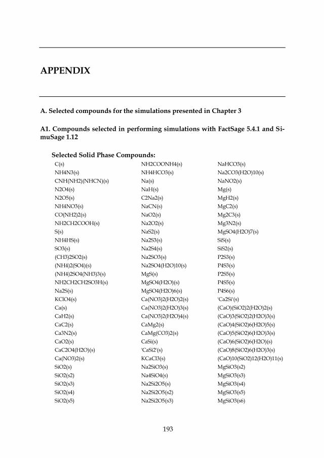
193
APPENDIX
A. Selected compounds for the simulations presented in Chapter 3
A1. Compounds selected in performing simulations with FactSage 5.4.1 and Si-muSage 1.12
Selected Solid Phase Compounds:
C(s) NH2COONH4(s) NaHCO3(s)
NH4N3(s) NH4HCO3(s) Na2CO3(H2O)10(s)
CNH(NH2)(NHCN)(s) Na(s) NaNO2(s)
N2O4(s) NaH(s) Mg(s)
N2O5(s) C2Na2(s) MgH2(s)
NH4NO3(s) NaCN(s) MgC2(s)
CO(NH2)2(s) NaO2(s) Mg2C3(s)
NH2CH2COOH(s) Na2O2(s) Mg3N2(s)
S(s) NaS2(s) MgSO4(H2O)7(s)
NH4HS(s) Na2S3(s) SiS(s)
SO3(s) Na2S4(s) SiS2(s)
(CH3)2SO2(s) Na2SO3(s) P2S3(s)
(NH4)2(SO4)(s) Na2SO4(H2O)10(s) P4S3(s)
(NH4)2SO4(NH3)3(s) MgS(s) P2S5(s)
NH2CH2CH2SO3H(s) MgSO4(H2O)(s) P4S5(s)
Na2S(s) MgSO4(H2O)6(s) P4S6(s)
KClO4(s) Ca(NO3)2(H2O)2(s) 'Ca2Si'(s)
Ca(s) Ca(NO3)2(H2O)3(s) (CaO)(SiO2)2(H2O)2(s)
CaH2(s) Ca(NO3)2(H2O)4(s) (CaO)3(SiO2)2(H2O)3(s)
CaC2(s) CaMg2(s) (CaO)4(SiO2)6(H2O)5(s)
Ca3N2(s) CaMg(CO3)2(s) (CaO)5(SiO2)6(H2O)3(s)
CaO2(s) CaSi(s) (CaO)6(SiO2)6(H2O)(s)
CaC2O4(H2O)(s) 'CaSi2'(s) (CaO)8(SiO2)6(H2O)3(s)
Ca(NO3)2(s) KCaCl3(s) (CaO)10(SiO2)12(H2O)11(s)
SiO2(s) Na2SiO3(s) MgSiO3(s2)
SiO2(s2) Na4SiO4(s) MgSiO3(s3)
SiO2(s3) Na2Si2O5(s) MgSiO3(s4)
SiO2(s4) Na2Si2O5(s2) MgSiO3(s5)
SiO2(s5) Na2Si2O5(s3) MgSiO3(s6)
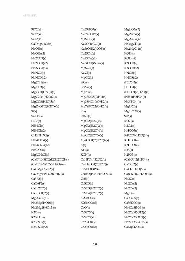
APPENDIX
194
SiO2(s6) Na6Si2O7(s) MgSiO3(s7)
SiO2(s7) Na6Si8O19(s) Mg2SiO4(s)
SiO2(s8) MgSiO3(s) Mg2SiO4(s2)
Ca3MgSi2O8(s) Na2OHNO3(s) NaMgCl3(s)
NaOH(s) Na3(OH)2(NO3)(s) Na2MgCl4(s)
NaOH(s2) Na2SO4(s) KOH(s)
Na2CO3(s) Na2SO4(s2) KOH(s2)
Na2CO3(s2) Na3(OH)(SO4)(s) K2CO3(s)
Na2CO3(s3) MgSO4(s) K2CO3(s2)
NaNO3(s) NaCl(s) KNO3(s)
NaNO3(s2) MgCl2(s) KNO3(s2)
Mg(OH)2(s) SiC(s) (P2O5)2(s)
MgCO3(s) Si3N4(s) H3PO4(s)
MgCO3(H2O)3(s) Mg2Si(s) (H3PO4)2(H2O)(s)
MgC2O4(H2O)2(s) Mg3Si2O5(OH)4(s) (NH4)H2PO4(s)
MgCO3(H2O)5(s) Mg3Si4O10(OH)2(s) Na3(PO4)(s)
Mg(NO3)2(H2O)6(s) Mg7Si8O22(OH)2(s) Mg3P2(s)
Si(s) P(s) Mg3P2O8(s)
Si2H6(s) P3N5(s) SiP(s)
P4S7(s) MgCl2(H2O)(s) KO2(s)
NH4Cl(s) MgCl2(H2O)2(s) K2O2(s)
NH4Cl(s2) MgCl2(H2O)4(s) KHCO3(s)
CH3NH3Cl(s) MgCl2(H2O)6(s) K4C2O6(H2O)3(s)
NH4ClO4(s) Mg(ClO4)2(H2O)6(s) KH2PO4(s)
NH4ClO4(s2) K(s) K2HPO4(s)
NaClO4(s) KH(s) K2S(s)
Mg(OH)Cl(s) KCN(s) K2SO3(s)
(CaO)10(SiO2)12(H2O)21(s) CaHPO4(H2O)2(s) (CaSO4)2(H2O)(s)
(CaO)12(SiO2)6(H2O)7(s) Ca(H2PO4)2(H2O)(s) CaOCl2(s)
CaOMgOSiO2(s) Ca5HO13P3(s) CaCl2(H2O)6(s)
Ca2Mg5Si8O22(OH)2(s) Ca8H2(PO4)6(H2O) (s) Ca(ClO4)2(H2O)4(s)
Ca3P2(s) CaS(s) Na2O(s)
CaO6P2(s) CaSO3(s) Na2O(s2)
Ca2P2O7(s) CaSO3(H2O)2(s) Na2O(s3)
Ca3(PO4)2(s) CaSO4(H2O)2(s) MgO(s)
Mg2SiO4(s3) K2Si4O9(s) Ca3SiO5(s)
Na2MgSi4O10(s) K2Si4O9(s2) Ca3Si2O7(s)
Na2Mg2Si6O15(s) CaO(s) Na4CaSi3O9(s)
K2O(s) CaSiO3(s) Na2CaSi5O12(s)
K2SiO3(s) CaSiO3(s2) Na2Ca2Si3O9(s)
K2Si2O5(s) Ca2SiO4(s) Na2Ca3Si6O16(s)
K2Si2O5(s2) Ca2SiO4(s2) CaMgSi2O6(s)
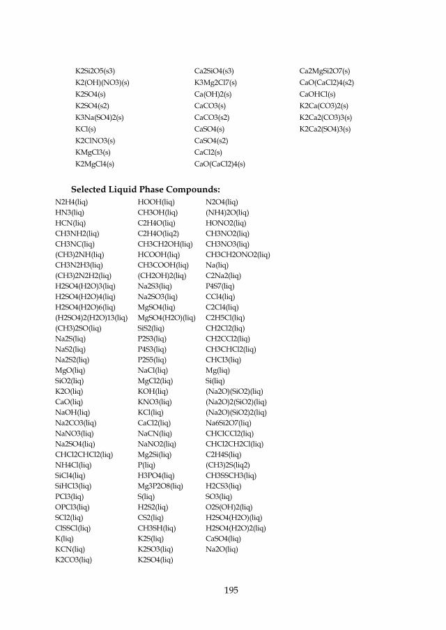
195
K2Si2O5(s3) Ca2SiO4(s3) Ca2MgSi2O7(s)
K2(OH)(NO3)(s) K3Mg2Cl7(s) CaO(CaCl2)4(s2)
K2SO4(s) Ca(OH)2(s) CaOHCl(s)
K2SO4(s2) CaCO3(s) K2Ca(CO3)2(s)
K3Na(SO4)2(s) CaCO3(s2) K2Ca2(CO3)3(s)
KCl(s) CaSO4(s) K2Ca2(SO4)3(s)
K2ClNO3(s) CaSO4(s2)
KMgCl3(s) CaCl2(s)
K2MgCl4(s) CaO(CaCl2)4(s)
Selected Liquid Phase Compounds:
N2H4(liq) HOOH(liq) N2O4(liq)
HN3(liq) CH3OH(liq) (NH4)2O(liq)
HCN(liq) C2H4O(liq) HONO2(liq)
CH3NH2(liq) C2H4O(liq2) CH3NO2(liq)
CH3NC(liq) CH3CH2OH(liq) CH3NO3(liq)
(CH3)2NH(liq) HCOOH(liq) CH3CH2ONO2(liq)
CH3N2H3(liq) CH3COOH(liq) Na(liq)
(CH3)2N2H2(liq) (CH2OH)2(liq) C2Na2(liq)
H2SO4(H2O)3(liq) Na2S3(liq) P4S7(liq)
H2SO4(H2O)4(liq) Na2SO3(liq) CCl4(liq)
H2SO4(H2O)6(liq) MgSO4(liq) C2Cl4(liq)
(H2SO4)2(H2O)13(liq) MgSO4(H2O)(liq) C2H5Cl(liq)
(CH3)2SO(liq) SiS2(liq) CH2Cl2(liq)
Na2S(liq) P2S3(liq) CH2CCl2(liq)
NaS2(liq) P4S3(liq) CH3CHCl2(liq)
Na2S2(liq) P2S5(liq) CHCl3(liq)
MgO(liq) NaCl(liq) Mg(liq)
SiO2(liq) MgCl2(liq) Si(liq)
K2O(liq) KOH(liq) (Na2O)(SiO2)(liq)
CaO(liq) KNO3(liq) (Na2O)2(SiO2)(liq)
NaOH(liq) KCl(liq) (Na2O)(SiO2)2(liq)
Na2CO3(liq) CaCl2(liq) Na6Si2O7(liq)
NaNO3(liq) NaCN(liq) CHClCCl2(liq)
Na2SO4(liq) NaNO2(liq) CHCl2CH2Cl(liq)
CHCl2CHCl2(liq) Mg2Si(liq) C2H4S(liq)
NH4Cl(liq) P(liq) (CH3)2S(liq2)
SiCl4(liq) H3PO4(liq) CH3SSCH3(liq)
SiHCl3(liq) Mg3P2O8(liq) H2CS3(liq)
PCl3(liq) S(liq) SO3(liq)
OPCl3(liq) H2S2(liq) O2S(OH)2(liq)
SCl2(liq) CS2(liq) H2SO4(H2O)(liq)
ClSSCl(liq) CH3SH(liq) H2SO4(H2O)2(liq)
K(liq) K2S(liq) CaSO4(liq)
KCN(liq) K2SO3(liq) Na2O(liq)
K2CO3(liq) K2SO4(liq)

APPENDIX
196
K2SiO3(liq) Ca(liq) K2Si2O5(liq) CaO6P2(liq)
K2Si4O9(liq) Ca2P2O7(liq)
Selected Gase Phase Compounds:
H2(g) C2H5N(g) C2H4O(g2)
C(g) O2(g) CH3CH2OH(g)
CH4(g) CO(g) HCOOH(g)
C2H4(g) CO2(g) CH3COOH(g)
C2H6(g) HCO(g) N2O(g)
N2(g) H2CO(g) NO2(g)
NH3(g) CH3OH(g) NO3(g)
HCN(g) CH2CO(g) HNO(g)
HNCO(g) CH3SSCH3(g) CH2CCl2(g)
S2(g) SO2(g) CH3CHCl2(g)
H2S(g) SO3(g) C2Cl5H(g)
CS(g) C2H4OS(g)
CS2(g) CCl4(g)
CH3SH(g) C2Cl6(g)
C2H4S(g) C6Cl6(g)
(CH3)2S(g2) CH3Cl(g)
Selected Aqueous Phase Compounds:
H[+](aq) NH3(aq) CH3NH3[+](aq)
H2(aq) NH4[+](aq) (CH3)2NH2[+](aq)
CH4(aq) N2H4(aq) O2(aq)
C2H2(aq) N2H5[+](aq) OH[-](aq)
C2H4(aq) HN3(aq) HO2[-](aq)
C2H6(aq) CN[-](aq) HOOH(aq)
N2(aq) HCN(aq) CO(aq)
N3[-](aq) CH3NH2(aq) CO2(aq)
Mg(C2O4)2[2-](aq) PH4[+](aq) HP2O7[3-](aq)
Mg(C2H3O2)[+](aq) PO4[3-](aq) H2P2O7[2-](aq)
MgHCO3[+](aq) P2O7[4-](aq) H3P2O7[-](aq)
Mg(NH2CH2COO)[+](aq) HPO3[2-](aq) H4P2O7(aq)
H2SiO3(aq) H2PO3[-](aq) (NH4)H2PO4(aq)
H4SiO4(aq) HPO4[2-](aq) MgP2O7[2-](aq)
HSi(OH)6[-](aq) H2PO4[-](aq) S[2-](aq)
PH3(aq) H3PO4(aq) S2[2-](aq)
CO3[2-](aq) CH3COOH(aq) (NH2)2CONH(aq)
C2O4[2-](aq) HCO3[-](aq) NH2CH2COO[-](aq)
CH3OH(aq) HC2O4[-](aq) NH2CH2COOH(aq)

197
C2H5O[-](aq) ONO[-](aq) CH2COOHNH3[+](aq)
CH3CH2OH(aq) N2O2[2-](aq) Na[+](aq)
HCOO[-](aq) NO3[-](aq) NaHCO3(aq)
HCOOH(aq) HONO(aq) Mg[2+](aq)
CH3COO[-](aq) CNO[-](aq) MgOH[+](aq)
S3[2-](aq) SO3[2-](aq) S4O6[2-](aq)
S4[2-](aq) SO4[2-](aq) S5O6[2-](aq)
S5[2-](aq) S2O3[2-](aq) HSO3[-](aq)
HS[-](aq) S2O4[2-](aq) HSO4[-](aq)
H2S(aq) S2O5[2-](aq) HS2O4[-](aq)
CNS[-](aq) S2O6[2-](aq) H2S2O4(aq)
HCNS(aq) S2O8[2-](aq) NH2CH2CH2SO3[-](aq)
SO2(aq) S3O6[2-](aq) NH2CH2CH2SO3H(aq)
MgSO4(aq) ClO3[-](aq) Ca(C2H3O2)[+](aq)
Cl[-](aq) ClO4[-](aq) CaSO4(aq)
Cl2(aq) HOCl(aq)
Cl3[-](aq) HClO2(aq)
CH3Cl(aq) ONCl(aq)
ClO[-](aq) K[+](aq)
ClO2[-](aq) Ca[2+](aq)
ClO2(aq) CaOH[+](aq)
A2. Simulation results using Kohler-Toop and Helgeson solution models for the subcritical region with FactSage 5.4.1 (section 3.1.2.3 Calculations in the sub-critical region).
Kohler-Toop model: Except from the aqueous solution database, the same da-tabases and temperature interval have been used for the calculations based on Kohler-Toop model. For the aqueous solution compounds, a new database has been created using the Kohler-Toop solution model feature of FactSage. The ther-modynamic data required for this new aqueous solution compounds have been acquired from the FACT53 database of the software.
Helgeson model: For the calculations based on Helgeson model, FThelg data-base has been used for the aqueous solution compounds. FThelg database of the software uses the thermodynamic properties provided by the SUPCRT92 software [170]. The database has thermodynamic data for 84 elements, 22 gaseous constitu-ents, 1343 dilute aqueous constituents, and 192 pure condensed phases. Three con-centration-dependent versions are included within the database: the ideal dilute solution model, the model with Debye–Hückel and Davies equations and the model with an extended Debye–Hückel and Davies equations [167]. The last one has been used for the calculations.

APPENDIX
198
Among 358 aqueous compounds, 56 of them have been selected for the calcula-tions. The criteria for the selection was to be consistent with the former 2 models by means of selecting the same aqueous compounds. To make the model more consistent within itself, instead of FACT53, FThelg database has been selected for solid carbon and 11 gas compounds: H2, CH4, C2H4, N2, NH3, O2, CO, CO2, H2S, S2, SO2. The SUPCRT92 software [170] has a temperature limitation of 350 °C for the ionic aqueous compounds. Besides, the simulations returned non-realistic results at temperatures higher than 350 °C. Thus, the temperature interval for this model has been chosen as 100 – 340 °C.
A2.1. Results and discussions
A2.1.1. Kohler-Toop model
Behavior of elements: The results for the Kohler-Toop model are given in Fig-ure A1 – Figure A10 which represent the results for 10 elements on compound and phase basis for the temperature region of 100 – 580 °C. Please note that for the temperature region of 100 – 389.6 °C, the calculations have been performed based on the aforementioned Kohler-Toop solution model and for the temperature re-gion of 390 – 580 °C, the calculations have been performed based on the aforemen-tioned supercritical region model. After performing numerous trial and error cal-culations, 367 °C has found to be the temperature which the phase transition of water is completed. Below this temperature, both liquid and vapor phase for water exist in an equilibrium, however above this temperature only vapor phase exists for water. The reason for a 22.6 °C of difference is that although Kohler-Toop solu-tion model feature of FactSage takes into account of the effect of gases on the de-crease of phase transition temperature of water, it does not take into account of the effect of ions on the increase of phase transition temperature for water. Thus, it can be stated that at 240 bars the formation of gases decreases the pseudo-critical point of water from 381.2 °C [12] to 367 °C, whereas the formation of ions increases to 389.6 °C. To make the two models in consistent with each other, 389.6 °C has been accepted to be the phase transition temperature for Kohler-Toop model as well. The results do not include the elements H and O as the great majority of these two elements form H2O either in liquid or gas state.
The results show that molar fractions of elements are in agreement with the Henrian model (see Figure 3.3 – Figure 3.12) except for the temperatures between 367 °C and 389.6 °C. The reason for this difference is that in Kohler-Toop model phase transition for water completes at 367 °C. Unlike Henrian and Helgeson model, Kohler-Toop model performs calculations assuming that liquid water and the other aqueous compounds form a multicomponent solution where the water is not a solvent but a part of the solution instead. From 367 °C to 389.6 °C as there is no liquid water, the reactions in gas phase and the nature of aqueous solution change which causes irrationalities in results such as having aqueous species at

199
380 and 389.6 °C although there is no liquid water in the system. For this reason, the results at these temperatures will not be discussed.
Figure A1 shows the molar fractions of carbon compounds in Kohler-Toop model. The results show that for the temperature region of 100 – 300 °C, the two models are in a very good agreement with each other. At temperatures 340 °C and 360 °C, there is a remarkable difference for aqueous and gas methane. Although the sum of these two compounds are the same for both models, Kohler-Toop mod-el gives less gas methane and more aqueous methane as a result. The difference between the two models are more likely due to the rapid decrease in liquid water amount at these temperatures which causes a change in the nature of aqueous so-lution. Another explanation could be the difference in aqueous methane databases as the Henrian model uses the Gibbs free energy data obtained by Helgeson EOS results at 240 bars.
Figure A2 shows the molar fractions of calcium compounds in Kohler-Toop model. Hydroxyapatite is the only stable compound for the temperature region of 100 – 360 °C. The only difference between the Henrian model is the shift in the formation temperature of devitrite. In Kohler-Toop model, devitrite is formed at 380 °C and 389.6 °C, whereas in Henrian model it is only at 360 °C. This can be ex-plained by the difference in sodium ion concentration in aqueous solution phase for the temperature region of 360 – 389.6 °C (see Figure A7).
Figure A3 and Figure A4 show the molar fractions of chloride and potassium compounds in Kohler-Toop model, respectively. Like the Henrian model, the only stable compound of these elements are the ionic forms in aqueous solution for the temperature region of 100 – 360 °C.
Figure A5 shows the molar fractions of magnesium compounds in Kohler-Toop model. Both Henrian and Kohler-Toop model have the same results on compound and amount basis for the temperature region of 100 – 340 °C. At 360 °C, there is a significant difference between the molar amounts of talc and chrysot between the models. Although there is not any magnesium compound which is formed with the contribution of sodium, the reason for this difference comes from the ionic so-dium amount difference at 360 °C (see Figure 3.9 and Figure A7). This difference results in the formation of devitrite in Henrian model which causes the change in silicon compounds (see Figure 3.12 and Figure A10) in these two models. As both talc and chrysot are stable magnesium-silicon compounds at 360 °C, their amount are affected by the change in silicon amount.
Figure A6 shows the molar fractions of nitrogen compounds in Kohler-Toop model. The results show that the two models have similar trends for the formed compounds for the temperature region of 100 – 360 °C and the amount of nitrogen gas and aqueous nitrogen are less than 10% different than the Henrian model. In Kohler-Toop model, the aqueous nitrogen amount is higher at 100 °C, however be-tween the temperatures 150 – 360 °C it is lower.
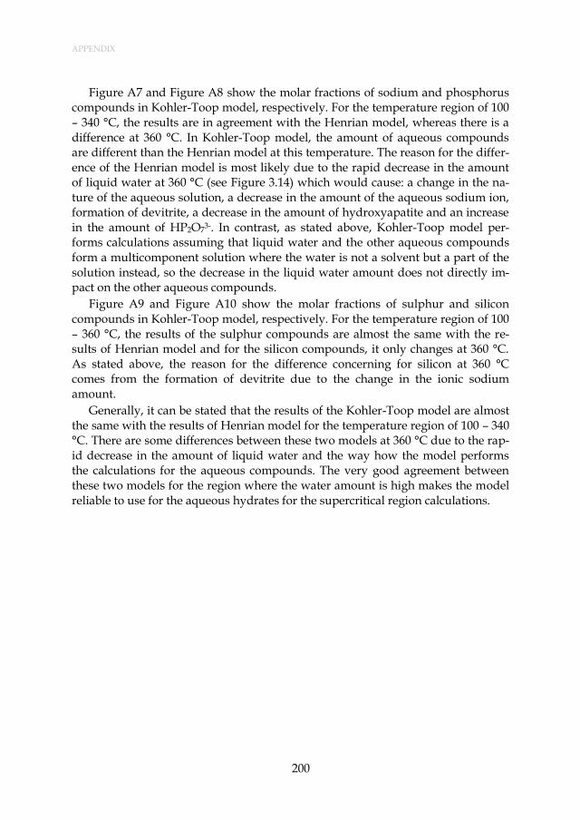
APPENDIX
200
Figure A7 and Figure A8 show the molar fractions of sodium and phosphorus compounds in Kohler-Toop model, respectively. For the temperature region of 100 – 340 °C, the results are in agreement with the Henrian model, whereas there is a difference at 360 °C. In Kohler-Toop model, the amount of aqueous compounds are different than the Henrian model at this temperature. The reason for the differ-ence of the Henrian model is most likely due to the rapid decrease in the amount of liquid water at 360 °C (see Figure 3.14) which would cause: a change in the na-ture of the aqueous solution, a decrease in the amount of the aqueous sodium ion, formation of devitrite, a decrease in the amount of hydroxyapatite and an increase in the amount of HP2O7
3-. In contrast, as stated above, Kohler-Toop model per-forms calculations assuming that liquid water and the other aqueous compounds form a multicomponent solution where the water is not a solvent but a part of the solution instead, so the decrease in the liquid water amount does not directly im-pact on the other aqueous compounds.
Figure A9 and Figure A10 show the molar fractions of sulphur and silicon compounds in Kohler-Toop model, respectively. For the temperature region of 100 – 360 °C, the results of the sulphur compounds are almost the same with the re-sults of Henrian model and for the silicon compounds, it only changes at 360 °C. As stated above, the reason for the difference concerning for silicon at 360 °C comes from the formation of devitrite due to the change in the ionic sodium amount.
Generally, it can be stated that the results of the Kohler-Toop model are almost the same with the results of Henrian model for the temperature region of 100 – 340 °C. There are some differences between these two models at 360 °C due to the rap-id decrease in the amount of liquid water and the way how the model performs the calculations for the aqueous compounds. The very good agreement between these two models for the region where the water amount is high makes the model reliable to use for the aqueous hydrates for the supercritical region calculations.

201
Figure A1: Mole fractions of carbon compounds during SCW gasification of ma-nure at 24 MPa with a water weight fraction of 80% at different temperatures. The results for the subcritical region are based on the aforementioned Kohler-Toop model.
Figure A2: Mole fractions of calcium compounds during SCW gasification of ma-nure at 24 MPa with a water weight fraction of 80% at different temperatures. The results for the subcritical region are based on the aforementioned Kohler-Toop model.
0%
20%
40%
60%
80%
100%
100 150 200 250 300 340 360 380 389.60 390 400 420 460 500 540 580
Temperature (°C)
Mole Fractions of Carbon CO₂ (aq) HCO₃⁻ (aq) C_graphite(s)
CO₂ (g) MgCO₃ (s) NaHCO₃ (aq) CH₄ (aq) CH₄ (g) CO(g)
0%
20%
40%
60%
80%
100%
100 150 200 250 300 340 360 380 389.60 390 400 420 460 500 540 580
Temperature (°C)
Mole Fractions of Calcium
Ca₅HO₁₃P₃_hdroxyapat(s) Na₂Ca₃Si₆O₁₆(s)
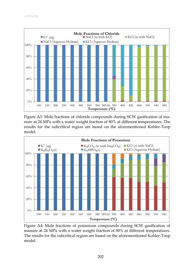
APPENDIX
202
Figure A3: Mole fractions of chloride compounds during SCW gasification of ma-nure at 24 MPa with a water weight fraction of 80% at different temperatures. The results for the subcritical region are based on the aforementioned Kohler-Toop model.
Figure A4: Mole fractions of potassium compounds during SCW gasification of manure at 24 MPa with a water weight fraction of 80% at different temperatures. The results for the subcritical region are based on the aforementioned Kohler-Toop model.
0%
20%
40%
60%
80%
100%
100 150 200 250 300 340 360 380 389.60 390 400 420 460 500 540 580Temperature (°C)
Mole Fractions of Chloride Cl⁻ (aq) NaCl (ss with KCl) KCl (ss with NaCl)
NaCl (Aqueous Hydrate) KCl (Aqueous Hydrate)
0%
20%
40%
60%
80%
100%
100 150 200 250 300 340 360 380 389.60 390 400 420 460 500 540 580
Temperature (°C)
Mole Fractions of Potassium
K⁺ (aq) K₂CO₃ (ss with Na₂CO₃) KCl (ss with NaCl)
K₂Si₂O₅(s) K₂HPO₄(s) KCl (Aqueous Hydrate)

203
Figure A5: Mole fractions of magnesium compounds during SCW gasification of manure at 24 MPa with a water weight fraction of 80% at different temperatures. The results for the subcritical region are based on the aforementioned Kohler-Toop model.
Figure A6: Mole fractions of nitrogen compounds during SCW gasification of ma-nure at 24 MPa with a water weight fraction of 80% at different temperatures. The results for the subcritical region are based on the aforementioned Kohler-Toop model.
0%
20%
40%
60%
80%
100%
100 150 200 250 300 340 360 380 389.60 390 400 420 460 500 540 580
Temperature (°C)
Mole Fractions of Magnesium MgP₂O₇²⁻ (aq) MgCO₃_magnesite(s) Mg₃Si₄O₁₀(OH)₂_talc(s)
Mg₂SiO₄_forsterite(s) Mg₃Si₂O₅(OH)₄_chrysot(s)
0%
20%
40%
60%
80%
100%
100 150 200 250 300 340 360 380 389.60 390 400 420 460 500 540 580
Temperature (°C)
Mole Fractions of Nitrogen
N₂ (aq) NH₃ (aq) NH₄⁺ (aq) N₂ (g) NH₃ (g)

APPENDIX
204
Figure A7: Mole fractions of sodium compounds during SCW gasification of ma-nure at 24 MPa with a water weight fraction of 80% at different temperatures. The results for the subcritical region are based on the aforementioned Kohler-Toop model.
Figure A8: Mole fractions of phosphorus compounds during SCW gasification of manure at 24 MPa with a water weight fraction of 80% at different temperatures. The results for the subcritical region are based on the aforementioned Kohler-Toop model.
0%
20%
40%
60%
80%
100%
100 150 200 250 300 340 360 380 389.60 390 400 420 460 500 540 580
Temperature (°C)
Mole Fractions of Sodium
Na⁺ (aq) NaHCO₃ (aq) Na₂Ca₃Si₆O₁₆(s)
Na₂CO₃ (ss with K₂CO₃) NaCl (ss with KCl) NaCl (aqueous hydrate)
Na₂CO₃ (aqueous hydrate) Na₃(PO4)(s)
0%
20%
40%
60%
80%
100%
100 150 200 250 300 340 360 380 389.60 390 400 420 460 500 540 580
Temperature (°C)
Behaviour of Phosporus
HPO₄²⁻(aq) HP₂O₇³⁻ (aq) H₂P₂O₇²⁻ (aq) MgP₂O₇²⁻ (aq) Ca₅HO₁₃P₃_hdroxyapat(s) K₂HPO₄(s) Na₃(PO₄)(s)

205
Figure A9: Mole fractions of sulphur compounds during SCW gasification of ma-nure at 24 MPa with a water weight fraction of 80% at different temperatures. The results for the subcritical region are based on the aforementioned Kohler-Toop model.
Figure A10: Mole fractions of silicon compounds during SCW gasification of ma-nure at 24 MPa with a water weight fraction of 80% at different temperatures. The results for the subcritical region are based on the aforementioned Kohler-Toop model.
0%
20%
40%
60%
80%
100%
100 150 200 250 300 340 360 380 389.60 390 400 420 460 500 540 580
Temperature (°C)
Behaviour of Sulphur
H₂SO₄(H₂O)₆(liq) HS⁻ (aq) H₂S (g) S²⁻ (aq) H₂S (aq)
0%
20%
40%
60%
80%
100%
100 150 200 250 300 340 360 380 389.60 390 400 420 460 500 540 580Temperature (°C)
Behaviour of Silicon H₂SiO₃ (aq) H₄SiO₄ (aq) SiO₂_quartz(s) Mg₃Si₄O₁₀(OH)₂_talc(s) Mg₃Si₂O5(OH)4_chrysot(s) Na₂Ca₃Si₆O₁₆(s)

APPENDIX
206
A2.1.2. Helgeson model
Behavior of elements: The results for the Helgeson model are given in Figure A11 - Figure A20 which represent the results for 10 elements on compound and phase basis for the temperature region of 100 – 340 °C and 390 – 580 °C. Please note that for the temperature region of 100 – 340 °C, the calculations have been performed based on the aforementioned Helgeson aqueous solution model and for the temperature region of 390 – 580 °C, the calculations have been performed based on the aforementioned supercritical region model. The results do not in-clude the elements H and O as the great majority of these two elements form H2O either in liquid or gas state.
Figure A11 shows the molar fractions of carbon compounds in Helgeson mod-el. The results are significantly different from the other two models. First of all, aqueous NaHCO3 is not formed at 100 °C with this model. The reason is that in FThelg database NaHCO3 is not defined. Secondly, the amount of dissolved gases in the aqueous phase are significantly higher in this model as Helgeson EOS takes the effect of pressure on thermodynamic properties into account [170] which re-sults in different Gibbs free energy values and activity coefficients for aqueous compounds. Furthermore, the amount of solid carbon and the total amount of car-bon dioxide and methane in aqueous and gas phases are in a very good agreement with the other two models. This is an indication of how the effect of pressure on the thermodynamic properties of aqueous and gaseous compounds are significant and how this effect is insignificant for the solid compounds.
Figure A12, Figure A13 and Figure A14 show the molar fractions of calcium, chloride and potassium compounds in Helgeson model, respectively. The results are the same with the other two models for the temperature region of 100-340 °C.
Figure A15 shows the molar fractions of magnesium compounds in Helgeson model. For the temperature region of 100 – 200 °C, the results are the same with the other two models except for the ionic magnesium compound. As MgP2O7
2- is not defined in FThelg database, the ionic magnesium compound is the magnesium ion (Mg2+) itself in Helgeson model. It seems that the trend in the other two mod-els is shifted to lower temperatures in Helgeson model which the formation of talc is observed at 250 °C and chrysot is at 340 °C. The reason for the difference comes from the change in the amount of magnesium carbonate. As the FThelg database has been used for the rest of the carbon compounds, the equilibrium within the carbon compounds has changed which resulted in a change in magnesium car-bonate amount, thus changed the equilibrium within the magnesium compounds.
Figure A16 shows the molar fractions of nitrogen compounds in Helgeson model. The results show that there are significant differences between the Helge-son model and the other two models. The amount of dissolved nitrogen gases in aqueous phase (N2 (aq) and NH3 (aq)) are significantly higher in Helgeson model due to the usage of Helgeson EOS.

207
Figure A17 shows the molar fractions of sodium compounds in Helgeson mod-el. The results are in an agreement with the other two models in a way that sodium is only stable in aqueous phase. As the FThelg database does not have thermody-namic data for the aqueous sodium bicarbonate, sodium is only stable in ionic form (Na+) for the temperature region of 100 – 340 °C.
Figure A18 shows the molar fractions of phosphorus compounds in Helgeson model. The results show that the total amount of aqueous phase in all of the mod-els are the same, however, the amount and type of compounds are different. There two reasons for the difference: i) in FThelg database MgP2O7
2- is not defined and in FACT53 database, H2PO4
- and P2O74- are not defined and ii) using Helgeson EOS
results in difference in the equilibrium composition of these aqueous compounds.
Figure A19 shows the molar fractions of sulphur compounds in Helgeson model. The results show that for the temperature region of 100 – 200 °C, sulphuric acid hexahydrate is also the only stable sulphur compound in Helgeson model. Compared to the other two models, the decomposition of sulphuric acid to aque-ous sulphur compounds is higher at 250 °C. At 300 °C, the amount of hydrogen sulfide gas is significantly lower and at 340 °C hydrogen sulfide ion is the most stable aqueous sulphur compounds. For the temperature region of 250 – 340 °C, hydrogen sulfide amount in the aqueous phase is significantly higher. The lack of ionic sulphur data in FThelg database and using Helgeson EOS are the reasons for these significant differences.
Figure A20 shows the molar fractions of silicon compounds in Helgeson model. The results show that for the temperature region of 100 – 250 °C, quartz is the only stable silicon compound and at 300 °C talc is the only stable silicon compound as silicic acid compounds are not defined in FThelg database. Compared to the other two models, the formation of chrysot is shifted from 360 °C to 340 °C in Helgeson model. The difference at this temperature is due to the change in MgCO3 amount as stated above.
Generally, it can be stated that there are significant differences in the molar fractions of some elements as the Helgeson model uses Helgeson EOS which is more accurate for high temperature and high pressure aqueous compounds. In contrast to the other two models, Helgeson EOS takes the effect of pressure on thermodynamic properties into account which results in different Gibbs free ener-gy values and activity coefficients for aqueous compounds. The other reason is that FThelg database of FactSage does not include all of the aqueous species of FACT53 database or vice versa.

APPENDIX
208
Figure A11: Mole fractions of carbon compounds during SCW gasification of ma-nure at 24 MPa with a water weight fraction of 80% at different temperatures. The results for the subcritical region are based on the aforementioned Helgeson model.
Figure A12: Mole fractions of calcium compounds during SCW gasification of ma-nure at 24 MPa with a water weight fraction of 80% at different temperatures. The results for the subcritical region are based on the aforementioned Helgeson model.
0%
20%
40%
60%
80%
100%
100 150 200 250 300 340 360 380 389.60 390 400 420 460 500 540 580
Temperature (°C)
Mole Fractions of Carbon CO₂ (aq) HCO₃⁻ (aq) C_graphite(s) CO₂ (g)
MgCO₃ (s) CH₄ (aq) CH₄ (g) CO(g)
0%
20%
40%
60%
80%
100%
100 150 200 250 300 340 360 380 389.60 390 400 420 460 500 540 580
Temperature (°C)
Mole Fractions of Calcium
Ca₅HO₁₃P₃_hdroxyapat(s)
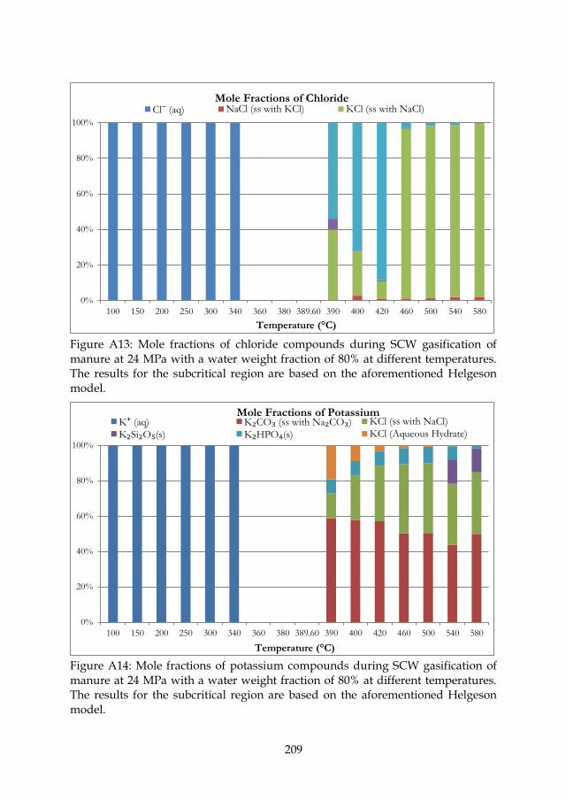
209
Figure A13: Mole fractions of chloride compounds during SCW gasification of manure at 24 MPa with a water weight fraction of 80% at different temperatures. The results for the subcritical region are based on the aforementioned Helgeson model.
Figure A14: Mole fractions of potassium compounds during SCW gasification of manure at 24 MPa with a water weight fraction of 80% at different temperatures. The results for the subcritical region are based on the aforementioned Helgeson model.
0%
20%
40%
60%
80%
100%
100 150 200 250 300 340 360 380 389.60 390 400 420 460 500 540 580
Temperature (°C)
Mole Fractions of Chloride Cl⁻ (aq) NaCl (ss with KCl) KCl (ss with NaCl)
0%
20%
40%
60%
80%
100%
100 150 200 250 300 340 360 380 389.60 390 400 420 460 500 540 580
Temperature (°C)
Mole Fractions of Potassium K⁺ (aq) K₂CO₃ (ss with Na₂CO₃) KCl (ss with NaCl)
K₂Si₂O₅(s) K₂HPO₄(s) KCl (Aqueous Hydrate)
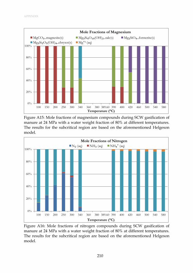
APPENDIX
210
Figure A15: Mole fractions of magnesium compounds during SCW gasification of manure at 24 MPa with a water weight fraction of 80% at different temperatures. The results for the subcritical region are based on the aforementioned Helgeson model.
Figure A16: Mole fractions of nitrogen compounds during SCW gasification of manure at 24 MPa with a water weight fraction of 80% at different temperatures. The results for the subcritical region are based on the aforementioned Helgeson model.
0%
20%
40%
60%
80%
100%
100 150 200 250 300 340 360 380 389.60 390 400 420 460 500 540 580
Temperature (°C)
Mole Fractions of Magnesium
MgCO₃_magnesite(s) Mg₃Si₄O₁₀(OH)₂_talc(s) Mg₂SiO₄_forsterite(s)
Mg₃Si₂O₅(OH)₄_chrysot(s) Mg⁺² (aq)
0%
20%
40%
60%
80%
100%
100 150 200 250 300 340 360 380 389.60 390 400 420 460 500 540 580
Temperature (°C)
Mole Fractions of Nitrogen
N₂ (aq) NH₃ (aq) NH₄⁺ (aq)

211
Figure A17: Mole fractions of sodium compounds during SCW gasification of ma-nure at 24 MPa with a water weight fraction of 80% at different temperatures. The results for the subcritical region are based on the aforementioned Helgeson model.
Figure A18: Mole fractions of phosphorus compounds during SCW gasification of manure at 24 MPa with a water weight fraction of 80% at different temperatures. The results for the subcritical region are based on the aforementioned Helgeson model.
0%
20%
40%
60%
80%
100%
100 150 200 250 300 340 360 380 389.60 390 400 420 460 500 540 580Temperature (°C)
Mole Fractions of Sodium Na⁺ (aq) Na₂CO₃ (ss with K₂CO₃) NaCl (ss with KCl)
NaCl (aqueous hydrate) Na₂CO₃ (aqueous hydrate) Na₃(PO4)(s)
0%
20%
40%
60%
80%
100%
100 150 200 250 300 340 360 380 389.60 390 400 420 460 500 540 580
Temperature (°C)
Behaviour of Phosporus HPO₄²⁻(aq) HP₂O₇³⁻ (aq) H₂P₂O₇²⁻ (aq)
Ca₅HO₁₃P₃_hdroxyapat(s) K₂HPO₄(s) Na₃(PO₄)(s)
H₂PO₄⁻ (aq) P₂O₇⁴⁻ (aq)

APPENDIX
212
Figure A19: Mole fractions of sulphur compounds during SCW gasification of ma-nure at 24 MPa with a water weight fraction of 80% at different temperatures. The results for the subcritical region are based on the aforementioned Helgeson model.
Figure A20: Mole fractions of silicon compounds during SCW gasification of ma-nure at 24 MPa with a water weight fraction of 80% at different temperatures. The results for the subcritical region are based on the aforementioned Helgeson model.
0%
20%
40%
60%
80%
100%
100 150 200 250 300 340 360 380 389.60 390 400 420 460 500 540 580
Temperature (°C)
Behaviour of Sulphur
H₂SO₄(H₂O)₆(liq) HS⁻ (aq) H₂S (g) H₂S (aq)
0%
20%
40%
60%
80%
100%
100 150 200 250 300 340 360 380 389.60 390 400 420 460 500 540 580
Temperature (°C)
Behaviour of Silicon SiO₂_quartz(s) Mg₃Si₄O₁₀(OH)₂_talc(s) Mg₃Si₂O5(OH)4_chrysot(s)
K₂Si₂O₅(s) Mg₂SiO4_forsterite(s) SiO₂ (aqueous hydrate)
HSiO₃⁻ (aq)

213
A2.2. Conclusions
Henrian and Kohler-Toop models are in a very good agreement for the tem-perature region of 100 – 340 °C. There are some differences between these two models at 360 °C due to the rapid decrease in the amount of liquid water and the way how the Kohler-Toop model performs the calculations for the aqueous com-pounds. The agreement between the Kohler-Toop and the other models for the re-gion where the water amount is high (100 – 340 °C) makes the Kohler-Toop model reliable to use for the aqueous hydrates for the supercritical region calculations.
The results of the Helgeson model for some of the compounds are significantly different from the other two models as the Helgeson model uses FThelg database and Helgeson EOS for the calculations.
Taking the effect of pressure on thermodynamic properties of aqueous com-pounds makes Helgeson model more realistic for the subcritical region. However, as Helgeson EOS has a temperature limitation of 350 °C for the aqueous ionic compounds, the temperature region of 350 – 389.6 °C remains as a mystery for this model. Even the results at temperatures between 340 and 350 °C show irrationali-ties for some of the compounds. On the other hand, for the temperature region of 367 – 389.6 °C, also the Kohler-Toop model gives irrational results. These con-straints make the Henrian model the only applicable model for the temperature region of 340 – 389.6 °C. One can consider using the Helgeson model for the region of 100 – 340 °C and the Henrian model for the region of 340 – 389.6 °C.
A3. Compounds selected in performing simulations with the developed thermodynamic equilibrium model
Selected Pure Condensed Phase Compounds:
C(s) NH4HCO3(s) Na2CO3(H2O)10(s)
NaCl(s) Na(s) NaNO2(s)
NH4N3(s) NaH(s) Mg(s)
CNH(NH2)(NHCN)(s) C2Na2(s) MgH2(s)
N2O4(s) NaCN(s) MgC2(s)
N2O5(s) NaO2(s) Mg2C3(s)
NH4NO3(s) Na2O2(s) Mg3N2(s)
CO(NH2)2(s) NaHCO3(s) Mg(OH)2(s)
S(s) NaS2(s) SiS(s)
NH4HS(s) Na2S3(s) SiS2(s)
SO3(s) Na2S4(s) P2S3(s)
(CH3)2SO2(s) Na2SO3(s) P4S3(s)
(NH4)2(SO4)(s) Na2SO4(H2O)10(s) P2S5(s)
(NH4)2SO4(NH3)3(s) MgS(s) P4S5(s)
NH2CH2CH2SO3H(s) MgSO4(H2O)6(s) P4S6(s)
Na2S(s) MgSO4(H2O)7(s) P4S7(s)
KClO4(s2) Ca(NO3)2(H2O)2(s) (CaO)(SiO2)2(H2O)2(s)
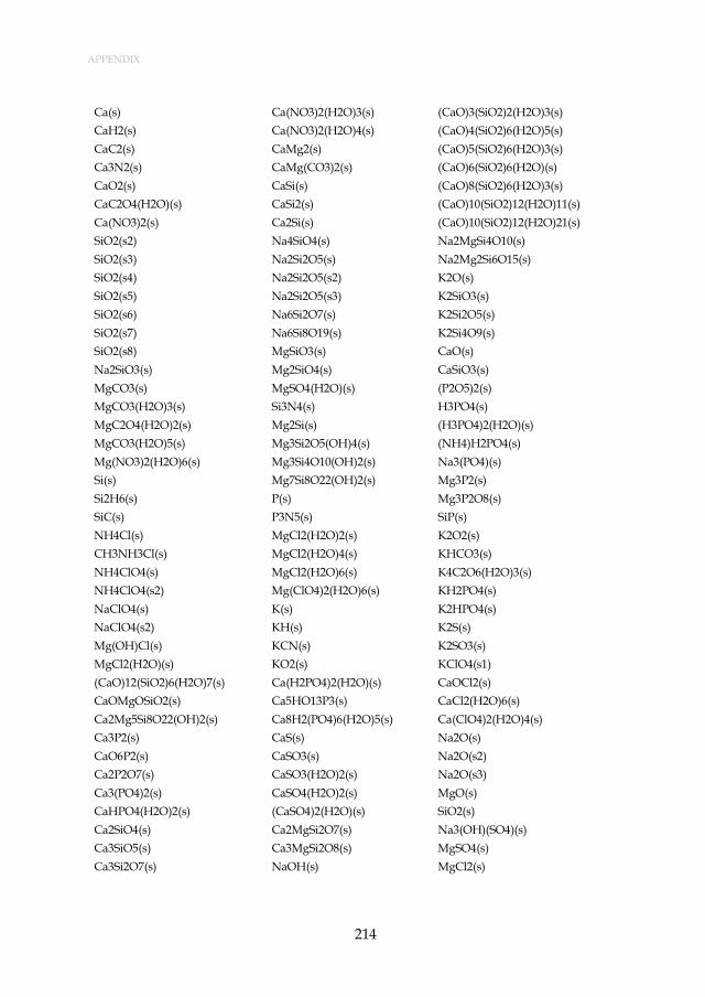
APPENDIX
214
Ca(s) Ca(NO3)2(H2O)3(s) (CaO)3(SiO2)2(H2O)3(s)
CaH2(s) Ca(NO3)2(H2O)4(s) (CaO)4(SiO2)6(H2O)5(s)
CaC2(s) CaMg2(s) (CaO)5(SiO2)6(H2O)3(s)
Ca3N2(s) CaMg(CO3)2(s) (CaO)6(SiO2)6(H2O)(s)
CaO2(s) CaSi(s) (CaO)8(SiO2)6(H2O)3(s)
CaC2O4(H2O)(s) CaSi2(s) (CaO)10(SiO2)12(H2O)11(s)
Ca(NO3)2(s) Ca2Si(s) (CaO)10(SiO2)12(H2O)21(s)
SiO2(s2) Na4SiO4(s) Na2MgSi4O10(s)
SiO2(s3) Na2Si2O5(s) Na2Mg2Si6O15(s)
SiO2(s4) Na2Si2O5(s2) K2O(s)
SiO2(s5) Na2Si2O5(s3) K2SiO3(s)
SiO2(s6) Na6Si2O7(s) K2Si2O5(s)
SiO2(s7) Na6Si8O19(s) K2Si4O9(s)
SiO2(s8) MgSiO3(s) CaO(s)
Na2SiO3(s) Mg2SiO4(s) CaSiO3(s)
MgCO3(s) MgSO4(H2O)(s) (P2O5)2(s)
MgCO3(H2O)3(s) Si3N4(s) H3PO4(s)
MgC2O4(H2O)2(s) Mg2Si(s) (H3PO4)2(H2O)(s)
MgCO3(H2O)5(s) Mg3Si2O5(OH)4(s) (NH4)H2PO4(s)
Mg(NO3)2(H2O)6(s) Mg3Si4O10(OH)2(s) Na3(PO4)(s)
Si(s) Mg7Si8O22(OH)2(s) Mg3P2(s)
Si2H6(s) P(s) Mg3P2O8(s)
SiC(s) P3N5(s) SiP(s)
NH4Cl(s) MgCl2(H2O)2(s) K2O2(s)
CH3NH3Cl(s) MgCl2(H2O)4(s) KHCO3(s)
NH4ClO4(s) MgCl2(H2O)6(s) K4C2O6(H2O)3(s)
NH4ClO4(s2) Mg(ClO4)2(H2O)6(s) KH2PO4(s)
NaClO4(s) K(s) K2HPO4(s)
NaClO4(s2) KH(s) K2S(s)
Mg(OH)Cl(s) KCN(s) K2SO3(s)
MgCl2(H2O)(s) KO2(s) KClO4(s1)
(CaO)12(SiO2)6(H2O)7(s) Ca(H2PO4)2(H2O)(s) CaOCl2(s)
CaOMgOSiO2(s) Ca5HO13P3(s) CaCl2(H2O)6(s)
Ca2Mg5Si8O22(OH)2(s) Ca8H2(PO4)6(H2O)5(s) Ca(ClO4)2(H2O)4(s)
Ca3P2(s) CaS(s) Na2O(s)
CaO6P2(s) CaSO3(s) Na2O(s2)
Ca2P2O7(s) CaSO3(H2O)2(s) Na2O(s3)
Ca3(PO4)2(s) CaSO4(H2O)2(s) MgO(s)
CaHPO4(H2O)2(s) (CaSO4)2(H2O)(s) SiO2(s)
Ca2SiO4(s) Ca2MgSi2O7(s) Na3(OH)(SO4)(s)
Ca3SiO5(s) Ca3MgSi2O8(s) MgSO4(s)
Ca3Si2O7(s) NaOH(s) MgCl2(s)

215
Na4CaSi3O9(s) Na2CO3(s) NaMgCl3(s)
Na2CaSi5O12(s) NaNO3(s) Na2MgCl4(s)
Na2Ca2Si3O9(s) Na2OHNO3(s) KOH(s)
Na2Ca3Si6O16(s) Na3(OH)2(NO3)(s) K2CO3(s)
CaMgSi2O6(s) Na2SO4(s) KNO3(s)
K2(OH)(NO3)(s) Ca(OH)2(s) K2Ca2(SO4)3(s)
K2SO4(s) CaCO3(s) KCaCl3(s)
K3Na(SO4)2(s) CaSO4(s) H3PO4(liq)
KCl(s) CaCl2(s) H2SO4(H2O)(liq)
K2ClNO3(s) CaO(CaCl2)4(s) H2SO4(H2O)2(liq)
KMgCl3(s) CaOHCl(s) H2SO4(H2O)3(liq)
K2MgCl4(s) K2Ca(CO3)2(s) H2SO4(H2O)4(liq)
K3Mg2Cl7(s) K2Ca2(CO3)3(s) H2SO4(H2O)6(liq)
Selected Gase Phase Compounds:
H2O(g) H2S(g)
H2(g) C2H4(g)
O2(g) C2H6(g)
CH4(g) C3H6(g)
CO(g) C3H8(g)
CO2(g)
N2(g)
NH3(g)
Selected Solution Phase Compounds:
H2O ClO3- H2PO4-
Ca+2 ClO4- H3P2O7-
CaCl+ CN- HCO2-
CaHCO3+ CO3-2 HCO3-
CaOH+ H+ HO2-
Cl- H2P2O7-2 HP2O7-3
ClO- H2PO2- HPO3-2
ClO2- H2PO3- HPO4-2
HS- KSO4- NO3-
HS2O3- Mg+2 OH-
HS2O4- MgCl+ P2O7-4
HSiO3- MgOH+ PO4-3
HSO3- Na+ S2-2
HSO4- NaSO4- S2O3-2
HSO5- NH4+ S2O4-2
K+ NO2- 2O5-2
S2O6-2 SO3-2 H2(aq)
APPENDIX
216
S2O8-2 SO4-2 H2S(aq)
S3-2 CaCl2(aq) H2S2O3(aq)
S3O6-2 CaCO3(aq) H2S2O4(aq)
S4-2 CaSO4(aq) H3PO2(aq)
S4O6-2 CH4(aq) H3PO3(aq)
S5-2 CO(aq) H3PO4(aq)
S5O6-2 CO2(aq) HClO(aq)
HCN(aq) NaHSiO3(aq)
HNO3(aq) NaOH(aq)
KCl(aq) NH3(aq)
KHSO4(aq) O2(aq)
KOH(aq) SiO2(aq)
MgCO3(aq) SO2(aq)
N2(aq)
NaCl(aq)
Selected Aqueous Hydrate Complexes:
NaCl(aq) KH2PO4(aq)
KCl(aq) MgSO4(aq)
NaNO3(aq) Na2SO4(aq)
KNO3(aq) Na2CO3(aq)
MgCl2(aq) SiO2(aq)
CaCl2(aq) KOH(aq)

217
APPENDIX B. Algae case input details for the simulations performed in Chap-ter 4
Table B1. Elemental compositions of the algae sample (Nannochloropsis sp.) used as an input for the simulations given in section “4.3.3. Algae case”.
Component Mole Input Mass (g)
(C) Carbon 36.05329 433.0253
(H) Hydrogen 59.527 59.99964
(O) Oxygen 15.6875 250.9906
(N) Nitrogen 4.571 64.02463
(S) Sulfur 0.156 5.00214
(Ca) Calcium 1.871351 75
(Cl) Chlorine 1.833413 65
(K) Potassium 0.383648 15
(Mg) Magnesium 0.411438 10
(Na) Sodium 0.086995 2
(P) Phosphorus 0.628178 19.457
(Si) Silicon 0.017803 0.5
Please note that the mole input for C, H, O, N and S elements is from the au-thors’ work [247] and the remaining elements are based on the composition given in [115].
Table B.2. Selected gas phase compounds
H2O CH4 N2 C2H6
H2 CO NH3 SO2
O2 CO2 H2S

APPENDIX
218
Table B.3. Selected liquid phase compounds
Formic Acid (CH2O2)
Oxalic Acid
(H2C2O4) Aspartic Ac-id (C4H7NO4)
Glutamine (C5H10N2O3)
Lysine
(C6H14N2O2) Thymine (C5H6N2O2)
Acetaldehyde (C2H4O)
Phenol
(C6H6O) Cysteine (C3H7NO2S)
Glycine
(C2H5NO2)
Lyxose
(C5H10O8) Valine (C5H11NO2)
Acetic Acid (C2H4O2)
Propanoic Ac-id (C3H6O2)
Cytidine (C9H13N3O5)
Glycolic-Acid (C2H4O3)
m-Cresol (C6H4OHCH3)
Xylose
(C5H10O6)
Ethanol
(C2H6O) Acetamide (CH3CONH2)
Cytosine (C4H5N3O)
Guanine (C5H5N5O)
o-Cresol (C6H4OHCH3)
Xylulose (C5H10O9)
Formaldehyde (CH2O)
Adenine
(C5H5N5) Ethylamine (C2H5NH2)
Guanosine (C10H13N5O5)
p-Cresol (C6H4OHCH)
Methyla-mine (CH3NH2)
Glucose
(C6H12O6)
Alanine
(C3H7NO2) Ethanethiol (C2H5SH)
Histidine (C6H9N3O2)
Proline
(C5H9NO2) Toluene (C6H5CH3)
Lactic Acid
(C3H6O3) Arginine (C6H14N4O2)
Ethylben-zene (C6H5C2H5)
Isoleucine (C6H13NO2)
Threonine (C4H9NO3)
Benzene
(C6H6)
Methanol
(CH4O) Asparagine (C4H8N2O3)
Glutamic-Acid (C5H9NO4)
Leucine (C6H13NO2)
Thymidine (C10H14N2O6)

219
B.2 Constraints that were used throughout the simulations in Chapter 4
Table B.4 The constraints that have been used for the different cases shown in Figure 4.1 – Figure 4.9
Figures Constraints
CGE DCC HGE H2 amount
CH4 amount
CO2 amount
C2H6
amount
Figure 4.1 Approach I X X
Approach II X X
GTE
Figure 4.2 Approach I X X
Approach II X X
GTE
Figure 4.3 Approach I X X
Approach II X X
GTE
Figure 4.4 Approach I X X
Approach II X X
GTE
Figure 4.5 X X
Figure 4.6 Case 1 X
Case 2 X X X
Case 3 X X X
GTE
Figure 4.7 Case 1 X
Case 2 X X
Case 3 X X
Figure 4.8 Case 1 X
Case 2 X X
Case 3 X X
Figure 4.9 Case 1 X X X
Case 2 X X X X
Case 3 X X X X
B.3. Constraint equilibrium predictions for the algae case
Figure B.1 shows the constrained equilibrium predictions for the behavior of ammonia (NH3), nitrogen (N2) and solid carbon (C) at different process conditions for the supercritical water gasification of the algae sample (Nannochloropsis sp.) simulations. Throughout the simulations, only carbon gasification efficiency (CGE), methane, hydrogen and carbon dioxide amount were as the additional constraints. Please note that no constraints were used for any nitrogen containing species nor the solid carbon as well as the organic intermediate compounds.

APPENDIX
220
The results indicate that at 450 °C and 500 °C char formation increases with an increase in the residence time. However, at 550 °C, it can be seen that the char for-mation is not observed in the first 12 minutes, reaches a peak at 32 minutes and then gradually decreases with an increase in time. The results for 550 °C indicate that in the beginning, liquefaction takes place through intermediates regarding which some of them start forming char, which further decompose to gaseous products. Please note that the solid carbon may indicate both char formation as well as the formation of carbonaceous solid intermediates.
NH3 seems to be the major nitrogen containing gas whereas N2 is almost neg-ligible for all of the cases. The authors [95] also stated in their experimental paper that N2 amount was too low to be measurable. Please note that at the end of the gasification when the reactor is depressurized to atmospheric conditions, NH3 will dissolve in water which is also stated by the authors [95]. A similar phenomenon was observed by Yildiz Bircan et al. [72]. Regarding hydrothermal gasification of a nitrogen containing amino acid (L-cysteine), the authors observed that more than 95 wt. % of nitrogen was converted into NH4
+ in the aqueous phase which indicat-ed the formation of NH3. The predicted NH3 conversion by our modelling ap-proach perfectly agrees with the reported results of Yildiz Bircan et al. [72].
Figure B.1: The predicted behavior of ammonia (NH3), nitrogen (N2) and solid carbon (C) at different process conditions for the supercritical water gasification of an algae sample (Nannochloropsis sp.).
Table B.5 shows the predicted liquid phase products for the same algae sample (Nannochloropsis sp.) simulations at a residence time of 32 minutes at different tem-peratures. The predicted compounds are in agreement with the experimental re-

221
sults of the authors [95]: tar compounds as well as ethylbenzene were also identi-fied in the experimental work. However, it should be noted that some of the iden-tified tarry compounds in the experiments (such as naphthalene and indole) do not exist in the SUPCRT92 database. However, nitrogen containing liquid phase compounds are in very good agreement with the experimental results of Klingler et al. [51] who studied the decomposition of amino acids in in sub- and supercriti-cal water. Klingler et al. [51] state that amino acid decomposition forms ethylamine and methylamine as well as lactic acid and propanoic acid which were predicted by the constrained equilibrium model as well.
Table B.5: The predicted liquid phase products for the algae sample (Nanno-chloropsis sp.) simulations based on data at a residence time of 32 minutes at differ-ent temperatures.
Compounds
Amount (mol·(kg-dry-algae)-1)
450 °C 500 °C 550 °C
Ethanol 4.421311 0.991534 0.007331
Acetaldehyde 1.830488 2.164324 0.153322
Toluene 0.812191 0.211831 0.000143
Methanol 0.726472 0.373303 0.016886
Acetamide 0.309939 0.225841 0.039585
Formic Acid 0.046764 0.202016 0.550683
Ethylamine 0.034382 0.006105 0.000108
Ethylbenzene 0.025503 0.00273 1.14E-05
Formaldehyde 0.021474 0.082384 0.055164
Methylamine 0.016785 0.005415 5.36E-05
Benzene 0.015253 0.008037 8.67E-05
Ethanethiol 0.012997 0.012997 2.98E-08
Propanoic Acid 0.012094 0.006571 0.000359
Acetic Acid 0.006037 0.005928 0.001949

APPENDIX
222
APPENDIX C. Arrhenius parameters of the reactions given in section “7.2. An Integrated Kinetic Model for the Prediction of Product Compounds” and sensi-tivity analysis.
C1. Arrhenius Parameters
Tables S1 – S8 show the Arrhenius parameters of the reactions that have been indicated in the manuscript.
C.1.1. Arrhenius parameters for cellulose reactions in sub– and supercritical wa-ter
Table C1. Arrhenius parameters for cellulose reactions in sub– and supercriti-cal water
Symbol Ea (kJ/mol) A, (s-1) Ref.
1 66.89 3.1ˣ104 [116]*
2 69.30 7.8 ˣ104 [116]*
3 108.60 1.4 ˣ109 [116]*
ge.g 106.10 3.6 ˣ108 [116]*
gg.g 110.50 1.4 ˣ108 [116]*
g.a 65.93 9.0 ˣ103 [42]*
f.gly 133.04 1.2 ˣ1011 [42]*
f.e 140.44 5.3 ˣ1011 [42]*
g.e 141.34 1.2 ˣ1012 [42]*
g.gly 95.69 2.5 ˣ107 [42]*
g.f 112.69 3.0ˣ109 [42]*
gly.dih 154.36 1.5ˣ1013 [231]
gly.p 82.56 7.6ˣ106 [231]
dih.gly 77.32 4.6ˣ105 [231]
dih.p 88.65 1.8ˣ107 [231]
g.5 114.39 1.48ˣ108 [232]*
f.5 42.25 1.15ˣ103 [232]*
e.acid 124.72 2.1ˣ1010 [233]
a.acid 109.29 8.0ˣ107 [233]
p.acid 94.00 6.59ˣ107 [233]
f.acid 128.63 7.4ˣ1010 [233]
glyo.acid 124.72 2.1ˣ1010 [233]a
5.lf 95.60 8.0ˣ107 [235]
5.ff 114.8 7.1ˣ109 [235]
*: Arrhenius parameters are estimated based on the given reaction rate con-stants at different temperatures. a: Due to its similar molecular structure, Arrheni-us parameters for erythrose conversion are assumed.

223
C.1.2. Arrhenius parameters for hemicellulose reactions in sub– and supercriti-cal water
C.1.2.1. Arrhenius parameters for hemicellulose reactions in subcritical water
Table C2. Arrhenius parameters for hemicellulose reactions in subcritical wa-ter
Symbol Ea (kJ/mol) A, (s-1) Ref.
kxy.fu 76.6 1230 [237]*
kxy.gm 153.8 7.38 ˣ108 [237]*
kfu.aa 24.2 2.95 ˣ10-14 [237]*
*: Arrhenius parameters are calculated based on the given reaction rate con-stants at different temperatures.
C1.2.2. Arrhenius parameters for hemicellulose reactions in supercritical water
Table C3. Arrhenius parameters for hemicellulose reactions in supercritical water
Symbol Ea (kJ/mol) A, (s-1) Ref.
xy.wshs 154.7 6.6ˣ1014 [47]
fu.wshs 100.5 1.7ˣ106 [47]
aa.ga 142.7 3.5ˣ108 [47]
xy.fu 147.5 1.3ˣ1013 [47]
fu.ch 87.9 13718.5 [239]*,a
*: Arrhenius parameters are calculated based on the given reaction rate con-stants at different temperatures. a: Furfural to char formation has been reported in the literature [232], however, the reaction rate constants were missing. Due to its similar ring structure, phenol to char formation reaction rate constants are as-sumed and the reaction is assumed to take place only in the supercritical region.

APPENDIX
224
C.1.3. Arrhenius parameters for lignin reactions in sub– and supercritical water
C.1.3.1. Arrhenius parameters for lignin reactions in subcritical water
Table C4. Arrhenius parameters for lignin reactions in subcritical water
Symbol Ea (kJ/mol) A, (s-1) Ref.
gu.t 101.32 0.7726 [241]*
gu.ga 168.75 6.7 ˣ1010 [241]*
gu.b 84.64 8284.2 [241]*
gu.c 82.43 6833.6 [241]*
gu.oc 0 3.11 ˣ10-2 [241]*
c.t 10.87 0.3 [241]*
c.oc 8.48 0.005 [241]*
t.p 37.51 1.8 [241]*
oc.t 162.86 9.5 ˣ1010 [241]*
t.ch 66.89 30946 [241]*
t.b 79.79 1129.9 [241]*
t.ga 18.20 0.08 [241]*
b.ch 299.45 3.4 ˣ1022 [241]*
*: Arrhenius parameters are calculated based on the given reaction rate con-stants at different temperatures in the subcritical region. Please note that a zero ac-tivation energy refers to an average rate constant as these reactions have a strong non Arrhenius behavior.
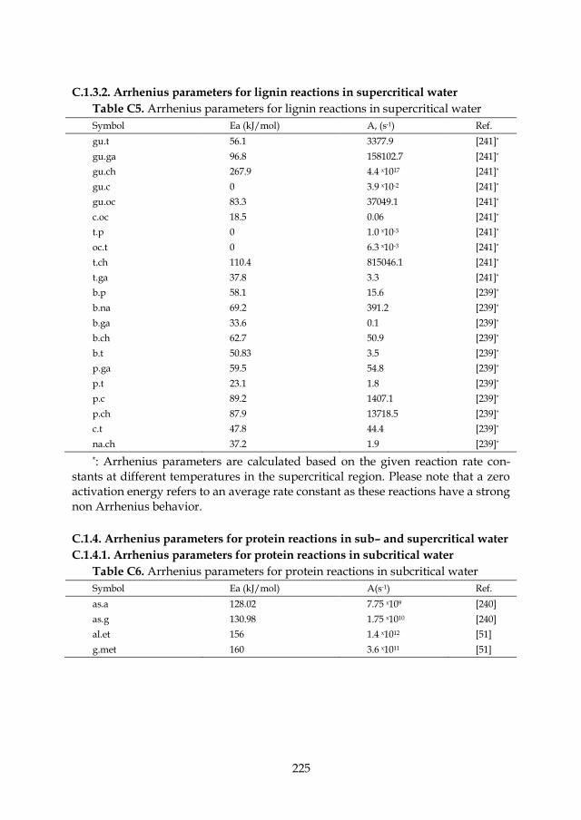
225
C.1.3.2. Arrhenius parameters for lignin reactions in supercritical water
Table C5. Arrhenius parameters for lignin reactions in supercritical water
Symbol Ea (kJ/mol) A, (s-1) Ref.
gu.t 56.1 3377.9 [241]*
gu.ga 96.8 158102.7 [241]*
gu.ch 267.9 4.4 ˣ1017 [241]*
gu.c 0 3.9 ˣ10-2 [241]*
gu.oc 83.3 37049.1 [241]*
c.oc 18.5 0.06 [241]*
t.p 0 1.0 ˣ10-3 [241]*
oc.t 0 6.3 ˣ10-3 [241]*
t.ch 110.4 815046.1 [241]*
t.ga 37.8 3.3 [241]*
b.p 58.1 15.6 [239]*
b.na 69.2 391.2 [239]*
b.ga 33.6 0.1 [239]*
b.ch 62.7 50.9 [239]*
b.t 50.83 3.5 [239]*
p.ga 59.5 54.8 [239]*
p.t 23.1 1.8 [239]*
p.c 89.2 1407.1 [239]*
p.ch 87.9 13718.5 [239]*
c.t 47.8 44.4 [239]*
na.ch 37.2 1.9 [239]*
*: Arrhenius parameters are calculated based on the given reaction rate con-stants at different temperatures in the supercritical region. Please note that a zero activation energy refers to an average rate constant as these reactions have a strong non Arrhenius behavior.
C.1.4. Arrhenius parameters for protein reactions in sub– and supercritical water
C.1.4.1. Arrhenius parameters for protein reactions in subcritical water
Table C6. Arrhenius parameters for protein reactions in subcritical water
Symbol Ea (kJ/mol) A(s-1) Ref.
as.a 128.02 7.75 ˣ109 [240]
as.g 130.98 1.75 ˣ1010 [240]
al.et 156 1.4 ˣ1012 [51]
g.met 160 3.6 ˣ1011 [51]

APPENDIX
226
C.1.4.2. Arrhenius parameters for protein reactions in supercritical water
Table C7. Arrhenius parameters for protein reactions in supercritical water
Symbol Ea (kJ/mol) A, (s-1) Ref.
al.et 156 1.4 ˣ1012 [51]
g.met 160 3.6 ˣ1011 [51]
al.gas 131 7.37 ˣ105 [242]
et.gas 131 7.37 ˣ105 [242]
g.gas 131 7.37 ˣ105 [242]a
m.gas 131 7.37 ˣ105 [242]a
a: The Arrhenius parameters of alanine and glycine gasification reactions are assumed for these reactions.
C.1.5. Arrhenius parameters for organic acid and other intermediate compounds reactions in sub– and supercritical water
Table C8. Arrhenius parameters for organic acid and other intermediate com-pounds reactions in sub– and supercritical water
Symbol Ea (kJ/mol) A, (s-1) Ref.
f.ga1 85.01 1.6 ˣ106 [243]*,sub
f.ga1 168.2 4.8 ˣ1012 [243]*,sup
f.ga2 0 4 ˣ10-3 [243]*,sub
f.ga2 244 3.4 ˣ1017 [243]*,sup
aa.ga 94 2.5 ˣ104 [244]sup
pa.ga 89.4 1.4 ˣ105 [47]sup
mf.aa 250.7 7.5 ˣ1023 [47]sup
la.acry 68.8 6.89 ˣ102 [245]*
acry.la 35.4 2.00 ˣ10-1 [245]*
la.acet 147.7 2.37 ˣ109 [245]*
acet.aa 0 3.25 ˣ10-2 [245]*
acry.hpa 80.1 4.13 ˣ103 [245]*
hpa.acry 0 2.65 ˣ10-2 [245]*
acry.pa 34.9 6.00 ˣ10-1 [245]*
hpa.glyco 0 1.31 ˣ10-3 [245]*
glycol.ga 94 2.5 ˣ104 [244]a,sup
levu.lacet 94.00 6.59 ˣ107 [233]b
wgs 116 3.8 ˣ105 [89]sup
fal.ga 168.2 4.8 ˣ1012 [243]*,c,sup
*: Arrhenius parameters are calculated based on the given reaction rate con-stants at different temperatures in the supercritical region. sub: only for subcritical conditions. sup: only for supercritical conditions. a: Due to its similar molecular structure, Arrhenius parameters for acetic acid conversion are assumed. b: Due to its similar molecular structure, Arrhenius parameters for pyruvaldehyde conver-sion are assumed. c: Due to its similar molecular structure, Arrhenius parameters

227
for formic acid conversion are assumed. Please note that a zero activation energy refers to an average rate constant as these reactions have a strong non Arrhenius behavior.
- All of the given reactions except from al.et and g.met are first order with re-spect to the given compounds shown in Figure 7.16 – Figure 7.24. al.et and g.met follow an nth order reaction for which the n values are 0.47 and 0.78 for alanine and glycine, respectively.
- The compounds which do not exist in AspenPlusTM 8.2 software are intro-duced as user defined compounds by drawing the actual chemical structure of the compound.
C.2. Stream analysis
Table C9 shows the composition of the stream that leaves the reactor for mi-croalgae, pig-cow manure mixture and paper pulp at reactor temperatures of 500 and 600 °C. The pressure is 25 MPa and dry biomass concentration in the feed is 10 wt.%. Please see section “7.2.4. Case studies: SCWG of microalgae, manure and paper pulp” and Figure 7.32 for the simulation conditions. The results show that the cellulose, hemicellulose, lignin and protein content of the biomass fully de-composes to intermediates and gaseous products at the exit of the reactor. As ex-pected, at lower rector temperatures or shorter residence times, the amount of the intermediates are higher due to the unfinished gasification reactions. Cellulose and hemicellulose derived compounds consist of organic acids, aldehydes and furfural; lignin derived compounds consist of aromatic compounds such as benzene, o-cresol, catechol and diphenyl; and protein derived compounds consist of amino acids and amino acid derived amine and organic acid compounds. Char formation also takes place. Nitrogen content of the protein mainly leaves the reactor in the form of NH3 gas.

APPENDIX
228
Table C.9: The composition of the stream that leaves the reactor for microalgae, pig-cow manure mixture and paper pulp at reactor temperatures of 500 and 600 °C. The pressure is 25 MPa and dry biomass concentration in the feed is 10 wt.%. Please see section “7.2.4. Case studies: SCWG of microalgae, manure and paper pulp” and Figure 7.32 for the simula-tion conditions.

229
Table C.9 (Continued)

APPENDIX
230
Table C.9 (Continued)

231
C3.The individual behavior of cellobiose, xylose, guaiacol and aspartic acid
In order to study the effect of each biomass constituent compound, simulations have been performed for individual constituent compounds using the same condi-tions used in the real biomass simulations, see section “7.2.4. Case studies: SCWG of microalgae, manure and paper pulp” and Figure 7.32 for the simulation condi-tions. The results are shown in Figure C.1 and Figure C.2 and indicate that xylose has a better gasification behavior than any other biomass constituent compound. Xylose seems to be completely gasifiable even at shorter residence times at a reac-tor temperature of 600 °C. Xylose is followed by cellobiose which can attain more than 90% CGE at a reactor temperature of 600 °C and at a residence time of 60 s. Aspartic acid shows a relatively weak gasification behavior at 500 °C, however, at 600 °C and at a residence time of 60 s, CGE can reach up to 70%. Among the oth-ers, guaiacol, which is the representative of the lignin content of the biomass, ap-pears to show the poorest gasification behavior. The results show that it is hardly gasifiable even at a reactor temperature of 600 °C. Another interesting result re-garding the behavior of guaiacol is its slightly lower CGE at 600 °C compared to the CGE at 500 °C. It can be concluded that the reaction rate of the formation of the aromatic compounds and char from guaiacol are faster than the gasification reac-tions at higher temperatures. This observation is due to the reaction rates retrieved from Yong and Matsumura [239,241] from which the guaiacol kinetic model has been acquired. The preliminary simulations show that the only way to overcome the competing reactions of the aromatic compounds’ and char formation, and to realize a higher CGE is to establish a rapid heating profile under subcritical condi-tions (the heat exchanger in Figure 7.32 in the manuscript). The influence of the heating profile in the heat exchanger on CGE is shown in section C.4.
The results also show that the most suitable biomass for supercritical water gasification should be high in hemicellulose and cellulose content and low in lig-nin. Depending on the protein content, higher reactor temperatures as well as longer residence times should be chosen.

APPENDIX
232
Figure C.1: The gasification behavior of each biomass constituent compound at a reactor temperatures of 500 °C. The pres-sure is 25 MPa and dry biomass concentration in the feed is 10 wt.%. Please see section “7.2.4. Case studies: SCWG of mi-croalgae, manure and paper pulp” and Figure 7.32 for the simulation conditions.

233
Figure C.2: The gasification behavior of each biomass constituent compound at a reactor temperatures of 600 °C. The pres-sure is 25 MPa and dry biomass concentration in the feed is 10 wt.%. Please see section “7.2.4. Case studies: SCWG of mi-croalgae, manure and paper pulp” and Figure 7.32 for the simulation conditions.

APPENDIX
234
C4. The effect of the heating profile in the heat exchanger on the gas compo-sition
In order to see the effect of the heating profile in the heat exchanger on the gas composition and CGE, simulations have been performed with different heating profiles. Figure C.3 shows the configuration used for the simulations in this sec-tion, Figure C.4 shows the temperature profile in the heat exchanger along the heat exchanger length and Table C.10 shows the heating profiles and residence time along the heat exchanger, heater and reactor for different investigated cases. The results are given in Figure S5.
Figure C.3. The process scheme that was used throughout the SCWG simulations of microalgae, pig-cow manure and paper pulp.
Figure C.4: The heating profile along the length of heat exchanger for linear heat-ing, slow heating and rapid heating cases.

235
Table C.10: The heating profiles and residence time along the heat exchanger, heater and reactor for different investigated cases.
Case Number
Heat exchanger Heater Reactor
Heat-ing Profile
Resi-dence Time (min)
Heat-ing Profile
Resi-dence Time (s)
Heat-ing Profile
Resi-dence Time (s)
1 Linear 5 Linear 20 Linear 30
2 Linear 1 Linear 20 Linear 30
3 Slow 1 Linear 20 Linear 30
4 Rapid 1 Linear 20 Linear 30
The results indicate that a rapid heating profile enhances the CGE compared to linear and slow heating profiles for microalgae and manure. In addition, a linear heating profile results in a better CGE than a slow heating profile. These are all ex-pected phenomena as the rapid heating of the heat exchanger not only suppresses the char and aromatic compounds’ formation but also results in longer residence times at higher stream temperatures inside the heat exchanger which enhances the CGE. A rapid heating profile with a residence time of 1 minute can result in as high a CGE value as a linear heating profile with a residence time of 5 minutes. However, the effect of the heating profile on the gasification behavior of paper pulp is almost insignificant. This is due to the high cellulose and hemicellulose content of the paper pulp, as these two biomass constituent compounds are al-ready found to be relatively easily gasified compared to lignin and protein (please see section C.3). In summary, it can be conclude that in order to realize a higher CGE, a rapid heating profile at subcritical conditions is required.

APPENDIX
236
Figure C.5: The effect of the heating profile in the heat exchanger on the gas yields and CGE at the exit of the reactor for microalgae, pig-cow manure mixture and paper pulp at a reactor temperature of 600 °C. The pressure is 25 MPa and dry biomass concentration in the feed is 10 wt.%. Please see Table S10 for the definition of the Cases.

237
C.5. Comparison of the experimental results reported in Chapter 6 with the integrated kinetic model predictions.
Comparison of the experimental results reported in Chapter 6 with the inte-grated kinetic model are given in Figures C.6 and C.7. Please see Chapter 5 for process flow diagram and the dimensions of the process units of the experimental setup, and Chapter 6 for the temperature profiles and gas composition results. Here, starch was modeled as cellobiose. Besides, the heat exchanger (both for the feed flow and return flow), heater and reactor were modeled as RPlug reactors in AspenPlus software in order to simulate the experimental setup reported in Chap-ter 5. Similar to the section 7.2.3.2, the heat exchanger’s subcritical and supercritical zones were modeled in two different RPlug reactors based on the temperature pro-files reported in Chapter 6.
Figure C.6: Comparison of the carbon gasification efficiency (CGE) and gasifi-
cation efficiency (GE) results between the experimental results reported in Chapter 6 and the integrated kinetic model predictions using AspenPlus.
0.0 0.1 0.2 0.3 0.4 0.5 0.6 0.7 0.8 0.9 1.0
0.0
0.1
0.2
0.3
0.4
0.5
0.6
0.7
0.8
0.9
1.0
-20 %
+20 %
-10 %
CGE
GE
exp
erim
en
tal re
su
lts
kinetic model predictions
+10 %

APPENDIX
238
Figure C.7: Comparison of the gas concentration results between the experi-
mental results reported in Chapter 6 and the integrated kinetic model predictions using AspenPlus.
The results indicate that the developed kinetic model predicts quite accurately the CGE, GE and HE results, however, fails in predicting the gas concentrations. Although the CH4, CO and CO2 predictions are relatively more accurate, the model significantly under predicts C2-C3 gases and over predicts hydrogen. These obser-vations indicate similar results with section 7.2.3.1: the gas forming reaction rates of the proposed kinetic model are quite accurate, however, the stoichiometry of gas forming reactions from the intermediates are less accurate.
0.0 0.1 0.2 0.3 0.4 0.5
0.0
0.1
0.2
0.3
0.4
0.5
experim
enta
l m
ole
fra
ctio
ns
Compound:
CO2
CH4
H2
CO
C2-C
3
kinetic model predictions for the mole fractions
+20 %+10 %
-10 %
-20 %

239
EPILOGUE & ACKNOWLEDGEMENTS
When I started my doctoral studies in July 2011, I had serious doubts if I could get to that point where I am now. A doctoral study can be quite challenging in-deed: it requires not only the fundamental academic background related to the subject, but also motivation and enthusiasm. Besides, the latter two are challenged by moving to another country – especially if it is a rainy, windy, cloudy and less sunnier one. Fortunately, I was one of those luckier ones who actually enjoyed his/her doctoral studies (not all of it for sure!). However, I owe that pleasure to all of these great people I met from all over the world who took a part in my life throughout my doctoral studies.
My first and immense thankfulness is for my co-promotor and daily supervisor Dr. Ir. Wiebren de Jong, who actually allowed all of this journey to happen. Thank you for providing me the opportunity to work in this topic and supporting me for all of the works we have conducted together. Many of the works I have done throughout my doctoral studies would not be the way they are if you did not give me such freedom and support which significantly increased my motivation and success. I enjoyed all of our discussions we had (both scientific and non-scientific ones), especially on our hours of way to Breezand. I cordially hope to collaborate in near future with other projects as well.
In addition, I would like to thank my promotor Prof. Dr. Ir. Bendiks Jan Bo-ersma for reviewing my work, to Prof. Dr. Ir. Thijs Vlugt and to Dr. Brian Tighe for valuable discussions on thermodynamic modeling and to Dr. Elif Genceli Güner for valuable discussions on crystallization and for her support throughout my first year in Delft.
I also would like to thank Dr. Ir. John Harinck (an excellent scientist) and Ir. Ing. Gerton Smit (an amazing engineer) for their collaboration and support throughout my doctoral studies. John and Gerton; I learned a lot from you, and I really enjoyed our discussions on modeling (esp. heat transfer and fluid dynamics) and on designing the setup (esp. how to implement a sapphire glass to the reac-tor). I wish you the best concerning the project’s and Gensos’ future. I would also like to express my gratitude to other members of Gensos B.V.: to Martijn Al, Wouter Glas, Max van de Leijgraaf and to all of the work shop team for their price-less supports.
I am deeply thankful to Prof. Frédéric Vogel and his catalytic process engineer-ing group in Paul Scherrer Institut in Switzerland. My 3 weeks of visit to his group made me to gain significant experiences on performing experiments with super-critical water gasification of biomass setups. I also thank to Biofuels Research In-frastructure for Sharing Knowledge (BRISK) for making this visit to happen.

240
My sincere thanks to my talented Masters students for their excellent co-operation: to Güçhan Yapar, Ivo Albrecht and Clemens Schönlein for insightful discussions and their contributions to this dissertation, and to Georgios Gkranas, Cheng Zeng (Aaron), Aldin Wibisono and Enrique Garcia Franco for their enthu-siasm and contributions in the modeling aspects of supercritical water gasification of biomass processes.
I also would like express my gratitude to my dearest friends which made me to enjoy my Process & Energy days. George Tsalidis; the guy who is more Turkish than I am. I will always miss your conspiracy theories and the discussions we had on politics, women, science, games, football and music. I am grateful to you for developing me to be a more “patient” man. Gerasimos Sarras; the mathematician. I will always miss our night outs in Den Haag, discussions we had on politics, sci-ence (esp. on quantum mechanics), philosophy (esp. on Nietzsche and Camus), books (esp. on Dostoevsky), music and women. Nafiseh Taleban Fard; I will al-ways miss our foosball games, coffee breaks, discussions on relationships, and you and Dariush’s company in concerts. Kostas Anastasakis; I will always miss the dis-cussions we had on hydrothermal conversion (esp. your help in analysis), politics, lunch talks and your advises on after PhD life. Manuela di Marcello; I will always miss your lectures in analytical chemistry, your advises and the similarity we have in musical taste. Yash Joshi; I will always miss our discussions on music, culture and your solutions to engineering problems. George Krintiras; I will always miss our lunch talks, your complaints and your enthusiasm in Greek culture. Piotr Pla-za; many thanks for your help in FactSage/SimuSage. Martina Fantini; many thanks for all those great Italian food. Alessandro, Hassan, Aditya, Wijittra, Sawat, Xiangmei, Marco, Alvaro and all the others I forgot: thanks for being a part of this journey and all of the moments we shared together.
I would like to state my sincere thanks to my Turkish “panpa”s in Delft as well: Murat Demirtaş, Cem, Doğan, Can, Nazlı, Öncü, Necdet, Murat, Kaan, Özge Deniz, Candan, Sine, Çağrı, Noyan and Vanya; thanks for all of the football games, night outs, dinners, “mantı”s , “aşure”s, “mangal”s and other countless moments we had together which made my PhD years way more beautiful.
Haktan, Serkan, Umut, Berkin and Emrah: my old friends; Aslı, Zuhal, Yusuf, Emre, Gamze, Burak, Eda and Damla: my friends from my chemical engineering studies in Istanbul; many thanks for your friendship and supports for all of these years. Funda; many thanks for your motivational discussions. Gamze; many thanks for your friendship for all of these years. My dear friends Didem and Tutku; my sincere thanks for your kindness, help, hospitality and the dinners. The other members of “Tatavlalılar”, Beril and Yasemin; thanks for your company, and Ayça; many thanks for the Skype conversations we had. My “kız tarafı” friends, Fırat, Elvin, Başak and Nurfer; thanks for all of the joyful moments and the amaz-ing holiday we had together. Engin and Duygu; I am so happy that you were al-ready in Netherlands when I moved. I will never forget your support.
241
My dearest “Güliz Abla” “panpa”s; you made my Delft days nicer and enjoya-ble. I am grateful to all of you. Thanks for all of your support and company for the last years. Argun; you are a good friend and a great cook (but a crazy driver). Bu-rak; Delft wouldn’t be that fun for Turkish students, if you weren’t the “muhtar” of it. Cansın; thanks for lessons in preparing sushi. Ekin; I wish you so much “ek-meks” for the rest of your life. Mustafa Can; I suggest you to improve your DJ skills (esp. when taking control of someone else’s laptop). Tilbe; panpam, I am still waiting for the “check-out” and “hanımeller”! Yasemin; panpi, many thanks for your excellent dolmas and hospitality. “Panpalar”, I feel so lucky that I met you. I will never forget all of the beautiful moments, discussions, breakfasts, dinners, Bouwpub and Bebop days we had together.
Sinan Tüfekçioğlu; panpam, I am so much grateful that we met. I owe you a lot. I will always miss the coffee breaks and the Monday morning football talks (and other lots of discussions) we had in P&E as well as the “kapso”s. Emre Mül-azımoğlu; panpam; I owe you a lot, too. I will always miss our Bebop nights (espe-cially the “last” beers), FIFA matches and discussions. You both contribute to this dissertation more than you could think of.
I am forever grateful to all members of my family. My dearest brother, Endom; you are my best friend and teacher, and an amazing physicist. I feel so lucky that you were right there in front me when I was born. My dearest sister-in-law, Özgecan; even a real sister wouldn’t be that close to me. You are one of the wisest person I ever knew. My dearest mom and dad; I am grateful for all of your price-less supports in every aspects of my life. My beloved grandfather Mehmet Kartal, to whose memory this dissertation is dedicated; without you and your tremen-dous wisdom, I would not be here.
Onursal

242

243
CURRICULUM VITAE
Onursal Yakaboylu was born on 5 March 1986, in Eskişehir, Turkey. He ob-tained his MSc degree in chemical engineering at Istanbul Technical University in 2010. He started his doctoral research at the Process and Energy Department of Delft University of Technology on July 2011, within the energy from biomass group of Dr. ir. Wiebren de Jong. During his doctoral studies, he joined Prof. Frédéric Vogel’s catalytic process engineering group in Paul Scherrer Institut in Switzerland.

244
LIST OF PUBLICATIONS
PEER-REVIEWED PUBLICATIONS
O. Yakaboylu, I. Albrech, J. Harinck, K.G. Smit, W. de Jong. Supercritical water gasification of biomass in TU Delft/Gensos semi-pilot scale setup. (To be Submited)
O. Yakaboylu, G. Yapar, M. Recalde, J. Harinck, K.G. Smit, E. Martelli, W. de Jong, Supercritical Water Gasification of Biomass: An Integrated Kinetic Model for the Prediction of Product Compounds, Industrial & Engineering Chemistry Re-search 54 (33) (2015) 8100–8112.
O. Yakaboylu, J. Harinck, K.G. Smit, W. de Jong, Supercritical Water Gasifica-tion of Biomass: A Detailed Process Modeling Analysis for a Microalgae Gasifica-tion Process, Industrial & Engineering Chemistry Research 54 (21) (2015) 5550–5562.
O. Yakaboylu, J. Harinck, K.G. Smit, W. de Jong, Testing the constrained equi-librium method for the modeling of supercritical water gasification of biomass, Fuel Processing Technology 138 (2015) 74–85.
O. Yakaboylu, J. Harinck, K.G. Smit, W. de Jong, Supercritical Water Gasifica-tion of Biomass: A Literature and Technology Overview, Energies. 8 (2015) 859–894.
O. Yakaboylu, J. Harinck, K.G. Smit, W. de Jong, Supercritical Water Gasifica-tion of Biomass: A Thermodynamic Model for the Prediction of Product Com-pounds at Equilibrium State, Energy & Fuels. 28 (2014) 2506–2522.
O. Yakaboylu, J. Harinck, K.G. Gerton Smit, W. de Jong, Supercritical water gasification of manure: A thermodynamic equilibrium modeling approach, Bio-mass Bioenergy. 59 (2013) 253–263.
INTERNATIONAL CONFERENCES
O. Yakaboylu, I. Albrech, J. Harinck, K.G. Smit, W. de Jong. Supercritical water gasification of biomass: first results and experiences obtained from TU Delft/Gensos semi-pilot scale setup. (To be presented in 24th European biomass confer-ence, Amsterdam, June 2016)
O. Yakaboylu, J. Harinck, K.G. Smit, W. de Jong. Supercritical water gasifica-tion of microalgae: process modeling and analysis. In The 5th International Con-ference on Algal Biomass, Biofuels and Bioproducts, San Diego, USA 2015. (oral presentation)
O. Yakaboylu, J. Harinck, K.G. Smit, W. de Jong. On the modeling of supercriti-cal water gasification of biomass: determination of additıinal constraints In Gibbs

245
free energy minimization. In The 5th International Conference on Engineering for Waste and Biomass Valorisation, Rio de Janeiro, Brazil 2014. (oral presentation)
O. Yakaboylu, J. Harinck, K.G. Smit, W. de Jong. Supercritical water gasifica-tion of biomass: Prediction of compounds with a thermodynamic equilibrium ap-proach. In Thermodynamics 2013 Conference, Manchester, UK 2013. (oral & poster presentation)
O. Yakaboylu, J. Harinck, K.G. Smit, W. de Jong. Hydrothermal conversion of manure up to near-critical conditions: a thermodynamic equilibrium approach. In 20th European biomass conference - setting the course for a biobased economy, Mi-lan, Italy 2012. (poster presentation)