Study of surface nuclear magnetic resonance inverse problems

Study of surface nuclear magnetic resonance inverse problems

Peter B. Weichman a,*, Dong Rong Lun b, Michael H. Ritzwoller b, Eugene M. Lavely a

aALPHATECH, Inc., 50 Mall Road, Burlington, MA 01803, USAbDepartment of Physics, University of Colorado at Boulder, Boulder, CO 80309-0390, USA

Abstract

Motivated by the recent application of the Earth-field nuclear magnetic resonance (NMR) technique to the detection and

mapping of subsurface groundwater (to depths of 100 m or so), and making use of a recently developed theory of the method,

we consider in detail the resulting inverse problem, namely the inference of the subsurface water distribution from a given

sequence of NMR voltage measurements. We consider the simplest case of horizontally stratified water distributions in a

horizontally stratified conducting Earth. Inversion methods based both on the singular value decomposition (SVD) and Monte

Carlo are used and compared. The effects of random measurement errors and of systematic errors in the assumed subsurface

conductivity structure are studied. It is found that an incorrectly modeled highly conducting layer leads to a ‘‘screening effect’’

in which the water content of layers lying below it is severely underestimated. We investigate also the ability of different source-

receiver loop geometries to provide complementary information that may improve a combined inversion. Finally, inversion of

experimental data from Cherry Creek, CO, USA is performed. Since only the absolute magnitude of the NMR voltage is

measured accurately, a nonlinear Monte Carlo inversion is performed. D 2002 Elsevier Science B.V. All rights reserved.

Keywords: Surface NMR; Imaging; Inverse problems; Noise; Near surface; Water

1. Introduction

The nuclear magnetic resonance (NMR) technique

has been widely used for nondestructive determina-

tion of the structure and the dynamics of diverse

systems. This method generally probes the nuclear

spin dynamics of a system, which can then be used to

infer both the quantity of magnetically active nuclei

(through the amplitude of signal) as well as their local

magnetic environment (through the different observed

Larmor frequencies) and, hence, the chemical struc-

ture of the latter. By applying dc magnetic fields with

carefully controlled spatial gradients, along with

clever pulse sequences of uniform ac fields, the

method also allows spatially resolved measurements

of these same properties, i.e., imaging.

In certain important cases, the nuclear spins of

interest are free: the internal fields acting on them are

basically random in time and average to zero. Such is

the case, e.g., for water or hydrocarbon molecules in

the fluid state. The nuclear spins of interest are the

various hydrogen protons contributing to the mole-

cule. The fluid state leads to a randomly varying

orientation of the molecules, and it is this ‘‘motional

narrowing’’ effect that leads to the freeness of the

spins.

Free spins are, therefore, very sensitive to exter-

nally applied static fields, and the NMR technique

takes advantage of this sensitivity. Specifically, a

0926-9851/02/$ - see front matter D 2002 Elsevier Science B.V. All rights reserved.

PII: S0926 -9851 (02 )00135 -0

* Corresponding author.

E-mail address: [email protected] (P.B. Weichman).

www.elsevier.com/locate/jappgeo

Journal of Applied Geophysics 50 (2002) 129–147

static field, B0, polarizes the spins, leading to a local

nuclear magnetic moment

MN ðrÞ ¼ vN ðTÞnNðrÞB0, ð1Þ

where nN(r) is the local number density of free nuclear

spins [for water, e.g., one has nN(r) = 2nH2O(r)], and

vN ðTÞ ¼ c2t2SðS þ 1Þ=3kBT ð2Þ

is the (temperature-dependent) single spin suscepti-

bility (Abragam, 1983). Here, S = 0, 1/2, 1, 3/2, . . ., isthe spin and c ( = 26752 G � 1 s� 1 for free protons) is

the gyromagnetic ratio.

The induced dipole field due to the polarization

(Eq. (1)) is too small to be measured directly, but by

applying an additional ac pulse at the (angular)

Larmor frequency, xL= 2pmL= cB0, the spins can be

tipped away from B0. Their subsequent precession

about B0 at the same frequency xL then produces an

ac field that is large enough to be measured by an

inductive pickup coil (Abragam, 1983). The ampli-

tude of the ac pickup coil voltage (again at frequency

xL) is proportional to the magnitude of the original

total (spatially integrated) induced moment, and via

Eq. (1), the corresponding spatially integrated nuclear

spin density can be inferred. In combination with

controlled spatial gradients in the static field, the

imaging technique alluded to above allows determi-

nation of the spin distribution nN(r) itself. When

applied to water in the human body, the above

analysis forms the basis of certain forms of medical

MRI.

In the absence of the ability to provide controlled

gradients in the static field and uniformity of the ac

field, the imaging problem becomes much more

difficult. Such is the case with surface NMR, where

due to economic, physical and/or geometrical limi-

tations, the external fields must be applied using a

surface loop away from the sample region of interest.

The resulting field has a nontrivial spatial structure,

and the relation between the measured NMR voltage

and the nuclear spin distribution becomes very

complicated. The situation is exacerbated further

when the sample volume is large. The applied field

may then be significantly affected by the electrical

properties of the sample. In particular, an ac field

penetrating a conducting sample will experience a

finite electromagnetic skin depth, ds(x). If the sample

dimensions are comparable to or larger than the skin

depth at the given Larmor frequency, significant

distortion of the signal takes place and must be

accounted for.

In recent work (Weichman et al., 1999, 2000) [see

also Weichman, 2001 for a concise review], some of

us have considered the theoretical problem of analyz-

ing surface NMR data in the geophysical context of

groundwater detection. The experimental geometry

(Goldman et al., 1994; Trushkin et al., 1995; Hen-

drickx et al., 1999) consists of a large Lg100-m-

diameter loop laid out in a circle or figure-eight on the

Earth’s surface. The rule of thumb is that the max-

imum depth sensitivity will be of the same order as L.

The Earth’s field B0g0.5 G is used as the static field,

implying a Larmor frequency, mLg2.1 kHz, and ac

current amplitudes, IT0, of order 300 A in the loop are

used to generate the tipping field. Once the tipping

field is turned off, this same loop is then used to detect

the NMR signal (though there is nothing in principle

to forbid the use of a second, independent receiver

loop). Typical ground resistivities vary from about 1

V m for highly conducting soils to greater than 100 V

m for resistive soils. This leads to skin depths ranging

from 50 to 500 m, precisely of the same order as L.

Moreover, the Earth tends to have a layered structure

so that the resistivity varies with depth within this

same range.

In Weichman et al. (1999, 2000), a very general

equation was derived, which accounts for an arbitrary

ground conductivity distribution and arbitrary trans-

mitter and receiver loop geometries and relates the

measured complex voltage amplitude, V (the complex

phase of V measuring the phase lag between the

transmitter loop current and the received signal) to

the nuclear spin distribution. This relationship takes

the form of a linear integral equation,

V ðq,x0Þ ¼Z

d3rKðq,x0; rÞnNðrÞ ð3Þ

where q = IT0sp, with sp the length of the time interval

for which the tipping field is applied, is the so-called

pulse moment, which is the single combined param-

eter that determines the angle by which the spins are

tipped, and x0 represents the overall position of the

transmitter and receiver loops on the Earth’s surface.

There is also implicit dependence on the experimen-

P.B. Weichman et al. / Journal of Applied Geophysics 50 (2002) 129–147130

tally controllable shape, orientation, relative position,

etc., of the loops. For a horizontally stratified spin

distribution, nN = nN(z), Eq. (3) reduces to

V ðq,x0Þ ¼Z

dzK̃ðq,x0; zÞnNðzÞ

K̃ðq,x0; zÞuZ

dxdyKðq,x0; x,y,zÞ: ð4Þ

The complex kernel K encodes (a) the thermodynamic

relationship (Eq. (1)), (b) the field at r generated by

the given transmitter loop in the presence of the given

ground conductivity distribution (which must then be

inferred from other measurements), (c) the angle and

phase of the resulting precessing spin at r, and (d) the

sensitivity of the given receiver loop to the precessing

spin at r in the presence of the same conductivity

distribution.

Eqs. (3) and (4) define a linear inverse problem for

the nuclear spin distribution. A form of the inverse

problem (4) has been considered in Trushkin et al.

(1995) and Legchenko and Shushakov (1998) using a

Tikhonov regularization. However, the kernel K̃ used

there is purely real and, therefore, fails to account for

the diffusive phase delay and interference effects

when the ground is conducting. Given a discrete set

of measurements of V, one seeks to determine nN to

some degree of confidence. Clearly, if nN(r) has a

nontrivial 3-d distribution, then a fully three-dimen-

sional set of data in ( q, x0) parameter space is required

to perform, even in principle, a successful inversion.

However, experiments to date are all based on fixing

x0, scanning q (via the pulse length, sp), and assuming

a horizontally stratified spin distribution. With this

assumption, Eq. (4) provides a consistent inverse

problem, with the one-dimensional data set V( q), at

least in principle, sufficient to determine the one-

dimensional vertical profile nN(z).

Explicit expressions for the kernel K are given in

Weichman et al. (1999, 2000), extending the approx-

imate form used in earlier literature (Trushkin et al.,

1995; Legchenko and Shushakov, 1998), but require

far too many extraneous definitions to reproduce here.

In this paper, we will be content with showing only

graphical representations of K and K̃ in various

physical situations.

In the present work, we follow the experimental

lead and consider only the one-dimensional inverse

problem based on Eq. (4). As is often the case in

geophysical inverse problems, Eq. (4) is ill-condi-

tioned (Legchenko and Shushakov, 1998). This arises

from the fact that both the magnetic field generated by

the transmitter loop, and the sensitivity of the receiver

loop decay rapidly with depth. Therefore, very large

changes in nN at depths zkL lead to very small

changes in V. The always-present random measure-

ment errors in V will be greatly magnified in the

inferred nN at these depths.

A more subtle form of systematic error is contained

in the assumed conductivity distribution. A highly

conducting Earth leads to a triple attenuation of the

NMR voltage: first, the transmitted field is attenuated

by a factor e� z/ds(xL), leading to a proportionately

smaller tipping angle for the spins and, hence, a

corresponding decrease in the effective size of the

precessing moment. Second, the signal generated by

the precessing moment attenuates by the same factor

as it propagates back to the receiver coil at the surface.

Third, signals from different depths are out of phase

due to diffusive delay and, therefore, interfere destruc-

tively when they sum to form the total measured

voltage. These three effects are reflected in a strong

exponential decayf e� 2z/ds(xL) and a strongly vary-

ing phasef e� 2iz/ds(xL) of K and K̃ with depth. If this

attenuation is not correctly accounted for, an ever-

increasing systematic underestimate of nuclear spin

density will occur with increasing depth.

In Weichman et al. (1999, 2000), a very prelimi-

nary study of the inverse problem based on Eq. (4)

was performed, using coincident, circular transmitter

and receiver loops and modeling the subsurface as a

homogeneous conducting half-space. In the remainder

of this paper, we study in detail the effects of the

random and systematic errors discussed above, using

several different transmitter and receiver loop geo-

metries and a general horizontally stratified conduc-

tivity structure. In Section 2, Eq. (4) is reduced to a

finite dimensional matrix problem by considering a

finite number of layers with constant conductivity and

spin density within each layer, and with spin density

arbitrarily set to zero beyond a certain depth. The

forward problem is then solved, generating synthetic

voltage data for various assumed forms of the con-

ductivity and spin density distributions. These syn-

thetic data subsequently form the basis for the inverse

problem studied in Section 3. Gaussian noise is added

to the data, and inversions are performed using both

P.B. Weichman et al. / Journal of Applied Geophysics 50 (2002) 129–147 131

the correct (i.e., that used to generate the data in the

first place) and various incorrect conductivity struc-

tures. Two different methods for performing the

inversion are tested—the Monte Carlo method and

the singular value decomposition (SVD) method—

and are found to give commensurable results. We test

also the idea that simultaneous inversions of data

obtained from the same subsurface structure, but

measured using different loop geometries, can reduce

the effects of error. Surprisingly, we find that the

improvement is marginal at best. For completeness,

in Section 4, we analyze also some real experimental

data and discuss some of the shortcomings that

complicate its interpretation. The paper is concluded

in Section 5.

2. The forward problem

In our computations, we take the Earth’s field to be

tilted by 25j northwards away from the vertical

(declination 0jE, inclination 65jN) with a magnitude

B0 = 0.587 G, consistent with a Larmor frequency,

mL= 2.5 kHz. Pulse moments vary in the range 102

A msV qV 1.6� 104 A ms. For transmitter loop

current amplitude, IT0 = 300 A, this corresponds to

pulse lengths 0.33 msV spV 53 ms. Most of the

signal comes from regions where the spins have been

tipped near 90j. Due to the decay of the tipping field,

the depth at which this occurs increases with q, and at

the upper end of the range corresponds to a depth

close to 100 m. Experimental data are also limited

roughly to this same range because decay processes in

the ground (that will not be discussed further in this

article) limit the lifetime of a precessing spin to tens to

hundreds of milliseconds. In particular, the average

lifetime decreases as the size of the pores in which the

fluid is entrained decreases (Kleinberg et al., 1994;

Hendrickx et al., 1999). The tipping pulse must then

be shorter than this lifetime in order to ensure that the

voltage is recorded before significant signal decay

occurs.

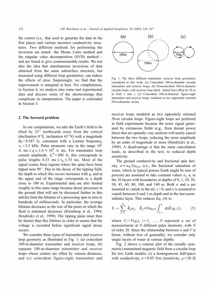
We consider three types of transmitter and receiver

loop geometry as illustrated in Fig. 1: (a) coincident

100-m-diameter transmitter and receiver loops, (b)

separate 100-m-diameter transmitter and receiver

loops whose centers are offset by various distances,

and (c) coincident figure-eight transmitter and

receiver loops modeled as two oppositely oriented

50-m circular loops. Figure-eight loops are preferred

in field experiments because the noise signal gener-

ated by extraneous fields (e.g., from distant power

lines) that are spatially very uniform will nearly cancel

between the two loops, reducing the noise amplitude

by an order of magnitude or more (Hendrickx et al.,

1999). A disadvantage is that the same cancellation

leads, as described in the text, to reduced depth

sensitivity.

The ground conductivity and fractional spin den-

sity, nu nN/2nH2O(i.e., the fractional saturation of

water, which in typical porous Earth might be tens of

percent) are assumed to take constant values rj, nj inthe 10 layers with boundaries at depths of 0, 1, 10, 20,

30, 45, 60, 80, 100, and 140 m. Both r and n are

assumed to vanish in the air, z > 0, and n is assumed to

vanish between 0 and 1-m depth and in the last (semi-

infinite) layer. This reduces Eq. (4) to

Vi ¼X8j¼1

K̃ijnj, K̃iju2nH2O

Z zj

zj�1

dzK̃ðqi; zÞ, ð5Þ

where Vi = V( qi), i = 1, . . ., N represent a set of

measurements at N different pulse moments, with N

of order 20. Since the relationship between n and V is

linear, without loss of generality, we consider only

single layers of water at various depths.

Fig. 2 shows a contour plot of the (axially sym-

metric) transmitted magnetic field from a circular loop

for two Earth models: (i) a homogeneous half-space

with conductivity, r = 0.05 S/m (resistivity, q = 20 V

Fig. 1. The three different transmitter– reciever loop geometries

considered in this work. (a) Coincident 100-m-diameter circular

transmitter and receiver loops. (b) Noncoincident 100-m-diameter

circular loops, with receiver loop (dash–dotted line) offset by 50 m

in both x and y. (c) Coincident 100-m-diameter figure-eight

transmitter and receiver loops, modeled as two oppositely oriented

50-m-diameter circles.


Fig. 2. Contour plot of the radial and vertical components of the axially symmetric transmitted magnetic field in the subsurface as a function of radius and depth. The field scales (in

Gauss/StatAmp) are normalized by the number shown at the bottom left of each panel. The circular transmitter loop lies in the horizontal plane z = 0, with center at the origin, and has

radius 50 m. The top row is for a homogeneous subsurface conductivity (r= 0.05 S/m). The bottom row is for subsurface conductivity r= 1 S/m from 20 to 40 m and 0.05 S/m

elsewhere. Details regarding how these fields are computed can be found in Weichman et al. (2000).

P.B.Weich

manet

al./JournalofApplied

Geophysics

50(2002)129–147

133

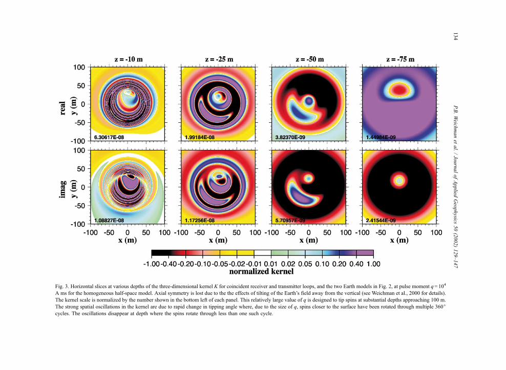
Fig. 3. Horizontal slices at various depths of the three-dimensional kernel K for coincident receiver and transmitter loops, and the two Earth models in Fig. 2, at pulse moment q= 104

A ms for the homogeneous half-space model. Axial symmetry is lost due to the the effects of tilting of the Earth’s field away from the vertical (see Weichman et al., 2000 for details).

The kernel scale is normalized by the number shown in the bottom left of each panel. This relatively large value of q is designed to tip spins at substantial depths approaching 100 m.

The strong spatial oscillations in the kernel are due to rapid change in tipping angle where, due to the size of q, spins closer to the surface have been rotated through multiple 360jcycles. The oscillations disappear at depth where the spins rotate through less than one such cycle.

P.B.Weich

manet


Geophysics

50(2002)129–147

134

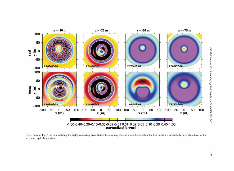
Fig. 4. Same as Fig. 3 but now including the highly conducting layer. Notice the screening effect in which the kernels in the first model are substantially larger than those for the

second at depths below 40 m.

P.B.Weich

manet


Geophysics

50(2002)129–147

135

m); and (ii) a single highly conducting layer, r = 1 S/

m (resistivity, q = 1 V m) between 20 and 40 m in an

otherwise homogeneous half space with r = 0.05 S/

m. In the latter model, the highly conducting layer

has a width roughly half the corresponding skin

depth at the Larmor frequency. Comparison of these

two models demonstrates the ‘‘screening effect’’ in

which the high conductivity layer leads to a sub-

stantial attenuation of the transmitted field below it.

Spins below this layer will then be tipped far less

than when it is absent and, therefore, contribute a

smaller NMR signal. This is reflected quantitatively

in the contour plots of the three-dimensional kernel K

for the case of coincident transmitter and receiver

loops shown in Figs. 3 and 4 (one of whose inputs is

the corresponding field shown in Fig. 2) and perhaps

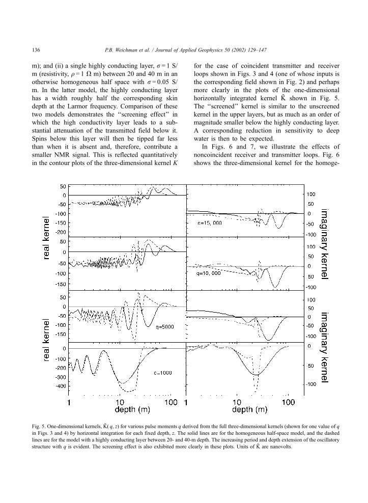
more clearly in the plots of the one-dimensional

horizontally integrated kernel K̃ shown in Fig. 5.

The ‘‘screened’’ kernel is similar to the unscreened

kernel in the upper layers, but as much as an order of

magnitude smaller below the highly conducting layer.

A corresponding reduction in sensitivity to deep

water is then to be expected.

In Figs. 6 and 7, we illustrate the effects of

noncoincident receiver and transmitter loops. Fig. 6

shows the three-dimensional kernel for the homoge-

Fig. 5. One-dimensional kernels, K̃( q, z) for various pulse moments q derived from the full three-dimensional kernels (shown for one value of q

in Figs. 3 and 4) by horizontal integration for each fixed depth, z. The solid lines are for the homogeneous half-space model, and the dashed

lines are for the model with a highly conducting layer between 20- and 40-m depth. The increasing period and depth extension of the oscillatory

structure with q is evident. The screening effect is also exhibited more clearly in these plots. Units of K̃ are nanovolts.


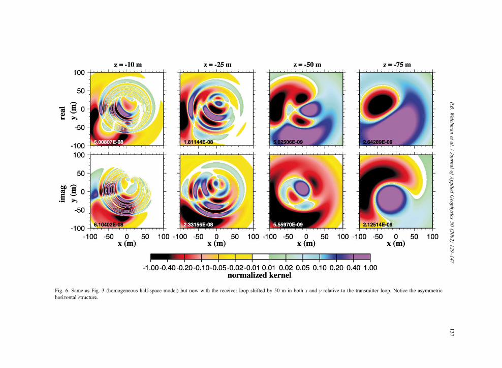
Fig. 6. Same as Fig. 3 (homogeneous half-space model) but now with the receiver loop shifted by 50 m in both x and y relative to the transmitter loop. Notice the asymmetric

horizontal structure.

P.B.Weich

manet


Geophysics

50(2002)129–147

137

neous half-space model in the case where the

receiver loop is shifted away from the transmitter

loop by 50 m in both x and y directions. When the

two loops are coincident, the kernel retains a certain

approximate axial symmetry. When the receiver is

displaced from the transmitter, the axial symmetry is

destroyed completely. This symmetry breaking could

be an advantage when the spin distribution has a

nontrivial three-dimensional structure: comparison of

signals for coincident and noncoincident loops may

provide greater sensitivity to lateral variations in the

spin distribution. A test of this idea, which would

require comparisons also with the lateral sensitivity

gained simply by moving both loops, lies beyond the

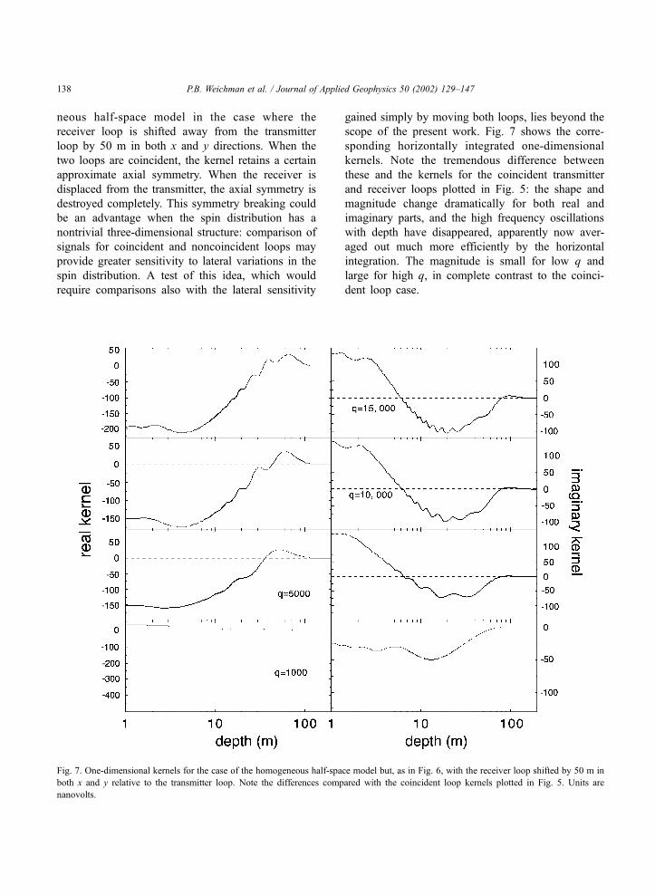
scope of the present work. Fig. 7 shows the corre-

sponding horizontally integrated one-dimensional

kernels. Note the tremendous difference between

these and the kernels for the coincident transmitter

and receiver loops plotted in Fig. 5: the shape and

magnitude change dramatically for both real and

imaginary parts, and the high frequency oscillations

with depth have disappeared, apparently now aver-

aged out much more efficiently by the horizontal

integration. The magnitude is small for low q and

large for high q, in complete contrast to the coinci-

dent loop case.

Fig. 7. One-dimensional kernels for the case of the homogeneous half-space model but, as in Fig. 6, with the receiver loop shifted by 50 m in

both x and y relative to the transmitter loop. Note the differences compared with the coincident loop kernels plotted in Fig. 5. Units are

nanovolts.


3. The inverse problem

Having gained some intuition in the previous

section regarding the interesting variation in NMR

sensitivity with depth, we consider now the inverse

problem: the estimation of the nuclear spin density as

a function of depth. We consider here two methods:

(a) the SVD method, which directly finds a single

solution which minimizes the mean square error; and

(b) the Monte Carlo method, in which the space of

possible solutions is explored to find the optimal one,

with a wide range of definitions of optimality allowed.

The SVD method (Parker, 1994), is most appro-

priate for linear inverse problems. The singular values

and eigenvectors of the SVD matrix provide a quan-

titative measure of the propagation of random errors

in the voltage measurement to this single inferred

nuclear spin distribution.

In the Monte Carlo inversion method (see, e.g.,

Press et al., 1986), solutions to the forward problem

for a large random sampling of spin distributions are

used to find the best fit to the given set of voltage data

V( qi). The distribution of ‘‘nearby’’ solutions subse-

quently provides statistical information about error

propagation. In applications such as the present one,

where one has no a priori knowledge that significantly

reduces the size of the search space, Monte Carlo is

limited to problems where the dimension of this space

is not too large. Its chief advantages are that it allows

an unbiased search of a prespecified range of forward

problems, and that it works equally well for linear and

nonlinear problems. The enforcement of certain

classes of a priori constraints, such as the positivity

of the spin density, is then trivial. This is especially

advantageous in nonlinear problems where widely

separated ‘‘islands’’ of forward problems (in the space

of spin distributions) may both yield voltage data very

close to the observed data. Such islands are forbidden

in linear inverse problems because, by linearity, the

entire straight line of solutions interpolating between

any two good solutions provides a family of equally

good solutions.

Although the formulation (5) of the inverse prob-

lem is linear, there are two important nonlinear

versions of the problem for which the Monte Carlo

method will be useful. First, as will be discussed in

Section 4 below, present experiments measure the

absolute magnitude of the voltage far better than they

do the individual real and imaginary parts—for some

reason, tremendous phase noise exists in the instru-

mentation. It is then advantageous to define a new

nonlinear inverse problem by taking the absolute

magnitude of both sides of Eq. (5) and invert for

the water distribution from the voltage magnitudes

alone.

Second, of ultimate interest is the problem in which

both the spin distribution and the ground conductivity

are estimated simultaneously. The ground conductiv-

ity is determined, e.g., from an independent time

domain electromagnetic (TDEM) measurement, con-

stituting another inverse problem with its own set of

random errors. Although in the present work the

ground conductivity is assumed given a priori, more

properly its errors should be propagated into the NMR

inversion. Furthermore, the conductivity, as in the

case of highly saline water, can be correlated with

the spin distribution, and a joint inversion of NMR

and TDEM data may then be appropriate. Since the

conductivity enters the NMR sensitivity kernel in a

highly nonlinear fashion, Monte Carlo inversion may

be the method of choice. Such a study would be

appropriate for future work.

3.1. SVD analysis

Since the number N of voltage data points Vi is

typically larger than the number M of free model

parameters nj, Eq. (5) will generally have no solution

if voltage noise is present. In this case an optimal

solution is obtained by choosing the nj to minimize an

appropriate error function E. A common choice is the

L2 norm

E ¼XNi¼1

Vi �XMj¼1

Kijnj

��2

, ð6Þ

whose minimization then yields, in matrix notation,

n ¼ S�1ReðKyVÞ, ð7Þ

where S = Re(KyK) is a real symmetric, positive

definite, M�M matrix. With independent Gaussian

noise of standard deviation DV in the real and imag-

inary parts of each Vi so that hyVi * yVji = 2 (DV)2dijand hyViyVji= 0, one obtains correspondingly,

hyniynji ¼ ðDV Þ2½S�1�ij: ð8Þ


The eigenvalues of S are real, positive, and we there-

fore denote them by {kl2}l = 1

M , where {kl}l = 1M define

the singular values of K. If {rl}l = 1M are the corre-

sponding orthonormal set of eigenvectors of S, and

one decomposes n ¼XMl¼1

mlrl, then

hymlymmi ¼ðDV Þ2

k2ldlm: ð9Þ

The singular values, therefore, determine the amplifi-

cation of the voltage noise along the corresponding

eigendirections in model space. The smallest singular

values determine the combinations of model parame-

ters most susceptible to noise.

In Weichman et al. (1999, 2000), an SVD analysis

was used to investigate sensitivity to horizontally stra-

tified water using coincident circular loops. Here, we

extend that analysis to coincident figure-eight loops.

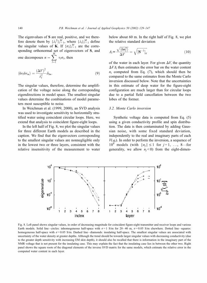
In the left half of Fig. 8, we plot the singular values

for three different Earth models as described in the

caption. We find that the eigenvectors corresponding

to the smallest singular values are nonnegligible only

in the lowest two or three layers, consistent with the

relative insensitivity of the measurement to water

below about 60 m. In the right half of Fig. 8, we plot

the relative standard deviation

Diu

ffiffiffiffiffiffiffiffiffiffiffihyn2i i

pDV

¼ffiffiffiffiffiffiffiffiffiffiffiffiffi½S�1�ii

qð10Þ

of the water in each layer. For given DV, the quantity

DVDi then estimates the error bar on the water content

ni computed from Eq. (7), which should then be

compared to the same estimates from the Monte Carlo

inversion discussed below. Note that the uncertainties

in this estimate of deep water for the figure-eight

configuration are much larger than for circular loops

due to a partial field cancellation between the two

lobes of the former.

3.2. Monte Carlo inversion

Synthetic voltage data is computed from Eq. (5)

using a given conductivity profile and spin distribu-

tion. The data is then contaminated by adding Gaus-

sian noise, with some fixed standard deviation,

independently to the real and imaginary parts of each

V( qi). In order to perform the inversion, a sequence of

108 models (with AnjAV 1 for j = 1, . . ., 8—for

generality, we allow nj < 0) from the eight-dimen-

Fig. 8. Left panel shows singular values, in order of decreasing magnitude for coincident figure-eight transmitter and receiver loops and various

Earth models. Solid line–circles: inhomogeneous half-space with r= 1 S/m for 20–40 m, r= 0.05 S/m elsewhere. Dotted line–squares:

homogeneous half-space with r= 0.05 S/m. Dashed line–diamonds: insulating half-space. The smallest singular values are associated with

uncertainty of the water density at greater depths. Although the trend should be towards larger singular values with decreasing conductivity (due

to the greater depth sensitivity with increasing EM skin depth), it should also be recalled that there is information in the imaginary part of the

NMR voltage that is not present for the insulating case. This may explain the fact that the insulating case lies in between the other two. Right

panel shows the square roots of the diagonal elements of the inverse SVD matrix for the same models, which estimate the relative error in the

computed water content in each layer.


sional spin distribution space is randomly chosen, the

voltage data computed via Eq. (5), and the v2 of the fitto the synthetic data is computed. In order to facilitate

comparison of the various factors that influence the

inversion, in each simulation, we pick 100 models out

of the 108 that give the best v2 fit to the data. For these100 models, we compute the average and the standard

deviation. Each Monte Carlo simulation takes about

1.5 h of computer time on a SUN Ultra workstation,

corresponding to about 2� 104 models/s. Note that

the calculation for each model simply involves the

evaluation of the sum in Eq. (6) which, since the Kij

are the same for all models, is extremely fast. Table 1

summarizes the five different simulations we perform.

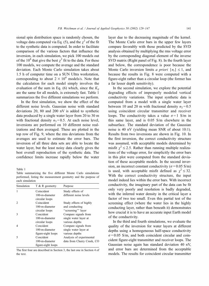
In the first simulation, we show the effect of the

different noise levels. Gaussian noise with standard

deviations 20, 80 and 200 nV is added to synthetic

data produced by a single water layer from 20 to 30 m

with fractional density n3 = 0.5. At each noise level,

inversions are performed on 10 different noise real-

izations and then averaged. These are plotted in the

top row of Fig. 9, where the rms deviations from the

averages are used to estimate the error bars. The

inversion of all three data sets are able to locate the

water layer, but the least noisy data clearly gives the

best overall reproduction of the synthetic data. The

confidence limits increase rapidly below the water

layer due to the decreasing magnitude of the kernel.

The Monte Carlo error bars in the upper few layers

compare favorably with those predicted by the SVD

analysis obtained by multiplying the rms voltage error

by the corresponding diagonal element of the inverse

SVD matrix (Right panel of Fig. 8). In the fourth layer

and below, the correspondence is poor because the

Monte Carlo inversion limits a priori AniAV 1, and

because the results in Fig. 8 were computed with a

figure-eight rather than a circular loop (the former has

a far lesser depth sensitivity).

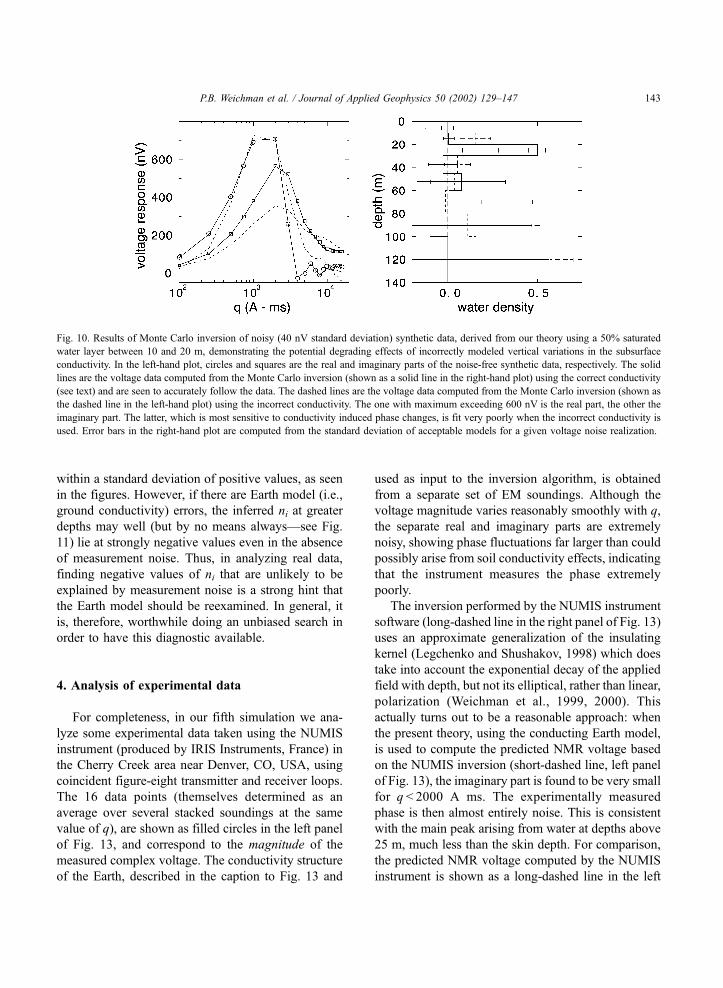
In the second simulation, we explore the potential

degrading effects of improperly modeled vertical

conductivity variations. The input synthetic data is

computed from a model with a single water layer

between 10 and 20 m with fractional density n2 = 0.5

using coincident circular transmitter and receiver

loops. The conductivity takes a value r = 1 S/m in

this same layer, and is 0.05 S/m elsewhere in the

subsurface. The standard deviation of the Gaussian

noise is 40 nV (yielding mean SNR of about 10:1).

Results from two inversions are shown in Fig. 10. In

the first inversion, the correct conductivity structure

was assumed, with acceptable models determined by

misfit v2V 2.5. Rather than running multiple realiza-

tions of the voltage error, for simplicitly the error bars

in this plot were computed from the standard devia-

tion of these acceptable models. In the second inver-

sion, an incorrect constant conductivity (r = 0.05 S/m)

is used, with acceptable misfit defined as v2V 32.

With the correct conductivity structure, the input

model indeed lies within the error bars. With incorrect

conductivity, the imaginary part of the data can be fit

only very poorly and resolution is badly degraded,

with the inferred water density in the critical layer a

factor of two too small. Even this partial test of the

screening effect (where the water lies in the highly

conducting layer, rather than beneath it) demonstrates

how crucial it is to have an accurate input Earth model

of the conductivity.

In the third and fourth simulations, we evaluate the

quality of the inversion for water layers at different

depths using a homogeneous half-space conductivity

r = 0.05 S/m, and both coincident circular and coin-

cident figure-eight transmitter and receiver loops. The

Gaussian noise again has standard deviation 40 nV,

and error bars are determined from the acceptable

models. The results for coincident circular transmitter

Table 1

Table summarizing the five different Monte Carlo simulations

performed, listing the measurement geometry and the purpose of

each simulation

Simulation T & R geometry Purpose

1 Coincident

100-m-diameter

circular loops

Study effects of

different noise levels

2 Coincident

100-m-diameter

circular loops

Study effects of highly

and conducting

‘‘screening’’’ layer

3 Concident

100-m-diameter

circular loops

Compare signals from

single water layer at

various depths

4 Concident

100-m-diameter

figure-eight loops

Compare signals from

single water layer at

various depths

5 Concident

100-m-diameter

figure-eight loops

Analysis of experimental

data from Cherry Creek, CO

The first four are described in Section 3, the last one in Section 4 of

the text.


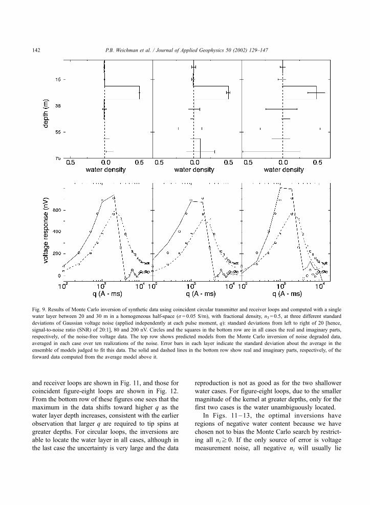
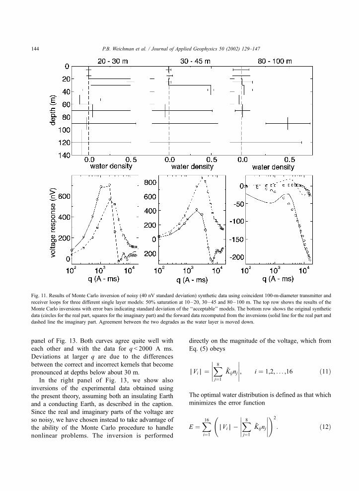
and receiver loops are shown in Fig. 11, and those for

coincident figure-eight loops are shown in Fig. 12.

From the bottom row of these figures one sees that the

maximum in the data shifts toward higher q as the

water layer depth increases, consistent with the earlier

observation that larger q are required to tip spins at

greater depths. For circular loops, the inversions are

able to locate the water layer in all cases, although in

the last case the uncertainty is very large and the data

reproduction is not as good as for the two shallower

water cases. For figure-eight loops, due to the smaller

magnitude of the kernel at greater depths, only for the

first two cases is the water unambiguously located.

In Figs. 11–13, the optimal inversions have

regions of negative water content because we have

chosen not to bias the Monte Carlo search by restrict-

ing all niz 0. If the only source of error is voltage

measurement noise, all negative ni will usually lie

Fig. 9. Results of Monte Carlo inversion of synthetic data using coincident circular transmitter and receiver loops and computed with a single

water layer between 20 and 30 m in a homogeneous half-space (r= 0.05 S/m), with fractional density, n3 = 0.5, at three different standard

deviations of Gaussian voltage noise (applied independently at each pulse moment, q): standard deviations from left to right of 20 [hence,

signal-to-noise ratio (SNR) of 20:1], 80 and 200 nV. Circles and the squares in the bottom row are in all cases the real and imaginary parts,

respectively, of the noise-free voltage data. The top row shows predicted models from the Monte Carlo inversion of noise degraded data,

averaged in each case over ten realizations of the noise. Error bars in each layer indicate the standard deviation about the average in the

ensemble of models judged to fit this data. The solid and dashed lines in the bottom row show real and imaginary parts, respectively, of the

forward data computed from the average model above it.


within a standard deviation of positive values, as seen

in the figures. However, if there are Earth model (i.e.,

ground conductivity) errors, the inferred ni at greater

depths may well (but by no means always—see Fig.

11) lie at strongly negative values even in the absence

of measurement noise. Thus, in analyzing real data,

finding negative values of ni that are unlikely to be

explained by measurement noise is a strong hint that

the Earth model should be reexamined. In general, it

is, therefore, worthwhile doing an unbiased search in

order to have this diagnostic available.

4. Analysis of experimental data

For completeness, in our fifth simulation we ana-

lyze some experimental data taken using the NUMIS

instrument (produced by IRIS Instruments, France) in

the Cherry Creek area near Denver, CO, USA, using

coincident figure-eight transmitter and receiver loops.

The 16 data points (themselves determined as an

average over several stacked soundings at the same

value of q), are shown as filled circles in the left panel

of Fig. 13, and correspond to the magnitude of the

measured complex voltage. The conductivity structure

of the Earth, described in the caption to Fig. 13 and

used as input to the inversion algorithm, is obtained

from a separate set of EM soundings. Although the

voltage magnitude varies reasonably smoothly with q,

the separate real and imaginary parts are extremely

noisy, showing phase fluctuations far larger than could

possibly arise from soil conductivity effects, indicating

that the instrument measures the phase extremely

poorly.

The inversion performed by the NUMIS instrument

software (long-dashed line in the right panel of Fig. 13)

uses an approximate generalization of the insulating

kernel (Legchenko and Shushakov, 1998) which does

take into account the exponential decay of the applied

field with depth, but not its elliptical, rather than linear,

polarization (Weichman et al., 1999, 2000). This

actually turns out to be a reasonable approach: when

the present theory, using the conducting Earth model,

is used to compute the predicted NMR voltage based

on the NUMIS inversion (short-dashed line, left panel

of Fig. 13), the imaginary part is found to be very small

for q < 2000 A ms. The experimentally measured

phase is then almost entirely noise. This is consistent

with the main peak arising from water at depths above

25 m, much less than the skin depth. For comparison,

the predicted NMR voltage computed by the NUMIS

instrument is shown as a long-dashed line in the left

Fig. 10. Results of Monte Carlo inversion of noisy (40 nV standard deviation) synthetic data, derived from our theory using a 50% saturated

water layer between 10 and 20 m, demonstrating the potential degrading effects of incorrectly modeled vertical variations in the subsurface

conductivity. In the left-hand plot, circles and squares are the real and imaginary parts of the noise-free synthetic data, respectively. The solid

lines are the voltage data computed from the Monte Carlo inversion (shown as a solid line in the right-hand plot) using the correct conductivity

(see text) and are seen to accurately follow the data. The dashed lines are the voltage data computed from the Monte Carlo inversion (shown as

the dashed line in the left-hand plot) using the incorrect conductivity. The one with maximum exceeding 600 nV is the real part, the other the

imaginary part. The latter, which is most sensitive to conductivity induced phase changes, is fit very poorly when the incorrect conductivity is

used. Error bars in the right-hand plot are computed from the standard deviation of acceptable models for a given voltage noise realization.


panel of Fig. 13. Both curves agree quite well with

each other and with the data for q < 2000 A ms.

Deviations at larger q are due to the differences

between the correct and incorrect kernels that become

pronounced at depths below about 30 m.

In the right panel of Fig. 13, we show also

inversions of the experimental data obtained using

the present theory, assuming both an insulating Earth

and a conducting Earth, as described in the caption.

Since the real and imaginary parts of the voltage are

so noisy, we have chosen instead to take advantage of

the ability of the Monte Carlo procedure to handle

nonlinear problems. The inversion is performed

directly on the magnitude of the voltage, which from

Eq. (5) obeys

AViA ¼X8j¼1

K̃ijnj

��, i ¼ 1,2, . . . ,16 ð11Þ

The optimal water distribution is defined as that which

minimizes the error function

E ¼X16i¼1

AViA�X8j¼1

K̃ijnj

��

!2

: ð12Þ

Fig. 11. Results of Monte Carlo inversion of noisy (40 nV standard deviation) synthetic data using coincident 100-m-diameter transmitter and

receiver loops for three different single layer models: 50% saturation at 10–20, 30–45 and 80–100 m. The top row shows the results of the

Monte Carlo inversions with error bars indicating standard deviation of the ‘‘acceptable’’ models. The bottom row shows the original synthetic

data (circles for the real part, squares for the imaginary part) and the forward data recomputed from the inversions (solid line for the real part and

dashed line the imaginary part. Agreement between the two degrades as the water layer is moved down.


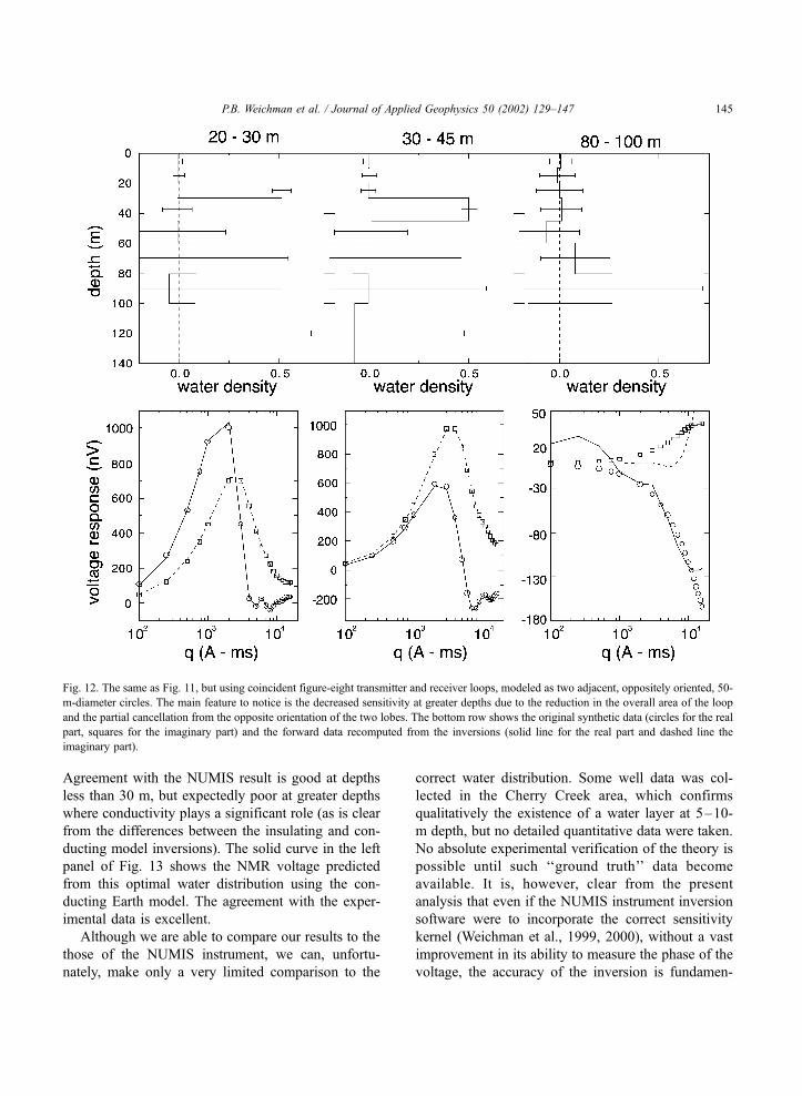
Agreement with the NUMIS result is good at depths

less than 30 m, but expectedly poor at greater depths

where conductivity plays a significant role (as is clear

from the differences between the insulating and con-

ducting model inversions). The solid curve in the left

panel of Fig. 13 shows the NMR voltage predicted

from this optimal water distribution using the con-

ducting Earth model. The agreement with the exper-

imental data is excellent.

Although we are able to compare our results to the

those of the NUMIS instrument, we can, unfortu-

nately, make only a very limited comparison to the

correct water distribution. Some well data was col-

lected in the Cherry Creek area, which confirms

qualitatively the existence of a water layer at 5–10-

m depth, but no detailed quantitative data were taken.

No absolute experimental verification of the theory is

possible until such ‘‘ground truth’’ data become

available. It is, however, clear from the present

analysis that even if the NUMIS instrument inversion

software were to incorporate the correct sensitivity

kernel (Weichman et al., 1999, 2000), without a vast

improvement in its ability to measure the phase of the

voltage, the accuracy of the inversion is fundamen-

Fig. 12. The same as Fig. 11, but using coincident figure-eight transmitter and receiver loops, modeled as two adjacent, oppositely oriented, 50-

m-diameter circles. The main feature to notice is the decreased sensitivity at greater depths due to the reduction in the overall area of the loop

and the partial cancellation from the opposite orientation of the two lobes. The bottom row shows the original synthetic data (circles for the real

part, squares for the imaginary part) and the forward data recomputed from the inversions (solid line for the real part and dashed line the

imaginary part).


tally limited within or below conductive layers.

Although we have not done a careful comparison

using synthetic data between inversions based on

Eqs. (6) and (12), in our earlier work, we considered

SVD inversions based on the real part of the signal

alone (Weichman et al., 1999, 2000), which should

yield similar results. There we showed that stability of

the inversion, as measured by the size of the smallest

singular value obtained from the SVD analysis, is

improved by nearly two orders of magnitude when

separate real and imaginary voltage data are included.

5. Conclusions

Using physically motivated noise levels and

ground conductivities, we conclude that the NMR

method should in principle be able to detect and

map water to depths of about 100 m. We have shown,

however, that incorrectly modeled ground conductiv-

ities can lead to extremely poor inversions, especially

when a highly conducting layer screens the signal

from greater depths. Correcting problems of this

nature requires both an accurate Earth model, which

relies on separate geoelectric section soundings, and

an accurate theoretical form for the kernel K.

We have considered in this paper two approaches

to solving the inverse problem: singular value decom-

position and Monte Carlo. In cases where a quadratic

error function, such as Eq. (6), is used, SVD provides

the more straightforward solution to the problem,

including detailed stability information through the

computed singular values. The results of Section 3

and of our earlier work (Weichman et al., 1999, 2000)

basically serve to confirm that the two approaches

give equivalent results for such cases. For more

complicated error functions, such as Eq. (12), SVD

is inappropriate (without further approximations, such

as linearizing the error function in the neighborhood

of a presumed solution), and Monte Carlo is the

method of choice, assuming that the search space is

not too large. In Section 4, we demonstrated the utility

of this method in a physically motivated inversion in

which only the signal magnitude was known accu-

rately.

Our results also point the way toward needed

improvements in the instrument technology. Not only

must the ‘‘dead time’’ between the end of the trans-

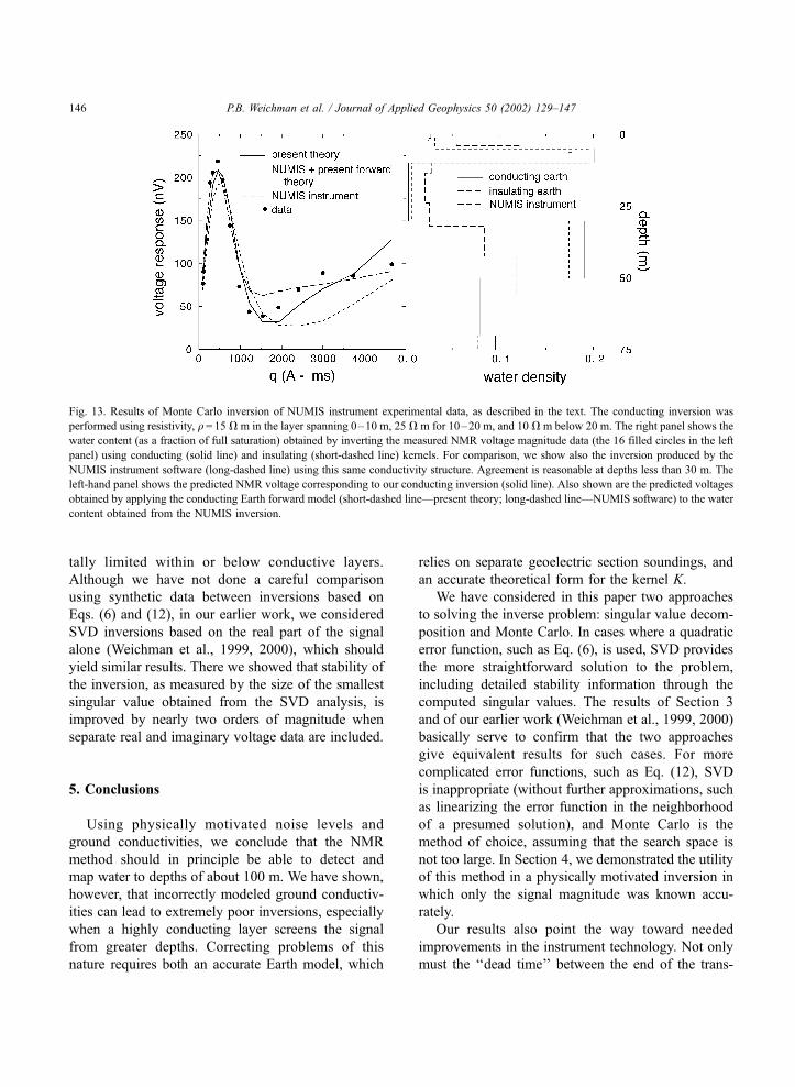
Fig. 13. Results of Monte Carlo inversion of NUMIS instrument experimental data, as described in the text. The conducting inversion was

performed using resistivity, q = 15 V m in the layer spanning 0–10 m, 25V m for 10–20 m, and 10 V m below 20 m. The right panel shows the

water content (as a fraction of full saturation) obtained by inverting the measured NMR voltage magnitude data (the 16 filled circles in the left

panel) using conducting (solid line) and insulating (short-dashed line) kernels. For comparison, we show also the inversion produced by the

NUMIS instrument software (long-dashed line) using this same conductivity structure. Agreement is reasonable at depths less than 30 m. The

left-hand panel shows the predicted NMR voltage corresponding to our conducting inversion (solid line). Also shown are the predicted voltages

obtained by applying the conducting Earth forward model (short-dashed line—present theory; long-dashed line—NUMIS software) to the water

content obtained from the NUMIS inversion.


mitted tipping pulse and the beginning of detection of

the received NMR signal be reduced as much as

possible to observe water in finer pores, but much

greater accuracy in the measured phase of the voltage

signal (i.e., of both its real and imaginary parts) will

be required. Only with full phase information will

inversions [based on Eq. (6), as compared to, say, Eq.

(12)] be sufficiently stable so as to obtain accurate

images of water deeper than, say, half a skin depth.

This is especially true when figure-eight loops, which

greatly reduce the effects of external noise, but at a

cost of reduced depth sensitivity, are used.

Acknowledgements

We are indebted to Mark Blohm and Pieter

Hoekstra for numerous insightful conversations about

the experimental data. We thank Pierre Valla and Ugur

Yaramanci for organizing this special issue on SNMR,

and A. Guillen for a careful review of the manuscript.

The support of the DOE through Contract No. DE-

FG07-96ER14732 is gratefully acknowledged.

References

Abragam, A., 1983. Principles of Nuclear Magnetism. Oxford Univ.

Press, New York.

Goldman, M., Rabinovich, B., Rabinovich, M., Gilad, D., Gev, I.,

Schirov, M., 1994. Application of the integrated NMR-TDEM

method in groundwater exploration in Israel. J. Appl. Geophys.

31, 27–52.

Hendrickx, J.M.H., Yao, T., Kearns, A., Hoekstra, P., Blohm, R.J.,

Blohm, M.W., Weichman, P.B., Lavely, E.M., 1999. Nuclear

magnetic resonance imaging of water content in the subsur-

face, Report to the DOE under agreement no. DE-FG07-

96ER14732.

Kleinberg, R.L., Kenyon, W.E., Mitra, P.P., 1994. J. Magn. Reson.,

Ser. A 108, 206–214.

Legchenko, A.V., Shushakov, O.A., 1998. Inversion of surface

NMR data. Geophysics 63, 75–84.

Parker, R.L., 1994. Geophysical Inverse Theory. Princeton Univ.

Press, Princeton, NJ.

Press, W.H., Flannery, B.P., Teukolsky, S.A., Vetterling, W.T., 1986.

Numerical Recipes. Cambridge Univ. Press, Cambridge.

Trushkin, D.V., Shushakov, O.A., Legchenko, A.V., 1995. Surface

NMR applied to an electroconductive medium. Geophys. Pros-

pect. 43, 623–633.

Weichman, P.B., 2001. Nuclear magnetic resonance imaging of

water content in the subsurface. Proceedings of the Symposium

on Application of Geophysics to Engineering and Environmen-

tal Problems.

Weichman, P.B., Lavely, E.M., Ritzwoller, M.H., 1999. Surface

nuclear magnetic resonance imaging of large systems. Phys.

Rev. Lett. 82, 4102–4105. This paper has also been featured

on the Physical Review Focus website, Dowsing with

Nuclear Magnetic Resonance, http://focus.aps.org/v3/

st27.html, May 17, 1999.

Weichman, P.B., Lavely, E.M., Ritzwoller, M.H., 2000. Theory of

surface nuclear magnetic resonance with applications to geo-

physical imaging problems. Phys. Rev. E 62, 1290–1312.


Study of surface nuclear magnetic resonance inverse problems

Documents

Transcript of Study of surface nuclear magnetic resonance inverse problems