Studying the Vulnerability of Steel Moment Resistant Frames Subjected to Progressive Collapse
Upload
khangminh22Category
view
1download
0
Study of Steel Structural SystemsSubjected to Fire
Mian Zhou
A dissertation submitted in partial fulfillment
of the requirements for the degree of
Doctor of Philosophy
of
Brunel University London.
Department of Civil Engineering
Brunel University London
October 25, 2019

2
I, Mian Zhou, confirm that the work presented in this thesis is my own. Where
information has been derived from other sources, I confirm that this has been indi-
cated in the work.

Abstract
Performance-based engineering design aims to improve codified, rule-based prac-
tice by allowing a more flexible, and performance focused approach. In structural
fire design, it enables more complex fire loading scenarios to be considered, ranging
from fire following earthquakes to a localised fire travelling through a large com-
partment space, or a combination of both. However, the tools used for performance-
based structural fire design rely on accurate material models to capture the structural
response to complicated fire loading.
One critical limitation in the current generation of performance-based tools is
that thermo-mechanical analysis with fire has been frequently performed using ma-
terial models which do not take strain reversals into account. The assumption of
“no strain reversals” in the building materials at elevated temperatures was estab-
lished because the fire loading is traditionally simplified to a temperature time curve
only considering heating stage, and the structural components are usually consid-
ered subjected to uniform heating. However this assumption is no longer valid when
complex fire loading is applied.
A new rate-independent combined isotropic-kinematic hardening plasticity
model was developed in this research for the thermo-mechanical analysis of steel
materials in fire. This model is capable of modelling: strain reversals, the
Bauschinger effect with its associated transient hardening behaviour and material
non-linearity at elevated temperatures. Its accuracy is demonstrated through five
validation studies of the proposed material model against experimental data.
The engineering value of the proposed material model is demonstrated in this
work through three case studies. The new material model was adopted for: (1)

Abstract 4
evaluating the remaining structural fire resistance after a moderate earthquake, (2)
investigating stainless steel structural systems in fire, and (3) studying the fire per-
formance of a single steel beam subjected to travelling fires. These studies demon-
strated that the new material model produces a more accurate analysis of the struc-
tural fire resistance than can be achieved using existing methods.
This research proposes an improved computational tool for evaluating struc-
tural fire resistance of complex steel structures. It therefore represents a contribution
to the improvement and adoption of performance-based engineering for structural
fire design, and can be used for various engineering applications.
Publications
Journal PapersM. Zhou, R. Cardoso, and H. Bahai, “A new material model for thermo-
mechanical analysis of steels in fire”, International Journal of Mechanical Sciences,
vol. 159, pp. 467 – 486, 2019
M. Zhou, L. Jiang, S. Chen, A. Usmani and R. Cardoso, “Remaining fire resis-
tance of steel frames following a moderate earthquake —A case study”, Journal of
Constructional Steel Research, accepted, 2019
M. Zhou, R. Cardoso, H. Bahai, and A. Usmani, “A thermo-mechanical analy-
sis of stainless steel structures in fire”, Engineering Structures, under review, 2019
Conference PapersM. Zhou, L. Jiang, Y. Wang, S. Chen, A. Usmani, “Case study of residual fire
resistance of multi-story steel frames following moderate earthquakes”, in The 8th
International Conference on Steel and Aluminium Structures, 2016
M. Zhou, L. Jiang, Y. Wang, S. Chen, A. Usmani, “Case study of residual fire
resistance of multi-story steel frames following moderate earthquakes”, in The 1st
European Conference on OpenSEES, 2017
M. Zhou, R. Cardoso, H. Bahai, and A. Usmani, “Thermo-mechanical be-
haviour of structural stainless steel frames in fire”, in The 10th International Con-
ference on Structures in Fire, 2018

Publications 6
M. Zhou, R. Cardoso, H. Bahai, and A. Usmani, “A novel steel material model
for structural thermo-mechanical analysis in fire ”, in The 1st Eurasia Conference
on OpenSEES, 2019

Acknowledgements
Mother says I am a lucky kid, not the smart kid but the lucky one. I have turned up
at the right place at the right time for so many times. Like that mundane Aberdeen
afternoon 4 years ago when I emailed Prof. Asif Usmani then in Edinburgh asking
whether he had a PhD position for me. I would like to express my sincere gratitude
to Prof. Usmani for having faith in me and offering me this PhD position, and for
all the advice and support he has provided me with over the years.
There is the chinese saying that for a good story you can guess the start but
never the ending. Being the not smart kid, I only had the location of my PhD story
right. Being the lucky kid, I am grateful for Prof. Hamid Bahai being a great listener
and facilitator, and to Dr. Giulio Alfano whose open mindedness and dedication to
students I admire greatly. I would also like to thank Dr. Rui Cardoso. For the
patience, guidance and advice he showed me, I could not have asked for a better
first supervisor. He taught me the great lesson of sticking with the principles of the
academic life, i.e., zero tolerance for any violations of Newton’s laws. My PhD is a
good story after all, owing to all the brilliant academics and wonderful friends who
helped me along the way.
I think I am indeed a lucky kid because I have always had the best support from
my dear mum and dad. I thank them for always being my rock. Last but certainly
not least, I would like to thank my Dr. wind turbine soon to be himself indoors, who
has been there for me through the peaks and troughs of the whole journey.

Contents
1 Introduction 22
1.1 Motivation and aims . . . . . . . . . . . . . . . . . . . . . . . . . 22
1.2 Research scope and approach . . . . . . . . . . . . . . . . . . . . . 26
2 Literature Review 28
2.1 History of structural fire resistance design . . . . . . . . . . . . . . 28
2.2 Performance-based structural fire resistance design framework . . . 33
2.2.1 Estimate of fire demand . . . . . . . . . . . . . . . . . . . 33
2.2.1.1 Analytical fire models . . . . . . . . . . . . . . . 34
2.2.1.2 Computational fire dynamics models . . . . . . . 37
2.2.1.3 Design fires and fire scenarios . . . . . . . . . . . 38
2.2.2 Heat transfer for structures in fire . . . . . . . . . . . . . . 38
2.2.3 Estimate of structural fire resistance . . . . . . . . . . . . . 40
2.2.3.1 Material softening at elevated temperatures . . . . 41
2.2.3.2 Global structural mechanisms in fire . . . . . . . 44
2.2.4 Damage of Passive Fire Protection coatings . . . . . . . . . 48
2.3 Stainless steel structures in fire . . . . . . . . . . . . . . . . . . . . 50
2.3.1 Thermal expansion . . . . . . . . . . . . . . . . . . . . . . 51
2.3.2 Thermal properties . . . . . . . . . . . . . . . . . . . . . . 54
2.3.3 Existing research on stainless steel structures in fire . . . . . 56
2.4 Material models for thermo-mechanical analysis with fire . . . . . . 57
2.4.1 Material non-linearity . . . . . . . . . . . . . . . . . . . . 57
2.4.2 Existing non-linear material models . . . . . . . . . . . . . 59

Contents 9
2.4.3 Bauschinger effect . . . . . . . . . . . . . . . . . . . . . . 64
2.4.4 Strain rate dependency for structural fire analysis . . . . . . 65
2.4.5 Existing kinematic hardening plasticity models at room
temperature . . . . . . . . . . . . . . . . . . . . . . . . . . 67
2.4.5.1 Mroz’s multi-surface model . . . . . . . . . . . . 67
2.4.5.2 Two yield-surface models . . . . . . . . . . . . . 68
2.4.5.3 Non-linear kinematic hardening models . . . . . 69
3 A New Material Model for Thermo-mechanical Analysis of Steels in
Fire 72
3.1 Temperature effects on plasticity models . . . . . . . . . . . . . . . 72
3.1.1 Parametric dependency on temperature . . . . . . . . . . . 74
3.1.2 Temperature rate dependency for internal variables . . . . . 74
3.2 Decoupling thermal and mechanical step . . . . . . . . . . . . . . . 75
3.2.1 Elastic modulus at elevated temperatures . . . . . . . . . . 77
3.2.2 Yield surfaces at elevated temperatures . . . . . . . . . . . 77
3.2.3 Plastic flow potential at elevated temperatures . . . . . . . . 78
3.2.4 Internal state variables’ evolution at elevated temperatures . 80
3.3 A new plasticity model for thermo-mechanical analysis with fire . . 81
3.3.1 Thermal step . . . . . . . . . . . . . . . . . . . . . . . . . 81
3.3.2 Mechanical step . . . . . . . . . . . . . . . . . . . . . . . 85
3.3.2.1 First kinematic hardening variable β1β1β1 . . . . . . . 86
3.3.2.2 Second kinematic hardening variable β2β2β2 . . . . . 88
3.3.3 Thermal step during reverse loading . . . . . . . . . . . . . 90
3.3.4 Elastoplastic consistent tangent modulus DepDepDep . . . . . . . . 91
3.3.5 Summary of the new model . . . . . . . . . . . . . . . . . 92
3.4 Validation of isotropic & kinematic hardening during monotonic
loading . . . . . . . . . . . . . . . . . . . . . . . . . . . . . . . . 96
3.4.1 Bauschinger effect determination at elevated temperatures . 97
3.4.2 FE model descriptions . . . . . . . . . . . . . . . . . . . . 97
3.4.3 Results and discussion . . . . . . . . . . . . . . . . . . . . 99

Contents 10
3.5 Validation of Bauschinger effect and transient hardening . . . . . . 101
3.6 Validation of thermal unloading algorithm . . . . . . . . . . . . . . 105
3.7 Validation for multi-axial loadings . . . . . . . . . . . . . . . . . . 106
3.7.1 Experiments in literature review . . . . . . . . . . . . . . . 106
3.7.1.1 Room temperature . . . . . . . . . . . . . . . . . 107
3.7.1.2 Elevated temperature 650 °C . . . . . . . . . . . 108
3.7.2 Validation model in Abaqus . . . . . . . . . . . . . . . . . 108
3.7.2.1 Model descriptions . . . . . . . . . . . . . . . . 108
3.7.2.2 Material properties . . . . . . . . . . . . . . . . . 109
3.7.3 Validation results . . . . . . . . . . . . . . . . . . . . . . . 109
3.7.3.1 Initial yield surfaces . . . . . . . . . . . . . . . . 109
3.7.3.2 Subsequent yield surface after radial pre-loading
at room temperature . . . . . . . . . . . . . . . . 111
3.7.3.3 Subsequent yield surface after pure torsion pre-
loading at 650 °C . . . . . . . . . . . . . . . . . 111
3.8 Validation for transient loadings during heating and cooling . . . . . 112
3.8.1 Experimental model . . . . . . . . . . . . . . . . . . . . . 112
3.8.2 Validation model . . . . . . . . . . . . . . . . . . . . . . . 113
3.8.3 Validation of isothermal thermo-mechanical experiments . . 114
3.8.4 Validation of transient (anisothermal) thermo-mechanical
experiments . . . . . . . . . . . . . . . . . . . . . . . . . . 116
3.8.4.1 Comparison with isotropic hardening model . . . 118
3.9 Uniaxial material model . . . . . . . . . . . . . . . . . . . . . . . 119
3.10 Summary and conclusions . . . . . . . . . . . . . . . . . . . . . . 119
4 Remaining Fire Resistance of PFP Coated Steel Frames Subjected to A
Moderate Earthquake 121
4.1 Introduction . . . . . . . . . . . . . . . . . . . . . . . . . . . . . . 121
4.2 Cementitious PFP damage indicator . . . . . . . . . . . . . . . . . 123
4.3 Impact of seismic steel frame designs on PFP damage . . . . . . . . 126
4.3.1 FE Model geometry . . . . . . . . . . . . . . . . . . . . . 127

Contents 11
4.3.2 FE model Loadings . . . . . . . . . . . . . . . . . . . . . . 129
4.3.2.1 Gravity loads . . . . . . . . . . . . . . . . . . . . 129
4.3.2.2 Earthquake load . . . . . . . . . . . . . . . . . . 130
4.3.3 FE model Materials . . . . . . . . . . . . . . . . . . . . . . 130
4.3.4 FE models for seismic analysis . . . . . . . . . . . . . . . . 130
4.3.5 Earthquake response . . . . . . . . . . . . . . . . . . . . . 131
4.3.6 Damage to cementitious PFP . . . . . . . . . . . . . . . . . 132
4.3.7 Comparison study of strain results . . . . . . . . . . . . . . 133
4.3.7.1 Moment resisting frame . . . . . . . . . . . . . . 133
4.3.7.2 Concentrically braced frame . . . . . . . . . . . . 133
4.3.7.3 Discussion . . . . . . . . . . . . . . . . . . . . . 135
4.3.8 Sensitivity study of modelling assumptions of MRF . . . . . 135
4.3.8.1 Effect of floor slabs on strain distributions . . . . 148
4.3.9 Conclusions of sensitivity study . . . . . . . . . . . . . . . 151
4.4 Remaining fire resistance assessment of MRF . . . . . . . . . . . . 152
4.4.1 PFP damage area identification . . . . . . . . . . . . . . . . 152
4.4.2 Heat transfer analysis . . . . . . . . . . . . . . . . . . . . . 155
4.4.2.1 Fire loading . . . . . . . . . . . . . . . . . . . . 155
4.4.2.2 Fire protection required . . . . . . . . . . . . . . 155
4.4.2.3 Coefficients for heat transfer analysis . . . . . . . 155
4.4.2.4 Heat transfer analysis results . . . . . . . . . . . 156
4.4.3 Thermo-mechanical analysis . . . . . . . . . . . . . . . . . 157
4.4.3.1 FE model . . . . . . . . . . . . . . . . . . . . . 157
4.4.3.2 Thermo-mechanical analysis results . . . . . . . . 158
4.5 Discussion and conclusions . . . . . . . . . . . . . . . . . . . . . . 160
5 A Thermo-mechanical Analysis of Stainless Steel Structures in Fire 163
5.1 Introduction . . . . . . . . . . . . . . . . . . . . . . . . . . . . . . 163
5.2 Temperature development in stainless steel I sections . . . . . . . . 164
5.2.1 Heat transfer model validation . . . . . . . . . . . . . . . . 164
5.2.2 Heat transfer parametric study . . . . . . . . . . . . . . . . 166

Contents 12
5.3 Stainless steel structural behaviour in fire . . . . . . . . . . . . . . 167
5.3.1 Simply supported beams in fire . . . . . . . . . . . . . . . 168
5.3.1.1 FE model validation . . . . . . . . . . . . . . . . 168
5.3.1.2 Comparison study . . . . . . . . . . . . . . . . . 170
5.3.1.3 Discussion . . . . . . . . . . . . . . . . . . . . . 174
5.3.2 Plane frame structures in fire . . . . . . . . . . . . . . . . . 175
5.3.2.1 FE model validation . . . . . . . . . . . . . . . . 175
5.3.2.2 Comparison study . . . . . . . . . . . . . . . . . 177
5.3.2.3 Effect of axial restraints . . . . . . . . . . . . . . 181
5.4 Conclusions . . . . . . . . . . . . . . . . . . . . . . . . . . . . . . 189
6 Bauschinger Effect in Steel Beams Subjected to Realistic Building Fire 191
6.1 Introduction . . . . . . . . . . . . . . . . . . . . . . . . . . . . . . 191
6.2 Thermal loading . . . . . . . . . . . . . . . . . . . . . . . . . . . . 193
6.3 Numerical analysis in 3D . . . . . . . . . . . . . . . . . . . . . . . 194
6.3.1 FE model . . . . . . . . . . . . . . . . . . . . . . . . . . . 194
6.3.2 Stress/Deformation analysis ––Case 1 . . . . . . . . . . . . 197
6.3.3 Stress/Deformation analysis ––Case 2 . . . . . . . . . . . . 199
6.3.4 Comparison study . . . . . . . . . . . . . . . . . . . . . . 200
6.4 Numerical analysis in 2D . . . . . . . . . . . . . . . . . . . . . . . 202
6.4.1 Stress deformation analysis . . . . . . . . . . . . . . . . . . 202
6.5 Summary . . . . . . . . . . . . . . . . . . . . . . . . . . . . . . . 205
7 Conclusions and Future Work 206
7.1 Summary and conclusions . . . . . . . . . . . . . . . . . . . . . . 206
7.1.1 Application to remaining structural fire resistance . . . . . . 207
7.1.2 Application for novel construction materials . . . . . . . . . 208
7.1.3 Application for advanced structural design . . . . . . . . . 209
7.2 Limitations and future work . . . . . . . . . . . . . . . . . . . . . 209
Appendices 211

Contents 13
A Numerical Algorithm for Combined Isotropic and Kinematic Harden-
ing Model 211
B Implementation for Plane Stress Material Model 214
C Derivation of Elastoplastic Consistent Tangent Modulus DepDepDep 217
D Tables of Parameters 221
Bibliography 224

List of Figures
1.1 Performance based engineering design framework for structures in
fire . . . . . . . . . . . . . . . . . . . . . . . . . . . . . . . . . . . 22
2.1 Stiffness reduction of carbon steel and stainless steel at elevated
temperatures [1, 2] . . . . . . . . . . . . . . . . . . . . . . . . . . 42
2.2 2% Strength reduction of stainless steel and carbon steel at elevated
temperatures . . . . . . . . . . . . . . . . . . . . . . . . . . . . . . 43
2.3 Thermal elongation . . . . . . . . . . . . . . . . . . . . . . . . . . 53
2.4 Thermal conductivity . . . . . . . . . . . . . . . . . . . . . . . . . 54
2.5 Specific heat . . . . . . . . . . . . . . . . . . . . . . . . . . . . . . 55
2.6 Material model construction illustrations . . . . . . . . . . . . . . . 60
a Case A . . . . . . . . . . . . . . . . . . . . . . . . . . . . 60
b Case B . . . . . . . . . . . . . . . . . . . . . . . . . . . . 60
2.7 Construction of stress strain path, proposed by Bailey et al. [3] . . . 63
2.8 A schematic view of two surface model . . . . . . . . . . . . . . . 68
3.1 Stiffness reduction factors . . . . . . . . . . . . . . . . . . . . . . 77
3.2 EC3 stress-strain curves vs Least square fitting . . . . . . . . . . . 79
3.3 Stress-strain curves at elevated temperatures, Nominal vs Curve fitting 80
a Austenitic group III . . . . . . . . . . . . . . . . . . . . . . 80
b Duplex group II . . . . . . . . . . . . . . . . . . . . . . . . 80
3.4 Combined isotropic/kinematic hardening yield surfaces with tem-
perature changes in the deviatoric stress space . . . . . . . . . . . . 82
3.5 Re-positioning of yield surface due to changing temperatures . . . . 84

List of Figures 15
3.6 Reverse loading criterion . . . . . . . . . . . . . . . . . . . . . . . 86
3.7 Proposed model during loading ––reverse loading in the deviatoric
stress space . . . . . . . . . . . . . . . . . . . . . . . . . . . . . . 87
a Loading . . . . . . . . . . . . . . . . . . . . . . . . . . . . 87
b Reverse loading . . . . . . . . . . . . . . . . . . . . . . . . 87
3.8 Typical Bauschinger ratio and Reverse loading ratio evolution . . . 89
3.9 Proposed model during reverse loading in the deviatoric stress space 90
3.10 Yield surface evolution, T0 to T2 . . . . . . . . . . . . . . . . . . . 94
a Initial yield surface at T0 and T1 . . . . . . . . . . . . . . . 94
b Yield surface T1 . . . . . . . . . . . . . . . . . . . . . . . . 94
c Thermal step, T1 to T2 . . . . . . . . . . . . . . . . . . . . 94
d Mechanical step, T1 to T2 . . . . . . . . . . . . . . . . . . . 94
3.11 Bauschinger ratio, least square fitting . . . . . . . . . . . . . . . . . 98
3.12 Reverse yield test specimen (all dimensions in mm) [4] . . . . . . . 98
3.13 Hardening variables comparison . . . . . . . . . . . . . . . . . . . 100
a Isotropic . . . . . . . . . . . . . . . . . . . . . . . . . . . 100
b Kinematic . . . . . . . . . . . . . . . . . . . . . . . . . . . 100
3.14 Stress-strain curves comparison . . . . . . . . . . . . . . . . . . . 102
a T= 300°C . . . . . . . . . . . . . . . . . . . . . . . . . . . 102
b T= 700°C . . . . . . . . . . . . . . . . . . . . . . . . . . . 102
3.15 Hardening models comparison . . . . . . . . . . . . . . . . . . . . 104
a T= 300°C . . . . . . . . . . . . . . . . . . . . . . . . . . . 104
b T= 700°C . . . . . . . . . . . . . . . . . . . . . . . . . . . 104
3.16 Thermal unloading validation . . . . . . . . . . . . . . . . . . . . . 106
3.17 Abaqus plate model . . . . . . . . . . . . . . . . . . . . . . . . . . 109
3.18 Initial yield surfaces comparison . . . . . . . . . . . . . . . . . . . 110
a Room temperature . . . . . . . . . . . . . . . . . . . . . . 110
b 650 °C . . . . . . . . . . . . . . . . . . . . . . . . . . . . 110
3.19 Subsequent yield surfaces comparison . . . . . . . . . . . . . . . . 112
a Room temperature . . . . . . . . . . . . . . . . . . . . . . 112
List of Figures 16
b 650 °C . . . . . . . . . . . . . . . . . . . . . . . . . . . . 112
3.20 Thermo-mechanical test specimen (all dimensions in mm) [5] . . . 114
3.21 Stress strain curves comparison, Isothermal thermo-mechanical ex-
periments . . . . . . . . . . . . . . . . . . . . . . . . . . . . . . . 115
a T =150 °C . . . . . . . . . . . . . . . . . . . . . . . . . . . 115
b T =350 °C . . . . . . . . . . . . . . . . . . . . . . . . . . . 115
c T =600 °C . . . . . . . . . . . . . . . . . . . . . . . . . . . 115
d T =850 °C . . . . . . . . . . . . . . . . . . . . . . . . . . . 115
e T =1000 °C . . . . . . . . . . . . . . . . . . . . . . . . . . 115
3.22 Stress strain curves comparison, Transient thermo-mechanical ex-
periments . . . . . . . . . . . . . . . . . . . . . . . . . . . . . . . 116
a Tmax =350 °C . . . . . . . . . . . . . . . . . . . . . . . . 116
b Tmax =600 °C . . . . . . . . . . . . . . . . . . . . . . . . 116
c Tmax =850 °C . . . . . . . . . . . . . . . . . . . . . . . . 116
d Tmax =1000 °C . . . . . . . . . . . . . . . . . . . . . . . . 116
4.1 εcritical vs. Stress reversal Number . . . . . . . . . . . . . . . . . . 126
4.2 Acceleration history of 1994 Northridge earthquake . . . . . . . . . 127
4.3 Moment resisting frame in N-S direction (penthouse not shown) . . 128
4.4 Concentrically braced frame in N-S direction (Typical) . . . . . . . 129
4.5 Max. tensile strain diagram, MRF . . . . . . . . . . . . . . . . . . 135
a Strain distribution in Pier 1 . . . . . . . . . . . . . . . . . . 135
b Strain distribution in Pier 2 . . . . . . . . . . . . . . . . . . 135
c Strain distribution in Pier 3 . . . . . . . . . . . . . . . . . . 135
d Strain distribution in Floor beams . . . . . . . . . . . . . . 135
4.6 Max. tensile strain diagram, Concentrically braced frame . . . . . . 137
a Strain distribution in Pier 1 . . . . . . . . . . . . . . . . . . 137
b Strain distribution in Pier 2 . . . . . . . . . . . . . . . . . . 137
c Strain distribution in Pier 3 . . . . . . . . . . . . . . . . . . 137
d Strain distribution in Floor Beams . . . . . . . . . . . . . . 137
4.7 Model 1, Schematic illustration . . . . . . . . . . . . . . . . . . . . 140

List of Figures 17
4.8 Model 2, Schematic illustration . . . . . . . . . . . . . . . . . . . . 140
4.9 Panel zone, Schematic representation . . . . . . . . . . . . . . . . . 141
4.10 Model 3, Schematic illustration . . . . . . . . . . . . . . . . . . . . 141
4.11 Model 4, Schematic illustration . . . . . . . . . . . . . . . . . . . . 142
4.12 Leaning column system, Schematic representation . . . . . . . . . 142
4.13 Strain distribution in Pier 3, MRF . . . . . . . . . . . . . . . . . . 145
a Model 2 . . . . . . . . . . . . . . . . . . . . . . . . . . . . 145
b Model 3 . . . . . . . . . . . . . . . . . . . . . . . . . . . . 145
c Model 4 . . . . . . . . . . . . . . . . . . . . . . . . . . . . 145
d Model 5 . . . . . . . . . . . . . . . . . . . . . . . . . . . . 145
4.14 Strain distribution in floor beams, MRF . . . . . . . . . . . . . . . 147
a Model 2 . . . . . . . . . . . . . . . . . . . . . . . . . . . . 147
b Model 3 . . . . . . . . . . . . . . . . . . . . . . . . . . . . 147
c Model 4 . . . . . . . . . . . . . . . . . . . . . . . . . . . . 147
d Model 5 . . . . . . . . . . . . . . . . . . . . . . . . . . . . 147
4.15 Bending moment diagram of floor beams, Gravity load . . . . . . . 149
a Model 1 . . . . . . . . . . . . . . . . . . . . . . . . . . . . 149
b Model 2 . . . . . . . . . . . . . . . . . . . . . . . . . . . . 149
c Model 3 . . . . . . . . . . . . . . . . . . . . . . . . . . . . 149
4.16 Pier 3 moment diagram, Gravity load . . . . . . . . . . . . . . . . . 150
4.17 Pier 3 Max. moment diagram, Seismic load . . . . . . . . . . . . . 150
4.18 Max. negative &positive moments in floor beams, Seismic load . . . 151
a Model 2 . . . . . . . . . . . . . . . . . . . . . . . . . . . . 151
b Model 3 . . . . . . . . . . . . . . . . . . . . . . . . . . . . 151
4.19 Schematic view of the cementitious PFP damage identified in MRF,
Model 4 . . . . . . . . . . . . . . . . . . . . . . . . . . . . . . . . 153
4.20 Strain distribution in Pier 1 & 2, Model 4 . . . . . . . . . . . . . . 154
a Pier 1 . . . . . . . . . . . . . . . . . . . . . . . . . . . . . 154
b Pier 2 . . . . . . . . . . . . . . . . . . . . . . . . . . . . . 154
4.21 Temperature history results . . . . . . . . . . . . . . . . . . . . . . 157

List of Figures 18
4.22 Schematic illustration of thermal loading application . . . . . . . . 157
4.23 Pier 3 joint displacement comparison . . . . . . . . . . . . . . . . . 159
4.24 Vertical reaction development, with PFP damage . . . . . . . . . . 160
5.1 I section subjected to 4 sides heating . . . . . . . . . . . . . . . . . 165
5.2 Temperature development within sections . . . . . . . . . . . . . . 165
5.3 Temperature difference in bottom flange, 4 sides heated . . . . . . 167
5.4 Temperature difference in web, 4 sides heated . . . . . . . . . . . . 167
5.5 Validation of simply supported beam model . . . . . . . . . . . . . 169
a Four sides heating . . . . . . . . . . . . . . . . . . . . . . 169
b Three sides heating . . . . . . . . . . . . . . . . . . . . . . 169
5.6 Deflection comparisons, Simply supported beam . . . . . . . . . . 172
a Series 1 and 2 . . . . . . . . . . . . . . . . . . . . . . . . . 172
b Series 3 and 4 . . . . . . . . . . . . . . . . . . . . . . . . . 172
5.7 Stress strain development, simply supported beam . . . . . . . . . . 174
a Series 1 . . . . . . . . . . . . . . . . . . . . . . . . . . . . 174
b Series 2 . . . . . . . . . . . . . . . . . . . . . . . . . . . . 174
c Series 3 . . . . . . . . . . . . . . . . . . . . . . . . . . . . 174
d Series 4 . . . . . . . . . . . . . . . . . . . . . . . . . . . . 174
5.8 EHR3 frame configuration . . . . . . . . . . . . . . . . . . . . . . 176
5.9 EHR3 frame deflection comparison . . . . . . . . . . . . . . . . . . 177
5.10 Beam midspan deflection V4 . . . . . . . . . . . . . . . . . . . . . 179
5.11 Column midspan deflection U2 . . . . . . . . . . . . . . . . . . . . 180
5.12 Stress strain at the beam-column joint . . . . . . . . . . . . . . . . 182
a Stress strain in the beam . . . . . . . . . . . . . . . . . . . 182
b Stress strain in the Column . . . . . . . . . . . . . . . . . . 182
5.13 EHR3 frame with external axial restraints applied . . . . . . . . . . 183
5.14 Beam midspan def (V4), Beam L.R.=0.30 . . . . . . . . . . . . . . 184
5.15 Column vertical disp, Column L.R.=0.15 . . . . . . . . . . . . . . . 184
5.16 Beam axial force vs. temp., Beam L.R.=0.30 . . . . . . . . . . . . 185
5.17 Beam midspan def vs. temp, Beam L.R.=0.60 . . . . . . . . . . . . 187

List of Figures 19
5.18 Column vertical disp vs. temp, Column L.R.=0.30 . . . . . . . . . . 187
5.19 Stress strain developments at beam-column joint . . . . . . . . . . . 188
a Stress strain in the column, 0.05Kβ . . . . . . . . . . . . . 188
b Stress strain in the column, 0.15Kβ . . . . . . . . . . . . . 188
c Stress strain in the beam, 0.05Kβ . . . . . . . . . . . . . . . 188
d Stress strain in the beam, 0.15Kβ . . . . . . . . . . . . . . . 188
6.1 Structural model geometries . . . . . . . . . . . . . . . . . . . . . 193
a Case study structural plan view with predefined travelling
fire trajectory . . . . . . . . . . . . . . . . . . . . . . . . . 193
b Schematic view of the investigated beam cross-section . . . 193
6.2 Temperature history . . . . . . . . . . . . . . . . . . . . . . . . . . 195
a Case 1 . . . . . . . . . . . . . . . . . . . . . . . . . . . . . 195
b Case 2 . . . . . . . . . . . . . . . . . . . . . . . . . . . . . 195
6.3 Single steel beam modelled, half of the model length shown . . . . 196
6.4 Midspan cross-section results, Case 1 . . . . . . . . . . . . . . . . 198
a Deflection, ε p vs. temp . . . . . . . . . . . . . . . . . . . . 198
b Axial stress (S11) vs. temp . . . . . . . . . . . . . . . . . . 198
6.5 Midspan cross-section results, Case 2 . . . . . . . . . . . . . . . . 200
a Deflection, ε p vs. temp . . . . . . . . . . . . . . . . . . . . 200
b Axial stress (S11) vs. temp . . . . . . . . . . . . . . . . . . 200
6.6 Proposed material model vs. Isotropic hardening model . . . . . . . 201
a Endspan S11 vs. Temp . . . . . . . . . . . . . . . . . . . . 201
b Midspan S11 vs. Temp . . . . . . . . . . . . . . . . . . . . 201
6.7 Midspan deflection, 2D compared with 3D . . . . . . . . . . . . . . 203
6.8 Midspan S11 vs. Temperature, 2D . . . . . . . . . . . . . . . . . . 204
a Case 1 . . . . . . . . . . . . . . . . . . . . . . . . . . . . . 204
b Case 2 . . . . . . . . . . . . . . . . . . . . . . . . . . . . . 204

List of Tables
2.1 Simplified grade family at elevated temperatures . . . . . . . . . . . 43
2.2 Mean coefficient of thermal expansion (10−6/°C) . . . . . . . . . . 53
2.3 Types of the constitutive equations . . . . . . . . . . . . . . . . . . 58
3.1 Model parameters, Isothermal experiments . . . . . . . . . . . . . . 114
3.2 Model parameters, Transient experiments . . . . . . . . . . . . . . 117
4.1 Gravity loads . . . . . . . . . . . . . . . . . . . . . . . . . . . . . 129
4.2 Fundamental building periods . . . . . . . . . . . . . . . . . . . . 131
4.3 Inter-story drift ratios, Moment frame model . . . . . . . . . . . . . 132
4.4 Inter-story Drift Ratios, Braced Frame Model . . . . . . . . . . . . 132
4.5 Number of cycles in Pier 3, Moment frame model . . . . . . . . . . 132
4.6 MFR inter-story drift ratios (%), Pier 3 . . . . . . . . . . . . . . . . 143
4.7 Cementitious PFP thickness . . . . . . . . . . . . . . . . . . . . . 155
5.1 Section dimensions and Section factors . . . . . . . . . . . . . . . 166
5.2 Material properties . . . . . . . . . . . . . . . . . . . . . . . . . . 171
5.3 Comparison study series, Simply supported beams . . . . . . . . . 171
5.4 Test parameters used in Validation . . . . . . . . . . . . . . . . . . 177
5.5 Comparison study series, EHR3 frame . . . . . . . . . . . . . . . . 178
A.1 Numerical algorithm for the proposed combined isotropic- kine-
matic hardening model . . . . . . . . . . . . . . . . . . . . . . . . 211
B.1 Numerical algorithm for plane stress material . . . . . . . . . . . . 215

List of Tables 21
D.1 Least square fitting results for hardening law, EC3 carbon steel . . . 221
D.2 Least square fitting results for hardening law, Austenitic III . . . . . 221
D.3 Least square fitting results for hardening law, Duplex II . . . . . . . 222
D.4 Least square fitting results, 304L stainless steel in Section 3.4 . . . . 222
D.5 Least square fitting results, Low carbon steel in Section 3.5 . . . . . 222
D.6 Least square fitting results, 316 stainless steel in Section 3.7 . . . . 222
D.7 Least square fitting results for hardening law, St 37.2 carbon steel
in [6] . . . . . . . . . . . . . . . . . . . . . . . . . . . . . . . . . . 222
D.8 Least square fitting results, 304 Stainless Steel . . . . . . . . . . . . 223
D.9 Bauschinger ratio calibration results, based on Fig.8 in [5] . . . . . 223

Chapter 1
Introduction
1.1 Motivation and aimsThis project aims to improve the performance-based structural fire design, and sub-
sequently apply it to a range of parametric studies to gain valuable engineering
insights into realistic steel structural behaviour in building fires.
The most important advantage of performance-based engineering for structural
fire design is that the structural resistance or capacity is gauged accurately against
realistic representations of demand, in this case, fire loading. Figure 1.1 illustrates
the performance-based engineering design framework for structures in fire [1, 7]. It
brings together demand (fire modelling), propagation (heat transfer analysis), struc-
tural capacity design (thermo-mechanical analysis) and re-evaluation. The integra-
tion of this framework has been greatly facilitated by the continuous development
of computational tools, for instance computation fluid dynamic (CFD) method and
finite element analysis (FEA) method.
Figure 1.1: Performance based engineering design framework for structures in fire

1.1. Motivation and aims 23
Performance-based design allows engineers to take advantage of computa-
tional tools in novel design cases where a traditional prescriptive approach becomes
unsuitable. The computational tools have also allowed engineers to explore struc-
tural behaviour in realistic building fire scenarios, unbound from the limitations of
experiments, to embrace innovations in building design. As computational tools are
being applied to an increasingly wide range of design scenarios, the fundamental
assumptions adopted at the early stage of structural fire design have to be revisited
and reviewed, because their applicability in new design scenarios might become
inappropriate.
For decades, the fire demand on structures was estimated by using sets of sim-
plified temperature time curves encompassing only heating stage, assuming uniform
gas temperatures within building compartments. This fundamental assumption has
allowed thermo-mechanical analysis to use simple material models that did not con-
sider strain reversals during fire.
In modern architectural designs where large open spaces prevail, the ‘uni-
form gas’ assumption has been criticised for being unrealistic. A statistical sur-
vey [8] carried out on the Informatic Forum Building at the University of Edin-
burgh, opened in 2009, with a modern open-plan design, indicated that the fun-
damental assumptions made for traditional fire safety design methods in Eurocode
1 [9], e.g., opening factor <0.2, compartment height <4m, compartment size <500
m2, are applicable to only 8% of the total volume of the building. With the con-
tinuous development of travelling fire methodology framework [10–12], which ac-
counts for the spatial development of building fires, Dai et al. [13] have demon-
strated that structures will experience cross-sectional temperature gradient reversals
and ‘cyclic’ heating and cooling during the course of a fire development. Conse-
quently, when performing structural analysis subjected to realistic building fire, the
“no (mechanical) strain reversals in the material during fire” simplification can no
longer be assumed valid.
For estimating the structural fire resistance, the global structural behaviour has
not always been taken into consideration. The traditional structural design has been

1.1. Motivation and aims 24
component based, with fire protection applied as an ad hoc solution. Investigations
into how buildings actually respond to a fire as a structural system only started after
the observation during the Broadgate fire incident [14] in London in 1990. During
the Broadgate fire, the partly completed 14 story office block exhibited no collapse
despite the passive fire protection to the steelwork being incomplete. The backbone
of the performance-based structural fire design is taking global structural behaviour
into account. It allows for load redistributions between the hot and the cold part of
the structures, and structural redundancies to be taken advantages of.
The importance of selecting a realistic design fire scenario; the significance
of taking global structure behaviour into account are further acknowledged and
reinforced by the numerous research [15–19] carried out investigating the global
collapse mechanism of tall buildings after the collapse of the World Trade Centre
buildings on September 11, 2001. As a result, the “no (mechanical) strain rever-
sals in the material during fire” simplification becomes unsuitable for estimating
structural fire resistance.
Another field where the performance-based structural fire design is gaining
growing attention and research interests is its application to multi-hazard analy-
sis frameworks, whether adopting it as a design tool to consider fire following
earthquake, or using it to evaluate remaining fire resistance of structures post-
earthquakes. For this type of applications, strain history from seismic loadings has
to be taken into account for the structural behaviour in fire. Therefore, for multi-
hazard analysis frameworks, it is inappropriate to use material models that are not
able to handle strain reversals during fire.
The post-earthquake structural fire resistance can be undermined by the dam-
age to the passive fire protection (PFP) systems caused by earthquakes. New con-
struction materials that are able to survive building fires without any PFP provide a
potential solution to mitigate this safety hazard. Additionally, economical and en-
vironmental benefits can be achieved by eliminating the application of PFP to steel
frame structures.
Recent experimental research [20–22] on structural stainless steel materials

1.1. Motivation and aims 25
has suggested that structural stainless steel has potentially superior performance in
fire, compared to normal carbon steel. However, there is little experimental data on
large fire tests for stainless steel structures, because testing the behaviour of steel
sub-assemblies and frame structures in a fire is extremely expensive and one single
test provides only a limited amount of data. The current research gap in under-
standing stainless steel structural systems in fire can be approached economically
and efficiently by using the FEA. One of the distinctive material characteristics of
stainless steel when compared to carbon steel is its higher material non-linearity.
The non-linear stress-strain behaviour of the steel materials have to be represented
properly by the material models. The material non-linearity is regarded as a norm
in other engineering fields. But it is not commonly modelled in structural engineer-
ing design, largely owing to the elastic perfectly plastic behaviour that carbon steel
exhibits favourably at room temperature.
Reviewing the present development of the performance-based framework of
structural design in fire, it has revealed that the assumption “no (mechanical) strain
reversals in the material during fire”, made in the early days of structural in fire de-
sign is no longer suitable for today’s engineering requirements. When considering
a global structure subjected to a simple uniform heating compartment fire, mechan-
ical strains develop as thermal strains being converted into mechanical strains due
to restrained thermal expansions. The mechanical stress re-distributions between
the cold and hot part of the structure can therefore lead to non-monotonic load-
ing at certain parts of the structure. Furthermore, complex building fires, such as
travelling fires that bring about simultaneous heating and cooling within one large
compartment, can cause non-monotonic mechanical strain development in the struc-
tural components within the compartment due to their complicated thermal loading
history. Additionally, mechanical strain reversals are likely to develop during the
heating stage of a fire in structures where high initial strains already exist due to
historically experienced earthquakes.
Therefore, the performance-based structural fire design framework requires
a sophisticated material model for thermo-mechanical analysis with fire that can

1.2. Research scope and approach 26
model the following material behaviour at elevated temperatures:
1. Handle non-monotonic loading paths;
2. Include the Bauschinger effect and transient hardening behaviour associated
with strain reversals at elevated temperatures;
3. Model material non-linearity at elevated temperatures.
1.2 Research scope and approachThis research aims to develop a plasticity material model for the purpose of thermo-
mechanical analysis of steel structures in fire. A combined isotropic and kinematic
hardening model is developed to account for the Bauschinger effect and the transient
hardening behaviour of steels at elevated temperatures. The numerical algorithm
developed for the new material model is firstly implemented in the Abaqus Umat
subroutine [23] and validated using experimental data from a literature review. The
work is presented in Chapter 3.
The new multi-axial material model is also adapted to a 1D plasticity model
and implemented in the open source software OpenSEES [24] as a uniaxial material
model. It is adopted to investigate the remaining structural fire resistance of steel
frame structures with damaged PFP resulted from a moderated earthquake. An
integrated multi-hazard framework for assessing the post-earthquake remaining fire
resistance of steel frames protected by cementitious PFP is proposed in Chapter 4.
Chapter 5 investigates the structural behaviour of stainless steel in fire using
the FEA method with the new material model, focusing on the behavioural differ-
ences between carbon steel and stainless steel structures. The impact of stainless
steel’s high material non-linearity and high thermal expansion on its structural fire
performance is analysed and discussed.
In Chapter 6, the proposed material model is adopted to investigate the struc-
tural behaviour of a steel I-section beam subjected to realistic building fires simu-
lated using the extended travelling fire framework (ETFM) model [12]. The FEA in-
vestigation is performed using a 3D model in Abaqus with the proposed multi-axial

1.2. Research scope and approach 27
material model implemented in Umat, and also using a 2D model in OpenSEES
with the new material model implemented as a uniaxial model.
Chapter 2
Literature Review
2.1 History of structural fire resistance design
The structural fire resistance design philosophy can be generally divided into the
prescriptive-based and performance-based approaches. The prescriptive approach
can be considered an application of a general set of rules or well-known solutions,
that provides a previously accepted level of safety. The performance-based ap-
proach focuses on the aims of protecting and crafting solutions to meet the aims. In
prescriptive codes, the safety solutions are prescribed without explicitly stating the
intent of the requirement. Whereas in performance-based design procedures, de-
sired objectives are presented and the engineers are given the freedom of selecting
the solution that will meet the targets.
Yet the actual boundary of prescriptive and performance-based design princi-
ples is always evolving. It’s commonly said that “yesterday’s performance is today’s
prescription”. Matured solutions of today will become the standards of tomorrow.
Historically, fire resistance design of structures has been based on upon single
element behaviour in standard fire resistance test. It can be said that fire resistance
testing methods relate to the behaviour of components and structures in the post-
flashover fire stage. This method enables elements of construction such as walls,
floor, columns and beams to be assessed according to their ability to remain stable,
resist the passage of flame and hot gases and provide resistance to heat transmission.
The origin of the standard fire curve was the work conducted by Robinson in

2.1. History of structural fire resistance design 29
1917 [25]. Robinson took temperature data from a number of furnace tests and
specified a standard curve that fitted the data most closely. This temperature time
curve has been incorporated into a number of national and international standards,
for example ISO 834 [26], Eurocode 1 [9], ASTM E-119 [27], with essentially no
changes since its development. The standard temperature time curve is defined as:
T = 20+354log(8t +1) (2.1)
where T is the fire temperature and t is time.
Because this fire curve is derived based on the test data from furnaces, it nat-
urally does not represent accurately the realities of a building fire. As a result, the
validity of this curve has always been a subject of criticism. However, due to the
urgent need to develop a reliable test method to achieve world-wide harmonisation
of fire test results, the adoption of an internationally uniform standard fire curve was
pursued at the turn of the 20th century, so that a result obtained in one laboratory
will be equally valid in all other test centres. As indicated by Ira Woolson [28], then
Chairman of the National Fire Protection Association’s (NFPA) Committee on Fire
Resistive Construction, the overarching goal of those efforts was to adopt one single
standard for all fire tests and remove an immense amount of confusion within the
fire testing community.
In 1928, based on the recognition that the standard time temperature curve was
not a ‘real’ fire, Simon Ingberg [29] presented a method for quantifying a fire’s
‘severity’ resulting from burnout of all the combustible contents in a compartment.
Ingberg’s method assumes that if the area under the temperature time curves of two
fires are equal then the severity of the fires is also equal. Using this argument,
Ingberg suggested that the standard fire curve could represent real fires since the
area under it and the area under the curves from real fires tended to be about equal.
However, in reality, the equal area hypothesis was proved to be false according to
the work done by Drysdale [30] and by Thomas [31]. Drysdale pointed out that
the radiative heat flux from fire is proportional to T 4 (T in K), so simple scaling
is impossible as heat transfer is dominated by radiation, e.g., 10 minutes at 900 °C

2.1. History of structural fire resistance design 30
will not have the same effect as 20 minutes at 450 °C.
Despite it not being obvious at the time, Ingberg’s publications on this topic
fundamentally (and unfortunately) linked the concept of ‘time’ to the performance
objectives used to define the ‘fire resistance’ of structural elements. In the decades
that followed, alternative severity metrics were introduced, and in some cases
adopted, by the structural fire engineering community. These included: the ‘Maxi-
mum Temperature Concept’, the ‘Minimum Load Capacity Concept’, and the ‘Time
Equivalent’ Formulae; however, all of these were fundamentally linked to results
from isolated elements tested under the ‘standard’ time temperature curve [32].
Apart from criticisms of the standard temperature time curve, the reliability of
standard fire tests has also always been a matter of concern. Harmathy [33] pointed
out that tests in different furnaces were unlikely to give the same results.
In short, the problem of measuring temperature in furnaces stems from the fact
that the furnace gas temperature is not the same as the corresponding black body
heat radiation level. The difference between the two is generally greater in shallow
(often gas fuelled) furnaces than in deeper (often oil fuelled) furnaces. UK fire resis-
tance testing furnaces are mostly powered by natural gas while many European test
furnaces are fuelled by oil.According to the current ISO 834 [26] and correspond-
ing national standards, the furnace temperature is controlled and obtained by rather
thin thermocouples. They give, in principle, the gas temperature. The specimens,
however, are more sensitive to the radiation level, particularly in shallow furnaces,
depends very much on the furnace wall temperature. The wall temperature is much
lower than the gas temperature and therefore the specimen will be exposed to less
onerous tests in shallow furnaces than in deep ones.
There have been continuous efforts to develop a method to achieve reliable fire
resistance testing results. Harmathy [33] proposed the normalised heat concept, on
the basis that the severity of the fire can be expressed as the overall heat penetrating
into the enclosure, which provides an approach to compare testing results obtained
in unlike furnaces. More recently, Maluk [32] proposed a novel test method —the
Heat-Transfer Rate Inducing System (H-TRIS). H-TRIS directly controls the ther-

2.1. History of structural fire resistance design 31
mal exposure by time history of incident heat flux instead of temperature, conse-
quently is capable of produce testing results of higher repeatability.
Closely linked to the standard fire resistance test is the application of fire pro-
tection materials. The fire protections can be designed in accordance with the pre-
scription provided by the ‘yellow book’ (ASFP, 2000) [34] or the BSI PD 7974-
3 [35], or determined using EC 3 Part 1-2 [1]. All the approved fire protection
materials have been tested according to the standard fire test procedures, as speci-
fied in BS 476 Part 21 [36].
The adoption of fire protection materials approved by standard fire testing
caused the separation of fire safety engineering design from structural engineering
design. From the separation point onward, it has become a common practice that
structural engineers design a structure for a room temperature environment, with
fire protection requirement being left as an add-on design after the structural design
process.
Unfortunately the repercussions of this separation are profound. To an extent
it has allowed structural engineers to focus on structural analysis and optimisation,
freed from fears of losing structural capacity due to elevating temperatures within
structural components. Meanwhile it left fire safety engineers to focus their research
on fire dynamics and fire prevention systems. However for decades, this led to an
unawareness of how building structures actually behave in fire within the structural
engineering community.
The realisation that building resists fire in a far more complex manner than
standard fire tests suggest was brought home forcibly in June 1990 during the fire
incident in a partly completed 14 story office block on the Broadgate development
in London [14]. Despite the passive fire protection to the steelwork was incomplete
at the time of fire, no structural failure occurred and the integrity of the floor slab
was maintained during the fire.
The observations from real building fire events provoked pondering about how
buildings can be designed to resist fire. In order to better understand the global
structural behaviour of multi-story steel frame building, Building Research Estab-

2.1. History of structural fire resistance design 32
lishment (BRE) conducted large scale tests in an eight-story steel frame structure,
which was designed and constructed to resemble a typical modern city centre office
structure, at the Cardington Large Building Test Facility. The Cardington frame
fire tests provided researchers a wealthy amount of testing data to investigate and
understand the behaviour of the whole frame composite steel concrete structures in
response to fire [37–39].
Since the Cardington tests, and the later 9/11 World Trade Centre events, the
importance of selecting a realistic design fire scenario; the significance of taking
global structure behaviour into account have been acknowledged in present design
codes and standards. Structural Eurocode 1-4 gives guidance on design procedures
following both prescriptive rules and performance-based codes. Both design ap-
proaches allow for using advanced calculation models for analysing mechanical
behaviour of individual structural members, part of the structure or the entire struc-
ture.
One of the major differences between the prescriptive approach and the
performance-based approach proposed by the current Eurocodes lies in the se-
lection of fire load, with prescriptive approach using nominal fire curves while
performance-based approach allowing for fire models defined by designers based
on physical and chemical parameters.
In order to define a fire model according to the performance-based approach,
it requires expertise in both structural mechanics and fire dynamics. Consequently
there is a present need to ‘reunite’ the fire safety engineers and structural engineers.
Buchanan [40] in 2008 expressed his view that “fire engineers and structural engi-
neers need to talk to each other much more than they do now, and each group needs
to learn as much as possible of the other discipline”. This viewpoint is recently
strengthened again by Dai et al. [12] when discussing the current advancement in
‘travelling fire’ research.
2.2. Performance-based structural fire resistance design framework 33
2.2 Performance-based structural fire resistance de-
sign frameworkAs the performance-based engineering design framework enables the determination
of structural resistance against realistic fire demand, it requires a much higher level
of understanding of the available capacity of the analytical and computational tools
that aid the design framework. These state of the art tools are able to provide reliable
estimate of demand and capacity meanwhile taking into account, in some reasonable
way, the uncertainties inherent in these estimations. This section reviews the tools
developed for the four cornerstones of the performance-based structural in design
framework, namely estimate of fire demand; heat transfer; estimate of structural fire
resistance and evaluation of remaining structural fire resistance.
2.2.1 Estimate of fire demand
A performance-based approach to fire safety evaluation and building design is an
elaborate process consisting of many steps and requires the use of decision making
tools based on analytical and computational models. The selection of a suitable
fire of assumed characteristics, which is referred to as the “design fire”, is one of
the most important steps in this process [41]. A design fire is generally considered
to be a quantitative description of the main time-varying properties of a fire based
on reasonable assumptions about the type and quantity of combustibles, ignition
method, growth of the fire and its spread from the first item ignited to subsequent
items, and the decay and extinction of the fire [42].
Following ignition, the evolution of a fire within a building generally consists
of three stages: growth or pre-flashover period; fully-developed or post flashover
period, and decay period. The flashover marks the beginning of a fully developed
fire and is generally associated with enclosed spaces [30], and can be defined as the
transition from a localised fire to the general conflagration within the compartment
when all fuel surfaces are burning [43]. The occurrence of the flashover is generally
believed to be promoted by hot-gas temperature between 500 and 600 °C, and heat
flux levels of about 15-20 kW/m2 at the floor level of the enclosure [30].
2.2. Performance-based structural fire resistance design framework 34
Each component of a holistic fire safety design is related to a different stage of
the fire development. The life safety of occupants is particularly important during
the pre-flashover stage since toxic products of combustion can quickly give rise
to untenable conditions. Therefore, the fire growth rate critically influences the
egress design, while the smoke production largely determines the smoke ventilation
system design. The most common method to describe fire growth is using the t-
square model, which gives the Heat Release Rate (HRR) by [30]:
Q = αt2 (2.2)
where Q is HRR (kW); α is the fire growth coefficient (kW/s2); t is the time after
effective ignition (s).
The structural integrity of the building and the safety of fire rescue personnel
are the main concerns during the post-flashover, i.e., the fully developed fire stage.
When addressing structural behaviour, the growth and flashover within time scales
that are much smaller than those required to significantly affect the mechanical
strength of structural systems, consequently the focus of estimating fire demand for
structural fire resistance design has been on fully developed fires. Therefore, the
fire demand for structural fire resistance design is usually quantified as a simplified
time temperature relationship.
When quantifying the fire in a building environment for structural fire resis-
tance design, the concept of compartment fire has permeated through most of pre-
scriptive codes, acted as a pre-requisition for some fire models. Compartmentalisa-
tion was initially exploited as a means of reducing the rate of fire spread in buildings
to enable safe evacuation and a more effective intervention by fire service. Later, it
was adopted by engineers as a basis for establishing, under certain specific circum-
stances, temperatures and thermal loads imposed by a fire to the building structure.
2.2.1.1 Analytical fire models
One of the first formal attempts to account for fire action on building structures
emerged in 1918, when the American Society for Testing and Materials (ASTM)

2.2. Performance-based structural fire resistance design framework 35
standardised a time temperature relationship, called the fire curve, which subse-
quently became the ‘Standard Fire Curve’, as in Equation 2.1. It can be said that
the Standard Fire Curve can represent the fire demand of a fully developed com-
partment fire.
Kawagoe [44] questioned the physical basis of the Standard Fire Curve and es-
tablished the concept of the compartment fire. Through experimental observations,
he defined the link between ventilation, gas phase temperature and burning rate.
Numerous research [45–49] published during 1960-1990 provided refinements and
extensions to the fundamental concept initiated by Kawagoe [44]. Lie [45] pro-
posed a time temperature curve to represent a fire in a lightweight construction
building; Pettersson et al. [46] emphasised the time evolution of fire and proposed
the Swedish parametric fire curves; Ma and Makelainen [47] developed a parametric
time temperature curve to represent small to medium post-flashover fire tempera-
tures; Barnett [48, 49] developed an empirical model for compartment fire temper-
atures by curve fitting 142 natural fire tests using a single log normal equation to
represent both growth and decay phase.
The basic principle behind the compartment fire is that the characteristic time
scales for pre-flashover stage are very short. As a consequence, energy is assumed to
be released as a function of reactant supply, i.e., oxygen in the case of ‘ventilation-
controlled’ fire and fuel in the case of a ‘fuel-controlled’ fire.
On the basis of compartment fire concept, assuming uniform temperature dis-
tribution within the compartment, Eurocode 1 [9] provides a parametric fire model,
allowing a time temperature relationship to be obtained by a function of compart-
ment size, fuel load, ventilation openings and the thermal properties of wall lining
materials. In general, parametric curves include a non-linear heating phase, fol-
lowed by a linear cooling phase. The Eurocode parametric fire model is applicable
to compartments with mainly cellulosic type of fuel loads, floor areas up to 500 m2,
thermal inertia of the wall lining between 100 and 2200 J/m2s1/2K and opening
factors between 0.02 and 0.2 m1/2.
Eurocode parametric fire curves are the most popular approach to estimate

2.2. Performance-based structural fire resistance design framework 36
the fire demand in a post-flashover building fire environment. The limitation of
its validity roots in the fact that our knowledge of the behaviour of compartment
fires comes from experiments with near cubical compartments, with characteristic
dimensions ranging from 0.5m to 3m [30].
In circumstances where fuel distribution is localised, a fuel-controlled fire can
remain in pre-flashover stage. Such fire scenarios are likely to be found in parking
buildings [50], airports, metro stations, atriums and bridges [51], and are discovered
displaying significant spatial variation of heat flux or temperature. For estimating
fire demand of localised fires, the localised fire model of Eurocode 1 [9] can be used
provided that the fire plume impinges on the ceiling. The ‘plume impingement’ is
the pre-requisition to its application as Eurocode 1 localised fire model is based
on Hasemi localised fire tests [52, 53]. For smaller localised fires that produce no
plume impingement or in cases of fire in open air, Eurocode 1 [9] suggests that the
Heskestad method [54] may be adopted.
With contemporary structures becoming open and spacious, the validity of
compartment fire concept in modern structural design has been challenged in recent
years, based on the ground that in large building enclosures fire naturally evolves in
the scale of both time and space. The spatial and temporal distribution of tempera-
ture have been observed in recent large compartment fire tests [55–57]. In addition,
after reviewing various compartment fire tests conducted before 2010, Dai et al. [12]
concluded there had always been a fire spreading nature recorded in those early fire
tests despite the size of the tested compartments were smaller than 200 m2.
The spreading nature of fire presents a challenge to the estimate of fire demand
for large building compartments. In 2007, Rein et al. [58] firstly introduced the
terminology “travelling fire” to describe the spreading nature of fire observed in
large enclosures. Sten-Gottfried and Rein [10, 11] later proposed a travelling fire
model, which uses Alpert’s ceiling jet model [59] to calculate far field temperature
and assumes a uniform temperature (800-1200 °C) for near field.
Recently, Dai et al. [12] proposed a new travelling fire framework, which is
constructed based on a ‘mobile’ version of Hasemi’s localised fire model combined

2.2. Performance-based structural fire resistance design framework 37
with a simple smoke calculation for the areas away from the fire. Implemented in
open source finite element software OpenSEES [24], Dai’s fire model enables the
analysis of temperature development accounting for the existence of a smoke layer
and the varying surface fuel distribution which are ignored in Sten-Gottfried and
Rein’s model.
This section has reviewed various analytical fire models, providing engineers
with approaches to estimate the fire demand of a building fire for structural fire
resistance design. In order to select a suitable fire model for structural resistance
fire design, structural engineers have to be fully aware of each model’s limitations
and applicabilities.
2.2.1.2 Computational fire dynamics models
Fire behaviour in a building environment is complex, influenced by the building’s
geometry, ventilation and type of occupancy. Computational fluid dynamic (CFD)
models allow the simulation of complex physical phenomena for any combination
of geometry, ventilation condition and fuel density. CFD analyses systems solv-
ing fluid flow, heat transfer and associated phenomena, comply with the following
conservation laws of physics:
1. the mass of a fluid is conserved;
2. the rate of change of momentum equal the sum of the forces on a fluid particle
(Newton’s second law)
3. the rate of change of energy is equal to the sum of the rate of heat increase
and the rate of work done on a fluid particle (first law of thermodynamics)
There are many CFD tools now available, for example, Fire Dynamics Simu-
lator (FDS), OpenForm, Ansys Fluent, and Smartfire. Due to its complex nature,
it’s long been commented that the results of CFD models often show high incon-
sistency between various users, and high error margin when compared with testing
results as observed in Dalmarock fire experiments [60,61]. There has been an enor-
mous amount of effort put into model validations within FDS community with the

2.2. Performance-based structural fire resistance design framework 38
aim of building a broad database of validation studies which can help assess the
inconsistency of the simulation results between models and their users [62]. Never-
theless, for building environment that sits outwith the applicability of analytical fire
models, CFD equips engineers with a scientifically sound approach for fire demand
estimate.
2.2.1.3 Design fires and fire scenarios
The magnitude of fire demand is predominantly decided by the selection of design
fire. Analytical fire models and CFD models provide an engineering with descrip-
tion of a design fire scenarios in terms of a temperature time relationship or a HRR
time relationship.
Considering fire being a future event means that there is an endless number of
possible fire scenarios. The final choice of design fire can be one specific fire sce-
nario that is considered the worst case scenario, or a combination of a series of fire
scenarios. ISO [42] recommends risk assessment and introduced a method based on
the event tree analysis for ensuring that all relevant fire scenarios are accounted for,
and to make the design fire selection process clearer and more consistent. Baker et
al. [63] proposed to use probabilistic analysis to determine design fires, based on
the Monte Carlo technique in combination with a zone fire model.
To conclude, establishing a design fire requires detailed analysis within the
framework of performance-based engineering.
2.2.2 Heat transfer for structures in fire
Once the fire demand is established, the next step is to propagate this demand to the
structure through heat transfer analysis.
There are three basic mechanisms of heat transfer, which are conduction, con-
vection and radiation. Inside structural components, heat conduction occurs as a
flow of heat from high temperature regions to low temperature regions [30]. The
basic equation is the Fourier’s law, representing a one-dimensional heat conduction,
which is given by:
q” =−kdTdx
(2.3)

2.2. Performance-based structural fire resistance design framework 39
where dT represents the temperature difference across an infinitesimal distance dx,
and q” is the rate of heat transfer across the distance. k is the thermal conductivity,
which is temperature-dependent for most building materials.
The heat exchanges between a structural member and fire or ambient air are
primarily through convection and radiation. Convection occurs when a solid is sur-
rounded by a dynamic fluid, with an empirical relationship known as the Newton’s
law:
q” = h∆T (2.4)
where h is the convective heat transfer coefficient, and ∆T is the temperature differ-
ence between the solid surface and surrounding fluid. h is highly dependent on the
characteristics of the thermal system, which can be determined through a compre-
hensive study. Eurocode 1 [9] provides some typical coefficients of convection for
the commonly accepted fire models.
For perfect given conditions, the rate (E) at which energy is radiated from a
body is proportional to the fourth power of its absolute temperature:
E = εσT 4 (2.5)
where σ is the Stefan-Boltzmann constant, T is the absolute temperature (K), ε
is the emissivity, which is largely a function of surface finishes. ε is equal to its
absorptivity according to Kirchhoff’s Law [30]. For black body ε = 1.0.
The resulting heat flow by radiation between flame and a structural member
can be given by:
q” = Φεrσ(T 4f −T 4
m) (2.6)
where Tf is the absolute temperature of the fire flame, and Tm is the absolute temper-
ature of the structural member. Φ is known as the configuration factor and usually is
given a value of 1.0 if the member is completely surrounded by flames. εr represents
the resultant emissivity when considering reflectivity, which is given by:
εr =1
1/ε f +1/εm−1(2.7)

2.2. Performance-based structural fire resistance design framework 40
where ε f is the emissivity of the fire flame and εm is the emissivity of the structural
member.
Heat absorption of the material itself is taken into account in the transient form
of the heat conduction equation, which is governed by the following second order
diffusion equation:
ρcp∂T∂ t
= ∇(k∇T ) (2.8)
where ρ is the density of the structural member, cp is the specific heat capacity, and
k is the thermal conductivity.
The solution of this transient heat conduction requires the specification of ini-
tial condition and boundary conditions, which are given as:
Initial condition for the domain:
T (t0) = T0, in Ω (2.9)
Natural boundary condition:
T (t) = Tb, on ΓT (2.10)
Essential boundary condition:
− kOT = q, on Γq (2.11)
where q is the heat flux on the boundary, which consists of convective heat flux (qc),
radiant heat flux (qr), and prescribed heat flux (qpr),
q = qc +qr +qpr (2.12)
2.2.3 Estimate of structural fire resistance
Thermo-mechanical analysis is commonly used for analysing structures in fire for
estimating their structural fire resistance.
In a fully coupled thermo-mechanical analysis, the structure deformation af-
2.2. Performance-based structural fire resistance design framework 41
fects heat transfer as a result of plastic work while the heat transfer in turn affects
the structural deformation due to material thermal softening. The flame edge tem-
perature has been observed at about 550 °C in small-scale compartment fires and the
maximum temperature in a post-flashover building fire can reach 1200 °C [30]. As
a result, for most structures in fire, the internal heat accumulation generated from
plastic work during fire is commonly considered negligible when compared to the
heat received from the external fire source.
The thermo-mechanical interaction considered in structural fire analysis is a
one-way coupling thermo-mechanical analysis in which an uncoupled heat transfer
simulation drives a stress analysis through thermal expansion. The fire loading
is introduced to the structure as a temperature time history produced by the heat
transfer analysis. The temperature effects on the constitutive material model are
result of external fire heating only.
2.2.3.1 Material softening at elevated temperatures
The primary cause to the loss of structural fire resistance is the material softening at
elevated temperature which can be presented in two forms: reduction in the tangent
modulus and the yielding value.
Carbon steel, usually simply referred as the steel in construction industry. The
material properties of steel at high temperatures are very different to those at room
temperature. The characteristic form of the steel stress-strain curve at ambient tem-
perature is rapidly lost as temperature increases. At 200 °C there is no longer a clear
yield point and the stress-strain curve becomes increasingly non-linear at higher
temperatures. To obtain an alternative to a yield stress the proof stress concept is
often adopted [64, 65]. Typically the proof stress is defined as the stress required to
produce a plastic strain of 0.2%. Considering deformation under fire conditions is
less critical than at room temperature, Eurocode adopts the strength at 2% strain as
the yield strength for structural fire resistance analysis.
There are a number of means by which the stress-strain behaviour of steel
at elevated temperatures may be obtained. The two most common methods are
the isothermal and anisothermal methods. In the anisothermal method a sample is
2.2. Performance-based structural fire resistance design framework 42
subject to a known load then heated at a uniform rate; whereas in the isothermal
method a sample is heated to a uniform temperature and then loaded. It has been
noted that the data derived from any type of high temperature test is very variable
even for identical steels [64].
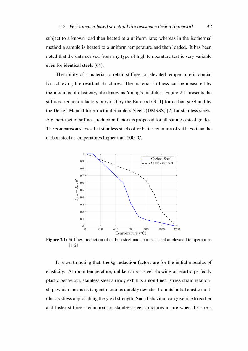
The ability of a material to retain stiffness at elevated temperature is crucial
for achieving fire resistant structures. The material stiffness can be measured by
the modulus of elasticity, also know as Young’s modulus. Figure 2.1 presents the
stiffness reduction factors provided by the Eurocode 3 [1] for carbon steel and by
the Design Manual for Structural Stainless Steels (DMSSS) [2] for stainless steels.
A generic set of stiffness reduction factors is proposed for all stainless steel grades.
The comparison shows that stainless steels offer better retention of stiffness than the
carbon steel at temperatures higher than 200 °C.
Figure 2.1: Stiffness reduction of carbon steel and stainless steel at elevated temperatures[1, 2]
It is worth noting that, the kE reduction factors are for the initial modulus of
elasticity. At room temperature, unlike carbon steel showing an elastic perfectly
plastic behaviour, stainless steel already exhibits a non-linear stress-strain relation-
ship, which means its tangent modulus quickly deviates from its initial elastic mod-
ulus as stress approaching the yield strength. Such behaviour can give rise to earlier
and faster stiffness reduction for stainless steel structures in fire when the stress
2.2. Performance-based structural fire resistance design framework 43
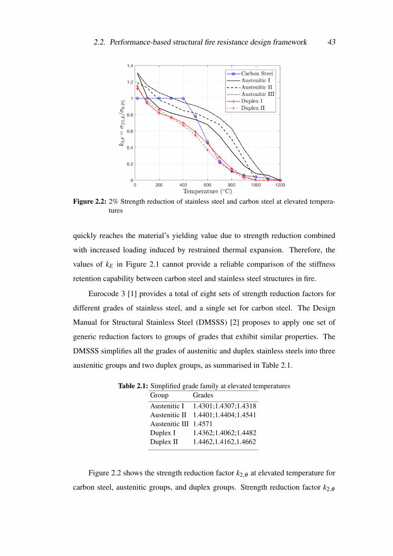
Figure 2.2: 2% Strength reduction of stainless steel and carbon steel at elevated tempera-tures
quickly reaches the material’s yielding value due to strength reduction combined
with increased loading induced by restrained thermal expansion. Therefore, the
values of kE in Figure 2.1 cannot provide a reliable comparison of the stiffness
retention capability between carbon steel and stainless steel structures in fire.
Eurocode 3 [1] provides a total of eight sets of strength reduction factors for
different grades of stainless steel, and a single set for carbon steel. The Design
Manual for Structural Stainless Steel (DMSSS) [2] proposes to apply one set of
generic reduction factors to groups of grades that exhibit similar properties. The
DMSSS simplifies all the grades of austenitic and duplex stainless steels into three
austenitic groups and two duplex groups, as summarised in Table 2.1.
Table 2.1: Simplified grade family at elevated temperaturesGroup GradesAustenitic I 1.4301;1.4307;1.4318Austenitic II 1.4401;1.4404;1.4541Austenitic III 1.4571Duplex I 1.4362;1.4062;1.4482Duplex II 1.4462,1.4162,1.4662
Figure 2.2 shows the strength reduction factor k2,θ at elevated temperature for
carbon steel, austenitic groups, and duplex groups. Strength reduction factor k2,θ

2.2. Performance-based structural fire resistance design framework 44
is the 2% strength at temperature θ , normalised by the 0.2% proof strength σ0.2%
at 20 °C. At lower temperatures, stainless steels have a reduction factor k2,θ of
greater than unity because of the 2% strain limit at elevated temperatures and the
use of 0.2% strain limit at room temperature. Unlike the elastic perfectly plastic
carbon steel whose σ0.2% is equivalent to σ2% at room temperature, stainless steels
exhibit substantial strain hardening and possess a greater strength at 2% strain than
that at 0.2% plastic strain at room temperature. As shown in Figure 2.2, gener-
ally, austenitic grades shows a better σ2% retention than carbon steel at temperature
above 500 °C. Overall, duplex grades offer poor strength retention with over 60%
σ2% lost at 500 °C. Austenitic III offers the best σ2% retention among all stainless
steel grades. Austenitic III also exhibits an overall better retention capability than
the carbon steel, with only a slight lower reduction factor between approximately
360 °C and 420 °C.
2.2.3.2 Global structural mechanisms in fire
Taking global structural behaviour into account for the estimate of structural fire ca-
pacity is essential to the performance-based engineering design. A real-life building
structure is a redundant/indeterminate structure in which the pattern of forces and
stresses cannot be determined by equilibrium alone, but also depend on the relative
stiffness of parts of the structure. Consequently, the pattern of forces and stresses
in a building structure are determined based on both equilibrium and compatibility
consideration. Conversely, the isolated members tested in fire furnaces are mostly
determinate structures, in which the pattern of internal forces and stresses can be
determined using equilibrium considerations alone.
Under collapse conditions, redundant and determinate structures are more
sharply differentiated. Provided it has adequate ductility and does not suffer from
instability, the redundant structure is capable of finding different load paths and
mechanisms to continue supporting additional load when its yield strength has been
reached at a single location. The determinate structure collapses when the most
highly stressed region reaches the local strength.
Due to the historical adoption of furnace fire testing on simply supported sin-

2.2. Performance-based structural fire resistance design framework 45
gle element for structural fire resistance design, the behaviour of structures in fire
has since been understood to be dominated by the material degradation under con-
stant loading at high temperatures, which leads to high deflections or ‘run-away’
mechanisms as observed in furnaces.
However, during Cardington investigation, it was discovered that this typical
‘run-away’ mechanism did not occur in the steel beams in the building, even though
the temperature of the bottom flange had exceeded 800 °C. This indicates that a steel
beam in a framed structure, with the aid of restraints from surrounding members,
has better fire resistant capability than individual steel beams [66].
Fire tests conducted on axially restrained steel beams by Li and Guo [67], and
Liu et al. [68], showed that the behaviour of the restrained beams were very different
from that of isolated beams. The most interesting finding from their experiments is
the observance of catenary action. Catenary action in a beam is the ability of the
beam to support itself by means of axial tension when the beam undergoes a large
deflection. When subjected to fire, catenary action develops in the beam as a result
of the deflected shape caused by thermal expansion and thermal bowing [69].
Heating induces thermal expansion strains (εT ) in most structural materials, as
given by Equation 2.13:
εT = α∆T (2.13)
where α is the thermal expansion coefficient and ∆T is the temperature increment.
The temperature distribution within structural components is usually not uni-
form. The cross-sectional thermal gradient of structural members causes the bottom
surface to expand more than the top surface, inducing bending in the member. This
effect is called thermal bowing.
Modelling and investigation of the full-scale Cardington frame fire tests show
that it is the axial forces induced by thermal expansion and large displacements re-
sulted from thermal bowing, and not material degradation that govern the structural
response in fire. Based on the study of Cardington tests, Usmani et al. [39] stated
that material degradation, such as steel yielding and buckling, can even be beneficial
in developing the catenary action prior to the final failure when material degrada-

2.2. Performance-based structural fire resistance design framework 46
tion and loads begin to dominate the behaviour once again. Kodur and Dwaikat [70]
shared a similar viewpoint and suggested that the statement by Usmani et al. [39]
summarised well the behaviour of a beam in a real redundant structure for a real
event of fire. Dwaikat and Kodur [71] presented a detailed interpretation of the
structural behaviour of a translationally and rotationally restrained beam exposed to
fire, dividing the behaviour into three distinctive stages, namely ’Elastic’, ’Elasto-
plastic’ and ’Catenary action’.
It is well understood that if an axially restrained beam is slender it will buckle
before the material reaches its yield stress. The classic Euler buckling Load Pcr for
a beam column is given by
Pcr =π2EI
l2 (2.14)
where E is the elastic modulus of the material, I is area of moment of inertia, and l
is effective length.
Equating Pcr to the thermal expansion induced compression (EAα∆T ), the crit-
ical buckling temperature is then given by
∆Tcr =π2
α(rl)2 =
π2
αλ 2 (2.15)
where r is the radius of gyration, λ is slenderness ratio, l/r.
Equation 2.15 is based on the ideal assumption that the axial restraint is per-
fectly rigid. While in practice the restraint stiffness is of a finite value. Assuming
the axial restraint is of a stiffness kt , the critical buckling temperature can be calcu-
lated by
∆Tcr =π2
αλ 2 (1+EAkt l
) (2.16)
where λ is the slenderness ratio.
The EA/lkt term in Equation 2.16 is the ‘relative stiffness’ ratio of the beam
to its restraints provided by end connections and surrounding structures.
The failure of the beam, either by yielding or buckling, causes a sudden change
in the deflection, leading to the subsequent catenary action. Consequently, the be-
haviour of a beam in a real redundant structure in a real event of fire undergoes four

2.2. Performance-based structural fire resistance design framework 47
distinct stages.
In Stage 1, elastic response dominates the behaviour wherein beam expands
as a result of continuous heating, compressive axial force and bending moment
develop in the beam due to the effect of end restraints.
Stage 2 sees a sudden increase in deflection, as a result of either yielding or
buckling failure of the beam, which leads to reduction of the compressive axial
force that’s induced by constrained thermal expansion.
Stage 3 begins when the axial force in the beam reverses from compression to
tension. Thus the fire induced compressive axial force completely vanished and the
tensile forces start to develop in the beam. The load bearing mechanism gradually
changes from flexural to catenary action.
In the final stage, the beam starts to ’runaway’ when the material degradation
and loading becomes unbearable for the catenary mechanism to continue.
Recognising the beneficial role of catenary action plays at carrying large dis-
placement in fire, there has been an ongoing research interest to achieve an efficient
method for structural fire resistance design by taking advantage of the catenary ac-
tion in a rational and reliable manner. Wang and Yin [72,73] developed an analytical
method for predicting the fire behaviour of restrained beams based on a parametric
study of finite element models. Wang and Yin’s method is only suitable for cases of
a specific deflection profile and neglects the additional bending moment generated
in the beam due to the shift of effective section centroid [71].
Kodur and Dwaikat [70] investigated the response of steel beam-columns ex-
posed to fire based on a set of numerical studies using finite element software AN-
SYS, and subsequently proposed a performance-based methodology for fire design
of restrained beams. Kodur and Dwaikat’s method assumes both the translational
and rotational restraints continue to perform elastically during the entire course of
the design fire. This assumption seems unrealistic because it has been demonstrated
that the stiffness of rotational restraints available to beams at the beginning can
reduce substantially early at around 200 °C [74].

2.2. Performance-based structural fire resistance design framework 48
2.2.4 Damage of Passive Fire Protection coatings
The fire resistance of steel structural components in composite steel frame build-
ings is commonly provided by passive fire protection (PFP) coatings. Current stan-
dards [9,27] measure the fire resistance of structural components using the concept
of time. For instance, a 2 hr fire-resistance rating means the PFP protected struc-
tural components can withstand a standard fire of 2 hours. There are two popular
categories of PFP: cementitious coating and intumescent coating.
Cementitious PFP has been and still is a popular choice due to its advantages
of being cost effective, ease of application and lightweight when compared with
the itumescent fireproof coatings [75]. The fireproof coatings are generally spray
or hand applied. The spray-applied cementitious coating is commonly referred to
as spray-applied fire resistive material (SFRM). Being specifically designed to be
lightweight, cementitious PFP are naturally fragile and brittle hence prone to dam-
age under deformation or vibration. Numerous research [76–91] have been carried
out to investigate the damage mechanisms in cementitious PFP, in order to inves-
tigate the fragility of it when the structures are subjected to large deformations in
earthquake, impact or blast.
At material level, Chen et al. [76] carried out tests to evaluate the mechanical
and inter-facial properties of cementitious coatings, including compressive and ten-
sile strength, normal bonding strength and shear bonding strength. However, they
did not measure the load-displacement response at the coating-steel interface and
reported only the maximum strength attained at fracture.
Braxtan and Pessiki [77] evaluated the bond strength of SFRM through tests on
small scale steel coupons, investigated the effect of mixing methods (wet mix or dry
mix) and the steel surface finish on bond performance. They reported that the bond
strength was three times higher for the wet mix than that for the dry mix, and mill
finish of steel can considerably degrade the adhesion strength. When strains become
large and strain compatibility at the interface becomes difficult to maintain, the
cementitious wet mix tends to crack in order to accommodate large deformations.
However they did not provide any load-displacement response at the SFRM-steel

2.2. Performance-based structural fire resistance design framework 49
interface.
Arablouei and Kodour [78] carried out Drop Mass Impact tests in conjunction
with numerical modelling to determine the Dynamic Increase Factor (DIF) of frac-
ture properties for SFRMs. Tan et al. [79] used single cantilever beam specimens to
measure the fracture energy of SFRMs under pure normal stress. Direct shear tests
were carried out by Arablouei and Kodur [80] to measure the stress-displacement
response under pure shear stress at the interface between the SFRM and the steel
plate.
At structural level, Keller and Pessiki [83, 84] investigated the damage of ce-
mentitious PFP at bolted connections of gravity beam-column frames subjected to
cyclic loading. Braxtan and Pessiki [81, 82] also carried out experiments to study
the damage pattern of SFRM that was applied on steel moment frame beam-column
assemblies under quasi-static cyclic loadings, representing strong seismic events.
The SFRM debonding was observed first to occur at the location where the steel
had yielded at the drift ratio of 1%. The large detachment of SFRM occurred at the
plastic hinge when the drift ratio exceeded 3%. In addition, delamination occurred
at places where the flange buckling occurred.
Chen et al. [76, 85] undertook an extensive testing programme of testing to
study the damage mechanisms in cementitious coatings applied on steel plates sub-
jected to monotonic axial loading and bending. They concluded that the plate cur-
vature had the most significant influence on the damage mechanism. They found
thicker insulation led to an earlier inter-facial damage.
Further experiments [86, 87] have also been carried out to study damage pat-
terns in cementitious coatings that are applied on structural columns subjected to
both monotonic and cyclic loadings, which found that the cracking initiated at a
lower load level and the complete delamination/peel-off failure occurred at a lower
strain level under cyclic loading than that under monotonic loading.
In order to develop an understanding on the process of the delamination be-
tween SFRM insulation and steel surface , Arablouei and Kodur [80, 88–91] have
been focusing on developing constitutive material models and employed the Cohe-
2.3. Stainless steel structures in fire 50
sive Zone Model (CZM) to simulate initiation and propagation of cracks at SFRM-
steel interface under various types of loadings. They associated the SFRM delam-
ination with plastic hinge formation and proposed a damage index factor based on
the material fracture energy.
Damage in cementitious coating caused by loading events such as windstorms,
fires or earthquakes can result in potential reductions in its structural fire resistance.
This fire safety concern is further compounded by the fact that cementitious PFP is
usually concealed by architectural claddings and finishes, which hinders any reg-
ular monitoring and post-earthquake inspections. As a result, the fire resistance
of structures using cementitious PFP system could suffer significant reductions af-
ter a period of use due to unaccounted for PFP damage. Especially if this period
consisted multiple small/moderate earthquakes.
It is worthy noting that the term ‘performance’ in performance-based design
not only refers to a building’s behaviour during the outbreak of a natural hazard, but
it also relates to a building’s survivability after a disaster. The performance-based
design offers a process or methodology to evaluate the reductions in buildings’
structural fire resistance as a result of post-earthquake damage in PFP system. The
functionality and the continued availability of services of building structures can be
effectively and efficiently protected from fire hazards using the performance-based
engineering framework for the structures in fire design.
2.3 Stainless steel structures in fire
The development of structural design codes, standards and specifications for stain-
less steel has been under increasing interest of the academics and the industry since
early 1960s. Several European research projects have been carried out to analyse
the performance of structural stainless steel, resulting in the publication of the De-
sign Manual for Structural Stainless Steel (DMSSS). The latest (fourth) edition of
the DMSSS [2] was published in 2017.
Recent experimental research [20–22] on stainless steel material behaviour at
elevated temperatures suggested that stainless steel exhibits superior stiffness and

2.3. Stainless steel structures in fire 51
strength retention capabilities, and a lower emissivity when compared with the car-
bon steel. The findings motivated further research on stainless steel structural be-
haviour in fire, as is the case of the European Coal and Steel Community (ECSC)
project ‘Development of the use of stainless steel in construction’ and the ECSC
project ‘Stainless steel in fire’.
The superior material behaviour of stainless steel at elevated temperatures
offers potential economical gains through savings on fire protection systems. A
comparison of the strength and stiffness retention capability between carbon steel
and stainless steel has been presented in Section 2.2.3.1. Besides the material’s
strength and stiffness retention capability, thermal expansion induced compression
also plays a crucial role in the steel structural behaviour in fire.
2.3.1 Thermal expansion
For thermo-mechanical analysis, in addition to the mechanical strain induced by
general external loading or geometry non-linearity due to deformation, thermal
strain caused by temperature increments through thermal expansion also needs to
be considered. The fundamental principal relationship that governs the behaviour
of structures in fire is [39]:
εtotal = εmechanical + εthermal (2.17)
The total strain (εtotal) governs the deformed shape of the structure through
kinematic or compatibility considerations, whereas, the stress state σ in the struc-
ture, elastic or plastic, depends only on the mechanical strain.
If the thermal expansion is free to develop in an unrestricted manner, axial
expansion or thermal bowing will result from thermal expansion while leading to
no additional stress:∆εtotal = ∆εthermal
∆εmech = 0 ∆σ = 0(2.18)
In contrast, if the thermal strains are fully restrained, stresses (σ ) in structural

2.3. Stainless steel structures in fire 52
members will result from the εmechanical:
∆εtotal = 0
∆εtotal = ∆εmech +∆εthermal ⇒ ∆εmech +∆εthermal = 0
⇒ ∆εmech =−∆εthermal
∆σ 6= 0
(2.19)
In real structures under fire, rigid connections between structural components
will result in high stresses being developed in structural members, which might lead
to structural plastification, even though the deflection might be small. Alternatively,
where less restraints are in place, larger deflections may develop but accompanied
with lower stress levels. Therefore, the structural behaviour due to material thermal
expansion in real structures is a complicated issue which depends strongly on the
structural restrains.
Eurocode 3 [1] suggests the thermal elongation ∆L/L of austenitic stainless
steel could be determined using the equation:
∆L/L = (16+4.79×10⁻³θa−1.243×10⁻⁶
θ2a )× (θa−20)×10−6 (2.20)
where L is the length at 20 °C, ∆L is the temperature induced expansion and θa is
the temperature.
The mean coefficients of thermal expansion for typical types of stainless steel
specified in DMSSS [2] are summarised in Table 2.2. The available results suggest
that austenitic grade exhibits the greatest thermal expansion while ferritic grade
expands the least amongst the three.
In analogy to the thermal elongation equation proposed by the Eurocode 3 [1]
for austenitic grade, an elongation equation as in Equation 2.21 is proposed for the
duplex grade. Equation 2.21 was determined by least square fitting the thermal
expansion coefficient vs. temperature relationship of the duplex grade as presented

2.3. Stainless steel structures in fire 53
Table 2.2: Mean coefficient of thermal expansion (10−6/°C)Steel Temperature range( °C) Duplex Austenitic Ferritic
100 13.2 16.7 10.3200 13.9 17.2 10.7300 14.3 17.7 11.1400 14.7 18.1 11.5500 15.1 18.4 11.8600 15.4 18.8 12.0700 15.9 19.1 12.4800 16.3 19.4 12.9900 16.7 19.4 13.41000 17.1 19.7 14.01100 17.5 20.0 -
in Table 2.2.
∆L/L = (12.88+4.6e−3θa−4e−7
θ2a )× (θa−20)×10−6 (2.21)
Figure 2.3: Thermal elongation
Overall, stainless steel grades show higher thermal elongation in comparison
with carbon steel, as shown in Figure 2.3, with the austenitic grade being the high-
est.
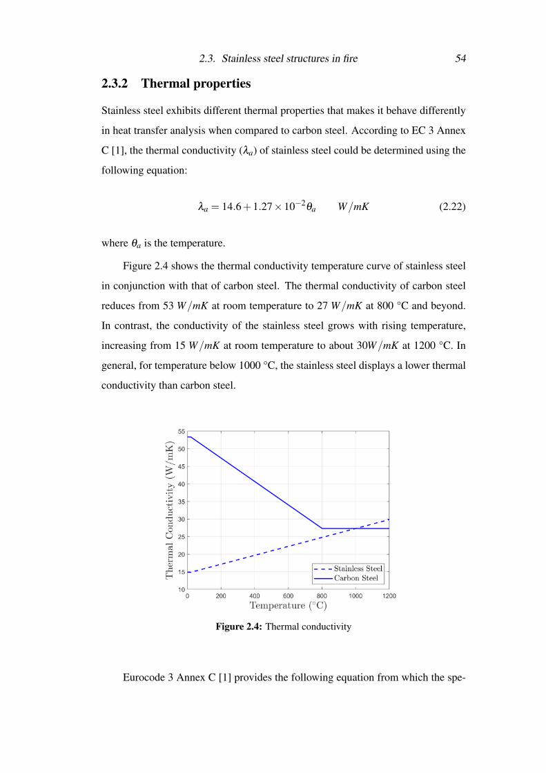
2.3. Stainless steel structures in fire 54
2.3.2 Thermal properties
Stainless steel exhibits different thermal properties that makes it behave differently
in heat transfer analysis when compared to carbon steel. According to EC 3 Annex
C [1], the thermal conductivity (λa) of stainless steel could be determined using the
following equation:
λa = 14.6+1.27×10⁻²θa W/mK (2.22)
where θa is the temperature.
Figure 2.4 shows the thermal conductivity temperature curve of stainless steel
in conjunction with that of carbon steel. The thermal conductivity of carbon steel
reduces from 53 W/mK at room temperature to 27 W/mK at 800 °C and beyond.
In contrast, the conductivity of the stainless steel grows with rising temperature,
increasing from 15 W/mK at room temperature to about 30W/mK at 1200 °C. In
general, for temperature below 1000 °C, the stainless steel displays a lower thermal
conductivity than carbon steel.
Figure 2.4: Thermal conductivity
Eurocode 3 Annex C [1] provides the following equation from which the spe-

2.3. Stainless steel structures in fire 55
cific heat (ca ) of stainless steel could be determined:
ca = 450+0.28×θa−2.91×10⁻⁴θ
2a +1.34×10⁻⁷
θ3a J/kgK (2.23)
where θa is the temperature.
Figure 2.5 compares the evolution of specific heat of stainless steel and carbon
steel over increasing temperatures. On average, the specific heat of stainless steel
is about 550 J/kgK, as compared with the approximately 600 J/kgK of carbon
steel. One significant difference is that the austenitic stainless steel shows no phase
change when subjected to heating up to 1200 °C, whereas the carbon steel exhibits
a phase change in the region of 723 °C.
Figure 2.5: Specific heat
Enthalpy formulation is the method commonly adopted in numerical solution
to tackle phase change problems in materials. The method enables the heat capacity
to be defined as a smooth function of temperature. Cheng and Usmani [92] proposed
that the enthalpy (H) within a temperature range could be defined as in Equation
2.24. This method has been implemented in the heat transfer module in OpenSEES
[93].
H =∫ T
Tr
ρcpdT (2.24)

2.3. Stainless steel structures in fire 56
where Tr is the reference temperature, cp is the specific heat, ρ is the density.
Eurocode 3 [1] stated that the unit mass of both carbon steel and stainless
steel could be considered independent of temperature and taken as 7850 kg/m3.
In addition, a lower emissivity of 0.4 can be adopted for stainless steel due to its
polished finish surface, in comparison to the 0.7 for carbon steel.
2.3.3 Existing research on stainless steel structures in fire
European Coal and Steel Community (ECSC) project ’Development of the use of
stainless steel in construction’ and the ECSC project ’Stainless steel in fire’ , co-
ordinated with the British Steel Construction Institution, has studied the behaviour
in fire of a range of structural stainless steel grades. Numerous experimental re-
search [21, 94–96, 96–98] has been carried out to obtain the material’s mechanical
properties at elevated temperatures and the property data has been included in the
latest DMSSS [2].
In addition, a range of research activities [99–101] have been conducted to
study the structural behaviour of stainless steel in fire. Available experimental data
[21, 102, 103] suggest that austenitic stainless steel columns and beams can retain
their load-carrying capacity for a longer period of time than carbon steel structural
members, due to their superior strength and stiffness retention capacity. However,
existing experimental data have been limited to the behaviour of individual stainless
steel structural components in fire.
Numerical investigations using finite element analysis has been employed to
study the stainless square hollow column behaviour in fire [104], and the lateral-
torsional buckling behaviour of beam column members in fire [101, 105]. The test-
ing of steel members, sub-assemblies and frame structures in a fire is extremely
expensive and any one test only provides limited useful data. In view of the richly
diversified grades of stainless steel family, numerical investigation can be consid-
ered as an economical and efficient approach to study stainless steel structural sys-
tems in fire.
2.4. Material models for thermo-mechanical analysis with fire 57
2.4 Material models for thermo-mechanical analysis
with fireThe Cardington tests [106], together with advances in computing power and mod-
elling techniques, have propelled for a generation of numerical models for heated
structures. Many programs have been specifically developed for structural analysis
under fire conditions, with early development focused on geometric non-linearity
resulted from large deflection due to thermal bowing and expansion. Most of these
programs belong to individual researchers or research groups, and most of them
have seen their development stalled after a while. Today, only some of them are
still being developed and probably used by other researchers, most notably are,
SAFIRE (University of Liege) and VULCAN (University of Sheffield).
The accuracy of finite element (FE) models is strongly dependent on the mate-
rial model adopted. Carbon steel and stainless steel exhibit non-linear stress- strain
relationships at elevated temperatures, hence require material non-linear analysis.
2.4.1 Material non-linearity
Ramberg and Osgood [107] proposed the expression in Equation 2.25 to describe
the non-linear relationship between stress and strain:
ε =σ
E+K(
σ
E)n (2.25)
where ε is the strain, σ is the stress, K and n are material constants.
Saab [108] proposed to use the Ramberg-Osgood equation to better represent
the non-linearity exhibited by carbon steel at elevated temperatures. Saab adopted
a modified version of the Ramberg-Osgood equation for stress-strain relationships
at high temperatures, given as:
ε =σ
E20+
37(σy20
E20)(
σ
σy20)50 0 < θ ≤ 80 °C
ε =σ
Eθ
+0.01(σ
σyθ
)ηθ 80 < θ ≤ 800 °C(2.26)
where E20 is the elastic modulus at ambient temperature; σy20 is the yield strength

2.4. Material models for thermo-mechanical analysis with fire 58
at ambient temperature; ε is the mechanical strain; σ is the mechanical stress; Eθ
is the elastic modulus at temperature θ ; σyθ is the yield strength at temperature θ ;
ηθ is the material constant at elevated temperatures. Saab also proposed methods
to calculate ηθ based on curving fitting.
The major drawback of a Ramberg-Osgood type stress strain equation is that
there is no closed-form inversion of the relation to describe stress in terms of strains,
hindering its application in strain-based finite element analysis. Graphic iteration
technique can be adopted to bypass this difficulty however it is very computationally
expensive. An explicit stress formulation will considerably improve the computa-
tion efficiency.
Mostaghel and Byrd [109] derived an approximated inversion of the typical
Ramberg-Osgood equation using a power law ε = Eε −αεβ to represent the σ
in the elastic strain dominated region and using a binomial series expansion up to
fourth order to obtain the stress-strain relation for the plastic dominated region.
Abdella [110] proposed an approximate inversion formula σ =Eε
1+ cε p , specifi-
cally for stainless steel stress-strain curves represented using Ramberg-Osgood type
equations.
Various strain-based constitutive equations, summarised in Table 2.3, offer
the capability to describe the non-linear stress strain behaviour. The Holloman
law [111] is a power law based equation. The parameter n is the strain harden-
ing exponent. In addition to the power law, the Ludwik law [112] introduces a third
material constant, initial yield stress (σ0), and the Swift law [113] accounts for the
prestrain (ε1). The Voce law [114] is exponential function based, and suitable for
materials exhibiting a saturation stress (σs).
Table 2.3: Types of the constitutive equationsAuthor(s) Equation ParametersHolloman σ = Kεn K,n=constantsLudwik σ = σ0 +Kεn σ0,K,n=constantsSwift σ = K(ε1 + ε)n K, n=constants, ε1=prestrainVoce σ = σ0 +(σs−σ0)exp(−nε) σ0, σs, n=constants

2.4. Material models for thermo-mechanical analysis with fire 59
2.4.2 Existing non-linear material models
Franssen [115] proposed that the constitutive material model for steels at elevated
temperatures could be constructed by using a set of temperature-dependent stress-
strain curves and the plastic strain to track the complete strain history at varying
temperatures; the transient hardening associated with the Bauschinger effect could
be modelled using the Masing’s rule [116].
This approach has been implemented in the finite element software SAFIR
[117] for Eurocode 3 [1] steel materials with an elliptical curve adopted for the
non-linear isotropic hardening behaviour [118]; and in OpenSEES as the uniaxial
material model Steel01Thermal for Eurocode 3 carbon steel [119], where a simpli-
fied tri-linear stress-strain relationship was adopted to represent the non-linear stress
strain relationship. Franssen’s approach has also been used by Bailey et al. [120],
Lu et al. [121] and Lien et al. [122] to study the cooling behaviour of steel structures.
Franssen’s approach can handle the stress reversals at increasing tempera-
tures caused by high initial strain or the stress reversals experienced during cool-
ing. Figure 2.6a illustrates the tracing of the stress-strain path under heating using
the Franssen’s model for the case where the strain reversal at increasing tempera-
tures is caused by high initial strain, denoted here as Case A. A set of temperature-
dependent stress-strain curves are constructed from the origin, with increasing non-
linear hardening at higher temperatures. Having reached equilibrium at the time
step (i), Point A on the stress-strain curve of temperature T (i), the plastic strain
εR(i) is calculated by unloading material state from Point A following the slope
E(i) to the intercept with the strain axis. At time step (i+ 1), temperature is in-
creased, resulting in a reduction in the elastic range which is represented by the
yield strength of proportional limit σp(i+1), and a reduction in the elastic modulus
E(i+1). The new stress-strain path at T (i+1) is constructed following the steps:
1. Reload from the strain axis interception Point O’ via the slope E(i+1), join
the original stress-strain curve of T (i+1) at the interception Point D.
2. Extend the line DO’, which is parallel to the tangent of the original stress-
strain curve, to Point C. Point C is defined by assuming the size of the elastic

2.4. Material models for thermo-mechanical analysis with fire 60
(a) Case A
(b) Case B
Figure 2.6: Material model construction illustrations

2.4. Material models for thermo-mechanical analysis with fire 61
zone is 2σp(i+ 1), considering the Bauschinger. Thus Point C defines the
new elastic limit on this path.
3. Join Point C and Point P’, assuming a linear relationship. The new stress-
strain curve at T (i+ 1) is now defined by the orange curve DO’CP’D’, re-
placing the original curve DPOP’.
The stress state at T (i+ 1) can therefore be determined using the new stress-
strain curve DO’CPD’. Point B at T (i+1) is the equivalent stress state of Point A
at T (i), which is determined by preserving the mechanical strain of Point A prior
to the first iteration at step T (i+ 1). At Point B, the material can be either further
loaded in tension or unloaded/loaded into compression.
The same principle applies in the case where the strain reversal is experi-
enced during cooling, denoted herein as Case B. Similar to the Case A, a set of
temperature-dependent stress-strain curves are constructed from the origin, assum-
ing the material regains its original properties when being cooled from the higher
temperature T (i− 1) to T (i+ 1). Figure 2.6b depicts the tracing of the stress and
strain during cooling using the Franssen’s approach. For simpler demonstration
purpose, a constant loading Ploading is considered, presenting a statically determi-
nate structures. High initial compressive mechanical strain (Point A) resulted from
heating is assumed. During cooling, the plastic strain εR(i−1) remains unaffected
by the temperature. The final equilibrium at T (i+ 1) is obtained at Point C. For
global structure analysis, member forces can increase at step T (i) as some part of
the structure regains its stiffness under cooling. If the loading at T (i) goes beyond
Point E, the εR(i) will change. Therefore the reference Point O’ should be computed
and updated at the end of each temperature step during the analysis, which then is
used to define the stress-strain relationship for the next temperature step.
Franssen’s approach always starts with a set of original stress-strain curves,
based on which the modified stress-strain relationship at elevated temperature is
determined. This procedure limits its application in scenario where multiple strain
reversals are expected. For example, in the event of fire immediately following an
earthquake, a series of localised fires are likely occur within buildings. As a result,

2.4. Material models for thermo-mechanical analysis with fire 62
combinations of Case A and Case B will prevail in the building materials since
simultaneous heating and cooling is expected for the structure.
Figure 2.6 schematically shows the elastic perfectly plastic behaviour of carbon
steel at the lower temperature, and the non-linear stress strain behaviour at elevated
temperatures. The elastic-plastic stress-strain relationship of carbon steel at room
temperature transforms into a non-linear relationship when the temperature exceeds
100 °C. For stainless steel, its stress-strain curves exhibits a non-linear relationship
in general.
Bailey et al. [3] used a Ramberg-Osgood relation to present the non-linear
stress-strain relationships, with Masing’s rule [116] implemented for defining hys-
teresis loop in unloading. Masing’s [116] rule offers that the unloading curve can
be uniquely defined based on the loading curve using polar scaling with a factor of
two. When the loading curve is defined by an equation σ = f (ε), if a new coordi-
nate system (σ ′,ε ′), with the origin at the strain reversal point used, the unloading
curve can be represented by a relation σ ′/2 = f (ε ′/2) [123]. The main procedures
proposed by Bailey et al. [3] for the stress strain paths construction, as illustrated in
Figure 2.7, can be summarised as follows:
1. The uniaxial stress-strain relationship is defined by a Ramberg-Osgood type
of equation: εT =σ(T )E(T )
+ k( σTσyT
)nT . Where E(T ) and σyT are temperature-
dependent elastic modulus and yield stress. K is a material constant.
2. Once the strain reversal Point A (εA1,σA1) is identified at temperature
T1, the unloading path can be constructed by εT 1 = εA1 − 2(σ(A1)−σ(T 1)
2E(T 1)+
0.01σ(A1)−σ(T 1)
2σ(T 1)
nT 1), using Masing’s Rule.
3. Calculate the Reference Point O2(εR,0). εR is the unrecoverable plastic strain,
εR = εA− σAET 1−0.02( σA
2σyT 1)nT 1 .
4. The stress-strain path for the next temperature T2 is constructed by position-
ing the unloading curve for T2 so it intersects the Reference Point O2. The
interception Point C (εA2,σA2) is obtained by solving the following equation:
0.02( σA22σyT 2
)nT 2−0.01( σA2σyT 2
)nT 2 + εR = 0.

2.4. Material models for thermo-mechanical analysis with fire 63
5. Repeat calculation for Reference Point O2 at Temperature T2 for the new
stress, which will be used to define the stress-strain relationship for the next
temperature step.
As shown in Figure 2.7, the assumed strain reversal Point A (εA1,σA1) at tem-
perature T1 is beyond the elastic limit. Prior to iteration at Temperature T2, by
preserving the mechanical strain from previous temperature step, Point B is located
on the new stress strain path of T2, highlighted in dashed orange line. The dashed
orange line represents the new elastic region on the stress strain path of T2. At tem-
perature T2, if the strain is increased to a point beyond Point C, then the original
stress-strain curve of T2 is used and a new reference point will have to be formed. If
the strain value is between−εA2 and εA2, the path of dashed orange line is followed.
Figure 2.7: Construction of stress strain path, proposed by Bailey et al. [3]
The mathematical process involved in this constitutive material model presents
three challenges for computational implementation:
1. The same Ramberg-Osgood type of equation is assumed for both tensile and
compressive stress-strain relationship. This means the exponent parameter n
has to be an odd integer.
2. Iteration method is required when solving the non-linear equation to deter-

2.4. Material models for thermo-mechanical analysis with fire 64
mine the new strain reversal point (Point C in the Step 4) for the next temper-
ature step. This considerably increases the computing time.
3. The nature of Ramberg-Osgood equation presents a challenge for displace-
ment based finite element modelling because there are no closed-from solu-
tions expressing the stress as an explicit function of the stress. As a result,
graphical or iterative numerical procedures have to be employed to compute
the stress corresponding to a given strain.
In conclusion, models using Franssen’s approach are only valid provided that
either only one unloading phase follows the loading phase or cyclic loading occurs
with always increasing stress level. In other words, they cannot reliably account
for multiple strain reversals (> 2) because the set of stress-strain curves are con-
structed always starting from the origin. Furthermore, the Bauschinger effect and
the transient hardening captured by the Masing’s rule is only an approximated rep-
resentation of the material’s behaviour.
2.4.3 Bauschinger effect
At room temperature, Silvestre et.al [124] experimentally evaluated the Bauschinger
ratio (B.R.) of Austenitic 316L and ferritic 430 BA stainless steel. The Bauschinger
ratio (ϑ ) is defined as in Equation 2.27. They observed that Austenitic 316L showed
a considerable Bauschinger effect (B.R.=0.81), while 430 BA showed a tendency
toward isotropic behaviour (B.R.=0.92). Olsson [125] conducted biaxial tests on the
Austenitic 1.4301, 1.4436 and Duplex 1.4462 stainless steel and determined their
B.R. as 0.75, 0.70 and 0.60 respectively. Following the same testing procedures,
Gozzi [126] further determined the Bauschinger ratio of Austenitic 1.4318 stainless
steel, and obtained B.R.=0.65. In light of the experimental results, the stainless
steels show a more pronounced Bauschinger effect.
ϑ =Yiso
Y1D(2.27)
where Yiso is the proportion of isotropic hardening, and Y1D is the total hardening.
At the starting point, there is only isotropic hardening, Yiso = Y1D⇒ ϑ = 1.0.

2.4. Material models for thermo-mechanical analysis with fire 65
For various metal materials it has been observed that the Bauschinger ef-
fect is temperature-dependent [5, 127–129]. Phillips et al. [127] observed that the
Bauschinger ratio of the aluminium decreased as the temperature increased. Har-
vey et al. [128] investigated the evolution of the isotropic hardening variable and
kinematic hardening variable of 304L stainless steel at elevated temperatures (20
°C, 200 °C, 600 °C, 800 °C and 1000 °C) using reverse yield experiments, and
demonstrated the temperature-dependent nature of the Bauschinger effect. When
investigating material’s kinematic hardening behaviour under cyclic loading at high
temperatures, Maciejewski et al. [129] and Ohno et al. [5] observed different de-
grees of the Bauschinger effect and transient hardening at varying temperatures for
low carbon steel and 304 stainless steel, respectively.
2.4.4 Strain rate dependency for structural fire analysis
Material models for representing steel behaviour at elevated temperatures are based
on a set of temperature-dependent stress-strain curves. The mathematical represen-
tation of these curves is usually determined by fitting the test data obtained from
stress or strain rate controlled testing of coupons heated under quasi-static condi-
tions. The strain rate range used for testing is usually restricted to approximately
0.00025 –0.0025 s−1, and the codified stress rate range is between 6 and 60 MPa
s−1 [130]. When strain rate is above 0.0001 s−1, structural steel material starts
to exhibit notable strain rate sensitivity, defined as the increase in yield strength
with increasing strain rate, [131]. The strain rate sensitivity increases with increas-
ing temperature [132]. The strain rate of 1.0 s−1 can be considered as an initial
starting point for evaluating dynamic load effect as related to material strain rate
sensitivity [133]. When subjected to building fire, structural loading is generally
static and moderate to high strain rate levels are not expected to occur until the
structure approaches its collapse state [134]. Steady state analysis is the common
approach for structural fire analysis, dynamic analysis has been adopted in various
research [135–137] for investigating the behaviour of fire-induced structural col-
lapse.
Heating rate has a great effect on the strain rate when the structure is under

2.4. Material models for thermo-mechanical analysis with fire 66
transient (anisothermal) loading conditions, where the structure is stressed to a spe-
cific level and then exposed to uniform heating [138]. This is the opposite of the
steady (isothermal) loading condition, in which the structure is heated up to a spe-
cific temperature, which is then held constant while the loading is applied. The
transient loading condition is generally considered to be more representative of ac-
tual fire scenarios, where an already stressed structure experiences increasing tem-
peratures. The heating rate of steel members under fire conditions depends on the
nature of the fire, the geometry of the structure and the section properties as well
as any fire insulation which has been applied. For a typical beam, with 2 hour fire
rated protection, the heating rate of steel generally varies between 3 and 7 °C/min,
while for unprotected steel sections, the heating rate can vary between 25 and 40
°C/min [138].
Creep is defined as the time-dependent plastic strain under constant stress and
temperature. At room temperature and under service load levels, creep deforma-
tions of steel are insignificant. Generally, the influence of creep in the steel strain
evolution becomes noticeable at temperatures above 450 °C [139].
The Eurocode 3 [1] temperature-dependent stress-strain curves for steel were
derived based on data from transient loading tests under a heating rate of 10 °C/min
[140]. This code specifies that a material model constructed based on the Eurocode
3 stress-strain curves is applicable for heating rates between 2 and 50 °C/min, and
states that “the effects of transient thermal creep need not be to given explicit con-
sideration”. In other words, a material model developed based on Eurocode 3 stress-
strain curves takes creep at high temperatures into account implicitly.
The ASCE manual [141] states that high temperature creep should be ac-
counted for in fire resistance analysis through the use of temperature-dependent
stress-strain curves derived from transient-state tests at relevant heating and strain
rates; or adopting specific creep models developed for structural steel at high tem-
peratures. Therefore it is left to the engineers to decide which model to use.
2.4. Material models for thermo-mechanical analysis with fire 67
2.4.5 Existing kinematic hardening plasticity models at room
temperature
It is well known that the theory of plasticity provides the framework for the con-
tinuum constitutive descriptions of the behaviour of solids that experience perma-
nent plastic deformations. The rate-independent plasticity theory is restricted to the
conditions for which the permanent deformations do not depend on the rate of the
loading applied. Several rate-independent plasticity models have been developed
using the rate-independent plasticity framework with internal variable concept to
model the non-linear strain hardening, and the complex material behaviour under
non-monotonous loading such as the Bauschinger effect and transient hardening.
Isotropic hardening models are adequate for proportional loading conditions
where the loading increases monotonically and no unloading occurs. In order to
properly represent material’s response under complex non-monotonous deforma-
tion paths, it has been common to adopt kinematic hardening models. In this sec-
tion, three main types of kinematic hardening models are briefly reviewed and dis-
cussed.
2.4.5.1 Mroz’s multi-surface model
Mroz’s model [142] uses a series of linear segments to model the non-linear stress-
strain behaviour, i.e., instead of using a single hardening modulus for the entire
stress-strain curve, each discretised segment of the stress-strain curve has one con-
stant hardening modulus. In three dimensional stress space, Mroz’s model can be
represented by several hypersurfaces f0, f1,... fn, where f0 is the initial yield surface,
and f1 to fn define regions of constant hardening moduli.
On one hand, to produce a smooth non-linear curve, a large number of yield
surfaces are necessary, requiring high computational power. On the other hand,
the plastic moduli (E p) under uniaxial loading of Mroz’s model can be determined
straightforwardly from the stress-plastic strain curve generated from uniaxial tensile
tests.

2.4. Material models for thermo-mechanical analysis with fire 68
2.4.5.2 Two yield-surface models
The two-surface model concept was proposed by Krieg [143] and Dafalias & Popov
[144] independently in the 70s. They introduced the concept of a bounding (outer)
surface and a loading (inner) surface. A schematic view of the two yield surface
model is illustrated in Figure 2.8. The current stress state (Point a) is defined on
the loading surface while a corresponding stress state is defined on the bounding
surface (Point A). The σσσ and ΣΣΣ are the Cauchy stress tensor of the loading surface
and bounding surface respectively, βββ is the backstress tensor that defines the centre
position of the loading surface and BBB is the backstress tensor that defines the centre
of the bounding surface.
Figure 2.8: A schematic view of two surface model
Compared with the Mroz’s multi-surface model that defines a set of piece-
wise plastic moduli, the two surface model defines a continuous variation of the
plastic modulus between the bounding surface and the loading surface. The non-
linear hardening behaviour —smooth transition between elastic and plastic region,
is realised through the relative movement of the two surfaces. The main difference
between Krieg’s model, and Dafalias & Popov’s model is the approach adopted for
incorporating the Bauschinger effect. Krieg [143] prescribes kinematic-isotropic
proportioning factors to decompose the total hardening into isotropic and kinematic
2.4. Material models for thermo-mechanical analysis with fire 69
hardening parts for the loading surface and the bounding surface respectively. In
Dafalias & Popov’s model [144], the Bauschinger effect is realised by defining the
plastic hardening modulus as a function of the gap (δ in Figure 2.8) between the
bounding and the loading surface.
Lee et al. [145] resolved the issue of ‘overshooting’, the unrealistic transient
behaviour of the two-surface model which may occur when the material is unloaded
before being reloaded to its original stress state, by only updating the hardening
behaviour when reverse loading occurs for plastic deformation.
Recently, Cardoso & Yoon [146] explicitly incorporated the Bauschinger ratio
in the constitutive equation of the two surface model by defining it as an exponential
function of the accumulated plastic strain (ε p).
2.4.5.3 Non-linear kinematic hardening models
The non-linear kinematic hardening model commonly used is a generalisation of
Prager’s [147] and Ziegler’s [148] linear kinematic hardening models. The Prager’s
linear kinematic hardening rule [147] assumes the yield surface translates in the di-
rection of plastic strain increment. Ziegler [148] modified Prager’s rule by assuming
yield surface translates along the direction of the relative stress tensor ηηη :
ηηη =σσσ −βββ (2.28)
where σσσ is Cauchy stress tensor and βββ is the backstress tensor.
The evolution equation for the kinematic hardening variable βββ can be ex-
pressed as:
βββ =23
Hεp
εp
εp and βββ =
23
Hε pε pε p (2.29)
the material constant H is the hardening modulus and ε pε pε p is the plastic strain tensor.
For modelling material behaviour under cyclic loading, Chaboche [149, 150]
proposed a non-linear kinematic hardening model as expressed in Equation 2.30.
The backstress (βββ ) is modelled using multiple (M) terms of non-linear kinematic
hardening, with different material constants γi assigned for each term to allow for a
2.4. Material models for thermo-mechanical analysis with fire 70
more extensive strain domain and a better description of the soft transition between
elasticity and the onset of plastic flow [151].
βββ =M
∑i=1
βββ i βββ i =23
Hi˙εp
εp
εp− γiβββ iε p (2.30)
with:
ε p =
√23
˙εp
εp
εp : ˙ε
pε
pε
p (2.31)
The variable ε p is the accumulated plastic strain rate and γ is a material con-
stant. The term −γβββ ε p , called the dynamic recovery term, includes the effect of
saturation in the kinematic hardening model.
Chaboche’s model is developed based on the non-linear kinematic harden-
ing model firstly proposed by Armstrong & Frederick [152] in 1966. Armstrong
& Frederick’s model can be considered as a particular case of Chaboche’s model
where M = 1, i.e., only one dynamic recovery term is used.
Another possible improvement upon Prager’s linear kinematic hardening rule
is introducing non-linearity by replacing the constant kinematic hardening modulus
H with a generic function of the accumulated plastic strain, ε p [153].
βββ =23
H(ε p)εpεpεp (2.32)
in this case, a scalar function,
β ≡ β (ε p) (2.33)
must be defined such that
H(ε p) =dβ
dε p (2.34)
defines the kinematic hardening curve. This curve can be obtained from simple
uniaxial tests in a manner analogous to the determination of the hardening curve for
the purely isotropic hardening model.
The models reviewed in this section are presented within the framework of
small strains and applicable to the scheme of rate-independent plasticity. The three
types of plasticity models are not completely independent from each other [154].

2.4. Material models for thermo-mechanical analysis with fire 71
Chaboche and Rousselier [149] demonstrated mathematically that the non-linear
kinematic hardening rule can be considered as a particular case of two-surface the-
ory where the bounding surface can only expand isotropically but cannot translate.

Chapter 3
A New Material Model for
Thermo-mechanical Analysis of
Steels in Fire
Adapted from M. Zhou, R. Cardoso, and H. Bahai, “A new material model for
thermo-mechanical analysis of steels in fire”, International Journal of Mechanical
Sciences, vol. 159, pp. 467 – 486, 2019
All of the existing kinematic hardening models reviewed in Section 2.4.5 focus
on the mechanical aspect of the material behaviour under isothermal conditions,
without explicitly stating the effects of temperature and temperature changes. Thus
the three objectives identified in the Introduction (Chapter1) have been answered to
some degree by the existing models for isothermal conditions. In order to develop
an appropriate plasticity model for thermo-mechanical analysis of steel materials
subjected to fire, the effects of temperature and temperature changes have to be
addressed, which is discussed in the following sections.
3.1 Temperature effects on plasticity modelsWithin the framework of thermodynamics, temperature changes in the material can
result from internal heat generation and external heat source. The flame edge tem-
perature has been observed at about 550 °C in small-scale compartment fires and
the maximum temperature in a post-flashover building fire can reach 1200°C [30].
3.1. Temperature effects on plasticity models 73
Therefore for general structural fire analysis, the heat transfer between the material
and the external fire is believed to predominate the temperature changes within the
material. Thus in this work the temperature rise in the material due to plastic work
is assumed negligible in comparison to that caused by external fires. Consequently,
it’s considered appropriate to decouple the heat transfer analysis from the thermo-
mechanical analysis for structural analysis with fire. Strictly referring to the effects
induced by external fire loading, the temperature effects on the parameters and vari-
ables in the constitutive equations and the evolution laws of a plasticity model is the
main focus of this chapter.
The influence of elevated temperatures on elastic/inelastic material response,
can be treated within the framework of theories of creep [123], or using the vis-
coplasitc theory [155–157], where material response is treated as time-dependent.
For general structural fire analysis, not considering the stage of fire-induced col-
lapse, the structural loading is generally static. Experimental evidence [158] has
shown that different loading rates have no significant influence on the initial yield
surfaces at elevated temperatures. Sun et al. [159] and Maciejewski et al. [129]
examined strain-rate sensitivity of carbon steel beams and steel-framed structures
subjected to elevated temperatures using the Chaboche and Rousselier’s viscoplas-
tic model [149]. Both [129, 159] concluded that the strain rate dependency only
becomes noticeable when the temperature goes beyond material’s transitional tem-
perature, about 700 °C for low carbon steel.
For steel structural fire design, EC 3 [1] implicitly includes the effects of tran-
sient thermal creep in its prescribed stress-strain curves. Material models con-
structed based on the EC3 stress-strain curves are applicable for heating rates be-
tween 2 and 50 °C/min, without the need to explicitly consider transient thermal
creep [1].
Hence a time-independent/rate-independent plasticity model is assumed to be
adequate for the structural fire analysis, as the strain rate has been shown insignif-
icant, and the thermal creep can be taken into account implicitly through stress-
strain curves. The influence of temperature and temperature changes within the

3.1. Temperature effects on plasticity models 74
framework of rate-independent plasticity model is investigated and discussed in the
following sections.
3.1.1 Parametric dependency on temperature
The material parameters in the constitutive equations are considered to be
temperature-dependent. For structural steel materials, e.g., carbon steel and stain-
less steel, EC3 [1] defines reduction factors of elastic modulus, yield stress (propor-
tional limit stress) and 0.2% proof stress at elevated temperatures 20-1200 °C, with
100 °C intervals. The plastic modulus can be determined using the uniaxial stress-
strain curves at elevated temperatures which can be found in design standards and
literature. For example, EC3 [1] provides formulas for determining the stress-strain
relationships of structural steels using its corresponding reduction factors.
3.1.2 Temperature rate dependency for internal variables
The most commonly adopted two internal state variables to be considered are the
accumulated plastic strain ε p and the backstress tensor βββ . The scalar ε p defines the
isotropic hardening of the von Mises yield surface, while the tensor βββ defines the
translation of the yield surface centre in the deviatoric stress space.
The evolution of βββ at elevated temperatures has been a subject of discussion for
decades and the inclusion of a temperature rate is considered necessary for obtaining
stable conditions [151]. Using the framework of thermodynamics with decoupled
heat transfer, considering only the kinematic hardening of the material, the thermo-
dynamic potential, or the Helmholtz free energy (ψ) can be defined as in Equation
3.1. The ψ can be split into a sum of an elastic contribution, ψe, which is dependent
on the elastic strain (εe) and the temperature (T ), and a contribution of hardening,
ψp.
ψ = ψe(εe
εe
εe,T )+ψp(ααα,T ) (3.1)
Where the ααα is the back-strain tensor. As the internal heat generation due to
plastic work is not considered in this work, the ψp in Equation 3.1 does not con-
tribute to the heat transfer analysis in the material model proposed in this chapter.

3.2. Decoupling thermal and mechanical step 75
If the part ψp of the Helmholtz free energy is expressed in a quadratic form as:
ψp(ααα) =13
H(T )ααα : ααα (3.2)
where the hardening modulus (H) is now a function of temperature. Then the cor-
responding backstress is given by:
βββ =∂ψ
∂ααα=
23
H(T )ααα (3.3)
Differentiating Equation 3.3 over temperature gives:
∂βββ
∂T=
23
H(T )∂ααα
∂T+
23
∂H(T )∂T
ααα (3.4)
The evolution of the internal variable backstress βββ over changing temperatures
can therefore be determined using Equation 3.4.
3.2 Decoupling thermal and mechanical step
For isotropic materials, the thermal expansion caused by a change in temperature
is uniform in all directions. It is an experimentally observed fact that a stress free
material body will experience relative elongations but no angular changes as re-
sults of an increase or a decrease in temperature. This thermally induced strain
can be imposed on the stress induced strains (mechanical strains), provided there
is no change in the temperature due to the deformation of the material. Thus the
total strain, which is a measure of the deformation of the material, consists of a
mechanical part and a thermal part, as expressed in Equation 2.17.
The stress state (σ ) for the structural material (elastic or plastic) depends only
on the mechanical strains, which means thermal expansion does not directly con-
tribute to plastic yielding if there is no boundary restraint. Where there is no bound-
ary restraint and no external loading, the material is free to expand resulting in
changes in the deformation such as axial expansion or thermal bowing. However
there is no mechanical strain developed in the material in this case, hence no change

3.2. Decoupling thermal and mechanical step 76
of the stress state, as summarised in Equation 2.18. By contrast, where there is still
no external loading but there exist boundary restraints that fully prevent any thermal
expansion, the deformation of the structural material remains unchanged. As seen
in Equation 2.19, in this case, the mechanical strains are developed, subsequently
cause changes in the stress state.
The above two scenarios represent two opposite boundary conditions in real
structures under fire. It can be clearly shown that any changes in the stress state that
would cause material yielding are direct results of mechanical strain development.
Therefore, rate-independent plasticity models developed for isothermal conditions
are appropriate for modelling the mechanical aspect of the thermo-mechanical anal-
ysis of structural materials subjected to fire.
A thermo-mechanical analysis of structural materials in fire can be viewed
as a series of isothermal mechanical analyses, each one corresponding to a ther-
mostatic state. At each state, the isothermal mechanical analysis is carried out
at the temperature related to that state. The temperature difference between two
neighbouring states affects the evolution of internal variables as discussed in Sec-
tion 3.1. By adding a thermal step upon the established isothermal mechanical
analysis to incorporate the temperature effects, a new material model developed
within the framework of rate-independent plasticity will become capable of thermo-
mechanical analysis with fire.
The main objective of the thermal step is to implement temperature effects into
the material parameters for the constitutive equations and the evolution equations
of the internal variables, thereby enabling the subsequent mechanical analysis to be
performed in an isothermal state. By isolating the mechanical aspect of the analysis
from any thermal effects, it allows us to take advantages of sophisticated stress
integration methods developed for existing plasticity models, such as forward-Euler
method incorporating sub-incrementation [160–163], midpoint method [164, 165],
radial return method [166–168], and backward-Euler method [169–171], in order to
achieve higher computing efficiency.
The material parameters that are temperature-dependent and have to be up-

3.2. Decoupling thermal and mechanical step 77
dated at the thermal step are the following:
1. Elastic modulus
2. Yield stress, defined as occurring at proportional limit
3. Parameters in the constitutive equation for ε pε pε p, or flow rule
4. Parameters in the evolution equations for internal variables
3.2.1 Elastic modulus at elevated temperatures
Figure 3.1 presents the reduction factors (kE) of initial elastic modulus provided by
EC3 [1] for carbon steel and Design Manual of Structural Stainless Steel (DMSSS)
[2] for stainless steel. Both steel materials exhibit reduction of stiffness at increasing
temperatures.
Figure 3.1: Stiffness reduction factors
3.2.2 Yield surfaces at elevated temperatures
The yielding, defined as occurring at the proportional limit, is temperature-
dependent. The initial yield surfaces at elevated temperatures shrink as temperature
rises. Figure 3.1 shows the reduction factors of yield stress (kp) for carbon steel
according to EC 3 [1].
At room temperature, the von Mises yield criterion has been shown to be in
excellent agreement with experiments for many ductile metals [172]. It predicts

3.2. Decoupling thermal and mechanical step 78
the initial yield surface to be a circle in the deviatoric stress space. At elevated
temperatures, Phillips et al. [127] experimentally determined yield surfaces of pure
aluminium at 66 °C, 108 °C and 152 °C; Lissenden et al. [158] experimentally
investigated the initial yield surface of type 316 stainless steel at 650 °C; Inoue
and Tanaka [173] obtained the initial yield surfaces of low carbon steel at 200 °C,
250 °C, 300 °C and 450 °C through a series of experiments. They all found that
the size and shape of the experimentally determined initial yield surfaces agreed
satisfactorily to that predicted using the von Mises yield criterion. It is therefore
reasonable to believe the von Mises yield criterion remains applicable at elevated
temperatures.
3.2.3 Plastic flow potential at elevated temperatures
The foundation of the plastic flow potential theory is the normality flow rule of a
potential function. At higher temperatures, Lissenden et al. [158] observed that for
316 stainless steel, the directions of the plastic increment pointed in the general
direction of the outward normal of the yield locus at 650 °C. It is believed that the
normality is still applicable for steels at elevated temperatures. Consequently, the
flow potential can be determined by the yield function and hardening law using the
associated flow theory [172].
The hardening law of the carbon steel material model can be obtained by least
square fitting the EC 3 [1] stress-strain curves at elevated temperatures using the
Voce law:
σy,T = σy0,T + vT (1− exp(−δT εp)) (3.5)
where σy0,T is the initial yield stress (yielding stress of proportional limit) at tem-
perature T, which can be calculated using reduction factor (kp) prescribed by the
EC3 or determined through least square fitting the stress-strain curves. The param-
eter vT and δT are both temperature dependant material constants. It’s found that
a better least square fitting results, using the Adj-R-square ratio as the indicator,
could be achieved by determining σy0,T through curve fitting. Figure 3.2 presents
the carbon steel stress ––plastic strain curves at elevated temperatures obtained using

3.2. Decoupling thermal and mechanical step 79
least square fitting in conjunction with the nominal EC 3 curves. A general good
agreement is achieved. The material parameters obtained are summarised in Table
D.1. The linear interpolation technique is employed for obtaining the values for
intermediate temperatures.
Figure 3.2: EC3 stress-strain curves vs Least square fitting
Unlike carbon steel displaying a saturation stress, stainless steel exhibits a
substantial strain hardening effect. Therefore, a modified Ludwik strain hardening
law [112] has been adopted for stainless steel:
σ = σ0 + k(εp,0 + εp)n (3.6)
where σ0 is the initial yield stress, and k and n are material parameters. The param-
eter εp,0 was introduced as the incipient plastic strain. Because stainless steel does
not exhibit a distinct yielding point, in this study the initial yielding point (σ0) is
defined at the stress point where the plastic strain reaches 0.1% of the total strain,
i.e., εp,0 = 0.001εtotal .
The advantages of adopting the modified Ludwik law are twofold. Firstly, by
keeping the proportion of plastic strain to total strain (εp/ε) constant, the elastic
range (σ0T /σ0.2%,T ) of the stress-strain curves was maintained uniform at elevated
temperatures. This approach differs from traditionally adopting one proof strain,

3.2. Decoupling thermal and mechanical step 80
e.g., 0.01% as the yield point for all temperatures. Secondly, the numerical insta-
bilities caused by the original Ludwik law were circumvented by the introducing of
εp,0, which had an order of magnitude of 10−6 for Austenitic III stainless steel and
10−7 for Duplex II stainless steel.
The hardening function parameters determined for the DMSSS Austenitic
group III using least square fitting are summarised in Table D.2. At each temper-
ature level, the curve fitting value of σ0T is about 22% of the 0.2% proof strength
(σ0.2%,T ). Table D.3 presents the hardening function parameters determined for the
DMSSS Duplex group II.
(a) Austenitic group III (b) Duplex group II
Figure 3.3: Stress-strain curves at elevated temperatures, Nominal vs Curve fitting
3.2.4 Internal state variables’ evolution at elevated tempera-
tures
The accumulated plastic strain(ε p)
remains constant during the thermal step. The
backstress tensor βββ evolves over changing temperatures as expressed in Equation
3.4. At the thermal step where no change in the (mechanical) strain increment
considered, ∂ααα
∂T = 0. Equation 3.4 can be reduced to:
∂βββ
∂T=
23
∂H(T )∂T
ααα (3.7)
Since βββ is deemed temperature rate-independent, its value at a temperature

3.3. A new plasticity model for thermo-mechanical analysis with fire 81
point T can be determined by:
βββ T = (βββ )T=0 +∂βββ
∂TT (3.8)
As the tangent hardening modulus H is linearly interpolated between two stress
––strain curves at different temperatures, H becomes HT —the hardnening modulus
at the temperature T, and substituting Equation 3.7 into Equation 3.8 gives:
βββ T = (βββ )T=0 +23
HTααα (3.9)
Equation 3.9 can therefore be used to determine the new position of the yield
surface centre due to a temperature change at the thermal step for current material
point position.
3.3 A new plasticity model for thermo-mechanical
analysis with fireThe new rate-independent plasticity model for thermo-mechanical analysis of steel
materials subjected to fire developed is a combined isotropic and kinematic hard-
ening model. It adopts the concept of yield and bounding surfaces of the two-
surface plasticity theory in combination with the Bauschinger ratio to model the
material’s Bauschinger effect. Meanwhile, two kinematic hardening variables are
used to model the transient hardening behaviour that material exhibits upon reverse
loading. The theoretical details of the proposed new model are described in this
section.
3.3.1 Thermal step
During the thermo-mechanical analysis, the thermal step is responsible for updat-
ing both the bounding and the yield surface at elevated temperatures. In the pro-
posed material model, the bounding surface at a temperature T is considered to
have isotropic hardening only, shown as dashed circles in Figure 3.4. The size
of the bounding surface can be obtained using the uniaxial tensile stress —plastic
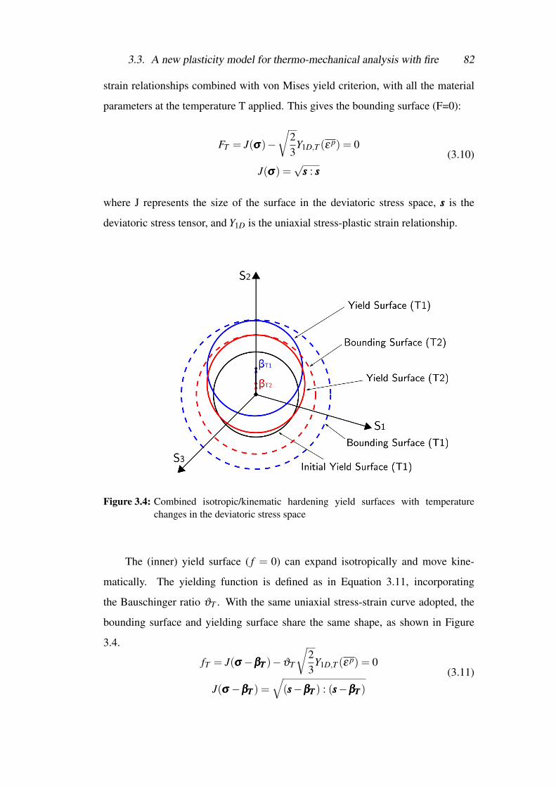
3.3. A new plasticity model for thermo-mechanical analysis with fire 82
strain relationships combined with von Mises yield criterion, with all the material
parameters at the temperature T applied. This gives the bounding surface (F=0):
FT = J(σσσ)−√
23
Y1D,T (ε p) = 0
J(σσσ) =√
sss : sss
(3.10)
where J represents the size of the surface in the deviatoric stress space, sss is the
deviatoric stress tensor, and Y1D is the uniaxial stress-plastic strain relationship.
Figure 3.4: Combined isotropic/kinematic hardening yield surfaces with temperaturechanges in the deviatoric stress space
The (inner) yield surface ( f = 0) can expand isotropically and move kine-
matically. The yielding function is defined as in Equation 3.11, incorporating
the Bauschinger ratio ϑT . With the same uniaxial stress-strain curve adopted, the
bounding surface and yielding surface share the same shape, as shown in Figure
3.4.
fT = J(σσσ −βTβTβT )−ϑT
√23
Y1D,T (ε p) = 0
J(σσσ −βTβTβT ) =√
(sss−βTβTβT ) : (sss−βTβTβT )
(3.11)
3.3. A new plasticity model for thermo-mechanical analysis with fire 83
The Bauschinger ratio ϑT decomposes the size of the bounding surface at the
current temperature into the isotropic and the kinematic hardening part of the yield
surface, and is defined by Equation 3.12. At the starting point there is only isotropic
hardening, Yiso,T = Y1D,T ⇒ ϑT = 1.0.
ϑT =Yiso,T
Y1D,T
0≤ ϑT ≤ 1(3.12)
The evolution of the Bauschinger ratio is evaluated using an exponential func-
tion of accumulated plastic strain (ε p):
ϑT = aT exp(−bT ε p)+ cT (3.13)
where aT , bT , cT are temperature-dependent material coefficients.
During thermo-mechanical analysis, the subsequent yield surfaces shrink due
to the reduction in the elastic region at elevated temperatures, meanwhile they also
expand and translate due to plastic hardening. As illustrated in Figure 3.4, at temper-
ature T1, the initial yield surface is the black circle, the bounding surface (FT 1 = 0)
is the dashed blue circle, and the yield surface ( fT 1 = 0) is the solid blue circle. The
yield surface sits inside the dashed blue circle and of a larger size than the black
circle since it considers both isotropic and kinematic hardening.
For an increasing temperature T2, the bounding surface (FT 2 = 0) is the red
circle in dashed line. At the thermal step, since there is no (mechanical) strain in-
crement considered, the yield surface at T2 ( fT 2 = 0) should not go beyond the
bounding surface. The movement of the yield surface caused by the evolution of
backstress due to changing temperatures should be restricted by the bounding sur-
face.
Upon a temperature change, the backstress tensor βTβTβT gives a new position of
the yield surface centre in the deviatoric stress space, and is determined by Equation
3.14. It is derived from Equation 3.9, by adopting uniaxial tensile stress-plastic
strain curves for the determination of hardening modulus and the Bauschinger ratio
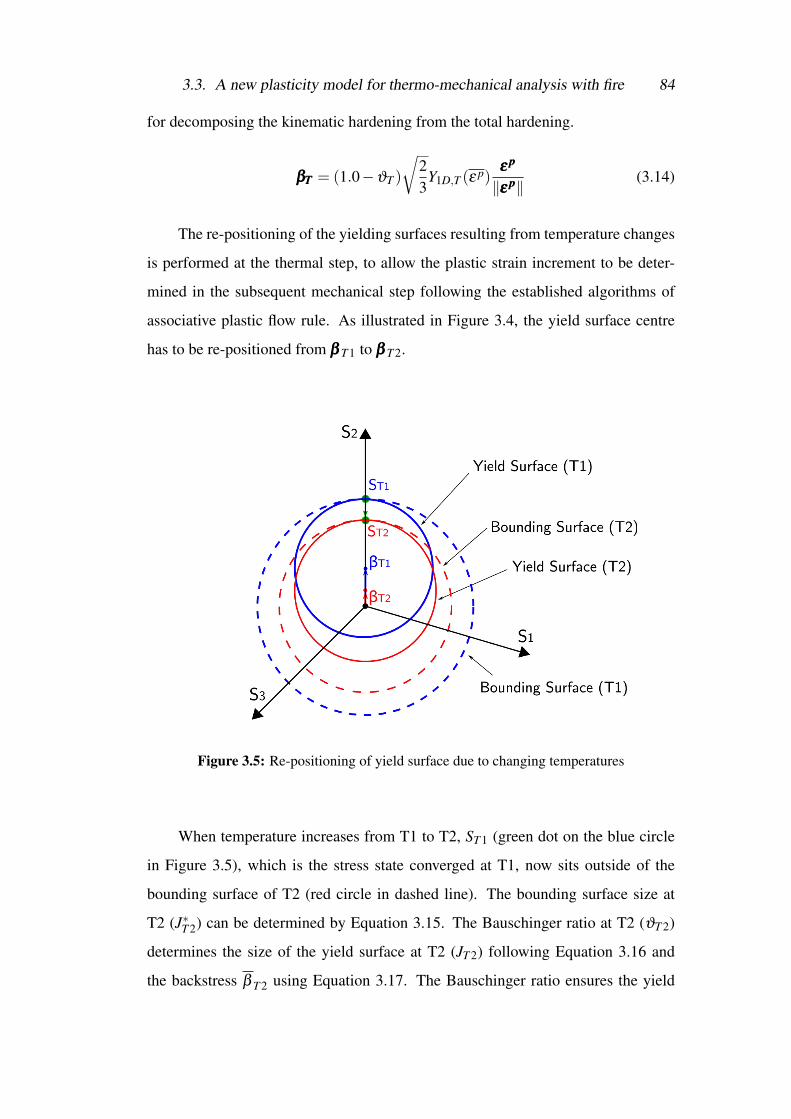
3.3. A new plasticity model for thermo-mechanical analysis with fire 84
for decomposing the kinematic hardening from the total hardening.
βTβTβT = (1.0−ϑT )
√23
Y1D,T (ε p)ε pε pε p
‖ε pε pε p‖
(3.14)
The re-positioning of the yielding surfaces resulting from temperature changes
is performed at the thermal step, to allow the plastic strain increment to be deter-
mined in the subsequent mechanical step following the established algorithms of
associative plastic flow rule. As illustrated in Figure 3.4, the yield surface centre
has to be re-positioned from βββ T 1 to βββ T 2.
Figure 3.5: Re-positioning of yield surface due to changing temperatures
When temperature increases from T1 to T2, ST 1 (green dot on the blue circle
in Figure 3.5), which is the stress state converged at T1, now sits outside of the
bounding surface of T2 (red circle in dashed line). The bounding surface size at
T2 (J∗T 2) can be determined by Equation 3.15. The Bauschinger ratio at T2 (ϑT 2)
determines the size of the yield surface at T2 (JT 2) following Equation 3.16 and
the backstress β T 2 using Equation 3.17. The Bauschinger ratio ensures the yield

3.3. A new plasticity model for thermo-mechanical analysis with fire 85
surface always stays inside the bounding surface.
J∗T 2 =
√23
Y1D,T 2(ε p) (3.15)
JT 2 = ϑT 2J∗T 2 (3.16)
β T 2 = (1−ϑT 2)J∗T 2 (3.17)
The direction of the backstress tensor at T2 (βββ T 2) is in the direction of the
plastic strain tensor, hence the βββ T 2 can be computed following Equation 3.18 :
βT 2βT 2βT 2 = β T 2ε pε pε p
‖ε pε pε p‖
(3.18)
The equivalent stress state (ST 2) on the yield surface of T2 (green dot on the
red circle in Figure 3.5) can therefore be determined following Equation 3.19:
ST 2ST 2ST 2 = JT 2ε pε pε p
‖ε pε pε p‖−βT 2βT 2βT 2 (3.19)
As can be seen in Equations 3.18 and 3.19, during the thermal re-positioning,
the direction of the yield surface centre and the equivalent stress state are determined
by the direction of the plastic strain tensor. In the proposed material model, plastic
strain tensor is the plastic internal variable at the thermal step.
3.3.2 Mechanical step
At the mechanical step, the stress state is considered isothermal hence the tempera-
ture dependence can be deemed “frozen” during the stress integration process. The
Bauschinger effect is captured by incorporating Bauschinger ratio (ϑ(ε p)) as an in-
ternal variable. The evolution function of ϑ(ε p) is an exponential growth function
of the accumulated plastic strain (ε p), thus ϑ(ε p) is a plastic internal variable as
it evolves over plastic hardening. Besides the Bauschinger effect, the material also
exhibits transient hardening upon reverse loading. In the proposed model, two non-
linear kinematic hardening variables are adopted to capture these two behaviour,
defined as in Equation 3.20. The second variable (β2β2β2) only gets activated upon

3.3. A new plasticity model for thermo-mechanical analysis with fire 86
Figure 3.6: Reverse loading criterion
reverse loading.
βββ = β1β1β1 + β2β2β2l (3.20)
The internal variable —reverse loading index (l) is introduced to track any
drastic changes in the loading direction. Figure 3.6 shows the reverse loading can
be detected by the angle θd between the old loading direction and the new loading
direction as follows:
cos(θd) =ηηηold ·ηηηnew
‖ηηηold‖‖ηηηnew‖; ηηη = sss−βββ
cos(θd)> 0, l = 0; cos(θd)< 0, l = 1(3.21)
3.3.2.1 First kinematic hardening variable β1β1β1
During monotonic loading, as illustrated in Figure 3.7a, the first backstress term (β1β1β1)
accounting for the movement of the yielding surface (solid blue circle) is determined
through the Bauschinger ratio (ϑ(ε p)) as follows:
β1β1β1 = (1− ϑ(ε p))
√23
Y1D(ε p)ηηη
‖ηηη‖(3.22)

3.3. A new plasticity model for thermo-mechanical analysis with fire 87
(a) Loading
(b) Reverse loading
Figure 3.7: Proposed model during loading ––reverse loading in the deviatoric stress space
Upon reverse loading, the β1β1β1 continues to develop in the reverse loading di-
rection as ε p increases. The ϑ(ε p) decomposes the kinematic hardening out of the

3.3. A new plasticity model for thermo-mechanical analysis with fire 88
total hardening at the new loading direction, illustrated as the green bracket portion
of the radius of the new bounding surface (dashed green circle) in Figure 3.7b.
3.3.2.2 Second kinematic hardening variable β2β2β2
In addition to the β1β1β1, a second kinematic hardening variable is introduced in the
proposed model to describe the shifted yield surface centre (blue dot in Figure
3.7) travelling back to the origin of the deviatoric stress space. Acknowledging
the evanescent characteristic of kinematic hardening, the second variable β2β2β2 can be
viewed as the yield surface exhibits an urgent tendency to move back quickly to the
origin upon reversing.
The exponential growth function of Equation 3.13 adopted for Bauschinger
ratio evolution indicates that the yield surface moves away from the origin at an
exponential speed during initial loading. It is reasonable to postulate that the yield
surface exhibits the same tendency upon reversing, shifting back to the origin at
an exponential rate, if not following the identical speed to that during the initial
loading. Based on this assumption, a reverse loading ratio (υ(ε pl )) is introduced as
an exponential decay function of the effective plastic strain of the new reloading
branch, denoted εpl , as in Equation 3.23. The scalar ε
pl accounts for the effective
plastic strain accumulated during each loading branch, and will be reset to zero
whenever reverse loading is detected. The material parameter in Equation 3.23
can be obtained from the testing data of reverse loading curves. Simplifying to
assume the same exponential speed for backtracking, the material constant b in the
Bauschinger ratio evolution Equation 3.13 can be applied to the parameter Vb.
υ = 1.0− exp(−Vbεpl ) (3.23)
The typical evolution of reverse loading ratio is compared with that of
Bauschinger ratio in Figure 3.8. The Bauschinger ratio starts at 1.0 indicating pure
isotropic hardening at the beginning of plastic hardening. It decays and steadies
at a value below 1.0 where kinematic hardening has reached its saturation value.
Contrarily, the reverse loading ratio starts from 0.0 meaning the backtracking is yet

3.3. A new plasticity model for thermo-mechanical analysis with fire 89
Figure 3.8: Typical Bauschinger ratio and Reverse loading ratio evolution
to start, and plateaus at the value of 1.0, which indicates at this point the entire dis-
tance travelled by the yield surface centre in the previous loading branch has been
recovered.
The kinematic hardening (β2β2β2) is therefore defined as:
β2β2β2 = υ
√23
βlηηη
‖ηηη‖(3.24)
The βl is a scalar —the distance the yield surface centre travelled during the
last loading branch in the uniaxial stress direction, as shown in Figure 3.9, and can
be obtained as follows:
βl =Vh
√32
βnβnβn : βnβnβn (3.25)
where βnβnβn is the rate of the (total) backstress tensor at the end of last loading branch
prior to the start of reserve loading. The material parameter Vh is introduced to
account for potential softening/hardening during reverse loading. It can be obtained
using experimental reverse stress-strain data.
The second variable β2β2β2 gets activated upon reverse loading, more precisely
only when re-yielding starts. Between the reverse loading point and the re-yielding
point, shown as the green dots in Figure 3.9, is the unloading range during which

3.3. A new plasticity model for thermo-mechanical analysis with fire 90
plastic internal variables remain unchanged.
Figure 3.9: Proposed model during reverse loading in the deviatoric stress space
3.3.3 Thermal step during reverse loading
The second kinematic variable β2β2β2 was introduced in Section 3.3.2 to account for ma-
terial’s transient hardening behaviour during reverse loading at the mechanical step.
The thermal step described in Section 3.3.1 applies to the temperature changes ex-
perienced by the internal variables during initial monotonic loading. For modelling
temperature changes that occur during reverse loading, the β2β2β2 has to be appropri-
ately incorporated in the thermal step to ensure the transient behaviour is retained.
The β2β2β2 describes the yield surface backtracking the distance (βl) that has been
travelled in the stress space prior to the reverse loading. Since the distance (βl) is
inherited from the previous loading branch, it remains constant during the reverse
loading. As shown in Equation 3.24, the temperature only affects the ‘speed’ of
the β2β2β2, as the material parameter Vb in the evolution function of the reverse loading
ratio (υ), Equation 3.23, is temperature-dependent.

3.3. A new plasticity model for thermo-mechanical analysis with fire 91
Therefore, the β2β2β2 does not actively contribute during the thermal step. The
procedures described in Section 3.3.1 for updating bounding and yield surface re-
sulting from temperature changes, can be viewed as taking place from the yield
surface centre that is positioned at β2β2β2 in the stress space. Thus the algorithm pro-
posed in Section 3.3.1 is still applicable, recognising that the backstress used in the
algorithm exclusively refers to the first kinematic hardening variable β1β1β1. The only
modification required is in the last step —calculating the equivalent stress state —to
take the β2β2β2 into account. Equation 3.19 now becomes:
ST 2ST 2ST 2 = JT 2ε pε pε p
‖ε pε pε p‖−β1T 2β1T 2β1T 2−β2β2β2 (3.26)
3.3.4 Elastoplastic consistent tangent modulus DepDepDep
The exact linearisation of the incremental stress updating procedure, rather than
to appeal to the rate stress —strain tangential relation, is essential for achieving
quadratic rates of convergence in the iterative solution of the finite element equilib-
rium equations as emphasised by Negtegaal [174], Simo and Taylor [175].
Linearising the incremental constitutive function of stress tensor (σσσ ) yields the
consistent tangent operator (DDD).
DDD =∂∆σσσ
∂∆εεε(3.27)
The fully implicit backward-Euler return mapping algorithm has been adopted
in the proposed material model to solve the yield condition equation:
Φ(∆γ)≡ ‖ηηη trialn+1‖−2µ∆γ−(β1n+1−β1n)− H(l)(β2n+1−β2n)−σy,iso = 0 (3.28)
where β1 is the first kinematic term contributing to overall hardening and is a func-
tion of accumulated plastic strain (ε p) as defined in Equation 3.17. β2 is the second
kinematic hardening term defined in Equation 3.24, l is the reverse loading index,
and σy,iso is the radius of the yield surface as defined in Equation 3.16. H is the
Heaviside step function.

3.3. A new plasticity model for thermo-mechanical analysis with fire 92
Equation 3.28 states the yield condition equation of full terms, using the Heav-
iside step function to include the second kinematic hardening term whenever re-
verse loading is detected. The Heaviside step function is a non-differentiable func-
tion, which means the elastoplastic consistent tangent modulus has to be derived for
monotonic loading and reverse loading differently.
The elastoplastic consistent tangent during monotonic loading has been ob-
tained as:
DepDepDep =DeDeDe−4µ2 1
ΘNNN⊗NNN− 4µ2
‖ηηη trialn+1‖
[IdevIdevIdev−NNN⊗NNN] (3.29)
Θ = 2µ +23
H1D(ε pn +
√23
∆γ) (3.30)
During reverse loading, Equation 3.29 is still applicable with the term Θ mod-
ified to include the β2β2β2 term as follows:
Θ = 2µ +23
H1D(ε pn +
√23
∆γ)− 23
βlexp(−Vb(ε
pl n +
√23
∆γ))(−Vb) (3.31)
A detailed derivation of the elastoplastic consistent tangent modulus is pro-
vided in Appendix C.
3.3.5 Summary of the new model
The proposed material model has been presented in this section, with the material
variables introduced and described in details. The new model solves the thermo-
mechanical behaviour of a material using two sequential steps, a thermal step fol-
lowed by a mechanical step. Figure 3.10 schematically summaries the evolution of
yield surfaces at changing temperatures. The initial yield surface (ε p = 0) at temper-
ature T0 is shown as the black solid circle in Figure 3.10a. As temperature increased
to T1, the initial yield surface shrinks into the blue solid circle in Figure 3.10a. At
T1, the material is stressed in the S2 direction to the stress state ST 1, achieving an
accumulated plastic strain of ε p. The solid blue circle in Figure 3.10b represents
the yield surface at T1 resulted from the combined isotropic and kinematic plastic
hardening of the ε p. The dashed blue circle in Figure 3.10b represents the corre-
sponding bounding surface, which is the yield surface considering only isotropic
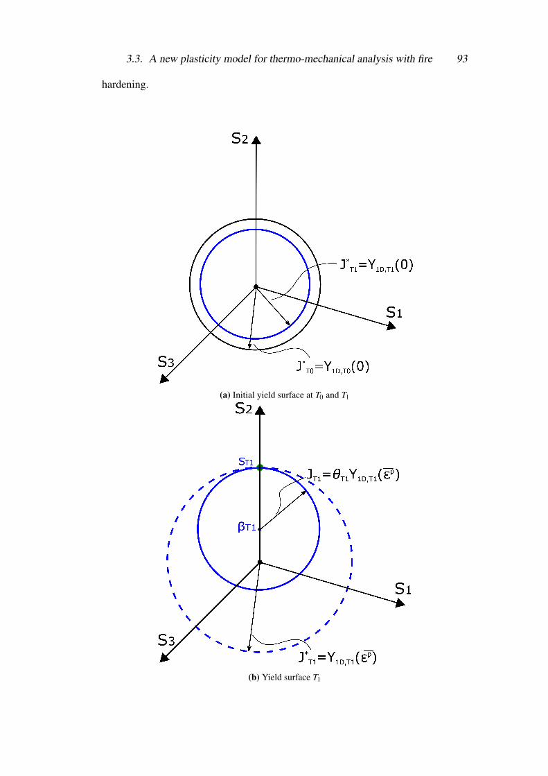
3.3. A new plasticity model for thermo-mechanical analysis with fire 93
hardening.
(a) Initial yield surface at T0 and T1
(b) Yield surface T1

3.3. A new plasticity model for thermo-mechanical analysis with fire 94
(c) Thermal step, T1 to T2
(d) Mechanical step, T1 to T2
Figure 3.10: Yield surface evolution, T0 to T2
When the yield surface at temperature T1 (the solid blue circle in Figure 3.10b
and 3.10c) experiences an increment to a higher temperature T2, the thermal step
3.3. A new plasticity model for thermo-mechanical analysis with fire 95
determines the current state (size and position) of the yield surface at T2 (the solid
red circle in Figure 3.10c). For the thermal step, the ε p remains constant, the solid
red circle can therefore be determined by the T2 hardening function (Y1D,T 2(ε p))
and the Basuchinger ratio ϑT 2. The size of the yield surface (JT 2,0) and the position
of the yield surface centre (βT 2,0βT 2,0βT 2,0) are determined following the Equation 3.15 to
Equation 3.19. The dashed red circle represents the bounding surface at T2 which
is the yield surface considering only isotropic hardening caused by the ε p. The
thermal step finds the equivalent stress state of ST 1 (the stress point sitting on the
yield surface of T1) on the yield surface of T2. The equivalent stress state ST 2,0 in
Figure 3.10c is determined using the Equation 3.26. The decrease in the stress from
ST 1 to ST 2,0 is caused by the shrinking of the yield surface due to the temperature
increase.
The mechanical behaviour (changes in the mechanical strain due to deforma-
tion) is handled in the subsequent mechanical step. If plastic hardening occurs at
T2, the stress state ST 2,0 is further stressed in the S2 direction to the ST 2, resulting
in an increment of ∆ε p, then the yield surface at T2 determined at the thermal step
(the solid red circle shown in Figure 3.10c and 3.10d) will be updated to the solid
green circle in Figure 3.10d , computed following the stress integration process. The
size of the yield surface (JT 2) is updated to take into account the increased isotropic
hardening, and the position of the yield surface centre (βT 2βT 2βT 2) is updated as a result of
increased kinematic hardening, which is determined following the Equation 3.20.
The total material parameters adopted for the new model is summarised as
follows:
1. Elastic modulus, ET .
2. Initial yield strength, σ0T .
3. Hardening function parameters.
4. Parameters of Bauschinger ratio (ϑT ) evolution function as shown in Equation
3.13.
5. Parameters of Reverse loading ratio (υT ) evolution function as shown in
Equation 3.23.

3.4. Validation of isotropic & kinematic hardening during monotonic loading 96
It is worth noting that the hardening function parameters are decided by the
strain hardening constitutive law selected for the material. In this work, the Voce
law adopted for the carbon steel required two function parameters vT and δT ; the
modified Ludwick law selected for the DMSSS stainless steels required two func-
tion parameters kT and nT .
3.4 Validation of isotropic & kinematic hardening
during monotonic loadingFor the thermo-mechanical analysis, the parameters in the evolution function of the
Bauschinger ratio becomes temperature dependant. The main objective of this sec-
tion is to validate the evolution of the Bauschinger ratio in the proposed material
model as a function of accumulation plastic strain (ε p) in conjunction with temper-
ature.
Harley et al. [128] conducted a series of reverse yield experiments to measure
the evolution of isotropic hardening variable (κ) and kinematic hardening variable
(β 11) in 304L stainless steel over a range of temperatures. The scalar isotropic
hardening variable κ is related to the size of a rate-independent yield surface. The
β 11 is associated with the translation of the yield surface centre in the uniaxial
stress direction. The experimental observations are consistent with the combined
isotropic/kinematic hardening framework. Despite their inability to directly capture
the initial elastic unloading behaviour in the reverse yield experiments largely due to
the inelastic material behaviour of 304L stainless steel, they determined the parame-
ters by correlating the data from additional Large Strain Reverse (LSR) experiments
and the tensile segment of the reverse yield experiments. Harley et al.’s [128] data
provided us an insight into how the Bauschinger effect evolves at elevated temper-
atures, particularly into how the two internal variables (κ and β 11) of a combined
isotropic/kinematic hardening plasticity model evolve at elevated temperatures.
In this validation study, at first, the κ and β 11 results of Harley et al.’s ex-
periments were analysed, based on which, a set of temperature-dependent evolution
function parameters of the Bauschinger ratio were determined using the least square

3.4. Validation of isotropic & kinematic hardening during monotonic loading 97
fitting technique. The parameters determined were implemented in the proposed
material model for thermo-mechanical analysis in Abaqus using the Umat subrou-
tine [23]. The validation was performed by comparing the Abaqus results with the
experimental data.
3.4.1 Bauschinger effect determination at elevated tempera-
tures
Based on the uniaxial stress state of the reverse yield experiment conducted in [128],
neglecting the term for rate dependence in yield strength, the Bauschinger ratio (ϑ )
can be determined following:
σ11 = κ +β11; ϑ =κ
σ11(3.32)
The Bauschinger ratios were calculated using Equation 3.32 at temperature 20
°C, 200 °C, 600 °C, 800 °C and 1000°C, respectively, and are presented in Figure
3.11. At each temperature level, Bauschinger ratios saw a general decreasing trend
except at 1000°C. The initial plummeting of ϑ1000 indicated a drastic shrink of the
yield surface. When considering the strain is kept constant, Figure 3.11 suggests
the Bauschinger ratios experienced a reduction from 20°C to 200°C followed by a
rise to 800°C, then a drop again as temperature raised to 1000°C.
The evolution function parameters of the Bauschinger ratios at each tempera-
ture level can be obtained using the least square fitting method, adopting the expo-
nential law as in Equation 3.13. The parameters were determined at each temper-
ature level individually and are summarised in Table D.4. They were subsequently
implemented in the Umat subroutine [23] for this validation study. The fitted curves
are plotted in Figure 3.11 along with the experimental values.
3.4.2 FE model descriptions
The experiments were conducted using specimens of 304L stainless steel rod, fol-
lowing the same reverse yield testing procedures Miller et al. [4] adopted for testing
OFHC copper. The specimen is illustrated schematically in Figure 3.12.

3.4. Validation of isotropic & kinematic hardening during monotonic loading 98
Figure 3.11: Bauschinger ratio, least square fitting
Figure 3.12: Reverse yield test specimen (all dimensions in mm) [4]

3.4. Validation of isotropic & kinematic hardening during monotonic loading 99
The cross-section of the gauge (outlined in Figure 3.12) was modelled using
the 4-node plane stress elements in Abaqus/CAE, shown as in Figure 3.12. The
model was restrained in axial direction at one end. The uniform temperature was
applied in the first step. In the second step, a horizontal monotonic tensile load was
applied at the other end to a maximum 5.0% axial strain.
The stress-strain curves of the 304L stainless steel used in the experiments
were applied in the material model for this validation. Thus the parameters of the
hardening function were obtained by least square fitting the stress-strain curves fol-
lowing the same approach adopted for EC3 carbon steel in Section 3.2.3, and are
summarised in Table D.4 . The Young’s modulus were applied following the re-
ported values : 195.3 GPa (20 °C), 182.8 GPa (200 °C), 153.8 GPa (600 °C), 125.7
GPa (800 °C), and 94.3 GPa (1000 °C).
3.4.3 Results and discussion
In the proposed material model, the isotropic hardening variable is computed fol-
lowing Equation 3.33.
κ = ϑTYT (ε p) (3.33)
where YT is the isotropic hardening function and ε p is the accumulated plastic strain.
The kinematic hardening variable in uniaxial stress state, β 11, is calculated as
follows:
β 11 =
√32‖βββ‖ (3.34)
where βββ is the total backstresses.
The Abaqus results for isotropic hardening (κ) and kinematic hardening (β 11)
are presented and compared with the experimental data in Figure 3.13a and Figure
3.13b, respectively. A generally good agreement is observed. The comparison has
demonstrated that the evolution of Bauschinger ratio has been successfully imple-
mented in the proposed material model as a function of temperature and accumu-
lated plastic strain.

3.4. Validation of isotropic & kinematic hardening during monotonic loading 100
(a) Isotropic
(b) Kinematic
Figure 3.13: Hardening variables comparison

3.5. Validation of Bauschinger effect and transient hardening 101
3.5 Validation of Bauschinger effect and transient
hardeningThe Bauschinger effect and the transient hardening behaviour typically observed
during reverse loading at room temperature also occur at elevated temperatures.
In this section, the capability of the proposed material model to capture the
Bauschinger effect and the transient hardening behaviour is validated using the ex-
perimental data obtained by Maciejewski et al. [129], who conducted a series of
monotonic and cyclic loading tests on low carbon steel material (A572 Grade) at
high temperatures. For the validation purpose, the experimental data of the reversed
stress-strain relationship of the very first loading loop associated with the mono-
tonic stress-strain curve has been used thereby the cyclic hardening/softening effect
was excluded.
The testing was performed on cylindrical specimens with an overall length of
114 mm, a gauge length of 25 mm, and a gauge diameter of 11 mm. The same finite
element modelling approach as in the previous validation was adopted. The pro-
posed material model was employed for the tested low carbon steel material. The
hardening function parameters were obtained by least square fitting the experimen-
tal stress-strain curves at 300 °C and 700 °C. The material properties of the Young’s
modulus and the initial yield stress were also calibrated from the experimental data.
The stress-strain curve (in red) at 300 °C and 700 °C obtained using least
square fitting is compared with the experimental data (blue circle) in Figure 3.14a
and Figure 3.14b respectively. The good agreement observed demonstrated that the
Voce hardening law successfully captured the non-linear stress-strain relationship
of the tested low carbon steel materials at elevated temperatures.
The hardening function parameters obtained, as summarised in Table D.5, were
subsequently implemented in the Abaqus Umat code. Three reverse loading tests
with varying prestrain levels were simulated in Abaqus to examine the hardening
behaviour during reverse loading at 300 °C and 700 °C. The Abaqus stress-strain
relationship results of monotonic loading range are compared with the curve fitting
stress-strain curves in Figure 3.14a and Figure 3.14b, the good agreement suggests

3.5. Validation of Bauschinger effect and transient hardening 102
the hardening functions have been successfully implemented in Umat. Varying de-
grees of transient hardening were predicted by the proposed material model at dif-
ferent prestrain levels. The Bauschinger effect and the transient hardening predicted
by the proposed material at the prestrain level experienced in the experiments has
been investigated for the validation in the following.
(a) T= 300°C
(b) T= 700°C
Figure 3.14: Stress-strain curves comparison
The Bauschinger ratio (ϑ ) was determined using Equation 3.35, based on the

3.5. Validation of Bauschinger effect and transient hardening 103
experimental data of the reversed stress-strain curves of the very first loading loop
at 300 °C and 700 °C respectively, as plotted in Figure 3.15a and Figure 3.15b. The
S11L is the highest stress point during monotonic loading, and S11U is the lowest
stress point before the material yields upon reverse loading, which is the transi-
tional point form the solid blue line to the dashed blue line in the two Figures. The
solid blue line presents the loading-unloading range of the stress-strain development
while the dashed blue line starts from the re-yielding point of the reverse loading
range.
κ11 =S11L−S11U
2; α11 =
S11L+S11U2
; ϑ =κ11
κ11 +α11(3.35)
where κ11 and α11 represents the amount of isotropic and the amount of kinematic
hardening respectively.
The Bauschinger ratio was therefore 0.597 at 20°C, 0.790 at 300 °C and 0.724
at 700 °C. The Equation 3.13 was adopted in least square fitting to describe the
Bauschinger ratio evolution, assuming it would achieve stabilisation shortly after
the first strain reversal. The determined evolution function parameters are sum-
marised in Table D.5. The value of bT in Equation 3.13 was adopted for the reverse
loading ratio evolution function —Equation 3.23, as discussed in Section 3.3.2.2.
Figure 3.15a and Figure 3.15b compares the stress-strain development during
the loading-unloading-reverse loading predicted using isotropic hardening model
and the proposed material model with the experimental data at 300 °C and 700°C
respectively. The proposed material model predicted the re-yielding point very well,
properly captured the Bauschinger effect. Beyond the yielding point, the proposed
material model also predicted the material’s transient hardening behaviour to a de-
gree of satisfactory at both temperature levels. On the other hand, the isotropic
hardening model was not able to capture the Bauschinger effect and the transient
hardening behaviour.

3.5. Validation of Bauschinger effect and transient hardening 104
(a) T= 300°C
(b) T= 700°C
Figure 3.15: Hardening models comparison

3.6. Validation of thermal unloading algorithm 105
3.6 Validation of thermal unloading algorithmThis section focuses on validating the implementation of the algorithm, developed
for the yield surface re-positioning due to changing temperatures, in the Abaqus
Umat code. At the thermal step, the new size of the yield surface is determined by
Equation 3.16 and the new position of the yield surface centre is computed using
Equation 3.18. The new position and size of the yield surface induces a reduc-
tion in the stress state, a phenomenon commonly referred to as thermal unloading.
While the re-positioning of yield surfaces is an invisible internal process, the ther-
mal unloading manifests itself in the changing of mechanical stress, hence can be
examined numerically. The validation was therefore performed by comparing the
thermal unloading result predicted by the proposed material model to its analytical
solution.
The model geometry and the material properties of the low carbon steel at ele-
vated temperatures from previous validation in Section 3.5 were utilised. A loading
scenario has been designed specifically in the following way to accommodate a
clear examination of the mechanical behaviour resulted from the yield surface re-
positioning at the thermal step:
1. Pre-strain the material to a mechanical strain level of 0.002, into the plastic
region at 300°C.
2. Increase temperature to 700°C while keeping mechanical strain constant. In
this manner any changes in the stress observed at the end of the thermo-
mechanical analysis is a result of the yield surface re-positioning due to tem-
perature changes. This was achieved by applying displacement controlled
boundary conditions.
3. The thermal expansion coefficient was set to zero so the observed strain re-
sults were entirely mechanical strains.
Figure 3.16 shows the stress-strain path during the designed loading process.
The prestrain at 300 °C produced an accumulated plastic strain of 5.481× 10⁻⁴.

3.7. Validation for multi-axial loadings 106
At 700 °C, the new yield stress =64.05 MPa (red point) is determined by Equa-
tion 3.16. For the mechanical strain =0.002, since 0.002×E700 < 64.05, the stress
state (0.002,48.91) (green cross) now sits within the yield surface. E700 is the
elastic modulus at 700 °C. The unloading stress-strain development predicted by
the proposed material model is shown in blue square, and the final stress state
=(0.002,48.89), was computed by the algorithm developed based on Equation 3.26.
As the thermal unloading behaviour has been successfully captured, it is believed
that the algorithm for the re-positioning of the yield surface due to changing tem-
peratures, has been correctly implemented in the Umat code.
Figure 3.16: Thermal unloading validation
3.7 Validation for multi-axial loadingsIn the previous three validations, the models were subjected to uniaxial loading
only. In this section, the proposed material model is further tested under multi-axial
loading conditions.
3.7.1 Experiments in literature review
Lissenden et al. [158] carried out experiments to determine the initial yield surface
of 316 stainless steel at room temperature and its subsequent yield surface at ele-
vated temperature 650 °C, with the impact of pre-loading on the subsequent yield

3.7. Validation for multi-axial loadings 107
surface also investigated. Tubular specimens fabricated from AISI type 316 stain-
less steel were used to determine the yield surfaces in the axial ––shear (σ11––σ12)
stress space. This particular stress space was used for the experiments because tubu-
lar specimens can be relatively easily subjected to combined axial-torsional load-
ing. A small offset strain definition of yield, 10µε = 10×10−6m/m, was adopted
by Lissenden et al. [158] to allow multiple probes in various directions to be con-
ducted on a single specimen for the yield surface determination. This process elim-
inated the specimen-to-specimen variation in the test results and ensured negligible
change in the material state. The extensometer was used to achieve the decoupled
measurements of axial and shear strain due plasitc hardening. For each surface de-
termination, 16 unique probes at different angles in the axial-shear (σ11––σ12) stress
space were performed to find the shape and size of the surface. The testing results
were plotted in the modified stress space (σ11/√
3––σ12) where a von Mises yield
surface was shown as a circle.
The experimental data obtained by Lissenden et al. [158] were employed for
the validation in the section. A brief description of the loading procedure and the
findings of the experiments at room temperature and at 650 °C is provided in the
following sections.
3.7.1.1 Room temperature
The testing results suggested the initial yield surface could be represented using a
circle of radius 82 MPa predicted by the von Mises yield criterion in the modified
stress space, with the centre located at (-8 MPa, -4 Mpa) rather than at the origin,
possibly due to initial residual stresses caused during the fabrication. The impact of
pre-stress on the subsequent yield surfaces was investigated by applying a radial pre-
loading, defined by σ12 = σ11/√
3, until 50% beyond the initial yield to a maximum
stress point (160 MPa, 84 MPa), followed by subsequent unloading to half of the
maximum stress level. The subsequent yield surface determined after pre-stressing
showed the distortion typically found for radial pre-loading which consists mainly
of contraction of the yield surface in the pre-loading direction with a particular
flattening on the side nearest origin [176].
3.7. Validation for multi-axial loadings 108
3.7.1.2 Elevated temperature 650 °C
The experiments found that the initial yield surface at 650 °C was a von Mises circle
in the modified stress space (σ12 = σ11/√
3) of a radius of 54 MPa, with its centre
located at (-4 MPa, -2 MPa).
Pre-loading was applied as pure torsion in the elevated temperature case. Max-
imum tensorial shear strain of 2500 µε was applied, followed by unloading. Three
subsequent yield surface determination tests were made for the specimen 316SS22
and 316SS16 respectively, showing translation and elongation in the direction of
the pre-loading (positive torsion).
3.7.2 Validation model in Abaqus
3.7.2.1 Model descriptions
The model geometry of Abaqus benchmark example 3.2.1 [177], a uniformly loaded
elastic-plastic plate, was utilised in this validation study. Since the main objective
was to validate the proposed material model algorithm implemented in the Abaqus
Umat subroutine, instead of constructing the entire tubular specimen, the simple
plate model was used. It allows for a clearer assessment of the accuracy of the
integration of the plasticity equations, provided the same loading effect from the
experiments can be reproduced in the finite element model.
The key aspect of the chosen loading process in the experiments, i.e., axial
loading in combination with torsion, was to ensure the applied axial stress and shear
stress were decoupled. The same loading effect was realised in the Abaqus plate
model by applying carefully designed boundary conditions as illustrated in Figure
3.17. The boundary conditions were constructed to ensure pure shear force and pure
axial force applied in a decoupled manner to the plate of examination, outlined in
red. Kinematic coupling was adopted for the nodal constraints.

3.7. Validation for multi-axial loadings 109
Figure 3.17: Abaqus plate model
3.7.2.2 Material properties
Initial yield stress of the 316SS material at room temperature (147 MPa) and at 650
°C (94 MPa) were calibrated from the experimental results. The elastic modulus is
approximately 194 GPa at room temperature, and 106 GPa at 650 °C. The hardening
parameters of the material were determined using the experimental stress-strain re-
sults and are summarised in Table D.6. The Bauschinger ratio was calculated using
the maximum positive and negative stress point in the pre-loading direction of the
yield surface results. The parameters of the Bauschinger ratio evolution function
are presented in Table D.6.
3.7.3 Validation results
3.7.3.1 Initial yield surfaces
Figure 3.18a compares the initial yield surfaces of 316SS at room temperature de-
termined by the experimental results with that predicted by the proposed material

3.7. Validation for multi-axial loadings 110
model. The predicted yield surface is an ideal circle in the modified stress space
as von Mises yield function is adopted. The experimental data suggests the initial
yield surface of 316SS is close to a circle with a degree of anisotropy in compressive
yield strength.
At elevated temperature 650 °C, the yield surface determined by the experi-
ments is closer to a von Mises circle than it was at room temperature. The compar-
ison between experimental results and predictions is shown in Figure 3.18b.
(a) Room temperature
(b) 650 °C
Figure 3.18: Initial yield surfaces comparison

3.7. Validation for multi-axial loadings 111
3.7.3.2 Subsequent yield surface after radial pre-loading at room
temperature
Figure 3.19a compares the subsequent yield surface of 316SS after radial pre-
stressing, determined by the experiments and the proposed material model. The
prediction of the proposed material model is an ideal von Mises circle being trans-
lated and expanded in the direction of the pre-loading. The distortion of the sub-
sequent yield surface due to radial pre-loading was not included. Nevertheless, the
translation and expansion of the subsequent yield surface in the direction of the
pre-loading has been clearly captured by the proposed material model.
3.7.3.3 Subsequent yield surface after pure torsion pre-loading at
650 °C
At the elevated temperature, pre-loading was applied as pure torsion resulting in
no noticeable distortion of the subsequent yield surface, as shown in Figure 3.19b.
Consequently, the experimental results suggest the subsequent yield surface is an
nearly ideal von Mises circle with slight anisotropy in compressive yield strength.
As a result, a highly satisfactory agreement has been observed between the experi-
mental results and the predictions. The translation and elongation of the subsequent
yield surface in the direction of pre-loading has been successfully captured by the
proposed material model.
(a) Room temperature

3.8. Validation for transient loadings during heating and cooling 112
(b) 650 °C
Figure 3.19: Subsequent yield surfaces comparison
3.8 Validation for transient loadings during heating
and coolingThe capability of the proposed material model in capturing the evolution of the
Bauschinger effect and transient hardening in steel materials has been validated at
elevated temperatures for isothermal loading conditions in previous sections. In
real fire, the structures experience simultaneous loading and temperature changes,
similar to a transient (anisothermal) loading condition.
In this section, the proposed material model is validated against the experimen-
tal data obtained by Ohno et al. [5], who conducted a series of thermo-mechanical
cyclic experiments on the 304 stainless steel, under both isothermal and anisother-
mal loading conditions.
3.8.1 Experimental model
In this section, a brief description of the experiments conducted by Ohno et al. [5]
is provided. The testing was conducted using a solid 160 mm long bar specimens
with a gauge of 20 mm long and of 10 mm diameter, as illustrated schematically in
Figure 3.20.

3.8. Validation for transient loadings during heating and cooling 113
The isothermal thermo-mechanical experiments were carried out at tempera-
ture levels of 150 °C, 350 °C, 600 °C, 850 °C and 1000 °C. With a strain rate of
10−4s−1 the specimen was first strained to a maximum tensile strain of 0.005, fol-
lowed by compressively strained to a strain of -0.005 while the temperature was
kept constant. The transient thermo-mechanical experiments were performed for
four temperature ranges of [Tmin,Tmax]. The Tmin is 150 °C for all the four ranges
whereas the Tmax varies from 350 °C, 600 °C, 850 °C to 1000 °C. Whilst being
heated from Tmin to Tmax, the specimen was loaded in compression at a strain rate
of 4.17−5s−1 to a maximum compressive strain of −0.01. In the subsequent cool-
ing from Tmax to Tmin, the specimen was subjected to tension at a strain rate of
8.33−5s−1 until it reached the final strain of 0.0. For the validation of the proposed
material model, the experimental stress-strain results of the very first loading loop
of the cyclic tests were used in this study.
3.8.2 Validation model
The cross-section of the gauge was modelled using 4-node plane stress elements in
Abaqus/CAE. The model was restrained in axial direction at one end, and is pre-
sented in Figure 3.20. The proposed material model implemented in the Abaqus
Umat subroutine was used for testing the 304 stainless steel. The hardening func-
tion parameters were obtained by least square fitting the experimental tensile stress-
strain curves from isothermal experiments using the modified Ludwik law of Equa-
tion 3.6. Table D.8 summarises the hardening function parameters obtained.
The Bauschinger ratio was determined based on the first loop of the stress-
strain results of the cyclic isothermal experiments reported in [5], using Equation
3.35. The obtained Bauschinger ratios are presented in Table D.9. The Bauschinger
ratios suggest that a substantial Bauschinger effect occurred in the tested 304 stain-
less steel at elevated temperatures, similar to what was observed in [128]. The ex-
ponential function of Equation 3.13 was adopted in least square fitting to describe
the Bauschinger ratio evolution. The obtained function parameters are presented in
Table D.8.
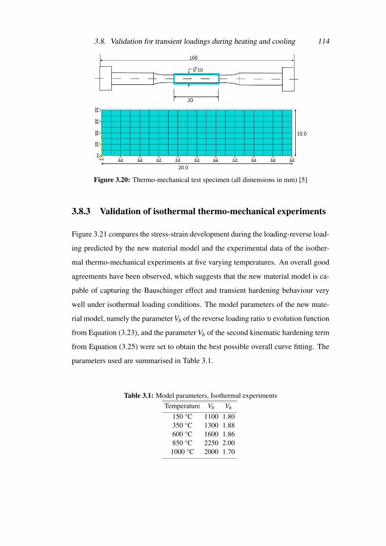
3.8. Validation for transient loadings during heating and cooling 114
Figure 3.20: Thermo-mechanical test specimen (all dimensions in mm) [5]
3.8.3 Validation of isothermal thermo-mechanical experiments
Figure 3.21 compares the stress-strain development during the loading-reverse load-
ing predicted by the new material model and the experimental data of the isother-
mal thermo-mechanical experiments at five varying temperatures. An overall good
agreements have been observed, which suggests that the new material model is ca-
pable of capturing the Bauschinger effect and transient hardening behaviour very
well under isothermal loading conditions. The model parameters of the new mate-
rial model, namely the parameter Vb of the reverse loading ratio υ evolution function
from Equation (3.23), and the parameter Vh of the second kinematic hardening term
from Equation (3.25) were set to obtain the best possible overall curve fitting. The
parameters used are summarised in Table 3.1.
Table 3.1: Model parameters, Isothermal experimentsTemperature Vb Vh
150 °C 1100 1.80350 °C 1300 1.88600 °C 1600 1.86850 °C 2250 2.00
1000 °C 2000 1.70

3.8. Validation for transient loadings during heating and cooling 115
(a) T =150 °C (b) T =350 °C
(c) T =600 °C (d) T =850 °C
(e) T =1000 °C
Figure 3.21: Stress strain curves comparison, Isothermal thermo-mechanical experiments

3.8. Validation for transient loadings during heating and cooling 116
(a) Tmax =350 °C (b) Tmax =600 °C
(c) Tmax =850 °C (d) Tmax =1000 °C
Figure 3.22: Stress strain curves comparison, Transient thermo-mechanical experiments
3.8.4 Validation of transient (anisothermal) thermo-mechanical
experiments
Figure 3.22 compares the stress-strain development during the loading-reverse load-
ing predicted by the proposed material model and the experimental data of the
four transient thermo-mechanical experiments. During initial compressive load-
ing, small deviation between the predicted stresses and the experimental data were
observed, particularity at higher temperatures. This is believed to be caused by the
different constitutive behaviour in tensile and compressive loading of stainless steel
material [178] as the hardening functions have been obtained based on the isother-
mal tensile stress-strain curves. The transient (anisothermal) state of loading could
also be a source for the deviation. Nevertheless, it can be seen that the varying hard-
ening modulus of the stress-strain curve during the heating has been captured well
by the proposed material model.

3.8. Validation for transient loadings during heating and cooling 117
Table 3.2: Model parameters, Transient experimentsTemperature Vb Vh
850 °C 2250 3.401000 °C 800 10.50
For the reverse loading curve during cooling, the predictions of the proposed
material model using the model parameters from Table 3.1 are in good agreement
with the experimental data at 350 °C and 600 °C. For 850 °C and 1000 °C, higher
values of Vh have to be adopted to achieve a satisfactory fit of the reverse stress-
strain relationship. It’s also noted that the material model parameter Vb ceased to be
temperature-dependent during cooling from 1000 °C, a value of 800 was adopted
for the entire cooling process. The model parameters used for at 850 °C and 1000
°C are presented in Table 3.2.
The mechanical behaviour of steel materials are a phenomenological mani-
festation of their microstructure. The effect of very high temperatures on the mi-
crostructure determines the material’s mechanical behaviour when being cooled
from the high temperature. Various experimental research [179–186] have discov-
ered that steel materials only display different mechanical behaviour after being
cooled from a critical maximum temperature (Tcr) or above, i.e., little change in
mechanical behaviour can be found if the materials are cooled down from a tem-
perature that’s lower than Tcr. Qiang et al. [179, 180] identified a Tcr of 600 °C
for high strength structural steels S460, S690 and S960. Wang et al. [181] found
that the high strength structural steel Q460 could recover its original tensile stress-
strain behaviour after experiencing temperatures up to 700 °C. Azhari et al. [182]
proposed a Tcr of 600 °C for the ultra-high strength steel (Grade 1200) based on
their experimental findings. For austenitic stainless steel (1.4307), Wang et al. [183]
and Tao et al. [184] found different behaviour in stress-strain curves when the max-
imum temperature exceeded 500 °C. Huang and Young [185, 186] observed that
the ferritic stainless steel and lean duplex stainless steel can generally regain its
mechanical properties after being cooled from a temperature up to 600 °C.
Sufficiently high temperature exposure that causes phase changes in the mi-
crostructure inevitably gives rise to different mechanical behaviour. It has been

3.8. Validation for transient loadings during heating and cooling 118
discovered that the transition of ferrite to austenite phase at high temperatures
causes the change in the material’s mechanical behaviour, which occurs above 650
°C in ultra-high strength steel [187] and around 800 °C in lean duplex stainless
steel [186]. The transition of ferrite to martensite above 800 °C causes change in
the mechanical behaviour in the ferritic stainless steel after being cooled from 800
°C [185]. Additionally, when exposed to a temperature higher than its Tcr, the ma-
terial’s post-fire mechanical behaviour becomes strongly influenced by the cooling
rate [182, 185, 186].
The existing literature provide a sound explanation why different model pa-
rameters had to be deployed for the validation of the stress-strain relationship dur-
ing cooling phase in the case of Tmax =850 °C and 1000 °C. Figure 3.22c and
3.22d demonstrate the new material model offered good predictions of the reverse
stress-strain behaviour for transient thermo-mechanical experiments.
3.8.4.1 Comparison with isotropic hardening model
In Figure 3.22, the results of the new material model are also compared with the
isotropic hardening model of Abaqus. The new combined isotropic-kinematic hard-
ening material model works the same as the isotropic hardening model during the
initial loading during heating. For the reverse loading during cooling, the isotropic
hardening model overestimates the stress response and cannot capture the transient
hardening behaviour and the variation in the hardening modulus satisfactorily.
The material model presented has been shown to have the capability of describ-
ing accurately the experimentally observed phenomena, which traditional models
are not capable to capture, e.g., the Bauschinger effect and the transient hardening
and their consequences on the mechanical response to subsequent loadings during
heating and cooling. Comparisons and experimental results in general showed good
agreement with respect to initial and subsequent yield stress as well as stress-strain
response, and the qualitative improvement compared to the simulations obtained
using isotropic hardening model is quite evident.
3.9. Uniaxial material model 119
3.9 Uniaxial material modelThe proposed multi-axial material model has also been adapted to a one-
dimensional J2 plasticity model, and implemented as uniaxial material models
in OpenSEES [24]. The uniaxial material “SteelEC02Thermal” has been imple-
mented for the carbon steel, “Stainless01Thermal” for the duplex stainless steel
and “Stainless02Thermal” for the austenitic stainless steel.
3.10 Summary and conclusionsIn this chapter, a new rate-independent combined isotropic-kinematic hardening
model has been developed for assessing steel materials for thermo-mechanical anal-
ysis with fire.
Harley et al. [128] observed substantial development of β11 and swift drop of
κ within the first 1.0% of straining at elevated temperatures in 304L stainless steel.
Different steel materials will exhibit different degrees of Bauschinger effects [188].
Due to limited available testing data on the evolution of isotropic and kinematic
hardening variables at elevated temperatures, it was not possible to carry out more
validations than those presented. However, it should be noted that the validation
was conducted to demonstrate the capability of the proposed material model to cap-
ture the temperature-dependent Bauschinger effects, not to justify for any particular
materials. Thus different sets of temperature-dependent function parameters should
be adopted for different materials accordingly.
By adopting two non-linear kinematic hardening variables, the proposed ma-
terial model is capable of modelling the Bauschinger effect and transient hardening
behaviour at elevated temperatures efficiently.
Due to the lack of experimental data on the re-positioning of yield surface cen-
tre at elevated temperatures, the corresponding algorithms was validated by com-
paring the thermal unloading stress result of the proposed material model to its
analytical solution.
The multi-axial validation results demonstrated that the proposed material
model has been successfully implemented for three dimensional analysis. It is ca-
3.10. Summary and conclusions 120
pable of capturing the expansion and translation of the yield surfaces, presenting
the yield surface as a von Mises circle.
The capability of the new material model has also been validated for transient
loading conditions during both heating and cooling. This demonstrated that the
proposed model is suitable for post-fire structural assessment..
In conclusion, the capability of the new material model proposed in this chap-
ter for capturing the Bauschinger effect and transient hardening behaviour at ele-
vated temperatures has been demonstrated. The algorithm for the proposed mate-
rial model in multi-axial state is presented in Appendix A, and has been successfully
implemented in the Abaqus Umat subroutine. The multi-axial material model has
also been adapted to a 1D plasticity model and implemented as a uniaxial material
model in the open source software OpenSEES [24].

Chapter 4
Remaining Fire Resistance of PFP
Coated Steel Frames Subjected to A
Moderate Earthquake
Adapted from M. Zhou, L. Jiang, S. Chen, A. Usmani and R. Cardoso, “Remaining
fire resistance of steel frames following a moderate earthquake —A case study”,
Journal of Constructional Steel Research, accepted, 2019
4.1 IntroductionThe fire resistance of steel structural components in composite steel frame build-
ings is commonly provided by passive fire protection (PFP) coatings. Current stan-
dards [9,27] measure the fire resistance of structural components using the concept
of time. For instance, a 2 hr fire-resistance rating means the PFP protected struc-
tural components can withstand a standard fire of 2 hours. There are two popular
categories of PFP: cementitious coating and intumescent coating. In USA and Asia,
cementitious PFP has been and still is a popular choice for its advantages of being
cost effective, ease of application and lightweight when compared with other type
of fire insulations [75]. Being specifically designed to be lightweight, Cementitious
PFP is naturally fragile and brittle hence prone to damage under deformation or vi-
bration. Damage in the coating caused by loading events such as windstorms, fires
or earthquakes can result in potential reductions in the structural fire resistance.

4.1. Introduction 122
This hazard should be of particular concern for small/moderate earthquakes be-
cause modern earthquake design philosophy widely accepts that structures should
be designed to resist moderate earthquakes without any structural damage [189].
For instance, ASCE/SEI 7-10 [190] specifies for structures categorized as Seismic
Design Category (SDC) C —approximately correlated to a Modified Mercalli In-
tensity (MMI) VII ground shaking according to FEMA P-750 [191], the damage
should be limited to non-structural components. In contrast, there is no equivalent
requirement currently in place to ensure the integrity of fire resistant coatings on
structural members. This fire safety concern is further compounded by the reality
that cementitious PFP is usually concealed by architectural claddings and finishes
—hindering any regular monitoring and post-earthquake inspections. As a result,
the fire resistance of structures, e.g., structural fire-resistance rating, could suffer
significant reductions after a period of use due to unaccounted for PFP damage.
Especially if this period consists of multiple small/moderate earthquakes.
An integrated FEA-based multi-hazard framework using the new material
model developed by Zhou et al. [192], also presented in Chapter 3, is proposed
in this chapter for assessing the remaining fire resistance of cementitious PFP pro-
tected steel frame structures subjected to moderate earthquakes. In this chapter, the
term ’remaining fire resistance’ is employed to refer to the fire resistance capacity
of PFP coated structures after being subjected to earthquakes. It provides structural
engineers with a practical solution to address the fire safety concern associated with
the undetected PFP damage. For significant structures, the proposed framework can
be integrated into its structural integrity assessment to provide on-line fire safety
monitoring.
This framework adopts a strain-based damage indicator to identify any poten-
tial PFP damage. Recent work as reviewed in Section 2.2.4 has offered fundamental
insights into the damage mechanisms of cementitious coatings under various load-
ing conditions and provided data for quantifying the damage scale sustained by such
coatings under seismic loadings. The development of damage indicator is presented
in Section 4.2.
4.2. Cementitious PFP damage indicator 123
In Section 4.3, the proposed framework is demonstrated by a case study of re-
maining fire resistance of multi-story steel frames subjected a moderate earthquake
loading. This case study uses two equivalent seismic steel frame designs: a steel
moment resisting frame (MRF); and the other a steel concentrically braced frame
(CBF), based on FEMA P-751, NEHRP Recommended Provisions: Design Exam-
ples [193]. Because it is of the greatest interest to analyse a loading scenario where
cementitious PFP suffers significant damage while the structure itself experiences
only superficial damage, an earthquake loading of mild to moderate intensity was
selected for the seismic analysis. A sensitivity study was carried out in Section 4.3.8
to investigate the impact of various design and modelling assumptions on the PFP
damage pattern in the MRF. The study results provide a benchmark guideline for
selecting an appropriate finite element model for PFP damage assessment.
In Section 4.4, a thermo-mechanical analysis was carried out to quantify the
remaining fire resistance of the frames subjected a moderate earthquake loading.
A 2-D heat transfer analysis was used to determine the temperature evolution over
time in the fully protected and the damaged steel members subjected to the Standard
Fire Curve (ISO 834) [26].
All three analyses, namely the time history seismic analysis, the cross-sectional
heat transfer analysis and the thermo-mechanical analysis have been performed us-
ing the native and developed capabilities in the open source software framework
OpenSEES [24].
4.2 Cementitious PFP damage indicator
A number of researchers have investigated damage mechanisms in cementitious
PFP. Keller and Pessiki [83, 84] investigated the damage of cementitious PFP
at bolted connections of gravity beam-column frame subjected to cyclic loading.
Braxtan and Pessiki [77,82] studied the damage pattern of PFP applied on steel mo-
ment frame beam-column assemblies under a strong seismic event, and revealed a
link between damage and plastic hinge formation. Chen et al. [76,85] undertook an
extensive testing programme to study damage mechanisms in cementitious coatings

4.2. Cementitious PFP damage indicator 124
applied to steel plates subjected to monotonic axial loading and bending.
Further experiments [86, 87] have been carried out to study damage patterns
in the cementitious coating applied structural columns subjected to both monotonic
and cyclic loading. Wang [87] noted that when the tested column was subjected
to cyclic loading, the cracking initiated at a lower load level, and the complete
delamination/peel-off failure occurred at a lower level of strain than that under
monotonic loading. This is believed to be caused by the cyclic loading/unloading
process and the frequent stress reversals experienced in the coating. It is also ob-
served that, under cyclic loading, cracks first appeared at the tensile side of the
member, and the transverse crack formed under tension resulted in the final com-
plete peel-off failure.
The interpretation of this phenomenon can be straightforward: under cyclic
loading cracks will be introduced on both flange surfaces by tensile force be-
cause cracks are able to form at a substantially lower tensile strain [85]. Once
the cracks opened, they will continue to absorb energy and keep growing until
delamination/peel-off failure occur as a result of the cyclic stress reversals. The
progression of tensile cracks prevents additional cracks from being generated. Con-
sequently it is essentially the tensile cracks that initiate and lead to the final peel-
off/detachment failure. This explanation can be further validated by Wang’s obser-
vation that the number of cracks remained constant throughout the cyclic loading
test. Wang [87] reported that, the strain level at which complete peel-off failure ob-
served in cementitious coatings was 0.00198 on the tension side under monotonic
loading and 0.00135 under cyclic loading. Correlating Wang’s data to drift ratios,
Chen et al. [86] reported the delamination occurred on the cyclic loaded column
at a drift ratio of 0.0155 whereas similar delamination observed on the monotonic
loaded column at a higher drift ratio of 0.0449.
As demonstrated by the experimental data, the damage strain under monotonic
loading (εmonotonic) is higher than that under cyclic loading (εcyclic). Subjected to re-
alistic loading conditions, a critical damage strain (εcritical) in cementitious coating
can be considered of a value in-between the εmonotonic and the εcyclic. For damage

4.2. Cementitious PFP damage indicator 125
assessment, simply adopting εmonotonic can underestimate the damage scale whereas
εcyclic can be conservative. The εmonotonic can be considered as the upper bound of
the critical damage strain while the εcyclic as the lower bound.
A power law based formula is considered suitable and proposed for estimating
the critical damage strain in cementitious coatings. The formula assumes that the
critical damage strain moves rapidly from the higher value under monotonic loading
to the lower value under cyclic loading with increasing number of stress reversals:
εcritical = εcyclic +(εmonotonic− εcyclic)exp−kn (4.1)
where
εcritical : the critical strain above which the coating is assumed completely lost
εmonotonic : Strain above which the coating delaminated under monotonic tensile
loading, obtained from testing results
εcyclic : Strain above which the coating delaminated under cyclic loading, obtained
from testing results
n : Number of stress reversals experienced in the coating
k : Material parameter
The proposed damage formula is a deterministic approach and there exists a
need for much greater volume of experimentation for refinement so a statistical
and probabilistic approach could be used to account for the uncertainties associated
with the damage phenomena in quasi-brittle cementitious materials, and for the
determination of the material variable k. The biggest uncertainty probably comes
from the cementitious material per se due to the manufacturers/suppliers owned
material recipes and application techniques.
For this study, we adopted the experimental values in [87] (εmonotonic = 0.0198
and εcyclic = 0.0135) as the upper and lower bound damage indicator. The upper
and lower bound damage indices provide a guideline for the potential PFP damage
assessment, and should not be deemed as definitive failure limits. For any specific
cementitious PFP damage assessment, variations in the bound limits are inevitable

4.3. Impact of seismic steel frame designs on PFP damage 126
as a result of the inherent uncertainties in the materials.
Figure 4.1 shows the relationship between the εcritical and the number of stress
reversals experienced in the cementitious coating, based on Equation 4.1. A value
of 0.1 was assumed for the material variable k. The critical strain approaches εcyclic
very rapidly and becomes nearly insensitive to the number of stress reveals when
n > 90. Earthquake loading usually consists of a large number of cycles. For in-
stance, Figure 4.2 presents the acceleration history of the 1994 Northridge earth-
quake based on Canoga Park record. In cases of earthquake loading, it can be
considered reasonable to estimate the damage scale in the cementitious PFP system
using εcyclic.
Figure 4.1: εcritical vs. Stress reversal Number
4.3 Impact of seismic steel frame designs on PFP
damageDesign examples and seismic design guidelines from American standards have been
adopted in this case study in order to fully take advantage of the analysis techniques
and tools offered by the OpenSEES. Since the software is developed as the com-
putational tool for research at the California based Pacific Earthquake Engineering

4.3. Impact of seismic steel frame designs on PFP damage 127
Figure 4.2: Acceleration history of 1994 Northridge earthquake
Research (PEER) Centre, the analysis techniques are mostly developed for struc-
tural designs using American standards, especially for seismic steel frame structural
designs.
The structural models are based on FEMA P-751 [193], which are two equiv-
alent alternatives —a steel moment resisting frame (MRF) and the other a steel
concentrically braced frame (CBF), designed for a seven-story office building in
Los Angeles California. The building is of a rectangular plan, which is 177 feet and
4 inches (54.0 m) along in the E-W direction and 127 feet and 4 inches (38.8 m)
wide in the N-S direction. It is framed in structural steel with 25 feet (7.6m) bays
in each direction. The typical story height is 13 feet and 4 inches (4.1 m) with the
exception of the first story which is 22 feet and 4 inches (6.8 m) high. The building
has a penthouse, which extends 16 feet (4.9 m) above the roof level and covers the
central bay areas.
4.3.1 FE Model geometry
The typical N-S direction frame of the two alternative designs were modelled, the
overall geometries are shown in Figure 4.3 and Figure 4.4 respectively, with the
member sizes displayed. The braced frames are in a two-story X configuration.
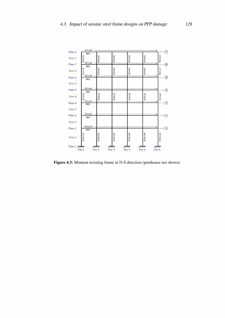
4.3. Impact of seismic steel frame designs on PFP damage 128
Figure 4.3: Moment resisting frame in N-S direction (penthouse not shown)

4.3. Impact of seismic steel frame designs on PFP damage 129
Figure 4.4: Concentrically braced frame in N-S direction (Typical)
4.3.2 FE model Loadings
4.3.2.1 Gravity loads
The gravity loads including structural self-weight, fireproofing, wall cladding and
equipment weights were applied as body force to the model in the first step of the
analysis. Table 4.1 presents the gravity loads for each floor level.
Table 4.1: Gravity loadsFloor Level Loads (kips)
Penthouse roof 94Lower roof 1537
Typical floor 1920

4.3. Impact of seismic steel frame designs on PFP damage 130
4.3.2.2 Earthquake load
The Canoga Park record from the 1994 Northridge earthquake occurred in Los An-
geles, California, from the OpenSEES library, as shown in Figure 4.2 was adopted.
The most serious fire safety risk results from a loading scenario where cementitious
PFP suffers significant damage while the structure itself experiences only superficial
damage. As the unaccounted for PFP damage seriously reduces the structural fire
resistance. Therefore, a ground motion reduction factor =0.65 was applied to the
Peak Ground Acceleration (PGA) to achieve the desired moderate earthquake level.
Under the reduced earthquake load, the global structural behaviour is constrained
to remain in the elastic region.
4.3.3 FE model Materials
For all the wide flange sections, ASTM A992, Grade 50 steel (fy= 50 ksi or
345MPa) was used. The ASTM A500 Grade B steel (fy= 46 ksi or 315MPa) was
adopted for the HSS sections.
4.3.4 FE models for seismic analysis
For the base model of the MRF and the CBF, the structural members were modelled
from centreline to centreline, using 2D Euler-Bernoulli Force-based Beam-Column
(FB) element which can account for geometric non-linearity. The strength, stiffness,
dimensions and shear distortions of panel zones were neglected in the base models.
The uniaxial material Steel02 [194] from OpenSEES library was adopted, which
can properly account for steel’s isotropic strain hardening when subjected to seismic
loading.
The braces of the CBF were modelled using the method proposed by Uriz and
Mahin [195] to ensure brace global buckling behaviour is captured, in which each
brace was modelled with 10 FB elements using corotational geometric transforma-
tion. Additionally, initial out-of-plane imperfection of 0.5% effective length was
applied at the middle of the braces that would help trigger lateral buckling in the
dynamic analyses. Gusset plate connection was modelled using pinned connection
which has been considered appropriate for analysing moderate earthquake response.

4.3. Impact of seismic steel frame designs on PFP damage 131
Fully fixed boundary conditions were applied to the MRF at the bottom and
pinned connections were applied to the CBF.
The implicit transient analysis using Newmark integrator was performed to
determine the seismic responses of the steel frames.
4.3.5 Earthquake response
Time history analyses of the two frames were performed. The approximate funda-
mental natural periods calculated using ASCE/SEI 7-10 Section 12.8.2 [190] and
the first mode natural periods from OpenSEES analysis are reported in Table 4.2. It
is expected and verified by the recommendations [193] that the modelling natural
periods will exceed the Standard’s approximation as a result of member selections.
Table 4.2: Fundamental building periodsFrame Type ASCE 7-10 (s) OpenSEES Results (s)
Moment resisting frame 1.596 1.617Concentrically braced frame 0.896 0.946
The inter-story drift ratios (IDR) are presented in Table 4.3 and 4.4 for the
MRF and CBF respectively. The corresponding IDRs from FEMA P-751 [193] are
included in the tables only as a benchmark reference since different seismic loadings
were used. The FEMA P-751 values were determined using the seismic design
ground motion specified by ASCE 7-10 [190] for office buildings in the region of
seismic design category D, i.e., Los Angeles, whereas the OpenSEES results were
obtained using the modified Northridge earthquake ground motion. For the MRF,
the FEMA P-751 and OpenSEES IDRs results display similar trends: lower values
at the bottom and at the top while higher values around the middle stories. For the
CBF, higher IDRs occurred at the upper stories. Lower consistency is found in the
OpenSEES CBF model results when compared with the FEMA P-751 values. This
is believed to be caused by the modelling methodology adopted for capturing the
global buckling behaviour of the braces. Overall, the IDRs in the CBF are lower
than that in the MRF, which is as expected.

4.3. Impact of seismic steel frame designs on PFP damage 132
Table 4.3: Inter-story drift ratios, Moment frame modelLevel FEMA P-751 OpenSEES Allowable Drift Ratio
(%) (%) (%)
Story7 1.2 0.77 2.0Story6 1.7 1.25 2.0Story5 2.0 1.56 2.0Story4 2.0 1.41 2.0Story3 1.8 1.02 2.0Story2 1.2 0.54 2.0Story1 1.1 0.60 2.0
Table 4.4: Inter-story Drift Ratios, Braced Frame ModelLevel FEMA P-751 OpenSEES Allowable Drift Ratio
(%) (%) (%)
Story7 0.93 0.57 2.0Story6 0.94 0.55 2.0Story5 0.84 0.57 2.0Story4 0.84 0.46 2.0Story3 0.71 0.53 2.0Story2 0.59 0.42 2.0Story1 0.52 0.55 2.0
4.3.6 Damage to cementitious PFP
Table 4.5 shows the number of stress reversals experienced in the Pier 3 of the MRF
model over its full height under the selected earthquake load. The large number of
stress reversals observed suggest a reasonable assessment of the PFP damage can
be achieved by using the lower bound damage indicator (εcyclic), as discussed in
Section 4.2.
Table 4.5: Number of cycles in Pier 3, Moment frame modelLevel Stress Reversals No. (n)Story7 100Story6 83Story5 93Story4 42Story3 29Story2 55Story1 62

4.3. Impact of seismic steel frame designs on PFP damage 133
4.3.7 Comparison study of strain results
The maximum tensile strain of the seismic analysis results in each structural mem-
ber of the MRF and the CBF are presented in this section. The strain distributions
within the columns and floor beams provide an immediate link to the potential PFP
damage pattern.
4.3.7.1 Moment resisting frame
The maximum tensile strain values of the seismic analysis results in the Pier 1, Pier
2 and Pier 3 are plotted in Figure 4.5a, 4.5b and 4.5c respectively. The surface strain
at the Left Hand Side (LHS) flange and at the Right Hand Side (RHS) flange of the
Piers are plotted separately. The strain values in the Pier 4, 5 & 6 are similar to that
in the Pier 3, 2 &1 correspondingly owing to the structural symmetry. As shown,
high strain values occurred around floor joints. With the indicative lower and upper
bound damage limit highlighted on Figure 4.5, any strain values that exceed the
εcyclic are considered an indication for potential damage in the cementitious PFP.
No damage in Piers is indicated by the strain results of the base model, as seen in
Figure 4.5.
The maximum tensile strain values of all the floor beams are plotted in Figure
4.5d. High strains are observed near beam-column joints. Potential damage were
observed at floors 5 and 6, which also ties back to the high IDRs observed at these
two floors.
4.3.7.2 Concentrically braced frame
For the concentrically braced frame, the maximum tensile strain values in the Pier
1, 2 and 3 are presented in Figure 4.6a, 4.6b and 4.6c. As shown, the strain levels in
the CBF columns are well below the εcyclic. Similarly, the maximum tensile strain
values in the beams are also lower than the εcyclic, as plotted in Figure 4.6d. High
strain values were observed in the braces during the seismic analysis however brace
members do not have any bearing on the fire resistance of the frame. As a result, no
potential damage in the PFP of the concentrically braced frame has been identified
based on the seismic analysis results.

4.3. Impact of seismic steel frame designs on PFP damage 134
(a) Strain distribution in Pier 1
(b) Strain distribution in Pier 2
(c) Strain distribution in Pier 3
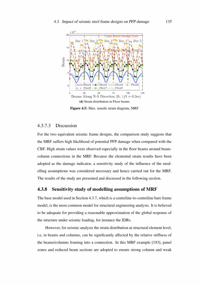
4.3. Impact of seismic steel frame designs on PFP damage 135
(d) Strain distribution in Floor beams
Figure 4.5: Max. tensile strain diagram, MRF
4.3.7.3 Discussion
For the two equivalent seismic frame designs, the comparison study suggests that
the MRF suffers high likelihood of potential PFP damage when compared with the
CBF. High strain values were observed especially in the floor beams around beam-
column connections in the MRF. Because the elemental strain results have been
adopted as the damage indicator, a sensitivity study of the influence of the mod-
elling assumptions was considered necessary and hence carried out for the MRF.
The results of the study are presented and discussed in the following section.
4.3.8 Sensitivity study of modelling assumptions of MRF
The base model used in Section 4.3.7, which is a centreline-to-centreline bare frame
model, is the most common model for structural engineering analysis. It is believed
to be adequate for providing a reasonable approximation of the global response of
the structure under seismic loading, for instance the IDRs.
However, for seismic analysis the strain distribution at structural element level,
i.e, in beams and columns, can be significantly affected by the relative stiffness of
the beams/columns framing into a connection. In this MRF example [193], panel
zones and reduced beam sections are adopted to ensure strong column and weak

4.3. Impact of seismic steel frame designs on PFP damage 136
(a) Strain distribution in Pier 1
(b) Strain distribution in Pier 2
(c) Strain distribution in Pier 3

4.3. Impact of seismic steel frame designs on PFP damage 137
(d) Strain distribution in Floor Beams
Figure 4.6: Max. tensile strain diagram, Concentrically braced frame
beam design of seismic frames. Such design decisions inevitably change the relative
stiffness between the beams and columns.
The second factor influencing the relative stiffness ratios is the contribution of
floor slabs to the stiffness of floor beams. Yet it is difficult to determine whether
the strains in the beams would consequently increase or decrease because the stiff-
ness contribution from the slabs will also attract more loads into the beams for the
seismic analysis.
Thirdly, as in most typical steel frame designs, the MRF is located on the
perimeter of the structure, with the interior frames designed for gravity loads. The
P-delta effect caused by the vertical loads on the interior frames is also worth ex-
amining.
The sensitivity study in this section focuses on evaluating the effects of these
factors on the PFP damage identification for the MRF. In addition to the base model
(Model 1), four more additional models were constructed for the sensitivity study:
1. Model 1: A basic centreline model of bare moment resisting frame, where the
beams and columns extend from centreline to centreline, as shown schemat-
ically in Figure 4.7. The strength, stiffness, dimensions, and shear distortion
of panel zones are neglected.

4.3. Impact of seismic steel frame designs on PFP damage 138
2. Model 2: Bare frame model (Model 1) with panel zone dimensions (depth of
beam by depth of column), strength, stiffness and shear distortions consid-
ered. The Model 2 is shown schematically in Figure 4.8. Columns and beams
are modelled to have clear span length. The panel zone is explicitly modelled
following the approach of Gupta and Krawinkler [196], as illustrated in Fig-
ure 4.9. The rectangle composes of eight very stiff beam-column elements
representing the rectangular joint area of the column web that lies between
the flanges of the connecting beams. The rotational spring at one corner al-
lows the shear distortions in the panel zone where as the other three corners
are jointed by a pin connection.
3. Model 3: Model 1 with the contribution of floor slabs to the beams’ strength
and stiffness considered. The floor slab is modelled as part of the beam us-
ing composite beam section. The contributing slab width (B) is calculated
following Equation 4.2. The stiffness contribution of slabs is accounted for
based on the assumption of isotropic composite action between the slabs and
the beams neglecting factors such as shear studs and reinforcements in the
slab.
B = b f +0.2L (for interior beam spans)
B = Min b f +0.1L, b f +overhang (for exterior beam spans)(4.2)
where b f is the flange width of the steel floor beam and L is the span of the
beam.
4. Model 4: Model 2 with the contribution of reduced beam section (RBS) de-
sign incorporated. Figure 4.11 shows schematically the Model 4, with the
RBSs highlighted in red. The detailing of the RBS is shown in the Section
B-B. In the FE model, the reduced beam section was divided into 8 segments
and each segment was represented using the averaged flange width size.
5. Model 5: Model 4 with effect of inner gravity columns considered. The P-
Delta effect is introduced to the model by modelling an imaginary leaning
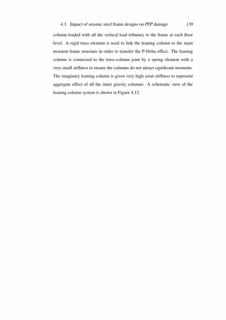
4.3. Impact of seismic steel frame designs on PFP damage 139
column loaded with all the vertical load tributary to the frame at each floor
level. A rigid truss element is used to link the leaning column to the main
moment frame structure in order to transfer the P-Delta effect. The leaning
column is connected to the truss-column joint by a spring element with a
very small stiffness to ensure the columns do not attract significant moments.
The imaginary leaning column is given very high axial stiffness to represent
aggregate effect of all the inner gravity columns. A schematic view of the
leaning column system is shown in Figure 4.12.
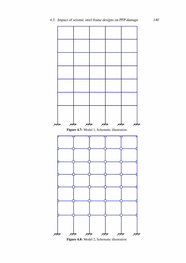
4.3. Impact of seismic steel frame designs on PFP damage 140
Figure 4.7: Model 1, Schematic illustration
Figure 4.8: Model 2, Schematic illustration

4.3. Impact of seismic steel frame designs on PFP damage 141
Figure 4.9: Panel zone, Schematic representation
Figure 4.10: Model 3, Schematic illustration
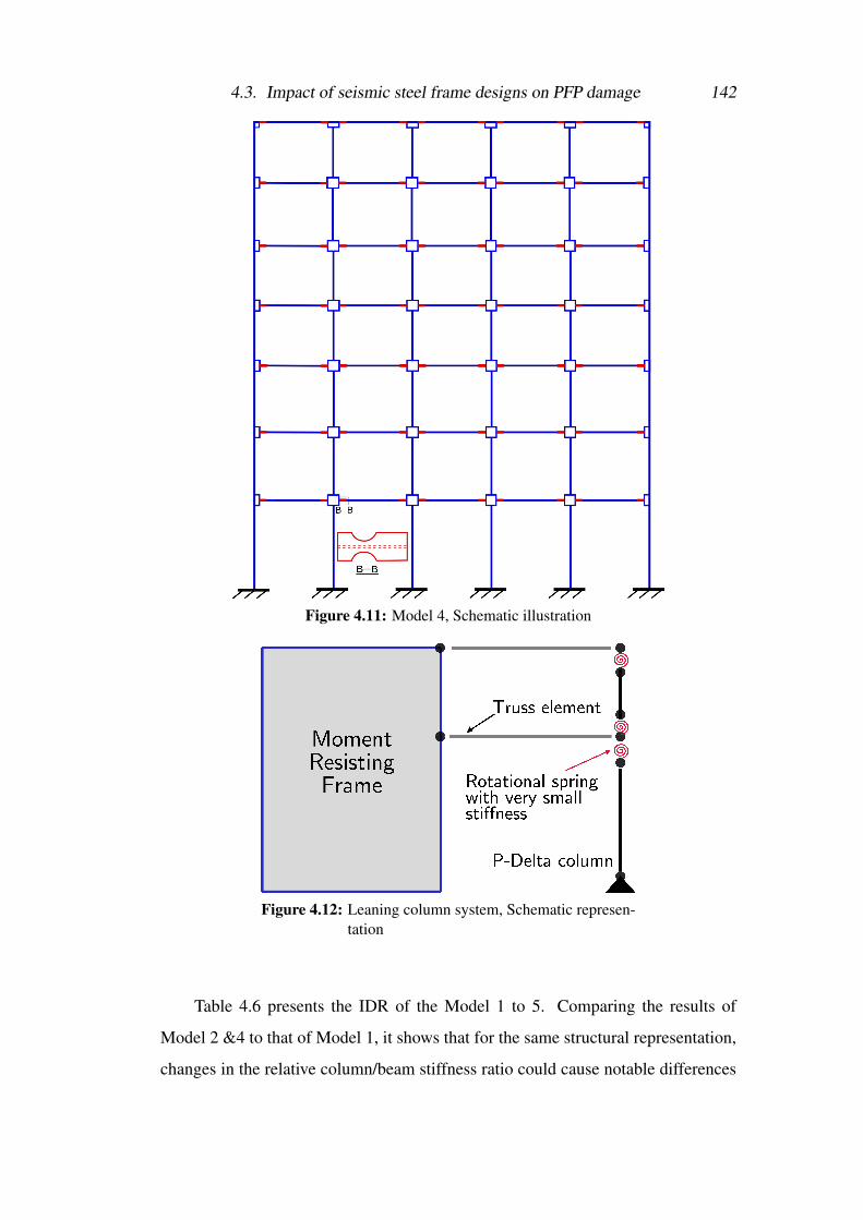
4.3. Impact of seismic steel frame designs on PFP damage 142
Figure 4.11: Model 4, Schematic illustration
Figure 4.12: Leaning column system, Schematic represen-tation
Table 4.6 presents the IDR of the Model 1 to 5. Comparing the results of
Model 2 &4 to that of Model 1, it shows that for the same structural representation,
changes in the relative column/beam stiffness ratio could cause notable differences
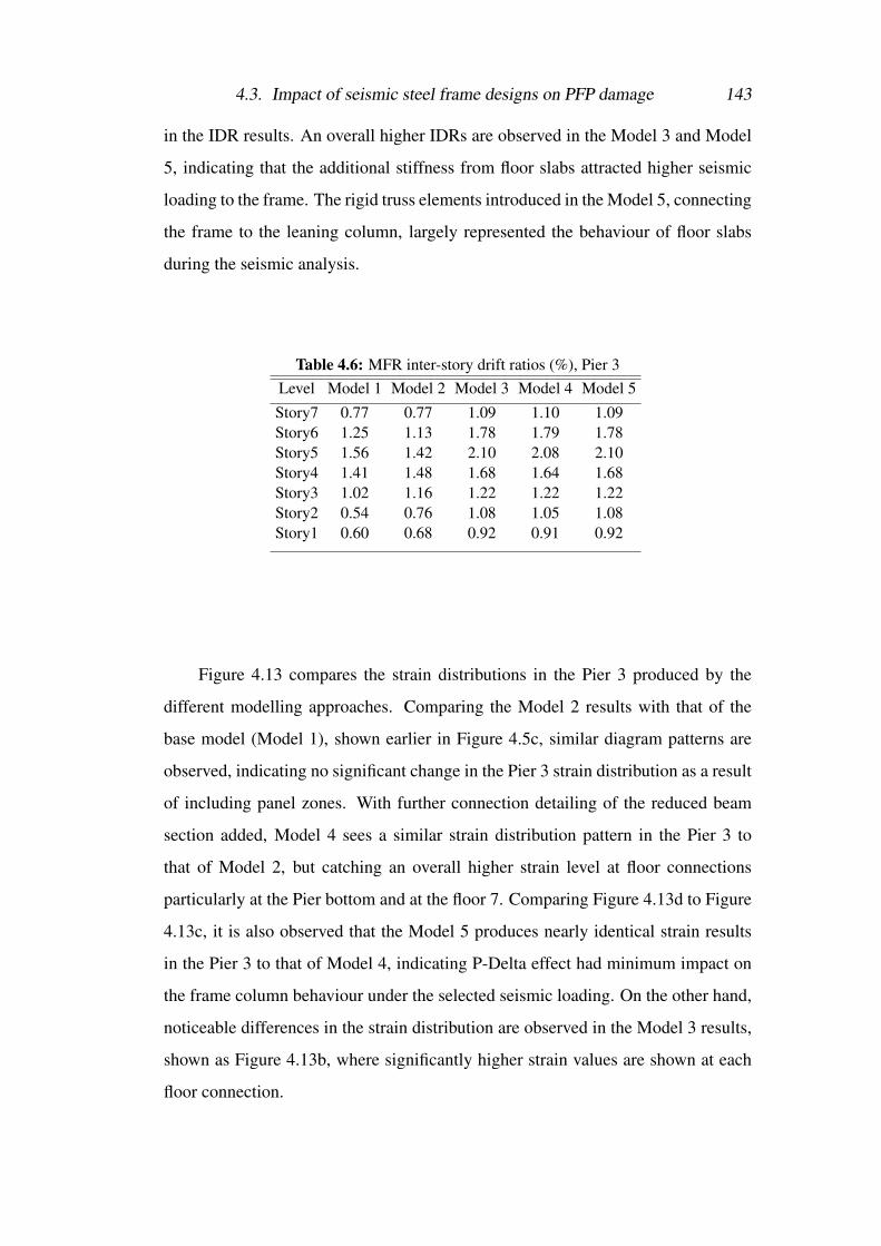
4.3. Impact of seismic steel frame designs on PFP damage 143
in the IDR results. An overall higher IDRs are observed in the Model 3 and Model
5, indicating that the additional stiffness from floor slabs attracted higher seismic
loading to the frame. The rigid truss elements introduced in the Model 5, connecting
the frame to the leaning column, largely represented the behaviour of floor slabs
during the seismic analysis.
Table 4.6: MFR inter-story drift ratios (%), Pier 3Level Model 1 Model 2 Model 3 Model 4 Model 5Story7 0.77 0.77 1.09 1.10 1.09Story6 1.25 1.13 1.78 1.79 1.78Story5 1.56 1.42 2.10 2.08 2.10Story4 1.41 1.48 1.68 1.64 1.68Story3 1.02 1.16 1.22 1.22 1.22Story2 0.54 0.76 1.08 1.05 1.08Story1 0.60 0.68 0.92 0.91 0.92
Figure 4.13 compares the strain distributions in the Pier 3 produced by the
different modelling approaches. Comparing the Model 2 results with that of the
base model (Model 1), shown earlier in Figure 4.5c, similar diagram patterns are
observed, indicating no significant change in the Pier 3 strain distribution as a result
of including panel zones. With further connection detailing of the reduced beam
section added, Model 4 sees a similar strain distribution pattern in the Pier 3 to
that of Model 2, but catching an overall higher strain level at floor connections
particularly at the Pier bottom and at the floor 7. Comparing Figure 4.13d to Figure
4.13c, it is also observed that the Model 5 produces nearly identical strain results
in the Pier 3 to that of Model 4, indicating P-Delta effect had minimum impact on
the frame column behaviour under the selected seismic loading. On the other hand,
noticeable differences in the strain distribution are observed in the Model 3 results,
shown as Figure 4.13b, where significantly higher strain values are shown at each
floor connection.

4.3. Impact of seismic steel frame designs on PFP damage 144
(a) Model 2
(b) Model 3
(c) Model 4
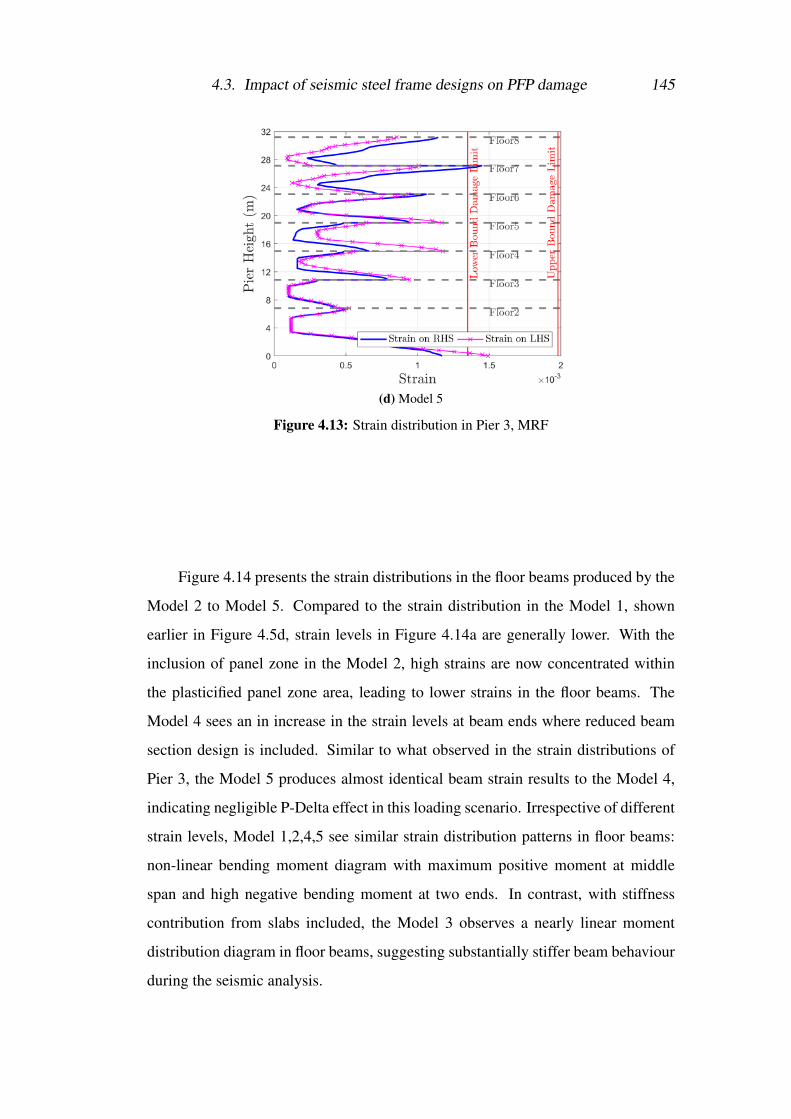
4.3. Impact of seismic steel frame designs on PFP damage 145
(d) Model 5
Figure 4.13: Strain distribution in Pier 3, MRF
Figure 4.14 presents the strain distributions in the floor beams produced by the
Model 2 to Model 5. Compared to the strain distribution in the Model 1, shown
earlier in Figure 4.5d, strain levels in Figure 4.14a are generally lower. With the
inclusion of panel zone in the Model 2, high strains are now concentrated within
the plasticified panel zone area, leading to lower strains in the floor beams. The
Model 4 sees an in increase in the strain levels at beam ends where reduced beam
section design is included. Similar to what observed in the strain distributions of
Pier 3, the Model 5 produces almost identical beam strain results to the Model 4,
indicating negligible P-Delta effect in this loading scenario. Irrespective of different
strain levels, Model 1,2,4,5 see similar strain distribution patterns in floor beams:
non-linear bending moment diagram with maximum positive moment at middle
span and high negative bending moment at two ends. In contrast, with stiffness
contribution from slabs included, the Model 3 observes a nearly linear moment
distribution diagram in floor beams, suggesting substantially stiffer beam behaviour
during the seismic analysis.

4.3. Impact of seismic steel frame designs on PFP damage 146
(a) Model 2
(b) Model 3
(c) Model 4

4.3. Impact of seismic steel frame designs on PFP damage 147
(d) Model 5
Figure 4.14: Strain distribution in floor beams, MRF
The examination of strain distributions in the floor beams and Pier 3 produced
by different models suggest Model 2 can reasonably capture the representative strain
distribution patterns. It is considered essential for the finite element model to cap-
ture the concentrated plastification phenomenon within the panel zone area.
The inclusion of the reduced beam section design in Model 4 increased the
strain levels in the Piers, particularly at the bottom and at the floor 7 because of the
increased column/beam stiffness ratio.
The comparison between the Model 4 and the Model 5 indicates minimum
impact of P-Delta effect in this moderate earthquake loading. It is worth noting
that the strains presented in this section are the strain results at the outmost layer of
the flanges. Plastic hinge does not form until the whole cross-section reaches the
yielding capacity. In spite of a few locations where the strain result exceeded the
material’s yield strain (0.0016), the global structure behaviour is still predominantly
elastic.
The sensitivity analysis found that the inclusion of floor slabs brings about a
different structural response in the frame structures, giving rise to higher strains
in the piers and floor beams, indicating that the dominating effect of the stiffness
contribution of floor slabs is attracting higher seismic loading. This behaviour is

4.3. Impact of seismic steel frame designs on PFP damage 148
investigated further in the following section.
4.3.8.1 Effect of floor slabs on strain distributions
When comparing Figure 4.15a with 4.15b, it is shown that the inclusion of panel
zone connection detailing caused no significant changes in the strain distribution
pattern in the floor beams for the gravity load case. Lower strain values were ob-
served in the Model 2 as stiffer panel zone connections took upon a larger portion
of the loading at the beam ends. Compared with the Model 1, Figure 4.15c shows
the inclusion of floor slabs in the Model 3 reduced the negative bending moments
at beam ends while raised the positive bending moments at middle span.
Figure 4.16 compares the bending moment diagrams of the gravity loading in
the Pier 3 predicted by the Model 1, 2 and 3 respectively. It is evident that changes
in the relative column/beam stiffness ratios can lead to different load distribution
within the structural frames. The inclusion of floor slabs forms stronger restraints
at the column ends, consequently columns experience higher moments at beam-
column joints.
Figure 4.17 compares the maximum bending moments experienced on either
side of the Pier 3 in the Model 1, 2 and 3 for the earthquake loading case, higher
bending moments are observed in the Model 3. Correspondingly, higher bending
moments are observed in the floor beams of the Model 3 as shown in Figure 4.18.
The comparison results show that the main influence of the floor slabs on the strain
distributions in the MRF is attracting higher seismic loading, which in turn leads to
higher strain values in the structure.
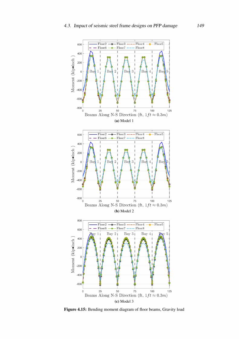
4.3. Impact of seismic steel frame designs on PFP damage 149
(a) Model 1
(b) Model 2
(c) Model 3
Figure 4.15: Bending moment diagram of floor beams, Gravity load

4.3. Impact of seismic steel frame designs on PFP damage 150
Figure 4.16: Pier 3 moment diagram, Gravity load
Figure 4.17: Pier 3 Max. moment diagram, Seismic load
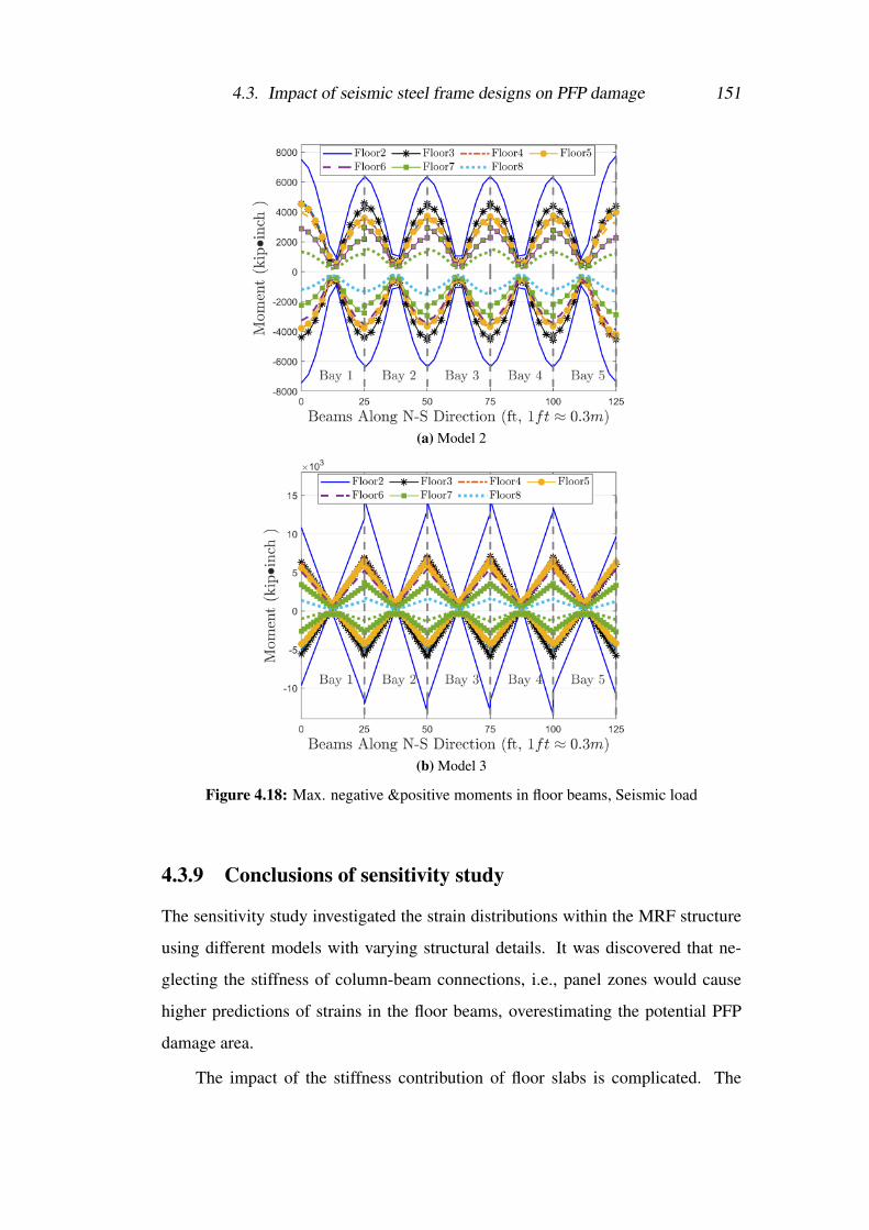
4.3. Impact of seismic steel frame designs on PFP damage 151
(a) Model 2
(b) Model 3
Figure 4.18: Max. negative &positive moments in floor beams, Seismic load
4.3.9 Conclusions of sensitivity study
The sensitivity study investigated the strain distributions within the MRF structure
using different models with varying structural details. It was discovered that ne-
glecting the stiffness of column-beam connections, i.e., panel zones would cause
higher predictions of strains in the floor beams, overestimating the potential PFP
damage area.
The impact of the stiffness contribution of floor slabs is complicated. The

4.4. Remaining fire resistance assessment of MRF 152
sensitivity study found higher seismic loading was attracted to the structure when
including the floor slabs in the model, resulting in higher strain levels in the overall
structure.
The response of the five models, ranging from the basic centreline model to
models that incorporate the strength and stiffness of the panel zones and the con-
tribution from gravity columns and floor slabs, is evaluated. It is evident that the
prediction of the scale of the PFP damage is strongly influenced by the model se-
lected. In order to achieve higher accuracy at the element level, a more sophisticated
model is generally required. However, a compromise between accuracy, efficiency
and practicality is usually necessary in the context of the problem being solved, es-
pecially for practical engineering problems. The sensitivity study forms the basis
for the selection of representative models for assessing the potential PFP damage in
MRFs.
Despite of the differences observed in the strain distributions from different
models, the analysis results of the five models agreed that the most vulnerable lo-
cations for cementitious PFP damage are near the column-beam connections at the
floor levels of high IDRs, particularly in the floor beams near the beam-column
connections.
4.4 Remaining fire resistance assessment of MRF
4.4.1 PFP damage area identification
The seismic analysis results of Model 4 is adopted for the PFP damage assessment
of the MRF because it captures the most structural details. Figure 4.19 schemati-
cally shows the damaged area identified using the εcyclic as the damage indicator.
The size of the damaged area was quantified based the assumption that the PFP is
deemed completely lost its function wherever the strain at the outmost surface of the
flange exceeded the εcyclic. Based on the strain results in Figure 4.13c (Pier 3 strain
distributions of Model 4), a damage length of approximately 400mm is identified
at the base and at the floor 7 of the Pier 3. Figure 4.20 presents the strain results in
Pier 1 &2 of the Model 4. A damage length of 250 mm is identified at the base and
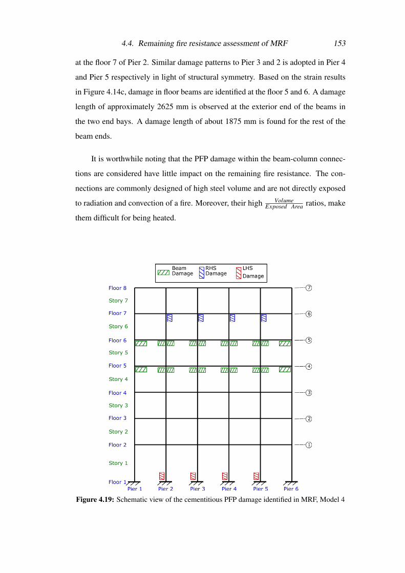
4.4. Remaining fire resistance assessment of MRF 153
at the floor 7 of Pier 2. Similar damage patterns to Pier 3 and 2 is adopted in Pier 4
and Pier 5 respectively in light of structural symmetry. Based on the strain results
in Figure 4.14c, damage in floor beams are identified at the floor 5 and 6. A damage
length of approximately 2625 mm is observed at the exterior end of the beams in
the two end bays. A damage length of about 1875 mm is found for the rest of the
beam ends.
It is worthwhile noting that the PFP damage within the beam-column connec-
tions are considered have little impact on the remaining fire resistance. The con-
nections are commonly designed of high steel volume and are not directly exposed
to radiation and convection of a fire. Moreover, their high VolumeExposed Area ratios, make
them difficult for being heated.
Figure 4.19: Schematic view of the cementitious PFP damage identified in MRF, Model 4

4.4. Remaining fire resistance assessment of MRF 154
(a) Pier 1
(b) Pier 2
Figure 4.20: Strain distribution in Pier 1 & 2, Model 4
The existence of potential damage in PFP can significantly jeopardise the sur-
vivability of the structure in an event of fire. In the following sections, the possi-
ble perilous consequences are analysed using a thermo-mechanical analysis of the
MRF.
4.4. Remaining fire resistance assessment of MRF 155
4.4.2 Heat transfer analysis
For structural fire analysis, it’s considered that the temperature evolution in the
structures are resulted from the external fire source, hence can be determined us-
ing a heat transfer analysis decoupled from the thermo-mechanical analysis.
4.4.2.1 Fire loading
The Standard Fire Curve (ISO 834) [26] was adopted to represent the temperature
development of a uniform compartment fire for this office building. The fire location
was selected at the compartment framed by the Pier 2 and Pier 3 at floor 1. This
was considered the most onerous fire scenarios since within this compartment the
PFP damage was identified at the base of the column (Pier 3). It’s worth mentioning
that the PFP damage identified at the base of Pier 2 was at the LHS (exterior of the
compartment) hence the Pier 2 was still considered protected for the selected fire
scenario.
4.4.2.2 Fire protection required
According to Table 25 of BS9999:2008 [197], a two hour fire resistance for struc-
tural components of office buildings over 30m tall is required. The PFP thickness of
the beams and columns have been determined based on BSI PD7974-3:2011, Part
3 Table 9 [35]. The coating thickness required to satisfy the 2 hrs fire resistance
requirement are summarised in Table 4.7. The columns were considered to be pro-
tected for 4 sides and the beams were considered to be protected for 3 sides with
the top flange shielded by floor slabs.
Table 4.7: Cementitious PFP thicknessSection Structural Type Thickness (mm)
W24x146 Story 1 Column 23W24x207 Floor 2 Beam 18
4.4.2.3 Coefficients for heat transfer analysis
The material properties specified in the heat transfer model include conductiv-
ity, specific heat and density. The HTMaterial –CarbonSteelEC3 developed in
OpenSEES for heat transfer analysis was used. The default thermal properties

4.4. Remaining fire resistance assessment of MRF 156
of the cementitious coating in OpenSEES were adopted (thermal conductivity
λ = 0.05W/m/K, density ρ = 350kg/m3, and specific heat cp = 1100J/kgK).
The boundary conditions for the heat transfer analyses include convection and
radiation. The structural cross-section was subjected to the 2 hrs fire exposure
(temperature-time history), defined by the Standard Fire Curve [26] on the exposed
sides. According to EC 3 [1], the convection coefficient for the unexposed and
exposed surfaces were applied as 4 W/m2K and 25 W/m2K, the emissivity for ra-
diation was adopted as 0.7 for steel and 0.9 for the cementitious coating.
4.4.2.4 Heat transfer analysis results
The wide flange beam W24x146 is used for the columns and the W24x207 is for
the beam of this compartment. For the heat transfer analysis, the LHS flange of the
Pier 3 and the RHS flange of the Pier 2 were considered subjected to the compart-
ment fire while the beam is subjected to the fire from three sides with the top being
shielded by the slab. The heat transfer analysis was performed for the unprotected
and the protected column cross-section, and for the protected beam cross-section
as no PFP damage was identified in the floor beam of this compartment. The tem-
perature evolution at 12 thermal points across the I-section were obtained. Figure
4.21 shows the temperature evolution at the flange surface of the unprotected and
protected columns (W24x146), and at the bottom flange surface of the protected
W24x207 beam.
Albeit the longitudinal conduction within a structural member is neglected by
a 2D cross-sectional heat transfer analysis, through parametric study, Jiang [198]
concluded that a transitional length of 1.0 metre can be prescribed to represent the
temperature gradient between the unprotected segment and the protected segment
of a steel member as illustrated in Figure 4.22. Thus 2D heat transfer analysis can
be used for a three dimensional frame structure subjected to a compartment fire.

4.4. Remaining fire resistance assessment of MRF 157
Figure 4.21: Temperature history results
Figure 4.22: Schematic illustration of thermal loading application
4.4.3 Thermo-mechanical analysis
4.4.3.1 FE model
The same finite element model developed for the seismic analysis was used for
the thermo-mechanical analysis, with appropriate modifications implemented. The
uniaxial material model SteelEC02Thermal was adopted, which is the new material
model proposed from Chapter 3 implemented in OpenSEES. The Voce hardening
law [114] was used to model the Eurocode 3 [1] non-linear stress-strain relation-

4.4. Remaining fire resistance assessment of MRF 158
ships for carbon steel at elevated temperatures. The model parameters applied in
the SteelEC02Thermal are presented in Table D.1. The 2D Euler-Bernoulli Dis-
placement based element “DispBeamColumn2dThermal” was used for all struc-
tural members. Thermal Action Wrapper function was employed for thermal load-
ing application. The cross-sectional temperature histories obtained from the heat
transfer analysis were adopted as the thermal loading, and applied to the 12 fibre
points across the I-section of the structural members as illustrated in Figure 4.22.
For the damaged column, the heat transfer results of the unprotected W24x146 was
applied to the damaged segment (shown in red in Figure 4.22 ) while that of the
protected W24x146 was applied to the protected segments (shown in blue in Figure
4.22). The 1.0 m transitional segment (shown in purple in Figure 4.22) between the
damaged and the protected was adopted to include the temperature gradient along
the length of the damaged column. The Thermal Action Wrapper function applies
a temperature distribution to the transitional segment by using a mixed order in-
terpretation between the high temperature of the damaged segment and the low
temperature of the protected segment. The heat transfer results of the W24x207
was adopted as the thermal loading for the floor beam. Longitudinal temperature
gradient was not considered for the beam as uniform temperature development was
assumed for the compartment fire. A static thermo-mechanical analysis was carried
out to determine the remaining fire resistance of the steel frame.
4.4.3.2 Thermo-mechanical analysis results
The displacement evolution of the Pier 3 at the floor 2 and at the top floor during
the fire are presented in Figure 4.23. At t = 0 s, the deformation is due to the
gravity loads. During the heating up to t = 1200 s, the Pier 3 shows clear upward
expansion, dragging its connected floor beams upwards, inducing tension into the
adjacent Pier 2 &4. This phenomenon is reflected in the evolution of the vertical
reactions at the column bases, as plotted in Figure 4.24, where axial load decreases
in the Pier 2 &4 while increases in the Pier 3. The Pier 3 still retains its stiffness at
this stage. At about t = 1700 s, as the Pier 3 displacements start to drop quickly,
substantial deformation and curvature were observed in the Pier 3 during the anal-
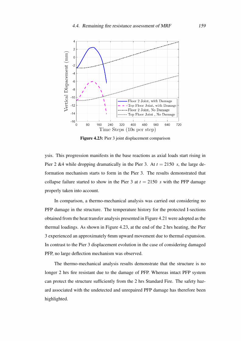
4.4. Remaining fire resistance assessment of MRF 159
Figure 4.23: Pier 3 joint displacement comparison
ysis. This progression manifests in the base reactions as axial loads start rising in
Pier 2 &4 while dropping dramatically in the Pier 3. At t = 2150 s, the large de-
formation mechanism starts to form in the Pier 3. The results demonstrated that
collapse failure started to show in the Pier 3 at t = 2150 s with the PFP damage
properly taken into account.
In comparison, a thermo-mechanical analysis was carried out considering no
PFP damage in the structure. The temperature history for the protected I-sections
obtained from the heat transfer analysis presented in Figure 4.21 were adopted as the
thermal loadings. As shown in Figure 4.23, at the end of the 2 hrs heating, the Pier
3 experienced an approximately 6mm upward movement due to thermal expansion.
In contrast to the Pier 3 displacement evolution in the case of considering damaged
PFP, no large deflection mechanism was observed.
The thermo-mechanical analysis results demonstrate that the structure is no
longer 2 hrs fire resistant due to the damage of PFP. Whereas intact PFP system
can protect the structure sufficiently from the 2 hrs Standard Fire. The safety haz-
ard associated with the undetected and unrepaired PFP damage has therefore been
highlighted.

4.5. Discussion and conclusions 160
Figure 4.24: Vertical reaction development, with PFP damage
4.5 Discussion and conclusions
In this chapter, the new material model [192] from Chapter 3 was implemented
in a framework for assessing the remaining fire resistance of steel frames using
the cementitious PFP system subjected to moderate earthquakes. The proposed
framework is implemented in the OpenSEES and demonstrated by a case study of
a multi-story steel frame subjected to a moderate earthquake loading, using two
equivalent seismic steel frame designs: a steel MRF and a steel CBF.
In this framework, the strain level in the beams and columns is adopted as the
PFP damage indicator. Experimental results revealed that cementitious PFP coat-
ings experience damage at a substantially lower strain level under cyclic loading
(εcyclic) than that under monotonic loading (εmonotonic). A power law based for-
mula is proposed as an attempt to correlate the two bounding strain values using
the number of cycles in the loading. Because of the large number of cycles com-
monly experienced under earthquake loading, it is believed conservative to adopt
the lower bound εcyclic as the damage indicator for the cementitious PFP damage
assessment, until a better estimate could be found trough future research. Given the
damage strain limit is highly influenced by the material properties and the applica-

4.5. Discussion and conclusions 161
tion techniques, e.g., spay-applied or plastered, it is the authors’ opinion that the
manufacturers/suppliers should be required in the future to provide the εmonotonic
and εcyclic value to facilitate the assessment of remaining structural fire resistant
post-earthquakes.
The PFP damage in the frame structure was identified based on the strain re-
sults of the seismic analysis. The comparison study shows that the PFP in the MRF
structure is more susceptible to earthquake induced damage than that in the CBF
structure. The sensitivity study of the various modelling assumptions of the MRFs
concludes that the PFP damage assessment is highly influenced by the structural de-
tails included in the finite element model. The panel zone and reduced beam section
detailing that ensure the strong column weak beam seismic design approach lead to
larger PFP damage in the floor beams. The stiffness contribution from floor slabs
attracts higher seismic loading to the frame, bringing about an overall higher strain
level in the structure, resulting in greater PFP damage in both columns and beams.
In conclusion, for the damage assessment it is recommended that the panel zone
and reduced beam section detailing should be included in the finite element model.
The commonly adopted centreline to centreline model is found underestimated the
damage scale.
The thermo-mechanical analysis results for the selected fire scenario demon-
strate that the post-earthquake PFP damage could result in significant reductions in
structural fire resistance, which, in the worst case scenario may lead to structural
collapse due to column failure at around 36 mins. In comparison, the structure with
an intact PFP system can withstand the full 2 hrs Standard Fire as designed.
The step by step procedure of using the framework can be summarised as fol-
lows:
1. Determine the εcyclic of the cementitious material used in the PFP system.
2. Perform seismic structural analysis, by selecting suitable ground motions as
the earthquake load input.
3. Establish PFP damage map.

4.5. Discussion and conclusions 162
4. Perform heat transfer analysis.
(a) Select a fire location within the frame.
(b) Define a fire scenario, e.g. the Standard Fire.
(c) Determine the required fire insulation thickness according to the build-
ing regulations.
(d) Analyse the cross-sectional and longitudinal temperature evolution for
the PFP damaged and protected structural components respectively.
5. Perform thermo-mechanical analysis.
The integrated multi-hazard framework as presented herein offers a practical
solution for assessing remaining fire resistance of PFP protected structures sub-
jected to fire following moderate earthquakes.

Chapter 5
A Thermo-mechanical Analysis of
Stainless Steel Structures in Fire
Adapted from M. Zhou, R. Cardoso, H. Bahai, and A. Usmani, “A thermo-
mechanical analysis of stainless steel structures in fire”, Engineering Structures,
under review, 2019
5.1 IntroductionThe development of structural design codes, standards and specifications for stain-
less steel has been a research focus since early 1960s. The first American specifi-
cation dealing with the design of structural stainless steel members was published
in 1968 by the AISI [199]. In Europe, the first edition of the design manual for
structural stainless steel was published in 1994. Since then, several European re-
search projects have been carried out to analyse the performance of structural stain-
less steel, resulting in the publication of the Design Manual for Structural Stainless
Steel (DMSSS) fourth edition [2] in 2017.
Large scale fire tests of carbon steel structures, such as Cardington tests [106],
have revealed significant difference between global structural behaviour in fire and
individual structural component tested in the furnace. However, testing steel sub-
assemblies and frame structures in a fire is extremely expensive and one single test
provides only a limited amount of data. The current research gap in understanding
stainless steel structural systems in fire can be approached economically and effi-

5.2. Temperature development in stainless steel I sections 164
ciently using FEA; by taking advantage of existing experimental observations and
experience using FEA on large carbon steel structures in fire.
This chapter investigates stainless steel structural behaviour in fire using finite
element modelling, focusing on comparisons between carbon steel and stainless
steel structures, with the aim of exploring potential advantages offered by the stain-
less steel materials. Using the new material model developed by Zhou et al. [192],
also presented in Chapter 3, the influence of stainless steel’s highly non-linear ma-
terial behaviour on its structural performance in fire is investigated, the impact of
its higher thermal expansion is also discussed. Due to limited available testing data
for stainless steel structures at elevated temperatures, structural models used in the
FEA were validated against existing testing data of carbon steel structures in fire.
5.2 Temperature development in stainless steel I sec-
tionsIn this section, the temperature development within structural stainless steel I-
sections is investigated using heat transfer analysis carried out in OpenSEES [24].
The impact of section factors (A/V), defined as the heated perimeter of the exposed
cross-section divided by the total sectional area, is examined. A comparison study
between structural stainless steels and structural carbon steel is performed.
5.2.1 Heat transfer model validation
Gardner and Ng [20] conducted a series of furnace tests of stainless steel beams
tp investigate the temperature development within the sections over the time. The
I section steel beams were subjected to four sides heating during the test as illus-
trated in Figure 5.1. Validations of the FE model is performed by comparing the
OpenSEES heat transfer results with the testing data and the Abaqus finite element
results obtained by Gardner and Ng [20]. The I cross sections were modelled using
the heat transfer element in the OpenSEES. The boundary conditions for the heat
transfer analyses include convection and radiation. The recordings of the furnace
temperature were adopted as the fire loading for the validation study. In accordance

5.2. Temperature development in stainless steel I sections 165
with Eurocode 3 [1], the convection coefficient of 25W/m2K was adopted for both
carbon steel and stainless steel sections; the emissivity for radiation is adopted as
0.7 for the carbon steel and 0.4 for the stainless steel. The comparison results are
presented in Figure 5.2, where a good agreement is observed. The sharp increase in
the furnace temperature at around 850 °C for I120x64 and I160x82 has been well
captured by the FE model.
Figure 5.1: I section subjected to 4 sides heating
Figure 5.2: Temperature development within sections

5.2. Temperature development in stainless steel I sections 166
5.2.2 Heat transfer parametric study
Temperature development within stainless steel I-sections is studied through a para-
metric study using the heat transfer model validated in the previous section. For
steel I-sections subjected to high temperatures, radiation is the predominant heat
transfer mode and conduction within the cross-section is almost instantaneous due
to the high thermal conductivity. A comparison study of the temperature develop-
ment within the carbon steel and the stainless steel I-sections was carried out for 9
typical I-sections subjected to 4 sides heating. A summary of the dimensions of the
9 I-sections and their section factors (A/V) is presented in Table 5.1.
Table 5.1: Section dimensions and Section factors
Section Depth (mm) Width (mm) Web t (mm) Flange t (mm) A/V (m−1)
UB914x305x289 926.6 307.7 19.5 32.0 83UB762x267x197 769.8 268.0 15.6 25.4 104UB914x419x388 921.0 420.5 21.4 36.6 71UB610x305x238 635.8 311.4 18.4 31.4 82UC305x305x198 339.9 314.5 19.1 31.4 76UC254x254x73 254.1 254.6 8.6 14.2 166UC356x406x634 474.6 424.0 47.6 77.0 32UC356x406x393 419.0 407.0 30.6 49.2 48UC356x406x235 381.0 394.8 18.4 30.2 78
The boundary conditions for the heat transfer analyses include convection and
radiation. The I-sections were subjected to a 1 hr fire exposure defined by the Stan-
dard Fire Curve [26] on all 4 sides. In accordance with Eurocode 3 [1], the convec-
tion coefficient of 25W/m2K was adopted for both carbon steel and stainless steel
sections; the emissivity for radiation is adopted as 0.7 for the carbon steel and 0.4
for the stainless steel.
Figure 5.3 shows the temperature difference vs.time relationships at the bottom
flange for each I-section. The temperature difference is determined as Tempcarbon−
Tempstainless through the duration of the heating. Tempcarbon is the temperature of
the carbon steel while Tempstainless is the temperature of the stainless steel.
At the same time step, carbon steel I-sections experienced higher temperatures
than stainless steel ones since only positive temperature differences were observed.
A maximum temperature difference of 122 °C was observed at the bottom flange of

5.3. Stainless steel structural behaviour in fire 167
section UC356x406x634, which is of the lowest A/V of 32 m−1, at around 2400 s.
The section of the highest A/V of 166 m−1 (UC254x254x73) experienced the low-
est maximum temperature difference of 80 °C at about 600s. In general, it has been
observed that higher A/V leads to a smaller magnitude and an earlier occurrence of
the maximum temperature difference.
The same trend has also been observed at the mid-web of the I-sections, as
shown in Figure 5.4. The slower temperature rise experienced in the stainless steel
is believed mainly attributed to its lower emissivity.
Figure 5.3: Temperature difference in bottom flange, 4 sides heated
Figure 5.4: Temperature difference in web, 4 sides heated
5.3 Stainless steel structural behaviour in fireFor this study, the multi-dimensional material model presented in Chapter 3 was
developed to a one-dimensional plasticity model, and implemented as uniaxial ma-
terial models in OpenSEES [24]. The uniaxial material “SteelEC02Thermal” has
been implemented for the carbon steel, “Stainless01Thermal” for the duplex stain-
less steel and “Stainless02Thermal” for the austenitic stainless steel. These three
material models were adopted for the comparison studies in the section. Due to

5.3. Stainless steel structural behaviour in fire 168
little available testing data for stainless steel structures at elevated temperatures, the
FE models used in this study were validated against existing testing data of carbon
steel structures in fire.
5.3.1 Simply supported beams in fire
5.3.1.1 FE model validation
The simply supported beam was modelled in OpenSEES [24] using the Euler-
Bernoulli beam theory based “DispBeamColumn2DThermal” element. The FE
beam model is pinned at one end and is free to move in the horizontal direction
at the other end. The FE analysis accounted for both material and geometric non-
linearities. A static thermo-mechanical analysis was performed to investigate the
behaviour of stainless steel beams in fire.
Rubert and Schaumann [6] carried out a series of tests on simply supported
beams subjected to 4 sides heating, with varying initial load ratios (L.R.) ranging
from 0.2 to 0.85. The tested beams were of a length (L) = 1140 mm, with cross-
section size IPE 80/ IPE 120, and made of St 37.2 Grade carbon steel. A point
load was applied at the mid-span of the beams. The L.R. was calculated as the the
maximum bending moment applied on the simply supported beam over the plastic
bending moment capacity of the beam at ambient temperature. The uniaxial ma-
terial model SteelEC02Thermal was used for the St 37.2 grade carbon steel. The
material parameters of the hardening functions applied in the SteelEC02Thermal
for the validation were determined by least square fitting the stress-strain curves of
the tested St 37.2 carbon steel in [6], and are summarised in Table D.7.
The FE model was validated by comparing model predictions of the midspan
deflection of the 4 sides heated beams with that of testing data. As shown in Figure
5.5a, a general good agreement has been observed between the testing data and the
OpenSEES simulations.

5.3. Stainless steel structural behaviour in fire 169
(a) Four sides heating
(b) Three sides heating
Figure 5.5: Validation of simply supported beam model
A series tests of simply supported beams in fire were also carried out by
the British Steel and documented in the Compendium of UK Standard Fire Test
Data [200]. The testing data of three beams, BS90 (UB356x171x67), BS91
(356x171x67) and BS94 (IPE 360) were also adopted for validation in this study.
The beams were heated from three sides with the top being protected by a concrete
slab. There were no composite actions between the steel beam and the slab. The

5.3. Stainless steel structural behaviour in fire 170
FE model was further validated by comparing model predictions of the midspan de-
flection of the three sides heated beams with the testing results. As shown in Figure
5.5b, a good agreement has been generally observed between the test data and the
OpenSEES results.
5.3.1.2 Comparison study
Using the validated structural FE model, a comparison study was carried out to
analyse the structural behaviour of simply supported stainless steel beams in fire.
For this study, carbon steel S235, Austenitic 1.4571 (group III) and Duplex 1.4162
(group II) stainless steels have been selected. As discussed in Section 2.2.3.1, the
Austenitic III shows the most promising stiffness and strength retention capability
while the Duplex II shows an overall better stiffness and strength retention capabil-
ity than the Duplex I. The lean duplex grade (Duplex 1.4162) was included in this
study also because there has been a significant increase in its application in onshore
building construction [22].
The room temperature values of the Young’s modulus and the 0.2% proof
strength (σ0.2) for the three selected steels are summarised in Table 5.2. It is
worth noting that DMSSS [2] proposes an identical Young’s modulus value for the
austenitic and duplex stainless steels, which is nearly the same to the value of carbon
steel. The σ0.2 of the austenitic steel is close to that of carbon steel, whereas the σ0.2
of the duplex stainless steel is almost double the σ0.2 of the carbon steel. The uni-
axial material model Stainless01Thermal and Stainless02Thermal were adopted for
the Duplex 1.4162 and Austenitic 1.4571 stainless steel respectively. The material
model parameters applied were obtained based on the nominal stress-strain relation-
ships of stainless steels at elevated temperatures in DMSSS [2], and are presented in
Table D.2 and Table D.3. For the S235, the material model parameters determined
using the EC 3 [1] stress-strain curves for carbon steel at elevated temperatures
were applied in the SteelEC02Thermal, and are summarised in Table D.1. For bet-
ter understanding the influence of stainless steel’s highly material non-linearity and
high thermal expansion on its structural fire behaviour, and the difference to carbon
steel structural fire behaviour, the Bauschinger effect is therefore not included in

5.3. Stainless steel structural behaviour in fire 171
this study. A Bauschinger ratio of 1.0 was adopted for all the materials.
Table 5.2: Material properties
Material Property S235 Austenitic DuplexYoung’s modulus (GPa) 210 200 200
σ0.2% (MPa) 235 220 450
In this study, four series of comparison analyses were performed. The applied
load, initial deflection and initial L.R. of each beam for each series are summarised
in Table 5.3. In each series, the magnitude of the applied load was kept constant
for the three beams of different steel materials. Comparable initial midspan deflec-
tions were attained due to the similar Young’s modulus of the carbon steel and the
stainless steels, with slightly higher deflection observed in stainless steels. In each
series, the initial L.R.s of the duplex steel beam was almost half of the carbon steel
and austenitic stainless steel beams because of its higher σ0.2 value. In the Series 3
&4, a notably higher initial deflection is observed for the austenitic stainless steel
beam, indicating the tangent modulus is already considerably lower than the initial
elastic modulus at higher L.R.s.
Table 5.3: Comparison study series, Simply supported beams
Series Applied Load Initial Deflection (mm) L.R.No. (kN) S235 Austenitic Duplex S235 Austenitic Duplex1 3.71 0.70 0.75 0.75 0.20 0.21 0.102 9.27 1.8 1.9 1.9 0.50 0.53 0.263 12.98 2.5 3.1 2.6 0.70 0.75 0.374 15.77 3.0 4.9 3.2 0.85 0.95 0.44
The midspan deflection vs. temperature curves are presented in Figure 5.6. In
the first series, the deflection of the carbon steel beam started to increase rapidly
at around 650 °C and the run-away mechanism occurred at about 750 °C. Iden-
tical deflections were observed for the austenitic and duplex beams until near the
occurrence of the run-away mechanism, which was at around 800 °C for the du-
plex and at around 900 °C for the austenitic steel. Based on the deflection results
of the first series, the two stainless steels exhibit superior behaviour to that of car-
bon steel with the run-away mechanism occurring at the highest temperature for the
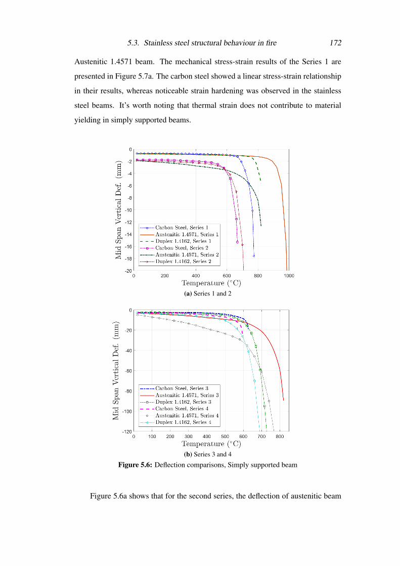
5.3. Stainless steel structural behaviour in fire 172
Austenitic 1.4571 beam. The mechanical stress-strain results of the Series 1 are
presented in Figure 5.7a. The carbon steel showed a linear stress-strain relationship
in their results, whereas noticeable strain hardening was observed in the stainless
steel beams. It’s worth noting that thermal strain does not contribute to material
yielding in simply supported beams.
(a) Series 1 and 2
(b) Series 3 and 4
Figure 5.6: Deflection comparisons, Simply supported beam
Figure 5.6a shows that for the second series, the deflection of austenitic beam

5.3. Stainless steel structural behaviour in fire 173
develops faster than the other two beams because the Austenitic 1.4571 steel ap-
proaches the non-linear region faster. The deflection vs. temperature curve sug-
gests that with the initial L.R. =0.53, the Austenitic 1.4571 experienced a faster and
greater reduction in its tangent modulus. The run-away mechanism was still evident
at the highest temperature for the austenitic beam, at around 800 °C. The run-away
mechanism for the carbon steel beam and for the Duplex 1.4162 beam initiated at
a similar temperature, around 600 °C. As shown in Figure 5.7b, substantial amount
of strain hardening was observed for the stainless steel beams.
For the third series, Figure 5.6b shows that with L.R. =0.75, higher initial
deflection and faster deflection development is observed for the austenitic beam.
This is due to faster reduction in the tangent modulus as the material approaches
plastic state. The run-away mechanism occurred at about 610 °for the carbon steel
beam, at around 700 °C for the duplex beam and at around 800 °C for the austenitic
beam.
For the fourth series, starting with similar initial deflections, the carbon steel
beam displayed a slower deflection development than the duplex beam until the
run-away occurred at around 550 °C. The deflection of the Duplex 1.4162 started
to increase quickly at around 500 °C and reached 114 mm (L/10) at about 690 °C.
Due to the high initial L.R., austenitic beam was already in the plastic state at the
start of the heating, resulting in significant reduction in the tangent modulus. This
was manifested as higher initial deflection and notably faster deflection rate in the
austenitic beam than the other two steel beams. However, due to its superior stiff-
ness retention, the austenitic beam reached the large deflection of 114 mm (L/10)
later at about 750 °C. Figure 5.7c and 5.7d show that in Series 3 and 4, substantial
strain hardening was able to develop in the simply supported stainless steel beams
while none was observed for the simply supported carbon steel beams.

5.3. Stainless steel structural behaviour in fire 174
(a) Series 1 (b) Series 2
(c) Series 3 (d) Series 4
Figure 5.7: Stress strain development, simply supported beam
5.3.1.3 Discussion
The deflection results suggest that the initiation of the run-away mechanism for
simply supported beams in fire is primarily determined by the material’s stiffness
degradation and the initial load ratio. At the lowest L.R., the run-away mechanism
occurs when the stiffness of the material starts to deteriorate rapidly, at around 500
°C for the carbon steel and 800 °C for the stainless steel. For carbon steel, the elas-
tic modulus retention capability at elevated temperatures is a good indication to the
occurrence of the run-away mechanism in simply supported beams. For simply sup-
ported stainless steel beams with higher initial L.R., the retention factor (kE,θ ) can-
not consistently indicate well the occurrence of the run-away mechanism, because
the early plastic state achieved in the material gives rise to significant reduction in
the tangent modulus.
The comparison study between the simply supported stainless steel and the car-
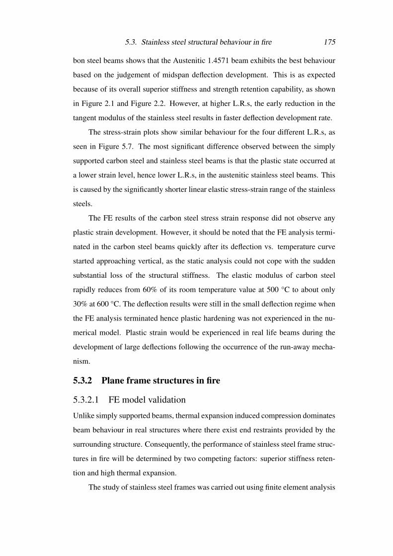
5.3. Stainless steel structural behaviour in fire 175
bon steel beams shows that the Austenitic 1.4571 beam exhibits the best behaviour
based on the judgement of midspan deflection development. This is as expected
because of its overall superior stiffness and strength retention capability, as shown
in Figure 2.1 and Figure 2.2. However, at higher L.R.s, the early reduction in the
tangent modulus of the stainless steel results in faster deflection development rate.
The stress-strain plots show similar behaviour for the four different L.R.s, as
seen in Figure 5.7. The most significant difference observed between the simply
supported carbon steel and stainless steel beams is that the plastic state occurred at
a lower strain level, hence lower L.R.s, in the austenitic stainless steel beams. This
is caused by the significantly shorter linear elastic stress-strain range of the stainless
steels.
The FE results of the carbon steel stress strain response did not observe any
plastic strain development. However, it should be noted that the FE analysis termi-
nated in the carbon steel beams quickly after its deflection vs. temperature curve
started approaching vertical, as the static analysis could not cope with the sudden
substantial loss of the structural stiffness. The elastic modulus of carbon steel
rapidly reduces from 60% of its room temperature value at 500 °C to about only
30% at 600 °C. The deflection results were still in the small deflection regime when
the FE analysis terminated hence plastic hardening was not experienced in the nu-
merical model. Plastic strain would be experienced in real life beams during the
development of large deflections following the occurrence of the run-away mecha-
nism.
5.3.2 Plane frame structures in fire
5.3.2.1 FE model validation
Unlike simply supported beams, thermal expansion induced compression dominates
beam behaviour in real structures where there exist end restraints provided by the
surrounding structure. Consequently, the performance of stainless steel frame struc-
tures in fire will be determined by two competing factors: superior stiffness reten-
tion and high thermal expansion.
The study of stainless steel frames was carried out using finite element analysis

5.3. Stainless steel structural behaviour in fire 176
with the FE model validated against the testing data of the EHR3 carbon steel frame
tests performed by Rubert and Schaumann [6]. The configuration of the EHR3
frame is illustrated in Figure 5.8. All members were uniformly heated during the
test. The frame beam was pinned at right end while the column was pinned at the
bottom. The lateral torsional displacement and the out-of-plane deformation were
prevented by using stiffeners during testing, hence a 2D plane frame model was con-
sidered suitable for this study. The frame was modelled in in OpenSEES [24] using
the Euler-Bernoulli beam theory based “DispBeamColumn2DThermal” element.
A static thermo-mechanical analysis was performed to investigate the behaviour
of stainless steel beams in fire. The FE analysis accounted for both material and
geometric non-linearities.
Figure 5.8: EHR3 frame configuration
Validation of the FE model was carried out by comparing the deformation vs.
temperature history (deflection U2 and V4 as illustrated in Figure 5.8), predicted by
the FE model with that from experimental results. The material model parameters
in Table D.7 for the St37 carbon steel were used. A general good agreement can be
observed for the results presented in Figure 5.9.
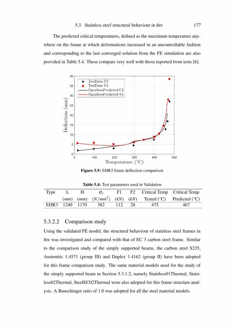
5.3. Stainless steel structural behaviour in fire 177
The predicted critical temperatures, defined as the maximum temperature any-
where on the frame at which deformations increased in an uncontrollable fashion
and corresponding to the last converged solution from the FE simulation are also
provided in Table 5.4. These compare very well with those reported from tests [6].
Figure 5.9: EHR3 frame deflection comparison
Table 5.4: Test parameters used in Validation
Type L H σy F1 F2 Critical Temp Critical Temp(mm) (mm) (N/mm2) (kN) (kN) Tested (°C) Predicted (°C)
EHR3 1240 1170 382 112 28 475 467
5.3.2.2 Comparison study
Using the validated FE model, the structural behaviour of stainless steel frames in
fire was investigated and compared with that of EC 3 carbon steel frame. Similar
to the comparison study of the simply supported beams, the carbon steel S235,
Austenitic 1.4571 (group III) and Duplex 1.4162 (group II) have been adopted
for this frame comparison study. The same material models used for the study of
the simply supported beam in Section 5.3.1.2, namely Stainless01Thermal, Stain-
less02Thermal, SteelEC02Thermal were also adopted for this frame structure anal-
ysis. A Bauschinger ratio of 1.0 was adopted for all the steel material models.

5.3. Stainless steel structural behaviour in fire 178
Three series of load ratios (L.R.s) of the frames were investigated, as sum-
marised in Table 5.5. The L.R. for the beam was calculated as the maximum bend-
ing moment applied on the beam to the plastic bending moment capacity of the
beam at ambient temperature. The L.R. for the column was calculated as the max-
imum axial force on the column over the axial capacity of the column at ambient
temperature.
Table 5.5: Comparison study series, EHR3 frame
Series No. L.R. in Beam L.R. in Column1 0.15 0.0752 0.30 0.153 0.60 0.30
Since there were no restraints at the beam-column joint, the beam could expand
to the left whilst the column could expand upwards during heating. As a result, the
V4 deflection of the beam moved upwards in the positive direction of the global Y
axis in the beginning, whereas the U2 displacement of the column moved leftwards
in the negative direction of the global X axis.
Figure 5.10 compares the midspan deflection results of the frame beam (V4)
of the three series. During heating, the V4 increased initially as a result of the ther-
mal expansion in the column. As the stiffness of the column reduced at increasing
temperatures, a rapid drop in the V4 was observed, indicating the collapse of the
column.
In the Series 1 to 3, the V4 of the Austenitic 1.4571 steel showed the highest
upward movement since the austenitic stainless steel possesses the highest thermal
elongation. In the Series 3, the upward behaviour was not observed in the V4 de-
flection of the Duplex 1.4162 steel, suggesting the duplex column was already in
the plastic state when L.R. reached the value of 0.30.
The column collapse occurred at the highest temperature for the Austenitic
1.4571 frame, however the degree of this advantage diminished as the L.R. in-
creased. When the column achieved L.R. =0.075, the Austenitic 1.4571 steel post-
poned the collapse by approximately 240 °C in comparison to the carbon steel. This
value dropped to 180 °C when the column L.R. increased to 0.30.

5.3. Stainless steel structural behaviour in fire 179
With similar initial deflection (Duplex 1.4162 in the Series 1 compared with
carbon steel and Austenitic 1.4571 in the Series 2; Series 2 Duplex 1.4162 compared
with the other two materials in the Series 3), the frame collapse occurred at higher
temperatures for the Duplex 1.4162 than for the carbon S235, but the temperatures
were still lower than that of the Austenitic 1.4571 steel. Within each series, the same
initial L.R.s were shared by the frame beams and columns of the three different steel
materials. For the Series 1, the Duplex 1.4162 frame collapsed at a temperature
about 10 °C higher than that of the carbon S235 and 210 °C lower than that of the
Austenitic 1.4571 steel. For the Series 2 and 3, the Duplex 1.4162 frame collapsed
at the lowest temperature among the three materials.
Figure 5.10: Beam midspan deflection V4

5.3. Stainless steel structural behaviour in fire 180
Figure 5.11: Column midspan deflection U2
The midspan deflection results of the frame column (U2) are plotted and com-
pared in Figure 5.11. During heating, the U2 displayed a linear increase along the
negative direction of the global X axis because of the beam expansion in that di-
rection, until the large deflection mechanism occurred as a result of the column
collapse.
The deflection results of the frame beam (V4) and the frame column (U2)
showed a clear advantage of the Austenitic 1.4571 steel in delaying the collapse of
the frame structure. For the duplex 1.4162, the superior behaviour when compared
with the carbon steel was only evident in the Series 1. The degree of the advantage
offered by the two stainless steel grades generally diminishes as the L.R. increases.
As seen from the previous comparison study of simply supported beams, stainless
steels enter the plastic domain at lower strains than carbon steel because of their
shorter elasticity range. The results of the Series 3 showed that the Duplex 1.4162
frame rapidly developed into the collapse mode since the column, with an initial
L.R.=0.30, was already in the plastic state at the start of the fire. The comparison
results demonstrate that the initial plasticity of stainless steel columns are detrimen-
tal to the structural fire performance of stainless steel frames.

5.3. Stainless steel structural behaviour in fire 181
Figure 5.12 presents the stress strain development at the beam-column joint
of the Series 1 during the heating, in the beam and in the column respectively.
The imposed vertical and horizontal displacements due to temperature effects at
the joint are inducing bending moments in the left extreme of the beam and in the
upper cross-section of the column. Hence the stress at the bottom of the joint cross-
section is in negative while at the top is in positive as seen in the figure. The stress
strain results of the Series 1 (which is of the lowest L.R.s) showed that substantial
plastic hardening was developed during the fire. The austenitic beam-column joint
experienced the highest plastic hardening for this case. The strain reversals occurred
at the lowest strain value for the duplex at the beam-column joint.
5.3.2.3 Effect of axial restraints
The EHR3 frame represents a single frame structure where the beam-column joint is
free to move without any external axial restraints during fire. In reality, during a fire,
there exist axial restraints on the beam-column joints provided by the surrounding
cooler structure. The effect of external axial restraints are of particular research
interest for stainless steel structural fire performance because stainless steels exhibit
higher thermal elongations when compared to carbon steel, as seen in Figure 2.3.
In this section, the effect of external axial restraints on the structural fire be-
haviour of the frame column and beam was studied by applying varying degrees of
axial restraints to them at the beam-column joint, as illustrated in Figure 5.13. The
axial restraints were modelled using elastic spring elements. Three levels of axial
restraints were investigated, which are 0.05Kβ , 0.15Kβ and 0.30Kβ , where Kβ is
the axial stiffness of the structural component (frame column or beam) at the room
temperature. The restraint stiffness was considered constant during the fire. The
L.R.s of the Series 2 and 3 from the previous comparison study was selected for
this parametric study. For the Series 2, the L.R. of beam =0.30 and L.R. of column
=0.15; for the Series 3, the L.R. of beam =0.60 and L.R. of column =0.30.

5.3. Stainless steel structural behaviour in fire 182
(a) Stress strain in the beam
(b) Stress strain in the Column
Figure 5.12: Stress strain at the beam-column joint

5.3. Stainless steel structural behaviour in fire 183
Figure 5.13: EHR3 frame with external axial restraints applied
Figure 5.14 compares the midspan deflection (V4) development of the frame
beam (L.R.=0.30) without/with varying degrees of external restraints at the beam-
column joint. It shows that as the restraint stiffness increases, the magnitude of
the initial upward movement resulting from column expansion reduces. Also, the
temperature at which the beam begins to displace downward lowers. When there
were no external restraints (kβ = 0.0), the run-away mechanism was observed at
around 910 °C for the austenitic steel beam, at about 700 °C for the carbon steel
beam and at about 680 °C for the duplex steel beam. These temperature values
correspond to the collapse temperatures of the columns (L.R.=0.15), as presented
in Figure 5.15. The initiation of the column collapse is considered to coincide with
the reversal of the direction of vertical displacement from positive to negative when
plotted against temperature.
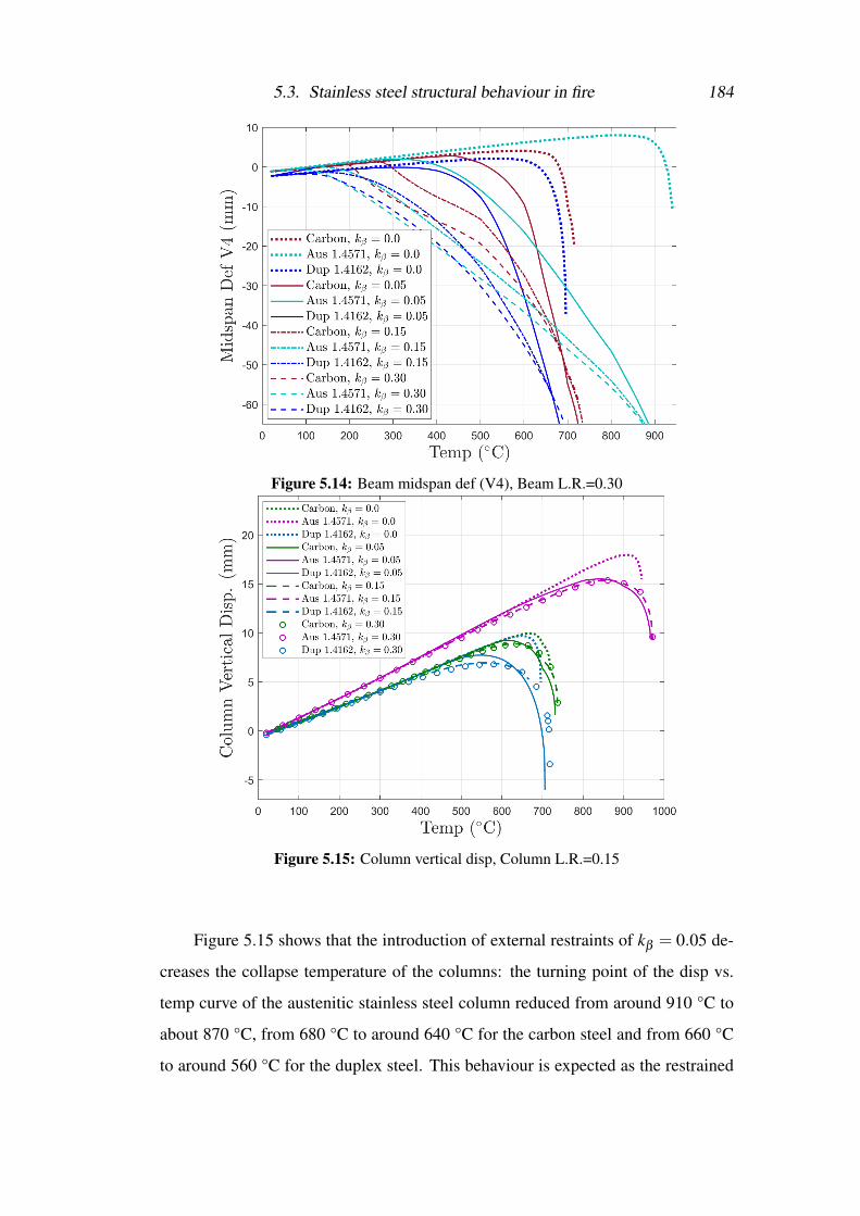
5.3. Stainless steel structural behaviour in fire 184
Figure 5.14: Beam midspan def (V4), Beam L.R.=0.30
Figure 5.15: Column vertical disp, Column L.R.=0.15
Figure 5.15 shows that the introduction of external restraints of kβ = 0.05 de-
creases the collapse temperature of the columns: the turning point of the disp vs.
temp curve of the austenitic stainless steel column reduced from around 910 °C to
about 870 °C, from 680 °C to around 640 °C for the carbon steel and from 660 °C
to around 560 °C for the duplex steel. This behaviour is expected as the restrained

5.3. Stainless steel structural behaviour in fire 185
thermal expansion increases the load on the columns. The inclusion of external re-
straints also induces gradual development of V4 into the large displacement regime,
in contrast to the abrupt run-away point observed in the unrestrained beams. Due to
the external restraints, instead of running away, the beam goes into catenary action
in the large displacement regime.
The increase of restraint stiffness level has little impact on the turning point
of the column vertical disp vs. temp curve. The same behaviour is seen in the
results of beam midspan deflection (V4), presented in Figure 5.14, as the beams of
the same material with varying levels of restraint stiffness entered large deflection
regime at similar temperatures. The three restrained austenitic steel beams reached
a large deflection of 70 mm (L/18) at around 900 °C; the restrained carbon steel
beams reached 60 mm (L/21) at about 720 °C and the restrained duplex steel beams
reached 60 mm (L/21) at about 680 °C.
Figure 5.16: Beam axial force vs. temp., Beam L.R.=0.30
Figure 5.16 compares the axial force in the frame beam without/with varying
degrees of axial restraints. The higher axial restraint stiffness is the higher the max-
imum compressive force will be. With the same degree of axial restraint stiffness,
the compression resulted from the restrained thermal expansion increased at the

5.3. Stainless steel structural behaviour in fire 186
fastest rate for the Austenitic 1.4571 beam due to its highest thermal elongation.
The maxima of the axial force vs. temp curve occurs when the beam cross-
section reaches its axial capacity. At the stiffness level of 0.15Kβ and 0.30Kβ ,
the carbon steel beam showed significantly higher maximum compression than the
other two stainless steel beams, because the carbon steel beam possesses higher
bending capacity in the lower temperature range. When compared with the stainless
steels, carbon steel exhibits superior stiffness retention capability at temperatures
lower than 200 °C, as seen in Figure 2.1.
The catenary action in the restrained beams starts as the axial force changes
from negative to positive. This occurs at around 920 °C for the austenitic beams,
about 720 °C for the carbon steel beams, and around 690 °C for the duplex beams.
These values generally correspond to the temperature levels at which large deflec-
tion was observed in the beams as identified previously based on the V4 results
plotted in Figure 5.14.
The displacement and axial force results suggest that the structural fire perfor-
mance of the frames was dominated by the column behaviour. The catenary action
in the frame beam occurred when the large deflection was induced because of ther-
mal expansion against the restraints.
Figure 5.17 presents the midspan deflection (V4) of the beams under the
L.R.=0.6 without/with varying degrees of external restraints. The corresponding
vertical displacements of the columns under the L.R.=0.3 are plotted in Figure 5.18.
Similar results to the Figure 5.14 and Figure 5.15 were observed.
As the Kβ increased from 0.0 to 0.05, the collapse temperature for the re-
strained columns reduced from 780 °C to around 650 °C for the austenitic, from
620 °C to 520°C for the carbon steel, and from 390 °C to about 350 °C for the
duplex stainless steel. The larger reduction in the collapse temperatures observed
for the stainless steel columns are caused by the significant reduction in the tangent
modulus at higher L.R.s.

5.3. Stainless steel structural behaviour in fire 187
Figure 5.17: Beam midspan def vs. temp,Beam L.R.=0.60
Figure 5.18: Column vertical disp vs. temp,Column L.R.=0.30
Figure 5.19 presents the stress-strain developments at the beam-column joint
during the fire , in the cross-section of the beam and the column respectively. An
negative bending moment —bottom flange in compression while top flange in ten-
sion is observed in the beginning of the fire due to the P− δ effect of the initial
beam deflection. During heating, compressive stresses developed across the entire

5.3. Stainless steel structural behaviour in fire 188
cross-section, manifested as the tensile stress at the top shifted to the compressive
side and the compressive stress at the bottom increased until the occurrence of the
collapse. Higher peak stresses were observed for the case of 0.15Kβ restraint when
compared to the 0.05Kβ restraint case.
Figure 5.19 show that the strain reversals were clearly experienced at the beam-
column joint, in both beams and columns. This occurrence demonstrated that the
strain reversals would occur with the presence of axial restraints within the structure.
(a) Stress strain in the column, 0.05Kβ (b) Stress strain in the column, 0.15Kβ
(c) Stress strain in the beam, 0.05Kβ (d) Stress strain in the beam, 0.15Kβ
Figure 5.19: Stress strain developments at beam-column joint
The comparison study showed that for structural fire performance, the inclu-
sion of external restraints is detrimental to the columns because it accelerates the
initiation of the column collapse; meanwhile beneficial to the beams since it en-
ables the catenary action. The stress redistributions due to the catenary action sub-
sequently result in strain reversals in the structure. Increasing the stiffness level
of restraints showed little impact on the column collapse temperature, however it
induced higher stresses in the frame.

5.4. Conclusions 189
5.4 Conclusions
In this chapter, the new material model from Chapter 3 has been implemented in
OpenSEES as uniaxial material models for the Austenitic 1.4571 and Duplex 1.4612
stainless steel in order to study their structural behaviour in fire.
The comparison study of temperature development between carbon steel and
stainless steel I-sections subjected to four sides heating using the Standard Fire
Curve [26], demonstrated a slower temperature rise for the stainless steel sections.
For thin-walled structures, lower emissivity is the main beneficial factor that stain-
less steel offers. The comparison study results showed that sections with a smaller
section factor (A/V ) benefit more from using stainless steels in terms of achieving
a slower temperature development.
The comparison study of simply supported beams suggest that the Austenitic
1.4571 stainless steel can generally postpone the onset of run-away mechanism in
the beam to a temperature more than 200 °C higher than that of the carbon steel.
At higher L.R.s (L.R.>0.75), the deflection rate of austenitic stainless steel beams
are significantly faster than that of carbon steel beams due to the reduction in its
tangent modulus, which can quickly reduce to about 50% of the material’s initial
value when stress approaches 50% of its strength capacity.
Similarly, the Duplex 1.4612 stainless steel showed the capability of delaying
the run-away mechanism of the simply supported beams during the heating at lower
L.R.. The Duplex 1.4612 steel experiences substantial reduction in the tangent mod-
ulus when L.R. exceeds 0.37, which accelerates the onset of run-away mechanism.
The comparison of EHR3 frames have shown that the Austenitic 1.4571 steel
offers a clear advantage in delaying the occurrence of frame collapse, and the de-
gree of advantage diminishes as the L.R. increases. The Duplex 1.4612 steel only
showed benefits of postponing the collapse of the EHR3 frame in the Series 1 study
where the L.R. is 0.15 in the beam and 0.075 in the column. The advantage offered
by the Duplex 1.4612 steel is believed probably uneconomic because of the low
level of L.R.s that has to be maintained.
The comparison study results show that the introduction of axial restraints at

5.4. Conclusions 190
the beam-column joint of the EHR3 frame causes earlier column collapse, where the
stainless steels suffer greater reduction in the collapse temperature when compared
to the carbon steel.
The study showed that evident strain reversals were experienced in the frame
beam and column when external restraints were included. The catenary action is
beneficial for structural fire performance of frames. However the strain reversals
experienced during the catenary action can cause reduction in the material tensile
strength due to the Bauschinger effect. Future investigation of the Bauschinger
effect on the structural behaviour of steel structures in fire using the new material
model is of great research interest.

Chapter 6
Bauschinger Effect in Steel Beams
Subjected to Realistic Building Fire
6.1 Introduction
One prominent feature of modern architectural design is its pursuit of large open-
plan space where sufficient ventilation inevitably turns fire growth into a fuel-
controlled regime. Consequently, the likelihood of an early flash-over phenomenon
of a ventilation-controlled fire that is commonly observed in traditional building
fires, has been substantially reduced. It has been observed in real life fire events,
for instance in the World Trade Centre Towers [201] and in the Windsor Tower in
Madrid [202], that fires in large compartments/open spaces, burn locally and have
the tendency to move across the entire floor over a period of time. The concept of a
travelling fire model [10–12,58,203] has been introduced to describe the movement
and spreading behaviour of fires observed in large and/or complex spaces, where
traditional concepts of compartment fire behaviour becomes inappropriate. The
“travelling nature” of fire has been of growing research interest to fire scientists
and engineers. Recently in 2017, a joint research project TRAFIR (characterisation
of travelling fires in large compartments), in collaboration with ArcelorMittal Bel-
val & Differdange, Liege University, the University of Edinburgh, RISE Research
Institute of Sweden and the University of Ulster, has set out to investigate what
are the conditions that cause the development of a travelling fire. The TRAFIR

6.1. Introduction 192
project focuses on studying the influence of compartment geometry and the inter-
action with representative fuel loads through fire tests and CFD simulation using
the FDS software. While, the research has focused on better understanding fire
demand estimation, the mechanical response of composite steel structures under
travelling fire scenarios has been little explored [13]. Using FEA, Rackauskaite et
al. [204] investigated the structural response a 2D steel frame subjected to multiple
floor horizontal and vertical travelling fire load computed using the Stern-Gottfried
& Rein’s travelling fire model [10, 11], where significantly different structural be-
haviour compared to a single compartment fire was observed.
Various travelling fire models [10–12, 58,203] have been proposed to describe
the moving behaviour of a fire commonly observed in a large open compartment
space, where the Standard Fire Curve [9] is no longer applicable. In this chapter,
the recently proposed travelling fire model — extended travelling fire methodology
(ETFM) framework [12] was adopted to obtain the structural thermal loading. The
ETFM enables temperature development in a realistic large and/or complex com-
partment space, capturing both spatial and temporal changes of the thermal field,
based on energy and mass conservation with smoke accumulation. With the ETFM
framework implemented in the SIFBuilder [205] of OpenSEES software [24], the
OpenSEES framework provides the facility to perform a streamlined heat transfer
and thermo-mechanical analysis for large structures in one software environment.
In this chapter, a case study was carried out to investigate the structural fire per-
formance of a single steel beam (UB 305x127x42) located in an idealised structural
layout, shown in Figure 6.1a, representing a 630 m2 floor area of a generic modern
office building with a central core structure of 162 m2. The structural behaviour of
the beam subjected to complex travelling fire loadings was investigated using the
new material model developed by Zhou et al. [192], also presented in Chapter 3.
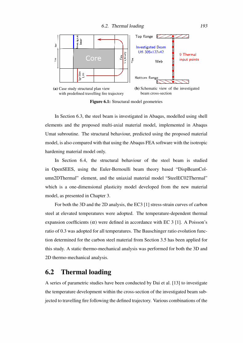
6.2. Thermal loading 193
(a) Case study structural plan viewwith predefined travelling fire trajectory
(b) Schematic view of the investigatedbeam cross-section
Figure 6.1: Structural model geometries
In Section 6.3, the steel beam is investigated in Abaqus, modelled using shell
elements and the proposed multi-axial material model, implemented in Abaqus
Umat subroutine. The structural behaviour, predicted using the proposed material
model, is also compared with that using the Abaqus FEA software with the isotropic
hardening material model only.
In Section 6.4, the structural behaviour of the steel beam is studied
in OpenSEES, using the Euler-Bernoulli beam theory based “DispBeamCol-
umn2DThermal” element, and the uniaxial material model “SteelEC02Thermal”
which is a one-dimensional plasticity model developed from the new material
model, as presented in Chapter 3.
For both the 3D and the 2D analysis, the EC3 [1] stress-strain curves of carbon
steel at elevated temperatures were adopted. The temperature-dependent thermal
expansion coefficients (α) were defined in accordance with EC 3 [1]. A Poisson’s
ratio of 0.3 was adopted for all temperatures. The Bauschinger ratio evolution func-
tion determined for the carbon steel material from Section 3.5 has been applied for
this study. A static thermo-mechanical analysis was performed for both the 3D and
2D thermo-mechanical analysis.
6.2 Thermal loadingA series of parametric studies have been conducted by Dai et al. [13] to investigate
the temperature development within the cross-section of the investigated beam sub-
jected to travelling fire following the defined trajectory. Various combinations of the
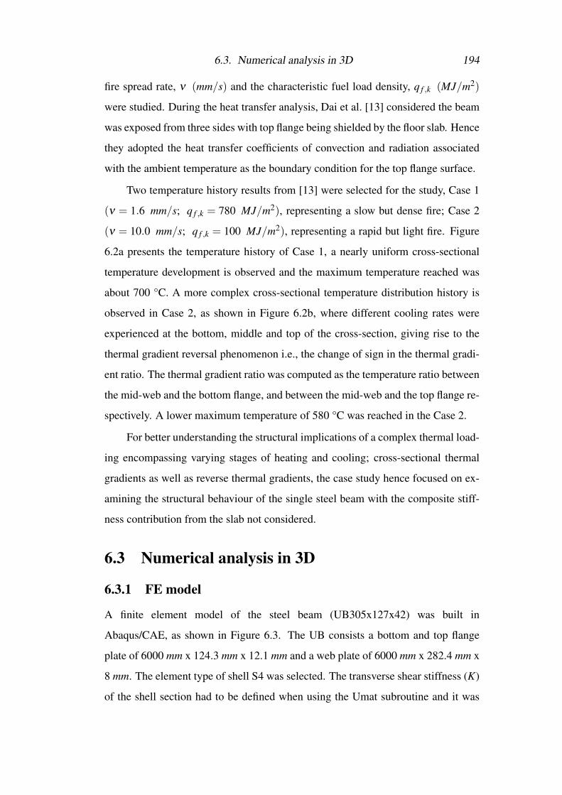
6.3. Numerical analysis in 3D 194
fire spread rate, ν (mm/s) and the characteristic fuel load density, q f ,k (MJ/m2)
were studied. During the heat transfer analysis, Dai et al. [13] considered the beam
was exposed from three sides with top flange being shielded by the floor slab. Hence
they adopted the heat transfer coefficients of convection and radiation associated
with the ambient temperature as the boundary condition for the top flange surface.
Two temperature history results from [13] were selected for the study, Case 1
(ν = 1.6 mm/s; q f ,k = 780 MJ/m2), representing a slow but dense fire; Case 2
(ν = 10.0 mm/s; q f ,k = 100 MJ/m2), representing a rapid but light fire. Figure
6.2a presents the temperature history of Case 1, a nearly uniform cross-sectional
temperature development is observed and the maximum temperature reached was
about 700 °C. A more complex cross-sectional temperature distribution history is
observed in Case 2, as shown in Figure 6.2b, where different cooling rates were
experienced at the bottom, middle and top of the cross-section, giving rise to the
thermal gradient reversal phenomenon i.e., the change of sign in the thermal gradi-
ent ratio. The thermal gradient ratio was computed as the temperature ratio between
the mid-web and the bottom flange, and between the mid-web and the top flange re-
spectively. A lower maximum temperature of 580 °C was reached in the Case 2.
For better understanding the structural implications of a complex thermal load-
ing encompassing varying stages of heating and cooling; cross-sectional thermal
gradients as well as reverse thermal gradients, the case study hence focused on ex-
amining the structural behaviour of the single steel beam with the composite stiff-
ness contribution from the slab not considered.
6.3 Numerical analysis in 3D
6.3.1 FE model
A finite element model of the steel beam (UB305x127x42) was built in
Abaqus/CAE, as shown in Figure 6.3. The UB consists a bottom and top flange
plate of 6000 mm x 124.3 mm x 12.1 mm and a web plate of 6000 mm x 282.4 mm x
8 mm. The element type of shell S4 was selected. The transverse shear stiffness (K)
of the shell section had to be defined when using the Umat subroutine and it was

6.3. Numerical analysis in 3D 195
(a) Case 1
(b) Case 2
Figure 6.2: Temperature history
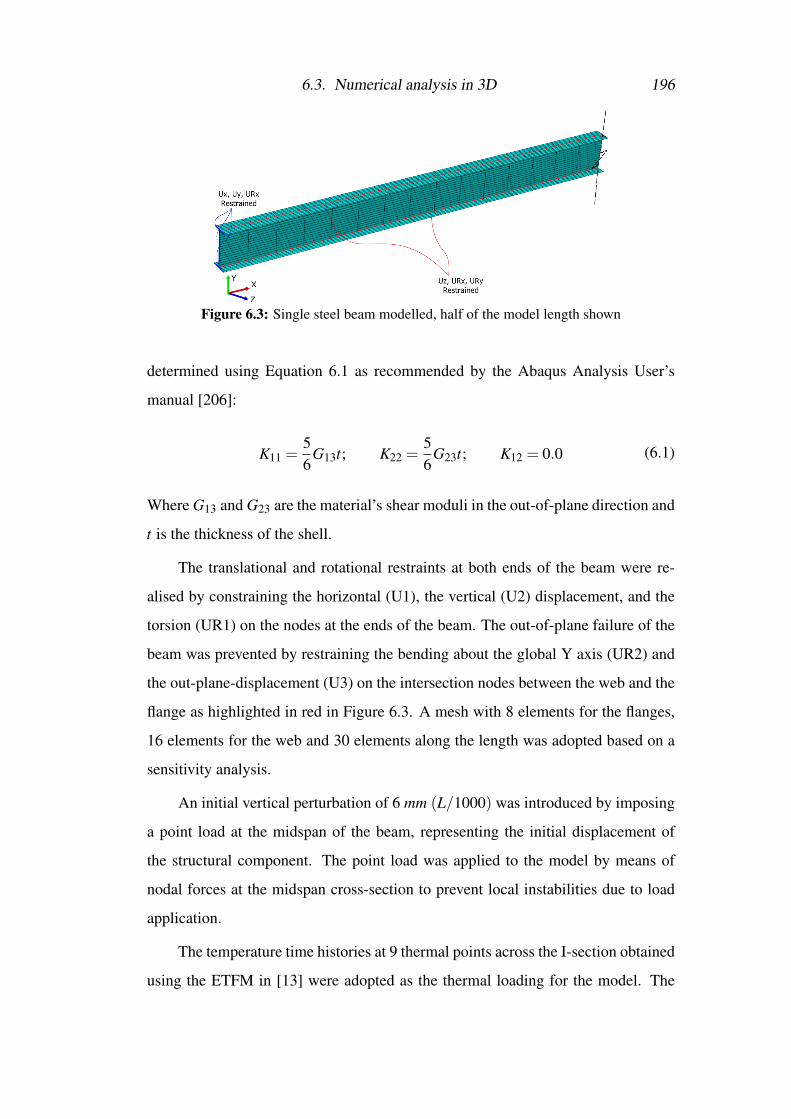
6.3. Numerical analysis in 3D 196
Figure 6.3: Single steel beam modelled, half of the model length shown
determined using Equation 6.1 as recommended by the Abaqus Analysis User’s
manual [206]:
K11 =56
G13t; K22 =56
G23t; K12 = 0.0 (6.1)
Where G13 and G23 are the material’s shear moduli in the out-of-plane direction and
t is the thickness of the shell.
The translational and rotational restraints at both ends of the beam were re-
alised by constraining the horizontal (U1), the vertical (U2) displacement, and the
torsion (UR1) on the nodes at the ends of the beam. The out-of-plane failure of the
beam was prevented by restraining the bending about the global Y axis (UR2) and
the out-plane-displacement (U3) on the intersection nodes between the web and the
flange as highlighted in red in Figure 6.3. A mesh with 8 elements for the flanges,
16 elements for the web and 30 elements along the length was adopted based on a
sensitivity analysis.
An initial vertical perturbation of 6 mm (L/1000) was introduced by imposing
a point load at the midspan of the beam, representing the initial displacement of
the structural component. The point load was applied to the model by means of
nodal forces at the midspan cross-section to prevent local instabilities due to load
application.
The temperature time histories at 9 thermal points across the I-section obtained
using the ETFM in [13] were adopted as the thermal loading for the model. The

6.3. Numerical analysis in 3D 197
thermal loading of each point was applied to its corresponding area of the cross-
section, as depicted as the hatched area in Figure 6.1b.
6.3.2 Stress/Deformation analysis ––Case 1
The evolution of the deflection and the accumulated plastic strain at the midspan
cross-section during the fire are presented in Figure 6.4a. The deflection started to
increase at around 100 °C, corresponding to the initiation temperature of the elastic
modulus degradation. The slight kink observed at around 250 °C was believed to
be caused by the small thermal gradient experienced in the temperature history. At
around 550 °C a distinctive change in the curvature of the temperature deflection
curve was observed, indicating large deflection mode has occurred. The beam has
become too weak to support the load as a result of material degradation. During the
cooling stage, the midspan deflection experienced a recovery as the steel material
regained its stiffness. The development of accumulated plastic strain (ε p) correlated
to that of the deflection during the heating stage. While under cooling, the ε p still
experienced growth due to the continuous stress development.
The development of the axial stress (S11) at midspan during the fire is plotted
in Figure 6.4b. At the start of the fire, the section is in sagging bending moment
—the bottom cross-section in positive S11 while the top in negative S11. As tem-
perature rises, compressive stresses started to develop due to restrained thermal ex-
pansion, manifested as the growth of compressive S11 until the whole cross-section
(bottom, mid and top) descended into compression at around 90 °C. Thereafter, due
to the increasing midspan deflection as observed in Figure 6.4a, thermal expansion
induced compression started to exert bending in the beam hence the S11 at the bot-
tom of the cross-section started shifting to tension. This is the P-delta effect of the
axial force. Furthermore, the difference of S11 between the top and the bottom
started to increase, indicating an increasing bending moment.
The plastic state was first observed at the top half of the cross-section at around
120 °C, when the mid and top S11 plateaued at its yield strength value. At around
300 °C, the entire midspan cross-section has reached the plastic state, indicating the
formation of a plastic hinge. Under heating, the tensile and compressive stresses
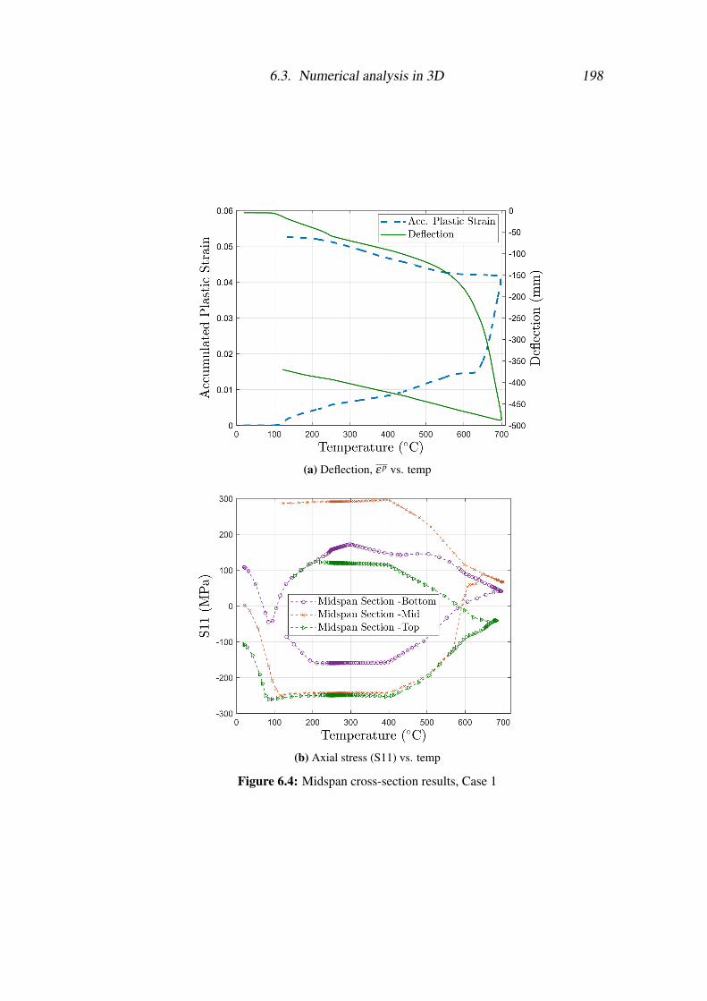
6.3. Numerical analysis in 3D 198
(a) Deflection, ε p vs. temp
(b) Axial stress (S11) vs. temp
Figure 6.4: Midspan cross-section results, Case 1
6.3. Numerical analysis in 3D 199
started to decrease at 400 °C due to the reduction in the yield strength of the steel
material. During cooling, the bending moment at the midspan cross reversed from
sagging to hogging —negative S11 at the bottom while positive at the top.
The modelled structure behaved as expected under the Case 1 thermal loading.
The analysis results showed that the plastic deformation due to heating and cooling
has been successfully captured.
6.3.3 Stress/Deformation analysis ––Case 2
Figure 6.5a presents the evolution of the deflection and the accumulated plastic
strain (ε p) at the midspan cross-section throughout the fire. The deflection also
started to increase at around 100 °C. The growth of deflection developed at a faster
rate when compared to the Case 1 as a result of the thermal bowing —the hotter
surface expands more than the cooler surface inducing the bending in the structure,
caused by the cross-sectional thermal gradient. At around 550 °C the curvature of
the temperature deflection curve started to increase significantly indicating substan-
tial stiffness reduction in the beam due to the material degradation. The midspan
deflection showed a recovery as the steel material regained its stiffness during cool-
ing. The ε p grew throughout the heating and cooling as a result of continuous stress
development.
The axial stress (S11) vs. temperature curves at midspan cross-section during
the fire are plotted in the Figure 6.5b. Similar S11 developments to the Case 1 have
been observed for the Case 2. The main difference is the entire midspan cross-
section remained in tension at the end of fire. It is interesting to note that the bottom
S11 did not show yielding until later during the cooling. This suggests that the
midspan cross-section did not reach the plastic state until much later at the cooling
stage, in contrast to what observed for the Case 1 where it became plastic at as early
as 300 °C.
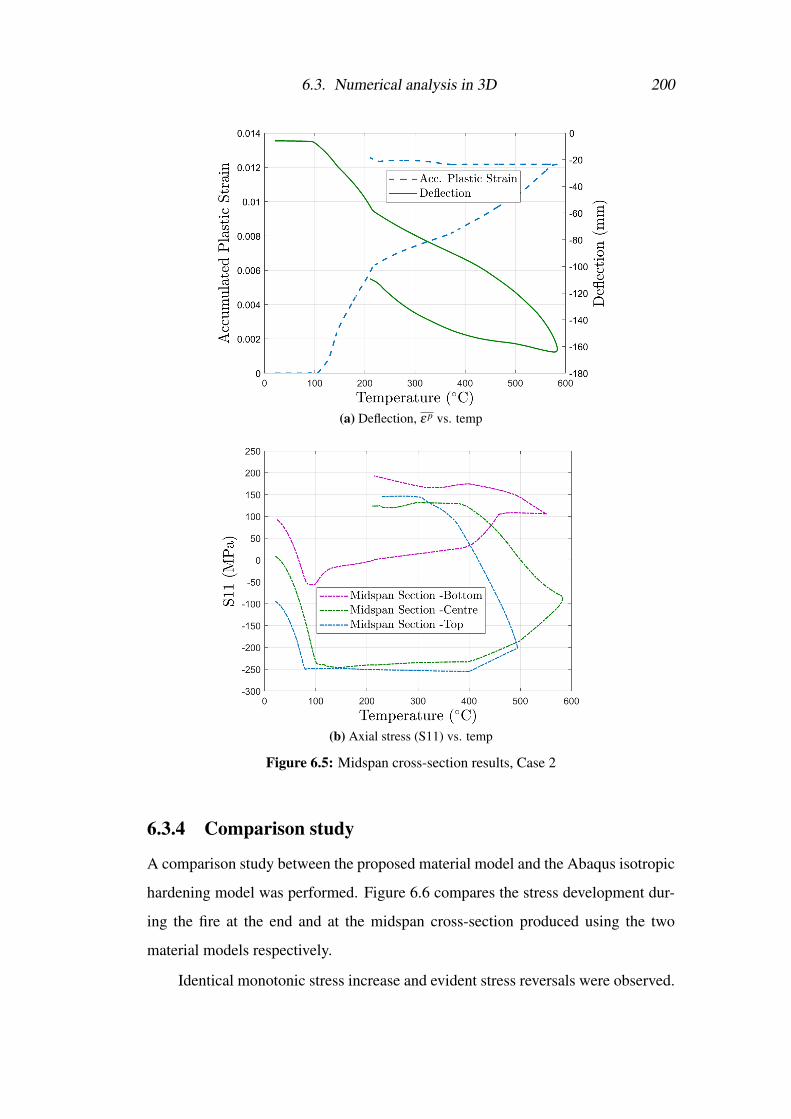
6.3. Numerical analysis in 3D 200
(a) Deflection, ε p vs. temp
(b) Axial stress (S11) vs. temp
Figure 6.5: Midspan cross-section results, Case 2
6.3.4 Comparison study
A comparison study between the proposed material model and the Abaqus isotropic
hardening model was performed. Figure 6.6 compares the stress development dur-
ing the fire at the end and at the midspan cross-section produced using the two
material models respectively.
Identical monotonic stress increase and evident stress reversals were observed.

6.3. Numerical analysis in 3D 201
(a) Endspan S11 vs. Temp
(b) Midspan S11 vs. Temp
Figure 6.6: Proposed material model vs. Isotropic hardening model

6.4. Numerical analysis in 2D 202
The key difference was the yielding during the reversal, where a lower yield stress
was observed in the results of the proposed material model. Thus the reduction in
the tensile strength due to the Bauschinger effect has been successfully captured
by the new model. Therefore, in cases where strain reversals exist, more accurate
evaluation of structural fire capacity can be achieved by adopting the new material
model proposed in Chapter 3.
6.4 Numerical analysis in 2DThe FE model of the investigated beam was also analysed in OpenSEES using the
2D BeamColumnElement. The composite stiffness contribution from the slab was
not included in this model. The beam was translationally and rotationally restrained
at both ends. The I-section was modelled using the fibre element [207], where the
cross-section was subdivided into fibres. The study model adopted 8 fibres along
the web, and 8 fibres along the flange. A mesh of 30 elements along the length was
adopted after performing a sensitivity study. The thermal loading was applied at
9 thermal points along the I-section, seen as in Figure 6.1b. Linear interpolation
was used to compute the thermal loading on the section fibres that are between the
application points.
Similarly to the 3D model, an initial vertical perturbation of 6 mm (L/1000)
was introduced by imposing a point load at the midspan, representing the initial
displacement of the structural component.
6.4.1 Stress deformation analysis
The evolution of the midspan deflection during the Case 1 and Case 2 fire are pre-
sented in Figure 6.7, and compared with that of the 3D analysis results. For the Case
1, similar deflection development to that of the 3D analysis was observed in the 2D
results until the deflection reached around 180 mm (L/33). Thereafter, the deflection
developed at a slower rate in the 2D model and reached a significant lower maxi-
mum deflection when compared to the 3D model. This is believed to be due to the
fact that the 2D beam model is stiffer because of the adoption of 2D Euler-Bernoulli
BeamColumn element, which disregards the shear deformation. When the beam en-

6.4. Numerical analysis in 2D 203
ters the large deflection regime, the shear deformation becomes significant in the 3D
shell model.
Figure 6.7: Midspan deflection, 2D compared with 3D
Because of the lower maximum temperature in the Case 2, lower maximum
midspan deflections were observed in comparison to that of the Case 1. The maxi-
mum midspan deflection obtained is 164.1 mm (L/36) for the 3D model and 148.8
mm (L/40) for the 2D model, both are lower than the L/33 observed in the Case 1.
This suggested that the deflections in the Case 2 fire did not develop into the large
deflection regime. Therefore the deflection vs. temperature curve predicted by the
2D model is very similar to that by the 3D shell model in this case. The 2D analysis
results show an overall lower deflection because of the stiffer Euler-Bernoulli beam
element adopted.
Significant shear deflections could be expected in deep carbon steel members
under temperatures higher than 550 °C as the stiffness decreases very rapidly be-
yond this value (from about 40% at 550 °C to about 10% at 700 °C). Since the
maximum temperature experienced in the Case 2 was about 580 °C, the shear de-
flection was still insignificant hence the 2D model could produce similar results to
the 3D model. In contrast, the higher maximum temperature of 700 °C in the Case
1 led to notable shear deflection in the beam which was been able to be captured by
the 3D shell model but not the 2D Euler-Bernoulli beam model, as seen in Figure

6.4. Numerical analysis in 2D 204
(a) Case 1
(b) Case 2
Figure 6.8: Midspan S11 vs. Temperature, 2D
6.7.
The 2D analysis results of the axial stress (S11) vs. temperature curves at
midspan cross-section during the fire of Case 1 and Case 2 are plotted in Figure
6.8. Similar results to the 3D model have been observed. At the end of Case 1
fire, the bending moment at the midspan cross reversed from sagging to hogging
—negative S11 at bottom while positive at top. While the midspan cross-section
ended in tension for the Case 2 fire.
6.5. Summary 205
The deflection and stress results showed that the steel beam modelled using
2D BeamColumn element in OpenSEES behaved as expected under the thermal
loading, the plastic deformation due to heating and cooling has been successfully
captured using the new material model.
6.5 SummaryIn this chapter, the new material model proposed in Chapter 3 was utilised to inves-
tigate the structural behaviour of a single steel beam subjected to travelling fires.
The proposed material model in multi-axial state was used to study the steel beam
modelled using shell elements in Abaqus, while the proposed material model in uni-
axial state was used for the 2D beam analysis conducted in OpenSEES. Reasonable
and comparable results of deformation and stress have been observed for the 3D
and 2D analysis.
The comparsion study between the proposed material model and the isotropic
hardening model from Abqus demonstrated that the reduction in the structural ca-
pacity due to the Bauschinger effect has been successfully captured by the new
model.
Therefore it is believed that the proposed material model has been successfully
implemented in the Abaqus Umat subroutine and in the OpenSEES uniaxial mate-
rial model and was able to analyse the structural behaviour of steel structures under
complex realistic building fires.

Chapter 7
Conclusions and Future Work
7.1 Summary and conclusionsA new rate-independent combined isotropic-kinematic hardening material model
was developed for the thermo-mechanical analysis of steel materials in fire. In
order to demonstrate the different aspects of its capability under various loading
conditions, five validations, as presented in Chapter 3, have been carried out:
1. Validation of the evolution of isotropic and kinematic hardening variables
during monotonic loading at elevated temperatures.
2. Validation of the Bauschinger effect and the transient hardening under isother-
mal loading conditions at elevated temperatures.
3. Validation of the thermal unloading algorithm.
4. Validation for multi-axial loading conditions at elevated temperatures.
5. Validation of the Bauschinger effect and the transient hardening under tran-
sient loading conditions during both heating and cooling.
The validations demonstrated that the new material model is capable of: han-
dling strain reversals, capturing the Bauschinger effect and transient hardening be-
haviour and modelling material non-linearity at elevated temperatures. As such,
the three objectives that were identified in the Introduction (Chapter 1) have been
successfully accomplished by the proposed material model.
7.1. Summary and conclusions 207
The goal of the proposed material model was to improve the FEA tools for
performance-based structural fire design. More accurate determination of structural
fire resistance can be achieved by adopting the new material model, with the reduc-
tion in the material strength due to strain reversals being properly calculated. In this
research, the new material model proposed in Chapter 3 was applied in three differ-
ent studies, each has provided valuable engineering insights into the behaviour of
steel structural systems subjected to fire. Additionally, the model’s capability of de-
scribing steel material behaviour for thermo-mechanical analysis, its applicability in
structural fire analysis and its integrability into the performance-based engineering
framework have been demonstrated through the studies.
7.1.1 Application to remaining structural fire resistance
The application of the new material model in a multi-hazard analysis, fire following
earthquake, was showcased in Chapter 4. Rather than investigating the structural
behaviour in a fire immediately following a severe earthquake, which is a loading
scenario commonly considered to be of low likelihood, Chapter 4 focused on the
reduction in the fire resistance of steel structures resulting from undetected PFP
damage, which is a serious fire safety concern that has been largely neglected. Be-
ing specifically designed to be lightweight, cementitious PFP is prone to damage
under deformation even caused by moderate earthquakes. Higher likelihood of this
fire safety concern is expected for the cementitious PFP that experienced multiple
small/moderate earthquakes during its service.
Chapter 4 implemented the new material model in a novel multi-hazard frame-
work for evaluating the remaining fire resistance of steel structures protected by
cementitious PFP, subjected to moderate earthquakes. A case study carried out us-
ing the proposed framework found that post-earthquake PFP damage could result
in significant reductions in the structural fire resistance, which, in the worst case
scenario, may lead to structural collapse due to column failure, reducing the fire
resistance from the designed 2 hrs to about 36 mins.
The proposed multi-hazard framework is implemented in the OpenSEES envi-
ronment, and offers structural engineers a practical solution to access the fire safety

7.1. Summary and conclusions 208
concern associated with the PFP damage. A step-by-step procedure of using the
multi-hazard framework is provided at the end of Chapter 4.
7.1.2 Application for novel construction materials
A comprehensive understanding of the fire performance of structures using novel
construction materials can be obtained economically and efficiently by utilising the
computational based engineering framework. However, the accuracy of FEA-based
study is strongly depended on the material model adopted. With its sophistication
demonstrated in Chapter 3, Chapter 5 used the new material model to investigate
the structural fire behaviour of stainless steel structures. The stainless steel grade
Austenitic 1.4571 and Duplex 1.4612 were studied in comparison to the carbon steel
S235.
The investigation of simply supported beams showed that the Austenitic 1.4571
stainless steel can generally postpone the onset of the run-away mechanism in the
beam to a temperature more than 200 °C higher than that of the carbon steel. The
Duplex 1.4612 stainless steel only showed limited advantage over the carbon steel
in terms of delaying the run-away when its L.R. is low (<0.37). The investigation
of EHR3 frames showed that the Austenitic 1.4571 steel offers a clear advantage
in delaying the occurrence of frame collapse, although the degree of advantage di-
minishes as the L.R. increases. The Duplex 1.4612 steel only showed benefits of
postponing the frame collapse in the case where the frame beam L.R. =0.15 and
the frame column L.R. =0.075. The high thermal expansion of stainless steels ac-
celerates the displacement development of the structural components when external
restrains are applied.
The investigations carried out in Chapter 5 showed that Austenitic 1.4571
stainless steel in general offers superior structural fire performance when compared
to the carbon steel, while the advantage offered by the Duplex 1.4612 steel is be-
lieved overall uneconomic because of the low L.R.s that have to be maintained.
Additionally, the comparison study of temperature development within I-sections
subjected to four sides heating using the Standard Fire Curve [26] showed a slower
temperature development for the stainless steel sections when compared to the car-

7.2. Limitations and future work 209
bon steel ones, and the sections of a smaller section factor (A/V) benefited more
from using stainless steels in terms of achieving a slower temperature development.
7.1.3 Application for advanced structural design
One motivation to develop a sophisticated plastic model for thermo-mechanical
analysis of steels was the desire to accurately analyse the steel structures subjected
to complex realistic building fires, simulated using the newly developed extended
travelling fire framework model. This enables the analysis of structural fire resis-
tance of modern architectural designs where travelling fire behaviour is expected to
occur.
The proposed material model was applied in Chapter 6 to study the structural
behaviour of a single carbon steel beam (UB 305x127x42) subjected to two different
travelling fire scenarios. One is a slow, but dense fire, and the other is a rapid, but
light fire. The structural fire behaviour of the beam was successfully captured by a
3D and a 2D model. The 3D analysis used the new material model in multi-axial
state while the 2D analysis used the the uniaxial model. Reasonable and comparable
structural behaviour were observed in the two analyses. An evident reduction in the
strength capacity using the new material model was observed when compared to the
results obtained using the isotropic hardening model of Abaqus.
7.2 Limitations and future workThe new material model adopted the von Mises yield criterion, which has been
shown, in the literature, able to provide satisfactory results for steel materials at
elevated temperatures. However, the distortion of the yield surface due to plastic
deformation could not be captured by the von Mises yield function. The yield func-
tion proposed by Barlat et al. [208] has become a popular approach to model the
distortion of yield surface shape due to anisotropic plastic hardening. Adopting this
yield function in the proposed material model will improve its accuracy and greatly
expand its applicability for thermo-mechanical analysis of other metals, e.g., alu-
minium.
The effect of the varying hardening and evolution function parameters on the
7.2. Limitations and future work 210
stability of the proposed model was not investigated in this work due to limited
available testing data. A sensitivity study dedicated to this subject in the future can
better demonstrate the applicability of the new material model to a wide range of
steel materials.
It has been observed that catenary action is beneficial for the structural fire
performance of frames. However, the strain reversals experienced during catenary
action can cause reduction in the material tensile strength due to the Bauschinger
effect and was not investigated in this research. Future investigation into the impact
of the Bauschinger effect on the catenary action of steel beam structures in fire
using the new material model can help to achieve a more accurate method for taking
advantages of the catenary action in structural fire design.

Appendix A
Numerical Algorithm for Combined
Isotropic and Kinematic Hardening
Model
The numerical algorithm of the proposed combined isotropic and kinematic hard-
ening model for thermo-mechanical analysis of structures in fire described in the
preceding section is summarised in the Table below. The proposed model is imple-
mented into the commercial finite element code Abaqus/Standard, using the user
subroutine ––Umat [23].
Table A.1: Numerical algorithm for the proposed combined isotropic- kinematic hardeningmodel
Last Converged Step n
If Temperature change ∆T 6= 0, Go to Thermal Step, Else Go to Mechanical Step
Thermal Step, Current Temperature Tn+1Tn+1Tn+1
1. Update Temperature-dependent parameters
Young’s modulus ET n+1, Initial yield stress σp,T n+1
Hardening function parameters vT n+1 and δT n+1
Bauschinger ratio evolution equation parameters aT n+1, bT n+1 and cT n+1
Material model parameter V hT n+1
2. Update Bauschinger ratio

212
ϑT n+1 = aT n+1 ∗ exp(−bT n+1 ∗ ε pn)+ cT n+1
3. Update the size of bounding surface
Y =√
23Y1D,T n+1(ε
pn )
4. Update the position of the yield surface centre, β1β1β1 term
β1β1β1n = (1.0−ϑT n+1)Y εpnεpnεpn‖ε p
nεpnεpn ‖
Mechanical Step, Strain Increment ∆εεε
1.1.1. Elastic predictor
σσσ trialn+1 =CCCn+1 · (εεεn +∆εεε−ε pε p
ε pn), β1β1β1
trialn+1 = β1β1β1n, β2β2β2
trialn+1 = β2β2β2n
ssstrialn+1 = IdevIdevIdev : σσσ trial
n+1 , IdevIdevIdev = III− 13111⊗111
ηηη trialn+1 = ssstrial
n+1−β1β1β1trialn+1−β2β2β2
trialn+1 , Nn+1Nn+1Nn+1 =
η trialn+1η trialn+1η trialn+1
‖η trialn+1η trialn+1η trialn+1 ‖
ϑn+1 = an+1 ∗ exp(−bn+1 ∗ ε pn)+ cn+1
νn+1 = 1.0− exp(−bn+1 ∗ εpl n)
Reverse loading index :ltrialn+1 = ln
βltrialn+1 = βln
• Check the reverse loading criterion according to Equation 3.21
If cos(θ)< 0.0 then
ltrialn+1 = ln +1
εpl
trialn+1 = 0.0
βltrialn+1 =V hT n+1
√32(β1β1β1n +β2β2β2n) : (β1β1β1n +β2β2β2n)
β2β2β2trialn+1 = 0.0
Else, Do nothing
• Check the yield condition
If f (η trialn+1η trialn+1η trialn+1 )−ϑn+1Y1D,n+1(ε p)< Tolerance, then Set (•)n+1 = (•)Trial Exit
Else Go to Plastic corrector
2.2.2. Plastic corrector
• Newton-Raphson iteration is employed to determine plastic multiplier
∆γ . Initialise ∆γ = 0.0
Iterate until |g(∆γ)|< Tolerance
g(∆γ) = ‖ηηη trialn+1 ‖−2∗µn+1 ∗∆γ−ϑn+1
√23 ∗Y1D,n+1(ε
pn +
√23∆γ)
dg(∆γ) =−2∗µn+1− 23 ∗ [Y
′1D,(n+1)(ε
pn +
√23∆γ)]∗ϑn+1

213
Y ′ is the first derivative of Y with regard to ∆γ
∆γ = ∆γ−g/dg
• ϑn+1 is considered a constant during the Newton-Raphson iteration for
small step of ∆γ .
The consequent ‘residual stress’ of this simplification will be solved in the
next iteration.
3.3.3. Update stress state
ε pε pε p
n+1 = ε pε pε p
n + ∆γNNNn+1 ; εpn+1 = ε
pn +
√23∆γ; εl
p(n+1) = ε
pl
trialn+1 +√
23∆γ
ln+1 = ltrialn+1
ϑn = c+a∗ exp(−b∗ εpn ); ϑn+1 = c+a∗ exp(−b∗ ε
pn+1)
If ln+1 6= 0 then
νn = 1− exp(−b∗ εpl (n)); νn+1 = 1− exp(−b∗ ε
pl (n+1))
β2 = (νn+1−νn)∗βltrialn+1 ; β2β2β2n+1 = β2β2β2
trialn+1 +β2NNNn+1
Endif
β1β1β1n+1 = β1β1β1trialn+1 +
√23 ∗ [(1 − ϑn+1)Y(n+1)(ε
pn+1) − (1 −
ϑn)Y(n+1)(εpn)]NNNn+1
σσσn+1 =σσσ trialn+1−2∗µ(n+1) ∗∆γNNNn+1

Appendix B
Implementation for Plane Stress
Material Model
The algorithms developed in the previous section are based on elastoplastic three-
dimensional constitutive equations. To implement the three-dimensional plasticity
algorithm to plane stress elements, a global Newton-Raphson iteration loop has
been used to enforce the plane stress constraint σ33 = 0 at the Gauss point level,
following the approach introduced by Dodds [209].
The overall algorithm implemented is summarised in Table B.1, where D22 is
the component of the axisymmetric consistent tangent matrix:
dσ11
dσ22
dσ12
dσ33
=
D11D11D11 D12D12D12
D21D21D21 D22
dεe trial
11
dεe trial22
2dεe trial12
dεe trial33
(B.1)

215
Table B.1: Numerical algorithm for plane stress material
1. Set initial guess for the elastic trial thickness strain to the converged value from last stepεe trial
33 = (εe33)n
2. Call the stress integration algorithm in Table A.13. For the obtained trial σ33, if |σ33|< Tolerance, Then Exit loop
4. Compute component D22 of the consistent tangent matrix5. Apply Newton-Raphon correction to the thickness trial strain
εe trial33 := εe trial
33 − σ33D22
6. Go to Step 2
It is noted that for the above methodology a number of iterations will be re-
quired in each Gauss point to ensure that the plane stress condition. Consequently,
the present procedure can be computational expensive. However the cost of the cal-
culations carried out at Gauss point level increases linearly with the problem size,
whereas the cost of the solution of the global linearised problem increases at a much
higher nonlinear rate [153].
The elastoplastic consistent tangent modulus obtained in Section 3.3.4 for three
dimensional plasticity was modified for the plane stress plasticity to ensure the
tangent operator remain consistent with the above nested iteration algorithm. The
elastoplastic consistent tangent modulus is derived by first differentiating the resid-
ual equation of the plane stress enforcement loop : σ33 = 0. Together with Equation
B.1, it gives:
dσ33 =D21D21D21dεεεe trialn+1 +D22dε
e trial33 = 0
⇒ dεe trial33 =
−1D22
D21D21D21dεεεe trial
(B.2)
Replacing Equation B.2 into Equation B.1 results in the following consistent
tangent relation between in-plane stress and strain components:
dσσσn+1
dεεεe trialn+1
=D11D11D11−1
D22D12D12D12D21D21D21 (B.3)
For the von Mises model, the above Equation B.3 relates the elastoplastic con-

216
sistent tangent modulus to generic three dimensional expression as follows:
Dep,PlaneStressi jkl = Dep,3D
i jkl −Dep,3Di j33
Dep,3D33kl
Dep,3D3333
(B.4)
The above Equation B.4 has been implemented in the Abaqus subroutine Umat
[23] for performing plane stress analysis using shell elements.

Appendix C
Derivation of Elastoplastic
Consistent Tangent Modulus DepDepDep
When the material is subjected to monotonic loading, the yield condition function
can be reduced to the Equation C.1 below, which then becomes differentiable:
Φ(∆γ)≡ ‖ηηη trialn+1‖−2µ∆γ− (β1n+1−β1n)−σy,iso = 0 (C.1)
During reverse loading, the elastoplastic consistent tangent modulus shall be
derived using the equation C.2:
Φ(∆γ)≡ ‖ηηη trialn+1‖−2µ∆γ− (β1n+1−β1n)− (β2n+1−β2n)−σy,iso = 0 (C.2)
The following section focuses on presenting in details the derivation of the
elastoplastic consistent tangent modulus for the proposed material model under
monotonic loading case. The derived elastoplastic consistent tangent operator for
the reverse loading case will be provided at the end of this section.
Substituting Equation 3.16 and 3.17 into Equation C.1 gives:
Φ(∆γ)≡ ‖ηηη trialn+1‖−2µ∆γ− [(1−ϑn)
√23
Y1D(ε pn +
√23
∆γ)−β n]
−ϑn
√23
Y1D(ε pn +
√23
∆γ) = 0

218
Re-arranging and combining the terms related to Y1D gives:
Φ(∆γ)≡ ‖ηηη trialn+1‖−2µ∆γ−β n−
√23
Y1D(ε pn +
√23
∆γ) = 0 (C.3)
where the Bauschinger ratio (ϑ ) is considered of constant value of ϑn during the
Newton-Raphson iteration for increment (n+1).
The mth Newton-Raphson iterative correction to ∆γ for the solution of Equation
C.3 reads:
∆γ(m) := ∆γ
(m−1)− Φ(∆γ(m−1))
d(C.4)
where
d =−2µ− 23
H1D(ε pn +
√23
∆γ) (C.5)
where H1D ≡ Y ′1D is the slope of the uniaxial tensile stress––plastic strain curve.
The incremental algorithmic constitutive update function for σn+1σn+1σn+1 for the von
Mises model with nonlinear combined hardening using back-Euler return mapping
is:
∆σσσ =DeDeDe : ∆εεε−2µ∆γNNN (C.6)
where ∆εεε is the deviatoric strain increment, γ is the plastic multiplier, DeDeDe is the
constant isotropic elasticity tensor
DeDeDe = κ111⊗111+2µIdevIdevIdev
IdevIdevIdev = III− 13
111⊗111(C.7)
where κ is the bulk modulus, µ is the shear modulus, III is the fourth-order symmetric
unit tensor, and 111 is the second-order symmetric unit tensor.
The deviatoric unit flow vector (NNN) is:
NNN =ηηηn+1
‖ηηηn+1‖=
ηηη trialn+1
‖ηηη trialn+1‖
(C.8)

219
Differentiate the stress update Equation C.6 gives:
∂∆σσσ
∂∆εεε=DDDe−2µNNN⊗ ∂∆γ
∂∆εεε−2µ∆γ
∂NNN∂∆εεε
(C.9)
The incremental plastic multiplier derivation ( ∂∆γ
∂∆εεε) is obtained by differentiat-
ing the yield condition Equation C.3 with respect to deviatoric trial strain εεε
Φ(ηηηn+1,εp
εp
εp
n+1) = Φ(ηηηn,εp
εp
εp
n) = 0
⇒ ∂Φ
∂∆εεε= 0
∂Φ
∂∆εεε=
∂
∂∆εεε[‖ηηη trial
n+1‖−2µ∆γ−β n−√
23
Y1D(ε pn +
√23
∆γ)] = 0
⇒∂‖ηηη trial
n+1‖∂∆εεε
−2µ∂∆γ
∂∆εεε− 2
3H1D(ε pn +
√23
∆γ)∂∆γ
∂∆εεε= 0
(C.10)
The derivative of relative stress tenor (∂ηηη trialn+1
∂∆εεε) can be obtained by following:
∂ηηη trialn+1
∂∆εεε=
∂ (ssstrialn+1−βββ n)
∂∆εεε= 2µIdevIdevIdev (C.11)
Subsequently we have:
‖ηηη trialn+1‖= (ηηη trial
n+1 : ηηηtrialn+1)
1/2
⇒∂‖ηηη trial
n+1‖∂∆εεε
=12(ηηη trial
n+1 : ηηηtrialn+1)
−1/22ηηηtrialn+1 :
∂ηηη trialn+1
∂∆εεε=
ηηη trialn+1
‖ηηηn+1‖: 2µIdevIdevIdev = 2µNNN
(C.12)
After substitution of Equation C.12 into Equation C.10 we can therefore obtain∂ηηη trial
n+1∂∆εεε
:
2µNNN−(2µ +
23
H1D(ε pn +
√23
∆γ))∂∆γ
∂∆εεε= 0
⇒ ∂∆γ
∂∆εεε= 2µNNN
1Θ
Θ = 2µ +23
H1D(ε pn +
√23
∆γ)
(C.13)

220
The derivative of the deviatoric unit flow vector ( ∂NNN∂∆εεε
) is obtained as follows:
∂NNN∂∆εεε
=∂NNN
∂∆ηηη trialn+1
:∂ηηη trial
n+1
∂∆εεε(C.14)
We have
∂NNN∂∆ηηη trial
n+1=
∂
∂ηηη trialn+1
(ηηη trial
n+1
‖ηηη trialn+1‖
)=
III‖ηηη trial
n+1‖−
ηηη trialn+1⊗ηηη trial
n+1
‖ηηη trialn+1‖3
=1
‖ηηη trialn+1‖
[III−NNN⊗NNN]
(C.15)
Substituting Equation C.15 and C.11 into Equation C.14 gives:
∂NNN∂∆εεε
=1
‖ηηη trialn+1‖
[III−NNN⊗NNN] : 2µIdevIdevIdev =2µ
‖ηηη trialn+1‖
[IdevIdevIdev−NNN⊗NNN] (C.16)
Finally, substituting Equation C.13 and C.16 into Equation C.9, the elastoplas-
tic consistent tangent can be obtained:
DepDepDep =DeDeDe−4µ2 1
ΘNNN⊗NNN− 4µ2
‖ηηη trialn+1‖
[IdevIdevIdev−NNN⊗NNN] (C.17)
During reverse loading, the elastoplastic consistent tangent can still be com-
puted following Equation C.17, with the term Θ modified to include the β2β2β2 term as
follows:
Θ = 2µ +23
H1D(ε pn +
√23
∆γ)− 23
βlexp(−Vb(ε
pl n +
√23
∆γ))(−Vb) (C.18)
where Vb is the material coefficient as adopted in the reverse loading evolution Equa-
tion 3.23. βl is the backstress from the last branch of loading as defined in Equation
3.25.
The above elastoplastic consistent tangent operators have been implemented in
the Abaqus Umat subroutine [23].
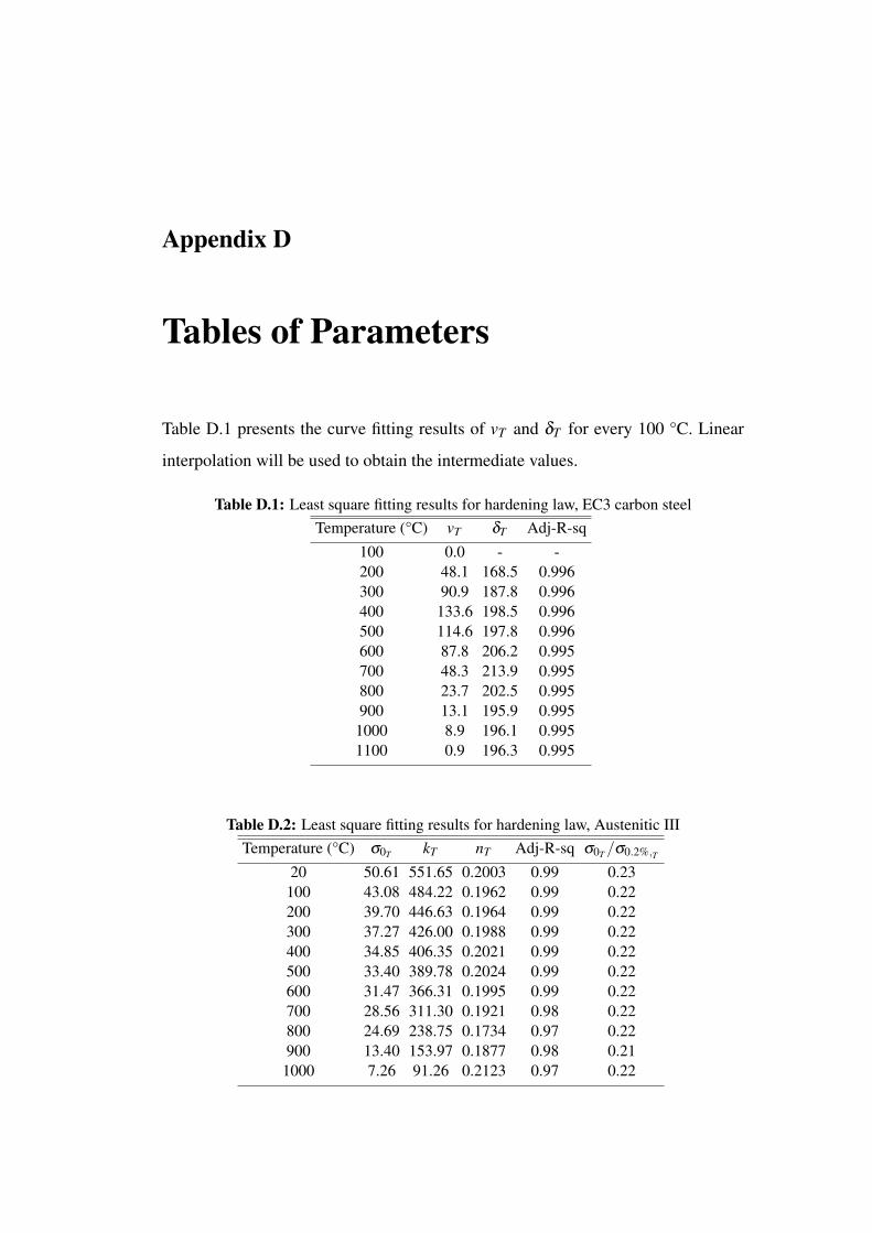
Appendix D
Tables of Parameters
Table D.1 presents the curve fitting results of vT and δT for every 100 °C. Linear
interpolation will be used to obtain the intermediate values.
Table D.1: Least square fitting results for hardening law, EC3 carbon steelTemperature (°C) vT δT Adj-R-sq
100 0.0 - -200 48.1 168.5 0.996300 90.9 187.8 0.996400 133.6 198.5 0.996500 114.6 197.8 0.996600 87.8 206.2 0.995700 48.3 213.9 0.995800 23.7 202.5 0.995900 13.1 195.9 0.995
1000 8.9 196.1 0.9951100 0.9 196.3 0.995
Table D.2: Least square fitting results for hardening law, Austenitic IIITemperature (°C) σ0T kT nT Adj-R-sq σ0T /σ0.2%,T
20 50.61 551.65 0.2003 0.99 0.23100 43.08 484.22 0.1962 0.99 0.22200 39.70 446.63 0.1964 0.99 0.22300 37.27 426.00 0.1988 0.99 0.22400 34.85 406.35 0.2021 0.99 0.22500 33.40 389.78 0.2024 0.99 0.22600 31.47 366.31 0.1995 0.99 0.22700 28.56 311.30 0.1921 0.98 0.22800 24.69 238.75 0.1734 0.97 0.22900 13.40 153.97 0.1877 0.98 0.211000 7.26 91.26 0.2123 0.97 0.22

222
Table D.3: Least square fitting results for hardening law, Duplex IITemperature (°C) σ0T kT nT Adj-R-sq σ0T /σ0.2%,T
20 171.16 1494.3 0.3673 0.98 0.38100 140.30 1170.8 0.3544 0.98 0.38200 116.60 951.3 0.3446 0.98 0.37300 108.30 883.5 0.3446 0.98 0.37400 99.96 808.7 0.3435 0.98 0.37500 85.91 682.0 0.3343 0.98 0.36600 66.18 514.1 0.3247 0.98 0.34700 41.32 316.1 0.3029 0.98 0.31800 2.93 22.5 0.2837 0.98 0.30900 9.45 75.3 0.2756 0.98 0.251000 1.12 11.1 0.2631 0.98 0.25
Table D.4: Least square fitting results, 304L stainless steel in Section 3.4Temperature Hardening Function Bauschinger Ratio Evolution Function
°C vT δT Adj-R-sq aT bT cT Adj-R-sq200 448.9 6.31 0.993 0.8504 184.5 0.1495 0.998600 312.7 9.941 0.999 0.6996 189.3 0.3004 0.980800 38.34 26.45 0.952 0.6786 267.2 0.3214 0.9871000 1000.0 0.1003 0.977 0.9050 500.0 0.0943 0.974
Table D.5: Least square fitting results, Low carbon steel in Section 3.5Temperature Hardening Function Bauschinger Ratio Evolution Function Material parameter
°C vT δT Adj-R-sq aT bT cT Adj-R-sq V hT
300 138.1 741.9 0.918 0.2212 5000.0 0.7781 0.996 1.45700 19.22 1331.0 0.957 0.2801 4274.0 0.7100 1.0 1.45
Table D.6: Least square fitting results, 316 stainless steel in Section 3.7Temperature Hardening Function Bauschinger Ratio Evolution Function
°C vT δT Adj-R-sq aT bT cT Adj-R-sq650 13.5 1533.0 0.854 0.3078 800.0 0.70 1.0
Table D.7: Least square fitting results for hardening law, St 37.2 carbon steel in [6]Temperature (°C) σ0T vT δT Adj-R-sq
100 250.0 0.0 - -200 226.4 23.61 22.84 0.980300 158.5 90.58 23.62 0.988400 143.6 105.5 24.42 0.982500 129.5 56.57 25.03 0.991600 56.58 67.48 24.27 0.990700 22.1 39.67 23.97 0.991

223
Table D.8: Least square fitting results, 304 Stainless SteelTemperature Hardening Function Bauschinger Ratio Evolution Function
°C vT δT Adj-R-sq aT bT cT Adj-R-sq150 302.1 0.1675 0.977 0.38 1143 0.62 1.0350 237.4 0.1729 0.984 0.28 1098 0.72 1.0600 208.2 0.2144 0.998 0.25 1055 0.75 1.0850 26.37 0.0748 0.975 0.26 974 0.74 1.0
1000 31.34 0.2569 0.939 0.37 1069 0.63 1.0
Table D.9: Bauschinger ratio calibration results, based on Fig.8 in [5]Temperature Bauschinger ratio ε p
150 °C 0.3756 0.0039350 °C 0.2766 0.0040600 °C 0.2463 0.0040850 °C 0.2797 0.0043
1000 °C 0.3675 0.0047
Bibliography
[1] Eurocode 3 : Design of steel structures - Part 1-2: General rules -Structural
fire design, vol. 3. British Standards Instituion, 2005.
[2] Design manual for structural stainless steel. The Steel Construction Institute,
4th ed., 2017.
[3] C. Bailey, I. Burgess, and R. Plank, “Analyses of the effects of cooling and
fire spread on steel-framed buildings,” Fire Safety Journal, vol. 26, no. 4,
pp. 273–293, 1996.
[4] M. Miller, E. Harley, and D. Bammann, “Reverse yield experiments and in-
ternal variable evolution in polycrystalline metals,” International Journal of
Plasticity, vol. 15, pp. 93–117, mar 1999.
[5] N. Ohno, R. Yamamoto, and D. Okumura, “Thermo-mechanical cyclic
hardening behavior of 304 stainless steel at large temperature ranges: Ex-
periments and simulations,” International Journal of Mechanical Sciences,
vol. 146-147, pp. 517 – 526, 2018.
[6] A. Rubert and P. Schaumann, “Structural steel and plane frame assemblies
under fire action,” Fire Safety Journal, vol. 10, pp. 173–184, may 1986.
[7] Y. Wang, I. Burgess, F. Wald, and M. Gillie, Performance Based Fire Engi-
neering of Structures. CRC Press LLC, Baton Rouge, 2012.
[8] A. Jonsdottir and G. Rein, “Out of range,” pp. 14–17, 2009.

Bibliography 225
[9] Eurocode 1 : Actions on structures -Part 1-2: Gerneral actions -Actions on
structures exposed to fire. British Standards Institution, 2013.
[10] J. Stern-Gottfried and G. Rein, “Travelling fires for structural design-Part I:
Literature review,” Fire Safety Journal, vol. 54, pp. 74–85, nov 2012.
[11] J. Stern-Gottfried and G. Rein, “Travelling fires for structural design - Part
II: Design methodology,” Fire Safety Journal, vol. 54, pp. 96–112, nov 2012.
[12] X. Dai, S. Welch, and A. Usmani, “A critical review of travelling fire sce-
narios for performance-based structural engineering,” Fire Safety Journal,
vol. 91, pp. 568–578, jul 2017.
[13] X. Dai, S. Welch, and A. Usmani, “Structural Implications due to an extended
travelling fire methodology (ETFM) framework using SIFBUILDER,” in The
10th International Conference on Structures in Fire, 2018.
[14] G. M. Newman, “Structural fire engineering investigation of Broadgate phase
8 fire,” The Steel Construction Institute, Ascot, 1991.
[15] FEMA, “World Trade Center Building Performance Study,” Tech. Rep. 403,
FEMA, 2002.
[16] J. Quintiere, M. di Marzo, and R. Becker, “A suggested cause of the fire-
induced collapse of the world trade towers,” Fire Safety Journal, vol. 37,
no. 7, pp. 707 – 716, 2002.
[17] A. Usmani, “Stability of the world trade center twin towers structural frame
in multiple floor fires,” Journal of Engineering Mechanics, vol. 131, no. 6,
pp. 654–657, 2005.
[18] G. Flint, A. Usmani, S. Lamont, B. Lane, and J. Torero, “Structural response
of tall buildings to multiple floor fires,” Journal of Structural Engineering,
vol. 133, no. 12, pp. 1719–1732, 2007.
Bibliography 226
[19] P. Kotsovinos and A. Usmani, “The world trade center 9/11 disaster and pro-
gressive collapse of tall buildings,” Fire Technology, vol. 49, pp. 741–765,
jul 2013.
[20] L. Gardner and K. Ng, “Temperature development in structural stainless steel
sections exposed to fire,” Fire Safety Journal, vol. 41, no. 3, pp. 185–203,
2006.
[21] L. Gardner and N. Baddoo, “Fire testing and design of stainless steel struc-
tures,” Journal of Constructional Steel Research, vol. 62, no. 6, pp. 532–543,
2006.
[22] N. Baddoo, “Stainless steel in construction: A review of research, appli-
cations, challenges and opportunities,” Journal of Constructional Steel Re-
search, vol. 64, no. 11, pp. 1199–1206, 2008.
[23] Abaqus 6.14 User subroutine reference guide. SIMULIA.
[24] F. McKenna, “Opensees: A framework for earthquake engineering simula-
tion,” Computing in Science Engineering, vol. 13, pp. 58–66, jul 2011.
[25] V. Babrauskas and R. B. Williamson, “The historical basis of fire resistance
testing - Part II,” Fire Technology, vol. 14, no. 4, pp. 304–316, 1978.
[26] ISO 834-1:1999, Fire-resistance tests - Elements of building construction -
Part 1: General requirements. International Organization for Standardisa-
tion, 1999.
[27] ASTM E119-18ce1,Standard test methods for fire tests of building construc-
tion and materials. ASTM International, 2018.
[28] C. Maluk and L. Bisby, “120 years of structural fire testing: Moving away
from the status quo,” in The Second Fire engineering conference, 2012.
[29] S. Ingberg, “Tests of the severity of building fires,” NFPA Quarterly, 1928.

Bibliography 227
[30] D. Drysdale, An Introduction to Fire Dynamics: Third Edition. Wiley Black-
well, 2011.
[31] G. Thomas, A. Buchanan, and C. Fleischmann, “Structural fire design: The
role of time equivalence,” Fire Safety Science, vol. 5, pp. 607–618, 1997.
[32] C. Maluk, “Motivation, drivers and barriers for a knowledge-based test en-
vironment in structural fire safety engineering science,” Fire Safety Journal,
vol. 91, pp. 103–111, jul 2017.
[33] T. Z. Harmathy, “The fire resistance test and its relation to real-world fires,”
Fire and Materials, vol. 5, no. 3, pp. 112–122, 1981.
[34] Fire protection for structural steel in buildings. The Association for Special-
ist Fire Protection, 2004.
[35] PD 7974-3: Application of fire safety engineering principles to the design of
buildings. Structural response to fire and fire spread beyond the enclosure of
origin (Sub-system 3). British Standards Institution, 2011.
[36] BS-476-20: Fire tests on building materials and structures. Method for de-
termination of the fire resistance of elements of construction (general princi-
ples). British Standards Institution, 1987.
[37] C. Bailey, D. Moore, and T. Lennon, “The structural behaviour of steel
columns during a compartment fire in a multi-storey braced steel-frame,”
Journal of Constructional Steel Research, vol. 52, pp. 137–157, Nov 1999.
[38] “The behaviour of multi-storey steel-framed buildings in a fire: A european
joint research programme,” tech. rep., Swinden Technology Centre, 1999.
[39] A. Usmani, J. M. Rotter, S. Lamont, A. Sanad, and M. Gillie, “Fundamental
principles of structural behaviour under thermal effects,” Fire Safety Journal,
vol. 36, no. 8, pp. 721–744, 2001.

Bibliography 228
[40] A. Buchanan, “The challenges of predicting structural performance in fires,”
Fire Safety Science, no. 9, pp. 79–90, 2008.
[41] V. Babrauskas, “Performance-Based Fire Safety Engineering Design: The
Role of Fire Models and Fire Tests,” in Interflam, pp. 799–807, 1999.
[42] ISO 16733:2015, Fire safety engineering - Selection of design fire scenarios
and design fires. Part 1: Selection of design fire scenarios. International
Organisation for Standardisation.
[43] P. H. Thomas, “Modelling of compartment fires,” Fire Safety Journal, vol. 5,
pp. 181–190, jan 1983.
[44] K.Kawagoe, “Fire Behaviour in Rooms,” tech. rep., Building Research Insti-
tute, Ministry of Construction, Tokyo, 1958.
[45] T. T. Lie, “Characteristic temperature curves for various fire severities,” Fire
Technology, vol. 10, no. 4, pp. 315–326, 1974.
[46] O. Pettersson, S. E. Magnusson, and J. Thor, “Fire Engineering Design of
Steel Structures,” tech. rep., Swedish institute of steel construction, 1976.
[47] Z. Ma and P. Makelainen, “Parametric temperature-time curves of medium
compartment fires for structural design,” Fire Safety Journal, vol. 34, no. 4,
pp. 361–375, 2000.
[48] C. R. Barnett, “BFD curve: A new empirical model for fire compartment
temperatures,” Fire Safety Journal, vol. 37, pp. 437–463, jul 2002.
[49] C. R. Barnett, “Replacing international temperature-time curves with BFD
curve,” Fire Safety Journal, vol. 42, pp. 321–327, jun 2007.
[50] B. Zhao and J. Kruppa, “Structural behaviour of an open car park under real
fire scenarios,” Fire and Materials, vol. 28, no. 2-4, pp. 269–280, 2004.

Bibliography 229
[51] M. Garlock, I. Paya-Zaforteza, V. Kodur, and L. Gu, “Fire hazard in bridges:
Review, assessment and repair strategies,” Engineering Structures, vol. 35,
no. Supplement C, pp. 89 – 98, 2012.
[52] A. Pchelintsev, Y. Hasemi, T. Wakamatsu, and Y. Yokobayashi, “Experimen-
tal and numerical study on the behaviour of a steel beam under ceiling ex-
posed to a localized fire,” Fire Safety Science, vol. 5, pp. 1153–1164, 1997.
[53] T. Wakamatsu, Y. Hasemi, K. Kagiya, and D. Kamikawa, “Heating mech-
anism of unprotected steel beam installed beneath ceiling and exposed to a
localized fire: Verification using the real-scale experiment and effects of the
smoke layer,” Fire Safety Science, pp. 1099–1110, 2003.
[54] G. Heskestad, “Peak gas velocities and flame heights of buoyancy-controlled
turbulent diffusion flames,” Symposium (International) on Combustion,
vol. 18, no. 1, pp. 951–960, 1981.
[55] K. Horova, T. Jana, and F. Wald, “Temperature heterogeneity during trav-
elling fire on experimental building,” Advances in Engineering Software,
vol. 62-63, pp. 119–130, aug 2013.
[56] J. L. Torero, A. H. Majdalani, A. E. Cecilia, and A. Cowlard, “Revisiting the
compartment fire,” Fire Safety Science, vol. 11, pp. 28–45, 2014.
[57] D. R. J. Degler, A. Eliasson, J. Anderson, D. Lange, “A-priori modelling of
the Tisova Fire Test as input to the experimental work,” in Proceedings of
the First International Conference on Structural Safety under Fire & Blast,
pp. 429–438, 2015.
[58] G. Rein, X. Zhang, P. Williams, B. Hume, and A. Heise, “Multi-storey fire
analysis for high-rise buildings,” in Interflam: The 11th international confer-
ence on fire science and engineering, pp. 605–616, 2007.
[59] R.L.Alpert, “Turbulent ceiling-jet induced by large-scale fires,” Combustion
Science and Technology, vol. 11, no. 5-6, pp. 197–213, 1975.

Bibliography 230
[60] G. Rein, W. Jahn, and J. Torero, “Modelling of the growth phase of dal-
marnock fire test one,” pp. 245–256, 2011.
[61] W. Jahn, G. Rein, and J. Torero, “A posteriori modelling of the growth
phase of dalmarnock fire test one,” Building and Environment, vol. 46, no. 5,
pp. 1065–1073, 2011.
[62] B. Merci, J. L. Torero, and A. Trouve, “Iafss working group on measurement
and computation of fire phenomena,” Fire Technology, vol. 52, pp. 607–610,
may 2016.
[63] G. Baker, C. Wade, M. Spearpoint, and C. Fleischmann, “Developing proba-
bilistic design fires for performance-based fire safety engineering,” Procedia
Engineering, vol. 62, pp. 639–647, 2013.
[64] G. Cooke, “An introduction to the mechanical properties of structural steel at
elevated temperatures,” Fire Safety Journal, vol. 13, no. 1, pp. 45–54, 1988.
[65] L. Twilt, “Strength and deformation properties of steel at elevated tempera-
tures: Some practical implications,” Fire Safety Journal, vol. 13, no. 1, pp. 9
– 15, 1988.
[66] Y. Wang, “An analysis of the global structural behaviour of the Cardington
steel-framed building during the two BRE fire tests,” Engineering Structures,
vol. 22, pp. 401–412, may 2000.
[67] G. Q. Li and S. X. Guo, “Experiment on restrained steel beams subjected
to heating and cooling,” Journal of Constructional Steel Research, vol. 64,
pp. 268–274, mar 2008.
[68] T. Liu, M. Fahad, and J. Davies, “Experimental investigation of behaviour
of axially restrained steel beams in fire,” Journal of Constructional Steel Re-
search, vol. 58, pp. 1211–1230, sep 2002.
Bibliography 231
[69] S. Lamont, B. Lane, A. Usmani, and D. Drysdale, “Assessment of the fire
resistance test with respect to beams in real structures,” Engineering Journal,
vol. 40, no. 2, pp. 63–75, 2003.
[70] V. Kodur and M. Dwaikat, “Response of steel beam - columns exposed to
fire,” Engineering Structures, vol. 31, pp. 369–379, feb 2009.
[71] M. Dwaikat and V. Kodur, “A performance based methodology for fire design
of restrained steel beams,” Journal of Constructional Steel Research, vol. 67,
pp. 510–524, mar 2011.
[72] Y. Yin and Y. Wang, “Analysis of catenary action in steel beams using a sim-
plified hand calculation method, Part 1: Theory and validation for uniform
temperature distribution,” Journal of Constructional Steel Research, vol. 61,
pp. 183–211, feb 2005.
[73] Y. Yin and Y. Wang, “Analysis of catenary action in steel beams using a sim-
plified hand calculation method, part 2: Validation for non-uniform tempera-
ture distribution,” Journal of Constructional Steel Research, vol. 61, pp. 213–
234, feb 2005.
[74] A. Sanad, J. Rotter, A. Usmani, and M. O’Connor, “Composite beams in
large buildings under fire - numerical modelling and structural behaviour,”
Fire Safety Journal, vol. 35, no. 3, pp. 165–188, 2000.
[75] V. Kodur and A. Shakya, “Effect of temperature on thermal properties of
spray applied fire resistive materials,” Fire Safety Journal, vol. 61, pp. 314 –
323, 2013.
[76] S. Chen, L. Jiang, A. Usmani, G. Q. Li, and C. Jin, “Damage mechanisms in
cementitious coatings on steel members under axial loading,” Construction
and Building Materials, vol. 90, pp. 18–35, 2015.

Bibliography 232
[77] N. L. Braxtan and S. Pessiki, “Bond performance of SFRM on steel
plates subjected to tensile yielding,” Journal of Fire Protection Engineering,
vol. 21, no. 1, pp. 37–55, 2011.
[78] A. Arablouei and V. Kodur, “Dynamic delamination of fire insulation applied
on steel structures under impact loading,” International Journal of Impact
Engineering, vol. 83, pp. 11–27, 2015.
[79] K. T. Tan, C. C. White, and D. L. Hunston, “An adhesion test method for
spray-applied fire-resistive materials,” Fire and Materials, vol. 35, no. 4,
pp. 245–259, 2011.
[80] A. Arablouei and V. Kodur, “Cohesive zone model properties for evaluating
delamination of spray-applied fire-resistive materials from steel structures,”
Engineering Fracture Mechanics, 2015.
[81] N. L. Braxtan and S. Pessiki, “Seismic performance of sprayed fire resistive
material (sfrm) on steel moment frame buildings,” Tech. Rep. ATLSS report
number 10-03, ATLSS Reports, 2010.
[82] N. L. Braxtan and S. P. Pessiki, “Postearthquake fire performance of sprayed
fire-resistive material on steel moment frames,” Journal of Structural Engi-
neering, vol. 137, no. 9, pp. 946–953, 2011.
[83] W. J. Keller and S. Pessiki, “Effect of earthquake-induced damage to spray-
applied fire-resistive insulation on the response of steel moment-frame beam-
column connections during fire exposure,” Journal of Fire Protection Engi-
neering, vol. 22, no. 4, pp. 271–299, 2012.
[84] W. J. Keller and S. Pessiki, “Cyclic load tests of SFRM-insulated steel gravity
frame beam-column connection assemblies,” Journal of Structural Engineer-
ing, vol. 141, oct 2015.

Bibliography 233
[85] S. Chen and L. Jiang, “Damage mechanisms in cementitious coatings on steel
members in bending,” Proceedings of the ICE - Structures and Buildings,
vol. 168, no. Volume 168, Issue 5, pp. 351–369, 2015.
[86] S. Chen, L. Jiang, L. Wu, Y. Wang, and A. Usmani, “Damage investigation
of cementitious fire resistive coatings under complex loading,” Construction
and Building Materials, vol. 204, pp. 659 – 674, 2019.
[87] Y. Wang, “Experimental studies on damage mechanisms in cementitious
coatings on structural members under complex loadings,” Master’s thesis,
Tongji University, 2016.
[88] M. Dwaikat, V. Kodur, and F. Asce, “Modeling fracture and delamination of
spray-applied fire-resisting materials under static and impact loads,” Journal
of Engineering Mechanics, vol. 137, no. 12, pp. 901–910, 2011.
[89] A. Arablouei and V. Kodur, “A fracture mechanics-based approach for
quantifying delamination of spray-applied fire-resistive insulation from steel
moment-resisting frame subjected to seismic loading,” Engineering Fracture
Mechanics, vol. 121-122, pp. 67–86, 2014.
[90] V. Kodur, P. Eng, F. Asce, and A. Arablouei, “Mechanics-based approach for
modeling delamination of fire insulation from steel structures,” Journal of
Engineering Mechanics, vol. 140, no. 6, 2014.
[91] V. Kodur and A. Arablouei, “Effective properties of spray-applied fire-
resistive material for resistance to cracking and delamination from steel struc-
tures,” Construction and Building Materials, vol. 84, pp. 367–376, 2015.
[92] Huang, Hou-cheng; Usmani, Asif, Finite element analysis for heat trans-
fer:Theory and software. Springer London Ltd, United Kingdom, 2010.
[93] Y. Jiang, Development and application of a thermal analysis framework in
OpenSees for structures in fire. PhD thesis, The university of Edinburgh,
2012.
Bibliography 234
[94] L. Gardner and D. Nethercot, “Experiments on stainless steel hollow sections
Part 1: Material and cross-sectional behaviour,” Journal of Constructional
Steel Research, vol. 60, no. 9, pp. 1291–1318, 2004.
[95] J. Chen and B. Young, “Stress strain curves for stainless steel at elevated
temperatures,” Engineering Structures, vol. 28, pp. 229–239, jan 2006.
[96] R. K. Desu, H. Nitin Krishnamurthy, A. Balu, A. K. Gupta, and S. K. Singh,
“Mechanical properties of Austenitic Stainless Steel 304L and 316L at ele-
vated temperatures,” Journal of Materials Research and Technology, vol. 5,
pp. 13–20, jan 2016.
[97] L. Gardner, A. Insausti, K. Ng, and M. Ashraf, “Elevated temperature ma-
terial properties of stainless steel alloys,” Journal of Constructional Steel
Research, vol. 66, no. 5, pp. 634–647, 2010.
[98] J. Sahu, U. Krupp, R. Ghosh, and H.-J. Christ, “Effect of 475 C embrit-
tlement on the mechanical properties of duplex stainless steel,” Materials
Science and Engineering: A, vol. 508, pp. 1–14, may 2009.
[99] E. Mirambell and E. Real, “On the calculation of deflections in structural
stainless steel beams: an experimental and numerical investigation,” Journal
of Constructional Steel Research, vol. 54, pp. 109–133, apr 2000.
[100] B. Young, “Experimental and numerical investigation of high strength stain-
less steel structures,” Journal of Constructional Steel Research, vol. 64,
pp. 1225–1230, nov 2008.
[101] N. Lopes, P. Vila Real, L. Simoes da Silva, and J.-M. Franssen, “Numerical
analysis of stainless steel beam-columns in case of fire,” Fire Safety Journal,
vol. 50, pp. 35–50, 2012.
[102] L. Gardner and D. Nethercot, “Experiments on stainless steel hollow sections
Part 2: Member behaviour of columns and beams,” Journal of Constructional
Steel Research, vol. 60, no. 9, pp. 1319–1332, 2004.
Bibliography 235
[103] M. Ashraf, L. Gardner, and D. Nethercot, “Compression strength of stainless
steel cross-sections,” Journal of Constructional Steel Research, vol. 62, no. 1,
pp. 105–115, 2006.
[104] S. Fan, L. Zhang, W. Sun, X. Ding, and M. Liu, “Numerical investigation
on fire resistance of stainless steel columns with square hollow section under
axial compression,” Thin-Walled Structures, vol. 98, pp. 185–195, 2016.
[105] P. M. M. Vila Real, N. Lopes, L. Simoes da Silva, and J. M. Franssen,
“Lateral-torsional buckling of stainless steel I-beams in case of fire,” Journal
of Constructional Steel Research, vol. 64, no. 11, pp. 1302–1309, 2008.
[106] “Results and observations from full-scale fire test at BRE Cardington,” Tech.
Rep. 215, BRE Centre, 2003.
[107] W. Ramberg and W. R. Osgood, “Description of stress-strain curves by three
parameters,” tech. rep., National Advisory Committee for Aeronautics, 1943.
[108] H. Saab and D. Nethercot, “Modelling steel frame behaviour under fire con-
ditions,” Engineering Structures, vol. 13, pp. 371–382, oct 1991.
[109] N. Mostaghel and R. Byrd, “Inversion of Ramberg-Osgood equation and de-
scription of hysteresis loops,” International Journal of Non-Linear Mechan-
ics, vol. 37, pp. 1319–1335, dec 2002.
[110] K. Abdella, “Inversion of a full-range stress-strain relation for stainless steel
alloys,” International Journal of Non-Linear Mechanics, vol. 41, no. 3,
pp. 456–463, 2006.
[111] J. Hollomon, “Tensile deformation,” Transactions of the Metallurgical Soci-
ety of AIME, vol. 162, pp. 268–290, 1945.
[112] P. Ludwik, Elemente der Technologischen Mechanik. Springer, 1909.
[113] H. Swift, “Plastic instability under plane stress,” Journal of the Mechanics
and Physics of Solids, vol. 1, no. 1, pp. 1–18, 1952.

Bibliography 236
[114] E. Voce, “A practical strain hardening function,” Metallurgia, vol. 51,
pp. 219–226, 1955.
[115] J. Franssen, “The unloading of building materials submitted to fire,” Fire
Safety Journal, vol. 16, no. 3, pp. 213–227, 1990.
[116] G. Masing, “Internal stresses and hardening of brass,” in Proceedings of 2nd
International Congress for Applied Mechanics, Zurich, sep 1926.
[117] J.-M. Franssen and T. Gernay, “Modeling structures in fire with SAFIR: theo-
retical background and capabilities,” Journal of Structural Fire Engineering,
no. 07, 2017.
[118] J.-M. Franssen, “Safir: A thermal/structural program for modeling structures
under fire,” Engineering Journal, vol. 42, no. 3, pp. 143–150, 2005.
[119] N. Elhami Khorasani, M. E. M. Garlock, and S. E. Quiel, “Modeling steel
structures in OpenSees: Enhancements for fire and multi-hazard probabilistic
analyses,” Computers and Structures, vol. 157, pp. 218–231, 2015.
[120] C. Bailey, “Development of computer software to simulate the structural be-
haviour of steel-framed buildings in fire,” Computers & Structures, vol. 67,
no. 6, pp. 421–438, 1998.
[121] C. K. Iu, S. L. Chan, and X. X. Zha, “Nonlinear pre-fire and post-fire analysis
of steel frames,” Engineering Structures, vol. 27, no. 11, pp. 1689–1702,
2005.
[122] K. Lien, Y. Chiou, R. Wang, and P. Hsiao, “Nonlinear behavior of steel struc-
tures considering the cooling phase of a fire,” Journal of Constructional Steel
Research, vol. 65, pp. 1776–1786, aug 2009.
[123] H. Armen, “Assumptions, models, and computational methods for plasticity,”
Computers & Structures, vol. 10, no. 1, pp. 161–174, 1979.

Bibliography 237
[124] E. Silvestre, J. Mendiguren, L. Galdos, and E. S. de Argandona, “Compar-
ison of the hardening behaviour of different steel families: From mild and
stainless steel to advanced high strength steels,” International Journal of Me-
chanical Sciences, vol. 101-102, pp. 10 – 20, 2015.
[125] A. Olsson, Stainless steel plasticity - Material modelling and structural ap-
plications. PhD thesis, Lulea University of Technology, 2001.
[126] J.Gozzi, Plastic behaviour of steel: Experimental invesitgation and mod-
elling. PhD thesis, Lulea University of Technology, 2004.
[127] A. Phillips, C. S. Liu, and J. W. Justusson, “An experimental investigation of
yield surfaces at elevated temperatures,” Acta Mechanica, vol. 14, pp. 119–
146, jun 1972.
[128] Harley, E.J and Miller, M.P and Bammann, D.J, “Experimental study of inter-
nal variable evolution in SS304L, at multiple rates and temperatures,” Jour-
nal of Engineering Materials and Technology, vol. 121, no. 2, pp. 162–171,
1999.
[129] K. Maciejewski, Y. Sun, O. Gregory, and H. Ghonem, “Time-dependent de-
formation of low carbon steel at elevated temperatures,” Materials Science
and Engineering: A, vol. 534, pp. 147 – 156, feb 2012.
[130] BS EN ISO 6892-1 Metallic materials - Tensile testing Part 1: Method of test
at room temperature. British Standards Institution, jul 2016.
[131] U. Lindholm and R. Bessey, “A survey of rate dependent strength properties
of metals,” Tech. Rep. AFRL-TR-69-119, Southwest research institue, jun
1969.
[132] Seif, Mina S. and Luecke,William E. and Choe, Lisa Y. and Main,Joseph A.
and McColskey, Joseph D. and Zhang, Chao and Weigand, Jonathan M. and
Gross, John L.and Sadek, Fahim, “Temperature-dependent material mod-
eling for structural steels: Formulation and application,” Tech. Rep. NIST
Bibliography 238
Technical Note 1907, National Institute of Standards and Technology, U.S.
Department of Commerce, 2016.
[133] L. M. Lindholm, U. S.and Yeakley, “High strain-rate testing: Tension and
compression,” Experimental Mechanics, vol. 8, pp. 1–9, jan 1968.
[134] N. Toric and I. W. Burgess, “A unified rheological model for modelling
steel behaviour in fire conditions,” Journal of Constructional Steel Research,
vol. 127, pp. 221 – 230, 2016.
[135] E. Stoddart, M. Byfield, J. Davison, and A. Tyas, “Strain rate dependent com-
ponent based connection modelling for use in non-linear dynamic progres-
sive collapse analysis,” Engineering Structures, vol. 55, pp. 35 – 43, 2013.
[136] B. Jiang, G. Q. Li, and A. Usmani, “Progressive collapse mechanisms in-
vestigation of planar steel moment frames under localized fire,” Journal of
Constructional Steel Research, vol. 115, pp. 160 – 168, 2015.
[137] H. Nguyen, A. Jeffers, and V. Kodur, “Computational simulation of steel
moment frame to resist progressive collapse in fire,” Journal of Structural
Fire Engineering, vol. 7, no. 4, pp. 286–305, 2016.
[138] V. Kodur, M. Dwaikat, and R. Fike, “High-temperature properties of steel
for fire resistance modeling of structures,” Journal of Materials in Civil En-
gineering, vol. 22, no. 5, pp. 423–434, 2010.
[139] I. Boko, N. Toric, and B. Peros, “Structural fire design parameters and pro-
cedures – analysis of the potential of eurocode 3,” Materialwissenschaft und
Werkstofftechnik, vol. 43, no. 12, pp. 1036–1052, 2012.
[140] L. Twilt, “Stress-strain relationships of structural steel at elevated tempera-
tures: Analysis of various options and european proposal -part f: mechanical
properties,” Tech. Rep. TNO Rep No. BI-91-015, Delft, The Netherlands,
1991.
[141] Structural fire protection. American Society of Civil Engineers, 1992.
Bibliography 239
[142] Z. Mroz, “On the description of anisotropic workhardening,” Journal of the
Mechanics and Physics of Solids, vol. 15, no. 3, pp. 163 – 175, 1967.
[143] R. D. Krieg, “A practical two surface plasticity theory,” Journal of Applied
Mechanics, vol. 42, no. 3, p. 641, 1975.
[144] Y. F. Dafalias and E. P. Popov, “Plastic internal variables formalism of cyclic
plasticity,” Mechanics Research Communications, vol. 3, no. 1, pp. 33–38,
1976.
[145] M. G. Lee, D. Kim, C. Kim, M. Wenner, R. Wagoner, and K. Chung, “A
practical two-surface plasticity model and its application to spring-back pre-
diction,” International Journal of Plasticity, vol. 23, no. 7, pp. 1189 – 1212,
2007.
[146] R. P. Cardoso and J. W. Yoon, “Stress integration method for a nonlinear
kinematic/isotropic hardening model and its characterization based on poly-
crystal plasticity,” International Journal of Plasticity, vol. 25, no. 9, pp. 1684
– 1710, 2009. Exploring New Horizons of Metal Forming Research.
[147] D. W. Prager, “The theory of plasticity: A survey of recent achievements,”
Proceedings of the Institution of Mechanical Engineers, vol. 169, no. 1,
pp. 41–57, 1955.
[148] H. Ziegler, “A modification of prager’s hardening rule,” Quarterly of Applied
Mathematics, vol. 17, no. 1, pp. 55–65, 1959.
[149] J. L. Chaboche and G. Rousselier, “On the Plastic and Viscoplastic Consti-
tutive Equations - Part I: Rules Developed With Internal Variable Concept,”
Journal of Pressure Vessel Technology, vol. 105, no. 2, p. 153, 1983.
[150] J. Chaboche, “Time-independent constitutive theories for cyclic plasticity,”
International Journal of Plasticity, vol. 2, no. 2, pp. 149–188, 1986.

Bibliography 240
[151] J. Chaboche, “A review of some plasticity and viscoplasticity constitutive
theories,” International Journal of Plasticity, vol. 24, no. 10, pp. 1642 –
1693, 2008. Special Issue in Honor of Jean-Louis Chaboche.
[152] C. Frederick and P. Armstrong, “A mathematical representation of the multi-
axial Bauschinger effect,” tech. rep., 1966.
[153] E. A. de Souza Neto, D. Peri, and D. R. J. Owen, Computational Methods
for Plasticity : Theory and Applications. Wiley-Blackwell, 2008.
[154] A. Khan and S. Huang, Continuum Theory of Plasticity. Wiley-Interscience
publication, Wiley, 1995.
[155] N. Rebelo and S. Kobayashi, “A coupled analysis of viscoplastic deformation
and heat transfer - i: Theoretical considerations,” International Journal of
Mechanical Sciences, vol. 22, no. 11, pp. 699 – 705, 1980.
[156] N. Rebelo and S. Kobayashi, “A coupled analysis of viscoplastic deformation
and heat transfer - ii: Applications,” International Journal of Mechanical
Sciences, vol. 22, no. 11, pp. 707 – 718, 1980.
[157] J. H. Kim, S. K. Kim, C. S. Lee, M. H. Kim, and J. M. Lee, “A constitutive
equation for predicting the material nonlinear behavior of aisi 316l, 321, and
347 stainless steel under low-temperature conditions,” International Journal
of Mechanical Sciences, vol. 87, pp. 218 – 225, 2014.
[158] C. J. Lissenden, B. A. Lerch, J. R. Ellis, and D. N. Robinson, “Verification of
experimental techniques for flow surface determination,” tech. rep., National
Aeronautics and Space Administration, feb 1996.
[159] Y. Sun, K. MacIejewski, and H. Ghonem, “Simulation of viscoplastic de-
formation of low carbon steel structures at elevated temperatures,” Journal
of Materials Engineering and Performance, vol. 21, no. 7, pp. 1151–1159,
2012.

Bibliography 241
[160] D. Bushnell, “A strategy for the solution of problems involving large deflec-
tions, plasticity and creep,” International Journal for Numerical Methods in
Engineering, vol. 11, no. 4, pp. 683–708, 1977.
[161] C. Nyssen, “An efficient and accurate iterative method, allowing large in-
cremental steps, to solve elasto-plastic problems,” Computers & Structures,
vol. 13, no. 1, pp. 63 – 71, 1981.
[162] S. Sloan, “Substepping schemes for numerical integration of elastoplastic
stress strain relations,” International Journal for Numerical Methods in En-
gineering, vol. 24, pp. 893 – 911, 05 1987.
[163] J. Marques, “Stress computation in elastoplasticity,” Engineering Computa-
tions, vol. 1, no. 1, pp. 42–51, 1984.
[164] J. Rice and D. Tracey, “Computational fracture mechanics,” Numerical and
Computer Methods in Structure Mechanics, pp. 585–623, feb 1973.
[165] M. Ortiz and E. P. Popov, “Accuracy and stability of integration algorithms
for elastoplastic constitutive relations,” International Journal for Numerical
Methods in Engineering, vol. 21, no. 9, pp. 1561–1576, 1985.
[166] M. Wilkins, L. L. Laboratory, and B. L. R. L. University of California, Cal-
culation of elastic-plastic flow. University of California Lawrence Radiation
Laboratory, 1963.
[167] R. D. Krieg and D. B. Krieg, “Accuracies of numerical solution methods for
the elastic-perfectly plastic model,” Journal of Pressure Vessel Technology,
vol. 99, no. 4, p. 510, 1977.
[168] J. Simo and S. Govindjee, “Exact closed-form solution of the return mapping
algorithm in plane stress elasto-viscoplasticity,” Engineering Computations,
vol. 5, no. 3, pp. 254–258, 1988.

Bibliography 242
[169] M. Ortiz and J. C. Simo, “An analysis of a new class of integration algorithms
for elastoplastic constitutive relations,” International Journal for Numerical
Methods in Engineering, vol. 23, no. 3, pp. 353–366, 1986.
[170] A. Lush, G. Weber, and L. Anand, “An implicit time-integration proce-
dure for a set of internal variable constitutive equations for isotropic elasto-
viscoplasticity,” International Journal of Plasticity, vol. 5, no. 5, pp. 521 –
549, 1989.
[171] J. Yoon, D. Yang, and K. Chung, “Elasto-plastic finite element method based
on incremental deformation theory and continuum based shell elements for
planar anisotropic sheet materials,” Computer Methods in Applied Mechanics
and Engineering, vol. 174, no. 1, pp. 23 – 56, 1999.
[172] R. Hill, The mathematical theory of plasticity. Oxford University Press,
1998.
[173] T. Inoue and K. Tanaka, “Subsequent yield conditions of metal under cyclic
loading at elevated temperature,” Ingenieur-Archiv, vol. 44, no. 2, pp. 53–62,
1975.
[174] J. C. Nagtegaal, “On the implementation of inelastic constitutive equations
with special reference to large deformation problems,” Computer Methods in
Applied Mechanics and Engineering, vol. 33, no. 1, pp. 469 – 484, 1982.
[175] J. Simo and R. Taylor, “Consistent tangent operators for rate-independent
elastoplasticity,” Computer Methods in Applied Mechanics and Engineering,
vol. 48, no. 1, pp. 101 – 118, 1985.
[176] J. R. Ellis, D. N. Robinson, and C. E. Pugh, “Time dependence in biaxial
yield of type 316 stainless steel at room temperature,” Journal of Engineering
Materials and Technology, vol. 105, no. 4, pp. 250–256, 1983.
[177] Abaqus 6.14 Benchmarks manual. SIMULIA.

Bibliography 243
[178] W. W. Yu and R. A. LaBoube, Cold-formed steel design. John Wiley & Sons,
Inc., 2010.
[179] X. Qiang, F. S. Bijlaard, and H. Kolstein, “Post-fire mechanical properties
of high strength structural steels s460 and s690,” Engineering Structures,
vol. 35, pp. 1 – 10, 2012.
[180] X. Qiang, F. S. Bijlaard, and H. Kolstein, “Post-fire performance of very
high strength steel s960,” Journal of Constructional Steel Research, vol. 80,
pp. 235 – 242, 2013.
[181] W. Wang, T. Liu, and J. Liu, “Experimental study on post-fire mechanical
properties of high strength q460 steel,” Journal of Constructional Steel Re-
search, vol. 114, pp. 100 – 109, 2015.
[182] F. Azhari, A. Heidarpour, X. L. Zhao, and C. R. Hutchinson, “Mechanical
properties of ultra-high strength (grade 1200) steel tubes under cooling phase
of a fire: An experimental investigation,” Construction and Building Materi-
als, vol. 93, pp. 841 – 850, 2015.
[183] X. Q. Wang, Z. Tao, T. Y. Song, and L. H. Han, “Stress strain model of
austenitic stainless steel after exposure to elevated temperatures,” Journal of
Constructional Steel Research, vol. 99, pp. 129 – 139, 2014.
[184] Z. Tao, X. Q. Wang, M. K. Hassan, T. Y. Song, and L. A. Xie, “Behaviour of
three types of stainless steel after exposure to elevated temperatures,” Journal
of Constructional Steel Research, vol. 152, pp. 296 – 311, 2019.
[185] Y. Huang and B. Young, “Post-fire behaviour of ferritic stainless steel mate-
rial,” Construction and Building Materials, vol. 157, pp. 654 – 667, 2017.
[186] Y. Huang and B. Young, “Mechanical properties of lean duplex stainless steel
at post-fire condition,” Thin-Walled Structures, vol. 130, pp. 564 – 576, 2018.

Bibliography 244
[187] F. Azhari, A. Heidarpour, X.-L. Zhao, and C. R. Hutchinson, “Post-fire me-
chanical response of ultra-high strength (grade 1200) steel under high tem-
peratures: Linking thermal stability and microstructure,” Thin-Walled Struc-
tures, vol. 119, pp. 114 – 125, 2017.
[188] E. Silvestre, J. Mendiguren, L. Galdos, and E. S. de Argandona, “Compar-
ison of the hardening behaviour of different steel families: From mild and
stainless steel to advanced high strength steels,” International Journal of Me-
chanical Sciences, vol. 101-102, pp. 10 – 20, 2015.
[189] D. Booth, Edmund; Key, Earthquake Design Practice for Buildings. Thomas
Telford Publishing, Thomas Telford Ltd, 2nd ed., 2006.
[190] M. Design and O. Structures, Minimum Design Loads for Buildings and
Other Structures. American Society of Civil Engineers, 2013.
[191] B. S. S. C. of the National Institute of Building Sciences National Insti-
tute of Building Sciences, NEHRP Recommended Seismic Provisions for
New Buildings and Other Structures (FEMA P-750). Federal Emergency
Management Agency of the U.S. Department of Homeland Security, 2009.
[192] M. Zhou, R. P. Cardoso, and H. Bahai, “A new material model for thermo-
mechanical analysis of steels in fire,” International Journal of Mechanical
Sciences, vol. 159, pp. 467 – 486, 2019.
[193] B. S. S. C. of the National Institute of Building Sciences, FEMA P-751:
2009 NEHRP Recommended Seismic Provisions: Design Examples. Fed-
eral Emergency Management Agency of the U.S. Department of Homeland
Security, 2012.
[194] E. B. V. Filippou, F.C.and Popov, “Effects of bond deterioration on hysteretic
behavior of reinforced concrete joints,” tech. rep., Earthquake engineering
research center, University of California, Berkeley, 1983.

Bibliography 245
[195] P. Uriz and S. Mahin, “Toward earthquake-resistant design of concentrically
braced steel-frame structures,” Tech. Rep. November, Pacific Earthquake En-
gineering Research Center, College of Engineering University of California,
Berkeley, 2008.
[196] A. Gupta and H. Krawinkler, “Seismic demands for performance evaluation
of steel moment resisting frame structures,” Tech. Rep. 132, The John A.
Blume Earthquake Engineering Centre, 1999.
[197] BS9999: Code of practice for fire safety in the design, management and use
of buildings, vol. 3. British Standards Institution, 2008.
[198] L. Jiang, Development of an integrated computational tool for modelling
structural frames in fire considering local effects. PhD thesis, The University
of Edinburgh, 2015.
[199] Specification for the design of light gauge cold-formed stainless steel struc-
tural members. American Iron and Steel Institute, 1968.
[200] “Compendium of UK standard fire test data - Unprotected structural steel -1,”
tech. rep., UK Department of the Environment Fire Research Station; British
Steel Corporation, 1988.
[201] R. G. Gann, A. Hamins, K. McGrattan, H. E. Nelson, T. J. Ohlemiller, K. R.
Prasad, and W. M. Pitts, “Reconstruction of the fires and thermal environment
in world trade center buildings 1, 2, and 7,” Fire Technology, vol. 49, pp. 679–
707, jul 2013.
[202] I. A. Fletcher, A. Borg, N. Hitchen, and S. Welch, “Performance of concrete
in fire: A review of the state of the art, with a case study of the windsor
tower fire,” in Proceeding of 4th international workshop in Structures in Fire,
pp. 779–790, sep 2007.
[203] C. Clifton, “Fire models for large firecells,” tech. rep., HERA, 1996.

Bibliography 246
[204] E. Rackauskaite, P. Kotsovinos, and G. Rein, “Structural response of a steel-
frame building to horizontal and vertical travelling fires in multiple floors,”
Fire Safety Journal, vol. 91, pp. 542–552, 2017.
[205] X. Dai, L. Jiang, J. Maclean, S. Welch, and A. Usmani, “Implementation
of a new design travelling fire model for global structural analysis,” in 9th
International Conference on Structures in Fire, pp. 959–966, 2016.
[206] Abaqus 6.14 Analysis user’s manual. SIMULIA.
[207] E. Spacone, F. Filippou, and F. Taucer, “Fibre beam–column model for non-
linear analysis of r/c frames: Part i. formulation,” Earthquake Engineering &
Structural Dynamics, vol. 25, no. 7, pp. 711–725, 1996.
[208] F. Barlat, H. Aretz, J. Yoon, M. Karabin, J. Brem, and R. Dick, “Linear
transfomation-based anisotropic yield functions,” International Journal of
Plasticity, vol. 21, no. 5, pp. 1009 – 1039, 2005.
[209] R. H. Dodds, “Numerical techniques for plasticity computations in finite ele-
ment analysis,” Computers & Structures, vol. 26, no. 5, pp. 767 – 779, 1987.
Copyright © 2022 FDOKUMEN