Proceedings of Ninth International Conference on Modelling, Monitoring, and Management of Air Pollution, September 12-14, 2001, Ancona, Italy

Study of Air Pollution due to Industrial Spots Nearby the Campus of Zagazig University (Egypt)

Ahmed F. Abdel Azim, A. F. Abdel Gawad, and M. M. Ibrahim

 

Study of air pollution due to industrial spots nearby the campus of Zagazig University (Egypt) Ahmed F. Abdel Azim1, Ahmed F. Abdel Gawad2 & Mostafa M. Ibrahim3 1Chairman, Mech. Power Eng. Dept., Zagazig Univ., Egypt. 2Assist. Prof., Mech. Power Eng. Dept., Zagazig Univ. 3Demonstrator, Mech. Power Eng. Dept., Zagazig Univ. Abstract Pollution is one of the important problems facing the developing countries. Air and water pollution may reach unacceptable limits. This situation affects greatly the health and overall activity of the humans. Air pollution is expected to have a pronounced effect on the students’ health, education, and all their daily activities. The present study concerns with the concentration and distribution of pollution emissions from industrial chimneys located in the neighborhood of the main campus of Zagazig University, Egypt. The investigation is based on the Cornell Mixing Zone Expert System (CORMIX, ver. 3) software. Useful remarks, which may help in reducing the pollution effect in the university campus, are concluded. 1 Introduction Due to the overpopulation and limited urban lands in the Nile Delta, people are forced to construct some industrial spots within residential areas. The industrial activities usually include food-related, construction materials, and automobile repair firms. A situation like this results in a wide range of pollution emissions and concentrations. The problem becomes even more complicated when there is a frequent change in wind direction and speed. The problem of air pollution has been previously studied both computationally and experimentally. Computational investigations are divided into two categories. The first category is based on studies of actual industrial and/or meteorological cases using validated and verified commercial codes. The second category goes for

developing numerical pollution models that are verified with experimental data. Investigations of the first category include the work of Božnar et al. [1] who applied Gaussian and hybrid models for complex terrain (COMPLEX-1, RTDM and CTDMPLUS), a puff model (TRAMES) and a Lagrangian particle model (SPRAY) to the data base obtained during an experimental campaign in the north of Slovenia. They found that Gaussian models give acceptable results in complex terrain as a global comparison. Dean et al. [2] and [3] evaluated several mesoscale and trajectory-diffusion type models (RAMS, SLAM, and HOTMAC) for source to sampler distances of up to 100 km in a complex terrain environment. Kassomenos et al. [4] and [5] used the meteorological and dispersion modeling system (EZM) to study the behavior of air pollutants released from elevated stacks in the vicinity of Athens, Greece. Cinotti et al. [6] performed an intercomparison of four different models (ISC3, DIMULA, HPDM, and KAPPAG) for the evaluation of air pollutant diffusion in steady conditions on flat terrain. Bonfiglio et al. [7] used a pollutant diffusion model (RTDM) and a Geographical Information System (GIS) for evaluating atmospheric emissions in industrial areas (Basilicata region, Southern Italy). The second category covers the work of Haan and Rotach [8] who presented a meso-scale puff diffusion model (PPM) that makes use of the concept of relative diffusion to disperse the puffs and moves their centers of mass by incorporating a Lagrangian stochastic dispersion model. Liu and Hong [9] applied the dust diffusion model method in environmental impact assessments and in establishing national environmental standards in China. Trunev [10] developed a turbulent diffusion model that is based on the similarity theory of random processes. Kadja et al. [11] reported a plane-by-plane procedure which computes pollutant concentrations on a fine grid using the interpolated mass fluxes and turbulent viscosities produced on a coarse grid by a three dimensional transient code. Yoshikawa and Kunimi [12] developed an atmospheric diffusion model for predicting air quality along urban main roads in Japan. Craig et al. [13] used Computational Fluid Dynamics (CFD) and mathematical optimization techniques to minimize pollution due to industrial sources like stacks. They considered the different parameters that affect the optimum placement of a new pollutant source. These parameters include stack height, stack distance from surrounding populated areas, barriers, local meteorological conditions, etc. Kumar and Wehrmeyer [14] described an experimental system to investigate the feasibility of using laser Raman spectroscopy to detect stack gas pollutants. In all the above investigations, it is noticed that there is a shortage in the parametric study of the effect of the different parameters on the pollutant diffusion. Also, there is a small consideration, theoretically or experimentally, of the visualization of the pollutant plumes. The present investigation deals with the pollution plumes emitting from the industrial stacks located in the neighborhood of the main campus of Zagazig University, Zagazig, El-Sharkia (one of the governorates of the Nile Delta), Egypt. These stacks are located within a circle of a radius of 1 km around the campus. The investigation uses the Cornell Mixing Zone Expert System (CORMIX, ver. 3) software. A parametric study of the effect of different parameters on the plume characteristics was carried out.

The results include the effect of wind speed, emission speed, stack height and emission angle on the maximum distance, height and diameter of the plume. Numerical visualization of the plumes of a single and multiple stacks is also presented. Up to our knowledge, this domestic study is the first of its kind in Egypt. 2 Pollutant diffusion model 2.1 Overview There are many types of environmental models, namely: Gaussian diffusion, puff, Lagrangian, and mesoscale models. For many years, the environmental community has used Gaussian diffusion models for real-time air quality analysis. The Gaussian models generally produce quick, reasonable results for short distances and static meteorological situations [3]. Thus, the Gaussian diffusion models are suitable for the present study. The study covers fairly short distances around the campus and the weather is generally stable for considerably long periods of the year in the Nile Delta. The Cornell Mixing Zone Expert System (CORMIX, ver. 3) package contains different subsystems that are capable of studying jet and plume formation and propagation in both water and air. CORJET (Cornell Buoyant Jet Integral Model) is a post-processor that concerns the detailed computation of near-field plume features. Actually, CORJET is used directly to study air plume problems. Thus, explanation is focused on the CORJET module. CORJET is a Fortran model that solves the three-dimensional jet integral equations for buoyant jets and plumes. In jet integral models, the equations governing the conservation of mass, momentum and other quantities as pollutant mass, density deficit, and temperature are solved step-wise along the general curved jet/plume trajectory. The solution yields values of the trajectory position itself and of the centerline concentrations of these quantities, while the actual cross-sectional distribution is fixed a priori (a Gaussian distribution) in these models. CORJET has a wide generality in discharge/ambient conditions and a reasonable verification base for a variety of conditions. It can deal with three-dimensional trajectories, with positive, neutral or negative discharge buoyancy, with first-order pollutant decay, with variable stable ambient density, and with sheared non-uniform air velocity. CORJET appears as a useful and efficient tool for the rapid analysis of the near-field stack discharges. It requires fairly little input data and is numerically efficient. For further details on the governing equations, structure, input and output of both CORMIX and CORJET, refer to Jirka and Fong [15] and Jirka et al. [16]. CORMIX and CORJET have extensively been tested and evaluated [17]. The State of Delaware Department of Natural resources, USA, the Austrian Verbundgesellschaft, and the State of Maryland Department of Natural resources, USA, supported the testing and evaluation [16]. Thus, CORJET can be used confidently in the present investigation. The authors had to post-process the output data of CORJET to produce the cases of multiple stacks as well as the numerical visualization that are presented in this work.

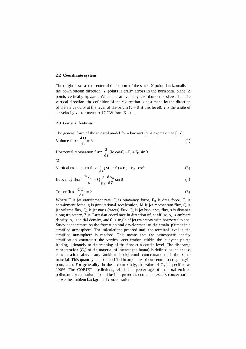
2.2 Coordinate system The origin is set at the center of the bottom of the stack. X points horizontally in the down stream direction. Y points laterally across in the horizontal plane. Z points vertically upward. When the air velocity distribution is skewed in the vertical direction, the definition of the x direction is best made by the direction of the air velocity at the level of the origin (τ = 0 at this level). τ is the angle of air velocity vector measured CCW from X-axis. 2.3 General features The general form of the integral model for a buoyant jet is expressed as [15]:

Volume flux: E s dQ d= (1)

Horizontal momentum flux: sin F F ) cos (M s d d

De θ+=θ

(2)

Vertical momentum flux: θ−=)θ cos F F sin (Ms d d

Db (3)

Buoyancy flux: θρ

ρ= sin

Zd dg Q

s dQ d a

o

g (4)

Tracer flux: 0 s d

Q d c = (5)

Where E is jet entrainment rate, Fb is buoyancy force, FD is drag force, Fe is entrainment force, g is gravitational acceleration, M is jet momentum flux, Q is jet volume flux, Qc is jet mass (tracer) flux, Qg is jet buoyancy flux, s is distance along trajectory, Z is Cartesian coordinate in direction of jet efflux, ρa is ambient density, ρo is initial density, and θ is angle of jet trajectory with horizontal plane. Study concentrates on the formation and development of the smoke plumes in a stratified atmosphere. The calculations proceed until the terminal level in the stratified atmosphere is reached. This means that the atmosphere density stratification counteract the vertical acceleration within the buoyant plume leading ultimately to the trapping of the flow at a certain level. The discharge concentration (Co) of the material of interest (pollutant) is defined as the excess concentration above any ambient background concentration of the same material. This quantity can be specified in any units of concentration (e.g. mg/L, ppm, etc.). For generality, in the present study, the value of Co is specified as 100%. The CORJET predictions, which are percentage of the total emitted pollutant concentration, should be interpreted as computed excess concentration above the ambient background concentration.

2.4 Test cases Different test cases are investigated for a single stack and a combination of three stacks. As well as the meteorological fields, the stack parameters (emission velocity and temperature, and stack height and relative location) were obtained through personal communications and field measurements. Wind speed is assumed to obey the power law. Test cases cover a wide range of wind speed (U) from 0.0 to 16.0 m/s (57.6 km/hr). Thus, the different wind speed categories (breeze, light wind, and strong wind) are covered. Emission speed (Vo) of the stack discharge varies from 0.5 m/s to 10 m/s. The emission angle (a) of discharge varies from 0.0 to 180 deg. relative to the wind direction. Stack height (Ho) varies from 10 to 100 m. Discharge temperature is kept constant at the value of 200 oC. The pollutant is considered as non-conservative, fairly rapidly decaying substance with a decay rate of 1 per minute or 0.0028/s. 3 Results and discussion The plume characteristics (maximum distance, smax, maximum height, hmax, and maximum diameter, dmax) for a single stack are presented firstly. These characteristics are taken when the plume reaches the terminal level in the stratified atmosphere and calculations stop. Then, the cases of multiple stacks are studied. The results represent time-averaged values and figures. 3.1 A single stack Fig. 1 shows the views of a plume emitting from a 10 m-height stack with a vertical discharge angle (a) of 90 deg. The free stream wind speed (U) is 5 m/s. The plume continues to develop and climb up until it reaches a terminal level where it stops developing. The variations of the plume maximum distance (smax), travelled by the plume, maximum height (hmax), and maximum diameter (dmax) with wind speed are shown in Figs. 2, 3, and 4, respectively, for different emission speeds (from 0.5 to 10 m/s) and a = 90 deg. Generally, the characteristic values increase with the emission speed (Vo). Fig. 2 shows that there is a peak value for the maximum distance (smax). The corresponding wind speed to this peak depends on the emission speed. This peak moves in the direction of increasing the wind speed as the emission speed increases. Fig. 3 illustrates that the maximum height (hmax) is reached when the air is calm (U ≅ 0). Increasing the wind speed decreases the maximum height reached by the plume. Fig. 4 shows that the peak value of the maximum diameter (dmax) is at a wind speed of 1 m/s for the particular conditions present here. It is obvious that the increase of the wind speed above a certain limit (e.g. U = 12 m/s for Vo = 0.5 m/s), the plume doesn’t even exist and the emitted pollutant is dispersed by the coming wind. The effect of stack height (from 0 to 100m) on the plume maximum travelling distance, height, and diameter are shown in Figs. 5, 6, and 7, respectively, for different emission speeds and a = 90 deg. Fig. 5 shows that

the stack height has almost no effect on the maximum distance for small emission speeds (up to 3 m/s). Then, a dramatic effect appears at Vo = 5 and 10 m/s. The maximum distance decreases up till Ho = 30 m/s, then increases gradually up till Ho = 80 m where it gains a constant value (smax = 1680 m). The variation of the plume maximum height (hmax) with the stack height (Ho) is shown in Fig. 6. For Vo = 0.5 and 1.5 m/s, the relation between hmax and Ho is almost linear. hmax increases gradually with Ho. In Fig. 7, the behavior of the plume maximum diameter (dmax) is similar to that of the maximum distance (smax) shown in Fig. 5, except that the two curves of Vo = 5 and 10 m/s don’t meet together. The angle of discharge from the stack has no effect on the plume characteristics as seen in Fig. 8 for Vo = 5 m/s. Fig. 9 shows the variation of the temperature difference (between the centerline of the plume and the ambient atmosphere), ΔT, with the distance along the centerline of the plume, s, at different wind speeds (from 0.5 to 10 m/s) and a = 90 deg. As it is expected, ΔT decreases to zero as s increases. An interesting phenomenon is noticed. As the wind speed increases (U = 5 m/s and 10 m/s). ΔT increases nearby the stack to values above that of the stack exit, then drops quickly. This may be attributed to heat concentration at the centerline of the plume. 3.2 Three stacks Fig. 10 shows a general view of three plumes emitting from three different stacks in calm air (U ≅ 0). The parameters of the three stacks are as follows:

Stack Height (Ho)

Outlet diameter (Do)

Emission speed (Vo)

Emission angle (a)

1 40 m 1 m 1.5 m/s 90 deg. 2 35 m 1.2 m 1.5 m/s 90 deg. 3 16 m 3 m 1.5 m/s 90 deg.

Plumes move directly in the vertical direction. Each plume resembles the form of a series of continuous puffs. Fig. 11 shows the views of the three plumes at a wind speed of 7 m/s in a different arrangement. Two of the three plumes interfere to each other. Interference of pollutant plumes is of a primary importance because the increase of the pollutant concentration is expected in the areas of interference. Fig. 12 shows a contour map of the concentration distribution of three interfering plumes at a cross section (y-z plane), s = 1000 m. As can be seen, the maximum concentration of the pollutant is found in the interference areas. 4 Conclusions The present investigation is a parametric study of the different factors that affect the plume characteristics of a single or multiple stacks. Based on the above results and discussion, the following conclusions can be stated:

1. There is a peak value for the plume maximum distance (smax) that depends on both the wind speed (U) and emission speed (Vo).

2. Maximum plume height (hmax) is reached when the air is calm (U ≅ 0). 3. The stack height has almost no effect on the plume maximum distance (smax)

and maximum diameter (dmax) for small emission speeds (up to 3 m/s). 4. For low emission speed (e.g. Vo = 0.5 m/s), the relation between the plume

maximum height (hmax) and the stack height (Ho) is almost linear. 5. Emission angle has no effect on the plume characteristics. 6. Pollutant concentration greatly increases in the areas of plume interference.

Thus, stacks should be arranged to minimize the possibility of interference between pollutant plumes.

The authors wish that the present investigation would lead to further theoretical studies and experimental verifications of the air pollution problems in Egypt. References [1] Božnar, M., Brusasca, G., Cavicchioli, C., Faggian, P., Finardi, S., Mlakar,

P., Morselli, M. G., Sozzi, R. & Tinarelli, G., Application of advanced and traditional diffusion models to an experimental campaign in complex terrain. Proc. of the 2nd Int. Conf. On Air Pollution, Barcelona, Spain, Computational Mechanics Publications, Boston, MA, USA, pp. 159-166, 1994.

[2] Dean, D., Atchison, M. K. & Seely, S., Operational evaluation of forecast and diagnostic atmospheric models in a complex terrain environment. Proc. of the 89th Annual Meeting & Exhibition, Air & Waste Management Assoc., Nashville, Tennessee, USA, No. 96-WA63.03, 1996.

[3] Dean, D., Atchison, M. K. & Seely, S., On the effect of data availability on model performance in a complex terrain environment. Proc. of the 90th Annual Meeting & Exhibition, Air & Waste Management Assoc., Toronto, Ontario, Canada, No. 97-WA69.05, 1997.

[4] Kassomenos, P., Lykoudis, S. & Petrakis, M., Vertical distribution of air pollutants released from elevated stacks in the Athens area. Proc. of the 4th Int. Conf. On Air Pollution, Toulouse, France, Monitoring, Simulation, and Control, Computational Mechanics Publications, Southampton, UK, pp. 677-686, 1996.

[5] Kassomenos, P., Lykoudis, S. & Petrakis, M., On the behaviour of air pollutants released from elevated stacks in the vicinity of Athens, Greece. Int. J. Environment and Pollution, 8(1/2), pp. 134-147, 1997.

[6] Cinotti, S., Gianfelici, F., Giovannini, I., Levy, A. & Tirabassi, T., Comparison of operational atmospheric pollutant diffusion models in actual situations. Proc. of the 5th Int. Conf. On Air Pollution, Bologna, Italy, Modelling, Monitoring and Management, Computational Mechanics Inc., Billerica, MA, USA, pp. 423-432, 1997.

[7] Bonfiglio, A., Macchiato, M., Minervini, L., Ragosta, M. & Santangelo, R., Pollutant diffusion model and G.I.S. integration procedure for evaluating atmospheric emissions in industrial areas. Proc. of the 6th Int. Conf. On Air

Pollution, Genoa, Italy, Computational Mechanics Publications, Boston, MA, USA, pp. 849-858, 1998.

[8] De Haan, P. & Rotach, M. W., A puff-particle dispersion model. Int. J. Environment and Pollution, 5(4-6), pp. 350-359, 1995.

[9] Liu, F. & Hong, Y., Applications of the dust diffusion model method in China. J. Aerosol Sci., 27(1), pp. S93-S94, 1996.

[10] Trunev, A. P., Similarity theory and model of diffusion in turbulent atmosphere at large scales. Proc. of the 5th Int. Conf. On Air Pollution, Bologna, Italy, Modelling, Monitoring and Management, Computational Mechanics Inc., Billerica, MA, USA, pp. 423-432, 1997.

[11] Kadja, M., Anagnostopoulos, J. S. & Bergeles, G. C., Development of an implicit air pollution model for regions of variable topography. J. Environmental Modelling & Software, 13, pp. 151-161, 1998.

[12] Yoshikawa, Y. & Kunimi, H., Numerical simulation model for predicting air quality along urban main roads: first report, development of atmospheric diffusion model. J. Heat Transfer-Japanese Research, 27(7), pp. 483-496, 1998.

[13] Craig, K. J., De Kock, D. J. & Snyman, J. A., Using CFD and mathematical optimization to investigate air pollution due to stacks. Int. J. Numer. Meth. Engng., 44, pp. 551-565, 1999.

[14] Kumar, P. C. & Wehrmeyer, J. A., Stack gas pollutant detection using Laser Raman Spectroscopy. J. Applied Spectroscopy, 51(6), pp. 849-855, 1997.

[15] Jirka, G. H. & Fong, H. L. M., Vortex dynamics and bifurcation of buoyant jets in crossflow. J. Engineering Mechanics Division, ASCE, 107, pp. 479-499, 1981.

[16] Jirka, G. H., Doneker, R. L. & Hinton, S. W., User’s manual for CORMIX: a hydrodynamic mixing zone model and decision support system for pollutant discharges into surface waters, DeFrees Hydraulics Laboratory, School of Civil and Environmental Engineering, Cornell University, 1996.

[17] Jirka, G. H., Akar, P. J. & Nash, J. D., Enhancements to the CORMIX mixing zone expert system: technical background, Tech. Rep., DeFrees Hydraulics Laboratory, School of Civil and Environmental Engineering, Cornell University, 1996.

0 2 4 6 8 10 12 14 16Wind speed (m/s)

0

500

1000

1500

2000

2500

Plum

em

axim

umdi

stan

ce(m

)

Emission speed= 0.5 m/sEmission speed = 1.5 m/sEmission speed = 3.0 m/sEmission speed = 5.0 m/sEmission speed = 10.0 m/s

10

20

30

Z(m

)

0100

200300

400500

X (m)20

30Y (m)

YX

Z

Figure 1a: General view of the plume, U=5 m/s,Ho=10 m, Do=1.2 m, and a=90 deg.

2030

0 100 200 300 400 500X (m)

0

10

20

30

40

Z(m

) Y X

Z

Figure 1b: Side view of the plume, U=5 m/s,Ho=10 m, Do=1.2 m, and a=90 deg.

20

25

30

Y(m

)

0 200 400X (m)

Z X

Y

Figure 1c: Plan view of the plume, U=5 m/s,Ho=10 m, Do=1.2 m, and a=90 deg.

Figure 2: Variation of plume maximum distance withwind speed, Ho=10 m, and Do=1.2 m.

10 20 30 40 50 60 70 80 90 100Stack height (m)

40

60

80

100

120

140

160

180

Plum

em

axim

umhe

ight

(m)

Emission speed= 0.5 m/sEmission speed= 1.5 m/sEmission speed= 3.0 m/sEmission speed= 5.0 m/sEmission speed= 10.0 m/s

10 20 30 40 50 60 70 80 90 100Stack height (m)

0

200

400

600

800

1000

1200

1400

1600

1800

Plum

em

axim

umdi

stan

ce(m

)

Emission speed= 0.5 m/sEmission speed= 1.5 m/sEmission speed= 3.0 m/sEmission speed= 5.0 m/sEmission speed= 10.0 m/s

0 2 4 6 8 10 12 14 16Wind speed (m/s)

20

40

60

80

100

120

140

160

180

200

Plum

em

axim

umhe

ight

(m)

Emission speed= 0.5 m/sEmission speed= 1.5 m/sEmission speed= 3.0 m/sEmission speed= 5.0 m/sEmission speed= 10.0 m/s

0 2 4 6 8 10 12 14 16Wind speed (m/s)

10

20

30

40

50

60

Plum

em

axim

umdi

amet

er(m

) Emission speed= 0.5 m/sEmission speed= 1.5 m/sEmission speed= 3.0 m/sEmission speed= 5.0 m/sEmission speed= 10.0 m/s

Figure 3: Variation of plume maximum heightwith wind speed, Ho=10 m, and Do=1.2 m.

Figure 4: Variation of plume maximum diameterwith wind speed, Ho=10 m, and Do=1.2 m.

Figure 5: Variation of plume maximum distancewith stack height, U=5 m/s, and Do=1.2 m.

Figure 6: Variation of plume maximum height withstack height, U=5 m/s, and Do=1.2 m.

Figure 7: Variation of plume maximum heightwith wind speed, U=5 m/s, and Do=1.2 m.

10 20 30 40 50 60 70 80 90 100Stack height (m)

05

1015202530354045505560

Plum

em

axim

umdi

amet

er(m

)

Emission speed= 0.5 m/sEmission speed= 1.5 m/sEmission speed= 3.0 m/sEmission speed= 5.0 m/sEmission speed= 10.0 m/s

Figure 8: Variation of plume characteristic distanceswith emission angle, U=5 m/s, and Ho=10 m, Do=1.2 m.

0 30 60 90 120 150 180Emission angle, a (deg)

101

102

103

Dis

tanc

e(m

)

Plume maximum distancePlume maximum heightPlume maximum diameter

0 10 20 30 40 50 60 70 80Y (m)

30

40

50

60

70

80

Z(m

)

C195182169156143130117104917865523926130

100

200

Z(m

)0

100200

300400

X (m)

0100Y (m)

XY

Z

12

3

Figure 9: Variation of temperature difference withdistance, Ho=10 m, Do=1.2 m, and Vo=5 m/s.

0 100 200 300 400 500Distance along the centerline of the plume, s (m)

0

20

40

60

80

100

120

140

160

180

200

Tem

pera

ture

dife

renc

e(d

eg)

Wind speed = 0.5 m/sWind speed = 1.5 m/sWind speed = 3.0 m/sWind speed = 5.0 m/sWind speed = 10.0 m/s

Figure 10: General view of three plumesin calm air.

Figure 11a: General view of three plumes,U=7 m/s.

Figure 12: Contour map of the concentration distributionof three plumes at a certain section (y-z plane),s=1000 m.

50

100

150

Z(m

)

0500

10001500

2000

X (m)0

100Y (m)

XY

Z

0100 Y

100

Z(m

)

0 500 1000 1500 2000X (m)

Y X

Z

Figure 11b: Side view of three plumes,U=7 m/s.

0

50

100

Y(m

)

100 Z

0 500 1000 1500 2000X (m)

X

Y

Z

Figure 11c: Plan view of three plumes,U=7 m/s.