Structure Property Relations in Complex Copolymer Systems
143
Structure Property Relations in Complex Copolymer Systems Dissertation zur Erlangung des Grades ‚Doktor der Naturwissenschaften’ am Fachbereich Chemie der Johannes Gutenberg-Universität in Mainz Ahmad Azhar Juhari Mainz, 2010
-
Upload
khangminh22 -
Category
Documents
-
view
1 -
download
0
Transcript of Structure Property Relations in Complex Copolymer Systems

Structure Property Relations in Complex Copolymer Systems
Dissertation
zur Erlangung des Grades ‚Doktor der Naturwissenschaften’
am Fachbereich Chemie der Johannes Gutenberg-Universität
in Mainz
Ahmad Azhar Juhari
Mainz, 2010


Datum der mündlichen Prüfung: 26. Juli 2010


4
Abstract
A thorough investigation was made of the structure-property relation of well-
defined statistical, gradient and block copolymers of various compositions.
Among the copolymers studied were those which were synthesized using
isobornyl acrylate (IBA) and n-butyl acrylate (nBA) monomer units. The
copolymers exhibited several unique properties that make them suitable materials
for a range of applications. The thermomechanical properties of these new
materials were compared to acrylate homopolymers. By the proper choice of the
IBA/nBA monomer ratio, it was possible to tune the glass transition temperature
of the statistical P(IBA-co-nBA) copolymers. The measured Tg’s of the
copolymers with different IBA/nBA monomer ratios followed a trend that fitted
well with the Fox equation prediction. While statistical copolymers showed a
single glass transition (Tg between -50 and 90 ºC depending on composition),
DSC block copolymers showed two Tg’s and the gradient copolymer showed a
single, but very broad, glass transition. PMBL-PBA-PMBL triblock copolymers
of different composition ratios were also studied and revealed a microphase
separated morphology of mostly cylindrical PMBL domains hexagonally arranged
in the PBA matrix. DMA studies confirmed the phase separated morphology of
the copolymers. Tensile studies showed the linear PMBL-PBA-PMBL triblock
copolymers having a relatively low elongation at break that was increased by
replacing the PMBL hard blocks with the less brittle random PMBL-r-PMMA
blocks. The 10- and 20-arm PBA-PMBL copolymers which were studied revealed
even more unique properties. SAXS results showed a mixture of cylindrical
PMBL domains hexagonally arranged in the PBA matrix, as well as lamellar.
Despite PMBL’s brittleness, the triblock and multi-arm PBA-PMBL copolymers
could become suitable materials for high temperature applications due to PMBL’s
high glass transition temperature and high thermal stability. The structure-
property relation of multi-arm star PBA-PMMA block copolymers was also
investigated. Small-angle X-ray scattering revealed a phase separated morphology
5
of cylindrical PMMA domains hexagonally arranged in the PBA matrix. DMA
studies found that these materials possess typical elastomeric behavior in a broad
range of service temperatures up to at least 250°C. The ultimate tensile strength
and the elastic modulus of the 10- and 20-arm star PBA-PMMA block copolymers
are significantly higher than those of their 3-arm or linear ABA type counterparts
with similar composition, indicating a strong effect of the number of arms on the
tensile properties. Siloxane-based copolymers were also studied and one of the
main objectives here was to examine the possibility to synthesize trifluoropropyl-
containing siloxane copolymers of gradient distribution of trifluoropropyl groups
along the chain. DMA results of the PDMS-PMTFPS siloxane copolymers
synthesized via simultaneous copolymerization showed that due to the large
difference in reactivity rates of 2,4,6-tris(3,3,3-trifluoropropyl)-2,4,6-
trimethylcyclotrisiloxane (F) and hexamethylcyclotrisiloxane (D), a copolymer of
almost block structure containing only a narrow intermediate fragment with
gradient distribution of the component units was obtained. A more dispersed
distribution of the trifluoropropyl groups was obtained by the semi-batch
copolymerization process, as the DMA results revealed more ‘‘pure gradient
type’’ features for the siloxane copolymers which were synthesized by adding F at
a controlled rate to the polymerization of the less reactive D. As with
trifluoropropyl-containing siloxane copolymers, vinyl-containing polysiloxanes
may be converted to a variety of useful polysiloxane materials by chemical
modification. But much like the trifluoropropyl-containing siloxane copolymers,
as a result of so much difference in the reactivities between the component units
2,4,6-trivinyl-2,4,6-trimethylcyclotrisiloxane (V) and hexamethylcyclotrisiloxane
(D), thermal and mechanical properties of the PDMS-PMVS copolymers obtained
by simultaneous copolymerization was similar to those of block copolymers. Only
the copolymers obtained by semi-batch method showed properties typical for
gradient copolymers.
6
Table of Contents
ABSTRACT .................................................................................................................................... 4
OVERVIEW.................................................................................................................................... 8
INTRODUCTION & MOTIVATION ........................................................................................ 10
1 METHODOLOGICAL SYSTEMS.................................................................................... 15
1.1 DYNAMIC MECHANICAL ANALYSIS ............................................................................... 15 1.1.1 Definitions................................................................................................................. 15 1.1.2 Oscillatory response of real systems......................................................................... 23 1.1.3 Mechanical models of linear viscoelasticity ............................................................. 27 1.1.4 Thermorheological simplicity and time-Temperature superposition ........................ 32 1.1.5 Origin of the liquid-to-glass “transition”................................................................. 36 1.1.6 Proposed fit function for the master curve................................................................ 47
1.2 SMALL ANGLE X-RAY SCATTERING .............................................................................. 48 1.2.1 Bragg’s law............................................................................................................... 49
2 MATERIALS & THEIR CHARACTERIZATION ......................................................... 52
2.1 ACRYLATE-BASED LINEAR COPOLYMERS...................................................................... 52 2.2 ACRYLATE-BASED TRIBLOCK AND MULTI-ARM BLOCK COPOLYMERS.......................... 55
2.2.1 PMBL-PBA-PMBL triblock copolymers ................................................................... 56 2.2.2 PBA-PMBL multi-arm block copolymers.................................................................. 57 2.2.3 PBA-PMMA multi-arm block copolymers ................................................................ 59
2.3 SILOXANE-BASED LINEAR GRADIENT COPOLYMERS ..................................................... 60 2.3.1 Fluorosiloxane-based copolymers ............................................................................ 60 2.3.2 Vinylsiloxane-based copolymers............................................................................... 62
2.4 MATERIAL CHARACTERIZATION .................................................................................... 63 2.4.1 Dynamic mechanical analyses (DMA)...................................................................... 63 2.4.2 Differential scanning calorimetry (DSC).................................................................. 65 2.4.3 Small-angle X-ray scattering (SAXS) analyses ......................................................... 65 2.4.4 Tensile tests............................................................................................................... 65
3 RESULTS & DISCUSSION................................................................................................ 66
3.1 COMPARING ACRYLATE-BASED COPOLYMERS TO HOMOPOLYMERS ............................. 66 3.1.1 Statistical P(IBA-co-nBA) copolymers...................................................................... 66
7
3.1.2 Statistical copolymers mimicking homopolymers. .................................................... 73 3.1.3 Gradient P(IBA-grad-nBA) and block PIBA-b-PnBA copolymers ........................... 76
3.2 ACRYLATE-BASED BLOCK COPOLYMERS AS THERMOPLASTIC ELASTOMERS ................ 80 3.2.1 PMBL-PBA-PMBL linear triblock copolymers......................................................... 81 3.2.2 PBA-PMBL multi-arm block copolymers.................................................................. 88 3.2.3 PBA-PMMA multi-arm block copolymers ................................................................ 95
3.3 SILOXANE-BASED LINEAR COPOLYMERS: GRADIENT OR BLOCK? ............................... 102 3.3.1 Fluorosiloxane-based Copolymers ......................................................................... 102 3.3.2 Vinylsiloxane-based Copolymers............................................................................ 112
4 CONCLUSION .................................................................................................................. 122
BIBLIOGRAPHY....................................................................................................................... 126
LIST OF FIGURES.................................................................................................................... 134
LIST OF TABLES...................................................................................................................... 140
8
Overview
The Introduction and Motivation section discusses briefly the development of the
study of copolymers from its infancy to the modern day discoveries and
techniques, as well as its motivation for this particular study. The methodological
systems used will then be discussed in Chapter 1, which covers dynamic
mechanical analysis and small angle X-ray scattering. In Chapter 2, each of the
studied materials as well as the devices involved (rheometer, tensiometer,
calorimeter etc.) are described in detail, with an explanation of the methods used.
Finally, all the findings of this work are discussed in three subchapters in Chapter
3, and are compared with available literature.

9
10
Introduction & Motivation
A polymer is a large molecule composed of many fundamental units, called
monomers, connected by chemical bonds. If these monomers are identical, the
result is a “homopolymer.” If the monomers are of two or more different types,
then the product is a hetero- or copolymer that can either be random or have a
well-defined sequence. Polymers are the most commonly encountered complex
material in the world. With the exception of metals and inorganic compounds,
most of the materials that we come into contact with everyday are polymeric.
These include elastomers in our automobile tires, paints, plastic wall and floor
coverings, foam insulation, and so forth, in our house.
Although there are many varieties of polymers, they all have some common
features. The rapid growth of polymer science over the past few decades has been
due in large part to a deeper understanding of the relationship between the
physical characteristics of polymers and the structure of the polymer molecules. It
has become apparent that molecular properties such as chain length, chain
stiffness, degree of branching, molecular architecture, and the number of charge
groups are more significant than the detailed chemical make-up of polymers in
determining their physical characteristics [1]. An understanding of the relationship
between such molecular properties and the physical characteristics can help
efficiently direct the synthesis of new materials with useful properties, as
constantly advancing technologies demand new, high performance and more
specialized materials with highly specialized functions [2-9].
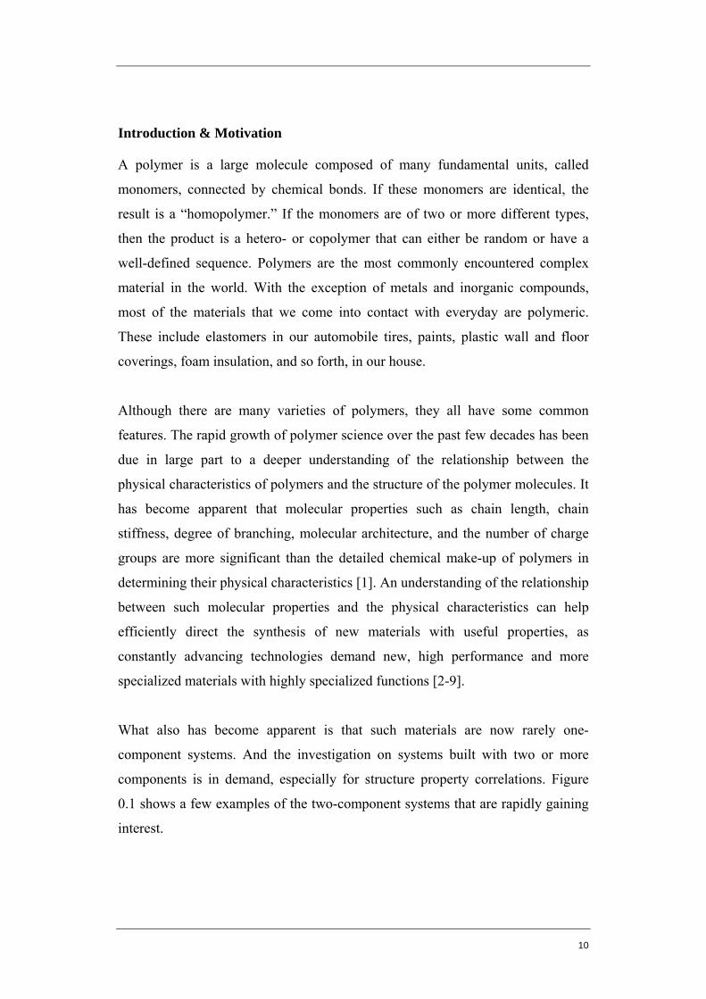
What also has become apparent is that such materials are now rarely one-
component systems. And the investigation on systems built with two or more
components is in demand, especially for structure property correlations. Figure
0.1 shows a few examples of the two-component systems that are rapidly gaining
interest.

11
Figure 0.1. Two component polymer systems, or copolymers.
Multi-component polymer systems can offer a huge potential because they can be
tailor-made for a vast number of applications. However, among the main
challenges in polymer technology today is the exact control of the polymer
architecture, as well as understanding the correlations between chemical structure
or architecture and a material’s characteristics. The pursuit of the design of these
new more specialized, and high performance materials require more precise
control over the polymerization process and over the structure of resulting
polymers. Among the factors to be controlled are: the molecular weight and its
distribution, structural topology of macromolecules, and the type and distribution
of functional groups in the chain.
One example of a two-component system is the block copolymer, in which the
instantaneous composition changes discontinuously and abruptly along the chain.
A block copolymer is composed of two or more sequences of monomers joined
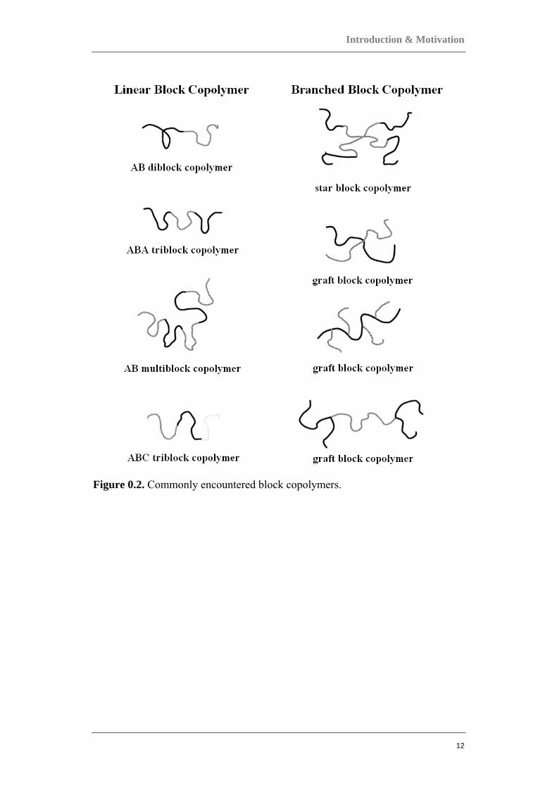
together by chemical bonds. Several commonly encountered block copolymers are
depicted in Figure 0.2. Block copolymers are fascinating materials with unique
mechanical, optical, and structural properties. They can be used as surfactants, as
compatibilizing agents in polymer blends, as adhesives etc.
Introduction & Motivation
12
Figure 0.2. Commonly encountered block copolymers.
13
The most important property of block copolymers is their ability to self-assemble.
Due to the possible incompatibility between different polymer species in a block
copolymer, the very low value of entropy of mixing for macromolecules, and the
fact that the different polymer blocks are connected by chemical bonds, block
copolymers can undergo a microphase separation and assemble into various
ordered structures [10-18]. Recently, self-assembled ordered polymer structures
with periodicities on the nanometer scale have become an important area of study
because of their potential applications in nanotechnology. For instance, it has been
suggested that block copolymers can be used in the development of new classes of
electronic devices [19] and in the synthesis of mesoporous solids that can be used
as catalysts and sorption media [20]. An important factor contributing to the block
copolymers’ widespread popularity is the controllability of the size and
morphology of the microstructure, and hence the material properties, by varying
the molecular weight, molecular architecture, and composition of the copolymers.
Another example of a two-component system, which has gained considerable
interest, is the gradient copolymer, in which instantaneous composition varies
continuously along the chain contour. Latest reports, both theoretical [21-24] and
experimental [25-28] show that the physical properties of gradient copolymers
differ considerably from those of the corresponding block and random
copolymers. The main effects observed were related to differences in local
dynamics, which in the case of the gradient copolymers with their broad range of
local compositions manifests itself in a very broad spectrum of relaxation times of
segmental motions. Qualitatively, in gradient polymers the temperature
dependencies of their dynamic properties and of their microphase separation
morphologies remain the same as compared to diblock copolymers, but changes in
the composition gradients will alter the microphase separation transition
temperature continuously along the temperature scale. The experimental data also
suggest a strong dependence of the morphological and dynamic states of the
gradient copolymer materials on their thermal history.

Introduction & Motivation
14
In contrast to block and gradient copolymers, one other example is the statistical
copolymer, which has a constant composition along the copolymer chain. All
three types of these copolymers that have just been mentioned, even if built with
the same type and number of units, may have completely different properties as a
result of their architecture alone. And it is this relationship that has become the
main motivation for this study. Despite early mechanical and thermodynamic
investigations of statistical, gradient, and block copolymers, there are still many
systems of great industrial and technological interest which can still further
explain the relationship between copolymer architecture and its effects on the
thermomechanical behavior. And it is the focus of this study to explore these
specific systems which have not been studied before.
Figure 0.3. Characterization of the properties of copolymer materials.
15
1 Methodological Systems
A significant portion of the studies reported in this volume involved dynamic
mechanical analysis and X-ray diffraction. This chapter discusses the theory, as
well as the basic underlying concepts behind these two methodological systems.
1.1 Dynamic Mechanical Analysis
Dynamic mechanical analysis (DMA) is a technique used to characterize a
material by analyzing its flow and deformation. A material’s reactions to periodic
variations or oscillations of an applied external mechanical field are recorded. The
possible resulting responses to such a field (stress or strain) are either dissipation
of the input energy in a viscous flow (non-reversible response), or storage of the
energy elastically (reversible response), or a combination of both of these two
extreme cases. Through the use of DMA it is possible to detect variations in both
contributions as a function of temperature or of the frequency of the oscillatory
deformation. The relaxation processes, which govern the behavior of a given
material, can therefore then be determined.
1.1.1 Definitions
Hooke’s and Newton’s law
Polymers are viscoelastic, exhibiting properties of both elastic solids as well as
viscous liquids. It is necessary to derive expressions that relate stress and strain in
order to better understand the mechanical behavior of polymers. For an ideal
elastic solid, Hooke’s law states that
εσ E= (1.1)
where tensile stress σ is the force applied per unit cross-sectional area, and linear
strain ε is the change in length divided by the original length of the material. E is
the material’s Young’s modulus.
Methodological Systems
16
A given force, F when applied to an ideal elastic solid or a spring, is proportional
to x which is the displacement of the spring from its equilibrium position, and can
be expressed as
kxF −= (1.2)
where k is the material specific spring constant.
For cases involving shearing, a shear stress σ is related to the corresponding shear
strain γ by the relationship
γσ G= (1.3)
where G is the shear modulus.
As with ideal elastic solids, an ideal viscous liquid can also be defined. A viscous
liquid obeys Newton’s law of viscosity
yV
∂∂
= ητ (1.4)
where V is the velocity and y is the direction of the velocity gradient in the liquid.
In cases of velocity gradients in single xy plane we can express the following
t∂∂
=γησ (1.5)
where the shear stress σ is directly proportional to the rate of change of shear
strain γ in time t. η is the liquid’s viscosity.
Chapter 1
17
With the assumption that the shear stresses related to stress and strain rate are
additives, a linear viscoelastic behavior can be formulated by combining
equations (1.3) and (1.5) to form the following
tG
∂∂
+=γηγσ (1.6)
which represents one of the simple models for linear viscoelastic behavior known
as the Voigt model, which is discussed in detail in Section 1.1.3.
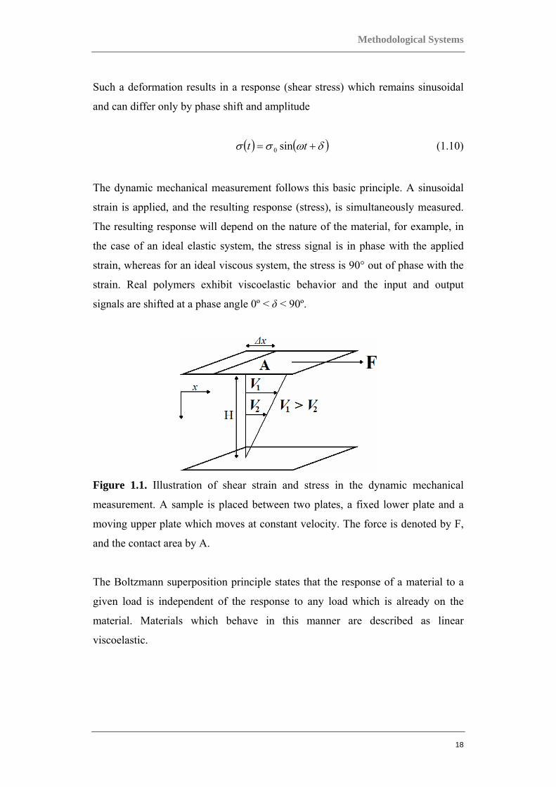
Stress and strain in DMA
Through the use of DMA the relationship between strain (deformation) and the
resulting stress is investigated. In the case where the sample being examined is
confined between two parallel plates (Figure 1.1), where the upper plate moves at
a constant velocity while the lower plate is stationary, the force F needed to move
the upper plate of contact area A can be expressed as
AF σ= (1.7)
where σ is the shear stress, which is constant through the gap. The shear strain
(deformation) is defined as the ratio of the horizontal displacement of the moving
plate Δx, to the distance between the two plates H
HxΔ
=γ (1.8)
In a dynamic mechanical experiment, the applied strain is a time- and frequency-
dependent sinusoidal shear strain of given amplitude 0γ
( ) ( )tt ωγγ sin0= (1.9)
Methodological Systems
18
Such a deformation results in a response (shear stress) which remains sinusoidal
and can differ only by phase shift and amplitude
( ) ( )δωσσ += tt sin0 (1.10)
The dynamic mechanical measurement follows this basic principle. A sinusoidal
strain is applied, and the resulting response (stress), is simultaneously measured.
The resulting response will depend on the nature of the material, for example, in
the case of an ideal elastic system, the stress signal is in phase with the applied
strain, whereas for an ideal viscous system, the stress is 90° out of phase with the
strain. Real polymers exhibit viscoelastic behavior and the input and output
signals are shifted at a phase angle 0º < δ < 90º.
Figure 1.1. Illustration of shear strain and stress in the dynamic mechanical
measurement. A sample is placed between two plates, a fixed lower plate and a
moving upper plate which moves at constant velocity. The force is denoted by F,
and the contact area by A.
The Boltzmann superposition principle states that the response of a material to a
given load is independent of the response to any load which is already on the
material. Materials which behave in this manner are described as linear
viscoelastic.

Chapter 1
19
If the incremental strains Δγ1, Δγ2, Δγ3 etc. are applied to the material at times τ1,
τ2, τ3, respectively, then the total stress at time t can be written as
( ) ( ) ( ) ( ) ...332211 +−Δ+−Δ+−Δ= τγτγτγσ tGtGtGt (1.11)
where the stress relaxation modulus ( )1τ−tG is a decreasing function of time. The
summation of (1.11) can generally be expressed in integral form as
( ) ( ) ( )τγτσ dtGtt
∫∞−
−= (1.12)
Different test geometries in DMA
Oscillatory shear experiments allow four possible sample geometries, depending
on the physical state of material. The different geometries are illustrated in Figure
1.2. For melts, Plate-plate and cone-plate are typically used, while rectangular
bars are more suited for solids, and couette for liquids or polymer solutions.
Figure 1.2. Types of test geometries used for different materials; (a) plate-plate
and (b) cone-plate for the melt, (c) rectangular bars for solids and (d) couette for
polymer solutions or liquids. Geometry (a) was used for this present investigation.
G’ and G”, storage and loss moduli
Properties of linear viscoelastic materials can be described by the storage G’ and
loss G” moduli, which correspond to the elastic and viscous components
respectively. The units of both these moduli are Pa.
Methodological Systems
20
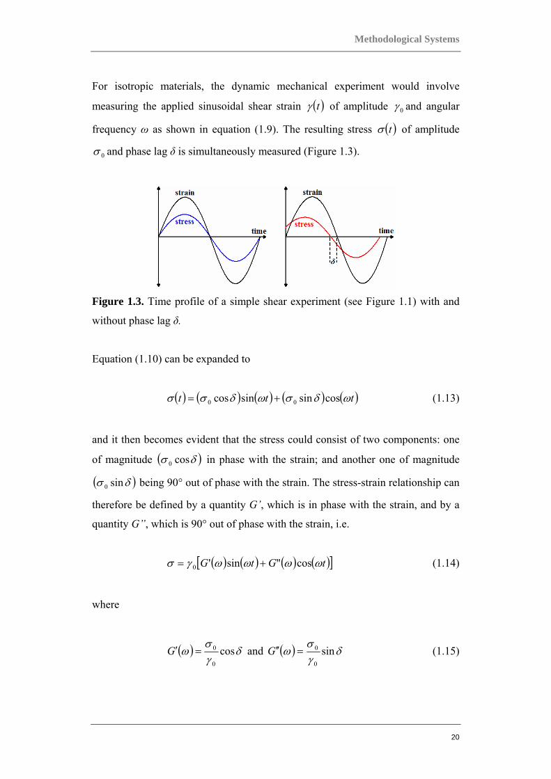
For isotropic materials, the dynamic mechanical experiment would involve
measuring the applied sinusoidal shear strain ( )tγ of amplitude 0γ and angular
frequency ω as shown in equation (1.9). The resulting stress ( )tσ of amplitude
0σ and phase lag δ is simultaneously measured (Figure 1.3).
Figure 1.3. Time profile of a simple shear experiment (see Figure 1.1) with and
without phase lag δ.
Equation (1.10) can be expanded to
( ) ( ) ( ) ( ) ( )ttt ωδσωδσσ cossinsincos 00 += (1.13)
and it then becomes evident that the stress could consist of two components: one
of magnitude ( )δσ cos0 in phase with the strain; and another one of magnitude
( )δσ sin0 being 90° out of phase with the strain. The stress-strain relationship can
therefore be defined by a quantity G’, which is in phase with the strain, and by a
quantity G”, which is 90° out of phase with the strain, i.e.
( ) ( ) ( ) ( )[ ]tGtG ωωωωγσ cos"sin'0 += (1.14)
where
( ) δγσ
ω cos0
0=′G and ( ) δγσ
ω sin0
0=′′G (1.15)

Chapter 1
21
Complex shear modulus
It is convenient to expresse the shear stress and shear strain by using complex
notation due to the phase lag δ
( ) γγωωγγ ′′+′=+=∗ itit sincos0 (1.16)
( ) ( )[ ] ( )[ ]δωσδωδωσσ +=+++=∗ titit expsincos 00 (1.17)
Hence, the complex shear modulus (Figure 1.4) is defined as
( ) GGiiG ′′+′=+=== ∗
∗∗ δ
γσ
δγσ
δγσ
γσ sincosexp
0
0
0
0
0
0 (1.18)
and 22
0
0 GGG ′′+′==∗
γσ (1.19)
Figure 1.4. Diagram showing the complex modulus GiGG ′′+′=∗ . G’
corresponds to the storage modulus (elastically stored energy) and G” to the loss
modulus (dissipated energy).
The compliance J* is also sometimes used instead of the shear modulus G*, and is
defined by
JiJJ ′′−′=* (1.20)
Methodological Systems
22
Therefore we obtain that
22 GGGJ
′′+′′
=′ and 22 GGGJ
′′+′′′
=′′ (1.21)
The loss tangent is also a useful parameter. It is a measure of the ratio of energy
lost (as heat) to energy stored in a material in one cyclic deformation, and is
expressed as
GG
′′′
=δtan (1.22)
The particular temperature dependence of tan δ will make useful as a test of
thermorheological simplicity. The tan δ is sometimes referred to as damping.
Chapter 1
23
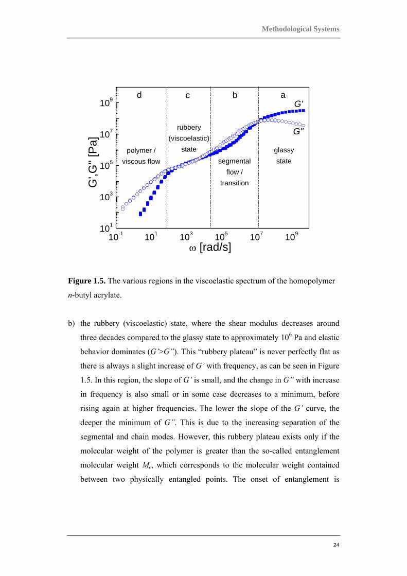
1.1.2 Oscillatory response of real systems
The “master curve,” a typical illustration of the G'(ω) and G'' (ω) behavior for a
homopolymer is illustrated in Figure 1.5, where the frequency dependence for n-
butyl acrylate is shown. The G’ and G” values are in the range of 1 to 109 Pa.
Compare this to the situation in crystalline solids where typically a constant,
frequency independent modulus of about 1011 Pa is obtained. The range of values
of the moduli, which change with temperature and frequency, is characteristic of
polymers and other soft viscoelastic materials. A number of specific regions of the
master curve can be identified, as follows:
a) the glassy state, where an elastic response at the higher frequencies is
observed and the storage modulus G’ predominates and reaches the value of
about 109 Pa. In this region, the polymer lacks molecular mobility since no
motion longer than a segment exists, so it maintains the disordered nature of a
melt. However, limited localized segmental movements are still possible
giving rise to weak sub-glass relaxations. These relaxations are characteristic
of all amorphous polymers and glass-forming liquids in general. The existence
of the segmental flow region indicates a transitional phase between the glassy
and the rubbery (viscoelastic) state. This transition however, is not a real
thermodynamic transition, meaning that there is no heat of fusion associated,
but only a change in the specific heat. The loss modulus (G”) predominates in
this region and decreases slower than G’. This is due to the energy dissipation
in the form of heat, caused by friction in the main chain segments, which
consist of a few repeating units that become mobile and as a result begin to
move. As the temperature continues to increase, an increasing fraction of
chain segments acquire enough energy to overcome the intra- and inter-
molecular forces.
Methodological Systems
24
10-1 101 103 105 107 109101
103
105
107
109
glassystatesegmental
flow /transition
rubbery(viscoelastic)
state
ω [rad/s]
G',G
'' [P
a]
d c b a
polymer /viscous flow
G'
G"
Figure 1.5. The various regions in the viscoelastic spectrum of the homopolymer
n-butyl acrylate.
b) the rubbery (viscoelastic) state, where the shear modulus decreases around
three decades compared to the glassy state to approximately 106 Pa and elastic
behavior dominates (G’>G”). This “rubbery plateau” is never perfectly flat as
there is always a slight increase of G’ with frequency, as can be seen in Figure
1.5. In this region, the slope of G’ is small, and the change in G” with increase
in frequency is also small or in some case decreases to a minimum, before
rising again at higher frequencies. The lower the slope of the G’ curve, the
deeper the minimum of G”. This is due to the increasing separation of the
segmental and chain modes. However, this rubbery plateau exists only if the
molecular weight of the polymer is greater than the so-called entanglement
molecular weight Me, which corresponds to the molecular weight contained
between two physically entangled points. The onset of entanglement is
Chapter 1
25
believed to occur at a critical molecular weight Mc ≈ 2.4Me [29-30]. The
extension of the plateau is proportional to the polymer molecular weight and
the height of the plateau is inversely proportional to Me.
c) the viscous state or the polymer flow region, where dissipation of energy
prevails and G” predominates. At this low frequency, motion of entire chains
takes place. When frequencies are low enough, G” increases linearly with
frequency and G’ is proportional to quadratic frequency. The behavior can be
derived from simple models of viscoelastic systems such as the Maxwell
model, which is discussed later.
Two relaxation processes taking place at specific relaxation times can also
separate the different regions discussed above:
1) At the border between the glassy state and segmental region, the G’ and G”
cross (Figure 1.5). This crossover point is a guide used to determine what is
known as the segmental relaxation time τs, which is given by the inverse of the
frequency at that point ( )1=sωτ . For narrow dispersions, the crossover
frequency is identical to the frequency where G” develops a maximum.
2) The chain relaxation time is determined from the crossover point of G’ and
G” at the border between the rubber region and the viscous state, using
1=cωτ .
These two crossover points and its correspondence to the relaxation times in the
polymer systems are mere approximations. A more accurate measure of the
characteristic relaxation times is the maximum in G”, which is located in the
approximate vicinity of the crossover points for narrow molecular weight
distributions. For broad distributions the crossing of the moduli and the maximum

Methodological Systems
26
in G” are shifted away from each other, making the crossing point a less accurate
indication of the relaxation times.
Both the segmental and chain relaxation times as functions of temperature can be
determined from the following equation
( ) ( ) ( )Tref aTT logloglog += ττ (1.23)
where Tref is the reference temperature and aT is the shift factor. Equation (1.23)
is applicable only for systems that are thermorheologically simple, which is
discussed later.
Entanglement molecular weight
The entanglement of a polymer chain is a type of intermolecular interaction,
which does not involve an energetic change and is purely an entropic and
topological phenomenon. Chain entanglement affects mainly polymer chain
motions. The molecular weight between two adjacent temporary entanglement
points, which is defined as the entanglement molecular weight Me, can be
calculated from the plateau modulus GN as
N
NNe G
RTM
ρ= (1.24)
where ρN is the density of the polymer at temperature TN, at which the plateau
modulus GN is measured and R is the ideal gas constant (R=8.314 Jmol-1K-1). The
value of the plateau modulus, GN can be obtained from the frequency where the
minimum of the loss tangent tan δ is located, shown in the following equation
( )mintanδωGGN ′= (1.25)
Chapter 1
27
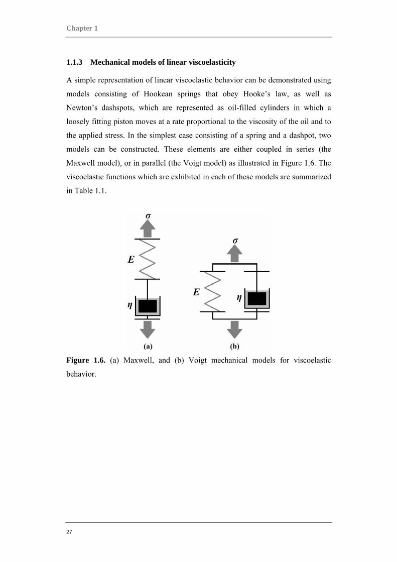
1.1.3 Mechanical models of linear viscoelasticity
A simple representation of linear viscoelastic behavior can be demonstrated using
models consisting of Hookean springs that obey Hooke’s law, as well as
Newton’s dashspots, which are represented as oil-filled cylinders in which a
loosely fitting piston moves at a rate proportional to the viscosity of the oil and to
the applied stress. In the simplest case consisting of a spring and a dashpot, two
models can be constructed. These elements are either coupled in series (the
Maxwell model), or in parallel (the Voigt model) as illustrated in Figure 1.6. The
viscoelastic functions which are exhibited in each of these models are summarized
in Table 1.1.
Figure 1.6. (a) Maxwell, and (b) Voigt mechanical models for viscoelastic
behavior.
Methodological Systems
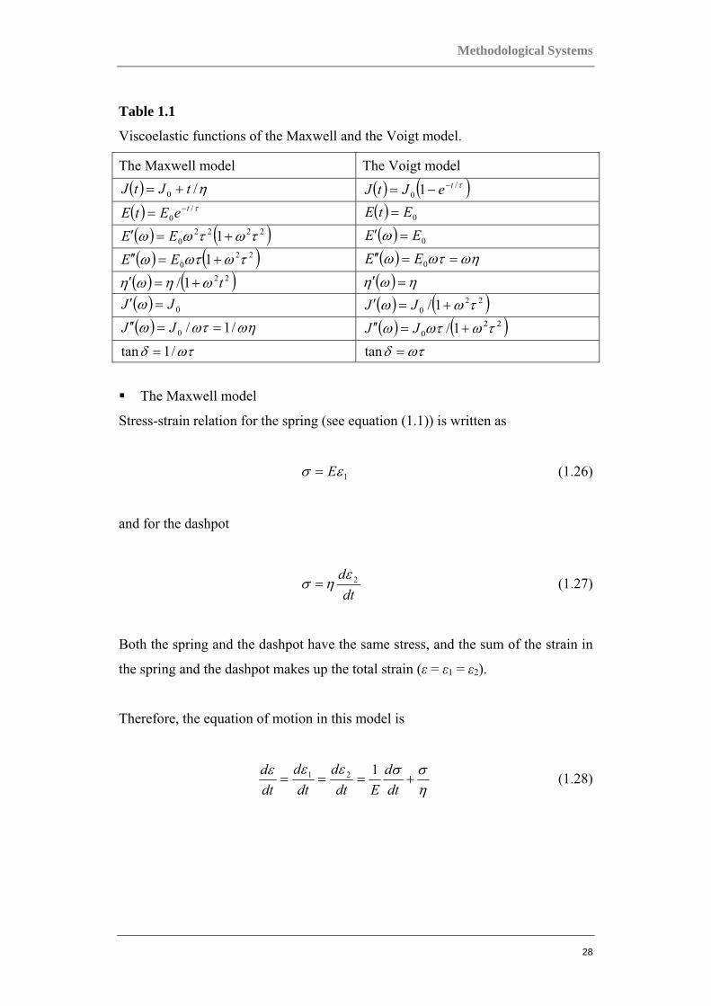
28
Table 1.1
Viscoelastic functions of the Maxwell and the Voigt model.
The Maxwell model The Voigt model ( ) η/0 tJtJ += ( ) ( )τ/
0 1 teJtJ −−= ( ) τ/
0teEtE −= ( ) 0EtE =
( ) ( )22220 1 τωτωω +=′ EE ( ) 0EE =′ ω
( ) ( )220 1 τωωτω +=′′ EE ( ) ωηωτω ==′′ 0EE
( ) ( )221/ tωηωη +=′ ( ) ηωη =′ ( ) 0JJ =′ ω ( ) ( )22
0 1/ τωω +=′ JJ ( ) ωηωτω /1/0 ==′′ JJ ( ) ( )22
0 1/ τωωτω +=′′ JJ ωτδ /1tan = ωτδ =tan
The Maxwell model
Stress-strain relation for the spring (see equation (1.1)) is written as
1εσ E= (1.26)
and for the dashpot
dtd 2ε
ησ = (1.27)
Both the spring and the dashpot have the same stress, and the sum of the strain in
the spring and the dashpot makes up the total strain (ε = ε1 = ε2).
Therefore, the equation of motion in this model is
ησσεεε
+===dtd
Edtd
dtd
dtd 121 (1.28)
Chapter 1
29
Two cases could be considered:
a) stress relaxation for a constant strain (dε/dt = 0)
In this first case,
01=+
ησσ
dtd
E (1.29)
and with the solution
dtEdησ
σ−= (1.30)
integration would then lead to
⎟⎠⎞
⎜⎝⎛−=⎟⎟
⎠
⎞⎜⎜⎝
⎛−=
τσ
ησσ tEt expexp 00 (1.31)
where σ0 is the initial stress at time t = 0, and Eητ = is the relaxation time in
this model. Equation (1.31) shows that in the Maxwell model, the stress decays
exponentially with the time t. It is obvious that the stress relaxation behavior
cannot usually be represented by a single exponential decay term for real
polymers, nor does it necessarily decay to zero at infinite time.
b) constant stress ( 0=dtdσ ).
In this case, from equation (1.28) we obtain that ησε =dtd , which is a constant
value. This would imply that the Maxwell model cannot describe creep. The time
dependence of stress is written as
( )tiωσσ exp0= (1.32)
Methodological Systems
30
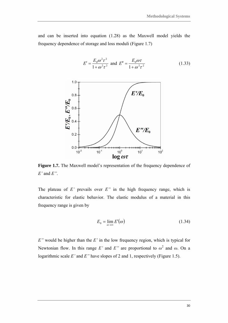
and can be inserted into equation (1.28) as the Maxwell model yields the
frequency dependence of storage and loss moduli (Figure 1.7)
22
220
1 τωτω
+=′ EE and 22
0
1 τωωτ
+=′′ E
E (1.33)
Figure 1.7. The Maxwell model’s representation of the frequency dependence of
E’ and E”.
The plateau of E’ prevails over E” in the high frequency range, which is
characteristic for elastic behavior. The elastic modulus of a material in this
frequency range is given by
( )ωω
EE ′=∞→
lim0 (1.34)
E” would be higher than the E’ in the low frequency region, which is typical for
Newtonian flow. In this range E’ and E” are proportional to ω2 and ω. On a
logarithmic scale E’ and E” have slopes of 2 and 1, respectively (Figure 1.5).
Chapter 1
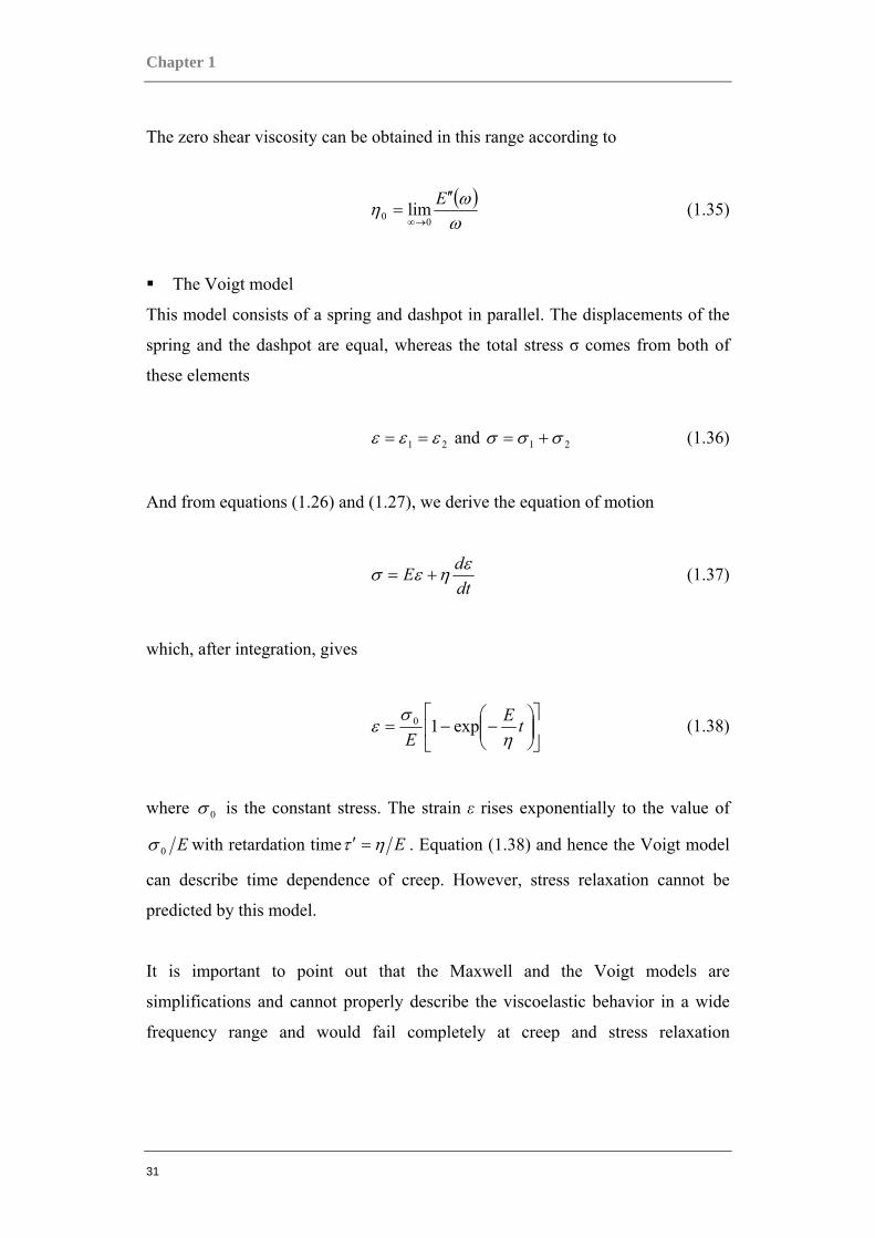
31
The zero shear viscosity can be obtained in this range according to
( )ω
ωη E ′′=
→∞ 00 lim (1.35)
The Voigt model
This model consists of a spring and dashpot in parallel. The displacements of the
spring and the dashpot are equal, whereas the total stress σ comes from both of
these elements
21 εεε == and 21 σσσ += (1.36)
And from equations (1.26) and (1.27), we derive the equation of motion
dtdE εηεσ += (1.37)
which, after integration, gives
⎥⎦
⎤⎢⎣
⎡⎟⎟⎠
⎞⎜⎜⎝
⎛−−= tE
E ησ
ε exp10 (1.38)
where 0σ is the constant stress. The strain ε rises exponentially to the value of
E0σ with retardation time Eητ =′ . Equation (1.38) and hence the Voigt model
can describe time dependence of creep. However, stress relaxation cannot be
predicted by this model.
It is important to point out that the Maxwell and the Voigt models are
simplifications and cannot properly describe the viscoelastic behavior in a wide
frequency range and would fail completely at creep and stress relaxation
Methodological Systems
32
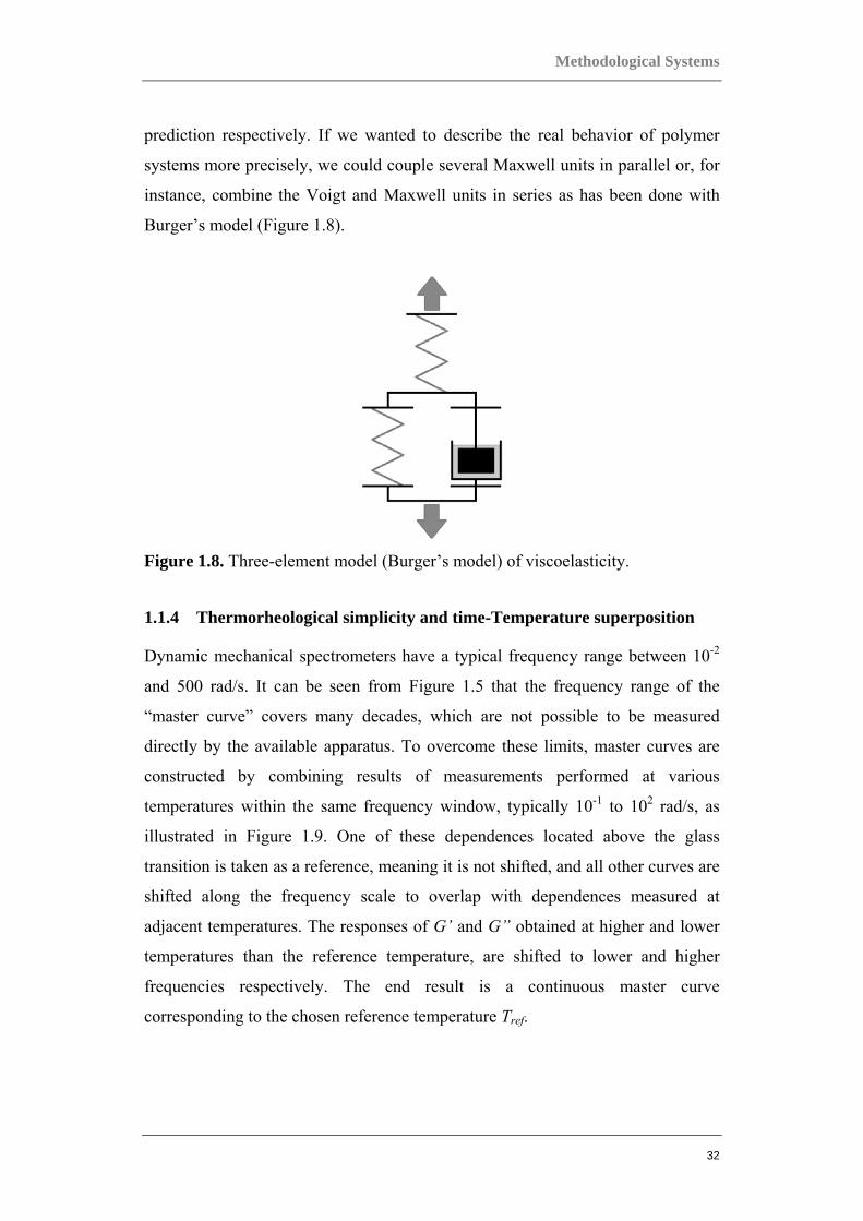
prediction respectively. If we wanted to describe the real behavior of polymer
systems more precisely, we could couple several Maxwell units in parallel or, for
instance, combine the Voigt and Maxwell units in series as has been done with
Burger’s model (Figure 1.8).
Figure 1.8. Three-element model (Burger’s model) of viscoelasticity.
1.1.4 Thermorheological simplicity and time-Temperature superposition
Dynamic mechanical spectrometers have a typical frequency range between 10-2
and 500 rad/s. It can be seen from Figure 1.5 that the frequency range of the
“master curve” covers many decades, which are not possible to be measured
directly by the available apparatus. To overcome these limits, master curves are
constructed by combining results of measurements performed at various
temperatures within the same frequency window, typically 10-1 to 102 rad/s, as
illustrated in Figure 1.9. One of these dependences located above the glass
transition is taken as a reference, meaning it is not shifted, and all other curves are
shifted along the frequency scale to overlap with dependences measured at
adjacent temperatures. The responses of G’ and G” obtained at higher and lower
temperatures than the reference temperature, are shifted to lower and higher
frequencies respectively. The end result is a continuous master curve
corresponding to the chosen reference temperature Tref.
Chapter 1
33
-8 -4 0 42
4
6
8376 K >
380 K >< 393 K
< 413 K
< 473 K
Tref= 384 K
G' G''
log
G',
log
G''
[Pa]
log ω [rad/s]
log(aT)
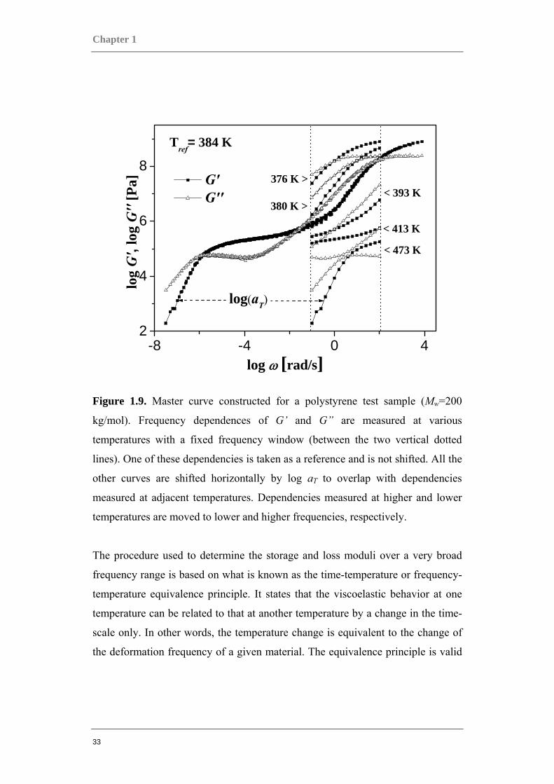
Figure 1.9. Master curve constructed for a polystyrene test sample (Mw=200
kg/mol). Frequency dependences of G’ and G” are measured at various
temperatures with a fixed frequency window (between the two vertical dotted
lines). One of these dependencies is taken as a reference and is not shifted. All the
other curves are shifted horizontally by log aT to overlap with dependencies
measured at adjacent temperatures. Dependencies measured at higher and lower
temperatures are moved to lower and higher frequencies, respectively.
The procedure used to determine the storage and loss moduli over a very broad
frequency range is based on what is known as the time-temperature or frequency-
temperature equivalence principle. It states that the viscoelastic behavior at one
temperature can be related to that at another temperature by a change in the time-
scale only. In other words, the temperature change is equivalent to the change of
the deformation frequency of a given material. The equivalence principle is valid
Methodological Systems
34
only for thermorheologically simple materials, that is, materials where the
distribution of relaxation times does not change with temperature. Therefore,
obviously it does not work in the temperature/frequency range where relaxation
processes with different temperature dependencies of relaxation times overlap.
The principle holds true only for amorphous homopolymers, and does not hold for
semicrystalline polymers, for polymer blends or block copolymers. In the case of
semicrystalline polymers and block copolymers, the reason for the failure of tTs is
the existence of molecular and supramolecular organization that change as a
function of temperature. In the case of immiscible polymer blends, tTs also fails
as a result of the different shift factors for the different components in the blend.
And in the case of miscible polymers, tTs fails again provided that the difference
in the glass transition temperatures (Tg) of the two components is above 40 K.
The Williams-Landel-Ferry (WLF) equation
The G’, G” dependencies obtained at various temperatures and their horizontal
shifts provide directly the temperature dependence of shift factor, log aT (T,Tref ),
as illustrated in Figure 1.10. This relationship between the shift factor and the
temperature can be expressed using the WLF equation, which was postulated by
Williams, Landel and Ferry [31], and written as
( )ref
Tref
T
T TTC
TTCa
ref
ref
−+
−=
2
1log (1.39)
where refTC1 and refTC2 are material dependent constants that depend on the reference
temperature Tref. For comparison purposes, it may be useful to express these
constants in correspondence to another reference temperature, particularly the
glass transition temperature Tg.
Chapter 1
35
The new constants then, gTC1 and gTC2 with Tg as a reference temperature, can be
determined using the following conversion relations
refgT
TTT
TTCCCC
ref
refrefg
−+=
2
211 (1.40)
refgTT TTCC refg −+= 22 (1.41)
Earlier assumptions based on analysis of limited data postulated that gTC1 and gTC2
were universal constants. However, these assumptions was not supported when
the results for a wider variety of viscoelastic materials were considered. From
(1.40) and (1.41), we derive that
refrefgg TTTT CCCC 2121 = (1.42)
∞≡−=− TCTCT refg Tref
Tg 22 (1.43)
where T∞ is the Vogel temperature or the “ideal” glass temperature at which,
regardless of the Tref, log aT becomes infinite in accordance with equation (1.39).
The WLF equation holds true above the glass temperature until Tg + 100 K.
Although the equation was originally based purely on empirical observations, it
can also be derived directly from free volume theories.
Methodological Systems
36
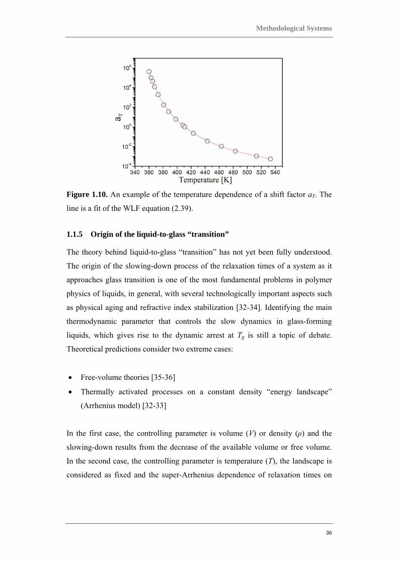
Figure 1.10. An example of the temperature dependence of a shift factor aT. The
line is a fit of the WLF equation (2.39).
1.1.5 Origin of the liquid-to-glass “transition”
The theory behind liquid-to-glass “transition” has not yet been fully understood.
The origin of the slowing-down process of the relaxation times of a system as it
approaches glass transition is one of the most fundamental problems in polymer
physics of liquids, in general, with several technologically important aspects such
as physical aging and refractive index stabilization [32-34]. Identifying the main
thermodynamic parameter that controls the slow dynamics in glass-forming
liquids, which gives rise to the dynamic arrest at Tg is still a topic of debate.
Theoretical predictions consider two extreme cases:
• Free-volume theories [35-36]
• Thermally activated processes on a constant density “energy landscape”
(Arrhenius model) [32-33]
In the first case, the controlling parameter is volume (V) or density (ρ) and the
slowing-down results from the decrease of the available volume or free volume.
In the second case, the controlling parameter is temperature (T), the landscape is
considered as fixed and the super-Arrhenius dependence of relaxation times on

Chapter 1
37
T(τ(T)) is attributed to changes in the barriers and the minima encountered in the
exploration of the landscape. Clearly these cases should be considered as extreme,
since molecular transport in general, is driven by thermal activation processes
with potential energy barriers, which depend on local density [37]. Both
approaches are described below.
A. Free volume theories of the glass “transition”
The theories imply that if conformational changes in the polymer chains are to
take place, there must be space available for the newly rearranged molecular
segments to exist in. The total amount of free space per unit volume of the
polymer is called the fractional free volume Vf. As the temperature of the polymer
system decreases towards the glass temperature, the polymer chains rearrange
themselves to reduce the free volume, to certain point until the polymer chains are
moving so slowly that they cannot rearrange within the time-scale of the
experiment and the volume of the material contracts like that of a solid. If Vg is
the fractional free volume at Tg. So ideally, above this temperature, the fractional
free volume can be written as
( )gfgf TTVV −+= α (1.44)
where αf is the expansion coefficient of free volume.
Based on experimental data for monomeric liquids, Doolittle’s equation [38] finds
a relationship between the viscosity and the free volume via
⎟⎟⎠
⎞⎜⎜⎝
⎛=
fVBAexpη (1.45)
where A and B are constants.
Methodological Systems
38
Taking into account the relationship between zero shear viscosity and the shift
factor
( )( ) T
ref
aTT
=0
0
ηη
(1.46)
we obtain that
⎟⎟
⎠
⎞
⎜⎜
⎝
⎛⎟⎟⎠
⎞⎜⎜⎝
⎛−=
⎟⎟⎠
⎞⎜⎜⎝
⎛
⎟⎟⎠
⎞⎜⎜⎝
⎛
= rff
rf
fT VV
B
VB
VB
a 11exp
exp
exp
(1.47)
where Vf is the fractional free volume at T and rfV is the fractional free volume at
the reference temperature. If the glass transition temperature is set as the reference
temperature and the fractional free volume at this temperature is gfV , then it
would result in the following equation
⎟⎟
⎠
⎞
⎜⎜
⎝
⎛⎟⎟⎠
⎞⎜⎜⎝
⎛−= g
ffT VV
Ba 11exp (1.48)
If we insert equation (1.44) into equation (1.48), it would give
( )
⎟⎟⎟⎟⎟⎟
⎠
⎞
⎜⎜⎜⎜⎜⎜
⎝
⎛
−+⎟⎟⎠
⎞⎜⎜⎝
⎛
−⎟⎟⎠
⎞⎜⎜⎝
⎛−
=
gf
gf
ggf
T
TTV
TTVB
a
α
exp (1.49)
Chapter 1
39
And by taking the logarithm of equation (1.49), the following can be obtained
( )
⎟⎟⎟⎟⎟⎟
⎠
⎞
⎜⎜⎜⎜⎜⎜
⎝
⎛
−+⎟⎟⎠
⎞⎜⎜⎝
⎛
−⎟⎟⎠
⎞⎜⎜⎝
⎛
−=
gf
gf
ggf
T
TTV
TTV
B
a
α
303.2log (1.50)
which is the WLF equation (1.39) with gfVBC 303.21 = and f
gfVC α=2 . It is
shown later that the WLF equation is equivalent to the Vogel Fulcher Tammann
(VFT) equation, and that the latter can also be derived from the free volume
theory.
Vogel-Fulcher-Tammann (VFT) relation
The Vogel-Fulcher-Tammann equation was introduced by Fulcher [39-41] and
Tammann and Hesse [41] and successfully relates viscosity to temperature.
( ) ⎟⎟⎠
⎞⎜⎜⎝
⎛−
=∞TT
BAT exp0η (1.51)
Taking the logarithm of equation (1.51) would give
( ) ⎟⎟⎠
⎞⎜⎜⎝
⎛−
+=∞
∗
TTBAT loglog 0η (1.52)
where 0η is the zero shear viscosity, ( )refTA 0η= , B is the “activation parameter”,
eBB log=∗ and ∞T is a temperature at which the viscosity becomes infinite.
Methodological Systems
40
By taking into account the relationship between zero shear viscosity and
relaxation time
( )( )
( )( ) T
refref
aTT
TT
==ττ
ηη
0
0 (1.53)
we can obtain that
( ) ⎟⎟⎠
⎞⎜⎜⎝
⎛−
=∞TT
BAT expτ (1.54)
( ) ⎟⎟⎠
⎞⎜⎜⎝
⎛−
+=∞
∗
TTBAT loglogτ (1.55)
Both pairs of equations, (1.51, 1.52) as well as (1.54, 1.55), are known as the
Vogel-Fulcher-Tammann (VLF) equation.
Interchangeability of VFT and WLF equations
Using the equation for the temperature dependence of the viscosity (1.52), we
may also formulate the shift factor log aT . Equations (1.53) and (1.52) can give
( )( ) ( ) ( )ref
refT TT
TT
a 000
0 loglogloglog ηηηη
−==
⎟⎟⎠
⎞⎜⎜⎝
⎛
−+−
−+=
∞
∗
∞
∗
TTBA
TTBA
ref
loglog
( )( )⎟⎟⎠
⎞⎜⎜⎝
⎛
−−
−=
∞∞
∗
TTTTTT
Bref
ref
( )∞∞
∗
−+−
−⋅
−=
TTTTTT
TTB
refref
ref
ref
(1.56)
Chapter 1
41
The last part of this equation can be expressed as
( )ref
refT TTC
TTCa
−+
−=
2
1log (1.57)
where
∞
∗
−=
TTBC
ref1 and ∞−= TTC ref2 (1.58)
This illustrates that WLF and VFT equations are in fact the same. A
comprehensive conversion list of VFT into WLF parameters and vice versa can be
written
( ) 1log CTA ref −= τ ( )∞
∗
−+=
TTBAT
refrefτlog
21CCB =∗ ∞
∗
−=
TTBC
ref1
2CTT ref −=∞ ∞−= TTC ref2 (1.59)
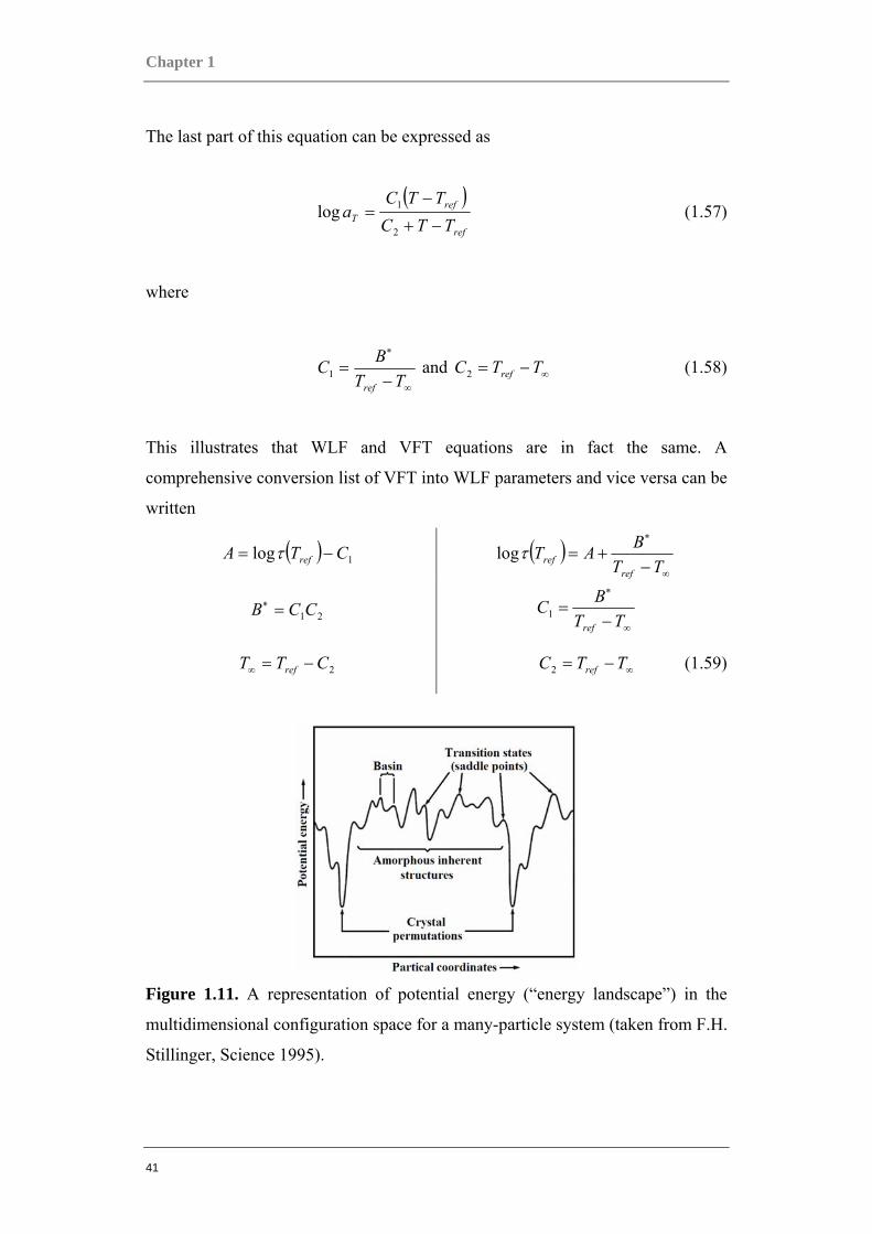
Figure 1.11. A representation of potential energy (“energy landscape”) in the
multidimensional configuration space for a many-particle system (taken from F.H.
Stillinger, Science 1995).
Methodological Systems
42
B. Thermally activated processes
Another approach to the liquid-to-glass transition is related to the thermally
activated processes on a constant “energy landscape” which is considered as fixed
for the entire system, meaning that it does not change upon cooling. A schematic
diagram of such an energy landscape is illustrated in Figure 1.11. Potential energy
depends on the spatial location of all the particles in system, and includes
contributions from various intermolecular as well as intramolecular forces such as
electrostatic polarization effects, covalency, hydrogen bonding, electron-cloud-
overlap repulsions and intermolecular force fields among other things [33]. In
Figure 1.11, the minima correspond to mechanically stable arrangements of all
particles. The smallest displacement from such an arrangement would restore
forces to the non-displaced particles arrangement. Equivalent minima can be
achieved by permutations of identical. Lower lying minima are occupied by the
system provided which is cooled to absolute zero slowly enough to maintain
thermal equilibrium. Pure substances then become virtually perfect crystals [33].
Higher lying minima correspond to less ordered systems with some or completely
amorphous regions.
C. Relative contribution of density and temperature on the segmental dynamics
Liquid-to-glass transition is a contentious issue and the domination of either
density or temperature in controlling the slowing-down process is still an open
question. However, it is possible to determine which of the two parameters plays
the more important role with respect to the dynamics. This can be accomplished
by calculating the ratio of the activation energy at constant volume to enthalpy of
activation ∗∗ HEv . This dynamic quantity provides a quantitative measure of the
relative importance of density and temperature on the dynamics [42] of the α-
process. By defining the enthalpy of activation as
( ) pTRH ⎟⎟
⎠
⎞⎜⎜⎝
⎛∂∂
=∗
1lnτ (1.60)
Chapter 1
43
and the activation energy at constant volume as
( )⎟⎟⎠
⎞⎜⎜⎝
⎛∂∂
=∗
TREV 1
lnτ (1.61)
it can be shown that the ratio ∗∗ HEV can be expressed as
τ⎟⎠⎞
⎜⎝⎛
∂∂
⎟⎠⎞
⎜⎝⎛
∂∂
−=∗ PT
TP
HE
V
V 1*
(1.62)
PT
TPV
TP
PTHE
⎟⎠⎞
⎜⎝⎛
∂∂
⎟⎠⎞
⎜⎝⎛
∂∂
⎟⎠⎞
⎜⎝⎛
∂∂
⎟⎠⎞
⎜⎝⎛
∂∂
−=∗ τρ
τρ
ln
ln
1*
(1.63)
P
TV
HE
⎟⎟⎠
⎞⎜⎜⎝
⎛∂
∂
⎟⎟⎠
⎞⎜⎜⎝
⎛∂
∂
−=∗
ρτ
ρτ
ln
ln
1*
(1.64)
Because a change in temperature (T) would affect both the thermal energy (kBT)
and the density (ρ), it is impossible to separate the two effects by T alone. To
disentangle the effects of T and ρ on the dynamics, pressure-dependent
measurements have been invaluable [43-44] since pressure (P) can be applied
isothermally, therefore affecting only ρ, and have been used to provide a
quantitative assessment of their relative importance. Not only do the pressure-
dependent experiments provide the Tg(P) dependence, but it also provides the
origin of the freezing of the segmental relaxation times (τS) at the liquid-to-glass
transition. Measuring the relaxation times, for example, as a function of the
thermodynamic variables T and P, coupled with the equation of state would allow
quantifying the role of temperature and density on the segmental dynamics [42,
Methodological Systems
44
45-46]. The ∗∗ HEv ratio can vary from 0, for volume dominated dynamics, to 1,
where thermal energy dominates. The monomeric volume plays a key role in
controlling the actual value [47]. In principle, this ratio can be calculated for any
substance provided that it is possible to measure the τS(T) and τS(P) dependencies
normally through dielectric spectroscopy measurements and the equation of state
from PVT measurements.
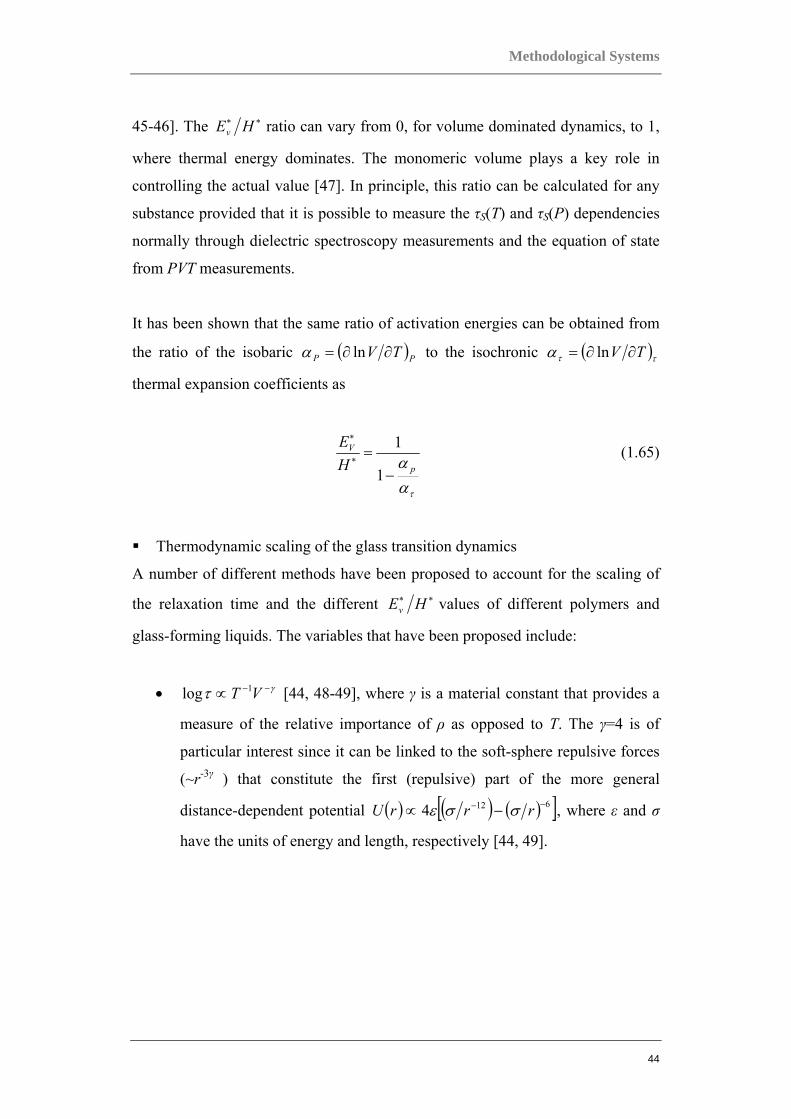
It has been shown that the same ratio of activation energies can be obtained from
the ratio of the isobaric ( )PP TV ∂∂= lnα to the isochronic ( )ττα TV ∂∂= ln
thermal expansion coefficients as
ταα p
V
HE
−=∗
∗
1
1 (1.65)
Thermodynamic scaling of the glass transition dynamics
A number of different methods have been proposed to account for the scaling of
the relaxation time and the different ∗∗ HEv values of different polymers and
glass-forming liquids. The variables that have been proposed include:
• γτ −−∝ VT 1log [44, 48-49], where γ is a material constant that provides a
measure of the relative importance of ρ as opposed to T. The γ=4 is of
particular interest since it can be linked to the soft-sphere repulsive forces
(~r-3γ ) that constitute the first (repulsive) part of the more general
distance-dependent potential ( ) ( ) ( )[ ]6124 −− −∝ rrrU σσε , where ε and σ
have the units of energy and length, respectively [44, 49].
Chapter 1
45
• lnτ ∝ ρ − ρ∗( )T −1, where ρ is an adjustable parameter. In many cases, this
thermodynamic scaling gives equally good results [50-52] the T and ρ
ranges are extremely large [52].
• monomer volume Vm and its correlation to the dynamic quantity ∗∗ HEv .
It has been shown that mv VHE 77.072.0~ −∗∗ for a series of glass-
forming liquids. This would suggest that the reason for the low ∗∗ HEv values in a number of glass-forming liquids and polymers is their
large monomer size. This proposed method suggests that monomer volume
and local packing play an important role in controlling the dynamics.
D. Parameters beyond free volume and thermal activation
Molecular transport is generally driven by thermal activation processes with
potential energy barriers E that depend on local density [37]. The probabilities for
local rearrangements can by given by
( ) ( )⎟⎠⎞
⎜⎝⎛−=
kTVETVP exp, (1.66)
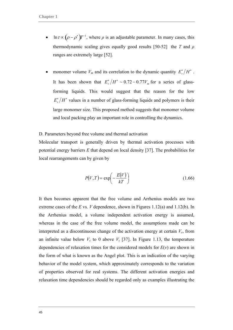
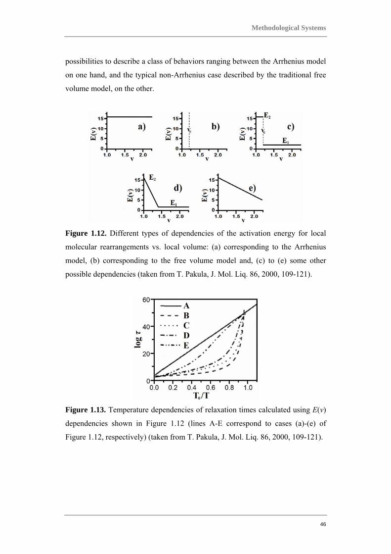
It then becomes apparent that the free volume and Arrhenius models are two
extreme cases of the E vs. V dependence, shown in Figures 1.12(a) and 1.12(b). In
the Arrhenius model, a volume independent activation energy is assumed,
whereas in the case of the free volume model, the assumptions made can be
interpreted as a discontinuous change of the activation energy at certain Vc, from
an infinite value below Vc to 0 above Vc [37]. In Figure 1.13, the temperature
dependencies of relaxation times for the considered models for E(v) are shown in
the form of what is known as the Angel plot. This is an indication of the varying
behavior of the model system, which approximately corresponds to the variation
of properties observed for real systems. The different activation energies and
relaxation time dependencies should be regarded only as examples illustrating the
Methodological Systems
46
possibilities to describe a class of behaviors ranging between the Arrhenius model
on one hand, and the typical non-Arrhenius case described by the traditional free
volume model, on the other.
Figure 1.12. Different types of dependencies of the activation energy for local
molecular rearrangements vs. local volume: (a) corresponding to the Arrhenius
model, (b) corresponding to the free volume model and, (c) to (e) some other
possible dependencies (taken from T. Pakula, J. Mol. Liq. 86, 2000, 109-121).
Figure 1.13. Temperature dependencies of relaxation times calculated using E(v)
dependencies shown in Figure 1.12 (lines A-E correspond to cases (a)-(e) of
Figure 1.12, respectively) (taken from T. Pakula, J. Mol. Liq. 86, 2000, 109-121).

Chapter 1
47
1.1.6 Proposed fit function for the master curve
To describe more completely the frequency dependence of storage and loss
moduli, all the master curves were successfully fitted to the following function
( ) ( ) ( ) ( ) ⎟⎠⎞
⎜⎝⎛
++
+= −−−−−−−− 24231211 10101010
log 21ltxbltxbltxbltxb
AAy (1.67)
( ) ( ) ( ) ( ) ⎟⎠⎞
⎜⎝⎛
++
+= −−−−−−−− 24231211 10101010
log 21ltxcltxcltxcltxc
AAz (1.68)
where A1 and A2 are related to the height of the plateaus of the real part of the
modulus (storage modulus) above the frequency corresponding to the reciprocal
relaxation time slt τlog1 −= , clt τlog2 = , where sτ and cτ are the segmental and
chain relaxation times, respectively. The parameters b1 to b4, and c1 to c4 describe
the slopes on both sides of the characteristic frequency related to the reciprocal
relaxation. These fit parameters are illustrated in Figure 1.14.
ω [rads-1]
A1
A2
-logτs
b2
c2c1
b1
b4
c4
G'G"
c3
b3-logτc
G',G
" [P
a]
Figure 1.14. Fit parameters of the empirical function (equation (1.67)).
Methodological Systems
48
1.2 Small Angle X-Ray Scattering
Small-angle X-ray scattering (SAXS), which involves X-rays of wavelength 0.1 to
0.2 nm, is capable of delivering structural information of macromolecules
between 5 and 25 nm, of repeat distances in partially ordered systems of up to
150 nm [53].
X-ray scattering occurs as a result of the interaction of X-rays with electrons in
the material. The X-rays scattered from different electrons interfere with each
other and produce a diffractive pattern that varies, if the material is not
homogeneous, with scattering angle. The variation of the scattered intensity with
angle provides information on the electron density distribution, and hence the
atomic positions in the material.
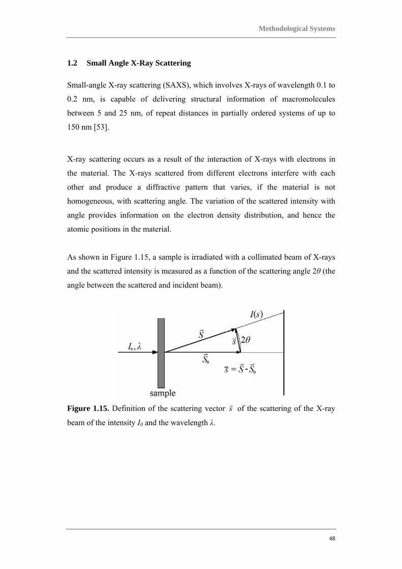
As shown in Figure 1.15, a sample is irradiated with a collimated beam of X-rays
and the scattered intensity is measured as a function of the scattering angle 2θ (the
angle between the scattered and incident beam).
Figure 1.15. Definition of the scattering vector sv of the scattering of the X-ray
beam of the intensity I0 and the wavelength λ.
Chapter 1
49
The incident beam is described by the unit vector 0Sv
, while the scattered beam by
Sv
. The scattering vector sv is defined as
λ0SSsvv
v −= (1.76)
where λ is the wavelength of the X-rays. The length of the scattering vector sv can
then be written as
λθsin2
=s (1.77)
SAXS patterns are typically represented as scattered intensity as a function of the
magnitude of the scattering vector
q =4π sinθ
λ (1.78)
where 2θ is the angle between the incident X-ray beam and the detector
measuring the scattered intensity.
1.2.1 Bragg’s law
Bragg's law states that when X-rays hit an atom, they make the electronic cloud
move, as does any electromagnetic wave. The movement of these charges re-
radiates waves with the same frequency, and this phenomenon is known as
Rayleigh scattering, or elastic scattering. The scattered waves can themselves be
scattered but this secondary scattering is assumed to be negligible. These re-
emitted wave fields interfere with each other either constructively or
destructively, producing a diffraction pattern on a detector. This resulting wave

Methodological Systems
50
interference pattern is the basis of diffraction analysis. X-ray wavelengths are
comparable with inter-atomic distances (~150 pm) and thus are an excellent probe
for this length scale.
When phase shift is a multiple of 2π, then the interference is constructive, and this
condition can be expressed by Bragg's law [53]. Suppose that a single
monochromatic wave is incident on aligned planes of lattice points, with
separation d, at angle θ, as shown in Figure 1.16.
Figure 1.16. An illustration of the Bragg’s law.
If we observe the figure, we see that there is a path difference between the ray that
gets reflected along AC' and the ray that gets transmitted, and then reflected, along
AB and BC respectively. This path difference is
(AB + BC) − (A ′ C )

Chapter 1
51
The two separate waves will arrive at a point with the same phase, and hence
undergo constructive interference, only if this path difference is equal to any
integer value of the wavelength
(AB + BC) − (A ′ C ) = nλ
where n is an integer determined by the order given, λ is the wavelength of the X-
rays, d, as shown in Figure 1.16, is the spacing between the planes in the lattice,
and θ is the angle between the incident ray and the scattering planes, both
incorporated into the equation
AB = BC =d
sinθ and AC =
2dtanθ
from which it follows that
A ′ C = AC cosθ =2d
tanθcosθ =
2dsinθ
cosθ⎛ ⎝ ⎜
⎞ ⎠ ⎟ cosθ =
2dsinθ
cos2 θ
When the equations are put together
nλ =2d
sinθ(1− cos2 θ ) =
2dsinθ
sin2 θ
which can be simplified to the Bragg’s law equation
nλ = 2d sinθ (1.79)

52
2 Materials & Their Characterization
The studies documented in this volume was made possible through close
collaboration with highly established synthesis groups, most notably the group of
xxxxxxxxx xxxxxxxxx xxxxxxxxxxxxx at the xxxxxxxxxx xx xxxxxxxxx,
xxxxxxxx xxxxxx xxxxxxxxxx in xxxxxxxxxx, xxxxxxxxxxxx, as well as the
group of xxx xxxxx xxxxxx of the xxxxxx xx xxxxxxxxx xxx xxxxxxxxxxxxxx
xxxxxxx, xxxxxx xxxxxxx xx xxxxxxxx in xxxx, xxxxxx, all of whom were
invaluable in their contributions to the design and innovation of the broad range of
materials studied and reported here. Various techniques were used for the
preparation of these materials, most noteworthy being that of atom transfer radical
polymerization (ATRP).
ATRP is a type of controlled/living radical polymerization which was developed
in the mid-1990s and can be applied to the preparation of many different
(co)polymers [54]. The technique allows for the preparation of polymers with
predetermined molecular weights, low polydispersity and controlled functionality,
composition and topology. Radical polymerization techniques including that of
ATRP are also known to be very tolerant of functional groups, allowing for the
polymerization of a broad range of unsaturated molecules [55]. This provides an
opportunity to form well-defined block, gradient and statistical copolymers with a
wide-ranging spectrum of properties [56-57].
2.1 Acrylate-based Linear Copolymers
For this first study, isobornyl acrylate (IBA) and n-butyl acrylate (nBA) were used
as component monomers to synthesize linear statistical, gradient and block
copolymers (Figure 2.1) via ATRP.
Chapter 2
53
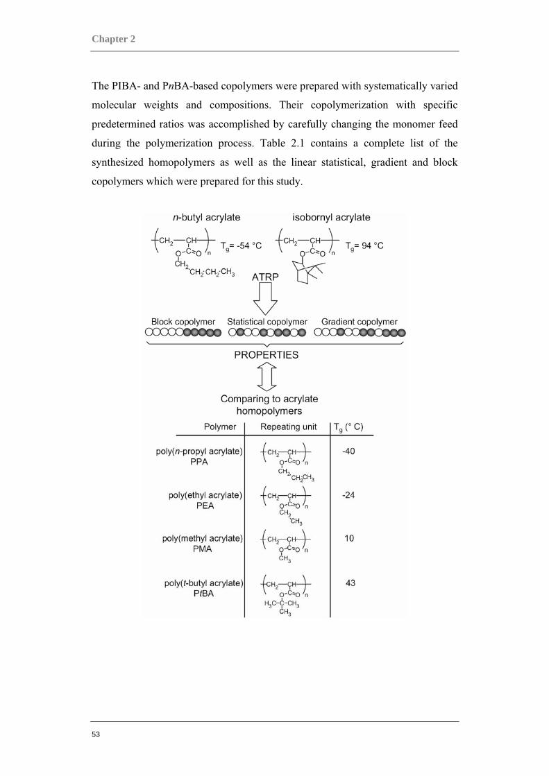
The PIBA- and PnBA-based copolymers were prepared with systematically varied
molecular weights and compositions. Their copolymerization with specific
predetermined ratios was accomplished by carefully changing the monomer feed
during the polymerization process. Table 2.1 contains a complete list of the
synthesized homopolymers as well as the linear statistical, gradient and block
copolymers which were prepared for this study.

Materials & Their Characterization
54
Figure 2.1. Copolymerization of isobornyl acrylate and n-butyl acrylate in
different fashion and comparison of properties of resulting copolymers with
acrylate-based homopolymers such as PtBA, PMA, PEA and PPA.
Table 2.1
Properties of different types of (co)polymers prepared by ATRP. GPC results
Sample Type of copolymer Unit M1 Unit M2
M1 wt% (GC)
Tg predicteda
M1 wt%
(NMR) PDI Mn Mn,theo
b
WJ-02-09 homopoly. ΙΒΑ (DP=290) - 100 94.0 - 1.06 28500 35400
WJ-02-11 homopoly. tBA (DP=470) - 100 43.0 - 1.07 48900 43800
WJ 135 homopoly. ΜΑ (DP=630) - 100 10.0 - 1.16 42200 40000
WJ-02-07 homopoly. EA (DP=900) - 100 -24.0 - 1.06 96900 70200
WJ-02-29 homopoly. nPA (DP=700) - 100 -40.0 - 1.06 86000 58800
WJ-02-10 homopoly. nΒΑ (DP=460) - 100 -54.0 - 1.07 47900 40800
WJ-02-13 random ΙΒΑ (DP=240)
nΒΑ (DP=100) 80 46.5 79 1.06 34000 48000
WJ-02-19 random ΙΒΑ (DP=480)
nΒΑ (DP=200) 80 46.5 78 1.08 63700 66000
WJ-02-14 random ΙΒΑ (DP=150)
nΒΑ (DP=245) 50 7.0 53 1.05 43500 51600
WJ-02-20 random ΙΒΑ (DP=300)
nΒΑ (DP=490) 50 7.0 54 1.06 69000 67000
WJ-02-35 random ΙΒΑ (DP=41)
nΒΑ (DP=90) 43 -10.6 41 1.08 26300 18400
WJ-02-36 random ΙΒΑ (DP=82)
nΒΑ (DP=180) 43 -10.6 39 1.07 39700 31600
WJ-02-28 random ΙΒΑ (DP=165)
nΒΑ (DP=360) 43 -10.6 44 1.07 53000 48800
WJ-02-24 random ΙΒΑ (DP=245)
nΒΑ (DP=540) 43 -10.6 42 1.10 10050
0 92400
WJ-02-16 random ΙΒΑ (DP=110)
nΒΑ (DP=315) 35 -20.4 38 1.06 44300 45000
WJ-02-22 random ΙΒΑ (DP=220)
nΒΑ (DP=630) 35 -20.4 33 1.12 10750
0 92400
WJ-02-15 random ΙΒΑ (DP=60)
nΒΑ (DP=390) 20 -32.7 19 1.05 44700 44400
WJ-02-21 random ΙΒΑ (DP=120)
nΒΑ (DP=780) 20 -32.7 22 1.07 81900 76800
WJ-02-17 random ΙΒΑ (DP=30)
nΒΑ (DP=440) 10 -41.9 13 1.06 55600 45000
WJ-02-23 random ΙΒΑ (DP=60)
nΒΑ (DP=880) 10 -41.9 16 1.13 94000 76900
WJ-02-30 block WJ-02-09 nΒΑ (DP=470) 50 94, -54 54 1.12 54600 46300
WJ-02-45 gradient ΙΒΑ (DP=192)
nΒΑ (DP=307) 47 - 47 1.13 74800 62300
a predicted using Fox equation; b Mn, theo=([M]0/[In]0) × conversion × Mmonomer

Chapter 2
55
2.2 Acrylate-based Triblock and Multi-arm Block Copolymers
The preparation of well-defined homopolymers as well as diblock and triblock
copolymers of methylene-γ-butyrolactone (MBL) using ATRP has been
previously reported. MBL, found in tulips, is the simplest member of
butyrolactones found and isolated from various plants [58-61]. Such natural
products are renewable, environmentally friendly, biocompatible, and
biodegradable. Also, they may possess some special physical and biomedical
properties. Recently, the possibility of using natural products to replace
petroleum-based raw materials in large commodity markets, such as plastics,
fibers, and fuels has been reviewed [61]. MBL consists of a five-membered ring
with an ester group and possesses structural features similar to those of methyl
methacrylate and polymerizes in a similar manner. Poly(α-methylene-γ-
butyrolactone) (PMBL) has good durability, a high refractive index of 1.540, and
high Tg (195 ºC) [62]. Various copolymers and blends containing MBL units have
good optical properties and resistance to heat, weathering, scratches and solvents.
In this section, block copolymers based on poly(n-butyl acrylate) (PBA), poly(α-
methylene-γ-butyrolactone) (PMBL) and poly(methyl methacrylate) (PMMA)
were synthesized. The copolymers were systematically prepared with different
composition ratios as well as different types of architecture, from linear A-B-A-
type triblock copolymers to multi-arm star-like block copolymers.

Materials & Their Characterization
56
2.2.1 PMBL-PBA-PMBL triblock copolymers
For this study, a series of well-defined triblock copolymers containing a middle
block of PBA and outer blocks of PMBL or random PMBL-PMMA were
synthesized via ATRP. The basic reaction taking place in the preparation of these
materials is illustrated in Figure 2.2.
Figure 2.2. Preparation of PMBL-b-PBA-b-PMBL triblock copolymers.
These linear triblock copolymers with hard PMBL outer segments and soft PBA
control segments were prepared with varied composition ratios between the soft
and hard components, as listed in detail in Table 2.2.
Table 2.2
Compositions of prepared PMBL-PBA-PMBL triblock copolymers with PMBL
outer hard blocks, and of prepared (PMBL-r-PMMA)-PBA-(PMBL-r-PMMA)
triblock copolymers with random copolymer outer hard blocks.
Sample Triblock composition Hard block
(mol%)a
Hard block
(wt%)a
MBL/MMA (mol%)a
B215-L40 PBA215(-b-PMBL20)2 15.8 12.6 100/0 B215-L68 PBA215(-b-PMBL34)2 23.7 19.3 100/0 B215-L120 PBA215(-b-PMBL60)2 36.3 30.3 100/0 B375-L32 PBA375(-b-PMBL16)2 7.9 6.1 100/0 B375-L60 PBA375(-b-PMBL30)2 13.8 10.9 100/0 B375-L144 PBA375(-b-PMBL72)2 27.6 22.7 100/0 B375-L106M26 PBA375(-b-PMBL53-r-PMMA13)2 26.0 21.3 80/20 B375-L82M50 PBA375(-b-PMBL41-r-PMMA25)2 26.0 21.4 62/38 B375-M132 PBA375(-b-PMMA66)2 26.0 21.6 0/100 abased on 1H NMR spectra
Chapter 2
57
2.2.2 PBA-PMBL multi-arm block copolymers
While linear A-B-A-type triblock copolymers have been commonplace, the
synthesis of polymers with hyperbranched, brush and star-shaped molecular
architecture has only in recent years attracted much interest due to their different
properties from those of linear polymers. And the expansion in the synthesis of
these polymers has been possible due to the emergence of various new controlled
polymerization techniques, which includes that of ATRP.
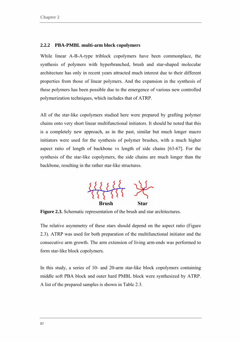
All of the star-like copolymers studied here were prepared by grafting polymer
chains onto very short linear multifunctional initiators. It should be noted that this
is a completely new approach, as in the past, similar but much longer macro
initiators were used for the synthesis of polymer brushes, with a much higher
aspect ratio of length of backbone vs length of side chains [63-67]. For the
synthesis of the star-like copolymers, the side chains are much longer than the
backbone, resulting in the rather star-like structures.
Figure 2.3. Schematic representation of the brush and star architectures.
The relative asymmetry of these stars should depend on the aspect ratio (Figure
2.3). ATRP was used for both preparation of the multifunctional initiator and the
consecutive arm growth. The arm extension of living arm-ends was performed to
form star-like block copolymers.
In this study, a series of 10- and 20-arm star-like block copolymers containing
middle soft PBA block and outer hard PMBL block were synthesized by ATRP.
A list of the prepared samples is shown in Table 2.3.
Materials & Their Characterization
58
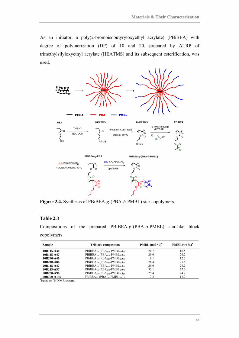
As an initiator, a poly(2-bromoisobutyryloxyethyl acrylate) (PBiBEA) with
degree of polymerization (DP) of 10 and 20, prepared by ATRP of
trimethylsilyloxyethyl acrylate (HEATMS) and its subsequent esterification, was
used.
Br BrBr BrBr
BrBr Br BrBr
PHEA PBA PMBL
Br BrBr BrBr
BrBr Br BrBr
Br BrBr BrBr
BrBr Br BrBr
PHEA PBA PMBLPHEA PBA PMBL
BrO Br
n-BA/ CuBr/ CuBr2PMDETA/ Anisole, 70°C
i) TMS cleavageKF/TBAFPMDETA/ CuBr/ EBiB
anisole/ 60 °C ii)OO
OTMS
nOO
OTMS
OO
OH
TEA, DCM
TMS-Cl
OO
O
n
O
Br
OO
O
n
O
Br
OO
Clm y
MBL/ CuCl/ CuCl2
bpy/ DMF
HEA HEATMS PHEATMS PBiBEA
PBiBEA-g-PBA PBiBEA-g-(PBA-b-PMBL)
O O
OO
O
n
O
OOm
Figure 2.4. Synthesis of PBiBEA-g-(PBA-b-PMBL) star copolymers.
Table 2.3
Compositions of the prepared PBiBEA-g-(PBA-b-PMBL) star-like block
copolymers.
Sample Triblock composition PMBL (mol %)# PMBL (wt %)#
10B115-A30 PBiBEA10-(PBA115-PMBL30)10 20.7 16.5 10B115-A47 PBiBEA10-(PBA115-PMBL47)10 29.0 24.2 10B240-A46 PBiBEA10-(PBA240-PMBL46)10 16.1 12.7 10B240-A86 PBiBEA10-(PBA240-PMBL86)10 26.4 21.6 20B115-A47 PBiBEA20-(PBA115-PMBL47)20 29.0 24.2 20B115-A57 PBiBEA20-(PBA115-PMBL57)20 33.1 27.6 20B230-A96 PBiBEA20-(PBA230-PMBL96)20 29.4 24.2 20B750-A156 PBiBEA20-(PBA750-PMBL156)20 17.2 13.7
#based on 1H NMR spectra
Chapter 2
59
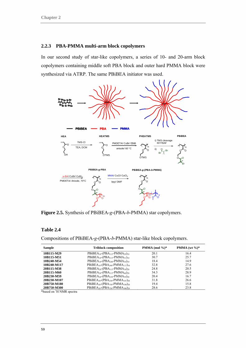
2.2.3 PBA-PMMA multi-arm block copolymers
In our second study of star-like copolymers, a series of 10- and 20-arm block
copolymers containing middle soft PBA block and outer hard PMMA block were
synthesized via ATRP. The same PBiBEA initiator was used.
Br BrBr BrBr
BrBr Br BrBr
PBiBEA PBA PMMA
Br BrBr BrBr
BrBr Br BrBr
Br BrBr BrBr
BrBr Br BrBr
PBiBEA PBA PMMAPBiBEA PBA PMMA
BrO Br
n-BA/ CuBr/ CuBr2
PMDETA/ Anisole, 70°C
i) TMS cleavageKF/TBAFPMDETA/ CuBr/ EBiB
anisole/ 60 °C ii)OO
OTMS
nOO
OTMS
OO
OH
TEA, DCM
TMS-Cl
OO
O
n
O
Br
OO
O
n
O
OO
OO
O
n
O
OO OOm m y
MMA/ CuCl/ CuCl2
bpy/ DMF
HEA HEATMS PHEATMS PBiBEA
PBiBEA-g-PBA PBiBEA-g-(PBA-b-PMMA)
Figure 2.5. Synthesis of PBiBEA-g-(PBA-b-PMMA) star copolymers.
Table 2.4
Compositions of PBiBEA-g-(PBA-b-PMMA) star-like block copolymers.
Sample Triblock composition PMMA (mol %)* PMMA (wt %)*
10B115-M29 PBiBEA10-(PBA115-PMMA29)10 20.1 16.4 10B115-M51 PBiBEA10-(PBA115-PMMA51)10 30.7 25.7 10B240-M54 PBiBEA10-(PBA240-PMMA54)10 18.4 14.9 10B240-M117 PBiBEA10-(PBA240-PMMA117)10 32.8 27.6 20B115-M38 PBiBEA20-(PBA115-PMMA38)20 24.8 20.5 20B115-M60 PBiBEA20-(PBA115-PMMA60)20 34.3 28.9 20B230-M59 PBiBEA20-(PBA230-PMMA59)20 20.4 16.7 20B230-M107 PBiBEA20-(PBA230-PMMA107)20 31.8 26.6 20B750-M180 PBiBEA20-(PBA750-PMMA180)20 19.4 15.8 20B750-M300 PBiBEA20-(PBA750-PMMA300)20 28.6 23.8
*based on 1H NMR spectra

Materials & Their Characterization
60
2.3 Siloxane-based Linear Gradient Copolymers
In this section, siloxane-based linear gradient copolymers were synthesized
mainly via anionic ring-opening copolymerization of cyclotrisiloxanes. Gradient
organic copolymers have commonly been synthesized using mostly controlled
radical polymerization (CRP) techniques [21, 25, 27, 68-72]. However, there are
only a few examples of gradient copolymers obtained by anionic [21, 73-74] and
cationic [75] polymerizations. And reports on the synthesis of gradient
polysiloxanes are very scarce [76-77]. Nevertheless, gradient functionalized
polysiloxanes of well-defined structure may be of interest due to the unique
surface properties of polysiloxanes [78] and the advantageous features related to
the gradient copolymer backbone structure.
2.3.1 Fluorosiloxane-based copolymers
Copolymers based on fluorosilicones are studied here for the very first time, as
previously, only the synthesis of vinylmethyl polysiloxanes of gradient structure
has been published [78]. For this study, gradient and block copolymers which are
composed of 2,4,6-tris(3,3,3-trifluoropropyl)-2,4,6-trimethylcyclotrisiloxane (F)
with hexamethylcyclotrisiloxane (D) were synthesized. A detailed list of the
synthesized copolymers and homopolymers is shown in Table 2.5.
Figure 2.6. Synthesis of PMTFS-PDMS copolymers.
O Si O
Si O Si
H 3C H 3C
C H 3
C H 3C H3
C H3
O Si
O
SiO
SiH 3C
F 3C H 2 C H 2C
CH3CH2CH2CF3
CH2CH2CF3CH3
+1)
BuLi
2) Me3SiClTHF Bu SiO S iO
CH3
CH3
C H 2C H 2C F 3
C H3
SiM e3n m
D F

Chapter 2
61
Table 2.5
List of prepared block, spontaneous gradient and forced gradient D-F copolymers.
Polymer D-F Mn (theoretical) Mn
NMR Mn-SECa
in CH2Cl2 (Mw/Mn) Block copolymer 1:1 15,000 14,600 13,500 (1.13) Gradient spontaneous 1:1 11,000 14,700 10,000 (1.13) Gradient spontaneous 2:1 10,000 13,600 11,000 (1.12) Gradient spontaneous 1:2 11,000 16,700 13,000 (1.20) Gradient spontaneous 1:1 11,000 15,400 11,000 (1.15) Forced Gradient 1:1 15,000 - 16,700 (1.17) Gradient spontaneous DFDb 1:1 40,000 44,000 (1.15) Forced Gradient DFDb 1:1 40,000 39,300 45,800 (1.15) Homopoly. PDMS - 15,000 - - Homopoly. PMTFPS - 20,000 - 18,000 (1.07)
aRelative to PS standards bDFD copolymers (initiator Pb2Si(OLi)2)
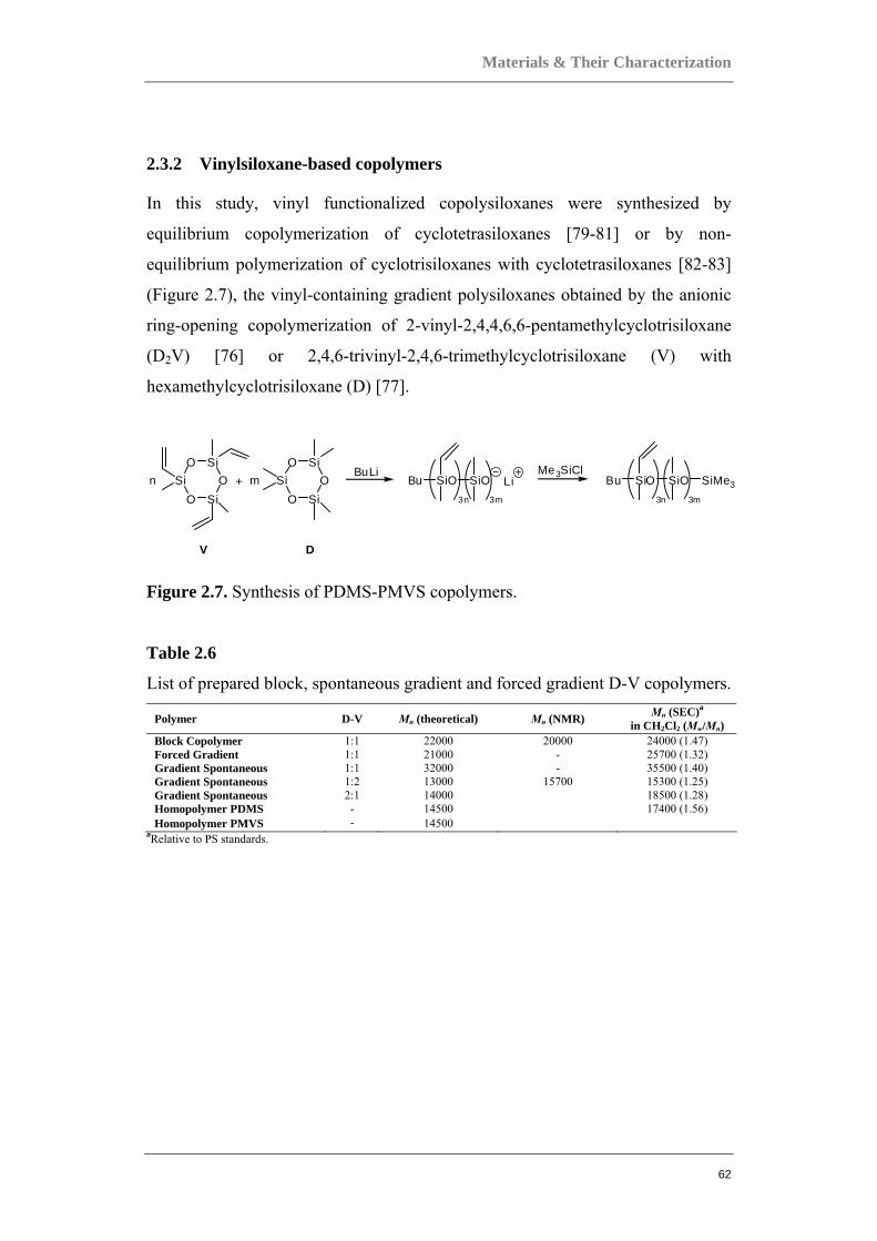
Materials & Their Characterization
62
2.3.2 Vinylsiloxane-based copolymers
In this study, vinyl functionalized copolysiloxanes were synthesized by
equilibrium copolymerization of cyclotetrasiloxanes [79-81] or by non-
equilibrium polymerization of cyclotrisiloxanes with cyclotetrasiloxanes [82-83]
(Figure 2.7), the vinyl-containing gradient polysiloxanes obtained by the anionic
ring-opening copolymerization of 2-vinyl-2,4,4,6,6-pentamethylcyclotrisiloxane
(D2V) [76] or 2,4,6-trivinyl-2,4,6-trimethylcyclotrisiloxane (V) with
hexamethylcyclotrisiloxane (D) [77].
Figure 2.7. Synthesis of PDMS-PMVS copolymers.
Table 2.6
List of prepared block, spontaneous gradient and forced gradient D-V copolymers.
Polymer D-V Mn (theoretical) Mn (NMR) Mn (SEC)a in CH2Cl2 (Mw/Mn)
Block Copolymer 1:1 22000 20000 24000 (1.47) Forced Gradient 1:1 21000 - 25700 (1.32) Gradient Spontaneous 1:1 32000 - 35500 (1.40) Gradient Spontaneous 1:2 13000 15700 15300 (1.25) Gradient Spontaneous 2:1 14000 18500 (1.28) Homopolymer PDMS - 14500 17400 (1.56) Homopolymer PMVS - 14500
aRelative to PS standards.
Si O Si
O SiO
SiO Si
O Si O
V D
+BuLi
Bu SiO SiO Li3n 3m
n mMe3SiCl
Bu SiO SiO 3n 3m
SiM e3
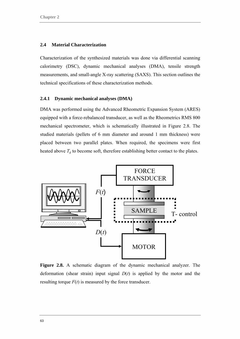
Chapter 2
63
2.4 Material Characterization
Characterization of the synthesized materials was done via differential scanning
calorimetry (DSC), dynamic mechanical analyses (DMA), tensile strength
measurements, and small-angle X-ray scattering (SAXS). This section outlines the
technical specifications of these characterization methods.
2.4.1 Dynamic mechanical analyses (DMA)
DMA was performed using the Advanced Rheometric Expansion System (ARES)
equipped with a force-rebalanced transducer, as well as the Rheometrics RMS 800
mechanical spectrometer, which is schematically illustrated in Figure 2.8. The
studied materials (pellets of 6 mm diameter and around 1 mm thickness) were
placed between two parallel plates. When required, the specimens were first
heated above Tg to become soft, therefore establishing better contact to the plates.
Figure 2.8. A schematic diagram of the dynamic mechanical analyzer. The
deformation (shear strain) input signal D(t) is applied by the motor and the
resulting torque F(t) is measured by the force transducer.
MOTOR
FORCE TRANSDUCER
SAMPLE
D(t)
F(t)
T- control
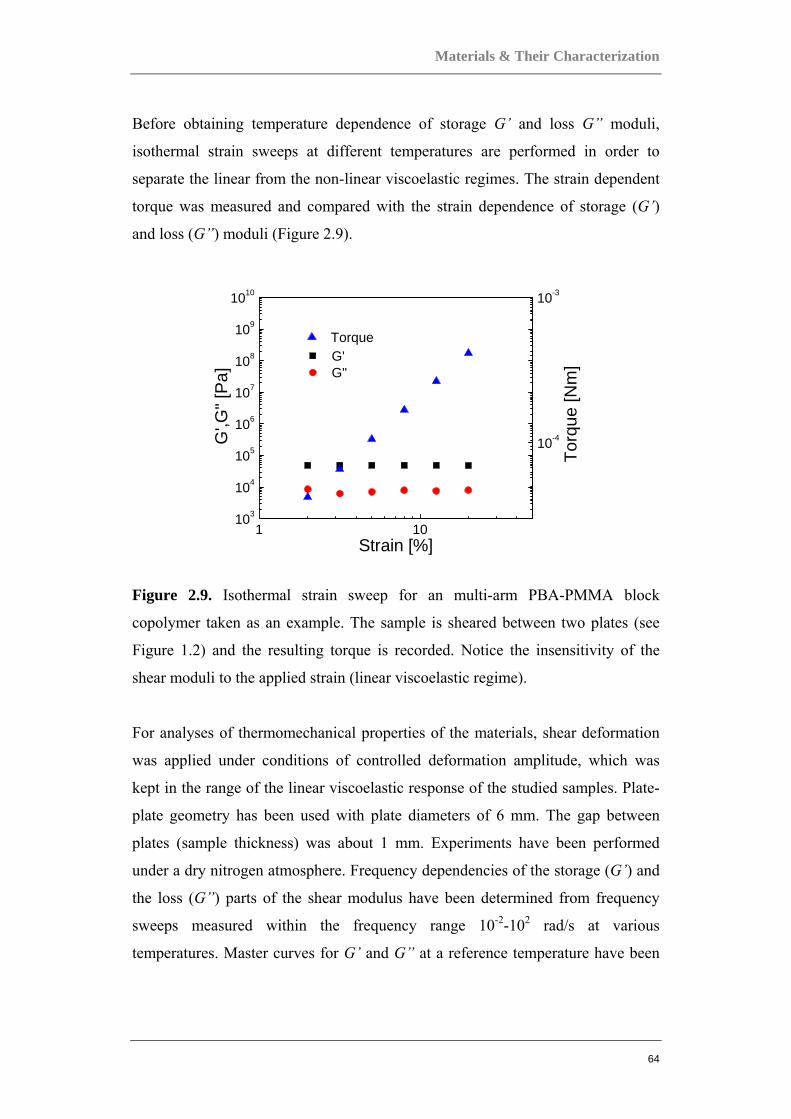
Materials & Their Characterization
64
Before obtaining temperature dependence of storage G’ and loss G” moduli,
isothermal strain sweeps at different temperatures are performed in order to
separate the linear from the non-linear viscoelastic regimes. The strain dependent
torque was measured and compared with the strain dependence of storage (G’)
and loss (G”) moduli (Figure 2.9).
1 10103
104
105
106
107
108
109
1010
10-4
10-3
Torq
ue [N
m]
G' G"
G',G
" [Pa
]
Strain [%]
Torque
Figure 2.9. Isothermal strain sweep for an multi-arm PBA-PMMA block
copolymer taken as an example. The sample is sheared between two plates (see
Figure 1.2) and the resulting torque is recorded. Notice the insensitivity of the
shear moduli to the applied strain (linear viscoelastic regime).
For analyses of thermomechanical properties of the materials, shear deformation
was applied under conditions of controlled deformation amplitude, which was
kept in the range of the linear viscoelastic response of the studied samples. Plate-
plate geometry has been used with plate diameters of 6 mm. The gap between
plates (sample thickness) was about 1 mm. Experiments have been performed
under a dry nitrogen atmosphere. Frequency dependencies of the storage (G’) and
the loss (G”) parts of the shear modulus have been determined from frequency
sweeps measured within the frequency range 10-2-102 rad/s at various
temperatures. Master curves for G’ and G” at a reference temperature have been
Chapter 2
65
obtained using the time-temperature superposition, i.e., shifting the data recorded
at various temperatures only along the frequency coordinate.
2.4.2 Differential scanning calorimetry (DSC)
Thermal characterization of polymers was performed using a Mettler DSC-30
calorimeter as well as a DuPont 2000 thermal analysis system. Experiments were
conducted with cooling and heating rates of 10 K/min. The transition temperatures
were taken as corresponding to the maximum of the enthalpic peak and
determined from the second heating run at the inflection point.
2.4.3 Small-angle X-ray scattering (SAXS) analyses
Small-angle X-ray scattering measurements were conducted using a rotating
anode (Rigaku RA-Micro 7) X-ray beam with a pinhole collimation and a two-
dimensional detector (Bruker Highstar) with 1024 x 1024 pixels. A double
graphite monochromator for the Cu Kα radiation (λ = 0.154 nm) was used. The
beam diameter was about 0.8 mm, and the sample to detector distance was 1.8 m.
The recorded scattered intensity distributions were integrated over the azimuthal
angle and are presented as functions of the scattering vector q ( λθ )sin(2=s ,
where 2θ is the scattering angle).
2.4.4 Tensile tests
Tensile tests were performed using a mechanical testing machine Instron 6000.
Samples with thickness in the order of 0.2– 0.5 mm were drawn with the rate of 5
mm/min at room or at elevated temperature. Dependencies of stress vs draw ratio
were recorded. Elastic modulus, elongation at break and stress at break were
determined by the averaging of 3–5 independent drawing experiments performed
at the same conditions.
66
3 Results & Discussion
This chapter extensively documents the findings of our investigations on the
various complex copolymer systems. The morphology and thermomechanical
properties of all of the synthesized materials were analyzed mainly via DSC,
DMA, tensile strength measurements, and SAXS.
3.1 Comparing Acrylate-based Copolymers to Homopolymers
The primary goal of this work was to compare thermomechanical properties of
block, gradient and statistical copolymers of nBA and IBA with various acrylate
homopolymers. As shown in the last chapter in Figure 2.1, the copolymers were
prepared with systematically varied molecular weights and compositions to assist
in the investigation of structure property correlation. The choice of nBA and IBA
was dictated by the very different thermal properties of its homopolymers. The
glass transition temperature (Tg) of PnBA is -54 ºC whereas Tg of PIBA is 94 ºC.
Thus, their copolymerization with carefully selected ratios could result in
polymers with thermal properties similar to various acrylate homopolymers such
as poly(t-butyl acrylate) (PtBA), poly(methyl acrylate) (PMA), poly(ethyl
acrylate) (PEA) and poly(n-propyl acrylate) (PPA). For example, the glass
transition temperature (Tg) of the resulting statistical poly(isobornyl acrylate-co-n-
butyl acrylate) (P(IBA-co-nBA)) copolymers could be tuned by changing the
monomer feed during the polymerization process. This way, it may be possible to
generate materials which could hopefully mimic thermal behavior of the
homopolymers mentioned above.
3.1.1 Statistical P(IBA-co-nBA) copolymers
When comparing the thermomechanical properties of acrylate homopolymers and
P(IBA-co-nBA) copolymers, the first important question is whether the
copolymer system is isotropic in the bulk state or rather exhibits a micro-phase
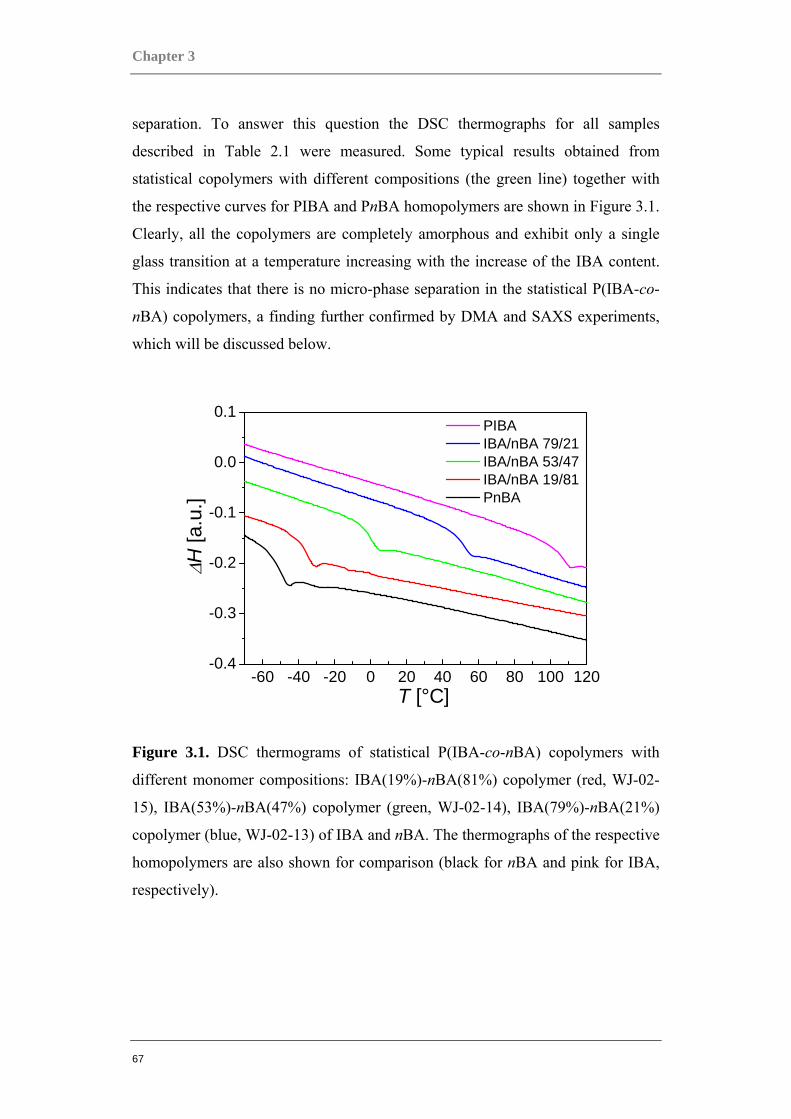
Chapter 3
67
separation. To answer this question the DSC thermographs for all samples
described in Table 2.1 were measured. Some typical results obtained from
statistical copolymers with different compositions (the green line) together with
the respective curves for PIBA and PnBA homopolymers are shown in Figure 3.1.
Clearly, all the copolymers are completely amorphous and exhibit only a single
glass transition at a temperature increasing with the increase of the IBA content.
This indicates that there is no micro-phase separation in the statistical P(IBA-co-
nBA) copolymers, a finding further confirmed by DMA and SAXS experiments,
which will be discussed below.
-60 -40 -20 0 20 40 60 80 100 120-0.4
-0.3
-0.2
-0.1
0.0
0.1 PIBA IBA/nBA 79/21 IBA/nBA 53/47 IBA/nBA 19/81 PnBA
ΔH [a
.u.]
T [°C]
Figure 3.1. DSC thermograms of statistical P(IBA-co-nBA) copolymers with
different monomer compositions: IBA(19%)-nBA(81%) copolymer (red, WJ-02-
15), IBA(53%)-nBA(47%) copolymer (green, WJ-02-14), IBA(79%)-nBA(21%)
copolymer (blue, WJ-02-13) of IBA and nBA. The thermographs of the respective
homopolymers are also shown for comparison (black for nBA and pink for IBA,
respectively).
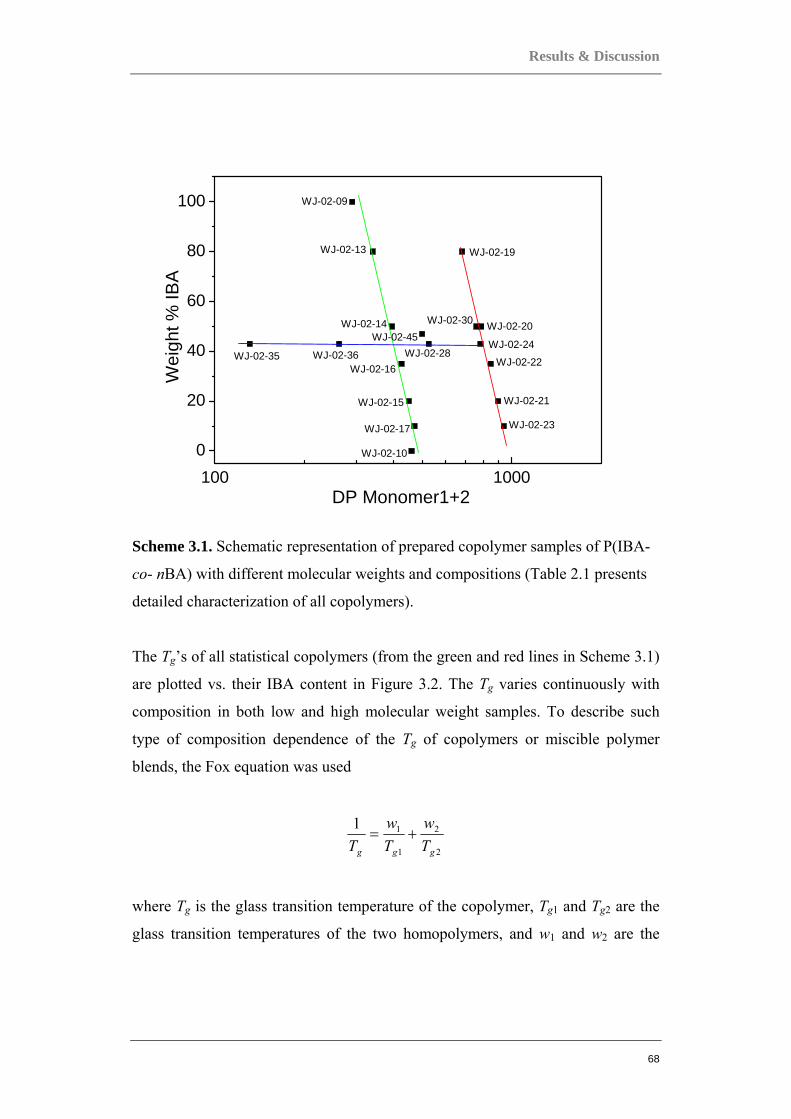
Results & Discussion
68
100 10000
20
40
60
80
100
WJ-02-23WJ-02-17
WJ-02-21WJ-02-15
WJ-02-22WJ-02-16
WJ-02-24WJ-02-28WJ-02-36WJ-02-35
WJ-02-45WJ-02-20WJ-02-30WJ-02-14
WJ-02-19WJ-02-13
WJ-02-10
WJ-02-09
Wei
ght %
IBA
DP Monomer1+2
Scheme 3.1. Schematic representation of prepared copolymer samples of P(IBA-
co- nBA) with different molecular weights and compositions (Table 2.1 presents
detailed characterization of all copolymers).
The Tg’s of all statistical copolymers (from the green and red lines in Scheme 3.1)
are plotted vs. their IBA content in Figure 3.2. The Tg varies continuously with
composition in both low and high molecular weight samples. To describe such
type of composition dependence of the Tg of copolymers or miscible polymer
blends, the Fox equation was used
2
2
1
11
ggg Tw
Tw
T+=
where Tg is the glass transition temperature of the copolymer, Tg1 and Tg2 are the
glass transition temperatures of the two homopolymers, and w1 and w2 are the
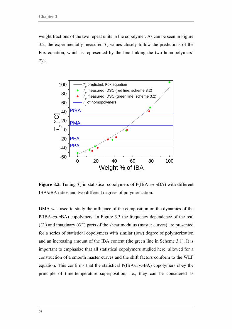
Chapter 3
69
weight fractions of the two repeat units in the copolymer. As can be seen in Figure
3.2, the experimentally measured Tg values closely follow the predictions of the
Fox equation, which is represented by the line linking the two homopolymers’
Tg’s.
0 20 40 60 80 100-60
-40
-20
0
20
40
60
80
100
PPAPEA
PMA
Tg predicted, Fox equation
Tg measured, DSC (red line, scheme 3.2)
Tg measured, DSC (green line, scheme 3.2)
Tg of homopolymers
T g [°C
]
Weight % of IBA
PtBA
Figure 3.2. Tuning Tg in statistical copolymers of P(IBA-co-nBA) with different
IBA/nBA ratios and two different degrees of polymerization.
DMA was used to study the influence of the composition on the dynamics of the
P(IBA-co-nBA) copolymers. In Figure 3.3 the frequency dependence of the real
(G’) and imaginary (G”) parts of the shear modulus (master curves) are presented
for a series of statistical copolymers with similar (low) degree of polymerization
and an increasing amount of the IBA content (the green line in Scheme 3.1). It is
important to emphasize that all statistical copolymers studied here, allowed for a
construction of a smooth master curves and the shift factors conform to the WLF
equation. This confirms that the statistical P(IBA-co-nBA) copolymers obey the
principle of time-temperature superposition, i.e., they can be considered as

Results & Discussion
70
thermorheologically simple. This subject can be addressed more quantitatively by
analyzing the temperature dependence of the minimum of tan(δ), as recently
shown for a series of cycloolefin copolymers with different norbornene content
[84]. Such analyses, however, are beyond the scope of this study.
10-5 10-3 10-1 101 103 105 107 109101
103
105
107
109
ω [rad/s]
G',G
'' [Pa
]
Tref=15°C
G' G'' IBA/nBA 53/47 38/62 19/81 0/100
Figure 3.3. Typical examples of G’ and G” dependencies (master curves) on
frequency for a linear PnBA homopolymer and statistical P(IBA-co-nBA)
copolymers with similar degrees of polymerization and different IBA/nBA ratios
(Scheme 3.1, the green line).
Let us first consider the pure PnBA. As can be seen in Figure 3.3, the relaxation
spectrum of this homopolymer shows the two distinct characteristic regions which
was discussed in Chapter 1. The one at high frequencies is related to segmental
(local) motions of the polymer chains and the lower frequency, or terminal one, is
related to relaxation of entangled chains. These two parts of the spectra are
characterized with their respective relaxation times, τs and τc [23]. These
relaxation times determine the time range within which the characteristic rubbery
Chapter 3
71
plateau is observed for linear polymers. For most of the linear flexible polymers,
as well as for PnBA, the plateau height is between 105 and 106 Pa. Outside the
rubbery plateau range the linear polymer melts become glassy at high frequencies
and flow within longer time periods, i.e., at low frequencies.
As can be seen from Figure 3.3, the increased amount of IBA in the copolymer
composition leads to a systematic shift of the master curves to lower frequencies.
This effect is related to the strong increase of the glass transition temperatures of
the respective copolymers. However, the shape of the master curves does not
change significantly and there is no evidence of any new relaxation processes in
the copolymers as compared to a PnBA homopolymer. This is an additional
indication that the statistical P(IBA-co-nBA) copolymers do not exhibit a phase
separation. In order to better understand the influence of the composition on the
dynamics of the statistical copolymers, we have determined the characteristic
times τc related to the terminal relaxation process by the crossing points of the G’
and G” curves observed at the transition to the flow range at low frequency.
Results are shown in Figure 3.4(a) as a function of the IBA content for the
copolymers from the green and the red line in Scheme 3.1. As in earlier study
[85], the terminal relaxation times are normalized to the relaxation times of the
segmental motion, which makes the results nearly independent of the reference
temperature and free of effects related to the chain length dependence of the
segmental motion, usually observed for short chains.

Results & Discussion
72
0 20 40 60 80 100
103
104
105
106
107
high DP low DP
Weight % of IBA
τ c/τs
(a)
104 105 106
104
105
106 high DP low DP varying DP
(b)
τ c/τs
Mw [g/mol]
Figure 3.4. Effect of (a) the composition, and (b) the molecular weight, of
statistical copolymers P(IBA-co-nBA) on the chain relaxation times.
As can be seen in Figure 3.4(a), the terminal relaxation times of the copolymers
depend weakly on the IBA content and much stronger on the degree of
polymerization. Furthermore even this weak dependence is most likely related to
the slight decrease of the copolymers molecular weight with the decrease of IBA
Chapter 3
73
content (see Table 2.1). This is further illustrated in Figure 3.4(b) where the same
data are plotted versus the molecular weight of the copolymers. For comparison,
the data for statistical copolymers with similar composition but different degree of
polymerization (the blue line on Scheme 3.1) are also shown. All statistical
copolymers show similar molecular weight dependence of the terminal relaxation
times independent of their composition. The slope of this dependence is
approximately 4, a value slightly higher than that typically found for
homopolymer melts in the entangled regime, i.e., ~3.4.
3.1.2 Statistical copolymers mimicking homopolymers.
As shown in a previous section, the glass transition of the statistical P(IBA-co-
nBA) copolymers can be tuned to any value between the Tg’s of the two
homopolymers (i.e., between -54 and 94 ºC) by proper choice of the comonomer
ratio. It is possible therefore, to synthesize copolymers with glass transition
temperatures matching the Tg of other acrylate homopolymers. This is illustrated
in Figure 3.2, where the glass transition temperatures of the PPA, PEA, PMA and
PtBA are shown as horizontal lines. It is interesting to verify if the statistical
P(IBA-co-nBA) copolymers can mimic not only the Tg’s of the acrylate
homopolymers, but also their mechanical properties. In order to do this, we
plotted in Figure 3.5(a) the DMA master curves measured for PPA homopolymer
and IBA(16%)-nBA(84%) copolymer with similar molecular weight. The two
master curves overlap very well both in the high frequency region (due to the
similar Tg’s) and in the low frequency region (due to the similar Mn).
Nevertheless, a closer look at Figure 3.5(a) reveals also some differences.

Results & Discussion
74
10-4 10-1 102 105 108 1011100
102
104
106
108
1010
(a)
G' G'' PPA IBA(16%)/nBA(84%)
ω [rad/s]
G',G
'' [P
a]
Tref=15°C
10-5 10-3 10-1 101 103 105 107100
102
104
106
108
1010
(b)
G' G'' PEA IBA(33%)/nBA(67%)
Tref=15°C
ω [rad/s]
G',G
'' [P
a]
10-3 10-1 101 103 105 107 109 1011100
102
104
106
108
1010
(c)
G' G'' PtBA IBA(78%)/nBA(22%)
ω [rad/s]
G',G
'' [Pa
]
Tref=110°C
Figure 3.5. Comparison of the shear moduli spectra of (a) PPA (Tg = -40 ºC, Mn =
86 000 g/mol; WJ-02-29) and IBA(16%)-nBA(84%) copolymer (Tg = -39 ºC, Mn
= 94 000 g/mol; WJ-02-23); (b) PEA (Tg = -24 ºC, Mn = 96 900 g/mol; WJ-02-07)
Chapter 3
75
and IBA(33%)-nBA(67%) copolymer (Tg = -20 ºC, Mn = 107 500 g/mol; WJ-02-
22); (c) PtBA (Tg = 37 ºC, Mn = 48 900 g/mol; WJ-02-11) and IBA(78%)-
nBA(22%) copolymer (Tg = 42 ºC, Mn = 63 700 g/mol; WJ-02-19).
Most importantly, in the characteristic rubbery plateau region, the storage
modulus (G’) of the P(IBA-co-nBA) copolymer is significantly lower than the
corresponding value for the PPA homopolymer. This effect is even more evident
in Figure 3.5(b), which compares the master curve of statistical copolymer with
IBA(33%)/nBA(67%) with that of the PEA homopolymer of similar molecular
weight. Again, the overlap of the two spectra is remarkably good at high and low
frequencies, but the significant difference in the storage modulus is observed in
the plateau region. This means that while mimicking perfectly the glass transition
temperatures of the PEA and PPA, the P(IBA-co-nBA) copolymers are
significantly softer than their homopolymer counterparts. It is interesting to verify
if similar observations can be made also when comparing the copolymers with
higher IBA content, i.e., higher glass transition temperature with the PMA and
PtBA homopolymers. Unfortunately, as can be seen from Figure 3.2, none of the
synthesized copolymers had the appropriate composition in order to match the Tg
of the PMA. Nevertheless, the IBA(78%)-nBA(22%) copolymer (WJ-02-19) has a
glass transition temperature very similar to that of the PtBA. The DMA master
curves of these two materials are shown in Figure 3.5(c). The spectra are very
similar although slightly shifted due to the small difference in the glass transition
temperatures. More importantly, the copolymer is again softer than the
homopolymer, i.e., has a lower G’ value in the rubbery plateau region.
The data for the G’ in this region for all materials presented in Figure 3.5 are
summarized in Table 2. For comparison the values for nBA and IBA
homopolymers are also shown. As can be seen from the table in all cases, the
P(IBA-co-nBA) copolymers are significantly softer than the respective
homopolymers having same glass transition temperatures. The lower plateau
modulus of the copolymers indicates that they should have higher entanglement
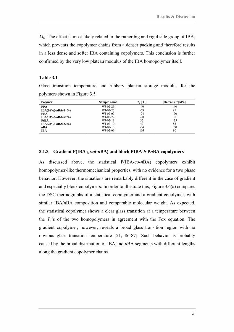
Results & Discussion
76
Mw. The effect is most likely related to the rather big and rigid side group of IBA,
which prevents the copolymer chains from a denser packing and therefore results
in a less dense and softer IBA containing copolymers. This conclusion is further
confirmed by the very low plateau modulus of the IBA homopolymer itself.
Table 3.1
Glass transition temperature and rubbery plateau storage modulus for the
polymers shown in Figure 3.5 Polymer Sample name Tg [°C] plateau G’ [kPa] PPA WJ-02-29 -40 140 IBA(16%)-nBA(84%) WJ-02-23 -39 95 PEA WJ-02-07 -24 170 IBA(33%)-nBA(67%) WJ-02-22 -20 70 PtBA WJ-02-11 37 135 IBA(78%)-nBA(22%) WJ-02-19 42 85 nBA WJ-02-10 -54 130 IBA WJ-02-09 105 80
3.1.3 Gradient P(IBA-grad-nBA) and block PIBA-b-PnBA copolymers
As discussed above, the statistical P(IBA-co-nBA) copolymers exhibit
homopolymer-like thermomechanical properties, with no evidence for a two phase
behavior. However, the situations are remarkably different in the case of gradient
and especially block copolymers. In order to illustrate this, Figure 3.6(a) compares
the DSC thermographs of a statistical copolymer and a gradient copolymer, with
similar IBA/nBA composition and comparable molecular weight. As expected,
the statistical copolymer shows a clear glass transition at a temperature between
the Tg’s of the two homopolymers in agreement with the Fox equation. The
gradient copolymer, however, reveals a broad glass transition region with no
obvious glass transition temperature [21, 86-87]. Such behavior is probably
caused by the broad distribution of IBA and nBA segments with different lengths
along the gradient copolymer chains.
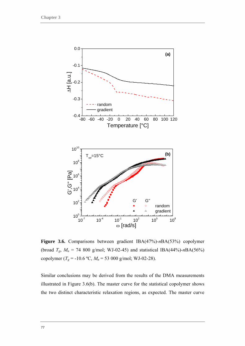
Chapter 3
77
-80 -60 -40 -20 0 20 40 60 80 100 120-0.4
-0.3
-0.2
-0.1
0.0
Temperature [°C]
ΔH [a
.u.]
random gradient
(a)
10-7 10-4 10-1 102 105 108100
102
104
106
108
1010
Tref=15°C
G',G
'' [P
a]
ω [rad/s]
G' G'' random gradient
(b)
Figure 3.6. Comparisons between gradient IBA(47%)-nBA(53%) copolymer
(broad Tg, Mn = 74 800 g/mol; WJ-02-45) and statistical IBA(44%)-nBA(56%)
copolymer (Tg = -10.6 ºC, Mn = 53 000 g/mol; WJ-02-28).
Similar conclusions may be derived from the results of the DMA measurements
illustrated in Figure 3.6(b). The master curve for the statistical copolymer shows
the two distinct characteristic relaxation regions, as expected. The master curve

Results & Discussion
78
for the gradient copolymer, however, shows very broad distribution of relaxation
processes, particularly in the segmental relaxation region.
-80 -60 -40 -20 0 20 40 60 80 100 120-0.3
-0.2
-0.1
0.0
Temperature [°C]
ΔH
random block
(a)
10-16 10-9 10-2 105 1012100
102
104
106
108
1010
Tref=15°C
G',G
'' [Pa
]
ω [rad/s]
G' G'' random block
(b)
Figure 3.7. Comparisons of block IBA(54%)-nBA(46%) copolymer (Tg = -54 ºC,
94 ºC, Mn = 54 600 g/mol; WJ-02-230) and statistical IBA(54%)-nBA(46%)
copolymer (Tg = 7 ºC, Mn = 69 000 g/mol; WJ-02-20).

Chapter 3
79
It was previously reported that this broadening could be related to compositions’
fluctuations in the studied copolymers [88-89]. A recent study of a similar system
has shown that using experimental techniques such as photon correlation
spectroscopy and dielectric spectroscopy the relaxation dynamic can be addressed
in greater detail [90].
In Figure 3.7(a), the DSC thermographs of statistical and block copolymers with
similar molecular weight and similar IBA/nBA composition are compared. While,
the statistical copolymer has a single glass transition, the block copolymer shows
two glass transition temperatures corresponding to the Tg’s of each component
indicating a micro-phase separation in the sample. In Figure 3.7(b) the frequency
dependence of G’ and G” of the same copolymers are compared. It is important to
emphasize that in the case of the block copolymer, merely an attempt for
constructing a master curve is shown, as the temperature dependence of the shift
factors does not conform to the WLF equation. Nevertheless such an approach
was shown to reveal important information for the morphology and order-disorder
transitions in a number of block copolymer systems [91-93]. In our case, the block
copolymer ‘‘master curve’’ provides additional evidences for the micro-phase
separation in this sample. First of all the glass transitions of the two blocks are
clearly distinguishable at low and high frequencies, respectively. Furthermore the
behavior of the ‘‘master curve’’ in the very low frequency region, namely G’(ω)
overlapping with G”(ω) and having a slope of ~0.5 may indicate the formation of
a lamella structure as theoretically predicted [94].
In order to verify these findings, SAXS experiments were performed on the same
pair of block and statistical copolymers. As expected the statistical copolymer has
revealed a smooth scattered intensity distribution without any peaks. The block
copolymer, however, showed a weak maximum, which may result from distance
correlations between PnBA and PIBA domains. There are no other peaks in the
spectra probably as result of the small contrast in the electronic densities of the
two blocks. For this reason it is not possible to make any conclusions concerning

Results & Discussion
80
type of order or to identify any specific morphological forms. From the position of
the maxima, however, a structural periodicity of = 20 nm can be assigned to the
block copolymer sample.
3.2 Acrylate-based Block Copolymers as Thermoplastic Elastomers
Thermoplastic elastomers (TPEs) form an important class of materials combining
elastomeric behavior with thermoplastic properties. Commonly these are A-B-A
type triblock copolymers that combine a soft central block with glassy end blocks.
These blocks should be immiscible and should phase separate with formation of
thermoplastic microdomains, which act as physical cross-links for the soft matrix.
One of the most common TPEs is the polystyrene–polybutadiene–polystyrene
(SBS) triblock copolymer [95]. However, SBS suffers from two drawbacks. First,
the unsaturated polybutadiene block is easily oxidized and is sensitive to UV
degradation. Second, the upper service temperature is limited by Tg of the
polystyrene block (ca. 100 ºC). Therefore, there is a continuous effort to replace
polystyrene by thermoplastics with higher Tg and also substitute polybutadiene
with more stable rubbery block [96].
Among the alternatives which have been considered are various fully acrylic
TPEs based on combination of polyacrylates as soft blocks with different
polymethacrylates as hard blocks synthesized by anionic [97] or controlled radical
polymerization [86, 98-101] techniques. One of the advantages of acrylates is
their versatility. For example, (meth)acrylic monomers cover a wide range of Tg
from ca. -50 to +200 ºC. Furthermore, these polymers are not sensitive to UV and
oxidation.
Chapter 3
81
3.2.1 PMBL-PBA-PMBL linear triblock copolymers
In this section, the findings of our investigation into the morphology and
thermomechanical properties of the synthesized PMBL-PBA-PMBL triblock
copolymers containing a middle block of PBA and outer blocks of PMBL or
random PMBL-PMMA are discussed.
Morphology
Due to the incompatibility between PBA and PMBL, the prepared triblock
copolymers were expected to show strong phase separation. In order to gain
insight on the effects of this phase separation and its resulting microstructures,
SAXS analysis of thick films of the PMBL–PBA–PMBL triblock copolymers was
performed. Typical results are presented in Figure 3.8. The triblock copolymers
which did not undergo any additional thermal treatment were studied first. As
shown in Figure 3.8(a), only the copolymer with a high PMBL content (B215-
L120, 30.3 wt% PMBL) showed a well-ordered structure, consistent with
hexagonally packed cylinders (three relatively sharp peaks at relative
positions sss 7,3, ). The copolymers with moderate PMBL content (19.3 and
12.6 wt% PMBL) did not exhibit well defined secondary peaks, indicating mainly
short-range ordered. The SAXS experiments were then repeated after thermal
annealing of the PMBL–PBA–PMBL samples at 150 ºC for 1 h in order to
examine the effect of the annealing process on the morphology of the copolymer
films. The comparison of Figure 3.8(b) with Figure 3.8(a) shows that the annealed
films exhibited better ordering than the untreated samples, displaying at least three
scattering peaks in each of the SAXS spectra. Furthermore, the ratios of the
relative peak positions in all cases were sss 7,3, , i.e. consistent with a
hexagonal lattice. A closer look at Figure 3.8 shows that for the same length of the
PBA segment, an increase in PMBL block length leads to increase in the d-
spacing. Similar cylindrical morphology was observed via SAXS for most
PMBL–PBA–PMBL copolymers.
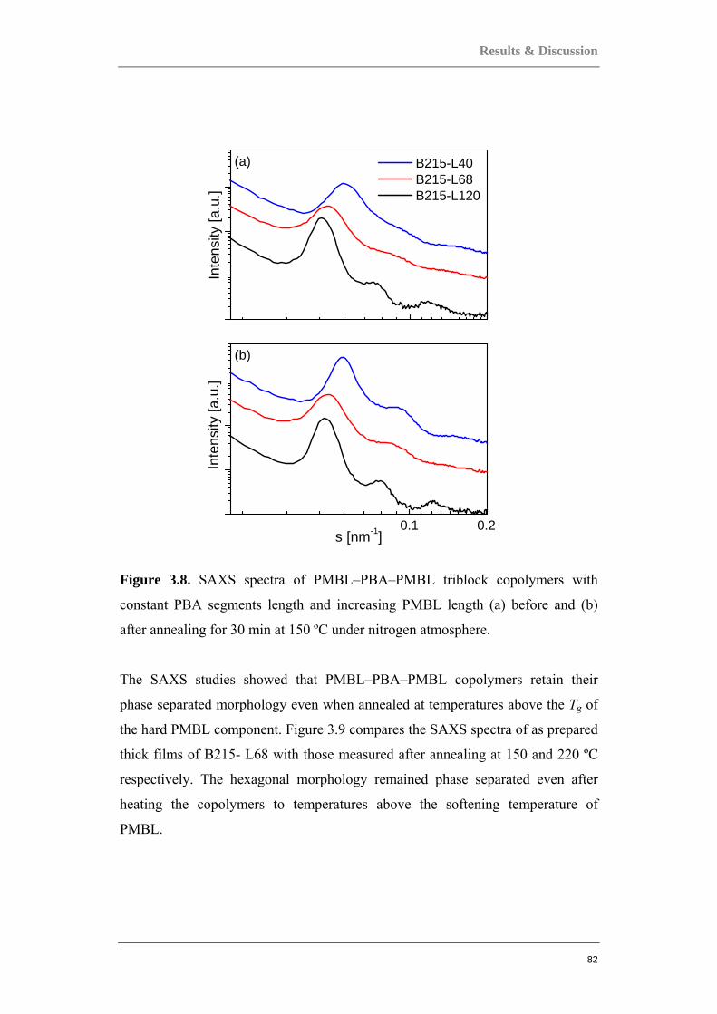
Results & Discussion
82
0.1 0.2
(b)
Inte
nsity
[a.u
.]
s [nm-1]
Inte
nsity
[a.u
.]
B215-L40 B215-L68 B215-L120
(a)
Figure 3.8. SAXS spectra of PMBL–PBA–PMBL triblock copolymers with
constant PBA segments length and increasing PMBL length (a) before and (b)
after annealing for 30 min at 150 ºC under nitrogen atmosphere.
The SAXS studies showed that PMBL–PBA–PMBL copolymers retain their
phase separated morphology even when annealed at temperatures above the Tg of
the hard PMBL component. Figure 3.9 compares the SAXS spectra of as prepared
thick films of B215- L68 with those measured after annealing at 150 and 220 ºC
respectively. The hexagonal morphology remained phase separated even after
heating the copolymers to temperatures above the softening temperature of
PMBL.
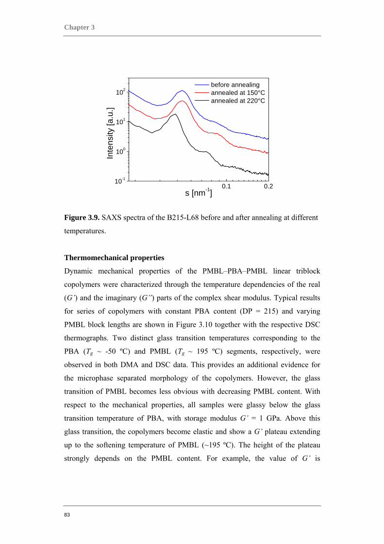
Chapter 3
83
0.1 0.210-1
100
101
102
Inte
nsity
[a.u
.]
s [nm-1]
before annealing annealed at 150°C annealed at 220°C
Figure 3.9. SAXS spectra of the B215-L68 before and after annealing at different
temperatures.
Thermomechanical properties
Dynamic mechanical properties of the PMBL–PBA–PMBL linear triblock
copolymers were characterized through the temperature dependencies of the real
(G’) and the imaginary (G”) parts of the complex shear modulus. Typical results
for series of copolymers with constant PBA content (DP = 215) and varying
PMBL block lengths are shown in Figure 3.10 together with the respective DSC
thermographs. Two distinct glass transition temperatures corresponding to the
PBA (Tg ~ -50 ºC) and PMBL (Tg ~ 195 ºC) segments, respectively, were
observed in both DMA and DSC data. This provides an additional evidence for
the microphase separated morphology of the copolymers. However, the glass
transition of PMBL becomes less obvious with decreasing PMBL content. With
respect to the mechanical properties, all samples were glassy below the glass
transition temperature of PBA, with storage modulus G’ = 1 GPa. Above this
glass transition, the copolymers become elastic and show a G’ plateau extending
up to the softening temperature of PMBL (~195 ºC). The height of the plateau
strongly depends on the PMBL content. For example, the value of G’ is
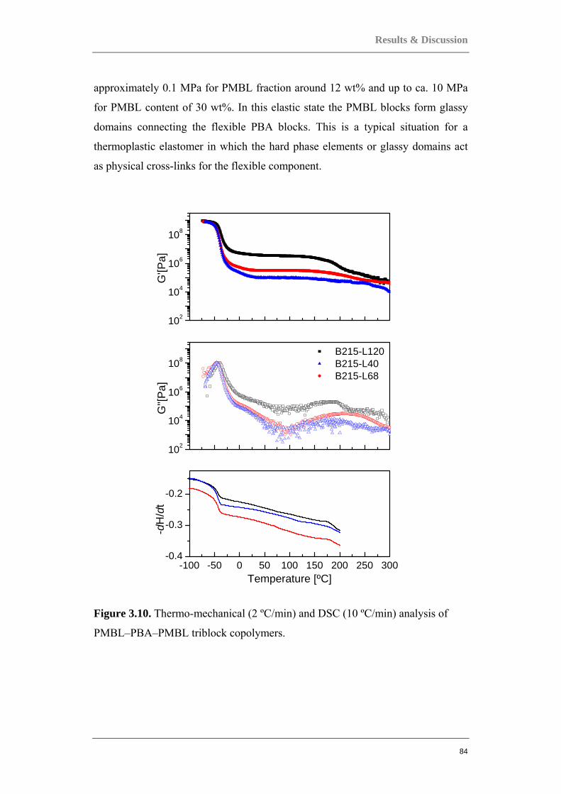
Results & Discussion
84
approximately 0.1 MPa for PMBL fraction around 12 wt% and up to ca. 10 MPa
for PMBL content of 30 wt%. In this elastic state the PMBL blocks form glassy
domains connecting the flexible PBA blocks. This is a typical situation for a
thermoplastic elastomer in which the hard phase elements or glassy domains act
as physical cross-links for the flexible component.
102
104
106
108
102
104
106
108
-100 -50 0 50 100 150 200 250 300-0.4
-0.3
-0.2
B215-L120 B215-L40 B215-L68
G'[P
a]
G"[P
a]
-dH
/dt
Temperature [ºC]
Figure 3.10. Thermo-mechanical (2 ºC/min) and DSC (10 ºC/min) analysis of
PMBL–PBA–PMBL triblock copolymers.
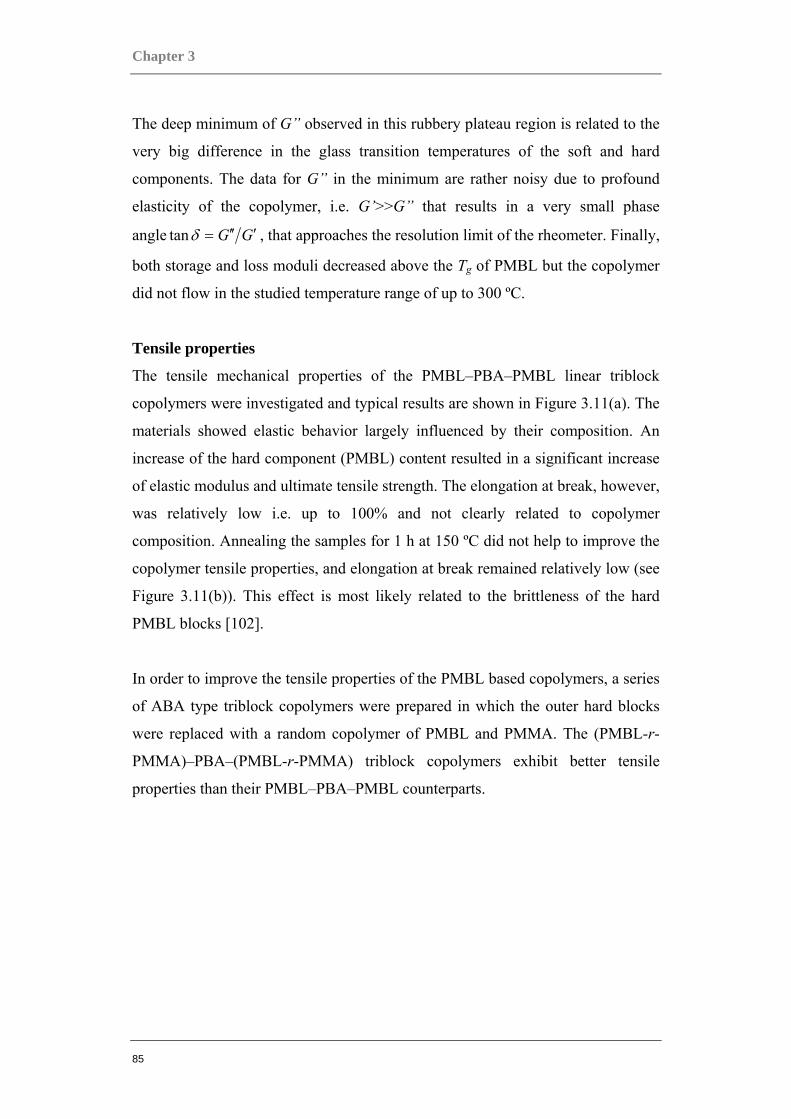
Chapter 3
85
The deep minimum of G” observed in this rubbery plateau region is related to the
very big difference in the glass transition temperatures of the soft and hard
components. The data for G” in the minimum are rather noisy due to profound
elasticity of the copolymer, i.e. G’>>G” that results in a very small phase
angle GG ′′′=δtan , that approaches the resolution limit of the rheometer. Finally,
both storage and loss moduli decreased above the Tg of PMBL but the copolymer
did not flow in the studied temperature range of up to 300 ºC.
Tensile properties
The tensile mechanical properties of the PMBL–PBA–PMBL linear triblock
copolymers were investigated and typical results are shown in Figure 3.11(a). The
materials showed elastic behavior largely influenced by their composition. An
increase of the hard component (PMBL) content resulted in a significant increase
of elastic modulus and ultimate tensile strength. The elongation at break, however,
was relatively low i.e. up to 100% and not clearly related to copolymer
composition. Annealing the samples for 1 h at 150 ºC did not help to improve the
copolymer tensile properties, and elongation at break remained relatively low (see
Figure 3.11(b)). This effect is most likely related to the brittleness of the hard
PMBL blocks [102].
In order to improve the tensile properties of the PMBL based copolymers, a series
of ABA type triblock copolymers were prepared in which the outer hard blocks
were replaced with a random copolymer of PMBL and PMMA. The (PMBL-r-
PMMA)–PBA–(PMBL-r-PMMA) triblock copolymers exhibit better tensile
properties than their PMBL–PBA–PMBL counterparts.
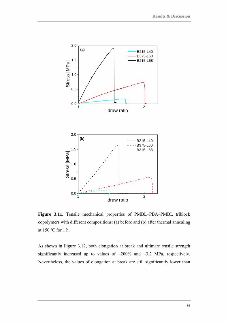
Results & Discussion
86
1 20.0
0.5
1.0
1.5
2.0
Stre
ss [M
Pa]
draw ratio
B215-L40 B375-L60 B215-L68
(a)
1 20.0
0.5
1.0
1.5
2.0
Stre
ss [M
Pa]
draw ratio
B215-L40 B375-L60 B215-L68
(b)
Figure 3.11. Tensile mechanical properties of PMBL–PBA–PMBL triblock
copolymers with different compositions: (a) before and (b) after thermal annealing
at 150 ºC for 1 h.
As shown in Figure 3.12, both elongation at break and ultimate tensile strength
significantly increased up to values of ~200% and ~3.2 MPa, respectively.
Nevertheless, the values of elongation at break are still significantly lower than
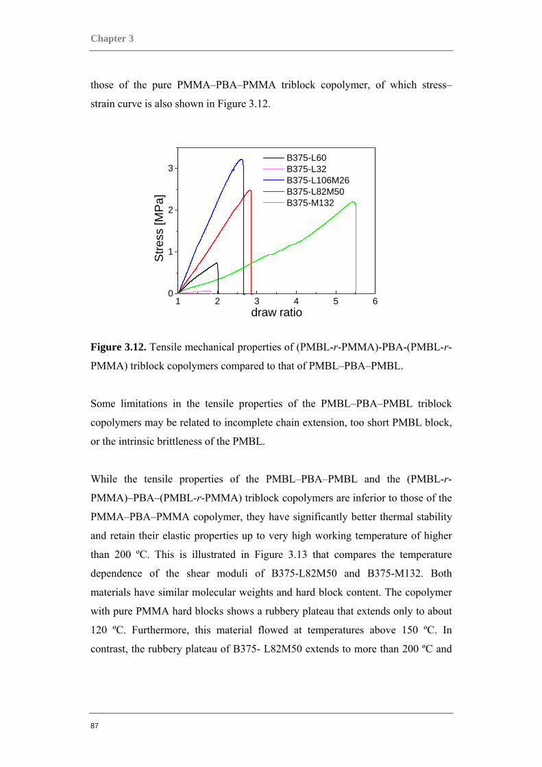
Chapter 3
87
those of the pure PMMA–PBA–PMMA triblock copolymer, of which stress–
strain curve is also shown in Figure 3.12.
1 2 3 4 5 60
1
2
3
Stre
ss [M
Pa]
draw ratio
B375-L60 B375-L32 B375-L106M26 B375-L82M50 B375-M132
Figure 3.12. Tensile mechanical properties of (PMBL-r-PMMA)-PBA-(PMBL-r-
PMMA) triblock copolymers compared to that of PMBL–PBA–PMBL.
Some limitations in the tensile properties of the PMBL–PBA–PMBL triblock
copolymers may be related to incomplete chain extension, too short PMBL block,
or the intrinsic brittleness of the PMBL.
While the tensile properties of the PMBL–PBA–PMBL and the (PMBL-r-
PMMA)–PBA–(PMBL-r-PMMA) triblock copolymers are inferior to those of the
PMMA–PBA–PMMA copolymer, they have significantly better thermal stability
and retain their elastic properties up to very high working temperature of higher
than 200 ºC. This is illustrated in Figure 3.13 that compares the temperature
dependence of the shear moduli of B375-L82M50 and B375-M132. Both
materials have similar molecular weights and hard block content. The copolymer
with pure PMMA hard blocks shows a rubbery plateau that extends only to about
120 ºC. Furthermore, this material flowed at temperatures above 150 ºC. In
contrast, the rubbery plateau of B375- L82M50 extends to more than 200 ºC and
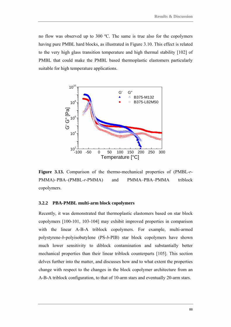
Results & Discussion
88
no flow was observed up to 300 ºC. The same is true also for the copolymers
having pure PMBL hard blocks, as illustrated in Figure 3.10. This effect is related
to the very high glass transition temperature and high thermal stability [102] of
PMBL that could make the PMBL based thermoplastic elastomers particularly
suitable for high temperature applications.
-100 -50 0 50 100 150 200 250 300102
104
106
108
1010
G
' G" [
Pa]
G' G" B375-M132 B375-L82M50
Temperature [°C]
Figure 3.13. Comparison of the thermo-mechanical properties of (PMBL-r-
PMMA)–PBA–(PMBL-r-PMMA) and PMMA–PBA–PMMA triblock
copolymers.
3.2.2 PBA-PMBL multi-arm block copolymers
Recently, it was demonstrated that thermoplastic elastomers based on star block
copolymers [100-101, 103-104] may exhibit improved properties in comparison
with the linear A-B-A triblock copolymers. For example, multi-armed
polystyrene-b-polyisobutylene (PS-b-PIB) star block copolymers have shown
much lower sensitivity to diblock contamination and substantially better
mechanical properties than their linear triblock counterparts [105]. This section
delves further into the matter, and discusses how and to what extent the properties
change with respect to the changes in the block copolymer architecture from an
A-B-A triblock configuration, to that of 10-arm stars and eventually 20-arm stars.
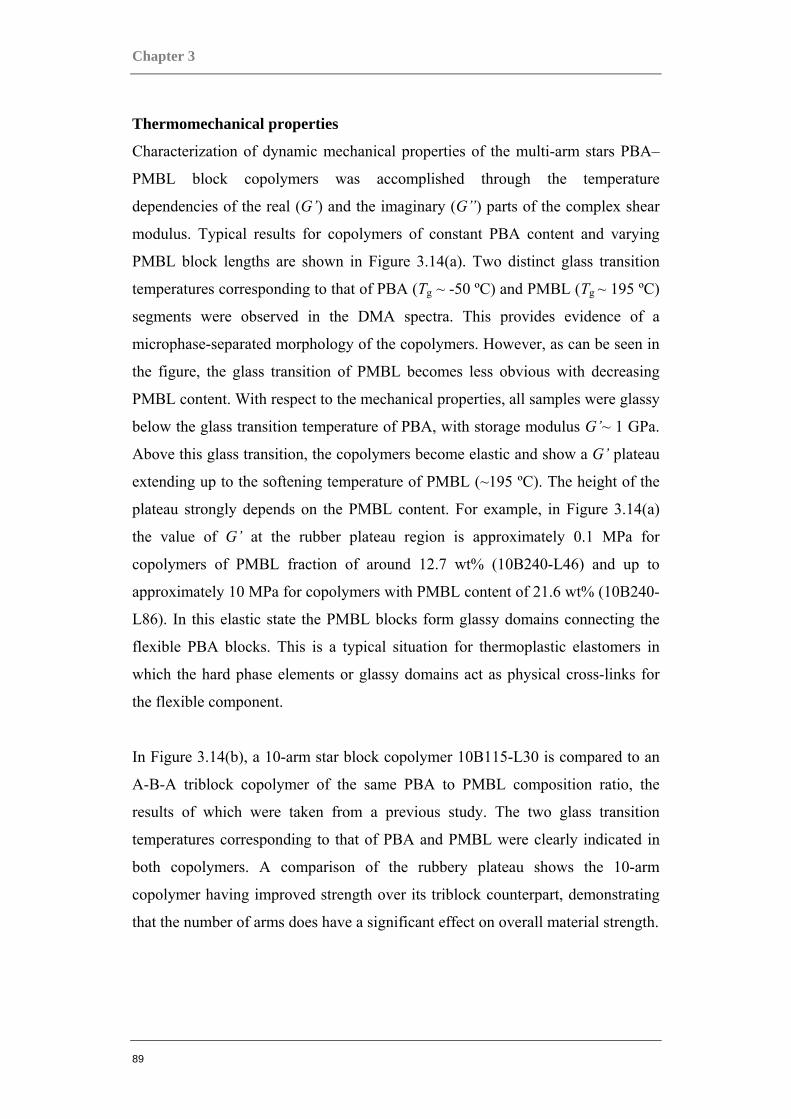
Chapter 3
89
Thermomechanical properties
Characterization of dynamic mechanical properties of the multi-arm stars PBA–
PMBL block copolymers was accomplished through the temperature
dependencies of the real (G’) and the imaginary (G”) parts of the complex shear
modulus. Typical results for copolymers of constant PBA content and varying
PMBL block lengths are shown in Figure 3.14(a). Two distinct glass transition
temperatures corresponding to that of PBA (Tg ~ -50 ºC) and PMBL (Tg ~ 195 ºC)
segments were observed in the DMA spectra. This provides evidence of a
microphase-separated morphology of the copolymers. However, as can be seen in
the figure, the glass transition of PMBL becomes less obvious with decreasing
PMBL content. With respect to the mechanical properties, all samples were glassy
below the glass transition temperature of PBA, with storage modulus G’~ 1 GPa.
Above this glass transition, the copolymers become elastic and show a G’ plateau
extending up to the softening temperature of PMBL (~195 ºC). The height of the
plateau strongly depends on the PMBL content. For example, in Figure 3.14(a)
the value of G’ at the rubber plateau region is approximately 0.1 MPa for
copolymers of PMBL fraction of around 12.7 wt% (10B240-L46) and up to
approximately 10 MPa for copolymers with PMBL content of 21.6 wt% (10B240-
L86). In this elastic state the PMBL blocks form glassy domains connecting the
flexible PBA blocks. This is a typical situation for thermoplastic elastomers in
which the hard phase elements or glassy domains act as physical cross-links for
the flexible component.
In Figure 3.14(b), a 10-arm star block copolymer 10B115-L30 is compared to an
A-B-A triblock copolymer of the same PBA to PMBL composition ratio, the
results of which were taken from a previous study. The two glass transition
temperatures corresponding to that of PBA and PMBL were clearly indicated in
both copolymers. A comparison of the rubbery plateau shows the 10-arm
copolymer having improved strength over its triblock counterpart, demonstrating
that the number of arms does have a significant effect on overall material strength.
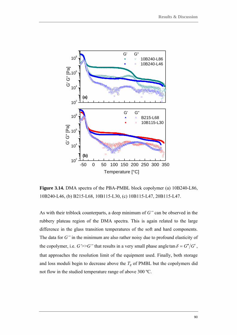
Results & Discussion
90
102
104
106
108
-50 0 50 100 150 200 250 300 350102
104
106
108
G
' G" [
Pa]
G' G"10B240-L8610B240-L46
(a)
Temperature [°C]
G' G
" [Pa
]
G' G"B215-L6810B115-L30
(b)
Figure 3.14. DMA spectra of the PBA-PMBL block copolymer (a) 10B240-L86,
10B240-L46, (b) B215-L68, 10B115-L30, (c) 10B115-L47, 20B115-L47.
As with their triblock counterparts, a deep minimum of G” can be observed in the
rubbery plateau region of the DMA spectra. This is again related to the large
difference in the glass transition temperatures of the soft and hard components.
The data for G” in the minimum are also rather noisy due to profound elasticity of
the copolymer, i.e. G’>>G” that results in a very small phase angle GG ′′′=δtan ,
that approaches the resolution limit of the equipment used. Finally, both storage
and loss moduli begin to decrease above the Tg of PMBL but the copolymers did
not flow in the studied temperature range of above 300 ºC.
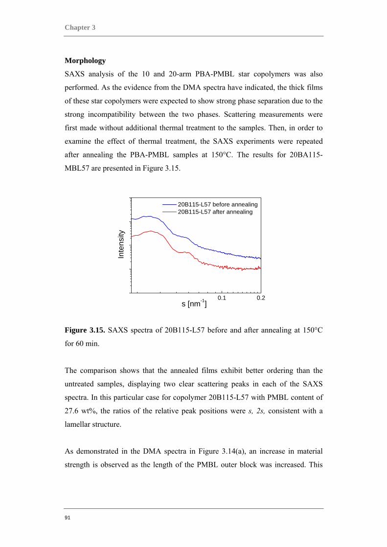
Chapter 3
91
Morphology
SAXS analysis of the 10 and 20-arm PBA-PMBL star copolymers was also
performed. As the evidence from the DMA spectra have indicated, the thick films
of these star copolymers were expected to show strong phase separation due to the
strong incompatibility between the two phases. Scattering measurements were
first made without additional thermal treatment to the samples. Then, in order to
examine the effect of thermal treatment, the SAXS experiments were repeated
after annealing the PBA-PMBL samples at 150°C. The results for 20BA115-
MBL57 are presented in Figure 3.15.
0.1 0.2
s [nm-1]
Inte
nsity
20B115-L57 before annealing 20B115-L57 after annealing
Figure 3.15. SAXS spectra of 20B115-L57 before and after annealing at 150°C
for 60 min.
The comparison shows that the annealed films exhibit better ordering than the
untreated samples, displaying two clear scattering peaks in each of the SAXS
spectra. In this particular case for copolymer 20B115-L57 with PMBL content of
27.6 wt%, the ratios of the relative peak positions were s, 2s, consistent with a
lamellar structure.
As demonstrated in the DMA spectra in Figure 3.14(a), an increase in material
strength is observed as the length of the PMBL outer block was increased. This
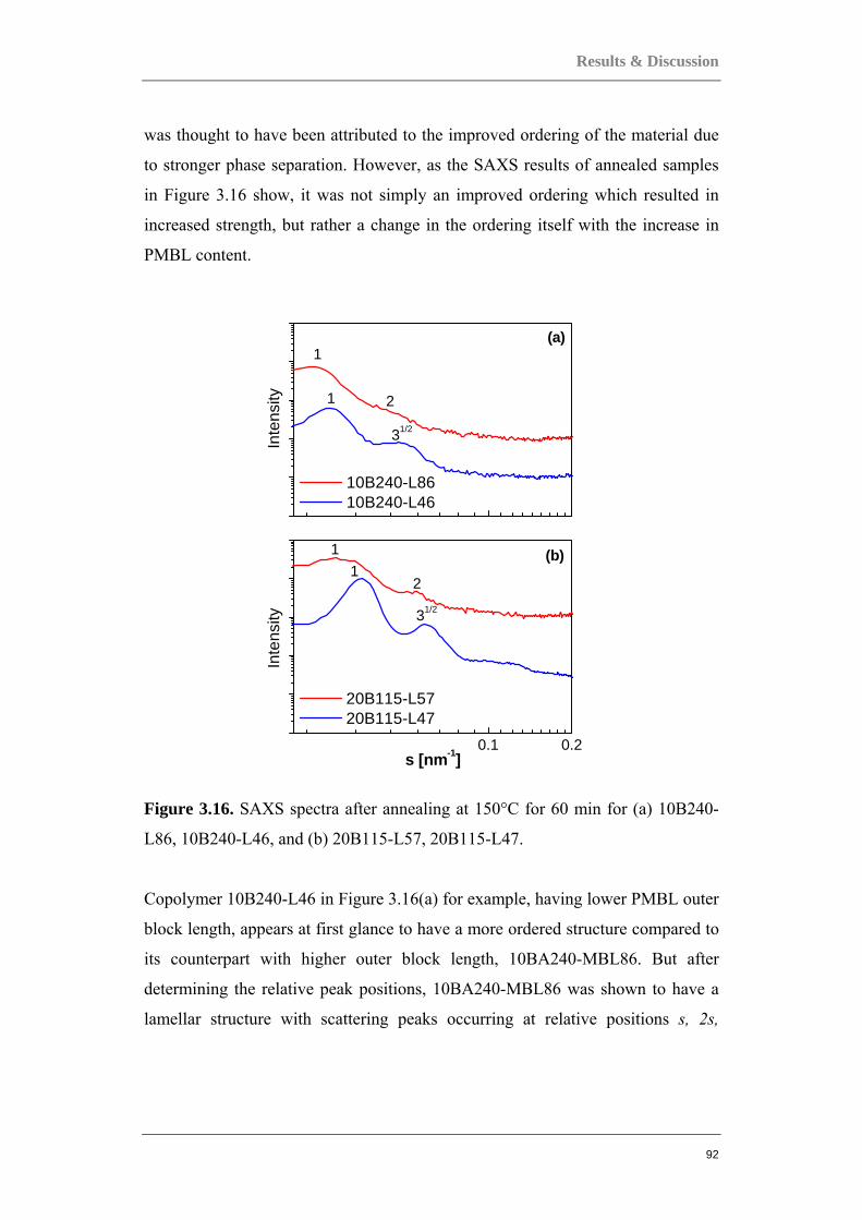
Results & Discussion
92
was thought to have been attributed to the improved ordering of the material due
to stronger phase separation. However, as the SAXS results of annealed samples
in Figure 3.16 show, it was not simply an improved ordering which resulted in
increased strength, but rather a change in the ordering itself with the increase in
PMBL content.
0.1 0.2
(b)
31/2
21
1
Inte
nsity
s [nm-1]
20B115-L57 20B115-L47
31/2
21
Inte
nsity
10B240-L86 10B240-L46
1(a)
Figure 3.16. SAXS spectra after annealing at 150°C for 60 min for (a) 10B240-
L86, 10B240-L46, and (b) 20B115-L57, 20B115-L47.
Copolymer 10B240-L46 in Figure 3.16(a) for example, having lower PMBL outer
block length, appears at first glance to have a more ordered structure compared to
its counterpart with higher outer block length, 10BA240-MBL86. But after
determining the relative peak positions, 10BA240-MBL86 was shown to have a
lamellar structure with scattering peaks occurring at relative positions s, 2s,
Chapter 3
93
whereas 10BA240-MBL46 exhibited structures consistent with hexagonal-packed
cylinders (two relatively sharp peaks at relative positions ss 3, ). This change in
ordering from hexagonal cylinders to lamellar may be the cause of the very large
improvement in strength exhibited by copolymer 10B240-L86 in the DMA
spectra (Figure 3.14(a)). Samples 20B115-L47 and 20B115-L57 also exhibited
similar ordering changes, as shown in the Figure 3.16(b).
The different compositions of the 10-arm and 20-arm PBA-PMBL copolymers is
shown to have an effect on the d-spacing in the micro-phase separated structures.
As shown in the Table 3.2, the increase of PMBL block length leads to an
increase in the d-spacing at the same length of the PBA segment. And
demonstrated earlier in Figure 3.16, the SAXS results show that the multi-arm
block copolymers with lower outer PMBL content revealing a micro phase
separated morphology of cylindrical PMBL domains hexagonally arranged in the
PBA matrix. Samples with higher PMBL content revealed a lamellar structure. At
even higher molecular weight, in particular for samples 20B230-L96 and 20B750-
L156, no clear indication of structure was revealed from the SAXS results. The
number of arms did not seem to affect the d-spacing as shown in Table 3.2 when
comparing for example, copolymers 10B115-L47 and 20B115-L47, both having
the same PBA to PMBL ratio, but different number of arms.

Results & Discussion
94
Table 3.2
Compositions of the prepared PBA-PMBL star-like block copolymers, their phase
separation spacing values and corresponding structure.
Sample SAXS (before annealing)
SAXS (after annealing) Structure
10BA115-MBL30 26.7 nm 25.3 nm hexagonal cylinders 10BA115-MBL47 28.9 nm 28.5 nm hexagonal cylinders 10BA240-MBL46 37.5 nm 36.7 nm hexagonal cylinders 10BA240-MBL86 42.7 nm 42.1 nm lamellar 20BA115-MBL47 28.9 nm 28.5 nm hexagonal cylinders 20BA115-MBL57 35.7 nm 35.3 nm lamellar 20BA230-MBL96 52.6 nm 49.6 nm - 20BA750-MBL156 71.9 nm 73.3 nm -
Tensile Properties
Tensile strength comparisons made between copolymers with varying PMBL
contents demonstrate again that an increase in the PMBL block length results in a
stronger material. However, in Figure 3.17(a) we observe that for copolymer
10B240-L86, elasticity is significantly reduced as a result of the higher PMBL
content when compared to copolymer 10B240-L46 of lower PMBL content. This
observation is due to the fact that the change in outer PMBL block lengths
contributes to stronger physical cross-linking of the material, enhancing overall
strength, however, sacrificing elasticity, and causing the material to become more
brittle in the process.
2 40
2
4
6
8
Stre
ss [M
Pa]
10B240-L86 10B240-L46
draw ratio
Figure 3.17. Tensile properties of copolymers 10B240-L86 and 10B240-L46.
Chapter 3
95
3.2.3 PBA-PMMA multi-arm block copolymers
While thermoplastic elastomers containing PMBL have excellent thermal stability
and retain their elastic properties up to a very high working temperature (more
than 200 ºC), their intrinsic brittleness seriously limits their potential as
thermoplastic elastomers. In this study, PMMA is used in place of PMBL in hopes
of solving the brittleness issue. PMMA, though having improved elasticity, has a
significantly lower glass transition temperature when compared to PMBL, making
them unsuitable for high temperature applications, but nevertheless a possible
candidate for use as hard blocks in thermoplastic elastomers.
Morphology
SAXS analysis of thick films of the star-like block copolymers illustrated that that
the majority of the samples reveal an expected micro phase separated morphology
of cylindrical PMMA domains hexagonally arranged in the PBA matrix (three
relatively sharp peaks at relative positions sss 7,3, ). The samples with
shortest arm length and lower PMMA content, 10B115-M29 and 20B115-M38,
did not reveal a clear structure. They exhibited a short-range ordering only, as
indicated from the single broad peak observed in their SAXS spectra. The
different compositions of the 10-arm and 20-arm PBA-PMMA copolymers also
affect the d-spacing in the micro-phase separated structures. Table 3.3 shows the
calculated results of the d-spacing obtained from AFM and SAXS data of the
measured PBA-PMMA star block copolymers. As can be seen in Table 3.3, the
increase of PMMA block length leads to an increase in the d-spacing at the same
length of the PBA segment. Number of arms seems to have negligible influence
on change in d-spacing.
In order to examine the effect of thermal treatment on the copolymer films
morphology, the SAXS experiments were repeated after annealing the PBA-
PMMA copolymer samples at 150 °C. The experiment showed that there was no
lost of phase separation after annealing for 60 minutes and the annealed films
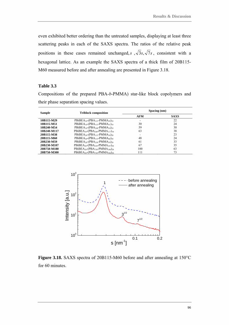
Results & Discussion
96
even exhibited better ordering than the untreated samples, displaying at least three
scattering peaks in each of the SAXS spectra. The ratios of the relative peak
positions in these cases remained unchanged, sss 7,3, , consistent with a
hexagonal lattice. As an example the SAXS spectra of a thick film of 20B115-
M60 measured before and after annealing are presented in Figure 3.18.
Table 3.3
Compositions of the prepared PBA-b-PMMA) star-like block copolymers and
their phase separation spacing values.
Spacing (nm) Sample Triblock composition
AFM SAXS 10B115-M29 PBiBEA10-(PBA115-PMMA29)10 - 22 10B115-M51 PBiBEA10-(PBA115-PMMA51)10 30 24 10B240-M54 PBiBEA10-(PBA240-PMMA54)10 59 30 10B240-M117 PBiBEA10-(PBA240-PMMA117)10 63 38 20B115-M38 PBiBEA20-(PBA115-PMMA38)20 - 23 20B115-M60 PBiBEA20-(PBA115-PMMA60)20 48 24 20B230-M59 PBiBEA20-(PBA230-PMMA59)20 61 33 20B230-M107 PBiBEA20-(PBA230-PMMA107)20 67 35 20B750-M180 PBiBEA20-(PBA750-PMMA180)20 100 63 20B750-M300 PBiBEA20-(PBA750-PMMA300)20 111 73
0.1 0.2100
101
102
103
71/2
s [nm-1]
Inte
nsity
[a.u
.]
before annealing after annealing1
31/2
Figure 3.18. SAXS spectra of 20B115-M60 before and after annealing at 150°C
for 60 minutes.
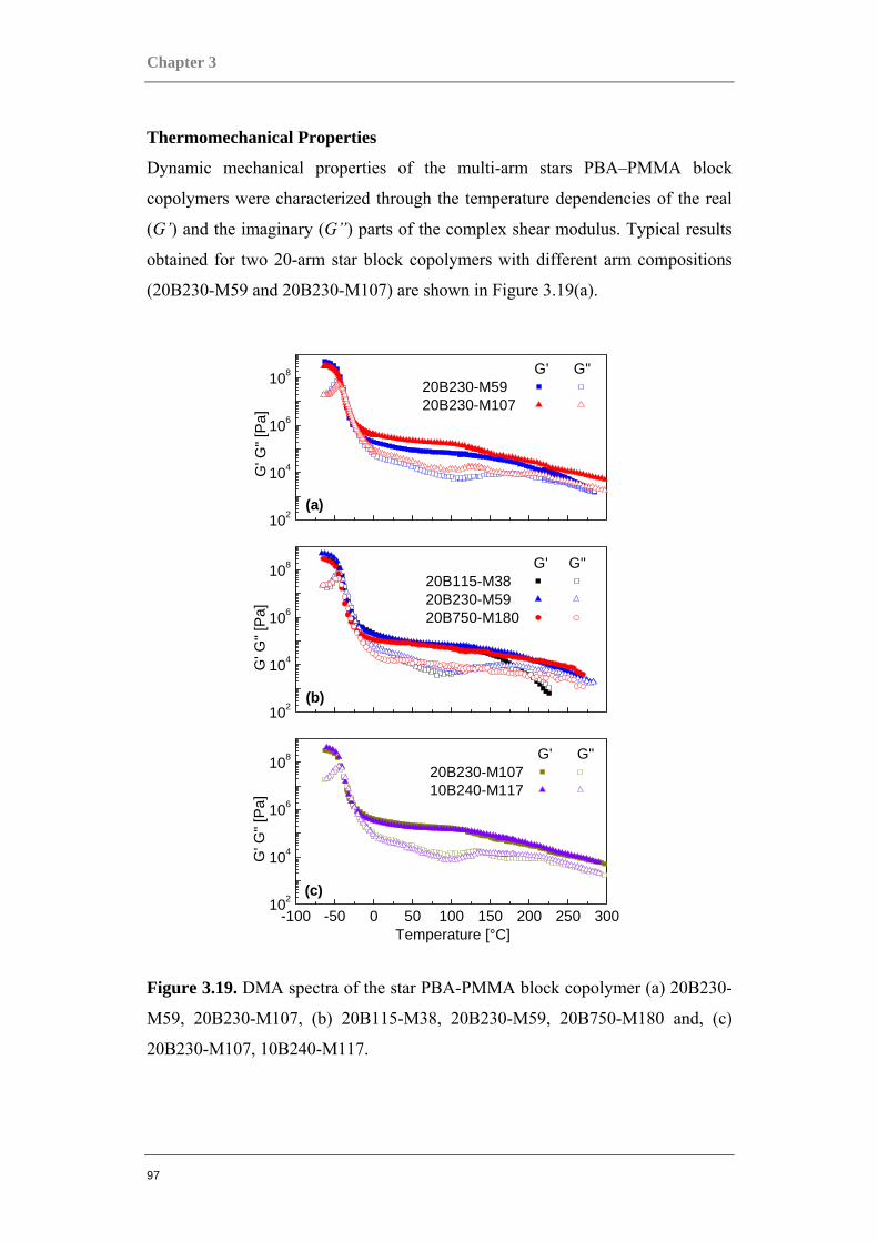
Chapter 3
97
Thermomechanical Properties
Dynamic mechanical properties of the multi-arm stars PBA–PMMA block
copolymers were characterized through the temperature dependencies of the real
(G’) and the imaginary (G”) parts of the complex shear modulus. Typical results
obtained for two 20-arm star block copolymers with different arm compositions
(20B230-M59 and 20B230-M107) are shown in Figure 3.19(a).
102
104
106
108
102
104
106
108
-100 -50 0 50 100 150 200 250 300102
104
106
108
Temperature [°C]
(a)
G
' G" [
Pa]
G' G"20B230-M59 20B230-M107
G
' G" [
Pa]
G' G"20B115-M38 20B230-M59 20B750-M180
(b)
(c)
G
' G" [
Pa]
G' G"20B230-M10710B240-M117
Figure 3.19. DMA spectra of the star PBA-PMMA block copolymer (a) 20B230-
M59, 20B230-M107, (b) 20B115-M38, 20B230-M59, 20B750-M180 and, (c)
20B230-M107, 10B240-M117.
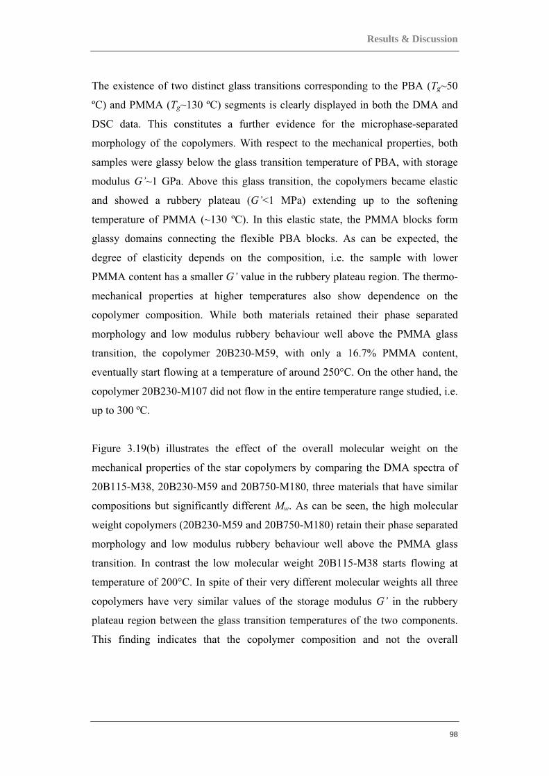
Results & Discussion
98
The existence of two distinct glass transitions corresponding to the PBA (Tg~50
ºC) and PMMA (Tg~130 ºC) segments is clearly displayed in both the DMA and
DSC data. This constitutes a further evidence for the microphase-separated
morphology of the copolymers. With respect to the mechanical properties, both
samples were glassy below the glass transition temperature of PBA, with storage
modulus G’~1 GPa. Above this glass transition, the copolymers became elastic
and showed a rubbery plateau (G’<1 MPa) extending up to the softening
temperature of PMMA (~130 ºC). In this elastic state, the PMMA blocks form
glassy domains connecting the flexible PBA blocks. As can be expected, the
degree of elasticity depends on the composition, i.e. the sample with lower
PMMA content has a smaller G’ value in the rubbery plateau region. The thermo-
mechanical properties at higher temperatures also show dependence on the
copolymer composition. While both materials retained their phase separated
morphology and low modulus rubbery behaviour well above the PMMA glass
transition, the copolymer 20B230-M59, with only a 16.7% PMMA content,
eventually start flowing at a temperature of around 250°C. On the other hand, the
copolymer 20B230-M107 did not flow in the entire temperature range studied, i.e.
up to 300 ºC.
Figure 3.19(b) illustrates the effect of the overall molecular weight on the
mechanical properties of the star copolymers by comparing the DMA spectra of
20B115-M38, 20B230-M59 and 20B750-M180, three materials that have similar
compositions but significantly different Mw. As can be seen, the high molecular
weight copolymers (20B230-M59 and 20B750-M180) retain their phase separated
morphology and low modulus rubbery behaviour well above the PMMA glass
transition. In contrast the low molecular weight 20B115-M38 starts flowing at
temperature of 200°C. In spite of their very different molecular weights all three
copolymers have very similar values of the storage modulus G’ in the rubbery
plateau region between the glass transition temperatures of the two components.
This finding indicates that the copolymer composition and not the overall

Chapter 3
99
molecular weight is the main factor that determines the elastic properties of these
thermoplastic elastomer materials.
As discussed earlier, another important parameter that could influence the thermo-
mechanical properties of the star-like copolymers is the number of arms. Figure
3.19(c) compares the DMA spectra of a 10 and 20 arm star copolymers with
similar block lengths and compositions: 10B240-M117 and 20B230-M107. As
can be seen the two materials show practically identical spectra which indicates
that the number of arms have little influence on their mechanical properties. This
finding is not that surprising taking into account that both materials have a rather
large number of arms, i.e. 10 and 20 respectively. Indeed earlier studies of
polystyrene-b-polyisobutylene [104] and polystyrene-b-polydiene [106] star like
block-copolymers, have shown that the tensile properties of these materials reach
a plateau in the Narm = 5-10 range. Evidently the presence of such a plateau
explains the similar mechanical properties of the 10 and 20 arm PBA-PMMA star
block copolymers.
Tensile Properties
The tensile properties of the PBA-PMMA star-like block copolymers listed in
Table 3 were also studied. Typical examples of the measured stress–strain
dependencies are shown in Figure 3.20(a). As expected the composition has a
major effect on the tensile properties of the PBA-PMMA star copolymers. We
found that both the initial modulus (E) and the tensile strength (σ break) increase
strongly with PMMA content, while the draw ratio at break seems to increase with
the length of PBA segment and be reduced with increasing PMMA content.
During the last several years it was demonstrated that thermoplastic elastomers
based on star block copolymers [107-111] may exhibit superior properties as
compared to the linear ABA triblock type TPEs. Furthermore it was also shown
that the tensile properties of the star block copolymers improve with the number
of arms until reaching saturation at the Narm = 5-10. In an attempt to explore these
effects in the case of PBA-PMMA based materials we have compared the newly
Results & Discussion
100
synthesized 10 and 20 arm 10B115-M51 and 20B115-M60 to the 3-arm star
copolymer 3B164-M76 that we have studied recently [101] and to a linear
PMMA-PBA-PMMA block copolymer prepared using ATRP by the Jerome
group[112].
0
2
4
6
8
10
1 2 3 4 5 60
2
4
6
8
10(b)
(a)
S
tress
[MP
a] 20B230-M59 20B230-M107
draw ratio
Stre
ss [M
Pa]
20B115-M60 10B115-M51 3B164-M76
Figure 3.20. Tensile properties of copolymers (a) 20B230-M59, 20B230-M107,
and (b) 20B115-M60, 10B115-M51, 3B164-M7.
Table 3.4
Ultimate tensile strength and maximum elongation at break of PBA-PMMA block
copolymers with similar composition but varying numbers of arms.
Sample Mn (g/mol) PDI
PMMA content (wt %)
ultimate tensile strength σ (MPa)
maximum elongation
at break λ (%) linear ABA type copolymer 69,000 1.15 26 4.2 520
3-arm star B164-M76 block copolymer 85,800 1.19 26 4.8 545
10-arm B115-M51 copolymer 197,000 1.25 25.7 6.4 430
20-arm B115-M60 copolymer 412 000 1.36 28.9 7.4 375
Chapter 3
101
As shown in Table 3.4 all four materials have practically the same polymer chain
composition ratio. As the 3-arm star copolymer B164-M76 has the same overall
composition and only slightly higher molecular weight as compared to the linear
PMMA-PBA-PMMA, in Table 3.4 we compared the properties of these materials.
While tensile strength and DMA results of the 10 and 20 arm star block
copolymers suggest that the number of arms have little influence on their
mechanical properties, an attempt was made to compare the tensile properties of
these new samples to earlier studies performed on 3-arm star PBA-PMMA block
copolymers as well as linear triblock PBA-PMMA copolymers. In the table below
we compare the properties of 4 materials. As can be seen from the table, there is
an increase in ultimate tensile strength with the increase in number of arms.
Particularly, the ultimate tensile strength of the 10-arm 10B115-M51 is
significantly better than that of the 3-arm copolymer. The improvement isn’t as
significant when comparing the 10-arm versus the 20-arm samples, which
suggests a plateau or saturation point in the improvement of the tensile properties
with respect to number of arms. The table also shows that for the star block
copolymers, the improvement in ultimate tensile strength results in the draw ratio
being sacrificed, as the maximum elongation of the thermoplastic elastomers is
significantly reduced with the increase in number of arms and ultimate tensile
strength.
Results & Discussion
102
3.3 Siloxane-based Linear Copolymers: Gradient or Block?
Gradient copolymers, with a controlled composition along the backbone but with
a homogeneous composition among the chains, are a promising class of materials
with tunable microstructures and physical properties. They can potentially be used
as polymer blend compatibilizers, surfactants, and environment-sensitive
materials, for example, materials for vibration and noise dampening. They also
can serve as the building blocks for the synthesis of complex macromolecular
architectures, such as polymer brushes, hyperbranched polymers, dendrimers, and
hybrid organic-inorganic materials [113-114].
3.3.1 Fluorosiloxane-based Copolymers
Fluorosilicones are polymers consisting of fluorocarbon groups, which have the
lowest known inter-molecular forces of all pendant groups, with the unique
flexibility of the siloxane backbone. The first and still the most common
commercial fluorosilicone is poly[methyl(trifluoropropyl)siloxane], PMTFPS.
PMTFPS products are used in many applications where resistance to fuel, oils and
hydrocarbon solvents is required. Examples are lubricants in bearings exposed to
such materials and sealants and elastomers for automotive fuel systems.
Fluorosilicone rubber shows good performance at extremely low temperatures
down to -70 ºC which makes it unrivalled material for aerospace applications.
Other applications include antifoams for organic liquids and in cosmetics and
other skin use formulations where long-lasting oil and water repellency is desired,
release agents for PDMS-based pressure-sensitive adhesives, and antifouling
coatings and lubricants [21, 113]. Because fluorinated polysiloxanes are quite
expensive, their copolymers which can be used as additives to other polymers,
improving their properties, are of great interest.
Chapter 3
103
Thermomechanical Properties
It has previously been reported that the tapering nature of gradient copolymers
affect the Tg’s of both component monomers. In the case of fluorosiloxane-based
copolymers, the Tg’s of the corresponding homopolymers PDMS and PMTFPS
are -127 ºC and -70 ºC, respectively [115]. DSC results of the PDMS
homopolymer, illustrated in Figure 3.21(a), shows a characteristic crystallization
band at -88 ºC and two endothermic peaks at -48.3 and -36.4 ºC, which are typical
for PDMS if the chain length exceeds Mn = 5000, which corresponds to
approximately 20 D3 (PDMS) units [116]. From the differential scanning
calorimetry (DSC), these transitions are still present in block and spontaneous
gradient copolymers (Figure 3.21(c) and (d)) in which the dimethylsiloxane block
is sufficiently long, that is, more than approximately 5000, although, the
crystallization band becomes broader and moves to higher temperatures. The
enthalpy of crystallization depends on the Mw (length of the pure dimethylsiloxane
block). There is only one broad melting transition which appears at temperature
between the two peaks occurring in the PDMS homopolymer. Assuming the
enthalpy of melting of the crystalline PDMS to be 61.2 J/g [116], a PDMS
homopolymer having a total enthalpy of fusion of about 40 J/g is 60–65%
crystalline (under the fast cooling regime applied here). The enthalpy of
crystallization decreases to approximately 15 J/g for the block copolymer (Figure
3.21(c) (Mw of the D block is approximately 5000) and to 8.6 J/g for the gradient
copolymer synthesized via spontaneous copolymerization (Figure 3.21(d))(Mw of
the D block is approximately 2800). These enthalpy values correspond to
approximately 24% and 14% of the crystalline character of the PDMS block,
respectively. The ‘‘forced’’ gradient copolymer (Figure 3.21(e)), or the gradient
copolymer synthesized via semi-batch method, does not reveal any crystallization
because the PDMS block is too short.
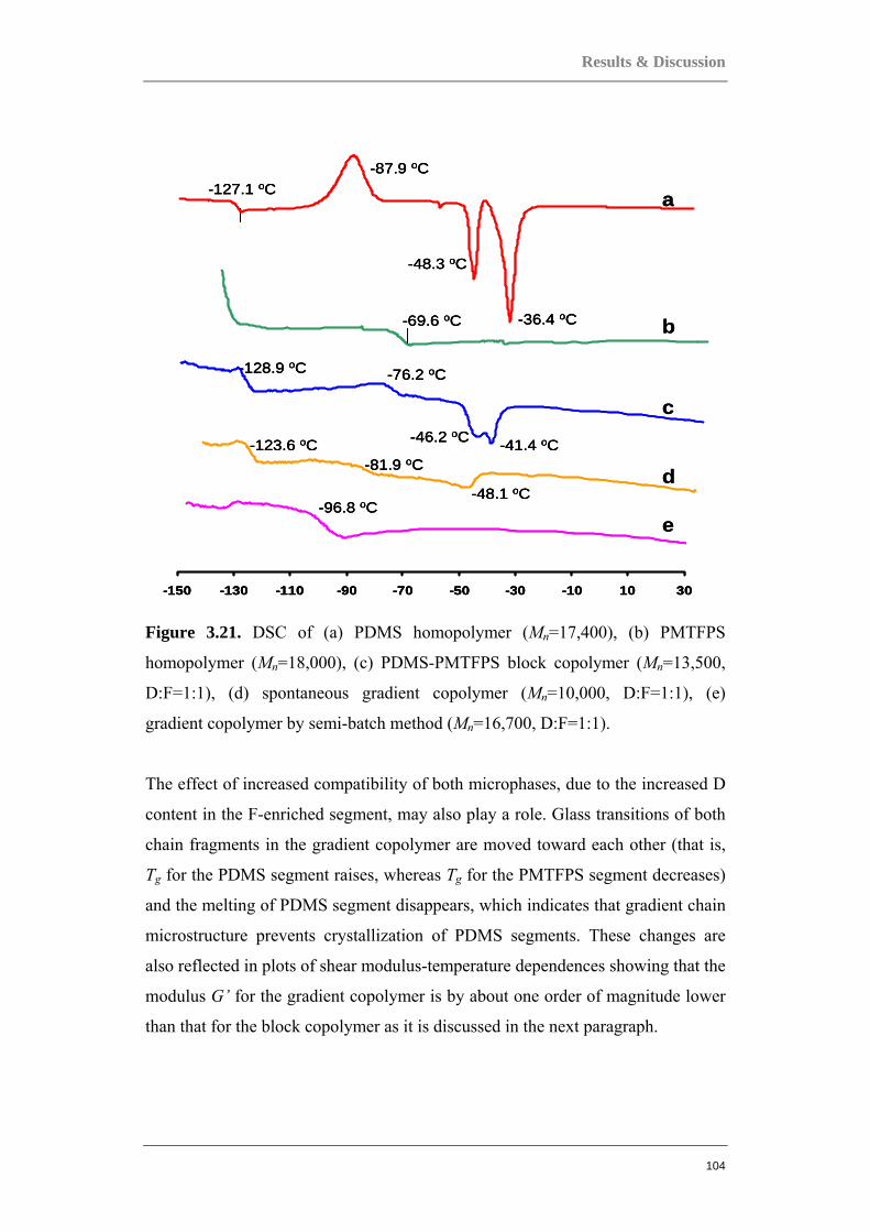
Results & Discussion
104
-150 -130 -110 -90 -70 -50 -30 -10 10 30
-87.9 oC
-48.3 oC
-127.1 oC
-36.4 oC
-128.9 oC -76.2 oC
-46.2 oC -41.4 oC-123.6 oC-81.9 oC
-48.1 oC
-69.6 oC
-96.8 oC
b
a
c
d
e
-150 -130 -110 -90 -70 -50 -30 -10 10 30
-87.9 oC
-48.3 oC
-127.1 oC
-36.4 oC
-128.9 oC -76.2 oC
-46.2 oC -41.4 oC-123.6 oC-81.9 oC
-48.1 oC
-69.6 oC
-96.8 oC
-150 -130 -110 -90 -70 -50 -30 -10 10 30
-87.9 oC
-48.3 oC
-127.1 oC
-36.4 oC
-128.9 oC -76.2 oC
-46.2 oC -41.4 oC-123.6 oC-81.9 oC
-48.1 oC
-69.6 oC
-96.8 oC
b
a
c
d
e
Figure 3.21. DSC of (a) PDMS homopolymer (Mn=17,400), (b) PMTFPS
homopolymer (Mn=18,000), (c) PDMS-PMTFPS block copolymer (Mn=13,500,
D:F=1:1), (d) spontaneous gradient copolymer (Mn=10,000, D:F=1:1), (e)
gradient copolymer by semi-batch method (Mn=16,700, D:F=1:1).
The effect of increased compatibility of both microphases, due to the increased D
content in the F-enriched segment, may also play a role. Glass transitions of both
chain fragments in the gradient copolymer are moved toward each other (that is,
Tg for the PDMS segment raises, whereas Tg for the PMTFPS segment decreases)
and the melting of PDMS segment disappears, which indicates that gradient chain
microstructure prevents crystallization of PDMS segments. These changes are
also reflected in plots of shear modulus-temperature dependences showing that the
modulus G’ for the gradient copolymer is by about one order of magnitude lower
than that for the block copolymer as it is discussed in the next paragraph.

Chapter 3
105
Dynamic mechanical analysis for the copolymers in Figure 3.21(a), (b) and (c)
were performed for the evaluation of their properties under shear deformation in a
broad temperature range. Temperature sweep tests were conducted during both
heating and cooling of the samples. The results are summarized in Figure 3.22. In
the case of the block copolymer (Figure 3.22(a)), the glass transition of the PDMS
block is clearly indicated in both cooling and heating curves by the drop in G’ and
the maximum in G” at low temperatures around -130 ºC. The softening related to
this transition is considerable and involves a drop of the real part of the shear
modulus by almost one order of magnitude. The glass transition of the PMTFPS
block is not clearly visible as it is covered by the crystallization of PDMS which
takes place in the same temperature region. Remarkably strong recrystallization of
the PDMS on heating is observed despite the fact that cooling was done rather
slowly at 2 K/min. This process is manifested by the strong increase of G’ in the
heating curve at temperatures of around -80 ºC. At even higher temperatures
(above -50 ºC) the melting of the crystalline PDMS leads to a strong drop in the
shear moduli. The temperature dependences of the G’ and G” of the spontaneous
gradient copolymer (Figure 3.22(b)) differ significantly from those of the block
copolymer. Although the glass transitions of the two components are still well
pronounced, the crystallization of the PDMS is prevented by the gradient chain
structure of these copolymers. Furthermore, in the temperature range between the
two Tg’s, the storage modulus G’ of the gradient copolymer is significantly lower
than that of the block copolymer. Finally, the spectra of the copolymer prepared
by semi-batch method (Figure 3.22(c)) reveals ‘‘pure gradient type’’ features, that
is, single glass transition around -97 ºC (between the Tg’s of the PDMS and
PMTFPS) which is roughly at the some position as that of the statistical (random)
copolymer, but is much broader as a result of the pure gradient structure.
It is important to emphasize at this point that the DMA data fit very well to DSC
results despite the fact that different cooling/heating rates (2 K/min in the case of
DMA and 10 K/min in the case of DSC) were used in the experiments.
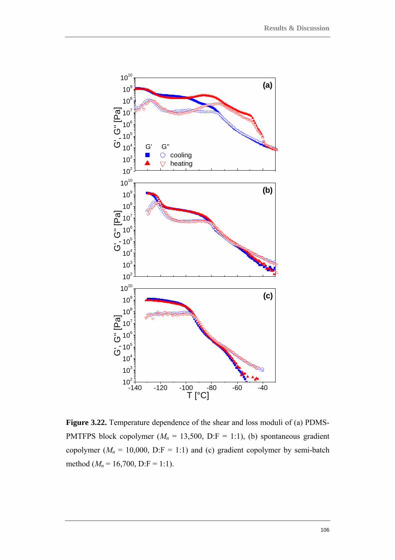
Results & Discussion
106
102
103
104
105
106
107
108
109
1010
102
103
104
105
106
107
108
109
1010
-140 -120 -100 -80 -60 -40102
103
104
105
106
107
108
109
1010
G',
G'' [
Pa]
G',
G'' [
Pa]
G' G''coolingheating
G',
G'' [
Pa]
T [°C]
(a)
(b)
(c)
Figure 3.22. Temperature dependence of the shear and loss moduli of (a) PDMS-
PMTFPS block copolymer (Mn = 13,500, D:F = 1:1), (b) spontaneous gradient
copolymer (Mn = 10,000, D:F = 1:1) and (c) gradient copolymer by semi-batch
method (Mn = 16,700, D:F = 1:1).
Chapter 3
107
Morphology
As described above, both the DSC and DMA results have indicated a phase
separation in the block and the spontaneous gradient copolymers. To explore this
effect in more details and examine the type of the formed microstructures we have
performed temperature dependent SAXS experiments. The results summarized in
Figure 3.23 in the form of scattered intensity versus the scattering vector q, show
a strong phase separation and ordering in both block and spontaneous gradient
copolymers at all temperatures. Nevertheless, we again have significant
differences between these two types of materials. In the case of the block
copolymers (Figure 3.23(a)), several peeks are observed at relative positions
1:31/2:41/2:71/2:91/2 which may indicate a hexagonal arrangement of cylinders,
although the peak intensity does not precisely correspond to this structure,
because the 31/2 reflection has suppressed intensity. For the gradient copolymer
obtained by simultaneous copolymerization (Figure 3.23(b)) two peaks were
observed at relative positions 1:2 which suggest a lamellar structure. On the other
hand, the gradient copolymer D-F, obtained by semi-batch method showed only
one weak and broad peak corresponding to a characteristic correlation length of
approximately 11 nm. This peak disappears after heating to T > -40 ºC.
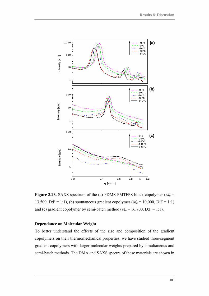
Results & Discussion
108
1
1 0
10 0
100 0
2 5 °C 0 °C -2 0°C -6 0°C -1 40 C
Inte
nsity
[a.u
.]
1
10
1 00
Inte
nsity
[a.u
.]
25 °C 0 °C -20 °C -60 °C -14 0 °C
0 .2 0 .4 0 .6 0 .8 1 1 .2
1
10
100
Inte
nsity
[a.u
.]
q [nm -1]
0 °C -2 0°C -6 0°C -1 00 °C -1 40 °C
(a)
(b)
(c)
1
1 0
10 0
100 0
2 5 °C 0 °C -2 0°C -6 0°C -1 40 C
Inte
nsity
[a.u
.]
1
10
1 00
Inte
nsity
[a.u
.]
25 °C 0 °C -20 °C -60 °C -14 0 °C
0 .2 0 .4 0 .6 0 .8 1 1 .2
1
10
100
Inte
nsity
[a.u
.]
q [nm -1]
0 °C -2 0°C -6 0°C -1 00 °C -1 40 °C
(a)
(b)
(c)
Figure 3.23. SAXS spectrum of the (a) PDMS-PMTFPS block copolymer (Mn =
13,500, D:F = 1:1), (b) spontaneous gradient copolymer (Mn = 10,000, D:F = 1:1)
and (c) gradient copolymer by semi-batch method (Mn = 16,700, D:F = 1:1).
Dependance on Molecular Weight
To better understand the effects of the size and composition of the gradient
copolymers on their thermomechanical properties, we have studied three-segment
gradient copolymers with larger molecular weights prepared by simultaneous and
semi-batch methods. The DMA and SAXS spectra of these materials are shown in
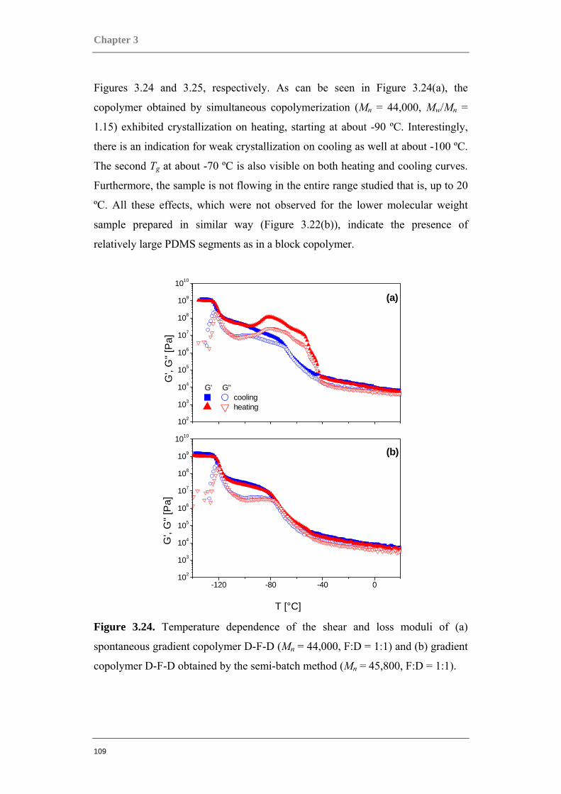
Chapter 3
109
Figures 3.24 and 3.25, respectively. As can be seen in Figure 3.24(a), the
copolymer obtained by simultaneous copolymerization (Mn = 44,000, Mw/Mn =
1.15) exhibited crystallization on heating, starting at about -90 ºC. Interestingly,
there is an indication for weak crystallization on cooling as well at about -100 ºC.
The second Tg at about -70 ºC is also visible on both heating and cooling curves.
Furthermore, the sample is not flowing in the entire range studied that is, up to 20
ºC. All these effects, which were not observed for the lower molecular weight
sample prepared in similar way (Figure 3.22(b)), indicate the presence of
relatively large PDMS segments as in a block copolymer.
102
103
104
105
106
107
108
109
1010
-120 -80 -40 0102
103
104
105
106
107
108
109
1010
G',
G'' [
Pa]
G' G''coolingheating
G',
G'' [
Pa]
T [°C]
(a)
(b)
Figure 3.24. Temperature dependence of the shear and loss moduli of (a)
spontaneous gradient copolymer D-F-D (Mn = 44,000, F:D = 1:1) and (b) gradient
copolymer D-F-D obtained by the semi-batch method (Mn = 45,800, F:D = 1:1).

Results & Discussion
110
The SAXS spectra of the high molecular weight spontaneous gradient copolymer,
which is shown on Figure 3.25(a), reveal four well defined peaks (as in the case of
the block copolymer in Figure 3.23(a)) indicating again a very strong phase
separation. Nevertheless, in contrast to the block copolymer that showed a
hexagonal microstructure, here the positions of the scattering peaks are observed
at q values of 1:2:3.4 indicating a lamellar structure. This is consistent with what
was found for the similarly prepared gradient copolymer with lower molecular
weight (Figure 3.23(b)).
0.2 0.4 0.6 0.8 1
1
10
100
(b)
q [nm-1]
Inte
nsity
[a.u
.]
20°C -60°C -100°C -140°C
1
10
100
In
tens
ity [a
.u.]
20°C -60°C -100°C -140°C
(a)
(a)
(b)
0.2 0.4 0.6 0.8 1
1
10
100
(b)
q [nm-1]
Inte
nsity
[a.u
.]
20°C -60°C -100°C -140°C
1
10
100
In
tens
ity [a
.u.]
20°C -60°C -100°C -140°C
(a)
(a)
(b)
Figure 3.25. SAXS spectra of (a) spontaneous gradient copolymer D-F-D (M =
44,000, F:D = 1:1) and (b) gradient copolymer D-F-D obtained by the semi-batch
method (M = 45,800, F:D = 1:1).
Chapter 3
111
The high molecular weight gradient copolymer D-F-D obtained by the semi-batch
method (Mn = 45,800, Mw/Mn = 1.15) also shows properties significantly different
from those of its lower Mw counterpart (Mn = 16,000, D:F = 1:1). For example, the
temperature dependences of G’ and G” of this material shown on Figure 3.24(b)
clearly reveal two Tg’s, which was not the case for the low Mw copolymer (Figure
3.22(c)). Furthermore, the sample is not flowing in the entire range studied, that
is, up to 20 ºC although the low molecular one was flowing above about -70 ºC.
The observed differences in the mechanical properties are strongly related to the
different microstructures of the two materials as manifested by their SAXS
spectra. Although we were not able to identify a clear phase separation for the
lower molecular weight copolymer (Figure3.23(c)), a lamella type microstructure
was clearly observed for the high molecular weight material at all temperatures
(Figure 3.25(b)). The presence of only two scattering peaks however shows that
the effect is still weaker than those observed for the spontaneous gradient
copolymer with similarly high molecular weight (Figure 3.25(a)).
Thus, the thermomechanical properties and the microstructure formation in these
materials depend strongly on the molecular weight of the copolymers and on the
lengths of the uniform block at the chain ends.
Results & Discussion
112
3.3.2 Vinylsiloxane-based Copolymers
The precise synthesis of polysiloxanes having vinyl groups attached to the
polymer chain has the potential to open new routes to a wide class of functional
siloxane copolymers with controlled chain structure, as the vinyl group at silicon
is a known versatile precursor that can be easily modified by chemical
transformations giving rise to a variety of side functionalized polysiloxanes. It can
be converted into many useful functional groups by various kinds of addition
reactions [117], such as hydrosilylation [82, 118-120], thiolene addition [116,
121-123], hydroboration [124], epoxidation [125-126], and others [127-128].
The apparent rate constants and reactivity ratios were estimated by computer
simulation to be 011.03
≈Dr , 3.493
≈Vr . As a result of so much difference in
reactivity rates, simultaneous polymerization is predicted to lead to copolymers of
blocky structure containing a narrow intermediate fragment with gradient
distribution of siloxane units. Polymers having more uniform distribution of the
vinyl groups would be expected from the semi-batch process, by adding V3 at a
controlled rate to the polymerization of less reactive D3.
The Tg’s of the corresponding homopolymers, i.e., PDMS and PMVS are very
close to each other, -127 °C and -131.8 °C, respectively (Figure 3.26). Thus, the
differences related to the change in microstructure are hardly visible. PDMS
homopolymer shows a characteristic crystallization band at -88 °C and two
endothermic peaks at -48.3 and -36.4 °C, which are typical for PDMS if the chain
length exceeds Mn=10000 [129]. These transitions are still present in block and
spontaneous gradient copolymers if Mn>15000 in which the dimethylsiloxane
block is sufficiently long. The crystallization band becomes broader and moves to
higher temperatures and the enthalpy of transition depends on the Mn (size of the
homogeneous dimethylsiloxane chain segment). There is only one broad melting
transition which appears at temperature between the two peaks occurring in the
Chapter 3
113
PDMS homopolymer. Assuming the enthalpy of melting of the crystalline PDMS
to be 61.2 J/g, the PDMS homopolymer shown in Figure 3.26(A) having a total
enthalpy of fusion of about 40 J/g is 60-65% crystalline (under the fast cooling
regime applied here). The degree of crystallinity decreases to around 15 J/g for the
block copolymer (Figure 3.26(C)) and to 8.6 J/g for the spontaneous gradient
copolymer (Figure 3.26(D)). These enthalpy values correspond to approximately
24% and 14% of the crystalline character of the PDMS block, respectively. Of
course the degree of crystallinity varies with the length of pure dimethylsiloxane
block in the copolymer. Semi-batch gradient copolymer (Figure 3.26(E)) does not
reveal the crystallization probably because the PDMS block is too short (the
weight of the PDMS block estimated from monomer conversion is 10000 in the
semi-batch gradient copolymer). The effect of increased compatibility of both
microphases, due to the increased D content in the V-enriched segment, may also
play a role.
The rate of temperature change in the DSC measurements also appears to have an
effect on crystallization and microstructural behaviors exhibited by the
copolymers. This is demonstrated in Figure 3.27 (b) and (c) with the block
copolymer as well as in Figure 3.28 (b) and (c) with the spontaneous copolymer.
The figures illustrate the results of DSC measurements performed at rates of
temperature change of 2 K/min and 10 K/min. From these results, we can clearly
see that the glass transition temperature is generally unaffected by the different
cooling and heating rates. This melting points of the copolymers were also
unaffected by the different rates of temperature change. However, when we take a
look at the crystallization temperatures, we are able to see that at different cooling
and heating rates, the recrystallization process can take place not only at different
temperature points upon cooling, but could also in fact take place upon heating.
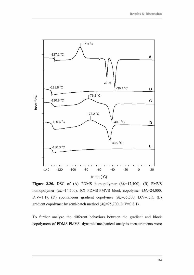
Results & Discussion
114
temp (oC)
-140 -120 -100 -80 -60 -40 -20 0 20
heat
flow
A
B
C
D
E
-127.1 oC
-131.8 oC
-130.8 oC
-130.6 oC
-130.3 oC
-87.9 oC
-76.2 oC
-73.2 oC
-36.4 oC
-40.9 oC
-43.9 oC
-48.3
Figure 3.26. DSC of (A) PDMS homopolymer (Mn=17,400), (B) PMVS
homopolymer (Mn=14,500), (C) PDMS-PMVS block copolymer (Mn=24,000,
D:V=1:1), (D) spontaneous gradient copolymer (Mn=35,500, D:V=1:1), (E)
gradient copolymer by semi-batch method (Mn=25,700, D:V=0.8:1).
To further analyze the different behaviors between the gradient and block
copolymers of PDMS-PMVS, dynamic mechanical analysis measurements were
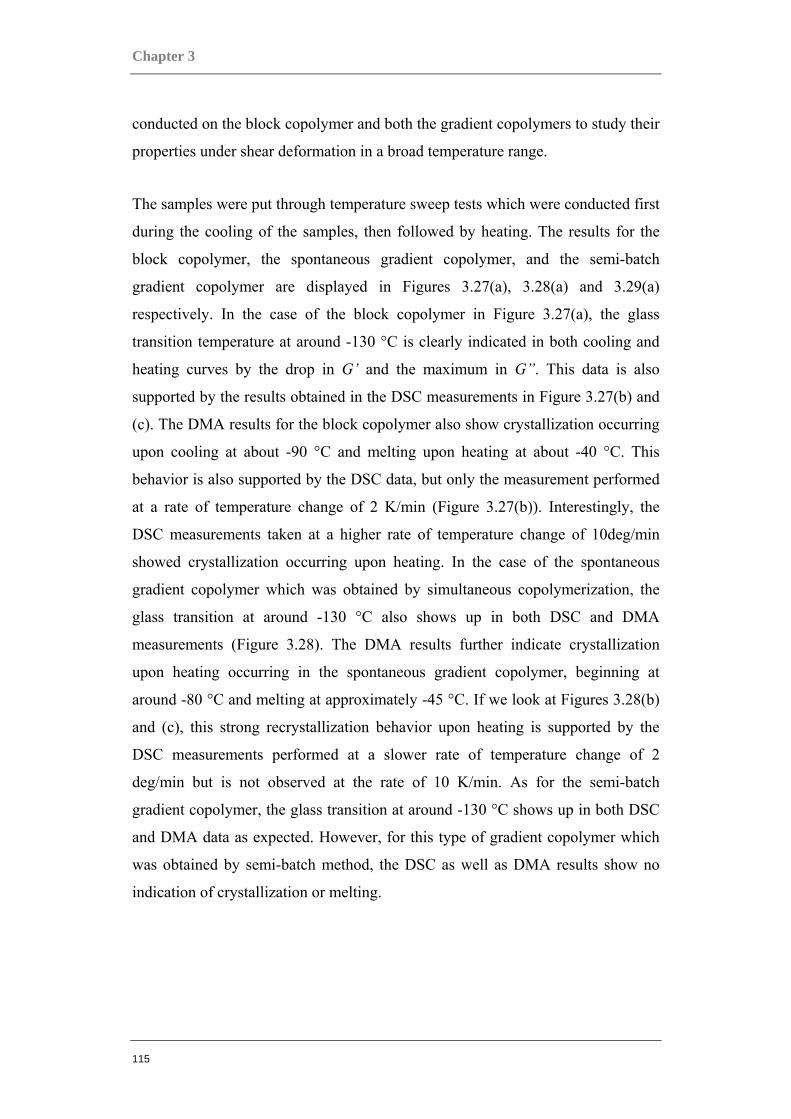
Chapter 3
115
conducted on the block copolymer and both the gradient copolymers to study their
properties under shear deformation in a broad temperature range.
The samples were put through temperature sweep tests which were conducted first
during the cooling of the samples, then followed by heating. The results for the
block copolymer, the spontaneous gradient copolymer, and the semi-batch
gradient copolymer are displayed in Figures 3.27(a), 3.28(a) and 3.29(a)
respectively. In the case of the block copolymer in Figure 3.27(a), the glass
transition temperature at around -130 °C is clearly indicated in both cooling and
heating curves by the drop in G’ and the maximum in G”. This data is also
supported by the results obtained in the DSC measurements in Figure 3.27(b) and
(c). The DMA results for the block copolymer also show crystallization occurring
upon cooling at about -90 °C and melting upon heating at about -40 °C. This
behavior is also supported by the DSC data, but only the measurement performed
at a rate of temperature change of 2 K/min (Figure 3.27(b)). Interestingly, the
DSC measurements taken at a higher rate of temperature change of 10deg/min
showed crystallization occurring upon heating. In the case of the spontaneous
gradient copolymer which was obtained by simultaneous copolymerization, the
glass transition at around -130 °C also shows up in both DSC and DMA
measurements (Figure 3.28). The DMA results further indicate crystallization
upon heating occurring in the spontaneous gradient copolymer, beginning at
around -80 °C and melting at approximately -45 °C. If we look at Figures 3.28(b)
and (c), this strong recrystallization behavior upon heating is supported by the
DSC measurements performed at a slower rate of temperature change of 2
deg/min but is not observed at the rate of 10 K/min. As for the semi-batch
gradient copolymer, the glass transition at around -130 °C shows up in both DSC
and DMA data as expected. However, for this type of gradient copolymer which
was obtained by semi-batch method, the DSC as well as DMA results show no
indication of crystallization or melting.

Results & Discussion
116
-140 -120 -100 -80 -60 -40100
102
104
106
108
1010
cooling, G' cooling, G'' heating, G' heating, G''
G',
G''
[Pa]
T [°C]
-140 -120 -100 -80 -60 -40-0.10
-0.05
0.00
0.05
0.10
T [°C]
ΔH
cooling heating
2 K/min
-140 -120 -100 -80 -60 -40
-0.5
0.0
cooling heating
10 K/min
T [°C]
ΔH
Figure 3.27. PDMS-PMVS block copolymer (Mn=24,000, D:V=1:1), (a)
Temperature dependence curves of the shear and loss moduli (b) DSC
measurement at 2 K/min (c) 10K/min.

Chapter 3
117
-140 -120 -100 -80 -60 -40100
102
104
106
108
1010
cooling, G' cooling, G'' heating, G' heating, G''
G',
G''
[Pa]
T [°C]
-140 -120 -100 -80 -60 -40-0.1
0.0
0.1
T [°C]
ΔH
cooling heating
2 K/min
-140 -120 -100 -80 -60 -40-0.3-0.2-0.10.00.10.20.3
cooling heating
10 K/min
T [°C]
ΔH
Figure 3.28. Spontaneous gradient copolymer (Mn=35,500, D:V=1:1), (a)
Temperature dependence curves of the shear and loss moduli (b) DSC
measurement at 2 K/min (c) 10K/min.

Results & Discussion
118
-140 -120 -100 -80 -60100
102
104
106
108
1010
cooling, G' cooling, G'' heating, G' heating, G''
G',
G'' [
Pa]
T [°C]
(a)
-140 -120 -100 -80 -60
-0.25
-0.20
-0.15
-0.10
-0.05
0.00
0.05
0.10
0.15
0.20
0.25
0.30
cooling heating
10 K/min
T [°C]
Δ H
Figure 3.29. Gradient copolymer prepared using semi-batch method (Mn=25,700,
D:V=1:1). (a) Temperature dependence curves of the shear and loss moduli (b)
DSC measurement at 10 K/min.

Chapter 3
119
From the data gathered by the DSC and DMA measurements, it can be concluded
that DSC measurements taken at cooling and heating rates of 2 K/min fit well
with the DMA measurements performed. And it should also be emphasized that
DSC measurements taken at a faster cooling and heating rate of 10 K/min showed
conflicting results when compared to the results from the DMA measurements.
Morphology
In order to further examine the microstructure formation in block and gradient
copolymers we performed temperature dependent SAXS experiments on samples.
The results are summarized in Figure 3.30 in the form of scattered intensity vs. the
scattering vector q. The results show significant differences between these two
copolymer materials. In the case of the block copolymer, peaks are observed at -
60°C and -100°C at the relative positions 1:2 which suggest a lamellar structure.
For the spontaneous gradient copolymer, two peaks were also observed at the
same temperatures, but at relative positions 1:3. However, the secondary peak
obtained from the spontaneous gradient copolymer was weaker and broader when
compared to the block copolymer. And in the case of both copolymers, the
structures seemed to have been lost when either cooled down to 140°C or when
heated back to room temperature.
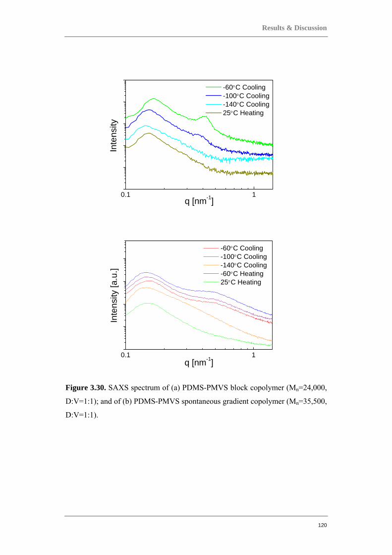
Results & Discussion
120
0.1 1
Inte
nsity
q [nm-1]
-60°C Cooling -100°C Cooling -140°C Cooling 25°C Heating
0.1 1
Inte
nsity
[a.u
.]
q [nm-1]
-60°C Cooling -100°C Cooling -140°C Cooling -60°C Heating 25°C Heating
Figure 3.30. SAXS spectrum of (a) PDMS-PMVS block copolymer (Mn=24,000,
D:V=1:1); and of (b) PDMS-PMVS spontaneous gradient copolymer (Mn=35,500,
D:V=1:1).

Chapter 4
121
122
4 Conclusion
The main focus of the studies discussed in this volume was to explore specific
systems which have not been studied before in hopes of having a better
understanding of structure-property relations in complex copolymer systems. And
from these various different studies which were done, it is clear that molecular
properties such as chain length, chain stiffness, degree of branching, molecular
architecture, and the number of charge groups, are of great significance, and
perhaps even more so than the detailed chemical make-up of polymers, in
determining their physical characteristics. This was well-demonstrated with the
different physical properties exhibited by the statistical, block and gradient
copolymers. All three types of these copolymers, even when built with the same
type and number of units, have completely different properties as a result of their
different architectures. The studies revealed that a deeper understanding of this
relationship between the molecular architecture and the physical characteristics is
vital for aiding in the design of new materials with more useful properties, as
constantly advancing technologies demand new, high performance and more
specialized materials with highly specialized functions. And it is this deeper
understanding of the structure-property relations that would undoubtedly be one
of the key factors contributing to the continuing rapid growth in the field of
polymer science.

123

124

125
126
Bibliography
1. Flory, P.J., Fundamental Principles of Condensation Polymerization. Chemical Reviews, 1946. 39(1): p. 137-197.
2. Leibler, L., Nanostructured plastics: Joys of self-assembling. Progress in Polymer Science, 2005. 30(8-9): p. 898-914.
3. Choi, H.S. and N. Yui, Design of rapidly assembling supramolecular systems responsive to synchronized stimuli. Progress in Polymer Science, 2006. 31(2): p. 121-144.
4. Frechet, J.M.J., Functional polymers: from plastic electronics to polymer-assisted therapeutics. Progress in Polymer Science, 2005. 30(8-9): p. 844-857.
5. Higgins, J.S., M. Tambasco, and J.E.G. Lipson, Polymer blends; stretching what we can learn through the combination of experiment and theory. Progress in Polymer Science, 2005. 30(8-9): p. 832-843.
6. Khandare, J. and T. Minko, Polymer-drug conjugates: Progress in polymeric prodrugs. Progress in Polymer Science, 2006. 31(4): p. 359-397.
7. Macosko, C.W., H.K. Jeon, and T.R. Hoye, Reactions at polymer-polymer interfaces for blend compatibilization. Progress in Polymer Science, 2005. 30(8-9): p. 939-947.
8. Meijer, H.E.H. and L.E. Govaert, Mechanical performance of polymer systems: The relation between structure and properties. Progress in Polymer Science, 2005. 30(8-9): p. 915-938.
9. Sukhorukov, G., A. Fery, and H. Mohwald, Intelligent micro- and nanocapsules. Progress in Polymer Science, 2005. 30(8-9): p. 885-897.
10. Matsen, M.W. and F.S. Bates, Origins of complex self-assembly in block copolymers. Macromolecules, 1996. 29(23): p. 7641-7644.
11. Helfand, E. and Z.R. Wasserman, Block Co-Polymer Theory .6. Cylindrical Domains. Macromolecules, 1980. 13(4): p. 994-998.
12. Semenov, A.N., Contribution to the Theory of Microphase Layering in Block-Copolymer Melts. Zhurnal Eksperimentalnoi I Teoreticheskoi Fiziki, 1985. 88(4): p. 1242-1256.
13. Ohta, T. and K. Kawasaki, Equilibrium Morphology of Block Copolymer Melts. Macromolecules, 1986. 19(10): p. 2621-2632.
14. Ohta, T. and K. Kawasaki, Comment on the Free-Energy Functional of Block Copolymer Melts in the Strong Segregation Limit. Macromolecules, 1990. 23(8): p. 2413-2414.
15. Hong, K.M. and J. Noolandi, Theory of Inhomogeneous Multicomponent Polymer Systems. Macromolecules, 1981. 14(3): p. 727-736.
16. Muthukumar, M., Fluctuation Effects in the Density-Functional Theory of Order-Disorder Transitions in Block-Copolymers. Macromolecules, 1993. 26(19): p. 5259-5261.
17. Matsen, M.W. and M. Schick, Lamellar Phase of a Symmetrical Triblock Copolymer. Macromolecules, 1994. 27(1): p. 187-192.
18. Olmsted, P.D. and S.T. Milner, Strong-Segregation Theory of Bicontinuous Phases in Block-Copolymers. Physical Review Letters, 1994. 72(6): p. 936-939.

127
19. Morkved, T.L., et al., Mesoscopic Self-Assembly of Gold Islands an Diblock-Copolymer Films. Applied Physics Letters, 1994. 64(4): p. 422-424.
20. Archibald, D.D. and S. Mann, Template Mineralization of Self-Assembled Anisotropic Lipid Microstructures. Nature, 1993. 364(6436): p. 430-433.
21. Matyjaszewski, K., et al., Gradient copolymers by atom transfer radical copolymerization. Journal of Physical Organic Chemistry, 2000. 13(12): p. 775-786.
22. Aksimentiev, A. and R. Holyst, Phase behavior of gradient copolymers. Journal of Chemical Physics, 1999. 111(5): p. 2329-2339.
23. Pakula, T. and K. Matyjaszewski, Copolymers with controlled distribution of comonomers along the chain .1. Structure, thermodynamics and dynamic properties of gradient copolymers. Computer simulation. Macromolecular Theory and Simulations, 1996. 5(5): p. 987-1006.
24. Shull, K.R., Interfacial activity of gradient copolymers. Macromolecules, 2002. 35(22): p. 8631-8639.
25. Kim, J., et al., Polymer blend compatibilization by gradient copolymer addition during melt processing: Stabilization of dispersed phase to static coarsening. Macromolecules, 2005. 38(4): p. 1037-1040.
26. Matyjaszewski, K. and D. Greszta, Thermal properties of gradient copolymers and their compatibilizing ability. Abstracts of Papers of the American Chemical Society, 1997. 213: p. 330-POLY.
27. Kim, J., et al., Uniquely broad glass transition temperatures of gradient copolymers relative to random and block copolymers containing repulsive comonomers. Macromolecules, 2006. 39(18): p. 6152-6160.
28. Jakubowski, W., et al., Comparison of thermomechanical properties of statistical, gradient and block copolymers of isobornyl acrylate and n-butyl acrylate with various acrylate homopolymers. Polymer, 2008. 49(6): p. 1567-1578.
29. Berry, G.C., Translational Frictional Constant of Comb-Branched Polymers. Journal of Polymer Science Part a-2-Polymer Physics, 1968. 6(8pa2): p. 1551-&.
30. Graessley, W.W., Some Phenomenological Consequences of the Doi-Edwards Theory of Viscoelasticity. Journal of Polymer Science Part B-Polymer Physics, 1980. 18(1): p. 27-34.
31. Williams, M.L., R.F. Landel, and J.D. Ferry, Mechanical Properties of Substances of High Molecular Weight .19. The Temperature Dependence of Relaxation Mechanisms in Amorphous Polymers and Other Glass-Forming Liquids. Journal of the American Chemical Society, 1955. 77(14): p. 3701-3707.
32. Angell, C.A., Formation of Glasses from Liquids and Biopolymers. Science, 1995. 267(5206): p. 1924-1935.
33. Stillinger, F.H., A Topographic View of Supercooled Liquids and Glass-Formation. Science, 1995. 267(5206): p. 1935-1939.
34. Sokolov, A.P., Why the glass transition is still interesting. Science, 1996. 273(5282): p. 1675-1676.
35. Grest, G.S., et al., Density of States and the Velocity Auto-Correlation Function Derived from Quench Studies. Journal of Chemical Physics, 1981. 74(6): p. 3532-3534.
128
36. Bendler, J.T., J.J. Fontanella, and M.F. Shlesinger, A new Vogel-like law: Ionic conductivity, dielectric relaxation, and viscosity near the glass transition. Physical Review Letters, 2001. 8719(19): p. -.
37. Pakula, T., Collective dynamics in simple supercooled and polymer liquids. Journal of Molecular Liquids, 2000. 86(1-3): p. 109-121.
38. Doolittle, A.K., Studies in Newtonian Flow .2. The Dependence of the Viscosity of Liquids on Free-Space. Journal of Applied Physics, 1951. 22(12): p. 1471-1475.
39. Fulcher, G.S., Analysis of recent measurements of the viscosity of glasses. II. Journal of the American Ceramic Society, 1925. 8(12): p. 789-794.
40. Fulcher, G.S., Analysis of recent measurements of the viscosity of glasses. Journal of the American Ceramic Society, 1925. 8(6): p. 339-355.
41. Tammann, G. and W. Hesse, The dependancy of viscosity on temperature in hypothermic liquids. Zeitschrift Fur Anorganische Und Allgemeine Chemie, 1926. 156(4): p. -.
42. Naoki, M., H. Endou, and K. Matsumoto, Pressure Effects on Dielectric-Relaxation of Supercooled Ortho-Terphenyl. Journal of Physical Chemistry, 1987. 91(15): p. 4169-4174.
43. Ferrer, M.L., et al., Supercooled liquids and the glass transition: Temperature as the control variable. Journal of Chemical Physics, 1998. 109(18): p. 8010-8015.
44. Tolle, A., et al., Fast relaxation in a fragile liquid under pressure. Physical Review Letters, 1998. 80(11): p. 2374-2377.
45. Mpoukouvalas, K., et al., Pressure-enhanced dynamic heterogeneity in block copolymers of poly(methyl vinyl ether) and poly(isobutyl vinyl ether). Physical Review E, 2005. 72(1): p. -.
46. Roland, C.M., et al., Volume and temperature as control parameters for the dielectric a relaxation of polymers and molecular glass formers. Philosophical Magazine, 2004. 84(13-16): p. 1573-1581.
47. Floudas, G., K. Mpoukouvalas, and P. Papadopoulos, The role of temperature and density on the glass-transition dynamics of glass formers. Journal of Chemical Physics, 2006. 124(7): p. -.
48. Dreyfus, C., et al., Temperature and pressure study of Brillouin transverse modes in the organic glass-forming liquid orthoterphenyl. Physical Review E, 2003. 68(1): p. -.
49. Casalini, R. and C.M. Roland, Thermodynamical scaling of the glass transition dynamics. Physical Review E, 2004. 69(6): p. -.
50. Alba-Simionesco, C., et al., Scaling out the density dependence of the a relaxation in glass-forming polymers. Europhysics Letters, 2004. 68(1): p. 58-64.
51. Tarjus, G., et al., Disentangling density and temperature effects in the viscous slowing down of glassforming liquids. Journal of Chemical Physics, 2004. 120(13): p. 6135-6141.
52. Roland, C.M. and R. Casalini, Comment on: "Disentangling density and temperature effects in the viscous slowing down of glass forming liquids" [J. Chem. Phys. 120, 6135 (2004)]. Journal of Chemical Physics, 2004. 121(22): p. 11503-11504.
53. Bragg, W.L., The diffraction of short electromagnetic waves through a crystal. Zeitschrift Fur Anorganische Chemie, 1914. 90(2/3): p. 153-168.
129
54. Matyjaszewski, K., Macromolecular engineering: From rational design through precise macromolecular synthesis and processing to targeted macroscopic material properties. Progress in Polymer Science, 2005. 30(8-9): p. 858-875.
55. Coessens, V., et al., Functionalization of polymers prepared by ATRP using radical addition reactions. Macromolecular Rapid Communications, 2000. 21(2): p. 103-109.
56. Matyjaszewski, K., et al., Molecular brushes with variable composition and topology by ATRP: Synthesis and properties. Abstracts of Papers of the American Chemical Society, 2006. 231: p. -.
57. Patten, T.E. and K. Matyjaszewski, Atom transfer radical polymerization and the synthesis of polymeric materials. Advanced Materials, 1998. 10(12): p. 901-+.
58. Wong, H.F. and G.D. Brown, beta-methoxy-gamma-methylene-alpha,beta-unsaturated-gamma-butyrolactones from Artabotrys hexapetalus. Phytochemistry, 2002. 59(1): p. 99-104.
59. Vuckovic, I., et al., Phytochemical investigation of Anthemis cotula. Journal of the Serbian Chemical Society, 2006. 71(2): p. 127-133.
60. Trendafilova, A., et al., Sesquiterpene lactones from Achillea collina J. Becker ex Reichenb. Phytochemistry, 2006. 67(8): p. 764-770.
61. Williams, C.K. and M.A. Hillmyer, Polymers from renewable resources: A perspective for a special issue of polymer reviews. Polymer Reviews, 2008. 48(1): p. 1-10.
62. Akkapeddi, M.K., Poly(Alpha-Methylene-Gamma-Butyrolactone) Synthesis, Configurational Structure, and Properties. Macromolecules, 1979. 12(4): p. 546-551.
63. Sheiko, S.S., B.S. Sumerlin, and K. Matyjaszewski, Cylindrical molecular brushes: Synthesis, characterization, and properties. Progress in Polymer Science, 2008. 33(7): p. 759-785.
64. Neugebauer, D., et al., Densely-grafted and double-grafted PEO brushes via ATRP. A route to soft elastomers. Macromolecules, 2003. 36(18): p. 6746-6755.
65. Sheiko, S.S., et al., Single molecule rod-globule phase transition for brush molecules at a flat interface. Macromolecules, 2001. 34(23): p. 8354-8360.
66. Sheiko, S.S., et al., Adsorption-induced scission of carbon-carbon bonds. Nature, 2006. 440(7081): p. 191-194.
67. Qin, S.H., et al., Synthesis and visualization of densely grafted molecular brushes with crystallizable poly(octadecyl methacrylate) block segments. Macromolecules, 2003. 36(3): p. 605-612.
68. Greszta, D. and K. Matyjaszewski, Mechanism of controlled/''living'' radical polymerization of styrene in the presence of nitroxyl radicals. Kinetics and simulations. Macromolecules, 1996. 29(24): p. 7661-7670.
69. Greszta, D. and K. Matyjaszewski, Living radical polymerization: Kinetic results - Comments. Macromolecules, 1996. 29(15): p. 5239-5240.
70. Greszta, D. and K. Matyjaszewski, Gradient copolymers - A new class of materials. Abstracts of Papers of the American Chemical Society, 1996. 211: p. 85-Poly.
130
71. Arehart, S.V., D. Greszta, and K. Matyjaszewski, Gradient copolymers of styrene and n-butyl acrylate through atom transfer radical polymerization. Abstracts of Papers of the American Chemical Society, 1997. 213: p. 329-POLY.
72. Matyjaszewski, K. and J.H. Xia, Atom transfer radical polymerization. Chemical Reviews, 2001. 101(9): p. 2921-2990.
73. Ishizu, K. and A. Ichimura, Synthesis of cyclic diblock copolymers by interfacial condensation. Polymer, 1998. 39(25): p. 6555-6558.
74. Yu, G.E., et al., Association and surface properties of tapered statistical copolymers of ethylene oxide and butylene oxide in water. Journal of the Chemical Society-Faraday Transactions, 1997. 93(18): p. 3383-3390.
75. Okabe, S., et al., Small-angle neutron scattering study on block and gradient copolymer aqueous solutions. Polymer, 2006. 47(21): p. 7572-7579.
76. Chojnowski, J., et al., Controlled synthesis of vinylmethylsiloxane-dimethylsiloxane gradient, block and alternate copolymers by anionic ROP of cyclotrisiloxanes. Polymer, 2002. 43(7): p. 1993-2001.
77. Chojnowski, J., et al., Synthesis of branched polysiloxanes with controlled branching and functionalization by anionic ring-opening polymerization. Macromolecules, 2003. 36(11): p. 3890-3897.
78. Cypryk, M., et al., Modifications of siloxane polymers. Polimery, 2007. 52(7-8): p. 496-502.
79. Cazacu, M., et al., Heterogeneous catalyzed copolymerization of octamethylcyclotetrasiloxane with 1,3,5,7-tetravinyl-1,3,5,7-tetramethylcyclotetrasiloxane. Journal of Macromolecular Science-Pure and Applied Chemistry, 1996. A33(1): p. 65-76.
80. Ziemelis, M.J. and J.C. Saam, Sequence Distribution in Poly(Dimethylsiloxane-Co-Methylvinylsiloxanes). Macromolecules, 1989. 22(5): p. 2111-2116.
81. Teng, C.J., W.P. Weber, and G.P. Cai, Anionic and cationic ring-opening polymerization of 2,2,4,4,6,6-hexamethyl-8,8-divinylcyclotetrasiloxane. Macromolecules, 2003. 36(14): p. 5126-5130.
82. Cai, G.P. and W.P. Weber, Synthesis and chemical modification of poly(divinylsiloxane). Polymer, 2002. 43(6): p. 1753-1759.
83. Herczynska, L., et al., Synthesis of microsequential methylvinylsiloxane-dimethylsiloxane copolymers by nonequilibrium copolymerization. Journal of Polymer Science Part a-Polymer Chemistry, 1998. 36(1): p. 137-145.
84. Blochowiak, M., et al., Thermodynamics and rheology of cycloolefin copolymers. Journal of Chemical Physics, 2006. 124(13): p. -.
85. Zhang, Y., et al., Structure and properties of poly(butyl acrylate-block-sulfone-block-butyl acrylate) triblock copolymers prepared by ATRP. Macromolecular Chemistry and Physics, 2005. 206(1): p. 33-42.
86. Matyjaszewski, K., et al., Simple and effective one-pot synthesis of (meth)acrylic block copolymers through atom transfer radical polymerization. Journal of Polymer Science Part a-Polymer Chemistry, 2000. 38(11): p. 2023-2031.
87. Kim, S. and J.M. Torkelson, Self-referencing fluorescence-based oxygen sensor with temperature-independent response: Novel pressure-sensitive paint based on polydimethylsiloxane films. Abstracts of Papers of the American Chemical Society, 2003. 226: p. U107-U107.
131
88. Karatasos, K., et al., Composition fluctuation effects on dielectric normal-mode relaxation in diblock copolymers .2. Disordered state in proximity to the ODT and ordered state. Macromolecules, 1996. 29(4): p. 1326-1336.
89. Kumar, S.K., et al., Concentration fluctuation induced dynamic heterogeneities in polymer blends. Journal of Chemical Physics, 1996. 105(9): p. 3777-3788.
90. Alvarez, F., et al., Segmental Dynamics in Bulk Poly(Isobornyl Methacrylate) and Its Random Copolymer with Poly(Methyl Methacrylate) near T-G. Macromolecules, 1995. 28(19): p. 6488-6493.
91. Floudas, G., R. Ulrich, and U. Wiesner, Microphase separation in poly(isoprene-b-ethylene oxide) diblock copolymer melts. I. Phase state and kinetics of the order-to-order transitions. Journal of Chemical Physics, 1999. 110(1): p. 652-663.
92. Floudas, G., et al., Microphase separation in star block copolymers of styrene and isoprene. Theory, experiment, and simulation. Macromolecules, 1996. 29(11): p. 4142-4154.
93. Hodrokoukes, P., et al., Microphase separation in normal and inverse tapered block copolymers of polystyrene and polyisoprene. 1. Phase state. Macromolecules, 2001. 34(3): p. 650-657.
94. Rubinstein, M. and S.P. Obukhov, Power-Law-Like Stress-Relaxation of Block Copolymers - Disentanglement Regimes. Macromolecules, 1993. 26(7): p. 1740-1750.
95. Abreu, F.O.M.S., M.M.C. Forte, and S.A. Liberman, SBS and SEBS block copolymers as impact modifiers for polypropylene compounds. Journal of Applied Polymer Science, 2005. 95(2): p. 254-263.
96. El Sheemy, H., Thermoplastic elastomers and mineral oils. Kautschuk Gummi Kunststoffe, 1999. 52(9): p. 586-587.
97. Tong, J.D., et al., Synthesis and bulk properties of poly(methyl methacrylate)-b-poly(isooctyl acrylate)-b-poly(methyl methacrylate). Polymer, 2000. 41(12): p. 4617-4624.
98. Moineau, G., et al., Controlled radical polymerization of (meth)acrylates by ATRP with NiBr2(PPh3)(2) as catalyst. Macromolecules, 1999. 32(1): p. 27-35.
99. Braunecker, W.A. and K. Matyjaszewski, Controlled/living radical polymerization: Features, developments, and perspectives. Progress in Polymer Science, 2007. 32(1): p. 93-146.
100. Dufour, B., et al., Polar three-arm star block copolymer thermoplastic elastomers based on polyacrylonitrile. Macromolecules, 2008. 41(7): p. 2451-2458.
101. Dufour, B., et al., PBA-PMMA 3-arm star block copolymer thermoplastic elastomers. Macromolecular Chemistry and Physics, 2008. 209(16): p. 1686-1693.
102. Mosnacek, J., et al., Synthesis, morphology and mechanical properties of linear triblock copolymers based on poly(alpha-methylene-gamma-butyrolactone). Polymer, 2009. 50(9): p. 2087-2094.
103. Shim, J.S. and J.P. Kennedy, New polyisobutylene stars part XXI - Novel thermoplastic elastomers. III. Synthesis, characterization, and properties of star-block copolymers of poly(indene-b-isobutylene) arms emanating from cyclosiloxane cores. Journal of Polymer Science Part a-Polymer Chemistry, 2000. 38(2): p. 279-290.

132
104. Shim, J.S. and J.P. Kennedy, New polyisobutylene stars part XIX - Novel thermoplastic elastomers. II. Properties of star-block copolymers of PSt-b-PIB arms emanating from cyclosiloxane cores. Journal of Polymer Science Part a-Polymer Chemistry, 1999. 37(6): p. 815-824.
105. Huckstadt, H., V. Abetz, and R. Stadler, Synthesis of a polystyrene-arm-polybutadiene-arm-poly(methyl methacrylate) triarm star copolymer. Macromolecular Rapid Communications, 1996. 17(8): p. 599-606.
106. Puskas, J.E., et al., The effect of hard and soft segment composition and molecular architecture on the morphology and mechanical properties of polystyrene-polyisobutylene thermoplastic elastomeric block copolymers. European Polymer Journal, 2003. 39(10): p. 2041-2049.
107. Storey, R.F., B.J. Chrisholm, and K.R. Choate, Synthesis and characterization of multi-arm star-branched polyisobutylenes. Journal of Polymer Science, Part A: Polymer Chemistry, 1994. 34: p. 2003-2017.
108. Storey, R.F. and K.A. Shoemake, Effect of reaction conditions on synthesis and properties of multiarm star-branched polyisobutylenes. Journal of Polymer Science, Part A: Polymer Chemistry, 1998. 36: p. 471-483.
109. Shim, J.S., et al., Novel thermoplastic elastomers. I. Synthesis and characterization of star-block copolymers of PSt-b-PIB arms emanating from cyclosiloxane cores. Journal of Polymer Science, Part A: Polymer Chemistry, 1998. 36(17): p. 2997-3012.
110. Shim, J.S. and J.P. Kennedy, Novel thermoplastic elastomers. II. Properties of star-block copolymers of PSt-b-PIB arms emanating from cyclosiloxane cores. Journal of Polymer Science, Part A: Polymer Chemistry, 1999. 37(6): p. 815-824.
111. Shim, J.S. and J.P. Kennedy, Novel thermoplastic elastomers. III. Synthesis, characterization, and properties of star-block copolymers of poly(indene-b-isobutylene) arms emanating from cyclosiloxane cores. Journal of Polymer Science, Part A: Polymer Chemistry, 2000. 38(2): p. 279-290.
112. Tong, J.D., et al., Synthesis, Morphology, and Mechanical Properties of Poly(methyl methacrylate)-b-poly(n-butyl acrylate)-b-poly(methyl methacrylate) Triblocks. Ligated Anionic Polymerization vs Atom Transfer Radical Polymerization. Macromolecules, 2000. 33(2): p. 470-479.
113. Borner, H.G., et al., Synthesis of molecular brushes with gradient in grafting density by atom transfer polymerization. Macromolecules, 2002. 35(9): p. 3387-3394.
114. Chojnowski, J., et al., Controlled synthesis of all siloxane-functionalized architectures by ring-opening polymerization. Synthesis and Properties of Silicones and Silicone-Modified Materials, 2003. 838: p. 12-25.
115. Kelen, T. and F. Tudos, Analysis of Linear Methods for Determining Copolymerization Reactivity Ratios .1. New Improved Linear Graphic Method. Journal of Macromolecular Science-Chemistry, 1975. A 9(1): p. 1-27.
116. Herczynska, L., et al., Modification of polysiloxanes by free-radical addition of pyridylthiols to the vinyl groups of the polymer. European Polymer Journal, 1999. 35(6): p. 1115-1122.

133
117. Boutevin, B., F. Guida-Pietrasanta, and A. Ratsimihety, Synthesis of photocrosslinkable fluorinated polydimethylsiloxanes: Direct introduction of acrylic pendant groups via hydrosilylation. Journal of Polymer Science Part a-Polymer Chemistry, 2000. 38(20): p. 3722-3728.
118. Hempenius, M.A., R.G.H. Lammertink, and G.J. Vancso, Side-chain liquid-crystalline polysiloxanes via anionic polymerization: (n-undecyloxy)arenecarboxylic acid mesogens linked to poly(dimethylsiloxane-co-methylvinylsiloxane). Macromolecules, 1997. 30(2): p. 266-272.
119. Paulasaari, J.K. and W.P. Weber, Preparation and orthogonal polymerizations of 1-hydrido-1-vinyldimethylsiloxy-3,3,5,5-tetramethylcyclotrisiloxane. Macromolecules, 1999. 32(16): p. 5217-5221.
120. Vadala, M.L., et al., Block copolysiloxanes and their complexation with cobalt nanoparticles. Polymer, 2004. 45(22): p. 7449-7461.
121. Abdellah, L., B. Boutevin, and B. Youssef, Synthesis and Applications of Photolinkable Poly(Dimethylsiloxanes) .2. Synthesis of Polysiloxane with Urethane Acrylate Groups. European Polymer Journal, 1991. 27(8): p. 821-825.
122. RozgaWijas, K., et al., Controlled synthesis of siloxane copolymers having an organosulfur group by polymerization of cyclotrisiloxanes with mixed units. Macromolecules, 1996. 29(8): p. 2711-2720.
123. Scibiorek, M., N.K. Gladkova, and J. Chojnowski, Controlled synthesis of amphiphilic siloxane-siloxane block copolymers with carboxyl functions. Polymer Bulletin, 2000. 44(4): p. 377-384.
124. Brunner, A.R., et al., Synthesis and ceramic conversion reactions of pinacolborane- amd diethylborazine-modified poly(vinylsiloxane)s. The development of a processable single-source polymeric precursor to boron-modified silicon carbide. Chemistry of Materials, 2000. 12(9): p. 2770-2780.
125. Bauer, J., N. Husing, and G. Kickelbick, Synthesis of new types of polysiloxane based surfactants. Chemical Communications, 2001(01): p. 137-138.
126. Bauer, J., N. Husing, and G. Kickelbick, Preparation of functional block copolymers based on a polysiloxane backbone by anionic ring-opening polymerization. Journal of Polymer Science Part a-Polymer Chemistry, 2002. 40(10): p. 1539-1551.
127. Ganicz, T., et al., A novel organometallic route to phenylethenyl-modified polysiloxanes. Journal of Materials Chemistry, 2005. 15(5): p. 611-619.
128. Gupta, S.K. and W.P. Weber, Ruthenium-catalyzed chemical modification of poly(vinylmethylsiloxane) with 9-acetylphenanthrene. Macromolecules, 2002. 35(9): p. 3369-3373.
129. Wang, B.Y. and S. Krause, Properties of Dimethylsiloxane Microphases in Phase-Separated Dimethylsiloxane Block Copolymers. Macromolecules, 1987. 20(9): p. 2201-2208.
134
List of Figures
0.1. Two component polymer systems, or copolymers. 11
0.2. Commonly encountered block copolymers. 12
0.3. Characterization of the properties of copolymer materials. 14
1.1. Illustration of shear strain and stress in the dynamic mechanical measurement. A sample is placed between two plates, a fixed lower plate and a moving upper plate which moves at constant velocity. The force is denoted by F, and the contact area by A. 18
1.2 Types of test geometries used for different materials; (a) plate-plate and (b) cone-plate for the melt, (c) rectangular bars for solids and (d) couette for polymer solutions or liquids. Geometry (a) was used for this present investigation. 19
1.3 Time profile of a simple shear experiment (see Figure 1.1) with and without phase lag. 20
1.4 Diagram showing the complex modulus GiGG ′′+′=∗ . G’ corresponds to the storage modulus (elastically stored energy) and G” to the loss modulus (dissipated energy). 21
1.5 The various regions in the viscoelastic spectrum of the homopolymer n-butyl acrylate. 24
1.6 (a) Maxwell, and (b) Voigt mechanical models for viscoelastic behavior. 27
1.7 The Maxwell model’s representation of the frequency dependence of E’ and E”. 30
1.8 Three-element model (Burger’s model) of viscoelasticity. 32
1.9 Master curve constructed for a polystyrene test sample (Mw=200 kg/mol). Frequency dependences of G’ and G” are measured at various temperatures with a fixed frequency window (between the two vertical dotted lines). One of these dependencies is taken as a reference and is not shifted. All the other curves are shifted horizontally by log aT to overlap with dependencies measured at adjacent temperatures. Dependencies measured at higher and lower temperatures are moved to lower and higher frequencies, respectively. 33
1.10 An example of the temperature dependence of a shift factor aT. The line is a fit of the WLF equation (2.39). 36
1.11 A representation of potential energy (“energy landscape”) in the multidimensional configuration space for a many-particle system (taken from F.H. Stillinger, Science 1995). 41
135
1.12 Different types of dependencies of the activation energy for local molecular rearrangements vs. local volume: (a) corresponding to the Arrhenius model, (b) corresponding to the free volume model and, (c) to (e) some other possible dependencies (taken from T. Pakula, J. Mol. Liq. 86, 2000, 109-121). 46
1.13 Temperature dependencies of relaxation times calculated using E(v) dependencies shown in Figure 1.12 (lines A-E correspond to cases (a)-(e) of Figure 1.12, respectively) (taken from T. Pakula, J. Mol. Liq. 86, 2000, 109-121). 46
1.14 Fit parameters of the empirical function (eq. 1.67). 47
1.15 Definition of the scattering vector sv of the scattering of the X-ray beam of the intensity I0 and the wavelength λ. 48
1.16 An illustration of the Bragg’s law. 50
2.1 Copolymerization of isobornyl acrylate and n-butyl acrylate in different fashion and comparison of properties of resulting copolymers with acrylate-based homopolymers such as PtBA, PMA, PEA and PPA. 53
2.2 Preparation of PMBL-b-PBA-b-PMBL triblock copolymers. 56
2.3 Schematic Representation of the Brush and Star Architectures. 57
2.4 Synthesis of PBiBEA-g-(PBA-b-PMBL) star copolymers. 58
2.5 Synthesis of PBiBEA-g-(PBA-b-PMMA) star copolymers. 59
2.6 Synthesis of PMTFS-PDMS copolymers. 60
2.7 Synthesis of PDMS-PMVS copolymers. 62
2.8 A schematic diagram of the dynamic mechanical analyzer. The deformation (shear strain) input signal D(t) is applied by the motor and the resulting torque F(t) is measured by the force transducer. 63
2.9 Isothermal strain sweep for an multi-arm PBA-PMMA block copolymer taken as an example. The sample is sheared between two plates (see Figure 1.2) and the resulting torque is recorded. Notice the insensitivity of the shear moduli to the applied strain (linear viscoelastic regime). 64
3.1 DSC thermograms of statistical P(IBA-co-nBA) copolymers with different monomer compositions: IBA(19%)-nBA(81%) copolymer (red, WJ-02-15), IBA(53%)-nBA(47%) copolymer (green, WJ-02-14), IBA(79%)-nBA(21%) copolymer (blue, WJ-02-13) of IBA and nBA. 67
3.2 Tuning Tg in statistical copolymers of P(IBA-co-nBA) with different IBA/nBA ratios and two different degrees of polymerization. 69
136
3.3 Typical examples of G’ and G” dependencies (master curves) on frequency for a linear PnBA homopolymer and statistical P(IBA-co-nBA) copolymers with similar degrees of polymerization and different IBA/nBA ratios (Scheme 3.1, the green line). 70
3.4 Effect of (a) the composition, and (b) the molecular weight, of statistical copolymers P(IBA-co-nBA) on the chain relaxation times. 72
3.5 Comparison of the shear moduli spectra of (a) PPA (Tg = -40 ºC, Mn = 86 000 g/mol; WJ-02-29) and IBA(16%)-nBA(84%) copolymer (Tg = -39 ºC, Mn = 94 000 g/mol; WJ-02-23); (b) PEA (Tg = -24 ºC, Mn = 96 900 g/mol; WJ-02-07) and IBA(33%)-nBA(67%) copolymer (Tg = -20 ºC, Mn = 107 500 g/mol; WJ-02-22); (c) PtBA (Tg = 37 ºC, Mn = 48 900 g/mol; WJ-02-11) and IBA(78%)-nBA(22%) copolymer (Tg = 42 ºC, Mn = 63 700 g/mol; WJ-02-19). 74
3.6 Comparisons between gradient IBA(47%)-nBA(53%) copolymer (broad Tg, Mn = 74 800 g/mol; WJ-02-45) and statistical IBA(44%)-nBA(56%) copolymer (Tg = -10.6 ºC, Mn = 53 000 g/mol; WJ-02-28). 77
3.7 Comparisons of block IBA(54%)-nBA(46%) copolymer (Tg = -54 ºC, 94 ºC, Mn = 54 600 g/mol; WJ-02-230) and statistical IBA(54%)-nBA(46%) copolymer (Tg = 7 ºC, Mn = 69 000 g/mol; WJ-02-20). 78
3.8 SAXS spectra of PMBL–PBA–PMBL triblock copolymers with constant PBA segments length and increasing PMBL length (a) before and (b) after annealing for 30 min at 150 ºC under nitrogen atmosphere. 82
3.9 SAXS spectra of the B215-L68 before and after annealing at different temperatures. 83
3.10 Thermo-mechanical (2 ºC/min) and DSC (10 ºC/min) analysis of PMBL–PBA–PMBL triblock copolymers. 84
3.11 Tensile mechanical properties of PMBL–PBA–PMBL triblock copolymers with different compositions: (a) before and (b) after thermal annealing at 150 ºC for 1 h. 86
3.12 Tensile mechanical properties of (PMBL-r-PMMA)-PBA-(PMBL-r-PMMA) triblock copolymers compared to that of PMBL–PBA–PMBL. 87
3.13 Comparison of the thermo-mechanical properties of (PMBL-r-PMMA)–PBA–(PMBL-r-PMMA) and PMMA–PBA–PMMA triblock copolymers. 88
3.14 DMA spectra of the PBA-PMBL block copolymer (a) 10B240-L86, 10B240-L46, (b) B215-L68, 10B115-L30, (c) 10B115-L47, 20B115-L47. 90
137
3.15 SAXS spectra of 20B115-L57 before and after annealing at 150°C for 60 min. 91
3.16 SAXS spectra after annealing at 150°C for 60 min for (a) 10B240-L86, 10B240-L46, and (b) 20B115-L57, 20B115-L47. 92
3.17 Tensile properties of copolymers 10B240-L86 and 10B240-L46. 94
3.18 SAXS spectra of 20B115-M60 before and after annealing at 150°C for 60 minutes. 96
3.19 DMA spectra of the star PBA-PMMA block copolymer (a) 20B230-M59, 20B230-M107, (b) 20B115-M38, 20B230-M59, 20B750-M180 and, (c) 20B230-M107, 10B240-M117. 97
3.20 Tensile properties of copolymers (a) 20B230-M59, 20B230-M107, and (b) 20B115-M60, 10B115-M51, 3B164-M7. 100
3.21 DSC of (a) PDMS homopolymer (Mn=17,400), (b) PMTFPS homopolymer (Mn=18,000), (c) PDMS-PMTFPS block copolymer (Mn=13,500, D:F=1:1), (d) spontaneous gradient copolymer (Mn=10,000, D:F=1:1), (e) gradient copolymer by semi-batch method (Mn=16,700, D:F=1:1). 104
3.22 Temperature dependence of the shear and loss moduli of (a) PDMS-PMTFPS block copolymer (Mn = 13,500, D:F = 1:1), (b) spontaneous gradient copolymer (Mn = 10,000, D:F = 1:1) and (c) gradient copolymer by semi-batch method (Mn = 16,700, D:F = 1:1). 106
3.23 SAXS spectrum of the (a) PDMS-PMTFPS block copolymer (Mn = 13,500, D:F = 1:1), (b) spontaneous gradient copolymer (Mn = 10,000, D:F = 1:1) and (c) gradient copolymer by semi-batch method (Mn = 16,700, D:F = 1:1). 108
3.24 Temperature dependence of the shear and loss moduli of (a) spontaneous gradient copolymer D-F-D (Mn = 44,000, F:D = 1:1) and (b) gradient copolymer D-F-D obtained by the semi-batch method (Mn = 45,800, F:D = 1:1). 109
3.25 SAXS spectra of (a) spontaneous gradient copolymer D-F-D (M = 44,000, F:D = 1:1) and (b) gradient copolymer D-F-D obtained by the semi-batch method (M = 45,800, F:D = 1:1). 110
3.26 DSC of (A) PDMS homopolymer (Mn=17,400), (B) PMVS homopolymer (Mn=14,500), (C) PDMS-PMVS block copolymer (Mn=24,000, D:V=1:1), (D) spontaneous gradient copolymer (Mn=35,500, D:V=1:1), (E) gradient copolymer by semi-batch method (Mn=25,700, D:V=0.8:1). 114
3.27 PDMS-PMVS block copolymer (Mn=24,000, D:V=1:1), (a) Temperature dependence curves of the shear and loss moduli (b) DSC measurement at 2 K/min (c) 10K/min. 116
138
3.28 Spontaneous gradient copolymer (Mn=35,500, D:V=1:1), (a) Temperature dependence curves of the shear and loss moduli (b) DSC measurement at 2 K/min (c) 10K/min. 117
3.29 Gradient copolymer prepared using semi-batch method (Mn=25,700, D:V=1:1). (a) Temperature dependence curves of the shear and loss moduli (b) DSC measurement at 10 K/min. 118
3.30 SAXS spectrum of (a) PDMS-PMVS block copolymer (Mn=24,000, D:V=1:1); and of (b) PDMS-PMVS spontaneous gradient copolymer (Mn=35,500, D:V=1:1). 120

139
140
List of Tables
1.1. Viscoelastic functions of the Maxwell and the Voigt model. 28
2.1 Properties of different types of (co)polymers prepared by ATRP. 54
2.2 Compositions of prepared PMBL-PBA-PMBL triblock copolymers with PMBL outer hard blocks, and of prepared (PMBL-r-PMMA)-PBA-(PMBL-r-PMMA) triblock copolymers with random copolymer outer hard blocks. 56
2.3 Compositions of the prepared PBiBEA-g-(PBA-b-PMBL) star-like block copolymers. 58
2.4 Compositions of PBiBEA-g-(PBA-b-PMMA) star-like block copolymers. 59
2.5 List of prepared block, spontaneous gradient and forced gradient D-F copolymers. 61
2.6 List of prepared block, spontaneous gradient and forced gradient D-V copolymers. 62
3.1 Glass transition temperature and rubbery plateau storage modulus for the polymers shown in Figure 3.5. 76
3.2 Compositions of the prepared PBA-PMBL star-like block copolymers, their phase separation spacing values and corresponding structure. 94
3.3 Compositions of the prepared PBA-b-PMMA star-like block copolymers and their phase separation spacing values. 96
3.4 Ultimate tensile strength and maximum elongation at break of PBA-PMMA block copolymers with similar composition but varying numbers of arms. 100

141

142