
Exploring pole walking as a health enhancing physical activity ...
Upload
independentCategory
view
4download
0
March 17, 2004 12:9 Geophysical Journal International gji2156
Geophys. J. Int. (2004) 157, 36–54 doi: 10.1111/j.1365-246X.2004.02156.xG
JIG
eom
agne
tism
,ro
ckm
agne
tism
and
pala
eom
agne
tism
Structure and thermal regime beneath the South Pole region, EastAntarctica, from magnetotelluric measurements
Philip E. Wannamaker,1 John A. Stodt,1 Louise Pellerin,1 Steven L. Olsen2
and Darrell B. Hall31University of Utah, Energy & Geoscience Institute, 423 Wakara Way, Suite 300, Salt Lake City, UT 84108, USA. E-mail: [email protected] Analog Design, Salt Lake City, UT 84105, USA3University of Utah, Department of Geology and Geophysics, Salt Lake City, UT 84112, USA
Accepted 2003 September 16. Received 2003 August 30; in original form 2003 April 15
S U M M A R YTen tensor magnetotelluric (MT) soundings have been acquired in a 54 km long profile acrossthe South Pole area, East Antarctica. The MT transect was offset from the South Pole station∼5 km and oriented 210 grid north, approximately normal to the Trans-Antarctic Mountains.Surveying around South Pole station was pursued for four main reasons. First, we soughtto illuminate first-order structure and physico-chemical state (temperatures, fluids, melts) ofthe crust and upper mantle of this part of East Antarctica. Secondly, conditions around theSouth Pole differ from those of previous MT experience at central West Antarctica, so thatthe project would help to define MT surveying feasibility over the entire continent. Thirdly,the results would provide a crustal response baseline for possible long-term MT monitoring todeep upper mantle depths at the South Pole. Fourthly, because Antarctic logistics are difficult,support facilities at the South Pole enable relatively efficient survey procedures. In makingthe MT measurements, the high electrical contact impedance at the electrode-firn interfacewas overcome using a custom-design electrode pre-amplifier at the electrode with low outputimpedance to the remainder of the recording electronics. Non-plane-wave effects in the datawere suppressed using a robust jackknife procedure that emphasized outlier removal from thevertical magnetic field records. Good quality data were obtained, but the rate of collectionwas hampered by low geomagnetic activity and wind-generated, electrostatic noise inducedin the ice. Profile data were inverted using a 2-D algorithm that damps model departuresfrom an a priori structure, in this case a smooth 1-D profile obtained from inversion of anintegral of the TM mode impedance along the profile. Inverse models show clear evidence fora pronounced (∼1 km thickness), conductive section below the ice tentatively correlated withporous sediments of the Beacon Supergroup. Substantial variations in sedimentary conductanceare inferred, which may translate into commensurate variations in sediment thickness. Lowresistivities below ∼30 km suggest thermal activity in the lower crust and upper mantle,and mantle support for this region of elevated East Antarctica. This contrasts with resistivitystructure imaged previously in central West Antarctica, where resistivity remains high into theupper mantle consistent with a fossil state of extensional activity there.
Key words: Antarctica, electrometer, magnetotellurics, thermal regime, South Pole.
I N T RO D U C T I O N
Approximately 95 per cent of Antarctica is covered with thick (1–3 km) ice, and so most crust and mantle structure must be de-duced geophysically. Nevertheless, this major land mass is an es-sential but still poorly understood component of lithospheric platereconstructions especially of the Pre-Cambrian and Early Paleozoictimes (Dalziel 1997; Dalziel & Lawver 2001). Moreover, evidenceis strong that Antarctica has been subject to Cenozoic plume activity
and represents an important location to study modification of previ-ously stable cratonic lithosphere by plume processes, but which hasresulted in only limited surface rifting.
Geophysical deductions must make use of only a handful ofphysical properties of the Earth, one of which is its electrical re-sistivity. The geophysical method that can provide images of re-sistivity to deep crustal or upper mantle depths is magnetotellurics(MT) (Vozoff 1991; Wannamaker & Hohmann 1991; Jones 1992,1999; Wannamaker 2000). This physical property in turn can supply
36 C© 2004 RAS
March 17, 2004 12:9 Geophysical Journal International gji2156
Structure beneath the South Pole 37
information on primary structures (sedimentary distributions, litho-logic contrasts, major fault offsets), geochemical fluxes (hydrother-mal alteration, remobilized graphite and sulphides) and thermalregime (prograde or melt-exsolved fluids, crustal or upper mantlemelts, mineral semi-conduction). While the technology to acquiregood MT data in temperate zones is reasonably well understood,polar regions present special challenges.
For the MT method to be feasible throughout the Antarctic conti-nent, one must be able to acquire high-quality electric field data overthe highly resistive, interior ice sheets. Electrode contact resistancesin near-surface ice (firn) may reach several Mohms (Shabtaie &Bentley 1995) requiring specialized electronics to acquire accurateelectric field data. Using an in-house design, we acquired profilesof good-quality MT sites, first in central West Antarctica (CWA),and more recently across the region of the South Pole station, EastAntarctica. The latter, upon which we report here, consist of 10sites over a transect length of 54 km. Our measurements provide anew view of the geology and physical state below the South Polearea, and characterize important environmental variables pertinentto obtaining high-quality MT results in polar regions.
G E O L O G I C A L S E T T I N G
Antarctica is divided fundamentally into eastern and western por-tions separated by the continent-dissecting Trans-Antarctic Moun-
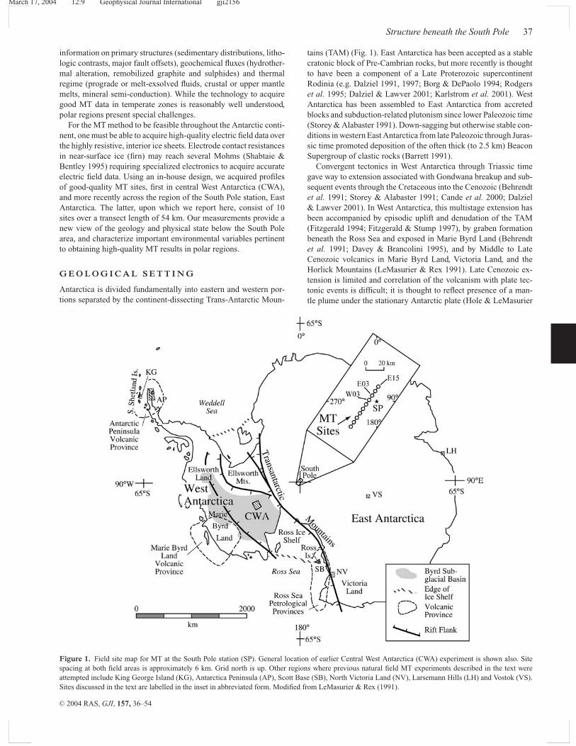
Figure 1. Field site map for MT at the South Pole station (SP). General location of earlier Central West Antarctica (CWA) experiment is shown also. Sitespacing at both field areas is approximately 6 km. Grid north is up. Other regions where previous natural field MT experiments described in the text wereattempted include King George Island (KG), Antarctica Peninsula (AP), Scott Base (SB), North Victoria Land (NV), Larsemann Hills (LH) and Vostok (VS).Sites discussed in the text are labelled in the inset in abbreviated form. Modified from LeMasurier & Rex (1991).
tains (TAM) (Fig. 1). East Antarctica has been accepted as a stablecratonic block of Pre-Cambrian rocks, but more recently is thoughtto have been a component of a Late Proterozoic supercontinentRodinia (e.g. Dalziel 1991, 1997; Borg & DePaolo 1994; Rodgerset al. 1995; Dalziel & Lawver 2001; Karlstrom et al. 2001). WestAntarctica has been assembled to East Antarctica from accretedblocks and subduction-related plutonism since lower Paleozoic time(Storey & Alabaster 1991). Down-sagging but otherwise stable con-ditions in western East Antarctica from late Paleozoic through Juras-sic time promoted deposition of the often thick (to 2.5 km) BeaconSupergroup of clastic rocks (Barrett 1991).
Convergent tectonics in West Antarctica through Triassic timegave way to extension associated with Gondwana breakup and sub-sequent events through the Cretaceous into the Cenozoic (Behrendtet al. 1991; Storey & Alabaster 1991; Cande et al. 2000; Dalziel& Lawver 2001). In West Antarctica, this multistage extension hasbeen accompanied by episodic uplift and denudation of the TAM(Fitzgerald 1994; Fitzgerald & Stump 1997), by graben formationbeneath the Ross Sea and exposed in Marie Byrd Land (Behrendtet al. 1991; Davey & Brancolini 1995), and by Middle to LateCenozoic volcanics in Marie Byrd Land, Victoria Land, and theHorlick Mountains (LeMasurier & Rex 1991). Late Cenozoic ex-tension is limited and correlation of the volcanism with plate tec-tonic events is difficult; it is thought to reflect presence of a man-tle plume under the stationary Antarctic plate (Hole & LeMasurier
C© 2004 RAS, GJI, 157, 36–54
March 17, 2004 12:9 Geophysical Journal International gji2156
38 P. E. Wannamaker et al.
1994; LeMasurier & Landis 1996; Behrendt 1999; Dalziel & Lawver2001).
G E O P H Y S I C A L I N F E R E N C E S
Crustal thickness of East Antarctica appears to average approxi-mately 40 km based on seismic refraction profiles near its NE coast,and gravity interpretations region-wide, in contrast to 20–30 kmfor much of rifted West Antarctica (Bentley 1991; Behrendt 1999).Surface wave studies confirm separateness of East and West Antarc-tica, with the former showing more craton-like velocities on aver-age, and with the highest lateral gradient in model velocities typ-ically occurring below the South Pole itself (Bentley 1991; Roultet al. 1994; Danesi & Morelli 2000; Ritzwoller et al. 2001). Seismicrefraction surveying measured no return energy at the South Pole(Bentley & Clough 1970), which may be taken at face value or couldsuggest that there is subcropping sedimentary section (Beacon Su-pergroup?) beneath the South Pole ice sheet of ∼1 km thicknessor more (Bentley 1973, 1991). Ice thickness at the South Pole is∼2800 m based on radar sounding (Jiracek 1967; Bentley 1991).Ice-stripped, rebounded basement elevations of East Antarctica areanomalously high (1–3 km) suggesting some kind of active tectonicsupport (Bentley 1991).
Seismicity throughout Antarctica is low, consistent with a slow-moving plate almost entirely surrounded by mid-ocean ridges, butwith the west approximately 10 times more active than the east(Bentley 1991; Hole & LeMasurier 1994). Aeromagnetic and seis-mic refraction surveys suggest basaltic rocks are present along thebase of the West Antarctica ice sheet (Byrd Subglacial Basin), com-parable with outcrop and geophysical characteristics of Marie ByrdLand (Behrendt et al. 1991, 1994; Blankenship et al. 1993; Behrendt1999) (Fig. 1). Recent aerogeophysical surveying (magnetics, grav-ity, radar, altimetry) with sparse ground geophysics (seismic refrac-tion, MT discussed below) provide a picture for the Byrd Basin oflocalized Late Cenozoic volcanism along zones of weakness orig-inating in the main Cretaceous rifting event and reactivated duringrecent plume uplift (Blankenship et al. 2001).
The character and scale of the geomorphology and tectonic stylehave lead some to compare West and East Antarctica with the exten-sional northern Basin and Range (Great Basin) and stable interior ofthe western US, with the TAM representing a regional rift shouldersimilar to the Wasatch Range (Storey & Alabaster 1991; Rochollet al. 1995). Important differences, however, include time of rift-ing, plate boundary forces, and magmatic petrogenesis (ten Brinket al. 1993; Hole & LeMasurier 1994; Humphreys & Dueker 1994;Sonder & Jones 1999). More recently, ten Brink et al. (1997) mod-elled gravity and seismic structure across the Ross Sea-TAM tran-sition in southern Victoria Land in terms of flexural uplift, with aneffective elastic thickness in this part of East Antarctica of ∼80 km,which is thick compared with other uplifted but otherwise inactiveterranes such as the Colorado Plateau (Lowry et al. 2000).
B R I E F I N T RO D U C T I O N T OM A G N E T O T E L L U R I C S
The MT method uses naturally occurring electromagnetic (EM)wavefields as sources for imaging the electrical resistivity struc-ture of the Earth (Vozoff 1991). The incident EM waves usually aretreated as planar in geometry and propagating vertically downward.In the conducting Earth, EM waves at typical frequencies of themethod (<1000 Hz, for example) travel diffusively, such that high-
frequency (short period) waves penetrate a relatively short distancewhile low-frequency (long period) waves can reach into the man-tle. Special challenges to collecting good MT data over polar icesheets include the very high contact impedance at the electrode-firninterface for the E-field measurement and possible violations of theplanar EM wave assumption due to proximity to the polar electrojet(Mareschal 1986; Pirjola 1998; Jones & Spratt 2002).
The electric (E) and magnetic (H) vector fields scattered by buriedstructure and measured at the surface may have arbitrary polarizationrelative to the incident fields. This requires a tensor relationshipbetween the measured fields as a function of frequency (or periodT , its inverse) denoted for the horizontal components through
[E] = [Z][H],
where Z is the 2 × 2 complex impedance. The individual impedanceelements typically are transformed into an apparent resistivity (ρ a)and an impedance phase (ϕ) for presentation and modelling. On auniform half-space of resistivity ρ, ρ a = ρ and ϕ = 45◦. For morecomplex structures, ρ a versus T approximates a smoothed versionof ρ versus distance below the measurement. The phase ϕ tends tobe proportional to slope of ρ a versus T , and thus is more reflectiveof spatial gradients in the subsurface resistivity. These primary datain turn are transformed to constrained resistivity models throughthe process of inversion, specified in the model construction sectionbelow.
Over 2-D structures where one of the measurement axes is parallelto geoelectric strike (x here by convention), the diagonal entries of Zare zero (Vozoff 1991). In this situation, the MT response separatesinto two independent modes. These are the transverse electric (TE)mode, where Ex = ZxyHy and electric current flows parallel to strike(x-axis), and the transverse magnetic (TM) mode, where Ey = ZyxHx
and current flows perpendicular to strike (y-axis). Additionally, a 1 ×2 tensor K z relates the vertical and horizontal magnetic fieldsthrough
[Hz] = [K z][H].
For a 2-D Earth, Kzx = 0 and Kzy reflects cross-strike changes incurrent flowing along strike (TE mode).
P R E V I O U S M T I N A N TA RC T I C A
Hessler & Jacobs (1966) recorded analogue, long period (T > 1min) E-fields over glacial ice at Vostok with 200 m bipoles and cop-per screen electrodes buried in brine-soaked firn. Correlations werevisible with simultaneous magnetic records, but large spike noisewas common and no MT impedances were estimated. MT measure-ments were taken by Fournier (1994) on the Antarctic peninsula butelectrical contact either was on exposed earth or sea ice of similarresistivity (1000 ohm m) and so not characteristic of the continentalinterior. This appears to have been the case as well in the surveys ofKong et al. (1993, 1994) on the Fildes peninsula of West Antarcticaand near the Larsmann Hills of East Antarctica.
Good-quality MT data at relatively long periods (20–2000 s) wereacquired by Beblo & Liebig (1990) over thin glacial ice cover inNorth Victoria Land. They used copper screens as electrodes over a25 m bipole span and an electrometer of very high input impedance(10+12 ohm m). Signals in this longer period range are due to high-amplitude ionospheric micropulsations, but the lack of shorter pe-riod data makes it difficult to quantify resistivity of most of thecrustal column. However, the authors did show that sounding re-sults during both low- and high-activity times of the polar electrojet
C© 2004 RAS, GJI, 157, 36–54
March 17, 2004 12:9 Geophysical Journal International gji2156
Structure beneath the South Pole 39
were very similar, from which they concluded that non-plane-wavesource effects were not a serious issue.
The first high-quality broad-band MT soundings over the thickinterior ice sheet of Antarctica were obtained by Wannamaker et al.(1996) in CWA over Whitmore Mountains–Ross Embayment transi-tional crust (Blankenship et al. 2001) (Fig. 1). The primary technicaldifficulty of acquiring the E-field measurements on thick glacial icewas overcome using a custom electrometer system, discussed inAppendix A. A total of ten tensor soundings in the period range0.01–500 s approximately were taken in a profile closely parallelto a seismic reflection line as part of the Antalith project (Clarkeet al. 1997; Sen et al. 1998). 2-D, trial-and-error modelling of thedata profile using the finite-element algorithm of Wannamaker et al.(1987) was carried out with ice thickness variation constrained ac-cording to seismic reflection results (Sen et al. 1998) and an averageice resistivity of 300 000 ohm m (Shabtaie & Bentley 1995).
In the model of Wannamaker et al. (1996), most of the subicesection even into the upper mantle is resistive (>1000 ohm m),implying a dormant state of rifting at most (cf. Wannamaker et al.1997). Our correlations are supported by the reversed refraction pro-filing at CWA which implies upper mantle Pn velocities of 8.0–8.1km s−1 (Clarke et al. 1997). Mantle S-velocity structure of the WestAntarctic Rift region is lower than the global average, but nearlyindistinguishable from that of other dormant rift zones worldwidesuch as the western Mediterranean and the Sea of Japan (Ritzwolleret al. 2001). We concur with the earlier description of LeMasurier& Rex (1991) and Hole & LeMasurier (1994) that volcanic activityat present is restricted to occasional, narrow conduits ultimately fedfrom a deep plume source. These in turn are interpreted to be re-activation zones originating in the previous, mainly Cretaceous riftevent (Blankenship et al. 2001). However, it is noted that the profilewe acquired is 54 km in length and may not be representative ofother areas of West Antarctica.
M T S U RV E Y I N G AT S O U T H P O L E
Deep electrical resistivity investigations at the South Pole stationwere pursued for four principal reasons. First, such results wouldbe the first ever sampling the interior of East Antarctica, revealingfirst-order structural information. Secondly, if MT can be done inthe severe temperature conditions of the South Pole, it should bepossible nearly anywhere on the continent. Thirdly, the resultingresistivity model determines the crustal response baseline for deepmantle resistivity profiles (100–1000 km depth range) that sorelyneed representation from this part of the globe (Egbert & Booker1992; Everett & Schultz 1996). Fourthly, the South Pole stationhas been occupied continuously since 1956 and its facilities easedlogistical requirements for this first MT deployment in the EastAntarctic interior.
MT data collection procedure
MT sites were collected using the University of Utah system as si-multaneous pairs spaced 6 km apart at the South Pole (Fig. 1), similarto CWA. Given the ∼3 km of ice sheet thickness, this spatial sam-pling appears adequate because the ice serves to upward-continuethe response from near-surface ‘static’ effects which trouble manyland surveys (Groom & Bailey 1989; Pellerin & Hohmann 1990;Wannamaker 1999). Synchronized EM time-series from each five-channel site were transmitted via digital FM radio telemetry to thecentrally located recording hut. Appendix A contains a description
of our MT system including the custom electrometer designed tohandle the high electrode-firn contact impedance.
The profile was offset ∼5 km from the South Pole station to avoidartificial EM interference from the station, although none was ob-served. The initial orientation of the profile was grid 210◦, where gridnorth is Greenwich meridian, approximately normal to the Trans-Antarctic Mountains. The maximum distance of a sounding fromthe South Pole station was ∼40 km, and location and navigationwere by hand-held GPS. The average recording time per site wasapproximately 3 d. This is slow compared with most MT surveys onland, and was the result in part of the additional logistical require-ments of Antarctica. It also was the result of serious wind-drivenelectrostatic noise which is discussed in Appendix B.
Observed MT data and its processing
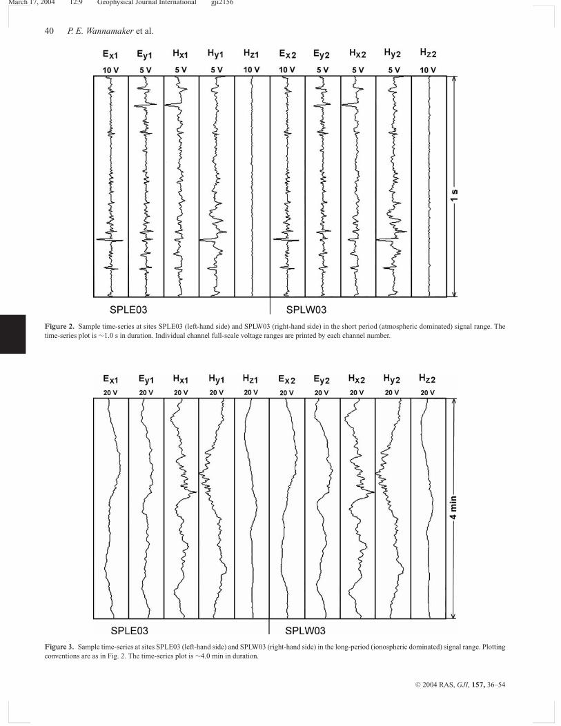
Despite difficulties, patient surveying led to the acquisition of10 good quality MT sites. When external noise sources were ab-sent, high quality MT time-series such as those in Figs 2 and 3 wereobtained. Under environmentally quiet (low wind) conditions, closecorrelations were seen between electric and magnetic fields takensimultaneously at two separated (6 km) sites at both high and lowfrequencies, with second-order differences at the lower frequenciesrelated mainly to differences in geology between sites. Thunder-storms are essentially unheard of in Antarctica so that the sphericsignals visible in Fig. 2 likely have propagated from the southerntemperate or equatorial regions. The EM energy at T < 0.01 s waveperiods is substantially damped through propagation over such dis-tances, making it difficult to attain good shorter period responses,but this turns out to be unimportant for our geological interpreta-tion of the data. Under the plane-wave assumption, variations in thevertical magnetic field (Fig. 3) would denote the presence of lateralresistivity heterogeneity in the earth (Vozoff 1991). However, at highlatitudes, non-planar source components may also cause variationsin Hz at the longer periods and need to be rejected during time-seriesprocessing (Mareschal 1986; Garcia et al. 1997; Pirjola 1998; Jones& Spratt 2002) as described below.
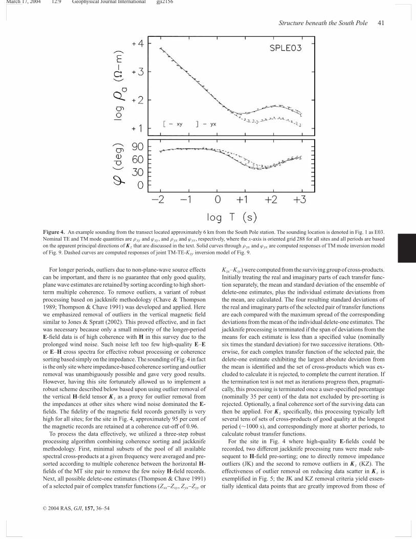
The apparent resistivity and impedance phase response for thesounding closest to the South Pole itself (SPLE03, Fig. 1) afterrobust processing are shown in Fig. 4. The most striking featureis the degree to which both modes of apparent resistivity fall fromshort period values around 5000 ohm m to long-period values of10s or even <10 ohm m at other sites. High impedance phase values(>70◦) accompany the fall in ρ a. This response implies a substantialconductive section just below the ice sheet. Lateral variations in thissection, or in deeper basement, may be causing the long-periodresponse anisotropy. The response anisotropy is not strong here,and is usually weaker at the other sites. Low values of long-periodapparent resistivity unfortunately signify weak MT E-field signalsthat are especially prone to contamination by environmental noise,such as from the wind.
Our processing for the middle and shorter periods (T < 10s) wasbased on a coherence-sorting scheme. Cascade decimation (Wight& Bostick 1980; Stodt 1983; Jones & Jodicke 1984) was used to ob-tain Fourier harmonics and spectral averages from short time-seriessubsets of data recorded simultaneously at two MT sites. Time-seriessegments at an individual site showing low multiple field coherence(<0.75) were rejected, and the remainder subject to remote refer-ence processing using the corresponding data from the companionsite (Gamble et al. 1979). This is similar to MT processing we haveapplied in temperate region surveys, and served well here.
C© 2004 RAS, GJI, 157, 36–54
March 17, 2004 12:9 Geophysical Journal International gji2156
40 P. E. Wannamaker et al.
Figure 2. Sample time-series at sites SPLE03 (left-hand side) and SPLW03 (right-hand side) in the short period (atmospheric dominated) signal range. Thetime-series plot is ∼1.0 s in duration. Individual channel full-scale voltage ranges are printed by each channel number.
Figure 3. Sample time-series at sites SPLE03 (left-hand side) and SPLW03 (right-hand side) in the long-period (ionospheric dominated) signal range. Plottingconventions are as in Fig. 2. The time-series plot is ∼4.0 min in duration.
C© 2004 RAS, GJI, 157, 36–54
March 17, 2004 12:9 Geophysical Journal International gji2156
Structure beneath the South Pole 41
Figure 4. An example sounding from the transect located approximately 6 km from the South Pole station. The sounding location is denoted in Fig. 1 as E03.Nominal TE and TM mode quantities are ρ xy and ϕ xy, and ρ yx and ϕ yx, respectively, where the x-axis is oriented grid 288 for all sites and all periods are basedon the apparent principal directions of K z that are discussed in the text. Solid curves through ρ yx and ϕ yx are computed responses of TM mode inversion modelof Fig. 9. Dashed curves are computed responses of joint TM-TE-Kzy inversion model of Fig. 9.
For longer periods, outliers due to non-plane-wave source effectscan be important, and there is no guarantee that only good quality,plane wave estimates are retained by sorting according to high short-term multiple coherence. To remove outliers, a variant of robustprocessing based on jackknife methodology (Chave & Thompson1989; Thompson & Chave 1991) was developed and applied. Herewe emphasized removal of outliers in the vertical magnetic fieldsimilar to Jones & Spratt (2002). This proved effective, and in factwas necessary because only a small minority of the longer-periodE-field data is of high coherence with H in this survey due to theprolonged wind noise. Such noise left too few high-quality E–Eor E–H cross spectra for effective robust processing or coherencesorting based simply on the impedance. The sounding of Fig. 4 in factis the only site where impedance-based coherence sorting and outlierremoval was unambiguously possible and gave very good results.However, having this site fortunately allowed us to implement arobust scheme described below based upon using outlier removal ofthe vertical H-field tensor K z as a proxy for outlier removal fromthe impedances at other sites where wind noise dominated the E-fields. The fidelity of the magnetic field records generally is veryhigh for all sites; for the site in Fig. 4, approximately 95 per cent ofthe magnetic records are retained at a coherence cut-off of 0.96.
To process the data effectively, we utilized a three-step robustprocessing algorithm combining coherence sorting and jackknifemethodology. First, minimal subsets of the pool of all availablespectral cross-products at a given frequency were averaged and pre-sorted according to multiple coherence between the horizontal H-fields of the MT site pair to remove the few noisy H-field records.Next, all possible delete-one estimates (Thompson & Chave 1991)of a selected pair of complex transfer functions (Zxx–Zxy, Zyx–Zyy or
Kzx–Kzy) were computed from the surviving group of cross-products.Initially treating the real and imaginary parts of each transfer func-tion separately, the mean and standard deviation of the ensemble ofdelete-one estimates, plus the individual estimate deviations fromthe mean, are calculated. The four resulting standard deviations ofthe real and imaginary parts of the selected pair of transfer functionsare each compared with the maximum spread of the correspondingdeviations from the mean of the individual delete-one estimates. Thejackknife processing is terminated if the span of deviations from themeans for each estimate is less than a specified value (nominallysix times the standard deviation) for two successive iterations. Oth-erwise, for each complex transfer function of the selected pair, thedelete-one estimate exhibiting the largest absolute deviation fromthe mean is identified and the set of cross-products which was ex-cluded to calculate it is rejected, to complete the current iteration. Ifthe termination test is not met as iterations progress then, pragmati-cally, this processing is terminated once a user-specified percentage(nominally 35 per cent) of the data not excluded by pre-sorting isrejected. Optionally, a final coherence sort of the surviving data canthen be applied. For K z specifically, this processing typically leftseveral tens of sets of cross-products of good quality at the longestperiod (∼1000 s), and correspondingly more at shorter periods, tocalculate robust transfer functions.
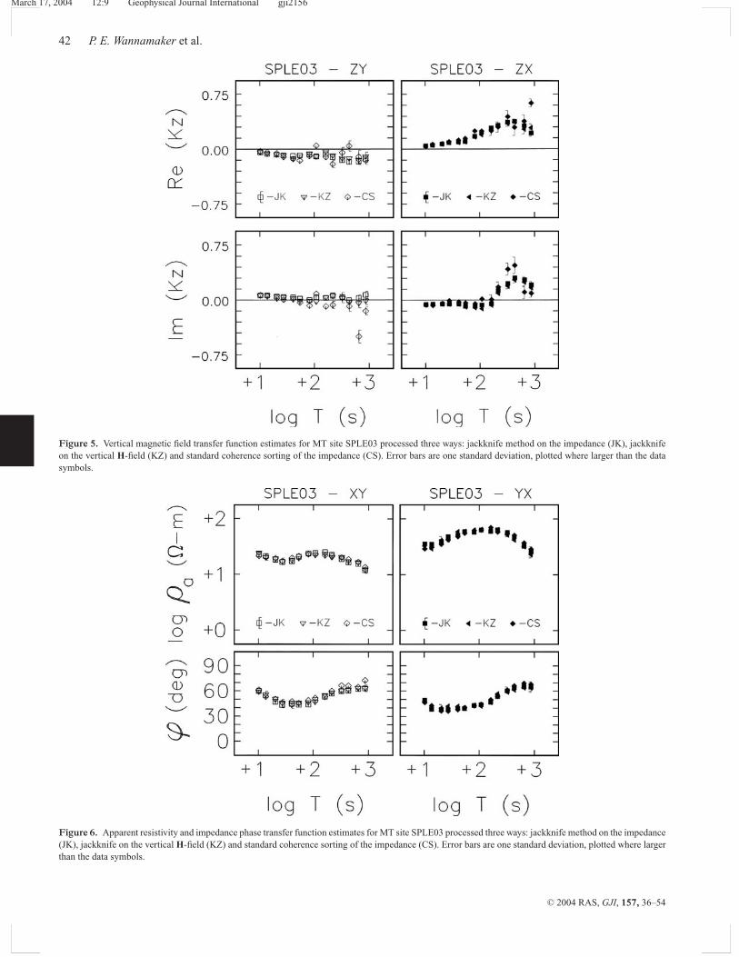
For the site in Fig. 4 where high-quality E-fields could berecorded, two different jackknife processing runs were made sub-sequent to H-field pre-sorting; one to directly remove impedanceoutliers (JK) and the second to remove outliers in K z (KZ). Theeffectiveness of outlier removal on reducing data scatter in K z isexemplified in Fig. 5; the JK and KZ removal criteria yield essen-tially identical data points that are greatly improved from those of
C© 2004 RAS, GJI, 157, 36–54
March 17, 2004 12:9 Geophysical Journal International gji2156
42 P. E. Wannamaker et al.
Figure 5. Vertical magnetic field transfer function estimates for MT site SPLE03 processed three ways: jackknife method on the impedance (JK), jackknifeon the vertical H-field (KZ) and standard coherence sorting of the impedance (CS). Error bars are one standard deviation, plotted where larger than the datasymbols.
Figure 6. Apparent resistivity and impedance phase transfer function estimates for MT site SPLE03 processed three ways: jackknife method on the impedance(JK), jackknife on the vertical H-field (KZ) and standard coherence sorting of the impedance (CS). Error bars are one standard deviation, plotted where largerthan the data symbols.
C© 2004 RAS, GJI, 157, 36–54
March 17, 2004 12:9 Geophysical Journal International gji2156
Structure beneath the South Pole 43
coherence sorting alone (CS). The difference between coherence-sorted and jackknife-processed impedance estimates is much lessthan for K z, due to greater apparent stability of the CS results, withonly a modest improvement in ϕ xy visible in Fig. 6. The greater im-provement in K z response is consistent with other experience thatsource effects have stronger deleterious influence on the verticalmagnetic field (Egbert 2002; Jones & Spratt 2002). Nevertheless,the similarity between the two jackknife processing results suggeststhat removal of outliers from one set of MT functions (e.g. verticalH-field) can serve as a proxy for outlier removal from other functions(e.g. impedance). Consequently, we performed jackknife processingof the K z tensor elements at all sites, and computed bulk averages ofthe impedance values from the remaining spectra when wind noiseappeared dominant. We presume these results are relatively free ofnon-planar source field effects.
Processing to remove outliers greatly smoothed the vertical mag-netic field responses, and improved the impedance responses some-what, but it did not substantially change the basic trends of the re-sponses versus period from those by coherence sorting alone. Thisdiffers somewhat from the experience of Jones & Spratt (2002) per-haps because of the much lower apparent resistivities we encoun-tered. Our values at long periods typically lie in the 10s of ohmm while those of Jones & Spratt (2002) were in the 1000s of ohmm. Because the non-plane-wave effects they encountered occurredmainly for T > 100 s, our lower resistivity environment should notexperience similar effects until T > 1000 s according to basic EM
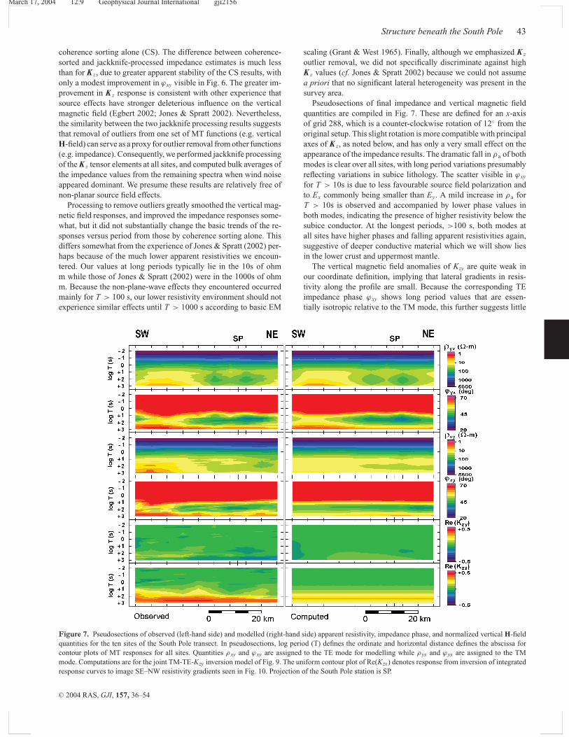
Figure 7. Pseudosections of observed (left-hand side) and modelled (right-hand side) apparent resistivity, impedance phase, and normalized vertical H-fieldquantities for the ten sites of the South Pole transect. In pseudosections, log period (T) defines the ordinate and horizontal distance defines the abscissa forcontour plots of MT responses for all sites. Quantities ρ xy and ϕ xy are assigned to the TE mode for modelling while ρ yx and ϕ yx are assigned to the TMmode. Computations are for the joint TM-TE-Kzy inversion model of Fig. 9. The uniform contour plot of Re(Kzx) denotes response from inversion of integratedresponse curves to image SE–NW resistivity gradients seen in Fig. 10. Projection of the South Pole station is SP.
scaling (Grant & West 1965). Finally, although we emphasized K z
outlier removal, we did not specifically discriminate against highK z values (cf. Jones & Spratt 2002) because we could not assumea priori that no significant lateral heterogeneity was present in thesurvey area.
Pseudosections of final impedance and vertical magnetic fieldquantities are compiled in Fig. 7. These are defined for an x-axisof grid 288, which is a counter-clockwise rotation of 12◦ from theoriginal setup. This slight rotation is more compatible with principalaxes of K z, as noted below, and has only a very small effect on theappearance of the impedance results. The dramatic fall in ρ a of bothmodes is clear over all sites, with long period variations presumablyreflecting variations in subice lithology. The scatter visible in ϕ xy
for T > 10s is due to less favourable source field polarization andto Ex commonly being smaller than Ey. A mild increase in ρ a forT > 10s is observed and accompanied by lower phase values inboth modes, indicating the presence of higher resistivity below thesubice conductor. At the longest periods, >100 s, both modes atall sites have higher phases and falling apparent resistivities again,suggestive of deeper conductive material which we will show liesin the lower crust and uppermost mantle.
The vertical magnetic field anomalies of Kzy are quite weak inour coordinate definition, implying that lateral gradients in resis-tivity along the profile are small. Because the corresponding TEimpedance phase ϕ xy shows long period values that are essen-tially isotropic relative to the TM mode, this further suggests little
C© 2004 RAS, GJI, 157, 36–54
March 17, 2004 12:9 Geophysical Journal International gji2156
44 P. E. Wannamaker et al.
remaining influence of non-uniform field effects. In contrast, thereis a significant anomaly in Kzx for T >∼ 30 s for all sites on the profile,which implies a large scale conductor lying roughly parallel to andgrid southeast of our profile.
R E S I S T I V I T Y M O D E L S O F T H E S O U T HP O L E T R A N S E C T
Because the propagation of EM waves in the Earth at the periods ofinterest is diffusive, MT fields cannot resolve sharp structure in thesubsurface without additional constraints (Parker 1994). One way toproceed is by solving for a limited number of resistivity parameters,such as in a discrete layered model, in a least-squares sense (e.g.Petrick et al. 1977). Alternately, the Earth model can be divided intoseveral thousand incremental parameters or ‘pixels’, constrained asan ensemble to produce conservative model variations (de Groot-Hedlin & Constable 1990; Smith & Booker 1991), and often referredto as a minimum structure model. We consider both approaches.
Given the first-order similarity of all the sites, a quick initial in-terpretation is carried out by integrating the nominal TM (yx) modeimpedance along the profile. Provided our measured responses are
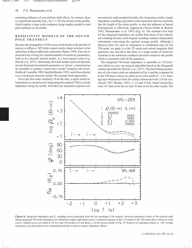
Figure 8. Integrated impedance and Kz sounding curves generated from the ten soundings of the transect. Inversion parameter values of five-layered earthfitting integrated TM mode impedance are tabulated in upper right-hand corner. Computed response of this 1-D model to the TM mode data is shown as solidcurves. Dashed curves are fitted to TE (xy) and TM modes (yx) and Re(Kzx) of the inverse model of Fig. 10. Rollover in impedance phase to <90◦ at highfrequencies was determined to be instrumental and due in part to contact impedance effects.
not seriously undersampled laterally, this integration yields a singleimpedance sounding equivalent to that measured with one electrodeline the length of the entire profile, so that the influence of lateralheterogeneity is effectively suppressed (Torres-Verdin & Bostick1992; Wannamaker et al. 1997) (Fig. 8). The nominal error barsfor the integrated impedance are smaller than those of any individ-ual sounding because each original sounding contains independentinformation concerning the regional average profile. Although aphysical basis for such an integration is established only for theTM mode, we apply it to the TE mode and vertical magnetic fieldquantities also and show that there is a single model of resistivityvariation in the northwest-southeast direction normal to the profilewhich is consistent with all the quantities.
The integrated TM mode impedance is amenable to 1-D inver-sion which we carry out using an algorithm based on the Marquardtmethod described by Petrick et al. (1977). The best-fitting parame-ters of a five-layer earth are tabulated in Fig. 8 and the computed fitto the TM data is shown as solid curves (rms misfit of ∼3.2). Start-ing layer thicknesses from the surface downward were 2.8 km (ice;Jiracek 1967; Bentley 1991), 2, 15 and 15 km. Initial resistivitieswere 105 ohm m for the ice and 10 ohm m for the other media. The
C© 2004 RAS, GJI, 157, 36–54
March 17, 2004 12:9 Geophysical Journal International gji2156
Structure beneath the South Pole 45
final ice thickness changed only slightly from the initial value andshowed a parameter standard deviation of <3 per cent. We also per-formed 1-D inversions on both modes of each individual sounding;the resulting ice thicknesses remained within 150 m of 2.9 km withsimilarly small parameter standard deviations in all cases, indicat-ing that little subice topography exists beneath our profile. However,the estimated ice resistivity is only somewhat larger than 104 ohmm (Fig. 8), which results from fitting the subtle rollover in ϕ yx fromnear 90◦ at 0.1 s to ∼78◦ at 0.01 s. Ice resistivities >105 ohm m,which are more compatible with Antarctic radar and DC resistivitysurveying (Bentley 1991; Shabtaie & Bentley 1995) keep phasesnear 90◦ up to 0.01 s. We believe the discrepancy is instrumentaland due in part to the effects of electrode contact impedance at theshorter periods, as discussed in Appendix A. Ice values >105 ohmm are compatible with our MT data to periods as short as 0.1 sand cause negligible changes in the earth parameter values in 1-Dinversion from those tabulated in Fig. 8.
The conductive layer below the ice in the 1-D model is ∼1 kmthick and is of low resistivity (∼3 ohm m). Increasing the resistiv-ity to 10 ohm m and allowing a greater thickness in the inversionproduces a significantly poorer fit (e.g. ∼3◦ at T = 10s, not shown).The deeper crust is moderately more resistive, but only reaches a fewtens of ohm m. However, because thin resistive layers are difficultto resolve with MT (Madden 1971; Vozoff 1991), higher resistivitydomains of limited extent could exist with little influence on thedata. Below ∼20 km depth, the lower crust and upper mantle resis-tivities become low (2–6 ohm m). These small values are surprisingand suggest active tectonic processes below the polar plateau in thisregion, as discussed later.
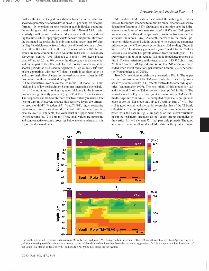
Figure 9. 2-D resistivity cross-sections from TM-only (top) and joint TM-TE-Kzy (bottom) inversions. The 1-D smooth resistivity profile (Apr) serving as apriori and starting models is shown as a column to the left-hand side of each section. Note the vertical exaggeration of 4:1 in the upper 4.6 km. Projection ofthe South Pole station is denoted by SP and of site SPLE03 by E03 along the top section.
2-D models of MT data are estimated through regularized in-version techniques intended to minimize model artefacts caused bydata noise (Tarantola 1987). Our inversion algorithm uses the finite-element simulator of Wannamaker et al. (1987) and DeLugao &Wannamaker (1996) and damps model variations from an a prioristructure (Tarantola 1987). As depth increases in the model, pa-rameter thicknesses and widths expand to help equalize parameterinfluence on the MT response according to EM scaling (Grant &West 1965). The starting guess and a priori model for the 2-D in-versions is a smooth 1-D profile derived from an analogous 1-D apriori inversion of the integrated TM mode impedance response ofFig. 8. The ice resistivity and thickness are set to 13 300 ohm m and2960 m from the 1-D layered inversions. The 2-D inversions wereended when misfit reductions per iteration became <0.05 per cent.(cf. Wannamaker et al. 2002).
Two 2-D inversions models are presented in Fig. 9. The upperone is from inversion of the TM mode only, due to its likely lowersensitivity to finite strike (3-D) effects relative to the other MT quan-tities (Wannamaker 1999). The rms misfit of this model is ∼2.6and the good fit of the TM response is exemplified in Fig. 3. Thesecond model in Fig. 9 is from joint inversion of the TM and TEmodes together with sKzy. The computed response is not quite asclose as for the TM mode only (Fig. 3), with an rms of ∼4.1, butstill is good overall and the model resembles that of the TM-onlycalculation. The computations from the joint inversion are com-pared with the data in Fig. 7. In particular, the lateral variationsin subice resistivity structure do not cause strong anomalies inthe vertical H-field element Kzy (real part only plotted). The goodagreement between all modes of MT data in the joint inversion
C© 2004 RAS, GJI, 157, 36–54
March 17, 2004 12:9 Geophysical Journal International gji2156
46 P. E. Wannamaker et al.
suggests that the 2-D approximation is reasonable (Wannamaker1999).
In both 2-D models, a pronounced conductive layer is visiblebeneath the ice sheet within which there are thickness variationsreproducing the fundamental lateral variations especially in the TMresponse. Mid-crustal resistivities are somewhat variable but reach100 ohm m in places. Low resistivity in the deep crust and uppermantle is also seen, as implied previously from the falling ρ a and1-D models. Sensitivity tests using the integrated impedance datasuggest that such low resistivities persist to depths of at least 60 km.Under the western portion of the transect, a lower resistivity zoneis seen extending upward from the lower crust to depths of ∼10km. This is seen in both the TM only and joint inversion models,although its somewhat more pronounced nature in the joint modelmay be due in part to finite strike effects in the overlying shallowconductive subice section as reflected in particularly low values ofρ xy and high ϕ xy at the southwest end.
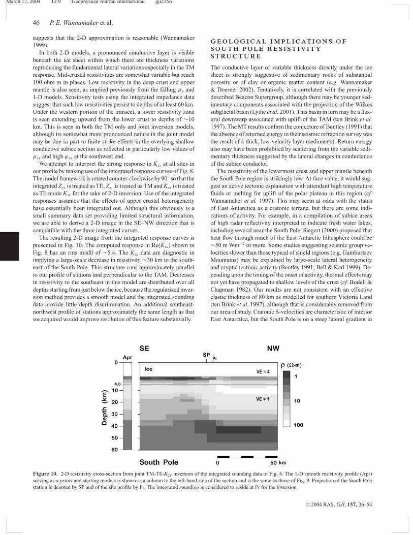
We attempt to interpret the strong response in Kzx at all sites inour profile by making use of the integrated response curves of Fig. 8.The model framework is rotated counter-clockwise by 90◦ so that theintegrated Zyx is treated as TE, Zxy is treated as TM and Kzx is treatedas TE mode Kzy for the sake of 2-D inversion. Use of the integratedresponses assumes that the effects of upper crustal heterogeneityhave essentially been integrated out. Although this obviously is asmall summary data set providing limited structural information,we are able to derive a 2-D image in the SE–NW direction that iscompatible with the three integrated curves.
The resulting 2-D image from the integrated response curves ispresented in Fig. 10. The computed response in Re(Kzx) shown inFig. 8 has an rms misfit of ∼5.4. The Kzx data are diagnostic inimplying a large-scale decrease in resistivity ∼30 km to the south-east of the South Pole. This structure runs approximately parallelto our profile of stations and perpendicular to the TAM. Decreasesin resistivity to the southeast in this model are distributed over alldepths starting from just below the ice, because the regularized inver-sion method provides a smooth model and the integrated soundingdata provide little depth discrimination. An additional southeast-northwest profile of stations approximately the same length as thatwe acquired would improve resolution of this feature substantially.
Figure 10. 2-D resistivity cross-section from joint TM-TE-Kzy inversion of the integrated sounding data of Fig. 8. The 1-D smooth resistivity profile (Apr)serving as a priori and starting models is shown as a column to the left-hand side of the section and is the same as those of Fig. 9. Projection of the South Polestation is denoted by SP and of the site profile by Pr. The integrated sounding is considered to reside at Pr for the inversion.
G E O L O G I C A L I M P L I C AT I O N S O FS O U T H P O L E R E S I S T I V I T YS T RU C T U R E
The conductive layer of variable thickness directly under the icesheet is strongly suggestive of sedimentary rocks of substantialporosity or of clay or organic matter content (e.g. Wannamaker& Doerner 2002). Tentatively, it is correlated with the previouslydescribed Beacon Supergroup, although there may be younger sed-imentary components associated with the projection of the Wilkessubglacial basin (Lythe et al. 2001). This basin in turn may be a flex-ural downwarp associated with uplift of the TAM (ten Brink et al.1997). The MT results confirm the conjecture of Bentley (1991) thatthe absence of returned energy in their seismic refraction survey wasthe result of a thick, low-velocity layer (sediments). Return energyalso may have been prohibited by scattering from the variable sedi-mentary thickness suggested by the lateral changes in conductanceof the subice conductor.
The resistivity of the lowermost crust and upper mantle beneaththe South Pole region is strikingly low. At face value, it would sug-gest an active tectonic explanation with attendant high temperaturefluids or melting for uplift of the polar plateau in this region (cf.Wannamaker et al. 1997). This may seem at odds with the statusof East Antarctica as a cratonic terrane, but there are some indi-cations of activity. For example, in a compilation of subice areasof high radar reflectivity interpreted to indicate fresh water lakes,including several near the South Pole, Siegert (2000) proposed thatheat flow through much of the East Antarctic lithosphere could be∼50 m Wm−2 or more. Some studies suggesting seismic group ve-locities slower than those typical of shield regions (e.g. GamburtsevMountains) may be explained by large-scale lateral heterogeneityand cryptic tectonic activity (Bentley 1991; Bell & Karl 1999). De-pending upon the timing of the onset of activity, thermal effects maynot yet have propagated to shallow levels of the crust (cf. Bodell &Chapman 1982). Our results are not consistent with an effectiveelastic thickness of 80 km as modelled for southern Victoria Land(ten Brink et al. 1997), although that is considerably removed fromour area of study. Cratonic S-velocities are characteristic of interiorEast Antarctica, but the South Pole is on a steep lateral gradient in
C© 2004 RAS, GJI, 157, 36–54
March 17, 2004 12:9 Geophysical Journal International gji2156
Structure beneath the South Pole 47
all velocity models so far, clouding a comparison with our resistivitystructure.
An alternative non-thermal explanation for low resistivity in thelower crust and upper mantle, namely graphite, is given lower prior-ity than that of fluids or melts. Although there are exceptions in areasof former deep sedimentary underthrusting (Wannamaker 2000),most lower crustal and upper mantle terranes have oxidation statesnear the quartz–fayalite–magnetite (QFM) buffer (Winkler 1979;Gaetani & Grove 1999; Canil 2002). In thermal regimes where tem-peratures exceed ∼500◦C, graphite under QFM is unstable (Frost &Bucher 1994; Pasteris 1999). Moreover, the deep conductivity struc-ture we resolve appears to be quite isotropic. Deep terranes with highconductivity interpreted to be controlled by graphite tend to havehigh apparent anisotropy due to stress orientation or rock fabricduring deposition or emplacement (Hjelt & Korja 1993; Mareschal1995; Wannamaker 2000), although there may be exceptions (Joneset al. 2001). Graphite could be important in the narrower, mid-crustalconductive structures imaged near the western end of our profile orto the southeast of the South Pole because temperatures are likelycooler at these levels making metamorphic fluids less likely andgraphite more stable (Wannamaker 2000).
The degree of extensional activity in Antarctica today is lim-ited, perhaps related to its being surrounded by oceanic ridges, sothat the volcanism and thermal processes are hypothesized to stemfrom mantle plume processes (Hole & LeMasurier 1994; LeMa-surier & Landis 1996). Continents are estimated to migrate over∼5 hotspot plumes every 150 Myr on average that may contributeup to one-third of lower crustal material (Condie 1999; Johnston &Thorkelson 2000). Plume fronts are modelled to interact with litho-spheric basal ‘topography’, thereby localizing zones of melting andthermal processes (Burke 1996; Sleep 1997; Ebinger & Sleep 1998;Maza et al. 1998; Ayadi et al. 2000), which may explain regional-ized East Antarctic uplifts such as the Gamburtsev–Vostok areas.Additionally, Lake Vostok with its great depth is reminiscent of riftbasins and, if so, active geothermal vents may constitute a favourableenergy regime for life forms in this extreme environment (Bell &Karl 1999). Timing of initiation of any activity under East Antarc-tica is difficult to bracket, but Fitzgerald & Stump (1997) resolveat least three distinct episodes of uplift affecting the TAM closerto the South Pole. In addition to possible plume-related causes, thethermal state under the South Pole may be enhanced by thermalencroachment including perhaps non-uniform extensional compo-nents from relatively active West Antarctica, such as the somewhatanalogous situation at the Great Basin–Colorado Plateau transitionin the western United States (Bodell & Chapman 1982; Storey &Alabaster 1991; Rocholl et al. 1995; Wannamaker et al. 2001).
C O N C L U S I O N S
High-quality MT measurements may be gained from the Antarcticinterior with proper attention to instrument design and time-seriesprocessing. Incorporation of high-impedance electrode buffer am-plifiers and non-reactive electrodes can yield electric field records ofhigh fidelity over thick ice. The robust removal of non-plane-waveoutliers with emphasis on the vertical magnetic field appears toyield stable MT transfer functions for both the impedance and thevertical magnetic field. The principal impediment to high qualityMT data that we experienced was wind-induced electrostatic noisein the polar ice due to blowing ice particles, particularly over sur-vey areas with conductive crustal sections that reduce MT E-fieldsignal. Signal-to-noise ratio may be improved by lengthening the E-field bipoles and by ensuring that a locally level surface is defined
around the implanted electrodes. Magnetic field recording appearedto present no special problems relative to surveying in temperateclimates, although calibration factors appropriate to low operatingtemperatures should be ensured.
Our MT results have provided some of the first definitive indi-cations of subice structure and physical state below the South Poleregion. A substantial and widespread sedimentary section with sig-nificant porosity or matured organic content is inferred just below theice sheet, corroborating earlier conjecture from refraction seismicdata. The section may correlate with the regionally extensive Paleo-zoic Beacon Supergroup with possible younger components. Deepresistivity structure of the South Pole region at present appears todiffer from that typical of cratonic lithosphere worldwide in exhibit-ing low resistivity in the lower crust and upper mantle. We believethermal activity generating high-temperature fluids or melts is morelikely than solid phases for explaining the low resistivity, althoughthe interpretation is not unique. Regionalized plume-related dynam-ics in the deep lithosphere may be the dominant process behind ther-mal activity, with possible contributing influence from nearby WestAntarctica.
A C K N O W L E D G M E N T S
The South Pole field survey and its interpretation were supportedunder US National Science Foundation grant OPP96-15254. Thedesign and construction of the high impedance components of ourMT instrumentation were supported under grants OPP92-19503 andOPP96-15254. The remainder of the instrumentation developmentwas funded by US Department of Energy contract 95ID13274 andNational Science Foundation grant EAR-9616450 (EMSOC facil-ity). Algorithms for robust outlier removal and response inversionwere developed under DOE contract 95ID13274. We are grateful toUgo Conti for suggesting titanium as a possible low-noise metalelectrode material. Additional field assistance in the South Polesurvey was provided by Keri Petersen (safety personnel). Manage-ment and staff of the South Pole and McMurdo stations are thankedfor excellent logistical support. Constructive reviews were providedby Charles Bentley, Paul Bedrosian and Associate Editor MartynUnsworth.
R E F E R E N C E S
Ayadi, A., Dorbath, C., Lesquer, A. & Bezzeghoud, M., 2000. Crustal andupper mantle velocity structure of the Hoggar swell (Central Sahara, Al-geria), Phys. Earth planet. Inter., 118, 111–123.
Barrett, P.J., 1991. The Devonian to Jurassic Beacon Supergroup of theTransantarctic Mountains and correlatives in other parts of Antarctica,in The Geology of Antarctica, ed. Tingey, R.J., pp. 120–152, Clarendon,Oxford.
Beblo, M. & Liebig, V., 1990. Magnetotelluric measurements in Antarctica,Phys. Earth planet. Inter., 60, 89–99.
Behrendt, J.D., 1999. Crustal and lithospheric structure of the West AntarcticRift system from geophysical investigations—a review, Global Planet.Change, 23, 25–44.
Behrendt, J.D., LeMasurier, W.E., Cooper, A.K., Tessensohn, F., Trehu, A.and D. Damaske, 1991. Geophysical studies of the West Antarctic riftsystem, Tectonics, 10, 1257–1273.
Behrendt, J.D., Blankenship, D.D., Finn, C.A., Bell, R.E., Sweeney, R.E.,Hodge, S.M. & Brozena, J.M., 1994. CASERTZ aeromagnetic data reveallate Cenozoic flood basalts (?) in the West Antarctic rift system, Geology22, 527–530.
Bell, R.E. & Karl, D.M., 1999. Evolutionary processes a focus of decade-longecosystem study of Antarctic’s Lake Vostok, EOS, Trans. Am. geophys.Un., 80(48), 573, 579.
C© 2004 RAS, GJI, 157, 36–54
March 17, 2004 12:9 Geophysical Journal International gji2156
48 P. E. Wannamaker et al.
Bentley, C.R., 1973. Crustal structure of Antarctica, Tectonophysics 20, 229–240.
Bentley, C.R., 1991. Configuration and structure of the subglacial crust,in The Geology of Antarctica, pp. 335–364, ed. Tingey, R.J., Clarendon,Oxford.
Bentley, C.R. & Clough, J.W., 1970. Antarctic subglacial structure fromseismic refraction measurements, in Antarctic geology and geophysics,pp. 292–297, ed. Adie, R.J., Universitetsforlaget, Oslo.
Blankenship, D.D., Bell, R.E., Hodge, S.M., Brozena, J.M., Behrendt, J.C. &Finn, C.A., 1993. Active volcanism beneath the West Antarctic ice sheetand implications for ice-sheet stability, Nature, 361, 526–529.
Blankenship, D.D. et al., 2001. Geologic controls on the initiation of rapidbasal motion for West Antarctic ice streams: a geophysical perspectiveincluding new airborne radar sounding and laser altimetry results, in TheWest Antarctic Ice Sheet: Behavior and Environment, pp. 105–121, edsAlley, R.B. & Bindschadler, R.A., Antarctic Res. Ser., 77, Amer. Geophys.Union, Washington, DC.
Bodell, J.M. & Chapman, D.S., 1982. Heat flow in the north-central ColoradoPlateau, J. geophys. Res., 87, 2869–2884.
Borg, S.G. & DePaolo, D.J., 1994. Laurentia, Australia, and Antarctica asa Late Proterozoic supercontinent: constraints from isotopic mapping,Geology 22, 307–310.
Burke, K., 1996. The African plate, S. Afr. J. Geol., 99, 341–409.Cande, S.C., Stock, J.M., Muller, R.D. & Ishihara, T., 2000. Cenozoic motion
between East and West Antarctica, Nature, 404, 145–150.Canil, D., 2002. Vanadium in peridotites: mantle redox and tectonic envi-
ronments: Archean to present, Earth planet. Sci. Lett., 95, 75–90.Chave, A.D. & Thompson, D.J., 1989. Some comments on magne-
totelluric response function estimation, J. geophys. Res., 94, 14 215–14 225.
Clarke, T.S., Burkholder, P.D., Smithson, S.B. & Bentley, C.R., 1997. Opti-mum seismic shooting and recording parameters and a preliminary crustalmodel for the Byrd Subglacial Basin, Antarctica, in The Antarctic Region:Geological Evolution and Processes, pp. 485–493, ed. Ricci, C.A., TerraAntarc. Publ., Sienna.
Condie, K.C., 1999. Mafic crustal xenoliths and the origin of the lowercontinental crust, Lithos, 46, 95–101.
Dalziel, I.W.D., 1991. Pacific margins of Laurentia and East Antarctica–Australia as a conjugate rift pair: evidence and implications for an Eo-cambrian supercontinent, Geology 19, 598–601.
Dalziel, I.W.D., 1997. Neoproterozoic–Paleozoic geography and tectonics:review, hypothesis, environmental speculation, Geol. Soc. Am. Bull., 108,16–42.
Dalziel, I.W.D. & Lawver, L.A., 2001. The lithospheric setting of the WestAntarctic ice sheet, in The West Antarctic ice sheet: behavior and envi-ronment, pp. 105–121, eds Alley, R.B. & Bindschadler, R.A., AntarcticRes. Ser., 77, Amer. Geophys. Union, Washington, DC.
Danesi, S. & Morelli, A., 2000. Group velocity of Rayleigh waves in theAntarctic region, Phys. Earth planet. Inter., 122, 55–66.
Davey, F.J. & Brancolini, G., 1995. The Late Mesozoic and Cenozoic struc-tural setting of the Ross Sea region, in Geology and Seismic Stratigraphyof the Antarctic Margin, pp. 167–182, eds Cooper, A.K., Barker, P.F. &Brancolini, G., Antarctic Res. Ser., 68, AGU.
de Groot-Hedlin, C.D. & Constable, S.C., 1990. Occam’s inversion to gen-erate smooth, two-dimensional models from magnetotelluric data, Geo-physics, 93, 1613–1624.
DeLugao, P.P. & Wannamaker, P.E., 1996. Calculating the two-dimensionalmagnetotelluric Jacobian in finite elements using reciprocity, Geophys. J.Int., 127, 806–810.
Ebinger, C.J. & Sleep, N.H., 1998. Cenozoic magmatism throughout eastAfrica resulting from impact of a single plume, Nature, 395, 788–791.
Edminister, J.A., 1965. Schaum’s outline of theory and problems of electriccircuits, p. 289, McGraw-Hill, New York.
Egbert, G.D., 2002. Processing and interpretation of electromagnetic induc-tion array data, Surv. Geophys., 23, 207–249.
Egbert, G.D. & Booker, J.R., 1992. Very long period magnetotellurics at Tuc-son observatory: implications for mantle conductivity, J. geophys. Res.,97, 15 099–15 112.
Everett, M.E. & Schultz, A., 1996. Geomagnetic induction in a heteroge-neous sphere: azimuthally symmetric test computations and the responseof an undulating 660-km discontinuity, J. geophys. Res., 101, 2765–2783.
Fitzgerald, P., 1994. Thermochronologic constraints on post-Paleozoic tec-tonic evolution of the central Trans Antarctic Mountains, Antarctica, Tec-tonics, 13, 818–836.
Fitzgerald, P.G. & Stump, E., 1997. Cretaceous and Cenozoic episodic de-nudation of the Transantarctic Mountains, Antarctica: new constraintsfrom apatite fission track thermochronology in the Scott Glacier region,J. geophys. Res., 102, 7747–7765.
Fournier, H.G., 1994. Geophysical studies of the Antarctic peninsula, Acta.Geod. Geoph. Hung., 29, 19–38.
Frost, B.R. & Bucher, K., 1994. Is water responsible for geophysical anoma-lies in the deep continental crust? A petrological perspective, Tectono-physics 231, 293–309.
Gaetani, G.A. & Grove, T.L., 1999. Wetting of mantle olivine by sulfidemelt: implications for Re/Os ratios in mantle peridotite and late stagecore formation, Earth planet. Sci. Lett., 169, 147–163.
Gamble, T., Goubau, W. & Clarke, J., 1979. Magnetotellurics with a remotereference, Geophysics, 44, 53–68.
Garcia, X., Chave, A.D. & Jones, A.G., 1997. Robust processing of mag-netotelluric data from the auroral zone, J. Geomag. Geoelectr., 49, 1451–1468.
Grant, F.S. & West, G.F., 1965. Interpretation Theory in Applied Geophysics,p. 584, McGraw-Hill, New York.
Groom, R.W. & Bailey, R.C., 1989. Decomposition of magnetotelluricimpedance tensor in the presence of local three-dimensional galvanic dis-tortion, J. geophys. Res., 94, 1913–1925.
Hessler, V.P. & Jacobs, J., 1966. A telluric current experiment on the Antarcticice cap, Nature, 210, 190–191.
Hjelt, S.-E. & Korja, T., 1993. Lithospheric and upper mantle structures,results of electromagnetic soundings in Europe, Phys. Earth planet. Inter.,79, 137–177.
Hole, M.J. & LeMasurier, W.E., 1994. Tectonic controls on the geochem-ical composition of Cenozoic, mafic alkaline volcanic rocks from WestAntarctica, Contr. Min. Petr., 117, 187–202.
Humphreys, E.D. & Dueker, K.G., 1994. Physical state of the western USmantle, J. geophys. Res., 99, 9635–9650.
Jiracek, G.R., 1967. Radio sounding of Antarctic ice, Research Ser. Rep. 67–1, Geophys. & Polar Res. Ctr., p. 127, Dept Geol., Univ. Wisc., Madison.
Johnston, S.T. & Thorkelson, D.J., 2000. Continental flood basalts: episodicmagmatism above long-lived hotspots, Earth planet. Sci. Lett., 175, 247–256.
Jones, A.G., 1992. Electrical conductivity of the continental lower crust, inContinental lower crust, pp. 81–143, eds Fountain, D.M., Arculus, R.J. &Kay, R.W., Elsevier, Amsterdam.
Jones, A.G., 1999. Imaging the continental upper mantle using electromag-netic methods, Lithos, 48, 570–580.
Jones, A.G. & Jodicke, H., 1984. Magnetotelluric transfer function estima-tion improvement by a coherence-based rejection technique, 54th Soc.Explor. Geophys. Ann. Mtg, Atlanta, Dec. 2–6, Ext. Abstr., Tulsa, OK,51–55.
Jones, A.G. & Spratt, J., 2002. A simple method for deriving the uniformfield MT responses in the auroral zone, Earth Planets Space, 54, 443–450.
Jones, A.G., Ferguson, I.J., Chave, A.D., Evans, R.L., Spratt, J. & Garcia,X., 2001. The electrical structure of the Slave craton, Geology 29, 423–426.
Karlstrom, K.E., Ahall, K.-I., Harlan, S.S., Williams, M.L., McLelland, J.& Geissman, J.W., 2001. Long-lived (1.8–1.0 Ga) convergent orogen insouthern Laurentia, its extensions to Australia and Baltica, and implica-tions for refining Rodinia, Precamb. Res., 111, 5–30.
Kong, X., Zhang, J. & Jiao, C., 1993. Deep electrical conductivity structurein the region of Great Wall station, Fildes peninsula, west Antarctica,Antarctic Res., Chinese Edn, 5, 40–47.
Kong, X., Zhang, J. & Jiao, C., 1994. Magnetotelluric deep sounding study inthe region of Zhongshan station, East Antarctica, Antarctic Res., ChineseEdn, 6, 32–36.
C© 2004 RAS, GJI, 157, 36–54
March 17, 2004 12:9 Geophysical Journal International gji2156
Structure beneath the South Pole 49
LeMasurier, W.E. & Landis, C.A., 1996. Mantle-plume activity recorded bylow-relief erosion surfaces in West Antarctica and New Zealand, Geol.Soc. Am. Bull., 108, 1450–1466.
LeMasurier, W.E. & Rex, D.C., 1991. The Marie Byrd Land volcanicprovince and its relation to the Cainozoic West Antarctic rift system,in The Geology of Antarctica, pp. 249–284, ed. Tingey, R.J., Clarendon,Oxford.
Lowry, A.R., Ribe, N.M. & Smith, R.B., 2000. Dynamic elevation of theCordillera, western United States, J. geophys. Res., 105, 23 371–23 390.
Lythe, M.B., Vaughan, D.G. & the BEDMAP consortium, 2001. BEDMAP:a new ice thickness and subglacial topographic model of Antarctica, J.geophys. Res., 106, 11 335–11 351.
MacGorman, D.R. & Rust, W.D., 1998. The Electrical Nature of Storms,p. 422, Oxford University Press, New York.
Madden. T.R., 1971. The resolving power of geoelectric measurements fordelineating resistive zones within the crust, in The Structure and Physi-cal Properties of the Earth’s Crust, AGU Mono. 14, pp. 95–105, AGU,Washington, DC.
Mareschal, M., 1986. Modelling of natural sources of magnetospheric ori-gin in the interpretation of regional induction studies: a review, Surv.Geophys., 8, 261–300.
Mareschal, M., 1995. Archaean cratonic roots, mantle shear zones and deepelectrical anisotropy, Nature, 375, 134–137.
Maza, M., Briqueu, L., Dautria, J.-M. & Bosch, D., 1998. The AchkalOligocene ring complex: Sr, Nd, Pb evidence for transition between tholei-itic and alkali Cenozoic magmatism in Central Hoggar (South Algeria),Sci. Terre Planet., C.R. Acad. Sci., Paris, 327, 167–172.
Parker, R.L., 1994. Geophysical Inverse Theory, p. 386, Princeton UniversityPress, Princeton.
Pasteris, J.D., 1999. Causes of the uniformly high crystallinity of graphitein large epigenetic deposits, J. Struct. Geol., 17, 779–787.
Pellerin, L. & Hohmann, G.W., 1990. Transient electromagnetic inversion:a remedy for magnetotelluric static shifts, Geophysics, 55, 1242–1250.
Petrick, W.R., Pelton, W.H. & Ward, S.H., 1977. Ridge-regression inversionapplied to crustal resistivity sounding data from South Africa, Geophysics,42, 995–1005.
Pirjola, R.J., 1998. Modeling the electric and magnetic fields at the Earth’ssurface due to an auroral electrojet, J. Atmos. Solar Terres. Phys., 60,1139–1148.
Reynolds, J.M., 1985. Dielectric behaviour of firn and ice from the Antarcticpeninsula, J. Glaciol., 31, 253–262.
Ritzwoller, M.H., Shapiro, N.M., Levshin, A.L. & Leahy, G.M., 2001.Crustal and upper mantle structure beneath Antarctica and surroundingoceans, J. geophys. Res., 106, 30 645–30 670.
Rocholl, A., Stein, M., Molzahn, M., Hart, S.R. & Worner, G., 1995. Geo-chemical evolution of rift magmas by progrssive tapping of a stratifiedmantle source beneath the Ross Sea Rift, Northern Victoria Land, Antarc-tica, Earth planet. Sci. Lett., 131, 207–224.
Rodgers, J.J.W., Unrug, R. & Sultan, M., 1995. Tectonic assembly of Gond-wana, J. Geodyn., 19, 1–34.
Roult, G., Rouland, D. & Montagner, J.P., 1994. Antarctica II: upper-mantlestructure from velocities and anisotropy, Phys. Earth planet. Inter., 84,33–57.
Schmidt, S. & Dent, J.D., 1993. A theoretical prediction of the effects ofelectrostatic forces on saltating snow particles, J. Glaciol., 18, 234–238.
Sen, V., Stoffa, P.L., Dalziel, I.W.D., Blankenship, D.D., Smith, A.M. &Anandakrishnan, S., 1998. Seismic surveys in central West Antarctica:data and processing examples from the ANTALITH field tests (1994–1995), Terra Antarctica, 5, 761–772.
Shabtaie, S. & Bentley, C.T., 1995. Electrical resistivity sounding of the EastAntarctic ice sheet, J. geophys. Res., 100, 1933–1954.
Siegert, M.J., 2000. Antarctic subglacial lakes, Earth-Sci. Rev., 50, 29–50.Sleep, N.H., 1997. Lateral flow and ponding of starting plume material, J.
geophys. Res., 102, 10 001–10 012.Smith, J.T. & Booker, J.R., 1991. Rapid inversion of two and three dimen-
sional magnetotelluric data, J. geophys. Res., 96, 3905–3922.Sonder, L.J. & Jones, C.H., 1999. Western United States: how the west was
widened, Annu. Rev. Earth planet. Sci., 27, 417–462.
Storey, B.C. & Alabaster, T., 1991. Tectonomagmatic controls on Gondwanabreak-up models: evidence from the proto-Pacific margin of Antarctica,Tectonics, 10, 1274–1288.
Stodt, J.A., 1983. Processing of conventional and remote reference magne-totelluric data, PhD thesis, p. 223, University of Utah.
Stratton, J.A., 1941. Electromagnetic Theory, p. 615, McGraw-Hill,New York.
Tarantola, A., 1987. Inverse Problem Theory, p. 613, Elsevier, New York.ten Brink, U.S., Bannister, S., Beaudoin, B.C. & Stern, T.A., 1993. Geo-
physical investigations of the tectonic boundary between East and WestAntarctica, Science, 261, 45–50.
ten Brink, U.S., Hackney, R.I., Bannister, S., Stern, T.A. & Makovsky,Y., 1997. Uplift of the Trans Antarctic Mountains and the bedrockbeneath the East Antarctic ice sheet, J. geophys. Res., 102, 27 603–27 621.
Thompson, D.J. & Chave, A.D., 1991. Jackknifed error estimates for spectra,coherences, and transfer functions, in Advances in Spectrum Analysis andArray Processing, pp. 58–113, ed. Haykin, S., Prentice Hall, EnglewoodCliffs.
Torres-Verdin, C. & Bostick, F.X., Jr, 1992. Principles of spatial surfaceelectric field filtering in magnetotellurics: electro-magnetic array profiling(EMAP), Geophysics, 57, 603–622.
Vozoff, K., 1991. The magnetotelluric method, in Electromagnetic Methodsin Applied Geophysics, 2B, pp. 641–711, ed. Nabighian, M.N., Soc. ofExplor. Geophys., Tulsa.
Wannamaker, P.E., 1999. Affordable magnetotellurics: interpretation of MTsounding profiles from natural environments, in Three-dimensional Elec-tromagnetics, pp. 349–374, eds Oristaglio, M. & Spies, B., Devel. Ser.,no. 7, Soc. Explor. Geophys., Tulsa.
Wannamaker, P.E., 2000. Comment on ‘The petrologic case for a dry lowercrust’, by Yardley, B.D. & Valley, J.W., J. geophys. Res., 105, 6057–6064.
Wannamaker, P.E. & Doerner, W.M., 2002. Crustal structure of the RubyMountains and southern Carlin trend region, northeastern Nevada, frommagnetotelluric data, Ore Geol. Rev., 27, 185–210.
Wannamaker, P.E. & Hohmann, G.W., 1991. Electromagnetic InductionStudies, US National Report to IUGG, Rev. Geophys., Supplement,pp. 405–415.
Wannamaker, P.E., Stodt, J.A. & Rijo, L., 1987. A stable finite elementsolution for two-dimensional magnetotelluric modeling, Geophys. J. R.astr. Soc., 88, 277–296.
Wannamaker, P.E., Stodt, J.A. & Olsen, S.L., 1996. Dormant state of riftingin central west Antarctica implied by magnetotelluric profiling, Geophys.Res. Lett., 23, 2983–2987.
Wannamaker, P.E., Doerner, W.M., Stodt, J.A. & Johnston, J.M., 1997. Sub-dued state of tectonism of the Great Basin interior relative to its easternmargin based on deep resistivity structure, Earth planet. Sci. Lett., 150,41–53.
Wannamaker, P.E. et al., 2001. Great Basin-Colorado Plateau transition incentral Utah: An interface between active extension and stable interior, inThe Geological Transition: Colorado Plateau to Basin and Range, Proc. J.Hoover Mackin Symp., pp. 1–38, eds Erskine, M.C., Faulds, J.E., Bartley,J.M. & Rowley, P., Utah Geol. Assoc./Amer. Assoc. Petr. Geol. Guideb.30/GB78, Cedar City, Utah, September 20–23.
Wannamaker, P.E., Jiracek, G.R., Stodt, J.A., Caldwell, T.G., Gonzalez, V.M.,McKnight, J.D. & Porter, A.D., 2002. Fluid generation and pathways be-neath an active compressional orogen, the New Zealand Southern Alps,inferred from magnetotelluric data, J. geophys. Res., 107(B6), ETG 6 1–20.
Wight, D.E. & Bostick, F.X., Jr, 1980. Cascade decimation—a techniquefor real time estimation of power spectra, IEEE Proc. Int. Conf. AcousticSpeech and Signal Proc., pp. 626–629.
Winkler, H.G.F., 1979. Petrogenesis of Metamorphic Rocks, p. 348, Springer-Verlag, New York.
Zonge, K.L. & Hughes, L.J., 1985. Effect of electrode contact resistanceon electric field measurements, in Expanded Abstracts of 1985 TechnicalProgramme of 55th Ann. Int. SEG Meeting, contribution MIN 1.5, Tulsa,OK, 231–234.
C© 2004 RAS, GJI, 157, 36–54
March 17, 2004 12:9 Geophysical Journal International gji2156
50 P. E. Wannamaker et al.
A P P E N D I X A : M T I N S T RU M E N TAT I O NOV E R P O L A R I C E S H E E T S
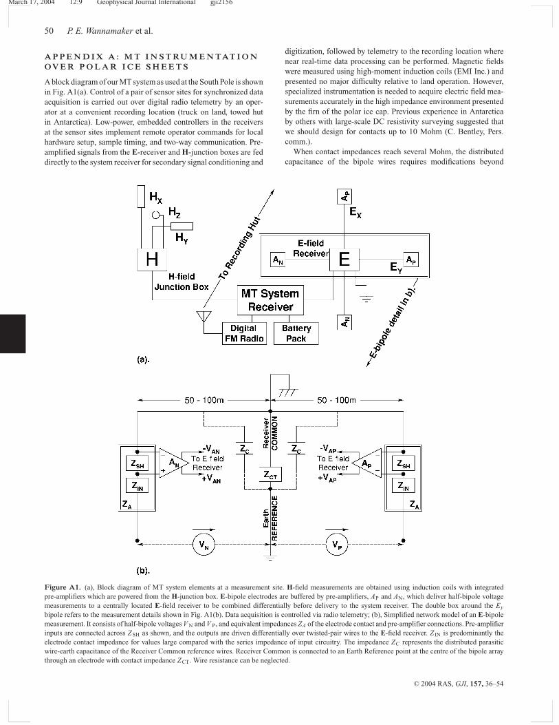
A block diagram of our MT system as used at the South Pole is shownin Fig. A1(a). Control of a pair of sensor sites for synchronized dataacquisition is carried out over digital radio telemetry by an oper-ator at a convenient recording location (truck on land, towed hutin Antarctica). Low-power, embedded controllers in the receiversat the sensor sites implement remote operator commands for localhardware setup, sample timing, and two-way communication. Pre-amplified signals from the E-receiver and H-junction boxes are feddirectly to the system receiver for secondary signal conditioning and
Figure A1. (a), Block diagram of MT system elements at a measurement site. H-field measurements are obtained using induction coils with integratedpre-amplifiers which are powered from the H-junction box. E-bipole electrodes are buffered by pre-amplifiers, AP and AN, which deliver half-bipole voltagemeasurements to a centrally located E-field receiver to be combined differentially before delivery to the system receiver. The double box around the Ey
bipole refers to the measurement details shown in Fig. A1(b). Data acquisition is controlled via radio telemetry; (b), Simplified network model of an E-bipolemeasurement. It consists of half-bipole voltages V N and V P, and equivalent impedances ZA of the electrode contact and pre-amplifier connections. Pre-amplifierinputs are connected across ZSH as shown, and the outputs are driven differentially over twisted-pair wires to the E-field receiver. Z IN is predominantly theelectrode contact impedance for values large compared with the series impedance of input circuitry. The impedance ZC represents the distributed parasiticwire-earth capacitance of the Receiver Common reference wires. Receiver Common is connected to an Earth Reference point at the centre of the bipole arraythrough an electrode with contact impedance ZCT. Wire resistance can be neglected.
digitization, followed by telemetry to the recording location wherenear real-time data processing can be performed. Magnetic fieldswere measured using high-moment induction coils (EMI Inc.) andpresented no major difficulty relative to land operation. However,specialized instrumentation is needed to acquire electric field mea-surements accurately in the high impedance environment presentedby the firn of the polar ice cap. Previous experience in Antarcticaby others with large-scale DC resistivity surveying suggested thatwe should design for contacts up to 10 Mohm (C. Bentley, Pers.comm.).
When contact impedances reach several Mohm, the distributedcapacitance of the bipole wires requires modifications beyond
C© 2004 RAS, GJI, 157, 36–54
March 17, 2004 12:9 Geophysical Journal International gji2156
Structure beneath the South Pole 51
simply increasing the shunt input impedance of a typical E-field re-ceiver, because the capacitance and the contact impedance interactto cause attenuation and phase shifts due to unwanted voltage di-viders. In a simple model, signal voltage is modified by the complexattenuation factor [1 + j0.5X ]/[1 + j X ], where X = ω RCW L , R iselectrode contact resistance, CW is wire capacitance per unit length,L is wire length, and ω is angular frequency (Zonge & Hughes 1985,with correction). For plausible values R = 2 Mohm and C W L = 1nf, the (magnitude, phase) is (0.735, −19.3◦) at 100 Hz and (0.999,−1.1◦) at 3 Hz. Moreover, proximal environmental noise couplesto the receiver input through a series impedance Z W = 1/ jω C W Lrepresenting the wire capacitance, and may contaminate the signalif the condition R |Z W| is violated. Note that at 100 Hz, |Z W| ∼=1.6 Mohm when C W L = 1 nf.
Our E-field measurements were carried out differentially, using a‘plus’ electrode array with a central common mode reference elec-trode, as illustrated in Figs A1(a) and (b). Total bipole lengths were100–200 m. For robust and electrochemically stable operation in thiscold environment, we used 18 × 24 inch expanded metal titaniumsheets, buried vertically in the firn, as electrodes. Pre-amplifiers (AP,AN) were utilized at the positive (P) and negative (N) electrodes toisolate the high-impedance contact and thereby minimize complexvoltage dividers and capacitive noise coupling. We implementedan in situ calibration scheme described below to quantify remain-ing voltage divider effects. Bipole lines to the preamps were notsingle wires as in land surveys, but were standard unshielded eight-conductor network cables. These carried bipolar DC power, a powerreturn (current carrying) and a receiver common reference (current-free), differential signal, and differential calibration/control, config-ured in four twisted pairs as listed.
Fig. A1(b) shows a simplified network model of our E-field bipolemeasurement system. The electrode and pre-amplifier circuitry ofeach half-bipole are represented as an impedance ZA, assumed equalfor all half-bipoles. The impedance ZC , of the distributed para-sitic wire-earth capacitance of the receiver common reference wires(analogous to ZW above), has no effect on the measurement of V N
and V P, but does affect our in situ calibration as will be shown. Stan-dard circuit analysis and equivalence concepts (Edminister 1965)have been used to reduce our actual circuit topology to that ofFig. A1(b). Further details and more general circuit models canbe provided (contact JAS).
In Fig. A1(b), ZA is a series combination of two impedances, Z IN
and ZSH. Z IN, a combination of the electrode contact impedanceZCT and input circuitry impedance, acts in series with the ‘+’ inputof a pre-amplifier, and the pre-amp is connected across a shuntimpedance ZSH. The pre-amp senses a voltage V PR that is amplifiedand delivered differentially to the E-field receiver at the centre of thearray. Delivery of a balanced differential signal over a twisted pair ofwires minimizes dielectric leakage currents across their distributedparasitic wire-earth capacitance by minimizing the effective averagevoltage across the capacitance. ZSH is equivalently a parallel RCcircuit element. The capacitive component of ZSH includes 60 pfdue to the connection from an electrode to its pre-amp ‘+’ inputusing a 0.6 m coaxial cable (100 pf/m) with its shield connected topre-amp common. Laboratory measurements of the total effectivecapacitance of ZSH, including the coaxial cable connection, averaged∼120 pf and varied less than 3 per cent between amplifiers. About40 pf of this value is parasitic, due to the physical layout of thecircuit board or non-ideal performance of circuit components. WithC = 120 pf, the equivalent impedance of ZSH at frequency f is
ZSH = 909.1 Mohm/[1 + j0.6854 f ].
The DC impedance of ZSH, ∼909 Mohm, is a design tradeoff to pro-vide stable open-circuit operation and to allow appropriate circuitryto protect sensitive amplifier inputs for robust field operations. Atthe E-field receiver, the half-bipole voltages are received, combinedinto a bipole measurement, and delivered to the MT system receiverthrough galvanic isolation amplifiers for further system processing.
Together, Z IN and ZSH create a voltage divider at the pre-amplifierinputs, i.e. V P,N is developed across ZA, while V PR is developedacross ZSH. Therefore, V PR is essentially a low-pass filtered versionof the desired voltage, so that V P,N must be recovered from V PR
through
VP,N = VPR[1 + ZIN/ZSH].
Anticipating that Z IN could be significant compared with ZSH, acalibration procedure was implemented to estimate Z IN in situ. Thiswas done by delivering a calibration signal V CAL through a knownresistor RCAL to the ‘+’ input of each electrode pre-amplifier inturn, and observing the complex voltage ratio Q = V PR/V CAL.From Fig. A1(b), note that a network consisting of both x and y E-field bipoles is actually driven by V CAL due to their interconnectionacross ZCT. Considering all the impedance elements of this network,circuit analysis yields
[ZIN + (ZCT||Z )] ∼= RCAL ∗ Q/[1 − Q(1 + RCAL/ZSH)],
where Z = ZC/4||ZA/3, and the notation A ||B indicates the parallelcombination of A and B. This approximation is valid when V P,N V CAL[Z IN/ RCAL].
When |Z CT| |Z |, the left-hand side of the equation is essentially[Z IN + Z CT]. Z IN is approximated well by ZCT when Z IN is largeenough to necessitate calibration, so Z IN and ZCT are estimatedby halving the calculation on the right-hand side. Best stability isachieved when RCAL
∼= 2|Z CT|, so |Q| ∼= 0.5. However, note that|Z| decreases as frequency increases. When the condition |Z CT| |Z | is violated, |Z IN| and |Z CT| will be underestimated, as much asa factor of two when |Z | |Z CT|. Again for a wire capacitance of1 nf, |ZC/4| ∼= 400 Kohm at 100 Hz, and because |ZA/3|> |Z SH/3|∼= 4.43 Mohm, |Z| is slightly <|ZC/4|.
To our pleasant surprise, low-frequency (∼DC) individual elec-trode contact impedances at CWA were 0.2–0.25 Mohm, giving riseto voltage divider effects no greater than the data errors at the short-est periods (0.01 s). However, average temperatures at the SouthPole were ∼30 ◦C less than at CWA. Shabtaie & Bentley (1995)specify an Arrhenius dependence for firn resistivity that translatesto approximately a factor of two increase per 10 ◦C decrease, sug-gesting contact impedances could approach 2 Mohm at the SouthPole. Individual DC electrode contact impedances measured in situat the South Pole lay in the 0.75–1.25 Mohm range. We noted atrend towards the lower values as our survey progressed, and specu-late that this was at least partially due to near surface warming as thesummer season progressed. Low-frequency in situ measurements ofZCT from our MT system were generally consistent with simple mea-surements of DC resistance between electrode pairs using a Fluke87 multimeter.
Our calibration methodology gave stable estimates of |ZCT| insitu, but unfortunately did not produce stable estimates of the phaseof ZCT. Our experience at the South Pole indicates that V CAL did notalways obey the condition V P,N V CAL[Z IN/RCAL] due to compet-ing MT or wind-induced signals, often resulting in noisy calibrationdata. Our design value of RCAL = 10 Mohm could be lowered ad-vantageously here, but V CAL cannot be increased due to currentsystem limitations. Nor can calibration data currently be acquiredat sufficiently high frequencies to fully characterize the complex
C© 2004 RAS, GJI, 157, 36–54
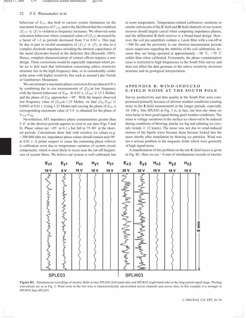
March 17, 2004 12:9 Geophysical Journal International gji2156
52 P. E. Wannamaker et al.
behaviour of ZCT, due both to current system limitations on themaximum frequency of V CAL and to the likelihood that the condition|Z CT| |Z | is violated as frequency increases. We observed somerelaxation behaviour where computed values of |Z CT| decreased bya factor of >2 as periods decreased from 5 to 0.02 s. This maybe due in part to invalid assumption of |Z CT| |Z |, or also to acomplex electrode impedance including the intrinsic capacitance ofthe metal electrodes buried in the dielectric firn (Reynolds 1985).Hence, complete characterization of contact effects requires a newdesign. These corrections would be especially important where po-lar ice is thin such that information concerning subice resistivitystructure lies in the high-frequency data, or in considerably colderpolar areas with higher resistivity firn such as around Lake Vostokor Gamburtsev Mountains.
We can estimate a maximum phase correction for our data at 0.01 sby combining the in situ measurements of |Z IN|at low frequencywith the known behaviour of ZSH. At 0.01 s, |Z SH| ∼= 13.3 Mohm,and the phase of ZSH approaches −90◦. With the largest observedlow-frequency value of |Z IN|at 1.25 Mohm, we find |Z IN/ZSH| ∼=0.0943 at 0.01 s. Using 1.25 Mohm and varying the phase of Z IN, acorresponding maximum value of 5.4◦ is obtained for the phase ofV P,N/V PR.
Nevertheless, MT impedance phase contamination greater than5–6◦ at the shortest periods appears to exist in our data (Figs 3 and8). Phase values are >85◦ at 0.1 s but fall to 75–80◦ at the short-est periods. Calculations show that with resistive ice values (e.g.∼300 000 ohm m), impedance phase values should remain near 90◦
at 0.01 s. A prime suspect to cause the remaining phase rolloveris calibration error due to temperature variation of system circuitcomponents, which is most likely to occur near the cut-off frequen-cies of system filters. We believe our system is well calibrated, but
Figure B1. Simultaneous recordings of electric fields at sites SPLE03 (left-hand side) and SPLW03 (right-hand side) in the long period signal range. Plottingconventions are as in Fig. 2. Wind noise at the two sites is characteristically uncorrelated across channels and across sites; in this example it is stronger atSPLW03 than SPLE03.
at room temperature. Temperature-related calibration variations insimilar subcircuits of the E-field and H-field channels of our systemreceiver should largely cancel when computing impedance phases,and the differential E-field receiver is a broad-band design. How-ever, the coil pre-amplifiers contain a 3-pole filter with a cut-off at∼500 Hz and the proximity to our shortest measurement periodsraises suspicions regarding the stability of the coil calibrations, be-cause they are being operated at approximately −50 ◦C, ∼70 ◦Ccolder than when calibrated. Fortunately, the phase contaminationissue is restricted to high frequencies in the South Pole survey anddoes not affect the data germane to the subice resistivity inversionstructure and its geological interpretation.
A P P E N D I X B : W I N D - I N D U C E DE - F I E L D N O I S E AT T H E S O U T H P O L E
Survey productivity and data quality at the South Pole were com-promised primarily because of adverse weather conditions creatingnoise in the E-field measurement at the longer periods, especially10–100 s. Site SPLE03 in Fig. 3 is, in fact, our best site when wewere lucky to have good signal during quiet weather conditions. Thenoise is voltage variations in the surface ice observed to be inducedduring conditions of blowing, patchy ice fog and saltating ice crys-tals (winds >∼ 12 knots). The noise was not due to wind-inducedmotion of the bipole wires because these became locked into thesnow shortly after installation by blowing ice particles. Wind wasnot a serious problem in the magnetic fields which were generallyof high signal/noise.
A manifestation of this problem on the raw E-field traces is givenin Fig. B1. Here we see ∼8 min of simultaneous records of electric
C© 2004 RAS, GJI, 157, 36–54
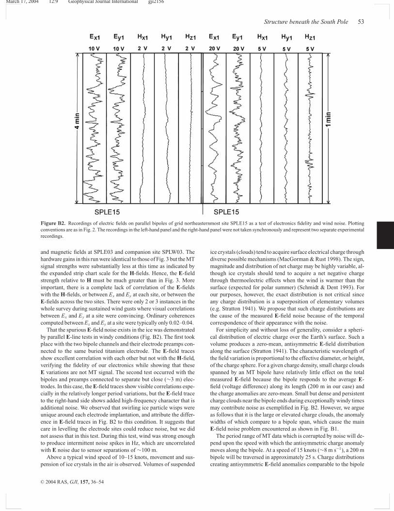
March 17, 2004 12:9 Geophysical Journal International gji2156
Structure beneath the South Pole 53
Figure B2. Recordings of electric fields on parallel bipoles of grid northeasternmost site SPLE15 as a test of electronics fidelity and wind noise. Plottingconventions are as in Fig. 2. The recordings in the left-hand panel and the right-hand panel were not taken synchronously and represent two separate experimentalrecordings.
and magnetic fields at SPLE03 and companion site SPLW03. Thehardware gains in this run were identical to those of Fig. 3 but the MTsignal strengths were substantially less at this time as indicated bythe expanded strip chart scale for the H-fields. Hence, the E-fieldstrength relative to H must be much greater than in Fig. 3. Moreimportant, there is a complete lack of correlation of the E-fieldswith the H-fields, or between Ex and Ey at each site, or between theE-fields across the two sites. There were only 2 or 3 instances in thewhole survey during sustained wind gusts where visual correlationsbetween Ex and Ey at a site were convincing. Ordinary coherencescomputed between Ex and Ey at a site were typically only 0.02–0.04.
That the spurious E-field noise exists in the ice was demonstratedby parallel E-line tests in windy conditions (Fig. B2). The first tookplace with the two bipole channels and their electrode preamps con-nected to the same buried titanium electrode. The E-field tracesshow excellent correlation with each other but not with the H-field,verifying the fidelity of our electronics while showing that theseE variations are not MT signal. The second test occurred with thebipoles and preamps connected to separate but close (∼3 m) elec-trodes. In this case, the E-field traces show visible correlations espe-cially in the relatively longer period variations, but the E-field traceto the right-hand side shows added high-frequency character that isadditional noise. We observed that swirling ice particle wisps wereunique around each electrode implantation, and attribute the differ-ence in E-field traces in Fig. B2 to this condition. It suggests thatcare in levelling the electrode sites could reduce noise, but we didnot assess that in this test. During this test, wind was strong enoughto produce intermittent noise spikes in Hz, which are uncorrelatedwith E noise due to sensor separations of ∼100 m.
Above a typical wind speed of 10–15 knots, movement and sus-pension of ice crystals in the air is observed. Volumes of suspended
ice crystals (clouds) tend to acquire surface electrical charge throughdiverse possible mechanisms (MacGorman & Rust 1998). The sign,magnitude and distribution of net charge may be highly variable, al-though ice crystals should tend to acquire a net negative chargethrough thermoelectric effects when the wind is warmer than thesurface (expected for polar summer) (Schmidt & Dent 1993). Forour purposes, however, the exact distribution is not critical sinceany charge distribution is a superposition of elementary volumes(e.g. Stratton 1941). We propose that such charge distributions arethe cause of the measured E-field noise because of the temporalcorrespondence of their appearance with the noise.
For simplicity and without loss of generality, consider a spheri-cal distribution of electric charge over the Earth’s surface. Such avolume produces a zero-mean, antisymmetric E-field distributionalong the surface (Stratton 1941). The characteristic wavelength ofthe field variation is proportional to the effective diameter, or height,of the charge sphere. For a given charge density, small charge cloudsspanned by an MT bipole have relatively little effect on the totalmeasured E-field because the bipole responds to the average E-field (voltage difference) along its length (200 m in our case) andthe charge anomalies are zero-mean. Small but dense and persistentcharge clouds near the bipole ends during exceptionally windy timesmay contribute noise as exemplified in Fig. B2. However, we argueas follows that it is the large or elevated charge clouds, the anomalywidths of which compare to a bipole span, which cause the mainE-field noise problem encountered as shown in Fig. B1.
The period range of MT data which is corrupted by noise will de-pend upon the speed with which the antisymmetric charge anomalymoves along the bipole. At a speed of 15 knots (∼8 m s−1), a 200 mbipole will be traversed in approximately 25 s. Charge distributionscreating antisymmetric E-field anomalies comparable to the bipole
C© 2004 RAS, GJI, 157, 36–54

March 17, 2004 12:9 Geophysical Journal International gji2156
54 P. E. Wannamaker et al.
length will induce positive/negative temporal swings in the mea-sured E-field over a similar period. Larger charge distributions oflonger spatial wavelength may affect longer MT data periods fora given wind speed. If E-field noise variations of all wavelengthshave equal amplitudes, MT data periods longer than a certain value(>∼10s in our case) should all be equally corrupted. Curiously, ourdata suggest that the problem diminished somewhat for T > 200–300 s, based on somewhat reduced impedance error bars, implyingthat the wind-generated noise may be somewhat band-limited spa-tially and hence in period.
This is supported by the observation that the E-field noise al-most invariably is not correlated across x- and y-bipoles of a single
site (Fig. B1), let alone across different sites. It implies that thecausative charge volumes are not coherent over large distances or,equivalently, each volume has a short time duration before disinte-grating and being replaced by another. It strongly suggests that thewind noise problem, at least for moderate wind velocities, could beovercome by substantially increasing the E-field bipole length andhence the signal/noise. Particle noise from cloud wavelengths muchgreater than the bipole should also be suppressed by the commonmode rejection of our electronics, which could in part explain dataimprovement at the longest periods. Parallel E-line tests with greatlyvarying line length could help quantify spatial wavelengths of iceparticle wind noise and its influence on MT recording.
C© 2004 RAS, GJI, 157, 36–54
Copyright © 2022 FDOKUMEN