Structural Analysis in CATIA
102
Student Notes: Generative Part Structural Analysis Expert Copyright DASSAULT SYSTEMES Copyright DASSAULT SYSTEMES Generative Part Structural Analysis Expert CATIA V5 Training Foils Version 5 Release 19 September 2008 EDU_CAT_EN_GPE_FF_V5R19
Transcript of Structural Analysis in CATIA
Student Notes:
Generative Part Structural Analysis Expert������������
Copyright DASSAULT SYSTEMES �
Cop
yrig
ht D
AS
SA
ULT
SY
STE
ME
S
Generative Part Structural Analysis Expert
CATIA V5 TrainingFoils
Version 5 Release 19September 2008
EDU_CAT_EN_GPE_FF_V5R19
Student Notes:
Generative Part Structural Analysis Expert������������
Copyright DASSAULT SYSTEMES �
Cop
yrig
ht D
AS
SA
ULT
SY
STE
ME
S
About this courseObjectives of the courseUpon completion of this course you will be able to:- Define and customize material properties- Apply pressure, acceleration and force density loads; and define virtual parts- Apply pivot, ball-joint, and user-defined restraints- Compute a frequency analysis for a single part- Create planar sections with which to visualize internal result values- Compute and refine a mesh using adaptive meshing in order to achieve a pre-defined accuracy
Targeted audienceMechanical Designers
PrerequisitesStudents attending this course should have knowledge of CATIA V5Fundamentals, Generative Part Structural Analysis Fundamentals
1 Day

Student Notes:
Generative Part Structural Analysis Expert������������
Copyright DASSAULT SYSTEMES �
Cop
yrig
ht D
AS
SA
ULT
SY
STE
ME
S
Table of Contents
GPS Extended Pre-Processing 4Advanced Pre-Processing Tools 5Frequency Analysis 41To Sum Up 51
Computation 52Computing a Frequency Solution 53Computing with Adaptivity 60Historic of Computation 63To Sum Up 66
GPS Advanced Post-Processing Tools 67Results Visualization 68Results Management 83Refinement 88To Sum Up 101

Student Notes:
Generative Part Structural Analysis Expert������������
Copyright DASSAULT SYSTEMES �
Cop
yrig
ht D
AS
SA
ULT
SY
STE
ME
S
GPS Extended Pre-ProcessingIn this lesson you will see the pre-processing tools used for advanced analysis
Advanced Pre-Processing ToolsFrequency AnalysisTo Sum Up
Student Notes:
Generative Part Structural Analysis Expert������������
Copyright DASSAULT SYSTEMES �
Cop
yrig
ht D
AS
SA
ULT
SY
STE
ME
S
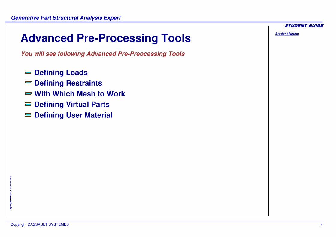
Advanced Pre-Processing ToolsYou will see following Advanced Pre-Preocessing Tools
Defining LoadsDefining RestraintsWith Which Mesh to WorkDefining Virtual PartsDefining User Material

Student Notes:
Generative Part Structural Analysis Expert������������
Copyright DASSAULT SYSTEMES �
Cop
yrig
ht D
AS
SA
ULT
SY
STE
ME
S
Defining LoadsYou will see different types of loads
AccelerationPressure LoadsForce Density
Student Notes:
Generative Part Structural Analysis Expert������������
Copyright DASSAULT SYSTEMES �
Cop
yrig
ht D
AS
SA
ULT
SY
STE
ME
S
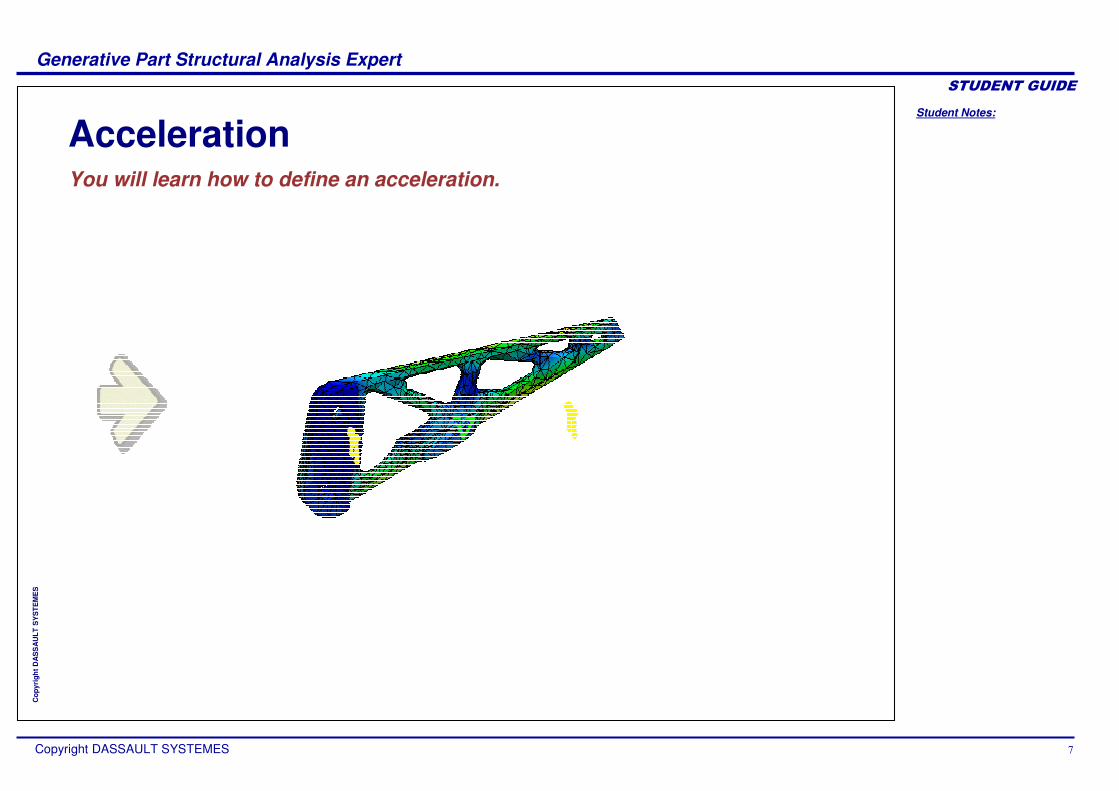
AccelerationYou will learn how to define an acceleration.
Student Notes:
Generative Part Structural Analysis Expert������������
Copyright DASSAULT SYSTEMES �
Cop
yrig
ht D
AS
SA
ULT
SY
STE
ME
S
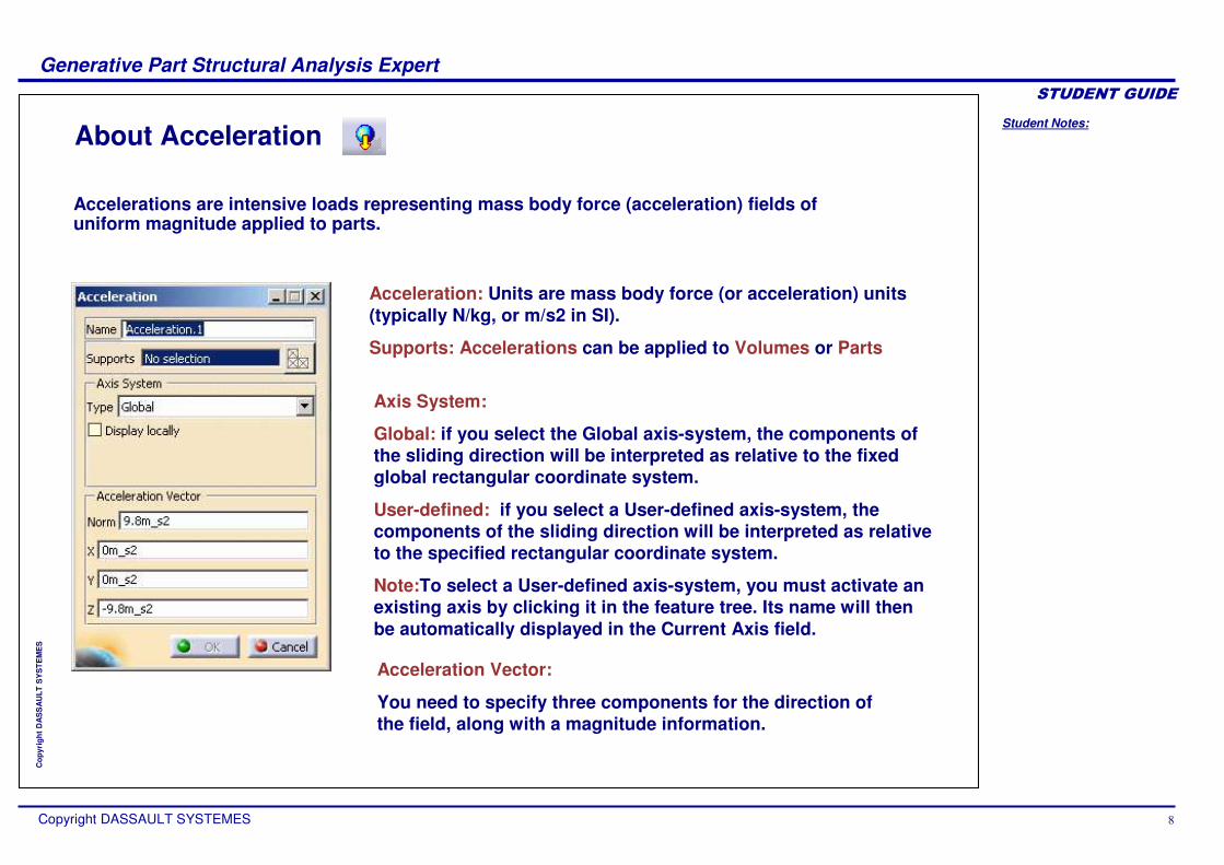
About Acceleration
Accelerations are intensive loads representing mass body force (acceleration) fields of uniform magnitude applied to parts.
Acceleration: Units are mass body force (or acceleration) units (typically N/kg, or m/s2 in SI).
Supports: Accelerations can be applied to Volumes or Parts
Acceleration Vector:
You need to specify three components for the direction of the field, along with a magnitude information.
Axis System:
Global: if you select the Global axis-system, the components of the sliding direction will be interpreted as relative to the fixed global rectangular coordinate system.
User-defined: if you select a User-defined axis-system, the components of the sliding direction will be interpreted as relative to the specified rectangular coordinate system.
Note:To select a User-defined axis-system, you must activate an existing axis by clicking it in the feature tree. Its name will then be automatically displayed in the Current Axis field.
Student Notes:
Generative Part Structural Analysis Expert������������
Copyright DASSAULT SYSTEMES
Cop
yrig
ht D
AS
SA
ULT
SY
STE
ME
S
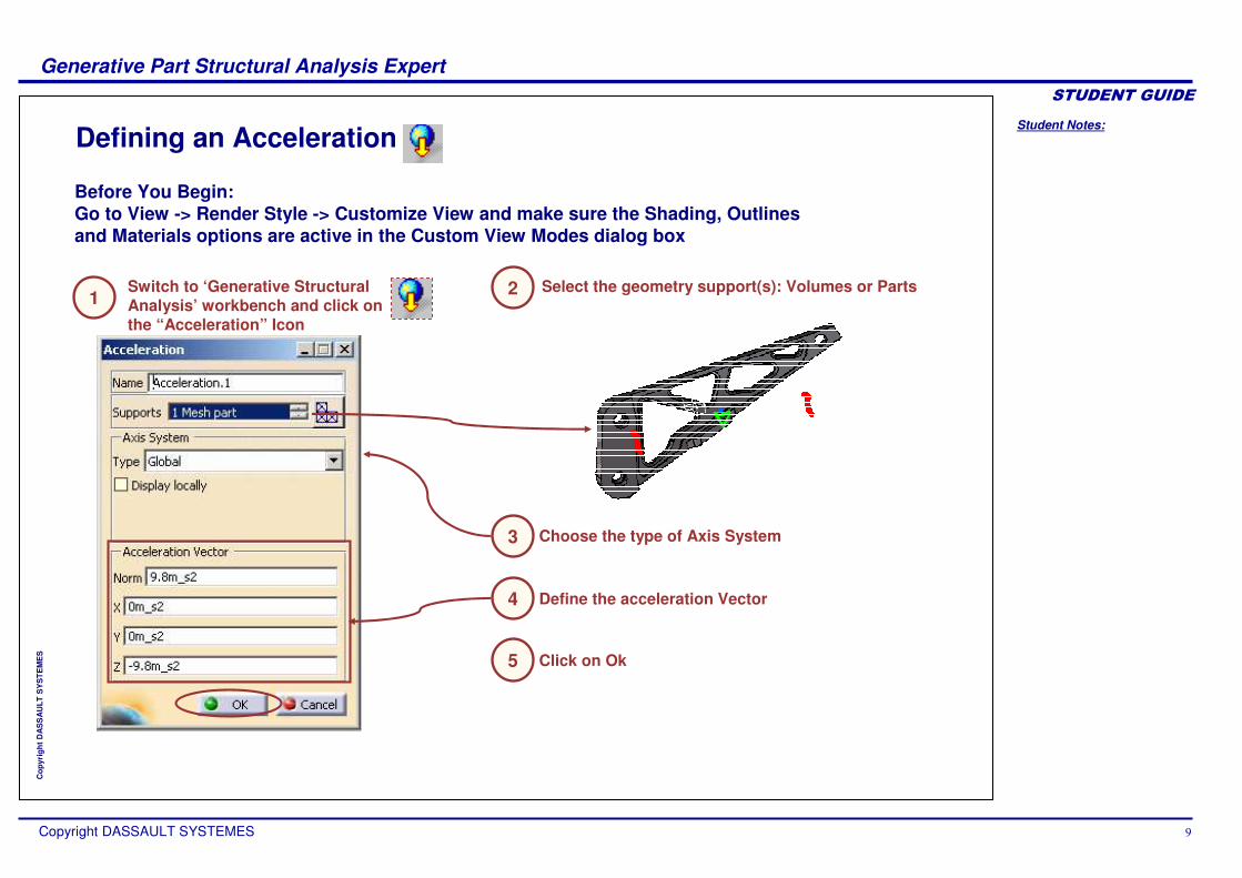
Defining an Acceleration
Select the geometry support(s): Volumes or Parts2Switch to ‘Generative Structural Analysis’ workbench and click on the “Acceleration” Icon
1
3 Choose the type of Axis System
Before You Begin:Go to View -> Render Style -> Customize View and make sure the Shading, Outlines and Materials options are active in the Custom View Modes dialog box
4 Define the acceleration Vector
5 Click on Ok

Student Notes:
Generative Part Structural Analysis Expert������������
Copyright DASSAULT SYSTEMES �
Cop
yrig
ht D
AS
SA
ULT
SY
STE
ME
S
About Rotation force
Rotation Forces are intensive loads representing mass body force (acceleration) fields induced by rotational motion applied to parts.
Rotation Force: Units are angular velocity and angular acceleration units (typically rad/sec and rad/sec2 in SI).
Supports: Accelerations can be applied on Volumes or Parts
Rotation Axis: The user specifies a rotation axis and values for the angular velocity and angular acceleration magnitudes, and the program automatically evaluates the linearly varying acceleration field distribution.
Student Notes:
Generative Part Structural Analysis Expert������������
Copyright DASSAULT SYSTEMES ��
Cop
yrig
ht D
AS
SA
ULT
SY
STE
ME
S
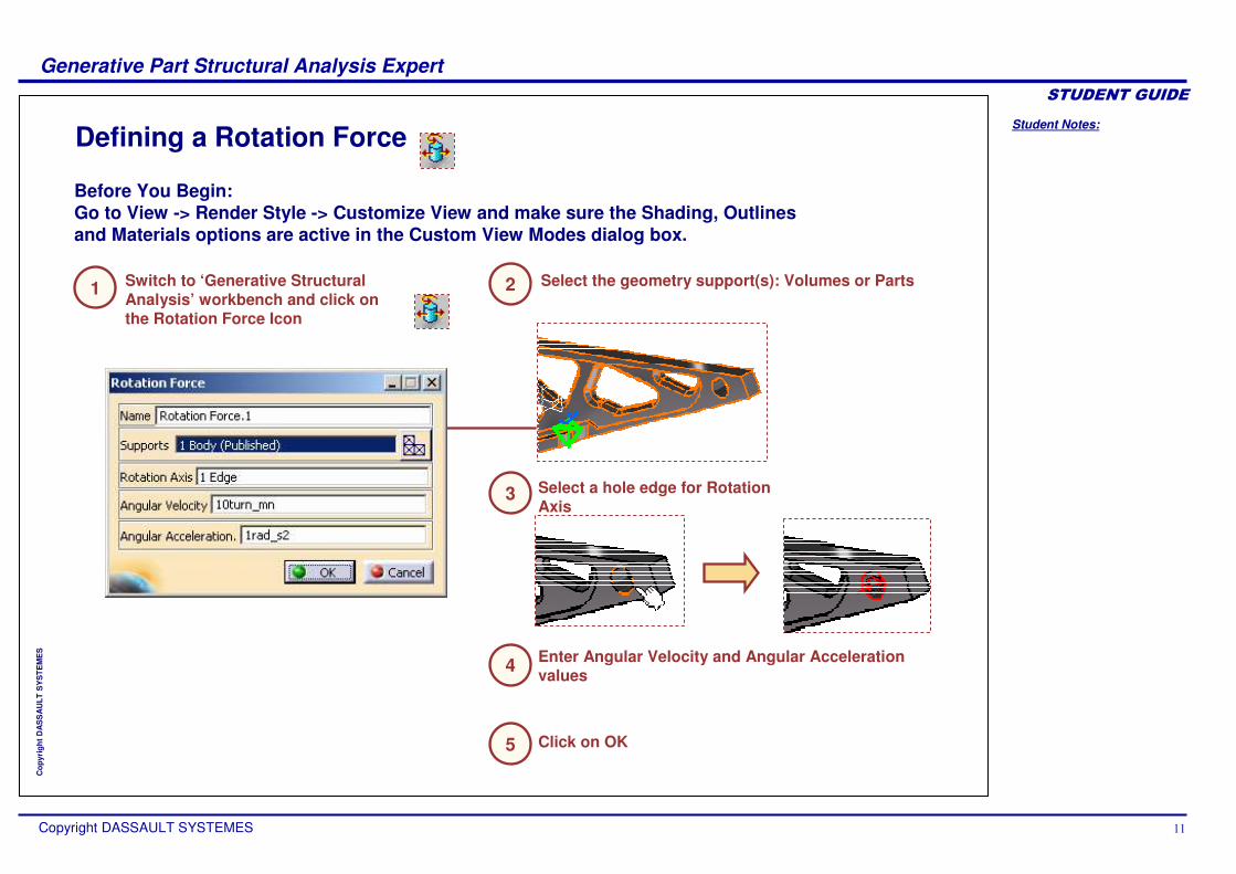
Defining a Rotation Force
Select the geometry support(s): Volumes or PartsSwitch to ‘Generative Structural Analysis’ workbench and click on the Rotation Force Icon
Select a hole edge for Rotation Axis
Before You Begin:Go to View -> Render Style -> Customize View and make sure the Shading, Outlines and Materials options are active in the Custom View Modes dialog box.
Enter Angular Velocity and Angular Acceleration values
Click on OK
21
3
4
5

Student Notes:
Generative Part Structural Analysis Expert������������
Copyright DASSAULT SYSTEMES ��
Cop
yrig
ht D
AS
SA
ULT
SY
STE
ME
S
Pressure LoadsYou will learn how to apply a pressure.
Student Notes:
Generative Part Structural Analysis Expert������������
Copyright DASSAULT SYSTEMES ��
Cop
yrig
ht D
AS
SA
ULT
SY
STE
ME
S
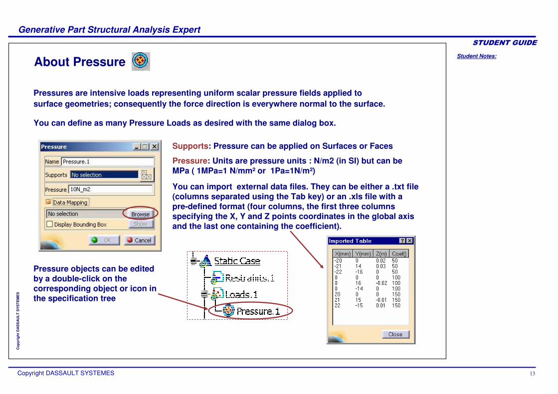
About Pressure
Pressures are intensive loads representing uniform scalar pressure fields applied to surface geometries; consequently the force direction is everywhere normal to the surface.
Supports: Pressure can be applied on Surfaces or Faces
Pressure: Units are pressure units : N/m2 (in SI) but can be MPa ( 1MPa=1 N/mm² or 1Pa=1N/m²)
You can import external data files. They can be either a .txt file (columns separated using the Tab key) or an .xls file with a pre-defined format (four columns, the first three columns specifying the X, Y and Z points coordinates in the global axis and the last one containing the coefficient).
You can define as many Pressure Loads as desired with the same dialog box.
Pressure objects can be edited by a double-click on the corresponding object or icon in the specification tree
Student Notes:
Generative Part Structural Analysis Expert������������
Copyright DASSAULT SYSTEMES ��
Cop
yrig
ht D
AS
SA
ULT
SY
STE
ME
S
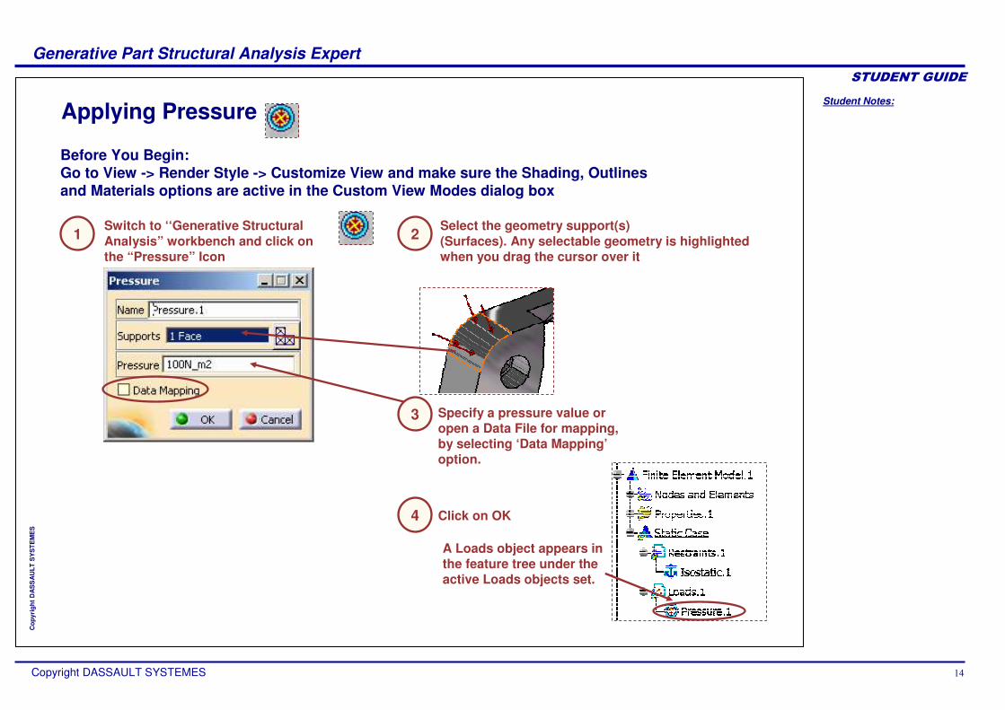
Applying Pressure
Select the geometry support(s)(Surfaces). Any selectable geometry is highlighted when you drag the cursor over it
Switch to ‘‘Generative Structural Analysis” workbench and click on the “Pressure” Icon
Click on OK
Specify a pressure value or open a Data File for mapping, by selecting ‘Data Mapping’option.
A Loads object appears in the feature tree under the active Loads objects set.
Before You Begin:Go to View -> Render Style -> Customize View and make sure the Shading, Outlines and Materials options are active in the Custom View Modes dialog box
21
3
4
Student Notes:
Generative Part Structural Analysis Expert������������
Copyright DASSAULT SYSTEMES ��
Cop
yrig
ht D
AS
SA
ULT
SY
STE
ME
S
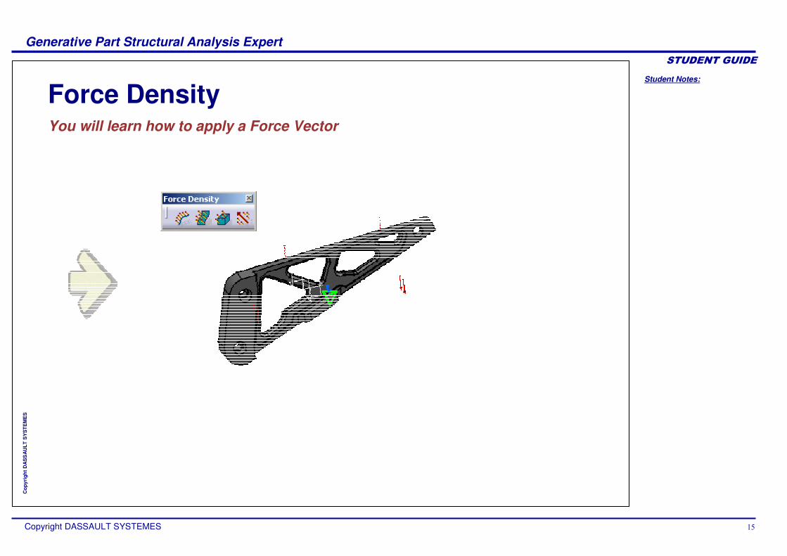
Force DensityYou will learn how to apply a Force Vector
Student Notes:
Generative Part Structural Analysis Expert������������
Copyright DASSAULT SYSTEMES ��
Cop
yrig
ht D
AS
SA
ULT
SY
STE
ME
S
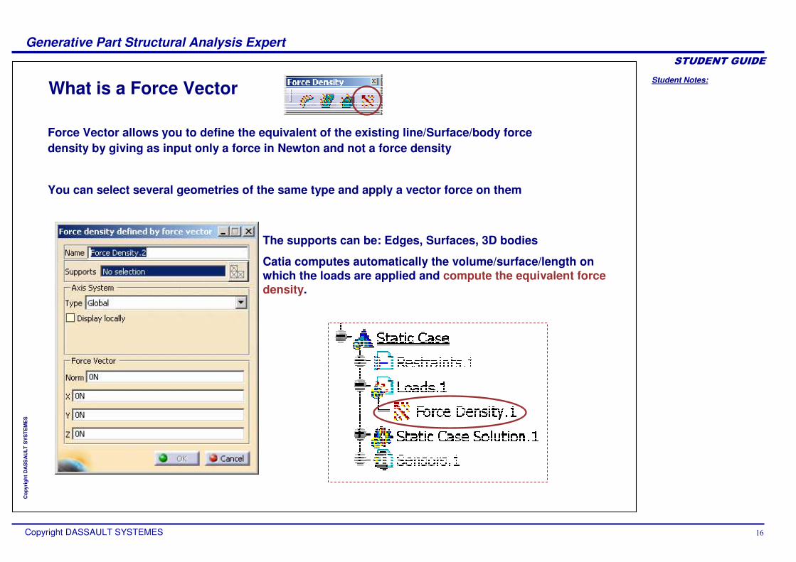
What is a Force Vector
Force Vector allows you to define the equivalent of the existing line/Surface/body force density by giving as input only a force in Newton and not a force density
You can select several geometries of the same type and apply a vector force on them
The supports can be: Edges, Surfaces, 3D bodies
Catia computes automatically the volume/surface/length on which the loads are applied and compute the equivalent force density.
Student Notes:
Generative Part Structural Analysis Expert������������
Copyright DASSAULT SYSTEMES ��
Cop
yrig
ht D
AS
SA
ULT
SY
STE
ME
S
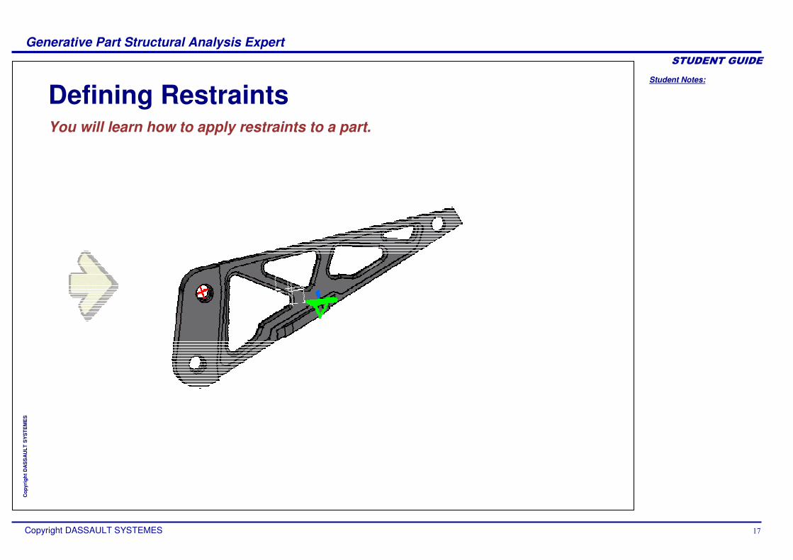
Defining RestraintsYou will learn how to apply restraints to a part.

Student Notes:
Generative Part Structural Analysis Expert������������
Copyright DASSAULT SYSTEMES ��
Cop
yrig
ht D
AS
SA
ULT
SY
STE
ME
S
Work with the Geometry: A faster way to apply restraints/loads
Introduction
The restraints and the loads will be applied directly onto the geometry (surfaces, lines, points, groups) as shown on the example below:
This restraint is applied onto the yellow surface
This restraint is applied onto the circle
Then the computation will automatically apply the restraints/loads to the mesh.
Even if you work with the geometry, the part must be meshed to take into account the restraints/Loads.
Student Notes:
Generative Part Structural Analysis Expert������������
Copyright DASSAULT SYSTEMES �
Cop
yrig
ht D
AS
SA
ULT
SY
STE
ME
S
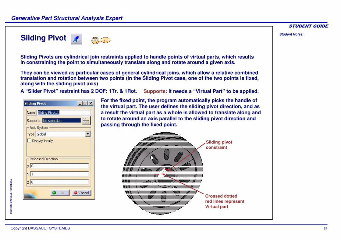
Sliding Pivot
A “Slider Pivot” restraint has 2 DOF: 1Tr. & 1Rot.
Sliding Pivots are cylindrical join restraints applied to handle points of virtual parts, which results in constraining the point to simultaneously translate along and rotate around a given axis.
They can be viewed as particular cases of general cylindrical joins, which allow a relative combined translation and rotation between two points (in the Sliding Pivot case, one of the two points is fixed, along with the sliding pivot axis)
For the fixed point, the program automatically picks the handle of the virtual part. The user defines the sliding pivot direction, and as a result the virtual part as a whole is allowed to translate along and to rotate around an axis parallel to the sliding pivot direction and passing through the fixed point.
Supports: It needs a “Virtual Part” to be applied.
Crossed dotted red lines represent Virtual part
Sliding pivot constraint
Student Notes:
Generative Part Structural Analysis Expert������������
Copyright DASSAULT SYSTEMES �
Cop
yrig
ht D
AS
SA
ULT
SY
STE
ME
S
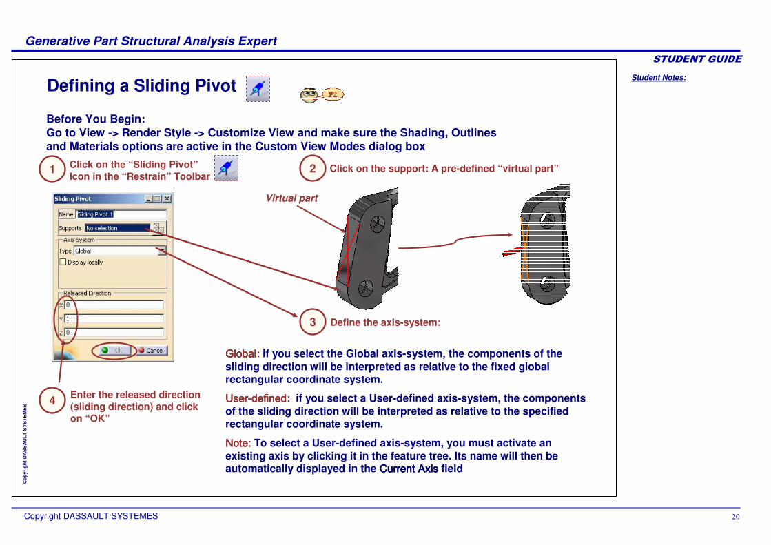
Defining a Sliding Pivot
Click on the support: A pre-defined “virtual part”
Virtual part
Click on the “Sliding Pivot”Icon in the “Restrain” Toolbar
Enter the released direction (sliding direction) and click on “OK”
Define the axis-system:
: if you select the Global axis-system, the components of the sliding direction will be interpreted as relative to the fixed global rectangular coordinate system.
: if you select a User-defined axis-system, the components of the sliding direction will be interpreted as relative to the specified rectangular coordinate system.
To select a User-defined axis-system, you must activate an existing axis by clicking it in the feature tree. Its name will then be automatically displayed in the field
Before You Begin:Go to View -> Render Style -> Customize View and make sure the Shading, Outlines and Materials options are active in the Custom View Modes dialog box
21
3
4
Student Notes:
Generative Part Structural Analysis Expert������������
Copyright DASSAULT SYSTEMES ��
Cop
yrig
ht D
AS
SA
ULT
SY
STE
ME
S
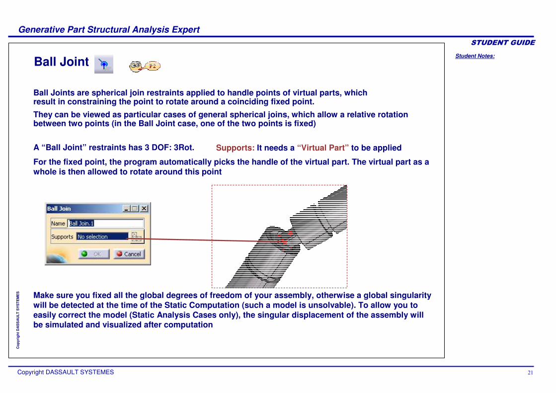
Ball Joint
A “Ball Joint” restraints has 3 DOF: 3Rot.
Ball Joints are spherical join restraints applied to handle points of virtual parts, which result in constraining the point to rotate around a coinciding fixed point.
They can be viewed as particular cases of general spherical joins, which allow a relative rotation between two points (in the Ball Joint case, one of the two points is fixed)
Make sure you fixed all the global degrees of freedom of your assembly, otherwise a global singularity will be detected at the time of the Static Computation (such a model is unsolvable). To allow you to easily correct the model (Static Analysis Cases only), the singular displacement of the assembly will be simulated and visualized after computation
For the fixed point, the program automatically picks the handle of the virtual part. The virtual part as a whole is then allowed to rotate around this point
Supports: It needs a “Virtual Part” to be applied
Student Notes:
Generative Part Structural Analysis Expert������������
Copyright DASSAULT SYSTEMES ��
Cop
yrig
ht D
AS
SA
ULT
SY
STE
ME
S
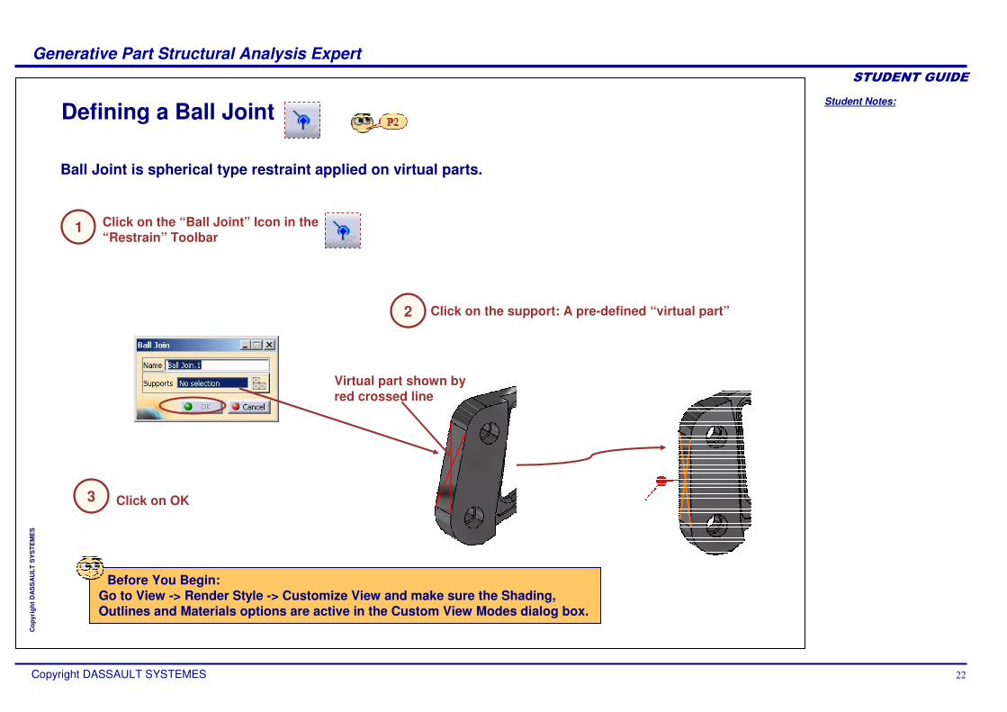
Defining a Ball Joint
Click on the support: A pre-defined “virtual part”
Virtual part shown by red crossed line
Click on the “Ball Joint” Icon in the “Restrain” Toolbar
Ball Joint is spherical type restraint applied on virtual parts.
Click on OK
2
1
3
Before You Begin:Go to View -> Render Style -> Customize View and make sure the Shading, Outlines and Materials options are active in the Custom View Modes dialog box.
Student Notes:
Generative Part Structural Analysis Expert������������
Copyright DASSAULT SYSTEMES ��
Cop
yrig
ht D
AS
SA
ULT
SY
STE
ME
S
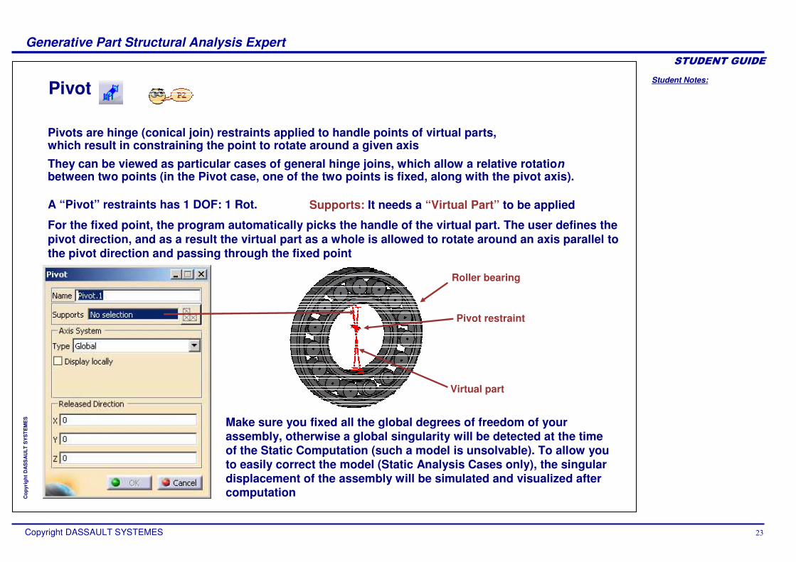
Pivot
A “Pivot” restraints has 1 DOF: 1 Rot.
Pivots are hinge (conical join) restraints applied to handle points of virtual parts, which result in constraining the point to rotate around a given axis
They can be viewed as particular cases of general hinge joins, which allow a relative rotation between two points (in the Pivot case, one of the two points is fixed, along with the pivot axis).
Make sure you fixed all the global degrees of freedom of your assembly, otherwise a global singularity will be detected at the time of the Static Computation (such a model is unsolvable). To allow you to easily correct the model (Static Analysis Cases only), the singular displacement of the assembly will be simulated and visualized after computation
For the fixed point, the program automatically picks the handle of the virtual part. The user defines the pivot direction, and as a result the virtual part as a whole is allowed to rotate around an axis parallel to the pivot direction and passing through the fixed point
Supports: It needs a “Virtual Part” to be applied
Roller bearing
Virtual part
Pivot restraint
Student Notes:
Generative Part Structural Analysis Expert������������
Copyright DASSAULT SYSTEMES ��
Cop
yrig
ht D
AS
SA
ULT
SY
STE
ME
S
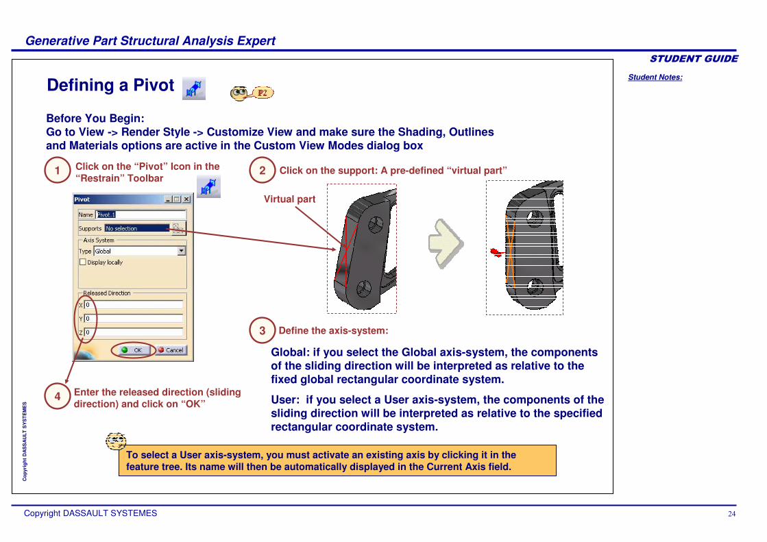
Defining a Pivot
Click on the support: A pre-defined “virtual part”
Virtual part
Click on the “Pivot” Icon in the “Restrain” Toolbar
Enter the released direction (sliding direction) and click on “OK”
Define the axis-system:
Global: if you select the Global axis-system, the components of the sliding direction will be interpreted as relative to the fixed global rectangular coordinate system.
User: if you select a User axis-system, the components of the sliding direction will be interpreted as relative to the specified rectangular coordinate system.
Before You Begin:Go to View -> Render Style -> Customize View and make sure the Shading, Outlines and Materials options are active in the Custom View Modes dialog box
To select a User axis-system, you must activate an existing axis by clicking it in thefeature tree. Its name will then be automatically displayed in the Current Axis field.
21
4
3

Student Notes:
Generative Part Structural Analysis Expert������������
Copyright DASSAULT SYSTEMES ��
Cop
yrig
ht D
AS
SA
ULT
SY
STE
ME
S
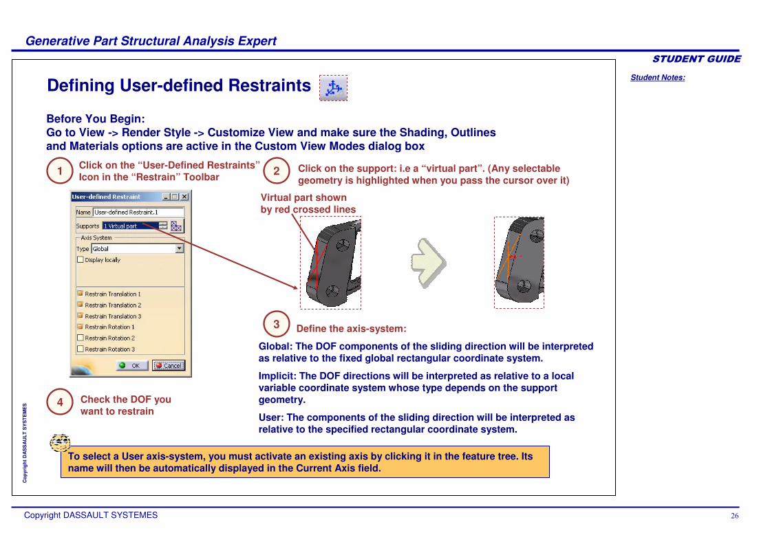
User-defined Restraints
Make sure you fixed all the global degrees of freedom of your assembly, otherwise a global singularity will be detected at thetime of the Static Computation (such a model is unsolvable). To allow you to easily correct the model (Static Analysis Cases only), the singular displacement of the assembly will be simulated and visualized after computation
Supports: Points or Vertex, Curves or Edges, Faces or Surfaces,Virtual Parts, groups
User-defined Restraints are generic restraints allowing you to fix any combination of available nodal DOF on arbitrary geometries. 3Tr. freedom per node for continuum element meshes, and 3Tr. and 3Rot. of freedom per node for structural element meshes
means no translation degree of freedom in that direction
means no rotation degree of freedom in the direction
Impeller section
Student Notes:
Generative Part Structural Analysis Expert������������
Copyright DASSAULT SYSTEMES ��
Cop
yrig
ht D
AS
SA
ULT
SY
STE
ME
S
Defining User-defined Restraints
Click on the support: i.e a “virtual part”. (Any selectable geometry is highlighted when you pass the cursor over it)
Virtual part shown by red crossed lines
Click on the “User-Defined Restraints”Icon in the “Restrain” Toolbar
Check the DOF you want to restrain
Define the axis-system:
Global: The DOF components of the sliding direction will be interpreted as relative to the fixed global rectangular coordinate system.
Implicit: The DOF directions will be interpreted as relative to a local variable coordinate system whose type depends on the support geometry.
User: The components of the sliding direction will be interpreted as relative to the specified rectangular coordinate system.
Before You Begin:Go to View -> Render Style -> Customize View and make sure the Shading, Outlines and Materials options are active in the Custom View Modes dialog box
To select a User axis-system, you must activate an existing axis by clicking it in the feature tree. Its name will then be automatically displayed in the Current Axis field.
21
4
3

Student Notes:
Generative Part Structural Analysis Expert������������
Copyright DASSAULT SYSTEMES ��
Cop
yrig
ht D
AS
SA
ULT
SY
STE
ME
S
You will learn how to define mesh part filter trough preprocessing tools
With Which Mesh to Work
Student Notes:
Generative Part Structural Analysis Expert������������
Copyright DASSAULT SYSTEMES ��
Cop
yrig
ht D
AS
SA
ULT
SY
STE
ME
S
What is a ‘Mesh Part’ Filter
This tool is available on every pre-processing tool.
This “Mesh Part” filter allows you to select the mesh parts on which you want to apply the preprocessing feature.
The default is « All », that means all the mesh parts will be taken into account. It means, If you add a new mesh part on the support, the preprocessing feature will be automatically applied on the new mesh part.
On the other hand, If you select one or many mesh parts, this will not change if you define a new mesh part on the support.
Student Notes:
Generative Part Structural Analysis Expert������������
Copyright DASSAULT SYSTEMES �
Cop
yrig
ht D
AS
SA
ULT
SY
STE
ME
S
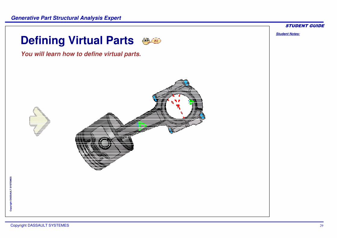
Defining Virtual PartsYou will learn how to define virtual parts.

Student Notes:
Generative Part Structural Analysis Expert������������
Copyright DASSAULT SYSTEMES �
Cop
yrig
ht D
AS
SA
ULT
SY
STE
ME
S
Introduction to Virtual Parts
Virtual Parts are used to transmit actions at a distance. Therefore they can be thought of as rigid bodies, except for the case where a lumped flexibility is explicitly introduced by the means of a spring element.
There are 6 kinds of Virtual Parts:
Virtual Parts are structures created without a geometric support. They represent bodies for which no geometric model is available, but which play a role in the structural analysis of single parts or assembly systems.
Rigid Virtual partsThey stiffly transmit their actions : they locally stiffen the deformable body
Smooth Virtual partsThey softly transmit their actions : they don’t stiffen the deformable body
Contact Virtual partsThey softly transmit their actions while preventing from body inter-penetration
Rigid Spring Virtual partsThey stiffly transmit their actions and behave like a 6 DOF spring
Smooth Spring Virtual partsThey softly transmit their actions and behave like a 6 DOF spring
Periodicity Conditions
Student Notes:
Generative Part Structural Analysis Expert������������
Copyright DASSAULT SYSTEMES ��
Cop
yrig
ht D
AS
SA
ULT
SY
STE
ME
S
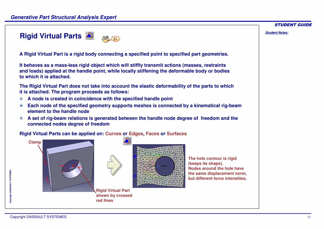
Rigid Virtual Parts
A Rigid Virtual Part is a rigid body connecting a specified point to specified part geometries.
It behaves as a mass-less rigid object which will stiffly transmit actions (masses, restraints and loads) applied at the handle point, while locally stiffening the deformable body or bodies to which it is attached.
A node is created in coincidence with the specified handle pointEach node of the specified geometry supports meshes is connected by a kinematical rig-beam element to the handle nodeA set of rig-beam relations is generated between the handle node degree of freedom and the connected nodes degree of freedom
Rigid Virtual Parts can be applied on: Curves or Edges, Faces or Surfaces
FThe hole contour is rigid (keeps its shape).Nodes around the hole have the same displacement norm, but different force intensities.
Rigid Virtual Part shown by crossed red lines
Clamp
The Rigid Virtual Part does not take into account the elastic deformability of the parts to which it is attached. The program proceeds as follows:
Student Notes:
Generative Part Structural Analysis Expert������������
Copyright DASSAULT SYSTEMES ��
Cop
yrig
ht D
AS
SA
ULT
SY
STE
ME
S
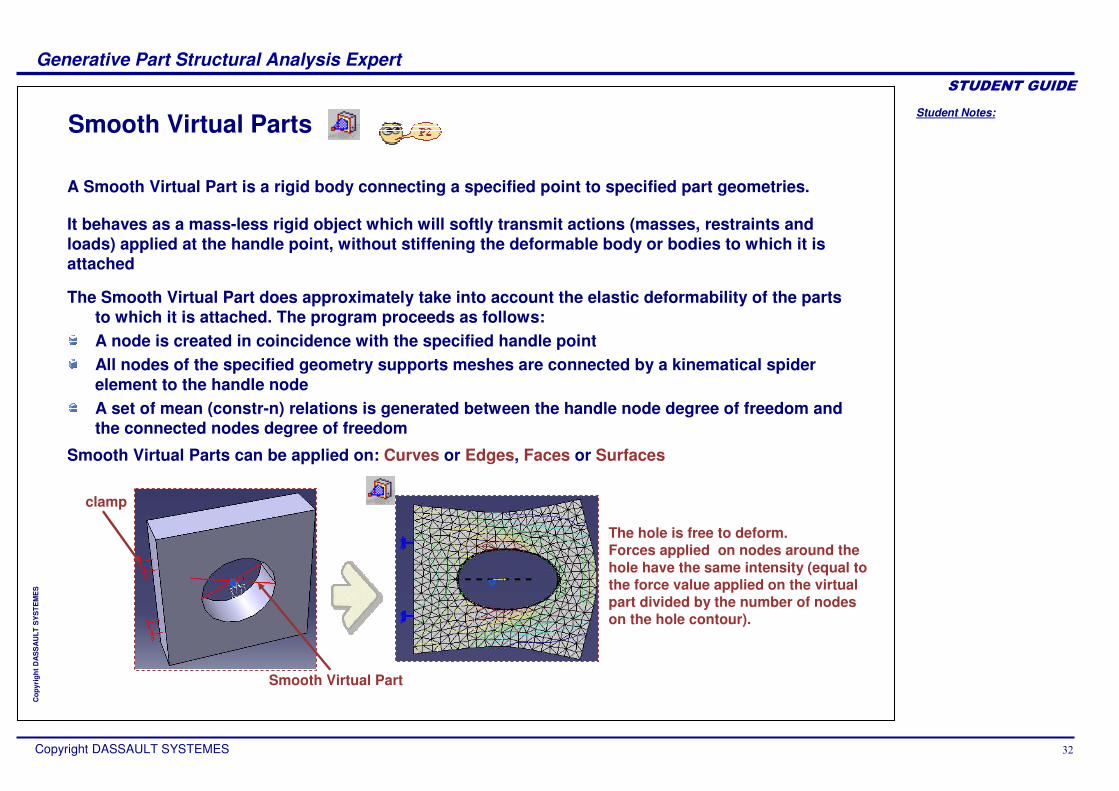
Smooth Virtual Parts
It behaves as a mass-less rigid object which will softly transmit actions (masses, restraints and loads) applied at the handle point, without stiffening the deformable body or bodies to which it is attached
The Smooth Virtual Part does approximately take into account the elastic deformability of the parts to which it is attached. The program proceeds as follows:A node is created in coincidence with the specified handle pointAll nodes of the specified geometry supports meshes are connected by a kinematical spider element to the handle nodeA set of mean (constr-n) relations is generated between the handle node degree of freedom and the connected nodes degree of freedom
Smooth Virtual Parts can be applied on: Curves or Edges, Faces or Surfaces
A Smooth Virtual Part is a rigid body connecting a specified point to specified part geometries.
The hole is free to deform.Forces applied on nodes around the hole have the same intensity (equal to the force value applied on the virtual part divided by the number of nodes on the hole contour).
Smooth Virtual Part
clamp
Student Notes:
Generative Part Structural Analysis Expert������������
Copyright DASSAULT SYSTEMES ��
Cop
yrig
ht D
AS
SA
ULT
SY
STE
ME
S
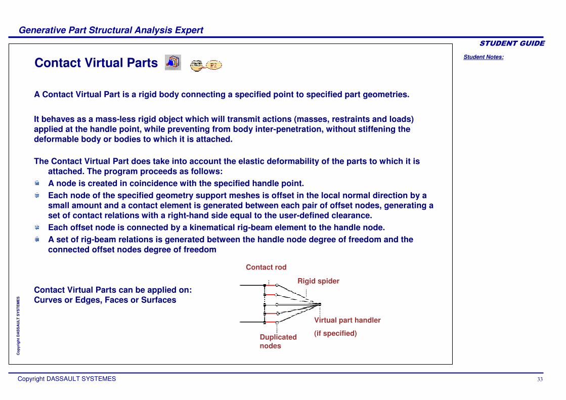
Contact Virtual Parts
A Contact Virtual Part is a rigid body connecting a specified point to specified part geometries.
It behaves as a mass-less rigid object which will transmit actions (masses, restraints and loads) applied at the handle point, while preventing from body inter-penetration, without stiffening the deformable body or bodies to which it is attached.
The Contact Virtual Part does take into account the elastic deformability of the parts to which it is attached. The program proceeds as follows:A node is created in coincidence with the specified handle point.Each node of the specified geometry support meshes is offset in the local normal direction by a small amount and a contact element is generated between each pair of offset nodes, generating a set of contact relations with a right-hand side equal to the user-defined clearance.Each offset node is connected by a kinematical rig-beam element to the handle node.A set of rig-beam relations is generated between the handle node degree of freedom and the connected offset nodes degree of freedom
Virtual part handler
(if specified)Duplicated nodes
Contact rod
Rigid spiderContact Virtual Parts can be applied on:Curves or Edges, Faces or Surfaces
Student Notes:
Generative Part Structural Analysis Expert������������
Copyright DASSAULT SYSTEMES ��
Cop
yrig
ht D
AS
SA
ULT
SY
STE
ME
S
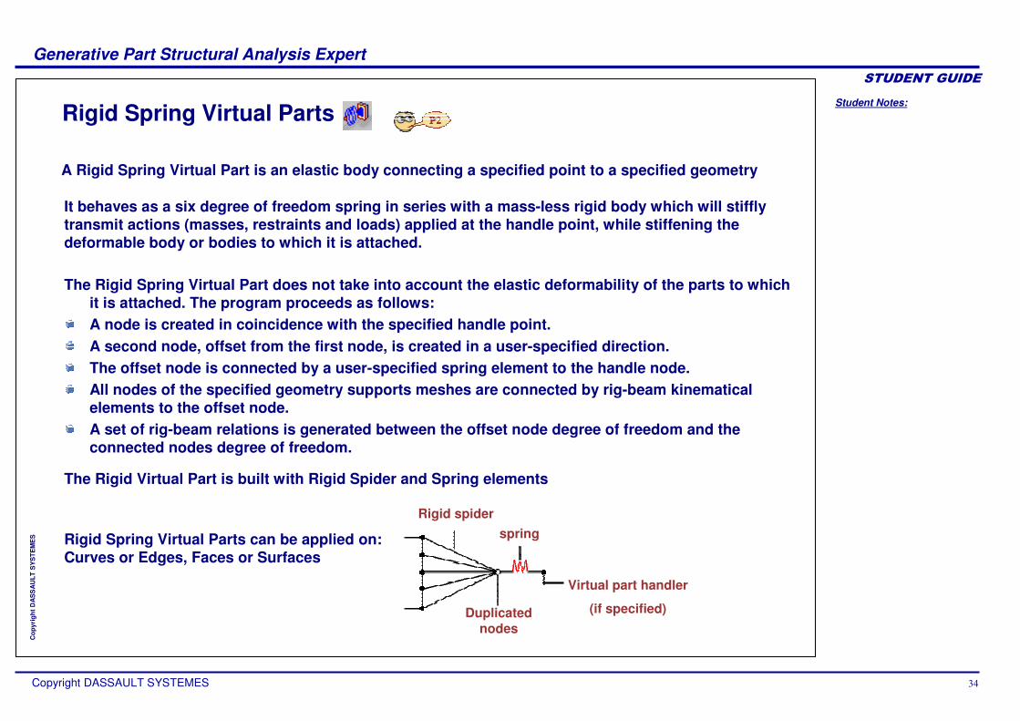
Rigid Spring Virtual Parts
A Rigid Spring Virtual Part is an elastic body connecting a specified point to a specified geometry
It behaves as a six degree of freedom spring in series with a mass-less rigid body which will stiffly transmit actions (masses, restraints and loads) applied at the handle point, while stiffening the deformable body or bodies to which it is attached.
The Rigid Spring Virtual Part does not take into account the elastic deformability of the parts to which it is attached. The program proceeds as follows:A node is created in coincidence with the specified handle point.A second node, offset from the first node, is created in a user-specified direction.The offset node is connected by a user-specified spring element to the handle node.All nodes of the specified geometry supports meshes are connected by rig-beam kinematical elements to the offset node.A set of rig-beam relations is generated between the offset node degree of freedom and the connected nodes degree of freedom.
The Rigid Virtual Part is built with Rigid Spider and Spring elements
Rigid Spring Virtual Parts can be applied on:Curves or Edges, Faces or Surfaces
Virtual part handler
(if specified)
Rigid spiderspring
Duplicated nodes

Student Notes:
Generative Part Structural Analysis Expert������������
Copyright DASSAULT SYSTEMES ��
Cop
yrig
ht D
AS
SA
ULT
SY
STE
ME
S
Smooth Spring Virtual Parts
A Smooth Spring Virtual Part is an elastic body connecting a specified point to a specified geometry.
It behaves as a 6-degree of freedom spring in series with a mass-less rigid body which will softly transmit actions (masses, restraints and loads) applied at the handle point, without stiffening the deformable body or bodies to which it is attached.
The Smooth Spring Virtual Part does approximately take into account the elastic deformability of the parts to which it is attached. The program proceeds as follows:A node is created in coincidence with the specified handle point.A second node, offset from the first node, is created in a user-specified direction.The offset node is connected by a user-specified spring element to the handle node.All nodes of the specified geometry supports meshes are connected by a kinematical spider element to the offset node.A set of mean ( ) relations is generated between the offset node degree of freedom and the connected nodes degree of freedom.
The Smooth spring Virtual Part is built with Smooth Spider and Spring elements
Rigid Spring Virtual Parts can be applied on:Curves or Edges, Faces or Surfaces Virtual part handler
(if specified)
Smooth spiderspring
Duplicated nodes

Student Notes:
Generative Part Structural Analysis Expert������������
Copyright DASSAULT SYSTEMES ��
Cop
yrig
ht D
AS
SA
ULT
SY
STE
ME
S
To use periodicity conditions, you need to make sure the geometry as well as the created restraints and loads are periodic. The geometry also needs to be regular at the place the section is cut, discontinuity is not allowed.
Periodicity Conditions
Periodicity conditions enable you to perform an analysis on the solid section of a periodic part.
This solid section should represent a cyclic period of the entire part. Applying periodicity conditions is cost saving: you compute only a section of the part and get a result that is representative of the whole part.
There are 2 kinds of periodicity conditions:
Cyclic symmetry: of the geometry as well as both restraints and loads
A Regular symmetry:of the sectioned geometry as well as both restraints and loads
Student Notes:
Generative Part Structural Analysis Expert������������
Copyright DASSAULT SYSTEMES ��
Cop
yrig
ht D
AS
SA
ULT
SY
STE
ME
S
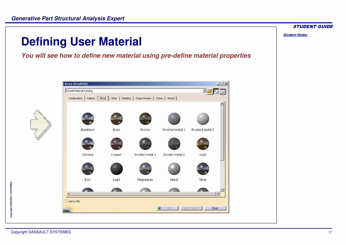
Defining User MaterialYou will see how to define new material using pre-define material properties

Student Notes:
Generative Part Structural Analysis Expert������������
Copyright DASSAULT SYSTEMES ��
Cop
yrig
ht D
AS
SA
ULT
SY
STE
ME
S
About User Material Tool
The User Material tool allows you to define a new material inside the material set in Generative Structural Analysis. You can apply material properties on your parts/productspre-defined materials or straight on a mesh ( coming from I.e “advanced Meshing Tools”workbench)
A “User Material” object appears in the tree. You can edit this object and customize its material analysis properties according to your needs
Student Notes:
Generative Part Structural Analysis Expert������������
Copyright DASSAULT SYSTEMES �
Cop
yrig
ht D
AS
SA
ULT
SY
STE
ME
S
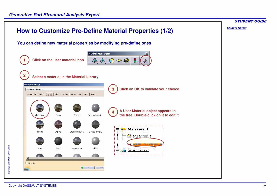
You can define new material properties by modifying pre-define ones
Click on the user material Icon
Select a material in the Material Library
How to Customize Pre-Define Material Properties (1/2)
Click on OK to validate your choice
A User Material object appears in the tree. Double-click on it to edit it
2
1
4
3
Student Notes:
Generative Part Structural Analysis Expert������������
Copyright DASSAULT SYSTEMES �
Cop
yrig
ht D
AS
SA
ULT
SY
STE
ME
S
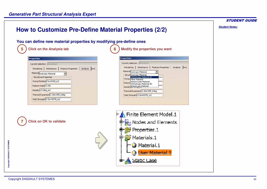
Click on the Analysis tab Modify the properties you want
How to Customize Pre-Define Material Properties (2/2)
Click on OK to validate
You can define new material properties by modifying pre-define ones
5 6
7
Student Notes:
Generative Part Structural Analysis Expert������������
Copyright DASSAULT SYSTEMES ��
Cop
yrig
ht D
AS
SA
ULT
SY
STE
ME
S
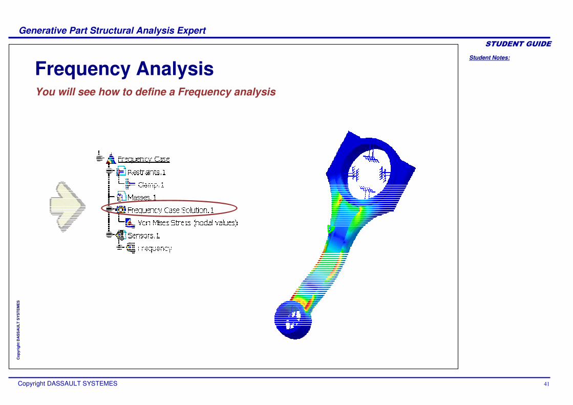
Frequency Analysis You will see how to define a Frequency analysis
Student Notes:
Generative Part Structural Analysis Expert������������
Copyright DASSAULT SYSTEMES ��
Cop
yrig
ht D
AS
SA
ULT
SY
STE
ME
S
Why Frequency Analysis (1/2)
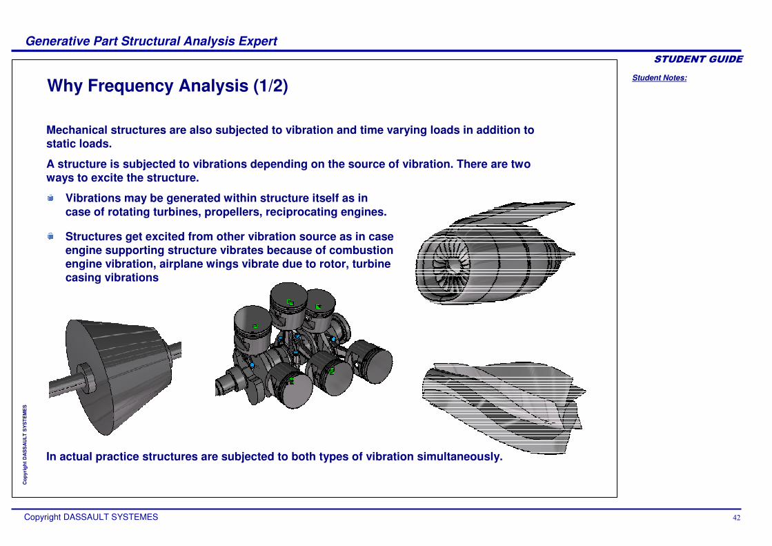
Structures get excited from other vibration source as in case engine supporting structure vibrates because of combustion engine vibration, airplane wings vibrate due to rotor, turbine casing vibrations
Mechanical structures are also subjected to vibration and time varying loads in addition to static loads.
Vibrations may be generated within structure itself as in case of rotating turbines, propellers, reciprocating engines.
In actual practice structures are subjected to both types of vibration simultaneously.
A structure is subjected to vibrations depending on the source of vibration. There are two ways to excite the structure.
Student Notes:
Generative Part Structural Analysis Expert������������
Copyright DASSAULT SYSTEMES ��
Cop
yrig
ht D
AS
SA
ULT
SY
STE
ME
S
Why Frequency Analysis (2/2)
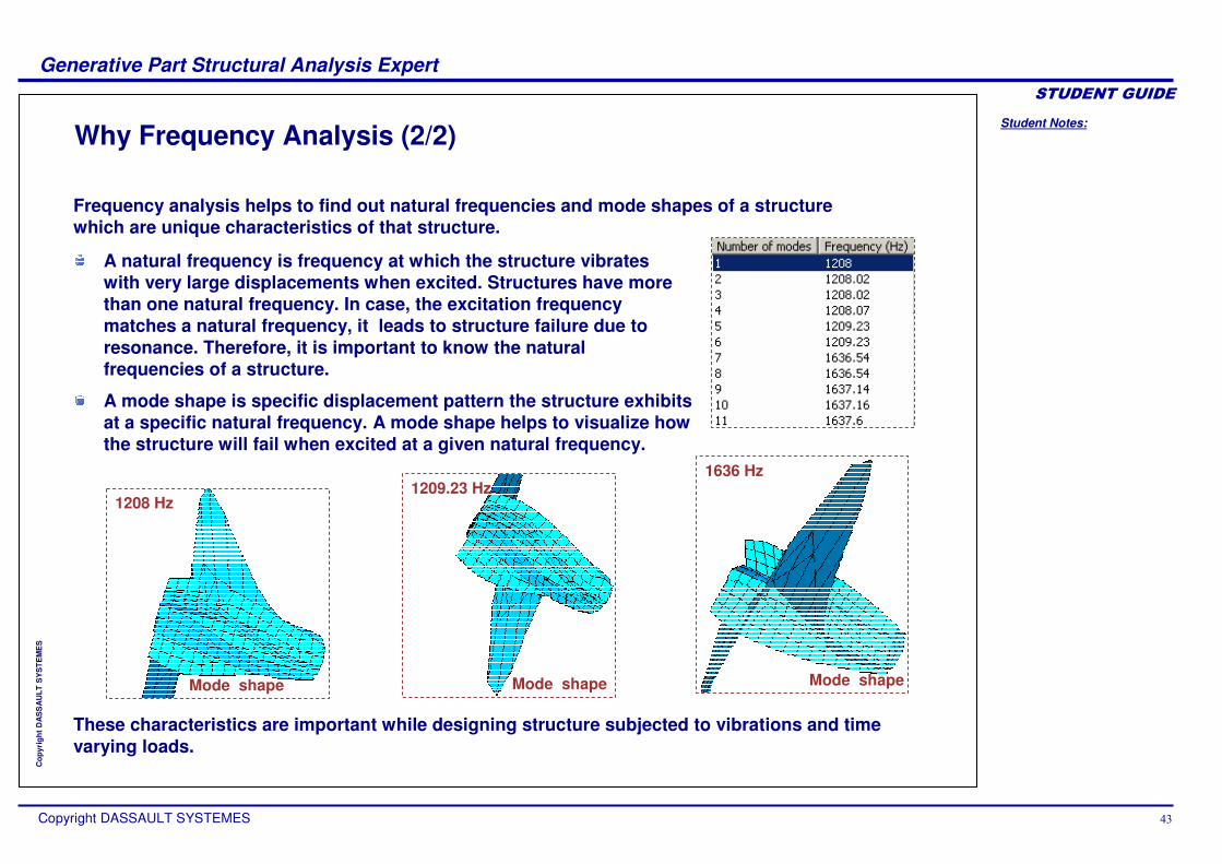
Frequency analysis helps to find out natural frequencies and mode shapes of a structure which are unique characteristics of that structure.
A natural frequency is frequency at which the structure vibrateswith very large displacements when excited. Structures have morethan one natural frequency. In case, the excitation frequency matches a natural frequency, it leads to structure failure due to resonance. Therefore, it is important to know the natural frequencies of a structure.
A mode shape is specific displacement pattern the structure exhibits at a specific natural frequency. A mode shape helps to visualize how the structure will fail when excited at a given natural frequency.
These characteristics are important while designing structure subjected to vibrations and time varying loads.
1208 Hz
Mode shape
1209.23 Hz
Mode shape
1636 Hz
Mode shape
Student Notes:
Generative Part Structural Analysis Expert������������
Copyright DASSAULT SYSTEMES ��
Cop
yrig
ht D
AS
SA
ULT
SY
STE
ME
S
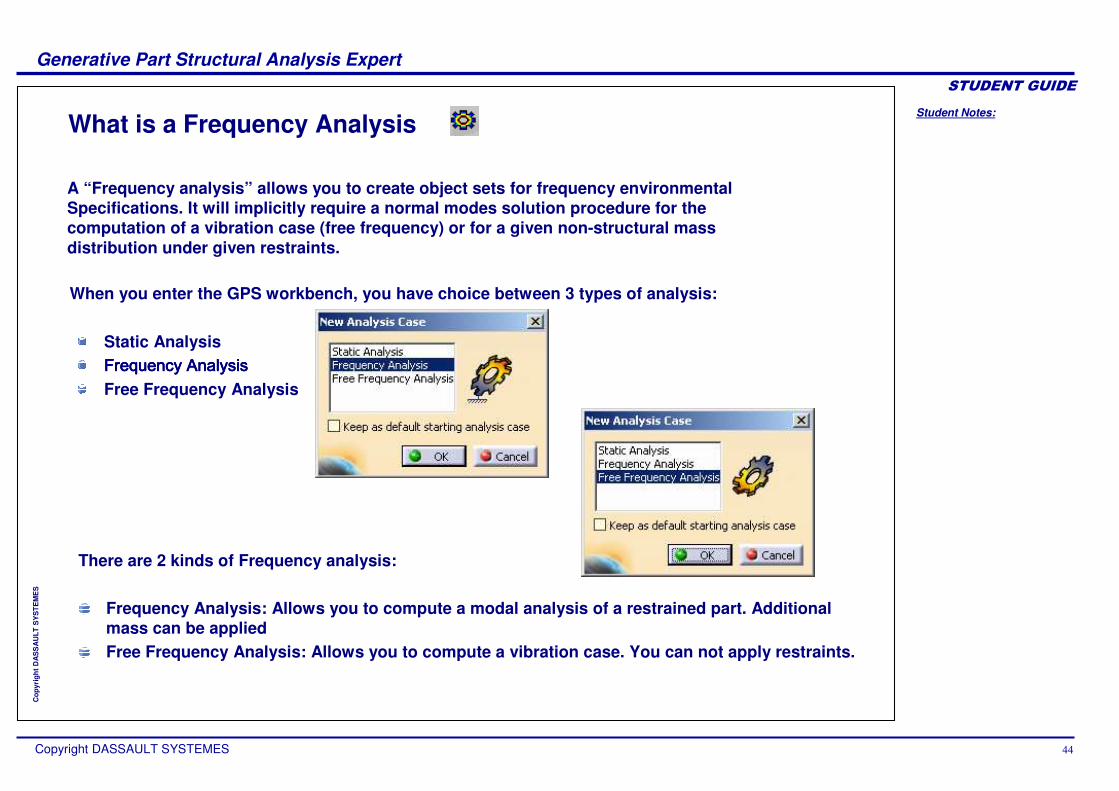
What is a Frequency Analysis
A “Frequency analysis” allows you to create object sets for frequency environmental Specifications. It will implicitly require a normal modes solution procedure for the computation of a vibration case (free frequency) or for a given non-structural mass distribution under given restraints.
When you enter the GPS workbench, you have choice between 3 types of analysis:
Static Analysis
Free Frequency Analysis
There are 2 kinds of Frequency analysis:
Frequency Analysis: Allows you to compute a modal analysis of a restrained part. Additional mass can be appliedFree Frequency Analysis: Allows you to compute a vibration case. You can not apply restraints.
Student Notes:
Generative Part Structural Analysis Expert������������
Copyright DASSAULT SYSTEMES ��
Cop
yrig
ht D
AS
SA
ULT
SY
STE
ME
S
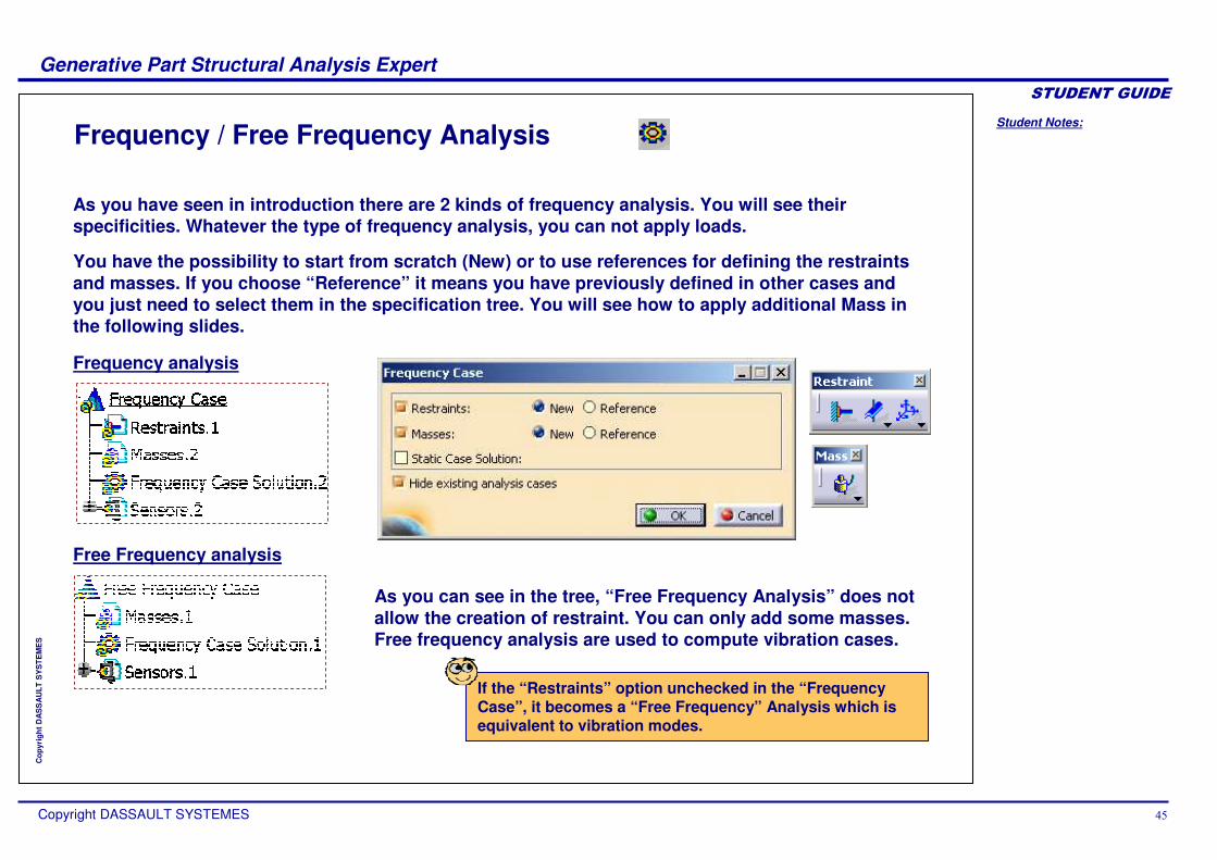
Frequency / Free Frequency Analysis
You have the possibility to start from scratch (New) or to use references for defining the restraints and masses. If you choose “Reference” it means you have previously defined in other cases and you just need to select them in the specification tree. You will see how to apply additional Mass in the following slides.
As you have seen in introduction there are 2 kinds of frequency analysis. You will see their specificities. Whatever the type of frequency analysis, you can not apply loads.
Free Frequency analysis
Frequency analysis
As you can see in the tree, “Free Frequency Analysis” does not allow the creation of restraint. You can only add some masses. Free frequency analysis are used to compute vibration cases.
If the “Restraints” option unchecked in the “Frequency Case”, it becomes a “Free Frequency” Analysis which is equivalent to vibration modes.
Student Notes:
Generative Part Structural Analysis Expert������������
Copyright DASSAULT SYSTEMES ��
Cop
yrig
ht D
AS
SA
ULT
SY
STE
ME
S
Distributed mass
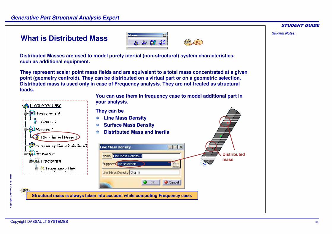
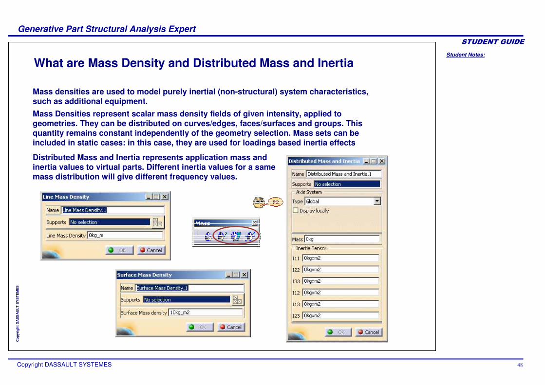
What is Distributed Mass
They represent scalar point mass fields and are equivalent to a total mass concentrated at a given point (geometry centroid). They can be distributed on a virtual part or on a geometric selection. Distributed mass is used only in case of Frequency analysis. They are not treated as structural loads.
Distributed Masses are used to model purely inertial (non-structural) system characteristics, such as additional equipment.
They can be Line Mass Density Surface Mass DensityDistributed Mass and Inertia
You can use them in frequency case to model additional part in your analysis.
Structural mass is always taken into account while computing Frequency case.
Student Notes:
Generative Part Structural Analysis Expert������������
Copyright DASSAULT SYSTEMES ��
Cop
yrig
ht D
AS
SA
ULT
SY
STE
ME
S
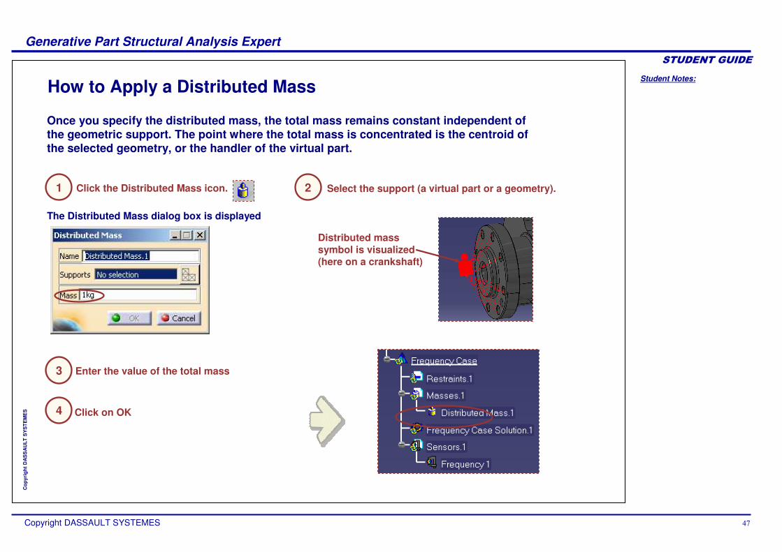
How to Apply a Distributed Mass
Select the support (a virtual part or a geometry).
Enter the value of the total mass
Once you specify the distributed mass, the total mass remains constant independent of the geometric support. The point where the total mass is concentrated is the centroid of the selected geometry, or the handler of the virtual part.
Click the Distributed Mass icon.
The Distributed Mass dialog box is displayed
Click on OK
Distributed mass symbol is visualized (here on a crankshaft)
1 2
3
4
Student Notes:
Generative Part Structural Analysis Expert������������
Copyright DASSAULT SYSTEMES ��
Cop
yrig
ht D
AS
SA
ULT
SY
STE
ME
S
What are Mass Density and Distributed Mass and Inertia
Mass densities are used to model purely inertial (non-structural) system characteristics, such as additional equipment.Mass Densities represent scalar mass density fields of given intensity, applied to geometries. They can be distributed on curves/edges, faces/surfaces and groups. This quantity remains constant independently of the geometry selection. Mass sets can be included in static cases: in this case, they are used for loadings based inertia effects
Distributed Mass and Inertia represents application mass and inertia values to virtual parts. Different inertia values for a same mass distribution will give different frequency values.

Student Notes:
Generative Part Structural Analysis Expert������������
Copyright DASSAULT SYSTEMES �
Cop
yrig
ht D
AS
SA
ULT
SY
STE
ME
S
How to Apply a Mass Density
Select the support :
Specify the mass density
Mass Densities represent scalar mass density fields of given intensity, applied to geometries. The user specifies mass density. The total mass then depends on the geometry selection.
Click on a Mass Density icon
A mass density dialog box appears
Click on OK
curves/edges if Line Mass Densityfaces/surfaces if Surface Mass Densitiesgroups
1
2
3
4
Student Notes:
Generative Part Structural Analysis Expert������������
Copyright DASSAULT SYSTEMES �
Cop
yrig
ht D
AS
SA
ULT
SY
STE
ME
S
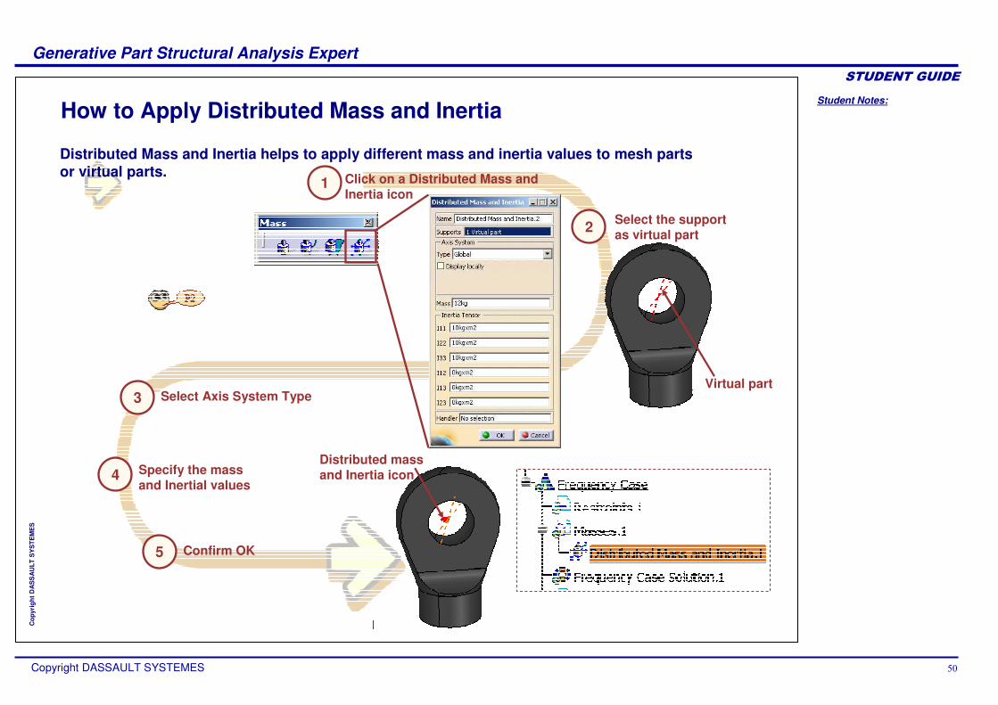
How to Apply Distributed Mass and Inertia
Select Axis System Type
Distributed Mass and Inertia helps to apply different mass and inertia values to mesh parts or virtual parts.
Confirm OK
Specify the mass and Inertial values
Distributed mass and Inertia icon
Click on a Distributed Mass and Inertia icon
1
Select the support as virtual part
Virtual part
2
3
4
5
Student Notes:
Generative Part Structural Analysis Expert������������
Copyright DASSAULT SYSTEMES ��
Cop
yrig
ht D
AS
SA
ULT
SY
STE
ME
S
In the Advanced Pre-Processing tools, you have seen how to :
Define advanced LoadsDefine advanced restraintsSelect a Mesh PartDefine Virtual PartsDefine User MaterialDefine a Frequency Analysis
To Sum Up ...
Student Notes:
Generative Part Structural Analysis Expert������������
Copyright DASSAULT SYSTEMES ��
Cop
yrig
ht D
AS
SA
ULT
SY
STE
ME
S
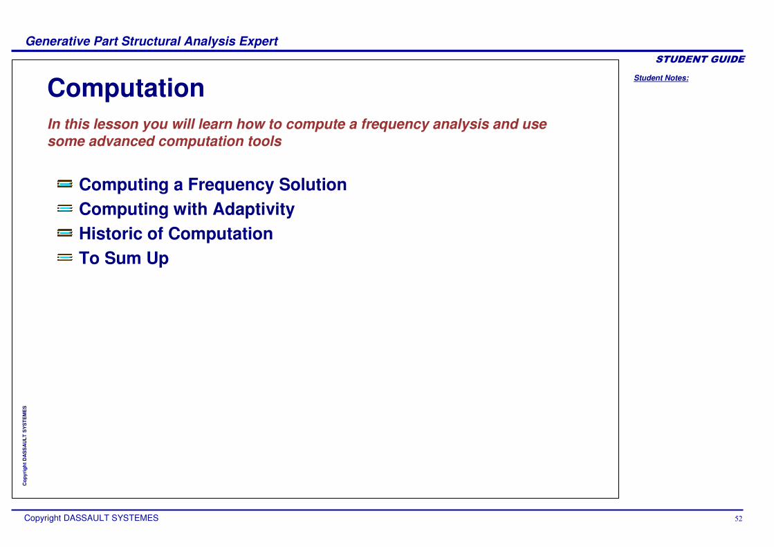
ComputationIn this lesson you will learn how to compute a frequency analysis and use some advanced computation tools
Computing a Frequency SolutionComputing with AdaptivityHistoric of ComputationTo Sum Up
Student Notes:
Generative Part Structural Analysis Expert������������
Copyright DASSAULT SYSTEMES ��
Cop
yrig
ht D
AS
SA
ULT
SY
STE
ME
S
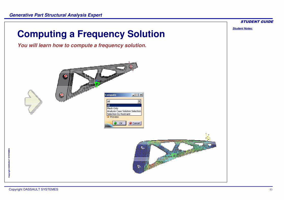
Computing a Frequency SolutionYou will learn how to compute a frequency solution.

Student Notes:
Generative Part Structural Analysis Expert������������
Copyright DASSAULT SYSTEMES ��
Cop
yrig
ht D
AS
SA
ULT
SY
STE
ME
S
Introduction
The combo box allows you to choose between several options for the set of objects to update:All : All the objects defined in the analysis features tree will be computed Mesh only: the preprocessing parts and connections will be meshed. The preprocessing data (loads, restraints and so forth) will be applied onto the mesh. In case the “Mesh only” option was previously activated, you will then be able to visualize the applied data on the mesh by using the Visualization on Mesh option (contextual menu) Analysis Case Solution Selection: only a selection of user-specified Analysis Case Solutions will be computed, with an optimal parallel computation strategy Selection by Restraint: only the selected characteristics will be computed (Properties, Restraints, Loads, Masses).
The primary Frequency Solution Computation result consists in a set of frequencies and associated modal vibration shape vectors whose components represent the values of the system DOF for various vibration modes.
The program can compute simultaneously several Solution object sets, with optimal parallel computation whenever applicable.
At this step of your work you must make sure that your materials, restraints and loads are successfully defined. The computation will generate the analysis case solution, along with partial results for all objects involved in the definition of the Analysis Case.
Student Notes:
Generative Part Structural Analysis Expert������������
Copyright DASSAULT SYSTEMES ��
Cop
yrig
ht D
AS
SA
ULT
SY
STE
ME
S
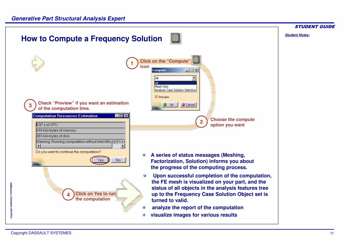
How to Compute a Frequency Solution
Choose the compute option you want
Check “Preview” if you want an estimation of the computation time.
Click on the “Compute”icon
Upon successful completion of the computation, the FE mesh is visualized on your part, and the status of all objects in the analysis features tree up to the Frequency Case Solution Object set is turned to valid.
A series of status messages (Meshing, Factorization, Solution) informs you about the progress of the computing process.
Click on Yes to run the computation
analyze the report of the computationvisualize images for various results
1
2
3
4
Student Notes:
Generative Part Structural Analysis Expert������������
Copyright DASSAULT SYSTEMES ��
Cop
yrig
ht D
AS
SA
ULT
SY
STE
ME
S
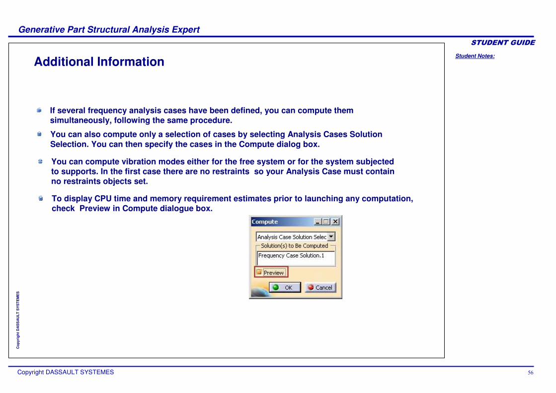
If several frequency analysis cases have been defined, you can compute them simultaneously, following the same procedure.
You can compute vibration modes either for the free system or for the system subjected to supports. In the first case there are no restraints so your Analysis Case must contain no restraints objects set.
To display CPU time and memory requirement estimates prior to launching any computation, check Preview in Compute dialogue box.
You can also compute only a selection of cases by selecting Analysis Cases Solution Selection. You can then specify the cases in the Compute dialog box.
Additional Information
Student Notes:
Generative Part Structural Analysis Expert������������
Copyright DASSAULT SYSTEMES ��
Cop
yrig
ht D
AS
SA
ULT
SY
STE
ME
S
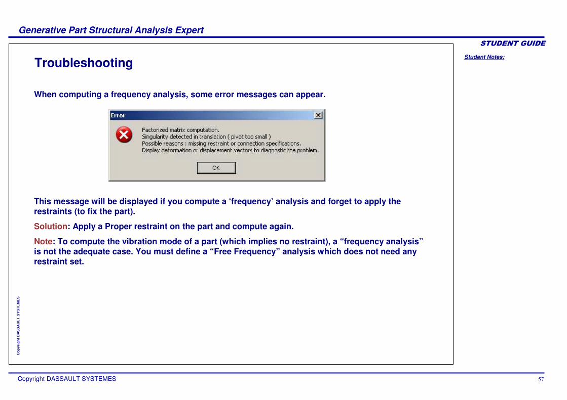
Troubleshooting
When computing a frequency analysis, some error messages can appear.
This message will be displayed if you compute a ‘frequency’ analysis and forget to apply the restraints (to fix the part).
Solution: Apply a Proper restraint on the part and compute again.
Note: To compute the vibration mode of a part (which implies no restraint), a “frequency analysis”is not the adequate case. You must define a “Free Frequency” analysis which does not need any restraint set.
Student Notes:
Generative Part Structural Analysis Expert������������
Copyright DASSAULT SYSTEMES ��
Cop
yrig
ht D
AS
SA
ULT
SY
STE
ME
S
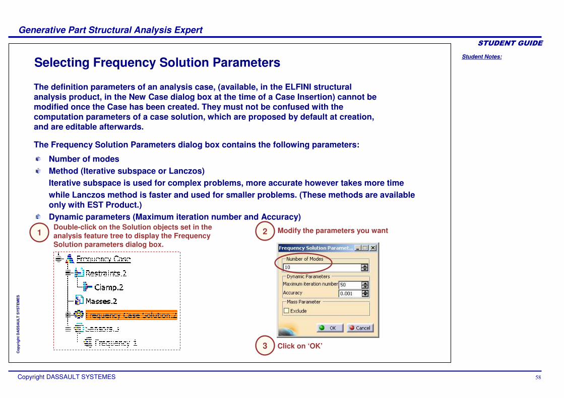
Number of modes Method (Iterative subspace or Lanczos) Iterative subspace is used for complex problems, more accurate however takes more timewhile Lanczos method is faster and used for smaller problems. (These methods are available only with EST Product.)Dynamic parameters (Maximum iteration number and Accuracy)
Selecting Frequency Solution Parameters
The Frequency Solution Parameters dialog box contains the following parameters:
The definition parameters of an analysis case, (available, in the ELFINI structural analysis product, in the New Case dialog box at the time of a Case Insertion) cannot be modified once the Case has been created. They must not be confused with the computation parameters of a case solution, which are proposed by default at creation, and are editable afterwards.
Double-click on the Solution objects set in the analysis feature tree to display the Frequency Solution parameters dialog box.
1 Modify the parameters you want2
Click on ‘OK’3
Student Notes:
Generative Part Structural Analysis Expert������������
Copyright DASSAULT SYSTEMES �
Cop
yrig
ht D
AS
SA
ULT
SY
STE
ME
S
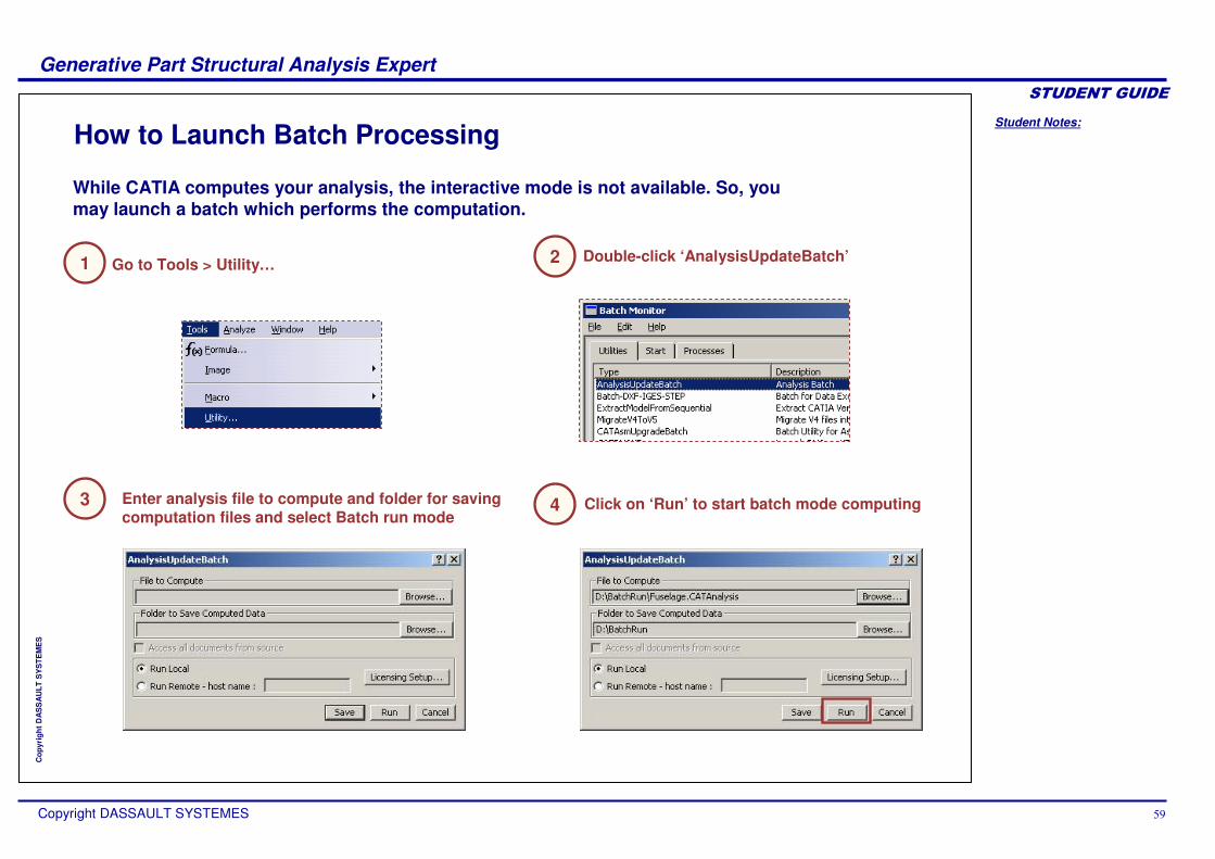
How to Launch Batch Processing
While CATIA computes your analysis, the interactive mode is not available. So, you may launch a batch which performs the computation.
Go to Tools > Utility…1 Double-click ‘AnalysisUpdateBatch’2
Enter analysis file to compute and folder for saving computation files and select Batch run mode
3 Click on ‘Run’ to start batch mode computing4
Student Notes:
Generative Part Structural Analysis Expert������������
Copyright DASSAULT SYSTEMES �
Cop
yrig
ht D
AS
SA
ULT
SY
STE
ME
S
Computing with AdaptivityYou will learn how to compute an analysis taking into account the objectives error defined thanks to the adaptivity tools (Post-Processing)
Note: For all information about “adaptivity”, please see the skillet “Mesh Adaptivity” in the post-processing lesson

Student Notes:
Generative Part Structural Analysis Expert������������
Copyright DASSAULT SYSTEMES ��
Cop
yrig
ht D
AS
SA
ULT
SY
STE
ME
S
About Adaptivity
The mesh refining criteria are based on a technique called predictive error estimation, which consists in determining the distribution of a local error estimate field for a given Static Analysis Case. “Adaptivity Management” consists in setting global adaptivity specifications and computing adaptive solutions.
After you have run the “Adaptive” computation, you can return to the static solution and check that the mesh has been refined according to your specifications in the Adaptivity Entities.You can create several Adaptivity Entities associated to different Static Solutions and corresponding to different regions of your part, i.e:create several Adaptivity entities associated to the same Static Solution and corresponding to the different regions of your partcreate several Adaptivity Entities associated to different Static Solutions and corresponding to the same region of your partThe computation is such as all adaptivity entities specifications are simultaneously respected within the global Maximum Number of Iterations specification.
‘Adaptivity’ consists in selectively refining the mesh in such a way as to obtain a desired result accuracy in a specified region (see post-Pros. Lesson)
The Adaptivity functionalities are only available with static analysis solution or a combined solution that references a static analysis solution.
Student Notes:
Generative Part Structural Analysis Expert������������
Copyright DASSAULT SYSTEMES ��
Cop
yrig
ht D
AS
SA
ULT
SY
STE
ME
S
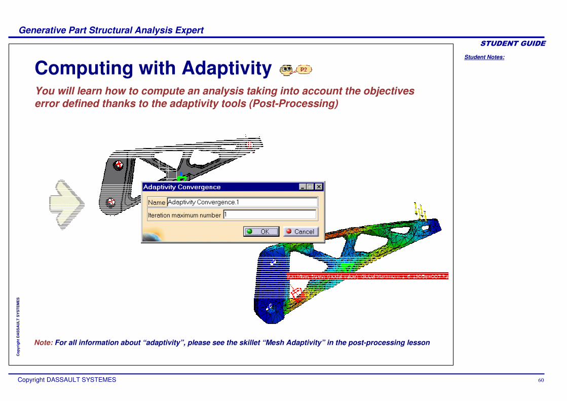
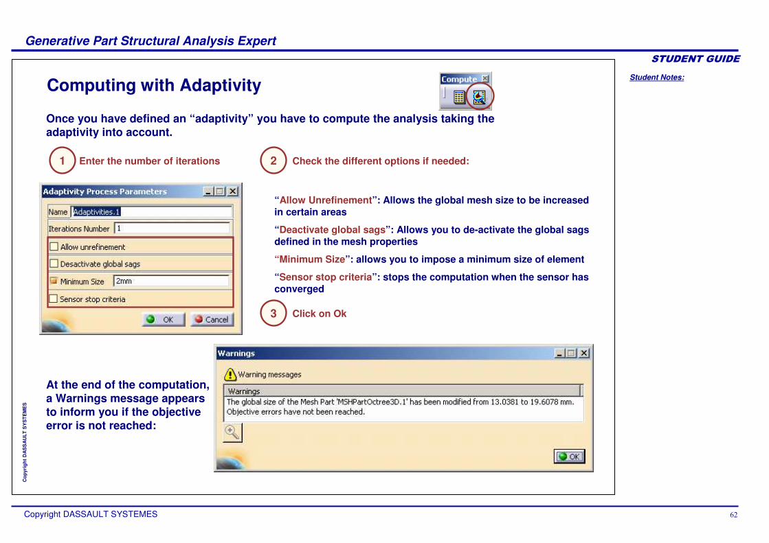
Computing with Adaptivity
Once you have defined an “adaptivity” you have to compute the analysis taking the adaptivity into account.
“Allow Unrefinement”: Allows the global mesh size to be increased in certain areas
“Deactivate global sags”: Allows you to de-activate the global sags defined in the mesh properties
“Minimum Size”: allows you to impose a minimum size of element
“Sensor stop criteria”: stops the computation when the sensor has converged
At the end of the computation, a Warnings message appears to inform you if the objective error is not reached:
Enter the number of iterations Check the different options if needed:
Click on Ok
1 2
3
Student Notes:
Generative Part Structural Analysis Expert������������
Copyright DASSAULT SYSTEMES ��
Cop
yrig
ht D
AS
SA
ULT
SY
STE
ME
S
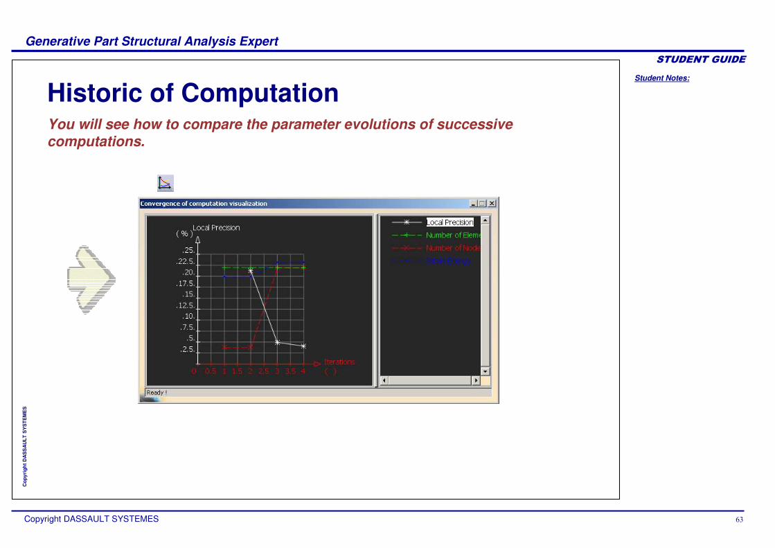
Historic of ComputationYou will see how to compare the parameter evolutions of successive computations.
Student Notes:
Generative Part Structural Analysis Expert������������
Copyright DASSAULT SYSTEMES ��
Cop
yrig
ht D
AS
SA
ULT
SY
STE
ME
S
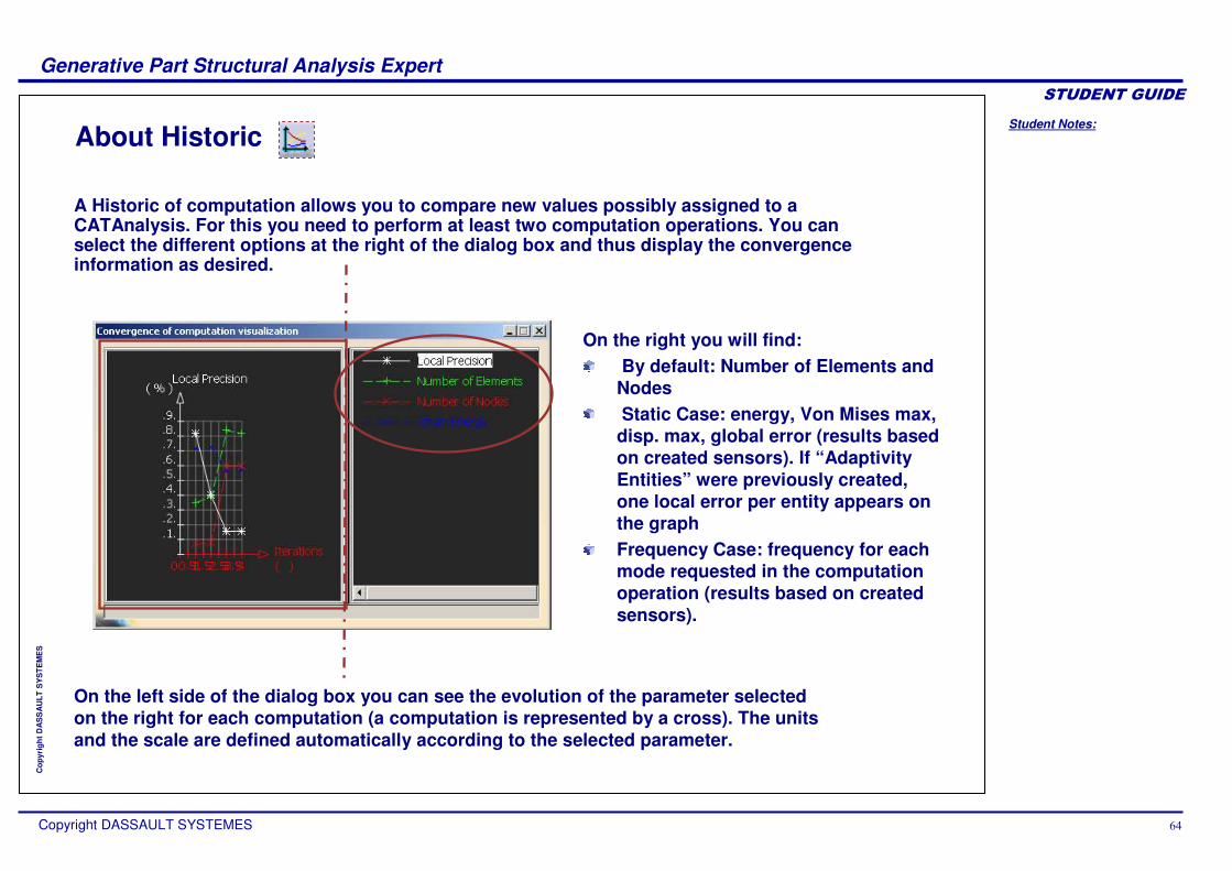
About Historic
A Historic of computation allows you to compare new values possibly assigned to a CATAnalysis. For this you need to perform at least two computation operations. You can select the different options at the right of the dialog box and thus display the convergence information as desired.
On the left side of the dialog box you can see the evolution of the parameter selected on the right for each computation (a computation is represented by a cross). The units and the scale are defined automatically according to the selected parameter.
On the right you will find:By default: Number of Elements and
NodesStatic Case: energy, Von Mises max,
disp. max, global error (results based on created sensors). If “Adaptivity Entities” were previously created, one local error per entity appears on the graphFrequency Case: frequency for each mode requested in the computation operation (results based on created sensors).
Student Notes:
Generative Part Structural Analysis Expert������������
Copyright DASSAULT SYSTEMES ��
Cop
yrig
ht D
AS
SA
ULT
SY
STE
ME
S
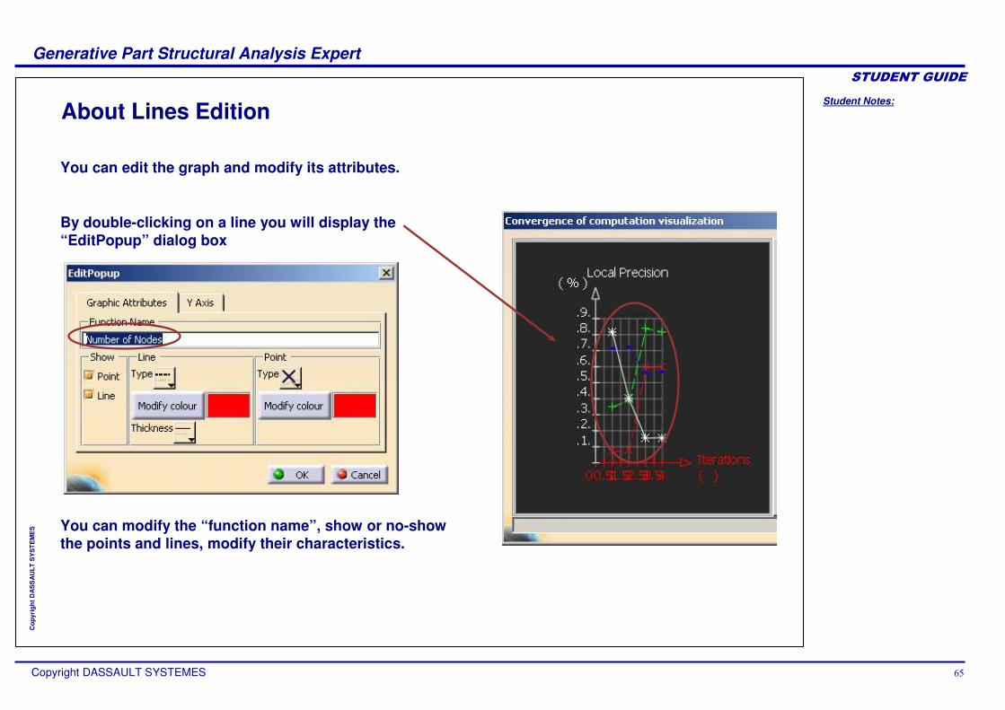
About Lines Edition
You can edit the graph and modify its attributes.
By double-clicking on a line you will display the “EditPopup” dialog box
You can modify the “function name”, show or no-show the points and lines, modify their characteristics.
Student Notes:
Generative Part Structural Analysis Expert������������
Copyright DASSAULT SYSTEMES ��
Cop
yrig
ht D
AS
SA
ULT
SY
STE
ME
S
In the Computation lesson, you have seen how to :
Compute Frequency Analysis Compute the Analysis with adaptivitySee the historic of computation
To Sum Up ...
Student Notes:
Generative Part Structural Analysis Expert������������
Copyright DASSAULT SYSTEMES ��
Cop
yrig
ht D
AS
SA
ULT
SY
STE
ME
S
GPS Advanced Post-Processing ToolsIn this lesson you will see the advanced post-processing tools to visualize results and optimize analysis
Results VisualizationResults ManagementRefinementTo Sum Up
Student Notes:
Generative Part Structural Analysis Expert������������
Copyright DASSAULT SYSTEMES ��
Cop
yrig
ht D
AS
SA
ULT
SY
STE
ME
S
Results VisualizationIn this lesson, you will see advanced tools to visualize results
Image CreationCut Plane AnalysisTo Sum Up
Student Notes:
Generative Part Structural Analysis Expert������������
Copyright DASSAULT SYSTEMES �
Cop
yrig
ht D
AS
SA
ULT
SY
STE
ME
S
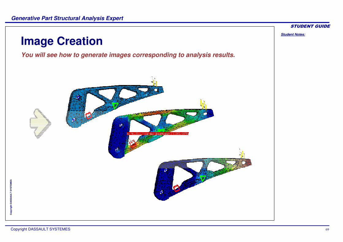
Image CreationYou will see how to generate images corresponding to analysis results.
Student Notes:
Generative Part Structural Analysis Expert������������
Copyright DASSAULT SYSTEMES �
Cop
yrig
ht D
AS
SA
ULT
SY
STE
ME
S
Introduction
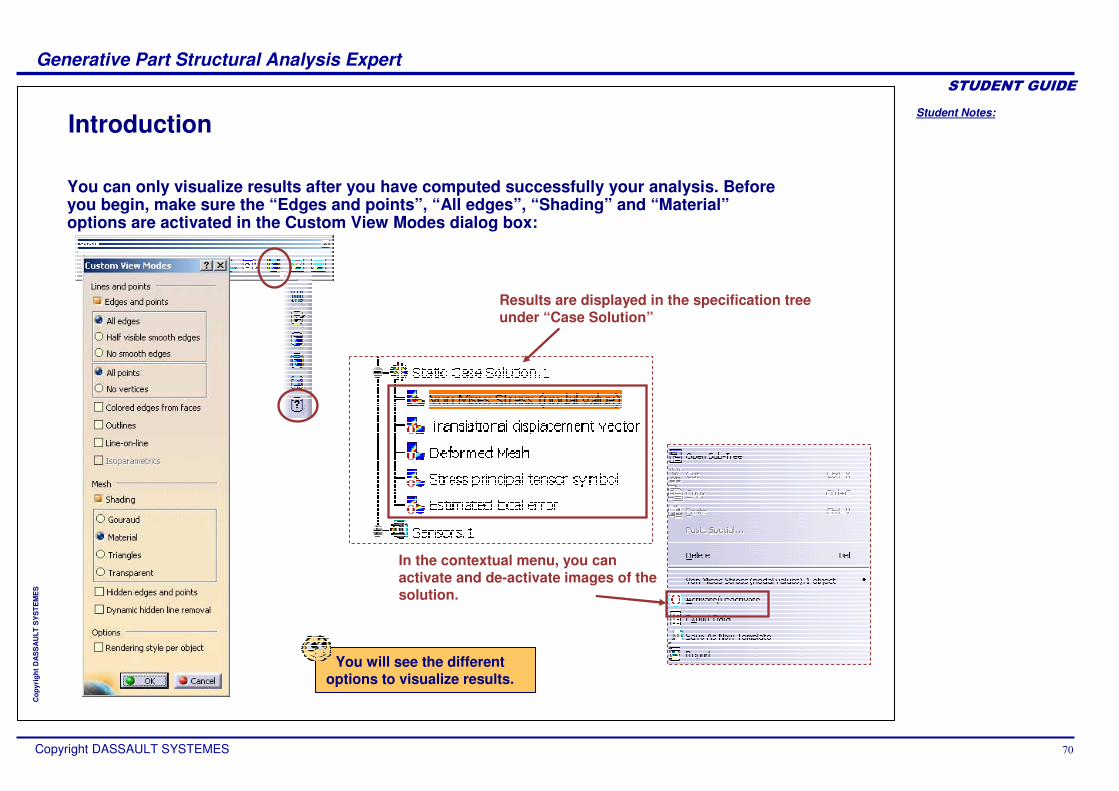
You can only visualize results after you have computed successfully your analysis. Before you begin, make sure the “Edges and points”, “All edges”, “Shading” and “Material”options are activated in the Custom View Modes dialog box:
Results are displayed in the specification tree under “Case Solution”
In the contextual menu, you can activate and de-activate images of the solution.
You will see the different options to visualize results.
Student Notes:
Generative Part Structural Analysis Expert������������
Copyright DASSAULT SYSTEMES ��
Cop
yrig
ht D
AS
SA
ULT
SY
STE
ME
S
Generating Images
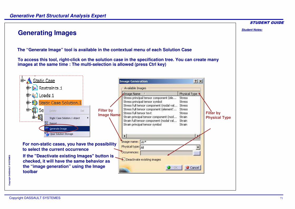
The “Generate Image” tool is available in the contextual menu of each Solution Case
To access this tool, right-click on the solution case in the specification tree. You can create many images at the same time : The multi-selection is allowed (press Ctrl key)
If the "Deactivate existing Images" button is checked, it will have the same behavior as the “image generation” using the Image toolbar
For non-static cases, you have the possibility to select the current occurrence
Filter by Image Name Filter by
Physical Type

Student Notes:
Generative Part Structural Analysis Expert������������
Copyright DASSAULT SYSTEMES ��
Cop
yrig
ht D
AS
SA
ULT
SY
STE
ME
S
About Principal Stresses
At each point, the principal stress tensor gives the directions relative to which the part is in a state of pure tension/compression (zero shear stress components on the corresponding planes) and the values of the corresponding tensile/compressive stresses.
To edit the image using Image Edition dialog box you have to double click on the solution object in the specification tree
At each point, a set of three directions is represented by line symbols (principal directions of stress).Arrow directions (inwards / outwards) indicate
the sign of the principal stress. The color code provides quantitative information.
Stress principal tensor symbol images are used to visualize principal stress field patterns, which represent a tensor field quantity used to measure the state of stress and to determine the load path on a loaded part.
The principal values stress tensor distribution on the part is visualized in symbol mode, along with a color palette:

Student Notes:
Generative Part Structural Analysis Expert������������
Copyright DASSAULT SYSTEMES ��
Cop
yrig
ht D
AS
SA
ULT
SY
STE
ME
S
Principal Stresses Image Edition
The “Image Edition” dialog box is composed of 2 tabs:
Visu: provides a list with visu types (Average-Iso, Discontinuous-Iso, Text) and a list with criteria (Principal-Value).Selections: In the case of CATProducts, pre-defined groups of elements belonging to given mesh parts can be multi-selected.
More: provides different filters. You can choose to generate images on nodes, elements, nodes of elements, center of elements or Gauss points of elements. You can also choose Value Type options.

Student Notes:
Generative Part Structural Analysis Expert������������
Copyright DASSAULT SYSTEMES ��
Cop
yrig
ht D
AS
SA
ULT
SY
STE
ME
S
Visualizing Principal Stresses
(Optional) Double-click on the generated Principal Stress Image object in the specification tree to edit the image
Click OK to quit the Image Editor dialog box
If needed, modify the parameters.
Click on the Principal Stresses icon
This task shows how to generate Principal Stresses images on parts.
1 2
3
Student Notes:
Generative Part Structural Analysis Expert������������
Copyright DASSAULT SYSTEMES ��
Cop
yrig
ht D
AS
SA
ULT
SY
STE
ME
S
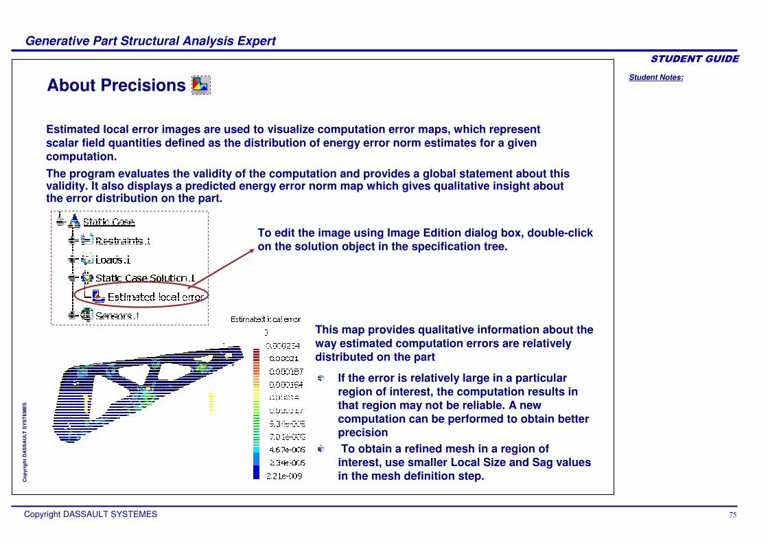
About Precisions
The program evaluates the validity of the computation and provides a global statement about this validity. It also displays a predicted energy error norm map which gives qualitative insight about the error distribution on the part.
To edit the image using Image Edition dialog box, double-click on the solution object in the specification tree.
If the error is relatively large in a particular region of interest, the computation results in that region may not be reliable. A new computation can be performed to obtain better precisionTo obtain a refined mesh in a region of
interest, use smaller Local Size and Sag values in the mesh definition step.
Estimated local error images are used to visualize computation error maps, which represent scalar field quantities defined as the distribution of energy error norm estimates for a given computation.
This map provides qualitative information about the way estimated computation errors are relatively distributed on the part
Student Notes:
Generative Part Structural Analysis Expert������������
Copyright DASSAULT SYSTEMES ��
Cop
yrig
ht D
AS
SA
ULT
SY
STE
ME
S
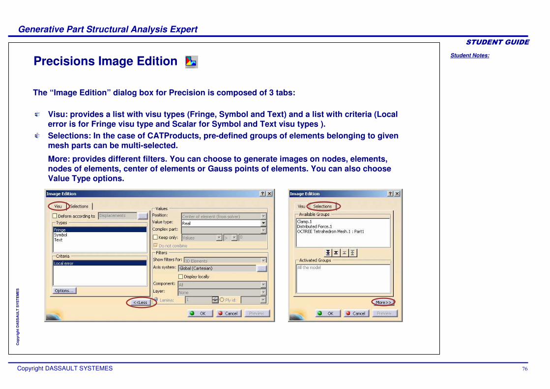
The “Image Edition” dialog box for Precision is composed of 3 tabs:
Visu: provides a list with visu types (Fringe, Symbol and Text) and a list with criteria (Localerror is for Fringe visu type and Scalar for Symbol and Text visu types ). Selections: In the case of CATProducts, pre-defined groups of elements belonging to given mesh parts can be multi-selected.
More: provides different filters. You can choose to generate images on nodes, elements, nodes of elements, center of elements or Gauss points of elements. You can also choose Value Type options.
Precisions Image Edition
Student Notes:
Generative Part Structural Analysis Expert������������
Copyright DASSAULT SYSTEMES ��
Cop
yrig
ht D
AS
SA
ULT
SY
STE
ME
S
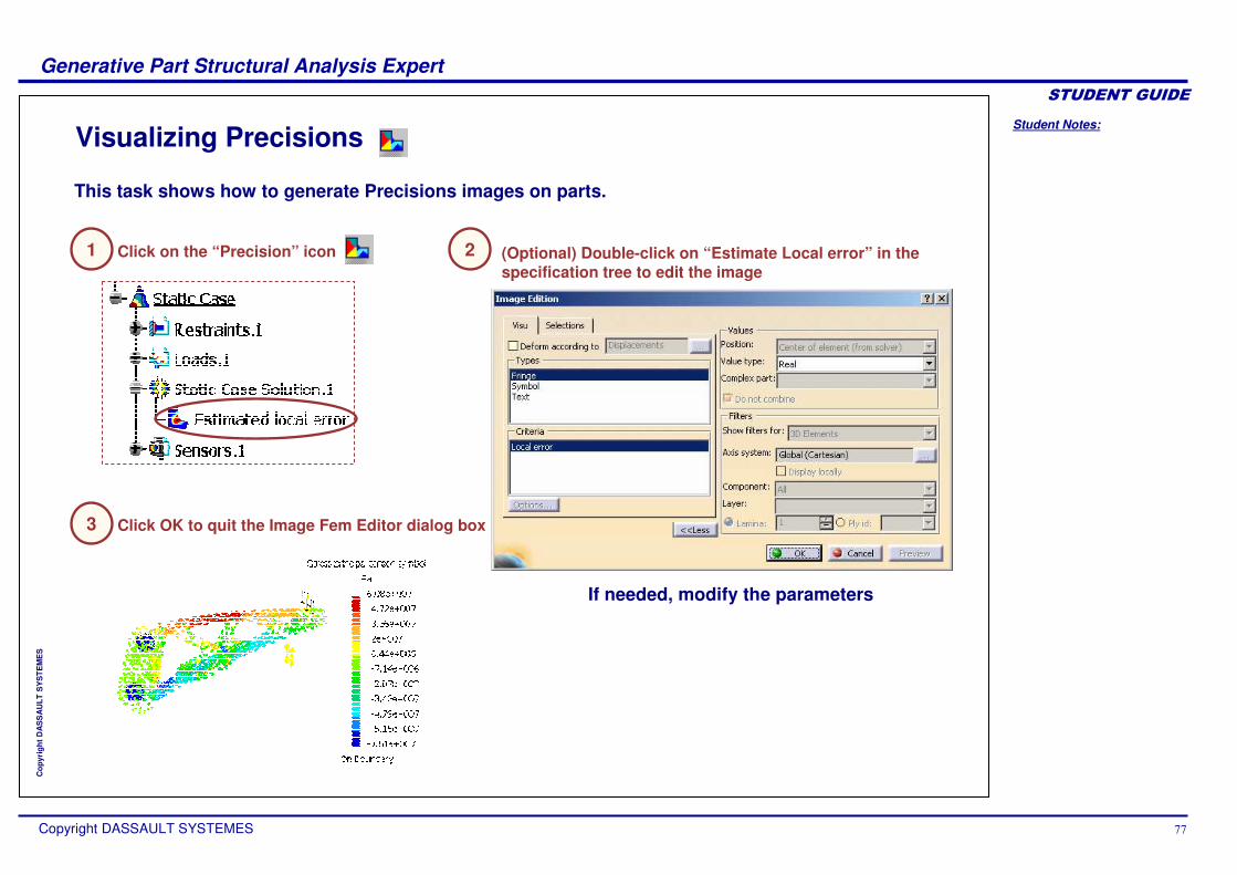
Visualizing Precisions
(Optional) Double-click on “Estimate Local error” in the specification tree to edit the image
Click OK to quit the Image Fem Editor dialog box
If needed, modify the parameters
Click on the “Precision” icon
This task shows how to generate Precisions images on parts.
1 2
3
Student Notes:
Generative Part Structural Analysis Expert������������
Copyright DASSAULT SYSTEMES ��
Cop
yrig
ht D
AS
SA
ULT
SY
STE
ME
S
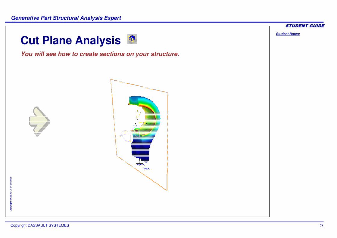
Cut Plane AnalysisYou will see how to create sections on your structure.
Student Notes:
Generative Part Structural Analysis Expert������������
Copyright DASSAULT SYSTEMES �
Cop
yrig
ht D
AS
SA
ULT
SY
STE
ME
S
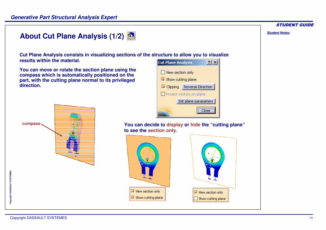
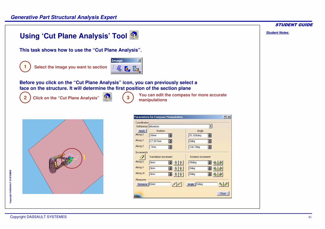
About Cut Plane Analysis (1/2)
You can move or rotate the section plane using the compass which is automatically positioned on the part, with the cutting plane normal to its privileged direction.
You can decide to display or hide the “cutting plane”to see the section only.
Cut Plane Analysis consists in visualizing sections of the structure to allow you to visualize results within the material.
compass
Student Notes:
Generative Part Structural Analysis Expert������������
Copyright DASSAULT SYSTEMES �
Cop
yrig
ht D
AS
SA
ULT
SY
STE
ME
S
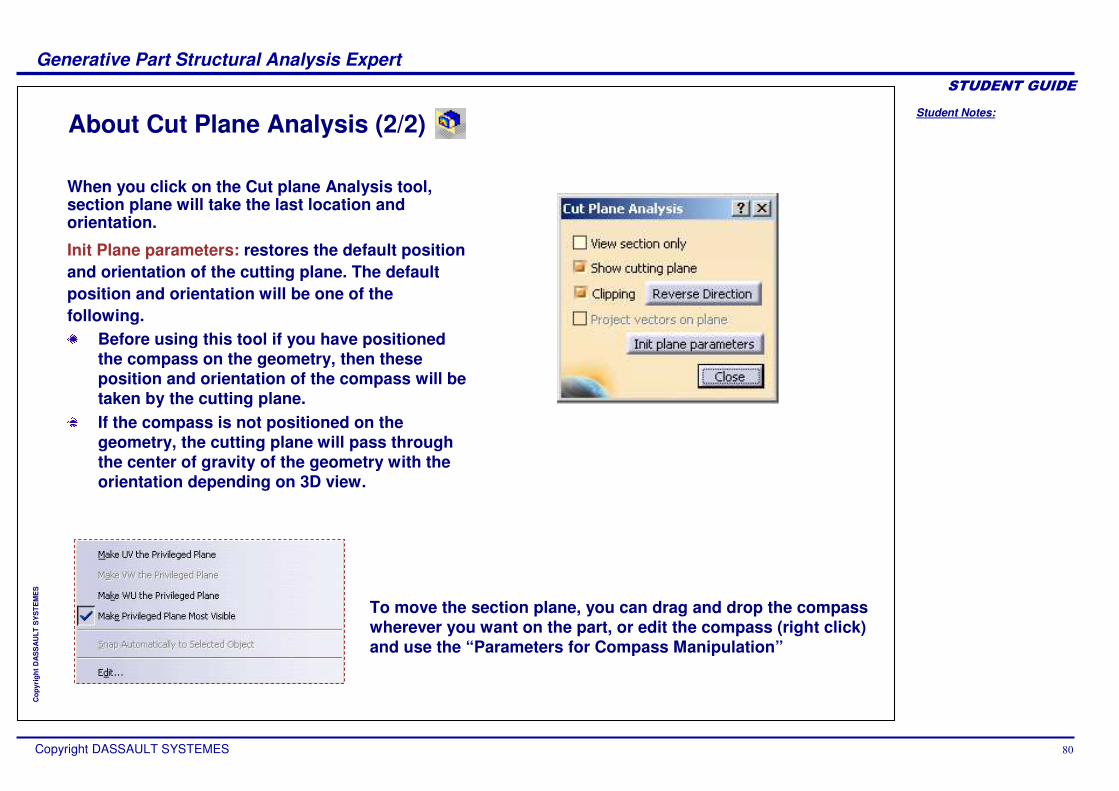
About Cut Plane Analysis (2/2)
When you click on the Cut plane Analysis tool, section plane will take the last location and orientation.
Init Plane parameters: restores the default positionand orientation of the cutting plane. The default position and orientation will be one of the following.
Before using this tool if you have positioned the compass on the geometry, then these position and orientation of the compass will be taken by the cutting plane. If the compass is not positioned on the geometry, the cutting plane will pass through the center of gravity of the geometry with the orientation depending on 3D view.
To move the section plane, you can drag and drop the compass wherever you want on the part, or edit the compass (right click)and use the “Parameters for Compass Manipulation”
Student Notes:
Generative Part Structural Analysis Expert������������
Copyright DASSAULT SYSTEMES ��
Cop
yrig
ht D
AS
SA
ULT
SY
STE
ME
S
Using ‘Cut Plane Analysis’ Tool
Select the image you want to section
You can edit the compass for more accurate manipulations Click on the “Cut Plane Analysis”
Before you click on the “Cut Plane Analysis” icon, you can previously select a face on the structure. It will determine the first position of the section plane
This task shows how to use the “Cut Plane Analysis”.
1
2 3
Student Notes:
Generative Part Structural Analysis Expert������������
Copyright DASSAULT SYSTEMES ��
Cop
yrig
ht D
AS
SA
ULT
SY
STE
ME
S
You have seen how to :
Display ImagesUse the Section Plane
To Sum Up ...
Student Notes:
Generative Part Structural Analysis Expert������������
Copyright DASSAULT SYSTEMES ��
Cop
yrig
ht D
AS
SA
ULT
SY
STE
ME
S
Results ManagementIn this lesson, you will learn how to use some tools for results exploitation
Publishing Advanced ReportsTo sum up
Student Notes:
Generative Part Structural Analysis Expert������������
Copyright DASSAULT SYSTEMES ��
Cop
yrig
ht D
AS
SA
ULT
SY
STE
ME
S
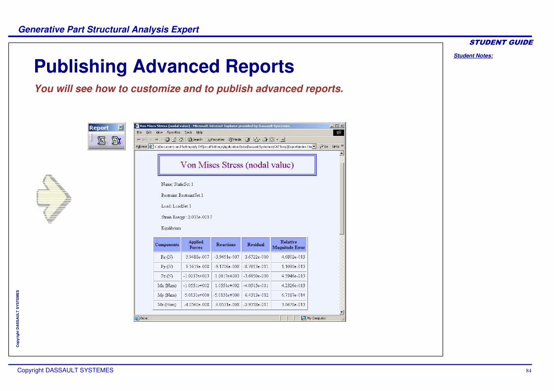
Publishing Advanced ReportsYou will see how to customize and to publish advanced reports.
Student Notes:
Generative Part Structural Analysis Expert������������
Copyright DASSAULT SYSTEMES ��
Cop
yrig
ht D
AS
SA
ULT
SY
STE
ME
S
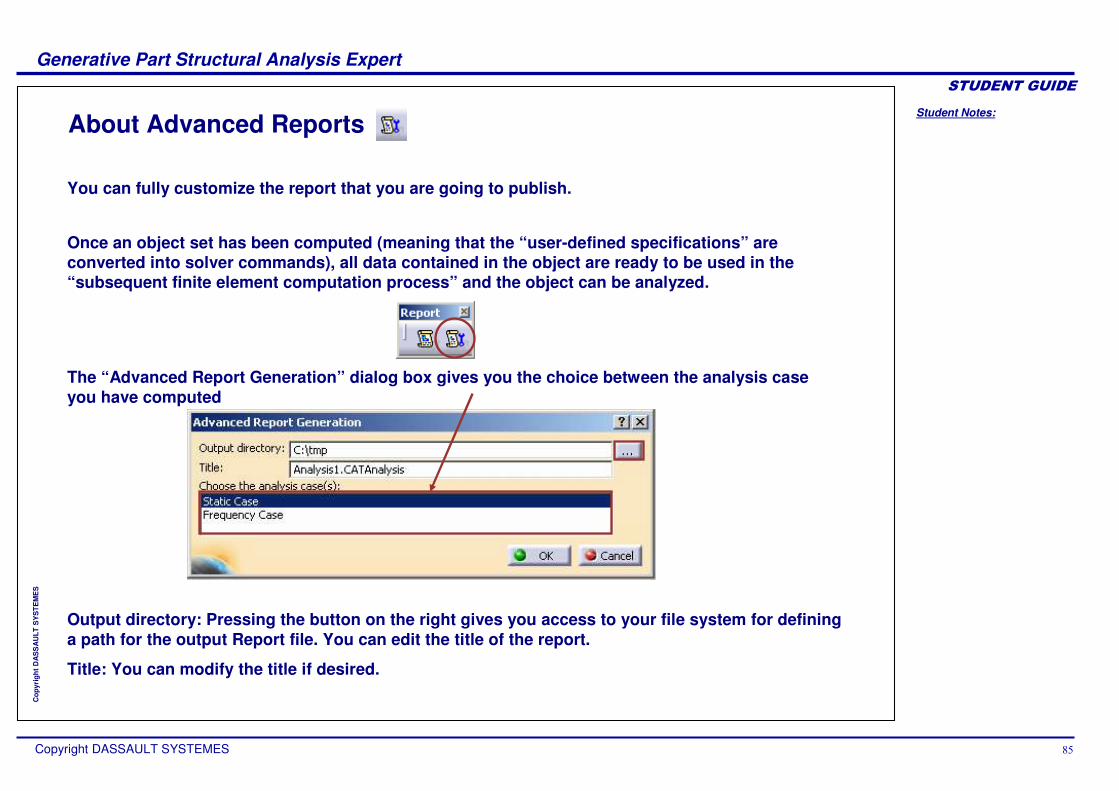
About Advanced Reports
Once an object set has been computed (meaning that the “user-defined specifications” are converted into solver commands), all data contained in the object are ready to be used in the “subsequent finite element computation process” and the object can be analyzed.
The “Advanced Report Generation” dialog box gives you the choice between the analysis case you have computed
Output directory: Pressing the button on the right gives you access to your file system for defining a path for the output Report file. You can edit the title of the report.
Title: You can modify the title if desired.
You can fully customize the report that you are going to publish.

Student Notes:
Generative Part Structural Analysis Expert������������
Copyright DASSAULT SYSTEMES ��
Cop
yrig
ht D
AS
SA
ULT
SY
STE
ME
S
How to Use the Advanced Report Tool
1 Select the data you want to see in your report
2 Click on the middle arrow to validate the selection
3 Click on OK
The Generate Advanced Report tool allows you to define which information you need to extract from all the specifications before launching the browser, creating and if needed updating the output Report file.
P2-EST
1
2
3
1
Student Notes:
Generative Part Structural Analysis Expert������������
Copyright DASSAULT SYSTEMES ��
Cop
yrig
ht D
AS
SA
ULT
SY
STE
ME
S
You have seen how to:
Publish advanced report
To Sum Up ...
Student Notes:
Generative Part Structural Analysis Expert������������
Copyright DASSAULT SYSTEMES ��
Cop
yrig
ht D
AS
SA
ULT
SY
STE
ME
S
RefinementIn this lesson you will see different ways to improve the precision of your results.
Refining the MeshMesh AdaptivityTo Sum Up
Student Notes:
Generative Part Structural Analysis Expert������������
Copyright DASSAULT SYSTEMES �
Cop
yrig
ht D
AS
SA
ULT
SY
STE
ME
S
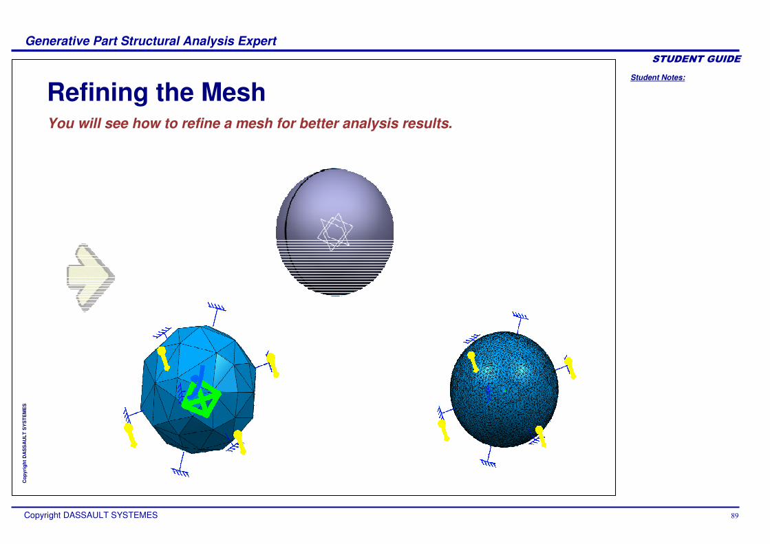
Refining the MeshYou will see how to refine a mesh for better analysis results.

Student Notes:
Generative Part Structural Analysis Expert������������
Copyright DASSAULT SYSTEMES
Cop
yrig
ht D
AS
SA
ULT
SY
STE
ME
S
Global and Local Mesh Refinement
The first step when you want to improve the precision of your analysis results is to refine the mesh of your part. You can refine the Size of a mesh, and the Sag (chord error). This can be performed both globally and locally.
Mesh
Real boundary
Sag
Size
The mesh “size” is the length of the element edges and the “sag” is the maximum distance allowed by the user between an element edge and the geometry. Consequently, a fine mesh and a small sag provide more accurate results.
Coarse mesh Fine mesh
Student Notes:
Generative Part Structural Analysis Expert������������
Copyright DASSAULT SYSTEMES �
Cop
yrig
ht D
AS
SA
ULT
SY
STE
ME
S
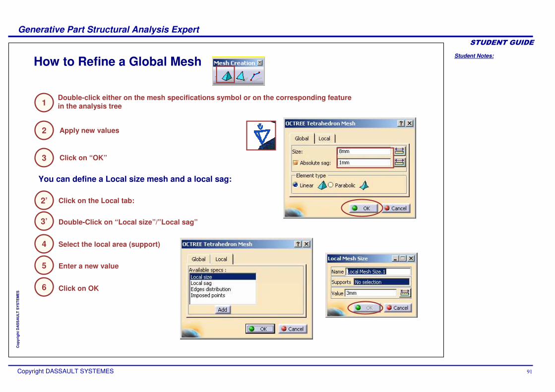
How to Refine a Global Mesh
Double-click either on the mesh specifications symbol or on the corresponding feature in the analysis tree1
You can define a Local size mesh and a local sag:
Apply new values
Click on “OK”
2
3
4
Click on the Local tab:
Double-Click on “Local size”/”Local sag”3’
Select the local area (support)
5 Enter a new value
6 Click on OK
2’
Student Notes:
Generative Part Structural Analysis Expert������������
Copyright DASSAULT SYSTEMES �
Cop
yrig
ht D
AS
SA
ULT
SY
STE
ME
S
How to Refine a Local Mesh
Double-click either on the mesh specifications symbol or on the corresponding feature in the analysis tree.
2
3
4
Click on the Local panel:
Double-Click on “Local size”/”Local sag”
Select the local area (support)
5 Enter a new value
6 Click on OK
Symbol of Local Mesh and local Sag
1

Student Notes:
Generative Part Structural Analysis Expert������������
Copyright DASSAULT SYSTEMES �
Cop
yrig
ht D
AS
SA
ULT
SY
STE
ME
S
Mesh AdaptivityYou will see how to refine a given mesh in areas of interest only.
Student Notes:
Generative Part Structural Analysis Expert������������
Copyright DASSAULT SYSTEMES �
Cop
yrig
ht D
AS
SA
ULT
SY
STE
ME
S
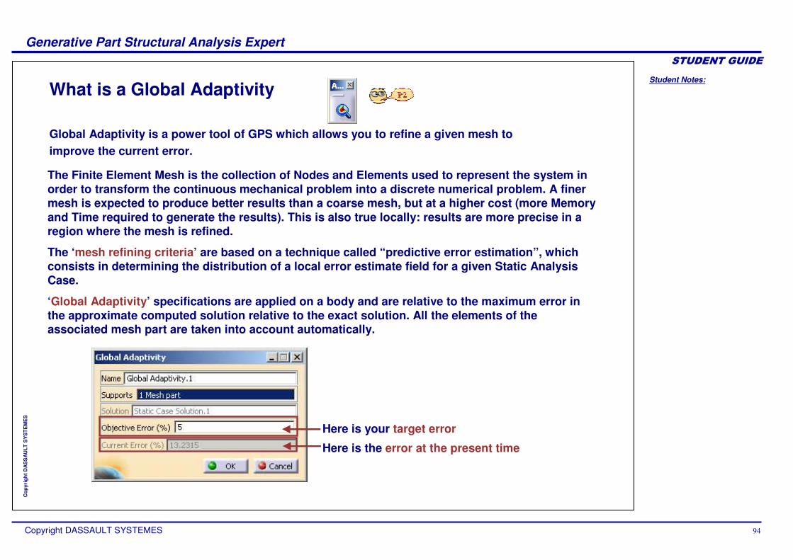
What is a Global Adaptivity
Global Adaptivity is a power tool of GPS which allows you to refine a given mesh to improve the current error.
The Finite Element Mesh is the collection of Nodes and Elements used to represent the system in order to transform the continuous mechanical problem into a discrete numerical problem. A finer mesh is expected to produce better results than a coarse mesh, but at a higher cost (more Memory and Time required to generate the results). This is also true locally: results are more precise in a region where the mesh is refined.
The ‘mesh refining criteria’ are based on a technique called “predictive error estimation”, which consists in determining the distribution of a local error estimate field for a given Static Analysis Case.
‘Global Adaptivity’ specifications are applied on a body and are relative to the maximum error in the approximate computed solution relative to the exact solution. All the elements of the associated mesh part are taken into account automatically.
Here is your target error
Here is the error at the present time
Student Notes:
Generative Part Structural Analysis Expert������������
Copyright DASSAULT SYSTEMES �
Cop
yrig
ht D
AS
SA
ULT
SY
STE
ME
S
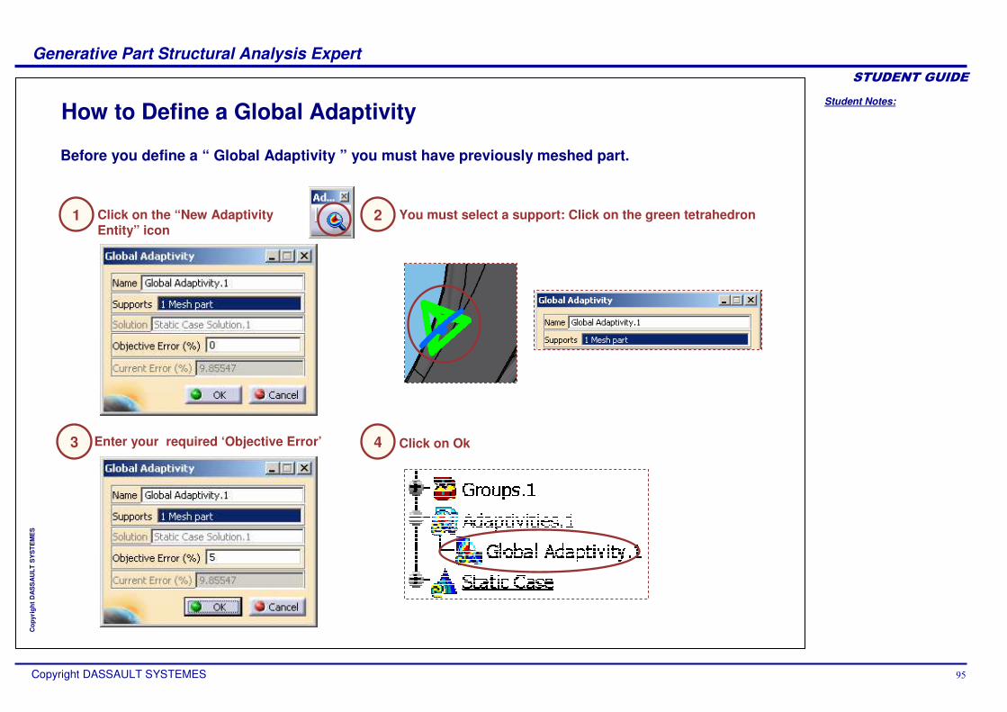
How to Define a Global Adaptivity
1 Click on the “New Adaptivity Entity” icon
Before you define a “ Global Adaptivity ” you must have previously meshed part.
2 You must select a support: Click on the green tetrahedron
4 Click on OkEnter your required ‘Objective Error’3

Student Notes:
Generative Part Structural Analysis Expert������������
Copyright DASSAULT SYSTEMES �
Cop
yrig
ht D
AS
SA
ULT
SY
STE
ME
S
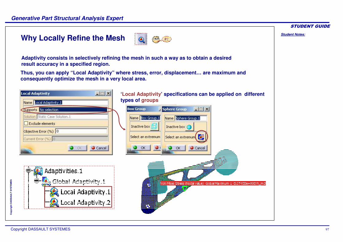
What is a Local Adaptivity
The user can define a local adaptivity specification, to locally overload the global objectives.
It is necessary to define a Global Adaptivity’ specification. Local Adaptivity is optional but can be defined using the contextual menu:
Local Adaptivity specifications can be applied on different types of groups : A geometry group (elements connected to an edge, a surface, a vertex) A box group
Box groups (cube or sphere) are easier to manipulate: their volume is filled and made transparent to show the intersected part of the geometry. Besides, they can be snapped on extrema, whatever their nature.
Student Notes:
Generative Part Structural Analysis Expert������������
Copyright DASSAULT SYSTEMES �
Cop
yrig
ht D
AS
SA
ULT
SY
STE
ME
S
Why Locally Refine the Mesh
Adaptivity consists in selectively refining the mesh in such a way as to obtain a desired result accuracy in a specified region.
Thus, you can apply “Local Adaptivity” where stress, error, displacement… are maximum and consequently optimize the mesh in a very local area.
‘Local Adaptivity’ specifications can be applied on different types of groups
Student Notes:
Generative Part Structural Analysis Expert������������
Copyright DASSAULT SYSTEMES �
Cop
yrig
ht D
AS
SA
ULT
SY
STE
ME
S
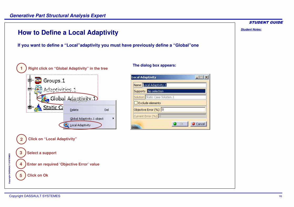
How to Define a Local Adaptivity
1 Right click on “Global Adaptivity” in the tree
If you want to define a “Local”adaptivity you must have previously define a “Global”one
2 Click on “Local Adaptivity”
5 Click on Ok
Select a support3
The dialog box appears:
Enter an required ‘Objective Error’ value4
Student Notes:
Generative Part Structural Analysis Expert������������
Copyright DASSAULT SYSTEMES
Cop
yrig
ht D
AS
SA
ULT
SY
STE
ME
S
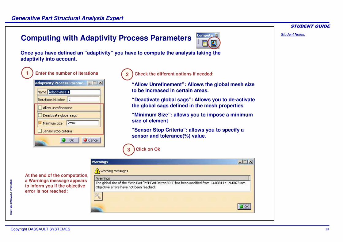
Computing with Adaptivity Process Parameters
Once you have defined an “adaptivity” you have to compute the analysis taking the adaptivity into account.
“Allow Unrefinement”: Allows the global mesh size to be increased in certain areas.
“Deactivate global sags”: Allows you to de-activate the global sags defined in the mesh properties
“Minimum Size”: allows you to impose a minimum size of element
“Sensor Stop Criteria”: allows you to specify a sensor and tolerance(%) value.
At the end of the computation, a Warnings message appears to inform you if the objective error is not reached:
2
3
1 Enter the number of iterations Check the different options if needed:
Click on Ok
Student Notes:
Generative Part Structural Analysis Expert������������
Copyright DASSAULT SYSTEMES �
Cop
yrig
ht D
AS
SA
ULT
SY
STE
ME
S
In the “refinement” lesson, you have seen how to improve the analysis by:
Refining the Mesh either globally or locallyUsing “Adaptivity”
To Sum Up ...
Student Notes:
Generative Part Structural Analysis Expert������������
Copyright DASSAULT SYSTEMES ��
Cop
yrig
ht D
AS
SA
ULT
SY
STE
ME
S
In the Advanced Post-processing lesson, you have seen how to :
Visualize ResultsManage ResultsRefine the analysis
To Sum Up ...

Student Notes:
Generative Part Structural Analysis Expert������������
Copyright DASSAULT SYSTEMES ��
Cop
yrig
ht D
AS
SA
ULT
SY
STE
ME
S
In the course, you have seen how to :
Use Advanced Pre-Processing toolsCompute Frequency AnalysisUse Advanced Post-Processing tools
To Sum Up ...