Stress formulation for frictionless contact ofan elastic-perfectly-plastic body

Mircea Sofonea†, Nicolas Renon†, and Meir Shillor‡

† Laboratoire Theorie des Systemes, Universite de Perpignan,

52 Avenue de Villeneuve, 66860 Perpignan, France

‡ Department of Mathematics and Statistics, Oakland University

Rochester, MI 48309, USA∗

1 July 2003

Abstract

A mathematical model for frictionless contact of a deformable body with a rigidmoving obstacle is analyzed. The Prandtl-Reuss elastic-perfectly-plastic constitu-tive law is used to describe the material’s behavior and contact is modelled with aunilateral condition imposed on the surface velocity. The problem is motivated bythe process of the plowing of the ground. A variational formulation of the problemis derived in terms of the stresses and the existence of the unique weak solutionis proven. The proof is based on arguments for differential inclusions obtained inAmassad et al. (2001). Finally, a study of the continuous dependence of the solutionon the data is presented.

Keywords and phrases : Perfectly plastic material, quasistatic, unilateral frictionless

contact, weak solution, differential inclusion.

AMS Subject Classification : 74C05, 74M15, 35R70.

1 . Introduction

Evolution problems involving elastic-perfectly-plastic solids have developed remarkablyin the last few decades, based on new developments in convex analysis and the theoryof nonlinear equations with maximal monotone operators. An existence and uniquenessresult for the stress field in the quasistatic problem for elastic-plastic materials was ob-tained by Moreau [10] using the geometrical theory of catching up by a moving convex set.

∗email: sofonea@gala.univ-perp.fr, shillor@oakland.edu

1

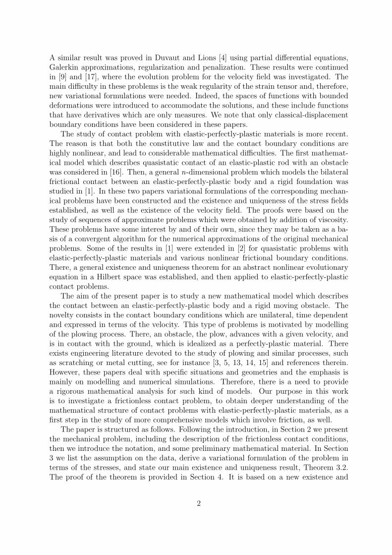
A similar result was proved in Duvaut and Lions [4] using partial differential equations,Galerkin approximations, regularization and penalization. These results were continuedin [9] and [17], where the evolution problem for the velocity field was investigated. Themain difficulty in these problems is the weak regularity of the strain tensor and, therefore,new variational formulations were needed. Indeed, the spaces of functions with boundeddeformations were introduced to accommodate the solutions, and these include functionsthat have derivatives which are only measures. We note that only classical-displacementboundary conditions have been considered in these papers.

The study of contact problem with elastic-perfectly-plastic materials is more recent.The reason is that both the constitutive law and the contact boundary conditions arehighly nonlinear, and lead to considerable mathematical difficulties. The first mathemat-ical model which describes quasistatic contact of an elastic-plastic rod with an obstaclewas considered in [16]. Then, a general n-dimensional problem which models the bilateralfrictional contact between an elastic-perfectly-plastic body and a rigid foundation wasstudied in [1]. In these two papers variational formulations of the corresponding mechan-ical problems have been constructed and the existence and uniqueness of the stress fieldsestablished, as well as the existence of the velocity field. The proofs were based on thestudy of sequences of approximate problems which were obtained by addition of viscosity.These problems have some interest by and of their own, since they may be taken as a ba-sis of a convergent algorithm for the numerical approximations of the original mechanicalproblems. Some of the results in [1] were extended in [2] for quasistatic problems withelastic-perfectly-plastic materials and various nonlinear frictional boundary conditions.There, a general existence and uniqueness theorem for an abstract nonlinear evolutionaryequation in a Hilbert space was established, and then applied to elastic-perfectly-plasticcontact problems.

The aim of the present paper is to study a new mathematical model which describesthe contact between an elastic-perfectly-plastic body and a rigid moving obstacle. Thenovelty consists in the contact boundary conditions which are unilateral, time dependentand expressed in terms of the velocity. This type of problems is motivated by modellingof the plowing process. There, an obstacle, the plow, advances with a given velocity, andis in contact with the ground, which is idealized as a perfectly-plastic material. Thereexists engineering literature devoted to the study of plowing and similar processes, suchas scratching or metal cutting, see for instance [3, 5, 13, 14, 15] and references therein.However, these papers deal with specific situations and geometries and the emphasis ismainly on modelling and numerical simulations. Therefore, there is a need to providea rigorous mathematical analysis for such kind of models. Our purpose in this workis to investigate a frictionless contact problem, to obtain deeper understanding of themathematical structure of contact problems with elastic-perfectly-plastic materials, as afirst step in the study of more comprehensive models which involve friction, as well.

The paper is structured as follows. Following the introduction, in Section 2 we presentthe mechanical problem, including the description of the frictionless contact conditions,then we introduce the notation, and some preliminary mathematical material. In Section3 we list the assumption on the data, derive a variational formulation of the problem interms of the stresses, and state our main existence and uniqueness result, Theorem 3.2.The proof of the theorem is provided in Section 4. It is based on a new existence and

2

uniqueness result for differential inclusions which contain time dependent convex sets,that was obtained in [2]. Finally, in Section 5 we study the continuous dependence of thesolution on the velocity of the obstacle.

2 . The model, notation and preliminaries

We consider a deformable body which occupies a domain Ω ⊂ Rd (d = 2, 3) whoseboundary Γ = ∂Ω is assumed to be Lipschitz and is divided into three disjoint measurableparts ΓD,ΓN and ΓC , such that meas(ΓD) > 0. Let T > 0 and let [0, T ] represent thetime interval of interest. The body is acted up by body forces of density fB in Ω and giventraction forces of density fN on ΓN , while its displacement is imposed on ΓD. Moreover,it may come in contact with a rigid moving obstacle on the potential contact surface ΓC

and here is where our interest lies. Since Γ is Lipschitz continuous, the outer unit normalν = (ν1, . . . , νd) is defined at almost all the points of the surface.

We denote by u = (u1, · · · , ud) the displacement field, by σ = (σij) the stress tensorand ε(u) = (εij) = (ui,j+uj,i)/2 the linearized strain tensor. Here and below, i, j = 1, ..., d,summation over repeated indices is implied and an index that follows a comma indicatesa partial derivative with respect to the corresponding component of the spatial variable.

We model the behavior of the material with the Prandtl-Reuss elastic-perfectly-plasticconstitutive law, i.e.,

Aσ + ∂IK(σ) ∋ ε(u).

Here, A denotes the tensor of elastic compliances, K is the set of elastic stresses and,throughout this paper, a dot above a variable represents the derivative with respect totime. Also, ∂IK denotes the subdifferential of the indicator function IK on the space ofsymmetric tensors, see (2.12) and (2.13) for details. We refer the reader to [4, 6, 7, 17], andreferences therein, for a more detailed description of elastic-perfectly-plastic constitutivelaws.

The motion of part ΓC is restricted by the presence of a rigid obstacle which is movingtowards the body. We denote by v⋆ the velocity of the obstacle and use the subscripts νand τ to indicate the normal and tangential components of vectors and tensors on ΓC . Weuse the unilateral condition imposed on the velocity and, since the contact is frictionless,we impose the following conditions on ΓC :

uν ≤ v⋆ν , σν ≤ 0, σν(uν − v⋆ν) = 0, (2.1)

στ = 0. (2.2)

A version of these contact conditions, with friction, but with v⋆ = 0, was considered in[8] in the study of a dynamic problem for viscoelastic bodies.

The motivation for this study comes from the recent publications [13, 14, 15] wherea model for the process of plowing of the ground has been proposed and numericallysimulated. In this model a rigid body, the plow, is moving in a elasto-plastic medium, theground, with a more or less constant or known velocity. The problem that we study heremay be considered as a step towards a more comprehensive description of the process ofplowing.

3

This is, to best of our knowledge, the only example of a real process where the unilateralcondition on the velocity correctly models the process. In some mathematically orientedpapers, see e.g., [8], the condition was used for mathematical reasons. The point is thefollowing. If the obstacle is stationary or moves tangentially to the contact surface, thecondition (2.1) in the normal direction implies that uν ≤ 0 (since v⋆ν = 0), which meansthat once contact is lost it cannot be regained. That is usually not the case in applications.On the other-hand, in the plowing process the ground has to move away from the plow,which yields condition (2.1).

Finally, we assume that the process is quasistatic and we neglect the inertial terms inthe equations of motion. The following is our model of the frictionless contact betweenan elastic-perfectly-plastic body and a rigid moving foundation.

Problem P . Find a displacement field u : Ω × [0, T ] → Rd, and a stress field σ :Ω× [0, T ] → Sd such that

Aσ + ∂IK(σ) ∋ ε(u) in Ω× (0, T ), (2.3)

Div σ + fB = 0 in Ω× (0, T ), (2.4)

u = u⋆ on ΓD × (0, T ), (2.5)

σν = fN on ΓN × (0, T ), (2.6)

uν ≤ v⋆ν , σν ≤ 0, σν(uν − v⋆ν) = 0, στ = 0 on ΓC × (0, T ), (2.7)

u(0) = u0, σ(0) = σ0 in Ω. (2.8)

Here, the surface traction vector is given by (σν)i = σijνj (see below for notation), Sd

represents the space of second order symmetric tensors on Rd, u⋆ is the given displacementfield on ΓD, and u0, σ0 are the initial conditions. We need both the initial displacementsand stress, since dealing with possible plastic deformations makes it impossible to deducethe initial stress from the initial displacements .

To obtain a variationnal formulation of Problem P we need to introduce some notationand preliminaries. We use “ · ” and | · | to denote the inner product and the Euclideannorm on Rd and Sd, respectively, and 0d will denote the zero element of Sd. We usestandard notation for Lp and Sobolev spaces associated to Ω and Γ and, moreover, weuse the spaces

H =u = (ui) | ui ∈ L2(Ω)

, H =

σ = (σij) | σij = σji ∈ L2(Ω)

,

H1 =u = (ui) | ui ∈ H1(Ω)

, H1 =

σ ∈ H | σij,j ∈ H

.

The spaces H, H, H1 and H1 are real Hilbert spaces endowed with their canonical innerproducts given by

(u, v)H =

∫Ω

uivi dx, (σ, τ)H =

∫Ω

σijτij dx,

(u, v)H1 = (u, v)H + (ε(u), ε(v))H, (σ, τ)H1 = (σ, τ)H + (Div σ,Div τ)H ,

respectively, where ε : H1 → H and Div : H1 → H are the deformation and the divergenceoperators, respectively, defined by

ε(v) = (εij(v)), Div σ = (σij,j).

4

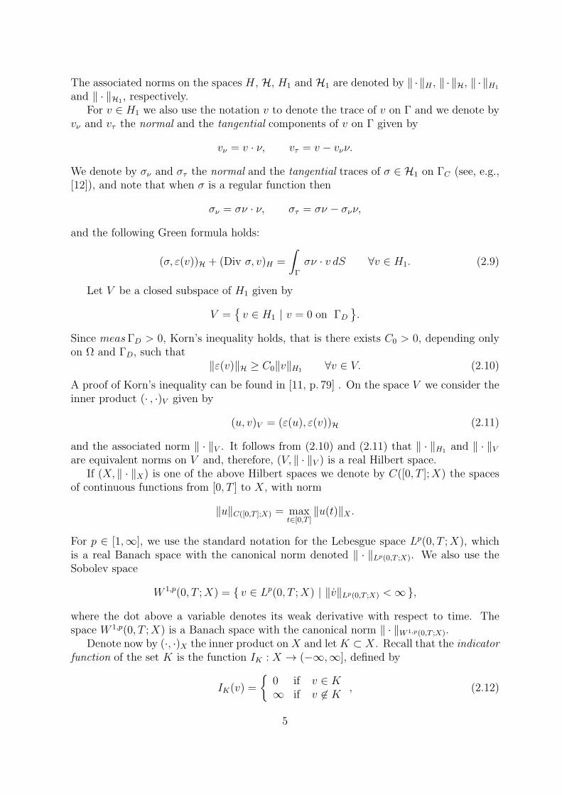
The associated norms on the spaces H, H, H1 and H1 are denoted by ∥ · ∥H , ∥ · ∥H, ∥ · ∥H1

and ∥ · ∥H1 , respectively.For v ∈ H1 we also use the notation v to denote the trace of v on Γ and we denote by

vν and vτ the normal and the tangential components of v on Γ given by

vν = v · ν, vτ = v − vνν.

We denote by σν and στ the normal and the tangential traces of σ ∈ H1 on ΓC (see, e.g.,[12]), and note that when σ is a regular function then

σν = σν · ν, στ = σν − σνν,

and the following Green formula holds:

(σ, ε(v))H + (Div σ, v)H =

∫Γ

σν · v dS ∀v ∈ H1. (2.9)

Let V be a closed subspace of H1 given by

V =v ∈ H1 | v = 0 on ΓD

.

Since measΓD > 0, Korn’s inequality holds, that is there exists C0 > 0, depending onlyon Ω and ΓD, such that

∥ε(v)∥H ≥ C0∥v∥H1 ∀v ∈ V. (2.10)

A proof of Korn’s inequality can be found in [11, p. 79] . On the space V we consider theinner product (· , ·)V given by

(u, v)V = (ε(u), ε(v))H (2.11)

and the associated norm ∥ · ∥V . It follows from (2.10) and (2.11) that ∥ · ∥H1 and ∥ · ∥Vare equivalent norms on V and, therefore, (V, ∥ · ∥V ) is a real Hilbert space.

If (X, ∥ · ∥X) is one of the above Hilbert spaces we denote by C([0, T ];X) the spacesof continuous functions from [0, T ] to X, with norm

∥u∥C([0,T ];X) = maxt∈[0,T ]

∥u(t)∥X .

For p ∈ [1,∞], we use the standard notation for the Lebesgue space Lp(0, T ;X), whichis a real Banach space with the canonical norm denoted ∥ · ∥Lp(0,T ;X). We also use theSobolev space

W 1,p(0, T ;X) = v ∈ Lp(0, T ;X) | ∥v∥Lp(0,T ;X) < ∞,

where the dot above a variable denotes its weak derivative with respect to time. Thespace W 1,p(0, T ;X) is a Banach space with the canonical norm ∥ · ∥W 1,p(0,T ;X).

Denote now by (·, ·)X the inner product on X and letK ⊂ X. Recall that the indicatorfunction of the set K is the function IK : X → (−∞,∞], defined by

IK(v) =

0 if v ∈ K∞ if v ∈ K

, (2.12)

5

and its subdifferential, denoted by ∂IK , is the multivalued operator defined by

∂IK(v) =

f ∈ X | (f, v − u)X ≤ 0 ∀v ∈ K if u ∈ K

∅ if u ∈ K. (2.13)

The subdifferential is used to enforce the plastic flow when the stresses reach the yieldlimit, i.e., the boundary of the set K.

3 . Variationnal Formulation and main result

We describe, in this section, the assumptions on the data, obtain a variational formulationin terms of the stress field, and state the main result of this paper.

We begin with the assumptions on the data for problem (2.3)–(2.8).

The operator A = (Aijkl) : Ω× Sd −→ Sd satisfies,(a) Aijkl ∈ L∞(Ω) ∀ i, j, k, l = 1, ..., d;

(b) Aσ · τ = σ · Aτ σ, τ ∈ Sd, a.e. in Ω;

(c) there exists m > 0 such that Aσ · σ ≥ m∥σ∥2∀σ ∈ Sd, a.e. in Ω.

(3.1)

K ⊂ Sd is a closed convex set such that 0d ∈ K. (3.2)

fB ∈ W 1,∞(0, T ;H), fN ∈ W 1,∞(0, T ;L2(ΓN)d). (3.3)

Using the Riesz representation theorem we define the function F : [0, T ] → V by

(F (t), v)V =

∫Ω

fB(t) · v dx+

∫ΓN

fN(t) · v dS ∀v ∈ V, t ∈ [0, T ], (3.4)

which is a formal way of combining the prescribed body forces and surface tractions intoone expression, acting as an input to the problem. We notice that from (3.3) it followsthat

F ∈ W 1,∞(0, T ;V ). (3.5)

We assume there exists v ∈ L2(0, T ;H1) such that

v(t) = u⋆(t) on ΓD, vν(t) = v⋆ν(t) on ΓC , a.e. t ∈ (0, T ), (3.6)

which represents both a regularity and a compatibility condition involving the data u⋆

and v⋆ of the mechanical problem (2.3)-(2.8).Let t ∈ [0, T ]. Keeping in mind the time dependent boundary conditions (2.5) and

(2.7) we need to introduce the set of admissible velocity fields, U(t), given by

U(t) = v ∈ H1 | v = u⋆(t) on ΓD, vν ≤ v⋆ν(t) on ΓC . (3.7)

6

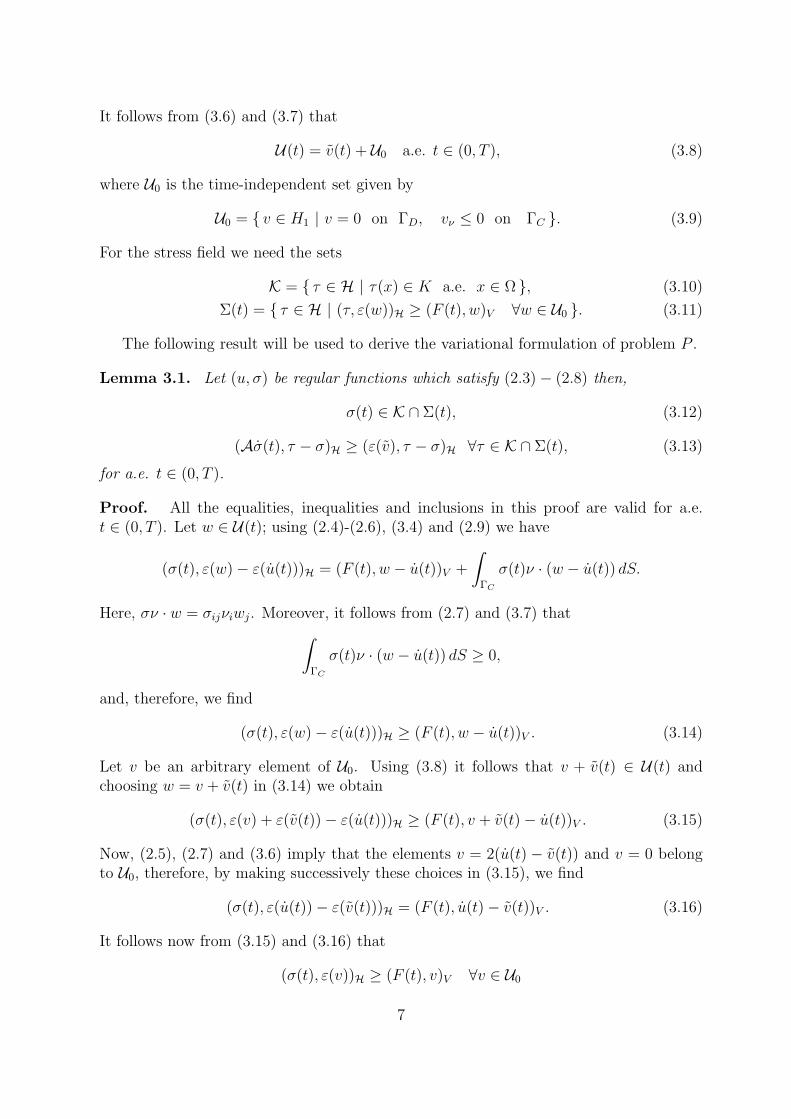
It follows from (3.6) and (3.7) that

U(t) = v(t) + U0 a.e. t ∈ (0, T ), (3.8)

where U0 is the time-independent set given by

U0 = v ∈ H1 | v = 0 on ΓD, vν ≤ 0 on ΓC . (3.9)

For the stress field we need the sets

K = τ ∈ H | τ(x) ∈ K a.e. x ∈ Ω , (3.10)

Σ(t) = τ ∈ H | (τ, ε(w))H ≥ (F (t), w)V ∀w ∈ U0 . (3.11)

The following result will be used to derive the variational formulation of problem P .

Lemma 3.1. Let (u, σ) be regular functions which satisfy (2.3)− (2.8) then,

σ(t) ∈ K ∩ Σ(t), (3.12)

(Aσ(t), τ − σ)H ≥ (ε(v), τ − σ)H ∀τ ∈ K ∩ Σ(t), (3.13)

for a.e. t ∈ (0, T ).

Proof. All the equalities, inequalities and inclusions in this proof are valid for a.e.t ∈ (0, T ). Let w ∈ U(t); using (2.4)-(2.6), (3.4) and (2.9) we have

(σ(t), ε(w)− ε(u(t)))H = (F (t), w − u(t))V +

∫ΓC

σ(t)ν · (w − u(t)) dS.

Here, σν · w = σijνiwj. Moreover, it follows from (2.7) and (3.7) that∫ΓC

σ(t)ν · (w − u(t)) dS ≥ 0,

and, therefore, we find

(σ(t), ε(w)− ε(u(t)))H ≥ (F (t), w − u(t))V . (3.14)

Let v be an arbitrary element of U0. Using (3.8) it follows that v + v(t) ∈ U(t) andchoosing w = v + v(t) in (3.14) we obtain

(σ(t), ε(v) + ε(v(t))− ε(u(t)))H ≥ (F (t), v + v(t)− u(t))V . (3.15)

Now, (2.5), (2.7) and (3.6) imply that the elements v = 2(u(t) − v(t)) and v = 0 belongto U0, therefore, by making successively these choices in (3.15), we find

(σ(t), ε(u(t))− ε(v(t)))H = (F (t), u(t)− v(t))V . (3.16)

It follows now from (3.15) and (3.16) that

(σ(t), ε(v))H ≥ (F (t), v)V ∀v ∈ U0

7

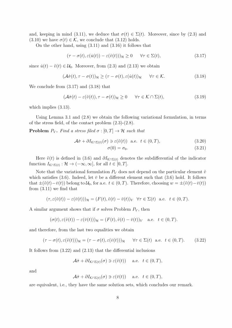
and, keeping in mind (3.11), we deduce that σ(t) ∈ Σ(t). Moreover, since by (2.3) and(3.10) we have σ(t) ∈ K, we conclude that (3.12) holds.

On the other hand, using (3.11) and (3.16) it follows that

(τ − σ(t), ε(u(t))− ε(v(t)))H ≥ 0 ∀τ ∈ Σ(t), (3.17)

since u(t)− v(t) ∈ U0. Moreover, from (2.3) and (2.13) we obtain

(Aσ(t), τ − σ(t))H ≥ (τ − σ(t), ε(u(t))H ∀τ ∈ K. (3.18)

We conclude from (3.17) and (3.18) that

(Aσ(t)− ε(v(t)), τ − σ(t))H ≥ 0 ∀τ ∈ K ∩ Σ(t), (3.19)

which implies (3.13).

Using Lemma 3.1 and (2.8) we obtain the following variational formulation, in termsof the stress field, of the contact problem (2.3)-(2.8).

Problem PV . Find a stress filed σ : [0, T ] → H such that

Aσ + ∂IK∩Σ(t)(σ) ∋ ε(v(t)) a.e. t ∈ (0, T ), (3.20)

σ(0) = σ0. (3.21)

Here v(t) is defined in (3.6) and ∂IK∩Σ(t) denotes the subdifferential of the indicatorfunction IK∩Σ(t) : H → (−∞,∞], for all t ∈ [0, T ].

Note that the variational formulation PV does not depend on the particular element vwhich satisfies (3.6). Indeed, let v be a different element such that (3.6) hold. It followsthat ±(v(t)−v(t)) belong to U0, for a.e. t ∈ (0, T ). Therefore, choosing w = ±(v(t)−v(t))from (3.11) we find that

(τ, ε(v(t))− ε(v(t)))H = (F (t), v(t)− v(t))V ∀τ ∈ Σ(t) a.e. t ∈ (0, T ).

A similar argument shows that if σ solves Problem PV , then

(σ(t), ε(v(t))− ε(v(t)))H = (F (t), v(t)− v(t))V a.e. t ∈ (0, T ).

and therefore, from the last two equalities we obtain

(τ − σ(t), ε(v(t)))H = (τ − σ(t), ε(v(t)))H ∀τ ∈ Σ(t) a.e. t ∈ (0, T ). (3.22)

It follows from (3.22) and (2.13) that the differential inclusions

Aσ + ∂IK∩Σ(t)(σ) ∋ ε(v(t)) a.e. t ∈ (0, T ),

andAσ + ∂IK∩Σ(t)(σ) ∋ ε(v(t)) a.e. t ∈ (0, T ),

are equivalent, i.e., they have the same solution sets, which concludes our remark.

8

To prove the well posedness of problem PV we need the function χ : [0, T ] → H definedby

χ(t) = ε(F (t)), (3.23)

where F is given by (3.4). This is done for mathematical reasons, which will become clearbelow. Moreover, we assume that there exists a positive δ such that

χ(t) + τ ∈ K for all t ∈ [0, T ] and for all τ ∈ H such that ∥τ∥H ≤ δ, (3.24)

and, finally,σ0 = χ(0). (3.25)

We note that assumptions (3.24) and (3.25) represent a compatibility condition on theproblem data similar to the one used in [1, 2, 9, 10, 17].

The main result of this paper is stated in the following theorem.

Theorem 3.2. Assume that (3.1) − (3.3), (3.6), (3.24) and (3.25) hold. Then, thereexists a unique solution of the Cauchy problem (3.20) and (3.21). Moreover, the solutionsatisfies σ ∈ W 1,2(0, T,H), and Div σ ∈ W 1,∞(0, T,H).

We conclude from Theorem 3.2 the existence of a unique weak solution, in terms ofthe stresses, to the frictionless contact problem (2.3)-(2.8).

4 . Proof of Theorem 3.2

To prove Theorem 3.2 we need an abstract result that we now present. First, let X be areal Hilbert space with the inner product (·, ·)X and the associated norm ∥ · ∥X . We have,

Theorem 4.1. Let A : X → X be a positive definite and symmetric operator defined onX. Let K and Σ0 be two closed convex sets in X and let χ : [0, T ] → X be given, whereT > 0. Let Σ(t), for all t ∈ [0, T ], be the set

Σ(t) = Σ0 + χ(t). (4.1)

Denote by IK∩Σ(t) : H −→ (−∞,∞] the indicator function of the set K ∩ Σ(t). Assumethat

f ∈ L2(0, T ;X), (4.2)

χ ∈ W 1,∞(0, T ;X), (4.3)

and also, there exists a positive δ such that

χ(t) + z ∈ K for all t ∈ [0, T ] and for all z ∈ X such that ∥z∥X ≤ δ, (4.4)

χ(0) ∈ Σ(0). (4.5)

Then, there exists a unique function y ∈ W 1,2(0, T ;X) such that

Ay(t) + ∂IK∩Σ(t)(y(t)) ∋ f(t) a.e. t ∈ (0, T ), (4.6)

y(0) = χ(0). (4.7)

9

The proof of Theorem 4.1 may be found in [2] and it is based on classical resultsfrom the theory of evolution equations with maximal monotone operators, fixed pointarguments and regularization.

We use Theorem 4.1 to prove Theorem 3.2 when X = H. To this end, we define theset

Σ0 = τ ∈ H | (τ, ε(w))H ≥ 0 ∀w ∈ U0 . (4.8)

Clearly Σ0 is a closed convex subset of H and it follows from (3.11) and (3.23) thatequality (4.1) holds for all t ∈ [0, T ]. Notice that 0H ∈ Σ0 and, therefore, we obtain from(4.1) that (4.5) holds, too. Moreover, (3.5) and (3.23) imply that

χ ∈ W 1,∞(0, T ;H). (4.9)

Furthermore, since v ∈ L2(0, T ;H1) then,

ε(v) ∈ L2(0, T ;H). (4.10)

Recall that (3.2) implies that the set K, (3.10), is a closed and convex subset of H, and(3.1) allows us to consider A as a positive definite and symmetric operator on H.

Using now (4.9), (4.10), and (3.24), we may apply Theorem 4.1, with the space H andf = ε(v). Thus, we obtain the existence and uniqueness of a function σ ∈ W 1,2(0, T,H)which satisfies (3.20) and σ(0) = χ(0). Using now (3.25) it follows that (3.21) holds too.Since σ(t) ∈ K ∩ Σ(t), for all t ∈ [0, T ], it follows from (3.11) that

(σ(t), ε(w))H ≥ (F (t), w)V ∀w ∈ U .

Therefore, by choosing w = ±ϕ ∈ D(Ω)d, where D(Ω)d is the space of infinitely differen-tiable vector functions with compact support in Ω, and using (3.4) we deduce

Div σ(t) + fB(t) = 0 in Ω, for all t ∈ [0, T ]. (4.11)

Keeping now in mind (3.3) we find that Div σ ∈ W 1,∞(0, T,H) which concludes theexistence part of the Theorem. The uniqueness ot the solution is a consequence of theunique solvability of the abstract problem (4.6), (4.7), guaranteed by Theorem 4.1.

5 . Continuous dependence results

In this section we provide estimate on the solution of the problem, which lead to itscontinuous dependence on the data. We suppose in what follows that (3.1)-(3.3), (3.24)and (3.25) hold, and for α ≥ 0 we denote by u⋆

α and v⋆α a perturbation of the data u⋆ andv⋆, respectively. We assume that there exists vα ∈ L2(0, T ;H1) such that

vα(t) = u⋆α(t) on ΓD, vαν(t) = v⋆αν(t) on ΓC , a.e. t ∈ (0, T ), (5.1)

and we consider the following family of variational problems, parametrized by α.

10

Problem PαV : Find a stress field σα : [0, T ] → H such that

Aσα + ∂IK∩Σ(t)(σα) ∋ ε(vα(t)) a.e. t ∈ (0, T ), (5.2)

σα(0) = σ0. (5.3)

Problem P αV represents the variational formulation of the mechanical problem (2.3)-

(2.8), when the displacement field u⋆ and the velocity field v⋆ are replaced by the u⋆α and

v⋆α, respectively.It follows from Theorem 3.2 that problem Pα

V has a unique solution σα which satisfiesσα ∈ W 1,2(0, T ;H) and Div σα ∈ W 1,2(0, T ;H).

The main result of this section is the following estimate, which will lead to the con-tinuous dependence on v⋆.

Theorem 5.1. Assume that (3.1)− (3.3), (3.6), (3.24), (3.25) and (5.1) hold and denoteby σα and σ the solutions of problems Pα

V and PV , respectively. Then, the followinginequality holds:

∥σα(s)− σ(s)∥H ≤ 1

m

∫ s

0

∥vα(t)− v(t)∥H1 dt ∀s ∈ [0, T ]. (5.4)

Proof. It follows from (3.20) and (5.2) that σ ∈ K ∩ Σ(t), σα ∈ K ∩ Σ(t) for all t ∈ [0, T ],and

(Aσ(t), τ − σ(t))H ≥ (ε(v(t)), τ − σ(t))H

(Aσα(t), τ − σ(t))H ≥ (ε(vα(t)), τ − σ(t))H

for all τ ∈ K ∩ Σ(t), a.e. t ∈ (0, T ). We choose τ = σα(t) in the first inequality, τ = σ(t)in the second one and add the resulting inequalities to obtain

(Aσα(t)−Aσ(t), σα(t)− σ(t))H ≤(ε(vα(t))− ε(v(t)), σα(t)− σ(t))H a.e. t ∈ (0, T ).

Let s ∈ [0, T ]. We integrate the previous inequality on [0, s], then we use (3.1), (3.21) and(5.3) to obtain

1

2∥σα(s)− σ(s)∥2H1

≤ 1

m

∫ s

0

∥σα(t)− σ(t)∥H∥ε(vα(t))− ε(v(t))∥H dt. (5.5)

Inequality (5.4) follows now from (5.5), by using Gronwall’s inequality.

This result allows us to show the convergence of the weak solution to problem Pwith respect to the velocity of the obstacle v⋆. Indeed, let HΓ = H

12 (Γ)d; denote by

γ : H1 → HΓ the trace operator; and let Z : HΓ → H1 be a linear continuous operatorsuch that

γ(Z(ξ)) = ξ ∀ξ ∈ HΓ. (5.6)

11

We refer the reader to [7] for further details about Z. We assume that

v⋆α ∈ L2(0, T ;HΓ), v⋆ ∈ L2(0, T ;HΓ), (5.7)

and use the notation

vα(t) = Zv⋆α(t), v(t) = Zv⋆(t) a.e. t ∈ (0, T ). (5.8)

We assume, in addition, that the data v⋆ and v⋆α are such that

Z(v⋆α(t)) = u⋆α(t), Z(v⋆(t)) = u⋆(t) on ΓD, a.e. t ∈ (0, T ). (5.9)

We have the following result.

Corollary 5.2. Assume that (3.1)−(3.3), (3.24), (3.25), (5.7), (5.8) and (5.9) hold. Then,there exists a unique solution σα to problem Pα

V , and there exists a unique solution σ toproblem PV . Moreover, the regularity ot the solutions is as in Theorem 3.2, and

σα → σ in C([0, T ];H1) as v⋆α → v⋆ in L2(0, T ;HΓ). (5.10)

Proof. We use (5.7)-(5.9) to show that vα ∈ L2(0, T ;H1), v ∈ L2(0, T ;H1) and, that(3.6) and (5.1) hold. The unique solvability of problems Pα

V and PV is now a consequenceof Theorem 3.2. Moreover, it follows from (4.11) that

Div σα(s) = Div σ(s) ∀s ∈ [0, T ].

Using (5.4) we obtain

∥σα(s)− σ(s)∥H1 ≤1

m

∫ s

0

∥vα(t)− v(t)∥H1 dt ∀s ∈ [0, T ], (5.11)

and, keeping in mind (5.8) and the continuity of the operator Z, (5.11) implies (5.10).

In addition to the mathematical interest, the convergence result (5.10) is of importancein applications since it states that small perturbation in the velocity of the obstacle lead tosmall perturbation in the solution. We conclude that the weak solution of the quasistaticproblem (2.3)-(2.8) depends continuously on the velocity of the obstacle.

6 Conclusions

The problem of frictionless contact between an elastic-perfectly-plastic material and arigid moving obstacle, with contact modelled by a unilateral constraint on the velocity,has been shown to have a unique weak solution, in terms of the stress. The material wasassumed to obey the Prandtl-Reuss elastic-perfectly-plastic constitutive relation. Such aproblem may be used as a first step in the modelling of the plowing of the ground.

The proof was based on a new abstract result for differential inclusions establishedin [2]. It was also shown that the problem depends continuously on the velocity of the

12

obstacle, and small perturbations of the obstacle velocity lead to correspondingly smallchanges in the solution.

The same contact problem, but for elastic-perfectly-plastic materials with hardeningis interesting, but remains an open problem. Indeed, there seems to be some experimentalevidence that hardening may take place following a plastic flow of the ground. Anotheropen problem is the addition of friction to the model. There may be considerable meritin the investigation of the corresponding dynamic problems.

Effective numerical methods with proven convergence should be constructed and an-alyzed, and numerical simulations performed.

Finally, a very challenging mathematical problem directly relevant to the plowing isthe modeling and well-posedness of the process using large deformations.

References

[1] A. Amassad, M. Shillor and M. Sofonea, A quasistatic contact problem for an elasticperfectly plastic body with Tresca’s friction, Nonlin. Anal., 35 (1999), 95–109.

[2] A. Amassad, M. Shillor and M. Sofonea, A non linear evolution inclusion in perfectplasticity with friction, Acta Math. Univ. Comenianae, LXX(2) (2001), 215–228.

[3] J. L. Bucaille, Simulation numrique de l’indentation et de la rayure des verres or-ganiques, Ph. D Thesis, Ecole Nationale Suprieure des Mines de Paris, 2001.

[4] G. Duvaut and J. L. Lions, “Inequalities in Mechanics and Physics”, Springer, Berlin,1976.

[5] L. Fourment, J.L. Chenot, K. Mocellin, Numerical formulations and algorithm forsolving contact problems in metal forming simulations, Int. J. Num. Meth. Enging.,46 (1999), 1435-1462.

[6] W. Han and M. Sofonea, “ Quasistatic Contact Problems in Viscoelasticity and Vis-coplasticity”, Studies in Advanced Mathematics 30, American Mathematical Society-International Press, 2002.

[7] I. R. Ionescu and M. Sofonea, “Functional and Numerical Methods in Viscoplastic-ity”, Oxford University Press, Oxford, 1993.

[8] Jarusek, J., Eck. C, Dynamic contact problems with small Coulomb friction forviscoelastic bodies. Existence of Solutions, Math. Models Meth. in Appl. Sci., 9 (1999),11-34.

[9] C. Johnson, Existence theorems in plasticity. J. Math. Pures et Appl. 55(1976),431-444.

[10] J. J. Moreau, Application of convex analysis to the treatment of elasto-plastic sys-tems, in Springer Lecture Notes in Mathematics No. 503, P. Germain and B. Nayroles(Eds.), 1975.

13

[11] J. Necas and I. Hlavacek, “Mathematical Theory of Elastic and Elastoplastic bodies:an introduction”, Elsevier, Amsterdam, 1981.

[12] P. D. Panagiotopoulos, “Inequality Problems in Mechanics and Applications”,Birkhauser, Basel, 1985.

[13] N. Renon, Simulation numrique par elements finis des grandes deformations des Sols.Application a la scarification., Ph. D Thesis, Ecole Nationale Superieure des Minesde Paris, 2002.

[14] N. Renon, P. Montmitonnet, P. Laborde, A 3D Finite Element Model for Soil/ToolInteraction in large Deformation, preprint (2003).

[15] N. Renon, M. Sofonea and M. Shillor, Un modele mathematique pour un problemede contact elasto-plastique avec ecrouissage. Application a la scarification, Actes du10 eme Colloque Franco-Polonais de Mecanique, Ecole Polytechnique de Varsovie etEcole Polytechnique Universitaire de Lille (2002), 7–16.

[16] M. Shillor and M. Sofonea, A quasistatic contact problem for an elastoplastic rod, J.Math. Anal. Appl., 217(1998), 579-596.

[17] P. Suquet, Evolution problems for a class of dissipative materials, Quart. J. Appl.Math., 38 (1981), 391–414.

14