Strategic and Tactical Planning of the Downstream

Petroleum Supply Chain

Carolina Diniz Melo

Thesis to obtain the Master of Science Degree in

Petroleum Engineering

Supervisors: Doctor Ana Paula Ferreira Dias Barbosa Póvoa

Doctor Susana Isabel Carvalho Relvas

Examination Committee

Chairperson: Doctor Maria João Correia Colunas Pereira

Supervisor: Doctor Susana Isabel Carvalho Relvas

Members of the Committee: Doctor Leão José Fernandes

July 2019

i

Dedicatory

To all women in science.

Our path is harder but we can change the world.

ii

Declaration

I declare that this document is an original work of my own authorship and that it fulfills all the

requirements of the Code of Conduct and Good Practices of the Universidade de Lisboa.

iii

ABSTRACT

Petroleum Supply Chain (PSC) is divided into three main segments: upstream, midstream

and downstream. Considering these three segments, there are still some research gaps in the

downstream supply chain considering the strategic-tactical decision levels. Therefore, the aim of this

thesis is to develop a Mixed Integer Linear Programming (MILP) mathematical model that will support

the definition of a distribution strategy for supplying markets that may span over more than one

country.

The model is based on that developed by Kazemi & Szmerekovsky (2015), which addresses

strategic and tactical decisions (such as determining optimal location and capacities for distribution

centers, selection of transportation modes, determining flow allocation, etc.) considering multiple

products while minimize the fixed and distributing costs. The model proposed in this work extends

the previous work and adds terms in objective function and constraints related to imports and exports

between countries, not yet considered.

In order to test and validate the model developed, an illustrative case study was considered

and to show the applicability of the model, a real case comprising the Portuguese oil supply chain

and its operation in Iberia was used considering one of the market players present in both countries.

The model was implemented in GAMS programming language and solved using the solver CPLEX.

The results analyzed not only consider the current network and how it can be optimized in

terms of resource usage, but also foresee which network adjustments would be more advantageous

in the case study selected.

Keywords: downstream petroleum supply chain, optimization, mathematical programming, mixed

integer linear programming, strategic and tactical planning.

iv

RESUMO

A cadeia de abastecimento do petróleo é dividida em três segmentos: upstream, midstream

e downstream. Considerando estes três segmentos, ainda há oportunidade de pesquisa na cadeia

downstream compreendendo os níveis estratégico e tático. Sendo assim, o objetivo dessa

dissertação de mestrado é desenvolver um modelo de programação matemática linear inteira-mista,

que fundamentará a definição de uma estratégia de distribuição para abastecer mercados em mais

de um país.

O modelo desenvolvido é baseado em Kazemi & Szmerekovsky (2015), o qual determina

decisões estratégicas e táticas (tais quais a determinação da localização e capacidades ótimas para

centros de distribuição, seleção de modos de transporte, determinação do fluxo de materiais, etc.)

considerando múltiplos produtos enquanto minimiza os custos fixos e de distribuição. O modelo

proposto neste trabalho expande o trabalho anterior e adiciona termos na função objetivo e restrições

relacionadas a importação e exportação entre países, aspectos ainda não considerados.

Para testar e validar o modelo desenvolvido, um caso ilustrativo foi considerado e para

mostrar a aplicabilidade do modelo, um caso de estudo real considerando a cadeia de abastecimento

do petróleo em Portugal e a sua operação na península Ibérica foi utilizado considerando um dos

players do mercado presente em ambos os países. O modelo foi implementado na linguagem de

programação GAMS e resolvido utilizando o solver CPLEX.

Os resultados analisados não só consideram a presente rede e como esta pode ser

otimizada em termos de utilização de recursos, mas também prevê quais ajustes seriam mais

vantajosos considerando o caso de estudo selecionado.

Palavras-chave: cadeia de abastecimento do petróleo downstream, otimização, programação

matemática, programação linear inteira-mista, planejamento estratégico e tático.

v

Acknowledgments

First, I want to thank God for blessing me with an amazing family. I could not have been born

in a better place.

I want to thank my family for being always supportive in my decisions (even the craziest

ones), being there for me in the toughest moments and visiting me in Portugal. A special thanks to

my parents, who have been always encouraging me, to my grandmother, who is always by my side

and took a plane for the first time (a 10-hour flight) just to visit me and to my godmother, who always

listens to me. You are awesome and I love you all!

I want to thank Polytechnic School of University of São Paulo for making possible the

opportunity of studying these two years abroad at Instituto Superior Técnico in the Double Degree

program and Banco Santander for awarding me with the scholarship.

A special thanks to my supervisors Professor Ana Póvoa and Professor Susana Relvas for

supervising this Master thesis and bringing amazing contributions to this work. Thank you for the

patience and guidance, for providing me an office at Taguspark and for presenting me the colleagues

of Center for Management Studies (CEG-IST), who helped me with GAMS and many other issues.

I want to thank Professor Elsa Vásquez Alvarez from Polytechnic School of University of São

Paulo for supervising my first scientific researches and for presenting me the amazing field of study

of operations research.

Last but not least, to all my friends, thank you for being supportive, listening to me and never

letting me give up. Thanks to my friends that came to Portugal to visit me. Thanks to my friends who

invited me to visit them in Italy and Ireland. Thanks to my friends since childhood who still talk to me

and are there for me no matter how far we are. Thanks to my friends that could not come here but

were always present. Thanks to my friends that I lived with and together we could share many

moments of happiness.

vi

Table of Contents

Chapter 1 – Introduction .................................................................................................... 1

1.1. Motivation and Context ............................................................................................ 1

1.2. Objectives ............................................................................................................... 2

1.3. Methodology ............................................................................................................ 2

1.4. Structure of the thesis .............................................................................................. 3

Chapter 2 – Petroleum Supply Chain ................................................................................. 5

2.1. The Petroleum Supply Chain ................................................................................... 5

2.2. The downstream segment of the Petroleum Supply Chain ....................................... 6

2.3. Decision-Planning Levels......................................................................................... 8

2.4. Operations research in PSC .................................................................................... 8

2.4.1. A brief history of operations research and some currently applications ............... 8

2.4.2. The models in operations research .................................................................... 9

2.4.3. Why use operations research techniques in petroleum supply chain ................ 10

2.5. Conclusion ............................................................................................................ 12

Chapter 3 – Literature Review .......................................................................................... 13

3.1. Strategic planning .................................................................................................. 13

3.1.1. Strategic planning – Deterministic approaches ................................................ 13

3.1.2. Strategic planning – Stochastic problem .......................................................... 15

3.2. Tactical planning ................................................................................................... 15

3.2.1. Tactical planning – Deterministic approaches .................................................. 15

3.2.2. Tactical planning – Stochastic approaches ...................................................... 16

3.3. Operational planning ............................................................................................. 16

3.3.1. Operational planning – Deterministic approaches ............................................ 16

3.4. Strategic and tactical planning ............................................................................... 17

3.4.1. Strategic and tactical planning – Deterministic approaches .............................. 17

3.4.2. Strategic and tactical planning – Stochastic approaches .................................. 19

3.5. Tactical and operational planning ........................................................................... 21

3.5.1. Tactical and operational planning – Deterministic approaches ......................... 21

vii

3.5.2. Tactical and operational planning – Stochastic approaches ............................. 22

3.6. Conclusion ............................................................................................................ 22

Chapter 4 – Problem Definition, Model Formulation and Validation................................... 25

4.1. Problem Definition ................................................................................................. 25

4.2. Mathematical model .............................................................................................. 26

4.2.1. Sets, subsets and parameters ......................................................................... 26

4.2.2. Variables ......................................................................................................... 28

4.2.3. Objective function............................................................................................ 28

4.2.4. Constraints...................................................................................................... 29

4.3. Main contributions of the present developed model ................................................ 31

4.4. Illustrative case study ............................................................................................ 32

4.5. Illustrative case results .......................................................................................... 38

4.6. Conclusion ............................................................................................................ 41

Chapter 5 – Case study ................................................................................................... 43

5.1. Real case study ..................................................................................................... 43

5.1.1. Portuguese downstream oil supply chain ......................................................... 43

5.1.2. The Iberian market .......................................................................................... 45

5.2. Real case database ............................................................................................... 46

5.3. Real case results ................................................................................................... 49

5.3.1. General analysis ............................................................................................. 49

5.3.2. Long-term analysis .......................................................................................... 51

5.4. Suggestions for further works ................................................................................ 53

5.5. Conclusion ............................................................................................................ 54

Chapter 6 – Conclusion ................................................................................................... 57

References ...................................................................................................................... 59

Appendix A – Supplementary results for the illustrative case study ................................... 64

Appendix B – Portuguese PSC and Iberian market database ........................................... 65

Appendix C – Results obtained with the real case study ................................................... 73

viii

List of Figures

Figure 1. Methodology followed. ........................................................................................ 3

Figure 2. Structure of the thesis. ........................................................................................ 4

Figure 3. The petroleum supply chain. ............................................................................... 6

Figure 4. The downstream petroleum supply chain............................................................. 7

Figure 5. Map of the illustrative case. ............................................................................... 33

Figure 6. Available routes in illustrative case. ................................................................... 34

Figure 7. Pipelines (in red) to be built or not. .................................................................... 35

Figure 8. The Portuguese PSC. (Adapted from Autoridade da Concorrência, 2018). ........ 44

Figure 9. The refineries, storages and supply bases in Iberia. (DGEG - Direção-Geral de

Energia e Geologia, s.d.). .................................................................................. 46

Figure 10. Location of possible new distribution center and pipelines ............................... 49

Figure 11. Strategic decisions in long-term ....................................................................... 53

Figure 12. Linear regression analysis of demand forecast in Spain. .................................. 71

List of Tables

Table 1. Summary of papers used in Literature Review. ................................................... 24

Table 2. Sets, subsets and parameters used in the mathematical model .......................... 27

Table 3. Variables used in the mathematical model .......................................................... 28

Table 4. Distance in miles between refineries and depots in Country A ............................ 36

Table 5. Annual maximum transportation capacity between refineries and depots in Country

A ....................................................................................................................... 36

Table 6. Distance in miles between depots and customer nodes in Country A .................. 36

Table 7. Annual maximum transportation capacity between depots and customer nodes in

Country A.......................................................................................................... 36

Table 8. Distance in miles between refineries in Country A and refineries in Country B .... 37

Table 9. Annual maximum transportation capacity between refineries in Country A and

refineries in Country B ....................................................................................... 37

Table 10. Annual refining capacity of each refinery i ......................................................... 37

Table 11. Fraction of total refinery capacity used to produce each product p .................... 37

Table 12. Maximum fraction of product p that is reasonable to be produced by each refinery

in Country A ...................................................................................................... 37

Table 13. Annual demand for each product p at demand nodes u .................................... 38

Table 14. Transportation costs considered in illustrative case study ................................. 38

Table 15. Illustrative case study results for variable Y ...................................................... 39

ix

Table 16. Illustrative case study results for variable Z ....................................................... 39

Table 17. Analysis in a long-term planning horizon ........................................................... 40

Table 18. Performance results for Illustrative case study .................................................. 40

Table 19. Strategic decisions in long-term analysis .......................................................... 52

Table 20. Performance results for real case study ............................................................ 52

Table 21. Illustrative Model 2 results for variable Y. .......................................................... 64

Table 22. Illustrative Model 2 results for variable Z. .......................................................... 64

Table 23. Illustrative Model 2 results for variable IMP. ...................................................... 64

Table 24. Illustrative Model 2 results for variable EXP. ..................................................... 64

Table 25. Illustrative Model 2 results for variable γ. .......................................................... 64

Table 26. Distance in km between refineries in Portugal and depots................................. 65

Table 27. Distance in km between depots and customer nodes in Portugal through trucks.

......................................................................................................................... 66

Table 28. Distance in km between depots and customer nodes in Portugal through barge.67

Table 29. Distance in km between depots and customer nodes in Portugal through pipeline.

......................................................................................................................... 67

Table 30. Distance in km between depots and customer nodes in Portugal through rail. ... 68

Table 31. Distance in km between Portuguese and Spanish refineries through trucks and

barge. ............................................................................................................... 68

Table 32. Maximum refining capacity of Portuguese and Spanish refineries in bbl/day and

m3/year. ............................................................................................................ 69

Table 33. Fraction of the total amount refined by refinery b that is used to produce product p.

......................................................................................................................... 69

Table 34. Ex-refinery prices per m3 of each product p in Portugal and Spain. ................... 69

Table 35. Estimated annual demand for products p in Portugal (tonnes)........................... 70

Table 36. Annual demand for each product p in Spain in thousand tonnes. ...................... 70

Table 37. Transportation costs considered in EUR/ton-km. .............................................. 71

Table 38. Maximum fraction of each product that refineries in Portugal can produce. ....... 72

Table 39. Real case considering Portuguese refineries working at maximum capacity results

for variable Y..................................................................................................... 73

Table 40. Real case considering Portuguese refineries working at maximum capacity results

for variable Z. .................................................................................................... 74

Table 41. Real case considering Portuguese refineries working at maximum capacity results

for variable EXP. ............................................................................................... 74

Table 42. Results obtained for variable Y when considering the real case with 7-year planning

horizon. ............................................................................................................. 75

Table 43. Results obtained for variable Z (gasolines 95 and 98) when considering the real

case with 7-year planning horizon. .................................................................... 76

x

Table 44. Results obtained for variable Z (diesel and jet fuel) when considering the real case

with 7-year planning horizon.............................................................................. 77

Table 45. Results obtained for variable EXP when considering the real case with 7-year

planning horizon................................................................................................ 77

Table 46. Results obtained for variable Y when considering the real case with 10-year

planning horizon................................................................................................ 78

Table 47. Results obtained for variable Z (gasolines 95 and 98) when considering the real

case with 10-year planning horizon. .................................................................. 79

Table 48. Results obtained for variable Z (diesel and jet fuel) when considering the real case

with 10-year planning horizon. ........................................................................... 80

Table 49. Results obtained for variable EXP when considering the real case with 10-year

planning horizon................................................................................................ 81

xi

Acronyms

A1 – Jet Fuel

ARIMA – Autoregressive Integrated Moving Average

B5 – Diesel

BIP – Binary Integer Programming

C3 – Propane

C4 – Butane

CLC – Companhia Logística de Combustíveis

CORES – Corporación de reservas estratégicas de productos petrolíferos

CVaR – Conditional Value-at-Risk

DC – Distribution Center

DSS – Decision Support System

ENPV – Expected Net Present Value

ENSE – Entidade Nacional para o Setor Energético

EUR – Euro

FU – Fuel Oil

GAMS – General Algebraic Modeling System

GO – Gas Oil

IP – Integer Programming

IRP – Integrated Refinery-Planning

LP – Linear Programming

LPG – Liquefied Petroleum Gases

MILFP – Mixed Integer Linear Fractional Programming

MILP – Mixed Integer Linear Programming

MINLP – Mixed Integer Nonlinear Programming

MIP – Mixed Integer Programming

NLP – Nonlinear Programming

NPV – Net Present Value

OR – Operations Research

OSC – Oil Supply Chain

PSC – Petroleum Supply Chain

xii

SAA – Sample Average Approximation

U5 – Gasoline 95

U8 – Gasoline 98

US – United States

USD – US Dollar

1

Chapter 1 – Introduction

This chapter aims to introduce the topic of this Master’s thesis, the objectives and the

methodology. This chapter is structured as follows: Section 1.1 briefly introduces the motivation and

context of the topic of the thesis; Section 1.2 comprises the objectives to be achieved in the thesis;

Section 1.3 explains the methodology followed to develop the thesis; Section 1.4 shows how the

thesis is structured.

1.1. Motivation and Context

Until the middle of the eighteenth century, the world economy relied on the manual

manufacture of products. However, the need of increasing production in order to attend market

demands implied a reinvention of the production methods from hands to machine production powered

by steam. This was the begin of a new era in the world history, better known as First Industrial

Revolution, which took place in England and used coal as a major source of energy (Hobsbawm,

2000).

In spite of coal is still used today, mainly in China, it is not the main source of energy anymore

because it generates a lot of pollution and other more powerful sources of energy were discovered

(BP - British Petroleum, 2018). Thus, during the Second Industrial Revolution in the end of nineteenth

century, the exploration of oil has begun. In Pennsylvania, Edwin Drake successfully drilled the first

modern oil well and the first refineries were built to extract kerosene from crude oil in order to use it

as a lighting and heating fuel. In the early twentieth century, the advent of automotive industry

required another oil product (that was an unwanted product from crude oil at first) to be extracted:

gasoline (Yergin, 1991).

Today the oil and gas industry supplies more than 50% of the whole world energy. Other

energy sources such as renewables are increasing their share but they still far from overcome oil and

natural gas. Oil is also a source of raw material to petrochemical industry, which uses it to produce

plastics, rubber, solvents, etc. Therefore, it is expected that the world will still depend on oil and gas

industry for a few decades to supply its energy needs (BP - British Petroleum, 2018). Since this

industry is the world’s major supplier of energy today and there are enough proven reserves, there

are many research opportunities for studies regarding the oil industry as a constant need of

improvement exists.

One important field of study regarding the oil industry is the planning and management of its

supply chain. Petroleum Supply Chain (PSC) is a complex and dynamic system, which involves high

revenues and high costs. It is divided into three main sectors: upstream, which comprises oil

exploration and production; midstream, responsible for refining operations; and downstream,

considering oil products distribution (Lima, et al., 2018).

2

As the upstream sector has been well researched, there is a great opportunity to explore the

downstream sector in research terms (Fernandes, et al., 2014). As this segment deals with several

products’ distribution it includes a set of diverse facilities such as storage depots, wholesale and retail

market that are linked to two types of distribution: primary and secondary. The distribution includes

several transportation modes, which may even be combinable with each other (Lima, et al., 2016).

Therefore, the complexity of the downstream segment is huge since it deals with a multi-product

distribution between several storages in wholesale and retail market that can be performed using

several types of transportation modes including a combination of more than one mode.

The activities of such systems are costly and in order to seek for minimum costs or maximum

profit, without compromising safety and quality of the operations there is a need of decision supporting

tools to aid the decision-making process (Lima, et al., 2018). This work explores this need and aims

to develop a mathematical model for the downstream supply chain to support the associated planning

process.

1.2. Objectives

The main purpose of this Master’s thesis is to develop a strategy for optimizing the distribution

of oil derivatives in markets that may span over more than one country and to develop a Mixed Integer

Linear Programming (MILP) mathematical model in order to do it. A secondary goal is to apply a real

case of Portuguese PSC and its operation in Iberia to the model in order to demonstrate its potential.

In order to achieve the main purpose of the thesis, intermediate objectives are to be

accomplished: i) to understand the Petroleum Supply Chain and each of the three segments that

composes it: upstream, midstream and downstream; ii) to explore further the downstream segment;

iii) to define the planning levels and how operations research can be used to develop decision support

tools; iv) to build up a literature review on the topic; v) to understand the main sources of literature

that may help the problem resolution; vi) to define and characterize the problem approached in the

model; vii) to develop a MILP model in order to solve the problem and validate it using a illustrative

case study; and viii) to apply the real case of Portuguese PSC to the model developed.

1.3. Methodology

The methodology followed in order to develop the thesis includes six steps, which are

presented in Figure 1, which schematizes the methodology followed.

3

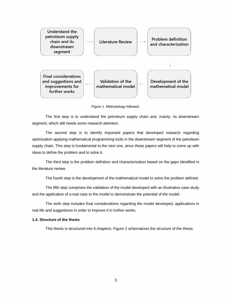
Figure 1. Methodology followed.

The first step is to understand the petroleum supply chain and, mainly, its downstream

segment, which still needs some research attention.

The second step is to identify important papers that developed research regarding

optimization applying mathematical programming tools in the downstream segment of the petroleum

supply chain. This step is fundamental to the next one, since these papers will help to come up with

ideas to define the problem and to solve it.

The third step is the problem definition and characterization based on the gaps identified in

the literature review.

The fourth step is the development of the mathematical model to solve the problem defined.

The fifth step comprises the validation of the model developed with an illustrative case study

and the application of a real case to the model to demonstrate the potential of the model.

The sixth step includes final considerations regarding the model developed, applications in

real life and suggestions in order to improve it in further works.

1.4. Structure of the thesis

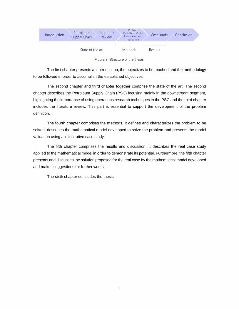
This thesis is structured into 6 chapters. Figure 2 schematizes the structure of the thesis.

4

Figure 2. Structure of the thesis.

The first chapter presents an introduction, the objectives to be reached and the methodology

to be followed in order to accomplish the established objectives.

The second chapter and third chapter together comprise the state of the art. The second

chapter describes the Petroleum Supply Chain (PSC) focusing mainly in the downstream segment,

highlighting the importance of using operations research techniques in the PSC and the third chapter

includes the literature review. This part is essential to support the development of the problem

definition.

The fourth chapter comprises the methods. It defines and characterizes the problem to be

solved, describes the mathematical model developed to solve the problem and presents the model

validation using an illustrative case study.

The fifth chapter comprises the results and discussion. It describes the real case study

applied to the mathematical model in order to demonstrate its potential. Furthermore, the fifth chapter

presents and discusses the solution proposed for the real case by the mathematical model developed

and makes suggestions for further works.

The sixth chapter concludes the thesis.

5

Chapter 2 – Petroleum Supply Chain

This chapter aims to explain the structure of the petroleum supply chain and the importance

of applying operations research techniques in PSC. This chapter is structured as follows: Section 2.1

discusses the concept of supply chain and the structure of the petroleum supply chain; Section 2.2

highlights the downstream segment of the PSC; Section 2.3 gives a brief history of operations

research; Section 2.4 explains the elements that composes a mathematical model and some of the

categories used to classify a model; Section 2.5 comprises the planning levels that classifies the

decision process in PSC; Section 2.6 shows the importance of using operations research techniques

in PSC.

2.1. The Petroleum Supply Chain

The Petroleum Supply Chain (PSC), also called Oil Supply Chain (OSC), is divided into three

segments: upstream, midstream and downstream (see Figure 2). The upstream involves oil

exploration and production, which includes the search for areas that may contain hydrocarbons,

drilling operations and production, which means to bring the hydrocarbons to the surface, and crude

oil transportation. Some authors consider the crude oil transportation as an upstream segment activity

(Lima, et al., 2018) and others consider as a midstream activity (Leiras, et al., 2011). Despite these

disagreements, the midstream regards refining operations. The downstream refers to storage and

refined products distribution and marketing (Lima, et al., 2018). Some authors divide the PSC into

only two segments: upstream and downstream. In this case, the downstream segment includes the

refining operations (Lima, et al., 2016).

PSC begins in upstream segment with oil exploration and production (Sahebi, et al., 2014).

After exploration, oil terminals receive crude oil that is transported by tankers. Moreover, crude oil

can be also imported. Then, pipelines transport crude oil from oil terminals to refineries (Neiro & Pinto,

2004). After that, the midstream segment comprises refineries and petrochemicals to transform crude

oil and produce oil products (Sahebi, et al., 2014). Crude oil is a mixture of hydrocarbons, so each of

its fractions must be separated in different products. At refineries, crude is heated and put on a

distillation column, where the products are recovered at different temperatures. Some refineries, that

are more complex, reprocess the heavier fractions in order to obtain more of the lighter products such

as liquid petroleum gases (LPG), gasoline and naphtha (EIA - U.S. Energy Information Administration,

2012). Refineries can be connected to each other and take advantage of the degree of complexity of

each one (Neiro & Pinto, 2004). Finally, the downstream segment is responsible for transporting oil

products to distribution centers (DC) in wholesale segment and then transporting from wholesale to

retail segment (Neiro & Pinto, 2004).

6

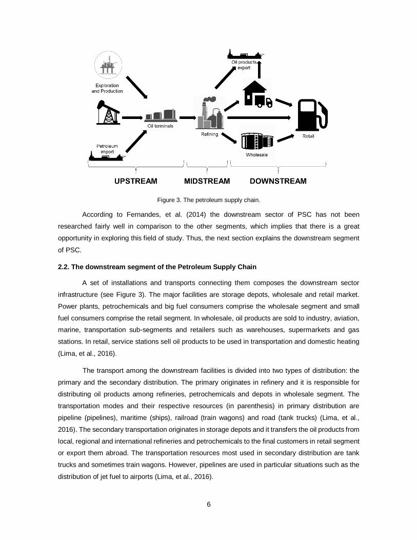
Figure 3. The petroleum supply chain.

According to Fernandes, et al. (2014) the downstream sector of PSC has not been

researched fairly well in comparison to the other segments, which implies that there is a great

opportunity in exploring this field of study. Thus, the next section explains the downstream segment

of PSC.

2.2. The downstream segment of the Petroleum Supply Chain

A set of installations and transports connecting them composes the downstream sector

infrastructure (see Figure 3). The major facilities are storage depots, wholesale and retail market.

Power plants, petrochemicals and big fuel consumers comprise the wholesale segment and small

fuel consumers comprise the retail segment. In wholesale, oil products are sold to industry, aviation,

marine, transportation sub-segments and retailers such as warehouses, supermarkets and gas

stations. In retail, service stations sell oil products to be used in transportation and domestic heating

(Lima, et al., 2016).

The transport among the downstream facilities is divided into two types of distribution: the

primary and the secondary distribution. The primary originates in refinery and it is responsible for

distributing oil products among refineries, petrochemicals and depots in wholesale segment. The

transportation modes and their respective resources (in parenthesis) in primary distribution are

pipeline (pipelines), maritime (ships), railroad (train wagons) and road (tank trucks) (Lima, et al.,

2016). The secondary transportation originates in storage depots and it transfers the oil products from

local, regional and international refineries and petrochemicals to the final customers in retail segment

or export them abroad. The transportation resources most used in secondary distribution are tank

trucks and sometimes train wagons. However, pipelines are used in particular situations such as the

distribution of jet fuel to airports (Lima, et al., 2016).

7

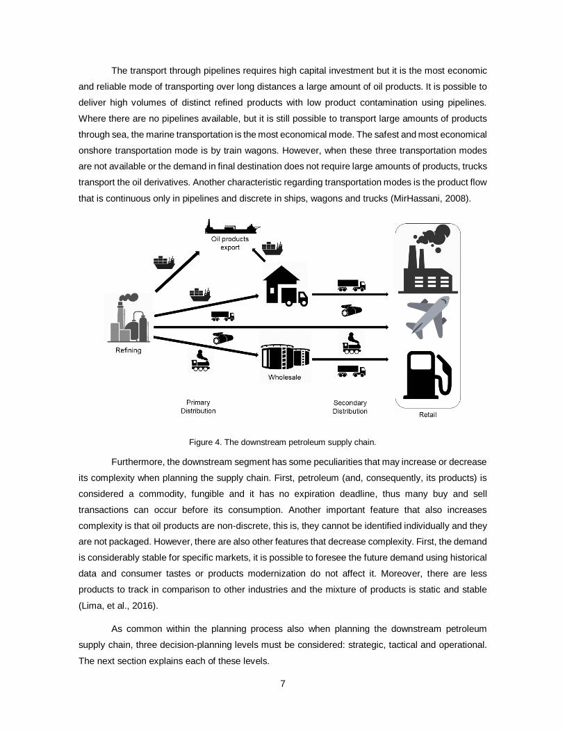
The transport through pipelines requires high capital investment but it is the most economic

and reliable mode of transporting over long distances a large amount of oil products. It is possible to

deliver high volumes of distinct refined products with low product contamination using pipelines.

Where there are no pipelines available, but it is still possible to transport large amounts of products

through sea, the marine transportation is the most economical mode. The safest and most economical

onshore transportation mode is by train wagons. However, when these three transportation modes

are not available or the demand in final destination does not require large amounts of products, trucks

transport the oil derivatives. Another characteristic regarding transportation modes is the product flow

that is continuous only in pipelines and discrete in ships, wagons and trucks (MirHassani, 2008).

Figure 4. The downstream petroleum supply chain.

Furthermore, the downstream segment has some peculiarities that may increase or decrease

its complexity when planning the supply chain. First, petroleum (and, consequently, its products) is

considered a commodity, fungible and it has no expiration deadline, thus many buy and sell

transactions can occur before its consumption. Another important feature that also increases

complexity is that oil products are non-discrete, this is, they cannot be identified individually and they

are not packaged. However, there are also other features that decrease complexity. First, the demand

is considerably stable for specific markets, it is possible to foresee the future demand using historical

data and consumer tastes or products modernization do not affect it. Moreover, there are less

products to track in comparison to other industries and the mixture of products is static and stable

(Lima, et al., 2016).

As common within the planning process also when planning the downstream petroleum

supply chain, three decision-planning levels must be considered: strategic, tactical and operational.

The next section explains each of these levels.

8

2.3. Decision-Planning Levels

According to Lima et al. (2016), the decision process is classified into three planning levels:

strategic, tactical or operational. Each of these levels diverge on the type of decisions and time

planning horizon (Lima, et al., 2018). There is a hierarchy among these levels: the strategic imposes

limit to the tactical and the tactical imposes limit to the operational (Lima, et al., 2016). Moreover, the

decision planning can be vertically integrated, combining two planning levels of decision, for example,

strategic-tactical, strategic-operational or tactical-operational (Misni & Lee, 2017).

The strategic planning level deals with long-term decisions, in an annual scale (Lima, et al.,

2018). The decisions within the strategic level are related to identify the facilities best locations to be

structured, to determine their capacities and to select the technologies to be applied at each facility.

Facility relocation problems, outsourcing and investment planning are also considered as strategic

decisions (Sahebi, et al., 2014). The strategic level decisions are the most complex ones because as

they comprise the definition of the structure of the supply chain, the set-up costs for implementation

are high (Lima, et al., 2016).

The decisions in tactical planning have medium-term implications, in a monthly scale and

they are restrained by the configurations established in the strategic planning. In this planning level,

the decisions are related to the establishment of the best material flow across the chain (Lima, et al.,

2016), and to the production planning and inventory management (Misni & Lee, 2017).

The operational planning level deals with short-term decisions, in a weekly scale. These

decisions are restrained by the operating policies established in the tactical level (Lima, et al., 2018).

The decisions in this level concern to vehicle routing and scheduling of products and activities (Misni

& Lee, 2017).

Being the planning process related to future events, uncertainty needs to be accounted for.

Its presence in each stage depends on the decision horizon. The higher the decision horizon, the

higher the uncertainties are. That is, there are more uncertainties in strategical planning than in

tactical and there are more in tactical than in operational (Lima, et al., 2016).

As the PSC involves high costs and high revenues, it is important to make the optimal

decisions in each planning level. In order to find optimal solutions to a certain planning situation,

operations research models and methodologies can be very helpful. The next section presents how

operations research’s tools can be used in PSC.

2.4. Operations research in PSC

2.4.1. A brief history of operations research and some currently applications

Operations or Operational (in British) Research (OR) is a field of study, which involves a set

of techniques to assist in the decision-making process in problems that involve how to lead and

9

coordinate operations in an organization. The decision-making process initiates with the problem

characterization and definition. Then, a mathematical model is developed in order to solve the

problem as it may optimize the performance by reducing costs or increasing profit, for example. After

that, an OR software solves the model and the solutions obtained go to the model validation step,

which tests if they are valid for the real problem (Hillier & Lieberman, 2005).

However, OR techniques have not always been dependent of computers since it has begun

during the World War II, when the resources to military operations were scarce and, therefore, they

had to be allocated in the most effective manner. Then, scientists were hired by the British and U.S.

military management to solve this and other strategic and tactical issues. These scientists developed

very effective techniques that enabled the victory of the Allies in some battles during the war (Hillier

& Lieberman, 2005).

After the war, it was possible to see that organizations in business, industry and government

were facing problems that were very close to those faced by the militaries. Therefore, the OR

techniques were spread to other fields beyond the military (Hillier & Lieberman, 2005). Currently, the

applications of OR in companies includes logistics, supply chain management, scheduling of

production and many other areas that have much information to be processed and a decision to be

taken.

In the 1980s, the computer revolution boosted OR techniques and applications since the

computers provide solution in seconds of complex problems that could be almost impossible to do by

hand. Nowadays, there are many software and algorithms to solve OR problems (Hillier & Lieberman,

2005). The General Algebraic Modeling System (GAMS) is an example of software that is used to

solve OR problems.

2.4.2. The models in operations research

As the OR techniques were improved, the problems were categorized according to the type

of the model developed and many methods of solution were created. A model simplifies the real

system through mathematical expressions. As a model is simply a representation of the reality, it

does not contain all the elements that composes the real problems but the most important ones.

The following elements composes a typical mathematical model: the decision variables (and

sometimes parameters), the objective function and the constraints. The mathematical model consists

in maximize or minimize an objective function subject to a series of constraints that may be equalities

or inequalities in order to find an optimal solution. It is important to emphasize that there may be

multiple best solutions, and this is the reason why the model tries to find “an” optimal solution (Hillier

& Lieberman, 2005). The objective function commonly represents the profit to be maximized or the

cost to be minimized.

10

There are many categories to classify a mathematical model and some of the most important

ones are explained below.

In Linear Programming (LP), also known as linear optimization, the objective function and the

constraints must be linear functions and the type of decision variable is continuous.

In Integer Programming (IP), the objective function and the constraints are linear functions

and the decision variables may be all integer or integer and continuous. If all the decision variables

are integer, this is a Pure Integer Programming. If these integer decision variables are discrete and

restricted to 0 or 1, this is a Binary Integer Programming (BIP) problem. The binary variables have an

enormous importance in a situation to make a yes-or-no decision. However, if only some decision

variables are integer, this is a Mixed Integer Programming (MIP) problem, also called Mixed Integer

Linear Programming (MILP). Another characteristic of Integer Programming is that it is NP-complete.

In Nonlinear Programming (NLP), the objective function or at least one of the constraints is a

nonlinear function and the decision variables can be all continuous or integer and continuous. If some

of the decision variables are integer, the problem is a Mixed Integer Nonlinear Programming (MINLP).

Some problems that are modeled using LP, MILP, NLP, etc. are extremely complex, causing

an issue that can be overcome applying decomposition strategies such as Benders decomposition,

Lagrangean decomposition and bilevel decomposition (Andersen, et al., 2013)

The mathematical models can also be deterministic or stochastic. The deterministic models

produce the same output when the initial conditions and the parameters are the same. However,

there is a randomness present in the stochastic models. That is, the same set of initial conditions but

with uncertainty in a part or the whole set of parameters will produce different outputs. Variables will

obtain different values when uncertainty is realized.

Furthermore, when a problem considers uncertainty, there are several approaches to deal

with them such as stochastic programming, robust optimization and fuzzy programming. If the

acquired data has a particular distribution, the stochastic programming is commonly used. However,

if there is no particular distribution regarding the data, fuzzy programming can be applicable but it

must be possible to determine membership functions and boundaries (Azadeh, et al., 2017).

2.4.3. Why use operations research techniques in petroleum supply chain

The oil and gas industry has a huge impact worldwide due to the world energy supply that

this industry provides (Ghaithan, et al., 2017). Since 1990, petroleum represents over 30% of the

world’s energy demand (Saad, et al., 2018) and natural gas represents over 20% currently, therefore,

together these fuels supply more than 50% of the world’s energy (BP - British Petroleum, 2018). The

applications of oil and gas industry are not limited only to powering vehicles but to production of

plastics, detergents, rubber, textiles, etc. and also to electricity generation (Saad, et al., 2018).

11

Although this industry is very profitable, their costs are huge. These costs involve rigs,

equipment, maintenance, crew, etc. For example, in offshore hydrocarbon reserves, (that represents

more than one third of global reserves), the cost of exploration and well development represents a

large share of the total costs and the rigs represent a major part in these costs (Skjerpen, et al., 2018).

According to Bassi et al. (2012), rigs can cost up to US$600,000 daily.

In addition to the large costs, the investments are also huge in the oil industry. The

investments must be high because the facilities for exploration and production offshore need to

operate over the entire life span of the project (around 10 to 30 years) besides their expensive cost.

If the investments are not planned carefully and if the wrong decisions were made, this would affect

the entire project’s profitability (Goel & Grossmann, 2004).

Within this setting is very important to plan carefully in the oil industry namely on the supply

chain area. To do so is important to account for this system characteristics and to that consider the

presence of uncertainty. So the variations in the production level, the unpredictable oil market prices

and the unforeseeable demands are important sources of uncertainty in the Oil Supply Chain (OSC)

(Lima, et al., 2018). The demand for oil products is always changing and some markets begin to stand

out (Lima, et al., 2016). From 2007 to 2017, while oil consumption in U.S. and Europe decreased by

5% and 10% respectively, in Asia Pacific it has increased by almost 33% and it now represents almost

twice of U.S. oil consumption. In the same period, oil consumption increased by 32% in Africa, 27%

in Middle East, 16% in South and Central America and 9% in CIS. In 2007, the oil consumption in

these four regions represented 97% of U.S. consumption but in 2017 these four regions consumption

represented 125% of U.S.’s (BP - British Petroleum, 2018).

Moreover, the oil industry is inserted in an unstable context with many geopolitical issues that

reinforces all of these uncertainties, risks, high costs and investments (Lima, et al., 2016).

Therefore, professionals in this field are challenged constantly to take the best decisions in

order to spend the less but earn the most. These professionals’ objective is to plan a secure and

resilient supply chain that considers the uncertainties and responds to unforeseeable events in a fast

and cost effective manner. If Operations Research’s tools are used, the decision-making process can

improve, costs can reduce and revenues can increase (Lima, et al., 2016). Moreover, the Operations

Research’s tools can be applied in the three segments of the PSC. The models referring to the

upstream sector usually select the oil wells to be drilled and the operations decisions associated are

crude oil transportation, scheduling and platform production. In midstream segment, the models

include planning and scheduling of refinery production. The decisions in downstream sector refer to

the network design and the material flow, which include products distribution, optimization in

transports from refinery to storage depots and storage (Kazemi & Szmerekovsky, 2015). Because of

this, it is possible to have plenty of applications of Operations Research in many fields of oil and gas

industry. This will be detailed in the next chapter.

12

2.5. Conclusion

In this chapter the structure of the Petroleum Supply Chain was described, highlighting its

downstream segment, which has not been sufficiently researched. Furthermore, this chapter

presented the decision levels used when planning and managing the PSC. Finally, it was explained

the importance of applying operations research’s techniques in PSC.

The downstream segment of PSC is inserted in a scenario full of uncertainties and many

mathematical models can be developed based on it. The activities included in this sector are mainly

distribution and storage of oil products. The OR models in downstream PSC try to find an optimal

solution for profit maximization or cost minimization by making decisions regarding many activities

such as the planning of the transportation modes to be used, the amounts of each product is to be

transported by each mode and the location and capacity of the storages.

Thus, after understanding the PSC, the next step will be devoted to produce a literature

review on optimization in downstream segment of PSC. This is presented in the next chapter.

13

Chapter 3 – Literature Review

The objective of this chapter is to present a literature review in downstream PSC optimization.

The papers selected were classified in five different categories based on their decision-planning level

(or the integration of more than one level). A set of several keywords such as “downstream”, “oil and

gas”, “petroleum supply chain”, “optimization” and “operations research” and their combination were

used to search for papers in platforms as Google Scholar, Science Direct and Web of Knowledge.

The search resulted in 39 papers but only the most relevant and recent ones were analysed. The

discarded papers presented models in the upstream and midstream segments of the PSC and,

therefore, they were not considered relevant as this work will focus on the downstream supply chain.

It is true that some of the 24 selected papers are more focused in refining operations than in the

downstream segment itself but these papers also consider the products distribution to the customers

and so they were analysed. The majority of papers reviewed were published in the last 10 years,

despite that the time frame of the collected papers covers the last 20 years. Still, the older papers are

still relevant in the field.

The chapter is structured in six sections: Section 3.1 presents the models developed

considering strategic planning; Section 3.2 presents the models that considered tactical planning;

Section 3.3 presents the models that considered operational planning; Section 3.4 integrates the

models with strategic and tactical planning; Section 3.5 integrates the models with tactical and

operational planning; and Section 3.6 concludes the chapter, summarizing all the papers analyzed.

3.1. Strategic planning

Strategic planning comprises long-term decisions such as the network design (number,

location and capacity of the facilities) (Barbosa-Póvoa, 2014). This problem has been treated by

several authors but five main papers were considered relevant and are analysed below. This can be

divided in two main groups: the papers that addressed the problem as deterministic and the papers

that considered the presence of uncertainty. In the latter a single paper was identified.

3.1.1. Strategic planning – Deterministic approaches

Fernandes et al. (2013) developed a deterministic MILP model coded in GAMS with strategic

planning, considering a multi-entity, multi-product, multi-echelon and multi-transportation downstream

PSC. The objective was to maximize the total network profits considering six terms: the refinery

margin (the difference between ex-refinery price and refining costs, multiplied by the refined volume,

minus the crude oil supply costs and the result is multiplied by the capital percentage per entity) plus

the retail segment margin, minus the exportation and importation costs and transportation and storage

depots tariffs. The model determines the optimal storage depot locations (consists of installation of

new ones or closure of the existents), storage capacities, allocation of volumes for crude oil,

transportation modes and routes, refinery production and network affectations for long term planning.

14

Finally, a real-case involving a Portuguese PSC network was used to test the model (Fernandes, et

al., 2013).

Andersen, et al. (2013) developed two deterministic MILP models (aggregated and detailed)

and both models considered strategic planning. The number of discrete variables in detailed model

was 53,660 compared to 1,400 in aggregated model. Because of this, the computational model

required to solve the detailed model was quite large and, therefore, a bilevel decomposition was

proposed to achieve a computational saving of 40%. The problem comprises the integration of

ethanol and gasoline supply chains. Ethanol is one of the most promising alternatives to fossil fuels

for the next decades, since it is produced from biomass. The problem considered two types of

biomass (wood residues and switchgrass) that, after harvesting and drying, are transported to

biorefineries, where ethanol and a blend of 85% ethanol and 15% gasoline called E85 are produced.

Gasoline is produced at refineries and a part of it feeds ethanol plants and the other part is sent to

gasoline distribution centers. The E85 blend is also sent to gasoline distribution centers and the

blending of ethanol and gasoline (to produce E10 or E30) can happen in the retail center or at the

distribution centers (Andersen, et al., 2013).

The difference between the models developed by Andersen, et al. (2013) is at the retail

centers: the first model (aggregated) comprises the fuel demand per region without details of gas

stations and the second (detailed) comprises the amount of gas stations per region. The

transportation modes considered were truck, railway and pipeline. The objective function of both

models was minimize the costs and it consisted in five terms: investment cost, processing and

maintenance cost, transportation cost, storage cost and purchase cost of gasoline (in order to perform

the blending). The results concluded that the aggregated model is an approximation of the detailed

one, since the aggregated did not consider all the gas stations considered in detailed model.

Therefore, the detailed model comprised the costs of these gas stations, making an increase of 18%

in total cost (Andersen, et al., 2013).

Saad, et al. (2018) developed a deterministic and a simulation model. The deterministic LP

model was developed at the strategic planning level in downstream segment with a one year planning

horizon, while the simulation model was proposed at operational level, combining continous and

discrete simulation techniques and it was focused in crude oil separation and distillation unit

(midstrream segment). In the deterministic model, the objective function consisted in minimize the

cost, considering the sum of the following costs: production and transportation of crude oil, production

and transportation of the final product, storage and penalty for shortage or exceed of product, minus

sales revenue. The constraints considered were transportation and storage constraints, material and

demand balance and production yield (Saad, et al., 2018).

15

3.1.2. Strategic planning – Stochastic problem

A single paper was identified addressing the strategic problem at the PSC considering

uncertainty. This is the paper by MirHassani & Noori (2011) that developed a two stage stochastic

MILP with strategic planning considering a 12-month planning horizon. The decisions in first stage

comprise the planning of capacity installments and they must be taken before determining the

uncertainty. The decisions in second stage considers routes planning and they must be taken after

considering the oil demand. The objective is to study the capacity expansion of an oil products

distribution network in an uncertain environment and minimize the total cost over the planning horizon.

The uncertainty considered was the product demand (MirHassani & Noori, 2011).

3.2. Tactical planning

Tactical planning comprises medium-term decisions such as inventory policies definition,

material flows, transportation strategies and resources planning (Barbosa-Póvoa, 2014). In this area

two papers were identified as relevant. Again as in the previous section also two groups of papers

are here considered. The ones that addressed the problem as deterministic and the ones that

considered the presence of uncertainty.

3.2.1. Tactical planning – Deterministic approaches

Ghaithan, et al. (2017) developed a multi-dimensional and multi-objective model in

downstream segment of PSC. The model considered a medium-term planning horizon of 6 months.

The tactical planning decisions that the model determines are flow volume of crude oil, oil products

and gas products between each node, optimal processing plans, import and export volumes and

allocation of local customers to bulk plants. The three objective function were cost minimization,

revenue maximization and service level maximization. The model did not consider uncertainties and

it was solved using the Improved Augmented ε-Constraint algorithm. Finally, a case study from Saudi

Arabia was used to test and validate the model (Ghaithan, et al., 2017).

Furthermore, as OPEC countries are questioning about if reducing their oil production quotas

would help to increase crude oil and petroleum products sales price, the sensitivity analysis is a matter

of major importance. The results of model showed that if OPEC quota or oil production decreases

and if price increases simultaneously, a higher total revenue would be obtained compared to a case

with high OPEC quota and low price. Therefore, the model shows that in case of a decrease in oil

price, the best strategy would imply in increasing the price to get higher returns. The sensitivity

analysis was also performed regarding the domestic demand in Saudi Arabia and resulted in increase

the local selling price, that, hence, would decrease the domestic demand and high revenue would be

achieved. As Saudi Arabia has enough reserves and resources, the model also verifies that it is able

to fulfill most of oil products demand with high value of service. Finally, it is suggested to expand the

16

model by integrating upstream and downstream sectors or adding uncertainties such as oil price and

oil demand (Ghaithan, et al., 2017).

3.2.2. Tactical planning – Stochastic approaches

Lima, et al. (2018) developed a multistage stochastic linear programming model in order to

make decisions regarding refinery production planning, inventory management and distribution

planning with a tactical planning. The decisions include transportation modes, material flows and

import & export management in a discrete time scale. The model considered two sources of

uncertainty: oil price and oil demand. The methodology autoregressive integrated moving average

(ARIMA) that forecasts the uncertainty based on past data was used to deal effectively with the

uncertainties. The objective function was to maximize the profit. Finally, the model was tested using

a real case study of a multi-echelon, multi-transportation, multi-product and uni-entity Portuguese

downstream oil supply chain.

3.3. Operational planning

Operational planning deals with decisions that have short-lasting effect, such as allocation of

human resources, truck loading, scheduling and routing (Barbosa-Póvoa, 2014). In this area, three

papers were identified as relevant and all of them addressed the problem as deterministic.

3.3.1. Operational planning – Deterministic approaches

Pinto et al. (2000) developed deterministic MILP and MINLP models with operational

planning. The planning horizon was 3 days discretizes in 2-hours intervals. The first model was a

non-convex mixed integer non-linear programming (MINLP) and, hence, there was no global solution

ensured by conventional MINLP algorithms. Thus, a MILP model was derived from the first in order

to be solved optimally. The objective function of the models was to maximize the profit and the

objective was to show planning and scheduling applications for refinery operations, which are

problems that can be efficiently represented by large-scale MIP optimization models. The model was

validated using a real case from Brazilian PSC (Pinto, et al., 2000).

Neiro & Pinto (2004) developed a deterministic large-scale MINLP model that integrates the

three segments of oil supply chain with operational planning. The problem considers a set of crude

oil suppliers, refineries and distribution centers. The model should decide which oil types to select

and their transportation plan, production levels and how to distribute the products and to manage the

inventory along the planning horizon. The objective function is to maximize the profit by subtracting

costs related to raw material, transportation, inventory and operation from product sales. The

constraints are based on three classes of elements: processing units, storage tanks and pipelines. In

this problem, pipelines distribute crude oil from petroleum terminals to refineries and oil products from

refineries to intermediate terminals or directly to distribution centers. It is possible to apply this model

17

to real problems and, therefore, it was validated using a case study from Petrobras in Brazilian PSC

(Neiro & Pinto, 2004).

Ye et al. (2017) developed two MILP models in order to deal with the refined-oil shipping

problem based on a real case from an oil company in China. The first model uses a time-slot concept

under a continuous-time representation and the second uses a discrete-time representation and

together these models unite their advantages: the continuous-time reduces binary variables and the

discrete-time is a modelling approach that can fit in other scheduling problems with more complex

operating rules. Moreover, no uncertainties were considered in these models. In this problem two

types of refined-oil are considered: diesel and gasoline and 12 subtypes. It is considered only one

starting place and 40 destination portals and the transportation mode includes only a fleet of ships of

different sizes. At the beginning of each month, the demand for each oil subtype is announced by

each of the portals and the time horizon to deliver the demanded oil subtype is one month. Each

combinations of a destination portal with a demanded oil subtype is referred as a task. Therefore, in

order to optimize the vessel scheduling, the objective was to minimize the shipping cost by combining

tasks and dividing them into vessels of different sizes (Ye, et al., 2017).

3.4. Strategic and tactical planning

Models developed integrating strategic and tactical planning consider long and medium-term

decisions, such as the structure of the supply chain and material flows, respectively (Barbosa-Póvoa,

2014). Several authors approached this problem but only ten main papers were considered relevant

and were analysed below. This section can be divided in two main groups: the papers that addressed

the problem as deterministic and the papers that considered the presence of uncertainty. In the first

four papers were identified and in the latter six papers were identified.

3.4.1. Strategic and tactical planning – Deterministic approaches

Kim, et al. (2008) developed an integrated model of supply network and production planning

for oil products with strategic and tactical planning. The decisions that the deterministic MILP model

developed considered relocation of distribution centers and reduction of the distribution costs.

Moreover, a MINLP model was developed by joining the MILP model with a non-linear production

model. The objective function of both models was to maximize the profit. The model was validated

using a real world example from South Korea including three refineries with four products. Three case

studies were considered to test the model: separate planning of individual refineries, collaborative

network planning by all the refineries and network integration among all the refineries. The results

demonstrated that there were potential benefits in collaborative planning for production and

distribution of oil products (in both single refinery and multiple refinery models). Moreover, results

showed the importance of separately planning the supply network and production for each oil product

in order to obtain the most efficient routes from the sources to the markets (Kim, et al., 2008).

18

Fernandes, et al. (2014) developed a deterministic MILP model with strategic and tactical

planning. The model considers multiple companies, products, echelons, refineries and transportation

modes. The decisions involve to determine the optimal network including: installation, closure and

operation of storage depot locations, definition of storage capacity, individual costs and tariffs,

planning of transporation modes and routes, allocation of volumes for crude oil, import, export,

refinery production and depot transfers and customer fulfillment. The restrictions considered were

satisfy customer demands and production, storage depot and transportation capacity. The objective

function was to maximize the profit by subtracting costs of refinery margin, exportation, importation,

inventory (crude, refinery, depot and retail), unsatisfied demand and transportation and storage depot

tariffs from the sum of oil companies revenues, oil companies shared revenues in participated

infrastructures, retail margin and entities participation in transportation operator margin and storage

depot operator margin (Fernandes, et al., 2014).

Fernandes, et al. (2014) verified its model using a real-case of downstream PSC in Portugal.

This model obtained higher profits compared to the model developed by Fernandes, et al. (2013),

which considered individualistic operation. In large countries (such as Spain), there are single-entity

PSC networks and in smaller countries (such as Portugal), there are multientity networks and the

petroleum entities compete for the smaller market. The study concluded that although logistics costs

and tariffs in multientity networks with individualistic strategies are higher than those in single-entity

network, in a collaborative strategies environment the results are close to the more efficient single-

entity (Fernandes, et al., 2014).

Kazemi & Szmerekovsky (2015) developed a deterministic MILP model coded in GAMS with

strategical and tactical planning of the downstream Petroleum Supply Chain (PSC). Their objective

was to minimize the fixed and distributing costs along refineries, distribution centers, transportation

modes and demand nodes and to determine the optimal locations and capacities for the distribution

centers, transportation mode selection (pipeline, waterway carriers, rail and truck), product allocation

and transfer volumes. The strategic part concerns in determining distribution centers’ locations and

capacities and the tactical part in flow allocation and transportation modes. This research focused in

the following fuel products: gasoline, diesel and jet fuel. Finally, a case study with real data from U.S.

oil industry and transportation networks was presented (Kazemi & Szmerekovsky, 2015).

Another essential characteristic of the model developed by Kazemi & Szmerekovsky (2015)

is that there was a comparison between the use in strategic planning of a multimodal transportation

or a single-mode (pipeline), which is a specific case of the multimode model that considers only

pipeline transportation. The analysis resulted in a cost increase of 2% using the pipeline-based

planning and, therefore, it was concluded that it is critical to use multi-modal transportation to take

cost-effective decisions in strategic planning (Kazemi & Szmerekovsky, 2015).

19

Fiorencio et al. (2015) developed a Decision Support System (DSS) in order to aid investment

decisions and to optimize the distribution of the oil products. The DSS was based on a deterministic

MILP model with strategic and tactical planning and two case studies were use in order to evaluate

the model using real data from Brazilian PSC. The first case study compares two projects, which the

first analyses the increase in the capacity of vessels and the second analyses the increase in the

capacity of a pipeline between a maritime terminal and a distribution base. The second case study

analyses an expansion project for a pipeline that supplies several distribution bases. The objective

was to minimize costs considering the sum of five terms (investments, freight, holding, operation and

demurrage costs) minus national commercialization income and international commercialization

profit. The strategic planning manages investments to be made in logistics infrastructure such as

storage and product-handling capacities for terminals and tactical planning manage issues such as

modes of transportation and flow allocation. The authors also performed a sensitivity analysis of the

Net Present Value (NPV) that accounts for investment costs in both case studies in order to aid the

decision-making process. The first case study showed that the expansion of the vessels capacity

together with the pipeline expansion resulted in an increase of NPV. Hence, both investments work

well together. The second case study showed that if pipeline capacity was expanded, it would reduce

transportation costs because it would require less transporation by trucks. However, NPV sensitivity

analysis showed that each pipeline section has a different investment cost (Fiorencio, et al., 2015).

3.4.2. Strategic and tactical planning – Stochastic approaches

MirHassani (2008) developed a stochastic MILP model considering oil demand as an

uncertainty and comprising strategic and tactical planning. The model considers pipelines, ships,

railway and trucks as transportation modes for oil products. The objective function is to minimize the

costs related to transferring oil products by each transportation mode, penalties for shortage and

exceed and inventory cost. Moreover, the model should also calculate the minimum and maximum

amount of each oil derivative that could be imported and exported and take care of the worst case

regarding shortage. The model was solved using a real-life problem and the conclusion was that this

model could be efficiently solved for realistic large-scale problems (MirHassani, 2008).

Oliveira & Hamacher (2012) developed a two-stage stochastic MILP in order to optimize the

investment planning process of a logistics infrastructure of oil products distribution considering the

demand levels as an uncertainty. The model considers issues of tactical planning to evaluate

decisions of strategic nature and it uses the Sample Average Approximation (SAA) methodology in

order to produce approximations of the optimal solution, since there are lots of possible scenarios.

The objective function is to minimize the costs of investment, inventory, freight, operations,

demurrage in marine terminals, commercialization and backlog. The model was validated using a real

case of northern Brazil (Oliveira & Hamacher, 2012).

20

Tong, et al. (2014) developed a MILP model in order to deal with hydrocarbon biofuel supply

chain design and production planning and used robust optimization to deal with the uncertainties

considered, which were fuel demand (gasoline, diesel and jet fuel) and biomass availability. Both

models resulted in a single Mixed-Integer Linear Fractional Programming (MILFP) model with

strategic and tactical planning. The objective function was to minimize the functional-unit-based

economic performance by dividing the annual cost by total biofuel sold to the customers. The supply

chain design decisions involve location, size, number and technology selection of preconversion

facilities and the planning decisions involve harvesting, production and distribution decisions. The

model was tested using a real case considering the state of Illinois (US) (Tong, et al., 2014).

Oliveira, et al. (2014) developed a two-stage stochastic MILP model in order to deal with the

investment planning problem based on stochastic Benders decomposition, considering the oil

products demand as the source of uncertainty. The model involves strategic and tactical decisions,

which the first regard the location of facilities such as terminals and distribution bases, capacities of

storage and product-handling and construction or expansion of the transportation modes and the

latter consists in flow allocation. The model’s first stage determines the projects to implement and

when and the second determines the best flow of products and inventory and supply levels. The

objective function in both stages is to minimize the investment and logistics cost (Oliveira, et al.,

2014).

Fernandes, et al. (2015) developed a stochastic MILP in order to design and plan the

downstream PSC under uncertainty and considering strategic and tactical planning. The uncertainty

considered is the products demand, the strategic decisions regard installation, sizing and operation

of facilities, tariffs and the fair price strategic cost and the tactical decisions rergard inventory levels,

products routing and periodic depot. The model is biobjective and its two objective functions are to

maximize the Expected Net Present Value (ENPV) and to minimize the Conditional Value-at-Risk

(CVaR). The model was validated using a real case of Portuguese PSC (Fernandes, et al., 2015).

Although Azadeh, et al. (2017) focused their work in upstream and midstream segments, it

was also proposed to consider downstream segment in a single model, since the dual complication

of distribution. Azadeh, et al. (2017) developed a multi-objective MINLP model with strategic and

tactical planning. Long-term and mid-term decisions were integrated considering a planning horizon

of 15 years discretized into 6-month periods. The two objective functions in the model were to

maximize the profit using the net present value method (that is, divide net earning minus total

depreciable capital by the interest during the period under analysis) and to minimize environmental

threats using Eco indicator 99. The model consisted of making some decisions such as facilities

location (wells, platforms, refineries, depots and external markets), establishment planning (this is, to

determine, for example, when facilities will be established) and production, transportation and

distributing planning. This model also considers upstream and midstream segments via green

21

aspects. Fuzzy programming was used to deal with the following uncertainties: cost and production

capacity of refined products and consumption rate of oil products. As the problem was so large, a

unique meta-heuristics approach based on MOEA-D was developed to solve the problem,

decomposing it into several sub problems. Finally, the model was verified using a real case in Persian

Gulf (Azadeh, et al., 2017).

3.5. Tactical and operational planning

Tactical and operational planning combine these two levels of planning and involve a medium

to short planning horizon, addressing activities such as transportation strategies and scheduling,

respectively (Barbosa-Póvoa, 2014). In this section, five main papers were identified as relevant and

were analyzed below. Three of them addressed the problem as deterministic and two as stochastic.

3.5.1. Tactical and operational planning – Deterministic approaches

Kuo & Chang (2008) developed a deterministic MILP model considering integration of two

activities hierarchically linked: production planning and scheduling schemes for the refinery segment

of PSC. The model involved both tactical and operational decisions. The tactical ones are considered

higher-level decisions such as the amounts of crude oil to be acquired and production and inventory

levels of several oil products, according to the market demands, which are planned over a medium-

term horizon (months). The operational decisions are considered lower-level scheduling tasks, which

includes determining the specific time that each unit must be operated to achieve the production

goals. These decisions are planned over a short-term horizon (weeks). The objective function was

profit maximization over a specified planning horizon given by the total revenue minus the total costs

that includes raw materials, operation, transportation and inventory. The transportation modes

considered were pipelines to transport process materials from one unit to another, tankers to import

raw materials and intermediates and pipelines or trucks to deliver products and byproducts to

domestic customers (Kuo & Chang, 2008).

Alabi & Castro (2009) developed a deterministic large primal three-blocks-angular LP model

considering a planning horizon from 2 to 300 days, this is, both tactical and operational planning. The

problem approached was the integrated refinery-planning (IRP) that can be divided into three sub-

problems: crude oil supply, refining and product distribution. In order to simplify the model, energy

balance was not considered (only mass balance). The objective function is to maximize the profit.

However, the function was described as the minimization of a seven terms sum (cost of all crude

consumed, refining operations, purchased materials, transportation and inventory of blending,

product and storage tanks) minus total revenue. As the problem was too large to be solved, interior-

point algorithms together with two decomposition techniques (Dantzig-Wolfe and block coordinate-

descent) effectively approached it. The most effective approach for optimal and approximate feasible

solutions was interior-points with block coordinate-descent (Alabi & Castro, 2009).

22

Guyonnet, et al. (2009) integrates oil procuring, refinery planning and product distribution in

an integrated deterministic MINLP model with tactical and operational planning. Three models

composes the integrated model, namely: crude oil unloading model, production planning model and

distribution model. The objective function in each model was to maximize the profit. The crude oil

unloading model considered the perceived revenue of crude sent to refinery, purchase cost of crude

and safety stock penalties in its objective function. The production planning model considered total

revenue minus costs (crude oil, intermediate commodities, storage and unsatisfied demands). The

distribution model considered total amount of sales minus the transportation cost, the penalties

incurred by a stock below the safety stock, and the unsatisfied demand. This paper concluded that it

is possible to reach better results if the different parts of the refinery supply chain are integrated than

if considers each part alone. The integrated model can ensure that the profit is optimize in the entire

system and not only in subparts (Guyonnet, et al., 2009).

3.5.2. Tactical and operational planning – Stochastic approaches

Tong, et al. (2012) developed a two-stage stochastic MILP with tactical and operational

planning approaching an optimal refinery planning problem under uncertainties, which were products

demand and yield. The model uses the Conditional Value-at-Risk theory in order to deal with the

uncertainties and risks (customer dissatisfaction and inventory violation). Moreover, the model used

Markov Chains to perform the distribution of product yield uncertainty, which has achieved better

results when compared with uniform distribution. The objective function was to minimize the costs

regarding transporation, inventory, purchase, holding, changeover and penalty with customer

dissatisfaction and inventory violation (Tong, et al., 2012).

Leiras, et al. (2013) developed two two-stage stochastic MILP models in order to plan a

multisite refineries network considering different planning levels in each model (tactical and

operational). The uncertainties considered in tactical planning are the oil price and products demand

and in operational planning are oil supply and process unit capacity. The objective function in both

models is to maximize the profit. The decisions in tactical planning comprise allocation of oil quantities

to each refinery and production targets of products to each refinery. The decisions in the operational

model comprise the material amount that should be processed at each time interval in each unit at

each refinery. The models were validated using a real case of Brazilian industry (Leiras, et al., 2013).

3.6. Conclusion

This chapter main goal was to identify relevant papers that addressed the planning process

in the PSC using optimization approaches. Within this, deterministic and stochastic approaches were

considered. Twenty-four papers were considered as relevant and these were analyzed with some

detail and their main characteristics summarized in Table 1.

23

From the performed analysis it is possible to conclude that there are some research gaps

regarding the downstream segment of PSC that are still to be addressed. Namely it is important to

look into the strategic and tactical planning considering the presence of uncertainties, where the

treatment of real cases should be explored, as this allows the validation of the developed models.

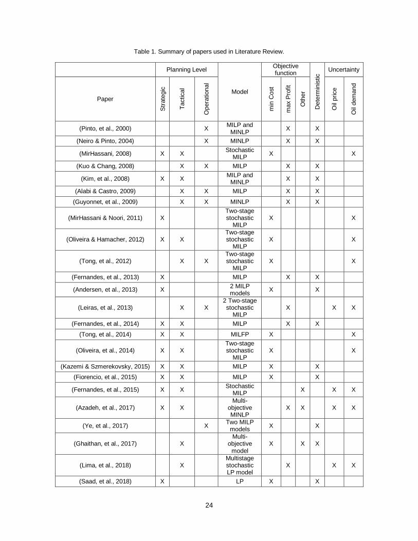
24

Table 1. Summary of papers used in Literature Review.

Planning Level

Model

Objective function

Dete

rmin

istic Uncertainty

Paper

Str

ate

gic

Tactical

Opera

tional

min

Cost

max P

rofit

Oth

er

Oil

price

Oil

dem

and

(Pinto, et al., 2000) X MILP and

MINLP X X

(Neiro & Pinto, 2004) X MINLP X X

(MirHassani, 2008) X X Stochastic MILP

X X

(Kuo & Chang, 2008) X X MILP X X

(Kim, et al., 2008) X X MILP and

MINLP X X

(Alabi & Castro, 2009) X X MILP X X

(Guyonnet, et al., 2009) X X MINLP X X

(MirHassani & Noori, 2011) X Two-stage stochastic

MILP X X

(Oliveira & Hamacher, 2012) X X Two-stage stochastic

MILP X X

(Tong, et al., 2012) X X Two-stage stochastic

MILP X X

(Fernandes, et al., 2013) X MILP X X

(Andersen, et al., 2013) X 2 MILP models

X X

(Leiras, et al., 2013) X X 2 Two-stage stochastic

MILP X X X

(Fernandes, et al., 2014) X X MILP X X

(Tong, et al., 2014) X X MILFP X X

(Oliveira, et al., 2014) X X Two-stage stochastic

MILP X X

(Kazemi & Szmerekovsky, 2015) X X MILP X X

(Fiorencio, et al., 2015) X X MILP X X

(Fernandes, et al., 2015) X X Stochastic

MILP X X X

(Azadeh, et al., 2017) X X Multi-

objective MINLP

X X X X

(Ye, et al., 2017) X Two MILP

models X X

(Ghaithan, et al., 2017) X Multi-

objective model

X X X

(Lima, et al., 2018) X Multistage stochastic LP model

X X X

(Saad, et al., 2018) X LP X X

25

Chapter 4 – Problem Definition, Model Formulation and Validation

The aim of this chapter is to characterize the problem studied in this Master thesis, to present

the mathematical model developed and to validate the model. The chapter is divided into six sections:

Section 4.1 is responsible for defining and characterizing the problem to be developed; Section 4.2

describes the mathematical model developed; Section 4.3 brings the main contributions of the model

developed in comparison with the base model; Section 4.4 describes the illustrative case study;

Section 4.5 analyses the results obtained after validating the model using the illustrative case study;

and Section 4.6 concludes the chapter.

4.1. Problem Definition

As identified in the previous chapter there are some space for research in the downstream

supply chain considered the strategic-tactical decision levels. This is the focus of this Master thesis,

where the aim was to develop a MILP mathematical model that supports the definition of a distribution

strategy for supplying markets that may span over more than one country. This later feature is

important since in different countries, different public policies may apply to the distribution operation

and these must be accounted when managing the supply chain.

Knowing that strategic decisions comprise the determination of locations and capacities of

storage, terminals and distribution bases and planning of transportation modes; and that tactical

decisions look into aspects such as the planning of transportation modes, flows’ allocation and

evaluation of the need to import products or the opportunity to export them, the problem addressed

can be generically described as follows:

Given a downstream PSC, in which one company fully manages a set of oil products from a

set of refineries to supply a set of locations according to their demands through a set of depots using

possible and available transportation modes.

Determine the design and planning of the supply chain, which consists on the installation and

and/or closure of facilities while considering its required capacity and how these are going to be

operated at a planning level – which transportation modes and routes to use, what are the material

flows, refinery productions and import or export of materials.

Subject to customer demands, oil products yield, material balance and storage and

transportation capacity constraints.

So as to minimize the costs regarding opening new distribution centers and distribution, which

are mainly related to transportation, inventory, import and export.

In order to solve the problem defined, a mathematical model was developed and it will be

approached in the next sections.

26

4.2. Mathematical model

After defining the problem, the following step was to formulate a mathematical model in order

to solve it. The model was based on that developed by Kazemi & Szmerekovsky (2015), which

addresses strategic and tactical decisions (such as determining optimal location and capacities for

distribution centers, selection of transportation modes, determining flow allocation, etc.) considering

multiple products while minimize the fixed and distributing costs.

In order to formulate the MILP mathematical model, we consider two countries A and B, that

are commercial partners, and the model was developed under country A’s perspective. This is, the

objective of the problem is to design and plan the downstream petroleum supply chain minimizing

country A’s costs. It is also possible to consider more than two countries, this is a more generic model

considering a country of origin A and a set B of countries, and all data regarding the other countries

considered would replace country B’s.

The case study in Iberia illustrates well the problem proposed, in which Portugal is

represented as country A and Spain as country B, because the country that Portugal imports and

exports the largest amount of oil derivatives is from/to Spain (Autoridade da Concorrência, 2018).

4.2.1. Sets, subsets and parameters

It was considered a set I of refineries i with capacities Si, subdivided in subset A of refineries

a located in country A and in subset B of refineries b located in country B; and a set J of distribution

centers (storage depots) j, subdivided in subset N of possible new depots n to be opened in country

A and in subset H of existent depots h in country A. Each of the possible new depots n are associated

with a fixed cost fn to open each of them and a cost per unit of capacity βn.

The model also includes a set P of oil products p; a set U of customer nodes u with annual

demands Dp,u for each product p, subdivided in subset K of customer nodes k located in country A

and in subset W of customer nodes w in country B; and a set R of transportation modes r, which

transport products p with cost per unit of product, Cp,a,j,r, from refineries a to depots j, transport

products p with cost per unit of product, Tp,j,k,r, from depots j to customer nodes k and transport

imported products p from refineries b to refineries a with cost per unit of product, TIMPp,b,a,r. In this

study, four transportation modes are considered: pipelines, barge, rail and truck.

Other parameters considered were: the price per unit of product p, PIMPp,b,a,r, transported by

transportation mode r, that refinery a must pay to import product p from refinery b; the price per unit

of product p, PEXPp,a,b, that refinery a charges to export product p to refinery b; the fraction αb,p of

refinery b capacity used to produce product p; and the annual maximum capacity of transportation:

from refinery a to depot j using transportation mode r, QRDa,j,r, from depot j to customer node k using

transportation mode r, QDCj,k,r, and from refinery b to refinery a using transportation mode r, QRRa,b,r.

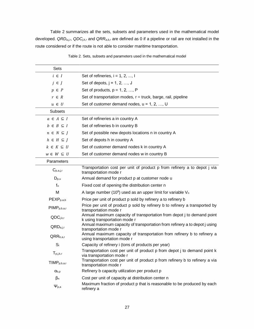
27

Table 2 summarizes all the sets, subsets and parameters used in the mathematical model

developed. QRDa,j,r, QDCj,k,r and QRRa,b,r are defined as 0 if a pipeline or rail are not installed in the

route considered or if the route is not able to consider maritime transportation.

Table 2. Sets, subsets and parameters used in the mathematical model

Sets

𝑖 ∈ 𝐼 Set of refineries, i = 1, 2, ..., I

𝑗 ∈ 𝐽 Set of depots, j = 1, 2, …, J

𝑝 ∈ 𝑃 Set of products, p = 1, 2, …, P

𝑟 ∈ 𝑅 Set of transportation modes, r = truck, barge, rail, pipeline

𝑢 ∈ 𝑈 Set of customer demand nodes, u = 1, 2, …, U

Subsets

𝑎 ∈ 𝐴 ⊆ 𝐼 Set of refineries a in country A

𝑏 ∈ 𝐵 ⊆ 𝐼 Set of refineries b in country B

𝑛 ∈ 𝑁 ⊆ 𝐽 Set of possible new depots locations n in country A

ℎ ∈ 𝐻 ⊆ 𝐽 Set of depots h in country A

𝑘 ∈ 𝐾 ⊆ 𝑈 Set of customer demand nodes k in country A

𝑤 ∈ 𝑊 ⊆ 𝑈 Set of customer demand nodes w in country B

Parameters

Cp,a,j,r Transportation cost per unit of product p from refinery a to depot j via transportation mode r

Dp,u Annual demand for product p at customer node u

fn Fixed cost of opening the distribution center n

M A large number (109) used as an upper limit for variable Vn

PEXPp,a,b Price per unit of product p sold by refinery a to refinery b

PIMPp,b,a,r Price per unit of product p sold by refinery b to refinery a transported by transportation mode r

QDCj,k,r Annual maximum capacity of transportation from depot j to demand point k using transportation mode r

QRDa,j,r Annual maximum capacity of transportation from refinery a to depot j using transportation mode r

QRRb,a,r Annual maximum capacity of transportation from refinery b to refinery a using transportation mode r

Si Capacity of refinery i (tons of products per year)

Tp,j,k,r Transportation cost per unit of product p from depot j to demand point k via transportation mode r

TIMPp,b,a,r Transportation cost per unit of product p from refinery b to refinery a via transportation mode r

αb,p Refinery b capacity utilization per product p

βn Cost per unit of capacity at distribution center n

Ψp,a Maximum fraction of product p that is reasonable to be produced by each refinery a

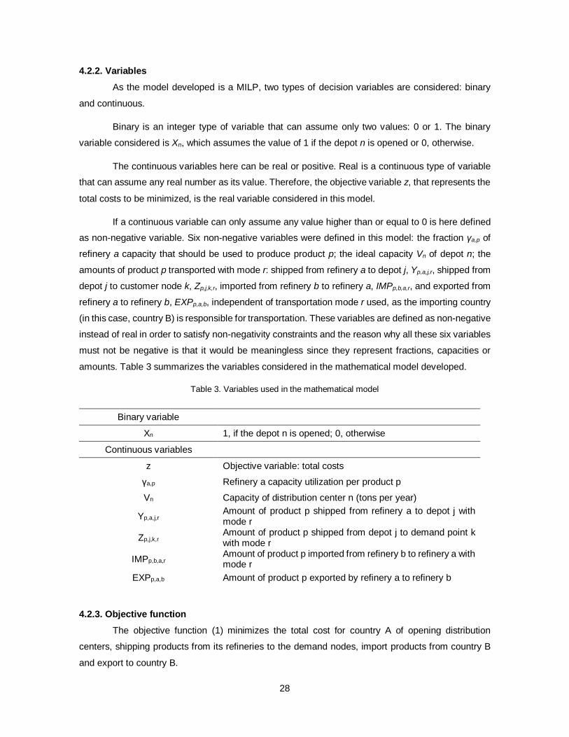
28

4.2.2. Variables

As the model developed is a MILP, two types of decision variables are considered: binary

and continuous.

Binary is an integer type of variable that can assume only two values: 0 or 1. The binary

variable considered is Xn, which assumes the value of 1 if the depot n is opened or 0, otherwise.

The continuous variables here can be real or positive. Real is a continuous type of variable

that can assume any real number as its value. Therefore, the objective variable z, that represents the

total costs to be minimized, is the real variable considered in this model.

If a continuous variable can only assume any value higher than or equal to 0 is here defined

as non-negative variable. Six non-negative variables were defined in this model: the fraction γa,p of

refinery a capacity that should be used to produce product p; the ideal capacity Vn of depot n; the

amounts of product p transported with mode r: shipped from refinery a to depot j, Yp,a,j,r, shipped from

depot j to customer node k, Zp,j,k,r, imported from refinery b to refinery a, IMPp,b,a,r, and exported from

refinery a to refinery b, EXPp,a,b, independent of transportation mode r used, as the importing country

(in this case, country B) is responsible for transportation. These variables are defined as non-negative

instead of real in order to satisfy non-negativity constraints and the reason why all these six variables

must not be negative is that it would be meaningless since they represent fractions, capacities or

amounts. Table 3 summarizes the variables considered in the mathematical model developed.

Table 3. Variables used in the mathematical model

Binary variable

Xn 1, if the depot n is opened; 0, otherwise

Continuous variables

z Objective variable: total costs

γa,p Refinery a capacity utilization per product p

Vn Capacity of distribution center n (tons per year)

Yp,a,j,r Amount of product p shipped from refinery a to depot j with mode r

Zp,j,k,r Amount of product p shipped from depot j to demand point k with mode r

IMPp,b,a,r Amount of product p imported from refinery b to refinery a with mode r

EXPp,a,b Amount of product p exported by refinery a to refinery b

4.2.3. Objective function

The objective function (1) minimizes the total cost for country A of opening distribution

centers, shipping products from its refineries to the demand nodes, import products from country B

and export to country B.

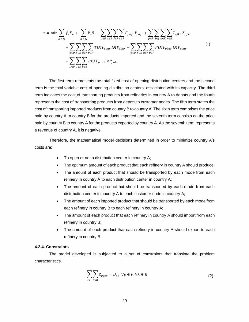
29

𝑧 = min ∑ 𝑓𝑛𝑋𝑛

n ∈ 𝑁

+ ∑ 𝑉𝑛𝛽𝑛

n ∈ N

+ ∑ ∑ ∑ ∑ 𝐶𝑝𝑎𝑗𝑟

𝑟∈𝑅𝑗∈𝐽𝑎∈𝐴

𝑌𝑝𝑎𝑗𝑟

𝑝∈𝑃

+ ∑ ∑ ∑ ∑ 𝑇𝑝𝑗𝑘𝑟

𝑟∈𝑅𝑘∈𝐾𝑗∈𝐽

𝑍𝑝𝑗𝑘𝑟

𝑝∈𝑃

+ ∑ ∑ ∑ ∑ 𝑇𝐼𝑀𝑃𝑝𝑏𝑎𝑟

𝑟∈𝑅𝑎∈𝐴𝑏∈𝐵

𝐼𝑀𝑃𝑝𝑏𝑎𝑟

𝑝∈𝑃

+ ∑ ∑ ∑ ∑ 𝑃𝐼𝑀𝑃𝑝𝑏𝑎𝑟

𝑟∈𝑅𝑎∈𝐴𝑏∈𝐵

𝐼𝑀𝑃𝑝𝑏𝑎𝑟

𝑝∈𝑃

− ∑ ∑ ∑ 𝑃𝐸𝑋𝑃𝑝𝑎𝑏

𝑏∈𝐵𝑎∈𝐴𝑝∈𝑃

𝐸𝑋𝑃𝑝𝑎𝑏

(1)

The first term represents the total fixed cost of opening distribution centers and the second

term is the total variable cost of opening distribution centers, associated with its capacity. The third

term indicates the cost of transporting products from refineries in country A to depots and the fourth

represents the cost of transporting products from depots to customer nodes. The fifth term states the

cost of transporting imported products from country B to country A. The sixth term comprises the price

paid by country A to country B for the products imported and the seventh term consists on the price

paid by country B to country A for the products exported by country A. As the seventh term represents

a revenue of country A, it is negative.

Therefore, the mathematical model decisions determined in order to minimize country A’s

costs are:

To open or not a distribution center in country A;

The optimum amount of each product that each refinery in country A should produce;

The amount of each product that should be transported by each mode from each

refinery in country A to each distribution center in country A;

The amount of each product hat should be transported by each mode from each

distribution center in country A to each customer node in country A;

The amount of each imported product that should be transported by each mode from

each refinery in country B to each refinery in country A;

The amount of each product that each refinery in country A should import from each

refinery in country B;

The amount of each product that each refinery in country A should export to each

refinery in country B.

4.2.4. Constraints

The model developed is subjected to a set of constraints that translate the problem

characteristics.

∑ ∑ 𝑍𝑝𝑗𝑘𝑟

𝑟∈𝑅𝑗∈𝐽

= 𝐷𝑝𝑘 ∀𝑝 ∈ 𝑃, ∀𝑘 ∈ 𝐾 (2)

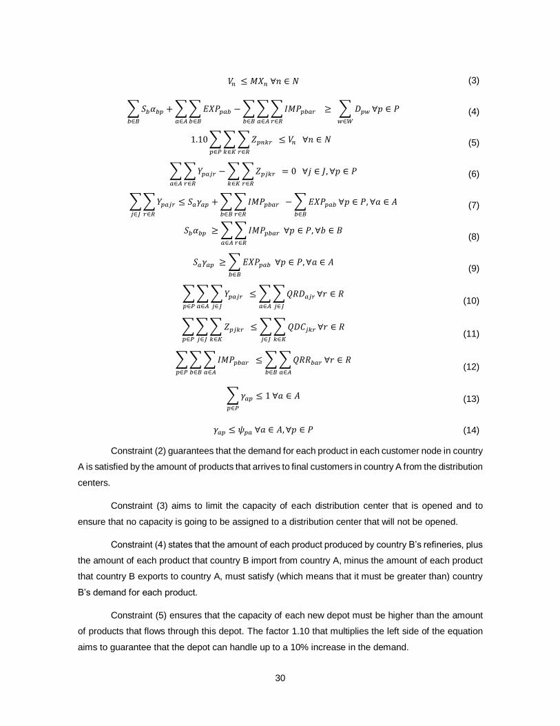
30

𝑉𝑛 ≤ 𝑀𝑋𝑛 ∀𝑛 ∈ 𝑁 (3)

∑ 𝑆𝑏𝛼𝑏𝑝 + ∑ ∑ 𝐸𝑋𝑃𝑝𝑎𝑏

𝑏∈𝐵

− ∑ ∑ ∑ 𝐼𝑀𝑃𝑝𝑏𝑎𝑟

𝑟∈𝑅𝑎∈𝐴

𝑏∈𝐵

≥ 𝑎∈𝐴𝑏∈𝐵

∑ 𝐷𝑝𝑤

𝑤∈𝑊

∀𝑝 ∈ 𝑃 (4)

1.10 ∑ ∑ ∑ 𝑍𝑝𝑛𝑘𝑟

𝑟∈𝑅𝑘∈𝐾

≤ 𝑉𝑛 ∀𝑛 ∈ 𝑁

𝑝∈𝑃

(5)

∑ ∑ 𝑌𝑝𝑎𝑗𝑟

𝑟∈𝑅

− ∑ ∑ 𝑍𝑝𝑗𝑘𝑟

𝑟∈𝑅

𝑘∈𝐾𝑎∈𝐴

= 0 ∀𝑗 ∈ 𝐽, ∀𝑝 ∈ 𝑃 (6)

∑ ∑ 𝑌𝑝𝑎𝑗𝑟

𝑟∈𝑅𝑗∈𝐽

≤ 𝑆𝑎𝛾𝑎𝑝 + ∑ ∑ 𝐼𝑀𝑃𝑝𝑏𝑎𝑟

𝑟∈𝑅

− ∑ 𝐸𝑋𝑃𝑝𝑎𝑏

𝑏∈𝐵𝑏∈𝐵

∀𝑝 ∈ 𝑃, ∀𝑎 ∈ 𝐴 (7)

𝑆𝑏𝛼𝑏𝑝 ≥ ∑ ∑ 𝐼𝑀𝑃𝑝𝑏𝑎𝑟

𝑟∈𝑅𝑎∈𝐴

∀𝑝 ∈ 𝑃, ∀𝑏 ∈ 𝐵 (8)

𝑆𝑎𝛾𝑎𝑝 ≥ ∑ 𝐸𝑋𝑃𝑝𝑎𝑏

𝑏∈𝐵

∀𝑝 ∈ 𝑃, ∀𝑎 ∈ 𝐴 (9)

∑ ∑ ∑ 𝑌𝑝𝑎𝑗𝑟

𝑗∈𝐽𝑎∈𝐴𝑝∈𝑃

≤ ∑ ∑ 𝑄𝑅𝐷𝑎𝑗𝑟

𝑗∈𝐽𝑎∈𝐴

∀𝑟 ∈ 𝑅 (10)

∑ ∑ ∑ 𝑍𝑝𝑗𝑘𝑟

𝑘∈𝐾𝑗∈𝐽𝑝∈𝑃

≤ ∑ ∑ 𝑄𝐷𝐶𝑗𝑘𝑟

𝑘∈𝐾𝑗∈𝐽

∀𝑟 ∈ 𝑅 (11)

∑ ∑ ∑ 𝐼𝑀𝑃𝑝𝑏𝑎𝑟

𝑎∈𝐴𝑏∈𝐵𝑝∈𝑃

≤ ∑ ∑ 𝑄𝑅𝑅𝑏𝑎𝑟

𝑎∈𝐴𝑏∈𝐵

∀𝑟 ∈ 𝑅 (12)

∑ 𝛾𝑎𝑝

𝑝∈𝑃

≤ 1 ∀𝑎 ∈ 𝐴 (13)

𝛾𝑎𝑝 ≤ 𝜓𝑝𝑎 ∀𝑎 ∈ 𝐴, ∀𝑝 ∈ 𝑃 (14)

Constraint (2) guarantees that the demand for each product in each customer node in country

A is satisfied by the amount of products that arrives to final customers in country A from the distribution

centers.

Constraint (3) aims to limit the capacity of each distribution center that is opened and to

ensure that no capacity is going to be assigned to a distribution center that will not be opened.

Constraint (4) states that the amount of each product produced by country B’s refineries, plus

the amount of each product that country B import from country A, minus the amount of each product

that country B exports to country A, must satisfy (which means that it must be greater than) country

B’s demand for each product.

Constraint (5) ensures that the capacity of each new depot must be higher than the amount

of products that flows through this depot. The factor 1.10 that multiplies the left side of the equation

aims to guarantee that the depot can handle up to a 10% increase in the demand.

31

Constraint (6) is a mass balance constraint. It states that all of the amount that arrive in a

depot from a refinery will be transported from this depot to each customer node.

Constraint (7) ensures that the amount of each product produced and imported by refineries

in country A, minus the amount of each product exported by country A, must satisfy the amount that

is transported to refineries to depots.

Constraint (8) indicates that the amount of each product that a refinery in country B can

produce must be higher than the amount of the same product that it exports.

Constraint (9) indicates that the amount of each product that a refinery in country A can

produce must be higher than the amount of the same product that it exports.

Constraint (10) ensures that the total amount of products transported by each mode from

refinery a to depot j does not exceed the mode’s maximum capacity.

Constraint (11) ensures that the total amount of products transported by each mode from

depot j to customer node k does not exceed the mode’s maximum capacity.

Constraint (12) ensures that the total amount of imported products transported by each mode

from refinery b to refinery a does not exceed the mode’s maximum capacity.

Constraint (13) states that in each refinery the sum of refinery capacity utilization per product

must be equal or less than 1, as γa,p represents the percentage of total refinery capacity used to

produce a product.

Constraint (14) states the maximum reasonable fraction of product p that should be produced

by each refinery a.

4.3. Main contributions of the present developed model

As the model developed was based on Kazemi & Szmerekovsky (2015) – base model, it is

important to analyse both models and emphasize the main contributions of the model developed in

comparison with the base one.

Firstly, the model developed creates a distribution strategy that spans over more than one

country, while Kazemi & Szmerekovsky (2015) considered the distribution in a single country.

Therefore, this model incorporates costs regarding import and export that were not considered in the

previous model.

Another point is that Kazemi & Szmerekovsky (2015) did not limit the transportation mode

selection. However, this model establishes the annual maximum capacity of each transportation

mode represented by the parameters QRDa,j,r, QDCj,k,r and QRRb,a,r. Moreover, these parameters are

32

declared 0 when a route is infeasible, limiting the selection of a pipeline when it is not built or the

selection of barge if a port is not available in the location.

Furthermore, the model developed can define the optimal fractions of each product that each

refinery should produce. In order to better fit the model to the reality, the parameter Ψp,a was

established to limit to a reasonable value the maximum fraction of each product to be produced.

Unfortunately, it is not possible to convert 100% of the crude oil in gasoline.

Regarding to the distribution centers, Kazemi & Szmerekovsky (2015) only analyses potential

new depots and therefore, does not consider the depots that are already opened in its network. On

the other hand, the model developed considers the existent distribution center and also makes the

decision of opening or not a distribution center in a determined location.

Finally, another important feature of the model is versatility. It is possible to analyse the

decision of building a pipeline between two nodes in a simple manner. In order to do this, a new depot

should be supposed in the same location of the depot that the new pipeline starts or ends. The fixed

cost of this new depot is actually the total cost of the pipeline in question and the variable cost is null.

Then, the pipeline distance between the depot and the refinery or customer node is defined. After

that, the model will decide to open or not this fictional new depot and only if it is decided to be opened,

the pipeline will be considered.

An important observation about the situation of deciding or not to build a pipeline in an

existent depot is that all the possible and available routes through this depot must also be assigned

to the fictional depot, resulting in two equal routes with the same annual maximum capacity.

Therefore, a constraint must be created to define that the sum of two equal routes must be less than

the annual maximum capacity assigned to the original route.

4.4. Illustrative case study

Before applying a real case to the model, it is important to validate it using an illustrative case.

The reason why an illustrative case was used in first place is that it is very smaller than the real case

and, therefore, it was easier to check for mistakes and if the model was working properly.

The illustrative case study comprises two countries called Country A and Country B. Country

A has two refineries i1 and i2 and Country B has only refinery i3. Country A has one distribution center

j1 and it is evaluating to build a distribution center j2 or/and j3. There are three customer demand

nodes (u1, u2 and u3) and one airport (uair1) in Country A. There is only one customer demand node

(u4) and one airport (uair2) in Country B. The illustrative case is represented in a map below (see

Figure 5).

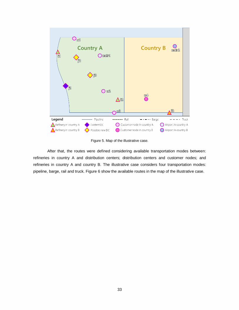
33

Figure 5. Map of the illustrative case.

After that, the routes were defined considering available transportation modes between:

refineries in country A and distribution centers; distribution centers and customer nodes; and

refineries in country A and country B. The illustrative case considers four transportation modes:

pipeline, barge, rail and truck. Figure 6 show the available routes in the map of the illustrative case.

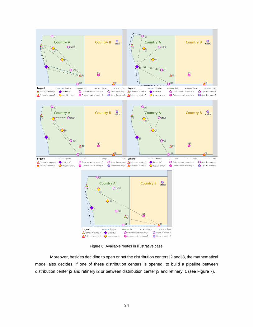
34

Figure 6. Available routes in illustrative case.

Moreover, besides deciding to open or not the distribution centers j2 and j3, the mathematical

model also decides, if one of these distribution centers is opened, to build a pipeline between

distribution center j2 and refinery i2 or between distribution center j3 and refinery i1 (see Figure 7).

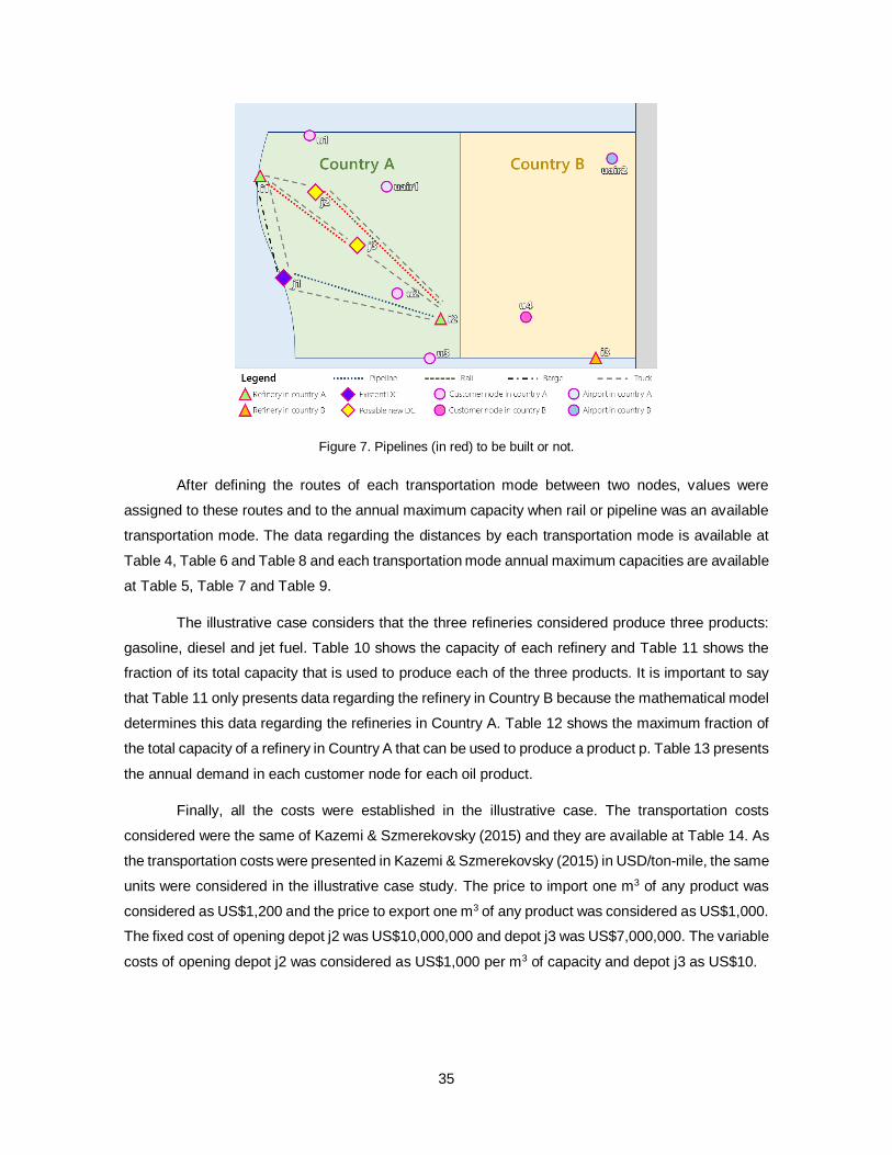
35

Figure 7. Pipelines (in red) to be built or not.

After defining the routes of each transportation mode between two nodes, values were

assigned to these routes and to the annual maximum capacity when rail or pipeline was an available

transportation mode. The data regarding the distances by each transportation mode is available at

Table 4, Table 6 and Table 8 and each transportation mode annual maximum capacities are available

at Table 5, Table 7 and Table 9.

The illustrative case considers that the three refineries considered produce three products:

gasoline, diesel and jet fuel. Table 10 shows the capacity of each refinery and Table 11 shows the

fraction of its total capacity that is used to produce each of the three products. It is important to say

that Table 11 only presents data regarding the refinery in Country B because the mathematical model

determines this data regarding the refineries in Country A. Table 12 shows the maximum fraction of

the total capacity of a refinery in Country A that can be used to produce a product p. Table 13 presents

the annual demand in each customer node for each oil product.

Finally, all the costs were established in the illustrative case. The transportation costs

considered were the same of Kazemi & Szmerekovsky (2015) and they are available at Table 14. As

the transportation costs were presented in Kazemi & Szmerekovsky (2015) in USD/ton-mile, the same

units were considered in the illustrative case study. The price to import one m3 of any product was

considered as US$1,200 and the price to export one m3 of any product was considered as US$1,000.

The fixed cost of opening depot j2 was US$10,000,000 and depot j3 was US$7,000,000. The variable

costs of opening depot j2 was considered as US$1,000 per m3 of capacity and depot j3 as US$10.

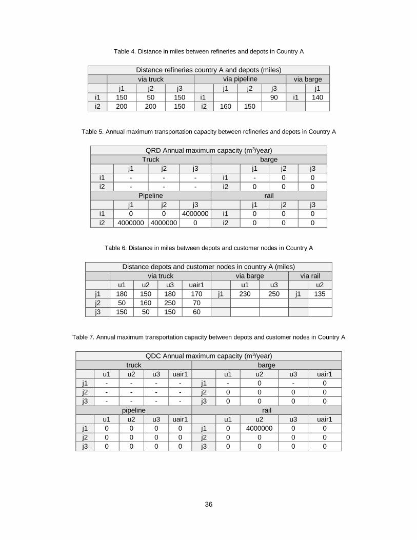
36

Table 4. Distance in miles between refineries and depots in Country A

Distance refineries country A and depots (miles)

via truck via pipeline via barge

j1 j2 j3 j1 j2 j3 j1

i1 150 50 150 i1 90 i1 140

i2 200 200 150 i2 160 150

Table 5. Annual maximum transportation capacity between refineries and depots in Country A

QRD Annual maximum capacity (m3/year)

Truck barge

j1 j2 j3 j1 j2 j3

i1 - - - i1 - 0 0

i2 - - - i2 0 0 0

Pipeline rail

j1 j2 j3 j1 j2 j3

i1 0 0 4000000 i1 0 0 0

i2 4000000 4000000 0 i2 0 0 0

Table 6. Distance in miles between depots and customer nodes in Country A

Distance depots and customer nodes in country A (miles)

via truck via barge via rail

u1 u2 u3 uair1 u1 u3 u2

j1 180 150 180 170 j1 230 250 j1 135

j2 50 160 250 70

j3 150 50 150 60

Table 7. Annual maximum transportation capacity between depots and customer nodes in Country A

QDC Annual maximum capacity (m3/year)

truck barge

u1 u2 u3 uair1 u1 u2 u3 uair1

j1 - - - - j1 - 0 - 0

j2 - - - - j2 0 0 0 0

j3 - - - - j3 0 0 0 0

pipeline rail

u1 u2 u3 uair1 u1 u2 u3 uair1

j1 0 0 0 0 j1 0 4000000 0 0

j2 0 0 0 0 j2 0 0 0 0

j3 0 0 0 0 j3 0 0 0 0

37

Table 8. Distance in miles between refineries in Country A and refineries in Country B

Distance refineries in country A and refineries in country B (miles)

via truck via barge

i3 i3

i1 500 750

i2 200

Table 9. Annual maximum transportation capacity between refineries in Country A and refineries in Country B

QRR Annual maximum capacity (m3/year)

truck barge pipeline rail

i3 i3 i3 i3

i1 - - 0 0

i2 - 0 0 0

Table 10. Annual refining capacity of each refinery i

Capacity of refineries i (m3/year)

Si

i1 20000000

i2 8000000

i3 70000000

Table 11. Fraction of total refinery capacity used to produce each product p

αb,p

gasoline diesel jetfuel other

i3 0.2 0.4 0.3 0.1

Table 12. Maximum fraction of product p that is reasonable to be produced by each refinery in Country A

Maximum reasonable amount (ψa,p)

gasoline diesel jetfuel

i1 0.25 0.5 0.2

i2 0.25 0.5 0.2

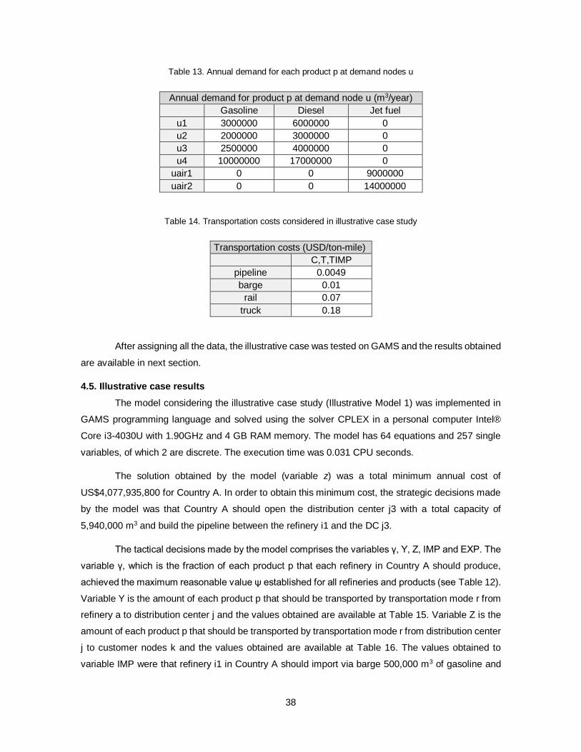
38

Table 13. Annual demand for each product p at demand nodes u

Annual demand for product p at demand node u (m3/year)

Gasoline Diesel Jet fuel

u1 3000000 6000000 0

u2 2000000 3000000 0

u3 2500000 4000000 0

u4 10000000 17000000 0

uair1 0 0 9000000

uair2 0 0 14000000

Table 14. Transportation costs considered in illustrative case study

Transportation costs (USD/ton-mile)

C,T,TIMP

pipeline 0.0049

barge 0.01

rail 0.07

truck 0.18

After assigning all the data, the illustrative case was tested on GAMS and the results obtained

are available in next section.

4.5. Illustrative case results

The model considering the illustrative case study (Illustrative Model 1) was implemented in

GAMS programming language and solved using the solver CPLEX in a personal computer Intel®

Core i3-4030U with 1.90GHz and 4 GB RAM memory. The model has 64 equations and 257 single

variables, of which 2 are discrete. The execution time was 0.031 CPU seconds.

The solution obtained by the model (variable z) was a total minimum annual cost of

US$4,077,935,800 for Country A. In order to obtain this minimum cost, the strategic decisions made

by the model was that Country A should open the distribution center j3 with a total capacity of

5,940,000 m3 and build the pipeline between the refinery i1 and the DC j3.

The tactical decisions made by the model comprises the variables γ, Y, Z, IMP and EXP. The

variable γ, which is the fraction of each product p that each refinery in Country A should produce,

achieved the maximum reasonable value ψ established for all refineries and products (see Table 12).

Variable Y is the amount of each product p that should be transported by transportation mode r from

refinery a to distribution center j and the values obtained are available at Table 15. Variable Z is the

amount of each product p that should be transported by transportation mode r from distribution center

j to customer nodes k and the values obtained are available at Table 16. The values obtained to

variable IMP were that refinery i1 in Country A should import via barge 500,000 m3 of gasoline and

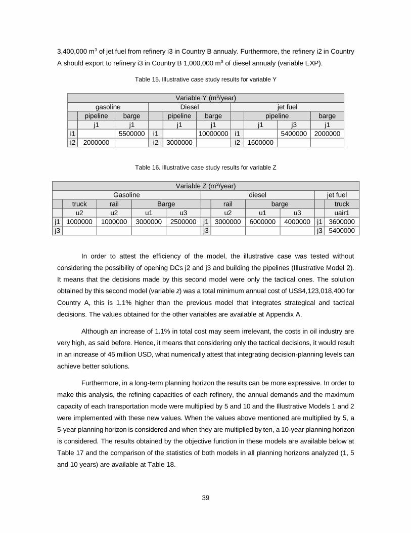
39

3,400,000 m3 of jet fuel from refinery i3 in Country B annualy. Furthermore, the refinery i2 in Country

A should export to refinery i3 in Country B 1,000,000 m3 of diesel annualy (variable EXP).

Table 15. Illustrative case study results for variable Y

Variable Y (m3/year)

gasoline Diesel jet fuel

pipeline barge pipeline barge pipeline barge

j1 j1 j1 j1 j1 j3 j1

i1 5500000 i1 10000000 i1 5400000 2000000

i2 2000000 i2 3000000 i2 1600000

Table 16. Illustrative case study results for variable Z

Variable Z (m3/year)

Gasoline diesel jet fuel

truck rail Barge rail barge truck

u2 u2 u1 u3 u2 u1 u3 uair1

j1 1000000 1000000 3000000 2500000 j1 3000000 6000000 4000000 j1 3600000

j3 j3 j3 5400000

In order to attest the efficiency of the model, the illustrative case was tested without

considering the possibility of opening DCs j2 and j3 and building the pipelines (Illustrative Model 2).

It means that the decisions made by this second model were only the tactical ones. The solution

obtained by this second model (variable z) was a total minimum annual cost of US$4,123,018,400 for

Country A, this is 1.1% higher than the previous model that integrates strategical and tactical

decisions. The values obtained for the other variables are available at Appendix A.

Although an increase of 1.1% in total cost may seem irrelevant, the costs in oil industry are

very high, as said before. Hence, it means that considering only the tactical decisions, it would result

in an increase of 45 million USD, what numerically attest that integrating decision-planning levels can

achieve better solutions.

Furthermore, in a long-term planning horizon the results can be more expressive. In order to

make this analysis, the refining capacities of each refinery, the annual demands and the maximum

capacity of each transportation mode were multiplied by 5 and 10 and the Illustrative Models 1 and 2

were implemented with these new values. When the values above mentioned are multiplied by 5, a

5-year planning horizon is considered and when they are multiplied by ten, a 10-year planning horizon

is considered. The results obtained by the objective function in these models are available below at

Table 17 and the comparison of the statistics of both models in all planning horizons analyzed (1, 5

and 10 years) are available at Table 18.

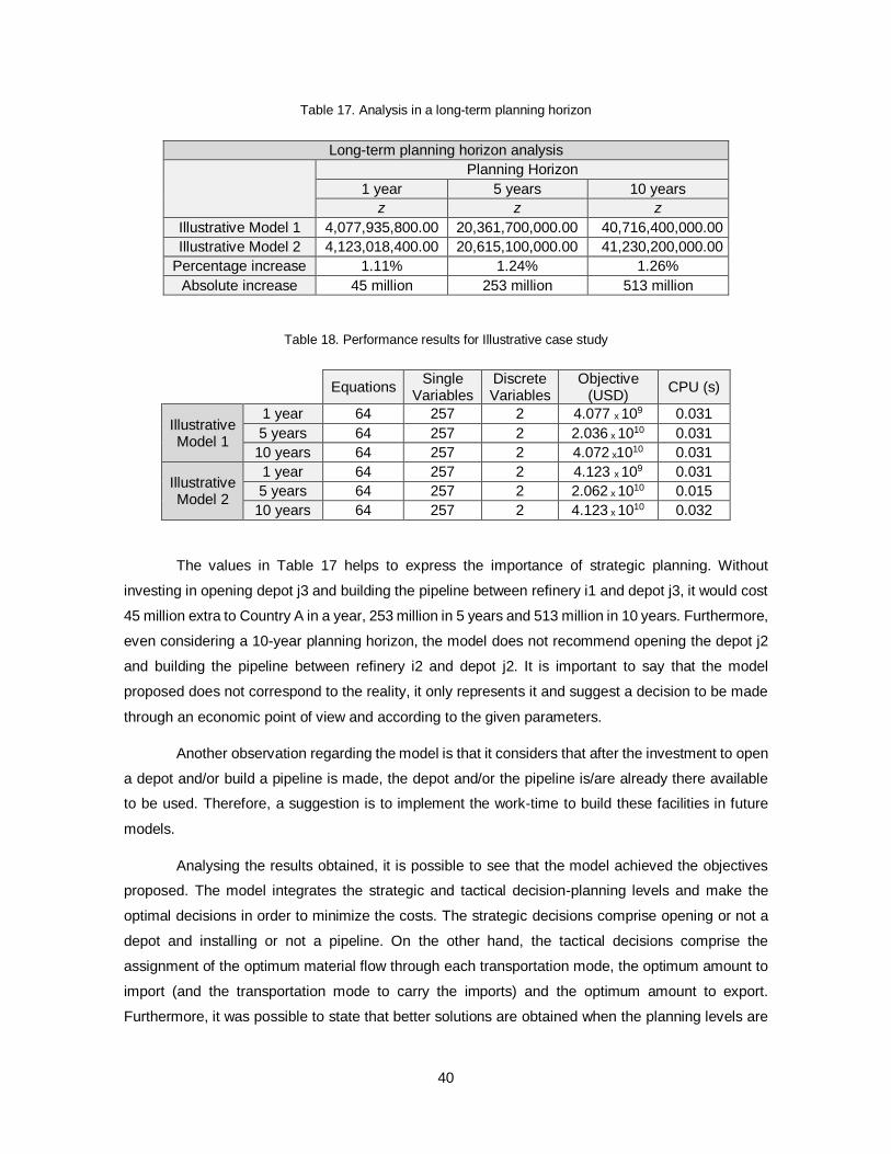
40

Table 17. Analysis in a long-term planning horizon

Long-term planning horizon analysis

Planning Horizon

1 year 5 years 10 years

z z z

Illustrative Model 1 4,077,935,800.00 20,361,700,000.00 40,716,400,000.00

Illustrative Model 2 4,123,018,400.00 20,615,100,000.00 41,230,200,000.00

Percentage increase 1.11% 1.24% 1.26%

Absolute increase 45 million 253 million 513 million

Table 18. Performance results for Illustrative case study

Equations Single

Variables Discrete Variables

Objective (USD)

CPU (s)

Illustrative Model 1

1 year 64 257 2 4.077 x 109 0.031

5 years 64 257 2 2.036 x 1010 0.031

10 years 64 257 2 4.072 x1010 0.031

Illustrative Model 2

1 year 64 257 2 4.123 x 109 0.031

5 years 64 257 2 2.062 x 1010 0.015

10 years 64 257 2 4.123 x 1010 0.032

The values in Table 17 helps to express the importance of strategic planning. Without

investing in opening depot j3 and building the pipeline between refinery i1 and depot j3, it would cost

45 million extra to Country A in a year, 253 million in 5 years and 513 million in 10 years. Furthermore,

even considering a 10-year planning horizon, the model does not recommend opening the depot j2

and building the pipeline between refinery i2 and depot j2. It is important to say that the model

proposed does not correspond to the reality, it only represents it and suggest a decision to be made

through an economic point of view and according to the given parameters.

Another observation regarding the model is that it considers that after the investment to open

a depot and/or build a pipeline is made, the depot and/or the pipeline is/are already there available

to be used. Therefore, a suggestion is to implement the work-time to build these facilities in future

models.

Analysing the results obtained, it is possible to see that the model achieved the objectives

proposed. The model integrates the strategic and tactical decision-planning levels and make the

optimal decisions in order to minimize the costs. The strategic decisions comprise opening or not a

depot and installing or not a pipeline. On the other hand, the tactical decisions comprise the

assignment of the optimum material flow through each transportation mode, the optimum amount to

import (and the transportation mode to carry the imports) and the optimum amount to export.

Furthermore, it was possible to state that better solutions are obtained when the planning levels are

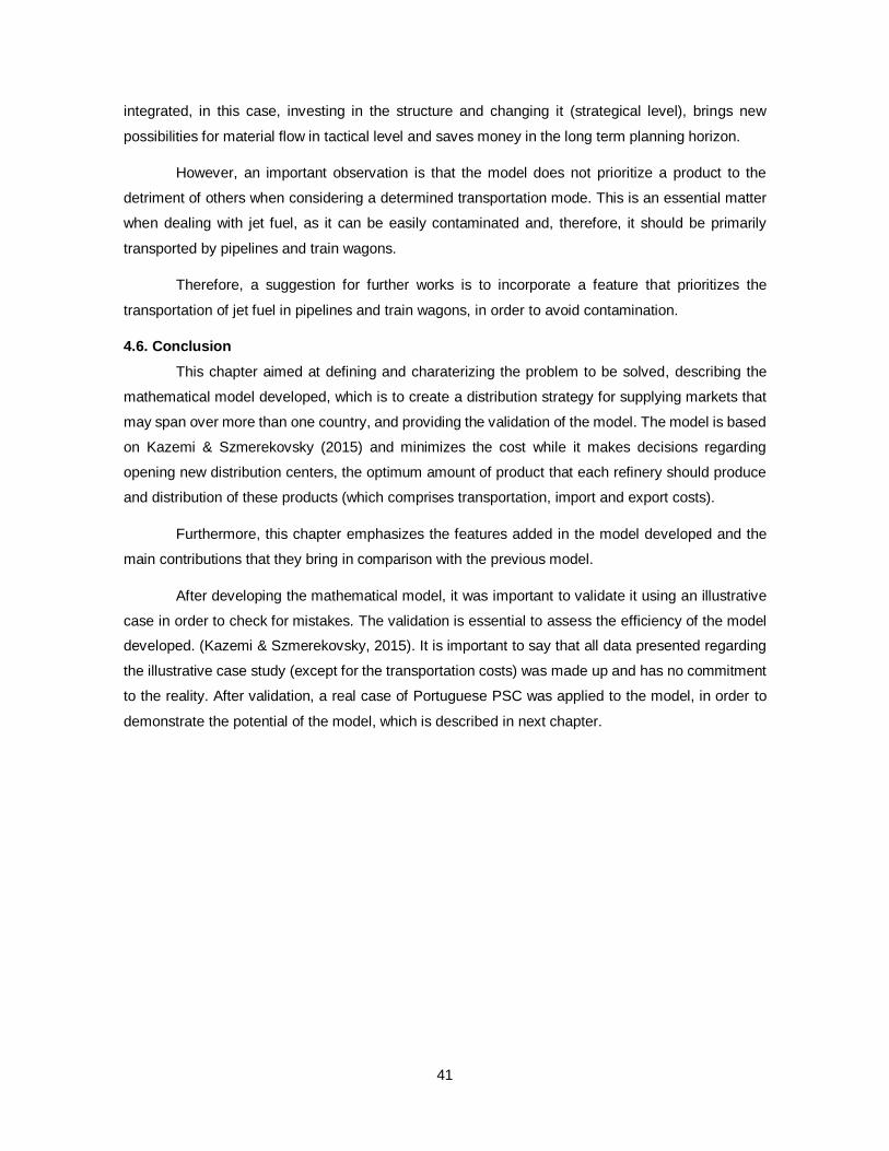
41

integrated, in this case, investing in the structure and changing it (strategical level), brings new

possibilities for material flow in tactical level and saves money in the long term planning horizon.

However, an important observation is that the model does not prioritize a product to the

detriment of others when considering a determined transportation mode. This is an essential matter

when dealing with jet fuel, as it can be easily contaminated and, therefore, it should be primarily

transported by pipelines and train wagons.

Therefore, a suggestion for further works is to incorporate a feature that prioritizes the

transportation of jet fuel in pipelines and train wagons, in order to avoid contamination.

4.6. Conclusion

This chapter aimed at defining and charaterizing the problem to be solved, describing the

mathematical model developed, which is to create a distribution strategy for supplying markets that

may span over more than one country, and providing the validation of the model. The model is based

on Kazemi & Szmerekovsky (2015) and minimizes the cost while it makes decisions regarding

opening new distribution centers, the optimum amount of product that each refinery should produce

and distribution of these products (which comprises transportation, import and export costs).

Furthermore, this chapter emphasizes the features added in the model developed and the

main contributions that they bring in comparison with the previous model.

After developing the mathematical model, it was important to validate it using an illustrative

case in order to check for mistakes. The validation is essential to assess the efficiency of the model

developed. (Kazemi & Szmerekovsky, 2015). It is important to say that all data presented regarding

the illustrative case study (except for the transportation costs) was made up and has no commitment

to the reality. After validation, a real case of Portuguese PSC was applied to the model, in order to

demonstrate the potential of the model, which is described in next chapter.

42

43

Chapter 5 – Case study

These chapter goals are to present the real case study that was applied to the model

developed in order to demonstrate its potential and to analyze the results obtained. Section 5.1

describes the real case and it is developed in two subsections, as the real case considers two

countries; Subsection 5.1.1 presents the Portuguese downstream oil supply chain, which is the first

part of case study to be used in order to validate the mathematical model; Subsection 5.1.2 presents

the Iberian market, which is the second part of the case study; Section 5.2 presents the Iberia

database and its sources; Section 5.3 analyses the results obtained after applying the real case to

the model; Section 5.4 presents suggestions for improvement for further works; and Section 5.5

concludes the chapter.

5.1. Real case study

In order to show the model applicability, this is now applied to a real case that aims to develop

a distribution strategy for supplying Iberia with oil products produced by a single company in Portugal

while minimizing the costs for Portugal.

5.1.1. Portuguese downstream oil supply chain

As mentioned the case study that was used in the thesis considers the Iberian market with

oil products produced in Portuguese refineries. The oil products to be considered are gasoline 95,

gasoline 98, gas oil (diesel) and jet fuel. At first, the model will not consider uncertainties.

In Portugal there are two oil refineries (Matosinhos and Sines) managed by a single company

and 278 local markets (Portuguese cities) in Portuguese network. In the model, the local markets

were simplified to 18, considering only the capital city of each Portuguese district as a demand node.

The transportation modes used in Portuguese PSC are pipelines, maritime, railway and road. Sines

and Matosinhos produce eight different oil products: jet fuel (A1), biodiesel (B5), propane (C3), butane

(C4), fuel oil (FU), gas oil (GO), gasoline 95 (U5) and gasoline 98 (U8). (Lima, 2018). There are

thirteen storage depots in Portugal. (Autoridade da Concorrência, 2018). However, the single

company considered in the model owns only six depots and these are the ones that were considered

in the case study. Figure 8 shows the location of refineries, storages, pipeline and terminals in

Portugal.

44

Figure 8. The Portuguese PSC. (Adapted from Autoridade da Concorrência, 2018).

The refining capacity of Sines and Matosinhos refineries together is 330 thousand barrels per

day and Sines is responsible for 70% of this total capacity (around 220 kbbl/day). Therefore, Portugal

owns 20% of total refining capacity at Iberian Peninsula. (GALP, s.d.).

Matosinhos refinery began operations in 1969 and it is a hydroskimming refinery, this is, a

refinery that executes primarily distillation. Sines began operations in 1978, it was improved in 2013

and it is a complex refinery today that owns a unit of hydrocracking and fluid catalytic cracking. (GALP,

s.d.). Hence, as Sines is more modern, it receives fuel oil loadings from Matosinhos through maritime

transportation. The objective is to produce products that are more valuable such as gas oil. (Mota,

2012).

It is possible to deliver oil products indirectly (through one of the six distribution centers) or

directly to the 18 capital city of Portuguese districts but the model always considers primary and

secondary distribution. However, if a direct distribution is recommended, the model will indicate the

primary distribution starting at the refinery and finishing at its own depot. Pipelines, rail, maritime and

45

road transportation modes are used for primary distribution (origin in refineries), while only roads are

used for secondary distribution (origin in distribution centers). Maritime transportation is used to

import crude oil and to export and import refined products. There are two pipelines in Portuguese

PSC: one multiproduct from Sines refinery to CLC and a jet fuel pipeline between Matosinhos and

Porto airport. (Lima, 2018).

Jet fuel is an oil product that can be easily contaminated and, therefore, it is important to deal

with its logistics apart from the other products. These refineries are responsible for supplying jet fuel

through trucks to the following airports: Lisbon (all the time), Porto and Faro (only in case of

eventuality). Lisbon airport is supplied by Companhia Logística de Combustíveis (CLC) through

trucks, Porto airport is supplied by Matosinhos refinery through pipelines and Faro airport is supplied

by Cepsa refinery in Huelva (Spain) through trucks and by Sines refinery using train wagons. (Mota,

2012).

5.1.2. The Iberian market

The case study considered the distribution of oil products produced in Portugal to the Iberian

Peninsula (see Figure 5) and, therefore, the Azores, Madeira, Balearic Islands and Canary Islands

were not considered. 45 provinces in Spain and 18 districts in Portugal compose the Iberian market.

The two Portuguese refineries can supply the Spanish market using trucks and ships. Moreover,

Portugal can import oil products from the eight refineries in Spain and trucks and ships can transport

the imports.

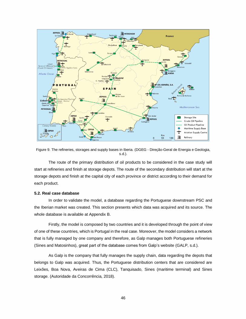
46

Figure 9. The refineries, storages and supply bases in Iberia. (DGEG - Direção-Geral de Energia e Geologia, s.d.).

The route of the primary distribution of oil products to be considered in the case study will

start at refineries and finish at storage depots. The route of the secondary distribution will start at the

storage depots and finish at the capital city of each province or district according to their demand for

each product.

5.2. Real case database

In order to validate the model, a database regarding the Portuguese downstream PSC and

the Iberian market was created. This section presents which data was acquired and its source. The

whole database is available at Appendix B.

Firstly, the model is composed by two countries and it is developed through the point of view

of one of these countries, which is Portugal in the real case. Moreover, the model considers a network

that is fully managed by one company and therefore, as Galp manages both Portuguese refineries

(Sines and Matosinhos), great part of the database comes from Galp’s website (GALP, s.d.).

As Galp is the company that fully manages the supply chain, data regarding the depots that

belongs to Galp was acquired. Thus, the Portuguese distribution centers that are considered are

Leixões, Boa Nova, Aveiras de Cima (CLC), Tanquisado, Sines (maritime terminal) and Sines

storage. (Autoridade da Concorrência, 2018).

47

After that, the distances via truck and barge (if available) between the refineries (Sines and

Matosinhos) and the distribution centers and between the distribution centers and the capital city of

each Portuguese district were computed using Google Maps and Google Earth. Pipeline and rail

distances were acquired in CLC website (CLC - Companhia Logística de Combustíveis, s.d.) and

Fernandes, et al. (2013).

In addition to this, the annual maximum capacities database was created. Regarding trucks

and barges (when available) there is no maximum capacity assigned. The maximum capacity of the

pipeline between Sines and Aveiras de Cima was collected in CLC website. However, only few

information was found regarding the pipelines between Matosinhos refinery and Leixões maritime

terminal and between Matosinhos and Porto airport. Therefore, no maximum capacity of these

pipelines was established. The maximum capacity of the pipelines that the model decides to build or

not are also assumed to be the same as the CLC pipeline. In order to assign the maximum capacity

via rail, the total capacity of Portuguese tank wagons (Instituto Nacional de Estatística, 2010) was

multiplied by 365, considering that all the available tank wagons use the rail route established only

once a day. If a route is not available via barge, pipeline or rail, the annual maximum capacity value

is assigned as 0.

Then, information regarding the Iberian market was acquired. Firstly, data regarding the

annual demand for gasoline 95, gasoline 98, jet fuel and diesel in Spain were acquired at CORES -

Corporación de reservas estratégicas de productos petrolíferos (2018). The data obtained covers

from 2013 to 2017. Thus, it was made an estimation of the demand in Spain using linear regression.

The annual demand in 2018 for the four products in Portugal was acquired at ENSE (ENSE - Entidade

Nacional para o Setor Energético , s.d.). However, as the data acquired was the total for the whole

country, each product total demand was divided by Portugal population and then multiplied by each

district population, in order to estimate the district demand for each product. This estimation

procedure was used in Kazemi & Szmerekovsky (2015).

After that, as in this model it is considered that the refineries are resposible for import and

export oil derivatives, all refineries in Iberia were considered in this model, except for Asesa because

this is an atypical refinery, that distillates heavy and extra heavy crude oil to obtain mainly bitumen

(Asesa, s.d.). Thus, the maximum refining capacity and the fraction of this capacity that was used to

produce each product were obtained for refineries Petronor, Cartagena, La Coruña, Puertollano and

Tarragona at Repsol’s Integrated Management Report (Repsol, 2017), for refineries La Rabida and

San Roque at Cepsa’s Annual and Corporate Responsibility Report (Cepsa, 2018) and for Castellón

at BP’s website (BP - British Petroleum, s.d.). The maximum refining capacity of Portuguese refineries

and the fractions of each product produced in 2018 were obtained at Galp’s website (GALP, s.d.).

The fractions were used to estimate the parameter ψ (2018 data added by 0.02), the maximum

reasonable amount that a refinery in Portugal should produce. An important observation is that no

48

information was found regarding the fractions of gasoline 95 and gasoline 98 that were produced in

Spain, only about both types of gasoline. Therefore, the percentage produced of each type was

estimated based on the demand in Spain.

Then, the distances via truck and barge (if available) between Portuguese and Spanish

refineries were computed in Google Maps and Google Earth. Alongside with, the annual maximum

capacity for the routes that are infeasible via barge were defined as 0.

In order to evaluate the decisions of opening a distribution center or not and building a pipeline

or not, the costs considered were based on the values used for the construction of Aveiras de Cima

depot and the pipeline between this depot and Sines refinery. The total amount invest in the whole

project (depot and pipeline) were 215,000,000 EUR, of which 65% corresponded to the depot

(139,750,000 EUR) and 35% to the 147 km pipeline (75,250,000 EUR). However, the model consider

fixed and variable costs in order to open a depot or not. Therefore, it was arbitrarily considered that

62% of the cost of opening the depot corresponded to the fixed cost (87,250,000 EUR) and 38%

corresponded to the variable cost related to the DC capacity. As the capacity of Aveiras de Cima

depot is 350,000 m3, the variable cost βn per m3 of storage capacity was considered as 150 EUR/m3.

Thus, the parameter fn was considered as 87,250,000 EUR when n is a possible new depot. These

values were obtained at CLC website. (CLC - Companhia Logística de Combustíveis, s.d.).

Furthermore, in order to assign values to the parameters PIMP and PEXP, the ex-refinery

prices in Portugal and Spain for diesel and gasoline were obtained at FuelsEurope Statistical Report

(FuelsEurope, 2017). As only gasoline was stated in the report, the same ex-refinery prices were

assigned to gasoline 95 and gasoline 98. As no information was acquired regarding jet fuel, the 2013

ex-refinery price available at Fernandes, et al. (2013) was considered for both countries. The 2013

price was chosen because it was the most recent data in Fernandes, et al. (2013) and because the

prices regarding gasoline and diesel were very close to 2017 values found at FuelsEurope (2017).

Regarding transportation costs, only a few information regarding Iberia was available.

Therefore, the transportation costs available in Kazemi & Szmerekovsky (2015) were considered,

after converted from USD per ton-mile to EUR per ton-km. These transportation costs are the

parameters Cp,a,j,r, Tp,j,k,r and TIMPp,b,a,r.

After acquiring the data regarding the Portuguese PSC and the Iberian market, the location

for a possible new depot and two possible new pipelines were decided (see Figure 10). The location

of the possible new depot was chosen at Portalegre district because the capital city (Portalegre) is

almost equally distant of both refineries and it is located in the middle of the country, what can lead

to a better distribution in this area. The first pipeline was chosen to connect Lisbon and Aveiras de

Cima (CLC) depot mainly because the largest airport in Portugal is located in Lisbon and it is supplied

only through trucks. The problems of supplying only through trucks the country’s largest airport

49

includes jet fuel contamination and vulnerability for unforseeable events such as strikes. As the length

of the pipeline between Lisbon and Aveiras de Cima would be 50 km, approximately a third of pipeline

between Aveiras de Cima and Sines refinery, the parameter fn was considered as 25,000,000 EUR.

The second pipeline was chosen to connect the storage in Sines refinery to Faro, where is located

another airport. Faro airport is supplied through train wagons from Sines refinery and through trucks

from refinery La Rabida in Spain. As the length of this pipeline would be 130 km, approximately the

same as the pipeline between Aveiras de Cima and Sines refinery, the parameter fn was considered

as 75,250,000 EUR.

Figure 10. Location of possible new distribution center and pipelines

5.3. Real case results

The real case was analyzed considering a one-year planning horizon and in a long-term

planning horizon (5, 7 and 10 years). The analysis considering a one-year planning horizon is

presented in subsection 5.3.1 and regarding long-term is presented in subsection 5.3.2. Furthermore,

Appendix C presents the results for the decision variables.

5.3.1. General analysis

The model considering the real case study was implemented in GAMS programming

language and was solved using the solver CPLEX in a computer Intel® Xeon® CPU X5680 @

50

3.33GHz 3.33GHz (2 processors) and 24 GB RAM memory. The model has 194 equations and 3,359

single variables, of which 3 are discrete. The execution time was 0.047 CPU seconds.

The solution obtained by the model considering the real case (variable z) was -4.4828x109.

At first the value obtained seems weird as the objective function is the total cost but analysing the

objective function, it is possible to see that there is a negative term, which is the total amount earned

by exporting products. Therefore, if the amount exported is high, this term in the objective function

equation can overlap the other terms. Analysing the results obtained and considering that both

Portuguese refineries are operating in maximum capacity, that is exactly what happened. All the

results obtained are available at Appendix C.

As Portugal has an annual refining capacity installed of approximately 19.2 million m3 (of

which almost 14.8 million m3 are used to produce gasoline 95, gasoline 98, jet fuel and diesel, if the

refineries are operating at maximum capacity) and the total demand for gasoline 95, gasoline 98, jet

fuel and diesel is approximately 7.5 million tonnes, which is less than half of the total refining capacity,

Portugal can export around 7 million tonnes of these fuels annualy. The results show that exporting

this extra production, the amount earned counterbalances all the transportation costs and still remains

a revenue of EUR 4.4828x109. However, it is important to remember that the refineries in Portugal

are not operating currently at maximum capacity (according to Galp’s website, 100 MMboe are refined

annualy in Portugal, what corresponds to approximately 82% of the maximum refining capacity

installed) and the costs of refining and importing crude oil are not considered in this model. Therefore,

the decision of operating in maximum capacity may not be the wisest from an economic point of view,

although the model shows an enoumous revenue as result.

Another result proposed by the model is that there is no need for Portugal to import oil

derivatives. However, in order to be self sufficient in terms of oil derivatives, crude oil must be

imported and there are also refining costs, which were not considered in this model. Therefore, a

suggestion for further works is to incorporate these costs in order to better analyse this decision.

Furthermore, an analysis was performed in order to find out what is the lowest capacity that

refineries in Portugal can work (considering that refineries in Spain are working at maximum capacity)

in order to fully supply Iberia along with Spanish refineries. This analysis was made by reducing the

refining capacity of Sines and Matosinhos and running the model until the software finds no solution

because if the production in Portugal is below a certain number, the demand will not be satisfied and

the model will not find any solution. The result was that if Spanish refineries are working at maximum

capacity, Portuguese refineries must be working at 69% of their capacities so all these refineries

together can fully supply Iberia. In this scenario, Sines and Matosinhos together are able to supply

entirely Portugal and export 2,181,940 m3 of gasoline 95,455,686 m3 of gasoline 98,672,823 m3 of

diesel and 223,293 m3 of jet fuel to Spain.

51

Another analysis was performed in order to find out what is the lowest capacity that refineries

in Portugal can work at without needing to import oil derivatives. This analysis was made by reducing

the refining capacity of Sines and Matosinhos and running the model until the solution indicates an

amount to import. Also, the refining capacity of Spanish refineries was increased, supposing that they

are importing derivatives, because as shown in previous analysis, when Portuguese refineries are

working at 69% of their capacity they have to export to Spain to fully supply the Spanish market along

with Spanish refineries. The result was that only if Portuguese refineries are working at 60% of their

capacity that they would not be able to fully supply Portugal and diesel must be imported, while the

amount produced of gasoline 95, gasoline 98 and jet fuel are enough to supply Portugal and even to

be exported.

Considering a one-year planning horizon, the model suggested that the possible new depot

in Portalegre should not be opened and both pipelines should not be built. However, as the investment

is high, it is important to analyse these decisions in a long-term planning horizon. Therefore,

subsection 5.3.2 analyses the results obtained considering a 5, 7 and 10-year planning horizon.

Regarding the material flow, two important observations must be made about the results

obtained. The first is that the model did not consider the transportation through rail from Sines storage

to Faro. The reason that it happened is that the model chose the maritime route through Tanquisado

depot, as maritime transportation is cheaper than via rail. However, as jet fuel can be easily

contaminated and Faro demands jet, at least jet fuel should be transported via rail.

The second observation is that the supply in Lisbon is occurring only through the depot of

Tanquisado using maritime transportation. However, the problem is that Lisbon airport demands a

high amount of jet fuel and, as jet fuel can be easily contaminated, it would be better to transport the

jet from Sines refinery to Aveiras de Cima depot through pipelines and after that through trucks to

Lisbon airport, which is the route used today.

Therefore, it is important to consider in further works that jet fuel should be transported

through pipeline and rail preferably and the shorter distance as possible through barge and trucks.

5.3.2. Long-term analysis

As the model proposed considering a 1-year planning horizon decided that the possible new

depot in Portalegre should not be opened and both pipelines should not be built, a long-term analysis

was performed, considering a time frame of 5, 7 and 10 years. It is important to perform a long-term

analysis because the decisions of opening a new depot and building a new pipeline are strategical

decisions and, sometimes, as the investment is high, the results appear in a longer planning horizon.

In order to do this analysis, the annual demands and the maximum capacity of each

transportation mode were multiplied by the horizon and these values were replaced in the original

model. The refining capacity of Portuguese refineries was considered as 82% of the maximum

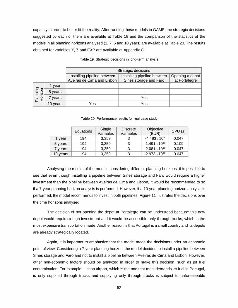
52

capacity in order to better fit the reality. After running these models in GAMS, the strategic decisions

suggested by each of them are available at Table 19 and the comparison of the statistics of the

models in all planning horizons analyzed (1, 7, 5 and 10 years) are available at Table 20. The results

obtained for variables Y, Z and EXP are available at Appendix C.

Table 19. Strategic decisions in long-term analysis

Strategic decisions

Installing pipeline between Aveiras de Cima and Lisbon

Installing pipeline between Sines storage and Faro

Opening a depot at Portalegre

Pla

nnin

g

Horizon

1 year - - -

5 years - - -

7 years - Yes -

10 years Yes Yes -

Table 20. Performance results for real case study

Equations Single

Variables Discrete Variables

Objective (EUR)

CPU (s)

1 year 194 3,359 3 -4.483 x 109 0.047

5 years 194 3,359 3 -1.491 x 1010 0.109

7 years 194 3,359 3 -2.081 x 1010 0.047

10 years 194 3,359 3 -2.973 x 1010 0.047

Analysing the results of the models considering different planning horizons, it is possible to

see that even though installing a pipeline between Sines storage and Faro would require a higher

investment than the pipeline between Aveiras de Cima and Lisbon, it would be recommended to so

if a 7-year planning horizon analysis is performed. However, if a 10-year planning horizon analysis is

performed, the model recommends to invest in both pipelines. Figure 11 illustrates the decisions over

the time horizons analysed.

The decision of not opening the depot at Portalegre can be understood because this new

depot would require a high investment and it would be accessible only through trucks, which is the

most expensive transportation mode. Another reason is that Portugal is a small country and its depots

are already strategically located.

Again, it is important to emphasize that the model made the decisions under an economic

point of view. Considering a 7-year planning horizon, the model decided to install a pipeline between

Sines storage and Faro and not to install a pipeline between Aveiras de Cima and Lisbon. However,

other non-economic factors should be analyzed in order to make this decision, such as jet fuel

contamination. For example, Lisbon airport, which is the one that most demands jet fuel in Portugal,

is only supplied through trucks and supplying only through trucks is subject to unforeseeable

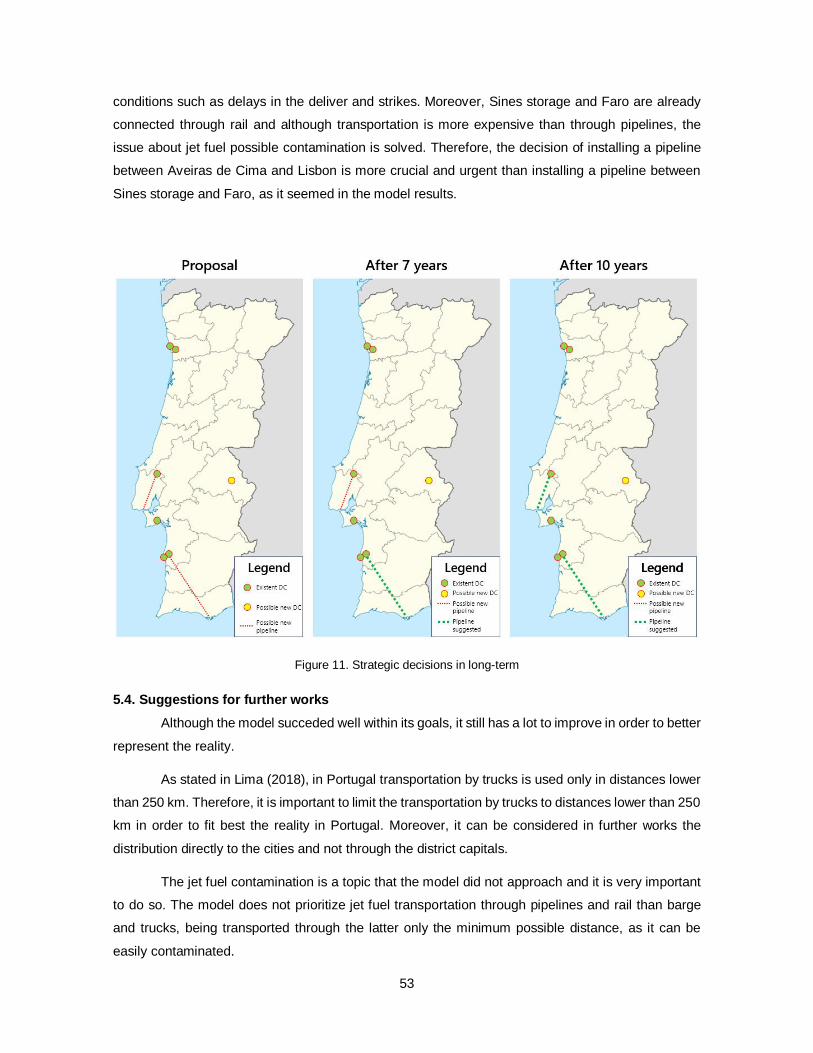
53

conditions such as delays in the deliver and strikes. Moreover, Sines storage and Faro are already

connected through rail and although transportation is more expensive than through pipelines, the

issue about jet fuel possible contamination is solved. Therefore, the decision of installing a pipeline

between Aveiras de Cima and Lisbon is more crucial and urgent than installing a pipeline between

Sines storage and Faro, as it seemed in the model results.

Figure 11. Strategic decisions in long-term

5.4. Suggestions for further works

Although the model succeded well within its goals, it still has a lot to improve in order to better

represent the reality.

As stated in Lima (2018), in Portugal transportation by trucks is used only in distances lower

than 250 km. Therefore, it is important to limit the transportation by trucks to distances lower than 250

km in order to fit best the reality in Portugal. Moreover, it can be considered in further works the

distribution directly to the cities and not through the district capitals.

The jet fuel contamination is a topic that the model did not approach and it is very important

to do so. The model does not prioritize jet fuel transportation through pipelines and rail than barge

and trucks, being transported through the latter only the minimum possible distance, as it can be

easily contaminated.

54

Another suggestion is to integrate the model with upstream and midstream segments. It

would be interesting including the cost of importing crude and transporting it to the refineries and the

costs related to refining operations. Considering these costs, would be possible to analyze what would

be the optimum fraction of its refining capacity that each refinery should work at because depending

on these costs, importing oil derivatives may be an advantage.

Integrating biofuels to the products considered in the model would be an interesting

suggestion for further works because Spain and Portugal have different agreements regarding the

amount of biofuels that they should incorporate.

As many uncertainties affect the petroleum supply chain, another important observation is

that these uncertainties should be considered and the problem should be approached stochastically.

Finally, another suggestion would be to integrate the whole distribution in Iberia, in a way that

the costs for all companies would be optimized.

5.5. Conclusion

These chapter goals were to present the real case used to show the applicability of the

mathematical model developed and to analyze the results obtained. Firstly, the real case considering

the Portuguese PSC and the Iberian market was presented and data was acquired regarding it.

Furthermore, all data presented is public information and, therefore, it is not classified. The main

sources of information to the real case consisted in the websites of the oil companies that operate in

Iberia (Galp, Repsol, Cepsa and BP Oil España) and Fernandes, et al. (2013).

The analysis presented regarding the validation with the illustrative case study of the

mathematical model in Chapter 4 and the application of a real case to the model developed in Chapter

5 shows that it achieved the goals proposed and it is able to make strategic and tactical decisions.

The strategic decisions comprise:

Opening or not a new distribution center and determining its capacity;

Installing or not a new pipeline between two nodes.

On the other hand, the tactical decisions consisted in:

Choosing the best material flow in each route between two nodes via each

transportation mode;

Choosing the amount that should be imported and exported.

Moreover, according to the literature, decision planning can vertically integrate more than

one decision-planning level (Misni & Lee, 2017), which is a strategy that may help to improve the

outcomes (Lima, et al., 2016). Thus, it is worth noting that the analysis performed regarding the

55

illustrative case study verified what was stated in literature: the results were better when strategic and

tactical planning were integrated.

Analyzing the real case study in the long-term, the model shows that it would be a good

strategic decision to install two pipelines in Portugal: from Sines storage to Faro and from Aveiras de

Cima to Lisbon. These decisions are important, as airports must be supplied with jet fuel in both

capital cities, Faro and Lisbon, and it is a fuel that can be easily contaminated. Moreover, the decision

is even more crucial regarding the pipeline between Aveiras de Cima and Lisbon because Lisbon

airport is the largest in Portugal and it is supplied only through trucks, what exposes it to

unforeseeable risks that go beyond jet fuel contamination, such as delays and strikes.

However, a mathematical model is not an exact representation of the reality; it only simplifies

it through mathematical equations. Hence, it has some features to improve in order to fit it best to the

reality and give better results. Therefore, some suggestions for further works were presented in this

chapter:

Limit the transportation by trucks to distances lower than 250 km in order to fit best

the reality in Portugal;

Prioritize jet fuel transportation through pipeline and rail rather than through barge

and trucks due to the fact that jet fuel can be easily contaminated;

Integrate the model with features of upstream and midstream segments such as cost

of importing and transporting crude oil and refining cost;

Consider also biofuels because Spain and Portugal have different agreements

regarding the amount of biofuels that they should incorporate;

Approach the problem stochastically due to the many uncertainties that affect the

PSC;

Integrate the whole distribution in Iberia, minimizing the cost for all companies that

operate in Iberia in a cooperative manner.

56

57

Chapter 6 – Conclusion

The Master’s thesis in Petroleum Engineering aimed at developing a mathematical model

that solved a problem regarding the downstream petroleum supply chain. To do so, several steps

were developed:

Firstly, the Petroleum Supply Chain and its downstream segment were understood in Chapter

2. Moreover, it was highlighted the importance of using Operations Research tools in PSC. This

chapter also explained the decision-planning levels when planning and managing the PSC and the

structure of a mathematical model.

Then, Chapter 3 provided the literature review where a set of relevant papers exploring

mathematical models regarding the downstream PSC were analyzed. These papers were

categorized according to their planning level or the combination of two levels.

After that, the problem was defined and the mathematical model developed was presented

in Chapter 4. The objective was to develop a deterministic mathematical model in order to define a

strategy for supplying markets that may span over more than one country considering strategic and

tactical planning. This chapter has also emphasized the main contributions of the model developed

when compared with Kazemi & Szmerekovsky (2015):

More than one country is considered and, therefore, costs related to import and

export were incorporated;

The model limits the capacity of a transportation mode and it does not establish flow

in an unfeasible route;

The model decides the fraction of total refinery capacity should be used to produce

each product considered;

Already existent distribution centers are considered along with the decision of

opening or not a new distribution center;

The model is versatile and it can determine if a distribution center should be opened

or not, if a pipeline should be built or not or both features together.

After developing the model, it was important to validate it in order to attest the efficiency of

the model. To do so, an illustrative case study was considered and presented in Chapter 4. The model

developed was validated and it was verified that it achieved the objectives proposed of making

strategic and tactical decisions. The strategic decisions involve opening or not a distribution center

and installing or not a pipeline, while the tactical decisions comprise deciding the best material flow

in each route through possible and available transportation modes and the amount that should be

imported and/or exported.

58

The analysis performed regarding the illustrative case study verified that the results were

better when strategic and tactical planning were integrated, what was stated in literature (Lima, et al.,

2016).

Then, Chapter 5 presented and discussed the results obtained from applying the real case

study to the model. The real case objective consisted in a distribution strategy for supplying the

Iberian market with oil products produced in Portuguese refineries managed by a single company.

It is worth noting that the model made important strategic decisions regarding the real case

study. The model decided when analyzing in the long-term that a pipeline between Sines storage and

Faro and a pipeline between Aveiras de Cima and Lisbon should be installed. These decisions are

very important, mainly regarding the second pipeline because Lisbon airport is the largest airport in

Portugal and it is supplied only through trucks. Supplying the largest airport only through trucks

involves risks such as jet fuel contamination and lack of supply due to strikes.

Furthermore, the model made the tactical decision that, before installing these pipelines, Faro

and Lisbon airports should be supplied through barge. However, Faro airport is supplied through rail

from Sines storage and through trucks from refinery La Rabida in Spain due to the ease of jet fuel

contamination and Lisbon airport is supplied through the routes Sines refinery to Aveiras de Cima via

pipeline and from Aveiras de Cima to the airport via trucks due to the same reason. Therefore, it is

important to incorporate features in the model that would prioritize jet fuel transportation through

pipelines and rail.

Other suggestions proposed for further works comprise limiting the transportation by trucks

to distances lower than 250 km, integrating the model with features of upstream and midstream

segments, considering also biofuels, approaching the problem stochastically and integrating the

whole distribution in Iberia, considering a multi-company cooperative model.

59

References

Alabi, A. & Castro, J., 2009. Dantzig-Wolfe and block coordinate-descent decomposition in

large-scale integrated refinery-planning. Computers & Operations Research, Volume 36, pp. 2472-

2483.

Andersen, F. E., Díaz, M. S. & Grossmann, I. E., 2013. Multiscale strategic planning model

for the design of integrated ethanol and gasoline supply chain. AIChE J, 59(12), pp. 4655-4672.

Asesa, s.d. Refino de Petróleo. [Online]

Available at: http://www.asesa.es/oil-refining-xcid

[Acedido em 23 05 2019].

Autoridade da Concorrência, 2018. Análise ao Setor dos Combustíveis Líquidos Rodoviários

em Portugal Continental, s.l.: s.n.

Azadeh, A. et al., 2017. Evolutionary multi-objective optimization of environmental indicators

of integrated crude oil supply chain under uncertainty. Journal of Cleaner Production, Volume 152,

pp. 295-311.

Barbosa-Póvoa, A. P., 2014. Process supply chains management - where are we? Where to

go next?. Process and Energy Systems Engineering, pp. 2-23.

Bassi, H. V., Filho, V. J. M. F. & Bahiense, L., 2012. Planning and scheduling a fleet of rigs

using simulation–optimization. Computers & Industrial Engineering, Volume 63, pp. 1074-1088.

BP - British Petroleum, 2018. BP Statistical Review of World Energy, s.l.: s.n.

BP - British Petroleum, s.d. BP España. [Online]

Available at: https://www.bp.com/es_es/spain.html

[Acedido em 23 05 2019].

Cepsa, 2018. 2018 Annual and Corporate Responsibility Report, s.l.: s.n.

CLC - Companhia Logística de Combustíveis, s.d. CLC - Companhia Logística de

Combustíveis, S. A.. [Online]

Available at: http://www.clc.pt/

[Acedido em 23 05 2019].

CORES - Corporación de reservas estratégicas de productos petrolíferos, 2018. Informe

estadístico anual 2017, s.l.: s.n.

60

DGEG - Direção-Geral de Energia e Geologia, s.d. Oleodutos. [Online]

Available at: http://www.dgeg.gov.pt/

[Acedido em 11 12 2018].

EIA - U.S. Energy Information Administration, 2012. Crude oil distillation and the definition of

refinery capacity. [Online]

Available at: https://www.eia.gov/todayinenergy/detail.php?id=6970#

[Acedido em 6 December 2018].

ENSE - Entidade Nacional para o Setor Energético , s.d. Introduções ao Consumo. [Online]

Available at: http://www.ense-epe.pt/introducoes-consumo/

[Acedido em 23 05 2019].

Fernandes, L. J., Relvas, S. & Barbosa-Póvoa, A. P., 2013. Strategic network design of

downstream petroleum supply chains: Single versus multi-entity participation. Chemical Engineering

Research and Design, Volume 91, pp. 1557-1587.

Fernandes, L. J., Relvas, S. & Barbosa-Póvoa, A. P., 2014. Collaborative Design and Tactical

Planning of Downstream Petroleum Supply Chains. Ind. Eng. Chem. Res., 53(44), pp. 17155-17181.

Fernandes, L. J., Relvas, S. & Barbosa-Póvoa, A. P., 2015. Downstream Petroleum Supply

Chain Planning under Uncertainty. Computer Aided Chemical Engineering, Volume 37, pp. 1889-

1894.

Fiorencio, L., Oliveira, F., Nunes, P. & Hamacher, S., 2015. Investment planning in the

petroleum downstream infrastructure. International Transactions in Operational Research, 22(2), pp.

339-362.

FuelsEurope, 2017. Statistical Report, s.l.: s.n.

GALP, s.d. Aprovisionamento, refinação e logística. [Online]

Available at: https://www.galp.com/corp/pt/sobre-nos/o-que-fazemos/refinacao-

distribuicao/aprovisionamento-refinacao-e-logistica

[Acedido em 11 12 2018].

Ghaithan, A. M., Attia, A. & Duffuaa, S. O., 2017. Multi-objective optimization model for a

downstream oil and gas supply chain. Applied Mathematical Modelling, Volume 52, p. 689–708.

Goel, V. & Grossmann, I. E., 2004. A stochastic programming approach to planning of

offshore gas field developments under uncertainty in reserves. Computers and Chemical Engineering

, Volume 28, pp. 1409-1429.

61

Guyonnet, P., Grant, F. H. & Bagajewicz, M. J., 2009. Integrated Model for Refinery Planning,

Oil Procuring, and Product Distribution. Ind. Eng. Chem. Res., Volume 48, pp. 463-482.

Hillier, F. S. & Lieberman, G. J., 2005. Introduction to Operations Research. 8th ed.

s.l.:McGraw-Hill .

Hobsbawm, E. J., 2000. Da Revolução Industrial Inglesa ao Imperialismo. 5 ed. Rio de

Janeiro: Forense Universitária.

Instituto Nacional de Estatística, 2010. Estatísticas dos Transportes 2009, s.l.: s.n.

Kazemi, Y. & Szmerekovsky, J., 2015. Modeling downstream petroleum supply chain: The

importance of multi-mode transportation to strategic planning. Transportation Research Part E ,

Volume 83, pp. 111-125.

Kim, Y. et al., 2008. An integrated model of supply network and production planning for

multiple fuel products of multi-site refineries. Computers and Chemical Engineering, Volume 32, pp.

2529-2535.

Kuo, T.-H. & Chang, C.-T., 2008. Application of a Mathematic Programming Model for

Integrated Planning and Scheduling of Petroleum Supply Networks. Ind. Eng. Chem. Res., Volume

47, pp. 1935-1954.

Leiras, A., Ribas, G. & Hamacher, S., 2013. Tactical and Operational Planning of Multirefinery

Networks under Uncertainty: An Iterative Integration Approach. Ind. Eng. Chem. Res., Volume 52,

pp. 8507-8517.

Leiras, A., Ribas, G., Hamacher, S. & Elkamel, A., 2011. Literature review of oil refineries

planning under uncertainty. Int. J. Oil, Gas and Coal Technology, 4(2), p. 156–173.

Lima, C. G., 2018. Tactical and Operational planning of the Downstream Oil Supply Chain

under uncertainty, Lisboa: s.n.

Lima, C., Relvas, S. & Barbosa-Póvoa, A., 2018. Stochastic programming approach for the

optimal tactical planning of the downstream oil supply chain. Computers and Chemical Engineering,

Volume 108, pp. 314-336.

Lima, C., Relvas, S. & Barbosa-Póvoa, A. P. F. D., 2016. Downstream oil supply chain

management: A critical review and future directions. Computers and Chemical Engineering, Volume

92, pp. 78-92.

MirHassani, S. A., 2008. An operational planning model for petroleum products logistics

under uncertainty. Applied Mathematics and Computation, Volume 196, pp. 744-751.

62

MirHassani, S. A. & Noori, R., 2011. Implications of capacity expansion under uncertainty in

oil industry. Journal of Petroleum Science and Engineering, Volume 77, pp. 194-199.

Misni, F. & Lee, L. S., 2017. A Review on Strategic, Tactical and Operational Decision

Planning in Reverse Logistics of Green Supply Chain Network Design. Journal of Computer and

Communications, Volume 5, pp. 83-104.

Mota, N. M. M. d. A. d. C., 2012. Análise de cenários para definição de planos de contingência

na distribuição secundária de produtos petrolíferos, Lisboa: s.n.

Neiro, S. M. S. & Pinto, J. M., 2004. A general modeling framework for the operational

planning of petroleum supply chains. Computers and Chemical Engineering, Volume 28, pp. 871-

896.

Oliveira, F., Grossmann, I. E. & Hamacher, S., 2014. Accelerating Benders stochastic

decomposition for the optimization under uncertainty of the petroleum product supply chain.

Computers & Operations Research, Volume 49, pp. 47-58.

Oliveira, F. & Hamacher, S., 2012. Optimization of the Petroleum Product Supply Chain under

Uncertainty: A Case Study in Northern Brazil. Ind. Eng. Chem. Res., Volume 51, pp. 4279-4287.

Pinto, J. M., Joly, M. & Moro, L. F. L., 2000. Planning and scheduling models for refinery

operations. Computers and Chemical Engineering, Volume 24, pp. 2259-2276.

Repsol, 2017. Integrated Management Report, s.l.: s.n.

Saad, S. M., Elsaghier, E. H. & Ezaga, D., 2018. Planning and optimising petroleum supply

chain. Procedia Manufacturing, Volume 17, pp. 803-810.

Sahebi, H., Nickel, S. & Ashayeri, J., 2014. Strategic and tactical mathematical programming

models within the crude oil supply chain context—A review. Computers and Chemical Engineering,

Volume 68, pp. 56-77.

Skjerpen, T., Storrøsten, H. B., Rosendahl, K. E. & Osmundsen, P., 2018. Modelling and

forecasting rig rates on the Norwegian Continental Shelf. Resource and Energy Economics, Volume

53, pp. 220-239.

Tong, K., Feng, Y. & Rong, G., 2012. Planning under Demand and Yield Uncertainties in an

Oil Supply Chain. Ind. Eng. Chem. Res., Volume 51, pp. 814-834.

Tong, K., You, F. & Rong, G., 2014. Robust design and operations of hydrocarbon biofuel

supply chain integrating with existing petroleum refineries considering unit cost objective. Computers

and Chemical Engineering, Volume 68, pp. 128-139.

63

Yergin, D., 1991. The Prize: The Epic Quest for Oil, Money & Power. New York: Simon &

Schuster .

Ye, Y., Liang, S. & Zhu, Y., 2017. A mixed-integer linear programming-based scheduling

model for refined-oil shipping. Computers and Chemical Engineering, Volume 99, pp. 106-116.

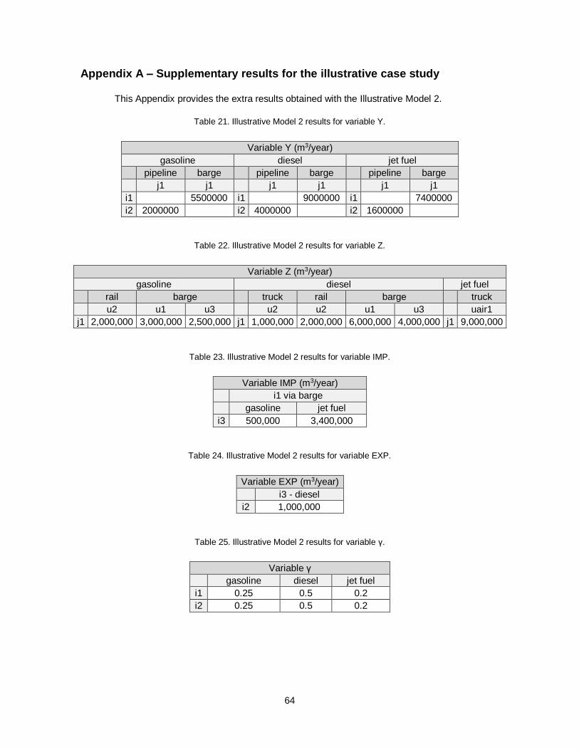
64

Appendix A – Supplementary results for the illustrative case study

This Appendix provides the extra results obtained with the Illustrative Model 2.

Table 21. Illustrative Model 2 results for variable Y.

Variable Y (m3/year)

gasoline diesel jet fuel

pipeline barge pipeline barge pipeline barge

j1 j1 j1 j1 j1 j1

i1 5500000 i1 9000000 i1 7400000

i2 2000000 i2 4000000 i2 1600000

Table 22. Illustrative Model 2 results for variable Z.

Variable Z (m3/year)

gasoline diesel jet fuel

rail barge truck rail barge truck

u2 u1 u3 u2 u2 u1 u3 uair1

j1 2,000,000 3,000,000 2,500,000 j1 1,000,000 2,000,000 6,000,000 4,000,000 j1 9,000,000

Table 23. Illustrative Model 2 results for variable IMP.

Variable IMP (m3/year)

i1 via barge

gasoline jet fuel

i3 500,000 3,400,000

Table 24. Illustrative Model 2 results for variable EXP.

Variable EXP (m3/year)

i3 - diesel

i2 1,000,000

Table 25. Illustrative Model 2 results for variable γ.

Variable γ

gasoline diesel jet fuel

i1 0.25 0.5 0.2

i2 0.25 0.5 0.2

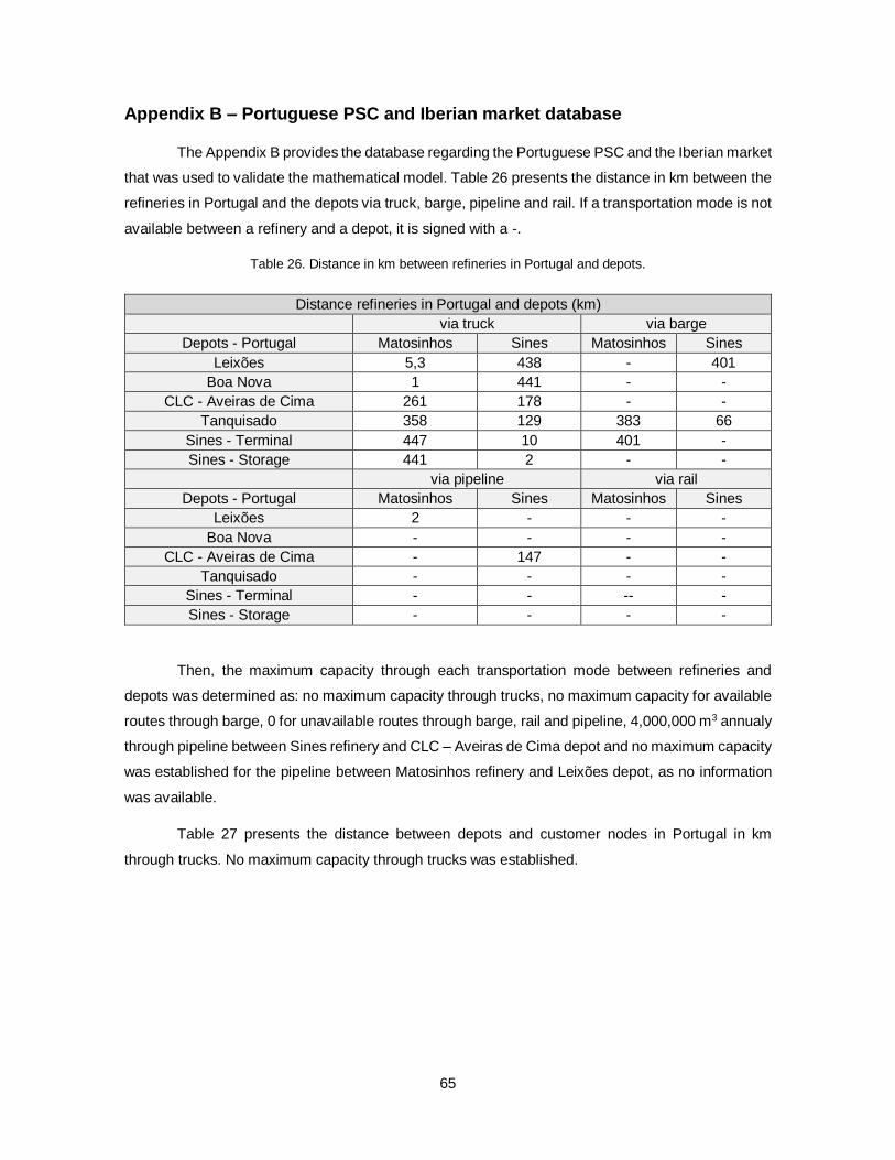
65

Appendix B – Portuguese PSC and Iberian market database

The Appendix B provides the database regarding the Portuguese PSC and the Iberian market

that was used to validate the mathematical model. Table 26 presents the distance in km between the

refineries in Portugal and the depots via truck, barge, pipeline and rail. If a transportation mode is not

available between a refinery and a depot, it is signed with a -.

Table 26. Distance in km between refineries in Portugal and depots.

Distance refineries in Portugal and depots (km) via truck via barge

Depots - Portugal Matosinhos Sines Matosinhos Sines

Leixões 5,3 438 - 401

Boa Nova 1 441 - -

CLC - Aveiras de Cima 261 178 - -

Tanquisado 358 129 383 66

Sines - Terminal 447 10 401 -

Sines - Storage 441 2 - -

via pipeline via rail

Depots - Portugal Matosinhos Sines Matosinhos Sines

Leixões 2 - - -

Boa Nova - - - -

CLC - Aveiras de Cima - 147 - -

Tanquisado - - - -

Sines - Terminal - - -- -

Sines - Storage - - - -

Then, the maximum capacity through each transportation mode between refineries and

depots was determined as: no maximum capacity through trucks, no maximum capacity for available

routes through barge, 0 for unavailable routes through barge, rail and pipeline, 4,000,000 m3 annualy

through pipeline between Sines refinery and CLC – Aveiras de Cima depot and no maximum capacity

was established for the pipeline between Matosinhos refinery and Leixões depot, as no information

was available.

Table 27 presents the distance between depots and customer nodes in Portugal in km

through trucks. No maximum capacity through trucks was established.

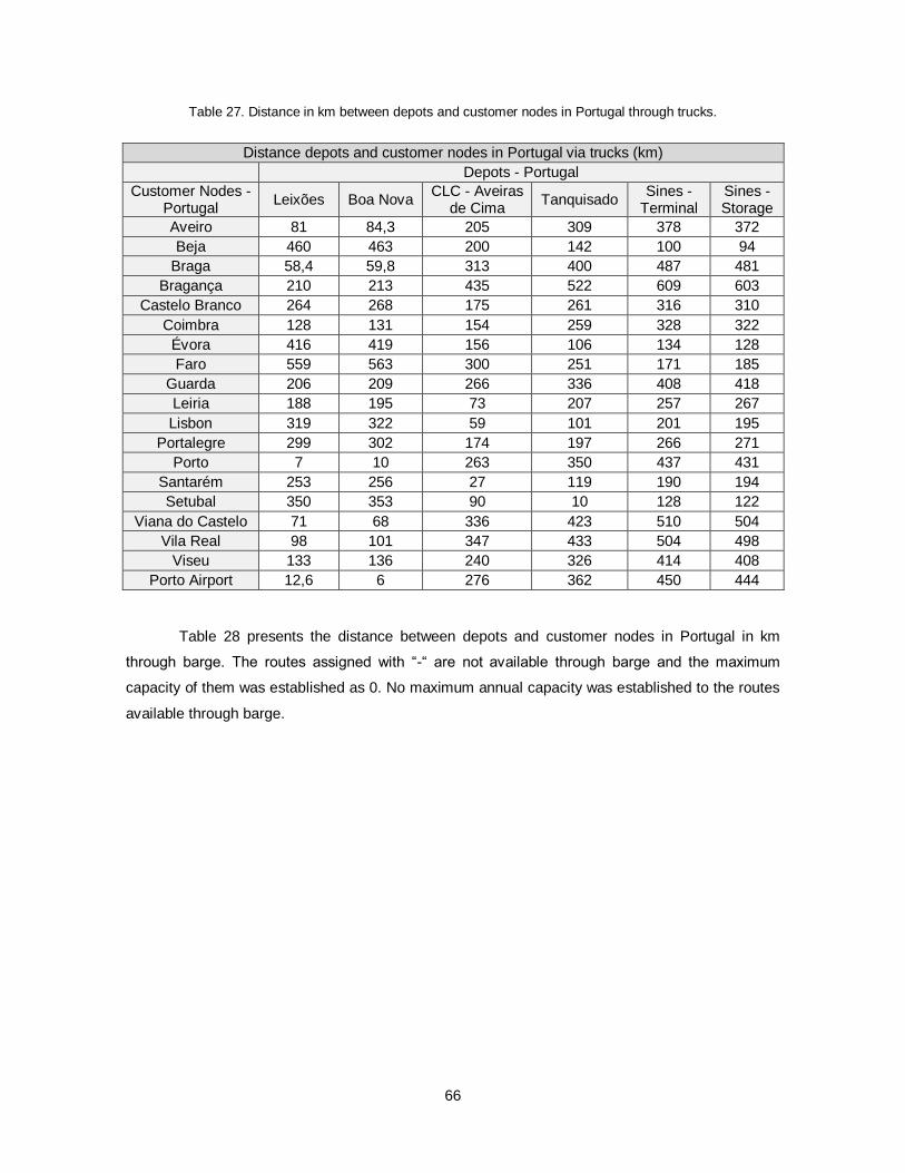
66

Table 27. Distance in km between depots and customer nodes in Portugal through trucks.

Distance depots and customer nodes in Portugal via trucks (km)

Depots - Portugal

Customer Nodes - Portugal

Leixões Boa Nova CLC - Aveiras

de Cima Tanquisado

Sines - Terminal

Sines - Storage

Aveiro 81 84,3 205 309 378 372

Beja 460 463 200 142 100 94

Braga 58,4 59,8 313 400 487 481

Bragança 210 213 435 522 609 603

Castelo Branco 264 268 175 261 316 310

Coimbra 128 131 154 259 328 322

Évora 416 419 156 106 134 128

Faro 559 563 300 251 171 185

Guarda 206 209 266 336 408 418

Leiria 188 195 73 207 257 267

Lisbon 319 322 59 101 201 195

Portalegre 299 302 174 197 266 271

Porto 7 10 263 350 437 431

Santarém 253 256 27 119 190 194

Setubal 350 353 90 10 128 122

Viana do Castelo 71 68 336 423 510 504

Vila Real 98 101 347 433 504 498

Viseu 133 136 240 326 414 408

Porto Airport 12,6 6 276 362 450 444

Table 28 presents the distance between depots and customer nodes in Portugal in km

through barge. The routes assigned with “-“ are not available through barge and the maximum

capacity of them was established as 0. No maximum annual capacity was established to the routes

available through barge.

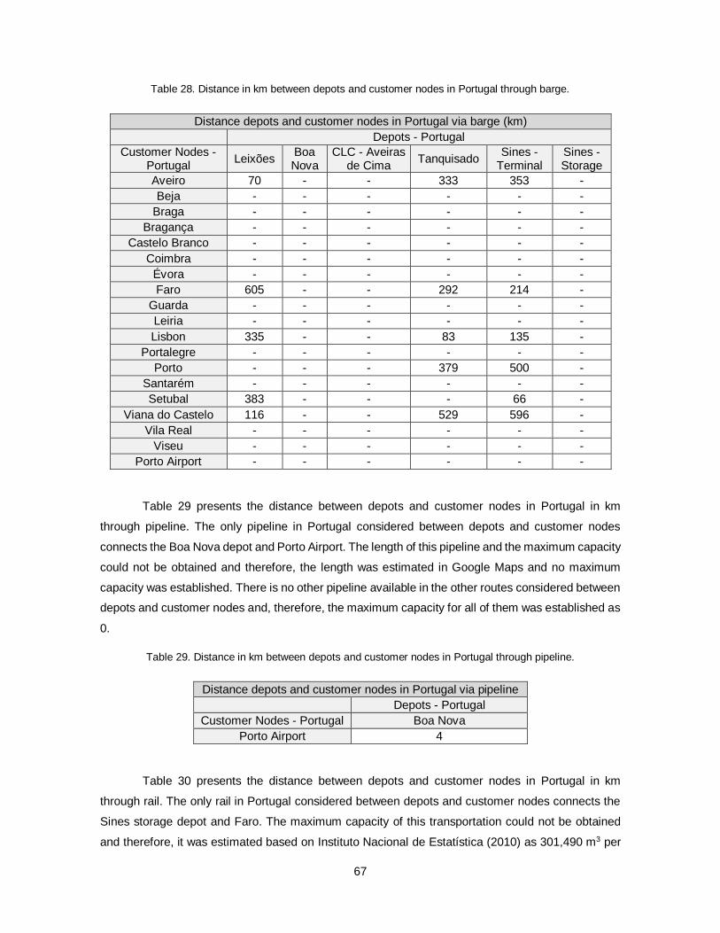
67

Table 28. Distance in km between depots and customer nodes in Portugal through barge.

Distance depots and customer nodes in Portugal via barge (km) Depots - Portugal

Customer Nodes - Portugal

Leixões Boa Nova

CLC - Aveiras de Cima

Tanquisado Sines -

Terminal Sines - Storage

Aveiro 70 - - 333 353 -

Beja - - - - - -

Braga - - - - - -

Bragança - - - - - -

Castelo Branco - - - - - -

Coimbra - - - - - -

Évora - - - - - -

Faro 605 - - 292 214 -

Guarda - - - - - -

Leiria - - - - - -

Lisbon 335 - - 83 135 -

Portalegre - - - - - -

Porto - - - 379 500 -

Santarém - - - - - -

Setubal 383 - - - 66 -

Viana do Castelo 116 - - 529 596 -

Vila Real - - - - - -

Viseu - - - - - -

Porto Airport - - - - - -

Table 29 presents the distance between depots and customer nodes in Portugal in km

through pipeline. The only pipeline in Portugal considered between depots and customer nodes

connects the Boa Nova depot and Porto Airport. The length of this pipeline and the maximum capacity

could not be obtained and therefore, the length was estimated in Google Maps and no maximum

capacity was established. There is no other pipeline available in the other routes considered between

depots and customer nodes and, therefore, the maximum capacity for all of them was established as

0.

Table 29. Distance in km between depots and customer nodes in Portugal through pipeline.

Distance depots and customer nodes in Portugal via pipeline Depots - Portugal

Customer Nodes - Portugal Boa Nova

Porto Airport 4

Table 30 presents the distance between depots and customer nodes in Portugal in km

through rail. The only rail in Portugal considered between depots and customer nodes connects the

Sines storage depot and Faro. The maximum capacity of this transportation could not be obtained

and therefore, it was estimated based on Instituto Nacional de Estatística (2010) as 301,490 m3 per

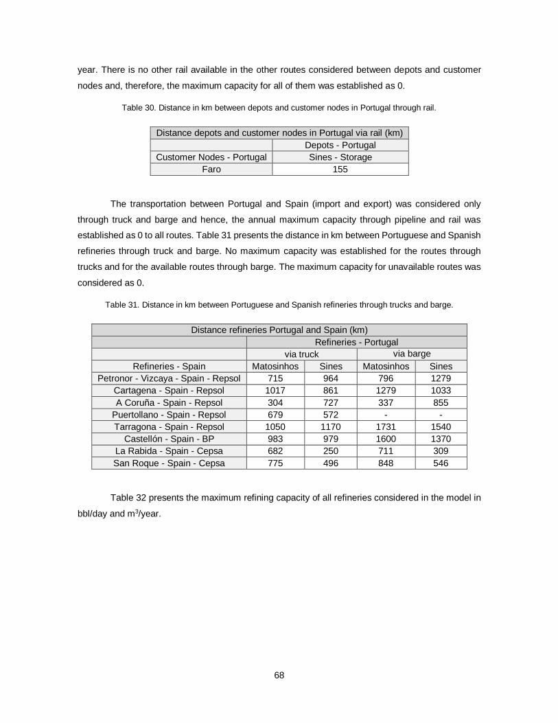
68

year. There is no other rail available in the other routes considered between depots and customer

nodes and, therefore, the maximum capacity for all of them was established as 0.

Table 30. Distance in km between depots and customer nodes in Portugal through rail.

Distance depots and customer nodes in Portugal via rail (km) Depots - Portugal

Customer Nodes - Portugal Sines - Storage

Faro 155

The transportation between Portugal and Spain (import and export) was considered only

through truck and barge and hence, the annual maximum capacity through pipeline and rail was

established as 0 to all routes. Table 31 presents the distance in km between Portuguese and Spanish

refineries through truck and barge. No maximum capacity was established for the routes through

trucks and for the available routes through barge. The maximum capacity for unavailable routes was

considered as 0.

Table 31. Distance in km between Portuguese and Spanish refineries through trucks and barge.

Distance refineries Portugal and Spain (km)

Refineries - Portugal via truck via barge

Refineries - Spain Matosinhos Sines Matosinhos Sines

Petronor - Vizcaya - Spain - Repsol 715 964 796 1279

Cartagena - Spain - Repsol 1017 861 1279 1033

A Coruña - Spain - Repsol 304 727 337 855

Puertollano - Spain - Repsol 679 572 - -

Tarragona - Spain - Repsol 1050 1170 1731 1540

Castellón - Spain - BP 983 979 1600 1370

La Rabida - Spain - Cepsa 682 250 711 309

San Roque - Spain - Cepsa 775 496 848 546

Table 32 presents the maximum refining capacity of all refineries considered in the model in

bbl/day and m3/year.

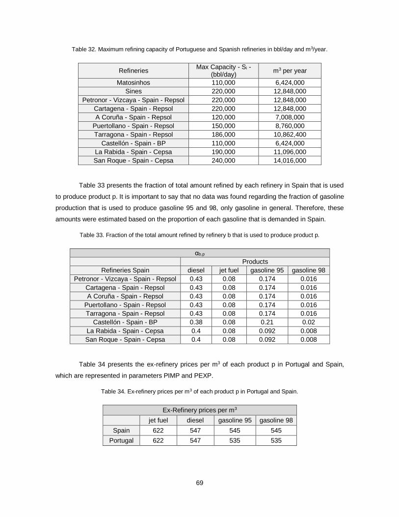
69

Table 32. Maximum refining capacity of Portuguese and Spanish refineries in bbl/day and m3/year.

Refineries Max Capacity - Si -

(bbl/day) m3 per year

Matosinhos 110,000 6,424,000

Sines 220,000 12,848,000

Petronor - Vizcaya - Spain - Repsol 220,000 12,848,000

Cartagena - Spain - Repsol 220,000 12,848,000

A Coruña - Spain - Repsol 120,000 7,008,000

Puertollano - Spain - Repsol 150,000 8,760,000

Tarragona - Spain - Repsol 186,000 10,862,400

Castellón - Spain - BP 110,000 6,424,000

La Rabida - Spain - Cepsa 190,000 11,096,000

San Roque - Spain - Cepsa 240,000 14,016,000

Table 33 presents the fraction of total amount refined by each refinery in Spain that is used

to produce product p. It is important to say that no data was found regarding the fraction of gasoline

production that is used to produce gasoline 95 and 98, only gasoline in general. Therefore, these

amounts were estimated based on the proportion of each gasoline that is demanded in Spain.

Table 33. Fraction of the total amount refined by refinery b that is used to produce product p.

αb,p Products

Refineries Spain diesel jet fuel gasoline 95 gasoline 98

Petronor - Vizcaya - Spain - Repsol 0.43 0.08 0.174 0.016

Cartagena - Spain - Repsol 0.43 0.08 0.174 0.016

A Coruña - Spain - Repsol 0.43 0.08 0.174 0.016

Puertollano - Spain - Repsol 0.43 0.08 0.174 0.016

Tarragona - Spain - Repsol 0.43 0.08 0.174 0.016

Castellón - Spain - BP 0.38 0.08 0.21 0.02

La Rabida - Spain - Cepsa 0.4 0.08 0.092 0.008

San Roque - Spain - Cepsa 0.4 0.08 0.092 0.008

Table 34 presents the ex-refinery prices per m3 of each product p in Portugal and Spain,

which are represented in parameters PIMP and PEXP.

Table 34. Ex-refinery prices per m3 of each product p in Portugal and Spain.

Ex-Refinery prices per m3

jet fuel diesel gasoline 95 gasoline 98

Spain 622 547 545 545

Portugal 622 547 535 535

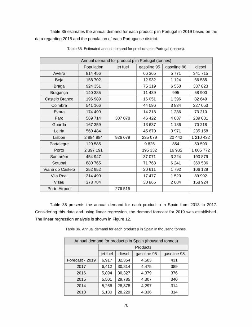
70

Table 35 estimates the annual demand for each product p in Portugal in 2019 based on the

data regarding 2018 and the population of each Portuguese district.

Table 35. Estimated annual demand for products p in Portugal (tonnes).

Annual demand for product p in Portugal (tonnes)

Population jet fuel gasoline 95 gasoline 98 diesel

Aveiro 814 456 66 365 5 771 341 715

Beja 158 702 12 932 1 124 66 585

Braga 924 351 75 319 6 550 387 823

Bragança 140 385 11 439 995 58 900

Castelo Branco 196 989 16 051 1 396 82 649

Coimbra 541 166 44 096 3 834 227 053

Évora 174 490 14 218 1 236 73 210

Faro 569 714 307 078 46 422 4 037 239 031

Guarda 167 359 13 637 1 186 70 218

Leiria 560 484 45 670 3 971 235 158

Lisbon 2 884 984 926 079 235 079 20 442 1 210 432

Portalegre 120 585 9 826 854 50 593

Porto 2 397 191 195 332 16 985 1 005 772

Santarém 454 947 37 071 3 224 190 879

Setubal 880 765 71 768 6 241 369 536

Viana do Castelo 252 952 20 611 1 792 106 129

Vila Real 214 490 17 477 1 520 89 992

Viseu 378 784 30 865 2 684 158 924

Porto Airport 276 515

Table 36 presents the annual demand for each product p in Spain from 2013 to 2017.

Considering this data and using linear regression, the demand forecast for 2019 was established.

The linear regression analysis is shown in Figure 12.

Table 36. Annual demand for each product p in Spain in thousand tonnes.

Annual demand for product p in Spain (thousand tonnes)

Products

jet fuel diesel gasoline 95 gasoline 98

Forecast - 2019 6,917 32,354 4,503 431

2017 6,412 30,814 4,475 389

2016 5,894 30,327 4,379 376

2015 5,501 29,785 4,307 340

2014 5,266 28,378 4,297 314

2013 5,130 28,229 4,336 314

71

Figure 12. Linear regression analysis of demand forecast in Spain.

Table 37 presents the transportation costs considered in EUR/ton-km. These costs were

acquired at Kazemi & Szmerekovsky (2015) and converted from USD to EUR using the conversion

rate on December 31st 2013 (1 EUR = 1.38 USD), as the data in Kazemi & Szmerekovsky (2015) was

established in 2013.

Table 37. Transportation costs considered in EUR/ton-km.

Transportation costs (EUR/ton-km)

C,T,TIMP

pipeline 0.0022

barge 0.0045

rail 0.0315

truck 0.0810

Table 38 presents the maximum fraction of each product that the Portuguese refineries can

produce. As no information was found regarding each refinery separately, the same fractions were

considered to both of them. Moreover, the maximum fraction is considered with an additional 2% in

comparison to the fraction of each product produced in 2018, obtained at Galp’s website (GALP, s.d.).

y = 712x - 1,404,972 y = 319.2x - 637547 y = 36x - 68181 y = 21.2x - 42371

0

1000

2000

3000

4000

5000

6000

7000

27500

28000

28500

29000

29500

30000

30500

31000

31500

2013 2014 2015 2016 2017

Jet

fuel

an

d g

aso

lines

dem

and

(th

ou

san

d t

on

nes

)

Die

sel d

eman

d (t

ho

usa

nd

to

nn

es)

Year

Demand forecast in Spain

Diesel Jet fuel Gasoline 95 Gasoline 98

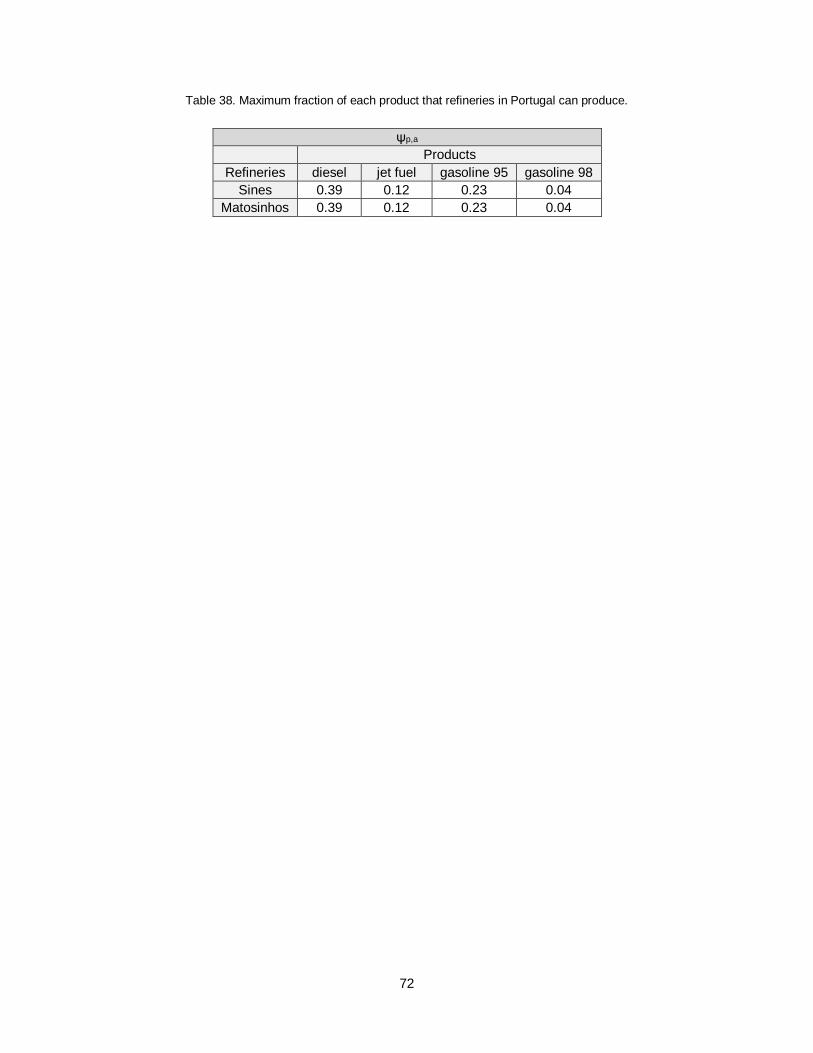
72

Table 38. Maximum fraction of each product that refineries in Portugal can produce.

ψp,a Products

Refineries diesel jet fuel gasoline 95 gasoline 98

Sines 0.39 0.12 0.23 0.04

Matosinhos 0.39 0.12 0.23 0.04

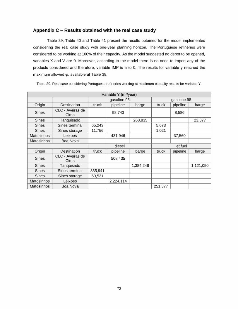
73

Appendix C – Results obtained with the real case study

Table 39, Table 40 and Table 41 present the results obtained for the model implemented

considering the real case study with one-year planning horizon. The Portuguese refineries were

considered to be working at 100% of their capacity. As the model suggested no depot to be opened,

variables X and V are 0. Moreover, according to the model there is no need to import any of the

products considered and therefore, variable IMP is also 0. The results for variable γ reached the

maximum allowed ψ, available at Table 38.

Table 39. Real case considering Portuguese refineries working at maximum capacity results for variable Y.

Variable Y (m3/year) gasoline 95 gasoline 98

Origin Destination truck pipeline barge truck pipeline barge

Sines CLC - Aveiras de

Cima 98,743 8,586

Sines Tanquisado 268,835 23,377

Sines Sines terminal 65,243 5,673

Sines Sines storage 11,756 1,021

Matosinhos Leixoes 431,946 37,560

Matosinhos Boa Nova

diesel jet fuel

Origin Destination truck pipeline barge truck pipeline barge

Sines CLC - Aveiras de

Cima 508,435

Sines Tanquisado 1,384,248 1,121,050

Sines Sines terminal 335,941

Sines Sines storage 60,531

Matosinhos Leixoes 2,224,114

Matosinhos Boa Nova 251,377

74

Table 40. Real case considering Portuguese refineries working at maximum capacity results for variable Z.

Variable Z (m3/year) gasoline 95 gasoline 98 diesel jet fuel

Origin Destination truck barge truck barge truck barge pipeline barge

Leixões Aveiro 60,331 5,246 310,650

Leixões Braga 68,471 5,954 352,566

Leixões Bragança 10,399 904 53,545

Leixões Coimbra 40,087 3,485 206,411

Leixões Guarda 12,397 1,078 63,834

Leixões Porto 177,574 15,440 914,338

Leixões Viana do Castelo

18,737 1,629 96,480

Leixões Vila Real 15,888 1,381 81,810

Leixões Viseu 28,059 2,440 144,476

CLC - Aveiras de Cima

Castelo Branco

14,591 1,269 75,135

CLC - Aveiras de Cima

Leiria 41,518 3,610 213,780

CLC - Aveiras de Cima

Portalegre 8,932 776 45,993

CLC - Aveiras de Cima

Santarem 33,700 2,930 173,526

Tanquisado Évora 12,925 1,123 66,554

Tanquisado Faro 42,201 3,670 217,300 279,161

Tanquisado Lisbon 213,708 18,583 1,100,392 841,889

Sines - Terminal

Setubal 65,243 5,673 335,941

Sines - Storage

Beja 11,756 1,021 60,531

Boa Nova Porto Airport 251,377

Table 41. Real case considering Portuguese refineries working at maximum capacity results for variable EXP.

Variable EXP (m3/year)

Product Origin Amount (m3)

gasoline 95 Sines 2,510,460

gasoline 95 Matosinhos 1,045,573

gasoline 98 Sines 475,260

gasoline 98 Matosinhos 219,399

diesel Sines 2,721,562

diesel Matosinhos 281,245

jet fuel Sines 420,709

jet fuel Matosinhos 519,502

Table 42, Table 43, Table 44 and Table 45 present the results obtained for the model

implemented considering the real case study with 7-year planning horizon. The Portuguese refineries

were considered to be working at 82% of their capacity. The results obtained for variable X for j4 was

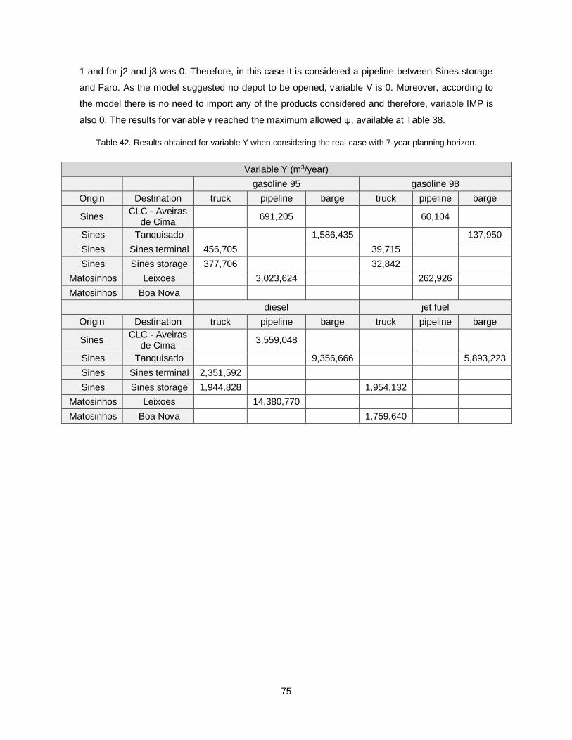
75

1 and for j2 and j3 was 0. Therefore, in this case it is considered a pipeline between Sines storage

and Faro. As the model suggested no depot to be opened, variable V is 0. Moreover, according to

the model there is no need to import any of the products considered and therefore, variable IMP is

also 0. The results for variable γ reached the maximum allowed ψ, available at Table 38.

Table 42. Results obtained for variable Y when considering the real case with 7-year planning horizon.

Variable Y (m3/year)

gasoline 95 gasoline 98

Origin Destination truck pipeline barge truck pipeline barge

Sines CLC - Aveiras

de Cima 691,205 60,104

Sines Tanquisado 1,586,435 137,950

Sines Sines terminal 456,705 39,715

Sines Sines storage 377,706 32,842

Matosinhos Leixoes 3,023,624 262,926

Matosinhos Boa Nova

diesel jet fuel

Origin Destination truck pipeline barge truck pipeline barge

Sines CLC - Aveiras

de Cima 3,559,048

Sines Tanquisado 9,356,666 5,893,223

Sines Sines terminal 2,351,592

Sines Sines storage 1,944,828 1,954,132

Matosinhos Leixoes 14,380,770

Matosinhos Boa Nova 1,759,640

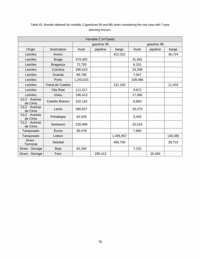
76

Table 43. Results obtained for variable Z (gasolines 95 and 98) when considering the real case with 7-year

planning horizon.

Variable Z (m3/year)

gasoline 95 gasoline 98

Origin Destination truck pipeline barge truck pipeline barge

Leixões Aveiro 422,322 36,724

Leixões Braga 479,302 41,681

Leixões Bragança 72,793 6,331

Leixões Coimbra 280,610 24,398

Leixões Guarda 86,780 7,547

Leixões Porto 1,243,021 108,086

Leixões Viana do Castelo 131,160 11,403

Leixões Vila Real 111,217 9,672

Leixões Viseu 196,413 17,080

CLC - Aveiras de Cima

Castelo Branco 102,142 8,883

CLC - Aveiras de Cima

Leiria 290,627 25,270

CLC - Aveiras de Cima

Portalegre 62,529 5,434

CLC - Aveiras de Cima

Santarem 235,906 20,516

Tanquisado Évora 90,478 7,865

Tanquisado Lisbon 1,495,957 130,085

Sines - Terminal

Setubal 456,705 39,715

Sines - Storage Beja 82,294 7,152

Sines - Storage Faro 295,412 25,690

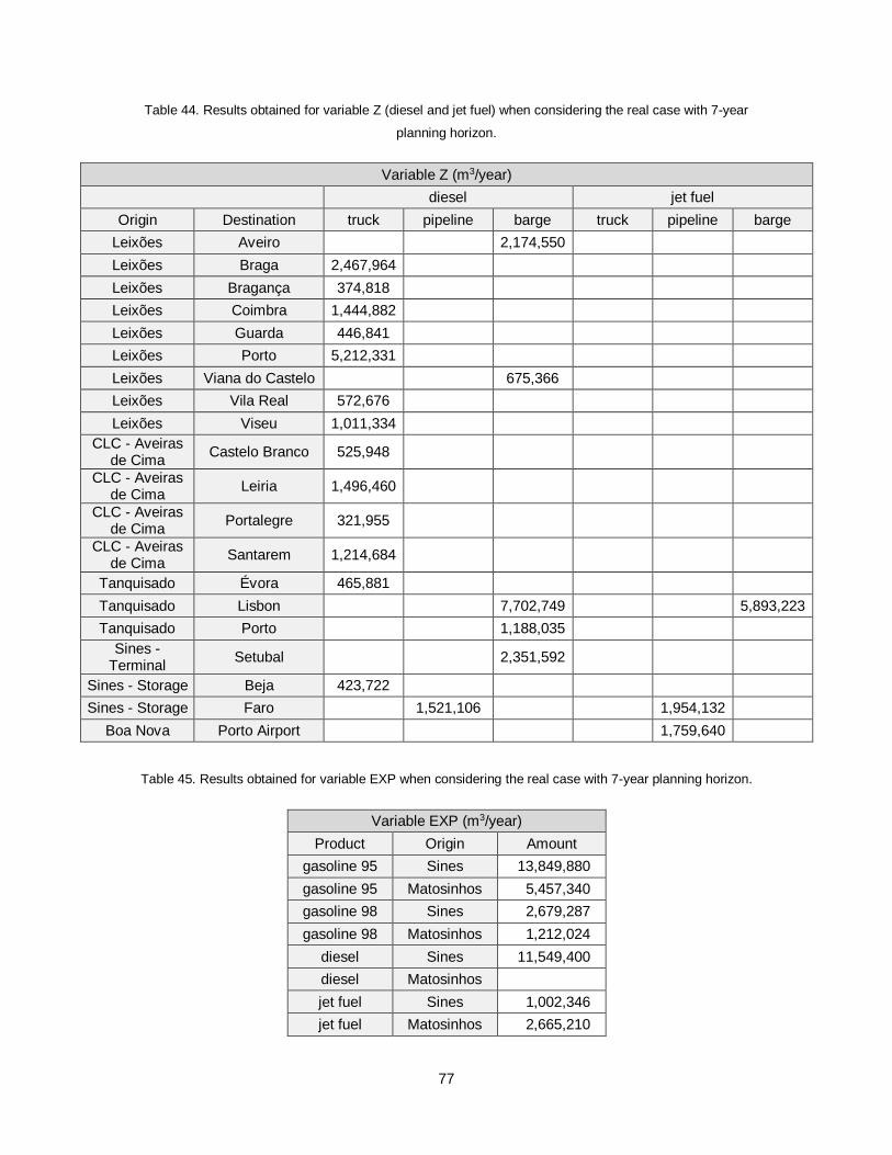
77

Table 44. Results obtained for variable Z (diesel and jet fuel) when considering the real case with 7-year

planning horizon.

Variable Z (m3/year)

diesel jet fuel

Origin Destination truck pipeline barge truck pipeline barge

Leixões Aveiro 2,174,550

Leixões Braga 2,467,964

Leixões Bragança 374,818

Leixões Coimbra 1,444,882

Leixões Guarda 446,841

Leixões Porto 5,212,331

Leixões Viana do Castelo 675,366

Leixões Vila Real 572,676

Leixões Viseu 1,011,334

CLC - Aveiras de Cima

Castelo Branco 525,948

CLC - Aveiras de Cima

Leiria 1,496,460

CLC - Aveiras de Cima

Portalegre 321,955

CLC - Aveiras de Cima

Santarem 1,214,684

Tanquisado Évora 465,881

Tanquisado Lisbon 7,702,749 5,893,223

Tanquisado Porto 1,188,035

Sines - Terminal

Setubal 2,351,592

Sines - Storage Beja 423,722

Sines - Storage Faro 1,521,106 1,954,132

Boa Nova Porto Airport 1,759,640

Table 45. Results obtained for variable EXP when considering the real case with 7-year planning horizon.

Variable EXP (m3/year)

Product Origin Amount

gasoline 95 Sines 13,849,880

gasoline 95 Matosinhos 5,457,340

gasoline 98 Sines 2,679,287

gasoline 98 Matosinhos 1,212,024

diesel Sines 11,549,400

diesel Matosinhos

jet fuel Sines 1,002,346

jet fuel Matosinhos 2,665,210

78

Table 46, Table 47, Table 48 and Table 49 present the results obtained for the model

implemented considering the real case study with 10-year planning horizon. The Portuguese

refineries were considered to be working at 82% of their capacity. The results obtained for variable X

for j2 and j4 was 1 and for j3 was 0. Therefore, in this case it is considered a pipeline between CLC

– Aveiras de Cima and Lisbon and another pipeline between Sines storage and Faro. As the model

suggested no depot to be opened, variable V is 0. Moreover, according to the model there is no need

to import any of the products considered and therefore, variable IMP is also 0. The results for variable

γ reached the maximum allowed ψ, available at Table 38.

Table 46. Results obtained for variable Y when considering the real case with 10-year planning horizon.

Variable Y (m3/year)

gasoline 95 gasoline 98

Origin Destination truck pipeline barge truck pipeline barge

Sines CLC - Aveiras de

Cima 3,124,517 271,699

Sines Tanquisado 129,254 11,236

Sines Sines terminal 652,436 56,736

Sines Sines storage 539,581 46,918

Matosinhos Leixoes 4,319,463 375,609

Matosinhos Boa Nova

diesel jet fuel

Origin Destination truck pipeline barge truck pipeline barge

Sines CLC - Aveiras de

Cima 16,088,284 8,418,890

Sines Tanquisado 2,362,738

Sines Sines terminal 3,359,418

Sines Sines storage 2,778,327 2,791,618

Matosinhos Leixoes 20,543,950

Matosinhos Boa Nova 2,513,772

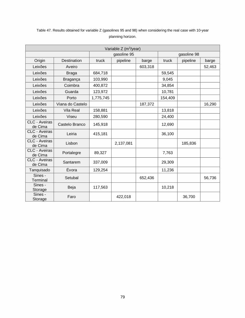
79

Table 47. Results obtained for variable Z (gasolines 95 and 98) when considering the real case with 10-year

planning horizon.

Variable Z (m3/year)

gasoline 95 gasoline 98

Origin Destination truck pipeline barge truck pipeline barge

Leixões Aveiro 603,318 52,463

Leixões Braga 684,718 59,545

Leixões Bragança 103,990 9,045

Leixões Coimbra 400,872 34,854

Leixões Guarda 123,972 10,781

Leixões Porto 1,775,745 154,409

Leixões Viana do Castelo 187,372 16,290

Leixões Vila Real 158,881 13,818

Leixões Viseu 280,590 24,400

CLC - Aveiras de Cima

Castelo Branco 145,918 12,690

CLC - Aveiras de Cima

Leiria 415,181 36,100

CLC - Aveiras de Cima

Lisbon 2,137,081 185,836

CLC - Aveiras de Cima

Portalegre 89,327 7,763

CLC - Aveiras de Cima

Santarem 337,009 29,309

Tanquisado Évora 129,254 11,236

Sines - Terminal

Setubal 652,436 56,736

Sines - Storage

Beja 117,563 10,218

Sines - Storage

Faro 422,018 36,700

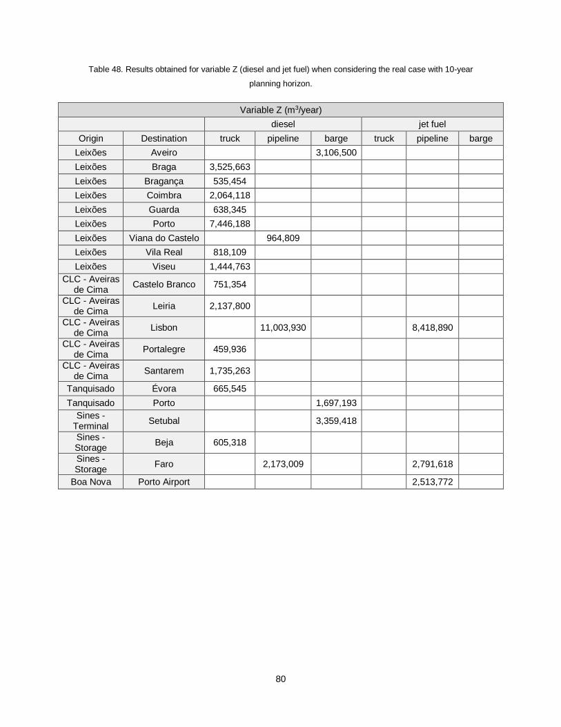
80

Table 48. Results obtained for variable Z (diesel and jet fuel) when considering the real case with 10-year

planning horizon.

Variable Z (m3/year)

diesel jet fuel

Origin Destination truck pipeline barge truck pipeline barge

Leixões Aveiro 3,106,500

Leixões Braga 3,525,663

Leixões Bragança 535,454

Leixões Coimbra 2,064,118

Leixões Guarda 638,345

Leixões Porto 7,446,188

Leixões Viana do Castelo 964,809

Leixões Vila Real 818,109

Leixões Viseu 1,444,763

CLC - Aveiras de Cima

Castelo Branco 751,354

CLC - Aveiras de Cima

Leiria 2,137,800

CLC - Aveiras de Cima

Lisbon 11,003,930 8,418,890

CLC - Aveiras de Cima

Portalegre 459,936

CLC - Aveiras de Cima

Santarem 1,735,263

Tanquisado Évora 665,545

Tanquisado Porto 1,697,193

Sines - Terminal

Setubal 3,359,418

Sines - Storage

Beja 605,318

Sines - Storage

Faro 2,173,009 2,791,618

Boa Nova Porto Airport 2,513,772

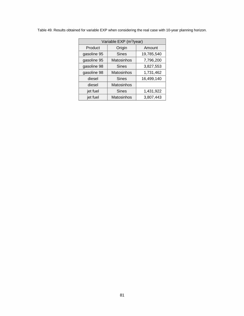
81

Table 49. Results obtained for variable EXP when considering the real case with 10-year planning horizon.

Variable EXP (m3/year)

Product Origin Amount

gasoline 95 Sines 19,785,540

gasoline 95 Matosinhos 7,796,200

gasoline 98 Sines 3,827,553

gasoline 98 Matosinhos 1,731,462

diesel Sines 16,499,140

diesel Matosinhos

jet fuel Sines 1,431,922

jet fuel Matosinhos 3,807,443