OPERATIONS RESEARCHVol. 53, No. 1, January–February 2005, pp. 48–60issn 0030-364X �eissn 1526-5463 �05 �5301 �0048

informs ®

doi 10.1287/opre.1040.0140©2005 INFORMS

Stochastic Transportation-InventoryNetwork Design Problem

Jia Shu, Chung-Piaw TeoHigh Performance Computation for Engineered Systems, Singapore-MIT Alliance, and Department of Decision Sciences,

National University of Singapore, Singapore {tlisj@nus.edu.sg, bizteocp@nus.edu.sg}

Zuo-Jun Max ShenDepartment of Industrial Engineering and Operations Research, University of California, Berkeley, California 94720,

shen@ieor.berkeley.edu

We study the stochastic transportation-inventory network design problem involving one supplier and multiple retailers. Eachretailer faces some uncertain demand, and safety stock must be maintained to achieve suitable service levels. However, risk-pooling benefits may be achieved by allowing some retailers to serve as distribution centers for other retailers. The problemis to determine which retailers should serve as distribution centers and how to allocate the other retailers to the distributioncenters. Shen et al. (2003) formulated this problem as a set-covering integer-programming model. The pricing problem thatarises from the column generation algorithm gives rise to a new class of the submodular function minimization problem.In this paper, we show that by exploiting certain special structures, we can solve the general pricing problem in Shen et al.efficiently. Our approach utilizes the fact that the set of all lines in a two-dimension plane has low VC-dimension. Wepresent computational results on several instances of sizes ranging from 40 to 500 retailers. Our solution technique can beapplied to a wide range of other concave cost-minimization problems.

Subject classifications : facilities/equipment planning: stochastic; inventory/production: uncertainty, stochastic;programming: nonlinear.

Area of review : Transportation.History : Received October 2001; revision received December 2002; accepted September 2003.

1. IntroductionManaging inventory has become a major challenge forcompanies as they simultaneously try to reduce costs andimprove service levels in today’s increasingly competitivemarket. Managing inventory consists of two critical tasks.First, we must determine the optimum number and loca-tion of distribution centers. Second, we must determine theamount of inventory to maintain at each of the distribu-tion centers. Often these tasks are undertaken separately,resulting in a degree of suboptimization. Research in thisarea deals with the modelling, design, planning, and controlof integrated supply chains as they occur in both indus-trial and service organizations. Important aspects concernthe development of new control architectures, as well asthe development of decision-support systems for planningand scheduling these systems. In addition, methods for theperformance analysis of alternative supply chain structures,under stochastic demand, is an important research area. Thecurrent research seeks to optimally exploit the possibilitiesto achieve an ideal network that must have the optimumnumber, size, and location of DCs to support the inventoryreplenishment activities of its retailers.We study the design of a stochastic distribution network

in which a single supplier ships products to a set of dis-tribution centers (DCs). Each DC serves a pool of retailerswith uncertain customer demand. The number and locations

of DCs are not given a priori. They are chosen from the setof retailers. After being chosen as a DC, this retailer-basedDC is served directly by the supplier and distributes prod-ucts to other retailers assigned to it. The central issue inthe stochastic distribution network design problem is howmany and which retailers should be selected to be the DCs,how to assign the other retailers to the DCs, and how tomanage the inventory at each DC.The problem we presented above was motivated by a

study conducted by Shen et al. (2003) and Daskin et al.(2002) at a Chicago-based blood bank. The blood bank sup-plied roughly 30 hospitals in the greater Chicago area. Itsfocus was on the production and distribution of platelets,the most expensive and most perishable of all blood prod-ucts. If a unit of platelets is not used within five days of thetime it is produced from whole blood, it must be destroyed.The demand for platelets is highly variable, as they areneeded in only a limited number of medical contexts. Whenthey are used, however, multiple units are often needed. Bystoring platelets at regional centers (located at a subset ofthe hospitals) instead, and distributing platelets to nearbyhospitals on an as-needed or daily basis, three objectiveswere likely to be achievable:• Inventory cost can be reduced due to risk pooling.

The safety stocks needed to protect against shortages willreduce with pooling of safety stocks;

48

Shu, Teo, and Shen: Stochastic Transportation-Inventory Network Design ProblemOperations Research 53(1), pp. 48–60, © 2005 INFORMS 49

• The cost of emergency shipments can be reducedbecause platelets would be stored closer to each of thehospitals; and• The training cost for inventory managers in an

improved supply chain distribution network system can bereduced because the stock would be stored at a small num-ber of regional distribution centers instead of being main-tained at each individual hospital.Shen et al. (2003) and Daskin et al. (2002) modelled the

above problem as a special case of a more general con-cave cost network design problem, often encountered inpractice. For instance, consider the following case problemfrom a widely used supply chain management textbook byChopra and Meindl (2001). ALKO Inc., a company thatdevelopes, produces, and distributes lighting fixtures, madeover 100 products through its production line. These prod-ucts were stored in five regional DCs operated by ALKO tomeet the market demand nationwide. It classified the prod-ucts into three categories in terms of volume of sales, andeach one has a different demand mean and standard devia-tion. The company wanted to determine whether it shouldconsolidate all or some of its products into a central DCand close all or some of the regional DCs, instead of stock-ing each item in every regional DC. The decision as towhether to set up the central DC depends on:• setup cost of a central DC if any;• closure cost of regional DCs if any; and• cycle inventory cost, safety stock cost, and transporta-

tion cost under the new distribution system.The setup cost of a central DC is modelled as a concave

cost function of the throughput of the DC. It depends onthe products stored at the DC and the regions served. Theassociated inventory cost and safety inventory cost compo-nents can be well approximated by another concave func-tion, depending on the DC-customer assignment decisionand the inventory replenishment policy used. This model,interestingly, turns out to be an (multiproduct) extension ofthe concave cost network design problem studied in thispaper.The rest of this paper is organized as follows. Section 2

reviews some literature on location theory and inventorymodels, and some earlier work on joint location-inventorymodels. Section 3 describes two models for the networkdesign problem, namely the nonlinear integer programmingmodel and the set covering model. In §4, we present anew method to solve the nonlinear pricing problem. In §5,we use the “variable fixing” method to further enhancethe computational performance of the column generationalgorithm. Finally, computational results that highlight theeffectiveness of the proposed algorithm are reported in §6.We conclude the paper with several ways to extend andgeneralize the approach presented in §7.

2. Literature ReviewThe goal of traditional inventory research (see, for exam-ple, Graves et al. 1993, Nahmias 1997, and Zipkin 1997

for a review) is to develop and evaluate inventory policiesso as to minimize the inventory-related costs while meetingsome service-level standards. Most of the papers in thisarea assumed a given distribution structure, with givenDC location and known customers assignment to theDC. In a different vein, the literature on facility locationand distribution network design (see, for example, Daskin1995, Mirchandani and Francis 1990, Drezner 1995, andGeoffrion and Power 1995 for a review) focuses mainlyon the trade-offs between the facility location and prod-uct transportation costs, usually ignoring or simplifyinginventory-related costs.Eppen (1979) showed that significant inventory-cost sav-

ings can be achieved at the network design stage by group-ing retailers demand together and thus capitalizing on theso-called “risk-pooling effects.” The location issue is there-fore an important factor in the overall performance of dis-tribution inventory system. Barahona and Jensen (1998)studied a version of the distribution network design prob-lem for computer spare parts. Their model takes intoaccount the costs of building the DCs and maintaininginventories at the various locations. To make the modeltractable, they imposed very restrictive assumptions on theinventory costs. Teo et al. (2001) studied the impact oninventory costs with consolidation of distribution centers.They design an algorithm that solves for a distribution sys-tem with the total fixed facility location cost and inventorycosts within

√2 of the optimum. Their approach, how-

ever, could not capture the impact of network design onthe transportation cost component. Erlebacher and Meller(2000) formulated a joint location-inventory model withhighly nonlinear integer objective functions. Continuousapproximation and some other heuristics are used to solvethe problem. For a 600-node problem, it took 117 hours ona Sun Ultra Sparcstation.Finally, Shen (2000), Shen et al. (2003), and Daskin et al.

(2002) studied the risk-pooling network design problem(presented in the next section). They were able to solve thepricing problem efficiently in time O�n logn� for two spe-cial cases: when the variance of the demand is proportionalto the mean (as in the Poisson demand case), or when thedemand is deterministic. Unfortunately, they are unable toaddress the general pricing problem. Although they provedthat the general pricing problem is a submodular functionminimization problem that can be readily solved in polyno-mial time (see, for example, Grotschel et al. 1981, Schrijver2000, Iwata et al. 2001), preliminary computational evi-dence shows that these algorithms are still not attractivecomputationally, especially because we need to solve thepricing problem in every iteration of the column generationalgorithm.Fortunately, the specific properties of the general pricing

problem make possible the use of a considerably simplerand faster algorithm. We propose a much faster algorithm�O�n2 logn�� to generate columns for the general case,using ideas from Chakravarty et al. (1985). We show that

Shu, Teo, and Shen: Stochastic Transportation-Inventory Network Design Problem50 Operations Research 53(1), pp. 48–60, © 2005 INFORMS

the pricing problem is related to a problem in compu-tational geometry. In fact, using an advance incrementalalgorithm for enumeration of vertices over a zonotope (seeOnn and Schulman 2001, where the pricing problem in thispaper can be shown to be a special case), the running timecomplexity can be further slashed to O�n2�. However, thereduction in running time comes at the expense of morecomplicated data structure to implement the incrementalalgorithm. The proposed algorithm, thus, is still not attrac-tive in practice. Instead, we show that by combining thevariable fixing idea (cf., Daskin et al. 2002) with our algo-rithm for the pricing problem, we are able to speed upthe running time by a factor of 10 and solve a realistic-sized transportation-inventory network design problem (upto 500 retailers) in just under 10 minutes.We emphasize the importance of being able to address

the general pricing problem efficiently. The two cases con-sidered in Shen et al. (2003) require that the demand beeither deterministic or �2i /�i = for every retailer. This ishardly the case in many real situations. Supply chain net-work design problems under the more general conditionsare the ones that management is most concerned with, andour model can be applied in the decision-making processfor problems of this kind.While the development of an integrated location/

inventory model will be valuable in its own right, it is likelyto have significant impacts in other areas as well. In a recentpaper, Current et al. (2002) cite over a dozen applicationsof location models in many different areas including chipmanufacturing, medical diagnosis, product procurement,and lot-sizing problems. Some of these problems are struc-turally similar to our integrated location/inventory model.Thus, there are likely to be significant applications of thiswork that extend well beyond integrated facility locationand inventory modelling and beyond supply chain networkdesign. One such example is Geunes et al. (2004), whoapply the algorithm in Shen et al. (2003) to an inven-tory model in which a seller maximizes profit by decidingwhether or not to satisfy each potential market demand.The decision depends on the revenue and cost parametersof each individual market and the economies of scale in theproduction/distribution costs.

3. Model FormulationThe generic risk-pooling network design problem is as fol-lows: Given a set I of retailers, we would like to (i) deter-mine the location of the DCs, and (ii) determine how theDC can be used to serve the retailers. We use the followingnotations:

Inputs and Parameters

• �i: mean (yearly) demand at retailer i for each i ∈ I .• �2i : variance of (daily) demand at retailer i for each

i ∈ I .• fj : fixed (annual) cost of locating a regional distribu-

tion center at retailer j for each j ∈ I .

We further assume that each retailer can only be servedusing a single DC; i.e., we do not split the demand at theretailer. When DC j is used to serve the retailers in set S,the associated cost is given by four cost components:

Cost Components

• fj : the fixed location cost.• ∑i∈S �ij�i: a term which is linear in �i.• Gj�∑

i∈S �i�: a term which is concave and nondecreas-ing in the expected throughput assigned.• Hj�

∑i∈S �2i �: a term which is concave and nondec-

reasing in the total demand variance experienced bythe DC.

For instance, when �ij corresponds to unit transportationcost between DC j and retailer i, the second term capturesthe total transportation cost associated with using DC j toserve retailers in set S. Gj�

∑i∈S �i� can be interpreted as

the DC operating and inventory replenishment cost. This isnormally assumed to be concave (as in the ALKO case oras in the EOQ model approximation) to reflect the economyof scales in inventory replenishment and handling. Lastbut not least, Hj�

∑i∈S �2i � can be interpreted as the safety

inventory cost component associated with the assignment.Again, this function can be well approximated as a concavefunction in the total variance in the demand assigned tothe DC, capturing the risk-pooling effect by consolidatingdemand at a centralized location.Let Xj = 1 if a DC is set up at location j , 0 otherwise,

and Yi� j = 1 if DC j is used to serve retailer i, 0 otherwise.The problem can be formulated as

min∑j∈I

(fjXj +

(∑i∈I��ij�i�Yij

)

+Gj

(∑i∈I

�iYij

)+Hj

(∑i∈I

�2i Yij

))(1)

subject to∑j∈I

Yij = 1 for each i ∈ I� (2)

Yij −Xj � 0 for each i� j ∈ I� (3)

Yij ∈ �0�1� for each i� j ∈ I� (4)

Xj ∈ �0�1� for each j ∈ I � (5)

The first two terms are structurally identical to those ofthe uncapacitated facility model. The last two terms arerelated to inventory costs, which are nonlinear in the assign-ment variables. The constraints of the model are identi-cal to those of the uncapacitated facility location problem,thus the problem we are studying is more difficult than thestandard uncapacitated facility location problem, which isalready a notorious NP-hard problem. Note that withoutthe risk-pooling term Hj�·�, the LP relaxation of the aboveproblem reduces to a classical concave cost transportationnetwork flow problem. The presence of the risk-poolingterm destroys the network flow structure and gives rise toa nasty combinatorial optimization problem.

Shu, Teo, and Shen: Stochastic Transportation-Inventory Network Design ProblemOperations Research 53(1), pp. 48–60, © 2005 INFORMS 51

3.1. Example of the Risk-Pooling Model

For ease of exposition and to make the paper self-contained, we introduce the model proposed by Shen et al.(2003) and Daskin et al. (2002) as a special case of theabove model. The readers may want to refer to the originalpapers for detailed derivation of the model.Two different types of inventories are kept at each DC:

the working inventory, which is determined by the inven-tory ordering policy adopted, and the safety stock, whichis kept at each DC to protect against the possibilities ofrunning out of stocks during replenishment lead time. Weassume each DC orders inventory from the supplier usingan economic order quantity model (EOQ). Other cost termsinclude the transportation costs from each DC to the retail-ers it serves and the level of safety stock to maintain, whichare also dependent on the decisions of retailer assignments.Following another assumption made in Shen et al.

(2003), we assume that the non-DC retailers maintain onlya minimal amount of inventory, and we therefore ignorethis inventory in the model below.To model this problem, we define the following addi-

tional notation:

Additional Inputs and Parameters

• dij : cost per unit to ship from retailer j to retailer i foreach i ∈ I and j ∈ I .• �: desired percentage of retailers’ orders satisfied

(fill rate).• �: weight factor associated with the shipment cost.• �: weight factor associated with the inventory cost.• z�: standard normal deviate such that P�z� z��= �.• h: inventory holding cost per unit of product per year.• Fj : fixed cost of placing an order at distribution cen-

ter j for each j ∈ I .• L: lead time in days.• gj : fixed shipment cost from external supplier to dis-

tribution center j .• aj : per unit shipment cost from external supplier to

distribution center j .

Note that to simplify the notation, we have assumed thatall lead times are equal. In this case, the model reduced to

min∑j∈I

(fjXj +

[∑i∈I���idij +�aj�i�Yij

]

+√2�h�Fj +�gj�

√∑i∈I

�iYij + �hz�√L√∑

i∈I�2i Yij

)

≡∑j∈I

(fjXj +

(∑i∈I

d̂ijYij

)

+Kj

√∑i∈I

�iYij + q√∑

i∈I�2i Yij

)(6)

subject to∑j∈I

Yij = 1 for each i ∈ I� (7)

Yij −Xj � 0 for each i� j ∈ I� (8)

Yij ∈ �0�1� for each i� j ∈ I� (9)

Xj ∈ �0�1� for each j ∈ I� (10)

where

d̂ij = ��i�dij + aj��

Kj =√2�h�Fj +�gj��

q = �hz�√L�

The objective function minimizes the weighted sum ofthe following four cost components:• The fixed cost of locating facilities, given by the term∑j fjXj .• The annual shipment cost from the distribution centers

to the non-DC retailers, given by the term ��∑

i∈I ��idij +aj�i�Yij �.• The expected working inventory cost, given the solu-tion to the EOQ equation with ordering cost Fj +�gj , hold-ing cost �h, and demand

∑i∈I �iYij .

• The annual safety stock cost, given by �hz�√L ·√∑

i∈I �2i Yij .This is easily seen to be a special case of the generic

risk-pooling network design problem presented earlier.

3.2. The Set-Covering Formulation

The nonlinear integer-programming model proposed earlieris normally approximated by converting the problem toa linear integer-programming problem, through lineariz-ing the objective function (cf., Erlebacher and Meller2000). We can also solve the proposed nonlinear integer-programming problem directly using the Lagrangian relax-ation approach (cf., Daskin et al. 2002). We propose inthe rest of this section a different but equivalent way tostudy the generic risk-pooling network design problem. Theadvantage of this approach is that it gets rid of the nonlin-earity (using exponentially many variables) inherent in theprevious model, and it is known to be equivalent (“dual”)to the Lagrangian relaxation approach.Note that every feasible solution to our decision problem

consists of a partition of the set I of retailers into nonemptysubsets, R1�R2� � � � �Rn, together with one designated DCfor each of these n sets.Let � be the collection of all nonempty subsets of the

set I . Let cR� j be the total cost associated with DC j servingthe set of retailers in R. That is,

cR� j = fj +∑i∈R

�ij +Gj

(∑i∈R

�i

)+Hj

(∑i∈R

�2i

)�

Let zR� j = 1 if DC j is used to serve the set of retail-ers in R. The set-covering model for the network designproblem can now be formulated as

���� min∑R∈�

∑j∈I

cR� jzR� j

Shu, Teo, and Shen: Stochastic Transportation-Inventory Network Design Problem52 Operations Research 53(1), pp. 48–60, © 2005 INFORMS

subject to

∑R∈�% i∈R

(∑j∈I

zR� j

)� 1 ∀i ∈ I�

zR� j ∈ �0�1� ∀R ∈��

We begin each iteration by solving the linear relaxationof the above set-covering model, using a partial set ofcolumns, to obtain an optimal solution z̄R� j , R ∈�, and thecorresponding optimal dual solution &i, i ∈ I .We want to know for each column �R� j�, whether the

reduced cost

cR� j −∑i∈R

&i � 0

is nonnegative for each R ∈�. If the answer is yes, then z̄is an optimal solution to ����. If, on the other hand, acolumn �R� j� with negative reduced cost is found, thenthe column �R� j� is added to the master LP, and the nextiteration begins.Finding R⊆� and j ∈ I with negative reduced cost, or

proving that no such pair �R� j� exists, is called the pricingproblem.To solve the pricing problem, we need to solve for each

fixed j , the following integer-programming problem:

��j � min fj +∑i∈I��ij − &i�Yij

+Gj

(∑i∈I

�iYij

)+Hj

(∑i∈I

�2i Yij

)

subject to

Yij ∈ �0�1� ∀i ∈ I �

4. The Pricing ProblemIn this section, we propose an algorithm to solve the pricingproblem ��j �. To simplify the notation, we define

ai %= �ij − &i�

bi %=�i�

ci %= �2i �

zi %= Yij

for each i ∈ I . Note that fj does not depend on Yij and,hence, can be ignored for discussion here. We now havethe following problem �j for designated distribution centerj ∈ I :

�� ′j � min

∑i∈I

aizi +Gj

(∑i∈I

bizi

)+Hj

(∑i∈I

cizi

)

subject to

zi ∈ �0�1� ∀i ∈ I �

For each j ∈ I , define set function gj on I as follows: Foreach S ⊆ I ,

gj�S�≡∑i∈S

ai +Gj

(∑i∈S

bi

)+Hj

(∑i∈S

ci

)� (11)

The above problem can also be reformulated as

minS⊆I

gj�S��

Let z∗ be an optimal solution to �� ′j �, with associated

optimal objective value (∗j . The minimum reduced cost set

R∗j ⊂ I is then the collection of retailers i ∈ I with z∗i = 1.If (∗

j + fj � 0, then the column �R∗j � j� has nonnegative

reduced cost. Hence, we can conclude that there is no setR ∈� having designated distribution center j with negativereduced cost. Otherwise, we obtain a column with negativereduced cost.

Lemma 1. Given a retailer j ∈ I , there exists a minimumreduced cost set R∗

j ⊂ I with ai < 0 for every i ∈R∗j .

Proof. Let i ∈ R∗j . Because bi� ci � 0, and if ai � 0, then

for any solution z̄ with z̄i = 1, the objective function valueis at least as great as that of the solution obtained from z̄ bysetting z̄i = 0. This follows because Gj and Hj are assumedto be concave and nondecreasing. By repeating this process,we obtain a set R∗

j with the desired property. �

Hence, we may restrict our search for R∗j to retailers

in I−, where I− %= �i ∈ I % ai < 0�. We next identify a nicestructural property of the set R∗

j by extending an argumentin Chakravarty et al. (1985).Let aS =

∑i∈S ai, bS =

∑i∈S bi, and cS =

∑i∈S ci. Define

a new function

hj�x� y� z� %= x+Gj�y�+Hj�z�� (12)

Note that hj�x� y� z� is a separable concave function, and

minS⊆I−

gj�S�=minS⊆I−

hj�aS� bS� cS�� (13)

Because the set ��aS� bS� cS� % S ⊆ I−� is finite, its convexhull, which will be denoted by H , is a convex polyhedron.Now, because the function hj is concave,

minS⊆I−

gj�S�=minS⊆I−

hj�aS� bS� cS�

= min�a� b� c�∈H

hj�a� b� c��

as the latter minimization problem attains a minimum at anextreme point of H .Let �a∗� b∗� c∗� be an extreme point of H . Because H is

a polyhedron, it is well known that there exists a linearfunction f on H that attains its unique minimum over Hat �a∗� b∗� c∗�. Because f is linear, it has a representationf �a� b� c�= �′a+�′b+ ′c defined by real numbers �′, �′,

Shu, Teo, and Shen: Stochastic Transportation-Inventory Network Design ProblemOperations Research 53(1), pp. 48–60, © 2005 INFORMS 53

and ′. The uniqueness of �a∗� b∗� c∗� as the minimizerof f over H assures that we do not have �′ = �′ = ′ = 0.Because H is the convex hull of ��aS� bS� cS� % S ⊆ I−�,

�′a∗ +�′b∗ + ′c∗ = min�a� b� c�∈H

�′a+�′b+ ′c

=minS⊆I−

�′aS +�′bS + ′cS

=minS⊆I−

∑i∈S��′ai +�′bi + ′ci��

The set S∗ = �i ∈ I− % �′ai + �′bi + ′ci < 0� is clearlyoptimal for the above optimization problem. Hence, weconclude from the uniqueness property that �a∗� b∗� c∗� =�aS∗� bS∗� cS∗�; i.e., R

∗j = S∗.

Note that S∗ = �i % �′ai + �′bi + ′ci < 0� = �i % �′ +�′�bi/ai� + ′�ci/ai� > 0� = �i % �′xi + ′yi < �′�, wherexi =−bi/ai and yi =−ci/ai. Here, xi� yi � 0 for all i.To determine S∗, we need to determine the corresponding

values for �′, �′, and ′. Although there are infinitely manychoices for the parameters �′, �′, and ′, it turns out thatthe number of distinct partitions obtained by varying theparameters are limited. It is not difficult to see why thenumber of partitions obtained this way will not be large.Consider the following examples with four retailers (seeFigure 1).The position of the retailers in Figure 1 corresponds to

the coordinate �xi� yi� given above. By varying the param-eters �′, �′, and ′, we are looking for distinct partitionsof the set of retailers with half-space in the plane. Notethat instead of 24 = 16 possible partitions, the number isrestricted by the position of the points in the plane. Forinstance, Retailers 2 and 3 cannot be candidates, because itis not possible to separate them from Retailers 1 and 4 byusing the intersection of a half-space and the set of points.This phenomenon can be studied using a general result in

the theory of VC-dimension (cf., Vapnik and Chervonenkis1971). To describe this result, we need to first introducesome notations.

Figure 1. Partitioning.

1

42

3

The VC-dimension is defined for any set system � ⊂ 2Xon an arbitrary set X. It is the supremum of the sizes ofall shattered subsets � ⊂ X; here � is called shattered if� �� = 2�; i.e., for any �⊂� there exists a set S ∈� suchthat �= � ∩ S. For example, if � denotes the system ofall closed half-planes in the plane, then it is not difficult tocheck that the VC-dimension of the set system � is three,because no four points in the plane can be shattered byusing only half-planes.The following well-known result shows that the number

of possible candidates for S∗ is essentially small:

Lemma 2 (Vapnik and Chervonenkis 1971, Sauer1972). For any set system � of VC-dimension at most d,we have �� �X ��-d��X��, where

-d�m�=(m0

)+(m1

)+ · · ·+

(md

)�

The above lemma suggests that we need to search amongat most O�n3� possible subsets to determine S∗.The complexity of the above algorithm can be slashed

down further to O�n2�, by enumerating over the extremepoints of an associated zonotope (cf., Onn and Schulzman2001) using an incremental algorithm. This algorithm, how-ever, is not efficient in practice, because of the sophisticateddata structure needed to implement the incremental algo-rithm. In the rest of this section, we show a more efficientand direct approach.

Algorithm for the Pricing Problem

Note that the parameters ��′��′� ′� for the optimal S∗ canbe chosen to be the gradient function of hj�x� y� z�= x+Gj�y�+Hj�z� at the optimal solution �a∗� b∗� c∗�. Hence,we can assume that �′ = 1, �′ � 0, and ′ � 0. The problemreduces to finding S∗ such that

S∗ = �i % �′xi + ′yi < 1��

The case where �′ = 0 or ′ = 0 is easy to handle andreduces to the special cases discussed in Shen et al. (2003).We assume next that �′ > 0 and ′ > 0. Let

fi = �′xi + ′yi − 1�Let k1 = argmax�fi % fi < 0�; i.e., k1 corresponds to theretailer with the largest negative fi. Note that S

∗ must nowsatisfy

S∗ = �i % fi � fk1�∪ �k1�

= �i % �′�xi − xk1�+ ′�yi − yk1�� 0�∪ �k1�

for all i ∈ I−\�k1�.We partition the set I−\�k1� (say with cardinality L) into

four different subsets, S1, S2, S3, and S4, with �S1� =m1,�S2� = m2, �S3� = m3, and �S4� = L − m1 − m2 − m3. Forretailer i ∈ I−\�k1�, if �xi − xk1�/�yi − yk1� � 0, then i

Shu, Teo, and Shen: Stochastic Transportation-Inventory Network Design Problem54 Operations Research 53(1), pp. 48–60, © 2005 INFORMS

Figure 2. Different subsets.

X

Y

S1

S2

S3

S1

S4

(xk1,yk1

)

belongs to set S1. If �xi − xk1�/�yi − yk1� > 0 and xi < xk1 ,yi < yk1 , then retailer i belongs to set S2; if �xi − xk1�/�yi − yk1� > 0 and xi > xk1 , yi > yk1 , then retailer i belongsto set S3. All the remaining retailers in I−\�k1� belong toset S4. It is easy to see that yi = yk1 for i ∈ S4. See Figure 2for a graphical illustration of the four subsets.We further sort the retailers in subset S1 by relabelling

the indices if necessary, so that

x1− xk1y1− yk1

�x2− xk1y2− yk1

� · · ·� xm1 − xk1ym1 − yk1

� 0� �∗�

Because �′ > 0 and ′ > 0, i ∈ S∗ for all i in S2 andi � S∗ for all i in S3. For i ∈ S4, because �

′ > 0, i ∈ S∗ ifand only if xi − xk1 � 0.To determine whether i ∈ S∗ if i ∈ S1, first note that

xi − xk1yi − yk1

�xj − xk1yj − yk1

if and only if

�′ xi − xk1yi − yk1

+ ′� �′ xj − xk1

yj − yk1+ ′�

We consider the following three cases:

Case (a). Suppose that there exists a retailer k2 such thatthe (open) interval(�′ xk2 − xk1yk2 − yk1

+ ′��′ xk2+1− xk1yk2+1− yk1

+ ′)

contains the point 0.

Claim 1. If i� k2, then i ∈ S∗ if and only if yi − yk1 > 0.

Proof. Because

�′ xi − xk1yi − yk1

+ ′� �′ xk2 − xk1

yk2 − yk1+ ′ < 0�

we have

�′�xi − xk1�+ ′�yi − yk1� < 0

if and only if yi − yk1 > 0� �

Similarly,

Claim 2. If m1 � i � k2 + 1, then i ∈ S∗ if and only ifyi − yk1 < 0.

Proof. Because

�′ xi − xk1yi − yk1

+ ′� �′ xk2+1− xk1

yk2+1− yk1+ ′ > 0�

we have

�′�xi − xk1�+ ′�yi − yk1� < 0if and only if yi − yk1 < 0� �

Case (b). Suppose that there exists a retailer k2 such that�′�xk2 −xk1�/�yk2 −yk1�+ ′ = 0. Then, clearly, k2 satisfiesfk2 � fk1 and hence k2 ∈ S∗. Furthermore, all i with

xi − xk1yi − yk1

= xk2 − xk1yk2 − yk1

are also candidates for S∗ because they all satisfyfi = fk2 � fk1 .

Case (c). Suppose there is no retailer k2 that satisfiesCase (a) or Case (b), i.e., either

0<�′ x1− xk1y1− yk1

+ ′ or 0>�′ xm1 − xk1ym1 − yk1

+ ′�

Then, conditions similar to the two situations discussed inCase (a) can be used to determine whether i ∈ S∗. �

Therefore, we obtain the following characterization forthe set S∗:

Theorem 1. The optimal solution S∗ satisfies the follow-ing properties for some k1 and k2, and with the retailersordered as in �∗�:

1. k1 ∈ S∗.2. For all i ∈ S1, either Case (a) holds:• for all i ∈ �1�2� � � � � k2�, i ∈ S∗, if and only if

yi − yk1 > 0;• for all i ∈ �k2 + 1� � � � �m1�, i ∈ S∗, if and only ifyi − yk1 < 0;

or Case (b) holds:• for all i < k2, with

xi − xk1yi − yk1

<xk2 − xk1yk2 − yk1

� i ∈ S∗�

if and only if yi − yk1 > 0;• for all i > k2, with

xi − xk1yi − yk1

>xk2 − xk1yk2 − yk1

� i ∈ S∗�

if and only if yi − yk1 < 0;• for i such that

xi − xk1yi − yk1

= xk2 − xk1yk2 − yk1

� i ∈ S∗�

Shu, Teo, and Shen: Stochastic Transportation-Inventory Network Design ProblemOperations Research 53(1), pp. 48–60, © 2005 INFORMS 55

3. For all i ∈ S2, i ∈ S∗;4. For all i ∈ S3, i � S∗;5. For all i ∈ S4, i ∈ S∗, if and only if xi − xk1 � 0.

The above theorem provides an efficient method for find-ing S∗, thus solving the pricing problem �j . Although k1and k2 are not given a priori, we can simply guess k1 from 1to n and k2 from 1 to m1 (after sorting to satisfy �∗�).For each pair of k1 and k2, we can easily generate all thesolutions satisfying the above properties and then select theone with the lowest objective value. It is easy to see thatfor each specific k1, there are at most 2n such solutions.They can be listed immediately after sorting the values�xi − xk1�/�yi − yk1�. With a bit of reflection, it is easy tosee that we are able to compute the entire list of the can-didate solution for S∗ with O�n� multiplications, additions,and square-root computations. Thus, sorting, which can bedone in time O�n logn�, is the dominant step in this algo-rithm. We need to do this sorting n times, one for each k1ranging from 1 to n, so the computational complexity ofthis algorithm is O�n2 logn�.

Theorem 2. The problem minS⊆I− gj�S� can be solved inO�n2 logn� time.

5. Variable FixingIn the straightforward implementation of the above algo-rithm, we need to solve, for each retailer, a related submod-ular function minimization problem where the retailer isassumed to be the DC. This slows down the column gener-ation routine considerably. We show next how informationon the primal and dual solution can be used to “fix” vari-ables, so that we can determine whether a retailer will bea DC candidate in an optimal solution early in the columngeneration routine.Recall that the set-covering model we are trying to solve

is of the form

min∑R∈�

∑j∈I

cR� jzR� j

subject to

∑R∈�% i∈R

(∑j∈I

zR� j

)� 1 ∀i ∈ I�

zR� j ∈ �0�1� ∀R ∈��

At each stage of the column generation routine, we have• A set of dual prices �&j�.• A set of primal feasible (fractional) solution zS� j .• After solving the pricing problem (one for each

potential DC location), we obtain the reduced cost rj ≡minS% j∈S�cS� j −

∑k∈S &k�. Note that some of the rjs may be

nonnegative.Let ZIP and ZLP denote the optimal integral and fractional

solution to the set-covering problem.

Claim 3.∑

j% rj�0rj +

∑j &j is a lower bound to ZIP.

Proof. In the optimal IP solution, by concavity of theobjective function, it is easy to check that cS� j + cT � j �cS∪T � j . Hence, the inequality∑S

zS� j � 1

is a valid inequality for the problem. We can add the aboveinequality, one for each j , to the set-covering model, toobtain a stronger LP relaxation. The Lagrangian dual of thenew LP relaxation is thus equivalent to

L�3�=∑j

3j +min{(∑

j

∑S

(cS� j −

∑k∈S

3k

)zS� j

)%

1� zS� j � 0�∑S

zS� j � 1 ∀j}�

The problem decomposes for each retailer j , and henceZIP �max3 L�3�� L�&�=∑

j &j +∑

j% rj�0rj . �

Let j∗ be a retailer such that r∗j > 0. Let UB be an upperbound for ZIP.

Claim 4. If∑

j% rj�0rj +

∑j &j + rj∗ >UB, then retailer j∗

will never be used as a DC in the optimal solution to the(integral) set-covering problem.

Proof. To see this, suppose otherwise. Then, ZIP remainsunchanged if we impose the additional condition

∑S zS� j∗ =

1 to the existing set of constraints. The Lagrangian dual, inthis case, reduces to

L′�3�

=∑j

3j +min{(∑

j

∑S% j∈S

(cS� j −

∑k∈S

3k

)zS� j

)% 1� zS� j � 0�

∑S

zS� j � 1 ∀j� ∑S

zS� j∗ = 1}�

Hence, ZIP � max3 L′�3� � L′�&� = ∑

j &j +∑

j% rj�0rj +

rj∗ . On the other hand, we have ZIP �UB. This gives riseto a contradiction. �

Note that once we determine that the retailer j∗ willnever be used as a DC in the optimal solution, then we donot need to solve the pricing problem corresponding to j∗

anymore in the rest of the column generation procedure. Infact, all columns arising from using j∗ as a DC (generatedpreviously) can also be deleted from the LP. This is the keyadvantage of the variable fixing method.The variable fixing method depends largely on the qual-

ity of the upper bound UB. If ZLP = ZIP, then the solution∑S� j cS� jzS� j generated at each stage of the column gener-

ation routine will be an upper bound to ZIP. Unfortunately,this is not true for all instances. As in Daskin et al. (2002),we generate an upper bound for the IP by generating afeasible solution in the following way:• Let z∗ be the optimal LP solution obtained by solving

the problem using a partial set of columns.

Shu, Teo, and Shen: Stochastic Transportation-Inventory Network Design Problem56 Operations Research 53(1), pp. 48–60, © 2005 INFORMS

• Order the retailers according to nondecreasing valueof demand.• Starting from the first retailer (say i) on the list, if for

some S and j , i ∈ S and z∗S� j = 1, then retailer i is servedby DC j . Otherwise, there exist S, T , both containing i,and j , k, such that z∗S� j > 0 and z

∗T �k > 0. We serve i using

the DC that will lead to the least total cost, and removeretailer i from the list.• Repeat the previous step until the list is empty.In this way, we can generate a feasible solution to the

distribution network design problem. This solution will beused as a bound to perform variable fixing in the columngeneration routine.

6. Computational ResultsIn this section, we summarize our computational experi-ence with the algorithms outlined in the previous section.All the instances were solved on a COMPAQ P3-450 sta-tion running the Windows 2000 operating system. We usedthe risk-pooling model as described in Shen et al. (2003)to design the computational experiment for our model. Tofacilitate proper comparison, we have also imposed theadditional assumption, used in Shen et al. (2003), that a DCat retailer j must be used to serve the demand at retailer j .Note that this is not necessarily true in the optimal solution.The solution approach described for the general case canbe easily modified to handle this additional assumption. Weleave the details to the readers.

6.1. Submodular Function Minimization

The purpose of this section is to test the performance-of-pricing algorithm. The code is written in C++. � is ran-domly generated in 650%�100%7, � is generated uniformlyin 60�001�0�017, � is randomly generated in �0�207, and allthe other parameters are generated uniformly in 60�1007.Table 1 presents the relation between the average CPU

time needed (averaged over 20 different instances) and thenumber of retailers in the problem. For each instance, wevary the DC choices over all the possible retailer locations.The CPU time we report is the total running time for solv-ing all the pricing problems with each retailer as the DC ata time.Up to 320 retailers, each pricing problem can be solved

in less than two seconds. This shows that the pricing prob-lem for moderate to large-size problems can be solved effi-ciently using this method.

Table 1. CPU time of the pricing algorithm.

No. of retailers CPU time (seconds)

10 0�0120 0�0740 0�7380 6�91160 60�3320 554

6.2. Stochastic Network Design WithoutVariable Fixing

In this subsection, we report the results of solving the net-work design problem using the column generation method.The algorithm for the general network distribution prob-lem is coded in C++, and the LP problem is solved usingCPLEX LP Solver.The mean demands �i and �2i are randomly generated

in 6100�16007 for all i ∈ I . Holding cost is 1, z� = 1�96(97.5% service level), ai = 5, gi = 10, and Fi = 10 for alli ∈ I . Our goal is to find ranges of values for � and �that resulted in instances that varied in solution difficultyas well as the fraction of retailers used as DCs in thesolution.For each of the instances, we first solve the LP relaxation

of the set-covering model via column generation. The initialset of columns includes all singletons. The column labelled“No. of columns generated” indicates the total number ofcolumns added during this phase. The resulting final opti-mal objective value is denoted by ZLP. In most instancesgenerated, the corresponding optimal solutions are integral.We denote by ZH the best upper bound we obtained. Inthe case where the LP relaxation solution is not integral,ZH is obtained by applying an IP solver to the final masterproblem.To speed up the column generation algorithm, we do not

solve the pricing problem at every iteration. Instead, wemaintain a column pool and we first look for columns withnegative reduced cost in the column pool. If the search issuccessful, we add these columns to the master problem.We also update the reduced costs of the columns in thecolumn pool and remove those with large positive reducedcosts from the pool. We solve the pricing problem onlywhen the column pool is empty. When this happens, thepricing algorithm is run to either prove the optimality ofthe current solution or to find new columns with negativereduced costs.Tables 2, 3, and 4 show the results of our computational

study.The above algorithm becomes very time consuming

when the number of retailers exceeds 120. For this reason,we do not report computational results for larger instances.To tackle a larger-scale problem, we turn to the variablefixing method.

6.3. Stochastic Network Design withVariable Fixing

The column labelled “No. of DCs Out” indicates the num-ber of retailers ruled out from being possible DCs in theoptimal LP solution by the variable fixing technique. Theparameters we use for the instances below are the same aswhat we used for the previous subsection. Only when thecolumn pool is empty shall we do the variable fixing pro-cedure again. Tables 5, 6, 7, 8, and 9 highlight the resultsof our computational study.

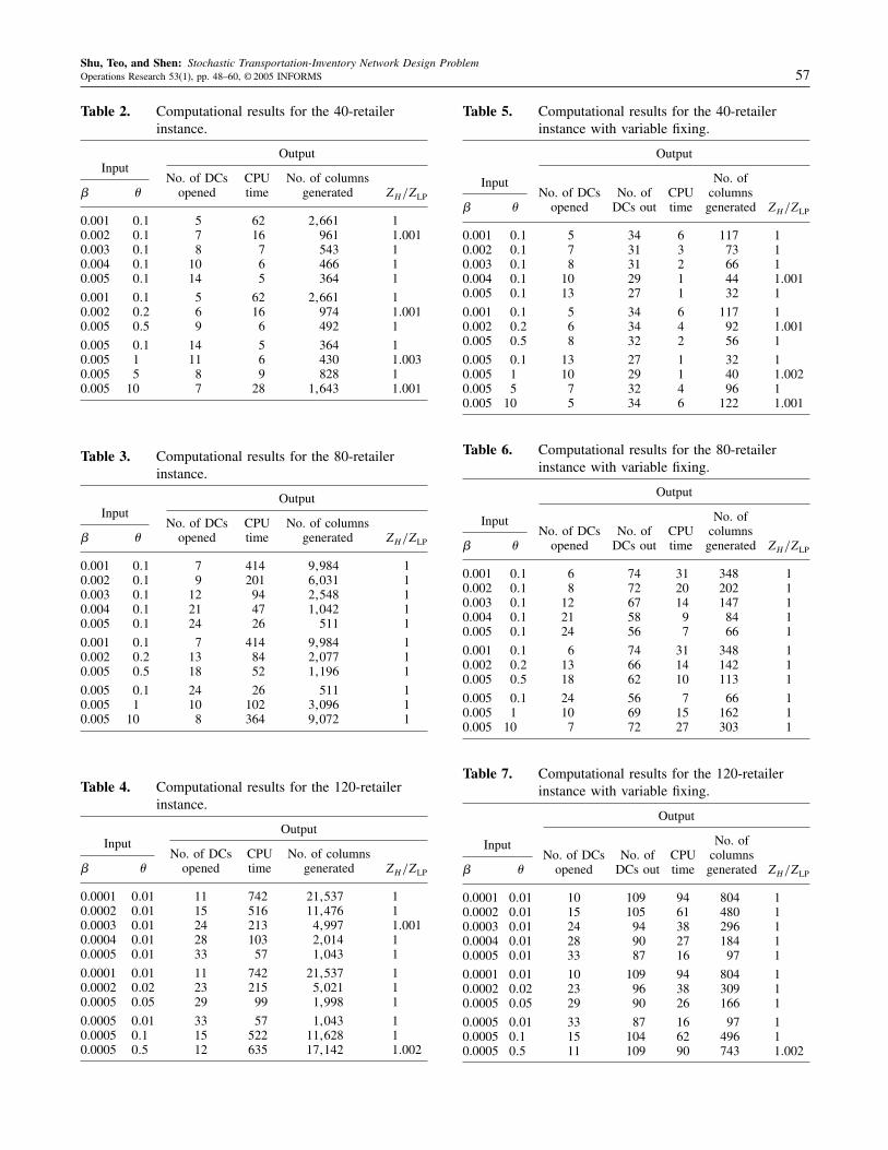
Shu, Teo, and Shen: Stochastic Transportation-Inventory Network Design ProblemOperations Research 53(1), pp. 48–60, © 2005 INFORMS 57

Table 2. Computational results for the 40-retailerinstance.

InputOutput

No. of DCs CPU No. of columns� � opened time generated ZH/ZLP

0.001 0�1 5 62 2�661 10.002 0�1 7 16 961 1�0010.003 0�1 8 7 543 10.004 0�1 10 6 466 10.005 0�1 14 5 364 1

0.001 0�1 5 62 2�661 10.002 0�2 6 16 974 1�0010.005 0�5 9 6 492 1

0.005 0�1 14 5 364 10.005 1 11 6 430 1�0030.005 5 8 9 828 10.005 10 7 28 1�643 1�001

Table 3. Computational results for the 80-retailerinstance.

InputOutput

No. of DCs CPU No. of columns� � opened time generated ZH/ZLP

0.001 0�1 7 414 9�984 10.002 0�1 9 201 6�031 10.003 0�1 12 94 2�548 10.004 0�1 21 47 1�042 10.005 0�1 24 26 511 1

0.001 0�1 7 414 9�984 10.002 0�2 13 84 2�077 10.005 0�5 18 52 1�196 1

0.005 0�1 24 26 511 10.005 1 10 102 3�096 10.005 10 8 364 9�072 1

Table 4. Computational results for the 120-retailerinstance.

InputOutput

No. of DCs CPU No. of columns� � opened time generated ZH/ZLP

0.0001 0�01 11 742 21�537 10.0002 0�01 15 516 11�476 10.0003 0�01 24 213 4�997 1�0010.0004 0�01 28 103 2�014 10.0005 0�01 33 57 1�043 1

0.0001 0�01 11 742 21�537 10.0002 0�02 23 215 5�021 10.0005 0�05 29 99 1�998 1

0.0005 0�01 33 57 1�043 10.0005 0�1 15 522 11�628 10.0005 0�5 12 635 17�142 1�002

Table 5. Computational results for the 40-retailerinstance with variable fixing.

Input

Output

No. ofNo. of DCs No. of CPU columns

� � opened DCs out time generated ZH/ZLP

0.001 0�1 5 34 6 117 10.002 0�1 7 31 3 73 10.003 0�1 8 31 2 66 10.004 0�1 10 29 1 44 1�0010.005 0�1 13 27 1 32 1

0.001 0�1 5 34 6 117 10.002 0�2 6 34 4 92 1�0010.005 0�5 8 32 2 56 1

0.005 0�1 13 27 1 32 10.005 1 10 29 1 40 1�0020.005 5 7 32 4 96 10.005 10 5 34 6 122 1�001

Table 6. Computational results for the 80-retailerinstance with variable fixing.

Input

Output

No. ofNo. of DCs No. of CPU columns

� � opened DCs out time generated ZH/ZLP

0.001 0�1 6 74 31 348 10.002 0�1 8 72 20 202 10.003 0�1 12 67 14 147 10.004 0�1 21 58 9 84 10.005 0�1 24 56 7 66 1

0.001 0�1 6 74 31 348 10.002 0�2 13 66 14 142 10.005 0�5 18 62 10 113 1

0.005 0�1 24 56 7 66 10.005 1 10 69 15 162 10.005 10 7 72 27 303 1

Table 7. Computational results for the 120-retailerinstance with variable fixing.

Input

Output

No. ofNo. of DCs No. of CPU columns

� � opened DCs out time generated ZH/ZLP

0.0001 0�01 10 109 94 804 10.0002 0�01 15 105 61 480 10.0003 0�01 24 94 38 296 10.0004 0�01 28 90 27 184 10.0005 0�01 33 87 16 97 1

0.0001 0�01 10 109 94 804 10.0002 0�02 23 96 38 309 10.0005 0�05 29 90 26 166 1

0.0005 0�01 33 87 16 97 10.0005 0�1 15 104 62 496 10.0005 0�5 11 109 90 743 1�002

Shu, Teo, and Shen: Stochastic Transportation-Inventory Network Design Problem58 Operations Research 53(1), pp. 48–60, © 2005 INFORMS

Table 8. Computational results for the 250-retailerinstance with variable fixing.

Input

Output

No. ofNo. of DCs No. of CPU columns

� � opened DCs out time generated ZH/ZLP

0.0001 0�01 19 229 221 1�663 10.0002 0�01 30 219 113 782 10.0003 0�01 49 201 78 466 1�0020.0004 0�01 57 192 59 346 10.0005 0�01 68 182 35 201 1

0.0001 0�01 19 229 221 1�663 10.0002 0�02 44 206 83 526 1�0010.0005 0�05 61 189 47 302 1

0.0005 0�01 68 182 35 201 10.0005 0�1 33 215 118 697 10.0005 0�5 20 230 211 1�479 1

By applying the variable fixing technique, we are able tocut down the computational time dramatically. The averageCPU time is only about 9% of the CPU time without thevariable fixing technique. The savings range from about83% to 94%. It is especially effective for those difficultinstances that required the most CPU times before. Forexample, for �= 0�001, �= 0�1 in the 80-retailer case, weare able to solve the problem in about 30 seconds afterapplying the variable fixing technique, which used to take414 seconds.As we can see from these tables, the problem takes

longer to solve when � decreases for fixed � or when �increases for fixed �. When the transportation costsincrease relative to other costs, i.e., � increases, the “No. ofDCs opened” increases too. However, when the inventorycosts increase relative to other costs, i.e., � increases, the“No. of DCs opened” decreases.

Table 9. Computational results for the 500-retailerinstance with variable fixing.

Input

Output

No. ofNo. of DCs No. of CPU columns

� � opened DCs out time generated ZH/ZLP

0.0001 0�01 42 458 512 3�742 10.0002 0�01 57 442 426 2�819 1�0010.0003 0�01 95 404 248 1�405 10.0004 0�01 114 386 146 717 10.0005 0�01 146 354 86 446 1

0.0001 0�01 42 458 512 3�742 10.0002 0�02 90 409 314 1�833 10.0005 0�05 132 368 117 586 1

0.0005 0�01 146 354 86 446 10.0005 0�1 61 439 404 2�633 10.0005 0�5 44 455 503 3�572 1

7. Extensions

7.1. Distance Constraint

In the distribution network design problem, it is quite com-mon to impose additional constraints on the collection ofretailers a DC can serve. For example, a typical geograph-ical constraint stipulates that the designated DC and theretailer cannot be too far apart. To enforce this constraintin our approach is easy, because we can set the distancefunction dij to a huge number if retailer j cannot act as theDC for retailer i (or vice versa).

7.2. Capacity Constraint

Another common constraint states that a DC cannot handletoo many retailers (say not more than k retailers can beserved by a single DC), due to capacity or other technicallimitations. In this paper, we describe how our techniquecan be extended to handle the additional constraint of thetype

∑i Yi� j � k for some fixed k. Note that we are assum-

ing that retailer j needs not be served by the DC located atits location.In this case, the column generation phase reduces to solv-

ing a problem of the type

min∑i∈I

aizi +Gj

(∑i∈I

bizi

)+Hj

(∑i∈I

cizi

)

subject to

zi ∈ �0�1� ∀i ∈ I�

zj = 1�∑i

zi � k�

Because the objective function is concave and separable,we can use the same argument to reduce the problem to aparametric version:

minS⊆I−

∑i∈S��′ai +�′bi + ′ci�zi

�PK�% subject to

zi ∈ �0�1� ∀i ∈ I−�∑i∈I−

zi � k�

The candidate solution for the column generation phasecomes out as the solution to the above linear discrete opti-mization problem for some choice of �′, �′, and ′.Let b��′��′� ′� denote the value of the kth smallest

entry in the set

��′ai +�′bi + ′ci % i ∈ I−��

It is clear that if zi = 1 in an optimal solution to prob-lem �PK�, then clearly �′ai + �′bi + ′ci � b��′��′� ′�because �′ai + �′bi + ′ci cannot be bigger than the kth

Shu, Teo, and Shen: Stochastic Transportation-Inventory Network Design ProblemOperations Research 53(1), pp. 48–60, © 2005 INFORMS 59

smallest value. Furthermore, we need �′ai+�′bi+ ′ci < 0,otherwise we would have zi = 0 in the optimal solution.Conversely, it is easy to see that zi = 1 in the optimal solu-tion if the point i satisfies both inequalities.The inequality

�′ai +�′bi + ′ci <min�b��′��′� ′��0�

determines a half-plane in 3D, and at most k out of possiblen− 1 points in the set

S ≡ ��ai� bi� ci� % i ∈ I−�

lies in this half-plane.Hence, the number of candidate solutions depends on the

number of �k-set. Here, a �k-set is the intersection of Sand a half-plane containing at most k points. Clarkson andShor (1989) showed that the number of such solutions in3D is bounded above by O�nk2�. Hence, the number ofcandidate sets is still bounded by a polynomial in n.

8. ConclusionIn this paper, we have outlined a formulation of a stochastictransportation-inventory network design model. The modeldetermines how many and where to locate regional DCsand how to assign retailers to the DCs to minimize the totalsystem costs, which include DC location costs, inventorycosts at the DCs, and the transportation costs within thistwo-echelon supply chain.The model was originally proposed in Shen et al. (2003).

They were able to solve efficiently only two special casesof the general model. We proposed an efficient algorithm tosolve the general pricing problem, with a worst-case run-ning time of O�n2 logn�. Together with the variable fixingtechnique, this yields a very efficient approach to solve amoderate to large-scale network design problem to nearoptimality.We would like to emphasize the importance of being

able to solve the general supply chain design problem. Thetwo cases considered in Shen et al. (2003) require thatthe demand be either deterministic or �2i /�i = for everyretailer. However, in a lot of real-life situations, the demandprocesses can be very different from retailer to retailer,and the ratio of demand variance to mean demand arenot the same for different retailers. Supply chain networkdesign problems under such conditions are the ones thatthe management is most concerned with, and our modelcan be applied successfully in the decision-making processfor problems of this kind. Furthermore, we show that oursolution techniques can handle a more general risk-poolingtype of network design problem, because our algorithmuses only the concavity property of the objective function.We propose two important related future research direc-

tions. First, we believe that the network design problemwhen each DC operates under the optimal �Q� r� policy

is worth exploring. This model captures the stochasticinventory replenishment cost at the DC using a moreaccurate cost model. The challenge in this problem, webelieve, lies in showing that the optimal cost of a �Q� r�policy is concave in the average demand assigned. Second,we hope to consider the cases with multiple items as wellas more general capacity constraints, and with more realis-tic transportation cost structures.

AcknowledgmentsThe authors thank the associate editor and two referees forconstructive comments that led to this improved versionof this paper. This work was supported in part by NSFgrant DMI-0223323. This support is gratefully acknowl-edged. The work of Zuo-Jun Max Shen was done while hewas with the University of Florida.

ReferencesBarahona, F., D. Jensen. 1998. Plant location with minimal inventory.

Math. Programming 83 101–111.

Chakravarty, A. K., J. B. Orlin, U. G. Rothblum. 1985. Consecutive opti-mizers for a partitioning problem with applications to optimal inven-tory groupings for joint replenishment. Oper. Res. 33 820–834.

Chopra, S., P. Meindl. 2001. Supply Chain Management: Strategy, Plan-ning and Operation. Pearson Prentice Hall, Upper Saddle River, NJ.

Clarkson, K. L., P. W. Shor. 1989. Applications of random samplingin computational geometry. II. Discrete Comput. Geometry 4(5)387–421.

Current, J., M. S. Daskin, D. Schilling. 2002. Discrete network loca-tion models. Z. Drezner, H. Hamacher, eds. Facility LocationTheory: Applications and Methods, Chap. 3. Springer-Verlag, Berlin,Germany, 81–118.

Daskin, M. S. 1995. Network and Discrete Location: Models, Algorithms,and Applications. Wiley-Interscience, New York.

Daskin, M. S., Collette R. Coullard, Z. J. Max Shen. 2002. An inventory-location model: Formulation, solution algorithm and computationalresults. Annals Oper. Res. 110 83–106.

Drezner, Z., ed. 1995. Facility Location: A Survey of Applications andMethods. Springer, New York.

Eppen, G. 1979. Effects on centralization on expected costs in a multi-location newsboy problem. Management Sci. 25(5) 498–501.

Erlebacher, S. J., R. D. Meller. 2000. The interaction of location andinventory in designing distribution systems. IIE Trans. 32 155–166.

Geoffrion, A. M., R. Power. 1995. Twenty years of strategic distribu-tion system design: An evolutionary perspective. Interfaces 25(5)105–127.

Geunes, J., Z. J. Shen, H. E. Romeijn. 2004. Economic ordering decisionswith market choice flexibility. Naval Res. Logist. 51(1) 117–136.

Graves, S. C., A. H. G. Rinnooy Kan, P. H. Zipkin. 1993. Logistics ofProduction and Inventory. Elsevier Science Publishers, Amsterdam,The Netherlands.

Grötschel, M., L. Lovasz, A. Schrijver. 1981. The ellipsoid method andits consequences in combinatorial optimization. Combinatorica 1169–197.

Iwata, S., L. Fleischer, S. Fujishige. 2001. A combinatorial, stronglypolynomial-time algorithm for minimizing submodular functions.J. ACM 48 761–777.

Mirchandani, P. B., R. L. Francis. 1990. Discrete Location Theory. JohnWiley and Sons, New York.

Shu, Teo, and Shen: Stochastic Transportation-Inventory Network Design Problem60 Operations Research 53(1), pp. 48–60, © 2005 INFORMS

Nahmias, S. 1997. Production and Operations Management, 3rd ed. Irwin,Chicago, IL.

Onn, S., L. Schulman. 2001. The vector partition problems for convexobjective functions. Math. Oper. Res. 26 583–590.

Rado, R. 1942. A theorem on independence relations. Quart. J. Math.Oxford 213 83–89.

Sauer, N. 1972. On the density of families of sets. J. Combinatorial TheorySeries A 1 145–1472.

Schrijver, A. 2000. A combinatorial algorithm minimizing submodularfunctions in strongly polynomial time. J. Combinatorial Theory,Series B 80 346–355.

Shen, Z. J. Max. 2000. Approximation algorithms for various supply chain

problems. Ph.D. thesis, Department of Industrial Engineering andManagement Sciences, Northwestern University, Evanston, IL.

Shen, Z. J. Max, C. Coullard, M. S. Daskin. 2003. A joint location-inventory model. Transportation Sci. 37 40–55.

Teo, C. P., J. H. Ou, K. H. Goh. 2001. Impact on inventory costs withconsolidation of distribution centers. IIE Trans. 33(2) 99–110.

Vapnik, V. N., A. Ya. Chervonenkis. 1971. On the uniform convergence ofrelative frequencies of events to their probabilities. Theory Probab.Appl. 16 264–280.

Zipkin, P. H. 1997. Foundations of Inventory Management. Irwin, BurrRidge, IL.