1

Multi-product Multi-chance-Constraint Stochastic Inventory Control Problem with

Dynamic Demand and Partial Back-Ordering: A Harmony Search Algorithm

Ata Allah Taleizadeh

Department of Industrial Engineering, Iran University of Science and Technology, Tehran, Iran E-mail: ata.taleizadeh@gmail.com

Seyed Taghi Akhavan Niaki 1

Department of Industrial Engineering, Sharif University of Technology P.O. Box 11155-9414 Azadi Ave, Tehran 1458889694 Iran

Phone: (+9821) 66165740, Fax: (+9821) 66022702, E-mail: Niaki@sharif.edu

Seyed Mohammad Haji Seyedjavadi Department of Computer Engineering, Islamic Azad University, Qazvin Branch, Qazvin, Iran

E-mail: seyedjavady_erfan@yahoo.com

Abstract

In this paper, a multiproduct inventory control problem is considered in which the periods between

two replenishments of the products are assumed independent random variables, and increasing and

decreasing functions are assumed to model the dynamic demands of each product. Furthermore, the

quantities of the orders are assumed integer-type, space and budget are constraints, the service-level

is a chance-constraint, and that the partial back-ordering policy is taken into account for the

shortages. The costs of the problem are holding, purchasing, and shortage. We show the model of

this problem is an integer nonlinear programming type and to solve it, a harmony search approach is

used. At the end, three numerical examples of different sizes are given to demonstrate the

applicability of the proposed methodology in real world inventory control problems, to validate the

results obtained, and to compare its performances with the ones of both a genetic and a particle

swarm optimization algorithms.

Keywords: Inventory Control; Multi-product Multi-constraint; Dynamic Demand; Stochastic

Replenishment; Partial Back-ordering; Harmony Search Algorithm

1. Introduction and Literature Review

Since the introduction of economic order quantity (EOQ) model by Harris [1], an extensive

research works on the extension of inventory control models involving constant demand rate have

been reported in the literature. However, in real-world environments there are many situations in

1Corresponding author

2

which the demand rate over a planning horizon is not constant. For example, the demand rates of

some seasonal products such as seasonal garments, shoes, drug, and the like is low at the beginning

of the season and increases as the season progresses. In other words, the demand rate changes with

time or it is time-dependent [2]. To name some research works in which the demand rate is not

considered constant, Silver and Meal [3] developed the EOQ model with dynamic demand. Dey et

al. [4] first proposed a model with an increasing demand function in which the lead-time was

considered fuzzy. Then, Dey et al. [5] extended their previous work under inflation and time value

of money. Donaldson [6] developed an inventory control model with dynamic demand where the

demand follows a linear trend. Chang and Dye [7] proposed a replenishment policy for deteriorating

items with time-dependent demand and partial back ordering. Goyal et al. [8] extended an inventory

replenishment problem with shortages over finite time- horizon. Gao et al. [9] presented various

modeling and approaches for the coordinated replenishment problem with deterministic dynamic

demand. Kim and Mabert [10] developed a model for discrete shopping and time dependent

demand. Martel and Gascon [11] introduced a new formulation of the dynamic demand and price in

inventory problems where the unit inventory holding costs in a period was a function of the

procurement quantity made in previous cycles. Hu and Munson [12] discussed the roles of lot sizing

when the demand was time-dependent and an incremental quantity discount policy was present.

Wang et al. [13] proposed two supply chain models for deteriorating items with stochastic and

dynamic demands. Pentico [14] developed a multi-period assortment problem in which demands

meet the conditions of a dynamic demand economic lot size problem where substitution costs have

a `scrap' component. Hopp and Xu [15] proposed an approximation method for the dynamic

demand substitution models that is useable in competitive markets.

In periodic-review inventory-control models, sometimes the replenishment times are not

under the retailers' control and happen stochastically. The product replenishments of many small

supermarkets and drug stores are examples of this condition where distributors visit them in

irregular intervals and ask them to order their products based on their current inventories, demand

3

rates, and the random visit time until the next replenishment opportunity. Retailers that are located

in geographically disadvantageous remote locations are another example in which the

replenishment times are not under the retailers' control. In this case, the suppliers would likely to be

the ones making the decision as to when to visit and replenish the retailers' inventories. This

problem that is called the stochastic replenishment intervals, has been investigated in the literature

(see for example, [16] and [17] and the references within).

In this paper, a stochastic replenishment intervals inventory control problem with one

provider and several products is considered in which the demands are dynamic and take increasing

or decreasing rates. To the best of authors' knowledge, this is the first time this problem, which

quite possibly happen in real-world inventory control environments along with its constraints, is

attacked. The constraints are the minimum service level of each product, the minimum required

warehouse space, the minimum required budget, and the integer decision variables. Moreover, a

harmony search algorithm is proposed to solve the developed integer-nonlinear models of the

problem.

The rest of the paper is organized as follows: in section 2, the problem along with the

assumptions is defined. In section 3, we model the defined problem of section 2. To do this we first

introduce the parameters and the variables of the problem. Then, a single product problem is

modeled, and finally the multiproduct problem is formulated. In the fourth section of the paper, we

introduce a harmony search algorithm to solve the model at hand and analyze it under special

conditions. Incorporating a numerical example, the solution method is investigated in section 5. The

conclusion and recommendations for future research come in section 6.

2. Problem Definition

The setting of the problem at hand is similar to the periodic review models with fundamental

difference that the replenishment times are not under retailer’s control. Consider a periodic

inventory control model for one provider in which the times required to order each of several

4

available products are stochastic in nature. Let the time-periods between two replenishments be

independent random variables and in case of shortage, a fraction is considered back-order and a

fraction lost-sale. The demands of the products are dynamic and take two general forms of

increasing and decreasing forms. The costs associated with the inventory control system are

holding, back-order, lost-sales, and purchasing costs. Furthermore, the service level of each product,

warehouse space, and budget are considered constraints of the problem and the decision variables

are integer digits. The aim of this research is to determine the inventory level of each product such

that the constraints are satisfied and the expected profit is maximized.

3. Problem Modeling

For the problem at hand, since the time-periods between two replenishments are

independent random variables, in order to maximize the expected profit of the planning horizon we

need to consider only one period. Moreover, since we assumed the costs associated with the

inventory control system are holding, shortage (back-order and lost-sale), and purchasing we need

to calculate the expected inventory level and the expected required storage space in each period.

Before doing this, we first define the parameters and the variables of the model.

For 1,2,...,i n , define the parameters and the variables of the model as

iR : The maximum inventory level of the ith product

iT : A random variable denoting the time-period between two replenishments (cycle length) of the ith

product

)( iT tfi

: The probability density functions of iT (Uniform density function)

:iW The purchasing cost per unit of the ith product

iFI : A fraction of the purchasing cost of the ith product used to calculate its holding cost

ih : The holding cost of the ith product per unit inventory per unit time ( i i ih FI W )

i : The back-order cost per unit demand of the ith product

5

ˆi : The shortage cost for each unit of lost sale of the ith product

iP : The sale price per unit of the ith product

)(tDi : The dynamic demand functions of the ith product

iSL : The lower limit of the service level for the ith product

iDt : The time at which the inventory level of the ith product reaches zero

i : The percentage of unsatisfied demands of the ith product that is back-ordered

iI : The expected amount of inventory units of the ith product per cycle

iH : The inventory level of the ith product per cycle

( )iI t : The inventory level of the ith product at time t

iL : The expected amount of the ith product lost-sale in each cycle

iB : The expected amount of the ith product back-order in each cycle

iQ : The expected amount of the ith product order in each cycle

if : The required warehouse space per unit of the ith product

F : Total available warehouse space

:TB Total available budget

ihC : The expected holding cost per cycle of the ith product

ibC : The expected shortage cost in back-order state of the ith product

ilC : The expected shortage cost in lost-sale state of the ith product

ipC : The expected purchase cost of the ith product

ir : The expected revenue obtained from sales of the ith product

)(RZ : The expected profit obtained in each cycle

For sake of simplicity, in section 3.3 we first consider a single-product problem. Then,

section 3.3.1 and 3.3.2 are devoted for a single-product problem with dynamic demand functions

6

and constraints, respectively. In section 3.4, we extend the single-product to a multiproduct model.

To do all these, we first introduce the pictorial representation of the single-product problem in

section 3.1.

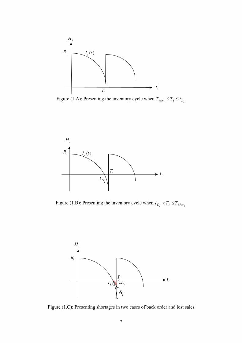
3.1. Inventory Diagrams

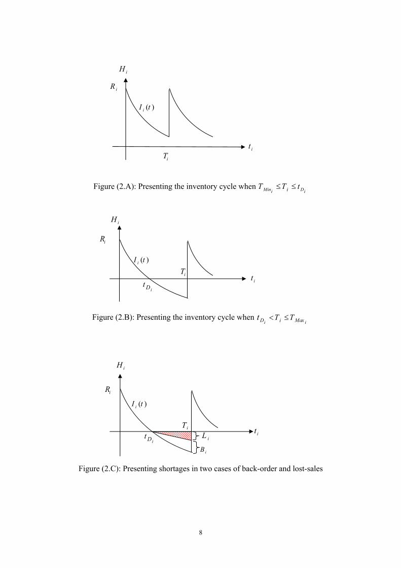
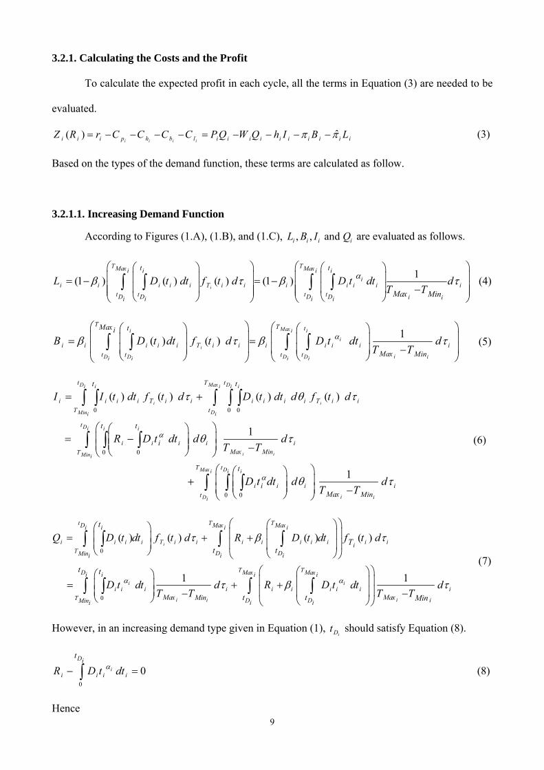
Considering the fact that the time-periods between replenishments are stochastic variables,

two cases may occur. In the first case, the time between replenishments is less than time required

for the inventory level to reach zero. In this case, as two types of increasing and decreasing demand

functions are employed to model the dynamic demand, Figures (1.A) and (2.A) show the inventory

diagram of a single product. In the second case, the time between replenishments is greater than the

time required for the inventory level to reach zero and Figures (1.B) and (2.B) show the inventory

diagrams of this case. Figures (1.C) and (2.C) depict the shortages in both cases. Furthermore, the

increasing and decreasing demand functions are assumed in Equations (1) and (2), respectively.

These are only examples of increasing and decreasing functions of the demands that may exist in

real-world inventory systems. They are chosen such that the model development process of the next

section becomes possible. Depending on the demand, other increasing or decreasing functions may

be utilized as well.

( ) ; 1, 0ii i i iD t D t D (1)

2( ) ; 0, 1ii i i

i i

DD t D

t

(2)

3.2. Single Product Model – Back Order and Lost Sales Cases

In this section, we first model the costs, the constraints, and the profit of a single-product

inventory problem in which the replenishments are stochastic, the demand is dynamic and back-

order and lost-sales are allowed. Then, the multi-product multi-constraint model will be presented

in section 3.3.

7

Figure (1.A): Presenting the inventory cycle when Min Di iiT T t

Figure (1.B): Presenting the inventory cycle when i iD MaxiT Tt

Figure (1.C): Presenting shortages in two cases of back order and lost sales

iR

it iL

iDtiT

iB

iH

it iT

( )iI tiR

iH

iR

it

iH

iDt

( )iI t

iT

8

Figure (2.A): Presenting the inventory cycle when Min Di iiT T t

Figure (2.B): Presenting the inventory cycle when i iD MaxiT Tt

Figure (2.C): Presenting shortages in two cases of back-order and lost-sales

iT

iR

( )iI t

iDt

iL

iB

it

iH

iT

iR

( )iI t

it

iH

iH

it

iR

( )iI t

iT

iDt

9

3.2.1. Calculating the Costs and the Profit

To calculate the expected profit in each cycle, all the terms in Equation (3) are needed to be

evaluated.

ˆ( )i i i ii i i p h b l i i i i i i i i i iZ R r C C C C P Q W Q h I B L (3)

Based on the types of the demand function, these terms are calculated as follow.

3.2.1.1. Increasing Demand Function

According to Figures (1.A), (1.B), and (1.C), , , and i i i iL B I Q are evaluated as follows.

1(1 ) ( ) ( ) (1 )

i

T TMax Maxi i i ii

i i i i i T i i i i i i i

t t t tD D D D i ii i i i

t t

Max Min

L D t dt f t d D t dt dT T

(4)

1( ) ( )

i

Maxi i i

i

i iD D D Di i i i

T T t

i i i i i T i i i i i i i

t t t t

Max ti

Max Min

B D t dt f t d D t dt dT T

(5)

0 0 0

0 0

0 0

( ) ( ) ( ) ( )

1

1

i i

i i

D Max Di i i i i

DMin ii

Di i i

Mini

Max Di i i

iDi

t T t

i i i i T i i i i i i T i i

T t

t

i i i i iMax MinT

T t

i i i

t

t t

t t

i

t

iMax Min

I I t dt f t d D t dt d f t d

R D t dt d dT T

D t dt dT T

i

id

(6)

0

0

( ) ( ) ( ) ( )

1 1

i

i i

i ii

t T T

i i i i T i i i i i i i i i

T

T

i i i i i i i i i

T

D Max Maxi i i i

iD DMin i ii

D Maxi i i

iDMin iiMax MaxMin

t

Tt t

t t

t Min

Q D t dt f t d R D t dt f t d

D t dt d R D t dtT T T T

T

i

Maxi

Dit

d

(7)

However, in an increasing demand type given in Equation (1), iDt should satisfy Equation (8).

0

0i

Di

i i i i

t

R D t dt (8)

Hence

10

1 01

i ii i

iD

DR t

(9)

1( 1)

ii

D iii

t RD

(10)

3.2.1.2. Decreasing Demand Function

According to Figures (2.A), (2.B), and (2.C), , , and i i i iL B I Q are evaluated by the following

equations:

2

1 1(1 ) (1 )

T TMax Maxi i i iii

i i i i i i i i i

t t i iD D D Di ii ii i i i

t t

t tMax MaxMin Min

DL D t dt d dt d

T T T Tt

(11)

2

1( ) ( )

i

T Ti i

ii i i i i T i i i i i

i iD D D D i ii i i i

Max Maxi i

t t t t

t t

Max Min

DB D t dt f t d dt d

T Tt

(12)

0 0 0

20 0

20 0

( ) ( ) ( ) ( )

1

1

i i

Maxi

Mini

Mini

Maxi

TD Di i i i

i i i i T i i i i i i T i i

Di

Di i ii

i i i i

T i i i i

T Di ii

i i

i iD ii

t t

T t

t

t

t t

t t

Max Min

t

t Max M

I I t dt f t d D t dt d f t d

DR dt d d

T Tt

Ddt d

T Tt

i

iin

d

(13)

0

2 20

( ) ( ) ( ) ( )

1

i

t T T

i i i i T i i i i i i i i i

T

T T

i ii i i i i

T i i i i

D Max Maxi i i i

iD DMin i ii

D Max Maxi i i i

D DMin i i i ii

t

Tt t

t t

t tMax Min

Q D t dt f t d R D t dt f t d

D Ddt d R dt

T Tt t

1

i

i iMax Min

dT T

(14)

In a decreasing demand type given in Equation (2), iDt should satisfy Equation (15).

20

0Di

ii i

i i

tD

R dtt

(15)

Therefore,

11

0( )

i

i

ii D i

iDD tR

t

(16)

2i i

i i iiD

Rt

D R

(17)

3.2.2. Presenting the Constraints

As the total available warehouse space is F , the space required for each unit of the ith

product is if , and the inventory level of the ith product is iR , the space constraint will be

FRf ii (18)

Since the total available budget is TB , the cost for each unit of product is iW and the order quantity

is iQ , the budget constraint is

i iW Q TB (19)

In order to model the service-level as a chance constraint, Liu [18] first defined a stochastic

constraint function in the form of ( , )G X Y in which X and Y were decision vector and stochastic

vector, respectively. Since ( , ) 0G X Y does not define a deterministic feasible set, he then

introduced a confidence level at which it was desired the stochastic constraint ( , ) 0G X Y hold.

In other words, he defined a chance constraint as

( , ) 0P G X Y (20)

For the problem at hand since the shortages of the ith product only occur when the cycle time

is more than iDt and that the lower limit for the service level is iSL , then we have

11

i

i i

i D i i

Maxi

DiMax Min

T

t

P T t dt SLT T

(21)

12

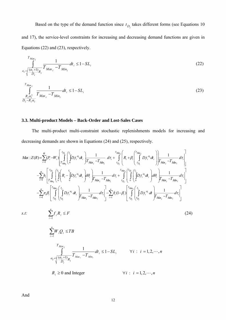
Based on the type of the demand function since iDt takes different forms (see Equations 10

and 17), the service-level constraints for increasing and decreasing demand functions are given in

Equations (22) and (23), respectively.

1 ( 1)

11i i

Max i

i iii ii

T

Max MinR

D

dt SLT T

(22)

2

11i i

Max i

i ii i

i i i

T

Max MinRD R

dt SLT T

(23)

3.3. Multi-product Models – Back-Order and Lost-Sales Cases

The multi-product multi-constraint stochastic replenishments models for increasing and

decreasing demands are shown in Equations (24) and (25), respectively.

0

0 0

1

1 1: ( ) ( )

1

i i

i

T T

i i i i i i i i i i i i

i i i i i i

D Max Maxi i i i

iD DMin i ii i ii

Di i i

Min ii

i

t t

T t tMax MaxMin Min

t t t

T Max M

nMax Z R P W D t dt d R D t dt d

T T T T

h R D t dt dT T

0 01

1

1 1ˆ (1 )

i

i i

T

i i i i i i

T T

i i i i i i i i i i i

Max Di i i

iD ii i

Max Maxi i i i

i iD D D Di ii i i i

n

i

t t

t Maxin Min

t t

t t t tMax MaxMin Min

d D t dt d dT T

D t dt d D t dt dT T T T

11

n

i

n

i

s.t: 1

n

i ii

f R F

(24)

1

n

i ii

W Q TB

1 ( 1)

11

i i

i iMax Min

Max i

ii

ii

T

RD

dt SLT T

: 1, 2, ,i i n

0 and IntegeriR : 1, 2, ,i i n

And

13

20

1

2

1

: ( ) ( )1

ii i

T i in

i i Ti

ii i i i

i i

Di i

Min i ii

Max Maxi i

D D i ii i

t t

Max Min

T

t t Max Min

Ddt d

T TtMax Z R P W

DR dt d

T Tt

20 0

1

20 0

2

1

1

1

ii i i i

T i i

ii

ii i i

i i

ii i i

i i

Di i i

Mini

Max Di i i

Di

Maxi i

D Di i

ni i

i i

i

t t t

T t t

t

T t

t t

Max Min

Max Min

Max

DR dt d d

T Tth

Ddt d d

T Tt

Ddt

T Tt

1

21

1ˆ (1 )

n

ii

ni

i i i ii i i

Maxi i

D Di i

i

i i

T t

t t

Min

Max Min

d

Ddt d

T Tt

s.t: 1

n

i ii

f R F

(25)

1

n

i ii

W Q TB

2

11i i

Max i

i ii i

i i i

T

Max MinRD R

dt SLT T

: 1, 2, ,i i n

0 and IntegeriR : 1, 2, ,i i n

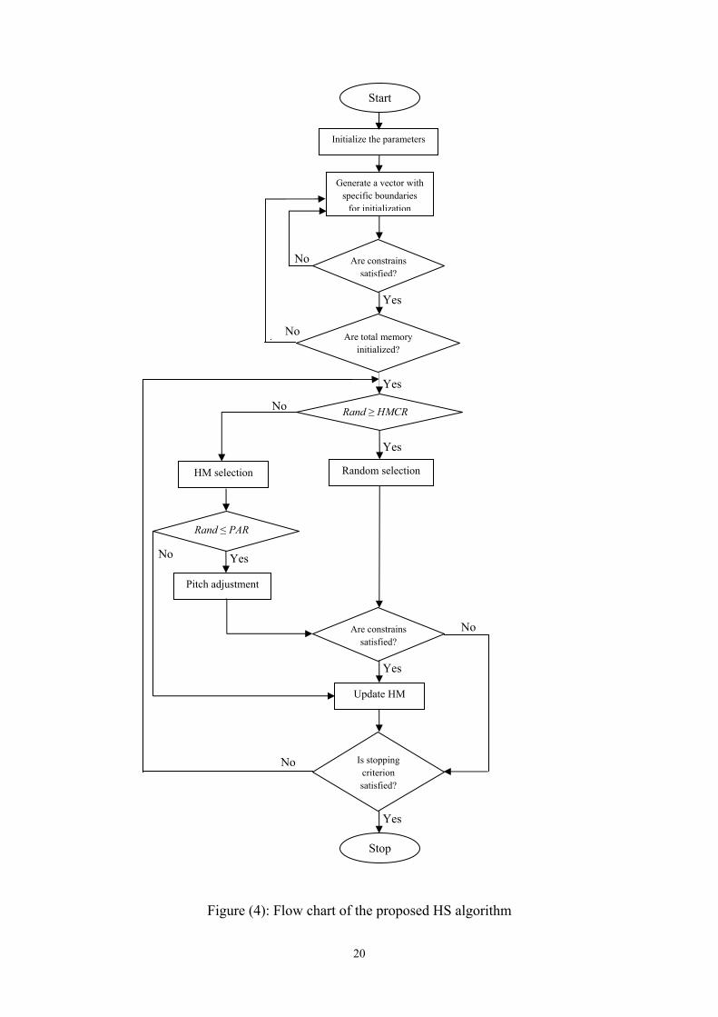
4. A Harmony Search Algorithm

Since the models in (24) and (25) are integer-nonlinear in nature, reaching an analytical

solution (if any) to the problem is difficult [19]. Hence, we need to employ a meta-heuristic search

algorithm to solve them.

14

4.1. Introduction to Harmony Search Algorithm

Recently, scientists mimicked nature to solve different kinds of complex optimization

problems called heuristic [20]. A meta-heuristic algorithm is a heuristic method that combines user-

given black-box procedures, usually heuristics themselves.

Lee and Geem [21] and Vasebi et al. [22] showed the harmony search (HS) algorithm

outperforms genetic algorithm (GA) [23] because of its multi-vector consideration and fast

calculation. One of the main advantages of HS versus GA is its simple implementation. Unlike GA,

that has genetic operators like crossover and mutation, the HS algorithm does not have these types

of operators for new generations. This causes an iteration to be faster in HS than that in GA.

Therefore, we employ an HS algorithm to solve the models under different criteria.

The HS algorithm inspired from the act of musician groups, was introduced in an analogy

with music improvisation process where musicians in an ensemble continue to polish their pitches

to obtain better harmony [24]. There is a similarity between musician groups and this algorithm.

According to the analogy of improvisation and optimization, fantastic harmony is considered as

global optimum, aesthetic standard is determined by the objective function, pitches of instruments

are desired values of the variables, and each practice is the same in each iteration.

The HS optimization method has been applied successfully to various engineering problems

such as satellite heat pipe design [25], vehicle routing [26], water network design [27, 28]. Mahdavi

et al. [29] described an improved harmony search (IHS) algorithm for solving optimization

problems.

Although HS algorithm has proven its ability of finding near global regions within a

reasonable amount of time, because of its needs to having large enough solution space to move and

optimize the solution vectors, it is comparatively inefficient in performing local search [21].

Fesanghari et al. [30] proposed a hybrid harmony search (HHS) algorithm to solve engineering

optimization problems with continuous design variables and employed a sequential quadratic

programming (SQP) model to speed up local search and improve precision of the HS solutions.

15

The HS optimization algorithm applied in this paper is performed by the following steps.

4.1 Initialization

The process of initialization has two parts; parameter initialization and HM initialization as

described below.

4.1.1 Parameter Initialization

The constant parameters of the HS algorithm include harmony memory size ( HMS ),

harmony memory considering rate ( HMCR ), pitch adjusting rate ( PAR ), number of decision

variables ( N ), and the maximum number of improvisations ( NI ).

The HMS is the number of simultaneous solution vectors in HM. Based on the frequently

used HMS values in other HS applications available in the literature [21, 25, 26, 27, 28] it seems

that using a small HMS is a good and logical choice with the added advantage of reducing space

requirements. Further, since HM resembles the short-term memory of a musician and since the

short-term memory of the human is known to be small, it is logical to use a small HMS . In this

paper, the numbers 10, 20 and 30 are chosen as different values of HMS .

The HMCR is the probability of choosing HM. Choosing a very small HMCR decreases the

algorithm efficiency and the HS algorithm behaves like a pure random search with less assistance

from the HM. Hence, it is generally better to use a large value for the HMCR (i.e. ≥ 0.9). In this

research 0.93, 0.95, and 0.99 have been used for HMCR .

The pitch adjustment is similar to the adjustment of each musical instrument in a jazz so that

pleasing harmony can be achieved. The efficiency of the algorithm lies within this pitch adjustment

because of the fact that once a feasible design is determined, it searches new solution vectors

around this design vector rather than generating arbitrary design vectors. Thus, this operation

prevents stagnation and improves the HS for diversity with a greater chance of reaching the global

16

optimum. The PAR is the probability of pitch adjustment where its typical value ranges from 0.3 to

0.99. In this research, 0.3, 0.7, and 0.9 have been utilized for PAR .

The value of N , the number of variables for optimization, is fully depended on the

characteristics of the problem. For the proposed HS algorithm of this research N has been chosen

to be 8.

Finally, NI is the maximum number of iterations the objective function is evaluated. In this

research, 100, 500, and 1000 are chosen as different iteration numbers.

4.1.2. Harmony Memory Initialization

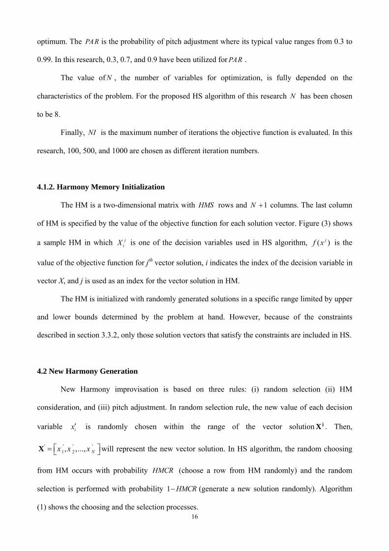
The HM is a two-dimensional matrix with HMS rows and 1N columns. The last column

of HM is specified by the value of the objective function for each solution vector. Figure (3) shows

a sample HM in which jiX is one of the decision variables used in HS algorithm, ( )jf x is the

value of the objective function for jth vector solution, i indicates the index of the decision variable in

vector X, and j is used as an index for the vector solution in HM.

The HM is initialized with randomly generated solutions in a specific range limited by upper

and lower bounds determined by the problem at hand. However, because of the constraints

described in section 3.3.2, only those solution vectors that satisfy the constraints are included in HS.

4.2 New Harmony Generation

New Harmony improvisation is based on three rules: (i) random selection (ii) HM

consideration, and (iii) pitch adjustment. In random selection rule, the new value of each decision

variable ix is randomly chosen within the range of the vector solution jX . Then,

' ' ' '1 2, ,..., Nx x x X will represent the new vector solution. In HS algorithm, the random choosing

from HM occurs with probability HMCR (choose a row from HM randomly) and the random

selection is performed with probability 1 HMCR (generate a new solution randomly). Algorithm

(1) shows the choosing and the selection processes.

17

Memory Columns

Figure (3): The sample harmony memory

Algorithm (1): Choosing and selection processes of HM algorithm

For 1:i N

If ; ~ (0,1)i iRand HMCR Rand Uni

1 2[ , , , ]i i iHMS

i ix x x x x

Else

generate a new one within the allowable rangeix

End If

End For

In pitch adjustment, every component obtained by the memory consideration, is examined to

determine whether it should be pitch adjusted or not. The value of the decision variable is changed

by Equation (26) with probability of PAR , and this value is kept without any change with

probability1 PAR . In Equation (26), the BW stands for bandwidth, showing the change for pitch

adjustment, and rand is a uniform random number between 0 and 1. In this equation, for each

component of the vector the selection for increasing or decreasing are carried out with the same

probability.

( )( ) ; ~ 0,1rand BW rand U ' 'X X (26)

11X 1

2X .. . 1NX 1( )f x

21X 2

2X .. . 2NX 2( )f x

. .

. .

. . 1

1HMSX 1

2HMSX .. . 1HMS

NX 1( )HMSf x

1HMSX2

HMSX .. . HMSNX ( )HMSf x

HM

S

18

4.3. Harmony Memory Update

The constraint handling part of the algorithm is performed before the HM update. There are

three constraints in each of the proposed models. The constraint handling part checks whether these

constraints are satisfied or not. If they are satisfied, then the HM update action occurs. In this stage,

by the objective function evaluation, if the new fitness value is better than the worst case in the HM,

the worst harmony vector is replaced by the new solution vector. The remaining steps of the HS

algorithm are performed after the HM update.

4.4. Stopping Criterion

The last step in a HS method is to check if the algorithm has found a solution that is good

enough to meet the user’s expectations. Stopping criteria is a set of conditions such that when

satisfied a good solution is obtained. Different criteria used in literature are: 1) stopping the

algorithm after a specific number of iterations, 2) no improvement in the objective function, and 3)

reaching a specific value of the objective function. In this research, we stop when a predetermined

number of consecutive iteration is reached. The number of sequential iterations depends on the

specified problem and the expectations of the user. In summary, the steps involved in the HS

algorithm used in this research are:

1. Initialize both the parameters and the HM of the HS algorithm.

2. Make a new vector 'X . For each component ix :

With probability HMCR pick the component from memory,

With probability 1 HMCR generate a new vector in the allowed range.

3. Pitch adjustment: For each component ix :

With probability PAR , a small change is made to ix .

With probability 1 PAR do nothing.

4. If X is better than the worst jX in the memory, then replace jX by X .

5. Go to step two until a maximum number of iterations has been reached.

19

The detailed flow chart of the proposed HS algorithm is shown in Figure (4).

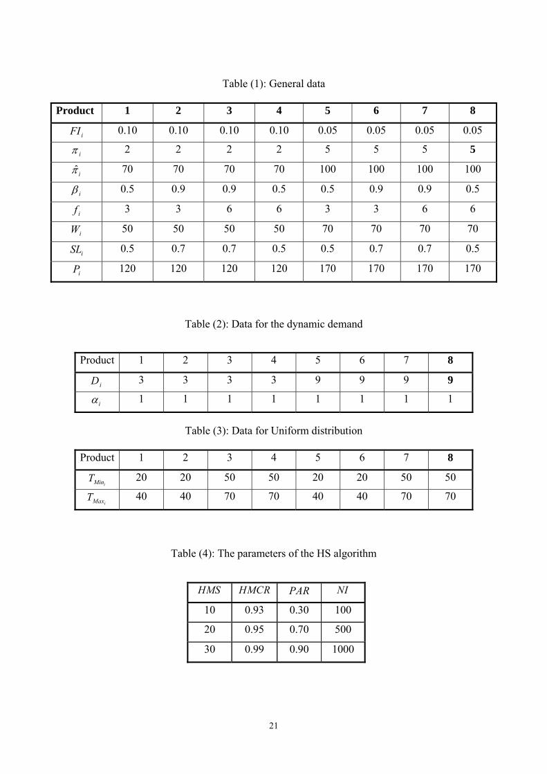
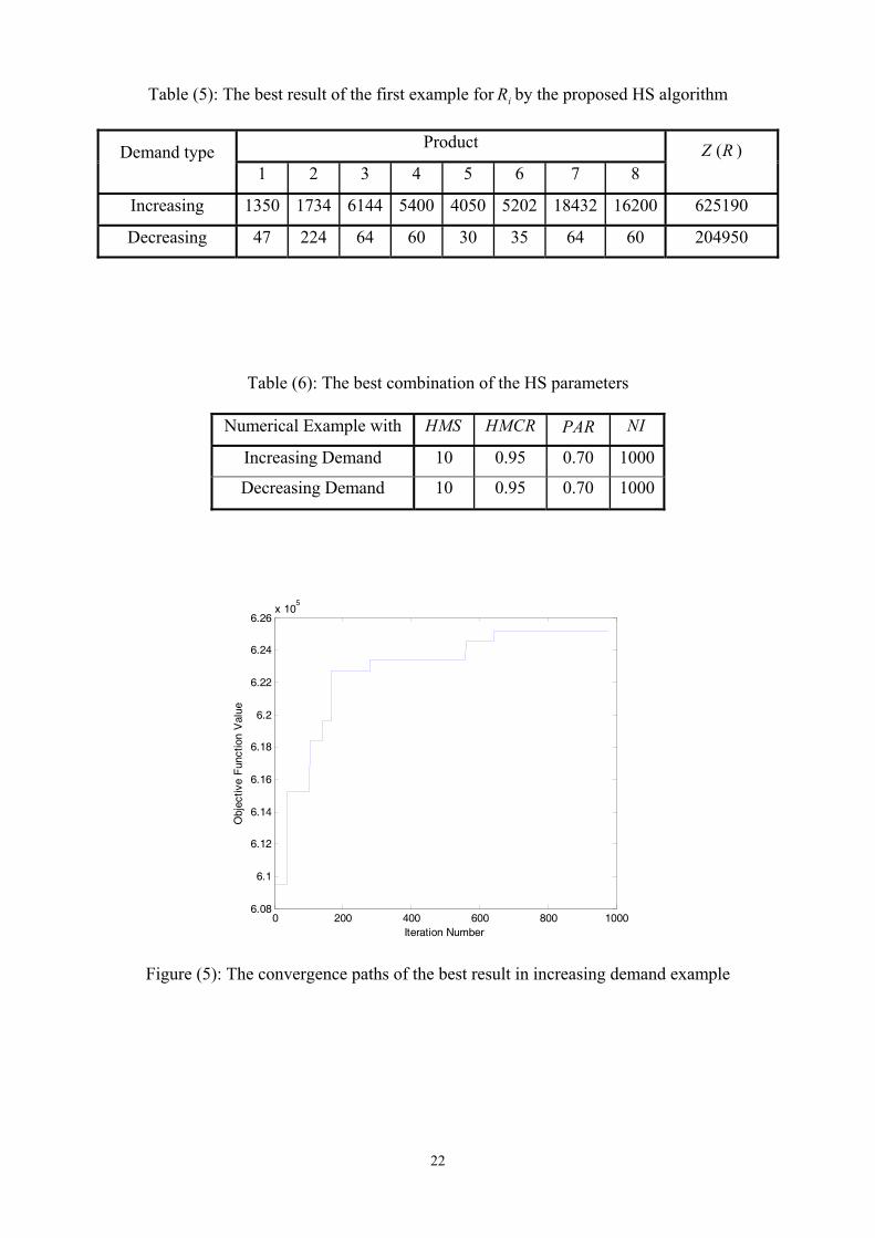
5. Numerical Examples

In this section, three numerical examples of different sizes (small, medium, and large) are

used to demonstrate the application and the performances of the proposed methodology. For the

first example consider a multiproduct inventory control problem with eight products where its

general data is given in Table (1). Table (2) and (3) show the parameters of the demand functions

and the uniform distribution of the time between replenishments, respectively. For an increasing

demand, the total available warehouse space and the total budget are F =320000 and

TB =4000000, respectively. These values for decreasing demand are F =2500 and TB =30000,

respectively. Table (4) shows different values of the HS parameters used to obtain the solution. In

this research, all the possible combinations of the HS parameters given in Table (4) are employed

and using the max (max) strategy, the best combination of the parameters has been selected. Table

(5) shows the best result for the increasing and decreasing demand. The best combination of the HS

algorithm is shown in Tables (6). Furthermore, the convergence paths of the best result of the

objective function values in different generations of the increasing and decreasing demand are

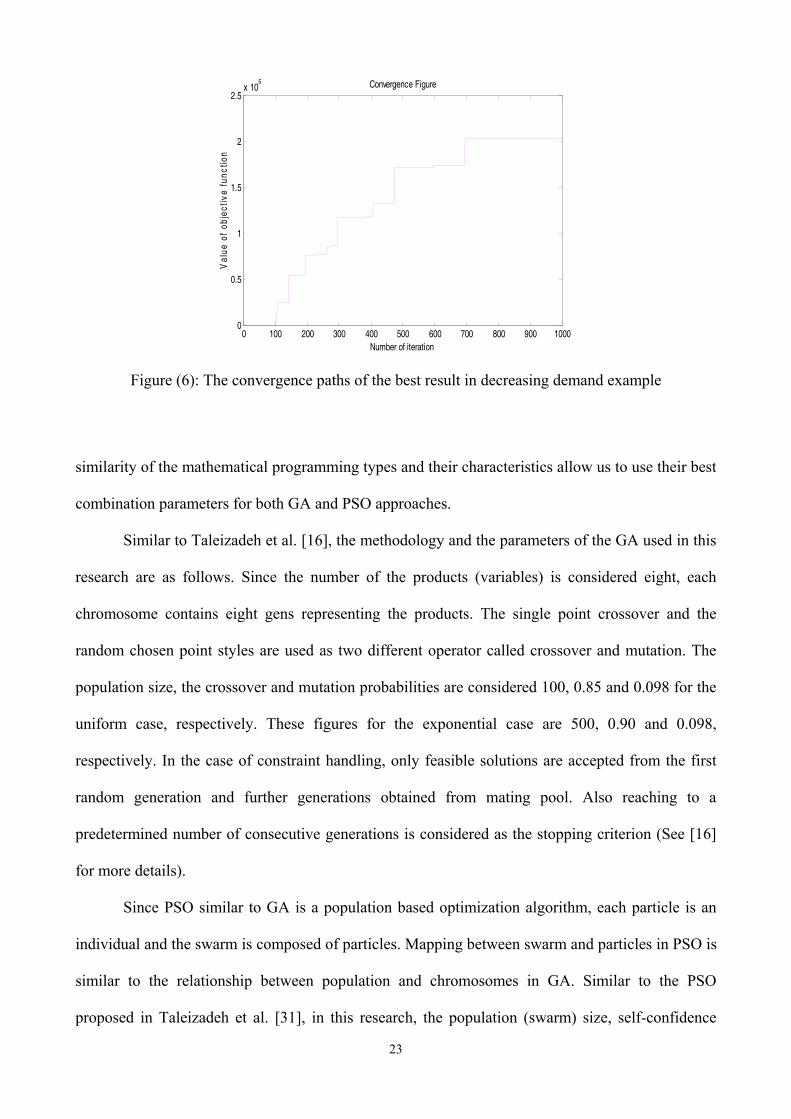
shown in Figures (5) and (6), respectively.

In order to show that the proposed HS algorithm is an effective means for solving the

complicated inventory model of this research, both the genetic algorithm of Taleizadeh et al. [16]

and the particle swarm optimization (PSO) method of Taleizadeh et al. [31] are also employed to

solve the given numerical example. In fact, since HS is a population based meta-heuristic algorithm,

this algorithm should be compared with other kinds of population based meta-heuristic algorithms

such as Genetic Algorithm (GA) and Particle Swarm Optimization (PSO) to validate and compare

the efficiency of the proposed HS method. Moreover, in the case of tuning the GA and the PSO

parameters, we have used the experimental case of Taleizadeh et al. [16 and 31] in which the best

combination of the parameters that can be used in the model of this paper are chosen. Indeed the

20

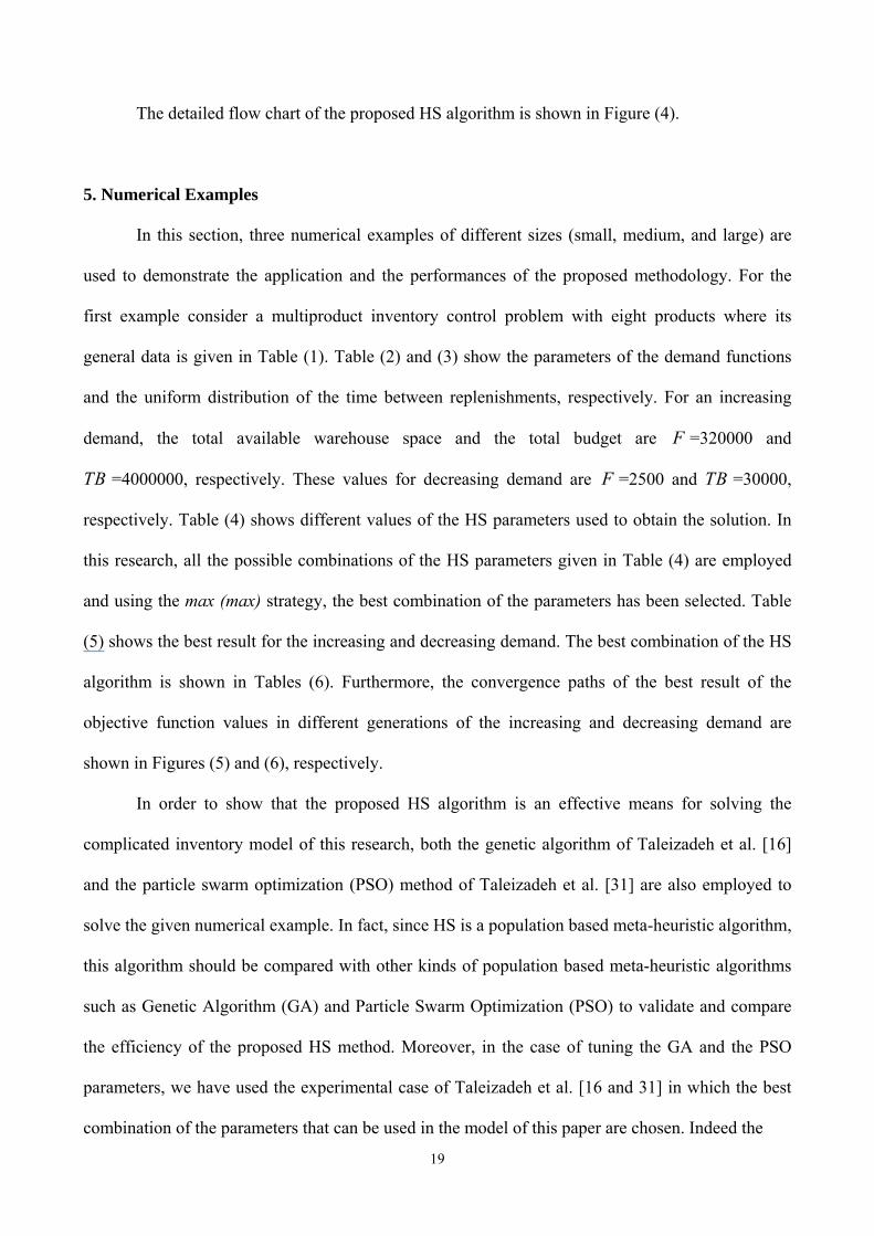
Figure (4): Flow chart of the proposed HS algorithm

Yes

No

Yes

No

Yes

No

Yes

Yes

No

Yes

No

Generate a vector with specific boundaries

for initialization

Start

Are constrains satisfied?

Are total memory initialized?

Rand ≥ HMCR

HM selection

Rand ≤ PAR

Pitch adjustment

Are constrains satisfied?

Update HM

Random selection

Is stopping criterion satisfied?

Stop

Initialize the parameters

No

21

Table (1): General data

8 7 6 5 4 3 2 1 Product

0.05 0.05 0.05 0.05 0.10 0.10 0.10 0.10 iFI

5 5 5 5 2 2 2 2 i

100 100 100 100 70 70 70 70 ˆi

0.5 0.9 0.9 0.5 0.5 0.9 0.9 0.5 i

6 6 3 3 6 6 3 3 if

70 70 70 70 50 50 50 50 iW

0.5 0.7 0.7 0.5 0.5 0.7 0.7 0.5 iSL

170 170 170 170 120 120 120 120 iP

Table (2): Data for the dynamic demand

8 7 6 5 4 3 2 1 Product

9 9 9 9 3 3 3 3 iD

1 1 1 1 1 1 1 1 i

Table (3): Data for Uniform distribution

8 7 6 5 4 3 2 1 Product

50 50 20 20 50 50 20 20 iMinT

70 70 40 40 70 70 40 40 iMaxT

Table (4): The parameters of the HS algorithm

NIPAR HMCRHMS

100 0.30 0.93 10

500 0.70 0.95 20

1000 0.90 0.99 30

22

Table (5): The best result of the first example for iR by the proposed HS algorithm

( )Z R Product Demand type

8 7 6 5 4 3 2 1

625190 16200 1843252024050540061441734 1350 Increasing

204950 60 64 35 30 60 64 224 47 Decreasing

Table (6): The best combination of the HS parameters

NI PAR HMCRHMSNumerical Example with

1000 0.70 0.95 10 Increasing Demand

1000 0.70 0.95 10 Decreasing Demand

0 200 400 600 800 10006.08

6.1

6.12

6.14

6.16

6.18

6.2

6.22

6.24

6.26x 10

5

Iteration Number

Obj

ectiv

e F

unct

ion

Val

ue

Figure (5): The convergence paths of the best result in increasing demand example

23

0 100 200 300 400 500 600 700 800 900 10000

0.5

1

1.5

2

2.5x 10

5 Convergence Figure

Number of iteration

Val

ue o

f ob

ject

ive

func

tion

Figure (6): The convergence paths of the best result in decreasing demand example

similarity of the mathematical programming types and their characteristics allow us to use their best

combination parameters for both GA and PSO approaches.

Similar to Taleizadeh et al. [16], the methodology and the parameters of the GA used in this

research are as follows. Since the number of the products (variables) is considered eight, each

chromosome contains eight gens representing the products. The single point crossover and the

random chosen point styles are used as two different operator called crossover and mutation. The

population size, the crossover and mutation probabilities are considered 100, 0.85 and 0.098 for the

uniform case, respectively. These figures for the exponential case are 500, 0.90 and 0.098,

respectively. In the case of constraint handling, only feasible solutions are accepted from the first

random generation and further generations obtained from mating pool. Also reaching to a

predetermined number of consecutive generations is considered as the stopping criterion (See [16]

for more details).

Since PSO similar to GA is a population based optimization algorithm, each particle is an

individual and the swarm is composed of particles. Mapping between swarm and particles in PSO is

similar to the relationship between population and chromosomes in GA. Similar to the PSO

proposed in Taleizadeh et al. [31], in this research, the population (swarm) size, self-confidence

24

factor, and swarm confidence factor, are considered 100, 2 and 2, for both decreasing and

increasing cases, respectively. The first swam is generated randomly between the predefined lower

and upper values chosen for each variable which should satisfy the constraints. After each

generation the solution should be checked for the constraints. Infeasible solutions are not accepted.

Furthermore, reaching a predetermined number of consecutive generations is also considered as the

stopping criterion (See [31] for more details).

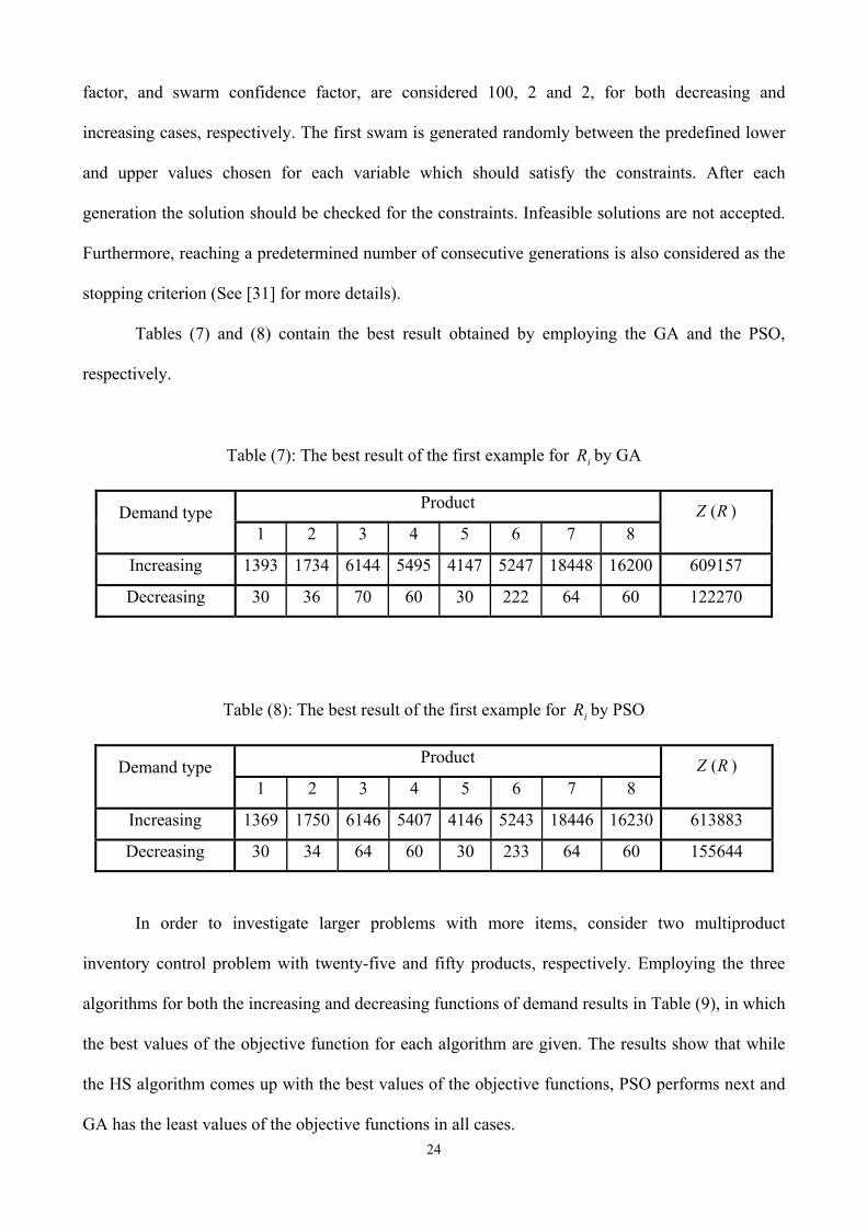
Tables (7) and (8) contain the best result obtained by employing the GA and the PSO,

respectively.

Table (7): The best result of the first example for iR by GA

( )Z R Product Demand type

8 7 6 5 4 3 2 1

609157 16200 1844852474147549561441734 1393 Increasing

122270 60 64 222 30 60 70 36 30 Decreasing

Table (8): The best result of the first example for iR by PSO

( )Z R Product Demand type

8 7 6 5 4 3 2 1

613883 16230 1844652434146540761461750 1369 Increasing

155644 60 64 233 30 60 64 34 30 Decreasing

In order to investigate larger problems with more items, consider two multiproduct

inventory control problem with twenty-five and fifty products, respectively. Employing the three

algorithms for both the increasing and decreasing functions of demand results in Table (9), in which

the best values of the objective function for each algorithm are given. The results show that while

the HS algorithm comes up with the best values of the objective functions, PSO performs next and

GA has the least values of the objective functions in all cases.

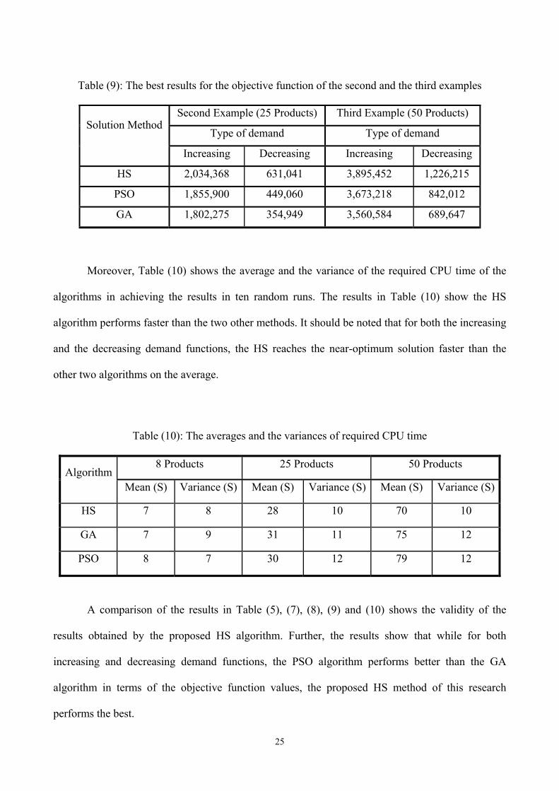
25

Table (9): The best results for the objective function of the second and the third examples

Third Example (50 Products) Second Example (25 Products) Solution Method

Type of demand Type of demand

Decreasing Increasing Decreasing Increasing

1,226,215 3,895,452 631,041 2,034,368 HS

842,012 3,673,218 449,060 1,855,900 PSO

689,647 3,560,584 354,949 1,802,275 GA

Moreover, Table (10) shows the average and the variance of the required CPU time of the

algorithms in achieving the results in ten random runs. The results in Table (10) show the HS

algorithm performs faster than the two other methods. It should be noted that for both the increasing

and the decreasing demand functions, the HS reaches the near-optimum solution faster than the

other two algorithms on the average.

Table (10): The averages and the variances of required CPU time

Algorithm8 Products 25 Products 50 Products

Mean (S) Variance (S) Mean (S) Variance (S) Mean (S) Variance (S)

HS 7 8 28 10 70 10

GA 7 9 31 11 75 12

PSO 8 7 30 12 79 12

A comparison of the results in Table (5), (7), (8), (9) and (10) shows the validity of the

results obtained by the proposed HS algorithm. Further, the results show that while for both

increasing and decreasing demand functions, the PSO algorithm performs better than the GA

algorithm in terms of the objective function values, the proposed HS method of this research

performs the best.

26

6. Conclusion and Recommendations for Future Research

In this paper, a stochastic replenishment intervals multiproduct inventory model with

dynamic demand was investigated. Two mathematical modeling for two cases of increasing and

decreasing demand have been developed and shown to be integer-nonlinear programming problems.

Then, a meta-heuristic algorithm (harmony search) has been proposed to solve the integer non-

linear problems with different sizes (small, medium, large) and its performance was compared to

the ones of a GA and a PSO. The results of the comparison study showed that for the problems

investigated the proposed HS algorithm performs better than both the GA and PSO in terms of the

objective function values. Moreover, it requires the least CPU time to solve the problems on the

average.

For future work, some parameters of the model may be considered fuzzy or some other

probability density functions may be considered for the time between replenishments. Moreover,

demands can be either fuzzy or random variables.

8. References

[1]. F. Harris, Operations and Cost, Factory Management Service. A.W. Shaw Co., Chicago,

1915.

[2]. J.K. Dey, S. Kar, A.K. Bhuina, M. Maiti, Inventory of differential items selling from two

shops under a single management with periodically increasing demand over a finite time-

horizon, Int. J. Production Economics 100 (2006): 335–347.

[3]. E.A. Silver, H.C. Meal, A heuristic for selecting lot size quantities for the case of a

deterministic time varying demand rate and discrete opportunities for replenishment.

Production and Inventory Management 14 (1973): 64–74.

[4]. J.K. Dey, S. Kar, M. Maiti, An interactive method for inventory control with fuzzy lead-

time and dynamic demand, European Journal of Operational Research 167 (2005): 381–

397.

27

[5]. J.K. Dey, S.K. Mondal, M. Maiti, Two storage inventory problem with dynamic demand

and interval valued lead-time over finite time horizon under inflation and time-value of

money, European Journal of Operational Research 185 (2008) 170–194.

[6]. W.A. Doneldson, Inventory replenishment policy for a linear trend in demand – An

analytic Solution, Operational Research Quarterly 28 (1977): 663–670.

[7]. H.J. Change, C.Y. Dye, An EOQ model for deteriorating items with time-varying demand

and partial backlogging, Journal of the Operational Research Society 50 (1999): 1176–

1182.

[8]. S.K. Goyal, D. Mortin, F. Nebebe, The finite time horizon trended inventory

replenishment problem with shortages, Journal of the Operational Research Society 43

(1992): 1173–1178.

[9]. L.L. Gao, N. Altay, E. Powell Robinson, A comparative study of modeling and solution

approaches for the coordinated lot-size problem with dynamic demand, Mathematical and

Computer Modeling 47 (2008): 1254–1263.

[10]. D. Kim, V.A. Mabert, Cycle scheduling for discrete shipping and dynamic demands,

Computers & Industrial Engineering 38 (2000): 215–233.

[11]. A. Martel, A. Gascon, Dynamic lot-sizing with price changes and price-dependent

holding costs, European Journal of Operational Research, 111 (1998): 114-128.

[12]. J. Hu, C.L. Munson, Dynamic demand lot-sizing rules for incremental quantity

discounts, Journal of Operational research Society, 53 (2002): 855-863.

[13]. L. Wang, F. Dang, X. Sun, Game analysis for supply chain of perishable products

under dynamic demand, Huazhong Keji Daxue Xuebao (Ziran Kexue Ban)/Journal of

Huazhong University of Science and Technology (Natural Science Edition), 37 (2009):

79-81.

28

[14]. D.W. Pentico, Assortment problem with dynamic deterministic demands and

stationary stocking-substitution policies, Proceedings - Annual Meeting of the Decision

Sciences Institute, 2 (1997): 936-938.

[15]. W.J. Hopp, X. Xu, A static approximation for dynamic demand substitution with

applications in a competitive market, Operations Research, 56 (2008): 630-645.

[16]. A.A. Taleizadeh, M.B. Aryanezhad, and S.T.A. Niaki, Optimizing multi-product

multi-constraint inventory control systems with stochastic replenishment, Journal of

Applied Sciences 8(2008): 1228-1234.

[17]. A.A. Taleizadeh, S.T.A. Niaki, and M.B. Aryanezhad, Multi-product multi-

constraint inventory control systems with stochastic replenishment and discount under

fuzzy purchasing price and holding costs, American Journal of Applied Sciences 6(2009):

1-12.

[18]. B. Liu, Uncertainty Theory: An Introduction to Its Axiomatic Foundations, Springer,

Berlin, Germany, 2004.

[19]. M. Gen, Genetic Algorithm and Engineering Design, John Wiley & Sons, New

York, NY, U.S.A., 1997.

[20]. M. Dorigo and T. Stutzle, Ant Colony Optimization, MIT Press, Cambridge, MA,

USA, 2004.

[21]. K.S. Lee and Z.W. Geem, A new structural optimization method based on the

harmony search algorithm, Comput. Struct. 82(2004): 781–798.

[22]. A. Vasebi, M. Fesanghary, S.M.T. Bathaee, Combined heat and power economic

dispatch by harmony search algorithm, International Journal of Electrical Power and

Energy Systems 29(2007): 713-719.

[23]. D.E. Goldberg, Genetic Algorithms in Search Optimization and Machine Learning,

Addision-Wesley, Boston, MA, U.S.A., 1989

29

[24]. Z.W. Geem, J.H. Kim, and G.V. Loganathan, A new heuristic optimization

algorithm: Harmony search, Simulation 76(2001): 60–68.

[25]. Z.W. Geem and H. Hwangbo, Application of harmony search to multi-objective

optimization for satellite heat pipe design, UKC AST-1.1 (2006).

[26]. Z.W. Geem, K.S. Lee, and T. Park, Application of harmony search to vehicle

routing, American Journal of Applied Sciences 2(2005): 1552–1557.

[27]. Z.W. Geem, J.H. Kim, and G.V. Loganathan, Harmony search optimization:

Application to pipe network design, International Journal of Modeling and Simulation

22(2002): 125-133.

[28]. Z.W. Geem, Optimal cost design of water distribution networks using harmony

search, Engineering Optimization 38(2006): 259–280.

[29]. M. Mahdavi, M. Fesanghari, and E. Damangir, An improved harmony search

algorithm for solving optimization problem, Applied Mathematics and Computations

188(2007): 1567-1579.

[30]. M. Fesanghari, M. Mahdavi, M. Minari-Jolandan and Y. Alizadeh, Hybridizing

harmony search algorithm with sequential quadratic programming for engineering

optimization problems, Computer Methods in Applied Mechanics and Engineering

197(2008): 3080-3091.

[31]. A.A. Taleizadeh, S.T.A. Niaki, N. Shafii, and R. Ghavamizadeh-Meibodi,

Jabbarzadeh A., A particle swarm optimization approach for constraint joint single buyer-

single vendor inventory problem with changeable lead-time and (r,Q) policy in supply

chain, International Journal of Advanced Manufacturing Technology , 51 (2010): 1209-

1223.