This article was downloaded by: [McGill University Library]On: 24 July 2014, At: 08:22Publisher: Taylor & FrancisInforma Ltd Registered in England and Wales Registered Number: 1072954 Registeredoffice: Mortimer House, 37-41 Mortimer Street, London W1T 3JH, UK

Click for updates

Engineering OptimizationPublication details, including instructions for authors andsubscription information:http://www.tandfonline.com/loi/geno20

Stochastic production phase designfor an open pit mining complex withmultiple processing streamsMohammad Waqar Ali Asada, Roussos Dimitrakopoulosb & Jeroenvan Eldertc

a Department of Mining Engineering, Western Australian School ofMines, Curtin University, Kalgoorlie, Australiab COSMO Stochastic Mine Planning Laboratory, Department ofMining and Materials Engineering, McGill University, FDA Building,3450 University Street, Montreal, Quebec, Canada H3A 2A7c Department of Mining and Materials Engineering, McGillUniversity, FDA Building, 3450 University Street, Montreal,Quebec, Canada H3A 2A7Published online: 19 Sep 2013.

To cite this article: Mohammad Waqar Ali Asad, Roussos Dimitrakopoulos & Jeroen van Eldert(2014) Stochastic production phase design for an open pit mining complex with multiple processingstreams, Engineering Optimization, 46:8, 1139-1152, DOI: 10.1080/0305215X.2013.819094

To link to this article: http://dx.doi.org/10.1080/0305215X.2013.819094

PLEASE SCROLL DOWN FOR ARTICLE

Taylor & Francis makes every effort to ensure the accuracy of all the information (the“Content”) contained in the publications on our platform. However, Taylor & Francis,our agents, and our licensors make no representations or warranties whatsoever as tothe accuracy, completeness, or suitability for any purpose of the Content. Any opinionsand views expressed in this publication are the opinions and views of the authors,and are not the views of or endorsed by Taylor & Francis. The accuracy of the Contentshould not be relied upon and should be independently verified with primary sourcesof information. Taylor and Francis shall not be liable for any losses, actions, claims,proceedings, demands, costs, expenses, damages, and other liabilities whatsoever orhowsoever caused arising directly or indirectly in connection with, in relation to or arisingout of the use of the Content.

This article may be used for research, teaching, and private study purposes. Anysubstantial or systematic reproduction, redistribution, reselling, loan, sub-licensing,

systematic supply, or distribution in any form to anyone is expressly forbidden. Terms &Conditions of access and use can be found at http://www.tandfonline.com/page/terms-and-conditions

Dow

nloa

ded

by [

McG

ill U

nive

rsity

Lib

rary

] at

08:

22 2

4 Ju

ly 2

014

Engineering Optimization, 2014Vol. 46, No. 8, 1139–1152, http://dx.doi.org/10.1080/0305215X.2013.819094

Stochastic production phase design for an open pit miningcomplex with multiple processing streams

Mohammad Waqar Ali Asada*, Roussos Dimitrakopoulosb and Jeroen van Eldertc

aDepartment of Mining Engineering, Western Australian School of Mines, Curtin University, Kalgoorlie,Australia; bCOSMO Stochastic Mine Planning Laboratory, Department of Mining and Materials

Engineering, McGill University, FDA Building, 3450 University Street, Montreal, Quebec, CanadaH3A 2A7 cDepartment of Mining and Materials Engineering, McGill University, FDA Building, 3450

University Street, Montreal, Quebec, Canada H3A 2A7

(Received 14 January 2013; accepted 11 June 2013)

In a mining complex, the mine is a source of supply of valuable material (ore) to a number of processesthat convert the raw ore to a saleable product or a metal concentrate for production of the refined metal. Inthis context, expected variation in metal content throughout the extent of the orebody defines the inherentuncertainty in the supply of ore, which impacts the subsequent ore and metal production targets. Traditionaloptimization methods for designing production phases and ultimate pit limit of an open pit mine not onlyignore the uncertainty in metal content, but, in addition, commonly assume that the mine delivers ore to asingle processing facility.A stochastic network flow approach is proposed that jointly integrates uncertaintyin supply of ore and multiple ore destinations into the development of production phase design and ultimatepit limit. An application at a copper mine demonstrates the intricacies of the new approach. The case studyshows a 14% higher discounted cash flow when compared to the traditional approach.

Keywords: stochastic optimization; maximum flow algorithm; mining engineering applications; produc-tion planning

1. Introduction

An open pit mining complex constitutes multiple open pits, processing streams and products. Atypical open pit produces materials of various categories. This material is fed to the appropriateprocessing streams for recovering metal as a valuable product. Owing to the large scale of open pitmining operations, the optimal long-term planning in the context of production phase design andproduction scheduling is a complex technical challenge. Long-term planning of a typical openpit mining operation involves three sequential steps (Hustrulid and Kuchta 2006): (i) developinga three-dimensional orebody model that consists of an accumulation of mining units (blocks)with their available metal content (quality) and tonnage (quantity); (ii) accomplishing productionphase design, i.e. a phase-wise sequence of extraction that reaches the ultimate pit limit or overallextent of extraction; and (iii) scheduling production of mining blocks within each phase subjectto the physical mining and processing constraints. The outcome of the first step is the economicvalue of a mining block, which is calculated using available metal content, tonnage, and economicparameters such as metal price, marketing or sales cost, mining cost, processing cost and recovery.

*Corresponding author. Email: waqar.asad@curtin.edu.au

© 2013 Taylor & Francis

Dow

nloa

ded

by [

McG

ill U

nive

rsity

Lib

rary

] at

08:

22 2

4 Ju

ly 2

014

1140 M.W.A. Asad et al.

The mining blocks are then classified as ore and waste blocks based on the positive and negativeeconomic values, respectively. Depending upon the geometry of the orebody and the size of miningblocks, a typical orebody model consists of millions of blocks. The input to the second and thirdsteps is the economic value of these blocks (Asad 2011). The objective of these steps is to maximizethe net present value (NPV) over the life of the operation (Ramazan 2007). While a mixed-integerprogramming (MIP) based production scheduling model combining steps two and three promisesan optimum solution to the long-term planning problem, the size of MIP models—due to theexistence of millions of blocks or binary variables—limits the solution strategies to heuristicsthat may lead to suboptimal solutions (Denby et al. 1998; Caccetta and Hill 2003). Consequently,it is an established practice to divide the long-term planning problem into two sub-problemsdeclared in steps (ii) and (iii), where the second step identifies the mining blocks included in theultimate pit limit, thereby reducing the size of the MIP based production scheduling model instep three (Lerchs and Grossmann 1965; Tachefine and Soumis 1997; Whittle 1998; Hochbaum2001; Hustrulid and Kuchta 2006; Albor and Dimitrakopoulos 2010). The work presented hereinaddresses the second step and develops production phase design and ultimate pit limit.

The development of production phase design and ultimate pit limit is possible through con-ventional (deterministic) or stochastic approaches. The conventional optimization approaches donot account for geological uncertainty, more specifically, uncertainty in available metal content,material types, and/or metal recoveries. The underlying assumption in conventional models is thatthe inputs are perfectly known. Consequently, these models cannot handle input uncertainty andutilize an estimated average type orebody model containing single or constant economic valuefor a particular mining block (Dowd 1994; Dimitrakopoulos 2011). However, in the presenceof geological and/or financial uncertainty, the implications of economic decisions suggested inconventional optimization studies may lead to the closure of capital intensive mining projects(Dimitrakopoulos and Abdel Sabour 2007; Godoy and Dimitrakopoulos 2011).

Stochastic approaches, on the other hand, honour geological and/or economic parameters uncer-tainty. Accordingly, stochastic optimization models utilize a set of equally probable simulatedorebody and/or economic parameter realizations as an input. Therefore, for a particular miningblock, a set of equally probable economic values are utilized in the optimization process, givingan opportunity to quantify and manage the risk of wrongly identifying a waste block as an oreblock at the time of extraction (Ramazan and Dimitrakopoulos 2013). However, the detrimentaleffects of geological risk to mining projects have been acknowledged and documented, and thisbecomes a driving force for the majority of stochastic optimization models to focus exclusivelyon geological uncertainty. For instance, Baker and Giacomo (1998) demonstrated that out of 48mining projects in Australasia, 9 realized reserves less than 20% originally expected and 13 over20% more reserves than forecasted; with the vast majority of inconsistencies coming from poorunderstanding and description of the orebody being mined. For Canada and the USA, Vallee(2000) referred to a World Bank survey showing that 73% of mining projects were closed prema-turely due to problems in their ore reserve estimates, and led to severe losses in capital investment.Recognizing these important facts, Goodfellow and Dimitrakopoulos (2013) proposed a simu-lated annealing based stochastic model for phase design under uncertainty in metal content andmaterial types considering multiple ore processing destinations. While the heuristic model pro-poses a computationally efficient method, it is restricted to modifying or improving an existingphase design (conventional or stochastic) incorporating uncertainty in metal content and materialtypes. Montiel and Dimitrakopoulos (2013) account for geological uncertainty in terms of metalcontent and material types, as well as multiple processes; however, the simulated annealing basedmodel develops the production schedule rather than solving the phase design and ultimate pit limitproblem. Alternatively, a stochastic network flow approach is proposed that focuses on the phasedesign and ultimate pit limit problem under geological uncertainty in terms of metal content,material types, and metal recoveries associated with multiple processing facilities.

Dow

nloa

ded

by [

McG

ill U

nive

rsity

Lib

rary

] at

08:

22 2

4 Ju

ly 2

014

Engineering Optimization 1141

A directed graph describes the production phase design and ultimate pit limit problem (Johnson1968; Picard 1976). However, the structure of the graph in a stochastic framework is differentfrom the graph representing a conventional framework. An input in terms of a set of equallyprobable simulated orebody realizations (Goovaerts 1997; Horta and Amilcar 2010; Boucher andDimitrakopoulos 2012; Machuca-Mory and Deutsch 2013) as well as the number of ore processingstreams in the open pit mining complex dictate the difference in the structure of the graph.Meagher et al. (2010) as well as Asad and Dimitrakopoulos (2013) acknowledged the differencein structure of the graph between conventional and stochastic frameworks. While Meagher et al.(2010) demonstrated the theoretical background of the open pit mine design under uncertainsupply and demand, Asad and Dimitrakopoulos (2013) utilized the Lagrangian relaxation of thepit (mine) production capacity constraint and presented an implementation of the maximum flowalgorithm for production phase design under economic and geological uncertainties. However,both studies are lacking in their application to an open pit mining operation with multiple oreprocessing options.

In this article, the stochastic optimization model given in Asad and Dimitrakopoulos (2013)becomes a basis for the proposed method, such that the maximum flow algorithm solves a graphrepresenting the stochastic framework that jointly accounts for multiple equally probable orebodyrealizations and ore processing streams. Additionally, as opposed to utilizing the Lagrangianrelaxation of the mine capacity constraint as in Asad and Dimitrakopoulos (2013), the Lagrangianrelaxation of processing capacity constraints has been integrated to develop successive productionphases leading to the ultimate pit limit design. This article contributes a comparison of the proposedstochastic and conventional approaches through an application at a copper mine. More specifically,the article (i) describes the structure of the graph representing the stochastic framework, (ii)develops a strategy for designing production phases and ultimate pit limit by solving this graphthrough the maximum flow algorithm, and (iii) compares the production phase design and ultimatepit limit in the stochastic and conventional approaches.

2. Phase design and ultimate pit limit

Generally, if vi represents the economic value of a mining block i, then a directed graph, G =(N , A), best describes the phase design and ultimate pit limit problem. Where a mining block i isrepresented as a node in the set of nodes N , and A is the set of arcs from node i to i′ translating theextraction precedence of a set of successors (i′ ∈ ξi) over node i. The mathematical formulationof this problem is given as (Tachefine and Soumis 1997; Hochbaum and Chen 2000):

max∑i∈N

vixi (1)

xi − xi′ � 0, i′ ∈ ξi, i ∈ N (2)

xi ∈ {0, 1}, i ∈ N . (3)

The solution to this problem lies in finding the maximum closure on the graph, i.e. maximizingEquation (1) for a set N ′ ⊆ N containing all predecessor nodes corresponding to the maximumvalue nodes. Equation (2) identifies the precedence arcs on the graph and the binary variable xi is 1if block i is inside the phase or pit (or closure), and 0 otherwise. However, owing to the geologicaluncertainty, a number of equally probable economic values are associated with a particular miningblock, requiring a different framework to create and solve the graph.

More specifically, the production phase design and ultimate pit limit considering the uncertaintyin grade, tonnage, and metal recoveries requires the development of a stochastic framework.Therefore, the orebody model for an open pit mining operation contains varying values of metal

Dow

nloa

ded

by [

McG

ill U

nive

rsity

Lib

rary

] at

08:

22 2

4 Ju

ly 2

014

1142 M.W.A. Asad et al.

content (grade), quantity of material (tonnes), and metal recovery for a particular mining blockover a number of equally probable realizations. The procedure for achieving a solution to thisparticular problem includes the calculation of a set of block economic values, the creation of agraph for the stochastic framework, and the implementation of the maximum flow algorithm tosolve the graph.

Given the following notation:

P is the set of processes,� is the set of orebody realizations,gγ i is the grade (% or g/tonne or oz/ton) of block i in realization γ ,Qγ i is the available quantity (tonnes) of material in block i and realization γ ,bp is the processing capacity (tonnes) of process p,S is the metal price ($lb or g or oz of metal),yγ pi is the recovery (%) of block i in process p and realization γ ,m is the mining cost ($/tonne of material),cp is the processing cost ($/tonne of ore) of process p,r is the recovery (%) of block i in process p and realization γ ,vγ pi is the economic value of block i in process p and realization γ ,

then vγ pi may be calculated as

vγ pi = [(S − r)gγ iyγ pi − m − cp]Qγ i. (4)

However, the economic value of the block i is adjusted as

vγ pi ={

vγ pi if vγ pi > 0, i.e. i is an ore block in realization γ ;

−mQγ i if vγ pi � 0, i.e. i is a waste block in realization γ .

Equation (4) presents the general definition of the economic value of a mining block. In practice(Hustrulid and Kuchta 2006), it identifies ore and waste blocks in an orebody model. If a miningblock i with vγ pi > 0 is identified as an ore block, then Qγ i, i.e. the quantity of material in miningblock i is considered as the quantity of ore, and the term gγ iyγ piQγ i corresponds to the quantityof metal in the output (i.e. concentrate) from the processing stream p. Similarly, if a mining blocki with vγ pi � 0 is identified as a waste block, then Qγ i is considered as the quantity of waste.Furthermore, Equation (4) reflects that a mining block identified as an ore block not only incursthe cost of processing in the relevant processing stream, but also it covers the marketing or refiningcost for sale as the final product or production of the refined metal.

The formulation from (1)–(3) may be updated as follows:

max∑γ∈�

∑p∈P

∑i∈N

vγ pixγ pi (5)

xγ pi − xγ pi′ � 0, i′ ∈ ξi, i ∈ N , ∀γ p (6)

xγ pi ∈ {0, 1}, i ∈ N , ∀γ p. (7)

Consequently, the stochastic framework described in graph problem (5)–(7) constitutes �PNnumber of nodes for a particular mining block as compared to i number of nodes in the conven-tional framework described in graph problem (1)–(3). Nevertheless, irrespective of the numberof orebody realizations � and the number of available ore processing streams P, the decision tomine a particular block i is binary, i.e. a block is either inside or outside the production phase or

Dow

nloa

ded

by [

McG

ill U

nive

rsity

Lib

rary

] at

08:

22 2

4 Ju

ly 2

014

Engineering Optimization 1143

ultimate pit limit. Therefore, the stochastic framework requires an additional constraint ensuringthat, if a given block is inside the closure, it remains inside in all orebody realizations, and if itis an ore block, then it is processed in one of the processing facilities (Meagher et al. 2010). Assuch, graph problem (5)–(7) may be augmented as

∑γ∈�

∑p∈P

xγ pi � 1, ∀i. (8)

Equation (8) maintains (�P − 1) number of arcs for a particular mining block i among the nodesrepresenting this block in different ordebody realizations and processing options. The structureof the stochastic framework shown in problem (5)–(8) is not only different from the conventionalframework in problem (1)–(3), but also the increased number of nodes and arcs leads to thecomputational complexity of the graph (Asad and Dimitrakopoulos 2013). However, the problem(5)–(8) maintains the structure of the maximum closure problem.

The Lerchs and Grossman (LG) algorithm (Lerchs and Grossmann 1965), a graph theorybased approach to solving problem (1)–(3), has been improved in several variations (Whittle1998) to facilitate successful implementation in commercial mining software, which becomes areason for its acceptance in the mining industry. However, the maximum flow algorithm has beenrecognized as an alternative for solving the open pit mine design problem. Hochbaum and Chen(2000) described problem (1)–(3) as the dual of the maximum flow problem, i.e. a minimum cutproblem, and presented a performance analysis of the LG and maximum flow algorithms. Picard(1976) created a related graph G = (N , A) by augmenting a source s and a sink t into problem(1)–(3), such that N = N ∪ {s, t}, and implemented the minimum cut algorithm to generate themaximum closure (i.e. the ultimate pit limit) on the graph.

Figure 1 explains the structure of the related graph for the stochastic framework. If the strategydescribed in Picard (1976) is implemented, the related graph for problem (5)–(8) constitutes thefollowing.

Figure 1. The structure of the related graph in the stochastic framework.

Dow

nloa

ded

by [

McG

ill U

nive

rsity

Lib

rary

] at

08:

22 2

4 Ju

ly 2

014

1144 M.W.A. Asad et al.

(1) The set of nodes N+ = {i ∈ N |vi > 0, ∀γ p}, representing ore blocks over all orebodyrealizations and processing streams.

(2) The set of nodes N− = {i ∈ N |vi ≤ 0, ∀γ p}, representing waste blocks over all orebodyrealizations and processing streams.

(3) The set of arcs from source s to nodes representing ore blocks {(s, n)|n ∈ N+}, over allorebody realizations and processing streams. The capacity of these arcs is equal to |vn|, suchthat v(s, n) = vn for n ∈ N+.

(4) The set of arcs from nodes representing waste blocks to sink t {(n, t)|n ∈ N−}, over allorebody realizations and processing streams. The capacity of these arcs is equal to |vn|, suchthat v(n, t) = −vn for n ∈ N−.

(5) The set of arcs in A with capacity equal to ∞ (Equation 6), maintaining precedence of blocki′ ∈ ξi over block i, over all orebody realizations and processing streams.

(6) The set of arcs from block i in one orebody realization and processing stream to block iin another orebody realization and processing stream, ensuring that, if block i is inside theclosure, it remains inside the closure over all realizations and processing streams. The capacityof these arcs is also ∞.

3. Solution strategy

Traditionally, the LG algorithm (Lerchs and Grossmann 1965) solves problem (1)–(3) anddevelops an optimal ultimate pit limit. Nevertheless, for production phase design, it requiresmodification in vi by changing (increasing or decreasing) a parameter λ through an arbitrary ortrial and error procedure, such that vi(λ) = αλ − β, where α and β represent revenue and costparameters, respectively. Thus, an arbitrary increase in λ increases the revenue factor and theeconomic value of mining blocks. Consequently, the number of ore blocks increases, resultingin a larger size pit as compared to the previous value of λ. This arbitrary procedure generatesmultiple pits (called nested pit shells), which are subsequently used for developing productionphases design (Whittle 1998, 1999). Therefore, the traditional approach achieves the phase designin two separate steps (Asad and Dimitrakopoulos 2012). The solution to graph problem (5)–(8) forproduction phase design and ultimate pit limit may be generated by implementing the maximumflow algorithm. However, as opposed to the traditional approach that accomplishes productionphase design in two standalone steps of an arbitrary or trail and error procedure, the proposedmethod incorporates the processing capacity constraints in graph problem (5)–(8) for guidingthe selection of λ values, such that the development of operationally practical and successivephases leading to the ultimate pit limit is achieved through an exclusive computation of the proce-dure implementing maximum flow algorithm (Asad and Dimitrakopoulos 2013). The processingcapacity constraint is given as follows:

∑γ∈�

∑i∈N

Qγ ixγ pi � bp, ∀p. (9)

However, the left side of Equation (9), i.e. [∑γ∈�

∑i∈N Qγ ixγ pi], corresponds only to the set

of nodes N+ = {i ∈ N |vi > 0, ∀γ p} inside the closure. Equation (9) restricts the application ofthe maximum flow algorithm because it violates the classical structure of the maximum closureproblem. However, the Lagrangian relaxation of the processing capacity constraints as suggestedin Tachefine and Soumis (1997) and implemented in Asad and Dimitrakopoulos (2013) recapturesthe structure of the maximum closure problem and allows application of the maximum flowalgorithm. If λ � 0 is the Lagrangian multiplier for Equation (9), the modified graph problem

Dow

nloa

ded

by [

McG

ill U

nive

rsity

Lib

rary

] at

08:

22 2

4 Ju

ly 2

014

Engineering Optimization 1145

(5)–(8) may be presented as

Z(λ) = max

⎧⎨⎩

⎡⎣∑

γ∈�

∑p∈P

∑i∈N

(vγ pi − λpQγ i)xγ pi

⎤⎦ +

∑p∈P

λpbp

⎫⎬⎭ (10)

xγ pi − xγ pi′ � 0, i′ ∈ ξi, i ∈ N , ∀γ p (11)∑γ∈�

∑p∈P

xγ pi � 1, ∀i (12)

xγ pi ∈ {0, 1}, i ∈ N , ∀γ p, and λ � 0, ∀p. (13)

An application of the maximum flow algorithm solves the problem (10)–(13) over a number ofiterations updating λp and vγ pi to develop the production phase design and ultimate pit limit. Atiteration e = 1, keeping the initial value of λ1

p = 0, the algorithm utilizes the actual block economicvalues vγ pi and produces the ultimate pit limit, then it is updated using λe+1

p = [λep − σ e

p ], such thatσ e

p represents the subgradient as follows (Tachefine and Soumis 1997; Asad and Dimitrakopoulos2013):

σ ep = [Z(λe

p) − Z] [bp − ∑

i∈N qixγ pi(λep)

] [μbpit�P]∥∥bp − ∑i∈N qixγ pi(λe

p)∥∥2

[∑γ∈�

∑p∈P

∑i∈N qixγ pi(λ1

p)] , (14)

where Z is an estimate of the solution, qi = ∑γ∈� Qγ i/�, xγ pi(λ

ep) relates to the ore blocks in

the solution vector for γ and p corresponding to the solution, μ is the number of years in whicha production phase may be mined, and bpit is the pit production capacity.

Over successive iterations, the term bp − ∑i∈N qixγ pi(λ

ep) remains negative, which gives σ e

p <

0, i.e. λe+1p increases and vγ pi for the set of nodes N+ = {i ∈ N |vi > 0, ∀γ p} decreases, generating

production phases within the ultimate pit limit until the smallest production phase is developeddepending upon the pit production capacity or mining capacity and the number of years μ inwhich a production phase may be mined.

4. Numerical results and comparisons

The open pit mining complex constitutes an open pit, four ore processing facilities, and a wastedump. The open pit produces sulphide, mixed, and oxide ores, as well as waste material. Thesulphide ore may be processed in one of the two flotation-mills or the bio-leach pad, the mixedore is restricted to processing in the bio-leach pad, the oxide ore is sent to the acid leaching plant,and finally the waste material is destined for the waste dump. The pit production capacity standsat 182.5 million tonnes of ore and waste. The processing capacity of flotation-mills, acid-leachingplant, and bio-leaching pad is 43.8 million, 21.9 million, and unlimited tonnes of ore, respectively(Eldert 2011). Figure 2 explains the flow of material from the mine to processing facilities andwaste dump.

A set of 15 simulated orebody realizations (Goovaerts 1997; Horta and Amilcar 2010; Boucherand Dimitrakopoulos 2012; Machuca-Mory and Deutsch 2013) have been used in this case study.The input information in an orebody realization includes the block location in terms of the x, y andz coordinates, quantity of material (tonnes) in each block, block grade (%), and its recovery (%) forall four processing options. The uncertainty in grade (metal content), material type, and processingrecovery is reflected through a variation in their values over all orebody realizations. However,for establishing the difference among processing streams, the average processing recovery forflotation-mill A, flotation-mill B, acid-leaching plant, and bio-leaching pad is equal to 79, 81,

Dow

nloa

ded

by [

McG

ill U

nive

rsity

Lib

rary

] at

08:

22 2

4 Ju

ly 2

014

1146 M.W.A. Asad et al.

Mine(182.5 million)

Flotation-mill A(43.8 million)

Flotation-mill B(43.8 million)

Bio-leaching pad(21.9 million)

Acid-leaching plant(unlimited capacity)

Waste dump

Figure 2. Flow of material from the mine to processing streams and the waste dump.

35 and 55%, respectively. Given the x, y and z coordinates, the size (in metres) of a particularmining block is 25 × 25 × 15, i.e. (9375 m3), which leads to division of the orebody into 573,192mining blocks with an average block tonnage approximately equal to 23,000 tonnes. Similarly,the numerical results are produced by fixing the economic parameters including the metal price(S) at $2.00 per lb. of copper, mining cost (m) at $1.50 per tonne of material, flotation-milling cost(c1, c2) at $6.00 per tonne of ore, bio-leaching cost (c3) at $1.50 per tonne of ore, acid-leachingcost (c4) at $4.00 per tonne of ore, marketing or selling cost (r) at $0.1 per lb. of copper, anddiscount rate at 8% (Eldert 2011). Joining the input information in orebody realizations and theeconomic parameters, the block economic values are calculated using Equation (4).

Since material types in various parts of the open pit define the block precedence relationship, thedeposit is divided into four zones for maintaining pit wall slope angles at 35, 35, 33 and 40◦ alongthe North, South, East and West directions, respectively. Given the minimum and maximum valuesof block z-coordinates and block height = 15 m, the orebody is divided into 56 levels, requiring aset of 667 arcs for a particular mining block for satisfying the precedence constraint as describedin Equation (11).

Considering this arrangement, the graph described in Figure 1 constitutes 34,391,520 (15 × 4 ×573,192 = 34,391,520) nodes, 22,939,143,840 (34,391,520 × 667 = 22,939,143,840) infinite-capacity arcs corresponding to Equation (11), 2063,491,200 (34,391,520 × 15 × 4 =2063,491,200) infinite-capacity arcs corresponding to Equation (12), and 34,391,520 (15×4 ×573, 192 = 34,391,520) arcs from source s to an ore block or a waste block to sink t. The solutionstrategy described in the previous section and an implementation of an open source Goldbergalgorithm (Goldberg and Tarjan 1988) from Microsoft™ Research (Babenko and Goldberg 2006)have been employed to solve this graph. However, owing to the size of this graph problem, thealgorithm could not offer a solution and generate a production phase design and ultimate pit limitfor this full-scale orebody model.

To demonstrate this computational complexity and knowing that mining of the initial productionphases has been completed, only 54,858 of the remaining mining blocks (sufficient to supply orefor the next 15 to 20 years) are considered, and the production phase design and ultimate pit limitfor the following cases have been developed.

A: Simplified stochastic framework This case considers a set of three (among fifteen) orebodyrealizations with a constant pit slope angle of 45◦ (which requires only 25 instead of 667precedence arcs), and solves the graph described in Figure 1.

B: Modification of the stochastic framework This case proposes a modification in the struc-ture of the graph allowing a reduction in the number of infinite-capacity arcs, solves thismodified graph, and compares the solutions from the original (i.e. Case A) and the modifiedgraph structures.

Dow

nloa

ded

by [

McG

ill U

nive

rsity

Lib

rary

] at

08:

22 2

4 Ju

ly 2

014

Engineering Optimization 1147

C: Full-scale stochastic and conventional frameworks This case utilizes all fifteen orebodyrealizations along with variable slope angles, solves this stochastic framework using the mod-ified graph introduced in Case B, and compares this solution with the conventional frameworkthat utilizes the Etype orebody model (by averaging fifteen orebody realizations).

5. Case A: Simplified stochastic framework

The stochastic framework considers a set of three (� = 3) orebody realizations, four process-ing options (P = 4), and 54,858 mining blocks in each orebody realization (i.e. N = 54,858).Having a slope angle of 45◦, the related graph comprises 658,296 (3 × 4 × 54,858 = 658,296)nodes, 658,296 arcs from source s to ore blocks and waste blocks to sink t, and 11,415,618infinite-capacity arcs satisfying Equations (11) and (12). An implementation of the maximumflow (minimum cut) algorithm (Goldberg and Tarjan 1988; Babenko and Goldberg 2006) fol-lows the solution strategy described in the previous section to develop production phase designand ultimate pit limit. At each iteration, the algorithm solved an approximately 554,174 kB inputmatrix, and converged to generate the final solution in three hours. The solution suggests mining51,337 blocks in three production phases, including 16,555 blocks in Phase 1, 11,646 blocks inPhase 2, and 23,136 blocks in Phase 3, respectively.

6. Case B: Modified stochastic framework

For the simplified stochastic framework in Case A, Equation (12) maintains 11 infinite-capacityarcs for a particular node i over three orebody realizations and four processing options. Thisensures that a mining block remains on same side of the cut in all orebody realizations, and if it isan ore block, then it is processed in one of the four processing options. This fact allows merging ofthe nodes connected through the infinite-capacity arcs from one orebody realization to the next intoa single node (Meagher et al. 2010). For example, if nodes representing three orebody realizationsin Case A are merged, then only three infinite-capacity arcs (instead of 11) for a particular blockin four processing options would be required to ensure that an ore block is processed in onlyone of the processing streams. Similarly, for arcs from source s to node or node to sink t, thecapacity of the arc is the sum of the capacities of the arcs from the source to the merged nodesor the sum of capacities of the arcs from the merged waste nodes to the sink over all realizations.Figure 3 explains this concept, where only one infinite-capacity arc from a node representinga block in process 1 to the node representing same block in process 2 is required to satisfyEquation (12), as compared to three arcs in Figure 1. Also, +v11 = +v111, −v11 = −v211, +v12 =+v212, −v12 = −v112, +v13 = +v213, −v13 = −v113, +v14 = [+v114 + v214], −v14 = 0, +v21 =+v221, −v21 = −v121, +v22 = [+v122 + v222], −v22 = 0, +v23 = 0, −v23 = [−v123 − v223], and+v24 = [+v124 + v224], −v24 = 0, for all arcs from source s to node or node to sink t (Asad andDimitrakopoulos 2013).

By applying this proposed modification in the stochastic framework in Case A, the relatedgraph constitutes 219,432 (4 × 54,858 = 219,432) nodes, 264,394 arcs from source s to oreblocks and waste blocks to sink t, and 3768,634 infinite-capacity arcs satisfying Equations (11)and (12). While solving this related graph in an implementation of the maximum flow (minimumcut) algorithm (Goldberg and Tarjan 1988; Babenko and Goldberg 2006), at each iteration thealgorithm solves an approximately 185,110 kB input matrix and finally converges to generate thesolution in 46 minutes. The solution suggests mining 45,784 blocks in four production phases,including 5582 blocks in Phase 1, 13,266 blocks in Phase 2, 12,295 blocks in Phase 3 and 14,641blocks in Phase 4, respectively.

Dow

nloa

ded

by [

McG

ill U

nive

rsity

Lib

rary

] at

08:

22 2

4 Ju

ly 2

014

1148 M.W.A. Asad et al.

Figure 3. The structure of the related graph with merging of the nodes for orebody realizations.

Figure 4. Cross sections of phase design and ultimate pit limit in Cases A and B.

Figure 4 shows the section maps of production phases and ultimate pit limit for Cases A andB. Table 1 presents a comparison of Cases A and B in terms of tonnes of ore and waste in eachphase, production stripping (the ratio of tonnes of waste to tonnes of ore), and discounted andun-discounted cash flows. As shown in Table 1, the production phase design and ultimate pit limitin Case A promises higher ore and metal production as compared to Case B. However, Case A

Dow

nloa

ded

by [

McG

ill U

nive

rsity

Lib

rary

] at

08:

22 2

4 Ju

ly 2

014

Engineering Optimization 1149

Table 1. Production phase design and ultimate pit limit in Cases A and B.

Quantity (tonnes) Cash flow ($ million)Stripping

Cases Phase Ore Waste Copper ratio Discounted @ 8% Undiscounted Blocks

A 1 290,944,547 87,561,907 2058,166 0.30 6386 7280 16,5552 207,863,884 61,326,201 1095,531 0.30 2044 2674 11,6463 299,284,992 241,091,402 1236,864 0.81 1377 2215 23,136

Ultimate pit 798,093,423 389,979,510 4390,561 0.49 9807 12,169 51,337B 1 102,555,218 25,078,913 928,532 0.24 3438 3713 5582

2 230,469,882 73,508,171 1382,242 0.32 3533 4208 13,2663 222,704,502 62,625,423 1113,596 0.28 1972 2629 12,2954 225,201,237 118,375,507 907,164 0.53 1094 1681 14,641

Ultimate pit 780,930,839 279,588,014 4331,534 0.36 10,037 12,231 45,784

requires higher production stripping, which offsets the ore and metal production with lower totaldiscounted and un-discounted cash flows as compared to Case B.

While Case B demonstrates better performance than CaseA in terms of discounted cash flows, itis clear that Cases A and B have demonstrated the proposed method and its limitations, otherwiseit is expected that utilizing as few as three orebody realizations may not regenerate identical resultsif different orebody realizations are swapped as an input to the proposed model.

7. Case C: Full-scale stochastic and conventional frameworks

In this case, the application of the modified approach introduced in Case B continues with inputfrom all 15 orebody realizations. The block precedence constraint is satisfied by maintainingpit wall slope angles at 35, 35, 33 and 40◦ along the North, South, East and West directions,respectively.

For the stochastic framework, the related graph constitutes 219,432 (4 × 54,858 = 219,432)nodes, 314,380 arcs from source s to ore blocks and waste blocks to sink t, and 15,972,322 infinite-capacity arcs satisfying Equations (11) and (12). An application of the maximum flow (minimumcut) algorithm (Goldberg and Tarjan 1988; Babenko and Goldberg 2006) solves this graph.At eachiteration, the algorithm solves an approximately 747,535 kB input matrix and finally convergesto generate the production phase design and ultimate pit limit in 4.5 hours. The solution suggestsmining of 54,028 blocks in four production phases, including 13,127 blocks in Phase 1, 13,459blocks in Phase 2, 13,081 blocks in Phase 3 and 14,361 blocks in Phase 4, respectively.

For the conventional framework, the block metal content, block tonnages and processing recov-eries are averaged over 15 orebody realizations to develop an Etype orebody model. The relatedgraph for the conventional framework constitutes 219,432 (4 × 54,858 = 219,432) nodes and219,432 arcs from source s to ore blocks and waste blocks to sink t. This shows that, as opposedto the stochastic framework shown in Figure 3, the conventional framework maintains constanteconomic values for a particular mining block, i.e. a mining block is either an ore block, keepingan arc from source s to this block, or it is a waste block, keeping an arc from this block to sink t.Additionally, the related graph maintains 15,972,322 infinite-capacity arcs satisfying Equations(11) and (12). An application of the maximum flow (minimum cut) algorithm (Goldberg and Tar-jan 1988; Babenko and Goldberg 2006) solves this graph. At each iteration, the algorithm solvesan approximately 743,177 kB input matrix and finally converges to generate the production phasedesign and ultimate pit limit in 3.5 hours. The solution suggests mining 49,670 blocks in fourproduction phases, including 4109 blocks in Phase 1, 13,135 blocks in Phase 2, 14,600 blocks inPhase 3 and 17,826 blocks in Phase 4, respectively.

Dow

nloa

ded

by [

McG

ill U

nive

rsity

Lib

rary

] at

08:

22 2

4 Ju

ly 2

014

1150 M.W.A. Asad et al.

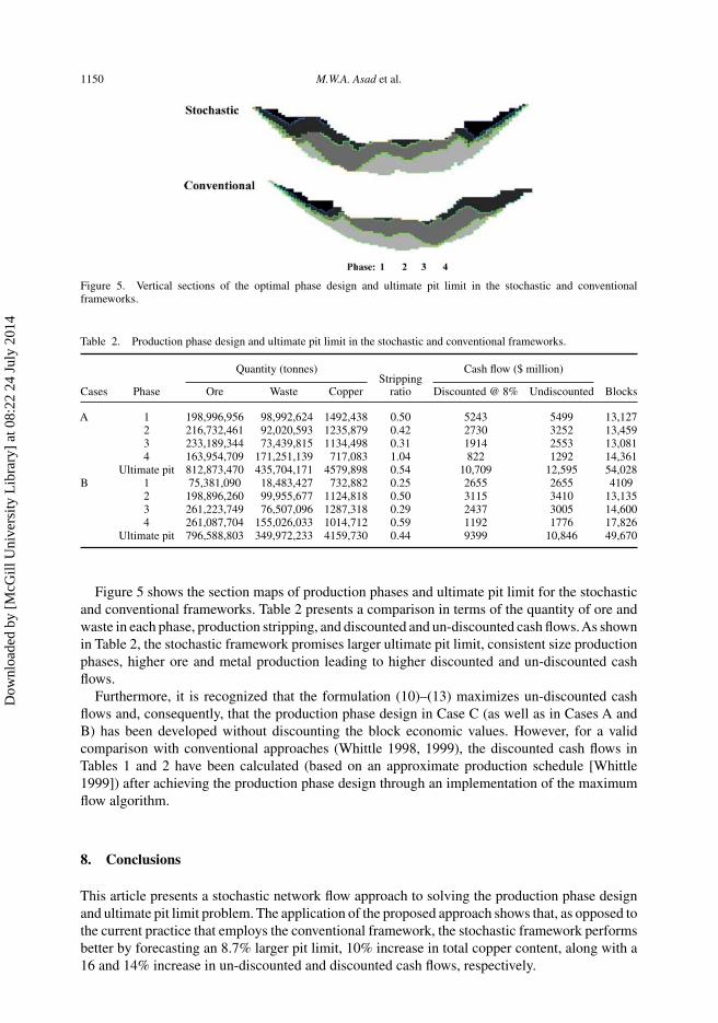
Figure 5. Vertical sections of the optimal phase design and ultimate pit limit in the stochastic and conventionalframeworks.

Table 2. Production phase design and ultimate pit limit in the stochastic and conventional frameworks.

Quantity (tonnes) Cash flow ($ million)Stripping

Cases Phase Ore Waste Copper ratio Discounted @ 8% Undiscounted Blocks

A 1 198,996,956 98,992,624 1492,438 0.50 5243 5499 13,1272 216,732,461 92,020,593 1235,879 0.42 2730 3252 13,4593 233,189,344 73,439,815 1134,498 0.31 1914 2553 13,0814 163,954,709 171,251,139 717,083 1.04 822 1292 14,361

Ultimate pit 812,873,470 435,704,171 4579,898 0.54 10,709 12,595 54,028B 1 75,381,090 18,483,427 732,882 0.25 2655 2655 4109

2 198,896,260 99,955,677 1124,818 0.50 3115 3410 13,1353 261,223,749 76,507,096 1287,318 0.29 2437 3005 14,6004 261,087,704 155,026,033 1014,712 0.59 1192 1776 17,826

Ultimate pit 796,588,803 349,972,233 4159,730 0.44 9399 10,846 49,670

Figure 5 shows the section maps of production phases and ultimate pit limit for the stochasticand conventional frameworks. Table 2 presents a comparison in terms of the quantity of ore andwaste in each phase, production stripping, and discounted and un-discounted cash flows.As shownin Table 2, the stochastic framework promises larger ultimate pit limit, consistent size productionphases, higher ore and metal production leading to higher discounted and un-discounted cashflows.

Furthermore, it is recognized that the formulation (10)–(13) maximizes un-discounted cashflows and, consequently, that the production phase design in Case C (as well as in Cases A andB) has been developed without discounting the block economic values. However, for a validcomparison with conventional approaches (Whittle 1998, 1999), the discounted cash flows inTables 1 and 2 have been calculated (based on an approximate production schedule [Whittle1999]) after achieving the production phase design through an implementation of the maximumflow algorithm.

8. Conclusions

This article presents a stochastic network flow approach to solving the production phase designand ultimate pit limit problem. The application of the proposed approach shows that, as opposed tothe current practice that employs the conventional framework, the stochastic framework performsbetter by forecasting an 8.7% larger pit limit, 10% increase in total copper content, along with a16 and 14% increase in un-discounted and discounted cash flows, respectively.

Dow

nloa

ded

by [

McG

ill U

nive

rsity

Lib

rary

] at

08:

22 2

4 Ju

ly 2

014

Engineering Optimization 1151

The results presented in CasesA and C also reveal the importance of accounting for the expectedvariability and uncertainty in a number of orebody realizations. The stochastic framework in CaseC considers 15 orebody realizations and projects a 5% larger ultimate pit limit, as compared toCase A that considers only three orebody realizations.

Even though the structure of problem (10)–(13) imitates the structure of the production schedul-ing problem, the proposed method is intended to solve the production phase design and ultimatepit limit problem. The processing capacity constraints are included only to facilitate the selectionof values through Lagrangian relaxation of these constraints. The results also demonstrate thatthe difference in structure of the graph in the stochastic and conventional frameworks and thesystematic selection of λ values yields relatively consistent size production phases coupled withhigher cash flows.

Acknowledgements

The work in this article was funded from Natural Sciences and Engineering Research Council of Canada CRDPJ Grant411270-10 and the members of the COSMO Stochastic Mine Planning Laboratory—AngloGold Ashanti, Barrick, BHPBilliton, De Beers, Newmont and Vale. Thanks are in order to Brian Baird, Peter Stone, Darren Dyck and Gavin Yates ofBHP Billiton for their support, collaboration and technical comments.

References

Albor, F., and Dimitrakopoulos, R. 2010. “Algorithmic Approach to Pushback Design Based on Stochastic Programming:Method, Application, and Comparisons.” IMM Transactions, Section A, Mining Technology 119 (2): 88–101.

Asad, M. W. A. 2011. “A Heuristic Approach to Long-Range Production Planning of Cement Quarry Operations.”Production Planning & Control 22 (4): 353–364.

Asad, M. W. A., and Dimitrakopoulos, R. 2012. “Performance Evaluation of New Stochastic Network Flow Approach toOptimal Open Pit Mine Design Application at a Gold Mine.” The Journal of the South African Institute of Miningand Metallurgy 112 (7): 649–655.

Asad, M. W. A., and Dimitrakopoulos, R. 2013. “Implementing Parametric Maximum Flow Algorithm for Optimal OpenPit Mine Design Under Uncertain Supply and Demand.” Journal of the Operational Research Society 64: 185–197.doi: 10.1057/jors.2012.26.

Babenko, M. A., and Goldberg, A. V. 2006. “Experimental Evaluation of a Parametric Flow Algorithm.” MicrosoftResearch Technical Report: MSR-TR-2006-77.

Baker, C. K., and Giacomo, S. M. 1998. “Resource and Reserves: Their Uses and Abuses by the Equity Markets.” In:Mineral Resource and Ore Reserve Estimation – The AusIMM Guide to Good Practice, Monograph 23, Edited By:A. C. Edwards (ed.), 666–676. Melbourne: The Australian Institute of Mining and Metallurgy (AusIMM).

Boucher, A., and Dimitrakopoulos, R. 2012. “Multivariate Block-Support Simulation of the Yandi Iron Ore Deposit,Western Australia.” Mathematical Geosciences 44 (4): 449–468.

Caccetta, L., and Hill, S. 2003. “An Application of Branch and Cut to Open Pit Mine Scheduling.” Journal of GlobalOptimization 27: 349–365.

Denby, B., Schofield, D., and Surme, T. 1998. “Genetic Algorithms for Flexible Scheduling of Open Pit Operations.”Proceedings of the 27th Symposium on the Application of Computers and Operations Research in the MineralIndustry, 605–616.

Dimitrakopoulos, R. 2011. “Stochastic Optimization for Strategic Mine Planning: A Decade of Developments.” Journalof Mining Science 47 (2): 138–150.

Dimitrakopoulos, R., and Abdel Sabour, S. A. 2007. “Evaluating Mine Plans Under Uncertainty: Can the Real OptionsMake a Difference?” Resources Policy 32 (3): 116–125.

Dowd, P. A. 1994. “Risk Assessment in Reserve Estimation and Open-Pit Planning.” Transactions of the Institute ofMining and Metallurgy 103: 148–154.

Eldert, J. V. 2011. “Stochastic Open Pit Design with a Network Flow Algorithm: Application at Escondida Norte, Chile.”Master of science thesis, Delft University of Technology (TUDelft), The Netherlands.

Godoy, M., and Dimitrakopoulos, R. 2011. “A Risk Quantification Framework for Strategic Mine Planning: Method andApplication.” Journal of Mining Science 47 (2): 235–246.

Goldberg, A. V., and Tarjan, R. E. 1988. “A New Approach to the Maximum Flow Problem.” Journal of the Associationfor Computing Machinery 35 (4): 921–940.

Goodfellow, R., and Dimitrakopoulos, R. 2013. “Algorithmic Integration of Geological Uncertainty in Pushback Designsfor Complex Multi-Process Open Pit Mines.” IMM Transactions, Section A, Mining Technology 122 (2): 67–77.

Goovaerts, P. 1997. Geostatistics for Natural Resources Evaluation. New York: Oxford University Press.Hochbaum, D. S. 2001. “A New–Old Algorithm for Minimum-Cut and Maximum-Flow in Closure Graphs.” Networks

37 (4): 171–193.

Dow

nloa

ded

by [

McG

ill U

nive

rsity

Lib

rary

] at

08:

22 2

4 Ju

ly 2

014

1152 M.W.A. Asad et al.

Hochbaum, D. S., and Chen, A. 2000. “Performance Analysis and Best Implementations of Old and New Algorithms forthe Open-Pit Mining Problem.” Operations Research 48 (6): 894–914.

Horta, A., and Amilcar, S. 2010. “Direct Sequential Co-Simulation with Joint Probability Distributions.” MathematicalGeosciences 42 (3): 269–292.

Hustrulid, W., and Kuchta, M. 2006. Open Pit Mine Planning and Design. 2nd ed. Leiden, The Netherlands: Taylor &Francis/Balkema.

Johnson, T. B. 1968. “Optimum Open Pit Mine Production Scheduling.” PhD thesis, Department of IEOR, University ofCalifornia, Berkeley, CA.

Lerchs, H. and Grossmann, I. F., 1965. “Optimum Design of Open Pit Mines.” Transactions CIM 58: 17–24.Machuca-Mory, D. F., and Deutsch, C. V. 2013. “Non-Stationary Geostatistical Modeling Based on Distance Weighted

Statistics and Distributions.” Mathematical Geosciences 45 (1): 1–30.Meagher, C., Abdel Sabour, S. A., and Dimitrakopoulos, R. 2010. “Pushback Design of Open Pit Mines Under Geological

and Market Uncertainties.” Advances in Orebody Modeling and Strategic Mine Planning I,AusIMM Spectrum Series17: 297–304.

Montiel, L., and Dimitrakopoulos, R. 2013. “Stochastic Mine Production Scheduling with Multiple Processes:Applicationat Escondida Norte, Chile.” Journal of Mining Science, to be published.

Picard, J. C. 1976. “Maximal Closure of a Graph and Applications to Combinatorial Problems.” Management Science 22(11): 1268–1272.

Ramazan, S. 2007. “The New Fundamental Tree Algorithm for Production Scheduling of Open Pit Mines.” EuropeanJournal of Operational Research 177 (2): 1153–1166.

Ramazan, S., and Dimitrakopoulos, R. 2013. “Production Scheduling with Uncertain Supply: A New Solution to the OpenPit Mining Problem.” Optimization and Engineering 14 (2): 361–380. doi: 10.1007/s11081-012-9186-2.

Tachefine, B., and Soumis, F. 1997. “Maximal Closure on a Graph with Resource Constraints.” Computers and OperationsResearch 24 (10): 981–990.

Vallee, M. 2000. “Mineral Resource + Engineering, Economic and Legal Feasibility = Ore Reserve.” CIM Bulletin 93:53–61.

Whittle, J. 1998. “Beyond Optimization in Open Pit Design.” Proceedings of the Canadian Conference on ComputerApplications in the Mineral Industries, Quebec, Canada. Rotterdam: Balkema. 331–337.

Whittle, J. 1999. “A Decade of Open Pit Mine Planning and Optimisation—The Craft of Turning Algorithms into Pack-ages.” Proceedings of the 28th International Symposium on the Application of Computers and Operations Researchin the Mineral Industry, 15–24. Golden, CO: Colorado School of Mines.

Dow

nloa

ded

by [

McG

ill U

nive

rsity

Lib

rary

] at

08:

22 2

4 Ju

ly 2

014