
Thermally-Assisted-Occupation Density Functional Theory with Generalized-Gradient Approximations
Upload
khangminh22Category
view
0download
0
Statistical Physics
Stephan Korden
Molecular Density Functional TheoryBased on aHard-Particle Reference Potential

Molecular Density Functional TheoryBased on a
Hard-Particle Reference Potential
Von der Fakultat fur Maschinenwesen der Rheinisch-Westfalischen TechnischenHochschule Aachen zur Erlangung des akademischen Grades eines Doktors der
Naturwissenschaften genehmigte Dissertation
vorgelegt von
Stephan Korden
Berichter: Juniorprofessor Dr. rer. nat. Kai Olaf LeonhardUniversitatsprofessor Dr. rer. nat. Roland Roth
Tag der mundlichen Prufung: 26. Oktober 2015
Diese Dissertation ist auf den Internetseiten der Universitatsbibliothek onlineverfugbar.

Acknowledgements
In these first lines, I would like to express my gratitude to all people who contributed to thisthesis. Especially I would like to thank my supervisor Prof. Kai Leonhard for his support andencouragement over the past years, and whose interest in lattice models was the starting pointfor the current investigation of classical DFT. Also Prof. Roland Roth from the University ofTubingen for his time and effort to take the part as second reviewer and Prof. Peter Loosenfor taking the chair of the doctoral Commitee. Likewise, I would like to thank Prof. AndreBardow as head of the Institute of Technical Thermodynamics for his continuous encouragementand Prof. Matthias Schmidt from the University of Bayreuth for his interest in the mathematicalapproach and bringing me in contact with the FMT community, as well as Prof. Andreas Klamtfrom the University of Regensburg for helpful insights into his off-lattice model. I would alsolike to highlight the influence of Matthieu Marechal on this work. His helpful discussions andintense e-mail correspondence were a great motivation. Without his insight into Ree-Hooverdiagrams, the solution of the hard-particle problem would not have been complete. Many thanksalso goes to Annett Schwarz and Christian Jens for their helpful comments on the manuscriptsand to Van Nhu Nguyen for many discussions on the thermodynamics of liquids. Many morehave contributed to this work in more indirect ways, especially all colleagues from the Institute ofTechnical Thermodynamics, who patiently bridged the worlds between engineers and physicists.Finally, I would also thank my family for their long lasting support, patience, and motivation.
i


Fur meine Eltern
Beatrix Korden
und
Joachim Korden


Abstract
The aim of the current doctorate thesis is the development of a density functional theory (DFT) forclassical intermolecular interactions. In the first part, we begin with an analysis of the structure ofthe grand-canonical potential and demonstrate that for pair potentials only two independent rep-resentations exists: the direct-correlation functional and its Legendre transformation with respectto the pair potential. Using far-reaching assumptions, this dual grand-canonical potential reducesto the free-energy functions of Flory-Huggins, Staverman-Guggenheim, and Guggenheim, fromwhich again derive the lattice-models UNIQUAC, UNIFAC, and COSMO-RS. We conclude thisfirst part by discussing possible generalizations of this approach to a continuum formulation.
As is well known from quantum mechanics, the central problem of the DFT approach is thederivation of the functionals, which is further complicated for intermolecular interactions by theirstrongly repulsive potential. A well established approach is the separation of the potential into aflat but long-ranged contribution and the approximation of the repulsive part using the geometryof hard particles. In the second part of this work, we develop the necessary methods for thenon-perturbative derivation of their corresponding hard-particle functionals.
We first begin with a discussion of the fundamental measure theory and interpret the semi-heuristic Rosenfeld functional as the leading order of an expansion in the number of intersectioncenters of the particles. For the generalization of the approach we demonstrate the equivalencebetween intersection configurations and classes of Ree-Hoover diagrams, whose sum defines ageneric functional decoupling into a convolute of intersection kernels. Each such kernel deter-mines the local intersection probability of a set of particles under the group of translations androtations. For the case of two particles this result has been first derived by Blaschke, Santalo,and Chern. Here, we generalize their approach to an arbitrary set of particles and obtain a closedexpression for the free-energy functional and the n-particle densities for any dimension.
As examples, we derive the functional of the free energy for up to four intersection centers,whose leading order agrees with Rosenfeld’s result. We then calculate for the 2-particle densityan upper limit of the contact probability for hard spheres, which is in excellent agreement withthe result of Carnahan and Starling. Comparing the same level of approximation with Kirkwood’ssuperposition ansatz for correlation functions of higher orders, shows that the contact probabilityof spheres is significantly overestimated by the superposition approximation. Finally, we derivethe leading perturbative corrections for long-range interactions.
With the methods developed in the current work, the hard-particle interaction is now the onlyknown example, whose density functionals can be derived systematically to any order of precision.We conclude our work with a discussion of possible applications in biology and chemistry.
v

Zusammenfassung
Das Ziel der vorliegenden Dissertation ist die Entwicklung einer Dichtefunktionaltheorie (DFT)fur klassische intermolekulare Wechselwirkungen. Wir beginnen im ersten Teil der Arbeit miteiner Analyse der Struktur des großkanonischen Potentials und zeigen, dass es fur Paarwech-selwirkungen nur zwei unabhangige Darstellungen erlaubt: das der direkten Korrelationsfunk-tion und das seiner Legendre-Transformation bezuglich des Paarpotentials. Es wird gezeigt,dass sich unter weitreichenden Modellannahmen das duale Funktional auf die Ausdrucke derfreien Energie von Flory-Huggins, Staverman-Guggenheim und Guggenheim reduziert, aus de-nen sich wiederum die Gittermodelle UNIQUAC, UNIFAC und COSMO-RS herleiten lassen.Abschließend diskutieren wir mogliche Erweiterungen als Kontinuumsbeschreibung.
Wie aus der Quantenmechanik bekannt, besteht das grundlegende Problem des DFT Ansatzesin der Berechnung der Funktionale, was im Fall der intermolekularen Wechselwirkungen durchden stark repulsiven Anteil zusatzlich erschwert wird. Ein etablierter Ansatz ist daher die Zer-legung des Potentials in einen flachen aber weitreichenden Beitrag und die Naherung des repul-siven Anteils durch die Geometrie eines harten Korpers. Im zweiten Teil der Arbeit entwickelnwir die Methoden fur die nichtperturbative Berechnung der Funktionale harter Korper.
Wir beginnen mit einer Einfuhrung in die Fundamental Measure Theory und interpretieren dassemi-heuristische Rosenfeld Funktional als die fuhrende Ordnung einer Entwicklung nach der An-zahl der Schnittzentren der Korper. Um diesen Ansatz zu verallgemeinern, zeigen wir die Aquiv-alenz zwischen Schnittkonfigurationen und Klassen von Ree-Hoover Diagrammen, deren Summeein generisches Funktional bestimmt, das in ein Konvolut von Schnittkernen zerfallt. Dabeiberechnet sich jeder Schnittkern aus der lokalen Schnittwahrscheinlichkeit der Teilchen unterTranslationen und Rotationen. Fur zwei Korper wurde dieses Ergebnis bereits durch Blaschke,Santalo und Chern berechnet. Hier verallgemeinern wird diesen Ansatz auf eine beliebige Anzahlvon Teilchen und geben eine geschlossene Losung fur die freie Energie und die n-Teilchendichtenin beliebiger Dimension an.
Als Beispiele berechnen wir das Funktional der freien Energie fur bis zu vier Schnittzentren,dessen fuhrende Ordnung mit Rosenfelds Ergebnis ubereinstimmt. Ferner leiten wir fur die 2-Teilchendichte eine obere Abschatzung der Kontaktwahrscheinlichkeit fur harte Kugeln ab, dasdas Ergebnis von Carnahan und Starling sehr gut wiedergibt. Vergleicht man nun die gleicheNaherung mit Kirkwoods Superpositionsansatz fur Korrelationen hoherer Ordnung, so zeigt sichferner, dass die Kontaktwahrscheinlichkeit durch den Superpositionsansatz signifikant uberschatztwird. Schließlich berechnen wir noch die ersten storungstheoretischen Terme fur attraktive Kor-rekturen.
Mit den hier entwickelten Methoden ist das Hartkorperpotential das einzige heute bekannteBeispiel, fur das samtliche Korrelationsfunktionale systematisch berechnet werden konnen. Wirbeenden die Arbeit mit einer Diskussion moglicher Anwendungen in Biologie und Chemie.
vii


Contents
1 Preface xi
2 Introduction 1
3 Density Functionals and Lattice Models 73.1 The dual Free-Energy Functional . . . . . . . . . . . . . . . . . . . . . . . . . . 73.2 Lattice-Fluid Models derived from the Dual Functional . . . . . . . . . . . . . . 10
4 The Direct Correlation Functionals for Hard Particles 194.1 The Virial Expansion . . . . . . . . . . . . . . . . . . . . . . . . . . . . . . . . 19
4.1.1 FMT as an expansion in intersection centers . . . . . . . . . . . . . . . . 194.1.2 Resummation of Ree-Hoover Diagrams . . . . . . . . . . . . . . . . . . 22
4.2 Intersection Probability in N Dimensions . . . . . . . . . . . . . . . . . . . . . . 284.3 The Rosenfeld Functional and Beyond . . . . . . . . . . . . . . . . . . . . . . . 34
5 The Distribution Functionals for Hard Particles 415.1 The Generic Distribution Functional for Hard Particles . . . . . . . . . . . . . . 415.2 Examples of R-Particle Correlation Functionals . . . . . . . . . . . . . . . . . . 47
6 Discussion and Conclusion 51
A The Integral Measure of the Minkowski Sum 55
B Proof of the generalized Blaschke-Santalo-Chern Equation 57
C Deriving Rosenfeld’s 1-particle Weight Functions 61
ix


Chapter 1
Preface
As any doctorate thesis, the current text is the result of a dynamic process with unforseen prob-lems and findings. Some results have already been published and others recently submitted. Thecomplete list of texts that have been prepared over the last years include the following articles inchronological order of their writing:
1. S. Korden, N. Van Nhu, J. Vrabec, J. Gross, and K. Leonhard: On the Treatment of Electro-static Interactions of Non-Spherical Molecules in Equation of State Models, Soft Materials,10, 81-105, (2012)
2. S. Korden: Deriving the Rosenfeld Functional from the Virial Expansion, Phys. Rev. E, 85,041150, (2012)
3. S. Korden, Density Functional Theory for Hard Particles in N Dimensions, Commun. Math.Phys., 337, 1369-1395, (2015)
4. M. Marechal, S. Korden, and K. Mecke, Deriving fundamental measure theory from thevirial series: Consistency with the zero-dimensional limit, Phys. Rev. E, 90, 042131, (2014)
5. S. Korden, Distribution Functionals for Hard Particles in N Dimensions, (2015),arXiv:1502.04393, submitted to Commun. Math. Phys.
6. S. Korden, Lattice-Fluid Models derived from Density Functional Theory, (2015),arXiv:1503.02327, submitted to Mol. Phys.
The outgoing problem of the current thesis was the development of fast and universal methodsto derive the phase structure of homogeneous fluids from the structure of their molecular com-pounds. The first approach we followed tried to reduce the overall number of parameters of anequation of state by correlating its values to the data of single molecules calculated by quantummechanical methods. Article (1) shows this for the example of dipole and quadrupole moments.But the relationship proved to be too irregular to be of practical use. The different types of in-teractions result in cross-correlations in the fitted parameters, which cannot be decoupled andassigned to individual potentials. A true understanding of the relation between interaction poten-tials and the phase diagram therefore requires the determination of the density functional of thegrand canonical potential itself, which became the topic of the current thesis.
A common approach to construct the grand canonical potential for molecular systems is theperturbative coupling of soft interactions to the correlation functionals of hard particles. But for
xi
xii Chapter 1. Preface
a long time a suitable approach for their derivation was not known. It was therefore an importantstep when Rosenfeld introduced the “fundamental measure theory” for spheres. In Article (2), weanalyze this semi-heuristic approach and identify several contradictions in its underlying assump-tions. Instead of using Rosenfeld’s intuitive approach, we then show that the same functional canbe derived from the virial expansion for particles overlapping in a common intersection center, cal-culating the intersection probability for an infinite set of overlapping particles under translationsand rotations, generalizing previous results from Blaschke, Santalo, and Chern.
However, although this result explains the mathematical structure of the Rosenfeld functional,it still fails to extend its applicability to more complex particles than spheres. This problem issolved in Article (3). Starting from an observation of Matthieu Marechal that the intersectionpattern of particles is related to Ree-Hoover diagrams, we classify all virial integrals belongingto a given type of intersection networks. Generalizing our previous results from Article (2) to Ndimensional particles, we have a now an efficient set of mathematical methods at hand to derivethe free-energy functional for a given class of intersection networks.
In a parallel approach, we also followed a set-theoretic ansatz in Article (4) to derive theRosenfeld functional, confirming our previous results.
But the derivation of the hard-particle direct correlation functionals is not sufficient for theperturbative construction of a molecular DFT. For this it is still necessary to construct the n-particle distribution functionals to couple the soft-interaction potentials to the free energy. Thisis done in Article (5), using the previous techniques of diagrammatic resummation and integralgeometry. With this result, we have all the necessary hard-particle correlation functionals at handfor the construction of a molecular density functional.
The structure of the grand canonical potential is not a unique, but allows different represen-tations related by symmetry transformations. For the pair-potential it is shown in Article (6) thatonly two possible representations exist. The better known example is the direct correlation func-tional and its perturbative expansion for weak interactions. But here we argue that for the strongmolecular interactions the dual grand potential is to be preferred because of its unique minimumwith respect to the pair-correlation functional and its analytical simplicity at first perturbation or-der. Both properties are demonstrated by comparing the functional to lattice excess free-energymodels, completing the cycle to develope the framework and mathematical tools to improve andextend existing models based on DFT.
Chapter 2
Introduction
The investigation of the gas, liquid, and crystalline phases of molecular matter is one of the oldesttopics in the history of natural science. And, with a delay of several decades of solid-state domi-nated physics, it is nowadays at the center of an interdisciplinary revolution triggered by molecularbiology and its increasing understanding of inner-cellular processes. The development of new ex-perimental techniques, e.g. X-ray and neutron scattering, NMR, force field, and laser scanningmicroscopy, to investigate the microscopic properties of fluids and the dynamics of individualmolecules is among the major achievements of the last decades and intensified the developmentof mathematical methods for the prediction of their properties [81, 71].
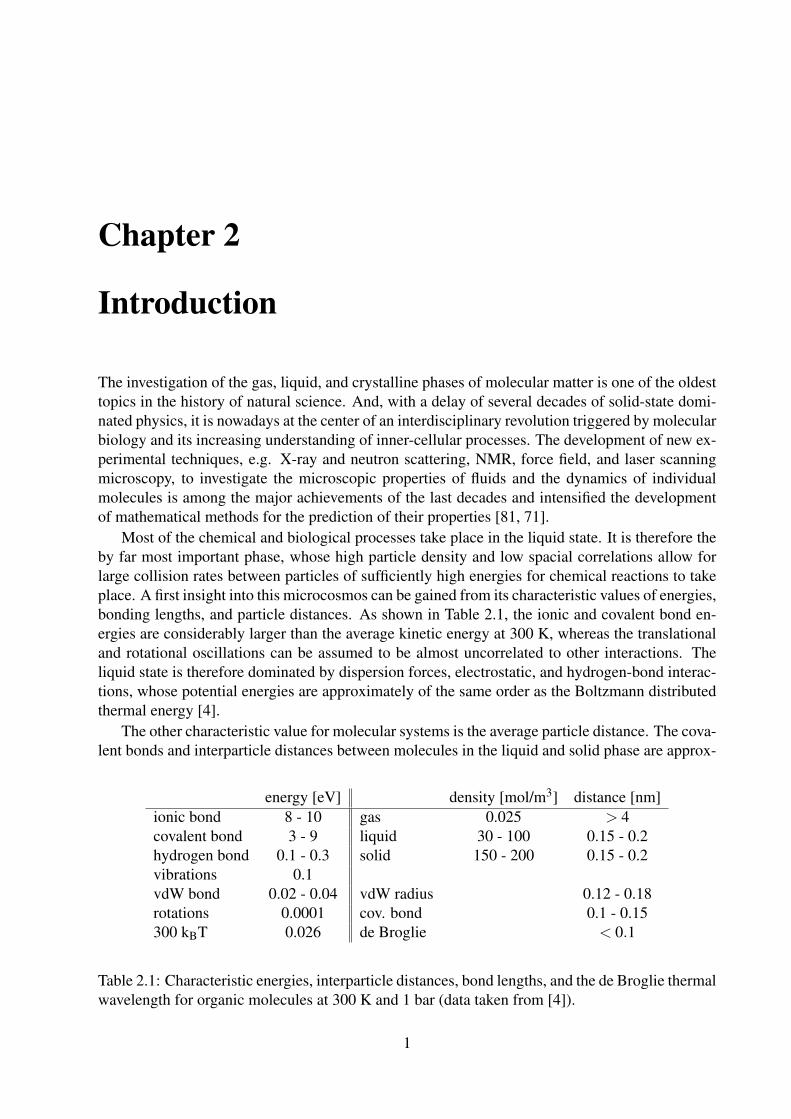
Most of the chemical and biological processes take place in the liquid state. It is therefore theby far most important phase, whose high particle density and low spacial correlations allow forlarge collision rates between particles of sufficiently high energies for chemical reactions to takeplace. A first insight into this microcosmos can be gained from its characteristic values of energies,bonding lengths, and particle distances. As shown in Table 2.1, the ionic and covalent bond en-ergies are considerably larger than the average kinetic energy at 300 K, whereas the translationaland rotational oscillations can be assumed to be almost uncorrelated to other interactions. Theliquid state is therefore dominated by dispersion forces, electrostatic, and hydrogen-bond interac-tions, whose potential energies are approximately of the same order as the Boltzmann distributedthermal energy [4].
The other characteristic value for molecular systems is the average particle distance. The cova-lent bonds and interparticle distances between molecules in the liquid and solid phase are approx-
energy [eV] density [mol/m3] distance [nm]ionic bond 8 - 10 gas 0.025 > 4covalent bond 3 - 9 liquid 30 - 100 0.15 - 0.2hydrogen bond 0.1 - 0.3 solid 150 - 200 0.15 - 0.2vibrations 0.1vdW bond 0.02 - 0.04 vdW radius 0.12 - 0.18rotations 0.0001 cov. bond 0.1 - 0.15300 kBT 0.026 de Broglie < 0.1
Table 2.1: Characteristic energies, interparticle distances, bond lengths, and the de Broglie thermalwavelength for organic molecules at 300 K and 1 bar (data taken from [4]).
1
2 Chapter 2. Introduction
imately of the same order as the de Broglie wavelength and thus dominated by quantum effects.But due to the rapid exponential decline of the quantum correlations between electrons of differ-ent molecules, they are largely suppressed, which justifies the introduction of classical molecularpotentials. The only notable exception is the hydrogen atom, whose large thermal wavelengthindicates that effects of discrete energies and tunneling can occur for strong interactions, resultingin the hydrogen bonding between polar molecules [4, 57].
Quantum effects arise, e.g., when the attractive potential exceeds critical values in depth andinteraction width, leading to the association of molecules [49]. If the lifetime of such a cluster issufficiently small this is in no contradiction with classical statistical mechanics. But the formationof temporarily long-lived associates is incompatible with the ergodicity assumption of the Boltz-mann distribution for classical interactions. Instead of a configurational ensemble, such processescan only be described by an average over time [2]. In the following, we will exclude such systemsand assume that the time-scales of associated and dissociated states are sufficiently separated tobe considered as thermodynamically individual states.
The description of molecular interactions by effective potentials applies to the most relevantparts of the phase diagram, including the equilibrium states of gases, liquids, and the variouscrystalline states, but also the metastable non-equilibrium states of granular matter and glasses.In the thermodynamic equilibrium, each phase domain in the diagram is adjacent to at least oneother state, with the maximum number of n+2 neighboring phases determined by Gibbs’ rule fora system of n compounds and separated by a f = n+2−r dimensional boundary for r neighboringstates. Any domain is therefore locally represented by a function of n+3 variables, depending ontemperature T , entropy S, volume V , pressure P, densities ρi, and the chemical potentials µi for amixture of i = 1, . . . ,n compounds [50].
Following Ehrenfest’s Theorem, each transition in the phase diagram is related to a changein the symmetries of the free-energy functional [71]. This is easily seen for a crystalline state ofdensity ρ(~r) with lattice structure Λ and periodic coordinates~r ∈ R3/Λ or the gas ρ(~r) = const.as the state of highest symmetry. The corresponding change of symmetry in the liquid state, onthe other hand, is less obviously related to a reduced radial translation invariance. To illustrate thiseffect, consider two particles with radial-symmetric potential U(r), reduced mass m, and angularmomentum L, whose energy E = mr2/2+ L2/(2mr2) +U(r) is a function of the translationalpart mr2/2 and the effective potential Ueff(r) = U(r)+ L2/(2mr2). The relative motion of thetwo particles is then characterized by the minimum of Ueff(r) as a function of L. The particles arebonded if the minimum is negative and unbonded when positive, with a critical value U ′eff(Lc) = 0,where the extremum degenerates to zero. A similar picture applies to the statistical average 〈Ueff〉if the system is dominated by pair correlations. Below a critical value of L2
c ∼ Tc, the particlescondense into a state of classically bonded particles and move unrestrained for T ≥ Tc, where〈Ueff〉 is zero or strictly repulsive. The effective potential of a fluid near the critical point istherefore similar to the potential surface the φ 4-theory with its second order phase transition [99].
The different approaches to derive the phase diagram from molecular potentials can be classi-fied into three groups. The most general method is the molecular dynamic (MD) simulation [2].The thermodynamic variables are determined as time-averages over particle ensembles derived bysolving Newton’s equation of motion. This approach applies to equilibrium and non-equilibriumsituations alike, and also represents molecules with flexible bond lengths and angles, thus includ-ing transitions between conformers and the classical kinetic energies of vibrations and rotations.The second group covers the Markov-Chain Monte Carlo (MC) simulations which uses stochasticensembles to average over configurational variables [2, 48]. With the kinetic energy decoupled, it
3
is the preferred simulation technique for equilibrium thermodynamics. The third group is basedon density functional theory (DFT) [57, 19]. It determines the thermodynamic equilibrium byminimizing the grand canonical potential with respect to the density ρi(~r). But in contrast to theMD/MC techniques, its sampling function is not known in general and far-reaching approxima-tions are often necessary to derive its form. This reduces its accuracy to derive thermodynamicinformation, but on the other hand also offers a more varied set of approximations that can be usedto reduce the considerable numerical efforts accompanied by MD/MC calculations.
Apart from these three groups, there exists two further representations to derive parts of thephase diagram: equations of state (EoS) and lattice models of the excess free-energy [66, 5].Examples of EoS are the van der Waals model, the statistical associated fluid theories (SAFT)[13, 14, 57], and the Landau free-energy function for liquid crystals [50], each depending onparameters that characterize the change of symmetry related to the phase transition. In contrast toDFT, an EoS parametrizes the minimum of the grand canonical potential for a single realizationof the local density. But for most interactions the topology of this hypersurface of the free energyis too complex to be globally representable by a simple function, why any practical realization isrestricted to the description of a small domain of the phase diagram. This limitation also extendsto the prediction of the properties of mixtures from the parameters of their pure compounds.To describe the related changes in the interparticle correlations, it is thus necessary to definead hoc mixing rules and mixture coefficients. These parameters are strictly model dependentand contain no further physical information. But their comparatively small number are easilyfitted to experimental data sets, why EoS are often used to parametrize the gas-liquid domain ofhomogeneous fluids [65].
Closely related to DFT are the lattice-fluid models of the excess free-energy. Based on thephysically incorrect assumption of a lattice structure as background with tightly packed particleswithout free volume, the lattice cells form a hard-particle reference fluid with an additional inter-action between its cell surfaces [5, 39]. Its phase diagram is thus restricted to a fixed referencevalue of density and pressure for an artificial state of the liquid phase. This simple ansatz has beenimplemented by Abrams and Prausnitz in the universal quasichemical model (UNIQUAC), ex-tended by Prausnitz and Maurer by including functional group-activity coefficients (UNIFAC),and the conductor like screening model for real solvents (COSMO-RS) developed by Klamt[56, 1, 22, 65, 39, 38, 40]. These three examples start from the same density functional of thegrand-canonical potential but use different strategies for its minimization and different interactionmodels. Together with the group contribution ansatz, the UNIFAC and COSMO-RS models haveboth been successfully applied to predict the mixture diagrams of liquids under the given set ofassumptions.
These five methods for determining the liquid phase diagram illustrate the dilemma of soft-matter physics. Either one uses the simple but limited methods of EoS and lattice models, or thecomputationally expensive but universal ansatz of MD/MC. The aim of the current thesis is to finda compromise in the framework of DFT that is numerically manageable but still applies to thefull range of the phase diagram. For this purpose we will use the lattice models as a guideline andderive the technical framework to develope further continuum functionals for molecular potentialsapproximated by a hard-particle core and soft interactions.
In Chapter 3, we begin with a detailed analysis of the representation of the grand-canonicalpotential. Widely constrained by the Hohenberg, Kohn, Mermin theorem [57], only two realiza-tions exist for pair interactions. One representation is based on the direct correlation functionalfrom which, e.g., the van der Waals and SAFT equations of state descent. The second representa-
4 Chapter 2. Introduction
tion follows from its Legendre transformation in the pair potentials [7, 59, 60, 61]. Together withthe quasichemical approximation, this is the functional from which the lattice excess functionalsoriginate, differing by their various strategies to minimize the grand potential [47]. The Wilsonansatz is used in the UNIQUAC and UNIFAC models, which is shown to yield a physically in-consistent solution of the Euler-Lagrange equation [97], whereas the COSMO-RS model appliesthe correct Larsen-Rasmussen approach [51]. Deriving both approaches, we show that the latticevariables miss important information about the geometry of the molecules and that long-rangedpotentials not only change the free energy but also the self-consistent equation of its lattice mod-els. Including the molecular geometry and the long-range interactions therefore prove problematicif not impossible in this framework and thus require the formulation of an unconstrained densityfunctional, introducing the new problem of deriving the pair-correlation functionals for any in-termolecular potential. A common and well tested strategy to reduce the complexity of this taskis the approximation of the strongly repulsive part of the molecular interaction by a hard-particlepotential and to expand the functional in a perturbative series in the residual soft interactions [57].This approach reduces the construction of a molecular DFT to the non-perturbative derivation ofthe hard-particle correlations functionals.
In Chapter 4, we take a first step in this direction and derive an approximate direct correla-tion functional for hard particles. Using hard spheres as a reference geometry for molecules goesback to van der Waals and Boltzmann, with its mathematical structure first analyzed by Isiharaand Kihara, who calculated the second virial integral for convex particles using the Minkowskisum of their domains [37, 36]. This result is the starting point of the scaled particle theory (SPT)developed by Reiss, Frisch, and Lebowitz for spherical particles [72], which has been generalizedby Rosenfeld to the fundamental measure theory (FMT) [74, 75, 78] with an alternative represen-tation developed by Rosinberg and Kierlik [35, 62]. Its ansatz is based on three assumptions: 1.the Fourier splitting of the second virial integrand into a convolute of 1-particle weight functions,2. the scale invariance of the free energy, and 3. the SPT differential equation. However, theserules only determine two of the three terms of the Rosenfeld functional uniquely, while an ap-proximation for the third term has been found only later by Tarzona, focusing on the consistencyin the zero-dimensional limit [86, 85]. When compared to simulated data, the predicted phasediagram of the Rosenfeld functional proves to be highly accurate for spheres at packing fractionswell below the crystallization point but shows significant deviations at higher packing fractions,for mixtures, and alternative geometries [83, 11, 18, 63]. One reason for this failure has been ex-plained by Wertheim and, independently, by Rosenfeld and Tarazona, who observed the similaritybetween the second virial integral and the Gauss-Bonnet equation [92, 93, 94, 95, 77]. Using thisrelation as additional information, Mecke and Hansen-Goos extended the Rosenfeld functional toconvex particles [25, 26, 27]. The resulting Rosenfeld-Tarazona functional describes the phasediagram of spheres even for the crystalline state but still shows systematic deviations for mixtures.
A complementary approach to improve the Rosenfeld functional has been taken by Roth et al.[80] and Hansen-Goos and Roth [28], using the Mansoori-Carnahan-Starling-Boublik equation ofstate to solve for the pressure in the SPT differential equation [53]. The resulting White-Bear IIfunctional shows a significant improvement compared to the Percus-Yevick approximation of theRosenfeld functional and provides the most reliable functional as of today. For a more detailedintroduction to the development of FMT, we refer to the review [79].
However, despite its remarkable success, the construction of the functional leaves many ques-tions unanswered. First of all, higher order virial integrals depend on more than one intersectioncenter. As shown by Wertheim, the third virial integral for elongated convex particles is not
5
well represented by the 1-center approximation, which neglects important contributions of the3-particle correlations [92, 93, 94, 95]. Also, the mathematical connection between the secondvirial integrand, the Gauss-Bonnet equation, and the calculation of Isihara and Kihara is unex-plained. Here, we will give a more detailed analysis, demonstrating that most assumptions usedin constructing the Rosenfeld functional only apply to spherical particles in odd dimensions. Thiscan be seen for the Fourier decoupling of the second virial integrand, which maps the extrinsiccurvature to its intrinsic form, but also for the Minkowski sum as well as its assumed relation tothe Gauss-Bonnet equation. As we will show in Chapter 4, the solution of these and more appar-ent paradoxes is the Blaschke-Santalo-Chern equation of integral geometry [82, 9]. First provenby Chern for two intersecting n-dimensional domains [15, 16, 17], we generalize the theorem toan arbitrary set of particles, overlapping in at least a common point. Its derivation thus dependssolely on the extrinsic representation of the imbedded particles and explains the deeper connectionto the Gauss-Bonnet identity.
The intersection probability of particles with one intersection center is all that is necessary toderive the Rosenfeld functional from the virial expansion in Mayer diagrams. For higher ordercorrections, however, the identification and summation of Mayer graphs for a given type of in-tersection pattern is more complex. As pointed out by Matthieu Marechal, this problem can bereduced by transforming the virial expansion from Mayer to Ree-Hoover diagrams [67, 69], whichdefines a unique relationship between virial clusters and the intersection pattern of the particles.Classifying the graphs by their intersection patterns, we determine their symmetry factors andsum over all elements of its equivalence class to determine the generic functional for the directcorrelations.
In Chapter 5, we extend these methods to derive the r-particle distribution functionals for hardparticles from the virial expansion. Starting from the representation in rooted Ree-Hoover dia-grams [68, 70], each intersection pattern defines an equivalence class of diagrams that determinesa generic distribution functional. Focusing on the example of the pair-correlation functional, thisroute adds a third approach to its derivation in addition to solving the Bogoliubov-Born-Green-Kirkwood-Yvon integral equation or the Ornstein-Zernike equation in the Percus-Yevick approxi-mation [87, 57]. For the 2-center approximation, we also determine an upper bound for the contactprobability of spheres, which is in excellent agreement with the Carnahan-Starling parametrizationas well as the Wertheim, Thiele, Baxter solution of the Ornstein-Zernike equation [90, 91, 88, 6].We also compare the pole-structure of the n-particle correlation functions to its correspondingvalue predicted by Kirkwood’s superposition ansatz, demonstrating that this approximation failsat short distances. Finally, we derive the perturbative expansion of the pair-correlation functionalsfor soft interactions, which completes our investigation of the molecular grand-canonical poten-tial.
In Chapter 6, we summarize our results and give an outlook to further applications and imple-mentations of molecular DFT.

6 Chapter 2. Introduction
Chapter 3
Density Functionals and Lattice Models
Before constructing a molecular density functional, one has to decide on its representation. In thefollowing chapter, it will be shown that the Hohenberg-Kohn-Mermin theorem constrains theirnumber for a given potential. For the pair interaction, e.g., only two representations are possible,the free-energy functional ΩF and the dual functional ΩD. In Sec. 3.1, we discuss their structureand respective perturbation expansions. By comparing the excess free energy of the dual func-tional to the UNIQUAC, UNIFAC lattice, and the COSMO-RS off-lattice models, it is shown inSec. 3.2 that ΩD is the most promising candidate. It is the only functional that allows the use ofCOSMO data for its interaction potential, and different levels of approximations can be used tointerpolate between the continuum or off-lattice description and the lattice models, customizingthe molecular functional to its specific applications.
3.1 The dual Free-Energy FunctionalThe Hohenberg, Kohn, Mermin theorem shows the unique mutual relationship between inter-action and grand-canonical potential [57], forming the foundation of DFT, as it guarantees thatdifferent representations of the functional determine the same thermodynamic ground state. Itthus constrains the number of alternative representations for a given interaction potential, whichare related by similarity transformations. Ignoring mappings that correspond to internal symme-tries of the potential or result in contributions which cancel in the Euler-Lagrange equations, theonly nontrivial symmetry is the Legendre transformation of the grand potential Ω, exchanging itscanonically conjugate variables. For the simplest and most relevant case of pair interactions, itreplaces the potential φi j by its dual pair-correlation functional gi j, defined by
δΩ
δφi j=
12
ρiρ jgi j . (3.1)
This shows that Ω for 2-particle potentials has only two representations, either as the free-energyfunctional ΩF(φi j) or its Legendre-dual counterpart ΩD(gi j).
Most molecular functionals use ΩF as the starting point, as its perturbation expansion in r-particle densities ρi1...ir is algebraically well understood [57]. But it will be shown in the nextsection that the lattice models derive from the dual functional ΩD, whose analytic form is morecomplex and the perturbation expansion of g2 does not result in either the direct or the distribu-tion functionals. For comparison, we will derive both representations, analyze their respectiveperturbation expansions, and discuss their advantages and limitations.
7
8 Chapter 3. Density Functionals and Lattice Models
Beginning with the free-energy representation, the functional ΩF(β ,µi,φexi |ρi,φi j) of the par-
ticle density ρi depends on the inverse temperature β = 1/kBT , chemical potential µi, and externalpotentials φ ex
i for a mixture of i = 1, . . . ,M compounds. It is an integral
βΩF =
M
∑i=1
∫ [ρi(ln(ρiΛi)−1)−βρi(µi−φ
exi )]
dγi− c0(ρi) (3.2)
over the positions and orientations γi ∈ Rn× SO(n) of the n-dimensional Euclidean space anddepending on the thermal wavelength Λi and direct correlation functional c0(ρi).
Its perturbation expansion in the potential φ = φ H+φ S of hard-particle φ H and soft interactionφ S is a formal Taylor series of the logarithm of the grand canonical partition integral, whose firstand second order in the Mayer functions f S
2 have the form
βΩF = βΩ
FH−
12
∫ρ
Hi1i2 f S
i1i2 dγi1i2−12
∫ρ
Hi1i2i3 f S
i1i2 f Si2i3 dγi1i2i3
− 18
∫(ρH
i1i2i3i4−ρHi1i2ρ
Hi3i4) f S
i1i2 f Si3i4 dγi1i2i3i4− . . . ,
(3.3)
where a sum over paired indices is implied [57]. Higher order terms are readily obtained usingdiagrammatic techniques [46], where each product [ f S
2 ]m couples to a homogeneous polynomial
of r-particle densities of order 2 ≤ r ≤ 2m, integrated over the (m− 1)n(n+ 1)/2 coordinates ofposition and orientation. The rapid increase in the dimensionality of the integrals effectively limitsthe perturbative approach to the first or second order.
In deriving (3.3), we assumed the particles to interact by pair potentials. But the same approachalso applies to irreducible m-particle interactions, with the fully f S
2 -bonded subdiagrams [ f S2 ]
m
replaced by the Mayer function f Sm. For the 3-particle interaction φi1i2i3 , e.g., this adds the leading
correctionβΩ
F = βΩF(φi j)+
16
∫ρ
Hi1i2i3 f S
i1i2i3 dγi1i2i3 + . . . (3.4)
to the 2-particle functional ΩF(φi j).The second representation is the dual functional ΩD. First derived by Morita and Hiroike using
diagrammatic techniques [59, 60, 61, 7], it replaces φi j by its canonically conjugate variable gi j.To perform the Legendre transformation, we integrate (3.1) over δφi j
Ω = Ωkin +12
∫ρiρ jgi jφi j dγi j−
12
∫ρiρ jφi jδgi j dγi j . (3.5)
To complete the integration over δgi j, Morita and Hiroike derive the self-consistent closure rela-tion between φi j and gi j [61]:
ln(gi j) =−βφi j +di j +hi j− ci j , (3.6)
introducing the bridge functional di j of 2-path connected clusters, the pair correlation hi j = gi j−1,and 2-particle direct correlation functionals ci j. To eliminate the remaining dependence on thefree-energy representation, ci j is then replaced by the Ornstein-Zernike equation
ci j−hi j =−∫
ρk hik ck j dγk =∞
∑n=1
∫(−1)n
ρk1 . . .ρkn hik1 . . .hkn j dγk1...kn . (3.7)

3.1. The dual Free-Energy Functional 9
Inserting this result into (3.5), they form the infinite sum over h-bonded ring integrals∫ρiρ j(ci j−hi j)δhi j dγi j =
∞
∑n=3
∫(−1)n
nρk1 . . .ρkn hk1k2 . . .hknk1 dγk1...kn (3.8)
in the final representation of the dual grand-canonical potential [61, 7]:
βΩD = ∑
i
∫ρi ln(ρiΛi)−ρi−β µiρi dγi +
12 ∑
i j
∫ρiρ j
(gi j ln(gi j)−gi j +1
)dγi j
+β
2 ∑i j
∫ρiρ j gi j φi j dγi j +
12
∞
∑n=3
∫(−1)n
nρk1 . . .ρkn hk1k2 . . .hknk1 dγk1...kn (3.9)
− 12
∫ρiρ jdi j δgi j dγi j ,
where the integration constant +1 in the second integral has been chosen to reproduce the idealgas in the limit φi j→ 0.
Compared to the free energy representation (3.2), the analytic structure of the dual functionalis considerably more complex, although containing exactly the same information for pairwiseinteracting particles. A common simplification is therefore to set di j = 0 and to use either thePercus-Yevick (PY) or the hypernetted chain approximation (HNC) for the closure relation (3.6)
PY : gi j exp(βφi j) = exp(di j +hi j− ci j)≈ 1+hi j− ci j
HNC : ln(gi j) ≈−βφi j +hi j− ci j .(3.10)
In combination with the Ornstein-Zernike equation [57], they provide easier to solve self-consistent integral equations for h2 and c2.
Probably the best known example is the PY approximation for hard spheres and its solution forg2 developed by Wertheim, Thiele, and Baxter [90, 91, 88, 6]. Another example is the Coulombpotential φ = q2/r for point-particles of charge ±q. Its slow radial decline allows the long-rangeapproximation c2 ≈−βφ , for which the HNC equation can be solved, using the Fourier transfor-mation c2 = F(c2) to decouple the Ornstein-Zernike equation
ln(g2) =−βφ +h2− c2 ≈ h2 = F−1( c2
1−ρ c2
)=−β
q2
rexp(−kDr) . (3.11)
This result reproduces the characteristic Debye-Huckel screening for an ionic liquid of wavenum-ber kD = (4πβρq2)1/2 and, together with the infinite sum over the ring integrals∫
ρ(c2− h2)δ h2 dγ = ρ h2−12
ρ2h2
2− ln(1+ρ h2) , (3.12)
yields the Debye-Huckel functional for charged particles [57, 64].The calculation illustrates how the combination of the Ornstein-Zernike and the closure equa-
tion (3.6) improves the low order approximation. Actually, it is an example of a duality trans-formation that inverts the length scales by exchanging a pair of canonically conjugate variables,mapping the perturbative sector of one functional to the non-perturbative of its dual. This showsthat the two representations ΩF and ΩD, although equivalent in their total information, have dif-ferent application ranges when the perturbation series are restricted to a finite order. In summary,
10 Chapter 3. Density Functionals and Lattice Models
ΩD depends only on one class of correlation functionals, allows a simple consistency test for itsperturbative corrections, and applies for short- and long-range interactions alike. A disadvantage,however, is its limitation to pair interactions. But as higher-order irreducible m-particle potentialsare often very short-ranged, they can be coupled perturbatively using the expansion (3.4). Thus,despite its complex structure, the dual functional is the preferred ansatz for the perturbative con-struction of a molecular model, which will be further supported in the next section, where wemake contact with the lattice theories.
3.2 Lattice-Fluid Models derived from the Dual FunctionalLattice models for fluids use a discretized Euclidean space, with molecules represented by linearchains of cells. Instead of the configuration integral, one therefore calculates the partition inte-gral of all allowed particle insertions [23, 66, 65, 5]. To simplify the derivation, two additionalassumptions are made: 1. molecules are closely stacked, i.e. the packing fraction for all systemsis η = 1, and 2. interactions only occur between next neighbors.
A mixture of N = ∑i Ni particles with i = 1, . . . ,M compounds is therefore independent ofvolume effects, from which follows that the free-energy of mixing
FM(xi) = F(xi)−∑i
xi Fi(xi = 1) (3.13)
is a function only of the temperature and molar fractions xi = Ni/N. This definition compares theoverall free energy before and after the mixing process. For practical calculations, however, it ismore convenient to consider the influence of the interaction potentials and to subtract the idealcombinatorial entropy contribution, resulting in the definition of the excess free-energy:
FE(xi) = FM(xi)−N/β ∑i
xi ln(xi) . (3.14)
To derive the lattice model from the functional ΩD, we have to interpret its two assumptions interms of the continuum formulation. The first constraint of close packing is readily implementedfor a mixture of constant densities ρi = Ni/V and their pure-compound systems ρi = Ni/Vi withpartial volumes Vi = xiV and molecular volumes vi:
1 = η = ∑k
ρkvk = ρivi = ηi . (3.15)
The second constraint reduces the correlation length of the pair-distribution function to its nextneighbors. In a first step, we therefore neglect all g2 in the functional (3.9) beyond the leadingorder O(g2
i j)
βF = ∑i
∫ρi ln(ρiΛi)−ρi dγi +
12 ∑
i j
∫ρiρ j
(gi j ln(gi j)−gi j +1+βgi jφi j)dγi j , (3.16)
thus removing the bridge and ring integrals responsible for the Debye-Huckel screening. Next,we restrict the spacial range of g2 to the first particle shell Λi j, which comes closest to the idea ofnext-neighbor correlations between cell elements. Introducing the definitions
zi j = ρ jgi j|Λi j , zi = ∑j
∫Λi j
ρ jgi j dγ j , z =12 ∑
i j
∫Λi j
ρiρ jgi j dγi j , (3.17)

3.2. Lattice-Fluid Models derived from the Dual Functional 11
the pair distribution and correlation function can be rewritten
ρiρ jgi j|Λi j =zi j
z j
ρ jz j
zz = θi j θ j z , gi j|Λi j =
zi j
z j
z j
ρi=
θi j
θi
zi z j
z
zi =ρizi
zzρi
=θi
φi
zρ, φi =
ρi
ρi=
ηi
η
(3.18)
in terms of the local coordination number θi j, surface fraction θi, and volume fraction φi of latticetheories. These variables are not independent, but related by the permutation symmetry ρi j = ρ jiand normalization
θi jθ j = θ jiθi , ∑i
∫Λi j
θi j dγi = 1 , ∑i
∫Λi j
θi dγi = 1 . (3.19)
Using these identities, the continuum functional (3.16) can now be written in the basis of latticevariables.
Beginning with the potential energy
12 ∑
i j
∫V×V
ρiρ jgi jφi j dγi j =12
N ∑i j
∫Λi j
ρiρ jgi jφi j dγi j =12
zN ∑i j
θi j θ j εi j , (3.20)
the integration over V ×V separates into a sum over N/2 particle pairs of volume Λi j, while thepotential φi j is approximated by the constant energy parameter εi j of neighboring cells. The sametransformation also applies to the logarithmic term of (3.16)
12 ∑
i j
∫V×V
ρiρ jgi j ln(gi j)dγi j =12
zN ∑i j
θi jθ j ln(
θi j
θi
zi z j
z
)=
12
zN ∑i j
θi j θ j ln(
θi j
θi
)+ zN ∑
iθi ln
(θi
φi
)+
12
zN ln( z
ρ2
),
(3.21)
whose constant contribution cancels in the excess free energy (3.14). The same applies to thelinear term
12 ∑
i j
∫V×V
ρiρ j(gi j−1)dγi j =12
N(2z−N) . (3.22)
Slightly more complicated is the transformation of the kinetic energy, as the integration overthe configuration space Λi j effectively reduces the number of independently moving molecules.The excess kinetic energy of unpaired particles
βFE,1kin = ∑
i
∫V(ρi ln(ρiΛi)−ρi)dγi−∑
i
∫Vi
(ρi ln(ρiΛi)− ρi)dγi
= ∑i
Ni ln(
ρi
ρi
)= N ∑
ixi ln(φi) ,
(3.23)
has to be corrected by the kinetic energy of clusters. To determine their contribution observe thatthe translational and rotational degrees of freedom of one particle is bound to the second particleof the cluster. We therefore have to subtract for each pair the kinetic energy of one particle. The
12 Chapter 3. Density Functionals and Lattice Models
amount of energy bound by the density of ρizi/2 particle pairs is determined by the difference:
12 ∑
i
∫V(ρizi ln(ρiziΛi)−ρizi)dγi−
12 ∑
i
∫V
zi(ρi ln(ρiΛi)−ρi)dγi
=12 ∑
i
∫V
ρizi ln(zi) .
(3.24)
From this derives the excess kinetic energy stored by the clusters
βFE,2kin =
12 ∑
i
∫V
ρizi ln(zi)dγi−12 ∑
i
∫Vi
ρizi ln(zi)dγi
=12
zN ∑i
θi ln(
θi
φi
zρ
)− 1
2zN ln
( zρ
)=
12
zN ∑i
θi ln(
θi
φi
).
(3.25)
Subtracting this result from the excess kinetic energy of the free particles (3.23), yields the effec-tive kinetic energy of the lattice fluid
βFEkin = βFE,1
kin −βFE,2kin = N ∑
ixi ln(φi)−
12
zN ∑i
θi ln(
θi
φi
). (3.26)
Combining the previous results (3.20), (3.22), (3.21) with the identities θii = 1, θi = 1 for thepure compounds and omitting constant contributions, we finally arrive at the excess free energy ofthe lattice liquid
βFE/N = ∑i
xi ln(
φi
xi
)+
z2 ∑
iθi ln
(θi
φi
)+
z2 ∑
i jθi jθ j
[ln(
θi j
θi
)+β (εi j− ε j j)
], (3.27)
whose first two terms correspond to the Flory-Huggins and Staverman-Guggenheim energies [20,21, 32, 23]. The corresponding grand canonical excess functional follows by adding the excesschemical potential of paired particles
ΩE(θi j) = FE(θi j)− zN ∑
iθiµi . (3.28)
Mixtures are now uniquely determined by the four sets of variables θi j, θi, φi, z, and theconstraints (3.19). But only θi j is fixed by the Euler-Lagrange equations of ΩE. The remainingvariables still need to be determined from their definitions (3.17), (3.18), and the assumptions ofthe lattice model. The molecules, e.g., are flexible, linear chains of cells without self-intersection.Their specific shape is therefore undefined, but the volumes vi and surfaces ai are constant andthe contact probability independent of positions and orientations gH
i j|Λi j ≈ c. This corresponds toa hard-particle pair-correlation function
gHi j(t)|Λi j = cei j(t)δ (t) (3.29)
of particles whose surfaces are separated by a distance t = 0.To derive its coordination numbers (3.17), we use the representation derived in App. A for the
integral measure dγi j of two particles with principal curvatures κ(i)α at a distance t = 0 and rotation
angle 0≤ φ < 2π . Expanding the determinant (A.10)
det [λ (1)+u−1λ(2)u] = κ
(1)1 κ
(1)2 +κ
(2)1 κ
(2)2 + sin2 (φ)(κ
(1)1 κ
(2)1 +κ
(1)2 κ
(2)2 )
+ cos2 (φ)(κ(1)1 κ
(2)2 +κ
(2)1 κ
(1)2 )
(3.30)
3.2. Lattice-Fluid Models derived from the Dual Functional 13
and integrating (3.29) over all relative orientations of the two particles, yields the surface of theWeyl tube: ∫
Λi j
gHi j dγi ≈ 8π
2c∫
eHi j(t)δ (t)dt dσi = 8π
2caiδi j (3.31)
and the surface of their Minkowski sum:∫Λi j
gHi jdγi j ≈ c
∫det [λ (1)+u−1
λ(2)u]dφdσidσ j = 8π
2c(ai +a j +1
4πκ(i)
κ( j)) . (3.32)
This shows that the Minkowski surface is not simply the sum of its individual surfaces butcorrected by the product of mean curvatures. Its counterpart in the lattice representation are cellsegments adjoined at the edges of the molecule but not its surface segments. These cells, however,are ignored in the next-neighbor approximation, explaining why the lattice models cannot repre-sent the specific geometry of a particle. Thus, omitting the non-additive part and introducing thepacking fraction η = ∑i ρivi, determines the remaining three groups of variables
φi =xivi
∑k xkvk, θi =
xiai
∑k xkak, z = z0 ∑
kxkak (3.33)
as a function of the universal model parameter z0.The last, but subtle, step in determining the thermodynamic equilibrium is the minimization
of the functional
δΩD =
δΩD
δρkδρk +
12
δΩD
δgi j
δgi j
δρkδρk = 0 . (3.34)
The Euler-Lagrange equation of the first term defines the chemical potential, while the secondreproduces the constraint (3.6) as a self-consistent equation. To compare this equation to its ana-logue in ΩE, we apply the previous approximations by omitting terms of g2 beyond the linearorder ln(g2) =−βφ +d2+h2−c2 ≈−βφ and rewrite the correlation function in the basis of thelattice variables (3.18)
gi j|Λi j =θi j
θi
zi z j
z≈ exp(−βφi j)|Λi j = exp(−βεi j) (3.35)
The corresponding minimization of ΩE with respect to θi j and the constraints (3.19) yields theEuler-Lagrange equation for the lattice model [23]
δΩE
δθi j= 0 :
θi jθ ji
θiiθ j j= exp(−β [2εi j− εii− ε j j ]) (3.36)
for which we introduce use the notations:
τ2i j := exp(−β [2εi j− εii− ε j j ]) , ti j := exp(−β [εi j− ε j j]) , τ
2i j = ti j t ji . (3.37)
By inserting (3.35) into gi jg ji/(giig j j), it is easily seen that the minimum of the continuum func-tional and that of its lattice counterpart (3.36) agree, therefore proving that the first-shell approxi-mation does not violate the thermodynamic consistency of the functional.
In the literature, two different approximate self-consistent solutions for (3.36) can be found.The first one, developed by Larsen and Rasmussen (LR) [51], uses the symmetry properties (3.19)to derive the square root(
θi j
θ j
)2=
θii
θi
θ j j
θ jτ
2i j , b2
i :=θii
θi⇒ 1
b j= ∑
iτi j θi bi , (3.38)
14 Chapter 3. Density Functionals and Lattice Models
which can be numerically solved for bi and back-inserted to obtain θi j. The alternative approachgoes back to Wilson (W) [97] and uses the ad hoc separation
θi j
θ j j=
θi
θ jti j ,
θ ji
θii=
θ j
θit ji ⇒ θi j =
θi ti j
∑k θk tk j, θ ji =
θ j t ji
∑k θk tki(3.39)
to obtain two independent solutions for (3.36) in terms of ti j. This approach, however, is inconsis-tent, as can be seen from the missing permutation invariance of ti j in its indices and by inserting(3.35) into gi j/g j j:
θi j
θ j j=
θi
θ j
z j
ziti j =
φi
φ jti j . (3.40)
The Wilson ansatz is therefore only a formal solution, depending either on the volume or thesurface fraction and at most applicable for molecules of similar spherical size zi ≈ z j.
Inserting (3.38), (3.39) into the functional (3.27) and taking account of the two independentsolutions of the Wilson model, yields the minimum of the excess free-energy with respect to θi j
βFELR/N = ∑
ixi ln
(φi
xi
)+
z2 ∑
iθi ln
(θi
φi
)+
12
z∑i
θi ln[
θii
θi
], (3.41)
βFEW/N = ∑
ixi ln
(φi
xi
)+
z2 ∑
iθi ln
(θi
φi
)− z∑
iθi ln
[∑
jθ j t ji
], (3.42)
where the second result corresponds to the UNIQUAC model introduced by Prausnitz, Abrams,and Maurer [56, 1].
The liquid-liquid equilibrium at a given reference point of density and pressure is now deter-mined by the excess free-energy function and the parameters vi, ai, τi j and ti j respectively. Theirvalues can be adjusted to experimental values if a sufficiently large data set is known. This isespecially convenient for the analytical solution of the Wilson ansatz (3.39), which partly explainsthe popularity of the UNIQUAC model. If, however, the data set is too small, one has to resortto further models to specify the geometry and intermolecular potentials. One such approach isthe group-contribution approximation, which uses the observation that the chemical and physicalproperties of organic compounds are often dominated by their functional groups. Together withthe lattice assumption of next-neighbor interactions, the potential φi j is replaced by a superpositionof interactions φαβ of its α,β = 1, . . . ,NG functional groups
φi j = ∑αβ
nαi nβ
j φαβ , (3.43)
related to an analogous transformation of the pair-correlation functionals
δΩ
δφi j= ∑
αβ
δΩ
δφαβ
niαn j
β: ρi j = ∑
αβ
ρiρ jniαn j
βgαβ . (3.44)
The functional groups are the lattice equivalent of the site-site interactions used for molecularfluids [57]. But in combination with the next-neighbor approach, they decouple and formallyreplace the molecules as individual particles in the potential part of the free energy. Writing itscontribution in group indices, the transformation leaves the particle density ρi and the productof canonically conjugate variables gi jφi j = gαβ φαβ invariant. Only the integral measure dγi j =
3.2. Lattice-Fluid Models derived from the Dual Functional 15
nαi nβ
j dγαβ is changed by the transition dσi = |dσi/dqα |dqα from surface elements to surfacegroups or charges qα . The transformation of the potential energy therefore remains formallyinvariant
∑i j
∫ρiρ jgi jφi jdγi j = ∑
i j∑αβ
∫ρiρ jgαβ φαβ nα
i nβ
j dγαβ = ∑αβ
∫ραρβ gαβ φαβ dγαβ , (3.45)
if the particle density is redefined as the density of group elements
ρα = ∑i
nαi ρi . (3.46)
Because the partial integration (3.5) commutes with the coordinate change (3.43), the sametransformation applies to the complete functional. The excess free energy (3.27) and the models(3.41), (3.42) therefore remain formally invariant, using the substitution xi = nα
i xα for the molarfractions. This yields the lattice variables of the group-contribution models
θα =∑i xinα
i aα
∑k xkak, θαβ , ταβ , tαβ , (3.47)
of the group surface aα = niαai and the group volume vα = ni
αvi.Writing the UNIQUAC equation in the basis of group contributions reproduces the UNIFAC
model [22]. Its larger number of fitting parameters improves the accuracy of the UNIQUAC modeland allows to interpolate between molecules of similar chemical classes. But its dependence onthe Wilson ansatz, the low spacial resolution of the interaction potential, and the heuristic notionof functional groups limits its value as a guideline for further improvements.
An approach that avoids these complications is the COMOS-RS model [38, 39]. Instead ofthe functional groups it uses partial charges qiα localized at the segments aiα of the discretizedsurface of the molecule. Their values are derived by a quantum mechanical COSMO calculation,approximating the dielectric background of the liquid by the boundary condition of a conductingsurface. Solving the Laplace equation and determining the surface charges of the molecule isthen a problem simply solved by the method of mirror charges [43]. With the virtual electricalfield ~E pointing into the volume of the conductor and thus being antiparallel to the surface vectorniα ‖ −~E of the segments aiα , the energy of the electrical field as a function of surface charges σiand the potential φi
Upot =1
8π
∫V~E2d3r =− 1
8π
∫V~E∇φd3r =− 1
8π
∫V
∇(~Eφ)d3r =1
8π∑
iφi
∮Σi
n~Ed2r
=− 18πε0
∑i
φiσi ≈ ∑iα jβ
φiα jβ
(3.48)
can be approximated by the sum over its discretized surface elements aiα and point charges qiα ,separated by the distance tiα jβ :
φiα jβ =− 18πε0
qiα q jβ
niα n jβ
tiα jβ. (3.49)
Inserting this result into (3.37) and assuming an average distance t0 := tiα jβ between all interactingsurface segments, yields the interaction matrix of (3.38) for κ := 1/(8πε0t0)
τiα jβ = exp [−β
2κ(qiα niα −q jβ n jβ )
2] . (3.50)

16 Chapter 3. Density Functionals and Lattice Models
Figure 3.1: Comparing the interaction models of COSMO-RS and the molecular functional: a)The COSMO-RS model maps the surfaces of the molecules to unit spheres, with partial chargesinteracting over a fixed distance t0. b) The molecular functional determines the pair-correlationfunctional, coupling the hard-particle geometry to the soft interaction of partial charges. The grandpotential is the integral over all segment-segment combinations, distances t, and axial rotations φ .
However, solving the self-consistent equation is still a time-consuming task even for smallmolecules. Given a mixture of particles with Si surface segments, the rank of the matrix is S1 +. . .+SM, which for binary mixtures is typically of order ∼ 103−104. To shorten the calculationtime, the COSMO-RS model introduces group variables to coarse grain the number of chargesqα = ni
αqiα and segments aα = niαaiα , simplifying the self-consistent equation [39]
1bβ
= ∑α
ταβ θαbα , ταβ = exp [−β
2κ(qα +qβ )
2] , (3.51)
for molecules separated by the average distance t0 and oppositely positioned surface segments,patched into a common coordinate system by the constraint niα =−n jβ . Together with the refer-ence geometry of the unit sphere, this corresponds to the interaction model shown in Fig. 3.1a).
A special situation occurs when the local electrostatic binding energy between moleculesexceeds a critical limit and the representation by classical mechanics is no longer valid, as inthe case of hydrogen bonding (HB). It is known from quantum mechanics [49] that the contin-uous energy spectrum of a scattered wave function developes discrete eigenvalues, dependingon the width and depth of the potential well. This picture can be used as a simplistic modelfor hydrogen bonding, represented by a particle of mass m inside a spherical well potential ofU(r < t0) =−U0 = κHBqαqβ and zero everywhere else. From the continuity condition of the wavefunction at r = t0 follows that a binding state only forms below U0 = h2
π2/(8mt20) =: −κHBq2
HBwith a corresponding energy value ε = 0. Lowering the potential depth U0 by a small amount|U0/U0| 0 while keeping t0 fixed, results in a corresponding change of the first discrete energyvalue, which to second order in U0/U0 is εαβ ≈ −κHB(qαqβ + q2
HB)2/q2
HB for qαqβ < q2HB and
εαβ = 0 else. The effective potential of a hydrogen bond is of course neither symmetric nor dis-continuous, and a more detailed investigation shows that an appropriate description is given bythe linear order
εαβ = κHB(T )min(0,qαqβ +q2HB) , (3.52)
which reproduces the experimental data quite satisfyingly [41, 42].Apart from the electrostatic interaction and hydrogen bonds, the COSMO-RS model also in-
cludes dispersion effects, but fails for the Coulomb interaction. This is to be expected, as the
3.2. Lattice-Fluid Models derived from the Dual Functional 17
next-neighbor ansatz requires the correlation length to be of the order of the first particle shell,whereas the correlation length of strong electrolytes is significantly longer. As a result, the ringintegrals (3.8) can no longer be ignored. A first approximation is therefore to couple the Debye-Huckel (3.12) or Debye-Huckel-Pitzer terms to the grand potential and to derive the new closureidentity from the Euler-Lagrange equation for g2. For the previous example of the electrolyte ofpoint charges ±q, this yields the correction
ln(g2) =−βφ −F−1(
ρ h22
1+ρ h2
). (3.53)
This implicit equation in g2 cannot be solved algebraically. But the pair correlation is still dom-inated by φ at particle contact r = t0 and only modified by the Debye-Huckel contribution atdistances r0 = 2π/kD. If therefore r0 ≈ t0, the screening term is small and can be ignored. If,however, r0 t0, the pair-correlation function h2(r0) can be approximated by (3.11). This addsa background potential to φ , while preserving the additive structure required to derive the self-consistent equation of the lattice model (3.38).
Despite this generalization, lattice models remain limited by the fixed reference value of den-sity and pressure and the neglect of the molecular geometry. Any improvement therefore re-quires the construction of the density functional. A natural link between both descriptions is theCOSMO model. The cavity and partial charges provide the relevant information to define thehard-particle geometry and soft interaction, necessary to derive the approximate pair-correlationfunctional gi j(σi,σ j, ti j,φ), shown in Fig. 3.1b). It is a function of the surfaces σi, σ j, sepa-rated by the distance ti j, and rotated by the axial angle φ . It also introduces correlations betweenseveral surface segments, thus dismissing the free-segment approximation. This increases thecalculation time, but this is a necessary step to generalize the density functional approach to theimportant problems of biology and chemistry, which are rooted in the detailed spacial structure ofthe molecules.

18 Chapter 3. Density Functionals and Lattice Models
Chapter 4
The Direct Correlation Functionals forHard Particles
The perturbation expansion of the grand potential reduces the problem of determining the func-tional for the wide range of molecular interactions to the more manageable problem of calculatingthe hard-particle functionals. In the current chapter, we develope the mathematical methods thatare necessary for their derivation. Beginning in Sec. 4.1 with an introduction to the semi-heuristicRosenfeld functional [74, 76, 86], we show that the underlying idea of its construction is a resum-mation of intersection networks formed by the particles. In the picture of Ree-Hoover diagrams[68] this corresponds to elements of an equivalence class, whose resummation yields a convo-lute of integral kernels for each intersection center. The explicit form of this kernel is derivedin Sec. 4.2, generalizing the Blaschke-Santalo-Chern equation in App. B. Finally, we derive thefree-energy functional in Sec. 4.3 in the approximations for up to four intersection centers.
4.1 The Virial ExpansionThe decoupling of the Mayer function of hard particles into a convolute of 1-particle weight func-tion dictates the further structure of the FMT functional which is independent of geometry anddimensions. This is discussed in Sec. 4.1.1 and motivates a change from particle to intersectioncoordinates. In Sec. 4.1.2 it is shown that this transformation requires a similar change of thevirial expansion from Mayer to Ree-Hoover diagrams.
4.1.1 FMT as an expansion in intersection centersLet us consider a set of i = 1, . . . ,N particles Σi imbedded into the finite subset V of the flat,Euclidean space Di : Σi → V ⊂ Rn. In the thermodynamic limit N,V → ∞, the particle densityρ = N/V is kept constant, while the free energy F(N,V,T ) at temperature T becomes the func-tion F(ρ,T ). For more than one type of particle, the free energy generalizes correspondingly toF(ρk,T ) for a mixture of k = 1, . . . ,M compounds.
Following Hohenberg, Kohn, and Mermin, the thermodynamic equilibrium is defined as theminimum of the positive definite grand-canonical free energy Ω([µk],T ), a functional of thechemical potentials µk and the temperature T
Ω([µk],T )≥Ω([µ(0)k ],T )≥−PV , (4.1)
19
20 Chapter 4. The Direct Correlation Functionals for Hard Particles
where µ(0)k indicates the chemical potential at thermodynamic equilibrium [57]. Taking into ac-
count possible external potentials φk(~r) at~r ∈ Rn, the grand-canonical potential is related to thefree-energy functional by the Legendre transformation in the local 1-particle densities ρk(~r):
Ω([ρk],T ) = F([ρk],T )+M
∑k=1
∫ρk(~r)(φk(~r)−µk)dγ , (4.2)
where we introduced the abbreviation
γ(D) := γ = (~r, ~ω) |~r ∈ D, ~ω ∈ SO(n)
dγi = dnri d12 n(n−1)
ωi(4.3)
for the differential volume element of the Euclidean or isometric group ISO(n) = Rn nSO(n).However, the fundamental problem of the DFT approach is that, although the Hohenberg-
Kohn theorem assures an almost unique relationship between interaction potential and free energy,it provides no hint for its derivation. It was therefore surprising, when the Rosenfeld functionalcould be derived from the virial expansion alone [44].
Substituting the Boltzmann function ei j by Mayer’s f-function fi j = ei j−1 in the configurationintegral and expanding the product in a series of cluster integrals yields the virial representationof the free energy:
F = Fid +Fex = kBTM
∑k=1
∫ρk(~r)(ln(ρk(~r)Λn
k)−1)dγ
+ kBTV∞
∑n=2
M
∑k1,...,kn=1
∫ 1n
Bn(Γn)ρk1(~r1) . . .ρkn(~rn)dγ1 . . .dγn ,
(4.4)
with the “thermal wavelength” Λk of the kinetic part Fid. The excess energy Fex is an infinite sumover virial integrals, depending on particle densities and sums over products of f-functions Bn(Γn),with the Mayer clusters (also called diagrams or graphs) Γn representing an unordered sum overall labeled, 2-connected star-diagrams Γn,k with n≥ 2 nodes and counting index k:
Γn = ∑k
Γn,k for Bn(Γn,k) := ∏i, j∈Γn,k
fi j . (4.5)
The number of graphs is a rapidly increasing function of n, whose asymptotic dependence forunlabeled diagrams has been estimated by Riddell and Uhlenbeck to be 2n(n−1)/2/n! [89, 73].This diverging number of cluster integrals and the difficulties of their evaluation are the principalreasons why the virial approach is mostly limited to the gaseous state.
In order to go beyond the low-density limit, several alternative approaches have been devel-oped. An early attempt has been taken by Reiss, Frisch, and Lebowitz, resulting in the develop-ment of the scaled particle theory for hard spheres [72]. This approach is based on a heuristic butnon-perturbative relation between the low- and high-density limit of the free energy and an ana-lytic solution of the second virial integral [33, 37, 36]. Later on, this ansatz has been extended toconvex particles based on results from Ishihara and Kihara, who derived B2 in terms of Minkowskimeasures [58] and developed further by Rosenfeld into a local formulation in weight functions,suitable for density functionals [76]. However, the equivalence between the volume form of theMinkowski sum of domains and their respective intersection probability is strictly restricted to

4.1. The Virial Expansion 21
convex surfaces and limited to two particles. This approach therefore does not generalize to higherorder virial clusters.
Starting from the f-function of hard particles, which is a negative step-function vanishing fornon-intersecting domains Di,D j:
fi j =
−1 if Di∩D j 6= 0
0 else ,(4.6)
Rosenfeld observed that its Fourier transformed integrand factorizes into 1-particle contributions.Transforming back, the Mayer function can be written as the sum over a convolute of distributionand tensor valued 1-particle weight functions:
fi j(~ri−~r j) =−∫
CAiA j wiAi(~ri−~ra)w
jA j(~r j−~ra)dγa , (4.7)
with the constant and symmetric coefficient matrix CAiA j depending on the dimension of theimbedding space but otherwise independent of the particles’ geometry. The transformation in-troduces the intersection coordinate~ra ∈Di∩D j as a new variable relative to the particle positionsand orientations~ri ∈ Di. Here and in the following, we will omit the orientational dependence forthe sake of clarity.
Rosenfeld’s weight functions wiA are the local counterparts to the Minkowski measures of in-
tegral geometry [82, 84]. In 3 dimensions they depend on the normal vector ~n, Gaussian curvatureκG, mean curvature κ , curvature difference ∆, surface σ , and the volume v:
wG(~ri−~ra) =1
4πκGδ (~n~ra) , wκL(~ri−~ra) =
14π
κ~n⊗Lδ (~n~ra) ,
w∆L(~ri−~ra) =1
4π∆~n⊗L
δ (~n~ra) , wσL(~ri−~ra) = ~n⊗Lδ (~n~ra) ,
wv(~ri−~ra) = Θ(~n~ra) ,
(4.8)
where the L-fold tensor product of the normal vector ~n⊗L follows from a Taylor expansion oftrigonometric functions, while the theta- and delta-functions restrict the integration to the particlevolume, respective surface, as introduced in the appendix of [44].
Because the splitting (4.7) had originally been derived for spherical particles, its general de-pendence on ∆ and the infinite set of tensor-valued weight functions had been obtained only laterby Wertheim [92, 93, 94] and, independently by Mecke et al. [25], using the connection between(4.7) and the Gauss-Bonnet identity [77]. Wertheim also introduced the notion of n-point densityfunctions [92, 93]:
nA1...An(~ra1, . . . ,~ran) =M
∑i=1
∫wi
A1(~ri−~ra1) . . .w
iAn(~ri−~ran)ρi(~ri)dγi (4.9)
in which any Mayer integral can be rewritten. Given the example of the third virial integral
B3 =16
∫f12 f23 f31 ρ1ρ2ρ3 dγ1dγ2dγ3
=−16
CA1A2CB2B3CC3C1
∫nA1C1nA2B2nB3C3 dγadγbdγc ,
(4.10)
22 Chapter 4. The Direct Correlation Functionals for Hard Particles
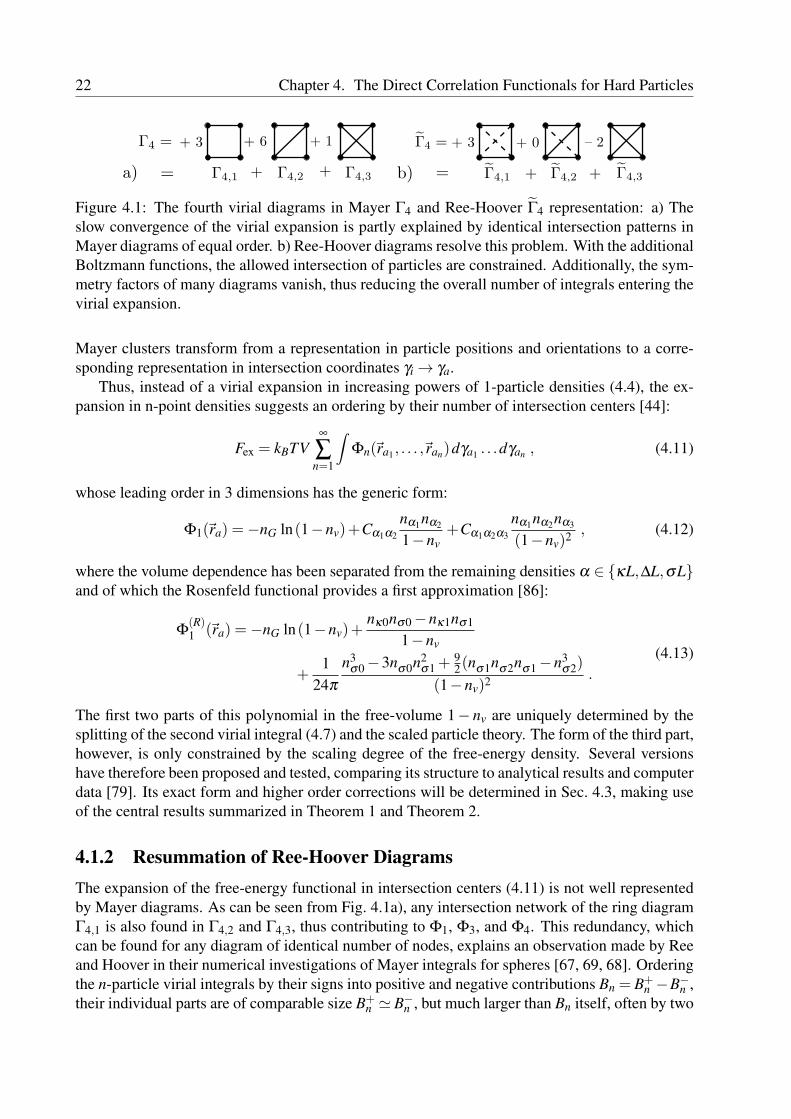
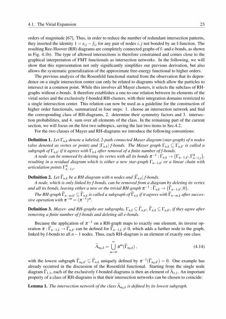
Figure 4.1: The fourth virial diagrams in Mayer Γ4 and Ree-Hoover Γ4 representation: a) Theslow convergence of the virial expansion is partly explained by identical intersection patterns inMayer diagrams of equal order. b) Ree-Hoover diagrams resolve this problem. With the additionalBoltzmann functions, the allowed intersection of particles are constrained. Additionally, the sym-metry factors of many diagrams vanish, thus reducing the overall number of integrals entering thevirial expansion.
Mayer clusters transform from a representation in particle positions and orientations to a corre-sponding representation in intersection coordinates γi→ γa.
Thus, instead of a virial expansion in increasing powers of 1-particle densities (4.4), the ex-pansion in n-point densities suggests an ordering by their number of intersection centers [44]:
Fex = kBTV∞
∑n=1
∫Φn(~ra1, . . . ,~ran)dγa1 . . .dγan , (4.11)
whose leading order in 3 dimensions has the generic form:
Φ1(~ra) =−nG ln(1−nv)+Cα1α2
nα1nα2
1−nv+Cα1α2α3
nα1nα2nα3
(1−nv)2 , (4.12)
where the volume dependence has been separated from the remaining densities α ∈ κL,∆L,σLand of which the Rosenfeld functional provides a first approximation [86]:
Φ(R)1 (~ra) =−nG ln(1−nv)+
nκ0nσ0−nκ1nσ1
1−nv
+1
24π
n3σ0−3n
σ0n2σ1 +
92(nσ1n
σ2nσ1−n3
σ2)
(1−nv)2 .
(4.13)
The first two parts of this polynomial in the free-volume 1− nv are uniquely determined by thesplitting of the second virial integral (4.7) and the scaled particle theory. The form of the third part,however, is only constrained by the scaling degree of the free-energy density. Several versionshave therefore been proposed and tested, comparing its structure to analytical results and computerdata [79]. Its exact form and higher order corrections will be determined in Sec. 4.3, making useof the central results summarized in Theorem 1 and Theorem 2.
4.1.2 Resummation of Ree-Hoover DiagramsThe expansion of the free-energy functional in intersection centers (4.11) is not well representedby Mayer diagrams. As can be seen from Fig. 4.1a), any intersection network of the ring diagramΓ4,1 is also found in Γ4,2 and Γ4,3, thus contributing to Φ1, Φ3, and Φ4. This redundancy, whichcan be found for any diagram of identical number of nodes, explains an observation made by Reeand Hoover in their numerical investigations of Mayer integrals for spheres [67, 69, 68]. Orderingthe n-particle virial integrals by their signs into positive and negative contributions Bn = B+
n −B−n ,their individual parts are of comparable size B+
n ' B−n , but much larger than Bn itself, often by two
4.1. The Virial Expansion 23
orders of magnitude [67]. Thus, in order to reduce the number of redundant intersection patterns,they inserted the identity 1 = ei j− fi j for any pair of nodes i, j not bonded by an f-function. Theresulting Ree-Hoover (RH) diagrams are completely connected graphs of f- and e-bonds, as shownin Fig. 4.1b). The type of allowed intersections is therefore constrained and comes close to thegraphical interpretation of FMT functionals as intersection networks. In the following, we willshow that this representation not only significantly simplifies our previous derivation, but alsoallows the systematic generalization of the approximate free-energy functional to higher orders.
The previous analysis of the Rosenfeld functional started from the observation that its depen-dence on a single intersection center can only be related to diagrams which allow the particles tointersect in a common point. While this involves all Mayer clusters, it selects the subclass of RH-graphs without e-bonds. It therefore establishes a one-to-one relation between its elements of thevirial series and the exclusively f-bonded RH-clusters, with their integration domains restricted toa single intersection center. This relation can now be used as a guideline for the construction ofhigher order functionals, summarized in four steps: 1. choose an intersection network and findthe corresponding class of RH-diagrams, 2. determine their symmetry factors and 3. intersec-tion probabilities, and 4. sum over all elements of the class. In the remaining part of the currentsection, we will focus on the first two subtopics, saving the last two items to Sec.4.2.
For the two classes of Mayer and RH-diagrams we introduce the following conventions:
Definition 1. Let Γn,k denote a labeled, 2-path connected Mayer diagram (star-graph) of n nodes(also denoted as vertex or point) and |Γn,k| f-bonds. The Mayer graph Γn,k ⊆ Γn,k′ is called asubgraph of Γn,k′ if it agrees with Γn,k after removal of a finite number of f-bonds.
A node can be removed by deleting its vertex with all its bonds π−1 : Γn,k→Γn−1,k′,ΓAn−1,t,
resulting in a residual diagram which is either a new star-graph Γn−1,k′ or a linear chain witharticulation points ΓA
n−1,t .
Definition 2. Let Γn,k be a RH-diagram with n nodes and |Γn,k| f-bonds.A node, which is only linked by f-bonds, can be removed from a diagram by deleting its vertex
and all its bonds, leaving either a new or the trivial RH-graph π−1 : Γn,k→Γn−1,k′,0.The RH-graph Γn−m,k′ ⊆ Γn,k is called a subgraph of Γn,k if it agrees with Γn−m,k after succes-
sive operation with π−m = (π−1)m.
Definition 3. Mayer- and RH-graphs are subgraphs, Γn,k ⊆ Γn,k′ , Γn,k ⊆ Γn,k′ , if they agree afterremoving a finite number of f-bonds and deleting all e-bonds.
Because the application of π−1 on a RH-graph maps to exactly one element, its inverse op-eration π : Γn−1,k → Γn,k′ can be defined for Γn−1,k 6= 0, which adds a further node to the graph,linked by f-bonds to all n−1 nodes. Thus, each RH-diagram is an element of exactly one class
Λn0,k =∞⋃
m=0
πm(Γn0,k) , (4.14)
with the lowest subgraph Γn0,k′ ⊆ Γn,k uniquely defined by π−1(Γn0,k′) = 0. One example hasalready occurred in the discussion of the Rosenfeld functional. Starting from the single nodediagram Γ1,1, each of the exclusively f-bonded diagrams is then an element of Λ1,1. An importantproperty of a class of RH-diagrams is that their intersection networks can be chosen to coincide:
Lemma 1. The intersection network of the class Λn0,k is defined by its lowest subgraph.
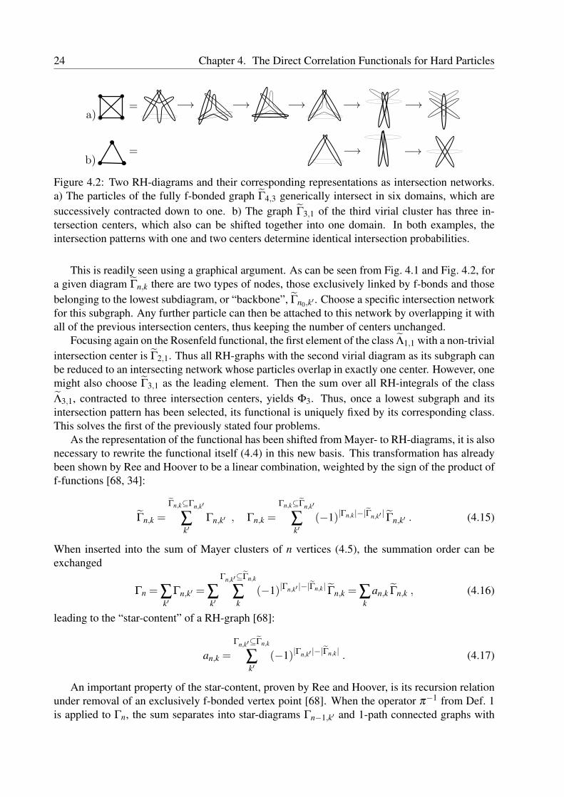
24 Chapter 4. The Direct Correlation Functionals for Hard Particles
Figure 4.2: Two RH-diagrams and their corresponding representations as intersection networks.a) The particles of the fully f-bonded graph Γ4,3 generically intersect in six domains, which aresuccessively contracted down to one. b) The graph Γ3,1 of the third virial cluster has three in-tersection centers, which also can be shifted together into one domain. In both examples, theintersection patterns with one and two centers determine identical intersection probabilities.
This is readily seen using a graphical argument. As can be seen from Fig. 4.1 and Fig. 4.2, fora given diagram Γn,k there are two types of nodes, those exclusively linked by f-bonds and thosebelonging to the lowest subdiagram, or “backbone”, Γn0,k′ . Choose a specific intersection networkfor this subgraph. Any further particle can then be attached to this network by overlapping it withall of the previous intersection centers, thus keeping the number of centers unchanged.
Focusing again on the Rosenfeld functional, the first element of the class Λ1,1 with a non-trivialintersection center is Γ2,1. Thus all RH-graphs with the second virial diagram as its subgraph canbe reduced to an intersecting network whose particles overlap in exactly one center. However, onemight also choose Γ3,1 as the leading element. Then the sum over all RH-integrals of the classΛ3,1, contracted to three intersection centers, yields Φ3. Thus, once a lowest subgraph and itsintersection pattern has been selected, its functional is uniquely fixed by its corresponding class.This solves the first of the previously stated four problems.
As the representation of the functional has been shifted from Mayer- to RH-diagrams, it is alsonecessary to rewrite the functional itself (4.4) in this new basis. This transformation has alreadybeen shown by Ree and Hoover to be a linear combination, weighted by the sign of the product off-functions [68, 34]:
Γn,k =
Γn,k⊆Γn,k′
∑k′
Γn,k′ , Γn,k =
Γn,k⊆Γn,k′
∑k′
(−1)|Γn,k|−|Γn,k′ | Γn,k′ . (4.15)
When inserted into the sum of Mayer clusters of n vertices (4.5), the summation order can beexchanged
Γn = ∑k′
Γn,k′ = ∑k′
Γn,k′⊆Γn,k
∑k
(−1)|Γn,k′ |−|Γn,k| Γn,k = ∑k
an,k Γn,k , (4.16)
leading to the “star-content” of a RH-graph [68]:
an,k =
Γn,k′⊆Γn,k
∑k′
(−1)|Γn,k′ |−|Γn,k| . (4.17)
An important property of the star-content, proven by Ree and Hoover, is its recursion relationunder removal of an exclusively f-bonded vertex point [68]. When the operator π−1 from Def. 1is applied to Γn, the sum separates into star-diagrams Γn−1,k′ and 1-path connected graphs with
4.1. The Virial Expansion 25
articulation points ΓAn−1,t , each weighted by their sign of f-numbers in order to avoid overcounting
of contributions:
π−1(Γn) = ∑
k
Γn−1,k′⊂Γn,k
∑k′
(−1)|Γn,k|−|Γn−1,k′ |Γn−1,k′
+∑k
ΓAn−1,t⊂Γn,k
∑t
(−1)|Γn,k|−|ΓAn−1,t |ΓA
n−1,t .
(4.18)
Focusing on the first part, the order of summation can be exchanged, resulting in a sum overthose Γn,k-graphs, which lead to the same Γn−1,k′ diagram after the removal of a node. If this nodeis linked by m bonds, these bonds can be distributed in (n− 1)!/(m!(n−m)!) ways among theresidual n− 1 vertex points, each weighted by a sign-factor of (−1)m. The first sum thereforesimplifies to:
∑k′
Γn,k⊃Γn−1,k′
∑k
(−1)|Γn,k|−|Γn−1,k′ |Γn−1,k′ = ∑k′
n−1
∑m=2
(n−1
m
)(−1)m
Γn−1,k′
= (n−2)Γn−1 .
(4.19)
The second part is a sum over Γn,k and its 1-path connected subgraphs ΓAn−1,t . Again, the order
of summation can be exchanged, resulting in a weighted sum over all permutations of 0 ≤ m ≤n−1 bonds linked to the residual n−1 nodes. In order to perform this sum, observe that a 1-pathconnected diagram is a linear chain of star-graphs, connected by articulation points, here indicatedby ′∗′:
ΓAn−1,t = Γn1,k1 ∗Γn2,k2 ∗ . . .∗Γnp,kp , (4.20)
with n−1 = n1+n2+ . . .+np nodes. Any partition of m bonds between the vertex Pn, which is tobe removed from Γn,k, and the non-articulation points can now be compensated by a copy of thissame diagram with an additional bond between Pn and one of the articulation points. Having thesame subgraph but differing by one f-bond, the two diagrams cancel each other in Eq. (4.18). Thesum therefore decouples into the partition of bonds on non-articulation vertices and articulationones. The flanking graphs Γn1,k1 , Γnp,kp are each joined by one articulation point, while the centerones carry two. Their individual contributions to the weighted sum are therefore
ni−2
∑m=0
(ni−2
m
)(−1)m = 0 ,
ni−1
∑m=1
(ni−1
m
)(−1)m =−1 (4.21)
yielding an overall factor of (−1)2 = 1 and leaving a sum over all permutations of bonds betweenthe articulation points and Pn:
∑t
Γn,k⊃Γn−1,t
∑k
(−1)|Γn,k|−|Γn−1,t |Γn−1,t = ∑k
p−1
∑m=0
(p−1
m
)(−1)m
Γn−1,t = 0 . (4.22)
Combining the two results (4.19), (4.22), the total sum of (4.18) reduces to the recursion relationof Ree and Hoover [68]:
π−1(Γn) = (n−2)Γn−1 . (4.23)
26 Chapter 4. The Direct Correlation Functionals for Hard Particles
An analogous relation can be derived for RH-diagrams, inserting the recursion relation into(4.16) and observing that π−1 removes n−1 f-bonds from a RH-diagram Γn,k:
π−1(Γn) = ∑
kπ−1(an,k Γn,k) = (−1)n−1
∑k
an,k Γn−1,k
= (n−2)Γn−1 = (n−2)∑k′
an−1,k′ Γn−1,k′ .(4.24)
Comparing terms, the resulting recursion relation is again independent of k:
an,k = (−1)n−1(n−2)an−1,k′ (4.25)
and by repeated application yields the star-content [68]:
an,k = (−1)(n2)−(
m2)(n−2)!(m−2)!
am,k′ . (4.26)
Thus, once it has been calculated for the lowest diagram of a class Λn0,k, the coefficients for allfurther graphs are known.
So far, we have focused on labeled graphs, ignoring that the physical particles in the parti-tion function are indistinguishable. Transferring to unlabeled RH-diagrams therefore introducesan additional sum over all inequivalent permutations of the labels on the vertex points. For itsderivation the e-bonds can be ignored, as they do not change the graph’s symmetry, yielding the“symmetry factor” σn,k already known from Mayer clusters. In combination with the star-content,we define the combinatorial prefactor of the virial clusters in RH-graphs:
σn,k =−1n!
σn,k an,k , (4.27)
where the additional factor 1/n! has been inserted for later convenience. The last step in provingthe resummability of cluster integrals for a given class Λn0,k therefore requires the derivation of arecursion relation for σn,k.
The symmetry factor counts the number of inequivalent labelings of a RH- or Mayer graphΓn,k under the permutation group Sn. Its group elements operate on the product of f-functions,which define a representation space by λ : Γn,k→ prod( fi j) and are symmetric under exchange ofpositions and indices:
γ := fi j = f ji, fi j fkl = fkl fi j , γ λ (Γn,k) = λ (Γn,k) . (4.28)
The group of equivalent labelings is then the automorphism group of its diagram and a subset ofthe symmetric group Sn
Aut(Γn,k) = g ∈ Sn | gλ (Γn,k) = γ λ (Γn,k) (4.29)
subject to the invariance relation γ−1 g = id. Correspondingly, the set of inequivalent labelingsis generated by the coset Sn/Aut(Γn,k), whose number of elements is the symmetry factor of thegraph
σn,k =|Sn|
|Aut(Γn,k)|. (4.30)
An extensive list of Mayer diagrams and their automorphism groups has been tabulated by Uhlen-beck and Riddell [89, 73].
In general, determining the automorphism group of a given graph is non-trivial. However, if itis known for the lowest element of a class Λn0,k, the groups of all further diagrams are known:
4.1. The Virial Expansion 27
Lemma 2. Let Γn,k ∈ Λn0,k with lowest element Γn0,k. Its automorphism group then factorizes intothe direct product:
Aut(Γn,k) = Sn−n0×Aut(Γn0,k) . (4.31)
The proof is as follows: Because Γn0,k is the lowest element of the class, π−1Γn0,k = 0, eachvertex is connected to at least one e-bond, whereas the remaining n− n0 nodes are only linkedby f-bonds. Shifting an f-bonded label to a vertex with an e-bond would therefore result in aninequivalently labeled diagram. Thus, f-bonded nodes can only be permuted under themselves bySn−n0 , completing the proof.
With the recursion relation for the star content (4.26) and the dimension of the automorphismgroup
|Aut(Γn,k)|= (n−n0)! |Aut(Γn0,k)| , (4.32)
the RH-diagrams of a given class have the symmetry factor:
Lemma 3. Let Γn,k be an element of the class Λn0,k of RH-graphs with lowest element Γn0,k. Itssymmetry factor is then:
σn,k =−(−1)(n2)−(
n02 )(
n−2n0−2
)an0,k
|Aut(Γn0,k)|: n0 ≥ 3
σn,k = (−1)(n2)
1n(n−1)
: n0 = 1(4.33)
The case n0 ≥ 3 follows from the previous calculations. But n0 = 1 and n0 = 2 have to beconsidered separately, because the recursion relation (4.26) only applies to n0 ≥ 2, while (4.31)requires Γn0,k to be the lowest element of the class. Observing that Γ1,1 = π−1(Γ2,1) and a2,1 =a1,1 = 1 closes the proof.
It is instructive to derive the symmetry factors for the diagrams of Fig. 4.1. Γ4,3 is a fully f-bonded graph and therefore belongs to Λ1,1, already covered by (4.33). The next diagram Γ4,2 hasstar-content a4,2(|)= 0. Thus, all graphs with a single e-bond drop out of the virial series σn(|)= 0.Actually, the same applies to roughly half of the RH-diagrams, improving the convergence ofthe virial expansion. The final example Γ4,1 has two separate e-bonds, star-content a4,1(||) = 1,and cyclic permutation symmetry Aut(Γ4,1) = Z4×Z2. The prefactors of all related graphs aretherefore
σn(||) = (−1)(n2)
116
(n−2)(n−3) . (4.34)
Eq. (4.33) solves the second of the four problems stated at the beginning of this section andalso holds the solution to the fourth one. As has been shown before in 3 dimensions [44], the inter-section probability of a network of overlapping particles decouples into a convolute of curvatureforms Kn(~ra) for each intersection center with n particles. This observation is sufficient to writedown a generic functional for a given intersection network and RH-class:
Theorem 1. Let Γn0,k be the lowest element of the class Λn0,k. The free-energy functional of anetwork with p≥ 1 intersection centers is then determined by
Φ1(Γ1,1|~ra) = ∑n≥2
1n(n−1)
∫Kn(~ra,γi)ρ(γ1) . . .ρ(γn)dγ1 . . .dγn (4.35)
28 Chapter 4. The Direct Correlation Functionals for Hard Particles
for n0 = 1, while higher order functionals for n0 > 3 are derived by
Φp(Γn0,k|~ra1, . . . ,~rap) =−(−1)(n02 )
an0,k
|Aut(Γn0,k)|∑
n≥n0
(n−2n0−2
)×∫
Kn1(~ra1,γi1) . . .Knp(~rap,γip)ρ(γ1) . . .ρ(γn)dγ1 . . .dγn
(4.36)
with the integral kernel Kn j(~ra,γi) determining the intersection probability of n j particles whichintersect in~ra and with particle positions γi for i = 1, . . . ,n j.
The first half of the proof determines the numerical prefactor, combining the symmetry factorof (4.33) and the sign of f-bonds (−1)|Γn,k|, which is not accounted for by the intersection forms.It partially cancels with the sign of σn,k using
|Γn,k|= |Γn0,k|+(
n2
)−(
n0
2
), (4.37)
leaving a constant only depending on the lowest element of Λn0,k and an n-dependent binomialcoefficient. The second half of the proof deals with the factorization of the intersection probabilityinto integral kernels, which will be the topic of the next section. There it will also be shown, howto generalize the functionals to e-bonds and mixtures of particles.
4.2 Intersection Probability in N DimensionsIn this section we complete the proof of Theorem 1, determining the intersection probability fornetworks of overlapping particles. First, the basic idea of integral geometry is summarized, de-termining the intersection probability of clusters of particles with one intersection center which isthen generalized to networks of clusters.
Integral geometry determines the intersection probability between manifolds under transla-tions and rotations with respect to their imbedding space. It has a long history [82, 84], but itsmodern representation has been founded by Blaschke and Santalo, and further generalized byChern to n dimensions using differential forms [15, 16, 17]. Chern also explained the connec-tion between the kinematic measure and the Euler form, determining the Blaschke-Santalo-Chernequation for two intersecting manifolds [15, 82]. Up to a sign, this result coincides with Rosen-feld’s decoupling of the second virial integral (4.7). Using this approach, we calculated the inter-section probability for an arbitrary set of particles overlapping in a common domain, rederivingthe Rosenfeld functional for 3 dimensions. This calculation will be simplified in the followingand extended to arbitrary dimension n.
For now, let Σk be a set of identical, n−1 dimensional, smooth, orientable, compact, boundaryfree, Riemannian manifolds with particle index k = 1, . . . ,N, imbedded into Dk : Σk → Rn. Forphysical reasons we will further assume that the particles Dk only have cavities that are accessibleto all other particles. Each domain is then covered by coordinate patches with an orthonormal,positively oriented coordinate frame (e(k)1 , . . . , e(k)n ) at each point p ∈ Dk, with the normal vectore(k)n pointing into the outside direction of the surface Σk = ∂Dk. Being a differential manifold, thegeometry of Σ and D is represented by vielbein and connection forms
θi = eid p , ωi j = eide j for i, j = 1, . . . ,n , (4.38)
4.2. Intersection Probability in N Dimensions 29
and the intrinsic forms of torsion and curvature
Ti = dθi−ωi j∧θ j , Ωi j = dωi j−ωik∧ωk j , (4.39)
with the torsion Ti = 0 vanishing for a Riemannian manifold. Here and in the following weimplicitly assume a sum over pairs of identical indices. Coordinate frames of different patches areconnected by gi j ∈ SO(n), transforming vectors e′i = gi j e j and differential forms
θ′i = gi jθ j , ω
′i j = g−1
ik ωklgl j +g−1ik dgk j , Ω
′i j = g−1
ik Ωklgl j . (4.40)
Each Riemannian manifold also defines a semisimple group [29], which for the imbeddingspace Rn is the isometric or Euclidean group ISO(n) = SO(n)nRn. Its Lie algebra iso(n) has arepresentation in the vielbein and connection forms generating translations and rotations(
ωi j θi−θ j 0
)∈ iso(n) (4.41)
and whose volume form, or Haar measure, is the “kinematic measure”
K(Rn) =∧
1≤i< j≤n
ωi j∧
1≤i≤n
θi . (4.42)
An alternative interpretation uses the representation as a chain of cosets
SO(k)/SO(k−1) = Sk−1 , vol(Sk−1) = 2πk/2/Γ(k/2) , (4.43)
with the Gamma function Γ, which allows to rewrite products of connection forms into integralmeasures of spheres
dSk−1 = ω1,k∧ . . .∧ωk−1,k . (4.44)
With a particle D imbedded, the vector space of Rn splits into the tangential T Σ and normalspace NΣ along with a similar decoupling of the rotation group into SO(n− 1) and the cosetSO(n)/SO(n−1). The kinematic measure (4.42) separates correspondingly into the three parts
K(∂D) =n−1∧α=1
ωα n
n∧i=1
θi ∧ dvol(SO(n−1)) (4.45)
of the curvature (also Euler or highest Chern-Simons) form, the measure of translations, and thevolume form of SO(n−1).
This result readily generalizes to two and more overlapping domains which intersect in at leasta common point. Introducing the notation for identical particles
Σk1 ∩Dk2 := Σ∩ . . .∩Σ︸ ︷︷ ︸
k1-fold
∩D∩ . . .∩D︸ ︷︷ ︸k2-fold
, (4.46)
the intersection Dm is again a n dimensional subset of Rn and therefore applies to the reducedform of the kinematic measure (4.45). When inserted, K(∂Dm), the boundary of the intersectiondomain can be expanded in the series
∂Dm =k≤n
∑1≤k≤m
(mk
)Σ
k∩Dm−k , (4.47)
setting all terms Σk for k ≥ n+ 1 to zero. This restriction of the sum is a useful consequence ofthe following rules of K:
30 Chapter 4. The Direct Correlation Functionals for Hard Particles
Lemma 4. Let D be a domain in Rn with hypersurface Σ. The kinematic measure K of intersectingmanifolds then has the properties:
K(a1Σ1 +a2Σ2) = a1K(Σ1)+a2K(Σ2) (4.48)
K(Σk1 ∩Dk2) = K(Σk1)∧K(D)k2 (4.49)
K(Σ1∩Σ2) = K(Σ2∩Σ1) (4.50)
K(Σk) = 0 for k ≥ n+1 (4.51)
for Σ1∩Σ2 = 0 and the constants a1,a2 ∈ N:
The proof: By construction, the differential form (4.42) is a locally defined probability mea-sure, which decouples for Σ1 ∩Σ2 = 0, thus showing (4.48). The second identity follows fromthe observation that the kinematic measure of a point pt ∈ Rn moving in the domain D is trivialK(pt∩D) = K(D). Setting pt ∈ Σk1 ∩Dk2−1 then proves (4.49) by iteration. While the local mea-sure and set theoretic relation Σ1∩Σ2 = Σ2∩Σ1 explains (4.50). The last equation (4.51), whichjustifies the finite sum (4.47), implies that the intersection probability between a point pt ∈ Σn anda hypersurface Σ is of measure zero. This follows from K being defined on the tangential spaceof Σk, spanned by the normal and tangential vectors (e(1)n , . . . , e(k)n , e1, . . . , en−k), proving that thecoordinate basis is not defined for k ≥ n+1 and therefore vanishes for dimensional reasons.
Applying these rules to the boundary of intersections (4.47), yields the sum
K(∂Dm) =k≤n
∑1≤k≤m
(mk
)K(Σk)∧K(D)m−k , (4.52)
with K(D) and the curvature forms K(Σk) decoupled. For m = 1 this reproduces (4.45). But toderive the remaining differential forms we need an explicit representation of the orthonormal andpositively oriented vector field at Σk. For simplicity, let us define a fixed ordering of surfacesΣ1∩ . . .∩Σk. The vector
(e(1)n , . . . , e(k)n , e1, . . . , en−k) ∈ T Dk (4.53)
of the tangential space T Dk then defines a coordinate frame at the intersection, spanned by the koutward pointing normal vectors and the n−k tangential directions which can be chosen by (4.40)to coincide for all surfaces. This frame, however, is neither orthonormal nor positively orientated.
The Gram-Schmidt transformation turns this vector frame into an orthonormal basis
vA =
Babe(b)n for a,b = 1, . . . ,k
eα for α = 1, . . . ,n− k(4.54)
whose upper triangular matrix Bab ∈ Gl(k,R) combines into the general coordinate mapping:
BAB =
(Bab 00 1αβ
). (4.55)
The coordinate frames of individual surfaces are now related by a rotation of the normal vectors
ηA =
Gabvb for a,b = 1, . . . ,k
vα for α = 1, . . . ,n− k(4.56)
4.2. Intersection Probability in N Dimensions 31
generated by Gab ∈ SO(k,R) and extended to the matrix representation
GAB =
(Gab 0
0 1αβ
). (4.57)
Combining both transformations, the connection forms ηAB = ηAdηB at an intersection point canbe written in the basis of the tangential ωαβ and normal directions ω
(a)βn of the coordinate frames
of Σa keeping the normal vector de(a)n = 0 constant
ηAB =
ηab = G−1
ac dGcb
ηaβ = Gab Bbc ω(c)βn
ηαβ = ωαβ
. (4.58)
The curvature form, which generalizes (4.45) to the intersection space Σk, is the product ofconnection forms with one axial direction fixed. Let us choose ηk as the new normal vector,leaving Gak to be an element of the coset space SO(k)/SO(k−1) = Sk−1
n−k∧β=1
ηβk
k−1∧a=1
ηak = (n−k∧β=1
GkaBab ω(b)βn )(
k−1∧a=1
G−1ab dGbk)
= Pf n−k1,...,k(GBω)∧dvolG(Sk−1) ,
(4.59)
introducing the notation Pf n−k1,...,k for the Pfaffian of an n− k-form on the ordered set of surfaces
Σ1∩ . . .∩Σk.In the derivation of (4.59) we ignored the orientation of the coordinate frame of T Σk which is
not fixed by the Gram-Schmidt process. However, changing the orientation, e.g. by permuting theorder of the particles in (4.54), changes the sign of (4.59) by (−1)n−1. For n odd, this poses noproblem. For n even, however, the orientation of the vector frame is relevant and has to be chosenpositively orientated to ensure a positive surface form. This uniquely defines the intersection formKm introduces in Theorem 1:
Theorem 2. Let Di1 ∩ . . .∩Dim be a set of n-dimensional domains overlapping in the commonintersection point~ra ∈ Dm and assigned with a positively orientated coordinate frame. Denote by|Sk−1| the volume of the Sk−1 sphere and by Θ(D) the step function confining the integral measureto the volume of D. Then the integral kernel of the functionals (4.35) and (4.36) has the form:
Ki1...im(~ra,γi) =1|Sn−1|
k≤n
∑1≤k≤m
(mk
)∫G∈Sk−1
Pf(GBω)n−ki1...ik ∧dvolG(Sk−1)
×Θ(Dik+1) . . .Θ(Dim) ,
(4.60)
with an integration over the inner area of the Euler sphere Sk−1.
This result follows from inserting the curvature form (4.59) into the kinematic measure (4.52)and observing that the vectors~ra are already determined by the coordinates γi of the 1-particledensities. The integration over γi therefore shifts part of the kinematic measure into the definitionof the functionals (4.35) and (4.36) and leaves the integral kernel with the step functions Θ(D) and
32 Chapter 4. The Direct Correlation Functionals for Hard Particles
the differential form Pf(GBω)n−k. Finally, the normalization |Sn−1| has been added to compensatethe volume form introduced by (4.59).
The curvature form (4.60) defines the integral kernel for one intersection center. To generalizethis result to arbitrary networks of overlapping particles, let us introduce the following notation:
Definition 4. Networks of intersecting particle domains are represented by products of γi1...ima for
each intersection center~ra ∈ Di1 ∩ . . .∩Dim of the intersecting domains Di1, . . . ,Dim .
When applied to the third virial cluster, shown in Fig. 4.2b), the generic diagram Γ3,1 is anintersection network of pairwise overlapping domains, which can be successively contracted fromthree centers into networks of two and one
γi1i2a γ
i2i3b γ
i1i3c → γ
i1i2i3a γ
i1i3c → γ
i1i2i3a . (4.61)
While Γ4,3 has the generic network of six centers, with consecutive contraction into five to oneintersection domains, as shown in Fig. 4.2a)
γi1i2a γ
i2i3b γ
i3i1c γ
i1i4d γ
i2i4e γ
i3i4f → γ
i1i2i4a γ
i2i3b γ
i3i1c γ
i2i4e γ
i3i4f → γ
i1i2i4a γ
i2i3i4b γ
i3i1c γ
i3i4f
→ γi1i2i4a γ
i2i3i4b γ
i1i3i4c → γ
i1i2i3i4a γ
i1i3i4c → γ
i1i2i3i4a .
(4.62)
This notation for intersection networks readily translates to the integral kernel:
Lemma 5. Let γ ia and γ
jb denote intersection clusters at centers ~ra and ~rb with particle indices
i = i1, . . . , ip and j = j1, . . . , jq. And let ek1k2 denote a Boltzmann function with arbitraryparticle indices k1,k2. Introducing the notation K(γ i1...im
a ) = Ki1...im(~ra) for the intersection formK, the integral kernel for intersection networks is a linear and multiplicative operator
K(γ ia + γ
jb) = Ki(~ra)+K j(~rb) (4.63)
K(γ iaγ
jb) = Ki(~ra)K j(~rb) (4.64)
K(γ iaek1k2) = Ki(~ra)ek1k2 . (4.65)
The first identity (4.63) is a generalization of (4.48), while the product structure (4.64) isa consequence of the properties of f-bonds, whose intersection centers overlap independently.Boltzmann functions, however, do not contribute to the curvature form, but define constraints onthe integration domain, justifying (4.65).
Less trivial, however, is the meaning of the indices. In γi1...ipa , each index ik ∈ i points to
an individual domain Dik of the ik = 1, . . . ,N particles, while the same index in Ki1...ip points tothe compound ik = 1, . . . ,M represented by the 1-particle density ρik . This change of meaningis a consequence of the thermodynamic limit introduced in Sec. 4.1.1 and corresponds to thesubstitution
Dk→M
∑ik=1
Dikρik . (4.66)
When inserted into the kinematic measure (4.52), the combinatorial prefactors remain unchanged,while the differential forms are weighted by the density functions. Thus each particle index has tobe paired by a corresponding density function:
M
∑i1,i2,i3=1
K(γ i1i2a γ
i2i3b γ
i3i1c )ρi1ρi2ρi3 . (4.67)
4.2. Intersection Probability in N Dimensions 33
The generalization to mixtures completes the proof of Theorem 1. And together with theintegral kernel (4.60) and its algebraic structure, we have the necessary tools to systematicallyderive the density functional for any given class of intersection diagrams. However, to do soefficiently, let us introduce some further notation. First observe that for any k, the curvature form(4.59) can be written as a volume form
Pf(GBω)n−ki1...ik = det(GBh)i1...ik
n−k∧α=1
θα
=∫Rn[J det(GBh)]i1...ikδ (Σi1) . . .δ (Σik)
n∧i=1
θi ,
(4.68)
introducing the curvature matrix ωα,n = hαβ θβ and the delta-function δ (Σ), which projects theintegration domain from Rn to the tangential space of the surface Σ. Correspondingly, products ofdelta-functions project to the intersection space Σi1 ∩ . . .∩Σik associated with the Jacobi determi-nant
Ji1...ik = det(e1, . . . , en−k, e(i1)n , . . . , e(ik)n ) . (4.69)
This transformation allows to factor out the overall volume form and to rewrite the integralkernel (4.60) as the derivative of a generating function:
Lemma 6. Define the weight functions for k = 1, . . . ,n intersecting surfaces
wi1...ikk =
1|Sn−1|
∫G∈Sk−1
[J det(GBh)]i1...ikdvolG(Sk−1)δ (Σi1) . . .δ (Σik) (4.70)
and the weight function for the domain
wi10 = Θ(Di1) . (4.71)
The integral kernel (4.60) of the intersection form is then the functional derivative of the productof w0-weights:
K(γ i1...ima ) = Da wi1
0 (~rai1) . . .wim0 (~raim) , (4.72)
with the derivative on the weight functions at intersection~rai =~ra−~ri defined by
Da =n
∑k=1
∑i1...ik
1k!
wi1...ikk (~rai1, . . .~raik)
δ k
δwi10 (~rai1) . . .δwik
0 (~raik), (4.73)
operating on two and more w0-weight functions.
To simplify the notation for the functional derivative and its corresponding contraction
δ
δwi0(~rai)
w j0(~rb j) = δ (~ri−~r j)δ (~ra−~rb) ,
∫w j
0(~r ja)δ (~ri−~r j)dγ j = wi0(~ria) , (4.74)
we introduced the Kronecker delta-functional in the definition of (4.73), which transforms theoperations
δ
δwi0(~rbi)
w j0(~ra j) =: δ
ji δ
ba , ∑
jδ
ijw
j0(~ra j) = wi
0(~rai) , (4.75)
34 Chapter 4. The Direct Correlation Functionals for Hard Particles
into a tensor-like representation. The proof of (4.72) then reduces to the derivation of a conven-tional polynomial, whose coefficients coincide with those of (4.60).
Less trivial, however, is the observation that the curvature form (4.68) and therefore the weightfunctions are symmetric in the particle indices. This is a consequence of the coupled coordinatesystem of T Σk, which can be diagonalized using the SO(n− k)× SO(k) invariance of its vec-tor basis. Its explicit calculation gives no further insight and therefore is postponed to App. B,completing the proof of Theorem 2.
The derivative (4.73), which is a consequence of (4.47), simplifies the construction of a func-tional in two aspects: first, it hides the sum over the k = 1, . . . ,n differential forms in the inter-section kernel (4.60). Second, it leaves the volume weight wi
0 as the only variable in the sums of(4.35), (4.36). Thus each functional is the derivative of a generating function in the virial series ofwi
0. In combination with Theorem 1, this reveals that:
Lemma 7. The virial series of the free-energy functional for a finite number of intersection centersis convergent.
The proof is as follows: It is sufficient to show that the generating function is a convergentseries. If γ0 is the intersection diagram of the lowest element Γn0,k with p intersection centers.Then, the integral kernel of any higher order element πmΓn0,k decouples:∫
K(πmγ0)ρ
n0+m = (xa1...ap)m∫
K(γ0)ρn0 , (4.76)
with the density function defined by
xa1...ap =∫
wi0(~ra1i) . . .wi
0(~rapi)ρidγi . (4.77)
When inserted into the functionals (4.35), (4.36), the sum simplifies to a polynomial in x withsingularities in x = 1 and x = 0. However, the virial series is finite in the low-density limit andtherefore x = 0 a regular point. This leaves x = 1 as the only singularity. At thermodynamicequilibrium and with all intersection centers collapsed into a single point, the packing fractionapproaches η = 1, proving that the functional is convergent for η < 1.
This final result proves the resummability of the approximate density functional and solves thelast of the four problems presented at the beginning of Sec. 4.1.2.
4.3 The Rosenfeld Functional and Beyond
This last section presents four examples, which provide some insight into the construction offunctionals. We begin with the integral kernel for 3 dimensions and derive the functional withone intersection center. It is then shown that Rosenfeld’s result is an approximation for almostperpendicular normal vectors. The remaining examples then focus on the functionals with two,three, and four intersection centers.
Starting point for the construction of any functional is the derivation of the integral kernel. Thishas to be done once for any dimension and is independent of the particle geometry or boundaryconditions. For n = 3 dimensions, only three differential forms exist:
4.3. The Rosenfeld Functional and Beyond 35
The case k = 1 is elementary. With G = B = 1 and assuming a positively oriented orthonormalcoordinate frame, the Pfaffian reduces to the Euler form Pf2
i1(GBω) = ω(i1)13 ∧ω
(i1)23 and a trivial
integral over the S0-sphere ∫Pf2
i1(GBω)∧dvol(S0) = ω(i1)13 ∧ω
(i1)23 . (4.78)
For k = 2, the Gram-Schmidt scheme and SO(2) rotation have the matrix representation:
B =
1 0 0
−cos(φi1i2)
sin(φi1i2)
1sin(φi1i2)
0
0 0 1
, G =
cos(α) sin(α) 0−sin(α) cos(α) 0
0 0 1
φi1i2 = arccos(e(i1)3 e(i2)3 ) , 0≤ α ≤ φi1i2 ≤ 2π ,
(4.79)
depending on the intersection angle φi1i2 . The associate Pfaffian yields the 1-form:
Pf1i1i2(GBω) =
[cos(α)− cos(φi1i2)
sin(φi1i2)sin(α)
]ω
(i1)13 +
1sin(φi1i2)
sin(α)ω(i2)13 (4.80)
whose integral over α ∈ S1 simplifies to∫α∈S1
Pf1i1i2(GBω)∧dvolα(S1) =
1− cos(φi1i2)
sin(φi1i2)
[ω
(i1)13 +ω
(i2)13]. (4.81)
Finally, for k = 3 the integral over the curvature form (4.59) reduces to the area of the sphericaltriangle ∆⊆ S2
∫G∈S2
Pf0i1i2i3(GBω)∧dvolG(S2) = area(∆⊆ S2) = 2π−φ
i1i2i3−φ
i2i1i3−φ
i3i1i2 (4.82)
whose value is determined by the Euler or dihedral angles φi3i1i2 [31]:
φi1i2i3 = arccos(Ei2Ei3) , Ei1 =
e(i2)3 × e(i3)3
|e(i2)3 × e(i3)3 |. (4.83)
Comparing these results to the definition (4.70) and taking into account the permutation symmetryin the particle indices, we obtain the three weight functions:
wi11 =
14π
det(h(i1))δ (Σi1), wi1i22 =
12π
1− cos(φi1i2)
sin(φi1i2)[Jh12]
(i1)δ (Σi1)δ (Σi2)
wi1i2i33 =
14π
(2π−3φi1i2i3)Ji1i2i3δ (Σi1)δ (Σi2)δ (Σi3) .
(4.84)
These agree with the weight function wi1i22 first derived by Wertheim [92, 93] and rediscovered in
[25], while wi1i2i33 first occurred in [54].
36 Chapter 4. The Direct Correlation Functionals for Hard Particles
Next, we will illustrate the application of the derivative and generating function on the func-tional restricted to one intersection center Φ|1. It is therefore of type (4.35), and the virial seriessums up to the generating function in the x-variable (4.77) of the volume weight:
Φ|1(Γ1,1,~ra) =∫
∑m=2
1m(m−1)
K(γ i1...ima )ρi1 . . .ρim dγi1 . . .dγim
= Da
∫∑
m=2
1m(m−1)
wi10 (~ra) . . .w
im0 (~ra)ρi1 . . .ρim dγi1 . . .dγim
= Da ∑m=2
1m(m−1)
xma = Da[(1− xa) ln(1− xa)+ xa] .
(4.85)
Introducing the weight density
nk(~ra) =∫
wi1...ikk (~rai1, . . . ,~raik)ρi1(~ri1) . . .ρik(~rik)dγi1 . . .dγik , (4.86)
the derivative of the generating function yields the three terms
Φ|1(Γ1,1,~ra) =−n1 ln(1−n0)+12
n2
1−n0+
16
n3
(1−n0)2 (4.87)
whose structure is well known from the Rosenfeld functional (4.13). It is well established that theweight functions (4.8) derive from a Taylor expansion in the sin and cos terms of the intersectionangles. This has been shown before for n2 in [25, 26] and by using differential forms [44]. Forn3, however, we made an inconvenient choice of coordinates for ∆ ∈ S2 and give here a clearerargument. A more detailed discussion that also includes the zero-dimensional limit is presentedin App. C.
Let us introduce the notation ei := e(i)n for the i = 1,2,3 normal vectors of Σ1, Σ2, Σ3 andei j := eie j for their scalar product. Further assume that the three vectors approximately set up anorthonormal basis
e1 ≈ e2× e3 . (4.88)
The area of the spherical triangle is then ∆ ≈ π/2 with the Jacobi determinant J123 =det(e1, e2, e3)) ≈ 1 and Euler angles φ k
i j close to zero. Thus expanding the argument of arccosup to the 5’th order
z := E1E2 = (e23e13− e12)(1+12
e223)(1+
12
e313)+O(e5
i j) , (4.89)
yields the small-angle correction of ∆:
2π−3arccos(z) =π
2+3(z+
16
z3)+O(z5)
=π
2−3[e12− e23e13 +
12
e12(e223 + e2
13)+16
e312]+O(e4
i j)
(4.90)
where only e312 follows from order z3. Rewritten in the weight densities (4.8), n3 is to first order
in the Euler angle:
n3 =π
2n3
σ0−3nσ0n2σ1 +3[nσ1nσ2nσ1−nσ1nσ2nσ3]−
12
n2σ3nσ0 +O(e4
i jρ3). (4.91)
4.3. The Rosenfeld Functional and Beyond 37
The second term agrees with the Rosenfeld functional, while the prefactor of the third term is 4.5compared to our 3, which is acceptable given that the terms of (4.13) have been fitted to numericaldata. The fourth term disagrees, but is of lower order. More remarkably, the prefactor of thefirst term disagrees also. Choosing a different point of reference for the Taylor expansion can setthe coefficient of the leading term from π/2 to 0, but never to 1. Here, Tarazona’s term for the3-particle intersection is a better approximation [86], which also includes additional terms fromthe third order in z. For a more detailed discussion, we refer to App. C.
Our next example derives the functional for three intersection centers, whose lowest RH-diagram is Γ3,1, which belongs to the class Λ1,1. Its intersection diagram is the exact third virialcluster γ
i1i2a γ
i2i3b γ
i3i1c as shown in Fig. 4.2b). The next particle added to the triangle diagram has to
overlap with all three intersection centers, as illustrated by the fourth figure of Fig. 4.2a) and rep-resented by γ
i1i2i4a γ
i2i3i4b γ
i3i1i4c . Adding more particles includes copies of the last one, corresponding
to the intersection patternγ
i1i2i4...ima γ
i2i3i4...imb γ
i3i1i4...imc . (4.92)
To further simplify the notation, let us define wia := wi
0(~rai) for the volume weight at intersectioncenter~ra and particle position~ri. The functional (4.35) for the 3-center diagrams then factorizesinto weight densities of 2 and 3 centers:
∞
∑m=3
1m(m−1)
∫K(γ i1i2i4...im
a γi2i3i4...imb γ
i1i3i4...imc )ρi1 . . .ρim dγi1 . . .dγim
= DaDbDc
∞
∑m=3
1m(m−1)
∫(wi1
a wi1c ρi1)(w
i2a wi2
b ρi2)(wi3b wi3
c ρi3)
× (wi4a wi4
b wi4c ρi4) . . .(w
ima wim
b wimc ρim)dγi1 . . .dγim .
(4.93)
Introducing the x-densities of (4.77) and adding the second virial, we finally arrive at the functionalrestricted to three and less intersection centers:
Φ|3(Γ1,1,~ra,~rb,~rc) =12Dax2
a
+DaDbDc
[xabxbcxac
x3abc
((1− xabc) ln(1− xabc)+ xabc−
12
x2abc)]
.(4.94)
With three intersection centers, it is exact in the second and third virial order, but alsosignificantly more complex due to additional correlation and autocorrelation functions suchas wi4
1 (~ra)wi41 (~rb)w
i41 (~rc), which have been shown by Wertheim to be nontrivial to evaluate
[93, 94, 95].Nevertheless, Lemma 6 is an efficient tool to derive new functionals. To compare different
levels of approximation, let us summarize all cases of up to four intersection centers. With onecenter covered by (4.85), the next level is the 2-center approximation, beginning with the partiallycontracted third virial cluster, shown in Fig. 4.2b). All further intersection diagrams are then ofthe form:
γi1i2i3 i4...ima γ
i2i3 i4...imb . (4.95)
The case of three centers has already been covered by (4.92). This leaves the functional with fourintersection centers of the two RH-classes Γ4,1 and Γ4,3, while the star-content of Γ4,2 vanishes.

38 Chapter 4. The Direct Correlation Functionals for Hard Particles
The corresponding intersection graphs are:
γi1i2 i5...ima γ
i2i3 i5...imb γ
i3i4 i5...imc γ
i1i4 i5...imd ei1i3ei2i4
+ γi1i2a γ
i2i3 i4...imb γ
i1i3 i4...imc γ
i2i4...imd ,
(4.96)
with the Boltzmann functions ei j included. Determining their generating functions and adding thelower order virial terms, yields the complete list of functionals up to four intersection centers
Φ|1 = Da[(1− xa) ln(1− xa)+ xa]
Φ|2 =12Dax2
a +12DaDb
xa + xb
xab
[(1− xab) ln(1− xab)+ xab−
12
x2ab
]Φ|3 =
12Dax2
a +DaDbDcxabxbcxac
x3abc
[(1− xabc) ln(1− xabc)+ xabc−
12
x2abc
]Φ|4 =
12Dax2
a +16DaDbDcxabxbcxac (4.97)
+DaDbDcDdxacxbcxabd
x4bcd
[(1− xbcd) ln(1− xbcd)+ xbcd−
12
x2bcd−
16
x3bcd
]− 1
8DaDbDcDd
yab|cdyad|bc
(1− xabcd)3 ,
where we replaced xa → (xa + xb)/2 in Φ|2 to satisfy the diagram’s symmetry and defined theBoltzmann weighted density
yab|cd =∫(wi
awibρi)(w j
cw jdρ j)ei jdγidγ j . (4.98)
However, not all intersection networks result in different functionals. The probability measurefor two centers, e.g., is identical to the 1-center functional as the orientation and position of thefirst determines the coordinates of the second. Φ|1 and Φ|2 are therefore of the same order ofprecision. To go beyond the Rosenfeld functional one has to apply Φ|3, which reduces to Φ|1in the limit of coincident intersection centers ~rb,~rc →~ra. Further corrections can be added byallowing for the the e-bonded part of Φ|4, whose negative contribution compensates the tendencyof the fully f-bonded terms to overrate tightly packed particle configurations. As an improvedmodel we therefore propose
Φ =12Dax2
a +DaDbDcxabxbcxac
x3abc
[(1− xabc) ln(1− xabc)+ xabc−
12
x2abc
]− 1
8DaDbDcDd
yab|cdyad|bc
(1− xabcd)3
(4.99)
as a reasonable approximation, whose integrals can be evaluated by Wertheim’s application of theRadon transformation [93].
The formalism of Lemma 6 is not restricted to the free energy but applies to any thermody-namic object representable by Mayer or RH-graphs. As a final example, let us consider the leadingorder of the pair-correlation function g2. As has been shown for spheres in [68, 70], the domi-nating RH-graphs are again the fully f-bonded diagrams with two rooted points connected by ane-bond. The network with the lowest number of intersection centers is therefore
γi1 i3...ima γ
i2 i3...imb ei1i2 , (4.100)
4.3. The Rosenfeld Functional and Beyond 39
whose combinatorial prefactors have been shown in [70] to combine to 1. The sum over alldiagrams then yields g2 approximated by two intersection centers
gi1i2|2(~ri1,~ri2|~ra,~rb) = ei1i2
(1+DaDb
wi1a wi2
b1− xab
), (4.101)
without summation over the particle indices i1, i2. Higher order correlation functionals and theirapplication in perturbation theory will be considered in the next chapter.

40 Chapter 4. The Direct Correlation Functionals for Hard Particles
Chapter 5
The Distribution Functionals for HardParticles
The transformation between Mayer, Ree-Hoover, and intersection diagrams allows the derivationof any hard-particle functional that can be expanded in a virial series. In the current chapter, weuse this relationship to derive the remaining class of distribution functionals. In analogy to theprevious line of reasoning, Sec. 5.1 translates their virial expansion from rooted Mayer diagramsto rooted Ree-Hoover graphs, from which follows the generic distribution functional. Exampleswill be presented in Sec. 5.2, where the 2- and 3-particle distributions for up to four intersectioncenters are presented. We also compare the leading order of the contact probability of spheres tothe Wertheim, Thiele, and Baxter solution and conclude by deriving the perturbation expansion ofthe pair-correlation functional.
5.1 The Generic Distribution Functional for Hard Particles
The main difference between the free-energy and the distribution functionals is their respectivevirial expansion in Mayer clusters. Once this is known, it is a mere technicality to identify theirintersection classes and to write the functional in intersection kernels. In the following, we willtherefore first derive the Mayer representation of the r-particle distribution functionals ρi1...ir , ormore conveniently of their normalized form gi1...ir , translate them into Ree-Hoover diagrams, fromwhich follows the generic correlation functional.
A convenient starting point for the derivation of the Mayer representation is the perturbationexpansion of the grand canonical potential [57]. Introducing the hard φ H and soft φ S contributionsof the interaction potential φi j = φ H
i j + φ Si j results in a corresponding splitting of the Boltzmann
functionsei j = eH
i j + eHi j f S
i j = eHi j +λFi j for λ = 1 , (5.1)
where we introduced the auxiliary variable λ to count the number of F-terms. Next observe thatthe partition function of N particles is a fully e-bonded cluster integral of N labeled nodes ΓN(e)and that the expansion of the product ∏(eH
i j + λFi j) yields a sum of products, with a subset ofe-bonds replaced by F-bonds. Using the invariance of the partition function under relabeling ofparticle numbers, it is always possible to define a unique, labeled subgraph Γr,k(eH,F) of r nodesand counting index k, such that each node is linked to at least one F-bond. The Taylor expansion
41
42 Chapter 5. The Distribution Functionals for Hard Particles
of the partition function in λ can now be written as a functional derivative of cluster diagrams
Dλ =∞
∑r=2
|Γr|
∑k=1
λ [Γr,k|
|Γr,k|!σr,k
r!Γr,k(eH,F)
δ
δΓr(e)
∣∣∣λ=0
, (5.2)
where |Γr,k| denotes the number of F-bonds, |Γr| the total number of Γr,k diagrams, and σr,k thenumber of inequivalent particle labelings.
The Taylor expansion of the partition function Ξ(λ ) up to second order includes the threeleading diagrams:
Ξ(λ ) =∞
∑N=0
zN
N!ZN(λ ) =
∞
∑N=0
zN
N!
∫ N
∏i, j=1
(eHi j +λFi j)dγi1...iN =
∞
∑N=0
zN
N!ZN(0)
[1+Dλ
ZN(λ )
ZN(0)]
= Ξ(0)[1+λ
∫ 12
ρHi1i2 f S
i1i2 dγi1i2 +λ 2
2
∫(ρH
i1i2i3 f Si1i2 f S
i2i3 +14
ρHi1i2i3i4 f S
i1i2 f Si3i4)dγi1i2i3i4 (5.3)
+O(λ 3)]
introducing the grand-canonical r-particle distribution functionals ρHi1...ir as a function of zi :=
exp(β (µi−φi). Expanding its logarithm and setting λ = 1 reproduces the well known perturba-tion expansion of the grand-canonical potential [57]
βΩ = βΩH−12
∫ρ
Hi1i2 f S
i1i2 dγi1i2−12
∫ρ
Hi1i2i3 f S
i1i2 f Si2i3 dγi1i2i3
− 18
∫(ρH
i1i2i3i4−ρHi1i2ρ
Hi3i4) f S
i1i2 f Si3i4 dγi1i2i3i4− . . .
(5.4)
where an implicit sum over paired indices is understood. Higher order corrections are determinedlikewise by successive insertion of further F-bonds into the cluster diagrams.
This calculation shows that the operator Dλ not only provides a compact notation for theperturbation expansion but also for the correlations, where each diagram Γr,k(eH,F) correspondsto exactly one functional ρH
i1...ir . Reinserting F = eH f S, eH = f H +1 and expanding the graph inthe virial series
Γr,k( f H +1,F) = [ f S]|Γr,k|∞
∑n≥r
Γ(r)n,k( f H,eH) (5.5)
yields a corresponding representation in terms of r-rooted Mayer diagrams Γ(r)n,k
gr(~r1, . . . ,~rr) = ∑n≥r
∑k
σ(r)n,k
(n− r)!
∫Γ(r)n,k( f ,e)ρir+1 . . .ρin dγir+1 . . .dγin , (5.6)
where we omitted the hard-particle index and introduced the symmetry factor σ(r)n,k , transforming
from labeled to unlabeled graphs [73, 89].An alternative representation can be derived by observing that completely e- and f-bonded
graphs are uniquely related Γr(e)∼ Γr( f ) by the substitution e = f +1 and ignoring all diagramsof lower order
Γr(e) = Γr( f )+|Γr,k|<|Γr|
∑k
Γr,k( f ) . (5.7)
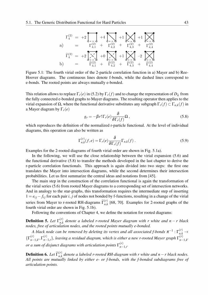
5.1. The Generic Distribution Functional for Hard Particles 43
Figure 5.1: The fourth virial order of the 2-particle correlation function in a) Mayer and b) Ree-Hoover diagrams. The continuous lines denote f-bonds, while the dashed lines correspond toe-bonds. The rooted points are always mutually e-bonded.
This relation allows to replace Γr(e) in (5.2) by Γr( f ) and to change the representation of Dλ fromthe fully connected e-bonded graphs to Mayer diagrams. The resulting operator then applies to thevirial expansion of Ω, where the functional derivative substitutes any subgraph Γr( f )⊂ Γn,k( f ) ina Mayer diagram by Γr(e)
gr =−β r!Γr(e)δ
δΓr( f )Ω , (5.8)
which reproduces the definition of the normalized r-particle functional. At the level of individualdiagrams, this operation can also be written as
Γ(r)n,k( f ,e) = Γr(e)
δ
δΓr( f )Γn,k( f ) . (5.9)
Examples for the 2-rooted diagrams of fourth virial order are shown in Fig. 5.1a).In the following, we will use the close relationship between the virial expansion (5.6) and
the functional derivative (5.8) to transfer the methods developed in the last chapter to derive ther-particle correlation functionals. This approach is again divided into two steps: the first onetranslates the Mayer into intersection diagrams, while the second determines their intersectionprobabilities. Let us first summarize the central ideas and notations from [45].
The main step in the construction of the correlation functional is again the transformation ofthe virial series (5.6) from rooted Mayer diagrams to a corresponding set of intersection networks.And in analogy to the star-graphs, this transformation requires the intermediate step of inserting1 = ei j− fi j for each pair i, j of nodes not bonded by f-functions, resulting in a change of the virialseries from Mayer to r-rooted RH-diagrams Γ
(r)n,k [68, 70]. Examples for 2-rooted graphs of the
fourth virial order are shown in Fig. 5.1b).Following the conventions of Chapter 4, we define the notation for rooted diagrams:
Definition 5. Let Γ(r)n,k denote a labeled r-rooted Mayer diagram with r white and n− r black
nodes, free of articulation nodes, and the rooted points mutually e-bonded.A black node can be removed by deleting its vertex and all associated f-bonds π−1 : Γ
(r)n.k →
Γ(r)n−1,k′,Γ
(r)n−1,t, leaving a residual diagram, which is either a new r-rooted Mayer graph Γ
(r)n−1,k′
or a sum of disjunct diagrams with articulation points Γ(r)n−1,t .
Definition 6. Let Γ(r)n,k denote a labeled r-rooted RH-diagram with r white and n− r black nodes.
All points are mutually linked by either e- or f-bonds, with the f-bonded subdiagrams free ofarticulation points.

44 Chapter 5. The Distribution Functionals for Hard Particles
A black node without e-bonds can be removed by deleting its vertex and all associated f-bondsπ−1 : Γ
(r)n,k→Γ
(r)n−1,k′ , 0, leaving either a new or the trivial RH-graph.
To rewrite the virial integrals (5.6) in rooted RH-diagrams, observe that the rooting-process(5.9) only exchanges fully f-bonded subdiagrams Γr( f ) ⊆ Γn,k by its corresponding e-bondedgraph Γr(e), whereas the Ree-Hoover transformation only operates on pairs of unbonded nodes.The two operations are therefore mutually exclusive and commute. From this follows that thesame functional derivative (5.9), which transforms star-diagrams into rooted Mayer graphs, alsoapplies to RH-diagrams
Γr(e)δ
δΓr( f )Γn,k = Γ
(r)n,k . (5.10)
The previously derived results for unrooted RH-graphs therefore remain valid for its rooted forms.This connection can be immediately applied to rewrite the transformation between Mayer and
RH-diagrams
Γ(r)n,k =
Γ(r)n,k⊆Γ
(r)n,k′
∑k′
Γ(r)n,k′ , Γ
(r)n,k =
Γ(r)n,k⊆Γ
(r)n,k′
∑k′
(−1)|Γ(r)n,k|−|Γ
(r)n,k′ | Γ
(r)n,k′ (5.11)
and to express the sum over rooted RH-diagrams
Γ(r)n = ∑
k′Γ(r)n,k′ = ∑
ka(r)n,k Γ
(r)n,k (5.12)
in terms of the “root-content”
a(r)n,k =
Γ(r)n,k′⊆Γ
(r)n,k
∑k′
(−1)|Γ(r)n,k′ |−|Γ
(r)n,k| , (5.13)
which satisfies an analogous recursion relation as the star-content (4.25) under removal of a blacknode. This is readily seen by commuting π−1 with the functional derivative (5.9) and using (4.25)
π−1(Γ
(r)n ) = Γr(e)
δ
δΓr( f )π−1(Γn) = Γr(e)
δ
δΓr( f )(n−2)Γn−1 = (n−2)Γ
(r)n−1 , (5.14)
with the corresponding relation for RH-diagrams, where the removal of a black node and its n−1f-bonds
π−1(Γ
(r)n ) = ∑
kπ−1(a(r)n,k Γ
(r)n,k) = (−1)n−1
∑k′
a(r)n,k′ Γ(r)n−1,k′
= (n−2)Γ(r)n−1 = (n−2) ∑
k′a(r)n−1,k′ Γ
(r)n−1,k′
(5.15)
yields the recursion relationa(r)n,k = (−1)n−1(n−2) a(r)n−1,k . (5.16)
The successive application of π−1 traces each diagram to a unique lowest elementπ−1(Γ
(r)n0,k
) = 0, which is the first element of the RH-class
Λ(r)n0,k
=∞⋃
m=0
πm(Γ
(r)n0,k
) , (5.17)

5.1. The Generic Distribution Functional for Hard Particles 45
defined by the inverse map π : Γ(r)n−1,k→ Γ
(r)n,k′ which attaches a node to the previous n−1 vertices
by f-bonds. The set of rooted RH-diagrams therefore separates into RH-classes, whose root-contents can be recursively calculated by (5.16), proving
Lemma 8. The root-content of Γ(r)n,k ∈ Λ
(r)n0,k
with lowest element Γ(r)n0,k
is determined by
a(r)n,k = (−1)(n2)−(
n02 )
(n−2)!(n0−2)!
a(r)n0,k′. (5.18)
The last step in rewriting the correlation function (5.6) in RH-graphs is the transition fromlabeled to unlabeled diagrams. As for the star-diagrams (4.27), (4.30), the symmetry factor σ
(r)n,k
counts the number of inequivalent permutations of particle indices, determined by the coset of thepermutation and automorphism group of rooted diagrams.
Lemma 9. Let Γ(r)n,k ∈ Λ
(r)n0,k
denote an element of the RH-class with lowest element Γ(r)n0,k
. Itsinequivalent labelings of the r white and n− r black nodes are permuted by the coset group
Sr×Sn−r/Aut(Γ(r)n,k) (5.19)
whose automorphism group factorizes into the direct product
Aut(Γ(r)n,k) = Sn−n0×Aut(Γ(r)
n0,k) . (5.20)
This is shown as follows: The white and black nodes are labeled independently, resulting in thedecoupling of the permutation group Sr×Sn−r, proving (5.19). Whereas the automorphism groupfactorizes, because each of the n0 nodes is linked to at least one e-bond, while the residual n−n0nodes are completely f-bonded. Any exchange of labels between these two groups therefore resultsin an inequivalent permutation, leaving the n− n0 vertices as an invariant set under relabeling,proving (5.20).
To rewrite the virial expansion (5.6) in RH-diagrams, let us define the symmetry factor ofRH-integrals
σ(r)n,k =
1(n− r)!
σ(r)n,k a(r)n,k , (5.21)
combining the root-content (5.18) and the number of inequivalent labelings
σ(r)n,k =
|Sr×Sn−r||Aut(Γ(r)
n,k)|=
r!(n− r)!(n−n0)!
1
|Aut(Γ(r)n0,k
)|, (5.22)
which yields the numerical prefactor of the rooted RH-class:
Corollary 1. The symmetry factor of the r-rooted RH-diagram Γ(r)n,k ∈ Λ
(r)n0,k
with lowest element
Γ(r)n0,k
for r ≥ 2 is determined by
σ(r)n,k = (−1)(
n2)−(
n02 )(
n−2n0−2
) r! a(r)n0,k
|Aut(Γ(r)n0,k
)|. (5.23)

46 Chapter 5. The Distribution Functionals for Hard Particles
This result follows by inserting (5.18), (5.22) into (5.21).Up to now, no approximation has been made on the virial expansion (5.6). The next step is
therefore to simplify the integrals by restricting the number of intersection centers in which theparticles are allowed to overlap. A useful observation is the following property of intersectiondiagrams of a RH-class:
Lemma 10. The intersection network of the class Λ(r)n0,k
is defined by its lowest subgraph.
The proof begins with the intersection diagram of the lowest element. Any further particle,added by π , can then be chosen to overlap with the previous intersection centers. This showsthat a new particle can be added without changing their number. Repeated operation with π thencompletes the proof.
The intersection diagram with the lowest number of intersection centers therefore defines the“backbone” diagram for the entire RH-class. This is the basic idea for the resummation of RH-diagrams of a given RH-class and the approximation transferring the virial series (5.6) to thegeneric r-particle correlation functional:
Theorem 3. Let Γ(r)n0,k
denote the lowest element of the RH-class Λ(r)n0,k
. The generic r-particle cor-
relation functional of the intersection network γI1
a1 . . .γIp
ap [e . . .e] with particle indices I ∈ (i1, . . . , in)is determined by
gi1...ir |p(~ri1, . . . ,~rir |~ra1, . . . ,~rap) = Γ(r)r,1 (e)δn0,rδAI +(−1)|Γ
(r)n0,k| r! a(r)n0,k
|Aut(Γ(r)n0,k
)|
× ∑n≥n0
∑I
(n−2n0−2
)∫K(γ I1
a1. . .γ
Ipap [e . . .e])ρir+1 . . .ρin dγir+1 . . .dγin ,
(5.24)
with the notation δAI = δ (~ra1i1) . . .δ (~rarir)δ (~rar+1) . . .δ (~rap) for the product of delta-functions.
This result follows from inserting (5.23) into the cluster expansion (5.6) and the cancelationof signs due to the identity
|Γ(r)n,k|= |Γ
(r)n0,k|+(
n2
)−(
n0
2
), (5.25)
which leaves an overall constant, depending only on the lowest element of the RH-class and ann-dependent binomial coefficient. An exception provides the leading diagram n0 = r of each r-correlation functional. Without an f-bond, its intersection probability vanishes and therefore hasto be included separately. Finally, the delta-functions δAI have been added in (5.24) to achieve asymmetric formulation of the integrals
[gi1i2 fi1,i2](~ri1,~ri2) =∫
gi1,i2|3(~ri1 ,~ri2 |~ra,~rb,~rc) fi1i2(~ri1,~ri2)dγadγbdγc (5.26)
[gi1i2 fi1,i2](~ra,~rb,~rc) =∫
gi1,i2|3(~ri1,~ri2|~ra,~rb,~rc) fi1i2(~ri1,~ri2)dγi1dγi2 (5.27)
in the particle and intersection coordinates, which proves useful in later applications.

5.2. Examples of R-Particle Correlation Functionals 47
5.2 Examples of R-Particle Correlation FunctionalsThis last section presents four examples. We begin with the explicit derivation of the 2-particlecorrelation functional with two intersection centers and compare its contact probability with theOrnstein-Zernike solution of Wertheim, Baxter, and Thiele. The 2- and 3-particle correlations arethen calculated for up to four intersection centers and compared to the Kirkwood superpositionapproximation.
The first f-bonded RH-diagram of the 2-particle correlation functional gi1i2 is Γ(2)3,1, whose two
white and one black nodes define a backbone diagram with two intersection centers. All furthernetworks of the same RH-class can then be contracted to the pattern
Λ(2)2,1 : ei1i2 + ei1i2 γ
i1i3...ina γ
i2i3...inb . (5.28)
Applying the rules of Lemma 5 and Lemma 6 for the representation of the intersection kerneland introducing the notation wi
a = wi0(~rai) for the volume weight, the virial series sums up to the
generating function
gi1i2|2(~ri1,~ri2|~ra,~rb)
= ei1i2δAI + ∑n≥2
∑i3...in
∫K(γ i1i3...in
a γi2i3...inb ei1i2)ρi3 . . .ρindγi3 . . .dγin
= ei1i2(δAI + ∑n≥2
∑i3...in
DaDb
∫wi1
a wi3a . . .win
a wi2b wi3
b . . .winb ρi3 . . .ρin dγi3 . . .dγin)
= ei1i2(δAI +DaDb wi1a wi2
b ∑n≥2
xn−2ab ) ,
(5.29)
where we used the x-variable (4.77) and the property of Lemma 6 that the intersection probabilityfor a single particle is zero Dawi1
a = 0. The final correlation functional has then the analytic form
gi1i2|2(~ri1 ,~ri2 |~ra,~rb) = ei1i2
(δ (~rai1)δ (~rbi2)+DaDb
wi1a wi2
b1− xab
). (5.30)
This result is exact up to the third virial order, but significantly improved by the additionalpole at xab = 1. To illustrate this effect of the resummation process, let us derive the approximatecontact probability for a system of 3-dimensional balls B : S2 → R3 of radius R and diameterD = 2R at constant density ρ . The expansion of the derivatives of (5.30) to leading order in xabresults in two terms
g12|2(~r1,~r2) = e12
∫ (δAI +DaDb
w1aw2
b1− xab
)dγadγb
= e12
∫ (δAI +Da
w1a∫
w3aDb(w2
bw3b)ρ3 dγ3 + . . .
(1− xab)2
)dγadγb (5.31)
= e12
∫ (δAI +
1(1− xab)2
∫(Daw1
aw3a)(Dbw2
bw3b)ρ3 dγ3 +O(ρ2)
)dγadγb ,
corresponding to the resummed second and third virial contributions. For the particle positions~ri ∈ Bi of i = 1,2,3 and intersection coordinates~ra ∈ B1∩B3,~rb ∈ B2∩B3, the correlation functionxab(~rab) for~rab =~ra−~rb reduces to the volume of a lens-shaped domain
xab(~rab) =∫~r3∈B3
w30(~r3−~ra)w3
0(~r3−~rb)ρ dγ3 =4π
3R3
ρ
[1− 3
4rab
R+
116
(rab
R
)3](5.32)
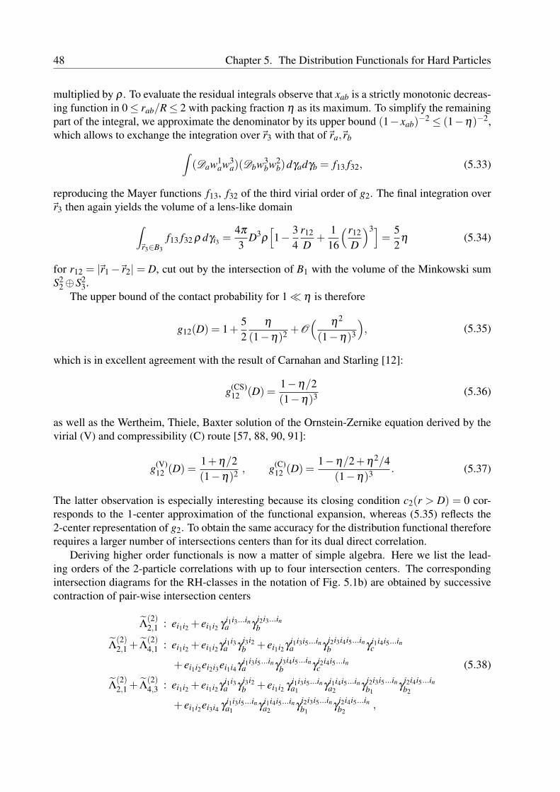
48 Chapter 5. The Distribution Functionals for Hard Particles
multiplied by ρ . To evaluate the residual integrals observe that xab is a strictly monotonic decreas-ing function in 0≤ rab/R≤ 2 with packing fraction η as its maximum. To simplify the remainingpart of the integral, we approximate the denominator by its upper bound (1−xab)
−2 ≤ (1−η)−2,which allows to exchange the integration over~r3 with that of~ra,~rb∫
(Daw1aw3
a)(Dbw3bw2
b)dγadγb = f13 f32, (5.33)
reproducing the Mayer functions f13, f32 of the third virial order of g2. The final integration over~r3 then again yields the volume of a lens-like domain∫
~r3∈B3
f13 f32 ρ dγi3 =4π
3D3
ρ
[1− 3
4r12
D+
116
(r12
D
)3]=
52
η (5.34)
for r12 = |~r1−~r2| = D, cut out by the intersection of B1 with the volume of the Minkowski sumS2
2⊕S23.
The upper bound of the contact probability for 1 η is therefore
g12(D) = 1+52
η
(1−η)2 +O(
η2
(1−η)3
), (5.35)
which is in excellent agreement with the result of Carnahan and Starling [12]:
g(CS)12 (D) =
1−η/2(1−η)3 (5.36)
as well as the Wertheim, Thiele, Baxter solution of the Ornstein-Zernike equation derived by thevirial (V) and compressibility (C) route [57, 88, 90, 91]:
g(V)12 (D) =
1+η/2(1−η)2 , g(C)
12 (D) =1−η/2+η2/4
(1−η)3 . (5.37)
The latter observation is especially interesting because its closing condition c2(r > D) = 0 cor-responds to the 1-center approximation of the functional expansion, whereas (5.35) reflects the2-center representation of g2. To obtain the same accuracy for the distribution functional thereforerequires a larger number of intersections centers than for its dual direct correlation.
Deriving higher order functionals is now a matter of simple algebra. Here we list the lead-ing orders of the 2-particle correlations with up to four intersection centers. The correspondingintersection diagrams for the RH-classes in the notation of Fig. 5.1b) are obtained by successivecontraction of pair-wise intersection centers
Λ(2)2,1 : ei1i2 + ei1i2 γ
i1i3...ina γ
i2i3...inb
Λ(2)2,1 + Λ
(2)4,1 : ei1i2 + ei1i2γ
i1i3a γ
i3i2b + ei1i2γ
i1i3i5...ina γ
i2i3i4i5...inb γ
i1i4i5...inc
+ ei1i2ei2i3ei1i4γi1i3i5...ina γ
i3i4i5...inb γ
i2i4i5...inc (5.38)
Λ(2)2,1 + Λ
(2)4,3 : ei1i2 + ei1i2γ
i1i3a γ
i3i2b + ei1i2 γ
i1i3i5...ina1
γi1i4i5...ina2
γi2i3i5...inb1
γi2i4i5...inb2
+ ei1i2ei3i4 γi1i3i5...ina1
γi1i4i5...ina2
γi2i3i5...inb1
γi2i4i5...inb2
,
5.2. Examples of R-Particle Correlation Functionals 49
with the corresponding 2-particle correlation functionals
gi1i2 |2 = ei1i2
(δAI +DaDb
wi1a wi2
b1− xab
)gi1i2 |3 = ei1i2
(δAI +DaDbwi1
a wi2b xab +DaDbDcwi1
a wi2b wi1
cxabxbc
1− xabc
−DaDbDcwi1
a wi2c yi1i2
abc(1− xabc)3
)(5.39)
gi1i2 |4 = ei1i2
(δAI +Da1Db1wi1
a1wi2
b1xa1b1
+Da1Da2Db1Db2(wi1a1
wi1a2)(wi2
b1wi2
b2)
xa1b1xa2b2
1− xa1a2b1b2
+12Da1Da2Db1Db2
wi1a1wi2
a2wi1b1
wi2b2
ya1a2b1b2
(1− xa1a2b1b2)3
),
where we introduced the Boltzmann weighted densities
yi1i2abc = ∑
i3,i4
∫ei1i4ei2i3wi3
a wi3b ρi3 wi4
b wi4c ρi4 dγi3dγi4
ya1a2b1b2 = ∑i3,i4
∫ei3i4wi3
a1wi3
b1ρi3wi4
a2wi4
b2ρi4 dγi3dγi4 .
(5.40)
As a last example, we present the leading term of the 3-particle correlation functional with 3intersection centers. Its intersection diagram has the form
Λ(3)3,1 : ei1i2ei2i3ei1i3 + ei1i2ei2i3ei1i3γ
i1i4...ina γ
i2i4...inb γ
i3i4...inc , (5.41)
with the corresponding correlation functional
gi1i2i3|3 = ei1i2ei2i3ei1i3
(δAI +DaDbDc
wi1a wi2
b wi3c
(1− xabc)2
). (5.42)
The contact probability is therefore to leading order g3 ∼ (1− η)−3, which shows that theKirkwood approximation gi1i2i3 ≈ gi1i2gi2i3gi3i1 = [g2]
3 ∼ (1− η)−6 is not applicable when allthree particles are close together, in accordance with results obtained from computer simula-tions [87]. It is not difficult to generalize this result to an arbitrary r-particle correlation func-tion, whose leading term is gr ∼ (1− η)−r, whereas the Kirkwood approximation suggests[g2]
r(r−1)/2 ∼ (1−η)−r(r−1). This excludes the superposition approximation as a constructionprinciple for any distribution functional.
With the derivation of this second class of correlation functionals, we can finally solve thelast problem stated in chapter 3, the perturbative expansion of g2 for the molecular dual grandcanonical potential. Contrary to (3.3), the perturbation theory for ΩD is an expansion of g2 in thesoft-correction term Fi j = eH
i j f Si j of the Mayer function fi j = f H
i j +Fi j. Its lowest order diagramsare shown in Fig. 5.2, illustrating the successive replacement of f H-bonds by F-functions. Thecorresponding substitution in the functional is generated by the formal derivative
gi j = eSi jg
Hi j + eS
i j
∫δgH
i j
δ f Hik
Fik dγk +12
eSi j
∫δgH
i j
δ f Hk1k2
Fk1k2 dγk1k2 + . . .
≈ gi j|2,0 +gi j|2,1 +gi j|4,1 + . . . ,
(5.43)
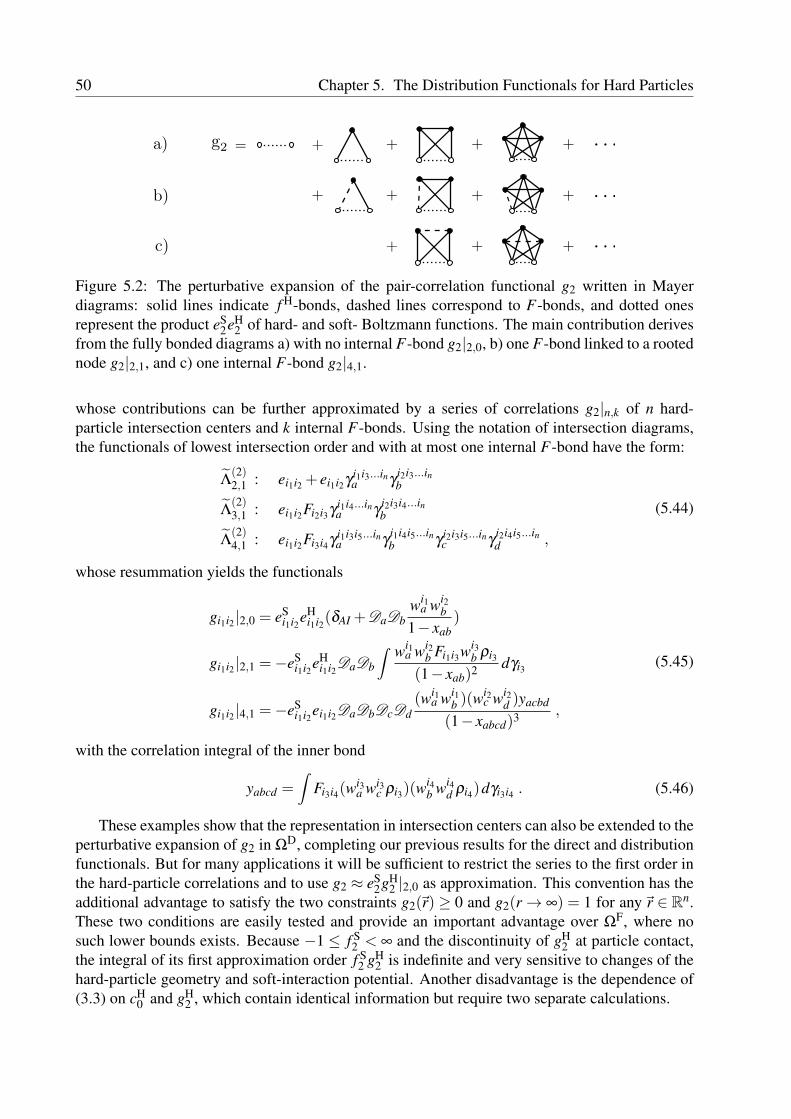
50 Chapter 5. The Distribution Functionals for Hard Particles
Figure 5.2: The perturbative expansion of the pair-correlation functional g2 written in Mayerdiagrams: solid lines indicate f H-bonds, dashed lines correspond to F-bonds, and dotted onesrepresent the product eS
2eH2 of hard- and soft- Boltzmann functions. The main contribution derives
from the fully bonded diagrams a) with no internal F-bond g2|2,0, b) one F-bond linked to a rootednode g2|2,1, and c) one internal F-bond g2|4,1.
whose contributions can be further approximated by a series of correlations g2|n,k of n hard-particle intersection centers and k internal F-bonds. Using the notation of intersection diagrams,the functionals of lowest intersection order and with at most one internal F-bond have the form:
Λ(2)2,1 : ei1i2 + ei1i2γ
i1i3...ina γ
i2i3...inb
Λ(2)3,1 : ei1i2Fi2i3γ
i1i4...ina γ
i2i3i4...inb
Λ(2)4,1 : ei1i2Fi3i4γ
i1i3i5...ina γ
i1i4i5...inb γ
i2i3i5...inc γ
i2i4i5...ind ,
(5.44)
whose resummation yields the functionals
gi1i2|2,0 = eSi1i2eH
i1i2(δAI +DaDbwi1
a wi2b
1− xab)
gi1i2|2,1 =−eSi1i2eH
i1i2DaDb
∫ wi1a wi2
b Fi1i3wi3b ρi3
(1− xab)2 dγi3
gi1i2|4,1 =−eSi1i2ei1i2DaDbDcDd
(wi1a wi1
b )(wi2c wi2
d )yacbd
(1− xabcd)3 ,
(5.45)
with the correlation integral of the inner bond
yabcd =∫
Fi3i4(wi3a wi3
c ρi3)(wi4b wi4
d ρi4)dγi3i4 . (5.46)
These examples show that the representation in intersection centers can also be extended to theperturbative expansion of g2 in ΩD, completing our previous results for the direct and distributionfunctionals. But for many applications it will be sufficient to restrict the series to the first order inthe hard-particle correlations and to use g2 ≈ eS
2gH2 |2,0 as approximation. This convention has the
additional advantage to satisfy the two constraints g2(~r) ≥ 0 and g2(r→ ∞) = 1 for any~r ∈ Rn.These two conditions are easily tested and provide an important advantage over ΩF, where nosuch lower bounds exists. Because −1 ≤ f S
2 < ∞ and the discontinuity of gH2 at particle contact,
the integral of its first approximation order f S2 gH
2 is indefinite and very sensitive to changes of thehard-particle geometry and soft-interaction potential. Another disadvantage is the dependence of(3.3) on cH
0 and gH2 , which contain identical information but require two separate calculations.

Chapter 6
Discussion and Conclusion
The results of the current thesis can be viewed from three different perspectives: the mathematicsof integral geometry, the physics of DFT, and the lattice excess free-energy models used by en-gineers. In combination, they contribute to the development of the molecular density functionaltheory. But they are also topics of their own, which can be further extended in their individualdirections. In the following, we will thus focus on each of these three topics seperately and finallyconclude with an overview of possible applications.
The mathematical aspects: The central observation necessary for the derivation of the Rosen-feld functional from the virial expansion is its connection to integral geometry. It explains therelation between the second virial integral and the Gauss-Bonnet equation and also clarifies the ar-guments used by Isihara and Kihara, who derived the intersection probability from the Minkowskisum of its surfaces instead of the kinematic measure. Using the Blaschke-Santalo-Chern equationalso avoids the Fourier decomposition of the second virial integrand that fails in even dimensionswhere the Euler-characteristic is trivially zero.
The introduction of integral geometry not only clarifies the mathematical basis of the Rosen-feld functional, it also allows its generalization. A particularly satisfying result is the simplealgebraic structure obtained by the introduction of the functional derivative, D , to combine then-particle weight functions into a single expression to sum over all w0. In principal, it would bepossible to follow the lines of Rosenfeld and Wertheim and to expand these weight functions inan infinite series of 1-particle weight functions. But for non-spherical particles the evaluation ofthe resulting integrals cannot be done analytically and the splitting would provide no advantagecompared to the unrestricted use of the n-particle weights.
The occurrence of the functional derivative in this framework is no coincidence. As has beenargued in [44], the boundary operator for the surface of the intersection domains translates to acorresponding operator on the differential forms of the kinematic measure and thus on the weightfunctions of the particle volume ∂ → D . For a single complex manifold, a similar structure hasbeen discussed by Chern and Simons, leading to the corresponding Chern-Simons classes [3],which contain important geometric information about the underlying complex manifolds. From amathematical point of view, it would therefore be interesting to extend the free-energy functionalto particles with such a complex structure imbedded in either Cn or CPn. Another direction isthe inclusion of surfaces Σk → Rn of codimension n− k > 1 to allow for threads of polymersor random coils as 1-dimensional curves, making contact to topics of knot theory and complextopology [10].
The hard-particle functional also provides unique insight into the characterization of non-local
51

52 Chapter 6. Discussion and Conclusion
geometry, described by the convolute of local differential forms. Determining, e.g., the packingfraction for a periodic particle distribution is comparatively simple, as the lattice structure mapsthe infinite space to its primary cell and thus to an almost local problem. But less symmetricalor even random partitions are more difficult to distinguish. Using the pair-correlation functionalis therefore an obvious first ansatz, while a more manageable representation is the free-energyfunctional itself. But it would also be of interest to understand the dependence of the crystallinelattice structure as a function of the particle geometry.
The physical aspects: The intersection kernel together with the symmetry factors of the Ree-Hoover diagrams determine the hard-particle direct correlation and distribution functionals forany given equivalence class of Ree-Hoover diagrams. As of today, the hard-particle potential istherefore the only example whose density functionals can be explicitly calculated in a convergentseries with increasing precision using a larger number of intersection centers. This expansion alsoexplains the shortcomings of the Rosenfeld functional, whose 1-center approximations is insuffi-cient to determine the correlations between particles of non-spherical geometry, for mixtures, andat higher packing fractions.
However, as the calculational complexity increases significantly with the number of intersec-tion centers, any progress in FMT will require the development of further approximation methods.For particles with a distinct symmetry axis, e.g., the functionals can be expanded in tensor prod-ucts of their descriptive vectors, resulting in phase-field crystal models, reproducing the Landau-Ginzburg and Swift-Hohenberg free energies for nematic fluids [98].
An equally important aspect, one that had not been considered systematically in the literaturebefore, is the choice of an optimal representation for the grand-canonical potential. Most ap-proaches start from the direct correlation functional and use perturbation theory to couple furthersoft potentials. But this low-order expansion is not the best ansatz for strong interactions. Alsothe combination of the direct and distribution functionals in the free energy is redundant, whileill-chosen splitting of hard and soft potentials can violate the positivity of the grand potential. TheLegendre-dual grand-canonical potential, on the other hand, is a function of the pair correlationalone with exactly one minimum for short-ranged interactions. It is therefore well behaved foralmost all molecular potentials, and even approximate pair correlations provide stable solutionsfor the self-consistent equation, as the unphysical Wilson ansatz shows.
The engineering aspects: To obtain a better understanding of the dual grand-canonical po-tential, we rederived the lattice free-energy in the quasichemical approximation from its contin-uum counterpart. The calculation shows that the Flory-Huggins, Staverman-Guggenheim, and theGuggenheim excess energies are independent of the underlying lattice structure, with the param-eter z0 determined by the 2-particle density integrated over the first particle shell. The derivationalso justifies the validity of the excess functionals under the given constraints on the packing frac-tion and the next-neighbor interactions. These results are almost exclusively consequences of theunique structure of the two possible representations of the grand potential for pair interactions, butindependent of the actual state of phase the model has been designed for, justifying the applicationof the excess lattice energy from the crystal to the liquid state.
As the derivation of the lattice models indicates, the single minimum of the dual functional isexceptionally stable under variations of the pair correlations, explaining why the UNIQUAC andUNIFAC models provide reasonable results despite their usage of the inconsistent Wilson ansatz.And it also explains, why the quasichemical approximation is incompatible with the inclusion ofthe detailed molecular geometry, whose additive structure of the lattice variables is a consequenceof the neglect of its curvature terms.
53
Another aspect of the continuum and lattice theory is the relationship between the Euler-Lagrange equation for the pair-correlation functional and the self-consistent equation of the latticemodels. Solving this equation corresponds to minimizing the grand potential for a homogeneousdensity. Together with the Larsen-Rasmussen approach, it also provides an alternative derivationof the self-consistent equation of COSMO-RS that is complementary to the approach by Klamtand clarifies some of its assumptions. E.g., the chemical potential derived by COSMO-RS is thecanonical dual to the pair-correlation function and not of the particle density, which is constant andtherefore not a dynamical variable of the lattice ansatz. Another misleading idea, often found inthe literature, is the idea of the surface charges as “free segments” [52, 30]. As the Euler-Lagrangeequation shows, the self-consistent identity is a local function and therefore applies to each pairof surface segments individually. The spacial correlation between separate segments is thereforepart of the integral of the free energy, which in the next-neighbor approximation is replaced by asum over pairs of segments. It is also customary to create new models by ad hoc combinationsof separate energy terms. An example, where this approach has failed so far, is the inclusion ofthe Coulomb potential. But we have shown, the self-consistent equation and the free-energy func-tional are related by the Euler-Lagrange equation and cannot be modified independently. This hasbeen demonstrated for the Debye-Huckel ansatz of the Coulomb interaction for which we derivedthe generalization of the continuum model and its possible extension to COSMO-RS.
Prospective developments: The derivation of the COSMO-RS model from the continuum func-tional is based on far reaching approximations. Probably the most restrictive one is the neglectof the particle geometry apart from volume and surface. A first step to generalize this ansatz istherefore the transition from the lattice to the continuum description, containing the full geomet-ric information while holding on to the simplified representation of the pair-correlation functiongi j ∼ cei j. The resulting model would still be independent of a free volume, but depending onthe hard-particle geometry defined by the COSMO cavity. For a homogeneous liquid, the mini-mization of the grand potential now includes the integration over all particle orientations at a fixeddistance, summing over all segment pairs of the molecules for any axial rotation angle, as shownin Fig. 3.1b).
This model should be sufficient to calculate the contact probability between molecules of com-plex geometries in the liquid state. For enzymatic reactions, e.g., the affinity between the enzymeand the dissolved substrates is an important information. The same applies to high-performanceliquid chromatography, where the optimal selection of the substrate is central for the separation ofenantiomer mixtures into their chiral compounds. Another field of applications is the calculationof the solubility of protein conformers to distinguish between the large number of possible tertiaryfolding structures.
The next level of generalization is the replacement of the constant c by a reference pair-correlation function g2(ρ0;r0) of spheres with volumes of molecular size. The resulting modelis a coarse approximation of the density dependence of homogeneous gases and liquids, whosemaximum of the first shell is replaced by the radial particle distance r0 calculated for the givendensities. For inhomogeneous fluids and crystals, however, such an approximation is no longer ap-propriate and the pair-correlation functionals for the hard-particle geometry has to the determinedat least to leading order in the 2-center approximation g2|2(ρ(~r); t0) at a fixed average distancet0. But its computational costs for a triangulated surface are comparable or even higher than forMD/MC simulations, and the advantage of the DFT ansatz is lost. However, scanning throughthe 1700 molecules of the COSMO-SAC database, one finds that almost all particle surfaces aresufficiently regular to be representable by elementary polynomials. Thus instead of a triangulated
54 Chapter 6. Discussion and Conclusion
surface, the intersection domains can be determined by numerically solving algebraic equations.Whereas the small group of concave molecules can be represented by Voronoi tesselation, reduc-ing the Euler form into a sum over convex subdomains of complementary intersections.
It is interesting to speculate, which of the current results will reach a wider audience over thecoming years. The mathematical interest in integral geometry is currently dominated by the notionof valuations [8], whereas the proof of the generalized Blaschke-Santalo-Chern equation is basedon the local representation of differential forms. The hard-particle functionals are therefore outsidethe current mathematical mainstream. Similarly pessimistic is the prospect for the extension of theRosenfeld functional. Although the current derivation of the hard-particle correlation functionalcloses a chapter that was started more than a hundred years ago by van der Waals and Boltzmann,the equations of state are outdated by the current progress of MD/MC simulations. This leavesus with the derivation of the lattice models from the dual grand potential. Actually, the simplestresult might prove the most useful. The generalization of the lattice models to include the particlegeometry is easily implemented, while offering a wide range of applications. But as stated in thePreface of the current thesis, it is not possible to predict research’s future course.
Appendix A
The Integral Measure of the MinkowskiSum
The r-particle correlation functionals are always accompanied by an integration over the kinematicmeasure dγi1...ir of translations and rotations of r particles. For the most common case of r = 2,we will now derive an explicit realization using methods from integral geometry [96, 24, 31, 58].
Let Σk denote a n− 1 dimensional, smooth, boundary free, convex, Riemannian manifold,imbedded into Dk : Σk → Rn. Each point pk ∈ Σk is then related to an orthonormal, positivelyoriented coordinate frame (e(k)1 , . . . , e(k)n ) with the outward pointing normal vector e(k)n and thedifferential basis and connection forms
d p = θiei , dei = ωi je j , den = ωnα eα = hαβ θβ eα , λαβ := h−1αβ
. (A.1)
Each point of the smooth surface is uniquely related to a tangential plane up to an axial rotationaround e(k)n . From this follows that the tangential planes of two convex surfaces Σ1, Σ2, touchingin a common point p1 = p2, also agree up to an axial rotation and an inversion of their normalvectors e(1)n = −e(2)n . This property remains unchanged even when the particles are shifted apartin the normal direction. Surface points of closest distance t ∈ R+ and their frames are thereforerelated by
p2 = p1 + te(1)n , e(1)n =−e(2)n , e(1)α = uαβ e(2)β
for uαβ ∈ SO(n−1) (A.2)
using the index conventions i, j = 1, . . . ,n and α,β = 1, . . . ,n−1.Having defined the relative coordinate frames for the two particles, we can now write the
integral∫g12(~r1,~r2)dγ1dγ2 =
∫g12(~r1−~r2)dγ12dγ =V vol(SO(n))
∫gH
12(~r1−~r2)dγ12 (A.3)
in a comoving dγ12 and a reference system dγ . The integral of the latter can be carried out,contributing the volume V = vol(Rn) and the volume of the group SO(n). The analogous trans-formation in the representation of base forms corresponds to the shift
dγ1dγ2 =∧
k=1,2
∧i
θ(k)i
∧i< j
ω(k)i j =
∧i
(θ(1)i −θ
(2)i )
∧i< j
ω(1)i j
∧i
θ(2)i
∧i< j
ω(2)i j = dγ12dγ (A.4)
55
56 Appendix A. The Integral Measure of the Minkowski Sum
as can be seen by expanding the skew-symmetric product and setting dγ = dγ2 for the referencesystem.
The trivial contribution dγ will be ignored in the following, leaving us with the transformationof dγ12. To simplify the calculation, observe that the translation of Σ2 can also be written asp2 + t2e(2)2 = p1 + t1e(1)n for any t1, t1 ∈ R+ and t1 + t2 = t. This allows to first determine Weyl’shalf-tube Σ(t) : p(t) = p + ten for Σ1, Σ2 separately and then to derive their Minkowski sumΣ1(t1)⊕Σ2(t2) at p1(t1) = p2(t2) [96, 58].
The differential forms θi(t),ωi j(t) of the half-tube surface Σ(t) are determined by differenti-ating each point p(t) = p+ ten
d p(t) = d p+ endt + tωnα eα (A.5)
and separating their components into the directions of en and eα
θn(t) = θn +dt , θα(t) = θα + tωnα = (δαβ + thαβ )θβ . (A.6)
The new basis also determines the connection forms, as the orthonormal vectors eα and theirdifferentials are invariant under translations
ωnα(t) = ωnα ⇒ hαβ θβ (t) = hαβ θβ . (A.7)
Inserting (A.6), finally yields the curvature matrix and its inverse for the half-tube Σ(t)
hαβ (t) = hαγ (δγβ + thγβ )−1 , λαβ (t) = t δαβ +λαβ (A.8)
The second step requires to determine the differential volume element for the domain Σ1(t1)⊕Σ2(t2), covered by Σ1(t1) while circling Σ2(t2). To write dγ12 in a common coordinate frame weuse the transformation (A.2), which relates the connection forms ω
(1)nα = −uαβ ω
(2)nβ
of the twoparticles at their intersection point p1(t1) = p2(t2) and also defines the transformation of theirbasis forms using the inverse Weingarten map λ . With Σ2(t2) as the reference system, the formsof Σ1(t1) are rotated into the new coordinate frame
θ(2)α = λ
(2)αβ
ω(2)nβ
, θ(1)α = uαβ θ
′(1)β
=−uαβ λ(1)βγ
uγµω(2)nµ . (A.9)
Inserting this result into (A.4), together with the transformation of the normal componentθ(1)n −θ
(2)n =−dt and the Jacobi determinant J =−1, yields the reduced kinematic measure
dγ12 =∧
i
(θ(1)i −θ
(2)i )
∧i< j
ω(1)i j
=∧α
(uλ(1)(t1)u−1 +λ
(2)(t2))αβ ω(2)nβ∧dt
∧α
ω(1)nα
∧α<β
ω(1)αβ
= det(λ (1)+ tδ +u−1λ(2)u)κ
(1)G κ
(2)G dσ1∧dσ2∧dSO(n−1)∧dt ,
(A.10)
where we introduced the unit matrix δ , the Gaussian curvature ∧αωnα = κG dσ , the differentialsurface element dσ , used the orthonormal property det(u) = 1 and (A.8) to write the final resultin a symmetric form.

Appendix B
Proof of the generalizedBlaschke-Santalo-Chern Equation
The current section completes the proof Lemma 6, demonstrating that the weight functions (4.70)are symmetric in the particles indices and permuted by SO(k) rotations.
For the surfaces Σ1, . . . ,Σk, let us define the k coordinate frames
Σm : (e(m)1 , . . . , e(m)
n−m︸ ︷︷ ︸tangential
, e(m)n−m+1, . . . , e
(m)n︸ ︷︷ ︸
normal
) for m = 1, . . . ,k (B.1)
and the Pfaffian form (4.68)
Pf(GBω)n−k1...k = det(GBh)1...k
n−k∧α=1
θ(1)α . (B.2)
This choice of the vector basis defines a specific ordering of the particles’ indices 1, . . . ,k, whichcan be viewed as a nested intersection of surfaces
(((Σ1∩Σ2)∩Σ3)∩Σ4) . . . , (B.3)
with Σ1 as the reference system. The intersection product therefore fails the permutation invari-ance of the intersection probability. However, not the curvature form but the kinematic measure(4.50) has to be SO(n− k)×SO(k) invariant. We therefore have to prove the permutation sym-metry of the integral∫
K(Σ1∩ . . .∩Σk)∧K(D2)∧ . . .∧K(Dk)
=∫
det(GBh)1...k
n−k∧α=1
θ(1)α
dvol(SO(n− k))|SO(n− k)|
∧K(D2)∧ . . .∧K(Dk) .(B.4)
Generalizing Chern’s arguments for two intersecting surfaces [16, 82], the translational mea-sure of Σk has been extended by SO(n− k) to the kinematic measure of Rn−k. This leaves us torotate the normal vectors e(2)n , . . . , e(k)n into the tangential direction of Σ1. For the nested coordinateframe (B.3), we can chose the SO(m) transformations of the “normal” directions to rotate e(m)
n intothe basis of Σ1 while keeping the vectors of Σ2, . . . ,Σm−1 fixed:
Σm→ Σ1 : SO(m)/SO(m−1) = Sm−1 . (B.5)
57
58 Appendix B. Proof of the generalized Blaschke-Santalo-Chern Equation
Introducing the spherical vector (x(m)1 , . . . ,x(m)
m ) ∈ Sm−1, the normal vector of Σm transforms intothe basis of Σ1
e(m)n =
m
∑p=1
x(m)p e(1)n−p+1 for
m
∑p=1
(x(m)p )2 = 1 (B.6)
and their corresponding dual differential forms
θ(m)n =
m
∑p=2
x(m)p θ
(1)n−p+1 = x(m)
m θ(1)n−m+1 +O(θ
(1)α )
for n−m+2≤ α ≤ n−1 .
(B.7)
Here the symbol O(θ(1)α ) indicates elements which drop out when inserted into the skew symmet-
ric product (B.4) as they already occur at a lower m. This transforms the normal directions intothe tangential forms of Σ1
θ(2)n ∧ . . .∧θ
(k)n = x(2)2 . . .x(k)k θ
(1)n−1∧ . . .∧θ
(1)n−k+1 , (B.8)
which are complementary to the already existing elements in (B.4).The analogous transformation has to be done for the connection forms. Adopting the notation
of (B.1), we separate the forms into two groups
Σm : ω(m)1,n ∧ . . .∧ω
(m)n−m,n︸ ︷︷ ︸
tangential
∧ω(m)n−m+1,n∧ . . .∧ω
(m)n−1,n︸ ︷︷ ︸
normal
. (B.9)
Again, the tangential directions transform by the coset elements of Sm−1
ω(m)α,n = x(m)
m ω(1)α,n−m+1 +O(ω
(1)α,β )
for 1≤ α ≤ n−m , n−m+2≤ β ≤ n−1 ,(B.10)
whose products provide the complementary part to the SO(n− k) form of (B.4)
k∧m=2
n−m∧α=1
ω(m)α,n =
[ k
∏m=2
(x(m)m )n−m] k∧
m=2
n−m∧α=1
ω(1)α,n−m+1 . (B.11)
On the other hand, the normal components of the connection forms (B.9) transform under theadjoint of gαβ ∈ SO(m)
ω(m)α,n = g−1
αβe(1)
βd(gnγ e(1)γ ) = g−1
αβdgnβ +O(ω
(1)βγ
)
for n−m+1≤ β < γ ≤ n−1(B.12)
with the coset element gnα ∈ SO(m)/SO(m− 1) leaving the normal vectors invariant. Formingtheir product, they combine into the group measure of SO(k) modulo further connections
k∧m=2
n−1∧α=n−m+1
ω(m)α,n =
k∧m=2
[dvol(Sm−1)+O(ω(1)βγ
)]
= dvol(SO(k))+O(ω(1)βγ
) .
(B.13)
59
Finally, inserting the transformed normal components into the kinematic measure (B.4), yieldsa differential form which is obviously SO(k) invariant∫
K(Σ1∩ . . .∩Σk)∧K(D2)∧ . . .∧K(Dk)
=∫ det(GBh)|SO(n− k)|
k
∏m=2
(x(m)
m)n−m+1 dvol(SO(k))∧K(Σ1)∧ . . .∧K(Σk) .
(B.14)
The product of x(m)m terms is the Jacobian J of the transformation into spherical coordinates with
the parameterization in terms of SO(m) rotation angles for m = 1, . . . ,k
x(m)m =
m−1
∏α=1
sin(φα,m) , (B.15)
proving the invariance of the weight functions (4.70) under SO(k)-generated permutations of par-ticles indices and thus completing the proof of Lemma 6.

60 Appendix B. Proof of the generalized Blaschke-Santalo-Chern Equation
Appendix C
Deriving Rosenfeld’s 1-particle WeightFunctions
In the following, we will give a short account of how to transform the 2- and 3-particle Eulerform (4.81) to the coordinate dependent representation of 1-particle weight functions introducedby Rosenfeld, Wertheim, and Tarazona [76, 92, 85]
The Euclidean metric ηi j in the orthonormal principal frame (~ν1,~ν2,~n) is the diagonal tensor
ηi j = ei⊗ e j = Ii j = (~ν1⊗~ν1 +~ν2⊗~ν2 +~n⊗~n)i j . (C.1)
with the corresponding connection tensor written in the normal vector e3 =~n:
de3 = ω3αeα = καθα ⊗ eα = καeα ⊗ eαd~p =(καeα ⊗ eα
)~t ds
=(κ1~ν1⊗~ν1 +κ2~ν2⊗~ν2
)~t ds =K~tds
(C.2)
using Rodrigues formula den = καναeα , the representation of the vielbein θα = eαd~p, and byobserving that the tangential vector at each point ~p∈ Σ1∩Σ2 lies in the direction of~t ∼~n(1)×~n(2).The derivative d~p =~t ds therefore is the differential line element ds pointing into the direction of~t.
In order to separate the normal vectors from the principal frame, Wertheim rewrites the con-nection form [92]:
K=12(κ1~ν1⊗~ν1 +κ2~ν2⊗~ν2
)+
12
κ1(I−~n⊗~n−~ν2⊗~ν2
)+
12
κ2(I−~n⊗~n−~ν1⊗~ν1
)=
12(κ1 +κ2)(I−~n⊗~n
)+
12(κ1−κ2)(~ν1⊗~ν1−~ν2⊗~ν2
)=: κ
(I−~n⊗~n
)+ ∆
(C.3)
introducing the mean and tangential curvatures κ , ∆. The connection form then yields the form
ω13 = e1de3 =~tK~t ds . (C.4)
In a second step, the normal vector~n(2) is separated from the curvature depending parts of particle1:
(~n(1)×~n(2))K(1) (~n(1)×~n(2)) =−~n(2)×~n(1)
(κ1~ν1⊗~ν1 +κ2~ν2⊗~ν2
)~n(1)×~n(2)
61
62 Appendix C. Deriving Rosenfeld’s 1-particle Weight Functions
=−~n(2)(κ1~n(1)×~ν1⊗~ν1×~n(1)+κ2~n(2)×~ν2⊗~ν2×~n(1)
)~n(2)
=~n(2)(κ1~ν2⊗~ν2 +κ2~ν1⊗~ν1
)~n(2) =~n(2) K†
(1)~n(2) ,
using the orthonormal relation~ν1×~ν2 =~n and introducing the adjoint connection tensor:
K† = κ(I−~n⊗~n
)− ∆ . (C.5)
Inserting these results into (4.81)
1− c12
s12ω
(1)13 =
1− c12
s12~t K(1)~t ds =
1− c12
s12
[~n(1)×~n(2)s12
K(1)~n(1)×~n(2)
s12
]ds
=1− c12
s212
~n(2)K†(1)~n
(2) dss12
=1
1+ c12~n(2)K†
(1)~n(2) ds
s12
=1
1+ c12~n(2)
[κ(1)(I−~n(1)⊗~n(1))−∆
(1)]~n(2) dss12
=1
1+ c12
[κ(1)(1− c2
12)−~n(2)∆(1)~n(2)] ds
s12
=[(1−~n(1)~n(2))κ(1)−~n(2)∆(1)~n(2)
1+~n(1)~n(2)
] ds|~n(1)×~n(2)|
and using the integral representation by δ -functions
1− c12
s12ω
(1)13 =
∫D1∩D2
[(1−~n(1)~n(2))κ(1)−~n(2)∆(1)~n(2)
1+~n(1)~n(2)
]δ (~n(1)~rA)δ (~n(2)~rA)d3rA , (C.6)
this reproduces the first part of Wertheim’s decomposition ([92]), from which derive the 1-particleweight functions by Taylor-expanding sin and cos in tensor products of their normal vectors.
The integral representation used in (C.6) extends the integration along the line element dsto the entire embedding space. This and similar relations are readily derived from the linearcoordinate transformation
η =~n~p , ζ = ~m~p , ξ =~e1x+~e2y+~e3z (C.7)
at the point ~p = (x,y,z) and its corresponding Jacobi determinant:
dη ∧dζ ∧dξ = |det(~n,~m,~e)| dx∧dy∧dz = |~n×~m| d3 p . (C.8)
Applied for the integral of an arbitrary test function F and two δ -functions∫F(~p)δ (~n~p)δ (~m~p)d3 p =
∫F(η ,ζ ,ξ ) δ (η)δ (ζ )
dη dζ dξ
|~n×~m|=∫
F(ξ )dξ
|~n×~m|, (C.9)
it reduces to the line integral along ξ , as used in equation (C.6).With one δ -function included, the corresponding transformation
η =~n~p , ζ = ξ =~e1x+~e2y+~e3z (C.10)
and~e∧~e =~e yields the result:∫F(~p)δ (~n~p)d3 p =
∫F(η ,ζ ,ξ ) δ (η)
dη dζ dξ
|~e~n|=∫
F(ζ ,ξ )dSn
|~e~n|=∫
F(ζ ,ξ )dS (C.11)

63
with det(~n,~e,~e) =~e~n and the differential surface element dSn in the outward pointing~n direction.Analogously, the integral of three δ -functions reduces to a sum of intersection points pt in
the variablesη =~n~p , ζ = ~m~p , ξ =~l~p , (C.12)
solving the algebraic equation η = ζ = ξ = 0∫F(~p)δ (~n~p)δ (~m~p)δ (~l~p)d3 p = ∑
pt
F(pt)
|(~n×~m)~l |(C.13)
yields the inverse Jacobi determinant related to three intersecting surfaces.To derive the 3-particle intersection term proposed by Tarazona in the zero-dimensional limit
[85], observe that the 3-particle Euler form (4.82) reduces to the surface of the spherical trianglearea(∆⊆ S2), whose sides are bounded by S1 of unit radius. Following our arguments of [55], thisallows to rewrite the triangular surface by its corresponding volume section area(S2)= 3vol(B3) ofa ball B3, which is then approximated by the volume of the tetrahedral simplex det(~n1,~n2,~n3)/6,corresponding to 1/6 of its Jacobi denterminent J. Including the prefactor 1/6 from (4.87), theleading correction of the 3-particle intersection probability thus reduces to
16
14π
J area(∆⊆ S2) =1
8πJ vol(B3|∆) =
148π|(~n1×~n2)~n3|2 + . . . , (C.14)
whose first term agrees with the functional introduced by Tarazona [85]. Higher order correctionscan be derived by subdiving the spherical cap ∆ into a finer grid of tetrahedons. But the simple re-lationship between its volume and the Jacobi determinant would be lost, resulting in a significantlymore complex functional expression.

64 Appendix C. Deriving Rosenfeld’s 1-particle Weight Functions
Bibliography
[1] Abrams, D.S., Prausnitz, J.M.: Statistical thermodynamics of liquid mixtures: A new expres-sion for the excess gibbs energy of partly or completely miscible systems. AIChE Journal21, 116–128 (1975)
[2] Allen, P., Tildesley, D.: Computer Simulation of Liquids. Oxford Science Publ. ClarendonPress (1989)
[3] Alvarez-Gaume, L., Ginsparg, P.: The structure of gauge and gravitational anomalies. Ann.Phys. 161, 423–490 (1985)
[4] Atkins, P., de Paula, J.: Atkins’ Physical Chemistry. Oxford University Press, Oxford (2010)
[5] Baxter, J.: Lattice Theories of the Liquid State. Pergamon Press, Oxford (1963)
[6] Baxter, R.: Ornstein-zernike relation for a disordered fluid. Aust. J. Phys. 21, 563–569(1968)
[7] Baxter, R.: Distribution Functions, vol. VIII A, pp. 267–334. Academic Press, New York(1971)
[8] Bernig, A.: Algebraic integral geometry (2010). arXiv:1004.3145
[9] Blaschke, W.: Vorlesungen uber Integralgeometrie. Deutscher Verlag der Wissenschaften(1955)
[10] Bott, R., Tu, L.W.: Differential Forms in Algebraic Topology. Springer (1995)
[11] Brader, J.M., Esztermann, A., Schmidt, M.: Colloidal rod-sphere mixtures: Fluid-fluid in-terfaces and the onsager limit. Phys. Rev. E 66(3), 031,401 (2002)
[12] Carnahan, N.F., Starling, K.E.: Equation of state for nonattracting rigid spheres. J. Chem.Phys. 51, 635–636 (1969)
[13] Chapman, W.G., Gubbins, K.E., Jackson, G., Radosz, M.: Saft: Equation of state model forassociating fluids. Fluid Phase Equilb 52, 31 (1989)
[14] Chapman, W.G., Gubbins, K.E., Jackson, G., Radosz, M.: New reference equation of statefor associating liquids. Ind. Eng. Chem. Res. 29, 1709 (1990)
[15] Chern, S.S.: On the kinematic formula in the euclidean space of n dimensions. Am. J. Math.74, 227–236 (1952)
65

66 Bibliography
[16] Chern, S.S.: Integral formulas for hypersurfaces in euclidean space and their applications touniqueness theorems. Indiana Univ. Math. J. 8, 947–955 (1959)
[17] Chern, S.S.: On the kinematic formula in integral geometry. J. Math. Mech. 16, 101–118(1966)
[18] Esztermann, A., Reich, H., Schmidt, M.: Density functional theory for colloidal mixtures ofhard platelets, rods, and spheres. Phys. Rev. E 73, 011,409 (2006)
[19] Evans, R.: The nature of the liquid-vapour interface and other topics in the statistical me-chanics of non-uniform, classical fluids. Adv. Phys. 28, 143–200 (1979)
[20] Flory, P.: Thermodynamics of high polymer solutions. J. Chem. Phys. 9, 660 (1941)
[21] Flory, P.: Thermodynamics of high polymer solutions. J. Chem. Phys. 10, 51–61 (1942)
[22] Fredenslund, A., Jones, R.L., Prausnitz, J.M.: Group-contribution estimation of activity co-efficients in nonideal liquid mixtures. AIChE Journal 21, 1086–1099 (1975)
[23] Guggenheim, E.: Mixtures. Clarendon Press, Oxford (1952)
[24] Guggenheimer, H.W.: Differential Geometry. Dover Publications, New York (1963)
[25] Hansen-Goos, H., Mecke, K.: Fundamental measure theory for inhomogeneous fluids ofnonspherical hard particles. Phys. Rev. Lett. 102(1), 018,302 (2009)
[26] Hansen-Goos, H., Mecke, K.: Tensorial density functional theory for non-spherical hard-body fluids. J. Phys.: Condens. Matter. 22, 364,107 (2010)
[27] Hansen-Goos, H., Mecke, K.: Tensorial density functional theory for non-spherical hard-body fluids. J. Phys.: Condens. Matter 22, 364,107 (2010)
[28] Hansen-Goos, H., Roth, R.: Density functional theory for hard-sphere mixtures: The white-bear version mark ii. J. Phys.: Condens. Matter 18, 8413–8425 (2006)
[29] Helgason, S.: Differential Geometry, Lie Groups, and Symmetric Spaces. Academic Press(1978)
[30] Hsieh, C.M., Sandler, S.I., Lin, S.T.: Improvements of cosmo-sac for vapor-liquid and liquid-liquid equilibrium predictions. Fluid Phase Equilibria 297, 90–97 (2010)
[31] Hsiung, C.C.: A First Course in Differential Geometry. International Press, Boston (1981)
[32] Huggins, M.: Solutions of long chain compounds. J. Chem. Phys. 9, 440 (1941)
[33] Isihara, A.: Determination of molecular shape by osmotic measurement. J. Chem. Phys.18(11), 1446–1449 (1950)
[34] Kaouche, A., Leroux, P.: Mayer and Ree-Hoover weights of infinite families of 2-connectedgraphs. Seminaire Lotharingien de Combinatoire 61 A, B61Af (2009)
[35] Kierlik, E., Rosinberg, M.: Free-energy density functional for the inhomogeneous hard-sphere fluid: Application to interfacial adsorption. Phys. Rev. A 42, 3382 (1990)
Bibliography 67
[36] Kihara, T.: The second virial coefficient of non-spherical molecules. J. Phys. Soc. Japan6(5), 289–296 (1951)
[37] Kihara, T.: Virial coefficients and models of molecules in gases. Rev. Mod. Phys. 25, 831–843 (1953)
[38] Klamt, A.: Conductor-like screening model for real solvents: A new approach to the quanti-tative calculation of solvation phenomena. J. Phys. Chem. 99, 2224–2235 (1995)
[39] Klamt, A.: COSMO-RS: From Quantum Chemistry to Fluid Phase Thermodynamics andDrug Design. Elsevier Science, Amsterdam (2005)
[40] Klamt, A., Eckert, F., Arlt, W.: Cosmo-rs: An alternative to simulation for calculating ther-modynamic properties of liquid mixtures. Annu. Rev. Chem. Biomol. Eng. 1, 101–122(2010)
[41] Klamt, A., Reinisch, J., Eckert, F., Graton, J., Questel, J.Y.L.: Interpretation of experimentalhydrogen-bond enthalpies and entropies from cosmo polarisation charge densities. Phys.Chem. Chem. Phys. 15, 7147–7154 (2013)
[42] Klamt, A., Reinisch, J., Eckert, F., Hellweg, A., Diedenhofen, M.: Polarisation charge den-sities provide a predictive quantification of hydrogen bond energies. Phys. Chem. Chem.Phys. 14, 955–963 (2012)
[43] Klamt, A., Schuurmann, G.: Cosmo: A new approach to dielectric screening in solvents withexplicit expression for the screening energy and its gradient. J. Chem. Soc., Perkin Trans. 2,799–805 (1993)
[44] Korden, S.: Deriving the rosenfeld functional from the virial expansion. Phys. Rev. E 85(4),041,150 (2012)
[45] Korden, S.: Density functional theory for hard particles in n dimensions. Commun. Math.Phys. 337, 1369–1395 (2015). arXiv:1403.2054
[46] Korden, S.: Distribution functionals for hard particles in n dimensions (2015).arXiv:1502.04393
[47] Korden, S.: Lattice-fluid models derived from density functional theory (2015).arXiv:1503.02327
[48] Landau, D., Binder, K.: A Guide to Monte Carlo Simulations in Statistical Physics. Cam-bridge University Press (2000)
[49] Landau, L.D., Lifschitz, E.M.: Lehrbuch der Theoretischen Physik, vol. 3. Akademie-VerlagBerlin, Berlin (1979)
[50] Landau, L.D., Lifschitz, E.M., Pitajewski, L.P.: Lehrbuch der Theoretischen Physik, vol. 5.Akademie-Verlag Berlin, Berlin (1987)
[51] Larsen, B., Rasmussen, P.: A comparision between the quasichemical model and two-fluidlocal-composition models. Fluid Phase Equilibria 28, 1–11 (1986)
68 Bibliography
[52] Lin, S.T., Sandler, S.I.: A priori phase equilibrium prediction from a segment contributionsolvation model. Ind. Eng. Chem. Res. 41, 899–913 (2002)
[53] Manssori, G.A., Carnahan, N.F., Starling, K.E., Leland, T.W.: Equilibrium thermodynamicproperties of the mixture of hard spheres. J. Chem. Phys. 54, 1523 (1971)
[54] Marechal, M., Goetze, H.H., Hartel, A., Lowen, H.: Inhomogeneous fluids of colloidal harddumbbells: Fundamental measure theory and monte carlo. J. Chem. Phys 135, 234,510(2011)
[55] Marechal, M., Korden, S., Mecke, K.: Deriving fundamental measure theory from the virialseries: Consistency with the zero-dimensional limit. Phys. Rev. E 90, 042,131 (2014)
[56] Maurer, G., Prausnitz, J.: On the derivation and extension of the uniquac equation. FluidPhase Equilibria 2, 91–99 (1978)
[57] McDonald, I.R., Hansen, J.P.: Theory of Simple Liquids. Elsevier Science, University ofCambridge (2008)
[58] Minkowski, H.: Volumen und oberflache. Math. Ann. 57, 447–495 (1903)
[59] Morita, T., Hiroike, K.: A new approach to the theory of classical fluids, i. Prog. Theor.Phys. 23, 1003–1027 (1960)
[60] Morita, T., Hiroike, K.: A new approach to the theory of classical fluids, ii. Prog. Theor.Phys. 24, 317–330 (1960)
[61] Morita, T., Hiroike, K.: A new approach to the theory of classical fluids, iii. Prog. Theor.Phys. 25, 537–578 (1961)
[62] Phan, S., Kierlik, E., Rosinberg, M., Bildstein, B., Kahl, G.: Equivalence of two free-energymodels for the inhomogeneous hard-sphere fluid. Phys. Rev. E 48, 618 (1993)
[63] Phillips, J., Schmidt, M.: Bulk phase behaviour of binary hard platelet mixtures from densityfunctional theory. Phys. Rev. E 81, 041,401 (2010)
[64] Pitzer, K.S.: Electrolyte theory - improvements since debye and huckel. Acc. Chem. Res.10, 371–377 (1977)
[65] Prausnitz, J., Lichtenthaler, R., de Azevedo, E.G.: Molecular Thermodynamics of Fluid-Phase Equilibria. Prentice-Hall, Englewood Cliff, NJ (1999)
[66] Prigogine, I.: The Molecular Theory of Solutions. North-Holland Pub. Co., Amsterdam(1957)
[67] Ree, F.H., Hoover, W.G.: Fifth and sixth virial coefficients for hard spheres and hard disks.J. Chem. Phys. 40, 939 (1964)
[68] Ree, F.H., Hoover, W.G.: Reformulation of the virial series of classical fluids. J. Chem. Phys41, 1635 (1964)
Bibliography 69
[69] Ree, F.H., Hoover, W.G.: Seventh virial coefficients for hard spheres and hard disks. J.Chem. Phys 46, 4181 (1967)
[70] Ree, F.H., Keeler, N., McCarthy, S.L.: Radial distribution function of hard spheres. J. Chem.Phys 44, 3407–3425 (1966)
[71] Reichl, L.: A Modern Course in Statistical Physics. Wiley (2009)
[72] Reiss, H., Frisch, H.K., Lebowitz, J.L.: Statistical mechanics of rigid spheres. J. Chem.Phys. 31(2), 369–380 (1959)
[73] Riddell, R.J., Uhlenbeck, G.E.: On the theory of the virial development of the equation ofthe state of monoatomic gases. J. Chem. Phys. 21, 2056 (1953)
[74] Rosenfeld, Y.: Scaled field particle theory of the structure and the thermodynamics ofisotropic hard particle fluids. J. Chem. Phys. 89(7), 4272–4287 (1988)
[75] Rosenfeld, Y.: Free-energy model for the inhomogeneous hard-sphere fluid mixture anddensity-functional theory of freezing. Phys. Rev. Lett. 63(9), 980–983 (1989)
[76] Rosenfeld, Y.: Density functional theory of molecular fluids: Free-energy model for theinhomogeneous hard-body fluid. Phys. Rev. E 50(5), R3318–R3321 (1994)
[77] Rosenfeld, Y.: Free energy model for the inhomogeneou hard-body fluid: Application of thegauss-bonnet theorem. Mol. Phys. 86, 637–647 (1995)
[78] Rosenfeld, Y., Levesque, D., Weis, J.: Free-energy model for the inhomogeneous hard-sphere fluid mixture - triplet and higher-order direct correlation-functions in dense fluids. J.Chem. Phys. 92(11), 6818–6832 (1990)
[79] Roth, R.: Fundamental measure theory for hard-sphere mixtures: A review. J. Phys.: Con-dens. Matter 22, 063,102–063,120 (2010)
[80] Roth, R., Evans, R., Lang, A., Kahl, G.: Fundamental measure theory for hard-sphere mix-tures revisited: The white bear version. J. Phys.: Condens. Matter 14, 12,063–12,078 (2002)
[81] Samios, J., Durov, V.: Novel Approaches to the Structure and Dynamics of Liquids: Experi-ments, Theories and Simulations. Nato Science Series II. Springer Netherlands (2013)
[82] Santalo, L.A.: Integral Geometry and Geometric Probability. Addison-Wesley (1976)
[83] Schmidt, M.: Fluid structure from density-functional theory. Phys. Rev. E 62(4), 4976–4981(2000)
[84] Schneider, R., Weil, W.: Stochastic and Integral Geometry. Springer (2008)
[85] Tarazona, P.: Density functional for hard sphere crystals: A fundamental measure approach.Phys. Rev. Lett. 84, 694–697 (2000)
[86] Tarazona, P., Rosenfeld, Y.: From zero-dimensional cavities to free-energy functionals forhard disks and hard spheres. Phys. Rev. E 55, R4873–R4876 (1997)
70 Bibliography
[87] Taylor, M.P., Lipson, J.: On the born-green-yvon equation and triplet distributions for hardspheres. J. Chem. Phys. 97, 4301–4308 (1992)
[88] Thiele, E.: Equation of state for hard spheres. J. Chem. Phys. 39, 474–479 (1963)
[89] Uhlenbeck, G.E., Ford, G.W.: The Theory of Linear Graphs with Applications to the Theoryof the Virial Development of the Properties of Gases, Studies in Statistical Mechanics, vol. 1.Interscience Publishers (1962)
[90] Wertheim, M.S.: Exact solution of the percus-yevick integral equation for hard spheres.Phys. Rev. Lett. 10, 321–323 (1963)
[91] Wertheim, M.S.: Analytic solution of the percus-yevick equation. J. Math. Phys. 5, 643–651(1964)
[92] Wertheim, M.S.: Fluids of hard convex molecules i. basic theory. Mol. Phys. 83, 519–537(1994)
[93] Wertheim, M.S.: Fluids of hard convex molecules ii. two-point measures. Mol. Phys. 89,989–1004 (1996)
[94] Wertheim, M.S.: Fluids of hard convex molecules iii. the third virial coefficient. Mol. Phys.89, 1005–1017 (1996)
[95] Wertheim, M.S.: Third virial coefficient of hard spheroids. Mol. Phys. 99, 187–196 (2001)
[96] Weyl, H.: On the volume of tubes. Am. J. Math. 61, 461–472 (1939)
[97] Wilson, G.: Vapor-liquid equilibrium. xi. a new expression for the excess free energy ofmixing. J. Am. Chem. Soc. 86, 127–130 (1964)
[98] Wittkowski, R., Lowen, H., Brand, H.R.: Derivation of a three-dimensional phase-field-crystal model for liquid crystals from density functional theory. Phys. Re. E 82(3), 031,708(2010)
[99] Zinn-Justin, J.: Quantum Field Theory and Critical Phenomena. Oxford Science Publ. (2002)
Copyright © 2022 FDOKUMEN