arX

iv:c

ond-

mat

/000

6239

v1 [

cond

-mat

.mtr

l-sc

i] 1

4 Ju

n 20

00

Real-space mesh techniques in density functional theory

Thomas L. Beck

Department of Chemistry, University of Cincinnati, Cincinnati, OH 45221-0172

to be published in Reviews of Modern Physics.

Abstract

This review discusses progress in efficient solvers which have as their foundation a

representation in real space, either through finite-difference or finite-element formu-

lations. The relationship of real-space approaches to linear-scaling electrostatics and

electronic structure methods is first discussed. Then the basic aspects of real-space

representations are presented. Multigrid techniques for solving the discretized prob-

lems are covered; these numerical schemes allow for highly efficient solution of the

grid-based equations. Applications to problems in electrostatics are discussed, in

particular numerical solutions of Poisson and Poisson-Boltzmann equations. Next,

methods for solving self-consistent eigenvalue problems in real space are presented;

these techniques have been extensively applied to solutions of the Hartree-Fock and

Kohn-Sham equations of electronic structure, and to eigenvalue problems arising in

semiconductor and polymer physics. Finally, real-space methods have found recent

application in computations of optical response and excited states in time-dependent

density functional theory, and these computational developments are summarized.

Multiscale solvers are competitive with the most efficient available plane-wave tech-

niques in terms of the number of self-consistency steps required to reach the ground

state, and they require less work in each self-consistency update on a uniform grid.

Besides excellent efficiencies, the decided advantages of the real-space multiscale

approach are 1) the near-locality of each function update, 2) the ability to han-

dle global eigenfunction constraints and potential updates on coarse levels, and 3)

the ability to incorporate adaptive local mesh refinements without loss of optimal

multigrid efficiencies.

CONTENTS

I. INTRODUCTION 2II. DENSITY FUNCTIONAL THEORY 6

A. Kohn-Sham equations 7B. Classical DFT 8

III. LINEAR-SCALING CALCULATIONS 10A. Classical electrostatics 10B. Electronic structure 12

IV. REAL-SPACE REPRESENTATIONS 14A. Finite differences 15

1. Basic finite-difference representation 15

1

2. Solution by iterative techniques 163. Generation of high-order finite-difference formulas 18

B. Finite elements 191. Variational formulation 192. Finite-element bases 20

V. MULTIGRID TECHNIQUES 21A. Essential features of multigrid 21B. Full approximation scheme multigrid V-cycle 22C. Full multigrid 24

VI. ELECTROSTATICS CALCULATIONS 25A. Poisson solvers 25

1. Illustration of multigrid efficiency 252. Mesh-refinement techniques 26

B. Poisson-Boltzmann solvers 28C. Computations of free energies 31D. Biophysical applications 33

VII. SOLUTION OF SELF-CONSISTENT EIGENVALUE PROBLEMS 35A. Fixed-potential eigenvalue problems in real-space 36

1. Algorithms 362. Applications 38

B. Finite-difference methods for self-consistent problems 39C. Multigrid methods 42D. Finite-difference mesh-refinement techniques 46E. Finite-element solutions 48F. Orbital-minimization methods 51

VIII. TIME-DEPENDENT DFT CALCULATIONS IN REAL SPACE 51A. TDDFT in real time and optical response 52B. TDDFT calculation of excited states 54

IX. SUMMARY 55ACKNOWLEDGMENTS 57Appendix A 57References 57

I. INTRODUCTION

The last decade has witnessed a proliferation in methodologies for numerically solvinglarge-scale problems in electrostatics and electronic structure. The rapid growth has beendriven by several factors. First, theoretical advances in the understanding of localizationproperties of electronic systems have justified at a fundamental level approaches which uti-lize localized density matrices or orbitals in their formulation (Kohn, 1996; Ismail-Beigi andArias, 1998; Goedecker, 1999). Second, a wide variety of computational methods have ex-ploited that physical locality, leading to linear scaling of the computing time with systemsize (Goedecker, 1999). Third, general algorithms for solving electrostatics and eigenvalueproblems have been improved or newly developed including particle-mesh methods (Hock-ney and Eastwood, 1988; Darden et al., 1993; Pollock and Glosli, 1996), fast-multipoleapproaches (Greengard, 1994), multigrid techniques (Brandt, 1977, 1982, 1984; Hackbusch,1985), and Krylov subspace and related algorithms (Booten and van der Vorst, 1996). Last,and perhaps not least, the ready availability of very fast processors for low cost has al-lowed for quantum modeling of systems of unprecedented size. These calculations can beperformed on workstations or workstation clusters, thus creating opportunities for a widerange of researchers in fields both inside and outside of computational physics and chemistry(Bernholc, 1999). Several monographs and collections of reviews illustrate the great varietyof problems recently addressed with electrostatics and electronic structure methods (Gross

2

and Dreizler, 1994; Bicout and Field, 1996; Seminario, 1996; Springborg, 1997; Banci andComba, 1997; Von Rague Schleyer, 1998; Jensen, 1999; Hummer and Pratt, 1999).

This review examines one subset of these new computational methods, namely real-space techniques. Real-space methods can loosely be categorized as one of three types:finite differences (FD), finite elements (FE), or wavelets. All three lead to structured, verysparse matrix representations of the underlying differential equations on meshes in real space.Applications of wavelets in electronic structure calculations have been thoroughly reviewedrecently (Arias, 1999) and will therefore not be addressed here. This article discusses thefundamentals of FD and FE solutions of Poisson and nonlinear Poisson-Boltzmann equationsin electrostatics and self-consistent eigenvalue problems in electronic structure. As implied inthe title, the primary focus is on calculations in density functional theory (DFT); real-spacemethods are in no way limited to DFT, but since DFT calculations comprise a dominanttheme in modern electrostatics and electronic structure, the discussion here will mainly berestricted to this particular theoretical approach.

Consider a physical system for which local approaches such as real-space methods areappropriate: a transition metal ion bound to several ligands embedded in a protein. Thesesystems are of significance in a wide range of biochemical mechanisms (Banci and Comba,1997). Treating the entire system with ab initio methods is presently impossible. However,if the primary interest is in the nature of the bonding structure and electronic states of thetransition metal ion, one can imagine a three-tier approach (Fig. 1). The central region,including the metal ion and the ligands, is treated with an accurate quantum method suchas DFT. A second neighboring shell is represented quantum mechanically but is not allowedto change during self-consistency iterations. The wavefunctions in the central zone must beorthogonalized to the fixed orbitals in the second region. Finally, the very distant portionsof the protein are fixed in space and treated classically; the main factors to include fromthe far locations are the electrostatic field from charged or partially charged groups on theprotein and the response of the solvent (typically treated as a dielectric continuum). Real-space methods provide a helpful language for representing such a problem. The real-spacegrid can be refined to account for the high resolution necessary around the metal ion andcan be adjusted for a coarser treatment further away. There is clearly no need to allow themetal and ligand orbitals to extend far from the central zone, so a localized representationis advantageous. Also, the electrostatic potential can be generated over the entire domain(quantum, classical, and solvent zones) with a single real-space solver without requiringspecial techniques for matching conditions in the various regions. The same ideas could beapplied to defects in a covalent solid or impurity atoms in a cluster.

In order to place the real-space methods in context, we first briefly examine other com-putational approaches. The plane-wave pseudopotential method has proven to be a powerfultechnique for locating the electronic ground state for many-particle systems in condensedphases (Payne et al., 1992). In this method the orbitals are expanded in the nonlocalplane-wave basis. The core states are removed via pseudopotential methods which allowfor relatively smooth valence functions in the core region even for first-row and transitionelements (Vanderbilt, 1990). Therefore, a reasonable number of plane-waves can be usedto accurately represent most elements important for materials simulation. Strengths of thismethod include the use of efficient fast Fourier transform (FFT) techniques for updates ofthe orbitals and electrostatic potentials, lack of dependence of the basis on atom positions,

3

and the rigorous control of numerical convergence of the approximation with decrease inwavelength of the highest Fourier mode. Algorithmic advances have led to excellent con-vergence characteristics of the method in terms of the number of required self-consistencysteps (Payne et al., 1992; Hutter et al., 1994; Kresse and Furthmuller, 1996); only 5-10 self-consistency iterations are required to obtain tight convergence of the total energy, even formetals. In spite of the numerous advantages of this approach, there are restrictions centeredaround the nonlocal basis set. Even with the advances in pseudopotential methods, strongvariations in the potential occur in the core regions (especially for first-row and transition el-ements), and local refinements would allow for smaller effective energy cutoffs away from thenuclei. This issue has been addressed by the development of adaptive-coordinate plane-wavemethods (Gygi, 1993). If any information is required concerning the inner-shell electrons,plane-wave methods suffer severe difficulties. Of course such states can be represented witha sufficient number of plane waves (Bellaiche and Kunc, 1997), but the short-wavelengthmodes required to build in the rapidly varying local structure extend over the entire domainto portions of the system where such resolution is not necessary. Also, for localized systemslike molecules, clusters, or surfaces, nontrivial effort is expended to accurately reproduce thevacuum; the zero-density regions must be of significant size in order to minimize spuriouseffects in a supercell representation. In addition, charged systems create technical difficul-ties since a uniform neutralizing background needs to be properly added and subtractedin computations of total energies. Lastly, without special efforts to utilize localized-orbitalrepresentations, the wavefunction orthogonality step scales as N3, where N is the numberof electrons.

In quantum chemistry, localized basis sets built from either Slater-type orbitals (STOs)or Gaussian functions have predominated in the description of atoms and molecules (Szaboand Ostlund, 1989; Jensen, 1999). The molecular orbitals are constructed from linear com-binations of the atomic orbitals (LCAO). An accurate representation can be obtained withless than thirty Gaussians for a first-row atom. In relation to plane-wave expansions, thelocalized nature of these basis functions is more in line with chemical concepts. With STOsor other numerical orbitals, the multicenter integrals in the Hamiltonian must be evaluatednumerically, while with a Gaussian basis, the Coulomb integrals are available analytically.The ‘price’ for using Gaussians is that more basis functions are required to accurately de-scribe the electron states, since they do not exhibit the correct behavior at either small orlarge distances from the nuclei. Techniques such as direct inversion in the iterative subspace(DIIS) have been developed to significantly accelerate the convergence behavior of basis-setself-consistent electronic structure methods (Pulay, 1980, 1982; Hamilton and Pulay, 1986).1

The LCAO methods have led to a dramatic growth in accurate calculations on moleculeswith up to tens of atoms. It is now common to see papers devoted to detailed comparisonsof experimental results and electronic structure calculations on systems with more than onehundred electrons (Rodriguez et al., 1998). Often in basis-set calculations, care must betaken to account for basis-set superposition errors which arise due to overlap of nonorthog-onal atom centered functions for composite systems. Also, linear dependence is a problem

1One must be cautious, however, to properly initialize the orbitals in the DIIS procedure. See

Kresse and Furthmuller (1996).

4

for very large basis sets chosen to minimize the errors. These factors lead to difficulty inobtaining the basis-set limit for a given level of theory.2 The scaling of basis-set methodscan be severe, but recent developments (see Section III) have brought the scaling down tolinear for large systems.

With the successes of plane-wave and quantum chemical basis functions, what is the mo-tivation to search for alternative algorithms? Ten years ago, a review article discussing therelevance of Gaussian basis-set calculations for lattice gauge theories argued for the utiliza-tion of Gaussian basis sets in place of grids (Wilson, 1990). The author states (concerningthe growth of quantum chemistry): “The most important algorithmic advance was the intro-duction of systematic algorithms using analytic basis functions in place of numerical grids,first proposed in the early 1950s.” The point was illustrated by examination of core statesfor carbon: only a few Gaussians are required (with variable exponential parameters), whileup to 8 × 106 grid points are necessary for the same energy resolution on a uniform mesh.What developments have occurred over the last decade which could begin to overcome sucha large disparity in computational effort?

This review seeks to answer the above question by summarizing recent research on real-space mesh techniques. To locate them in relation to plane-wave expansions and LCAOmethods, some general features are introduced here and further developed throughout thearticle. The representation of the physical problems is simple: the potential operator is diag-onal in coordinate space and the Laplacian is nearly local, depending on the order of the ap-proximation. The near-locality makes real-space methods well suited for incorporation intolinear-scaling approaches. It also allows for relatively straightforward domain-decompositionparallel implementation. Finite or charged systems are easily handled. With higher-orderFD and FE approximations, the size of the overall domain is substantially reduced from theestimate above. Adaptive mesh refinements or coordinate transformations can be employedto gain resolution in local regions of space, further reducing the grid overhead. Real-spacepseudopotentials result in smooth valence functions in the core region, again leading tosmaller required grids. As mentioned above, the grid-based matrix representation producesstructured and highly banded matrices, in contrast to plane-wave and LCAO expansions(Payne et al, 1992; Challacombe, 2000). These matrix equations can be rapidly solved withefficient multiscale (or other preconditioning) techniques. However, while more banded thanLCAO representations, the overall dimension of the Hamiltonian is substantially higher.3 Ina sense, the real-space methods are closely linked to plane-wave approaches: they are both‘fully numerical’ methods with one or at most a few parameters controlling the convergenceof the approximation, for example the grid spacing h or the wavevector of the highest modek.4 On the other hand, the LCAO methods employ a better physical representation of the

2Moncrieff and Wilson (1993) presented a comparative analysis of FD, FE, and Gaussian basis-set

computations for first row diatomics to assess their relationship.3To provide a crude estimate of this point, a 4th-order FD Hamiltonian on a 653 mesh leads

to roughly 0.005% nonzero elements or ≈ 3.6 × 106 total terms; with 2000 basis functions in an

STO-3G/LDA water cluster calculation, about 10% of the elements are nonzero implying 4 × 105

remaining matrix terms. See Millam and Scuseria (1997).4The expression ‘fully numerical’ is somewhat misleading as all the methods discussed here employ

5

orbitals (thus requiring fewer basis functions); attached with this representation, however,are some of the problems discussed above related to the art of constructing nonorthogonal,atom- or bond-centered basis sets. The purposes of this paper are 1) to provide a basicintroduction to real-space computational techniques, 2) to review their recent applicationsto chemical and physical problems, and 3) to relate the methods to other commonly usednumerical approaches in electrostatics and electronic structure.

The numerical problems addressed in this review can be categorized into four types inorder of increasing complexity:

∇2φ(r) = ? ; Real-Space Laplacian (1)

∇2φ(r) = f(r) ; Poisson (2)

∇2φ(r) = f(r, φ) ; Poisson-Boltzmann (3)

∇2φ(r) + v(r, φ)φ(r) = λφ(r) ; Eigenvalue (4)

The first expression symbolizes the generation of the Laplacian on the real-space grid. Thesecond is the linear, elliptic Poisson equation. The third is the nonlinear Poisson-Boltzmannequation of electrostatics which describes the motion of small counterions in the field of fixedcharges. The final equation is an eigenvalue equation such as the self-consistent Schrodingerequation occurring in electronic structure. Note that both the third and fourth equationsare nonlinear. The Poisson-Boltzmann equation includes exponential driving terms on therhs. The self-consistent eigenvalue problem is ‘doubly nonlinear’: one must solve for boththe eigenvalues and eigenfunctions, and the potential generally depends nonlinearly on theeigenfunctions. The multigrid method allows for solution of both linear and nonlinear prob-lems with similar efficiencies.

The article is organized into several sections beginning with background discussion andthen following the order of problems listed above. Section II introduces the central equa-tions of DFT for electronic structure and charged classical systems. Section III reviewsdevelopments in linear-scaling computational algorithms and discusses their relationshipto real-space methods. Section IV presents the fundamental aspects of representation inreal space by examination of Poisson problems. Section V discusses multigrid methodsfor efficient solution of the resulting matrix representations. Section VI summarizes recentadvances in electrostatics computations in real space including both Poisson and nonlinearPoisson-Boltzmann solvers. Applications in biophysics are illustrated with several examples.Section VII discusses real-space eigenvalue methods for self-consistent problems in electronicstructure. Section VIII summarizes recent computations of optical response properties andexcitation energies with real-space methods. The review concludes with a short summaryand discussion of possible future directions for research.

II. DENSITY FUNCTIONAL THEORY

Motivated by the fundamental Hohenberg-Kohn theorems (Hohenberg and Kohn 1964)of DFT, Kohn and Sham (1965) developed a set of accessible one-electron self-consistent

some combination of analytical and numerical procedures. A more accurate statement is that the

representations are more systematic than in the LCAO approach.

6

eigenvalue equations. These equations have provided a practical tool for realistic electronicstructure computations on a vast array of atoms, molecules, and materials (Parr and Yang,1989). The Hohenberg-Kohn theorems have been extended to finite-temperature quantumsystems by Mermin (1965) and to purely classical fluids in subsequent work (Hansen andMcDonald, 1986; Ichimaru, 1994). An integral formulation of electronic structure has alsobeen discovered in which the one-electron density is obtained directly without the introduc-tion of orbitals (Harris and Pratt, 1985; Parr and Yang, 1989). This approach is in the spiritof the original Hohenberg-Kohn theorems, but to date this promising theory has not beenused extensively in numerical studies. This section reviews the basic equations of DFT forelectronic structure and charged classical systems. These equations provide the backgroundfor discussion of the real-space numerical methods.

A. Kohn-Sham equations

The Kohn-Sham self-consistent eigenvalue equations for electronic structure can be writ-ten as follows (atomic units are assumed throughout):

[−1

2∇2 + veff(r)]ψi(r) = ǫiψi(r), (5)

where the density-dependent effective potential is

veff (r) = ves(r) + vxc([ρ(r)]; r). (6)

The classical electrostatic potential ves(r) is due to both the electrons and nuclei, and the(in principle) exact exchange-correlation potential vxc([ρ(r)]; r) incorporates all nonclassicaleffects. The exchange-correlation potential includes a kinetic contribution since the expec-tation value of the Kohn-Sham kinetic energy is that for a set of non-interacting electronsmoving in the one-electron effective potential. The electron density, ρ(r), is obtained fromthe occupied orbitals (double occupation is assumed here):

ρ(r) = 2Ne/2∑

i=1

|ψi(r)|2. (7)

The electrostatic portion of the potential for a system of electrons and nuclei (Hartreepotential plus nuclear potential) is given by

ves(r) =∫

ρ(r′)

|r− r′|dr′ −

Nn∑

i=1

Zi

|r−Ri|. (8)

This potential can be obtained by numerical solution of the Poisson equation:

∇2ves(r) = −4πρtot(r), (9)

where ρtot(r) is the total charge density due to the electrons and nuclei.If the exchange-correlation potential is taken as a local function (as opposed to functional)

of the density with the value the same as for a uniform electron gas, the approximation is

7

termed the local density approximation (LDA). Ceperley and Alder (1980) determined theexchange-correlation energy for the uniform electron gas numerically via Monte Carlo simula-tion. The data have been parametrized in various ways for implementation in computationalalgorithms (see, for example, Vosko et al., 1980). The LDA theory has been extended tohandle spin-polarized systems (Parr and Yang, 1989). The LDA yields results with accura-cies comparable to or often superior to Hartree-Fock, but generally leads to overbinding inchemical bonds among other deficiencies. One obtains the Hartree-Fock approximation ifthe local exchange-correlation potential in Eq. (6) is replaced by the nonlocal exact exchangeoperator.

In recent years, a great deal of effort has gone into developing more accurate exchange-correlation potentials (see Jensen, 1999, for a review). These advances involve both gradientexpansions which incorporate information from electron density derivatives and hybrid meth-ods which include some degree of exact Hartree-Fock exchange. With the utilization of thesemodifications, results of chemical accuracy can be obtained. Since the main focus of thisreview is on numerical approaches for solving the self-consistent equations, we do not furtherexamine these developments.

Pseudopotential techniques allow for the removal of the core electrons. The valence elec-trons then move in a smoother (nonlocal) potential in the core region while exhibiting behav-ior the same as in an all-electron calculation outside the core. Recently developed real-spaceversions of the pseudopotentials allow for computations on meshes (Troullier and Martins,1991a, 1991b; Goedecker et al., 1996; Briggs et al., 1996). Inclusion of the pseudopotentialssubstantially reduces the computational overhead since fewer orbitals are treated explicitlyand the required mesh resolution can be coarser. However, truly local mesh-refinement tech-niques may allow for the efficient inclusion of core electrons when necessary (see SectionsVI.A.2 and VII.D).

Self-consistent solution of the Kohn-Sham equations [Eq. (5)] for fixed nuclear locationsis conceptually straightforward. An initial guess is made for the orbitals. This yields anelectron density from which the effective potential is constructed by solution of the Poissonequation and generation of the exchange-correlation potential. The eigenvalue equation issolved with the current effective potential [Eq. (6)], resulting in a new set of orbitals. Theprocess is repeated until the density or total energy change only to within some desiredtolerance. Alternatively, the total energy can be minimized variationally using a techniquesuch as conjugate gradients (Payne et al., 1992); the orbitals at the minimum correspond tothose from the iterative process described above.

B. Classical DFT

The ground-state theory discussed above has been extended to finite-temperature quan-tum and classical systems and has found wide use in the theory of fluids (Rowlinson andWidom, 1982; Hansen and McDonald, 1986; Ichimaru, 1994). Here I discuss the formulationfor systems of charged point particles (mobile ions) moving in the external potential pro-duced by other charged particles in the solution (for example, colloid spheres or cylinders).The solvent is assumed to be a uniform dielectric with dielectric constant ǫ in these equa-tions. The free energy for an ion gas of counterions can be written as the sum of an idealterm, the energy of the mobile ions in the external field due to the fixed colloid particles

8

(this term incorporates both the electrostatic potential from the fixed charges on the colloidsand an excluded-volume potential),

Fext = q∫

drρm(r)Vext(r, Rj), (10)

the Coulomb interaction potential energy of the mobile ions with each other, and a correla-tion free energy. The mobile-ion density ρm(r) is the number density, not the charge density,in the solution. The charge on the counterions is q, and the approximate correlation free en-ergy typically assumes a local density approximation for a one-component plasma. Thus thetheory includes ion correlations, but the approximation is not systematically refineable, justas in the Kohn-Sham LDA equations. Lowen (1994) utilized this free energy functional inCar-Parrinello-type simulations (Car and Parrinello, 1985) of charged rods with surroundingcounterions.

The equilibrium distribution is obtained by taking the functional derivative of the freeenergy with respect to the mobile-ion density and setting it to zero. It is clear that, ifthe correlation term is set to zero, the equilibrium density of the mobile counterions isproportional to the Boltzmann factor of the sum of the external and mobile ion Coulombpotentials:

ρm(r) ∼ exp−βq[Vext(r) + φm(r)]. (11)

The potential φm(r) is that due to the mobile ions only and β = (kT )−1.Since the total charge (fixed charges on colloid particles and mobile ion charges) at

equilibrium must satisfy the Poisson equation, the following nonlinear differential equationresults for the equilibrium distribution of the mobile ions in the absence of correlations. Thetreatment is generalized here to account for the possibility of additional salt in the solutionand a dielectric constant that can vary in space (Coalson and Beck, 1998):

∇ · (ǫ(r)∇φ(r)) = −4π[ρf (r) + qn+e−βqφ(r)−v(r) − qn−e

βqφ(r)−v(r)], (12)

where φ(r) is the total potential due to the fixed colloid charges and mobile ions, ρf(r) isthe charge density of the fixed charges on the colloids, n+ and n− are the bulk equilibriumion densities at infinity (determined self-consistently so as to conserve charge in the regionof interest), and v(r) is a very large positive excluded-volume potential which prevents pen-etration of the mobile ions into the colloids. Fushiki (1992) performed molecular dynamicssimulations of charged colloidal dispersions at the Poisson-Boltzmann level; the nonlinearPoisson-Boltzmann equation was solved numerically at each time step with FD techniques.

An alternative elegant statistical mechanical theory for the ion gas has been formulated(Coalson and Duncan, 1992). It uses field theoretic techniques to convert the Boltzmannfactor for the ion interactions into a functional-integral representation of the partition func-tion. The Poisson-Boltzmann-level theory results from a saddle-point approximation to thefunctional integral. The distinct advantage of this theory is that correlations can be sys-tematically included by computing the corrections to the mean-field approximation via loopexpansions. However, in practice the corrections are computationally costly for real-spacegrids of substantial size. This theory was used in simulations of colloids (Walsh and Coalson,1994), and the deviations from mean-field theory were investigated. For realistic concen-trations of monovalent background ions, the corrections are often small in magnitude, thus

9

justifying the Poisson-Boltzmann-level treatment. Correlations must be considered, how-ever, for accurate computations involving divalent ions (Guldbrand et al., 1984; Tomac andGraslund, 1998; Patra and Yethiraj, 1999).

III. LINEAR-SCALING CALCULATIONS

Several new methods have appeared for computations involving systems with long-rangeinteractions. In this section, developments in linear-scaling methods for classical and quan-tum systems are summarized. Goedecker (1999) has clearly reviewed applications in elec-tronic structure, so the discussion of this topic will be limited. The purpose is to illustratethe context in which real-space methods can be utilized in linear-scaling solvers for electro-statics and electronic structure.

A. Classical electrostatics

Three algorithms have been most widely used in classical electrostatics calculations whichrequire consideration of long-range forces. The first is the Ewald (1921) summation, whichpartitions the Coulomb interactions into a short-range sum handled in real space and a long-range contribution summed in reciprocal space. Both sums are convergent. The partitioningis effected by adding and subtracting localized Gaussian functions centered about the discretecharges (Pollock and Glosli, 1996). In the original Ewald method, the Coulomb interactionof the Gaussians is obtained analytically:

EGauss =1

2

∑

k 6=0

4π

Ω

exp(−k2/2G2)

k2|S(k)|2, (13)

once the charge structure factor,

S(k) =N∑

i=1

Zi exp(ik · ri), (14)

is computed. In Eq. (13), Ω is the cell volume and G is the Gaussian width. This methodscales as N3/2 (where N is the number of particles) so long as an optimal exponential factor isused in the Gaussians. Discussion of the optimization equation which yields the N3/2 scalingis given in Pollock (1999). The Ewald technique has been used extensively in simulations ofcharged systems (Allen and Tildesley, 1987). An efficient alternative procedure for Madelungsums in electronic structure calculations on crystals was proposed by Harris and Monkhorst(1970).

The scaling of the Ewald method has been reduced by an alternative treatment for theinteraction energy of the Gaussians. Instead of solving the problem analytically, 1) thecharge density is assigned to a mesh, 2) the Poisson equation is solved using FFT methods,3) the potential is differentiated, and lastly 4) the forces are interpolated to the particles.These methods are termed particle-particle particle-mesh (Hockney and Eastwood, 1988) orparticle-mesh Ewald (Darden et al., 1993) [or an improved version called smooth particle-mesh Ewald (Essmann et al., 1995)]. Since the potential is generated numerically via FFT,

10

the methods scale as N lnN (or N√

lnN if an optimal G is used; see Pollock, 1999). Theabove-mentioned methods differ in how the four steps in the force generation are performed,but all three center on the use of FFT algorithms for their efficiency. Comparative studieshave suggested that the original particle-particle particle-mesh method is more accuratethan the particle-mesh Ewald versions; Deserno and Holm (1998) recommend its use withmodifications obtained from particle-mesh Ewald. See also Sagui and Darden (1999), whereit is shown that similar accuracies can be obtained with particle-mesh Ewald as comparedto the particle-particle particle-mesh method.

The second algorithmic approach utilizes the fast multipole method (FMM) (Greengard,1994) or related hierarchical techniques. In these methods, the near-field contributionsare treated explicitly, while the far field is handled by clustering charges into spatial cellsand representing the field with a multipole expansion. The methods are claimed to scalelinearly with system size, but recent work contends the scaling is slightly higher (Perez-Jorda and Yang, 1998). Fast multipole techniques and the quantum chemical tree code(QCTC) of Challacombe et al. (1996), have been widely applied in Gaussian-based electronicstructure calculations. Since the classical Coulomb part of the problem is a significant or evendominant part of the overall computational effort, near linear scaling is required for an overalllinear-scaling solver (Strain et al., 1996; White et al., 1996). Perez-Jorda and Yang (1997)have developed an alternative efficient recursive bisection method for obtaining the Coulombenergy from electron densities. The FMM has also been utilized extensively in particlesimulations. In comparative studies of periodic systems, Pollock and Glosli (1996) andChallacombe et al. (1997), have shown that, for the case of discrete particles, the particle-mesh related techniques are more efficient than the fast multipole method over a widerange of system sizes (up to 105 particles). However, for the case of continuous overlappingdistributions, it is difficult to develop systematic ways in the particle-mesh approach tohandle the charge penetration in large-scale Gaussian calculations (Challacombe, 1999a).Recently, Cheng et al. (1999) have developed a more efficient and adaptive version of thefast multipole method which will make the technique competitive with the particle-meshmethod. Also, Greengard and Lee (1996) presented a method combining a local spectralapproximation and the fast multipole method for the Poisson equation.

A third set of linear-scaling algorithms for classical electrostatics employs real-spacemethods, which will be discussed in-depth in subsequent sections. The problem is repre-sented with FD equations, FE methods, or wavelets, and solved iteratively on the mesh.Since all operations are near-local in space, the application of the Laplacian to the potentialis strictly linear scaling. However, the iterative process on the fine mesh typically suffersfrom slowing down in the solution process, so efficient preconditioning techniques must beemployed to obtain the linear scaling. The multigrid method (Brandt, 1977, 1982, 1984,1999; Hackbusch, 1985) is a particularly efficient method for solving the discrete equations.Linear-scaling real-space methods have been developed for solution of the Poisson problemin DFT (White et al., 1989; Merrick et al., 1995, 1996; Gygi and Galli, 1995; Briggs et al.,1995; Modine et al., 1997; Goedecker and Ivanov, 1998a). These studies have illustrated theaccuracies and efficiencies of the real-space approach. One possible application of multigridtechniques which has not received attention is in solving for the Coulomb energy of theGaussian charges in the particle-mesh algorithms. Since the multigrid techniques are highlyefficient, scale linearly, and allow for variable resolution, they may provide a helpful counter-

11

part to the FFT-based methods currently used. An advantageous feature of the multigridsolution during a charged-particle simulation is that, once the potential is generated for agiven configuration, it can be saved for the next solution process for the updated positionswhich have changed only slightly. Thus the required number of iterations is likely to below. Tsuchida and Tsukada (1998) utilized similar ideas in their FE method for electronicstructure, where they employed MG acceleration for rapid solution of the Poisson equationand discussed the relation of their method to the particle-mesh approach.

B. Electronic structure

Electronic structure calculations involve computational complexities which go well be-yond the necessity for efficient solution of the Poisson equation. In order to obtain linearscaling, physical localization properties must be exploited either for the range of the densitymatrix or the orbitals. Goedecker (1999) categorized the various linear-scaling electronicstructure methods as follows: Fermi operator expansion (FOE), Fermi operator projection(FOP), divide and conquer (DC), density matrix minimization (DMM), orbital minimization(OM), and optimal-basis density matrix minimization (OBDMM). He further classified thealgorithms into those which employ small basis sets (LCAO-type approaches) and ones whichutilize large basis sets (FD or FE).5 Clearly the methods most relevant to the present discus-sion are those which can be implemented with large basis sets (FOP, OM, and OBDMM).The two approaches most directly related to the FD and FE mesh techniques consideredhere are the OM and OBDMM methods, so we review their characteristics.

The OM method obtains the localized Wannier functions by minimization of the func-tional:

Ω = 2∑

n

∑

i,j

cni H′i,jc

nj −

∑

n,m

∑

i,j

cni H′i,jc

mj

∑

l

cnl cml . (15)

The minimization is unconstrained in that no orthogonalization is required; the orthonor-mality condition is automatically satisfied at convergence. In Eq. (15), Ω is the ‘grandpotential’, the cni are the expansion coefficients for the Wannier function n with basis func-tion i, and the H ′

i,j are the matrix elements of H − µI, where µ is the chemical potentialcontrolling the number of electrons and I is the identity matrix. The functional can bederived by making a Taylor expansion of the inverse of the overlap matrix occurring in thetotal energy expression (Mauri et al., 1993). Ordejon et al. (1995) presented an alternativederivation and related the OM functionals to the DMM approach. Assuming no localizationrestriction on the orbitals, it can be shown that the functional Ω gives the correct groundstate at its minimum. However, some problems arise when localization constraints are im-posed: 1) the functional can have multiple minima, 2) the number of required iterations toreach the ground state can be quite large, 3) there may be runaway solutions depending onthe initial guess, and 4) the total charge is not conserved for all stages of the minimization(although charge is accurately conserved close to the minimum).

5See Section IV.A.1 for discussion of the use of basis set terminology in reference to the FD

method.

12

The original OM methods utilized underlying plane-wave (Mauri et al., 1993; Mauri andGalli, 1994) and tight-binding or LCAO-type bases (Kim, et al., 1995; Ordejon et al., 1995;Sanchez-Portal et al., 1997) for the representation of the localized orbitals. In the work ofSanchez-Portal et al. (1997) on very large systems, a fully numerical LCAO basis developedby Sankey and Niklewski (1989) was implemented for the orbitals, and the Hartree problemwas solved via FFT techniques on a real-space grid. Lippert et al. (1997) developed a relatedhybrid Gaussian and plane-wave algorithm which uses Gaussians in place of the numericalatomic basis. Also, Haynes and Payne (1997) formulated a new localized spherical-wavebasis which has features in common with plane waves in that a single parameter controlsthe convergence.

Real-space formulations have also applied OM ideas; since the real-space approachis inherently local, it provides a natural representation for the linear-scaling algorithms.Tsuchida and Tsukada (1998) incorporated unconstrained minimization into their FE elec-tronic structure method. Hoshi and Fujiwara (1997) also employed unconstrained minimiza-tion in their FD self-consistent electronic structure solver. Finally, Bernholc et al. (1997)utilized the original localized-orbital functional of Galli and Parrinello (1992) in their FDmultigrid method to obtain linear scaling. They are also investigating other order N func-tionals. These real-space algorithms will be the subject of extensive discussion in SectionVII.

The OBDMM method is an efficient combination of density matrix and orbital-basedmethodologies. The optimization process to locate the ground state is divided into twominimization steps. In the inner loop, the usual DMM procedure is followed to obtain thedensity matrix for a fixed contracted basis. The density matrix F (r, r′) is represented interms of contracted basis functions ψi and a matrix K which is a purified form from theDMM method:

F (r, r′) =∑

i,j

ψ∗i (r)Ki,jψj(r

′), (16)

and

K = 3LOL− 2LOLOL, (17)

where L is the contracted basis density matrix and O the overlap matrix. The matrix K is‘purified’ in that if the eigenvalues of L are close to zero or one, the eigenvalues of K will beeven closer to those values. The outer loop searches for the optimal basis with fixed L. TheOBDMM method was developed independently by Hierse and Stechel (1994) and Hernandezand Gillan (1995). The two approaches differ in that the algorithm of Hernandez and Gillanallows for a number of basis functions larger than the number of electrons. Also, Hierse andStechel (1994) used tight-binding and Gaussian bases, while Hernandez and Gillan (1994)employed a FD difference representation in their original work. Later, Hernandez et al.

(1997) developed a blip-function basis (a local basis of B-splines, see Strang and Fix, 1973),very closely related to FE methods.

In the quantum chemistry literature, efforts have focused on Gaussian basis-functionalgorithms. As discussed above, the Coulomb problem is typically solved with the FMMor other hierarchical techniques (White et al., 1996; Strain et al., 1996; Challacombe et al.,1996; Challacombe and Schwegler, 1997). Additional algorithmic advances include linear

13

scaling for the exchange-correlation calculation in DFT (Stratmann et al., 1996), for theexact exchange matrix in Hartree-Fock theory (Schwegler and Challacombe, 1996; Schwegleret al., 1997), and for the diagonalization operation (Millam and Scuseria, 1997; Challacombe,1999b). Alternative linear-scaling algorithms include the early Green’s function based FDmethod of Baroni and Giannozzi (1992) and the finite-temperature real-space method ofAlavi et al. (1994).

It is evident from the above discussion that real-space methods, in particular FD and FEapproaches,6 are well suited for linear-scaling algorithms. In classical electrostatics calcu-lations, the multigrid method provides an efficient and linear-scaling technique for solutionof Poisson problems given a charge distribution on a mesh (finite or periodic systems). Inelectronic structure, FD and FE representations have been extensively employed in the OMand OBDMM localized-orbital linear-scaling contexts.

IV. REAL-SPACE REPRESENTATIONS

The early development of FD and FE methods for solving partial differential equationsstemmed from engineering problems involving complex geometries, where analytical ap-proaches were not possible (Strang and Fix, 1973). Example applications include structuralmechanics and fluid dynamics in complicated geometries. However, even in the early daysof quantum mechanics, attention was paid to FD numerical solutions of the Schrodingerequation (Kimball and Shortley, 1934; Pauling and Wilson, 1935). Also, fully converged nu-merical solutions of self-consistent electronic structure calculations have played an importantrole in atomic physics (see Mahan and Subbaswamy, 1990, for a discussion of the methodol-ogy for spherically symmetric systems) and more recently in molecular physics (Laaksonenet al., 1985; Becke, 1989).

Real-space calculations are performed on meshes; these meshes can be as simple asCartesian grids or can be constructed to conform to the more demanding geometries arisingin many applications. Finite-difference representations are most commonly constructed onregular Cartesian grids. They result from a Taylor series expansion of the desired functionabout the grid points. The advantages of FD methods lie in the simplicity of the represen-tation and resulting ease of implementation in efficient solvers. Disadvantages are that thetheory is not variational (in the sense of providing and upper bound, see below), and it isdifficult to construct meshes flexible enough to conform with the physical geometry of manyproblems. Finite-element methods, on the other hand, have the advantages of significantlygreater flexibility in the construction of the mesh and an underlying variational formulation.The cost of the flexibility is an increase in complexity and more difficulty in the implemen-tation of multiscale or related solution methods. In this Section, we review the technicalaspects of real-space FD and FE representations of differential equations by examination ofPoisson problems.

6See Arias (1999) and Goedecker (1999) for discussion of linear-scaling applications of wavelets.

14

A. Finite differences

1. Basic finite-difference representation

The second-order FD representation of elliptic equations is very simple but serves toillustrate several key features. Consider the Poisson equation in one dimension (the 4π isleft here since we will be considering three-dimensional problems):

d2φ(x)

dx2= −4πρ(x), (18)

where φ(x) is the potential and ρ(x) the charge density. Expand the potential in the positiveand negative directions about the grid point xi:

φ(xi+1) = φ(xi) + φ′(xi)h +1

2φ′′(xi)h

2 +1

6φ′′′(xi)h

3 +1

24φ(iv)(xi)h

4 . . .

φ(xi−1) = φ(xi)− φ′(xi)h+1

2φ′′(xi)h

2 − 1

6φ′′′(xi)h

3 +1

24φ(iv)(xi)h

4 . . . (19)

The grid spacing is h, here assumed uniform. If these two equations are added and the sumis solved for φ′′(xi), the following approximation results:

d2φ(xi)

dx2≈ 1

h2[φ(xi−1)− 2φ(xi) + φ(xi+1)]−

1

12φ(iv)(xi)h

2 +O(h2) (20)

The first contribution to the truncation error is second order in h with a prefactor involvingthe fourth derivative of the potential. Depending on the nature of the function φ(x), theerrors can be of either sign. When φ(x) is used to compute a physical quantity such as thetotal electrostatic energy, the net errors in the energy can be either positive or negative. Inthis sense, the FD approximation is not variational. As we will see below, the solution canbe obtained by minimizing an energy (or action) functional, which is a variational process,but the solution does not necessarily satisfy the variational theorem obtained in a basis-setmethod. So the FD approach is not a basis-set method.

In matrix form, the one-dimensional discrete Poisson equation is

1

h2

−2 1 0 0 . . .1 −2 1 0 . . .0 1 −2 1 . . .0 0 1 −2 . . ....

......

.... . .

φ(x1)···

φ(xN)

= −4π

ρ(x1)···

ρ(xN )

. (21)

This equation can be expressed symbolically as

Lhuhex = fh, (22)

where Lh is the discrete Laplacian, uhex is the exact solution on the grid, and fh is −4πρ.

The operator −L is positive definite. An observation from the matrix form Eq. (21) is thatthe Laplacian is highly sparse and banded in the FD representation; its application to thepotential is thus a linear-scaling step. In one dimension the matrix is tridiagonal, while in

15

two or three dimensions it is no longer tridiagonal but is still extremely sparse with nonzerovalues only near the diagonal. This differs from the wavelet representation, which is sparsebut includes several bands in the matrix (Goedecker and Ivanov, 1998b, Fig. 7; Arias, 1999,Fig. 10).

In addition to the truncation error,

th = − 1

12φ(iv)(xi)h

2 +O(h4), (23)

estimates can be made of the function error itself (see Strang and Fix, 1973, p. 19):

eha = uh

ex − ua = e2h2 +O(h4), (24)

where ua is the exact solution to the continuous differential equation and e2 is proportionalto the second derivative of the potential. Therefore, one can test the order of a given solverfor a case with a known solution by computing errors over the domain and taking ratios forvariable grid spacing h. For example, the ratio of the errors on a grid with spacing H = 2hto those on h for overlapping points should be close to 4.0 in a second-order calculation.

The two- and three-dimensional representations are obtained by summing the one-dimensional case along the two or three orthogonal coordinate axes (this holds for higher-order forms as well). Since the Laplacian is the dot product of two vector operators, off-diagonal terms are not necessary. The second-order two-dimensional Laplacian consists offive terms with a weight of -4 instead of -2 on the diagonal, and the three-dimensional casehas seven terms with a weight of -6 along the diagonal. See Abramowitz and Stegun (1964,Sections 25.3.30 and 25.3.31), for the two-dimensional representation of the Laplacian.

2. Solution by iterative techniques

Consider the action functional:

S[φ] =1

2

∫

|∇φ|2 d3x− 4π∫

ρφd3x. (25)

If the first term on the rhs is integrated by parts (assuming the function and/or its derivativego to zero at infinity or are periodic), one obtains

S[φ(r)] = −1

2

∫

φ∇2φd3x− 4π∫

ρφd3x. (26)

Take the functional derivative of the action with respect to variations of the potential, anda ‘force’ term results,

−δSδφ

= ∇2φ+ 4πρ, (27)

which can be employed in a steepest-descent minimization process:

δφ

δt= −δS

δφ, (28)

16

where t is a fictitious time variable.Then discretize the problem in space and time, leading to (for simplicity of representation

a one-dimensional form is given here)

φ(xi)t+1 = (1− ω)φ(xi)

t +ω

2[φ(xi−1)

t + φ(xi+1)t + 4πρ(xi)h

2], (29)

The parameter ω is 2δt/h2. The two- and three-dimensional expressions are easily obtainedfollowing the same procedure. Since the action as defined in Eq. (26) possesses only a singleminimum, the iterative process eventually converges so long as a sufficiently small time stepδt is chosen to satisfy the required stability criterion (below).

Several relaxation strategies result from the steepest-descent scheme of Eq. (29). Asit is written, the method is termed weighted-Jacobi iteration. If the previously updatedvalue φ(xi−1)

t+1 is used in place of φ(xi−1)t on the right hand side, the relaxation steps are

called Successive Over-Relaxation or SOR. If the parameter in SOR is taken as ω = 1, theresult is Gauss-Seidel iteration. Gauss-Seidel and SOR do not guarantee reduction in theaction at each step since they use the previously updated value. Generally, Gauss-Seideliteration is the best method for the smoothing steps in multigrid solvers (Brandt, 1984).If one cycles sequentially through the lattice points, the ordering is termed lexicographic.Higher efficiencies (and vectorization) can be obtained with red-black ordering schemes inwhich the grid points are partitioned into two interlinked sets and the red points are firstupdated, followed by the black (Brandt, 1984; Press et al., 1992). Similar techniques canbe used for high orders with multicolor schemes. Conjugate-gradient methods (Press et al.,1992) significantly outperform the above relaxation methods when used on a single gridlevel. However, in a multigrid solver the main function of relaxation is only to smooththe high-frequency components of the errors on each level (see Section V.A), and simplerelaxation procedures (especially Gauss-Seidel) do very well for less cost.

An important issue in iterative relaxation steps relates to the eigenvalues of the updatematrix defined by Eq. 29 (Briggs, 1987). Solution of the Laplace equation using weighted-Jacobi iteration illustrates the basic problem. For that particular case, the eigenvalues ofthe update matrix are

λk = 1− 2ω sin2

(

kπ

2N

)

; 1 ≤ k ≤ N − 1, (30)

where ω is the relaxation parameter defined above, N + 1 is the number of grid points inthe domain, and k labels the mode in the Fourier expansion of the function. Generally,the Fourier component of the error with wavevector k is reduced in magnitude by a factorproportional to λt

k in t iterations.First, it is easy to see that if too large an ω value (that is ‘time’ step for fixed h) is taken,

the magnitude of some modes will exceed one, leading to instability. This shows up veryquickly in a numerical solver! Second, for the longest-wavelength modes, the eigenvalues areof the form:

λ = 1−O(h2). (31)

As more grid points are used to obtain increased accuracy on a fixed domain, the eigenvaluesof the longest-wavelength modes approach one. Therefore, these modes of the error are very

17

slowly reduced. This fact leads to the phenomenon of critical slowing down in the iterativeprocess (Fig. 2), which motivated the development of multigrid techniques. Multigrid meth-ods utilize information from multiple length scales to overcome the critical slowing down(Section V).

3. Generation of high-order finite-difference formulas

Mathematical arguments lead to the conclusion that the FD scheme discussed aboveis convergent in the sense that Eh → 0 as h → 0 (Strang and Fix, 1973; Vichnevetsky,1981). Therefore, one only needs to proceed to smaller grid spacings to obtain results with adesired accuracy. This neglects the practical issues of computer time and memory, however,and it has become apparent that orders higher than second are most often necessary toobtain sufficient accuracy in electronic structure calculations on reasonable-sized meshes(Chelikowsky, Troullier, and Saad, 1994).

The higher-order difference formulas are well known (Hamming, 1962; Vichnevetsky,1981), and can easily be generated using computer algebra programs (see Appendix A).Why does it pay to use high-order approximations? Consider the three-dimensional Poissonequation with a singular-source charge density:

∇2φ(x) = −4πδ(x). (32)

The Dirac delta function is approximated by a unit charge on a single grid point. Let ussolve the FD version of Eq. (32) on a 653 domain using 2nd- and 4th-order Laplacians andcompare the potential eight grid points away from the origin.7 In order to obtain the samenumerical accuracy with a 2nd-order Laplacian, a grid spacing with one third that for the4th-order case is required. This implies a 27-fold increase in storage and roughly a 14-foldincrease in computer time, since the application of the Laplacian contains 7(13) terms forthe 2nd(4th)-order calculations.

As a second example, we solve for five states of the hydrogen-atom eigenvalue problemusing the fixed potential generated in the solution of Eq. (32). The grid parameters are thesame as those used in the multigrid eigenvalue computations of Section VII.A.2. The vari-ation of the eigenvalues, the first orbital moments, and the virial ratios with approximationorder are presented in Figs. 3, 4, and 5. A possible accuracy target is the thermal energyat room temperature (kT ≈ 0.001 au); this accuracy is achieved at 12th order. Clearlythe results at 2nd order are not physically reasonable, but accurate results can be obtainedwith the higher orders. Merrick et al. (1995) and Chelikowsky, Trouller, Wu, and Saad(1994) have presented analyses of the impact of order on accuracy in DFT electrostatics andKohn-Sham calculations; in the Kohn-Sham calculations, 8th or 12th orders were requiredfor adequate convergence.

There exist alternative high-order discretizations such as the Mehrstellen form used inthe work of Briggs et al. (1996). This discretization is 4th order and leads to terms which are

7The calculations in this section were performed with multigrid solvers discussed in Sections V

and VII.

18

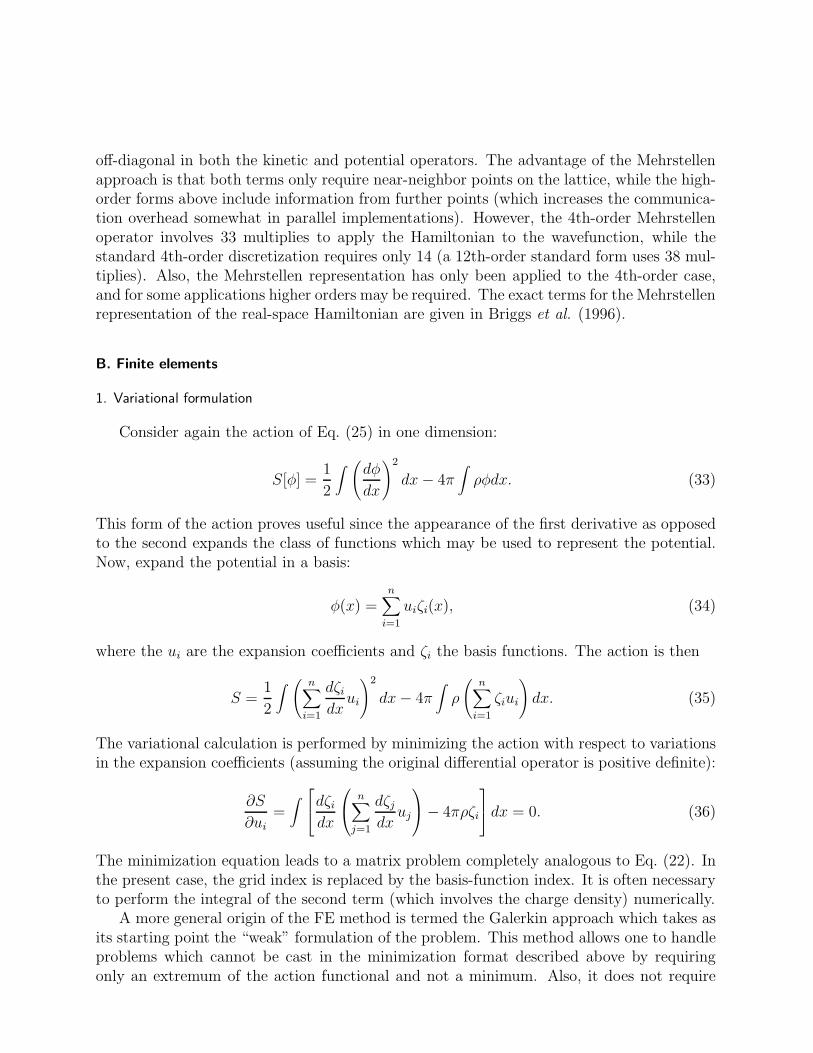
off-diagonal in both the kinetic and potential operators. The advantage of the Mehrstellenapproach is that both terms only require near-neighbor points on the lattice, while the high-order forms above include information from further points (which increases the communica-tion overhead somewhat in parallel implementations). However, the 4th-order Mehrstellenoperator involves 33 multiplies to apply the Hamiltonian to the wavefunction, while thestandard 4th-order discretization requires only 14 (a 12th-order standard form uses 38 mul-tiplies). Also, the Mehrstellen representation has only been applied to the 4th-order case,and for some applications higher orders may be required. The exact terms for the Mehrstellenrepresentation of the real-space Hamiltonian are given in Briggs et al. (1996).

B. Finite elements

1. Variational formulation

Consider again the action of Eq. (25) in one dimension:

S[φ] =1

2

∫

(

dφ

dx

)2

dx− 4π∫

ρφdx. (33)

This form of the action proves useful since the appearance of the first derivative as opposedto the second expands the class of functions which may be used to represent the potential.Now, expand the potential in a basis:

φ(x) =n∑

i=1

uiζi(x), (34)

where the ui are the expansion coefficients and ζi the basis functions. The action is then

S =1

2

∫

(

n∑

i=1

dζidxui

)2

dx− 4π∫

ρ

(

n∑

i=1

ζiui

)

dx. (35)

The variational calculation is performed by minimizing the action with respect to variationsin the expansion coefficients (assuming the original differential operator is positive definite):

∂S

∂ui=∫

dζidx

n∑

j=1

dζjdx

uj

− 4πρζi

dx = 0. (36)

The minimization equation leads to a matrix problem completely analogous to Eq. (22). Inthe present case, the grid index is replaced by the basis-function index. It is often necessaryto perform the integral of the second term (which involves the charge density) numerically.

A more general origin of the FE method is termed the Galerkin approach which takes asits starting point the “weak” formulation of the problem. This method allows one to handleproblems which cannot be cast in the minimization format described above by requiringonly an extremum of the action functional and not a minimum. Also, it does not require

19

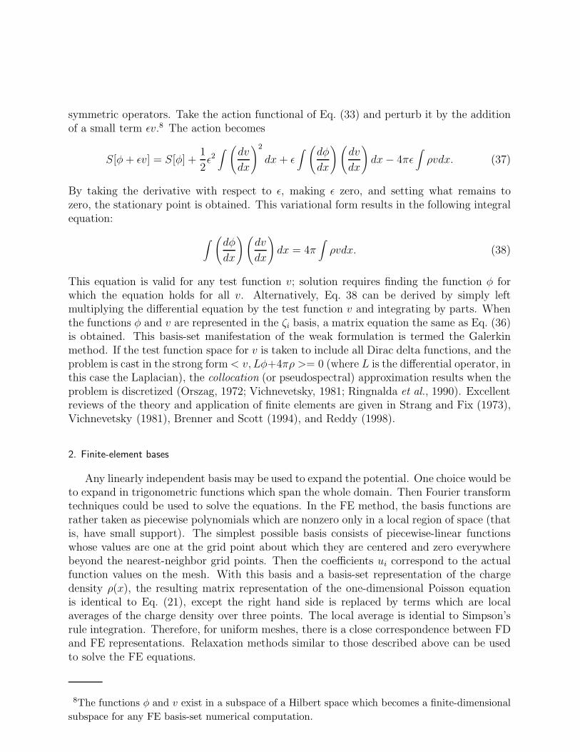
symmetric operators. Take the action functional of Eq. (33) and perturb it by the additionof a small term ǫv.8 The action becomes

S[φ+ ǫv] = S[φ] +1

2ǫ2∫

(

dv

dx

)2

dx+ ǫ∫

(

dφ

dx

)(

dv

dx

)

dx− 4πǫ∫

ρvdx. (37)

By taking the derivative with respect to ǫ, making ǫ zero, and setting what remains tozero, the stationary point is obtained. This variational form results in the following integralequation:

∫

(

dφ

dx

)(

dv

dx

)

dx = 4π∫

ρvdx. (38)

This equation is valid for any test function v; solution requires finding the function φ forwhich the equation holds for all v. Alternatively, Eq. 38 can be derived by simply leftmultiplying the differential equation by the test function v and integrating by parts. Whenthe functions φ and v are represented in the ζi basis, a matrix equation the same as Eq. (36)is obtained. This basis-set manifestation of the weak formulation is termed the Galerkinmethod. If the test function space for v is taken to include all Dirac delta functions, and theproblem is cast in the strong form< v, Lφ+4πρ >= 0 (where L is the differential operator, inthis case the Laplacian), the collocation (or pseudospectral) approximation results when theproblem is discretized (Orszag, 1972; Vichnevetsky, 1981; Ringnalda et al., 1990). Excellentreviews of the theory and application of finite elements are given in Strang and Fix (1973),Vichnevetsky (1981), Brenner and Scott (1994), and Reddy (1998).

2. Finite-element bases

Any linearly independent basis may be used to expand the potential. One choice would beto expand in trigonometric functions which span the whole domain. Then Fourier transformtechniques could be used to solve the equations. In the FE method, the basis functions arerather taken as piecewise polynomials which are nonzero only in a local region of space (thatis, have small support). The simplest possible basis consists of piecewise-linear functionswhose values are one at the grid point about which they are centered and zero everywherebeyond the nearest-neighbor grid points. Then the coefficients ui correspond to the actualfunction values on the mesh. With this basis and a basis-set representation of the chargedensity ρ(x), the resulting matrix representation of the one-dimensional Poisson equationis identical to Eq. (21), except the right hand side is replaced by terms which are localaverages of the charge density over three points. The local average is idential to Simpson’srule integration. Therefore, for uniform meshes, there is a close correspondence between FDand FE representations. Relaxation methods similar to those described above can be usedto solve the FE equations.

8The functions φ and v exist in a subspace of a Hilbert space which becomes a finite-dimensional

subspace for any FE basis-set numerical computation.

20

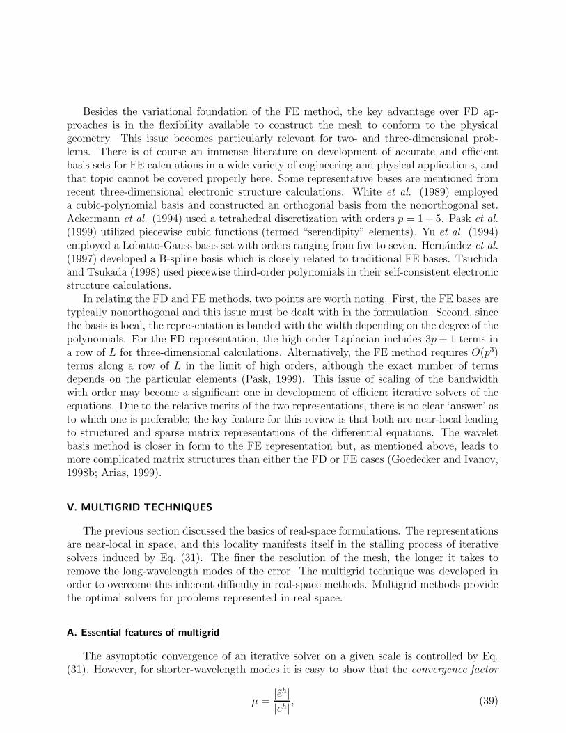
Besides the variational foundation of the FE method, the key advantage over FD ap-proaches is in the flexibility available to construct the mesh to conform to the physicalgeometry. This issue becomes particularly relevant for two- and three-dimensional prob-lems. There is of course an immense literature on development of accurate and efficientbasis sets for FE calculations in a wide variety of engineering and physical applications, andthat topic cannot be covered properly here. Some representative bases are mentioned fromrecent three-dimensional electronic structure calculations. White et al. (1989) employeda cubic-polynomial basis and constructed an orthogonal basis from the nonorthogonal set.Ackermann et al. (1994) used a tetrahedral discretization with orders p = 1− 5. Pask et al.

(1999) utilized piecewise cubic functions (termed “serendipity” elements). Yu et al. (1994)employed a Lobatto-Gauss basis set with orders ranging from five to seven. Hernandez et al.

(1997) developed a B-spline basis which is closely related to traditional FE bases. Tsuchidaand Tsukada (1998) used piecewise third-order polynomials in their self-consistent electronicstructure calculations.

In relating the FD and FE methods, two points are worth noting. First, the FE bases aretypically nonorthogonal and this issue must be dealt with in the formulation. Second, sincethe basis is local, the representation is banded with the width depending on the degree of thepolynomials. For the FD representation, the high-order Laplacian includes 3p+ 1 terms ina row of L for three-dimensional calculations. Alternatively, the FE method requires O(p3)terms along a row of L in the limit of high orders, although the exact number of termsdepends on the particular elements (Pask, 1999). This issue of scaling of the bandwidthwith order may become a significant one in development of efficient iterative solvers of theequations. Due to the relative merits of the two representations, there is no clear ‘answer’ asto which one is preferable; the key feature for this review is that both are near-local leadingto structured and sparse matrix representations of the differential equations. The waveletbasis method is closer in form to the FE representation but, as mentioned above, leads tomore complicated matrix structures than either the FD or FE cases (Goedecker and Ivanov,1998b; Arias, 1999).

V. MULTIGRID TECHNIQUES

The previous section discussed the basics of real-space formulations. The representationsare near-local in space, and this locality manifests itself in the stalling process of iterativesolvers induced by Eq. (31). The finer the resolution of the mesh, the longer it takes toremove the long-wavelength modes of the error. The multigrid technique was developed inorder to overcome this inherent difficulty in real-space methods. Multigrid methods providethe optimal solvers for problems represented in real space.

A. Essential features of multigrid

The asymptotic convergence of an iterative solver on a given scale is controlled by Eq.(31). However, for shorter-wavelength modes it is easy to show that the convergence factor

µ =|eh||eh| , (39)

21

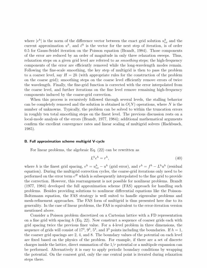
where |eh| is the norm of the difference vector between the exact grid solution uhex and the

current approximation uh, and eh is the vector for the next step of iteration, is of order0.5 for Gauss-Seidel iteration on the Poisson equation (Brandt, 1984). Those componentsof the error are reduced by an order of magnitude in only three relaxation sweeps. Thus,relaxation steps on a given grid level are referred to as smoothing steps; the high-frequencycomponents of the error are efficiently removed while the long-wavelength modes remain.Following the fine-scale smoothing, the key step of multigrid is then to pass the problemto a coarser level, say H = 2h (with appropriate rules for the construction of the problemon the coarse grid); smoothing steps on the coarse level efficiently remove errors of twicethe wavelength. Finally, the fine-grid function is corrected with the error interpolated fromthe coarse level, and further iterations on the fine level remove remaining high-frequencycomponents induced by the coarse-grid correction.

When this process is recursively followed through several levels, the stalling behaviorcan be completely removed and the solution is obtained in O(N) operations, where N is thenumber of unknowns. Typically, the problem can be solved to within the truncation errorsin roughly ten total smoothing steps on the finest level. The previous discussion rests on alocal-mode analysis of the errors (Brandt, 1977, 1984); additional mathematical argumentsconfirm the excellent convergence rates and linear scaling of multigrid solvers (Hackbusch,1985).

B. Full approximation scheme multigrid V-cycle

For linear problems, the algebraic Eq. (22) can be rewritten as

Lheh = rh, (40)

where h is the finest grid spacing, eh = uhex − uh (grid error), and rh = fh − Lhuh (residual

equation). During the multigrid correction cycles, the coarse-grid iterations only need to beperformed on the error term eH which is subsequently interpolated to the fine grid to providethe correction. However, this rearrangement is not possible for nonlinear problems. Brandt(1977, 1984) developed the full approximation scheme (FAS) approach for handling suchproblems. Besides providing solutions to nonlinear differential equations like the Poisson-Boltzmann equation, the FAS strategy is well suited to handle eigenvalue problems andmesh-refinement approaches. The FAS form of multigrid is thus presented here due to itsgenerality. In the case of linear problems, the FAS is equivalent to the error-iteration versionmentioned above.

Consider a Poisson problem discretized on a Cartesian lattice with a FD representationon a fine grid with spacing h (Eq. 22). Now construct a sequence of coarser grids each withgrid spacing twice the previous finer value. For a 4-level problem in three dimensions, thesequence of grids will consist of 173, 93, 53, and 33 points including the boundaries. If h = 1,the coarser grid spacings are 2, 4, and 8. The boundary values of the potential on each levelare fixed based on the physics of the problem. For example, if there are a set of discretecharges inside the lattice, direct summation of the 1/r potential or a multipole expansion canbe performed. Alternatively it is easy to apply periodic boundary conditions by wrappingthe potential. On the coarsest grid, only the one central point is iterated during relaxationsteps there.

22

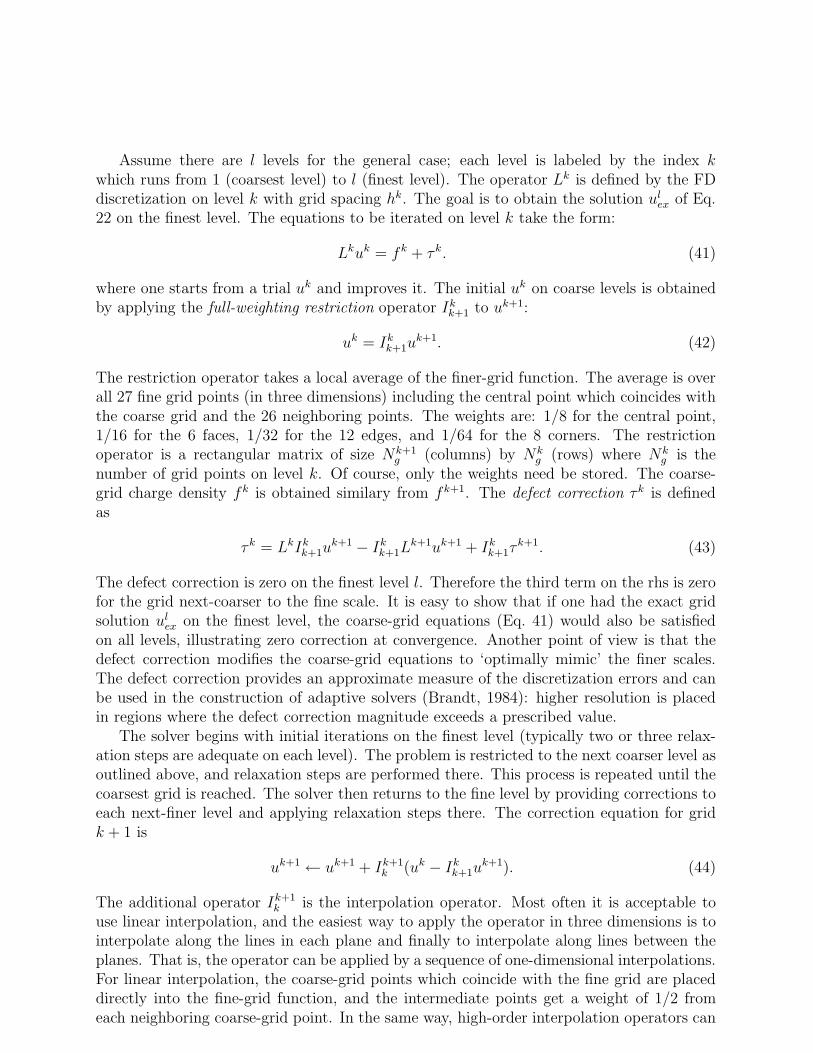
Assume there are l levels for the general case; each level is labeled by the index kwhich runs from 1 (coarsest level) to l (finest level). The operator Lk is defined by the FDdiscretization on level k with grid spacing hk. The goal is to obtain the solution ul

ex of Eq.22 on the finest level. The equations to be iterated on level k take the form:

Lkuk = fk + τk. (41)

where one starts from a trial uk and improves it. The initial uk on coarse levels is obtainedby applying the full-weighting restriction operator Ik

k+1 to uk+1:

uk = Ikk+1u

k+1. (42)

The restriction operator takes a local average of the finer-grid function. The average is overall 27 fine grid points (in three dimensions) including the central point which coincides withthe coarse grid and the 26 neighboring points. The weights are: 1/8 for the central point,1/16 for the 6 faces, 1/32 for the 12 edges, and 1/64 for the 8 corners. The restrictionoperator is a rectangular matrix of size Nk+1

g (columns) by Nkg (rows) where Nk

g is thenumber of grid points on level k. Of course, only the weights need be stored. The coarse-grid charge density fk is obtained similary from fk+1. The defect correction τk is definedas

τk = LkIkk+1u

k+1 − Ikk+1L

k+1uk+1 + Ikk+1τ

k+1. (43)

The defect correction is zero on the finest level l. Therefore the third term on the rhs is zerofor the grid next-coarser to the fine scale. It is easy to show that if one had the exact gridsolution ul

ex on the finest level, the coarse-grid equations (Eq. 41) would also be satisfiedon all levels, illustrating zero correction at convergence. Another point of view is that thedefect correction modifies the coarse-grid equations to ‘optimally mimic’ the finer scales.The defect correction provides an approximate measure of the discretization errors and canbe used in the construction of adaptive solvers (Brandt, 1984): higher resolution is placedin regions where the defect correction magnitude exceeds a prescribed value.

The solver begins with initial iterations on the finest level (typically two or three relax-ation steps are adequate on each level). The problem is restricted to the next coarser level asoutlined above, and relaxation steps are performed there. This process is repeated until thecoarsest grid is reached. The solver then returns to the fine level by providing corrections toeach next-finer level and applying relaxation steps there. The correction equation for gridk + 1 is

uk+1 ← uk+1 + Ik+1k (uk − Ik

k+1uk+1). (44)

The additional operator Ik+1k is the interpolation operator. Most often it is acceptable to

use linear interpolation, and the easiest way to apply the operator in three dimensions is tointerpolate along the lines in each plane and finally to interpolate along lines between theplanes. That is, the operator can be applied by a sequence of one-dimensional interpolations.For linear interpolation, the coarse-grid points which coincide with the fine grid are placeddirectly into the fine-grid function, and the intermediate points get a weight of 1/2 fromeach neighboring coarse-grid point. In the same way, high-order interpolation operators can

23

be applied as a sequence of one-dimensional operations; see Beck (1999b) for a listing ofthe high-order interpolation weights. The high-order weights are used in interpolating tonew fine levels in full multigrid eigenvalue solvers (Brandt et al., 1993) and in high-orderlocal mesh-refinement multigrid methods (Beck, 1999b). The interpolation operator is arectangular matrix of size Nk

g (columns) by Nk+1g rows. Only the weights need be stored,

just as for the restriction operator. All of the operators defined above can be initialized onceand used repeatedly throughout the algorithm. The multigrid cycle defined by the abovediscussion is termed a V-cycle which is shown schematically in Fig. 6. Alternative cyclingmethods have been employed as well, such as W-cycles. Reductions in the norm of theresidual in one V-cycle are generally an order of magnitude. The same set of operations isemployed in a high-order solver; the second-order Laplacian is simply replaced by the high-order version. The form of the multigrid solver is quite flexible; for example, a lower-orderrepresentation could be used on coarse levels during the correction cycles. In our own work,we have observed similar optimal convergence rates for high-order solvers as for second-orderones, so there is no degradation in efficiency with order. Applications in electrostatics andextensions for eigenvalue problems are discussed in Sections VI and VII.

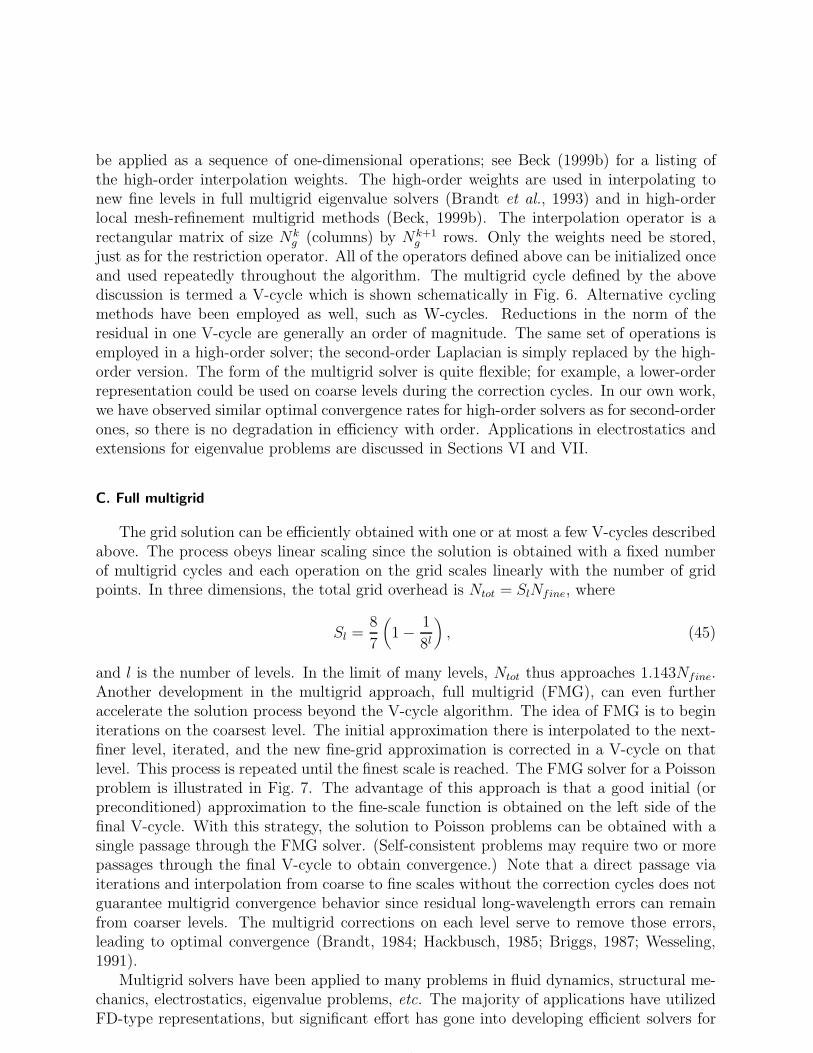
C. Full multigrid

The grid solution can be efficiently obtained with one or at most a few V-cycles describedabove. The process obeys linear scaling since the solution is obtained with a fixed numberof multigrid cycles and each operation on the grid scales linearly with the number of gridpoints. In three dimensions, the total grid overhead is Ntot = SlNfine, where

Sl =8

7

(

1− 1

8l

)

, (45)

and l is the number of levels. In the limit of many levels, Ntot thus approaches 1.143Nfine.Another development in the multigrid approach, full multigrid (FMG), can even furtheraccelerate the solution process beyond the V-cycle algorithm. The idea of FMG is to beginiterations on the coarsest level. The initial approximation there is interpolated to the next-finer level, iterated, and the new fine-grid approximation is corrected in a V-cycle on thatlevel. This process is repeated until the finest scale is reached. The FMG solver for a Poissonproblem is illustrated in Fig. 7. The advantage of this approach is that a good initial (orpreconditioned) approximation to the fine-scale function is obtained on the left side of thefinal V-cycle. With this strategy, the solution to Poisson problems can be obtained with asingle passage through the FMG solver. (Self-consistent problems may require two or morepassages through the final V-cycle to obtain convergence.) Note that a direct passage viaiterations and interpolation from coarse to fine scales without the correction cycles does notguarantee multigrid convergence behavior since residual long-wavelength errors can remainfrom coarser levels. The multigrid corrections on each level serve to remove those errors,leading to optimal convergence (Brandt, 1984; Hackbusch, 1985; Briggs, 1987; Wesseling,1991).

Multigrid solvers have been applied to many problems in fluid dynamics, structural me-chanics, electrostatics, eigenvalue problems, etc. The majority of applications have utilizedFD-type representations, but significant effort has gone into developing efficient solvers for

24

FE representations as well (Brandt, 1980; Deconinck and Hirsch, 1982; Hackbusch, 1985;Braess and Verfurth, 1990; Brenner and Scott, 1994). An additional difficulty with FEmultigrid methods is a proper representation of the problem on coarse levels: the moreregular the fine-scale mesh, the easier is the coarsening process.

VI. ELECTROSTATICS CALCULATIONS

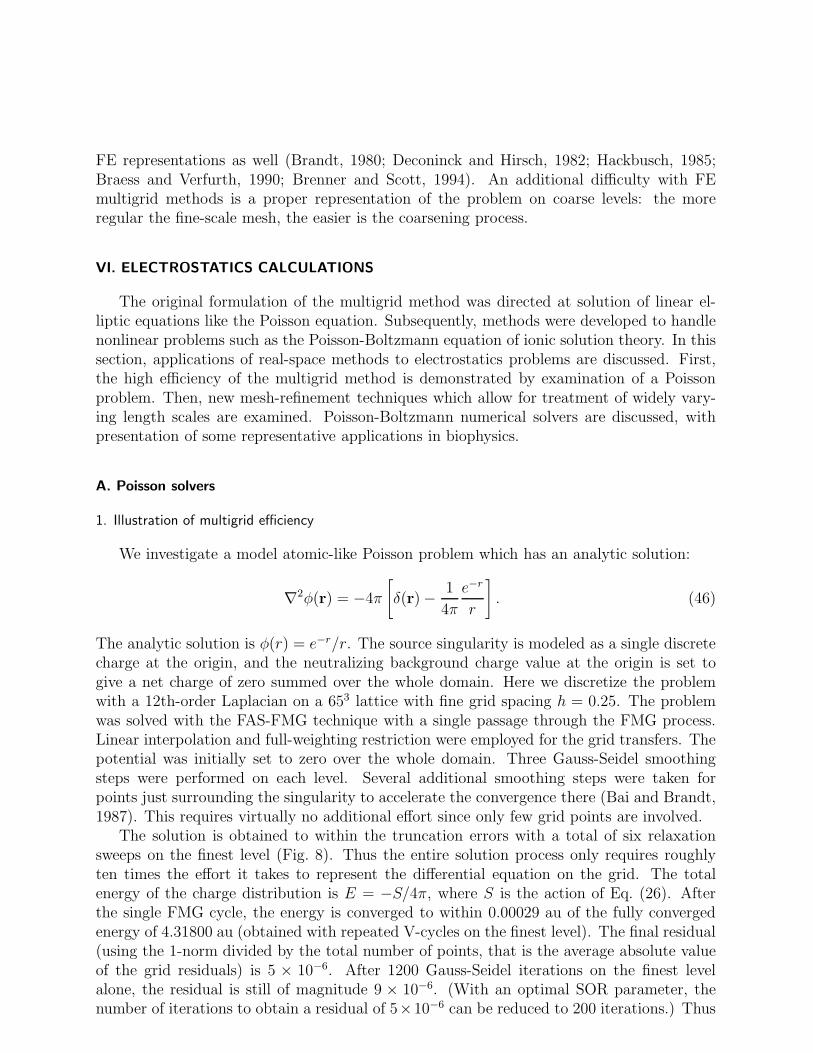
The original formulation of the multigrid method was directed at solution of linear el-liptic equations like the Poisson equation. Subsequently, methods were developed to handlenonlinear problems such as the Poisson-Boltzmann equation of ionic solution theory. In thissection, applications of real-space methods to electrostatics problems are discussed. First,the high efficiency of the multigrid method is demonstrated by examination of a Poissonproblem. Then, new mesh-refinement techniques which allow for treatment of widely vary-ing length scales are examined. Poisson-Boltzmann numerical solvers are discussed, withpresentation of some representative applications in biophysics.

A. Poisson solvers

1. Illustration of multigrid efficiency

We investigate a model atomic-like Poisson problem which has an analytic solution:

∇2φ(r) = −4π

[

δ(r)− 1

4π

e−r

r

]

. (46)

The analytic solution is φ(r) = e−r/r. The source singularity is modeled as a single discretecharge at the origin, and the neutralizing background charge value at the origin is set togive a net charge of zero summed over the whole domain. Here we discretize the problemwith a 12th-order Laplacian on a 653 lattice with fine grid spacing h = 0.25. The problemwas solved with the FAS-FMG technique with a single passage through the FMG process.Linear interpolation and full-weighting restriction were employed for the grid transfers. Thepotential was initially set to zero over the whole domain. Three Gauss-Seidel smoothingsteps were performed on each level. Several additional smoothing steps were taken forpoints just surrounding the singularity to accelerate the convergence there (Bai and Brandt,1987). This requires virtually no additional effort since only few grid points are involved.

The solution is obtained to within the truncation errors with a total of six relaxationsweeps on the finest level (Fig. 8). Thus the entire solution process only requires roughlyten times the effort it takes to represent the differential equation on the grid. The totalenergy of the charge distribution is E = −S/4π, where S is the action of Eq. (26). Afterthe single FMG cycle, the energy is converged to within 0.00029 au of the fully convergedenergy of 4.31800 au (obtained with repeated V-cycles on the finest level). The final residual(using the 1-norm divided by the total number of points, that is the average absolute valueof the grid residuals) is 5 × 10−6. After 1200 Gauss-Seidel iterations on the finest levelalone, the residual is still of magnitude 9 × 10−6. (With an optimal SOR parameter, thenumber of iterations to obtain a residual of 5×10−6 can be reduced to 200 iterations.) Thus

25

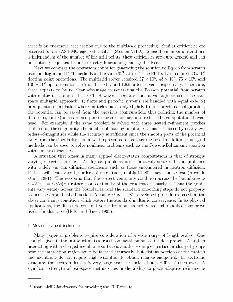
there is an enormous acceleration due to the multiscale processing. Similar efficiencies areobserved for an FAS-FMG eigenvalue solver (Section VII.A). Since the number of iterationsis independent of the number of fine grid points, these efficiencies are quite general and canbe routinely expected from a correctly functioning multigrid solver.

Next we compare the operations count for generating the solution to Eq. 46 from scratchusing multigrid and FFT methods on the same 653 lattice.9 The FFT solver required 33×106

floating point operations. The multigrid solver required 27 × 106, 43 × 106, 75 × 106, and106× 106 operations for the 2nd, 4th, 8th, and 12th order solvers, respectively. Therefore,there appears to be no clear advantage in generating the Poisson potential from scratchwith multigrid as opposed to FFT. However, there are some advantages to using the real-space multigrid approach: 1) finite and periodic systems are handled with equal ease, 2)in a quantum simulation where particles move only slightly from a previous configuration,the potential can be saved from the previous configuration, thus reducing the number ofiterations, and 3) one can incorporate mesh refinements to reduce the computational over-head. For example, if the same problem is solved with three nested refinement patchescentered on the singularity, the number of floating point operations is reduced by nearly twoorders-of-magnitude while the accuracy is sufficient since the smooth parts of the potentialaway from the singularity can be well represented on coarser meshes. In addition, multigridmethods can be used to solve nonlinear problems such as the Poisson-Boltzmann equationwith similar efficiencies.

A situation that arises in many applied electrostatics computations is that of stronglyvarying dielectric profiles. Analogous problems occur in steady-state diffusion problemswith widely varying diffusion coeffcients such as those encountered in neutron diffusion.If the coefficients vary by orders of magnitude, multigrid efficiency can be lost (Alcouffeet al., 1981). The reason is that the correct continuity condition across the boundaries isǫ1∇φ(r1) = ǫ2∇φ(r2) rather than continuity of the gradients themselves. Thus the gradi-ents vary widely across the boundaries, and the standard smoothing steps do not properlyreduce the errors in the function. Alcouffe et al. (1981) developed procedures based on theabove continuity condition which restore the standard multigrid convergence. In biophysicalapplications, the dielectric constant varies from one to eighty, so such modifications proveuseful for that case (Holst and Saied, 1993).

2. Mesh-refinement techniques

Many physical problems require consideration of a wide range of length scales. Oneexample given in the Introduction is a transition metal ion buried inside a protein. A proteininteracting with a charged membrane surface is another example: particular charged groupsnear the interaction region must be treated accurately, but distant portions of the proteinand membrane do not require high resolution to obtain reliable energetics. In electronicstructure, the electron density is very large near the nucleus but is diffuse further away. Asignificant strength of real-space methods lies in the ability to place adaptive refinements

9I thank Jeff Giansiracusa for providing the FFT results.

26

in regions where the desired functions vary rapidly while treating the distant zones with acoarser description.

Two approaches exist for such refinements in the FD method (FE methods allow quiteeasily for grid adaptation): grid curving and local mesh refinements. While grid curving isan elegant procedure for adapting higher resolution in certain regions of space, generally thecoordinate transformations are global. Therefore, the higher resolution tends to spread somedistance from where the refinement is necessary (Modine et al., 1997, Figs. 1, 4, and 5), anddepending on the geometry of the problem it may be difficult or impossible to design anappropriate grid transformation. Also, the transformations can be quite complex leading toadditional difficulties in the solution process. Finally, the grid-curving transformations alterthe underlying spectral properties of the operators which can in principle lead to degradationof the multigrid efficiency in the solution process. However, this does not appear to havebeen a problem in the methods of Gygi and Galli (1995) and Modine et al. (1997), althoughthe convergence behavior of their multigrid Poisson solvers was not extensively discussed inthose works. Mesh-curving strategies for electronic structure calculations are discussed inSection VII.D.

An alternative procedure is to place nested uniform patches of refinement locally in space(Fig. 9). Then the overall structure of the multigrid solver is the same, except fine-leveliterations are performed only over the nested patches. The same forms for the Laplacian,restriction, interpolation, and smoothing operators are maintained. This procedure is highlyflexible since the nested refinements can be centered about any locations of space and canmove as the problem evolves. The placement of the refinements can be adaptively controlledby examination of the defect correction τH ; higher resolution should be placed in regionswhere τH is large. If an underlying FD representation is employed, it is relatively easy toextend the method to high-order solvers since the mesh of the refinement patch is uniform.

Bai and Brandt (1987) developed an FAS multigrid mesh-refinement method for treatingwidely varying length-scale Poisson-type problems. They first developed a λ-FMG exchange-rate algorithm which minimizes the error obtained for a given amount of computationalwork. Since the number of visits to the coarse levels (which extend over the whole domain)is proportional to the number of patches, direct application of the multigrid algorithm doesnot scale strictly linearly for many levels; the λ-FMG process restores the linear scaling fora solver including the mesh refinements. Second, they showed that extra local relaxationsaround structural singularities restore asymptotic convergence rates which can otherwisedegrade. Third, they developed a conservative-differencing technique for handling sourcesingularities.

To motivate the need for conservative differencing in the FAS-FMG mesh-refinementsolver, consider Eq. (41) and a two-level problem with one nested patch. The defect cor-rection on the coarse level H is initially defined only over the interior region of the patch.However, if one examines the sum of τH over the refinement, most of the terms in the in-terior cancel, but nonzero values remain near the boundaries. The remaining terms closelyresemble flux operators at the boundary. The net effect is thus the introduction of addi-tional sources in the Poisson equation, which pollutes the solution severely over the wholedomain. By balancing the local fluxes with additional defect correction terms on the patchboundary, the correct source strength is restored. Bai and Brandt (1987) solved this problemfor second-order equations and tested the method on a source-singularity problem in two

27

dimensions.Recently the method has been extended to high-order FD approximations by Beck

(1999b, 2000). The boundary defect correction terms were determined by examinationof the noncancelling terms for the high-order approximations. Without the conservativescheme, significant errors are apparent over the whole domain. With the inclusion of theboundary corrections, the sum of τH over the patch is zero to machine precision and thecorrect high-order behavior is obtained over the whole domain. The method was tested on asource-singularity problem in three dimensions for multiple nested patches. Typical multi-grid efficiencies were observed. Additional corrections will be necessary at the boundariesfor continuous charge distributions which cover the refinement boundaries, but these areindependent of the order of the Laplacian. These techniques are currently being includedin high-order FD electronic structure calculations. They will significantly reduce the gridoverhead in comparison to uniform-grid calculations while still maintaining the linear-scalingproperties of the multigrid method. It is not possible to handle truly local refinements withthe FFT approach.

In related work, Goedecker and Ivanov (1998a) developed a linear-scaling multiresolutionwavelet method for the Poisson equation which allows for treatment of widely varying lengthscales. They utilized second-generation interpolating wavelets since the mapping from gridvalues to expansion coefficients is easy for these functions, and they have a fast wavelettransform. They solved the Poisson equation for the challenging case of the all-electronuranium dimer. Their solver employed 22 hierarchical levels, and the potential was obtainedto six significant digits.

B. Poisson-Boltzmann solvers

As discussed in Section II.B, the Poisson-Boltzmann equation arises from the assumptionof no ion correlations. That is, it is a mean-field treatment. Onsager (1933) showed thatthere exists an inherent asymmetry at the Poisson-Boltzmann level. Nevertheless, calcula-tions performed at this level of theory can yield accurate energetics for monovalent ions atmoderate concentrations (Honig and Nicholls, 1995; Tomac and Graslund, 1998; Patra andYethiraj, 1999). Linearization of the Poisson-Boltzmann equation restores the symmetry,but for many cases of experimental interest the linearization assumption is too severe. So-lution of the Poisson-Boltzmann equation produces the electrostatic potential throughoutspace, which in turn generates the equilibrium mobile-ion charge densities and the totalfree energy of the ion gas (below). By computing the total energies for several macroionconfigurations, the potential of mean force due to electrostatic effects can be approximated(Rice, 1959). In this section, we focus on real-space numerical methods for solution of thenonlinear Poisson-Boltzmann equation [Eq. (12)].

Numerical solution of nonlinear partial differential equations is problematic. For thePoisson-Boltzmann case, the nonlinearities can be severe near fixed charges since the ratioof the potential to kT can be large. Also, strong dielectric discontinuities at the boundary ofa large molecular ion and the solution create technical difficulties. However, it is known thatthere is a single stable minimum of the action functional whose derivative yields the Poisson-Boltzmann equation (Coalson and Duncan, 1992; Ben-Tal and Coalson, 1994). Therefore,properly constructed iterative processes can be expected to locate that minimum.

28

Early numerical work centered on FD representations. Nicholls and Honig (1991) de-veloped an efficient single-level SOR method which included special techniques for memoryallocation and for locating the optimal relaxation parameter. For the test cases considered,between 76 and 184 iterations were required for convergence. They also observed divergencefor some highly nonlinear cases. Davis and McCammon (1989) and Luty et al. (1992)used instead a conjugate-gradients relaxation method. Between 90 and 118 iterations wererequired to obtain convergence. They observed a factor of at least two improvement inefficiency in comparison with SOR relaxation in their test calculations.

After the development of multigrid methods for solving linear Poisson-type problems,efforts focused on nonlinear problems. The FAS algorithm presented above is well suited forsolving nonlinear problems (Brandt, 1984). Two modifications are needed: the driving termfh on a given level now includes the nonlinear terms, and additional terms must be includedin the defect correction to ensure zero correction at convergence. The defect correction forthe Poisson-Boltzmann problem is of the form (a single monovalent positive ion componentwith uniform dielectric is considered here):

τH = LHIHh u

h − IHh L

huh +4π

ǫ

[

nH+e

−βuH−vH − nh+I

Hh e

−βuh−vh]

, (47)

where the additional terms reflect the differing representations of the nonlinear terms on thetwo levels. The concentration on a given level is given by

nh+ =

N+

h3∑

e−βuh−vh . (48)

The sum is over the lattice and N+ is the number of positive ions in the computation domain(Coalson and Duncan, 1992). This procedure for obtaining the bulk ion concentrationsensures charge conservation at all steps of iteration. Simple smoothing steps can be takento relax on a given level, or Newton iterations (Press et al., 1992) may also be conductedon each level. Variable ω parameters may be required in the relaxation steps due to thediffering degrees of nonlinearities on the respective levels. Related multigrid techniques fornonlinear problems are presented in Stuben and Trottenberg (1982) and Hackbusch (1985).

Holst and Saied (1995) developed a highly efficient method which combines linear multi-level techniques with inexact-Newton iterations. They compared the convergence behaviorof the inexact-Newton multigrid method with SOR and conjugate-gradients minimizationon a single level. Their multilevel technique converged robustly and more efficiently thanthe relaxation methods on all problems investigated including challenging source problemswith dielectric discontinuities. Conjugate gradients and SOR exhibited similar convergencerates when compared with each other. They also examined a standard nonlinear multigridmethod similar to that outlined above. For some cases, the nonlinear multigrid techniquegave good convergence, but under certain conditions it diverged. The authors thus recom-mended caution in applying the FAS multigrid method directly to the Poisson-Boltzmannequation. Coalson and Beck (1998) tested the FAS approach on model problems in the latticefield theory including source singularities and found convergence for each case. Oberei andAllewell (1993) have also developed a convergent multigrid solver for the Poisson-Boltzmannequation. It is not entirely clear at the present time whether differences in observed conver-gence are due to the model problems investigated or to differences in the algorithms.

29

One issue that has not been addressed to date concerns charge conservation on the variouslevels. The standard form of the Poisson-Boltzmann equation (Honig and Nicholls, 1995)assumes fixed and equal concentrations of the mobile ions at infinity where the potentialis zero. The ion charge density can then be expressed as the product of a constant terminvolving the Debye length of the ion gas and a sinh term involving the potential. Typicallythe boundary potential is fixed with the linearized Debye-Huckel value. This representationconserves charge if the system size is allowed to go to infinity due to the infinite extentof the bath. However, charge is not conserved for finite system sizes, and in a multilevelprocedure differing charge states will be encountered on the various levels. In the lattice fieldtheory of Coalson and Duncan (1992), on the other hand, the charge is naturally conserved(maintaining overall charge neutrality) by updating the parameters n+ and n− during eachstep of iteration (see Eqs. 12 and 48). Lack of conservation of charge on the grid levels in thestandard approach may impact the convergence behavior of a multilevel solver; this issuedeserves further attention.

In a recent study, Tomac and Graslund (1998) extended the Poisson-Boltzmann level oftheory to include ion correlations in an approximate way. They solved for the Kirkwood(1934) hierarchy of equations on a FD grid assuming a closure proposed by Loeb (1951).Multigrid techniques were used to solve the initial Poisson-Boltzmann equation and to im-plement the inclusion of ion correlations. Coarser grids were used to estimate the fluctuationterm, and the impact of large grid spacing on the accuracy of the correlation term was ex-amined. Excellent agreement with previous theoretical results and Monte Carlo simulationwas obtained for divalent ion distributions around a central sphere. Test calculations werealso performed on ion distributions around an ATP molecule. This work allows for the moreaccurate treatment of systems containing multivalent ions. The computational expense ofobtaining the fluctuation contribution is extensive, however.

What is clear from the multigrid studies to date is that multilevel methods can yieldsolutions to the Poisson-Boltzmann equation (and its modifications to include ion correla-tions) with efficiencies resembling those for linear problems and with linear-scaling behavior.Hence, they show a great deal of promise for large-scale colloid and biophysical applications.Under some circumstances, special measures may be necessary to obtain correct multigridconvergence efficiencies. To my knowledge, all FD Poisson-Boltzmann calculations so farhave employed second-order Laplacians; going to higher orders improves accuracy for littleadditional cost, so higher-order solvers should be considered. However, high-order techniquesnear dielectric discontinuities introduce some additional complexity.

In addition to FD-related methods for solving the Poisson-Boltzmann equation, FE solu-tions have appeared. The FE discretization leads to a more accurate physical representationof complex molecular surfaces at the expense of additional computational overhead. You andHarvey (1993) developed a three-dimensional FE method for solving the linearized Poisson-Boltzmann equation. More accurate results were obtained with the FE approach comparedwith FD solutions in model problems. Potential distributions were computed surroundingtRNA molecules and the enzyme superoxide dismutase. This was the first application ofthe FE method to large-scale biological macromolecular electrostatics. Cortis and Friesner(1997) formulated a method for constructing tetrahedral FE meshes around macromolecules.The authors discussed the relative merits of FD and FE representations including applica-tions of multilevel methods in their solution. They used their discretization procedure to

30

solve the linearized Poisson-Boltzmann equation. Bowen and Sharif (1997) presented a FEnumerical method for solution of the nonlinear Poisson-Boltzmann equation in cylindricalcoordinates. Adaptive mesh refinements were employed to gain accuracy near curved sur-faces. They considered applications to membrane separation processes by examining thecase of a charged spherical particle near a cylindrical pore. Alternative formulations ofelectrostatic problems include boundary element methods which reduce Poisson problemsto calculations involving the molecular surface (Yoon and Lenhoff, 1990, 1992; Pratt et al.,1997). They lead to dense matrix representations of the problem; if nonlinear salt effectsare to be included, volume integrals, in addition to surface integrals, must be incorporated.

C. Computations of free energies

Several proposals have appeared concerning computation of free energies of the ion gasonce the solution of the Poisson-Boltzmann equation is obtained. The free energies arecrucial for determining electrostatic interaction energies of charged macromolecules at themean-field level. The energies can be obtained either by charging methods or volume/surfaceintegrations (Verwey and Overbeek, 1948; Marcus, 1955; Rice, 1959; Reiner and Radke,1990). The most commonly used volume integration approach stems from the variationalformulation of Sharp and Honig (1990b). They postulated a form for the free energy which,when extremized, produces the Poisson-Boltzmann equation. Fogolari and Briggs (1997)critiqued this variational form, showing that the extremum in the free energy is a maxi-mum, not a minimum, with respect to variations of the potential. They presented anotherform which is minimized. The lattice field theoretic free energy is derived from a rigorousrepresentation of the grand partition function of the ion gas (Coalson and Duncan, 1992).In this section, we will derive the variational form from the lattice field theory formulationto illustrate differences between the two; the variational form is obtained from the infinitesystem size limit of the lattice field theory. We assume here the case of uniform dielectricand monovalent ions; the extensions for variable dielectric and higher valences follow thesame arguments.

The mean-field lattice field theory Helmholtz free energy is

βF = −SLFT +N+ ln(n+h3) +N− ln(n−h

3), (49)

where SLFT is an action term (defined below) and N+ and N− are the total numbers ofpositive and negative mobile ions in the calculation domain. In order to handle periodicas well as finite domains, we assume that the total number of mobile and fixed charges issuch that overall charge neutrality is maintained. The free energy Eq. (49) is invariant to auniform shift of the potential, which is the correct physical result. The concentration n+ isgiven by Eq. (48), while n− is obtained by the analogous formula for negative charges.

Consider the action which, when minimized, results in the Poisson-Boltzmann equation:

S = −1

2

∫

φ∇2φd3x− 4π

ǫ

∫

[

ρfφ−n+

βe−βφ−v − n−

βeβφ−v

]

d3x. (50)

The action of Eq. (49) is related to S by

31

SLFT =βǫ

4πS. (51)

Then the total Helmholtz free energy on the lattice is

βF =βǫh3

8π

∑

φhLhφh + βh3∑

ρhfφ

h +N+ ln(n+h3/e) +N− ln(n−h

3/e), (52)

where the grid potential is φh, and the sums are over the lattice points.Let us examine a process in which two macroions are moved relative to each other

(Fig. 10). The macroions are assumed to reside in a large calculation domain which containscounterions plus perhaps salt ions, so the potential is screened at large distances. We assumethat the potential decays effectively to zero some finite distance from the ions and is zeroall the way to the boundaries. The mobile ions behave as an ideal gas where the potential iszero. The numbers of fixed and mobile ions is maintained constant throughout the process.Now, consider the free energy change from the ‘activity’ term for the positive mobile ionsupon moving from configuration 1 to 2:

β∆Fa+ = N+ ln

∑

e−βφh1−vh

1

∑

e−βφh2−vh

2

. (53)

Call the number of free sites in the domain where the potential is effectively zero Nf1 and

Nf2 . The sums over regions where the potential is nonzero are labelled Σ1 and Σ2. The free

energy change ∆Fa+ is then

β∆Fa+ = N+ ln

[

Nf1 + Σ1

]

[

Nf2 + Σ2

] . (54)

Factor out the Nf terms:

β∆Fa+ = N+ lnNf

1

[

1 + Σ1

Nf1

]

Nf2

[

1 + Σ2

Nf2

] . (55)

The term involving the ratio of the free sites can be represented as

N+ lnNf

1

Nf2

= N+ lnN ′

tot

[

1− Σ1g

N ′

tot

]

N ′tot

[

1− Σ2g

N ′

tot

] , (56)

where N ′tot is the total number of grid points outside any excluded volume regions and

Σ1g and Σ2g count the numbers of grid points outside of excluded volume zones where thepotential is nonzero.

For very large system sizes, the above expressions can be approximated as

β∆Fa+ ≈ N+

(

Σ1

Nf1

− Σ2

Nf2

)

+N+

N ′tot

(−Σ1g + Σ2g) . (57)

32

Analogous terms are obtained for the negative ion case. As the system size approachesinfinity, we can make the further approximations N+ ≈ N− and Nf

1 ≈ Nf2 ≈ N ′

tot.The resulting free energy change for both ionic species is then

β∆Fa =N+

N ′tot

[

∑

(

e−βφh1 + eβφh

1 − 2)

e−vh1 −

∑

(

e−βφh2 + eβφh

2 − 2)

e−vh2

]

. (58)

If we call the grid concentration cg = N+/N′tot = N−/N

′tot, then the free energy change

can be written as

β∆Fa = −2cg[

∑

(

cosh(βφh2)− 1

)

e−vh2 −

∑

(

cosh(βφh1)− 1

)

e−vh1

]

. (59)

The grid ‘activity coefficient’ γ is cg/h3 which can be assumed to be γ =

√n+n−. In the

continuum limit the free energy change due to the logarithmic terms in the total free energyis thus

β∆Fa = −2γ[∫

[cosh(βφ2)− 1] e−v2d3x−∫

[cosh(βφ1)− 1] e−v1d3x]

. (60)

The overall free energy change can then be written as the difference of two terms, one foreach configuration:

βF = β∫

ρfφd3x− 2γ

∫

[cosh(βφ)− 1] e−vd3x+βǫ

8π

∫

φ∇2φd3x (61)

So long as the potential and/or its derivative go to zero on the boundaries, Eq. (61) canbe rewritten as

βF = β∫

ρfφd3x− 2γ

∫

[cosh(βφ)− 1] e−vd3x− β

8π

∫

ǫ |∇φ|2 d3x (62)

which is identical to Eq. (13) in Sharp and Honig (1990b). Thus the variational free energy ofSharp and Honig is derived as the infinite system limit of the lattice field theory expression,where the potential is assumed to go to zero at the distant boundaries. Since the variationalform is not invariant to a uniform shift of the potential, some arbitrariness is introduced.In addition, charge conservation is not maintained as discussed above. The issue of chargeconservation is particularly relevant if one considers periodic boundary domains. Therefore,it is recommended to use the lattice field theoretic form for computations of free energiesfor cases where these considerations are deemed important.

D. Biophysical applications

One reason for a resurgence of interest in continuum models of solvation for large macro-molecules is that, for many systems of interest, the total number of particles is simply toolarge to accurately model at the atomic level. For example, consider a protein interact-ing with a DNA strand: the atomistic treatment including solvent and salt effects wouldinvolve several tens of thousands of atoms, and the motions occur over time scales longerthan nanoseconds. So long as the energetics are proven to be reasonable in testable modelcalculations, some confidence can be placed in the Poisson-Boltzmann calculations on larger

33

systems. The number of applications of Poisson-Boltzmann-level theory to biological macro-molecules is now very large. Previous reviews summarize progress in this area (Sharp andHonig, 1990a; Honig and Nicholls, 1995). A few representative studies from the main cate-gories of application are presented here to give a flavor of the types of problems which areaccessible.

The first type of application concerns the computed average electrostatic potential andthe resulting charge distributions. Haggerty and Lenhoff (1991) performed FD calculationsto generate the electrostatic potential on the surfaces of proteins. They found a clear correla-tion between retention data in ion-exchange chromatography and the average protein surfacepotential. Ion-exchange chromatography is one of the important techniques for separatingmixtures of proteins. Montoro and Abascal (1998) compared Monte Carlo simulations andFD Poisson-Boltzmann calculations on distributions of monovalent ions around a model ofB-DNA. They found good agreement between the simulations and Poisson-Boltzmann cal-culations for low to moderate ion concentrations, but for concentrations above 1 M, theagreement deteriorates. Pettit and Valdeavella (1999) compared electrostatic potentialsobtained from molecular dynamics simulations and Poisson-Boltzmann calculations for atetra-peptide. They observed qualitative differences for the electrostatic potentials aroundthe peptide. However, they argued that the free energies obtained by integration over theentire domain include cancellation of errors and yield more reliable results compared withthe potential itself. Patra and Yethiraj (1999) developed a DFT method for the ion atmo-sphere around charged cylinders (a model for DNA or tobacco mosaic virus). Their theoryincludes contributions from finite ion size and ion correlations beyond the mean-field level.Their DFT approach gave good agreement with simulations for both monovalent and diva-lent ion atmospheres. The Poisson-Boltzmann level theory does well for low axial chargedensities on the cylinder. Interesting charge inversion effects were seen for divalent saltswhich are entirely absent from the Poisson-Boltzmann calculations. Recently Baker et al.

(1999) developed a highly adaptive multilevel FE method for solving the Poisson-Boltzmannequation. By placing adaptive meshes in the regions of the dielectric discontinuities, largereductions in overall computation cost were observed. Computations were performed toobtain the electrostatic potential around large protein and DNA systems.

The second utility of Poisson-Boltzmann calculations lies in the computation of free ener-gies and resulting interaction energies for variable macromolecule conformations. Yoon andLenhoff (1992) used a boundary-elements method to compute interaction energies for a pro-tein and a negatively charged surface at the linearized Poisson-Boltzmann level. They foundthe most favorable orientation with the protein active site facing the surface. Zacharias et

al. (1992) investigated the interaction of a protein with DNA utilizing the FD Poisson-Boltzmann method. They studied the distribution of ions in the region between the twospecies and the energetics for protein binding. The interaction energy depends strongly onthe charge distributions on the DNA and protein. The computed number of ions releasedupon complexation agreed well with experiment. Misra et al. (1994) performed FD Poisson-Boltzmann calculations to study the influence of added salt on protein-DNA interactions.Long-range salt effects play a significant role in relative stabilities of competing structures ofprotein-DNA complexes. Ben-Tal et al. (1997) examined electrostatic effects in the bindingof proteins to biological membranes. The binding constant for the protein-membrane com-plex was successfully compared with experimental data. Chen and Honig (1997) extended

34

their FD Poisson-Boltzmann method to mixed salts including both monovalent and divalentspecies. They found that, for pure salt cases, the electrostatic contribution to binding varieslinearly with the logarithm of the ion concentration; for divalent salts, nonlinear effects wereobserved due to competitive binding of the two ionic species.

A third type of problem addressed with Poisson-Boltzmann level computations is thedetermination of pH-dependent properties of proteins. Since the net charge of the proteinis crucial in understanding its properties, a predictive method is desired for computing elec-trostatic effects (due to other charged groups) on the pKa’s of ionizable groups. Antosiewiczet al. (1994, 1996) presented extensive calculations on a large data set for several proteins.Somewhat surprisingly, they obtained the best agreement with experiment assuming an in-terior dielectric constant of 20 for the protein. Possible explanations of this effect werediscussed, including approximate accounting for specific ion binding and conformational re-laxation of the protein. They also found improvements if NMR structural sets were usedas opposed to single crystal X-ray structures for the proteins. Vila et al. (1998) recentlyperformed boundary-element multigrid calculations to determine pKa shifts; they obtainedexcellent agreement with experiment for polypentapeptides.

Fourth, Poisson-Boltzmann methods have been incorporated into electronic structurecalculations to study solvation effects. As an example, Fisher et al. (1996) performed DFTelectronic structure calculations on a model for the manganese superoxide dismutase enzymeactive site. The region treated explicitly included 37 or 38 atoms (115 valence electrons).The surrounding solvent was modeled as a dielectric continuum (water). The electronicstructure was computed self-consistently by updating the reaction-field potential due tothe solvent following calculations with fixed potential. Typically, the continuum solvationprocedure converged within seven iterations. The authors computed redox potentials andpKa’s for the complex. Differences from measured redox potentials were observed, and theauthors stressed the importance of explicitly including electrostatic effects from the rest ofthe protein in the calculations.

As a final biophysical real-space application, a lattice relaxation algorithm has beendeveloped by Kurnikova et al. (1999) to examine ion transport through membrane-boundproteins. The coupled Poisson and steady-state diffusion equations (Poisson-Nernst-Planckor PNP equations) were solved self-consistently on a FD real-space grid for motion througha membrane protein, the Gramicidin A dimer. The charges embedded in the channel interiorhad a large impact on computed diffusion rates. The computed current-voltage behavioragreed well with experimental findings. The accuracy of the continuum mean-field treatmentis encouraging for the further study of ion transport through a wide range of membraneproteins. A recent study (Corry et al., 2000) has critiqued the mean-field approach fornarrow ion channels, so some modifications in the PNP theory may be required for thosecases.

VII. SOLUTION OF SELF-CONSISTENT EIGENVALUE PROBLEMS

Eigenvalue problems arise in a wide range of applications. Solution of the Schrodingerequation with fixed or self-consistent potential is of course a dominant one. However, eigen-value problems occur in several other areas. Included are computation of modes and fre-quencies for molecular vibrations (Jensen, 1999) and optical modes of waveguides (Coalson

35

et al., 1994). Self-consistent eigenvalue problems also arise in polymer theory (Tsonchevet al., 1999). This section reviews recent research on real-space methods for fixed and self-consistent potential eigenvalue problems. The main focus is on novel methods for solving theKohn-Sham equations in electronic structure. Additional discussion concerns applicationsin semiconductor and polymer physics.

A. Fixed-potential eigenvalue problems in real-space

1. Algorithms

Let us consider the problem of minimizing the total energy for a single quantum particlesubject to the constraint that the wavefunction must be normalized. With the inclusion ofa Lagrange multiplier term for the constraint, the energy functional reads

E[ψ(r)] = −1

2

∫

ψ∗∇2ψd3x+∫

ψ∗V ψd3x− λ∫

ψ∗ψd3x, (63)

where λ is the Lagrange multiplier. If multiple states are desired, then the single Lagrangemultiplier becomes a matrix of multipliers designed to enforce orthonormality of all theeigenfunctions. The ‘force’ analogous to Eq. (27) is then

− δEδψ∗

=1

2∇2ψ − V ψ + λψ. (64)

When the force term is set to zero indicating location of the minimum, the eigenvalueequation for the ground state results. Discretizing this equation on a one-dimensional gridleads to the second-order FD representation of the Schrodinger equation:

− 1

2h2

−2 1 0 . . .1 −2 1 . . .0 1 −2 . . ....

......

. . .

ψ(x1)···

ψ(xN )

+

V (x1) 0 0 . . .0 V (x2) 0 . . .0 0 V (x3) . . ....

......

. . .

ψ(x1)···

ψ(xN )

= λ

ψ(x1)···

ψ(xN )

(65)

Solution of this matrix equation with standard diagonalization routines (excluding the Lanc-zos and multigrid methods) results in an N3

g scaling of the solution time, where Ng is thenumber of grid points. Since the matrix is sparse, iterative techniques are expected to leadto increased efficiencies, just as for Poisson problems. We can note that the solution of Eq.(65) is a nonlinear problem since we seek both the eigenvalues and eigenvectors. In this sec-tion, we consider necessary extensions of the FAS-FMG method for the eigenvalue problemand discuss applications of FD and FE real-space methods for fixed-potential cases. Cleardiscussion of alternative Lanczos and related algorithms (such as the conjugate-gradient,GMRES, and Jacobi-Davidson algorithms) for handling sparse matrix diagonalization isgiven in Golub and van Loan (1996) and Booten and van der Vorst (1996).

The derivation of the FD matrix eigenvalue equation above parallels that for the Poissonproblem. The additional complexities introduced are: 1) the necessity of solving for multiple

36

eigenfunctions, 2) computation of eigenvalues, and 3) enforcement of orthonormality relatedconstraints. Brandt et al. (BMR, 1983) extended the FAS-FMG algorithm to eigenvalueproblems. Hackbusch (1985) discussed related eigenvalue methods. The algorithm of BMRallows for fully nonlinear solution of the eigenvalue problem; due to the nonlinear treatment,the eigenvalues and constraint equations only need to be updated on the coarsest level wherethe computational expense is small. One exception to the previous statement in the originalBMR algorithm is a Ritz projection (below) on the finest level at the end of each V-cycle,preceded by a Gram-Schmidt orthogonalization. Costiner and Ta’asan (1995a) have sinceextended the method to process the Ritz projection on coarse levels as well.

The same basic FAS-FMG procedure is followed in the BMR eigenvalue algorithm asdiscussed above for Poisson problems. The Laplacian operator Lh in Eq. (22) is replacedby the real-space Hamiltonian minus the eigenvalue λi. There is no source term fh, andthere are q equations, where q is the number of eigenfunctions. Since the orthogonalizationconstraints are global operations involving integrals over the whole domain, these processescan be performed on the coarse levels. The relaxation sweeps (two or three) on finer levelssmooth the high-frequency errors and do not destroy the existing orthonormality of thefunctions; of course, if many unconstrained iterations were performed on fine levels, allwavefunctions would begin to collapse to the ground state. Linear interpolation and full-weighting restriction are sufficient, but use of cubic interpolation results in more accurateeigenfunctions upon entry to a new finer level. A direct Gram-Schmidt orthogonalization isnot applicable on coarse levels; if the exact grid solution is restricted to the coarse levels, theresulting eigenfunctions are no longer orthonormal. Therefore, to satisfy the zero correctionat convergence condition, a coarse grid matrix equation for the constraints is

〈uHi , I

Hh u

hj 〉 = 〈IH

h uhi , I

Hh u

hj 〉. (66)

Solution requires inversion of a q× q matrix. The inversion can be effected by direct matrixmethods if q is small or iterative procedures as performed by BMR in their solver. Thegrid overhead for the operation is very small since it is performed on the coarsest level; forexample, if three levels were employed in the eigenvalue solver, the coarse grid operationswould require 1/64 the effort compared to the fine scale in three dimensions. An additionalconsideration in the eigenvalue problem is that the coarse grid must contain enough pointsto ‘properly resolve’ the eigenfunctions; BMR give a criterion of Ncg = 4q for the requirednumber of points.

The eigenvalues can also be updated on the coarse levels by inclusion of the defectcorrection:

λi =< HHuH

i − τHi , u

Hi >

< uHi , u

Hi >

. (67)

The grid Hamiltonian on the coarse level is HH . The same set of eigenvalues applies on alllevels with this formulation. Relaxation steps are performed on each level with Gauss-Seideliterations.

A final addition to the FAS-FMG technique in the eigenvalue algorithm of BMR is a Ritzprojection performed at the conclusion of each V-cycle in the FMG solver. The purpose ofthis step is to improve the occupied subspace by making all residuals orthogonal to thatsubspace. The eigenfunctions are first orthogonalized with a Gram-Schmidt step and the

37

q× q Hamiltonian matrix in the space of the occupied orbitals is diagonalized. The orbitalsare then corrected. This step improves the convergence rate. The Ritz projection can bewritten as

ωTHhωzi − λizi = 0, (68)

where ω is the q ×Ng (Ng is the total number of grid points) matrix of the eigenfunctions,Hh is the grid Hamiltonian, and the zi are the solved-for coefficients used to improve theoccupied subspace. We have closely followed this algorithm in our own work with twochanges: 1) we update the eigenfunctions simultaneously (as opposed to sequentially in theoriginal algorithm) and 2) high-order approximations are used in the FD Hamiltonian.

In the form presented above, the algorithm exhibits q2Ng scaling due to the Ritz pro-jection on the fine scale. The scaling of the relaxation steps is qNg so long as the orbitalsspan the entire grid. If a localized representation of the orbitals is possible (Fattebert andBernholc, 2000), then linear scaling of each step in the algorithm results. Further discus-sion of the scaling of each operation is presented in Wang and Beck (2000). Costiner andTa’asan (1995a) have generalized the BMR algorithm in several ways. They transferred theRitz projection step to coarse grids and added a backrotation to prevent rotations of thesolutions in subspaces of equal or close eigenvalues. They also developed an adaptive clus-tering algorithm for handling groups of eigenfunctions with near eigenvalues. The scalingof their algorithm is qNg when the eigenfunctions span the entire grid. Several numericalexperiments in two and three dimensions demonstrated the high efficiency of their method,and the method was extended to handle self-consistency (Costiner and Ta’asan, 1995b).

2. Applications

To demonstrate the efficiency of the BMR FAS-FMG eigenvalue solver, consider thethree-dimensional hydrogen atom. While this may seem a very simple case, it presentsnumerical difficulties for a real-space method due to the presence of the Coulomb singularityin the potential. In addition, the s-orbitals exhibit cusps at the singularity and the l > 0angular momentum states are degenerate. Beck (1999a) presented numerical results forthe hydrogen atom which exhibit the excellent convergence characteristics of the nonlinearFAS-FMG eigensolver. The potential was generated numerically with a 12th-order Poissonsolver as described above. The grid was taken as a 653 Cartesian lattice. The boundarypotentials were set to the analytical 1/r values. The fine grid uniform spacing was h = 0.5au, and a 12th-order FD discretization was employed. Five eigenfunction/eigenvalue pairswere computed. The fully converged eigenvalues (obtained by repeated V-cycles on thefinest scale) were -0.50050 for the 1s state, -0.12504 for the 2s state, and -0.12496 for thethree 2p states (which are degenerate out to 10 decimal places when fully converged), so theresults are accurate to better than kT . The eigenvalues were converged to five decimal placesfollowing one passage through the FAS-FMG solver with three relaxation sweeps on eachlevel on each side of the V-cycles. Thus, only six fine-scale applications of the Hamiltonianto the wavefunctions were required to obtain the solution. The major computational cost forthis system occurred during the relaxation steps on the fine scale. The total solution timewas roughly 90 seconds on a 350 MHz Pentium II machine. These results show that similarconvergence behavior can be expected for eigenvalue solvers as for Poisson solvers so long as

38

the nonlinear FAS-FMG methodology is followed. Mesh refinements will yield comparableaccuracies with much less numerical overhead. The required high-order methods are now inplace (Beck, 1999b) and are being incorporated into the eigenvalue solver.

We now consider related efforts at efficient solution of real-space fixed-potential eigen-value problems. Grinstein et al. (1983) developed a second-order FD multigrid method tosolve for a single eigenfunction. They employed an FAS-FMG approach and used a Gausselimination method to exactly solve the equations on the coarsest level. Since they solved forsingle eigenfunctions, constraints were not necessary. The eigenvalue was fixed and not com-puted, so the problem was effectively linear. Seitsonen et al. (1995) solved fixed-potentialeigenvalue problems using a high-order FD representation and a conjugate-gradient methodfor obtaining the eigenfunctions and eigenvalues. They tested their method on the P2 dimerand obtained rapid convergence of the approximation with decreasing grid size. The rep-resentation of the wavefunctions was better than in corresponding plane-wave calculations.They also computed eigenfunctions for positron states centered at a Cd vacancy in CdTe.

Extensive effort has also been applied to development of FE methodology for fixed-potential problems. Hackel et al. (1993) proposed a two-dimensional FE method in whichCoulomb singularities were handled with condensed special elements around the nuclei.Test calculations were performed on the linear H2+

3 molecule, and highly accurate results(to 10−7 au) were obtained. Ackerman and Roitzsch (1993) proposed an adaptive multilevelFE approach which utilized high-order shape functions. Inverse iteration was used to solvethe large-dimension eigenvalue problem for the two-dimensional harmonic oscillator and thelinear H2+

3 molecule; accuracies comparable or even superior to the previous study werereported. Subsequently, they extended their method to three dimensions (Ackerman et al.,1994); in this work, conjugate-gradient techniques were employed to solve the eigenproblem.Results were presented for the three-dimensional harmonic oscillator and H2+

3 in the equi-lateral triangle geometry. Sugawara (1998) presented a hierarchical FE method in whichthe mesh points and polynomial orders are generated adaptively to gain high accuracy. Themethod was tested on the one-dimensional harmonic oscillator. Batcho (1998) proposed aspectral element method which combines ideas from FE and collocation approaches. TheCoulomb singularity was treated with a Duffy (1982) transformation. Pask et al. (1999)have recently developed a FE method for periodic solid-state computations. The methoduses a flexible C0 piecewise-cubic basis and incorporates general Bloch boundary conditions,thus allowing arbitrary sampling of the Brillouin zone. Band structure results were presentedwhich illustrate the rapid convergence of the method with decreasing grid size. The authorsemphasized the structured, banded, and variational properties of the FE basis. Sterne et

al. (1999) subsequently applied the method to large-scale ab initio positron calculations forsystems of up to 863 atoms.

B. Finite-difference methods for self-consistent problems

In this section, we begin our examination of real-space methods for solving self-consistenteigenvalue problems with a discussion of FD methods. The focus here is mainly on thebasic FD formulation and its relationship to other numerical methods in terms of accuracy.Later sections will discuss specialized techniques for solution in the real-space representationincluding multigrid, mesh refinements, FE formulations, and related LCAO methods.

39

One direction has been to develop atom-centered numerical grids in order to obtainconverged results independent of basis-set approximations. Becke (1989) presented a fullynumerical FD method for performing molecular orbital calculations. In this method, thephysical domain was partitioned into a collection of single-center components, with radialgrids centered at each nucleus. A polyatomic numerical integration scheme was developed.This work was the first which extended the previous two-dimensional methods for diatomics(see, for example, Laaksonen et al., 1985). This numerical method has allowed for accuratecomputations to test various levels of DFT approximations on small molecules withoutconcerns of basis-set linear-dependence effects. The main focus of this approach has beenon numerically converged results and not on scaling and efficiency for large-scale problems.

In contrast to the atom-centered grids discussed above, recent work has focused on de-velopment of high-order pseudopotential methods on uniform Cartesian grids. Chelikowsky,Troullier, and Saad (1994) and Chelikowsky, Troullier, Wu, and Saad (1994) proposed aFD pseudopotential method in which high-order forms were utilized for the Laplacian (Ap-pendix). They employed the real-space pseudopotentials of Troullier and Martins (1991a,1991b). The simplicity of the FD method in relation to plane-wave approaches was high-lighted. The Hartree potential was obtained either by a direct summation on the grid or byiterative subspace techniques. They also employed iterative subspace methods for the eigen-value problem. A main emphasis was on the accuracy of the FD approximation in relationto plane-wave methods. A multipole expansion was used to generate the fixed potential onthe boundaries. Three parameters determine the accuracy in their FD calculations: the gridspacing, the order of the Laplacian, and the overall domain size.

Results were presented concerning the convergence of the eigenvalues with order anddecreasing grid spacing. The 12th-order form of the Laplacian was found to be sufficient forwell-converged results. Accurate eigenvalues (to 0.01 au) were obtained for atomic states.Extensive calculations on diatomic molecules were also presented. The high-order FD ap-proximation gave good results for binding energies, bond lengths, and vibrational frequen-cies. Comparisons were made to plane-wave calculations with two supercell sizes, one with12 au and one with 24 au on a side. The FD calculation box was 12 au on a side. The plane-wave energies were not converged with the smaller box size, but the plane-wave calculationsapproached the FD results when a supercell of 24 au was used, suggesting that quite largesupercells must be employed (even for nonpolar molecules) for converged orbital energies inlocalized systems (see Table I). The authors obtained a dipole value of 0.10 D for the COmolecule (with the C−O+ orientation). The experimental value is 0.1227 D with the sameorientation, while Hartree-Fock theory yields the wrong sign for the dipole. However, thefully converged LDA dipole is 0.24 D (Laaksonen et al., 1985).10 The error is most likelydue to the restricted overall domain size in their calculation (see Kim, Stadele, and Martin,1999; Wang and Beck, 2000). To conclude, the authors emphasized that the FD method isideal for localized and charged systems, is easy to implement, and is well suited for parallelcomputations. Related work which has analyzed the impact of FD order on accuracy for

10This paper uses the Dirac-Slater Xα form for the exchange-correlation potential. However, the

computed dipole is insensitive when that potential is changed to the LDA form. See Jensen (1999)

for converged basis set LDA results.

40

Poisson problems can be found in the multigrid papers of Merrick et al. (1995), Gupta et

al. (1997), and Zhang (1998). Also, see Section IV.A.3.Subsequently, Jing et al. (1994) extended the high-order FD method to compute forces

and perform molecular dynamics simulations of Si clusters. For most of their work, theyperformed Langevin molecular dynamics simulations with a random force component tosimulate a heat bath. The clusters were annealed from high temperature to room temper-ature and the cluster structures were examined; the FD method gave excellent agreementwith other numerical methods. When the heat bath was turned off, the trajectory exhibitedtotal energy fluctuations two orders of magnitude smaller than the potential energy fluc-tuations. The fluctuations agreed in magnitude with those in a plane-wave simulation towithin a few percent. Vasiliev, et al. (1997) recently utilized the higher-order FD methodsin computations of polarizabilities of semiconductor clusters with finite-field methods for theresponse. The results of the high-order FD method from Chelikowsky’s group clearly showthat the FD representation can yield results of comparable or superior accuracy comparedwith plane-wave calculations on similar-sized meshes.

In related work, Hoshi et al. (1995) presented a supercell FD method in which theyused an exact form of the FD Laplacian which spans the whole domain along each direction.Therefore, 3N1/3

g points are necessary to apply the Laplacian to the wavefunction at each gridpoint; the method is equivalent to a very high-order representation. Fast Fourier transformroutines were used to solve for the Hartree potential. A preconditioning technique similar tothat of Payne et al. (1992) was employed to improve convergence. Pseudopotential resultswere presented for the He atom and the H2 molecule. Their method required 45 stepsof iteration to converge within 10−5 au with the preconditioning. Subsequently, Hoshi andFujiwara (1997) incorporated the unconstrained OM linear scaling scheme into their method.Windowing functions were employed to confine the orbitals to localized regions of space. Testcalculations were performed on the diamond crystal with four localized orbitals per atom.They obtained a ground state energy of 5.602 au/atom which compared reasonably wellwith their previous result of 5.617 au/atom.

As mentioned above, FD methods have found application in areas outside of tradi-tional electronic structure theory. Abou-Elnour and Schuenemann (1993) developed a self-consistent FD method for computing wave functions, carrier distributions, and sub-bandenergies in semiconductor heterostructures. Only one-dimensional problems were examined.They compared the FD method to a basis set calculation and found the FD approach tobe faster. In polymer physics, self-consistent FD methods have also appeared. Tsonchev et

al. (1999) derived a formal field theory for the statistical mechanics of charged polymersin electrolyte solution. The theoretical development parallels the earlier work of Coalsonand Duncan (1992) for the ion gas. A functional-integral representation was derived for thepartition function of the coupled polymer/ion system. The mean-field theory solution leadsto coupled Poisson-Boltzmann (for the ion gas moving in the field of the other ions andthe polymer charges) and eigenvalue (for the polymer chain distribution) equations. Theseequations were solved numerically with FD methods for polymers confined within sphericalcavities. The three-dimensional eigenvalue problem was solved with the Lanczos technique.Electrostatics plays a key role in the chain structure for high chain charge densities and lowsalt concentrations in the cavities.

41

C. Multigrid methods

The finite-difference results of the previous section show that accurate results can beobtained on uniform grid domains with high-order approximations. Multiscale methodsallow for accelerated solution of the grid-based equations. The first application of multigridmethods to self-consistent eigenvalue problems in electronic structure was by White et al.

(1989). Many of the important issues related to real-space approaches were laid out inthis early paper. The authors developed an orthogonal FE basis and solved the Poissonequation numerically with multigrid. Due to the orthogonal basis, a standard FD solveronly required simple revisions to apply to the FE case. They also presented preliminaryresults of multigrid methods applied to the eigenvalue portion of the problem, but onlysingle orbital cases were considered. They found that the multigrid solver was faster than aconjugate-gradient method (without preconditioning). Computations were performed on thehydgrogen atom, the H+

2 molecular ion, the He atom, and the H2 molecule. More discussionof their method will be given below in Section VII.E on FE methods. Another early methodby Davstad (1992) proposed a two-dimensional multigrid solver for diatomic molecules inthe Hartree-Fock approximation. He combined multigrid and Krylov subspace methods inthe solver. High-order FD discretization was employed. The Orthomin procedure (a Krylovsubspace method) was used for iterations on all coarse levels, with Gauss-Seidel iteration aspreconditioner. Computations were performed on the diatomics BH, HF, CO, CuH, and theZn atom. Good convergence rates were observed (presented in terms of orbital residuals),and excellent agreement with previous numerical work was obtained for total energies andorbital eigenvalues.

Since this early work, several groups have utilized multigrid solvers for many-orbitalproblems in three dimensions. Bernholc’s group has developed a multigrid pseudopotentialmethod for large systems. Preliminary calculations (Bernholc et al., 1991) were reportedfor the H atom and the H2 molecule. A grid-refinement strategy for adding resolutionaround the nuclei was also presented. Subsequently, Briggs et al. (1995) included real-space pseudopotential techniques into their multigrid method and presented calculationsfor large condensed-phase systems on uniform grids. They introduced the FD Mehrstellendiscretization which leads to a 4th-order representation. Variations of the total energy ofatoms when moved in relation to the grid points were investigated. With increasing gridresolution, the errors decrease, so this criterion can be used to choose the necessary fine-grid spacing for accurate dynamical simulations. The Hartree potential was also generatedwith a multigrid solver. In their method, the computation time to perform one multigridstep is comparable to a single propagation step in the Car-Parrinello method. Results werepresented for a 64-atom diamond supercell, the C60 molecule, and a 32-atom GaN cell. Forlarge systems, the multigrid method was found to converge to the ground state an order-of-magnitude faster than their Car-Parrinello code. For the GaN case, 240 multigrid iterationswere required to reach the ground state from random initial wavefunctions, while for an8-atom diamond cell roughly 20 iterations were necessary to converge the total energy to atolerance of 10−8 au.

Their multigrid algorithm was further developed in Briggs et al. (1996), where extensivedetails of the solver were presented. Calculations were performed on a Si supercell, bulkAl, and an AlN supercell with comparisons made to Car-Parrinello calculations to test the

42

accuracy of the approximations. Excellent agreement with the Car-Parrinello results wasobtained. Their multigrid implementation for the eigenvalue problem utilized a double-discretization scheme; on the fine level the Mehrstellen discretization was employed, whileon the coarse grids a seven-point central-difference formula was used. Full-weighting restric-tion and trilinear interpolation were used for the grid transfers, and Jacobi iterations wereperformed for the smoothing steps. The eigenvalue problem was linearized by computing theeigenvalues only on the fine grid and performing coarse-grid corrections on each eigenvector.The constraints were imposed on the fine scale at the end of the double-discretization correc-tion cycle. Subspace diagonalization was performed to accelerate convergence. Tests of theconvergence were conducted on a 64-atom Si cell and a 64-atom diamond cell with a substi-tutional N impurity. Substantial accelerations were obtained with multigrid in comparisonto steepest-descent iterations; roughly 20 self-consistency iterations were required in themultigrid solver to obtain 10−3 Ry convergence in the total energy. While these convergencerates are a significant improvement over steepest-descent iterations, they are non-optimaldue to the linearization in their method (see below). The overhead for implementing multi-grid in addition to steepest-descent iterations was only 10% of the total computing time.The authors discussed extensions of the multigrid method for molecular dynamics (testedon a 64-atom Si supercell which exhibited good energy conservation). Applications to otherlarge-scale systems appear in Bernholc et al. (1997).

In an algorithm very similar to that described above, Ancilotto et al. (1999) developed asolver which included FMG processing to provide a good initial guess on the finest level. TheMehrstellen discretization was employed on all levels. With the FMG addition, the initialstate of the orbitals is irrelevant since it takes very little numerical effort to obtain theinitial fine-grid approximation during the preliminary coarse-grid cycles. They performedred-black Gauss-Seidel smoothing steps on each level and used full-weighting restriction andtrilinear interpolation for grid transfers. Eigenvalues were computed only on the finest level,and Ritz projections were also performed to accelerate convergence. They also reported 20self-consistency iterations to obtain convergence on several diatomic molecules (C2, O2, CO,and Si2), and good agreement with plane-wave results was observed for equilibrium bondlengths and vibrational frequencies (both to within 1%). They presented numerical resultsfor the C2 dimer (pseudopotential calculations) which illustrated the convergence of theiralgorithm in comparison to a Car-Parrinello (damped molecular dynamics) plane-wave code.Superior convergence was found even in relation to state-of-the-art Car-Parrinello algorithms(Tassone et al., 1994), which exhibit performance similar to conjugate-gradient algorithms.The method was tested by using simulated annealing cycles to locate the most stable groundstate of the Al6 cluster. Then calculations were performed to find stable minima for chargedLi clusters with sizes N = 9 − 11. The numerical results indicated that the fragmentationbehavior observed in experiments likely has a strong non-statistical component.

In addition to the two-dimensional solver of Davstad discussed above, all-electron multi-grid methods in three dimensions have been developed. Iyer et al. (1995) discussed amultigrid method for solving the Kohn-Sham equations in which the entire problem wasdiscretized on a three-dimensional Cartesian lattice, including all electron orbitals and thenuclear charge densities. An eighth-order FD form for the Laplacian was used in this work.The nuclear charge densities were discretized as a single cube on the lattice, and the Poissonequation was solved with the standard multigrid technique. Since the total charge density

43

included both the electron and nuclear densities, all the electrostatic interactions were han-dled in a single linear-scaling step, including the nucleus-nucleus term. A self energy mustbe subtracted from the total energy, but this is a one-time computation for each order of theLaplacian since the self energy scales as Z2/h. Computations were performed on hydrogenicatoms and the H+

2 molecule. A simple nested procedure was utilized for the Kohn-Shamsolver in which an initial approximation was generated on a coarse level, smoothing stepswere performed, and the problem was interpolated to the next finer grid followed by re-laxations. This process significantly accelerated the convergence, but some critical slowingdown remained due to incomplete decimation of long-wavelength modes on the coarse levels.These results show that a one-way multigrid procedure without coarse-grid corrections doesnot guarantee proper multigrid convergence. Various relaxation procedures were compared;conjugate gradients gave the best convergence per step but required more numerical effortthan simple Gauss-Seidel iterations, so Gauss-Seidel is equally efficient. This result illus-trates the important point that simple smoothing iterations are enough to decimate theerrors with wavelength on the order of a few grid spacings on a given level, and specialtechniques are not necessary. Results were presented for the all-electron Ne atom whichexhibited the significant speedup due to a multiscale treatment, but the residual stallingon the fine levels was used to motivate inclusion of the BMR FAS-FMG method for theeigenvalue problem.

Beck et al. (1997) presented the first application of the BMR FAS-FMG algorithm(Section VII.A.1) to self-consistent electronic structure problems. In this initial effort, theBMR algorithm was followed, except the orbitals were updated simultaneously during thecorrection cycle as opposed to sequentially in the original method. Also, Gram-Schmidtorthogonalization steps were implemented on each level, so the constraint procedure outlinedin Section VII.A.1 was not followed exactly. Convergence calculations were performed onthe Ne atom on a 333 grid; the FAS-FMG approach led to faster convergence than the one-way multigrid calculations of Iyer et al. (1995). Beck (1997) extended these calculations tothe CO molecule (all electrons and three dimensions) and developed an FAS solver for thePoisson-Boltzmann equation. The convergence of the CO molecular calculation was limitedby the handling of the constraints discussed above. A relatively accurate dipole moment of0.266 D (C−O+) was obtained on a 333 mesh.

Subsequently, Beck (1999a) and Wang and Beck (2000) developed a fully convergentFAS-FMG Kohn-Sham self-consistent all-electron solver. In this work, the eigenfunctionconstraint equations [Eq. (66)] were implemented on the coarsest grid only, and the eigen-values were also updated on the coarsest level via Eq. (67). Ritz projection was performedon the finest level at the conclusion of each V-cycle. The effective potential was updatedonce upon entry to the next finest level and at the end of each V-cycle. Both sequential andsimultaneous updates of the orbitals were examined to test the efficiency of each approach.The sequential method leads to slightly more rapid convergence to the ground state, but itresults in a qNg scaling in a self-consistent method since the effective potential is updatedfollowing coarse-grid corrections on each orbital. The discretized problem was solved on a653 grid domain with a 12th-order form for the Laplacian. Atomic ionization potential com-putations were performed to illustrate the ease of applicability to charged, finite systems.Numerical results were presented for the all-electron CO molecule. The CO eigenvalueswere accurate to within 0.015 au for all states above the core, and the highest occupied

44

π(2p) and σ(2p) states were accurate to within 0.006 au. The computed dipole was 0.25D, in good agreement with previous fully numerical results on diatomics (Laaksonen et al.,1985). Convergence data was presented for the Be atom and the CO molecule (Fig. 11).Implementation of the nonlinear FAS-FMG strategy leads to order-of-magnitude efficiencyimprovement in relation to linearized versions of the multigrid algorithm (Ancilotto et al.,1999). The converged ground state was obtained in only two or three self-consistency cycles,with three orbital relaxation steps on each side of the V-cycle. Therefore, the entire self-consistent solution process required a total of only 12-18 smoothing steps on the finest gridand a few updates of the effective potential. One self-consistency cycle for the 14 electronCO molecule on a 653 grid required roughly a minute of CPU time on a 350 MHz Pentium-IImachine. The update of the Hartree potential involves the same effort as the update of asingle eigenfunction; it is therefore a small contributor to the overall numerical effort. Dueto the handling of the constraints and eigenvalues on the coarsest level, each self-consistencyupdate requires less computation than the algorithms of Briggs et al. (1996) and Ancilottoet al. (1999).

Since these FAS-FMG computations included all electrons and the nuclear singularitiesin three dimensions, the rapid convergence in relation to the pseudopotential computationsof Ancilotto et al. (1999) is noteworthy (the total energy is nearly three orders-of-magnitudelarger than in the pseudopotential calculation). These results are the first to exhibit thefull power of the nonlinear BMR technique for solution of self-consistent electronic structureproblems. The slightly slower convergence for the CO molecule (compared with the Beatom) is due to the relatively poor treatment of the core electrons on a uniform grid; witha finer grid, the convergence is even more rapid. Wang and Stuchebrukhov (1999) haveapplied the FAS-FMG algorithm described above to computation of tunneling currents inelectron transfer; they found that real-space calculations give a significantly more accuraterepresentation of current densities than Gaussian basis-set calculations.

Some simple arguments can be made concerning the total number of operations for themultigrid solution vs. the conjugate-gradient plane-wave method. The present discussionassumes the orbitals span the entire physical domain. Payne et al. (1992) showed that theconjugate-gradient method requires 6qNFFT +2q2NPW operations to update all the orbitals.The second term is for the orthogonalization constraints. The variable q is the number oforbitals and NFFT is 16NPW lnNPW where NPW is the number of plane waves. Thus NFFT

is the number of operation counts for Fourier transformation on the real-space grid. Themultigrid method requires qNmgop + 2q2Ng + Nmgop = (q + 1)Nmgop + 2q2Ng operations,where Nmgop is the number of operations to update one orbital with the multigrid methodand Ng is the number of fine grid points. The q2 dependent term is for the orthogonalizationconstraints (Gram-Schmidt followed by Ritz projection) which are performed once at theend of each correction cycle, and the second Nmgop term is for the Poisson solver. Sincea multigrid update of one eigenfunction (with say an 8th-order approximation) requiresroughly four times the number of operations count of a single FFT (see Section VI.A.1),the net cost for the multigrid update (neglecting the relative constraint costs which aremuch smaller with multigrid, see below) is slightly less than that for the conjugate-gradientmethod. Figure 11 shows that the number of self-consistency iterations is also very lowwith the multigrid solver. The study of Ancilotto et al. (1999) compared damped moleculardynamics to their linearized multigrid method (on diatomic molecules). They also compared

45

multigrid (favorably) with the optimized dynamics method of Tassone et al. (1994) whichin turn exhibits convergence rates very similar to conjugate-gradients. Since the nonlinearFAS-FMG solver outperforms the linearized multigrid method by an order-of-magnitude,this suggests the multigrid solver is more efficient than the conjugate-gradient approach.The best available plane-wave techniques (see, for example, Kresse and Furthmuller, 1996)can reduce the number of self-consistency iterations to 5-10, so the multigrid solver is atleast as efficient as the most efficient plane-wave techniques for uniform-domain problemswhere the orbitals span the whole domain. The major benefits of the multigrid approach inaddition to the above discussion are: 1) all the constraint and subspace orthogonalizationoperations can be removed to coarse levels where the cost is minimal; for example if theyare performed two levels removed from the fine level, the cost is 1/64 that on the finelevel (Costiner and Ta’asan, 1995a), 2) it is quite easy to impose localization constraints inthe real-space multigrid approach (Fattebert and Bernholc, 2000), and 3) mesh refinementscan be incorporated while maintaining the same convergence rates (see Beck, 1999b, forthe Poisson version). The mesh-refinement methods are in place and are currently beingincorporated into Kohn-Sham solvers; they should lead to a further near order-of-magnitudereduction in computational cost. Finally, Costiner and Ta’asan (1995b) have shown thatby updating the effective potential simultaneously with the eigenfunctions on coarse levelsself-consistent solutions can be obtained in a single passage through the final V-cycle of theFMG process. Therefore, multiscale real-space approaches offer a promising alternative toplane-wave techniques.

Recently, Lee et al. (1999) proposed a one-way multigrid method similar to that ofIyer et al. (1995). Initial approximations were obtained on coarse levels, and the solutionwas interpolated to the next finer level without multigrid correction cycles. High-orderinterpolation was used to proceed to the next finer grid. Conjugate-gradient techniques wereemployed to relax the orbitals on each level. The method led to a factor of five reduction incomputation time compared to a single-grid calculation. Computations were performed ona 20-electron quantum dot and charged H clusters. Kim, Lee, and Martin (1999) developedan object-oriented code for implementation of the one-way multigrid algorithm. Severalother groups have utilized multigrid solvers as components of real-space electronic structurealgorithms; these will be discussed in the following sections on mesh-refinement techniquesand FE methods.

D. Finite-difference mesh-refinement techniques

The previous sections have discussed FD methods for electronic structure; the calcu-lations were performed primarily on uniform grids. With the incorporation of real-spacepseudopotentials, results with accuracies comparable to plane-wave methods (with similargrid cutoffs) can be obtained with high-order FD techniques. The calculations of Beck(1999a) and Wang and Beck (2000) are instructive in that surprisingly accurate results arepossible even in all-electron calculations on uniform grids; in addition, their work showsthat multigrid efficiencies are obtainable for the challenging case of very harsh effective po-tentials which include the nuclear singularities. However, it is clear that increasing uniformgrid resolution until acceptable accuracy is reached is a wasteful process since small gridspacings are only required in the neighborhood of the atomic cores. This section reviews

46

recent work on development of FD mesh-refinement techniques which address this issue forthe eigenvalue problem.

As discussed in Section VI.A.2 which covered closely related methods for the Poissonequation, there are presently two strategies for mesh refinements: grid curving and local re-finements which are included within a coarser mesh (Fig. 9). Gygi and Galli (1995) extendeda previous plane-wave method of Gygi (1993) to adaptive-coordinate FD calculations. Acurvilinear coordinate system was developed which focused resolution near the nuclei. Thenecessary extensions of the standard FD method to handle the curvilinear Laplacian werepresented. FD forms of order 2 and 4 were utilized, and norm-conserving pseudopotentialswere employed. The Poisson equation was solved with a multigrid method. The calculationswere implemented on a Cray-T3D massively parallel machine. Test calculations were con-ducted on diatomics and the CO2 molecule. The calculations of the total energy of the CO2

molecule vs. internuclear distance exhibited a spurious double minimum with a uniform gridtreatment (cutoff energy of 227 Ry). This double minimum is due to the numerical errorsfrom a grid which is too coarse. When the adaptive coordinate transformation was included(with effective cutoffs of 360 Ry for carbon and 900 Ry for oxygen), a single minimum wasobserved near the correct experimental bond length.

Modine et al. (1997) presented another adaptive-coordinate FD method which theytermed ACRES (adaptive-coordinate real-space electronic structure). They first discussedthe goals of their real-space method: 1) sparsity, 2) parallelizability, and 3) adaptability. Thereal-space approach satisfies these criteria, while the plane-wave method does not. Extensivedetails were given concerning the construction of their grid-curved meshes and the resultingLaplacian. One issue to note is that the FD Laplacian in curvilinear coordinates containsoff-diagonal terms and the number of terms scales as 3((2n)2 + 4n + 1), where n is theorder. Therefore, high-order derivative forms add complexity to the adaptive-coordinateapproach. Computations were performed on atoms and molecules at both the all-electronand pseudopotential levels. The authors discussed the limitations of the Lanczos methodfor the eigenvalue problem; the width of the real-space spectrum is dominated by the largesteigenvalue which in turn is determined by the minimum grid spacing, so the method slowswith increasing resolution. Instead, they used a modified inverse iteration eigensolver. Theequations were solved with a conjugate-gradient algorithm. Conjugate-gradient techniqueswere also employed for the Poisson equation, with multigrid used for preconditioning. Highlyaccurate all-electron results were obtained for the O atom and the H2 and O2 molecules;computed bond lengths for O2 agreed with both the previous calculations of Chelikowsky,Trouller, Wu, and Saad (1994) and experiment to within 0.02A. To conclude, they discussedthe high efficiency of ACRES in relation to uniform grid computations.

Two works have appeared which utilize nested mesh refinements as opposed to grid-curving techniques for increased resolution. Fattebert (1999) developed an algorithm totreat a single grid refinement placed inside a coarser-level grid domain. A FD Mehrstellendiscretization was employed over the whole domain, with nonuniform difference stencils atthe boundaries between the fine and coarse levels. The discretization is 4th order over theuniform regions and 2nd order at the boundaries. The impact of this nonuniformity of therepresentation order on the solution order was not examined. The eigenvalue problem wassolved with a block Galerkin inverse iteration in which multigrid methods were used to solvethe linear systems. Smoothing iterations were enacted with the GMRES algorithm (Golub

47

and van Loan, 1996). Pseudopotential calculations were performed on the furan moleculewhich requires treatment of 13 eigenfunctions. Excellent convergence rates were observed,especially on the finer composite meshes; the coarse grid convergence was not as rapid. Theauthor also presented results for the total energy of the CO molecule which are similar tothose of Gygi and Galli (1995) described above. Incorporation of the grid refinements ledto smooth variations of the energy, while the coarser-grid computation resulted in irregularvariations. Ono and Hirose (1999) proposed another double-grid method in which the innerproducts of the wavefunctions and pseudopotentials are treated on a fine grid. The double-grid treatment leads to smooth forces without the necessity of Pulay (1969) corrections(which are required in the adaptive-coordinate method).

E. Finite-element solutions

Just as for the FD formulation, the application of FE methods to self-consistent eigen-value problems has followed two different tracks. In the first, the FE basis has been utilizedto obtain highly accurate results for atoms and small molecules. The FE method can achievevery high accuracies since it does not suffer from the linear-dependence problems of LCAOapproximations, and the mesh can be arbitrarily refined. The second type of applicationconcerns development of efficient methods for large-scale electronic structure problems. Webegin with methods designed to obtain high accuracies.

Levin and Shertzer (1985) performed FE calculations on the He atom ground state. Theproblem reduces to three-dimensional for the s state. A basis of cubic Hermite polynomi-als was employed. They computed both the ground-state energy and the moments 〈rn〉of the wavefunction. An energy within 0.0005 au of the numerically exact result was ob-tained. Also, the orbital moments were substantially more accurate than those computedin basis-set calculations. This occurs since the LCAO basis functions are global; if thefunctions are optimized to give a good wavefunction near the nucleus (where the largestcontribution to the total energy occurs), they cannot be adjusted simultaneously to give agood representation far from the origin. The FE basis overcomes this difficulty. Heinemannet al. (1987) and Heinemann et al. (1988) developed a two-dimensional FE method andapplied it to computations on the H2, N2, BH, and CO molecules. Using a 5th-order ba-sis, accuracies to better than 10−8 au for the total energies were observed, which exceedsby two orders the accuracy of the FD calculations by Laaksonen et al. (1985). Yu et al.

(1994) implemented an order 5 or 6 Lobatto-Gauss FE basis and employed a block Lanczosalgorithm to solve the eigenvalue problem. A Duffy (1982) transformation allowed for han-dling of the Coulomb singularity. Calculations were performed on diatomic and triatomichydrogen molecules and ions; these three-dimensional results were not as accurate as in thetwo-dimensional study of Heinemann et al. (1987), differing by .00051 au in the total energyof H2. More recently, Kopylow et al. (1998) incorporated an FMG solver into their two-dimensional method for diatomics. Conjugate-gradient smoothing steps were employed oneach level. Excellent convergence rates were obtained for the solver which was tested on theBe2 molecule; only 5 self-consistency iterations were required to obtain 10−6 au convergencein the energy. Dusterhoft et al. (1998) combined the LCAO and FE methods in a defectcorrection approach which allowed for a more rapid attainment of the ground state due toa better representation around the nuclei.

48

Next, we consider methods directed toward larger systems. The FE method of Whiteet al. (1989) was discussed above related to multigrid methods for self-consistent prob-lems. They utilized a high-order FE basis and constructed orthogonal functions from thenonorthogonal basis. The cost of this construction is the requirement of more functions toobtain the same level of completeness. The three-dimensional basis functions were productsof the one-dimensional functions on a Cartesian grid. The Coulomb singularity was handledwith an integral transform representation of 1/r. The Hamiltonian is sparse in their basissince only near-neighbor overlaps need to be considered. To solve the Poisson equation,multigrid techniques were employed with a double-discretization procedure similar to thatof Briggs et al. (1996); on coarser levels, the problem was represented with a FD form ratherthan with a FE basis. As discussed above, multigrid solution of the eigenvalue problem wasfaster than conjugate gradients. To conclude, they emphasized the importance of developingnew grid methods for refinements around the nuclei, where the largest errors occur.

Gillan and coworkers have developed a general method for linear-scaling electronic struc-ture (of the OBDMM form discussed in Section III.B). Closely related is the work of Hierseand Stechel (1994), which differs in the choice of basis and the number of basis functions.In their initial work (Hernandez and Gillan, 1995), the OBDMM strategy was developed,and the calculations were performed directly on a real space grid with second-order FDtechniques. The total energy was minimized with conjugate-gradients iterations. Typically,50 iterations were required to obtain energy convergence to within 10−4 eV/atom.

Hernandez et al. (1997) developed a blip-function basis instead of the previous FD rep-resentation. This method is general in the sense that any local function (that is, completelyrestricted to a finite volume) can be used for the basis; however, we examine this method inrelation to FE bases since it is so closely related. The actual basis employed in their work isa set of B-splines (see, for example, Strang and Fix, 1973, p. 60). The basis was implementedon a Cartesian mesh as products of three one-dimensional functions. The kinetic and over-lap terms were treated analytically, but the matrix elements of the potential were evaluatednumerically on a grid different from the blip grid. The blip-function basis agreed very wellwith plane-wave results in calculations on Si solids; a discrepancy of only 0.1 eV/atom wasobserved between the two different approaches. Goringe et al. (1997) discussed implemen-tation of the algorithm on very large systems (up to 6000 atoms) on parallel machines. Theessential features of the OBDMM method were reviewed. Fast Fourier transform methodswere used to solve for the electrostatic potential on a grid. Complete discussion was given ofthe steps in parallelizing every portion of the code using real-space domain decomposition.The numerical results on a Cray-T3D parallel machine exhibited linear scaling of CPU timewith the number of atoms using between 32 and 512 processors.

As discussed in Bowler et al. (1999) and reviewed in Goedecker (1999), three forms ofill-conditioning can lead to degradation of convergence to the ground state in the OBDMMmethod: length-scale, superposition, and redundancy ill-conditioning. The first is an in-herent feature of any real-space solver (Section IV.A.2). The second form results from thelocalization constraints imposed in the method, and is similar to problems in OM methods.The third is related to the fact that their method includes more basis functions than occu-pied orbitals; the localization constraints lead to small but nonzero occupation numbers ofthe higher-lying states, and they have little influence on the total energy. Bowler and Gillan(1998) addressed the length-scale ill-conditioning problem. They developed a precondition-

49

ing technique related to the plane-wave method of Payne et al. (1992). The blip-functionpreconditioning matrix only needs to be calculated once. Test calculations were performedfor a Si crystal with significant accelerations of the convergence due to the precondition-ing. However, the convergence efficiency of their method decreased both with decreasinggrid spacing and with increasing localization radius. It is an interesting question whethermultigrid methods might lead to higher efficiencies in the context of the OBDMM method.

An alternative FE method for large-scale electronic structure has been developed byTsuchida and Tsukada (1995, 1998). In their original method, the authors utilized first-and second-order shape functions and derived the appropriate variational expression for thetotal energy at the LDA level. The Hartree potential was generated by conjugate-gradientiteration. They also implemented the OM linear-scaling method. Nonuniform meshes wereemployed to focus resolution around the nuclei in the H2 molecule. Test calculations werealso performed on an 8-atom Si solid with 163 uniform elements of the second order. Goodagreement with plane-wave calculations and experiment were obtained for the lattice con-stant, cohesive energy, and bulk modulus. Due to the integral formulation of the totalenergy, the Coulomb singularity in the potential becomes finite. In Tsuchida and Tsukada(1998), the method was substantially extended for large-scale condensed-phase systems.Third-degree polynomials were used as FE basis functions. They implemented the grid-curving method of Gygi and Galli (1995) to adapt for higher resolution near the nuclei.Pulay (1969) corrections were computed to obtain accurate forces on the ions. A multi-grid procedure was followed to solve the FE Poisson equation. The multigrid aspect wasused as preconditioner to final conjugate-gradient iterations on the finest scale. Again, OMtechniques were used to obtain linear scaling. They also utilized a one-way multigrid-typeapproach for the eigenvalue problem, where a good initial approximation was obtained onthe finest level from previous iterations on a coarser level. With this approach, 20 to 30self-consistency iterations were required for convergence on the fine level. Calculations werelimited to the Γ point; for the treatment of general Bloch boundary conditions, see Pasket al. (1999). A parallel code was written using real-space domain decomposition. Manyapplications were considered in this work, including computations on diamond lattices, cu-bic BN, the C60 molecule, molecular dynamics simulations, and parallel implementations.Pseudopotential calculations on systems with up to 512 carbon atoms were presented. Thefinal statement from this paper captures well the rapid development of real-space methodsin the last decade: “About ten years ago, the FE method was described to be in its infancyfor electronic structure calculations (White et al., 1989). We have shown in this paper thatit can be routinely used for large systems today.”

As a final application of FE methods to self-consistent eigenvalue problems, Lepaulet al. (1996) considered semiconductor quantum nanostructures. They solved the two-dimensional Schrodinger equation self-consistently with updates of the Poisson equation(variable dielectric case) to obtain carrier densities, conduction bands, and the potentialdistribution at finite temperatures. The image potential and exchange-correlation energieswere neglected. The carrier confinement was due to heterojunction discontinuities and theelectrostatic potential. By varying the potential bias, a bidimensional quantum gas wasobserved. The real-space approach allowed for treatment of realistic device geometries.

50

F. Orbital-minimization methods

To conclude our review of real-space self-consistent eigenvalue problems, we consider a re-lated OM linear-scaling algorithm which uses LCAO bases (Sanchez-Portal et al., 1997). Thereason for its inclusion here is that the bases (Sankey and Niklewski, 1989) are 1) numericaland 2) confined to a local region of space. Therefore, the method shares features in commonwith FD and FE approaches. The authors discussed construction of the Hamiltonian matrixelements and the total energy in the numerical bases. The total energy was re-expressed ina form which has terms involving only two-centered integrals which are interpolated fromcalculated tables (one-time calculation) and other terms computed entirely on a real-spacegrid (involving screened neutral-atom potentials and the Hartree and exchange-correlationpotentials). The Hartree potential was computed via FFT methods. Rapid convergence ofthe approximations with decreasing grid spacing was observed. The OM functional of Kimet al. (1995) was employed to obtain linear scaling.

The method was applied in calculations on several diatomics and triatomics wherevarious-quality basis sets were tested in computations of bond lengths, bond angles, andbinding energies. Gradient corrections to the LDA approximation were also considered. Fi-nally, large-scale computations were performed on a turn of the DNA double helix consistingof ten guanine-cytosine base pairs in periodic boundaries (650 atoms). The equilibrium ge-ometry was obtained in 200 minimization steps, requiring 5 days of computation on an HPC110 workstation. The number of self-consistency iterations required for each minimizationstep was not given. Also, it is not entirely clear what is the sparsity of the Hamiltonian inthe numerical localized LCAO basis in relation to FD and FE methods. The spherical-wavebasis set of Haynes and Payne (1997) should also prove useful since it is localized in spaceand its truncation is controlled by a single parameter, the kinetic energy cutoff (similar toplane-wave methods). Hybrid basis-set/grid type methods such as discrete variable repre-sentations (DVR) and distributed approximating functionals (DAFs) also exist which yieldaccurate local representations (Light et al., 1985; Marchioro et al., 1994; Schneider andFeder, 1999).

VIII. TIME-DEPENDENT DFT CALCULATIONS IN REAL SPACE

The Kohn-Sham method for electronic structure lies on solid theoretical ground dueto the Hohenberg-Kohn theorems. Extensions of DFT to excited states and/or frequency-dependent polarizabilities present more difficult challenges, but significant progress has beenmade in this area in the last few years. The developments include real-space computations ofexcitation energies and response properties (Yabana and Bertsch, 1996; Vasiliev et al., 1999;Kim, Stadele, and Martin, 1999). Thorough reviews of the foundations of time-dependentDFT (TDDFT) methods are available (see, for example, Gross and Kohn, 1990; Casida,1996). The starting point for practical computations is typically the solution of the time-dependent LDA (TDLDA) equations:

[−1

2∇2 + veff (r, t)]ψi(r, t) = i

∂ψi(r, t)

∂t, (69)

where the density-dependent effective potential is just the Kohn-Sham LDA potential (Eqs.6 and 8) for the set of orbitals at time t. The TDLDA method includes dynamic screening

51

effects which modify the excitation frequencies away from the Kohn-Sham LDA eigenvaluedifferences toward the physical ones. Inclusion of gradient corrections does not significantlyimprove the results (Bauernschmitt and Ahlrichs, 1996; Casida et al., 1998). There are twoimportant approximations involved in Eq. (69): 1) the static LDA potential exhibits theincorrect asymptotic behavior at long range (exponential rather than −1/r), and 2) no timedependence is incorporated in the exchange-correlation potential (adiabatic approximation).It is generally recognized that the first approximation is the most severe (Van Gisbergenet al., 1998); with improvements to the LDA which yield the correct asymptotic large-r behavior, quite accurate results are obtainable even for Rydberg states (Casida, 1996;Jamorski et al., 1996; Casida et al., 1998; Van Gisbergen et al., 1998; Tozer and Handy,1998). The adiabatic approximation makes physical sense for slow processes, and integrals(over frequency) of the response in the mean-field theory obey rigorous sum rules which aresatisfied for the small-amplitude TDLDA (Yabana and Bertsch, 1999). Proper modeling ofthe long-range behavior of the effective potential is important for the higher-lying Kohn-Sham states, which in turn are crucial for obtaining accurate excitation energies abovethe highest occupied Kohn-Sham LDA eigenvalue. These states are also important forcomputing accurate polarizabilities. For low-lying excitations, the TDLDA-level of theoryis remarkably accurate (Casida et al., 1998; Yabana and Bertsch, 1999). Observed errors inexcitation energies are on the order of one or a few tenths of an eV for small molecules incomparison with experiments.

Two main approaches have been followed in development of the TDDFT method. Inthe first (Yabana and Bertsch, 1996), Eq. (69) is solved directly in real time by propagatingthe orbitals on a real-space grid. The frequency-dependent polarizability and the strengthfunction are obtained by Fourier transformation of the time-dependent dipole moment com-puted on the grid. In the second approach (Petersilka et al., 1996; Casida, 1996), the prob-lem is recast in the energy representation by calculating the response at the linear-responselevel. Solution of an eigenvalue problem involving the Kohn-Sham energy differences and acoupling matrix yields the excitation energies and oscillator strengths and from them thefrequency-dependent polarizabilities. Applications of the second theoretical approach haveemployed both basis-set (Casida, 1996; Van Gisbergen et al., 1998; Tozer and Handy, 1998)and real-space (Vasiliev et al., 1999) formulations. The real-time and energy representationsshould give equivalent results for physical situations which allow a linear-response treatment.In this section, we review recent real-space computations in TDLDA theory.

A. TDDFT in real time and optical response

The real-time approach directly integrates Eq. (69) once an initial impulse has been givento the one-electron orbitals (obtained from a previous ground-state calculation). Yabana andBertsch (1996) propagated the wavefunctions in time with a 4th-order Taylor expansion ofthe TDLDA equation. The procedure followed the previous time-dependent Hartree-Fockmethod of Flocard et al. (1978) in nuclear physics. That method was shown to conserve

52

the energy and wavefunction norms to high accuracy.11 A predictor-corrector method wasimplemented to fix the density at times between successive wavefunction evaluations. TheHamiltonian was represented with a FD form on a uniform Cartesian mesh. An 8th-orderexpression was employed for the Laplacian operator, and the real-space pseudopotentials ofTroullier and Martins (1991a, 1991b) were utilized to remove the core electrons. The methodscales as qNg since it only requires repeated applications of the Kohn-Sham Hamiltonian tothe wavefunctions, here assumed to cover the whole domain. If the orbitals could be confinedto local regions of space, the method would scale linearly. Roughly 104 time-propagationsteps are required to obtain the frequency-dependent response. As mentioned above, thephysical quantities generated are the frequency-dependent polarizability and the closelyrelated dipole strength function. The entire spectrum is produced in a single calculationwithout computations of excited-state Kohn-Sham orbitals, and the method is not restrictedto the linear-response level of theory. In addition, the method only requires storage of theoccupied states.

Computations were first performed on the jellium model for Li138 to compare with previ-ous numerical results; the dipole strength function agreed well with that computed using aGreen’s function technique. Then calculations were performed on more physically realisticmodels of large charged Na clusters and C60. The strength function yields the polarizability;for the C60 case, a value of α = 80A3 was computed compared with the experimental value of85A3 obtained from the dielectric constant. A tight-binding model predicted a much lowerpolarizability of 45A3. In a second study, Yabana and Bertsch (1997) applied the methodto carbon chains and rings which are found in interstellar matter. For the C7 chain, thelowest TDLDA mode occurs at roughly twice the frequency of the HOMO-LUMO gap in theKohn-Sham LDA states. The size dependence of the transitions was modeled as the classicalresonance of electrons in a conducting needle. The ring and chain geometries led to widelydifferent frequencies for the lowest collective mode. Yabana and Bertsch (1999) presentedfurther computations on conjugated hydrocarbons including polyenes, retinal (C20H28O),benzene, and C60. In this work, the scaling of the method was displayed vs. system sizeand was found to be even below N2. The TDLDA dipole strength was compared to preciseexperiments for the benzene molecule, and excellent agreement for the dipole strength wasobtained. The computed lowest π → π∗ sharp transition was at 6.9 eV, the same as theexperimental value, and a broad feature above 9 eV due to σ → σ∗ transitions was alsorelatively accurately reproduced. Discussion was given of the applicability of the HuckelHamiltonian; the Huckel treatment performed well for the π → π∗ manifold. In light ofthe large systems already addressed with the real-time TDLDA method, it holds signifi-cant promise for examining such problems as solvation effects on electronic excitations incondensed phases.

11Alternative accurate methods for propagating wavefunctions developed in the chemical physics

community are discussed in Leforestier et al. (1991). See also Yu and Bandrauk (1995) which

discusses a FE method for propagating wavefunctions in real time. The method was used to

examine molecules in intense laser fields.

53

B. TDDFT calculation of excited states

In the spin-unrestricted linear-response energy representation (Casida, 1996), the exci-tation energies are obtained from an eigenvalue equation:

ΩFI = ω2IFI , (70)

where the excitation energy differences are ωI and the matrix Ω is

Ωijσ,klτ = δσ,τδi,kδj,l(ǫlτ − ǫkτ )2 + 2

√

(fiσ − fjσ)(ǫjσ − ǫiσ)Kijσ,klτ

√

(fkτ − flτ )(ǫlτ − ǫkτ ).

(71)

The (fiσ − fjσ) terms are the occupation differences between the i and j σ-spin states,(ǫjσ − ǫiσ) are the corresponding Kohn-Sham energy differences, and the response matrix is

Kijσ,klτ =∂vSCF

ijσ

∂Pklτ, (72)

where Pklτ is the linear response of the Kohn-Sham density in the basis of the unperturbedorbitals. The resulting full expression for Kijσ,klτ in terms of the Kohn-Sham orbitals canbe found in Casida (1996) and Vasiliev et al. (1999); it involves the unperturbed orbitalsonly and (in the adiabatic approximation) the second derivatives of the static exchange-correlation functional Exc with respect to the spin densities. Therefore, at this level oftheory Kijσ,klτ is time- and frequency-independent. However, it includes screening effectswhich alter the spectrum toward the correct physical result. The eigenvalues of Eq. (70)give the transition energies, and the eigenvectors yield the oscillator strengths from whichthe dynamic polarizability can be computed. The oscillator strengths in this formulationsatisfy the same sum rule as for the real-time version presented above. The method scales asN3 [where N is the number of electrons, see Casida (1996)]; however, linear-scaling methodscan be applied just as for the ground-state Kohn-Sham theory.

Vasiliev et al. (1999) utilized the high-order FD pseudopotential method of Chelikowsky,Troullier, and Saad (1994) in solving Eq. (70) for excitation energies. They considered theexact form for Ω [Eq. (71)] and two approximate forms, one of which was employed byPetersilka et al. (1996) in their work. They first examined excitations in closed-shell atomsand found that the exact expression resulted in the highest accuracies. Errors for low-lyingexcitations attributed to the LDA exchange-correlation potential in Petersilka et al. (1996)were corrected by using the exact expression. Computed energies were in error by only a fewtenths of an eV in comparison with experiment for singlet excitations. They also found thattransition energies for singlet and triplet excitations computed with TDLDA theory are inbetter agreement with experiment than optimized effective potential (OEP, see Talman andShadwick, 1976) or ordinary self-consistent field methods due to the approximate inclusion ofcorrelation effects. The authors proceeded to apply the TDLDA method to computations ofabsorption spectra for Na clusters. Only computations using the exact formulation resultedin spectra that agreed with experiment (to within 0.2 eV). This indicates the importance ofcollective excitations since the approximate forms neglect these contributions. Finally, theycomputed the static polarizabilities of Na and Si clusters with the exact and approximateformulations and found that only the exact representation yielded good agreement with

54

finite-field calculations. In related work, Ogut et al. (1997) computed ab initio optical gapsfor very large Si nanocrystals (up to Si525H276) with high-order FD methods. Kim, Stadele,and Martin (1999) have recently utilized the high-order FD pseudopotential method incalculations on small molecules at the Krieger-Li-Iagrate (KLI, 1992) level for the effectivepotential. This potential is an approximation to the OEP theory which is computationallytractable and has the correct −1/r tail in the effective potential. The calculations yieldedbetter approximations to excited-state energies in relation to the Kohn-Sham LDA values,but the full TDDFT energy-representation method was not employed for corrections to theKohn-Sham KLI levels.

IX. SUMMARY

Real-space methods for solving electrostatics and eigenvalue problems involve either localTaylor expansions of the desired functions about a point or localized basis-set representa-tions. Higher accuracy is obtained by increasing the order of the approximation and/or theresolution of the mesh. However, standard iterative processes become less efficient on finermeshes due to the difficulty of reducing the long-wavelength modes of the errors. Multi-grid methods provide a remedy for this slowing-down phenomenon inherent in real-spacenumerical methods. Many of the early limitations of real-space methods (such as very largerequired meshes) have been overcome in recent years with the development of efficient high-order finite-difference and finite-element methods. This review has surveyed a wide range ofphysical applications of real-space numerical techniques including biophysical electrostatics,ground-state electronic structure, and computations of electronic response and excitationenergies. Recent real-space computations have tackled problems with hundreds to thou-sands of atoms at a realistic level of representation. The discussion presented in this reviewleads to several conclusions:

• The underlying representation is relatively simple in real space. The finite-differencemethod is particulary straightforward, while the finite-element and wavelet methodsinvolve some increased complexity. As an example, a self-consistent Kohn-Sham LDAmultigrid program using the high-order finite-difference method requires less than 5000lines of computer code.

• With the incorporation of high-order methods, accuracies comparable to plane-wavecalculations are obtained on similar-sized meshes.

• The Laplacian and Hamiltonian operators require information only from close latticepoints; that is, the operators are near-local in space. Therefore, the matrices aresparse, highly banded, and very structured. Each application of the operators scaleslinearly with system size, and the method is readily implemented on parallel computersby partitioning the problem in space. The locality also allows for incorporation intolinear-scaling electronic structure methods.

• Multigrid methods provide the optimal solvers for problems represented in real space.For Poisson problems, the multigrid method scales linearly with system size and re-quires only about 10 iterations on the finest level to obtain convergence. Eigenvalue

55

solvers scale as q2Ng (where q is the number of eigenfunctions and Ng the number offine grid points) if the eigenfunctions span the whole space.12 If a localized orbitalrepresentation is possible, the multigrid eigenvalue methods scale linearly with sizedue to the locality of each operation in the algorithm.

• Nonlinear multigrid methods require fewer operations per self-consistency update thanplane-wave methods on uniform grids with orbitals that span the physical domain. Inaddition, the multigrid method is at least as efficient as the best plane-wave methods interms of the number of self-consistency steps to reach the ground state. The multigridsolution requires at most a few self-consistency iterations. The solution involves 10-20total applications of the Hamiltonian to the wavefunctions on the finest level and afew updates of the effective potential (one for each self-consistency cycle); each updateof the Hartree potential requires the same effort as the update of one orbital.

• Real-space methods allow for higher resolution in space without loss of efficiency. Thatis, they are readily adaptable and thus can handle problems with a wide range of lengthscales.

• The eigenfunction constraint and subspace orthogonalization operations can be per-formed on coarse levels where the cost is very low. Also, the effective potential can beupdated on coarse levels leading to the possibility of complete solution in a single self-consistency cycle. These developments, along with the mesh-refinement techniques,will lead to reductions in computational cost of an order-of-magnitude compared withexisting algorithms.

• The flexibility of the representation has been utilized both in very high accuracy com-putations and in applications to large systems. The real-space methods do not sufferfrom linear dependence problems which occur in LCAO methods. Typically, the nu-merical convergence is controlled by a few parameters such as grid spacing, domainsize, and order of the representation.

• Real-space algorithms very similar to those for electrostatics and ground-state elec-tronic structure can be employed to solve time-dependent problems.

In the view of the author, the most promising areas for future work on real-space methodsconcern the development of highly adaptive and efficient numerical techniques which focusresolution in key regions of space as the iterative process moves towards the ground-statesolution or evolves in real time. There will always exist a tradeoff between the simplicity ofthe representation (where finite differences are best) and the flexibility and accuracy of localbasis functions (where finite element methods are superior). The related local LCAO meth-ods allow for significantly smaller overall basis-set size in relation to real-space formulations,but the Laplacian and Hamiltonian operators are not as well structured and banded. The in-tersection between the simple structured approaches on the one hand and the more physical

12With algorithmic improvements, this scaling can be reduced to qNg. See Costiner and Ta’asan

(1995).

56

local bases on the other should provide for a fruitful growth of new ideas in computationalmaterials science. Multiscale methods for solving the problems will figure prominently sincethey allow for flexibility in the representation while maintaining high efficiency. A briefsurvey of physical and chemical problems which have already been addressed serves to il-lustrate the wide range of length scales accessible with real-space techniques: electrostaticsof proteins interacting with nucleic acids, charged polymers in confined geometries, large-scale electronic structure of materials, and computation of spectroscopic quantities for largemolecules in the gas phase. One can imagine a time in the not-too-distant future when it ispossible to simulate the motion of a solute molecule in a liquid with the inclusion of all theelectrons and model the solvent influence on the electronic absorption spectra. Real-spacemethods possess many of the features that would be required to address such a challengingproblem.

ACKNOWLEDGMENTS

I would like to thank Matt Challacombe, Rob Coalson, and John Pask for helpful discus-sions, and Victoria Manea for a critical reading of the manuscript. I gratefully acknowledgethe significant contributions from the members of my research group: Karthik Iyer, MichaelMerrick, and Jian Wang. I especially thank Achi Brandt for his advice on multigrid methods.The research was partially supported by the National Science Foundation.

APPENDIX A

As an example of the ease of generating a high-order form for the Laplacian operator,the following Mathematica script for the 10th-order case is included:

g[x_]:=

Evaluate[InterpolatingPolynomial[x0-5,ym5,x0-4,ym4,x0-3,ym3,

x0-2,ym2,x0-1,ym1,x0,y0,x0+1,yp1,x0+2,yp2,x0+3,yp3,

x0+4,yp4,x0+5,yp5,x]]

gp[x_]:=Evaluate[D[g[x],x,2]]

r=Simplify[Expand[Collect[gp[x0+0],ym5,ym4,ym3,ym2,ym1,y0,yp1,yp2,

yp3,yp4,yp5]]]

OUTPUT:

Out[1]=(-73766 y0 + 42000ym1 - 6000ym2 + 1000ym3 - 125ym4 + 8ym5 +

42000yp1 - 6000yp2 + 1000yp3 - 125yp4 + 8yp5)/25200

The weights obtained for the FD Laplacian up through 12th order are presented in Ta-ble II. For the three-dimensional case, the pth order approximation requires 3p + 1 terms.Hamming (1962) also discusses procedures for generating other high-order formulas such asinterpolation and integration.

57

REFERENCES

Abramowitz, M., and I. A. Stegun, 1964, Handbook of Mathematical Functions (NationalBureau of Standards, Washington, DC).

Abou-Elnour, A., and K. Schuenemann, 1993, J. Appl. Phys. 74, 3273.Ackermann, J., B. Erdmann, and R. Roitzsch, 1994, J. Chem. Phys. 101, 7643.Ackerman, J., and R. Roitzsch, 1993, Chem. Phys. Lett. 214, 109.Alavi, A., J. Kohanoff, M. Parrinello, and D. Frenkel, 1994, Phys. Rev. Lett. 73, 2599.Alcouffe, R. E., A. Brandt, J. E. Dendy, and J. W. Painter, 1981, SIAM J. Sci. Stat. Comput.2, 430.

Allen, M. P., and D. J. Tildesley, 1987, Computer Simulation of Liquids (Oxford, New York).Ancilotto, F., P. Blandin, and F. Toigo, 1999, Phys. Rev. B 59, 7868.Antosiewicz, J., J. A. McCammon, and M. K. Gilson, 1994, J. Mol. Biol. 238, 415.Antosiewicz, J., J. A. McCammon, and M. K. Gilson, 1996, Biochemistry 35, 7819.Arias, T. A., 1999, Rev. Mod. Phys. 71, 267.Bai, D., and A. Brandt, 1987, SIAM J. Sci. Stat. Comput. 8, 109.Baker, N., M. Holst, and F. Wang, 1999, J. Comput. Chem. (submitted).Banci, L., and P. Comba, 1997, Editors, Molecular Modeling and Dynamics of Bioinorganic

Systems (Kluwer, Boston).Baroni, S., and P. Giannozzi, 1992, Europhys. Lett. 17, 547.Batcho, P. F., 1998, Phys. Rev. A 57, 4246.Bauernschmitt, R., and R. Ahlrichs, 1996, Chem. Phys. Lett. 256, 454.Beck, T. L., 1997, Intl. J. Quantum Chem. 65, 477.Beck, T. L., 1999a, in Simulation and Theory of Electrostatic Interactions in Solution, AIPConference Proceedings No. 492, edited by G. Hummer and L. R. Pratt (AIP, New York).

Beck, T. L., 1999b, J. Comput. Chem. 20, 1731.Beck, T. L., 2000, in Multiscale Computational Methods in Chemistry and Biology, editedby J. Bernholc, K. Binder, and A. Brandt, NATO Proceedings of Eilat Workshop, in press.

Beck, T. L., K. A. Iyer, and M. P. Merrick, 1997, Intl. J. Quantum Chem. 61, 341.Becke, A. D., 1989, Intl. J. Quantum Chem.: Quantum Chem. Symp. 23, 599.Bellaiche, L., and K. Kunc, 1997, Intl. J. Quantum Chem. 61, 647.Ben-Tal, N., and R. D. Coalson, 1994, J. Chem. Phys. 101, 5148.Ben-Tal, N., B. Honig, C. Miller, and S. McLaughlin, 1997, Biophys. J. 73, 1717.Bernholc, J., 1999, Physics Today, September issue, page 30.Bernholc, J., E. L. Briggs, D. J. Sullivan, C. J. Brabec, M. Buongiorno Nardelli, K.Rapcewicz, C. Roland, and M. Wensell, 1997, Intl. J. Quantum Chem. 65, 531.

Bernholc, J., J.-Y. Yi, and D. J. Sullivan, 1991, Faraday Disc. Chem. Soc. 92, 217.Bicout, D., and M. Field, 1996, Editors, Quantum Mechanical Simulation Methods for Study-

ing Biological Systems (Springer, New York).Booten, A., and H. van der Vorst, 1996, Computers in Physics 10, 239.Bowen, W. R., and A. O. Sharif, 1997, J. Coll. Int. Sci. 187, 363.Bowler, D. R., I. J. Bush, and M. J. Gillan, 1999, preprint xxx.lanl.gov/abs/cond-mat/9902343. Submitted to Intl. J. Quantum Chem.

Bowler, D. R., and M. J. Gillan, 1998, Comput. Phys. Commun. 112, 103.Braess, D., and R. Verfurth, 1990, SIAM J. Numer. Anal. 27, 979.Brandt, A., 1977, Math. Comput. 31, 333.

58

Brandt, A., 1980, in Special Topics of Applied Mathematics, ed. J. Frehse, D. Pallaschke,and U. Trottenberg (North-Holland, New York).

Brandt, A., 1982, in Multigrid Methods, edited by W. Hackbusch and U. Trottenberg(Springer-Verlag, New York).

Brandt, A., 1984, Multigrid Techniques: 1984 Guide, with Applications to Fluid Dynamics;GMD-Studien Nr. 85; Available from GMD-AIW, Postfach 1316. D-53731, St. Augustin 1,Germany.

Brandt, A., 1999, Multiscale Scientific Computation: Six Year Research Summary. Availableat www.wisdom.weizmann.ac.il/∼achi.

Brandt, A., S. F. McCormick, and J. Ruge, 1983, SIAM J. Sci. Stat. Comput. 4, 244.Brenner, S. C., and L. R. Scott, 1994, The Mathematical Theory of Finite Element Methods

(Springer, New York).Briggs, E. L., D. J. Sullivan, and J. Bernholc, 1995, Phys. Rev. B 52, R5471.Briggs, E. L., D. J. Sullivan, and J. Bernholc, 1996, Phys. Rev. B 54, 14362.Briggs, W. L., 1987, A Multigrid Tutorial (SIAM Books, Philadelphia).Car, R., and M. Parrinello, 1985, Phys. Rev. Lett. 55, 2471.Casida, M. E., 1996, in Recent Developments and Applications of Modern Density Functional

Theory, edited by J. M. Seminario (Elsevier, New York).Casida, M. E., C. Jamorski, K. C. Casida, and D. R. Salahub, 1998, J. Chem. Phys. 108,4439.

Ceperley, D. M., and B. J. Alder, 1980, Phys. Rev. Lett. 45, 566.Challacombe, M., 1999a, personal communication.Challacombe, M., 1999b, J. Chem. Phys. 110, 2332.Challacombe, M., 2000, Comput. Phys. Commun., in press.Challacombe, M., and E. Schwegler, 1997, J. Chem. Phys. 106, 5526.Challacombe, M., E. Schwegler, and J. Almlof, 1996, J. Chem. Phys. 104, 4685.Challacombe, M., C. White, and M. Head-Gordon, 1997, J. Chem. Phys. 107, 10131.Chelikowsky, J. R., N. Troullier, and Y. Saad, 1994, Phys. Rev. Lett. 72, 1240.Chelikowsky, J. R., N. Troullier, K. Wu, and Y. Saad, 1994, Phys. Rev. B 50, 11355.Chen, S. W., and B. Honig, 1997, J. Phys. Chem. B 101, 9113.Cheng, H., L. Greengard, and V. Rokhlin, 1999, J. Comput. Phys. 155, 468.

Coalson, R. D., and T. L. Beck, 1998, in Encyclopedia of Computational Chemistry, editedby P. von Rague Schleyer, Vol. 3, p. 2086 (John-Wiley, New York).

Coalson, R. D., and A. Duncan, 1992, J. Chem. Phys. 97, 5653.Coalson, R. D., D. K. Pant, and D. W. Langer, 1994, J. Lightwave Tech. 12, 1015.Corry, B., S. Kuyucak, and S.-H. Chung, 2000, Biophys. J. 78, 2364.Cortis, C. M., and R. A. Friesner, 1997, J. Comput. Chem. 18, 1570.Costiner, S., and S. Ta’asan, 1995a, Phys. Rev. E 51, 3704.Costiner, S., and S. Ta’asan, 1995b, Phys. Rev. E 52, 1181.Darden, T., D. York, and L. Pedersen, 1993, J. Chem. Phys. 98, 10089.Davis, M. E., and J. A. McCammon, 1989, J. Comput. Chem. 10, 386.Davstad, K., 1992, J. Comput. Phys. 99, 33.Deconinck, H., and C. Hirsch, 1982, in Multigrid Methods, edited by W. Hackbusch and U.Trottenberg (Springer-Verlag, New York).

Deserno, J., and C. Holm, 1998, J. Chem. Phys. 109, 7678.

59

Duffy, M. G., 1982, SIAM J. Numer. Anal. 19, 6.Dusterhoft, C., D. Heinemann, and D. Kolb, 1998, Chem. Phys. Lett. 296, 77.Essmann, U., L. Perera, M. L. Berkowitz, T. Darden, H. Lee, and L. Pedersen, 1995, J.Chem. Phys. 103, 8577.

Ewald, P., 1921, Ann. Phys. 64, 253Fattebert, J.-L., 1999, J. Comput. Phys. 149, 75.Fattebert, J.-L., and J. Bernholc, 2000, preprint.Fisher, C. L., J.-L. Chen, J. Li, D. Bashford, and L. Noodleman, 1996, J. Phys. Chem. 100,13498.

Flocard, H., S. E. Koonin, and M. S. Weiss, 1978, Phys. Rev. C 17, 1682.Fogolari, F., and J. M. Briggs, 1997, Chem. Phys. Letts. 281, 135.Fushiki, M., 1992, J. Chem. Phys. 97, 6700.Galli, G., and M. Parrinello, 1992, Phys. Rev. Lett. 69, 3547.Goedecker, S., 1999, Rev. Mod. Phys. 71, 1085 .Goedecker, S., and O. V. Ivanov, 1998a, Solid State Commun. 105, 665.Goedecker, S., and O. V. Ivanov, 1998b, Computers in Phys. 12, 548.Goedecker, S., M. Teter, and J. Hutter, 1996, Phys. Rev. B 54, 1703.Golub, G. H., and C. F. van Loan, 1996, Matrix Computations (Johns Hopkins University,Baltimore).

Goringe, C. M., E. Hernandez, M. J. Gillan, and I. J. Bush, 1997, Comput. Phys. Commun.102, 1.

Greengard, L., 1994, Science 265, 909.Greengard, L., and J.-Y. Lee, 1996, J. Comput. Phys. 125, 415.Grinstein, F. F., H. Rabitz, and A. Askar, 1983, J. Comput. Phys. 51, 423.Gross, E. K. U., and R. M. Dreizler, 1994, Editors, Density Functional Theory (Plenum,New York).

Gross, E. K. U., and W. Kohn, 1990, in Advances in Quantum Chemistry: Vol. 21, editedby S. B. Trickey (Academic Press, New York).

Guldbrand, L., B. Jonsson, H. Wennerstrom, and P. Linse, 1984, J. Phys. Chem. 80, 2221.Gupta, M. M., J. Kouatchou, and J. Zhang, 1997, J. Comput. Phys. 132, 226.Gygi, F., 1993, Phys. Rev. B 48, 11692.Gygi, F., and G. Galli, 1995, Phys. Rev. B 52, R2229.Hackbusch, W., 1985, Multigrid Methods and Applications (Springer-Verlag, New York).Hackel, S., D. Heinemann, D. Kolb, and B. Fricke, 1993, Chem. Phys. Lett. 206, 91.Haggerty, L., and A. M. Lenhoff, 1991, J. Phys. Chem. 95, 1472.Hamilton, T. P., and P. Pulay, 1986, J. Chem. Phys. 84, 5728.Hamming, R. W., 1962, Numerical Methods for Scientists and Engineers (Dover, New York).Hansen, J.-P., and I. R. McDonald, 1986, Theory of Simple Liquids (Academic Press, NewYork).

Harris, F. E., and H. J. Monkhorst, 1970, Phys. Rev. B 2, 4400; (errata) 1974, 9, 3946.Harris, R. A., and L. R. Pratt, 1985, J. Chem. Phys. 82, 856.Haynes, P. D., and M. C. Payne, 1997, Comput. Phys. Commun. 102, 17.Heinemann, D., B. Fricke, and D. Kolb, 1988, Chem. Phys. Lett. 145, 125.Heinemann, D., D. Kolb, and B. Fricke, 1987, Chem. Phys. Lett. 137, 180.Hernandez, E., and M. Gillan, 1995, Phys. Rev. B 51, 10157.

60

Hernandez, E., M. J. Gillan, and C. M. Goringe, 1997, Phys. Rev. B 55, 13485.Hierse, W., and E. B. Stechel, 1994, Phys. Rev. B 50, 17811.Hockney, R. W., and J. W. Eastwood, 1988, Computer Simulation Using Particles (AdamHilger, New York).

Hohenberg, P., and W. Kohn, 1964, Phys. Rev. 136, B864.Holst, M. J., and F. Saied, 1993, J. Comput. Chem. 14, 105.Holst, M. J., and F. Saied, 1995, J. Comput. Chem. 16, 337.Honig, B., and A. Nicholls, 1995, Science 268, 1144.Hoshi, T., M. Arai, and T. Fujiwara, 1995, Phys. Rev. B 52, R5459.Hoshi, T., and T. Fujiwara, 1997, J. Phys. Soc. Jpn. 66, 3710.Hummer, G., and L. R. Pratt, 1999, Editors, Simulation and Theory of Electrostatic Inter-

actions in Solution, AIP Conference Proceedings No. 492 (AIP, New York).Hutter, J., H. P. Luthi, and M. Parrinello, 1994, Comput. Mat. Sci. 2, 244.Ichimaru, S., 1994, Statistical Plasma Physics Volume II: Condensed Plasmas (Addison-Wesley, New York).

Ismail-Beigi, S., and T. Arias, 1998, Phys. Rev. B 57, 11923.Iyer, K., M. P. Merrick, and T. L. Beck, 1995, J. Chem. Phys. 103, 227.Jamorski, C., M. E. Casida, and D. R. Salahub, J. Chem. Phys. 104, 5134.Jensen, F., 1999, Introduction to Computational Chemistry (Wiley, New York).Jing, X., N. Troullier, D. Dean, N. Binggeli, J. R. Chelikowsky, K. Wu, and Y. Saad, 1994,Phys. Rev. B 50, 12234.

Kim, J., F. Mauri, and G. Galli, 1995, Phys. Rev. B 52, 1640.Kim, Y.-H., I.-H. Lee, and R. M. Martin, 1999, preprinthttp://xxx.lanl.gov/abs/physics/9911031.

Kim, Y.-H., M. Stadele, and R. M. Martin, 1999, preprintxxx.lanl.gov/abs/physics/9909006.

Kimball, G. E., and G. H. Shortley, 1934, Phys. Rev. 45, 815.Kirkwood, J. G., 1934, J. Chem. Phys. 2, 767.Kohn, W., 1996, Phys. Rev. Lett. 76, 3168.Kohn, W., and L. J. Sham, 1965, Phys. Rev. 140, A1133.Kopylow, A. v., D. Heinemann, and D. Kolb, 1998, J. Phys. B 31, 4743.Kresse, G., and J. Furthmuller, 1996, Phys. Rev. B 54, 11169.Krieger, J. B., Y. Li, and G. J. Iafrate, 1992, Phys. Rev. A 45, 101.Kurnikova, M. G., R. D. Coalson, and A. Nitzan, 1999, Biophys. J. 76, 642.Laaksonen, L., D. Sundholm, and P. Pyykko, 1985, Intl. J. Quantum Chem. 27, 601.Lee, I.-H., Y.-H. Kim, and R. M. Martin, 1999, preprinthttp://xxx.lanl.gov/abs/physics/9911030.

Leforestier, C., R. H. Bisseling, C. Cerjan, M. D. Feit, R. Friesner, A. Guldberg, A. Ham-merich, G. Jolicard, W. Karrlein, H.-D. Meyer, N. Lipkin, O. Roncero, and R. Kosloff,1991, J. Comput. Phys. 94, 59.

Lepaul, S., A. de Lustrac, and R. Bouillault, 1996, IEEE Trans. Magn. 32, 1018.Levin, F. S., and J. Shertzer, 1985, Phys. Rev. A 32, 3285.Light, J. C., I. P. Hamilton, and J. V. Lill, 1985, J. Chem. Phys. 82, 1400.Lippert, G., J. Hutter, and M. Parrinello, 1997, Mol. Phys. 92, 477.Loeb, A. L., 1951, J. Coll. Sci. 6, 75.

61

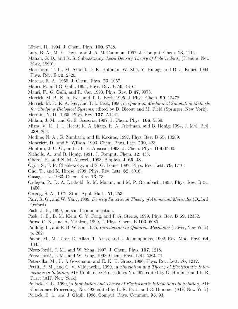
Lowen, H., 1994, J. Chem. Phys. 100, 6738.Luty, B. A., M. E. Davis, and J. A. McCammon, 1992, J. Comput. Chem. 13, 1114.Mahan, G. D., and K. R. Subbaswamy, Local Density Theory of Polarizability (Plenum, NewYork, 1990).

Marchioro, T. L., M. Arnold, D. K. Hoffman, W. Zhu, Y. Huang, and D. J. Kouri, 1994,Phys. Rev. E 50, 2320.

Marcus, R. A., 1955, J. Chem. Phys. 23, 1057.Mauri, F., and G. Galli, 1994, Phys. Rev. B 50, 4316.Mauri, F., G. Galli, and R. Car, 1993, Phys. Rev. B 47, 9973.Merrick, M. P., K. A. Iyer, and T. L. Beck, 1995, J. Phys. Chem. 99, 12478.Merrick, M. P., K. A. Iyer, and T. L. Beck, 1996, in Quantum Mechanical Simulation Methods

for Studying Biological Systems, edited by D. Bicout and M. Field (Springer, New York).Mermin, N. D., 1965, Phys. Rev. 137, A1441.Millam, J. M., and G. E. Scuseria, 1997, J. Chem. Phys. 106, 5569.Misra, V. K., J. L. Hecht, K. A. Sharp, R. A. Friedman, and B. Honig, 1994, J. Mol. Biol.238, 264.

Modine, N. A., G. Zumbach, and E. Kaxiras, 1997, Phys. Rev. B 55, 10289.Moncrieff, D., and S. Wilson, 1993, Chem. Phys. Lett. 209, 423.Montoro, J. C. G., and J. L. F. Abascal, 1998, J. Chem. Phys. 109, 6200.Nicholls, A., and B. Honig, 1991, J. Comput. Chem. 12, 435.Oberoi, H., and N. M. Allewell, 1993, Biophys. J. 65, 48.Ogut, S., J. R. Chelikowsky, and S. G. Louie, 1997, Phys. Rev. Lett. 79, 1770.Ono, T., and K. Hirose, 1999, Phys. Rev. Lett. 82, 5016.Onsager, L., 1933, Chem. Rev. 13, 73.Ordejon, P., D. A. Drabold, R. M. Martin, and M. P. Grumbach, 1995, Phys. Rev. B 51,1456.

Orszag, S. A., 1972, Stud. Appl. Math. 51, 253.Parr, R. G., and W. Yang, 1989, Density Functional Theory of Atoms and Molecules (Oxford,Oxford).

Pask, J. E., 1999, personal communication.Pask, J. E., B. M. Klein, C. Y. Fong, and P. A. Sterne, 1999, Phys. Rev. B 59, 12352.Patra, C. N., and A. Yethiraj, 1999, J. Phys. Chem. B 103, 6080.Pauling, L., and E. B. Wilson, 1935, Introduction to Quantum Mechanics (Dover, New York),p. 202.

Payne, M., M. Teter, D. Allan, T. Arias, and J. Joannopoulos, 1992, Rev. Mod. Phys. 64,1045.

Perez-Jorda, J. M., and W. Yang, 1997, J. Chem. Phys. 107, 1218.Perez-Jorda, J. M., and W. Yang, 1998, Chem. Phys. Lett. 282, 71.Petersilka, M., U. J. Gossmann, and E. K. U. Gross, 1996, Phys. Rev. Lett. 76, 1212.Pettit, B. M., and C. V. Valdeavella, 1999, in Simulation and Theory of Electrostatic Inter-

actions in Solution, AIP Conference Proceedings No. 492, edited by G. Hummer and L. R.Pratt (AIP, New York).

Pollock, E. L., 1999, in Simulation and Theory of Electrostatic Interactions in Solution, AIPConference Proceedings No. 492, edited by L. R. Pratt and G. Hummer (AIP, New York).

Pollock, E. L., and J. Glosli, 1996, Comput. Phys. Commun. 95, 93.

62

Pratt, L. R., G. J. Tawa, G. Hummer, A. E. Garcia, and S. A. Corcelli, 1997, Intl. J.Quantum Chem. 64, 121.

Press, W. H., S. A. Teukolsky, W. T. Vetterling, and B. P. Flannery, 1992, Numerical Recipes

in C: The Art of Scientific Computing (Cambridge, New York).Pulay, P., 1969, Mol. Phys. 17, 197.Pulay, P., 1980, Chem. Phys. Lett. 73, 393.Pulay, P., 1982, J. Comput. Chem. 3, 556.Reddy, B. D., 1998, Introductory Functional Analysis with Applications to Boundary Value

Problems and Finite Elements (Springer, New York).Reiner, E. S., and C. J. Radke, 1990, J. Chem. Soc. Faraday Trans. 86, 3901.Rice, S. A., 1959, Rev. Mod. Phys. 31, 69.Ringnalda, M. N., M. Belhadj, and R. A. Friesner, 1990, J. Chem. Phys. 93, 3397.Rodriguez, J. H., D. E. Wheeler, and J. K. McCusker, 1998, J. Am. Chem. Soc. 120, 12051.Rowlinson, J. S., and B. Widom, 1982, Molecular Theory of Capillarity (Oxford, New York).Sagui, C., and T. A. Darden, 1999, in Simulation and Theory of Electrostatic Interactions

in Solution, AIP Conference Proceedings No. 492, edited by L. R. Pratt and G. Hummer(AIP, New York).

Sanchez-Portal, D., P. Ordejon, E. Artacho, and J. M. Soler, 1997, Intl. J. Quantum Chem.65, 453.

Sankey, O. F., and D. J. Niklewski, 1989, Phys. Rev. B 40, 3979.Schneider, B. I., and D. L. Feder, 1999, Phys. Rev. A 59, 2232.Schwegler, E., and M. Challacombe, 1996, J. Chem. Phys. 105, 2726.Schwegler, E., M. Challacombe, and M. Head-Gordon, 1997, J. Chem. Phys. 106, 9708.Seminario, J. M., 1996, Editor, Recent Developments and Applications of Modern Density

Functional Theory (Elsevier, New York).Seitsonen, A. P., M. J. Puska, and R. M. Nieminen, 1995, Phys. Rev. B 51, 14057.Sharp, K. A., and B. Honig, 1990a, Annual Rev. Biophys. Biophys. Chem. 19, 301.Sharp, K. A., and B. Honig, 1990b, J. Phys. Chem. 94, 7684.Springborg, M., 1997, Editor, Density-Functional Methods in Chemistry and Materials Sci-

ence (Wiley, New York).Sterne, P. A., J. E. Pask, and B. M. Klein, 1999, Appl. Surf. Sci. 149, 238.Strain, M. C., G. E. Scuseria, and M. J. Frisch, 1996, Science 271, 51.Strang, G., and G. J. Fix, 1973, An Analysis of the Finite Element Method (Prentice-Hall,Englewood Cliffs).

Stratmann, R. E., G. E. Scuseria, and M. J. Frisch, 1996, Chem. Phys. Lett. 257, 213.Stuben, K., and U. Trottenberg, 1982, in Multigrid Methods, ed. W. Hackbusch and U.Trottenberg (Springer-Verlag, New York).

Sugawara, M., 1998, Chem. Phys. Lett. 295, 423.Szabo, A., and N. S. Ostlund, 1989, Modern Quantum Chemistry (McGraw-Hill, New York).Talman, J. D., and W. F. Shadwich, 1976, Phys. Rev. A 14, 36.Tassone, F., F. Mauri, and R. Car, 1994, Phys. Rev. B 50, 10561.Tomac, S., and A. Graslund, 1998, J. Comput. Chem. 19, 893.Tozer, D. J., and N. C. Handy, J. Chem. Phys. 109, 10180 (1998).Troullier, N., and J. L. Martins, 1991a, Phys. Rev. B 43, 1993.Troullier, N., and J. L. Martins, 1991b, Phys. Rev. B 43, 8861.

63

Tsonchev, S., R. D. Coalson, and A. Duncan, 1999, Phys. Rev. E 60, 4257.Tsuchida, E., and M. Tsukada, 1995, Phys. Rev. B 52, 5573.Tsuchida, E. and M. Tsukada, 1998, J. Phys. Soc. Jpn. 67, 3844.Van Gisbergen, S. J. A., F. Kootstra, P. R. T. Schipper, O. V. Gritsenko, J. G. Shijders,and E. J. Baerends, 1998, Phys. Rev. A 57, 2556.

Vanderbilt, D., 1990, Phys. Rev. B 41, 7892.Vasiliev, I., S. Ogut, and J. R. Chelikowsky, 1997, Phys. Rev. Lett. 78, 4805.Vasiliev, I., S. Ogut, and J. R. Chelikowsky, 1999, Phys. Rev. Lett. 82, 1919.Verwey, E. J., and J. Th. G. Overbeek, 1948, Theory of the Stability of Lyophobic Colloids

(Elsevier, New York).Vichnevetsky, R., 1981, Computer Methods for Partial Differential Equations: Volume I

(Prentice-Hall, Englewood Cliffs).Vila, J. A., D. R. Ripoll, Y. N. Vorobjev, and H. A. Scheraga, 1998, J. Phys. Chem. B 102,3065.

Von Rague Schleyer, P., 1998, Editor, Encyclopedia of Computational Chemistry (John-Wiley, New York).

Vosko, S. H., L. Wilk, and M. Nussair, 1980, Can. J. Phys. 58, 1200.Walsh, A. M., and R. D. Coalson, 1994, J. Chem. Phys. 100, 1559.Wang, J., and T. L. Beck, 2000, J. Chem. Phys. 112, 9223 (2000).Wang, J., and A. A. Stuchebrukhov, 1999, preprint.Wesseling, P., 1991, An Introduction to Multigrid Methods (John Wiley, New York).White, C. A., B. G. Johnson, P. M. W. Gill, and M. Head-Gordon, 1996, Chem. Phys. Lett.253, 268.

White, S. R., J.W. Wilkins, and M. P. Teter, 1989, Phys. Rev. B 39, 5819.Wilson, K. G., 1990, Nucl. Phys. B (Proc. Suppl.) 17, 82.Yabana, K., and G. F. Bertsch, 1996, Phys. Rev. B 54, 4484.Yabana, K., and G. F. Bertsch, 1997, Z. Phys. D 42, 219.Yabana, K., and G. F. Bertsch, 1999, Intl. J. Quantum Chem. 75, 55.Yoon, B. J., and A. M. Lenhoff, 1990, J. Comput. Chem. 11, 1080.Yoon, B. J., and A. M. Lenhoff, 1992, J. Phys. Chem. 96, 3130.You, T. J., and S. C. Harvey, 1993, J. Comp. Chem. 14, 484.Yu, H., and A. D. Bandrauk, 1995, J. Chem. Phys. 102, 1257.Yu, H., A. D. Bandrauk, and V. Sonnad, 1994, Chem. Phys. Lett. 222, 387.Zacharias, M., B. A. Luty, M. E. Davis, and J. A. McCammon, 1992, Biophys. J. 63, 1280.Zhang, J., 1998, J. Comput. Phys. 143, 449.

64

TABLES

TABLE I. Orbital energies for the oxygen dimer, from Chelikowsky, Troullier, Wu, and Saad

(1994). FD-12 refers to high-order FD calculations in a 12 au box. PW-12 and PW-24 refer to

plane-wave calculations with supercells of 12 and 24 au on a side. Energies are in eV.

Orbital FD-12 PW-12 PW-24

σs -32.56 -32.09 -32.60

σ∗s -19.62 -19.11 -19.57

σp -13.63 -12.93 -13.37

πp -13.24 -12.54 -12.98

π∗p -6.35 -5.53 -5.98

TABLE II. Coefficients for the Laplacian. One side plus the central point are shown. Each

coefficient term should be divided by the prefactor. The Laplacian is symmetric about the central

point.

Points Order Prefactor Coefficients

N=3 2nd 1 1 -2

N=5 4th 12 -1 16 -30

N=7 6th 180 2 -27 270 -490

N=9 8th 5040 -9 128 -1008 8064 -14350

N=11 10th 25200 8 -125 1000 -6000 42000 -73766

N=13 12th 831600 -50 864 -7425 44000 -222750 1425600 -2480478

65

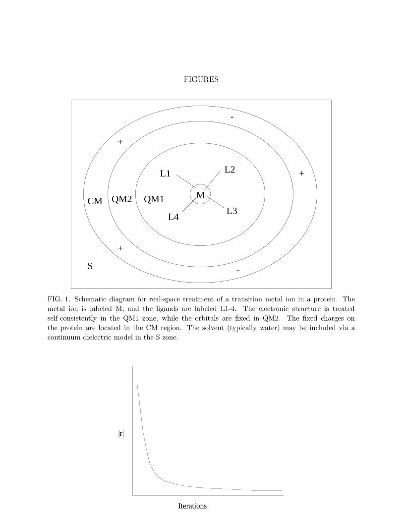
FIGURES

M

L1 L2

L3L4

QM1QM2CM

S

+

-

+

-

+

FIG. 1. Schematic diagram for real-space treatment of a transition metal ion in a protein. The

metal ion is labeled M, and the ligands are labeled L1-4. The electronic structure is treated

self-consistently in the QM1 zone, while the orbitals are fixed in QM2. The fixed charges on

the protein are located in the CM region. The solvent (typically water) may be included via a

continuum dielectric model in the S zone.

|r|

Iterations

66

FIG. 2. Typical behavior of the residual during iterations on a fine level only.

-0.65

-0.6

-0.55

-0.5

-0.45

-0.4

-0.35

-0.3

-0.25

-0.2

-0.15

-0.1

2 4 6 8 10 12

Ener

gy(a

u)

Order

FIG. 3. Effect of order on the eigenvalues for the H atom. The (+) symbols are for the 1s orbital,

(x) is for 2s, and the stars are for 2p. The analytical results are -0.5, -0.125, and -0.125 respectively.

1

1.5

2

2.5

3

3.5

4

4.5

5

5.5

6

2 4 6 8 10 12

<r>

Order

FIG. 4. Effect of order on the orbital first moments for the H atom. The (+) symbols are for the 1s

orbital, (x) is for 2s, and the stars are for 2p. The analytical results are 1.5, 6, and 5 respectively.

67

1.65

1.7

1.75

1.8

1.85

1.9

1.95

2

2 4 6 8 10 12

-<V>

/<T>

Order

FIG. 5. Effect of order on the orbital virial ratios for the H atom. The (+) symbols are for the 1s

orbital, (x) is for 2s, and the stars are for 2p. The analytical result is 2.

R

R

R

R C

C

C

C

Fine Level

Coarse Level

FIG. 6. A multigrid V-cycle. Iterations begin on the fine level on the left side of the diagram.

R indicates restriction of the problem to the next coarser level. Corrections (C) begin as the

computations move from the coarsest level to the finest level.

Fine Level

Coarse Level

68

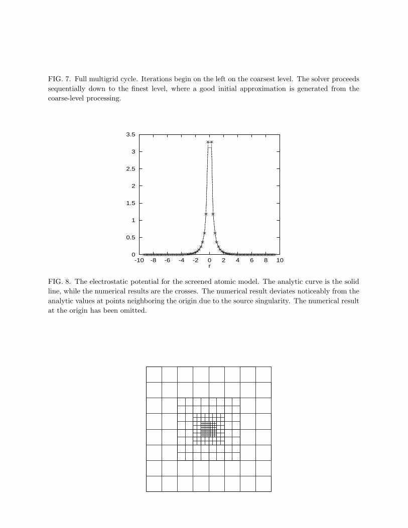
FIG. 7. Full multigrid cycle. Iterations begin on the left on the coarsest level. The solver proceeds

sequentially down to the finest level, where a good initial approximation is generated from the

coarse-level processing.

0

0.5

1

1.5

2

2.5

3

3.5

-10 -8 -6 -4 -2 0 2 4 6 8 10r

FIG. 8. The electrostatic potential for the screened atomic model. The analytic curve is the solid

line, while the numerical results are the crosses. The numerical result deviates noticeably from the

analytic values at points neighboring the origin due to the source singularity. The numerical result

at the origin has been omitted.

69

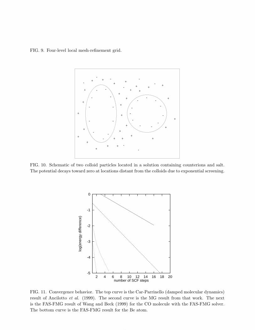
FIG. 9. Four-level local mesh-refinement grid.

-

-

-

-

--

-

-

-

-

-

-

--

-

-

-

---

-

-

+

+ ++ +

+

+

+

++

+

+

+ +

+

+

+

+ ++

+ +

+

+

+

+

+

+

++ +

-

- -

-

--

--

FIG. 10. Schematic of two colloid particles located in a solution containing counterions and salt.

The potential decays toward zero at locations distant from the colloids due to exponential screening.

-5

-4

-3

-2

-1

0

2 4 6 8 10 12 14 16 18 20

log(

ener

gy d

iffer

ence

)

number of SCF steps

FIG. 11. Convergence behavior. The top curve is the Car-Parrinello (damped molecular dynamics)

result of Ancilotto et al. (1999). The second curve is the MG result from that work. The next

is the FAS-FMG result of Wang and Beck (1999) for the CO molecule with the FAS-FMG solver.

The bottom curve is the FAS-FMG result for the Be atom.

70