Status and Trends in Demography of Northern Spotted Owls, 1985–2003

STATUS AND TRENDS IN DEMOGRAPHY OF NORTHERN SPOTTED OWLS,

1985–2003

ROBERT G. ANTHONY

U.S. Geological Survey, Oregon Cooperative Fish and Wildlife Research Unit, Department of

Fisheries and Wildlife, Oregon State University, Corvallis, OR 97331, USA

ERIC D. FORSMAN

USDA Forest Service, Pacific Northwest Research Station, Forestry Sciences Laboratory,

Corvallis, OR 97331, USA

ALAN B. FRANKLIN

Colorado Cooperative Fish and Wildlife Research Unit, Department of Fishery and Wildlife

Biology, Colorado State University, Fort Collins, CO 80523 USA

DAVID R. ANDERSON

Department of Fishery and Wildlife Biology, Colorado State University, Fort Collins, CO 80523

USA

KENNETH P. BURNHAM

U.S. Geological Survey, Colorado Cooperative Fish and Wildlife Research Unit, Department of

Fishery and Wildlife Biology, Colorado State University, Fort Collins, CO 80523 USA

GARY C. WHITE

Department of Fishery and Wildlife Biology, Colorado State University, Fort Collins, CO 80523,

USA

CARL J. SCHWARZ

Department of Statistics and Actuarial Science, 8888 University Drive, Simon Fraser University,

2

Burnaby, BC V5A 1S6, Canada

JIM NICHOLS

U.S. Geological Survey, Patuxent Wildlife Research Center, 11510 American Holly Drive,

Laurel, MD 20708, USA

JIM E. HINES

U.S. Geological Survey, Patuxent Wildlife Research Center, 11510 American Holly Drive,

Laurel, MD 20708, USA

GAIL S. OLSON

Oregon Cooperative Fish and Wildlife Research Unit, Department of Fisheries and Wildlife,

Oregon State University, Corvallis, OR 97331, USA

STEVEN H. ACKERS



STEVE ANDREWS



BRIAN L. BISWELL

USDA Forest Service, Pacific Northwest Research Station, Forestry Sciences Laboratory,

Olympia, WA 98502

PETER C. CARLSON

Hoopa Tribal Forestry, P.O. Box 368, Hoopa, CA 95546, USA

LOWELL V. DILLER

3

Simpson Resource Company, 900 Riverside Road, Korbel, CA, USA

KATIE M. DUGGER



KATHERINE E. FEHRING

Point Reyes Bird Observatory, 4990 Shoreline Highway, Stinson Beach, CA 94970, USA

TRACY L. FLEMING

National Council For Air and Stream Improvement, 23308 NE 148th, Brush Prairie, WA 98606,

USA

RICHARD P. GERHARDT

Sage Science, 319 SE Woodside Ct., Madras, OR 97741, USA

SCOTT A. GREMEL

USDI National Park Service, Olympic National Park, Port Angeles, WA 98362, USA

R. J. GUTIÉRREZ

Department of Fisheries, Wildlife and Conservation Biology, University of Minnesota, 200

Hodson Hall, 1880 Folwell Ave., St. Paul, MN 55108, USA

PATTI J. HAPPE

USDI National Park Service, Olympic National Park, Port Angeles, WA 98362, USA

DALE R. HERTER

Raedeke Associates Inc., 5711 NE 63rd Street, Seattle, WA 98115, USA

J. MARK HIGLEY

Hoopa Tribal Forestry, PO Box 368, Hoopa, CA 95546, USA

4

ROB B. HORN

USDI Bureau of Land Management, Roseburg District Office, 777 Garden Valley Blvd.,

Roseburg, OR 97470, USA

LARRY L. IRWIN

National Council For Air and Stream Improvement, PO Box 68, Stevensville, MT 59870, USA

PETER J. LOSCHL



JANICE A. REID

USDA Forest Service, Pacific Northwest Research Station, Roseburg Field Station, 777 Garden

Valley Blvd., Roseburg, OR 97470, USA

STAN G. SOVERN



Abstract: We analyzed demographic data from northern spotted owls (Strix occidentalis

caurina) from 14 study areas in Washington, Oregon, and California for the time period of

1985–2003. The purpose of our analyses was to provide an assessment of the status and trends

of northern spotted owl populations throughout most of their geographic range. The 14 study

areas comprised approximately 12% of the range of the subspecies and included federal, tribal,

private, and mixed federal and private lands. The study areas also included all of the major

forest types that the subspecies inhabits. The analyses followed rigorous protocols that were

5

developed a priori and were the result of extensive discussions and consensus among the

authors. Our primary objective was to estimate fecundity, apparent survival (N), and annual rate

of population change (8) and to determine if there were any temporal trends in these population

parameters. In addition to analyses of data from individual study areas, we conducted 2 meta-

analyses on each demographic parameter. One meta-analysis was conducted on all 14 areas and

the other was restricted to the 8 areas that constituted the Effectiveness Monitoring Plan for

northern spotted owls under the Northwest Forest Plan. The average number of years of

reproductive data per study areas was 14 (range = 5-19), and the average number of recapture

occasions per study area was 13 (range = 4-18). Only 1 study area had <12 years of data. Our

results were based on 32,054 captures and resightings of 11,432 banded individuals for

estimation of survival, and 10,902 instances in which we documented the number of young

produced by territorial females.

The number of young fledged per territorial female (NYF) was analyzed with PROC

MIXED in SAS to fit a suite of a priori models that included: (1) the effects of age, (2) linear or

quadratic time trends, (3) the effects of barred owls (Strix varia), and (4) an even-odd year

effect. NYF varied among years on most study areas with a biennial cycle of high reproduction

in even-numbered years and low reproduction in odd-numbered years. These cyclic fluctuations

did not occur on all study areas, and the even-odd year effect waned during the last 5 years of the

study. There also were differences in NYF among age classes with highest productivity for

adults (>2yrs. old), lower for 2-year olds, and very low for 1-year olds. In addition, we found

that fecundity was stable over time for 7 study areas (Wenatchee, Rainier, Olympic, Warm

Springs, H.J. Andrews, Klamath, and Marin), likely declining for 5 areas (Cle Elum, Oregon

6

Coast Range, Southern Oregon Cascades, Northwest California, and Simpson), and slightly

increasing for 2 areas (Tyee, Hoopa). We found little association between NYF and the

proportion of spotted owl territories where barred owls were detected, although results were

suggestive of a negative effect of barred owls for the Wenatchee and Olympic study areas. The

meta-analysis on fecundity indicated substantial annual variability with no increasing or

decreasing trends, and fecundity was highest in the mixed-conifer region of eastern Washington

(Cle Elum, Wenatchee).

We used Cormack-Jolly-Seber open population models in program MARK and

information-theoretic statistics to estimate apparent survival rates of owls >1 year old. We did

not estimate survival rates of juvenile (<1 year old) owls because of estimation problems and the

potential bias due to permanent emigration from the study areas by juveniles. Apparent survival

rates for >1 year old owls varied from 0.750 to 0.886 (sexes combined) and were comparable to

estimates from previous analyses on the subspecies. Estimates of apparent survival from

individual study areas indicated that there were differences among age classes with adults

generally having higher survival than 1- and 2- year olds. We found evidence for negative time

trends in survival rates on 5 study areas (Wenatchee, Cle Elum, Rainier, Olympic, and Northwest

California) and no trends in survival for the remaining areas. There was evidence for negative

effects of barred owls on apparent survival on 3 study areas (Wenatchee, Cle Elum, and

Olympic). We found no differences in apparent survival rates between sexes except for 1 study

area (Marin) which had only a few years of data. Survival rates of owls on the 8 Monitoring

Areas generally were high, ranging from 0.85 to 0.89; but were declining on the Cle Elum,

Olympic, and Northwestern California study areas. In the meta-analysis of apparent survival, we

7

found differences among regions and changes over time with a downward trend in the mixed-

conifer and Douglas-fir (Pseudotsuga menziesii) regions of Washington. The meta-analysis also

suggested that there was a cost of reproduction on survival the following year, but this effect was

limited to the Douglas-fir and mixed conifer regions of Washington and the Douglas-fir region

of the Oregon Cascade Mountains.

We estimated annual rate of population change with the reparameterized Jolly-Seber

method (8RJS) which refers to the population of territorial owls on the study areas. It answers the

question: are these territorial owls being replaced in this geographically open population?

Point estimates of 8RJS were <1.0 for 12 of 13 study areas. The analyses provided strong

evidence that populations on the Wenatchee, Cle Elum, Rainier, Olympic, Warm Springs, H.J.

Andrews, Oregon Coast Ranges and Simpson study areas were declining during the study. The

mean RJS for the 13 study areas was 0.963 (SE=0.009 ), suggesting that populations over all$λ

of the areas were declining about 3.7% per year during the study. The mean RJS for the 8

monitoring areas on federal lands was 0.976 (SE = 0.007) compared to a mean of 0.942 for the

other study areas, a 2.4 vs 5.8% decline per year. This suggested that owl populations on federal

lands had better demographic rates that elsewhere. Populations were doing poorest in

Washington where apparent survival rates and populations were declining on all 4 study areas.

Our estimates of 8RJS were generally lower than those reported in a previous analysis ( RJS =

0.997, SE = 0.003) for many of the same areas at an earlier date (Franklin et al. 1999). Whether

this was due to continued habitat loss from timber harvest and fires, competition with barred

owls, weather patterns, or other factors is unclear. The Northwest Forest Plan appeared to be

having a positive affect on demography of northern spotted owls, but a recent invasion of barred

8

owls (Strix varia) may be having an affect most of their geographic range.

CONTENTS

INTRODUCTION.........................................................................................................................8

Acknowledgments.................................................................................................12

STUDY AREA.............................................................................................................................13

METHODS...................................................................................................................................16

Data Analysis....................................................................................................................16

Fecundity...........................................................................................................................18

Fecundity on Individual Study Areas....................................................................19

Meta-analysis of Fecundity on All Study Areas....................................................21

Estimation of Apparent Survival.......................................................................................21

Meta-analysis of Apparent Survival......................................................................25

Annual Rate of Population Change (8).............................................................................26

Annual Rate of Population Change for Individual Study Areas...........................29

Meta-analysis of Annual Rate of Population Change...........................................31

Estimates of Realized Population Change............................................................32

RESULTS......................................................................................................................................33

Fecundity...........................................................................................................................33

Individual Study Areas..........................................................................................33

Variance Component Analysis..............................................................................35

Meta-analysis of Fecundity...................................................................................36

9

Apparent Survival Rates....................................................................................................37


Meta-analysis of Adult Apparent Survival............................................................39

Effects of Reproductive Output on Survival..........................................................40

Effects of Land Ownership....................................................................................41

Effects of Barred Owls in Analyses of Individual Study Areas.............................41

Effects of Barred Owls in the Meta-analysis of Survival......................................42



Precision and Variance Components....................................................................44

Meta-analysis of Annual Rate of Population Change...........................................45

Estimates of Realized Population Change............................................................46

DISCUSSION................................................................................................................................47

Fecundity...........................................................................................................................50

Apparent Survival.............................................................................................................53


Effects of Barred Owls......................................................................................................58

Correlation Between Fecundity and Apparent Survival Rates..........................................60

Possible Causes of Population Declines............................................................................61

Status of Owls on the 8 Monitoring Areas........................................................................64

SUMMARY AND RECOMMENDATIONS...............................................................................65

LITERATURE CITED..................................................................................................................69

10

APPENDICES...............................................................................................................................83

INTRODUCTION

The northern spotted owl is a medium-sized, nocturnal owl that inhabits coniferous

forests along the Pacific Coast of North America from southern British Columbia to central

California (Gutierrez et al. 1995). Adult spotted owls are territorial, exhibit high site fidelity,

and occupy relatively large home ranges (Forsman et al. 1984, Carey et al. 1990, Thomas et al.

1990). In contrast, juvenile spotted owls are highly mobile and typically do not acquire

territories until they are 1–3 years old (Franklin 1992, Forsman et al. 2002). Northern spotted

owls feed primarily on small mammals, especially northern flying squirrels (Glaucomys

sabrinus) in Washington and Oregon, and woodrats (Neotoma spp.) in southwestern Oregon and

California (Barrows 1980, Forsman et al. 1984, 2001, Ward et al. 1998). The subspecies is

closely associated with old forests throughout most of its range (Forsman et al. 1984, Thomas et

al. 1990), but is also common in young redwood (Sequoia sempervirens) forests in northwestern

California (Diller and Thome 1999).

Because of the close association between northern spotted owls and old forests,

conservation of the owl and its habitat has been extremely contentious among environmentalists,

the timber industry, land managers, and scientists since the early 1970's (Forsman and Meslow

1986, Thomas et al. 1990, Durbin 1996, Gutierrez et al. 1996, Marcot and Thomas 1997, Noon

and Franklin 2002). This controversy started when it became apparent that federal agencies

were harvesting old forests at levels that were not sustainable (Parry et al. 1983). In spite of

these concerns, the U.S. Congress continued to increase harvest levels of old forests on federal

11

lands during the 1970's and 1980's, until harvest levels on federal lands in western Oregon and

Washington reached a peak of nearly 2.7 billion cubic feet per year in the late 1980's (Parry et

al. 1983, Haynes 2003). As the rate of harvest increased, field surveys suggested that loss of old

forests was leading to declines in numbers of northern spotted owls (Forsman et al. 1984,

Anderson and Burnham 1992). Meanwhile, management options decreased; litigation increased;

and a number of committees, task forces, and work groups were organized to develop solutions

that were biologically sound and politically acceptable (Meslow 1993, Durbin 1996). This

controversy intensified in 1988–1992, when a series of lawsuits by environmental groups halted

all harvest of suitable spotted owl habitat on federal lands (Dwyer 1989) and forced the U.S. Fish

and Wildlife Service to list the northern spotted owl as a threatened subspecies (Zilley 1988,

U.S. Fish and Wildlife Service 1990). The primary reasons given for listing the owl as

threatened were that: (1) suitable habitat was declining, (2) there was evidence of declining

populations, and (3) there were inadequate regulatory mechanisms to protect the owl or its

habitat.

To meet the requirements of the National Forest Management Act and the Endangered

Species Act, federal agencies in the Pacific Northwest adopted the Northwest Forest Plan

(NWFP) in 1994. The NWFP was designed to protect habitat for spotted owls and other species

associated with late-successional forests (Thomas et al. 1993), while allowing a greatly reduced

amount of commercial logging on federal lands (USDA and USDI 1994). The NWFP also

placed large amounts of the federal land within the range of the northern spotted owl into

riparian and late-successional forest reserves, in which the primary objective was to maintain or

restore habitat for spotted owls and other fish and wildlife species. Although the NWFP met the

12

legal requirements for protection of spotted owls and other species associated with old forests, it

has continued to be controversial. Some environmental groups argued that it was not adequate

because it still allowed some harvest of old forests, while some industry groups argued that it

was too extreme because it did not produce the estimated levels of timber harvest on federal

lands. Regardless of one’s viewpoint, the controversy over management of spotted owls and old

forests has led to an almost complete reversal of management objectives on federal forest lands

in the Pacific Northwest. With the adoption of the Northwest Forest Plan, the primary focus of

forest management has shifted from timber production to maintaining biological diversity and

ecological processes.

The controversy surrounding the spotted owl has led to considerable research on the

species, including numerous studies of its distribution, population trends, habitat use, home

range size, diet, prey ecology, genetics, dispersal, and physiology (for reviews see Gutiérrez et

al. 1995, Marcot and Thomas 1997, Noon and Franklin 2002). As a result, the spotted owl is

one of the most intensively studied birds in the world. Despite this repository of knowledge, the

effectiveness of current management plans for protecting the owl is still uncertain. This

uncertainty has increased in recent years, as the barred owl has invaded the entire range of the

northern spotted owl (Dunbar et al. 1991, Dark et al. 1998, Pearson and Livezey 2003) and

appears to be affecting their territory occupancy (Kelly et al. 2003).

Most of the scientific and public debate regarding the northern spotted owl has focused

on the degree to which the owl is negatively influenced by harvest of old forests (FEMAT 1993).

To address this issue, the U.S. Forest Service, U.S. Bureau of Land Management, U.S. National

Park Service, and several non-federal groups initiated several demographic studies on spotted

13

owls from 1985–1990. These long-term studies were designed to provide information on

survival and fecundity rates of territorial owls, which could then be used to estimate annual rates

of population change (Forsman et al. 1996, Lint et al. 1999). In 2003, there were 14 of these

demographic studies still being conducted on the northern spotted owl. Eight of these studies

were part of the Monitoring Plan for the northern spotted owl under the NWFP (Lint et al. 1999).

The other 6 were conducted by Indian Tribes, timber companies, and private consulting firms.

Data from the demographic studies have been examined in 3 workshops since 1991, and

the results have been reported in 4 different documents (Anderson and Burnham 1992; Burnham

et al. 1994, 1996; Franklin et al. 1999). Because of the contentious debate over management of

spotted owls, participants in these workshops adopted formal protocols for error-checking data

sets and selecting an a priori group of models for estimation of survival, fecundity and annual

rate of population change (Anderson et al. 1999). These protocols ensured that data were

collected and prepared in a consistent manner among study areas and avoided the analyses of

additional models after post-hoc examination of results (i.e., data dredging).

Subsequent to the analysis conducted by Franklin et al. (1999), we collected an additional

5 years of data from most of the demographic study areas. In January 2004, we conducted a

workshop at Oregon State University, during which we updated and analyzed all of these data,

using a process and protocols that were similar to those used in previous analyses (Anderson et

al. 1999). Our primary objectives were to:

(1) estimate age-specific survival and fecundity rates, and their sampling variances,

for territorial owls on individual study areas;

(2) determine if there were any trends in apparent survival or fecundity rates among

14

study areas;

(3) estimate annual rates of population change (8) and their sampling variances for

individual study areas and across study areas; and

(4) compare the demographic performance of spotted owls on the 8 areas that are the

basis of the Monitoring Plan for the NWFP (Lint et al. 1999) to that of owls on

other areas.

We were particularly interested in examining the hypothesis that owl populations were

stationary or increasing (8 > 1) versus declining (8 < 1) during the period of study. We also

examined temporal trends in survival and fecundity rates, as increases or decreases in these rates

could indicate fundamental changes in the dynamics of owl populations. We also included 2

covariates in the analyses of temporal trends. First, the proportion of spotted owl territories with

barred owl detections was used to test the hypothesis that barred owls were having a negative

effect on survival and fecundity of spotted owls. Second, we hypothesized that successful

reproduction in 1 year had a negative effect on survival of adult owls the following year (i.e., a

cost of reproduction). In this paper, we describe the results of our analyses, including an

assessment of the status and trends of northern spotted owl populations throughout most of the

range of the subspecies.

Acknowledgments.--We are particularly indebted to the many dedicated biologists and

field technicians who helped us collect the data used in this report. Although we cannot name

them all, they are the ones who made this study possible. We also thank J. Blakesley, M.

Conner, S. Converse, S. Dinsmore, P. Doherty Jr., V. Dreitz, P. Lukacs, B. McClintock, T.

McDonald, E. Rexstad, M. Seamans, and G. Zimmerman for analytical assistance during the

15

workshop. We thank T. Hamer, K. Hamm, S. Turner-Hane, C. McAfferty, J. Schnaberl, T.

Snetsinger, J. Thompson, and F. Wagner for technical assistance before and after the workshop.

J. Lint, E. Meslow, and 4 anonymous reviewers provided valuable comments on earlier drafts of

the paper. F. Oliver made most of the color bands used to identify individual owls in this study.

J. Toliver at the Oregon Cooperative Fish & Wildlife Research Unit and D. Beaton at the Oregon

Agricultural Research Foundation provided administrative support for the workshop. We

particularly thank J. Lint for his support of these studies and encouragement over the last 2

decades. Funding for demographic studies of northern spotted owls on federal lands was

provided primarily by the U.S. Forest Service, U.S. Bureau of Land Management, and U.S.

National Park Service. Funding for studies on non-federal lands came from a variety of sources,

including the Simpson Resource Company, Plum Creek Timber Company, National Council for

Air and Stream Improvement, Louisiana Pacific Lumber Company, Confederated Tribes of

Warm Springs, and the Hoopa Tribe. Funding for the workshop was provided by the U.S. Forest

Service, U.S. Bureau of Land Management, and U.S. Fish and Wildlife Service.

STUDY AREAS

The 14 study areas included 4 study areas in Washington: Wenatchee (WEN), Cle Elum

(CLE), Rainier (RAI), and Olympic Peninsula (OLY); 6 study areas in Oregon: Warm Springs

Reservation (WSR), H.J. Andrews (HJA), Oregon Coast Ranges (COA), Tyee (TYE), Klamath

(KLA), and southern Oregon Cascades (CAS); and 4 study areas in California: Northwest

California (NWC), Hoopa Tribal Area (HUP), Simpson Resource area (SIM), and Marin

(MAR)(Table 1, Fig. 1, Appendix A).. The combined area of the 14 study areas was 28,430 km2

16

(Table 1), which included about 12% of the 230,690 km2 range of the northern spotted owl

(USDA and USDI 1994). One study area (SIM) was entirely on private land, 2 (HUP, WSR)

were on Indian Reservations, 5 (OLY, HJA,CAS, NWC, MAR) were primarily on federal lands,

and 6 (CLE, WEN, RAI, COA, TYE, KLA) were characterized by a mixture of federal, private,

and state lands (Fig. 1, Table 1). Study areas that were partly or entirely on lands administered

by the U.S. Bureau of Land Management (BLM) typically included an ownership pattern in

which 2.56 km2 sections of BLM lands alternated with 2.56 km2 sections of private land (KLA,

TYE, COA, CAS).

Our study areas differed slightly from those in a previous analysis by Franklin et al.

(1999) by exclusion of 3 study areas that were discontinued after 1998 (Astoria, Elliott State

Forest, and East Eugene BLM) and inclusion 1 study (MAR) that was started in 1998. We also

modified the Olympic Peninsula Study Area to exclude non-federal lands that were included in

the previous analysis; we did this to distinguish population trends of owls on federal lands on the

Olympic Peninsula from trends on non-federal lands. Eight study areas (CLE, OLY, HJA, COA,

TYE, KLA, CAS, NWC) were established by the U.S. Forest Service and U.S. Bureau of Land

Management to monitor population trends of the northern spotted owl (hereafter referred to as

the 8 monitoring areas) under the Northwest Forest Plan (Table 1, Appendix A, Lint et al. 1999).

All study areas were characterized by mountainous terrain, but there was great variation

in the types of topographic relief among areas. Study areas in coastal regions of western Oregon

and northern California were in areas where elevations rarely exceeded 1250 m and where forest

vegetation generally extended from the lowest valleys to the highest ridges. In contrast, study

areas in the Cascades Ranges and Olympic Peninsula typically included larger mountains, with

17

the highest peaks and ridges extending well above timberline. Climate and precipitation were

highly variable among areas, ranging from relatively warm and dry conditions on study areas in

southern Oregon (CAS, KLA) and northern California (NWC, HUP) to temperate rain forests on

the west side of the Olympic Peninsula (OLY), where precipitation ranged from 280S460

cm/year. Study areas on the east slope of the Cascades (WEN, CLE, WSR) were generally

characterized by warm dry summers and cool winters, with most precipitation occurring as snow

during winter.

Vegetation generally consisted of forests dominated by conifers or mixtures of conifers

and hardwoods (Franklin and Dyrness 1973, Küchler 1977). Forests on study areas in

Washington and Oregon were mostly characterized by mixtures of Douglas-fir and western

hemlock (Tsuga heterophylla), or by mixed-conifer associations of Douglas-fir, grand fir (Abies

grandis), western white pine (Pinus monticola), and ponderosa pine (P. ponderosa). Incense

cedar (Libocedrus decurrens) was a common associate of mixed-conifer forests in Oregon.

Forests on study areas in southwest Oregon and northern California were mostly mixed-conifer

or mixed-evergreen associations. In mixed-evergreen forests, evergreen hardwoods such as

tanoak (Lithocarpus densiflorus), Pacific madrone (Arbutus menziesii), California laurel

(Umbellularia californica), and canyon live-oak (Quercus chrysolepis) formed a major part of

the forest canopy, usually in association with Douglas-fir. The Simpson and Marin study areas

in California also included large areas dominated by coastal redwoods and evergreen hardwoods.

Forest condition was highly variable among study areas, ranging from mostly young

forests (< 60 years old) on 1 study area (SIM) to some study areas on federal lands (OLY, HJA,

MAR, CAS) where >40% of the landscape was covered by mature (80-200 years old) or old-

18

growth (>200 years) forests as described by Thomas et al. (1990). Although the types and

amounts of disturbance differed among areas, all study areas were characterized by a diverse

mixture of forest seral stages that were the result of historic patterns of logging, wildfire,

windstorms, disease, and insect infestations. On some study areas (OLY, RAI), forest cover was

also naturally fragmented by high elevation ridges covered by snow, ice, and alpine tundra.

Selection of study areas by the groups that participated in the analyses was based on

many considerations, including logistics, funding, and land ownership boundaries. As a result,

study areas were not randomly selected or systematically spaced. Nevertheless, we believe that

the broad distribution of study areas on federal lands was representative of the overall condition

of northern spotted owl populations on federal lands (Fig. 1) and some private lands. Because

coverage of state and private lands was less extensive and management practices varied widely,

our results likely were not applicable to all state and private lands.

METHODS

Data Analysis

The demographic parameters of interest in our analyses were age-specific survival

probabilities (N), age-specific fecundity (b), and annual rate of population change (8). Data sets

from each study area included a complete capture history of each owl banded during the study.

Data were coded with sex and age (juveniles=0-1year old, S1=1-2 year old, S2=2-3year old,

A=adult, S1+S2+A=non-juveniles) of owls when they were first banded. In some analyses we

combined age classes (S1 + S2 + A) into a single “non-juvenile” class. We estimated

productivity as the number of young fledged (NYF) by each female that was located each year.

19

We estimated annual rate of population change (8) from a file that included the sex, age, and

capture histories of all territorial owls that met certain criteria (see Annual Rate of Population

Change below). Prior to data analysis, we used an error-checking process similar to Franklin et

al. (2004) to ensure that all data sets were accurate and formatted correctly.

Prior to analyzing data, we discussed and agreed upon a protocol for the analyses and

developed a priori lists of models for estimation of survival (N), fecundity (b), and annual rate

of population change (8). The a priori models were developed from biological hypotheses

following the procedures described by Anderson et al. (1999). These a priori models differed

somewhat by response variable and whether the analyses were on the individual study areas or

part of a meta-analysis of all study areas combined. In all analyses, we examined time effects

with models that had variable time (t), linear time (T), or quadratic time (TT) effects. We also

included a barred owl covariate in the analyses of survival and fecundity, because we predicted

that presence of barred owls would have a negative effect on demographic rates of spotted owls

(Kelly et al. 2003). The barred owl covariate that we used was the proportion of spotted owl

territories in which barred owls were detected each year (Appendix B). Although we recognized

that the impacts of barred owls were more likely to occur at the territory level, the only data that

were available for all of the study areas was this year-specific covariate. Thus, we included the

presence of barred owls as an exploratory variable to determine if the effects were detectable

with this coarse-scale covariate. For the meta-analysis of apparent survival, we also included a

covariate for the potential effect of reproduction on survival during the following year (i.e. a cost

of reproduction variable). We used the mean number of young fledged (NYF) per occupied

territory per year to model this effect (Appendix C). In all meta-analyses, we developed models

20

that grouped study areas into larger categories related to ecological regions, ownership, or

latitude (Appendix A).

We used estimates of regression coefficients ($) and their 95% confidence intervals as

evidence of an effect on either fecundity or apparent survival by various factors or covariates.

The sign of the coefficient represented a positive (+) or negative (-) effect of a factor or

covariate, and the 95% confidence intervals were used to evaluate the evidence for $ < 0.0

(negative effect) or $ > 0.0 (positive effect). Because the choice of " = 0.05 is somewhat

arbitrary, the 95% confidence intervals were not used as a strict test of $ = 0.0 but for the

strength of evidence for an effect.

Fecundity

We used the methods described by Franklin et al. (1996) to determine the number of

young produced by resident female owls on each study area each year. We will not repeat those

methods here except to note that field technicians used a standardized protocol to locate owls,

determine their nesting status, and document the number of young that fledged (NYF) from the

nest (Franklin et al. 1996). We conducted analyses on NYF per female or nest (also referred to

as productivity), but to be consistent with previous analyses of spotted owl demography

(Forsman et al. 1996, Franklin et al. 2004), results are reported as fecundity (number of females

produced/female). We estimated fecundity as NYF/2, assuming a 1:1 sex ratio of young

produced at birth. Our assumption of a 1:1 sex ratio was based on a sample of juveniles that

were sexed from genetic analysis of blood samples (Fleming et al. 1996, Fleming and Forsman,

unpublished data). We assumed that the owls sampled were a representative sample of the owls

21

in each age class and that sampling was not biased towards birds that reproduced. We believe

these assumptions were reasonable, because spotted owls stay on the same territories year-

around and usually can be located even in years when they do not reproduce.

Fecundity on Individual Study Areas.—We used PROC MIXED in SAS (SAS Institute

1997) to fit a suite of models for each study area that included: (1) the effects of age (a), (2)

linear or quadratic time trends, (3) the barred owl (BO) covariate (Appendix D), and (4) an even-

odd year effect (EO). We included the even-odd year effect because a previous analysis

(Franklin et al. 1999) suggested a cyclic biennial pattern to the number of young fledged, with

higher reproductive rates in even-numbered years compared to odd numbered-years. A full set

of models was developed for each study area before analyses began. Model ranking and

selection of best models within study areas were based on minimum AICc (Burnham and

Anderson 2002).

A plot of the variance-to-mean ratio within years for all study areas indicated that the

variance of NYF was nearly proportional to the mean of NYF with some evidence of a reduction

in variance at higher levels of reproduction. This plot was consistent with a truncated Poisson

distribution, with owls seldom raising more than 2 young. Despite the integer nature of the data,

the sample sizes were sufficiently large to justify the assumption of a normal distribution (see

White and Bennetts 1996), as long as allowance was made for the dependence of the variation on

the mean. We considered using Poisson regression for these data, but the normal regression

model is less biased when Poisson assumptions are even modestly violated (White and Bennetts

1996). Consequently, we used the normal regression model for analyses of NYF.

22

We also reduced the effect of the variance-to-mean relationship by fitting models to the

yearly mean NYF by age class. These means for each study area were modeled as:

PROC MIXED; MODEL MEAN_NYF = fixed effects.

Thus, residual variation was a combination of year-to-year variation in the actual mean and

variation estimated around the actual mean and is approximately equal to:

var(residual) = var(year effects) + var(NYF)/n

where n = the number of territorial females checked in a particular year. We thought this

approach was justified for a number of reasons. First, a variance components analysis on the raw

data comparing spatial variance among territories to temporal variance among years showed the

former to be small relative to the latter and other residual effects (see Results). Therefore, we

concluded that ignoring spatial variance within study areas would not bias the results. Secondly,

we were able to support the key assumption that the var(residual) was relatively constant

because: (1) var(NYF)/n was small relative to var(year effects), (2) the total number of female

owls sampled was roughly constant over time for each study area so that var(NYF)/n was

roughly constant, and (3) fewer measurements were taken on subadult owls such that

var(NYF)/n was also about constant even though var(NYF) may decline with increasing age

class. These assumptions were verified by Levine’s test for homogeneity of variances. Thirdly,

we assumed that residual effects were approximately normally distributed, because, based on the

central limit theorem, the average of the measurements will have an approximate normal

distribution with large sample sizes even if the individual measurements are quite discrete.

Lastly, covariates that operate on the study-area level (such as BO) are easily modeled.

Because there was no consistent pattern to the best fitting model among study areas, we

23

used a non-parametric approach to estimate the mean NYF. First the mean NYF was computed

for each year and age class, then these averages were averaged across years within each age

class. The estimated standard error was computed by the standard error of the average of the

averages across the years. This method gave equal weight to all years regardless of the number

of birds actually measured in a year, and it did not force a model for changes over time.

Essentially, it treated years as random effects with year effects being large relative to within-year

sampling variation. Estimates weighted by sample sizes in each year were not substantially

different.

Meta-analysis of Fecundity on All Study Areas.—We performed 2 meta-analyses of NYF

data. In 1 analysis we used all 14 study areas and in the other we used the 8 monitoring areas

(Lint et al. 1999). In both analyses, we used data from adult females because samples of 1- and

2-year-old owls were small. In addition, we analyzed NYF for the same geographic regions and

ownership categories used in conducting the meta-analyses of survival and 8RJS (Appendix A).

We used mixed models to perform meta-analyses on mean NYF per year for the same

reasons specified above for the study area analyses. A particular region*year treatment

combination was defined for each study area with owls within study areas as units of measure.

Thus, the experimental units were study areas within region*year, which we used as a random

effect in the mixed models. As ownership and ecological region apply at the study-area level

rather than at the bird level, model selection was performed on average NYF by study area and

year. We evaluated models that allowed for effects of ownership, geographic region, even-odd

years, barred owls, linear and quadratic time trends, and variable time effects. Model rankings

and selection of best models were based on minimum AICc (Burnham and Anderson 2002).

24

Estimation of Apparent Survival

We used Cormack-Jolly-Seber open population models (Cormack 1964, Jolly 1965,

Seber 1965, Burnham et al. 1987, Pollock et al. 1990, Franklin et al. 1996) in program MARK

(White and Burnham 1999) to estimate apparent survival of owls for each year (roughly from 15

June to 15 June). Owls that were not banded as juveniles were assigned to age classes based on

plumage attributes (Forsman 1983, Moen et al. 1991, Franklin et al. 1996). We did not estimate

juvenile survival rates because these estimates were confounded by emigration (Burnham et al.

1996, Forsman et al. 2002). In contrast, annual site fidelity of territorial owls was high (Forsman

et al. 2002), so emigration was not a serious bias in survival estimates from territorial owls.

We used capture-recapture data to estimate recapture probabilities (p, the probability that

an animal alive in year t +1 is recaptured, given that it is alive at the beginning of year t) and

annual apparent survival probabilities (N, the probability that an owl survives from time t to t+1,

given that it is alive at the beginning of year t. Our general approach to estimate survival rates

was to: (1) develop a priori models for analysis, (2) evaluate goodness-of-fit and estimate an

over-dispersion parameter ( ) for each data set, (3) estimate capture probabilities and apparent$c

survival for each capture-recapture data set with the models developed in Step 1 using program

MARK (White and Burnham 1999), (4) adjust the covariance matrices and AICc values with

to obtain QAICc values, and (5) select the most parsimonious model for inference based on

QAICc model selection (Burnham and Anderson 2002). Additional detail on methods of

estimation of survival from capture-recapture data from northern spotted owls are provided by

Burnham et al. (1994, 1996) and Franklin et al. (1996). The statistical analyses were based on

25

maximum likelihood theory and methods (Brownie et al. 1978, Burnham et al. 1987) and current

philosophy of parametric statistical analysis of large, inter-related data sets (Anderson et al.

1999).

The goal of the data analysis and model selection process was to find a model from an a

priori list of models that best fit the data and was closest to the truth based on Kullback-Leibler

information (Burnham and Anderson (2002). Prior to model fitting we used the global model

{N(s*t), p(s*t)} for adults to test each data set for goodness-of-fit to the assumptions of the

Cormack-Jolly-Seber model. The global model included estimates of sex (s) and time (t) effects,

plus the interaction between sex and time for both N and p. We used program RELEASE

(Burnham et al. 1987) to test for goodness-of-fit to the Cormack-Jolly-Seber model and estimate

overdispersion. Overdispersion in the data was estimated by = P 2/df using the combined P 2$c

values and degrees of freedom (df) from Test 2 and Test 3 from program RELEASE (Lebreton et

al. 1992). Estimates of were used to inflate standard errors and adjust for the lack of$c

independence in the data. We estimated capture probabilities and apparent survival with 56 a

priori models that were developed during the protocol session (Tables 2, 3). Models, which

included age, sex, time, time trends (linear and quadratic), and a barred owl covariate (Appendix

B), were then fit to each data set to model apparent survival (Table 3).

We used maximum likelihood estimation to fit models and optimize parameter estimation

using program MARK (White and Burnham 1999). We used QAICc for model selection

(Lebreton et al. 1992, Burnham and Anderson 2002), which is a version of Akaike's Information

Criterion (Akaike 1973, 1985; Sakamoto et al. 1986) corrected for small sample bias (Hurvich

26

and Tsai 1989) and overdispersion (Lebreton et al. 1992, Anderson et al. 1994). We computed

QAICc according to Burnham and Anderson (2002:66–70):

where the log(Likelihood) is evaluated at the maximum likelihood estimates under a given

model, K is the number of estimable parameters in the model, is the estimated quasi-likelihood

variance inflation for overdispersion, and is the effective sample size (number of releases for

the capture-recapture data). QAICc was computed for each candidate model and the best model

for inference was the model with the minimum QAICc value. Two additional tools based on

QAICc values were also computed for each model, )QAICc for model i (where )QAICci =

QAICci - minQAICc) and Akaike weights (Buckland et al.1997, Burnham and Anderson 2002).

Akaike weights were computed over a set of R models as:

where )i = the information lost in approximating full reality by model i (standardized by the best

model) and wi = the probability that model i is in fact the Kullback-Leibler best model (Burnham

and Anderson 2002). Akaike weights were used to address model selection uncertainty and the

degree to which ranked models were considered competitive. We used Akaike weights to

compute estimates of time-specific, model-averaged survival rates and their standard errors for

each study area (Burnham and Anderson 2002:162). We did this because there were often

27

several competitive ()QAICc < 2.0) models for a given data set (Burnham and Anderson 2002).

For each study area, we used the variance components module of program MARK to

estimate temporal (σ2temporal) process variation (White et al. 2002, Burnham and White 2002).

This approach allowed us to separate sampling variation (variation attributable to estimating a

parameter from a sample) in apparent survival estimates from total process variation. Process

variation was decomposed into temporal (parameter variation over time) and spatial (parameter

variation among different locations) components.

Meta-analysis of Apparent Survival.—The meta-analysis of apparent survival rates was

based on capture histories of adult males and females from the 14 study areas. Apparent survival

and capture probabilities were estimated with the Cormack-Jolly-Seber model using program

MARK (White and Burnham 1999). The global model for these analyses was {φ(g*s*t)

p(g*s*t)}, where g was study area, t was time (year), and s was sex. Goodness-of-fit was

assessed with the global model in program RELEASE (Burnham et al. 1987), and the estimate of

overdispersion, c, was used to adjust model selection to QAIC and to inflate variance estimates.

We initially evaluated 6 models of recapture probability {p(g+t), p(r), p(g+s+t), p(r+s),

p([g+t]*s), p(r*s)}with a general structure on apparent survival {N(g*t*s)} where r indicates the

effect of reproduction in the current year. Using the model for p with minimum QAIC from the

initial 6 models, we evaluated 13 additional models for apparent survival to test for various

combinations of area, sex, time, barred owl effects (BO), and effects of reproductive output (r)

(Table 4). The sex effect was then removed from the best model above to check for strength of

the sex effect. Then, we ran 4 more models in which study area (group) effect was replaced with

the group surrogates “ownership”, “geographic region”, “ownership*region”, and “latitude” for a

28

total of 27 models. Ownership referred to whether the area was privately owned, federally

owned, or of mixed private and federal ownership (Appendix A). Each study area was classified

into 1 of 5 geographic regions that incorporated geographic location and the major forest type in

the study area (Appendix A). Latitude was a continuous variable measured at the center of each

study area.

Annual Rate of Population Change (8)

One of the first topics we discussed during the protocol session was whether we should

estimate the annual rate of population change (8) from estimates of age-specific survival and

fecundity with the Leslie projection matrix (8PM) (Caswell 2000) or the reparameratized Jolly-

Seber method (8RJS)(Pradel 1996). The 8PM method was used in the 1993 and 1998

demographic analyses of northern spotted owls (Franklin et al. 1996, 1999). The 8RJS method,

which uses direct estimation of 8 from capture-recapture data, was used in an exploratory

manner in the 1998 analyses (Franklin et al. 1999) and was used in analyses of data from

California spotted owls (S. o. occidentalis) (Franklin et al. 2004).

Estimates of 8PM are computed from projection matrices using age-specific survival and

fecundity for juvenile, subadult, and adult owls, assuming a stable age distribution (i.e., constant

rates over time) over the period of study. The estimate of 8PM represents the asymptotic growth

rate of a population exposed to constant demographic rates over time, but it is not necessarily the

best estimate of annual rate of population change on a study area for several reasons. First, there

is asymmetry in the way movement is treated in vital rates representing gains or losses. In

demographic studies of spotted owls, apparent survival rates are estimated using capture-

29

recapture models, whereas fecundity rates are estimated from direct observation of productivity

of territorial females. Population losses thus include both death and permanent emigration,

whereas gains come solely from reproduction, as reflected by fecundity estimates. Second, 8PM

is an asymptotic value expected to result from the absence of temporal variation in the vital rates,

whereas we know from previous analyses (Burnham et al. 1996, Franklin et al. 1999) that there

is considerable temporal variation in both survival and fecundity of spotted owls. Thus, 8PM is a

theoretical, asymptotic rate assuming constant fecundity and survival rates over the period of

study, whereas 8RJS is an estimate of a rate that reflects annual variability in rates of population

change. Third, values of fecundity may be positively biased if non-breeders or unsuccessful

breeders are not detected as readily as successful breeders (Raphael et al. 1996). Lastly and most

importantly, estimates of juvenile survival are negatively biased because of permanent

emigration from study areas, which is of paramount concern for northern spotted owls. The

Cormack-Jolly-Seber estimates of apparent survival can not distinguish between undetected

emigrants and individuals that have died. To the extent that banded juveniles (or non-juveniles)

emigrate from study areas, survive at least 1 year, and are never observed again, the estimates of

survival will be negatively biased. As a result, estimates of 8PM will be biased low (Raphael et

al. 1996, Franklin et al. 2004). The strength of the 8RJS method is that it takes into account the

combination of gains and losses to the population by direct estimation from the capture-recapture

data. Also, the interpretation of 8RJS as a rate of change in the number of territorial owls on the

study is clear and unambiguous. Because of these reasons, we used only the 8RJS method to

estimate annual rates of population change.

Pradel (1996) introduced a reparameterization of the Jolly-Seber model permitting

30

estimation of 8(t), the finite rate of population increase [defined by N(t+1)/N(t) where N(t)

represents population size at time t] in addition to apparent survival (N) and recapture

probability (p). We used this method to estimate 8RJS and determine whether populations were

increasing (8>1.0), decreasing (8<1.0), or stationary (8=1.0). Annual rates of population

change, 8(t), were estimated directly from capture history data for territorial owls from areas that

were consistently surveyed each year (Pradel 1996). For models that had a variable time

structure (t) on 8, we used a random-effects model to estimate 8(t) and its standard error. In

addition to the ability to obtain time-specific estimates of 8RJS, the models implemented in

program MARK also allowed for constraints, such as linear (T) or quadratic (TT) time effects on

8RJS.

Estimates of 8RJS reflect changes in population size resulting from reproduction,

mortality, and movement. The data used in the analyses included only territorial individuals of

mixed age-classes (e.g., no differentiation between adults and 1-, or 2-year old owls). Thus,

estimates of 8RJS from any particular capture-recapture data set should correspond to changes in

the territorial population within the area sampled. Gains in the territorial population can result

from recruitment of owls born on the study area and from immigration of owls from outside the

study area. Losses in the population result from mortality or emigration from the study area. To

apply this method correctly, it is critical that the area sampled remains constant from year-to-

year, coverage of the area is reasonably constant each year, and all areas or territories in the

initial sample be visited during each subsequent year of study, regardless of recent occupancy

status (e.g., even if no owls were detected on sites for several consecutive years). Observers on

all study areas followed a set of survey protocols to assure these conditions (Franklin et al.

31

1996). In our analyses, there were 2 kinds of data sets for territorial owls, those for which all of

the area within a study area was surveyed each year (density study areas or DSAs) and those for

which specific owl territories within a large geographic region were surveyed each year

(territorial study areas or TSAs). DSAs included TYE, NWC, HUP, and SIM, and TSAs

included WEN, CLE, RAI, OLY, WRS, HJA, COA, KLA, CAS, and MAR. For both survey

types, the interpretation of λRJS is the change in the number of territorial owls in the sampled

area. We analyzed the data from DSAs and TSAs separately because the capture-recapture data

were collected with different sampling protocols. We did not make direct comparisons of the

8RJS from the 2 types of surveys, because DSAs were mostly in the southern part of the owl’s

range and TSAs in the northern portion; therefore, survey type and geographic area were

confounded.

Annual Rate of Population Change for Individual Study Areas.—Although most areas

sampled in TSAs were initially selected because they were occupied by owls or had been

occupied by owls prior to the study, any bias towards occupied sites in early years of the study

was eliminated, because we removed the first 2-5 years of data from each TSA and from 3 of the

4 DSA’s for 8RJS estimates (Appendix A). We did this to avoid any potential bias in estimates of

8 associated with any artificial population growth attributable to the initial location and banding

of owls that occurs in the first few years of a study. To evaluate whether study areas were

saturated with territorial owls (i.e., were capable of population growth), we computed the

proportion of territories in which owls were detected in the first year used to estimate 8RJS.

Mean estimates for the proportion of territories that were occupied the first year of estimation

were 0.629 (range = 0.547–0.700) and 0.791 (range = 0.680–0.906) for DSAs and TSAs,

32

respectively. This indicated there was room for population growth or decline for both types of

survey areas. Once the data were truncated, boundaries of 8 study areas remained unchanged for

the duration of the study, and 6 areas had a one-time increase in the study area to include areas

that were added to the sample after the study was initiated (Appendix A). In the latter cases, owl

territories located after the initial year of study were brought into the sample in a single

expansion year, with any data prior to the expansion year removed from the capture histories of

the owls that occupied those territories.

To estimate (average λRJS) and λt (year-specific λ) for each study area, we used theλ

random effects module in program MARK (White et al. 2002). We fit 2 general λRJS models

{(φ(t) p(t) λ(t)} and {φ(s*t) p(s*t) λ(s*t)} to the area-specific data. In some cases, study areas

were expanded mid-way through the time interval. In these cases, we used group-effect models

[{φ(g*t) p(g*t) λ(g*t)} and {φ(g*s*t) p(g*s*t) λ(g*s*t)}] to model parameters associated with

pre-expansion areas differently than post-expansion areas. Regardless of the global models used,

we used QAICc to choose the best of the initial models to proceed with the estimation of

using the following random effects models: constant across time (8.), a linear time trend (λT),λ t

and a quadratic time trend (8TT). The first 2 and last 8t estimates were removed from the base

model before we fit the 3 models to the data. This was done to eliminate potential biases due to:

(1) a trap response, (2) a learning curve often exhibited by field crews on a new study area, or (3)

capture probabilities differing between marked and unmarked birds early in each study (Hines

and Nichols 2002). As with the survival analysis, we estimated overdispersion (c) for the λRJS

data using program RELEASE and the global model {φ(s*t) p(s*t) λ(s*t)} for each study area.

33

Estimates of were generated from the best random effects model. In cases where a linearλ

trend (T) or quadratic trend (TT) on λ was supported, we used the beta estimates from the

random effects model and the midpoint of the time period of the study as the independent

variable to estimate average λRJS. Standard errors for these estimates were developed using the

Taylor series (i.e., “delta method”). We used the variance components module in program

MARK to compute estimates of temporal process variation (σ2temporal) for λRJS on each study area

(White et al. 2002, Burnham and White 2002).

Meta-Analyses of Annual Rate of Population Change.—In addition to estimates of 8RJS

for each study area, we conducted 2 meta-analyses of 8RJS in which we computed average

estimates of 8RJS for multiple study areas combined. One meta-analysis included the 10 TSAs

and the other included the 4 DSAs. We used similar procedures in both analyses.

We evaluated goodness-of-fit for the global model {N(g*t) p(g*t) 8(g*t)} using program

RELEASE and estimated overdispersion as P2/degrees of freedom, as in other analyses. The

meta-analysis of 8t involved the fitting of models focusing on 3 different groups of study areas.

The first grouping simply treated each of the study areas separately. The second grouping

aggregated study areas by ownership and the third aggregated them by geographic region. For

each of these groupings, 3 models for 8t were fit to the data. Model {N(g*t) p(g*t) 8(g*t)} was

the most general model which included full study area by time interactions on all 3 parameters.

Model {N(g*t) p(g*t) 8(g+t)} represented the hypothesis that temporal variation in 8t occurred

in parallel among the different groups for shared years, suggesting similar responses to

environmental factors of population growth. Model {N(g*t) p(g*t) 8(t)} represented the

hypothesis of no variation in 8t among locations. Model {N(g*t) p(g*t) 8(g)} represented area-

34

specific population growth that did not vary from year to year. We also included the model

{N(g*t) p(g*t) 8(.)} reflecting constant 8 over areas and years. There were a total of 11 models

fit to the data for each of the DSAs.

We attempted to fit the same models to the data from TSAs but the maximum likelihood

estimates of 8 would not converge under models with many parameters. The most general

model {N(g*t) p(g*t) 8(g*t)} could not be fit to the data using a single data structure. Instead,

we obtained estimates for this model by fitting a model to each group separately. Goodness-of-

fit and model selection statistics were obtained using results of these individual analyses. None

of the models retaining the general structure (g*t) on survival and capture parameters could be

evaluated. Thus, we tried to fit models in which survival and capture parameters, as well as

population growth rate, were grouped by ownership or by geographic region. Because of these

numerical difficulties, our final results were limited to 5 models.

Estimates of Realized Population Change.—To provide an additional interpretation to the

estimates of 8(t), we converted them into estimates of realized population change using the

methods described by Franklin et al. (2004). Annual realized changes in populations were

estimated and expressed relative to the initial population size (i.e., in the initial year used for

analysis). Thus, we focused on the ratio of the population size in year t to that in the initial year

(i.e., )t = Nt/Nx where x is the initial year). Consequently, the estimates of realized change

corresponded to the proportional change in the population over the time period for which the

8’s were estimated. Realized change ()t) was estimated as:

35

where x was the year of the first estimated 8t. For example, if was 0.9, 1.2, and 0.7 for 3$λt

time intervals, then would be computed as (0.9)(1.2)(0.7) = 0.756 indicating that the ending

population was 75.6% of the size of the initial population. To compute 95% confidence

intervals for , we used a parametric bootstrap algorithm with 1000 simulations. Our approach

was similar to that of Franklin et al. (2004) except that our 95% confidence intervals were based

on the ith and jth values of )t arranged in ascending order where i = (0.025)(1,000) and j =

(0.975)(1,000).

RESULTS

Fecundity

Individual Study Areas.—Estimates of fecundity were based on 10,902 observations of

the number of young produced by territorial females. Most of the fecundity data were from

territories that were occupied by adult females, which reflects the low frequency of territory

occupancy and breeding attempts by 1- or 2-year old females (Table 5). For all areas, age was a

primary factor that affected fecundity (Table 6). Mean fecundity was lowest for 1-year old

females (0 = 0.074, SE = 0.029), intermediate for 2-year olds (0 = 0.208, SE = 0.032), and

highest for adults (0 = 0.372, SE = 0.029). Fecundity of adult females was highest (>0.40) on

the CLE, WEN, WSR, KLA, and MAR study areas, whereas fecundity was lowest (<0.30) on

RAI, OLY, COA, and HUP.

Among the individual study areas, the model that was most frequently selected as best (n

= 7) was female age + an even-odd year effect (a+EO), indicating high fecundity in even-

36

numbered years and low fecundity in odd-numbered years with parallel changes among age

groups (Fig. 2). This model also was within 2 AICc units of the best model for 3 other study

areas (Table 6). The best models for 2 additional areas contained the similar effects: (a*EO) for

RAI, and (a+EO+TT) for HJA. Thus, age and the even-odd year effects were important in

explaining variability in fecundity for most areas, despite some weakening of the latter effect in

recent years (Figure 2). The even-odd year pattern was most prevalent for adults during the

1990s. In the 3 areas for which EO was not an important factor, (a+T) was the top model for

TYE and NWC, indicating linear changes in fecundity over time (see below). There were no

factors (constant model) that affected fecundity on the MAR study area. The MAR study was

initiated in 1998 about the time the even-odd year effect waned and had few owls in younger age

classes, so it was not surprising that the simplest model was selected.

Our results indicate that changes in fecundity over the period of study was variable

among study areas. Linear (T) or quadratic (TT) time trends were evident in the model selection

results of NYF on 9 of the 14 study areas (Table 7). On 5 study areas (HJA, TYE, CAS, NWC,

HUP), time trends were included in the best model, and on 4 areas (WEN, CLE, COA, SIM)

time trends were in models <2 AICc units from the best model. All of these time effects on

productivity were linear except for HJA, which was quadratic but stable overall. The time trends

for 2 areas (TYE and HUP) were positive with > 0.0 (Table 7). In contrast, there was$β

evidence for negative trends in fecundity on 5 study areas (CLE, COA, CAS, NWC, SIM) with

the upper confidence intervals barely > 0.0 (Table 7). Fecundity appeared to be stable over the

period of study on WEN, RAI, OLY, WSR, HJA, KLA, and MAR study areas.

The barred owl covariate (BO) was not a part of the best model structure for any of the

37

study areas, but there were 9 study areas for which BO effects were included in competing

()AIC<2.0) models (Table 8). Of these, 5 (WEN, OLY, COA, NWC, SIM) had a negative

association between fecundity and barred owl presence and 4 (TYE, KLA, HUP, MAR) had a

positive relationship. Confidence intervals were generally large and most substantially

overlapped 0.0 except for HUP and MAR for which the relation was positive. Results for these 2

areas were suspect, because barred owls were rare on both areas (detections on <5% of spotted

owl territories) and because MAR had only 6 years of data. Northern study areas where barred

owls were most common were not more likely to have competing models with the BO covariate;

in fact, the reverse seemed to be true with 4 of 4 areas in California, 3 of 6 areas in Oregon, and

2 of 4 areas in Washington having BO models within 2 AICc units of the best model (Table 8).

The best BO model for CLE, thought to be the area most affected by barred owl encroachment,

was >2.5 AICc units from the best model. In summary, we were unable to show any negative

effects of barred owls on spotted owl productivity with the time-specific covariate.

Variance Component Analysis.—Estimation of spatial (site to site), temporal (year to

year), and residual variance on the territory-specific data indicated that spatial and temporal

variance within all study areas was low relative to the other variance components (Table 9).

With the exception of MAR, for which spatial variance was 12% of the total variability in NYF,

spatial variability within all study areas was <8%. Temporal variation in NYF ranged from

0.054–0.227, but never accounted for >30% of the total variability. The largest proportion of

temporal variation occurred in the data from OLY and CLE (28 and 23%, respectively), but the

temporal variation for the other study areas in Washington was not greater than that for the 6

study areas in Oregon (Table 9). Three of the 4 study areas with the lowest (<10%) temporal

38

variation were in California (NWC, SIM, and MAR). Residual variance was by far the greatest

component of total variance (ranging from 68–92%) and was largely due to individual

heterogeneity among owls. There was no discernable pattern of residual variance among study

areas. Total variability ranged from 0.495 (HUP) to 0.969 (CLE), but again there was no

discernable pattern to the magnitude of variability among study areas.

Meta-analysis of Fecundity.—The ranking of models in the meta-analysis of all 14 study

areas and the 8 monitoring areas was nearly identical. There were differences between the 2

analyses only in the ordering of models with essentially no support (Akaike weights < 0.00);

therefore we present the results for only the 14 study areas combined. The best model included

additive effects of region and a time effect (region + t) and contained 55% of the weight of

evidence (Table 10). Time trends (T) in fecundity were not supported by the meta-analysis; the

best ranking trend model was (region + T) with an AIC weight of 0.000. Models that included

ownership (O) effects also were ranked much lower than the best model (AIC weight = 0.015).

Estimates of adult female fecundity by region, averaged over years, indicated that fecundity was

highest for the mixed-conifer region in Washington and lowest for the Douglas-fir region of

Washington and the Oregon coast (Table 11). Fecundity was intermediate for the Douglas-fir

region of the Oregon Cascades, the mixed-conifer region of California and Oregon, and the

redwood region of coastal California.

The even-odd year (EO) effect was not as important in the meta-analysis as it was in the

analyses of individual study areas, but was apparent between 1990-2000 (Fig. 3). The higher

ranking of the year-specific model (region + t) was likely due to the additional power from the

combined data to detect individual year effects. This model also detected the waning of the

39

even-odd year effect in more recent years and the variability in amplitude of the difference

between even and odd years. There appeared to be a downward trend in the yearly fluctuations

of fecundity (Fig. 3), but we were not able to verify this in our analysis.

Although the model that included the BO covariate was the second best in both meta-

analyses, this was attributed primarily to the region and even-odd year effects in the model. The

regression coefficient estimate for the BO effect for this model (all areas combined) was -0.404

(SE = 0.340). Thus the 95% CI on this effect was large (-1.069 to 0.262) and overlapped 0.0

substantially. In general, models containing the BO covariate were not highly ranked for both

meta-analyses of fecundity.

Apparent Survival Rates

Individual Study Areas.—We used 4,963 banded non-juvenile spotted owls to

estimate apparent survival rates, including 574 1-year old owls, 684 2-year old owls, and 3,705

adults (Table 1). The number of recaptures of marked owls was approximately 5 times the

number of initial markings which resulted in 32,054 initial captures and recaptures. The overall

P2 goodness-of-fit for the global model from program RELEASE was 1600.03 with 925 degrees

of freedom = 1.73, p < 0.001), indicating that there was good fit of the data to Cormack-Jolly-

Seber open population models (Table 12). Estimates of in the individual data sets ranged from

0.84–2.74 (Table 12) which indicated no to moderate overdispersion of recaptured owls and

good fit of the data to the models. What little lack of fit that occurred was due to temporary

emigration of owls from study areas with subsequent return in later years.

Annual estimates of recapture probabilities, p, were between 0.70–0.99 on most study

40

areas (Appendix D). However, there were occasional years when < 0.70 on the WEN, RAI$p

and OLY Study Areas in Washington and the KLA Study Area in Oregon (Appendix D). The

most unusual case was a year on the OLY Study Area in which = 0.26 following a winter with$p

record snowfall and a persistent snow on the ground during spring (Appendix D). The

combination of high recapture probabilities along with high estimates of survival likely reduced

any bias that may have been associated with heterogeneity of recapture probabilities (Pollock et

al. 1990, Hwang and Chao 1995). The best model structure on recapture probabilities varied

among study areas with 1 or more areas having effects of sex, reproductive output, presence of

barred owls, time, or time trends (Table 13). For many study areas, there was an increasing time

trend, p(T), in recapture probabilities in 1 or more of the competitive models ()QAICc < 2.0),

indicating that field biologists got better at locating and re-observing banded owls as the studies

progressed. Recapture probabilities of owls were higher in years with higher productivity, and

males were generally easier to re-observe than females.

The best model structure for apparent survival, N, was not consistent among study areas

(Table 13). Age, sex, presence of barred owls, time, or time trends were important effects on

apparent survival in 1 or more of the best models. Age of territorial owls was important on 8 of

the 14 study areas (Table 13). On average, apparent survival were higher for older owls with

rates ranging from 0.42–0.86 for 1-year olds (0 = 0.68, SE = 0.054), 0.63–0.89 for 2-year olds

(0 = 0.81, SE = 0.030), and 0.75–0.92 for adults (0 = 0.85, SE = 0.016) (Table 13). Apparent

survival rates for adults were >0.85 for most study areas except WEN, WSR, MAR, and RAI.

Apparent survival rates were different between males and females for only the MAR study area,

and the effect of barred owls was important only for the WEN and OLY study areas (also see

41

below).

The best or competitive ()QAICc < 2.0) models for apparent survival suggested a linear

or quadratic time effect for 11 of the 14 study areas (Table 14, Appendix E). There was strong

evidence for declines in apparent survival on 5 study areas (WEN, CLE, RAI, OLY, NWC)

(Table 14). In addition, there was evidence for a slight decrease in apparent survival on COA

during the last 5 years of study (Table 14, Fig. 4b). Declines in apparent survival were most

evident in Washington (Fig. 4a) where all $ estimates were negative and 95% confidence

intervals for 3 (WEN, RAI, OLY) of the 4 study areas did not overlap zero. In addition, apparent

survival for owls on the WEN and RAI areas during the latter years of the study were <0.80

which were the lowest rates recorded for the 14 study areas. In Oregon, there were no time

trends in apparent survival rates for 4 (HJA, KLA, WSR, CAS) of the 6 study areas (Table 14,

Fig. 4b). Apparent survival rates for COA increased slightly during the early years of the study,

then decreased slightly from 1997-2003. In contrast, apparent survival rates on the TYE study

area decreased during the initial years of the study, then increased from 1995-2003. In

California, there was a significant linear decline in apparent survival on the NWC study area

(Fig. 4c) and evidence of a slight decline on the SIM area. There was little evidence of time

trends in apparent survival on the HUP and MAR study areas.

Meta-analysis of Adult Apparent Survival.— We used 5,342 and 3,702 encounter

histories (initial captures + recaptures) in the meta-analysis of apparent survival for all 14 study

areas and the 8 monitoring areas, respectively. Estimates of overdispersion from program

RELEASE were <2.0 for the 14 study areas combined and the 8 monitoring areas ( = 1.730 and

1.738, respectively, Table 12) indicating good fit of the data to the Cormack Jolly-Seber open

42

population models. Because the results for all 14 study areas and that of the 8 monitoring areas

were similar, we only report the results for all the study areas.

The best model for the meta-analysis of the 14 study areas was {N(region + t) p(g + t +

s)} with 55 parameters. This model indicated both regional and variable time effects on apparent

survival, and study area, time, and sex effects on recapture probabilities (Table 15). This model

accounted for 78% of the weight of evidence (Akaike weight) among all of the models, so it was

strongly supported by the data. There was no evidence of a sex effect on survival as noted by the

differences in QAICc for models {N(g + t) p(g + s + t)} and {N(g + t + s) p(g + s + t)} (Table

15). The highest ranked model with a sex effect on N was {N(g + t + s) p(g + t + s)}with 64

parameters; this model had a )QAICc of 6.45 and an Akaike weight of only 0.031. Similarly,

there was little evidence of latitude or ownership effects in the meta-analysis of survival;

)QAICc values for models N(latitude + t) and N(ownership + t) were >12.00, suggesting that

latitude and ownership were not good surrogates for the study area effect in the highest ranked

model. Because of the high Akaike weight of the top model, it was used to estimate apparent

survival of adults (Fig. 5). This figure suggests a downward trend in survival with time; however,

the year-to-year variation was so large that time trend models did not rank high in the list of

models (Table 15). As a result, we fit 2 a posteriori models {N(region * T) p(g + t + s)} and

{N(region + T) p(g + t + s)} to the data to test for a time trend in apparent survival. Because

{N(region * T) p(g + t + s)} with 44 parameters was the more highly ranked of these 2 models

(Table 15), we investigated the interaction between region and time trends (Fig. 6). This relation

indicated that the major downward trends in survival were taking place in the mixed-conifer and

Douglas-fir regions of Washington. This result was consistent with the results of individual study

43

areas where we found declines in apparent survival rates for all of the study areas in Washington.

Effects of Reproductive Output on Survival.—The )QAICc for the highest ranked model

that included the reproductive effect (r) was 18.40 suggesting that it had little effect on survival.

However, this value applies to differences among models and not necessarily the importance of

individual variables in the model. Consequently, we examined the estimates of the individual

variable effects, $ estimates, and their confidence intervals in the best model where the r effect

occurred. Results from this analysis suggested a cost of reproduction on survival based on model

{N(region + r) p(g + t + s)} (Table 15). The $ estimate of the r coefficient for this model was

!0.257 (95% confidence interval = !0.432 to !0.082). Similarly, the estimate of $ for the r

coefficient for the same model for the 8 monitoring areas was !0.292 (95% confidence interval =

!0.507 to !0.078). These results indicated that high reproductive rates in 1 year were followed

by lower survival rates during the following year, but this effect was found in just a few regions

as shown by model {N(region * r) p(g + t + s)}. The strength of this relationship was greatest in

the more northern latitudes and higher elevation study areas, particularly the Douglas-fir and

mixed-conifer regions of Washington and the Douglas-fir zone of the Oregon Cascades (Table

16). This effect, if any, was small for study areas in California and the mixed-conifer and coastal

Douglas-fir regions in Oregon.

Effects of Land Ownership.—Model {N(ownership + t) p(g + t + s)} with 52 parameters

had a )QAICc of 13.43, and the 95% confidence intervals for the estimate for this effect included

0.0 (Table 15). Similarly, the model with land ownership in the meta-analysis on the 8

monitoring areas {N(ownership + t) p(g + t + s)} had 45 parameters and a )QAICc of 11.55, and

the 95% confidence interval for this effect included 0.0. Thus, there was little evidence that land

44

ownership was an important predictor of apparent survival rates in the meta-analyses.

Effects of Barred Owls in Analyses of Individual Study Areas.—In the analysis of the 14

individual study areas, we found a negative effect of barred owls ( = !6.75, 95% CI = !11.65$β

to !1.86) on recapture probabilities (p) of spotted owls for only the Warm Springs (WSR) study

area. The effects of barred owls on recapture probabilities was positive for some areas, opposite

to what we hypothesized. In contrast, we found strong evidence for a negative effect of barred

owls on apparent survival on the OLY and WEN study areas (Table 17); estimates of $ and 95%

confidence intervals for the 2 areas were !4.24 (!7.83 to !0.65) and !4.69 (-7.32 to !2.07),

respectively. There also was some evidence for a negative effect of barred owls on apparent

survival on the CLE, HJA, and NWC study areas, as models with the barred owl effect were

competitive with the top models. Results for the Rainier study areas suggested that barred owls

had a positive effect on spotted owl survival, but we believe this result was spurious. The best

model of survival for Rainier, N(T), was 10.86 )AICs better than N(BO). In addition, the barred

owl covariate for this area was a quadratic function (Appendix B), a much different trend than

that for the other study areas. The evidence for the effects of barred owls on survival of spotted

owls on the remaining study areas was weak (2.0 < )QAICc < 3.0) to negligible ()QAIC > 3.0).

Effect of Barred Owls in the Meta-analysis of Survival.—The barred owl covariate was

not a good predictor of time variation in apparent survival in the meta-analysis of the 14 study

areas. The )QAICc value for the best model containing barred owls {N(g * BO + s) p(g + t + s)}

for this analysis was 23.37 (Table 15). This analysis suggested that the effects of barred owls

differed by study area with 9 negative and 5 positive estimates of $ (Table 18). There was strong

45

evidence of a negative effect of barred owls on apparent survival for WEN and OLY and some

evidence of a negative effect for CLE. In contrast, there was evidence of a positive effect of

barred owls on apparent survival for CAS, the opposite of our original hypothesis. This may be a

spurious result as the occurrence of barred owls at spotted owl territories on the CAS study area

was <10% during most of the study period (Appendix B). Confidence intervals for the effect of

barred owls ($) broadly overlapped zero for the remainder of the study areas indicating little

evidence of an effect. Study areas in California had the lowest occurrence of barred owls at

spotted owl territories (<5%), so the potential effect of barred owls on these study areas was

minimal compared to study areas farther north, where barred owls were detected on many spotted

owl territories (Appendix B).

Annual Rate of Population Change, 8

Individual Study Areas.—We used 4,963 banded territorial owls to estimate annual rates of

population change (8RJS). Estimates of overdispersion (c) in the capture-recapture data ranged

from 0.690–3.02 (Table 12) indicating reasonable fit of the data to the Cormack-Jolly-Seber

models for most data sets. Estimates of 8 could not be computed for the MAR study area because

there were too few years of capture-recapture data for that area.

Model selection indicated that the sex- and time-specific model {N(g*t) p(g*t) 8(g*t)}

was not important for any of the study areas; therefore we used the time-specific model {N(t) p(t)

8(t)} for estimating temporal process variation (Table 19). Estimates of 8RJS ranged from

0.896–1.005 for the 13 areas, and all but 1 (TYE) of the estimates were <1.0, suggesting

population declines for most areas. There was strong evidence that populations on the WEN,

46

CLE, WSR, and SIM study areas declined during the study (Table 19, Fig. 7), and there also was

evidence that populations on the RAI, OLY, COA, and HJA study areas were decreasing.

Precision of the 8RJS estimates for RAI and OLY were poor and not sufficient to detect a

difference from 8 = 1.00. Moreover, the estimate of 8RJS for RAI (0.896) was the lowest of all of

the areas. Populations on TYE, KLA, CAS, NWC, and HUP appeared to be stationary during the

study, but there was some suggestion that the last 3 were declining ( RJS < 1.00) also. The$λ

weighted mean RJS for all of the study areas was 0.963 (SE = 0.009, 95% CI = 0.945–0.981)$λ

which suggested a 3.7% decline per year for all the study areas over the period of study.

Of the 8 monitoring areas, there was evidence that populations were declining on CLE,

COA and HJA based on 95% confidence intervals that did not overlap 1.0 or barely included 1.0.

The remainder of the areas had confidence intervals that substantially overlapped 1.00, so we

could not conclude that those populations were declining. The weighted mean RJS for the 8$λ

monitoring areas was 0.976 (SE = 0.007, 95% CI = 0.962–0.990) which suggested an overall

decline of 2.4% per year. The weighted mean RJS for the other 6 study areas was 0.942 (SE =$λ

0.016, 95% CI = 0.910–0.974), suggesting a decline of 5.8% per year..

Precision and Variance Components.—Precision of the estimates was good for most study

areas; coefficients of variation ranged from 1.2–6.1% with a mean of 2.6% (Table 19). Precision

of the estimates for RAI, OLY, CAS, and KLA was lower than those for the other areas, which

resulted in wider confidence intervals and lower power to detect a difference in 8 from 1.0.

Precision of the estimates was generally higher for the density study areas than the territory-

specific study areas, possibly because 2 of the density study areas (TYE, NWC) were the longest

studies in the sample of areas. Results of the variance components analysis provided little

47

evidence of temporal variability for the CLE, OLY, COA, HJA, WSR, NWC, and HUP study

areas (Table 19). Estimated temporal variability was highest for the OLY, CAS, and TYE study

areas, but all confidence intervals included zero.

Meta-analysis of the Four Density Study Areas.—The estimate of overdispersion (c) for

this analysis was 1.54 indicating a good fit to the Cormack-Jolly-Seber model and, hence, to the

Pradel (1996) model. The model with the lowest QAIC for this analysis was {N(g*t) p(g*t) 8(.)}

with 113 parameters, which indicated that λ(t) did not differ among the 4 study areas or over time

(Table 20). This model received 37% of the weight of evidence, but there were 3 other models

that received weight. Those models included {N(g*t) p(g*t) 8(region)}; {N(g*t) p(g*t)

8(ownership)}; and {N(g*t) p(g*t) 8(g)} with Akaike weights of 0.283, 0.244, and 0.098,

respectively. Neither the more general model {N(g*t) p(g*t) 8(g*t)} with full time by study area

interaction, nor the model {N(g*t) p(g*t) 8(g+t)} with parallel changes in λ(t) over time received

any support. The estimate of 8RJS from the best model was 0.988 (SE = 0.006) with a 95%

confidence interval of 0.977–0.999.

The results from model {N(g*t) p(g*t) 8(g)}indicated that there are slight differences

among the 4 study areas and time effects (Fig. 7). The (t) associated with the different$λ

geographic regions from model {N(g*t) p(g*t) 8(region)} indicated slightly higher (t) for the

Douglas-fir region on the Oregon Coast (TYE), lower (t) for the mixed-conifer region of

California (NWC, HUP), and lowest (t) for the redwood region of the California coast (SIM).

The (t) associated with different ownership categories from model {N(g*t) p(g*t)

8(ownership)} indicated slightly higher (t) for mixed ownership lands (TYE), followed by

federal (NWC), then by private (HUP, SIM) lands. Confidence intervals for these (t)

48

overlapped substantially, and the RJS for NWC and HUP were similar.

Meta-analysis of Territory-specific Study Areas.—The estimate of overdispersion for this

analysis was 1.621 indicating relatively good fit to the Cormack-Jolly-Seber model and, hence,

the Pradel (1996) model. The model with the lowest QAIC was {N(g*t) p(g*t) 8(g*t)} which

indicated that the annual rate of population change varied among study areas and years and that

the change over time was different for the study areas (i.e. a strong interaction among areas)

(Table 20). This model accounted for 100% of the model weight and was a much better fit to the

data than the next best model {N(g*t) p(g*t) 8(ownership+t)}. As noted in the Methods, this

analysis was hampered by numerical problems in fitting models to this large and complicated data

set that included different starting and ending times and expansion areas in some studies. Among

the small set of models that could be fit to the data, the most general model was the only one

receiving any support. Grouping the study areas by ownership or region did not produce models

that received any support (Table 20). This limited meta-analysis thus provided little reason to

combine the area-specific analyses and suggested that inferences about population change should

be based on individual study areas. A plot of the annual rates of population changes for these

areas from model {N(t) p(t) 8(t)} clearly shows that changes in (t) over time were quite$λ

different among study areas (Fig. 8).

Estimates of Realized Population Change.—Estimates of realized population change

represented the trend in numbers over the entire period of study for each of the 13 study areas

(Fig. 9). These estimates were based solely on the estimates of 8(t) and did not require estimation

of annual population size, N(t). The trends represent the ratio of the population size in each focal

year, expressed relative to the population in the first year. For example, if there were 100 owls on

49

the CLE study area in 1994 and 54 in 2002, then the population in 2002 would be only 54% of the

1994 population. Based on this interpretation, there was strong evidence that populations on the

CLE, WEN, OLY, RAI, WSR, HJA, COA, and SIM study areas declined during the study (Fig.

9a-c). Estimated population declines on the CLE, WEN, RAI, and WSR study areas were

substantial over the last decade where population sizes were only 50-70% (30-50% decline) of the

initial populations. Declines on the OLY, HJA, COA, and SIM study areas were not as great but

are noteworthy; population sizes in 2002 were approximately 70-80% (20-30% decline) of the

initial populations on those areas. The decline in the population on HJA appeared to occur during

1992-93, whereas the decline on COA occurred during the last 4 years of the study (Fig. 9c).

There appeared to be a decline in the population on the NWC study area, but precision was

insufficient to detect a difference from 8 = 1.0 (Fig. 9a). In contrast, populations on the KLA,

TYE, CAS, and HUP study areas remained relatively stationary, as confidence intervals around

the )s overlapped 1.0 substantially. There were not enough years of data for MAR to assess

population trends with estimates of realized population change.

DISCUSSION

This study is the fourth meta-analysis of demographic rates of northern spotted owls in the

last 2 decades. The first of these analyses included only 5 study areas common to this study

(OLY, TYE, HJA, CAS, NWC) and a limited number of years of data (Anderson and Burnham

1992). The major findings of that analysis were that annual survival rates of adult females had

declined significantly, and populations of territorial females had declined an average of 7.5% per

year from 1985–91. The second analysis was conducted in 1993 and included 11 study areas, 6

50

of which were new to the previous study (Burnham et al. 1996, Forsman et al. 1996). The 4

major findings of the second analysis were: (1) fecundity rates varied among years and age

classes, with no increasing or decreasing trends over time, (2) survival rates were dependent on

age and there was a decreasing trend in adult female survival (i.e., an accelerated rate of female

mortality), (3) the annual rate of population change, 8PM, was significantly <1.0 for 10 of 11

areas, and (4) the average rate of population decline was 4.5% (Burnham et al. 1996). The most

alarming result of their study was the decline in adult female survival, because the population

projection matrices used to estimate 8PM are most sensitive to changes in adult female survival

(Lande 1988, Noon and Biles 1990). The third analysis was conducted in 1998 and included 15

study areas (Franklin et al. 1999). Results of this analysis indicated that apparent survival of

adult females varied among years, but did not exhibit a negative trend. Thus, the negative trend

in apparent survival observed by Burnham et al. (1996) had apparently stabilized during the time

between the second and third meta-analyses. Fecundity also varied among years but did not

exhibit any consistent linear trend (Franklin et al. 1999). Based on estimates of demographic

parameters averaged across study areas, Franklin et al. (1999) estimated an overall 8PM of 0.961

(Leslie matrix models), which indicated a 3.9% decline per year in the population of territorial

females. This estimate included an adjustment to juvenile survival rates due to emigration based

on a sample of radio-marked juveniles from 3 study areas (see Forsman et al. 2003).

Coincident with the release of the results of the first 2 meta-analyses, the Final Draft

Recovery Plan for the Northern Spotted Owl was released (USDI 1992). The final draft recovery

plan was soon followed by the Northwest Forest Plan which was developed to conserve habitat

for spotted owls and other species of plants and animals associated with late-successional forests

51

(FEMAT 1993, USDA and USDI 1994). This Plan, and the Record of Decision that followed,

established a network of late-successional reserves to protect spotted owl habitat and was based

on the reserve design developed for spotted owls by the Interagency Scientific Committee

(Thomas et al. 1990). The reserve design in the Northwest Forest Plan excluded large areas of

late-successional forests from timber harvest and provided an ad hoc test of the effect of habitat

preservation and restoration on population trends of spotted owls. Although no cause-and-effect

could be established, results from the third demographic analysis indicated that the declining

trends in owl populations and adult female survival in earlier analyses were reduced or stabilized

(Franklin et al. 1999).

Before we provide an overview of the results of this study, we must ask: what is the frame

of reference and what kind of inferences can we make from the results of the present study? From

a statistical standpoint, a formal inference can be made only from the sample of marked and

recaptured owls to the population of owls on the study areas in which the marked owls were

located. Although the 14 study areas covered a large latitudinal as well as elevational gradient,

they were not selected randomly. Consequently, the results of our analyses can not be considered

representative, by virtue of the study design, of demographic trends of northern spotted owls

throughout their entire range. For example, there were no study areas in the northern Coast

Range of Oregon, coastal mountains of southwestern Washington, nor the California Cascades

province. However, spotted owl populations in those areas were so low that demographic studies

of the type we report here would not be possible. Nevertheless, our 14 study areas were large and

covered much of the owl’s geographic range, including a variety of land ownerships (private,

tribal, mixed private and federal, federal lands) and management strategies. Consequently, we

52

believe that our results are representative of most populations of northern spotted owls on federal

lands in the United States. In the following sections, we discuss the status and trends in

fecundity, apparent survival, and annual rate of population change. This is followed by a

discussion of some of the characteristics of spotted owl populations on the individual study areas

and the possible causes for the recent population declines.

Fecundity

Our results indicate that there was substantial annual variation in fecundity on most study

areas with a biennial cycle of high fecundity in even-numbered years and low fecundity in odd-

numbered years. However, this cycle was not apparent on at least 4 study areas, and it waned in

the latter years of the study. There also were differences among age classes with highest

fecundity for adult (>3 yrs.) owls, lower fecundity rates for 2-year olds, and very low fecundity

for 1-year old owls. In addition, we found that time trends in fecundity rates varied among study

areas. Fecundity was slightly increasing on TYE and HUP; stable on WEN, RAI, OLY, WSR,

HJA, KLA, and MAR; and decreasing on CLE, COA, CAS, NWC, and SIM (Table 21). Our

meta-analysis of fecundity indicated differences among regions and substantial annual variability

with no apparent time trend. Spotted owls in the mixed-conifer region of Washington (CLE,

WEN) had the highest fecundity rates among all study areas.

The high temporal variability in fecundity and the biennial cycle of high and low years

was consistent with results of previous meta-analyses on northern spotted owls (Burnham et al.

1996, Franklin et al. 1999). This high temporal variability agrees with general predictions for life

history patterns of long-lived species (Gaillard et al. 1998, Pfister 1998) and is typical of

53

reproductive patterns in many species of northern hemisphere owls (Houston and Francis 1995,

Rohner et al. 1995, Rohner 1996, Brommer et al. 2002). Temporal variability in productivity was

probably related to climatic factors, prey abundance, or both (Franklin et al. 2000, Rosenberg et

al. 2003). Climatic models explained all of the temporal variation in fecundity in a population of

northern spotted owls in northern California (Franklin et al. 2000), which was due to a negative

effect of precipitation on reproductive output during the late nesting period. Other studies of

northern spotted owls have shown a negative effect of precipitation on fecundity during the

preceding fall and winter (Wagner et al. 1996) or during the nesting season (Zabel et al. 1996,

Olson et al. 2004). Mean fledgling production was negatively correlated with precipitation during

the nesting season for California spotted owls (S. o. occidentalis) in both oak woodlands and

conifer forests (North et al. 2000). In contrast, reproductive output of Mexican spotted owls (S. o.

lucida) in the xeric regions of Arizona and New Mexico was positively related to precipitation

during the monsoon season in the previous year (Seamans et al. 2002). They suggested that this

response was due to an increase in plant growth that resulted in an increase in small mammals

that were used as prey (Seamans et al. 2002). The potential influence of prey abundance on

annual variation in reproduction in northern spotted owls has not been well studied. In the

Oregon Cascade Mountains, Rosenberg et al. (2003) found a positive correlation between

productivity of northern spotted owls and the abundance of deer mice (Peromyscus maniculatus)

during the nesting season; however, deer mice were not the most important prey in the owl’s diet,

so this might not have been a cause-and-effect relationship. Similarly, Ward and Block (1995)

described a year of high reproduction by Mexican spotted owls in southern New Mexico that was

associated with an irruption of white-footed mice (Peromyscus leucopus), one of their primary

54

prey species. The relation of spotted owl reproduction to prey abundance needs further study

throughout the range of all 3 subspecies.

The effects of female age on fecundity of northern spotted owls has been well documented

(Burnham et al. 1996, Franklin et al. 1999) with older females occupying most of the territories

and responsible for most of the productivity in any given year. Our estimates of mean fecundity

for 1- and 2-year olds and adults (0 = 0.074, 0.208, 0.372, respectively) were similar to those (0

= 0.068, 0.205, 0.339, respectively) reported by Burnham et al. (1996) for many of the same study

areas. Similar differences in fecundity among age groups have been reported for California

spotted owls (Blakesley et al. 2001) and Mexican spotted owls (Seamans et al. 1999, 2001). Our

estimate of mean adult fecundity (0 = 0.372, SE = 0.029) was comparable to estimates for other

spotted owl populations. For example, estimates of mean fecundity for the California spotted owl

include 0.291 (SE = 0.33) for Lassen National Forest (Blakesley et al. 2001) and 0.400 (SE =

0.005) for the Eldorado National Forest (Seamans et al. 2001). Mean fecundity estimates for

adults from 2 populations of Mexican spotted owls were 0.494 (SE = 0.022) and 0.380 (SE =

0.019) (Seamans et al. 1999). The highest adult fecundity rates in our study were 0.574 (SE =

0.069), 0.530 (SE = 0.056) and 0.491 (SE = 0.058) for the CLE, MAR and WEN study areas,

respectively. CLE and WEN were in mixed-conifer forests east of the Cascade crest in

Washington, and fecundity for these 2 areas were the highest rates recorded for northern spotted

owls. The reasons for these high fecundity rates in the mixed-conifer forests of Washington may

include a higher diversity or biomass of prey. For example, Lehmkuhl (unpublished data) has

found higher abundance of northern flying squirrels on the eastern slope of the Cascade

Mountains in Washington in comparison to estimates reported by Carey et al. (1992) for western

55

Washington. The higher fecundity of spotted owls in eastern Washington also may be a

compensatory response to lower survival rates on these areas (see below). The high fecundity

rates for MAR are believed to be due to consistent breeding success among years (no even-odd

year effects), mild weather, and abundant prey (Willy 1992).

We found that time trends in fecundity rates were variable among study areas, but the

reasons for these differences were unknown. We suspect that this variation was due to regional or

local variation in weather and prey abundance, but an analysis of these effects was beyond the

scope of this study. Contrary to our a priori hypothesis, there was no evidence for a negative

effect of barred owls on spotted owl fecundity. This result agrees with a previous study in which

there was little evidence that fecundity of spotted owls was influenced by the presence of barred

owls (Kelly 2001). In contrast, Olson et al. (2004) found a negative effect of barred owls on

fecundity of spotted owls with a territory-specific approach on the TYE study area. Kelly (2001)

cautioned that surveys of territorial owls may not detect spotted owls that have been displaced by

barred owls, which, in turn, would not reflect the real impact of barred owls on fecundity of

spotted owls. In addition, the covariate we used for the effect of barred owls was a coarse-scaled,

year-specific variable and lacked the specificity to individual territories that may be necessary to

fully evaluate the effect of barred owls on spotted owl fecundity. This, along with the small

sample of barred owls in some study areas (especially California), may account for some of the

counter-intuitive results we observed, particularly the positive relation between barred owls and

fecundity on 2 of the California study areas.

Apparent Survival

56

Our analyses of data from individual study areas indicated that apparent survival differed

among age classes for most areas, were declining on 5 (WEN, CLE, RAI, OLY, NWC) of the 14

areas (Table 21), and were negatively associated with the presence of barred owls on 2 (WEN,

OLY) areas. Apparent survival of males and females were similar throughout most of the range

of the subspecies; only owls on the southernmost study area (MAR) exhibited sex-specific

survival rates. We believe that the reason for this result was the small sample size for this area.

In the meta-analysis of apparent survival, we found differences among ecological regions and

changes over time with a downward trend in apparent survival in the mixed-conifer and Douglas-

fir regions of Washington. The meta-analysis also indicated a negative correlation between

reproductive output and survival rates the following year (discussed in more detail below), but

this effect was limited to the Douglas-fir and mixed-conifer regions of Washington and the

Douglas-fir region of the Oregon Cascade Mountains.

Estimates of apparent survival of territorial owls in our study ranged from 0.750&0.913

for adults, 0.626&0.890 for 2-year olds, and 0.415&0.817 for 1-year olds. These survival rates

were generally comparable to those reported by Burnham et al. (1996) and Franklin et al. (1999)

for some of the same study areas at an earlier date. Estimates of apparent survival of adult

California spotted owls on 5 areas ranged from 0.813–0877 (SE = 0.015–0.020) and were similar

to ours (Franklin et al. 2004). Our estimates of adult survival were comparable to or higher than

estimates for adult California spotted owls in Lassen National Forest (0 = 0.827, SE = 0.008)

(Blakesley et al. 2001) and Eldorado National Forest (0 = 0.795, SE = 0.006) (Seamans et al.

2001, Franklin et al. 2004), and for adult Mexican spotted owls in Arizona (0 = 0.814, SE =

0.003) and New Mexico (0 = 0.832, SE = 0.015) (Seamans et al. 1999). Our results and those of

57

the authors above, indicate that spotted owls have evolved a life history strategy throughout their

range of high adult survival with low annual variability, coupled with high annual variability in

fecundity. Because spotted owls inhabit variable environments, high survival rates allow

individuals to retain territories and persist through periods of less favorable weather conditions to

reproduce in later years. This strategy has been referred to as “bet hedging”, where natural

selection favors adult survival at the expense of present fecundity if recruitment of offspring is

unpredictable from year to year (Stearns 1976, Franklin et al. 2000). High adult survival is also

important, because sensitivity analyses on population dynamics of northern spotted owls indicate

that annual rates of population change are most sensitive to changes in adult survival (Noon and

Biles 1990, Lande 1991, Blakesley et al. 2001).

Our results indicated that apparent survival rates were stable on 9 (COA, HJA, WSR,

TYE, KLA, CAS, HUP, SIM, MAR) study areas, but there was strong evidence for declines in

apparent survival on 5 study areas (WEN, RAI, OLY, CLE, NWC) (Table 21). Results of the

meta-analysis also indicated a significant decline in survival for the mixed-conifer and Douglas-

fir regions of Washington which included the WEN, CLE, OLY, and RAI study areas. Declining

survival rates were reported in a meta-analysis for some of these same populations in an earlier

publication (Burnham et al. 1996), but these declines appeared to have stabilized in a more recent

meta-analysis (Franklin et al. 1999). The reasons for these declines in apparent survival are not

readily apparent but may include loss of habitat due to timber harvest or wildfire, changing

weather patterns, declines in prey abundance, and/or increasing competition with barred owls (see

below).

58

Annual Rate of Population Change, 8

Our decision to use the reparameterized Jolly-Seber method (Pradel 1996) to estimate

annual rates of population change (8RJS) was a departure from most demographic analyses on

northern spotted owls (Anderson and Burnham 1992, Burnham et al. 1996), California spotted

owls (LaHaye et al. 1992, Blakesley et al. 2001) and Mexican spotted owls (Seamans et al. 1999,

2002). Consequently, our results are most comparable to those of Franklin et al. (1999, 2004),

who also used the reparameterized Jolly-Seber method. Most of the earlier studies used Leslie

matrix models to estimate 8PM (Caswell 2000) but cautioned that the estimates were likely biased

low. This bias was due to the fact that estimates of juvenile survival for northern spotted owls

from Cormack-Jolly-Seber open population models are negatively biased (Raphael et al. 1996).

This assessment was based on the realization that mortality is confounded with emigration in

estimates of apparent survival from open population models, and it is well known that juvenile

spotted owls often disperse long distances from their natal areas (Forsman et al. 2002). For this

reason and others mentioned in the methods section (see also Franklin et al. 2004), we used only

8RJS to estimate the annual rate of population change.

Point estimates of 8RJS for the individual study areas were <1.0 for all areas except TYE.

We found strong evidence that spotted owl populations on the WEN, CLE, WSR, and SIM study

areas were declining during the period of study. There also was evidence that populations were

declining on the RAI, OLY, COA, and HJA areas as well because 95% confidence intervals

barely included 1.0. Estimates of realized population change, )8, illustrate that populations on

all of the above 8 study areas declined from the initial numbers of territorial owls at the start of

the study, and some of the declines were as much as 40-50% over the last decade. Populations

59

appeared to be stationary on the TYE, KLA, CAS, and HUP study areas as a result of high

survival and fecundity rates which were stable over the period of study (Table 21). The status of

the owl population on the NWC study area was somewhat questionable; we found slight

decreases in fecundity and apparent survival on this area, suggesting population declines, but

estimates of 8RJS and realized population change lacked the precision to detect any small declines

that may have occurred. Our estimate of mean 8RJS for the 13 study areas was 0.963 (SE = 0.009)

which suggested that the populations declined 3.7% per year during the period study. These

results are consistent with the recent declines in apparent survival on many of the study areas and

declines in fecundity on 5 of the areas. This is a higher rate of decline than was reported in a

previous analysis (8RJS = 0.997, SE = 0.043, Franklin et al. 1999), which included many of the

same study areas as our analyses.

A demographic analysis of 5 California spotted owl populations (Franklin et al. 2004)

indicated that the estimates of 8RJS were not significantly <1.0 and that populations were,

therefore, stationary. However, Franklin et al. (2004) stated that estimates of population change

in their study were “not sufficiently precise to detect declines” if they occurred. Estimates of 8RJS

in our study were reasonably precise for most study areas; coefficients of variation ranged from

1.2–6.1%. Coefficients of variation in this study were >5% for only 1 study area (RAI=6.1%).

As a result, the estimate of 8RJS for RAI had a wide confidence interval and lacked the precision

to detect a difference from 8RJS = 1.0. Although estimates of temporal process variation were

high for the CAS, TYE, and WEN study areas, 95% confidence intervals for all study areas

overlapped considerably, and all of the intervals included zero. The rate of population change

from the meta-analysis was constant for the 4 density study areas. In contrast, estimates of

60

population change from the meta-analysis for the territory-specific study areas were not constant,

and the variation over time was different among areas. This result was expected, as the rate of

population change varied considerably among the 10 territorial study areas.

Our estimates of 8RJS apply only to the years during which the studies were conducted,

approximately 1990-2003; therefore, any predictions about past or future trajectories of these

populations are not recommended. In addition, estimates of 8RJS indicate the average annual rate

of population change in the number of owls on each study area. For example, estimates of 8(t)

that were <1.0 for any of the areas represented a decrease in the number of owls; however,

subsequent values of (t) >1.0 for these populations did not indicate that the population had

increased to its original numbers. They merely indicated that numbers had increased relative to

the number of owls the preceding year. Consequently, a fluctuating pattern in (t) can exist that

ultimately results in losses or gains in the number of owls, which would be reflected by the mean

8RJS over time for each area. We attempted to understand how changes in (t) was related to

trends in populations over time by estimating realized changes in populations, ) , for each study$λ

area. Based on these estimates, spotted owl populations on the WEN, CLE, RAI, and WRS study

areas declined 40-60% during the study, and populations on the OLY, HJA, COA, and SIM study

areas declined by 20-30%. The population on the NWC study area appeared to have declined

about 15% but the precision of this estimate was too low to detect a significant decline.

Populations on the remainder of the areas (TYE, KLA, CAS, and HUP) were approximately

stationary during the period of the study. The number of populations that have declined and the

rate at which they have declined are noteworthy, particularly the precipitous declines on the 4

Washington study areas and WSR in Oregon.

61

Effects of Barred Owls

Because barred owls are similar to spotted owls both morphologically and ecologically,

and because there is evidence for competitive interactions between these 2 species (Herter and

Hicks 2000, Kelly et al. 2003, Pearson and Livezey 2003), we hypothesized that barred owls

would have a negative effect on demographic rates of spotted owls. Contrary to our hypothesis,

we found little evidence for an effect of barred owls on fecundity of spotted owls, although the

results were suggestive of a negative effect for WEN and OLY. In contrast, there was some

indication that barred owls may have had an effect on survival rates of spotted owls, but this was

specific to 3 study areas in Washington. In the meta-analysis of the 14 study areas, we found

evidence of a negative effect of barred owls on spotted owl survival for the WEN and OLY study

areas plus this effect was close to being significant for CLE. Similarly, the results for individual

study areas indicated a negative effect of barred owls on spotted owl survival for the OLY and

WEN study areas with the effect for CLE being suggestive. These results provide some evidence

that barred owls may have had a negative effect on spotted owl survival in the northern part of the

spotted owl’s range. This is the portion of the spotted owl’s range where barred owls have been

present the longest and are most abundant and where populations of spotted owls are doing the

poorest. We found little evidence for an effect of barred owls on survival of spotted owls in

Oregon. Kelly (2001) found that barred owls were having a negative effect on occupancy of

territories by spotted owls in Oregon but not reproduction. The occurrence of barred owls in

spotted owl territories in California was quite low (<5%), so we doubt that they were having

much of an effect on the 4 study areas in California. However, barred owls have been increasing

62

their geographic range southward and are becoming more abundant throughout most of the range

of the northern spotted owl (Kelly et al. 2003), so their effect on spotted owl populations should

be monitored closely in the future.

Many of us were of the opinion that barred owls were having more of an effect on

occupancy (a population parameter that we did not analyze) of territories by spotted owls than

fecundity or survival. This observation was consistent with previously published reports that

have documented a negative influence of barred owls on occupancy of territories by spotted owls

(Kelly et al. 2003, Pearson and Livezey 2003). If this is indeed true, this displacement is likely a

form of interference competition (Connell 1983). In order to investigate the potential effect of

barred owls on spotted owls in the future, any covariate for the occurrence of barred owls should

be territory-specific as well as time-specific, and analyses should investigate the effects on

occupancy as well as fecundity and survival. The barred owl covariate that we used in this study

was not site-specific, so our results can not be considered definitive. The recent methods of

MacKenzie et al. (2002, 2003), which incorporate probabilities of detection, could be used to

estimate occupancy, colonization, and extinction rates of 1 or both species. This type of analysis

is needed to assess the influence of barred owls on spotted owls in future analyses.

Correlation between Fecundity and Apparent Survival Rates

Our meta-analyses of apparent survival of spotted owls indicated a negative correlation

between annual survival and productivity in the Douglas-fir and mixed-conifer regions of

Washington and the Douglas-fir region of Oregon. We found no significant correlations for the

Oregon Coast Range, southern Oregon, and California regions. The regions where we found the

63

negative correlations were the more northern or higher elevation areas among our study areas. We

also found that productivity was highest during even-number years for most study areas (Figure

2) followed by low survival on all areas the following year (Figure 5). These negative

correlations between annual fecundity and apparent survival on some study areas suggest that: 1)

there was a cost of reproduction, or 2) there was some other ultimate factor(s) influencing

fecundity and survival of owls. The cost of reproduction on body condition of birds has been

documented (Maigret and Murphy 1997, Golet and Irons 1999, Hanssen et al. 2003), and there is

evidence that reproduction can have a negative effect on survival of western gulls (Larus

occidentialis; Pyle et al. 1997), greater flamingos (Phoenicopterus ruber; Tavecchia et al 2001),

great tits (Parus major; McCleery et al. 1996), and lesser scaup (Aythya affinis; Rotella et al.

2003). Consequently, a cost of reproduction is a plausible explanation for the negative

correlations we observed between fecundity and survival. In addition, past research on spotted

owls has shown that cold, wet winters or springs can have a negative effect on reproduction of

northern spotted owls in southern Oregon (Wagner et al. 1996, Zabel et al. 1996) and on both

reproduction and survival in northern California (Franklin et al. 2000) and the Coast Range of

Oregon (Olson et al. 2004). Because winter weather is more severe in northern regions and high

elevations, where we saw the potential effect of reproduction, this may indicate that the effects of

winter weather on fecundity and/or survival may be the ultimate factor. Consequently, the cost

of reproduction on survival of spotted owls in the northern regions may be driven ultimately by

winter and/or spring weather patterns.

Possible Causes of Population Declines?

64

Assessment of the possible causes of population declines for the most part was beyond the

scope of this study because the potential causes were numerous, and we were unable to develop

reliable covariates for the analyses of fecundity, survival, and population change for all study

areas. Consequently, we can only speculate about possible causes of population declines.

Based on estimates of 8RJS and realized population change ()8), there was strong

evidence for declines in populations on the WEN, CLE, OLY and RAI study areas in Washington

and the WSR, HJA, and COA study areas in Oregon. These population declines were due, at

least in part, to the declines in apparent survival on some of these study areas, particularly those

in Washington. Reasons for these declines in survival and populations were unknown, but may

include, but are not limited to, the following possible causes: (1) the high density of barred owls

on study areas in Washington and parts of Oregon (Herter and Hicks 2000, Kelly 2001, Pearson

and Livezey 2003), (2) loss of habitat due to wildfire, ( 3) harvest of spotted owl habitat, (4) poor

weather conditions, and (5) forest defoliation caused by insect infestations (Hummel and Agee

2003). For example, large areas of spotted owl habitat on private land in the CLE study area were

harvested from 1990–2003, and large areas in the WEN study area were impacted by wildfires

during the same period (Gaines et al. 1997). Because spotted owls are a long-lived species and

large amounts of their habitat was harvested during the 1980s, some of the declines during our

study may have been due to “lag effects” from the loss of habitat during that time. In contrast

WEN and CLE, RAI is comprised mostly of federal lands, and there was little timber harvest or

wildfire on this area during the study, yet populations on this area declined also. The reason for

the decline on the WSR study area is probably loss of habitat, as there has been continued logging

of old forests on the area over the last 2 decades, and there have been wildfires in some nesting

65

territories. The decline on the HJA area occurred during 1992-93 before barred owls became very

abundant, and there also has been very little habitat loss due to timber harvest or wildfire on this

area. Consequently, the possible causes of declines on HJA are unknown but may include poor

weather conditions and/or declining prey abundance. Population declines on the COA area

occurred from 1999 to 2002 and may be the result of continued harvest of owl habitat on private

lands within the area and the gradual increase in barred owls. The evidence for declining

populations of spotted owls in the northernmost study areas in Washington and Oregon may

indicate an effect from barred owls which have invaded much of western North America (Kelly et

al. 2003) and are more abundant in Washington and northern Oregon. The cause of this range

expansion is unknown, but it is likely a natural event that was triggered by gradual changes in

climate and vegetation. If it is a natural event and numbers of barred owls continue to increase,

we can only hope that numbers of the two species will reach a stable equilibrium. Although

barred owls have invaded the entire range of the northern spotted owl, we suspect that barred

owls had little influence on demography of spotted owls in California during our study. This is

based on the relatively low frequency of occurrence of barred owls on spotted owl territories in

this area during our study. Obviously, no single factor can account for declines in spotted owl

populations in Washington and northern Oregon, and this needs further investigation.

The slight declines in fecundity and apparent survival on NWC in California have likely

caused a slow but gradual decline in owl populations on that area. The reasons for this decline

are not clear, because there has been little loss of habitat and barred owls were not numerous

during our study. Populations declined by about 3% per year on SIM during the study. The lands

on the SIM study area are privately owned and were subjected to timber harvest during our study,

66

which included incidental take of spotted owls under a federally approved Habitat Conservation

Plan. Consequently, this decline was expected and likely reflects the loss of suitable owl habitat

on this area. Data from the SIM area were important to our analyses because these are private

lands, and this is the only long-term demographic study within the coastal redwood zone of

California.

Populations on the TYE, KLA, CAS, and HUP study areas were stationary during the

study (Table 21), and these populations had some of the highest demographic rates among the 14

study areas. The stability of populations on these 4 study areas was a result of the high, stable, or

increasing rates of survival and fecundity. The TYE and KLA study areas are mixed federal

(Bureau of Land Management) and private lands, and there was consistent harvest of young and

mature forests on private lands in these areas during our study. The CAS study area is mostly

federal land, and there has been minor amounts of harvest in the area. The relative stability of

spotted owl populations on HUP was particularly interesting, because harvest of old forests has

continued on that area. However, the current Tribal Forest Management Plan does not allow

intensive clear-cut logging, and 30% of the forested lands are retained as old-forest reserves in

riparian protection zones, tribal reserves, and spotted owl core nesting areas. Selective logging is

used throughout most of the Reservation, and some large trees are retained in all harvest units.

The reason(s) for the better demographic performance of spotted owls on these 4 areas compared

to the other 9 areas is not known.

Status of Owls on the 8 Monitoring Areas

The status of northern spotted owl populations on the 8 monitoring areas (CLE,OLY,TYE,

67

HJA, COA, KLA, CAS, NWC) is of special interest to federal agencies (Lint et al. 1999). These

study areas are comprised of federal (U.S. Forest Service, National Park Service) or mixed private

and federal lands (Bureau of Land Management), and portions of these study areas are in late-

successional reserves for the maintenance and restoration of spotted owl habitat (FEMAT 1993).

Consequently, we predicted that demographic rates of spotted owl populations would be higher

on these areas than on other areas. Based on the estimates of 8RJS for individual study areas, there

was evidence for population declines on CLE, OLY, COA, and HJA. In spite of these declines,

demographic rates on the 8 monitoring areas were higher than those on the other study areas. The

weighted mean RJS for the 8 monitoring areas was 0.976 (SE = 0.007) compared to 0.942 (SE =$λ

0.016) for the other areas, a 2.4 vs 5.8% decline per year. Although the overall estimate of 8RJS

was higher for the 8 monitoring areas, the negative trends in productivity and survival on some of

these areas should be monitored closely in the future.

SUMMARY AND RECOMMENDATIONS

Our objectives were to determine if there were trends in apparent survival and fecundity

rates across the range of the northern spotted owl and to determine if populations were increasing,

decreasing, or stationary. The federal agencies also wanted to know the status of spotted owl

populations on the 8 study areas that comprise the Monitoring Plan for the northern spotted owl

(Lint et al. 1999). Our 14 study areas were large in size, encompassed a significant portion of the

owl’s geographic range, included a variety of land ownerships and management strategies, and

spanned a relatively large number of years. Consequently, we believe that our results were

representative of most populations of northern spotted owls on federal lands in Washington,

68

Oregon, and California. Because sampling of state and private lands was less extensive and

management practices vary widely, we were less certain that the results were generally applicable

to non-federal lands.

The 4 major findings of this study were: (1) fecundity rates were variable among the 14

study areas but declining on 5 study areas, (2) survival rates were declining on 5 study areas and

stable on the remaining areas, (3) populations were declining on 8 study areas and stationary on

the remainder, and (4) the mean 8RJS = 0.963 (SE = 0.009) suggested a 3.7% decline over all

study areas (Table 21). Demographic performance of northern spotted owls was poorest in

Washington where there were declines in survival rates and populations in all 4 study areas

(OLY, WEN, RAI, CLE). Demographic performance was generally better in Oregon where

survival was stable, and there was evidence for populations declines on WSR, COA, and HJA but

stationary populations on TYE, KLA, and CAS. Spotted owl populations in California were

performing slightly better than those in Oregon and much better than those in Washington.

Fecundity was variable among the 4 study areas in California; survival was stable on 3 areas but

declining on NWC; and populations were declining on SIM.

In general, demographic rates on the 8 monitoring areas were higher than those on other

study areas. Overall, populations on 13 study areas that were part of a previous meta-analysis

(Franklin et al. 1999) were doing poorer than they were 5 years ago. These results emphasize the

need for further monitoring of northern spotted owl populations and research on the potential

causes of population declines. Consequently, we recommend the following:

1. Continued monitoring of fecundity, survival, and rates of population change on

all of the study areas and particularly the 8 monitoring areas. The apparent

69

declines in survival and abundance in Washington and parts of Oregon suggest a

need for more intensive research to determine the cause(s) of these population

declines. Continued monitoring will allow the agencies to determine if the current

trends in demographic rates continue and a more detailed analysis of the factors

that may be influencing populations. The diversity of ownership, past

management strategies, and ecological conditions within the 14 study areas also

allows wider interpretations of the results than a more limited set of study areas.

2. Additional covariates should be developed to evaluate the effect of barred owls

on fecundity and survival of spotted owls. Any barred owl covariate should be

territory-specific and should be used to look at the barred owl effect on territory

occupancy as well as fecundity and survival of spotted owls.

3. More intensive studies on the competitive interactions of barred owls and

spotted owls are needed, including resource partitioning of prey, habitat, and space

as well as behavioral interactions between the species.

4. Research is needed on the effects of weather on demographic performance of

spotted owls, both separately and as part of the next meta-analysis. The even-odd

year fluctuations in fecundity and survival suggest some underlying cause which

could be related to weather patterns or prey abundance. Our results suggested

there is a correlation between reproduction and survival rates, and this possibility

needs further study also.

5. We anticipate that the reparameterized Jolly-Seber method (Pradel 1996) will be

used to estimate annual rates of population change, 8RJS, in the future. Thus, it is

70

paramount that there are no alterations in study area boundaries and the intensity

of monitoring on the study areas be consistent from year to year. Expansion of

study area boundaries during the present study created some challenging modeling

which was not easily handled (see meta-analysis of 8RJS for the territorial study

areas). Contraction of study area boundaries would create similar problems.

6. Sampling within the Density Study Areas versus the Territorial Study Areas was

done differently, but it is not clear whether this had an effect on the estimates of

8RJS or not. Additional analyses on these 2 types of data should be completed to

more fully understand this question, and these results should be retained and

consulted in future demographic analyses.

7. Estimates of demographic rates varied widely among the 14 study areas. This

variability in demographic rates could be more fully understood if future analyses

included covariates on weather patterns, vegetative characteristics, rates of habitat

loss due to logging and wildfire, and territory-specific data on the presence of

barred owls. This will require the development of comprehensive and accurate

vegetation maps for all of the study areas within the next 5 years.

8. Estimation of survival rates of juvenile spotted owls from capture-recapture data

is problematic, because current open population models can not distinguish

between mortality and permanent emigration. Another approach would be the use

of multi-strata models (Brownie et al. 1993) to estimate the probabilities of

juveniles moving from the non-breeding to the breeding population at various

ages. These models also may provide less biased estimates of juvenile survival.

71

Some reviewers of this manuscript urged us to make recommendations regarding

management of spotted owl populations and their habitats based on our findings. We do not

believe that this would be appropriate for several reasons. First, management of the northern

spotted owl has been an incredibly complicated interagency effort that has lead to much federal

land being reserved as habitat for owls and other species (USDA and USDI 1994). Because it is

not clear if additional protection of owl habitat will reverse the population declines, we think it

would not be appropriate for us to propose additional management recommendations. Secondly,

the U. S. Department of Interior, U.S. Fish and Wildlife Service, is currently conducting a post-

listing Status Review of the northern spotted owl, and they have the mandate and legal authority

under the Endangered Species Act to evaluate the status of the species periodically. We

anticipate that our results will be considered in their review of all information on spotted owls and

their final assessment. Thirdly, the results of our study did not identify the causes of the

populations declines, so we can not say with certainty that any management strategies would be

successful in halting the declines. Lastly, some of the possible causes of the declines are natural

events (e.g., weather, wildfires), so management strategies are not possible nor particularly

appropriate.

The northern spotted owl has been studied intensively over the last 3 decades, but there

are still questions about the factors that affect its survival and fecundity rates and overall

population status. Answers to these questions will be challenging, because the species is long-

lived and has high site- and mate-fidelity. These demographic and behavioral characteristics have

a tendency to confound any interpretations of the effects of habitat alterations on the species.

However, the potential causes of population declines should be the focus of future demographic

72

analyses on the species by using more definitive covariates.

LITERATURE CITED

Akaike, H. 1973. Information theory as an extension of the maximum likelihood principle.

Pages 267-281 in B. N. Petrov and F. Csaki, editors. Second international symposium on

information theory. Akademiai Kiado, Budapest, Hungary.

_____. 1985. Prediction and entropy. Pages 1-24 in A. C. Atkinson and S. E. Fienberg, editors.

A celebration of statistics: the ISI centenary volume. Springer-Verlag, New York, New

York, USA.

Anderson, D. R., and K. P. Burnham. 1992. Demographic analysis of northern spotted owl

populations. Pages. 66-75 in U.S. Fish and Wildlife Service. Final draft recovery plan for

the northern spotted owl. Volume 2. Portland, Oregon, USA.

_____, _____, A. B. Franklin, R. J. Gutiérrez, E. D. Forsman, R. G. Anthony, G. C. White, and T.

M. Shenk. 1999. A protocol for conflict resolution in analyzing empirical data related to

natural resource controversies. Wildlife Society Bulletin 27:1050-1058.

_____, _____, and G. C. White. 1994. AIC model selection in overdispersed capture-recapture

data. Ecology 75:1780-1793.

Barrows, C. 1980. Feeding ecology of the spotted owl in California. Journal of Raptor Research

14:73-78.

Blakesley, J. A., B. R. Noon, and D. W. H. Shaw. 2001. Demography of the California spotted

owl in northeastern California. Condor 103:667-677.

Brommer, J. E., H. Pietiäinen, and H. Kolunen. 2002. Reproduction and survival in a variable

73

environment: Ural owls (Strix uralensis) and the three-year vole cycle. Auk 119:544-550.

Brownie, C., D. R. Anderson, K. P. Burnham, and D. S. Robson. 1978. Statistical inference from

band recovery data - a handbook. U.S. Fish and Wildlife Service Resource Publication

No. 131.

Brownie, C., J. E. Hines, J. D. Nichols, K. H. Pollock, and J. B. Hestbeck. 1993. Capture-

recapture studies for multiple strata including non-Markovian transitions. Biometrics

49:1173-1187.

Buckland, S. T., K. P. Burnham, and N. H. Augustin. 1997. Model selection: an integral part of

inference. Biometrics 53:603-618.

Burnham, K. P., and D. R. Anderson. 2002. Model selection and multimodel inference: a

practical information-theoretical approach. Second edition. Springer-Verlag, New York,

New York, USA.

_____, _____, and G. C. White. 1994. Estimation of vital rates of the northern spotted owl. Pages

1-26 in Appendix J of the Final supplemental environmental impact statement on

management of habitat for late-successional and old-growth forest related species within

the range of the northern spotted owl. Volume 2. U.S. Forest Service and U.S. Bureau of

Land Management, Portland, Oregon, USA.

_____, _____, and _____. 1996. Meta-analysis of vital rates of the northern spotted owl. Studies

in Avian Biology 17:92-101.

_____, _____, _____, C. Brownie, and K. H. Pollock. 1987. Design and analysis of fish survival

experiments based on release-recapture. American Fisheries Society, Monograph 5,

Bethesda, Maryland, USA.

74

_____, and G. C. White. 2002. Evaluation of some random effects methodology applicable to

bird ringing data. Journal of Applied Statistics 29:245-264.

Carey, A. B., J. A. Reid, and S. P. Horton. 1990. Spotted owl home range and habitat use in

southern Oregon Coast Ranges. Journal of Wildlife Management 54:11-17.

Carey, A. B., S. P. Horton, and B. L. Biswell. 1992. Northern spotted owls: influence of prey base

and landscape character. Ecological Monographs 62:223-250.

C.Caswell, H. 2000. Matrix population models: construction, analysis and interpretation. 2nd

Edition. Sinauer Associates, Sunderland, Massachusetts, USA.

Connell, J. H. 1983. On the prevalence and relative importance of interspecific competition:

evidence from field experiments. American Naturalist 122:661-696.

Cormack, R. M. 1964. Estimates of survival from the sighting of marked animals. Biometrika

51:429-438.

Dark, S. J., R. J. Gutiérrez, and G. I. Gould, Jr. 1998. The barred owl (Strix varia) invasion in

California. Auk 115:50-56.

Diller, L. V., and D. M. Thome. 1999. Population density of northern spotted owls in managed

young-growth forests in coastal northern California. Journal of Raptor Research 33:275-

286.

Dunbar, D. L., B. P. Booth, E. D. Forsman, A. E. Hetherington, and D. J. Wilson. 1991. Status

of the spotted owl, Strix occidentalis, and barred owl, Strix varia, in southwestern British

Columbia. Canadian Field-Naturalist 105:464-468.

Durbin, K. 1996. Tree huggers: victory, defeat and renewal in the northwest ancient forest

campaign. The Mountaineers, Seattle, Washington, USA

75

Dwyer, W. 1989. Seattle Audubon Society et al. versus Robertson. U.S. District Court, Seattle,

Washington. Civil Case C89-160.

FEMAT (Forest Ecosystem Management Assessment Team). 1993. Forest ecosystem

management: an ecological, economic, and social assessment. U.S. Forest Service, U.S.

Bureau of Land Management and U.S. Fish and Wildlife Service, Portland, Oregon, USA.

Fleming, T. L., J. L. Halverson, and J. B. Buchanan. 1996. Use of DNA analysis to identify sex of

northern spotted owls (Strix occidentalis caurina). Journal of Raptor Research 30:118-

122.

Forsman, E. D. 1983. Methods and materials for locating and studying spotted owls. U.S. Forest,

Pacific Northwest Research Station, Portland, Oregon. General Technical Report PNW-

162.

_____, R. G. Anthony, J. A. Reid, P. J. Loschl, S. G. Sovern, M. Taylor, B. L. Biswell, A.

Ellingson, E. C. Meslow, G. S. Miller, K. A. Swindle, J. A. Thrailkill, F. F. Wagner, and

D. E. Seaman. 2002. Natal and breeding dispersal of northern spotted owls. Wildlife

Monograph No. 149.

_____, S. DeStefano, M. G. Raphael, and R. J. Gutiérrez, editors. 1996. Demography of the

northern spotted owl. Studies in Avian Biology No. 17.

_____, and E .C. Meslow. 1986. The spotted owl. Pages 742-761 in Audubon Wildlife Report:

1986. National Audubon Society, New York, New York, USA.

_____, _____, and H. M. Wight. 1984. Distribution and biology of the spotted owl in Oregon.

Wildlife Monograph No. 87.

_____, I. A. Otto, S. G. Sovern, M. Taylor, D. W. Hays, H. Allen, and D. E. Seaman. 2001.

76

Spatial and temporal variation in diets of spotted owls in Washington. Journal of Raptor

Research 35:141-150.

Franklin, A. B. 1992. Population regulation in northern spotted owls: theoretical implications for

management. Pages 815-830 in D. R. McCullough and R. H. Barrett, editors. Wildlife

2001: populations. Elsevier Applied Science, London, England.

_____, D. R. Anderson, E. D. Forsman, K. P. Burnham, and F. W. Wagner. 1996. Methods for

collecting and analyzing demographic data on the northern spotted owl. Studies in Avian

Biology 17:12-20.

_____, _____, R. J. Gutiérrez, and K. P. Burnham. 2000. Climate, habitat quality, and fitness in

northern spotted owl populations in northwestern California. Ecological Monographs

70:539-590.

_____, K. P. Burnham, G. C. White, R. J. Anthony, E. D. Forsman, C. Schwarz, J. D. Nichols,

and J. Hines. 1999. Range-wide status and trends in northern spotted owl populations.

Colorado Cooperative Fish and Wildlife Research Unit, Colorado State University, Fort

Collins, Colorado.

_____, R. J. Gutiérrez, J. D. Nichols, M. E. Seamans, G. C. White, G. S. Zimmerman, J. E. Hines,

T. E. Munton, W. S. LaHaye, J. A. Blakesley, G. N. Steger, B. R. Noon, D. W. H. Shaw,

J. J. Keane, T. L. McDonald and S. Britting. 2004. Population dynamics of the California

Spotted Owl (Strix occidentalis occidentalis): a meta-analysis. Ornithological

Monographs No. 54.

Franklin, J. F., and C. T. Dyrness. 1973. Natural vegetation of Oregon and Washington. U.S.

Forest Service, General Technical Report PNW-8.

77

Gaillard, J.-M., M. Festa-Bianchet, and N. G. Yoccoz. 1998. Population dynamics of large

herbivores: variable recruitment with constant adult survival. Trends in Ecology and

Evolution 13:58-63.

Gaines, W. L., R. A. Strand, and S. D. Piper. 1997. Effects of the hatchery complex fires on

northern spotted owls in the eastern Washington Cascades. Pages 123-129 in J. M.

Greenlee, editor. Proceedings of the first conference on fire effects on rare and

endangered species and habitats, November 1995, Coeur d’Alene, Idaho. International

Association of Wildland Fire, Fairfax, Virginia, USA.

Golet, G. H., and D. B. Irons. 1999. Raising young reduces body condition and fat stores in

black-legged kittiwakes. Oecologia 120:530-538.

Gutiérrez, R. J., E. D. Forsman, A. B. Franklin, and E. C. Meslow. 1996. History of

demographic studies in the management of the northern spotted owl. Studies in Avian

Biology 17:6-11.

_____, A. B. Franklin, and W. S. Lahaye. 1995. Spotted owl. In A. Poole and F. Gill, editors.

The birds of North America No. 179. Academy of Natural Sciences, Philadelphia,

Pennsylvania, and American Ornithologists’ Union, Washington, DC, USA.

Hanssen, S. A., I. Folstad, and K. E. Erikstad. 2003. Reduced immunocompetence and cost of

reproduction in common eiders. Oecologia 136:457-464.

Haynes, R. W. (Technical coordinator). 2003. An analysis of the timber situation in the United

States: 1952-2050. U.S. Forest Service, Pacific Northwest Research Station, Portland,

Oregon. General Technical Report PNW-GTR-560.

Herter, D. R., and L. L. Hicks. 2000. Barred owl and spotted owl populations and habitat in the

78

central Cascade Range of Washington. Journal of Raptor Research 34:279-286.

Hines, J. E., and J. D. Nichols. 2002. Investigations of potential bias in the estimation of 8 using

Pradel’s (1996) model for capture-recapture data. Journal of Applied Statistics 29:573-

588.

Houston, C. S., and C. M. Francis. 1995. Survival of great-horned owls in relation to the

snowshoe hare cycle. Auk 112:44-59.

Hummel, S., and J. K. Agee. 2003. Western spruce budworm defoliation effects on forest

structure and potential fire behavior. Northwest Science 77:159-169.

Hurvich, C. M., and C.-L. Tsai. 1989. Regression and time series model selection in small

samples. Biometrika 76:297-307.

Hwang, W.-D., and A. Chao. 1995. Quantifying the effects of unequal catchabilities on Jolly-

Seber estimators via sample coverage. Biometrics 51:128-141.

Jolly, G. M.. 1965. Explicit estimates from capture-recapture data with both death and

immigration - stochastic model. Biometrika 52:225-247.

Kelly, E. G. 2001. The range expansion of the northern barred owl: an evaluation of the impact

on spotted owls. M.S. Thesis, Oregon State University, Corvallis, Oregon, USA.

_____, E. D. Forsman, and R. G. Anthony. 2003. Are barred owls displacing spotted owls?

Condor 105:45-53.

Küchler, A. W. 1977. The map of the natural vegetation of California. Pages 909-938 in M.G.

Barbour, and J. Major, editors. Terrestrial vegetation of California. J. Wiley and Sons,

New York, New York, USA.

LaHaye, W. S., R .J. Gutiérrez, and D. R. Call. 1992. Demography of an insular population of

79

Spotted Owls (Strix occidentalis occidentalis). Pages 803-814 in D. R. McCullough and

R. H. Barrett, editors. Wildlife 2001: populations. Elsevier Applied Science, London,

England.

Lande, R. 1988. Demographic models of the northern spotted owl (Strix occidentalis caurina).

Oecologia 75: 601-607.

_____. 1991. Population dynamics and extinction in heterogeneous environments: the northern

spotted owl. Pages 566-580 in C. M. Perrins, J. D. Lebreton, and G. J. M. Hirons, editors.

Bird population studies: relevance to conservation and management. Station Biologique

de la Tour du Valat, France.

Lebreton, J-D., K. P. Burnham, J. Clobert, and D. R. Anderson. 1992. Modeling survival and

testing biological hypotheses using marked animals: a unified approach with case studies.

Ecological Monographs 62:67-118.

Lint, J., B. Noon, R. Anthony, E. Forsman, M. Raphael, M. Collopy, and E. Starkey. 1999.

Northern spotted owl effectiveness monitoring plan for the northwest forest plan. U.S.

Forest Service, Pacific Northwest Research Station, Portland, Oregon. General Technical

Report PNW-GTR-440.

Maigret, J., and M. Murphy. 1997. Costs and benefits of parental care in eastern kingbirds.

Behavioral Ecology 8:250-259.

Marcot, B. G., and J. W. Thomas. 1997. Of spotted owls, old growth, and new policies: a history

since the Interagency Scientific Committee report. U.S. Forest Service, Pacific Northwest

Research Station, Portland, Oregon. General Technical Report PNW-GTR-408.

MacKenzie, D. I., J. D. Nichols, G. B. Lachman, S. Droege, J. A. A. Royle, and C. A. Langtimm.

80

2002. Estimating site occupancy rates when detection probabilities are less than one.

Ecology 83:2248-2255.

MacKenzie, D. I., J. D. Nichols, J. E. Hines, M. G. Knutson, and A. B. Franklin. 2003. Estimating

site occupancy, colonization, and local extinction when a species is detected imperfectly.

Ecology 84:2200-2207.

McCleery, R. H., J. Clobert, R. Julliard, and C. M. Perrins. 1996. Nest predation and delayed

cost of reproduction in the great tit. Journal of Animal Ecology 65:96-104.

Meslow, E. C. 1993. Spotted owl protection: unintentional evolution toward ecosystem

management. Endangered Species Update 3/4:34-38.

Moen, C. A., A. B. Franklin, and R. J. Gutiérrez. 1991. Age determination of subadult northern

spotted owls in northwest California. Wildlife Society Bulletin 19:489-493.

Noon, B. R., and C. M. Biles. 1990. Mathematical demography of spotted owls in the Pacific

Northwest. Journal of Wildlife Management 54:18-27.

_____, and A. B. Franklin. 2002. Scientific research and the spotted owl (Strix occidentalis):

opportunities for major contributions to avian population ecology. Auk 119:311-320.

North, M. P., G. N. Steger, R. Denton, G. E. Eberlein, T. E. Munton, and K. D. Johnson. 2000.

Association of weather and nest-site structure with reproductive success in California

spotted owls. Journal of Wildlife Management 64:797-807.

Olson, G. S., E. Glenn, R. G. Anthony, E. D. Forsman, J. A. Reid, P. J. Loschl, and W. J. Ripple.

2004. Modeling demographic performance of northern spotted owls relative to forest

habitat in Oregon. Journal of Wildlife Management 68.

Parry, B. T., H. J. Vaux, and N. Dennis. 1983. Changing conceptions of sustained-yield policy

81

on the national forests. Journal of Forestry 81:150-154.

Pearson, R. R., and K. B. Livezey. 2003. Distribution, numbers, and site characteristics of

spotted owls and barred owls in the Cascade Mountains of Washington. Journal of Raptor

Research 37:265-276.

Pfister, C. A. 1998. Patterns of variation in stage-structured populations: evolutionary

predictions and ecological implications. Proceedings of the National Academy of Science

95:213-218.

Pollock, K. H., J. D. Nichols, C. Brownie, and J. E. Hines. 1990. Statistical inference for

capture-recapture experiments. Wildlife Monograph No. 107.

Pradel, R. 1996. Utilization of capture-mark-recapture for the study of recruitment and

population growth rate. Biometrics 52:703-709.

Pyle, P., N. Nur, W. Sydeman, and S. Emslie. 1997. Cost of reproduction and the evolution of

deferred breeding in the western gull. Behavioral Ecology 8:140-147.

Raphael, M.. G., R. G. Anthony, S. DeStefano, E. D. Forsman, A. B. Franklin, R. Holthausen, E.

C. Meslow, and B. R. Noon. 1996. Use, interpretation, and implications of demographic

analyses of northern spotted owl populations. Studies in Avian Biology 17:102-112.

Rohner, C. 1996. The numerical response of great horned owls to the snowshoe hare cycle:

consequences of non-territorial “floaters” on demography. Journal of Animal Ecology

65:359-370.

_____, J. N. M. Smith, J. Stroman, M. Joyce, F. I. Doyle, and R. Boonstra. 1995. Northern

hawk-owls in the nearctic boreal forest: prey selection and population consequences of

multiple prey cycles. Condor 97:208-220.

82

Rosenberg, D. K., K. A. Swindle, and R. G. Anthony. 2003. Influence of prey abundance on

northern spotted owl reproductive success in western Oregon. Canadian Journal of

Zoology 81:1715-1725.

Rotella, J. J., R. G. Clark, and A. D. Afton. 2003. Survival of female lesser scaup: effects of

body size, age, and reproductive effort. Condor 105:336-347.

Sakamoto, Y., M. Ishiguro, and G. Kitagawa. 1986. Akaike information criterion statistics.

KTK Scientific Publishers, Tokyo, Japan.

SAS Institute. 1997. SAS/STAT® Software: changes and enhancements through release 6.12.

SAS Institute, Inc., Cary, North Carolina, USA.

Schwarz, C. J., and A. N. Arnason. 1996. A general methodology for the analysis of capture-

recapture experiments in open populations. Biometrics 52:860-873.

Seamans, M. E., R. J. Gutiérrez, and C. A. May. 2002. Mexican spotted owl (Strix occidentalis)

population dynamics: influence of climatic variation on survival and reproduction. Auk

119:321-334.

_____, _____, _____, and M. Z. Peery. 1999. Demography of two Mexican spotted owl

populations. Conservation Biology 13:744-754.

_____, _____, C. A. Moen, and M. Z. Peery. 2001. Spotted owl demography in the central

Sierra Nevada. Journal of Wildlife Management 65:425-431.

Seber, G. A. F. 1965. A note on the multiple-recapture census. Biometrika 52:249-259.

Stearns, S. C. 1976. Life-history tactics: a review of ideas. Quarterly Review of Biology. 51:3-

47.

Tavecchia, G., R. Pradel, V. Boy, A. R. Johnson, and F. Cézilly. 2001. Sex- and age-related

83

variation in survival and cost of first reproduction in greater flamingos. Ecology 82:165-

174.

Thomas, J. W., E. D. Forsman, J. B. Lint, E. C. Meslow, B. R. Noon, and J. Verner. 1990. A

conservation strategy for the northern spotted owl: report of the Interagency Scientific

Committee to address the conservation of the northern spotted owl. U.S. Forest Service,

U.S. Bureau of Land Management, U.S. Fish and Wildlife Service, and U.S. National Park

Service. Portland, Oregon, USA.

_____, M. G. Raphael, R. G. Anthony, E. D. Forsman, A. G. Gunderson, R. S. Holthausen, B. G.

Marcot, G. H. Reeves, J. R. Sedell, and D. M. Solis. 1993. Viability assessments and

management considerations for species associated with late-successional and old-growth

forests of the Pacific Northwest. U. S. Forest Service, Portland, Oregon, USA.

USDA and USDI. 1994. Final supplemental environmental impact statement on management of

habitat for late-successional and old-growth forest related species within the range of the

northern spotted owl. Volumes 1-2 + Record of Decision. U.S. Forest Service and U.S

Bureau of Land Management, Portland, Oregon, USA.

USDI. 1992. Final draft recovery plan for the northern spotted owl. Volumes 1-2. U.S.

Department of Interior, Washington, D.C., USA.

U.S. Fish and Wildlife Service. 1990. Endangered and threatened wildlife and plants:

determination of threatened status for the northern spotted owl. Federal Register

55:26114-26194.

Wagner, F. F., E. C. Meslow, G. M. Bennett, C. J. Larson, S. M. Small, and S. DeStefano. 1996.

Demography of northern spotted owls in the southern Cascades and Siskiyou Mountains,

84

Oregon. Studies in Avian Biology 17:67-76.

Ward, J. P., Jr.,and W. M. Block. 1995. Mexican spotted owl prey ecology. Chapter 5 (pages 1-

48) in U.S. Fish and Wildlife Service, Recovery plan for the Mexican spotted owl.

Volume 2. Albuquerque, New Mexico, USA.

_____, R. J. Gutiérrez, and B. R. Noon. 1998. Habitat selection by northern spotted owls: the

consequences of prey selection and distribution. Condor 100:79-92.

White, G. C., and R. E. Bennetts. 1996. Analysis of frequency count data using the negative

binomial distribution. Ecology 77:2549-2557.

_____, and K. P. Burnham. 1999. Program MARK: survival estimation from populations of

marked animals. Bird Study 46:120-138.

_____, _____, and D. R. Anderson. 2002. Advanced features of program MARK. Pages 368-

377 in R. Fields, editor. Integrating people and wildlife for a sustainable future. Wildife

Society, Bethesda, Maryland, USA.

Willy, A. G. 1992. The habitat associations of the dusky-footed woodrat in Marin County, CA.

M.S. Thesis, University of California, Berkeley, CA, USA.

Zabel, C. J., S. E. Salmons, and M. Brown. 1996. Demography of northern spotted owls in

southwestern Oregon. Studies in Avian Biology 17:77-82.

Zilly, T. 1988. Northern spotted owl versus Hodel. U.S. District Court, Seattle, Washington.

Case C88-573Z.

85

LIST OF APPENDICES

Appendix A. Study areas included in the January 2004 analysis of demographic trends ofnorthern spotted owls.

Appendix B. Barred owl covariate used to model northern spotted owl fecundity, survival andcapture probability on 14 study areas in Washington (WA), Oregon (OR), and California(CA) (study area acronyms specified in Table 1; Appendix A).

Appendix C. Reproductive covariate (number of young fledged per year) used to model northernspotted owl fecundity, survival, and capture probability on 14 study areas in Washington(WA), Oregon (OR), and California (CA) (study area acronyms specified in Table 1;Appendix A).

Appendix D. Estimates of annual recapture probabilities (p) for banded northern spotted owls in14 demographic study areas in Washington, Oregon, and California. Estimates are fromthe best AICc model for each study area. Study areas that had a sex effect on p includeseparate columns for males and females.

Appendix E. Model averaged apparent survival estimates with 95% confidence intervals for maleand female northern spotted owls on the 4 study areas in Washington (WEN, CLE, RAI,OLY), 6 study areas in Oregon (COA, HJA, WSR, TYE, KLA, CAS), and 4 study areas inCalifornia (NWC, HUP, SIM, MAR). Study area acronyms specified in Table 1,Appendix A.

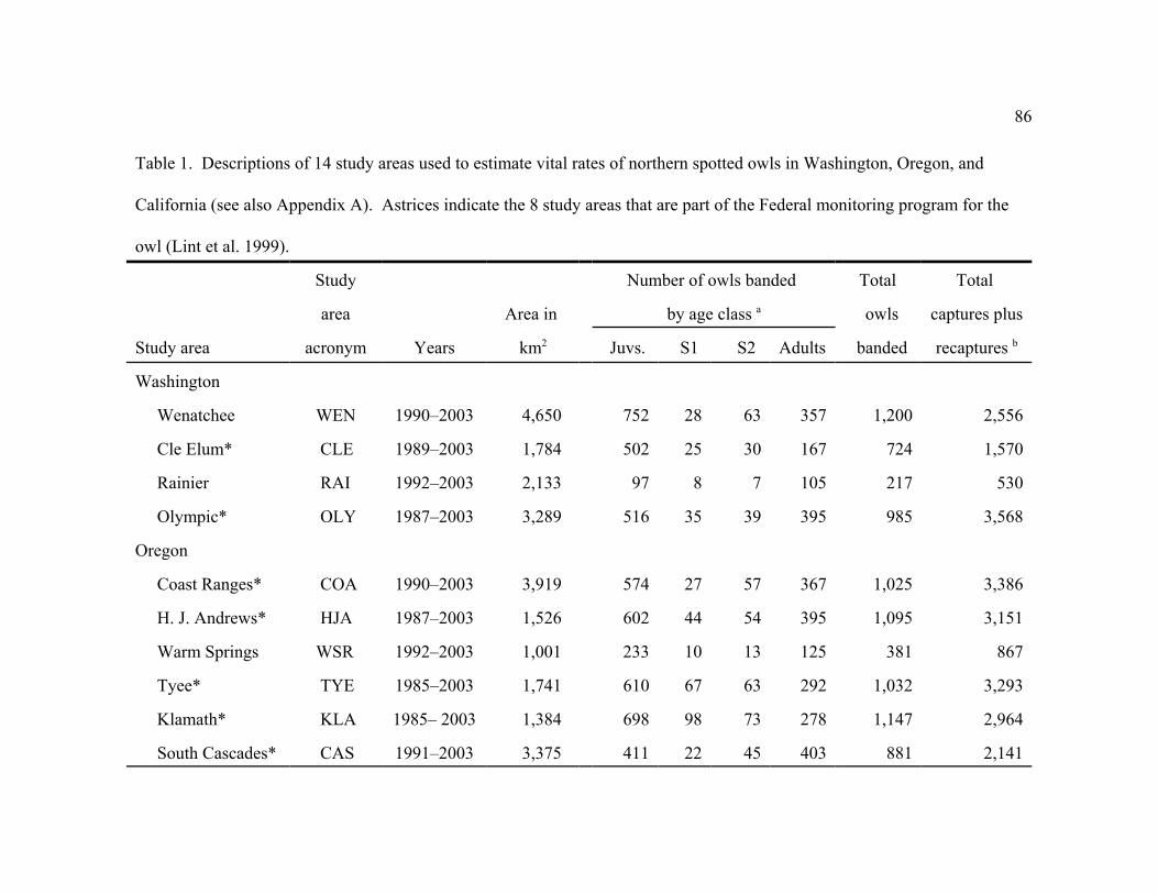
86

Table 1. Descriptions of 14 study areas used to estimate vital rates of northern spotted owls in Washington, Oregon, and

California (see also Appendix A). Astrices indicate the 8 study areas that are part of the Federal monitoring program for the

owl (Lint et al. 1999).

Study Number of owls banded Total Total

area Area in by age class a owls captures plus

Study area acronym Years km2 Juvs. S1 S2 Adults banded recaptures b

Washington

Wenatchee WEN 1990–2003 4,650 752 28 63 357 1,200 2,556

Cle Elum* CLE 1989–2003 1,784 502 25 30 167 724 1,570

Rainier RAI 1992–2003 2,133 97 8 7 105 217 530

Olympic* OLY 1987–2003 3,289 516 35 39 395 985 3,568

Oregon

Coast Ranges* COA 1990–2003 3,919 574 27 57 367 1,025 3,386

H. J. Andrews* HJA 1987–2003 1,526 602 44 54 395 1,095 3,151

Warm Springs WSR 1992–2003 1,001 233 10 13 125 381 867

Tyee* TYE 1985–2003 1,741 610 67 63 292 1,032 3,293

Klamath* KLA 1985– 2003 1,384 698 98 73 278 1,147 2,964

South Cascades* CAS 1991–2003 3,375 411 22 45 403 881 2,141

87

California

Table 1. (continued).

Study Number of owls banded Total Total

area Area in by age class a owls captures plus

Study area acronym Years km2 Juv. S1 S2 Adults banded recaptures b

NW California* NWC 1985–2003 1,790 609 97 73 247 1,026 2,865

Hoopa HUP 1992–2003 356 116 24 30 109 279 851

Simpson SIM 1990–2003 1,265 708 80 127 429 1,344 4,087

Marin MAR 1998–2003 217 41 9 10 36 96 225

Totals 28,430 6,469 574 684 3,705 11,432 32,054a Age class codes indicate owls that were 1 year old (S1), 2 years old (S2) or $ 3 years old (Adults). b All captures and recaptures, regardless of age.

88

Table 2. A priori models used for analysis of recapture probabilities (p) of northern

spotted owls on 14 demographic study areas in Washington, Oregon, and California. N

structure for all models was N(a*s*t).

Model a Description of p structure1. p(a*s*t) Age, sex, and time effects with all interactions (global model)

2. p(.) Constant model (no effects)

3. p(s) Sex effect

4. p(r) Effect of annual reproduction on p in following year

5. p(r+s) Additive reproduction and sex effects

6. p(t) Annual time effect

7. p(s+t) Additive sex and time effects

8. p(T) Linear time trend effect

9. p(s+T) Additive sex and linear time trend effects

10. p(BO) Barred owl effect

11. p(s+BO) Additive sex and barred owl effects

12. p(s+BO+r) Additive sex, barred owl, and reproduction effects

13. p(choice) Biologist’s choice b

a Model notation indicates structure for effects of age (a), sex (s), annual time (t),

linear time trend (T), reproduction (r), barred owls (BO), or biologist’s choice (choice).

Age structure included 3 age classes (1-year-old, 2-year-old, and $ 3 years old).

b Up to 3 additional models of choice that incorporated potential area-specific effects

on p (i.e., survey effort, study area subregions, survey method, etc.)

89

Table 3. A priori models used for analysis of apparent survival (N) of northern spotted

owls on 14 demographic study areas in Washington, Oregon, and California. Models

for each study area used the best p-structure from the initial analysis of p-structure on

each study area.

Model a Description of N structure

1. N(S1=S2=A) Constant N, no age, sex or time effects

2. N([S1=S2=A]+s) Sex effect only

3. N(S1, S2=A) Age effect ( S2=A, S1 different)

4. N([S1, S2=A]+s) Age effect ( S2=A, S1 different), additive sex effect (s)

5. N(S1=S2, A) Age effect (S1=S2, A different)

6. N([S1=S2, A]+s) Age effect (S1=S2, A different), additive sex effect (s)

7. N(S1, S2, A) Age effect (all age classes different)

8. N([S1, S2, A}+s) Age effect (all age classes different), additive sex effect (s)

9. N(models 1-8+t) Models 1-8 above with additive time effect (t)

10. N(models 1-8+T) Models 1-8 above with additive linear time effect (T)

11. N(models 1-8*T) Models 1-8 above with interactive linear time effect (T)

12. N(models 1-8+TT) Models 1-8 above with additive quadratic time effect (TT)

13. N(models 1-8*TT) Models 1-8 above with interactive quadratic time effect (TT)

14. N(models 1-8+BO) Models 1-8 above with additive barred owl effect (BO)

a Model notation indicates structure for effects of age (S1, S2, A), sex (s), annual

time (t), linear time trend (T), or quadratic time trend (TT). Age classes (S1, S2, A)

indicate owls that were 1, 2, or $ 3 years old, respectively. Symbols separating age

classes indicate if they were combined (=) or estimated separately (,).

90

Table 4. A priori models used for meta-analysis of apparent survival (N) and recapture

probabilities (p) of adult female northern spotted owls on 14 study area in Washington,

Oregon, and California.

Model a Description of model structure

1. N(g*t*s) p(g*t*s) N(area, time, and sex effects with all interactions):

p(area, time, and sex effects with all interactions)

2. N([g*t]+s) p(g+t) N(area and time effects with interactions, plus

additive sex effect): p(additive area and time effects)

3. N([g*t]+s) p(g+s+t) N(area and time effects with interactions, plus

additive sex effect): p(additive area, sex, and time

effects)

4. N([g*t]+s) p([g+t]*s) N(area and time effects with interactions, plus

additive sex effect): p(additive area and time effects,

interacting with sex)

5. N([g*t]+s) p(r) N(area and time effects with interactions, plus

additive sex effect): p(reproduction effect)

6. N([g*t]+s) p(r+s) N(area and time effects with interactions, additive

sex effect): p(additive reproduction and sex effects)

7. N([g*t]+s) p(r*s) N(area and time effects with interactions, plus

additive sex effect): p(reproduction and sex effects

with interactions)

8. N(g+s) p(best) N(additive area and sex effects): p(best p-structure

from models 2-7 above).

9. N(g+s+t) p(best) N(additive area, sex and time effects): p(= model 8)

91



10. N([g*T]+s) p(best) N(area and linear time effects with interactions, plus

additive sex effect): p(= model 8)

11. N(g+T+s) p(best) N(additive area, linear time trend, and sex effects):

p(= model 8)

12. N([g*TT]+s) p(best) N(area and quadratic time effects with interactions,

plus additive sex effect): p(= model 8)

13. N(g+s+TT) p(best) N(additive area, sex, and quadratic time effects):

p(= model 8)

14. N(s+t) p(best) N(additive sex and time effects): p(= model 8)

15. N(s+TT) p(best) N(additive sex and quadratic time effects):

p(= model 8)

16. N(s+T) p(best) N(additive sex and linear time effects): p(= model 8)

17. N(s) p(best) N(sex effect): p(= model 8)

18. N(BO+s) p(best) N(additive barred owl and sex effects): p(= model 8)

19. N(g+BO+s) p(best) N(additive area, barred owl, and sex effects):

p(= model 8)

20. N([g*BO]+s) p(best) N(area and barred owl effects with interactions, plus

additive sex effect): p(= model 8)

21. N(no sex) p(best) N(lowest QAICc model from models 8-20 with sex

effect removed): p(= model 8)

22. N(owner) p(best) N(replace area effect in lowest QAICc model from

models 8-21 with ownership effect): p(= model 8)

92

TABLE 4. (continued).


23. N(region) p(best) N(replace area effect in lowest QAICc model from

models 8-21 with region effect): p(= model 8)

24. N(owner*region) p(best) N(replace area effect in lowest QAICc model from

models 8-21 with ownership and region effects with

interactions): p(= model 8)

25. N(best+latitude) p(best) N(additive latitude effect with best area effect model

from models 8-24): p(= model 8)

a Model notation indicates structure for effects of study area (g), annual time (t),

linear time trend (T), quadratic time trend (TT), geographic region (region), land

ownership (owner), latitude (latitude), or barred owls (BO).

93

Table 5. Estimates of age-specific fecundity (number of female young produced per female) of northern spotted owls on 14 study

areas in Washington, Oregon and California.

1-year-old owls 2-year-old owls Adults ($ 3 years old)

Study area Years n a SE n a SE n a SEx xWashington

WEN 1990–2003 20 0.050 0.050 49 0.290 0.085 758 0.491 0.058

CLE 1989–2003 23 0.136 0.097 34 0.467 0.117 423 0.574 0.069

RAI 1992–2003 4 0.000 0.000 7 0.000 0.000 184 0.253 0.061

OLY 1987–2003 11 0.071 0.050 19 0.267 0.098 883 0.293 0.057

Oregon

COA 1990–1992 17 0.000 0.000 53 0.111 0.045 1,168 0.260 0.050

HJA 1987–2003 22 0.109 0.091 35 0.113 0.060 1,026 0.321 0.045

WSR 1992–2003 7 0.000 0.000 16 0.311 0.110 303 0.424 0.070

TYE 1985–2003 72 0.054 0.032 90 0.201 0.047 973 0.319 0.040

KLA 1985–2003 69 0.070 0.028 103 0.285 0.052 795 0.445 0.040

CAS 1991–2003 26 0.061 0.046 42 0.223 0.082 780 0.377 0.059

California

NWC 1985–2003 64 0.101 0.066 78 0.205 0.052 938 0.333 0.032

HUP 1992–2003 10 0.000 0.000 15 0.056 0.056 273 0.216 0.043

SIM 1990–2003 60 0.109 0.040 104 0.118 0.030 1,168 0.326 0.037

94

MAR 1998–2003 12 0.275 0.195 12 0.271 0.159 156 0.530 0.056

Table 5. (continued).1-year-old owls 2-year-old owls Adults ($ 3 years old)

Study area Years n a SE n a SE n a SEx

Total/Mean 417 0.074 0.029 657 0.208 0.032 9,828 0.372 0.029

a Sample size indicates the number of cases in which we sampled owls in each age class. This is not the sample that was used

to calculate means and standard errors. Those estimates were based on the number of years in the survey period. Estimates were

determined using a non-parametric approach.

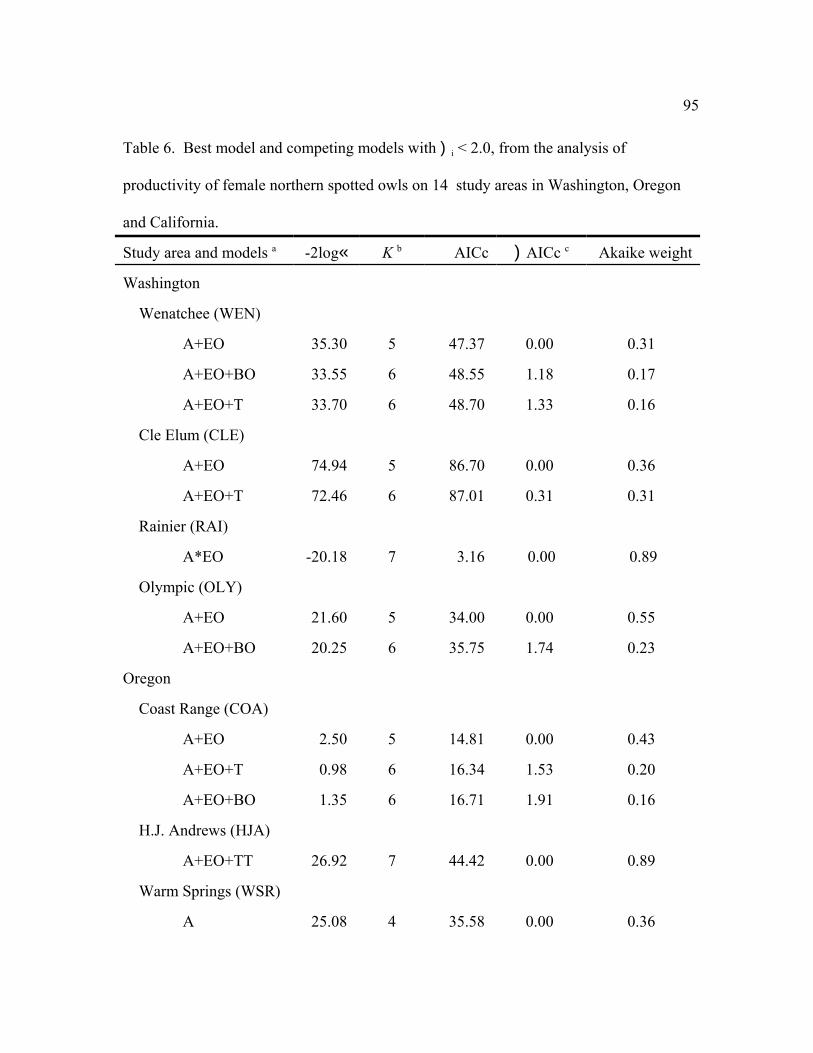
95

Table 6. Best model and competing models with )i < 2.0, from the analysis of

productivity of female northern spotted owls on 14 study areas in Washington, Oregon

and California.

Study area and models a -2log‹ K b AICc )AICc c Akaike weight

Washington

Wenatchee (WEN)

A+EO 35.30 5 47.37 0.00 0.31

A+EO+BO 33.55 6 48.55 1.18 0.17

A+EO+T 33.70 6 48.70 1.33 0.16

Cle Elum (CLE)

A+EO 74.94 5 86.70 0.00 0.36

A+EO+T 72.46 6 87.01 0.31 0.31

Rainier (RAI)

A*EO -20.18 7 3.16 0.00 0.89

Olympic (OLY)

A+EO 21.60 5 34.00 0.00 0.55

A+EO+BO 20.25 6 35.75 1.74 0.23

Oregon

Coast Range (COA)

A+EO 2.50 5 14.81 0.00 0.43

A+EO+T 0.98 6 16.34 1.53 0.20

A+EO+BO 1.35 6 16.71 1.91 0.16

H.J. Andrews (HJA)

A+EO+TT 26.92 7 44.42 0.00 0.89

Warm Springs (WSR)

A 25.08 4 35.58 0.00 0.36

96

A+EO 22.71 5 36.71 1.13 0.20



Constant 32.57 2 37.23 1.66 0.16

Tyee (TYE)

A+T 27.31 5 38.62 0.00 0.31

A 30.80 4 39.65 1.03 0.18

A+BO 29.23 5 40.53 1.92 0.12

Klamath (KLA)

A+EO 30.20 5 41.59 0.00 0.22

A 32.73 4 41.64 0.05 0.22

A*EO 26.69 7 43.42 1.83 0.09

A+BO 32.07 5 43.47 1.88 0.09

S. Cascades (CAS)

A+EO+T 31.92 6 46.72 0.00 0.36

A+EO 35.84 5 47.78 1.06 0.21

A+EO+TT 30.85 7 48.71 1.99 0.13

California

NW California (NWC)

A+T 51.40 5 62.68 0.00 0.27

A+BO 52.66 5 63.93 1.25 0.14

A 55.22 4 64.05 1.37 0.13

A+TT 50.30 6 64.13 1.45 0.13

Hoopa (HUP)

A+EO+T -7.99 6 7.83 0.00 0.32

A+EO+BO -7.47 6 8.35 0.53 0.25

A+EO -3.73 5 8.88 1.06 0.19

97

Simpson (SIM)



A+EO -0.66 5 11.01 0.00 0.42

A+EO+T -1.76 6 12.64 1.64 0.19

A+EO+BO -1.46 6 12.94 1.93 0.16

Marin (MAR)

Constant 34.34 2 39.20 0.00 0.52

a Model notation indicates structure for effects of owl age (A), even-odd years (EO),

linear time (T), quadratic time (TT), or barred owls (BO).

b K = number of parameters in model, including covariance parameters.

c )AICc = difference between the model listed and the best AICc model.

98

Table 7. Regression coefficients ( ) from the best productivity model containing a

linear (T) or quadratic (TT) time trend for 14 northern spotted owl study areas in

Washington, Oregon, and California.

Best time 95% CI

Study area trend model )AICc b SE Lower Upper

Washington

WEN A+EO+T 1.325 -0.022 0.017 -0.055 0.011

CLE A+EO+T 0.305 -0.038 0.024 -0.085 0.009

RAI A*EO+T 5.534 0.005 0.011 -0.016 0.026

OLY A+EO+T 2.935 -0.005 0.013 -0.030 0.020

Oregon

COA A+EO+T 1.529 -0.014 0.011 -0.036 0.008

HJA A+EO+TT c 0.000 -0.024 0.011 -0.046 0.002

0.009 0.003 0.003 0.015

WSR A+T 3.444 0.007 0.028 -0.048 0.062

TYE A+T 0.000 0.016 0.008 0.000 0.317

KLA A+T 2.384 0.004 0.009 -0.014 0.022

CAS A+EO+T 0.000 -0.034 0.017 -0.067 0.001

California

NWC A+T 0.000 -0.019 0.010 -0.039 0.001

HUP A+EO+T 0.000 0.023 0.011 0.001 0.044

SIM A+EO+T 1.636 -0.010 0.009 -0.028 0.008

MAR A+T 7.995 0.029 0.092 -0.151 0.209

a Notation indicates model structure for effects of age (A), even-odd year (EO), linear

time trend (T), or quadratic time trend (TT).

b )AICc = difference between the best time-trend model and the best AICc model for

each study area (Appendix F).

99

c The first estimate is the linear term and the second is the quadratic term.

Table 8 . Regression coefficients ( ) for the barred owl effect on productivity of$β

northern spotted owls on 14 study areas in Washington, Oregon, and California.

Estimates are from the best productivity model containing the barred owl (BO) covariate

Study area Model a )AICc b SE

95% CI

Lower Upper

Washington

WEN A+EO+BO 1.173 -0.942 0.701 -2.316 0.433

CLE A+EO+BO 2.533 -0.550 1.102 -2.710 1.610

RAI A+EO+BO 10.700 0.202 0.548 -0.871 1.275

OLY A+EO+BO 1.744 -1.026 0.872 -2.735 0.682

Oregon

COA A+EO+BO 1.907 -0.280 0.259 -0.787 0.228

HJA A+EO+BO 9.604 -0.428 1.011 -2.411 1.554

WSR A+BO 3.355 -0.503 1.316 -3.081 2.078

TYE A+BO 1.915 0.733 0.580 -0.404 1.869

KLA A+BO 1.875 1.316 1.617 -1.853 4.484

CAS A+EO+BO 2.755 -1.385 1.270 -3.874 1.105

California

NWC A+BO 1.253 -2.069 1.278 -4.575 0.436

HUP A+EO+BO 0.525 2.114 1.058 0.040 4.187

SIM A+EO+BO 1.929 -1.932 2.144 -6.134 2.270

MAR BO 1.102 22.533 15.951 8.730 53.797

a Notation indicates model structure for effects of age (A), even-odd year (EO), or

barred owls (BO).

100

b )i = difference between the best model with the BO covariate and the best AICc

model for each study area (Appendix F).

Table 9. Variance components of the number of young fledged per pair of northern

spotted owls, from a mixed model analysis of year- and territory-specific estimates.

Spatial variability is the random effects estimate of territory variability, and temporal is

the random effects estimate of year variability.

Source of Variation

Spatial Temporal Residual Total

Study

area Estimate

% of

total Estimate

% of

total Estimate

% of

total Estimate

Washington

WEN 0.058 6 0.166 18 0.691 75 0.915

CLE 0.058 5 0.227 23 0.684 70 0.969

RAI 0.000 0 0.109 17 0.505 82 0.613

OLY 0.021 2 0.201 28 0.481 68 0.703

Oregon

COA 0.015 2 0.127 21 0.450 76 0.592

HJA 0.000 0 0.108 15 0.601 84 0.709

WSR 0.000 0 0.195 22 0.675 77 0.871

TYE 0.030 4 0.079 11 0.569 83 0.678

KLA 0.000 0 0.056 7 0.704 92 0.760

CAS 0.022 2 0.153 19 0.615 77 0.790

California

NWC 0.028 3 0.059 8 0.623 87 0.710

HUP 0.035 7 0.056 11 0.404 81 0.495

101

SIM 0.025 3 0.054 8 .0585 88 0.663

MAR 0.108 12 0.058 6 0.701 80 0.867

102

Table 10. Model selection results from the meta-analysis of productivity of female

northern spotted owls on 14 study areas in Washington, Oregon, and California.

Model a -2log‹ K b AICc )AICc c Akaike weight

region+t 57.215 26 117.238 0.000 0.547

region+t+BO 55.832 27 118.522 1.284 0.288

t 72.838 21 119.972 2.734 0.139

owner+t 72.182 23 124.385 7.147 0.015

region*BO+t 48.627 32 125.124 7.886 0.011

region+EO 141.543 9 160.480 43.242 0.000

region*EO 133.320 14 163.566 46.328 0.000

owner+EO 154.193 6 166.624 49.386 0.000

owner*EO 153.921 8 170.668 53.430 0.000

owner*t 47.154 54 195.562 78.324 0.000

region+T 190.340 9 209.277 92.039 0.000

region+BO 193.846 9 212.784 95.546 0.000

T 205.554 4 213.757 96.519 0.000

region*BO 188.671 13 216.607 99.369 0.000

owner+T 204.825 6 217.255 100.018 0.000

Constant 211.243 3 217.364 100.127 0.000

BO 210.334 4 218.537 101.299 0.000

region*T 188.294 14 218.540 101.302 0.000

owner*T 204.686 8 221.432 104.194 0.000

a Notation indicates model structure for effects of geographic region (region), land

ownership (owner), even-odd year (EO), annual time (t), linear time (T), or barred owls

(BO).

b K = number of parameters in model, including covariance parameters.

103

c )AICc = difference between the model listed and the best AICc model.

Table 11. Estimates of mean annual fecundity (number of female young produced per

female) of adult northern spotted owls, subdivided by geographic regions.

95% CI

Geographic region SE Lower Upper

All 14 study areas

Washington - Douglas-fir 0.313 0.041 0.233 0.393

Washington - Mixed-Conifer 0.560 0.041 0.480 0.640

Oregon Coastal - Douglas-fir 0.306 0.039 0.230 0.382

Oregon Cascades - Douglas-fir 0.404 0.034 0.337 0.471

Oregon/California - Mixed-Conifer 0.350 0.032 0.287 0.413

California Coast 0.442 0.045 0.354 0.530

104

Table 12. Estimates of overdispersion ( ) in capture-recapture data from 14 northern

spotted owl demographic study areas in Washington, Oregon and California.

CJS a 8RJS a

Study area P2 df $c P2 df $c

Washington

WEN 165.67 71 2.33 147.42 84 1.18

CLE 63.92 68 0.94 35.21 51 0.69

RAI 45.24 46 0.98 33.73 47 0.72

OLY 170.35 86 1.98 156.42 104 1.50

Oregon

COA 179.51 68 2.64 168.87 56 3.02

HJA 210.40 85 2.47 167.29 78 2.14

WSR 49.31 46 1.07 46.95 41 1.14

TYE 133.41 95 1.40 69.68 64 1.09

KLA 117.93 95 1.24 87.48 74 1.18

CAS 139.67 62 2.25 142.91 65 2.20

California

NWC 86.84 75 1.16 124.93 81 1.54

HUP 41.07 49 0.84 46.06 52 0.89

SIM 186.39 68 2.74 139.81 50 2.80

MAR 10.33 11 0.94 NAb NAb NAb

Totals 1600.04 925 1.73 1366.76 847 1.61

a CJS indicates data sets used for Cormack-Jolly-Seber estimates of apparent survival,

and λRJS indicates data sets used to estimate annual rates of population change. Values

for P2, and df are from TEST 2 and TEST 3 in program RELEASE. Estimates of $c

<1.0 were set to 1.00 for analysis.

105

b λRJS could not be estimated for the MAR Study Area because of small sample size.

106

Table 13. Estimates of average apparent survival ( ) for 3 age-classes of northern spotted owls on 14 study areas in

Washington, Oregon, and California.

Best model a 1-year-old b 2-year old b $ 3 yrs old b

Study area structure p structure SE( ) SE( ) SE( ) φ

Washington

WEN (S1=S2,A)+BO T 0.626 0.073 0.626 0.073 0.750 0.026

CLE t s+r 0.860 0.017 0.860 0.017 0.860 0.017

RAI T t 0.832 0.020 0.832 0.020 0.832 0.020

OLY (S1,S2=A)+BO t 0.570 0.117 0.855 0.011 0.855 0.011

Oregon

COA S1,S2=A (.) 0.721 0.107 0.886 0.010 0.886 0.010

HJA S1,S2=A TT 0.415 0.111 0.883 0.010 0.883 0.010

WSR (.) r+BO 0.823 0.015 0.823 0.015 0.823 0.015

TYE (S1,S2=A)+TT s+T 0.817 0.042 0.878 0.011 0.878 0.011

KLA (.) T 0.849 0.009 0.849 0.009 0.849 0.009

CAS S1=S2,A TT 0.725 0.079 0.725 0.079 0.854 0.014

California

NWC (S1=S2,A)+TT meth+by 0.810 0.027 0.810 0.027 0.869 0.011

107

HUP S1=S2,A TT*EW 0.781 0.049 0.781 0.049 0.853 0.014


Best model a 1-year-old b 2-year old b $ 3 yrs old b

Study area structure p structure SE( ) SE( ) SE( )

SIM (.) s 0.850 0.010 0.850 0.010 0.850 0.010

MAR s s+r & 0.824 0.045 0.824 0.045 0.824 0.045

% 0.913 0.035 0.913 0.035 0.913 0.035

a Model notation indicates structure for additive (+) or interactive (*) effects of sex (s), time (t), linear time trend (T),

quadratic time trend (TT), reproduction (r), barred owls (BO), age-class (S1, S2, A), east-west binomial subdivision of study

area (EW), survey method (meth), or years of poor weather (by). For age-classes, an (=) sign means that age classes were

combined, and a (,) indicates that they were modeled separately. Age classes (S1, S2, A) indicate owls that were 1, 2 or $3

years old.

b For study areas with time structure in the top model, we estimated average survival as follows: For variable time (t)

models we calculated the arithmetic mean and standard error using the delta method. For linear (T) models, we used the

median value and its standard error (odd number of survival estimates) or the lower of the 2 median values and its standard

error (even number of survival estimates). For quadratic (TT) models we used the annual estimate from the model that was

closest to the arithmetic average of the maximum and minimum annual survival estimates.

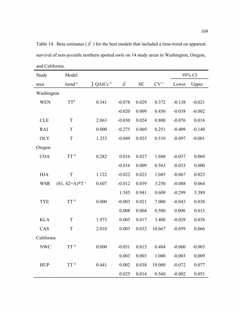
109

Table 14. Beta estimates ( ) for the best models that included a time-trend on apparent

survival of non-juvenile northern spotted owls on 14 study areas in Washington, Oregon,

and California..

Study Model 95% CI

area trend a )QAICc b SE CV c Lower Upper

Washington

WEN TTd 0.341 -0.078 0.029 0.372 -0.138 -0.021

-0.020 0.009 0.450 -0.038 -0.002

CLE T 2.063 -0.030 0.024 0.800 -0.076 0.016

RAI T 0.000 -0.275 0.069 0.251 -0.409 -0.140

OLY T 1.253 -0.049 0.025 0.510 -0.097 -0.001

Oregon

COA TT d 0.282 0.016 0.027 1.688 -0.037 0.069

-0.016 0.009 0.563 -0.033 0.000

HJA T 1.122 -0.022 0.023 1.045 -0.067 0.023

WSR (S1, S2=A)*T e 0.607 -0.012 0.039 3.250 -0.088 0.064

1.545 0.941 0.609 -0.299 3.389

TYE TT d 0.000 -0.003 0.021 7.000 -0.043 0.038

0.008 0.004 0.500 0.000 0.015

KLA T 1.973 0.005 0.017 3.400 -0.029 0.038

CAS T 2.010 0.003 0.032 10.667 -0.059 0.066

California

NWC TT d 0.000 -0.031 0.015 0.484 -0.060 -0.003

0.003 0.003 1.000 -0.003 0.009

HUP TT d 0.441 0.002 0.038 19.000 -0.072 0.077

0.025 0.014 0.560 -0.002 0.051

110

SIM T 1.596 -0.015 0.024 1.600 -0.062 0.032


Study Model 95% CI

area trend a )QAICc b SE CV c Lower Upper

MAR T 2.118 0.048 0.206 4.292 -0.357 0.452

a T = linear trend over time, TT = quadratic trend over time.

b )QAICc = difference between the model listed and the best QAICc model.

c Coefficient of sampling variation (CV) computed as .

d The first row estimate is the linear term and the second is the quadratic term.

e First row is for linear term, second is for interaction.

111

Table 15. Model selection criteria for a priori models used in the meta-analysis of

apparent survival of adult northern spotted owls on 14 demographic study areas in

Washington, Oregon, and California, 1985-2003.

Model a QAICc )QAICc b

Akaike

weights K c Q Deviance d

N(region+t) p(g+s+t) 18459.906 0.000 0.780 55 7206.936

N([owner*region]+t) p(g+s+t) 18464.024 4.119 0.099 58 7205.020

N(g+t) p(g+s+t) 18464.554 4.648 0.076 63 7195.489

N(g+s+t) p(g+s+t) 18466.353 6.448 0.031 64 7195.277

N(region*T) p(g+s+t) 18468.722 8.816 0.010 44 7237.861

N(latitude+t) p(g+s+t) 18472.213 12.307 0.002 51 7227.286

N(s+t) p(g+s+t) 18473.263 13.357 0.001 51 7228.335

N(owner+t) p(g+s+t) 18473.338 13.433 0.001 52 7226.400

N(region*r) p(g+s+t) 18478.302 18.396 0.000 44 7247.441

N(region+r) p(g+s+t) 18478.557 18.652 0.000 39 7257.737

N(g+t) p(g+t) 18479.624 19.719 0.000 62 7212.572

N(g+s+t) p(g+t) 18480.976 21.070 0.000 63 7211.912

N([g*BO]+s) p(g+s+t) 18483.279 23.374 0.000 61 7218.240

N([g*T]+s) p(g+s+t) 18483.811 23.905 0.000 61 7218.771

N(region+T) p(g+s+t) 18484.238 24.332 0.000 39 7263.419

N([g*TT]+s) p(g+s+t) 18489.309 29.403 0.000 75 7196.079

N(g+s+T) p(g+s+t) 18491.662 31.756 0.000 48 7252.764

N(g+s) p(g+s+t) 18492.032 31.126 0.000 47 7255.143

N(g+BO+s) p(g+s+t) 18492.843 32.937 0.000 48 7253.945

N(g+s+TT) p(g+s+t) 18493.620 33.715 0.000 49 7252.713

N(s) p(g+s+t) 18502.671 42.765 0.000 34 7291.888

112

N(s+T) p(g+s+t) 18502.852 42.946 0.000 35 7290.062


Model a

QAICc

)QAICc b

Akaike

weights K c Q Deviance d

N(BO+s) p(g+s+t) 18503.635 43.729 0.000 35 7290.845

N(s+TT) p(g+s+t) 18504.377 44.471 0.000 36 7289.581

N([g*t]+s) p(g+s+t) 18601.916 142.010 0.000 223 7008.269

N([g*t]+s) p(g+t) 18616.032 156.126 0.000 222 7024.429

N([g*t]+s) p([g+t]*s) 18627.672 167.767 0.000 251 6976.690

N([g*t]+s) p(r+s) 18810.165 350.259 0.000 191 7281.848

N([g*t]+s) p(r*s) 18812.197 352.291 0.000 192 7281.841

N([g*t]+s) p(r) 18822.324 362.418 0.000 190 7296.045

N(g*t) p(g*s*t) 18929.102 469.196 0.000 553 6649.370

N(g*s*t) p(g*s*t) 19215.200 755.295 0.000 728 6562.237

a Codes indicate model structure for additive (+) or interactive (*) effects of region

(region), study area (g), sex (s), annual time (t), linear time trend (T), quadratic time trend

(TT), land ownership (owner), latitude (latitude), barred owls (BO), or reproduction (r).

b )QAICc = difference between the model listed and the best QAICc model.

c Number of parameters in model.

d Q Deviance is the difference between -2log(‹)/ of the current model and

-2log(‹)/ of the saturated model.

113

Table 16. Estimates of for the effect of reproduction (r) on apparent survival of adult

northern spotted owls in different regions. Estimates are from model {N(region*r)

p(g+t+s)} in the meta-analysis of 14 demographic study areas in Washington, Oregon,

and California.

95% CI

Region SE Lower Upper

Washington Douglas-fir -0.596 0.234 -1.055 -0.136

Washington Mixed-Conifer -0.315 0.185 -0.677 0.047

Oregon Coastal Douglas-fir -0.119 0.209 -0.530 0.291

Oregon Cascades Douglas-fir -0.507 0.182 -0.863 -0.151

Oregon/California Mixed-Conifer 0.010 0.221 -0.424 0.443

California Coast 0.398 0.318 -0.226 1.023

114

Table 17. Estimates of )QAIC a and for the effects of barred owls on apparent

annual survival of adult northern spotted owls on 14 demographic study areas in

Washington, Oregon, and California. Estimates were based on the best QAIC model that

included the barred owl effect.

95% CI

Study area )QAICc SE Lower Upper

Washington

WEN 0.00 -4.69 1.34 -7.32 -2.07

CLE 1.58 -1.40 0.99 -3.33 0.54

RAI 10.86 4.44 2.18 0.16 8.72

OLY 0.00 -4.24 1.83 -7.83 -0.65

Oregon

COA 2.01 0.03 0.68 -1.31 1.37

HJA 0.89 -1.83 1.69 -5.14 1.48

WSR 2.04 0.08 1.57 -2.98 3.15

TYE 2.37 1.35 1.21 -1.03 3.72

KLA 2.05 0.02 3.34 -6.51 6.56

CAS 1.55 1.80 2.70 -3.49 7.10

California

NWC 0.95 -2.39 1.68 -5.68 0.90

HUP 1.18 -3.18 3.10 -9.26 2.90

SIM 0.70 -5.80 5.05 -15.68 4.08

MAR 1.99 11.61 27.48 -42.26 65.48

a )QAICc = difference between the best QAICc model and the best model with the

barred owl effect.

115

Table 18. Estimates of for the effect of the barred owl parameter on apparent

survival of adult northern spotted owls from the meta-analysis of 14 demographic study

areas in Washington, Oregon, and California. Model was {N(BO*region) p(g+s+t)}.

95% CI

Model/area SE Lower Upper

Washington

WEN -4.122 1.218 -6.509 -1.734

CLE -1.884 1.422 -4.671 0.904

RAI 2.241 2.209 -2.089 6.571

OLY -4.718 1.649 -7.951 -1.485

Oregon

COA 0.308 0.584 -0.836 1.452

HJA -0.777 1.894 -4.889 2.936

WSR -1.141 2.077 -5.211 2.929

TYE 2.544 1.523 -0.441 5.529

KLA 1.775 3.770 -5.614 9.165

CAS 6.813 2.804 1.317 12.309

California

NWC -2.256 2.087 -6.347 1.836

HUP -3.678 4.398 -12.298 4.943

SIM -4.919 4.245 -13.238 3.401

MAR -5.702 47.727 -99.247 87.843

116

Table 19. Estimates of RJS and temporal process standard deviation ( ) for northern spotted owls on 13 study areas in

Washington, Oregon, and California. Estimates are based on means (intercepts only) random effects models using time-

specific estimates of N , p and 8, except where noted.

95% CI 95% CI

Study Model a RJS SE CV Lower Upper Lower Upper

Density study areas

TYE N(t) p(t) λ(t) REλ(mean) 1.005 0.019 0.019 0.967 1.043 0.050 0.000 0.126

NWC N(t) p(t) λ(t) REλ(mean) 0.985 0.013 0.013 0.959 1.011 0.000 0.000 0.017

HUP N(t) p(t) λ(t) REλ(mean) 0.980 0.019 0.019 0.943 1.017 0.000 0.000 0.131

SIM N(t) p(t) λ(t) REλ(mean) 0.970 0.012 0.012 0.947 0.993 0.015 0.000 0.077

Territory study areas b

WEN N(t) p(t) λ(t) REλ(mean) 0.917 0.018 0.019 0.882 0.952 0.038 0.000 0.147

CLE N(t) p(t) λ(t) REλ(mean) 0.938 0.019 0.020 0.901 0.976 0.000 0.000 0.090

RAI N(t) p(t) γ(t) c 0.896 0.055 0.061 0.788 1.003 c c c

OLY N(ea*t) p(ea*t) λ(ea*t) REλ(mean) 0.956 0.032 0.034 0.893 1.018 0.091 0.000 0.222

COA N(t) p(t) λ(t) REλ(mean) 0.968 0.018 0.019 0.932 1.004 0.000 0.000 0.067

HJA N(ea*t) p(ea*t) λ(ea*t) REλ(mean) 0.978 0.014 0.015 0.950 1.005 0.000 0.000 0.064

WSR N(t) p(t) λ(t) REλ(mean) 0.908 0.022 0.024 0.866 0.951 0.000 0.000 0.152

117


95% CI 95% CI

Study Model a RJS SE CV Lower Upper Lower Upper

KLA N(t) p(t) λ(t) REλ(T) 0.997 0.034 0.042 0.930 1.063 0.026 0.000 0.135

CAS N(ea*t) p(ea*t) λ(ea*t) REλ(mean) 0.974 0.035 0.035 0.906 1.042 0.082 0.000 0.269

Mean for density study areas 0.985 0.016

Mean for territory study areas 0.951 0.027

Mean for all areas 0.959 0.024

a Best capture-recapture model structure from analysis of the a priori model set. Model notation indicates structure for

effects of time (t), expansion year (ea), linear time trend (T) or constant (mean). RE = random effects.

b Marin Study Area not included because sample was too small to estimate 8.

c Model fit using a N and ( parameterization; 8 was calculated via arithmetic mean.

118

Table 20. Models selected in the meta-analysis of 8RJS of northern spotted owls in

Washington, Oregon, and California. Analyses were conducted separately for the 4

Density Study Areas (1985–2003) and 10 Territory Study Areas (1987-2003).

Model a QAICc

)QAICc bAkaike

weight K c

Density study areas

N(g*t) p(g*t) λ(.) 9302.567 0.000 0.374 113

N(g*t) p(g*t) λ(region) 9303.128 0.561 0.283 115

N(g*t) p(g*t) λ(owner) 9303.418 0.851 0.244 115

N(g*t) p(g*t) λ(g) 9305.241 2.674 0.098 116

N(g*t) p(g*t) λ(region+t) 9316.061 13.494 0.000 129

N(g*t) p(g*t) λ(owner+t) 9316.800 14.233 0.000 129

N(g*t) p(g*t) λ(g+t) 9318.121 15.554 0.000 130

N(g*t) p(g*t) λ(t) 9318.896 16.329 0.000 127

N(g*t) p(g*t) λ(region*t) 9340.882 38.315 0.000 144

N(g*t) p(g*t) λ(owner*t) 9341.759 39.192 0.000 145

N(g*t) p(g*t) λ(g*t) 9354.079 51.512 0.000 152

Territory study areas

N(g*t) p(g*t) λ(g*t) 19790.239 0.000 1.000 324

N(owner*t) p(owner*t) λ(owner+t) 19956.233 165.994 0.000 114

N(owner*t) p(owner*t) λ((owner*t) 19971.521 181.282 0.000 126

N(t) p(t) λ(t) 19981.221 190.982 0.000 69

N(region*t) p(region*t) λ(region+t) 20090.581 300.342 0.000 226

a Model notation indicates structure for study area (g), time (t), geographic region

(region), land ownership (owner), or constant (.).

b )QAICc = the difference between the model listed and the best QAICc model.

119

c Number of parameters in model.

Table 21. Summary of trends in demographic parameters for northern spotted owls

from 14 study areas in Washington, Oregon, and California, 1985-2003.

Study Area Land

ownership a Fecundity

Apparent

survival 8RJS )8 b

Washington

WEN Private Stable Declining 0.917 Declining

CLE USFS Declining c Declining? d 0.938 Declining

RAI USFS Stable Declining 0.896 Declining

OLY NPS & USFS Stable Declining 0.956 Declining

Oregon

COA USFS & BLM Declining? c Stable 0.968 Declining

HJA USFS Stable? e Stable 0.978 Declining

WSR Tribal Stable Stable 0.908 Declining

TYE BLM & private Increasing Stable 1.005 Stationary

KLA BLM & private Stable Stable 0.997 Stationary

CAS USFS & BLM Declining Stable 0.974 Stationary

California

NWC USFS Declining Declining 0.985 Declining? f

HUP Tribal Increasing Stable 0.980 Stationary

SIM Private Declining c Stable 0.970 Declining

MAR NPS Stable Stable NA g NA g

a Acronyms indicate U.S. Forest Service (USFS), Bureau of Land Management

(BLM), and U.S. National Park Service (NPS).

120

b Trend based on estimates of realized population change ()8).

c Best model included age and even-odd year effects, but a competing model had a

negative time effect on productivity.

d Variable among years, but with a declining trend.

e Decreasing in early years, increasing in last 5 years, but stable overall.

f Gradual declines in fecundity and apparent survival, plus estimates of realized

population change suggest a decline in last 8 years.

g Sample too small to estimate 8.

122

Fig. 1. The location and distribution of 14 northern spotted owl demographic study areas

for which data were analyzed.

123

0.0

0.2

0.4

0.6

0.8

1.0

1.2

1985 1987 1989 1991 1993 1995 1997 1999 2001 2003Year

Mea

n Fe

cund

ity

WEN CLE RAI OLY

Fig. 2a. Raw estimates of mean annual fecundity (number of young fledged per female) for

adult northern spotted owls on 4 study areas in Washington (study area acronyms specified

in Table 1; Appendix A).

125

0.0

0.2

0.4

0.6

0.8

1.0

1.2

1985 1987 1989 1991 1993 1995 1997 1999 2001 2003Year

Mea

n Fe

cund

ityCOA HJA WSR TYE KLA CAS

Fig. 2b. Raw estimates of mean annual fecundity (number of young fledged per female) for

adult northern spotted owls on 6 study areas in Oregon (study area acronyms specified in

Table 1; Appendix A).

127

0.0

0.2

0.4

0.6

0.8

1.0

1.2

1985 1987 1989 1991 1993 1995 1997 1999 2001 2003Year

Mea

n Fe

cund

ityNWC HUP SIM MAR

Fig. 2c. Raw estimates of mean annual fecundity (number of young fledged per female) for

adult northern spotted owls on 4 study areas in California (study area acronyms specified in


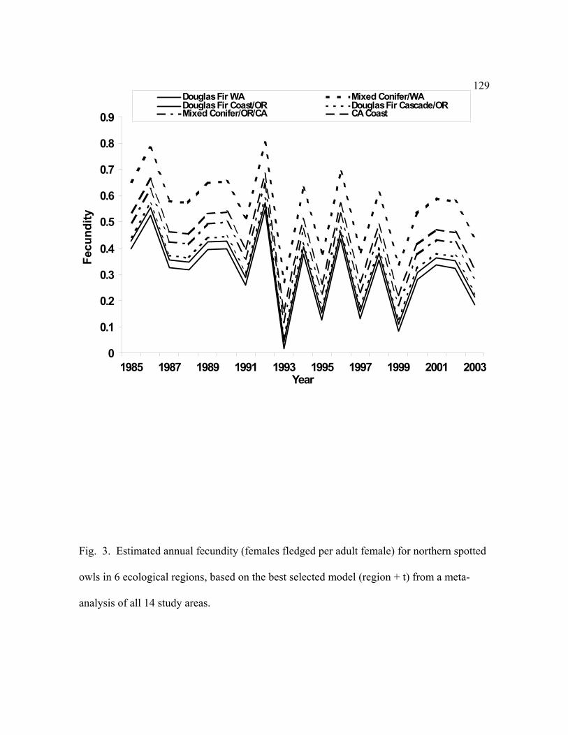
129

0

0.1

0.2

0.3

0.4

0.5

0.6

0.7

0.8

0.9

1985 1987 1989 1991 1993 1995 1997 1999 2001 2003Year

Fecu

ndity

Douglas Fir WA Mixed Conifer/WADouglas Fir Coast/OR Douglas Fir Cascade/ORMixed Conifer/OR/CA CA Coast

Fig. 3. Estimated annual fecundity (females fledged per adult female) for northern spotted

owls in 6 ecological regions, based on the best selected model (region + t) from a meta-

analysis of all 14 study areas.

130Washington

0.65

0.70

0.75

0.80

0.85

0.90

0.95

1.00

1987 1989 1991 1993 1995 1997 1999 2001Year

WEN CLE RAI OLY

App

aren

t Sur

viva

l

131

Fig. 4a. Model averaged estimates of female, non-juvenile apparent survival for northern

spotted owls on 4 study areas in Washington (study area acronyms specified in Table 1;

Appendix A).

132Oregon

0.65

0.70

0.75

0.80

0.85

0.90

0.95

1.00

1985 1987 1989 1991 1993 1995 1997 1999 2001

Year

COA HJA WSR TYE KLA CAS

App

aren

t Sur

viva

l

Fig. 4b. Model averaged estimates of female, non-juvenile apparent survival for northern

spotted owls on 6 study areas in Oregon (study area acronyms specified in Table 1;

Appendix A).

133California

0.65

0.70

0.75

0.80

0.85

0.90

0.95

1.00

1986 1988 1990 1992 1994 1996 1998 2000Year

NWC HUP SIM MAR

App

aren

t Sur

viva

l

Fig. 4c. Model averaged estimates of female, non-juvenile apparent survival for northern

spotted owls on 4 study areas in California (study area acronyms specified in Table 1;

Appendix A).

134

0.75

0.80

0.85

0.90

0.95

1985 1987 1989 1991 1993 1995 1997 1999 2001

Year

App

aren

t Sur

viva

lRAI TYE HUP COA HJACLE KLA NWC CAS SIMMAR WSR WEN OLY

Fig. 5. Model averaged estimates of apparent survival for adult, female northern spotted

owls from the meta-analysis of 14 study areas (study area acronyms specified in Table 1;

Appendix A).

135

0.75

0.80

0.85

0.90

0.95

1985 1987 1989 1991 1993 1995 1997 1999 2001Year

Douglas fir/WA Douglas fir coast/ORMixed Conifer//OR/CA Douglas fir Cascades/ORMixed Conifer/WA CA Coast

App

aren

t Sur

viva

l

Fig. 6. Estimates of apparent survival from model {φ (region*T), p(g+t+s)} for adult

northern spotted owls from the meta-analysis of 14 study areas.

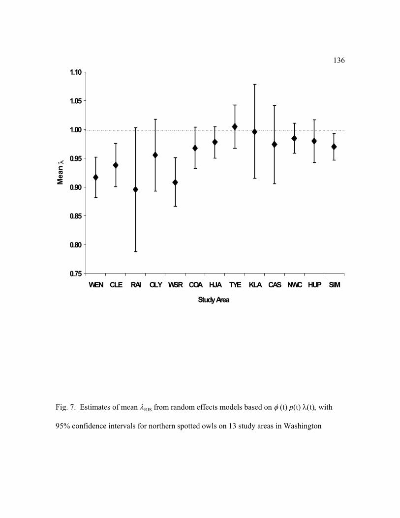
136

0.75

0.80

0.85

0.90

0.95

1.00

1.05

1.10

WEN CLE RAI OLY WSR COA HJA TYE KLA CAS NWC HUP SIM

Study Area

Mea

n λ

Fig. 7. Estimates of mean λRJS from random effects models based on φ (t) p(t) λ(t), with

95% confidence intervals for northern spotted owls on 13 study areas in Washington

137

(WEN, CLE, RAI, OLY), Oregon (WSR, COA, HJA, TYE, KLA, CAS), and California

(NWC, HUP, SIM) (study area acronyms specified in Table 1; Appendix A).

138

WA

0.0

0.2

0.4

0.6

0.8

1.0

1.2

1.4

1992 1993 1994 1995 1996 1997 1998 1999 2000 2001

Year

λτ

WEN CLE RAI OLY

OR

0.0

0.2

0.4

0.6

0.8

1.0

1.2

1.4

1992 1993 1994 1995 1996 1997 1998 1999 2000 2001Year

λτ

COA HJA WSR KLA CAS

139

Fig. 8. Annual estimates of λRJS for adult northern spotted owls on 9 Territory Study Areas

(TSA) in Washington (WEN, CLE, RAI, OLY) and Oregon (COA, HJA, WSR, KLA,

CAS), generated from model {φ (t), p(t), λ(t)}for each study area where t represents time

(study area acronyms specified in Table 1; Appendix A).

140

HUP

0.00.20.40.60.81.01.21.41.61.8

1988 1990 1992 1994 1996 1998 2000 2002

Year

∆λ

NWC

0.00.20.40.60.81.01.21.41.61.8

1988 1990 1992 1994 1996 1998 2000 2002Year

∆λ

TYE

0.00.20.40.60.81.01.21.41.61.8

1988 1990 1992 1994 1996 1998 2000 2002

Year

∆λ

SIM

0.00.20.40.60.81.01.21.41.61.8

1988 1990 1992 1994 1996 1998 2000 2002Year

∆λ

Fig. 9a. The realized change in population size (∆ ) with 95% confidence intervals for$λ

northern spotted owls in the 4 Density Study Areas (DSA) (study area acronyms in Table 1;

Appendix A).

141WEN

0.0

0.2

0.4

0.6

0.8

1.0

1.2

1.4

1993 1995 1997 1999 2001

Year

∆λ

OLY

0.0

0.2

0.4

0.6

0.8

1.0

1.2

1.4

1993 1995 1997 1999 2001

Year

∆λ

CLE

0.0

0.2

0.4

0.6

0.8

1.0

1.2

1.4

1993 1995 1997 1999 2001

Year

∆λ

RAI

0.0

0.2

0.4

0.6

0.8

1.0

1.2

1.4

1993 1995 1997 1999 2001

Year

∆λ

142

Fig. 9b. The realized change in population size ( ) with 95% confidence intervals for∆ $λ

northern spotted owls on the 4 Territory Study Areas (TSA) in Washington (study area

acronyms in Table 1; Appendix A).

143

CAS

0.0

0.20.4

0.6

0.8

1.01.2

1.4

1993 1995 1997 1999 2001

Year

∆λ

WSR

0.0

0.2

0.4

0.6

0.8

1.0

1.2

1.4

1993 1995 1997 1999 2001

Year

∆λ

HJA

0.0

0.2

0.4

0.6

0.8

1.0

1.2

1.4

1993 1995 1997 1999 2001

Year

∆λ

COA

0.0

0.2

0.4

0.6

0.8

1.0

1.2

1.4

1993 1995 1997 1999 2001

Year

∆λ

KLA

0.0

0.2

0.4

0.6

0.8

1.0

1.2

1.4

1993 1995 1997 1999 2001

Year

∆λ

144

Fig. 9c. The realized change in population size ( ) with 95% confidence intervals for∆ $λ

northern spotted owls on the 5 Territory Study Areas (TSA) in Oregon (study area

acronyms in Table 1; Appendix A).

145

Appendix D. Barred Owl covariate used to model northern spotted owl fecundity, survival

and capture probability on 14 study areas in Washington (WA), Oregon (OR), and

California (CA) (study area acronyms specified in Table 1; Appendix A).

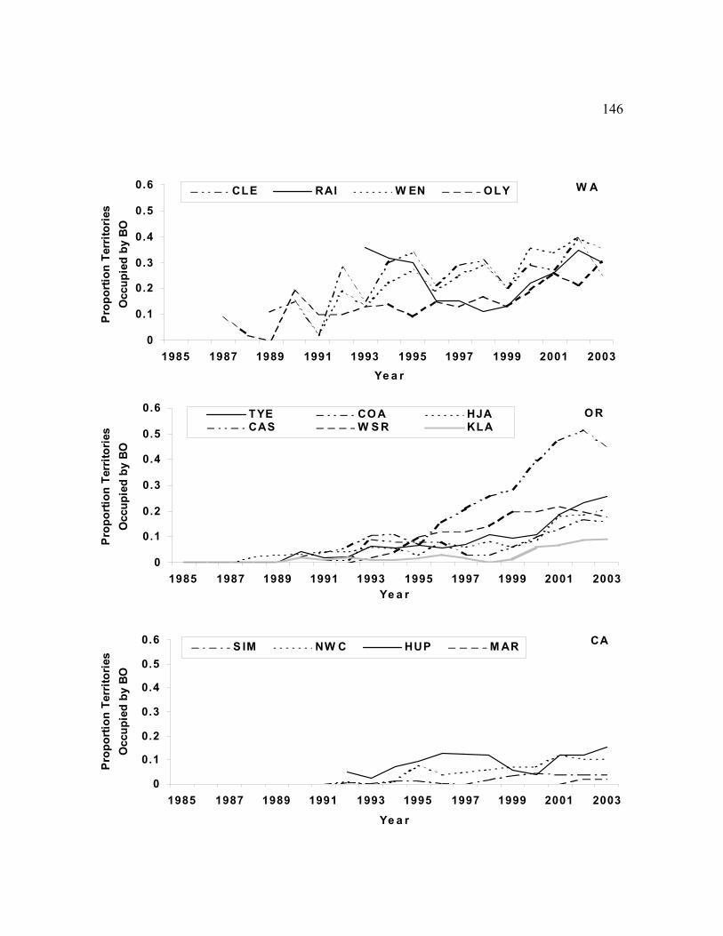
146

W A

0

0.1

0.2

0.3

0.4

0.5

0.6

1985 1987 1989 1991 1993 1995 1997 1999 2001 2003Ye a r

Pro

porti

on T

erri

tori

es

Occ

upie

d by

BO

CLE RAI W EN O LY

O R

0

0.1

0.2

0.3

0.4

0.5

0.6

1985 1987 1989 1991 1993 1995 1997 1999 2001 2003Ye a r

Pro

porti

on T

erri

torie

s O

ccup

ied

by B

O

TYE CO A HJACAS W S R KLA

CA

0

0.1

0.2

0.3

0.4

0.5

0.6

1985 1987 1989 1991 1993 1995 1997 1999 2001 2003

Ye a r

Prop

ortio

n Te

rrito

ries

Occ

upie

d by

BO

S IM NW C HUP M AR

147

Appendix E. Reproductive covariate (number of young fledged per year) used to model

northern spotted owl fecundity, survival and capture probability on 14 study areas in

Washington (WA), Oregon (OR), and California (CA) (study area acronyms specified in


148

W A

0.00.20.40.60.81.01.21.41.61.8

1985 1987 1989 1991 1993 1995 1997 1999 2001 2003

Ye a r

Num

ber o

f Yg

Fled

ged

CLE OLY RAI W EN

OR

0.00.20.40.60.81.01.21.41.61.8

1985 1987 1989 1991 1993 1995 1997 1999 2001 2003Ye a r

Num

ber o

f Yg

Fled

ged

HJA KLA COACAS TYE W S R

CA

0.00.20.40.60.81.01.21.41.61.8

1985 1987 1989 1991 1993 1995 1997 1999 2001 2003Ye a r

Num

ber o

f Yg

Fled

ged

HUP M AR NW C SIM

149

Appendix I. Model averaged apparent survival estimates with 95% confidence intervals for

male and female northern spotted owls on the 4 study areas in Washington (WEN, CLE,

RAI, OLY), 6 study areas in Oregon (COA, HJA, WSR, TYE, KLA, CAS), and 4 study

areas in California (NWC, HUP, SIM, MAR). Study area acronyms specified in Table 1;

Appendix A.

150

W EN

0.60

0.65

0.70

0.75

0.80

0.85

0.90

0.95

1.00

1990 1992 1994 1996 1998 2000

M aleFe m ale

App

aren

t Sur

viva

l

CLE

0.60

0.65

0.70

0.75

0.80

0.85

0.90

0.95

1.00

1989 1991 1993 1995 1997 1999 2001

M aleFe m ale

App

aren

t Sur

viva

l

RAI

0.60

0.65

0.70

0.75

0.80

0.85

0.90

0.95

1.00

1993 1995 1997 1999 2001

M aleFe m ale

App

aren

t Sur

viva

l

OLY

0.60

0.65

0.70

0.75

0.80

0.85

0.90

0.95

1.00

1987 1989 1991 1993 1995 1997 1999 2001

M aleFe m ale

App

aren

t Sur

viva

l

151

Appendix I cont.

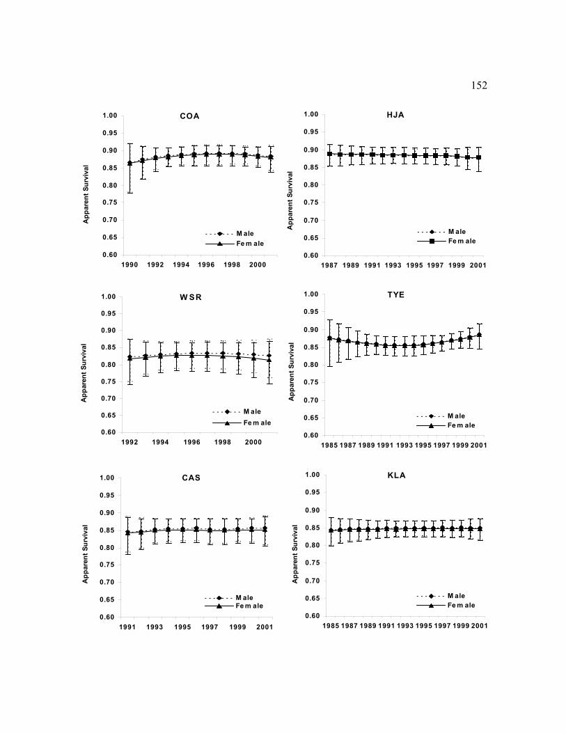
152

COA

0.60

0.65

0.70

0.75

0.80

0.85

0.90

0.95

1.00

1990 1992 1994 1996 1998 2000

M aleFe m ale

App

aren

t Sur

viva

l

HJA

0.60

0.65

0.70

0.75

0.80

0.85

0.90

0.95

1.00

1987 1989 1991 1993 1995 1997 1999 2001

M aleFe m ale

App

aren

t Sur

viva

lW SR

0.60

0.65

0.70

0.75

0.80

0.85

0.90

0.95

1.00

1992 1994 1996 1998 2000

M aleFe m ale

App

aren

t Sur

viva

l

TYE

0.60

0.65

0.70

0.75

0.80

0.85

0.90

0.95

1.00

1985 1987 1989 1991 1993 1995 1997 1999 2001

M aleFe m ale

App

aren

t Sur

viva

l

CAS

0.60

0.65

0.70

0.75

0.80

0.85

0.90

0.95

1.00

1991 1993 1995 1997 1999 2001

M aleFe m ale

App

aren

t Sur

viva

l

KLA

0.60

0.65

0.70

0.75

0.80

0.85

0.90

0.95

1.00

1985 1987 1989 1991 1993 1995 1997 1999 2001

M aleFe m ale

App

aren

t Sur

viva

l

154

HUP

0.60

0.65

0.70

0.75

0.80

0.85

0.90

0.95

1.00

1992 1994 1996 1998 2000

M aleFe m ale

App

aren

t Sur

viva

l

NCA

0.60

0.65

0.70

0.75

0.80

0.85

0.90

0.95

1.00

1986 1988 1990 1992 1994 1996 1998 2000

M aleFe m ale

App

aren

t Sur

viva

l

S IM

0.60

0.65

0.70

0.75

0.80

0.85

0.90

0.95

1.00

1990 1992 1994 1996 1998 2000

M aleFe m ale

App

aren

t Sur

viva

l

M AR

0.60

0.65

0.70

0.75

0.80

0.85

0.90

0.95

1.00

1998 1999 2000 2001

M aleFe m ale

App

aren

t Sur

viva

l

Appendix I cont.

156

Appendix A. Study areas included in the January 2004 analysis of demographic trends of northern spotted owls.a

Study 8RJS area Study area Start start Expansion Land

Study area code typeb yearc yeard yeare Ownerf Region LatitudeWashington Wenatchee WEN TSA 1990 1992 1994 Mixed Washington Mixed-Conifer 46.996 Cle Elum CLE TSA 1989 1992 none Mixed Washington Mixed-Conifer 47.195 Rainier RAI TSA 1992 1993 1998 Mixed Washington Douglas-fir 47.041 Olympic OLY TSA 1987 1990 1994 Federal Washington Douglas-fir 47.800Oregon Coast Ranges COA TSA 1990 1992 none Mixed Oregon Coastal Douglas-fir 44.381 Tyee TYE DSA 1985 1990 none Mixed Oregon Coastal Douglas-fir 43.468 HJ Andrews HJA TSA 1987 1990 2000 Federal Oregon Cascades Douglas-fir 44.213 Warm Springs WSR TSA 1992 1993 none Tribal Oregon Cascades Douglas-fir 44.938 South Cascades CAS TSA 1991 1992 1998 Federal Oregon Cascades Douglas-fir 42.695 Klamath KLA TSA 1985 1991 1998 Mixed Oregon/California Mixed-Conifer 42.736California NW California NWC DSA 1985 1985 none Federal Oregon/California Mixed-Conifer 40.848 Hoopa HUP DSA 1992 1992 none Tribal Oregon/California Mixed-Conifer 41.051 Simpson SIM DSA 1990 1993 none Private California Coast 41.122 Marin MAR TSA 1998 1998 none Federal California Coast 37.994 a We analyzed data through 2003 on all study areas, except that we only analyzed 8RJS. on the Wenatchee Study Area through 2002, because that

study area was not completely surveyed in 2003. b TSA = study area in which a sample of owl territories was surveyed each year; DSA = density study area in which the entire study area was

sampled each year. c Year that mark-recapture study was started. d First year that data were used for analysis of 8RJS. e Year that study area size was increased, if any, for analysis of 8RJS. f Federal = Forest Service, Bureau of Land Management, National Park Service. Mixed = federal lands mixed with inclusions of private or state

lands. Tribal and private study areas were lumped together for analyses of ownership.

157

Appendix B. List of participants at the workshop on analysis of demographic rates for the northern spotted owl held 4-11

January 2004 in Corvallis, Oregon.

BIOLOGISTS WITH DEMOGRAPHIC DATA (listed by study area and state)

Cle Elum (Washington)

Stan Sovern Oregon Cooperative Wildlife Research Unit, Oregon State University

Eric Forsman U.S. Forest Service, Pacific Northwest Research Station

Olympic Penninsula (Washington)

Scott Gremel U.S. National Park Service, Olympic National Park

Patti Happe U.S. National Park Service, Olympic National Park

Brian Biswell U.S. Forest Service, Pacific Northwest Research Station


158

Rainier (Washington)

Dale Herter Raedeke Associates

Lorin Hicks Plum Creek Timber Company

Jim Schaberl U.S. National Park Service, Mount Rainier National Park

Wenatchee (Washington)

Tracy Flemming National Council for Air & Stream Improvement

Larry Irwin National Council for Air & Stream Improvement

Oregon Coast Range (Oregon)

Peter Loschl Oregon Cooperative Wildlife Research Unit, Oregon State University

Tom Snetsinger Oregon Cooperative Wildlife Research Unit, Oregon State University

Chris McAfferty Oregon Cooperative Wildlife Research Unit, Oregon State University


159

H. J. Andrews (Oregon)

Steve Ackers Oregon Cooperative Wildlife Research Unit, Oregon State University

Sheila Turner-Hane Oregon Cooperative Wildlife Research Unit, Oregon State University

Robert Anthony Oregon Cooperative Wildlife Research Unit, Oregon State University

Roseburg BLM - Klamath (Oregon)

Robert Horn U.S. Bureau of Land Management, Roseburg District Office

Roseburg BLM - Tyee (Oregon)

Janice Reid U.S. Forest Service, Pacific Northwest Research Station


Southern Cascades (Oregon)

Steve Andrews Oregon Cooperative Wildlife Research Unit, Oregon State University

Frank Wagner Oregon Cooperative Wildlife Research Unit, Oregon State University

160


Warm Springs Tribal Lands (Oregon)

Rick Gearhart Private Consultant (NEED COMPANY NAME??)

Hoopa Tribal Lands (California)

Mark Higley Hoopa Tribal Forestry

Peter Carlson Hoopa Tribal Forestry

Simpson Resource Company (California)

Lowell Diller Simpson Resource Company, Redwood Division

Joel Thompson Simpson Resource Company, Redwood Division

Keith Hamm Simpson Resource Company, Redwood Division

NW California (California)

161

Alan Franklin Colorado Cooperative Fish & Wildlife Research Unit, Colorado

State University

Tammy Hamer Colorado Cooperative Fish & Wildlife Research Unit, Colorado

State University

Marin (Point Reyes) (California)

Katie Fehring Point Reyes Bird Observatory

ANALYSTS

David Anderson Colorado Cooperative Fish & Wildlife Research Unit, Colorado

State University

Jennifer Blakesley Sustainable Ecosystems Institute

Kenneth Burnham Colorado Cooperative Fish & Wildlife Research Unit, Colorado

State University

Mary Conner Utah State University

162

Sarah Converse Department of Fishery & Wildlife Biology, Colorado State University

Steven Dinsmore Department of Wildlife and Fisheries, Mississippi State University

Paul Doherty Department of Fishery & Wildlife Biology, Colorado State University

Vicky Dreitz Colorado Division of Wildlife

Katie Dugger Oregon Cooperative Wildlife Research Unit, Oregon State University


State University

James Hines Patuxent Wildlife Research Center, U.S. Geological Survey

Paul Lukacs Department of Fishery & Wildlife Biology, Colorado State

University

Brett McClintock Department of Fishery & Wildlife Biology, Colorado State

University

Trent McDonald Western Ecosystems Technologies, Inc.

Jim Nichols Patuxent Wildlife Research Center, U.S. Geological Survey

Gail Olson Oregon Cooperative Wildlife Research Unit, Oregon State University

163

Eric Rexstad Institute of Arctic Biology, University of Alaska - Fairbanks

Carl Schwarz Department of Statistics and Actuarial Science, Simon Fraser

University

Mark Seamans Department of Fisheries, Wildlife and Conservation Biology,

University of Minnesota

Gary White Department of Fishery and Wildlife Biology, Colorado State

University

Guthrie Zimmerman Department of Fisheries, Wildlife and Conservation Biology,

University of Minnesota.

OTHER ATTENDEES

Betsy Glenn Oregon State University

Karl C. Halupka U.S. Fish and Wildlife Service

Gina King Yakama Tribe

Joe Lint Bureau of Land Management

164

Jim Thrailkill U.S. Fish and Wildlife Service

ORGANIZERS



Gail Olson Oregon Cooperative Wildlife Research Unit, Oregon State University

Katie Dugger Oregon Cooperative Wildlife Research Unit, Oregon State University

Pete Loschl Oregon Cooperative Wildlife Research Unit, Oregon State University

Tom Snetsinger Oregon Cooperative Wildlife Research Unit, Oregon State University

David Anderson Colorado Cooperative Fish & Wildlife Research Unit, Colorado

State University

Kenneth Burnham Colorado Cooperative Fish & Wildlife Research Unit, Colorado

State University


State University

165

Gary White Department of Fishery and Wildlife Biology, Colorado State

University

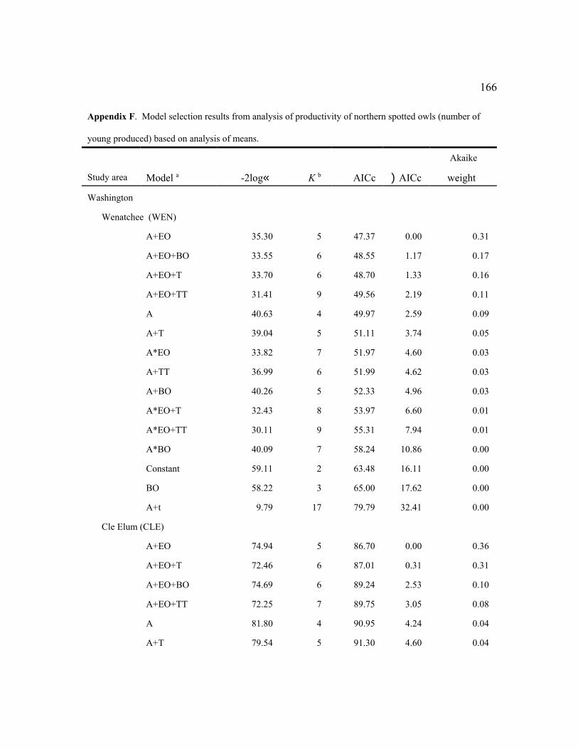
166

Appendix F. Model selection results from analysis of productivity of northern spotted owls (number of

young produced) based on analysis of means.

Akaike

Study area Model a -2log‹ K b AICc )AICc weight

Washington

Wenatchee (WEN)

A+EO 35.30 5 47.37 0.00 0.31

A+EO+BO 33.55 6 48.55 1.17 0.17

A+EO+T 33.70 6 48.70 1.33 0.16

A+EO+TT 31.41 9 49.56 2.19 0.11

A 40.63 4 49.97 2.59 0.09

A+T 39.04 5 51.11 3.74 0.05

A*EO 33.82 7 51.97 4.60 0.03

A+TT 36.99 6 51.99 4.62 0.03

A+BO 40.26 5 52.33 4.96 0.03

A*EO+T 32.43 8 53.97 6.60 0.01

A*EO+TT 30.11 9 55.31 7.94 0.01

A*BO 40.09 7 58.24 10.86 0.00

Constant 59.11 2 63.48 16.11 0.00

BO 58.22 3 65.00 17.62 0.00

A+t 9.79 17 79.79 32.41 0.00

Cle Elum (CLE)

A+EO 74.94 5 86.70 0.00 0.36

A+EO+T 72.46 6 87.01 0.31 0.31

A+EO+BO 74.69 6 89.24 2.53 0.10

A+EO+TT 72.25 7 89.75 3.05 0.08

A 81.80 4 90.95 4.24 0.04

A+T 79.54 5 91.30 4.60 0.04

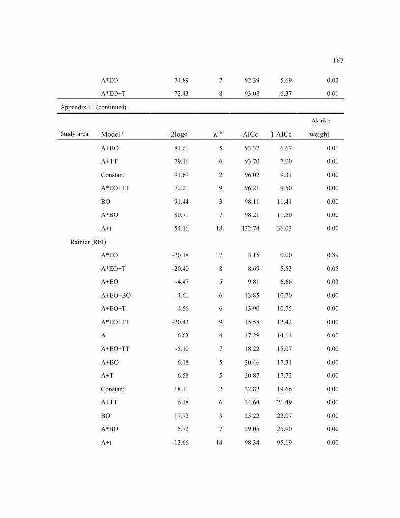
167

A*EO 74.89 7 92.39 5.69 0.02

A*EO+T 72.43 8 93.08 6.37 0.01

Appendix F. (continued).

Akaike


A+BO 81.61 5 93.37 6.67 0.01

A+TT 79.16 6 93.70 7.00 0.01

Constant 91.69 2 96.02 9.31 0.00

A*EO+TT 72.21 9 96.21 9.50 0.00

BO 91.44 3 98.11 11.41 0.00

A*BO 80.71 7 98.21 11.50 0.00

A+t 54.16 18 122.74 36.03 0.00

Rainier (REI)

A*EO -20.18 7 3.15 0.00 0.89

A*EO+T -20.40 8 8.69 5.53 0.05

A+EO -4.47 5 9.81 6.66 0.03

A+EO+BO -4.61 6 13.85 10.70 0.00

A+EO+T -4.56 6 13.90 10.75 0.00

A*EO+TT -20.42 9 15.58 12.42 0.00

A 6.63 4 17.29 14.14 0.00

A+EO+TT -5.10 7 18.22 15.07 0.00

A+BO 6.18 5 20.46 17.31 0.00

A+T 6.58 5 20.87 17.72 0.00

Constant 18.11 2 22.82 19.66 0.00

A+TT 6.18 6 24.64 21.49 0.00

BO 17.72 3 25.22 22.07 0.00

A*BO 5.72 7 29.05 25.90 0.00

A+t -13.66 14 98.34 95.19 0.00

168

Olympic Peninsula (OLY)

A+EO 21.60 5 34.00 0.00 0.55

A+EO+BO 20.25 6 35.75 1.74 0.23

A+EO+T 21.44 6 36.94 2.94 0.13


Akaike


A*EO 20.32 7 39.19 5.19 0.04

A+EO+TT 20.38 7 39.25 5.25 0.04

A*EO+T 20.19 8 42.74 8.74 0.01

A 34.59 4 44.12 10.12 0.00

Constant 39.74 2 44.17 10.17 0.00

BO 38.14 3 45.03 11.03 0.00

A*EO+TT 19.17 9 45.74 11.73 0.00

A+BO 33.70 5 46.10 12.10 0.00

A+T 34.40 5 46.80 12.80 0.00

A+TT 32.20 6 47.70 13.70 0.00

A*BO 33.30 7 52.17 18.17 0.00

A+t -16.95 20 107.05 73.05 0.00

Oregon Study Areas

Coast Ranges (COA)

A+EO 2.50 5 14.81 0.00 0.43

A+EO+T 0.98 6 16.34 1.53 0.20

A+EO+BO 1.35 6 16.71 1.91 0.16

A*EO -0.91 7 17.76 2.95 0.10

A+EO+TT 0.96 7 19.63 4.83 0.04

A*EO+T -2.47 8 19.79 4.99 0.04

A 12.02 4 21.50 6.69 0.01

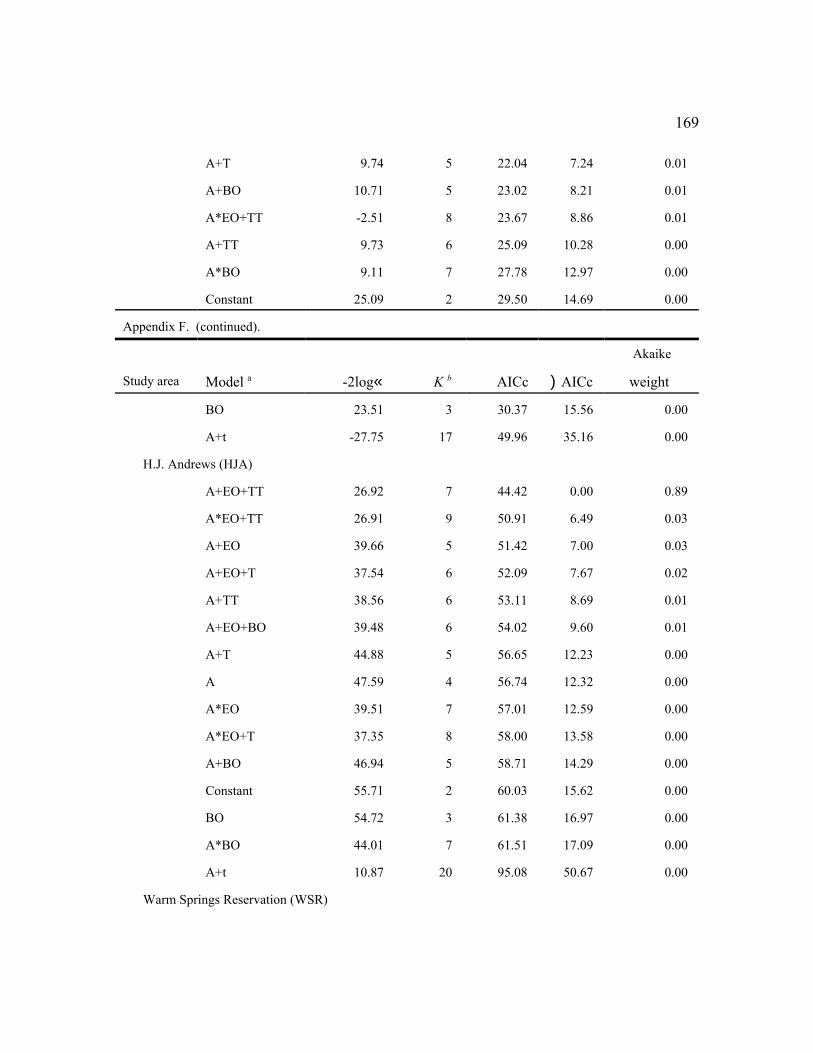
169

A+T 9.74 5 22.04 7.24 0.01

A+BO 10.71 5 23.02 8.21 0.01

A*EO+TT -2.51 8 23.67 8.86 0.01

A+TT 9.73 6 25.09 10.28 0.00

A*BO 9.11 7 27.78 12.97 0.00

Constant 25.09 2 29.50 14.69 0.00


Akaike


BO 23.51 3 30.37 15.56 0.00

A+t -27.75 17 49.96 35.16 0.00

H.J. Andrews (HJA)

A+EO+TT 26.92 7 44.42 0.00 0.89

A*EO+TT 26.91 9 50.91 6.49 0.03

A+EO 39.66 5 51.42 7.00 0.03

A+EO+T 37.54 6 52.09 7.67 0.02

A+TT 38.56 6 53.11 8.69 0.01

A+EO+BO 39.48 6 54.02 9.60 0.01

A+T 44.88 5 56.65 12.23 0.00

A 47.59 4 56.74 12.32 0.00

A*EO 39.51 7 57.01 12.59 0.00

A*EO+T 37.35 8 58.00 13.58 0.00

A+BO 46.94 5 58.71 14.29 0.00

Constant 55.71 2 60.03 15.62 0.00

BO 54.72 3 61.38 16.97 0.00

A*BO 44.01 7 61.51 17.09 0.00

A+t 10.87 20 95.08 50.67 0.00

Warm Springs Reservation (WSR)

170

A 25.08 4 35.58 0.00 0.36

A+EO 22.71 5 36.71 1.13 0.20

Constant 32.57 2 37.23 1.66 0.16

A+BO 24.93 5 38.93 3.36 0.07

A+T 25.02 5 39.02 3.44 0.06

BO 32.55 3 39.96 4.39 0.04

A+EO+T 22.34 6 40.34 4.76 0.03

A*EO 22.51 6 40.51 4.93 0.03


Akaike


A+EO+BO 22.70 6 40.70 5.12 0.03

A+TT 24.18 6 42.18 6.61 0.01

A+EO+TT 21.01 7 43.62 8.05 0.01

A*EO+T 22.20 7 44.82 9.24 0.00

A*BO 23.23 7 45.85 10.27 0.00

A*EO+TT 20.95 8 48.95 13.38 0.00

A+t -18.93 15 107.07 71.50 0.00

Tyee ( TYE)

A+T 27.31 5 38.62 0.00 0.31

A 30.80 4 39.65 1.03 0.18

A+BO 29.23 5 40.53 1.92 0.12

A+EO+T 27.10 6 40.97 2.35 0.10

A+TT 27.27 6 41.14 2.52 0.09

A+EO 30.61 5 41.91 3.30 0.06

A+EO+BO 28.99 6 42.86 4.24 0.04

A*EO+T 23.57 8 42.92 4.31 0.04

A+EO+TT 27.07 7 43.62 5.00 0.03

171

A*EO 27.28 7 43.83 5.22 0.02

A*BO 27.97 7 44.52 5.90 0.02

A*EO+TT 23.56 9 45.84 7.23 0.01

Constant 49.82 2 54.07 15.45 0.00

BO 49.15 3 55.65 17.03 0.00

A+t -1.55 22 77.34 38.73 0.00

Klamath (KLA)

A+EO 30.20 5 41.59 0.00 0.22

A 32.73 4 41.64 0.05 0.22

A*EO 26.69 7 43.42 1.83 0.09


Akaike


A+BO 32.07 5 43.47 1.88 0.09

A+EO+BO 29.67 6 43.67 2.08 0.08

A+T 32.58 5 43.98 2.38 0.07

A+EO+T 30.07 6 44.07 2.48 0.06

A+EO+TT 27.53 7 44.26 2.67 0.06

A+TT 30.70 6 44.70 3.11 0.05

A*EO+T 26.48 8 46.08 4.49 0.02

A*EO+TT 23.55 9 46.17 4.58 0.02

A*BO 30.08 7 46.81 5.22 0.02

Constant 60.93 2 65.19 23.60 0.00

BO 60.90 3 67.44 25.84 0.00

A+t -12.52 22 70.41 28.81 0.00

Southern Cascades (CAS)

A+EO+T 31.92 6 46.72 0.00 0.36

A+EO 35.84 5 47.78 1.06 0.21

172

A+EO+TT 30.85 7 48.71 1.99 0.13

A+EO+BO 34.67 6 49.47 2.76 0.09

A*EO+T 28.37 8 49.51 2.79 0.09

A*EO 32.97 7 50.83 4.11 0.05

A*EO+TT 26.74 9 51.40 4.69 0.03

A+T 41.82 5 53.75 7.04 0.01

A 45.18 4 54.43 7.71 0.01

A+BO 43.96 5 55.90 9.18 0.00

A+TT 41.49 6 56.29 9.58 0.00

Constant 55.60 2 59.95 13.24 0.00

BO 54.38 3 61.11 14.39 0.00

A*BO 43.72 7 61.58 14.86 0.00


Akaike


A+t 15.13 16 74.33 27.61 0.00

California Study Areas

Northwest California (NWC)

A+T 51.40 5 62.68 0.00 0.27

A+BO 52.66 5 63.93 1.25 0.14

A 55.22 4 64.05 1.37 0.13

A+TT 50.30 6 64.13 1.45 0.13

A+EO+T 51.14 6 64.97 2.29 0.08

A+EO 54.95 5 66.23 3.55 0.04

A*EO+T 46.98 8 66.25 3.57 0.04

A+EO+TT 49.86 9 66.35 3.67 0.04

A+EO+BO 52.56 6 66.38 3.70 0.04

A*EO 51.20 7 67.69 5.01 0.02

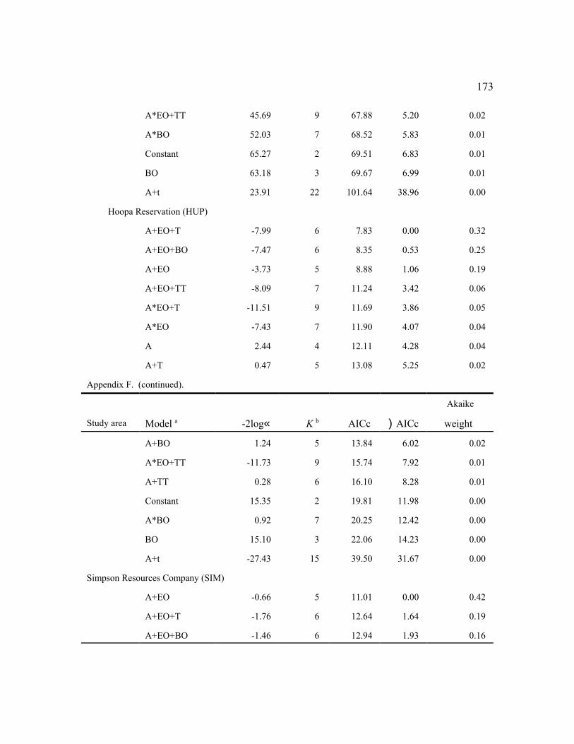
173

A*EO+TT 45.69 9 67.88 5.20 0.02

A*BO 52.03 7 68.52 5.83 0.01

Constant 65.27 2 69.51 6.83 0.01

BO 63.18 3 69.67 6.99 0.01

A+t 23.91 22 101.64 38.96 0.00

Hoopa Reservation (HUP)

A+EO+T -7.99 6 7.83 0.00 0.32

A+EO+BO -7.47 6 8.35 0.53 0.25

A+EO -3.73 5 8.88 1.06 0.19

A+EO+TT -8.09 7 11.24 3.42 0.06

A*EO+T -11.51 9 11.69 3.86 0.05

A*EO -7.43 7 11.90 4.07 0.04

A 2.44 4 12.11 4.28 0.04

A+T 0.47 5 13.08 5.25 0.02


Akaike


A+BO 1.24 5 13.84 6.02 0.02

A*EO+TT -11.73 9 15.74 7.92 0.01

A+TT 0.28 6 16.10 8.28 0.01

Constant 15.35 2 19.81 11.98 0.00

A*BO 0.92 7 20.25 12.42 0.00

BO 15.10 3 22.06 14.23 0.00

A+t -27.43 15 39.50 31.67 0.00

Simpson Resources Company (SIM)

A+EO -0.66 5 11.01 0.00 0.42

A+EO+T -1.76 6 12.64 1.64 0.19

A+EO+BO -1.46 6 12.94 1.93 0.16

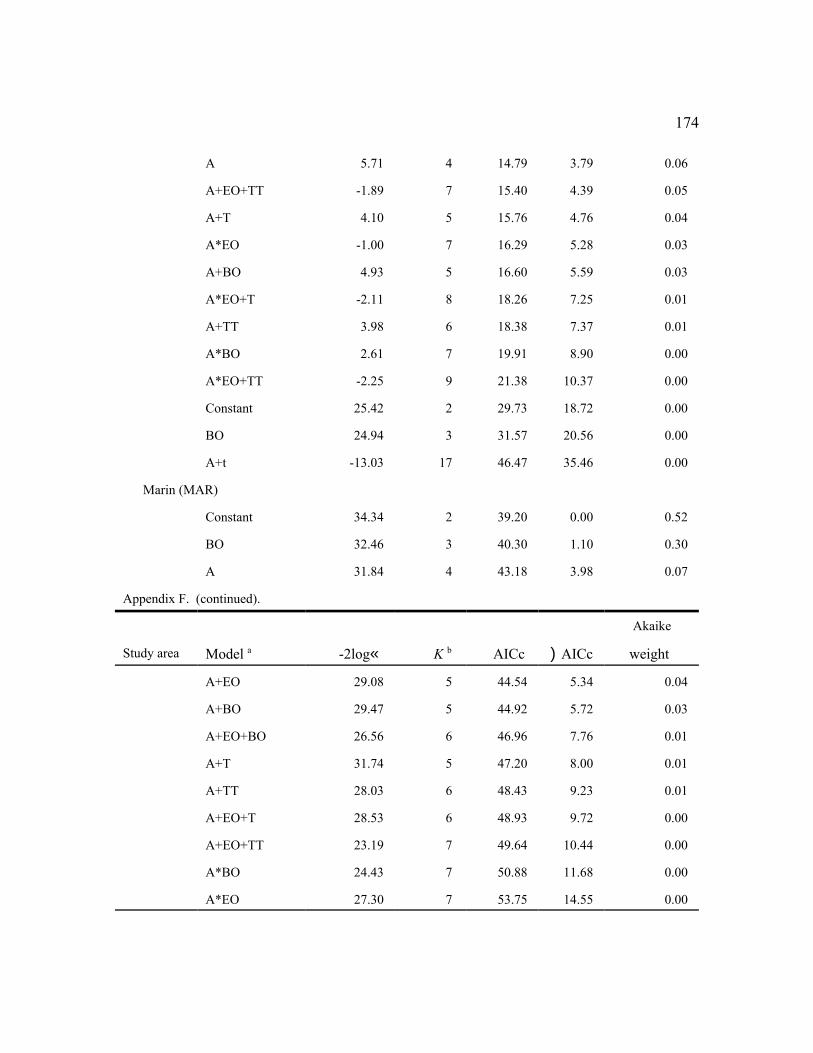
174

A 5.71 4 14.79 3.79 0.06

A+EO+TT -1.89 7 15.40 4.39 0.05

A+T 4.10 5 15.76 4.76 0.04

A*EO -1.00 7 16.29 5.28 0.03

A+BO 4.93 5 16.60 5.59 0.03

A*EO+T -2.11 8 18.26 7.25 0.01

A+TT 3.98 6 18.38 7.37 0.01

A*BO 2.61 7 19.91 8.90 0.00

A*EO+TT -2.25 9 21.38 10.37 0.00

Constant 25.42 2 29.73 18.72 0.00

BO 24.94 3 31.57 20.56 0.00

A+t -13.03 17 46.47 35.46 0.00

Marin (MAR)

Constant 34.34 2 39.20 0.00 0.52

BO 32.46 3 40.30 1.10 0.30

A 31.84 4 43.18 3.98 0.07


Akaike


A+EO 29.08 5 44.54 5.34 0.04

A+BO 29.47 5 44.92 5.72 0.03

A+EO+BO 26.56 6 46.96 7.76 0.01

A+T 31.74 5 47.20 8.00 0.01

A+TT 28.03 6 48.43 9.23 0.01

A+EO+T 28.53 6 48.93 9.72 0.00

A+EO+TT 23.19 7 49.64 10.44 0.00

A*BO 24.43 7 50.88 11.68 0.00

A*EO 27.30 7 53.75 14.55 0.00

175

A*EO+T 26.81 9 60.81 21.61 0.00

A+t 17.13 9 60.85 21.64 0.00

A*EO+TT 19.88 9 63.59 24.39 0.00

a Model notation indicates additive (+) or interactive (*) effects of owl age (A), even-odd years (EO),

linear time (T), quadratic time (TT) or barred owls (BO). "Constant" indicates models with no structure.

176

Appendix G. Estimates of annual recapture probabilities ( ) of banded northern spotted owls in 14

demographic study areas in Washington, Oregon and California. Estimates are from the best AICc model

for each study area. Study areas that had a sex effect on p include separate columns for males and

females.

WEN CLE%% CLE&& RAI OLY

Year SE SE SE SE SE

1988 0.600 0.163

1989 0.793 0.096

1990 0.899 0.017 0.844 0.021 0.818 0.060

1991 0.625 0.050 0.886 0.017 0.826 0.021 0.781 0.055

1992 0.643 0.042 0.909 0.019 0.859 0.025 0.813 0.047

1993 0.660 0.034 0.860 0.027 0.790 0.034 0.729 0.052

1994 0.676 0.028 0.908 0.019 0.858 0.025 1.000 0.000 0.764 0.049

1995 0.693 0.023 0.882 0.018 0.821 0.022 0.895 0.056 0.669 0.056

1996 0.708 0.020 0.905 0.018 0.853 0.024 0.890 0.051 0.784 0.048

1997 0.724 0.020 0.856 0.029 0.785 0.038 0.652 0.083 0.749 0.048

1998 0.738 0.021 0.904 0.018 0.852 0.023 0.883 0.053 0.774 0.049

1999 0.753 0.025 0.876 0.020 0.812 0.024 0.560 0.076 0.296 0.053

2000 0.766 0.029 0.890 0.017 0.832 0.020 0.635 0.078 0.746 0.058

2001 0.780 0.032 0.888 0.017 0.829 0.020 0.733 0.079 0.763 0.055

2002 0.792 0.036 0.884 0.017 0.823 0.021 0.789 0.090 0.843 0.056

2003 0.804 0.040 0.901 0.017 0.848 0.022 0.988 0.189 0.698 0.082

COA HJA WSR TYE%% TYE&&

Year SE SE SE SE SE

1986 0.857 0.031 0.805 0.038

1987 0.867 0.027 0.819 0.033

177

1988 0.846 0.043 0.876 0.023 0.831 0.029

1989 0.829 0.035 0.886 0.020 0.843 0.025

Appendix G (continued).

COA HJA WSR TYE%% TYE&&

Year SE SE SE SE SE

1990 0.813 0.029 0.894 0.017 0.854 0.022

1991 0.863 0.012 0.800 0.023 0.902 0.015 0.864 0.019

1992 0.863 0.012 0.790 0.021 0.909 0.013 0.874 0.016

1993 0.863 0.012 0.784 0.021 0.903 0.033 0.916 0.012 0.883 0.015

1994 0.863 0.012 0.781 0.022 0.934 0.020 0.923 0.011 0.892 0.013

1995 0.863 0.012 0.783 0.022 0.892 0.019 0.929 0.010 0.900 0.013

1996 0.863 0.012 0.788 0.022 0.865 0.019 0.934 0.009 0.908 0.012

1997 0.863 0.012 0.797 0.020 0.795 0.042 0.939 0.009 0.915 0.012

1998 0.863 0.012 0.809 0.019 0.906 0.027 0.944 0.009 0.921 0.012

1999 0.863 0.012 0.825 0.018 0.772 0.033 0.948 0.009 0.927 0.012

2000 0.863 0.012 0.842 0.019 0.786 0.032 0.952 0.009 0.933 0.012

2001 0.863 0.012 0.860 0.023 0.707 0.049 0.956 0.009 0.938 0.012

2002 0.863 0.012 0.880 0.026 0.745 0.037 0.960 0.009 0.943 0.012

2003 0.863 0.012 0.899 0.030 0.873 0.034 0.963 0.009 0.947 0.012

KLA CAS NWC MAR%% MAR&&

Year SE SE SE SE SE

1986 0.669 0.227 0.765 0.041

1987 0.609 0.147 0.765 0.041

1988 0.581 0.102 0.917 0.009

1989 0.731 0.077 0.917 0.009

1990 0.851 0.050 0.917 0.009

178

1991 0.851 0.043 0.917 0.009

1992 0.791 0.042 0.878 0.040 0.917 0.009

1993 0.757 0.046 0.832 0.035 0.872 0.020

1994 0.858 0.036 0.788 0.029 0.917 0.009

Appendix G (continued).

KLA CAS NWC MAR%% MAR&&

Year SE SE SE SE SE$p $p $p $p $p

1995 0.772 0.043 0.754 0.027 0.872 0.020

1996 0.732 0.046 0.734 0.030 0.917 0.009

1997 0.748 0.049 0.730 0.031 0.917 0.009

1998 0.859 0.035 0.745 0.030 0.917 0.009

1999 0.882 0.033 0.775 0.027 0.872 0.020 0.996 0.007 0.981 0.027

2000 0.881 0.032 0.816 0.025 0.917 0.009 0.989 0.013 0.956 0.040

2001 0.950 0.022 0.862 0.027 0.917 0.009 0.940 0.059 0.786 0.097

2002 0.953 0.021 0.906 0.027 0.917 0.009 0.976 0.024 0.905 0.048

2003 0.897 0.041 0.942 0.025 0.872 0.020 0.976 0.024 0.905 0.048

HUP SIM %% SIM &&

Year SE SE SE$p $p $p

1991 0.859 0.017 0.819 0.019

1992 0.859 0.017 0.819 0.019

1993 0.868 0.039 0.859 0.017 0.819 0.019

1994 0.861 0.027 0.859 0.017 0.819 0.019

1995 0.861 0.024 0.859 0.017 0.819 0.019

1996 0.867 0.025 0.859 0.017 0.819 0.019

1997 0.879 0.025 0.859 0.017 0.819 0.019

1998 0.895 0.022 0.859 0.017 0.819 0.019

179

1999 0.914 0.019 0.859 0.017 0.819 0.019

2000 0.933 0.017 0.859 0.017 0.819 0.019

2001 0.950 0.017 0.859 0.017 0.819 0.019

2002 0.965 0.017 0.859 0.017 0.819 0.019

2003 0.977 0.016 0.859 0.017 0.819 0.019

Status and Trends in Demography of Northern Spotted Owls, 1985–2003

Documents

Transcript of Status and Trends in Demography of Northern Spotted Owls, 1985–2003