Vienna Yearbook of Population Research 2003, Vol. 1, pp. 35-50 35

Austrian Demography and Housing Demand:is there Connection*

Gabriel S. Lee**, Philipp Schmidt-Dengler, Bernhard Felderer,

and Christian Helmenstein

Abstract

This paper analyses the role of demographic factors in the Austrian housing market. Link-ing demographic issues, in conjunction with the Austrian private housing finance, to the hous-ing demand is the focus of the empirical model developed in this paper. We find statisticalsupport that the demographic factors help to explain for housing demand. However, we em-phasize that demographic factor such as the adult population with net migration effect is onlyone of the key variables which contributes in understanding the Austrian housing demand.Some of our other empirical findings indicate that the Austrian housing demand is inelastic tovarious economic factors is a concern for some housing policies.JEL Codes: R21, R23, J11; Keywords: Housing Demand, Demography, Migration,

1 Introduction

The purpose of this paper is to analyse the role of demographic factors in the Austrianhousing market. The effect of demographics in the U.S. housing market has been contro-versial and inconclusive. The work by Mankiw and Weil (1989) leads a group of research-ers who supports the hypothesis that the demographic change has a strong effect in hous-ing prices: There is a statistical support for the conclusion that the U.S. baby-boom cycleswas a major source of the real housing prices increase in the amount of 20% during 1969-89, and the real housing prices will sharply decline over the next 30 years till 2007.

On the other hand, there is a strong dissenting group of researchers who argues that theMankiw and Weil’s estimates and conclusions are the results of a mispecification andmisinterpretation of their housing price equation (e.g. Hamilton, 1991; Hendershott, 1991;Green and Hendershott, 1996; Peek and Wilcox, 1991; Swan, 1995). These studies empha-size; first, ‘’the negative time trend in the Mankiw and Weil’s study, not the age-demandrelationship, is responsible for the large forecasted drop in real prices’’ (Green and Hend-ershott, 1996, p. 466). The main debate between these two groups has been the statisticalinterpretation of Mankiw and Weil’s housing demand estimates.1

1 In steady state, it can be shown that housing service demand and population represent the samesteady state growth process. We thank the referee for clarifying this point.

* Reprint from Empirica, 28 (3), pp. 259-276 (2001). Kluwer Academic Publishers.** Corresponding author

36 Austrian Demography and Housing Demand: is there Connection

Although Mankiw and Weil’s conclusion has been challenged and questioned in aca-demic journals in the U.S., their approach has not been widely applied to other countries,except for Canada (Engelhard and Poterba, 1991) and Japan (Ohtake and Shintani, 1996).Consequently, we believe that linking housing demand to the size of adult population forAustrian housing market is a valid and useful exercise, especially when Austria faces everchanging adult population due to the European Union, the war in former Yugolavia, andthe downing of the Iron Curtain. In this paper, we bring two new aspects in analysing thelinkage. First, we include net migration effect on the linkage: Austria has experiencedunusually rapid adult population growth on the account of migration starting from the late1980’s till the early 1990’s. Second, we analyse whether the recent developments of pri-vate housing finance in Austria, in conjunction with age, can help to explain the linkage.Like many social welfare states in Europe, Austrian government plays a key role in thehousing market. Large amount of subsidies in various forms (in construction, in rents, andin mortgage payments) lends interesting platform for analysing the effect of governmentrole on the housing market.

We begin our analysis in the next section with some facts regarding the Austrian hous-ing market. In section 3, we state some facts about the Austrian demography and presentinformal evidence suggesting that cyclical movements in housing prices are linked withthe size of adult population in Austria. The boom and bust cycles in housing prices arepositively correlated with the size of adult population.

Linking demographic issues, in conjunction with the Austrian private housing finance,to the housing demand is the focus of the empirical model developed in section 4. We findstatistical support that the demographic issues do help to explain for housing demand. Weconclude that the adult population with net migration is a better statistical measure inexplaining Austrian housing demand than the demographic measure proposed by Mankiwand Weil. Further, we emphasize the fact that the adult population with net migrationeffect is only one of the key variables which contributes in understanding housing demand:income, cost of housing finance, subsidy effect, and cost shifters such as unemploymentrate need to be addressed when analysing Austrian housing demand. Section 5 concludes,and the data description is reported separately from the main text at the end of the paper.

2 Some Facts about the Austrian Housing Market

Traditionally there has been strong public intervention in the housing sector in Austria,justified by the idea of a right to the scarce good housing. The general housing policymeasures are supposed to lower the construction and financing costs and also to providecheap standard housing for lower income groups. For Austria, the primary focus of thehousing policy, however, has been on the housing quality management.

The expenditures are financed by a legally prescribed share of total direct tax revenue,the debt service for public loans, and sources drawn from the general budget. The subsidysystem mainly focuses on the “object”, namely the construction, renovation and upgradingof dwellings, by providing annuity grants and public loans at preferential rates and matu-rities.

Eligibility for these subsidies is determined by household income, which has been selfreported (no longer the case after the late 1990s). However, as the subsidy amounts are not

37G.S. Lee, P. Schmidt-Dengler, B. Felderer, and C. Helmenstein

indexed to life cycle incomes, this subsidy policy is mainly ineffective. Further, the gov-ernment pays premiums on savings deposits in savings and loans associations (“Bauspar-kassen”).2 However, means tested allowances for housing expenditures play only a minorpart.

Housing is further indirectly subsidized by a preferential tax treatment; since 1973,Austria has been following the consumption good principle, which implies that imputedincome from owner occupied housing is not tax eligible. Rents are subject to a reducedexcise tax rate. Irrespective of the consumer good principle, expenditures related to acqui-sition like mortgage repayments, remain tax deductible. The rate on the purchase of prop-erty has consequently been reduced during the last decades. According to Lehner (1992)foregone tax revenues amount to ATS 3.3 billion. In addition to these direct and indirectsubsidies there is a complex system of rent regulation and tenant protection. The main setof regulations concerns tenant protection, rent levels and the landlady’s responsibility tomaintain dwellings. Rent control, however, mainly affects old dwellings.

Table 1 shows the relative importance of the different groups of developers for newlycompleted dwellings during the past twenty years for Austria; almost half of constructionactivities is carried out by private households for self use. Traditionally, these types ofconstruction activities are not translated into market activities. That is, personal develop-ing is almost never on the housing market for sale. The developers, who are classified as“non-profit” and “other legal entities”, could loosely be translated as the “co-ops” andother “socialized” firms. These developers mainly build apartments and other large com-munal buildings. For the rest of the provinces in Austria, the patterns for constructionactivities by different developers are similar to each other. However, for Vienna (with onefifth of Austrian population), the “non-profit” and “other legal entities” developers domi-nate the “private” developers. Consequently, the housing market in Vienna reflects thelarge part of the housing market in Austria.

2 The Bausparkassen system works like the following; the potential borrower has to meet a sav-ings target first. After that she is entitled to raise a loan of about the double amount. To makesaving in this scheme more attractive the government offers premiums on interest and tax cred-its. For a more detailed discussion and a critical evaluation of the Bausparkassen system andother methods of housing subsidies see Lamel, et al. (1986), Schmidinger, et al. (1991, 1992a,1992b), Deutsch, et al. (1993) and Deutsch (1995, 1997).

Table 1: Relative importance of developers

Year 1975 1980 1985 1990 1995

Private persons(percentage)

50 60 56 62 45

Non-profit(percentage) 34 26 29 27 31

Other legalentities(percentage)

9 8 6 9 22

Municipalites(percentage) 7 6 9 2 2

Total(in 1000 units) 48570 77845* 41153 36553 53353

* The numbers for 1980 are strongly upward biased. A large number of previously completed dwellings werereported during that year, because the registration procedure had been simplified then.

38 Austrian Demography and Housing Demand: is there Connection

An important feature of the Aus-trian market is the high share that de-tached family houses take in the totalstock (see table 2). These are usuallyhigh quality dwellings, with a strongdegree of diversification, adjusted forthe specific personal needs of the ten-ant, who is in most cases also the de-veloper. As mentioned previously, these types of dwellings are usually not for sale, conse-quently, the provinces with high shares of detached family houses do not display a clearsign of a developed housing market.

One other noticeable features of Austrian housing market is the method of market clear-ing; the market is cleared by cueing of the applicants for subsidized and social housing. Onthe other hand there are vacant dwellings, mostly subsidized and/or developed by the mu-nicipalities with the aim to meet the excess demand (and recently, to stabilize excess sup-ply), which are merely too expensive to be rented by lower income groups. Rent regulationcauses high entry costs, because landladies often require key-money to compensate forlow rents (this practice is not only illegal but has also declined in importance over time). Afurther problem is the predominance of home ownership accompanied by a poor-perform-ing private rental sector. This structure of the housing market with its entry (and moving)barriers causes labour immobility which may attribute to unemployment, although sincethe mid-nineties we observe a reversed mobility towards urban regions.3

Thus there is a sub-optimal allocation of different types of housing. For example, awidowed old person, living in a large rent-regulated downtown apartment, for whom itwould be too costly to move to a dwelling more suitable to her living conditions. Further-more the subsidy system seems to exhibit regressive effects.

3 Construction Activities, Prices, andAdult Population

The main series to be explained are the housing prices, investment, and adult popula-tion for Austria. Figure 1 shows the real detrended housing residential investment (includ-ing apartments) and real detrened housing prices from 1970 to1996 data in annualizedform to exhibit the cyclical patterns most clearly. We take the construction investmentdeflator relative to the gross national product deflator as the proxy for the Austrian resi-dential housing prices.4 The cycles in prices take usually 3-4 years swing, suggesting a

3 Oswald (1996) tries to link homeownership rates to unemployment using cross-section datafrom industrialized countries. However, his findings yet lack theoretical foundation.

4 For Austria, there is no such thing as “the market price” for housing nor the housing prices,which are based on the hedonically adjusted houses of certain year’s characteristics as in theU.S. We have also tried with the housing expenditures series as a proxy for housing price. Theresults are not qualitatively different than the ratio of two deflators. The composition of theconstruction investment deflator is roughly 50\% residential construction and the rest are com-mercial construction and structures (Tiefbau). The housing expenditure series is a compositionof regular fees for housing: this includes the rent, repayments for ownership, “usage fees” fordwellings by construction firms, operating costs (e.g. cost of heating and water), taxes, and feesfor usage of fixtures (e.g. furniture).

Vienna Austria

Family houses 7,6 48

Condominiums 92,4 52

Total 100,0 100

Table 2: Share of detached family houses

39G.S. Lee, P. Schmidt-Dengler, B. Felderer, and C. Helmenstein

slow adjustment to economic conditions. The major peaks occurred at 1973, 1977, 1981,1988, 1991 and 1995. The peak at 1981 needs to be discounted as there was a major changein the government regulation concerning the reporting of dwelling completion: the loop-hole in the new regulation allowed the households to artificially appreciate their reportingfor the tax benefits in 1982. Furthermore, owners were keen to register completions be-cause the regional governments offered premature sales of public mortgages at reducedrates. Over the sample period, the last two large peaks occurred in 1988 and 1991 followedby a sharp decline.

Visually comparing the detrended real housing price and housing investment seriessuggests that the price movements and construction activity are positively correlated, ex-cept for the earlier part of the series between 1972-75. Apart from mis-timing of a few datapoints, this observation suggests a rising supply price of new houses. For the investmentseries, it took a huge boom in 1970-72 followed by a sharp decline of equal magnitude in1973-75. The next episode for the boom and bust cycles are less prominent with cyclestaking longer swings. A more substantial boom and bust occurred during the 1986-95 withthe activities peaking at 1988, 1992, and 1995. The peak-to-trough ratio of building activ-ity in the last cycle of 1990-93 is approximately little over 2: an expansion doubles theoutput of new homes and a contraction cuts it in half.

The other main series to be explained is demography changes. Figure 2 shows the num-ber of births in the period 1946-1996. A clear baby boom and bust cycles can be observed:first baby boom occurred right after the World War II, and the last major baby boom oc-curred in late 1950’s and peaked in 1962. The baby bust of the 1970’s seems to be dramat-ic in comparison to the baby boom of the 1950’s as the bust out-measures the boom 2 to 1.Further, after the baby bust in the 1970’s, there are no significant baby booms in the mag-nitude of the 1950’s.

Figure 1: Times Series of housing investment and prices, 1970-1996

-4000

-2000

0

2000

4000

6000

8000

10000

12000

14000

1972

1973

1974

1975

1976

1977

1978

1979

1980

1981

1982

1983

1984

1985

1986

1987

1988

1989

1990

1991

1992

1993

1994

1995

-4

-2

0

2

4

6

8

10

Change in Real Investment

Change in Real Construction Price

40 Austrian Demography and Housing Demand: is there Connection

Figure 2: Live Births in Austria, 1946-1996

60000

70000

80000

90000

100000

110000

120000

130000

140000

19

46

19

48

19

50

19

52

19

54

19

56

19

58

19

60

19

62

19

64

19

66

19

68

19

70

19

72

19

74

19

76

19

78

19

80

19

82

19

84

19

86

19

88

19

90

19

92

19

94

19

96

One way to measure the magnitude of the baby boom is to look at the adult population,which is usually defined as the age group of 20 to 30 years old. Figure 3 graphs the adultpopulation, live birth (25 years lag), and net migration from 1969 to 1995. A visual com-parison of the adult population and the live birth (25 years lag) suggests that there is apositive co-movement between the two series up to 1987: the live birth (25 years lag)peaked in 1987, but the adult population is still rising and peaked in 1992. The mis-timingof the two series could be partly explained by the movement of the net migration. Anincrease in the adult population beyond 1987 could be attributed to the sharp rise in the netmigration starting from 1987 to 1991. And a decline of equal magnitude for the net migra-tion after 1991 along with the decline in the live birth (25 years lag) could explain thesharp decline in the adult population after 1992. Consequently, we think that it is the adultpopulation (including the net migration), which is a better measure of consumer purchasepower rather than the live birth (20 or 30 years lagged).

One of the main hypothesis to be tested in our paper is whether there is a direct linkbetween the number of adult population over time and the housing prices. Figure 4 graphsthe real housing price and the adult population from 1970 to 1996. We look at the adultpopulation because previous work (e.g. Mankiw and Weil) and our own assessment indi-cate that the late 30’s age group spends the most amount for the housing expenditures.Figure 4 shows informal evidence that there is a positive relationship between the adultpopulation and housing prices. The two series co-move, with a few minor mis-timing be-tween 1988 and 1991, and peaking around 1992. Our main empirical task is to analyse andconfirm statistically whether the adult population with net migration can be linked directlywith the housing demand.

Figures 5 and 6, which graph prices versus net migration and live birth (25 years lagged)respectively, show that there seems to be no clear correlation between live births (lagged

41G.S. Lee, P. Schmidt-Dengler, B. Felderer, and C. Helmenstein

-40000

-20000

0

20000

40000

60000

80000

100000

120000

140000

19

69

19

71

19

73

19

75

19

77

19

79

19

81

19

83

19

85

19

87

19

89

19

91

19

93

19

95

Bir

ths

an

d N

et

Mig

rati

on

1000000

1050000

1100000

1150000

1200000

1250000

1300000

1350000

1400000

20

-29

Ye

ar

Gro

up

Births (25 year lag)Net Migration20-29 Year Group

Figure 3: Adult population, live birth (25 years lag), and net migration in Austria, 1969-1995

Figure 4: Housing prices and adult population, 1969-1996

42 Austrian Demography and Housing Demand: is there Connection

25 years) with housing price for the periods after 1984; on the other hand, looking at thenet migration with housing price, two series co-move after 1985 indicating indeed that oneshould look at the adult population (which includes net migration) instead of live birth forthe analysis of demographic effects on housing demand.

Figure 5: Housing prices and net migration, 1970-1996

-0,05

-0,03

-0,01

0,01

0,03

0,05

0,07

0,09

0,11

0,13

1969

1970

1971

1972

1973

1974

1975

1976

1977

1978

1979

1980

1981

1982

1983

1984

1985

1986

1987

1988

1989

1990

1991

1992

1993

1994

1995

-40000

-20000

0

20000

40000

60000

80000

100000

Real Constructionprice (detrended)

Net Migration

-0,04

-0,02

0

0,02

0,04

0,06

0,08

0,1

0,12

1969

1970

1971

1972

1973

1974

1975

1976

1977

1978

1979

1980

1981

1982

1983

1984

1985

1986

1987

1988

1989

1990

1991

1992

1993

1994

1995

100000

105000

110000

115000

120000

125000

130000

135000

Real Constructionprice (detrended)

Births (25 year lag)

Figure 6: Housing prices and live birth (25 years lagged), 1970-1996

43G.S. Lee, P. Schmidt-Dengler, B. Felderer, and C. Helmenstein

4 Estimates for Demand for Housing

4.1 Demography and Housing Demand

In this section, we take the dissenting view from Mankiw and Weil, and present theirmeasure of housing demand as instead a measure of demography. Nevertheless, we be-lieve in the importance of their measure of the age structure of the population, especiallythe adult population, as one of the crucial explanatory variables for the housing demand.

Although the housing demand equation (1) can be derived from the consumer’s utilityfunction, the approach here is to analyse the time-series model that captures the empiricallinkage between housing demand and demography. Thus, the reduced form equation usedin estimation is

H P Y D Xt t t mwt t t= + + + + +α α α α α ε0 1 2 3 . (1)

where, Ht is the net stock of residential capital (includes apartment building),5 P

t denotes

the housing price measured by the residential construction deflator by the GNP deflator, Yt

is the real income per capita, Dmwt

is the demand measure based on population structure(Mankiw and Weil),6 X

t represents the vector of unobserved demand cost shifters, and e

t

are residuals.

4.2 Housing Demand, Housing Stock and Population

We begin our empirical section with some simple regressions using the Mankiw andWeil’s housing demand, D

mwt, housing stock and the adult population variables. These

regressions are estimated with annual time-series data over the 1961-1996 period. ForAustria, there is no Census data where for owner-occupied units, owners report the valueof the property for the unit in which the household resides, i.e. V

t Consequently, it is

impossible to estimate ia ’s according to equation of Vt. However, we found informal evi-

dence that the time series of age 20-29 is most correlated with the housing expendituresthan any other age group, suggesting that the estimated values of ia ’s for Austria shouldbe similar to Mankiw and Weil’s finding: “the primary feature of the estimates is a sharpjump in the demand for housing between the ages of 20 and 30”. (Mankiw and Weil,p. 240) We constructed ia~ ’s for Austria using the data from Consumption Survey 1984.This survey reports “Housing Expenditures” by the age of the family head in 1984. i.e.

5 All the variables are expressed in logarithm for our empirical work, unless stated otherwise.6 The demand measure based on population structure is calculated as in Mankiw and Weil:

∑=i

imwt tiNaD ),(

where, the ais are estimated coefficients of the average housing demand of persons in age group

i using the census data, and the N(i,t) are the number of individuals of age i in year t. The ais can

be estimated by running the cross-sectional regression of

∑∑∑ +++=jjj

t jDummyajDummyajDummyaV 99......10 9910

where, tV is the housing demand by a household which is measured by the value of the propertyfor the unit in which the household resides, j denotes the j th member in the household, andDummy0=1 if age = 0, Dummy1=1 if age=1, etc.

44 Austrian Demography and Housing Demand: is there Connection

Age Group ai_s Age Group ai_s

0-4 677,6 50-54 7892,8

5-9 312,2 55-59 7550,2

10-14 217,6 60-64 7632,2

15-19 1301 65-69 7209,2

20-24 5128,2 70-74 6936,6

25-29 7582,4 75-79 6769,4

30-34 8673,6 80-84 6200,8

35-39 9364,8 85-89 6347,2

40-44 9106,6 90-94 6845,4

45-49 8541,6 95- 4176,6

Table 3: Mankiw-Weil’s original cross-sectional esti-

mates of housing demand by age

Age Group ai_s (Mankiw-Weil) ai_s (Austria)

20-29 6355,30 3696,60

30-39 9019,20 4669,39

40-49 8824,10 3251,20

50-59 7775,36 2386,10

60-64 7632,20 1997,50

65-74 7072,90 1691,20

75- 4650,00 1243,71

Table 4: Mankiw-Weil’s cross-sectional estimates of

housing demand by age for Austria

Each household reports howmuch it is spending on theirhousing. The results report theaverage spending of all house-holds with family heads in therespective age-group.7

Consequently, we construct-ed the Mankiw and Weil’s hous-ing demand variable, D

mwt, using

their (Mankiw and Weil’s tableA.1) estimates for ia ’s as wellas the demand variable, D

t, us-

ing ia~ ’s. Since our populationdata set is for each five-year ageclass running from 0-4 to 95-over, we take the average of ia ’sand ia~ ’s on each five year ageclass. Table 3 and 4 show thevalues for ia ’s and ia~ ’s that weuse to construct D

mwt and D

t.

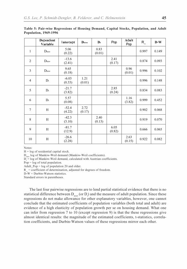
Table 5 reports the pair-wiseregressions between D

mwt, D

t ,

adult population, and real hous-ing stock (all represented in log-arithms). The adult populationincludes the net migration effect.Consequently, we believe thatfor the housing demand analy-sis, the adult population is thecorrect measure of change indemography instead of the livebirths cycles. The basic message from table 5 is that there is no statistical difference be-tween Mankiw and Weil’s measure of housing demand D

mwt (or D

t) and the measure of

adult population.The first three regressions of D

mwt on the total population and adult population lend

partial evidence that population, especially adult population, can statistically explain theMankiw and Weil’s measure of housing demand. As expected, the adult population giveshigher correlation (higher R2) and adjusts faster in the age structure (higher Durbin-Wat-son) than the total population when the these variables are regressed on D

mwt. The next

three regressions replicate the first three: whether we use Mankiw-Weils ia ’s or ia~ ’s usingAustrian figures, the housing demand variables D

mwt and D

t produce qualitatively the same

results.

7 The housing expenditures include a) regular fees for housing such as: rent (also for sublease)and repayments for ownership, and “usage fees” for dwellings constructed by corporate dwell-ings, b) operating costs and taxes, and c) fees for usage of fixtures (especially in cases of sub-lease), cost of heating and warm water.

45G.S. Lee, P. Schmidt-Dengler, B. Felderer, and C. Helmenstein

The last four pairwise regressions are to lend partial statistical evidence that there is nostatistical difference between D

mwt (or D

t) and the measure of adult population. Since these

regressions do not make allowance for other explanatory variables, however, one cannotconclude that the estimated coefficients of population variables (both total and adult) areevidence of a high elasticity of population growth per se on housing demand. What onecan infer from regression 7 to 10 (except regression 9) is that the these regressions givealmost identical results: the magnitude of the estimated coefficients, t-statistics, correla-tion coefficients, and Durbin-Watson values of these regressions mirror each other.

Table 5: Pair-wise Regressions of Housing Demand, Capital Stocks, Population, and Adult

Population, 1969-1996

DependentVariable

Intercept Dtmw Dt Pop AdultPop

R_ D-W

1 Dtmw5.06

(0.22)0.83

(0.01) 0.997 0.149

2 Dtmw-13.6(2.41)

2.41(0.17) 0.874 0.093

3 Dtmw9.65

(0.18)0.96

(0.01) 0.996 0.102

4 Dt-6.03(0.33)

1.21(0.01) 0.996 0.148

5 Dt-21.7(3.82)

2.85(0.24) 0.834 0.083

6 Dt5.57

(0.08)1.16

(3.82) 0.999 0.452

7 H-52.4(4.22)

2.72(0.17) 0.902 0.068

8 H-42.3(3.10)

2.40(0.13) 0.919 0.070

9 H-81.7(12.9)

6.05(0.82) 0.666 0.065

10 H-26.6(2.28)

2.63(0.15) 0.922 0.082

Notes:H = log of residential capital stock.D

tmw log of Mankiw-Weil demand (Mankiw-Weil coefficients).

Dt = log of Mankiw-Weil demand, calculated with Austrian coefficients.

Pop = log of total population.Adult_Pop = log of population 20 and older.R_ = coefficient of determination, adjusted for degrees of freedom.D-W = Durbin-Watson statistics.Standard errors in parentheses.

46 Austrian Demography and Housing Demand: is there Connection

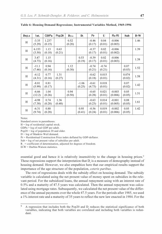
4.3 Housing Demand, Population and Subsidy Effects

Before presenting our empirical results, we make a few remarks in regards to the esti-mates of the demand parameters. We face two serious limitations when estimating mean-ingful demand parameters from our data: one is a limitation of data, and the other is animprecise measure of the capital stock. We have an annual data set of 25 years. Using theInstrumental Variable Method with five to seven explanatory variables, the usable datapoints are greatly reduced.

In order to estimate equation (1), we require constructing a time series on stocks Ht

using perpetual inventory methods.8 But investment is such a small fraction of existinghomes that the imputed stock series is too smooth and trend like to be informative aboutdemand. Further, we do not take into account many subtle intertemporal issues in the housingmarket.

To be consistent with Mankiw and Weil, and other subsequent studies, we also chooseto measure house prices by the ratio of the GNP residential construction deflator to theoverall GNP deflator. Equation (1) is estimated using the Instrumental Variable Methodsince the price is endogenous. We use the known instruments (a la Swan, 1995) such asthe current and lagged real construction costs (materials and other construction compo-nents), real construction wages and real short-term interest rates. For the demand costshifters, we use the unemployment rate and the difference of the short- and long terminterest rates. The regressions are estimated over the period from 1971 to 1995.

The regressions in table 6 attempt to explain the demand for the stock of houses. Thefirst three regressions are to compare whether there is statistical and qualitative differenc-es between the adult population (Pop20) and D

mwt (or D

t) in explaining the demand for

housing. Both variables, Pop20 and Dmwt

(or Dt), are statistically significant in their own

regressions. The negative sign on the housing price coefficient, Pr, indicates that we areestimating the demand function. The cost shifters are also statistically significant in ex-plaining for the housing demand, although the sign on the unemployment rate is positive:from economic theory, one would expect a negative sign on the unemployment rate. How-ever, a positive coefficient lends a possible support for the interpretation that people buildmore houses (private) when they are laid off (or unemployed). Since these unemployedpeople have more “leisure” time, they contribute more to the “household production”,namely building their own houses (assuming that this group of people have enough initialcapital). When taking the fact that for Austria private construction activity accounts foralmost 50% of all construction activities into a consideration, the last remark is not trivial.The estimated coefficients for the real interest rate difference between short and long termsindicate that both nominal interest and inflation rates are statistically significant but has asmall effect on explaining the housing demand. Indeed, with Austrian capital market beingrelatively imperfect, in terms of mortgage market and other banking aspects, small interestrate effects on housing demand is expected: a possible interpretation of high intergenera-tional private housing financing in Austria (Deutsch, 1997).

The income and price elasticities are in reasonable ranges. An income elasticity of 1.0gives statistical evidence that housing has unitary income elasticity at all points: a onepercent increase in money income results in a one percent increase in the total quantitydemanded. The price elasticities of 0.465 and 0.377 indeed indicate that housing is an

8 We use the capital stock that Czerny et al. (1990, 1992) have constructed.

47G.S. Lee, P. Schmidt-Dengler, B. Felderer, and C. Helmenstein

essential good and hence it is relatively insensitivity to the change in housing prices.9

These regressions support the interpretation that Dt is a measure of demography instead of

housing demand. However, we also empathize here that our empirical results support theimportance of the age structure of the population, ceteris paribus.

The rest of regressions deals with the subsidy effect on housing demand. The subsidyvariable is calculated using the net present value of money spent on subsidies in the rele-vant period. For the subsidized loans, the annual repayment using with an interest rate of0.5% and a maturity of 47.5 years was calculated. Then the annual repayment was calcu-lated using mortgage rates. Subsequently, we calculated the net present value of the differ-ence of the annual payments over the whole 47.5 years. For the periods after 1985, we useda 1% interest rate and a maturity of 35 years to reflect the new law enacted in 1984. For the

Notes:Standard errors in parentheses.H = log of residential capital stock.GDPa = log of real GDP per adult.Pop20 = log of population 20 and older.D = log of Mankiw-Weil demand.Pr = Residentiual Construction Price index deflated by GDP-deflator.Sub = log of net present value of subsidies per adult.R_ = coefficient of determination, adjusted for degrees of freedom.D-W = Durbin-Watson statistics.

Dep.s Int. GDPa Pop20 Dtmw Dt Pr U Rs-Rl Sub D-W

H-3.35(5.29)

1.237(0.15)

0.52(0.20)

-0.46(0.17)

0.04(0.01)

-0.006(0.003)

1.46

H6.153(3.50)

1.13(0.18)

0.63(0.21)

-0.37(0.17)

0.02(0.01)

-0.006(0.002)

1.39

H3.47

(4.73)1.15

(0.16)0.53

(0.19)-0.39(0.17)

0.02(0.01)

-0.006(0.003) 1.38

H-11.1(7.46)

0.94(0.16)

1.12(0.30)

-0.74(0.21)

-0.74(0.21)

0.07(0.03) 1.52

H-4.12(4.31)

0.77(0.16)

1.31(0.27)

-0.62(0.18)

0.015(0.01)

0.074(0.02) 1.58

H-8.81(5.99)

0.81(0.17)

-1.06(0.25)

-0.61(4.73)

0.018(0.01)

0.07(0.02) 1.42

H-6.66(12.2)

1.04(0.26)

0.94(0.50)

-0.65(0.28)

0.021(0.01)

-0.003(0.006)

0.05(0.05) 1.51

H-4.98(7.38)

0.74(0.28)

1.36(0.48)

-0.63(0.23)

0.014(0.01)

-0.001(0.005)

0.08(0.05) 1.61

H-6.31(9.74)

0.88(0.28)

0.95(0.41)

-0.56(0.24)

0.019(0.01)

-0.002(0.006)

0.05(0.05)

1.42

Table 6: Housing Demand Regressions; Instrumental Variables Method, 1969-1996

9 A regression that includes both the Pop20 and Dt reduces the statistical significance of both

variables, indicating that both variables are correlated and including both variables is redun-dant.

48 Austrian Demography and Housing Demand: is there Connection

loans to replace personal capital injections a 10 year maturity was used with a 3% realinterest rate, and the same procedure was applied. The renovation subsidies, annuity sub-sidies and construction subsidies were simply added, although some of them are repay-able.

Regressions 3-6 look at the subsidy effects on housing demand when the cost of hous-ing finance, which is captured by R

s - R

l, is ignored. These regressions imply that the de-

mand schedule for housing varies directly with wealth per capita, demographic measuresand subsidies. Again, the stock varies inversely with housing price but directly with unem-ployment. The message from these regressions is that the subsidy variable has significantand positive effect on housing demand.

In contrast to regressions 3-6, regressions 7-9 that include the cost of housing financealong with the subsidy variable lead to quite different implications for the subsidy effectson housing demand. Subsidy and interest rates difference variables are no longer statisti-cally significant and have a weak effect on housing demand. The interest rate differencebeing statistically insignificant lends some empirical support that for Austria, the demandfor housing is insensitive to the cost of housing finance. As Deutsch (1997) states, a largepart of Austrian housing finance is done through bequest or direct inter-family cash trans-fers. Indeed, with Austrian capital market, especially the mortgage market, being imper-fect and coupled with an easy access to other ways of financing, the demand and desire forhousing being insensitive to both variables is, at least, understandable if not justifiable.

5 Summary and Remarks

We present a model that links demographic issues, in conjunction with the Austrianprivate housing finance, to the housing demand. We find statistical support that the de-mographic issues do help to explain for housing demand, ceteris paribus. Further, weemphasize the fact that the demography, especially the adult population that includes netmigration effect, is only one of the key variables which contributes in understanding hous-ing demand: other major factors that influence Austrian housing demand are the income,cost of housing finance, subsidy effect, and cost shifters such as unemployment rate.

Our estimates also reveal deficiencies of a housing demand model based on static,homogeneous capital and costless transaction market assumptions. To obtain and recovermore precise and meaningful estimates of structural parameters, at least, we need a longerdata series as well and a better understanding of the user cost and capital stocks. It remainsto be studied in detail. Nonetheless, we provide some statistical evidence for the move-ment of future Austrian housing demand.

Data Appendix

• GNP: Gross National Product at current prices (SNA 68). Source: Austrian Institute ofEconomic Research (WIFO).

• GDP: Gross Domestic Product, current prices. Source: OECD Derived Series: General.• DEFL: Implicit GDP Price Deflator. Source: OECD Derived Series: General.• POP: Total Population in Austria. Population data in five year groups: data from census

49G.S. Lee, P. Schmidt-Dengler, B. Felderer, and C. Helmenstein

years (1961, 1971, 1981, 1991). Extrapolation of Census data for all years. Source: Aus-trian Central Statistical Office (OESTAT). See also Fassmann, et al (1996).

• POP20: Population 20 years and older. Source: see above.• MWIndex: Calculated from Mankiw and Weil (1989) and Austrian population data:

5 year averages of Mankiw and Weil’s estimated alphas, corresponding to the five yeargroups in Austrian population data, were taken an used to calculate the index for Aus-tria.

• Investment: Series of Residential Investment in Austria. Calculated from financial datacontained in Residential Construction Surveys. Source: Austrian Central Statistical Of-fice (OESTAT).

• ResCCIV: Construction Cost Index for Residential Construction for Vienna. (Includingspecial tax for Vienna underground -UBahn- construction) Source: Austrian Central Sta-tistical Office (OESTAT).

• ResCCIA: Construction Cost Index for Residential Construction for Rest of Austria.(Excluding tax for underground construction.). Source: See ResCCIV.

• U: Austrian unemployment rate with respect to total labour force. Source: OECD, MainEconomic Indicators: Basic Series.

• GVBond: Austrian Public Sector Bonds (>1 Year). Yields. Source: OECD, Main Eco-nomic Indicators: Basic Series.

• SRate: Interest rates for day to day money (call money). Source: Oesterreichische Kon-trollbank.

• INF: Annual inflation rate. Source: Austrian Institute of Economic Research (WIFO).• CCI: Overall Construction Cost Index. Source: Austrian Central Statistical Office

(OESTAT).• Mortgage: Mortgage Rates. Source: Raiffeisen Bank \Oesterreich.• Housing Expenditures: per square meter taken from Census data: it includes a) regular

fees for housing such as: rent (also for sublease) and repayments for ownership, and“usage fees” for dwellings constructed by corporate dwellings b) operating costs andtaxes, c) fees for usage of fixtures (especially in cases of sublease), cost of heating andwarm water. Source: Microcensus: Austrian Central Statistical Office (OESTAT).

Acknowledgements

We thank participants at various workshops and conferences for comments and criti-cisms. Franz Koziol and an anonymous referee deserve special thanks for making thispaper a better read and setting the facts straight. This paper is funded by a research grantfrom the Austrian Ministry of Economics Affairs. The usual disclaimer applies here.

References

Deutsch, E., B. Riessland, and J. Schmidinger, J. (1993): “Recent and Future Developments ofPrivate Housing Finance in Austria”, in Turner B. and Ch. Whithead (eds.), Housing Finance inthe 1990’s. The National Swedish Institute for Building Research.

Deutsch, Edwin (1995): “Home Ownership Finance in Austria and Germany”, Real Estate Econom-ics 23, pp. 441-474.

Deutsch, Edwin (1997): “Indicators of Housing Finance Related Intergenerational Wealth Trans-fers”, Real Estate Economics 25, pp. 129-172.

50 Austrian Demography and Housing Demand: is there Connection

Donner, Christian (1995): Das Ende der Wohnbauförderung: Versuch eines wohnpolitischen Gesa-mtsystems. Vienna: Published by the Author.

Czerny, Margarete (1990): “Zur Neugestaltung der Wohnungspolitik in Österreich”, Czerny, M., G.Lehner, P. Mooslechner, N. Nemeth, G. Thury, and M. Wüger. Vienna: Austrian Institute ofEconomic Research.

Czerny, Margarete (1992): “Gesamtnachfrage und Erneuerungpotential der Wohnungswirtschaftbis 2000”, Czerny, M., F. Hahn, A. Kodym, and M. Wüger. Vienna: Austrian Institute of Eco-nomic Research.

Engelhardt, Gary V. and James M. Poterba (1991): “House Prices and demographic change: Cana-dian Evidence”, Regional Science and Urban Economics 21, pp. 539-546.

Fassmann, H., J. Kytir, and R. Münz (1996): Bevölkerungsprognosen für Österreich 1991-2021.ÖROK-Schriftenreihe 126. Wien.

Green, Richard and Patric H. Hendershott (1996): “Age, Housing Demand, and Real House Prices”,Regional Science and Urban Economics 26, pp. 465-480.

Hamilton, Bruce W. (1991): “The Baby Boom, the Baby Bust, and the Housing Market: A SecondLook”, Regional Science and Urban Economics 21, pp. 547-552.

Hendershott, Patric H. (1991): “Are Real House Prices Likely to Decline by 47 Percent”, RegionalScience and Urban Economics 21, pp. 553-563.

Lamel, J., C. Festa, R. Gisser, and O. Lackinger (1986): “Prognose des Wohnungsbedarfes in Ös-terreich bis 2000”. Linz: Trauner-Verlag.

Mankiw, N. Gregory and David N. Weil (1989): “The Baby Boom, the Baby Bust, and the HousingMarket”, Regional Science and Urban Economics 19, pp. 235-258.

Mankiw, N. Gregory and David N. Weil (1995): “The Baby Boom, the Baby Bust, and the HousingMarket: A Reply to Our Critics”, Regional Science and Urban Economics 25, pp. 573-579.

Ohtake, Fumio and Mototsugu Shintani (1996): “The Effect of Demographics on the JapanesesHousing Market”, Regional Science and Urban Economics 26, pp. 189-201.

Schmidinger, J., B. Riessland, and E. Negrin (1991): “Überlegungen zur Wohnbaufinanzierung inÖsterreich”, Österreichisches Bankarchiv 7/91, pp. 500-505.

Schmidinger, J., B. Riessland, and E. Negrin (1992a): “Überlegungen zur Neukonzeption derWohn-bauförderung und Wohnbaufinanzierung: Teil 1: Analyse des Wohnungsfinanzierungsmarktes”,Österreichisches Bankarchiv 4/92, pp. 303-313

Schmidinger, J., B. Riessland, and E. Negrin (1992b): “Überlegungen zur NeukonzeptionderWohnbauf\örderung und Wohnbaufinanzierung: Teil 2: Lösungsvorschläge”, Österreichi-sches Bankarchiv 6/92, pp. 543-551.

Swan, Craig (1995): “Demography and the Demand for Housing: A Reinterpretation of the Man-kiw-Weil Demand Variable”, Regional Science and Urban Economics 25, pp. 41-58.