THE URBAN DEMOGRAPHY OF INDUSTRIALISATION

AND ITS ECONOMIC IMPLICATIONS,

WITH PARTICULAR REFERENCE TO A REGION

OF INDIA FROM 1951 TO 1971

Nigel Royden Crook

Thesis Submitted for the Degree of Doctor of Philosophy, University of London

School of Oriental and African Studies

October 19^3

ProQuest Number: 10673034

All rights reserved

INFORMATION TO ALL USERS The quality of this reproduction is dependent upon the quality of the copy submitted.

In the unlikely event that the author did not send a com p le te manuscript and there are missing pages, these will be noted. Also, if material had to be removed,

a note will indicate the deletion.

uestProQuest 10673034

Published by ProQuest LLC(2017). Copyright of the Dissertation is held by the Author.

All rights reserved.This work is protected against unauthorized copying under Title 17, United States C ode

Microform Edition © ProQuest LLC.

ProQuest LLC.789 East Eisenhower Parkway

P.O. Box 1346 Ann Arbor, Ml 48106- 1346

ABSTRACTThis thesis is an examination of the demographic character­istics of urban localities that were subject to a planned industrialisation strategy in India beginning in the 1950s*It studies the local age and sex structures that emerged and evolved in these populations over time, down to 1971, using the Censuses as the main sources of data, and focus­ing on the iron and steel producing region of Eastern India, with comparisons drawn from the West of the country. To aid interpretation a simulation model of urban demographic growth is constructed, and various growth patterns are projected#At the same time, the empirical evidence of migration and fertility differentials in different types of towns is explored. The study addresses the hypothesis that modern technology, in combination with factor proportions typical of a developing country (with relatively abundant labour) gives rise to the formation of local population structures that are unusual if -not unique in history - (some comparative historical material from 19th Century England is presented here) -, and that these demographic features, as they emerge over time, carry exceptional implications for the allocation of local welfare expenditure (especially in the field of housing), and for the local labour market, as subsequent generations enter the labour force# The implications are of most interest in the case of the fastest growing localities (related to heavy industry), and the slowest growing localities, and these therefore are discussed the most# The welfare and employment implications are further analysed at the level of the household (using additionally the 1959 Labour Bureau survey data), and the strategies adopted by the households themselves to mitigate the more adverse consequences, especially in single-industry towns, are investigated and assessed# Similarly, strategies that have been adopted by the State are reviewed, and alternatives suggested*

3

CONTENTS

PART I

Chapter

Chapter

Chapter

PART II

Chapter

Hypotheses and Model

1 INTRODUCTION AND EMPIRICAL OVERVIEW 15

Summary of the Argument and Discussion 15Setting of the Problem in the Context of Existing Scholarship and Planning Policy:Neglect of the Demographic Dynamics Implicit in Industrialisation 17Overview of Growth Patterns, Industrial and Demographic, in Eastern India; and the Introduction of Hypotheses for Exploration and Examination 29Appendix 1*1 Selection of the Study Sample 58A brief Overvieitf 61

2 TECHNOLOGY OF SCALE AND ITS DEMOGRAPHICCORRELATES 62A Summary of the Argument 62The Development of the Iron and Steel Industry in England and India 65Scale, Agglomeration, and Demography in other Industries 79A Note on Industrial Technology in Theory and Practice 95A brief Overview 113

3 THE MODEL 11AA Summary of the main Indications of theModel 11AA brief Overview 1A8

Exploring the Empirical EvidenceA DISCUSSION OF THE PARAMETERS USED IN THE

MODEL AND EXPLORATION OF THE FERTILITY FACTOR 150A Summary of the main Empirical Points 150

Overview of Parameters 151Fertility Differentials: Evidence fromBombay 160Fertility Differentials in the Regionunder Study 172

4

Chapter 5

Chapter

Alternative Cultural Traditions; SimilarIndustry, Similar Factor Endowments 177

Case Study: Burdwan District 179

Comparative Study of Selected Districts in MaharashtraAppendix *t-c1 Sensitivity to Changes in Demographic Parameters 203A brief Overview 205THE MIGRATION COMPONENT EXPLORED 206

A Summary of the main Empirical Points 206The Migration Schedules 207

Age and Education in the Structure of the Industrial Workforce 216A Case Study from Eastern Madhya Pradesh 227

Sources of Migration and Recruitment 232A Note on the Relationship between theFastest and Slowest Growing Areas 253Appendix 5*1 Statistical Analyses A The Regression to Explain Female Migration B Statistical Analysis of Male Migration PatternsA brief Overview 302THE REGION OF EASTERN INDIA'S INDUSTRIAL BELT- DEMOGRAPHIC STRUCTURE AND ITS DEVELOPMENT OVER TIME 303Empirical Overview 303

Interpretation of the Demographic Structure and its Development 30**Observations on the Relationship between the Empirical Evidence and the Simulation Model 317

Eastern Madhya Pradesh: Analysis of a Sub-Region 323Burdwan in West Bengal: Analysis of a District 335

Cultural Differentiation over Time; Bengalis and Non-Bengalis in Burdwan 3*4-2Class Structure in the Development of Urban Demography: a Study of the Newly Industrialising Areas 3*4-7

&

Appendix 6*1 A Note on the Statistical Significance of Three Types of UrbanDemographic Growth. 379A brief Overview 383

PART III Implications of the HypothesesChapter 7 DEMOGRAPHY, THE STATE, AND SOCIAL WELFARE:

THE HOUSING PROBLEM 385

A Summary of the Analysis 383

Demographic Recapitulation 386The Housing Problem 390Analysis of Official Policy 397Strategies adopted by the People themselves *+07Appendix 7*1 Projections of Housing Needs:Two Models *+32A brief Overview *+38

Chapter 8 THE FAMILY, MIGRANT GROUPS, AND THEIREMPLOYMENT STRATEGIES *+39A Summary of Empirical Findings *+39Family Formation and Household Distributionsin Urban Areas *+*+3Industrial and Employment Concentrationamong Migrants **66A brief Overview **99

Chapter 9 FAMILY INCOME SECURITY, EMPLOYMENT ASPIRATIONS,AND THE STATE 500A Summary of the Argument 500Concentration of Industry and Security of Incomes: the Policy Issues 501The Implications for Employment over Time:Local Level Disequilibria Explored 509Strategies to achieve Economic-Demographic Equilibria: Case S.tudy of Bhilainagar revisited 517The Dynamic Implications and the Politics of Migration: a Conclusion 525Appendix 9.1 Industrial Location Policy Issues: a Quantitative Assessment 555A brief Overview 566

Bibliography . 567

A Postscript 580

6

FIGURES AND TABLESChapter 1. Figures:1.1 Map of India Indicating Districts Studied in this Thesis1.2 Map of India Indicating Cities Studied in this Thesis1.5 Indices of Industrial Production from 1951-19711.4 Distribution of Urban Populations by Decadal Growth1*5 Map Showing major Mineral Resources in the Iron and

Steel Region of Eastern India1.6 Tableau Showing major Manufacturing Activities and

Principal Urban Characteristics in Study Region1.7a Diagrammatic Map Indicating Decadal Growth Rates of

Urban Populations from 19 -1-19 1 in Eastern India1,7b Diagrammatic Map Indicating Decadal Growth Rates of

Urban Populations from 19 -1-1981 in Selected Districts of Maharashtra

Chapter 2. Figures;2.1 Production Possibilities in an Industry (and Extended Note)2.2 Employment Size Distribution of Factories in Selected

Industries: Comparative Data, Cross-National and Inter-Temporal

2.5 Map of England Indicating Places referred to in the Comparative Analyses

Chapter 2. Tables:2.1 Growth Rates and Age Structures in 19th Century Steel

Towns in England (with a contemporary Indian Comparison)2e2 Growth in Average Employment Size in Large Plant in

West Bengal 1961-19712.5 Scale of Manufacturing Plant in Contemporary India,

with Comparisons from the UK and the US,2.4 Growth Rates and Age Structures in 19th Century Textile

Towns in England (with a Contemporary Indian comparison)2.5 Size and Age Structure of 20th^Century Steel Towns in

England (with an Indian Comparison)

Chapter 5. Figures:5.1 Demographic Effects on a Locality of Three Contrasting

Migration Patterns3.2 Age Structures and Proportions of Migrant and Local

Populations: inter-temporal Comparisons

t

4748 ^950

51

52

56

57

100

102

104

105

107

109

111

112

135

135

7

Chapter 3. Tables:3*1 The Models of Urban Demographic Growth and Populations

Subject to Various Patterns of Migration 137

3*2 Three Cases of Contrasting Urban Models 1463*3 Ratios of Migrant to Original (or Local) Populations 1A7

Chapter Figures:^.1 Life Tables for Use in Simulation Model 189

4.2 Fertility Schedules for Use in Simulation Model 190

4.3 Comparison between Indian and Stable Age Structures-used in the.Simulation Model 191

Chapter 4. Tables i4.1 Marital Status of Migrants in Bombay 1924.2 Child-Woman Ratios among Migrants to Bombay, and other

Indices 193

4.3 Indicators of Birth Rate in Sample Districts 194

4.4 Indicators of Fertility in Burdwan District Towns 196

4.5 Pre-Independence Child-Woman Ratios in Cities of Bihar 196

4.6 Educational Differentials among Burdwan DistrictUrban Populations 197

4.7 Marital Status in Selected Contrasting Urban Localities 198

4.8 Marital Status and Fertility Indicators in Contrasting Urban Localities of 19th Century England 199

4.9 Indicators of Mortality in Contrasting Urban Areas 2004.10 Change in Fertility Indicators between 1961 and 1971

in Urban Areas of West Bengal 2014.11 Change in Fertility Indicators between 1961 and 1971

in Urban Areas of Maharashtra 202Chapter 5* Figures:3*1 Age Profile of Current Migrants 2575*2, 5*3, 5.4, 5*5 The Relationships between Migrant

Workers, their Origins, Literacy, and Manufacturing:the Evidence from the Cities 258

5B.1, 5B.2, 5B.3 The Relationships between Migrants, their Origins, and Manufacturing Industry: the Evidence from the Urban Districts 295

5B.4 The Migrant Labour Model 297

Chapter 5. Tables;5.1 Age Profile of Current Migrants to Urban Areas 260

5.2 Age Distribution of Male Migrants by Occupation in Ahmedabad City (1 9 6 1) 261

5.5 Age Structure and Literacy by Occupational Groups among Migrants to Cities 262

5 A Age, Education, and Occupation among Migrants to Durg Steel Town Area 268

5.5 Sex Patios in Industries in Bilaspur and Durg 269

5.6 Areas of Origin among Migrants to Steel Towns 270

5.7 ’Areas of Origin among Steel-working Migrants to Jamshedpur 272

5.8 Secondary Education among Unclassified Labourers in Industrialising Cities (Migrants) 275

5.9 Urbanward Migration in India: Comparison of two Censuses 27^

5 .1 0 Migration and Areas of Origin in Five States under Study: Contrasts between the Censuses 27^

5.11 Migration Flows between Growing and Stagnating Urban Areas: Bihar 1961 27 7

5 .1 2 Migration Flows between Growing and Stagnating Urban Areas: Orissa 1971 278

5.15 Sex Ratios among Recent Migrants 2795.1^ Secondary Education by Occupation: Developments between

the Censuses, Bihar 280

5.15 Secondary Education according to Industrial Employment: Developments between the Censuses, Madhya Pradesh 282

5 .1 6 Migrant Origins according to Place of Birth and Place of Last Residence 283

5B.1 Origins of the Migrant Men to Urban Areas of Eastern India 298

5B.2 The Urban Origins of the Urban Workforce 301

Chapter 6 . Figures:6 .1 Examples of Contrasting Urban Age Structures 3566 .2 Map of Sub-Region of Eastern Madhya Pradesh 360

6.5 Map of District of Burdwan in West Bengal 360

Chapter 6. Tables!6,1a Selected Indices from the Models, for Empirical

Comparison.361

6.1b Grouping of Empirical Cases by Model Variants 363

6.2 Demographic Indices from the Study Districts over Two Decades 36*+

6.3 Sex Ratios among Workers in Manufacturing Industry 3676,4 Examples of Age Distributions in Stagnating Areas 368

6.3 Origins of the Migrant Men in the Case Study Areas 3706 .6 Comparisons of Growth of Manufacturing and General

Populations in Selected Towns of Eastern Madhya Pradesh 3726.7 Youth Dependency Ratios in Selected Towns of Eastern

Madhya Pradesh 3736 ,8 Demographic Characteristics of Major Towns in

Burdwan District 374

6.9 Backward Classes in Developing Areas 3756 ,1 0 Industrial Participation of Backward Classes in

Selected Districts of Eastern Madhya Pradesh 3766 .1 1 Backward Classes in Contrasting Cities of Bihar 3776 .1 2 The Linguistic Composition of Burdwan District

between 1961 and 1971 378

Chapter 7. Tables:7.1 Welfare Facilities at Place of Work by Industrial

Type of Town 4217.2 Housing Conditions of Factory Workers in Selected

Industrial Cities 4227.3 Size and Growth of "Pure Slums" 4247.4 Municipal Revenues, Expenditures, and Services

according to Size Class of Town (1970) 4257.5a Sex Ratios among Migrants to Urban Areas 42 67.5b Sex Ratios among Short and Long-Distance Migrants

in Contrasting Urban Areas 4287.6 Sex Ratios in Rural Areas neighbouring the Towns 4297.7 Participation of Resident Rural Population in Core-

Sector and Construction Industries in Steel Town areas 4307.8 Comparison of Sex Ratios among Backward Classes and

the General Population in Selected Towns 430

7.9 Housing Occupancy Rates 431

i o

Chapter 8. Tables:8.1 Household Size Distributions in Bihar and West Bengal V?68.2 Sex Ratios in Rural Areas associated with Mining and

Industrial Towns *+7 78.3 Household Composition in Bihar and West Bengal, 1971 *+788mk Urban Household Size and Sex Distributions in the Study

Districts i+798.5 Changing Family Composition in Selected Industrial

Areas between the Censuses **82

8*6 Composition of Family Earners and Incomes among Industrial Workers in Selected Cities ^83

8.7 All Households and Industrial Households compared by Size Distribution: selected Cities in Eastern India *+8**

8.8 All Households and Industrial Households compared by Size Distribution: selected Cities in Western India **86

8.9 Renat tances and Family Structure among Industrial Workers **87

8.10 Concentration of Household Industry Workers by Industry m8,11 Migrant versus Non-Migrant Concentration of Industrial

Occupations **928 .1 2 Indices of Industry-Specific Concentration among Migrants

of Different Origins in Two Centres of Heavy Industry **96

8.13 Concentration of Industrial Employment according to Dur­ation of Residence in Two Centres of Heavy Industry *+97

8 .1A Concentration of Industry-Specific Employment among Migrants to Ahmedabad according to Duration of Residence **98

Chapter 9. Figures:9.1 Industrial Employment Diversification in Three

Contrasting Localities 5339.2 Diagrammatic Illustration of Family-level Income

Security 5339.3a Concentration of Manufacturing Industry (Eastern

Industrial Region) 19&1 53*+9.3b Changes in the Concentration of Manufacturing Industry

in the Eastern Industrial Region 1961-1971 5359.3c Concentration of Manufacturing Industry (Western

Maharashtra) 1961 536

i 1

9.^ Illustrative Model of Dynamic Economic-Demographic Relationship based on Bhilainagar (and extended Notes) 537

9A.1 Cost-Benefit Analysis of Subsidised Industrial Diversification 562

9A.2 Scenarios of Public Policy Intervention in the Economic-Demographic Relationship 565

Chapter 9« Tables:9.1 Changes in the Proportion of Workers in non-household

Manufacturing in Steel Town Areas 5A79.2 Industrial Diversification in 1961 and 1971: Steel

Town areas and a Comparative New-Town area 5A8

9.3 Industrial Workforce Distributions in Case Study Districts in 1961 550

9*^ Age and Sex Distributions in the Durg Town Group 5519.5 Estimation of Birth Cohorts among Married Women with

Husbands working in Bhilai 5529.6 Survival Ratios used in Bhilai Simulations 5539.7 Age-Specific Marriage Rates in,.Durg District urban

Populations 5539.8 Categories of Steel Workers at Bhilai 55^

' 9.9 Industrial Distribution of Workers at Bhilai, 1 9 6 1, 1971 55^

1 3

PREFACE

I would, like to think this thesis will be read by various readers with differing interests, I would like its possible significance (besides any intrinsic interest in the detail of the analysis) to be considered on „the following scores. Firstly, as the first attempt to write a demographic history of post-Independence industrial­isation in India, Secondly, as a didactic exercise throughout: as a simulation of industrial-demographic relationships, where interrelated variables are more or less systematically incorporated from macro to micro in a chain-like formation not previously explored in the literature, (In formal terms, the demographic side alone is modelled, in a rather short­term perspective. But the rest of the scenario is selectively introduced to enable a wide range of socio-economic considerations to be explored without an unwieldy technical model: some rigour may be lost this way, but the resultsare more easily communicated to others,) Thirdly, as the exploration of a hypothesis (rather than its rigorous testing) linking technology and demography in a fairly innovative way (see Chapter 1), Finally, perhaps as a study that leads to the introduction of an original thesis (that will need sharper tooling) on the vulnerability in the overlapping of sources of transfer payments and sources of direct income (see Chapter 9)*

It was C.R,Malaker of I.S,I, Calcutta who first really encouraged me to use the 1961 Census, And an academic interest in unstable populations, plus an interest in migrants, that turned me towards urban demography. It waB not apparent at that time that some of the issues would be of such social and economic significance that I now believe they are. And it was M.Bapat of C,D.S,A. in Poona who first stimulated my interest in housing conditions in developing cities, and

steered me in the direction of valuable literature in that field* including her own contribution.

I firmly believe that in the 1961 Census there are more data, and probably of no worse quality, than could be got from anything other than numerous survey case studies.In a sense, it is a set of case studies, I would agree (from my own survey work, in a different field, in Poona) that some mistakes are made through an imperfect local experience; but as many mistakes are made through an inadequate perspective arising from an insufficient familiarity with a wide range of data. This the 1961 and 1971 Censuses and the Labour Bureau Industrial Worker Surveys provide $ both sources had been underutilised. I have combed through most of the ten volumes of 1961 Census material for each of the five States studied, in addition to the special volumes for four of the Cities. Practically every table I present is a derivation or manipulation of Census data (and I have not troubled to indicate this fact at the foot of each table).The data are still being published for 1971 (as also for 1 9 8 1). The continuing nature of the data makes it imperative that one stop somewhere and report.

Nearly every Chapter has been subjected to seminar and presentation given before colleagues and students, in India and in England, too numerous to mention by name.Their hospitality is gratefully acknowledged* Their critique has been invaluable.

My Supervisor, T.J,Byres, gave the work a perspective: he sensed what I was after, and encouraged me to draw it out more explicitly.

But what is offered here, for good or bad, remains basically my own.

This thesis is dedicated to my Father and to the memory of my Mother; for they encouraged me more than anyone else to bring the study to fruition.

Goring-by-Sea 2 6 .9 .8 3

PAST ONE

Hypotheses and Model

CHAPTER 1

Introduction and Empirical Overview

A Summary of the Argument and Discussion

Here we try to encapsulate within the confines of a single shell what this study is about# We offer a survey of the literature and discussion that has taken place, up to the time of writing, on demographic aspects of industrialis­ation# It is pointed out that academic economists, on the one hand, have looked at the effects of population growth and dynamics on the aggregate economies of developing countries; but we wish to emphasise here how these effects may be much more dramatic on the economies of localities within those countries, especially when some localities are industrialising rapidly while others stagnate# Practical planners, on the other hand, indeed have focused on sub-national populations, but have usually failed to study the dynamics of local - demography as they develop through time# Our study concentrates on the effects of very rapid local urbanisation, accompanied by a huge wave of migration, on the evolving population structure- that follows, with its sympathetic waves of future generations of workforce (descendants of the migrants), and on the likely employment and income opportunities, and provision of munic­ipal services, that face individual families caught up in the inexorable repercussions, as it were, of a stirring in the calm of the demographic sea#

The second part describes the economic and demo­graphic development of the region of India that first prompted the author to investigate this problem - the iron and coal belt, sometimes called the Chota Nagpur Crescent. We find that a substantial proportion of the Second Five-Year Plan’s investment v*as concentrated on a small number of localities, especially the integrated iron and steel towns. We also find that huge populations are involved, growing from a few hundred to a hundred thousand in a single township in the space of a decade or less. We also note that this economic momentum was not sustained for a further decade in complementary, or "accelerator"-type industrial investments, since the industrial structure changed towards oil-based manufacturing located in the West of the country.

To help focus this empirical study of economic demography, a hypothesis is suggested. Its most incisive component reads as follows: that modern technology incombination with factor proportions typical of a developing country gives rise to local population structures that are unusual if not unique in history, and that carry with them over time exceptional economic welfare implications for localities and households.

Setting of the Problem in the Context of existing Scholar­ship and Planning Policy: Neglect of the Demographic Dynamics Implicit in Industrialisation

This thesis is a study in the recent historicaldemography of an industrialising oriental country. It

is about local people caught up in the broad processof industrialisation. It focuses on the growth of thefactory manufacturing sector and its implications forlocal demographic formation; in particular it concernsitself with the spearhead of this industrial advance -on the basic industries that experienced so large ashare of India's national investment after Independence,(an experience shared in the development strategies of

other countries). The effect of industrial recruitmentor attraction of labour, the streams of migration, thedemographic characteristics of the migrants, and theresultant demography of the population agglomeration in

the vicinity of the industry - these have all been

remarked upon by many scholars* Perhaps the earliestcomparative study of this nature was done by Adna Weber on

1the 19th Century industrialisation in Europe and America.

A.Weber, The Growth of Cities in the Nineteenth Century, 1 8 9 9, reprinted 1 9 6 3* Cornell University Press, Ithaca and New York. The comparative theme has been taken up more recently in E.A.Wrigley, Population and History. Weidenfield and Nicolson, London, 19&9*

IB

Many of the more detailed economic-demographic studies have been monographs on individual cities: Bombay,Jakarta, and Shanghai, to name a few from Asia* These studies are essentially exercises in comparative statics

(as far as their demography is concerned): they do notexplore in any detail the evolution of demographic characteristics that occurs as the towns develop, that is as the industry expands, diversifies, or contracts, and, more crucially in the short run, as the population cohorts drawn in by the first round of industrial investment, marry, reproduce themselves, and grow old*

Turning to consider India more specifically, I find that the comparative approach has not to date fulfilled two descriptive-analytical objectives I set myself* It has not been able to disaggregate to the degree necessary to compare and contrast industrial type within the manufacturing sector - cotton textiles, agro-processing,

1 See H* and V* Joshi, Surnlus Labour and the City: A Study of Bombay-, Oxford University Press, Delhi, 1976;S BV 0Sethuraman, Jakarta: Urban Development and Employment* International Labour Office, Geneva, 1976; C.Howe (ed*), Shanghai: Revolution and Development in an Asian Metropolis, Cambridge University Press, Cambridge, 19^1* A classic study in the social demography of an industrial city in England is R*Glass, The Social Background of a Plan: A Study of Middlesbrough, Routledge and Kegan Paul, London, 19 -8.

1 9

heavy engineering, etc*, (in this context consider, for example, the economic-demographic studies of A*Mitra or A*Mamood) ; nor has this approach pursued a dynamics path at the level of the town, or groups of towns,(the comparative statistical work of A,Bose, for instance, is mainly a study in comparative statics) * Equally the few studies made of the evolution of individual towns over time have been less concerned with matters demographic (c*f* the excellent contemporary study of Poona by M*Bapat)^* These weaknesses are particularly true of monographs of industrialising towns of the kind that have taken my part­icular interest: for instance the Indian Labour Bureau studies of industrial worker families (in Jamshedpur and Asansol, among M-0 other towns) , the Planning Commission and other officially sponsored studies (which include Ranchi, Jamshedpur,

1 A.Mitra et al., Indian Cities, Their Industrial Structure* In-migration^ and Capital Investment. 1961-71 , Abhinav Publications, New Delhi, 1980; A Mamood, ''Patterns of Migration into Indian Cities and their Socio-Economic Correlates - a Multi-variate Regional Analysis", M*Phil* thesis, Jawaharlal Nehru University, Delhi, 1975.

2 A,Bose, Studies in India's Urbanisation 1901-1971* Tata McGraw-Hill Publishing Co*, New Delhi 197^ (2nd* Ed* 1978)*

5 M.Bapat, Shanty-town and City: the Case of Poona* Pergamon, Oxford, 1982; (and Ph*D* thesis cited in Chapter 5 below)*

k Government of India, Labour Bureau, Ministry of Labour, Employment and Rehabilitation, Family Living Surveys among Industrial Workers. 1958-59, Delhi, 1 9 6 8*

30

Dhanbad, and Nagpur) , and other monographs relating to the newly developing urban areas in the North (for instancethose of M.Mohsin on Chittaranjan, S.D.Badgaiyan on Bhilai,

2and the Census monograph on Rourkela) all experience this defect. Most recent of all, the study on New-towns, undertaken by the Secretary of the Calcutta Metropolitan Development Authority, K.C.Sivaramakrishnan, explicitly

■3neglected this aspect.

This approach to case-study or regional material reflects the pre-occupation of theoretical analysis in the regional planning schools. This pre-occupation is with the size of demographic agglomerations (as in the work of B»

Berry, for instance, in his world-wide comparative study, or of R.P.Misra or the authors of the Stanford-Delhi-

1 For a summary analysis of these see J.F.Bulsara,Problems of Rapid Urbanisation in India. Popular Prakashan, Bombay, 196 ,

2 M.Mohsin, Chittaran.jan; a Study in Urban Sociology,Popular Prakashan, Bombay, 196 ; S,D,Badgaiyan,"A Sociological Study of the Effects of Industrialisation of Bhilai on the Surrounding Villages", Ph,D, thesis,Dept, of Sociology, Delhi University, 197^; Government of India, Census of India 1961, Social Processes in the Industrialisation of Rourkela, (Special Monograph), New Delhi.

3 K,C.Sivaramakrishnan, "New Towns in India: A Report on a Study of selected New-Towns in the Eastern Region", Indian Institute of Management, Calcutta, 1976-7* He told me personally that he had no brief to cover demography, and thought that my study and his would be complementary (1976),

'IHyderabad studies on India) • That is to say, there has been a neglect of that other essential element in demographic analysis, time. For it has to be remembered that size is achieved through growth, and as is well-known to demographers, many of the interesting features of populations (for example, their age structures and changes in relative cohort sizes) derive largely from growth rates.

It is striking that only in 19&1 have the early papers of the Indian Census publication contained ranking of cities by growth rates as well as by size. Yet any observation of the link between the new industrialisation, often centred on New-towns, and local demography, would have prompted the observation that the Calcuttas of tomorrow are only medium­sized (but fast growing) towns today: surely they should

2command our attention. Perhaps the worst example of thas

1 B.Berry, The Human Consequences of Urbanisation:Divergent Paths in the Urban Expansion of the 20th Century« Macmillan, London & Basingstoke, 1973$ R*P» Misra (ed.), Regional Planning. Concents. Techniques. Policies andCase Studies.Prasaranga - University of Mysore, Mysore, 19^9$ Stanford Research Institute (California), School of Planning & Architecture (New Delhi), Small Industry Extension Training Institute (Hyderabad), Costs of Urban Infra­structure for Industry as related to City Size in Developing Countires (India Case Study). 1 9 6 8.

2 A point made to me by D.K.Bose of the Indian Statistical Institute, Calcutta, who had himself worked in planning for the Government of West Bengal, and agreed there was a lack of demographic dynamics in the analysis.

static thinking and planning is indicated in the future picture that was officially envisaged for the public sector Steel Towns: that Rourkela, for example, should

'Iaim at a population target of 100,000, By when, exactly this should be achieved, and what should happen then, were not suggested: in actual fact by 1981 (only 20 years after its inauguration) the town was a third of a million (321326) in population size (despite no expansion in steel capacity).

This thesis, as was stated above, is a study in aspects of India’s recent demographic history (from

about 1955 to 1975 with emphasis on the years preceding the 1961 Census), But its scope is, hopefully, beyond that.It is a major contention of the author’s that the evolution of local urban demography, induced by specific types of

Industrial growth, has important”economic implications*In a broad sense these implications have been adequately recognised by economists working at the level of the national aggregation of economy and population. Pioneers in the field, who incidentally worked on India, were A,J,Coale and E,M,Hoover

1 The same target-setting was apparently practised in all the public sector steel New-towns: see V.Prakash,New Towns in India, Duke University Monograph No,8, 1 9 6 9* (Appendix C),

2 A,J,Coale and E.M,Hoover, Population Growth and Economic Development in Low-Income Countries. Princeton University Press, Princeton, 1958,

Important modifications and refinements to their argument have been incorporated in a contemporary study of India’s

population and economy as a single conceptual entity, the excellent work of R*H,Cassen, In some ways my own study is an attempt to focus these arguments and empirical

discussion on the urban sector (which Cassen left, explicitly,

relatively under-researched). The crux of the relevant aspects

of the Coale-Cassen theory would be that the highly dependant age-structure that emerges from a rapidly growing population will, or may, restrict the investible funds that are channelled toward high-yielding projects* Schools, housing, medical and health-promoting infrastructural services, whose main component is sometimes viewed as current consumption, enjoyed once and for all, rather than investment for future

continuous consumption, and whose investment component is

in any case a long time maturing, all make greater claims on the resource allocation if the youth or aged predominate (although, of course, this is only true if those claims are met: as Cassen emphasises, they may be simply ignored).My point is that if this is all true of a national population, how more so must it be true of a local population, as in a town, whose age-structure may change dramatically in a quinquennium or a decade, New-towns may fill rapidly with

1 R,H,Cassen, India: Population Economy. Society. Macmillan, London and Basingstoke, 197&,

24

productive workforce, rapidly acquire a young dependant population, stabilise, then age as growth declines; these are the sequences that I seek to explore in theory and in fact, and their implications for local social expenditure and planning.

But the demographic-economic theory takes us further than this* The more unstable the population structure, the more rapidly the labour force changes in character: the importance of its turnover rate for innovative potential -

what has been described as its "metabolic rate" - has been noted by 25UB*Ryder, and the implications for job-seekers of their relatxve cohort sizes have been outlined by R.A.Easterlin. I am particularly interested in addressing the possibilities

of a mismatch between the dynamic demand for new entrants to ' the labour force, and their dynamic supply: the mismatch emerges from the evolution of a town that once grew rapidly, and now stabilises or declines. The sociological implications of this mismatch in terms of alienated youth, and especially the ethnically divisive characteristic of this process in multi-regional societies like India's have been

1 N.B.Ryder,"The Cohort as a Concept in the Study of Social Change", American Sociological Review* 30:6, Dec. 1965$ R.A.Easterlin, "The Conflict between Aspirations and Resources", Population and Development Review. 2:3 &Sept, and Dec* 1976.

2 5

suggested by M.Weiner; but the possible demographic determinants of this political atmosphere, due to differential changes in age-structures among the social groups, need exploring (which he did not do)*

The empirical scope of this study could easily get out of hand, I wished to avail myself of the opportunity to use data down to 19^1 from Independence, and especially the rich Census data from the 1961 Census*I wished also to view India in a comparative context,

to pinpoint the distinct contribution made to this demographic process through the current factor proportions being what they are in the economy, and the currently known technologies being what they are (and their use in India, appropriate or otherwise, being taken as it is)* To enable the complexity

of the analysis to be handled, I concentrate rather on heavy industry, and, as a special case, on the development of the iron and steel industry (often regarded, whether appropriately or not, as a spearhead to Industrial

development)* This has enabled the comparative approach to include an analysis of some regions of England in the industrial revolution, and some of England’s "de-industrial­ising" localities of the 1970s, once again concentrating on

1 M*Weiner, Sons of the Soil? Migration and Ethnic Conflict in India. Princeton University Press, Princeton, 1978*

Steel Towns*

Now the study of these towns has raised a further

theoretical issue, which is the subject of a later Chapter*

For a time-at least, heavy industrial towns tend to be1’’mono-industrial”* In such a potentially risky environment

how far can (and do) the individual families safeguard their

source of income by spreading the risk, by having their

adult members participate in a wide range of employments?'This particular economic implication of demographic

formation due 'to the concentration of a specific industrial

type (industrial ”monoculture” to coin a phrase) has notbeen explored before, although the question of family

income diversification has been raised in the context of the2familial mode of production, in a recent paper by M.Lipton.

It is an extreme form of A.Sen’s identification of wage-labourvulnerability that emerges during the early development of

3capitalism* It is also an extreme case of the overall

1 This term was apparently first coined in the 1930s: see A.Lttsch, The Economics of Location. 1939, reprinted by Yale University Press, New Haven, 193^*

2 M.Lipton, ”Family, Fungibility, and Formality: Rural Advantages of informal Non-farm Enterprise versus the Urban-formal State’-’, International Economic Association meeting held at Mexico City, August, 1980* Family income composition has been discussed most recently in Y.Ben- Porath, ed*, ’’Income Distribution and the Family”, suppl* to Population and Development Review* 8:3, Sept., 1 9 8 2*

3 A,Sen, Poverty and Famines. Oxford University Press,1 9 8 1#

an?

argument that industrialisation determines dynamic demography din a manner that has economic implications,

often neglected at the level of the locality. It is further to be noted that there are not only future implications for the towns that grow, but also current implications for those that stagnate or decline.

Of course, ‘’monocultures" are not confined to Steel Towns with their single massive plant sizes. Particular localities may be dominated by textiles for instance, but with numerous small units in simultaneous operation. For comparison and contrast we shall analyse some of these also. Our particular interest in the heavy industrial towns is due to our belief that both the scale and character of the difficulty in providing sustained and secure employment over time are currently unique,A combination of current internationally traded technology and local labour endowments in developing countries of

Asia (and elsewhere) renders these socio-economic phenomena particularly interesting (and the potential long-term problems particularly acute).

Essentially, this is intended to be an objective analysis. But it is not without relevance that the industrial demography and resultant social economy of cities are subject to various degrees of planning in most countries of the world, I shall restrict my study and say

38

rather little about the viability of planning for the particular industry under discussion or its specific location in the first place. These objectives I have taken as largely given* But I will consider what may usefully be said about the phasing-in of new industry over time or diversification in a given locality. 1

will also have some regard for what may be said about demographic planning to meet the problems outlined above, though this is a highly esoteric field into which only the Chinese seem to have ventured to any significant extent. Finally, and more mundanely, the important implications for economic planning to meet the requirements of the evolving populations, the appropriate financing and

provision of social infrastructure (particularly housing) for individual cities, be they growing or stagnating (juvenating or aging), will all be reviewed, particularly in the Indian context, albeit under the assumption that the political will is there, at least in part, to meet those needs. To whom these analyses and suggestions are addressed I will not here specifically indicate. Suffice it to say that I believe a wider knowledge of the situation

may be of use to parties concerned from local community to

central government.

& y

Overview of Growth Patterns, Industrial and Demographic,

in Eastern India; and the Introduction of Hypotheses for Exploration and Examination

We will start with an overview of the region of India that will he the main focus of this study - the

coal, iron, and steel industrial belt known as the

Chota Nagpur Crescent (Figures 1*1 and 1*5)* It was a passing familiarity with the characteristics of this region that first induced the author to formulate the

demographic hypotheses on which this study hinges# It will perhaps highlight this inductive process if the historical and economic context is first surveyed#

What is striking about the region known as Chota Nagpur is that it was the focus of one of the most ambitious industrial development plans in any largely agricultural developing nation having recently gained independence: about ten years of concentrated investment in heavy industry. At the All-India level net investment

rates rose from around 6% to around 13% from 1930 to 19^5 ! the major rise occurred from 1955 to 19&0, the Second Plan period. Disaggregation reveals the regional concentration#

1 Economic data in this chapter are culled from one of the most recent secondary sources (unless otherwise stated): P.Chaudhuri, The Indian Economy: Poverty and Development. Crosby Lockwood Staples, London, 1978.

In i960 11% of industrial production was in basic metals and machinery: over the previous five years the formerhad doubled and the latter tripled. Over the subsequent quinquennium those growth rates were repeated (Figure 1.3)* increasing the contribution to industrial production to around 1 +%. Most of that growth occurred in the Chota Nagpur Crescent. Additionally, mining, counting for 10% of industrial production, grew by a third in each quinquennium iron ore and coal are again largely the product of this one region, and hence the rationale behind siting the steel and heavy engineering industries here. In short,Nehru's vision of building up the heavy industry both to maximize the long-term growth rate and (a rather separate point) to ensure self-reliance in the essential ingredients

of growth, dictated a regional concentration in the first

phase of industrialisation.

We can now disaggregate further, and, to take a specific example, we concentrate on steel. During the decade 1950 - 1960 finished steel output doubled from1 .0 to 2,h million tonnes, doubling again to ^ . 5 by 1 9 6 5.

1 This is derived from P.Chaudhuri, The Indian Economy.., (cited in note 1 previous page), Table 1f on page 6 6 .

In the Second Plan (1955-60) 11% of the total outlay went towards Iron and steel. That level of steel productionsufficed for 90% of domestic consumption and exports

2 ^(which were 2,6 m.t, in 1960 and 9 m,t, in 1 9 6 5)*The remarkable feature to note is that this level of output,

supplying a manufacturing industrial sector that soonifbecame the tenth largest in the world in sheer size ,

was fabricated in just five major plants, with a combined capacity of six million tonnes, four of the five being rated at one million tonnes each. That is to say, this enormous expansion in steel output was focused on five localities; and three of them were villages at the start of the Second Plan, It is immediately apparent that national industrial strategy may have remarkable social implications at the level of the locality, something Nehru’s vision may not have quite encompassed,

1 See WoA„Johnson, The Steel Industry of India, Harvard University Press, Cambridge, Massachusetts, 1 9 6 6,

2 See S,D0Kshirsagar, "Growth in Consumption of Steel in India", Economic and Political Weekly (Bombay), August 1977 (Review of Management), page M101,

3 By 197^ production stood at t-,9 nut., 8 f% of consumption and exports*

A- This is taken from estimates for the late 1970s, In the mid-1970s India, was supplying about of Asian steel prod- uctionj but note that the manufacturing sector is less than

of the total Indian economy, see Tata Services Limited, Statistical Outline of India 1976. Bombay, 1976 , Tables 9&11

3 a

How do the social implications come to stem from the size of industrial capacity and investment? This is to be explored in detail through the chapters that follow*

But, put graphically, the picture is this* Hindustan Steel

(the public sector producer), investing in the three plants on "green-field" sites, employs 13-1 5 *0 0 0 menper million tonnes of output, a number sufficient in itself

1 .to form a small town. Ancillary and induced manufacturingemploys another 10-15*000. With steel output reaching between 1 ,5 and 2 ,0 m.t, by 1 9 7 0, the total population of these New-towns had attained in each case a minimum of 200,000 (taking Durgapur and Bhilai as examples), that is within fifteen years of their birth. Such in

outline is the demographic component.

It is difficult to know on what quantitative criteria to judge the demographic importance of Steel Towns, At Independence the urban population of Eastern India, by which I mean the current States of Bihar, Orissa, West Bengal, and the Eastern Divisions of Madhya Pradesh,

1 See W,A.Johnson, The Steel Industry of India*,, cited in note 1 on the previous page.

3 3

1 2were dominated by Calcutta "like a colossus", 1 Calcutta's aggregate working population engaged in manufacturing was about 8 5 0 ,0 0 0 in 1 9 6 1; the five integrated iron and steel-making localities together employed about one fifth of that number in manufacturing in 1 9 6 1, and by 1981 the adult male workforces of all the Steel Towns (with the addition of Bokaro, which was built in the 1970s) amounted to 22,5% of Calcutta's workforce in size. We are not talking about trivial numbers of people (but we would agree that India's manufacturing workforce as a whole is numbered in millions at this time, not mere hundreds of thousands: fO million in 1981 is the Census estimate of male urban workers according to their "main" employment, with 600,000 in the integrated Steel

Towns),

Of course the case of industrial location on "green-field" sites is the exception rather than the rule.An urban base was already established in West Bengal by

1 This was the colourful expression used by Moonis Raza of Jawaharlal Nehru University, Delhi* (1976),

2 For reasons discussed in an Appendix on Homogeneity at the end of this chapter, we restrict much of our analysis to only 26 Districts in the Chota Nagpur region (Figure 1,1), But to put the figures in perspective we refer here to all the Districts in the region.

the time of Independence; Burdwan and Singbhum Districts (in West Bengal and Bihar) were the homes of the original steel and engineering industries of the massive scale# Smaller-scale factory manufacturing and processing was already established in such towns as Cuttack in Orissa, Patna and Gaya in Bihar# But the exceptional demographic result of the First and Second Five-year Plan strategy is illustrated in Figure 1.^ a# The distribution is noticeably skewed to the right of the All-India mean (which is a growth rate in urban population of 3 +%, close to the modal value of our distribution of urban growth rates in the Eastern region, but well below our mean of 61% )# Our distribution displays a notable peakat the very fast growth rates (above 130% per decade)*

During the Third and Fourth Plans, including the "inter-regnum", a sea-change was experienced in the Indian economy (from 1960 to 1975 or thereabouts)# Not only did the rate of investment level off at around 13%» but the compodtion of investment changed too. The growth of the heavy industries based on the resources of iron and coal was much reduced (from 10% to 7% annual growth)# For

1 See P.Chaudhuri, The Indian Economy,., (cited above), Table 16, For a graphical presentation of the change in the composition of output see our Figure 1,3 and note the contrasts in slopes of the various industrial growth curves before and after the mid-1960s.

35

reasons now clear this industrial sea-change will impinge on demographic growth specifically in the Eastern region,(and, to take an example, engineering employment expanded

in West Bengal from 236,000 to 303,000 during 1961-3,'ibut was still 293,000 in 1969) • Now let us observe

Figure 1.^ a again: the distribution of growth rates

in urban populations has shifted leftwards. In fact the modal value is below the All-India mean of 37% decadal growth (as adjusted for redefinitions of "urban").

But during the Third and Fourth Plans the industries that expanded were oil-based (growing at 8%, nearly twice the rate of overall industrial growth), and the growth in consumer durables also prevalent in that period was to some extent enabled by the plastics and chemicals expansion related to that oil base. Indeed the changing base of consumer demand, arguably symptomatic of a changing

politico-economic power structure, could be regarded as another facet in the change in the heavy industrial structure, most noticeable after the mid-1960s (Figure 1$3)*Oil is found in the Gulf of Cambay (Figure 1.2). And hence if we observe the demographic growth in areas of the Western region we will expect to see a reversal of the picture in the East, To parallel the 26 Districts in our Eastern

1 Data from Indian Chamber of Commerce, Background Paper for I,C,C0 Conference on Calcutta - 2 0 0 0, "A Demographic and Economic Profile of the Calcutta Metropolitan District'} I.C.C., India Exchange, Calcutta, 1976.

sample we record the growth rate of the 26 Districts in

Maharashtra. Both aggregate urban populations number about 11 million. First we note from Figure 1*4- b'that the distribution shifts rightward not leftward from the first to the second decade in question: the modal valueshifts from below to above the All-India mean. Secondly we note the relative absence of Mgreen»fieldn sites, or, more precisely, of urbanisation in Mgreen-fieldM Districts. The rapid expansion of the chemical industries indeed gave rise to very fast~growing towns, but on the

whole these were in Districts where industry had already been established (and note that the data here presented are for the aggregate urban populations of each District),The grafting of the chemical industry on to the textile industrial base in Bombay, and the chemical industry at Pimpri on to the engineering industrial base at Pune are

examples, A fairly straightforward point emerges. If a broad industrial base has been established at the District level, rapid expansion of new industry has a less dramatic local demographic effect: and conversely, as we will argue

later, severe contraction in an industry has less dramatic social consequences.^

1 For a politico-economic analysis of the industrial change see S ,L.ShettyStructural Retrogression in the Indian. Economy", Economic and Political Weekly. Annual Number, February 197$. For the economic effect on the Eastern region see D .Banerjee," Industrial Stagnation in Eastern India: A statistical Investigation", E,P.W., Feb. 20, 1982,

The forthcoming analysis devotes attention to the

area I am describing as the Eastern region of India, or the Chota Nagpnr Crescent with the addition of Calcutta (Figures 1.1,1.2,1*3). Its unifying characteristic is that its industrial development is heavily dependent on the rich iron ore resources and more variable coal resources (including some of metallurgical grade). With the exception of the Calcutta Metropolitan region and the pre-Independence Steel Towns of Jamshedpur and Burnpur, the industrial base was not well-established in 1931* As a seat of industrial capital Calcutta was already losing place to Bombay; this process was hastened by, and possibly contributory toward, the local industrial unrest that was to develop especially in the late 1960s* There were thus indigenous reasons for stagnation that must be distinguished, in examining their

local demographic implication, from the national economic malaise, and restructuring, referred to above* A further characteristic important to note is that in 1951 the region was prominent in its high incidence of agricultural labour (as recorded in the Census) in what was in any case a largely rural population, an incidence that was apparently to increase faster than the Indian average over the subsequent decades* Finally we note that we are dealing with a population that is ethnically differentiated: much of the region is Hindi­

speaking, but industrialisation has resulted in migration

3 8

of some of these people into the Bengali heartland*

The Districts I have chosen for observation sum to between one half and two-thirds of the population in this

region, depending on precisely where you draw the boundaries. We will now describe them in a little more detail (Figures 1,6 and 1,7 a- )•

A major growth centre in the Chota Nagpur Crescent

lies in the Damodar valley amid the rich higher grade coal seams that stretch from Karanpura to Raniganj,(Figure It is the closest that India comes to an industrial belt, though by the mid-1970s, when the author travelled through the region by train, it still amounted to no more than an array of smoke-stacks among the palms, Burdwan is the District comprising Burnpur Steel Town, and the Second Plan steel plant at Durgapur and associated engineering works; there is also the town of Asansol of mixed engineering including the production of railway wagons, and Chittaranjan, the new locomotive works. The growth of the urban population reflects these developments clearly, with increases of

1 My "Eastern region" does not coincide with the Eastern Region or Eastern 3one as they are officially defined: these include Assam and exclude any of Madhya Pradesh,The closest official classification to mine would be the South East Resources Development Region drawn up for pLanning purposes by the Government of India,The criterion for selection of Districts in our study is discussed in the Appendix to this chapter.

3©

sJid. 59% in the three post-Independence decades (Figure 1.7 a ). The surrounding Districts are largely agricultural-based# Midnapore, Birbhum, and Bankura have old-established rice mills: their urban demographicgrowth rates are therefore more modest, averaging below 30% per decade, in line with the scale of these scattered processing industries* Their enhanced rates of growth during the 1 9 5 1 -6 1 decade will be in part due to the derived growth in demand for their consumer products (a multiplier effect), a prosperity not to be sustained through the 1 9 6 1 -7 1

decade: indeed the aggregate urban populations came closeto stagnation, with net out-migration occurring in some of the individual towns.

Travelling Westward up the Damodar valley and on to the plateau between the Hazaribagh and Rajmahal Hills we are in the coal-mining District of Dhanbad whose rapid urban expansion in the 1950s is clearly derived from the demand for coking coal for iron production, as well as being due to the construction and enlargement of the fertiliser plant at Sindri# The demand for coal is also high in the 1970s and beyond,due to the expansion of the existing iron and steel plants, and partly due to the industrial expansion related to the siting of the next steel mill at Bokaro (which was due on stream by the early 1970s). Hence the

urban growth ±n the District remains rapid though much reduced# The machine-tools and heavy engineering equipment required for the steel plants (among other users) were fabricated at Ranchi, though not until the mid-1 960s, and despite shortfalls in production this has remained the major centre for such requirements as long as the continued growth of national output (albeit with fluctuations) called forth additional investment in industrial capacity (on the “accelerator*1 principle); the earlier growth in Ranchi District, however, relates to aluminium and cement manufacture#

Between the Damodar and Ganges valleys are a number of large towns of earlier foundation# The Districts of Gaya, Patna, Monghyr, Bhagalpur and Shahabad are mainly engaged -in food and raw materials processing# Patna and Monghyr have additionally produced and repaired transport equipment, and Shahabad is a source of limestone, an essential ingredient in the purification of iron#Urban demographic growth in all these Districts of Bihar has remained fairly constant without fluctuations through­out the three decades, though the largest towns (Patna excepted) have experienced sluggish growth: any regional"multiplier11 effects must have been barely felt# At the same time Bihari labour has tended to migrate Eastward within Bihar, and into West Bengal in general and Burdwaii

District in particular# Singbhum District, also in Bihar, is the home of Indian steel-making: Jamshedpur

was already producing a million tonnes at Independence, but a significant expansion took place in the 1950s, doubling the capacity# The town was also the homeland of heavy industrial and transport equipment, a broad manufacturing base thus having been achieved already by the 1960s# Urban demographic growth was again in this case sustained at at least one third above the rate of natural

increase throughout the three decades#

The neighbouring State of Orissa is among the most rural in India# The new steel mill of the Second Plan built with West German collaboration was founded here on an entirely "green-field" site, at Rourkela in Sundargarh, and the demographic growth was explosive (800%)» The same District includes other New-towns: cement production created Rajnagar for instance, limestone quarrying created Birmitrapur# The springing up of new settlements in neighbouring Districts is related to the opening of ore mines (Figure 1#5)» again in previously undisturbed lands. But in addition Orissa has traditionally had a textile - industry# Textiles have been the slowest growing manu­facturing sector since Independence (Figure 1#3)* with capacity barely expanding between 1956 and 1968 In the industry that is the largest single employer of all Indian

industries# Mayurbanj, a small centre of the industry,

owed its sudden demographic growth to the establishment of a power station at Baripada# Cuttack, a large centre of textiles, engages more generally in manufacturing, with more steady demographic consequences# Other Districts in Orissa are raw-material based, with rice-milling in the rich green coastal plains South in Ganjam, and saw-milling on the forested slopes of the Eastern Ghats, as in Bolangir# These areas enjoyed little expansion, indeed Bolangir clearly stagnated, untouched by the Second Plan; by contrast both enjoyed the local prosperity of projects in

the 1960s# The influence of industrial development in neighbouring Districts can be observed in the fate of Baudh-Khondmals: traditional household manufacturing was unable to retain the local labour force over the first two decades#

Inland of Orissa, high on the central Indian plateau known as the Deccan, in Eastern Madhya Pradesh, lies an area of industrial activity best depicted as something of an outlier from the centre of the iron and steel belt (Figure 1*5)# The District of Durg is the home of the integrated iron and steel plant at Bhilai (or Bhilainagar), whose rapid expansion is reflected in a demographic growth rate of 200% over the 1951-61 decade; (below we shall take this Steel Town for a special case study in employment dynamics*) The whole sub-

region we talce as a control against which to compare the more complex picture in West Bengal, looking more fully at the surrounding Districts to assess their demographic reaction to the rapid growth of this isolated locality;(we shall also make some comparisons with a similarly isolated iron and steel -making town in 19th Century

England.) All three of the contiguous Districts were characterised hy agricultural product processing, and Bilaspur and Bastar also by the manufacture of local cigarettes (beedis). All three Districts witnessed a

growth in their urban populations that was well above the likely natural increase, during the period when the steel works were being developed and to a lesser extent through the subsequent decade, though in the latter period the differential growth between different towns is particularly

marked. In Bilaspur District lies the source of the coal that was- initially used to fire the furnaces of Bhilai.The failure of this whole sub-region to diversify further (at least until the late 1 9 7 0s) has provided a good case through which to study the demographic and economic dynamics of rapid growth followed by relative stagnation (taken up

in Chapters 6 and 9 below).

This overview should conclude with a reference to the comparative region and selected Districts of Western

India that we refer to in the course of this study (Figuresis

1 .1 and 1 .7 b). This/traditionally the home of the textile industry, being also a major area of cotton production.As was mentioned earlier, later developments in oil in the Gulf of Cambay, among other factors, have led to the diversification of the region, with new growth centred on Bombay and its New-town developments in Thana District (with sustained growth rates between A-0% and 70% pe^ decade) related industrial expansion has taken place in Poona District (where again an industrial base of a varied nature had already been laid). By contrast, the old inland textile-manufacturing District of Sholapur has continued to

decline (without diversifying), with urban demographic growth below the rate of natural increase, whereas, further North, in Gujarat State, the famous textile City of Ahmedabad has modernised its technology (though also without much diversification) and maintains a healthy growth rate throughout the period* (The development of the textile industry in the different socio-demographic setting of 19th Century England is analysed below.)

Four Hypotheses

This completes our overview of the experience of an industrialising region in Eastern India, in comparison

with other industrialising regions of rather' different character in Western India (and later we make further

comparison with industrial localities in England,both contemporary and historical (especially in Chapter 2))#The point of comparison to be developed throughout the work is as follows# Localities are affected demographically and socially by the establishment and fate of specific industries, and by the health of industry generally. The rate of investment levelled off in India during the ten years 1965-75! but that will have affected Western India as well as Eastern India. The more specific switch in the industrial

Gontent of what investment did take place will have affected

the two regions differently. Thus Western India can be taken as a control against which to observe the demographic effect in the East of the country. The differential impact under different demographic pre-conditions is observed by

regarding an industry with identical technology in contemporary Britain; and another differential is observed by regarding somewhat similar demographic conditions under the influence of a very different technology in the same industry in 19th Century England, though of c.ourse there remain contrasts within the comparisons, and some of these we shall exploit in our analysis.

From this overview four inferences were drawn, four hypotheses formulated, not for direct rejection or support so much as to bestow a more incisive quality, and to

provide an analytic frame in the following economic-demographic

4 6

history of industrialisation in a region of India since Independence, They are these:1 # Industrial strategy determines demographic structure

in terms of age, sex, and migrant characteristics and their development over time#

2# Current technology is responsible for unprecedented demographic features, not experienced in earlier

industrial revolutions#3# The macro-economic-demographic relationships proposed

in models founded on the Coale-Hoover tradition are acutely observed, and fundamentally important, at local levels of demographic aggregation, in the town

or city#*f# In addition to, and maybe more important than, the issues

raised in the models just referred to, there are implications in the urban demographic dynamics that follow from industrialisation for the current and future social and economic health of urban societies, particularly relating to continuing employment opportunities#

These four hypotheses may be summarised in a rather stronger hypothesis quoted in the Abstract: that modernindustrial technology in combination with factor proportions typical of a developing country gives rise to local population structures that are unusual if not unique in history and that carry with them over time exceptionally complex economic welfare implications for the localities and households involved#

47

w

i f <*

X

Vs / / o/ z

•p

Kilorwttff

4 8

o' 1 1

■pKn

ii

Figure 1.3Indices of Industrial Production from 1951 to 1971

HtfccdS

TilOftft

'YAxlucKDib ICUf l°»60s (00

ScH/vot M .ft.. f lh.U«.fttckL tK )* tW L Tv'-uf t (Nt > b U k i, 11

Figure 1**fDistribution of Urban Populations by Decadal Growth

50

ui'lrAM. a.«tciS CfrtW cjvoUlt.

ticiit Iooq .

tfoo -

loco

$be -

( d . ) E A S T ^ M U s f > l A (Stwl'J S&nplt uvtn>i>, 2>l|tw&W)

■*o*-l<5 io-fr liO'i,*) fo-f*} 6o-t#> 7 o-n<i 5°-£9 9o-99

c W C°/0)

PtCfpvyoM Tof,3 OPO -

Xfeo

Xeee

ifoo -

}ooo

foo m

CM MAHA&ASK»fcA(uvbAw T>isWeb)

— I i (-----,— --,---------- ,-,---- ,---- ~iX o - 2^ 3 0 - 1*7 H ^ - V ? f o - F i io'ifj 7 0-73 S’ o ^ i IOO +

3>t£eJ.cJL Q/outt.2o

CN»tC.; il*~ I.ittr 141 (Acf-'irw'.p.dM. Cif UVlr<V.v 'tf tfcjTOliAW*rtfc ch*t- +oU i V C j t « - v . M V i r ‘ c i t d c J Y t f , r c - l ; c » ^ ' ' I n f t l a . t r S f c t o t * - )

51

Figure 1,5Map showing major Mineral Resources in the Iron and Steel.Region of Eastern India

TotT. ~9hah

a / \ Mi to

TJw<krhvIv , . . R*"se V ,n D«-rA ~yT y'"£i£f sgfu;«TA ^ Cl

~ £, H o T '* _7) 0 c c fit \ hi

■jKvio;To

via >6lU **R JhcvA.

C « ° ^ /V — M J i„ K(Q x>. ,• /. „ s,.--"12c0 htlc; (*'

A \ *"

ii j ,,jv

t. VAfodvAi

52

Figure 1 *6

Tableau showing manor Manufacturing Activities and principal Urban Characteristics in study Region of Eastern India

District(and size oftotal urban

\ apopulation)

West Bengal CALCUTTA

(1815791)(1111 98)

HOWRAH(501822)(323270)

2^-PARGANAS(1 1 5 0 2 0 5) (8^7752)

HOOGLEY(331287)(2 -7996)

MIDNAPORE(182687)(151399)

BURDWAN(330311)(230767)

Manufacturing Activity (1951-6 1 )

Jute products

Small-scale workshops

Jute products Small-scale engineering

Jute products

Rice milling

Heavy industry Iron and Steel Coal mining

Size in 196-1 males and females

Characteristics of Urban Population 19A1-51 - 1951-61 (see also Fig# 1o7a)

Metropolitan City (stagnation -

decline)Twin City (stagnation - moderate growth)

City Outgrowth (moderate growth)City Outgrowth (stagnation - moderate growth)Lakh* City and medium towns (moderate growth/ stagnation)Two Lakh Cities and New Towns (moderate - fast growth)

* ^ 1 0 0 ,0 0 0 people

Figure 1#6 continuedBIRBHUM

(54647)(46122)

BANKURA(64133)(58024)

BiharPATNA

(327525)(266371)

Rice milling

GAYA(142480)(1 2 2 6 1 8)

SINGBHUM(245256)(195395)

RANCHI(111447)(9 1 0 3 1)

Rice milling

Mixed industry - transport equipment, food and drink process­ing*

Food and raw material processing

Iron and Steel Heavy engineering

Mixed - minerals and textiles (machine tools later)

Medium towns (decline - moderate growth)

Large town (decline - stagnation)

Lakh City (moderate growth) Medium towns (stagnation - moderate growth)

Lakh City (stagnation - decline)

Medium and New Towns (stagnation - fast growth)

Lakh City and medium towns (moderate growth)

Lakh City (fast -moderate growth) New Towns

DHANBAD(176070)(113843)

Coking Coal and mineral- Lakh Town Group based industry (fast - rapidFertiliser growth) New Towns

Figure 1 .6 continuedMONGHYR(197117)(1 7 8 0 8 2)

Loco' - engineering, cigarettes(Oil - Refining later)

SHAHABAD(125538)(1 0 6 1 6 3)

Agro-based - food processing, leather- making Limestone

BHAGALPUR(101919)(84800)

Textiles

Eastern Madhya Pradesh RAIGARH Agro-based

(31504)(2 8 3 8 3)

cottonrice milling, forestry

DURG(138073)(97481)

Iron and steel Metal Products

BILASPTJR(8 8 5 8 1)(7 9 8 5 6)

Beedi*-making, textiles Coal-mining and mineral products

BASTAR Beedi-making(14132)(1 2 7 6 7)

Lakh City (stagnant)Large town (stagnant - rapid growth)

Medium and small towns(stagnant)

Lakh City (stagnant)New Towns

Medium and small towns(moderate growth - stagnation)

Lakh Town Group with New Town (stagnation - rapid growth)

Large and medium towns(stagnation - rapid growth)

Medium and small towns(stagnation - moderate growth)

♦local cigarette

Figure 1.6 continued OrissaMAYURBANJ Household textile industry

(1 5 6 9 9) Power plant(12721)

SUNDARGARH(8 3 2 8 7)(52473)

CUTTACK

‘c’g g jGAIT JAM

(79865)(75979)

Iron and Steel

Mixed manufactures textilesRice milling, saw milling

BOLANGIR(25824)(23835)

BAUDII-KHONDMALS(3123)(2965)

Rice milling, saw milling

Medium and New Town(decline - rapid growth)

New Towns (rural - rapid growth)

Lakh City (moderate growth)Large town and small towns and New Town (stagnation - moderate growth)Small towns (moderate growth - stagnation)

Small towns (decline)

Source: Government of India, Census of India 1 9 6 1.General Population Tables, New Delhi*

Figure 1.7 aDiagrammatic Map indicating Decadal Growth Rates of Urban Populations from 1941 to 1981 in Eastern India

V

MovfvVR-SHAHA&AJ*

TyfttHWit

(oV) /M«CW4(U)G£3S;* -« t 3i*-

,1W e H

CalcuttaRAnch*6-B7? 33

%

yieACPiJR KA»QA*hlrr W/J^CaRh

m.m'? R_ A T> k 5 H CUTTacK

V7 »"WUJS IA DAW>Mfr ■2- ji-i <iwr:

^OJRCV

Tigw/fcS vtpverovfc ^wcCkVc^ decretal

^ o U t h - of- 'b iJ M tV * uVfoftiW 'JSO^v CaITo^

itv to tU 0f <ftxN* e itt& d tS eivdi^g ;

iA H i-n , W - t l , lAOi -Tf, m i - f t ,

av vaw 4td u.w.o(f,'/ K&rv< ef "b tifcvfeir

tL cotvrecuArivt cwdc*.

b U a e U l ^ y ^ ltv v o ltf excte^U*^

$3f%. T*V lAtK*^6| C/»(- f ' iv c - i j tA ^

7 ton ^eviddf) <3« c uwMe*-ftoved ,

CJ«wev’n*wft\A.fc t*v>U<x k C/CMoJ Incite* 1^61 v 1^*71 (

V « t 1 A ' f o f t J U . I ’tOtv T * t o i i C j W lfc<. -ftfUN/ S t ' C j r l f ) , A » ^ £ w OkVvd 'Tcdlt.y CoUVIved , &*~d 0*w

'btCA-tfUd, n*o#- (uV*,*e, c * / < u U W t } • tftwfo? «p £kc(.;a lAft , I o ^ X a H o — T o tro J lf, U£" t

Figure 1*7„bDiagrammatic Map indicating Decadal Growth Rates of Urban Populations from 19VI to 1971 in selected Districts of Maharashtra

OTTfr fL?RAt>e5H

q 0 T ft *• A T

M A 3> H Y A

TRADISH

zv*tV ? r

SHOtAtV

Appendix 1.1 Selection of the Study Sample

The Indian Census data are fullest for the largest cities in 1961: in our region Calcutta is the sole example

(though we do make use of some comparative data for other major cities, notably Bombay)» A good intermediate category consists in the towns of 100,000 or more (One "lakh") people, of which there are a number in our region (Figure 1.2).Below this size the data for individual towns are rather meagre, the purely demographic data being available on size of male and female population and broad age groups only. There are no 5~year age group data, marital status data, or, worst of all, migration data® These statistics are available, however, for the urban populations of each District taken as a whole (the Urban District). It is possible therefore for a researcher interested, say, in towns of Class Three in population size (20-50,000 people) to select those Districts that are dominated by towns of that size: whose urbanpopulation has a majority of -frds, for instance, in towns of that size class. My study relates not to size per se, but to the speed and character of the growth of towns*The "character" of growth stems from migration characteristics, and hence can only be diagnosed at the Distx-ict level of aggregation. Growth rates alone, however, are to be had

for individual towns. I have tried to select those Districts where either there is a city of 1 0 0 ,0 0 0 population size (for which we have fairly full separate information), or at least ■frds of the towns were growing at approximately similar

59

rates from 1951 to 1 9 6 1, so that it becomes possible to describe the District as consisting in towns and cities Min stagnation" (0-30% decadal growth), or "of modest growth"(3 0-55%)» or "of fast growth" (over 55%)» and so on.An arbitrary cut-off point on the acceptable coefficient of variation of growth rates was taken as follows: if themean for the District is ^0% or below, 1*5 is the maximum tolerable coefficient of variation; if the mean is above -0%, 1.0 is the maximum acceptable. The growth rates of New-towns in 1961 were calculated from their rural constituents in 1951 • On this basis 26 Districts from the Eastern part -of India (described in the text above) were chosen (Figure 1.1). The sample is therefore systematically biased, it is not a probability sample. For some purposes

particular inclusions or exclusions are made (Calcutta is often excluded), and for comparative purposes, for instance in presenting data for Maharashtra, similar procedures are not adopted. In each case the possible bias involved in such comparisons will be indicated.

Generally speaking it should be noted that this sample tends to over-represent the heavy industrial towns within the region, just as the region itself is more heavily industrialised than India as a whole. Hence for example the growth of the urban population in the 26 Districts is 61% over the 19 5 1 -6 1 decade (and 98% if you exclude the

1 The coefficient of variation is the standard deviation divided by the mean.

Districts incorporated in Calcutta), as against the All-India average of This high figure is strongly influencedby the inclusion of all three "green-field" Steel Towns*

In the Appendices to chapters that follow we have undertaken statistical regressions to provide a check on the observations we make in the text (and occasionally to estimate parameters). In some cases we use a sample of large cities (described below), in other cases the sample

Districts (just described, and sometimes referred to here

as the "homogeneous sample" or "study sample"), and at times we use a sub-sample of either of these. We emphasise that the basic requirements of random sampling are not met: our results therefore tell us more about heavily industrialising

urban areas than about other types. Our interest has always been to focus on the extreme cases, the large and fast growing New-towns, and the large but stagnating old towns for example.

A brief Overview of Chapter 1

In a review of the literature on demographic- economic relationships we conclude that studies have too often focused on aggregate problems, whereas the more serious implications of too rapid or too slow a population growth occur at local levels; and secondly that studies of urban populations focus mainly on their size, and fail to analyse their growth and changing demographic structure over time (despite the more serious economic implications of the latter). In an overview of Eastern India we highlight how national investments during the Second Plan, being concentrated on heavy industry, and especially iron and steel production, were channelled towards a few localities, with significant and unforseen consequences for local population growth, structure, and migrant composition.

CHAPTER 2Technology of Scale and its Demographic Correlates

A Summary of the Argument

Here we begin to build a more detailed theory from the foregoing observations: to examine the hypotheses through comparisons and controls. The scale of investment in individual plant is the result of vast economies of scale exploitable in modern technologies. To examine this idea a little more closely we look back in time to the formation of the iron and steel industry in England when the supply of labour was also relatively plentiful as in India today.We find small plant and small townships and lower demo­graphic growth rates by comparison. We also observe the im­pact of contemporary technology in current England, over a period when labour supply was growing less rapidly than in India, and again the localities are found to be small and growing more slowly. We look at economies of scale in other industries. At the plant level, they are either much smaller (as in textiles) or highly labour-saving (as in chemicals), though in the former case economies of agglomeration are also noticeable (both historically and today). None of these comparisons suggests that the future will necessarily replicate the problem I am outlining in so acute a form as in heavy engineering, and especially iron and steel making; however, a less dramatic, more secular problem of similar kind can arise in the case of agglomeration economies in closely related industries. All these comparisons indicate that the maximum repercussions will be occurring over the current decades, owing to the current peak in the Indian labour supply.In these two senses the problem I outline may be historic - it never occurred before and may never occur again on such a scale. But it Is currently of considerable significance, and the repercussions will be felt long into the future as industrial restructuring takes place*

63

The Development of the Iron and Steel

Industry in England and India

Although this work is intended to he an historicalstudy of industrial and demographic inter-relationshipsduring the first twenty years of India's Independence,It is written with a number of specific questions in mind,

with the intention thereby of sharpening the analysisand increasing its contemporary relevance for understandingthe continuing character of that economic-demographicrelationship© This was made clear in the first chapter*The object in this chapter is to examine how the industrialdemographic relationship might differ under the conditionsof changing technologies on the one hand, and varying initialdemographic positions on the other* A problem of contemporaryinterest would be to gauge the future inter-relationshipsunder a number of assumptions regarding the technologicaland demographic future. To provide guidelines in this approachwe pursue an historical review; and to provide some degree

1of control we adhere at first to a single industry.

1 The method is still that of selected case studiess in our judgement the detail in which one can pursue such an approach compensates for the lack of wide representation; it is hoped that the contextual aware­ness which we try to maintain will tend to mitigate the latter defect.

8 4

The home of modern iron and steel making was very

much the North-East of England in the 19th Century. The important determinant of that location was the presence of the Cleveland ores (Figure 2.3)* Although the major centres established from the middle of the century were in the vicinity of Middlesbrough, the site that both typifies our examples of the Indian green-field plants (Bhilai above all), and exemplifies in an extreme way an industrial monoculture perpetuated as such down to the present day, is that of Consett*

High on the Durham moorland, on what was believed tobe a rich source of ore, Consett was foisted on the localfolk much as Bhilai was planted on the tribals of theEastern Deccan* Consett was regarded as a huge plant at thattime (early 1850s), but its output was only of the order of100,000 tons* Tracing the size of the associated townshipover time is not easy, but the population of the Lanchesterlocality, described in the Durham Chronicle at the time

*1as consisting of people dependant on the iron works ,2>numbered 2 0 ,0 0 0 by the late 1850s , considerably less than

a quarter of whom will have been employed directly or indirectly in the industry of iron-making* The point to

1 Durham Chronicle, 9th July 1 8 5 8, quoted in A,S.Wilson,"The Origin of the Consett Iron Company",Durham University Journal, 1977*

2 British Government, Census of England and Wales 1 8 6 1, Tables of the Ages.*.*of the People (Northern Counties), London*The total population of Lanchester is given as 2233$* males aged 20-60 number 5393* The township of "Conside-cum-Knitsley" numbered 2777 in 1851 (1589 males), and 195 in 19^1*

6 5

emphasise is this. The technology of industrialising Britain dictated local demogi'aphic features of a completely different magnitude; less plentiful labour resources (than India's today) enhanced that difference; so that a local population of a mere 2 0 ,0 0 0 grew up over a couple of

decades as a result of an investment in plant of the largest economic scale then known in the industry concerned (Table 2*1),

The limited size and growth rates of these local populations in iron-making areas - (Lanchester expanded at the fairly modest rates, in comparison with Indian Steel Town Districts, of 103% and 41% respectively over the decades 184-1-51, 1 8 5 1-6 1 ) - reduced the planning problems related to green-field siteSj and the dynamic population fluctuations that followed were modest, partly due to the relatively balanced sex ratios among the migrants, and partly due to their modest number (by Indian standards) in relation to the total local population (Consett*s sex ratio in 1851 wasabout 750 females to 1000 males; see Table 2.1 forcontrasting population age structures that follow from these

technological and demographic differences). On this we have more to say below. Furthermore, even modest industrial growth

1 By 1864 the 18 blast furnaces had a capacity of 150,000 tons of pig. By 1875 it was the largest iron plate works in the world. See II,W.Richardson and J.M.Bass, "The ConsettIron and Steel Company", Business History. 7s£, July 1 9 6 5.In the earlier period Consett is said to have employed 5-"6,000 men (50% of whom were Irish), To judge from the size of the working population of Lanchester in 1861 this must have been about 75% of the local workforce (migrants included). The figure is likely, to include the Company’s service sector.

6 6

rates (by modern developing country standards) weremore likely to shift the population in proportional terrasfrom rural to urban locations, given a slower rate ofrural natural increase (much less than India’s 2% perannum, and generally around '1%% in the 19th Century),thus relieving some of the demographic pressure on ruraleconomies, and reducing the relative attraction of urbannon-core manufacturing sector employment. Hence the localmultiplier effects of the new industry seem much reducedin comparison with those in contemporary India* However,

a minority of rural migrants at least would be attractedfrom more backward regions (no doubt actively encouragedas a source of cheaper labour) and hence a picture of ethnicdiversity (similar to that in Indian Steel Towns - see Chapter

6 below on Durgapur) follows: "the influx of many new workersof diverse origin into the infant towns such as Middlesbroughand Barrow created social problems for which there was at first

1no adequate machinery*"

From here we should turn to the origin of the steel industry in modern India, In 1911 the Tata Iron and Steel Company (TISCO) was founded in the District of Singbhum on a site in the jungle close to a vein of singularly pure ore:

1. J.CoCarr and W.Taplin, History of the British Steel Industry. Oxford University Press, Oxford, 19&2; see also the previous note.

67

the township that emerged was christened Jamshedpur (after

the entrepreneur JamshedjC Tata)* What is significant fromour point of view is the fact that the technology soughtwas the best currently available in the world, obtained

not from England but from the United States. The relativelabour and capital factor proportions in the two countries,India and America, seem not to.have been a consideration.Technical expertise, the physical eqiiipment embodying theadvanced technology, the skilled and semi-skilled labour,were all inevitably to be imported from overseas (Germanywas an important source of labour and also manufactured thefurnaces)* Capital it seems was forthcoming on the Indian

*1market. Despite the costs of importing skills and

technology, the plant was exporting steel by 1912. The very * high quality of the ore must have rendered India a competitive steel producer in those days, as in more recent

times, despite other disadvantages, though how far importation of unmodified Western technology was justifiable is open to question, and indeed in the 1 920s the‘industry needed protection at the rate of 33% in the face of world over­capacity. By 1915 the plant produced 100,000 tons per annum,

pand by 1921 170,000 tons with a workforce of 26,000. By that date the town had reached 5 7 *0 0 0 (which was comparable with only five other towns in Bihar and Orissa at that time, Patna

1 J.L.Keenan, A Steel Man in India, Duell, Sloan and Pearce, New York* 19^3* is a fascinating source of information here.

2 S.K.Sen, The House of Tata(1839-1959). Progressive,Calcutta, 1975.

alone being substantially larger at 120,000), By the time of Independence scale economies in the industry justified a million ton production unit: this was achieved at Jamshedpurwith a workforce of 2 5 *0 0 0 (less than in 1 9 2 0) as the result of an expansion programme to be completed in 1 9 5 5* prior to the erection of the public sector plants of the Second Five-Year Plan, The city's population was now heading for a quarter of a million.

While the giant Indian mills of the Second Planwere being expanded or erected in the late 1950s, a remarkablysimilar thing was taking place elsewhere: for a comparativecase we look again at the United Kingdom, Both at Corby(in Northamptonshire) and at Consett (in Durham) renewaland expansion of iron and steel plant were taking place,

2to take the capacity to the one million tonne mark. Scale economies were such that unit costs would rise by about one third between output levels of 2 5 0 ,0 0 0 and 1 ,0 0 0,0 0 0 . Essentially the technology was the same as in India, with open-hearth furnaces in the case of both Corby and Durgapur; indeed Britain built Durgapur, What is remarkable is the

1 Government of India, Census of India 1921, Bihar and Orissa, Patna*

2 From this period the metric tonne becomes the more frequent accounting measure. Fortunately the ton and tonne are similar in size, the latter being 0 ,9^^ of the former,

5 See, for example, B.Balassa et al., The Structure of Protection in Developing Countries, The Johns Hopkins University Press, Baltimore and London, 1971•

6 9

size of the labour forces. At Corby in the late 1960s about6 ,0 0 0 men were employed in the integrated iron and steel worksby British Steel; at Bhilai about 17,000 were employed by

1 2Hindustan Steel, and 20,000 at Burgapur. *

1 Bata from Master Plan for Corby published in 1975* It is fiendishly difficult to standardise production labour forces across different plants and in different countries. Ironand steel production workers at Corby numbered ^753 (excluding those in the tube plant). We should add to that a section of the general staff in the employment of the British Steel Corporation totalling 3216, who will have been employed at both plants. The figures are for 1971 when capacity was 1 million tonnes.Comparability is further confused by the difference in the final product: data rarely refer to theingot stage (indeed in continuous casting processes this will become a meaningless cut-off point). But the finished or semi-finished product may be rail, plate or billet, each requiring different processing. I have tried to exclude labour involved in any further processing than this (for instance in tube production), but inevitably some non­comparability remains. For India, data are from Hindustan Steel Limited, Statistics for Iron and Steel Industry in India 1970. Ranchi. They indicate the employment of 17270 process, service and maintenance workers at Bhilai, and 200 -3 &t Burgapur (excluding those in the alloy plant).This is for 196*1- when the plants were fully on stream and each rated at 1 million tonnes capacity or so (actually production rose to 1-r m.t. - 1-J m.t. in thatlyear),

2 W,A,Johnson, The Steel Industry of India. Harvard University Press, Cambridge, Massachusetts,19 6 6, suggests that 13,000-1 5 ,0 0 0 were employed, but that the target labour force at Bhilai was between 6000 and 8000; and a figure of 7500 is given as the standard for the three public sector plantsin the Times of India Yearbook for 1959. It cannot be said

The second point to note is that both Corby and Bhilai conspicuously failed to diversify (see further Chapter 9 on Bhilai). Employment in manufacturing was17,000 in Corby in 1966, with 12,000 in the whole of the British Steel plant (including the tube mill), and an estimated 6 -7 0 0 0 in the integrated iron and steel mill,

about 70% and k0% of manufacturing employment respectively.

In Bhilai about 70% of the manufacturing workforce (26000) are also in iron and steel. The whole of the manufacturing

note 2 continued from overleafthat pure market forces operated in dictating the manning levels in any of the cases under comparison; all were carrying excess labour, owing to political pressures.The figures we quote refer to operatives, maintenance, and service workers permanently on site, Construction workers inflate total labour force figures enormously during initial fabrication, and subsequent expansion phasesi 63,000 at Bhilai, 22,000 at Durgapur, *1-5,000 at Rourkela are the figures given in Iron and Coal' Trades Review, A Technical Survey of the Durgapur Works, undated but apparently i9 6 0 , page 2. It is difficult to dismiss (also to manage) such large forces, especially when expansion phases are in sight, and it is reported that construction workers get carried on in the overall workforce; (press reports in India in 19^1 claimed that the Bokaro plant had held over some *f000 workers in construction between the inauguration and the expansion phases).

and. services labour force supports a local population of about *1-0,000 in Corby (by the mid-1970s) and 39,000 in Consett (at the million tonne stage), whereas at Bhilai the figure is between 8 6 ,0 0 0 (1 9 6 1) and 1 7**,00 0 (1 9 7 1), that is about 120-150,000, or four times the size of the United Kingdom populations at roughly comparable production levels. Here the factor endowment and demographic contrasts between India and contemporary England are displayed to the full.In a single-industry town the core-manufacturing labour force in India is three times the size of the United Kingdom equivalent, and the total labour force is three to four

itimes the size. The size of the total dependant populationdepends on how many urban workers were supporting ruralfamilies in each case. The Indian dependant population

2is probably five to six times the size# Strictly open unemployment rates do not differ much in the two towns, but in India the massive labour force is absorbed in commerce, transport and services, like water in a sponge.

1 It is difficult to make comparisons between towns such that they represent similar degrees of maturity (following investments in a core industry), especially as steel capacity in India is continually being expanded. To compare like with like we should probably exclude the tube mill at Corby and estimate figures for Bhilai as of the early 19&0s. The labour forces compared would be 15-20,000 and 6 0-7 0 ,0 0 0 respectively.

2 India has about k dependants per adult worker, England has about 3. Bhilai’s skewed sex ratio (.80 f:m) in 1971 suggests more absent dependants than was the case in Corby.

For reasons to be discussed below an identical technology has been adopted in these two economies* But owing to the different circumstances of labour supply, the demographic implications can be sharply contrasted. In the case where labour is relatively abundant the core industry itself carries more labour per unit of capital, and the industries that grow up to provide the local goods and services

carry far more labour than in the case where labour is relatively scarce* Labour—force in-migration rates are therefore far higher* In the labour-abundant country family size is also larger (due to higher fertility without compensating high mortality, which has of course ensured the relative abundance of labour), so that total in-migration rates are also higher. These are reflected in a very sharp acceleration in the growth rates of the towns over a decade, and a very large local population at the end of the decade.The problem of planning social services and continuing full employment in such situations is discussed in detail in later chapters of this study. When the technology was different so that optimal scale of plant was smaller, the acceleration in growth rates was naturally smaller. At a time when Western economies were themselves relatively labour-abundant, in the mid-19th Century, optimal scale of plant was considerably smaller* The net effect of more abundant labour but smaller scale was to result in slowex* urban demographic growth, and smaller cities at the end of these periods of acceleration0

73

(It is true that natural growth was slower, since birth­rates were a little lower, and deathratas higher than in contemporary developing countries, but differential natural growth rates are not important components in overall growth rates of these magnitudes - natural growth is swamped by- in-migration rates*) These illustrations indicate our grounds for belief that the experience of the 1960s onwards in India is probably unique.

The argument may be pursued relentlessly; the

epilogue is as follows. The increasing economies of scalein iron and steel manufacture face no clearly forseeablelimit today. Currently the minimum efficient scale of an

1integrated plant xs six million tonnes. The next plant to be established in India will be of 3*2 m.t., destined for Visakhapatnam in Andhra Pradesh. The township, built on a green-field site and given current factor ratios in

1 See S.V.Char, ’’Viability of Vizag Steel Plant", Economic and Political Weekly. 10th Nov. 1979* He claims that 6 m.t* ensures that 9 0-95% of scale-dependent economies are reaped. Eight to nine m.t. seems to be the maximum size before we can be sure diseconomies will set in, (technically they currently set in when blast furnaces head towards 5 m.t. capacity each, owing to cooling and maintenance difficulties). See W*F.Cartwright, "Comp­arison of the Blast Furnace BOF Route with its Alternatives", in the Iron and Steel Institute , Alternative Routes to Steel, A.G.M. Proceedings 1971? J.Aylen," Plant Size and Efficiency in the Steel Industry: an International Comparison", University of Salford, 1 9 8 1.

industry and commerce, can expect to absorb something in excess of 2 5 0 *0 0 0 people in a decade (and perhaps well in excess of that for the six million tonne plant'ultimately hypothesised). But economies of scale are clearly going to become labour- saving in character; it would be absurd merely to extrapolate in this way. Suffice it to say that growth rates will be larger than experienced before in India (or in Britain), until the day when labour supply tightens significantly, follow!ng declines in natural increase, and factor proportions change.

A continuing increase in the economies of scale andimprovements in labour produc tivity are indicated in themore modern U.K. plant. By 1971 Consett was using two blastfurnaces and two L.D. converters (not Open Hearth, as at

Durgapur and Bhilai) to produce 1.*f m.t. with 3 605 operatorsfrom a local population that had fallen to 36,015 (from 39,000).Durgapur had reached a capacity of 1.6 m.t. by the late19?0s, employing about 2 3 ,0 0 0 men in the iron and steelworks (excluding the alloy plant) withalocal population

2of around 305000 Returning finally to Cleveland in North East England where we began the comparison, one of the most advanced plants in Europe has now been established. In the whole of the Teesside Division (including Consett before

1 British Steel Corporation, Teesside Division, Steel Times, Technical Survey, Sept. 1979*

2 Government of India, Census of India 19^1, Paper 3?New Delhi.

closure in 19^0 ) the iron and steel-producing labour force numbered only 2 5 ,0 0 0 and made 6-£ m.t, of steel ingots (5 m.t* in the Redcar-Cleveland complex after Redcar came on stream). Hence even if India were faced with U.K. long run factor proportions and a growth in labour supply reduced to zero (hardly a picture to be envisaged before the first half of the next century), new local populations based on local industry limited to steel-making would still be likely to number around 1 5 0-2 0 0 ,0 0 0 with each new

investment made* To continue the argument further we would need to estimate whether India is likely to be a world steel producer over the coming decades. What we can say is

'Ithat the industry has recently been competitive, it seems,

(though some doubts have been cast here regarding the capital costs of a plant the size of Bokaro), and given the resource position of a reserve of technically skilled manpower (in the requisite medium-level skills) and the continuing high-grade ore output, this happy situation is likely to continue. How far pressure from the State governments is likely to lead to smaller plants being established in more diverse locations depends on the currently uncertain outlook on the balance of State and Centre power. But certainly

1 D.Lal, Prices for Planning: toward the Reform of Indian Planning, Heinemann, London, 1 9 8 0, Statistical Appendix to Chapter Table S,A,1, gives supporting evidence on this point.

plants in the 2- m.t* range are the smallest likely, and anything less than 1 m.t, would be prohibitively costly in unit cost terms. These new plants are likely to be raised on coastal sites, having regard to export possibilities (to both developed and developing nations),

1 Until the building of the Redcar complex individual plant size has been small in the U.K. compared to West Germany and the U.S.A. The upper quartile of plant by employment size.averaged 4220 men in the 1970s in the U.K., but 85.OO in Germany and 12000 in the United States (see Table 2.3)*.

In the 1960s unit costs fell 30% between ^ and 1 m.t., and a further 10-15% between 1 and 4 m.t. Estimates for Bokaro suggest that a fall of around would be experienced between 1.7 and 4.0 m.t. See F.M.Scherer, The Economies of of Multi-Plant Operation, Harvard U.P., Cambridge (Mass.), 1975, and P.Desai, The Bokaro Steel Plant. North Holland, Amsterdam, 1972, Chapter 7, Table 4, (also B.Balassa cited earlier in this Chapter).

Currently (early 1980s) the best productivity capability in the world is supposed to be 7 manhours per million tonne of output, i.e. about 1 2 ,0 0 0 men on a 3 M.t. integrated plant (see, for example, a report in Middlesbrough Evening Gazette. 16 January 1 9 8 1). Indeed the Consett workforce was down to 3 6OO by date of closure in 1980 (producing partly plate and partly billet),(British Steel, Annual Report and Accounts 1979-81).In India we would expect at least 40,000 men on a 3 m.t, plant (if we maintain the inter-country ratio of 3*1 as up to now). India is not alone among oriental steel producers in using labour so generously; China is reported to employ 3 0 ,0 0 0 at 2 m.t, capacity (see Financial Times (U.K.) Supplement, 14 December 1 9 8 1).In fact the economies, given current technology, are

??

For reasons outlined in a note at the end of this Chapter I, expect a gradual worldwide convergence on the more technically efficient plant sizes despite differing factor price ratios for labour and capital. Clearly there will be leaders and laggards: but that does not imply that Indiawill be a laggard. Indeed in the inter-War period theaverage size of German plant was three times that of II.K. plant in the upper quartile range: and at that time India

was installing German technology at Jamshedpur, to make that complex the largest in the British Empire. But then, as now,and for the decades to come, the demographic implicationswere far more dramatic for the relatively labour-abundant

country. '1

footnote continued from previous pagemost noticeable in the capital, not in the labour, use, though m the case of the blast-furnace the economies are in maintenance and down-time. A rule-of-thumb calculation sugg­ests that capital costs fall by about a third, but labour costs by only a quarter as you move from 1 to m.t. size plant. Jumbo blast-furnaces and huge L.B, converters (in contrast to the O.H, furnace) are already largely mechanised by the time 1 m.t, is reached: this is due tothe fact that labour operatives cannot handle the necessary throughput in the confined physical space without mech­anisation (see W.Alexander and A.Street, Metals in the Service of Man, Penguin, Harmondsworth, 19^0, pp. 155-7)*But labour may be used more intensively In the loading and unloading of materials at either end of the process, and in maintenance (and construction),

1 A completely new technology could change the whole picture

footnote continued from previous pageso laboriously presented in the previous note* The Direct Reduction - Electric Arc Furnace route at present exhausts economies of scale at about -g- a million tonnes* A technical breakthrough in the construction of the Reduction kiln could change this.But currently the high cost of electricity in this process makes it unlikely that the mini integrated Direct Reduction plants will become widespread in India before the end of the century, by which time they may well cease to be mini. Direct Reduction seems to pave the way for a more direct and continuous process of iron-making and steel-making, less amenable to dividing up into stages, that can be carried out in different countries according to their differing factor endowments*

7 9

Scale, Agglomeration, and Demography in Other Industries

It has already been suggested that Increasing economies of plant size are unlikely to be of great significance in India in a number of the processing and manufacturing industries that have more to gain from the intensive use of cheap labour. Hence towns that form on the basis of such enterprises are unlikely to be subject to the same demographic characteristics as those of the Steel Towns described above* But are there other industries that exhibit similar characteristics to the steel industry?

For an answer to this question, we would expect first to look at the heavy engineering industries most closely related to iron and steel: these were an integral part ofIndia's Second Plan, and were also conceived on a "grand scale", a notable case being the Russian-aided plant at Ranchi in Bihar, As the Ranchi complex did not reach capacity production until the mid-1960s, data from the 1971

Census are the major source of information. By that date there are two distinct plants in the field of metal products in the District, with a total it was claimed of 17*6^8 on the payroll. This means that there must have been a maximum of

80

1882*f at the larger of the two plants. Both are now Included in Ranchi Urban Agglomeration (including the New- towns called Doranda and -a premonition? - Jagannathnagar), which numbers 2 5 5 ,0 0 0 people, an increase of 82% over 1 9 8 1.Another important engineering plant in the area, dating from the earlier decade, is the Chittaranjan railway workshop, whose labour force had reached 5000 by 1 9 6 1, resulting in a local population growth of 79% in the New-town built for the works, attaining a total of 29P00 by 1 9 6 1 . These are select examples from the area of our study* Taking the country as a whole we might consider the average size of factories in the engineering industry in the upper employment size range. In plants employing above 5000 employees in 1971 the average employment per unit (factory) worked out to be 7000 in machine-tools, 8000 in transport equipment,

1 Government of India, Census of India 1971, Bihar,Establishment Tables, New Delhi, Table E III. These figures are collected from the industrial establishments themselves. Hence they are likely to be minima, not fully accounting for casual labour, (and indeed a cross-check on the steel plants’ personnel data from the alternative sources supports this view). Ten thousand would be likely to be a more comprehensivefigure in this case.

2 M.Mohsin, Chittaran.ian: a Study in Urban Sociology. Popular Prakashan, Bombay, 1984-. Here the multiplier effect must have been felt more in nearby Asansol-Burnpur• The male workforce at Chittaranjan numbered 8620 in 1 9 6 1, with machinists and welders accounting for 5705, (Government of India, Census of India 1961* West Bengal, General Economic Tables, New Delhd).

8 1

1 2 ,0 0 0 in electrical machinery (compared to 1 1 ,0 0 0 in basic

metals, according to the sane source). In the U.K.,West Germany, and U.S.A. mechanical engineering factories contain on average between 1000 and 2000 employees, and

electrical engineering between 2000 and 3 0 0 0, in the upper quartile range of the employment size distribution (compared with *f000 to 1 2 ,0 0 0 in iron and steel) ,(see Table 2.3). The rank order is roughly the same, though the ratios are different. But in Europe and the United States the motor-vehicle, ship-building, and aerospace plants enjoy much more significant economies of scale to judge from the same data, apparently ahead of those experienced in iron and steel. India has yet to penetrate these industries

to any significant degree.

During the Third and subsequent Plan periods a switch of emphasis occurred (as we recorded in Chapter 1) towards products based on synthetic manufactures of the chemicals and oil-based industries. Would this new trend have different implications for local demography also? The largest chemical or chemical products plant in the country employed nearly1 3 ,0 0 0 men in 1 9 7 1? the next largest was below the 5000

mark. This scale is still not comparable to that of the

1 Government of India, Labour Bureau, Ministry of Labour, Statistics of Factories. Chandigarh, 1977#

2 S.J.Prais, Productivity and Industrial Structure (forthcoming).

3 Again allowing for the divergence between official factory statistics and the actual number of daily employees we could expect this figure (1 2 8 8 9) to be inflated to 1 5 *0 0 0.

steel industry, but the margin of difference is not great* European and American experience is extremely divergent on this point, underlining the operation of local economic

'Iand non-economic factors (on which see Scherer ), but, of interest to note, West Germany (which may enjoy a young capital age structure, and hence be more representative of minimum efficient scale) produces chemicals in plant larger by a small margin than its steel plant. The largest downstream plant in the chemicals industry in India (that is in rubber, plastics, and petroleum products) was emptying

only 6000 men in 1971• To complicate the picture, there are far less powerful economic forces attracting the heavy chemicals industry to green-field sites. Industrial or commercial economies of agglomeration (that is economies external to the plant) are likely to be of greater importance* This complication is taken up below in respect to the textile industry. Its immediate demographic implications are indicated in an earlier diagram (Figure 1**f) contrasting speed of growth of urban areas in Maharashtra with those in Eastern Indiao These large industrial investments affect the local demography rather less if they are attracted to already developed industrial localities, like Bombay or Poona* However, an agglomeration of similar industries renders

1 F.M.Scherer, The Economics of Multi-Plant Operation. Harvard University Press, Cambridge (Mass.), 1975*

83

the local population, generation upon generation, more vulnerable should there be a change in the wind#

If we are to predict where the Indian economy isgoing, insofar as it affects the populations in our sampleof Eastern States, we might glean a few seeds of informationby examining progress during the only decade for which we haveadequate comparable documentation as yet (19^1 - 1 9 7 1)•Restricting ourselves to factories employing more than100 men, let us see what happened to the average plant sizein that range# Data availability also forces us to con-

-]centrate on West Bengal (Table 2*2). Plants where averagesize increased were in chemicals, rubber, petroleum andcoal production (products), and in basic metals* Large

plants in capital and intermediate goods production seemtherefore to be moving toward the optimal scale economies(in this State of India at least)* The scale effect hasdominated any effect of capital for labour substitution#From an earlier analysis of the size structure of the factorysector undertaken by Ishikawa (Figure 2*2) it is clear thatin 1955 India was already moving toward a factory sizestructure comparable to that of the U.S.A, and Japan in the

2machinery and basic metals sector* I have updated these

1 Government of India, Census of India 1961* 1971« West Bengal Establishment Tables, New Delhi, Table E III. This is the only State that quotes the number of employees in the upper- size categories in both Censuses# Refer to Table 2#2 for caveats#

2 S,Ishikawa, Economic Development in Asian Perspective.Kinokuniya Bookstore Co#, Tokyo, 19&7*

84

comparisons with data from India in 1971 to indicate thecontinuing trend. A priori there is no reason to expectany difference in the case of heavy electricals orchemicals (which Ishikawa did not compare). By contrast,at that point in time (1956) at least, other South and EastAsian countries were lagging behind.

One industry that we expect to grow in the currentglobal economic situation is petroleum refining. Here wehave a case, however, where capital substitution seemsclearly to dominate the economies of scale. For all thedifficulties involved in valuing capital across industries,we can fairly confidently assert that the petroleum refiningindustry is more capital intensive in India than any industryso far described. In Europe and the U.S.A. the largestplant averages 1500 to 2000 employees, with capacity between

210 and 15 million tonnes. The largest Indian plant, at Trombay (outside Bombay), with a capacity of 5*2 m.t.,

3employs only 1000 men. Expansion here has rather little demographic implication for the locality. At the same time it implies very little transfer of population from rural to urban.

So far we have been looking at the heavy goods industries, particularly those producing investment goods* True, it is

1 See Statistical Abstract of India (various years), publishedby the Government of India’s Central Statistical Office, Delhi*

2 Britainte newest plant, in Kent, has a capacity of 10 m.t.

3 Times of India Yearbook. 19?S, section on Petroleum.

here that we expect to find most significant plantwise economies of scale, with few advantages from proximity to consumers, but where most transport economies are secured instead by proximity to sources of raw materials* In consumer goods industries giant plant is generally rare, but units in the 5 -7 0 0 0 employee range are to be found..A similar size relationship seems to hold for consumer compared with investment or intermediate goods in European manufacturing. In the U.K. food-processing is undertaken in some of the largest plants in the consumer goods sector,1300 being the average employment size in the upper quartile (Table 2.3)* Figure 2*2 shows clearly the humped distribution for food factories in contrast to the step-wise distribution for basic metals, with India having a similar distribution to its neighbours in 1 9 5 6, that is less employment concentrated in plant above 1000 employees. The pattern is not so clear by 1971 (partly because the data are not so complete)j the case of West Bengal suggests Ithat food and beverage Is something of an exceptional group in that the average factory size (above the 100 employee mark) has grown significantly (66%) over the 1961-71 decade. In most other consumer goods industries, in marked contrast to the heavy industries, there has been a substantial fall in average employment size of the large factory. Although retrenchment in a difficult period is a possible explanation (not to mention statistical inconsistencies in the data source) the substitution of more mechanised processes in the larger plant must have been a

c ompounding fac t or.

8 6

Crucial, however, to the discussion on consumergoods in India is the part played by the textile industry,historically the strength of her industrial development,and still the largest aggi'egate industrial employer inthe nation. In 1971 this was the single industry with thelargest number of factories employing more than 5000 workers

in the country* In this respect cotton outshadows jute.As far back as the 1950s the employment distribution wasskewed markedly towards the large-scale enterprises, indirect contrast to South Korea, and more in line with theU.S.A., Taiwan and Japan taking an intermediate position,(Figure 2.2, and reference to Ishikawa noted there). In 1971the employment size of plant, however, averaged only 6 7OOfor cotton manufacturing in the largest size range (that ismore than 5000 men). The Indian industry is currently based

on natural fibres; but there is an increasing investment inthe synthetics branch. In synthetics, the core Westerntechnology is capital intensive, with important scaleeconomies, and its adoption in India has meant large-scaleplant with larger labour to capital ratios than in the Westerneconomies, The New-town of Ulhasnagar in Maharashtra, forexample, has grown on the basis of this industry and the town’smanufacturing force was dominated by the 5 » 5 0 0 employees at

2the plant. Though technically a green-field site,

1 Government of India, Labour Bureau, Ministry of Labour, Statistics of Factories. Chandigarh, 1977*

2 Government of India, Census of India 1961« 1971«Maharashtra, Establishment Tables, New Delhi. The figure is 5 5 9 -, and recorded as exactly the same for both 1961 and 1971 (symtomatic of the inherent unreliability of these data).

8 7

Ulhasnagar is in close proximity to the major centres of Bombay and Thana, on a corridor of industrial expansion and diversification from the coast to the inland city of Poona* It is less alarming to note therefore that between 25% and 30% of the growing industrial labour force were

employed in this single plant*

Much more isolated a town is Sholapur, whosefortunes were also founded on the textile industry, incotton-growing country, in pre-Independence days. Thiscase brings us to an important development in the mainargument of this work. For Sholapur’s manufacturinglabour force is similarly dominated by the textile workers.However, these are distributed in a large number of factories:2000 handloom workshops and 18 powerloom. In SholapurDistrict’s urban areas (of which Sholapur City is thelargest by far) there are ko large handloom factoriesemploying more than 100 men each. By contrast Bombay hasonly 116 handloom workshops --.altogether, but 39 powerloom

-1factories (at this date, 1961), The demographic

1 Government of India, Census of India 1961. Maharashtra,Cities of Maharashtra, Establishment Tables, and Special Tables for Bombay, New Delhi. (Note that by a curious oversight Table E III was never published for the Cities, hence we have to use the urban District data).

Ahmedabad City had 155 powerloom and 163 handloom factories in an urban economy that is similarly dominated by the textile industry, (see Chapter 8 for further comparisons between Ahmedabad and Sholapur),

implications are clearly different from those of the massive single steel plant dominating the locality: the growth of a textile town is unlikely to have been so precipitous;' and it is likely to have been more balanced in terms of male and female workers, (though this is a very complex matter referred to later)# But, once established, the population is equally dependent on the fortunes of a single industry, with severe local social implications if an industry-specific recession sets in0

The implications are not, however, compounded by demographic fluctuations of the kind we associated with a heavy industrial

monoculture#

What has been the historical experience in regard to technical and demographic relationships in the textile

industry? As in the case of iron and steel we propose to investigate this a little more closely, and this takes us initially to the slopes of the Pennines in North West England, where we focus on a pioneer locality in the cotton spinning country, - Oldham in Lancashire (Table 2#*f and

Figure 2#3)#

Oldham was never a green-field site, strictly speaking# It was an agricultural village with a population estimated in 171^ at 1732#^ In 1776-78 the first six small cotton mills

1 No period in Sholapur’s growth was as fast as that ofthe steel towns, as far back as 1921 at least#

2 From the Annals of Oldham# quoted in E.Butterworth,A Statistical Sketch of the County Palatine of Lancaster18A1 . Longmans, Manchester, 18A1*

were established, 3 water-driven, 3 horse-driven# Thirtyspindles were used to employ ten men and two donkeys (inthe case of the "horse11 -powered technology) and 250 spindlesemployed 50 men in the case of water-driven machinery#

(Note incipient economies of scale, although the scale isstill minute)# Another poptilation count in 1792 recorded9A8O people. That must have seemed like a populationexplosion in the wake of an industrial revolution# Butclearly its industrial base was an agglomeration of tinyunits - "within its area (in 179*0 were at most a dozen

2small mills".. - seeking the advantage simply of appropriate environmental features that coincided more or less at that point: that is to say, fast-flowing streams off thePennines, sufficient humidity on the sheltered West-facing slopes, and proximity to the source of imported raw materials together with the minimum existing infrastructure, or amenity of the village# Chapman notes that small-scale was advantag­eous for jenny-spinning since selection of skilled operatives was important# Tight control over labour supply is crucial if the skill component is high. But the innovation of twist

1 S*J.Chapman, The Lancashire Cotton Industry. Manchester University Press, Manchester, 190*5-? Oldham and District Historical and Antiquarian Society, The Cotton Mills of Oldham# Oldham Libraries, 1979«

2 Oldham and Its Industries# Official Handbook of Corporation (undated)#

spinning reduced the skill component* Economies of scalewere enjoyed up to an employment of JOO operatives perplant (with one large Manchester mill having 600 men),

1though the average was below 100, By the second half of the 19th Century a textile plant would reap major economies at the level of 1 0 0 ,0 0 0 spindles (as compared with 250 in the late 18th Century), Oldham was principally a centre for the spinning of coarse cloth, and on the basis of this modest scale of plant size its population growth rate peaked to a modest A0% per decade (A2% between 1801 and 1 8 1 1),

Between 75% and 100% of that growth will have been due to migration, since at that date urban birth rates rarely exceeded urban death rates by more than 10 per thousand.The absolute addition to the population was a mere 5000

during the first decade of the century. This may be contrasted with the initial expansion of Middlesbrough, which was founded upon the iron-making industry, and added 1 0 ,0 0 0 and 2 0 ,0 0 0 to its population during two adjacent decades (starting from a population size comparable to Oldham's),At this early date we can safely say that the vast majority of the manufacturing employment in Oldham was in textiles (mainly in spinning), a picture similar to that in Sholapur in India today,

1 S .J.Chapman, cited in note 1 , previous page,2 R,Smith, MAn Oldham Limited Liability Company -1875-18 9 6",

Business History, A:1, Bee, 1961,

If we take spinning and weaving together as a single integrated industry for the moment, it is clear that the economies of scale have not taken employment levels per plant very much higher over the subsequent 150 years* The median plant size in terms of employment was only 290 in England in the 1970s (^30 in the United States and the upper quartile median only 530 (880 in the U.S.A.), (Table 2,3)* We have already commented on the only modest size of the large textile plant in India in comparison with basic metals (6 7OO employees compared with 11,300 in the 5000+ class). These economies of scale in textiles furthermore are relatively labour-using. But the change of technology has induced investments in newer vintage capital that already does exploit large and capital-using economies of scale, that is the technology involved in the spinning and weaving of synthetic fibres. In England the median plant size in these man-made fibre industries was 2A60 in the 1970s, with the upper quartile median reaching 3730 (or 6000 in the United States). But as these economies are relatively capital using, permitting little labour-capital substitution, the plant-wise employment levels in. the labour-abundant countries will not grow significantly larger (as is witnessed in the case of Ulhasnagar near Bombay, referred to above).

The case of Oldham is worth pursuing further.For it soon ceased to be solely a textile manufacturing town. And yet, in a sense, it remained monocultural. The town proved to be fairly and squarely sited on a steam-coal

outcrop. With the innovation of steam-powered machinery (first used in Oldham in 1798) the exploitation of the seam began. By 18M5 there were 62 collieries and 1300 miners.The fast growth rates of the town in the 1820s and 1830s (between 35% and 5% . a:-decade) were partly due to mining development. It was the siting of these collieries that gave Oldham so dreadful a reputation for.'aypolluted environment. Taking the social-environmental evidence into account it is unlikely that the death rate fell below that of Manchester during the 19th Century, which means that the growth rate continues to be predominantly due to in-migration, not

natural increase.

More significantly perhaps, Oldham began to develop (in the 1830s) what became the largest textile-machinery manufacturing enterprise in the world, with 2 0 ,0 0 0 employees by 1900. Now this is clearly a diversification, for whereas coal-mining could only be undertaken profitably on a limited scale (and was very much tied to the local demand for coal), textile machinery manufacture was an export industry

"I(exporting 75% of production in 1 9 0 0) , and could remainwholly independent of the local demand. -The engineering plant was evidently employing over one third of the

1 Oldham at Work, Exhibition and Booklet produced by Centre of Local Interest, Oldham, 1981.

9 3

workforce in 1881. This was a welcome diversification,and was subsequently to lead to a wide range of smallengineering production, when, in the 1920s, the bottomfell out of the cotton market* The particular vulnerabilityof Oldham lay in its continued production of coarse cloth,a speciality most readily adopted for manufacture in India

and elsewhere. Between 1931 and 1931 the labour force inengineering began to outnumber that in textiles. By 197tless than ten per cent (9 *0 ) of the economically activewere employed in the latter, over twenty per cent - (2 1*1 ) of

2the male workforce being employed in.engineering. Despite this, the rundown of so major an industrial employer as textile manufacture has rendered Oldham a depressed town, like Gonsett and Corby actively promoting itself as a new growth centre, and with a high rate of unemployment (though without so sudden an increase as in the former towns, this being the social advantage of an economy operating on a multiple plant basis, as well- as the ..fruit of some degree

1 From these few quantitative reports, I estimate that by 1881 not much more than >0% of the male wor-king force could be engaged in cotton cloth manufacture: "for there would be 1 2 ,5 0 0 working males, with about- 2000 in mining, and fOOO in machinery manufacturing. The Census does not categorise the population by occupation-at the urban_sanitary district level at this date*

2 British Government, Census of England and Wales, relevant years,.North West Counties, Occupation Tables, London.

of diversification.)#

These overall employment figures hide a crucialfeature of the change we have described# The textileindustry was an employer of women - 1*f0 to every 100

men among the operatives in the late 19th Century,according to Chapman ;(this was actually lower than forother towns in the North West)# By 1881 the region was onaverage employing 130 women per 100 men in the industry;

by 1971 the ratio had become 107 per 1 0 0, which was stillhigh by industrial standards. In contrast, engineeringnow employs about 600 men to every 100 itfomen (568).

Given the relative decline in the textile industry the2loss of female jobs has been enormous*

1 S.J.Chapman, The Lancashire Cotton Industry. Manchester University Press, Manchester, 190 -*

2 The demographic implications of this are discussed in Chapter below*

95

A Note on Industrial Technology! Theory and Practice (Figure 2 *1 )

Why is the technology adopted in the case ofIndian heavy industry, and particularly in the steelindustry, identical to that in the already industrialised

nations? Can ae predict a convergence, that is to say,

can we predict that the demographic features we analysewill become more widespread, and unbalanced or unstablepopulations more typical, with contrasts between localities

more frequent (and more intensive)., and social implications

of industrialisation and de-industrialisation more severe

throughout the developing world?There are a limited number of conditions that will

induce a labour-abundant country to invest in massive scale

of plant* It is rare for internal economies of scale,i.e. at the level of the plant, to be reaped in labour-intensive manufacturing, so the usual inference would be

that we are considering capital-intensive industry when we refer

to internal economies of scale* The first obvious sufficientcondition for this capital use is that factor prices are

-1distorted. There is evidence of this xn India. I know

1 See for example D.Lal, Appraising Foreign Investment - in Developing Countries. Heinemann, London, 1975* Part

of no reason why this situation should worsen (or indeed improve). Not a dissimilar argument relates to the "effective" prices of factors as perceived by the industrialist (be he public or private). For though

labour may be nominally cheap, it may be regarded by him

as unreliable and hence not actually so cheap (whether or not this is in fact the case). The larger the labour contingent on any one plant, the less reliable it may be

(the more likely it is to unionise, for example). The

more sophisticated is the plant, or the more continuous the

production process (as in modern steel manufacture where only a minimum cooling is allowed between the stages of

production) the more crucial the reliability of the labour

force becomes* Thus the supply price may be low, but the

potential price, allowing for costs of possible disruption,

may be high. Hence the factor market may look not dissimilar

to the industrialist in Britain and in India, and the adoption of the most capital-intensive plant, which

carries with it enormous economies of scale, becomes

economically rational. (This choice is made of course in the knowledge that political pressure may well require the employ­ment of a minimum labour force in excess of what would be Required for profit maximisation for any given technology).

1 On this we elaborate in Chapter 5 below.

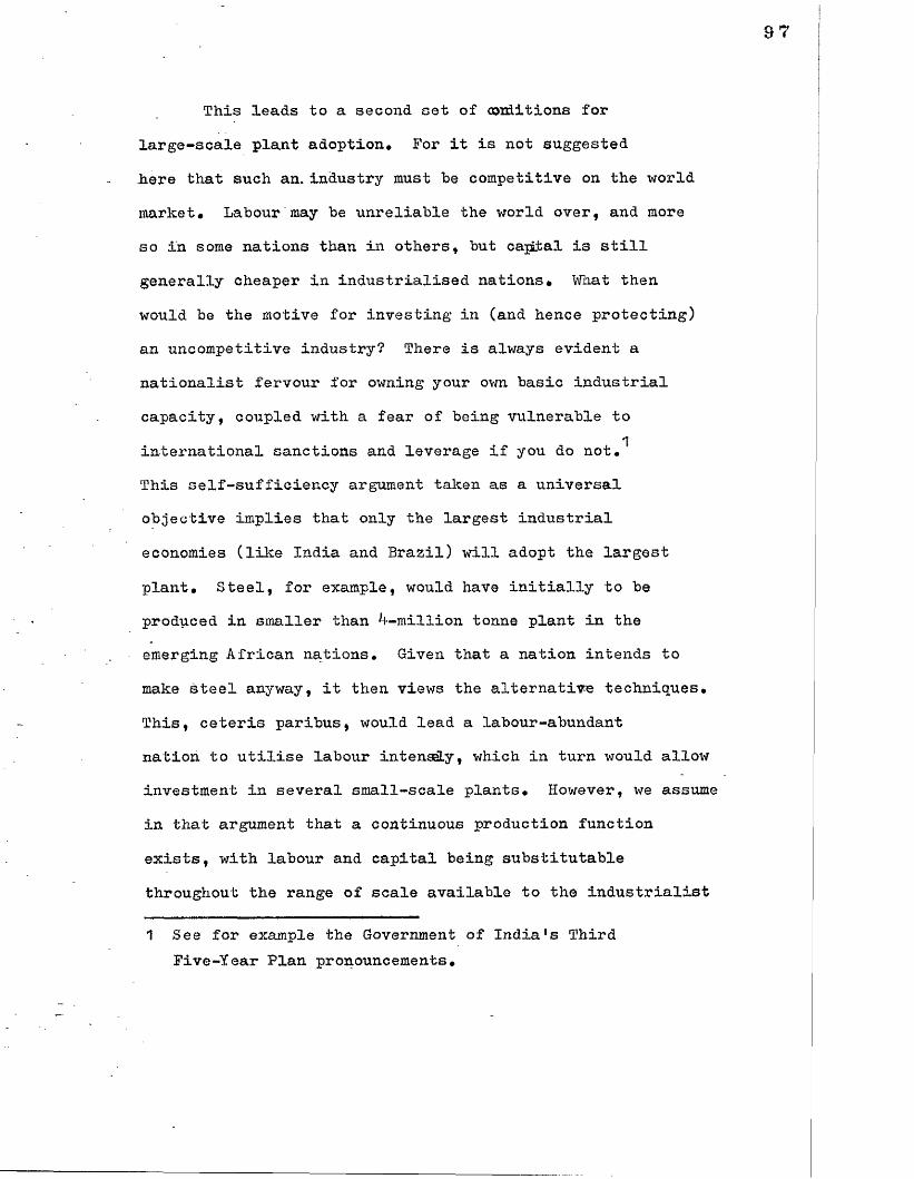
This leads to a second set of a>xditions for large-scale plant adoption. For it is not suggested .here that such an. Industry must be competitive on the world market. Labour'may be unreliable the world over, and more so In some nations than in others, but capital is still generally cheaper in industrialised nations. What then would be the motive for investing in (and hence protecting) an uncompetitive industry? There is always evident a nationalist fervour for owning your own basic industrial capacity, coupled with a fear of being vulnerable to

international sanctions and leverage if you do not.This self-sufficiency argument taken as a universal objective implies that only the largest industrial economies (like India and Brazil) will adopt the largest

plant. Steel, for example, would have initially to be produced in smaller than ^-million tonne plant in the emerging African nations. Given that a nation intends to make steel anyway, it then views the alternative techniques. This, ceteris paribus, would lead a labour-abundant nation to utilise labour intensely, which in turn would allow investment in several small-scale plants. However, we assume in that argument that a continuous production function exists, with labour and capital being substitutable throughout the range of scale available to the industrialist

1 See for example the Government of India's Third Five-Year Plan pronouncements.

98

(for any given quality of output). In practice a number of modern basic industries may show their highest productivity and profit rates (in a closed economy) at levels of output for which only a limited range of technical possibilities has been developed. The core process in oil-refining for instance can only be efficiently carried out within a very narrow range of factor ratios, so that whatever the factor prices (within a wide range), the core process has to be capital intensive. In summary then, self-sufficiency and technical discontinuity form a second set of condition's*

This leads us to the third set* Granted that in the real world there are more than two distinguishable factors of production, an industry may be competitively located in a developing country even though the core process may be capital intensive (whether to embody the latest innovations or to reap the available economies of scale). Complementary factors - semi-skilled labour, or raw materials, for example (like high-grade iron ore in the case of the Indian steel industry) may be relatively abundant, but only intensively exploitable in conjunction with a particular capital-using technology; while at the same time certain ancillary activities

can be made more intensive in the use of unskilled labour with very, .little complementary capital. In which case the non-labour factors, taken together, may be relatively cheap, and raw labour relatively costly, even in a developing

country#

In some industries of course it may be possible to

divide the production process into stages and to carry out the different stages in different countries# But if the newly developing technology makes this less easy (as with continuous steel casting for instance) or transport costs are high (as with the transport of iron ore) it may be more profitable to export the finished product (rather than any intermediate product) despite the fact that a country1

factor endowments would not favour the carrying out of some of the intermediate processes in that country (could they be isolated in this way)# If the country is particularly well-endowed with one out of the many factors of production, that fact alone may dominate the international location decision#

Figure 2 .1

Production Possibilities in an Industry

General Note: Individual plants are aggregated togive the industryfs output (Q) under different technological regimes (T);Labour is measured horizontally,Capital vertically;For illustration we take the iron and steel industry.

Interpre tation:1* Earlier Technologies (Tq) enable the production

of iron and steel with various combinations of capital and labour. Increased production levels would be achieved with equi-proportional increases in the two factors (no scale economies). The nation produce's its optimal output on for instance,say 2 m,t.,. in plants of m.t* each. Limited technological know-how prevents the use of larger plant.

New Technologies (T^) enable increased output to be produced over a range (limited) of factor combinations at lower unit cost: the new technologies relate toplant scale (i.e. they are internal to the unit of production) so that fewer plants can produce the same output as before* (Each plant is limited by know-how to, say, 4 m*t•)•

The nation decides to increase its output to , say m.t*

A labour-abundant economy might adopt the old technology (and produce at A, given its factor-price ratio of <k/l)", in % m.t* plants with heavy use of ancillary labour}.

The same economy, if factor prices are distorted, may adopt the new technology, producing at B say, in a single ^ m.t. plant, with rather less use of ancillary labour (and much less use of production labour). Indeed if wages are higher than (k/l)* there will be a shift to the new technology with .B preferred to C.

The 2 X 2 diagram fails to capture the case of the complementary inputsi but here is an approximation:If K (capital) and R (a raw material) are absolutelycomplementary, and R is relatively abundant to K, i.e.its true price is low, we can collapse R and K intoa new variable K*, price k*. In this case productiontakes place at B say. (This is an extreme case and thereader can readily consider the implications of relaxingthe rigidity of complete complementarity).

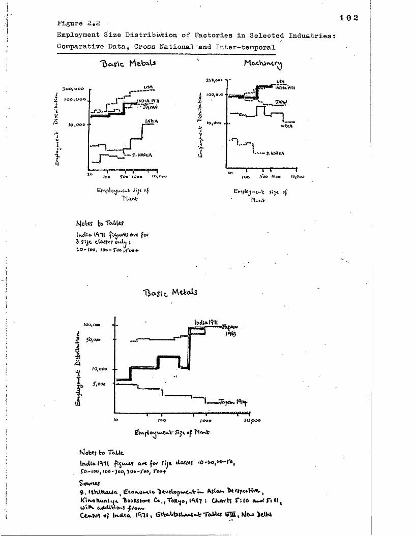
Figure 2*2 •Employment Size Distribution of Factories in Selected Industries Comparative Data, Cross National'and Inter-temporal

v)

ooo 100,000(

;o ,000 • •iMtr*

I

USA----

I . __.|N>lA

~n. S’. KOREA

-T(oo "V T ""'fito to so 10,0*0

2V&,00* 100,000*

i '

&

rI&

|0,00» „ >.

in>ls t»m

S 7A?'V

wbtA

f .V"!

).- 5-KciUA

T T^T“ floo JflO fooo (0,000

Etv\ploj(v»t*.V of ”P Lco>V

£»J-t of

iMoU? b T o liU f

IkcUc> IVU Awt fe*3 Jtjt tU-tt*/ OrvU t

lO-tW, J0o~ ro ,5oo+-

Uoy.3 . MttoAs

160,004

i <rx ft™0i

■iX£&

I0tooo * -

5,000

toT “i*>o I ooo to poo

j£**plovjV~e**.V' Sij«. •£ 1'lAfe

Mofctj to T<xWt.ItuU* mi f5«AAtt ft*efo* fijt lO-UJ.wJ-ro,$'O"|0U) l<H> "-JCOj 00 ro«tS«5vu.J$ , l$V \\ftA U <X j E cjo«v o **\3<- "bC0<ix>p*y*twlr I * - I k <#pt«-V?VC (

^«rootvuiv\u< ^oot^hKc C*. ( ToRtjo, 1^47 : Ckavt? T i io < w * f f : n ( o«^> culuUV'M

U a ic v Ill'll * £ stc4>tMW*A*-Vr TUVU? 6T £ , Nlea )«AK*

102

''Food "TbtiiU?

WTHA Wl\ MOV■J«J( o«» -J

f 00,000

to. QUO .

I.ooc .

loo Oja 1 0 *0

£rt.ploj(«C S e of 'Jtawfc

d"i

' i

OOo,ooo , )w(e»»AWtM)o .

oUl

lo.ooo .

1,000

l*t>|0» I'm (cofto.*)“wSa

_ _.i fai rri

i*** .fdwi*SK ;yXTA«J

1 ■■r’*i,"T,t !"■fCK> fOg <0003«- of

Tta t

M oU? U T a b U s

IrvcUe. $"11 -ft}*f t j * tte.tf«y o*V*j i o - ioo t joo" Sfoo $ foo *

SaovctjS. IsVvitaAt-la, £a»»\«f*ic I**"tarffCcVwi t iU'tfe.ftMt Co. TotVp *Ovft v r io t w5ft» cnUfHM fvosiwct***s of $ u , e$M>UjwtJL- T«Mt$ GUI* A/tw^ttk;.

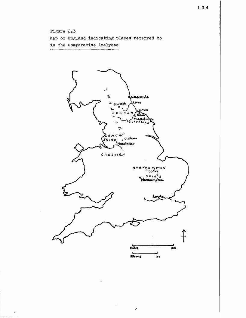
Figure 2*3

Map of England indicating places referred to in the Comparative Analyses

* Coast* S1U

D V ft. H A H

ttdUflr'V

A N C A• OUiho

‘WaCLeiHv*

C h F S m H e

IrfOATHA M ProAl 0Co<tq

0 S h t a. <£ N**ftlAr"fV,OK

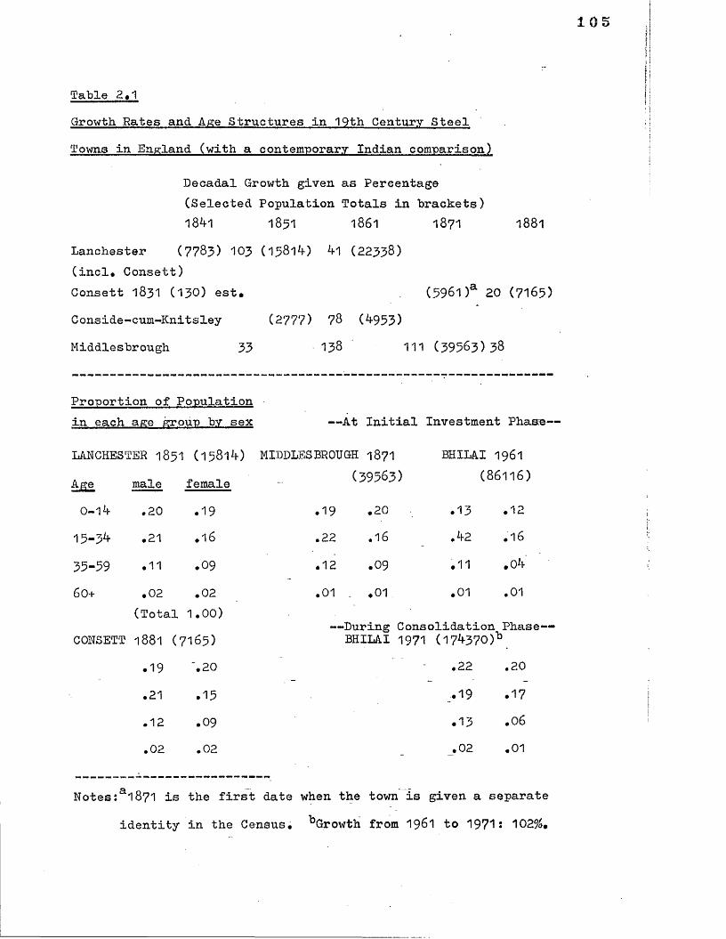
105

Table 2.1Growth Rates and Age Structures in 19th Century Steel Towns in England (with a contemporary Indian comparison)

Decadal Growth given as Percentage (Selected Population Totals in brackets)184-1 1851 1861 1871 1881

Lanchester (7783) 103 (15814-) 4-1 (22358)(incl. Gonsett)Consett 1831 (130) est. . (5961)a 20 (7165)

Conside-cum-Knitsley (2777) 78 (4-953)Middlesbrough 33 138 111 (395 63 )38

Proportion of Populationin each age fcroup bv sex — At Initial Investment Phaae*

LANCHESTER 1851 (15814-) MIDDLESBROUGH 1871 BHILAI 1961

Age male female (39563) (86116)

0-14- .20 .19 .19 .20 .13 .12

15-34- ♦ 21 .16 .22 .16 .4-2 .16

35-59 .11 .09 .12 .09 .11 .04-

60+ .02 .02 .01 . .01 .01 .01

CONSETT(Total 1,00)

1881 (7165)— During Consolidation

BHILAI 1971 (174-370)*Phase—i

.19 '.20 ,22 .20

.21 .15 .19 .17

.12 .09 .13 .06

.02 .02 - .02 .01

Notes:a1871 is the first date when the town is given a separate

identity in the Census, ^Growth from 1961 to 1971: 102%,

106

Sources for Table 2*1: British Government, Census of England and Wales (relevant dates), tables on Ages and Civil

Condition of the population, London, (tabulated under

Northern Counties); B.R,Mitchell with P.Deane,Abstract of British Historical Statistics. Cambridge

University Press, Cambridge, 1962; Government of India, Census of India. Madhya Pradesh, (relevant

dates), General Economic Tables, Table B II, New Delhi; for other estimates see text and references cited therein*

107

Table 2*2Change in Average Employment Size of Large Plant in West Bengal 1961 - 1971

Industrial Sector Average Plant* Size (Employment)

Decadal Change (Per Cent)

PoodBeverages and Tobacco products Cotton textiles Jute textiles Wool and Silk and Misc. textiles WoodPaper andPrintingLeatherRubber, petroleum

and coal ChemicalsNon-metal minerals Basic metals Machinery and Electrical mach. Transport equip. Misc.Repair

1961

180556290957

2 6^6

5882751*H2008693223031

^93■336438

537

6 2*f

1137191

1971

299

365

801

2^39

282

163

4-63

2010

580

^052Mf620

716

5^06 ^2

237571

66.1

•16.3-7.8

-18.5

-33.7

17.620.5 -44.315.5

*of plants employing more than 100 employeesNotes! Calculations not performed on non-comparable data;

Failure to include repair sector separately in 1961 is source of bias throughout.

Sources for Table 2 02 : Government of India, Census of India

1961« West Bengal, Establishment Tables, E III,New Delhi; Government of India, Census of India 1971. West Bengal, Establishment Tables, E II, New

Delhi o:

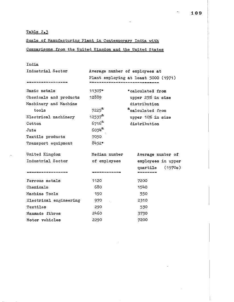
Table 2.3Scale of Manufacturing Plant in Contemporary India with

Comparisons from the United Kingdom and the United States

IndiaIndustrial Sector

Basic metals Chemicals and products Machinery and Machine

toolsElectrical machineryCottonJuteTextile products Transport equipment

United Kingdom Industrial Sector

Ferrous metalsChemicalsMachine ToolsElectrical engineeringTextilesManmade fibresMotor vehicles

Average number of employees at Plant employing at least 5000 (1971)

11307*12889

7225a

12537* 6716a 603^a 7050 8 -5 2*

♦calculated from upper 25% in size distribution

Calculated from upper 10% in size distribution

Median number of employees

Average number of employees in upper quartile (1970s)

1120680190970

2902*f602290

72001 5 ^ 0

550

2310530

37307200

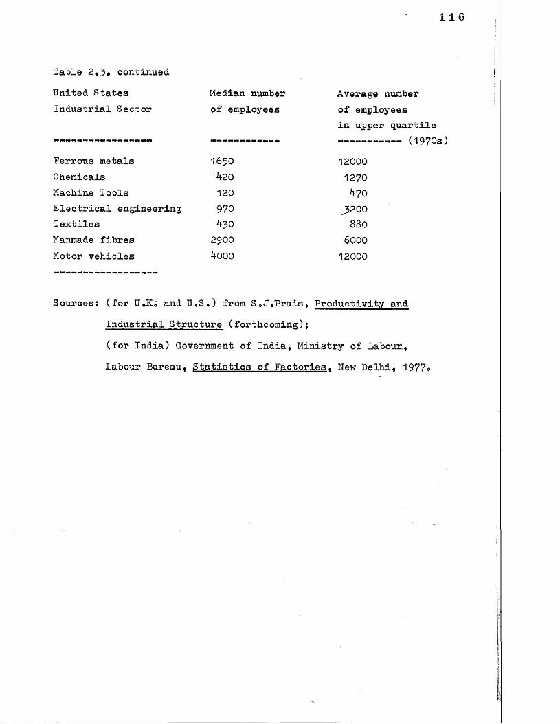
110

Table 2.3# continuedUnited States Industrial Sector

Ferrous metalsChemicalsMachine ToolsElectrical engineeringTextilesManmade fibresMotor vehicles

Median number of employees

1650420120

970^30

2900

*1-000

Average number of employees in upper quartile ------------ (1970s)

120001270

V70

3200

8806000

12000

Sources: (for U.K. and U,S.) from S.J.Prais, Productivity and

Industrial Structure (forthcoming);

(for India) Government of India, Ministry of Labour.,

Labour Bureau, Statistics of Factories* New Delhi, 1977o

ill

Table 2.4Growth Rates aad Age Structures in 19th Century Textile Towns in England (with a contemporary Indian comparison)

Oldham

Decadal Growth given as Percentage(Selective population totals to nearest thousand)1801 1811 1821 1831 1841 1851 1861 1871 1881 1891

42 29 45 34 23 36 15 34 18

(1 8 0 1: 1 2 0 0 0) (1891 : 1 3 1 0 0 0)

Manchester 19 42(1 8 0 1: 7 3 0 0 0)

44 29 29 12 4 32 9

(1891 : 5 0 5 0 0 0)

Proportion of Population

OLDHAM 1881 (111343) male female

MANCHESTER 1881

(341414)AHMEDABAD 1961

(1 2 0 6 0 0 1)a

0-14 .17 .1 8 .1 7 .1 8 .2 0 .1 8

15-34 .17 .19 .1 8 .1 9 .2 0 .16-

35-59 .11 .13 .1 1 .13 .13 .0 8

6 0+ .0 2

(Total.03

1 .0 0)b.02 .03 .0 2 .0 2

Notes: aGrowth between 1951 and 1961 was 38%. before rounding.Sources: As for Table 2*1 above (with British Census data

tabulated under North-Western Counties, and Indian Census data for the State of Gujaarat).

112

Table 2.5Population Size and Age Structure of 20th Century Steel Towns in England (with an Indian comparison)

Population Steel Capacity Core1951 1961 1971 (1960s) Workforce

Consett 39^80 36015 1 m.t. *f0 0 0-Corby 16735 *1-7990 1 m.t. - 1 .*f m.t. 5000

Bhilai 86116 17^370 1 m.t. - 2 m.t* 1 7 0 0 0- 25000

Proportion of Population ineach age group by sex

CONSETT 1971 BHILAI 1971Age male female

0-1*1- .1 2 .1 1 .2 2 .2 0

15-3^ .13 .1 2 .19 .1735-59 .1 6 .1 6 .13 .0 6

6 0+ .0 8

(Total.11

1.0 0 )b.0 2 .01

CORBT 1971

.1 6 .1 6

.15 .15• 17. -

.0*f .05

clNotes: For definition see text and footnote.bOwing to rounding, proportions will not always sum to 1.00.

Sources:.As for Table 2.1 above.(with British Census data tabulatedunder County Reports for Durham and Northamptonshire).

A brief Overview of Chapter 2

Here it becomes clear that economies of scale are a major consideration in modern industry, and especially in important sectors of heavy industry; this, in conjunction with a relatively abundant labour supply, results in the rapid demographic growth of local centres, which is the object of our analysis, and which can be held responsible for the problems of labour market equilibria and provision of welfare infrastructure associated with declining areas as well (especially when they too were the result of earlier growth of large-scale heavy industry).At no other point in time did technology and demography conspire to such an extent to this effect, and there are reasons for suggesting they will not combine again in such a way in the foreseeable future.

114

CHAPTER 3

The Model

A Summary of the Main Indications of the Model

The preceding demographic observations prompted the construction of a simple simulation model of local population structures and their development over time* This incorporates various contrasting patterns of migration to aid our understanding of how urban populations do develop as time goes on, and what underlies the changes we observe, and how changes in the periodic phasing of labour demand might modify the pattern described earlier* We find that the peculiar de-stabilising effect of migration to a "green-field1* site is due to the adverse adult sex ratio being rapidly equalised in conjunction with a fertility-promoting age- structure* The resultant severe fluctuations in the aggregate number of labour force entrants can be seen over time* Equilibrium is not improved by further migration during the troughs in the supply of entrants to the labour force: future disequilibrium is made worse* But simply spreading the labour demand over a longer period irons out fluctuations* The proportion of children builds up rapidly if demand for female labour equalises sex ratios earlier* (And we go on to show, with an illustration in Chapter 9 below, that more rapid growth in that dependency occurs in the town itself, if, as in the Steel Towns, the young male migrants are already married and subsequently bring their wives and children to the town*) Conversely, declining towns, having sex ratios, but not age structures, favourable to fertility, have both high young and old age dependencies.

By keeping the initial populations and new migrants cohorts separate, we can trace the relative sizes of the two groups: apart from the obvious sensitivity to differential fertility, the growth-promoting effects of the migrants1 young age, or favourable sex structure are also significant here.

115

The aim in constructing and operating a simulation model at this stage in the investigation is severalfold.But one feature combines all the objectives: the need tounderstand the real world more clearly. Without that feature the simulation becomes a mere toy. Furthermore, the costly temptation to elaborate a model to beyond the point where valuable insights can be seen to be forthcoming from it has been resisted# The risk of irrelevance becomes too great. It was hoped that in simulation some of the processes and implications of human population formation

would become clearer than they are apt to be in the eyes of an observer of the empirical data. Some of the questions a simulation might help answer are as follows. Why are birth rates so low in rapidly industrialising areas?And how long can you expect that experience to last in the absense of fertility change? Are changes in the growth rates of particular age cohorts, or changes in their proportionate size in the total population, the more important of the effects of different migration rates? And how do these depend on the age and sex structures of the migrants?How are they affected by different fertility and mortality levels? These models are not supposed to be used for long-term population projections: rather they have a didacticpurpose, for they show the kind of population disequilibria

that can occur (beyond, I think, those that are intuitively

obvious)* Hence the focus here is on the intermediate time span, up to the next twenty-five years at the outside, and particularly on the next ten to fifteen years, from the

initiation of a project and onset of major inmigration*

To maintain the sense of relevance, insights obtained specifically from the model and not from the data will be indicated as such in addition to those that

confirm the more readily intuitive observations from

the data* More importantly, allusions will be made to the empirical importance of some of the observations, allusions travelling back to our fore-going analysis on technology,

and forward to our discussions of the social implications of industrial strategy*

To help fix the basic patterns in our mind, first

we outline the models. We can thence compare them more

easily as a group* The basic model represents the

demography of the average Indian town, in that it adopts

approximately the recorded aggregate urban growth rate

in the 1950s (in the region of 30% per decade): one of the lessons of this whole thesis is that such towns represent

only one among a whole range of experience in urban demographic formation or dissolution, a fact easily

1 These are presented in detail in Table 3 *1* But threerepresentative major types are presented, with the indices essential to our dynamics argument, in Table 3 *2 , and Figure 3*1 is a graphical illustration*

117

disguised in the aggregate figures (or, to put it another way, these towns represent the modal experience of our

1951-71 growth distributions for the region illustrated in Figure 1.*0 . In this basic model inmigration is 1% per annum, and natural increase 1-J to 2% (depending on the fertility and mortality parameters used)* For our various

comparisons we take the version with natural increase of 1-J% (or 15 per thousand) implying an urban mortality and fertility close to rural levels (though with fertility on the

lower side), with a birth rate of around 38 per thousand

and death rate of around 23 per thousand of the population*

This reflects the correct parameters as far as we can judge for the mid-1950s, (see Chapter k for further discussion)*

We call this the‘Base11 migration model (Table 3*1 )*( or the

"Balanced Growth" example in Table 3 *2 )*

Then we have the models labelled "1" (Table 3 *1 » or "Concentrated heavy industry" in Table 3.2 ). These

represent decadal growth of 55% and upwards. The heavy

engineering towns fall into this category, Model "1 c"

is an extreme case,.typical of New-town growth - with a fivefold increase over a decade. An ■: immediate implication here is that

the migrant population quickly dominates the local population,

an important and neglected consideration in demographic

analysis (neglected because at the national urban level

aggregate internal migration is never significant enough in Asia for this domination to occur in so short a space of time, nor indeed does it do so in the major cities).Model "1 bM describes a fairly heavy growth of around

70% over the decade. The "primed" model ( "1 b*") introduces

a more heavily bunched migration age structure - fewer children, more workers - a characteristic more apparent in the less local migration streams. Model "1 a" has 50% more women

than is typical (see further discussion 'below-). All the Type "1" models have heavy net inmigration concentrated in

just five years: 1,500 males per annum in the cases "1 a","1 b", "1 b f", 15,000 males in M1 c", migrating into an

urban area of 1C£)00 males. Female migration, consisting

of spontaneous (occupational) and induced (marriage) migrations

is derived from regressions relating female to male migration streams (see further Chapter-5 below), and the initial female population in the urban area numbers 8*f10.

This sex ratio and the initial urban age structure are identical

to the all-India figures for the urban areas in 1961 (but

we test some of the migration models on stable age and sex structures also).

Next we have the models labelled "2". These have

urban population growth rates of around 50% per decade.

119

The principal didactic purpose here is to show what happens if the same number of migrants as in model "1" are spread

out over ten years instead of five, with 750 males migrating

per annum instead of 1,500. This would imply that the

component plants in an engineering project came on stream over a longer period, or that blast furnaces in an iron works were phased in gradually# But the model is also useful

in describing the effects of a more mixed industrial development, both less "lumpy" and more diversified in

its investments* The "2 a" version again (like "1 a") increases the number of women migrating, this time by 30%;

(the need to introduce these "a" variants only became apparent when we tried to explain the empirical evidence of high

female to male sex ratios in some fairly fast growing towns

in Eastern India)#

Finally the models labelled "3" are representative of the more depressing case of the towns that have become

net losers of population, or outmigrating towns (described

as "Lightly industrialised localities" in Table 3*2 #As with the above-described models, a graphical presentation

in Figure 3*1 highlights the migration dynamics in Panel A.

For comparative purposes the underlying fertility and

mortality were kept the same and constant over time for all

these cases# Then, in..order to examine the relative sizes

120

of migrant versus non-migrant population, these parameters were systematically varied in line with what probably took place,

in a few alternative models.

Observe first in Table 3*1 how the age compositional

effects of migration influence the birth and death rates.There is virtually no difference in the birth and death rates projected between the "Base" population model (decadal growth of 2 9%) and a stable population closed to migration (decadal growth 16%, outlined in Table 3*1 alongside the "Base")

'Iwith the same parameters;' i.e. taken in aggregate, urban growth in India is so slow that the age structure effects on fertility and -mortality can be ignored* But take now

the extreme case of "1 c" (decadal growth of 527%) and we can see that the birth and death rates are markedly reduced (the former from 59 to 30 per thousand). This was not

quite expected, since migrants are bunched in the reproductive

ages (Table 5*1 below). However, the enormous deficit in the sex ratio, resulting from," lagging the female migration

behind the male migration (as further detailed in Chapter 5

below), is responsible for this, and the model is approximately

in line with observed sex ratios observed in some of the

rapid growth towns of India (Table 6.1 below). Only in the more mixed industrial towns, which are growing more steadily,

1 A "stable" population is simply that which emerges if mortality and fertility have been unchanging for a reasonable length of time (50 years or so); (economists have a parallel in "steady-state" growth that emerges from an unchanging savings rate).

121

is the deficit reduced (as illustrated in model "2").

The cases of U1 b" and M1 b*" (with decadal growth rates

in the region of 70%) again show rather small age-

structural effects on birth and death rates (a few percentage points)* This is quite simply because, first, the migrant flow per annum is less than 10% of the

initial population, and second, the age composition of migrants, though concentrated on the working ages, is not wholly "unnatural11, that is to say it includes children and

old people. Clearly an extreme case of all migrants being aged 25 to 35, like an extreme case of a 1:1 sex ratio

among migrants (no lag between male and female streams), will raise the birth rate, as we had expected, but the

cases are rare in Eastern India (though we isolate an example

of very balanced sex ratios in Chapter 6 below). We shall

have more to say about dynamics shortly, but observe for,the

moment that birth rates recover from immediate shortfall

within five to ten years (as the women follow the men).

A sustained migration, (like any other sustained demographic phenomenon) results in a permanent displacement of the age structure and hence transformed birth and death rates;

1 In an advanced "Western11 type population with a far olderage structure the same migration composition will go much further toward reducing the death rate.

as Lotka taught us to realise, the population will recover

from a shock: but over the initial years (or quinquennia)

of recovery the dynamics behaviour of particular cohorts may be quite dramatic, and it is here, as I am eager to stress, that social and economic implications are crucial.

The cases of n2 bu and "2 a" (with decadal growth rates

of around 50%) of course show very little age-structure effects, Note also that in spite of a 50% increase in female migration the birth rate is only one per thousand higher as a short

term result (it was 2 to 3 per thousand higher in the 111 a"

variant over ” 1 b”)• The empirical evidence we have that points to quite heavily distorted birth rates (discussed

below) must result from significantly increased female

migration streams (which prompted our creation of the "1 a"

variant), or much higher fertility among migrants than among the pre-existing urban population.

Cases of declining or stagnant populations subject to

outmigration, as in model ,l3"« register rather high crude birth rates, since the pre-existing skewed sex ratio in

2favour of males is equalised by male-selective outmigration,

Death".rates are slightly higher (25 per thousand after 15 years compared with 23 per thousand in the populations

1 A, <J.Lotka, "A Contribution to the Theory of Self-Renewing Aggregates, with Special Reference to Industrial Replacement Annals of Mathematical Statistics, 10:1 , 1939*

2 I^gardless of migration, a skewed sex ratio is expected due to differential mortality in Northern India*

123

subject to inmigration) mainly due to the ageing of the population, but also, in a high mortality population,

due to the presence of infants (increased with the higher

birth rates)* In a society where local consumption,

of the poor at least, is largely determined by local production

and employment, the age-structural effects on welfare may be

quite severe,.: the incidence of the elderly population's

dependence on the active population increases, and the active labour force declines absolutely (at over 2% per annum in model"3" while outmigration continues, despite a

positive natural increase: see additionally part C of Table

3*2)# This is a fairly extreme case, where net outmigration rates are of the same magnitude as the inmigration rates assumed in model "2 b" (leading to an;overall decline in

decadal population of -16%)* The "Zero Base" model

illustrates the effect of stagnation (with decadal growth

of 13% resulting from no migration in conjunction with the pre-existing Indian urban age structure - indicative of

net inmigration in the-past).

The age structure phenomenon, as we have discussed it a.bove, is only significant for the provision of social

1 Here the subsequent developments of the age structure will depend purely upon the initial age structure (plus any sub­sequent change in fertility or mortality)* The low percent­age under 3 day denote a previous fall in fertility, and the adverse effects on the labour force structure can be seen in year 10 (when the 15-19 cohort declines)*

services specific to the young and old# Our interest in the

birth rate is that it tells us something about the size of the very young cohort (as well as the services required at birth)# The birth rate in the female population alone,

which is indicative of the future proportions of infants

to mothers, has additional implications for child care# It is of interest that in the sex-skewed populations the female birth rate is higher than the male (not illustrated in the

tables): that is to say, although inmigration may reduce

birth rates, it may do less to reduce child-to-women ratios*

(indeed if female migration is sufficiently bunched in the peak reproductive ages it will raise them). Similarly,

old-age dependency ratios have family care implications#

Initially inmigrant flows improve (i#e# decrease) the young

and old dependency burdens taken together# Later they

lead to an increase (Figure 3*1 * panel B)#We have shown that only in fairly extreme cases

would Indian towns and cities be radically affected by

distorted age structures* Greater distortions occur in

populations whose migrant age-structures are more in

contrast to their resident local population structures, which is typically truer as modern (i.e# older) age structures

develop, while the migrants continue to be concentrated in younger age groups. The distortions are enhanced if sex

structures, on the other hand, are more alike in both

i Z 5

resident and migrant populations; again this is more likely to be true in more developed societies where autonomous migration is less sex selective (in favour of males)#

The feature that deserves more investigation is a more truly dynamic one (illustrated in Figure Jit, panel C). If the age structures of inmigrant populations

\*ere very close to that of the resident population, all age cohorts would expand at a similar rate, say 10% per annum while migration continued* If,however, the sex ratio of the adult migrants is skewed in favour of males, this

picture will be modified in that the birth cohorts will grow initially at somewhat less than 10%, and then sub­

sequently, after the cessation of male migration, at somewhat

more than the rate of natural increase, assuming that female

migration continues and the adult sex ratio improves. However, if there is a hollow in the migrant age distribution in the age groups 5-9 and 10-1^ for example, there will come a.time when

the sensitive 15-19 age cohort (the age of labour force entry) grows less rapidly, subsequently to pick up strength when the birth cohorts of the initial wave of migrants reach

that age# This effect is clearly observable in the ” 1 c,r ,

1 It is a well-known characteristic of ’'stable1' populations (subject that is to unchanging mortality and fertility and with no migration) that each age cohort grows at the rate of natural increase#

or "New-town" model; (note especially the result of using a

stable population base, where declines of 7*1 and 1,6%

are: followed by increases of 1.7% per annum, and declines of 3*3% by increases of 7*1% per annum). What is perhaps

of more social significance can be seen if we relate the size

of the inmigrant 15-19 cohort to that of the native-born cohort, and if we continue to observe the relationship

over time, as we will below* It should be noted that the

power of this sudden growth of the age group about to

enter the labour force depends on how few children arrive with the original migrants: the more children aged 5-1kthey bring, the more gradual the growth over the quinquennia9

which is a crucial factor in the stabilising of the labour

market. If the delayed arrival of female migrants results

in a sudden growth of births, a further spurt' will occur in the growth of the 15-19 cohort up to 20 years after a project's initiation (as we have illustrated for the case

of "1 cM above). The major social problem attributed to

the sons of the migrants can thus be delayed by up to 20 years, or it can occur at once (if the .migrants bring

a large number of 15-19 year olds with them). In the ~

case of "1 b" the de-stabilising effect of migration

is more successfully damped by the’ steady growth of’ the base population. Generally speaking if a lower z'ate of

1 The simulation built on the actual urban age structure of .‘India as reported in the 19^1 Census over-emphasises this effect, since there is a considerable hollow, or

127

migration is sustained over a longer period of time the fluctuations in the age composition are swamped by the stability

of the natural growth* This can be clearly seen in Figure 3«1

where the "Balanced growth" industrial investment option

results in more stable dependency ratios and more stable growth in labour force entry cohorts. The implications for the labour market, for investment policy, and for social

welfare are discussed in Chapters 6 to 9 below* Examination of static age structures, or indeed vital rates, did not clearly reveal this phenomenon. We could view it further in the light of how fast the labour force is being quitted via

old age, but remembering that old and young workers are

by no means simple substitutes. We do this by observing the rates of male labour force growth* Ironically the more

concentrated migration cases ("1 b" rather than "2 b")

can mitigate the effect of rapid labour force entry rates since very large cohorts also age out of the labour force in later quinquennia (the older members of the original

migrant stream), so that the labour force growth rate is subdued* It should be emphasised that duch an observation

footnote continued from previous page

undercutting of the base age distribution, in the 0 -4

age group. This underlines how other-changes (which would result in the 0 -4 age group suddenly declining in proportion to the rest of the population) can enhance the effect of in- migration by reducing the native-born 15-19 cohort pre­ceding that of the migrant-born 13-19 cohort* To see this compare the effect on the "1 b" model of using both stable and actual initial age distributions.

depends crucially on the age structure of migrants and the

length of working life: for again the workforce could delay

shedding its largest cohorts until five years after the entry of the largest cohorts in the 15-19 age group# In all these cases, how easily a society can accomodate such changes

without precipitating changes in its own organisation

(administrative or political) is likely, inter alia, to

be a function of the instability and the size of the 15-19

cohorts, and both instability and size generally decline as one proceecfe through the models from "1 c" to "2 bn and "Base"# The other ingredient in the dynamic social implications, the relative size of migrant and non-migrant cohorts (in the same age groups), we will now go on to

discuss#

Whereas societies may well react to changes in age and size of their total populations, the differential changes

among the different groups or classes Is likely to be of

more significance# In the present context, let us consider

migrants in comparison with the native or locally born population# This is a first approximation to a more

1 The relative importance of differential mortality and differential fertility is indicated in an appendix to Chapter 4# In summary, a 50% decrease in fertility reduces the size of the labour force entry cohort by 50%, but increasing life expectancy by 43% increases that same cohort by between 29 and 36% only, depending upon the mortality pattern assumed within plausible limits#

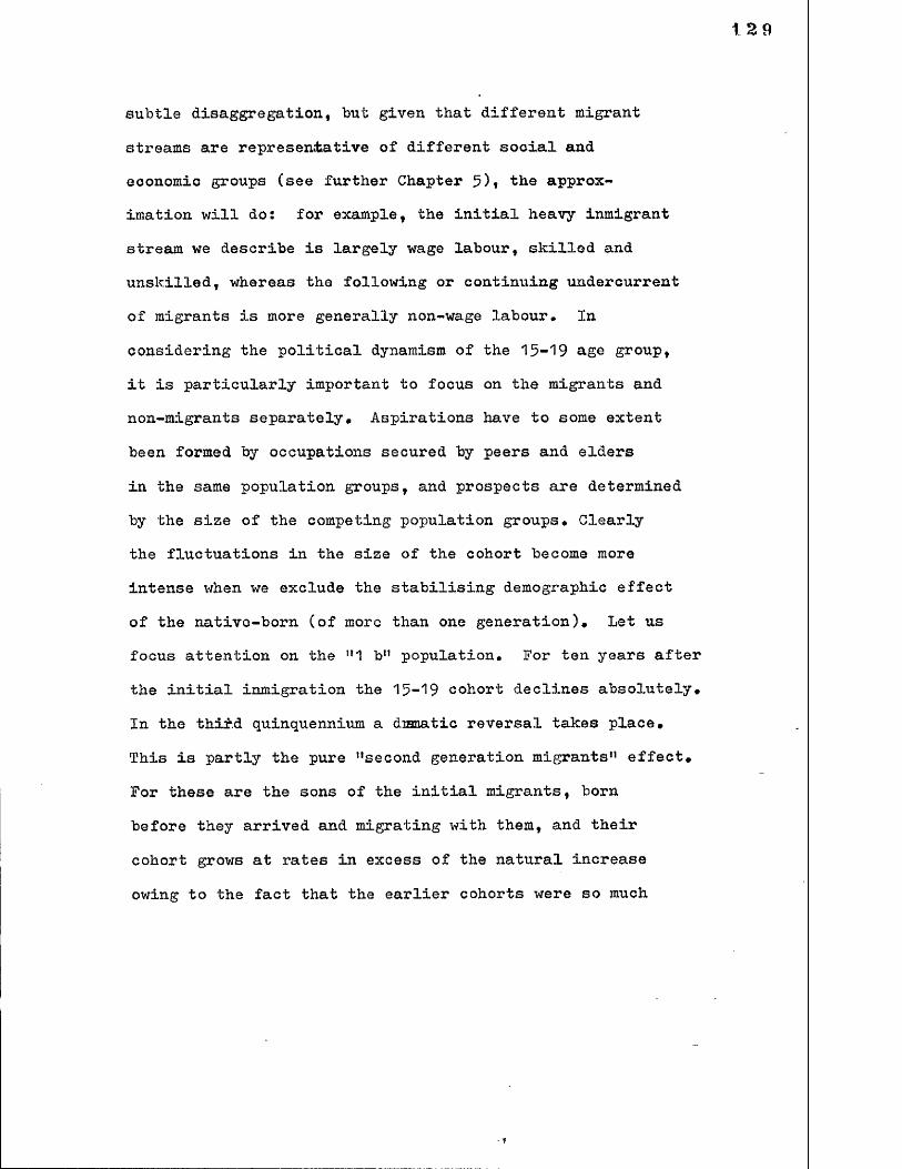
subtle disaggregation, but given that different migrant

streams are representative of different social and economic groups (see further Chapter 5 ), the approx­imation will do: for example, the initial heavy inmigrant

stream we describe is largely wage labour, skilled and unskilled, whereas the following or continuing undercurrent

of migrants is more generally non-wage labour. In

considering the political dynamism of the 15-19 age group, it is particularly important to focus on the migrants and non-migrants separately# Aspirations have to some extent

been formed by occupations secured by peers and elders

in the same population groups, and prospects are determined by the size of the competing population groups* Clearly the fluctuations in the size of the cohort become more intense when we exclude the stabilising demographic effect

of the native-born (of more than one generation)# Let us focus attention on the "1 bn population. For ten years after

the initial inmigration the 15-19 cohort declines absolutely#

In the thir.d quinquennium a dianatic reversal takes place.

This is partly the pure "second generation migrants" effect.

For these are the sons of the initial migrants, born

before they arrived and migrating with them, and their

cohort grows at rates in excess of the natural increase

owing to the fact that the earlier cohorts were so much

130

smaller than they would be in a stable population (for

the initial migrants aged 5-14 were few in number), and

there was no supplementation of their numbers by continuing migration on the same scale beyond the first quinquennium#

As we have noted, a further reversal takes place

between 20 and 25 years later when the sons of the migrants

actually born in the city reach labour force entry age#By contrast in model "2 b" there is the supplement of continuing migration for a second quinquennium: hence

the absolute decline in the 15-19 age group is delayed and the later increases are more gradual, (those in the sixth quinquennium, though for reasons discussed above those in the foirth are not)# The extreme sensitivity of these effects

to the age pattern of migration is illustrated in model

"1 b ,tf: the age bunching of women (into the high fertility

ages) in the quinquennium both contemporary with and following the initial male migration induces a baby boom

that reaches the labour market in quinquennia starting year 2 0, as well as year 25. A similar result occurs if female migration is increased by 50% (compare "1 a " with

"1 b11)# It would be an ironical response to these

fluctuations if a second wave of young migrants were encouraged in the quinquennia starting years 5 and 10 to fill the hollow that is causing a slack in the labour

supply, and thus exacerbate the excess supply that will

occur in the subsequent quinquennia# Labour market signals may be quite deceptive unless accompanied by a

knowledge of demographic dynamicsI

The overall social effects of these and similar observations must presumably depend on how large is the migrant population in relation to the native-born, and how

this ratio changes over time# We investigate this in Table

3#3 (Figure 3*2 ), counting the descendants of the main

migration stream (recorded in the first quinquennium) as

migrants, and counting the continuing undercurrent of

migration as local and therefore equivalent to native-born# Starting from a migrant to native ratio of 0 »5 :1#0 in the "1 b" model, the subdued rate of natural increase in

the migrant population (due to its initial sex structure)

tends to reduce this ratio (and age the migrant population'I

faster). In 20 years the ratio has fallen to 0.4 :1#0 #A slightly less substantial decline is sustained in the

migrant population if fertility is enhanced by the sex

structure of the migrants (as in "1 a")* A more evenly

1 If fertility is enhanced by the age structure within the migrant population, as in "1 b tn (not illustrated) the proportion of migrants will start and finish larger (i.estarting in quinquennium 3-10 when migrant children are first born in the town).

132

distributed migration (not illustrated) will obviously

start with a lower proportion migrant, and at the same terminal date have a substantially lower proportion

migrant (including descendants) due to the shorter period

of natural increase among the migrant families in the town

(compared with "1 b" , where all the migrants arrived together

at the start). In the extremely unbalanced case of New-town development ("1 c11), where the initial migrant population

is five times the native-born, the decline reaches L3*7-

times the native-born over the 20 year period. As before it has to be pointed out that if age-specific fertility were higher among migrants the ratio would have a tendency to rise rather than fall, at least until migrant fertility

began to decline. Small (but probably typical) differentials

in fertility do little to offset the effect of population

sex differentials (Table 3*3)* _Conversely, if the native population grows "faster owing to lower mortality offsetting

lower fertility, the migrant population - falls even faster

in relative size. In all these cases of unsustained migration

the ratio of migrant to native population falls rather than rises (which we show below in Chapter 6 is a fair reflection of what has happened in the areas of rapid migrant inflows

associated with industrial expansion in. the Second Plan period).

FigureDemographic Effects on a Locality of Three Contrasting Migration Patterns

i _

i s T v

Sa.J

Heavy

T W s l a

H iUTtOA/G»etr vfcttj

e I —I —tf-

S ©■

" - I -

U -i-3-*

'laUi»vc£c( dsovitK. — —

IQ tU tU ^ ttC ttv ic * 5^"IO

Ofc) (X*)

I/o~ir(3<A>

/r-iotWt.)

2-0-is" i<TK)

J

I

ft

\

Tam^u *&>5>ffAl € cyC y o v Hl 4 U vlioiV ' fo ^ te

C4U<VT-e %

•■i

khiu

rw

134

Figure 3*1 continued

■>AAiCjL C LA ooju. Fo&C-*? e/sfTOA/vrs

-r- \ / \' ' \ ;* i\\ / v

r-ioC u t ) M

Ilo-iro « 0

»T'*oU«fc)

I

IP*) £<S*fc)

Source: Simulation Model (see Table 3*2)

135

Figure 3*2Age Structures and Proportions of Migrant and Local Populations: Inter- Temporal Comparisons

halesA c,*

Modfcl Icm (fUMK t f l u h j 0 » v ^ ^

sr-n fO'fV MSr-vi

?r~*W-i*} 10-1

lo-tif

r-n

'— ” v — i---- r s 1---- 1--- 1— i---- rISO 160 IttO 1J0 loo SO Go tto 2-0

M 05, i*v <X»5

fr kfrfir

Uej: To? bar «S wI*Uilr4-UcaIlioHrom be^ I i r*$*.jo* c«uI

*6rtkttvll*v.t tU.ou)f tffttl" '|i\Ortaf(4 lift-- c»k«C| iw.t/&Klr3

136

Figure 3*2 cont’d

Modtl llr htodofeU. NV re&o**.o # v 1 » a { * « v o f c $ u l * | ( c l ' b *

toed

•'rwyftwfc' ,« r

TC5idewb

tt&lV

- ------------j------------1------------j-

NoS. C**fc to jftc-U

if m ecu's LabcrKaitJ

yttidtfc.b*- p .

os.

Table 3*1The Models of Urban Demographic Growth and Structure;Populations sub.iect to various Patterns of Migration

Notes and Overview of^Parameters

Initial Age Structure: All-India urban average asrecorded in 19^1 Census (unless otherwise stated)*

Fertility: Total Fertility Rate of 5*1•Average fertility for each five-year age group as follows, from 10-14 to 45-49: (.0 0 6 9,.1 3 6 1,*2 5 9 0, *2445,,1 8 7 1,.1252,,0542,*0 0 7 0) from Coale-Trussell

models (see Chapter 4 below and Figure 4*2)* (Variations noted where they are made*)

Mortality: Female Life Expectation at Birth of 40years* Survivorship pattern as in Princeton

Model Life Tables, West Level 9 ♦ paired with male level and pattern as therein (see Chapter 4 below and Figure 4*1)* (Variations noted as

appropriate*)

The reader may care to note that Table 3*2 offers a summary of three major variants

(illustrated in Figure 3*'l); Figures, 4,3 and

3 *1 illustrate age distributions and migration schedules respectively.

138

j BASEY ear 0 5

Project Initiated Migration starts

In-Migration Ratea (MMR) 1.0 0.9

Natural Increase 1.6

Decadal Growth B.R.b

1.5

39.3 38.7D.R.b 23.1 23.3Male Labour Growth (ages 15-59) a

3*1 3.2Male Age Group (15-19) Growth a

>•9 3.3Dependency Burden (Males<.15 ox* >59 t Labour Force)

68.5 67.4

ISMMR 0.9 NI 1.5BR 58.0DR 23.4MLG 2.415-19G 3.1 DB ”64.9

0.9

20

1 . 4

37.823.42.21.4

64.2

0.8

10

1.52 8 . 5

38.523.2

2.2

-0 . 9

6 2 .9

1.437.9 23.7

1 . 0

1 .6

64.2

Stable Model for

Comparison

0.0

1.5

3 8 . 5

2 3 . 3

Notes? a Simple annual average per cent for the quinquennium.In projection the net in-migration streams werecumulated into 5-year totalsf which became part ofthe urban population for the next 5 years on. Both sexes.'

b Birth and Death Rates are expressed traditionally . per thousand.

139

1 b |Year 0 5 10

ProjectInitiated

MMR 8 .1a 1 . 0

NI 1 . 6 1 . 1.5Decadal Growth 71.6BR 39.3 35.6 37.0DR 23.1 2 2 . 2 2 2. 3MLG 15.8 a 2.5 1.715-190 21 #7 a ••1 -1.3

15 20 25

MMR 0*7 0 . 6 0 . 6

NX 1 .k 1.3 1.3BR 36A 3 8 . 2 3 6 .5

DR ' 22.7 2 3 . 0 2 3 . 5

MLG 1 . 8 1 0 .7

15-190 3.3 0 . 1 . 8

Note: a As stated above, these are simple (arithmetic)annual average rates for the quinquennium 0 ~ 5 » and so on#

140

1 b*|Year 0 5 10

15-190 2 1 . 7 -*f.O -1 .1

15 20 25

15-190 5.0 1.5

Note: This is as 1 b but with the male migratmore heavily concentrated in the young

1 b STABLE|

Year 0 Ej 10

MMR 8.7 1 .1

NI 1 .6 1 .+ 1.5Decadal Growth 75.3|BR 3 8 .6 35.8 37.8DR 23.2 2 1 .6 22.3MLG 1 9 .2 2.7 2.315-190 19.7 -1 .8 1 .A-

-15 20 25

MMR 0.7 0.7 0.7NI 1.5 1 . 1.BR 37*^ 36.9 3 6 .8

DR 22.7 2 3 . 0 23.3MLG 1.9 1 .6 0 . 8

15-19G O.A- 0 . 7 2 . 0

Note: This is a projection from an initial stable,not Indian urban, age-structuref - see Figure *f.3.

141

1 a|Year 0 5 10

— — —.

MMR 9.1 1.3NI 1 . 6 1 . 6 1.7Decadal Growth 81 *6 |BR 39.3 37.9 39.6DR 23.1 2 2 . 2 2 2 . 8

MLG 15.8 2.5 1.715-190 2 1 . 7 -1 .A- ‘ -1.3

13 2 0 25— • ——

MMR 0.6 0 . 6 0 .6

NI 1.5 1.5 1 .*fBR 38. 37.7 37.8DR 2 3 . 0 23.1 23.^MLG 1 . 8 1.7 1 . 0

15-190 3.3 2.3 2.5

Note: Female migration is raised By 1 b. In-Migration Rate (MMR)

50% in 1 a ove is for both se

A O

1 0

Year 0 5 10

ProjectInitiated

MMR 8o»6 1 . 8

NI 1 .6 1 .1 1.5Decadal Growth |527.1|BR 39.3 29.7 35.6DR 23.1 1 8 .8 2 0 .8

MLG 1^ « 3 1.5 0 . 8

15-193 191.6 -7.0 -2.3

13 20 25

MMR O02 0 . 2 0 . 2

NI 1.3 1 . 2 1 .1

BR 3^.5 33.8 3^.3DR 2 1 .6 2 2 . 2 23.1MLG 0.7 -0 .1 0 . 2

15-193 2 . 6 -3.^ 7.0

M c s t a b l e ]Year 0 5 10

15-19G 1 8 6 .8 -7.1 -1 . 6

15 - 20 2515-190 1.7 -3.3 7.1

Note: This is a projection from an initial stable,not Indian urban, age-strueture, see Figure f.3 .

9

143

Year 0 J? 10Projects ,..*.InitiatedMigration . • • • Continues

MMR 2.9 2.4N I 1.6 1.6 1 . 5

Decadal Growth 15 0 . 2 1BR 39.3 38.4 3 8 . 0

DR 23.1 2 3 .0 22.7MLG 6.3 5.3 2.015-190 9.1 Zf.if -1.9

11 20 25MMR Oo9 0o7 0.7N I 1.5 1.4 1 .4BR 37.8 37.1 37.2DR 23 oO 23.1 23.4MLG 2.2 2.0 1.015-190 4.1 2 © 1 0.4

i2 aYear 0 10

MMR 3.1 2.6N I 1.6 1 .6 1 . 6

Decadal Growth 53.4BR 39.3 3 9 . 0 39.0DR 23.1 2 3 .0 22.915-190 9.1 -1.9

15 20 25MMR 0 .9 0 . 7 0.7N I 1 .6 1.5 1.4BR 38.7 38.9 37.7DR 2 3 .2 2 3 .2 23.515-190 4.3 2.5 0 . 8

Note: Female migration is raised by 3°% in 2over 2 b*

.

ZERO RASE

Year 0 5 10

MMR 0 . 0 0 . 0

NI 1 .6 1 . 6 1 .6

BR 39.5 39.1 39.2DR 23.3 23.6 23.7MLG 1.5 1 .8 0 . 9

15-196 ^ • 1 2 . 7 -2 . 2

Decadal Growth |1 3 .2

13 20 25

MMR 0 . 0 0 . 0

NI 1.5 1.5 1.5BR 38.9 38.9 39.2DR 23.9 2*f.1 2^.3MLG 1.3 1 . 2 1 . 2

15-196 3.1 1 .A- 1 . 6

Note; This is a projection without migration, from the Indian urban age-structure*

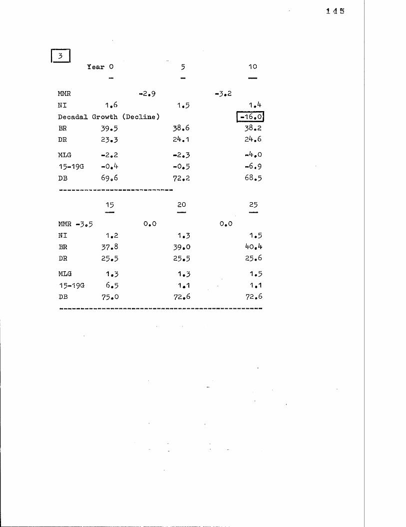
mYear 0 5 10

MMR -2.9 -3.2NI 1 . 6 1.5 1 .Decadal Growth (Decline) -1 6 . 0

BR 39.5 3 8 .6 5 8 . 2

DR 23.3 2^.1 2^.6

MLG -2.2 -2.315-196 —O. f -0.5 -6.9DB 6 9 .6 72.2 6 8 . 5

15 20 25

MMR -5.5 0.0 0.0NI 1.2 1.3 1.5BR 37.8 39.0DR 25.5 25.5 2 5 .6

MLG 1.3 1.3 1.515-196 6.5 1.1 1 .1

DB 75.0 72.6 7 2 .6

14 6

Table 3.2Three Cases of Contrasting Urban Models

Examples: a. Concentrated Heavy Industry on new siteb. Balanced Industrial Growth at existing centre c* Decline of lightly Industrialised locality

A Net-Inmigration Rate (annual average % per quinquennium)

Quinquennium1st 2nd 3rd 4th 5th 6 th(e.g 1953-60) (e.g. 1 9 8 0-8 5 )

a* 86.3 1*8 0.2 0.2 0.2 0•0

b. 1 . 0 0 . 9 0.9 0 .9 0.8 0.0c. -2.9 -3*2 -3.5 0.0 0.0 0.0

B Difference between Growth of Male Labour-force andGrowth of Total Population (annual average %)

a. 85.4 -1.4 -0.8 -0 . 8 -1.4 -0.8b. 0.5 0.8 -0.2 0.0 0.0 -0.4c. -0 . 9 -0 . 6 -1.9 0.1 0.0 0.0C Growth of Labour-force Entrants (males 15-19* annual av. %)

a. 186.8 -7*1 -1.6 1*7 -3.3 7.1b* 4.9 3.3 -0.9 3.1 1.4 1.6c. -0.4 -0.5 -6 . 9 6.5 1.1 1.1

Source: Simulation Model (Table 3.1)*a, = 1 c Stable, b. * Base, c• =*

This table is graphed in Figure 3*1

Table 3.3Ratios of Migrant to Original (or Local) Population

Migrant males divided by males locally borna

Year 0 j?Model1c 5 .2 0 b.67

1b 0 .V 7 O.bZ

1b low fertility and mortality among migrants and locals0.46 0.4-1 O. 3 8 0.34 0 .3 1

1a 0.47 0.44 0.42 0.40 0 .3 8

b1b with high fertility among migrants only0.47 0.42 0.40 0.37 0.35

Notes: a A continuing modest migration stream fromlocal areas is assumed as in the "Base’' model and this is counted in with the native-born to form a group called ’’locals”.Sons of the main migrants are counted as migrantst wherever born©

b Low fertility: T.F.R.-4.7; Low mortality: ej(fem)=43. High fertility: T.F.R»=5*7*

Source: Simulation model derivations (Table 3•1V

10 15 20

4 . 3 4 4 .0 1 3 .6 9

0.38 0.35 0.32

A brief Overview of Chapter 3

From this analysis we can say that demographic characteristics of new fast-growth towns will exacerbate the future labour market’s ability to equilibrate supply and demand (other things being equal). This is pre­dominantly due to the large population size accumulating over a very short period, and the rapid equalising of the adult sex ratios. The age-structure of migrants has a secondary effect. The demographic character of slow (or negative) growth towns will exacerbate their ability to find resources for maintaining local welfare, owing to their loss of adult men but retention of women and dependants (both young and old). The determination of the (short-run) relative sizes of competing migrants and local sub-populations is outlined*

PART TWO

Exploring the Empirical Evidence

150

CHAPTER kDiscussion of the Parameters used in the Model and Exploration of the Fertility Factor

A Summary of the Main Empirical Points

The speed at which a second generation population (the future, locally-generated, workforce) is created, depends in part on the fertility of the first generation migrants. Similarly the subsequent size of various pop­ulation groups, of different origins, with their individual aspirations towards achieving specific types of employment, depends on earlier and current fertility levels. There are three components here affecting the urban populations: marital fertility, proportions of population married (by age), and the presence of spouses. It is found that lighter manufacturing towns (e.g. textile towns) sustain higher and unchanging proportions of children in their populations, whereas heavy industrial towns experience rapid increases in the proportions of children (as existing families join the initial male migrants), but exhibit the socio-economic potential for a subsequent rapid fertility decline through later marriage or marital fertility control. This contrasts with experience in other societies (e.g. historical England), where we find light industry attracts single female labour, so that despite more balanced sex ratios overall, the proportions married and the proportions of children are lower than in India. Hence we infer that increased opportunities for female labour will currently enhance the birth rate in Indian cities, but need not continue to do so if the age at marriage rises (as it is clearly doing in all categories of towns). Finally we show that some migrant groups remain as split families (as we observe in Bombay, but find less in the heavy industrial towns), and hence will not necessarily retain their relative strength over time in the urban population.

151

Overview of Parameters

Although it is hoped that the model just discussed

will have wide application and usefulness in interpreting

the changing structure of urban populations in other

economies and at other periods of time, the fact that we intended to use it here in the analysis of data from

contemporary India prompted the choice of parameters we

used# Initially our ambition was to use mortality and

fertility schedules that were particularly appropriate

to the Eastern region of India under discussion. This ambition was abandoned for a number of reasons. First the

value of the mortality tables prepared by the Registrar General

for the decade 1951 to 1961 has been seriously questioned: for although the Registrar General did not indicate his method of calculation, it is clear that regional life-tables

can only be prepared from censuses after adjustments have been made for migration between the regions. Estimation

of the latter, however, cannot accurately be made on the

basis of place of birth data collected in the 19&1 Census

since, among other things, we need additional information on the place of last residence, and we need to allow for

1 Notably by Professor K* Dandekar, of the Gokhale Institute of Politics and Economics at Poona, in a personal interview*

misreporting of duration of stay, though it is true that for

some regions at least a reasonable approximation might be

made. The alternative then is to use census-survival methods to estimate the migration, but that of course

requires using regional life-tables, which is what we are

trying to construct in the first place. In the light of this argument it seemed pointless to indulge in the

1 K.E.Vaidyanathan, "Population Redistribution and Economic Change in India 1951-19^1", University of Pennsylvania, 19^7 (mimeograph), reported a similar problem in trying to construct estimates of urbanward migration by census-survival methodology. Briefly described, census survival methods entail observing an age-cohort,2 0 -2 5 say* in the first census, and following it through to the second decennial census, when it will be aged 30-3 5 # I£ we have age-specific survival rates (obtained from Life-tables) appropriate to the area of the country (in default of complete deaths registration) we can estimate the number of people who will have died in the 10-year interval and subtract them from the original 2 0 -2 5 age-cohort, thus reducing the expected number aged 3 0 -3 5 at the end of the interval. Any excess over that expected number is then to be attributed to net inmigration. The method is very sensitive to the survival rates we use*

153

sophistication of using local mortality data for model-1building purposes* Recourse was had accordingly to the

2Princeton Model life-tables* The "West" variant was

used (following the argument of Professor A. Coale that

1 For the 1961-1971 decade the introduction of the Sample Registration System of birth and death recording enables a more valid reconstruction of State-wise life-tables; but see also T.Dyson1s attempt (and commentary) using census-survival techniques: "Mortality Estimates for the States of India", Centre for Population Studies^ London School of Hygiene and Tropical Medicine, 1980 (mimeo)*

2 If- there is a reasonably complete registration of deaths, and age reporting is fairly accurate, it is possible to convert these mortality data into the probabilities of dying between the ages of 20 and 30 for example, and hence obtain the probabilities of survival. When such data do not exist (a» in the case of India) the probabilities of survival obtaining in other countries (e.g. Western Europe in the 19th Century) can be used instead. Sets of these have been grouped together and averaged (by Coale and Demeny, at Princ­eton University), the result being labelled the "West" model life-tables. These are graded for overall expectation of life at birth - A-Oyears, 50 years, 60 years etc# Knowing which level to take to apply to India is not easy, but - techniques have been developed to check the accuracy of one*s choice against the population age structure (inbroad terms) and decennial growth rates that would be implied by particular levels, (so long as the national population is closed to migration and is subject to un­changing mortality and fertility over time, * all roughly true of India in the 1950s). A.J.Coale and P.Deaaeny, Regional Model Life Tables and Stable Populations,Princeton University Press, Princeton, 1968

we know insufficient about Indian mortality((in the 1950s) to justify using anything other than this admittedly "residual"

table)* and the level chosen was " 9 % giving an expectation of life at birth close to what is thought to be the case for India in the late 1950s, namely about 40 years for women.

I have illustrated the Eastern Regional table (of the Registrar

General) and the Princeton West model in Fig* 4*1.

A priori the sharp decline in survivial of women in the Registrar General's table (and to a lesser extent of men)

around the ages 25-55 could be regarded as suspect, though in the case of women it could derive from exceptional

adverse nutrition in the child-bearing ages, and in ..the case

of men the high Incidence of tuberculosis and other respir­atory diseases may make adult survival worse than it was in

2Europe in the 19th Century. A possible error an the Registrar General's tables could be that too many net in­migrants were adjusted for in the earlier ages (for, as we

shall see more closely later, it is not accurate to take

the age distribution of migrants-to be the same as that in the general population); but a more general error may be that age misreporting (shifting numbers into the older

age groups specifically) has notrbeen sufficiently allowed

for. In that context note the better survival beyond the

1 Personal communication with Professor Coale at Princeton University (1975).

2 See N.R.Crook, '"The Changing Character of Mortality in the City of Poona"(manuscript), School of Oriental &

- African Studies, 1983*

155

age of 6% A second reason for not using the Eastern

Region (or Zone) mortality table of the Registrar Generalis that the region itself is heterogeneous. Registrationdata for the 1960s are hopelessly unreliable, but If we haveregard for the rather more satisfactory Sample Registration

System (SRS) data for the late 1960s and early 1970s we see.'a notable variance in crude death rates for the different

States in the region (a picture confirmed by life tablesconstructed from the two Censuses 1961 and 197'1)»For instance, the urban death rate for Orissa is 11*4

as against 6 .3 in West Bengal. Rural death rates are

about 50% higher, though, as we shall discuss below,this is not the case uniformly throughout the age groups.Presumably such variances held in the 1960s (early) andlate 1950s; indeed they might be expected to be larger in

a period when fairly rapid falls in the deata rate were2still bemng experienced. It seemed therefore useful to

1 Government of India, Sample Registration System Bulletin .Office of the Registrar General, various years, Rew Delhi.

2 A major drawback with non-Indian models is that the male tofemale mortality differential is inappropriate. In India,at most ages female mortality exceeds the male. But the regional contrasts are quite large and our region is hetero­geneous; nor do we know much about urban mortality sex differentials. The bias resulting from using the "West" model sex differential is that we have probably projected too large a female population at most ages*

take a single model of fairly broad application (i.e.

"West" level 9) &n.d to indicate, as the investigation

proceeds, the effects of using slightly different levels, or different models (including some differentiation between migrant and non-migrant sub-populations in these

respects), as we have done in Chapter 3*

There was never any question of using regional fertility schedules for 1 9 6 1, although vital statistics surveys including fertility information were carried out during

the 1961 Census: the data would need considerablemanipulation. Again, the Sample Registration System data suggest inter- State variations within the Eastern region.Again therefore recourse was had to models, though this; time they are arguably a little more Indian in character*The Coale-Trussell Princeton fertility model was fitted

to the National Sample Survey age-specific fertility schedule for 1958 (All-India). Following estimates made by Veena Soni

a total fertility rate of 5 *5 0 was assumed to be approximately

correct; but even as early as 1961 a rural to urban fertility

differential is likely to have existed, and perhaps a differential between migrant and non-migrant populations

(discussed further below), the effects of which are borne in mind in Chapter 3, so that for most of our simulation

'1 As with mortality, the under-reporting of vital events, and the inaccurate recording of people's ages, make it desirable to use a model schedule of fertility by age, derived from populations with better data.

model a level of was taken, which is close to the National Sample Survey figure for urban India in 1964,4.88'. The result of the fit is illustrated in Figufce 4.2.

As it was by now apparent that All-India rather than

specific regional parameters would best be used, with some

qualitative observations on local differences, an All- Indian urban base population, was also adopted, using the age

distribution as reported at the 1961 Census, without adjustments

(as these are only readily carried out on fairly stable populations not subject to migration). Particular problems arising from the use of unadjusted data are discussed

below, and (as was seen in Chapter 3 above) we use stable age distributions in alternative projections by way of control. The sex ratio adopted was 8 to 10 , females to

males (which is close to the average urban sex ratio in

India) . 2

1 The actual fitting was done for me by Basia Zaba at the Centre for Population Studies, London School of Hygiene and Tropical Medicine. The method is such that certain parameters characteristic of the Indian population are observed. The earliest age of marriage and survey estimates of the level of total fertility per woman are the principal parameters used.

2 At the State level these are given in 1961 as follows:Bihar 811 women per 1000 men, Madhya Pradesh 8 5 6 , Orissa 8 0 8, West Bengal 701, (all for urban areas). Government of India, Census of India 1961. General Population Tables, Delhi.

A Note on the Age Distribution

The urban age distribution revealed in the 1961 Census was used in some, but not all, of the simulations.It was felt that the attempt to simulate the peculiar effect

of welding migration on to an already distorted population

was worth making. But at the same time it is well-known that age misreporting and under-counting (especially in the 0-4 age group) would artificially distort the figures revealed in the Census: the problem with all unstable

populations is to distinguish the artificial from the real.

The shortfall in the All-India (rural plus urban) 0-4 group has been well discussed by Tim Dyson, who believes that, of the 12$ or so omitted from that group, about ■£■ has been

shifted into the 5 -9 group, and about ■§■ omitted from the

population altogether. This phenomenon may affect the female population more than the male. When we look at the urban population separately we find the 0-4 male cohort is

particularly small, 1 2.8$ of the male population (whereas

females 0-4 are 14.7$ of their own population), but this is due to the large number of adult males in a population subject to sex selective, age selective, inmigration (Figure 4.3). Both are of course significantly below

1 T.Dyson, "Analysis and Adjustment of the 1971 Indian Age Distribution", Demography India. 5s1 & 2, 1976.

what we would expect in a stable population (of appropriate mortality level and with fertility characteristics that

coincide with All-India demographic experience over the

decade; Figure 4.3)* This is confirmed by observing the

sex ratio by single years of age: throughout 0 -9 the urbanareas have excess males, (and a greater excess at each age than in the rural areas), but with the excess worsening further in the 5 -9 age group, (though to a smaller degree

than in rural areas, so that the rural-urban difference

begins to narrow). The male urban age distribution is

actually undercut in the 0-4 agsgroup (there are more males aged 5-9 than 0-4). How has this come about? It

is unlikely that age displacement or pure omission are

worse in urban areas than in rural* We do not know of

cultural reasons why survival rates for boys would be better in urban areas vis-a-vis those for girls than they are in rural areas; on the contrary, we might expect the

more educated population to be less likely to neglect girls.

The National Sample Survey Migration Survey (and the 19&1 Census data on migrants migrating within the last twelve months to Bombay, which are .cross-classified by age)

suggest that boys outnumber girls in the age groups 1-4.

The NSS suggests that girls outnumber boys among infant

migrants (under 1 year old) but the 0-4 age group as a.whole

turns out to be slightly male-dominant (f:m sex ratio

of .954 versus .992 in the All-India population)# This probably indicates that boys are a little more likely to

accompany their fathers (or elder brothers) if the latter are migrating alone, than are girls: they will stay withtheir mothers in the rural areas# Declining fertility in

urban areas (with their higher socio-economic class

composition), if not in rural areas, is likely to have taken place during the 1950s, and hence the small size of

the 0-4 cohort* All the States in our region have aggregate

urban populations with the 0-4 cohort smaller than the 5-9 (for both sexes) with the exception of Madhya Pradesh#

Fertility Differentials: Evidence From Bombay

It is well-known that fertility rather than mortality differentials are by far the more important determinants of natural growth rate differences in contemporary populations (and particularly of national

sub-populations), and hence also of their relative sizes#

Mortality differentials would modify, but always be dominated

by the fertility effect in populations of our experience*

161

(see below Appendix to Chapter *f). Furthermore, differentialage structures are largely determined by fertility, not

mortality. Xn our initial model-building we assumedfor clarity a single fertility schedule, derived from the

data collected as representative of All-India. In actualfact our urban populations are significantly more complex.

Not only may migrants have different fertility behaviour

from non-migrants, but migrants of different regionalbackground may have different fertility (and in Indiathose differences, even if we hold constant socio-economic

2 3characteristics, turn out to be considerable). ’ Similarly, migrants of different socio-economic status would be expected

to have different fertility, given that, by the 1960s at least, family limitation was clearly being practised, especially in urban populations. In theory we need to distinguish migrant types, and also the tvro major social components in overall

fertility per woman: the pace and ultimate extent of entry

of the female population into marital union, and the control of fertility within marriageo

1 See A.J.Coale, The Growth and Structure of Human Populations. Princeton University Press, Princeton, 1972.

2 T.Dyson,"India's Regional Demography", London School of Economics and Political Science, 19&1 (mimeo).

3 S *J.Jejeebhoy, "Status of Women and Fertility: a Socio­cultural Analysis of Regional Variations in Fertility in India", in IC.Srinivasan and S.Hukerji (eds.), Dynamics of Population and Family Welfare 1981. Himalaya, Bombay, 1981*

182

However, City-wise or District-wise data on

marital fertlity are non-existant, though we do have Census data on marital status* As an index of total fertility

we have of course child-to-woman ratios (but unfortunately these are confounded, as is well-known, by differential

child mortality, a not insignificant problem (see Appendix to

Chapter 4)). As for differentials between migrants and

non-migrants, further conceptual problems arise, discussed below, and we have to rely on evidence from two major Cities for which special tabulations were done in 1961; Bombay and

Ahmedabad. Despite these limitations, it seemed worthwhile

to investigate this evidence directly, in order perhaps to provide further insight into the shortfall in the number of children recorded as aged 0-4 in the 1961 Census (just

discussed). In particular we may discover how far such

a shortfall, insofar as it is real and not a mere undercount, could relate to differences in the marital status of the migrants (as compared with the rural or urban non-migrant

1 The 0-4 death-rates differ more noticeably than do those at adult ages. However their effect on the Child-Woman Ratio differentials between the States of India should not be exaggerated* For example, male rural death rates in the age group 0-4 are 41 .6 and 72*6 per thousand for Maharashtra and Gujarat respectively (SRS data), implying, cet. par., only . 3% in CWR due to child mortality differences. The Maharashtrian rural-urban difference in child mortality is only 1% of the child population* Note that in some of the analysis we have to make do with 0 -9 in the numerator of the CWR.

16 3

population)•

We can see from Table that for males there isreally very little difference in the singulate mean age of marriage (SMAM) I have calculated between migrants and

native-born# For males it is difficult to detect a consistent trend, though it is universally observed that urban-urban

migrants marry later; this reflects that they are more likely to be of middle-class status, in managerial

occupations,(though not all will fit this description)#

Our interest, however, must focus on women, since, in the simplified demographer's approach, only women are responsible for the birth of children (so that only the absense of women is a limitation on the birth rate)# The SMAM of females rises slightly with duration of residence, but,

more significantly, is highest of all for the non-migrant

population: that is to say, there is no evidence that thosecurrently migrating (or with less than one year's duration

of residence in the City) are more likely to be single than their urban peers#

This latter is a very important point# It would

seem from detailed examination of case studies (see further below) that migrants to green-field Steel Town sites

1 This is the average age at which first marriages take place.

are very heavily male-dominated for the first two to three

years* But it also becomes clear from the rapidity of

family formation subsequent to those three years or so that a majority of migrants are already married on migration (this is confirmed by some detective work on Bhilai in

Chapter 9)* and simply brought their fertility history with them (as it were), thereby rapidly pushing up the

child-adult dependency rates in the city# The evidence from Bombay seems to confirm this# There is however a

notable difference between the urban and rural migrants

(according to origin)# It appears that female migrants whose move is urban to urban, and who are more likely to

be joining husbands (or rather subsequently marrying men) of managerial or professional status will have

lower fertility (by virtue of a later age of marriage);

and they, as we shall see, are a more important demographic

component in the industrial sectors of heavy industrial towns (around 20% of factory sector employment) than in other towns, thus offsetting some of the boost to the numbers of children in these cities given by the

influx of young married migrants, but enhancing the significance of the class differentials in fertility in

the city# Some qualifications have to be added in extrapolating from the Bombay data in thisuway, which

we will do shortly#

A more drastic simplification we made in model- building was to assume that the same fertility behaviour would characterise migrants moving to join husbands

(the umarriage--responsen migrants as those moving in search of employment (the ■'•autonomous" migrants), the argument being that even the latter were generally speaking migrating as part of a household (and often as a marriage

partner) and not as individuals, even though the actual

decision, or timing of that decision, to come to the town

was influenced by work opportunities# Some light is shed

here from the useful tabulations on marital status and

labour force participation: .again the evidence is for Bombay# There are nearly 6 years between the ages of marriage (SMAM)

of working and non-working women of urban origin (and the

working women marry nearly years later than those in

the general city population including native-born; again note the qualifications on interpretation that follow)# These

will be the relatively sldXLedl working women in tbs.non manual trades* The rural working migrants marry nearly 3 years later than the' non^Vorkj.ng- and 3* years later than rural women generally, but 1 -year younger than the

general population in Bombayt (Table *f#l)#

These observations-should not be extended too~

readily to imply differential marital, and hence differential

166

fertility, status of subpopulations in any town or city*Working women migrating to Bombay are heavily represented among migrants from Kerala, Tamil Nadu, and the Southern States in general# And: we know that the average mean age

of female first marriages for all social classes together is higher in these particular States, viz# 20 years in Kerala, din contrast to 15 years of age in Bihar#

Cultural components cut across the purely economic,(a point more clearly demonstrated when we consider

contrasts between English, Japanese, and Indian textile<■]labour below)#

An additional source of information on differential

fertility is the child-woman ratio (CWR), available for

Bombay for migrants of different origins# Let us

first clarify the nature of the evidence* What is recorded is simply the migrant children present in the City* Assuming we have constant mortality, very low CWRs could imply two

things: first they might imply the existence of absent

sons and daughters (who may migrate later), and not

necessarily low fertility; second, assuming we can control separately for duration of residence and hence isolate migrants who have been in the city a long time, we might

infer from low CWRs a divided and hence impermanent family

1 Cultural characteristics may also determine the speed ofany fertility change, given a change in economic circumstances takes place: N#R#Crook, n0n Social Norms and Fertility Decline11, Journal of Development Studies, July, 1978*

167

(with migrants likely eventually to return to family of origin) and hence not one to contribute to the long-run

differential growth and size of regional groups within the City*

On the other hand, very high CWRs might imply (in addition to the opposite of the two possibilities just mentioned) the presence of young children with lone fathers, (whose

wives may be back in the rural home)* Finally, and most

important, in a migrant population we cannot actually

relate children to their mothers from the Census data: children born in the city should be, and often are,

recorded as native population, a bias in comparative work that

can only be partly mitigated by restricting the analysis

to recent migrants only (those arriving within the last year),

and children up to 5 years old, most of whom must have been born before arrival and hence classified as migrants#

The picture is as follows, (Table ^*2). Migrants

of between of between 1 and k years duration, from other

towns and cities within Maharashtra, have higher CWRs than the general Bombay population*'* We have already noted the

earlier age at marriage for those non-working migrants

from urban areas (and might additionally note their high

f:m sex ratios). The picture is one of permanent and fertility-enhancing local migration. On the other hand, migrants from rural areas of Maharashtra have lower CWRs

than the general population# This is also true of

rural migrants from every major State, despite their

younger age at marriage# Why is this? It would seem

unlikely that the whole of the differential is due

to lower marital fertility# Taking Maharashtra alone we

note a 10% CWR differential between rural and urban#But birth rates, in the late 19&0s at least, were

higher, not lower, in rural compared with urban

Maharashtra# The perverse reverse differential could be partly attributed to a longer inter-birth interval

during the period of migration when spouses may be

separated (except for infrequent visits) for up to

three years before finally settling in.ihe City

(and note that Bombay has about 10% of its households consisting of single males)# A further part of the

differential could be due to higher child mortality:

over a third of the difference could be explained by a

difference of five years in life expectancy at birth, a plausible rural-urban differential at the low average levels

of life expectancy experienced in the late 1950s.' We

should also allow for the fact that of the migrants of

1 - k years duration of residence a proportion will have had one, and a smaller proportion two, children since arrival in Bombay - and these children will have been classified

as non-migrants* Quantitatively this can easily account

for low CVJRs, but it cannot easily explain differentials*

The other expanations therefore remain interesting#

And when we observe in Table *f#2 the very skewed female

male sex ratios among the migrants (even for those from rural Maharashtra we have #6 2 , among the adults *5 2 , and taking the rural and urban together #70 as against

#82 in Bombay) the clear indication that families are

split makes it plausible that not only adults, but also

children, are being left behind. Correlation of low sex ratios (especially low adult sex ratios) and low

CVJRs favours this interpretation*

There might appear to be some evidence of women bringing their age-specific fertility with them, as it were. CWRs among both rural and urban migrants are lower in Karnataka than in Gujarat# This might be thought to

reflect the fertility differentials later observable in the two States# But again the migrating adults have very

different sex ratios, so what may differ is the degree of

1 By 1970-72 the birth rates are as follows; (SRS): Karnataka rural 55*9» urban 27#0; Gujarat rural ^-2.1; urban 5 5.6 #

divided families (children included)* From the point of view of the local labour market the demographic distinctions

are less important; it is the children alive and present in Bombay that count# Interestingly the political conflict in this multi-ethnic city has been largely between

Maharashtrians and migrants from the South (especially

Tamil Nadu (Madras))* But in fact the Gujaratis are the most likely to increase their share in the Bombay population insofar as natural increase (rather than migration) is concerned#

There is a distinct characteristic among migrants from

the North, mainly Bihar and Uttar Pradesh, which is of particular interest in' as much as these migrants feature significantly in our Eastern region studies# There are

very few women (Table A-#2). Thus despite the higher

fertility that we would have expected among migrants from

Uttar.Pradesh for example (to judge from later SRS data), albeit partly offset by higher childhood mortality, yet

the “dominant factor here in determining the birth rate in -Bombay is bound to be the adult sex ratio. In fact, in the case of the rural' migrants the CWR is very low

also# These migrants are distinctly impermanent* There

are barely two adult women to every ten men among migrants

1 Conventionally the birth rate is measured as births tothe total male and female population (which will be very low the sex ratio is very male dominant); whereas child-woman ratios refer to surviving children and female adults only.

171

of under five years* duration, and the ratio does not improve with duration of stay! the overall adult sex ratio among

these rural migrants is as low as #127» The possible social causes, and some implications for economic security, of

this experience, are to be discussed in Chapters 5 and

8 below# We will note here, however, that without

a continuing migration, the Bombay sub-population tracing its origin from these Northern States would rapidly

decline in proportion to the rest#

These findings are tempting to use in model-building

and projection for analysing the demography o§ other cities#

However, our analysis in Chapter 5 below shows that a construction worker migrating to Bombay or Sholapur may be a very different person in a social and economic sense

from a steel operative migrating to Durgapur or Jamshedpur, even though in both cases he may come from Bihar or Uttar Pradesh# The character of the wage labour demand, and whether

a provision of housing-or other amenities is included in the

implicit wage, is bound to affect fertility through the

-intermediate processes just described# Ec-onomy modifies,

if it does not create, culture#

But with these reservations in mind, we may still hazard

a reconstruction of migrant and non-migrant fertility behaviour

from the much less detailed data we have for the other urban

areas in the study.

17 2

Fertility Differentials in the Region under Study

A glance at Table will reveal that the heavy

engineering towns of the Chota Nagpur region have low

child to population ratios (which we take, ceteris paribus,-

as being indicative of low birth rates)# We can explain

this phenomenon largely through the low female to male sex ratios observed in those towns, and we also show below that this

distortion is only temporary# But what can we say about the

women who are already in (or subsequently will migrate to)

these towns, as far as their marital status and fertility are concerned?

The broad picture is as follows# In 19&1 the

recently industrialising areas, especially those involved in heavy industry, had relatively low CWRs vis-a-vis the urban areas in their respective States (thus re-inforcing

the effect of the adverse sex ratios, or at least adult sex ratios, on the birth rate, i#e# depressing it further

still); note especially in Table ^#3 the cases of Durg, Sundargarh, and Dhanbad, (Burdwan's CWR being on the

high side, a case we discuss in more detail below).

1 Child to Population ratios, like. Birth Rates, areparticularly influenced by age and sex structure# They have the additional disadvantage of incorporating child mortality: the 0-^ age group are the survivals of the previous five years' births. The bias becomes severe when we are forced, owing to data availability, to take 0-9.as the age group proxy for accumulated births*

There is evidence that these low birth rates are a transitory phenomenon. Detailed study of particular towns has suggested that the rapid uniting of. .families (already formed) in these urban areas leads to the equalising of

the sex ratios, and to an increase in CWRs, (see further below, and the case study of Bhilai in Chapters 6 and 9)«Why these two change together we cannot know for sure,

but our study of Bombay above has cast doubt on all the

hypotheses save that of split families: in those urbanenvironments where few men have been accompanied by women, those few women are less likely to be accompanied by their children. Table ^.10 shows how in Burdwan, where fertility seems hardly to decline between the Censuses, despite the trend in the rest of the State, the major contrast with neighbouring Districts lies in the improvement of the sex ratio among adults* There is also evidence that engineering towns whose major expansion was prior to the Second Five-Year Plan period of 1955/6 - 6 0 /6 1 had high CWRs once they too had passed the phase of initial rapid expansion: hence pre-

Independence Jamshedpur has higher CWR than average for cities in Bihar (Table ^.5) and Asansol-Burnpur has higher CWR than average for towns in Burdwan District by 1961 (Table

As we have said, if we are right in supposing that these

heavy engineering towns start with low CWRs and evolve into towns with higher CWRs (even higher*.than average), the

174

fact warrants some explanation. Despite the Bombay evidence, we will advance a hypothesis that may be more relevant to

the unique experience of these rapidly industrialising areas* On:.the establishment of a heavy engineering centre or Steel Town the workforce contains a large component of construction workers (not all recorded as

resident in the urban area,-see below), and of white-collar technical and managerial staff (the project designers and supervisors)* The latter form a link over time between the

departure of the ; construction workers and the arrival of

the plant operatives (insofar as they are entirely separate,

for in practice construction workers often stay on)*

The white-collar workers have a higher age at marriage

and hence lower CWRs (if not also lower marital fertility).

The subsequent influx of blue-collar workers, the majority

already married, is dominated by young adults* Their wives, who follow later, are also young (probably younger than the aver­

age population, see Chapter- 5 below for the age-structure of

males in various occupations). Thus the age-structure alone

could raise the CWR (and it may be this that can raise it above that of surrounding towns, where age-specific

marriage and fertility rates may be similar). It is also

175

possible that these migrants have lower child mortality,

being a self-selected, and hence possibly atypically healthy group, moving into an environment that also offers some

protection from disease; (compare the lower adult mortality

rates implied by the low widowhood rates observed in these heavy industrial areas, and see our evidence on amenitiea- supplied by employers in heavy industrial townships)#

Whether fertility or mortality is the cause, the effect is

the same: larger cohorts leaving childhood and approachinglabour participation and childbearing ages#

By contrast, the urban areas of light industry, and

the stagnating Districts seem to have high fertility in

1961, as well as high sex ratios and hence high birth rates

(inferred from Child-population ratios); we refer to places like Midnapore, Bankura, Ganjam, and Bastar, in Table ^#3,

but the picture iB certainly not clear-cut# Despite

the fact that some of these areas provide employment for women more extensively than do heavy engineering areas, the age-specific marital status data reveal that women in these

areas are generally speaking married, not single# The

scenario seems to be as follows: married women are more likely to join their husbands if there are jobs for them,

and the married women who are more likely to offer themselves -

1 N*R.Crook, 'The Economy of Mortality Decline", paper read at SSRC Development Group Seminar, held at London School of Oriental and African Studies, January, 1979, (mimeo); relevant table reproduced here as Table /+#9«-

for work (as for example from the Southern States of India) are more likely to migrate with their husbands and place themselves on the labour market in these circumstances#We find continuing high fertility, often particularly high fertility, in these towns over time# For instance, in

1931 Sholapur was a high fertility City in the Bombay

Presidency, and in 1961 it was still a high fertility City with high proportions married in the 15-2^ age group in comparison with other Maharashtran* Cities, (Table A - # ? ) *

In summary, the demographic types become hard to

distinguish over time. But there are striking differences in their evolution* In the short run the heavy industrial towns are subject to sharper fluctuations in these fertility-related variables, thereby further enhancing the de-stabilising effects of distorted age structures#In the long run their higher social and economic status may promote more rapid fertility decline# The clear evidence of differential birth rates in the short run between sub-populations in these cities indicates the potential for ethnic conflict, due, for example, to competition for jobs as the second generation of migrants and locals, Bengalis and Biharis, enters the labour market# The contrasts and comparisons with other cultures in these respects are followed up below in a review of the engineer­ing and textile towns of 19th Century England#

177

Alternative Cultural Traditions;Similar Industry, similar factor endowments

The experience of England in the last Century was

remarkably different for reasons wholly unrelated to

industrial technology (which indeed was different) or

the abundance of labour or the behaviour of capitalists,but purely due to the cultural character of that labour

supply# Controlling therefore somewhat for the .industry and

for the factor endowments, we may consider the culturaleffect alone. As in the case of Japan it was sociallyacceptable for women to offer themselves for employment

in the textile (and other light manufacturing) industry#

In that sense the process of sexual liberation had progressedfar further than in India, even than in India today. In the

early decades of this century Japan was employing nearly

four women.to.every man in the textile industry, India2four men to every woman# And there was a second crucial

1 I am not wishing to enter a debate here on whether culture determines economy or vice-versa. But the major cultural characteristics to which I refer were, if not exogenous, formed at this date by the pre-existing agricultural economy#

2 G#Saxonhouse and Y.Kiyokawa, "The Supply and Demand for Quality Workers in the Cotton Textile Industries in Japan and India", Papers and Proceedings of the Conference on Japan’s Historical Development Experience and the Contemp­orary Developing Countries, International Development Centre of Japan, Tokyo , October 1978#

difference in the labour supply* The women in England were single# Hence if we look at figures for a region of

textile manufacture, Lancashire in North West England, in 1861 (prior to the major fertility decline), we find high sex ratios (female:male) combined with low Child-Woman

ratios, and low Child-Population ratios, indicative of low

Birth Rates, (Table ^.8 )* Compare that with mining and

iron manufacturing areas across the Pennines* County Durham has low sex ratios, but high Child-Woman ratios, and very

few of the women present are single# Such broad regions

are rather heterogeneous, but town-wise data are not avail­

able for the towns of our interest until 1891, by which time fertility has begun to decline throughout the country#

Nevertheless analysis of some data from that latter date

is instructive, (Table *f#8 )# Talcing Middle&rough as

representative of heavy engineering and iron and steel making par excellence, we find higher fertility than is observed in the County of North Riding generally#

The cause of such low fertility can be clearly related to

the low proportion of single women, (only 2 9 *5% by ages 25-29). The sex ratio is only slightly depressed in favour of men, so the net effect is to raise the Child-Population

ratio (13*8%)# In the textile town of Oldham, where female

employment is far more dominant, sex ratios are over one

to one in favour of females, and as many as half (5^*3%) of women aged 25-29 are single# The differences in CWRs

are clearly therefore not only due to a differential fall in marital fertility between the two areaB, though this may have added to the result; all these effects (and others) are

compounded in the Child-Population ratio (11**f%)« there

can be no doubt that cultural differences cut across economic

ones, in the short run at least, in the determination of urban demography*

In a nutshell, in England heavy industrial towns,

after their initial expansion, apparently stabilised with higher fertility than light industrial towns, mainly due to the larger number of single female employees in these latter towns, in marked contrast to the case in India;

(and there were more gradual fluctuations on the road to

stability than in India, due to the more modest scale of migration)*‘

Case Study: Burdwan District

We will now look at the Chota Nagpur region in a little more detail, focussing on the District of Burdwan.

Our index of fertility, the CWR, has in this case to be restricted to the 0-9 child age group* The highest

CWBs are to be found in Asansol and Hirapur, where the

workers in the Indian Iron and Steel Company foundries

live (CWRs of 1*5 and 1*^ respectively, Table

The other mining and industrial townships in the area have high ratios* The exceptions are Durgapur (and Kulti) with CWR of 1*2* The large City of light processing and manufacturing, and administrative centre, Burdwan Municipality, also has a low ratio (1*2)# In this City,57% of women aged 1 5 -1 9 and 81% aged 2 0-2A* are reported as married, compared with 60% and 90% respectively in Asansol, a generally lower pace of entry into marriage; in both cases virtually all females are married by age 50* The socio­economic class structure of these towns may be responsible for these differences, and Table gives an indicator here, using education as the measure of status* Unfortunately for our ■ analytical purposes, Burdx an is a heterogeneous City: we cannot tease out separately any information on the females employed in the light industry for instance, for comparison with those whose husbands are employed in the administrative occupations# But it does not appear to be the case that Burdwan is a City of low socio-economic status*

The engineering town of Chittaranjan, the site of the locomotive factory established in 19^8 , has a high proportion of married women aged 20 and over, but large proportions single below that age# Our reconstruction would be that these women are the daughters of the original migrants,- well-endowed

181

with high levels of education (Table 4.6). If this is so, the implication for the future will be a fall in

fertility in Chittaranjan# By contrast Durgapur, a

more recent New-town has already a large .proportion

of its 15-19 population married, and judging from the skewed adult sex ratio a large addition to the adult female cohorts is still to arrive (in the most prolific child-bearing ages), accompanied by their existing children# This

will have the effect of both raising fertility (or offsetting any decline), as well as raising the child-population ratios# The family composition tables (Chapter 8 below)

point to a contrast between towns in nearby Birbhum District

and those here in Burdwan, confirming the picture outlined

above. Currently (1 96 1) there are smaller households, and fewer married daughters and other relations in

Burdwan, but more married sons# Table 4.10 indicates that

Burdwan was not the highest fertility District in 19&1;

ten years later, however, it was# This is despite

the fact that in 1961 the socio-economic status of the area (the increase in high-level manpower) might have suggested

it was ripe for a fertility fall of substantial size.

To check the components in this quite mild decline in CWR (and new status at the top of the CWR league) we

examine the differences between Burdwan and other Districts in West Bengal, (Table 4.10). Burdwan has become increasingly

a heavy industrial area by 1971, with Burdwan Municipality

itself taking diminishing demographic importancef whereas Birbhum and Midnapore retained their characteristics

of being primarily rice-milling Districts# Given that fertility decline apparently takes place throughout the State, why is it least in the most rapidly industrialising

District? Burdwan1s Singulate Mean Age at Marriage

rose less than the average for the other Districts in the State, from 18#1 to 18*6, less than a year compared to the average of 3 years# The District’s proportion of single

women rose in the 15-19 age group (from below that in

neighbouring Birbhum to 20% above)# This may well indicate

the potential for fertility decline in the future# But for the purposes of explaining fertility in the 1961-71

decade, the following age group (regarded generally as a higher

contributor to the-fertility rate per woman) is of more interest*

In this (20-24) age group the proportion single increased

less than in Birbhum (or Bankura), though by 25-29 roughly

the same proportions were still single in all the Districts under study# But what did change dramatically were the age- specific sex ratios, improving in favour of females by about one. third in the higher fertility age groups in Burdwan,

but by less than a quarter in Birbhum (where they were already at a high, i*e. well-balanced level)} the improvement is from 0#61 to 0#87 in the 20-24 age group# If as we argue female migrants bring children with them, increased proportions

of female migrants (during the early 1960s) must have raised,

183

or countered any fall in, the child to population ratios in

the towns of this District (which of course is all thatconcerns us in our analysis of future growth of the labourforce, or of dependency ratios); it may also have increasedthe CWRs (or retarded the fall) if migrant women are younger(or have higher age-specific fertility than the already

resident population). The contribution of a differentialimprovement in child mortality was probably slight: it is

true that adult mortality (as far as can be indicated by

widowhood) did reduce faster in Burdwan than in Birbhum,but at the same rate (though from lower levels) as in Midnapore.

But it is hazardous to infer child from adult mortality.

What unequivocally distinguishes Burdwan is the improvementin adult sex ratios. Altogether the evidence is suggestivethat continuing female migration to heavy industrial areasmay raise fertility as well as raising the birth rate, -at least in the short run, with the likelihood of a decline

1m the. longer run; but the precise mechanism is complex.

Finally it is of interest to note from Table 4.4 that the mining towns have only moderate CWRs but high

proportions married in all age groups. High child mortality

1 A further attempt to tease out the factors involved is made, using theoretical models, in the Appendix. Note- that an improvement of 5 years life expectancy could result in a CWR falling from 0 .6 6 to only O.6 3 , rather than O.5 8 , when Total Fertility falls from 5*0 to 4.4*

among miners1 children is a likely explanation for

subdued CWRs* But the hypothesis of split families is also plausible: children would remain to be looked ..

after in rural areas in those cases where their mothers have migrated to be employed as surface workers in the

mining towns# In Chapter 8 below we find that second

earners in mining families are rare, but usually wives,

not children as in other towns*

Comparative Study of Selected Districts in Maharashtra

For a comparison with the more detailed study of Burdwan District, we take a look at the State of Maharashtra with particular reference to the Cities we discuss elsewhere

in this study (and for which special tabulations were made in

the Census of 1961). Maharashtra is a State with not dissimilar, though somewhat higher, levels of fertility than those obtaining in West Bengal, and with not dissimilar changes over the

decade, though they are somewhat larger# Notably the older interior urban localities-of the Deccan plateau have higher CWRs than the new industrialising coastal regions in proximity to Greater Bombay# These interior localities are small

marketing towns, and their-high fertility (apparent at the

District level) reflects that of surrounding rural areas#

The contrast also exists, however, between the. long-establiBhed

185

textile City of Sholapur, with a CWR of 0*697, and the New-towns of Thana, Ulhasnagar, and Nasik (0.592,

0.652, and 0.675), and, at the other end of the social spectrum, the more cosmopolitan and administrative Cities

of Poona (0.608) and Bombay (0.552), (selected examples

in ®able^*7)» What are the components? Sholapur has few single women aged 15-29 (54.8% in the 15-19 age-group,11.4% of age 20-24). This contrasts with the New-towns of Thana and Ulhasnagar (60.4% and 19*0% respectively in Thana,

and 57*5% and 45.9% respectively in Ulhasnagar). Ulhasnagar

is a City engaged in manufacturing the new synthetic textiles. There is high female literacy, but only modest participation

pby women in industrial (blue-collar).occupations. It

would appear that the large single female cohorts aged 2 0 -25

and above are the sisters and daughters of the earlier male- migrants (compare the case of Chittaranjan described above).

The employment of women as industrial labour is far higher

in Sholapur City (mainly in cotton textiles). This has not affected their marital status (nor apparently their marital

1 As data on the larger Cities suggests lower than average urban mortality among infants, we can be reasonably sure the figures largely reflect genuine fertility differentials.

2 It is also largely a refugee New-town, as was Chittaranjan. The data are derived from Government of India, Census of India 1961. Cities of Maharashtra, Delhi, Tables B Vand C II for the relevant Cities.

fertility). The large component of local migrants has evidently ensured that local (i.e. rural) fertility conditions prevail (as occurred in 19th. Century England,

with precisely the opposite effect). Industrialisation

as a mechanism of social change is irrelevant in the

traditional (and stagnating) textile towns.

Now let us consider the components in the change 1over time. The crude changes in CWR are roughly speaking

inversely related to the level in 19&1 , the largest fall occurring in Sholapur District, the smallest in Bombay (Table 4.11). The fertility reduction in Sholapur,

and to a lesser extent in Poona, is attributable to rising proportions remaining single in the 2 0 -2 9 age-groups (and indeed in the 1 5 -19 age group, where the proportions rose

from 35 to 52% in Sholapur), as well as to possible declines

in marital fertility. These contrast notably with Thana District (containing the modern towns of Thana and Ulhasnagar) where the 20-24 cohort (which, due to migration, is large

in relative size) undergoes virtually no change in the '

1 Here we have to compare the urban areas of each District taken together, since data for the Cities themselves are not. published for 1971* It was a curious idiosyncracy for them to be published for the State of Maharashtra-alone in 1961. See Government of India, Census of India 196 1. 1971, Maharashtra, Social and Cultural Tables, Delhi, Table C II.

2 Again we assume no offsetting differences in the rate of improvement of child mortality; indeed we would expect -a higher level and rate in Sholapur. - ,

187

already high proportions still single (22%). To judge

from the rather modest fall in CWR there was little change in marital fertility either, despite the modern industry that was introduced into the area; and seeing that there is

no perceptible change in sex ratios there is no reason to

suppose there have been arrivals of migrant women with their high fertility, or young age structure, offsetting any tendency for the pre-existing female population to

experience fertility decline.

It remains true that much of the fertility change

in industrialising regions has come about (in the 1960s at least) through increased age at marriage, and that

some of these changes are most noticeable in the moderately industrialised well-established towns (not the New-towns),

where the age of marriage was especially low. It might be argued that the potential for further change (e.g in

marital fertility) now lies, however, more in the more

sophisticated industrial cities (often New-towns) with

their proportionally higher skilled labour forces, more literate, aspiring towards middle-class values, and with less

to gain from their children's participation in the informal

labour force from an early age (or less economic compulsion

to encourage such participation). Particularly low proportions married in the 1 5 -19 age group may be an indicator of this incipient trend: we have to follow those cohorts through

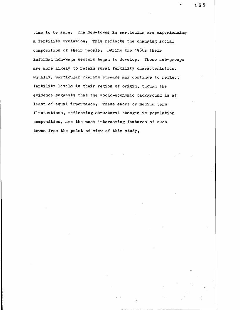
time to be sure* The New-towns in particular are experiencing a fertility evolution# This reflects the changing social

composition of their people# During the 1960s their

informal non-wage sectors began to develop* These sub-groups

are more likely to retain rural fertility characteristics* Equally, particular migrant streams may continue to reflect fertility levels in their region of origin, though the

evidence suggests that the socio-economic background is at least of equal importance* These short or medium term fluctuations, reflecting structural changes in population composition, are the most interesting features of such

towns from the point of view of this study#

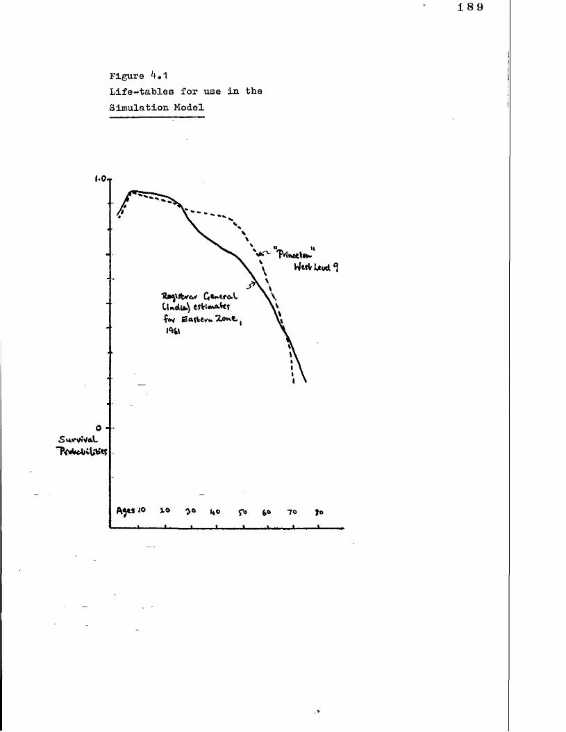
FigureLife-tables for use in the Simulation Model

Figure k.2Fertility Schedules for use in the Simulation Model

T^ccw’' (>•** 1f * #.r

JO-Ilf

A<je*Mr-Vl

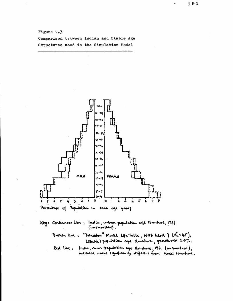
191

Figure ^*3Comparison between Indian and Stable Age Structures used in the Simulation Model

'fopJbsJbfe*. \w totA*. o^a

Ktn*. U*u. *, ln«A;o. t 'pofJU.fa*- c*)t H6(

‘Voakftv^ U **t *. M cwttL JLif t T&bU, t W ttlrtS fecJU O 'JO p -lM rio w Owtye f^ w n - k ^ ( g v d u f e v ^ - i * O * / * ,

Rc»l * )*A\6» t /mv^ oj»AfcVlo»v 6 4 3b**tt'u<c, k (unf»**•• M%edJ jUW brt ^v«iw K\t>4(i fim U 'U v t ,

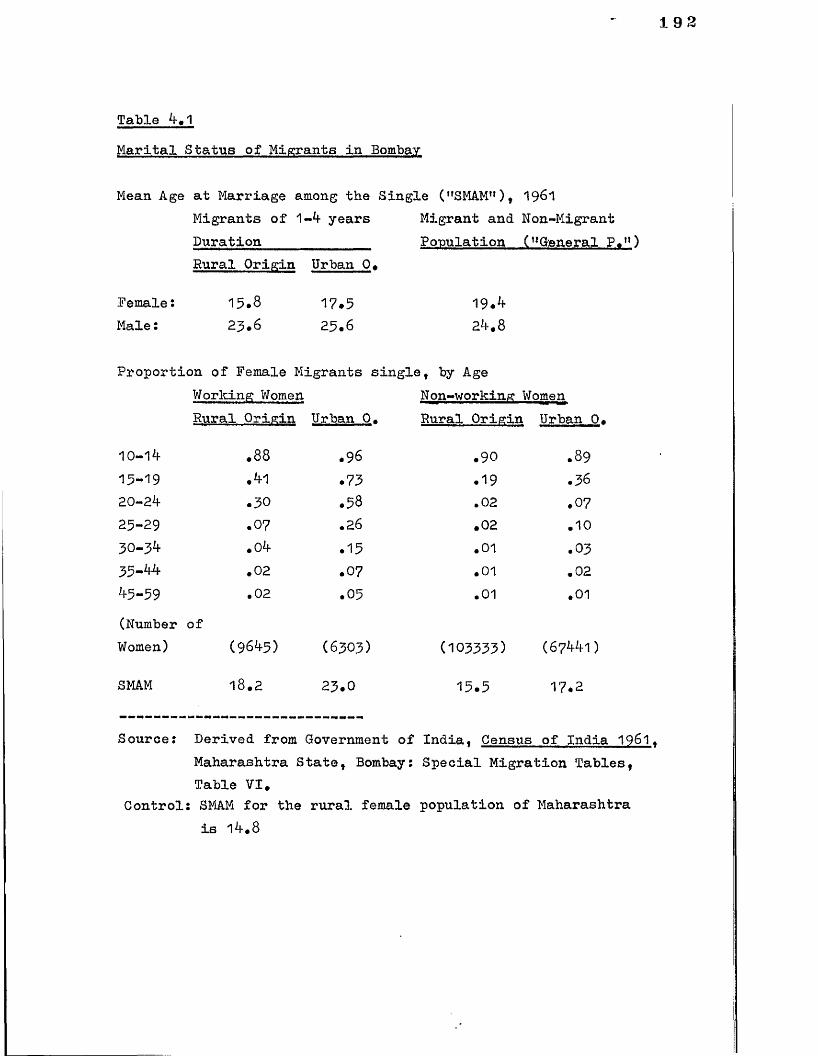
19 2

Table *f.1Marital Status of Migrants in Bombay

Mean Age at Marriage among the Single ("SMAM11), 196*1Migrants of 1-4 years Migrant and Non-MigrantDuration______________ Population ("General P.u )

Female: Male:

Rural Origin Urban 0 .

15.82 5 .6

17.525.6

19.^2*f.8

Proportion of Female Migrants single, by AgeWorking WomenRural Origin Urban 0 .

10-1*1- CO00. • 961 5 -1 9 .*H .752 0-2*f .50 .5825-29 .07 .2 6

3 0-3*1- .0*f .1535-*^ .0 2 .07*1-5-59 .0 2 .05(Number ofWomen) (96*l-5) (6303)

SMAM 1 8 .2 2 3 .0

Source: Derived from Governme:

Non-working Women Rural Origin Urban 0.

.90

.19

.02

.02

.01

.01

.01

(103555)

15.5

.89

.56

.0 7

.10

.03

.02

.01

(6 7H 1 )

17.2

Maharashtra State, Bombay: Special Migration Tables, Table VI.

Control: SMAM for the rural female population of Maharashtra is 1*f.8

Table 4.2Child-Women Ratios among Migrants to Bombay (and other Indices)

State of Origin(by birth)(Number of Migrants of 1-4 yrs. Duration in brackets)

C.W.R.Migrants of 1-4 years Duration

C.W.R.

< 1 years Duration

Sex Ratio Migrants 1-4 yrs. Duration

.a

Sex Ratio Child* Migrants 1-4 yrs. Duration

MAHARASHTRARural (134226) .508 .619 }

, .734 }.919Urban (8 9 3 0 6) .6 6 6 3 .821 3

GUJARATRural (39228) .708 , .721 \

f .912 } .952Urban (30675) .8 8 1 3 .8 5 8 3

UTTAR PRADESH and BIHARRural (63138) .336 j .202 7 ■

f .466 L .973Urban (14902) .5 9 0 3 .3 3 3 -J

KARNATAKARural (22935) .530 7 .577 7

> .735 J .983Urban (15358). .549 * .759 3

TAMIL NADURural (14791) .462 7 .5 1 8 1

f .827 \ .987Urban (8489) .6 0 3 * .644 3

KERALARural (16323) .533 ) .316 }

\ .734 ) .8 8 5Urban (6 1 5 6) .532 .449 3

Notes: Children aged 0-4, Women aged 15-44j f. : m.Source: As for Table 4.1 above, derived from Table II* Control: CWR for Bombay = .553

Table *f.3Indicators of Birth Rates in Sample Districts

Per Cent of Male Child-WomenPopulation under Ratio5 (1 9 6 1)

WEST BENGALCalcutta 7.2 .^ 8 8

Howrah 9.6 .6 2 7

Parganas 10.5 • 6 ^9

Hoogley 10.5 .6 2 5

Burdwan ; 1 0 .3 .6 3 1 See TableMidnapore 12.5 .611

Bankura 13.6 .6 8 2

Birbhum 13.1 .693BIHARPatna 1 2 .8 .7 0 0

Gaya 13.5 .719Shahabad 13.0 .6 8 9

Bhagalpur 12.7 .7 1 2

Monghyr 1 ^ .2 .737Dhanbad 1 0 .2 .6 8 9 Rapid Growth - HeavyRanchi 13.1 Industry.732Singbhum 12.9 .7 0 0

ORISSAMayurbanj 1 2 .6 .711Sundargarh 9.3 .5 5 6 Rapid Growth - HeavyCuttack 1 1 .0 - .6 6 1 IndustryBaudh-Kh. 9.3 .509Bolangir 1*f. 2 ♦ 637MADHYA PRADESHRaigarh 13.7 .6 2 0

Bilaspur 13.5 .329Durg 1 1 .2 .6l*f Rapid Growth - Heavy

IndustryBastar 13.6 .623

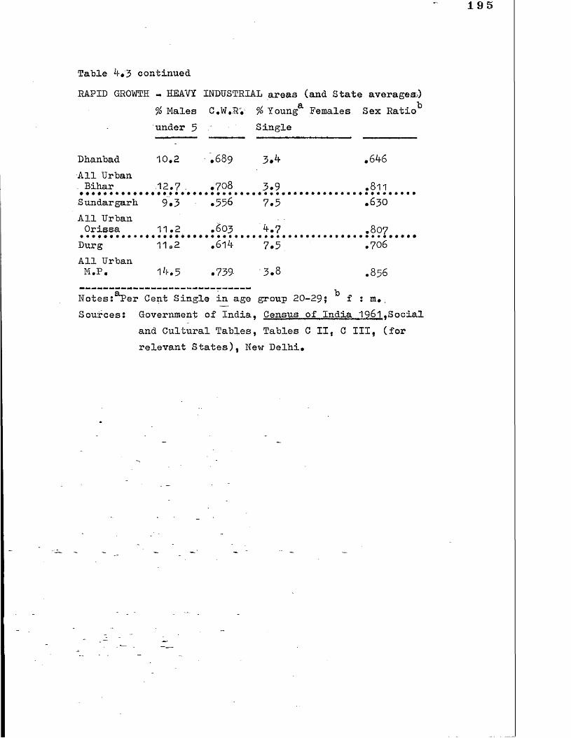
Table 4.3 continuedRAPID GROWTH - HEAVY INDUSTRIAL areas (and State averages,)

o b% Males C.W.RV % Young Females Sex Ratiounder 5 Single

Dhanbad 1 0 .2 • .689 3.4 .646All Urban . Bihar 12.7 - .7 0 8 3.9 .8 1 1

Sundargarh 9.3 .556 7.5 .6 3 0

All Urban Orissa 11 .2 .6 0 3 4.7 .8 0 7

Durg 11 o2 .614 7.5. .7 0 6

All Urban M.P. 14.5 .739 3.8 *8 5 6

Notes:^Per Cent Single in age group 20-29; ^ f : m*. Sources: Government of India, Census of India 1961.Social

and Cultural Tables, Tables C II, C III, (for relevant States), New Delhi*

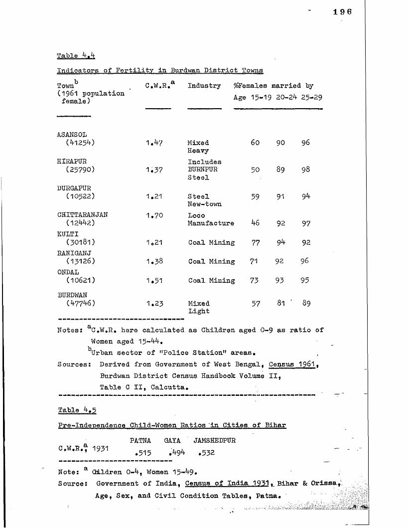
19

Table *f.*fIndicators of Fertility in Burdwan District TownsTown(1 9 6 1 population female)

ASANSOL

C.W.R.' Industry ^Females married byAge 15-19 2.0-2*+ 25-29

(**•125*0 1.*f? MixedHeavy

60 90 96

HIRAPUR(25790) 1.37

IncludesBURNPURSteel

50 89 98

DURGAPUR(1 0 5 2 2) 1 .2 1 Steel

New-town59 91 9*f

CHITTARANJAN (1 2**-**-2 )

1.70 LocoManufacture *f6 92 97

KULTI(3 0 1 8 1) 1 .2 1 Coal Mining 77 94 92

RANIGANJ (1 3 1 2 6) 1.38 Coal Mining 71 92 96

ONDAL(1 0 6 2 1) 1.51 Coal Mining 73 93 95

BURDWAN(^77^6) 1.23 Mixed

Light57 81 ’ 89

Notes: aC.W.R. here calculated as Children aged 0-9 as ratioWomen aged 15-^*

■jUrban sector of ‘'Police Station" areas*

Sources: Derived from Government of West Bengal, Census 19&1« Burdwan District Census Handbook Volume II,Table C II, Calcutta*

Table *f*5Pre-Indenendence Child-Women Ratios in Cities of Bihar

PATNA GAYA JAMSHEDPUR .515 f a 1* .532C ,W.R., 1931

Note: a Children 0-**-, Women 15-^9.Source: Government of India, Census of India 1931. Bihar & Orissa,.

Age, Sex, and Civil Condition Tables, Patna*

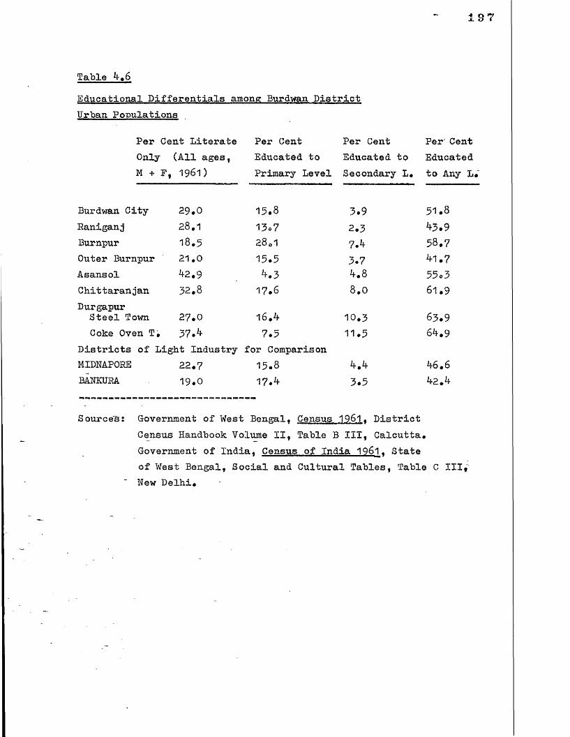
197

Table A.6Educational Differentials among Burdwan. District Urban Populations

Per Cent Literate Per Cent Per Cent Per CentOnly (All ages, Educated to Educated to EducatedM + F, 1961) Primary Level Secondary L. to Any L<

Burdwan City 2 9 .0 1 3 .8 3.9 51.8Raniganj 2 8 .1 13o7 2.3 ^3.9Burnpur 18,5 28 o1 7.*f 58.7Outer Burnpur 2 1 .0 1 5 .5 3.7 Vi. 7

Asansol ^2.9 ^•3 k.8 55o3Chittaranjan 3 2 .8 1 7 .6 8 .0 61.9Durgapur

Steel Town 2 7 .0 1 6.^ 1 0 .3 63.9Coke Oven T . 37.^ 7.5 11.5 6^*9

Districts of Light Industry for ComparisonMIDNAPORE 22.7 15.6 A-6 .6

BANKURA 1 9 .0 17.4 3.5 A-2.4

Sources: Government of West Bengal, Census 1961. DistrictCensus Handbook Volume II, Table B III, Calcutta, Government of India, Census of India 1961^ State of West Bengal, Social and Cultural Tables, Table C IIIf New Delhi#

Table 4.7Marital Status in Selected Contrasting: Urban Localities

Per Cent of women single by ' C.W.R. age group, 1961

15-19 20-24 25-29

Burdwan District_

ASANSOL(Police Station)

27.7 5.6 1 .0(City)

.6 8 5

BURDWAN(PoS.)

42.5 17.6 6 .8(City)

.551

DURGAPUR 40.6 8 .8 4.2 n.a.CHITTARANJAN 54.0 8 .1 2 .0

West Bengal (rural+ur ban)

11.a. .753

East Madhya PradeshDURG(Urban District) 15.6 1 2 .8 1 .0 ,6l4BILASPUR(U.D.) 24.6 4.6 1 .0

Mad. Prad* (rural+urban)

*634.769

MaharashtraPOONA(City)

5^.6 19.1 5.5 .6 0 8

THANA(City)

60.4 1 9 .0 6 .1 .592

SHOLAPUR 3^.8 11.4 1.5 .697(City)

Maharashtra .710 (rural+urban)

Sources: Government of West Bengal, Census 1961, DistrictCensus Handbook (Burdwan), Vol II, Calcutta;Government of India, Census of India 1961.Maharashtra, Cities of Maharashtra, New Delhi;Madhya Pradesh, Social and Cultural Tables, New Delhi; Tables CII and CIII in all cases* ~ -

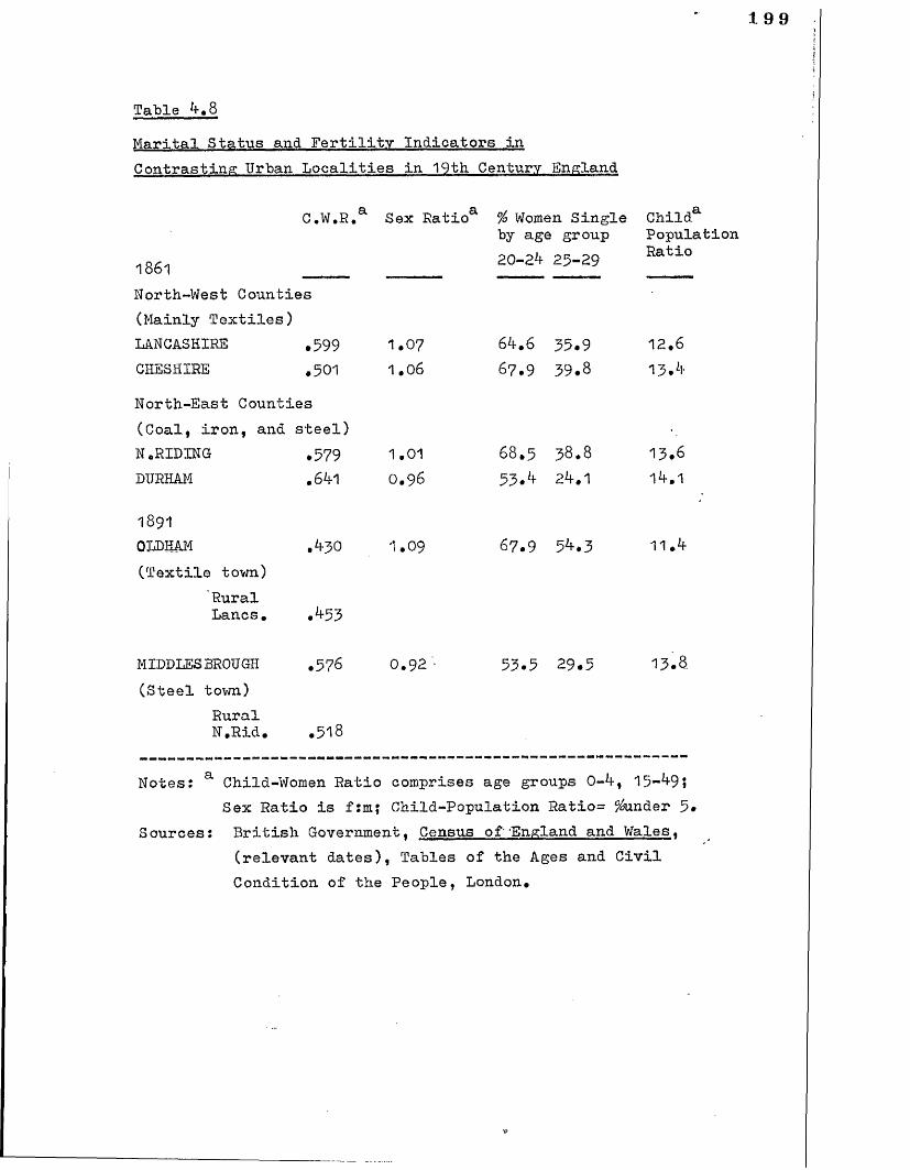
Table 4.8Marital Status and Fertility Indicators inContrasting Urban Localities in 19th Century England

C.W,R.a Sex Ratioa % Women Single Child3-

1861 2 0 - 2if 2 5 " 2 9

by age group Population Ratio

North-West Counties (Mainly Textiles)LANCASHIRE .5 9 9 1*0? 64.6 35*9 1 2 .6

CHESHIRE .501 1 .0 6 67.9 39.8 13.4North-East Counties (Coal, iron, and steel)N.RIDING .5 7 9 1.01 68.5 38.8 13.6DURHAM .641 0 .9 6 53.4 24.1 14.1

1891

OLDHAM .430 1.09 67.9 54.3 11.4(Textile town)

RuralLancs. .453

MIDDLESBROUGH .5 7 6 0 .9 2 - 53.5 29.5 1 3 .8

(Steel town)RuralN.Rid. .518

Notes: a Child-Women Ratio comprises age groups 0-4, 15-49;Sex Ratio is f:m; Child-Population Ratio= Sunder 5.

Sources: British Government, Census of-England and Wales.(relevant dates), Tables of the Ages and Civil Condition of the People, London.

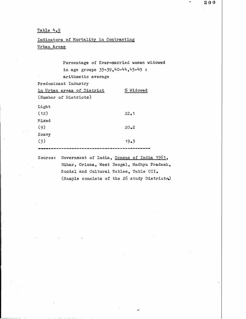
Table *f.9Indicators of Mortality in ContrastingUrban Areas

Percentage of Ever-married women widowed in age groups 3 5-3 9* , ^ 5 - ^ 9 ; arithmetic average

Predominant Industryin Urban areas of District % Widowed(Number of Districts)Light(1 2) 22.1

Mixed(9) 20.2Heavy(5) 19.3

Source: Government of India, Census of India 1961.Bihar, Orissa, West Bengal, Madhya Pradesh, Social and Cultural Tables, Table CII* (Sample consists of the 26 study Districts)

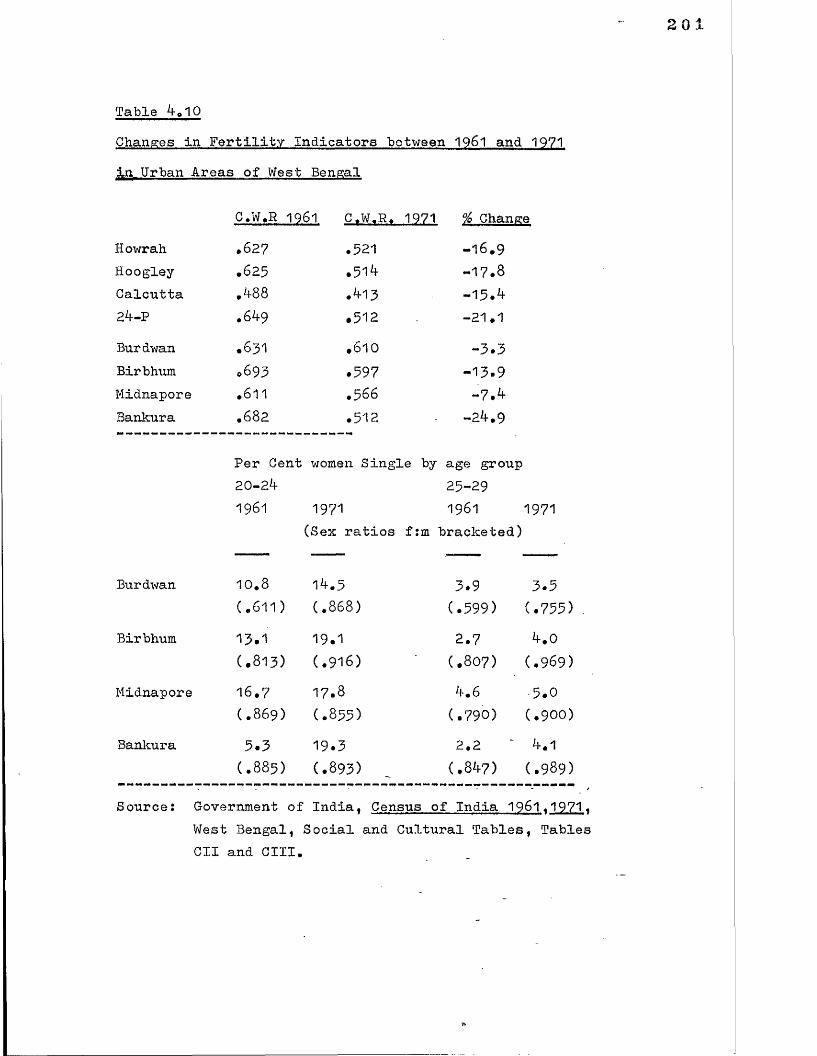
Table 4.10Changes in Fertility Indicators between 1961 and 1971 In Urban Areas of West Bengal

C.W.R 1961 C.W.R. 1971 % ChangeHowrah .6 2 7 .521 -1 6 .9

Hoogley .625 .51** -1 7 .8

Calcutta .488 .**13 -15.424-P • 6^9 .512 -2 1 .1

Burdwan .6 3 1 .6 1 0 -3.3Birbhum 0693 .597 -13.9Midnapore .611 .5 6 6 -7.**Bankura • 682 .5 1 2 -24.9

Per Cent women Single by age group20-24 25-291961 1971 1961 1971

(Sex ratios f:m bracketed)

Burdwan 1 0 .8 14.5 3.9 3.5(.6 1 1) (.8 6 8) (.599) (.755)

Birbhum 13.1 19.1 2.7 4.0(.813) (.916) (.807) (.969)

Midnapore 1 6 .7 1 7 .8 4.6 5.0(.8 6 9) (.855) (.790) (.9 0 0)

Bankura 5.3 19.3 2 .2 4.1(.8 8 5) (.893) (.847) (.989)

Sourcei Government of India, Census of India 1961.1971* West Bengal, Social and Cultural Tables, Tables CII and CIII.

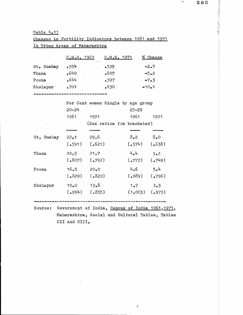
202

Table 4. 11Changes in Fertility Indicators between 1961 and 1971 In Urban Areas of Maharashtra

C.W.K. 1961 C.W.R. 1971 % ChangeGt• Bombay • 55^ #539 -2.7Thana .640. .607 -5.2Poona .644 #597 -7.3Sholapur

i• -0 O _A .6 3 0 -1 0 .1

Per Cent women Single by age group2 0 -2 4

1961 197125-291961 1971

(Sex ratios f:m bracketed)

Gt * Bombay 22.1 29 06 8.2 8.0(.591) (.6 2 1) (.57*0 (.6 3 8)

Thana ZZ 0 3 21.7 4. 4 5.2(.807) (.792) (.777) (.7^9)

Poona 16.5 2 0 .0 4.6 5.4(.829) (.8 2 0 ) (.989) (.798)

Sholapur 1 0 .0 1 3 .8 1.7 3.3(.99*0 (.855) (1.003) (.973)

Source: Government of India, Census of India 1961<1971«Maharashtra, Social and Cultural Tables, Tables CII and CIII#

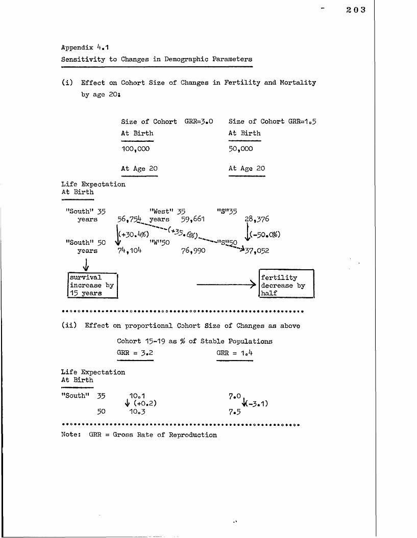
Appendix *+.1Sensitivity to Changes in Demographic Parameters

(i) Effect on Cohort Size of Changes in Fertility and Mortality by age 2 0t

Size of Cohort GRR~3 *0 Size of Cohort GRR=1„5At Birth 100,000

At Age 20

At Birth 50,000

At Age 20

Life Expectation At Birth

"South" 35 years

"South" 50 years

"West" 35 "S"3528,376

$0- 1(-50.C80"W"50 '*"--"Sm50 ^7^,10 7 6 ,9 9 0 ^ 3 7 ,0 5 2

56,75^ years 59,661

l(+30.W) '(*35.

Isurvival v fertilityincrease by ■ ...... ... decrease by15 years half

(ii) Effect on proportional Cohort Size of Changes as aboveCohort 15-19 as % of Stable Populations GKR = 3.2 GRR = 1<A

Life Expectation At Birth

"South" 35 10«1 7.0,^ (+0.2) k-3* 1)

50 10.3 7.5

Note: GRR = Gross Rate of Reproduction

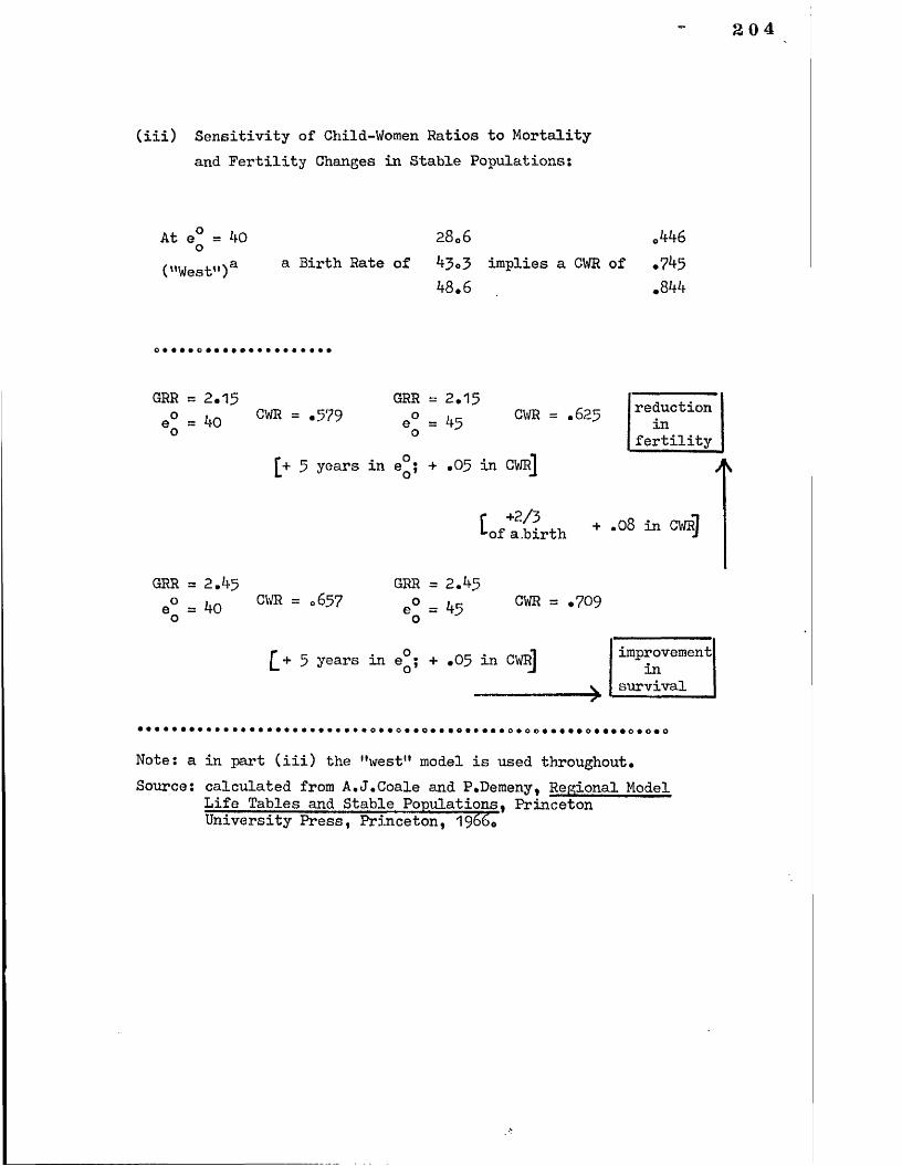
204

(iii) Sensitivity of Child-Women Ratios to Mortality and Fertility Changes in Stable Populations:

At e° = hO 2806 0Vf6o("West")3, a Bat© of ^3o3 implies a CWR of *7 5

*f8.6 .84^

GRR = 2.15e° a ko o

GRR = 2.15 CWR = .579 e° s lf5 CWR = .625

o£+ 5 years in e°; + .0 5 in CWRj

reductionin

fertility

[ + -08 in CWR]uof a.birth J

GRR = 2.^5e° a lto G m =

GRR = 2.^5eO = k3 CWR = .709 o

£ + 5 years in e°; + .05 in CWR] improvement in

survival

Note: a in part (iii) the "west" model is used throughout.Source: calculated from A.J.Coale and P.Demeny, Regional Model

Life Tables and Stable Populations. Princeton University Press, Princeton, 19660

A brief Overview of Chapter k

Fertility can only modify the effects of migration gains or losses of the scale described in local populations# But differential fertility may have a sub­stantial effect on the relative future size of population groups (with implications for social tensions) and of cohorts of the same age but from different regional background (with implications for the future competition for the most prized industrial jobs)# Empirically there are clear indications of such differential fertility and differential fertility change.

206

CHAPTER 5

The Migration Component Explored

A Summary of the Main Empirical Points

The characteristics of the migrants to towns and cities of differing industrial structure are examined as an indicator of the effect of labour demand (and especially wage-labour demand) on the demography of the urban areas#There is some evidence of particularly young (adaptable) labour forces being favoured in industries with new technology; and of female labour being favoured in certain processing household-based industries. It is overwhelmingly clear that heavy industrialisation has promoted long-distance migration, and hence towns of mixed linguistic composition: but the rather high average component of urban-origin labour among migrants in our area (retarding effectively an overall rural to urban population transfer), is less easy to relate to industrial composition. It seems that heavy:industrialis­ation is not the major cause. Nor do heavy industrial town areas draw disproportionately from stagnating urban areas (though, being large, merely to take their proportionate share is to make anon-ftrivial', impact).- We argue, as a working hypothesis, that wage-labour migrants are a fairly distinct social category (likely to have possessed small land-holdings, and, a small proportion having retained divided families - especially those employed in more traditional industries), in contrast with the local "multiplier^-type migrants, less often working as wage labourers, (and likely to be landless, and-, in'part, forced into-migration, and moving usually as a family whole).

207

The Migration Schedules

Central to the thesis are the age-specific migration schedules, and to these we now turn. The level of male

migration is a variable in the model. It is this that we seek to change over a wide range in order to indicate the demographic result of decisions on industrial strategy, the size, and the time-phasing of projects. But the age distribution of the schedule is taken to be rather more of a parameter,, Our basic source for this is the National Sample Survey (NSS) of 196^ on Internal Migration (Table 5*1). Initially we can concentrate on the rural to urban male migrants1 age profile, as from the 1961 Census it is clear that at least frds of male migrants in our region are of

this kind (Table 5 #10). The Survey of course records gross in-migration (there being separate tables on gross outmigration). The Census also tells us that, on average, the place of origin of migrants is fairly evenly divided between the "same District", "another District" and "another State" (West Bengal being an exception at the State level of aggregation). So the schedules used for the model were made to be an arithmetic average of the age profiles of these three streams. We then had to re-arrange the data

2 0 8

into age groups appropriate to population projection, i.e. 5-year cohorts (from the idiosyncratic grouping adopted in the NSS report), and this re-allocation was done "by eye" to obtain the reults illustrated in Figure

5.1.Now it was our initial assumption that most female

migrationwas due to male migration: what requiredestimation, we believed, was the appropriate lag

structure. To obtain this, female migrants of less than one yeai s duration were related to male migrants of less than one year's duration, one to five years duration, six to ten years duration, in a linear regression.The data used were from the sample Districts in the Eastern region. Interestingly, only 2/5ths of the squared variation (R ) in female migration on a District-wise basis could be explained by male migration. Low though this explained variation may be, it should be noted that the National Sample Survey of female migrants conducted in 196^ found that only 12% migrated for marriage purposes and 30% to join family members (including husbands presumably) so that altogether only 62% of female migration could be linked directly with male migration. Appendix 3 presents the statistics of our regression. As a check on this a similar regression was done for all the Districts of Maharashtra, with similar results. The male migration of 6-10 years

previous was not significant in determining female migration flows. The other two variables (less than

one year, and 1 -5 years) were highly significant.They indicate that the coefficient of response (as we may call it) is about 0 .3 2 (unlagged) and about 0 .1 7

(for a lag of between 1 and 5 years): that is to say,an increase nf 1000 in male migrants to a town would elicit a response of 320 female migrants in the same year, and a further 170 over the next five years. The response function, then, would be of a declining exponential kind (not unimodal, or lagged in the strict sense, for in that case the response would have been greater in the following five years, not less). Again a check using

the data for Maharashtra substantiates the order of magnitude of these coefficients. For the purposes of the model autonomous female migration, like the male migration, is regarded as a variable, that is we can change it at will in different models, or model variants.However, there is reason to believe that a proportion of this female migration must relate to the demographic structure of the non-migrant population: perhaps a proportion that are reported as migrating for domestic purposes (in the NSS) are joining or marrying the native- born. These would not be explained by our female migration "response" equations*

A further explanation for the apparent "autonomous" migration of females may lie in the large variation in

male migration. If the latter relates specifically to the variation in impermanent (or "turnover", or seasonal) migration, that would not precipitate a female response, then the female migration may be more fully explained

by the permanent male migration alone, of men whose jobs are pre-arranged, or at least of men who have come to stay. Unfortunately there is no accurate method of estimating the proportion of male migrants^-who are of the latter category, nor of knowing how far they were included in

the Census count in urban areas. We can make estimates of the long-term split-family migrants, but they are very much in a minority (see the discussion on Bombay in Chapter k above). But we do not have estimates of different degrees of "marriage response" (as we shall call it) according to the occupation or class of migrant: in the course of thisstudy we follow through the argument that factory-employed

1 It is also universally observed that the sex ratios among recent*migrants are higher (more women to men) in migration streams from urban to urban areas. Split families are less likely to be maintained for more than a brief interval in these cases (partly because of the high cost of maintaining two urban dwellings (Table 5.1 3)•

migrants, who are typically from small-farm owning

backgrounds, bring their wives into the town aftera short time period once their position is secured(or in a minority of cases remain as a split family),whereas other migrant workers, especially those inthe non-wage sector, who are more likely to be landless,

1migrate with their wives in the first instance* It follows that the sex ratio among migrants will, over the short run of five years at least, be variable^dependant upon the pi’edominant characteristics of the migrant streams: we try to predict this from the industrialcomposition of different urban areas, though clearly the condition in the rural areas (especially of the same

1 This is supported by a survey recently undertaken in Bombay that indicates that 79% of females who joined other family members (largely husbands) in the factory sector did so once they had secured employment, and only 11% came before a job was secure, whereas in the case of casual workers 60% joined joined husbands with jobs, and 33% came with them in speculation. See L.K.Deshpande, "The Bombay Labour Market" (unpublished), Department of Economics, University of Bombay, 1979*

212

District) is an important determinant here too* The differences in sex ratio that persist in the long-run among migrants are of more demographic significance in the eventual population composition of the town, once some degree of stability is achieved (and these were discussed above in Chapter *0.

1 A survey with which the author is familiar, carried out in Poona, throws some light on the economic back­grounds of migrants in different urban industrial employments or occupations: a slum settlement in which over 2/3rds of the household heads surveyed were in formal industry, municipal service, or working as skilled labour, contained bk% of migrants who still had land, one half of them, however, owning less than two acres. In a contrasting slum settlement where over 2/3rds of household heads were in petty trade or casual service only 12% had land (though 87% had previously been employed in agriculture). This was

■ despite the fact that a higher proportion of the latter migrants were local. See M.Bapat, 11 Occupational and Spatial Mobility among Shanty Dwellers in Poona,"Ph.D. Thesis, University College London, 1979#

Similar findings come from the survey carried out in Bombay (referred to in the previous Note) by L.K.Deshpande. The population was divided into factory workers, casual workers, and those in small establishments. Of the factory workers, 72% owned land in rural areas, with an average holding of 2 .7 acres, whereas of the casual workers, at the other end of the scale, 5 1% owned land with an average holding of 2.1 acres. These surveys are at least consistent with what we have inferred from demographic indicators: that factory manufacturing workers are morelikely to own land than other (non-white collar) workers.

We have devoted some time to explaining the variance in female migration when related to male migration* For all this, there will be a small proportion of women who migrate alone for jobs or further education, as revealed in the Sample Survey (where about 15% were so categorised)* Initially, for the purposes of model-building, these women will be ignored;, their inclusion is one of the more important varations we make in the model (see Chapter 3)*The "turnover” and seasonal male migrants are also ignored.

And the women who join the native-born are also left out; they would be partly balanced by an outmigration of women who join rural husbands, in any case* Hence the response coefficient will be taken to suggest the absolute size of the female in-migrant flow* To repeat, 1,000

males will be followed by 320 females in the same time period, and 1?0 in the following quinquennium; in some variants up to 250 additional females are allowed to migrate*

From this starting point a more elaborate hypothesis will be adopted. The age distribution of these migrants has to be heavily reconstructed. Insofar as female migration is a response, its age distribution is related to the past male migration history: i.e. the NSS female age profiles are only appropriately related to a combination of the male migration streams that preceded, and those that took place during, the NSS reference period (one year).

1 Some areas of the country, especially in South India, experience net female outmigration to urban areas.

Given the age differential at marriage (about 5 years in•i

1 9 6 1) , a five-year lag would be needed to give a similar male and female age distribution (cet# par*) among migrants.

These phenomena are compounded in the NSS data# First I will offer an explanation of these data, and hence I hope to justify the age-specific female response migration schedules I have constructed (Figure 5*1)* To anticipate, the effect of reconstruction is to make the current female migration profile that relates to current male migrants alone rather younger than the NSS age profile#

Hestricting ourselves still to rural-urban movements we see first a higher proportion of female infants among female migrants (than male infants among male migrants),

though the absolute number of males is a little higher than females in this age group (as is the case in the national population also) due to superior survival# The next age group has a distortion of the same kind# The 5-17 age groups are roughly similar in the "Same District” category but the female percentages are higher for the other cat­egories# Male ”turnover" migration will be concentrated in the earlier years of age and also is likely to be pre­dominantly local, hence females fail to dominate this first

category significantly* The female proportions in this age group among the non-local female migrants are high, and this illustrates the incidence of marriage migration, either to join residential males, or of females migrating

1 C.R.Malaker, personal communication on material from his Ph.D* thesis on Nuptiality in India, still in progress when this Chapter was prepared, Demographic Unit, Indian Statistical Institute, Calcutta*

contemporaneously with migrant males: in both cases the age differential at marriage accounts for the dominance of females in this: age group. The l8-2*f group of females is also proportionally quite high, combining those responding to male migrants migrating when in the 25-3*+ age group (and recorded in the NSS male stream), together with those joining male migrants who migrated a few years earlier (not recorded in the NSS)# Disentangling these sub-groups in order to construct a female response migration schedule is not possible on a rigorous basis* The schedules we present are the result of first re-grouping the NSS data into 5-year age groups and smoothing the result; then talcing the mode of the new female schedule that we construct to be 2 0-2 - years of age for those in the 1 -5 year lagged response group,(who will have been 1 5 -1 9 when they married), and 1 5 -1 9 years of age for the unlagged response. (By applying the weights suggested by

the regression coefficients to these two groups we can reproduce the NSS female migrant age profile again as a broad check on the validity of the method). Clearly there is a crudity here: the regressions were notage-specific, and there must in fact be a lagged and unlagged "response" of pre-marriage migrant females to male migration; and additionally the pre-marriage male migration is itself a response to the migration of married males and females* But further sophistication would be

1 Some degree of autocorrelation in the error term will have resulted.

216

pure guesswork without age-specific Census data on current migration flows* Proceeding now to the tail- end of the schedules, the migration of the *+5+ group is insignificant quantitatively, and I have adopted a fairly arbitrary smoothing procedure* But interestingly these elder migrants are a not insignificant proportion of the elder total population (native and migrant), particularly in the case of females. I suspect they

are female widows, and aged couples whose ^oung folk have migrated, leaving an unviable family farm as the parents age**1

Age and Education in the Structure of the Industrial Workforce

In the economics of production, age is only significant in respect of the command it implies over the means of production. If an economy is expanding rapidly into new industries, or adopting radically new technology in the old ones, and if this implies an increasing need for new skills and new learning for which a secondary education is a sine-qua-non, then only the younger age groups in an economy are employable*It is a paradox that, in this sense, the stock of labour in India (as also in England today) is too old, not too

1 More information on age and marital status of migrantshas now been published in the 1971 Census, and is consistent with this particular hypothesis* See M.K.Premi,"Aspects of Female Migration in India", Economic and Political Weekly* April 12, 19^0*

21?

young, since it has a disproportionate number of people

over fifteen years of age who are illiterate, and adisproportionate number over twenty-five who are without a

•1secondary education* These people will be more costly to train than the younger cohorts* A steady supply of pre-school children plus 100% primary education is

necessary to provide the required future labour force in a technically modernising economy#

It is conceivable that a modern industrial estate or New-town would actually seek (i*e* demand, in the economists sense) a younger local age structure than the national#The neo-classical economist imbued with comparative statics will argue that this is irrational. If the skills are so scarce, then industrial specialisation .should not proceed in those industries that.are skill-intensive. This argument fails to address the question of the next generation, and fails to provide guidance on the question of how natural resource endowments change over time (whence would follow a change in comparative advantage). Indeed it relegates all education to the rank of consumption goods#

1 Data on literacy are available from the Indian Census down to 1981. Restricting ourselves to males only, even as late as 1981 crude literacy in Bihar is only 38%# In 1961 it was only 30%* and ^3 »5% in the 2 0-2*f age group (compared with ^9*8% for All-India)# In 1971 crude literacy rates were still generally below 50%: Bihar 31%* Orissa 38%, M.P* 33%* West Bengal ^3% and Maharashtra 51 %• Government of India, Census of India 1961* 1971. Social and Cultural Tables, Delhi.

218

It is possible, though not easy, to see how far particular industries select young labour forces deliberately, since the age structure of the occupations 1b recorded for a particular sample in the 19&1 Census: the sample consistsof large towns (above one lakh, i.e. 1 0 0 ,0 0 0 in population size, conventionally referred to as Cities), where these statistics are available for migrants only# I have selected

about 20 cases comprising virtually all those from the Districts under study in Eastern India supplemented with a number from Gujarat and Maharashtra (and one from Western Madhya Pradesh). The idiosyncracies of the Census-taking and publication mean that not all the Cities are equally well documented#

Interpretation of the data must proceed warily#Older industries, if they fail to expand at the rate of

supply of the labour force, will develop an older age structure than the average# The only way to check this is to examine the data in the special migration tables for Bombay, Ahmedabad, Jamshedpur and Dhanbad, where duration of residence is cross-classified by age in

particular occupations, and by levels of education#For the purpose of this analysis we need to exclude those occupations whose age structure is dependant on promotion through seniority; the administrative and managerial classes

1 In a detailed survey of factory labour in Poona, R.D'.Lambert came to the conclusion (too hasty in the view of the author of this thesis) that differential age structure was solely due to this cause. See R#D.Lambert, Workers. Factories and Social Change in India. Princeton University Press, Princeton, 19&%

219

are likely to be both more educated and older* In fact we will restrict ourselves to concentrate on the manual

employee groups, workers in transport and communications, production workers, and service workers (to use the National Occupation Classifications)* Miners will be

referred to later* From Table 3*3 it can be seen that production workers are more heavily represented in the younger age group, i.e. 15-3 * than are other workers.This remains true when we standardise (as we can only in the case of the special sample mentioned above) for recency of arrival* This is broadly consistent with our hypothesis that in the new or modernising industries (which are all well represented in many of these Cities) young recruits are preferred.

It would be better, however, to have information for particular occupations within that large industrial category of production or manufacturing workers*Unfortunately this limits us to one City, Ahmedabad (Table 3*2). Of the six production occupations we have, two are characterised by higher literacy rates (and a higher incidence of secondary education): tailors and tool-makers (and makers of precision instruments), and indeed these two groups are characterised by a younger age structure at both durations of residence recorded, including current migrants

-j(Tables 3*2 and 5*3)* Of course these data are only broadly

1 Textile workers generally are in large part factory workers* Tailors are more likely to be self-employed small business­men* Hence presumably the importance of literacy.

in line with our expectations, and anyway Ahmedabad could be a special case*^

1 A regression on this small sample attempts to attribute the age structure quantitatively to both forces, recency of recruitment and educational attainment* All occupations reported, except the administrative and professional^are included. We find that the two factors between them explain only of the squared variationin age structure (R )• Education is wholly insignificant.This indicates: ;a number of things in regard to the sample* First, although we set it up as though it were a demand schedule, clearly it is not, since the measured characteristics are those that cleared the market (supply and demand interacting). We have come across this phenomenon in other cities inhere a high local supply of educated labour resulted in high levels of education appearing in the residual (largely casual) worker categories* Secondly, and more substantially, the relationship can be expected to be discontinuous. There are a limited number of occupations where the demand for young labour is determined by educational requirements (in theory); these may be restricted to the spearhead of modern industry*

The other variable, duration of residence, is highly significant. A 10% addition to the proportion of recent (1-3 years) migrants raises the proportion aged 15-3^ by 7%* This underlines the importance of duration as an over-riding determinant of age structure, taldng all occup­ations together+ and hence also of the speed of expansion or contraction of the industry in question* Lamberts contention would seem to be vindicated (see note above).But we (and he) are concerned principally with the manufact­uring industry (and the sample was too small to confine the test to those occupations alone). Table 5*2 (and Table 5*3) would suggest that duration alone loses its explanatory dominance in the analysis of age structures within the manufacturing industry.

With the caveat of a likely bias introduced through recency of recruitment kept in mind, let us look now at the recorded occupational age structure in the City sample (Table 3*3)* I have selected for illustration occupations that are representative of the industries under study* In particular this means that tool - makers and other metal - workers feature predominantly in the Eastern States, whereas textile - workers predominate in the Western States. The average age of the former two occupations is below that of the latter, and the education level is higher, but clearly this relates partly to the age of the industrial capital stock. Less ambiguously the occupational group of electricians is significantly younger in all areas (and their educational level higher). It is particularly instructive, however, to look down the columns in Table 3*3 under particular occupations. It is noticed for example that a particularly young age structure is found among the textile workers in Ulhasnagar near Bombay: this new industrial development incorporatesthe latest technology (and the largest scale of plant, as noted in Chapter 2 above). Consistent with this, the proportion of secondary school matriculates in that age

group is far higher than in the rest of Maharashtra's textile workforce (and illiteracy lower). The other newly developing industry of the Western States is the chemicals

industry, which was still at a very early stage of development in 1 9 6 1s here again Thana and Baroda have a highly qualified v/orkforce in that occupation to judge from age-specific education rates, and a very young age structure. The high

qualifications of tool-makers and their young age structure is clear in the new industry at Ranchi, and the metal- making industry will be discussed in more detail below

in the case of the only modern integrated steel plant in our City sample, at Bhilai (Durg-Bhilainagar Town Group).

It is. .also worth discussing the exceptions, and this leads us to look along the rows in Table 5*3 rather than down the columns. One City that seems to be a consistent exception to any hypothesis is Jamshedpur, the private sector Company Steel Town. Here the educational qualifications are particularly notable, yet the age structure is curiously old. The latter can be related to the paucity

of migrants during the 1951-1961 decade, in comparison with some of the other heavy industrial Cities. The foundation of the industry here pre-dates the Second Plan. Exceptionally (in their day) the Tatas recruited a migrant labour force for work in their mills and then trained it on the spot to a high level of skill. Subsequent capital expansions were carried out with less further labour recruitment (and, more recently, no doubt with the sons of the labour force already there and educated in the local

223

schools•) With the establishment of public-sector training centres, near emerging industrial localities, this

phenomenon is likely to be repeated, and in this repsect we refer to the City of Ranchi again below* We deliberately included Bhopal (in Madhya Pradesh) in the City sample to discover whether a centre with a newly developed modern electrical or engineering industry would also put a premium on education* In fact it illustrates one of the best-educated cohorts in the Table, and almost all the electricians are in the younger age group; in a State with a low education record (noted above) this is clearly not the result simply of a supply of youthful migrants, but a feature of demand requirements* We cite specific example in the section that follows to indicate the care with which

1 Daily employment at the Tata Iron and Steel Companywas on average 2 2 ,6 6 2 in 1 9 1 6 -2 3 (with output • at 2 0 0 ,0 0 0

tons). From 1935-39 employment was reduced to 19*309(while output rose to 700,000)* By the time of the 1961

Census the mill was rated at 2 million tons, double pre­war capacity, but its labour force was only 3 0 ,0 0 0.By then its ever-migrant labour force of 25,000 was no larger than in 1926-7* What had changed was the white-collar contingent in the work-force: its increase had perhapscontributed towards the ageing of the employees (i.e. with capital-using expansion there was relatively more labour recruitment (or less retrenchment) at the senior end of the scale* See S.K.Sen, The House of Tata (1859-1959). Calcutta Progressive Publishers, Calcutta, 1975? and Government of India, Census of India 1921. 1951< 19^1,State of Bihar (& Orissa in 1921), Delhi (Patna in 1921), (Special Tables for Jamshedpur in 1961)*

the post-Independence heavy industries selected their labour forces*

To point up the contrast I have illustrated the thesis with a very traditional occupational group* millers, bakers, and brewers* Here, on average, only 55% of the workers are in the 15-3^ age group (as against 68% in the case of electricians). Needless to say, secondary school matriculates

(data not provided here) are uniformly a very low proportion, illiterates (Table 5*3) a uniformly high one. Of course this reflects the fact that bakeries have always existed in thetowns even before the impact of modern industrialisation*

However, there will have been a local multiplier effect, or at least an increased local demand for manufactured food and drink, and yet the resultant migration or absorption of resident labour has not selected noticeably the younger cohorts. This can be seen strikingly in the New-town

area of Durg (containing Bhilai Steel Town) where the proportion of young millers, though above average (61%) is still below the proportion of young electricians (7 2%)*

Finally it is instructive to look at the residual column, that is those labourers ’’not elsewhere classified” (in the Standard Occupational Classification); this will probably consist predominantly of casual labour whose occupational- ’’mix" defied the Census investigators. It is a large category. It tends to have an older age structure, but

this also relates quite closely to the rate of growth of the town in question# In a few exceptional cases it has a notable proportion of matriculates (i#e# 3% rather than 1% or less), as in Gaya, Asansol, and Jamshedpur in particular (Table 5*8)# These latter two are Cities that

acquired their modern industry at an earlier date; steel at Jamshedpur and also at Asansol's twin town of Burnpur, and hence built up an educated labour force# The Second Plan period of expansion of these existing plants failed to absorb this stock of qualified labour, and hence follows

its comparatively high representation in the residual occupational categories# How far this story may be repeated for the new engineering towns when their well-educated cohorts come on to the labour market in the 1970s and 1980s remains to be seen, but some indications of this emerging problem are illustrated below*

The overall age distribution of the work-force in a town will clearly be dictated, in most cases, by its duration of residence# The declining industries, and the tertiary sector (a labour absorbing sector) will have the older structures# The new industries will have young structures, though quickly ageing if subsequent expansion is accompanied by substitution of capital for labour#On the green-field, or greenish, industrial sites local industrial workforces are likely therefore to be younger

in all economic sectors initially, but especially so if the industry is of high technology# Skill-specific demand is likely to turn out to be age-specific (given the increasing illiteracy with age in the Indian population)# We would probably be right to "bunch11 our migrants specifically into the younger working age groups when illustrating the effects of migration to newly industrialising sites (as in our Model "1 b,u in Chapter 3) (which exacerbates future instabilities in the labour market)# As we have argued in Chapter 2, only in the case of iron and steel and heavy engineering is this phenomenon likely to coincide with very large local work-forces.In other modern plant capital substitution tends to out­weigh the effects of scale alone as far as the individual plant is concerned, though it still may be the case that economxes of agglomeration are significant#

1 Attributes of the work-force in a single industry areby no means standard across societies# We have noted this in Chapter above principally in regard to the employment of women# In a very careful comparative study of the textile industry, Saxonhouse and Kiyokawa show how Indian and Japanese mills differed in this respect over a similar period (and despite crude technical and demographic similarities). It is worth quoting their conclusion in full: "The high productivity, high turnover, high absentee.,closely supervised, largely female Japanese labour force can be contrasted with the low productivity, lower turnover, also high absentee and loosely supervised, mostly male Indian labour force* It is evident that the

A Case Study from Eastern Madhya Pradesh

We discuss here the sub-region of the new Steel Town development at Bhilai# As we noted above, older industries, if they fail to expand at the rate of supply of the labour force, will be inclined to have an older age structure than the average# For that reason alone, workers in transport, trades and communications, are

often older than their industrial colleagues in the newly developed industries for there were passenger buses before the steel workers arrived. The age Structure of an occupation represents an interaction of demand and supply, whereas our

current interest is to focus on demand# If we confine our observations to a single industry we tend to overcome that bias# The iron and steel industry at Bhilai employs both furnacemen and electricians, the latter on average being

footnote continues^acquisition of a mature, stable labour force does not necessarily result in industrial success#" G.Saxonhouse and Y. Kiyokawa,"The Supply and Demand for Quality Workers in.the Cotton Textile Industries in Japan and India",(Paper from a Conference on Japan’s Historical Development Experience and-the Contemporary Developing Countries, Feb. 1978), International Development Centre of Japan, 1978.

The Japanese textile worker was also more highly educated (they note): $3% being literate in 1 933 and 30% having post-primary education#

more skilled (and less illiterate): we see from Table(derived from the 1961 Census) that the age structure among migrants is slightly younger among the latter* The contrast with the age structure of the construction workers, whose skills are much less specific to the

plant, is clear; yet they were recruited at approximately the same time - only three years earlier.

The future implications of this are important*

The young work-force cohorts in modernising industries will tend to remain with those industries over time: their chances of recruitment into another industry elsewhere will diminish as they grow older. If a steel or engineering plant becomes outmoded it will cease to recruit new labour.Its labour force will age. If it faces closure its labour force will seek employment in industries whose demand for labour is not specifically toward the young. Thus the older the population age structure the more serious are the effects of an industrial monoculture when it goes into decline.

1 What is interesting is that this remains true if we consider the illiterates alone. They are slightly younger in the case of electricians than furnacemen, and in both cases clearly younger than illiterate construction workers.This is consistent with the argument that the potential for trainig can best be found in the younger groups.It is not simply a question of having to recruit young men if literacy is lequired as a qualification. Furnace­men, for example, are being recruited young so that they are trainable in the operation of the most modern equipment. Construction workers, on the other hand, need little specific knowledge of the technology of the plant,(a point brought out strongly in the context of Jamshedpur steel plant in the next section).

229

On a recent visit to Corby (United Kingdom) the authorfound it reported in the local press that the steelworkers now made redundant, on the closure of most ofthe integrated iron and steel works, were unlikely tofind employment in the county of Northampton (Figure 2*3).There is industrial growth in this County, but the newindustries, light manufacturing and electronics, favour

a younger work-force# The sons of the steel-workerswill have the opportunity in nearby Kettering andelsewhere to find employment in these expanding industries.Similar opportunities do not exist in the case of the SteelTown of Consett, also recently closed down, where thelocality, in the generally more depressed North Fast ofEngland, has no neighbouring growth centres. In a countrylike India with a "younger age structure, these particularproblems are less severe for the present: if layoffs mustoccur during stagnation, they will be of a less aged, more

redeployable, work-force# But in the young age structure wehave a more serious problem regarding the second-generationworkforce: the_sons of the migrants will not only be more in

thannumber/in the United Kingdom , but may be fired with stronger aspirations, given the novelty and promise of industrialisation#

T The comparative case-studies were pursued in some detail in Chapter 2 above#

This requires more rapid expansion of new industries, failing which, cet# par# the potential frustration will

be stronger.

We turn here to look briefly at sex structure in •

employment in the same region of Madhya Pradesh# Again it can be argued that wre have an interaction of demand and supply, in the sense that since the supply of women through migration to an urban locality is not wholly, or even mainly,

called forth by the demand for their labour, the actual employ­ment of women is not a simple case of a specific industrial demand# A significant feature will be that women are absorbed

in the non-factory sector simply because they are aleady in

the urban locality and will be seeking additional household income even for a considerable amount of effort expended or loss of leisure.

The District-wise sex ratios for workers, available

from the Census, are thus difficult to interpret# More enlightening is their disaggregation# For this purpose we look at contrasts in Durg and Bilaspur Districts# Both are subject to high rates of inmigration (from 1951-61): the former depends largely on the steel industry, the latter is more diversified# In the case of Durg, men preceded the women. The demand for labour could, a priori, be regarded as male biased; furnacemen and other steel workers will be recruited for their physical strength potential#

We note from Table 5*5 that the sex ratio (f:m) in metal goods production is 0.023, which is very low* By contrast, tobacco manufacture or textile manufacture can more easily be done by women, which induces industrialists to select women specifically5 for the level of training is low, so that instability in the work-force can be tolerated,

and this facilitates the payment of low wages; but more importantly, with the possibility of a nputting-outM system, manufacturing work is not incompatible with household occupations, which facilitates piece-rating

and even lower remuneration. The very elastic supply of female labour makes it easy to adopt a differential pay policy, effectively, albeit not explicitly, awarding women lower wages. We observe that the sex ratio in textiles is around 1.1 (f:m) in household industry; in tobacco manufacturing, the making of "bidis" (a^local cigarette) is mainly household-based , and the sex ratio is around

1.5. In the non-household sector it is of course lower (more men are employed). One quarter of the household- sector female work-force in Bilaspur is employed in­tobacco manufacture, and -frds in textiles; and the household sector is far larger than the non-household sector as an employer of women, in Bilaspur. Xt is true-that both-sectors may attract female labourers from outside the towns, or encourage their earlier migration (than would otherwise have

232

occurred) to join husbands in factory employment.But it is also apparent that whatever the attraction, once the pool of female labour is present, there is some evidence here that the female labour available but not absorbed in the female-intensive industries is taken up in the less-specifically female intensive industries: hence in the household sector of manufacturing the female labour coefficient (f:m sex ratio) is higher in nearly every branch of manufacturing in Bilaspur than in Durg. Similarly in services the female labour coefficient is again higher in Bilaspur than in Durg. Unfortunately

a re-definition of what constitutes economic activity plays

havoc with the recorded female participation, and in household industry especially, so that we cannot pursue this analysis forward over time to the 1971 Census.

Sources of Migration and Recruitment

It has been emphasised from the outset that there is

no simple model of the industrial migrants' demographic characteristics. These are determined by an interaction between demand for and supply of labour; perhaps too much academic analysis has concentrated on the supply side, on

migrants looking for jobs, rather than on jobs (or jobbers)

1looking for migrants# Different types of jobs seek different types of migrants, but it- is not equally true to say that different types of migrants seek different types of jobs. The landless labourer or small-scale farmer would be eager for employment at the right wage (on his

criterion) whether in bakery, textiles, or engineering industry: but the three industries would select their

. labour, sometimes quite carefully, each on-' rather different 2criteria# These points have been made and the practice

1 The most recent and readable exposition of this thesis is by M,P,Todaro, ’’Rural Urban Migration, Unemployment, and Job Probabilities in recent Theoretical and Empirical Research1’, in A,J.Coale (ed.) Economic Factorsin Population Growth. Macmillan, London & Basingstoke, 1976#My main criticism of this approach is that it ignores rigidities and constraints that were and still are the very essence of the Indian labour market# The probability of getting an industrial job is very slight indeed for a villager with no urban contacts# It is very high for a villager whose area is visited by an agency recruiting for TISCO (see further below)# Hence the urban unemployment rate is likely to be a very weak indicator of job prospects in industry (especially in unstable populations).

2 The work-force for one of the first post Independence industrial enterprises, the Chittaranjan locomotive works, was decribed as being a ’’large contingent specially recruited from various parts of the country”, by M.Mohsin, Chittaranjan: a Study in Urban Sociology. Popular Prakashan, Bombay, 196^.Only 8% of the work-force was local, from within Buidtfan Distict. Similarly in the Bihar coal-fields there was a ’’long tradition of systematic recruitment of individual workers from outside Dhanbad region ”, (mainly from Uttar Pradesh): Rothermund D.,et al# (ed^), Urban Growth and Rural Stagnation: Studies in the Economy of an Indian Coalfield and its Rural Hinterland* Manohar, Delhi»j980#

234

1documented in some detail by M.D.Morris, and the .wholeissue of labour commitment has been surveyed and debated

2critically in this light.

Morris pointed to the distinction between the

advantage to employers of a floating labour force in the textile industry (where the industrial work ethic was relatively unimportant, and commitment could be" a positive problem by encouraging unionisation) and the advantages of

a more permanent work-force in iron and steel(where skills acquired on the job were crucial to the smooth functioning of the production process). At this point it should be noted that commitment is equally important a disadvantage in the iron and steel industry, as the early strikes at Jamshedpur surely indicate. Although documentation is difficult, it would seem that' management might seek to obviate this problem in rather different ways therefore in the steel and engineering industries, and, to extend the argument further, especially in the more continuous-process industries, like oil and chemicals production in the current era. Labour’s disruptive power becomes acute: one break in the. chainand the whole process halts - it is not even easy to accumulate stock further down the line. Worse still, stoppage may cause damage (as in iron-ore refining if furnaces are allowed to cool rapidly), or danger

1 M.D,Morris, The Emergence of an Industrial Labour Force in India: A Study of the Bombay Cotton MillsOxford University Press, Bombay, 19^5#

2 S. Munshi,’’Industrial Labour in Developing Economies”, Economic & Political Weekly. (Review of Management), August, 1977.

■1even. One natural response to all this is to reduce the\tfork-force per unit of capital. That is to say, even in

a poor country, the full cost of labour (including theserisks of disruption) may be sufficiently high in someindustries to .be an inducement to capital substitution

2(despite the monetary cost), A second possible response is deliberately to recruit a work-force that is more likely to be "tame", Recruitment of labour from afar may suit this purpose: hopefully the unemployed local people,T,sons of the soil", will fight it out with the in-migrants in the streets, not on the shop.floor. If economies of scale exist at the plant level, and if large plant labour forces are especially risky (on which point some European

evidence seems to be emerging), then the inducement to

1 The effect of a stoppage by the blast-furnace crane operators at Jamshedpur (a small group of specialised, but technically unsophisticated, workers) is documented in J,L,Keenan, A Steel Man in India. Duell, Sloan,and Pearce, New York, 19^3* Substitute crane-operators from elsewhere on the site were recruited and productivity fell about five-fold,

2 The argument is by now familiar to analysts in the field o£ Indian agriculture; the parallel was first suggested to me on reading T.J,Byres, "The New Technology, Class Formation and Class Action in the Indian Countryside", Journal of Peasant Studies, 8 : , July, 1 9 8 1,

■1substitute is strengthened. Written documentation ofsuch a conscious policy is, for perhaps rather obvious reasons,hard to find. Selective reading between the lines isrisky, but part of the hue and cry on the conflict

between locals and migrants (the "sons of the soil"issue) can surely be seen in that light. Managementclearly resented being told whom to notify of jobs(despite not being told whom to recruit): witness theChairman of the Indian Iron and Steel Company (who ownthe Burnpur works in Burdwan District) deploring thenew legislation regarding local employment exchangeson the grounds that it was "fostering the evils ofprovincialism" instead of promoting the "mobility of

industrial labour....of benefit both to workers and to2their employers."

1 See S.J.Prais, Productivity and Industrial Structure, (forthcoming). As far as India is concerned some recent surveys have supported the suggestion that_the increasing ancillarisation of Indian industry (farming out engineering jobs to small-scale factories, for example) is prompted by the desire to avoid the accumulation of large plant-based labour forces. See for example J.Harriss, "Two Theseson Small Industry: Notes from a Study in Coimbatore,South India" (Proceedings of 7th European Conference onModern South Asian-Studies-held in London, July, 1 9 8 1,forthcoming in edited collection, eds* D.Taylor and K.Ballhatchet). Harriss notes "the most commonly statedreason for starting new small-scale units rather thanbuilding up one unit is, broadly, this factor of labour control".

2 Economic & Political Weekly, "From the Chair: Chairman of IISCO", 26 Nov., 1960.

Whatever the motives or compulsions facing themanagement, the rapidly growing heavy industrial towns of

Eastern India have always recruited labour from outsidethe District. In the early days, the Tata Iron and SteelCompany (TISCO) at Jamshedpur used new local firms ascontractors to recruit labour directly from Mayurbanj andSambalpur Districts of Orissa, as vfell as from Manbhum andSingbhum Districts in Bihar, thus establishing the precedent

-1of multi-ethnicity in the Steel Town. Forty years laterthe Orissan steel plant atRourkela (in Sundargarh District,neighbouring Sambalpur) was to recruit or attract labourfrom urban Bihar (Table 5*8). Jamshedpur would takelabour from rural Bengal. Durgapur, Chittaranjan, andBurnpur in West Bengal would take labour from rural Bihar.Durg, the site of the steel industry in Madhya Pradesh,acquires labour from rural Andhra. These practices ofinter-State migration become fuel to the fires of the

2"sons of the soil".

Naturally shortages of educated or skilled labour may require searching far afield. This was clearly the case in the early days at Jamshedpur, where special construction skills needed in the erection of the furnaces,

1 S.K.Sen, The House of Tata(l8:59-1931). Calcutta Progressive Publishers, Calcutta, 1975*

2 M. Weiner, Sons of the Soil: Migration and Ethnic Conflict in India. Princeton University Press, Princeton, 1978*

were obtained from among the ship-builders of Bombay Presidency. In addition, white-collar workers came from Bengal, Bombay (Parsees), and Madras. Skilled and semi­skilled labour in the production process came from the United States, Germany, and South Wales. The pattern was to repeat itself with the new generation of steel plants built post-Independence, scarce skills being provided by the Russian work-force at Bhilai, the West Germans at Rourkela, and so on. Unfortunately the Census data do not allow detailed investigation of skills in particular occupations according to the origin of migrants. But we can make some headway by restricting the analysis to the larger Cities in our area. Jamshedpur is particularly well-documented (with special tabulations in the 19&1 Census). The integrated steel plant had been expanded in output to two million tonnes by i9 6 0. The stock of migrants as of

1961 represents a history of labour migration (18% claiming to have arrived during the period of expansion). Of all manufacturing workers, 83% are migrant (Table 5*6) and

k8% came from beyond the boundaries of Bihar, 38% from1rural origins beyond the State, It would not be apparent

in this case that recruitment from afar has by now much to

1 For all worker categories urban labour tended to come from West Bengal. It is reasonable to link this with skill requirements: Bengalis are generally more highlyeducated than their neighbours in Eastern India. The manufacturing and commercial sectors used the most long-distance rural migrants. Their origins were chiefly Orissa and Uttar Pradesh,

do with searching out skilled labour. In fact Jamshedpur had come to acquire its skills by technical training in a captive Institute, established in 1921, (which can be viewed as part of the tactic of ensuring good labour relations by training the unskilled in the Company Town). Looking at those long-distance migrants employed in manufacturing industry,

we can see (Table 3*7) that 62% of those rural migrants were employed in iron and steel making, and 33% of the urban migrants in the same, making an .average of 61%,

This compares with only 32% of all manufacturing migrants, that is including migrants from shorter distances. West

Bengal, Uttar Pradesh, Punjab and Orissa are the major sources of supply. Even in the case of West Bengal, three times as many migrants were rural as urban in

origin* There seems to have been little selection specifically for migrants from urban localities* There is a caveat, however. These data are for place of birth, not place of last residence. The only control we have over this obvious defect is by observation on the 1971 Census, only partly published, and the picture that emerges is not one of rural to urban to urban movements ("stepwise migration") in India, That is to say, it seems on balance that the large majority of rural migrants (by place of birth) are rural migrants by iplace of last residence also, but

verification on such a level of disaggregation as industrial group within a City would have to await further information*

We cannot analyse the other Steel Towns in quite the same detail (Table 5*6). But working from the District level urban figures we can say tha;t between 2/3rds and

V*5ths the manufacturing populations were drawn from outside the locality with 35% or more of both the working and the specifically manufacturing population coming from other States. In the case of Durg (the home of the Bhilai

steel plant) the proportion of the male population from another State reaches 58%* Bhilai is in the heart of Madhya Pradesh, a region of Scheduled Tribes and Castes (the lowest socio-economic group in the community). Its labour force was obtained from the South (Andhra Pradesh)

1 See Table 5•'16 , drawn from Government of India, Census of India 1971* Special Monograph No. 1, "Birthplace Migration",

‘ New Delhi* Outmigration from urban localities is increased by only 8 .5% if last residence is the criterion for migration status, rather than birthplace, in the case of intrar- District migrants; for those crossing State boundaries the difference falls to only 3 *0%* i.e. on average our estimate of the proportion of inter-State migrants from urban areas should increase by only 3% to account for "stepwise migration", provided that (i) the 1961 differences would be similar to those of 1 9 7 1* and (ii) the heavy engineering towns (in this case) are not exceptional in this respect.

241

and the West (Mahaisshtra) predominantly from rural back­grounds* A similar picture holds for all the Steel Town areas (Table 5*6), in marked contrast to our control,Burdwan City, a mixed manufacturing and administrative centre* inter State migration is dominant* But the urban areas of Sundiargarh District, where Rourkela steel plant is located, are exceptional in having obtained the majority of long-distance migrants from urban areas, especially from urban Bihar and West Bengal. This

phenomenon (not apparently a statistical error) may be related to the West German management of the plant. It was reported that little effort was made to seek out the necessary skills (not even those of carpenters, who were reported to be unobtainable in India!) , migrants from West Germany being readily resorted to. With such an attitude of mind would go the tendency to recruit in urban areas (where necessary skills might be thought to lie). Whatever the motivation in this .case, the point is thereby underlined that demand characteristics are quite important in explaining

the origins of these huge work-forces. For there can be no reason to explain a greater supply of urban Biharxs to one steel plant, and of rural Biharis to another, both in neighbouring States to Bihar*

1 This anecdote is reported in a column in Economic and Political Weekly, Special Number, June i9 6 0.

In fact whether supply or demand features the more powerfully in explaining the distant (and usually rural) origins of these labour forces is of little concern

to the basic argument: the point I am demonstratingis that large industrial complexes promote the emergence of a multi-regional or multi-ethnic urban locality, with its potential for conflict in the future labour market (depending in part on differential proportions of children in the populations)* But idiosyncracies of demand may

'Iaccentuate these effects*

1 It should be noted of course that the designation of "Other State" in the Census need not imply a particularly distant origin* Both Singbhunr District (Jamshedpur) and Durg District (Bhilai) border on neighbouring States* But what it does imply in the Indian context in many cases is a foreign origin in linguistic and cultural terms*

A stable labour force was clearly isquired for these public-sector steel plants* For a considerable investment was made in the men themselves. The target labour force had been 7,500 per plant. About l/7th were engineers', given preliminary training at Jamshedpur, then overseas.The skilled workers and operatives were also given train­ing, at existing steel or engineering works* In these circumstances a fairly careful recruitment scheme is to be expected. In other public sectors of heavy industry captive training schools were established in the late 1950s; the heavy electricals at Bhopal and heavy engineering at Ranchi are examples. About 10% of investment in the heavy . sector is for these training schools.

In contemporary Europe there is evidence that rural labour is favoured for new manufacturing plant owing to its relative docility. This is made explicit in replies to a survey (late 1960s); see F.M.Scherer et al», The Economics of Multi-Plant Operation. Harvard U.P., Massachusetts, 1975*

The time-honoured textile Cities of the Western.States, Ahmedabad, Bombay, and Sholapur (to take threenotable examples) have not been drawing their labour fromso far afield# This is what we might expect from thedetailed historical work of Morris on the Bombay textile

1industry. But those fewer migrants who have travelled from afar are, as in the cases documented above, from rural backgrounds. The remaining Cities,in the sample we took,experienced even less long distance migration#The reasons for this, however, are by no means uniform, and it is certainly not the case that they are all towns requiring only unskilled labour (available locally).Asansol for instance is a modern manufacturing town, producing chemicals, glass, and bicycles; Poona has a mixed tradition of modern and less modern manufacturing, brass metal working and small-scale engineering#

It might be argued that an indicator of the demand for educated labour would be the proportion of migrant manufacturing labour coming from any urban area (more local, and distant). This we have graphed against a measure of education, basic literacy (Figure 5#2f* and Appendix 5 B),

1 M#D.#Morris, The Emergence of an Industrial Labour Force s A Study of the Bombay Cotton Mills 185^— 19 -7, OUP,Bombay, 1

2. The City Sample is not random (as we indicated above).Hence X have refrained from discussing statistical analysis in the body of this text. The pre-conditions for such work are simply not fulfilled. A major concern of this whole study is to focus on those cases that are at the spearhead of development, the crucial exceptional rather than the unimportant average experience. However, in the Appendix we do present the major statistical results.

The relationship is not a close one (the simple correlation

between literacy and urban origins is 0.3)* At this date,

1 9 6 1, the weakness of the relationship is unlikely to be so much due to characteristics on the supply side (as it may become later), namely that literates would be offering themselves for jobs not inquiring literacy, having been brought up in a town and gained the qualification of literacy simply because there were more schools there. We shall see below that the picture is different by 1971* and certainly so by 1 9 8 1# We would

conclude that recruitment of migrants from urban origins is necessary largely because of the skills required, or

basis on which to create those skills, namely literacy; but that this is only a component in explaining urban to urban migration flows.

Since our interest is to develop an understanding of the overall demographic effect of industrialisation, we should ask what if any is the relationship between manufacturing workers and the urban work-force in general, including the trades and service workers* Are the former a typical group? Here some interesting observations arise.

First (Figure 5*3)* generally speaking workers in manufacturing are no more likely to be migrant than are non-manufacturing workers* Furthermore, this relationship extends to the question of the source of labour supply in that manufacturing

and non-manufacturing migrants from other States of origin

also correlate, across the Districts and the Cities under study (Figure 5#^; and for both these observations, Figures in Appendix 5B,1 and 2).

It seems clear that the larger the manufacturing content of the work-force in a given city, the larger its migrant content is, and, as we have just seen, the larger is the migrant component in both broad sectas of the work-force (manufacturing and non- manufacturing)* It seems that the desire and the need to search further afield are promoted by the onset of industrialisation, and especially heavy industrialisation, and in the process a source of labour supply is mobilised for all work-force sectors* This is the strongest con­clusion to arise from our regression analysis (Appendix 5B).An externality of industrialisation, one might argue,is the development, if not the creation, of a labour

1market. To summarise then, the increased likelihood of multi-ethnicity (implied by distant origins) is promoted by rapid, and particularly by heavy, industrialisation.

Now beneath these -generalisations is revealed a more disturbing feature from some points of view. The Indian population has remained approximately 20% urban

2throughout the twenty post-Independence years of our study.

1 And hence the relevance of the Todaro model referred to critically above may be enhanced the more indjEfcrialised an economy becomes: better information ensures a freer flow of labour.

2 In 1951 1 7.6% urban, 1961 18.3%, 1971 20.2% ; (in 1981 a clearer shift occurred: 2 3*7%)#

But its labour force in our industrialising region at least, when drawn from beyond the locality itself, has been drawn disproportionately from urban areas (according to birth), the mean values being 3 5*6% for the urban Districts in our study (and 28*5% for the City sample). This readily illustrates how India managed to remain close on 20% urban for two decades. Broadly speaking, industrialisation did not promote a transfer of labour from rural to urban areas in proportional terms, despite a rural natural increase that was only modest by traditional population growth

standards, at between 2 and 2 annually). However, if we take the newly industrialising towns separately, the tendency is for the workforce to be more predominantly rural in origin, and especially so in the case of heavy industrialisation. This is because rapid growth on nearly green-field sites reduces dramatically the proportion of local urban self-recruitment that is possible in the labour force* But it is certainly not clear that the migrants to these engineering towns are substantially less than average (less than 2 0%) from urban origins, as Table 5*6 on Steel Towns indicated. There are two counter forces, to recap the argument.The requirement for skills (or at least for literacy) and the substitution of capital for labour both encourage

less re-allocation from rubai to urban areas, whereas the desire for a captive and potentially passive labour enclave may favour a continuing transfer* The substitution will continue as long as the price of capital is kept, or is perceived to be, relatively low (or so long as the value of its product, shielded from world markets, is kept artificially high)*

As we have shown, the age structure of current migrants is not uniform., The generalisation that the majority are aged 20-3^ hides variation. We have already discussed to what degree those variations are determined by differing occupational requirements. In the late 1950s a modern industry favoured the younger end of the age-group# Seen in conjunction with policies on recruitment

outlined above, the influence of distance alone on age-structure is a combination of factors. According to the National Sample Survey (Table 5*1) adult migrants from far afield turn out to be younger than those who travel a shorter distance. The same is true of adult migrants from urban origins of afar (though urban migrants are generally older than rural migrants). This is all to be expected if the more local migrants are attracted in by the developing opportunities, to work in the non-wage

1 M. Weiner has suggested that the potential for ethnic conflict may worsen as the rapid urbanisation increases the volume of migrants. If however the rate of urbanisation stagnates, the proportion of native-born rises. But the sons of the migrants are typically regarded as migrants still (in v/hich case differential fertility, sex, and age structure are what matter). M.Weiner, Sons of the Soil,Princeton, 1978 (noted above).

24 8

sector, often from the poorest backgrounds, and withoutland; they will be young and old alike. But all thesewould be insecure grounds on which to predict thedemographic effects of any particular industrial

1investment. There can be no substitute for a knowledge of recruitment policy and local labour market conditions.

The seeds of change were sown in the 19^0 to 1970 decade. The disproportionate advance in secondary

education affected the supply of labour significantly.

The graduates of "captive" training institutions began to multiply, reducing the need to search beyond the

locality for literate labour. This, if no other reason, might account for the fall in migrant manufacturing workers (see below); given that supply does not readily respond to changing demand conditions, the fall may be less in other worker categories. Aggregate All-India data indicate a dramatic increase in registered non-manufacturing employment in urban areas during the decade., especially in the public sector. Manufacturing employment on the other hand only crept up, and in the private sector did not register any change at all. Whereas the urban population increased by 3 7*9% over the decade, the number of urban-dwellers

1 Rather bold inferences on the migrant composition of an industrial project are drawn by D.Lal on the basis of aggregate regressions: D.Lal, Prices for Planning, Heinemann, London, 1 9 8 0.

249

claiming to have been born elsewhere increased by only 3 0.8%, and those from rural areas alone by only 2 8 .3%.Although misreporting of place of birth, and differential

fertility and mortality, make direct comparison difficult, this evidence strongly suggests that the rural to urban transfer was stagnating (Table 5*9)* Furthermore, the State of West Bengal (and to a lesser extent Madhya Pradesh) seems to have born the brunt of stagnation as far as the region of our study is concerned*

Orissa, Bihar, and in Western India Maharashtra, have continued to experience tangible transfers of population from rural to urban areas (Table 5 *1 0). More detailed

figures now available for Maharashtra indicate the decreased migrant component most clearly in the category of manufacturing (data also available for Gujarat), even in some of the cases where the manufacturing work-force was increasing proportionally to the rest (as in the Cities of new industry, like Baroda, Thana, Ulhasnagar, and Poona). To aggravate the excess supply there are always periods of severe agricultural conditions. The droughts in Maharashtra of the late 1960s help account for the increase in migrants among the workforce in the cases of Poona and Sholapur, despite their conspicuous

absence in manufacturing industry (Table 5*3)# Only very grad­ually do these people succeed in competing with the rest for

ajobs in the latter, generally favoured, sector. Such

1 See further in Chapter 8 below an analysis of inter-sectoral mobility. The case of the drought refugees is documented in M.M.Bapat, "Occupational and Spatial Mobility among Shanty Dwellers in Poona", Ph.D. thesis, University College, London, 1979*

migrants are by necessity predominantly local, and generally of all ages (i.e. representative of the rural age structure) except that the weakest, be they young or old, do not survive to reach the haven of the City.

The problem of adjustment to a greater supply of not always appropriate education was already being faced locally in the late 1950s. Above we have commented on the high proportion of secondary school matriculates employed

in the residual manufacturing categories, or in non-skill intensive activities (like milling and baking), who are resident in centres of higher education and training (geared to the expansion of heavy industry) like Ranchi in Bihar* By 1970 the sons and brothers of the migrants are beginning to matriculate (though it is not until the late 1 970s that the full effects of the migrant cohorts will begin to become apparent). A glance at the proportions of matriculates in the various occupations in the case of Bihar (Table 5*1^), or in the various industries in the case of Madhya Pradesh (Table 5.15)» indicates the extent to which the process has gone. Ranchi District still stands out. The production workers have “quadrupled their educational achievement over the decade. But at the same time the residual workers increased theirs too

in contrast to other Districts in the State* Furthermore the Service occupations witnessed a doubling in the

proportion of matriculates. From first-hand experience Weiner comments on this phenomenon in Ranchi City:"An afternoon walk around the movie houses in Ranchi ....reveals where most of the unemployed matriculates

hang out. They constitute not just a reserve labour pool, but a reserve political pool as well." He is thinking of . the disturbances in Calcutta in the .late 1960s. His own study in the Chota Nagpur region indicates clearly how

2the migration process ends up in potential ethnic conflict. — In the mid1970s the Chief Mechanical Engineer of Chittaranjan Locomotive works told me how that town too was suffering from an over-expansion of education among the young.

We might add here that the pent-up energy could more usefully be channelled elsewhere than in the direction of ethnic conflict. In the 1920s at Jamshedpur Sikhs and Biharis joined hands versus the management; many of their demands were constructive: the new civil townshipwas built following the—disturbances (though the. connection between the two would require careful investigation).

But the overall effect was to render labour more costly

1 M,Weiner, Sons of the Soil, Princeton, 1978, cited in note above*, page 18 -.

2 Note my qualification on that judgement in note on M,Weiner above.

in the eyes of the management* The crucial test of the long-term constructiveness of such frustration would be if it led to the promotion of increased real investment in the regions concerned. The short-term effect is unfortunately the opposite, as the case of stagnation in West Bengal eloquently testifies. The District of Singbhum in

Bihar, however, seems to have used its matriculated labour more efficiently, . in •' . that it has reducedthe proportions of matriculates in the residual category. Turning finally to Madhya Pradesh, all the industrial sectors expanded their use of matriculate labour at least as much as did the manufacturing sector; and the

residual sector nearly doubled its percentage of these secondary school graduates* In an atmosphere such as this the new migrant sees his prospect of employment diminish.And the older migrant becomes less likely to see his sons

follow in their father’s footsteps at the spearhead of the industrial labour force. The prospects of migrating out, with a special skill to offer, from Bihar to Gujarat (for instance) are as remote as are the days when the Gujarati shipbuilders built the furnaces of Jamshedpur.

A Note on the Relationship between the Fastest and the Slowest Growing Areas

It would be of interest to know whether, other things like accessability being equal, the fastest growing urban localities tend to draw a disproportionate amount of their population from the slowest growing urban localities* In Chapters 7 and 8 we point to the problem of maintaining urban infrastructure in towns that lose their potentially most productive members (typically

young males in the Indian culture). If these outmigrants tend to go to the new growth areas, and to form their families there, they incur the costs of new dwellings, and this may reduce their ability to support the urban family of origin (typically the older members). They also incur the risks of an uncertain future in a town that has yet to establish itself on a secure diversified base. For a time this family nexus between new towns and declining towns would be especially insecure in that neither side could easily assist the other.

It is not possible to trace migration flows between towns. But the Census does enable us to construct migration flows between the aggregate urban

254

areas of Districts where the State Census authorities have undertaken these tabulations* So far this restricts us to Bihar in 1961, and Orissa in 1971, which we s t u d y (Tables 11 and 5»12; data are also published for

Maharashtra in 1971)* There is no question of an extreme concentration of migrants from slow-growth areas making their presence in fast-growth areas. For example

(Table 5*11* and refer to Figure 1.7) Dhanbad has taken 2 ,5 0 0 of its migrants from Patna and Gaya together, 1000 from Monghyr, and 600 from distant Shahabad (all urban Districts): over time this has amounted to less than

1% of Gaya's 1961 population, or 17% of its life-time outflow, and about -J-% of Shahabad's and of Monghyr's, or 11% and 18% of their outflows respectively* Only Patna in our sample has attracted percentages as large

as these (taking 23% of Gaya's outflow and 3^% of nearby Shahabad's; Patna is of course the State capital, is well diversified in economic activity, and until the 1951-61 decade its District's urban population was far larger than Dhanbad*s. Ranchi and Singbhum, the other fast-growing Districts take a similarly small percentage of Gaya's urban population as does Dhanbad.

For Orissa the data date from 1971 j by which time the Districts have lost their homogeneous qualities, for which they were originally selected for study; also by this date there are no slow-growing Districts as such. The best we can do with the material is to express the in-migration flows as a percentage of out­migration flow from a District. We note that Cuttack, Bolangir and Ganjam lost most population, Cuttack contains the State capital and has always had a large urban population. But the other two localities were based on agro-industry and were fairly slow-growing in the 1 9 5 1 -6 1 decade. Sundargarh (the District of Rourkela Steel Town) takes a substantial proportion (13*7%) of Bolangir's outflow (but not surprisingly in view of its proximity),

and 1^.5% of Mayurbanj's. But Cuttack takes proportionally more (despite its less precipitous development than the Steel Town area) with Zk% of Mayurbanj's and 20% of Ganjam's out­migration heading there*

To reiterate, there is not an extreme concentration of migrants from any one District of origin in the heavy industrial Districts. They do tend to attract slightly higher proportions of the outflows of the declining Districts than do other areas generally with the exception of the State capital Districts, which contain large diversified towns. And there is a lack of

concentration around the diagonal in Figure 5*11 that would occur if pure proximity were a dominant determinant of inter-District migration. The question that we cannot answer is whether 15% of a Districts urban outflow is indicative of high degrees of concentration at the level of the town: is 50% of a single town's out-migrationconcentrated on a single destination like Rourkela for example? Only more detailed disaggregation than the Census allows would reveal whether there is a network of vulnerability stretching back from the monocultural centres of production and spreading out to the weakest towns, without the moderate-growth and more diversified towns playing a mediating role.

Figure 5*1Age Profile of Current Migrants

tnp-Uj: blo \yc*jC

4c*nalej;

}0

20 H

ivav*.Wv e£ 39/4cf e-wdV

Do&cd. Uht, (t"*) "^eSc/vts Hu rw e lt j -fct^aU vaVlo ta tU o^fe

i.e. s 2.Htvx *

( v w i l t S : a/ptpaje*-AUS-

3o

io

/o

U'TS’&W " Cj/OfcS

#£ ,vuaJlt$ ruo-Artv 0J. 2, 1 8

-- J--- ,----1--- (--- 1---—r~---1---Hi--- 1 "° ' l t S'"? (o-iif tf 'ic , U i-u * v<T'i~*i jr-rJ So-tjtt it( +

Soiwee: QovevK*«t t of IrxcliCv { K«rUJty Tw^ce, |4c.V.o 4> Scxr*.pU.

*TeJbUj eJtN. ok. lK.tjtt*vo-L M'i OwVuk*. , Jsfeo ('Rv^y^tA 'lh, r^< *<)«• l>y o**^

258Figures 5*2 to 5*5The Relationships between Migrant Workers, their Origins, Literacy, and Manufacturing: evidence from the Cities

%jru*tt4*£octva"- uKo art(,U0fVvCvi)

IfO

3 o

Xa

5.2t5 .3 4

4 Hcn*fo\o

4* Cc-lcult-e. 4-ULUor ViWLJ

+• ScKiv<_

“ToOmA4* HtA»6

■fr £Vayu4- Affi'xoL

+ GKr-. '•'B'WW* +?c>tna RawtKk

■4

~rxo xo——r--— --— r~— ----— t—

3 0 i ^ o So

°}o ° f r v t i g y c . i . t ju o atfc uvUfti. ovicjjt

/

Uttvo £\v-e. x»-w!gyc«i*t

9o -

to

Co

So -

¥>

y>

ao -

yo -

/

A

/ * +4-

/ +/ +4*

//

//

//

/

4^“T“3-t>

—r3o

MMUfaaM “ “1“<}t>

“T"/oono So k> 7c yo

9 / 0 kA.ot-v- ► v\C m -iA |V vc lrM .« 'l r».A U lO f h t V S U Kc> cw<. vvv! V&nAr

OJq htAnu— fCH.ktlt'tHtj PXtCjS <i*4V UUc CiC 7o f/onv OKcVkerSt<*te.

60 H

5*

40 -

*

/

/

/V4**M*

+ *V/

//V"

V " " l“ ......i-------—I— ------,............ 1........fio "7o Jo Ojo oj. all uivUe//tJU-i civt -p/on» Ai'vo-C*' State.

Figures 5*^*5*54>

°l**{(nftnujftthrfi' iuft OtwUtxf Uh<) &<t •PXiCjfftut

•f+4.+

*♦*

4-

1----1---- 1---- j----1---- 1— ......'~‘i-i---1---°}o oj- Lj«svh*S I(V.

CSoovte- Sc* Append ;x 533)

26 0

gable 5.1Profile of Current KiKrauts to Urban Areas

Kale migrants from rural origins (Number in brackets,with % of all male Age Distribution (%*)migrants to urban 1 1«4 5-17 18~24 25~34 35“ -4 45+ *areas)From

3 4 .3 0 20,2? 14.382 8 ,9 2 23.05 16 .81

27 .81 23.69 18 .2 2

Same District 3*13 8 .1? 33,28 18.?4 20,04 9.18 7*36(2127 33*0$)Another District 3*27 7.70 1 8 .5 6 37.37 18,42 9.77 4.91(1134 17.6*0Another State 1 .6 6 5.43 17,72 33.26 2 3 .1 6 11.45 7 ,3 2

( 655 10.30

The same repeated for females in selected age groups for comparison Same District Another District Another State

Male migrants from urban origins FromSame District 4.07 13.03 26.93 13.34 23.22 11.93 7.48( 850 13.2*0

Another District 1.46 8.81 22.92 2 3 .2 5 2 2 .5 5 12.13 8 ,8 8

(1063 16.5£)Another State 2.30 9*99 24.34 2 2 .5 3 22.40 10.79 7.65( 567 8.8*0

All male migrants to urban areas (in sample) *(6450 100.0*5) Rows BUm

Source: Government of India, Ministry of Finance, Dept, of Economic Affairs,National Sample Survey No, 182 (1964), Tables with Notes on Internal Migration, New Delhi, 1972.

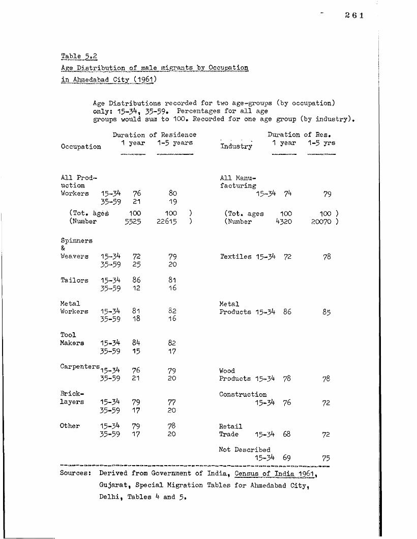
2 6 1

Table 5*2Age Distribution of male migrants by Occupation in Ahmedabad City C 1,961)

Age Distributions recorded for two age-groups (by occupation) only: 15-34, 35-59* Percentages for all agegroups would sum to 100* Recorded for one age group (by industry).

Duration of Residence Duration of Res*Occupation ^ year 1 -5 years Industry 1 year 1-5 yn£

All Prod­uction Workers 15-34

35-597621

8019

All Manu­facturing

15-34 74 79

(Tot. ages 100 (Number 5525

100 ) 22615 )

(Tot* ages 100 (Number 4320

10020070

Spinners&Weavers 15-34

35-597225

7920

Textiles 15-34 72 78

Tailors 15-3435-59

8612

8116

MetalWorkers 15-34

35-598118

8216

MetalProducts 15-34 86 85

ToolMakers 15-34

35-598415

8217

Carpenters^ ^ 35-59

7621

7920

WoodProducts 15-34 78 78

Brick­layers 15-34

35-597917

7720

Construction15-34 76 72

Other 15-3435-59

7917

7820

RetailTrade 15-34 68 72

Not Described15-34 69 75

Sources: Derived from Government of India, Census of India 1961.Gujarat, Special Migration Tables for Ahmedabad City,Delhi, Tables 4 and 5*

Table

5.3

Age Structure

and Literacy by

Occupational Groups amo

ng Migrants to

Cities

262

-p •H r—I i—I *H v03O Pf

MI3o•H-PO3Oft

A1AT3£03

43-p3)h<y*Hr-iH•rl

§43 rH•H J- ■P A X 1 H © lA a p r-

J) <Hfl ° 8)SC 3

OnOj

o-(A

IN-rvj

AVO

AVO ENOJ rsjA3-'xO-A A

C\j

ft*0>- fVJLTV VO OJA

AA AOl

rvA OJVO CO

8•H -P O 3 03

CO-p CO

&s&•Hft A

fcO.3 ■HJH■ao3: a l43 AV"Cv>ft ■t34)bQo 3

•rt

oft ft hCO o (d 5•H*H

r~X03&

^ 43 43 A

OCNAA-vO OJ OJ

3O•H

fta

3.J vO +j Ov •H r" O

VOft*AA Ov O A CO OJ

T- 0- /"xft* OJ O VO O nOJ OJ OJ ft" VOA a - OJ Oi OA ft- ft- A J" T* oj ft- ft- ft'r* w r~ ■w T~ W ft- T~

IN A A A A COr~ A-d-

O r*A A•r-XOn .■—xCO 00ft O j A

SH fN AEH OJ ft OJ35 A f t T“O OJ ft Ai-l -p 3: x—'ft OU ft

ft ONft OJ H OJ03 O c£ VO ft OJ

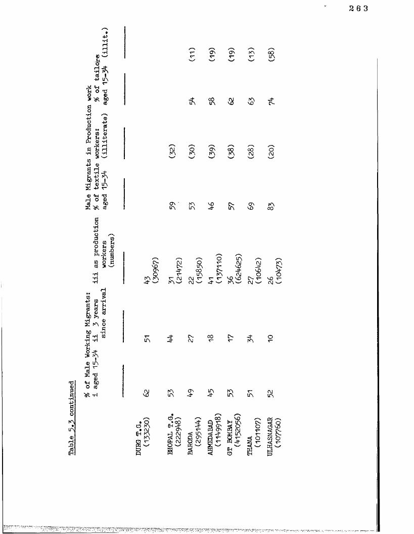
283

ON ON A C OA

& COA

ANO A-

AJfA R A OO CO 3A A AJ'w' AJV-/

ONLA IALA NO-d* A~LA O nNO IAOO

A-NO/—NAJA- RA 00O V AA A v AJ AJ r ~

-d" 'w' A A)

O?— \ A s—1

r* AJ AJV" NO -d-A- -d- NOA Or- c~ NO NO A- r-'w' A ' — ' AJ

{AA-

NOAl

r*LA A*AJ COv J-IA

-pIdOOA•A<UH■S'&

'&■ *H &

• OCD A• AJ*" Ra§

AA ON A-d- AA A AJA

P-i AJ

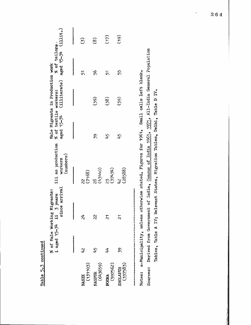
26 4

p

tHH

6H -d- •H A a i P ITS

V -

•S O tJ§•<& |>

§ "•H •'■*''■P ©O Ps td'd •* h o © ©Is U P ft © -H J* H £ P H •H O *rltOP ©C r-t•H -d- P a K I *H © A S P t-# <h *d3 0 &E m «

fe

©

flOP y ssG ifl IhO F-t ©Fs © P£Fh dS 2 ctd >*H•H

IQ > P CO -H§ & £fig, 3*H ©S fA o.0 .9G *H (0 *H *H

O -G > A© A

‘H

IA OO G>

LA v©IA LA LALA

o COy SO'K-\ rA’W IA

O nA A-d* S>

' a/-N~d" /—vOO

s -d- A CO-d" -d- AT“ A A- oOCM A- CO -d" A A OJ OJOJ ' OJ 'w- CM '~" -d* w

-d"oj AJ<M Al CM

CM-d“ A-d-

&A

-d" AA

t— >.ON OJ AA v© ft OONO A S AA A- & IN--d- << A < AN© g A ft Av—' *w* O N/ffito

> I—Ift©HAaS

&

3rd©ftto © i—1P8g•HP«5*HJ£(0©P<spCO

>©rH©>M

©(HPa©©HP5

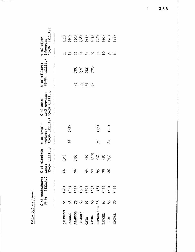
265

H rH © *H U ©^ -d

a a'JR H r

Is©XIoO

A A O CO v- A NO O O r-A NO A A -d VO d" vO A- 00

A r~ A r* -d A -dA VO vo A A no ir \ S OJ -d A VO

•»•© •HIs rH© HrH ■rlH*H8<H AO 1Ar~

CO A (M oOA A A CNJ

A A VO -d •d A A A

EJloO

U P Fs *rt © rH ft H Js *Ho *-3-•31?O A*ri V

I

■Sp•HHrH*HP© © w E U

© -d «H f t A 0 U IS A V"

COA

VOVO

AV-

AA

voOJ

-d00

IoIsPt>©rH©*Ho

p•HrHH•H

*A

A✓—s ,—s o /s r*s /sA VO r - VO 00 A

VO -d- t - A A VOA VO A d" A 00

T3©IGO0A•A©H1E-t

© •Is P © *H■ShGOP

-d *H A O I A "3R r-

0 0 r - A 0 j O A 0 0 A O 0 JO J - d ^ - A A ^ v ^ r - T - T -

VQ tR A A OJ A CO A VO VO VO d"

2

8

S

A00 OA

ft§

2 6 6 1

T3a>3pcooAin0)h§

pr *H•• rH52 5° HXi Is -H P Q) v_«>

<h O IAo x> \^ CtJ LA ^ H r

• e pW «ri H tt> H rH -H (H n-' *H

g ?« IP

IW P t-l ’rl 0> rHE X H $ -H

>§ g ~O LA

•tft. *H r-

I■ap 0! to

p•HrHrH•H

U 0) -3*^ 0 IO LA5 r-

IO •HhP Oa>H a> »• -7f"tH GQ A O ti I 3 LA

r

P*HrHrH»H

—%A-

/■—\ s

A✓'—vA

r~s-4 A A VO i

-4 A A OJ A A A A i■— ■— '—' x~*s

AA

OJVO

v~VO

OJVO OJVO VO4 5

A~4

A4

A OJ v* LA v- CO LA4- 4- IA IA A N IA

A 'r~ r- -4 r- CO OJVO MD IA IA IA LA 4

A/—\A /—A CO CO<r~ OJ A s- OJ'— '

A CO V 4A VO A VD A

s-~\ —s S~sCO VO 4 CO 4 4 VO QA A A OJ 4 A 4 4v x v / 'w' Vw' v—*

VO VO A co A A A 00VO VO A VO A 4 A 4

»^s #**>.A A A O A A'w ' v—s T**

A OJ A A O 4VO A CO A VO A

(M LA ON r* OJ r- IA vfl 4-OJ

O W l ^ l A l A N r r O 'N VO VO A A A A VO A

3 a«E3 <H Or (Htq o p O

<5 < ! p WS 55 ft CO

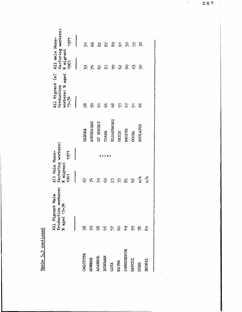
2 6 7

»*

oo

co

ts

CN J" Ox O*vO CN IA x£> ia ir\ in ooCM ^ OO -d-

■P

v£> IN OIA ITN VO (A O' OO P-4- IA C'x. v£>

tr\ IA H

to the Durg Steel Town Area

Age Distributions (%) (male migrants 1 9^1)all durations

Furnacemen illiterates literate but uneducated0 -1 if 00 00 00

1 8if 77 8335-59 15 22 17

60+ 00 00 00

number5090 100&* 10t$* 10Q&* •subject to

^illiterate 27.3 rounding

Construction Workers0-1*+ 01 02 0015-3^ 72 69 7235-59 25 27 26

60+ 03 02 00

number2339 100 100 100

^illiterate 51.^

Electricians

0-1 00 00 0015-31* 86 79 8i+35-59 1 20 16

60+ 00 00 00

number3069 100 100 100

^illiterate 13.7• c-> re» £= 9 e* e- **■ ■*» e» c* tm M

Source: Derived from Government of India, Census of India 1961

Madhya Pradesh, Migration Tables, New Delhi, Table D IV*

Table 3 .5

Sex Ratios in Industries in Bilaspur and Durg

Bilaspur District (urban) Durg District (urban)Sex i atio (f:m) of workers Sex ratio of workers

Household Non-household House* Non-house#

Industry

All workers (number in brackets)0.795 0.257 0.595 0*193

(m5010 f398if511137295 f9573 m3374 f2008511185138 f16454)Tobacco 1.476 0.581 1.647 1.418Construction - 0 .2 1 8 - 0 .2 7 0

Cotton Textile 1 .0 9 8 - - 0 .161

Misc. Textile 0*32? 0.047 O.138 0 .051

Leather Goods 0.336 0 .2 6 0 0 .281 0 .221

Metal Goods 0 .2 3 6 0 .0 2 0 0.131 0 .0 2 3

Source: Derived from Government of India, Census of India 1961, Madhya Pradesh, General Economic Tables, New Delhi, Table B IV C.

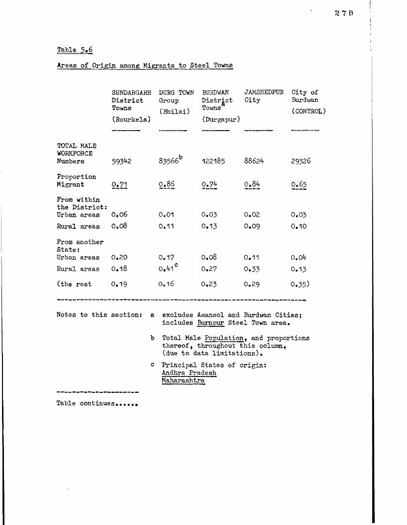
Table 5*6Areas of Origin among Migrants to Steel Towns

27 0

SUNDARGARH BURG TOWN BURDWAN District Group DistrictTo>ms (Bhilai) TownB(Rourkela) (Durgapur)

JAMSHEDPUR City of City Burdwan

(CONTROL)

TOTAL MALEWORKFORCENumbers 59342 83566b 122185 88624 29326

ProportionMigrant 0*71 0 .8 6 0.74 0.84 0.65From within the District: Urban areas 0*0 6 0 .0 1 0.03 0 .0 2 0.03Rural areas 0 .0 8 0 .11 0.13 0.09 0 .1 0

From another State:Urban areas 0 *2 0 0 .1 7 0*08 0 .11 0.04Rural areas 0 .1 8 0.41c 0.27 0.33 0 .1 3

(the rest 0.19 0 *16 0*23 0.29 0.35)

Notes to this section: a excludes Asansol and Burdwan Cities;includes Burnpur Steel Town area*

b Total Male Population, and proportions thereof, throughout this column,(due to data limitations)*

c Principal States of origin:Andhra Pradesh Maharashtra

Table continues

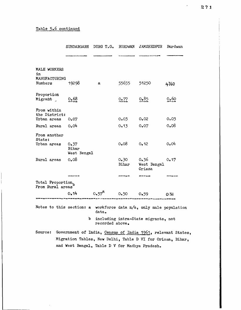
Table 5*6 continued

SUNDARGARH DURG T.G. BURDWAN JAMSHEDPUR Burdwan

MALE WORKERS inMANUFACTURING Numbers 19296

ProportionMigrant 0 .6 8

From within the District:Urban areas 0.07Rural areas 0.04

From another State:Urban areas

Rural areas

0.37BiharWest Bengal 0 ,0 8

55655

0.77

51250

0.85

0.03 0.020.13 0.07

0 .0 8 0 .1 2

V760

0 .6 0

0 .0 3

0 .0 8

o.o4

0 .3 0 0 .3 6 0 .1 7Bihar West Bengal

Orissa

Total Proportion^ From Rural areas

0.14 0.57 0.50 0.59 0/5i

Notes to this section: a workforce data n/a, only male populationdata.

b including intra-State migrants, not recorded above.

Source: Government of India, Census of India 1961. relevant States,Migration Tables, New Delhi, Table D VI for Orissa, Bihar, and West Bengal, Table D V for Madhya Pradesh.

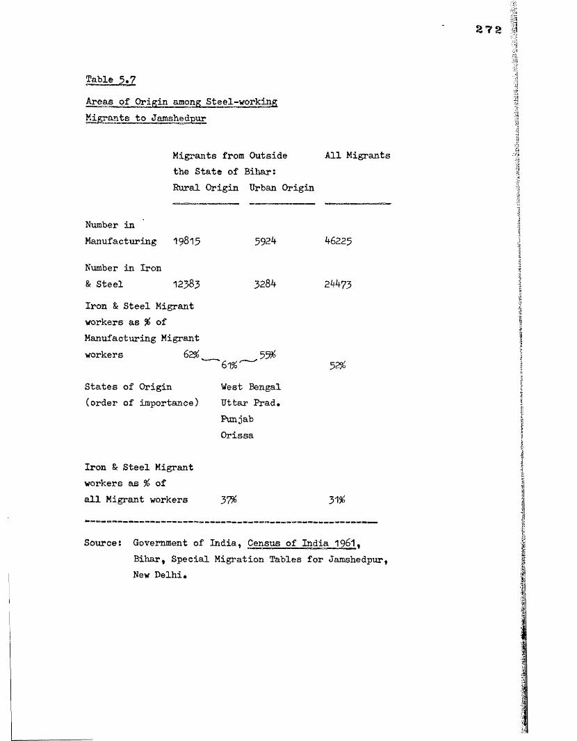
37S

Areas of Origin among Steel-workingph— r— is i nim in i ii« itiwi j ■ ipii i Mi winwu I ■! iinni t1 ■■iimrmnTi—irr-*--

Migrants to Jamshedpur

Migrants from Outside the State of Bihar:Rural Origin Urban Origin

All Migrants

Number inManufacturing 19&15

Number in Iron & Steel 12>83Iron & Steel Migrant workers as # of Manufacturing Migrant workers 62#,

States of Origin (order of importance)

592

328*f

6223

2kh73

GVo'

West Bengal Uttar Prad* Punjab Orissa

52#

Iron 8c Steel Migrant workers as % of all Migrant workers 37# 31#

Source: Government of India, Census of India 1961.Bihar, Special Migration Tables for Jamshedpur, New Delhi*

Secondary Education among Unclassified Labourersin Industrialising Cities (Migrants)

West Bengal Proportion MaharashtraMatriculate

Burdwan 0 .0 1 Thana 0 .0 1

Asansol 0.05 Ulhasnagar 0.04Howrah 0 .0 1 Nasik 0 .0 1

Calcutta 0 .0 0 Sholapur 0.03Bihar Nagpur 0 .0 1

Poona 0 .0 1

Gaya 0 .0 6 Bombay 0 .0 1

Patna 0 .0 0 GujaratJamshedpur 0 .0 5

Ranchi 0 ,0 1 Baroda 0 .0 0

Madhya Pradesh Ahmedabad 0 .0 1

Durg 0 .0 1

Bhopal 0 .0 0

Source: Government of India, Census of India 19&1. Migration Tables, Delhi, Table D IV.

Table 5*9Urbanward Migration in India; Comparison of two Censuses

Lifetime migration according to place of birth; numbers in millions, % decadal change in bracketsMale Female

1961 1971 1961 1971

RuraltoUrban 10*3 13.0 (26.2) 9o1 11.9 (30.8)UrbantoUrban 5.3 7.1 (34.0) 5.5 7.5 (36.4)(Urban to Rural

1 .8 3.0 (66.7) 3.0 5.1 (70.0 ) )

Source: Government of India, Census of India 1971.Special Monograph No. 1, Birth-Place Migration, Delhio

Table 5.10Migration and Areas of Origin in Five States under Study: Contrasts between the Censuses

MAHARASHTRA

% born:In Same urban Area

Urban Population Place of Birth (males)

1961

45.4In Same District 10.3In Another DistrictIn Another State

2 0 .2

21.4

1 0 0 .0

1971

51.1 9.4

1 8 .6

19.2

1 0 0 .0

Distribution of Migration Streams (males)^

R-RR-UU-RU-U

1961

7217

6

5

100

1971

68

1975

100

Number; 605a 8.0State Population Total Male^__20.4____26o1_a- millions b- 'fever-migrant"

275

Table 5.10 continued

Urban Population Place Distribution of Migration of Birth (males) Streams (males)

1961 197 1961 1971BIHAR _ _ _ _% born:In Same Urban R-R 80 77Area 59.0 65.9 R-U 15 17In Same U-R 2 2District 14.2 10 .2 U-U 3 3In Another District 15.4 1 5 .0

100 100

In Another N. 2.9 3.1State 9.2

100T0

7.5ioo7o

TP. 23.3 2 8 .8

ORISSA% born: R-R 84 83In Same Urban Area 56.5 53.7 R-U 10 13In Same U-R 2 2

District 17.8 17.3 U-U 4 2

In Another 100 100District 12.4 15.6 N. 1.3 1.9In Another State 1 2 .0

1 0 0 .0

1 2 .2

1 0 0 .0

TP. 8 .8 1 1 .0

WEST BENGAL% born: R-R 76 78In Same Urban Area 45.5 6 2 .7

R-U 15 11

In Same U-R 2 4District 6 .1 3.5 U-U 7 5In Another 100 100District 9.3 6.7 N. 5.5 5 .1In Another State 2 3 .0 15.1 TP. 1 8 .6 2 3 .5

1 0 0 .0 1 0 0 .0

276

Urban Population Place Distribution of Migrationof Birth (males) Streams (males)

1961 1971 1961 1971

MADHIA PRADESH% born:In Same UrbanArea 55*6 6 1 .0

In SameDistrict 11*9 10,7In AnotherDistrict 12*3 11*9In AnotherState 16*6 1^*1

100.0 100.0

R-R 83 81

R-U 11 12

U-R 3 k

U-U 3 3100 100

• • 00 *u7TP.1 6 .6 2 1*'k

pNotes: millions, and similarly for all rows N. and IP*R = rural, U = urbanN* = Absolute number of male migrantsTP* = Total male population of the State

Source: Government of India, Census of India 1971§Special Monograph No* 1, "Birth-Place Migration", Delhi*

Table 5»

HMigration

Flows

between

Growing

and Stagnating Urb

an Areas

in Bihar

277

1r* 1VQ TOA Ov~ •H

PO TO4* •ad

'npTO to

P oTO PirHP sr j 10o q'_'q 11O I*H JP 1aSr. 1Ife I•H is ITO

cd

MCDKOS

£«4CD

P

>0 ®H p*H toP p§ *?TOto qcoPo qqCDAsoqCDr~vo1§ s~P Aq At=>T~

LA CO A A~ (\l OJ r- [NMD CO ♦ A • LA • OJ • VO CM O A OJ LfV O VO O W r* c* r* r-

vO r- A A 4 oj A v O c or* • o j * O t * cOA r- A' VO VO v O A- OJV s" r" r* v- v r*

r vO (M A • A -4 CN OJ r- |A

IA

VO8

.'d' V?-A CO OJ -4

VOAACO

LA VO r* A- • A r A ’r- A

00 A OJ A- 00 A

A- O OJ • -4 OJ v~ c-

O-4

At—OJ

AOOJ

OJOJ

coIN

CO-4OJ

A-A

A A- A ‘ -4 A • VO IN A- (N

COCO

■4AA

voCO

AVD

COA

A00

A•4

I r 0 0 0 4 A vO o j A-VO oO IN1 A • A Q A • VD * VO • OJI O ACO 4 r O V D 4 ‘lNO''ri r f\J r A r M r- r*

r - A COCO VO ACO A Ar- (N A

A A A Q A- A A 4 “

OA

OA

OOOJ

AA 3) •4*

AOJ

&a HKas

OJA-VO • A A

OJ

A IN O •4 - IN

OJ

OA

AVO

ft

OO CN OJ o OJ A

OJ A Avo VO A00 4 -4A V

AA

P <DP b TOP TO U TOJbO

•TO TO toto 4J q P •Hd P o *H TO TO0) O TO TOP TO i—Id •H O P TO o TOp c X TO TO «i 1P TO TO TO TOo to p TO TO *»S3 •H to TO TO TOP ■HP P TO TOP TO i—LTO to

P<X) TO TO< H to■&* TO

TO •H P E-fo S .TOTO * o O +j qrH TO H •H 0P p P toP •rHE TO•rt P PTO•P E o P 'd TOCO CO*HH O TOpr~> o O P TO •Hd p h P • Oq p O -X•Hp p •«CO Pto oTO.3 bTO o s> TOP to hoO TO *HP po PP &

'O CQq ■H TOrH A> *••H k TO > r*P SjTOP o , voto to o rPP rH Ap •H g>P <H r-o P TOP*H •*O P TOU rH TO P •rt o •rtP r*HP o TO dTO TO (rt*H & P TO*H g 4J■w* o M« O ■H TO •HP U rH TO *H0) O CtJP oIQ Sh•H TO TOo TO P E O •H TOP «M P hOP PP <D TOP TO TOU o •HrH Co nd TO TOf—J top p P Ocj iH hoq TO Oo TO TOTOPPO ■S.S P TO

TO•H«» •TO E O d

P rH *H P Poto -pTOuS4 to 0) to -P oq uH CD dtQTOPO2;

d C <0 -Hto toq E

«Hotouosqo

flH«HOPTOtoE

HQopX»HdqtoPhp<s

too**oco

-— — utStoo rreqaji*

27 8

oLA CO -3- • C""QN (A

ON O • ICM -J- IV T~ I W |

LA

LAr -LA

VO

LA•J-

ROJ

L A • O • Ir J - r r I A f\J r r I ^ |LT\ ^

° *• I

&

voVO

O • LA LA 00 OJ v- v- K \

£

On-J-

OJ LA •

VO ON -tf- C- OJ '

v- O- O • O o Q ( AOO 04 LA IA V O r *r r I A r OJr - >-«' w r *

OJ

LA

©«H

Eh

aS*0m

b

awrt©u

PJhPG©(1)

-P0)ptoo

eo•P&•Hse

o ©H -P*H■P -Pg 5?IQ 2 to *P2.9O w

J—I

p v a>1 ON P r -

I OI ?AII

LAOt A

LAON

Sn OJ S OON S ' LA CO

ON OJ

*[ N LA

-J - CS

$PO

H

§a

oA-

00OJ

# *r * CNOJ VOOJ

IP

— UtSIvTQ

Sex Ratios among Recent Migrants

Census 19&1 (f' tm) Duration 1 year 1 -5 years

NSS (f Current

Rural-Urban (number) of males)

0 .6 2 2

O506)a0.721(5322)

0 .^ 9 6

(3916)

Urban-Urban O.8 1 6 0.911 0.999(792) (1791) (2if8 0)

Note: Census figures in thousandsSources: NSS - National Sample Survey (see Table 5.1 )

Census - Government of India, Census of India 19&1. Migration Tables, Delhi, Table D II.

Table

5^

Secondary

Education

by Occupation:

Developments between

the Censuses

<, Bihar

2 8 0

COa a0) o,Si *H 4) f-( *P -} O a Rj ’> Q H fh O rH O P r-l a *H •°i & PI

8o

V" -4IN VO« •O OCM CO (A VO o -4*(N o- A A CN D-• 0 0 • 0 •O O O O O O

•aoao•rtP3oa•a<u

ar3aoo<yto,dp

ao•rtPfHOOrO&COFk30aCD10•H•P1O0 O1W4)

rHs*3•HWOJA

IPo3o aA *H

’AO•rtfHOrHO

2I P d 3 •rt H S P TD W << *rt

ICO03<0 r-t fH COP a 1■* ° fH *H

O A A VO A o IN r* N rCM V V” O K” A v~ \~ t-a 0 « • • » ■» • • *o O O O o o O o o o

-4o 8 ■3O o o

AO ■s Aoo o o

-4- IN O O

n4-o o

Noo

J- OO VO AO r - O O* • o oO O O O

A VO o o

■8 8 « *o o

IA ON O O

r* (A O O • •o o

A VD O OO O O O O' O o o

O CM -4* A IN-4

VO-4

O A A A

CM CMCMoO

A VO O O * •o o

s & » •o o

co N A A A A co EN A (No r* O r- r - r* O V O« a • • e « 0 * * 0o o O O O O O O O O

VO CO A AO O O O O O O O

A co A CO A O VO IN VO COA A A A A A A A A A• • a • • 0 • • • «O O O O O O O O O O

~4 A O -4 co A O A r* OA A A A A A A A A A• • • 0 • • « • * »O O O O O O O O O O

r* r - r - V" c~ x~ r~ v~ V- Vvo IN VO N VO IN vo N vo INA A A A A A A A A Ar- v- T“ r~ v~ v v- r v

<s( MW i s

§ s o 5 CDS< -4 3 }t{ MfH CD A Q to

03ao•B§ao•rtPO3t30&.PO

•80)apaa>,dpu*Mao*Hao•rt4j3.3Paoo0)0)ca

i

Sable

5«14

continued

2 8 1

0« «to

rt 00 CO w2 rt

5020 rt

600 0•H o rtrt •rto 0 ft60 .rt rt0 -P oft0 fc »O 0 i 'rt

0 0 0rH £ rt -P

rt-P ft0 0 so ft H 0

*H rQ pft •rt •rH0 0 •P 0ft b0rt rt ft rto 0 B 0o ft o 0

O o o 40

w0p!§

Cv-O''o> **

0 VO •rt ON <rs v"5 a

•HfH fd°ap0 fH0 OH Wrt rt0 IQ> rt o 0) o o

oto

CO0HP0EHo-rt0ftrtoom

ft}. 0

r t rH 0 ft rt rt 0 Eh art *rt

• r i 0CQ P

«ftofihH • •rto•rtft0 0rH Pft 0ft PO COft Ort fA0 •rt •H OCO 0s p0H rtto 0 vP P VOo •H OnEH ft V"

O

0•<H■rtrtftotortIQrt0O

K V

1rt&<2

PtQ0ft

tQ P rt rt0 Q W

f t f t r t rt IQ 0£ S *

Irt o*Hp O IQ rt rt 'rt 0

fO\ CT\o o

o o

I 1

V T-VO IN- CJN a\

ft

CM VO O OO O

CT\ VO CMO O r-O

VO IN On CSV v~ V*

S ’s

■s

vo

oCM

tr\O

& to,o o o o

CM EN r* CM o oO O

OO CM VO -0-r * V“ v-* « • •O O O o

• •-0-v~

v~O ■3 •s

FA 1 r - 1 rto• ■ * • • | •rt VOo O O o O 1 f t ONO x~0U2 **

r* v V” r - v~ i IQCN VO IN VO in i IQ &ON ON ON ON ON | •rt OV r* r* \~* r 1 44 f t

P f tOs O

0 >-H P rnPH m CQ ■8J3 o 03 a Pw f t 1 Oft CO 1 is;

tQ0•rt©O■arto•rtP0S1rtO rt- O ON O r-

CO rt ON ON o ojfcii p W CO v VO 0 **rt-oo rt rt-

COirwo oif

&.gs

IQ rt p 0 wa a

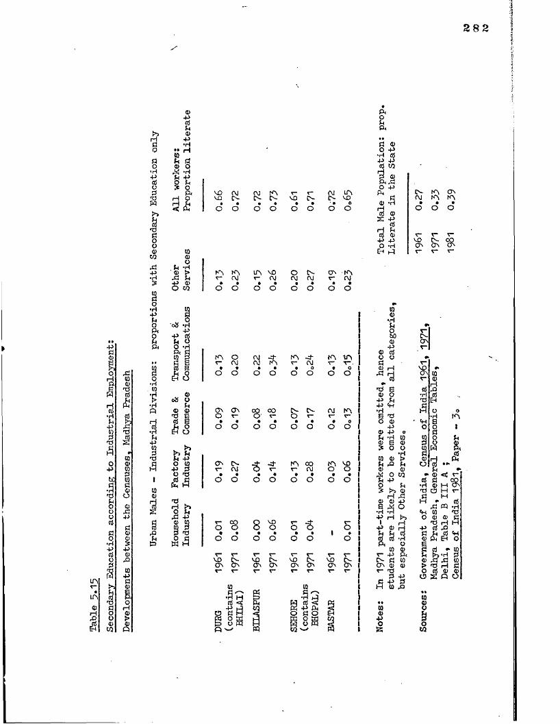
Table 5.15

Secondary

Education

according; to

Industrial Employment

Developments between

the Censuses+ Madhya Pradesh

282

a>-p2(DP■H•• Hto

Q> O •M -HO f-t£ oft H O

. U(DrP

to<1)O&4>co

VD OJ OJ A r “ r- OJ AVD CN c^ CN VD CN CN VD

• • • • • • ■ ■ oO o o O O O O O

A A r- <M A VO r- OJ O CN OJ OJ

o o o o o oCO A r~ OJ * •o o

ftohftF3 <D O P *H CtJ P Prt co*3 oft .d o Pft<D*3S*3poEH

CN A COOJ A A• « •o O O

r- t“ Vvo CN 00CO CO COV T“

•0»p&ftW

o08 O© ©*Ct g rt g£ o

&p O (015 5

fH >»2 H p© to co rt{3 T3tS i9

A O v- OJ • •O O

ON CO O r- • •o o

CO CN r* OJ • •o o

OJOJ A

■8

A -cf v OJ

O O O O

OO IN CNv O r"

o o o o

A 1A v -v . • oO O

OJ A*o

CD R P ft

oO

<h A 00 A voV T™ OJ O o« • • • •O o O o o

r~O• COo• 8•VDO• O• 8 • 1

X~O•o o O O O O or- r- c~ r~ r~VD CN VD £N vo IN VD ftCO co CO CO CO CO COr r V" r* T- r- T” V

&

CQ0)POa

rt *"10b *d 3© .if ,£3 10 > rtJ rH Cjo rt © ©U S Q OCO0)oEfom

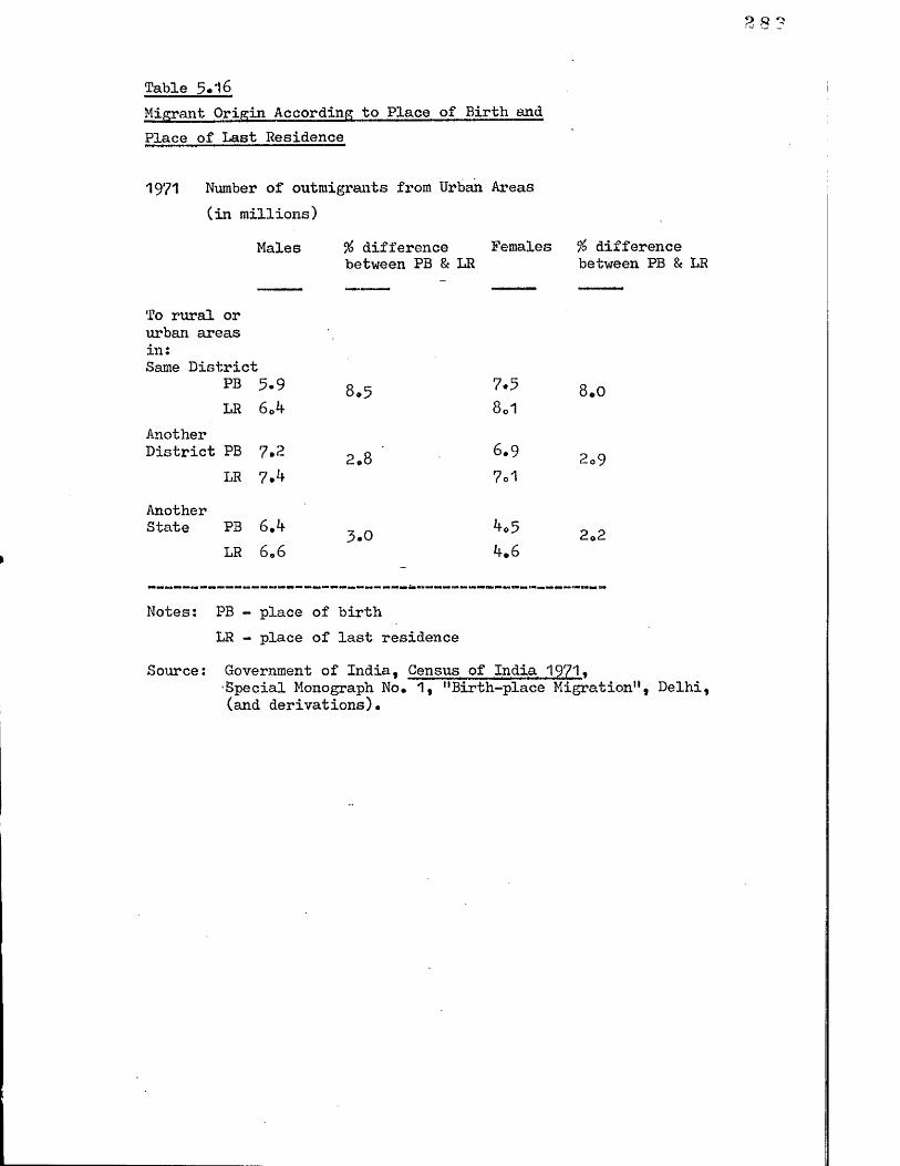
Table 5 .1 6

Migrant Origin According to Place of Birth and Place of Last Residence

1971 Number of outraigrants from Urban Areas (in millions)

Males % difference Females between PB & LR

difference between PB & LR

To rural or urban areas in:Same District

PB 5.9LR 6<A

8*5 7.58o1

8 .0

Another District PB

LR7.27.^

2 *8 6 .9

7o12o9

Another State PB

LR6*if6 *6

3.0k.6

2 *2

Notes: PB - place of birthLR - place of last residence

Source: Government of India, Census of India 1971 .Special Monograph No* 1, "Birth-place Migration", Delhi, (and derivations)*

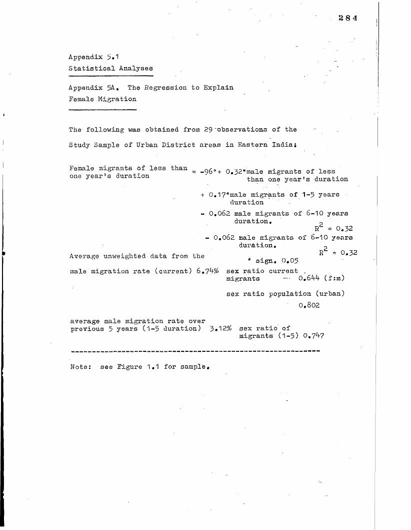
28 4

Appendix 5.1 Statistical Analyses

Appendix 5A, The Regression to Explain Female Migration

The following was obtained from 29 'observations of the Study Sample of Urban District areas in Eastern India;

Average unweighted data from the sample:male migration rate (current) 6 ,7*+% sex ratio current _

average male migration rate overprevious 5 years (1 -5 duration) 3 .12% sex ratio of

Female migrants of less than one year’s duration 9 6*+ 0 ,3 2*male migrants of less

than one year’s duration

+ 0 ,1 7*male migrants of 1 -5 years duration

0 ,0 6 2 male migrants of 6 -1 0 years duration,p

IT - 0.32* sign, 0,05

migrants 0 .6^ (f:m)sex ratio population (urban)

0.802

migrants (1-5) 0.7*+7

Note: see Figure 1.1 for sample.

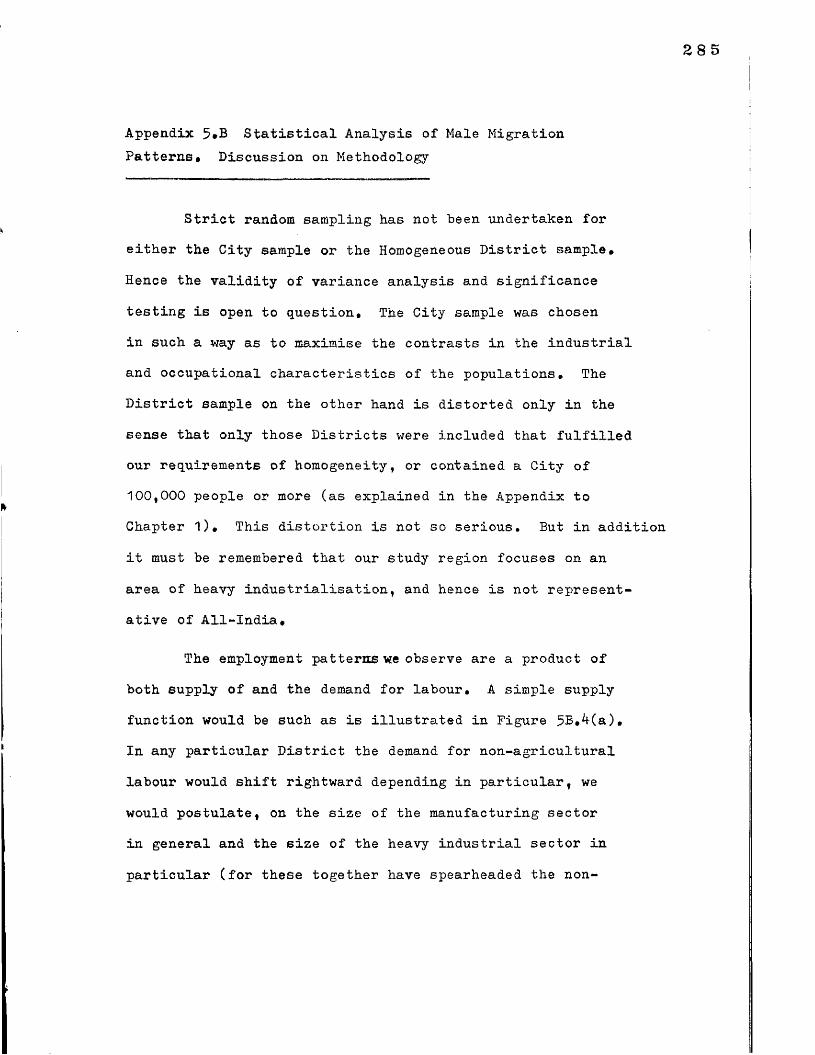
285

Appendix 5*B Statistical Analysis of Male Migration Patterns# Discussion on Methodology

Strict random sampling has not been undertaken for

either the City sample or the Homogeneous District sample#

Hence the validity of variance analysis and significance

testing is open to question# The City sample was chosen

in such a way as to maximise the contrasts in the industrial and occupational characteristics of the populations. The

District sample on the other hand is distorted only in the

sense that only those Districts were included that fulfilled our requirements of homogeneity, or contained a City of 100,000 people or more (as explained in the Appendix to

Chapter 1), This distortion is not so serious. But in addition

it must be remembered that our study region focuses on an

area of heavy industrialisation, and hence is not represent­

ative of All-India#

The employment patterns we observe are a product of

both supply of and the demand for labour, A simple supply

function would be such as is illustrated in Figure 5B,Ma).

In any particular District the demand for non-agricultural

labour would shift rightward depending in particular, we

would postulate, on the size of the manufacturing sector

in general and the size of the heavy industrial sector in

particular (for these together have spearheaded the non-

agricultural growth in our region and our period, whereas

expansion in commercial activities has tended to follow rather than lead that growth). Demand on this scale would soon exhaust the supply of local labour at low wage levels,

so that the same analysis extends to other Districts in the

same State, and to other States (Figure 5B,*+(b)), If we disaggregate further, we postulate that the demand for labour of specifically urban origin would also shift rightward (Figure 5B,*f(c)), depending on factors related

to the character of the industry in the District(i)* we have postulated that a rightward shift occurs if high levels of education are required in manufacturing industry,

and, in the extreme, that no shift occurs if they'are not, or if the potential malleability or docility of a rural workforce is actually preferred, (this consideration also might determine the shift to other States of origin, in

addition to insufficient supply). It is postulated that the latter considerations will tend to dominate more in the case of heavy industry (in basic metals production and engineering)

than in manufacturing generally: there will be more rural

labour and it will be from further afield.

287

We throw some light on these hypotheses by observing the size of the correlation coefficient (Spearman’s ) and the significance (and value) of regression coefficients

qualifying variables that can be derived from the Census data. These variables amount to: the male labour force engaged in manufacturing, and, of that, the component in heavy engineering; the proportion of the labour force that is migrant, and those from other States by birth, and the component that comes from urban areas (again by birth); for the City sample we have data on the literacy of migrants.

How shifts in labour demand just described will affect the

expected corfelations between these variables is illustrated in Figure 5B,*+(d), It is hypothesised that there will be more migration if there is more manufacturing industry in

the urban economy, and there will be more migration from

far afield in this case, and especially if there is heavy industry; there will be more migration from urban areas if there is manufacturing industry, but heavy industry may promote the use of rural labour; and urban migration will be associated with literacy.

The greatest risk with this methodology is that the assumption of identical supply functions in each District

or each State may not hold good. For within these aggregate

supply functions there will be different components of

1 It has been necessary to exclude Madhya Pradesh from some of the tests due to a peculiar data deficiency in the publication of the 1961 Census volumes on migration for this State,

2

labour from different backgrounds, more Backward Classes

in some local areas than in others for instance, and perhaps

more enveloped information networks in some areas* If these

supply schedules are not similar, then our observations on

changing composition of the labour actually employed are

not based on the changing composition of demand alone, but also on the changing composition of supply* Estimation of coefficients becomes impossible. Worse still, the supply

schedules, if not similar, ms,y not be independent of demand,

in that better information networks, for instance, may exist in areas of heavy industry, in which case the coefficients

in the equations we estimate will be biased. The root of

these difficulties is the identification problem (and the

possible bias is illustrated in the model in Figure

The other problem of interpretation is that of the ^ecological fallacy”. Just because manufacturing towns are

associated with long distance migrants does not mean that

manufacturing migrants themselves come from long distances,

or, if they do, that they alone do so. Where possible the actual

industrial employment of the migrants themselves is considered

in the testsj the possibility that manufacturing and non­

manufacturing migrants come from similar origins arose in the

course of analysis, giving rise to further tests also reported

below.

389

Finally we should not wish to attach too great a significance to the predictive value of the intercept in

the regression. We have too few observations close to the

origin (i.e. in the range of 10% of workers in manufacturing for instance) to be confident how any relationship may behave in this region: the assumption of linearity may simply break down. We cannot confidently say, therefore,

if the intercept suggests that 2 0% of workers are migrant (when there is no manufacturing), that this represents exogenous supply, that is those subject to rural push factors or urban natural increase alone*

Analysis: the following correlations can be reported:

Correlation Coefficient

The proportion of workers in manufacturingby the proportion of workers of urban origin - * 6 3 5 (D)

-.572 (C)The proportion^of manufacturing workers inheavy industry by the proportion of workersof urban origin -*M+5 (D)The proportion of workers in manufacturing bythe proportion of migrants of urban origin + .3 7 9 (Df)

(Figure 5B.3)The proportion of manufacturing workers inheavy industry by the proportion of migrantsof urban origin +.176 (D')

(Fig. 5B.3)The proportion of migrants in manufacturingby the proportion of migrants of urban origin +.030 (C)The proportion of migrants who are illiterate by the proportion of migrants of urban origin -*310 (C)

Mean value of urban origin of migrants 35.6% (D)2 8.5% (C)

(Fig. 5.2)

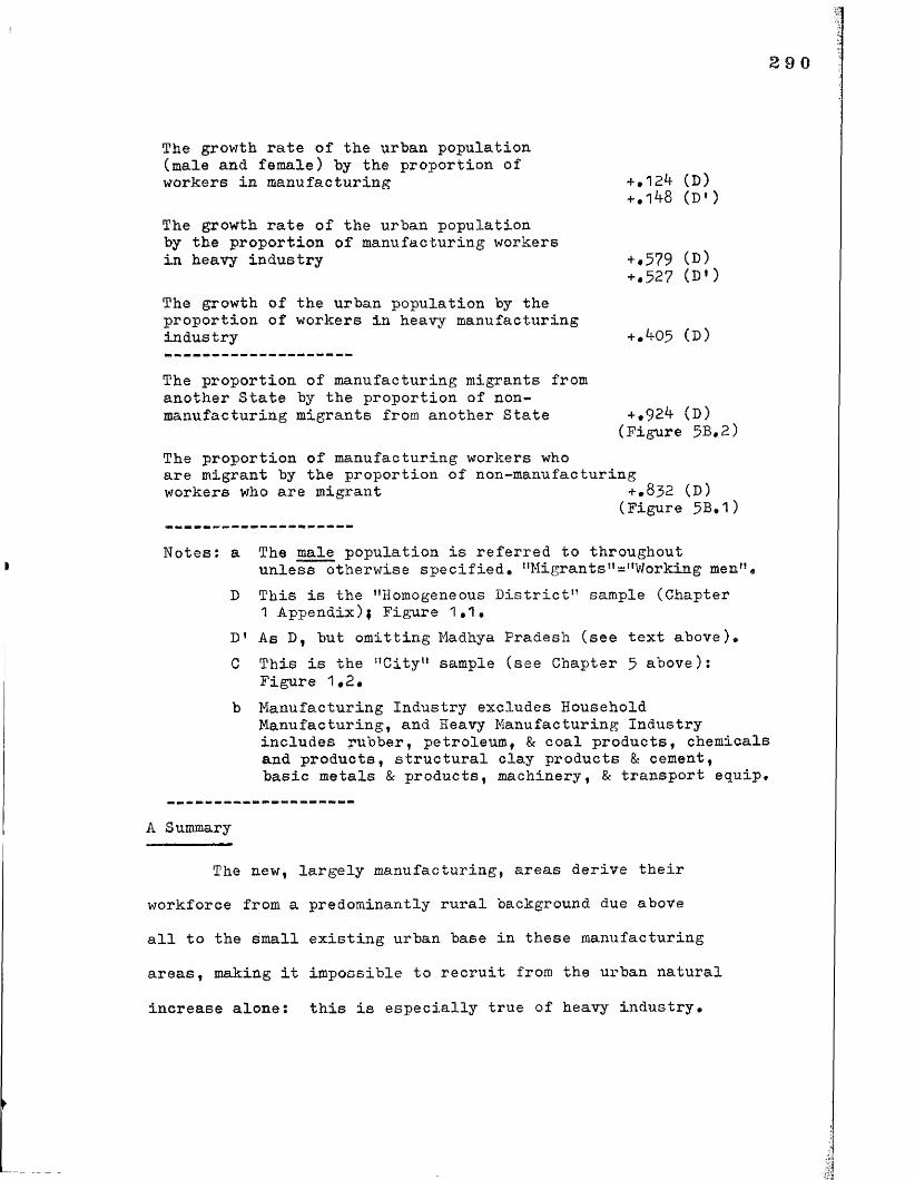
The growth rate of the urban population (male and female) by the proportion of workers in manufacturing + .12*f (D)

+.1*f8 (D‘)The growth rate of the urban populationby the proportion of manufacturing workersin heavy industry +#579 (D)

+#527 (D»)The growth of the urban population by theproportion of workers in heavy manufacturingindustry +*^05 (D)

The proportion of manufacturing migrants from another State by the proportion of non­manufacturing migrants from another State +#92^f (D)

(Figure 5B.2)The proportion of manufacturing workers whoare migrant by the proportion of non-manufacturingworkers who are migrant +#832 (D)

(Figure 5B.1)

Notes: a The male population is referred to throughoutunless otherwise specified. "Migrants"-"Working men".

D This is the "Homogeneous District" sample (Chapter 1 Appendix)| Figure 1.1.

D' As D, but omitting Madhya Fradesh (see text above).C This is the "City" sample (see Chapter 5 above):

Figure 1#2*b Manufacturing Industry excludes Household

Manufacturing, and Heavy Manufacturing Industry includes rubber, petroleum, & coal products, chemicals and products, structural clay products & cement, basic metals & products, machinery, & transport equip.

A Summary

The new, largely manufacturing, areas derive their

workforce from a predominantly rural background due above

all to the small existing urban base in these manufacturing

areas, making it impossible to recruit from the urban natural

increase alone: this is especially true of heavy industry.

291

There is little clear determination of the origin, whether

rural or urban, of the migrants themselves, but, by All-

India standards, they are generally over-represented in

the category of urban origin (i.e. more than 20% are from such origins). But although manufacturing areas have large

proportions of migrants from urban areas, the migrants

themselves in those cases are not particularly likely to be employed in manufacturing. And in the case of heavy manu­

facturing areas, there is virtually no association between

the large numbers of heavy industrial workers in those areas

and the urban origins of the migrants. Furthermore, manufacturing

and non-manufacturing workers are highly correlated both in respect of migrancy and in the distance of that migrancy

(i.e. proportion from another State). This suggests that

migrants who are responding to a direct demand for manufacturing

labour (that is neither met by natural increase in the towns,

nor from within the same State) encourage the migration of

others from the same origins to find employment in the trades

and services sectors. An information network is thus

established; (and this throws into doubt the true independence

of the demand and supply schedules).

2 8 2

Analysis: the following regressions were undertaken:

% workers of urban birth = 7 1.2 ** -6 2.5** % workers in ^manufacturing (D) R .40

» = 7 0.6 ** -64.4* " (C) R2#53" - 6 6 ,0** -25,4* % manufacturing workers

in heavy industry (D) R *2 0

% migrants of urban birth = 2 9*2** +6 6 .8 (*) % workers inmanufacturing -4,3 % manufacturing workers in heavy 2

industry (D) R *16

% migrants of urban birth = 48.6** -120,5(*) % migrants 2who are illiterate +3 8 ,5 % migrants in manufacturing (C) R *1 6

Mean value of urban origin of all workers: 57% (D)Mean value of urban origin of all migrants: 38% (D)% workers who are migrants from other States

= 40.1 +77*4** % workers in 2manufacturing (C) R *66

% migrants who are from other States- 8 - *0 ( * ) +5 9.6 * % workers in

manufacturing +1 8.2 (*) % manufacturing workers in 2heavy industry (D1) R ,55

% migrants who are from other States_ -18,5** +1 0 2,2** % workers in 2

heavy manufacturing (D1) R .49

Notes: as for correlations above, and ** significant at level ,01 * significant at level .0 5 (*) significant at level .1 0

Summary

The significance of manufacturing industry as a determinant of rural migration to urban areas in our region

is confirmed, with a suggestion that it is chiefly heavy manufacturing that accounts for this, and that other

manufacturing would be as likely to acquire recruits from

293

urban centres, particularly if literacy were required*

Manufacturing is also significant in promoting long-distance

migration, and again this is probably more likely if the

manufacturing is heavy. The reliable coefficients have

values (indicating elasticites) of between •§■ and 1: for

example, if one doubled the proportion of heavy industry in

employment in a town, one would double the proportion of

migrants from other States, and if one doubled the proportion of manufacturing in general, one would reduce the .urban-born

proportion of the workforce by about two-thirds (through vastly

increasing migration generally, not through selecting rural

migrants specifically, except perhaps in the case of heavy industry). If there was little manufacturing, and hence little migration, it seems that over two-thirds of the work­

force would be urban-born (mainly within the same town) but

that a small proportion would still be migrant from rural

areas (as one would expect in poor agricultural areas like

parts of Bihar): but we argued above that the constant terms

are not quantitatively reliable. Finally it must be remembered

that our interest is on the demographic effects of industr­

ialisation: we do not wish to argue that all demographiceffects are due to this cause, and indeed in our regressions

only between -J and •§■ of the dependent (demographic) variable's

squared variation is explained by the manufacturing component

in the Districts1 urban areas. The strongest single

conclusion is that heavy industry has promoted inter-State

migration*

It should be clear from elsewhere in this study that

migration is regarded as an important social phenomenon in

itself* It is the uprooting of a way of life, whether temporarily or permanently, and, with the ageing of the migrants,

often irrevocably* But migration is also symptomatic of other

social phenomena: it has been suggested that migrants from

urban origins, migrants from distant origins, and migrants from local origins, may fall into three fairly distinct social

groups in terms of education and other assets* A completely

new data set would need to be created in the field, to examine

the relationship between industrialisation and these more

definitive categories. Hopefully we have at least pointed

interested researchers and census takers in that direction.

295Figures 5B*1 to 5B*3The Relationships between Migrants, their Origins, and Manufacturing Industry: evidence from the urban Districts

+- 'DKqȣ*<(UlcuJhi

MpK<aK

HO '

L*> ->0 HO Co CO ~lx>

5B.1*5B.2*

UOKC-TJ UVmw Cl*IfmigvrifJ:

f r v . o f c f c * U r v c f ; n c d '*% \fWc& ic3tc.

to *70 % of micjviVvi c*ve. S b d -

ro>o/£>

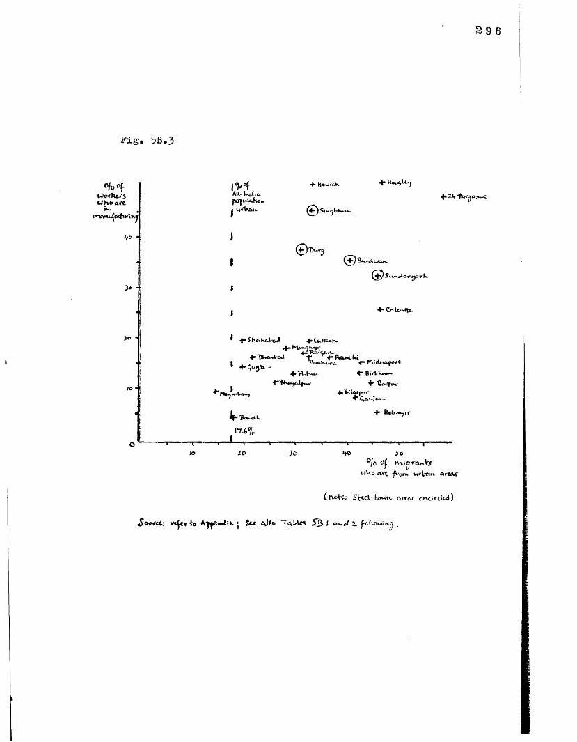
2 B S

Fig. 5B.3

Ukwhx.'5 ufHo <wtPVin

IfO ■

> ■!

7.0 ■

| MWl'lwcfiC* 1 U/tf£Wv

^ Hou't-X

©Si*^U~

S*t*«lQirjcvk

+■«*

't' Wcwttt-

4“ 4* CutttfcKXiM fm aW4— 'Ruic.c.vw DkAittEj t'0«wU»-w +*•f*£ojvU. -

4 4”Ci<Wim>*4*-"]

114%i—f ZP }o *to rc% »vi4 Va~h>

UVvo AVX. -fvorM. t*» Vc«M- O t t A f

Ct\ofce; cc'xJluL)

JTooi'ct: VH v-hs A pc*<rf:x « $&c cjfo TaJUc< 55 I 2- f o l i c u i i ^

297

Figure 5B**fThe Migrant Labour Model

* (ru*v-AAnc..Ub**td.^~v. II 5 ’v t /v ^ ’5 CJ l o L * u r \T> c k' U baw \ 1 bxj>*- fcctB )

V ^> y ° li“"^■V o* W ^ v >k f ** u>*fc < ^ o a A

* \O tv

*kC^HLolroo ir •fVoKwOtear iJ iUj

+ Otfce»- StclfcJ

jUxtrou'r ',k.Dirtr'c-t S t&te j „

it(u> u“)eV ! ‘j'V**-1 j dul»v*(: U-bcwtj

W cfV-v<S * .SbaKs )

T Of t t * - ftiiC J

JfC^ w<,/i

Mar

i w WOvJtjtrVj-

II <*- [ u v tra u tab-ou^ iV j) fw-tfcr iff «(«toH«.)

! | l r U -b o » * f tS-for »ts hclt/ci I* b »j *)

4(4)% 0ftru<ri>i.btcJb£K.<rwining■fifty**'

SUKL

TSiXh^ O h hs)6m ( tOKKoB

lfc<*v-

C .Ir f*- W )

L c mmjut (M )t AlV icJromr uvV>"c.k. ft«a( o| Cj HcA.^ tivii»ftAC.V LcArotiV CH) fr

AS ftMT Xtff' Ka.»H

Kc J +& defined y{t<c.*~*c\rt'Tfi f-fv.ee. income. . C* c*>fK *p t*i‘»Cy k «v- ? C-* 0 cj st * C « * '(h iK t ' ft>< 6 l | f l t t . f r O v : ^ i - J , £ ; S d « C t h o u t L |< t - M i u * « - + C ,

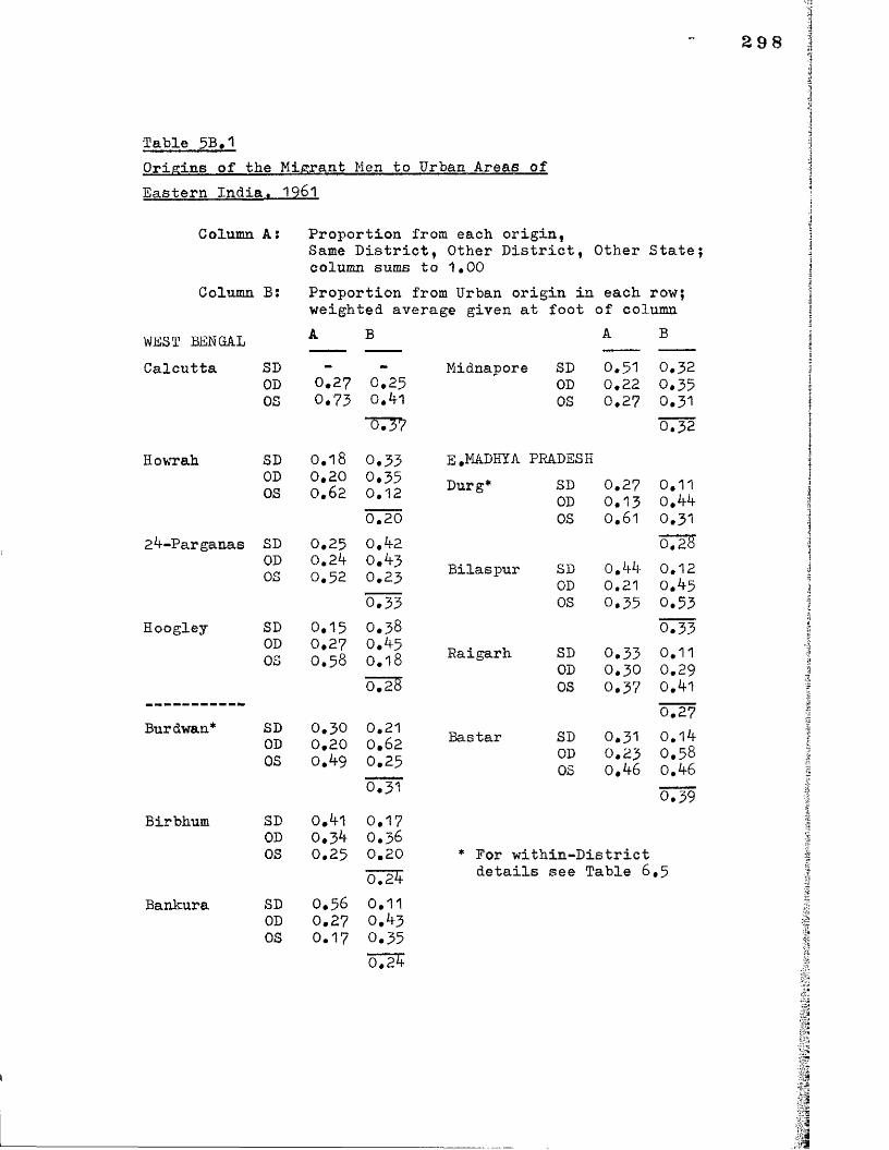
298

Table 5B.1Origins of the Migrant Men to Urban Areas of Eastern India. 1961

Column A:

Column B:

WEST BENGAL Calcutta

Howrah

Hoogley

Burdw&n*

Birbhum

Bankura

SDODOS

SDODOS

24-Parganas SD OD OS

SDODOS

SDODOS

SDODOS

SDODOS

Proportion from each origin,Same District, Other District, Other State; column sums to 1 .0 0

Proportion from Urban origin in each row; weighted average given at foot of columnA B

0.2?0.73

0 .1 80.200 .6 2

0.250.240.52

0.150.270 .5 8

0 .3 00.200.49

0.410.340.25

0.560.270.17

0.250.4-1

0.330.330.120.200,4-20.4-30.230.330.380.4-50 .1 8

0 .2 8

0,210 .6 20.25_ _

0.170.360.200.24-0.110.430 .3 5

0,24

A B

Midnapore SD 0.51 0.32OD 0 .2 2 0.35OS 0.27 0.31

0 .3 2

E.MADHYA PRADESHDurg* SD 0.27 0 .1 1

OD 0.13 0.44OS 0 .6 1 0,31

0 ,2 8

Bilaspur SD 0 .4-4 0 .1 2OD 0 .2 1 0.45OS 0.35 0.53

0.33Raigarh SD 0.33 0 .1 1

OD 0 .3 0 0.29OS 0.37 0.41

0.27Bastar SD 0.31 0.14

OD 0.23 0 .5 8OS 0.46 0.46

0.39

* For within-District details see Table 6 ,5

299

Table 5B.1 continuedBIHAR A B

Patna SD 0.39 0 .2 6OD 0.^9 0 .2 0OS 0 .1 2 0.56

0.2?Gaya SD 0 .6 2 0 .0 8

OD 0.29 0.25OS 0.09 0.V7

0.17Singbhumi Jamshedpur

SD 0 .1 6 0.15OD 0 .2? 0 .2 0OS 0.57 ■0.-15

0 .1 6

Ranchi GitySD 0 .2 8 0 .1 6OD 0.^3 0.35OS 0 .2 8 0 .5 2

0.3*fDhanbad

SD 0 .1 1 0 .3 1OD 0.5*5- 0 .1 1OS 0.30 0.25

0.17Monghyr

SD 0.50 0.19OD 0.35 0.25OS 0 .1 2 0 .*f8

0 .2 8

ShahabadSD 0.56 0.13OD 0.25 0 .2*fOS 0.17 0.33

A B

Other urban areas in SingbhumSD 0.31 0.3?OD 0.25 0 .2 8OS 0.^3 0.33

0.33Other urban areas in Ranchi

SD 0 .^ 6 0 .2 0OD 0.35 0 .2 8OS 0.19 0 .V7

0 .2 8

0.19

Table 5B.1 continued

OSISSACuttack SD

OD OS

MayurbanjSDODOS

Bolangir SD OD OS

Ganjam SD OD OS

Baudh Khondmals SD OD OS

Sundargarh.SDODOS

A B

0.55 0.290.30 0.29O .1 3 0.50

0.31

0.^9 O .0 50 .2 8 0 .2 00 .2 0 0.23

0.130.54 0.380 .3 1 0.490.14 0 .6 8

0.450*46 0.350 .2 3 0.430 .3 0 0 .5 0

0.41

0.39 0 .0 00.55 0 .2 60 .0 5* 0.52*

(0.17)

0 .2 7 0.3^0.18 0.390 .5 5 0 .5 1

oTW

*small numbers

Source: Government of India, Census of India 1961.(relevant States), Migration Tables, Delhi*

3 01

Table 5B.2The Urban Origins of the Urban Workforce

% of Total Male % of Total Male Ratio of Urban toWorkers who were Workers who were Rural among Maleborn in an Urban bom in another Workers bom inArea State another State

WEST BENGAL24-Parganas* 42.4 2 6 .0 0 .2 6

Calcutta 40.1 31*1 0 .2 3

Howrah* 39.6 41.2 0 .1 2

Hoogley 39*5 39*8 0 .2 0

Burdwan* 44.5 30.9 0 .31

Birbhum 51*8 15.3 0.24Bankura 6 7 .5 6.7 0.45Midnapore 6 5 .2 11.5 0.33BIHARPatna 64.3 5.3 0 .9 1

Gaya 71.1 3.4 0 .7 2

Shahabad 66.1 7.8 0 .3 8

Bhagalpur 73*8 3.8 0 .7 0

Ranchi* 61.4 13.7 0 .81

Dhanbad* 2 7 .2 24.4 0 .2 5

Singbhum* 36.5 40.7 O.3 6

Monghyr 74.0 4.1 0 .7 0

ORISSAGanjam 71.9 17.2 0 .9 0

Sundargarh* 6 1 .9 38.3 1 .0 8

Cuttack* 71*2 55.5 1 .0 0

Majurbanj* 48.0 15*0 0 .2 6

Bolangir 70.7 7.0 2.48B-K 6 2 .9 2 .9 0 .7 8

Note:* 1951-1961 decadal increase in urban population over 50#Sources Government of India, Census of India. 1961. (relevant States),

Migration Tables, Delhi

A brief Overview of Chapter 5

From this Chapter we can say that migrant origins, near or afar, rural or urban, and migrant age and sex composition, are all in part the result of recruitment strategy; these factors reduce further the ability of future labour markets to equilibrate supply and demand in rapidly growing towns of the present, due to the resultant inflexibility (barring major outmigrations) in future labour supply. Indirectly at least the new growth areas contribute to the loss of urban population in the stagnating areas.

303

CHAPTER 6

The Region of Eastern India's Industrial Belt: Demographic Structure and its Development over Time

Empirical Overview

The short-run evolution of our Eastern Region of India is looked at in dynamic demographic terms over the 1961 - 1971 decade: comparisons and contrasts with thepredictions of the models are noted* Two or three points of some importance emerge: first the rapidity with whichfemales become attached to the initial male migrants in the rapidly growing New-town areas (like the Steel Towns); secondly the large proportion of migrants that have arrived within the last twelve months (preceding 1961), especially in the more slowly growing mature towns, suggesting high rates of "turnover" migration! thirdly, even in a population like India's of moderate natural increase, the age structure developing in the most stagnant urban centres, with some of the characteristics of depressed localities (e.g. an increasingly old age structure), as currently experienced in England.

We also note how the lowest caste groups among migrants (probably of local origin) have failed to.penetrate the manufacturing sector in the newly industrialising areas, and are well represented in the stagnating towns and in mining areas. Finally we note that the rise in the proportions of, for example, migrant Biharis in developing areas of West Bengal is largely attributable to family formation, not to continuing male migration in response to industrial demand, and is unlikely therefore to become a significant phenomenon.

Interpretation of the Demographic Structure and its Development

In Chapter 1 we gave an account of the 1951-71 period of industrialisation and subsequent stagnation,

and of its demographic manifestation, in an overview

of urbanisation in the Eastern region of India characterised as the Chota Nagpur Crescent. We now proceed to fill in some of the demographic detail.

To anticipate slightly, we will find some guide to an

interpretation of that detail by looking back at the simulation models, though that of course must not prevent us from challenging the sacrosanctity of the model;

rather, a dialectic should occur: let the model help

us interpret the facts, and the facts help us question the model*

To start in the East of the Study region, the Districts of West Bengal are dominated by the urban agglomeration of Calcutta, and Calcutta is in some ways unique. The central District, Calcutta City, grew very slowly down to 1 9 5 1, and almost stopped growing at all after that date. Yet the rate of gross inmigration, recorded as 3*0% in the last year before the 1961 Census, was about k times higher than the overall population

growth rate, an annual average of less than 0 ,8%,(Table 6,2). Calcutta’s growth fits between our ’£ero Base” Model and our Model ”3", and in the former

the net migration (that is gross in-migration minus

gross out-migration) was 0% while in the latter it was

-3$ Per annum. Since the (arithmetic) average recorded gross in-migation for the previous five years was also around 3% (net of mortality) the implication would, at first sight, seem to be that there have been fairly heavy rates of out-migration. Furthermore, the gross

1 The data I have recorded from the Census rely upon correct recall of time of entry. They are also deficient as an estimate of annual gross in-migration in that those who have entered the city and sub­sequently died before the Census are excluded: this error clearly compounds the further back in time the entry occurred. In-migrants who stay less than the reference period used in recall (whether 1

year or ;6 years) are similarly unrecorded. In Table6.2 I have computed the recorded gross migrations as proportions of the Census population (expressed as annual averages). Where the gross in-migration is an annual average of the recorded migration from 1 - 5 years prior to the Census, the correct population to use as a denominator would be that estimated 3 years prior to the Census. The bias in not doing so is only acute if rapid rates of growth are experienced per annum We can illustrate with an example: suppose the urbanpopulation is 100 thousand in 1 9 5 1, 200 thousand in 1958

and 400 thousand in 1 9 6 1, i.e. doubling every five years

in-migrant stream is more heavily dominated by males

than was the case in our Model (see Tables 6.2 and 6.1a), and this must have been equally true in the past, since the overall sex ratio (f:m) is at most -frds what it would be in a steady migration model at this low level of growth.

footnote continuedDecadal growth is 300%, average annual (compound) growth is 15%, 2% of which we assume to be natural increase. Then the 1961 population would have reached 220 thousand due to natural increase alone since 1 9 5 6, and the rest of the quinquennial growth (2 0 0 - 20 = 1 8 0) would have been due to net in-migration. Ignoring mortality and out-migration and assuming accurate reporting, 180 of the 1961 population would claim to have migrated over the last 5 years, an arithmetic average of 180 f 5 = 36 thousand per annum. Expressed as a percentage of the 1961 population this gives a gross migration rate of 9%. Expressed as a percentage of the 1956 population it gives a growth rate of 18%. And we know the real rate is 15% - 2% = 13%* In the text I assume a natural increase of about 2%. Hence, in this illustration, if the last year’s reported migration rate was 13% and decadal growth was 3°0% we would argue there was approx­imately 0 gross out-migration. If the reported rate had been 15% (and the past five years average 11%) we would have surmised an approximate rate of outmigration of 2%, and so on. This methodology serves perfectly adequately for the kind of qualitative comments we wish to make.

But this characteristic gives the City's central District very few children, well below the replacement of the labour force (7 *2% of the male population is aged

below 5 , ia contrast with 14.9% i& the moderate growth Model "2" for instance, Table 6.4). Such a low birth rate, as implied by such a low child-population ratio, indicates that net migration may be higher than we thought, gross

migration being less. For instance, in tie.extreme, natural increase could be 0 , gross in-migration 3 2%, and gross out-migration about 3% per annum. The continuing stagnation in demographic growth of the following decade

(an annual average of less than 0 .8%) implies continuing large

outward flows, unless there has been a sharp decrease in inward flows, or alternatively ageing population and increasing death rate, (see Table 6.4 for the potential future ageing of Calcutta's population). The problem of

economic support for this dependent population in a very poor economy will be discussed later. An inner City demographic problem of this nature and on this scale is virtually unique in India, though it may well be the writing on the wall for other great Cities still in their

1 We always have to assume that child mortality is not dramatically worse than in the Model.

prime. Bombay may be a case in. point.

Taking the Calcutta Metropolitan area as a whole (included in the Districts of Hoogley, Howrah, and

24-Parganas), the City flourished, then declined, in our period. Howrah, similarly, had low sex ratios, but in contrast, there is clear evidence of higher net

in-migration here (the growth rate of 4.7% per annum

is twice the likely rate of natural increase of between2.2 and 2.5%). High in-migration with moderately skewed

sex ratios would explain the low birth rate implied by the relative size of the 0 - 4 cohort, as indeed in the

Model (Tables 6 .1 and 6.2). This could be predicted to improve marginally, given a slow-down in migration and equalisation of the sex ratios, though, as we have argued above in Chapter 5, we do not know with much precision what determines the sex ratio of migrants, and the relatively favourable ratio.of the latter experienced in Howrah in 1961, in marked contrast with the District of Calcutta, would seem at odds with its overall sex ratio (and its some- "what depressed implied birth rate).

By contrast again, 24-Parganas and Hoogley Districts

had high female in-migration rates and population sex ratios (as compared with our Models) with 24-Parganas, however,

heading in the reverse direction by 1 9 7 1: the latterdevelopment would be consistent with increasing "turnover11

migration, that is in-migration of less than one year's

duration (for in "turnover" migration male migrants always tend to predominate, as families are only formed with settlement). It might be added that of the three non-central Districts of the City, Hoogley seems to

provide most female employment, which may be an added attraction to female migrants (Table 6.3). A further interpretation of these high female to male sex ratios

might follow from the consideration that the largest

City is a refuge in times of decreasing prosperity, and the outskirts are entered first if you come by road. During the 1961-71 decade the general slow-down in economic growth and crop failures in the late 1960s may have driven complete families (men and women) into the City. But Hoogley District does not share equally with 24-Parganas in that characteristic. Both start from a position in 1961 where 10% of the male population is under five, equally low for both. But the implications for the two areas from there on are divergent. Hoogley

with increasing sex ratios in 1971 is destined to add to its burden of youthful dependency (and, ceteris paribus, to

overfulfil its labour requirements in the future),

and 24-Parganas with decreasing sex ratios in 19<71

faces the reverse consequences. The disbalance could induce intra-City migration, though labour markets do not necessarily equilibrate in this simple fashion.

From the unique City of Eastern India we should proceed to a more representative view of the empirical evidence of the types that are underlying this analysis.

We have grouped the Districts according to their similarity with the various simulations (Table 6,1b): Model "1"

heavy inmigration, "2" modest in-migration, "Base" or "3" stagnation or net out-migration, (Table 3*1 for further details). Focussing still on West Bengal, we see that the iron and steel producing and engineering District of Burdwan approximates the sex ratios we would expect (for Model"!") though still we notice too many women and

too few children. We will comment on this later.The migration rates (gross in-migration of 4.5% and overall growth of 5 *6% and average in-migration of 2 ,9 % over the previous 5 years suggests little "turnover"

-Imigration) imply little out-migration. _of any kind;

1 An estimate of "turnover" migration is obtained by comparing the migration rates recorded over the last 12 months with the annual average recorded over the previous 5 years. If the former exceeds the latter by a long way, out-migration of migrants who spend less than 5 years in the city areas is suspected.

311

the migrants are, we know (Chapter 5) more long-distant, less speculative, and rather more certain of jobs,(and this may also account for the high sex ratio among the recent migrants, despite the continuing growth of

the area, in that they feel it safe to bring their wives sooner, reducing the lag between the male and female

migration streams). The other heavy engineering towns are mainly in Bihar, in the Districts of Singbhum, Ranchi,

and Dhanbad. The latter two are fast growing (Model "1") types (though in the case of Dhanbad the recorded migration

rate over the previous 5 years is too low) . In Ranchi, females were also migrating at a high rate, a fact not unrelated to the presence of the textile and pottery industries. The high level of youth dependency that

will occur particularly rapidly in that District as a result

during a period of rapid overall demographic growth may have serious implications for labour market competition and hence social harmony (issues discussed further in Part III of this study). Singbhum District falls only marginally into the Model M1u category, its continued more balanced growth, really characteristic of Model "2", being

1 In-migration rate over the previous year is given as 8.#8%, and the average over the previous 5 years as 4.2%, taking the 1961 population as the denominator, whereas the growth rate of 294% over the decade would imply migration rates of 13*8% and 8*2% (with 1961 denominator), assuming a natural increase of 2%.

due to the more diversified structure of industry within Jamshedpur having prevailed over a longer period of time than in the new Steel Town areas. The high sex

ratio of recent migrants may he evidence of low "turnover"

or simply of the fact that the expansion in the Steel Town took place rather earlier than elsewhere, so that the peak male migration will have occurred earlier in the decade. Outside of Bihar and West Bengal the heavy industry is

confined to Sundargarh in Orissa and Durg in Madhya Pradesh. The former qualifies as a case of "1 c", but again with more than the expected number of females present. This tendency is confirmed by the rapidly improving sex ratio over the decade. In Durg District the improvement in the overall population sex ratio is also faster than predicted, and the initial level of the ratio is again too high.

The migrant sex ratio is lower than in Sundargarh, which is unexpected if male migration is slowing down, but Sundargarh is exceptional in the proportion of

migrants coming from urban areas (see Chapter 5 above) and this will account for the higher proportion of women, since urban to urban migration streams always have high sex ratios. This concludes analysis of the heavy engineering areas in the sample$ but it does not

3 13

exhaust the instances of rapid urban growth, for Bilaspur District fits the "1 a" Model quite well and a well- established household industry in cigarette manufacture

accounts for the presence of a large proportion of women and high sex ratios among migrants, in contrast to neighbouring

Durg (see also Table 6.3)* Mayurbanj is a peculiar case also of rapid growth, related to the installation of a power-generating plant in an almost '&reenM District.

Already by 1961 a number of urban localities had achieved the balanced demographic growth associated with a structure of mixed industry, or industry not so

clearly subject to vast economies of scale (agro-processing industries being a typical case where fewer scale economies prevail). These resemble our "Base" or Model "211 type.Gaya and Patna Districts are typical of mixed industrial urbanisation. Their current in-migration rates are about ^ to too high (i.e. above the trend net rate

implied by decadal growth), pointing to out-migration of fairly high proportions: annual growth is 2 .7%, net migration will be between 0 .5 and 0 .7%* but gross in- migration is recorded as 4 -.5%, so that gross outmigration

may be as high as 5% per annum. Heavy outmigration is to be expected, though it has not been quantitatively

documented in the literature, in the diversified, but only moderately expanding , municipal localities,(and intra-State outmigration was documented here in

Table 5*11 above); aspirations of in-migrants are simply not fulfilled. The sames feature of disappointment may yet become the norm in the currently fast-growing towns.Gaya has more women than might be expected: but it also

has more employment opportunities for women, being without a heavy engineering industry, whereas Patna produces transport equipment among its manufactures*The implied birth rate is appropriately higher in Gaya, and that will be maintained into the 197°s given the

relative stagnation of that locality* Cuttack in Orissa is of similar industrial structure, though textiles are a predominant sector here, and the demographic growth is rather faster. The contrast here lies in the high rate of recent migration (7 *4 %); given that the growth rate falls slightly and sex ratio rises slightly by 1 9 7 1* it appears that very considerable "turnover" migration is being experienced (in support of which we may note the very..low sex ratio among the current migrants,

440 l to a thousand (women to .men). The effect of this is to depress the numbers of children in the population, about

1 2% below age 5 * as against the 13% to 15% expected, a proportion that will probably rise over time. Cuttack is

on the borderline between our Model u1u and "2”,

The more balanced towns whose basis of industry is the processing of agricultural materials are typically

populated by more women (as in our M2 a" rather than "2 b" Model: Ganjam District, the rice-milling area in

Orissa, similarly Birbhum and Bankura in West Bengal, and Monghyr District, the bidi manufacturing area in

Bihar, all clearly have a higher female migration component than other areas of similar growth (Table 6,2), related to, if not determined by, their higher female employment ratios as compared to other Districts in the

State (Table 6.3). This partly determines a higher overall sex ratio, which in turn determines the higher child-

population ratios recorded for these areas (Table 4.3).This does not exhaust all the examples in our sample, but is sufficient to indicate the empirical patterns

(and the relevance of our Model) in these particular growth categories.

To consider now the Model ,,3U or "Base" type urban areas, i.e. those that show signs of net out-migration (or at least lack of net in-migration), it is difficult to attribute demographic stagnation directly to industrial composition. With the obvious exception of Calcutta,

those localities that failed to attract investment,

or to enjoy the multiplier effect of investment elsewhere,

were in the economic sectors of the processing and handicrafts industries (similar to those found in the more steadily growing urban areas of the Model "2" type).The lack of in-migration accounts for the high sex ratios.

But the lack of the usual urban age-structural bias towar. young men and women, associated with in- migration, should result in fewer children than would otherwise be expected; or so predicts the Model.

Shahabad District in Bihar and Baudh-Khondmals in . Orissa

are among the examples; the latter is an sctreme case of an out-migrating area, with overall growth under half what would be given, cet, par* by natural increase, (an annual growth of only 1%). The skewed age structure typical of an out-migrating area counteracts the sex ratio favourable

to fertility, and births are therefore very depressed,(see Table 6*4 for the "hollow" in the adult male age distribution). The reported gross in-migration rate

of nearly ‘ 2 '% indicates a balancing gross out-migration rate of 3 .0% (if natural increase is 2 .0%, or of 2 .0% if

natural increase is only 1.0%). The social implications of severely out-migrating localities (with no growth areas in proximity) are acute, especially in a country with few

317

material welfare services provided from resources raised outside of the declining community itself. In the case of Baudh, the rapid change in prospects during the

following decade will jack up the young population dramatically. The poor representation of complete Districts

subject to urban out-migration in our sample should not blind us to the reality of this problem within the

stagnating Districts (of which there are several, like Bankura, Bolangir, and Gaya), where smaller towns will be in decline (see Chapter 7 below), not to mention the problem outside the Chota Nagpur Crescent altogether: wewill comment on Sholapur District in Maharashtra in Chapter 8 below.

Observations on the Relationship between the Empirical Evidence and the Simulation Model

The Model was based on empirically estimated parameters. But the process of estimation often itself involved some modelling: there is clearly room for errorhere. There was also the construction of migration schedules to render them suitable for replication, and again the procedure may have been inadequate or the

1 A selection of these District's towns have been singled out for visual illustration: age and sex structures are plotted as familiar "pyramids" in the four broad age groups for which there are comparable data, in Figure 6 *1,

simplifications too cavalier. Some of the parameterswere estimated on an All-India basis, whereas our sample isof a region in Eastern India only. We tried to simulatesome variance on the basic assumptions, and hence forinstance we jacked up the sex ratio of the migrants

by an arbitrary 30 or 5 0 per cent in "a" variants on the

Model* We would hope that the real variables observedempirically would be distributed reasonably evenly around

1the mean values we predict for each Model type* There

is of course a possible source of error in the observed variables: the Census data themselves have been imperfectlycollected (and we have commented upon the likely undercount of women in 1971 in Chapter'4, and on deficiencies in recall of migration duration earlier in the current

Chapter)* But with this by way of general introduction, can we make some general observations on the relationship between the simulated and the observed ? And do these observations help us to refine the Model or re-interpret the

data?

The first point to make here is that the sex ratios in the urban populations, though generally in line with the Model, tend to be on the high side (females to males),

1 By this we mean that, having categorised the empirical (as types "I", !,2nt M3M etc*) on the basis of decadal growth rates, we would hope that the other empirical variables, like child-population ratios, or overall population sex ratios, would cluster around the values predicted in our Models*

319

As we have seen, young female cohorts are particularly under "-reported in the empirical data, so the cause of

the discrepancy lies not in our taking too low a fertility

rate in the Model, or too male-selective a survival rate

at the young ages (indeed quite the reverse)# It could he then that our idea of a typical migration schedule

contains insufficient female migration (our ”b” and "cn

variants are wrong)# Is it that autonomous migration,

or response migration, of females is higher than we estimated? The most clear indication of an error comes

from the sex ratios of current, and recent, migrants:

these are persistently higher than in the Model types,

but especially so in the fast-growing towns# If our regressions

were estimated correctly, then the source of the error lies

in the "unexplained” variation in female migration (amounting

to over 60% of total R )• We chose to ignore those female migrants because we could not predict them properly, but of course they do exist# It is also possible that the

male recent and current migration rate is understated

in the Census (thus biasing up the sex ratio) owing to

1 Higher fertility rates would mean, cet. par#, more children in the population, and as children have more balanced sex ratios in an urban population (subject to sex-selective adult in-migration), the tendency is for the overall sex ratio to improve, the higher fertility is#

temporary migrants overstating the duration of their

stay*

Our Model net-inmigration sex ratios were derived

from data on gross rural-urban in-migration flows. But

only ^rds of gross in-migration is from rural areas.

Both NSS and Census * data indicate (Table 5*13 ) that urban to urban migration streams have higher sex ratios:

urban to urban migrants migrate as a family, or form their

families quicker# It is this feature of the Model that is

least satisfactory, and the "a" variants are more appropriate

more often than would be predicted from the sex ratio of occupations. But as we argued in the previous Chapter,

it is the urban to urban component in migration that is

the least easy to predict, and at times (if we remember the

contrast between Rourkela and Bhilai) utterly capricious.

A fairly persistent disparity also observed is

between the proportion of children of under five years of

age in the Census and that indicated by simulation.

For reasons discussed in Chapter **■ above we can fairly

safely argue that the data are deficient here. This makes it all the more striking when the data do give a proportion

near to that of the Model (take the case of Bankura

District in West Bengal for example): in such cases we

should probably explain why the Census proportion is so high in comparison with the Model, and higher fertility

seems a likely examination*

Finally we should note that in a few cases the

reported in-migration rates of current migrants are too

low, especially in the fast-growing towns. So too are the

annual rates averaged from the 1-5 years duration data in those cases, (though mortality will have added a slight

downward bias here). The fast growth may have been

concentrated at the beginning of the decade, but in the case of most of the Steel and heavy engineering towns we know that it was not; quite the contrary in fact. Both current

and recent migration may be under-reported; there could be

deliberate falsification if security is felt to depend upon

stating to the authorities (whoever they may be) that you have been resident longer than you actually have.

Illegal squatters thus feel they have a stronger claim

to legality. Selectively that might be more true of men*

After all, women are expected to be migrants (and not to

stay in their place of birth) for purposes of marriage,

in India.

But the raw data disguise another important

phenomenon in the case of the fastest growing urban areas:

enlargement of the physical area of the towns. In this

case contiguous villages are incorporated in the expansion,

and the incremental population is neither in-migrant nor

native-born in the town as it was. They will be most likely

to state themselves as native-born, however, so that the

migration statistics and the plausible natural increase

will together be insufficient to explain the experienced

rate of aggregate growth. Furthermore, the sex ratio

of such incorporated villages will be balanced, pulling

up the overall sex ratio (though not the sex ratio of

current migrants).

On the other hand, the reported gross in-migration rates of the slower growing areas are too high (to

account for their only modest decadal growth rates).

This, as we have shown, points to the important phenomenon

of out-migration (and simultaneously high rates of both in and put-migration, probably of the same people, who came and went, equipped with inadequate knowledge of the

labour market in cities now past their prime).

323

Neither out-migration, nor incorporation, were immediately apparent, on the scale experienced, without the exploratory device of model-building. Inconsistencies

were then made apparent. Our attention has been drawn

to deficiencies in our understanding of the

demographic process of urbanisation, as well as some

deficiencies in the data recorded for urban areas.

Interesting as this is, it is also rather sad* It

reduces the value of a model for supplying the missing

details to supplement meagre raw data0 In particular it

lowers their predictive value. We have to compromise.

It may be that the didactic and interpretative qualities of simulation exercises outweigh their more grandiose aims.

Eastern Madhya Pradesh Analysis of a Sub-region

The reason for looking at the development that occurred

around the installation of the massive steel works with

Russian collaboration at Bhilai, in the District of Durg,

is that this is one of the most controlled "green-field"

developments that we can find. For although Rourkela

is clearly also a green-field site, yet not far North

from there we find the industrial development in Singbhum District (at Jamshedpur), in Dhanbad, and later Ranchi,

which obviously muddies the clarity of sub-regional demography.

But Bhilai is truly isolated.

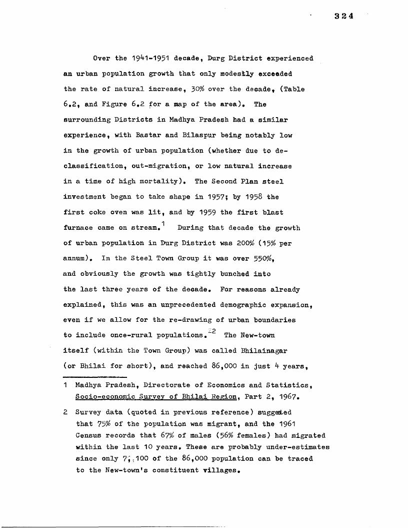
324

Over the 19^1-1951 decade, Durg District experienced an urban population growth that only modestly exceeded

the rate of natural increase, 30% over the decade, (Table 6.2, and Figure 6.2 for a map of the area). The

surrounding Districts in Madhya Pradesh had a similar

experience, with Bastar and Bilaspur being notably low

in the growth of urban population (whether due to de-

classification, out-migration, or low natural increase

in a time of high mortality). The Second Plan steel

investment began to take shape in 1957? by 1958 the

first coke oven was lit, and by 1959 the first blast“Ifurnace came on stream. During that decade the growth

of urban population in Durg District was 200% (15% perannum). In the Steel Town Group it was over 550%,

and obviously the growth was tightly bunched into

the last three years of the decade. For reasons already

explained, this was an unprecedented demographic expansion,even if we allow for the re-drawing of urban boundaries

22to include once-rural populations. The New-town

itself (within the Town Group) was called Bhilainagar

(or Bhilai for short), and reached 86,000 in just years,

1 Madhya Pradesh, Directorate of Economics and Statistics, Socio-economic Survey of Bhilai Region. Part 2, 1987*

2 Survey data (quoted in previous reference) suggested that 75% of the population was migrant, and the 1961 Census records that 67% of males (56% females) had migrated within the last 10 years. These are probably under-estimates since only 7J.100 of the 86,000 population can be tracedto the New-town's constituent villages.

(up to 1961, by which time the plant was producing736,000 tonnes of pig-iron)*

Where did the migrants come from? Being iron

and steel and heavy construction workers they were

predominantly men (see also Table 6 *3 ); the sex.ratio

in Durg Districts towns fell from 1*017 to 0*706, and in Bhilainagar Steel Town proper it was 0*^86, about

two men to every woman. Most of them (72% of those to

Durg Town Group) came from outside the State, and very few

(15%) from within the District, and, being largely unskilled

labour, nearly ip (72%) were of rural origin (Table 6 .3 )*

We move on to observe the demographic effect of

a backward linkage in the industrial complex, that is

a New-town whose investment was also necessary to sustain

the future intended expansion of the steel plant in the next decade, and for that reason referred to here as an

’'accelerator" town: the Jaran Dalli Rajahara Ore Mining

Colony (to give it its full multi-lingual name)* This is a town of 2 3 ,0 0 0 people and its more balanced sex ratio

(0.650) reflects the relatively high employment of women2in the ore-mining industry, presumably as surface workers*

1 Hindustan Steel Corporation Ltd*, Iron and Steel:Statistics for Iron and Steel Industry in India* 1970. Ranchi.

2 We have more to say about the (often depressed) social background of miners that may account for the supply of female labour, below* The sex ratio in the industry as a whole is 0*5^7* See further, Government of India,Labour Bureau, Women in Industry. Simjia, 1975* Chapter 2*

We now turn to assess how other towns in the District

were reacting to these dramatic changes in the economy#

The other large town is Rajnandgaon. Its principal exports

are cloth, size-wood, and pulses (additionally it manufactures

cement piping and curtains), but its growth of 92% during

the decade clearly indicates its dependence on the growth

of Bhilai. Its manufacturing sector was well established

(it was of the male work-force) , and it was evidently

not a mere dormitory town, but had reacted to the rapid

increase in demand for consumables in the locality#

We shall call it a "multiplier11 town (Table 6*6).Elsewhere in the District the towns stagnated or declined,

providing their labour to the growth centres# Again

from the Census we can infer that most of the labour

employed in the towns apart from the Steel Town was

local in origin (Table 6#5)j 50% of the migrants were from within the same District# There was no question of

searching for appropriate labour from further afield either to obtain the type or size of work-force required#

The object of carrying out this detailed study of a sub-region is to ascertain the indirect effects of a new

industry on the surrounding work-force and population

structure# A glance at the map (Fig. 1.7a) shows the spread of urban population growth in neighbouring Districts

in the same decade# The most outstanding District from this

point of view is Bilaspur. This contains the ill-fated Korba coal field; the New-town of Korba grew to

1 2 .0 0 0 in response to the required input to the iron

and steel industry of coking coal* But the District capital,

Bilaspur City, also flourished, growing to a town of87.000 by 1 9 6 1* Its manufactures, consisting of bidi, soap, bronze and brass utensils demark it as a "multiplier"

town, with a modest manufacturing sector established by 1961 (Table 6 .6 )* As in other Districts of this type, male migrants are mainly local (Table 6 .5 ), 65% from within the State, hk% from within the District, and mainly from rural areas in the case of the locals, but not in the case

of those from afar. But Bilaspur town (as it was in 1 9 6 1)is worth studying for different reasons: by Indian standardsit is a notable employer of women. This is due to the establishment of household-based bidi manufacture and cotton spinning, partly in operation before the industrial boom in the area, but expanding in its response, and continuing to attract a female work-force (Table 6 .3 ).The immediate effect is more rapid family formation,

illustrated in the high sex ratio maintained despite the

rapid growth of male migrants. The origin of the female

migrants is .more local than in the case of the heavy industrial

town (51% in Bilaspur District as against 28% in Durg District

coming from within the District, figures not dissimilar

from those for males - see Table 6*5)* It was argued above

(in Chapter 5) that these migrants are not wholly

attracted by job prospects but are more likely to follow

their husbands (or other family members) if job prospects

exist, and hence their presence in larger numbers in

Bilaspur than in other rapidly growing towns*

The other mining locality in the area is Surguja

District, which is strictly speaking outside the study

sample (being heterogeneous)* The fate of the collieries

has been very unstable as prospecting has shifted from one

place to another* The general economic problem is that theregion does not produce quality coking coal for iron manufact­

ure, but the intention was to blend it with better grade

coal from the Burdwan coal fields for use at Bhilai* In

Surguja District both Chirmiri and North JK Colliery

were revived in 1961* The slightly larger towns of

Manandragarh and Ambikapur flourished but purely as

trading or commercial centres, in the former case

prosperity being closely related to the output of coal.

Two further "multiplier" towns were selected for observation (in the 15-20,000 population size range):

Champa in Bilaspur, and Jagdalpur the principal town in Bastar District. Both grew by about ^0% over the

329

decade, produced cloth and metal-ware, and traded in

agricultural products# The towns of Bastar District follow the path outlined above: J>0% of their migrants are

local, and those that are less local are more urban.In both repects they contrast with those to the heavy industrial towns.

We now want to trace what happened to these towns

during the crucial decade of the 1960s, when the steel mill

was fully on stream, at its first-phase rated capacity, against

a background of economic depression setting in from around

1965 (when the plant had been expanded toward the 2-J m.t#

capacity stage, but with production of pigjron levelling

off at around 2 m.t. It should first be noted that Bhilai

was affected less by industrial problems than were its

sister mills, being as it was very much a pace-setter.

Its output was simpler to fabricate (heavy sections),

and apparently easily disposed of, at least until the onset

of the depression (perhaps by resorting to dumping) 5

but it is clear that the severe decline in consumption of non-flat products after 1965 set back the plant.

Similarly the decline in demand for other locally-

produced industrial items (like the cement piping)

or raw materials (like timber) afflicted these towns.

1 See W.A.Johnson, The Steel Industry of India. Cambridge, Massachusets, 1966.

2 See S.D.Kshersagar, "Growth in Consumption of Steel in India." Economic and Political Weekly. 2?th August, 1911 •

Finally there were specific problems in coal production, requiring prospecting for more suitable grades in the Korba

region.

Thus we may distinguish three economic features

that determine the stagnation of the local industry in

Eastern Madhya Pradesh. One, a twist in the industrial

structure away from heavy industry; two, an overall recession; three, technical-economic set-back in the plant

itself. It is not always easy to distinguish the effect

of each on the sub-region. But some attempt to so do

has been made here by investigating a sub-region with

a ..'different industrial base (compare Poona District in Maharashtra, in Chapters 1 and 9), and a sub-region with

different technical problems (compare Burdwan District

in West Bengal, later in this Chapter). The major thrust

of the investigation, however, is to compare the effects of

modern technology (specifically large-scale plant) per se

in such a crisis following upon the period of prosperity just described.

How did this era of economic change (and lack

of it) manifest itself in demographic terms? The

fuller social implications we leave until later in this Chapter. Here we focus simply on the economic structure of the incremen­

tal population and migratory movements of the male labour

force.

331

Bhilainagar grew rapidly* doubling over the decade* with male growth at 67% and female growth - implying family formation - at 175% (Table 6.6). But the manufacturing

male labour force grew at only 22%. This differential

raised the question of future employment prospects as

the younger cohorts enter the working ages. A fall in the ratio of manufacturing males to the total male population

need give no cause for alarm* but the size of the fall

in so short a space of time might well do so (4-3% to 31%

in 10 years). In this context it would be important to

observe neighbouring urban areas. Durg Municipality

is a town that could be expected to diversify and expand

in manufacturing activity, combining multiplier and accelerator

effects, in response to the steel industry growth pole.

But the story is a sad one. The growth in manufacturing

population was negative over the decade. Taken together* the Durg-Bhilai agglomeration experienced a growth of only 13*6% in its manufacturing force. Rajnandgaon, the other

multiplier town of the 1950s stagnated too* the urban

agglomeration (retaining comparable boundaries) grew at

only 25%; the incremental population contributed only 5% to the manufacturing labour force* that is less than

per year. Here we see the seriousness of the check in

terms of production-labour growth, in the wake of a dramatic

expansion. It is the quality and enormity of the change

1 Later we show that workers in the iron and steelindustry increased by about one third with the increase in capacity (i.e. well above the average for manufacuring generally).

that carry seriously and arguably unique demographic and

hence social implications. A glance at Table 6.6 reveals a similar picture throughout most of the sub-region.At Bilaspur the actual size of the manufacturing

labour force hardly changed (and that from an only

modest base of 11% of the work-force). However, the coal town of Korba grew more rapidly (coal-based manufacturing

included) though from a very small base of 12,000 so that

there was no question of this compensating, on a sub-regional

basis, for the overall stagnation. Its mining labour force

increased by only 21%. Similarly Ambikapur and Manendragarh

in the coal-producing District of Surguja expanded their

manufacturing sectors (albeit from minute bases). Ironically the prosperity was probably built on the over-production of

coal, in the sense that the Bhilai plant was being fuelled

with inferior grades in much higher proportions than was

technically desirable, leading to further increases in

down-time.

In summary, there was an enormous injection of capital

into the area during the Second Plan} its physical manifest­ation were the steel mill and iron works at Bhilainagar.To sustain an expansion of output from thsmill required

further investment in the industries supplying the raw

materials, in coal mining and ore mining in the sub-region

(with other inputs coming from outside). To sustain output

elsewhere in the economy (for instance in the steel-using industries) required further investment also: however,

little or none of this seems to have occurred in the subregion.

•'Accelerator" towns then are limited to Bhilainagar itself

and to the raw-material producing localities. They are

so closely related to the steel industry that their fate

is decided by that of the industry. The second part of

the decade saw a major stagnation in India's industrial

development, but especially in the heavy industries*Steel is a barometer in recession. Thus the state of the macro-economy can be held to be reflected in the fate of

these townships. However, had they been diversified,

so that accelerator effects were related to the progress of •

the economy as a whole, their fate would not have been so

grim: the chemical and oil-based industries and luxury

goods producers did not suffer so seriously in the stagnation, and their market remained relatively b^byant

during the slow-down in aggregate growth. The incomes

created by the Second Plan investment sought consumer goods, and hence most of the towns that had expanded

in the late 1950s were multiplier towns. Stagnation in

the late 1960s affected them also. Locally what we see is

a crystalisation of the effects of the failure in the macro­

economy.

The initial investment and the accelerator

effects that followed from increased industrial growth

filled the industrialising towns with able-bodied men.They were followed by (if not accompanied by) women, and families were created. The young now dominate their age structure. The other towns attracted migrants also,

and their families, but they additionally attracted

hopeful young men who would have seen their incomes grow had the multiplier effect been sustained by

1 See Figure 6.1 for Bhilai (and compare Durgapur) where the developing age structure is strikingly portrayed, and Table 6.7 where the increase in the under-15 age cohort is noticeable not only in the core Steel Town (where its proportion in the total population increases from 25% to k2% over the decade), but also for instance in the Korba mining and industrial manufacturing and processing agglomeration (an increase from 30% to 39%)* This Table also illustrates how respectable demographic growth rates can mask the fact that more than 50% of the growth is accounted for by the growth of the female population, relating to the earlier in-migration of men*

continued growth in the sub-region. They were dis­

appointed. Some of these towns expanded in the trades

and- services sector, but not in manufacturing. The

young migrants' incomes must have fallen short of

expectations. Still other towns failed to expand in

economic terms at all in the second decade, after an

initial boost in the Second Plan period. People left them, some to go on and try their fortunes in another town,

and probably some returned whence they came* Families were not formed. As a whole, the industrial region was

nipped in the bud. Yet, here and there, the sap is still

rising, for the youngest cohorts are maturing. The

1980s, for better or worse, will witness the result.

Burdwan in West Bengal Analysis of a District

The North of the Chota Nagpur Crescent is theindustrial heartland of India, among the palms and

dark waters of West Bengal. In the District of Burdwan India's second large private-sector steel works was

erected, at Burnpur, in 1936, and expanded from a million

tonnes from about half a million over the course of the

Second Plan period (1955-60). The work-force was

partly established in the adjacent town of Outer Burnpur.

1 This scenario is investigated, in some detail, in theform of a projection model, in Chapter 9 below.

During the same period the adjacent City of Asansol undertook a range of manufacturing and servicing activities

related to the heavy industry: liquid oxygen, glass, and locomotive manufacture, locomotive repairs and motor vehicle servicing. Additionally, both Burnpur and ABansol

(together called Asansol Town Group or Urban Agglomeration)

produced lighter manufactures, textile garments, and liquor, and processed rice and flour, while Outer Burnpur was a centre of sweetmeat manufacture (Table 6 .8 ). Asansol Town Group was therefore a combination of a diversified accelerator

and multiplier town, with a modest proportion of its labour force engaged in manufacturing. Its growth was rapid, ?8% during the decade (to reach 169»0 00 by 1 9 6 1): the migrant component, amounting to nearly -frds of that

growth was notably from outside the State (5^%), a pattern we have observed elsewhere in heavy industrial areasf and the disturbed sex ratio (0.6 6 *0 is indicative of selective male migration of the kind we are used to also.

Indicative of the migration, 30% of the population was recorded as Hindi-speaking (and as high as 61% were non- Bengali speakers) in a Bengali District; 10% were Muslims,

1 Unfortunately, the Census classification for migration purposes distinguished Asansol Municipality separately, and combined Burnpur with the other smaller towns in the District and with Durgapur. This makes Table 6 * 5 a little difficult to read in this respect.

1the refugees from East Bengal.

The major investment in the District, also in the Second Plan period, was a brand new integrated iron and steel works (built with British collaboration), the

second of the million tonne trio. This was at Durgapur,

something of a contrast with the plant at Bhilai in being grafted on to an already industrialising area, but, like

Bhilai, actually constructed on a greenfield site* The

first output of steel was in 1960-6 1, A-20,000 tonnes of

pig iron, by which date the new township bad grown to

A-2,000 people. The migrants initially were men, and to

judge from the only migration data that include Durgapur

as a major component, around 30% came from other States,

mainly from rural origins (Table 6 .5 ); ^3% of the population

was non-Bengali speaking. At this time nearly half the

male work-force was engaged in manufacturing, most of it

in the massive steel plant. The other town that sprang

up in this decade on a greenfield site was Chittaranjan,

the centre of railway locomotive manufacture (to which, of

course, steel is the major material input). This was much earlier than Durgapur, and its male population was also

1 Government of India, Census of India 19&1. West Bengal, District Census Handbook, Burdwan, Volume II, Calcutta, Tables C V and C VII.

2 M.R.Chaudhuri, Indian Industries. Development andand Location. Oxford University Press, Calcutta, 196 6; Hindustan Steel Corporation Ltd., Iron and Steel, cited in note above.

ky/o non-Bengali speaking (a similar proportion to that in

Hirapur locality where Burnpur Steel Town is situated).

This is the centre of India’s coking coal region, and the other towns in the North-West of the District

are mainly coal-mining towns; they displayed the same

erratic growth that we witnessed in Madhya Pradesh,

in response to two factors - dramatic change in the demand for coal, and the working of new seams. Ondal declined,

then grew very rapidly, doubling in the decade, Jamuria

and Kulti lost population despite earlier growth,

Raniganj continued to stagnate (see Figure 6.3 for locations). Their populations were also heavily dependent on migration from Bihar,

Further down the Damodar valley we find a contrasting

town of the type characterised by our Model u2iu : the old administratice centre of Burdwan City itself. The town

enjoyed the prosperity of the District that occurred with

the expansion of steel and engineering, and its growth rate increased to a modest kk% over the 1951-61 decade. But functionally, as far as its industry was concerned, it

remained a multiplier town, producing flour, rice,

sweetmeats, textiles, jewelry, and silverware in response

to the local increase in demand,. ; and, in any case,

manufacturing was only a minor activity, involving less

than 10% of the labour force. Migrants were mainly local (only 36% from outside West Bengal) with the population

predominantly Bengali speaking (80%), and, in line with

its administrative function (and white collar labour force)

over ■} of its migrants came from other urban areas (Table 6.5)*

The following decade witnessed, as in Madhya Pradesh,

first a sustained, then a decreased demand for heavy

industrial products. Durgapur began as a success story.

Not only did it reach the million tonne target by the middle of the decade, but industry diversified, and the

prospects of avoiding a brittle industrial ’'monoculture11

seemed promising. An alloy steel plant was established,

also a mining machinery plant, and other engineering concerns.A major fertiliser plant was set up. This activity manifested

itself in a rapid population growth in Durgapur. The male

population nearly quadrupled (276% growth) and the manufact­

uring population more than doubled(l2?% growth), with the

male work-force growing rather faster 041%) ; the female

1 There is a problem in that the urban boundaries were much extended to incorporate what had been previously described as a rural population. If we take the whole locality of Durgapur (urban and rural) at both Censuses, the figures become: male population growth 98.4%, maleworking population 43*4%, and male manufacturing labour 6 5 *5% growth.

population multiplied five-fold. This implies a slight

fall in the proportion of the working population

employed in factory manufacturing (from 60% to 56%)#

Stagnation in this proportion, given its high initial level,

need not cause alarm. The very rapid increase in the non­adult male population is quite anotherm matter, and poses

the question as to whether economic activity, and

particularly manufacturing, can be sustained at a level

high enough over the following decades to employ this

future work-force locally. In actual fact, by the end of1the decade Durgapur had become something of a disaster.

Inter alia, the growth in manufacturing labour force figures disguise the under-utilisation of that labour*

By 1971 the plant was expanded to produce 1.6 m.t. of

steel, and actually produced 0.6 million; its output of

pig iron had fallen since the mid-1960s to less than 1 m.t.A significant part of the reason for this failure was due

to circumstances at Durgapur itself, and not the general

stagnation in investment demand. In this respect it

serves as a contrast with the fate of Bhilai earlier described. Severe bottlenecks in production arose, stemming from erratic coal supplies and inappropriate design

of coal-loading equipment, and technical complaints of this

kind quickly interrelated with labour unrest to escalate

11 B.Tulpule, ’’Managing Durgapur: experience of a TradeUnionist” , Economic and Political Weekly. 25th Dec. 1976| Hindustan Steel Corporation Ltd., Iron and Steel, cited in note above.

towards a crisis. The coal towns during this period

continued their erratic development: Raniganj expanded both

its mining and manufacturing activities in line with its

fast population growth. Ondal declined severely, as did

Kulti*The older engineering towns grew modestly but lost

their manufacturing growth, a sign of the overall

depression, and Burnpur itself, the older Steel Town,

stagnated for the same reason. What is particularly telling

is the fate of the multiplier town Burdwan. Here again

the effect of falling productivity elsewhere in the District

was sufficient to reduce the demand for manufactures

and (as will be seen later) to drive manufacturing labour into the small-scale and household sectors, which grew in

proportional terms while the factory manufacturing work­

force fell* It was fortunate enough that this District,

where local conditions compounded the effect of national

recession, had acquired more diversified urban centres (and that Durg District in Madhya Pradesh, where less diversification had occurred, was subjected only to the

national recession). We return later to these economic aspects of industrial demographic formation*

Cultural Differentiation over time: Bengalis and non-Bengalis in Burdwan

The diversity of regional origins of these large newly formed local populations has serious implications

for the harmonious operation of the future labour market.

It has already been suggested that much recruitment in

India is done through personal contacts, rather than through competitive advertising. Contacts are made

on a regional-linguistic basis, as well as through the

more concentrated networks of caste and family. Labour

market rigidities are further strengthened by the

continuing association of caste (determined at birth)

and occupation. All this means that equilibrium is more likely to be achieved if the supply of labour for specific

industries or occupations grows at approximately the same

rate as does the specific demand. On the demand side,

changing industrial composition and changing technologies make this very unlikely. The unlikelihood is enhanced further by differential demographic growth in local supply* It has

already been mentioned that high sex ratios, implying the

pursuit of family formation in urban areas, presage the

more rapid growth of the future labour force in particular societal sub-groups. Social disharmony often follows on

two accounts: first, the sub-group, outgrowing its

employment opportunities, resents the labour market

rigidites that it sees discriminating against it;

secondly, the rest of the population resents the growth of the sub-group which it fears will compete for diminishing jobs with increasing success (and reacts

by tightening the rigidities of the labour market).

We cannot usually pursue these populations through time

empirically, though the problem was simulated in Chapter 3.

But in West Bengal the fairly clear linguistic differences

between locals and migrants enable us to make some

headway.

The Bengali-speakers in the Burdwan District towns

and cities have high (f:m) sex ratios relative to the

rest (Table 6.12), though perhaps lower fertility.

Projecting differential birth and death rates over time

and distinguishing the consequent natural increase from

net in-migration is hazardous. In the case of Burdwan

District this can be gauged approximately from noting that

the Hindi-speaking male population, once established through the massive migration of the late 1950s, grew slower than the male Bengali-speaking population down to 1971 (even despite

net in-migration of male Hindi-speakers). In fact a growth of

only 25.6% (Table 6.12) suggests that, if there was aiy net in-migration at all (which there clearly was into Durgapur

for instance), natural increase was subdued. The case can

be made even more strongly for the non-Bengali speakers

generally. This reflects the underlying bias against

natural growth that is created, as illustrated in the

simulations, by the adverse sex ratios among the migrants* Nonetheless, during the 1960s, family formation was

proceeding rapidly, so that the female Hindi-speaking

population increased much faster than the female Bengalis

in Burdwan. But this process will only continue until

the sex ratios are approximately equalised^ (if male migration

ceased in 1971* the female Hindi-speaking migrant population

would continue to grow, on this assumption, until the

ratio between the Hindi and Bengali populations reached

only 0 .1 3:1 .0 ).

Taking Durgapur alone (Table 6*12) we consider

separately Bengali and all non-Bengali speakers (of whom Hindi-speakers are a substantial proportion). Again

the native Bengali male population grew far faster

than did the non-Bengali speakers between 1961 and 1971,

reflecting increasing in-migration from within Bengal

(East .or West), relative to that from other Indian States.

In this case we cannot make any quantitative judgements on

relative rates of natural increase (though we do note that

in 1961 and in 1971 the sex ratios of the non-Bengalis

were well below those of the Bengalis. Over the , decade the growth of the non-Bengalis was primarily due to

the influx of women (but even that was lower than the rate

of growth of the Bengali female population). By 1971

3 45

the sex ratio of the non-Bengalis was 0.608: though

there are no clear precedents upon which to base a sure judgement, it would seem likely that a ratio of 0 .8 0 0

would be more likelynto remain stable (this is the sex

ratio among the non-Bengalis in Burnpur Steel Town in 1961) •

If that is the case, the female migrant population in Durgapur will continue to grow both absolutely and

proportionately. This should not be mistaken for a long­

term expansion of the migrant population: it is simply a

1 We have already seen empirically, in the case of Bombay, that some migrant sub-groups remain as split families, retaining very low adult sex ratios with no potential for growth: this is especially true of migrants fromNorth India, from Uttar Pradesh, and in some cases, Bihar. These are the longer-term, longer-distance migrants who are employed in factory manufacturing and almost certainly have small amounts of land (but less than 2 acres, see Chapter 5 above), but who are nevertheless compelled (or feel it wise) to keep all adult members of the family at work to survive. At the other end of the spectrum the locally poor (usually landless) migrate as complete families and have little hope of employment in factories. Between these two groups are the long-distance migrants who gain factory employment and form families rapidly in the towns, and are able to leave the rest of their extend­ed family to work the land, and still survive. Their sons will be born in the city. S.N.Sen in his study of Calcutta also found that the Hindi-speaking migrants were far more often single than were the Bengali-speakers (sex ratio of 0.253 versus 0.7^2, in the late 1950s). S.N.Sen,The Citv of Calcutta: A Socio-Economic Survey. Bookland Private Ltd., Calcutta, i9 6 0.

346

traverse towards a new stable state, in which there is no good reason to suppose that, one community will grow faster

than another. Indeed between 1961 and 1971 the proportion

of non-Bengalis in Burdwan's population remained constant at

around 17.5 per cent. The short run fluctuations and

instabilities in the labour market due to sudden increases

in particular age cohorts of particular regional origin

are quite another matter. These are the products of the

highly unstable initial migration patterns plus differential

patterns of family formation. The Bengalis' second

generation will enter the labour market rather earlier, and the peak in the non-Bengali labour supply will follow.The disequilibria and tension that this configuration may

cause are more fully worked out for the case of Bhilainagar

in Chapter 9 below. But there is no evidence to suppose that the longer run growth patters will differ substantially, once the new stable state has been approximately achieved.

The likely range in fertility between the two groups has

been illustrated in the simulation Model, where 5*1 ior local total fertility and 5»7 for migrant total fertility wensetakens the ratios of migrant to local population

ranged from 0.3251.0 (with same fertility) to 0.35s1.0

(with the higher migrant fertility) (Table 3*3)t within twenty years* In Durgapur differential migration patterns

caused that ratio to fall from 0 .3 8:1 .0 to 0.25:1 within

a decade. Problems in short-run dynamics are far more striking

than long term trends.

Class Structure in the Development of Urban Demography: A Study of the Newly Industrialising Areas

It is unfortunately not possible from the available

materials to analyse the class composition of the urban

areas of different character, nor to document how these areas might be changing in respect of class structure over

time. Most of this thesis has had to be restricted to the

demography of the aggregate urban population, with some

extra detail being incorporated in the case of the migrant populations; most of this has had to relate to locational

rather than economic background of the migrant, though

some attempt has been made to deduce the latter from the

former. In the Chapters that follow in Part III we shall make further attempts to reconstruct something of the

areas' socio-economic structure, when we focus more

strongly on occupational and income differentiation.Limited demographic information is available to us, however, relating to the Scheduled Castes and Scheduled

Tribes (known together as the Backward Classes); as these are predominantly the lowest socio-economic group,

we can at least take their recorded experience as an indicator

of the inter-play between demographic and social class

factors (to put it no stronger than that).

The Backward Classes participate considerably

less than their higher caste brethren in the industrial

expansion of the heavy industrial areas developed in the

Second Plan. This is perpetuated over time. In 1971 there were still no Backward Classes reported as employed

in factory-sector industry in the Bhilai-Durg urban

agglomeration (Table 6 .9 ). This is despite there

being 10,000 people of the Backward Clases in Bhilainagar town itself (and 35*000 in the urban locaities of Durg

District), It is to be noted that in this District

the participation of this social group in manufacturing

is mainly in towns like Rajnandgaon and Dongargarh,

where prosperity was least sustained.

Of further interest are their more balanced sex

ratios, than those of the general population (Table 6.10).

This may reflect in part simply a higher fertility

(on which there is no evidence however), and insofar as the

sex ratio is also higher in the adult population, it

will clearly promote a higher fertility (cet. liar.).The sex ratios are also higher among the workers, who will be predominantly adult. This was the case in 1961

when it may have reflected a lack of migrants among the

Backward Classes, for by 1971* in the case of Bhilainagar, the sex ratio of the Backward Classes did not differ

much from: that of the general population (being skewed

towards males In both cases), and in this case we know

that both Backward and general populations must have

been migrant since Bhilai did not exist prior to 1955

(Table 6.9).1

The picture is very similar in Durgapur with

its 25*000 Backward Class people; only 2.8% of the working

Backward Class population participated in the factory

sector manufacturing industry (Table 6.9)* as against

56.3% of general population. Again the well balanced sex ratios suggest that these people are just

as committed to an urban life, through forming families in

urban areas, as are their higher caste brethren. We

should note how their participation in the cities has

changed over the decades, enhancing the effect of a duality emerging in these industrial towns. The Backward Classes

have either congregated around Durgapur, or else the re­

drawing of the urban boundary has encompassed them,(or both), as they have grown from 5*8 to 12.3 per cent of the, v

total population; but their participation in the factory

sector remained small (2.8%) in 1971* In Bhilai there has

been much less congregation recorded over the decade,

indeed a slight proportional fall (from 7*1 to 6.1 per cent

of the total population) ,(Table 6.9). To take a comparison

from Western India during the same period, the New-town

1 The Census did not record details of S.C. and S.T. at the level of the town itself in 1961.

areas of Maharashtra also have the lowest proportions

of the Backward Classes: half as many in Pimpri-Chinchwad

New-town as in Indapur, an old town in the same District

(Poona), or as in Sholapur (Table 6,11),

Case studies that show large numbers of Scheduled

Caste migrants in cities have been able to point to

worsening rural conditions, rather than expanding

opportunities in urban areas, as the cause* In theCity of Poona in Maharashtra, for instance, the slum

settlements most peopled by migrants from drought-

stricken areas contain a high percentage of Scheduled

Castes (often over 50% compared with the average of ?%

in the City)* These migrants come as complete families,

from other Districts not far inland, and once located

there, having no rural land, they are effectively locked

in the city* If the latter fails to prosper, they are the

least likely to be able to return to a rural livelihood,

and the last to emigrate to other cities* It is interesting

to observe that this most depressed class group ischaracterised by a high sex ratio (and fairly mature

family structure) from the start, just as are the higherclass migrants from other urban areas. In between fall the

industrial wage labour groups, who tend to migrate as singlemales, but many of whom form families rapidly afterwards,

1 See M.M,Bapat, ’’Occupational and Spatial Mobility among Shanty Dwellers in Poona", Ph.D. thesis, University College London, 1979*

3 51

In the mining localities, where the Backward Classes are more dominant, their population’s sex ratios are higher than those of their colleagues, though this

is not specifically the case among the actual workers in

the mining industry (Table 6.10)* Clearly they are more

likely to be of local birth, and to have their families

stay with them, than are other caste groups. The employment of women among the Backward Classes is generally more

likely than is the case in the general population,

partly because the Backward Classes only participate in

branches of manufacturing that happen to be more suitable

to female employment anyway (not so much in iron and steel

production for instance), but partly, and more importantly, because women from the lower castes are permitted,

and indeed forced through economic compulsion (the two

are not unrelated) to work, when other women would not be.

Note the contrasting sex ratios in the construction

industry (O.6 5 for the Backward Classes versus 0.27 for the general population), (Table 6.10).

It is the Backward Classes who remain when the mines

close down or fail to expand (note the case of Chirmiri

in Madhya Pradesh, Tables 6*9 and 6*7). In a later Chapter we discover how migrants generally manage gradually to work

352

their way out of employment in mining and into employment

in manufacturing industry over time. The older the mine

the more local its workforce and the greater its component

of lower caste groups,; there is a concentration

of a class of people who are already the most vulnerable

in the rural areas (to losing employment as agricultural labour,

for instance, in the case of harvest failure). But

equally, the older the mine, the more likely it is to be

closed, which is the industrial equivalent to a harvest

failure in an urban monoculture with a clearly differentiated

class of wage labourers. At the community level the

problem is exacerbated by the older age structure of

a declining population, which we have seen characterises

older stagnating economies. At a family level the lack

of social mobility among the lowest class means that sons

will be of little help in diversifying the family income,

for they too will be miners*

The failure of the Backward Classes to be represented

in the developing localities can be observed to be long­

standing. In the heavy industrial City of Jamshedpur

(founded in the first decade of the Century) there was only 12.8% of the population recorded as Scheduled Caste

or Tribe as late as 1971, and that is in a District where the Scheduled Tribes alone number 58.6% of the rural

population. This is of course an extreme case* tribals

are predominant in this region of Bihar. But the observation strengthens the argument (consistent with our inference in Chapter 5 ) that recruitment managed, consciously or

unwittingly, to miss the local labour; for it would be hard

to argue that the Backward Classes were exceptional

in being more fully employed than their fellows in agriculture, and hence less eager to participate in the alternative

urban economy. But a further observation points in

the reverse direction. Of those small numbers in Jamshedpur, a very high proportion was employed in manufacturing industry, 5^%, almost the same proportion

as the general population in manufacturing. Without field

research one has to remain agnostic. What remains striking

however is the small number of tribals in this longstanding

industrial city in the heart of a tribal area.

We have presented separately some contrasting data

for other localities in Bihar (Table 6.11). The failure

to employ tribals in the developing areas, in preference

to migrants (who are mainly from West Bengal), has been

a highly contentious issue in the 1960s. As mentioned above, depite the high proportion of tribals in the rural Districts of Ranchi and Singbhum, their urban representation is

small. In the newly industrialising locality of

Bokaro Steel Town the representation of the Backward

classes is low but not negligible, and indeed their

presence in the town is higher than the rural average, but they are underrepresented in manufacturing,

with only 11% in that sector. In the New-town

of Jag&nnathnagar (part of Ranchi urban agglomeration) they are also well represented. But in Dhanbad urban agglom­

eration the familiar picture re-appears, with a small

proportion of the Backward Classes there, and those

predominantly engaged in mining. Developing Bihar is

an area undergoing social change. But the overall

picture conforms to that presented before, and analysed2by others elsewhere in. India: the Backward Classes are

under-represented in urban areas because the occupations

into which they are locked are under-represented. The

exceptions are the mining and the declining towns, from

where the more socially mobile have moved out, leaving the

1 N.Sengupta noted how Hindustan Steel employed local Bauri tribals in compensation for their loss of land, but only as temporary unskilled workers: the terms of contractual employment required literacy, thus effectively disqualifying the tribals. Since 1968, of the qualified, locals have to be found employment first. N.Sengupta, Destitutes and Development: a Study of the Bauri Community in the Bokaro Region. Concept, New Delhi, 19?8.

2 See for example V.S.D*Souza, "Scheduled Castes and Urbanisation In Punjab: an Explanation", Sociological Bulletin. March, 1975-

Backward Claeses over-represented. This may not, however, be the only reason for an increase in the proportional size of the Backward Classes: their more favourable sexratios are indicative of less disrupted family formation,

and unless high mortality compensates, their growth rates and hence relative future population size will indeed increase. If the caste system exacerbates the disabilities

of being born into a Backward Class by further restricting

mobility there will be an increasing supply of labour to compete for non-expanding occupations in stagnating towns. Whatever the cause, more Backward Classes sharing

a fixed resource means increased inequality between them

and the rest of the population.

35 6

Figure 6 .1

Examples of Contrasting Urban Age Structures

Rapid Growth Towns:

'k fo o

r rto o

•k r

'OtvtaafM ioiuv II(wy/‘) ^d4'

j ^ _ft"'3

r *-■»

/o rS' a

O -

ON j o t t f i j f e «S ^i«iv u<Hv d < u a i* L cjvOi-rffc*

Fig. 6.1 cont'dHistorical Growth of a Steel Town

A’I O-Uf 1—

so 5 O3'cMWt)AcL|>w<r |^|

J L

r

r°\» sr

C-/if — ^

Tcu*.tkMll}vW «)((6oU

358

Fie. 6.1 cont*dFast to Moderate Growth Towns:

TiuXiluotw * uvtlUc»~ ftlt •W»%

CmMc*c.K WiU• I tb io f(j*xrJ) 160 If

IkUnufBfnoc.1 £«*.») , , |6oI +

Controls

wr-*s*\

ir-w

359

Fig* 6.1 cont*d

Slow Growth Townes

MotvjWjr m it o

rP Hr i.

0-H

SK<il uir« ^ 1 1 TciAdUflvVA'T fill ■ V W

fifci

o-lt*

SKoIajkay ltlf & W { . 1

( j S . c ' k ) l 6 o | t

O'unts&.'r

a**«l Tc^Aifkjuj/ *•*< «*. U»KarT h K t if t r i ( jfc . r A f lk a r U fk iv ’a , . •

360

Figures 6.2 to 6.5Maps of Sub-region of Eastern Madhya Pradesh and District of Burdwan in West Bengal

T o C ia jj

aaltufejf

OndaL

R.,

loo VuW

WESTBENGAL

KoojU<| I t ,

To C ftltu H t.

fo JMU*K*lo<J MADHIAPRADESH

$u RAOrA

0 AMijlufH*To

fo ftovhtk- + «*»«(

tUji.tUjiwumii

to ^ 3°ti

SATTAfc.

loo tfiW-H

361

Table 6.1 aSelected Indices from the Model for Empirical Comparison

SEX RATIOS (fsm in total population with current migrants below)Year: 0 5 10 15ModelType1b 841 680 736 759

(484) (347) (1241) (486)

1a 841 742 816 830(484) (521) (1 8 6 2) (486)

1c 841 426 588 631

CHILD : POPULATION RATIOS (0-4 by total population with 0-14 m+fby total population below) (%)

Year: 0 5 10 15

1b male fern.

12.714.5

12.3 15.8 . (35.8)

11 *4 15.9

1 2 .115.7(35.2)

1a 12.714.5

12.315.9(35.9)

12.41 6 .1

13.415.9(36.5)

1c 12.714.5

10.41 6 .5(31.9)

8 .31 7 .2

10.916.9 (32.5)

URBAN GROWTH RATES (decadal growth) (%)below

Years: 0 - 5 5 - 1 0 1 0 - 1 51b , c66.8___9.1-— 9.7male { 81.9 19.8

c54.7_1-8.2„_13.1 > female [ ^3 .7

1a f66.8_10.4 __11.3 malel 84.2 22.9

. . ^ 7 . 0 _ 2 1 . 5 ^ 1 3 . 2female}

1c n «6o4.Q— .3.5.^ >5.8 malel 627.3 9.3 256.6_42.5 _^_13.6female^ ^

Table 6.1 a continuedSEX RATIOSYear: 0 5 10 152b 841

(4-84)800(442)

785(488)

811(713)

(2a 818(555)

819(635)

)

BASE 841 843 846 850

CHILD? POPULATION RATIOS

2b male female

13.51 5 .0

1 6 .217.7(37.4)

15.117.7(36.3)

13.41 6 .3

(2a 16.418.3

15.51 8 .3

)

BASE 1 2 .613.6

13.715.9(38.2)

13.515.6 (36.7)

13.415.4

URBAN GROWTH RATES (decadal rates below) 0 - 5 5 - 1 0 1 0 - 1 5

2b decadal «— *— - ------males 56*9 36.4

females 46.5 3&*3

BASE males/13.9„_13.1„4L2.7i 2 8 .8 277^

femalesfl4.2 13*4 1 3 .21 29.6 28.5

NATURAL INCREASE @0.02 per annum Decadal growth 22.0

Source: Simulation Model (See further Table 3.1)

363

Table 6.1bGrouping of Empirical Cases by Model variantsSEX RATIOS

1961 1971 1961 1971“ Bilaspur 901 907 —^ Bastar . 903 846

Ranchi 817 815 Bankura 905 920Mayurbanj 810 840 Birbhum 844 893Bhagalpur 832 821 Ganjam 951 955

Gaya 861 8741 b— Burdwan 699 785 Monghyr 903 864

Howrah 644 70224-Parg 737 702 — Hoogley 749 784

Singbhum 797 802 Patna 813 822Cuttack 745 772 Midnapore 830 865

(Bhagalpur 832 8 2 1)— Burg 706 864

Dhanbad 646 675Sundargarh 630 790CHILD^POPULATION RATIOS

1961 1971

■— ^ Baudh 949 865Raigarh 901 901Bolangir 923 -923

Calcutta 6 12 636Shahabad 846 845(Bankura 905 9 2 0)

1961 males 1961 males

—^ Bilaspur 13.5 ™ Bastar 13.6Ranchi 13.1 Bankura 13.6

Mayurbanj 1 2 .6 Birbhum 13.1Bhagalpur 1 2 .7 Ganjam 14.6

— BurdwanGaya 13.5

10.3 Monghyr 14.2Howrah 9*6 2b _ n — ■ Hoogley24-Parg 10.5 10.5

S ingbhum 12.9 Patna 1 2 .8Cuttack 1 1 .0 Midnapore 12.51 C -p.— Durg

(Bhagalpur 12.7)1 1 .2

Dhanbad 1 0 .2Sundargarh 9.3

—-^Baudh Raigarh Bolangir

Calcutta Shahabad (Bankura

1961 males

9.3 13.7 14.2 7.2 13.0 13.6)

DECABAL GROWTHla

1 9 3 1 -6 1

Bilaspur 140Ranchi 63

Mayurbanj 206Bhagalpur 53— Burdwan

Howrah 24-Parg

SingbhumCuttack1c -p.— Burg

DhanbadSundargarh

7358645553200294783

61-71576241195923A9454768

12079

1 1951 -6 1 6 1 -7 1 1951 -6 1 61-71™ Bastar 44 111 Baudh 11 220

Bankura 29 24 Raigarh 21 27Birbhum 46 24 Bolangir 22 75Ganjam 36 67 Calcutta 8 8Gaya 30 28 Shahabad 28 40Mongyhr 40 23 (Bankura 29 24)

“ Hoogley 47 3^Patna 30 35

Midnapore 32 26(Bhagalpur 53 19)

Notes:

See Table 6.1a for Models

Model allocation:1951-61 % decadal Model Growth 100+ 1c

5 0 -1 0 0 1b5 0 -5 0 2b50- B-3

1961 sex ratio 50%>h = a

364

Table 6.2Demographic Indices from the Study Districts over Two Decades

Decadal Growth (%) 1941-51 51-61 61-71

feex ratios below)

% aged 0-41961

current migration rate 1961 (previous average)a

sex ratio current migrants (previous average)a

E.MADHYA PRADESH

Durg 30 2 0 0(7 0 6)

69 1 2 .9(864)

14.5(•■7.9)

649(544)

Bilaspur 12 140(901)

57 14.2 (907)

.9.9(3.8)

701(853)

Bastar 14 44(903)

111 1 3 .8 (846)

1 1.?(3.il)

560(797)

Raigarh 55 21(901)

27 13.9 (901)

8 .J(3.1)

658(8 6 8)

Case-Study Selected Towns

Bhilainagar - to 86 ,1 1 6 (486)

102 b (799)

n.a.

Bilaspur 122(893)

13 (5 1 )° (897) ■

•

Rajnandgaon 92(944)

25(952) •

Korba - to 12,424 (? 0 5)

149(8 1 5)

•

Jagdalpur 48(891)

54(874)

Chirmiri -ve! to 6563 35__.C8l.6J

Notes: a average in-migration rate for the previous 5 years(see text for interpretation); ditto sex ratio.(f:m).

b n.a., but see Table 6.7 for % aged 0-14.c including outgrowth

Table 6.2 continuedDecadal Growth {%) % aged current sex ratio1941-51 5 1 -6 1 6 1 -7 1 0-4 migration current(sex ratios below) 1961 rate 1961 migrants

(previous (previousaverage) average)

WEST BENGAL

Howrah 22 58 23 11,4 5.2 593(644) (7 0 2) (3.0) (481)Calcutta 25 8 8 8 ,8 3.0 382

(6 1 2) (6 3 6) (2 .2 ) (3 8 1)24-Parganas 50 64 49 1 2 ,2 4.8 676

(737) (7 0 2) (3.3) (893)Hoogley 25 47 31 1 2 .1 6 . 0 788

(749) (784) (3.3) (854)

Burdwan 45 73 59 1 2 ,1 4.5 820(699) (785) (2.9) (595)

Midnapore 34 32 26 12.5 3.4 720(8 3 0) (8 6 5) (2.3) (791)

Birbhum 14 46 24 14, 0 4.8 768(844) (8 9 3) (2 .8 ) (1 0 1 7)

Bankura 3 29 24 14.0 2.5 1339(905) (9 2 0) (1.7) (9 0 8)

ORISSAMayurbanj 12 206 41 14,0 5.8 414

(8 1 0) (840) (3.2) (499)Sundargarh - 783 79 1 1 ,6 1 1 .1 698

(6 3 0) (790) (5.6) (8 2 0)B-K - 4 11 221 1 1 .2 1.7 93

(949) (865) (2 .8 ) (743)Cuttack 40 53 47 1 2 .6 7.4 440

(745) (772) (2 .3 ) (6 3 6)Ganjam 27 36 67 13.7 3.8 566

(951) (955) (1.7) (1 0 8 9)Bolangir 37 22 75 14.3 6.7 1130

(923) (923) (3.0) (1173)

366

Table 6.2 continuedDecadal Growth {%) % aged current sex ratio*19^+1 — 5 1 -6 1 61-71 0-4 migration current

1961 rate 1961 migrants(previous (previousaverage) average)

BIHARGaya 25 30

(8 6 1)28(87^)

14«4 4.2(2 .0 )

551(842)

Patna 31 30(8 1 3)

35(8 2 2)

13.8 5.1(2.4)

633(6 0 2)

Shahabad 24 28(846)

4o(845)

13.8 5.3(1 .8 )

555(6 1 8)

Bhagalpur 22 33(8 3 2)

19(8 2 1)

1 3 .8 3.2(1.9)

429(6 6 5)

Monghyr 29 40(903)

23(864)

14«8 2.9(1.9)

660(897)

Singbhum 33 53(797)

45(8 0 2)

14.3 5.4(3.0)

785(653)

Ranchi 63 62(8 1 7)

76(8 1 5)

13o9 8.5(3.1)

659(654)

Dhanbad 87 294(646)

120(675)

1 2 .8 8 .8(4.2)

471(543)

Sources: Government of India. Census of India 1961. 1971. (relevant States), General Population Tables,Social and Cultural Tables (C II), Migration Tables (D III), Delhi#

Table 6.3Sex Ratios among Workers in Manufacturing Industry

District Sex ratios female to male with % of(Urban Area) female manufacturing labour in household

industry (bracketed)Household Non-HouseholdManufacturing Manufacturing

WEST BENGALCalcutta ,0 8 8 (1 2) • 018

Howrah .0 6 6 (9 ) .0 2 1

24-Parganas .154 (15) .031Hoogley .327 (8 ) .057

Midnapore .227 (44) .048Burdwan .363 (2 2 ) .0 2 8

Birbhum ♦172 (23) .1 2 0

Bankura .487 (73) .133BIHARPatna .3 2 2 (77) .048Gaya .5 6 2 (8 2 ) .064S ingbhum .2 1 1 (1 3) .0 6 2

Ranchi .411 (65) .074Dhanbad .1 5 6 (2 8 ) .0 5 8

Monghyr .467 (8 0) .0 3 1

Shahabad .428 (8 0 ) .053Bhagalpur .467 (92) .059MADHYA PRADESHRaigarh .877 (6 5) .191Durg • 595 (46) .067Bilaspur .795 (79) .219Bastar .6 8 2 (42) .247

368

Table 6.3 continued

ORISSAMayurbanjSundargarhB-KCuttack Ganjam Bolangir

.498 (94) ,024

.155 (14) .073

.755 (84) ,6 6 7

.225 (73) .035

.7 7 6 (8 6) .1 3 8

.583 (8 1) .137

Source: Government of India, Census of India 1961.General Population Tables (relevant States), Delhi,

Table 6.4Examples of Age Distribution in Stagnating Areas

CALCUTTA DISTRICT male population, proportions by age (with comparisons)Age Proportion Comparison

10-14 ,0 8 6)Burdwan .345

1 3 -1 9 .0 8 8 20-24 .1 1 92 5 -2 9 .1 1 8 30-34 .1 0 6

35-39 .0 8 7 140-44 .073145-49 ,049} .2 8 1

Cuttack .244 Asansol .253 Patna .24450-54 .0421

55-59 .0 3 0 J

Table 6,4 continued.

Calcutta’s age distribution continued Age Proportion Comparison

60-64 *019) Cuttack ,0466 5 -6 9 ,010} ,039 Burdwan *04170+ .010J Asansol .031

Burnpur •0 2 2

Comparison with Stable model used as basis of this analysis Calcutta 3 5+ .320 Model .242

BAUDH KHONDMALS URBAN DISTRICT (Orissa) male population and Age Proportion (m,f) female P o r t i o n

0-4 .093) ,131]5-9 .1395*342 .142^.36410-14 .11 0 1 ,0 9 1J1 5 -1 9 .1 0 0 .0 9 420-24 .1 0 7 .0 8 525-29 .0 8 7 .0 8 63 0 -3 4 .079 *0 6 9

3 5 -3 9 .0 6 4 .0 7 140-44 .0 5 6 .04645-49 .043 .04550-54 .048 .0465 5 -5 9 ,0 2 8 .0 2 9

6 0 -6 4 .0 2 3 7 .03176 5 -6 9 .0 1 6 J.0 4 0 .0 0 8 } ,0 6 57 0+ .0 1 0J .0 2 6)

Sources: Calcutta, Government of India, Census of India 1961.West Bengal, Social and Cultural Tables; Baudh, G.O.I., Census of India 1961. Orissa, Cultural and Migration Tables, Delhi, Tables CII and CIII.

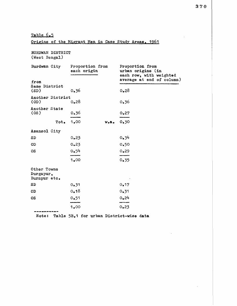
Table 6.5Origins of the Migrant Men in Case Study Areas. 1961

BURDWAN DISTRICT (West Bengal)Burdwan City Proportion from Proportion from

each origin urban origins (in— — — — each row, with weighted

„ average at end of column)Same District(SD) 0 .3 6 0 .2 8

Another District (OD) 0.28 O.3 6

Another State (OS) 0 .3 6 0.27

Tot. 00. w.a. 0 *3 0

Asansol CitySD 0.2-3 0,34OD 0.23 0.50OS 0.34 0.29

1 .0 0 0.35Other Towns Durgapur, Burnpur etc.SD 0.31 0 .1 7

OD 0 .1 8 0.31OS 0.31 0,24

1 .0 0 0 .2 3

Note: Table 3B.1 for urban District-wise data

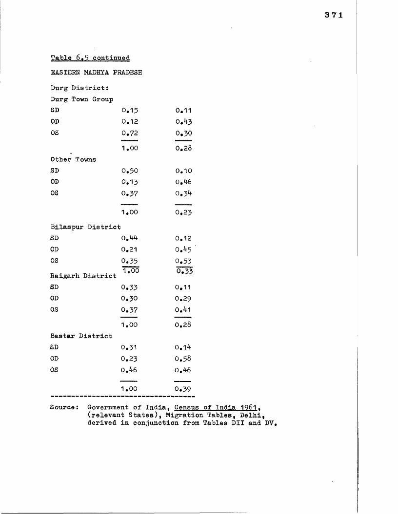
Table 6.3 continuedEASTERN MADHYA PRADESH

Durg District:Durg Town GroupSD 0.13 0.11OD 0.12 0.43OS 0.72 0.30

1.00 0.28Other TownsSD 0.50 0.10OD 0.13 0.46OS 0.37 0.34

1 .0 0 0 .2 3

Bilaspur DistrictSD 0.44 0.12OD 0.21 0.45OS 0.35 0.53

1.00 0.33Raigarh DistrictSD 0.33 0.11OD 0.30 0.29OS 0 .3 7 0.41

1.00 0.28Bastar DistrictSD 0.31 0.14OD 0.23 0.58OS 0*46 0,46

1.00 0.39

Source: Government of India, Census of India 1961.(relevant States), Migration Tables, Delhi, derived in conjunction from Tables DII and DV.

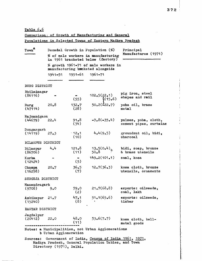
372

Table 6 .6

Comparisons of Growth of Manufacturing and General Populations in Selected Towns of Eastern Madhya Pradeah

Town8" Decadal Growth in Population (%) Principal' % of male workers in manufacturing Manufactures (1971)

in 1961 bracketed below (factory) ■ 1 1 - ■ — ........% growth 1 9 6 1 -7 1 of male workers in manufacturing bracketed alongside1941-51 1951-61 1961-71

DURG DISTRICTBhilainagar(8 6 1 1 6)

Durg 20.8(4-711*0Rajnandgaon(44679) 22.4

Dongargarh(14119) 27*3

BILASPUR DISTRICTBilaspur 4.4(8 6 7 0 6)Korba(12424)Champa 20,7(1 6 2 5 8)SURGUJA DISTRICTManendragarh (9708) 9.0

Ambik&pur 21.7 (15240)BASTAR DISTRICT Jagdalpur

102.5(22.1) (55) 1(15.6)

1 3 2 .7 5 0.2 C-2 2.7 )(2 8 )

91.8 -7.8(-35.4)(34)

1 2 .1 4.4(9.5)(10)

1 2 1 .8 13.5(0.4),(1 1) 5 0 .8 "

149.2(101.1)(5)

3 6 .5 12.7(36.3)(7)

79.0 21.7(68.8)(2)47.1 51.1(65.6)(8)

48.0 53.6(7.7)(11)

pig iron, steel shapes and railpoha oil, brass me tal

pulses, poha, cloth, cement pipes, curtains

groundnut oil, bidi, charcoal

bidi, soap, bronze & brass utensilscoal, kosa

kosa cloth, bronze utensils, ornaments

exports: oilseeds, coal, lakhexports: oilseeds, timber

kosa cloth, bell- metal; goods

(20412) 2 2 .0

Notes: a Municipalities, not Urban Agglomerations b Urban Agglomeration

Sources: Government of India, Census of India 1961. 1971«Madhya Pradesh, General Population Tables, and Town Directory (1971), Delhi.

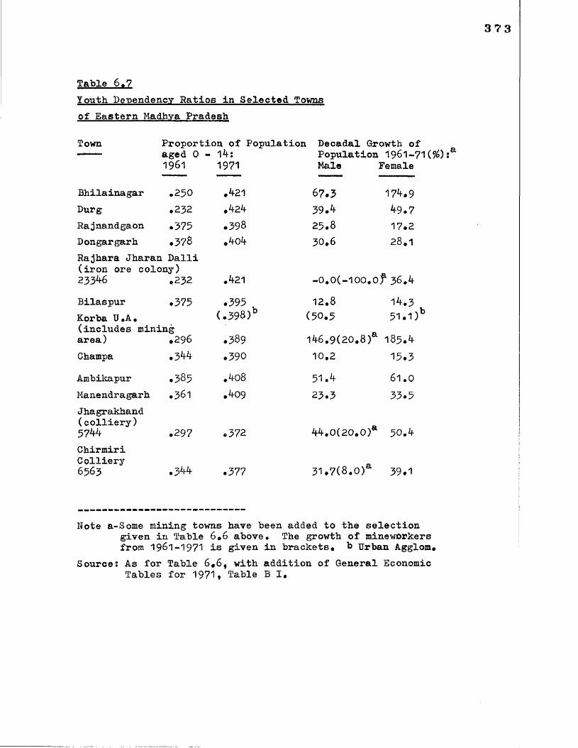
3 73

Table 6.7Youth Detiendency Ratios in Selected Towns of Eastern Madhya Pradesh

Town Proportion of Population Decadal Growth of— --- aged 0 - lif: Population 1961-71(90 :a

1961 1971 Male Female

Bhilainagar .2 3 0 *if21 67.3 17^.9Durg .232 39.4 if9.7Rajnandgaon .373 .398 2 5 .8 17.2Dongargarh .378 *ifOif 3 0 *6 2 8 .1

Rajhara Jharan Dalli (iron ore colony) 233^6 *232 *if21 -0 .0 (-1 0 0.0 f 3 6 .4

Bilaspur .373 .395 1 2 .8 14.3Korba U*A* (.398)b (50.3 51.1)(includes mining area) *2 9 6 .3 8 9 I46.9(20*8)a 1 8 3.ifChampa »3*t4 .390 1 0 .2 15.3Ambikapur .383 .if 08 51.^ 6 1 .0

Manendragarh .3 6 1 *if09 23.3 33.5Jhagrakhand (colliery) 57^ .297 *372 ifif *0 (2 0*0 )a 50.ifChirmiriColliery6563 .3 4 4 .377 31*7 (8 *0 )a 39.1

Note a-Some mining towns have been added to the selectiongiven in Table 6*6 above* The growth of mineworkers from 1961-1971 is given in brackets* b Urban Agglom*

Source: As for Table 6*6, with addition of General Economic Tables for 1971* fable B I.

374

Table 6.8Demographic Characteristics of Ma.ior Townsin Burdwan District

1961 Town 8c Population

Sex Ratio (f :m)

Per Cent: under 13 over 59

% of male Major workers in Manufacture factory manufacturing

Asansol103^05

,664 37.2 3.6 20.1 locomotives, garments, vehicle repair)

Burnpur6 5 2 8 -

.653 3 6 ,6 2.5 6 8 . iron & steel, railway equip.

Burdwan1 0 822^

.789 37.2 *W5 1 6 .2 flour & rice, sweetmeats, textiles

Durgapur .33$^1 6 9 6

1971(Decadal Growth)

2 1 .2 1 .Male pop. growth

6 0 .0 iron 8c steelAdditionalProducts

Asansol .752 ^8 .6 2 1 .8 liquid oxygen, liquor, glass

Burnpur(31**0

.764 i*i-7 23.3 6 7 .2 -

Burdwan (32. * 0

.8 0 7 3t-i» 31.2 11.5 mustard oil, steel furn­iture, soap

Durgapur(3 9 5.6 ) .764 '39. i 275.7 56.3 bricks,

fertiliser, food 8c bever­age

Note: Decadal growth rates are given as percentages.Source: Government of India, Census of India 1 9 6 1. 1971.

West Bengal, General Economic Tables, Delhi, Table B I| Government of West Bengal, District Census Handbook 1 9 6 1; and Town Directory"97^ (G.O.I, Census cited above).

375

Table 6.9Backward Classes in Developing Areas

Urban Locality % of Backward Classes in Po] ulationa 1961 1971

Sex Ratio: .of BCs of TP 1971 1971

(f:m)

% of male workers in factory manu­facturing (or mining)0 1 9 7 1:BCs TP

Durg District 9.8 8 .9 .9 0 6 .864 29.1 38.5Bhilainagar Steel Town 7.1 6 .1 .798 .795 0 .0 6 1 .5

Rajnandgaon 6.7 8.3 .970 .932 45.9 2 9 .0

Dongargarh 7.1 1 2 .3 1 .0 7 2 1 .0 0 2 2 1 .3 1 2 ,3

Chirmiri Mining Colony 2 0 .1 2 8 .8 .8 3 6 .941 8 3 .1 76.9Surguja District (mining) 1 7 .1 18.5 .915 .847 4 9 .8 37.3Burdwan District:Durgapur Steel Town 5.8 12.5 .842 .764 2 .8 56.3Chittaranjan (loco works) 7.0 6.4 .7 0 2 .774 74.5 85.1Jamuria(mining) 22.5 34.5 .899 .792 2 2 .1 2 8 .2

Raniganj (r+u) (mining) 35.1 29.1 .794 .695 40.3 38.5Burdwan City 1 0 ,6 7.8 .913 .8 0 6 15.5 11.4

Sources: Government of India, Census of India 1961. 1971 »

Notes:

(relevant States), General Population Tables, and Social and Cultural Tables (Tables oil Scheduled Castes and Scheduled Tribes), New Delhi*a The Scheduled Castes and Tribes (above) summed* b The total population*c Mining is substituted for manufacturing where indicated in first column*

376

Table 6.10Industrial Participation of Backward Classes in Selected Districts of Eastern Madhya Pradesh in 1961

In each case the figure for the total population is included (in brackets)

District sex ratio % of males in sex ratio inUrban of workers factory manufacturing fact, manufacturing

Durg District .523(.238) Bilaspur " .6 7 8(.3 8 8)Surguja " o263(.143)

19.5 (37.9)9.4 (9.9)2 .1 (4.7)

.356 (.0 6 7)

.527 (.219)

.246 (.0 7 8)

% of males in sex ratio in % of maleshousehold industry house* ind.

Durg 4.9 (3.6)

Bilaspur (10#5) Surguja 4.6 (5.1)

.642 (.595)

.8 8 7 (.795)

.2 9 1 (.2 0 8)

sex ratio in mining/ in mining/ construction construct.

12.4 (1 0.0 ) .653(.2 7 0)(construction)

45.5 (3 0 .0 )' .049(.043) (mining)

Source: Government of India, Census of India 1961. MadhyaPradesh, Social and Cultural Tables, Tables for Scheduled Castes and Scheduled Tribes(Special Table SCT 1), and General Population Tablea, Delhi.

377

Table 6.11Backward Classes in Contrasting Cities of Bihar. 1971

% of BCs in District’s % of Bt&s in the % of BCs in rural population City population manufacturing/

■ — ........ ---------------- mining (same fortotal pop* bracketed)

Monghyr City 17.9 6.5 17.6Jamalpur City 17*9 10.6 42.6Gaya City 2 5 .8 8 .6 13*4Bhagalpur City 15*3 6 .6 11.9

Developing Areas:Bokaro U*A,a 32*3 22.2 11.4Dhanbad U.A. 32.3 16.4 4.4

75*3(mining)

Ranchi U.A, 69*3 17*3 28.3Jamshedpur TJ.A, 61.6 12*8 54*4

Comparisons from MaharashtraPoona District:Poona Municipal Corp. 6.9Pimpri Chinehwad 3.9(New-town)Junnar 6*4Indapur 8*0Greater Bombay 4.0Sholapur M.C. 8.9

Note: a- Urban AgglomerationSource: Government of India, Census of India 1971.

Bihar, and Maharashtra, General Population Tables,and Social & Cultural Tables (C VIII), New Delhi.

378

Table 6.12The Linguistic Composition of Burdwan District between 1961 and 1971

BURDWAN District rural + urban

Growth rates (decadal %)1961-1971:males females

Bengali 27*3(1 6 71 0 00 males)

Hindi 25*6(22^-000 males)

All non-Bengali17*1

27.^

56*8

IfO.if

DURGAPUR Police Station rural + urban .

Growth rates 1961-71

Sex ratios: (f:m) 1961 1971

• 93^

• 59

• 935

• 573

Non-Bengalis as % total 1961 197117*6 17*^

Sex ratios:m ales fe m a le s 1961 1'971

B e n g a l i 119.^ 207,5 • 576 .8 0 8

N o n -B e n g a li ^3*1 1 3 0 .8 • 377 .6 0 8

R a t io1961m ales

Wu-o f ^ B e n g a li t o r

fe m a le s

B e n g a li P o p u la t io n :1971m ales fe m a le s

0 .38 :1 0.25:1 0.25:1 0 .19 :1

Sources: Government of West Bengal, Burdwan District CensusHandbook, 1961, Calcutta, Table C V.Government of India, Census of India 1971. Social and Cultural Tables, New Delhi, Table C V (A ii).

379

Appendix 6 .1 A Note on the Statistical Significance of Three Types of Urban Demographic Growth (Table 6A.1)

Clearly one would expect one industrial category of urban area to shade into another. Few towns are simply

heavy engineering towns for instance* Their demographic

characteristics would also tend to merge therefore.Nonetheless it seemed worthwhile to see how far there are distinct clusters of urban areas, with broadly similar

demographic, and industrial, features within each clusterf

by which the clusters might be differentiated. For a

statistical assessment of this hypothesis we undertake

some Discriminant analysis.

We have taken three characteristics of urban areas

within our sample (of Homogeneous Districts - see Appendix to Chapter 1): (i) demographic growth rates, (ii) percentage of male working population in (non-household) manufacturing, and

(iii) percentage of the latter engaged in heavy industry

(defined in Table 6A.1). Each in turn is subjected to discriminant

analysis to see if there are three distinct groups of towns:

the three groups postulated range from high to low, -

more than 55% growth, 30% - 55% growth, less than 30% growth, for example. We use three variables by which to try and

1 These can be regarded as roughly corresponding to three sets of our model types: (1 a,b,c) (2 a,b) (Base, 3)«

distinguish the groups: the variables are sex ratio, child to population ratio, and elderly to population ratio.

The program* then investigates whether the three groups

(of urban areas) can be regarded as significantly different

in respect of this bundle of variables; in our case it tries

out two different weighting systems, and presents them in

order of significance as functions 1 and 2 (Table 6A.1).

It can be seen from the Table that the three characteristics (sex, youth, and senility) divide the urban Districts into three significantly different groups, whether

the group is defined in terms of growth rates, manufacturing

intensity, or heavy industrial importance. This merely

confirms more strongly our contention that urban areas

can be distinguished on the basis of their industrial

structure (which we have shown to correlate closely with

their rates of demographic growth), and that the distinguishing

features do indeed include demographic structural variables

like sex ratios and dependency.

More specifically, the analysis indicates predictable

features and a few anomalies. The three urban growth groups

are best distinguished (with 99%> confidence) by a combination

of the variables that gives most prominence to the per cent of

1 The sex ratio is f:m, child population is 0-*f (m+f), elderly is 60+ (m+f).

e ld e r l y , and s e c o n d a ry im p o rta n c e to th e se x r a t i o ; t a k in g

a c c o u n t o f c h i ld r e n re d u c e s th e d i f fe r e n c e be tw een th e g ro u p s *

The th r e e m a n u fa c tu r in g i n t e n s i t y g ro up s a re b e s t d is t in g u is h e d

by th e se x r a t i o , w h ic h i s a d o m in a n t v a r ia b le h e re * F in a l l y

th e heavy i n d u s t r i a l c a te g o r ie s a re b e s t d is t in g u is h e d by th e

s e x r a t i o (a lm o s t as im p o r ta n t an e f f e c t as i n th e p re v io u s c a s e )

and c h i ld r e n once a g a in d e t r a c t fro m th e d is c r im in a t io n ; th e

e ld e r l y a re o f m o d era te im p o rta n c e i n d is t in g u is h in g th e g ro u p s *

I n t h i s l a t t e r case a second f u n c t io n i s a ls o s i g n i f i c a n t

( w i t h an a l t e r n a t i v e w e ig h t in g s y s te m ) , w h e re in th e se x

r a t i o and p e r c e n t o f c h i ld r e n r e t a i n t h e i r d i r e c t i o n o f

in f lu e n c e , b u t th e e ld e r l y d e t r a c t fro m th e d is c r im in a t io n *

A g e n e ra l c o n c lu s io n i s t h a t sex r a t i o s a re e s p e c ia l ly

a s s o c ia te d w i t h th e c h a r a c te r o f th e u rb a n g ro w th ( i t s speed

and i n d u s t r i a l c o m p o s it io n ) , w h ic h co n fo rm s w i t h o u r

o b s e rv a t io n s on d i f f e r e n t i a l s e x r a t i o s among m ig r a n ts . The

o b s e rv a t io n t h a t c h i ld r e n a re o n ly a m odera te in f lu e n c e , and

i n th e u n e x p e c te d d i r e c t i o n , can be u n d e rs to o d by n o t in g some

o f th e i n d i v id u a l a n o m a lie s ( t h a t have been e x p la in e d i n th e

c o u rs e o f th e C h a p te r ) , F o r in s ta n c e , i n th e t h i r d g ro up

(e * g * th e lo w g ro w th a re a s ) th e re a re u rb a n a re a s w i t h

lo w (u n e x p e c te d ) p r o p o r t io n s o f c h i ld r e n due t o a d v e rs e ly

d is t o r t e d age s t r u c t u r e s (e * g * T a b le 6 ,^ f ) , and i n th e f i r s t

g ro u p (e *g # f a s t g ro w th r a te a re a s ) th e re a re u rb a n a re a s w i t h

h ig h p r o p o r t io n s o f c h i ld r e n due to h ig h r a te s o f fe m a le

In-migration (the Model n 1 au types) in conjunction with

favourable age structures. It is constructive to note

here that, as a group, the stagnating towns are not so

obviously characterised by large proportions of children;

but they are characterised by larger than average proportions of elderly.

Table 6A.1 Discriminant Analysis

A Urban Growth Rates; Groups {% decadal) =55 5^-30 <30

Number of cases 10 10 ITFunction 1

Significance 0*001 Standard coeffs.

Sex 0.7107Child -0.5219Elderly 1.0999

B M a n u fa c tu r in g -p ro p o r t io n i n w o rk fo rc e {%) =30 2 9 -1 0 *10

Number of cases 7 14Function 1

Significance O.OO^f Standard coeffs.

Sex 1.68V?Child -0.5^09Elderly -O.O588

C Heavy Industrial*T)roportion in manuf. lab. {%) =35 *35 as for BNumber of cases 9 12 5Function 1 Function 2

Significance 0.001 O.'OlSStandard coeffs.

Sex 1.1269 1.7586Child -0.6106 -0.7599Elderly 0.5789 - 1 . W♦Industrial Manuf. groups 32,33*3^,36,37,38: described App. 5B,u Note b to first Analysis.

383

A brief Overview of Chapter 6

A number of empirical patterns emerge in line with the Model (of Chapter 3), and some inconsistencies that the Model helps to elucidate. There are heavy industrial towns, with many working adults at one Census, and significantly more children at the next. There are some rapidly growing light industrial towns with many more women present.There are more steadily growing mixed industrial town areas with a modest proportion of adult males and fairly constant composition over time. There are wildly fluctuating mining towns* Finally there are stagnant towns with rel­atively mope children and considerably more old people.And in the latter two cases there is a high proportion of the lowest caste groups.

PART THREE

Im p lic a t io n s o f th e Hypotheses

CHAPTER 7

Demography, the State, and Social Welfare: The Housing Problem

A Summary of the Analysis

We turn to the more serious social and economic implications of these emerging demographic patterns.We consider a major "welfare” expenditure, housing.Increasing dependency experienced in newly industrialising urban areas leads to an increase in occupancy rates. But areas with low incidence of modern industrialisation continue to endure poor quality housing; and a failure of product­ivity to rise significantly in the wake of continued in- migration in high productivity areas results in the emergence of low quality housing.: The initially high investment rates in this welfare sector are not sustained, despite increased need, i.e. dependency. It is made clear in a quantitative assessment that without dramatic change (that is hardly proposed in the planning literature) in technical construction standards, newly industrialising towns must face severe internal inequalities in housing provision. And without municipal transfers of funds towards the stagnat­ing cities, existing housing standards will deteriorate as occupancy rises.

D em ograph ic

R e c a p i t u la t io n

To h e lp fo c u s th e p ro b le m now u n d e r d is c u s s io n

we w i l l r e c a p i t u la t e th e b a s ic d e m og ra p h ic s c e n a r io ,

u n d e r l in in g some o f th e fe a tu r e s t h a t im p in g e m ost c lo s e ly

on th e h o u s in g q u e s t io n , and r e s t r i c t i n g o u r r e v ie w to

th e e x tre m e ty p e s i n o u r d em og ra p h ic c o n tin u u m .

The heavy i n d u s t r i a l tow ns a re d is t in g u is h e d

by th e v e ry r a p id g ro w th i n t h e i r la b o u r fo r c e s (M od e l

ty p e s "1 c " and "1 b " o r ” 1 a ” ) , The f i r s t n u m e r ic a l ly

la r g e com ponent i n t h a t g ro w th i s a c a te g o ry o f wage la b o u r

w h ic h , f o r v a r io u s re a s o n s , w i l l command an incom e t h a t

i s p e rh a p s 50 t o 100% above th e e q u iv a le n t i n r u r a l a re a s ,

i . e . be tw een Rs 7 aud 1 0 , r a t h e r th a n Rb 3 t o 5» a day

( i n 1 9 7 0 ,p r i c e s ) . These la b o u r e r s , a f t e r an i n i t i a l

p e r io d o f l i v i n g a lo n e i n th e c i t y , w i l l r a p id l y fo rm

a s m a ll h o u s e h o ld , u s u a l ly b r in g in g i n t o th e tow n n o t

o n ly a w i f e , b u t up to tw o c h i ld r e n a lr e a d y b o rn t o th e c o u p le .

And w i t h in th e f i r s t decade o f th e h u sb a n d ’ s re s id e n c e

i n th e to w n , a t h i r d c h i l d w i l l be b o rn ; ( th e case

s tu d y o f B h i la in a g a r i n C h a p te r 9 i l l u s t r a t e s t h i s p ro c e s s

q u i te v i v i d l y ) . The p o in t t o n o te i n th e c o n te x t o f t h i s

C h a p te r i s th e speed o f g ro w th , and th e f a c t t h a t th e

1 The e v id e n c e f o r t h i s comes fro m v a r io u s s o u rc e s . The m o n th ly wage o f e n g in e e r in g w o rk e rs can be o b ta in e d

387

single-member, or split, households are only very temporary#

In association with these migrants two other large

population movements are found. The first (which actually pre-dates the core labour migration flow just described)

consists of construction labour, about which we have said

very little, except to note that in the case of the Steel

towns where a subsequent expansion in capacity is expected,

the labour is not encouraged to move away. In practice construction labour is never eager to abandon a developing

city. Again, sometimes contrary to initial impressions

of those who live there, a population is being established

that will become far from temporary. Of greater numerical importance usually is the second population movement associat­

ed with the core migration, that is the rapid build-up of

what I have termed a "multiplier" population, a migration

stimulated by the prospects of supplying the goods and services demanded by the core labourers and their families. Typically

footnote continuedfrom Government of India labour statistics, and, after deflating for urban-rural price differentials, compared with average agricultural incomes, or agricultural wage rates. This is a rather crude methodology, but sophistication yields roughly similar results. For similar estimates, see H» and V.Joshi and L.Deshpande, references in following note.Ved Prakash, New Towns in India. Duke University,1 96 9, found from a survey that average public sector incomes in the Steel Towns were Rs 2,200 per annum in1963- .

its incomes are only marginally superior to those in

rural areas (around Rs 3 to 5 per day)# Again there is rapid family formation (indeed a proportion, the worst off,

tend to migrate as complete families). And again the

striking characteristic is the speed of growth; (in five years Rourkela grew from scattered villages to a population of 9 0 ,0 0 0; in the next decade it grew to beyond the size

of Middlesbrough in the U.K., and by 1981 had reached a

third of a million. At the current rate of growth it will

have taken three decades to reach the size of Sheffield; the Durg-Bhilai agglomeration is already that size (1981)).

This scenario has been presented as a stereotype,

and the variations, in particular the different migration

behaviours of different social groups or classes, will be

commented upon in more detail when we come to discuss the

1 The best comparative estimates for the service and petty manufacturing population can be obtained from the Joshis study of Bombay, and L.Deshpande's survey of the same.H* and V. Joshi, Surplus Labour and the City, OUP, Delhi 1976; L.K.Deshpande, The Indian Labour Market (mimeo), Dept, of Economics, University of Bombay, 1979* who kindly allowed me to read his valuable manuscript*The Labour Bureau Family Living Surveys, described in Chapter 8 , indicate differentials among factory sector workers•

2 Rourkela (1961) 9 02 7 8, (1971) 172502, (1 9 8 1) 321326, Middlesbrough (198 1) 149770; Durg-Bhilai (1 9 8 1) 490158, Sheffield (1981) 477142.

389

strategies migrants adopt to ensure adequate housing for

themselves and their families. How far the demographic

implications differ in the,less rapidly expanding,

more balanced industrial towns, will be discussed when we analyse the planning policies actually adopted by the State.

The other extreme stereotype to recapitulate at

this stage is the case of towns going into industrial decline

or stagnation (Model type ‘'Base" and uy %), of which many

of the mining towns are a special case. These populations

consist of fully mature families, often of two

generations, with large average household size (except

in the most extreme cases of out-migration). The demo­

graphic change is usually more gradual than in the growth

areas. It amounts to steady out-migration of the better- endowed (usually better educated) workers, who have the higher income potential* The older generations are

more likely to be left behind, as are the poorer sections

of the work-force generally. This can be seen particularly

clearly from Table 6*9 where we reviewed the caste composition of towns in a developing area. The stagnating

towns retained their relatively high proportions of Backward

Classes (i.e. Scheduled Castes and Scheduled Tribes): this

is especially true of mining towns* The only case where

a segment of the higher-income population remains in those

towns is where the latter acquired an administrative, religious, or educational significance which ensured the

presence of an elite whose bargaining .power in the

state political arena was not easily suppressed* This may assist the maintenance of a social infrastructure

even where there is a lack of industrial prosperity.

The Housing Problem

We will now present an economic model of the

problem that arises in the housing question. The

first observation is that the basic economic-demographic1model put forward by Coale and Hoover is especially

relevant in New-town growth (type "1 cu),though they

did not particularly observe this fact. Before the mills

begin to deliver steel (or whatever), a huge investment is

required in social infrastructure. This is a net

investment in the economy: the rural or urban dwellingfrom which the migrant comes continues 'to be occupied

2by other members of the family, or is allowed to decay.

For the same reason it is a net capital expenditure to

1 A.J.Coale and E.M.Hoover, Population Growth and Economic Development in Low-income Countries. Princeton U.P., Princeton, 1958, (discussed in Chapter 1 above).

2 Migrants from other urban areas may be able to realise some of the value of their abandoned asset by sale: towns typified by out-migration, however, suffer a low valuation of social assets.

the migrant, and immediate ownership is out of the question.

The first implication then is that these very heavy capital

expenditures (in proportion to local incomes) lasting overa ten to fifteen year period in the life of the rapidly

expanding town (and to a lesser extent beyond that time)

will have to be born by the State (or Central) Government,

unless the local Municipality, drawing revenues from its

own local incomes only, is prepared to devote most of its

budget to these causes* In a quantified model (Chapter 7

Appendix, which could be read in detail at the end of this

section) we estimate that the tax burden implied in this

policy is prohibitive. This is simply because of the

coincidence of the requirements of a large number ofnewly migrant labourers to a '’greenfield '1 site, where

there is no pre-existing local population with savings to1invest in municipal construction.

The second point to be made arises from the

detailed costing attempted in the budgeting exercise

(Appendix). For if investment levels are not allowed to rise on a permanent basis (i.e. regardless of the

temporary problem of the huge concentration of in-migration),

then housing costs must keep in line with urban worker

1 The problem is that the whole population is at the same point in its collective life-cycle; so is industry.In both cases this is before the point of maximum saving. The Model type ”1 b” would of course be a less extreme case, where there is a pre-existing local population*

3 9 2

productivities. As we indicated above that the rural-

urban income differential reaches 100% for industrialworkers, this means that dwelling costs (usually rents)

borne by the industrial worker should not exceed rural

dwelling costs (which usually means maintenance costs)

by more than 100% (with 50% being a safer target).That is to say, if we take the value of rural housing

to be between Rs 1500 and Rs 2500 for a landless labourer 2or small farmer , then the new urban investment should

not exceed Rs 5000 per dwelling for the core-sector

industrial worker (i.e. between 2 and 2-J times his

industrial income). For the remaining 75% of the

(non-elite) population who are not core-sector workers (the multiplier workforce), housing costs must approximate

those in rural areas experienced by the lowest income

1 Studies have shown that income elasticities of demand for housing are over 1, and increase with income. In developed countries a norm is usually established (e.g. by building societies) that the house value should not exceed 2-J times the annual income. See L.S.Burns and L.Grebler, The Housing of Nations, Macmillan, London and Basingstoke, 1977*

2 Rs 1000 was the compensation offered in the late 1950s by Hindustan Steel to the villagers whose homes were destroyed to make way for the Rourkela plant (Rs 1500 in 1970 prices). Government of India, Census of India 1961. "Social Processes in the Industrialisation of Rourkela", (Special Monograph), New Delhi*

3 93

g ro u p s ( i . e . s h o u ld n o t exceed Rs 2 0 0 0 ) . One s im p le b u t

s t r i k i n g o b s e rv a t io n em erges fro m t h a t r e q u ir e m e n t :

u rb a n h o u s in g has to a d o p t r u r a l c o n s t r u c t io n te c h n o lo g y

( o r some a d a p ta t io n t h e r e o f ) .

H o w e ve r, a t h i r d c o n s id e r a t io n c o m p lic a te s th e p ic t u r e .

I n a la n d -s c a rc e econom y, new in v e s tm e n t i n h o u s in g

has a p o s i t i v e la n d c o s t . I n te rm s o f space a lo n e , th e s o c ia l

re q u ire m e n ts o f a S te e l Town am ount to th e b u i ld in g o f a

h u n d re d -o d d v i l l a g e s o f 2000 p o p u la t io n s iz e each ( w i t h in

th e f i r s t f i f t e e n y e a r s ) . To m in im is e la n d -u s e c o s ts ,

p o p u la t io n d e n s i t ie s h ig h e r th a n th o s e i n th e v i l l a g e s

(w h ic h w ere i n i t i a l l y c o n c e iv e d when la n d was le s s s c a rc e )

a re d e s i r a b le . The e q u i l ib r iu m p o p u la t io n d e n s i t y o f

c o u rs e depends on th e q u a l i t y o f th e la n d , b u t i t s h o u ld be

n o te d t h a t t r u e la n d v a lu e s ( i . e . s o c ia l l y c o s te d ) may r i s e

on th e p e r ip h e r y o f th e new tow n i f th e n e ig h b o u r in g

a g r i c u l t u r e i s i n t e n s i f i e d and c h a n n e lle d i n t o th e

p r o d u c t io n o f h ig h - v a lu e cash c ro p s ( l i k e v e g e ta b le s )

to fe e d th e c i t y . H ig h e r p o p u la t io n d e n s i t ie s , h o w e ve r,

o r in d e e d even th e e q u iv a le n t o f r u r a l v i l l a g e p o p u la t io n

1 The a s s u m p tio n i s t h a t th e h ig h i n d u s t r i a l w o rk e r (and

p r o fe s s io n a l ) c la s s wages a re re g a rd e d as s o c ia l l y o p t im a l:

o th e rw is e p ro b le m s o f S e c o n d -B e s t v a lu a t io n a r i s e . I t i s

c e r t a i n l y t r u e t h a t m a rk e t p r ic e s o f la n d r i s e on th e

c i t y p e r ip h e r ie s , som etim es e n o rm o u s ly : see f o r exam ple

K .W adhva, "L a n d -u s e P a t te rn s i n U rban F r in g e A re a s " ,

E conom ic and P o l i t i c a l W e e k ly . 2nd A p r i l , 1 9 8 j .

394

d e n s i t ie s , r e q u i r e v a s t l y d i f f e r e n t s o c ia l i n f r a s t r u c t u r e

i f th e same l e v e l o f w e lfa r e i s t o he m a in ta in e d o v e r t im e .

B r i e f l y p u t , t h i s i s because th e e n v iro n m e n t i s in c a p a b le

o f d is p o s in g o f th e d o m e s tic w a s te o r p r o v id in g w a te r

f o r a la r g e p o p u la t io n ( th e th r e s h o ld s iz e d e p e n d in g

p a r t l y on th e l o c a l e c o lo g y ) a t th e s e d e n s i t ie s w ith o u t

th e i n s t a l l a t i o n o f l a t r i n e s , d r a in s , garbage d is p o s a l ,

and p ip e d w a te r f a c i l i t i e s . S m a ll v i l l a g e s c a n , i n th e o r y ,•i

c o p e . These la n d d e ve lo p m e n t c o s ts u s u a l ly d o u b le th e

c o s t o f p r o v id in g a b a s ic d w e l l in g , even i f th e l a t t e r

c o s ts a re k e p t lo w by th e a d o p t io n o f a r u r a l te c h n o lo g y :

in d e e d s i t e s and s e r v ic e s a lo n e w o rk o u t a t Rs 2500

( i n 1970 p r ic e s ) p e r u n i t b e fo re any d w e l l in g i s c o n s t ru c te d

above fo u n d a t io n s . T h is im p l ie s a r e n t a b o u t d o u b le t h a t

we c o u ld e x p e c t th e n o n -c o re s e c to r ( o r m u l t i p l i e r )2

w o rk e r t o a f f o r d *

1 T h is i s n o t t o a rg u e t h a t v i l l a g e s a re in h e r e n t ly h e a lth y

p la c e s : w i t h s e t t l e d a g r i c u l t u r e , d is p o s a l o f w as te

becomes a m a t te r o f c o n c e rn i f d is e a s e s l i k e d y s e n te ry

and hookworm a re t o be a v o id e d . B u t kn ow led g e and

o r g a n is a t io n a lo n e a re s u f f i c i e n t t o m a in ta in le v e ls o f

w e l fa r e i n t h i s c a s e . A f u r t h e r p o l lu t a n t comes fro m

th e b u r n in g o f s o f t f u e ls : a g a in c o s ts a re in c u r r e d i f

t h i s p ro b le m i s t o be m i t ig a te d i n c i t i e s .

2 The q u e s t io n h e re a r is e s , s h o u ld n o t th e " m u l t i p l i e r "

p o p u la t io n f lo w s cease when i t s p r o d u c t i v i t y le v e ls

f a l l so f a r as t o be u n a b le t o f in a n c e th e s e in f r a s t r u c t u r e

c o s ts ? W ould n o t th e s o c ia l l y o p t im a l l e v e l o f th e

m u l t i p l i e r fo r c e be a b o u t 2 t o 3 t r a t h e r th a n 4 to 5*

t im e s th e c o re la b o u r fo r c e ? The answ er m ig h t be y e s ,

395

We have now d is c u s s e d th e p ro b le m o f fu n d s f o r

h o u s in g d e v e lo p m e n t. The o th e r p ro b le m i s im m e d ia te ly

due t o th e r a p i d i t y o f g ro w th ( r a t h e r th a n one o f incom es

and te c h n o lo g y ) . F o r even g iv e n th e need f o r h ig h p o p u la t io n

d e n s i t ie s and heavy s o c ia l in f r a s t r u c t u r e t o m eet th e

im p l i c a t io n s o f la r g e - s c a le m ig r a t io n , h ig h le v e ls o f

fo o tn o te c o n t in u e d

i f ( i ) th e in f r a s t r u c t u r e c o s ts were t r u l y p a r a m e t r ic ,

and n o t s u b je c t t o t e c h n o lo g ic a l in n o v a t io n ; and

( i i ) th e m ig ra n t s tre a m s w ere t r u l y u n d i f f e r e n t ia t e d , i n

t h a t a l l m ig ra n ts w ere a t t r a c t e d to th e c i t y by th e p ro s p e c ts

o f h ig h e r incom es and s u b s id is e d c o s t o f l i v i n g . B u t i n

f a c t new te c h n o lo g ie s a re c o n s ta n t ly lo w e r in g u rb a n d e v e lo p ­

m ent c o s ts ( w h i le a t th e same t im e p o p u la t io n g ro w th i s

r a i s i n g r u r a l i n f r a s t r u c t u r a l c o s ts as v i l l a g e s re a c h th e

th r e s h o ld s iz e s r e f e r r e d t o a b o v e ) , and i t w o u ld be p re m a tu re

t o a rg u e t h a t u rb a n g ro w th i s p o t e n t i a l l y to o c o s t l y (e ve n

th o u g h i t may have been so a t some t im e i n th e p a s t ) .

S e c o n d ly , a p r o p o r t io n o f m ig ra n ts a re pushed o u t o f

th e r u r a l economy by re d u c e d em ploym ent o p p o r t u n i t ie s :

th e s e m ig ra n ts may be th e l a s t t o a r r i v e i n th e N ew -tow ns -

w itn e s s th e f a c t t h a t th e Backw ard C la sse s a re o v e r t im e

in c r e a s in g ly re p re s e n te d i n th e S te e l Town o f D u rg a p u r (T a b le

6 ,9 ) • I n a p o l i t i c a l sys te m w here th e r u r a l economy i s v e ry

l i t t l e u n d e r s o c ia l c o n t r o l , th e a c h ie v e m e n t o f w e lfa r e t a r g ­

e ts by p e r m i t t in g th e Backw ard C la sse s to m ig ra te where

o p p o r t u n i t ie s d ic t a t e may s t i l l be a le s s c o s t l y p o l ic y

th a n t r y i n g to i n i t i a t e program m es to meet th e s e t a r g e ts

i n r u r a l a re a s . B u t w h a te v e r th e a n s w e r, we w i l l le a v e a s id e

h e r e , as we do e ls e w h e re , th e b ro a d e r q u e s t io n o f w h e th e r

m ig ra n ts s h o u ld be r e s t r a in e d , and c o n c e n tra te .

on how s o c ie ty does and can m a in ta in th e s ta n d a rd s o f

w e l fa r e o f th o s e who do m ig ra te and l i v e i n d i f f e r e n t

ty p e s o f to w n s*

396

organisation are also required to ensure optimal location

of housing (to minimise the cost of meeting targeted

levels of welfare over time). In the case of heavy

industrial centres, it would not be premature to plan

for a.city of a million when the current population is a hundred thousand. The pure planning problem is of course

much eased in the case of a better distributed pattern

of demographic growth: the Model types "2 b" (and "2 a")

may be compared with the types "1 b" ("1 a") in this ' ,respect, in that the absolute volume of migration is the same, but the phasing over time is different.

To turn now to the mature towns (types "Base" and "3"

in our Model), as wehave said, they have a larger percentage of Backward Classes and an older population.The more they are subject to outmigration, the older,

1 This is no new problem. Observations, on the disorganised incorporation of villages as the city expands, and the resultant deterioration in welfare, are very similar whether one reads Engels on Manchester and other industrialising areas in England in the 19th Century, or Sivaramakrishnan on Durgapur today: the onlydifference is that the latter is growing far faster thaniarer did the cities in England's industrial revolution (see Chapter 2 above). F.Engels, The Bousing Question. 1872; K.C.Sivaramakrishnan, "Case Study of an Indian New Town" in J.L.Taylor and D.G.Williams (eds,) Urban Planning Practice in Developing Countries.Pergamon, Oxford, 1982

397

and usually poorer, they become# There is then a dis­

investment in social infrastructure* Merely to maintain

existing levels of welfare requires expenditure on the

housing stock (for a quantification, see the Appendix)* That should not, however, create so much of a problem

in terms of local expenditures, as occurs with very rapid

growth* But a rather more serious problem does occur*

For it is not possible to upgrade the social fabric of older towns - provide drainage for instance..- without

a considerable degree of demolition, as well as new

investment, thereby considerably increasing the costs

involved, particularly those of organisation incurred

in relocating, even locally, an ageing population*

(At this point it might be helpful to read through the

Appendix to this Chapter)*

Analysis of Official Planning

We proceed now to an analysis of planning policy,with particular reference to housing, in the newlyexpanding towns, and the older stagnating towns, of

India* The first thing that strikes us is the lack of

a co-ordinating body in New-town areas. None of the Steeltowns for instance had Municipal Councils, nor initiallydid any of them even have a Development Authority#

1 K ,C*rSivaramakrishnan, "NewTowns in India", Indian Institute of Management, Calcutta, 1979* (mimeo).

398

The planning was done /purely by the public sector industry,

and catered exclusively for its core-sector heavy industrial

work-force. As was mentioned above, the planners

.did envisage a "civil township" of the order of 100,000 people (given an. industrial output of 1 million tonnes

of steel). But the actual administrative system did

no more than lay down guidelines in the form of zoning

for future land use. A striking example is the case of

Durgapur, where, inspite of the setting up of a

Development Authority (after the initiation of the core

industrial investments), the official construction of

a central business area did not begin until ten years later

(197 1)| by which time an unofficial business area had already been established, on land zoned for residential

purposes onlyl ^

As regards housing, the public industrial companies

were eager to maintain their core work-forces (some of whom had been trained in colleges at public expense to the required level in engineering knowledge, and all of whom

were assumed to be acquiring an expertise on the job that

made them far less dispensable than, for instance, workers in the textile industries). This requirement of retaining

1 See K.C. Sivaramakrishnan, "Case Study of an Indian New Town", in J.L.Taylor and D.G.Williams (eds.)Urban Planning Practice in Developing Countries. Pergamon, Oxford, 1982.

399

the work-force implied ensuring adequate housing foremployee and family. In the Steel Towns the cost of housing

alone worked out at about Rs 1 5$000 per housing unit

(in 1970 prices) for those with average incomes of

about Rs 3 0 0 0, plus a further Rs 65OO for land development

and provision of public utilities. The total cost of

Rs 22,000 per unit required a huge subsidy, if we assume

the industrial core-sector workers were not prepared to

pay a rent equivalent to more than, say, 15% of theirincome: for a rental return of 8% this would imply a

property value of no more than Rs 6000 (as against the Rs 22,000

actually expended). In fact the subsidy provided amounted

to around 80%. A survey carried out in Bhopal and Bhilaiindustrial townships (both in Madhya Pradesh) found that

40.6% and 44.8% respectively of their core industrial1labour forces were provided with public housing,

(and it will be recalled that the core labour forces in the Steel Towns was supposed to be 7500 men in total,

not, as emerged in fact, 12,000 to 15,000 (see Chapter 2

above)).

Regarding the remainder of the city's population, no provision was made at all. It was blindly supposed

1 V* Prakash, New Towns in India. Duke University, Durham, 1969.

400

that much of this population would be temporary, relating

to construction requirements (and estimates of such labour

forces run into very large numbers, averaging, for instance, ^0,000 men for the public sector steel plants). Assuming

that this labour was actually counted at all at the 1961

Census it must have been largely classified outside the construction sector (which is recorded as quite small),

and much.iof it was clearly enumerated outside the formal

boundaries of the town (see further below). Visually it

would be easy to confuse such large numbers of truly temporary workers with equally large numbers of non,

temporary workers, who were to service the town in the

trades and consumer goods manufacturing sectors. Indeed,

in the event they will have been many of the same people.

1 Compare V .S .D'Souzia, writing about the New-town of his own residence, Chandigarh, in Punjab: "The slum problem has been allowed to grow because of misconceptions about the relationship of the slum dwellers with the community.They were regarded as a transient population catering to the temporary needs of the community such as building and road construction11, Economic and Political Weekly, 18th Sept., 1976.

The author of the current thesis witnessed this blatant manifestation of blindness, followed by self- inflicted blindness, on the part of the urban Authority in this particular City, in that unauthorised housing was eventually 'huthorised11 in the form of “labour colonies11 beyond the City boundary: these were kept behind a city wallwith slots in to allow access. This population amounted to 13% of the City in 1971* It was quite impossible to see it unless you went through one of the slots.

It would appear that a very sharp duality emerged in the rapidly industrialising areas. Part was planned,

part was not. The low level of facilities was experienced

by a population far beyond those who could be described as

the po:orest (and indeed the Backward Classes were initially a small minority in these towns, and in some, though

not all, cases have tended to remain so (Table 6.9))*

But it was not of concern to the public sector industry to provide amenities for the “multiplier11 sector work-force,

while the latteite own employers (insofar as this sector

consisted of wage labour at all) regarded their work­

force as dispensable, and hence were unconcerned about the risks of low productivity that might result from poor health

or general domestic dissatisfaction* There is admittedly

not much explicit evidence on this duality of attitude,

but data on provision of basic amenities at place of work (included in the Labour Bureau Family Living Surveys) are

suggestive* A simple index (compiled by the current author)

of water supply, latrines, canteens and medical services does indicate how the lighter manufacturing industries were less likely to provide such items at their own expense than were the heavy industries (Table 7.1). The same

general pattern holds regarding housing, though here the

mining sector was exceptional in providing housing, but not other facilities (Table 7*2).

At the same time as not providing housing, the

public authorities have often purchased land, earmarked itfor future development, and then left it vacant. Noprivate developer, or cooperative, could acquire that

1land for low-income housing schemes* Furthermore,

"Low Income Group” construction loans available from public funds were only permitted to finance up to 75% of the

construction costs, the total of which must amount to

at least Rs 15*000 per unit to be eligible (in'1977 prices,

or about Rs 8000 in 1971 prices). What was clearly required was for rather lower cost schemes to be implemented on

public land. The Housing and Urban Development Corporation

had expended Rs 2590 million by the mid-1970s, but only

Rs 0 million (1.5%) was for sites and services schemes (according to press reports). As time went on, it was

not as though funds were theoretically lacking at the local

level of the New-towns, and least of all in the the

thriving new industrial towns built on the oil and chemicals

boom in Western India, but without a Municipal Authority in existence there was very little attempt to mobilise them.

Of the public sector Steel Towns for instance only Durgapur

accepted an authority (a Notified Area Authority) with

1 The inevitable squatting that takes place on such landeventually becomes legitimised, as the author has witnessed in Poona, with the resulting complications of re-planning that becomes necessary when drainage and water are supplied, all of which could have been organised or prepared for in the first place.

403

power to levy a rate on the various company townships

that loosely made up the urban agglomeration (as it became

called)* And in some cases where funds were mobilised

through the eventual creation of a Municipal Authority,

they were kept, like the land, for more spectacular purposes

than co-operative housing, - the New-town of Pimpri-Chinchwad

in Maharashtra (in our comparative case-study area) being

an outstanding example* But in the case of these rapid

growth towns the effect of keeping funds idle is to encourage

unplanned development of a socially costly nature: again the

case of Pimpri-Chinchwad comes to mind, where unauthorised

housing has severely encroached on the main Bombay-Poona

highway*^

Official attention in the 1970s began to dwell

upon (or at least hover over) some of the contradictions

mentioned above* In 1972 the Working Group on slums reported to the Planning Commission on fifteen years

3of slum clearance and improvement schemes* It is

indicative of the failure to grasp the dynamics of the

1 V.K.Bawa, "Industrialisation, Urbanisation, and Planning in the Pune Metropolitan Region: A Study of Pimpri- Chinchwad" , paper presented to the 7th European Conference on Modern South Asian Studies, London 19&1, collected papers in press, eds* K.A.Ballhatchet and HD. Taylor*

The author of this thesis heard the City described on more than one occasion as being flush with funds, which were reserved for (among other things) the building of a stadium*

2 Reported in local press, e.g* Poona Herald, 22nd Oct. 1980.

3 Government of India, Planning Commission, Report of the Working GrQ-Up on Slums, New Delhi, 1972*

404

problem that the Group*s terms of reference were confined to cities of a population of 300,000 and over alone*

To the credit of the Group, they did point out this anomaly:

"slum growth is not exclusive to Metropolitan Cities and is prevalent to a varying degree in almost every town"*

By the time of the 1971 Census the Steel Towns* insubstantial

(or "katcha") housing stock had reached between 10% and 20%

of the total (Table 7*3)» but in 1961 when the previous

enumeration was made none of these towns had reached 3 0 0 ,0 0 0

in size, so that concern with slum growth would have been

regarded as premature Similarly, the deterioration of

housing stock of more substantial quality (or "pucca"

housing), and the continued low level of basic amenity provision, ensure that the population in those stagnating

industrial cities that have the misfortune to be smaller than 300,000 in size, will continue to lag behind the larger

cities' populations in their quality of life (as they

do also in their average incomes and hence in their

1 An anecdote quoted to the author comes to mind. Research students at a University in Northern India were given the brief to investigate the possibility of a project analysing the slum areas of small towns in Uttar Pradesh. They reported back utterly perplexed, and asked for a clear indication of what areas of small towns they could possibly exclude from the definition of a slum. (Reported to the author by Professor Bigit Ghosh of the School of Planning and Architecture in New Delhi),

taxable base)* Provision of "welfare” tends to be regressive

also# In Table 7*^ we have assembled the data provided

by the Municipal Authorities to the Census Authorities in

1971 on local expenditures and amenity provision; I select "protected water supply" as an example# Considerable

ommissions (noted at the foot of the Tables) constrain the

quality of these data, and a detailed discussion would

demand too much faith in their pzajision, but, for what they are worth, we can draw attention to.some general

implications# Not surprisingly the standards of amenity

provision deteriorate inversely with town size (from

100% in the larger to a mere *f0% in the smaller towns of Madhya Pradesh, for example); and yet the smallest

town class sizes in these data contain towns that are far :

larger than the threshold village populations that might

be able to deal with fresh water supplies (for example) without raising resouces for social expenditure* These

class-wise averages tell us nothing of course about the

distribution of amenities within those classes (some of

whose towns will be growing and prospering, while some stagnate or decline), nor do they tell us anything about

the distribution of amenity provision within individual

towns. The larger cities might be more clearly dual cities, in the sense noted above# But there is little a priori

406

reason to assume this, and indeed the only city within

our area to have instituted a fairly comprehensive slumrehabilitation scheme at an early date was Calcutta, with100% grant from Central Government, as recorded in the

1above-mentioned Planning Commission report#

At the end of pur period of current reference a further committee reported to the Ministry of Works and Housing on slum clearance and environmental improvement schemes# The latter programme has been transferred to the State administration (a major advance,given the lack of Municipal Authorities in New-towns and

othe lack of a local tax base in the declining towns)#

The recommended policy, which is fully costed out, is approaching the possible: i#e# land and service provision

1 In 1975 the author was told by the Secretary of Calcutta Metropolitan Development Authority that this scheme was concentrated in the North of the City (Baranagar especially); the vast areas in the South (around Garden Reach) had to await the World Bank financed project of the late 1970s#

In the mid-1970s Bombay instituted a large slum clearance (not upgrading) scheme in several Northern Wards of the City, Relocation was supposed to be to prepared sites, but these included distant areas like Deonar (on the main highway inland), some of which were reported not to have been "prepared" at all, and which, in any case, as the author observed, are highly polluted and generally in need of drainage# (See Economic and Political Weekly, 4th October, 1975X

2 Government of India, Ministry of Works and Housing, Report of the Committee set up to Review the Slum Clearance/Improvement Scheme and. Scheme for Environmental Improvement in Slum Areas and Other Matters« New Delhi, 1975*

costing Rs 1850 per unit in 1975 prices, and materials provided for do-it-yourself construction, worth Rs 150, the total amounting to below Rs 2000 in 1970 prices#

And for the first time there is a recommendation to prepare and use hilly and low-lying land and even land earmarked for parks# As our calculations in the Appendix to this Chapter suggest, these costs are still a little too high for a comprehensive housing of1 the incremental urban population, and besides, the problem of a backlog

still remains# Furthermore they do not address the question of the deteriorating standards in the older towns, or the declining towns (or the old-town areas in the modest- growth towns, like Patna, Cuttack, or Poona)# Laudable as it is to stress the need for safe water, and electrification, in villages, the same applies to the more "backward" towns which are areas of out-migration and declining productivity just as much as are the backward villages.

Strategies adopted by the People themselves

We' have reviewed official planning policy on growing and stagnating towns and cities (relevant to the cases under our study): on the whole we have condemned it

as inadequate. What then have been the unofficial strategies adopted by the people themselves to bridge the gap between their perceived needs (but insufficient purchasing power

or collective organisation) and the provision of social infrastructure by authorised bodies? Can these strategies be relied upon to ensure a reasonable level of welfare, or more concretely, an increasing life-expectancy for

example (toward which the social infrastructure on which we are concentrating is an undoubted contributor)?For our evidence we turn again to the Census, from which we can make suggestive inferences regarding residential behaviour, specifically from the tables on

migration# Secondly, we attempt some assessment of the degree of unauthorised hutment building in the areas under study, and its adequacy (though here, for reasons

discussed in the notes to the Tables, the quality, or

comparability, of the data leave much to be desired

for our interpretations to be conclusive).

It is sometimes taken to be an obvious strategy for migrants to keep their families permanently divided.

In the past that was believed to be the natural way of relieving the urban authorities (or private industrialists) of the economic costs associated with the agglomeration of large populations, and, at the same time, it could

1 Good housing could be regarded as a"merit" good, worthy of provision in itself on direct welfare grounds. That it also contributes to better health is widely postulated but not so precisely documented: see M.Bapat and N,Crook"The Environment, Nutrition, and Health in Urban Hutment Settlements: a study of Poona" (manuscript submitted to Habitat International) and references therein.

happily he rationalised in the case of North India on the grounds that the Hindu culture did not expect a

woman to work outside the house: hence, interestingly,

Conlon, writing about the housing problem in Bombay in the 19th Century, need hardly allude to the question of providing family housing# Tables 8#4 (and 8.7) below indicate that Bombay and Calcutta have a higher than average

proportion of single-member, predominantly male, households# Table 7*2 shows how industrial labour in the oldest textile Cities is still predominantly housed in "pucca" chawls (witness Bombay and Ahmedabad)# Furthermore, the sex ratios of migrants from other States living in these Cities remain remarkably skewed at least as late as 1961,

and in the particular case of Bombay, where we have later

data, down to 197%(Table 7*5 - note Bombay, Calcutta and Sowrali; the same can be shown for Ahmedabad). This is despite the fact that these are not the fastest growing cities where men tend to predominate awaiting the arrival P

of their wives: that is to say, their sex ratios arepermanently skewed (being more so than our Model would predict from their modest growth rates#) If we look at..*„ the more specific areas of origin of these migrants, we

1 F#C.Conlon, "YJorking Class Housing in Colonial Bombay", paper presented at the 7th European Conference on Modern South Asian Studies, London, 1 98 1* collected-papers in press, eds# K#A,Ballhatchet and B.D.Taylor.

find that those from Uttar Pradesh are particularly prone to remain single (as they always have been, Table 7.5a and 4.2 for the case of Bombay). Of course, split families are not an impossible solution to the housing problem, but such a policy, if officially adopted, would be socially restrictive, and not necessarily attract the most potentially productive (or the fittest) migrants - simply those under acute economic stress. Industrialists in the heavy industries

were quickly convinced of the need to attract whole families to migrate (as we noted above), and all the evidence from other urban areas shows that only a small minority, even of the more long-distance migrants, prefers to remain as a

split family, given the opportunity to do otherwise (Table

7.5). That is to say, by the mid-20th Century the preference (if it ever existed) of the Indian workers to keep their womenfolk back in the village was much reduced. Table 7*2 shows that the first Steel City of Jamshedpur

1 The evidence here, and that given in Chapters 4 and 5 ,suggests that the long-distance migrants are divided into two streams: those attracted and recruited and able to find family housing in the city; and (a smaller contingent)those under acute pressure, but not destitute, who willmigrate singly to help out the family income, like those from Uttar Pradesh, and to a lesser extent Bihar. The interpretation is generally consistent with findings from village surveys: J.Connell et.al*, Migration from Rural Areas. O.U.P*, Delhi, 1976.

411

(a private Company Town of the Tatate) had housed 43% of its industrial work-force in flats by the late 1950s (as against chawls or bustees), and even Asansol, a modern industrial City in Burdwan District, managed 18% at this relatively high standard. It is clear from the 1971

Census that migrants from the other States to the Steel

Towns were forming families in the New-towns like other migrants: in both Rourkela and Durgapur there are 700 women to a thousand men, still below the ratio experienced by short-distance migrants, but above that for 19&1

when these towns were recently formed (Table 7*5&)#

The other strategy, that might be adopted by the migrant labour forces is to seek accomodation in neighbouring villages, and to commute from there. Insofar as migrants remain single men, this would show up as a distorted sex

ratio in the neighbouring villages. As Table 7*6 shows, there is no evidence of such a strategy being adopted in

1 The Manager of a petro-chemical complex at Vellore in Madras told the author of this thesis that local people could not be persuaded to migrate without assurance of adequate services. His company provided workplace facilities, but not housing, as this proved to be prohibitively costly. (His firm could have taken out a loan, but as with Tata Steel, it is only after a lapse of time that the value of a more satisfied labour force becomes apparent; see Chapter 5 above).

412

the environs of the newly industrialising areas, with the possible exception of the Durgapur complex.(In Burdwan generally it is important to distinguish

between the mining and other rural areas, since mining settlements are often defined as rural, when manufacturing towns of similar size might not.be). It is true that Durgapur locality (tehsil) had a heavily distorted sex ratio in 1 9 6 1,

though not so in 1971 * as a temporary expedient the migrants may have housed themselves in the neighbouring villages.In the case of Durgapur we know that such villages became

absorbed within the new townships' areas. Similar practice of

migration residence is reported for Bhilai, though it does

not show up in the Census of 19&1, possibly because the villages were partly included in the urban area already. Vie observe a substantial proportion of houses recorded as

having "roofs of thatch" in Bhilai in the 1961 Census (Table 7»3)» but there are none in Durgapur until 1971« when they mushroom to 20% of all dwellings, presumably as a result of the incorporation of villages*

Of equal importance would be evidence of complete families taking up residence in surrounding villages, the husband commuting to the city. These should be

1 S.D.Badgaiyan, "A Sociological Study of the Effects ofIndustrialisation of Bhilai on the Surrounding Villages",Ph.D. thesis, Department of Sociology, University of Delhi,197 .

recorded, as resident in the rural areas of the District but engaged in industrial occupations. Table 7*7 indicates the extent of this practice in the Steel town areas. Again there is very little evidence of factory

sector employees in the core industry residing in villages,

and virtually none (less than 1%) of the iron and'steel workers do so, with the exception again of Burdwan

District (where 10*8% of these workers are recorded in rural localities)*

What can be said of the strategies adopted by the non-core sector workers? The first point that should be made is that in the industrial towns (of light or heavy industry) outside of the major Metropoles (Bombay and Calcutta) it is the majority's behaviour to

try and form the family within the area of employment: in all cases the sex ratios improve over time. This strategy is clearly achieved by building one's own dwelling on private or public land, or by renting from private landlords (or slumlords) dwellings of similar quality, or, to a lesser extent, by renting a room in an existing house in the old-town area of a City • The Census is not very helpful in identifying the extent of this practice, since its definition of housing quality depends simply on the materials used in construction.

Studies of hutment settlements have shown that such

hutments are rapidly upgraded by the occupants (if owners) themselves, so that materials alone become a rather inadequate indicator of deprivation or lack of planning: it is possible to have a solid roof but not even a shared

latrine. These studies emphasise another point (that

should also have become clear from our Census analysis by now): most hutment dwellers regard themselves as permanent,given the restricted scope of the private or public formal housing provision. Hence to argue that services provision

(latrines and drinking water, for example) is an unnecessary

luxury in what amounts to an encampment, is wrong. Field surveys depict about 40% of the habitation in the three Steel Towns as slums by the mid-1970s (the same being true

pof the later Steel Town of Bokaro). The Census recorded 30% of the houses in Bhilai as being constructed of "roofs of grass" in 1 9 6 1, and 21% in urban Sundargarh (there being no specific information on Rourkela itself), but barely 0*5% in Durgapur, probably for reasons outlined

above, (Table 7»3)* In some cases these proportions are above, in some cases below, the State average, and sometimes they increase and sometimes decrease over the decade. The

1 M.Bapat, Shanty Town and City; the Case of Poona.Pergamon, Oxford, 19^2.

2 K.C.Sivaramakrishnan,"New Towns of India" (mimeo),Indian Institute of Management, Calcutta, 1979*

most one can safely say is that the existence of insubstantial dwellings emerges in all the heavy industrial towns, and is still apparent after the lapse of a decade

(but it is quite impossible to make a useful comparison with the other towns in our area). Certainly the prestigious New-towns in our study did not escape this urban phenomenon (Table 7.3).

A little more analysis may be made of the populations

within these urban areas of industrialising Eastern India.It was argued earlier that the non-core workers in the rapid growth heavy industrial towns came substantially from

local areas. Local migrants have higher sex ratios (f:m),

indicative of earlier or more universal family formation

(Table 7.5). The question of split families arises even less here. This is also true of the more Backward Classes

among migrants, who, as we have said before, are also more local. The sex ratios among the Scheduled Castes is always above average (Table 7.8). As these migrants are more likely to have been forced out of their agricultural livelihood it is not surprising that the whole family migrates. On construction labour, an occupational group of predominantly low socio-economic status, there is

evidence of rural residence (Table 7*7) while their employment is almost certainly in the rapidly expanding

towns. In 1961, for instance, there were recorded some2 3 .0 0 0 formal sector construction workers in the Raipur

Division of (Eastern) Madhya Pradesh, of which only1 3 .0 0 0 were resident in urban areas, and of these only 9000 in the towns in Durg District, although the majority of the 2 3 ,0 0 0 must have been employed at some time in

building Bhilai steel works (and Town). Of the services and

trades sector workers in these cities, whose employment is usually more permanently dependent on the core-manufacturing process, we cannot say anything definitive regarding

residence. Some of these must be seasonal migrantsand hence unrecorded in the towns at time of Census taking: but their presence in the towns is related tomarketing at harvest or at festivals, and is of short

duration, and they are usually only a minority (except in centres of pilgrimage). On balance it seems that most of the low-income population in out towns will have sought residence as well as employment within the urban boundaries. Rapid growth will not have made the organisation of this very easy. Nor do migrants fully appreciate the effect of the coincidence of so much of the population in the same

age cohort implying a coincidence of family formation

41*7

1and dramatic increase in the demand for space.

An industrial sub-group that retains a tradition of split families are the miners (see further in Chapter 8

below). This is apparent whether we observe the urban or the rural areas of mining districts. We can see also that these areas have a particularly high concentration of Scheduled

Castes and Tribes (Table 6.9)* These Backward Classes, however, retain higher sex ratios than average, and we infer therefore that they are not dividing their familiesy

1 The author visited a number of hutment settlements that had grown very rapidly in the City of Poona in 1980.Areas bounded by existing buildings or natural features had often been settled upon initially, but very soon the area had become heavily populated. The local communities' own attempts at re-organisation to make way for drainage, for instance, proved frustrated in some cases by the difficulty in accomodating the re-aligned hutments within the same settlement area. Inevitably tensions arose: the author's interpreter vividly described one settlement as a case of the "Lord of the Flies". But on the whole the author was more impressed by the attempts at organisation than by the lack (or frustration) of them. Rapid demographic growth over a short period was not given as a cause of conflict or resentment, but it was cited as a reason for the repeated need to press the Municipal Authority for more toilet facilities, merely to maintain the existing stand­ards, in one settlement populated predominantly by industrial workers: one of the author's informants pointed out that the settlement had grown from 138 huts in 19&5 to between 1 ,A-00 and 1 ,5 0 0 in 19^0 , a tenfold increase over fifteen years. These anecdotal observations are unlikely to be very different from those one could make in some of the rapidly growing Steel Town hutment areas.

\

418

(Table 7*8). Indeed the Backward Classes will be predominantly locally born* Even among miners the Backward Classes remain a minority (though a much larger one). The rest of the mining population consists predominantly of divided

households, with single males being housed in Company

housing (88% in Raniganj, in Jharia so housed, forexample, Table 7*3). They are extremely badly provided with facilities at home or at place of work, over 9 0% being without a communal latrine in the late 1950s (Table

7*1» 7*2). This poor quality of welfare cannot be attributed to lack of planning during rapid demographic growth. Here is an industry where it apparently remained profitable to keep the work-force present on a temporary basis. Mining

towns are subject to rapid growth and. decline, and are inherently very unstable demographically (shifting rapidly from our Model type M1n to type "3"). The full demographic

implications are mitigated by the migrants retaining a stronger link in the rural areas than do other industrial groups* The male workers, however, suffer from the under­provision of facilities, and the whole population, 50% of which after all does consist in complete families, suffers from the inadequate urban infrastructure, from investment in which no-one sees any long-term financial gain.

From Table 7*5 it can be seen that the stagnating towns (characterised by urban areas of Districts like

Shahabad or Bankura) have exceptionally high sex ratios

4 19

among the short-distance migrants, and among migrants from urban areas (with more females than males frequently- occurring in the latter case). Male members of the household will have sought employment back in the place of origin, or more likely in another town. Such high sex ratios must indicate out-migration, in some cases

net out-migration (and this is confirmed by the household

sex ratios in small households, in Chapter 8 ); its particular high incidence in the case of migrants from urban areas is a reminder that the better endowed will be more mobile and more able to depart if prosperity dries up. Since figures on housing give no indication of the value of housing stock, we cannot tell whether such families manage to maintain their housing in good order despite the

unfavourable age and sex ratios they experience. What is clear, however, is the following: the dependant family does not return to some rural haven whence it came, nor does it migrate out with the potential job-seeker to a new urban location. This underlines the need to regard the declining towns as particularly vulnerable to deteriorating standards in whatever low levels of residential welfare and infra­structural provision they had once acquired. The only problem they may escape is that of over-crowding over time, although some of the slower growing areas (which are subject to positive natural increase) are still characterised

by high dwelling-occupancy rates in 1961,(see Table 7*9 and note for instance Patna, Midnapore, and Bolangir, all

with occupancy rates above the rural average, despite their

slow growth).

421

Table 7.1Welfare Facilities at Place of Work by Industrial Type of Town

Type Number in Per Cent of Industrial:Workers: Sample i) in specified ii) reporting

industry facilities

Mining Towns mining 91 63Cotton Textile Towns 6

Heavy Industrial Towns b

textiles83

heavy 78 industry

8591

Note a These are calculated as an unweighted average of workers reporting i) latrines

ii) canteens iii) medical facilities, at place of work.

Source: Government of India, Labour Bureau, Ministry ofEmployment, Family Living Surveys among IndustrialWorkers 1958-9.

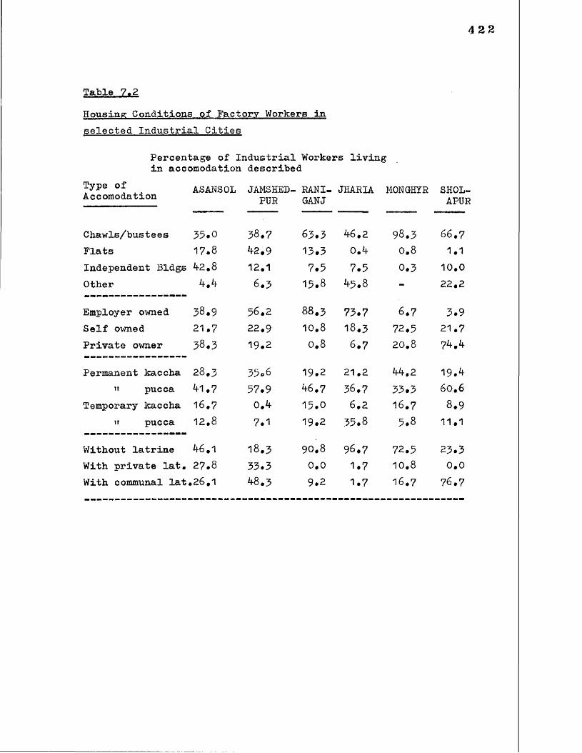
422

Table 7.2Housing Conditions of Factory Workers in- selected Industrial Cities

Percentage of Industrial Workers living in accomodation described

Type of Accomodation ASAN50L JAMSHED­

PURRANI-GANJ

JHARIA MONGHYR SH0L-APU]

C havrls/bus t e e s 55.0 58.7 63.3 46.2 98.3 66.7Flats 17.8 42.9 13.3 0.4 0.8 1.1Independent Bldgs 4-2.8 12.1 7.5 7.5 0 .3 10.0Other 4.4 6.3 15.8 45.8 - 22,2

Employer owned 58.9 5 6 .2 8 8 .3 73.7 6.7 3.9Self owned 21.7 22,9 1 0 .8 1 8 .3 72,5 21.7Private owner 58.5 19.2 0 .8 6.7 2 0 .8 74.4

Permanent kaccha 2 8 .3 35.6 19.2 2 1 .2 44.2 19.4" pucca 4-1.7 57.9 46.7 36.7 33.3 6 0 .6

Temporary kaccha 16.7 0.4 1 5 .0 6 .2 16.7 8.9» pucca 1 2 .8 7.1 19.2 35.8 5.8 1 1 .1

Without latrine 46.1 1 8 .3 9 0 .8 96.7 72.5 23.3With private lat. 2 7 .8 33.3 0 ,0 1.7 1 0 .8 0 .0

With communal lat.2 6 .1 48.3 9.2 1.7 1 6 .7 7 6 .7

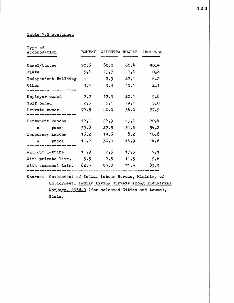
Table 7.2 continued

Type ofAccomodation BOMBAY

Chawl/bustee 90.6Flats 5,4Independent Building Other 3*5

Employer owned 7*7Self owned 2,3Private owner 72,5

Permanent kaccha 12,1tt pucca 59.8

Temporary kaccha 16.2tt pucca 1 1 .2

Without latrine 11.9With private latr. 3.3With communal latr, 82.5

CALCUTTA HOWRAH AHMEDABAD

8 0 .0 6o,4 90.413.7 7.4 0 ,8

2.9 2 2 .1 6 ,2

3.3 1 0 .1 2 .1

12.5 2 0 .1 5.87.1 19.1 5.0

8 0 .0 5 6 .0 77.9

22.9 43.4 20.427.5 31.2 54.219.6 8 .2 1 0 .8

30.0 16.9 14.6

2.5 17.3 7.12.5 11.3 9.693.0 71.3 83.3

Source: Government of India, Labour Bureau, Ministry ofEmployment, Family Living Surveys among Industrial Workers. 1958-9 (for selected Cities and towns),S imla *

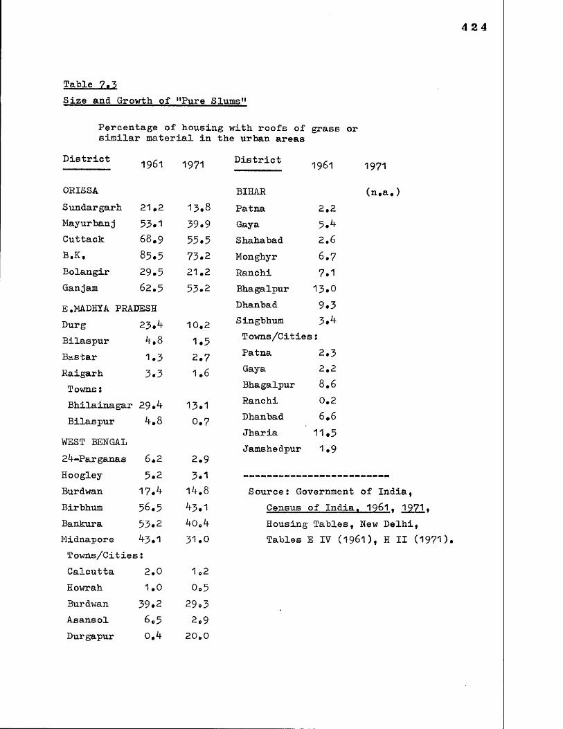
4 24

Table ,7.3Size and Growth of lfPure Slums11

Percentage of housing with roofs of grass or similar material in the urban areas

District 1961 1971 District 1961 1971

ORISSA BIHAR (n.a.)Sundergarh 2 1 *2 13.8 Patna 2 .2

Mayurbanj 53.1 39.9 Gaya 5.4Cuttack 6 8 .9 55.5 Shahabad 2 .6

B.K, 85.5 73.2 Monghyr 6.7Bolangir 29.5 2 1 .2 Ranchi 7.1Ganjam 62.5 53.2 Bhagalpur 13.0E. MADHYA PRADESH Dhanbad 9.3Durg 23.4 1 0 .2 S ingbhum 3.4Bilaspur 4.8 1.5 Towns/Cities:Bastar 1.3 2.7 Patna 2.3Raigarh 3.3 1 *6 Gaya 2 .2

Towns; Bhagalpur 8 .6

Bhilainagar 29.4 13.1 Ranchi 0 .2

Bilaspur 4.8 0.7 Dhanbad 6 .6

Jharia 11.5WEST BENGAL Jamshedpur 1.924-Parganas 6 .2 2.9Hoogley 5.2 3.1Burdwan 17.4 14.8 Source: Government of India,Birbhum 56.5 43.1 Census of India. 1 9 6 1. 1971Bankura 53.2 40.4 Housing Tables, New Delhi,Midnapore 43.1 31.0 Tables E IV (1961), H II (11

Towns/CitieE;:Calcutta 2 .0 1 o2

Howrah 1 .0 0.5Burdwan 39.2 29.3Asansol 6.5 2.9Durgapur 0.4 2 0 .0

425

Table 7.4Municipal Revenues. Expenditures- and Services, according to Size Class of Towns. 197Q

State & Per Capita Receipt Tax as % Per Cent ofSize Class (Expenditure) of Towns with--------- Rs per annum Receipt Protected Water

BIHAR I II 12.6(12.8)I I I 8c below 9 * 4

(11.4)O R I S S A I , I I 23.3

( 2 3 . 9 )

III & below 13.3( 1 3 . 9 )

MADHYA I,II 27.6 PRADESH (26.5)

I I I 8c below 1 5 . 8(14.7)

MAHARASHTRAI,II 47.8

(46.7)III 8c below 13.3

(12.4)

40.1

3 0 . 9

3 9 . 1

3 2 . 9

66.0

60.7

6 2 . 5

48.4

100.0

9 3 . 4

n.a.

n.a.

100.0

4 1 . 4

95.2

51.0

Note: Data are only available in some cases where Municipalities, (not, e.g., Notified Areas) exist. I have given unweighted averages for groups of size classes. It is possible that the Census authorities, who give averages for each size class, took unweighted averages for the towns within each class. If they did not, but..took weighted averages according to population size, thea Bombay heavily dominates Maharashtra's class I.

Source: Government of India, Census of India 1971. TownDirectories, New Delhi; (data for previous 2 or 3 years).

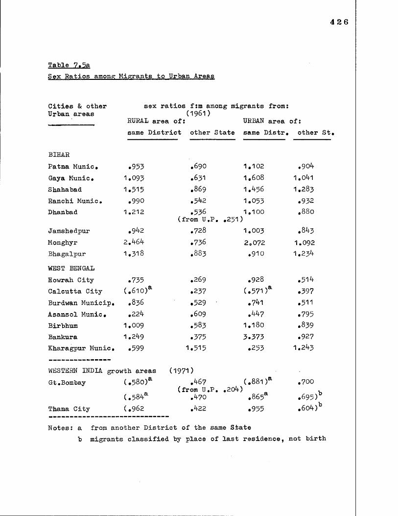
426

Table 7.5aSex Ratios among Migrants to Urban. Areas

Cities & other Urban areas

sex ratios fsm among migrants from:(1961)

RURAL area of: URBAN area of:same District other State same Distr. other St*

BIHARPatna Munic* .953 .6 9 0 1 .1 0 2 .904Gaya Munic* 1.093 .6 3 1 1 .6 0 8 1.041Shahabad 1.515 .8 6 9 1.456 1 .2 8 3

Ranchi Munic. *990 .542 1.053 .932Dhanbad 1 .2 1 2 .536 1 .1 0 0 .8 8 0

Jamshedpur .942(from U,P,

.7 2 8

.2 5 1)1 .0 0 3 .843

Monghyr 2 * 464 .736 2 .0 7 2 1 .0 9 2

Bhagalpur 1 .3 1 8 .8 8 3 .9 1 0 1.234WEST BENGALHowrah City .735 .2 6 9 .9 2 8 .514Calcutta City (.6 1 0)® .237 (.571)a .397Burdwan Municip*

VOOO• .529 ‘ .741 .511Asansol Munic# .224 .609 .447 .795Birbhum 1.009 .583 1 .1 8 0 .839Bankura 1.249 .375 3.373 .927Kharagpur Munic* .599 1.515 .253 1.243

WESTERN INDIA growth areas (197DGt.Bombay (.5 8 0)a .467 (.8 8 1)a .7 0 0

(,584a(from U.P.

.470.204)

.8 6 5 .695:Thana City ( .9 6 2 .422 .955 .604:

Notes: a from another District of the same Stateb migrants classified by place of last residence, not birth

427

Table 7.5a continued

Steel Town Urban areas

Sundargarh

Burdwan

Durg

Sundargarh

Rourkela City Burdwan

from Rural areasame Distro other St.

from Urban areasame Distr* other St.

.824

.695

1.067

1.199

(.9611.109

(1961)

.875 *589(from U.P. .647 from Bihar 1.054)

.480 ' .7 6 3(from U.P. .323 from Bihar .531)

.397(1971)

1.332

Durgapur City (0 8 9 5

.6 9 6 1.193(from Bihar .73^)

, 6 8 o ) a ,b

.550 .96^(from Bihar .540)

,686)a,b

.509

.586

.6 1 6

.780

.732

Notes: a classified by place of last residence b rural + urban origins together

428

Table 7.5 bSex Ratios among Short and Long-Distance Migrants in Contrasting Urban Areas

Steel Towns 1971 Migrants from:*— :------------ Same State* Another State*Durgapur .?6*f .6**4Rourkela .72*+ ,680

♦(place of last residence)

Contrasting Urban Areas 1971

Migrants born in:Same State Another State Same State Another St.

RURAL URBAN

Calcutta .4 7 8 .273 .776 .**■05

Burdwan District (Durgapur)

.9 4 3 .530 .8 0 8 .732

Bankura District 2 .4 0 5 .535 .8 0 6 1 .0 8 3

Birbhum District 1 .2 2 1 .958 .8 0 8 1 .2 1 1

Sundargarh D. (Rourkela)

.514 ,6 9 6 .8 5**- .7 8 0

Ganjam 1.390 1.299 .8 2 8 1 .2 1 6

Source: Government of India, Census of India 1971,M ig r a t io n T a b le s , New D e lh i .

Table 7>6

Sex Ratios in Rural Areas neighbouring the TownsBURDWAN DISTRICT 0Sex RatioRural Locality 1961

f :m 1971

Main Industry in Principal Town

Chittaranjan .8 8 5 .917 locomotive worksSalanpur .815 .8 9 5

Kulti .6 8 5 .7 8 5 iron worksHirapur .8 6 6 .8 1 8 Burnpur steel millsAsansol .7 2 0 .7 9 9 engineeringBarabani .8 0 8 .8 7 5

Jamuria .6 9 6 .752 miningRaniganj .64-9 .6 6 0 miningOndal .6 2 5 .671 miningFaridpur .772 .801

Durgapur .719 .976 iron and steel plantKaksa .938 .959(All West Bengal .8 7 8 .8 9 1)Other STEEL TOWN AREAS in 1961

Rural Locality Sex Ratio

Rourkela(Sundargarh)

PanposhSardarBonai

.9951 .0 1 0.9^2

(All Orissa 1.001)

Bhilai(Durg)

Kawardha Khairagarh Bemetara Rajnandgaon DurgSanjari Balod

1 .0 3 2 1 .OMf 1.051 1 .0 5 0 1 .0 2 1 1.053

(All Madhya Pradesh .

Rmiree! Government of India. Census of India 1861. 1971.(relevant States), General Population Tables, Delhi.

Table 7.7Participation of Resident Rural Population inCore-Sector and Construction Industries in Steel Town AreasIron and Steel occupations Construction

WorkersDistrict (rural) Number % of all in

that occup. in District

Number % of total in District

Durg District 250 1 .0 4075 30.4Raipur DMsion 253 1 .0 9885 4 5 .0

Sundargarh Dist. 0

0•0 440 8 .5Burdwan Dist. 3629 1 0 .8 7211 40.3

Source: Government of India. Census of India 1961. States), General Economic Tables, Delhi.

(relevant

Table 7.8Comparison of Sex Ratios among: Backward Classes and theGeneral Population in Selected Towns

Town or Urban Area

Sex Ratio f:m : General Population 1961

BackwardClasses

% of BCs in area

Durg District .864 .906 9.8Bhilainagar (steel town)

.795 .798 7.1

Rajnandgaon .932 .970 6.7Dongargarh .9 6 7 1 . 0 0 2 7.1Chirmiri(mining)

lv£>K\OO• .941 20 . 1

Surguja District (mining)

.847 .915 17.1

Bilaspur District .907 .936 14.1

Table 7.8 continuedSex Ratio.: General Pop

Burdwan District(urban) .785Jamuria(mining) .651Raniganj r+u(mining area) .6 8 7

1971 .695Note: See also Table 6,9Source: Government of India,

(relevant States), G Delhi,

% of BCs in 1961 BCs 1961 area

835 1 1 ,1

680 22.3

8^3 35.179^ 29.if

Census of India 1961. 1971. neral Population Tables,

Table 7*9Housing Occupancy Rates

Persons per house (same divided by rural State average)

WEST BENGALCalcutta 5 .0 1 (1 .2 6 )Howrah if. 88 (1.2 5 )Rif Parganas 5.01 (1 .2 6 )Hoogle^___ 4.81 (1 .2 1 )Midnapore 5.19 (1.31)Burdwan 5.15 (1.30)Birbhum 5 .1 6 (1.30)Bankura ^ .9 5 (1.25)BIHARPatna 6.9k (1 .0 2 )Gaya 6 .2 2 (0 .9 2 )Shahabad 6.57 (0 .9 7 )Bhagalpur 7.1^ (1 .0 5 )Monghyr 6 .9 0 (1 .0 2 )Singbhum 5 . ^ 0 (0 .8 0)Dhanbad 5.79 (0.85)Ranchi 6.7^ (0.99)

£ .MADHYAPRADESHRaigarh if.76 (0.92)Durg 3 .8 1 (0 .7 )Bilaspur (0 .9 1 )Bastar (0 .8 8 )ORISSAMayurbanj 5.32 (1.0 0 )Sundargarh ^.15 (0 .7 8 )B-K ^.87 (O.9 2 )Cuttack 5.90 (1 .1 1 )Bolangir 5.69 (1.0 7 )

Source: Government of India, Census of India 1961. (relevant States),Housing Tables, Delhi,

432

Appendix 7*1 Two Models

Projections of Housing Needs!

NEW-TOWNS(rapid growth: to 2^0,000 population in 15 years, and decadal growth of 66*6% for a further 10 years)*

1961 - 1971 1971 - 1981

Core Labour Households: 15,000Household income per month Rs 250

Industrial Housing & Utilities Capital cost per unit:Rs. 22,000Rent/rates atRe/ _

Maximum expenditure onrent! 10%x250 x 12 =:Rs 300<1760 per annum

Multiplier Labour Households (middle income):

5 0 ,0 0 0

Household income per month Rs 150Maximum expenditure on rent! 10%x150x12 = Rs 180

Low-income Housing Scheme Capital cost per unit:Rs 7500Rent etc* at 8% =

< 600 per annum

Sites and Services Capital cost per unit:Rs 2500Rent etc* @

— Rs 200 p.a*

Incremental Core Labour Households10,000Annual Housing1,000 units @Rs 22#000 =Rs 22 million

Total Income of Core sector Households:1971: 1 5 ,0 0 0 x

Rs 300 x 12 = Rs 5k million

1981: 25,000 x Rs 350 x 12 = Rs 105 million

Incremental Multiplier Labour HouseholdsA-0,000Annual Housing ^,000 units @Rs 2500 =Rs 10 million

Total Income of Multiplier Sector:1971: 6 0 ,0 0 0 x

Rs 150 x 12 =Rs 108 million

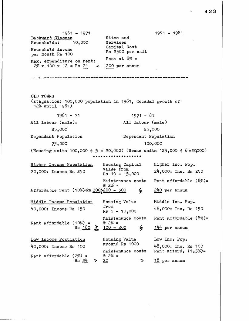
433

1961 - 1971 Backward Classes Households: 10,000Household income per month Rs 100Max. expenditure on rent: 2% x 100 x 12 = Rs 2k 4.

1971 - 1981Sites and Services Capital Cost Rs 2500 per unitRent at 8% =200 per annum

OLD TOWNS(stagnation: 1 0 0 ,0 0 0 population in 1961, decadal growth of

12% until 198 1)

1961 - 71 All labour (male):

2 5 ,0 0 0

Dependant Population75,000

(Housing units 100,000 t 5 =

1971 - 81

All labour (male)2 5 ,0 0 0

Dependant Population100,000

2 0 ,0 0 0 ) (House units 1 2 5 ,0 0 0 ? 6 =2qp00)

Higher Income Population 2 0 ,0 0 0: Income Rs 250

Housing Capital Value from Rs 10 - 15,000Maintenance costs @ 2% =

Affordable rent (10%)=RS 300^200 - 300 £

Middle Income Population 40,000: Income Rs 150

Housing Value fromRs 5 - 1 0 ,0 0 0

Maintenance costs Rent affordable (10%) = @ 2% =

Rs 180 >_ 100 - 200 £

Low Income Population 40,000: Income Rs 100

Rent affordable (2%) =Rs 24

Housing Value around Rs 1000Maintenance costs @ 2% =20 >

Higher Inc. Pop. 24,000: Inc. Rs 250

Rent affordable (8%);

240 per annum

Middle Inc. Pop. 48,000: Inc. Rs 150

Rent affordable (8%):

144 per annum

Low Inc. Pop.48,000: Inc. Rs 100 Rent afford. (1*5%)=18 per annum

434

Notes:

1* Projection 1 represents a rapid- growth town (like Rourkela or Bhilainagar)• The initial core-labour force of 1 5 ,0 0 0 males migrates to a "green-field.” site*A "multiplier" labour force of 60,000 males follows (1961-71)*

2* Assume that in each case family household size willstabilise at between 4 - 6 members in ten years (average of 5 members) with maximum of two members earning. Then family income is Rs 250 per month (1971 prices) for families with the main worker in the core sector, and Rs 150 for most of the multiplier sector families, but with the lowest 10,000 earning only Rs 100.

5* Assume that the core-sector families and the better-off multiplier families can afford 10% of their income on service and interest dharges that are made for urban living (typically in the form of rents and rates): i.e. Rs 300 and Rs 180 per annum respectively for the two groups{ assume the poorest families can afford only 2%, i.e. Rs 24 p.a*

4. The housing and facilities capital costs are taken asfollows: for the core sector, Rs 22^.000 per household unit(for explanation and sources see text above). The economic rent, at a minimum of 8%, totals Rs 1760 p.a. - i.e. about five to six times the ability to pay. This is as far as the official housing scheme goes. For the middle-income multiplier families assume a universal provision of the L.I.G. housing scheme (see text), capital cost Rs 7500, rent Rs 600 p.a* - i.e. over three times the ability to pay. For the poorest group assume a sites and services scheme, costing Rs 2500, rent Rs 200, - say ten times the ability to pay. (A village dwelling without services would cost about

435

Rs 1000, and could be maintained at a charge of about 2% of the capital cost*, Construction materials would have been gathered from the land over time, and building over time would employ family labour only. No cash payments would be required as interest on loans, and material costs for maintenance would just be covered, at Rs 20.)

Conclusion 1

Using standards currently adopted in New-town construction, a housing scheme cannot be self-financing.

5. Now take alternatives; self-financing is possible with capital costs of Rs 3750, 2250, 300 for each group (which is implausible for the poorest group given any imagineable technology beyond a pavement dwelling). Self-financing is possible with costs of Rs 3000, 2000,2000 for each group, i.e. with sites and services for all the multiplier population (using the cheapest technology developed up to 1975)* and fully constructed single-storey tenements as currently developed for the Economically Weaker Section (so called) for the core-labour sector families (politically difficult, if not unacceptable). If, however, core-sector incomes grow at 2% p.a. in real terms, then ia 35 years tenements of Rs 6000 would be affordable under the latter scheme, (and so on).

6 * Consider now the incremental growth, given tie initialestablishment of the population just described. The core­labour force grows by 1 0 ,0 0 0 between 1971 and 1981. By 1981

the incomes of the core-sector families are Rs 300 per month (with average family size still 5)» Incremental capital

436

cost of housing 1,000 families per annum is Rs 22 million#Can that sum be financed from municipal savings? In 1971 the core sector aggregate income amounted to Rs 5^ million, so that a savins rate of about 50% would be required#

Conclusion 2The incremental growth of heavy industrial towns cannot be financed entirely out of municipal revenues ‘(without changes in construction standards)#

7# Again there are alternatives# Housing plus facilities costing Rs 5000 could be financed; or with half the net migration rate and costs of Rs 10,000 financing would be possible, and so on. For the multiplier population various scenarios may be adopted too* Suppose for example an annual growth ".of 4000 per annum (adult males). Take the average family income for the whole group to be Rs 150 per month.Adopt sites and services at per unit cost of Rs 2500 for the whole group. The total incremental cost amounts to Rs 10 million annually, which has to be financed from an initial total multiplier family income of Rs 108 m.This implies a 10% savings rate (devoted entirely to "urban development bonds", or an equivalent)t leaving nothing over to finance industrial investment, unless the savings rate of the middle-income group exceeds 10%.

8 . Projection 2 assumes a stagnating population. The total male labour force remains at a level of 2 5 ,0 0 0 over 20

years (like some of the large towns in Bihar, e.g. Monghyr).The dependant population rises from 3/4 to 4/5 of the total. Divide it into three income groups: say 40% atRs 100 p.m., 40% at 1.5 0, 20% at 250, none of which increases over time.

9. The top two groups pay 10% of their income in rent etc., the poorest pays 2%, on dwellings valued at Rs 10-15,000, 7,500-10,000, and 1,000-2,000 respectively. Rent/rates

437

average at 2% per annum on stock that is about 50 years old for the top two groups, or that consists of self- built village-like accomodation, that may have started as slum hutments in earlier periods of prosperity or at Independence with the large urbanward migrations associated with Partition).

10. By 1981 per capita incomes have been reduced by 1/5, owing to incroEBed dependency, and on assumption of no remittances sent by out-migrating males, and that households have increased in size rather than split (see text above). Hence the maximum maintenance charges affordable are assumed to drop to 8% of family incomes for the upper two groups, and to 1 .5% for the lowest group. This is below the cost of maintenance on the higher values of housing stock (i.e.assuming that it has not deteriorated to below those values). The poorest groups, if originally in rented accomodation, will, cet. par..have become pavement dwellers#

Conclusion 3

Towns subject to outmigration are likely to face deteriorating welfare levels if relying on local finance.

11* Clearly, somewhere between these projections thereare cities that coulc^^eir eown housing and facilities. Typically they will be of the Type 2 Demographic Model (Chapter 3). Cities of the demographic Type 1, especially 1 c, and of Base or Type 3, will need outside finance, certainly over some periods of their life.Type 1 cities will have to adopt generally lower standards of housing (for core-sector and multiplier families) than have commonly been prescribed if they are ever to self- finance their maintenance charges* These standards can be improved, as incomes improve, over time*

A brief Overview of Chapter 7

This chapter shows empirically that without Central Government intervention the stagnant or declining towns have been unable to raise the same per capita resources for infrastructure in social amenities as have the more rapidly growing areas. This disequilibrium is enhanced by their age composition. Similarly, low quality housing is the norm in slowly growing areas (as would be expected from household age composition)? in rapidly growing areas low quality housing develops over time in so far as migrant families with lower income prospects migrate in.The State has come too late in the day to appreciate the dimension of these problems; the strategies adopted by the people themselves (in New-towns) could have been economically incorporated in overall planning from the start. At the same time positive intervention will be needed in the case of the slow-growing towns.

CHAPTER 8

The .Family, Migrant Groups, and their Employment Strategies

A Summary of Empirical Findings

The implications of the foregoing demographic factors impinge on the long-term employment and income prospects of the families established in specific localities. The distribution of family structures with cities of contrasting types is investigated: we areparticularly interested in the strategies adopted by families, or by larger groupings of migrants, to spread their employment over various industries or occupations.We find that families in heavy industrial towns usually rely on a single industrial earner; families in lower productivity towns require more. There is apparently an attempt by migrant subgroups of similar regional background to concentrate all their employment over time on the most rewarding industrial sector.to which they have access: a strategy of risk-spreading is not adopted. In towns dominated by a single industry such a strategy would in any case be ruled out; and in the stagnating towns of this type the regularMinks with the rural economy (the security of last resort) have usually, it seems, been severed.

At.the theoretical level we can observe the

following distinctions. A family may be composed of a number

of earners of various ages. In India its major source of income is likely to be from one or two adult males.

In the latter case, if both are employed as wage labour

in the same, industry, or, in a more extreme case, in the

same factory, the whole family is very vulnerable to the

fortunes of that industry or factory. Security is not much

enhanced in an alternative model, where the main bread­

winners are all empired in an industry providing goods

and services for the core industrial labour force* A

slightly better position is offered by the familial

mode of production, as work-sharing always becomes possible provided the average productivity in the family

does not fall below average consumption requirements.But once again, the closer the work is tied to a single

basic industry (for example through its contracting out

to the household) the more risky the household industrial mode of production becomes. Clearly what

emerges from all this is that the safest strategy is

to diversify the family portfolio, as it were. To have

two or more adult workers in quite distinct industries would be ideal. To have one member in an industry as

441

a wage labourer, and one self-employed in a less closely related sector, would be a moderately secure strategy

(perhaps at the cost of a higher income than would have

been enjoyed with both members in the same industry).

Similarly, a mixture of household industry and wage

labour (even in another family's household) could be

more secure, but again this implies income foregone.

In practice in India the choice is often limited, even

in the urban economy. There is some evidence that securityis preferred despite income foregone, even in low-income

2families, but there is no evidence to my knowledge of

strategies being deliberately adopted to diversify income

at the family level in the manner I outline here. Quite3apart from the constraints of an imperfect labour market,

there is the constraint of a lack of industrial diversification

in precisely those cases where the problem arises. You

cannot easily diversify your portfolio in an undiversified

world.

Whether or not families, let alone broader social groups of caste, class, regional or ethnic distinction,

1 It may be argued of course that a sufficiently high income will generate savings enough to carry the family through periods of instability or unemployment, thus reducing the risk involved in this option (a point made to me by Camilla Toulmin).

2 This was suggested to me by Meera Bapat from her study of low-income families in Poona, where she has worked and lived most of her life.

3 Such imperfections reduce the amount of choice a family from a Backward Caste, for example, may have#

consciously adopt such strategies, it is; .worthwhile

investigating whether in practice the familial vulnerability

problem arises. Are family income sources particularly

concentrated, or more concentrated than they need be,given the range of opportunities? For if they are, the

failure to diversify local industry in India becomes even

more socially undesirable (though whether the less costlysolution is to diversify industry, or to change family

behaviour, remains an open question). Furthermore it would

be possible to indicate to what extent the demographic

structure of the family, resulting from high or low

fertility in conjunction with various patterns of migration,

exacerbates, or alleviates, this vulnerability. And if the

strategies adopted are conscious, we could indicate in turnhow the vulnerability problem imposes constraints on

demography. For example, lower fertility might imply

higher family per capita income, but less scope for

security through diversification of employment that1becomes possible with a larger family.

1 The implications for fertility reduction programmes need hardly be spelled out. Yet the literature has focussed on the high fertility hedge against risks associated with ill-health and mortality, not on the security issue raised here. See, for example, R.H.Cassen, India: Population. Economy. Society. Macmillan, London, 1978, Chapter 3*

This chapter is devoted to implications. It is

not the intention to investigate the problem empirically

beyond establishing some indicators from our region of

study in India regarding the existence or otherwise of the family vulnerability problem* The first such

indicator deals with the household composition, and

some evidence on sources of household income through

employment, in towns enjoying various degrees of industrial diversification. The second considers the concentration

of geographical origins of migrants in particular industries

in the newly industrialising regions of Bihar (for which

special Census tabulations were undertaken). This,

strictly speaking, is evidence on community or ethnic

concentration, from which a few implications for the

family may be drawn. Later an even broader overview

of the evidence will be taken, on the industrial concentration

of migrants in general.

Family Formation and Household Distributions in Urban Areas

It has already been established that towns of different industrial character differ, often quite markedly, in their demography. Among the economic

implications this might have at the local level, one

that we are particularly concerned to suggest is the

4 44

effect on family welfare, and especially family income,and on the security of family income over time* To dothis we need to reconstitute household structure fromaggregate demographic structure: this is fairly immediatelydone since the Census tabulates household structure for

1the urban areas of the Districts, But it is a frustrating

limitation to draw our conclusions simply from the observationof the mean, and a sad reflection on statistical imagination

how often this, and this alone, is done# Fortunately

there are two sources of information from which ideas maybe culled on the distribution of household types withinthe urban areas under study: the first is the simpledistribution of household size from the Censuses, thesecond is the Labour Bureau Study of industrial worker

2households in selected towns, carried out in 1 9 5 8-9 *

1 A household is defined for Census purposes as a unit consisting of people eating at the same table, as it were (and it is closely co-terminous with residents in a single building): in India there are almost as many "houses" as "households" recorded in the Censuses,A family is less easy to define# Generally speakingwe will take it to be co-terminous with an Indian rural household not subject to past or present urbanward migration* Sometimes, however, we will be taking a somewhat more liberal interpretation# For our present economics analysis, what matters is how far financial or other welfare obligations would generally extend.

2 Government of India, Labour Bureau, Ministry of Labour, Report on Family Living Surveys among Industrial Workers, 1958-9* Delhi, 1968.

The latter can be compared with the 1961 Census to see

how far industrial wage-earner families are distinct fromother families in these towns and cities: additionally,

and unlike the Census, these Surveys indicate the distribution1of family composition within the urban wage-earner category.

They also enrich our knowledge, for these types of households at least, of members* contributions to household income

(though without unfortunately stating the occupational

source, only the value, of that contribution). And finally

they have some (though not much) usable information on

remittances.

We should begin with some controls in mind. One of

the more striking observations of demographers working on

household composition has been on the similar mean value

(and similar distributions) of household size in historical

Western European countries and contemporary India (among2other Oriental cases). For our rural areas of India,

the mean size is about 5 members (Table 8.1). The striking

difference, on the other hand, between the Orient and

historical Western Europe is that in the-latter the fifth

1 A household was defined as "industrial" if the main contributor to family income was a wage-earner in industry.

2 See J.Hajnal, "Household Formation Patterns in Historical Perspective", Population and Development Review. Sept. 1982, Vol 8:3* The reference is to a period pre-dating the industrial revolution in Europe.

member was typically a non-family member, living in as a servant, whereas in the former he or she is a member

of the family. But equally striking in the current author's

view is the fact that only a minority of families are

exactly of that five-member composition, or more significantly,

that the distribution is quite evenly spread (not uniform,

but distinctly "platycurtic"). In other words, most of the

time families are experiencing either some transition

toward or away from this "norm" of mean value 5 , with

fertility adding to the base of a family's pyramid or

mortality subtracting from its apex (and from below also),

or else they are stabilising at lower or higher "norms"

than the average, in association perhaps with their

economic mode of production or with their cultural

background. It is not our purpose here to explain the rural

family composition, though some interpretation has to be

offered owing to the observed fact (to which we later refer)

that some urban households represent split rural families.

Suffice it to remark on the following. Rural households

of single members only are rare (around five per cent), and must represent, on the whole, single males migrating

for employment as agricultural labour, or as rural infra­

structural or in some cases industrial labour; or they are

single females left behind in the course of such migration, (or widowed). The 2 -6 size group will consist of families that are in the process of formation and dissolution

within that group, with high mortality among agricultural

labour households for instance, or a greater tendency towards nucleation among some social groups (tribals,

for instance) keeping the maximum size of such households

usually below six. The quite significant proportion of

households above six in size (around 30%) will include

a lower mortality (probably higher fertility) subgroup

whose size will range from 3 - 10 in the course of its

life-cycle, associated with trading and commerce and land-ownership, and having little tendency towards

nucleation. The proportion of rural households with

above ten members (approaching 10%) is remarkable,

1 Seasonal migration of labour was not captured in the Censuses, taken as they were in February and April.The definition of "rural" and “urban11 can also be mis­leading here. The Census distribution of manufacturing establishments by size of workforce shows a small number of large enterprises established in rural areas* Similarly mining employees are often housed in "rural” villages; and so also in the rapidly industrialising areas are some of the urban workforce. Tables 7*6 and 8 ,2 are of relevance here.

44

especially when one considers that about 20% of the rural

population live in households of this size# A majority,

but not an overwhelming majority, of rural households, will represent the small-peasant stereotype, evolving during the family life-cycle between the limits of

3 to 7 members on the whole, the stereotype that Hajnal

has reported as the’horm".

It has not been the purpose of this thesis to

determine who migrates and why# The analysis of migration

has been restricted to changes in the demand for labour,

resulting from differential industrial composition of

urban localities, and the consequent change in the (broadly

defined) locational origin of the supply# Labour also migrates,

however, when conditions change at the rural end of the

migration chain* The family composition of such migration is often very different: as an extreme example, in distress,

total families move; in acute distress, only the able-

bodied do so. It would be of considerable xnterest, however, if we knew rather more about the rural background of these urban migrants, as it might help explain the

family earning strategies adopted* In an earlier Chapter

we argued that the balanced sex ratios and local origin

of social groups like the Scheduled Castes, and their lack

1 For a summary of the demographic characteristics of rural out-migrants see J.Connell, B.Dasgupta, R#Laishley, and M.Lipton, Migration from Rural Areas. Oxford University Press, Delhi, 1976.

of participation in the core industries in the newly industrialising areas, all suggested that these were

migrants who were virtually forced to migrate out,

and were not being recruited, nor very specifically

attracted, into the cities. In this case they were almost certainly landless (or with very small holdings)

otherwise they would have left family members behind,

at least for a while, while they reconnoitred for

suitable urban accomodation, as did their urban colleagues employed in the manufacturing industries. Further light

was shed on this in the surveys referred to in Chapter

5 above, giving evidence that factory industrial workers

were more likely to own small amounts of land than were

migrants who finished up in self-employment in smaller

enterprises, or as casual labour in the cities.

With this sketch of rural household composition as

a background, let us consider in more detail the composition in the towns, focussing on the manual labour categories, and especially on manufacturing wage labour.A generalisation we could make is that urban households

are smaller than rural in our region (Table 8 .1 ).

This will tend to follow if urban households are fragments

of rural families (and not just of the largest rural families). Apart from the Labour Bureau Survey data (and survey evidence

in general), the population structures we have derived from the Census for urban areas is clear evidence of such split families, (note especially the detailed analysis of

Bhilai in Chapter 9» where it is found that a majority

of males-only households consist of married males)#

Generally speaking then, households of one, two, or three

members are proportionally greater in number in urban

areas due to migration, not differential mortality,

fertility, or cultural traits, (though the latter

two factors undoubtedly work towards lowering urban

household size among the professional and even the more-

skilled wage labour categories, especially in the larger

cities). The largest size class, households above ten, are distributed in rather similar proportions in rural

and urban areas, so that it is the rural concentration

of families in the k - 9 size group that is especially responsible for the larger average rural household size. Again, this is partly due to the lower fertility in urban

areas, partly due to the absence of older relatives living

1 See above Chapter k for evidence on the marital status of the urban populations, compared with their rural counterparts: other things being the same, latermarriage will result in smaller household size.By 1bultural traits” , as distinct from ’’fertility” we refer to preferences for living in nucleated rather than extended households in urban areas.

451

with the urban migrant at the early stages of migration,

and partly the absence of married sons and their wives in these young households. This interpretation is

consistent with the smaller number of married relations

(if we exclude brothers) in the urban households (Table

8 .3 ) (though married relations could be living as couples

in separate households), and, more significantly, with

the absence of the higher age groups recorded in the aggregate urban age structures* On the whole, the small number

of differences (and their small degree) between the rural

and the urban is a striking feature, and this characterises

above all the experience of the moderate growth towns, and the relatively stagnant towns. The real differences

arise when we look at the rapidly growing towns.

The heavy engineering localities are immediately

distinguished by one feature - the high proportion of

single-member households. These are predominantly male,

(Table 8.4); the urban areas of Durg and Sundargarh are

good examples here. Given our estimate of a time-lag between initial male migration and the joining of wives

and family, this phenomenon is clearly a function of

rapid growth, and indeed between 1961 and 1971 these high proportions of single-member households in the Steel

Town localities have declined from around 20% to around 12%

452

(see Durg and Sundargarh Districts in 1971)* The migration data we examined suggest that individual families tend not to remain split for more than 2 years on average. So that although we are dealing with urban societies having large numbers of split families, they are not chronically split (with some notable exceptions to which we referred in Chapters 4 and 5)*And over a ten-year period the most noticeable change

in family composition in these heavy industrial towns,

apart from the addition of a spouse, is the addition of

unever-married!r members, i.e.predominantly children,

(Table 8.5)* which the aggregate age structure changes also confirm (see, for example, Figure 601). Continuing this aspect of the detective analysis further, we observe high proportions of the 2 - 3 member households in these rapidly growing urban areas: but what distinguish themmarkedly are their distorted sex ratios, indicative of brothers, or simply friends, among migrants, sharing accomodation, (note in Table 8.4 Sundargarh, Durg, Dhanbad,

and Burdwan, among the non-Metropolitan examples).

1 It is also clear from the more detailed 1971 data thaturban households have a larger number of unrelated members living in than do rural households (Tables 8.3* 8.5)#We may also note the high proportion (relative to rural areas) of already married males, mainly brothers, (not sons), (Tables 8.3 and 8.5), though we cannot confidently distinguish heavy industrial areas in this respect* The family composition, data were collected on a 20% sample basis,only.

453

It would be advantageous to be able to analyjse

the core industrial sector migrants separately (in the hope of discovering something regarding their

vulnerability, as families, to economic shocks). This

we cannot do for the most rapidly growing towns, but we

do have the industrial labour surveys for the heavy engineering and Steel Towns of a slightly older generation,

whose iron and steel works were expanded during our period of

study: namely, Asansol-Burnpur and Jamshedpur (Table 8 *6 ,

8.7)* Asansol's industrial workers are of remarkably small households: single members, ky/o between 2 and 5,(a proportion well above the average for Burdwan District

urban households as a whole, as is clear from Table 8*7)*

One third of the single-member households consist of

unmarried members. There are very few households of

adults alone living together: usually children are present.

This suggests that the single-member households consisting

of married men are in the course of transition towards

becoming multiple-member households consisting of married couples and children, as we suggested above. Nonetheless, the larger proportion of single-member households among industrial workers, as compared with the general urban

population, is remarkable. There are two possible explanations:

first, that industrial workers are more likely then other

454

workers to remain as split families (i.e. it is not just1a question of being in a transitional stage) ; secondly,

that industrial migrants are more likely to migrate singly2than are other migrants.

Jamshedpur, on the other hand, is sharply in contrast*

Only 14% of the households are single (yet the urban

District average compares well with that of Burdwan).

Jamshedpur’s population grew more slowly over the 1951-61

decade than did Asansol’s (39% versus 78%, and the male

population much more slowly, 40% versus 98%). It would be

tempting to infer from this that the industrial migrants in

Asansol-Burnpur are indeed in a state of transition, and

not that, in this respect as in many others, Jamshedpur is simply a special case. By 1971, Asansol City has as few single-member households as has the less industrialised Burdwan

City (7%), and roughly the same as Jamshedpur. Tentatively

we conclude that the migrant in heavy industry seeks to detach his nuclear family, at least, from its rural origin.

Perhaps this weakens the rural link, and to some extent the

support from two economic sources. We should now ask how

far he broadens the basis of his family's income in the urban

1 We know this is true of migrants from Uttar Pradesh: see Table 7*5 for evidence on Burdwan District (as well as Bombay).

2 This is supported by survey data for Bombay (Chapter 5)*

In the case of both Jamshedpur and Asansol the

answer is that multiple sources of income from work

are rare in industrial households, (Table 8 .6 ). In

80 and 89% of households respectively there was a sole earner (but in only 14 and 35% of cases was there a

single-member, and in 26 and 23% of cases there was

an adult member in addition to the married couple).

This is in line with survey data from elsewhere,

showing that industrial workers either do not allow,

or do not need, their wives or children to enter the

labour market (at least in times of prosperity).

In Jamshedpur and Asansol wage income was average or

above for industrial employees, and 57 and 66% of the

workers were in the iron and steel industry, most of the

rest being in other branches of heavy engineering.

To evaluate these findingsa little further, we

proceed to look at some contrasting types. We will keep first to the case of the "monocultural1' industrial town, and observe a group subject to large fluctuations in

growth and prosperity, the mining toms. The Labour

1 This is apparent from tne survey carried out by Meera Bapat in Poona (references in Chapters 5 and 7;, the relevant data and information being kindly communicated to tne present writer.

456

B ureau S u rv e y s include Raniganj (West Bengal) and Jharia

(Bihar)in our region. Neither is characterised by fast

demographic growth during the 1951 - 19^1 decade.(Indeed Raniganj was clearly subject to net outmigration given its growth rate of 16%, while Jharia grew at a

modest 27%). Both survey samples consist almost completely

of mine workers (Table 8.6), though not all will !

actually have been miners (below surface). Once again,

single male households are a large proportion of total

households (5 0 and 4-3% respectively). Given the towns’

modest growth rates, these would appear to be permanently

split households (especially when we consider that 3% or less are of unmarried males, far fewer than in the

Steel Towns above ). The other contrast with manufacturing

industrial towns is that 15 to 20% of households have

additional family members who are earning in the coal

producing towns( in 5 - 8% of cases the wife is an earner).

This is high, given that out of the 450 households

only 50% have more than one member in the town.A combination of lower wage rates, and probably larger families

to support overall (including the rural counterpart), has

compelled this higher participation. Notice, for instance, in support of this interpretation, (Table 8.6), that a

4-member household earns a per capita income Rs 25 to 35per month with an average of 1*6 workers in Jharia(1.4 in Raniganj), whereas in Asansol a 5-memberhousehold manages to earn the same per capita income

with only 1.1 working members, and in Jamshedpur a

6-member household manages to obtain the same income

with only 1 .2 worker members (and in that City a

4-member household needs only 1*3 workers to achievea per capita income twice as high, at between Rs 50 and 65 ).

In addition, Table 8.9 shows the relatively large number ofmultiple-member households who report sending home remittances

in the coal mining towns, similar proportions, thoughlower monetary amounts, as those recorded in the richer

industrial towns* In the two mining towns the additionalearners in the household must be employed in the mining

industry, the women presumably as surface workers,

since only 2 and 1% of the workers' - surveyed areemployed outside the coal industry, (whereas 14 and 20%of them are not the principal breadwinner). This extremevulnerability is witnessed in a tragic sequence of events,

reported in the press, that followed the closure of mines in

the same area of Bihar in the late 1970s: in 1979 therewere accounts of widespread starvation among miners.That could not have been possible if mining families

458

either held reasonable land acreages, or divided their

employment between mining and trading or services related to

agriculture or rural industry. It would also have been

less likely if public investment in mining towns had

ensured the establishment of independent manufacturing or1food-processing activities.

At this point we feel the need to learn more

precisely about the non-core industrial households in these industrial cities. Are they different in their

demographic character? Above we remarked that migrants

in these households may migrate more as a family unit

than do the industrial worker migrants. Do these households show a higher proportion of non-nuclear families, with,

say, seven or more members (taking this size range to be a

proxy indicator of non-nuclear families)? There is rather

little evidence that suggests this, despite the writerte

prior expectation that it would be the case . For

the fact, for instance, that Jamshedpur’s industrial

1 It is not possible from the Labour Bureau data to under­take a rigorous analysis of how many earners are needed to prevent destitution, since the per capita family incomes are not cross-classified by occupational earnings. The families of 7 members that engage two earners in Jamshedpur may be just as compelled by economic necessity as similar families in Raniganj. But we can argue that, if it is possible to live off 1 0 -1 5 rupees per month per head, then a family of 7 needs an income of Rs 70 - 105, making it unlikely that a single earner would be sufficient for family survival in Raniganj, Jharia, or indeed Sholapur, to take three examples.

sector has fewer large households than does the urban area of Singbhum District generally, may still reflect the transitional status of industrial households in the former.

For we observe how Asansol City in 1971 had alimost the same proportion of large households as has its non-industrial

neighbour Burdwan City (and Jamshedpur in 1971 resembles the average for Bihar). The evidence we have already looked at does point, however, to the likelihood that the non-core sector households will have more earners per family than

those with a core-sector industrial worker,(holding constant family size).

The only direct evidence available on this point relates to households engaged predominantly in a familial

mode of production, defined loosely as "household industry"

in the Census. There are drawbacks in using these data in direct comparison v/ith the industrial worker surveys used above. In common they have the disadvantage that households are defined by predominant source of income;

the subsidiary home-based economic contribution of women is probably under-reported in both cases. But subsidiary non-wage male labour is possibly under-reported in the industrial labour surveys, whereas wage labour is certainly not reported if undertaken outside the household in the Census data. Hence a biased dichotomy is created between the two household types. With these reservations in mind we can make some general points. The total contribution to

household labour is characteristically much higher in the household industry households than in the industrial

labour households. There are on average two members participating (including, however, one in ten households hiring in a worker). Between -J- and of households have a second male participating, (excluding hired-in labour, and therefore, incidentally, suggestive of larger family size). Looking in more detail (Table 8.10) at the heavy industrial localities, most household industries employ two family members. In most cases this appears to be the principal source of household income in that at least one male member is involved: in food production,for instance, in Singbhum

District (containing Jamshedpur) usually two males are involved, and this is true of half the households in Dhanbad. In the locality of Durg, cotton textile-producing households employ a second male family worker in two out of three cases.

It is ,one thing to observe higher rates of part­icipation; diversification is less easy to establish, but we can argue that those industries where households have two or more members involved are unlikely to be less than a major source of the household income. We would add to this that food production is less likely to be an urban "export” industry, and hence more vulnerable to changes in the

purchasing power of the core-industrial workers inengineering or iron and steel production. But theevidence is scanty, and the case of undue concentrationamong the non-core sector households is not proven;what is clear (from Table 8.10) is their reliance on

1multiple earners.

As a further control against which to observe the

heavy engineering workers, we turn again to textile manufacture. Here we are confronted with a wide range of technologies, as discussed earlier, and a range of modes of production. We draw upon two comparative case studies from Western India, the Cities of Ahmedabad and Sholapur,

(Tables 8.6 and 8.7). The similarity between these two lies in their both being dominated by the cotton mills.The difference lies in the more modernised industry in Ahmedabad, the more backward industry in Bholapur, and

in the corresponding demographic growth and structure of the two localities, with the latter having a predominant contribution from natural growth, and the former a greater contribution from migration, (1951-81 decadal growth was 37% in Ahmedabad and 22% in Sholapur).

1 As we have mentioned earlier, there is a further factor that can constrain family diversification of income source caste* The clearest evidence here (Table 8,10) is in the leather-making households, which are consistent in having more than one male worker (on average) per family in the same industry.

Ahmedabad would seem to resemble Asansol or Jamshedpur,

with 21% of its households consisting of single-members

and 22% of six members and over; 77% of its households

derive their incomes from one principal breadwinner, and 91% of its industrial employees are in the mills*

When we look at Sholapur, we are turning from cases of industrial growth to a case of industrial stagnation* The potential problem of the industrial monoculture is underlined in these cases, (though one problem is missing, in that the unstable demographic dynamics associated with an initially distorted age and

sex structure are absent in the industries where economies of agglomeration are more important than economies of plant size). Of Sholapur*s industrial workforce in the survey, 71% are in the textile mills* Only 4% of households are single-member, a striking contrast, and 45% have over six members* This is almost exactly the same as the distribution given for Sholapur City in the 1971 Census, and also for the whole of the urban District.The second and related point to note is the proportion

of single-earner households, which, at 55%, is very low.

Finally we note that the principal earners can expect to earn only about a third of the income of a fellow weaver

or spinner in Ahmedabad, or of an iron and steel worker

in Eastern India. Even after correcting for differences in

purchasing power in the Cities being compared this will be a large differential. The effect of the second earner

is unlikely to raise per capita income much above subsistence

rather, it will be prevented from falling below. In view

of the low wage it is perhaps surprising there are not more

second-earner households; only 20% of them have man and

wife at work (or recorded as such). Actually the household

industry data (Table 8.10) indicate that the textile industry households (operating handlooms) have on average at least one female at work in the household industry. Indeed

the textile household industry has on average 3 *8 persons

employed per unit. And textile household industry accounts

for 73% of all household industry in the Census sample.This represents an extreme degree of concentration of

earning power in a single industry; (in contrast, in

Ahmedabad, only 50% of the household industry sector consists of textile households). The City of Sholapur as a whole has both a family and age structure almost identical with that in the rural area of the District,

The scope for income transfers on an inter or intra-

1 The distinction between factory and household industry is likely to be extremely blurred in the case of Sholapur.It would not be surprising if workers in small factories received more than their marginal product in order to maintain the level of employment by work-sharing, exactly as in the household mode of enterprise, A similar lack of distinction is seen in that the so-called household sector hires on average one non-family worker.

464

family basis, between country and town, would seem to be minimal, unless urban households are also hiring out their labour to rural or other urban sectors* Here therefore we may witness over time the full implication of the single-industry town.

Sholapur happens to be a well-recorded case of

a declining or stagnating town, owing to its large size.There are no truly comparable examples from our area of Eastern India (though the City of Monghyr has similarities).

Looking at the District-wise data, we would not be able to discern much difference in these localities from the average experience in terms of household structure. We have indicated earlier that their demographic structures are such as to suggest the presence of more children and old people, and in extreme

cases there appears something of a hollow in the centre of the age structure on the male side (e,g. Table 6.4) due to outmigration. A deeper analysis, however, reveals an important difference in the sex composition of the smaller households. For example, Bolangir and Mayurbanj in Orissa both have a similar minority of single-member households (10%), and between 25 and 50% of 2-3 member households. In 1 9 6 1, only Bolangir was the declining area, (with a decadal growth of 2 2%), whereas Mayurbanjfs small urban sector had grown very fast (206%), In Mayurbanj, as we would expect, these

465

households are male-dominated. In Bolangir they are not,(Table 8.4),

which is clear evidence of outmigration (or mortality)among men. For a comparison, observe Sholapur and ThanaDistricts (Table 8.4) also in 19^1: similar proportions of

single-member households are found, but in Sholapur about■j consist in lone women. These declining urban areasbear comparison with rural areas in this respect.The small female-dominated households are only as viable, in India, as the link with other familiesor other

family members, is robust. That these absent members (if alive) are employed in a different economic environment is a strength,0 provided their purchasing power is channelled back to the original urban household. Unfortunately the only evidence we have on remittance flows is on those that are outward from urban areas ,(Table 8,9). As would be expected, households in the growth areas remit above average,

those in the declining areas below average, indeed in Sholapur virtually not at all. The question is whether

1 Note also how small are the remittances from industrial workers in Monghyr, with virtually all coming from single member households, which are themselves a minority.Monghyr is a declining town, but the industrial workers have retained reasonable incomes. On the whole it seems that they have broken their economic links with the rural areas.

1there are net flows in the reverse direction. Without these there will be an unfortunate coincidence of both familial and aggregate local deprivation.

Industrial and Occupational Employment Concentration among Migrants

Our interest in employment diversification among migrants is threefold. First, as we have said, the

major concern of this Chapter is with the stability of income (or, more broadly, welfare), which, we have suggested, depends on the mechanism for transferring incomes from those with employment to those without it. Generally speaking,

this will occur within families. But additionally it will usually occur between families that feel in some way a moral , emotional, or expedient responsibility for others. One of the strongest links here will be ethnicity; and a strong, if less strong, link will be place of birth#

1 Hiring out one’s family labour, in the historical Western European manner, to work in other households, may be a source of security, provided the household's economic base is different from one’s own. It is among the strategies that individual families could adopt when faced with the problem of "monoculture". The author is informed that, in historical England the domestic servant did nut ..usually work in a...family very far distant from his or her own,(a mean distance of 8 miles; personal communication from R,Schofield of the University of Cambridge); not perhaps the safest of strategies if crop failures, like coal pit closures, are fairly localised.

467

Hence migrant families of common origin, born in the same State for instance, may be expected to be supportive of one another in distress. If those migrants draw their incomes form diverse sources, the reliability of this source of

security is enhanced; if they do not, then distress itself will more likely be concentrated, and inter-family income stabilisation less easy.

Secondly we wish to assess what the strategy of

migrants in this situation actually is. Do they themselves see the importance of diversification or not? It is, after all, possible that a conflict arises in that the best incomes or best security for the individual is to be found in particular industries or occupations.Hence migrants would aspire, through whatever links they manage to forge via their own kith and kin, to enter those industries: furthermore, the more of their members theycan establish therein, the easier entry becomes. Thus the future wage of the potential migrant may be higher (i.e. the waiting period shorter) if he seeks entry to an employment in which his fellows are already well-represented. These atomistic advantages may appear to outweigh any collective

1 This likelihood is enhanced by the observation of residence patterns and social networks in the cities. It can be observed by eye hov; house-types among 'belf-built* hutments tend to cluster, indicative of the common origin of their inmates. Rather less casual evidence, however, can be obtained from, inter alia, M.S.Gore, In-migrants and Neighbourhoods . T a ta I n s t i t u t e o f S o c ia l S c ie n c e a , Bombay,

1 9 7 0 .

468

advantage of diversified employment (assuming the individual actually observes the collective advantage;

a true case of the "isolation paradox")# We attempt to cast

some light on the strategies adopted by observing, retrospectively, migrant behaviour over time (accepting the limitations that must be imposed by such a method)#

Thirdly we postulate that migrant occupational or

industrial diversification may cast some light on family diversification of economic activity# For provided that family behaviour in this respect is fairly uniform

throughout a particular migrant group, and provided migrant groups do not inter-marry, the more concentrated are

occupations in specific migrant groups, the more concentrated will be occupations in families within the same groups#In Northern India, many of the migrant groups under discussion are Hindi-speaking# One is told that inter-marriage between, for example, Biharis and Uttar Pradeshis, is quite

likely# This does indeed weaken the use of this methodology, (though, as has been pointed out, most of the first generation migrants in the new industrial towns are married before they arrive, so that inter-State marriages are less likely)#It is also possible that an occupationally concentrated migrant group may contain families that are more prone to seek diversification than any in a less concentrated

group# Nevertheless, the more occupationally concentrated a migrant group is, the less likely are families to achieve the same degree of diversification: if more than 50% of workers are in the same occupation, and each family has two workers, some families simply cannot be diversifying# They may be constrained, or they may have chosen, not to

follow such a strategy.

Now we turn to the evidence# The weakest evidence,

available for the large cities only, simply distinguishes the migrant from the non-migrant. It shows that in these Cities at least there is altogether rather little difference between the distribution of migrants and non-migrants

in occupational categories; nor is it immediately apparent whether migrants or non-migrants are the more likely to be diversified (though this is not a central issue).Part of the problem of interpretation is statistical: the residual category of "other labourer" is often

unhealthily large (amounting to J>0% of production workers or more) and usually particularly large among migrants# Insofar as this is a real (i.e. accurately recorded) observation, it may represent the pool of migrants

hoping for more specific employment , or a more permanent

1 Migrants, that is, waiting for entry into the high-wage sector in the manner immortalised by M.P.Todaro*"Rural Urban Migration.." in A.J#Coale (ed#), Economic Factors in Population Growth# Macmillan, London, 1976#

group of casual workers among the migrants, doomed for all1time to be nothing else ; on this we throw a little more

light below. It would be more suggestive, and more important for our study, to look closely at the experience in the "monocultural" towns, but none of these in Eastern India was large enough to feature in the City sample in 1961.

The most pertinent observation would be that in Asansol City, where tool-makers and machinists form 25% of the production worker force, migrants are a little more concentrated than non-migrants (only 5% difference),

(Table 8.11); and in parts of the Calcutta Metropolitan region, notably Baranagar and Kamarhati in Hoogley District, jute workers form about a tenth (1 1.6/&) of the production workforce, but with the migrants being more concentrated:

in Baranagar 21.59& of migrant production workers work in textiles, and in Kamarhati 10.7%, whereas the non-migrants in the two localities together have only 2*7% of their workforce in the mills. Though the differences between groups may be very large, the concentration is still below 50%: its significance would be greater for the employment stability of the migrant group as a whole, and for inter­family financial support, than for the internal stability

1 As would be argued by the anti-Todaro school: seefor instance H. and V. Joshi, Surplus Labour and the City. O.U.P., Delhi, 1976*

471

of family earnings# In a City in Western India,Ahmedabad, 60% of the production workforce is engaged in cotton textile manufacture, with the migrants having 7% higher participation than the non-migrants# In Sholapur

exactly similar proportions are found, but with the significant difference that the non-migrants outnumber the migrants in absolute size: hence as high a proportion of migrants as 75% are employed in textiles# We have shown that in Sholapur families typically have more than a single earner in industry: they have little option than for their second earner to be in the textile industry too#

More discriminatory evidence must be sought by relating migrants in particular occupational or industrial groups to their regions of origin. This can be done in detail for Jamshedpur and for the Dhanbad-Jharia-Sindri group

of towns in Bihar (using the special Census tabulations, see our Table 8,12). For Jamshedpur, it may be seen that the iron and steel industry employed 2 9.^% of the native Biharis, but 37*9% of the West Bengalis (a clearly distinct regional and linguistic group), and 38.7% of the .Orissans#In the Dhanbad Town Group, 36.9% of Biharis were in mining, but as high as ^8 .8% of Uttar Pradeshis# These are fairly clear indications of particularly high degrees of concentration among particular migrant groups in town complexes that are already characterised by employment concentration

472

in specific industries, and hence especially vulnerable to economic fluctuations# (If we divide even further into Districts of origin, we reveal even further degrees of concentration: for instance, *+3*3% of workers from neighbouring Hazaribagh are miners in Dhanbad)#

Comparing these observations with those from a textile

City, Ahmedabad reveals a clear parallel. Only A-1.6% of local Gujarati migrants are employed in the textile industry,

but 63*5% of the Uttar Pradeshis are so employed (a quite distinct regional group)# The skewed sex ratios among these migrants indicates that part of the family remains in the rural locality of origin# These families must have land, (like the industrial workers referred to in Poona, Chapter

5 above) but clearly feel the need to supplement their

income# The rural home will offer security in time of industrial distress, but the capacity of the village as a whole to perform that function is limited if there is a concentration

of migrants in the textile industry in those villages, (like the Bombay textile workers from Ratnagiri, or the Dhanbad miners from Hazaribagh)#

It remains to observe how these migrant, groups have behaved over time# We have only evidence of those who have remained in the town in question, - in some sense

1 The currently protracted strike of the Bombay textile workers (1 9 8 2-8 3 ) would provide an opportunity for field research into this phenomenon#

47 .

they may be referred to as the satisfied migrants#Have they become more concentrated in their employment characteristics over time or not? On the whole it would appear that they have# Production process workers in Jamshedpur (Table 8 #1 3), i.e# mainly iron and steel workers, are nearly twice as likely to be found among those migrants

of 1 to 5 years duration of residence as among new arrivals# This intensification is most strong among the West Bengalis

(who we noted were already more concentrated in iron and

steel work than the rest)# In the case of the Dhanbad Town

Group, there is, in contrast, very little evidence of such intensification# And in the case of the Dhanbad miners, the reverse, if anything, is true. Not surprisingly perhaps, there is an attempt to get out of mining over time,

(which is both badly paid and insecure, so that no question of a trade-off on that score need arise)# These inter­temporal movements are fairly uniform across the various migrant groups#

In the case of Ahmedabad (Table 8#1 f) we can distinguish further between industry and occupation.But either way, the overall pattern is uniform# All migrant groups tend to move towards jobs as production workers over time, whether in textiles or not# This

47 4

movement applies no less to the Uttar Pradeshis, whose employment is more heavily concentrated in production work

in the first place. What particularly distinguishes them from other groups is their initial degree of concentration. Indeed these migrants from U.P., of whom we noted a majority were in textile occupations (spinning and weaving), intensified their concentration in the textile industry over time, from a participation of 65% to 90% (of those

employed in manufacturing), an above average increase, and an extreme level of concentration indeed. It is true that migrants from Rajasthan and Maharashtra also achieved very high levels of concentration of their workforce within

the textile industry: but interestingly they were less

like^ to be operatives (spinners and weavers): for only about 65% of them (as against 75% of the Uttar Pradeshis) finished up in tbeoproduction worker category, the rest being in service or supervisory employment within the same

industry. We also note that a far larger proportion of Uttar Pradeshis started off as operatives in any industry (67%) than did their fellow migrants from Rajasthan (50%) or Maharashtra (33%). The implications of such extreme concentration, not only in a single industry, but in a

1 We noted above some general observations on using and interpreting this retrospective information. We add here that there may have been more jobs in textiles offered 6 to 10 years ago in proportion to other employment. This would indicate the more extreme vulnerability of the

47 5

single occupation within that industry, has manifold

ramifications. It seems to have particularly characterised the textile industry within India, And now (1980s), of all the industries we have studied in this thesis, the

textile industry is becoming the most 'hick1'. In the case of the Uttar Pradeshis there is a ray of hope: the extremely

skewed sex ratios among the migrants indicates that only the male members of the families are so employed in the Cities, By carrying on their employment at two centres, at home and in a "foreign11 city, they may have perhaps maintained at the family level the diversification we argue is so important (probably splitting their income between manufacturing and agriculture), A contrast may be made here with the family employment in textiles in Sholapur City, where the rural links may have been severed for good.

footnote continuedolder migrants, but not necessarily be indicative of an attempt by the migrants to improve their employment status by consolidating their position in textiles over time.However, I suspect that this is not the burden of what the data reveal. For the Uttar Pradeshis have, among current migrants, a slightly lower than average degree of concentration among all the migrant groups, but among those of 6 -1 0 years duration an above average concentration. Now there is unlikely to have been a relatively higher supply of textile jobs specifically for U.P, migrants in the past than in the present in comparison with the other migrant groups. It seems more likely that they have penetrated the textile industry more successfully over time than have the other groups. They seek the personal security or companionship, and risk the group instability associated with a single-industry participation.

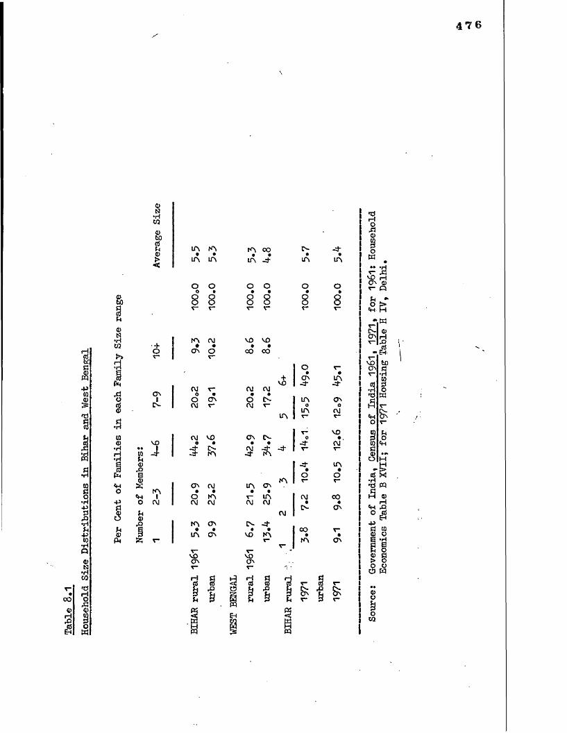
476S

O•rfCQ

fiO<

tn m ♦ •in in

tn oo • •in if in tn

o o o o&aroh©N•HCQ>>d

ocS©•H10•H • fti—l 10•rl uQ 0(3 rOEn SO«H So

«H■p o8 0

*§h© 3P4

8 8 8 8 8 8

' + O r

ONIC"-

VD

J

Vcm

m cm • *ON o

4 •O CTn CM r *

CM VD o t- if t>~- i f tn

ON CM • •o tnCM CM

tn * •in on

VO vo • •CO 0 0

CM CM

OCM

ON Cn. • •CM - i f - i f m

in on • •r - in CM CM

CN. if * •vo tn

+vo

in

tn

CM

ONifin

oin

if*o

CM

00tn

inifON

oCM

VO*.CM

in

o

00ON

ON

00©

0Eh

VOCTNH$

E 1

voOnV*

r- § r -

Bn 'S 8nr * p c *

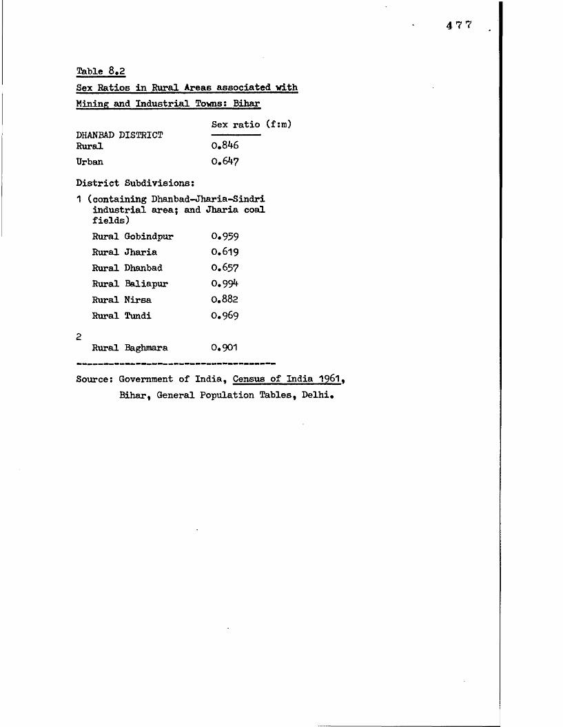
Table 8.2Sex Ratios in Rural Areas associated withMining and Industrial Towns; Bihar

Sex ratio (f:ro)DHANRAD DISTRICT ---------Rural 0.846Urban 0.647District Subdivisions:1 (containing Dhanbad-Jharia-Sindri

industrial area; and Jharia coalfields)Rural Gobindpur 0.959Rural Jharia 0.619Rural Dhanbad 0.657Rural Baliapur 0.994Rural Nirsa 0.882

Rural Tundi 0.969

2Rural Baghmara 0 .9 0 1

Source: Government of India, Census of India 1961. Bihar, General Population Tables, Delhi.

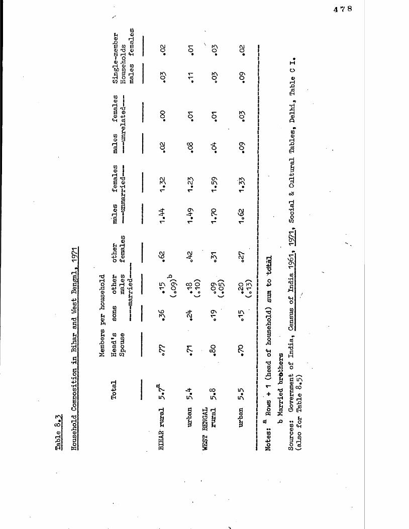
47 8

tsb 0043 *3E TO E CM r~0 T3 0 O OB rH «H » •1 O0 43H 0 TOg § 0H fA *-•H O TO O r -w w E • *

o

fAO

o

O NoH

O

0iHS>5

81 S

&

ONo

CM fA ON fAfA CM IA fA• • • •r * T~ r * t -

•H4 3

0Q

TO0

rH43_TO6h■3-P

O

08

-d"-3-

ON-4- R &

TO•HOo

w

r “A *O Nrm

HTO*£i3£43TO0no§«5

§•HPQ

■HFJO•H43*HTOOPEOO

fA -d• H00 0430 0H TOSt PTO OW

*oH0

430

1as043E03S

^ 10 J.0 0 tJ ^ H O 43 0 «H

tQ 0•O TO o 0 P W CQ

■a4->

a

ir\

vofA

(NA -

o

ONo

LA

3!o

CO O

-3*CM

LAo

ON LA O O o •

IA

ON

OCO

00IA

§ <? *0?Si U *

A -CMo

O fA CM v - * o

IA

R

LA*IA

rO&

oKTOTO043s

A -ON|

VOON

TO•H'TJA«HO

§«0

o

0

8H0 Ch

43£ LA 0 •<3 ° °Fl 0£ •"* ►> 43 O ttf O Eh

*4« ° $ *H

§ § I *CQ w

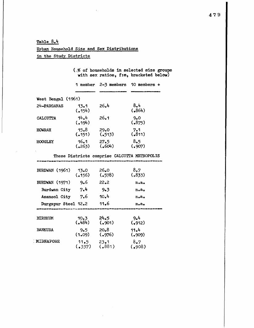
Table 8.4Urban Household Size and Sex Distributions in the Study Districts

{,% of households in selected size groups with sex ratios, f:m, bracketed below)1 member 2-3 members 10 members +

West Bengal (1961)24-PARGANAS 13.1 26.1+ 8.4

(.154) (.864)CALCUTTA 14.4 26.1 9.0

(.19*0 (.875)HOWRAH 15.3 29.0 7.1

(.151) (.513) (.811)HOOGLEY 16.1 27.5 8.5

(.263) (.6(A) (.907)These Districts comprise CALCUTTA METROPOLIS

BURDWAN (1961) 13.0 26.0 8.7(.156) (.573) (0833)

BURDWAN (1971) 9.6 22.2 n.a.Burdwan City 7.4 9.3 n.&oAsansol City 7.6 10.4 n.a.Durgapur Steel. 12.2 11.6 n.a.

BIRBHUM 10.3 24©5 9.*f(.484) (.901) (.912)

BANKURA 9.5 20.8 11.^(1.09) (.976) (.909)

MIDNAPORE 11.5 23.1 8.7(.337) (.881) (.908)

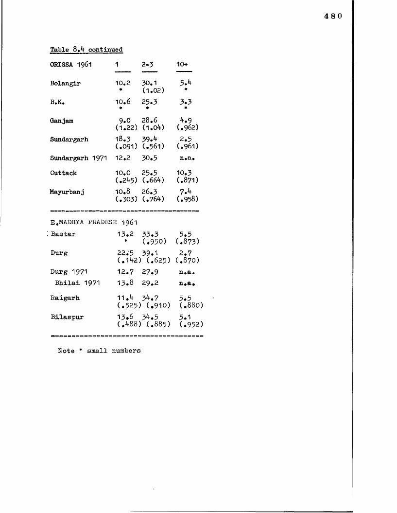
Table 8.4 continuedORISSA 1961 1 2-3 10+

Bolangir 10*2* 30.1(1.02)

3.4*B.K. 10.6* 25.3* 3.3*Ganjam 9.0

(1.22)28.6(1.04)

4.9(.962)

Sundargarh 18.3(.091)

39.4(.561)

2.5(o96l)

Sundargarh 1971 12.2 30.5 n.a.

Cuttack 10.0(.245)

25.3(.664)

10.3(.871)

Hayurbanj 10.8(.303)

26.3(.764)

7.4(.938)

E.MADHTA PRADESH 1961

Bastar 13.2 33.3 5.5* (.950) (.873)

Durg 22v5 39.1 2.7(.1^2 ) (.6 25) (.870)

Durg 1971 12.7 27.9 n.a.Bhilai 1971 1 3 .8 2 9 .2 n.a.

Raigarh 11.^ 3^.7 5 .5(.525) (.910) (.880)

Bilaspur 13 .6 3^.5 5.1(,W8) (.885) (.952)

Note * small numbers

Table 8.*f cont'dBihar (1961) 1 member 2-3 members 10members

PATNA 9.0 21.3 11.9(.2**3) (.693) (.889)

GAYA 10o5 22.1 10.8(.32*0 (.751) (•9**8)

RANCHI 8 .6 21.9 11.0(#217) (.707) (.902)

SINGBHUM 10.8 27.5 7.3(.202) (.659) (0888)

DHANBAD 15.** 28.3 7.0(.066) (.**65) (.777)

BHAGALPUR 7.0 20.6 11.1(.398) (.812) (.925)

SHAHABAD 9.3 22.** 11.8(.317) (o7*f7) (.9***0

MONGHYR 8.7 20.9 10.7(.362) (.815) (.926)

Rural Bihar 5.3 20.9 9.3(.99*0 (1.0W (.998)

Sources: Government of India, Census of India. 1961.1971 (relevant States): for 1961, Household Economics Tables, Table B XVII; for 1971* Housing Tables, Table H IV, Delhi#

Table

8*5

Changing Family

Composition

in Selected

Industrial

Areas

between

the

Cens

uses

482

T3 +> §§

•H Q

8pjo

CMVO

ir\(S

cfA

vocm

its

CM

oo

AJ•4*ON fA

COCM

fA

fACM

R

LT\ -d- fA US

IAVO

•aH5 ©1

6 tQ &13©S3

© © - CQ 'd d«J O © P4tn to

H$&

fACM 8

VOO

© ON

VOo

fAES

ONCM

OCM

00I N

R-d-

IAfA

ONo

CM

oco

fAIA

oo -4CM rvj

t"*

& « 5ONJv.ON

*-* < r - W W H§

V

OCM

IA

IA CM

IA fA VO IS • •

cr: ^+so•H+>© r -

•H vOa on &

£S CM fA fA

IA CM

O n oor r * •

fA IA O - IS

Ov O

VO IS ON ON

Source:

See Table

8*3

Table

8,6

Composition

of Family Earners

and Inc

ome amo

ng Industrial Workers

in Selected Cities

483

in *7 in° •-5r r~rn f\j

in

oj

on•OJv_xVD

VO

ino♦VOOJ

mvo

minin

mVO

00vom

o*INm

ovo

OJvo

OJ

VO

«H*0rH1

0>'OrH

3o

OJ

ONOO

OJo

ON m OJ O m• 0 • • oin 00 [N m r

oo n- IN in oo

OJOJ ooin

ONOJoobo5•9-E ON

CD <'■"*h mS r~a vo

ON

to

5ON

■a~oo

oo

*

ONl£k<D

H•H-PX■P

O ON O Np <—' +5 P -Po oo o

oo w o o' OQ W5

Table 8.7

All Households and Industrial Households compared by

Size

Distributions: selected Cities« Eastern

India

4 84

p<po&>x ioa$*H VO I

Ho in ia> -d-s§

8,?<\Jto

&4>X r *

■8rt4)

VOm

VOOJ

£•HIQTJ§VOP \ pH inO oa *H X•H o a

ojoi

o oo voK> A

o»

00 IT\ • »in inOJ OJ

O oo OJ

r CO rVD in IN CO - ON

VO.VOm

-4--d-OJ

£NOJ

C O N K \» * *o tn inr* OO v vo uS n» co on on

oONm

vo iw iiiiin oo vo i• o • Im o ioj oj ; oOJ VO

t ooi •mK\

inOJ

on -d-

n- oj • *00 o

On ON

>*♦HOCtf

• P• PPa

ajs§

§ 3

momm

inoOJ

v- O * •vo mOJ r -

-d- in • •-d -d k- int “ 00\o in on on

•ri■pIQ

00OJ

I

1W

IIIIIIN I • Iin i r- I

I I I ION OO

-d I

inoo0 t |in o j » r * in IIr 00 Ivo tn iON on I r r I

•H

■P . IQ I £ !»d _A |

1 1 & itS i

485

-P

O0O-•000)

rH

1

P<3o&AocSo

V.TSrHOA4 )

VOIJ-

5© K\ft(0&€£

IOJ

to OJ

&& o

M to<H hC

5

Table

8>8

All Households and Industrial Households

corn-p

ared

by

Size

Distributions; selected Cities« Western

India

4 8 6

&o&>■8oS0)

rH,8<D(0gtU&to4>'ia>5C

VO

-d-

OJ

LTVt)0 0)•3 S

ONK\

inOO

tn ono j v -

• •on oo

voON ONft

&I

s

'O_ 0 RJ.3 H 0 0*0 (d OJ ■S §

Afn-Pto■§a&i

coONm

mOJ

.4- ON • *-4 OOOJ OJ

r* OJ • •IN O N

m vo int * •on m mr OO rvo in inON - ON

to to

ON•00OJ

VO CN • om OJ OJ

oo inOJ5 ftcr\ ov

wICOa>01to

.3

g> XO IN? ON ON

Table

8,9

Remittances

and Family

Structure

among

Industrial Wo

rker

s

487

§Q a

■a>o I IS O fA OJ ONo • o • • *

r - fA OJ OJ O O

A- r* fA OJ On -j--4- 00OJ r* fN O -4- -4- OJOJ (A CO

O -4- On IS -4" fA fAfA fA fA OJ O LA

ISoft

IA LA ON VO OOo o o oVO OJ r*(\l 4 4 ISOJ

* 1ON fA*- o IS cs O fA

vo 1 r*V A-T” -4- ON *-K~

O IA

I Ir-r- A-r* CO T—*- VOT“ T“ -4-

I ILAfA VOfA IAOJ ofA LA fAT”

1CAVO ft vCs ft -4-LA fAr- fc

3 S'S ctfcti ? r- voo O LA •0) & ON LA

p C3 r- fAa- a-OJ IA OJ

-3

fAia i

0 4

< *-3cd xi tt<D

• P

is

aiH<t>P

CO

oto

Table 8.10Concentration of Workers in Household Industry, by Industry

This table gives the number of recorded workers per household in each specified household industry, for a selection of Districts©mph = males per householdfph a= females per householdhwph = hired workers per household(number of households in Census sample is provided in brackets)

Overview and controls at the State level:

ORISSAAll manufacturing household industry

ruralurban

BIHARAll manufacturing household industry

ruralurban

WEST BENGALAll manufacturing household industry

ruralurban

E. MADHYA PRADESHAll manufacturing household industry

ruralurban

Food processingruralurban

MAHARASHTRAAll manufacturing household industry

ruralurban

mph fph hwph

1.40 0.94 0*10

1*27 0.61 0o29

1.61 0 o95 0.551.1*5 0.60 0.1*5

1.40 0.57 0.221.40 0.59 0.48

1.51 1*09 0.151.22 0.78 0.15

1o59 1.34 0.581.21 0.70 0.58

1.45 0.92 0.09

1.19 0.85 0.24

489

Table 8*10 continued

ORISSA (urban Districts)GANJAM mph fph hwph (606)food 0*8? textiles 1.26 wood 0*88

0.961.060.9^

0o310.010.03

(11*0(12*0(162)

SUNDARGARH (5*0food 1*00 textiles 1*25 wood 1*00 non-metal minerals 1*50 basic metals 1.50

0.25 1.00 0.2 7

0.250.55

0.370.000.360.250.00

(8)(*0(11)(8)(6)

CUTTACK (**32)food 1.29 textiles 1.*f1 wood 1.**3 non met. mino1059 iaiscell.1 1.65

O.651„320.530.260.09

0.270.060.220.380.29

(59)(85)(**6)(**2)(95)

BIHAR (urban Districts)SINGBHUM mph fph hwph (1**0)food 1.?6 wood 0.92

0.320.58

1.2*f0.33

(25)(36)

non met. min.1.67 0.83 0.08 (12)DHANBAD '(201)

food 1.51 wood 2.15

0.350.62

0.380.*f6

(7**)(13)

RANCHI (253)food 1.25 wood 2.2*f non met. mind.**? basic metals 1o***f

0.520.29O .83O .89

0.160.820.*f20.00

(77)(17)(36)(9)

PATNA (1083)food 1.**5 wood 1*75 non met. min.1.65

0.5A0.280.83

1.210.311.^6

(217)(113)(72)

4 90

Table 8>10 continued

WEST BENGAL (urban Districts)BURDWAN mph fph hwph (209)

food 0*82 0.36 0.14 (22)tobacco 1.08 0.28 0 d 6 (25)cotton text* 0.97 0.29 0.17 (35)misc. text* 1.43 (7)wood 1.07 0.3** 0.45 (29)leather 1.70 (10)chemicals 0.75 0.50 1.25 (4)non met*min. 1.30 0.47 0.23 (30)basic metals 1.60 0.00 0.27 (15)BIRBHUM (83)food 0.73 0.45 0.09 (11)tobacco 1.05 0.32 0.11 (19)wood 1.75 0.58 0.00 (12)CALCUTTA (791)food 1.85 0.15 0.71 (48)tobacco 1.23 0.36 0.95 (44)text* misc* 1.37 0.07 0.90 (89)wood 1.47 0.19 0.47 (103)paper 1.11 0.82 O .63 (38)leather 2.65 0.12 0.91 (159)non met*min* 1.95 0.59 0.53 (73)basic metals 2.09 0.11 0.51 (47)24-PARGANAS (124?)tobacco 1.12 0.29 0.26 (58)cotton text. 1.24 0.61 0.38 (157)misc. text* 1.66 0.04 0.4o (659)wood 1.31 0.50 0..12 (132)non met* min..1.48 0.40 O .89 (63)

£. MADHYA PRADESH (urban Districts)DURG mph fph hwph (473) BILASPUR mph fph hwphfood 0.92 0.93 0.15 (71) 1.02 0.79 0.26cotton text. 1.53 1.40 0.10 (30) 1.69 1.73 0.04misc. text. 1.13 0.35 0.14 (72)wood 1.11 0.73 0.15 (62) 1.23 0.54 0.19basic metal 1*32 0.16 0.68 (25)

(43)

(26)

Table 8.10 continued

MAHARASHTRA (urban Districts)GREATER BOMBAY mph fph hwph (1738)

tobacco text. misc.

0.561.08

1.190.28

0.0*+0.29

(373)(399)

THANA (376)foodtext. misc. wood

0.500.661.03

1.200.570.56

0.120.100.16

(82)(131)(32)

POONA (1263)tobacco cotton text, text, misco wood leather

0.*+91.030.961.081.22

1.171.000.350.730.18

0.020.310.120.100.11

(398)(51)(237)(130)(107)

SHOLAPUR (1570)cotton text, text. misc. wood leather

1.221.051.131.30

1.1*+0.300.830.17

1.*+90.150.100.07

(869)(153)(113)(5*+)

AHMEDABAD mph fph hwph (855)food tobacco cotton text, misc. text, wood leather non met.min. basic metals

1.501.010.830.851.361.321.251.21

0.270.620.8*+0.560.350.070.*+60.51

0.350.0*+0.220.020.0*+0.630.580.12

(26)(68)(190)(23*+)(97)(60)(2*+)(57)

Source: Derived from Government of India, Census of India 19&1t Household Economic Tables, (relevant States), Delhi, Table B XVI.

492

35+>

sco° ^ OnO IN ; •

COU

1S68toUo

!ftCO

CO&

r- t•HJS

(0 too a>

O r* A-

ITN ^ N O' tN IN A- A-

00 0)1

tog

•H

£noo

O

■3•HU•PTJ

OCJ0

•H -P

1a>o§

o

s&

gss§toh£

&£

toft•ss

g•H-p■§

Ibog oo O IN

I-PB•Hbto*Ha

to0) «H 3

• 9 , 3■P hg g o t»o o

ONIN

10♦H■P

1OooCO *3 4>■P O ®HCO IA A-«Mo

£NIN

NOIN

ft

£

OA-

O r* • •VO VO

VO IN b •CO O

r*OJ Jt • oCO OJ

-±OJ

OJON

co r - • •vo ON

o n i a• oLA J-

IN VO • •O' O

L A -d - o •-d- LA

ON OJ • *f A VO

LA IN • ©OJ ONOJfA

O-d-

LAsOO Ooj|

A- OnB •OJ voA- VOB B

O COLA r - • •vo vo

ONB

OJ

IN O • #Ol OJ

OJI OJ

Or

LA•-d-*d-•fA at

N•>A<u

vo•-d~-d•LA

oU fA < • r

CNBOJ

INB

VOoOJfABOJ

OJBfA

LA•OJto-P LAI

* rt *1H r' IQ Oj| 10

.7 INBOJ

fABvoT“

O nftON

ti> a,& at to&6,

Table

8#11

continued

4 9 3

•rirH

-P•P -P

93 O « 00 OO

«> *» O r -

VO IN ( \ l CO N IA J -• * • • • • oCN O ^ O ' fVJ O ' 4 1[\1 K \ IA f\J IA v

cr\0000OO

C O

IA oo o o fA J -

V O -4- • •00 VO00

fA00VO O' • •fA VO

OO

00

00

Table

8*11

continued

494

COIN

OJorA

ON oj • •r- fAr - f A • *OJ f A

OJ I N • •

fA o j

£

INI N

VOt N

I AIN

•4*IN

fAA-

OIN

IA fA• •OJ COOJ O• • •LA V fAIN I VO ffNl

• I • °VO I VO fAoil oj|

00oL A

-tf- fA • *OJ NO

oo -3* • •T~ OJ

fAI A

VO 04 o •OJ VO

tA

rAfA

IA v • of A VO

OJL A I r - |INI VO

f A

00

aa

f A OJ • *OJ VO

LA

f A I

VO

o

& -P oi•h -p jo +>•H o a e ga § ti> fcO § *H • *rt& £ s +> *Eh CD

oo oo• oOJ OJ

I N r - • •I A CO

0 0 VO • •OJ OJ

fc CD *P

Table

8»11

contin

ued

495

ONCOCOCO

A-ooVOOOIACO

-4OO

fAOOOJOO

OO

OOO

rAoONOJ

•4VO

£•H

*3 , - 0) bo(0 r-38 08

in ia oo com vo

O - 4 o •O N OJ

OJ

rA rA • •r O O

Oo

fv. vo

fA O

A- tn• or- V O

IA oo

voojw- 4 OJ • oA- 00

LA IN • •r - OJ

LA A-

!£s

£•3t4Q)

□ ON•Joo « .2 °§ V 2 o 8 *«H *3O 0)10 HSo 4)

•H *3 •P&4 A o ® o 0) O rD

•3 ®O >

I 3H•s_ o> u > o oS'S^ toS>» 4) r—t *H fi P O -P§So

! at

(04)•P

J§

voON ■* > (0 H 4)■p a■$ a? oi a

»oj

■ps*> PQ 4)rH 10 4) O* 1■* atto EH4)H E

tJ J3 O

'Hto

•H

§ rrl -P

a s<H Co o•H - P + 5a $t

Eeg §4> W > »o -Po 5 to © 3 c oE to OO 4) 4) rl L

«H ,Qat 4> *3 Eh ,34>

• P Oat *h H S ®3 O *H

3.3 <34)OuOCQ

but

lack

of uniformity

in tabulation

limits us

to this

sub-sample

of Cities.

Table 8B12Indices of Industry-specific Concentration amongMigrants of different Origins in two Centres of Heavy Industry

Migrants to DHANBAD-JHARIA-SINDRI, Bihar (1961)

Origin Percentage of Male Workers of specified origin who are employed insMining (number in brackets)

Bihar 36*9 (14543)Within Bihar:

Dhanbad 38*3 (1933)Gaya 3309 (2607)Monghyr 26*8 (1646)Hazaribagh

43o3 (2279)

Uttar Pradesh48e8 (3633)

West Bengal 43*3 __(2880)_____

Migrants to JAMSHEDPUR, Bihar (1961)

1®in Percentage of Male Workers of specified origin who are employed in:Iron & Steel (Numbers) Transport Equipment (Numbers)

Bihar 29o4 (8843) 8 .8 (2648)Orissa 3807 (3072) 12.7 (1008)Punjab 34.3 (1300 13.7 (543)U.P. 34.5 (2372) 12.8 (881)West Bengal 37•9 (3682) 11.6 (1127)Outside 7Q k India 5 0 ,4 (2916) 4.8 (364)

Sources: Government of India, Census of India, 1961. SpecialMigration Tables for Dhanbad-Jharia-Sindri Town Group, Delhi, Table 5* Special Migration Tables for Jamshedpur, Delhi, Table

Table 8,13Concentration of Industrial Employment according to Duration of Residence at two Centres of Heavy Industry

DHANBAD-JHARXA-SINDRI Bihar, 1961

Migrants from. Duration of Residence in Dhanbad:1 year 1-5 years 6-10 years Proportion of all male workersa in Production Work

Other States(than Bihar) .202 .206 .2^9Uttar Pradesh d 68 .167 .2^9All places .2 6k .279 *308

Proportion in Mining

Uttar Pradesh *557 e^2b .386

All places *386 *353 *327

JAMSHEDPUR S.Proportion in Production Work

Other States (than Bihar)

o36*f 061O .530

Uttar Pradesh *352 .Gkk *503Orissa *3 k3 *538 *513Punjab •36? *509 **f73West Bengal *356 .676 .567All places .38^ 0625 .5^0

Notes: a The proportion of all male workers from the specifiedorigin and of the specified duration who are recorded in the occupation of production worker (miner)•

Sources: See Table 8#12 above0

Table 8.14Concentration of Industry-specific Employment among Migrants to Ahmedabad. according to Duration of Residence

Origin 1 year 1-5 years 6-10 yearsProportion of&all male Manufacturing

workers in

All places .311 .463 *563(numbers) (4320) (20070) (23190)

Maharashtra(7535)

.269 *539 *597

Uttar Pradesh (21764)

.480 0651 .731

Rajasthan o269 *392 *575(14826)

Proportion of all male manufacturing workers in Textiles®

All places • 660 (2852)

.743(14911)

.820(19027)

Maharashtra(6491)

.749 .765 .882

Uttar Pradesh (19369)

.647 .795 .895

Rajasthan(12649)

.582 .779 .895

Proportion of all Production Wor] Spinners and Weavers

Maharashtra(5396)

•^95 .544 .651

Uttar Pradesh (18009)

.577 .636 .781

Notes: a The proportion applies to each origin-duration-specific cell in following bank of figures.

Source: Government of India, Census of India, 1961, Special Tables on Migrants to Ahmedabad City, Delhi,Tables 4 and 5*

A brief Overview of Chapter 8

If the State does not resolve the labour market disequilibria and resultant income losses, how far can families protect themselves? It becomes clear that migrant groups do not attempt to spread their sources of employment, but rather seek to concentrate it in particular industries or occupations. At the same time families in urban areas tend to loosen their rural links by family formation in the towns (an exception being the miners).

CHAPTER 9

Family Income Security, Employment Aspirations, and the State

A Summary of the Argument

The adverse implications of rapid demographic growth for the equilibrium of the future labour market, and the adverse implications of single-industry towns for the long-term family income security, are considered finally in the light of possible interventions by the State Empirically a reconstruction of the local demography of Bhilai Steel Town helps to illustrate the first problem, and this is taken down to 19&1. Costs of alternative strategies that the State might adopt towards alleviating both these problems, - subsidised diversification or suboptimal scale of plant -, are assessed: in some casesthe costs are less than the loss of social income involved in the event of a local industrial stagnation or closure. Finally, an original hypothesis is put forward: that family or other social group, income security is at its worst when both direct income-producing employment and indirect transfer incomes from fellows in the same social group (or family) are, at source, concentrated in the same industry.

501

Concentration of Industry and Security of Incomes: the Policy Issues

Our interest in the relationship between demography and industrial structure, or demography and industrial technologies, has been prompted by a concern for some of the welfare implications of industrialisation strategy.A particular problem worth investigation has been the

security of incomes obtained through employment in single­

industry towns. It is a commonplace to observe that changes in industrial structure or technologies may render a high proportion of the workforce unemployed, and a higher

proportion in such towns than in more diversified locations.Before proceeding further it would be pertinent to ask whether that observation alone is in any way an argument for encouraging (i.e. subsidising) local diversification*The question is more complex than may be immediately appreciated.

Some of the major points, in regard to which careful quantification is needed, (and an illustration is attempted in the Appendix), are as follows,

1 For instance in the case of our comparative study from the U.K., we note unemployment rates of approximately M-0% soon after the closure of Consett steel works.

502

If there is a freely operating market, industries

of a similar nature, or highly inter-dependent industries(in an input-output sense), will tend to locate in closeproximity to one another to reap certain economies of

production, related to (inter alia) the physical fact of1their mutual proximxty itself* To attract wholly unrelated

industries to the same area may require heavy subsidies continuing over time* This we will document below.

To be sure, it will often be possible to attract modern industries providing consumption goods (particularly food) for the local population at rather low levels of subsidy, especially if the local population is close to the threshold size at which local industry (also subject to economies of scale) would in any case become profitable. But then,

as we shall argue, the social benefit of a subsidy in the case of a consumption goods industry will also be considerably smaller.

The question to ask is, how could any subsidies be

justified? Clearly they could not be justified on any

grounds of industrial efficiency (if, as we say, factor and product markets are competitive). The short answer would seem to be that if the State has a policy of providing

1 The availability of a particular factor of production will often decide the location in the first place. On the econ­omies of location and agglomeration there is a voluminous literature. For a summary, see, e.g., E.3.Mills,Urban Economics. Harvard University Press, Cambridge (Mass.), 1979.

unemployment relief (for the wholly unemployed) it is arguable at least that, provided unemployment levels

would be higher in the economy as a whole if industry remained locally concentrated, then the reduction in future unemployment relief might more than compensate for the cost of a continuing subsidy needed to promote and maintain some degree of local diversification.

But why should open unemployment rates be higher ifindustry is more concentrated? The argument is that in a .

recession or decline in demand for a locally produced

commodity exported from the locality for national (or international consumption), the reduction in incomes from direct

employment in the depressed industry further depresses localdemand for consumer goods and services, due to a reverse

1multxplier, as it were, setting xn# This puts more of

the local workforce wholly out of work# Whereas if, say,

50% of local industrial output (for export beyond the

community) held up in the case of a more diversified town despite recession or changes in the structure of aggregate demand, then those employed in consumer goods and services

production, through working shorter hours and receiving

1 If the recession is severe enough, the opportunity for viable work-sharing among the workforce supplying the ’'multiplier’* goods is severely curtailed: some peoplebecome wholly unemployed once average income from work reaches subsistence levels#

504

lower incomes, would not be out of work altogether, even

if one of the core industries closed down. This effect would be even stronger in a largely self-employed or household production economy. Shopkeepers will take a cut in income

rather than close down and seek unemployment relief or new work outside the locality. The fall in demand and employment is spread throughout the community and survival remains

possible: if the fall is a more significant proportion of

local demand, then spreading the incidence becomes impossible

without reducing the average income from work to below an acceptable subsistence level, and hence the work-sharing ethic

breaks down, and the marginal producers become wholly unemployed.

Thus the social returns to a policy that attracts a second exporting industry (unrelated to the first) would of course be higher than those from attracting an industry purely

intent on providing commodities or services for immediate

consumption in the town itself: for the consumer goods

industry would add to local unemployment if the first industry goes into a severe enough recession (since the

first industry's wage labour is the source of local consumption

demand. 1

1 There is a further consideration here, arguably in the realms of the unquantifiable, but almost certainly of significance. A level of unemployment concentrated in a locality may be socially more costly than the same amount of unemployment dispersed over a region. The psychology of aggregate depression may encourage crime and other social malaise, may discourage labour itself from seeking re-training or new job opportunities, or may discourage new private investment from entering the area (for reasons other than the more objective economic

505

So far we have been discussing the issue on the

assumption that the State provides unemployment relief#Insofar as it does not, the matter becomes one of income

distribution alone# Inequalities clearly become sharper if 40% of the town becomes wholly unemployed (i#e. 2 0%

due to the closure of the basic industry, and a further

20% due to the reverse multiplier described above), than

if only 15% of a town twice as large and more diversified becomes unemployed (i#e# 10% due to the closure of the basic

industry and only 5% due to the reverse multiplier), with an additional 5 to 10%, also affected by the reverse multiplier,

taking a considerable cut in income, but due to the continuation of other basic industries, not losing employment (at

"Isubsistence level remuneration) completely# Of course the effect of a local reverse multiplier is much more

severe on individual families if the workers in the core industry, who are made jobless, have to share in the existing local income to survive (thus considerably cutting local aggregate consumption), than it would be in a State with full unemployment relief financed out of national income

footnote continuedones suggested above)# Together these arguments may well justify an additional element of subsidy in an effort to encourage diversification (which is not to say they should be used to justify any level of subsidy)#1 It is appreciated of course that definitions of inequality

differ# At least one can say that the distributional effects are different in the two cases# The author's own value judgement would be that they are worse in the first case#

506

(implying a consumption transfer toward the locality 1

under relief). Indeed if large redundancy payments are also made, the immediate effect may be to increase

aggregate consumption in the' locality (again an experience

of the British Steel Towns). But as pointed out above,

there is no indication that such additions to consumption

compensate over time for the welfare loss in being out of

work in a morally depressed community. That is to say,

the unemployed labour force is constrained to use its

incremental income to purchase goods, rather than to

purchase the satisfaction of being at work. Unless the

redundancy pay is enormous, there may be a net welfare loss.

And if it is enormous, the question arises whether this

plus unemployment relief (plus any subsidies used to attract

new industry) may together be more costly than the option

of keeping the original industry open.

But it is in the context of an economy without

unemployment relief, but with a developing system of

industrial wage labour, that the demographic aspects of

single-industry towns become more important. This is because

the source of income to the wholly unemployed is the family

in the broadest sense (as we have argued in Chapter 8 above).

The scope for income sharing, by transfers alone, outside of

the immediate or extended family is very limited. There

might be, cet* par., opportunities for work (and hence income)

sharing outside the wage sector, but at times of industrial closure the redundant wage labour will find it less easy

to become absorbed in the non-wage sector: the potentialentrants will be just too many in an indiversified town*This is why we focus on the family.

The fact that there is no State unemployment relief does not necessarily imply no State intervention in, or planning of, industrial location. The National and

State Governments of India have enacted and implemented

rather more effectively regarding location than regarding unemployment# Furthermore, though one cannot immediately suggest political strategies that could be adopted at the

community or family level toward the effective adoption of

unemployment relief, one may be able to suggest strategies to ensure a more even sharing of the unemployment burden. This may look like a recipe to prevent structural reform,

I shall argue later, though cannot prove, that it is not.

In summary, the problem may be presented as follows. Welfare transfer systems operate between individuals. but the organisation of these transfers may take place

1 For details on regional subsidies see the references noted in the Appendix to this Chapter. For an appraisal and critique see J.W.Mackie, "Industrial Location and Regional Policy in South India", Ph. D. thesis, School of Oriental and African Studies, London, 1982; I am grateful to him for some useful references.

508

at the level of the family, local community, industry,

region, or nation# There is typically, but not necessarily, a spatial dimension involved here# On the other hand

factor incomes, as distinct from welfare transfers, that is, in this context, wages or payments dependent on work, are distributed across individuals in ways that make them, as individuals or groups of individuals, vulnerable to recessions or structural changes in the economy#

Again there is typically a spatial dimension here, of the

kind that this thesis has emphasised# But there need not be# All Chinese overseas in India might be restaurant workers for instance, but they could be geographically

scattered in all the major cities# Now the interesting problem arises with the overlapping of these two sets:

the income transfer, and the income source, (Figure 9*2)#

If they overlap completely (as would be the case if the Chinese re-distribute income among their own overseas community, receiving nothing from outside), then individual

welfare is at its most insecure in the event of economic

structural change (a fall in the demand for Chinese cuisine)#

1 Another example would be that of the textile workers fromRatnagiri in Maharashtra# Thay may work in textile towns all over the State, and live permanently where they work, but if they transfer income among' themselves, the problem of the overlapping sets arises, should the textile industry fail# In practice there is probably a spatial dimension: these migrants all work in Bombay and return to Ratnagiri regularly: the closure of a cotton mill could impoverish a village#

509

The Implications for Employment over time: Local-level Disequilibria Explored

A striking, and some would argue depressing, feature of the Indian Censuses is that they indicate

consistently a failure of the labour force to shift proportion­ally into non-agricultural employment, and a similar failure of the manufacturing sector to grow proportionally to the rest# This is thought to be depressing because productivity is believed to be higher in manufacturing (even when social pricing of outputs is used), and above all in particular branches of manufacturing outside the household sector,

than it is in agriculture# There are reasons to believe

that it is in India's economic interests to develop the

manufacturing sector: quite apart from achieving goals ofdynamic independence (which Governments of developing countries

have rightly or wrongly regarded as being promoted by the

development of the manufacturing sector), India undoubtedly has comparative advantage in world production in certain industries in that sector#

1 Quite apart from the question of the undesirability of a slow growth of industry, per se, the failure to absorb significant quantities of labour in this sector (even at times of its fairly rapid expansion) would be undesirable, given the importance of employment as a means to income in India. These are complex and fundamental issues, beyond the scope of the discussion in this thesis (but see Chapter 2)# •

This phenomenon is well illustrated in our region of

study. Its implication for growth of income is acutely

observed at the level of the locality. At the start of our period of study, in the mid-1950s we witness a major

investment in this region. This is physically centred on a few localities. The investment leads to a national

income flow that induces further investment: in physical

terms the output of basic materials like steel plates

is followed by the establishment of factories for manufact­

uring finished products, downstream, as economists say:

these developments in turn promote the creation of more

capacity in steel production, and in mining (through backward

linkage, in the jargon). In aggregate we are examining

an accelerator effect, again creating employment at the level

of the community.

The accelerator effect operates over time# But of

more immediate reaction is the change in purchasing power

of the working community (and families) employed in these

investment goods industries: this will stimulate a:

further utilisation of productive and service capacity,

as in turn will the increased purchasing power of those

employed in providing these consumer goods and services#

The local potential of this multiplier effect is often

missed in discussion of employment problems of developing

countries, simply because the disaggregation to the level

of the,locality is not done. But in actual fact there is

no doubt that towns neighbouring the growth centres just described expand their processing of consumer goods to meet the demand of the wage-labour migrating into the area

(though it cannot be denied that some of that demand is met by importing finished goods into the area, and even into

'ithe country, - leakages as the economist would say).

1 This is not the place for a social cost-benefit analysis of investment of this kind# Suffice it to say that a major dis-benefit is the rise in the local retail prices induced by the arrival of a high-productivity workforce: in the short-run at least this will cause a fall in the real income of the working members of the original community who are not sufficiently integrated into the new economy, and of dependent household members whose monetary allocation is fairly inflexible, and of those on fixed incomes established by non-market forces outside the locality (e.g. State transport workers). This point was made forcibly to the author by the manager of a chemicals factory outside the industrial areas in Madras •

We are to focus here on three growth centres, in the

Districts of Burdwan, Durg, and Sundargarh. Each District's urban area achieved a proportion of workforce in manufacturing of between JO and k0% in 1961. During the following decade that proportion stabilised in Burdwan, fell slightly

in Sundargarh, and stabilised in Durg (Table 9*1).Distinctions between Burdwan and Durg will become clearer when we view these Districts at the level of Municipalities*

Both Districts achieved a higher crude proportion of working males in manufacturing than did Sundargarh, There is no a priori reason why the proportion should level off at around

JO to k0%; in the non-central Districts of Metropolitan

Calcutta the proportion is around J0% (and in that case at least the high level cannot be ascribed to the high initial level of manufacturing with new growth running ahead of the expansion of tertiary establishments).

In each case the surrounding Districts have a farlower proportion in manufacturing, and no notable improvementin that proportion over time (in the case of Durg, see

‘ 1Table 9.1» quite the reverse). Within Burdwan District (Table 9#1)» as within the other rapidly growing Districts,

1 Owing to a change in the Census definition of activitystatus (among other inconsistencies) the safest comparisons are restricted to adult males only; see J.Krishnamurty, "Working Force in 1971 Census: Unilluminating 'Final1 Results", Economic and Political Weekly. August 1973,

513

there is considerable variance between urban localities;

the manufacturing labour force grew fast from 1 9 6 1 -7 1

in Durgapur, moderately in Asansol-Burnpur, and fell absolutely in Burdwan City, In Sundargarh (using slightly different data) we find it grows slowly in Rourkela,

but falls in Sundargarh Municipality, and particularly in

Birmitrapur. In Durg it grows moderately in Bhilainagar, but falls in Durg Municipality, and, more importantly, in Rajnan&gaon (see also Table 6 ,6 ),

It is a major thesis of this study that due to thedemographic nature of income-sharing#the maternal and social prosperity of a community requires it not being dependanton a single industry (see Chapter 8 ). A glance at thecomposition of manufacturing will help establish how

far this was avoided over the 1961 - 1971 decade (Tables

9*2, 9*3* and Figure 9*3)* The heavy concentration of large units in the basic metals, machinery, and transport equipment industries in Sundargarh and Durg Districts in 1961 is immediately apparent. In Sundargarh other developments

are under way by 1 9 7 1, noticeably a large-scale chemicals sector. That is a crucial diversification, Burdwan achieves a similar mix of heavy industry, including electricals.

It also has a large-scale food and beverage manufacturing

sector dating from the initial period. Arguably the broader

5 14

base accounted for the maintenance of the manufacturing sector

in Burdwan despite the depression in. the basic metals industry. In the latter sector, the large-scale units

in Burdwan increased only slightly. In Sundargarh, however,

there was a considerable expansion. But ten years is a short time on which to form the basis of a judgement. Confining our *

selves to observing the Steel Towns themselves we find

the contrasts are even stronger. Durgapur grew far faster

than the'other two, and diversified at the same time.

In this analysis, the question inevitably arises, where

should we draw the boundaries of the local economy, given

the ability of labour to migrate? Migration between towns as close as Durg and Bhilai may cause no serious

social upheaval; migration between Durg and Bhopal may

do so: family income and social ties become weakened.

It is true that inter-State migration took place readily when the New-towns were formed. But the rapid family

formation indicated that the migrants expected to stay

in their new location: and as they age, their propensity

to move again is diminished (so that the social costs of

forcing them to do so increase). The point to be made

here is simply that such a skewed industrial structure

as that of Durg or Sundargarh is known to be particularly

vulnerable to overall change in comparative advantage,

economic strategy, and national prosperity. The Western

world's experience is not irrelevant. Corby and Consett Steel Towns (see Chapter 2) are smarting from just such

an affliction. When incomes of local populations are

largely determined locally the problems are even more acute. Industrial monocultures have severe future employment and hence welfare implications. We have illustrated the contrast between Durg District and Burdwan in their degree of industrial diversification in Figure 9*1 (employing a technique that resembles the familiar Lorenz curve

analysis).

Earlier we drew some contrasts between regions of Eastern and Western India (Chapter 1). The case we want to review here for Western India is the urban District of Poona*

in Maharashtra. This consists predominantly of the large City of Poona itself, and the emerging New-town area of Pimpri-Chinchwad close by. The City has a history of commercial and administrative activity in Mughal and British

days; it was a military centre and hill station for escape

from the sweltering heat of Bombay by the sea. After Independence a steady growth of manufacturing was experienced in nearly every industrial sector (Table 9.2)* This was

maintained through to 1971# The growth was sustained for

several reasons. First, the City was not wholly dependant on the production of a commodity for which national demand

was to level off; admittedly there are metal products and

machinery establishments in Poona, and their expansion was

limited during the 1961 - 1971 decade, but they do not dominate the industrial sector. As can be seen from Table 9.2

almost every sector (at the two-digit level of aggregation) is represented with a large-scale unit. Secondly there is an established chemicals industry, a sector least affected by the depression of the 1960s, Thirdly there has been little experience of labour unrest, a situation possibly

assisted by the continued steady expansion and well- balanced age structure of the City, As an aside it may be observed that in the late 1960s the City was subjected to an unprecedented in-migration due to drought in rural areas.

But these migrants were not, and had no more than fleeting aspirations to be, absorbed in the modern industrial sector. They came with their families, and (initially at least) they presented little opposition to authority.

But the real expansion of chemical and modern . consumer-durable manufacturing has centred around Pimpri

and Chinchwad, By 1971 Poona and these outliers were regarded as a single urban agglomeration. But even taken

separately, the proportion of the workforce in manufacturing underwent a steady increase over the 1961-71 decade, from

below to above JQf/o in Poona, and from to 6 5% in

Chinchwad. It cannot be said that such a desirable industrial mix was planned; but it may be predicted that the results will be happier for employment and welfare prospects over

the coming decades, than the results of industrial expansion in parts of the iron and steel belt of Eastern India,

(Table 9*3» Figure 9*1)* So long as the District has a broad manufacturing potential it can more rapidly expand in

whatever sector it finds its comparative advantage to lie: and that way the second and third generations (and indeed other

dependants of the initial migrant families) will more readily

find local employment.

Strategies to Achieve Economic-Demographic Equilibria: case-study of Bhilainagar revisited

Y/e now return to the site of the most outstanding demographic disbalance, the Steel Town of Bhilainagar.

We try to reconstruct exactly what the demographic evolution

has been, in some detail down to 1 9 7 1♦ and with some

speculation beyond that date. We relate the expansion of

the steel plant to the expansion of the labour force to

see in practice how far an equilibrium has been achieved.

We then propose a scenario for future strategists posed with similar economic questions, the planners of Bofcaro and Vizag

being among them. Taking a number of parameters, social and political, as given, we suggest alternative investment

1 There is a fairly strong assumption here that the labour- to-capital ratios will not significantly change*

5 18

strategies in order to enquire how the desired equilibrium

might have been achieved. Finally we investigate alternative

demographic strategies to meet the same ends. In short we are

posing the following question: given that India intends to

make steel, and to make it at Bhilai (or at some specified

location), how can the supply of, and demand for, manufacturing

labour be matched, to avoid prolonged periods of local

unemployment, especially of the sons of the original migrants,

by the use of a limited number of policy variables over

which we can assume control?

In Figure 9*4 we present the essential demographic

data. A consistent reconstruction of what happened after

the arrival of the first 1 5*000 steel workers (that is

operatives and service workers for Hindustan Steel, not

including construction labour per se) is offered in a

note that follows below. Here we pinpoint the more

startling conclusions. First we note that Bhilainagargrew from 86,000 to 174,000 in a decade (the exact figures

are in the Tables 9*4 and following). However, the work

force in steel production increased to only 2 5 ,0 0 0, and

the total male labour force rose from 46,000 to only

57,000. What is more, we estimate that only 8,000 to

10,000 male migrants joined the labour force during that

decade. In other words, nearly 90% of the 100% decadal1 And perhaps only 5000 if we exclude migrating sons

of the original 46000 workforce.

5 19

demographic growth came from '’natural" demographic forces: given the structure of the population that had amassed

between 1956 and 19&1 , the rest followed naturally on the road to demographic stability.

But demographic stability takes nearly 100 years

before it achieves its recognisable characteristics,

its unchanging age structure for instance, not a mere 1decade. Hence our second rather surprising conclusion

(surprising in the light of demographic-industrial relationships that had generally been experienced historically in India,

and partly incorporated in our Model type "1 c"): toBhilainagar was transposed a segment of the stable rural population, with very little interruption resulting from the process of migration. Most of the men were already

married, and their wives followed soon after their husbands' arrival, brought their existing children with

them, and continued their child-bearing. Hence by 1971 a familiar age-pyramid was restored in Bhilai, similar in structure to the rural population except for its youthfulness

(being more youthful than the almost stable population from which.dt was drawn; see illustration in Figure 6.1).

The built-in potential for a fast natural increase that might have been seriously retarded by an adverse sex ratio

1 A.J.Lotka, "A Contribution to the Theory of Self-renewing Aggregates, with Special Reference to Industrial Replacement", Annals of Mathematical Statistics. 10:1,March 1939»

suffered no perceptible retardation. In ten years the

sex ratio had reached 0.800 (females to males), against the expected 0.600. I estimate the birth rate as being

about 42 per thousand in Bhilai in 1971; in the Model

it is still 56 per thousand 15 years after the first

major migrations, though in the stable state it reaches 43.The interruption caused by the process of migration was hardly sufficient to lower the fertility of the couples concerned

(the pattern traced out in Model ,?1 a" seems more appropriate).

If we concentrate now on the sons of the migrants in the manufacturing industries (whom I have called the "second

generation in this thesis), this phenomenon means that we have

a quinquennial addition to the labour supply of between6,000 and 9*000 (allowing for mortality from birth)

starting in 1970 and continuing and increasing until

1985 (Figure 9*4).^ This is a dramatic increase (the male population under 15 in 1961 had only been 11,000), and the absolute numbers are very large too; the instability of our Model is there, but without the period of slow or

negative growth in labour force entrants (at least as far

as our decennial data can indicate), (Table 3»1). On the demand side we have already noted the lack of diversification

of industry in the urban areas of the District of Durg between

1 The sons of the 46000 (196 1) workforce inrease the workforce by between 9000 and 14000, the sons of the core-sector steel workers by between 3000 5000*over this decade.

19^1 and 1971* Figures for manufacturing employment are hazardous to use due to the redefinition of employment between the Censuses, but it seems that males in factory manufacturing hardly increased as a percentage of the male

labour force# From 1971 to 1981 we are rather in the dark, but using alternative models to reconstruct figures

consistent with the few published so far from the 1981 Census, around 11,000 adult males seem to have been attracted

into the township# We also know that 'downstrearn" metal- goods manufacturing capacity was installed during this period,

coming on stream towards the end of the decade. Let us suppose some 30% of the adult migrants were recruited into manufacturing. The crucial question then is, were

they recruited after the second generation entrants to the

labour force (numbering about 2 3*000 f bad sought, and some failed to gain, employment in manufacturing, (in which case the latter may have faced a period of unemployment or underemployment), or before they had done so, (in

which case the latter may have faced a period of under­employment towards the end of the decade)? And certainly the prospect of mismatch still arises since the early 1980s will experience the largest-second..generation cohort

to date.

1 Various reports in Financial Express (Bombay) in 1 9 8 0,e.g. on 6th October, 1 9 8 0, page 10, column 3»

2 That is , over ten years: perhaps 8,000 the sons ofl!core-sectorn fathers.

5 2 2

No disequilibrium need have arisen if the demand and supply had been contemporaneous, more or less.However, the core industry was in iron and steel making. This employed 1 5 ,0 0 0 men in 1961 and 2 5 ,0 0 0

by 1971 (Table 9.8) by which time capacity had risen to 2 million tonnes, implying an output-employment elasticity of O .7 8 at this scale of production. By 1977, 2-J m.t* output was achieved* All this implies severely diminishing employment potential (in the face of increasing supply, at least of steel workers' sons). A well targeted expansion programme toward the original goal of 10 million tonnes could have provided all the employment needed at Bhilai: but the time-phasing becomes crucial. The current expansion programme to 4 m.t. will be particularly welcome if it is achieved by the mid-1980s.

1 Some occupational mobility is to be expected, though Ihave been told that steel workers' sons do aspire towards the secure and well-paid employment in that industry.Spatial mobility, the out-migration of the second generationin search of work is taken as an unacceptable solution to disequilibrium in this thesis. This may strike the reader as an unacceptable limitation on our solution strategies.The problem is the scale of redeployment needed, ''compressed into so Bhort a space of time, when economic expansion is now being concentrated in other parts of the country. When professional and academic people I met in India in 1976 raised the objection that the population in India was too mobile, not insufficiently so, they were thinking of the initial process of population formation in urban areas, of small-holders

523

We can now review alternative strategies toward labour market equilibrium in the context of the demographic situation at Bhilai (see also Appendix, Figure 2). They are fivefold:(i) Industrial diversification (see Appendix).(ii) Phased creation of additional capacity in steel production

(in discrete "lumps" of not less than 1 million tonnescapacity each, - this being the minimum efficient scale in 1955).

(iii) In-migration controls.(iv) Delayed fertility (especially among wage labour,

to prevent the build-up in new labour-force entrants pre-dating the planned investment expansion) (see note that follows).

(v) Mini steel plants, preferably to be installed fromstart of any new investment programme (i.e. in 500,000

tonne range, as are currently being built following the Direct Reduction technology (see Chapter 2)).

We note en passant the alternatives that I am taking to be unacceptable, socially or politically, in the contemporary Indian context. They are (i) the disallowance of green­field steel plants, or, more strongly, disallowance of any steel plants, or similar heavy engineering investment involving huge economies of scale; (ii) the forced out­

migration of large cohorts of young (or old) members of the

footnote continuedand landless labourers, rapidly drawn into one centre of industrial growth; my discussants were not, I would claim, trying to imagine the reversal of this process.

community, whether initially in-migrants or not (and, it might be noted here, for reasons suggested in Chapter 5 the strategic option (iii) of in-migration controls is

-inot favoured) ; (iii) prevention of marital unions, byadopting a sex selective migration control policy, or,a weaker control, the restriction on marital fertilityby limiting severely ultimate family size, for example toa single child per couple# To repeat, our objectivebehind the strategies put forward is first to minimisesecond generation underemployment, especially among thefamilies of manufacturing labour (and especially whenthat underemployment is specific to ethnic or regionalgroups), and second, to maximise family income securityover time, as discussed above (favouring the adoptionof option (i) above)# In all, a reliance on options(i) and (ii), and perhaps (v), would appear most practical

2and sensible#

1 The efficience and equity of migration control policies are described in N#R,Crook, "On the Management of Urban Migration and Residence'’, Asian Journal of Public Administration. 5i1, June 198j5*

2 As we noted in Chapter 2 , we are having to make strong assumptions here that the new technologies are not seriously labour displacing#

The D ynam ic Im p l ic a t io n s and P o l i t i c s o f

M ig r a t io n s a C o n c lu s io n

To p u rs u e th e im p l ic a t io n s o f th e dynam ics o f

i n d u s t r i a l i s a t i o n , n o n - in d u s t r ia l i s a t i o n , and d e - i n d u s t r i a l i s ­

a t io n t h a t we have been d e s c r ib in g i s o b v io u s ly a com p lex

u n d e r ta k in g . To a t te m p t t o fo r e c a s t w o u ld be p a t e n t ly

a b s u rd . We can o n ly p o in t t o a few s p e c i f i c im p l i c a t io n s ,

some more c o n c re te i n t h a t th e p re c e d e n ts a re c le a r , some

more s p e c u la t iv e i n t h a t e i t h e r th e re i s no p re c e d e n t ,

o r th e p re c e d e n ts were i n t h e i r t im e s t r o n g ly in f lu e n c e d

by d i f f e r e n t c o n d i t io n s .

The m ost c le a r - c u t case i s t h a t o f th e r a p id

d e ve lo p m e n t o f N ew -tow ns on g r e e n - f ie ld s i t e s . I t has

been shown t h a t , u n d e r c e r t a in c o n d i t io n s on th e age (and

s e x ) s t r u c t u r e o f m ig ra n ts , th e age g ro u p re a d y to e n te r

th e la b o u r m a rk e t i s i t s e l f s u b je c t to p e r io d s o f f a i r l y

d ra m a tic e x p a n s io n o v e r th e medium te rm o f 25 y e a r s .

As f a r as em ploym ent i s c o n c e rn e d , such f lu c t u a t io n s c o u ld be

h a n d le d by th e w o rk -s h a r in g c h a r a c te r o f th e n o n - fa c to r y

s e c to r . The im p l i c a t io n a t th e fa m i ly l e v e l i s t h a t sons

em p loyed i n th e n o n - fa c to r y s e c to r may become p a r t l y dependen t

526

on t h e i r f a t h e r s f o r th e m a in te n a n ce o f t h e i r in c o m e . T h a t

i n i t s e l f may c re a te te n s io n w i t h in th e f a m i ly - p e rh a p s

e s p e c ia l ly i n a s o c ie ty w here th e in t e r - g e n e r a t io n a l

incom e f lo w s a re e x p e c te d to be i n th e re v e rs e d i r e c t i o n ,

fro m son t o f a t h e r * A f u r t h e r s o u rc e o f te n s io n , h o w e v e r,

i s t h a t th e sons a re e x p e c te d a t le a s t t o a c h ie v e em ploym ent

o f th e same s ta tu s as t h a t o f t h e i r f a t h e r s . T h is s i t u a t i o n

i s e x a c e rb a te d i f th e f a m i ly i s fro m a n o th e r u rb a n a re a

o r th e sons a re e d u c a te d . A s p i r a t io n s w i l l be a t t h e i r h ig h e s t .

A n o th e r s o u rc e o f te n s io n a r is e s n o t fro m th e age

s t r u c t u r e as s u c h , b u t fro m th e f a c t t h a t th e im m ig ra n ts

a re fo r e ig n * They may e n jo y i n i t i a l a c c e p ta n c e i f e x p a n s io n

i n em ploym ent i s r a p id enough f o r m ig ra n ts and lo c a ls t o have

e q u a l a ccess to jo b s : once i t s lo w s down, th e re i s r i v a l r y

be tw een th e "s o n s o f th e s o i l * 1 and th e m ig ra n ts th e m s e lv e s ,

who a re th e n seen to be o c c u p y in g jo b s t h a t th e l o c a l g ro w in g

la b o u r fo r c e f e e ls i t s h o u ld have by r i g h t . The more r a p id th e

i n i t i a l i n d u s t r i a l e x p a n s io n , th e le s s l i k e l y th e same r a te

o f g ro w th can be m a in ta in e d ; i n any ca se , c o n t in u e d g ro w th

depends on th e in v e s tm e n t d e c is io n s o f i n d u s t r i a l i s t s , n o t

th e s o c ia l c o n s id e r a t io n s o f th e co m m u n ity . The more s p e c i f i c

52?

th e c o n d i t io n s fa v o u r in g th e o r i g i n a l lo c a t io n o f th e

in d u s t r y ( o r th e le s s c o m m e rc ia lly c o m p e t it iv e th e re a s o n s

f o r th e o r i g i n a l l o c a t i o n ) , th e le s s l i k e l y i t i s t h a t th e

g ro w th o f in v e s tm e n ts can he s u s ta in e d , u n le s s s im i la r o r o th e r

n o n -c o m p e t i t iv e fo r c e s a re p e rp e tu a te d o r in t r o d u c e d .

Now, to ta k e t h i s p o in t a l i t t l e f u r t h e r , th e p o l i t i c a l

re s p o n s e e n c o u n te re d i s l i k e l y to be a n t i - m ig r a n t (b y w h a te v e r

l o c a l i n t e r e s t g ro u p i t was t h a t p rom o ted th e o r i g i n a l in v e s tm e n t ) ,

r a t h e r th a n p ro f u r t h e r in v e s tm e n t . And i n an e n v iro n m e n t o f

r e g io n a l s ta g n a t io n , th e o r i g i n a l i n d u s t r i a l c o n c e rn i s

u n l i k e l y to fa v o u r f u r t h e r e x p a n s io n . The u p s h o t w i l l be

to keep m ig ra n ts o u t r a t h e r th a n to p ro v id e more jo b s . T h is

re s p o n s e i s e x a c e rb a te d i f th e m ig ra n t .p o p u la t io n su b g ro u p s

a re g ro in in g o w in g t o fa v o u ra b le age s t r u c t u r e ( o r h ig h

f e r t i l i t y ) . I n cases w here m ig ra n ts a re more l o c a l , i t

i s n o t u n l i k e l y t h a t th e more e n t e r p r is in g o f them w i l l

e m ig ra te fro m th e l o c a l i t y , b u t as we have s u g g e s te d , th e

more l o c a l m ig ra n ts seem, on th e w h o le , t o be th e le s s w e l l

endowed ( th e le s s l i k e l y t o own la n d ) ; th e r e s t s im p ly f a i l

to p o l i t i c i s e , o r , w o rse s t i l l , a re e a s i ly b o u g h t o f f by

th e p ro m is e s o f th e l o c a l p a r ty who have a lr e a d y a c h ie v e d t h e i r

m a jo r o b je c t iv e on th e in v e s tm e n t f r o n t . And h e n c e , f o r

e xa m p le , th e Backw ard C la s s e s have re m a in e d backw ard i n

th e s e a re a s o f i n d u s t r i a l g ro w th * B u t n e i t h e r o f th e se

528

g loom y s t o r ie s i s i n e v i t a b le , th o u g h d em og ra p h ic f a c t o r s a lo n e

c o u ld n o t d is t in g u is h be tw een a l t e r n a t i v e s . An a l t e r n a t i v e

i s t h a t th e te n s io n d e s c r ib e d g e ts c h a n n e lle d i n t o

b a r g a in in g , th ro u g h p o l i t i c a l m o b i l i s a t io n , f o r f u r t h e r

in v e s tm e n t fro m o u ts id e th e l o c a l i t y , t o m ax im ise l o c a l

g ro w th as w e l l as t o e n su re i t s e q u i ta b le d i s t r i b u t i o n

(b e tw e e n g ro u p s , and o v e r t im e ) . H e re , as we have s a id ,

th e d a n g e r i s t h a t b a r g a in in g i s seen as d is r u p t i v e , so

t h a t c a p i t a l i s s im p ly s c a re d aw ay.

I f th e f a i l u r e s t o r y i s th e r e a l one , w h a t a re th e

d e v e lo p m e n ts o v e r tim e ? T he re i s c o n t in u e d im p o v e r is h m e n t

o r o u t - m ig r a t io n o f th e y o u n g . G ive n th e f a i l u r e t o d i v e r s i f y

th e re i s a b r i t t l e n e s s i n th e i n d u s t r i a l s e c to r : t ra d e

f l u c t u a t i o n s , fo r tu n e s s p e c i f i c to th e in d u s t r y , a l l

im m e d ia te ly a f f e c t th e h o u s e h o ld incom e o f th e f a m i ly ,

whose o p p o r t u n i t ie s a re n o t d i v e r s i f i e d e i t h e r . I n th e case

o f an i n d u s t r i a l c lo s u re th e re i s maximum d is r u p t io n . I f t h i s

o c c u rs w i t h in t h i r t y y e a r s , th e c u r r e n t f i r s t g e n e ra t io n

m ig ra n ts a re s t i l l a l i v e , th o u g h th e y a re becom ing o ld e r

so t h a t th e p ro s p e c ts o f o u t - m ig r a t io n to a l t e r n a t i v e l i v e l i h o o d s

a re h o p e le s s . I f th e m a n u fa c tu r in g m ig ra n ts have r e ta in e d

529

t h e i r s m a ll la n d - h o ld in g s th e y may r e t u r n to a l i f e o f

r e l a t i v e (a n d p e rh a p s a b s o lu te ) d e p r iv a t io n .

These a re e x tre m e c a se s * L e s s e r deg re e s o f th e same

may be fo u n d i n o th e r tow ns and c i t i e s . P a r t i c u l a r

in d u s t r ie s may have a t t r a c t e d o r r e c r u i t e d fro m a

1p a r t i c u l a r a re a . Sons o f m ig ra n ts may have a s p i r a t io n s

r e la t e d t o a p a r t i c u la r e x p a n s io n o f em ploym ent w i t h in a

c i t y . B u t i n th e s e cases i t can be c la im e d t h a t th e l o c a l

p re s e n c e o f a l t e r n a t i v e em ploym ent te n d s to b lu n t th e is s u e ,

and th e n o n -m a n u fa c tu r in g s e c to r s a re no lo n g e r so c lo s e ly

t i e d to th e p r o s p e r i t y o f a s in g le in d u s t r y . To ta k e an e xa m p le ,

c o n s t r u c t io n w o rk e rs e x p e c t t o be m o b ile : b u t th e y w o u ld

r a t h e r be m o b ile w i t h in th a n be tw een c i t i e s , f o r th e l a t t e r

m o b i l i t y i s a h a za rd o u s b a s is f o r l i v e l i h o o d .

We have been a d d re s s in g tw o p ro b le m s . The f i r s t

i s th e em ploym ent o f th e "s e c o n d g e n e r a t io n " m ig r a n t .

The second i s th e s u s ta in e d em ploym ent o f th e f i r s t

g e n e ra t io n o v e r t im e . The l a t t e r n a t u r a l l y le a d s us

t o fo c u s on th e a re a s o f u rb a n s ta g n a t io n , th o u g h none o f

th e s e , w i t h th e p o s s ib le e x c e p t io n o f C a lc u t ta , was e v e r a

1 The heavy f lo w s o f i n d u s t r i a l m ig ra n ts fro m O r is s a and

B ih a r i n t o C a lc u t ta a re a good e xam p le . S im i l a r l y , i n

Bombay, some o f th e more v o c i fe r o u s p o l i t i c a l movements t o

r e la t q / t h e th e q u e s t io n o f in - m ig r a n ts fro m th e S o u th

( th e S iv a Sen m o ve m e n t).

a s t r o n g i n d u s t r i a l c i t y * I t i s th e f a c t o f econom ies

o f s c a le , b ro a d ly d e f in e d , t h a t has made i t a p o s s i b i l i t y

t h a t th e v ig o ro u s i n d u s t r i a l c i t i e s o f to d a y may become

a re a s o f u rb a n s ta g n a t io n i n th e f u t u r e *

The s ta g n a t in g tow ns in I n d ia a r e , on th e w h o le ,

a t th e o th e r end o f th e s p e c tru m , where th e i n d u s t r i a l s e c to r

i s t y p i c a l l y s m a ll and u n s o p h is t ic a te d , even i f d i v e r s i f i e d *

I t can be a rg u e d t h a t th e y possess .none o f th e d em og raph ic

fe a tu r e s t h a t c o u ld p o t e n t i a l l y p rom o te th e w i l l t o f i g h t

f o r th e m se lve s# I n s o f a r as th e w h o le fa m i ly i s p r e s e n t ,

o f t e n h a v in g been b o rn i n th e tow n i t s e l f , th e incom e

s t r u c t u r e o f th e fa m i ly w i l l be l i t t l e d i f f e r e n t i a t e d

and no r u r a l la n d w i l l be m a in ta in e d : sons w i l l f o l lo w in

th e lo w -in c o m e t ra d e o f t h e i r p a re n ts w i t h l i t t l e e x p e c ta t io n

t o do o th e rw is e # The w h o le f a m i ly i s n o t , h o w e v e r, p re s e n t

i n e v e ry c a s e : o u t - m ig r a t io n o f a m in o r i t y o f m a les

1o c c u rs , and w h o le f a m i l ie s a ls o m ig ra te o u t , p re s u m a b ly ,

th o u g h we have no e v id e n c e f o r o u r a re a , t h i s in v o lv e s

m ig r a t io n to a n o th e r to w n . T h is may w e l l p a r a l l e l th e

p ic t u r e o f r u r a l o u t - m ig r a t io n i n t h a t i t i s n o t th e p o o re s t

who le a v e , b u t th o s e w i t h th e re s o u rc e s and e n te r p r is e to

1 See M *K .P re m i, U rban O u tm ig r a t io n . A S tu d y o f i t s N a tu re

Causes and C onsequences. S t e r l i n g , New D e lh i , 1980 ,

The b e s t e v id e n c e on r u r a l o u t - m ig r a t io n i s c o l le c t e d

i n J ,C o n n e l l e t a l# , M ig r a t io n fro m R u ra l A re a s . 0 * U .P , ,

D e lh i , 1976*

c o n te m p la te a move, w i t h a t le a s t th e p ro s p e c ts o f s u c c e s s .

The B ackw ard C la s s e s , as we have s e e n , a re n o t among them *

I n w h ic h c a s e , th e incom e base o f th e l o c a l i t y i s f u r t h e r

d e p re s s e d .

As we s ta te d a t th e o u t s e t , u rb a n p o v e r ty has many

fu n d a m e n ta l in g r e d ie n ts s im i l a r to th o s e o f r u r & l p o v e r ty .

T h a t i s now here c le a r e r th a n i n th e tow ns whose econom ic

base i s c o m p le te ly i n th e n o n - fa c to r y s e c to r . F o r th e y

a re o v e rg ro w n v i l l a g e s * As such th e y sh a re th e same

p ro b le m s . A r u r a l m o n o c u ltu re r i s k s th e s c o u rg e o f

a p e s t , A m a n u fa c tu r in g m o n o c u ltu re r i s k s th e f l u c t u a t io n s ,

o r w o rs e , s e c u la r ch an g e , i n m a rk e t demand. T h is may

o c c u r a t th e lo w e s t le v e ls o f i n d u s t r i a l s o p h is t i c a t io n .

P o t te r y i s re p la c e d by s t a in le s s s t e e l , c o t to n t e x t i l e s

by s y n t h e t ic s . The w o rs t s c o u rg e s o f p o v e r ty may l i e in

th e s e ( o f t e n n e g le c te d ) to w n s . And a lth o u g h th e new g ro w th

a re a s c a n n o t be s a id t o d r a in s p e c i f i c a l l y th e m ost b a c k ­

w ard u rb a n a re a s o f t h e i r human re s o u rc e s (se e C h a p te r 5 ) ,

y e t th e y may i n t h i s way have p r e c ip i t a t e d t h e i r la c k o f

i n d u s t r i a l c o m p e t it iv e n e s s .

O f c o u rs e th e s e changes a re a n e c e s s a ry fe a tu r e o f

th e d e s i r a b le s h i f t to w a rd s h ig h e r p r o d u c t i v i t y . I t w o u ld be

a b s u rd to se ek p e r f e c t l y b a la n c e d g ro w th in e v e ry r e g io n

o r l o c a l i t y . B u t w i t h o u t i t , th e re m ust be la c k o f

d em og ra p h ic s t a b i l i t y a ls o # T h e ir i n t e r - r e l a t i o n s h ip

has been o u r m a jo r theme# I t seems a d e s i r a b le e x e rc is e

t o e x p lo re th e s o c ia l p ro c e s s e s t h a t n o t o n ly p ro m o te th e

r a p id c o n t in u i t y o f th e s h i f t to w a rd h ig h e r p r o d u c t i v i t y ,

b u t a ls o e n su re t h a t th e s id e e f f e c t s a re n o t to o p a in f u l

(e v e n th o u g h th e m i t ig a t io n o f th e l a t t e r may c a r r y i t s

own econom ic c o s ts )# These p ro c e s s e s have been an

u n d e r ly in g c o n c e rn i n t h i s d em og raph ic a c c o u n t o f

i n d u s t r i a l i s a t i o n #

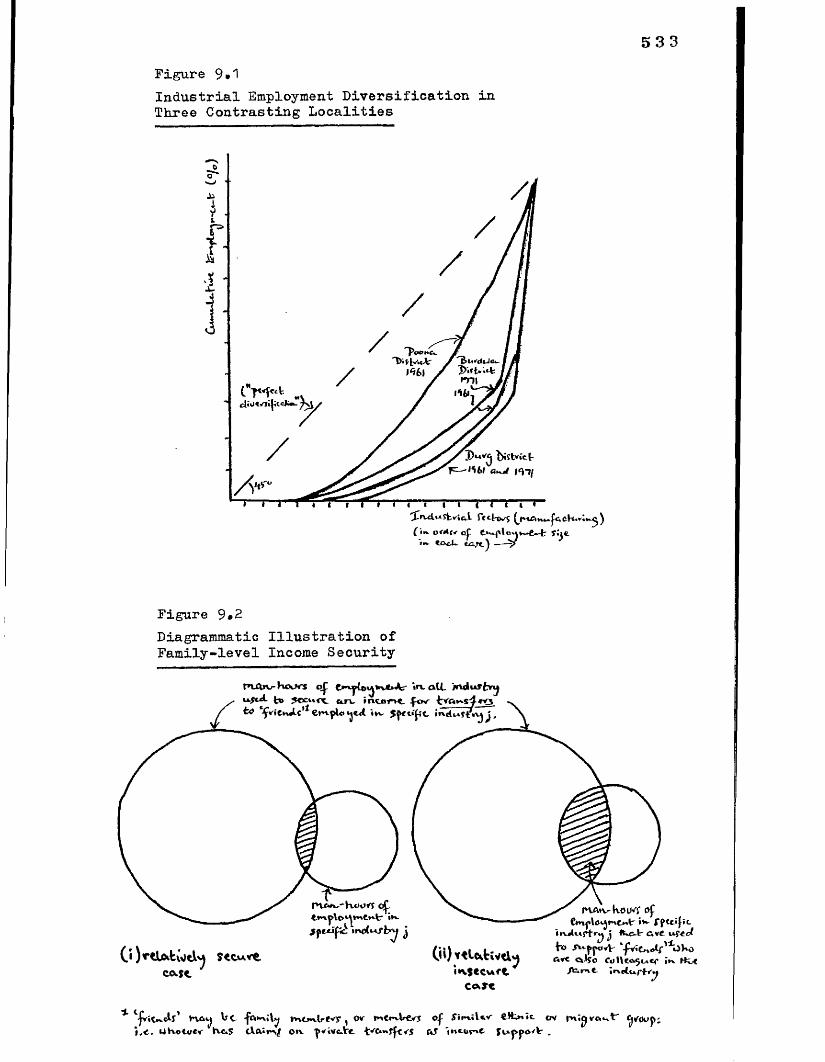
533Figure 9•'IIndustrial Employment Diversification inThree Contrasting Localities

( i » o r t w o C t 1 l o < i k v ^ v - t f i i e

• «£Xi tA /t)---

F ig u re 9*2D ia g ra m m a tic I l l u s t r a t i o n o f F a m i ly - le v e l Incom e S e c u r i t y

P U U v - I w f t o f C > n ^ {o ^ *v b A r i a a l l t» ?ecuft. an. intent fov

to ‘^ViCtd-C** tvx- irvdtAftVvj ,

0 ) re la te

PUxv.'K«i)rt of.llnjtVp IK-JpCJtip ir*(A**sby j

cas t0 0 tttfc tiv d M

Ca»«

PVAvv- h.OU*T Of

trutuj^r«| j Oc-t CVVt wf-Cc/to / JfjKJyV ‘-jViCrtotf'^Oko (ire aljo OiHb^ucc ,V*. rtu

A lrv t it\i(ur{Y^

^ tjv»t-.ctr> h6t| tt Iftn;!*! mtmlrfvy (Mr cf JintUv ttUit ov rnl v'Ci t'i,<, UKotutf Kt*F O n jnrivtrt C*S intor't .

Figure 9»3 &C o n c e n tra t io n o fM a n u fa c tu r in gIn d u s t r y

(E a s te rn I n d u s t r i a l R e g io n 1 96 1 )

! *J,00©

>* •"Pat*

vi

%\>WAWfK(L

MuifQHyR.

■I*"» itH

*VSHAHA3A&

n-Raachi

il,000

3$ -|S i

'IV^vWax

J*9 , TWvuaI

iStdc#H*+\ 4

">57000

m

3-1 -

gA«KKC

1*8

*-4SURT.UTA

3s, -jTWcaRM

A

60 J

n

**><**> 3 4

i\I 4

I \I

Jo

3o —

"BwWJAN sMQWRAJ

C AcCVtT*

I

v -

\

^ • iw n m oc-j

X H Wooc^ y /

Ca l c u t t a /(rVctr to JtAtt}

"BtUVSVOR

kTamm*wI>i

Duf«;

2s -4$ASf?K

3frlioUAVC.iR.

17 I'tm&ruAAiAt.

"Sawdh

m 4KOftAOtrrtt-lqpwSJAM

»R l 13-

B t / v c f l 1

Key: *lSLach. lrot< *** 00iiviUcalts t*v«JLe u)o*ltfo*tA. »h- fait&Qj »>iA«aiA«tuv{MA «|C(Cj . s c & e : (c “ % o o o i * v tw^Kv*^c*cfcwriwc

T K e X .K .S " 1 u1* ’ , r # /* w * * * * * * 5SW ouj H u. 0 /0

tee*»r X ,e> y *i*. *kx S i* A j l^ U ^ e r t »ett*< a t

535

Figure 9*5 bChange i n th e C o n c e n t ra t io n o f M a n u fa c tu r in g I n d u s t r y i n th e E a s te rn I n d u s t r i a l R e g io n , 1961 - 1971

Raipur.

u 1**DuRc,

TURUUA

Iff12-%AMwyRA

KAiQARfi

s - aM t31" *f 7 ***7HtHVftVI CAlCifrrA i t f Holley

CALCUTTA

s i * .MidVapor£

"Bastar

BAy OF

^ F a A l

keg** Tkt fU|twrM ^ % 9fl»vo.lt n^ixv^p*eA w \ *V U lroW t K,

Si*vJj(t (a*M-|1: r«cV*oir *. A-U.t *■ (<i4l ' r-k-5 = »9ll

Figure 9«3 c &Vl,OOC>C o n c e n t ra t io n o fM a n u fa c tu r in gIn d u s t r y

(W e s te rnM a h a ra s lit ra1961 )

11-

koi

000

SHom iR.

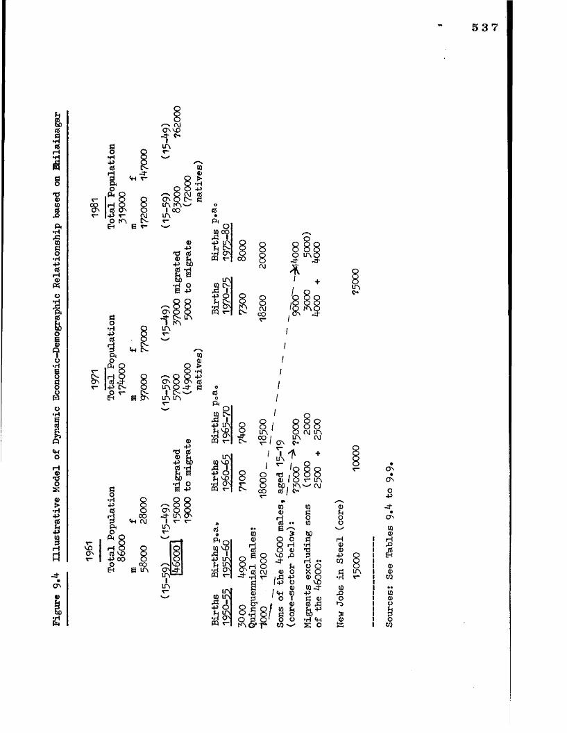
Figu

re 9»k

Il

lus

tra

tiv

e

Mod

el

of D

ynam

ic

Eco

nom

ic-D

emog

raph

ic

Re

latio

nsh

ip

base

d on

Bh

ilain

ag

ar

537

ON MO

A A

no cti O A

IA LA

P LA CM Ano as

CO NO

S i

ootH C\J

oO IO rlA ho. A'-' CM ccj /

p ooB A

v-x 9Pho© j MO1§ PP 1A/*>NO P Ao>-4 ffj ONA■ r*iAT” A|5 Vp on IQONw r-

«H CQ

ONONop

CQ ✓—s<1) -4"C U •O O ON(0 ov_* CQho CDP iH•H CD rOCD Rj2 p o E-i1—t »• CQ QO Q o OX O P A <D■H T“ CQCQ J- CQ ••P O CQfi O o CD3 Oa ,43 s•H «H o£ o £ CQ

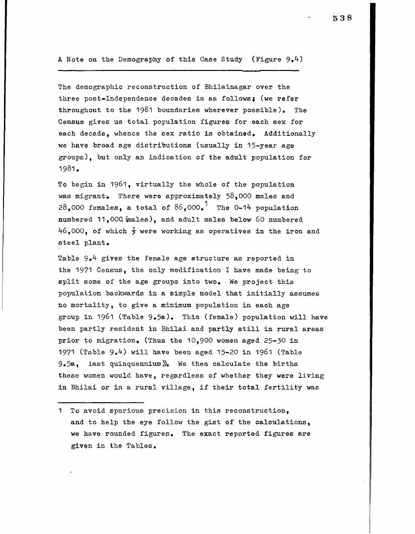
538

A N o te on th e Dem ography o f t h i s Case S tu d y ( F ig u r e 9*k)

The d em o g ra p h ic r e c o n s t r u c t io n o f B h i la in a g a r o v e r th e

th re e p o s t- In d e p e n d e n c e decades i s as f o l lo w s f (we r e f e r

th ro u g h o u t to th e 1981 b o u n d a r ie s w h e re v e r p o s s ib le ) . The

Census g iv e s us t o t a l p o p u la t io n f ig u r e s f o r each se x f o r

each d eca d e , whence th e se x r a t i o i s o b ta in e d . A d d i t i o n a l l y

we have b ro a d age d i s t r i b u t i o n s ( u s u a l ly i n 1 5 -y e a r age

g ro u p s ) , b u t o n ly an in d ic a t io n o f th e a d u l t p o p u la t io n f o r

1981 .

To b e g in i n 1 96 1 , v i r t u a l l y th e w ho le o f th e p o p u la t io n

was m ig ra n ts T h e re were a p p ro x im a te ly 5 8 ,0 0 0 m a les and

2 8 ,0 0 0 fe m a le s , a t o t a l o f 8 6 ,0 0 0 . The 0 -1 k p o p u la t io n

num bered 1 1 ,0 0 0 (m a le s ) , and a d u l t m a les b e lo w 60 num bered

^ 6 ,0 0 0 , o f w h ic h w ere w o rk in g as o p e ra t iv e s i n th e i r o n and

s t e e l p la n t .

T a b le 9»k g iv e s th e fe m a le age s t r u c t u r e as r e p o r te d i n

th e 1971 C ensus, th e o n ly m o d i f ic a t io n I have made b e in g to

s p l i t some o f th e age g ro u p s i n t o tw o . We p r o je c t t h i s

p o p u la t io n b ackw ards i n a s im p le m ode l t h a t i n i t i a l l y assumes

no m o r t a l i t y , t o g iv e a m inimum p o p u la t io n i n each age

g ro u p i n 19&1 (T a b le 9 * 5 a )* T h is ( fe m a le ) p o p u la t io n w i l l have

been p a r t l y r e s id e n t i n B h i l a i and p a r t l y s t i l l i n r u r a l a re a s

p r i o r t o m ig r a t io n . (Thus th e 1 0 ,9 0 0 women aged 2 5 -5 ° i n

1971 (T a b le 9 - ^ ) w i l l have been aged 1 5 -2 0 i n 1961 (T a b le

9 .5 a , l a s t q u in q u e n n iu m )). We th e n c a lc u la te th e b i r t h s

th e s e women w o u ld h a v e , re g a r d le s s o f w h e th e r th e y w ere l i v i n g

i n B h i l a i o r i n a r u r a l v i l l a g e , i f t h e i r t o t a l f e r t i l i t y was

1 To a v o id s p u r io u s p r e c is io n i n t h i s r e c o n s t r u c t io n ,

and t o h e lp th e eye f o l lo w th e g i s t o f th e c a lc u la t io n s ,

we have ro u n d e d f ig u r e s . The e x a c t r e p o r te d f ig u r e s a re

g iv e n i n th e T a b le s .

539

t o be 5 *0 ( b i r t h s p e r woman) and t h e i r age p a t t e r n o f

c h i ld - b e a r in g as i n th e a g e - s p e c i f ic s c h e d u le shown i n

T a b le 9 * 5 b . T h is w o u ld g iv e a n n u a l b i r t h s , m a le p lu s fe m a le ,

n u m b e rin g 7500 by th e la t e 1960s (T a b le 9 «5a , f i r s t q u in ­

q u e n n iu m ), and we go on to assum e, f o l lo w in g th e a rg um en t in

th e t e x t (C h a p te r 9 ) and d e t a i le d b e lo w , t h a t th e s e c h i ld r e n

w ere in d e e d b o rn d u r in g t h a t p e r io d and b ro u g h t i n to B h i l a i

(b y 1971 , i f n o t b o rn th e re i n th e f i r s t ...p lace ) • The b i r t h

r a te o f t h i s m ig r a t io n c o h o r t i s a t i t s maximum i n t h i s p e r io d

s in c e th e la r g e s t c o h o r ts a re a t t h e i r m a x im u m - fe r t i l i t y ages*

T h is g iv e s a t o t a l p o s s ib le o f be tw een 7 0 *OCX) and 7 5 ,0 0 0

b i r t h s d u r in g th e decade ( 7 00 0 -7 50 0 p e r annum ), o r a b o u t

3 5 *0 0 0 m a les u n d e r 15 i n 1971 *(we a re s t i l l ig n o r in g c o r r e c t ­

io n s f o r m o r t a l i t y : t h i s c o r r e c t io n w o u ld r a is e th e num ber

o f b i r t h s i n a b a c k - p r o je c t io n , b u t re d u ce th e num ber o f

s u r v iv o r s . A p p ly in g th e c o r r e c t io n p a ra m e te rs g iv e n i n

T a b le 9 .6 p ro d u ce s 3 0 ,0 0 0 as th e n e t r e s u l t ) . A c c o rd in g to th e

1971 Census a b o u t k0% o f th e m ale p o p u la t io n f e l l i n t o t h i s

(0 -1 ^ -) g ro u p , i . e . 3 ^ ,0 0 0 (T a b le 9#*0# The d i f f e r e n c e betw een:,

t h i s , and th e 3 0 ,0 0 0 o r so p r o je c te d , w i l l be made up o f

th e s u r v iv o r s o f th e b i r t h s p r e - d a t in g 19&1 : i . e . a

p r o p o r t io n o f th e y o u n g e s t o f th e 1 1 ,0 0 0 m a les o f th e 0 -1 4

u rb a n c o h o r t o f 1961 (s a y 3 *5 0 0 ) , p lu s any c h i ld r e n o f th e

m ig r a n ts , who vsre a ls o b o rn p r i o r t o 19^ 1 ; i n o u r back

p r o je c t io n th e tw o g ro up s sum to g e th e r as ^ ,9 0 0 b i r t h s a n n u a l lyA

(T a b le 9»5&* f i n a l q u in q u e n n iu m ). T h is f i l l s th e gap

o f 8000 ' s u f f i c i e n t l y : o u r f e r t i l i t y r a te s a re p o s s ib ly to o

■high. The sum s, h o w e v e r, add up q u i te w e l l .

I n 1971* th e re m a in in g 5 8 ,0 0 0 a d u l t m a les c o m p rise

th e f o l lo w in g : th e s u r v iv o r s o f th e 0 - 1k c o h o r t re c o rd e d i n

1961 a t B h i l a i , now aged i n t o th e 20 -29 age g ro u p , sa y 7500 ,

1 I . e . a b o u t 12000 m ale b i r t h s o v e r 5 y e a r s .

th e s u r v iv in g a d u l t s o f th e 1961 a d u l t c o h o r ts , and

new m ig r a n ts . The 1961 a d u l t c o h o r ts w ere h e a v i ly

c o n c e n tra te d i n th e lo w - m o r t a l i t y 1 5 -3 4 a-ge g ro u p (T a b le 9 * 4 ) ,

so t h a t o v e r 90% c o u ld have e x p e c te d to have s u r v iv e d f o r te n

y e a rs ( u s in g p a ra m e te rs i n T a b le 9 * 8 ) , a m o u n tin g to

4 1 ,5 0 0 . Thus th e t o t a l s u r v iv o r s i n t h i s age g ro u p

am ount t o be tw een 4 8 ,0 0 0 and 4 9 ,0 0 0 . The t o t a l re c o rd e d

i n th e 1971 Census i s 5 7 ,0 0 0 . T h is a l lo w s f o r be tw een

8 ,0 0 0 and 9 ,0 0 0 a d u l t m ale m ig ra n ts ( r a t h e r s m a ll com paredp

w i t h th e p o p u la t io n g ro w th o f 8 8 ,0 0 0 J ) .

O ver th e n e x t decade th e b i r t h s due to th e i n i t i a l i n -

m ig r a t io n s w i l l d e c l in e fro m t h e i r 1970s p e a k , b u t , to

ju d g e fro m th e se x r a t i o s p e r t a in in g i n th e more m a tu re

heavy i n d u s t r i a l c i t i e s , th e re may be 5000 women s t i l l t o come.

We do n o t have an age d i s t r i b u t i o n f o r 1981 fro m w h ic h to

p r o j e c t . backw ard any f u r t h e r b i r t h s . B u t by 1 9 7 5 -8 0 th e

d a u g h te rs o f th e la r g e i n i t i a l m ig ra n t c o h o r ts have th e m s e lv e s

begun to re p ro d u c e , th o u g h s t i l l i n th e e a r ly , lo w f e r t i l i t y ,

y e a rs o f c h i ld b e a r in g ( t h a t i s to s a y , b e fo re th e ages where

u n iv e r s a l m a rr ia g e can be e x p e c te d ) . The n e t e f f e c t i s to

o v e r-c o m p e n s a te f o r th e e f f e c t o f t h e i r own m o th e rs * a g e in g ,

so t h a t th e a g g re g a te num ber o f b i r t h s due to th e o r i g i n a l

m ig r a t io n (w h e th e r as c h i ld r e n o r g r a n d c h i ld r e n ) in c re a s e s

t o o v e r 7 000 . The s in u o u s q u in q u e n n ia l b i r t h p a t t e r n i s

im m e d ia te ly a p p a re n t (F ig u re 9 * 4 ) . Our o n ly c lu e on th e age

1 H ere we assume a m o r t a l i t y t a b le a p p ro x im a t in g t h a t o f th e

’ 'P r in c e to n S o u th " l e v e l 13* T h is i s a d e p a r tu re fro m th e

"W e s t" l e v e l 9 used h e r e to fo r e . A p r o je c t io n m ode l f o r a

s p e c i f i c a re a may as w e l l a t te m p t to in c o r p o r a te lo c a l

p a ra m e te rs . M o r t a l i t y i n N o r th and C e n tr a l I n d ia seems to

c o n fo rm r a t h e r more c lo s e ly to th e S o u th m ode ls w i t h t h e i r

h ig h le v e ls o f c h i ld m o r t a l i t y , and le v e l 13 ( fe m a le s 1 l i f e -

e x p e c ta t io n o f 5 0 ) seems more a p p r o p r ia te f o r th e 1970s , and

f o r th e c o r e - s e c to r i n d u s t r i a l p o p u la t io n .

2 These may in c lu d e some 3000 sons o f th e o r i g i n a l 46000 w o rk e rs .

5 4 1

d i s t r i b u t i o n i n 198*1 i s th e c l a s s i f i c a t i o n o f 48% o f m a les

as w o rk e rs . R o u g h ly s p e a k in g , and f o l lo w in g th e same m ethod­

o lo g y as a b o v e , t h i s means t h a t th e re were 1 1 ,0 0 0 new m ale

m ig ra n ts o f w o rk in g age d u r in g th e d eca d e , (s o n s in c lu d e d ) .

The o b je c t iv e o f any p o l i c y in t e r v e n t io n i s to m i t ig a t e th e

e f f e c t o f th e r a p id in c re a s e i n new e n t r a n ts ( 15- 1 9 ) t o th e

m ale la b o u r fo r c e fro m th e 5000 b o rn and s u r v iv in g o f th e

f i r s t g e n e ra t io n m ig ra n ts (w h e th e r p re o r p o s t 1961 m ig r a t io n s ) ,

and e n te r in g th e la b o u r fo r c e i n th e f i v e y e a rs 1966 - 7 1 ,

t o th e 14000 e n te r in g th e la b o u r fo r c e i n 197&-81 (a d e c a d a l

in c re a s e o f l80% ). To m i t ig a t e th e e f f e c t i t s e l f , changes

in th e p a t t e r n o f la b o u r demand have been s u g g e s te d ( i n

th e t e x t ) , as w e l l as th e p o s s i b i l i t y o f t e m p o r a r i ly h a l t i n g

th e in - m ig r a t io n o f th e 1 1 ,0 0 0 new m ig ra n ts t h a t w ere to

a r r i v e betw een 1871 and 198 1 . B u t a p u r e ly d em og ra p h ic

in t e r v e n t io n i s to in f lu e n c e th e p a t t e r n o f c h i ld b e a r in g .

The f i r s t v a r ia t i o n o f th e l a t t e r - a tte m p te d h e re ( i n i l l u s t r a t i o n )

i s to d e la y th e pace o f c h i ld b e a r in g w ith o u t r e d u c in g th e

o v e r a l l l e v e l (5 b i r t h s p e r wom an), t h a t i s to e x te n d th e

e a r ly b i r t h i n t e r v a l s , and c o n t r a c t th e m id d le and l a t e r o n e s .

T h is s m o o th in g p ro c e s s causes a t a n g ib le r e d u c t io n i n th e

t o t a l num ber o f b i r t h s d u r in g th e p e r io d i n q u e s t io n

( w i th o u t a f f e c t i n g th e t o t a l num ber t h a t w i l l o c c u r a l t o g e t h e r ) ,

s in c e th e peak age o f c h i ld b e a r in g no lo n g e r c o in c id e s w i th-1

th e peak i n th e m ig ra n t age c o m p o s it io n . T h e re i s a ( te m p o ra ry )

r e d u c t io n o f 6.% i n th e num ber o f b i r t h s , re d u c in g a c c o r d in g ly

th e 1976-81 la b o u r fo r c e e n t r y t o '1 3 ,2 0 0 . The a l t e r n a t i v e

d em og ra p h ic in t e r v e n t io n i s a f e r t i l i t y r e d u c t io n a t th e l a t e r

ages o f c h i ld b e a r in g o n ly ( r e d u c in g th e b i r t h s p e r woman to

4 .4 , and t h i s re d u c in g th e t o t a l num ber o f c h i ld r e n to be b o r n ) :

B u t t h i s re d u c e s th e b i r t h c o h o r t s p e c i f i c t o o u r c o n c e rn

1 The p o in t i s t h a t we can re d u ce th e t o t a l num ber o f b i r t h s

o v e r a g iv e n p e r io d o f t im e , w ith o u t re d u c in g th e t o t a l b i r t h s

t h a t an a g e -c o h o r t o f m o th e rs w i l l b e a r th ro u g h o u t t h e i r l i f e ­

s p a n , As a p o l i c y , t h i s may s t r i k e th e re a d e r as b iz a r r e $

i t i s , b u t th e C h in ese a re s e r io u s ly c o n s id e r in g i t as a

s o lu t i o n t o p r e c is e ly th e p ro b le m we a re d is c u s s in g h e r e 0

by le s s th a n 6 %, t o 1 3 ,4 i0 0 . C le a r ly , h o w e v e r, a c o m b in a t io n

o f o v e r a l l re d u c e d f e r t i l i t y and d e la y e d c h i ld b e a r in g w o u ld

have th e g r e a te s t e f f e c t . On a p r a c t i c a l n o te , th e f e r t i l i t y

r e d u c t io n , w h e th e r th ro u g h m a r i t a l f e r t i l i t y c o n t r o l , o r

d e la y e d age a t m a r r ia g e , needs to be in s t ig a t e d i n th e

r u r a l a re a s , s in c e i t i s h e r e , as we have s e e n , t h a t th e

h ig h f e r t i l i t y (a n d u n iv e r s a l m a r r ia g e ) ta k e s p la c e , p r i o r

t o th e m ig r a t io n o f th e women0

C om parison be tw een th e M o d e l "1 c " and B h i l a i

The c h ie f d i f f e r e n c e be tw een th e d em og raph ic e x p e r ie n c e a t

B h i l a i and th e s im u la t io n in te n d e d to r e p re s e n t th e case

o f g r e e n - f ie ld u rb a n dem ography i s due to th e a s s u m p tio n

I made on m a rr ia g e and c h i ld - b e a r in g b e h a v io u r* I n th e

M o d e l, m ale m ig ra n ts w ere assumed to a r r i v e s in g le

and m a rry s u b s e q u e n t ly , o r a t le a s t to s t a r t t h e i r c h i l d -

r e a r in g i n th e c i t y , on th e a r r i v a l o f t h e i r w iv e s ( o r w iv e s

to b e ) . Hence th e peak e n t r y to th e la b o u r fo r c e w o u ld be

d e la y e d u n t i l 1981 - 8 5 . I f t h a t a s s u m p tio n i s k e p t f o r th e

B h i l a i m ig r a n ts , i n s u f f i c i e n t b i r t h s a re g e n e ra te d to e q u a l

th e s iz e o f th e p o p u la t io n re c o rd e d as u n d e r 15 i n 1971 .

Hence c h i ld b e a r in g m ust have s t a r t e d b e fo re th o s e m ig r a t io n s

b e g a n ; n o r w ere any o f th e c h i ld r e n l e f t b e h in d i n th e r u r a l

a re a once th e women a r r i v e d . F u r th e r c o r r o b o r a t in g e v id e n c e

i s t h i s , (T a b le 9 .7 ) * I f we ta k e th e D u rg D i s t r i c t u rb a n

p o p u la t io n as a w h o le , we have a b o u t 3 4 ,0 0 0 m a r r ie d men aged

1 5 -3 0 i n 1 981 . L e t us assume t h e i r fe m a le p a r tn e r s t o be

aged 1 5 -2 5 * We o n ly have 18000 re c o rd e d i n u rb a n D u rg .

T h a t le a v e s 1 6 ,0 0 0 m a r r ie d women to be a c c o u n te d f o r e ls e w h e re .

I f we assume th e D i s t r i c t m a rr ia g e r a te s t o a p p ly t o B h i l a i

s p e c i f i c a l l y , th e n we have 2 4 ,0 0 0 m a rr ie d men, and 1 2 ,0 0 0

m a r r ie d women i n B h i l a i i n 1961 . T h a t le a v e s 13 *0 0 0 m a r r ie d

543

women s t i l l i n th e r u r a l a re a s o f o u t - m ig r a t io n ( o r

e ls e w h e re ) . T h e i r e x i s t i n g f e r t i l i t y i s a p p a r e n t ly g r a f te d

on to th e d e m o g ra p h ic s t r u c t u r e o f B h i l a i th e moment th e y

a r r i v e .

The o th e r d i f f e r e n c e has been d is c u s s e d i n C h a p te r 6 a b o v e .

I n th e S te e l Towns th e pace o f fe m a le m a rr ia g e re s p o n s e

m ig r a t io n i s r a t h e r f a s t e r th a n t h a t e s t im a te d fro m more

a g g re g a te d a ta # To ju d g e fro m se x r a t i o s o f r e c e n t m ig ra n ts ,

f a m i l ie s a re fo rm e d r a t h e r f a s t e r w i t h in th e d e ca d e .

T o g e th e r th e s e d i f f e r e n c e s a re s u f f i c i e n t t o a c c o u n t f o r

th e v e ry d ra m a t ic g ro w th i n th e age c o h o r t o f yo u n g p e o p le

i n B h i l a i , w h ic h in c re a s e s fro m 25% to 42% o f th e t o t a l

p o p u la t io n i n th e c o u rs e o f a decade , i n c o n t r a s t t o th e p e rh a p s

le s s u n s ta b le p ic t u r e g iv e n by th e M ode l (w h ic h does how ever

in c lu d e a m odest d e c l in e fo l lo w e d by a m odest r i s e i n th e

g ro w th o f th e 1 5 -1 9 c o h o r t f o r e xam p le , r a t h e r th a n p r e c ip i t o u s

g ro w th ) w here th e p r o p o r t io n re m a in s a ro u n d 33%* B o th

p o p u la t io n s a re u n s ta b le , b u t th e c h a r a c te r o f th e i n s t a b i l i t y

i s d i f f e r e n t .

A N o te on th e L a b o u r Demand

The o r i g i n a l p la n was f o r th e e x p a n s io n to 10 m i l l i o n to n n e s

o f a l l th e p u b l ic s e c to r p la n t s . I t i s .a ls o re p o r te d t h a t

i t w o u ld c o s t tw ic e as much to s t a r t a new in t e g r a t e d w o rks

( e . g . V i ja y n a g a r ) as to expand th e e x is t in g p la n t a t B h i l a i .

T h is s u g g e s ts t h a t th e re i s a p u r e ly econom ic j u s t i f i c a t i o n

f o r th e a d o p t io n o f a s t r a te g y o f in c re m e n ta l g ro w th on an

i n i t i a l l y g r e e n - f ie ld s i t e . T h is w o u ld e n su re a c o n t in u in g

in c re m e n t i n la b o u r demand, so t h a t th e second g e n e ra t io n

and in c r e m e n ta l m ig r a t io n e f f e c t s , on w h ic h we have been . .

com m enting on th e s u p p ly s id e , w o u ld be le s s d i f f i c u l t t o

a b s o rb on th e demand s id e *

544

I n p r a c t ic e w h a t has happened i s r a t h e r d i f f e r e n t . O u tp u t

o f f in is h e d s t e e l has been h o v e r in g a ro u n d th e 1 .5 m i l l i o n

to n n e m a rk , im p ly in g an o u tp u t o f p ig o f a b o u t 2 m . t . o v e r

th e 1970s ( th e l a t e s t f ig u r e to hand i s O c to b e r 1980 , -

1 .6 m . t . ) « T h is i s th e e x p a n d in g p ro d u c t io n to w a rd s a

c a p a c ity o f 2-g- m . t . We e s t im a te t h a t o n ly 5000 new jo b s

i n s te e l- m a k in g w i l l have been c re a te d s in c e 1971 ( t a k in g

i n t o a c c o u n t econom ies o f s c a le , th e q u a n t i t a t i v e e f f e c t o f

w h ic h we d is c u s s e d i n C h a p te r 2 ) . These p r iz e jo b s w i l l be

com peted f o r by th e 1 4 ,0 0 0 new e n t r a n ts d e r iv e d fro m th e

1956-1971 m ig r a t io n s , and th e 1 1 ,0 0 0 e n t i r e l y new m ig r a n ts .

O n ly be tw een -J and £ o f th e 1 4 ,0 0 0 a re sons o f th e s t e e l

w o rk e rs * C le a r ly th e la b o u r m a rk e t i s t i g h t , and th e

p o s s i b i l i t i e s o f c o n f l i c t a re s e r io u s (b e tw e e n m ig ra n ts and

n o n -m ig ra n t g ro u p s ) . N e v e r th e le s s , th e p ro b le m w o u ld have

been e x a c e rb a te d i f th e re had been no e x p a n s io n i n s t e e l ,

w i t h 1 4 ,0 0 0 l o c a l b o rn 15 y e a r o ld s s e e k in g e m p loym en t, and

p e rh a p s 5 - 7000 o f them h o p in g f o r a jo b i n heavy in d u s t r y .

By th e e a r ly 1980s th e p ro s p e c ts o f t a k in g up th e la b o u r s u p p ly

seem more h o p e fu l , w i t h c o n t in u in g o n - s i t e e x p a n s io n ( th o u g h

no a p p a re n t d i v e r s i f i c a t i o n o u t o f i r o n and s t e e l ) : t h i s i s

i n dow nstream p r o d u c t io n , - a new f la t - p r o d u c t s m i l l , and1a c o n t in u o u s c a s t in g m i l l ; a d d i t i o n a l l y w o rk i s s t a r t i n g on

a new oxygen p la n t , a c a p t iv e pow er p la n t , and a new c o n v e r te r

s h o p , i n t e r a l i a , f o r th e e x p a n s io n phase to b r in g th e in t e g r a te d

s t e e l p la n t to i t s now r e v is e d c a p a c ity t a r g e t o f 4 m . t *

The em ploym ent c re a te d up to th e 1970s decade can be gauged

fro m T a b le s 9 *8 and 9 ,9 ; t h a t g e n e ra te d by th e e x p a n s io n phases

( i n th e in t e g r a te d w o rk s ) has had to be e s t im a te d (F ig u re 9 . 4 ) .

1 C o l u m n i n F in a n c ia l E x p re s s . Bombay, 6 t h O c to b e r , 1980 .

2 T im es o f I n d ia Y e a rb o o k , 1979*

545

I n a l l t h i s d is c u s s io n we have s a id l i t t l e a b o u t th e

p ro b le m o f c o n s t r u c t io n la b o u r . Here th e re c o rd s a re n e a r ly

im p o s s ib le t o i n t e r p r e t . From T a b le 9 *8 i t can be seen

t h a t B h i l a i had 1 2 ,0 0 0 w o rk e rs in H in d u s ta n S te e l engaged

on c o n s t r u c t io n w o rk i n th e m id - 1960s , b u t o n ly 7900 by

1970 . T h is does n o t s q u a re w i t h th e p a y r o l l f i g u r e s , b u t

th e f lu c tu a t io n s , , a re i n th e r i g h t d i r e c t i o n . The 1961

Census re c o rd s 6 ,0 0 0 c o n s t r u c t io n w o rk e rs a t B h i l a i (T a b le

9 *9 ) , b u t a num ber o f w o rk e rs a c t u a l l y engaged i n c o n s t r u c t io n

may ha, e been re c o rd e d as b e in g i n th e m a n u fa c tu r in g in d u s t r y ,

and b e s id e s , we have a lr e a d y shown (C h a p te r 7 ) t h a t many o f

th o s e engaged i n c o n s t r u c t io n a re r e s id e n t i n n e ig h b o u r in g

r u r a l a re a s . I n any c a s e , u n d e r w h ic h c a te g o ry th e y s h o u ld

be re c o rd e d may be a m oot p o in t , as H in d u s ta n , S te e l a re

known to have k e p t i n i t i a l c o n s t r u c t io n la b o u r on th e p a y r o l l

o s te n s ib ly i n p r e p a r a t io n f o r e x p a n s io n phases , b u t no

d o u b t e m b a rrasse d by th e p o l i t i c a l d i f f i c u l t y o f la y in g o f f .

The new s t e e l p la n t a t B oka ro i n B ih a r i s r e p o r te d i n 1980

t o be s a d d le d w i t h 4000 re d u n d a n y la b o u re rs f o r j u s t t h a t

re a s o n . I t can be seen t h e r e fo r e t h a t th e em ploym ent o f th e

c o re c o n s t r u c t io n la b o u r w h ic h i s r e l a t i v e l y im m o b ile i s

s u b je c t t o th e same p ro b le m o f m a ss ive u p su rg e i n demand

fo l lo w e d by o n ly m odest r e c u r r e n t demand c y c le s t h a t c h a r a c te r ­

is e s th e la b o u r m a rk e t f o r th e c o re s te e l- m a k in g o p e r a t iv e s ,

an im p o r ta n t d i f f e r e n c e b e in g t h a t i n th e case o f c o n s t r u c t io n

an a c tu a l f a l l i n demand i s e x p e r ie n c e d , b u t as t h i s i s a t y p i c a l

fe a tu r e o f th e in d u s t r y th e w o rk fo rc e i s p re p a re d to be more

m o b ile (w h ic h s im p ly sa ys t h a t th e w ho le c o n s t r u c t io n in d u s t r y

i s c h a r a c te r is e d by a s o c ia l h a rd s h ip n o t p e c u l ia r to B h i l a i

a lo n e ) . The t r u l y te m p o ra ry and m o b ile s e c to r o f t h i s co n ­

s t r u c t i o n la b o u r w i l l be m isse d by b o th H in d u s ta n S te e l re c o rd s

1 Column i n F in a n c ia l E x p re s s (B om bay), 6 t h O c to b e r , 1980 .

and. th e C e nsuses . I t s m a ss ive num bers can be gauged fro m

a m anua l on th e D u rg a p u r s t e e l w o rks p r o je c t . C o m p a ra tive

d a ta a re g iv e n f o r R o u rk e la and B h i l a i , The l a t t e r , d u r in g

th e i n i t i a l c o n s t r u c t io n phase ( p r e - 196 0 ) em p loys 4 0 ,0 0 0

c o n t r a c t and 2 0 ,0 0 0 d i r e c t c o n s t r u c t io n la b o u r e r s , i . e . ,

i t i s c la im e d , 6 0 ,0 0 0 i n a l l on th e s i t e i

1 I r o n and C o a l T ra d e s R ev iew ( U .K . ) , "A T e c h n ic a l

S u rv e y o f th e D u rg a p u r W o rk s " , (u n d a te d , ? 1 9 6 0 )o

Table 9o1Change in the Proportion of workers in non-household Manufacturing in Steel Town Areas

Percentage of male workers in non-household manufacturing

1961 1971

38 3933 3136 37

Percentage of males aged 15-59 Decadal in non-household manufacturing Growth (%)

1961 1971

Districts neighbouring Durg (all urban)Durg 36 33 14.9Bilaspur 10 7 21*1

Raigarh 18 12 0 .2

Bastar 11 6 19*4

Towns within BurdwanAsansol 21 22 28 o3

Outer Burnpur 65 62 -0 .1

Burnpur 78 76 -0.0Durgapur 61 56 127.2

Burdwan City 17 12 -1 5 *0

Percentage of male workers in non-household manufacturing

Districts of Orissa (urban)

1961 1971

Sundargarh 33 31Mayurbanj 9 10Bolahgir 6 9Cuttack 19 18B»Ko 5 4Ganjam 9 8

Comparative New-town area in Maharashtra: % males aged 15-59 in non-household manufacturing: 1961 1971

Poona 28 33Pimpri-Chinchwad 45 66

District(urban)DurgSundargarhBurdwan

Source: Government of India, Census of India 1961, 1971.General Population Tables, & Economic Tables (B I), Delhi

54 8

Table 9.2Industrial Diversification in 1961 and 1971? Steel Town areas and a comparative New-town area

IndustrialEstablishments

Number of manufacturing units(number with more than 50 employees bracketed)

in: in:SUNDARGARH DURG BURDWAN

in:1961 1971 1961 1971 1961 1971

food 28 22** **72 * 785(17) 1595(19)beveragetobacco 5 1** 17

62**6(1)

16**(2) 158(1)cotton 8 7 107(1) 29 65

jute - 1 - 2(1) 3woolsilk, synthetics

- 2 13 11 1

misc. textiles **6 (1971 incl. products)

228 *+30 353 972

wood **9 97 173 167(1)paperprinting 3 17 18

17*f 159

leather 22 12 6** *f5 72rubber, petrol., coal w 20(**) ** 17 37chemicals 8 **6(10) 21(1) 37 125(2)minerals 23(5) 31 109(1) 1** 1**7(*0earthenware 2 - **5basic metals metal products 17(2) 23(1*0

**8(3) 89(11) 202(11) 15(11)350(*0

machinery - 28 33(8) 63(1) 73electrical mach. 1 - - **8 (5)transport equip. 15(2) 1 16**(11) 311(6) 17(*0misc. 16(3) **** 307(1) **08 822(3)repair (1971 only) 367 871(2)Notes: * not available at time of writingo The 1961 and 1971

categories are not all strictly comparable« In particular, "repaij** became a separate category in 1971*

Source: Government of India, Census of India« 1961* 1971 .E s ta b lish m e n t Tables^ D e lh i .

Table 9*2 continuedI n d u s t r ia l E s ta b lish m e n ts in :

fo o d

beverages and tobacco

c o tto n

s y n th e t ic s

ju te

t e x t i l e p ro d u c ts

wood

paper & p r in t in g

le a th e r

ru b b e r & p la s t i c

chem ica ls

non m e ta l* m in e ra ls

b a s ic m e ta ls & p ro d u c ts

m ach inery

t ra n s p o r t equ ip *

o th e r

r e p a ir

Number o f e s ta b lis h m e n ts in

POONA DISTRICT (th ose w ith more th a n 50 employees b ra cke te d )

in :

1961

1197(*0

908(7)

1 5^(9 )

2

1685(1)

**0**(**)

255(22)356

3 2 (1 )

1**1 ( 12)163(5)

736(11)

200 (9 )

911(1**)

1030(**)n*a*

1971

**180(3)

1003(**)

117(6)3

13

2072(5 )

1129(5)**8 0 ( 21 )

26**(1 )

92(**)

17*K9)

207 ( 23 )

892 ( 20 )

539(**-8 )

69

598(*01056( 21 )

N o te : As f o r f i r s t p a r t o f tab le©

S ource : Government o f I n d ia , Census o f In d ia 1961, 1971*M aharash tra , E s ta b lish m e n t T a b les , D e lh io

Table 9*3

I n d u s t r ia l W ork fo rce D is t r ib u t io n s in

C ase-S tudy D i s t r i c t s , 1961

S e c to r o f Number o f w orke rs in :M a n u fa c tu r in g DURG BURDWAN POOW

food 2406 3730 7433

beverage 229 202 297

tobacco 2010 2471 5808

c o tto n t e x t i l e 3178 733 3849

ju te t e x t i l e - 189 396

wool t e x t i l e 74 7 23

s i l k t e x t i l e 3 69 44

m isc . t e x t i l e 1379 2596 6632

wood 1936 2671 5384

paper 12 136 933

p r in t in g 176 840 3822

le a th e r 462 661 2097

ru b b e r 8c p e t r o l . 21 1621 1306

chem ica ls 277 633 11493

non m e ta l m in e ra ls 522 1324 3340

b a s ic m e ta ls 26738 36472 5425

m ach inery 1656 1873 4242

tra n s p o r t e q u ip . 732 12047 8172

m is c . 973 3513 4231

TOTAL 42804 71814 52252

Source: Government o f In d ia , Census o f In d ia , 1961,G enera l Economic T a b le s , D e lh i, ( r e le v a n t S ta te s ) .

551

Table 9»^

1961 Bhilai (total population 86116)age m f0-14 11228 10292

15-34 36365 1377735-59 9670 340960+ 620 624

Durg Municipality (total 47114)0-14 8768 823715-34 10981 835335-59 5046 391360+ 771 959

1971 Bhilai (and Outgrowth, total population 17^370)0-14 38333 3485615-59 57171 40767 Detail of 15-59 m f

15- 5987 456620- 6640 8881

60+ 1478 1845 25- 9376 10944Durg Municipality (total 70754)

30- 23141* 40- 9286 50- 2667

1101533501952

0-14 15591 14473 *10-year cohorts15-59 20320 1767460+ 1234 1462

Source: Government of India, Census of India 1961, 1971 General Economic Tables, Delhi,

, Madhya !

Table 9»5Estimation of Birth Cohorts among Married Womenwith Husbands working in Bhilai

Crude illustrative model based on age structure recordedin 1971 Census; no mortality*.

Ages of Number of" women in age groupWomen 1965-71 1960-65 1955-60

15- 4600 89OO 1090020- 8900 10900 700025- 10900 7000 400030- 7000 4ooo 210035- 4000 2100 120040- 2100 1200 100045- 1200 1000 900

(1961total=35000)

Births generated from above cohortsAltemative (period specific) and,, for ASF(1),Fertility in the two following quinquennia*Schedules •per annumASF(1) 8500* 7600* 7^00 :6800 4900

ASF(3) (calculated for '60-65)

b) Age specific fertility usedage ASF(1) ASF(2) ASF(3)

15- d 3 6 o100 .13620- ©259 .210 o25925- .234 .300 •24430- ♦ 187 •210 o15035- • 125 • 125 •09140- .054 .054 oOOO45- .007 .007 .000

TFR: ___5*2_____„ 5 a2____ 404

Note: * the 15-19 cohorts of 1971-85* generated from births of 1961-75 (and consistent with the 1971 0—14 cohort) are:71-75 75-80 80-8589OO 12600 13700 per annum.

Table 9*6

Survival Ratios used in the Bhilai Simulations

Males: Princeton "South” model, level 13 (female e° = 50)Survival Ratios

= 0.965L 5-11*

= 0.811,15-31,

Average 10-year ratio for 5-year age groups from 15 to 59 = 0,914

Females:Survival Ratios

Birth to15-19 = 0.736Average 10-year ratio for 5-year age groups from 15 to 49 - 0.944

Source: A.Coale and PoDemeny, Regional Model Life-Tablesand Stable Populations. Princeton University Press, Princeton, 1966.

Table 9©7Age-specific Marriage Rates in Durg District Urban Populations

Age Rate Male (number) Female (number)

15-19 0o31 (2864) 0,84 (7247)20-24 0.57 (13348) 0 o86 (11480)25-29 0 .7 6 (17627) 0 .9 6 (10313)30-34 0 .9 2 (13021) Oo93 (6745)weighted average 0 .6 7 0 .9 0

Source: Government of India, Census of India 1961. Madhya Pradesh, Social and Cultural Tables, Delhi.

Table 9*3Categories of Steel Workers at Bhilai

Category Date 196^ 1970

Process and Main workers 5623 9929Services 1161*7 15522Construction 12026 7578

Total on Payroll by date 196^ 1967 1970 1973 1977

1+1*158 1*9768 1*6386 4991^ n.a0

Total Output Pig-iron (000 tonnes) 1257 2080 2152 n#a0 (21*00)***«# p»—— #-———•» ■■ ■- 1- <Sources: Hindustan Steel Limited, Iron and Steel, Ranchi 1970*

(mainly), and * press reports.

Table 9»9Industrial Distribution of Workers at Bhilai t 1961 and 1971

1961 1971 (includ-

Mining & Quarry# 851 18Household Ind# 1*62 765Manufacturing 24691 30156Construction 6671 2389Trade & Commerce 2976 6019Transport etc# 2593 3521*Other services 6102 6986

Total ,1*1*825 51132(Manufacturing Workers at Durg Municipality

1*236 327^Total Workers 15072 168M*

Source: Census of India. 1961 and 1971. Madhya Pradesh, General Population Tables* Delhi#

Appendix 9*1 Industrial Location Policy Issues: A Quantitative Assessment

Unemployment relief is not the only policy tool

available to neutralise the social effects of industrial

restructuring# Incentives to labour mobility will also

serve# For these to be effective it is crucial that there

is a well-developed housing market also. But what is often

neglected by planners is that physical housing is not a

sufficient incentive to mobility# A satisfactory social

environment has to be created as well# That is why people

are so reluctant‘to leave their communities the moment

there is a local industrial recession, and especially people

of the older age groups. Additionally of course they have

to be assured that ' -they can move to secure alternative

employment# But the latter is not assured when a large

number of workers of like experience are thrown on the

labour market together# Absorption may take years.

Unemployment relief therefore may be a necesaary Second-Best

(to mobility); the question arises whether subsidised

diversification would be a better Second-Best. The problem

is that one is estimating quantities under uncertainty

over a time horizon of ten to fifteen years at least:

it would be efficient to postpone consideration of the

subsidy until early-warning signals of industrial

restructuring were seen (but not, as so often in

practice, later than that)#

In India there has been a package of subsidies

available to encourage industrial location in specific

areas; many of these have been restricted to the small-

scale industrial sector, on the mis-apprehension that such

industries would be more inclined to favour de-centralised

locations in any case# That this has not been the case is

well-documented# Industrial estates, establishing the

necessary infrastructure for new small-scale industry,3have similarly failed to attract entrepreneurs# Our

present study is however concerned with large-scale industry#

The subsidy needed to attract investment out of the

existing agglomerations (the Calcutta-Howrah belt, for

instance) could be estimated from the comparative costs

of locating in these agglomerations as against the new growth

areas like Burdwan District of West Bengal# Studies that

have attempted this estimate suggest that the costs of

1 See the Indian Investment Centre booklets: Industrial Investment: Facilities and Incentives, for individual

regions, New Delhi, 1979? also, Government of West Bengal,West Bengal Industrial Development Corporation, Assistance from Concents to Commissioning. Calcutta# The latter State includes subsidies in growth areas, like Asansol and Durgapur#

2 S*K#Saha,”Industrial Policy and Locational Dynamics of Small- scale Enterprises in India” , European Modern South Asian Studies Conference, London (SOAS), July, 19&1#

3 Government of India, NCAER, Perspective Plan of Industrial Development of'Bihar, New Delhi, 1979.

557

of location in Calcutta are in fact higher - the main component in the differential being the cost of land (four times as high

as in Burdwan, in the 1960s)• That this differential

only just reflects the intangible benefits of agglomeration

can be gauged from the fact that through tie subsequent

twenty years the workforce grew faster in...the urban .areas

of Burdwan than in the suburbs of Calcutta (e.g. Hoogley

District and H^-Parganas)t and marginally faster in the

less developed Districts of Midnapore and Birbhum. The

differences have become substantial by the 1971-19^1 decade

(though here some problems of interpretation arise, owing to

the non-comparability of Census definitions). The above-

mentioned studies make it clear that a major deterrent to

firms shifting out of Calcutta was sheer lack of information

on conditions in the Burdwan-Durgapur region. Nonetheless.,

even by 197 1* a substantial number of firms (in the private

sector) in the chemicals industry and in textiles, had

located in this region, thereby promoting its diversification.

It would appear therefore that a major constraint on earlier

location in the area was the need for assurance that sufficient

other enterprises were going to do the same to ensure a resulting

economic agglomeration with as attractive economies as Howrah-

1 J.MacDougall, Ancillary Industries in Asansol-Durga-pur.Asia Publishing House, London, 19&5*

558

Calcutta and suburbs bad* The lacking input was information,

and a capital subsidy would therefore be a rather poor Second-

Best.

But the case of Bhilai was different. Its relative

physical isolation moan t that it would not be an economic

centre of attraction for many decades (except for industries

particularly related to the natural resources of iron and

coal). But that allows sufficient time for the possible

collapse, or stagnation, of the local steel industry.Hence the question of a subsidy to promote early diversification

arises. The Government of India (in conjunction with the

State Governments in some cases) offers a capital subsidy of

15% to industries prepared to locate in designated backward areas* Because of a ceiling on permitted subsidy per

project, these measures will tend,to favour medium-scale

enterprises (or smaller). And only in exceptional cases are

they supplemented with employment subsidies as such (as,

for instance, currently is the case in West Bengal)*

These instruments were not therefore really designed to cure the malaise on which much of this study focuses; though they

could cure the malaise of the stagnating small towns.

1 The different States offer a complex collection of subsidies and incentives, relating to capital and current inputs. These are summarised in the Indian Investment Centre booklets, referred to in a note above.

55 9

For the purposes of the illustrative exercise

attempted here (Figure 1 in this Appendix), we have taken

a subsidy of 15% on capital and 15% on current costs (approximately),

which is not out of line with some of the packages offerred

in India, but we have applied these to a project as large

as Rs 50 crores (of initial investment). It must, however,

still be stressed that adequate information is often the

lacking input, and also that appropriate policies for

establishing socially efficient industrial localities often

go beyond mere cash subsidies. As was remarked earlier

(Chapter 5), the potential docility of the local labour force may feature highly in a location decision (whether taken

'Iby private or nationalised industry).

The simulation exercise (Figure 9A.1) takes as

a model, for the diversification intervention, a plant

of capital cost of Rs 50 crores (the size of a 50,000 tonne

steel plant in 1 98 2, or a fertiliser plant about 50% of the

size of the Trombay units near Bombay). The gross annual

revenue is Rs 20 crores, with current costs of Rs 15 croresat the location to which this enterprise is directed. In an

optimal location the costs of operation would be Rs 15 crores

(about 15% lower than at this location), and capital cost

would be heavily reduced (15% below that incurred at the

current location). The plant comes on stream in year three,

and is assumed to become obsolescent in year sixteen. At a

1 See P.Townroe, Planning Industrial Location. Leonard Hill Books, London, 1976, for evidence of this factor having an important weight in the location decisions of both U.K. and U.S. firms.

10% discount rate the present value of the projectte net

revenue is 30% below its capital cost# A 15% capital

subsidy plus a 10% gross revenue subsidy would be financially sufficient to attract the industry to the

location (which is currently occupied by a single undiversified

industry)} the subsidy would be provided by, say, a 74% sales tax holiday and a 34% input subsidy, lasting for six

years, i.e. half-way through the project's life# The

workforce is 8000 per annum, with monthly wages of Rs 500,

so that the wage bill amounts to 4 the recurrent costs#

In the first scenario, illustrated in Figure 9A#2a

the justification for the subsidies is that the full 8000

workforce (to be employed in the new plant) would be otherwise

redundant for five years from the date of initial operation

of the subsidised project, due to insufficient additional investment being undertaken in the core industry that

dominates this undiversified town; the additional investment

would have been needed to take up the labour generated by

the original migration dynamics# (Alternatively, as in

Figure 9A#2b, we can imagine the core plant having to be

closed, with the result that 8000 or more men would lose

their jobs#) We assume that the State would be committed

to the consumption costs of maintaining that workforce

(or be regarded as socially responsible for its continuing

consumption needs)# This would cost Rs 5 crores per annum,

1f See P.Townroe, Planning Industrial Location. Leonard Hill Books, London, 1976, for evidence of this factor having

• .an important weight in the location decisions of both UK and US firms#

561

the complete annual wage bill of the project# We examine

the effect .of taking different values and assuming different

scenarios in the notes to Figure 9A#1#

It should be said immediately that there are no

simple conclusions# But two general and important points

can be made# If the total value of the subsidies required

is closer to 15% than 30% of the present value of the

investment, then subsidised diversification is more likely

to be a superior policy to the financing of unemployment

relief# And if the wage bill is closer to *4f than -J* of the

recurrent costs, as might be the case in a labour-scarce

economy, then the same is true again# It cannot therefore be

said that subsidised diversification is an uneconomic strategy

under any plausible conditions#

Similarly, a subsidised medium-scale.investment,

losing some 15% to 30% of the potential net present value

to be got from a (larger) optimal scale investment, would

also be viable in certain circumstances, the object being to

ensure the continuing take-up of the labour supply generated

on the spot (as a repercussion of labour migration), or to

ensure less demographic instability over time# In this

case we need to add in additionally the social expenditure

savings that result from a better overall utilisation of

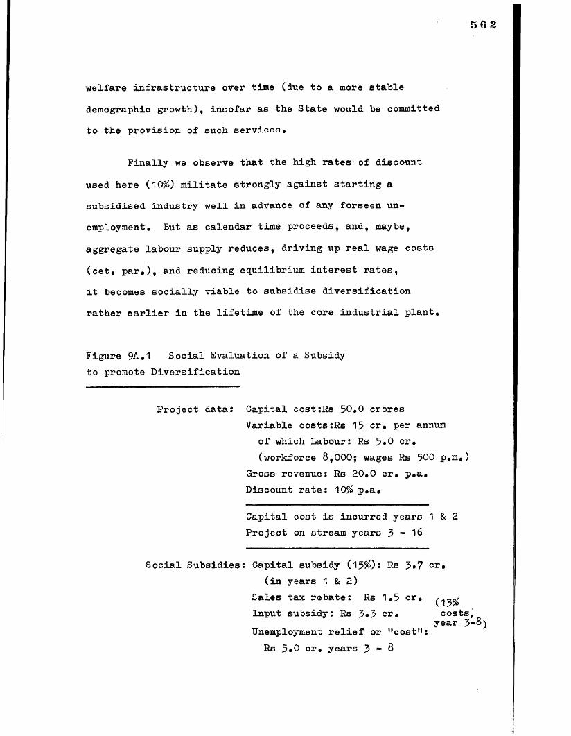
welfare infrastructure over time (due to a more stable

demographic growth), insofar as the State would be committed

to the provision of such services.

Finally we observe that the high rates of discount

used here (10%) militate strongly against starting a subsidised industry well in advance of any forseen un­employment# But as calendar time proceeds, and, maybe,

aggregate labour supply reduces, driving up real wage costs

(cet# par.), and reducing equilibrium interest rates, it becomes socially viable to subsidise diversification

rather earlier in the lifetime of the core industrial plant.

Figure 9A.1 Social Evaluation of a Subsidy to promote Diversification

Project data: Capital costsRs 50#0 croresVariable costs:Rs 15 cr# per annum

of which Labour: Rs 5*0 cr# (workforce 8,000; wages Rs 500 p.m.)

Gross revenue: Rs 20#0 cr. p#a. Discount rate: 10% p#a#

Capital cost is incurred years 1 & 2 Project on stream years 3 - 1 6

Social Subsidies: Capital subsidy (15%)* Rs 3 * 7 cr#(in years 1 8c 2 )

Sales tax rebate: Rs 1.5 cr# (*J2%Input subsidy: Rs 3 * 3 cr# costs

year 3Unemployment relief or "cost*1:

Rs 5*0 cr# years 3 - 8

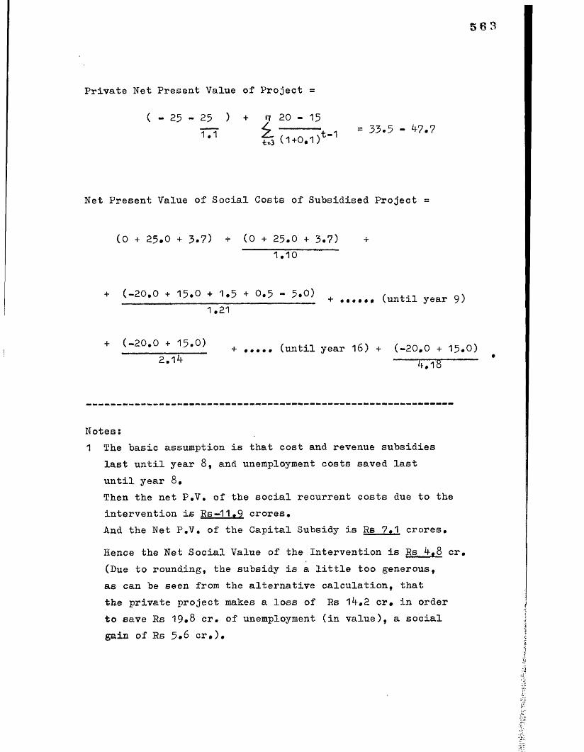
56 3

Private Net Present Value of Project =

( - 25 - 25 ) + rj 20 - 15TTT 4 ------- 1 1 = 35.5 - ^7.7tTj (1+0 .1 y

Net Present Value of Social Costs of Subsidised Project =

(0 + 2 5 .0 + 5.7) + (0 + 2 5 .0 + 3.7) +1.10

+ (-20.0 + * 1.5 * 0.5 - 5.0) + ...... (until year 9)1 .21

+ (-20.0 + 15.0) + (until year 1 6 ) + (-2 0 .0 + 1 5.0 )2 -1^ ------

Notes:1 The basic assumption is that cost and revenue subsidies

last until year 8 , and unemployment costs saved last until year 8 .Then the net P.V. of the social recurrent costs due to the intervention is Rs—11.9 crores.And the Net P.V. of the Capital Subsidy is Rs 7.1 crores.

Hence the Net Social Value of the Intervention is Rs ^ .8 cr. (Rue to rounding, the subsidy is a little too generous, as can be seen from the alternative calculation, that the private project makes a loss of Rs 1^.2 cr. in order to save Rs 19.8 cr* of unemployment (in value), a social gain of Rs 5.8 cr.).

564

2 This is simple but unrealistic. In practice the subsidy would be needed throughout the life of the project (to make up for the high current costs), or else the costs would fall over time (due to economies of agglomeration as other firms were attracted to the site). Suppose that a subsidy of Rs 1.2 crores per annum is needed from yearsv -

3 to 16, or that a subsidy of Rs 1*2 cr. is needed from years 3 to 8 , after which costs fall to 13*8 until year 16*In either case the firm breaks even; and in the first case the social value is the same as before, in the second it is higher (7 *9 )*

3 Suppose the capital cost is lower: Rs 23 cr. in year 1,and 22 in year 2. Then the capital subsidy needed to ensure the firm break even is approximately Rs 2.2 cr. (i.e. 5%)*The social value of the subsidised diversification is raised to 9*7* The high discount rate makes the scheme very sendtive to the capital subsidy.

A If the unemployment relief saved were to cost only Rs 2.5 cr., then the social value would become negative (-5 .1 )*This would be true whether the relief offered were halved per person, or the wage bill in the redundant industry were half what we assume, or if the new project only employed half of the unemployed.

5 The quantification here attempts to address the intervention of subsidised diversification only (Figure 9A.2a).Subsidised suboptimal scale is unlikely to be viable (given the economies of scale discussed in'.the text in the case of the iron and steel industry following convent­ional technology), unless the discount rate is very low, since unemployment relief is not saved until 10 to 15

years after the subsidies begin (Figure 9A.2.), Indeed,we need a discount rate as low as 2% to yield a social benefit of Rs 5 cr*, i.e. roughly similar to that inthe.first intervention model (^.7 )$ this is with a capital subsidy of 15% on two mini-plants, each half the size of the current one, initiated respectively in years 1 and 8 , with no subsidy on current costs, and unemployment of Rs 2.5 ia value saved from years 10 - 1 5*

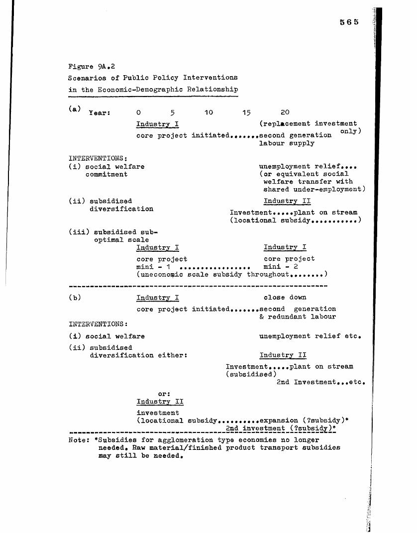
Figure 9A #2Scenarios of Public Policy Interventions in the Economic-Demographic Relationship

(a) Year: 0 5 10Industry Icore project initiated,

15

INTERVENTIONS:(i) social welfare

commitment

(ii) subsidiseddiversification

(iii) subsidised sub- optimal scale

Industry Icore project mini - 1 •.

20(replacement investment.second generation labour supply

unemployment relief#»•• (or equivalent social welfare transfer with shared under-employment)Industry II

Investment#.#•#plant on stream (locational subsidy.#••••*••••)

Industry Icore project mini - 2

(uneconomic scale subsidy throughout#•••»•••)

(b) Industry Icore project initiated,

close down.second generation & redundant labour

INTERVENTIONS:(i) social welfare(ii) subsidised

diversification either:

unemployment relief etc#

Industry IIInvestment #••••plant on stream (subsidised)

2nd Investment#..etc.or:

Industry II investment(locational subsidy...... ...expansion (?subsidy)* __ _2nd_inves tment (^subsid^*

Note: *Subsidies for agglomeration type economies no longerneeded# Raw material/finished product transport subsidies may still be needed#

A brief Overview of Chapter 9

If rapidly growing areas fail to diversify their industry, local labour market disequilibria are enhanced further (and the prospects for family income diversification outlined in Chapter 8 are reduced)# This is apparent from a detailed demographic study of a Steel Town. A solution that may be taken by the State would be to diversify industry (under subsidy) rather than bear the welfare costs of underemployment in a locality.

Modern technologies and contemporary demography combine in India to accentuate employment and welfare problems in urban areas, as they evolve over time•Strategies to mitigate these externalities of industrial­isation may be devised at the level of the State, or the level of the family. Either way, the implications of not doing so have to be seen well in advance. For these populations have a built-in momentum: largemigrant cohorts, once established, can no more have their progress checked than a huge groundswell in a calm sea.

BIBLIOGRAPHY

(Note: Government of India publications appear under "Government", British Government publications under "Her Majesty*s Government", and Public Sector industry publications and similar material under the name of the industry)

Alexander, W and A, Street, Metals in the Service of Man, Penguin, Harmondsv(orth, 1980.

Arya , V.P., A Guide to Industrial Licensing in India.Iyengar Consultancy Services, New Delhi, 1 9 8 1*

Aylen, J#, "Plant Size and Efficiency in the Steel Industry: An International Comparison" (mimeo), University of Salford, 1 9 8 1.

Badgaiyan, S.D., "A Sociological Study of the Effects of Industrialisation of Bhilai on the Surrounding Villages" (Ph.D. thesis), Department of Sociology, Delhi University, Delhi, 197^.

Balassa, B., The Structure of Protection in Developing Countries. The Johns Hopkins University Press,Baltimore and London, 1971*

Ballhatchet, K.A., and D.D, Taylor (eds.)i Changing South Asia: the Implications of Urban and Industrial.Development for Social Change. Asian Research Service, Hong Kong, 19&3*

5 6 8

Bauerjee, D*, "Industrial Stagnation in Eastern India: a Statistical Investigation", Economic and Political Weekly. 20th February, 1982.

Bapat, M#, "Occupational and Spatial Mobility amongShanty Dwellers in Poona" (Ph.D. thesis), University College London, London, 1979.

Bapat, M*f Shanty Town and City: the Case of Poona. Pergamon, Oxford, 1982.

Bapat, M., and N, Crook, "The Environment, Health, and Nutrition in Urban Hutment Settlements: a Study of Poona" (forthcoming, ?Habitat International). 1 9 8 3-^*

Bawa, V.K., "Industrialisation, Urbanisation, and Planning in the Pune Metropolitan Region: a Study of Pimpri- Chinchwad", Paper presented at the Seventh European Conference on Modern South Asian Studies, held at School of Oriental and African Studies, London", 1981; forthcoming in Ballhatchet and Taylor op. cit,

Ben-Porath, Y., (ed.), "Income Distribution and the Family",Population and Development Review. Supplement, 8:3, Sept. 1982.

Berry B., The Human Consequences of Urbanisation: divergent Paths in the Urban Expansion of the 20th Century.Macmillan, London and Basingstoke, 1973.

Bose, A*, Studies in India's Urbanisation 1901-1971.Tata McGraw Hill, New Delhi, 197^, revised 1978.

British Steel Corporation, Teesside Division, Steel Times. "Technical Survey", September, 1979.

British Steel, Annual Report and Accounts. 1979-81.

Bulsara, J.F., Problems of Rapid Urbanisation in India.Popular Prakashan, Bombay, 1964.

569

Burns, L.S., and L. Grebler, The Housing of Nations, Macmillan, London and Basingstoke, 1977*

Butterworth, E», A Statistical Sketch of the County Palatine of Lancaster 18*H. Longmans, Manchester, 18V 1#

Byres, T*J#, "The New Technology, Class Formation and Class Action in the Indian Countryside", Journal of Peasant Studies * 8 :*f, July 1981*

Carr, J.C,, and W* Taplin, History of the British Steel Industry. Oxford University Press, Oxford, 1962#

Cartwright, F*W», "Comparison of the Blast Furnace BOFRoute with its Alternatives" in Iron and Steel Institute, Alternative Routes to Steel. Proceedings of Annual General Meeting, 1971*

Cassen, R#H., India; Population. Economy. Society. Macmillan, London and Basingstoke, 1978*

Chapman, S.JM The Lancashire Cotton Industry. Manchester University Press, Manchester, 190*f#

Char, S#V., "Viability of Vizag Steel Plant", Economic and Political Weekly. 10th November, 1979*

Chaudhuri, M.R,, Indian Industries. Development and Location. Oxford University Press, Calcutta, 1966.

Chaudhuri, P., The Indian Economy; Poverty and Development. Crosby Lockwood Staples, London, 1978#

Coale, A.J#, The Growth and Structure of Human Populations« Princeton University Press, Princeton, 1972*

Coale, A*J., and P. Demeny, Regional Model Life Tables and Stable Populations. Princeton University Press, Princeton, 1 9 8 8.

Coale, A*J*, and E*M* Hoover, Population Growth and Economic Development in Low Income Countries. Princeton University Press, Princeton, 1958*

Conlon, F,C*, "Working Class Housing in Colonial Bombay", Paper presented at the Seventh European Conference on Modern South Asian Studies, held at School of Oriental and African Studies, London, 1981; forth­coming in Ballhatchet and Taylor (eds#), op* cit.

Connell, J», B. Dasgupta, R. Laishley, and M# Lipton, Migration from Rural Areas. Oxford University Press,Delhi, 1976*

Crook, N*R*, "On Social Norms and Fertility Decline",Journal of Development Studies. July, 1978*

Crook, N*R,, "On the Economy of Mortality Decline",Paper presented at the Social Science Research Council Development Group Seminar, held at the School of Oriental and African Studies, London, 1979*

Crook, N*R«, "On the Management of Urban Migration and Residence", Asian Journal of Public Administration.5:1, June 1 9 8 5.

Crook, N*R», "The Changing Character of Mortality in theCity of Poona"(manuscript), School of Oriental and African Studies, London, 1 9 8 3*

Desai, P., The Bokaro Steel Plant. North Holland,Amsterdam, 1972#

Deshpande, L*K,, "The Bombay Labour Market" (manuscript), Economics Department, Bombay University, 1979#

D ’Souza, V.S., "Scheduled Castes and Urbanisation inPunjab: an Explanation", Sociological Bulletin. 24-81*,March 1975#

Dyson, T,, "Analysis and Adjustment of the 1971 Indian Age Distribution", Demography India. 5: 1&2, 1978*

Dyson, T#, "Mortality Estimates for the States of India", (mimeo), Centre for Population Studies, London School of Hygiene and Tropical Medicine, London, 1 9 8 0#

Dyson, T#, "India's Regional Demography" (mimeo), London School of Economics and Political Science, London, 1 9 8 1#

Easterlin, R#A., "The Conflict Between Aspirations and Resources", Population and Development Review. 2:3&4-, Sept* and Dec# 1978#

Engels, F#, The Housing Question. 1 8 7 2, reprinted inF#Engels and K#Marx, Selected Works. Lawrence and Wishart, London, 1 9 8 8#

Glass, R#, The Social Background of a Plan: A Study of Middlesbrough. Routledge and Kegan Paul, London, 1948#

Gore, M.S*, Immigrants and Neighbourhoods; two Aspectsof Life in a Metropolitan City. Tata Institute of Social Sciences, Bombay, 1970#

Government of India, Census of India. 1921. Bihar and Orissa, Superintendent of Government Printing,Patna, 1923*

Government of India, Census of India. 1931* Bihar and Orissa, Sup# of Gov. Printing, Patna,1953#

Government of India, Census of India. 1961. All India,West Bengal, Bihar, Orissa, Madhya Pradesh, Maharashtra, Gujarat, Manager of Government ..Publications, Delhi,1963 onwards#

Government of India, Census of India. 1961> ’’Social Processes in the Industrialisation of Rourkela”,Special Monograph, Man* of Gov* Pub*, Delhi*

Government of India, Census of India. 1971. All India,West Bengal, Bihar, Orissa, Madhya Pradesh, Maharashtra, Controller of Government Publications, New Delhi,1973 onwards*

Government of India, Census of India* 1971. ’’Birth Place Migration”, Census Monograph No. 1, Contr* of Gov.Pubs., New Delhi.

Government of India, Census of India. 1981. ’’Provisional Population Totals, Workers and Non-workers”, Paper 3 of 1981, New Delhi.

Government of India, Central Statistical Office,Ministry of Planning, Statistical Abstract (various years), Man. of Gov. Pubs,, Delhi.

Government of India, Labour Bureau, Ministry of Labour, Employment and Rehabilitation, Family Living Surveys among Industrial Workers 1958-9 (for various towns),Man. of Gov. Pubs,, Delhi, 1 9 6 8.

Government of India, Labour Bureau, Ministry of Labour,Indian Labour Yearbook (various years), Man. of Gov* Pubs., Delhi.

Government of India, Labour Bureau, Ministry of Labour,Women in Industry. Man. of Gov.’Pubs., Delhi, 1975*

Government of India, Labour Bureau, Ministry of Labour, Statistics of Factories. Chandigarh, 1977*

Government of India, National Council of Applied Economic Research, Perspective Flan of Industrial Development of Bihar. New Delhi, 1979*

573

Government of India, Ministry of Finance, Department of Economic Affairs, National Sample Survey No. 182 (19 +),Tables with Notes on Internal Migration. New Delhi, 1972.

Government of India, Office of the Registrar General,Sample Registration System Bulletin (various years), New Delhi,

Government of India, Planning Commission, Report of the Working Group on Slums. New Delhi, 1972.

Government of India, Ministry of Works and Housing,Report of the Committee set u p to Review the Slum Clearance/Improvement Scheme for Environmental Improvement in Slum Aeas and Other Matters. New Delhi, 1975.

Government of Madhya Pradesh, Directorate of Economics and Statistics, Socio-Economic Survey of Bhilai Region. 1967#

Government of West Bengal, Census 1961. District Census Handbooks, Calcutta, 1963#

Government of West Bengal, Assistance to Entrepreneurs from Concepts to Commissioning. West Bengal Industrial Development Corporation, (undated, 71980).

Hajnal, J., "Household Formation Patterns in Historical Perspective”, Population and Development Review. 8:3,Sept. 1982.

Harriss, J., "Two Theses on Small Industry: Notes from aStudy in Coimbatore, South India”, Paper presented at the Seventh European Conference on Modern South Asian Studies, held at School of Oriental and African Studies, London,1 9 8 1; forthcoming in Ballhatchet and Taylor (eds.) op.cit,

Hindustan Steel Limited, Iron and Steel: Statistics for Iron and Steel Industry in India, (various years), Ranchi,

Her Majesty's Government, Census of England and Wales.(various years), Her Majesty's Stationery Office,London.

Howe, C#, (ed»), Shanghai; Revolution and Development in an Asian Metropolis. Cambridge University Press, Cambridge, 1981.

Indian Chamber of Commerce, A Demographic and EconomicProfile of the Calcutta Metropolitan District. Background Paper for the ICC Conference on"Calcutta-2000", ICC,India Exchange, Calcutta, 1978.

India Investment Centre, Industrial Investment Facilities and Incentives (for various regions), New Delhi, 1979*

Iron and Coal Trades Review (U.K.), "A Technical Survey of the Durgapur Works" (undated, 71960)#

Ishikawa, S., Economic Development in Asian Perspective. Kinokuniya Bookstore Company, Tokyo, 196?#

Jejeebhoy, S.J., "Status of Women and Fertility; a Socio­cultural Analysis of Regional Variations in Fertility in India", in K.Srinivasan and S.Mukerji (eds.),Dynamics of Population and Family Welfare 1981. Himalaya, Bombay, 1981.

Johnson, W.A., The Steel Industry of India. Harvard University Press, Cambridge (Mass.), 1966.

Joshi, H., and V., Surplus Labour and the City; a Study of Bombay. Oxford University Press, Delhi, 1976#

Keenan, J.L., A Steel Man in India. Duell, Sloan, and Pearce^ New York, 19^3*

Krishnamurty, J#, "Working Force in 1971 Census: Unilluminating 'Final1 Results", Economic and Political Weekly. Aug#, 1973*

Kshirsagar, S.D,, "Growth, in Consumption of Steel in India", Economic and Political Weekly, Review of Management,Aug, 1977.

Kulkarni, M,R., Industrial Development. National Book Trust, New Delhi, 1971*

Lai, D•, Appraising Foreign Investment in Developing Countries. Heinemann, London, 1975.

La-1 f D* t Prices for Planning; toward the Reform of Indian Planning. Heinemann, London, 19&0#

Lambert, R*D,, Workers, Factories and Social Change in India. Princeton University Press, Princeton, 19&3.

Lipton, M*, "Family, Fungibility, and Formality: Rural Advantages of Informal Non-farm Enterprise versus the Urban Formal State", (mimeo), International Economics Association Conference Paper, Mexico City, August, 19^0,

Losch, A,, The Economics of Location. 1939* reprinted by Yale University Press, New Haven, 195*U

Lotka, A,J., "A Contribution to the Theory of Self-Renewing Aggregates, with special reference to industrial replacement", Annals of Mathematical Statistics. 1 0 :1 ,

1939.

NacDougall, J #, Ancillary Industries in Asansol-Durgapur«Asia Publishing House, London, 1975.

Mackie, J*W*, "Industrial Location and Regional Policy in South India" (Ph,D» thesis), School of Oriental and African Studies, London, 19&2#

Malaker, C*R,, "Nuptiality in India" (Ph#D, thesis),Indian Statistical Institute, Calcutta, ?19$0#

57 6

Mamood, A., "Patterns of Migration into Indian Cities and their Socio-economic Correlates': a Multi-variate Regional Analysis" (M.Phil# thesis), Jawaharlal Nehru University, New Delhi, 1975.

Mills, E*S#, Urban Economics. Harvard University Press, Cambridge (Mass#), 1979*

Misra, R*P#, (ed#), Regional Planning. Concepts. Techniques. Policies and Case Studies. Prasaranga— University of Mysore, Mysore, 19^9*

Mitchell, B»R#, (with P#Deane), Abstract of British Historical Statistics. Cambridge University Press, Cambridge, 19&2#

Mitra, A*, et al*, Indian Cities. Their Industrial Structure and Capital Investment 1961-1971. Abhinav, New Delhi, 19^0*

Mohsin, M., Chittaran.ian: a Study in Urban Sociology. Popular Prakashan, Bombay, 1 9 6 #

Morris, M#D#, The Emergence of an Industrial Labour Force in India: a Study of the Bombay Cotton Mills 185^-19*<-7« Oxford University Press, Bombay, 1965.

Munshi, S#, "Industrial Labour in Developing Economies", Economic and Political Weekly. Review of Management,August, 1977#

Oldham & District Historical and Antiquarian Society,The Cotton Mills of Oldham. Oldham Libraries, Oldham,1979.

Oldham Centre of Local Interest, Oldham at Work. Oldham, 1 9 8 1# Oldham Corporation, Oldham and _Its Industries, undated, Oldham#

Prais, S*J*, Productivity and Industrial Structure (forth­coming, 1 9 8 2-3 )*

Prakash, V*, New Towns in India. Duke University Monograph No* 8, Durham,•1 9 6 9•

Premi, M.K*, " Aspects of Female Migration in India", Economic and Political Weekly. 12th April 1 9 8 0*

Premi, M*K,, Urban Out-migration: a Study of Its Nature. Causes and Consequences. Sterling Publishers, New Delhi, 1980*

Raza, M., and A* Habeeb, "Characteristics of ColonialUrbanisation: a Case-Study of the Satellitic 'Primacy* of Calcutta", Occasional Paper, Centre for Regional Development, Jawaharlal Nehru University, New Delhi, 1978.

Richardson, H*W., and J.M. Brass, "The Consett Iron and Steel Company", Business History. VII:2, July 198 3 *

Rothermund D., et, al*, (eds.), Urban Growth and RuralStagnation: Studies in the Economy of an Indian Coalfield and its Rural Hinterland. Manohar, New Delhi, 1 9 8 0.

Ryder, N*B., "The Cohort as a Concept in the Study of Social Change", American Sociological Review. 3 0 *8 ,Dec. 1985.

Saha, S.K., "Industrial Policy and Locational Dynamics of Small-Scale Enterprises in India", Paper presented at the Seventh European Conference on Modern South.Asian Studies, held at the School of Oriental and African Studies, London, 1981*

Saxonhouse, G., and Y. Kiyokawa, "The Supply and Demand for Quality Workers in the Cotton Textile Industries in Japan and India", Papers and Proceedings of the

Conference on Japan's Historical Development Experience and the Contemporary Developing Countries, International Development Centre of Japan, 1978.

Scherer, D., The Economics of Multi-Plant Operation.Harvard University Press, Cambridge (Mass.), 1975*

Sen, A., Poverty and Famines: an Essay on Entitlement and Deprivation. Oxford University Press, Oxford, 1 9 8 1.

Sen, S.K., The House of Tata (1839-1939). Progressive Publishers, Calcutta, 1975.

Sen, S.N., The City of Calcutta: a Socio-economic Survey. Bookland Private Ltd., Calcutta, 19&0.

Sengupta, N., Destitutes and Development: a Study of the Bauri Community, in .the Bokaro Region. Concept Publishing Co.,New Delhi, 1978.

Shetty, S.L., "Structural Retrogression in the Indian Economy since mid-Sixties", Economic and Political Weekly.Annual Number, Feb., 1978.

Sivaramakrishnan, K.C., "New Towns in India: a Report on a Study of Selected New Towns in the Eastern Region", (mimeo), Indian Institute of Management, Calcutta, 1976-7*

Sivaramakrishnan, K.C., "Case Study of an Indian New Town", in J.L.Taylor and D.G. Williams (eds.), Urban Planning Practice in Developing Countries. Pergamon, Oxford, 1982.

Smith, R*, "An Oldham Limited Liability Company 1875-18 9 6", Business History. *f:1, Dec. 1 9 6 1*

Stanford Research Institute (California), School of Planning and Architecture (New Delhi), Small Industry Extension Training Institute (Hyderabad), Costs of Urban Infra­structure for Industry as Related to City Size in Developing Countries (India Case Study) (no publishergiven), 1968

57

Tata Services Limited, Department of Economics andStatistics, Statistical Outline of India. D.R.Pendse,Bombay, 1976, and 1 9 8 0.

Times of India, Directory and Yearbook, (various years),Times of India Press, Bombay#

Todaro, M#P#, "Rural Urban Migration, Unemployment, and Job Probabilities in Recent Theoretical and Empirical Research", in A.J.Coale (ed#), Economic Factors in Population growth. Macmillan, London and Basingstoke, 1976#

Townroe, P#, Planning Industrial Location. Leonard Hill Books, London, 1976#

Tulpule, B#, "Managing Durgapur, Experience of a TradeUnionist", Economic and Political Weekly. 25th Dec., 1976.

Vaidyanathan, K.E., "Population Redistribution and Economic Change in India 1951-1961" (mimeo), University of Pennsylvania, Penn., 1 9 6 7#

Wadva, K., "Land Use Patterns in Urban Fringe Areas",Economic and Political Weekly, 2nd April, 19&3*

Weber, A.F., The Growth of Cities in the Nineteenth Century. 1 8 9 9, reprinted by Cornell University Press, Ithaca and New York, 1 9 6 3.

Weiner, M., Sons of the Soil; Migration and Ethnic Conflict in India. Princeton University Press, Princeton, 1978*

Wilson, A.S., "The Origins of the Consett Iron Company 18V1-186V1, Durham University Journal. 1977.

Wrigley, E.A., Population and History. Weidenfield and Nicolson, London, 1969*

580

A POSTSCRIPT

The study confirmed my hunch that modern industrial tednology in certain fields - especially heavy engineering - adopted by developing countries would give rise to curious social phenomena in towns; curious in that demographic structures would arise leading to serious second generation employment prospects. To this was added the observation that if, as was likely, such towns remained single industry towns, the total workforce would be as vulnerable to a change in industrial fortunes as would be an agricultural labourer or small-holder to the failure of the crop in a monoculture. It also became apparent that, at the other end of the scale, the older towns, in failing to attract new populations, would also face economic problems arising from their emerging demographic structures, notably a lack of taxable surplus for social spending* In all, the average or aggregate picture of the Indian urban population was misleading! at each end of the spectrum demographic phenomena exacerbated social difficulties.

What recommendations follow from this work? There:as, I believe, little social change without political revolution. But I also happen to believe that there is a human drive for social (as well as individual) survival, despite the fact that the two are often in conflict. There are implications in what I have to say for public policy, and for the strategies of smaller social groupings, right down to the family.

I advocate the adoption of a more balanced urban growth, by promoting a more diversified industrial structure in each town (despite the economic costs), and not uniformly, but selectively.This could be done through the complex of location subsidies that exist.

I advocate some demographic understanding to make these controls sensible: new industry too early or too late for the second generation is useless.

I am not certain if it is wise for extended families or people from particular origins, the same village or even district, to congregate in the same industry. If they would not all grow millet, they should not all make steel: theformer could fail for two years running, the latter could fail for ever.

I advocate cross-financing of urban social development and the planning for large areas of spontaneous settlements in rapidly growing towns from their inception.

Note that I am not suggesting pouring industrial development finance into sick cities: I am easing thedeath pangs, just as I am preventing fatal accidents to those of headlong growth.