Commentary: The Materials Project: A materials genome approach to accelerating materials innovation
Upload
khangminh22Category
view
4download
0

S E C O N D E D I T I O N
THE METHODS AND MATERIALS OF DEMOGRAPHY

This Page Intentionally Left Blank
S E C O N D E D I T I O N
THE METHODS ANDMATERIALS OFDEMOGRAPHY
Edited by
JACOB S. SIEGELDAVID A. SWANSON
Amsterdam • Boston • Heidelberg • London • New York • Oxford
Paris • San Diego • San Francisco • Singapore • Sydney • Tokyo
Academic Press in an imprint of Elsevier

Elsevier Academic Press525 B Street, Suite 1900, San Diego, California 92101-4495, USA84 Theobald’s Road, London WC1X 8RR, UK
This book is printed on acid-free paper.
Copyright © 2004, Elsevier Inc. All rights reserved.
No part of this publication may be reproduced or transmitted in any form or by any means,electronic or mechanical, including photocopy, recording, or any information storage and retrievalsystem, without permission in writing from the publisher.
Permissions may be sought directly from Elsevier’s Science & Technology Rights Department in Oxford, UK: phone: (+44) 1865 843830, fax: (+44) 1865 853333, e-mail:[email protected]. You may also complete your request on-line via the Elsevierhomepage (http://elsevier.com), by selecting “Customer Support” and then “ObtainingPermissions.”
Library of Congress Cataloging-in-Publication DataApplication submitted
British Library Cataloguing in Publication DataA catalogue record for this book is available from the British Library
ISBN: 0-12-641955-8
For all information on all Academic Press publications visit our Web site atwww.academicpress.com
Printed in the United States of America03 04 05 06 07 08 9 8 7 6 5 4 3 2 1

Acknowledgements viiDAVID A. SWANSON AND JACOB S. SIEGEL
Preface ixLINDA GAGE AND DOUGLAS S. MASSEY
1. Introduction 1DAVID A. SWANSON AND JACOB S. SIEGEL
2. Basic Sources of Statistics 9THOMAS BRYAN
3. Collection and Processing ofDemographic Data 43
THOMAS BRYAN AND ROBERT HEUSER
4. Population Size 65JANET WILMOTH
5. Population Distribution—GeographicAreas 81
DAVID A. PLANE
6. Population Distribution—Classification of Residence 105
JEROME N. MCKIBBEN AND KIMBERLY A. FAUST
7. Age and Sex Composition 125FRANK B. HOBBS
8. Racial and Ethnic Composition 175JEROME N. McKIBBEN
9. Marriage, Divorce, and Family Groups 191KIMBERLY A. FAUST
10. Educational and Economic Characteristics 211
WILLIAM P. O’HARE, KELVIN M. POLLARD, AND AMY R. RITUALO
11. Population Change 253STEPHEN G. PERZ
12. Mortality 265MARY McGEHEE
13. The Life Table 301HALLIE J. KINTNER
14. Health Demography 341VICKI L. LAMB AND JACOB S. SIEGEL
15. Natality—Measures Based on VitalStatistics 371
SHARON ESTEE
Contents
v

16. Natality—Measures Based on Censuses and Surveys 407
THOMAS W. PULLUM
17. Reproductivity 429A. DHARMALINGAM
18. International Migration 455BARRY EDMONSTON AND MARGARET MICHALOWSKI
19. Internal Migration and Short-DistanceMobility 493
PETER A. MORRISON, THOMAS BRYAN, AND DAVID A. SWANSON
20. Population Estimates 523THOMAS BRYAN
21. Population Projections 561M. V. GEORGE, STANLEY K. SMITH, DAVID A. SWANSON,
AND JEFF TAYMAN
22. Some Methods of Estimation forStatistically Underdeveloped Areas 603
CAROLE POPOFF AND D. H. JUDSON
Appendix AReference Tables for Constructing an Abridged Life Tableby the Reed-Merrell Method 643GEORGE C. HOUGH, JR.
Appendix BModel Life Tables and Stable Population Tables 653C.M. SUCHINDREN
Appendix CSelected General Methods 677D. H. JUDSON AND CAROLE L. POPOFF
Appendix DGeographic Information Systems 733KATHRYN NORCROSS BRYAN AND ROB GEORGE
Glossary 751
A Demography Time Line 779DAVID A. SWANSON AND G. EDWARD STEPHAN
Author Biographies 787
Index 791
vi Contents
Since its initial introduction in 1971, The Methods andMaterials of Demography has served well several genera-tions of demographers, sociologists, economists, planners,geographers, and other social scientists. It is a testament toboth its strong fundamental structure and its need that thebook has enjoyed such a long, successful run without sub-stantive revisions. By the mid 1990s, however, a number of important methodological and technological advances in demography had occurred that rendered “M&M” out-of-date. These advances led to the commissioning of this revi-sion of the 1976 Condensed version, an endeavor for whichacknowledgments are due.
We first and foremost thank the authors of the individualchapters, who so generously gave of their time and ex-pertise. We also thank Scott Bentley, Senior Editor, for his patience, suggestions, and steady guidance, and all theothers at Academic Press who dedicated themselves to thetask of seeing the work through to publication. A large debtof gratitude is owed to Tom Bryan for the long hours hespent “cleaning up” the original electronic files created fromscanning the entirety of the 1976 Condensed version ofM&M. Tom also provided several authors with formattingassistance and advice. His selfless generosity was instru-mental in the completion of this project. Special thanks alsogo to George Hough and Juha Alanko for their assistance in resolving a myriad of technical problems ranging fromcorrupted files to software incompatibilities.
The present editors, the contributors to the new volume,and users, past and present, owe a great debt to HenryShryock, Siegel’s distinguished collaborator in the prepara-tion of the original unabridged work. The present authorsand editors also owe a debt of gratitude to Edward G. Stockwell, Emeritus Professor of Sociology, Bowling GreenState University. In collaboration with the editors of theoriginal work, he was responsible for abridging the originaltwo-volume work published by the U.S. Census Bureau. Inso ably carrying out the time-consuming and demandingtask of condensing the longer text, he produced the volume
from which the present authors principally worked. We also owe much to the many contributors to the originalunabridged version of M&M. They provided an enduringlegacy that extends into this revision and likely well beyond.In this regard, we owe a special debt to many at the U.S.Census Bureau—past and present—but in particular, wewant to thank John Long and Signe Wetrogan for their assistance in making this revision become a reality.
We also want to thank our friends, colleagues, and insti-tutions for their forbearance, understanding, and assistance,and, in particular, our family members.
Jacob Siegel wants to thank his legions of students at the University of Connecticut, the University of SouthernCalifornia, Cornell University, the University of CaliforniaBerkeley, Howard University, the University of CaliforniaIrvine, and especially, Georgetown University, his homebase for almost a quarter century, for navigating with himthrough the earlier editions of the book and honing hisknowledge of demography. He also wants to thank hisfriends and colleagues who invited him to join them in training the next generations of demographers at their institutions, Jane Wilkie, Judy Treas, Joe Stycos, Ron Lee,Tom Merrick, Frank Edwards, and Maurice van Arsdol.Further, he wants to pay tribute to Dan Levine, Jeff Passel,Greg Robinson, Henry Shryock, Bob Warren, Meyer Zitter,and the late Conrad Taeuber, all former colleagues at theU.S. Census Bureau, who contributed over many years tothe high level of demographic scholarship in that agency.Finally, Siegel wishes to acknowledge his intellectual debtto Nathan Keyfitz and the late Ansley Coale, who con-tributed immensely to the development of demographicmethods in our time and who trained and inspired a multi-tude of demographers in our country and abroad.
David Swanson is grateful for the training and mentor-ing he received while an undergraduate student at WesternWashington University, a graduate student at the Universityof Hawaii, a staff researcher with the East-West Center’sPopulation Institute and, subsequently, with the Washington
Acknowledgments
vii

State Office of Financial Management. To his wife Rita,David owes a lot, for not only putting up with several yearsof lost vacations, weekends, and evenings, but for her assis-tance with the Glossary. Sacrifices she made surpassed those of Dave and Jane, Milt and Roz, Nikole, Danielle,
Gabrielle, and Brittany, in that the visits and activities theymissed became many more boring and lonely occasions for her.
Jacob S. Siegel and David A. Swanson
viii Acknowledgments
The original edition of the Methods and Materials ofDemography was written between 1967 and 1970. The worldof demography in the late 1960s was a far cry from the onewe know today. Many of the methods we now take forgranted had not yet been invented, and given the computa-tional intensity of techniques such as multistate life tablesand hazards modeling, some would have been impossible toimplement in the early days of the computer era.
Although computers existed in the late 1960s, they weremainframes: big, costly, cumbersome, and expensive. If youwanted to run a computer program, you typically began bywriting the code yourself, then keypunched the programonto a set of eighty-column cards, delivered the resultingdeck across a counter to a computer operator, who thenloaded it into a mechanical reader. Then your programentered a queue to compete with administrative jobs andother research applications for access to scarce “CPU”capacity, which never exceeded “640k.” After working itsway to the front of the queue, the program would finally run.If you hadn’t made a keypunching error, violated the syntaxof the programming language, or made a logical mistake thatproduced a mathematical impasse such as division by zeroor some other nonsensical result, the program might suc-cessfully conclude and produce meaningful output. It wouldthen be placed in a queue for printing on a mechanical lineprinter, and if the printer did not jam before getting to youroutput, it would be printed. It would then sit in a pile untilthe computer operator got around to separating it from other“print jobs” and then placing it in a specific cubbyhole asso-ciated with the first letter of your last name. There, hope-fully, you would find your output. If all went well, the wholeprocess might take four hours, but if the job was “big,” itwould be held in “batch” to run overnight, when competi-tion for CPU access and memory slackened.
The foregoing represents a common historical scenarioof demographic-data analysis for those fortunate enough tobe working in a research university, a well-funded researchinstitute, or the upper reaches of the federal bureaucracy
in the 1960s (and into the 1980s). If one was unfortunateenough to be working at a teaching college, second-tier uni-versity, the middle echelons of the federal bureaucracy, orin most positions of state and local government, calculationshad to be performed with electrical calculating machinesthat could handle only simple mathematical operations andlimited bodies of data. Those even more unfortunate enduredthe tedium of performing error-prone calculations by hand,with pencil and paper.
Whether by electronic machine or by hand, even the sim-plest calculations were laborious, costly, and profligate withrespect to time (hours spent adding, multiplying, and divid-ing dozens of numbers by hand), space (yielding file cabi-nets bulging with papers containing hand-entered data orcolumns of printed numbers), and personnel (squads of busy statistical clerks). Methodology was kept deliberatelysimple: descriptive rather than analytical, bivariate ratherthan multivariate, linear instead of nonlinear, scalar opera-tions instead of matrix operations. In terms of analysis,demographers and statisticians worked to derive computa-tional formulas that relied on simple sums and products andcould be implemented in a series of easily transmitted steps.This all has changed. Happily since the “good old days,”access to huge levels of computer power has become com-monplace and software packages for a wide range of statis-tical and demographic techniques, both simple and complex,have become available to analysts.
With respect to data, the principal sources in 1970, espe-cially in the more developed countries, were vital statisticsand the census. In the United States, other than the CurrentPopulation Survey, little demographic data came fromsurveys. Today, there is a plethora of sample surveys, bothgeneral-purpose and specialized, relating to demographic,social, economic, and health characteristics, and coveringboth the more developed and the less developed countries.Vital registration systems have been improved and extended,and administrative data of many kinds are being exploitedfor their demographic applications.
Preface
LINDA GAGE AND DOUGLAS S. MASSEY
ix

The high cost of gathering and manipulating data in thelate 1960s also meant that knowledge of the methods andmaterials of demography was not widely diffused. Expertiseon most demographic techniques was confined to a fewpractitioners working in federal and state bureaucracies, thelife insurance industry, or academia; and practically no onewas familiar with all the methods and techniques employedto gather, correct, and analyze demographic data.
As a result, there was no single comprehensive source ofinformation on demographic techniques, either for referenceor for training purposes. During the first half of the lastcentury a number of general textbooks on demographyappeared, but they tended to focus on specific areas of thefield or were too limited in the depth of their treatments. In1925, Hugh Wolfenden’s Population Statistics and TheirCompilation was published by the Society of Actuaries; itfocused on the compilation of census data and vital statis-tics and on mortality measures from an actuarial standpoint.The classic treatise on The Length of Life, published byLouis Dublin and Alfred Lotka in 1936 went into consider-able detail on the methodology and applications of the lifetable but offered little on other methods. In the same yearRobert Kuczynski published his monograph on The Mea-surement of Population Growth, which concentrated on fertility and mortality and their relation to population growthand included some international examples. A section ondemographic methods was included in Margaret Hagood’sStatistics for Sociologists, which was published in 1941.However, it was not until 1950, with the release of PeterCox’s Demography, that what many considered to be thefirst “comprehensive” textbook on demography appeared.This was followed in 1958 by George Barclay’s Techniquesof Population Analysis, which covered many of the princi-pal topics of demography—and with an international orien-tation. Unfortunately, Barclay’s work, like the work of thosepreceding him, also left many topics uncovered.
By the 1960s, a clear need had arisen for a current, com-prehensive source of information on demographic methodsand data that gave particular attention to the collection, com-pilation, and evaluation of census data and vital statistics. Inthe context of the Cold War, U.S. officials were workingassiduously to capture the hearts and minds of peoplethroughout the less developed world. As part of this effort,the U.S. Agency for International Development (AID) rannumerous training programs that brought officials from theless developed nations to the United States to acquire thetechnical expertise they needed to administer their rapidlygrowing states. The agency also sent out cadres of residentadvisors to provide direct training and technical support.
An important focus of AID’s training was demographicand statistical methods, designed to give officials in manynewly decolonized states the technical knowledge theyneeded to implement a census, maintain vital registries, andstaff an office of national statistics. In this effort, the lack
of a text on demographic methods emerged as a serioushandicap. AID subcontracted demographic training to theU.S. Bureau of the Census, but while its staff members hadthe demographic expertise, they too lacked teaching mate-rials and readings. As an early interim solution to thisproblem, in 1951, Abram Jaffe (formerly of the Bureau ofthe Census, but at Columbia University by 1951) compileda book of readings, with some introductory text, entitledHandbook of Statistical Methods for Demographers. In aneffort to secure a more satisfactory training instrument, AIDoffered a special contract to the Census Bureau to allocateits personnel and resources to the task. Henry Shyrock andJacob Siegel were named to coordinate the effort, which ulti-mately led to the completion of the two volumes known asThe Methods and Materials of Demography, published in1971 by the U.S. Government Printing Office for the U.S.Bureau of the Census. This two-volume work represents thefirst-ever systematic, comprehensive survey of demographictechniques and data.
Thus, the origins of Methods and Materials lay in a train-ing imperative—the need for a comprehensive text thatcould be given to students, particularly those from the lessdeveloped nations, as part of an extended seminar on demo-graphic techniques. It also was intended to serve as a refer-ence guide for trained demographers to use after theyreturned to work in government, the private sector, or aca-demia. The two volumes offered a detailed summary of theworking knowledge of demographers circa 1970, drawingheavily on the day-to-day wisdom that over the years hadbeen garnered by Census Bureau employees. In a very realway, it represented a systematic codification and extensionof the inherited oral culture and technical lore of the CensusBureau’s staff, recorded for general use by a wider public.
According to the preface, the original Methods and Materials sought to achieve
. . . a systematic and comprehensive exposition, with illustrations,of the methods currently used by technicians or research workers in dealing with demographic data. . . . The book is intended to serve both as a text for course on demographic methods and as a reference for professional workers. . . .
Methods and Materials was intended to be used as themanual in a year-long training course, and given its didac-tic purpose was self-consciously written so as to assumelittle mathematical sophistication on the part of the reader.Each method was laid out in clear, step-by-step fashion, andcomputations were illustrated with examples based on actualdemographic data.
Paradoxically, given the work’s origins in the need totrain students from the less developed countries, the exam-ples were taken almost entirely from the censuses and vitalstatistics registries of the United States and other moredeveloped countries. Shryock and Siegel were aware of thislimitation and in their preface they lamented the lack of
x Preface
reliable data from the less developed nations and sought toassure readers that “. . . certain demographic principles andmethods are essentially ‘culture free,’ and measures workedout for the United States could serve as well for any othercountry.”
Whatever its shortcomings, the two volumes of Methodsand Materials clearly addressed an unmet need and filled anessential niche in the field. The original publication run of1971 was soon sold out, necessitating a second printing in1973. But this printing also soon went out of stock, and athird printing was released in 1975 (followed by a fourth in 1980, shortly after which, the book went out of print).Clearly a bestseller by the standards of the Census Bureauand the U.S. Government Printing Office, the volumeattracted the attention of the private sector, notably Profes-sor Halliman Winsborough of the University of Wisconsin,who sought to publish a condensed version as part of hisseries entitled “Studies in Demography.” To reduce the twovolumes into a single compact work, he enlisted ProfessorEdward G. Stockwell of Bowling Green State University inOhio and in 1976 Academic Press brought out its CondensedEdition of Methods and Materials.
Whereas the original Shryock and Siegel volume con-tained 888 pages, 25 chapters, and four appendices, the condensed version had 559 pages, 24 chapters, and threeappendices. In preparing their original volume, Shryock andSiegel had each taken primary responsibility for writingeight chapters. For the remaining nine chapters they enlistedthe help of 11 “associate authors.” The two primary authorsthen read, edited, and approved all chapters before final publication. Conrad Taeuber, then Associate Director of theCensus Bureau, also read and commented upon the manu-script. Among the associate authors were people such asPaul Glick, Charles Nam, and Paul Demeny. When thesenames are combined with those of Shryock, Siegel, andTaeuber, we find that Methods and Materials was associatedwith the labors of six current, past, or future Presidents ofthe Population Association of America, one indicator of itscentrality to the discipline.
In the current volume, the number of chapters has beenreduced to 22. Of these, 21 correspond to the original chap-ters delineated by Shryock and Siegel, and a new chapter onhealth demography has been added. As before, there are fourappendices. Reflecting the greater scope and complexity ofdemography in the 21st century, however, is the expansionof the two primary and 11 associate authors of the firstedition to two primary and 32 associate authors in thesecond. That the ratio of authors to chapters has virtuallytripled, going from 0.52 to 1.55, may suggest somethingabout the accumulation of methodological knowledge thathas taken place over the past three decades.
Another perspective on the past three decades is offeredby the concept of evolution—that gradual process in whichsomething changes into a significantly different, especially
a more complex or more sophisticated form. It is impercep-tible on a daily basis. After three decades it was time to takestock of Methods and Materials and assess how demogra-phy had changed. Those fortunate enough to have a copy ofthe original still turn to it for definitions, formulas, andgeneral reference. The methods and materials of our disci-pline have changed so much that it was necessary to revisedemographers’ most cherished resource, the time-honoredvolumes that some refer to simply as “M&M.”
In 1971, a “tiger” was a tiger and a “puma” was a moun-tain lion. Today a “TIGER” can be a Topologically Inte-grated Geographic Encoding and Referencing System and a“PUMA” can be a Public Use Microdata Area. In 1971, an“ace” was a playing card, now an “ACE” can be an Accu-racy and Coverage Evaluation Survey. New alphabet com-binations have entered the demographic vocabulary: ACS(American Community Survey), CDP (Census DesignatedPlace), CMSA (Consolidated Metropolitan Statistical Area),GIS (Geographic Information System), and MAF (MasterAddress File). At the end of the 20th century, M&M was nolonger widely available and it was no longer current. Manywho teach and practice demography today were not yet bornwhen the original work was printed. Yes, it was time toupdate the “old” version.
Much had changed in 30 years. The evolution of demog-raphy was fostered by the availability of more data and datasources, and improved tools to access, analyze, and quicklycommunicate information. The discipline responded to theopportunities created by the new computer technology,including the Internet, growth in data storage, and comput-ing capacity; widespread availability of analytic softwareand Geographic Information Systems; and mass mediainterest in demography. The aging of the Post–World War II“baby boom” population, especially in the United States,also helped shift the focus of demography. Along with theintellectual progression of theories and improvements in andinvention of demographic methods, the reach of demogra-phy expanded within other scientific disciplines, in state andlocal governments, community-based organizations, plan-ning and marketing enterprises, and in the popular press.
The numerous authors selected to review and revise the chapters of M&M are specialists in their fields. Theycarefully preserved much of the original material, mademajor or minor modifications as needed, and brought the contents up to date by including recent research, refer-ences, and examples. Some chapters are little changed,while some changed significantly as new methods andimprovements to previous methods were introduced. Otherchapters and sections introduce topics, like health demogra-phy and geographic information systems, not included in theoriginal.
The new chapter on Health Demography is included inrecognition of the many questions on health that now appearregularly on population censuses and surveys, the close
Preface xi

relation of health to the analysis of mortality changes, andthe role of health as cause and consequence of various demo-graphic and socioeconomic changes. This chapter definesthe basic concepts relating to health and extends conven-tional life tables to measure “active” or “healthy” lifeexpectancy. The importance of health issues to demographyalso is discussed in a chapter addressing estimation methodsfor statistically underdeveloped areas that reports on recentmethodologies to incorporate the effects of the HIV/AIDSepidemic on life expectancy.
A Glossary is introduced that covers topics from abortionand abridged life table to zero population growth and zipcodes. Appended to the Glossary is a “Demography TimeLine,” which records significant demographic events begin-ning with the Babylonian census in 3800 b.c., covers the1971 publication of the Methods and Materials of Demog-raphy, and concludes with the release of United StatesCensus results through the Internet in 2000.
Other new features include an appendix on GeographicInformation Systems (GIS) that covers everything from theorigins of GIS to the products of GIS. There are discussionsabout what GIS is and how it can be used by demographersto enhance analysis and aid communication of results. Techniques for analyzing spatial distributions are described.There is a very helpful section on practical issues to con-sider in developing a GIS, such as data-storage formats,attributes of reliable data, and dimensions of data display.
New chapter sections discuss the development of cen-suses and surveys over the last 30 years and provide guide-lines on when is the most appropriate time to select neither,one or both. Many changes in the United States census arehighlighted. The chapter on Population Size sets forth theevolution of enumeration techniques and coverage evalua-tion in the United States from the 1970 to the 2000 census.Specific techniques for data collection and methods forassessing coverage in the most recent decennial census aredescribed. There is a candid discussion of the technical andpolitical debates and tensions surrounding the issue ofadjusting the U.S. census results for estimated undercounts.The chapter on Geographic Areas includes discussions ofnew statistical units in the U.S. and adds a new section onalternative ways of measuring an emerging concept of inter-est, namely “accessibility”—the relationship between dis-tance and opportunities.
The chapter on Racial and Ethnic Composition describeshow greatly the measurement of racial and ethnic composi-tion has changed in the United States since 1970 anddescribes the two major efforts of the U.S. government tocreate standards for collecting data on race and Hispanic ethnicity. (The most recently adopted standard allowedpeople to select more than one racial identity in federalcensus, survey, and administrative forms for the first time.) There is a rich description of the new standards forcollecting and tabulating data on race along with guidance
to those who must “bridge” race data collected under the disparate standards of 1990 and 2000 for trend or time-seriesanalysis.
Some chapters in the original were merged. Two chap-ters, one on Marital Characteristics and Family Groups andanother on Marriage and Divorce were blended to reflect thecurrent state of marriage, divorce, and living arrangementsthat include covenant marriages, cohabitation, living ar-rangements of adult children, grandparents as custodians ofgrandchildren, and a rise in the average age at first marriage.Previous chapters on Sex Composition and Age Composi-tion also were combined and integrated into one chapter. Thenew chapter updates the previous materials with morecurrent examples (usually through the 1990 round of censustaking), including examples with international data, and provides references on computer spreadsheet programs that greatly simplify the application of many of the basicmethods. The chapters on Educational Characteristics andEconomic Characteristics chapters were also joined toaddress an increase in data sources, especially labor forcesurveys both in the United States and internationally, as wellas new methodology since the early 1970s. As an example,this chapter contains a discussion of the World Bank’sLiving Standards Measurement Study (LSMS) that provideskey information on income, expenditures, and wealth in theless developed countries.
Improvements in data collection, combined with anincrease in computer capacity and analytic software, greatlysimplify the application of many basic methods. They arereferenced throughout the book but are especially empha-sized in the chapters on Population Estimates and Popula-tion Projections. The chapter on Population Estimatespresents the different types of estimation methods and astep-by-step approach for creating a population estimatesprogram, from accessing data through selecting the appro-priate methodology and finally applying evaluation tech-niques. In the chapter on Population Projections, newmaterial on structural models is included that expands thetreatment in the last version. This chapter also containsmaterials on economic-demographic models used to projectgrowth for the larger areas such as counties, metropolitanareas, and nations and urban systems models for small areaanalysis, including transportation planning.
The demographic basics—birth, death and migration—are covered in several chapters. Discussions in the chapterson Fertility and Natality adopt more current terminology todescribe measures of marital and nonmarital fertility andprovide up-to-date examples of fertility measures. The dis-cussion on research on children ever born and relationshipsbetween vital rates and age structure is expanded. Recentresearch on the use of multiple causes of death and the effectof the new international classification system of causes ofdeath trends in the leading causes of death is addressed inthe Mortality chapter. The construction of basic Life Tables
xii Preface

has changed little in 50 years but life tables are more widelyavailable today. As explained in the chapter on the LifeTable, the forms, and range of applications, of life tableshave been greatly expanded, particularly the use of multi-state life tables to measure social and economic characteris-tics in addition to mortality. Chapters on Internal Migrationand Short-Distance Mobility and International Migrationremain separate. Vastly improved sources of data on inter-nal migration that became available over the last twodecades are highlighted in the former chapter, especiallylongitudinal microdata that allow a more complete descrip-tion of the moves that people make, the contexts surround-ing moves, and the sequences of movement. In the latterchapter, there are discussions about the difficulty of meas-uring both illegal and nonpermanent immigration and theproblems surrounding data on refugee populations.
This new edition keeps the best features of the earlieredition, updates the chapters, and develops new tables usingreal data to illustrate methods for data analysis. There isincreased attention to sample survey data and international
materials, particularly taking account of the new data on lessdeveloped countries. The new edition provides the academicreferences, methodological tools, and sources of data thatdemographers can both apply to basic scientific research anduse to assist national, state and local government officials,corporate executives, community groups, the press, and thepublic to obtain demographic information. In turn, thisdemographic information can be used for advancing basicscience as well as supporting decision-making, budget pro-posals, long-range planning, and program evaluation. Thiscurrent work is consistent with the original in essentialways: careful definitions, detailed computational steps, and“real-life” examples. Concepts and methods are redesignedto state-of-the-art and updated with timely examples, currentreferences, and topics not available in the original. Thiswork, marking the significant evolution of demographysince the original edition, is an invaluable reference for academic and applied demographers and demographic practitioners at all levels of training and experience.
Preface xiii

This Page Intentionally Left Blank

WHAT IS DEMOGRAPHY?
Demography is the scientific study of human population,including its size, distribution, composition, and the factorsthat determine changes in its size, distribution, and com-position. From this definition we can say that demographyfocuses on five aspects of human population: (1) size, (2)distribution, (3) composition, (4) population dynamics, and(5) socioeconomic determinants and consequences of pop-ulation change. Population size is simply the number ofpersons in a given area at a given time. Population distri-bution refers to the way the population is dispersed in geographic space at a given time. Population compositionrefers to the numbers of person in sex, age, and other“demographic” categories. The scope of the “demographic”categories appropriate for demographic study is subject todebate. All demographers would agree that age, sex, race,year of birth, and place of birth are demographic charac-teristics. These are all characteristics that do not essentiallychange in the lifetime of the individual, or change in a per-fectly predictable way. They are so-called ascribed charac-teristics. Many other characteristics also are recognized aswithin the purview of the demographer. These fall into along list of social and economic characteristics, includingnativity, ethnicity, ancestry, religion, citizenship, maritalstatus, household characteristics, living arrangements, edu-cational level, school enrollment, labor force status,income, and wealth. Most of these characteristics canchange in the lifetime of the individual. They are so-calledachieved characteristics. Of course, some of these charac-teristics are the specialty of other disciplines as well, albeitthe focus of interest is different. Some would include asdemography all the areas about which questions are askedin the decennial population census. Our view of this ques-tion has a bearing on the subjects about which we write inthis volume.
Narrowly defined, the components of change are births,deaths, and migration. In a more inclusive definition, we addmarriage and divorce as processes affecting births, householdformation, and household dissolution; and the role of sick-ness, or morbidity, as a process affecting mortality. The studyof the interrelation of these factors and age/sex compositiondefines the subfield of formal demography. Beyond thesedemographic factors of change, there are a host of social andeconomic characteristics, such as those listed here, that repre-sent causes and consequences of change in the basic demo-graphic characteristics and the basic components of change.Study of these topics defines the subfields of social and eco-nomic demography. It should be evident that the boundariesof demography are not strictly defined and the field overlapsgreatly with other disciplines. This book deals with the topicsthat we think essentially define the scope of demography today.
SUBFIELDS OF DEMOGRAPHY
The subfields of demography can be classified in severalways. One is in terms of the subject matter, geographic area, or methodological specialty of the demographer—forexample, fertility, mortality, internal migration, state andlocal demography, Canada, Latin America, demography ofaging, mathematical demography, economic demography,historical demography, and so on. Note that these specialtiesoverlap and intersect in many ways. Another classificationproduces a simple dichotomy, but its two classes are alsoonly ideal typical constructs with fuzzy edges: basic demog-raphy and applied demography. The primary focus of basicdemography is on theoretical and empirical questions ofinterest to other demographers. The primary focus of applieddemography is on practical questions of interest to partiesoutside the field of demography (Swanson, Burch, andTedrow, 1996). Basic demography can be practiced from
1
C H A P T E R
1
Introduction
DAVID A. SWANSON AND JACOB S. SIEGEL
The Methods and Materials of DemographyCopyright 2003, Elsevier Science (USA).
All rights reserved.

either the perspective of formal demography or that ofsocioeconomic demography. The first has close ties to thestatistical and mathematical sciences, and the latter has closeties to the social sciences. The key feature of basic demogra-phy that distinguishes it from applied demography is that itsproblems are generated internally. That is, they are definedby theory and the empirical and research traditions of thefield itself. An important implication is that the audience for basic demography is composed largely of demographersthemselves (Swanson et al., 1996). On the other hand,applied demography serves the interests of business or gov-ernment administration (Siegel, 2002). Units in governmentor business or other organizations need demographic analy-sis to assist them in making informed decisions. Applieddemographers conceive of problems from a statistical pointof view, investing only the time and resources necessary to produce a good decision or outcome. Moreover, as notedby Morrison (2002), applied demographers tend to armthemselves with demographic knowledge and draw on what-ever data may be available to address tangible problems.However, it also is important to note that basic demographersand applied demographers share a common basic training inthe concepts, methods, and materials of demography, so thatthey are able to communicate with one another without dif-ficulty in spite of their difference in orientation.
OBJECTIVE OF THIS BOOK AND THEROLE OF DEMOGRAPHERS
In this book, we focus on fundamentals that can be usedby demographers of whatever specialty. We describe thebasic concepts of demography, the commonly used termsand measures, the sources of demographic data and theiruses. Our objective is twofold: (1) the primary objective isto give the reader with little or no training or experience indemography an introduction to the methods and materials ofthe field; (2) the secondary objective is to provide a refer-ence book on demography’s methods and materials for thosewith experience and training. Although the term “demo-graphics” has become part of the public’s vocabulary, thereare relatively few self-described demographers. There aremany more statisticians, economists, geographers, sociolo-gists, and urban planners, for example.
Demography is rarely found as a independent academicdiscipline in an independent academic department. It is morecommonly pursued as a subfield within departments of soci-ology, economics, or geography. However, practice of thefield is relatively widespread among academic departmentsand is found not only in the departments named but also insuch others as actuarial science, marketing, urban andregional planning, international relations, anthropology,history, and public health. Moreover, demographic centersare often found in affiliation with major research universi-
ties. These centers typically provide training and researchopportunities as well as a meeting place for scholars inter-ested in demographic studies but isolated in academicdepartments that have a different disciplinary focus.
In addition to those who would label themselves prima-rily as demographers, many who label themselves as some-thing other than demographers are knowledgeable aboutdemography and use its methods and materials. These wouldinclude, for example, many persons in actuarial science,economics, geography, market research, public health, soci-ology, transportation planning, and urban and regional planning. Few basic demographers work outside universitysettings, but many or most applied demographers do. Inaddition to those applied demographers employed in uni-versity institutes and bureaus of business research, there are those who work often as independent consultants or asanalysts in large formal organizations. In the latter case, theycollaborate with people representing a range of interests,from public health administration and human resourcesplanning to marketing and traffic administration.
Typically, every country has a national governmentalagency where demographic studies are the primary focus ofactivity. It is an organization responsible for providing infor-mation on population size, distribution, and composition toother agencies of government and to private organizations.In the United States, this organization is the Census Bureau.In other countries, such as Finland, it is the National Statis-tical Office, which in addition to providing information onsize, distribution, and composition also provides informa-tion on births, deaths, and migration. In most cases, thesegovernmental agencies prepare analyses of populationtrends as well as of the determinants and consequences ofpopulation change. Often, they are also the sources of inno-vations in the collection, processing, and dissemination ofdemographic data. In addition to national organizations,many countries have regional, state, and local organizationsthat compile, disseminate, and apply demographic informa-tion. In Finland, regional planning councils provide thisservice, and in Canada, most provincial governments as wellas large cities do so. In the United States, most state gov-ernments have such an organization as do many counties andcities with large populations. While the service they provideis not as comprehensive as that of the national organizations,the subnational ones often provide more timely and detailedinformation for their specific areas of interest.
WHY STUDY POPULATION?
Demography can play a number of roles and serve severaldistinct purposes. The most fundamental is to describechanges in population size, distribution, and composition asa guide for decision making. This is done by obtainingcounts of persons from, for example, censuses, the files of
2 Swanson and Siegel

continuous population registers, administrative records, orsample surveys. Counts of births and deaths can be obtainedfrom vital registration systems or from continuous popula-tion registers. Similarly, immigration and emigration datacan be obtained from immigration registration systems orfrom continuous population registers. Although individualevents may be unpredictable, clear patterns emerge when the records of individual events are combined. As is true inmany other scientific fields, demographers make use of thesepatterns in studying population trends, developing theoriesof population change, and analyzing the causes and conse-quences of population trends. Various demographic meas-ures such as ratios, percentages, rates, and averages may bederived from them. The resulting demographic data can thenbe used to describe the distribution of the population inspace, its degree of concentration or dispersion, the fluctu-ations in its rate of growth, and its movements from one areato another. One demographer may study them to determineif there is evidence to support the human capital theory ofmigration (DaVanzo and Morrison, 1981; Massey, Alarcon,Durando, and Gonzales, 1987; Greenwood, 1997). Others,usually public officials, use these data to determine a likely“population future” as guides in making decisions aboutvarious government programs (U.S. Census Bureau/Campbell, 1996; California/Heim et al., 1998; Canada/M.V. George et al., 1994; George, 1999). As describedearlier, demographic data play a role similar to that of datain other scientific fields, in that they can be used both forbasic and applied purposes. However, demography enjoystwo strong advantages over many other fields. First, themomentum of population processes links the present withthe past and the future in clear and measurable ways.Second, in many parts of the world, these processes havebeen recorded with reasonable accuracy for many genera-tions, even for centuries in some cases. Together, these twoadvantages form the conceptual and empirical basis onwhich the methods and materials of demography covered inthis book are based.
ORGANIZATION OF THIS BOOK
The chapters of this book are grouped into three primarysections and a supplementary fourth section. The first partcomprises Chapters 2 through 10 and covers the subjects ofpopulation size, distribution, and composition. The secondpart comprises Chapters 11 through 19 and covers popula-tion dynamics—the basic factors in population change. Thethird part comprises Chapters 20, 21, and 22 and covers thesubjects of population estimates, population projections, andrelated types of data that are not directly available from a primary source such as a census, sample survey, or registration system. The fourth part is made up of severalappendixes, a glossary, and a demographic timeline. Theappendixes present supporting methodological tables and
set forth various mathematical methods closely associatedwith the practice of demography. The book concludes witha glossary (an alphabetic list of common terms and their definitions) and a demographic timeline (a list of events andpersons, important in the development of demography as ascience, in chronological order).
As in all recorded presentations of text material, we hadto face the fact that the material in some chapters could notbe adequately described without drawing on the material ina later chapter. This problem would arise regardless of theorder of the topics or chapters followed. In the analysis ofage-sex composition in Chapter 7, for example, it is neces-sary to make use of survival rates, which are derived bymethods described in Chapter 13, “The Life Table.” We havetried to minimize this problem so as to produce a volumethat develops the material gradually and could serve moreeffectively as a learning instrument. A related problem is thata given method may apply to a number of subject fieldswithin demography. Standardization, also called age-adjust-ment, can be applied to almost all kinds of ratios, rates, andaverages: birth, death, and marriage rates; migration rates;enrollment ratios; employment ratios; and median years ofschool completed and per capita income. As a result, sometopics have been repeated with different subject matters. Wehave tried to cope with this problem in a manner slightly dif-ferent from that used in the preceding edition, which triedto avoid the repetition by describing different applicationsof the measures with different subject matter and whichmade frequent forward and backward references. To reducethis duplication, we assume that the reader will make judicious use of the detailed index to find the pertinent discussion.
Another issue we faced is the representation of the areasof the world outside the United States and the Westernindustrial countries both in terms of discussion materials andempirical examples. The majority of the authors reside inthe United States. Given this fact, the authors and the editorsmade conscious efforts to “internationalize” the material inthe book. We hope that we have succeeded at least as wellas the authors and editors of the previous edition. Many newcountries had to be brought into the fold, not only becauseof the proliferation of sovereign nations but also because ofthe recent availability of material for many important areasand countries (e.g., Russia, China, Indonesia).
In addition to discussing methods and materials, nearlyevery chapter contains a discussion of the uses and limita-tions of the data, materials, and methods, and some of thefactors important in their use. Actual examples are oftenused to show how given methods and materials are devel-oped and used. Of course, the illustrations do not coverevery possible way in which a given method or set of materials can be used. Thus, the reader should be cognizantof the assumptions underlying a given method or set ofmaterials. This becomes particularly important if he or she
1. Introduction 3

is considering the use of a given method in a new way. Forexample, a life table based on the mortality experience of agiven year does not describe the mortality experience of anyactual group of persons as they pass through life. Neitherdoes a gross reproduction rate based on the fertility experi-ence of a given year describe the actual fertility experienceof any group of women who started life together. With duecaution regarding their assumptions and limitations,however, these measures may be applied in many importantdescriptive and analytical ways.
Finally, as acknowledged in the “Author Biographies,”there is the issue of material taken from the original two-volume set of The Methods and Materials of Demography.Virtually every chapter incorporates material from the orig-inal and, as such, this edition owes a debt to the originalauthors (listed in Table 1.1, presented later).
Having outlined the book’s basic structure, we give abrief summary of the contents of each chapter, starting withChapter 2, “Basic Sources of Statistics,” by Thomas Bryan.This chapter covers both primary and secondary sources, atvarious geographic levels (international, national, subna-tional), as well as the quality of the data and related issues,such as confidentiality. Chapter 3, “Collection and Process-ing of Demographic Data,” by Thomas Bryan and RobertHeuser, describes how demographic data are obtained fromvarious sources, compiled, and disseminated. It covers dataissues in more detail than Chapter 2, particularly those relat-ing to standards and comparability. In Chapter 4, “Popula-tion Size,” Janet Wilmoth discusses population as a concept,its various definitions, the issue of international compara-bility, and the various ways the population sizes of countriesand their subdivisions have been measured. The next twochapters are concerned with the geographic aspects of population data and measurement. Chapter 5, “PopulationDistribution: Geographic Areas,” by David Plane coversgeographic concepts and definitions for the collection andtabulation of demographic data. In Chapter 6, “Popula-tion Distribution: Classification of Residence,” JeromeMcKibben and Kimberly Faust discuss the materials andmeasures associated with the dispersion of population ingeographic space.
The next four chapters discuss a range of population characteristics. In Chapter 7, Frank Hobbs covers concepts,materials, and measures associated with “Age and Sex Com-position,” two characteristics of fundamental importance indemography because they are basic in the description andanalysis of all the other subjects with which demographydeals. Similarly, Jerome McKibben covers “Race and EthnicComposition” in Chapter 8. This subject is fundamental indemography for a number of interrelated reasons, includingthe pronounced group variations observed, the relevance ofthese variations for understanding other classifications ofdemographic data, and their implications for public policy.In Chapter 9, “Marriage, Divorce, and Family Groups,”
Kimberly Faust deals with the concepts, materials, andmeasures pertaining to families and households and theprocesses by which they are formed and dissolved. WilliamO’Hare, Kelvin Pollard, and Amy Ritualo also deal withsocioeconomic or “achieved” characteristics in Chapter 10,“Education and Economic Characteristics.” Educationalattainment, school enrollment, labor force status, occupa-tion, and income status are all associated with variations insocioeconomic status. This is the last of the chapters on pop-ulation composition and concludes the first part of the book.
Part two of the book, “Components of PopulationChange,” brings together a series of chapters dedicated topopulation dynamics, that is, the basic factors of populationchange—natality, mortality, and migration—but it supple-ments these with an introductory chapter on total change andwith chapters on health, a factor associated with mortalitychange, and life tables, a specialized tool of mortality mea-surement. The discussion of marriage and divorce in Chapter9 may also be considered as appropriate here for its role asa component of change in household formation and disso-lution, and in natality. The section opens then with Chapter11, “Population Change,” by Stephen Perz. It is primarilyconcerned with the concepts and measurement of populationchange, particularly the alternative ways of measuringchange. Assumptions may vary as to the pattern of change,and the basic data may reflect errors in the data as well asreal change. The next two chapters are concerned with thetopic of mortality, the first of the basic components ofchange. In Chapter 12, “Mortality,” by Mary McGehee, thiscomponent is explored in terms of materials, concepts, andbasic measures. Hallie Kintner extends the discussion ofmortality in Chapter 13, focusing on “The Life Table,” animportant and versatile tool of demography that has appli-cations in all of the subject areas we consider. This chapterinforms us about how the life table expands our ability notonly to measure mortality but also to measure any of thedemographic characteristics previously considered as wellas the other components of change. For example, Chapter14, “Health Demography,” authored by Vicki Lamb andJacob Siegel, not only describes the materials, concepts, andmeasures of the field and their general association with mortality, but also introduces the reader to tables of healthylife, an extension of the conventional life table to the jointmeasurement of health and mortality.
The next two chapters explore natality, the second basiccomponent of change, distinguishing those statistics derivedfrom vital registration systems and those derived fromcensus or survey data. Chapter 15, “Natality: MeasuresBased on Vital Statistics,” by Sharon Estee, covers natalitydata from the first source. Chapter 16, “Natality: MeasuresBased on Censuses and Surveys,” by Thomas Pullum,covers natality data from the second source. Chapter 17,“Reproductivity,” by A. Dharmalingam, deals with thoseconcepts and measures that link natality and mortality
4 Swanson and Siegel

1. Introduction 5
in the analysis of population growth, one phase of which isdenominated population replacement. The third basic com-ponent of change, migration, is treated in the final two chap-ters of Part II of the book. The chapters distinguish thesource/destination of the migration as foreign and domestic.These naturally fall under separate titles because of differ-ences in sources, concepts, and methods. Chapter 18, “Inter-national Migration,” by Barry Edmonston, and MargaretMichalowski, covers the first topic. Chapter 19, “InternalMigration and Short-Distance Mobility,” by Peter Morrison,Thomas Bryan, and David Swanson, is concerned withdomestic movements in geographic space.
The third part of the book covers the derivation and useof demographic materials that are not directly available fromprimary sources such as a census, survey, or registrationsystem. This part comprises three chapters: Chapter 20,“Population Estimates,” by Thomas Bryan; Chapter 21,“Population Projections,” by M. V. George, Stanley Smith,David Swanson, and Jeffrey Tayman; and Chapter 22,“Methods for Statistically Underdeveloped Areas,” byCarole Popoff and Dean Judson. The first two chapters buildon reasonably acceptable demographic data from a varietyof sources to develop estimates and projections. The thirdchapter sets forth the methods of deriving estimates and projections where the basic data are seriously defective ormissing.
The final part of the book begins with four appendixes,which provide reference tables, general and specialized sta-tistical and mathematical material, and, finally, specializedgeographic material, designed to support the discussion inearlier chapters of the book. Appendix A, “Reference Tablesfor Constructing Abridged Life Tables,” by George Hough,sets forth the reference tables for elaborating abridged lifetables according to alternative formulas. Appendix B,“Model Life Tables,” by C. M. Suchindran, sets forth themodel tables of mortality, fertility, marriage, and populationage distribution to support the discussions in Chapters 17and 22. Appendix C, “Selected General Methods,” by DeanJudson and Carole Popoff, describes general statistical andmathematical techniques needed to understand and applymany of the demographic techniques previously presented.Finally, Appendix D, “Geographic Information Systems,” byKathryn Bryan and Rob George, describe the specializedgeographic methods for converting data into informationalmaps by computer.
Although the basic structure of this edition of The Methodsand Materials of Demography and its five predecessors (thecondensed version published by Academic Press in 1976 and the four printings of the original uncondensed versionreleased by the U.S. Census Bureau, 1971, 1973, 1975, and1980) remains the same, there are differences between thisedition and the earlier ones. The first is the inclusion of newmaterials and new methods. Since the book in its various pre-vious versions was released, the scope of demography, the
sources of demographic data, and the methods have greatlyexpanded. It is not feasible in a single volume to present anexposition of this new material in detail, in addition to thebasic materials and methods that must be covered if it is toserve as an introduction to the field. We have tried, however,to incorporate these new developments into the text insofar as feasible. We have already alluded to the developments incomputer applications and geographic information systems(GIS). During the past three decades demographers have beenbusy tackling new issues, such as how “age,” “period,” and“cohort” effects interact in influencing variation and changein demographic and socioeconomic phenomena. While thisissue is not confined to demographic phenomena, the cohortconcept, linking a demographic characteristic or event andtime, is central to the “demographic perspective.” During the past several decades we have seen the flowering of mathematical demography and the development of “multi-state” life tables of many kinds. This involves not only a considerable expansion in the application of the life-tableconcept to a wide array of demographic and socioeconomiccharacteristics, but a considerable expansion in the analyticproducts of such tables when the appropriate input data areavailable.
The need to find ways of filling the gaps or replacingdefective demographic data for countries yet without ade-quate data collection systems has led to the development ofmodel age schedules of fertility, marriage, and migration inaddition to those for mortality and population previouslyavailable. The need to manage uncertainty in population estimates and projections has led to applications of decisiontheory, time series analysis, and probability theory tomethods for setting confidence limits to estimates and projec-tions—a process called stochastic demographic estimationand forecasting. There has been an expansion of the applica-tions of demography in public health, local government plan-ning, business and human resources planning, environmentalissues, and traffic management. This expansion has helped to define the field of applied demography. The interplay ofdemography and a wide array of other applied disciplines hasmade its boundaries fuzzy but has given it a broad, evenunlimited, field in which to apply demographic data,methods, and the “demographic perspective.”
While the “demographic perspective” is largely a way ofdealing with data, it is present when we (1) bring into playessentially demographic phenomena, such as populationsize, change in population numbers, numbers of births,deaths, and migration, and age/sex/race composition; (2)apply essentially demographic methods or tools, such as sexratios, birth rates, probabilities of dying, and interstatemigration rates, and their elaboration in the form of modeltables, such as life tables, multistate tables, and model tablesof fertility or marriage; (3) seek to measure and analyze how these demographic phenomena relate to one anotherand change over time, such as by cohort analysis or by
analyzing the age-period-cohort interaction; and (4) con-struct broad theories as to the historical linkage or sequenceof demographic phenomena, such as the theory of the demo-graphic transition or theories accounting for internal migra-tion flows. In these terms, the demographic perspective canbe applied widely to serve a broad spectrum of applied disciplines as well as aid in interpreting broad historicalmovements. Burch (2001b) has stated that it is what weknow about how populations work that makes demographyunique. To a large degree, this knowledge is captured in thedemographic perspective. It provides demographers with aframework within which data, models, and theory can beused to explain how populations work. As such, the per-spective can contribute to the development of both modelsand theory, which Burch (2001a) and Keyfitz (1975), amongothers, argue is critical to the further development of demog-raphy as a science. The demographic perspective also aidsin helping us to understand the implications of how popula-tions work. That is, it furthers the aims of demography in itsapplied sense, not just its basic sense (Swanson et al., 1996).As such, the demographic perspective is important to thefurther development of demography as an aid to practicaldecision making (Kintner and Swanson, 1994).
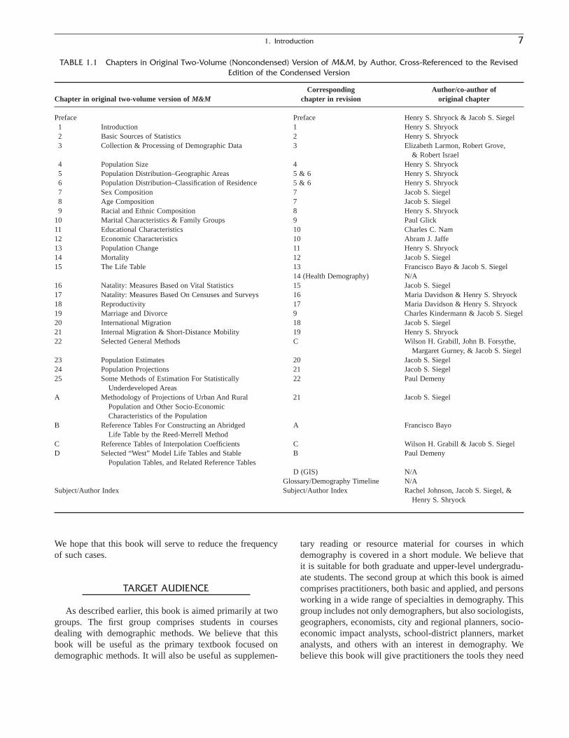
In addition to introducing new material, some reorgani-zation of the book’s original structure was carried out toreflect the changing concerns of demography and new tech-nological developments. Chapter 14, “Health Demography,”is new, and it reflects the growing interest in the interrela-tionship of health and demography, the recent application ofdemographic techniques to health data, and the emergenceof the field of the demography of aging. Another example is Appendix D, “Geographic Information Systems,” whichdeals with a technological innovation that occurred since theoriginal version was written. In addition, some chapters inthe original version were combined into single chapters. Inthe new edition, age composition and sex composition arecombined, as are educational and economic characteristics.The book’s reorganization is summarized in Table 1.1,which gives a “crosswalk” between chapters in the original(noncondensed) two-volume version of The Methods andMaterials of Demography, last published by the CensusBureau in 1980 and this revision. It includes the names ofthe authors of the chapters in the original two-volumeversion published in 1971. The new authors had freedom todraw on the original texts insofar they deemed this useful inpreparing the new texts; the extent to which they retainedthe original text was at their discretion. The inclusion ofTable 1.1 is intended to obviate the need for attribution orco-authorship, given the variable retention of the originaltext by the current authors.
Although mentioned in several places in this book, oneemerging area that we have not addressed in depth is the useof computer simulations in demographic analysis. This typeof calculation has been receiving much attention recently
and has the potential to be a powerful methodological devel-opment, but is so new that it is not yet possible to addressit in detail. It has primarily been used as a tool for popula-tion projections (Smith, Tayman, and Swanson, 2001), butit has also received attention as a tool for theory building(Burch, 1999; Griffiths, Matthews, and Hinde, 2000;Wachter, Blackwell, and Hammel, 1997). Another area wehave not addressed is demographic software. We decidedagainst covering this topic in depth for several reasons. First,software technology seemed to be undergoing a period ofrapid change as this volume was being prepared, and wewere fearful that any specific demographic software wecovered would be outdated by the time the book was pub-lished. The second reason is that we believed that the readercould implement any demographic method electronically,using standard, readily available spreadsheet and statisticalsoftware with only limited training and experience on com-puters. Third, we felt that, for the present purpose, it wasmore important to convey the logic of the methods ratherthan describe a device for accomplishing the result withoutthorough training as to its purpose and interpretation.
With respect to technological change, the reader shouldbear in mind that 30 years or so have passed since the orig-inal version of The Methods and Materials of Demographywas first published (Shryock and Siegel, 1971) and 25 yearshave passed since the publication of the condensed version(Shryock and Siegel, as condensed by Stockwell, 1976).During this period, demography as a field of study, like otherscientific disciplines and society in general, has been pro-foundly affected by technological change. In the 1970s,when the original and condensed editions were published,stand-alone mainframe computers run by “strange” com-puter languages were the norm. As both editors recall, thesecomputers were found only in large institutions. This meantthat access was profoundly limited and, even where pos-sible, an often frustrating experience for a demographerbecause of the slow speed with which a demographic pro-cedure could be carried out. Still, this was a major improve-ment over earlier days when an analytic procedure wascarried out with electrical and mechanical calculators, andeven paper and pencil. Today, networked personal comput-ers run by easily grasped commands are the norm. They arefound everywhere and access is virtually unlimited. Amongother things, this means that demographers now have greateraccess to data and, with the expanded computing power,many types of demographic analyses can be done veryquickly. The technological revolution, characterized by personal computers, online data sets, and tools for doingcomplex data analysis, has been responsible not only formethodological developments (e.g., computer simulation,which we discussed earlier in this section), but also for thediffusion of demographic data, materials, and methods. Thistrend is generally beneficial, but it can also contribute to anincrease in the number of inadequately conducted analyses.
6 Swanson and Siegel
1. Introduction 7
TABLE 1.1 Chapters in Original Two-Volume (Noncondensed) Version of , by Author, Cross-Referenced to the RevisedEdition of the Condensed Version
Corresponding Author/co-author ofChapter in original two-volume version of M&M chapter in revision original chapter
Preface Preface Henry S. Shryock & Jacob S. Siegel1 Introduction 1 Henry S. Shryock2 Basic Sources of Statistics 2 Henry S. Shryock3 Collection & Processing of Demographic Data 3 Elizabeth Larmon, Robert Grove,
& Robert Israel4 Population Size 4 Henry S. Shryock5 Population Distribution–Geographic Areas 5 & 6 Henry S. Shryock6 Population Distribution–Classification of Residence 5 & 6 Henry S. Shryock7 Sex Composition 7 Jacob S. Siegel8 Age Composition 7 Jacob S. Siegel9 Racial and Ethnic Composition 8 Henry S. Shryock
10 Marital Characteristics & Family Groups 9 Paul Glick11 Educational Characteristics 10 Charles C. Nam12 Economic Characteristics 10 Abram J. Jaffe13 Population Change 11 Henry S. Shryock14 Mortality 12 Jacob S. Siegel15 The Life Table 13 Francisco Bayo & Jacob S. Siegel
14 (Health Demography) N/A16 Natality: Measures Based on Vital Statistics 15 Jacob S. Siegel17 Natality: Measures Based On Censuses and Surveys 16 Maria Davidson & Henry S. Shryock18 Reproductivity 17 Maria Davidson & Henry S. Shryock19 Marriage and Divorce 9 Charles Kindermann & Jacob S. Siegel20 International Migration 18 Jacob S. Siegel21 Internal Migration & Short-Distance Mobility 19 Henry S. Shryock22 Selected General Methods C Wilson H. Grabill, John B. Forsythe,
Margaret Gurney, & Jacob S. Siegel23 Population Estimates 20 Jacob S. Siegel24 Population Projections 21 Jacob S. Siegel25 Some Methods of Estimation For Statistically 22 Paul Demeny
Underdeveloped AreasA Methodology of Projections of Urban And Rural 21 Jacob S. Siegel
Population and Other Socio-Economic Characteristics of the Population
B Reference Tables For Constructing an Abridged A Francisco BayoLife Table by the Reed-Merrell Method
C Reference Tables of Interpolation Coefficients C Wilson H. Grabill & Jacob S. SiegelD Selected “West” Model Life Tables and Stable B Paul Demeny
Population Tables, and Related Reference TablesD (GIS) N/A
Glossary/Demography Timeline N/ASubject/Author Index Subject/Author Index Rachel Johnson, Jacob S. Siegel, &
Henry S. Shryock
M&M
We hope that this book will serve to reduce the frequencyof such cases.
TARGET AUDIENCE
As described earlier, this book is aimed primarily at twogroups. The first group comprises students in coursesdealing with demographic methods. We believe that thisbook will be useful as the primary textbook focused ondemographic methods. It will also be useful as supplemen-
tary reading or resource material for courses in whichdemography is covered in a short module. We believe thatit is suitable for both graduate and upper-level undergradu-ate students. The second group at which this book is aimedcomprises practitioners, both basic and applied, and personsworking in a wide range of specialties in demography. Thisgroup includes not only demographers, but also sociologists,geographers, economists, city and regional planners, socio-economic impact analysts, school-district planners, marketanalysts, and others with an interest in demography. Webelieve this book will give practitioners the tools they need

to decide which data to use, which methods to apply, howbest to apply them, for which problems to watch, and howto deal with unforeseen problems. Members of either of thetwo target groups should note that most of the book does notrequire a strong background in mathematics or statistics,although it assumes that readers have at least a basic knowl-edge of both subjects. Some chapters and appendixes,however, are quite mathematical or statistical in nature (i.e.,Chapters 17 and 22, and Appendix C) and may require addi-tional training and practice to comprehend fully.
References
Burch, T. 1999. “Computer Modelling of Theory: Explanation for the 21stCentury.” Discussion Paper No. 99-4. Population Studies Centre, Uni-versity of Western Ontario, London, Canada.
Burch, T. 2001a. “Data, Models, Theory, and Reality: The Structure ofDemographic Knowledge.” Paper prepared for the workshop “Agent-Based Computational Demography.” Max Planck Institute for Demo-graphic Research, Rostock, Germany, February 21–23 (Revised draft,March 15).
Burch, T. 2001b. “Teaching the Fundamentals of Demography: A Model-Based Approach to Family and Fertility.” Paper prepared for theseminar on Demographic Training in the Third Millennium, Rabat,Morocco, May 15–18 (Draft, January, 29).
California 1998. County Population Projections with Race/Ethnic Detail.By M. Heim and Associates. Sacramento, CA: State of California,Department of Finance.
Canada Statistics. 1994. Population Projections for Canada, Provinces,and Territories, 1993–2016. By M. V. George, M. J. Norris, F. Nault,S. Loh, and S. Dai. Catalogue No. 91-520. Ottawa, Canada: Demogra-phy Division, Statistics Canada.
DaVanzo, J., and P. Morrison. 1981. “Return and Other Sequences ofMigration in the United States.” Demography 18: 85–101.
George, M. V. 1999. “On the Use and Users of Demographic Projectionsin Canada”. Joint ECE-EUROSTAT Workshop on Demographic Pro-jections, Perugia, Italy, May 1999. ECE Working Paper No. 15, Geneva.
Greenwood, M. 1997. “Internal migration in developed countries.” In M.Rosenzweig and O. Stark (Eds.), Handbook of Population and FamilyEconomics (pp. 647–720). Amsterdam, The Netherlands: ElsevierScience Press.
Griffiths, P., Z. Matthews, and A. Hinde, 2000. “Understanding the Sex Ratio in India: A Simulation Approach.” Demography 37: 477–488.
Keyfitz, N. 1975. “How Do We Know the Facts of Demography?” Popu-lation and Development Review 1: 267–288.
Kintner, H., and D. Swanson. 1994. “Estimating Vital Rates from Corpo-rate Data Bases: How Long Will GM’s Salaried Retirees Live?” In H.Kintner, T. Merrick, P. Morrison, and P. Voss (Eds.) Demographics: ACasebook for Business and Government (pp. 265–295). Boulder, CO:Westview Press.
Massey, D., R. Alarcon, R. Durand, and H. Gonzales. 1987. Return toAztlan: The Social Process of International Migration from WesternMexico. Berkeley, CA: University of California Press.
Morrison, P. 2002. “The Evolving Role of Demography in the U.S. Busi-ness Arena.” Paper presented at the 11th Biennial Conference of theAustralian Population Association, Plenary Session on Population andBusiness, Sydney, Australia, October 2–4.
Shryock, H., J. Siegel, and Associates. 1971. The Methods and Materialsof Demography. Washington, DC: U.S. Census Bureau/U.S. Govern-ment Printing Office.
Shryock, H., J. Siegel, and E. G. Stockwell. 1976. The Methods and Mate-rials of Demography, Condensed Edition. New York: Academic Press.
Siegel, J. 2002. Applied Demography: Applications to Business, Govern-ment, Law, and Public Policy. New York, NY: Academic Press.
Smith, S., J. Tayman, and D. Swanson. 2001. State and Local PopulationProjections: Methodology and Analysis. New York: Kluwer Academic/Plenum Press.
Swanson, D., T. Burch, and L. Tedrow. 1996. “What Is Applied Demogra-phy?” Population Research and Policy Review 15 (December):403–418.
U.S. Bureau of the Census. 1996. “Population Projections for States by Age,Sex, Race, and Hispanic Origin: 1995 to 2050.” By P. Campbell. ReportPPL-47. Washington, DC: U.S. Census Bureau.
Wachter, K, D. Blackwell, and E. A. Hammel. 1997. “Testing the Validityof Kinship Microsimulation.” Journal of Mathematical and ComputerModeling 26: 89–104.
8 Swanson and Siegel

To understand and analyze the topics and issues ofdemography, one must have access to appropriate statistics.The availability of demographic statistics has increased dramatically since the 1970s as a result of improved andexpanded collection techniques, vast improvements in com-puting power, and the growth of the Internet.
Demographic statistics may be viewed as falling into twomain categories: primary and secondary. Primary statisticsare those that are the responsibility of the analyst and havebeen generated for a very specific purpose. The generationof primary statistics is usually very expensive and time-consuming. The advantages of primary data are that they aretimely and may be created to meet very specific data needs.Secondary statistics differ in that they result from furtheranalysis of statistics that have already been obtained. Theseare regarded as data disseminated via published reports, the Internet, worksheets, and professional papers. These data may be disseminated freely, as is the case with publicrecords, or for a charge, as with data clearinghouses. Theirbenefit is that they generally save a great deal of time andcost. The drawback is that data are usually collected with a specific purpose in mind—sometimes creating bias. Addi-tionally, secondary data are, by definition, old data (Stewartand Kamins, 1993, p. 2).
Statistics may be viewed as having two uses: descriptiveand inferential. Descriptive statistics are a mass of data thatmay be used to describe a population or its characteristics.Inferential statistics, on the other hand, are a mass of datafrom which current or future inferences about a populationor its characteristics may be drawn (Mendenhall, Ott, andLarson, 1974).
Whether the statistics are primary or secondary, or des-criptive or inferential, the analyst must consider a number ofissues. The first is validity, which asks, do the data accuratelyrepresent what they claim to measure? The next is reliability,which asks, are the data externally and internally measured
consistently? The third is that of data privacy and data sup-pression. As data users have acquired ever more sophisti-cated analytical techniques and computing power, resistanceto access of private and government databases has been met.As the public faces a proliferation of requests for informationabout themselves and concerns mount about who may gainaccess to the information, resistance is building to participa-tion in surveys and others data retrieval efforts (Duncanet al., 1993, p. 271). In an era when theoretically “private”information about persons and their characteristics are easilyavailable through legitimate data clearinghouses (as well asless reputable sources), the analyst must thoroughly considerwhether the use of statistics is ethical, responsible, or in anyway violates confidentiality or privacy.
These issues have come into focus with the advent of theInternet. In the electronic arena of the Internet, anyone caneasily publish or access large quantities of social statistics.Unlike conventional publications and journals, these datacan hardly be reviewed, monitored or regulated by the statistics professor. The challenge for the analyst, given thevast quantity and array of statistics available from officialand unofficial sources on the Internet, is to be prudent in hisor her selection of the appropriate statistics. This may bedone by verifying the origin of the statistics, reviewingmethods and materials used in creating the data, makingdeterminations about the acceptable level of validity andreliability, then proceeding with considerations of ethicaluse and privacy. Analysts are warned to avoid unofficial sta-tistical sources, as well as data that cannot be verified or areafforded no corresponding documentation.
TYPES OF SOURCES
The sources of demographic statistics are the publishedreports, unpublished worksheets, data sets, and so forth that
9
C H A P T E R
2
Basic Sources of Statistics
THOMAS BRYAN
The Methods and Materials of DemographyCopyright 2003, Elsevier Science (USA).
All rights reserved.
are produced by official or private agencies through a varietyof media. The sources may simply report primary statistics,or they may additionally include text that describes how thestatistics are organized, and how the statistics were obtained,or an analysis that describes how valid or reliable the sta-tistics are deemed to be. These sources may also containdescriptive or inferential material based on the statistics theycontain. If the report is printed, descriptions or analysis ofstatistics may include graphical material, such as tables,charts, or illustrations. If the statistics have been released aspart of an electronic package or are available on the Inter-net, it is oftentimes possible for the analyst to generate customized graphics, tables, or charts.
The same statistics may be selectively reproduced orrearranged in secondary sources such as compendia, statis-tical abstracts, and yearbooks. Other secondary sources thatpresent some of these statistics are journals, textbooks, andresearch reports. Occasionally, a textbook or research reportmay include demographic statistics based on the unpub-lished tabulations of an official agency.
Many important demographic statistics are produced bycombining census and vital statistics. Examples are vitalrates, life tables, and population estimates and projections.Data gathered in population registers and other administra-tive records, such as immigration and emigration statistics,school enrollment, residential building permits, and regis-tered voters, may also provide the basis for population esti-mates and other demographic analysis.
Primary Demographic Data and Statistics
Primary demographic data are most commonly gatheredor aggregated at the national level. A country may have acentral statistical office, or there may be separate agenciesthat take the census and compile the vital statistics. Evenwhen both kinds of statistics emanate from the same agency,they are usually published in separate reports, reflecting the fact that censuses are customarily taken decennially orquinquennially and vital statistics are compiled annually ormonthly.
In some countries, subnational areas such as provinces orstates may have important responsibilities in conducting acensus or operating a registration system. Data gathered bythese regions may be for the sole use of the regions, or theymay be gathered for a central national office. The centraloffice may play a range of roles in the analysis and report-ing of regional statistics, from simply collecting and report-ing statistics that were tabulated in the provincial offices, to collecting the original records or abstracts and making its own tabulations. In either situation, both national andprovincial offices may publish their own reports and tabula-tions. Statistics from different governmental sources mayvary with respect to their arrangement, detail, and choice ofderived figures. Moreover, what purport to be comparable
statistics may differ because of variations in classification orediting rules, varying definitions, or because of processingerrors.
Demographic data may be collected either through cen-suses and surveys or through a population register. A popu-lation register in its complete form is a national system ofcontinuous population accounting involving the recording ofvital events and migrations as they occur in local communi-ties. The purpose of the census or survey is simply to producedemographic statistics. The registration of vital events andpopulation registers, on the other hand, may be at least asmuch directed toward the legal and administrative uses of itsrecords. In fact, the compilation and publication of statisticsfrom a population register may be rather minimal, partlybecause these activities tend to disturb the day-to-day opera-tion of the register. Even though the equivalent of census statistics could be compiled from a population register, thecountries with registers still find it necessary to conduct censuses through the usual method of enumerating all house-holds simultaneously. This partial duplication of data-gathering is justified as a means of making sure that the reg-ister is working properly and of including additional items(characteristics) beyond those recorded in the register. Thereare often restrictions imposed on the public’s access to theindividual census or registration records in order to protectthe privacy and interests of the persons concerned and toencourage complete and truthful reporting.
Statistics Produced from Combinations ofCensus and Registration Data
Some examples of data and measures based on combina-tions of population figures from a census with vital statisticswere given earlier. Rates or ratios that have a vital event asthe numerator and a population as the denominator are themost obvious type. The denominator may be a subpopula-tion, such as the number of men 65-to-69-years old (e.g.,divided into the number of deaths occurring at that age) orthe number of women 15-to-44-years old (e.g. divided intothe total number of births). Moreover, the population maycome from a sample survey or a population estimate, whichin turn was based partly on past births and deaths.
Products of more complex combinations include currentpopulation estimates, life tables, net reproduction rates, esti-mates of net intercensal migration, and estimates of relativecompleteness of enumeration in successive censuses. Thecomputation of population projections by the so-called com-ponent method starts with a population disaggregated by ageand sex, mortality rates by age and sex, and fertility rates byage of mother. There may be a series of successive compu-tations in which population and vital statistics are introducedat one or more stages.
All of these illustrative measures can be produced by thecombination of statistics. A different approach is to relate
10 Bryan

the individual records. This is the approach taken in match-ing studies. By matching birth certificates, infant death cer-tificates, and records of babies born in the correspondingperiod of time in the census, one can estimate both the pro-portion of births that were not registered and the proportionof infants who were not counted in the census. Other statis-tics of demographic value can be obtained by combining theinformation from the two sources for matched cases in orderto obtain a greater number of characteristics for use in thecomputation of specific vital rates. For example, if educa-tional attainment is recorded on the census schedule but isnot called for on the death certificate, a matching study canyield mortality statistics for persons with various levels ofeducational attainment. When the same characteristic, suchas age, is called for on both documents, the matching studiesyield measures of the consistency of reporting.
In a country with a population register, matching studieswith the census also can be carried out. Again, the resultingstatistics could be either of the evaluative type or couldproduce cross-classifications of the population based on agreater number of characteristics than is possible from eithersource alone.
Secondary Sources
Secondary sources may be either official or unofficial andinclude a wide variety of textbooks, yearbooks, periodicaljournals, research reports, gazetteers, and atlases. In thissection, only a few of the major sources of population sta-tistics are mentioned. These statistics address the populationand its components, as well as demographic aspects that canaffect these elements, such as health and migration statistics.
International Data
Oftentimes demographic analysts are faced with thedaunting task of gathering or relating information on asubject that they have never analyzed or on which theyperhaps have limited knowledge of all possible sources. Inthese cases, it is best to pursue an index of statistics, whichcan provide information by subject, geography, author, ormethod. Many countries publish their own indices, whileothers provide a more comprehensive international perspec-tive. An example is the Index to International Statistics(IIS), published by the U.S. Congressional InformationService. Begun in 1983, the IIS lists statistical publicationson economics, industry, demography, and social statistics by international intergovernmental organizations, such asthe United Nations, Organization for Economic Cooperationand Development, the European Union, the Organization ofAmerican States, commodity organizations, developmentbanks, and other organizations. The United Nations alsopublishes the Directory of International Statistics (DIS). Thedirectory is divided in two parts: The first part provides
statistics by subject matter and the second part provides aninventory of machine-readable databases of economic andsocial statistics by subject and by organization (UnitedNations, 1982a).
Additional indexes and resources may be accessed overthe Internet. Conventions on the Internet may change overtime, and hence the analyst is advised to use the referencesherein with caution.1 If over time these addresses are modified, then the analyst is encouraged to use a “searchengine” to find new addresses and reference material. Someof the best resources on the Internet are supported by thefollowing three agencies: the United Nations (un.org), thePopulation Reference Bureau (prb.org), and the Inter-national Programs Center of the U.S. Census Bureau(census.gov/ipc/www).
Of all producers of secondary demographic statistics forthe countries of the world, the United Nations is the mostprolific. Its relevant publications include the following:
The Demographic Yearbook (published since 1948) pres-ents basic population figures from censuses or estimates, andbasic vital statistics yearly, and in every issue it features aspecial topic that is presented in more detail (e.g., natalitystatistics, mortality statistics, population distribution, popu-lation censuses, ethnic and economic characteristics of pop-ulation, marriage and divorce statistics, population trends).Demographers, economists, public health workers, and sociologists have found the Yearbook a definitive source ofdemographic and population statistics. About 250 countriesor regions are represented. The first group of tables com-prises a world summary of basic demographic statistics. Thissummary is followed by statistics on the size, distribution,and trends in population, fertility, fetal mortality, infant andmaternal mortality, and general mortality.
The Statistical Yearbook (published since 1948) containsfewer demographic series than the foregoing, but alsoincludes four tables of manpower statistics. The Yearbook
2. Basic Sources of Statistics 11
1 The Internet is a global collection of people and computers that arelinked together. The Internet is physically a network of networks. It con-nects small computer networks by using a standard or common protocol(i.e. TCP/IP), which allows different networks worldwide to communicatewith one another. Several important services are provided by the Internet.E-mail, allows users to send messages and electronic files via a computerthat is connected to the Internet. File transfer protocol, or FTP, allows usersto copy files from one Internet host computer to another. Telnet is a servicethat allows a user to connect to remote machines via the Internet network.Gopher is a program that allows a user to browse the resources of the Inter-net. The World Wide Web (www) is a graphics-based interface with whichthe user can access Internet resources through convenient “trails” of infor-mation. The development of the Internet through the 1990s has been rapid.With this growth, there has been no assurance that the Internet will main-tain the same format or protocols for any period of time. Specific Internetaddresses are given in this chapter in parenthesis, with a “www” precursorimplied. To derive the most benefit from the Internet, analysts are encour-aged to acquaint themselves with the organizations, concepts, and logicintrinsic to the Internet, rather than memorizing or referencing specificaddresses.

is a comprehensive compendium of internationally compar-able data for the analysis of socioeconomic development at the world, regional, and national levels. It provides data on the world economy, its structure, major trends, and current performance, as well as on issues such as worldpopulation, employment, inflation, production of energy,supply of food, external debt of developing countries, education, availability of dwellings, production of energy,development of new energy sources, and environmental pollution and management.
The Population Bulletin of the United Nations providesinformation periodically on population studies, gives aglobal perspective of demographic issues, and presents ananalysis of the direct and indirect implications of populationpolicy.
World Population Prospects provides population esti-mates and projections; it has been published irregularly since1951. The most recent, World Population Prospects: 1998Revision, presents population estimates from 1950 to 1995and projections from 1995 to 2050. With the projectionhorizon extended to the year 2050, this publication presentsa full century of demographic history/projections (1950–2050). Of the three parts, part I discusses fertility decline andhighlights the demography of countries with economies intransition and the potential demographic impact of the AIDSepidemic in these countries, part II presents a world andregional overview of both historical and recent trends in pop-ulation growth and their demographic components, and partIII provides information on the more technical aspects of thepopulation estimates and projections.
In addition to these international indices and compendia,numerous countries publish their own statistical abstracts, asseen in Appendix 1 (U.S. Bureau of the Census, 2003, p.906). Several United States agencies also publish interna-tional population statistics. The primary U.S. producer is theCensus Bureau. The International Programs Center (IPC),part of the Population Division of the U.S. Census Bureau,conducts demographic and socioeconomic studies and streng-thens statistical development around the world through technical assistance, training, and production of softwareproducts. The IPC provides both published and unpublishedreports, as well as interactive databases for numerous inter-national demographic subjects, including the series listedhere. Access to much of these data may be gained throughthe IPC website at census.gov/ipc/www.
The published reports of the IPC include the following:
World Population Profile, Series WP, published irregularlysince 1985, presents a summary of world anddemographic trends, with special topics (e.g.,HIV/AIDS) and tables of data by region and country.
International Population Reports, Series IPC, (formerly P-95 and P-91) published irregularly, looks at differentpopulation topics in detail.
International Briefs, Series IB (formerly PopulationTrends, Series PPT) published irregularly, gives anoverview of selected topics or countries.
Women in Development, Series WID, covers aspects ofgender differentials.
Aging Trends, published irregularly, shows the impact ofpopulation aging on different countries.
Economic Profiles, published irregularly, focuses on thecountries of the former Soviet Union. The profilesprovide a description of the geography, population, andeconomy of the selected country.
Miscellaneous Reports
Unpublished reports of the IPC include the following:
Staff Papers, Series SP, published irregularly, examinessubjects of special interest to the staff of the IPC.
Health Studies Research Notes, biannual publication,presents information on AIDS and HIV.
Eurasia Bulletin, published irregularly, examines andinterprets new and existing data sets produced bystatistical organizations of Eastern Europe, the formerSoviet states, and Asia.
The International Data Base (IDB) is a computerized data bank containing statistical tables of demographic andsocioeconomic data for all countries of the world. It isaccessible through the IPC website. Data in the IDB areobtained from censuses and surveys (e.g., population by age and sex, labor force status, and marital status), fromadministrative records (e.g., registered births and deaths), orfrom the population estimates and projections produced byIPC. Where possible, data are obtained on urban/rural resi-dence. These reported data are entered for available yearsfrom 1950 to the present. The U.S. Census Bureau analyzesthe data and produces consistent estimates of fertility, mor-tality, migration, and population. Based on these analysesand on assumed future trends in fertility, mortality, andmigration, population projections are made to the year2050.
Of nongovernmental demographic and statisticalresources, the Population Reference Bureau (PRB) is mostprominent. Founded in 1929, the PRB is America’s oldestpopulation organization. The PRB, at PRB.org, publishes a monthly newsletter called Population Today, a quarterlytitled the Population Bulletin, and the annual World Popu-lation Data Sheet. PRB also produces specialized publica-tions covering population and public policy issues in theUnited States and in other countries.
The Population Association of America (PAA) is perhapsone of the best statistical resources and forums of discussionon international demography. The Population Index, whichis published quarterly by the Office of Population Researchat Princeton University (popindex.princeton.edu) for thePAA, has appeared since 1937. The editors and staff produce
12 Bryan
some 3500 annotated citations annually for the journal. Theindex covers all fields of interest to demographers, includ-ing historical demography, demographic and economicinterrelations, research methology, and applied demography,as well as the core fields.
United States
As there are numerous data sources for the United States, it may be prudent for the analyst to review statisticalindices prior to pursuing research and analysis. An exampleof such an index is the American Statistics Index (ASI),published annually, with monthly and quarterly updates, bythe U.S. Congressional Information Service (CIS). Theindex is a comprehensive guide to statistical publications of the U.S. government. It features all publications thatcontain comparative tabular data, by geographic, economic,and demographic categories (Stewart and Kamins, 1993).Additional sources include the Monthly Catalog of U.S.Government Publications and the Index to U.S. GovernmentPeriodicals.
As with international statistics, there are also multipleindices and directories of United States statistics on theInternet. The Federal Technology Service maintains the“Government Information Xchange” on the Internet atinfo.gov; it links data users with resources from the federalgovernment to local governments. The Federal InteragencyCouncil on Statistical Policy maintains the Fedstats page onthe Internet at fedstats.gov; it provides public access to statistics produced by more than 70 agencies in the UnitedStates federal government. Aside from these resources,searches for statistics may be conducted on the Internetusing a search engine.
The U.S. Census Bureau is the most prolific producer ofdemographic statistics for the United States. It is commonlythought of only in the context of the primary statistics pro-duced by the decennial census, but the U.S. Census Bureauis responsible for generating and publishing a great deal ofdemographic statistics of other types. These statistics aregenerally based on the series of ongoing surveys that it con-ducts. These include the Current Population Survey (CPS),the American Housing Survey (AHS), and the Survey ofIncome and Program Participation (SIPP), among others.The results of these surveys and other census data tabula-tions can be found in the following compendia:
Statistical Abstract of the United States. Publishedannually since 1878, the most comprehensivetabulation of statistics on the nation and states.Contains recent time series data at multiple geographiclevels. Also includes “Guide to Sources,” withreferences to statistical sources arranged alphabeticallyby subject.
County and City Data Book. Published approximatelyevery 5 years since 1939, provides most recent
population, housing, business, agriculture, andgovernmental data for small geographic areas.
State and Metropolitan Area Data Books. Patterned afterthe County and City Data Book and published in 1979,1982, 1986, 1991, and 1998; provides state rankingsfor more than 1900 statistical items and metropolitanarea rankings for 300 statistical items.
Congressional District Data Book. Similar to County andCity Data Book, but provides data for congressionaldistricts. Includes a congressional district atlas.
Access to these and other Census Bureau publications maybe made by searching the Census Bureau’s website atcensus.gov. For lists of publications, see the CensusCatalogue and Guide, published quarterly.
CENSUSES AND SURVEYS
The distinction between a population census and a pop-ulation survey is far from clear-cut. At one extreme, a com-plete national canvass of the population would always berecognized as a census. At the other extreme, a canvass ofselected households in a village to describe their living con-ditions would probably be regarded as a social survey. Butneither the mere use of sampling nor the size of the geo-graphic area provides a universally recognized criterion.Most national censuses do aim at a complete count or listingof the inhabitants. Sampling is also used at one or morestages for purposes of efficiently collecting detailed charac-teristics of the entire population. When the U.S. CensusBureau, at the request and expense of the local government,takes a canvass of the population of a village with 100 inhab-itants, it has no hesitation in calling the operation “a specialcensus.” The main objective of a population census is thedetermination of the number of inhabitants. The definitionused by the United Nations is as follows: “A census of pop-ulation may be defined as the total process of collecting,compiling, evaluating, analyzing and publishing or otherwisedisseminating demographic, economic and social data per-taining, at a specified time, to all persons in a country ordelimited part of a country” (United Nations 1998c, p. 3). Inmany modern population censuses, numerous questions arealso asked about social and economic characteristics as well.
Most modern population censuses are associated with ahousing census as well, which is defined by the UnitedNations as “the total process of collecting, compiling, eval-uating, analyzing and publishing or otherwise disseminatingstatistical data pertaining, at a specified time, to all livingquarters and occupants thereof in a country or in a well-delimited part of a country” (United Nations, 1998c, p. 3).
A survey, on the other hand, is a collection of standard-ized information from a specific population, or a samplefrom one, usually but not necessarily by means of question-naire or interview (Robson, 1993, p. 49). The main purpose
2. Basic Sources of Statistics 13

of a survey is to produce statistics about some aspects orcharacteristics of a study population (Fowler, 1993, p. 1).There are three distinct strands in the historical developmentof survey research: government/official statistics, academic/social research, and commercial/advertising research (Lyberg,1997, pp. 1–2). Today, each brings to the field of surveys aunique perspective on approach, methods, errors, analysis,and conclusions.
The line between census and survey is further blurred bythe concept of error. A census that failed to enumerate 100%of the population and its characteristics is, by definition, anincomplete census. Surveys have often been used in orderto determine the amount of error in censuses. For example,following the 1991 population census in England and Wales,a census validation survey (CVS) was carried out to assessboth the coverage and the quality of the census (Lyburg,1997, p. 633). Similar evaluative measures were taken withthe post-enumeration survey (PES) following the 1990 U.S.census and the Accuracy and Coverage Evaluation (ACE)Survey following the 2000 U.S. census.
The typical scope of a census or demographic survey isthe size, distribution, and characteristics of the population.In countries without adequate registration of vital events,however, a population census or survey may include ques-tions about births or deaths of household members in theperiod (usually the year) preceding the census. Moreover,even when vital statistics of good quality exist, the censusor survey may include questions on fertility (e.g., childrenever born, children still living, date of birth of each child)because the distribution of women by number of childrenever born and by interval between successive births cannotbe discovered from birth certificates.
Of special interest are the periodic national samplesurveys of households that have been established in anumber of countries. These may be conducted monthly,quarterly, or only annually. In some countries, they havebeen discontinued after one or two rounds because of finan-cial or other problems. Usually the focus of these surveys ison employment status, housing and household characteris-tics, or consumer expenditures attributable to certain limiteddemographic characteristics, rather than the demographicinformation itself.
Both censuses and surveys have also tended to grow inthe range of topics covered, in sophistication of procedures,in accuracy of results, and in the volume of statistics madeavailable to the public.
History of Census Taking
Census taking began at least 5800 years ago in Egypt,Babylonia, China, Palestine, and Rome (Halacy, 1980, p. 1)Few of the results have survived, however. The counts ofthese early censuses were undertaken to determine fiscal,
labor, and military obligations and were usually limited toheads of households, males of military age, taxpayers, oradult citizens. Women and children were seldom counted.
There may have been a Chinese census as early as 3000bc, but only since 2300 bc have there been tax records andtopographical data indicating the existence of formalrecords (Halacy, 1980, p. 17). The first of two enumera-tions mentioned in the Bible is assigned to the time of theExodus, 1491 bc. The second was taken at the order ofKing David in 1017 bc. The Roman censuses, taken quin-quennially, lasted about 800 years. Citizens and their prop-erty were inventoried for fiscal and military purposes. Thisenumeration was extended to the entire Roman Empire in5 bc. The Domesday inquest ordered by William I ofEngland in 1086 covered landholders and their holdings.The Middle Ages, however, were a period of retrogressionin census taking throughout Europe, North Africa, and theNear East.
As Kingsley Davis pointed out, it is hard to say when thefirst census in the modern sense was undertaken since cen-suses were long deficient in some important respects (Davis,1966, pp. 167–170). The implementation of a “first” censusis obfuscated by conflicting definitions. Nouvelle France(later Quebec) and Acadia (later Nova Scotia) had enumer-ations between 1665 and 1754. In Europe, Sweden’s censusof 1749 is sometimes regarded as the first, but those in someof the Italian principalities (Naples, Sicily, etc.) go back intothe l7th century. The clergy in the established LutheranChurch of Sweden had been compiling lists of parishionersfor some years prior to the time when it was required to takeannual (or later triennial) inventories. Whereas in Scandi-navia this ecclesiastical function evolved into populationregisters and occasional censuses, the parish registers ofbaptisms, marriages, and burials in England evolved into avital statistics system, as will be described later in thischapter.
Spain conducted its first true census in 1798, withEngland and France following shortly in 1801. Russiaattempted a census in 1802, but failed to establish a workingsystem until 1897. Though Norway had been performingpopulation counts since 1769, its first complete census wasnot conducted until 1815. Greece soon followed, with acensus in 1836, then Switzerland in 1860, and Italy in 1861.
In summary, the evolution of the modern census was agradual one. The tradition of household canvasses or popu-lation registration often had to continue for a long timebefore the combination of public confidence, administrativeexperience, and technology could produce counts that metmodern standards of completeness, accuracy, and simul-taneity. Beginning with objectives of determining military,tax, and labor obligations, censuses in the 19th centurychanged their scope to meet other administrative needs aswell as the needs of business, labor, education, and academic
14 Bryan

research. New items included on the census questionnairereflected new problems confronting state and society.
International Censuses
In developing countries, the availability of data hasimproved greatly in recent decades. All countries haveexpanded and strengthened the capabilities of their statisti-cal offices, including activities related to information onpopulation. Most countries have started to take populationcensuses, as well as housing, agricultural, and industrial cen-suses (U.S. Census Bureau/Arriaga et al., 1994, p. 1).
The classification and comparison of international cen-suses is a difficult task. Definitions of subjects, methods of data collection and aggregation, even language can allpresent problems in interpretation and use. The UnitedNations presents four major criteria for a census: individualenumeration, universality within a defined territory, sim-ultaneity, and defined periodicity. Given these standards,there are valid reasons why some countries cannot strictlyadhere to them and hence qualify as “census takers” (Goyer, 1980).
There are two excellent sources of international censusstatistics. The first is the Population Research Center (PRC)at the University of Texas. Founded in 1971, the PRC holdsthe results of over 80% of population censuses conductedworldwide. The PRC has an online international censuscatalog, available at prc.utexas.edu. The other compre-hensive source of international census statistics is the Handbooks of National Population Censuses (Goyer andDomschke, 1983–1992). The handbooks provide a detailedanalysis of the history of census taking in Latin America andthe Caribbean, North America, Oceania, Europe, Asia, andAfrica.
International Surveys
There are few true worldwide demographic surveys. Thelogistics of including all countries in a survey are simply tooformidable. A few efforts exist, however. The World Fertil-ity Survey (WFS), conducted by the International StatisticsInstitute (ISI), has reported cross-national summaries of fer-tility and other demographic characteristics from a widerange of countries since 1980.2 Another well-known inter-national survey program is the worldwide Demographic andHealth Surveys Program. Funded by the U.S. Agency forInternational Development (USAID) and implemented byMacro International, Inc., the surveys are designed to collectdata on fertility, family planning, and maternal and childhealth, and can be accessed through the Internet as well as
in published reports. See info.usaid.gov and measurepro-gram.org. The DHS has provided technical assistance formore than 100 health-related surveys in Africa, Asia, theNear East, Latin America, and the Caribbean. Surveys areconducted by host-country institutions, usually governmentstatistical offices.
Throughout the latter part of the past century, numeroushealth surveys related to particular health subjects and theireffects (such as AIDS), as well as health studies particularto specific regions of the world, were taken. The analyst isencouraged to search the Internet or contact the agenciesnoted earlier for the latest information.
Demographic surveys around the world are reported bythe United Nations in its Sample Surveys of Current Inter-est (United Nations, 1963). Surveys selected for the publi-cation vary depending on the country or area represented,the subject represented, the amount of information provided,and the sample design. The publication is organized bycountry and subject matter, with detailed explanations of thesurveys and their results.
Censuses in the United States
Population censuses developed relatively early in theUnited States. There were 25 colonial enumerations withinwhat is now the United States, beginning with a census ofVirginia in 1624–1625. The second census, however, did nottake place until 1698. Colonial censuses continued through-out the New England and Mid-Atlantic area through 1767.Colonial censuses were distinguished from the first U.S.census in that they enumerated American Indians. Manycolonies also enumerated blacks. The first census of theUnited States was conducted in 1790, and a scheduled roundhas never been missed since its inception.
Decennial Censuses
The U.S. census of population has been taken regularlyevery 10 years since 1790 and was one of the first to bestarted in modern times. At least as early as the 1940s, therehave been demands for a quinquennial census of popula-tion—the frequency in a fair number of other countries—but so far no mid-decade census has ever been mandated andsupported with appropriated funds by the Congress. TheU.S. decennial census is currently mandated by the Consti-tution, Article I, Section 2, and authorized by Title 13 of theU.S. code, enacted on August 31, 1954.
Evolution of the Population Census Schedule
The area covered by the census included the advancingfrontier within continental United States. Each outlying territory and possession has been included also, but the
2. Basic Sources of Statistics 15
2 Comparative studies are available through the International Statistical Institute, 428 Beatrixlaan, P.O. Box 950 2270 AZ, Voorburg, Netherlands.

TABLE 2.1 Questions Included in Each Population Census in the United States: 1790 to 2000
16 Bryan
Census of 1790
Name of head of family, free white males 16 years and over, free whitemales under 16, free white females, slaves, other persons, and occupation5 years ago, vocational training, and additional particulars designed toimprove the classification of occupation.
Census of 1800
Name of head of family, if white, age and sex, race, slaves.
Census of 1810
Name of head of family, if white, age, sex, race, slaves.
Census of 1820
Name of head of family, age, sex, race, foreigner not naturalized, slaves,industry (agriculture, commerce, and manufactures).
Census of 1830
Name of head of family, age, sex, race, slaves, deaf and dumb, blind,foreigners not naturalized.
Census of 1840
Name of head of family, age, sex, race, slaves, number of deaf anddumb, number of blind, number of’ insane and idiotic, whether in publicor private charge, number of person in each family employed in each ofsix classes of industry and one of occupation, literacy, pensioners forRevolutionary or military service.
Census of 1850
Name, age, sex, race, whether deaf and dumb, blind, insane, or idiotic,value of real estate, occupation, place of birth, whether married withinthe year, school attendance: literacy, whether a pauper or convict.
Supplemental schedule: for slaves, public paupers, and criminals,persons who died during the year.
Census of 1860
Name, age, sex, race, value of real estate, value of personal estate,occupation, place of birth, whether married within the year, schoolattendance, literacy, whether deaf and dumb, blind, insane, idiotic,pauper, or convict.
Census of 1870
Name, age, sex, race, occupation, value of real estate, value of personalestate, place of birth, whether parents were foreign born, month of birthif born within the year, month of marriage if married within the year,school attendance, literacy, whether deaf and dumb, blind, insane, oridiotic, male citizens 21 and over, and number of such person denied theright to vote for other than rebellion.
Supplemental schedules: for persons who died during the year,paupers, prisoners.
Census 1880
Address, name, relationship to head of family, sex, race, age, maritalstatus, month of birth if born within the census year, married within theyear, occupation, number of months unemployed during year, sickness ortemporary disability, whether blind, deaf and dumb, idiotic, insane,maimed, crippled, bedridden, or otherwise disabled, school attendance,literacy, place of birth of person and parents.
Supplemental schedules: for the Indian population, for persons whodied during the year, insane, idiots, deaf-mutes, blind, homeless, children,prisoners, paupers, and indigent persons.
Census of 1890
Address, name, relationship to head of family, race, sex, age, maritalstatus, number of families in house, number of persons in house, numberof persons in family, whether a soldier, sailor or marine during Civil War(Union or Confederate) or widow of such a person, whether marriedduring census year, for women, number of children born, and numbernow living, place of birth of person and parents, if foreign born, numberof years in the United States, whether naturalized or whethernaturalization papers had been taken out, profession, trade, or occupation,months unemployed during census year, months attended school duringcensus year, literacy: whether able to speak English, and if not, languageor dialect spoken, whether suffering from acute or chronic disease, withname of disease and length of time afflicted, whether defective in mind,sight, hearing, or speech, or whether crippled, maimed, or deformed, withname of defect whether a prisoner, convict, homeless child, or pauper,home rented or owned by head or member, of family, if owned by heador member, whether mortgaged, if head of family a farmer, whether farmrented or owned by him or member of his family, if owned, whethermortgaged, if mortgaged, post office address of owner.
Supplemental schedule: for the Indian population, for persons whodied during the year, insane, feeble-minded and idiots, deaf, blind,diseased and physically defective, inmates of benevolent institutions,prisoners, paupers, and indigent persons, surviving soldiers, sailors, andmarines, and widows of such, inmates of soldier’s’ homes.
Census of 1900
Address, name, relationship to head of family, sex, race, age, month andyear of birth, marital status, number of years married, for women,number of children born and number now living, place of birth of personand parents, if foreign born, year of immigration to the United States,number of years in the United States, and whether naturalized,occupation, months not employed, months attended school during censusyear, literacy, ability to speak English.
Supplemental schedules: for the blind and for the deaf.
Census of 1910
Address, name, relationship to head of family, sex, race, age, maritalstatus, number of years of present marriage, for women, number ofchildren born and number now living, place of birth and mother tongueof person and parent, if foreign born, year of immigration, whethernaturalized or alien, or whether able to speak English or if not, languagespoken, occupation, industry, and class of worker, if an employee,whether out of work on census day, and number of weeks out of workduring preceding year, literacy, school attendance, home owned or rented,if owned, whether mortgaged, whether farm or house, whether a survivorof Union or Confederate Army or Navy, whether blind or deaf and dumb.
Supplemental schedules: for the Indian population, blind, deaf, feeble-minded in institutions, insane in hospitals, paupers in almshouses,prisoners and juvenile delinquents in institutions.
Special notes: Not all of the 1910 census was indexed. Only thefollowing states were indexed for 1910: Alabama, Arkansas, California,Florida, Georgia, Illinois, Kansas, Kentucky, Louisiana, Michigan,Mississippi, Missouri, North Carolina, Ohio, Oklahoma, Pennsylvania,South Carolina, Tennessee, Virginia, and West Virginia. Conspicuouslyabsent are Massachusetts, New York, and a few other states in that area.
(continues)

TABLE 2.1 (continued)
2. Basic Sources of Statistics 17
Census of 1920
Address, name, relationship to head of family, sex, race, age, maritalstatus, year of immigration to United States, whether naturalized and yearof naturalization, school attendance, literacy, place of birth of person andparents, mother tongue of foreign born, ability to speak English,occupation, industry, and class of worker.
Supplemental schedule for blind and for the deaf.
Census of 1930
Address, name, relationship to head of family, sex, race, age, maritalstatus, age at first marriage, home owned or rented, value or monthlyrental, radio set, whether family lives on a farm, school attendance,literacy, place of birth of person and parents, if foreign born, languagespoken in home before coming to United States, year of immigration,naturalization, ability to speak English, occupation, industry, and class ofworker, whether at work previous day (or last regular working day),veteran status, for Indians, whether of full or mixed blood, and tribalaffiliation.
Supplemental schedule: for gainful workers not at work on the daypreceding the enumeration, blind and deaf-mutes.
(All inquiries in censuses from 1790 through 1930 were not asked ofthe entire population, only of applicable persons.)
Census of 1940
Information obtained from all persons: address, home owned or rented,value of monthly rental, whether on farm, name, relationship to head ofhousehold, sex, race, age, marital status, school or college attendance,educational attainment, place of birth, citizenship of foreign born, county,state, and town and village of residence 5 years ago and whether on afarm, employment status, if at work, whether in private or nonemergencygovernment work, or in public emergency work (WPA, NYA, CCC, etc.),if in private or nonemergency government work, number of hoursworked during week of March 24–30, if seeking work or on publicemergency work, duration of employment, occupation, industry, and classof worker, number of weeks worked last year, wages and salary incomelast year and whether received other income of $50 or more.
Information obtained from 5% sample: Place of birth of parents,language spoken in home of earliest childhood, veteran status, which waror period of service, whether wife or widow of veteran, whether a childunder 18 of a veteran and, if so, whether father is living, whether hasSocial Security number, and if so, whether deductions were made fromall or part of wages or salary, occupation, industry, and class of worker,of women ever married—whether more than once, age at first marriage,and number of children ever born.
Supplemental schedule for infants born during the 4 months precedingthe census.
Census of 1950
Information obtained from all persons: address, whether house is onfarm, name, relationship to head of household, race, sex, age, maritalstatus, place of birth, if foreign born, whether naturalized, employmentstatus, hours worked in week preceding enumeration, occupation,industry, and class of worker.
Information obtained from 20% sample: whether living in same housea year ago, whether living on a farm a year ago, country of birth parents,educational attainment, school attendance, if looking for work, number of
weeks, weeks worked last year, for each person and each family, earningslast year from wages and salary, from self-employment, other income lastyear, veteran status.
Supplemental schedule: for Americans overseas.Information obtained from 31/3% sample: For persons who worked lastyear but not in current labor force: occupation, industry, and class ofworker on last job, if ever married, whether married more than once,duration of present marital status, for women ever married, number ofchildren ever born.
Supplemental schedules: for persons on Indian reservations, infantsborn in first three months of 1950, American overseas.Special notes: The advent of the UNIVAC computer afforded the CensusBureau the opportunity to expand the sample from 5% to 20% of thetotal population.
Census of 1960
Information obtained from all persons: address, name, relationship tohead of household, sex, race, month and year of birth, marital status.
Information obtained from 25% sample: Whether residence is on afarm, place of birth, if foreign born, language spoken in home beforecoming to United States, country of birth of parents, length of residenceat present address, state, county, and city or town of residence 5 yearsago, educational attainment, school or college attendance, and whetherpublic or private school, whether married more than once and date offirst marriage, for women ever married, number of children ever born,employment status, hours worked in week preceding enumeration, yearlast worked, occupation, industry, and class of worker, place of work—street address, which city or town (and whether in city limits or outside),county, state, zip code, means of transportation to work, weeks workedlast year, earnings last year from wages and salary, from self-employment, other income last year, veteran status.
Supplemental schedule for Americans overseas.
Census of 1970
Information obtained from all persons: address, name, relationship tohead of household, sex, race, age, month and year of birth, marital status, if American Indian, name of tribe,
Information obtained from 20% sample: Whether residence is on afarm, place of birth, educational attainment, for women, number ofchildren ever born, employment status, hours worked in week precedingenumeration, year last worked, industry, occupation and class of worker,state or country of residence 5 years ago, activity 5 years ago, weeksworked last year, earnings last year from wages and salary, from self-employment, other income last year.
Information obtained from 15% sample: country of birth of parents,county, and city or town of residence 5 years ago (and whether in citylimits or outside), length of residence at present address, language spokenin childhood home, school or college attendance, and whether public,parochial, or other private school, veteran status, place of work—streetaddress, which city or town (and whether in city limits or outside),county, state, zip code, means of transportation to work.
Information obtained from 5% sample: whether of Spanish descent,citizenship, year of immigration, whether married more than once anddate of first marriage, whether first marriage ended because of death ofspouse, vocational training, for persons of working age, presence andduration of disability, industry, occupation, and class of worker 5 yearsago.
Supplemental schedule: for Americans overseas.
(continues)
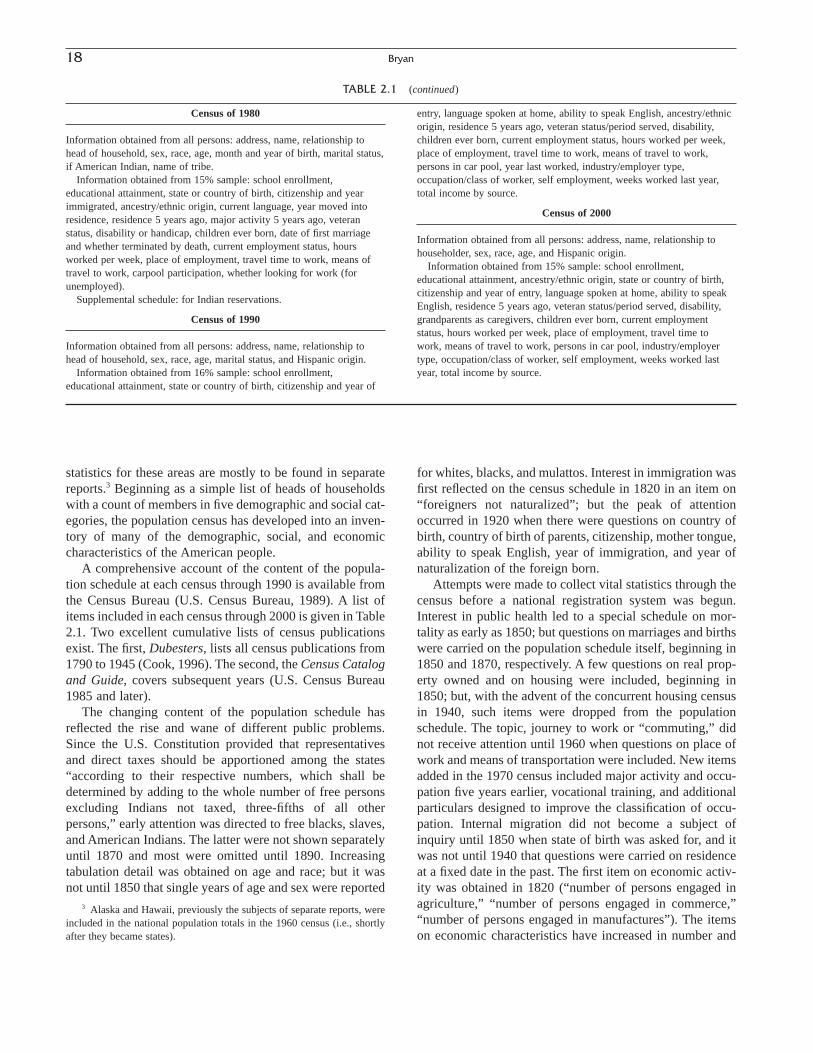
statistics for these areas are mostly to be found in separatereports.3 Beginning as a simple list of heads of householdswith a count of members in five demographic and social cat-egories, the population census has developed into an inven-tory of many of the demographic, social, and economiccharacteristics of the American people.
A comprehensive account of the content of the popula-tion schedule at each census through 1990 is available fromthe Census Bureau (U.S. Census Bureau, 1989). A list ofitems included in each census through 2000 is given in Table2.1. Two excellent cumulative lists of census publicationsexist. The first, Dubesters, lists all census publications from1790 to 1945 (Cook, 1996). The second, the Census Catalogand Guide, covers subsequent years (U.S. Census Bureau1985 and later).
The changing content of the population schedule hasreflected the rise and wane of different public problems.Since the U.S. Constitution provided that representativesand direct taxes should be apportioned among the states“according to their respective numbers, which shall bedetermined by adding to the whole number of free personsexcluding Indians not taxed, three-fifths of all otherpersons,” early attention was directed to free blacks, slaves,and American Indians. The latter were not shown separatelyuntil 1870 and most were omitted until 1890. Increasing tabulation detail was obtained on age and race; but it wasnot until 1850 that single years of age and sex were reported
for whites, blacks, and mulattos. Interest in immigration wasfirst reflected on the census schedule in 1820 in an item on“foreigners not naturalized”; but the peak of attentionoccurred in 1920 when there were questions on country ofbirth, country of birth of parents, citizenship, mother tongue,ability to speak English, year of immigration, and year ofnaturalization of the foreign born.
Attempts were made to collect vital statistics through thecensus before a national registration system was begun.Interest in public health led to a special schedule on mor-tality as early as 1850; but questions on marriages and birthswere carried on the population schedule itself, beginning in1850 and 1870, respectively. A few questions on real prop-erty owned and on housing were included, beginning in1850; but, with the advent of the concurrent housing censusin 1940, such items were dropped from the populationschedule. The topic, journey to work or “commuting,” didnot receive attention until 1960 when questions on place ofwork and means of transportation were included. New itemsadded in the 1970 census included major activity and occu-pation five years earlier, vocational training, and additionalparticulars designed to improve the classification of occu-pation. Internal migration did not become a subject ofinquiry until 1850 when state of birth was asked for, and itwas not until 1940 that questions were carried on residenceat a fixed date in the past. The first item on economic activ-ity was obtained in 1820 (“number of persons engaged inagriculture,” “number of persons engaged in commerce,”“number of persons engaged in manufactures”). The itemson economic characteristics have increased in number and
18 Bryan
TABLE 2.1 (continued)
Census of 1980
Information obtained from all persons: address, name, relationship tohead of household, sex, race, age, month and year of birth, marital status,if American Indian, name of tribe.
Information obtained from 15% sample: school enrollment,educational attainment, state or country of birth, citizenship and yearimmigrated, ancestry/ethnic origin, current language, year moved intoresidence, residence 5 years ago, major activity 5 years ago, veteranstatus, disability or handicap, children ever born, date of first marriageand whether terminated by death, current employment status, hoursworked per week, place of employment, travel time to work, means oftravel to work, carpool participation, whether looking for work (forunemployed).
Supplemental schedule: for Indian reservations.
Census of 1990
Information obtained from all persons: address, name, relationship tohead of household, sex, race, age, marital status, and Hispanic origin.
Information obtained from 16% sample: school enrollment,educational attainment, state or country of birth, citizenship and year of
entry, language spoken at home, ability to speak English, ancestry/ethnicorigin, residence 5 years ago, veteran status/period served, disability,children ever born, current employment status, hours worked per week,place of employment, travel time to work, means of travel to work,persons in car pool, year last worked, industry/employer type,occupation/class of worker, self employment, weeks worked last year,total income by source.
Census of 2000
Information obtained from all persons: address, name, relationship tohouseholder, sex, race, age, and Hispanic origin.
Information obtained from 15% sample: school enrollment,educational attainment, ancestry/ethnic origin, state or country of birth,citizenship and year of entry, language spoken at home, ability to speakEnglish, residence 5 years ago, veteran status/period served, disability,grandparents as caregivers, children ever born, current employmentstatus, hours worked per week, place of employment, travel time towork, means of travel to work, persons in car pool, industry/employertype, occupation/class of worker, self employment, weeks worked lastyear, total income by source.
3 Alaska and Hawaii, previously the subjects of separate reports, wereincluded in the national population totals in the 1960 census (i.e., shortlyafter they became states).
detail; they have included some on wealth and, morerecently, income. Education and veteran status were first recognized in 1840. Welfare interests in the defective, delinquent, and dependent were also recognized on the 1840schedule. Such inquiries were expanded over the course ofmany decades and did not completely disappear from themain schedule until 1920. In 1970, again, an item on dis-ability was introduced, and it was updated and improved inthe 1980, 1990, and 2000 censuses.
Census 2000
Definitions of subjects used in the census are a reflectionof the times. Changes in definitions are oftentimes necessaryto make current terms and concepts more relevant. However,the changing of definitions must be done with caution, ascensus data are designed to be longitudinal—that is, com-parable across time. A change in definitions cannot only bepotentially confusing, but can make longitudinal definitionsimpossible. One example is that of race definitions andterms. The Office of Management and Budget (OMB) isresponsible for the definition of race and race terminology.For Census 2000, the five major race categories included (1) American Indian or Alaska Native, (2) Asian, (3) blackor African American, (4) Native Hawaiian or other PacificIslander, and (5) white. In addition, respondents could identify themselves as Hispanic or Latino. The proliferationof interracial marriages in the latter part of the century hasled to a considerable increase in the number of persons whocould be considered to be of more than one race. In responseto this, the OMB has not only refined the definitions of racialcategories, but also decided to allow the use of multiple racecategories in Census 2000. The benefit of this action is theopportunity for more individuals to accurately report theirrace. The drawback is that it will subdivide race into somany categories that it will be very difficult to compare thedata with other census and survey data. Similar opportuni-ties and drawbacks exist for the development of other censusquestions as well.
Questions currently asked by the census have beenselected because they fill specific legislative requirements.The U.S. Census Bureau is central to this issue, not onlybecause the Census Bureau asks questions many people con-sider personal, but also because proposals under serious consideration would allow the Census Bureau to use itsauthority to dip into other government records to gather population information. Many countries, including demo-cratic nations, have long had population registers and/ornational address registers to facilitate and even replacecensus taking, but the United States does not have such aregister, in large part because of privacy concerns.
There has been rising public alarm over threats to privacyand confidentiality. These fears adversely affect people’sperceptions of the U.S. Census Bureau. Persons in only 63%
of housing units promptly returned 1990 census question-naires. This was below the 75% in 1980 and 78% in 1970.A Gallup poll taken a month before the census indicated thatjust 67% of Americans were fully or somewhat confidentthat census results would be kept confidential (Bryant andDunn, 1995). By 2000 the return rate rose to 67%.
With the completion of the 2000 census, there are threebroad areas with which users need to be acquainted to fullyunderstand and effectively use the results: the geographicsystem, the structure of the data available, and the maps and geographic products available. These are fully describedin the Geographic Area Reference Manual (U.S. CensusBureau, 2000a) and the Introduction to Census 2000 DataProducts (U.S. Census Bureau, 2000b).
Data Products
The methods used for tabulating and disseminating datafor Census 2000 differ significantly from previous censuses.For the first time, paper publications yield to electronic dissemination as the main census medium. Access to theCensus 2000 data will be primarily through the “AmericanFactfinder” at factfinder.census.gov on the Internet. TheAmerican Factfinder uses IBM parallel supercomputers,Oracle database capabilities, and ESRI geographic softwareto provide users with the capability to browse, search, andmap data from many Census Bureau sources: the 1990 Population and Housing Censuses, the 1997 EconomicCensus, the American Community Survey, and Census 2000.
The union between the proposed Census 2000 data prod-ucts and the American Factfinder can be depicted as a three-tiered pyramid (Figure 2.1). Each tier represents access totraditional types of census data as well as Census 2000 data.Each tier affords greater access to more detailed data whileprotecting confidentiality.
Most Census 2000 tabulations are also available on CD-ROMs or DVDs, with viewing software included, throughthe U.S. Census Bureau’s Customer Services Center or byclicking “Catalog” on the U.S. Census Bureau’s home page.
Data Available Electronically
Data available in an electronic format include the following:
1. Census 2000 (P.L. 94–171), Redistricting SummaryFile. These files contain the data necessary for local redis-tricting and include tabulations for 63 race categories, cross-tabulated by “Hispanic and not Hispanic” for the total population and the population 18 years old and over.Tabulations are available geographically down to the block level and are available electronically through theInternet and through two CD-ROM series (state andnational files).
2. Basic Sources of Statistics 19

race and Hispanic-origin groups, as well as AmericanIndians and Alaska Natives. The lowest geographic level inthis file is the census tract, and there are minimum popula-tion-size thresholds before information is shown for a par-ticular group.
4. Summary File 3 (SF 3). This file includes tabulationsof the population and housing data collected from a sampleof the population, with data provided down to the blockgroup or census tract level. Data are also summarized at theZCTA and congressional district levels.
5. Summary File 4 (SF 4). This file includes tabulationsof the population and housing data collected from a sampleof the population. As with SF 2, the tables in SF 4 are iter-ated for a selected list of detailed race and Hispanic-origingroups, as well as American Indians and Alaska Natives, andfor ancestry groups.
6. PUMS (public use microdata samples). In addition to tables and summary files, microdata are also available.They enable advanced users to create their own customizedtabulations and cross-tabulations of most population andhousing subjects. There are two ways to access the micro-data, through PUMS and the “advanced query function.”
Even with the availability of voluminous printed andelectronic publications, not all combinations and permuta-tions of data are possible. To accommodate many special-ized tabulations, the Census Bureau has provided microdataknown as PUMS (public use microdata samples). PUMSdata differ from summary data in that the basic unit ofanalysis for summary data is a specific geographic area, andfor microdata the unit of analysis is an individual housingunit and the persons who live in it (U.S. Census Bureau,1992).
PUMS contain records for a sample of housing units,with information on the characteristics of each unit and thepeople in it. The original PUMS data, however, are confi-dential until the unique identifiers of each record have beenremoved. Unusual data that could be attributed to a partic-ular individual housing unit or person are also suppressedfor confidentiality.
PUMS are taken from a unique geographic universeknown as PUMAs, or public use microdata areas. Theboundaries of PUMAs vary by state, but they are limited inthat they must exceed 100,000 persons in a concentratedarea. Two PUMS files are available; these represent samplesof the 16% of households that completed the census longform, not samples of the entire population. These files are(1) a 1% sample: information for the nation and states, aswell as substate areas where appropriate; and (2) a 5%sample: information for state and substate areas.
7. Advanced query function. The advanced query func-tion in the American Factfinder is designed to help replacethe Subject Summary Tape Files (SSTFs) and the SpecialTabulation Program (STP) of the 1990 census. The advanced
20 Bryan
2. Summary File 1 (SF 1). This file presents counts and basic cross-tabulations of information collected from allpersons and housing units (i.e., 100% file). This includesage, sex, race, Hispanic origin, household relationship, andwhether the residence is owned or rented. Data are availabledown to the block level for many tabulations and will beavailable at the census-tract level for others. Data are alsosummarized at other geographic levels, such as Zip CodeTabulation Areas (ZCTA) and congressional districts.
3. Summary File 2 (SF 2). This file also contains 100%population and housing unit characteristics, though the tables in this file are iterated for a selected list of detailed
FIGURE 2.1

query function will enable users to specify tabulations fromthe full microdata file, with safeguards and limitations toprevent disclosure of identifying information about individ-uals and housing units.
There are also two different files applicable to particularunits in a geographic class rather than compilations for geo-graphic levels per se. The first of these is the DemographicProfiles, which present demographic, social, economic, andhousing characteristics. The second is the Geographic Com-parison Tables, which contain population and housing char-acteristics for all geographic units in a specified parent area(e.g., all counties in a state).
Printed Reports
Though the scope of printed reports in 2000 is muchsmaller than in 1990, there are also three series of printedreports, with one report per state and a national summaryvolume. The report series are as follows:
1. “Summary Population and Housing Characteristics”(PHC-1). This series presents 100% data on states, counties,places, and other areas. It is comparable to the 1990 CensusCPH-1 series, “Summary Population and Housing Charac-teristics,” and is available on the Internet.
2. “Summary Social, Economic and Housing Charac-teristics” (PHC-2). This series includes tabulations of thepopulation and housing data collected from a sample of thepopulation for the same geographic areas as PHC-1, is com-parable to the 1990 Census CPH-5 series, “Summary Social,Economic and Housing Characteristics,” and is available onthe Internet.
3. “Population and Housing Unit Totals” (PHC-3). Thisseries includes population and housing unit totals forCensus 2000 as well as the 1990 and 1980 censuses. Infor-mation on area measurements and population density willis included. This series will include one printed report foreach state plus a national report and is available on theInternet.
Maps and Geographic Products
To support the data and help users locate and identifygeographic areas, a variety of geographic products are avail-able. These products are available on the Internet, CD-ROM,DVD, and as print-on-demand products. These productsinclude the following:
1. TIGER/line files. These files contain geographicboundaries and codes, streets, address ranges, and coordi-nates for use with geographic information systems (GIS). An online TIGER mapping utility is also available atcensus.gov.
2. Census block maps. These maps show the boundaries,names, and codes for American Indian or Alaska Nativeareas, Hawaiian home lands, states, counties, county subdi-visions, places, census tracts, and census blocks.
3. Census tract outline maps. These county maps showthe boundaries and numbers of census tracts and names offeatures underlying the boundaries. They also show theboundaries, names and codes for American Indian andAlaska Native areas, counties, county subdivisions, andplaces.
4. Reference maps. This series of reference maps showsthe boundaries for tabulation areas including states, coun-ties, American Indian reservations, county subdivisions(MCDs/CCDs), incorporated places, and census designatedplaces. This series includes the state and county subdivisionoutline maps, urbanized area maps and metropolitan areamaps.
5. Generalized boundary files. These files are designedfor use in a geographic information system or similarmapping software and are available for most census geo-graphic levels.
6. Statistical maps. Certain notable statistics are aggre-gated and presented in a special series of statistical maps.
Other Censuses: Special Federal Censuses
At the request and expense of local governments, manycomplete enumerations have been undertaken by the U.S.Census Bureau in postcensal periods. The local governmentalmost invariably chooses to collect only the minimum typesof information—name, relationship to the head of the house-hold, sex, age, and race. A special census is usually taken toobtain a certified count for some fiscal purpose. Most of thespecial censuses are requested for cities; but counties, minorcivil divisions, and annexations have also been covered andoccasionally even an entire state. Results were published inCurrent Population Reports, Series P-28 (until 1985), andlater in the PPL series.
Other Censuses: State and Local Censuses
The trend in the number of censuses taken by states andlocalities has been quite unlike the trend in the number ofspecial censuses taken by the federal government. In oraround 1905, 15 states took their own census; in 1915, 15states; in 1925, 9 states; in or around 1935, 6 states; in1945, 4 states; and in 1955 and 1965, only 2 states. Thelast survivors were Kansas and Massachusetts. Kansasneeded its own census because legislative apportionmentoccurred in the ninth year of every decade, making itimpossible to use federal decennial data. The Kansascensus was abolished in 1979 after more than 100 years,
2. Basic Sources of Statistics 21

but the constitutional requirement for a ninth-year reappor-tionment remained. A special law was enacted for a censusin 1988, after which year the constitution was amended torevise the timing of reapportionment to the third year ofeach decade. Massachusetts also maintained a state census,conducted every 10 years in years ending with the number5. After the last census was conducted in 1985, Massachu-setts moved to abolish the state census and the change wasratified in 1990.
Censuses conducted by cities and other local govern-ments are not currently, and never have been, very plentifulbecause of limited resources and considerable costs. Limitedexamples may be found in the State of California in the1960s and 1970s. Rather, state and local agencies haveworked with the Federal-State Cooperative for PopulationEstimates (FSCPE) to create necessary population andhousing statistics. State representatives of the FSCPE sup-ply selected input data for the Census Bureau’s estimatesprogram. Additionally, many members generate their ownstate, county, and subcounty estimates. The results ofFSCPE estimates were historically published in the CensusP-26 report series, but are now included in the Census P-25series. Information on state and local agencies preparingpopulation and housing estimates may be found in CensusP-25 Series, No. 1063, or updates thereof.
Surveys in the United States
Compared to the situation in the other countries of theworld, national sample surveys developed quite early in theUnited States. Government surveys are considered here first,followed by those conducted by private and academicsurvey organizations.
Government Surveys
The origins of U.S. Census Bureau surveys can be foundin the Enumerative Check Census, taken as a part of the1937 unemployment registration. During the latter half ofthe 1930s, the research staff of the Work Projects Adminis-tration (WPA) began developing techniques for measuringunemployment, first on a local-area basis and subsequentlyon a national basis. This research and the experience withthe Enumerative Check Census led to the Sample Survey ofUnemployment, which was started in March 1940 as amonthly activity by the WPA. In August 1942, responsibil-ity for the Sample Survey of Unemployment was transferredto the U.S. Census Bureau, and in October 1943, the samplewas thoroughly revised. In June 1947, it was renamed theCurrent Population Survey (CPS).
Today, the CPS is one of the most prominent demographicsurveys. Estimates obtained from the CPS include employ-ment, unemployment, earnings, hours of work, and othersocial, economic, and demographic indicators. CPS data are
available for a variety of demographic characteristics includ-ing age, sex, race, and Hispanic origin. They are also availablefor occupation, industry, and class of worker. Supplementalquestions to produce estimates on a variety of topics includingmarital status, school enrollment, educational attainment,mobility, household characteristics, income, previous workexperience, health, and employee benefits are also often addedto the regular CPS questionnaire (U.S. Bureau of Labor Statistics, 1998). Statistics are frequently released in officialBureau of Labor Statistics (BLS) publications, the CensusBureau’s Current Population Reports, Series P-60, P-20, or P-23, or as part of numerous statistical compendia. The pri-mary demographic data are released annually as a supplement.Additional supplements are available irregularly.
The special series of reports known as Current Popula-tion Reports usually present the results of national surveysand special studies by the U.S. Census Bureau:
P20, Population Characteristics. Intermittent summariesand analyses of trends in demographic characteristics inthe United States.
P23, Special Studies. Intermittent publications on socialand economic characteristics of the population of theUnited States and states.
P25, Population Estimates and Projections. Periodicestimates of the United States, states, counties, andincorporated areas; and projections of United Statesand subpopulations.
P26, Population estimates produced as a result of theFederal-State Cooperative Program for PopulationEstimates. Discontinued after 1988, and included withthe P-25 series.
P28, Special Censuses. Reports of the results of specialcensuses taken by the Census Bureau in postcensalyears at the request and expense of localities. Noreports have been released in the series coveringcensuses taken since 1985, but listings of specialcensus results appear for the later periods in thePopulation Paper Listing (PPL) series.
It should be noted that several of these reports may bediscontinued in published paper format and may be pre-sented entirely on the Internet.4
The U.S. Census Bureau also conducts other nationalsurveys.5 Among those most used is the American Housing
22 Bryan
4 Additional information on Current Population Reports may be found in the reports themselves (U.S. Census Bureau/Morris, 1996). The most recent publications may also be found on the Internet atcensus.gov/prod/www/titles.html#popspec.
5 Principal demographic surveys conducted by the U.S. Census Bureau:
American Community SurveyAmerican Housing SurveyCurrent Population SurveyHousing Vacancy SurveyNational Health Interview Survey
could be identified through the basic survey, or through theuse of supplemental questions. Targeted households can thenbe candidates for follow-up interviews; this provides a more robust sampling frame for other surveys. Moreover,the prohibitively expensive screening interviews nowrequired are no longer necessary.
The ACS provides more timely data for use in area estimation models that provide estimates of various specialpopulation groups for small geographic areas. In essence,detailed data from national household surveys (whosesample are too small to provide reliable estimates for statesor localities) can be combined with data from the ACS toprovide a new basis for creating population estimates forsmall geographic areas.
Finally, one of the largest national surveys conducted withassistance from the U.S. Census Bureau is the NationalHealth Interview Survey (NHIS). The National HealthSurvey Act of 1956 provided for a continuing survey andspecial studies to secure accurate and current statistical infor-mation on the amount, distribution, and effects of illness anddisability in the United States and the services rendered foror because of such conditions. The survey referred to in theact was initiated in July 1957 and is conducted by the Bureau of the Census on behalf of the National Center forHealth Statistics (NCHS). Data are collected annually fromapproximately 43,000 households including about 106,000persons. The survey is closely related to many other surveyssponsored or conducted by NCHS alone or jointly with theCensus Bureau and private organizations.
Since most other federal agencies do not have their ownnational field organizations for conducting householdsurveys, they tend to turn to the U.S. Census Bureau as thecollecting agency when social or economic data are neededfor their research or administrative programs. In recent yearssuch surveys have proliferated, partly in connection withprograms in the fields of human resources, unemployment,health, education, and welfare. Federal grants have beenmade in large numbers to state and city agencies, and espe-cially to universities, for surveys and research. Few of thesurveys are concerned directly with population but they mayinclude background questions on the demographic charac-teristics of the persons in the sample.
Research Surveys
There are a great many survey organizations in the UnitedStates, many of which conduct national sample surveys in which demographic data are collected. Demographicsurveys conducted by universities in particular communitiesare legion, and their number grows at an accelerated pace.In recent years, other organizations such as Westat, Inc., andMacro, Inc., have stepped in to provide substantial researchservices as well. Most research surveys are funded, at leastin part, by U.S. federal government agencies. Much of the
2. Basic Sources of Statistics 23
Survey (AHS). AHS national data are collected every otheryear, and data for each of 47 selected metropolitan areas arecollected about every 4 years, with an average of 12 metro-politan areas included each year. AHS survey data are idealfor measuring the flow of households through housing.
The most recent advance in Census Bureau surveys is the advent of the continuous measurement system (CMS).The CMS is a reengineering of the method for collecting thehousing and socioeconomic data traditionally collected inthe decennial census. It provides data every year instead ofonce in 10 years. It blends the strength of small area esti-mation from the census with the quality and timeliness ofthe current survey. Continuous measurement includes alarge monthly survey, the American Community Survey(ACS), and additional estimates through the use of admin-istrative records in statistical models. The ACS is in a devel-opmental period that started in 1996. Beginning in 2003,over the course of each year, 3 million households are to beselected in the sample.
Data users have asked for timely data that provides con-sistent measures for all areas. Decennial sample data are outof date almost as soon as they are published (i.e., about 2 to3 years after the census is taken), and their usefulnessdeclines every year thereafter. Yet billions of governmentdollars are divided among jurisdictions and populationgroups each year on the basis of their socioeconomic pro-files in the decennial census. The American CommunitySurvey can identify rapid changes in an area’s populationand gives an up-to-date statistical picture when data usersneed it, not just once every 10 years. The ACS provides esti-mates of housing, social, and economic characteristics everyyear for all states, as well as for all cities, counties, metro-politan areas, and population groups of 65,000 persons ormore. For smaller areas, it takes 2 to 5 years to sample a sufficient number of households for reliable results. Oncethe American Community Survey is in full operation, themultiyear estimates of characteristics will be updated eachyear for every governmental unit, for components of thepopulation, and for census tracts and block groups.
The American Community Survey also screens forhouseholds with specific characteristics. These households
National Survey of Fishing, Hunting, and Wildlife-Associated Recreation
Residential Finance SurveySurvey of Income and Program ParticipationSurvey of Program Dynamics
Some economic surveys conducted by the U.S. Census Bureau:
Annual Retail Trade SurveyAnnual Transportation SurveyAssets and Expenditures SurveyBusiness and Professional Classification SurveyCharacteristics of Business Owners SurveyMonthly Retail Trade SurveyMonthly Wholesale Trade SurveyWomen- and Minority-Owned Business Survey.

data collected in these surveys is held in archives, such asthe Inter-University Consortium for Political and SocialResearch (ICPSR) at the University of Michigan, and theSocial Science Data Archives (SSDA) at Michigan StateUniversity and Yale University. Some of the larger surveyresearch organizations are as follows:
1. The University of Chicago National Opinion ResearchCenter (NORC) is an independent, not-for-profit researchcenter that has been affiliated with the university for 50years. NORC conducts more than 30 social surveys per year,including the General Social Survey (GSS) used in collegeand university teaching programs across the nation.
2. The University of Michigan Survey Research Centeris part of the Institute for Social Research (ISR) at the University of Michigan and is the nation’s longest-standinglaboratory for interdisciplinary research in the social sciences(isr.umich.edu/src). It conducts, among other importantwork, two prominent surveys. The first is the Health, Retire-ment and Aging Survey (HRA), a result of the combinationin 1998 of the Health and Retirement Study (HRS) and Assetand Health Dynamics Among the Oldest Old (AHEAD) andfunded by the National Institute on Aging. The other is thePanel Study of Income Dynamics (PSID), funded by theNational Science Foundation. Begun in 1968, the PSID is a longitudinal study of a representative sample of U.S. individuals and their family units.
3. The Ohio State University Center for HumanResource Research was founded in 1965 as a multidiscipli-nary research institution concerned with the problems asso-ciated with human resource development, conservation, andutilization. Among other substantial research work, thecenter has been responsible for the National LongitudinalSurveys of Labor Market Experience (NLS). The NLSbegan in 1965 when the U.S. Department of Labor con-tracted with the center to conduct longitudinal studies oflabor market experience on four nationally representativegroups of the U.S. civilian population. The project hasinvolved repeated interviews of more than 35,000 U.S. residents, and it continues today.
4. The North Carolina Research Triangle Institute (RTI)is a nonprofit contract research organization located in NorthCarolina’s Research Triangle Park (rti.org). RTI was estab-lished in 1958 by the University of North Carolina at ChapelHill, Duke University, and North Carolina State University.Among numerous research projects, RTI’s National Surveyof Child and Adolescent Well-Being (NSCAW), sponsoredby the U.S. Department of Health and Human Services, isthe most prominent. The NSCAW is a 6-year study of 6000children and adolescents who have come into contact withthe child welfare system.
5. The University of Wisconsin-Madison Center forDemography and Ecology is another prominent national
research center, whose largest responsibility has been toconduct the National Survey of Families and Households.The NSFH is a comprehensive, cross-sectional survey of13,000 Americans in 1987–1988 and 1992–1994(ssc.wisc.edu/nsfh).
6. Westat, Inc., has worked closely with numerous U.S. government agencies to conduct surveys, primarily inthe areas of fertility, health, and military personnel. TenAmerican fertility surveys covering a 35-year period havebeen conducted by various organizations: the Growth ofAmerican Families in 1955 and 1960; the National FertilitySurveys in 1965, 1970, and 1975; the Princeton FertilitySurvey (1957, with reinterviews in 1960 and 1963–1967);and the National Survey of Family Growth in 1973, 1976,1982, and 1988. The latest of these surveys were sponsoredby the National Center for Health Statistics (NCHS) andconducted by Westat. The most prominent national healthstudies Westat is involved in are the Continuing Survey ofFood Intakes by Individuals and the National Health andNutrition Examination Surveys (the latter also being spon-sored by NCHS). Westat is also one of the few organizationsthat is responsible for gathering information on military personnel. It conducts the Communications and EnlistmentDecision Studies/Youth Attitude Tracking Study and theAnnual U.S. Army Reserve Troop Program Unit SoldierSurvey.
Numerous other quality research organizations exist, andthe analyst is encouraged to explore their work and becomefamiliar with other national surveys not mentioned here.
REGISTRATION SYSTEMS
A registration system is the other common method forcollecting demographic data. It differs from a census in thatthe registration system is conducted for both administrativeand statistical uses and in other ways. For present purposes,a population registration system can be defined as “an indi-vidualized data system, that is, a mechanism of continuousrecording, and/or of coordinated linkage, of selected infor-mation pertaining to each member of the resident popula-tion of a country in such a way to provide the possibility ofdetermining up-to-date information concerning the size andcharacteristics of that population at selected time intervals.”(United Nations, 1969).6
Definitions of the universal register, partial register, andvital statistics registration differ somewhat, but it is under-stood that the organization, as well as the operation, of all
24 Bryan
6 For a discussion of the various meanings of “civil registration” andthe roles of local registration offices, ecclesiastical authorities, public healthservices, and so forth, see United Nations, Handbook of Vital StatisticsSystems and Methods (1985).

goes back to 1608. Compulsory civil registration of births,deaths, stillbirths, and marriages was enacted in Finland(1628), Denmark (1646), Norway (1685), and Sweden(1686). The first regular publication of vital statistics by agovernment office is credited to William Farr, who wasappointed compiler of abstracts in the General RegisterOffice in 1839, shortly after England’s Registration Act of1837 went into effect.
For the Far East, Irene Taeuber’s generalization that thegreat demographic tradition of that region is that of popula-tion registration may be cited (Taeuber, 1959, p. 261). Thispractice began in ancient China with the major functionbeing the control of the population at the local level. Occa-sionally, the records would be summarized to successivelyhigher levels to yield population totals and vital statistics.The family may be viewed as the basic social unit in thissystem of record keeping. In theory, a continuous popula-tion register should have resulted, but in practice, statisticalcontrols were usually relatively weak and the compilationswere either never made or they tended to languish in inac-cessible archives.
The Chinese registration system diffused gradually tonearby lands. Until the present century, the statistics fromthis source were intended to cover only part of the total pop-ulation and contained gross inaccuracies. Japan’s adaptationof the Chinese system resulted in the koseki, or householdregisters. These had been in existence for more than a thousand years when, in 1721, an edict was issued that thenumbers registered should be reported. Such compilationswere made at 6-year intervals down to 1852 although certainrelatively small classes of the population were omitted.Thus, this use of the population register parallels that inScandinavia in the same centuries. The first census of Japanby means of a canvass of households was not attempted until1920; it presumably resulted from the adoption of theWestern practice that was then more than a century old.Fairly frequent compilations of populations and householdswere made in Korea during the Yi dynasty; the earliest wasin 1395.
Vital Statistics
International View
According to the United Nations’ Handbook of Vital Statistics Methods, “a vital statistics system can be definedas including the legal registration, statistical recording andreporting of the occurrence of, and the collection, compila-tion, analysis, presentation, and distribution of statistics per-taining to ‘vital events’, which in turn include live births,deaths, foetal deaths, marriages, divorces, adoptions, legiti-mations, recognitions, annulments, and legal separations”(United Nations, 1985). The end products of the system that
2. Basic Sources of Statistics 25
are made official by having a legal basis. It must be notedalso that the content, consistency, and completeness of pop-ulation registration systems vary not only by country, butover time and within countries as well. Events such as war,famine, or even unusual prosperity that might last for shortor long periods of time may create an impetus for greater orless registration or the linkage or destruction of existingrecords.
This chapter treats not only the possible statistics that areproduced by registration of vital events and the recording ofarrivals and departures at international boundaries, but alsouniversal population registers and registers of parts of thepopulation (e.g., workers employed in jobs covered bysocial insurance plans, aliens, members of the armed forces,voters). In most cases, one’s name is inscribed in a registeras the result of the occurrence of a certain event (e.g., birth,entering the country, attaining military age, entering gainfulemployment). Some registers are completed at a single date,some are repeated periodically, others are cumulative. Thecumulative registers may be brought up to date by record-ing the occurrence of other events (e.g., death, migration,naturalization, retirement from the labor force).
History
The chronology of important events in the developmentof civil registration and of the vital statistics derived from itbegins in antiquity. The earliest record of a register of house-holds and persons comes from the Han dynasty of Chinaduring the 2nd century bc. The registration of households in Japan began much later, in the 7th century ad, during the Taika Restoration. It may be noted that the recording ofmarriages, christenings, and burials in parish registers developed as an ecclesiastical function in Christendom butgradually evolved into a secular system for the compulsoryregistration of births, marriages, deaths, and so on thatextended to the population outside the country’s establishedchurch. The 1532 English ordinance that required weekly“Bills of Mortality” to be compiled by the parish priests inLondon is a famous landmark. In 1538, every Anglicanpriest was required by civil law to make weekly entries in aregister for weddings and baptisms as well as for burials, butthese were not compiled into statistical totals for all ofEngland. In fact, it was not until the Births, Marriages andDeaths Registration Act became effective in 1837 that theseevents were registered under civil auspices and a centralrecords office was established. Meanwhile, the Council ofTrent in 1563 made keeping of registers of marriages andbaptisms a law of the Catholic Church, and registers wereinstituted not only in many European countries but also intheir colonies in the New World.
Registration of vital events began relatively early inProtestant Scandinavia; the oldest parish register in Sweden
Compendia of world health statistics are prepared by theWorld Health Organization (WHO), a specialized agency ofthe United Nations. The WHO works in nearly 190 coun-tries to coordinate programs aimed at solving health prob-lems and the attainment of the highest possible level ofhealth. Two important statistical periodicals are published bythe WHO, World Health Report and World Health Statistics.Other important updates can be found on the WHO’s Inter-net site at who.int.
The World Health Report annually presents detailedcountry-specific statistical data on mortality rates, causes ofdeath, and other indicators of health trends at national andglobal levels. Health statistics, data for which are submittedto the WHO by national health and statistical offices, arecompiled each year to help policy makers interpret changesover time and compare key indicators of health status in different countries.
World Health Statistics is a quarterly presenting inter-country comparisons together with information based on theassessment of trends over time. Articles also chart changes insuch areas as morbidity and mortality, resource utilization,and the effectiveness of specific programs or interventions.
United States System: History
It has been mentioned that keeping records of baptisms,weddings, and burials was the function of the clergy in 17thcentury England. This practice was carried over to theEnglish colonies in North America but was mostly pursuedunder secular auspices. As early as 1639, the judicial courtsof the Massachusetts Bay Colony issued orders and decreesfor the reporting of births, deaths, and marriages as part ofan administrative-legal system, so that this colony may havebeen the first state in the Western world in which main-taining such records was a function of officers of the civilgovernment (Wolfenden, 1954, pp. 22–23). Massachusettsalso had the first state registration law (1842); but evenunder this program, registration was voluntary and incom-plete. By 1865, deaths were fairly completely reported,however.
The other states gradually fell into line, and since 1919all of the states have had birth and death records on file fortheir entire area even though registration was not complete.Several of the present states provided for compulsory regis-tration while they were still territories. Most of the states andthe District of Columbia now publish an annual or biennialreport on vital statistics, but there is considerable variationin the scope and quality of these publications.
As previously mentioned, statistics of births and deaths(in the preceding year) were collected in some of the U.S.censuses of the latter half of the 19th century. Earlier in thatcentury, the surgeon general of the army had begun a seriesof reports on mortality in the army (Willcox, 1933, p. 1).From the standpoint of civil registration systems, the role of
26 Bryan
are used by demographers are, of course, the vital statisticsand not the legal issues of the document.7
Events Registered
As sugggesed earlier, events registered may include livebirths, deaths, fetal deaths (stillbirths), marriages, divorces,annulments, adoptions, legitimations, recognitions, andlegal separations. Not all countries with a civil registrationsystem register all these types of events or publish statisticson their numbers. Moreover, some types are of marginalinterest to demographers. As is pointed out in the UnitedNations Handbook, other demographic events, such asmigration and naturalization, are not generally consideredpart of the vital statistics system because they are not usuallyrecorded by civil registration (United Nations, 1985). More-over, these events are not considered “vital” events.8
Items on the Certificate
In discussing the items of information on the certificateor other statistical report of the vital event, those that are ofdemographic value and those that are of legal or medicalvalue only may be distinguished. The former include thedate of occurrence, the usual place of residence of the dece-dent or of the child’s mother, age and sex of the decedent,sex of the child (birth), age and marital status of the mother,occupation of the father, order of the marriage (first, second,etc.), date of marriage for the divorce, and so on. The latterinclude such items as hour of birth, name of physician inattendance, name of person certifying the report, and date ofregistration. Some items such as weight at birth, period ofgestation, and place of occurrence (instead of usual place of residence) are of marginal demographic utility but maybe used in specialized studies.
Publications
Recommended annual tabulations of live births, deaths,fetal deaths, marriages, and divorces are outlined in theUnited Nations Handbook of Vital Statistics (United Nations,1985). Rates and indexes, essential to even the most superficial demographic analysis, are also treated in theHandbook (United Nations, 1985). Inasmuch as many of the publications containing vital statistics also include otherhealth statistics, the following discussion touches on bothtopics.
7 The English-speaking reader should be aware that what is called“vital statistics” in English is roughly equivalent to the French “mouvementde la population” and the Italian “moviemento della popolazione.” “Mou-vement” is used in the sense of change, not migration.
8 For a discussion of population and vital statistics, see United Nations,Population and Vital Statistics Report, 1998, Series A, Vol. L, No. 1,Department of Economic and Social Affairs.

the federal government begins with its setting up of theDeath Registration Area in 1900. A comprehensive reviewof the history of the U.S. vital statistics system may be foundin: U.S. Vital Statistics System: Major Activities and Devel-opments, 1950–95 (U.S. NCHS Hetzel, 1997).
It has been pointed out that the American system isfairly unusual in that states (and a few cities with inde-pendent registration systems) collect certificates of birthsand deaths from their local registrars and are paid to trans-mit copies to the federal government. In the beginning, the federal government recommended a model state law,obtained the adoption of standard certificates, and admittedstates to the registration areas as they qualified. Only 10states and the District of Columbia were in the originaldeath registration area of 1900. The U.S. Census Bureauset up its birth registration area in 1915, with 10 states and the District of Columbia initially qualifying. In theory,90% of deaths, or births, occurring in the state had to beregistered; but ways of measuring performance were verycrude. By 1933, all the present states except Alaska hadbeen admitted to both registration areas. The territory ofAlaska was admitted in 1950, the territory of Hawaii in1917 for deaths and 1929 for births, Puerto Rico in 1932for deaths and 1943 for births, and the Virgin Islands in1924.
Historically, the registration of marriages and divorces inthe United States has lagged even more than that of birthsand deaths. Indeed, national registration areas for marriagesand divorces were not established until 1957 and 1958,respectively. The compilation of data on marriages anddivorces by the federal government was discontinued in themid-1990s and only national estimates of the marriage rateand divorce rate have been published in recent years by theNational Center of Health Statistics. A complete discussionof the development of federal statistics on marriages anddivorces in the United States may be found in Vital Statis-tics of the United States (U.S. National Center for HealthStatistics, 1996).
Data on marriages and divorces are derived from com-plete counts of these events obtained from the states. From these counts, rates are computed for states, geographicdivisions, regions, the registration area, and the UnitedStates as a whole. In fact, an annual national series, partlyestimated, is available back to 1867 for marriages and to 1887 for divorces. Some of the underlying data repre-sent marriage licenses issued rather than marriages per-formed. Characteristics of the persons concerned areobtained from samples of the original certificates filed instate offices.
United States System: Federal Publications
The primary federal publications on vital statistics in theUnited States are in the form of several series of annual
2. Basic Sources of Statistics 27
reports. The U.S. Department of Health and Human Ser-vices (DHHS) is the United States government’s principalagency for researching health issues. As a division ofDHHS, the Centers for Disease Control and Prevention(cdc.gov) oversees 12 national agencies and programs, one of which is the National Center for Health Statistics(NCHS) (cdc.gov/nchswww).9 The NCHS sponsors anumber of national health surveys as well as state healthstatistics research. The NCHS is responsible for publishingprovisional monthly vital statistics data and detailed finalannual data. The volumes of mortality statistics began with190010 and those of natality statistics with 1915. In 1937,the two series were fused into Vital Statistics of the UnitedStates. Inclusion of marriages and divorces in the boundannual volumes began in 1946 and ended with 1988 whenNCHS stopped obtaining detailed data from the states. Thelast volumes of natality and mortality data were publishedin 1999 and 2002, respectively, with 1993 data. A reducednumber of tabulations for subsequent years will be avail-able electronically on CD-ROM. Additional tabulations areavailable on the Internet. Microdata files of births anddeaths are also available on CD-ROM.
The organization of the annual reports is as follows:
Volume I: NatalityVolume II: Mortality
Part A: General MortalityPart B: Geographic Detail for Mortality
Volume III: Marriage and Divorce
Volume I, Natality, is divided into four sections, Ratesand Characteristics, Local Areas Statistics, Natality—PuertoRico, the Virgin Islands (U.S.) and Guam, and TechnicalAppendix.
The two parts of Volume II, Mortality, are really contin-uous and are bound separately mainly because of the size ofthis volume. Part A contains seven sections, General Mor-tality, Infant Mortality, Fetal Mortality, Perinatal Deaths,Accidental Mortality, Life Tables, and Technical Appendix.Part B contains two sections, Section 8, Geographic Detailfor Mortality, and Section 9, Puerto Rico, Virgin Islands(U.S.), and Guam.
Volume III, Marriage and Divorce, is divided into foursections, Marriages, Divorces, Puerto Rico and VirginIslands (U.S.), and Technical Appendix.
9 National Center for Chronic Disease Prevention and Health Promo-tion, National Center for Environmental Health, Office of Genetics andDisease Prevention, National Center for Health Statistics, National Centerfor HIV, STD, and TB Prevention, National Center for Infectious Diseases,National Center for Injury Prevention and Control, National Institute forOccupational Safety and Health, Epidemiology Program Office, Office ofGlobal Health, Public Health Practice Program Office, and National Immu-nization Program.
10 This is the year when the annual series began. Several States andcities had made transcripts of death certificates in 1880 and 1890 for useby the Census Bureau.

In addition to the Vital Statistics of the United States, the NCHS publishes two other series with voluminous vitalstatistics data for the United States and other countries. Thefirst is the National Vital Statistics Report (previously theMonthly Vital Statistics Report), which has been publishedfrom January 1952 to the present. The report providesmonthly and cumulative data on births, deaths, marriages,and divorces, and infant deaths for states and the UnitedStates. In addition, annual issues present preliminary andfinal data for states and the United States with brief analy-sis of the data.
The other set of publications is the Vital and Health Statistics, which has been published from 1963 to present.Containing 18 series of reports, this set of publications givesthe results of numerous surveys, studies, and special datacompilations. The series are as follows:
Series 1. Programs and Collection ProceduresSeries 2. Data Evaluation and Methods ResearchSeries 3. Analytical and Epidemiological StudiesSeries 4. Documents and Committee ReportsSeries 5. International Vital and Health Statistics ReportsSeries 6. Cognition and Survey MeasurementSeries 10. Data from the National Health Interview SurveySeries 11. Data from the National Health Examination
Survey, the National Health and Nutrition ExaminationSurveys, and the Hispanic Health and NutritionExamination Survey
Series 12. Data from the Institutionalized PopulationsSurveys
Series 13. Data from the National Health Care SurveySeries 14. Data on Health Resources: Manpower and
FacilitiesSeries 15. Data from Special SurveysSeries 16. Compilations of Advance Data from Vital and
Health StatisticsSeries 20. Data on MortalitySeries 21. Data on Natality, Marriage, and DivorceSeries 22. Data from the National Mortality and
Mortality/Natality SurveysSeries 23. Data from the National Survey of Family
GrowthSeries 24. Compilations of Data on Natality, Mortality,
Marriage, Divorce, and Induced Terminations ofPregnancy
Other Sources of Vital Statistics
Since some states and local governments were active inthe field of vital statistics long before the federal govern-ment, it is not surprising that they also published the firstreports. The state of Massachusetts inaugurated an annualreport in 1843 (Gutman, 1959). Until 1949 the only tablesgiving the characteristics of brides and grooms were thosepublished by a number of the states. A number of state health
departments and state universities have also prepared andpublished life tables. On the whole, however, the annualreports on vital statistics published by state and city healthdepartments do not represent a major additional source ofdemographic information. They are usually much lessdetailed than the federal reports. The corresponding figuresin state and federal reports may differ somewhat because ofsuch factors as the inclusion of more delayed certificates inthe tabulations made in the state offices, different definitionsand procedures, sampling errors when tabulations arerestricted to a sample, and processing errors in either or bothoffices.
Another important nonfederal source of vital statistics inthe United States is Health and Healthcare in the UnitedStates (Thomas, 1999). Providing summary data on all vitalstatistics components for county and metropolitan areas,Health and Healthcare provides both current estimates aswell as projections of vital statistics.
Numerous religious institutions also track the vital statistics of their members and provide substantial insightinto the characteristics of their members. For example, theOfficial Catholic Church Directory (annual) provides in-formation on births, deaths, and marriages, the Catholic population, and the total population for each diocese.
Migration
Of the three demographic variables—fertility, mortality,and migration—procedures for the collection and tabulationof migration data are the least developed and standardized.As a result, there is a relative paucity of information onpopulation movements between countries (i.e., internationalmigration) and within the same country (i.e., internalmigration) (United Nations, 1980). For countries withoutpopulation registers, data on internal and internationalmigration are difficult to obtain. International differencesexist in defining what a migrant actually is, as well as inmethods of collecting and tabulating the data necessary togenerate migration statistics. Information regarding thenumber, sex, and ages of persons entering or leaving anarea may be obtained from a census, population register, orborder-control system. Migration is often measured,however, by using indirect information and methods, whichmay produce estimates with substantial error. Nevertheless,migration statistics are important for understanding the sizeand structure of a population in a defined place and time.Oftentimes, migration is the largest component of popula-tion change in an area and may transcend the other com-ponents of change.
International View
There has been a major shift in the direction of worldmigration in the past half century. Between 1845 and 1924,
28 Bryan
2. Basic Sources of Statistics 29
about 50 million migrants—mainly Europeans—settled per-manently in the Western Hemisphere. In the past severaldecades the flows have become polarized on a north-southaxis, with a majority of migrants coming from Asia, LatinAmerica, and Africa. Though the preferred destinations arestill the more developed countries, the rates of permanentmigration to the more developed nations is stabilizing(United Nations 1982b, p. 3).
National governments often publish statistics on the basisof the records of immigrants arriving at and emigrantsdeparting from the official ports of entry and stations on landborders. Migration statistics may also be generated frompassports issued, local registers, and miscellaneous sources.All such records tend to be most complete and detailed foraliens arriving for purposes of settlement, and least so forthe migration of the country’s own citizens. Population reg-isters of aliens may be of some value in studying immigra-tion and emigration, assimilation through naturalization, andthe characteristics of those foreign-born persons who havenot become citizens. For the most part, a register mainly sup-plements other sources of information on these subjects(from the census and migration/border-control records).
The United Nations publishes information on the scope ofinternational migration statistics, categories of internationaltravelers, and types of organizational arrangements for col-lecting and processing data in this field (United Nations,1980). The United Nations also produces detailed informa-tion on international migration policies, which affords theanalyst an in-depth understanding of the role and character-istics of migrants around the world (United Nations, 1998b).
The United Nations Demographic Yearbooks carrynumerous tables on international migration. Usually, statis-tics are given by countries, on major categories of arrivalsand departures, long-term immigrants by country of lastpermanent residence, long-term emigrants by country ofintended permanent residence, and long-term immigrantsand emigrants by age and sex. The UN also regularly pub-lishes specialized reports on the measurement of migrationand reporting methods, as well as the results of research onindividual countries.11 Other valuable studies on migrationhave been conducted recently.12
Perhaps one of the best sources of data on internationalmigration is the Organisation for Economic Cooperation andDevelopment (OECD.org), which comprises most industri-alized countries, including the United States. Migration sta-tistics are compiled, standardized, and compared annuallyfor all member countries, giving the migration analyst oneof the best portraits available of worldwide migration andmigration internal to the member countries.
United States View
The history of U.S. migration statistics may be traced tothe colonial period.13 One of the more difficult types of population change to study is immigration and emigration,especially illegal migration. The U.S. Immigration and Naturalization Service (INS) (ins.usdoj.gov) is responsiblefor compiling data on alien immigration as well as on nat-uralizations in the United States. For purposes of classifica-tion, the INS divides those aliens coming to the UnitedStates from a foreign country into six categories and com-piles statistics on all of them except one (U.S. INS, 1999):
1. Immigrants. Lawfully admitted persons who come tothe United States for permanent residence, includingpersons arriving with that status and those adjusting topermanent residence after entry.
2. Refugees. Aliens who come to the United States to seekrefuge from persecution abroad and who reside abroad.
3. Asylees. Aliens who come to the United States to seekrefuge from persecution abroad and who are in theUnited States or at a U.S. port of entry.
4. Nonimmigrant aliens. Aliens who come to the UnitedStates for short periods for the specific purpose ofvisiting, studying, working for an internationalorganization, and to carry on specific short-termbusiness.
5. Parolees. Aliens temporarily admitted to the UnitedStates for urgent humanitarian reasons or to serve a
11 Two important United Nations publications on international migra-tion are “National Data Sources and Programmes for Implementing theUnited Nations Recommendations on Statistics of International Migration.”Series F, No. 37, 1986, and “Recommendations on Statistics of Interna-tional Migration,” Series M, No. 58, 1980.
12 A valuable study of international migration was compiled by CharlesB. Nam, William Serow, David Sly, and Robert Weller (Eds.) in 1990:Handbook of International Migration, Greenwood Press, New York.Detailed concepts of international migration are presented, with specificstudies of Botswana, Brazil, Canada, China, Ecuador, Egypt, France,Germany, Guatemala, India, Indonesia, Israel, Italy, Japan, Kenya, theNetherlands, Poland, the Soviet Union, Thailand, the United Kingdom, andthe United States. Another notable study is International Handbook ofInternal Migration, Greenwood Press, New York, compiled by C.B. Nam,W. Serow, and S. Sly (Eds.) in 1990.
13 There are only a few fragmentary statistics on immigration from abroad during the colonial period. The continuous series of federal statistics begins in 1820. The statistics were compiled by the Department of State from 1820 to 1874, by the Bureau of Statistics of the Treasury Department from 1867 to 1895, and by the Office or Bureauof Immigration, now the Immigration and Naturalization Service, from1892 to the present, although publication was in abridged form or omittedfrom 1933 to 1942. Over this period, the coverage of the statistics hastended to become more complete, especially for immigrant aliens (thoseadmitted for permanent residence). The series for emigrants began morerecently—aliens deported (1892), aliens voluntarily departing (1927), andemigrant and nonemigrant aliens (1908). However, statistics on emigrantand nonemigrant aliens were discontinued in 1957 and 1956, respectively.For selected historical series and a good discussion of the development ofthe data, see U.S. Census Bureau, Historical Statistics of the United States:Colonial Times to 1957, 1960, pp. 48–66; idem, Historical Statistics of theUnited States: Continuation to 1962 and Revisions, 1965, pp. 10–11;Gertrude D. Krichefsky, “International Migration Statistics as Related tothe United States,” Part 1, I and N Reporter, 13(1): 8–15, July 1964.

refugees; temporary visitors; alien and citizen border-crossers over land boundaries; aliens excluded and deportedby cause; aliens who reported under the alien addressprogram and naturalizations by country of former allegiance,sex, age, marital status, occupation, and year of entry.
Another useful source of information on immigration isthe INS Immigration Reports, which provide data on legalimmigration to the United States and are available on theInternet at ins.usdoj.gov/stats/index.html. The format of thereports is as follows:
Section 1 Class of Admission
Table 1. Categories of Immigrants Subject to the Numerical Cap:Unadjusted and Fiscal Year Limits
Table 2. Immigrants Admitted by Major Category of Admission: FiscalYears
Section 2 U.S. Residence
Table 3. Immigrants Admitted by State and Metropolitan Area ofIntended Residence
Table 4. Immigrants Admitted by Major Category of Admission and Stateand Metropolitan Area of Intended Residence: Fiscal Year
Section 3 Region and Country of Origin
Table 5. Immigrants Admitted by Region and Selected Country of Birth:Fiscal Years
Table 6. Immigrants Admitted by Major Category of Admission andRegion and Selected Country of Birth: Fiscal Year
Table 7. Immigrants Admitted by Selected State of Intended Residenceand Country of Birth: Fiscal Year
Section 4 Age and Sex
Table 8. Immigrants Admitted by Sex and Age: Fiscal YearsTable 9. Immigrants Admitted by Major Category of Admission, Sex, and
Age: Fiscal Year
Section 5 Occupation
Table 10. Immigrants Aged 16 to 64 Admitted by Occupation: FiscalYears
Table 11. Immigrants Aged 16 to 64 Admitted by Major Category ofAdmission and Occupation: Fiscal Year
Table 12. Immigrants Aged 16 to 64 Admitted as Employment-BasedPrincipals by Occupation: Fiscal Year
Other specialized reports are published irregularly as bulletins.
Internal Migration
Internal migration statistics for the United States haveprimarily been generated by decennial censuses, nationalsurveys, and administrative records. While numerous stateand regional studies have been conducted on the basis ofthese sources, it has been the responsibility of the U.S.Census Bureau to provide comprehensive and standardizedmigration statistics for the U.S. and subareas.
The decennial census has primarily been relied upon intwo ways to provide migration statistics. First, general datacollected by the census can be used to calculate migration
30 Bryan
significant public benefit, and required to leave whenthe conditions supporting their admission end.
6. Illegal entrants. Persons who have violated U.S.borders, overstayed their visas, or entered with illegallyfabricated documents.
The INS also compiles information on naturalizations,and apprehensions and deportations of illegal aliens, andformerly compiled information on nonemigrant aliens.
The INS prepares numerous statistical studies on immi-gration and naturalizations. Data on legal immigration arecompiled from immigrant visas issued by the U.S. Depart-ment of State and collected by INS officials at official portsof entry. (Aliens residing in the United States on whom legalresidence (“adjustments”) is conferred are also included inthe immigrant statistics at the date of adjustment of status.)Data on visas and adjustments are collected by the INSImmigrant Data Capture (IMDAC) facility, yielding statis-tics on port of admission, type of admission, country ofbirth, last permanent residence, nationality, age, race, sex,marital status, occupation, original year and class of entry,and the state and zip code of intended residence.
The collection of statistics on emigrants was discontin-ued in 1957, and no national effort has been made to collectthem since that year. Secondary statistics compiled in theUnited States and abroad suggest that the number of emi-grants exceeded 100,000 per year between 1970 and 1990,and surpassed 200,000 every year in the 1990s. The U.S.Census Bureau currently uses an annual emigration figureof 222,000, representing both aliens and citizens, in the gen-eration of national population estimates. This number,however, has typically been regarded as being substantiallyshort of the actual volume of emigration.14
Just two publications of the Immigration and Naturaliza-tion Service provide the bulk of immigration statistics forthe United States annually, and are available on the Internetat ins.usdoj.gov/stats/annual/fy96/index.html.
The Statistical Yearbook of the Immigration and Natural-ization Service, published annually, is the most comprehen-sive publication on U.S. immigration statistics. Copies ofeach Statistical Yearbook (titled Annual Report of the Immi-gration and Naturalization Service prior to 1978) are avail-able from 1965 to the current year. The 2000 report containshistorical statistics on immigration and current statistics onarrivals and departures by month; immigrants by port ofentry, classes under the immigration law, quota to whichcharged, country of last permanent residence, country ofbirth, state of intended residence, occupation, sex and age,and marital status; aliens previously admitted for a temporarystay whose status was changed to that of permanent residents;
14 For additional information on emigration, see Robert Warren andEllen Percy Kraly, “The Elusive Exodus: Emigration from the UnitedStates,” Population Trends and Public Policy Paper, No. 8, March, 1985,Washington, DC: Population Reference Bureau.

The universal population register should be distinguishedfrom official registers of parts of the population. It is truethat the modern universal registers may have evolved fromregisters that excluded certain classes of the population(members of the nobility, etc.), but the intent of the modernregisters is usually to cover all age and sex groups, all ethnicgroups, all social classes, and so on. The partial registers, onthe other hand, are established for specific administrativepurposes and cover only those persons directly affected bythe particular program. Examples are registers of workers orother persons covered by national social insurance schemes,of males eligible for compulsory military service, of personsregistered as eligible to vote, of aliens, and of licensed auto-mobile drivers. Most such registers are continuous, but someare periodic or exist only during a particular emergency. Forexample, there have been wartime registrations for therationing of consumer goods. These may indeed include allor nearly all of the people; but, unlike the universal regis-ters, they are temporary rather than permanent.
The UN has documented the history of population regis-ters, their uses, general features (coverage, documents,information recorded, and administrative control), and theiraccuracy in their Handbook on Civil Registration and VitalStatistics Systems (United Nations, 1998a). It lists, by coun-tries, both the date of establishment of the original registerand the date of establishment of the register as then organ-ized. This list, however, also contains a number of “partialregisters” including some that exclude half or more of thepopulation.
Universal Registers
The universal population register is now the leastcommon, yet most comprehensive and timely statistical collection method. Until the 20th century, it flourished inonly two widely separated regions—Northwestern Europe(mainly Scandinavia) and the Far East. The data from pop-ulation registers are often available in separate sectionsbecause of many legal limitations and regulations, forexample, personal privacy protection.
Population registers have historically been establishedprimarily for identification, control, and police purposes,and often little use has been made of them for the compila-tion of population statistics. In a number of countries, datafrom the registers are used to produce one or more of thefollowing: (1) current estimates of population for provincesand local areas, (2) statistics of internal migration and inter-national migration, (3) vital statistics. Today, however, reg-isters are used more expansively for such things as policyanalysis and justifying the need for development of socialservices such as health care and education. Because of theprohibitively high cost of population and housing censuses,and even some statistical surveys, countries with populationregisters are experimenting with methods of combining their
2. Basic Sources of Statistics 31
statistics.15 Second, specific questions are contained in thecensus to determine migration patterns in relation to variouspopulation characteristics. These questions can includeplace of birth, place of residence 1 year ago or 5 years ago,and year moved to current residence.
Intercensal migration patterns are also measured bynational surveys and administrative records. The main surveyused to track migration in the United States is the CurrentPopulation Survey (CPS). The CPS presents information onthe mobility of the U.S. population one year earlier. Data areprovided for nonmovers; movers within counties, migrantsbetween counties, states, and regions; migrants from abroad;movers within and between metropolitan and nonmetropoli-tan areas; and movers with and between central cities andsuburbs of metropolitan areas. CPS data are released as partof the P-20 Current Population Reports series and are alsoavailable on the Internet at bls.census.gov/cps.
Another survey used for tracking intercensal migration isthe Survey of Income and Program Participation (SIPP). Firstimplemented in 1983, SIPP is a longitudinal survey of thenoninstitutionalized population of the United States. EachSIPP panel also includes a topical module covering migrationhistory. Though specific migration questions have variedfrom panel to panel, each migration history module hasincluded questions on month and year of most recent and pre-vious move, as well as the location of previous residences andplace of birth. Data are available for nonmovers, moverswithin and between counties (though specific counties are notidentified), movers between states, and movers from abroad.Some earlier modules contained questions on reasons formigration. SIPP data are released as special reports in theCensus Bureau’s P-70 Current Population Reports series.
Administrative records may also be used to measuremigration. For example, the Census Bureau receives confi-dential Internal Revenue Service data on tax returns. Afterbeing stripped of the most sensitive data, the individualreturns are linked to a county record and used to measuremovement from year to year.
Population Registers
The United Nations definition of a population register asgiven earlier may be regarded as the “ideal type,” to whichsome of the national registers described are only approxi-mations (United Nations, 1998a). Population registers arebuilt up from a base inventory of the population and its char-acteristics in an area, continuously supplanted by data onbirths, deaths, adoptions, legitimations, marriages, divorces,and changes of occupation, name, or address.
15 The population component estimating equation, representing therelation between population at two dates and the demographic componentsof change during the intermediate period may be used. (See Chapter 19 ofthis volume and Alan Brown and Egon Neuberger, Internal Migration, Academic Press, New York, 1977, p. 105.)

registers with other administrative records to conduct andimprove their decennial censuses.
Currently, registers are maintained in Denmark, Finland,Japan, Norway, the Netherlands, Sweden, Bahrain, Kuwait,and Singapore. A substantial effort to conduct a registrationsystem was once made in China, but essentially discontin-ued. China attempted to establish a population register basedon domicile registration. This includes registration of totalpopulation, births, deaths, immigration, emigration, andchanges in domiciles. When compared with census data, theregistration data were shown to be inaccurate. China todayrelies on a decennial census and sample surveys to deter-mine its population size and its characteristics. The Scandinavian countries all have historically established andwell-developed central population registers, with personal identification numbers and unified coding systems for theirpopulations. Bahrain also has a central registration system.In 1991, Bahrain conducted a national census and asked theenumerators to update the records of registration—essen-tially using one source to check the other. Kuwait had a rel-atively good population register before the 1991 Gulf War,though its future is uncertain. Singapore currently maintainsan ongoing population register. As mandated by the NationalRegistration Act of 1965, all persons who reside in Singapore are required to be registered and must file a noti-fication of change of residence. The system is not, however,used in conjunction with or for the production of censusdata. Numerous other countries have lesser or noncentral-ized population registration systems.
Partial Registers
As indicated earlier, partial registers are set up for specificadministrative programs and cover only those personsdirectly affected by the particular program or belonging to aparticular group. Examples are registers of workers or otherpersons covered by national social insurance programs, ofmales subject to compulsory military service, of registeredvoters, and of licensed automobile drivers. Most such regis-ters are continuous, but some are periodic or exist only duringa particular crisis. For example, there have been wartime registrations for the rationing of consumer goods. These mayindeed include all or nearly all of the papulation; but unlikethe universal registers, they are temporary rather than perma-nent. It is best to consider each type of partial register sepa-rately for the international arena and the United States sincethe various types do not have many features in common.
Partial Registers: International Partial Registers
A wide variety of partial registers are maintained in dif-ferent countries. The following are the most common:
1. Social insurance and welfare. Modern social insur-ance and social welfare systems (unemployment, retirement,
sickness, public assistance, family allowances, etc.) hadtheir origins in Europe and the British Dominions in thelatter half of the 19th century. From the millions of recordsaccumulated, statistics are compiled for administrative pur-poses. Some of these tables are of demographic interest,especially those relating to employment, unemployment, theaged, widows and orphans, mortality (including life tablesfor the population covered by certain programs), and births.From these records, moreover, special tabulations with ademographic orientation can be made; frequently such tab-ulations are based on a sample of the records. Finally, thestatistics may be used in the preparation of population esti-mates or estimates of the total labor force. Likewise, lifetables for a “covered” population may be used to estimatecorresponding life tables for the total population.
Current social insurance and welfare systems vary widelyin their administration and benefits, and this can substan-tially affect the quality of the data. In countries such asFinland, which also has a central universal register, the benefits and services included are universal entitlements.Accordingly, a person can receive benefits and services evenif he or she has not been employed, is not married to anemployed person, and does not have special insurance coverage.
Some countries, such as Ireland, have unilateral agree-ment with other countries. These agreements protect thepension entitlements of Irish people who go to work in thesecountries and they protect workers from those countries whowork in Ireland. They allow periods of residence, that arecompleted in one country to be taken into account by theother country so that the worker may get a pension. Thesearrangements not only afford equitable disbursement ofsocial benefits, but also can be used to create statistics ofinternational labor and migration flows. Other countries thathave little or no social insurance have few resulting data.
2. Military service. Countries that have compulsory military service ordinarily provide for the registration ofpersons attaining military age, and the person’s record ismaintained in the register until he passes beyond the prescribed maximum age. The U.S. Central IntelligenceAgency (CIA) provides military manpower statistics annually in its world factbook (odci.gov/cia/publications/factbook/index.html). Data on current military manpower,the availability of males and females aged 15 to 49, thosefit for military service, and those reaching military age annually, are presented for all countries. The University ofMichigan serves as a comprehensive resource on militarymanpower around the world via its Internet page athenry.ugl.lib.umich.edu/libhome/Documents.center.
3. Consumer rationing. Rationing of food, articles ofclothing, gasoline, and other consumer goods ordinarily represents an emergency national program in time of war,famine, and so on. Hence, registration of the population forrationing purposes is not to be considered as a permanent
32 Bryan
source of demographic statistics. Nonetheless, somerationing programs have continued for a number of years,and important demographic uses have been made of therecords. There are sometimes problems in the form ofexempt classes and illegal behavior (e.g., duplicate registra-tion, failure to notify the authorities of a death or removal);but these are often small and appropriate adjustments can bemade in the statistics.
4. Voters. In countries where voting is compulsory foradults or where a very high proportion of all adults are reg-istered as eligible voters, statistics of demographic valuemay be compiled. For example, in Brazil everyone eligiblemust vote. A certicate of proof of recent voting is one of therequired legal documents for several situations, includingsimply getting a job. In other cases, even if a very high pro-portion of all adults are registered as eligible voters, littleuseful information may be derived from voting statistics asa result of national circumstances. In 1998, after a bitter civilwar, Bosnia conducted national elections that were classi-fied universally as the most complicated in this century, withmore than 30 political parties and nearly 3500 candidates.Because many voting stations were located in “enemy” ter-ritory, many people were simply too fearful to cast theirvotes. Such challenges as voting irregularity, fraud, and theomission of data face the analyst when considering the useof voting registration data.
5. School enrollment and school censuses. Schoolrecords management is an integral part of a local informa-tion system and hence forms part of a national informationsystem. Data on school enrollment are important for meas-uring academic achievement and providing national school-age statistics for policy analysis and resource allocation.Most developed countries collect statistics of registered stu-dents according to grade—less often according to age—andoften tabulate the demographic characteristics, geographicorigin, and achievement of the students.
The primary source of international statistics on educa-tion is the United Nations Educational, Scientific and Cultural Organization (UNESCO). The UNESCO yearbookprovides annual information on a wide range of educationalstatistics for the countries of the world. Selected educationalstatistics are available at the UNESCO site on the Internetat unesco.org.
The quality of international education statistics varieswidely. Many developing countries have received assistancein developing a national education statistics system. Forexample, the Association for the Development of Educationin Africa recently developed the National Education Statis-tical Information System (NESIS) in Sub-Saharan Africaand served first to create educational statistical systems inEthiopia and Zambia based on sophisticated relational data-bases. Information about it is available on the Internet atnesis.easynet.fr. Other nations, which have established pop-ulation registers, have chosen to arrange their data accord-
ing to educational characteristics. For example, in 1985Sweden initiated an education register, which comprises the15- to 74-year-old population. Coordinated by StatisticsSweden (scb.se/scbeng/amhtm/ameng.htm), the system usesthe National Identification Number to link key demographicand education data. The main demographic variables tabulated are age, sex, municipality of residence, country ofbirth, and citizenship. These variables are cross-tabulatedwith the education variables: highest education completed,completion year, and municipality of completion.
Since school census statistics are sometimes substitutedfor school enrollment statistics in making population esti-mates, this source is mentioned here. The school census isreally a partial census rather than a register, however. Thereis a canvass of households either by direct interview or bymeans of forms sent home through the school children.Often the preschool children as well as the children of com-pulsory school age are covered.
6. Judicial system. Many developed countries employrigorous registration of those involved in the judicial system,especially those regarded as being the most iniquitous.Extensive details about them, including social, economic,and physical characteristics, are recorded in comprehensivedatabases and communication networks. While most data arekept confidential, detailed characteristics of those involvedin judicial systems are often tabulated, summarized, and pub-lished. These data may be used for both general demographicanalysis as well as for describing the characteristics of thejudicial system. As the judicial systems of individual coun-tries widely vary, so too do judicial registration systems.
Partial Registers: U.S. Partial Registers
Although the United States has never had a universalpopulation register, it has had several types of partial registers:
1. Social insurance and welfare. The U.S. social insur-ance and welfare program encompasses broad-based publicsystems for insuring workers and their families against insecurity caused by loss of income, the cost of health care,and retirement. The primary programs are Social Security,Medicare/Medicaid, workers’ compensation, and unemploy-ment insurance. In 1935, the Social Security Act was enactedto subsidize the retirement income of the elderly. Old-Age,Survivors, Disability Insurance, and Hospital Insurance, alsoknown as OASDI and HI, are now parts of the program. Asof 2000, there were over 45 million beneficiaries of theOASDI program. The program of health insurance for theelderly (Medicare-HI and SMI) in the United States affordsstatistics on registered persons 65 years old and over bycounty of residence beginning with 1966. Medicaid is a state-financed program of free medical care for the indigent, opento all ages. The program of health benefits for children andyouth known as Child Health Insurance Programs (CHIP)
2. Basic Sources of Statistics 33

34 Bryan
affords statistics on registered persons under 19 years of age.The Medicare and Medicaid Services Agency is the federalagency that administers the Medicare, Medicaid, and ChildHealth Insurance Programs (hcfa.gov/HCFA), whichprovide health insurance or free health care for more than 74million Americans. It is assumed that virtually all Medicare-and Medicaid-eligible persons have registered, while regis-tration in CHIP is more sporadic. Data derived from theseprograms may be accessed on the Internet at hcfa.gov.
Nearly all workers are covered by workers compensationlaws, which are designed to ensure that employees who areinjured or disabled on the job are provided with fixed mon-etary awards, eliminating the need for litigation. These pro-grams are typically administered by states, which reportcompensation claims to the Occupational Safety and HealthAdministration (OSHA). OSHA publishes national statisticson injuries, illnesses, and workers’ demographic character-istics on the Internet at osha.gov/oshstats/bls. Labor force,employment, and unemployment statistics are gathered bythe states, and are submitted to the Bureau of Labor Statis-tics for publication on the Internet at bls.gov/top20.html.Additional national data are derived from the Current Pop-ulation Survey, which provides comprehensive informationon the employment and unemployment of the nation’s pop-ulation, classified by age, sex, race, and a variety of othercharacteristics. These data are available on the Internet atbls.gov/cpshome.htm.
2. Military service. In the United States, demographicstatistics of those in military service are used in the con-struction of population estimates for the total and civilianpopulations. (See the following sections on “Estimates” and“Projections.”) The useful characteristics have included age,sex, and race; geographic area in which stationed; and geo-graphic area from which inducted. In estimating currentmigration, whether international or internal, it has beenfound desirable to distinguish military from civilian migra-tion. An excellent source of statistical information on theDepartment of Defense is the U.S. Directorate for Informa-tion Operation and Reports (DIOR), and it can be accessedon the Internet at web1.whs.osd.mil/mmid/mmidhome.htm.Military manpower statistics are the responsibility of theDefense Manpower Data Center (dmdc.osd.mil), which wasestablished in 1974 as the Manpower Research and DataAnalysis Center (MARDAC) within the U.S. Navy. Somebranches of the military provide their own demographic sta-tistics, such as the Air Force. The Interactive DemographicAnalysis System (IDEAS), available on the Internet atafpc.af.mil/sasdemog/default.html, provides data on activeduty officers, active-duty enlisted personnel, and civilianemployees.
3. Voters. Information on registration and voting in rela-tion to various demographic and socioeconomic character-istics is collected for the nation in November ofcongressional and presidential election years in the CurrentPopulation Survey (CPS). Tabulations of voters in local
districts are often made by local or state authorities. As few other data are gathered regularly at the voting-districtlevel, data on voters can be used as a variable in a “ratio-correlation model” to generate estimates of population andpopulation characteristics for voting districts and other smallareas. These data may be useful in areas where service dis-tricts, such as fire and water districts and school districts,need population estimates for purposes of funding or plan-ning. (See Chapter 20 on population estimates for furtherinformation.)
4. School enrollment and school censuses. Statisticscompiled from lists of children enrolled in school are widelyused in the United States because of their universality andpertinency for making estimates of current population. TheNational Center for Education Statistics (NCES) is theprimary federal entity for collecting and analyzing datarelated to education in the United States and other nations(nces.ed.gov).
Besides their use in making estimates, education data areused by federal, state, and local governments that requestdata concerning school demographic characteristics, pupil/teacher ratios, and dropout rates. At the federal level, suchstatistics are used for testimony before congressional com-mittees and for planning in various executive departments.Among the states, NCES statistics and assessment data areused to gauge progress in educational performance. Themedia use NCES data for reports on such topics as studentperformance, school expenditures, and teacher salaries.Researchers perform secondary analyses using NCES data-bases. Businesses use education data to conduct marketresearch and to monitor major trends in educatuon (U.S.National Center for Education Statistics, 1999).
Among the voluminous statistics published by the NCES,the most relevant to the concept of a partial register are theCommon Core of Data (CCD) and Private School Survey(PSS). The CCD is the primary database for basic elemen-tary and secondary education statistics. Every year the CCDsurveys all public elementary and secondary schools and allschool districts in the United States. The CCD providesgeneral descriptive statistics about schools and school dis-tricts, demographic information about students and staff, andfiscal data. The PSS provides the same type of informationfor private schools as does the CCD for public schools. ThePSS is conducted every 2 years and includes such variablesas school affiliation, number of high school graduates, andprogram emphasis.
The NCES founded the National Education DataResource Center (NEDRC) to serve the needs of teachers,researchers, policy makers, and others for education data.Data sets for some 16 studies maintained by NCES are cur-rently available through NEDRC. The purpose of NEDRCis to provide education information and data to those whocannot take advantage of the available NCES computerproducts or who do not have appropriate facilities to processthe available data. Education data may also be found at the
2. Basic Sources of Statistics 35
National Library of Education (NLE), which is the largestfederally funded library devoted entirely to education and isthe federal government’s principal center for information oneducation. As mentioned earlier, education statistics may betabulated and published by religious institutions as well. Forexample, enrollment in the Catholic schools is reported inthe Official Catholic Directory (annual).
5. Judicial system. The U.S. Department of Justice,Bureau of Justice Statistics (ojp.usdoj.gov/bjs) producesvoluminous data on persons involved with the judicialsystem. As with education statistics, the registration of thosein the judicial system may help localities with policy deci-sions on resource allocation and crime prevention.
MISCELLANEOUS SOURCES OF DATA
We list here some of the partial official registers that are less widely used for demographic studies, registers orother records maintained by private agencies, records thatapply directly to things but indirectly to people, and the like.Again, statistics from these sources are sometimes used forpopulation estimates. They include the following:
Tax office records of taxpayers and their dependentsCity directories (addresses of householders published by
private companies)Church membership recordsPostal delivery stopsPermits for new residential construction and for
demolitionUtility recordsPersonal property registration and special licensing
POPULATION ESTIMATES
Even though population estimates have been alluded to anumber of times, their importance as demographic sourcematerial calls for separate discussion. They are treated here in the last section of this chapter because they are notprimary data but are largely derived from the other sourcematerials already treated. The methodology of making pop-ulation estimates as well as other aspects of the subject istreated fully in Chapter 20.
The use of statistical methods of estimating population inareas without population registers, and for time periodsother than censal years, is a relatively recent phenomenon.Problems with defining geographic areas, a lack of data, andinadequate techniques have historically reduced populationestimates to conjecture and speculation. One may identifyessentially three types of population estimates. First, inter-censal estimates “interpolate” between two censuses andtake the results of these censuses into account. Second, post-censal estimates relate to a past or current date following acensus and take that census and possibly earlier censuses
into account, but not later censuses. Third, historical or pre-censal estimates relate to a period preceding the availabilityof the census data.
While population estimates may be made for areas withoutsupporting census or registration data, they usually involvecensuses, registration data, and other data and techniques.Estimates may be made for age, sex, race, and other groups, aswell as for the total population. Moreover, estimates may bemade for other demographic categories, such as marriages,households, the labor force, and school enrollment.
In 1891, Noel A. Humphries alluded to one of the first statistical population estimation techniques. Citing an“inhabited house method,” Humphries (1891, p. 328) con-cludes that “it is impossible to doubt that the increase ininhabited houses on the rate books affords a most valuableindication of the growth of the population.” Shortly afterHumphries’s publication, E. Cannan suggested that by ana-lyzing births, deaths, and population mobility in a particulararea, demographic components could be effectively createdwith which to generate estimates (Cannan, 1895). What fol-lowed is the development of numerous techniques, eachbased on data as varied as population time series and admin-istrative records. Today, the techniques used for intercensaland postcensal estimates are essentially the same, and differonly in their relationship to one or more censuses. Aside fromcensuses, population registers, and surveys, estimates may beproduced in many ways, set forth in detail in Chapter 20 asmentioned (U.S. Census Bureau/Byerly, 1990). These includemathematical, statistical, and demographic techniques, andmay employ one or more indicators of population changebased on administrative records, such as tax data and schoolenrollment. Oftentimes, information is known about parts ofa population, but not the population as a whole. In theseinstances, the benefits of different methods may be utilized.
International View
Estimates
Many of the international compilations of demographicstatistics that were mentioned in this chapter (UnitedNations Demographic Yearbook, etc.) contain annual esti-mates of total population, mainly for countries. The tablesof the Demographic Yearbook have copious notes indicat-ing the sources of the estimates, the methods used, and qualitative characterizations of accuracy. More detailedestimates (especially in greater geographic detail) areusually published in national reports. These national reportsmay range from statistical yearbooks in which only a smallpart of the content is devoted to these estimates, to unboundperiodicals that are restricted to population estimates.
Projections
International compilations of population projections are considerably less common than those of estimates. The

36 Bryan
United Nations has at various times compiled projectionsmade by national governments, modified them to conformto a global set of assumptions of its own devising, or madeprojections for regions or countries entirely on its own.
In the field of demography, there is a history of contentionbetween the use of the terms “forecasts” and “projections.”Producers of population “estimates” for future dates havetypically preferred the term “projection,” as different typesof projections may be made conditional on the assumptionsmade. A forecast is typically taken as a factual, uncondi-tional statement that the analyst concludes will be the mostlikely outcome. Needless to say, even when populationfigures are published as projections, they are oftentimesimmediately interpreted and utilized as forecasts.
Many countries publish their own population projectionsand projections for other demographic categories. Includedare population by age, sex, and race; households, families,married couples; marriages, births, and deaths; urban andrural population; population for geographic areas; schooland university enrollment; educational attainment of thepopulation; and economically active population, total and byoccupational distribution.
Oftentimes, less developed countries are not equipped tomake current population estimates, let alone projections.Several agencies have recently developed statistical pack-ages to help prepare population projections for use in population analysis. One of these was a collaborative effortbetween the U.S. Census Bureau and the U.S. Agency forInternational Development that resulted in the creation ofthe manual Population Analysis with Microcomputers (U.S.Census Bureau/Arriaga, 1994).
United States View
Estimates
The history of population estimates in the United Statesbegan around 1900.16 The Census Bureau is the primary
agency responsible for the generation of official populationand household estimates for the United States. Many currentpopulation estimates are prepared by state, county, andmunicipal statistical agencies; but the detail and the method-ology are not uniform from one agency to another. Fivemajor uses for the Census Bureau’s population estimates(Long, 1993) may be enumerated:
Allocation of federal and state fundsDenominators for vital rates and per capita measuresSurvey “controls”Administrative planning and marketing decisionsDescriptive and analytical studies
Over the years, the population estimates have been published in a number of different series of reports. CurrentPopulation Reports, Series P-25, Population Estimates andProjections, is the primary publication reporting officialpopulation estimates. The series includes monthly estimatesof the total U.S. population; annual midyear estimates of the U.S. population disaggegated by age, sex, race, and Hispanic origin; estimates for state population by age andsex; and population totals for counties, metropolitan areas,and 36,000 cities and other local governments. Severalreports of the P-25 series are available on the Internet at census.gov/prod/www/titles.html#popest. Additionalpopulation estimates are also available on the Internet at census.gov/population/www/estimates/popest.html, alongwith a schedule of releases, estimates concepts, estimatesmethodology, and current working papers. These estimatesare also available directly from the Census Bureau on CD-ROM. A series of household statistics and estimates is pre-sented in Current Population Reports, Series P-20, whichhas provided data on household and family characteristicsannually since 1947. Estimates of households, householdsby age of householder, and persons per household for states,as well as a schedule of releases and description of method-
16 One of the first problems that confronted the United States Censuswhen it was organized as a permanent bureau in 1902 was the need to makeofficial estimates of population. Previously, the Treasury Department hadbeen issuing estimates. The first annual report of the Census Bureau (U.S.Census Bureau, 1903, pp. 12–14) described plans for estimates and gavetheir projected frequency and scope.
Figures were to be issued as of the first of June for each year after 1900.These were for the continental United States as a whole, the several states,cities of 10,000 or more population, the urban balance in each state, andthe rural part of each state. County estimates were also published for someyears. This relatively ambitious program was based on the method of arith-metic progression, and the program gradually broke down as its inadequa-cies became apparent. The last city and county estimates under this programwere published for 1926. After that year, efforts were concentrated onmaking more accurate estimates of national and state population by morerefined methods that used postcensal data. A good deal of experimentationwent on during the 1930s. In the 1970s, with more experience and moreresources, the program was extended to cover all general purpose govern-mental areas, including counties, cities, and towns. Contracts with other
federal agencies earlier made it possible to make occasional estimates inmuch more detail, such as the estimates for all counties as of 1966.
The modern era of population projections might be considered to havebegun in the 1920s with two widely used sets of figures prepared by twoteams of eminent demographers associated with private organizations. Theywere R. Pearl and L. Reed at the Johns Hopkins University and W. S.Thompson and P. K. Whelpton of the Scripps Foundation for PopulationResearch.
The methodology of projections at the U.S. Census Bureau, however,has as its more proximate antecedents the projections made by the ScrippsFoundation using the “cohort-component method” (i.e., a method applyingseparate assumptions concerning fertility, mortality, and net immigration toa current population age distribution). By this method, the future distribu-tion of the population disaggregated by age and sex was obtained as anintegral product of the computations. The first published projections fromthis source were presented in an article by Whelpton (1928, pp. 253–270).Three of the subsequent sets of projections (1934, 1937, and 1943) werepublished by the National Resources Board and its successor agencies.Thereafter, the U.S. Census Bureau assumed an active role in the field ofnational population projections.

ology, are available on the Internet at census.gov/population/www/estimates/housing.html.
Informal cooperation between the federal governmentand the states in the area of local population estimatesexisted as early as 1953. In 1966, the National Governor’sConference, in cooperation with the Council of State Governments, initiated and sponsored the First NationalConference on Comparative Statistics, held in Washington,D.C. This conference gave national recognition to theincreasing demand for subnational population estimates.Between 1967 and 1973, a group of Census Bureau staffmembers and state analysts charged with developing annualsubnational population estimates, formalized the Federal-State Cooperative Program for Local Population Estimates(FSCPE). The goals of the FSCPE are to promote cooper-ation between the states and the U.S. Census Bureau;prepare consistent and jointly accepted state, county, andsubcounty estimates; assure accurate estimates through the use of established methods; afford comprehensive data review, reduce duplication of population estimates andimprove communication; improve techniques and method-ologies; encourage joint research efforts; and enhancerecognition of local demographic work. The results of theFSCPE, county population estimates, appeared in CurrentPopulation Reports, Series P-26, during the 1970s and1980s, as did estimates for the 39,000 general-purpose gov-ernments during the 1970s and 1980s. The P-26 series wasdiscontinued and incorporated into the P-25 series in 1988(see census.gov/population/www/coop/fscpe/html).
Projections
Official projections or forecasts of the population wereessentially a much later development in the United States,although there were a few modest beginnings in the 19thcentury that did not develop into a continuing program. Forthe most part, these projections were based on the assump-tion of the continuation of a past rate of growth or used arelatively simple mathematical function that provided for adeclining rate of growth.
As indicated above, Current Population Reports, Series P-25, is the primary publication for reporting official projec-tions. Current practice is to publish new national projectionsevery 3 or 4 years, while monitoring demographic develop-ments for indications of unexpected changes. All the reportson state projections have also been carried in Series P-25. Thefirst state projections for broad age groups were presented inAugust 1957 and the first for age groups and sex in October1967. The reports on demographic projections (e.g., house-holds, marital status) that are dependent on the basic popula-tion projections have been produced on an ad hoc basis,reflecting the availability of the national “controls,” the ex-pressed needs of users, and the extent to which earlier projec-tions were out-of-line with subsequent demographic changes.
2. Basic Sources of Statistics 37
The P-25 series of population projections available on theInternet at census.gov/prod/www/titles.html#popest are asfollows:
P25-1129, Projections of the Number of Households andFamilies in the United States: 1995 to 2010
P25-1130, Population Projections of the United States byAge, Sex, Race, and Hispanic Origin: 1995 to 2050
P25-1131, Population Projections for States, 1995 to 2025P25-1132, Projections of the Voting-Age Population for
States: November 1998
Additional population projections for the nation, states,households, and families, and the population of voting age, as well as a schedule of upcoming projections, des-criptions of methods of projections, working papers, andspecial reports are available on the Internet at census.gov/population/www/projections/popproj.html. For example,new national population projections, superseding those inP25-1130, were issued in year 2000.
As with the estimates program, the federal governmentand the states have worked together to generate state-leveldata. In August of 1979, the State Projections Task Force,the Census Bureau, the Bureau of Economic Analysis, andother agencies agreed to work closely in the preparation ofstate population projections, to facilitate the flow of techni-cal information on population projections between states,and to establish formal communications for the developmentof population projections for use in federal programs. In1981, the Federal-State Cooperative Program for PopulationProjections (FSCPPP) was created. State FSCPPP agencieswork in cooperation with the Census Bureau’s PopulationProjections Branch to exchange technical information on theproduction of subnational population projections. Informa-tion on the FSCPPP program may be found on the Internetat census.gov/population/www/fscpp/fscpp.html.
The advent of the electronic computer has notably facilitated the kinds of computations that are employed inmaking population projections. This technological change isleading to great expansion in the frequency, detail, and com-plexity of projections in those agencies that have such equip-ment. The vast improvements in computing power over thepast years have also facilitated the generation of projectionsby many other governmental departments and private firms,often for very small geographic areas.
References
Bryant, B. E., and W. Dunn. 1995, May. “The Census and Privacy.” American Demographics. Overland Park, KS: Cowles Business Media.
Cannan, E. 1895. “The Probability of a Cessation of the Growth of Popu-lation in England and Wales during the Next Century.” EconomicJournal 5 (20): 505–515.
Cook, K. 1996. Dubesters U.S. Census Bibiliography with SuDocs ClassNumbers and Indexes. Englewood, CO: Libraries Unlimited.
Davis, K. 1996. “Census.” Encyclopedia Britannica, Vol. 5. New York:Encyclopaedia Britannica.

Duncan, G. T., V. A. de Wolf, T. Jabine, and M. Straf. 1993. “Report of thePanel on Confidentiality and Data Access.” Journal of Official Statis-tics 9(2).
Fowler, F. J. 1993. Survey Research Methods. Newbury Park, CA: SagePress.
Goyer, D. 1980. The International Population Census Revision and Update,1945–1977. New York: Academic Press.
Goyer, D., and E. M. Domschke. 1983–1992. The Handbook of NationalPopulation Censuses. Westport, CN: Greenwood Press.
Gutman, R. 1959. Birth and Death Registration in Massachusetts:1639–1900. New York: Milbank Memorial Fund.
Halacy, D. 1980. Census: 190 Years of Counting America. New York: Elsevier/Nelson Books.
Humphries, N. A. 1891. Results of the Recent Census and Estimates of Population in the Largest English Towns. London: Royal StatisticalSociety.
Long, J. 1983. “Postcensal Population Estimates: States, Counties, andPlaces.” Technical Working Paper No. 3, Washington, DC: U.S. CensusBureau, Population Division.
Lyberg, L. 1997. Survey Measurement and Process Quality. New York:John Wiley and Sons.
Mendenhall, W., L. Ott, and R. F. Larson. 1974. Statistics, A Tool for theSocial Sciences. North Scituate, MA: Duxbury Press.
Official Catholic Directory Annual. New Providence, NJ: P. J. Kennedy andSons.
Robson, C. 1993. Real World Research. Oxford, UK: Blackwell.Stewart, D. W., and M. A. Kamins. 1993. Secondary Research, Informa-
tion Sources and Methods. Newbury Park, CA: Sage.Taeuber, I. B. 1959. “Demographic Research in the Pacific Area.” In P. M.
Hauser and O. D. Duncan (Eds.), The Study of Population. Chicago:University of Chicago Press.
Thomas, R. K. 1999. Health and Healthcare in the United States. Lanham,MD: Bernan Press.
United Nations. 1963. “Sample Surveys of Current Interest.” Series C. No.15 New York: United Nations.
United Nations. 1969. “Methodology and Evaluation of Population Registers and Similar Systems” Series F, No. 15. New York: UnitedNations.
United Nations. 1980. “Recommendations on Statistics of InternationalMigration.” Series M, No. 58. New York: United Nations, p. 1.
United Nations. 1982a. “Directory of International Statistics.” Volume 1,Series M, No. 56, Rev. 1. New York: United Nations.
United Nations. 1982b. “International Migration Policies and Programmes:A World Survey.” Population Studies, No. 80, New York: UnitedNations.
United Nations. 1985. “Handbook of Vital Statistics Systems andMethods.” Series F, No. 35. New York: United Nations.
United Nations. 1998a. “Handbook on Civil Registration and Vital Statis-tics Systems.” Series F. No. 69, New York: United Nations.
United Nations. 1998b. “International Migration Policies.”ST/ESA/SER.A/161. New York: United Nations.
United Nations. 1998c. “Principles and Recommendations for NationalPopulation Censuses.” Series M, No. 67. New York: United Nations.
U.S. Bureau of Labor Statistics. 1998. bls.census.gov/cps/ U.S. Bureau ofLabor Statistics, October 5, 1998.
U.S. Census Bureau. 1903. Report of the Director to the Secretary of Commerce and Labor. Washington, DC: U.S. Census Bureau.
U.S. Census Bureau. Annual. Census Catalog and Guide. Washington, DC:U.S. Census Bureau.
U.S. Census Bureau. 1989. 200 Years of Census Taking: Population andHousing Questions 1790–1990. Washington, DC: U.S. Census Bureau.
U.S. Census Bureau. 1990. “State and Local Agencies Preparing Popula-tion and Housing Estimates.” By E. Byerly. Series P-25, No. 1063.Washington, DC: U.S. Census Bureau.
U.S. Census Bureau. 1992. “Census of Population and Housing, 1990:Public Use Microdata Sample U.S. Technical Documentation.” Washington, DC: U.S. Census Bureau.
U.S. Census Bureau. 1994. Population Analysis with Microcomputers. ByE. Arriaga, P. Johnson, and E. Jamison. Washington, DC: U.S. CensusBureau.
U.S. Census Bureau. 1996. “Subject Index to Current Population Reportsand Other Population Report Series.” By L. Morris. Current Popula-tion Reports, P23–192. Washington, DC: U.S. Census Bureau.
U.S. Census Bureau. 2000a. Geographic Area Reference Manual (GARM)Online at www.census.gov/geo/www/garm.html, on September 9,2000.
U.S. Census Bureau. 2000b. Introduction to Census 2000 Data Products.Issued July 2000: MSO/00 CDP.
U.S. Census Bureau. 2003. Statistical Abstract of the United States. Washington, DC: U.S. Bureau of the Census.
U.S. Government Accounting Office. 1991. “Report to the Chairman, Subcommittee on Government Information and Regulation, Committeeon Government Affairs, U.S. Senate.” GAO/GGD-92-12. Washington,DC: USGAO.
U.S. Immigration and Naturalization Service. 1999. “Statistical Yearbookof the U.S. Immigration & Naturalization Service.” Washington, DC:U.S. Immigration and Naturalization Service.
U.S. National Center for Education Statistics. 1999. nces.ed.gov/help.Washington, DC: U.S. National Center for Education Statistics. October29, 1999.
U.S. National Center for Health Statistics. 1996. Vital Statistics of theUnited States. Vol. III, Marriage and Divorce. Hyattsville, MD: U.S.National Center for Health Statistics.
U.S. National Center for Health Statistics. 1997. U.S. Vital Statistics System:Major Activities and Developments, 1950–95. By A. M. Hetzel, (PHS)97-1003, Hyattsville, MD: U.S. National Center for Health Statistics.
Whelpton, P. K. 1928. “Population of the United States, 1925 to 1975.”American Journal of Sociology 34 (2): September.
Willcox, W. F. 1933. Introduction to the Vital Statistics of the United States:1900–1930. Washington DC: U.S. Census Bureau.
Wolfenden, H. H. 1954. Population Statistics and Their Compilation.Chicago: University of Chicago Press.
Suggested Readings
Anderson, M. 1988. The American Census, A Social History. New Haven,CT: Yale University.
Bernstein, P. 1998. Finding Statistics Online, How to Locate the ElusiveNumbers You Need. Medford, NJ: Information Today.
Chadwick, B., and T. Heaton. 1996. Statistical Handbook on Adolescentsin America. Phoenix, AZ: Oryx Press.
Choldin, H. 1994. Looking for the Last Percent: The Controversy overCensus Undercounts. New Brunswick, NJ: Rutgers University Press.
Courgeau, D. 1988. Méthodes de Mesure de la Mobilité Spatiale (InstitutNational d’Etudes Démographiques). Paris: INED.
Edmonston, B., and C. Schultze. 1995. Modernizing the U.S. Census. Washington, DC: National Academy Press.
Garoogian, R., A. Garoogian, and P. Weingart. Annual. America’s Top RatedCities, a Statistical Handbook. Boca Raton, FL: Universal ReferencePublications.
Lavin, M. R. 1996. Understanding the Census. Kenmore, NY: EpochBooks.
Myers, D. 1992. Analysis with Local Census Data. San Diego, CA: Academic Press.
Onate, B. T., and J. M. Bader. 1989. Sampling and Survey Statistics. LagunaPhilippines College.
Schick, F., and R. Schick. 1994. Statistical Handbook on Aging Americans.Phoenix, AZ: Oryx Press.
38 Bryan

2. Basic Sources of Statistics 39
Stahl, C. 1988. International Migration Today. Paris: United Nations Educational, Scientific and Cultural Organization.
Thomas, R. K. 1999. Health and Healthcare in the United States. Lanham,MD: Bernan Press.
United Nations. 1985. “Handbook of Vital Statistics Systems andMethods.” Studies in Methods. Series F, No. 35. New York: UnitedNations.
U.S. Census Bureau. 1989. 200 Years of Census Taking: Population and Housing Questions 1790–1990. Washington, DC: U.S. CensusBureau.
Wright, C. D., and W. C. Hunt. 1900. The History and Growth of the United States Census. Washington, DC: Government Printing Office.

This bibliography presents recent statistical abstracts forSlovakia, Russia, and member nations of the Organizationfor Economic Cooperation and Development. All sourcescontain statistical tables on a variety of subjects for the indi-vidual countries. Many of the publications provide text inEnglish as well as in the national language(s). For furtherinformation on these publications, contact the named statis-tical agency that is responsible for editing the publication.
AustraliaAustralian Bureau of Statistics, Canberra. Year Book Australia. Annual. 1997. (In English.)
AustriaStatistik Austria, Vienna.Statistisches Jahrbuch Osterreichs. Annual. 2002. (In
German with English translation of table headings.)
BelgiumInstitut National de Statistique, Brussels. Annuaire statistique de la Belgique. Annual. 1995. (In
French and Dutch.)
CanadaStatistics Canada, Ottawa, Ontario.Canada Yearbook: A review of economic, social, and
political developments in Canada. 2001. Irregular. (InEnglish.)
Czech RepublicCzech Statistical Office, Prague.Statisticka Rocenka Ceske Rpubliky. 1996. (In English
and Czech.)
DenmarkDanmarks Statistik, Copenhagen.Statistisk Arbog. 2001. (In Danish.)
FinlandStatistics Finland, Helsinki.
Statistical Yearbook of Finland. Annual.2001. (In English, Finnish, and Swedish.)
FranceInstitut National de la Statistique et des Etudes
Economiques, Paris.Annuaire Statistique de la France. Annual. 2002. (In
French.)
GermanyStatistische Bundesamt, Wiesbaden.Statistisches Jahrbuch für die Bundesrepublic Deutschland.
Annual. 1996. (In German.)Statistisches Jahrbuch für das Ausland. 1996.
GreeceNational Statistical Service of Greece, Athens.Concise Statistical Yearbook. 2000. (In English and Greek.)Statistical Yearbook of Greece. Annual. 2000. (In English
and Greek.)
HungaryHungarian Central Statistical Office, Budapest
Statistical Yearbook of Hungary. 2000. (In English andHungarian.)
IcelandHagstofa Islands/Statistics Iceland, Reykjavik.Statistical Yearbook of Iceland. 2001. Irregular. (In
English and Icelandic.)
IrelandCentral Statistics Office, Cort.Statistical Abstract. Annual. 1998–1999. (In English.)
ItalyISTAT (Istituto Centrale di Statistica), Rome.Annuario Statistico Italiano. Annual. 2001. (In Italian.)
A P P E N D I X
1
40
Guide to National Statistical Abstracts

2. Basic Sources of Statistics 41
JapanStatistics Bureau, Ministry of Public Management, Tokyo.Japan Statistical Yearbook. Annual. 2002. (In English and
Japanese.)
Korea, SouthNational Statistical Office, Seoul. Korea Statistical Yearbook. Annual. 2001. (In Korean and
English.)
LuxembourgSTATEC (Service Central de la Statistique et des Etudes),
Luxembourg.Annuaire Statistique. Annual. 2001. (In French.)
MéxicoInstituto Nacional de Estadística, Geografíae, Informática,
Distrito Federal.Anuario Estadístico de los Estados Unidos Méxicanos.
Annual. 1993. (In Spanish.) Agenda Estadística. 1999.
NetherlandsStatistics Netherlands. Voorburg.Statistisch Jaarboek. 2002. (In Dutch.)
New ZealandDepartment of Statistics, Wellington.New Zealand Official Yearbook. Annual. 1998. (In English.)
NorwayStatistics Norway, Oslo.Statistical Yearbook. Annual. 2001. (In English.)
PolandCentral Statistical Office, Warsaw.Concise Statistical Yearbook. 2001. (In both Polish and
English.)Statistical Yearbook of the Republic of Poland. 2000. (In
both English and Polish.)
PortugalINE (Instituto Nacional de Estatistica), Lisbon.Anuario Estatistico: de Portugal. 1995. (In Portugese.)
RussiaState Committee of Statistics of Russia, Moscow.Statistical Yearbook. 2001. (In Russian.)
SlovakiaStatistical Office of the Slovak Republic, Bratislava.Statisticka Rocenka Slovensak. 2000. (In English and
Slovak.)
SpainINE (Instituto Nacional de Estadística), Madrid.Anuario Estadístico de España. Annual. 1996. (In
Spanish.)
SwedenStatistics Sweden, Stockholm.Statistik Arsbox for Sverige. Annual. 2002. (In English
and Swedish.)
SwitzerlandBundesamt für Statistik, Bern.Statistisches Jahrbuch der Schweiz. Annual. 2002. (In
French and German.)
TurkeyState Institute of Statistics, Prime Ministry, Ankara.Statistical Yearbook of Turkey. 1999. (In English and
Turkish.)Turkey in Statistics. 1999. (In English and Turkish.)
United KingdomThe Stationary Office, Norwich.Annual Abstract of Statistics. Annual. 1991. (In English.)

This Page Intentionally Left Blank
This chapter deals with the collection and processing ofdemographic data. This topic is closely related to that of thepreceding chapter, which treated the important kinds ofdemographic statistics and their availability. The discussioncovers censuses and surveys and also registration systemsfor the collection of vital statistics. Practices differ consid-erably from country to country, and it would not be practi-cable to cover in this chapter all the important differencesin data collection methods. Instead, this subject is discussedmainly in terms of the norms as countries with a long historyof censuses or registration systems recognize them and asthey are presented in publications of the United Nations andother international organizations.
POPULATION CENSUSES AND SURVEYS
Since many of the procedures and problems of data collection are common to censuses and surveys, these twodata sources are treated together. Some distinctions betweencensuses and surveys were mentioned in Chapter 2. TheUnited Nations (UN) states, “Population and housing cen-suses are a primary means of collecting basic population andhousing statistics as part of an integrated program of datacollection and compilation aimed at providing a compre-hensive source of statistical information for economic andsocial development planning, for administrative purposes,for assessing conditions in human settlements, for researchand for commercial and other uses” (United Nations, 1998,pp. 4–5).
Essential Features of a Population Census
The essential features of a population census, as stated in a recent United Nations publication, are “individual
enumeration, universality within a defined territory, simul-taneity, and defined periodicity” (United Nations, 1998, p. 3).
Individual Enumeration
The principle to be observed here is to list persons indi-vidually along with their specified characteristics. However,in some earlier types of censuses, the “group enumeration”method is employed, whereby the number of adult males,adult females, and children is tallied within each group orfamily. This procedure was widely practiced in most of theenumerations of the African populations during the colonialera. The first few censuses of the United States representeda variation of such group enumeration methods. The maindisadvantage of this method is that no greater detail on char-acteristics can be provided in the tabulations than that con-tained in the tally cells themselves. Tabulation becomes aprocess of mere summation. It is impossible to cross-classify characteristics unless they were tallied in cross-classification during the enumeration.
Universality Within a Defined Territory
Ideally, a national census should cover the country’sentire territory and all people resident or present (dependingon whether the basis of enumeration is de jure or de facto).When these ideals cannot be achieved for some reason (e.g.,enemy occupation of part of the country in wartime or civilstrife), then the type of coverage attempted and achievedshould be fully described in the census publications.
Simultaneity
Ideally, a census is taken as of a given day. The canvassitself need not be completed on that day, particularly in the
43
C H A P T E R
3
Collection and Processing of Demographic Data
THOMAS BRYAN AND ROBERT HEUSER
The Methods and Materials of DemographyCopyright 2003, Elsevier Science (USA).
All rights reserved.
case of a de jure census. Often, the official time is midnightof the census day. The more protracted the period of thecanvass, however, the more difficult it becomes to avoidomissions and duplications. Some of the topics in a censusmay refer not to status on the census day but to status at aspecified date or period in the past, such as residence 5 yearsago, labor force status in the week preceding the census day,and income in the preceding calendar year.
Defined Periodicity
The United Nations recommends, “Censuses should betaken at regular intervals so that comparable information ismade available in a fixed sequence. A series of censusesmakes it possible to appraise the past, accurately describethe present and estimate the future” (United Nations, 1998,p. 3). If the censuses are spaced exactly 5 or 10 years apart,cohort analysis can be carried out more readily and theresults can be presented in more conventional terms.However, some countries may find that they need to conducta census at an irregular interval because of rapid changes in their population characteristics or major geographicchanges. In the interests of international comparability, theUnited Nations suggests that population censuses be takenas closely as feasible to the years ending in “0.”
Periodicity is obviously not an intrinsic requirement of acensus but sponsorship by a national government should beseen as such a requirement. The United Nations also empha-sizes the importance of sponsorship of the census by thenational government (United Nations, 1998, p. 4). A nationalcensus is conducted by the national government, perhapswith the active cooperation of state or provincial govern-ments. While it is feasible to have a national sample surveyconducted by a private survey organization or to have asmall-scale census (for a limited area) conducted by a citygovernment, university department, training center, or someother entity, only national governments have the resourcesto support the vast organization and large expenditures of afull-scale census.
Census Strategic Objectives
The development or substantial improvement of a censusinvolves a considerable amount of work. The task should be undertaken with the goal of fulfilling specific strategicobjectives. These objectives should include, but are notlimited to, census content and cost-effectiveness, censusimpact on the public, and the production of results.
The content of the census should be examined to ensurethat it meets the demonstrated requirements of the users, particularly national government agencies, within the con-straints of a budget. While the “requirements” of users maybe endless, they must be assigned priorities so that thelegally mandated and most important data are gathered
before less essential data are sought. Not only must data priorities be established, but efficiencies and economies ofscale in collecting, organizing, and disseminating resultsmust be established as well. The impact on the public of con-ducting a census can be measured by the burden it creates,its compliance with legal and ethical standards, and itsability to protect confidentiality. Obviously, the impact canvary widely, but in most cases the results of the census areused for distribution of political representation and of publicfunds and as the backbone of a national data system. Theaim of producing census results must be to deliver mandatedproducts and services that meet established standards ofquality and are released according to a reasonable timetable.This includes producing standardized outputs with aminimum of error for widely recognized and agreed-upongeographic areas (United Nations, 1998, p. 4).
Advantages and Uses of Sample Surveys
As vehicles for the collection of demographic data,sample surveys have certain advantages and disadvantages,and their purposes and applications differ somewhat fromthose of censuses. Generally, surveys are not nearly as largeand expensive, nor do they have the legal mandates andimplications of censuses. Yates (1981, 321) wrote, “surveysfall into two main classes: those which have as their objectthe assessment of the characteristics of the population or different parts of it and those that are investigational in character.” In the census type of survey, estimates of thecharacteristics, quantitative and qualitative, of the wholepopulation and usually also of various previously definedsubdivisions of it are required. In the investigational type ofsurvey, we are more concerned with the study of relation-ships between different variates.
Since surveys of either type rarely have the regimented,standardized requirements of censuses, one resulting advan-tage is the possibility of experimenting with new questions.The fact that a new question is not altogether successful isless critical in the case of a sample survey than in that of acensus, where the investment is much larger and wherefailure cannot be remedied until after the lapse of 5 or 10years. In a continuing survey, new features can be intro-duced not only in the questions proper but also in the instruc-tions to the canvassers, the coding, the editing, and thetabulations. Since a national population census is a multi-purpose statistical project, a fairly large number of differenttopics must be investigated, and no one of them can beexplored in any great depth. In a survey, even when there isa nucleus of items that have to be included on the form everytime, it is feasible in supplements, or occasional rounds, toprobe a particular topic with a “battery” of related questionsat relatively moderate additional cost.
In some instances, the data from a regular surveyprogram may be superior in some respects to those from a
44 Bryan and Heuser

census. The field staff for surveys is often retained frommonth to month or year to year. The smaller size of thesurvey operation makes it possible to do the work with asmaller, select staff and to maintain closer surveillance andcontrol of procedures.
The shorter time interval between surveys makes themmore suitable for studying those population characteristicsthat change frequently in some countries, such as householdformation, fertility, and employment status. With observa-tions taken more frequently, it is much more feasible toanalyze trends over time in the statistics. The analyst candelineate seasonal movements if the survey is conductedmonthly or quarterly. Even when the survey data are avail-able only annually, cyclical movements can be delineatedmore precisely than from censuses, and turning points intrends are more accurately located. The response of demo-graphic phenomena to economic changes and to politicalevents can also be studied more satisfactorily.
Among disadvantages of surveys, sampling error is themajor one. This disadvantage is offset to some extent by the ability to compute the sampling error for estimates ofvarious sizes and thus describe the limits of reliability. Onthe other hand, the magnitude of nonsampling error insurveys is oftentimes undetermined and the size of thesurvey samples is usually such that reliable statistics can beshown only in very limited geographic detail and for rela-tively broad cross-tabulations. For the latter reason, thecensus is the principal source of data for small areas anddetailed cross-classifications of population characteristics.There is also usually some sampling bias arising from thedesign of the survey or from failure to carry out the designprecisely. For example, it may not be practical to sample theentire population and coverage may not be extended tocertain population subgroups, such as nomadic or tribalpopulations or persons living in group quarters. Moreover,the public may not cooperate as well in a sample survey asin a national census, which receives a great deal of public-ity with attendant patriotic appeal.
The uses of censuses and surveys are sometimes interre-lated. The use of the sample survey for testing new ques-tions has already been mentioned. New procedures may alsobe tested. Census statistics may serve as benchmarks foranalyzing and evaluating survey data and vice versa. Thecensus can be used as a sampling frame for selecting thepopulation to be included in a survey or may be a means ofselecting a population group, such as persons in specifiedoccupations.
CENSUS RECOMMENDATIONS
Methods of data collection vary among countries accord-ing to their cultural and technical advancement, the amountof data-collecting experience, and the resources available.
Both the methods used and the practices recommended byinternational agencies are covered in a number of sources.The Statistical Office of the United Nations has produced aconsiderable body of literature on the various aspects of thecollection and processing of demographic statistics fromcensuses and surveys.
Definitions of Concepts
One requirement of a well-planned and executed censusor survey is the development of a set of concepts and classesto be covered and adherence to these definitions throughoutall stages of the collection and processing operations. Theseconcepts provide the basis for the development of questionwording, instructions for the enumerators, and specificationsfor editing, coding, and tabulating the data. Only when concepts are carefully defined in operational terms and consistently applied can there be a firm basis for later analy-sis of the results. Definitions of all of the recommendedtopics for national censuses and household surveys are pre-sented in the manuals of the United Nations and are recog-nized by many countries as international standard definitionsfor the various population characteristics (United Nations,1998).
Organization of National Statistical Offices
The statistical programs of a country may be largely cen-tered in one national statistical office, which conducts thecensus and the major sample surveys, or they may be scat-tered among a number of government agencies, each withspecific interests and responsibilities. Considerable differ-ences exist among countries in the organization and perma-nence of the national census office, which may be anautonomous agency or part of the central statistical office.The United Nations groups countries into three categoriesaccording to types of central organizations: (1) those with a permanent census office and subsidiary offices in theprovinces, (2) those with a permanent central office but nocontinuing organization of regional offices, so that theydepend on provincial services or officials or field organiza-tions of other national agencies, and (3) those that have nopermanent census office but create an organization for thetaking of each census and dissolve it when the census oper-ations are complete.
There are many advantages to maintaining a permanentcensus office. Much of the work, including analysis of thedata from the past census and plans and preparations for the next census, can best be accomplished by being spreadthroughout the intercensal period. The basic staff retainedfor this purpose forms a nucleus of experienced personnelto assume administrative, technical, and supervisory respon-sibilities when the organization is expanded for taking thecensus. The maintenance of this staff helps assure the
3. Collection and Processing of Demographic Data 45

timeliness and maintenance of maps and technical docu-ments necessary to conduct the census, as well as the secu-rity of historical census records.
Administration and Planning
The collection of demographic data by a census musthave a legal basis, whereas a national sample survey may ormay not have a legal foundation. The need for a legal basisis to establish administrative authority for the census. Theadministrative agency or organization is granted the author-ity to conduct a census and to use funds for this purposewithin a specified time frame. The law must also provide forthe conscription of the public to answer the census ques-tions, and to do so truthfully. However, the legal basis thatestablishes the national program of census taking must alsoensure the confidentiality of responses and ethical treatmentof census respondents.
Any national census or major survey involves a vastamount of preparatory work, some aspects of which maybegin years before the enumeration or survey date. Prelim-inary activities include geographic work, such as preparingmaps and lists of places; determining the data needs of thenational and local governments, business, labor, and thepublic; choosing the questions to be asked and the tabula-tions to be made; deciding on the method of enumeration;designing the questionnaire; testing the forms and proce-dures; planning the data-processing procedures; and acquir-ing the equipment to be used. Proper publicity for the censusis important to the success of the enumeration, especially incountries where a census is being taken for the first time andthe citizens may not understand its purpose. The publicshould also be assured of the confidentiality of the censusreturns—that is, that personal information will not be usedfor other than statistical purposes and will not be revealedin identifiable form by census officials.
Development of procedures for evaluation of the censusshould be part of the early planning to assure that they are included at the appropriate stages of the fieldwork anddata processing and to assure that funds will be set aside for them. The funding of the census itself is one of manyadministrative responsibilities involved in the taking of anational census. Legislation must be passed to provide alegal basis, funds must be appropriated and a budget pre-pared, a time schedule of census operations must be set up,and a huge staff of census workers must be recruited andtrained.
Quality Control
It is important from the outset of data collection to estab-lish quality control measures for each step. Many of theprocesses for conducting and evaluating a census are similarto those of a large sample survey. Having quality control
measures at each step of the process is important in order torecognize and identify problems as they occur, enablingproper intervention measures. In countries with only recentexperience in conducting a census, a quality control programis necessary to measure how census operations are proceed-ing. Even in countries with long-established censuses andlarge surveys, fluctuating numbers and the quality ofworkers, differences in data across multiple geographiclayers, multiple types of data inputs and outputs over time,and technological advances require a solid quality controlprogram to be in place.
Geography
In a national census, the geographic work has a twofoldpurpose: (1) to assure a complete and unduplicated count ofthe population of the country as a whole and of the manysubdivisions for which data are to be published; (2) to delin-eate the enumeration areas to be assigned to individual enumerators.
To successfully carry out censuses and surveys, a formalongoing cartographic program should be established. Anongoing operation not only affords a greater degree of com-parability over time, but also saves the resources necessaryto create such a program every time it is needed.
The boundaries that must be observed in a census include administrative, political, and statistical subdivisions(such as states or provinces and smaller political units). Incountries that have a well-established census program, thegeographic work is continuous and involves updating mapsfor changes in boundaries (e.g., annexations), redefiningstatistical areas, and so forth. When maps are not availablefrom a previous census, they may be developed from exist-ing maps obtained from various sources such as militaryorganizations, school systems, ministries of health or inte-rior, or highway departments, or they may be prepared fromaerial photographs. The materials from these various sourcesmay be compiled to produce working maps for the enumeration.
Once the maps have been prepared, the enumerationareas are delineated. There are two requirements for theestablishment of enumeration areas. First, the enumerationarea must not cross the boundaries of any tabulation area.Second, in the case of a direct-interview type of census, thepopulation of the enumeration area as well as its physicaldimensions must be such that one canvasser can completethe enumeration of the area in the time allotted. In somecountries, the preparation of adequate maps is not feasiblebecause of a lack of qualified personnel or because of thecost of producing the maps. In these cases, a complete listingof all inhabited places may be made by field workers as asubstitute for maps.
The geographic work is sometimes supplemented with a precanvass of the enumeration areas shortly before
46 Bryan and Heuser

enumeration. A precanvass serves to prepare the way for the enumeration by filling in any missing information on the map, providing publicity for the census, arranging withvillage chiefs or town officials for the enumerator’s visit,determining the time necessary for covering the area, andplanning the enumerator’s itinerary. Geographic work isequally important as a preparatory phase of sample surveys.The selection of the sample usually depends on the delin-eation of certain geographical areas to serve as primary sam-pling units, then subdivisions of those areas, and finallydelineation of small area segments of suitable size for theinterviewer to cover in the allotted time period.
One of the most difficult tasks in conducting a census orsurvey is to identify and delineate small areas. Not only dosmall areas pose problems for data collectors but for datapublication as well. The refinement of a geographic base isusually closely related to available resources. Each finerlevel of geographic detail usually entails an exponentiallygreater cost in conducting a census or survey. With limitedresources, the best method is to establish a hierarchicalcoding of all geographic, political, and statistical subdivi-sions. The smallest of these may be limited by a minimumpopulation, oftentimes established as 1000 or 2500. In atechnically more advanced setting, if more resources areavailable, it is possible to coordinate cartographic operationswith specific geographic identifiers. In such geocoding, eachcensus or survey record may be identified on a coordinateor grid system, such as latitude and longitude. More infor-mation on geographic information systems and geocodingare available in Appendix D.
Once a geographic base is established, records of livingquarters and housing-unit listings should be established andpreferably associated with unique geographic, political, orstatistical codes. This is particularly helpful in establishingenumeration districts, regardless of the type of areas forwhich the data are tabulated. Address lists, group quarters,government housing, shelters, and the like may be found inpopulation registers and the records of tax authorities andother administrative agencies.
Census Instruments
Census questionnaires may be classified into threegeneral types: first, the single individual questionnaire,which contains information for only one person; second, thesingle household questionnaire, which contains informationfor all the members of the household or housing unit; andthird, the multihousehold questionnaire, which containsinformation for as many persons as can be entered on theform, including members of several households. Each ofthese has certain advantages and disadvantages.
The single individual questionnaire is more flexible forcompiling information if the processing is to be donewithout the help of mechanical equipment. The single
household questionnaire has the advantage of being easy to manage in an enumeration and is especially convenientfor obtaining a count of the number of households and fordetermining the relationship of each person to the house-holder. If part of the census questions is to be confined to a sample of households, a single household schedule isrequired. The multihousehold questionnaire is more eco-nomical from the standpoint of printing costs and is con-venient for processing on conventional or electronictabulating equipment, but it may be awkward to handlebecause of its size.
Another type of questionnaire is that described earlier for group enumeration of nomadic people, when only thenumber of persons for broad age-sex groups is recorded.Although these summarized data do not provide census datain the strictest sense of the term, the group enumeration pro-cedure has been used to enumerate classes of the populationfor whom conventional enumeration methods are not practical.
Census Content
The census subjects to be included are a balance betweenneeds for the data and resources for carrying out the censusprogram. National and local needs are of primary impor-tance, but some consideration may also be given to achiev-ing international comparability in the subjects chosen. As arule, the list of subjects included in the previous census orcensuses provides the starting point from which further plan-ning of subjects proceeds. In general, it is desirable that mostquestions be retained from census to census in essentiallythe same form to provide a time series that can serve foranalysis of the country’s progress and needs. Some changesin subjects are necessary, however, to meet the changingneeds of the country. Advice is usually sought from variousnational and local government agencies. Advisory groupsincluding experts covering a wide range of interests may beorganized and invited to participate in the formulation of thequestionnaire content.
Census subjects may be classified as to whether they are mandated, required, or programmatic, as does the U.S.Census Bureau. Mandated subjects are those whose need for decennial census data is specifically cited in legislation.Required subjects are those that are specifically required by law and for which the census is the only source that has historically been used. Programmatic subjects are used for program planning, implementation, and evaluationand to provide legal evidence (U.S. Census Bureau, 1995).
Given this context, the United Nation’s list of recom-mended items for censuses is valuable as an indicator of thebasic items that have proved useful in many countries andas a guide to international comparability in subjects covered(United Nations, 1998, pp. 59–60). Its list of topics to be
3. Collection and Processing of Demographic Data 47
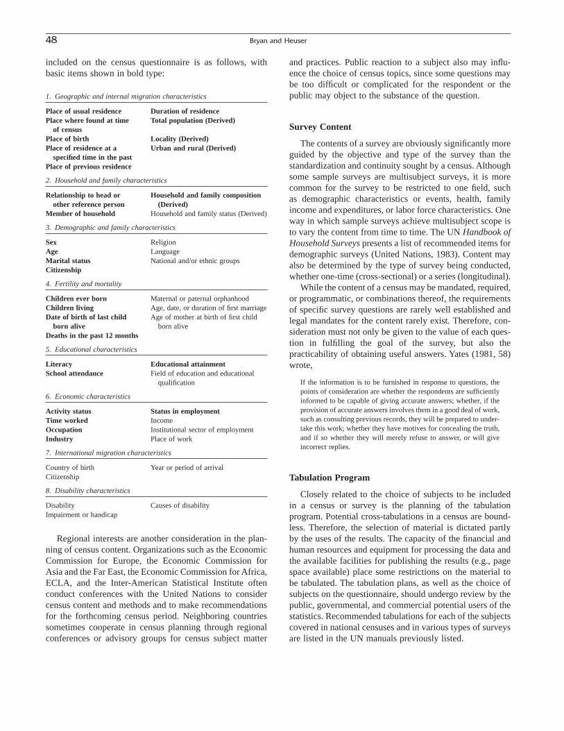
Regional interests are another consideration in the plan-ning of census content. Organizations such as the EconomicCommission for Europe, the Economic Commission forAsia and the Far East, the Economic Commission for Africa,ECLA, and the Inter-American Statistical Institute oftenconduct conferences with the United Nations to considercensus content and methods and to make recommendationsfor the forthcoming census period. Neighboring countriessometimes cooperate in census planning through regionalconferences or advisory groups for census subject matter
and practices. Public reaction to a subject also may influ-ence the choice of census topics, since some questions maybe too difficult or complicated for the respondent or thepublic may object to the substance of the question.
Survey Content
The contents of a survey are obviously significantly moreguided by the objective and type of the survey than the standardization and continuity sought by a census. Althoughsome sample surveys are multisubject surveys, it is morecommon for the survey to be restricted to one field, such as demographic characteristics or events, health, familyincome and expenditures, or labor force characteristics. Oneway in which sample surveys achieve multisubject scope isto vary the content from time to time. The UN Handbook ofHousehold Surveys presents a list of recommended items fordemographic surveys (United Nations, 1983). Content mayalso be determined by the type of survey being conducted,whether one-time (cross-sectional) or a series (longitudinal).
While the content of a census may be mandated, required,or programmatic, or combinations thereof, the requirementsof specific survey questions are rarely well established andlegal mandates for the content rarely exist. Therefore, con-sideration must not only be given to the value of each ques-tion in fulfilling the goal of the survey, but also thepracticability of obtaining useful answers. Yates (1981, 58)wrote,
If the information is to be furnished in response to questions, thepoints of consideration are whether the respondents are sufficientlyinformed to be capable of giving accurate answers; whether, if theprovision of accurate answers involves them in a good deal of work,such as consulting previous records, they will be prepared to under-take this work; whether they have motives for concealing the truth,and if so whether they will merely refuse to answer, or will giveincorrect replies.
Tabulation Program
Closely related to the choice of subjects to be includedin a census or survey is the planning of the tabulationprogram. Potential cross-tabulations in a census are bound-less. Therefore, the selection of material is dictated partly by the uses of the results. The capacity of the financial andhuman resources and equipment for processing the data andthe available facilities for publishing the results (e.g., pagespace available) place some restrictions on the material tobe tabulated. The tabulation plans, as well as the choice ofsubjects on the questionnaire, should undergo review by thepublic, governmental, and commercial potential users of thestatistics. Recommended tabulations for each of the subjectscovered in national censuses and in various types of surveysare listed in the UN manuals previously listed.
48 Bryan and Heuser
1. Geographic and internal migration characteristics
Place of usual residence Duration of residencePlace where found at time Total population (Derived)
of censusPlace of birth Locality (Derived)Place of residence at a Urban and rural (Derived)
specified time in the pastPlace of previous residence
2. Household and family characteristics
Relationship to head or Household and family compositionother reference person (Derived)
Member of household Household and family status (Derived)
3. Demographic and family characteristics
Sex ReligionAge LanguageMarital status National and/or ethnic groupsCitizenship
4. Fertility and mortality
Children ever born Maternal or paternal orphanhoodChildren living Age, date, or duration of first marriageDate of birth of last child Age of mother at birth of first child
born alive born aliveDeaths in the past 12 months
5. Educational characteristics
Literacy Educational attainmentSchool attendance Field of education and educational
qualification
6. Economic characteristics
Activity status Status in employmentTime worked IncomeOccupation Institutional sector of employmentIndustry Place of work
7. International migration characteristics
Country of birth Year or period of arrivalCitizenship
8. Disability characteristics
Disability Causes of disabilityImpairment or handicap
included on the census questionnaire is as follows, withbasic items shown in bold type:

Part of the planning of the tabulation program involvesdetermining the number of different levels of geographicdetail to be presented. Data are usually presented for theprimary administrative divisions of the country and theirprincipal subdivisions and for cities in various size cate-gories as well as for the country as a whole. For the small-est geographic areas, such as small villages, the results as arule are limited to a report of the total number of inhabitantsor perhaps the male and female populations only. At the nexthigher level, which may be secondary administrative divi-sions, the tabulations may provide only “inventory statis-tics.” These statistics are simply a count of persons in thecategories of age, marital status, economic activity, and soforth, with little cross-classification with other characteris-tics. For the primary administrative divisions and majorcities, most subjects are cross-tabulated by age and sex, andoften there are also cross-classifications with other socialand economic characteristics, such as educational attainmentby economic activity or employment status by occupation.Also, more detailed categories may be shown on such sub-jects as country of birth, mother tongue, or occupation. Thegreatest degree of detail, sometimes termed “analytical” tab-ulations as opposed to “inventory” statistics, is that in whichcross-tabulations involve detailed categories of each of thethree or four characteristics involved.
Conducting the Census or Survey
Recruitment and Training
One of the largest tasks in conducting a survey, and espe-cially a census, is the recruitment and training of staff.Anderson (1988, p. 201) states of the 1950 U.S. Census,
It was extraordinarily difficult to recruit in a number of months areliable, competent staff of census enumerators and to guaranteeuniform application of census procedures in the field. The 1950evaluation studies indicated that on simple census questions, suchas age and sex, the enumerators performed well. But in recordingthe answers to such complex questions as occupation and industry,two different interviewers recorded the answers differently in a suf-ficient number of cases to render the data suspect.
While retaining staff with the skills necessary forpreparatory work (such as coding and data entry) is rela-tively easy, it is having a sufficient number of skilledworkers conducting the enumeration that must be especiallyprepared for.
Pretesting
Pretesting of census content and methods has been foundto be very useful in providing a basis for decisions that mustbe made during the advance planning of the census. This isespecially so in countries without a long history of census
taking. Such pretests vary in scope. They may be limited totesting a few new subject items, alternate wording of a ques-tion, different types of questionnaires, or different enumera-tion procedures. Most census testing includes at least onefull-scale pretest containing all questions to be asked on thecensus itself and sometimes covering part or all of the pro-cessing phases as well. The suitability of topics that havenot been tried before may be determined from a small-scalesurvey in two or three localities. With enough other ques-tions on the questionnaire to achieve something close to anormal census situation, a reasonable assesment of the ques-tion may be made. A test involving only the employees ofthe census office and their families may sometimes sufficefor this purpose. Countries having an annual sample surveysometimes use this survey as a vehicle for testing prospec-tive census questions.
Enumeration
The crucial phase of a census or survey comes when the questionnaires are taken into the field and the task ofobtaining the required information begins. The kinds ofproblems encountered and the procedures used for collect-ing the data are similar for censuses and surveys. In a censusthe procedures for enumeration are affected by the type of population count to be obtained. The census may bedesigned to count persons where they are found on censusday (a de facto count) or according to their usual residence(a de jure count).
In a de facto census, the method is to list all personspresent in the household or other living quarters at midnightof the census day or all who passed the night there. In thistype of enumeration, there is a problem of counting personswho happen to be traveling on census day or who work atnight and consequently would not be found in any of theplaces where people usually live. It may be necessary tocount persons on trains and boats or to ask households toinclude such members on the census form as well as thosepersons actually present. In some countries all persons arerequested to stay in their homes on the census day or untila signal announces the completion of the enumeration.
In a de jure census, all persons who usually live in thehousehold are listed on the form whether they are present ornot. Visitors who have a usual residence elsewhere areexcluded from the listing but are counted at their usual res-idence. Provisions must be made in a de jure census forpersons away from home if those persons think it is likelythat no one at their usual residence will report them. Theusual practice is to enumerate such persons on a specialform, which is forwarded to the census office of their homeaddress. The form is checked against the returns for that areaand is added to the count there if the person is not alreadylisted. This is a complicated and expensive procedure, and
3. Collection and Processing of Demographic Data 49

there still remains a chance that some persons will be missedand some counted twice.
There are two major types of enumeration, the direct-interview or canvasser method and the self-enumeration or householder method. In the direct-interview method, acensus agent visits the household, lists the members livingthere, and asks the required questions for each person,usually by interviewing one member of the household. Theadvantage of this method is that the enumerator is a trainedperson who is familiar with the questions and their inter-pretation and he or she may assume a high degree of respon-sibility for the content of the census. Also, this methodreduces the difficulty of obtaining information in an areawhere there is a low level of literacy. For these reasons it isconsidered possible to include more complex forms of ques-tions in the direct-interview type of enumeration.
In self-enumeration, the census forms are distributed,usually one to each household, and one or more members ofthe household complete the form for all persons in thehousehold. With this method of enumeration, there is lessneed for highly trained enumerators. The census enumera-tor may distribute the forms and later collect them, or themail may be used for either the distribution or collection ofthe forms or for both. If enumerators collect the forms, theycan review them for completeness and correctness andrequest additional information when necessary. In a mailcensus, the telephone may be used to collect informationfound to be lacking on the forms mailed in, or the enumer-ator may visit the household to obtain the missing informa-tion. In some cases the enumerator may complete an entirequestionnaire if the household is unable to do so.
Self-enumeration has the advantage of giving the respon-dents more time to obtain the information and to consultrecords if necessary. People can supply the informationabout themselves, rather than having the information sup-plied by a household member who may not have completeor correct information. The possibility of bias resulting froma single enumerator’s erroneously interpreting the questionsis minimized in this method of enumeration. It is also morefeasible to achieve simultaneity with self-enumerationbecause all respondents can be asked to complete the ques-tionnaires as of the census day. Thus, in this respect, self-enumeration is the more suitable method if a de facto countis desired.
Self-enumeration is the more frequently used method inEuropean countries, the United States, Australia, and NewZealand, whereas direct interview is the usual method inother countries. A combination of these two main types ofenumeration is often used. The self-enumeration methodmay be considered appropriate for certain areas of thecountry and the interviewer method for others, or some of the information may be obtained by interview and theremainder by self-enumeration. In a census that uses theinterviewer method as its basic procedure, self-enumeration
may be used for some individuals, such as roomers, whenthe head of the household cannot supply the information orwhen confidentiality is desired.
One of the goals of censuses and surveys is to minimizeresponse burden. For years it has been possible to conductsurveys over the telephone, and more recently on the Inter-net. To make answering the census questionnaire easier andto ease respondent burden, many countries are exploring thepossibility of allowing respondents to complete the basicdemographic questions online over the World Wide Web,with Internet access to explanations about the questionsasked in the census. Another innovation is telephone inter-viewing, whereby dedicated telephone lines are provided for the public to provide answers to the basic demographicquestions, instead of their completing and mailing thecensus questionnaire.
Some special procedures for enumeration are required for certain groups of the population, such as nomads orpeople living in inaccessible areas (i.e., icy, mountainous, orforested areas). Levels of literacy may be low among certainsocial or geographically concentrated groups, who may havelittle understanding of the purpose of a census or interest inits objectives. A procedure sometimes followed is to requestthat all the members of such groups assemble in one placeon a given day, since enumerating them at their usual placeof residence might require from 4 to 5 months. For some ofthese, a method of group enumeration has been used. Ratherthan obtaining information for each individual or household,the enumerator obtains from the head of the group a countof the number of persons in various categories, such asmarital status, sex, and age groups.
Enumeration of persons in hotels, pensions, missions,hospitals, and similar group quarters usually requires specialprocedures. Since some are transients, inquiry must be madeto determine whether they have already been counted else-where. If a de jure count is being made, steps must be takento assure that they are counted at their usual residence.Special individual census forms are usually used in groupquarters, since the proprietor or other residents of the placecould not provide the required information about eachperson. Another segment of the population that presents anenumeration problem is the homeless population, becausepeople in this group have no fixed addresses and possiblyoccupy public spaces or temporary residences.
In some households the enumerator is unable to interviewanyone even after repeated visits because no one is at homeor, more rarely, because the occupants refuse to be enumer-ated. Since the primary purpose of a census is to obtain acount of the population, an effort is made to obtain infor-mation from neighbors about the number and sex of thehousehold members. Neighbors may also be able to supplyinformation about family relationships and marital status,which may, in turn, provide a basis for estimating age. Reli-able information on other subjects usually cannot be
50 Bryan and Heuser
obtained except from the members themselves, and thesequestions are left blank, perhaps to be supplied during pro-cessing operations according to procedures that are dis-cussed in “Processing Data.”
In a sample survey, it is less practical to get informationfrom neighbors because the emphasis is on characteristicsrather than on a count of the population. The usual proce-dure is to base the results on the cases interviewed and adjustthe basic weighting factors to allow for noninterview caseswhen the final estimates are derived from the sample returns.The effect of this procedure is to impute to the populationnot interviewed the same characteristics reported by theinterviewed population. Since this assumption may not bevery accurate, the presence of numerous noninterviewhouseholds may bias the sample.
When a conventional enumeration has been completed in the field, questionnaires are assembled into bundles,usually corresponding to the area covered by one enumera-tor. The number of documents, the geographic identificationof the area, and other appropriate information are recordedon a control form, which accompanies the set of documentsthroughout the various stages of processing. The tremendousvolume of records involved in a census or large surveymakes the receipt and control of material a very import-ant function. The identification of the geographic area provides a basis for filing the documents and a means oflocating a particular set of documents at any stage of the processing.
Processing Data
Regardless of the care expended on the preparation of acensus and the enumeration of the population, the qualityand the usefulness of the data will be compromised if theyare not properly processed. The processing of the dataincludes all the steps, whether carried out by hand or bymachine, that are required to produce from the informationon the original document the final published reports on thenumber and characteristics of the population. The extent towhich these operations are accomplished by mechanical orelectronic equipment or by hand varies among countries andamong surveys and censuses within countries.
Recent innovations in data processing have advancedprocessing capabilities immensely. However, few censusesare processed entirely electronically. Usually, some of thedata, such as preliminary counts of the population for geo-graphic areas, are obtained from a hand count. Even datathat are produced primarily by machine must undergo somemanual processing to correct for omissions or inconsisten-cies on the questionnaire and to convert certain types ofentries into appropriate input for the electronic equipment.Electronic output may undergo a certain amount of handprocessing before it is ready for reproduction in a publishedreport. Such factors as the cost and availability of
equipment, the availability of manpower, and the goals interms of tabulations to be made, reports to be published, and time schedules to be met determine the degree to which elec-tronic processing is used. The data-processing operations to be performed in a census or survey usually consist of the following basic steps: editing, coding, data capture, andtabulation.
Editing
There are two principal points at which data errors mayarise. The first occurs when a respondent provides erroneousor conflicting information, or an enumerator misrecordsgiven information. The other occurs when data are codedand entered for computer processing. In both instances,concise rules should be established to determine how theseerrors should be edited. Census or survey procedures ofteninclude some editing of the questionnaires in the field officesto correct inconsistencies and eliminate omissions. Errors inthe information can then more easily be corrected by check-ing with the respondent, and systematic errors made by theenumerator can more easily be rectified. Whether the editingis done in the field office or is part of central office pro-cessing, elimination of omissions and inconsistencies is anecessary step preliminary to coding.
A “not reported” category is permitted in some classifi-cations of the population, but it is desirable to minimize the number of such cases. Where information is lacking, areasonable entry can often be supplied by examining otherinformation on the questionnaire. For example, a reasonableassumption of the relationship of a person to the head of thehousehold or the householder can be made by checkingnames, ages, and marital status; or an entry of “married”may be assigned for marital status of a person whose relationship entry is “wife.” Other edits may be made bycomparing data entries with noncensus information, such as administrative records. For example, in 1980 the CensusBureau asked, “How many living quarters are in the build-ing in which you live?” During editing, clerks were requiredto compare answers with the census mailout count foraddresses with 10 or fewer units. If the clerk found that more units were reported in a building than questionnairesmailed, an enumerator was sent to investigate (Choldin,1994, p. 57).
In manual editing, the clerks are given detailed specifi-cations for assigning characteristics. Nonresponse cases maybe assigned to a modal category (e.g., persons with place ofbirth not reported may be classified as native), or they maybe distributed according to a known distribution of the pop-ulation based on an earlier census. Since much of the editingfor blanks and inconsistencies is accomplished by applyinguniform rules, the use of electronic equipment for perform-ing this operation is now commonplace. Electronic process-ing is designed to reject or to correct a record with missing
3. Collection and Processing of Demographic Data 51
or inconsistent data and assign a reasonable response on thebasis of other information.
Problems with data entry and coding can lead to volu-minous errors in raw data files, making testing and qualitycontrol procedures throughout the census especially impor-tant. Errors of this type are typically systematic and can leadto much more pervasive problems than erroneous individualrecords. Strict editing and error-testing rules should beestablished by data experts and operationalized by pro-grammers to ensure a minimum of problems.
Coding
Coding is the conversion of entries on the questionnaireinto symbols that can be used as input to the tabulatingequipment. Many of the responses on a census or surveyrequire no coding or may be “precoded” by having the codefor each written entry printed on the schedule. For those thatdo, there are three different types of coding techniques pos-sible. For questions that have a small number of possibleanswers, such as sex or marital status, and questions that areanswered in terms of a numerical entry, the appropriate codemay be entered directly. If there are multiple answers, thencomputer-assisted coding may be used. In this process,codes are stored in a database and are automaticallyaccessed and inserted at the prompting of the operator. Thethird alternative is automatic coding, which may be used ifthe coding scheme is extraordinarily complex—such aswhen the codes for an answer need to be recorded in morethan one place.
Data Capture
In most data-processing systems, there must be somemeans of transferring the data from the original documentto the tabulating equipment. After going through editing andcoding, the data on the questionnaire may be transferred to a format that is electronically recognizable. There is alengthy history of improvements in this field. In the 1880s,the U.S. Census Bureau sponsored the development ofpunched-card tabulation equipment. By 1946, the CensusBureau had contracted with the Eckert-Mauchley ComputerCorporation to design a machine for processing the 1950census, and the result of this collaboration was the UNIVAC.Special equipment developed for the 1960 census of theUnited States “reads” microfilmed copies of the question-naires and transfers the data directly to computer tape. Thisequipment, known as FOSDIC (film optical sensing devicefor input to computers), reads the schedule by means of amoving beam of light, decides which codes have beenmarked, and records them on magnetic tape. By the 1980s,optical mark reading (OMR) was being widely used. Akinto a “scan-tron,” OMR dramatically improved the speed and
accuracy with which data were captured. However, OMRlimited the format on which survey and census responsescould be printed.
Today, there are three techniques commonly used tocapture data. The first is simple keyboard entry by clerks. Atan average rate of between 5000 and 10,000 keystrokes perhour (depending on equipment and the skill of the clerk),manual entry is reserved for only the smallest data-capturetasks. The second is optical character recognition (OCR).OCR devices are programmed to look for characters incertain places on a census or survey response and convertthem to an accurate, electronically recognizable value. Thethird is electronic optical scanning, which can be especiallyuseful for recording handwritten answers and especiallyvoluminous data. Recent developments in OCR and scan-ning have led to substantial improvements in accuracythrough better character recognition, higher rates of input,and the acceptability of a wider range of paper and othermedia for input.
It was noted earlier that during the planning stage of acensus or survey, decisions are made about the tabulationsto be produced, and outlines are prepared showing how thedata are to be classified and what cross-tabulations are to bemade. The outlines may be quite specific, showing in detailthe content of each proposed table.
On the basis of these outlines, specifications for computerprograms are written for the various operations of sorting,adding, subtracting, counting, comparing, and other arith-metic procedures to be performed by the tabulating equip-ment. The input is usually punched cards or computer tape,and the output is the printed results in tabular arrangement.In the most advanced systems of tabulation, the final resultsinclude not only the absolute numbers in each of the pre-scribed categories but derived numbers such as percentagedistributions, medians, means, and ratios as well.
One of the most obvious indicators of the quality of thedata from a census or survey is the nonresponse rate. Evenwhen a nonresponse category is not published and charac-teristics are allocated for those persons for whom informa-tion is lacking, a count of the nonresponse cases should beobtained during processing. One advantage of performingthe edit in the computer is that not only the number of non-responses on a given subject but also the known character-istics of the nonrespondents may be recorded. This providesa basis for analyzing nonresponses and judging the effectsof the allocation procedures.
The nonresponse rate for a given item has more meaningif it is based on the population to which the question appliesor to which analysis of that subject is limited. The base fornonresponse rates on date of first marriage, for example,would exclude the single population, and nonresponse ratesfor country of birth would be limited to the foreign born. Aproblem arises in the establishment of a population base
52 Bryan and Heuser

if the qualifying characteristic also contains a substantialnumber of nonresponses.
Planning the tabulations includes making some basicdecisions about the treatment of nonresponses. Nonre-sponses may be represented in a separate category as “notreported” or they may be distributed among the specific cat-egories according to some rule, ideally on the basis of otheravailable characteristics of the person. Practices vary on theextent to which responses are allocated, but the eliminationof “unknowns” before publication is a growing practice,partly because the greater capabilities of modern tabulatingequipment have improved the possibilities of assigning areasonable entry without prohibitive cost and partly becauseconvenience to the user of the data favors the elimination ofnonresponses.
Data Review
It has been mentioned that maintaining quality controland testing for errors while conducting a census or surveyare imperative. Several steps may be taken to improve theaccuracy and validity of results.
Supervisors should review samples of each enumerator’swork for completeness and acceptability and accompany theenumerator on some of his or her visits. Progress-reportingof the enumeration enables census officials to know whenan individual enumerator or the enumerators in a given areaare falling seriously behind schedule and thus jeopardizingthe completion of the census within the allotted time. Handtallies of the population counted in each small area are com-pared with advance estimates, and the enumeration isreviewed if the results vary too widely from the expectednumber.
Reinterviewing is a common technique used for qualitycontrol of the data-collection process in sample surveys. Asample of households visited by the original interviewer isreinterviewed by the supervisor, and the results of the check-interview are compared with the original responses. Suchchecking determines whether the recorded interview actually took place and reveals any shortcomings of theinterviewer.
Verification
Verification of the operation is an important element ofeach stage in the processing. Verification is not done for thepurpose of removing all errors, as this is virtually impossi-ble and does not justify the expense of time and resources.The purpose rather is (1) to detect systematic errors through-out the operation that can be remedied by changes in theinstructions or by additional training of personnel, (2) todetect unsatisfactory performance on the part of an individ-ual worker, and (3) to determine whether the general error
rate of the operation is within tolerance. Therefore, it isseldom necessary to have 100% verification. A procedureoften followed is to verify an individual’s work until theworker is found to be qualified in terms of a maximumallowable error rate, and thereafter to verify only a sampleof the individual’s work. If during the operation, a workeris found to have dropped below the acceptable level of accu-racy, his or her work units may be subjected to a completereview and correction process.
Verification may be “dependent,” in which the verifierreviews the work of the original clerk and determineswhether it is correct, or “independent,” in which two personsdo the same work independently and then a comparison ismade of the results. Tests have shown that in dependent ver-ification, a large proportion of the errors are missed. Inde-pendent verification, in which the verifier is not influencedby what was done by the original worker, has been found tobe more successful in discovering errors.
The statistical tables produced by the tabulating equip-ment are usually subjected to editorial and statistical reviewbefore being prepared for publication. On the basis ofadvance estimates and data from previous surveys or otherindependent sources, judgments are made regarding the rea-sonableness of the numbers. Figures that are radically dif-ferent from the expected magnitudes may indicate an errorin the specifications for tabulation. Review at this stage mayshow the need for expansion of the editing procedure. Forexample, early tabulations of educational statistics occa-sionally showing impossible combinations of age and edu-cational attainment may lead to an addition to the editingspecifications to eliminate spurious cases of this nature.Tables are reviewed for internal consistency. It is not nec-essary that corresponding figures in different tables agreeperfectly to the last digit, since minor differences arecommon in tables produced by different passes through thetabulating equipment. Arbitrary corrections for all small dif-ferences are not feasible, and such changes would add littleto the accuracy of the data. If the tables printed out by thetabulating equipment are to be used for publication, thespelling, punctuation, spacing, and indentation are also care-fully reviewed so that corrections can be made before thetables are reproduced.
Evaluation
The evaluation of census results is frequently cited as arequirement of a good census. An initial distinction must bemade between the products of an evaluation program andthe uses of these products. The products of an evaluation aremeasures of census error and identification of the sources oferror.
Census errors may occur at any of the various stages ofenumeration and processing and may be either coverage
3. Collection and Processing of Demographic Data 53

errors, that is, the omission or double-counting of persons,or content errors, that is, errors in the characteristics of the persons counted, resulting from incorrect reporting orrecording or from failure to report. Methods for measuringthe extent of error include reenumeration of a sample of thepopulation covered in the census; comparison of censusresults with aggregate data from independent sources,usually administrative records; matching of census docu-ments with other documents for the same person; and demo-graphic analysis, which includes the comparison of statisticsfrom successive censuses, analysis of the consistency ofcensus statistics with estimates of population based on birth, death, and immigration statistics, and the analysis of census data for internal consistency and demographic reasonableness.
Uses of the results of census evaluation include guidingimprovements in future censuses, assisting census users ininterpreting results, and adjusting census results. Evaluationcan identify certain geographic areas or persons with char-acteristics that made it problematic to enumerate them. Theresults of special enumeration efforts in relation to theircosts may also be examined. Evaluation may also illustratethe usefulness and limitations of the census data, especiallyto novice users. It can alert the user to errors in the data andthe magnitude of those errors. Moreover, the introduction ofevaluation may inform users of additional sources of demo-graphic data. Finally, evaluation may be used to adjustcensus results. Adjustment may be decided upon if evalua-tion indicates serious methodological, content, or coverageerrors in the census (U.S. Census Bureau, 1985).
While there are a large number of methods for evaluat-ing censuses, two predominant techniques have emerged.The first is the use of post-enumeration surveys, whichemploy case-by-case matching of the census and the surveyto evaluate coverage and content error. The second is demo-graphic analysis, which applies demographic techniques todata from administrative records to develop population esti-mates for comparison with the census.
Post-Enumeration Surveys
Post-enumeration surveys (PES) may be conducted inorder to test census coverage and content error. While a PESmay provide valuable insight into coverage and contenterror, caution must be used when designing and conductinga PES, as it is a statistically complex task. A simplifiedexplanation of the method used by the U.S. Census Bureauin 1990 follows.
The Census Bureau’s coverage measurement program in1990 involving a post-enumeration survey was one in aseries from 1950 to 2000. It was modeled after capture-recapture techniques used to estimate the size of animal pop-ulations. In essence, by sampling the population shortly afterthe census is taken and matching the two sets of data, estimates of census omissions may be derived. In the PES,
the traditional census enumeration corresponds to the orig-inal capture sample, and the PES to the recapture sample.However, equating the proportion of the PES sample notfound in the census with the proportion of the census thatwas missed implicitly assumes that the chances of beingcounted in the capture sample and of being counted in therecapture sample are independent. It is known that the prob-ability of being counted differs by age, sex, geographic area,and race, among other factors. For this reason, the results of the PES cannot be simply applied to the entire population,but instead must be stratified by small areas and variousdemographic and socioeconomic characteristics. In this waydifferent coverage ratios are derived according to thesefactors.1
Demographic Analysis
In addition to the information afforded by a PES, simpledemographic techniques can be used to evaluate a census foraccuracy and reasonableness. Visually identifying resultsthat are statistically improbable can be considered demo-graphic analysis. However, much more refined demographictechniques are available not only for detecting error, but foridentifying its source as well. The goal of demographicanalysis is to provide population estimates that are inde-pendent of the census being evaluated, using data from othersources, including principally administrative records ondemographic variables such as births, deaths, and migration,and demographic techniques such as sex ratio and survivalanalysis (Kerr, 1998, p. 1).
Demographic analysis can be used in two contexts. Thefirst is to evaluate the quality of the results themselves, andthe other is to provide measures of error for possible adjust-ment of the census. Countries may use different types andeven different combinations of methods of demographicanalysis to evaluate census results. The results of this analy-sis may be used not only to estimate the overcoverage orundercoverage, but also to provide a basis for adjustment to the official census population statistics. In cases wheredemographic analysis shows results similar to those of thecensus, confidence in the census may be increased.
Different formal procedures of coverage evaluation maybe used, and in fact some may be more appropriate in certaincountries, based on their record-keeping systems. In Canada,for example, a combination of a reverse record check (RRC)and an overcoverage study are used for evaluating thecensus. The RRC is a comprehensive record-linkage system,which entails taking a sample from various administrative
54 Bryan and Heuser
1 Further information on post-enumeration surveys may be found inWilliam Bell, “Using Information from Demographic Analysis in Post-Enumeration Survey Estimation.” Statistical Research Report SeriesNo. RR92/04, Washington, DC: U.S. Census Bureau, Statistical ResearchDivision, 1992.
records of people who should have been enumerated andsurveying for those who were missed. The overcoveragestudy involves reenumerating a sample of enumeratedhouseholds to test whether the members should have beenenumerated and where they should have been enumerated(Kerr, 1998, pp. 3–4). In Australia, the National Demo-graphic Data Bank, established in 1926 to measure births,deaths, and international migration, is used to develop esti-mates, which are used in conjunction with a PES to evalu-ate that country’s census (Kerr, 1998, p. 20).
In the United States, the Census Bureau applies demo-graphic analysis, distinguished as being a macrolevelapproach to measuring coverage, and a Post-EnumerationSurvey distinguished as being a microlevel approach. In theanalytic method, estimates of the population below age 65are derived from the basic demographic accounting equa-tion, while Medicare data are used to estimate the popula-tion aged 65 and over. Some population groups, such asillegal entrants, have no associated administrative recordsand therefore must be estimated. While demographic analy-sis was not formally used to provide corrected populationsin the 1990 U.S. census, it was used to measure net cover-age error and “evaluate” the results of the PES (Robinson,1996, p. 59).
The evaluation techniques of PES, RRC, overcoveragesurveys, demographic analysis, and others are not withouttheir shortcomings. The PES and RRC techniques are hin-dered by difficulty in measuring nonsampling error. Over-coverage is always difficult to measure, as in the case of dejure censuses, and the respondents often do not know thatthey have been recorded twice. The quality of demographicestimates declines in older age categories as the length ofthe times series for births used in estimation grows, and difficulty in measuring certain components (such as inter-national migration) may compound error. Additionally, geo-graphic detail is often lost, affording analysis only for largecensus regions or a nation as a whole.
The benefits of demographic analysis, however, are thatit may be applied at a very low cost and that most of theadministrative records necessary for demographic analysisoftentimes exist already and only need to be compiled andsummarized for an evaluation. Demographic analysis is alsoeasy to complete on a timely basis and works independentlyof the census, thus affording a quick and valid evaluation ofcensus results. Finally, demographic analysis provides abenchmark of decennial census quality, affording the onlyconsistent historical time series of measures of census netundercount for age, sex, and race groups (Robinson, 1996,pp. 60–61).
Dissemination
Once data are tabulated and reviewed, they are dissemi-nated to users. Private, governmental, and other non-
commercial groups rely on timely and convenient access tocensus data. Historically, census data have primarily beenprovided as a series of printed tables and more recently asdata tapes and CD-ROMs. Recent advances in Internet tech-nology now afford data users the opportunity to gather dataonline and to design data sets and tabulations not previouslypossible.2
Publication of Results
The output of the tabulation equipment may be used asthe final statistical tables suitable for reproduction in thepublished reports, or it may be an interim tabular arrange-ment of the data from which the final tables will be pro-duced. In the latter situation, typing of the final tables iseither done directly from the machine printouts or requirespreliminary hand posting of the data on worksheets toarrange them as required for the publication tables. Theseadditional steps, of course, require verification, proofread-ing, and machine-checking.
Electronic Dissemination
The continuous improvement of computers and high-speed printers has made the automatic production of finaltables both feasible and economical. The elimination of oneor more manual operations in the production process reducesthe burden of quality control, improves the timeliness ofpublication, and reduces manpower requirements. The useof high-speed printer output demands very precise advanceplanning of the content of each table, the wording of cap-tions and stubs, and the spacing of lines and columns. Thetechnical skill involved and the lead time required for suchplanning have led some countries to use a compromise pro-cedure in which the machine printout is used for the bodyof the table but the stubs and captions are provided by meansof preprinted overlays. The programming of the computerprintout in these instances is designed to display the data inthe desired arrangement and to include rudimentary cap-tions, which identify the numbers.
As discussed in Chapter 2, the trend in the disseminationof survey and census data has been heavily toward electronicdissemination on CD-ROM and other high-capacity media,and it is now turning toward the Internet. There are manypotential methods for data dissemination on the Internet,ranging from free public access of easily downloadable
3. Collection and Processing of Demographic Data 55
2 A valuable source of international census enumeration, data tabula-tion, and dissemination is Diffusion: International Forum for Census Dis-semination, 1985, Statistics Canada. Published approximately every year,editorship rotates among participating countries. The journal provides inter-national perspectives on testing forms, designs, topics, and questions. Thejournal also provides evaluation of data tabulation and disseminationmethods.

data files and products, to interactive online software for thecreation of customized data sets by the user to commercial“for a fee” data available by subscription only. Data secu-rity on the Internet is an important consideration, not onlyfor users, but for data suppliers as well. Commercial datavendors often contend with security issues, such as unau-thorized users’ accessing their files without permission. Inaddition to the emplacement of sophisticated securitysystems, techniques have been devised whereby encoded/encrypted data are placed on the Internet, and authorizedusers are privately given special software with which toaccess it.
Storage
In addition to these improvements in data dissemination,consideration must be given to the voluminous data in exis-tence on other media. As already mentioned, many data havebeen stored on computer tape. Four alternate technologicalapplications are used to replace traditional hard-copyrecords. These include microforms, computer-assistedmicroforms systems, optical disk systems, and computer-based systems (Suliman, 1996). It should be noted that theseapplications are used for a wide variety of data-storage pur-poses in addition to censuses and surveys, including civilregisters, vital statistics, and population registers.
Microforms were one of the earliest replacements ofhard-copy records and developed into both roll microfilmand flat microfiche. This application provides very long-term preservation of written information and often enhanceswritten items on older records. An improvement of themicroform system has been the computer-assisted micro-form system (CAM). If records already exist in a manualmicroform system, they can be indexed electronically,allowing very fast searches and record retrieval. If recordsdo not already exist in a microform system, they may befilmed and placed directly into a CAM system. Shortcom-ings of both microform systems are the inability to evaluatethe data statistically and to make any subsequent changesonce the data have been filmed. The third application isknown as an optical disk system. In this application, largevolumes of records may be scanned electronically and storedon an optical disk. An electronic index may be created at thetime of scanning, again allowing for very fast data searchesand record retrieval. The optical disk system has the samelimitations as microform, however, in that tabulations andcalculations may not be made within the application, andrevisions or corrections must be rescanned. The final systemis the computer-based system. This has been described asthe system in which data are entered directly via keystrokesor optical scanning systems that are compatible with software that enables conversion to an electronic format(Suliman, 1996).
Use of Sampling in Censuses
Although censuses as a rule involve a complete count ofthe number of inhabitants according to certain basic demo-graphic characteristics, sampling is often used as an integralpart of the enumeration to obtain additional information. Asnoted by the United Nations:
The rapidly growing needs in a number of countries for extensiveand reliable demographic data have made sampling methods a verydesirable adjunct of any complete census. Sampling is increasinglybeing used for broadening the scope of the census by asking anumber of questions of only a sample of the population. Modernexperience in the use of sampling techniques has confirmed that itis not necessary to gather all demographic information on a com-plete basis; the sampling approach makes it feasible to obtainrequired data of acceptable accuracy when factors of time and costmight make it impracticable, or other considerations make it unnec-essary, to obtain the data on a complete count basis. (UnitedNations, 1998, p. 25)
Many data items may have to be collected on a complete-count basis because of legal requirements or because of the need for a high degree of precision in the data on basictopics so as to establish benchmarks for subsequent studies.However, the need in most countries for more extensivedemographic data has driven the collection of other itemson a sample basis. This practice not only expands the poten-tial coverage of subjects, but also saves time and moneythroughout the enumeration and processing stages as well.
Even when data collection is on a 100% basis, a repre-sentative sample of the schedules may be selected foradvance processing to permit early publication of basic infor-mation for the country as a whole and for large areas. Manyof the final tabulations in a census may be limited to a sampleof the population; thus the cost of tabulation is reduced con-siderably, especially when detailed cross-classifications areinvolved. In addition to its use in enumeration and process-ing, sampling is important in the testing of census question-naires and methods prior to enumeration, in the applicationof quality-control procedures during enumeration and pro-cessing, and in the evaluation of the census by means of aPES and field checks (United Nations, 1998, p. 47).
Sample Survey Methods
The role of sample survey methods in the collection ofdemographic data is well established. Some of the uses andadvantages of sample surveys were discussed earlier in thischapter. While a complete discussion of probability, surveydesign, and sampling concepts is not presented here, it isimportant to consider three aspects of sampling. The first isthe definition of the population. It is important for analyststo consider the population to be measured and characterizedand to take precautions to ensure that the sample instrumentaffords generalizability to that population. The second is thesampling methods being used. The choice among conven-
56 Bryan and Heuser

ience, typical-case, quota, or other designs in nonprobabil-ity sampling and among systematic, stratified, cluster, orother designs in probability sampling can have widelyvarying effects on the results of a survey. The third is theprecision being sought. While the variance of sample esti-mates is inversely proportional to sample size, the cost, efficiency, and proposed uses of the data must also be considered (Henry, 1990).
When deriving census values based on sample censusdata, the sampling ratio itself determines the basic weights tobe applied to each record (e.g., a sample of one in five leadsto a weight of five). The figures produced by the applicationof these weights, however, are often subjected to other adjust-ments to obtain the final estimates. The adjustments may bemade to account for the population not covered because offailure to obtain an interview. Also, independent population“controls” often are available to which the sample results areadjusted. In a census, the data obtained on a sample basis maybe adjusted to the 100% population counts for the “marginal”totals by means of a ratio-estimation procedure. In this casethe ratios of complete-count figures for specified demo-graphic categories (e.g., age, sex, race) to the sample figuresfor the same categories are computed and used for adjustingthe more detailed tabulations based on the sample. Similarly,the results of sample surveys may be adjusted to independ-ent population controls, which are postcensal estimatesderived by applying the basic population estimating equationto population figures from the previous census.
Other Demographic Record Systems
The administration of population registers differs some-what from country to country, but basically it calls for reg-istration at birth and entering specified subsequent events(marriage, change of residence, death, etc.) upon the indi-vidual or household record. A copy of this record, or anextract thereof, may be required to follow the person whenshe or he moves from one local jurisdiction to another. Thereare always local registers, and there may also be a centralnational register. The discussion of population registers inChapter 2 gave an indication of their general nature and citeda number of publications concerning them.
Some aspects of the collection and processing of immi-gration data, particularly the registration system associatedwith border control, are discussed in Chapter 18. Here weconsider, next, vital statistics registration systems in detail.
VITAL STATISTICS
Dual Functions of a Vital Statistics System
Vital statistics systems are designed primarily to accom-plish the registration of vital events. Vital statistics, are the
statistics derived from compiling vital events. Registrationof births, deaths, marriages, and divorces was originallyintended to meet public and private needs for permanentlegal records of these events, and these needs continue to be very important. However, equally important are thedemands for useful statistics that have come from the fieldsof public health, life insurance, medical research, and pop-ulation analysis.
Viewed as one of several general methods of collectingdemographic statistics, registration has certain advantagesand disadvantages. If events are registered near the time ofoccurrence, the completeness of reporting and the accuracyof the information are potentially greater than if reportingdepends on a later contacted by an official and recall of thefacts by the respondent. Also, continuous availability of thedata file tends to be assured by the dual uses of the infor-mation—for legal and for statistical and public purposes.
There are also certain limitations of the registrationmethod. The fact that the vital record is a legal documentlimits the amount and kind of nonlegal information that canbe included in it. The method is also affected by the numberand variety of persons involved in registering the events. Forexample, birth registration in some countries requiresactions by thousands or millions of individual citizens andhundreds of local officials. Thousands of physicians, nurses,or hospital employees may be involved, and all of thesepeople have other duties that they consider more urgent. Itseems inevitable that for the most part these many anddiverse persons will have less training and expertise in datacollection than the enumerators who interview respondentsin censuses or other population surveys. The latter areusually given intensive training in which the importance,purposes, and exact specifications of the information soughtare thoroughly explained.
Satisfactory conduct of registration, in terms of both thelegal and the statistical requirements, is closely related to thecompleteness and promptness with which events are regis-tered and the accuracy of the information in the registrationrecords. Certain functions such as indexing and filing of cer-tificates, issuance of copies, and amendment of records areimportant for their legal uses but do not significantly affectthe statistics. However, if the legal functions are poorly per-formed, the statistical program will suffer because publicpressures will demand that first priority be given to servingpeople’s needs for copies of their personal records.
International Standards and National Practices
The Handbook of Vital Statistics Systems and Methods,Volume I: Legal, Organizational and Technical Aspects(United Nations, 1991) and Handbook of Vital StatisticsSystems and Methods, Volume II: Review of National Prac-
3. Collection and Processing of Demographic Data 57

tice (United Nations, 1985), published by the United NationsStatistical Office, are the principal sources of the materialpresented in this section on international recommendationsfor the collection and processing of vital statistics.
Definitions of Vital Events
As in all systems of data collection, clear, precise defini-tions of the phenomena measured are prerequisites for accu-rate vital statistics. Use of standard definitions of vital eventsis essential for comparability of statistics for different countries.
Live Birth
Most countries follow the definition of a live birth rec-ommended by the World Health Assembly in May 1950, andby the United Nations Statistical Commission in 1953,which is as follows:
Live birth is the complete expulsion or extraction from its motherof a product of conception, irrespective of the duration of preg-nancy, which after such separation, breathes or shows any other evi-dence of life, such as beating of the heart, pulsation of the umbilicalcord, or definite movement of voluntary muscles, whether or not theumbilical cord has been cut or the placenta is attached; each productof such birth is considered live-born. (United Nations, 1991, p. 17)
Under this definition a birth should be registered as a livebirth regardless of its “viability” or death soon after birth ordeath before the required registration date. Although varia-tions in the statistical treatment of “nonviable” live births(defined by low birthweight or short period of gestation) donot significantly affect the statistics of live births, they canhave a substantial effect on fetal death and infant death statistics.
Death
Until very recently, there has been less difficulty withrespect to the definition of death than with definitions of livebirth and fetal death. For statistical purposes, the UnitedNations has recommended the following definition of death:
Death is the permanent disappearance of all evidence of life at anytime after live birth has taken place (postnatal cessation of vitalfunctions without capability of resuscitation). This definition there-fore excludes foetal deaths. (United Nations, 1991, p. 17)
Fetal Death
The definition of fetal death recommended by the WorldHealth Organization (WHO) and the United Nations Statistical Commission is as follows:
Foetal death is death prior to the complete expulsion or extractionfrom its mother of a product of conception, irrespective of the dura-tion of pregnancy; the death is indicated by the fact that after suchseparation the foetus does not breathe or show any other evidence
of life, such as beating of the heart, pulsation of the umbilical cord,or definite movement of voluntary muscles. (United Nations, 1991,p. 17)
Marriage
The Statistical Commission of the United Nations hasrecommended the following definition of marriage for sta-tistical purposes:
Marriage is the act, ceremony or process by which the legal rela-tionship of husband and wife is constituted. The legality of the unionmay be established by civil, religious, or other means as recognizedby the laws of each country. (United Nations, 1991, p. 17)
Divorce
The United Nations Statistical Commission’s recom-mended definition of divorce is as follows:
Divorce is the final legal dissolution of a marriage, that is, the sep-aration of husband and wife by a judicial decree which confers onthe parties the right to civil and/or religious remarriage, accordingto the laws of each country. (United Nations, 1991, p. 17)
This definition excludes petitions, provisional divorces,and legal separations since they do not imply final dissolu-tion of marriage and the right to remarry. In some countries,legal annulment is a statistically significant method of mar-riage termination. It is desirable in such countries to includeannulments with divorces in determining the statistics ofmarriage dissolution. The Handbook defines annulment as“the invalidation or voiding of a marriage by a competentauthority, according to the laws of each country, whichconfers on the parties the status of never having beenmarried to each other (United Nations, 1991, p. 17).
Collection of Vital Statistics
Vital statistics systems differ in the amount of authoritygiven to the collecting agency, the degree of national cen-tralization of its organization, and the type of agency carry-ing out the program. The basic features of a vital statisticscollection system are discussed in the following sections.
Civil Registration Method
This method of collecting vital statistics data is definedas the “continuous, permanent, compulsory recording of theoccurrence and characteristics of vital events . . . in accor-dance with the legal requirements of each country” (UnitedNations, 1991, p. 16). The registration of all vital eventsmust be done as they occur and must be maintained in orderto be retrieved as required. This must be done by a perma-nent governmental agency with administrative stability. Theunderpinning, however, is that vital registration is legallyrequired and there are penalties for failure to comply withthe law. “The compulsion or legal obligation to register a vital event is the basic premise of the entire civil
58 Bryan and Heuser

registration system. When registration is voluntary ratherthan compulsory, there can be no assurance of complete oraccurate vital records or statistics” (United Nations, 1973,p. 159). Without specific penalties, the fact that it is com-pulsory is meaningless.
Governmental Organization
The registration systems may be classified as organizedunder centralized or decentralized control. Most nationshave established a centralized national authority over regis-tration. In some countries, it is the civil registration office,in others, the department of public health, and in others, thecentral statistical agency. Again, in some countries the samenational agency is responsible for both registration and vitalstatistics, but in others two or occasionally three separateagencies control these two functions. Advantages of acentral registration office include direct and effective controlover the entire system, including a standard legal frame-work, uniform procedures, and consistent interpretation andenforcement of norms and regulations.
In a decentralized system, civil registration is adminis-tered by major civil divisions, for example, the state,province, or department. Many countries with federatedpolitical systems have decentralized registration systems.
The Statistical Office of the United Nations Secretariatundertook a Survey of Vital Statistics Methods during1976–1979. Of the 103 countries reporting on the type ofcivil registration system, 88 were centralized and 15 decen-tralized (United Nations, 1985, p. 8).
Local registration areas are the basic units of a vital registration system. They must have clearly defined geo-graphic boundaries and be small enough for the registrar to provide good registration services for the area and forpersons reporting vital events to come to or communicatewith the registration office without excessive difficulty. Oneof the most important responsibilities of the local registraris to encourage the general population, physicians, mid-wives, and others to report occurrences of vital eventspromptly and to supply complete and accurate informationabout them.
Informants and Reporters
The person responsible by law for reporting the occur-rence of a vital event may or may not also be the source ofthe facts associated with the event. In most countries, afamily member is responsible for reporting the occurrenceof a live birth, fetal death, or death, together with certainpersonal information, but the attendant physician or midwifeis also responsible for reporting the event along with certainmedical information. The officiant, civil or religious, at themarriage is required to report it in about one-half of thecountries; in the other half, the participants, bride andgroom, are responsible. Reporting of divorces is the respon-sibility of the court in slightly more than half of the
countries and of one or both of the parties to the divorce inthe remaining countries (United Nations, 1985, pp. 20–22).
Place of Registration
The United Nations recommends and, with few excep-tions, the countries of the world require registration of vitalevents in the local registration area where the eventoccurred. Statistics tabulated by the United Nations from the 1976–1979 survey of national practices show that the percentage of responding countries where vital events areregistered by place of occurrence is 92 for births and deaths,93 for fetal deaths, 90 for marriages, and only 55 fordivorces (United Nations, 1985, pp. 29–30). Tabulations arefrequently made by area of usual residence of the mother,decedent, and so forth; these are generally regarded as moreuseful for demographic purposes than tabulations by placeof occurrence.
Time Allowed for Current Registration
The registration record usually calls for both the date ofthe event and the date of registration. National laws usuallyspecify the maximum interval permitted between these twodates for each type of vital event. The 1976–1979 surveyshows that the time allowed for registering deaths tends tobe shorter than for births—94% within 30 days for deathscompared with 73% for births (United Nations, 1985, pp.26–27). The United Nations recommends that final tabula-tions for any calendar period should be based on events thatoccurred during that period and not on those registered.Information from the 1976–1979 survey indicates that two-thirds to three-quarters of the countries tabulated the recordsby date of registration (United Nations, 1985, pp. 34–35).
Content of Statistical Records
The need for national vital statistics data is the primarydeterminant of what items should be collected on vitalrecords. Another major consideration is international com-parability. The United Nations has recommended lists of sta-tistical items that should be included in the records of livebirths, fetal deaths, deaths, marriages, and divorces (UnitedNations, 1991, pp. 30–31). The World Health Organizationrecommended the form of the medical certificate of cause ofdeath. Some of the recommended items are designated aspriority items, that is, items all countries should include. Par-allel listings of priority items for the various vital statisticsrecords are shown in Table 3.1.
Compilation and Tabulation of Vital Statistics
The underlying purpose of a vital statistics system is tomake available useful statistics for the planning, adminis-tration, and evaluation of public health programs and toprovide basic statistics for demographic research. The doc-uments undergo much the same processing that is required
3. Collection and Processing of Demographic Data 59

for census and survey data, and similar planning is requiredto produce the desired tabulations.
In a majority of countries, the central statistical office hasbeen given responsibility for compilation of national vitalstatistics. In some countries, including the United States, thisfunction has been located in the national public healthagency. In other countries, responsibility has been dividedbetween the health agencies and the statistical and registra-tion agencies.
The United Nations has suggested four criteria for mea-suring the effectiveness of a national vital statistics program,(1) coverage of the statistics, (2) accuracy of the statistics,(3) tabulations of sufficient detail to reveal important rela-tionships, and (4) timeliness of availability of the data(United Nations, 1991, p. 46). One of the basic premises ofa vital statistics system is that every event should be reportedfor statistical purposes for all geographic areas and all pop-ulation subgroups. The time reference for the data should bethe date on which the event occurred. The geographic ref-erence for the statistics may be either the place where theevent occurred or the residence of the person to whom theevent occurred. Final tabulations for subnational geographicareas should be by place of residence. This allows for com-putation of meaningful population-based rates. Tabulationby place of occurrence may also be useful for specificadministrative purposes. Finally, the data and their analysis
need to be disseminated to be useful. Unless the data areavailable to the public, its willingness to support the systemcannot be expected. A wide variety of dissemination mediashould be used, including printed publications, public usedata tapes and disks, and the Internet.
It is also essential that statistics of births, deaths, and mar-riages be based on definitions and classifications that areidentical to or consistent with those used in the populationcensus. Computation of valid vital rates and use of theserates in population estimation depend on consistent treat-ment of vital statistics and population data. This objective is sometimes difficult to attain, however, especially whendifferent agencies are responsible for the two statistical programs.
Other Methods of Obtaining Vital Statistics
Every nation has as a goal the coverage of all its statesor other areas in its vital statistics system. This objective isoften not achieved without a long period during which theregistration system is being developed and its coveragegradually extended. Other data collection methods may supplement or be a substitute for the registration system.These may include surveys, censuses, and population registers.
60 Bryan and Heuser
TABLE 3.1 Priority Items Recommended for Inclusion in Statistical Reports of Live Birth, Fetal Death, Death, Marriage, and Divorce
Live birth Fetal death Death Marriage Divorce
Date of occurrence Date of occurrence Date of occurrence Date of occurrence Date of occurrenceDate of registration Date of registration Date of registration Date of registration Date of registrationPlace of occurrence Place of occurrence Place of occurrence Place of occurrence Place of occurrencePlace of usual residence Place of usual residence Place of usual residence1 Place of usual residence2
of motherSex Sex SexLegitimacy status Legitimacy status Marital status Marital status1
Date of marriage Date of marriage Date of marriage(legitimate births) (legitimate births)
Age of mother Age of mother Age Age1 Age2
Type of birth (single or Type of birth (single or Type of ceremonymultiple) multiple) (civil, religious, etc.)
Number of children born Number of children born Number of dependentto this mother to this mother children of divorcee2
Number of previous fetaldeaths to this mother
Weight at birthGestational age
Attendant at birthCauseCertifier
1 Of bride and groom.2 Of both divorcees.Source: United Nations. 1991. “Handbook of Vital Statistics Systems and Methods,” Volume I: “Legal, Organizational and Technical aspects.” Studies
in Methods, Series F, No. 35, pp. 30–31.

Surveys
Vital statistics may be obtained from a household samplesurvey by questioning members of the household regardingvital events that occurred in that household in some specificpast period. This method can be implemented in a relativelyshort time if the necessary technical skills can be mobilizedto plan and conduct the survey; and it can be expected toprovide some statistics rather speedily. Its success dependsheavily on the willingness of persons in the sample to supplythe information and on their ability to recall the vital eventsoccurring during some past period of time, and the date,place of occurrence, and other facts about the events. Also,the considerable skills required for sample design, surveyorganization and operation, and questionnaire constructionneed to be available on a continuing basis.
Censuses
Information on vital events is sometimes obtained in thepopulation census. Statistics on births, marriages, and deathsin the previous year are available from this source in somecountries. This method is essentially a special survey, whichincludes the entire population rather than a sample. It issubject to the same limitations as surveys with respect to therecall of events.
Population Registers
In countries that maintain a population register, birth,death, marriage, and divorce registration may be an integralpart of the register. The information obtained in the regis-tration of vital events must not only serve the needs for statistics on these subjects but must also be consistent in definitions and classifications with the information to bekept in the population register on the entire population.
The United States Vital Statistics System
National-State Relationships
The United States system for collecting vital records isdecentralized in that the legal authority over registration is located in each of the 50 states and the District of Columbia. New York City is an independent registrationarea that has its own laws and regulations and publishes itsown reports, as do Guam, Puerto Rico, and the VirginIslands of the United States. Many states are divided intolocal registration districts, for each of which a registrar isappointed. There are about 10,000 such registrars, appointedby the state governments or locally elected. Each state separately processes the statistics that it wishes for its ownarea and population. The processing of national vital statis-tics is centralized in the National Center for Health Statis-tics (NCHS), a federal agency located in the U.S. PublicHealth Service (US PHS). An extensive history of the U.S.vital registration and statistics system may be found in
History and Organization of the Vital Statistics System(Hetzel, 1997).
Uniformity of Reporting
Although registration of vital events is governed by statelaws, a considerable degree of uniformity has been achievedin definitions, organization, procedures, and forms. Unifor-mity has been promoted primarily by the development ofmodel laws and certificate forms that have been recom-mended for state use. The Model State Vital Statistics Lawhas been followed with variations in the laws enacted in thevarious states. It was first promulgated in 1907 and has beenrevised and reissued several times. The most recent versionwas promulgated in 1992 ( US PHS, 1995). Standard cer-tificates of the several vital events, issued by the respon-sible national agency, have been the principal means ofachieving uniformity in the certificates of the individualstates, which provide the information upon which nationalvital statistics are based. The last revision was promulgatedin 1989 (US NCHS/Tolson et al., 1991). The next revisionis being implemented gradually beginning in 2003.
The responsible national vital statistics agency (theCensus Bureau, 1903–1946, NOVS, 1947–1959, and NCHS,1960 to date) has actively assisted the state agencies inachieving complete, prompt, and accurate registration ofvital events. Tests of registration completeness and intensiveeducational campaigns to promote registration have beenjoint federal-state efforts. The national office has developedand recommended to the states model handbooks designedto instruct physicians, hospitals, coroners and medical exam-iners, funeral directors, and marriage license clerks oncurrent registration procedures and the meaning of the infor-mation requested in the certificates (e.g., US NCHS, 1987).
Functions Performed by State Offices
In the decentralized registration system of the UnitedStates, the primary responsibility for the collection of vitalrecords rests with each state. This responsibility encom-passes a number of functions that are carried out in eachstate’s vital statistics office.
Planning Content of Forms
It is the responsibility of the state’s vital statistics office to recommend the format and content of the vitalrecords used in its jurisdiction. These recommendations are usually based to a large extent on the United States standard certificates but also often reflect special interests or needs not encompassed in the federal model forms. Inspite of the efforts of the federal government to promotenational uniformity, state and local uses of vital records,especially in the health field, produce differences in recordcontent and format, which have an effect on the statistics.Some of the states have not included all of the standard
3. Collection and Processing of Demographic Data 61

demographic or health items on their vital records. Cur-rently, however, all states have birth and death certificatesthat conform very closely to the U.S. standard certificates incontent.
Confidentiality of Records
It is the responsibility of each sate or other registrationarea to determine the need for confidentiality and to main-tain confidentiality of the vital records. In some areas, vitalrecords are considered to be public documents; in otherareas, the vital statistics laws and administrative regulationspermit the release of information or certified copies of therecord only to certain authorized persons.
Receipt and Processing of Records
One of the major functions of a state office is to serve asthe repository for vital records of events occurring withinthe state, and thus to serve as a central source within eachstate for both the legal and statistical uses of the records.This function entails a number of related responsibilities,such as the handling of corrections, missing data, namechanges, and adoptions and legitimations and issuing certi-fied copies of records on file.
Electronic birth certificate (EBC) software has beendeveloped for use in the capture of the information on thebirth certificate at the reporting source (hospitals). This software has been designed to improve the timeliness andquality of birth registration. The information on the birthcertificate is entered into the software by hospital personneland transmitted to the appropriate registration authoritywithin the state. Before transmission, it is checked forquality and completeness by an edit program designed andinstalled by the state. Currently all states are using EBC soft-ware and approximately 90% of births are currently regis-tered through this process.
States are also in the process of developing Electronicdeath certificate (EDC) software. It is anticipated that withina few years most deaths will also be registered through anelectronic process.
Tabulation and Publication of the Data
Just as each state prepares and processes its own vital sta-tistics data, so does each state prepare an annual summaryof its vital statistics. These summaries vary in analytic detailand comprehensiveness, but almost all states publish somekind of annual vital statistics report. Some of these reportsmerely present selected vital statistics data, whereas otherscontain, in addition to tabular material, an analysis and inter-pretation of the statistics.
Another activity of the state vital statistics offices is thetransmittal of data to the National Center for Health Statistics (NCHS) for the purpose of assembling nationalstatistics. The NCHS purchases the data in electronic form from each registration area through a contractualarrangement, which includes a guarantee of confidentiality
prohibiting the center from releasing any data other than statistical summaries without the written consent of thestate’s vital statistics office.
In order to issue provisional statistics in its National VitalStatistics Report, NCHS receives reports from the states onthe total number of records (birth, death, infant death, mar-riage, and divorce) received during the month regardless ofdate of occurrence. Characteristics about these events arenot published in these provisional reports.
Functions Performed by the National Center forHealth Statistics
The NCHS performs a variety of functions designed toimprove the national vital statistics system. It exercises lead-ership in the revision of the standard certificates and in eval-uating the completeness of birth registration; represents theUnited States in international conferences on the standardclassification of causes of death; conducts a trainingprogram on vital and health statistics; and helps the states indeveloping forms, procedures, draft legislation, definitions,and tabulations.
The NCHS serves as the focal point for the collection,analysis, and dissemination of national vital statistics for the United States. Because of the diversity of practices and procedures existing in the decentralized U.S. system, the production of national statistics involves more than the combination of statistics from each registration area toproduce national vital statistics.
Detailed data on births, deaths, and fetal deaths areobtained in electronic form through contractual arrange-ments with the states. The data are subjected to a series ofcomputer edits that eliminate inconsistencies in the data andimpute missing data for certain items. This is generally doneonly when the number of items with missing data comprisesa very small proportion of the total. Sex, race, and geo-graphic classification are assigned if not reported on thebirth or death certificates, and age and marital status ofmother are assigned if not reported on the birth certificate.
The final computer tabulations of national vital statisticsappear in various publications prepared by NCHS and men-tioned in Chapter 2, “Basic Sources of Statistics.” Unpub-lished material and resource data for special investigationsare maintained by the NCHS and made available on theInternet (www.cdc.gov/nchs). In addition, unit record data onbirths, deaths, and linked birth-infant deaths are available onCD-ROMs.
References
Anderson, M. 1988. The American Census: A Social History. New Haven,CT: Yale University Press.
Choldin, H. 1994. Looking for the Last Percent: The Controversy over Census Undercounts. New Brunswick, NJ: Rutgers UniversityPress.
62 Bryan and Heuser
Henry, G. 1990. Practical Sampling. Newbury Park, CA: Sage.Hetzel, A. M., 1997. History and Organization of the Vital Statistics System.
Hyattsville, MD: National Center for Health Statistics.Kerr, D. 1998. “A Review of Procedures for Estimating the Net Undercount
of Censuses in Canada, the United States, Britain and Australia.”Demographic Documents. Ottawa: Statistics Canada.
Robinson, J. G. 1996. “What Is the Role of Demographic Analysis in the 2000 United States Census?” Proceedings of Statistics Canada Symposium, 96: Nonsampling Errors, Nov. 1996. pp. 57–63, Ottawa:Statistics Canada.
Suliman, S. H. 1996. “Automation of Administrative Records and Statis-tics,” http://www.un.org/Depts/unsd/demotss/tenjun96/suliman.htm,October 27, 1999.
United Nations, 1973. “Principles and Recommendations for a Vital Statistics System.” Statistical Papers, Series M, No. 19, Rev. 1. NewYork: United Nations.
United Nations, 1983. “Handbook of Household Surveys.” Studies inMethods, Series F, No. 10. New York: United Nations.
United Nations, 1985. “Handbook of Vital Statistics Systems andMethods,” Volume II: “Review of National Practices.” Studies inMethods, Series F, No. 35. New York: United Nations.
United Nations. 1991. “Handbook of Vital Statistics Systems andMethods,” Volume I: “Legal, Organizational and Technical Aspects.”Studies in Methods, Series F, No. 35. New York: United Nations.
United Nations. 1998. “Principles and Recommendations for Populationand Housing Censuses.” Statistical Papers, Series M. No. 67 / Rev. 1.New York: United Nations.
U.S. Census Bureau. 1985. “Evaluating Censuses of Population andHousing.” Special Training Document ISP-TR-5. Washington, DC:U.S. Census Bureau.
U.S. Census Bureau. 1995. “Solicitation of 2000 Census Content Needsfrom Non-federal Data Users: November 1994–March 1995.” Specialreport of the Decennial Management Division. Washington, DC: U.S.Census Bureau.
U.S. National Center for Health Statistics, 1987. Hospitals’and Physicians’Handbook of Birth Registration and Fetal Death Reporting. DHHSPub. No. (PHS) 87–1107. Washington, DC: National Center for HealthStatistics.
U.S. National Center for Health Statistics, 1991. “The 1989 Revision of theU.S. Standard Certificates and Reports,” by G. C. Tolson, J. M. Barnes,G. A. Gay, and J. L. Kowaleski. Vital Health Stat 4(28). Hyattsville,MD: National Center for Health Statistics.
U.S. Public Health Service. 1995. Model State Vital Statistics Act and Regulations. DHHS Pub. No. (PHS) 95–1115.
Yates, Frank. 1981. Sampling Methods for Censuses and Surveys. NewYork: Oxford University Press.
Suggested Readings
Anderson, M. 1988. The American Census: A Social History. New Haven,CT: Yale University Press.
Edmonston, B., and C. Schultze (eds.). 1995. Modernizing the U.S. Census.Washington, DC: National Academy Press.
Hetzel, A. M. 1997. History and Organization of the Vital Statistics System.Hyattsville, MD: National Center for Health Statistics.
Hogan, H. 1993. “The 1990 Post-Enumeration Survey: Operations andResults.” Journal of the American Statistical Association 88 (423),1047–1060.
Robinson, J. G., B. Ahmed, P. Das Gupta, and K. A. Woodrow. 1993. “Esti-mating the Population Coverage in the 1990 United States CensusBased on Demographic Analysis.” Journal of the American StatisticalAssociation 88 (423), 1061–1071.
United Nations. 1998. “Principles and Recommenolations for Populationand Housing Censuses.” Statistical Papers, Series M. No. 67/Rev. 1.New York: United Nations.
3. Collection and Processing of Demographic Data 63

This Page Intentionally Left Blank

The size of a population is usually the first demographicfact that a government tries to obtain. The initial censusesof a people are often a mere headcount. Particularly in pre-modern times, the emphasis in census taking was on fiscaland military potentials. Hence, women, children, aliens,slaves, or aborigines were usually relatively undercountedor omitted altogether (Alterman, 1969, Part I, Chapter 1).Modern censuses provide more comprehensive coverage,taking into consideration issues related to the individual enumeration of all persons living in a specific geographicarea at a given time and the completeness of coverage.
CONCEPTS OF TOTAL POPULATION
In general, modern censuses are designed to include the“total population” of an area. This concept is not so simpleas may at first appear. There are two “ideal” types of totalpopulation counts, the de facto and the de jure (Shryock,1955). The former comprises all the people actually presentin a given area at a given time. The latter is more ambi-guous. It comprises all the people who “belong” to a givenarea at a given time by virtue of legal residence, usual residence, or some similar criterion. In practice, whilemodern censuses call for one of these ideal types with spec-ified modifications, it is difficult to avoid some mixture ofthe two approaches.
Issues Related to National Practices
Specific National Practices
The practice followed in more than 220 national censusesis summarized in the United Nations Demographic Year-book: 1996, Table 3, page 134 (United Nations, 1998). Sincethe de facto type of census is considerably more common
than the de jure type on a worldwide basis, the table merelynotes which countries conduct a de jure census. For example,most African, Asian, South American, and Oceanic censusesare de facto. Notable exceptions include Algeria, Israel,Nepal, Philippines, Thailand, and Australia. The situation ismixed in North and Central America, with the followingcountries or dependent areas using the de jure approach:Canada, the Cayman Islands, Costa Rica, Greenland, Guadeloupe, Haiti, Martinique, Mexico, the NetherlandAntilles, Nicaragua, Puerto Rico, the United States, and theU.S. Virgin Islands. A mixed situation also exists in Europe.The de jure approach is used in Austria, Belgium, BosniaHerzegovina, Croatia, the Czech Republic, Denmark, theFaeroe Islands, Germany, Iceland, Luxembourg, the Nether-lands, Norway, Slovakia, Slovenia, Sweden, Switzerland,and Yugoslavia (United Nations, 1998).
For many countries, the distinction between de jure andde facto would not be very important for the national total.Usually, however, the choice would appreciably affect thecount for many geographic subdivisions. The effect wouldalso vary according to the census date.
The United Nations regards the method used to allocatepersons to a geographic subdivision of the country as beingbest determined by national needs. At first it seemed to favorthe de facto principle, but later it recognized the complica-tions of that approach for family statistics, migration statis-tics, and the computation of resident vital rates and othermeasures. The de jure concept seems to be rather ambigu-ous. Legal residence, usual residence, and still other criteriacould be used to define the people who “belong” to a givenarea at a given time. In the United States, moreover, there isno unique definition of “legal residence.” A person may havecertain rights or duties (voting, public assistance, admissionto a public institution, jury duty, certain taxes, and so forth)in one state or community and other rights or duties inanother state or community. A citizen who has recently
65
C H A P T E R
4
Population Size
JANET WILMOTH
The Methods and Materials of DemographyCopyright 2003, Elsevier Science (USA).
All rights reserved.
moved may not have some of these rights in any state. Incertain Asian societies, the people have sometimes beenenumerated at their familial or even ancestral home, wherethey actually may have lived only in childhood or never atall.
Thus, the relative difficulties of the de facto and de juremethods in census taking and their relative accuracy dependto some extent on the particular country. As a result, theHandbook of Population and Housing Censuses (UnitedNations, 1992, p. 91) recommends “that a combination ofthe two methods be adopted to obtain information that is ascomplete as possible.” In such a situation, people may belisted in the field in a particular manner, but when the tabu-lations are made, some of them may be reassigned to otherareas on the basis of recorded facts about where they spentthe previous night or their usual residence. Whatever cov-erage method is used, it must be clearly spelled out for thebenefit of those who report in the census, those who processthe data, and those who use the statistics.
Inclusion of Certain Groups
Despite the coverage method used (e.g., de jure, de facto,or a combination of both), special consideration has to begiven to certain groups because of their ambiguous situa-tions. According to the United Nations (1992, pp. 81–82),these groups include the following:
(a) Nomads(b) Persons living in areas to which access is difficult(c) Military, naval, and diplomatic personnel of the
country, and their families, located outside thecountry
(d) Merchant seaman and fisherman resident in thecountry but at sea at the time of the census (includingthose who have no place of residence other than theirquarters aboard ship)
(e) Civilian residents temporarily in another country asseasonal workers
(f) Civilian residents who cross the boarder daily to workin another country
(g) Civilian residents other than those in groups (c), (e),and (f) who are working in another country
(h) Civilian residents other than those in groups (c)through (g) who are temporarily absent from thecountry
(i) Foreign military, naval, and diplomatic or defensepersonnel and their families who may be located inthe country
(j) Civilian aliens temporarily in the country as seasonalworkers
(k) Civilian aliens who cross a frontier daily to work inthe country
(l) Civilian aliens other than those in groups (i), (j), and(k) who are working in the country
(m) Civilian aliens other than those in groups (i) through(l) who are temporarily in the country
(n) Transients on ships in harbor at the time of thecensus.
Particular attention is often given to providing separatecounts of the civilian and military population for severalreasons. In some ways, the civilian and military populationsconstitute separate economies. There are constraints on freemovement from one to another. Moreover, they have diff-erent components of change, and their geographic distri-butions are very different. The most feasible methods ofenumerating them may also differ. All these considerationshave led a few countries to publish separate statistics fortheir civilian and military populations.
While specific countries may have different reasons forincluding or excluding specific groups in the total popula-tion, census documentation should clearly indicate whichgroups are included in the total population. In addition, estimates of the size of each nonenumerated group shouldbe reported in the census documentation. This informa-tion can be gathered from administrative records or othersources. Alternatively, all of the people present in thecountry at the time of the census can be enumerated by usinga census questionnaire that distinguishes these differentgroups. This information can be used later to include orexclude certain groups from the total population.
International Standards
The information regarding groups included or excludedis critical for comparing population size across differentcountries and regions, as well as for arriving at estimates ofworld population.
The United Nations (1992, p. 83) recommends that“groups, . . . , (a) through (f), (h) and (l) be included in, and(g), (i) through (k), (m), and (n) be excluded from, the totalpopulation.” Even though this recommendation specifiesissues related to civilian residents and civilian aliens quiteclearly, it is consistent with earlier United Nations docu-ments that advocate an “international conventional total”(also called a “modified de facto population”). This popula-tion count consists of “the total number of persons presentin the country at the time of the census, excluding foreignmilitary, naval, and diplomatic personnel and their familieslocated in the country but including military, naval, anddiplomatic personnel of the country and their familieslocated abroad and merchant seamen resident in the countrybut at sea at the time of the census.”1
66 Wilmoth
1 This recommendation appeared first in Statistical Papers, Series M,No. 27, Principles and Recommendations for National Population Censuses, 1958, p. 10.

Evidence of a Person
In addition to questions of whether certain classes ofpeople are to be included in the national census count, andwhere a particular person should be counted, problems arisein actual practice as to whether there is sufficient evidenceof a person. For example, even after repeated attempts toobtain the information by mail, telephone, or personal visit,there may remain a number of marginal cases where the onlyevidence consists of (1) names copied by the enumeratorfrom mailboxes or (2) information from a neighbor that one or more people live at a given address. Decisions mustthen be made as to whether there is enough information towarrant listing these persons on the schedule. While specificdecision rules vary across countries, it is recommended thatcensus documentation clearly indicate the decision rulesused regarding evidence of a person.
Method of Enumeration
The size of the total population can be determinedthrough the use of several different methods.2 The first is thecanvasser method, which involves the use of trained enu-merators who visit each housing unit to conduct an inter-view. During this interview, information is obtained aboutthe housing structure and the characteristics of its occupants.The enumerator records this information on the appropriatecensus forms and then turns the forms in to his or her fieldsupervisor. A primary advantage of this enumeration methodis that the enumerators can be thoroughly trained in censusprocedures and instructions. This can increase the qualityand consistency of the data, particularly in countries wherea large proportion of the population is illiterate. The maindisadvantages are that in practice not all of the householdmembers can usually be directly interviewed and a mis-application of the rules by one enumerator can lead to misreporting in an entire enumeration area, i.e., enumerator-induced bias.
Another common method is the householder (or self-enumeration) method in which instructions and question-naires are distributed to each housing unit before the censusday. The census form is then completed by one member ofthe household, preferably the household head or anotherresponsible household member. This method can improveaccuracy by allowing the householder to consult with othermembers of the household at their convenience. It can alsoconsiderably lower costs, particularly when the mail-out/mail-back procedure of distribution is used extensively.This involves using the postal service to deliver and returnthe census forms, instead of an enumerator. The householder
method is most effective in countries in which a high per-centage of the population is literate and which have an effi-cient and universal postal system.
The census-station method involves developing a list ofall housing units in an area and then establishing a centrallylocated census station. The population in that area is askedto report to the census station, where the enumerator recordsthe relevant information on the appropriate forms. To ensurecomplete coverage, the enumerator is required to visit non-responding housing units. An alternative method involvesassembling all of the residents of a given area in one placewhere the enumeration is conducted. In this situation, thehead of the group often provides general information aboutthe number of people living in the area. Detailed populationcharacteristics are usually not collected. This method is particularly effective in enumerating individuals living inisolated areas and among particular groups.
In practice, a combination of methods is often used toensure that the size of the total population is being accu-rately assessed. Furthermore, over time the balance ofreliance on these methods can shift as the society changes.Changes in a population’s literacy level, geographic loca-tion, and composition, as well as developments in the postalsystem, can call for a reassessment of the most appropriateenumeration method for a given census.
The United States Decennial Census
The Constitution of the United States requires (in Article1, Section 2.3) merely that “Representatives . . . shall beapportioned among the several States which may beincluded within this Union, according to their respectivenumbers.” The Constitution does not provide a unique pre-scription for the type of enumeration to be made. In the 18thcentury, there was considerably less difference between thede jure and de facto populations of an area than there wasin the 20th, because the limited transportation facilities andthe way of life tended to keep people at home. Hence, theframers of the Constitution probably were unaware of theambiguity of their directive. Ordinarily, there would not bea great deal of difference at the national level, but in certainhistorical periods the two types of enumeration would haveresulted in substantially different population totals. Forexample, during the peak of activity in World War II, a de facto count would have yielded about 9 million fewerpersons than a count taken on a strict de jure basis. “Thecensus has never been taken on a de facto basis, however:and it has come to be considered that such a basis would beinconsistent with the spirit, if not the letter, of the Constitu-tion. The basic principle followed in American censuses isthat of ‘usual residence.’ This type of census more nearlyapproximates the de jure than the de facto” (Shryock, 1955,p. 877).
4. Population Size 67
2 See United Nations (1992, pp. 88–90) for addition information. Thissection only summarizes the discussion presented there.
Definition of Usual Residence
The meaning of “usual residence” itself is not a simplematter and has to be spelled out in some detail for the benefitof enumerators and respondents. While the general spirit of“usual residence” has remained the same since the decen-nial census was established in the United States in 1790, the inclusion of specific groups has varied (Shryock, 1960).Usual place of residence is the “place where he or she livesand sleeps most of the time or the place where the personconsiders to be his or her usual home” (U.S. Bureau of theCensus, 1992c). Since 1960 the procedures for conductingthe census have depended more on self-enumeration and lesson the canvasser method. As a result, the instructions to thehouseholder on the mail-out/mail-back forms regardingwhom to include on the household list are quite specific. Theinstructions on page 1 of the 1990 form asks the householderto “list on the number lines below the names of each personliving here on Sunday, April 1, including all persons stayinghere who have no other home (U.S. Bureau of the Census,1992d)”. This list was to include newborns, members of the household temporarily absent on vacation, visiting, onbusiness, or in a general hospital, as well as boarders orlodgers who usually slept in the housing unit. The instruc-tions also covered a number of special cases, some of whichare discussed in the sections that follow. Similar instructionswere given for the census of 2000.
Enumeration of Special Populations3
Members of the Armed Forces within the United States
Persons in the Army, Navy, Air Force, Marine Corps, andCoast Guard of the United States were supposed to havebeen counted as residents of the place where they were stationed, not at the place from which they were inducted orat their parental home. Those members who lived off postwere to be counted at their homes (with families, if any),whereas those who lived in barracks or similar quarters wereconsidered as residents of those group quarters. One excep-tion is the personnel assigned to the 6th or 7th Fleet of theNavy, who are counted as part of the overseas population.This information was collected in collaboration with theU.S. Department of Defense.
College Students
Beginning with the census of 1950, a student attendingcollege has been considered a resident of the enumerationdistrict in which she or he lives while attending college. Thatwas also apparently the rule up to 1850; but, in most of theintervening censuses, the student was counted at his or her
parental home. However, students away from home attend-ing schools below the college level have been consistentlycounted at their parental homes.
Persons in Institutions
Persons in types of institutions where usual stays are for long periods of time (regardless of the length of stay ofthe person considered) were enumerated as residents of theinstitution. These include “Federal or State prisons; localjails; Federal detention centers; juvenile institutions;nursing, convalescent, and rest homes of the aged anddependent; or homes, schools, hospitals, or wards of thephysically handicapped, mentally retarded, or mentally ill”(U.S. Bureau of the Census, 1992c). Individuals in generalhospitals or other institutions for medical care wherepatients usually stay for only a short period are counted attheir usual residences.
Persons with More Than One Residence
Persons with dual residences represent a variety of cir-cumstances. In the U.S.’s affluent and mobile society, withits long vacations and early retirement, the occupancy ofmore than one home during the year is increasinglycommon. Many people change residences with the seasons.This group is to be counted in the household where themajority of the calendar year is spent. Of course, there havealso long been classes of workers who changed their resi-dences seasonally with the jobs—lumbermen, fishermen,agricultural laborers, cannery workers, and so on. The ordi-nary rule is to choose the residence where the person livesthe greatest part of the year. However, if migrant agricul-tural workers or persons in worker camps do not report ausual residence, they are counted at their census-day loca-tion. Another class of dual residence consists of persons whowork and live away from their homes and families, perhapsreturning on weekends. In their case, the need for meaning-ful family statistics clashes with the need to include personsin the area where they are living most of the time. The res-idence rules for the 1990 and 2000 censuses are that indi-viduals in this situation should be enumerated in the locationwhere they live during the week.
Persons with No Usual Residence
Persons with no usual residence anywhere (migratoryagricultural workers, vagrants, some traveling salespeople,etc.) have been counted where they were found according toa provision that goes back to the Act of 1790. To obtain acomplete and unduplicated count of such persons, canvass-ing procedures like “T-night” (“T” for transient) and “M-night” (“M” for mission) were introduced some decadesago. Given the increased concern regarding the homelesspopulation since 1970, the Census Bureau has expanded itsefforts to enumerate the population living in shelters andpublic places such as bus and train terminals or outdoor
68 Wilmoth
3 For more information, see U.S. Bureau of the Census (1993), Appendix D. Collection and Processing Procedures, and U.S. Bureau of the Census (1995a), Appendix 1C, Table of Residence Rules for the 1990 Census.
locations. In the 1990 census, the “S-night” (“S” for streetsand shelters) canvassing procedure occurred during the nightof March 20–21. It involved trained census workers’ goingwhere homeless people were likely to be located, includingstreets, public parks, freeway overpasses, abandoned build-ings, or shelters specifically serving the homeless popula-tion. This special enumeration effort counted approximately240,000 people (U.S. Bureau of the Census, 1995b, Chapter11). The 2000 census included a specific service-based enu-meration (SEB), which counted people at communityservice organizations that typically serve people withouthousing, and targeted outdoor locations. In addition, censusforms were available at various public locations such as postoffices, community centers, and health care clinics (U.S.Bureau of the Census, 1999a).
Americans Abroad
This and the following category are of special interestfrom the standpoint of the United Nations’ “internationalconventional total.” It may be recalled that the recom-mendation called for the inclusion of the country’s own military and diplomatic personnel stationed abroad or at sea.However, historically the enumeration of this group in theU.S. censuses has been inconsistent (U.S. Bureau of theCensus, 1993). Only two censuses prior to 1900 (i.e., 1830and 1840) attempted to enumerate this group. For thoseyears in which Americans abroad were enumerated, the specific groups included (e.g., military personnel, federalcivilian employees, crews of U.S. merchant marine vessels,and private U.S. citizens) and the countries considered as“abroad” have varied. This information is usually providedby several different federal agencies, including the Depart-ment of Defense. Table 4.1 presents the number of Ameri-cans overseas and summarizes the changes in residencerules.4
The 1990 and 2000 censuses enumerated overseas mili-tary personnel and federal civilian employees, as well astheir dependents living with them. These groups, totaling922,845 people in 1990, were included in the official countsthat are used for congressional apportionment but omittedfrom other official statistics. Americans abroad only tem-porarily (as tourists, visitors, persons on short business trips,etc.) were supposed to be counted at their usual place of res-idence in the United States, whereas those away for longerperiods (employed abroad, enrolled in a foreign university,living in retirement, etc.) were excluded from the basiccount (U.S. Bureau of the Census 1993, 1995a, Chapter 1).
Foreign Citizens Temporarily in the United States
The U.S. census has adhered partially to the principle ofthe “international conventional total” by excluding foreign
military and diplomatic personnel and their families who arestationed here if they are living in embassies or similar quar-ters. In fact, such persons are not even listed. On the otherhand, it fails to list all other citizens of foreign countries tem-porarily in this country. The American rules for inclusion orexclusion parallel those given in the preceding subsection(e.g., foreigners working or studying in the United States arecounted). Failure to provide statistics on foreigners tem-porarily present and not on official assignments representsone of the points at which it is impossible to construct the“international conventional total” for the United States bythe combination of published statistics.
Doubtful Cases
It may be apparent by now that these rules require acertain amount of judgment in some cases because suchwords as “temporary” and “usual” are not precisely defined.Attempts to use a time criterion, such as at least 60 days,have not been satisfactory. For one thing, both past andprospective length of stay must be considered. It may alsobe apparent that the nature and purpose of the stay are justas important considerations as the duration.
It should be noted that most of the specific decisions concerning where a person should be enumerated are notmade in the central office, as is the case in some other coun-tries, but are made in the field. In the United States, theBureau of the Census formulates the general principles butleaves their application to the respondent or the enumerator.Except in the case of groups canvassed in certain specialoperations, the central office does not have the facts thatwould be needed to change the area to which the person isallocated.
Household Population
The allocation of these special groups can have a con-siderable effect on population counts in certain geographi-cal areas. Thus, published counts often distinguish the sizeand characteristics of the “normal” population of an area,which excludes not only members of the armed forces sta-tioned there and living in barracks or aboard ship but alsopersons living in institutions, college dormitories, and othergroup quarters. Table 1 of the 1990 census report, GeneralPopulation Characteristics for the United States (U.S.Bureau of the Census, 1992b) indicates that 97.3% of thetotal population lived in households and 2.7% (more than 6million people) lived in groups quarters. Table 35 in thesame publication indicates that, among those living in groupquarters, more than half are institutionalized while theremainder live in other group quarters. Although the conceptof the “normal” population of an area is a social construc-tion, the presence of a relatively large “nonnormal” popula-tion will distort its demographic composition and vital rates so as to obscure comparisons with other areas not
4. Population Size 69
4 See U.S. Bureau of the Census (1993) for a detailed discussion ofchanges in the residence rules regarding Americans abroad.

containing such a population. As a result, a distinction isoften made between the total population, which includes allusual residents of an area, and the household population,which includes only the population living in households. Forexample, Table 57 of the 1990 census report, General Population Characteristics for Kansas indicates that Leavenworth County, Kansas, which contains a federalprison and a military post, contains a total population of64,371 and a household population of 54,974 (U.S. Bureau
of the Census 1992a). The difference between these twonumbers (9397) represents the number of people living ingroup quarters.
Special Censuses and the Current Population Survey
For the most part, “usual residence” is defined the sameway in the national sample surveys conducted by the U.S.Bureau of the Census. They have mostly been limited to the
70 Wilmoth
TABLE 4.1 Americans Overseas, 1830–1840, 1900–1940, and 1950–1990 by Type (In 1850–1890 censuses, no figures were published for Americans overseas)
Dependents offederal employees
Total U.S. populationFederal employees
(armed forces Crews of U.S. Private U.S.Year abroad1 Total Armed forces Civilians and civilian) merchant vessels citizens
1990 925,8452 (NA) 529,2693 (NA)4 (NA)4 3,0265 (NA)1980 995,546 562,962 515,4083 47,5546 423,5846 (NA) (NA)1970 1,737,836 1,114,224 1,057,7767 56,4488 371,3668 15,9109 236,33610
1960 1,374,421 647,730 609,72011 38,0108 506,3938 32,46412 187,83410
1950 481,54513 328,505 301,59514 26,9108 107,3508 45,69015 (NA)1940 118,93316 (NA) (NA) (NA) (NA) (NA) (NA)1930 89,45317 (NA) (NA) (NA) (NA) (NA) (NA)1920 117,23818 (NA) (NA) (NA) (NA) (NA) (NA)1910 55,60817 (NA) (NA) (NA) (NA) (NA) (NA)1900 91,21919 (NA) (NA) (NA) (NA) (NA) (NA)1840 6,10020 (NA) (NA) (NA) (NA) (NA) (NA)1830 5,31820 (NA) (NA) (NA) (NA) (NA) (NA)
(NA) Not available.1 Excludes U.S. citizens temporarily abroad on private business, travel, etc. Such persons were enumerated at their usual place of residence in the United
States as absent members of their own households. Also excludes private, nonfederally affiliated U.S. citizens living abroad for an extended period, exceptfor 1970 and 1960, which include portions of this subpopulation.
2 Excludes 9460 persons overseas whose home state was not designated and 16,999 persons overseas whose designated home “state” was a U.S. outly-ing area.
3 Based on administrative records provided by Department of Defense.4 Not shown separately. Total number reported of overseas federal civilian employees and dependents (of both military and civilian personnel) was
393,550. Based on administrative records provided by 30 federal agencies (including Department of Defense) and survey results provided by Department ofDefense.
5 Vessels sailing from one foreign port to another or in a foreign port. Overseas status based on Census Location Report.6 Based on administrative records provided by Office of Personnel Management and Departments of Defense and State.7 For members of the Army, Air Force, and Marine Corps abroad, based on administrative records provided by Department of Defense. Crews of deployed
U.S. military vessels were enumerated on Report for Military and Maritime Personnel. Land-based Navy and Coast Guard personnel abroad were enumer-ated on Overseas Census Report.
8 Enumerated on Overseas Census Report.9 Vessels at sea with a foreign port as their destination or in a foreign port. Enumerated on Report for Military and Maritime Personnel.
10 U.S. citizens living abroad for an extended period not affiliated with the federal government, and their overseas dependents. Enumerated on OverseasCensus Report.
11 Enumerated on Overseas Census Report and Report for Military and Maritime Personnel.12 Vessels at sea or in a foreign port. Enumerated on Report for Military and Maritime Personnel.13 Based on 20% sample of reports received.14 Enumerated on Overseas Census Report and Crews of Vessels Report.15 Vessels at sea or in a foreign port. Enumerated on Crews of Vessels Report.16 Source of overseas count is unclear; see section on 1940 census.17 Enumerated on general population schedule.18 Enumerated on report for Military and Naval Population, etc., Abroad.19 Enumerated on report for Military and Naval Population and report for Civilians, Residents of U.S. at Military or Naval Stations.20 Persons on naval vessels in the service of the United States.Source: U.S. Bureau of the Census, 1993, Table 2.

civilian noninstitutional population. A noteworthy exceptionis the March supplement to the Current Population Survey(CPS). That survey’s focus on the labor force leads it toexclude people who are outside the market economy in theregular monthly survey, but the annual March supplementto the Current Population Survey covers the institutionalpopulation and members of the armed forces living off postor with their families on post. The CPS uses different residence rules for enumerating college students. They arecounted at their parental homes, partly because countingthem in the college communities during the academic yearand at home (or where they are employed) during the vaca-tion period would lead to seasonal variations in enumerationprocedures and in the resulting statistics.
TIME REFERENCE
As noted by the United Nations (1992), two essential fea-tures of a population census are simultaneity and definedperiodicity. Simultaneity refers to establishing a set censusreference time during which census data are to be collectedand recorded. Ideally, individuals should be enumerated ona given day and the information they provide should referto a set time period. If a census has a specific official hour,it is usually midnight, a time when most persons are at home.However, the census day varies across countries as a resultof seasonal fluctuations in weather, economic activity, andpublic observances. Considerations regarding the conduct ofa de facto population census of an area can also influencethe choice of a specific census time and day because such apopulation is subject to daily and seasonal fluctuations.These are relatively insignificant for most national totals, but particular areas could be greatly affected. Urban areas, especially the downtown districts of central cities, are par-ticularly affected by daily fluctuations, while resort areasand certain types of agricultural areas are particularlyaffected by seasonal factors.
Once a day and time have been established that are favorable for conducting a census, subsequent censusesshould also be conducted at the same time. However, thebest day and time for taking a census may change over timebecause of shifts in a country’s economic, social, and demo-graphic characteristics. For example, the date of the U.S.census changed from the first Monday in August for the1790 through 1820 censuses, to June 1 for the 1830 through1900 censuses. The 1910 and 1920 censuses were conductedon April 15 and June 1 respectively. It was not until 1930that the current census date of April 1 was established (U.S.Bureau of the Census, 1995a).
More important, the subsequent censuses should have adefined periodicity. In other words, they should occur atregular intervals. Even though some countries are able toconduct a census every 5 years, the United Nations (1992)
acknowledges that this is not feasible for most countries andrecommends that the established period between censusesshould be no longer than 10 years.
A national census should not be taken by a crew of enu-merators that moves from one district to another as it com-pletes its work; nor, in general, should the enumerationbegin on different dates in different parts of the country. Yetin practice, both have occurred. The enumeration in the earliest historic censuses and in contemporary censuses ofthe less developed countries typically extended over manymonths. If a day or month was cited, it meant nothing morethan the time when the fieldwork began. The disadvantagesof such protracted enumerations are that omissions andduplications are more difficult to avoid and it becomesincreasingly difficult to relate the facts to the official censusdate.
At a more advanced stage of census taking, there arespecifications like “the zero hour” (midnight) on July 1 (Li,1987). Occasionally, exceptional starting dates may be jus-tified by such considerations as gross variations in climateor the annual dispersal of nomads to isolated grazinggrounds. For example, the census of Alaska is often con-ducted prior to April 1 to avoid canvassing Alaska duringthe spring thaw.
In some cases a serious attempt is made to complete theenumeration in a day’s time. These censuses are character-istically on a de facto basis. Such rapid censuses are by nomeans limited to the more industrialized societies or thehouseholder (i.e., self-enumeration) method of enumeration.The most dramatic enumerations are those in which normalbusiness activities cease and the populace must stay at homeuntil the end of the census day or until it has been announcedthat the canvass has been completed. However, the “one-daycensus” usually turns out to be an ideal or a figure of speech.One-day enumerations are often localized in coverage (e.g.,focused only on particular geographic areas), based on pre-viously collected information that is updated on the censusday, or carried over into subsequent days.
COMPLETENESS OF COVERAGE
The completeness of coverage provided by a moderncensus is influenced largely by the degree of deliberate andunintentional exclusions. As has been mentioned already,countries often deliberately exclude from their censusescertain relatively small classes of population on the basis ofthe type of census being taken, whether de jure, de facto, orsome modification of one of these. Other deliberate exclu-sions are based on feasibility, cost, danger to census per-sonnel, or considerations of national security. Finally, somepersons will be deliberately or inadvertently omitted fromthe population as defined, while others will be incorrectlycounted. Official omissions by design then will be discussed
4. Population Size 71

separately from the net underenumeration (or overenumer-ation) that tends to occurs to some extent, in counting asizable population, as a result of deliberate action or over-sight on the part of respondents or enumerators.
Deliberate Exclusion of Territory or Group
It is not unusual for specific territories or various popu-lation subgroups to be excluded from a census for one reasonor another. In some countries, for example, either the indige-nous or nonindigenous population, or parts of them, may beomitted from the census count, or the two may be enumer-ated at different times. In addition to tribal jungle areas, cen-suses may omit parts of the country that are under the controlof alien enemies or of insurgents. Some examples from theUnited Nations (1998) are as follows:
Country Census date Excluded Group or Territory
Brunei Darussalam 1991 Transients afloatBrazil 1991 Indian jungle populationEcuador 1990 Nomadic Indian tribesFalkland Islands 1990 Dependent territories, such as
South GeorgiaJordan 1994 Territory under occupation by
foreign military forcesLebanon 1970 Palestinian refugees in campsPeru 1993 Indian jungle population
Attempts have also been made to estimate the populationof the excluded territory or groups, and the more credibleestimates are cited in the UN Demographic Yearbooks. Thesources vary from sample surveys, projections from past counts, reports of tribal or village chiefs, and aerial photographs, to guesses by officials, missionaries, or explorers.
Exclusions and Duplications of Individuals and Households
The more sophisticated users of census data have longbeen aware that even census counts of the population sizein a given area are not exact counts. The reader who has fol-lowed this discussion of the definition of population size willappreciate some of the uncertainties and the opportunitiesfor omission or duplication. Some familiarity with fieldsurveys will confirm the fact that it is not possible to makethe count for a fair-sized area with absolute accuracy.
Two principal types of error influence the accuracy ofcensus coverage: omissions and counting errors (Ericksenand DeFonso, 1993). Omissions include all of the peoplewho were not counted but should have been counted. Count-ing errors include erroneous enumerations, such as a personbeing counted twice, counted in the wrong geographic loca-tion, or counted when he or she is not eligible to be included(i.e., “out-of-scope”). Counting errors also include
fabricated cases and those that have insufficient information.The sum of omissions and counting errors is designatedgross coverage error. Typically, a census will contain moreomissions than counting errors, with the result that there isa net underenumeration (i.e., net undercount). Most users ofcensus data are more concerned with the net undercount. Asa result, a variety of methods have been developed over thepast 50 years to assess the degree to which a census under-estimates the true population size.
Methods of Evaluating Census Coverage
Two general types of methods are used to evaluate censuscoverage (Citro and Cohen, 1985, Chapter 4; Siegel, 2002,Chapter 4). The first is a microlevel method in which indi-vidual cases enumerated in the census are matched to inde-pendent records or samples. The second is a macrolevelmethod in which aggregate census data are compared toother aggregate estimates of the population based on publicrecords, such as vital statistics and immigration data. It alsoinvolves evaluating the census data for internal consistencyand consistency with previous census results.
The United Nation’s Handbook of Population andHousing Censuses (1992, p. 143) states the following:
Errors in the census will have to be determined through rigorousand technically acceptable methods. These will include (a) carryingout a post-enumeration survey in sample areas; (b) comparingcensus results, either at the aggregate or individual-record level withinformation available from other inquiries or sources; and (c) usingtechniques of demographic analysis to evaluate the data by check-ing for internal consistency, comparing those data with the resultsof previous censuses, and checking for conformity with the dataobtained from the vital registration and migration data systems.
The first recommendation is a microlevel method, thethird is a macrolevel method, and the second is a combina-tion of both. The basic features of each approach will be considered separately and then the implementation ofthese methods in the United States will be discussed indetail.
Post-Enumeration Surveys
The design of a post-enumeration survey (PES) is togather two different samples that can be used to estimate netcoverage error: the P sample and E sample (Citro and Cohen,1985, Chapter 4; Hogan, 1992, 1993; U.S. Bureau of theCensus, 1995b, Chapter 11). The P (or population) sample,provides insight into the number of omissions by serving asan independent sample that can be matched to censusrecords. The P sample “recaptures” people through one oftwo methods. The first method involves a re-enumeration ofselect areas in which trained enumerators revisit householdsin a sample of census geographic locations. The secondmethod uses an independent survey, such as the CurrentPopulation Survey (CPS), to identify the sample. The E (or
72 Wilmoth

enumeration) sample consists of a random sample of casesenumerated in the census. It provides estimates of erroneousenumerations. Together, these samples comprise the PESthat is used to estimate net coverage error. The estimate isbased on dual-system estimation or matching of the tworecords, the PES record and the census record.
In other words, dual-system estimation is the process ofmatching the PES sample to census records to determine the“true” number of people in an area (Wolter, 1986). It “con-ceptualizes each person as either in or not in the Census enu-meration, as well as either in or not in the PES” (Hogan,1992:261). For example,
assessing coverage error in specific populations, such aschildren, young adults, or the elderly. A reverse recordcheck, which has been extensively used in Canada, isanother microlevel evaluation method. The Canadianmethod involves constructing the sample from four frames:(1) persons counted in the previous census, (2) births in thesubsequent intercensal period, (3) immigrants in the sub-sequent intercensal period, and (4) persons determinedthrough coverage evaluation to have been missed in the pre-vious census (Citro and Cohen, 1985:123). These individu-als are traced to their location at the census date and thencensus records are checked to see if the person was enu-merated at that location. Interviews are used to verifycensus-day location and secure additional information thatcan be used to ascertain the characteristics of those not enumerated in the census. At the macrolevel, population registers, military service registries, or enrollment in enti-tlement programs (e.g., Social Security or Medicare) canprovide information on the aggregate size of the populationor of specific population groups that can then be comparedto the final census counts for those groups. While thesemethods are useful for assessing coverage errors in thenational count or among specific population groups, they arenot useful in generating adjustment factors for local areas.
Demographic Analysis
Another method that is useful for assessing coverage at the national level is demographic analysis (DA). DA,developed by Coale (1955), is based on demography’s fundamental population component estimating equation:
(4.2)
which states that the size of a population at a given time isa function of the population size at an earlier time plusnatural increase (i.e., births minus deaths) plus net immi-gration (i.e., immigration minus emigration). Given this, thesize of a population can be determined by obtaining esti-mates of the various components of population change fromdifferent administrative sources. In practice, these estimatesare constructed for subpopulations, usually specific age-sex-race groups, using direct and indirect methods (Himes andClogg, 1992). Ideally, these estimates should come fromindependent sources, but this is often impossible. Com-monly used sources of data include population registers,vital registration systems, immigration registration systems,enrollment records from social service programs, and evenprevious censuses. The quality of estimates derived fromthese sources depends on the accuracy and completeness of the particular source data (Citro and Cohen, 1985,Chapter 4).
While this method theoretically can be applied to subna-tional areas, the dearth of reliable independent data on inter-nal migration often makes it impossible to generate accurateregional, state, or local estimates. This is the primary
P P B D I Et t t t2 t t2 t t2 t t22 1 1 1 1 1= + -( ) + -( )- - - -
4. Population Size 73
Census enumeration
PES Total In Out
Total N++ N+1 N+2
In N1+ N11 N12
Out N2+ N21 N22
Source: U.S. Bureau of the Census,1995b, Chapter 11, p. 20.
Assuming that the probability of being in the census and theprobability of being in the PES are independent, the esti-mated total population (N++), is
(4.1)
The difference between the PES estimate and the finalcensus count identifies the net undercount, and the ratio ofthese two results is an adjustment factor that can be used tocorrect for the net undercount (Hogan, 1992, 1993).
The strength of a post-enumeration survey is that, ideally,it can provide synthetic estimates of the corrected popula-tion for subnational geographic areas that are based on localarea adjustment factors. These factors can be smoothedusing regression techniques to reduce their variance (SeeHogan, 1992 and 1993, for details). Even though these techniques continue to be developed and improved, theUnited Nations (1992, p. 145) recommends “that a post-enumeration survey be considered an essential componentof the overall census operations” and notes “To be ofmaximum utility, the post-enumeration survey should meetthree conditions. It should (1) constitute a separate count,independent of the original enumeration; (2) be representa-tive of the whole country and all population groups; and (c)involve one-to-one matching and reconciliation of records.”
Comparison with Other Data Sources
Information obtained from administrative or otherrecords can also be employed to assess coverage error at themicro- or macrolevel. Similar to the logic of a PES, a samplecould be drawn from administrative records, such as schoolenrollments, driver’s license registrations, social securityrecords, or Medicare enrollments; it is then matched withcensus records. This method is particularly effective when
N N N N++ + += ( )( ) ( )1 1 11

limitation of DA. Local estimates of net undercounts areusually preferred for adjusting for coverage errors since netundercounts tend to vary systematically across geographiclocations. Other limitations of DA include the potential forerror in the component estimates, the fact that it only pro-vides estimates of net coverage error (i.e., omissions cannotbe distinguished from erroneous inclusions), and the diffi-culty in assessing the uncertainty of the results. However,for national estimates of net undercount, it has several char-acteristics that make it a viable method. For example, it is atested technique that is grounded in fundamental demo-graphic methods, it provides estimates that are independentof PES estimates, and it is relatively cheap (Clogg andHimes, 1993).
Evaluation of Coverage in the United States
Although President Washington expressed his convictionthat the first census, that of 1790, represented an undercount,no estimate of its accuracy was attempted. Although, formore than 100 years thereafter, most census officials neveradmitted publicly that the census could represent an under-enumeration, there were a few wise exceptions, such asGeneral Francis A. Walker in his introduction to the 1870census. He complained of the “essential viciousness of aprotracted enumeration” because it led to omissions andduplications (Pritzker and Rothwell, 1968). Estimates ofcensus coverage error during this period were low. Forexample,
Francis A. Walker, Superintendent of the Ninth and Tenth Censuses,testified in 1892 to a select committee of the House: “I should con-sider that a man who did not come within half of 1 percent of thepopulation had made a great mistake and a culpable mistake.” Hon.Carroll D. Wright, Commissioner of Labor, who completed thework of the Eleventh Census, wrote in July, 1897: “I think that the Eleventh Census came within less than 1 percent of the true enumeration of the inhabitants,” and authorized the publication ofthis opinion. (U.S. Bureau of the Census, 1906, p. 16).
Later evidence, however, indicates that these contempo-rary guesses regarding accuracy were too optimistic.
Yet such assessments from census officials were the bestestimates available at the time. For example, Walter F.Wilcox in 1906:
A census is like a decision by a court of last resort—there is nohigher or equal authority to which to appeal. Hence there is no trust-worthy means of determining the degree of error to which a censuscount of population is exposed, or the accuracy with which any par-ticular census is taken. But no well-informed person believes thatthe figures of a census, however carefully taken, may be relied uponas accurate to the last figures. There being no test available, theopinions of competent experts may be put in evidence in support ofthis conclusion. (U.S. Bureau of the Census, 1906, p. 16)
As the 20th century progressed, and the U.S. CensusBureau was increasingly staffed with statistical and social
science professionals, statistical methods designed to eval-uate census coverage systematically were gradually devel-oped (Anderson, 1988, Chapter 8; Choldin, 1994, Chapter2; Citro and Cohen, 1985, Chapter 4). Before the middle ofthe century, the methods for evaluating census coverage pri-marily relied on comparing census results to other informa-tion sources. For example, checks against registrations formilitary service during World Wars I and II indicate someunderenumeration in the censuses of 1920 and 1940, respec-tively (e.g., Price, 1947). The total number of registrants forration books in World War II was also compared with thenumber expected from the 1940 census. The direction of the differences is consistent with underenumeration in the1940 census. These amounts, however, are merely sugges-tive since there are reasons why the registration figures themselves may not have measured the eligible populationexactly. There was even an attempt in 1940 to assess the percentage of people missed by the census through the useof survey methods. Shortly after the conclusion of the field-work for the 1940 census, the Gallup Poll of the AmericanInstitute of Public Opinion asked a sample of respondentswhether they thought they had been missed in the census.About 4% replied affirmatively. Their names and addresseswere supplied to the Census Bureau, which was able to findall but about one-quarter of the cases in its records; as aresult, the number of missed persons was reduced to 1%.(This “find” rate is fairly typical for persons who claim theyhave been missed. Only a minority of the population is actu-ally interviewed by the enumerators, and some of these donot understand the auspices of the interview.) The 1% under-enumeration is probably minimal since the quota samplethen used by the American Institute of Public Opinion waslikely to underrepresent the types of persons missed bycensus enumerators.
The first census of the United States to systematically andformally assess coverage with modern statistical methodswas that of 1950. A detailed description of evaluation programs over the past 50 years will not be provided here. Rather, the key features and outcomes of each census’evaluation program will be discussed.
1950
The initial 1950 census evaluation involved a post-enumeration survey (PES) based on a combined sample ofareas and individuals. The area sample was used to identifyomissions of households while the individual sample wasused to check for erroneous inclusions as well as exclusions(Citro and Cohen, 1985, Chapter 4). The PES yielded a netundercount of 1.4%. However, a chief shortcoming of the1950 PES, was that it grossly underestimated the number ofpersons missed within enumerated living quarters. An addi-tional evaluation, most notably Coale’s (1955) demographicanalysis, suggested that the PES estimate probably under-stated the true undercount. Demographic analysis indicated
74 Wilmoth

that the net undercount for 1950 was 4.1% for the entire pop-ulation, with undercount rates being higher among men andblacks (Robinson et al., 1993). On the basis of the availableevidence, the Bureau of the Census set its final “mini-mum reasonable estimate” at 3.5% of the estimated true population.
1960
Checks on population coverage as part of the Evaluationand Research Program of the 1960 census were more variedand complex than those for the 1950 census. The 1960 coverage checks included (1) a post-enumeration study, (2)a reverse record check, (3) an administrative record match,and (4) demographic analysis (Citro and Cohen, 1985,Chapter 4).
The PES consisted of (1) a re-enumeration of housingunits in an area sample of 2500 segments and (2) a re-enumeration of persons and housing units in a list sample of15,000 living quarters enumerated in the census. Thepurpose of the first re-interview study was to estimate thenumber of missed households and the population in them.The primary purpose of the second study was to check onthe accuracy of census coverage of persons in enumeratedunits. The net underenumeration for 1960 based on the PESstudies was 1.8% of the estimated “true” population. Thecorresponding figure for the 1950 census was 1.4%, but it is possible that all of the difference is attributable to thebetter design of the 1960 PES. As in 1950 the 1960 PESgrossly understated the number of persons in enumeratedhouseholds.
The reverse record check was based on samples drawnfrom an independent frame of categories of persons whoshould have been enumerated in the 1960 census. The frameconsisted of
1. Persons enumerated in the 1950 census2. Persons missed in the 1950 census but detected in the
1950 PES3. Children born during the intercensal period (as given
by birth certificates)4. Aliens who registered with the Immigration and
Naturalization Service in January 1960
The objective, of course, was to establish whether the personbeing checked had died or emigrated during the intercensaldecade, was enumerated in the 1960 census, or remainedwithin the United States but was missed in the census.However, this frame was logically incomplete at severalpoints, since it excluded persons missed in both the 1950census and its PES, unregistered births, and 1950–1960immigrants who were naturalized before January 1960 orelse failed to register. It is thought that the bias in the esti-mated net underenumeration rate attributable to these deficiencies was not very great. However, other tracing andmatching errors occurred, which also affected the results.
The final estimates of the net undercount based on thismethod ranged from 2.5 to 3.1% (Marks and Waksberg,1966).
The administrative record check focused on estimatingundercounts among two groups: college students and theelderly. A sample of college students enrolled during thespring of 1960 yielded an estimated undercount of 2.5 to2.7%. Undercount rates for the older population were muchhigher, approximately 5.1 to 5.7%, based on a sample ofpersons receiving Social Security (Marks and Waksberg,1966).
The 1960 estimates based on demographic analysis indi-cated a net undercount of 3.1%. However, the differences in the undercounts by gender and race persisted (Robinsonet al., 1993). On the basis of all the evidence, the Bureau ofthe Census concluded that the net underenumeration ratewas probably lower in 1960 than in 1950.
1970
The 1970 census did not use a post-enumeration surveybut instead relied primarily on the Current PopulationSurvey, selected records, and demographic analysis. Threemicrolevel analyses were completed. The first involvedmatching the March 1970 Current Population Survey to the census, which resulted in an undercount estimate of2.3% (Citro and Cohen, 1985, Chapter 4). The second andthird analyses were both record checks. As in 1960, therewas an interest in estimating undercounts for the elderly.However, the sample was drawn from Medicare enrolleesaged 65 and over instead of Social Security benefiaries. This sample was matched to the census records, and an esti-mated undercount among the elderly population of 4.9%was obtained. An additional sample of men aged 20 to 29was drawn from the driver’s license records of the Districtof Columbia. Although this was primarily an exploratorystudy, it did find that a large proportion of the sample (14%) was missed in the census (Citro and Cohen, 1985,Chapter 4).
The demographic analysis in 1970 contained severalchanges that improved the method (Himes and Clogg,1992). First, a new birth registration test indicated that birthregistration was more complete than previously estimated.Also, more accurate estimates of the black population wereconstructed (Coale and Rives, 1973). Finally, better esti-mates of the population aged 65 and over could be obtainedfrom Medicare records. The DA-estimated undercount was2.7% overall; yet the relative undercount of men and theblack population increased (Robinson et al., 1993).
During the 1960s and 1970s there was increased interestin obtaining estimated undercounts for subnational geo-graphic areas and specific population groups. This interestwas driven by a variety of factors including the “one person,one vote” principle established by the Supreme Court in1962, the increased spending in formula-funded federal
4. Population Size 75

programs, and state and local government’s increasingreliance on these funds (Choldin, 1994, Chapter 3).However, as previously mentioned, demographic analysiscannot provide detailed estimates of coverage error that canbe used to adjust local census counts; nor could a matchingstudy based on a single Current Population Survey. As aresult, the 1980 evaluation program reinstated the use of apost-enumeration survey.
1980
Once again, the Post-Enumeration Program (PEP) used adual-system estimation technique to evaluate the censusresults. The P sample was based on the 1980 April andAugust Current Population Survey (CPS) samples, while the E sample included more than 100,000 census records(U.S. Bureau of the Census, 1987, Chapter 9). This analy-sis resulted in 12 sets of undercount estimates at the nationallevel. The undercounts among the four estimates consideredto be representative ranged from -1.0 to 1.7% (U.S. Bureauof the Census/Faye et al., 1988).
The 1980 evaluation program also included demographicanalysis, which was methodologically similar to the 1970analysis. The major methodological change between the1970 and 1980 analyses was the technique used to estimatethe population aged 45 to 46 in 1980. Instead of carryingforward the Coale-Zelnik estimates, Whelpton’s (1950) estimates were used (Himes and Clogg, 1992). While thereliability of the estimates of most demographic componentsimproved between 1970 and 1980, the results of the 1980demographic analysis overall are not considered as accurateas previous undercount estimates because of increaseduncertainty regarding the net immigration component (Citroand Cohen, 1985, Chapter 4; Himes and Clogg, 1992). Still,the undercount estimated through DA (1.2%) fell within therange of PEP estimates. The evidence suggested that the1980 census was the most accurate count yet, but this waspossibly a spurious consequence of the numerous duplicateenumerations (Robinson et al., 1993).
Ultimately however, these estimates were not used toadjust the census because, the Census Bureau argued, theavailable methods did not have a sufficient level of accu-racy. Specifically, it maintained that there were serious lim-itations in both the PEP (e.g., correlation bias) and DA(e.g., immigration estimates). This decision generated a considerable amount of litigation and political controversy(see Choldin, 1994, Chapter 9; Ericksen and Kadane, 1985;Freedman and Navidi, 1986). Throughout the 1980s, theCensus Bureau investigated ways to improve existing evaluation methods. However, in 1987 it was announced that the 1990 census would not be adjusted for coverageerror. A coalition of states, cities, and organizations sued,with the result that there was an agreement to conduct a post-enumeration survey (PES) in 1990 that could
potentially be used to correct for the undercount (Choldin,1994, Chapter 9; Hogan, 1992; U.S. Bureau of the Census,1995b, Chapter 11). The final decision regarding adjustment,however, was to be determined after the 1990 PES was completed.
1990
The 1990 PES was carried out under specific guidelinesestablished prior to the census. It was similar to the 1980PEP in that two samples were to be matched to the census.However, the P and E samples were based on 5290 blockclusters that contained approximately 170,000 housingunits. The P sample included all persons living in each blockat the time of the PES, while the E sample included allcensus enumerations from each block (U.S. Bureau of theCensus, 1995b, Chapter 11). The initial estimated under-count based on the PES was 2.1%, but it was subsequentlyreduced to 1.6% (Hogan, 1993). This adjusted estimate isreasonably consistent with the results of the 1990 demo-graphic analysis, which showed a national undercount of 1.8% (Robinson et al., 1993). Similar to previous evalu-ations, the estimates indicate that undercount rates arehigher among men and “racial” minorities (i.e., blacks andHispanics), particularly those living in central cities. Astrength of the 1990 PES is that it provided detailed under-count estimates for 1392 post-strata based on region, censusdivision, race, place/size, housing tenure (i.e., home owner-ship), age, and sex (Hogan, 1993). Not only does this pro-vide adjustment factors for subnational geographic areasbut, if the post-strata are relatively homogeneous, theproblem of correlation bias is reduced (Schenker, 1993).These adjustment factors were further improved by smooth-ing them by generalized linear regression techniques. Theresulting synthetic estimates were used to produce theadjusted census counts (Hogan, 1992, 1993).
Despite the improvements in the PES, there was consid-erable debate regarding whether these estimates should be used to adjust the census (see Choldin, 1994, Chapter 11for details). Proponents of adjustment maintained that theadjusted census counts were more accurate than the unad-justed counts because the PES was able to partially correctfor the differential undercount, particularly the undercountof black males. Opponents of adjustment argued that thePES contained several problematic aspects, including corre-lation bias and sensitivity of synthetic estimates to changesin the smoothing procedure, which increase the error of theadjustment factors. Both sides had different opinions regard-ing the relative accuracy of the census and dual-system esti-mates based on the PES. Extensive analyses of the estimatesof error were conducted to inform this debate (U.S. Bureauof the Census, 1995b, Chapter 11; Mulry and Spencer,1993). Ultimately, the director of the U.S. Census Bureaurecommended adjustment, but the Secretary of Commerce—
76 Wilmoth
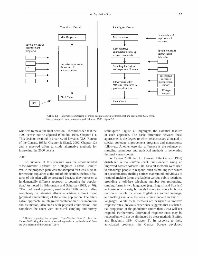
who was to make the final decision—recommended that the1990 census not be adjusted (Choldin, 1994, Chapter 11).This decision resulted in a variety of lawsuits (U.S. Bureauof the Census, 1995a, Chapter 1; Siegel, 2002, Chapter 12)and a renewed effort to study alternative methods forimproving the 2000 census.
2000
The outcome of this research was the recommended“One-Number Census” or “Integrated Census Count.”While the proposed plan was not accepted for Census 2000,for reasons explained at the end of this section, the basic fea-tures of this plan will be presented because they represent afundamentally different approach to counting the popula-tion.5 As noted by Edmonston and Schultze (1995, p. 76),“The traditional approach, used in the 1990 census, reliescompletely on intensive efforts to achieve a direct count(physical enumeration) of the entire population. The alter-native approach, an integrated combination of enumerationand estimation, also starts with physical enumeration, butcompletes the count with statistical sampling and survey
techniques.” Figure 4.1 highlights the essential features of each approach. The basic difference between theseapproaches is the degree to which resources are allocated tospecial coverage improvement programs and nonresponsefollow-up. Another essential difference is the reliance onsampling techniques and statistical methods in generatingthe final census count.
For Census 2000, the U.S. Bureau of the Census (1997)distributed a mail-out/mail-back questionnaire using animproved Master Address File. Several methods were usedto encourage people to respond, such as mailing two wavesof questionnaires, mailing notices that remind individuals torespond, making forms available in various public locations,providing a toll-free telephone number for responding,sending forms in two languages (e.g., English and Spanish)to households in neighborhoods known to have a high pro-portion of people for whom English is a second language,and making available the census questionnaire in any of 6languages. While these methods are designed to improveresponse rates, previous experience suggests that a substan-tial proportion of the population (more than 25%) will notrespond. Furthermore, differential response rates may bereduced but will not be eliminated by these methods (Steffeyand Bradburn, 1994, Chapter 3). In response to these anticipated problems, the Census Bureau developed
4. Population Size 77
5 Details regarding the proposed “One-Number Census” plans forCensus 2000 using alternative census-taking methods can be obtained fromthe U.S. Bureau of the Census (1997).
Integratedcoverage
measurementsurvey
“E”-typesample
FIGURE 4.1 Schematic comparison of major design features for traditional and redesigned U.S. censusSource: Adapted from Edmonston and Schultze, 1995, Figure 5.1
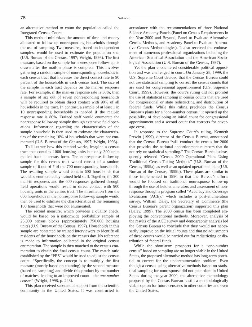
an alternative method to count the population called the Integrated Census Count.
This method minimizes the amount of time and moneyallocated to follow up nonresponding households throughthe use of sampling. Two measures, based on independentsamples, would be used to estimate the population size (U.S. Bureau of the Census, 1997; Wright, 1998). The firstmeasure, based on the sample for nonresponse follow-up, isdrawn after the mail-in phase is complete. This involvesgathering a random sample of nonresponding households ineach census tract that increases the direct contact rate to 90percent of the households in each census tract. The size ofthe sample in each tract depends on the mail-in responserate. For example, if the mail-in response rate is 30%, thena sample of six out of seven nonresponding households will be required to obtain direct contact with 90% of allhouseholds in the tract. In contrast, a sample of at least 1 in10 nonresponding households is needed if the mail-inresponse rate is 80%. Trained staff would enumerate thenonresponse follow-up sample through extensive field oper-ations. Information regarding the characteristics of thesample household is then used to estimate the characteris-tics of the remaining 10% of households that were not enu-merated (U.S. Bureau of the Census, 1997; Wright, 1998).
To illustrate how this method works, imagine a censustract that contains 1000 housing units but only 300 unitsmailed back a census form. The nonresponse follow-upsample for this census tract would consist of a randomsample of 6 out of 7 of the 700 nonresponding households.The resulting sample would contain 600 households thatwould be enumerated by trained field staff. Together, the 300mail-in responses and the 600 responses gathered throughfield operations would result in direct contact with 900housing units in the census tract. The information from the600 households in the nonresponse follow-up sample wouldthen be used to estimate the characteristics of the remaining100 households that were not enumerated.
The second measure, which provides a quality check,would be based on a nationwide probability sample of25,000 census blocks (approximately 750,000 housingunits) (U.S. Bureau of the Census, 1997). Households in thissample are contacted by trained interviewers to identify allresidents of the households on the census day. No referenceis made to information collected in the original census enumeration. The sample is then matched to the census enu-meration to obtain the final census count. The match ratioestablished by the “PES” would be used to adjust the censuscount. “Specifically, the concept is to multiply the firstmeasure (mostly based on counting) by the second measure(based on sampling) and divide this product by the numberof matches, leading to an improved count—the one numbercensus” (Wright, 1998, p. 248).
This plan received substantial support from the scientificcommunity in the United States. It was constructed in
accordance with the recommendations of three NationalScience Academy Panels (Panel on Census Requirements inthe Year 2000 and Beyond, Panel to Evaluate AlternativeCensus Methods, and Academy Panel to Evaluate Alterna-tive Census Methodologies). It also received the endorse-ment of numerous professional organizations including theAmerican Statistical Association and the American Socio-logical Association (U.S. Bureau of the Census, 1997).
Yet the plan encountered considerable political opposi-tion and was challenged in court. On January 28, 1999, theU.S. Supreme Court decided that the Census Bureau couldnot use statistical sampling to correct the census counts thatare used for congressional apportionment (U.S. SupremeCourt, 1999). However, the court’s ruling did not prohibitthe use of statistical sampling in census counts that are usedfor congressional or state redistricting and distribution offederal funds. While this ruling precludes the CensusBureau’s plans for a “one-number census,” it opened up thepossibility of developing an initial count for congressionalapportionment and a second count that corrects for cover-age error.
In response to the Supreme Court’s ruling, KennethPrewitt (1999), director of the Census Bureau, announcedthat the Census Bureau “will conduct the census for 2000that provides the national apportionment numbers that donot rely on statistical sampling.” The Census Bureau subse-quently released “Census 2000 Operational Plans Using Traditional Census-Taking Methods” (U.S. Bureau of theCensus, 1999a), as well as an updated operational plan (U.S.Bureau of the Census, 1999b). These plans are similar tothose implemented in 1990 in that the Bureau’s effortswould be focused on traditional nonresponse follow-upthrough the use of field enumerators and assessment of non-response through a program called “Accuracy and CoverageEvaluation (ACE),” which includes a post-enumerationsurvey. William Daley, the Secretary of Commerce (theCensus Bureau’s parent organization) supported this plan(Daley, 1999). The 2000 census has been completed em-ploying the conventional methods. Moreover, analysis of the results of the ACE survey and demographic analysis ledthe Census Bureau to conclude that they would not neces-sarily improve on the initial counts and that no adjustmentsof these counts would be carried out for redistricting or dis-tribution of federal funds.
While the short-term prospects for a “one-numbercensus” based on sampling are no longer viable in the UnitedStates, the proposed alternative method has long-term poten-tial to correct for the underenumeration problem. Eventhough a census using alternative methods based on statis-tical sampling for nonresponse did not take place in UnitedStates during the year 2000, the alternative methodologyproposed by the Census Bureau is still a methodologicallyviable option for future censuses in other countries and eventhe United States.
78 Wilmoth

References
Alterman, H. 1969. Counting People: The Census in History. New York:Harcourt, Brace & World.
Anderson, M. J. 1988. The American Census: A Social History. NewHaven, CT: Yale University Press.
Coale, A. J. 1955. “The Population of the United States in 1950 Classifiedby Age, Sex, and Color—A Revision of Census Figures.” Journal ofthe American Statistical Association 50: 16–54.
Coale, A. J., and N. W. Rives, Jr. 1973. “A Statistical Reconstruction of theBlack Population of the United States, 1880–1970: Estimates of TrueNumbers by Age and Sex, Birth Rates, and Total Fertility.” PopulationIndex 39: 3–36.
Choldin, H. M. 1994. Looking for the Last Percent: The Controversy overCensus Undercounts. New Brunswick, NJ: Rutgers University Press.
Citro, C. F., and M. L. Cohen (Eds.). 1985. The Bicentennial Census: NewDirections for Methodology in 1990. Washington, DC: NationalAcademy Press.
Clogg, C. C., and C. L. Himes. 1993. “Comment: Uncertainty in Demo-graphic Analysis.” Journal of the American Statistical Association 88:1072–1074.
Daley, W. M. 1999. “Statement of U.S. Secretary of Commerce William M.Daley on Plan for Census 2000.” U.S. Department of Commerce PressRelease, February 24, 1999.
Edmonston, B., and C. Schultze (Eds.). 1995. Modernizing the U.S. Census.Washington, DC: National Academy Press.
Ericksen, E. P., and T. K. DeFonso. 1993. “Beyond the Net Undercount:How to Measure Census Error.” Chance 6: 38–44.
Ericksen, E. P., and J. B. Kadane. 1985. “Estimating the Population in aCensus Year.” Journal of the American Statistical Association 80:98–131.
Freedman, D. A., and W. C. Navidi. 1986. “Regression Models for Adjust-ing the 1980 Census.” Statistical Science 1: 3–39.
Himes, C. L., and C. C. Clogg. 1992. “An Overview of DemographicAnalysis as a Method for Evaluating Census Coverage in the UnitedStates.” Population Index 58: 587–607.
Hogan, H. 1992. “The 1990 Post-Enumeration Survey: An Overview.” TheAmerican Statistician 46: 261–269.
Hogan, H. 1993. “The 1990 Post-Enumeration Survey: Operations andResults.” Journal of the American Statistical Association 88:1047–1060.
Li, C. (Ed.). 1987. A Census of One Billion People. Boulder, CO: Westview Press.
Marks, E. D., and J. Waksberg. 1966. “Evaluation of Coverage in the 1960Census of Population through Case-by-Case Checking.” Proceedingsof the Social Statistics Section, 1966. Washington, DC: American Statistical Association.
Mulry, M. H., and B. D. Spencer. 1993. “Accuracy of the 1990 Census andUndercount Adjustments.” Journal of the American Statistical Associ-ation 88: 1080–1091.
Prewitt, K. 1999. “Statement of Kenneth Prewitt, Director of the U.S.Census Bureau, on Today’s Supreme Court Ruling.” U.S. Departmentof Commerce, Economics and Statistics Administration, Bureau of theCensus Press Release, January 25, 1999.
Price, D. O. 1947. “A Check on Underenumeration in the 1940 Census.”American Sociological Review 12: 44–49.
Pritzker, L., and N. D. Rothwell. 1968. “Procedural Difficulties in takingPast Censuses in Predominately Negro, Puerto Rican, and MexicanAreas.” In D. M. Heer (Ed.), Social Statistics and the City. Cambridge,MA: Joint Center for Urban Studies of the Massachusetts Institute ofTechnology and Harvard University.
Robinson, J. G., B. Ahmed, P. D. Gupta, and K. A. Woodrow. 1993. “Esti-mation of Population Coverage in the 1990 United States Census Basedon Demographic Analysis.” Journal of the American Statistical Association 88: 1061–1071.
Schenker, N. 1993. “Undercount in the 1990 Census.” Journal of the American Statistical Association 88: 1044–1046.
Shryock, H. S. 1955. “The Concepts of De facto and De Jure Population:The Experience in Censuses of the United States.” Proceedings of theWorld Population Conference, 1954. Vol. IV, United Nations. E/CONF,13/416.
Shryock, H. S. 1960. “The Concept of ‘Usual’ Residence in the Census of Population.” Proceedings of the Social Statistics Section, 1960.Washington, DC: American Statistical Association, August 23–26,1960.
Siegel, J. S. 2002. Applied Demography: Applications to Business, Goverament, Law, & Public Policy. San Diego: Academie Press.
Steffey, D. L., and N. M. Bradburn (Eds.). 1994. Counting People in theInformation Age. Washington, DC: National Academy Press.
United Nations. 1992. Handbook of Population and Housing Censuses:Part I. Planning, Organization and Administration of Population andHousing Censuses. New York: United Nations.
United Nations. 1998. Demographic Yearbook: 1996. New York: UnitedNations.
U.S. Bureau of the Census. 1906. Special Reports of the Twelfth Census,Supplementary Analysis and Derivative Tables. Washington, DC: Government Printing Office.
U.S. Bureau of the Census. 1987. 1980 Census of Population and Housing:History. Part E. Washington, DC: Government Printing Office.
U.S. Bureau of the Census. 1988. The Coverage of Population in the 1980Census, by R. E. Fay, J. S. Passel, and J. G. Robinson. Evaluation andResearch Reports, PHC 80-EA, 1980 Census of Population andHousing. Washington, D.C.: U.S. Bureau of the Census.
U.S. Bureau of the Census. 1992a. 1990 Census of Population andHousing. General Population Characteristics. Kansas. Washington,DC: Government Printing Office.
U.S. Bureau of the Census. 1992b. 1990 Census of Population andHousing. General Population Characteristics. United States. Washing-ton, DC: Government Printing Office.
U.S. Bureau of the Census. 1992c. 1990 Census of Population andHousing. General Population Characteristics. United States. AppendixD. Collection and Processing Procedures. Washington, DC: Govern-ment Printing Office.
U.S. Bureau of the Census. 1992d. 1990 Census of Population andHousing. General Population Characteristics. United States. AppendixE. Facsimiles of Respondent Instructions and Questionnaire Pages.Washington, DC: Government Printing Office.
U.S. Bureau of the Census. 1993. Americans Overseas in the U.S. Censuses. Technical Paper 62. Washington, DC: Government PrintingOffice.
U.S. Bureau of the Census. 1995a. 1990 Census of Population andHousing: History. Part C. Washington, DC: Government PrintingOffice.
U.S. Bureau of the Census. 1995b. 1990 Census of Population andHousing: History. Part D. Washington, DC: Government PrintingOffice.
U.S. Bureau of the Census. 1997. Report to Congress—The Plan for Census2000, www.census.gov/dmd/www/plansop.htm
U.S. Bureau of the Census. 1999a. Census 2000 Operational Plan: UsingTraditional Census Taking Methods. Washington, DC: GovernmentPrinting Office.
U.S. Bureau of the Census. 1999b. Updated Summary: Census 2000 Operational Plan. Washington, DC: Government Printing Office.
U.S. Supreme Court. 1999. Nos. 98–404 and 98–564. Lexis-Nexis.Whelpton, P. K. 1950. “Birth and Birth Rates in the Entire United States,
1909 to 1948.” Vital Statistics Special Reports 33: 137–162.Wolter, K. M. 1986. “Some Coverage Error Models for Census Data.”
Journal of the American Statistical Association 81: 338–346.Wright, T. 1998. “Sampling and Census 2000: The Concepts.” American
Scientist 86: 245–253.
4. Population Size 79

Suggested Readings
Alterman, H. 1969. Counting People: The Census in History. New York:Harcourt, Brace & World.
Anderson, M. J. 1988. The American Census: A Social History, NewHaven, CT.: Yale University Press.
Choldin, H. M. 1994. Looking for the Last Percent: The Controversy overCensus Undercounts, New Brunswick, NJ: Rutgers University Press.
Cohen, P. 1982. A Calculating People. Chicago, IL: University of ChicagoPress.
Edmonston, B., and C. Schultze (Eds.). 1995. Modernizing the U.S. Census.Washington, DC: National Academy Press.
Himes, C. L., and C. C. Clogg. 1992. “An Overview of DemographicAnalysis as a Method for Evaluating Census Coverage in the UnitedStates.” Population Index 58: 587–607.
Hogan, H. 1992. “The 1990 Post-Enumeration Survey: An Overview.” TheAmerican Statistician. 46: 261–269.
Steffey, D. L., and N. M. Bradburn (Eds.). 1994. Counting People in theInformation Age. Washington, DC: National Academy Press.
United Nations. 1992. Handbook of Population and Housing Censuses:Part I. Planning, Organization and Administration of Population andHousing Censuses. New York: United Nations.
United Nations. 1998. Priniciples and Recommendations for Populationand Housing Censuses. New York, NY: United Nations.
U.S. Bureau of the Census. 1977. “Developmental estimates of the cover-age of the population of states in the 1970 census: Demographic analysis,” by J. S. Siegel, J. S. Passel, N. W. Rivers, and J. G. Robinson. Current Population Reports, Series P-23, No. 65. Washington, DC: U.S. Bureau of the Census.
U.S. Bureau of the Census. 1985. Evaluating Census of Population andHousing. Special Training Document. ISP-TR-S. Washington, DC: U.S.Bureau of the Census.
U.S. Bureau of the Census. 2002. Measuring America: The DecennialCensus from 1790 to 2000. Washington, DC: U.S. Census Bureau.
U.S. National Archives and Records Administration. 1997. The 1790–1890Federal Population Census, Revised. Washington, DC: NationalArchives and Records Administration.
80 Wilmoth

Since the first edition of The Methods and Materials ofDemography was written in 1967 through 1970, a wide arrayof new uses for demographic analysis has arisen at the sub-national and local scales. A booming “demographics” indus-try has developed that makes use of census materials andquantitative methods for the geographical analysis of pop-ulation for private-sector marketing, business decisionmaking, and public-planning applications. Thus today, morethan ever, for many purposes information on the size andcharacteristics of the total population of a country is not suf-ficient. Population data are often needed for geographic sub-divisions of a country and for other classifications of areasincluding smaller scale units with boundaries reflecting thesettlements and neighborhoods in which people live. In mostcountries, the geographic distribution of the population is noteven but is dense in some places and sparse in others, and thegeographic patterns of demographic characteristics are oftenquite complex. This chapter treats the geographic distribu-tion of the population by political areas and by several othertypes of geographic areas.
ADMINISTRATIVE OR POLITICAL AREAS
Political areas are not ordinarily created or delineated by a country’s central statistical agency or its census officebut instead are established by national constitutions, laws,decrees, regulations, or charters. In some countries, theprimary political subdivisions are empowered to create secondary and tertiary subdivisions. Even with modernadvances in methods for tabulating census data, it is stillvery challenging to do cross-country comparative work atthe subnational level. Wide variations exist in the definitionsof the fundamental geographic units for which data may beobtained for different countries.
The present discussion is confined to the major and minorcivil divisions and to cities proper. (“Urban agglomerations”and “urban and rural” areas are discussed in the next majorsection of this chapter and in Chapter 6.)
Primary Divisions
Data on total population and population classified byurban/rural residence are given for the major civil divisionsof most countries in several of the UN Demographic Year-books—for example, the 1993 Yearbook (United Nations,1995) with data from 1985–1993 censuses. The genericnames appear in English and French, and sometimes theyappear in the national language as well. As shown in Table5.1, the most common names in English for the primaryareas are provinces, regions, districts, and states. Thenumber of major civil divisions varies widely from countryto country as shown in column 2 of Table 5.1. Just as coun-tries themselves vary greatly in terms of their geographicareas and population sizes, so too are the areas and popula-tions of major civil divisions highly variable. The averagepopulation size of the major civil divisions listed in the 1993Demographic Yearbook ranges from just 1355 persons forthe 13 separate Cook Islands to 37,683,688 for the 30provinces, (independent) cities, and autonomous regions ofChina. Care should thus be exercised in comparing databetween countries for major civil divisions.
Special Units
It is fairly common for the capital city to constitute aprimary division in its own right and in a few countries,some of the larger cities are also primary political divisions.Countries that have been settled relatively recently or countries that contain large areas of virtually uninhabitedland or land inhabited mainly by aborigines may have a
81
C H A P T E R
5
Population DistributionGeographic Areas
DAVID A. PLANE
The Methods and Materials of DemographyCopyright 2003, Elsevier Science (USA).
All rights reserved.

different kind of primary subdivision that has a distinctivegeneric name and a rudimentary political character.
Secondary and Tertiary Divisions
To obtain data below the major civil division level, thestatistical or demographic yearbook or the actual censusreports for the specific nation will likely need to be consultedas the UN Demographic Yearbook generally does not givesuch detailed tabulations. The intermediate or secondarypolitical divisions also have a wide variety of names. Theseinclude county, district, and commune. Some small coun-tries have only primary divisions. Some large countries havethree or more levels. Examples of tertiary divisions are the
townships in the United States, the myun and eup in Korea,and the hsiang and chen in Taiwan. For different adminis-trative functions, a province, state, or other division may bedivided into more than one set of political areas.
Municipalities
It is difficult to find a universal, precise term for the typeof political area discussed in this subsection. The ideal typeis the city; but smaller types of municipalities such as townsand villages are also included. (Incidentally, in Puerto Rico,a municipio is the equivalent of a county in mainland UnitedStates.) In some countries, these areas could be described asincorporated places or localities. In some countries, again,
82 David A. Plane
TABLE 5.1 Major Civil Divisions Used to Report Census Data in 1993 U.N. Demographic Yearbook
English generic Countries with number of units English generic Countries with number of unitsname (and local generic name if listed in yearbook) name (and local generic name if listed in yearbook)
Primary UnitsCities and towns Republic of Moldavia 49Communes French Guiana 21, Martinique 33Counties Norway 19Departments Bolivia 9, Colombia 24, El Salvador 14, Paraguay
19, Uruguay 19Development Nepal 5
regionsDistricts Belize 6, Brunei 5, Cape Verde 9, Cayman Islands 6,
Gabon 9, Latvia 26, Lesotho 10, Madagascar 6, New Caledonia 31, Seychelles 5, Swaziland 4,Uganda 38
Divisions Bangladesh 4, Fiji 4, France 22, Tonga 5Governorates Iraq 18, Yemen 11Islands Comores Islands 3, Cook Islands 13, Turks and
Caicos Islands 6Local Vanuatu 11
government regions
Municipalities Qatar 9Parishes Antigua and Barbuda 7, Bermuda 7, Isle of Man 17,
Jamaica 14Popular Yugoslavia 6
republicsPrefectures Algeria 48, Central African Republic 16, Chad 15,
Japan 47, Rwanda 11Provinces Argentina 22, Benin 6, Bulgaria 27 (Okruzi),
Burkina Faso 30, Burundi 16, Canada 10, Chile 13, Ecuador 21, Egypt 15, Finland 12, Indonesia 27, Iran 24, Ireland 4, Kazakhstan 19, Korea 19 (Do), Kyrgyzstan 6 (Oblasts), Panama 9, Poland 48 (Voivodships), Sierra Leone 3, Solomon Islands 8, South Africa 4, Sweden 24 (Lans), Turkey 67 (Ili), Viet Nam 40, Zambia 9, Zimbabwe 10
Regional New Zealand 13councils
Regions Aruba 9, Bahrain 12, Cote d’Ivoire 10, Czech Republic 7, Mali 7, Malta 6, Mauritania 13, Namibia 27, Oman 8, Philippines 14, Romania 40,Russian Federation 12, Senegal 10, Slovakia 3, Sudan 9, Tanzania 25
States India 24, Malaysia 13, Mexico 31, Nigeria 31, United States 50, Venezuela 20
Subregions Malawi 24Towns Macedonia 30Urban areas Botswana 8
Secondary UnitsAutonomous China,1 Iraq1
regionsCapital Bulgaria 1, Czech Republic 1, Paraguay 1, Poland 1,
Slovakia 1Capital city/ Sierra Leone 2
rural areaCities Bermuda 2, Egypt 4, Kazakhstan 1, Korea1 6,
Kyrgyzstan 1Comisarias Colombia 5Districts Mali 1, Sierra Leone 13, United States 1Federal capitals Argentina 1Federal Malaysia 2
territoriesFrontier districts Egypt 5Intendencias Colombia 4Municipalities China,1 Romania 1Rural districts Botswana 11Self-governing South Africa 6
national statesTerritories Canada 2Towns Isle of Man 4Union territories India 7Villages Isle of Man 5
1 Not separately identified in tabulationsSource: Prepared by the author; based on the U.N. Demographic Yearbook, 1993, Table 30.

these municipalities are located within secondary or tertiarydivisions; but in other countries, they are simply those territorial divisions that are administratively recognized ashaving an urban character.
The larger municipalities are frequently subdivided for administrative purposes into such areas as boroughs or wards (Britain and some of its former colonies),arrondissements (France), ku (Japan and Korea), and chu(China, Taiwan). These subdivisions of cities, in turn, maybe divided into precincts (United States), chun (China,Taiwan), or dong (Korea). In China and Korea, even a fifthlevel exists—the lin and ban, respectively—for which“urban neighborhood” is as close as one could come inEnglish. These smaller types of administrative areas areordinarily not used for the presentation of official demo-graphic statistics, but they are sometimes used as units insample surveys.
Sources
Population totals for the major (primary) civil divisionsare published in several of the Demographic Yearbooks ofthe United Nations, and fairly frequently there is a tableshowing the total population of capital cities and cities of100,000 or more inhabitants.
The UN Demographic Yearbooks do not present statis-tics for smaller cities and other municipalities nor for thesecondary, tertiary, and other divisions. For these, one mustusually refer to the national publications.
Uses and Limitations
Statistics on the distribution of the population amongpolitical areas are useful for many purposes. For example,they may be used to meet legal requirements for deter-mining the apportionment of representation in legislativebodies; they are needed for studies of internal migration andpopulation distribution in relation to social, economic, andother administrative planning; and they provide base data forthe computation of subnational vital statistics rates and forpreparing local population estimates and projections.
A limitation of these political areas from the standpointof the analysis of population distribution, and even from thatof planning, is the fact that the boundaries may be ratherarbitrary and may not consider physiographic, economic, orsocial factors. Moreover, the areas officially designated ascities may not correspond very well to the actual physicalcity in terms of population settlement or to the functionaleconomic unit. Furthermore, in some countries the smallesttype of political areas does not provide adequate geographicdetail for ecological studies or city planning. Therefore,various types of statistical and functional areas have beendefined, in census offices and elsewhere, to meet these
needs. These may represent groups or subdivisions of thepolitical areas, or they may disregard them altogether. Suchareas are the subject of the second major section (“Statisti-cal Areas”) of this chapter and of Chapter 6.
Quality of the Statistics
Most of what can be said about the accuracy of totalnational population applies also to the country’s geographicdivisions. Furthermore, given a set of rules on who shouldbe counted and where people should be counted within acountry, there will be errors in applying these rules. Somepeople will be counted in the wrong area, others will bemissed, and still others will be counted twice. Hence theaccuracy of the counts for the areas will be impaired differentially.
Political Areas of the United States
The primary purpose of the census of the United Statesis the determination of the number of residents in each statefor the purpose of apportioning the representatives to theCongress of the United States among the states. Withinstates, population must be obtained for smaller areas fordetermining congressional districts and for setting up dis-tricts (by various methods) for electing representatives to theindividual state’s legislative body or bodies and for otherpurposes required by state or local laws.
States
There are now 50 states and the District of Columbiawithin the United States proper. The number of states andsome of their boundaries have changed in the course ofAmerican history; but from 1912 to 1959, there were 48states. That area is typically called the “conterminous UnitedStates.” For data presentation purposes, the Census Bureautreats the District of Columbia as the equivalent of a state.For some data the Bureau applies the same treatment to theterritories under U.S. sovereignty or jurisdiction. The territo-ries included for the 1990 decennial census were AmericanSamoa, Guam, the Northern Mariana Islands, Palau, PuertoRico and the U.S. Virgin Islands. With independence, Palauis no longer covered by U.S. population data.
The primary divisions of states are usually called coun-ties. These in turn are subdivided into political units collec-tively known as minor civil divisions (MCDs). In moststates, the places incorporated as municipalities are subor-dinate to minor civil divisions; but in some states, the incor-porated places are themselves minor civil divisions of thecounties. As will be shown, there are fairly numerous dif-ferences among the states in the nature and nomenclature oftheir political areas.
5. Population Distribution 83
Counties
The primary divisions of the states are termed “counties”in all but two states, although four states also contain one or more independent cities. The county equivalents inLouisiana are the parishes. The primary divisions in the stateof Alaska have been known as boroughs and census areassince the 1980 census (prior to that they were called elec-tion districts at the time of the state’s formation in 1960 and census divisions for the 1970 decennial census). Theindependent cities are Baltimore (Maryland), Carson City(Nevada), St. Louis (Missouri), and 40 cities in Virginia. Allin all, there were 3141 counties or county equivalents in theUnited States as of 2000 (with one new county under for-mation in Colorado).
Minor Civil Divisions
These are the tertiary subdivisions of the United States.The practice of reporting census data for county subdivi-sions goes all the way back to the first census in 1790, whichreported data for towns, townships, and other units of localgovernment. The minor civil divisions of counties havemany kinds of names, as illustrated in Table 5.2, whichshows the number of different types of MCDs used to report1990 census data. “Township” is the most frequent. In thesix New England States, New York, and Wisconsin, mostMCDs are called “towns”; these are unlike the incorporatedtowns in other states in that they are not necessarily denselysettled population centers. Some tertiary divisions have nolocal governmental organizations at all and may be unin-habited. Furthermore, in many states, some or all of theincorporated municipalities are also minor civil divisions. Afurther complication in some of the New England states isthat all of the MCDs, be they cities or towns, are viewedlocally as “incorporated” in that they exercise a number oflocal governmental powers. In the usage of Census Bureaupublications, however, the term “incorporated place” hasbeen reserved for localities or nucleated settlements and isnot applied to other areal subdivisions.
In addition to the minor civil divisions shown in thecensus volumes, there are thousands of school and other taxation units for which separate population figures are notpublished. According to a recent (1997) census of govern-ments, school districts numbered 13,726 nationwide andother specialized-function governmental units 34,683.Where more than one kind of primary subdivision exists ina county, the Census Bureau tries to select the more stablekind. In some states, however, no type of minor civil divi-sion has much stability. In some of the western states, forexample, the election precincts may be changed after eachelection on the basis of the number of votes cast. Obviously,such units have practically no other statistical value. Evenin states where the minor civil divisions do not change very
often, they may have so little governmental significance thatdata published for them are also of limited usefulness. Heretoo the minor civil divisions may be so unfamiliar locallythat it is very difficult for enumerators in the field to observetheir boundaries. This is the situation in some southernstates. At the other extreme are the stable towns of NewEngland, which are of more political importance than thecounties. For the 1990 census, 28 states had recognizedminor civil divisions or equivalents.
A statistical solution to the problem of the evanescent or little-known minor civil divisions is the “census countydivision,” which was first introduced in one state, Washington, in 1950 and then in many more states in the1960 and subsequent censuses. For the 1990 census, the 21census county division states were all in the West and South-east.1 The census county divisions, then, are the geographic-statistical equivalents of minor civil divisions; but because
84 David A. Plane
TABLE 5.2 Type and Number of County Subdivisions Usedfor the 1990 U.S. Census and as of 1999
1990 1999
Townships 18,154 18,087Census county divisions 5,581 5,581Incorporated places 4,533 4,581Towns 3,608 3,603Election precincts 948 933Magisterial districts 735 753Parish governing authority districts 627 601Supervisors’ districts 410 410Unorganized territories 282 285Election districts 276 284Census subareas 40 42Plantations 36 33Charter townships N/A 26Assessment districts 21 8American Indian reservations 7 17Grants 9 9Purchases 6 6Boroughs 5 5Gores 4 4Locations 4 4Pseudo county subdivision 1 1Road district 1 1
Total county subdivisions 35,298 35,274
Source: 1990 data from U.S. Bureau of the Census, Geographic AreasReference Manual. Washington, DC: U.S. Government Printing Office,1994. Currently available online at www.census.gov (U.S. Bureau of theCensus, 2000a). 1999 data from Memorandum August 11, 1999, U.S.Bureau of the Census, Geography Division, List of Valid Entity Types andNumber, by State.
1 The state of Alaska has no counties and no minor civil divisions.Census subareas (CSAs) have been adopted as the statistical equivalents ofMCDs. These are subdivisions of the boroughs and census areas that serveas the county equivalents.

they are not political areas, they are discussed in the nextmajor section.
Incorporated Places
The generic definition of a “place” is a concentration ofpopulation regardless of the existence of legally prescribedlimits, powers, or functions. While some incorporated placesmay serve as minor civil divisions, at the outset it should beclearly stated that place statistics and minor civil divisionstatistics are two separate geographic schemes for tabulat-ing census data. Depending on the vagaries of the variousstates’ constitutions, laws, and local political structures,places may be either coterminous with or completely sepa-rately bounded from the county subdivisions. Whereas greatpains are taken to provide a collectively exhaustive systemof MCDs, MCD equivalents, and census county divisions,not everyone lives within a recognized place. At the time ofthe 1990 census, 66 million persons (approximately 26% ofthe total national population) lived outside of places.
Places are of two types: incorporated places and census-designated places. By definition, the incorporated places are the only ones that are political areas. All states containincorporated places known as “cities.”2 Incorporated“towns” may be formed in 31 states, “villages” are permit-ted in 18, and “boroughs” in 3. New Jersey is the only statethat permits formation of all four types. Where a state hasmore than one kind of municipality, cities tend to be largerplaces than the other types.
Unincorporated places that are defined for statistical tabulation purposes are now known as census-designatedplaces (CDPs), with the criteria for designation based ontotal population size, population density, and geographicconfiguration. When CDPs were first recognized in 1950,they were called “unincorporated” places. CDPs are pro-posed and delineated by state, local, and tribal agencies andthen reviewed and approved by the Census Bureau. Thereare only about one-fifth as many CDPs as there are incor-porated places (4146 versus 19,289 at the time of the 1990census.) However, a sizable fraction of the U.S. population(11.9% in 1990) lives in such settlements; without CensusBureau recognition, data tabulations would not exist forthese commonly recognized localities.
Annexations
Beginning with 1970, the data shown for any area in acensus report refer to the area’s legally recognized bound-aries as of January 1 of the census year. There are a greatmany changes in place boundaries through municipal
annexations and detachments, mergers or consolidations,and incorporations and disincorporations. Since 1972, theCensus Bureau in most years conducts a mail-out Boundaryand Annexation Survey to track the changes.
Congressional and Legislative Districts
Congressional districts are the districts represented by a representative in the U.S. House of Representatives,whereas legislative districts are those represented by law-makers serving in the state legislatures. At present, there are 435 congressional districts. The U.S. Constitution set thenumber of representatives at 65 from 1787 until the firstcensus in 1790. The first apportionment, based on the 1790census, resulted in 105 members. From 1800 through 1840,the number of representatives was determined by a fixedratio of the number of persons to be represented. After 1840,the number of representatives changed with that ratio, aswell as with population growth and the admission of newstates. For the 1850 census and later apportionments, thenumber of House seats was fixed first, and the ratio ofpersons each representative was to represent changed. In1911, the number of representatives in the House wascapped at 433 with provision for the addition of one seateach for Arizona and New Mexico when they becamestates.3 The House size, 435 members, has been unchangedsince, except for a temporary increase to 437 at the timeAlaska and Hawaii were admitted as states (U.S. Bureau ofthe Census, 2000a). The geographical boundaries of con-gressional districts are redrawn in each state by proceduresspecified by state legislatures, although now in some statesbipartisan citizen’s committees have been created in anattempt to blunt the influence of the controlling politicalparty.
Except for Nebraska, every state legislature consists oftwo houses, each with its own districts, whose boundariesare also redrawn following each decennial census. These areall political areas, but they are not administrative areas.
General Considerations
The political uses of census data are so important thatthey go far to determine the basis of census tabulations ofpopulation for geographic areas. Fortunately, political unitsserve very well as statistical units of analysis in many demo-graphic problems. In the realm where they are less satisfac-tory the Census Bureau has provided other types of area orresidence classifications of population data with increasingusefulness over recent decades. A new tool in 1970, theaddress register, has subsequently been refined into a con-tinuously maintained and updated national address databasebeginning with the 2000 census. That innovation, along with
5. Population Distribution 85
2 Strictly speaking, there are no incorporated places in Hawaii, onlycensus designated places. The Census of Governments counts the combinedcity and county of Honolulu as a municipality. 3 U.S. Statutes at Large, 37 Stat 13, 14 (1911).

the development of geographic information systems and theCensus Bureau’s TIGER system, has greatly facilitated thecompilation of data for other types of units such as schooldistricts, traffic zones, neighborhood planning units, and,indeed, for any other areas, political or otherwise, that canbe defined or satisfactorily approximated in terms of com-binations of city and rural blocks. The 1990 census wasnotable for being the first for which the whole national ter-ritory was “blocked.” For the past several censuses, a “UserDefined Areas” option has existed for localities to obtainspecial tabulations tailored to their own specific needs. The2000 census for the first time provided standard tabula-tions for 5-digit zip code areas, though approximate datahave been created for some time by private-sector firmsdoing allocations from, for example, block and block-grouptabulations.4
The usefulness of demographic data for political areas ofthe United States for analysis of trends is greatest for thelargest political subdivisions, namely the states. Countiesand cities are probably next in order. Least satisfactory arethe minor civil divisions, which, as we stated, change theirboundaries frequently in some states. Another reason for thelimited amount of analytical work done on population datafor minor civil divisions is that many other types of data thatone might wish to relate to census data are not available forgeographic areas smaller than cities or counties. Moreover,the amount of detail and cross-classification of populationdata published by the census for minor civil divisions isquite limited.
For cross-sectional analyses that do not involve changesover time, counties, cities, and minor civil divisions, as wellas states, may be very useful as units of analysis. In general,the smaller the geographic area with which one deals, themore homogeneous will be the population living in the area.Rates, averages, and other statistical summarizing measuresare usually more meaningful if they relate to a relativelyhomogeneous population. However, if the geographic areaand the population residing in it are very small, rates suchas a migration rate or a death rate may be so unstable as tobe meaningless. Here the total population exposed to the riskof migration or death may be too small for the statistical reg-ularity of demographic events that is manifested when largepopulations are observed.
In publications of population statistics, data are oftenshown for a combination of political and nonpolitical areas,such as for the states and major geographic divisions, forcounties and their urban and rural populations, or for incor-porated and unincorporated places. The Census Bureau andother statistics-producing agencies present data for the states
sometimes listed in alphabetical order and sometimes in ageographic order. The usual geographic order conforms tothe regions and divisions that are defined next.
STATISTICAL AREAS
For many purposes, data are needed for areas other thanthose recognized as political entities by law. Nonpoliticalareas in common use for statistical purposes include bothcombinations and subdivisions of political areas. The mostgeneral objective in delineating such statistical areas is toattain relative homogeneity within the area, and, dependingon the particular purpose of the delineation, the homogene-ity sought may be with respect to geographic, demographic,economic, social, historical, or cultural characteristics. Also,groups of noncontiguous areas meeting specified criteria,such as all the urban areas within a state, are frequently usedin presentation and analysis of population data.
International Recommendations and National Practices
There are several types of such statistical areas; forexample, regions or functional economic areas; metropoli-tan areas, urban agglomerations, or conurbations; localities;and census tracts and block groups.
Regions or Functional Economic Areas
The terminology for this kind of geographic area is nottoo well standardized, but as used here, a “region” means alarge area. It ordinarily means something more, however,namely some kind of functional economic or cultural area(McDonald, 1966; Odum and Moore, 1938; Taeuber, 1965;Whittlesey, 1954).5 A region may represent a grouping of acountry’s primary divisions (e.g., states or provinces) or agrouping of secondary or tertiary divisions that cuts acrossthe boundaries of the primary divisions. (There are also in-ternational regions, which are either combinations of wholecountries or of areas which cut across national boundaries.)Among the factors on which regions are delineated are physiography, climate, type of soil, type of farming, culture,and economic levels and organizations. The cultural andeconomic factors include ethnic or linguistic differences,type of economy, and standard of living. The objective may be to create “uniform” (or “homogeneous”) regions—which are delineated so as to minimize differences withinregions and maximize differences among regions—or“nodal” regions—which feature a large city or urban
86 David A. Plane
4 Strictly speaking there is no such thing as a zip code area because zipcodes are designated by the Postal Service for convenience of mail deliv-ery. The Census Bureau units are “best approximations” delimited so as toprovide a mutually exclusive and collectively exhaustive set of contiguousgeographic areas for the national territory.
5 As used in geography, a “region” may be an area of any size so longas it possesses homogeneity or cohesion.

complex functionally tied to and economically dominantover a hinterland. Some regionalizations may be based onstatistical manipulations of a large number of indexes, for example, by cluster or factor analysis (Clayton, 1982;Morrill, 1988; Pandit, 1994; Plane, 1998; Plane and Isserman, 1983; Slater, 1976; Winchester, 1977). Theregions defined and used by geographers, anthropologists,and so on are somewhat more likely than those defined bydemographers and statisticians to ignore political areas alto-gether. The latter users have to be more concerned with theunits for which their data are readily available and to usesuch units as building blocks in constructing regions. Theremay be also a hierarchy of regions; the simplest type con-sists of the region and the subregion.
Large Urban Agglomerations
The concept of an urban agglomeration is defined by theUnited Nations as follows: “A large locality of a country(i.e., a city or a town) is often part of an urban agglomera-tion, which comprises the city or town proper and also thesuburban fringe or thickly settled territory lying outside of,but adjacent to, its boundaries. The urban agglomeration is,therefore, not identical with the locality but is an additionalgeographic unit that includes more than one locality”(United Nations, 1967, p. 51). (Discussion later in thechapter will show that this concept is broad enough toencompass both the metropolitan statistical areas and theurbanized areas used in the United States.)
A more detailed discussion of this concept is provided by Kingsley Davis and his associates (International UrbanResearch, 1959, pp. 1–17). According to them, the city asofficially defined and the urban aggregate as ecologicallyconceived may differ because the city is either under-bounded or overbounded. Cities in Pakistan, for example,usually are “truebounded”—that is, they approximate theactual urban aggregate fairly closely. The underbounded cityis the most common type elsewhere. Most of the cities inthe Philippines are stated to be overbounded, in that theyinclude huge areas of rural land within their boundaries. Theshi in Japan are also of this type.
To define an urban aggregate or agglomeration, one maymove in the direction of either an urbanized area or a met-ropolitan area. The former represents the territory “settledcontinuously in an urban fashion”; the latter typicallyincludes some rural territory as well. Urbanized areas havebeen delineated in only a few countries. Their boundariesignore political lines for the most part. In addition to theurbanized area in the United States, the conurbation inEngland and Wales is of this type. Metropolitan areas usepolitical areas as building blocks and are based on prin-ciples of functional integration and a high degree of spatialinteraction (such as commuting to workplaces) taking placewithin their bounds.
Although sometimes regarded as theoretically less desir-able as the actual limits of urban agglomeration, metropol-itan areas are often more feasible for both international andhistorical comparisons. They tend to be used more fre-quently than urbanized areas not only because of the greaterstability and recognition of their boundaries but also becauseof the greater availability of social and economic data.6 Datafor urbanized areas have been limited to those provided bydecennial census tabulations. Even if metropolitan areashave not been officially defined, they can be constructed inmost countries from the available statistics, following stan-dard principles, because metropolitan areas use standardpolitical areas as their building blocks.
Localities
A “locality” is a distinct population cluster (inhabitedplace, settlement, population nucleus, etc.) the inhabitants of which live in closely adjacent structures. The localityusually has a commonly recognized name, but it may benamed or delineated for purposes of the census. Localitiesare not necessarily the same as the smallest civil divisionsof a country.
Localities, places, or settlements may be incorporated orunincorporated; thus, it is only the latter, or the sum of thetwo types, that is not provided for by the conventional sta-tistics on political areas. The problem of delineating an unin-corporated locality is similar to that of delineating a largeurban agglomeration; but with the shift to the lower end ofthe scale, the areas required often cannot be approximatedby combining several political areas because small localitiesare often part of the smallest type of political area. Just howsmall the smallest delineated locality should be for purposesof studying population distribution is rather arbitrary incountries where there is a size continuum from the largestagglomeration down to the isolated dwelling unit. In viewof the considerable work required for such delineations, 200inhabitants seems about as low a minimum as is reasonable.7
In countries where there is essentially no scattered ruralpopulation but all rural families live in a village or hamlet,the answer is automatically provided by the settlementpattern. The rules for U.S. census designated place delin-eation have tended to set 1000 as the minimum population(and 2500 for designation as an “urban place”), althoughrural highway “sprawl” has made demarcation considerablymore problematic than in lesser developed countries with astrong pattern of rural village settlement.
5. Population Distribution 87
6 The one governmental use of the U.S. urbanized area boundariesprobably most visible to the general public is the federal requirement forlower speed limits on the portions of the interstate highways that lie withinsuch continuously built-up territories around major cities.
7 This is the class-mark between the lowest and the next to the lowestintervals in the table recommended by the United Nations, the lowest inter-val having no minimum.
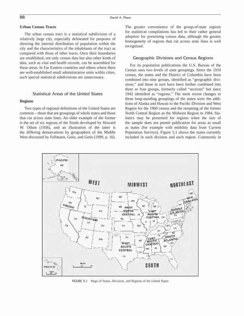
Urban Census Tracts
The urban census tract is a statistical subdivision of a relatively large city, especially delineated for purposes ofshowing the internal distribution of population within thecity and the characteristics of the inhabitants of the tract ascompared with those of other tracts. Once their boundariesare established, not only census data but also other kinds ofdata, such as vital and health records, can be assembled forthese areas. In Far Eastern countries and others where thereare well-established small administrative units within cities,such special statistical subdivisions are unnecessary.
Statistical Areas of the United States
Regions
Two types of regional definitions of the United States arecommon—those that are groupings of whole states and thosethat cut across state lines. An older example of the formeris the set of six regions of the South developed by HowardW. Odum (1936), and an illustration of the latter is the differing demarcations by geographers of the MiddleWest discussed by Fellmann, Getis, and Getis (1999, p. 16).
The greater convenience of the group-of-state regions for statistical compilations has led to their rather generaladoption for presenting census data, although the greaterhomogeneity of regions that cut across state lines is wellrecognized.
Geographic Divisions and Census Regions
For its population publications the U.S. Bureau of theCensus uses two levels of state groupings. Since the 1910census, the states and the District of Columbia have beencombined into nine groups, identified as “geographic divi-sions,” and these in turn have been further combined intothree or four groups, formerly called “sections” but since1942 identified as “regions.” The most recent changes tothese long-standing groupings of the states were the addi-tions of Alaska and Hawaii to the Pacific Division and WestRegion for the 1960 census and the renaming of the formerNorth Central Region as the Midwest Region in 1984. Sta-tistics may be presented for regions when the size of the sample does not permit publication for areas as small as states (for example with mobility data from Current Population Surveys). Figure 5.1 shows the states currentlyincluded in each division and each region. Commonly in
88 David A. Plane
FIGURE 5.1 Maps of States, Divisions, and Regions of the United States

population research papers authors erroneously referencethe divisions as “regions.”
The objective in establishing these state groupings isdescribed as follows: “The states within each of these divi-sions are for the most part fairly homogeneous in physicalcharacteristics, as well as in the characteristics of their population and their economic and social conditions, whileon the other hand each division differs more or less sharplyfrom most others in these respects. In forming these groupsof states the lines have been based partly on physical andpartly on historical conditions” (U.S. Bureau of the Census,1913, p. 13).8 The use of the Mason-Dixon line, for example,as the boundary between the South and Northeast Regions(and of the South Atlantic and Middle Atlantic Divisions) isone example of the use of “historical conditions.” Althougha contemporary multistate regionalization based on a set ofobjectively chosen variables used to maximize internalhomogeneity would doubtless differ from the groupings represented in the geographic divisions and regions, thesehave been retained to maintain continuity of data presenta-tion from census to census as interest in historical compar-isons has increased in recent decades.
Economic Subregions
The term “subregion” or “subarea” has been used in twosenses in the United States: (1) to denote the subparts of aregion (larger than a state), which may cut across state lines(e.g., Woofter, 1934), and (2) to denote subparts of states(Illinois Board of Economic Development, 1965). In eithercase, the delineation of the subregions may be based on anyone or any combination of several types of criteria: agricul-tural, demographic, economic, social, cultural, and so on.Moreover, subregional boundaries may be coincident withcounty lines or they may cut across county lines.
The idea of the decennial census as a national inventorycan be adequately implemented only by having material forexamination and analysis for areas more appropriate forcertain types of data than the conventional political units.This is especially important in the United States because ofits large area, the great mobility of its population, and thefact that political boundaries in the United States offer littleimpediment to the flow of commerce and population acrossthem. Because the political boundaries have so little effectin shaping the spatial patterns of economic and populationphenomena, they are inadequate for delineating the mostmeaningful areas for portraying and analyzing these phe-nomena. Ideally, the delineation of economic areas should
not have to follow county or even township lines, but areasthat did not do so would not be practicable or feasible forcensus purposes.
BEA Economic Areas
In recent years perhaps the most widely employed mul-ticounty units have been the “economic areas” defined bythe Bureau of Economic Analysis (BEA). In 1995 a new setof 172 BEA economic areas was redefined, replacing the183-area set of units first defined in 1977 (minor revisionshaving been made to those units in 1983). The BEA eco-nomic areas are based on economic nodes—metropolitanareas or similar areas serving as centers of economic activ-ity—and surrounding counties economically related to thenode. Counties are the building blocks for these units, andcommuting data from the 1990 Census of Population are theprimary data used to assign outlying counties to nodes. Theeconomic areas are collectively exhaustive and nonoverlap-ping. They may span state borders. The concept of the BEAeconomic areas is to provide a set of functional labor marketareas that contain both the workplace and residence loca-tions of the populations included, and about 80% of the 172areas have net commuting rates of 1% or less.9 Although theCensus Bureau does not currently tabulate its data for BEAeconomic areas, because these units are collections of coun-ties demographic data may be fairly readily aggregated toaccompany the earnings by industry, employment by indus-try, total personal income and per capita personal incomedata provided by the BEA. For migration analysis, theseunits based on functional labor markets are much better unitsfrom a conceptual standpoint than, for instance, the statesthemselves.
State Economic Areas
Prior to the definition of BEA economic areas, the “stateeconomic areas” (SEAs) were the most widely used, eco-nomically based, collectively exhaustive, multicounty, sub-state units. They failed, however, to enjoy the same historyof successful recognition and widespread acceptance as did the concurrent efforts in metropolitan-area definition. TheBureau of the Census and the Bureau of Agricultural Eco-nomics commissioned Donald J. Bogue to develop a set ofcounty groupings for the presentation of certain statisticsfrom the 1950 Censuses of Population and Agriculture (U.S.Bureau of the Census, 1951; see also Beale, 1967). The stateeconomic areas were relatively homogeneous subdivisionsof the states consisting of single counties or groups of
5. Population Distribution 89
8 Chapter 6 in “Statistical Groupings of States and Counties” of theCensus Bureau’s Geographical Areas Reference Manual (available onlineat the Census Bureau’s website; see U.S. Bureau of the Census 2000b)traces the history of the present regions and divisions back through eachcensus and to statistical practices during colonial times. Additional detailsare given in Dahmann (1992).
9 For more details about BEA economic areas and their 1995 redefini-tion, see Johnson (1995). This article and maps showing the boundaries of the 172 economic areas with the county constituents of each may cur-rently be found on the Bureau of Economic Analysis website at:www.bea.doc.gov.
counties that had similar economic and social characteris-tics. There were two principal types of SEAs: the metropol-itan and the nonmetropolitan. The former consisted of thelarger standard metropolitan statistical areas (SMSAs; seethe discussion that follows) except that when an SMSA waslocated in two or more states, each part became a separatemetropolitan SEA. In nonmetropolitan areas, demographic,climatic, physiographic, and cultural factors, as well asfactors pertaining more directly to the production andexchange of agricultural and nonagricultural goods, wereconsidered. Census data were tabulated and reported for 501 SEAs for the 1950 census, 509 SEAs for 1960, and 510for 1970 and 1980, after which they were dropped as offi-cial data-reporting units, ostensibly because of low usage.10
One application for which the SEAs were quite useful was for reporting detailed area-to-area migration statistics.The origin-destination-specific matrices were considerablyless clumsy to work with than the data-sparse county-to-county matrices that were made available through specialtabulations from the 1980 and 1990 censuses (althoughcounty-to-county flow data have the virtue that they can beaggregated into any desired units—at least by the computer-sophisticated who are not intimidated by the task of manip-ulating quite large data files).
Metropolitan Areas
As this edition of Methods and Materials was beingwritten, a major effort to review and refine metropolitan areadefinitions had just been completed. The units in use from2003 forward, defined according to the recommended andadopted alternative, will be considerably different from the “metropolitan districts,” “standard metropolitan areas”(SMAs), “standard metropolitan statistical areas” (SMSAs),“metropolitan statistical areas” (MSAs), and “metropolitanareas” (MAs) that represent the evolution of statistical prac-tice over the past 90 years. Although originally intendedmerely as units to present more useful data tabulations, the officially recognized federal metropolitan areas havebecome rather extensively written into federal legislation forpurposes of providing urban service, and the units havebecome not only widely recognized but also politically sen-sitive. This came about as suburban sprawl caused centralcities to become less and less representative of the vast func-tional urban complexes that they had historically spawned,and no new governmental structures emerged on any sort ofnational basis to replace or supplement the incorporatedcities and county governments.
Because of the widespread use of MAs throughout thefederal agencies, these units are no longer considered withinthe sole purview of the Census Bureau. Currently the federalOffice of Management and Budget (OMB) is charged withdesignating and defining metropolitan areas according to a set of official standards. The OMB is advised on these stan-dards by the Federal Executive Committee on MetropolitanAreas (FECMA). By the late 1990s these standards, as theresult of progressive bureaucratization of the process andseveral decades of political pressure and tinkering, hadbecome so arcane and complex that they called into questionthe legitimacy of the entire concept, thus prompting the cre-ation of a Metropolitan Area Standards Review Committee(MASRC) and the new system promulgated in the FederalRegistry on December 27, 2000, that will be discussed shortly.Before turning to the future, however, let us first review theroots of the metropolitan area concept and the underlyingbases for the criteria in effect through the 2000 census.
The “underbounding” of the major cities of the UnitedStates has long been noted—extending back even to prior tothe Civil War. However, the first official recognition of themetropolitan concept was the Census Bureau’s designationof metropolitan districts for cities with populations of100,000 or more for the 1910 census. By 1930, metropolitandistricts were extended down to cities with populations of50,000 or more, so that by 1940 there were 140 recognizedunits. From 1910 through 1940, metropolitan district bound-aries were drawn largely on the basis of population density,and minor civil divisions were used as the building blocks.In part because of the little-used MCD boundaries, otheragencies and statistical groups did not make extensive use ofthe metropolitan district units. A major change was initiatedby the federal Bureau of the Budget, which recognized that amore user-friendly metropolitan unit was needed. As a result,with the 1950 census, county-based metropolitan areas werefirst officially recognized (Shryock, 1957). At the same time,the Census Bureau launched the concept of the urbanizedarea (discussed shortly) to more accurately bound the actualphysical extent of the functional urban region.
Since 1950, counties have been the building blocks formetropolitan units, except in New England where the townsare the more powerful units of government. Most of thestandards for defining metropolitan areas date to the origi-nal set of rules agreed upon for the 1950 census when theunits became known as “standard metropolitan areas,” orSMAs. The general concept of a metropolitan area has beenthat “of an area containing a large population nucleus andadjacent communities that have a high degree of integrationwith that nucleus.”11 The definition of an individual metro-
90 David A. Plane
10 Shortly after the delineation of the state economic areas, Bogue andothers combined them into a smaller number of economic subregions,which disregarded state lines. Still later these were further combined into13 economic regions and 5 economic provinces. Bogue and Calvin Bealedescribed the whole system in a monumental volume of more than 1100pages. See Bogue and Beale (1953, 1961).
11 Federal Register, Wednesday, October 20, 1999, Part IV, Office ofManagement and Budget, Recommendations from the Metropolitan AreaStandards Review Committee to the Office of Management and BudgetConcerning Changes to the Standards for Defining Metropolitan Areas;notice, p. 56628.

politan area has involved two considerations: first, a city orcities of specified population to constitute the central cityand to identity the county in which it is located as the centralcounty and, second, economic and social relationships withcontiguous counties that are metropolitan in character, sothat the periphery of the specific metropolitan area may bedetermined. Standard metropolitan statistical areas maycross state lines if necessary in order to include qualifiedcontiguous counties.
Although the 1950 standards specified commuting as amajor criterion on which to base the inclusion of countiesoutside the population nucleus, the first question on place ofwork was not included in the decennial censuses until 1960.The standard for minimum population of a central city toform the nucleus of an MSA in the 1950s was 50,000,although changes have more recently allowed exceptions sothat smaller cities have been able to qualify. As the rulesevolved, changes in nomenclature were also adopted. Forseveral of the more recent censuses, the units were referredto as “standard metropolitan statistical areas” (SMSAs).Although since the 1980 census the first “S” has beendropped, the acronym SMSA is still widely (albeit, erro-neously) used by researchers in refering to the official met-ropolitan areas. At present the units are known collectivelyas simply “metropolitan areas” (MAs). However, the indi-vidual units are designated by a complicated nomenclaturebeginning with the term for the basic units “metropolitanstatistical areas” (MSAs) and continuing with the definitionsof “consolidated metropolitan statistical areas” (CMSAs),primary metropolitan statistical areas (PMSAs), and NewEngland County metropolitan areas (NECMAs). When re-vised MA rules were adopted in 1993 (which remained ineffect through the 2000 census) there were 250 MSAs, 18CMSAs consisting of 73 PMSAs, and 12 NECMAs. Weshall now briefly summarize the step-by-step process fordefining these units, which are those for which the 2000decennial census data are being tabulated.
A metropolitan area is formed where there is a city of50,000 or more or an urbanized area (discussed shortly) rec-ognized by the Census Bureau with 50,000 or more inhabi-tants and if the included population totals at least 100,000(or 75,000 in the six New England states). The county (orcounties or towns in New England) that include(s) thelargest city as well as any adjacent county that has at leasthalf of its population in the urbanized area surrounding thelargest city is (are) then designated as the “central county”(or “counties” or “towns”) of the MSA. Additional outlyingcounties (or towns in New England) are included in theMSA on the basis of a set of rules relating to the percentageof in-commuting (15% being the normal minimum thresh-old) and other factors that are used to define “metropolitancharacter.” These include population density, percentage of population classified as “urban,” and percentage growth inpopulation between the past two censuses.
For the 18 largest urban agglomerations, “consolidatedmetropolitan statistical areas” have been recognized that arecomposed of two or more constituent MSAs. When a CMSAis formed, the included MSAs then become known as“primary metropolitan statistical areas” (PMSAs). CMSAsmust have minimum populations of 1 million or more.
Four size categories of MSAs are officially recognized:Level A, with 1 million or more total population; Level B,with 250,000 to 999,999; Level C, with 100,000 to 249,999;and Level D, with fewer than 100,000. Detailed rules alsospecify the conventions for naming MAs. An MSA’s namecan include up to three cities and names of each state inwhich it contains territory.
A multiyear process during the 1990s that involved theactive participation of a number of demographers, geogra-phers, and other experts resulted in the 1999 publication inthe Federal Registry of new recommendations for a stream-lined system of rules and a substantially revamped approachto metropolitan area definition. The proposal that wasselected and promulgated in the form of the new officialstandards issued in December 2000 came after comment onand review of a number of alternatives that had been pro-posed exploring a wide spectrum of criteria and fundamen-tal building blocks.
Although a return to minor civil divisions or the use ofcensus tracts or zip code areas was contemplated, it wasdecided that the counties should be maintained as the fun-damental structural elements particles for putting togethermetropolitan areas. It was concluded that the much greateravailability and use of county data outweighed the disad-vantages of using units that are (particularly in the westernstates) too large to very precisely delimit the functionalurban realm. Only in New England will town-based unitscontinue to be permitted, although under the new schemaonly as an alternative to the primary county-based units.
After considering a variety of other indicators, commut-ing was retained and strengthened as the basis for aggregat-ing counties. The new definitions that have been put forwardsweep aside the complex mix of other variables such as population density that had progressively crept into andexcessively complicated MA definition. The recommenda-tions seek to disentangle notions of settlement structure (asused in UA definition) from the criterion of functional inte-gration has historically formed the basis for metropolitan-area recognition. The commuting threshold for qualifyingoutlying counties has been increased from 15% back to the25% level used originally. The committee noted that sincethe journey-to-work question was added on the 1960 census,the percentage of workers commuting outside their countyof residence increased from 15% to nearly 25% in 1990.Despite the increasingly non-nodal nature of many of ourmetropolitan complexes, the inward-commuting criterionhas be retained. However, an important conceptual changeis that an alternative qualification rule for outlying counties
5. Population Distribution 91
is that they will be included if 25% of their employed work-forces reside in the central county (or counties). Thus thedecentralization of jobs and “reverse” commuting areexplicitly recognized. Despite the recognition that commut-ing has fallen as a percentage of all trip making within urbanareas, and that a majority of the total population may not beengaged in regular monetary labor, no publicly availablealternative to commuting data has emerged.
Once again, a change in nomenclature is in the works,with the new system to be known as the “core-based statis-tical area” classification. The CBSAs to be defined will spanthe present metropolitan/nonmetropolitan continuum, withthe term “metropolitan” no longer to be officially recog-nized. The proposed core areas for CBSAs are to be eitherCensus Bureau defined urbanized areas (UAs) or new pro-posed units (also to be defined by the Census Bureau), tocalled “settlement clusters” (SCs). The SCs will have toencompass a population core of at least 10,000 inhabitantsand extend the urbanized-area concept of a continuouslybuilt-up area to a lower level of the urban hierarchy. Ratherthan referring to the “central city” as has been the practice to date, the new term “principal city” is proposedbecause “central city” has become increasingly associatedwith “inner city.”
The proposal as put forward envisions a four-level hier-archy based on total population size with the three types ofCBSAs to be called “megapolitan,” “macropolitan,” and“micropolitan” areas, plus remaining non-CBSA territory:12
Core-based statistical areas Population in cores
Megapolitan 1,000,000 and aboveMacropolitan 50,000 to 999,000Micropolitan 10,000 to 49,999
One million was conceded to be a well-establishedthreshold for many of the highest scale urban functions.Proxying the geographic areas that may result with the pro-posed rules after the 2000 census data become available, thecommittee estimated that approximately 35 megapolitanareas may be formed. These would encompass some 45% ofthe 1990 U.S. population. After the OMB review, however,the proposed distinction between megapolitan and macro-politan areas was dropped in favor of retaining the single,more familiar “metropolitan” term. The smaller micropoli-tan areas were adopted, and that term is being added to thelexicon of official U.S. governmental statistical units.
Although the micropolitan and metropolitan areas to bedefined will all be nonoverlapping entities, a two-tier hierarchical distinction has been adopted by the OMB,accepting the committee’s recommendation to recognize
some CBSAs clustering together to form “combined areas.”In essence, the combined areas extend the current two-levelPMSA/CMSA breakdown. Combined areas may be formednot only in the largest urban agglomerations but whereveradjacent CBSAs have moderately strong commuting link-ages. Thus a combined area might include, for example, ametropolitan area plus two micropolitan areas, or even justtwo or more micropolitan areas. Rules for merging (elimi-nating separate designations) versus combining (retainingseparate CBSA identities) are defined.
It will be interesting to watch the proposed CBSA systemas it is implemented and refined. On the one hand, the newrules greatly simplify and clarify the definitions, and mostof the decisions made opted to stick with more traditionalpractices rather than to substitute radical alternatives. On the other hand, the unfamiliar new nomenclature and themore detailed articulation of the national territory into thenew metropolitan, micropolitan, and combined areas couldfurther confuse statistical data users. As this edition wasgoing to press, the critical 2000 commuting data needed toimplement the new system had not yet been tabulated, andit thus remains to be seen exactly how the new standardswill ultimately be implemented and accepted.
Urbanized Areas
The urban agglomeration known as the metropolitan dis-trict was replaced in 1950 not only by the standard metro-politan area but also by the urbanized area. The distinctionbetween these two concepts was explained in the section on“Large Urban Agglomerations.” In brief. the latter may beviewed as the physical city, the built-up area that would beidentified from an aerial view, whereas the former alsoincludes the more thinly settled area of the day-to-day eco-nomic and social influence of the metropolis in the form ofworker commutation, shopping, newspaper circulation, andso on. Probably the greatest justification for setting up stillanother type of urban agglomeration, however, was theresulting improvement of the urban-rural classification.
Each urbanized area consists of a central city or cities anda densely settled residential belt outside the city limits thatis called the “urban fringe.” The basic criterion for definingthe extent of the fringe portion of urbanized areas is a resi-dential population density of 1000 persons per square mile.The boundaries of urbanized areas do not necessarily followthe lines of any governmental jurisdictions, and they are inprinciple subject to change whenever new developmenttakes place. These are excellent units for many statisticalpurposes; however, noncensus data are generally unavail-able and public awareness of their boundaries is virtuallynonexistent. Urbanized areas are not stable in territorial coverage from census to census, and thus some forms of historical comparison may be difficult. Because of these lim-itations, metropolitan areas have been much more widely
92 David A. Plane
12 An option still under consideration as of 2002 would split the broadmacropolitan category into a separate “mesopolitan” category (50,000 to249,999 population) and a (redefined) macropolitan category (250,000 to999,999). This would not result in a five- rather than four-part division ofthe national territory.
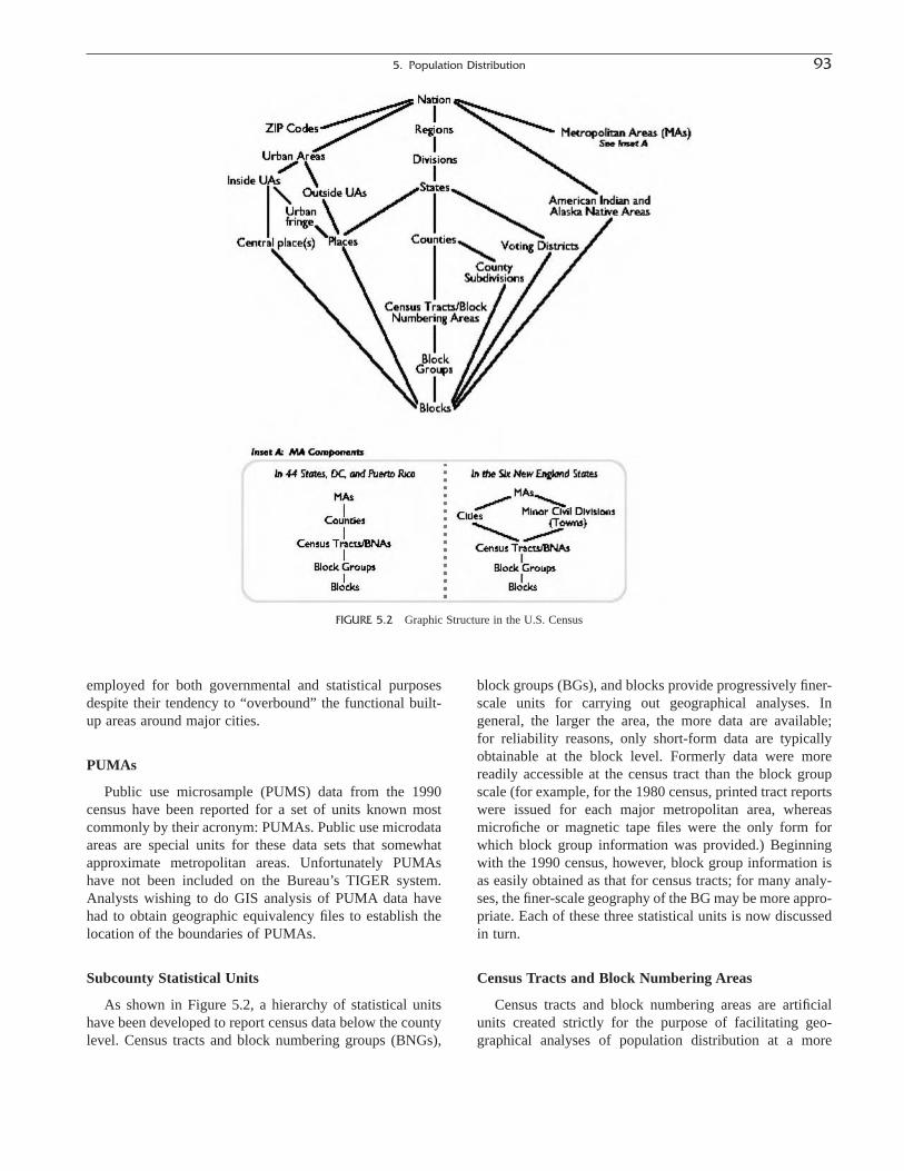
employed for both governmental and statistical purposesdespite their tendency to “overbound” the functional built-up areas around major cities.
PUMAs
Public use microsample (PUMS) data from the 1990census have been reported for a set of units known mostcommonly by their acronym: PUMAs. Public use microdataareas are special units for these data sets that somewhatapproximate metropolitan areas. Unfortunately PUMAshave not been included on the Bureau’s TIGER system. Analysts wishing to do GIS analysis of PUMA data havehad to obtain geographic equivalency files to establish thelocation of the boundaries of PUMAs.
Subcounty Statistical Units
As shown in Figure 5.2, a hierarchy of statistical unitshave been developed to report census data below the countylevel. Census tracts and block numbering groups (BNGs),
block groups (BGs), and blocks provide progressively finer-scale units for carrying out geographical analyses. Ingeneral, the larger the area, the more data are available; for reliability reasons, only short-form data are typicallyobtainable at the block level. Formerly data were morereadily accessible at the census tract than the block groupscale (for example, for the 1980 census, printed tract reportswere issued for each major metropolitan area, whereasmicrofiche or magnetic tape files were the only form forwhich block group information was provided.) Beginningwith the 1990 census, however, block group information isas easily obtained as that for census tracts; for many analy-ses, the finer-scale geography of the BG may be more appro-priate. Each of these three statistical units is now discussedin turn.
Census Tracts and Block Numbering Areas
Census tracts and block numbering areas are artificialunits created strictly for the purpose of facilitating geo-graphical analyses of population distribution at a more
5. Population Distribution 93
FIGURE 5.2 Graphic Structure in the U.S. Census

consistent and generally smaller scale than that afforded bypolitical jurisdictions such as minor civil divisions. Censustracts are delineated by committees of local data users whoare asked to designate units that follow recognizable bound-aries and encompass areas that include between 2500 and8000 persons. The boundaries are drawn based on principlesof homogeneity; committees are asked to create unitsexhibiting, as much as practicable, uniform population char-acteristics, economic status, and housing conditions. Onceestablished, usually only splits (or recombinations) of thetracts from a previous census are permitted. A major goal ofthe tracting program is to present units that can provide thebasis for historical comparisons. The tracts from a morerecent census are generally easily aggregated so as to re-create the areas encompassed by tracts designated for earliercensuses. The tract and BNA numbering systems used onrecent censuses have been designed to facilitate such aggre-gation.13 On the whole, the preservation of fixed boundariesis regarded as more basic than the preservation of homo-geneity within a tract.
The census tract idea began with Walter Laidlaw, whodivided New York City into tracts for the census of 1910.Census tracts were originally developed to subdivide thenation’s urban areas. However, now, with the inclusion ofblock numbering areas, coverage of the entire nation hasbeen achieved at this scale of analysis. Beginning with the1990 census, block numbering areas became essentially theequivalent of census tracts. BNAs are created for counties(or their statistical equivalents) where no local committeeexists to fix the boundaries. Typically state agencies andAmerican Indian tribes, with a fair amount of Census Bureauinvolvement, designate BNAs.
For the 1990 census there were 50,690 tracts and 11,586BNAs, with six states (California, Connecticut, Delaware,Hawaii, New Jersey, and Rhode Island) as well the Districtof Columbia being fully tracted. As of 2000, a total of 66,483tracts/BNAs have been designated.
Block Groups
Block groups are subdivisions of census tracts or blocknumbering areas. They are created by the same committeesor agencies that define tracts and BNAs. The block group isthe smallest area for which census sample data are nowreported. BGs replace the enumeration districts (EDs) thatwere sometimes formerly used to present small area data. A
block group consists of several census blocks that share thesame first-digit number within a census tract. For the 1990census, 229,466 block groups were designated; as of 2000,there are 212,147.
Blocks
Beginning with the 1940 census of housing, blocks incities of 50,000 inhabitants or more at the preceding censuswere numbered, and statistics and analytical maps were published using the block as a unit. In 1960, under specialarrangements, the block statistics program was extended to172 smaller cities as well. There was a total of about 737,000blocks in the block-numbered areas. For the first time, thepopulation total was also tabulated for blocks.14 The 1990census was the first for which the entire national territorywas encompassed by official census block units. The CensusBureau published data for 7,020,924 blocks. Rapid advancesin GIS and geocoding technology have made it sensible tobegin the hierarchy of reporting units with blocks. A possi-ble future (and perhaps ultimate step) would be the geocod-ing of the addresses of each housing unit. This would inprinciple permit complete flexibility in constructing themost appropriate small-area geographic units for any par-ticular statistical purposes while still preserving the confi-dentiality of respondents through the establishment ofminimum population or housing unit thresholds belowwhich data would be suppressed.
Conclusions
We think of geographic elements as being relativelystable and unchanging. Yet this section has reported a pictureof continuous change over the past few decades in the waysdeveloped for presenting data on the geographic distributionof population in the United States. With a highly developed,expanding economy and a highly mobile population, the sig-nificant classifications for examining population distributioncannot remain static if they are to be functionally adequate.Governmental structures have proven slow to adjust to newrealities leading to pressure to create more adequate unitsfor statistical purposes. Settlement structures have evolvedthat look very little like the historical norms of just a fewdecades ago. Yet some degree of comparability of classifi-cation used in successive decades must be maintained toafford a basis of revealing trends and permitting historicalanalyses. This is an ever-present dilemma in the planning ofpopulation censuses that faces statistical agencies in othercountries as well. If no changes were made, the concepts anddefinitions would increasingly fail to describe the current situation. If each census were planned afresh, with no regardto what had been done in the past, there would be no basis
94 David A. Plane
13 Census tracts and block groups are designated by up to four-digitnumbers with optional two-digit decimal suffixes. Numbers are unique toeach county and counties in the same metropolitan area may be requestedto use distinct numerical ranges. When tracts are split, the two-digit suf-fixes may be used. For instance, tract 101 may be divided into tracts 101.01and 101.02. Census tracts have numbers in the range 1 to 9499.99 whereasBNAs are numbered between 9501 to 9989.99. For more information seethe Geographic Areas Reference Manual available at www.census.gov.
14 U.S. Census of Housing: 1960, Vol. III, City Blocks, Series HC(3),Nos. 1 to 421, 1961 to 1962, Table 2.

for studying trends. An intermediate alternative is to intro-duce improvements, but in the year they are introduced tomake at least some data available on both the old and thenew basis.
A relatively new challenge in designing geographic unitsfor data reporting has been the popularity of public usesample data. Privacy issues are even more a matter ofconcern in this area than they are when evaluating ecologi-cal data, yet for good geodemographic analysis such sampledata must contain geographic identifiers at the smallest fea-sible scale. The use of special, ad hoc units such as PUMAsthat do not correspond to any level of the primary censusgeographic hierarchy is certainly less than ideal. With thearrival of the American Community Survey data comefurther challenges for constructing the geographic conceptsof reporting at the below-urban-area scale.
METHODS OF ANALYSIS
Figure 5.3 displays the population distribution of theUnited States. This “night-time” population map is anexample of a population dot map. There are a number ofmeasures for describing the spatial distribution of a popula-tion and many graphic devices other than dot maps for por-traying population distribution and population density. The
interdisciplinary nature of demography is particularly dis-played in this field. Geographers, statisticians, sociologists,and even physicists have contributed to it. In 1957 Duncanset out the following classification of measures, which hedid not claim to be exhaustive or mutually exclusive:
A. Spatial measures(1) Number and density of inhabitants by geographic
subdivisions(2) Measures of concentration(3) Measures of spacing(4) Centrographic measures(5) Population potential
B. Categorical measures(1) Rural-urban and metropolitan-nonmetropolitan
classification(2) Community size distribution(3) Concentration by proximity to centers or to desig-
nated sites
In this book, topics B (1) and (2) are treated more fullyin Chapter 6 than in this chapter. In this chapter, we shalldiscuss the others, combining treatment of A (5), populationpotential, with B(3) under the heading of the general conceptof “accessibility” measures, of which we shall detail twotypes designated threshold and aggregate.
5. Population Distribution 95
FIGURE 5.3 Population Distribution of the United States

Population Density
The density of population is a simple concept much usedin analyses of urban development and studies relating population size to resources and in ecological studies. Thissimple concept has a number of pitfalls, however, some ofwhich are discussed later. Density is usually computed aspopulation per square kilometer, or per square mile, of landarea rather than of gross area (land and water).15
The 1993 Demographic Yearbook of the United Nations(1995) gives population per square kilometer for continentsand regions (Table 1) and for countries (Table 5.3) as esti-mated using information from the 1990 round of censuses.Table 5.3 is abstracted from Table 1 in the Yearbook. Bymidyear 2000, with total population size up to approxi-mately 6.080 billion, the world’s density had increased to 45 persons per square kilometer. A few populous countriesnow have densities in excess of 250 persons per square kilometer (India, 274 persons / sq. km; Japan, 327; SouthKorea, 444; Belgium, 328; Netherlands, 375). From 500 to 2000, the country is likely to be a relatively small island (Barbados, 616; Bermuda, 1189; the Channel Islands,749; and Malta, 1152); beyond 2000, the country is essen-tially a city (Singapore, 4650; Macao, 21,560; Monaco,31,000; and Gibraltar, 4667).
At the other extreme, countries with considerable partsof their land area in deserts, mountains, tropical rain forests,ice caps, and so on have very low densities. The most thinlysettled countries of all tend to be close to the Arctic orAntarctic circles. Even if we use the area of the ice-freeportion of Greenland, its density is only about 0.1 per squarekilometer (for the total surface area the density is only 0.02).Even Canada has a density of only 3.
These illustrations suggest that, for some purposes, moremeaningful densities are obtained for a country or region byrelating the size of its population to the amount of settled
area. On this basis, the densities are often much greater, ofcourse, than the “arithmetic” or “crude” densities we havereported here.
Another measure of population density has been sug-gested by George (1955). His measure relates to the “ratiobetween the requirements of a population and the resourcesmade available to it by production in the area it occupies”(George 1955, p. 313). The ratio is De = Nk/Sk¢, where N isthe number of inhabitants, k the quantity of requirements percapita, S the area in square kilometers, and k¢ the quantityof resources produced per square kilometer. George con-cludes, however, that, “It is impossible to make a valid cal-culation of economic density in an industrial economy.”Duncan, Cuzzort, and Duncan (1961, pp. 35–38) have dis-cussed the conceptual difficulties in comparing the popula-tion density of different areas.
The most commonly employed alternative to crudedensity is “physiological” (sometimes alternatively called“nutritional”) density, which is calculated as populationdivided by the quantity of arable land in a country. Datareported by Fellmann, Getis, and Getis (1999, p. 125), forexample, show that the crude density of Bangladesh is sub-stantially higher than that of Japan (921 versus 334 personsper square kilometer); however, a much greater percentageof Bangladesh’s land area is devoted to agriculture than inhighly urbanized Japan and thus the physiological densitiesare of reverse magnitudes: 2688 for Japan and 1292 forBangladesh. A variation of physiological density is “agri-cultural” density, which is the farm population only dividedby arable land; it gives a perspective on the labor-to-landintensity of agriculture. Note that agricultural densitydefined in this way reflects both the technological efficiencyof farming as well as the labor intensity associated with thetypes of crops grown.
If there have been no changes in boundaries, the changein population density over a given period is, of course,simply proportionate to the change in population size. Thus,if the population has increased 10%, the density has alsoincreased 10%.
United States
The population densities of the United States in midyear2000 were as follows:
United States
Crude density per square mile 78Crude density per square kilometer 30Physiologic density per square mile 376Physiologic density per square kilometer 145
Percentage Distribution
A simple way of ordering the statistics that is appro-priate for any demographic aggregate is to compute the
96 David A. Plane
15 Note that 1 square kilometer (km2) = 0.386103 square miles; 1 squaremile = 2.58998km2.
TABLE 5.3 Estimated Population, Area, and Density forMajor Areas of the World, 1993
Estimated midyear Surface area Densitypopulation (thousands of
Major area (millions) square kilometers)(1) (2) (1) ∏ (2)
World total 5,544 135,641 41Africa 689 30,306 23America, Latin 465 20,533 23America, Northern 287 21,517 13Asia 3,350 31,764 105Europe 726 22,986 32Oceania 28 8,537 3
Source: U.N. Demographic Yearbook, 1995, Table 1, p. 129.

percentage distribution living in the geographic areas of agiven class. Table 5.4 is an illustration. Note that the changegiven in the last column is in terms of percentage points (i.e.,the numerical difference between the two percentages). Thepercentages as rounded may not add exactly to 100. In suchcases, however, it is conventional not to force the distribu-tion to add exactly or to show the total line as 99.9, 100.1,and so on. Where there is a very large number of geographicareas and many would contain less than 0.1% of the popu-lation, the percentages could be carried out to two decimalplaces.
Rank
Another common practice is to include a supplementarytable listing the geographic areas of a given class in rankorder. Again, the rankings can be compared from one censusto another and the changes in rank indicated. Table 5.5 givesan illustration for the “urban areas” of New Zealand. Incases of an exact tie, it is conventional to assign all tyingareas the average of the ranks involved; for example, if twoareas tied for seventh place, they would both be given a rankof 71/2. The choice of sign for the change in rank requires alittle reflection. It seems more intuitive to assign a positive
5. Population Distribution 97
TABLE 5.4 Percentage Distribution by Provinces and Territories of the Population of Canada, 1996 and 1999
1996 1999Change in percentage,
Province or territory Number (thousands) Percentage of total Number (thousands) Percentage of total 1996 to 1999
Canada, total 29,671.9 100.0 30,491.3 100.0 NANewfoundland 560.6 1.9 541.0 1.8 -0.1Prince Edward Island 136.2 0.5 138.0 0.5 —Nova Scotia 931.2 3.1 939.8 3.1 -0.1New Brunswick 753.0 2.5 755.0 2.5 -0.1Quebec 7,274.0 24.5 7,345.4 24.1 -0.4Ontario 11,100.9 37.4 11,513.8 37.8 +0.3Manitoba 1,134.3 3.8 1,143.5 3.8 -0.1Saskatchewan 1,019.5 3.4 1,027.8 3.4 -0.1Alberta 2,780.6 9.4 2,964.7 9.7 +0.4British Columbia 3,882.0 13.1 4,023.1 13.2 +0.1Yukon 31.9 0.1 30.6 0.1 —Northwest Territories 41.8 0.1 41.6 0.1 —Nunavut 25.7 0.1 27.0 0.1 —
— Less than 0.05.NA: Not applicable.Source: Statistics Canada, CANSIM (online database), matrices 6367–6378 and 6408–6409 and calculations by the author.
TABLE 5.5 Population and Rank of Main Urban Areas in New Zealand, 1936 and 1996
1936 1996Change in rank,
Population Rank Population Rank 1936–1996
Auckland 210,393 1 991,796 1 —Wellington 149,382 2 334,051 2 —Christchurch 132,282 3 325,250 3 —Dunedin 81,848 4 110,801 6 -2Napier-Hastings 36,158 5 112,793 5 —Invercargill 25,682 6 49,403 9 -3Wanganui 25,312 7 41,097 11 -4Palmerston North 23,953 8 73,860 7 -1Hamilton 19,373 9 158,045 4 +5New Plymouth 18,194 10 48,871 10 —Gisborne 15,521 11 32,608 12 -1Nelson 13,545 12 50,692 8 +4
Sources: New Zealand, Census and Statistics Department, Population Census, 1945, Vol. 1, p. ix,and Table 6, 1996 Census of Population and Dwellings, “Changes in Usually Resident Population forUrban Areas, 1986–1996”, Statistics New Zealand website www.stats.govt.nz.

sign to a rise in the rankings (movement “upward” towardnumber 1).16
Measures of Average Location and of Concentration
There has long been an interest in calculating some sortof average point for the distribution of population within acountry or other area. Both European and American statis-ticians have contributed to this concept (Bachi, 1966). Themost popular measures are the median point or location, ormedian center of population; the mean point, often calledthe “center of population”; and the point of minimum aggre-gate travel. A somewhat different concept is that of the pointof maximum “population potential.” There has been some-what less scientific interest in measuring the dispersion ofpopulation. Here we will describe Bachi’s “standard dis-tance.” Average positions and dispersion, density surfaces,and so on are treated systematically by Warntz and Neft(1960). Measures of population concentration (such as theLorenz curve and Gini index) are discussed in Chapter 6.
Mediain Lines and Median Point
The “median lines” are two orthogonal lines (at rightangles to each other), each of which divides the area intotwo parts having equal numbers of inhabitants. The “medianpoint” (or median center of population) is the intersection ofthese two lines. The median lines are conventionally thenorth-south and east-west lines, but the location of themedian point depends slightly on how these axes are rotated(Hart, 1954). Table 5.6 gives the location of the mediancenter of population of the United States for each censusyear since 1880. The 1990 median center was located inMarshall Township, Lawrence County, Indiana, approxi-mately 14 miles south of Bloomington.
Hart and others also mention that, in addition to medianlines that divide a territory into halves in terms of popula-tion, other common fractions may be used, such as quartersand tenths. For the population and area of the United States,equal tenths (“decilides”) have been computed in the north-south and the east-west directions (U.S. Bureau of theCensus, 1963). These devices describe population distribu-tion rather than central tendency, as does the median point.
Center of Population
The center of population, or the mean point of the popu-lation distributed over an area, may be defined as the center
of population gravity for the area, “in other words, the pointupon which the [area] would balance, if it were a rigid planewithout weight and the population distributed thereon, eachindividual being assumed to have equal weight and to exertan influence on the central point proportional to his distancefrom the point. The pivotal point, therefore, would be itscenter of gravity” (U.S. Bureau of the Census, 1924, p. 7).The formula for the coordinates of the mean center of population may be written as follows:
(5.1)
where pi is the population at point i and xi and yi are its hor-izontal and vertical coordinates, respectively.
Thus, the mean point, unlike the median point, is influ-enced by the distance of a person from it. It is greatlyaffected by extreme items and is influenced by any changeof the distribution over the total area. In the United States,for example, a population change in Alaska or Hawaii,which is far removed from the center, exerts a much greaterleverage than a change in Missouri, the state where thecenter is now located.
Hart (1954, pp. 50–54) outlines a simple method of calculating the center of population from a map, which is parallel to his method for locating the median point. This graphic method is suitable for only a relatively small area where a map projection like a Mercator projection doesnot distort too much the relative distances along differentparallels of latitude (i.e., where it may be assumed that equal distances in terms of degrees represent equal lineardistances).
x p x p y p y pi i i i i i= =Â Â Â Âand
98 David A. Plane
16 Earlier editions of The Methods and Materials of Demography (e.g.,Shryock and Siegel, 1973) adopted the opposite convention, using the signof the difference between the ranks in the more recent and less recent years.
TABLE 5.6 Median Center of Population of the UnitedStates, 1880–1990
North WestLatitude Longitude
Census Year ° ¢ ≤ ° ¢ ≤
United States1990 38 57 55 86 31 531980 39 18 60 86 08 151970 39 47 43 85 31 431960 39 56 25 85 16 601950 40 00 12 85 02 21
Conterminous United States1950 40 00 12 84 56 511940 40 04 18 84 40 111930 40 11 52 84 36 351920 40 11 52 84 43 601910 40 07 33 85 02 001900 40 03 32 84 49 011890 40 02 51 84 40 011880 39 57 00 84 07 12
Source: “Population and Geographic Centers,” U.S. Bureau of theCensus website at www.census.gov (U.S. Bureau of the Census, 2000a).

A more exact method for computing the center of population, and one that is required when dealing with avery large area, is described by the set of equations shownhere:
(5.2)
(5.3)
where x¢ and y¢ are the coordinates of the assumed mean, Xal
is any point east of that mean, xb is any point west of it, yc
is any point north of it, yd is any point south of it, and pa, pb,pc, pd are the populations in areas east, west, north, and southof the assumed mean, respectively.
The procedure is described in several publications of theU.S. Bureau of the Census. One such description is:
Through this point [the assumed center] a parallel and a meridianare drawn, crossing the entire country.
The product of the population of a given area by its distance fromthe assumed meridian is called an east or west moment. In calcu-lating north and south moments the distances are measured inminutes of arc: in calculating east and west moments it is necessaryto use miles on account of the unequal length of the degrees andminutes in different latitudes. The population of the country isgrouped by square degrees—that is, by areas included between con-secutive parallels and meridians—as they are convenient units withwhich to work. The population of the principal cities is thendeducted from that of the respective square degrees in which theylie and treated separately. The center of population of each squaredegree is assumed to be at its geographical center except where suchan assumption is manifestly incorrect; in these cases the position ofthe center of population of the square degree is estimated as nearlyas possible. The population of each square degree north and southof the assumed parallel is multiplied by the distance of its centerfrom that parallel; a similar calculation is made for the principalcities; and the sum of the north moments and the sum of the southmoments are ascertained. The difference between these two sums,divided by the total population of the country, gives a correction tothe latitude. In a similar manner the sums of the east and of the westmoments are ascertained and from them the correction in longitudeis made. (U.S. Bureau of the Census 1924, pp. 7–8)
For a large area, adjustments should be made for thesphericity of the earth.
The location of the center of population, unlike that ofthe median point, is independent of the particular axeschosen. The calculation of the center of population for alarge country is well suited to programming for a computer.There it is feasible to introduce an additional refinement forthe sphericity of the earth.
For illustrative computations of the center of population(and the median point), see the unabridged edition of TheMethods and Materials of Demography (Shryock andSiegel, 1973, pp. 136–141).
Table 5.7 shows the movement of the center of popula-tion of the United States from 1790 to 1990. Note the dif-ference between the locations for the “United States” (50states) and “conterminous United States” (48 states). Noticethat the mean centers tend to be farther south and substan-
y p y y p y y p yc c d d i= - ¢( ) - ¢ -( ){ } + ¢Â Âx p x x p x x p xa a b b i= - ¢( ) - ¢ -( ){ } + ¢Â Â
tially farther west than the median centers shown in Table 5.6. Back in 1910, the mean center of population was in Bloomington, Indiana, the closest city to the 1990median center. Although much more frequently seen thanthe median center, the mean center may actually be a some-what less intuitive concept to explain to a nontechnical audience.
The definition of the “geographic center of area” is analogous to that of the mean center of population, but the computation is somewhat simpler. In some countriesthose two centers may be a great distance apart. Thus, in1990, the mean center of population of the United States was in Missouri, whereas the geographic center of area was substantially to the northwest in Butte County, SouthDakota, where it has been since the 1960 census after Alaskaand Hawaii became states. The geographic center of area for the conterminous United States is in Smith County,Kansas.
In the last decades of the 19th and the early decades ofthe 20th century, there was great interest in the concept ofcenter of population and in the mean location of many otherunits that are reported in censuses. For example, the Statis-tical Atlas published as part of the 1920 census of the UnitedStates gave the center of population for individual states, ofthe Negro population, and of the urban and rural population,and the mean point of the number of farms. This traditionhas been revived to some extent by the Israeli demographerRoberto Bachi, who has computed or compiled centers ofpopulation for a variety of countries and population sub-groups (Bachi, 1962).
The center of population, being merely the arithmeticmean of the population distribution, need not fall in adensely settled part of the country. In fact, the center of pop-ulation of an archipelago may be in the sea. This is one ofthe circumstances that led the astronomer John Q. Stewartand the geographer William Warntz to regard the concept ofcenter of population as being more misleading than useful(Stewart and Warntz, 1958; Warntz, 1958). Stewart’s alter-native concept of “population potential” is discussed below.Nevertheless, there seems to be real merit in Hart’s view that the center of population is a useful summary measurefor studying the shifts of population over time (Hart, 1954,p. 59).
Point of Minimum Aggregate Travel
This centrographic measure, sometimes called the“median center,” is defined as “that point which can bereached by all items of a distribution with the least totalstraight line travel for all items,” or “the point from whichthe total radial deviations of an areal distribution are at aminimum” (Hart, 1954, pp. 56, 58). Hart gives a graphicmethod for locating this point. This concept has fairlyobvious applications to location theory (e.g., to estimating
5. Population Distribution 99

the optimum central location for a public or private serviceof some sort).
Standard Distance
Measures of the dispersion of population have been pro-posed from time to time, but the one that has been most thor-oughly developed is Bachi’s (1958) “standard distance.” Thestandard distance bears the same kind of relationship to thecenter of population that the standard deviation of any fre-quency distribution bears to the arithmetic mean. In otherwords, it is a measure of the dispersion of the distances ofall inhabitants from the center of population.
If x̄ and ȳ are the coordinates of the center of population,say its longitude and latitude, then the distance from anyitem i, with coordinates xi, and yi, is given by
(5.4)
and the standard distance by
(5.5)DD
n
ici
n
= =Â 2
1
D x x y yic i i= -( ) + -( )2 2
In practice, the distance would not be measured individ-ually for each person but rather we should use data groupedby political areas (or square degrees), and it would then beassumed that the population of a unit area is concentrated inits geographic center. Here, then,
(5.6)
where fi, is the number of persons in a particular unit of area.Duncan, Cuzzort, and Duncan (1961, p. 93) pointed out
that the standard distance is much less influenced by the setof real subdivisions used than are other measures of popu-lation dispersion (or concentration), such as the Lorenzcurve (see Chapter 6). In general, however, the smaller thetype of area used as a unit, the more closely will the com-puted standard distance approach the value computed fromthe locations of individual persons.
Standard distances can also be drawn on a map. Repre-senting the standard distance by a line segment, we knowthe length of the line and its origin at the center of the population, but the direction in which it is drawn is purelyarbitrary. One could appropriately draw a circle with the
Df x x
n
f y y
n
i ii
i ii=
-( )
+-( )Â Â2 2
100 David A. Plane
TABLE 5.7 Mean Center of Population of the United States, 1790–1990
North Westlatitude longitude
Census year ° ¢ ≤ ° ¢ ≤ Approximate location
United States1990 37 52 20 91 12 55 Crawford County, MO, 10 miles southeast of Steelville1980 38 08 13 90 34 26 Jefferson County, MO, 1/4 mile west of DeSoto1970 38 27 47 89 42 22 St. Clair County, MO, 5 miles east-southeast of Mascoutah1960 38 35 58 89 12 35 Clinton County, IL, 61/2 miles nothwest of Centralia1950 38 48 15 88 22 08 Clay County, IL, 3 miles northeast of Louisville
Conterminous United States1950 38 50 21 88 09 33 Richland County, IL, 8 miles north-northwest of Olney1940 38 56 54 87 22 35 Sullivan County, IN, 2 miles southeast by east of Carlisle1930 39 03 45 87 08 06 Greene County, IN, 3 miles northeast of Lincoln1920 39 10 21 86 43 15 Owen County, IN, 8 miles south-southeast of Spencer1910 39 10 12 86 32 20 Monroe County, IN, in the city of Bloomington1900 39 09 36 85 48 54 Bartholomew County, IN, 6 miles southeast of Columbus1890 39 11 56 85 32 53 Decatur County, IN, 20 miles east of Columbus1880 39 04 08 84 39 40 Boone County, KY, 8 miles west by south of Cincinnati, OH1870 39 12 00 83 35 42 Highland County, OH, 48 miles east by north of Cincinnati1860 39 00 24 82 48 48 Pike County, OH, 20 miles south by east of Chillicothe1850 38 59 00 81 19 00 Wirt County, WV, 23 miles southeast of Parkersburg1840 39 02 00 80 18 00 Upshur County, WV, 16 miles south of Clarksburg, WV1
1830 38 57 54 79 16 54 Grant County, WV, 19 miles west-southwest of Moorefield1
1820 39 05 42 78 33 00 Hardy County, WV, 16 miles east of Moorefield1
1810 39 11 30 77 37 12 Loudon County, VA, 40 miles northwest by west of Washington, DC1800 39 16 06 76 56 30 Howard County, MD, 18 miles west of Baltimore1790 39 16 30 76 11 12 Kent County, MD, 23 miles east of Baltimore
1 West Virginia was set off from Virginia on December 31, 1862, and admitted as a state on June 19, 1863.Source: “Population and Geographic Centers,” U.S. Bureau of the Census website at www.census.gov (U.S. Bureau of the Census, 2000a).
standard distance as its radius about the center of the popu-lation. Because the standard distance is equivalent to one standard deviation (1s), the circle would indicate thearea in which about two-thirds of the population is concen-trated. The exact proportion would vary with the specificdistribution.
Accessibility Measures
For many practical applications, such as for locating businesses or public facilities, it is desirable to attempt tomeasure the “accessibility” of various points with referenceto a particular population distribution. The word “accessi-bility” is used in a variety of contexts, including sometimesas a proxy for “ease of interaction.” Here, however, we shallrestrict the usage to measures that attempt to portray theproximity of a mass of persons to particular geographic loca-tions. Plane and Rogerson (1994, pp. 37–41) classified mostcommonly used measures into “threshold” and “aggregate”accessibility concepts. We examine each in turn.
Threshold Accessibility
One of the most widely employed forms of accessibilityis simply to count the population resident within a circulararea of radius R. Thus it may be reported that 3.2 millionpersons live within 50 miles of the proposed new majorleague ballpark, or 2000 households are located within 3miles of the site for a new supermarket. As discussed inAppendix D, many GIS systems are now capable of aggre-gating geo-referenced census data at the block-group orblock level to provide such estimates. For analytical pur-poses, one of the major uses of any accessibility measure isto compare the relative desirability of a number of differentfeasible sites for some activity. Sometimes a more refinedmeasure might take into account configurations of road net-works or even travel times so as to obtain the populationresiding within a (no longer circular) area defined by theoutward bounds of travel with M minutes or H hours.
Threshold accessibility may be sensitive to the choice ofthe radius, R, selected. The relative accessibility of variouslocations may change depending on how far the analystchooses to extend the threshold. Generally there should besome logically defensible rationale for the distance cutoff.It is possible to vary the R value continuously and to plotthreshold accessibility curves that show the cumulative per-centage of the population residing within any distance upuntil the radius encompasses the entire study area and 100%of the population. However, the virtue of the threshold-accessibility concept is its simplicity for communicating toa lay audience; so in most applications a single thresholdwould appear to be advisable.
Aggregate Accessibility
The principal alternative to threshold accessibility is ameasure that weights all population resident within the studyregion by the spatial separation between each person and the location at which accessibility is being measured. Themost commonly employed aggregate accessibility measureis known as “population potential,” or sometimes “Hansenaccessibility” after the author of a classic paper (Hansen,1959) that popularized the concept in the city planning lit-erature. The term “population potential” comes from thephysics notion of a field measure (such as electrical or grav-itational potential) and should not be invested with literaldemographic meaning. As developed by Stewart, populationpotential applies to the accessibility to the population, or“level of influence” on the population, of a point on a mapor of a small unit of area (Stewart and Warntz, 1959). If the“influence” of each individual at a point; is considered to beinversely proportional to his or her distance from it, the totalpotential of population at the point is the sum of the recip-rocals of the distances of all individuals in the populationfrom the point. In practice, of course, the computation ismade by assuming that all the individuals within a suitablysmall area are equidistant from point j. Thus the formula forthe potential at point j is
(5.7)
where the Pi are the populations of the n areas into which aterritory is divided, and the Dij are the respective distancesof these areas from point j (usually measured from the geo-graphic center or from the approximate center of gravity ofthe population, in each area) (Duncan, 1957, pp. 35–36).17
Like the center of population (but unlike threshold acces-sibility), the population potential at any point in the territoryis affected by the distribution of population over the entireterritory. When the potential has been computed for a suffi-cient number of points, those of equal potential may bejoined on the map to show contours or isopleths. It can bewell appreciated that each computation involves a good dealof labor so that to produce a fine-grained map, the compu-tations would need to be performed on a computer. On sucha fine-grained map, there would be peaks of potential aroundevery city that are not brought out on most of the availablemaps showing this measure.
To illustrate, we will show only the first few computa-tions needed to calculate the population potential at one particular point. This is a hypothetical case. Let the “point”j = 1 in question be a capital city A with a population of100,000. Let this population be P1. Assume that the popula-tion is evenly distributed over the city. Because this “point”is a relatively populous area, it is necessary to take into
Vj ==Â P Di iji
n
1
5. Population Distribution 101
17 The notation used in the formula has been changed from the original.

account the average distance of its own population from itsgeographic center. Let us say that this has been estimatedfrom the city’s map at 3 kilometers.18
Then measure the distance from the geographic center ofevery other political unit in the set being used to the centerof the capital city. This set of units should account for allthe national territory unless population potential is beingstudied for some other kind of area, such as a region. Thesegeographic centers can be plotted by inspections but, wherea primary unit has a very large and unevenly distributed pop-ulation, the secondary divisions within it can be used forincreased accuracy. Suppose we then have
Population Distribution
The commonest method of representing the distributionof the absolute number of inhabitants is a dot map (such asthe one given previously as Figure 5.3). A small dot or spotof constant size represents a round number of people suchas 100 or 1000. If a general impression is all that is wanted,the dots may be plotted more or less uniformly within theunits of area given on the map. For a more exact portrayal,regard should be paid to any actual concentrations of popu-lation within the unit areas. This procedure calls for refering to figures for geographic subdivisions below thelevel of those outlined on the map. For example, with acounty outline map of the United States, one could refer tothe published figures for minor civil divisions or for incor-porated places.
In maps of population distribution for a country or otherarea containing both thinly settled rural territory and largeurban agglomerations, there is a real problem in the appli-cation of the conventional dot method. A black dot that rep-resents few enough people to show the distribution of therural population requires so many plottings within the limitsof large cities that one sees only a solid black area, and eventhat may grossly underrepresent the actual number of dotsrequired. To portray the population of large cities, one coulduse a dot of the same size but of a different color to whicha higher value is assigned—for example, a black dot couldrepresent 100 people and a red dot, 10,000. Another varia-tion is to use circles of varying size for specific urban places.Such circles (or other graphic symbols) may be chosen in alimited number of sizes or forms, such as these:
• 2500 to 10,000• 10,000 to 25,000• 25,000 to 50,000
or, especially for larger cities, the circle may be drawn withthe area proportional to the size of the population.
In the latter case, it is best to start with the largest placeand determine the size of circle that can reasonably beaccommodated on the map. (Because a number of the circleswill overlap and will extend beyond the areas to which theyapply, they should be either “open,” that is, unshaded, orshaded in a light tint so that boundary lines can showthrough.) Suppose a circle with a diameter of 5cm is chosento represent a city of 500,000. Then, because the area of thecircle is drawn proportionate to the population, and the areais pr2, the radius required for a smaller population is solvedby the following equation:
(5.8)
or, alternatively
(5.9)rP=
80 000,cm
pp
r P2
6 25 500 000¥=
. ,
102 David A. Plane
18 A “quick and dirty” method for estimating such contribution of “self-potential” (as it is sometimes endearingly called!) is to use one-half of thedistance to the nearest neighbor.
Area (j) Pj Dij Pj/Dij
1 100,000 3 33,3332 25,000 8 3,1253 10,000 10 1,000. . . . . . . . .n 15,000 500 30
The population potential for the city is the sum of the lastcolumn. One does not have to work outward from the areain question while listing the areas; any systematic listing isacceptable. If the latitudes and longitudes of all the centersof geographic area (or, ideally, the centers of population ofall the areas) are known, these can be programmed for acomputer so that the distances to any point can be computedby triangulation.
Warntz and Neft (1960, p. 65) point out that “The peakof population potential coincides with the modal center onthe smoothed density surface for the United States”. Thestatement applied to 1950 but presumably it would still holdtrue.
The concept of population potential is more useful thanthat of aggregate travel distance and has sometimes provedvaluable as an indicator of geographical variations in socialand economic phenomena (e.g., rural population density,farmland values, miles of railway track per square mile, roaddensity, density of wage earners in manufacturing, and deathrates). Rural density, for example, tends to be proportionalto the square of the potential.
Mapping Devices
There is a voluminous literature on the mapping of de-mographic data to which demographers, geographers, andmembers of other disciplines have contributed (see, e.g.,Bachi, 1966; Schmid, 1954, pp. 184–222). Here we are con-cerned with mapping just the distribution of population andof population density.
so that, for a population of 100,000, a circle with a radiusof 1.12cm is needed. (Note that the radius varies with thesquare root of the population.)
To represent very wide ranges of population size, spher-ical symbols can be used instead of circles for the largestlocalities. The population of the large localities would thenbe proportional to the volume of the sphere implied. Othergraphic devices are sometimes used to denote the popula-tion in a geographical area, for example, the heights of a rectangle (two-dimensional bar) or of a three-dimensionalcolumn shown in perspective. Such devices are convenientfor only a relatively small number of areal units, such as theprimary divisions of a country.
Population Density
A conventional way of indicating population density isthat of shading or hatching, with the darker shadings repre-senting the greater densities.19 Such shadings may gloss overconsiderable internal variation within an area because theyrepresent simply the area’s average density. The contour orisopleth map also lends itself to the presentation of geo-graphic regularities in population density. Some of the prob-lems, considerations, and techniques in the construction ofsuch maps are discussed by Duncan (1957) and by Schmid(1954). A more recent and somewhat detailed treatment of issues in population mapping is given by Schnell andMonmonier (1983, pp. 33–41).
References
Bachi, R. 1958. “Statistical Analysis of Geographic Series,” Bulletin of theInternational Statistical Institute 36(2): 229–240.
Bachi, R. 1962. “Standard Distance Measures and Related Methods forSpatial Analysis.” Papers of the Regional Science Association 10:83–132.
Bachi, R. 1966. “Graphical Representation and Analysis of Geographical-Statistical Data,” Bulletin of the International Statistical Institute (Pro-ceedings of the 35th session, Belgrade, 1965) 41(1): 225.
Beale, C. L. 1967. “State Economic Areas—A Review after 17 Years.”Washington, DC: American Statistical Association, Proceedings of theSocial Statistics Section, 82–85.
Bogue, D. J., and C. L. Beale. 1953. U.S. Bureau of the Census and U.S.Bureau of Agricultural Economics, “Economic Subregions of theUnited States,” Series Census-BAE, No. 19.
Bogue, D. J., and C. L. Beale. 1961. Economic Areas of the United States.New York: Free Press of Glencoe.
Clayton, C. 1982. “Hierarchically Organized Migration Fields: The Application of Higher Order Factor Analysis to Population MigrationTables.” Annals of Regional Science 11: 109–122.
Dahmann, D. C. 1992. “Accounting for the Geography of Population: 200Years of Census Bureau Practice with Macro-Scale Sub-NationalRegions.” Paper presented at the Annual Meeting of the Association ofAmerican Geographers, San Diego, CA, April 18–22.
Duncan, O. D. 1957. “The Measurement of Population Distribution.” Pop-ulation Studies (London) 11(1): 27–45.
Duncan, O. D., R. P. Cuzzort, and B. Duncan. 1961. Statistical Geography.Glencoe, IL: The Free Press.
Fellmann, J. D., A. Getis, and J. Getis. 1999. Human Geography: Landscapes of Human Activities, 6th ed. New York, NY: WCBMcGraw-Hill.
George, P. O. L. 1955. “Sur un project de calcul de la densité économique de la population” (On a project for calculating the eco-nomic density of the population), pp. 303–313, in Proceedings of theWorld Population Conference, 1954 (Rome), Vol. IV, New York: UnitedNations.
Hansen, W. 1959. “How Accessibility Shapes Land Use,” Journal of theAmerican Institute of Planners 25: 72–77.
Hart, J. F. 1954. “Central Tendency in Areal Distributions.” EconomicGeography 30(1): 54.
Illinois Board of Economic Development. 1965. Suggested EconomicRegions in Illinois by Counties, by Eleanor Gilpatrick, Springfield (Illinois).
International Urban Research. 1959. The World’s Metropolitan Areas.Berkeley, CA: University of California Press.
Johnson, K. P. 1995. “Redefinition of the BEA Economic Areas,” Surveyof Current Business (February): 75–81.
McDonald, J. R. 1966. “The Region: Its Conception, Design, and Limita-tions.” Annals of the Association of American Geographers 56:516–528.
Morrill, R. L. 1988. Migration Regions and Population Redistribution.Growth and Change 19: 43–60.
Odum, H. W. 1936. Southern Regions of the United States. Chapel Hill:University of North Carolina Press.
Odum, H. W., and H. E. Moore. 1938. American Regionalism: A Cultural-Historical Approach to National Integration. New York: Henry Holtand Co.
Pandit, K. 1994. “Differentiating Between Subsystems and Typologies inthe Analysis of Migration Regions: A U.S. Example.” ProfessionalGeographer 46: 331–345.
Plane, D. A. 1998. “Fuzzy Set Migration Regions.” Geographical and Envi-ronmental Modelling 2(2): 141–162.
Plane, D. A., and A. M. Isserman. 1983. “U.S. Labor Force Migration: AnAnalysis of Trends, Net Exchanges, and Migration Subsystems.” Socio-Economic Planning Sciences 17: 251–266.
Plane, D. A., and P. A. Rogerson. 1994. The Geographical Analysis of Pop-ulation: With Applications to Planning and Business. New York: JohnWiley & Sons.
Schmid, C. F. 1954. Handbook of Graphic Presentation. New York: RonaldPress.
Schnell, G. A., and M. S. Monmonier. 1983. The Study of Population: Elements, Patterns, Processes. Columbus, OH: Charles E. Merrill Publishing.
Shryock, H. S., Jr. 1957. “The Natural History of Standard MetropolitanAreas.” American Journal of Sociology 63(2): 163–170.
Shryock, H. S., Jr., and J. S. Siegel. 1973. The Methods and Materials ofDemography, 2nd rev. ed. Washington, DC: U.S. Government PrintingOffice.
Slater, P. B. 1976. “A Hierarchical Regionalization of Japanese PrefecturesUsing 1972 Interprefectural Migration Flows.” Regional Studies 10:123–132.
Stewart, J. Q., and W. Warntz. 1958. “Macrogeography and SocialScience.” Geographical Review 48(2): 167–184.
Stewart, J. Q., and W. Warntz. 1959. “Some Parameters of the Geographi-cal Distribution of Population.” Geographical Review 49(2): 270–272.
Taeuber, C. 1965. “Regional and Other Area Statistics in the United States,”Bulletin of the International Statistical Institute (Proceedings of the 35th
session, Belgrade, 1965) 41(1): 161–162.United Nations. 1967. Principles and Recommendations for the 1970
Population Censuses, Statistical Papers, Series M, No. 44.
5. Population Distribution 103
19 For types of shadings available, see Schmid (1954, pp. 187–198).

United Nations. 1995. Demographic Yearbook. New York, NY: UnitedNations.
U.S. Bureau of the Census. 1913. Thirteenth Census of the United States,Abstract of the Census.
U.S. Bureau of the Census. 1924. Statistical Atlas of the United States,1924, pp. 7–24.
U.S. Bureau of the Census. 1951. State Economic Areas (by Donald J.Bogue).
U.S. Bureau of the Census. 1963. “Zones of Equal Population in the UnitedStates: 1960.” Geographic Reports, GE-10, No. 3.
U.S. Bureau of the Census. 2000a.www.census.gov/cao/www/congress/appormen.html#num.
U.S. Bureau of the Census. 2000b. Geographic Areas Reference Manual.www.census.gov/geo/www/garm.html.
Warntz, W. 1958. “Macrogeography and the Census.” The ProfessionalGeographer, 10(6): 6–10.
Warntz, W., and D. Neft. 1960. “Contributions to Statistical Methodologyfor Areal Distributions.” Journal of Regional Science 2(1): 47–66.
Whittlesey, D. 1954. “The Regional Concept and the Regional Method.” InP. E. James and C. F. Jones (Eds.). American Geography: Inventory andProspect. Published for the Association of American Geographers bySyracuse University Press.
Winchester, H. P. M. 1977. Changing Patterns of French Internal Migra-tion, 1891–1968. Research Paper No. 17. Oxford: Oxford UniversitySchool of Geography.
Woofter, T. J., Jr. 1934. “Subregions of the Southeast.” Social Forces 13(1):43–50.
104 David A. Plane

This chapter extends the geographic topics discussed inChapter 5 by considering classes of geographic residencethat are formed primarily for statistical purposes. Theemphasis here is on geographic groupings that are not nec-essarily contiguous pieces of territory. The major focus is onthe “urban-rural” classification. We start with a general dis-cussion of this classification and then turn to internationalconcepts and definitions dealing with it. We then discussselected national level concepts, with a primary focus on theUnited States. We conclude this chapter with a discussion ofcommonly used measures of population distribution.
The working definitions of “urban” and “rural” varygreatly, not only according to nation, but also according to organization and research discipline. Urban settlementshave been defined, for example, on the basis of an urbanculture, administrative functions, percentage of people innonagricultural occupations, and size or density of popula-tion (Palen, 2002). Rural areas are often defined as a residualcategory—that is, “areas not classified as urban”—but they may also be subdivided by criteria that vary accordingto nation, organization, and discipline. In spite of theseproblems, the urban-rural classification is widely used, asillustrated by Tables 6.1, 6.2, 6.3, and 6.4.
Table 6.1 shows the total population of selected countriesaround the world and the percentage in each country that is classified as urban. Over 96% of Kuwait’s population of 1.97 million is classified as “urban,” while only 17.6% of Papua-New Guinea’s population of 4.9 million is soclassified.
Table 6.2 shows the population of the United Statescounted in each decennial census from 1790 to 1990 classi-fied by urban and rural residence. Notice that a major changein the definition of urban went into effect in 1950 and thatdata under the old and new definitions were made availablefor two censuses, 1950 and 1960. Under the earlier defini-tion, the urban population of the United States in 1950 is
90.1 million, while under the revised definition it is 96.8million in 1950.
Table 6.3 shows changes in the population of size-classesof towns of India between the census of 1981 and the censusof 1991. The largest size class (Class I, towns having apopulation of 100,000 or more) experienced a 47% increasein population between 1981 and 1991, or an absoluteincrease of nearly 45 million people. The smallest size class(Class VI, towns having a population of fewer than 5000)experienced a 21% decline in total population from 1981 to1991, or an absolute decrease of only 164,000 people.
URBAN-RURAL: INTERNATIONALSTANDARDS AND DEFINITIONS
United Nations Recommendations
In an effort to bring some level of standardization tourban/rural statistics, the United Nations (UN) has beendeveloping and revising proposed standards for more than 40 years. The major purpose of this effort is to assistnations in both planning for and developing the content ofcensuses. Another goal is to improve international com-patibility through the use of standardized definitions andclassification, as noted in Chapters 2 and 3.
The most recent set of recommendations was developedwithin the framework of the 2000 World Population andHousing Census Program adopted in 1995 (United Nations,1998). Suggested topics to be included in censuses aredivided into two types. The first, “core” topics, are subjectsthat all nations should cover in their censuses using therecommended definitions and classification listed. Thesecond, “noncore” topics, are subjects that nations may wishto include in censuses. There are suggested definitions forsome, but not all, noncore topics. Noncore topics are
105
C H A P T E R
6
Population DistributionClassification of Residence
JEROME N. McKIBBEN AND KIMBERLY A. FAUST
The Methods and Materials of DemographyCopyright 2003, Elsevier Science (USA).
All rights reserved.
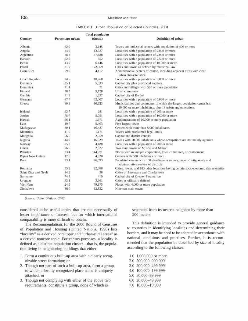
considered to be useful topics that are not necessarily oflesser importance or interest, but for which internationalcomparability is more difficult to obtain.
The Recommendations for the 2000 Round of Censusesof Population and Housing (United Nations, 1998) lists“locality” as a derived core topic and “urban-rural areas” asa derived noncore topic. For census purposes, a locality isdefined as a distinct population cluster—that is, the popula-tion living in neighboring buildings that either
1. Form a continuous built-up area with a clearly recog-nizable street formation; or
2. Though not part of such a built-up area, form a groupto which a locally recognized place name is uniquelyattached; or
3. Though not complying with either of the above tworequirements, constitute a group, none of which is
separated from its nearest neighbor by more than 200 meters.
This definition is intended to provide general guidance to countries in identifying localities and determining theirborders, and it may be need to be adapted in accordance withnational conditions and practices. Further, it is recom-mended that the population be classified by size of localityaccording to the following classes:
1.0 1,000,000 or more2.0 500,000–999,9993.0 200,000–499,9994.0 100,000–199,9995.0 50,000–99,9996.0 20,000–49,9997.0 10,000–19,999
106 McKibben and Faust
TABLE 6.1 Urban Population of Selected Countries, 2001
Total populationCountry Percentage urban (thous.) Definition of urban
Albania 42.9 3,145 Towns and industrial centers with population of 400 or moreAngola 34.9 13,527 Localities with a population of 2,000 or moreArgentina 88.3 37,488 Localities with a population of 2,000 or moreBahrain 92.5 652 Localities with a population of 2,500 or moreBenin 43.0 6,446 Localities with a population of 10,000 or moreBrazil 81.7 172,559 Cities and towns as defined by municipal lawCosta Rica 59.5 4,112 Administrative centers of cantón, including adjacent areas with clear
urban characteristics.Czech Republic 74.5 10,260 Localities with a population of 5,000 or moreDenmark 85.1 5,333 Capital city plus provincial capitalsDominica 71.4 71 Cities and villages with 500 or more populationFinland 58.5 5,178 Urban communesGambia 31.3 1,337 Capital city of BanjulGermany 87.7 82,007 Localities with a population of 5,000 or moreGreece 60.3 10,623 Municipalities and communes in which the largest population center has
10,000 or more inhabitants, plus 18 urban agglomerationsIceland 92.7 281 Localities with a population of 200 or moreJordan 78.7 5,051 Localities with a population of 10,000 or moreKuwait 96.1 1,971 Agglomerations of 10,000 or more populationLaos 19.7 5,403 Five largest townsMadagascar 30.1 16,437 Centers with more than 5,000 inhabitantsMauritius 41.6 1,171 Towns with proclaimed legal limitsMongolia 56.6 2,559 Capital and district centersNigeria 44.9 116,929 Towns with 20,000 inhabitants whose occupations are not mainly agrarianNorway 75.0 4,488 Localities with a population of 200 or moreOman 76.5 2,622 Two main towns of Muscat and MatrahPakistan 33.4 144,971 Places with municipal corporation, town committee, or cantonmentPapua New Guinea 17.6 4,920 Centers with 500 inhabitants or morePeru 73.1 26,093 Populated centers with 100 dwellings or more grouped contiguously and
administrative centers of districtsRomania 55.2 22,388 Cities, towns, and 183 other localities having certain socioeconomic characteristicsSaint Kitts and Nevis 34.2 38 Cities of Basseterre and CharlestownSuriname 74.8 419 Capital city of Greater ParamariboUruguay 92.1 3,361 Cities as officially definedViet Nam 24.5 79,175 Places with 4,000 or more populationZimbabwe 36.0 12,852 Nineteen main towns
Source: United Nations, 2002.
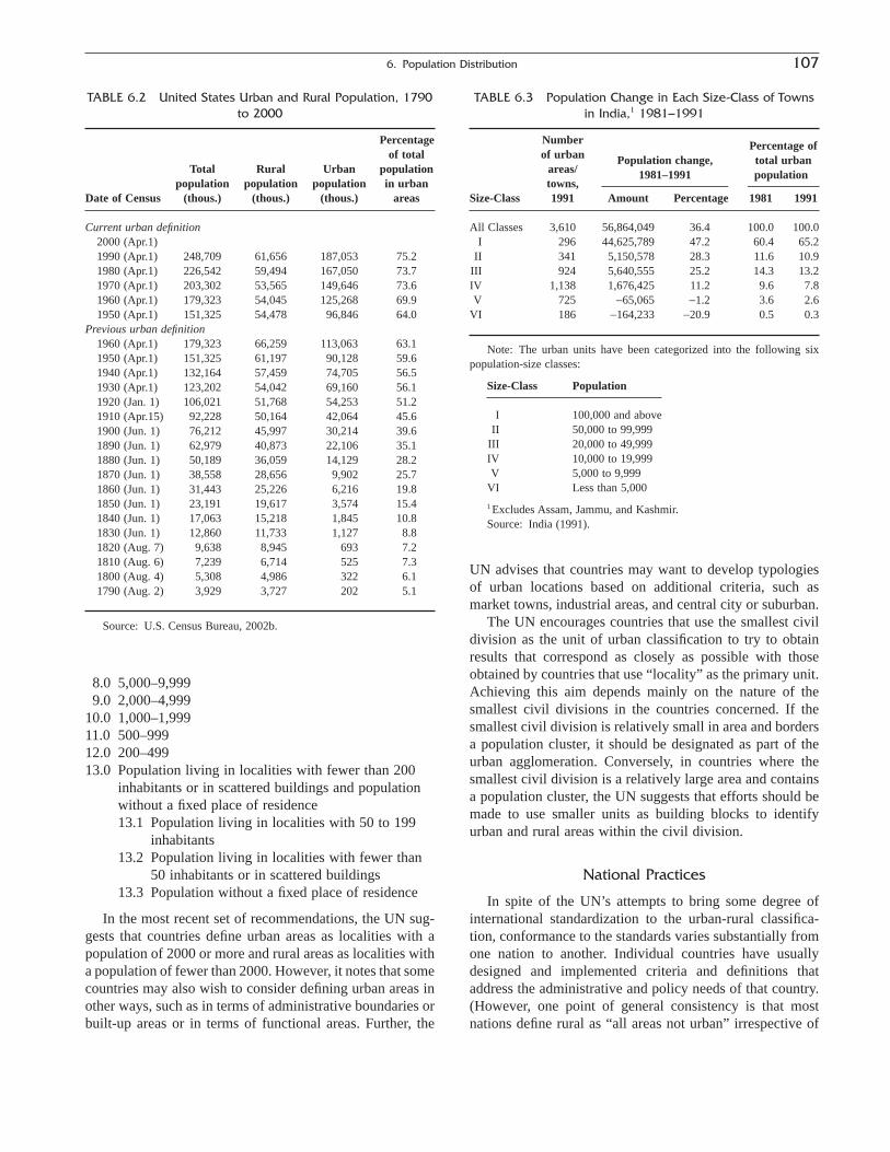
UN advises that countries may want to develop typologiesof urban locations based on additional criteria, such asmarket towns, industrial areas, and central city or suburban.
The UN encourages countries that use the smallest civildivision as the unit of urban classification to try to obtainresults that correspond as closely as possible with thoseobtained by countries that use “locality” as the primary unit.Achieving this aim depends mainly on the nature of thesmallest civil divisions in the countries concerned. If thesmallest civil division is relatively small in area and bordersa population cluster, it should be designated as part of theurban agglomeration. Conversely, in countries where thesmallest civil division is a relatively large area and containsa population cluster, the UN suggests that efforts should bemade to use smaller units as building blocks to identifyurban and rural areas within the civil division.
National Practices
In spite of the UN’s attempts to bring some degree ofinternational standardization to the urban-rural classifica-tion, conformance to the standards varies substantially fromone nation to another. Individual countries have usuallydesigned and implemented criteria and definitions thataddress the administrative and policy needs of that country.(However, one point of general consistency is that mostnations define rural as “all areas not urban” irrespective of
6. Population Distribution 107
8.0 5,000–9,9999.0 2,000–4,999
10.0 1,000–1,99911.0 500–99912.0 200–49913.0 Population living in localities with fewer than 200
inhabitants or in scattered buildings and populationwithout a fixed place of residence13.1 Population living in localities with 50 to 199
inhabitants13.2 Population living in localities with fewer than
50 inhabitants or in scattered buildings13.3 Population without a fixed place of residence
In the most recent set of recommendations, the UN sug-gests that countries define urban areas as localities with apopulation of 2000 or more and rural areas as localities witha population of fewer than 2000. However, it notes that somecountries may also wish to consider defining urban areas inother ways, such as in terms of administrative boundaries orbuilt-up areas or in terms of functional areas. Further, the
TABLE 6.2 United States Urban and Rural Population, 1790to 2000
Percentageof total
Total Rural Urban populationpopulation population population in urban
Date of Census (thous.) (thous.) (thous.) areas
Current urban definition2000 (Apr.1)1990 (Apr.1) 248,709 61,656 187,053 75.21980 (Apr.1) 226,542 59,494 167,050 73.71970 (Apr.1) 203,302 53,565 149,646 73.61960 (Apr.1) 179,323 54,045 125,268 69.91950 (Apr.1) 151,325 54,478 96,846 64.0
Previous urban definition1960 (Apr.1) 179,323 66,259 113,063 63.11950 (Apr.1) 151,325 61,197 90,128 59.61940 (Apr.1) 132,164 57,459 74,705 56.51930 (Apr.1) 123,202 54,042 69,160 56.11920 (Jan. 1) 106,021 51,768 54,253 51.21910 (Apr.15) 92,228 50,164 42,064 45.61900 (Jun. 1) 76,212 45,997 30,214 39.61890 (Jun. 1) 62,979 40,873 22,106 35.11880 (Jun. 1) 50,189 36,059 14,129 28.21870 (Jun. 1) 38,558 28,656 9,902 25.71860 (Jun. 1) 31,443 25,226 6,216 19.81850 (Jun. 1) 23,191 19,617 3,574 15.41840 (Jun. 1) 17,063 15,218 1,845 10.81830 (Jun. 1) 12,860 11,733 1,127 8.81820 (Aug. 7) 9,638 8,945 693 7.21810 (Aug. 6) 7,239 6,714 525 7.31800 (Aug. 4) 5,308 4,986 322 6.11790 (Aug. 2) 3,929 3,727 202 5.1
Source: U.S. Census Bureau, 2002b.
TABLE 6.3 Population Change in Each Size-Class of Townsin India,1 1981–1991
Numberof urban
Percentage of
areas/Population change, total urban
towns,1981–1991 population
Size-Class 1991 Amount Percentage 1981 1991
All Classes 3,610 56,864,049 36.4 100.0 100.0I 296 44,625,789 47.2 60.4 65.2
II 341 5,150,578 28.3 11.6 10.9III 924 5,640,555 25.2 14.3 13.2IV 1,138 1,676,425 11.2 9.6 7.8V 725 -65,065 -1.2 3.6 2.6
VI 186 -164,233 -20.9 0.5 0.3
Note: The urban units have been categorized into the following six population-size classes:
Size-Class Population
I 100,000 and aboveII 50,000 to 99,999
III 20,000 to 49,999IV 10,000 to 19,999V 5,000 to 9,999
VI Less than 5,000
1 Excludes Assam, Jammu, and Kashmir.Source: India (1991).
the definition of urban used.) In sum, a majority of nationsignore the United Nations recommendations on locality andurban-rural classifications and use their own definitions and standards.
Most nations use one of five schemes when designatingurban areas. The first and most widely used is simply estab-lishing a minimum population size that acts as a thresholdrequirement for a town or city to qualify as an urban area. However, this minimum population prerequisite variesgreatly from one country to another. Angola, for example,classifies any town with more than 2000 people as an urbanarea, while in Italy the requirement is 10,000 and in Nepalit is 9000.
There are other cases where population density is used incombination with population size to define an urban area.The Philippines requires that cities and municipalities haveat least 1000 persons per square mile as well as a popula-tion minimum of 2500. In India, an urban area needs to haveat least 5000 people and a population density of 1000 persquare mile to qualify. The use of population density isusually seen in countries that have several geographicallylarge municipalities.
Another popular classification system uses both popula-tion size and the primary economic activities of the area to determine if it is urban. For example, Estonia designatesareas as urban on the basis of population size and thepredominance of nonagricultural workers and their families.In Botswana, the standard is a population of at least 5000,where 75% of the economic activity is nonagricultural.Austria requires a commune to have 2000 persons and 85%of the active population to be engaged in nonagricultural/nonforestry work. These types of classification systems areoften seen in nations that link the concept of rural status tothe activity of farming.
There are several cases where cities and towns are legallydefined or established as urban by official decree of thenational government. Guatemala, Bulgaria, and the Repub-lic of Korea are examples of nations that use this system.The exact requirements for urban designation vary greatlyand frequently involve nondemographic and noneconomicfactors
Finally, many nations have established “defined urbancharacteristics” that an area must possess in addition topopulation size in order to qualify for urban status. Chile,for example, states that a population center must have“certain public and municipal services” in order to attainurban status. Cuba requires an urban place to have a popu-lation of at least 2000. However, an area of lesser popula-tion can qualify if it has paved streets, street lighting, pipedwater, sewage, a medical center, and educational facilities.
Because of the complex and varied nature of these criteria for urban designation, researchers must use cautionwhen conducting any comparisons of the level and extent of urbanization of one country with another. The United
Nations Demographic Yearbook lists the criteria that each country utilizes when designating areas as urban.Researchers should consult this volume to see the specificrequirement each country uses and to keep informed of anyrecent definitional changes.
URBAN-RURAL DEFINITIONS IN THE UNITED STATES
Development of the Classification System
Since its inception, the definition of urban in the UnitedStates has always involved the number of residents (ascounted by the census) in a given area although politicalcriteria, such as administrative status, were also involved. Asearly as 1874, urban areas were defined as any incorporatedplace with a population of 8000 or more. The minimum sizewas officially reduced to 4000 in 1880 and reduced again in1910 to the level of 2500. The practice of designating onlyincorporated places as urban (a standard that would continueuntil 1950) resulted in the labeling of many densely settledbut unincorporated areas as rural, a practice that greatlyinflated the rural population. Although the Census Bureauattempted to avoid some of the more glaring omissions byclassifying selected areas as “urban under special rules,”many large, closely built-up areas were excluded from theurban category (U.S. Census Bureau, 1995).
This practice proved to be particularly problematic inNew England, where a town is equivalent to a minor civildivision, much like a township in the Midwest. This led to the practice of classifying these areas in New England as “urban under special rules” (an application that was laterextended to New York and Wisconsin). Thus, any such areaswith a total population above the minimum threshold cameto be considered as urban (Truesdell, 1949).
Recognizing the shortcomings of these criteria and prac-tices, the Census Bureau implemented major changes in the definition and designation of urban areas after the 1950census. The most important of these changes was the intro-duction of two new types of geographic units, the urbanizedarea (UA) and the census designated place (CDP) (U.S.Census Bureau, 1994). The introduction of the CDP resultedin classifying as urban, any densely settled area with a population of 2500 or more. The demarcation of CDPboundaries was determined by the Census Bureau afterextensive fieldwork and mapping were conducted, withparticular attention placed on the population density of thedesignated area. This represented a major shift in theconcept of “urban.” Instead of relying solely on legal bound-aries and population size, factors such as population densityand self-identification of place were now being taken intoaccount as well (U.S. Census Bureau, 1996).
A further development was the UA concept, whichincludes built-up, but unincorporated areas, adjacent to
108 McKibben and Faust
cities and towns in the urban population. Initially, the baserequirement for a UA was a central place with a populationof 50,000 or more. Any area outside the city limits with atleast 500 housing units per square mile or approximately2000 persons per square mile (reduced to 1000 per squaremile in 1960) would be included in that city’s urban popu-lation count. These unincorporated areas had to be contigu-ous to or within one and a half miles of the core andconnected to it by a road (U.S. Census Bureau, 1994). Giventhe rapid suburban growth that most cities were experienc-ing (and probably would continue to experience over thenext several decades), this inclusion of the “urban fringe”population in the urban population would make the urbanpopulation counts much more reflective of the true urban-rural distribution of the population.
In 1970, the Census Bureau again modified the definitionof urban with its introduction of the “extended city.” Duringthe 1960s, several cities in the United States began extend-ing their municipal boundaries to include areas that werefundamentally rural in character. (e.g., San Diego, California, and Oklahoma City, Oklahoma). In addition,some cities adopted the “Unigov” system, whereby the citywould annex the unincorporated areas of the county and thenmerge all city and county governmental functions in to oneunit (e.g., Indianapolis, Indiana, and Columbus, Georgia).
To address the urban-rural classification in these situa-tions, the Census Bureau developed criteria for identifyingextended cities. An incorporated place would be consideredan extended city if it contained one or more areas that
1. Are 5 square miles or more in size2. Have a population density less than 100 persons per
square mile and either3. Comprise at least 25% of the total land area of the
place or4. Consist of 25 square miles or more.
To qualify, the first two conditions, and either the thirdor the fourth must apply. The rural portion of an extendedcity may consist of several separate pieces of territory, giventhat each section is at least 5 square miles in size and has apopulation density of fewer than 100 per square mile. If theextended city has low-density enclaves that are adjacent toits rural portions, these enclaves become part of the ruralportion. There is no population minimum for UA extendedcities; however, non-UA extended cities must have at least2500 residents (U.S. Census Bureau, 1994). These specifi-cations remained the same for the 1980 census. For the 1990census, this classification system was also applied to certainplaces outside of UAs.
Despite their long history, urban-rural definitions in theUnited States are sometimes confused with those used toidentify “metropolitan/nonmetropolitan areas (discussed inthe previous chapter). Since the introduction of the “metro-politan statistical area” after the 1950 census, aspects of the
definitions for metropolitan-nonmetropolitan and urban-rural have overlapped and continue to do so.
There are several fundamental differences between thedefinitions of metropolitan-nonmetropolitan and urban-rural, even though the terms are frequently (and mistakenly)used interchangeably. Metropolitan areas are identifiedthrough criteria developed by the Office of Management and Budget (OMB). These criteria are primarily based onsize of place, social and economic integration, and politicalboundaries. Urban-rural areas are identified through criteriadeveloped by the U.S Census Bureau (2001b). These criteria primarily involve contiguous areas meeting certainrequirements of population size and density.
Metropolitan areas can and, in fact, often do contain areasthat have been classified as rural. As an example, considerthe Mojave Desert, which is clearly a rural area, but one thatlies within “metropolitan” San Bernardino County. Exam-ples such as this have led the Office of Management andBudget (OMB) to stress that metropolitan statistical areas donot correspond to an urban-rural classification and shouldnot be used in lieu of one (U.S. Office of Management andBudget, 2000).
This warning notwithstanding, one of the criteria that theOMB uses to identify counties as metropolitan central coun-ties is the presence of a Census Bureau–defined UA. Forexample, immediately after the 2000 census was completed,the Census Bureau identified urbanized areas in the UnitedStates on the basis of its standards relating to populationdensity. The OMB uses these results in developing itsrevised metropolitan area standards. It is precisely this useof an “urban” criterion in a “metropolitan” classificationsystem that leads to much of the confusion of what is and isnot considered an urban area in the United States.
Census Bureau Criteria for Urban Status in the 2000 Census
Soon after the first results of the 2000 census were tabu-lated, the Census Bureau began identifying and delineatingthe revised UA boundaries. The boundaries are based onfinding a core of block groups or blocks that have a popu-lation density of at least 1000 per square mile and the sur-rounding blocks that have an overall density of at least 500persons per square mile (U.S. Census Bureau, 2001b).
Territory that has been designated as urban is subdividedinto two types: urbanized area (UA) and urban cluster (UC).The UC concept was introduced in conjunction with the2000 census. A UA is defined as a densely settled core ofblock groups and blocks, along with adjacent densely settledblocks that meet minimum population density requirements,of at least 50,000 people, of whom at least 35,000 do notlive in an area that is part of a military installation. A UC isdefined as a core of densely settled block groups or blocksand the adjacent densely settled blocks that meet the
6. Population Distribution 109

minimum population density requirements and have apopulation of at least 2500 but less than 50,000. An area canalso be designated a UC if it contains more than 50,000 iffewer than 35,000 of the residents live in an area that is notpart of a military installation (U.S. Census Bureau, 2001b).
The idea of the UC was developed to help provide a moreconsistent and accurate measure of population concentrationin and around places by eliminating the effect of state lawsgoverning incorporation and annexation or the level of localparticipation in the CDP program. The vast majority ofdensely settled unincorporated areas are located adjacent toincorporated places. States with strict annexation laws (e.g.,Michigan and New Jersey) will experience a higher propor-tion of urban population increases than will states likeMississippi and Texas that have more liberal annexationlaws. UCs replace the provision in the 1990 and previouscensuses that define as urban only those places with 2500 ormore people located outside of urbanized areas (U.S. CensusBureau, 2002b).
The definition of both the urbanized area and the urbancluster are built around the concept of the “densely settledcore.” The Census Bureau begins its delineation of apotential urban area by identifying a densely settled “initialcore.” The initial core is defined by sequentially includingthe following qualifying territory:
1. One or more contiguous block groups that have a totalland area less than or equal to 2 square miles and apopulation density of at least 1000 per square mile.
2. If no qualifying census block group exists, one or morecontiguous blocks that have a population density of atleast 1000 per square mile.
3. One or more block groups that have a land area lessthan or equal to 2 square miles, that have a populationdensity of at least 500 per square mile, and that arecontiguous to block groups or blocks that are identifiedby definition 1.
4. One or more contiguous blocks that have a populationdensity of at least 500 per square mile and that arecontiguous to qualifying block groups and blocks thatare defined by definition 1, 2, or 3.
5. Any enclave of contiguous territory that does not meetthe criteria above but is surrounded by block groups(BGs) and blocks that do qualify for inclusion in theinitial core by the preceding requirements will be designated urban, provided the area of the enclave isnot greater that 5 square miles.
There are several situations where the Census Bureauwill include noncontiguous blocks and block groups in acore area that would otherwise qualify based on populationdensity and landmass if the noncontiguous area can bereached from the core area using a “hop” or “jump” con-nection. The first step in this process is to identify all areasthat qualify for “hop” connections. The “hop” concept, new
for the 2000 census, was developed to extend the urbandefinition across small nonqualifying census blocks. Thisavoids the need to designate the break in qualifying blocksas a “jump.” A hop can be used if the distance from the initialcore to the noncontiguous area is no more than 0.5 milesalong the shortest road connection and the area being addedhas at least 1000 people or has a population density of atleast 500 per square mile.
After all “hop” situations have been identified, theCensus Bureau then begins to identify all areas that qualifyfor “jump” connections. A “jump” connection is used if the noncontiguous area is more that 0.5 mile, but less than2.5 miles of a core (at this stage it is now referred to as aninterim core), providing that the core has a total populationof at least 1500. The territory being added to the interim coremust have an overall population destiny of 500 per squaremile and a total population of at least 1000. The CensusBureau selects the shortest qualifying road connection thatforms the highest overall population density for the entireterritory (jump blocks plus qualifying blocks) being addedto the interim core.
These criteria also include several special rules to addressthe splitting of urbanized areas and designation of urban areatitles. Researchers should consult “Urban Area Criteria forCensus 2000, Proposed Criteria” (U.S. Census Bureau,2001b) for in-depth and detailed instructions on the require-ments and uses of hop and jump connections. For the revisedand final standards used in defining urban areas, see “UrbanArea Criteria for Census 2000” (U.S. Census Bureau,2002a).
Differences Between the 2000 CensusCriteria and the 1990 Census Criteria
The UA criteria used in conjunction with the 2000 censusrepresents significant changes from the standards used in the1990 census. In part this was due to technological advances,particularly in the field of geographic information systems.For example, it is now possible for the first time for all urbanand rural delineation to be completely automated. This will not only speed the process, but also ensure that morestandardized criteria will be used when designating urbanand rural status.
The Census Bureau estimates that by using the new cri-teria, approximately 5 million more people will be classifiedas urban than was the case with the 1990 criteria. The major-ity of this increase will come from the reclassification ofpopulation residing outside of UAs. Under the 1990 stan-dards, the urban population outside of UAs was limited to people living in an incorporated place and census-designated place having a population of 2500 or more. Withthe changes for 2000, many densely settled unincorporatedareas will be designated as urban for the first time. Thischange will also include places with a population of fewer
110 McKibben and Faust

than 2500 that adjoin densely settled areas and, as such,bring the total population of the area to 2500 or more (U.S.Census Bureau, 2001b).
While the total urban population is expected to increaseas a result of these definitional changes, these modificationsare also expected to reduce the amount of territory desig-nated as urban by as much as 7%. Part of this decrease isdue to the removal of the criteria relating to “whole places”and “extended cities.” Another factor is that the CensusBureau will not automatically recognize previously existingUA territory as part of the 2000 UA delineation process. Inkeeping with the goal of establishing a single set of rules for the designation of urban areas, UAs that had qualified in earlier censuses will not be “grandfathered.” Areas thatno longer qualify as UAs will most likely qualify as UCs for the 2000 census. States that have liberal annexation laws or overbounded places will notice the most significantdecreases in total urban land area.
In addition to the aforementioned changes, there areseveral other major differences between the 1990 and 2000census urban criteria (U.S. Census Bureau, 2002c). Some ofthe more important ones are the following:
1. For census 2000, the Census Bureau used urban clusters rather than places to determine the total urbanpopulation outside urbanized areas. Previously, placeboundaries were used to determine the urban and ruralclassification of territory outside of urbanized areas. Withthe creation of urban clusters, place boundaries are now“invisible.”
2. The extended-city (now called extended-places) crite-ria were modified extensively. Any place that is split by theboundary of an urbanized area or urban cluster is referred toas an extended place. Previously, sparsely settled areas wereexamined using density and area measurements to determinewhether or not they were to be excluded from the urbanizedarea. The new urban criteria, based solely on the populationdensity of block groups and blocks, provides a continuumof urban areas. This new definition, as is the case with thenewly developed urban-cluster concept, was implementedprimarily to reduce the bias in urban-area designation causedby the differences in state laws covering annexation andincorporation.
3. The permitted “jump” distance was increased from 1.5 to 2.5 miles. This increase was proposed as a means ofrecognizing improvements in the transportation network andthe associated changes in development patterns that reflectthese improvements.
4. The “uninhabitable jump” criteria are now morerestrictive regarding the types of terrain over which an unin-habitable jump can be made.
5. The criteria relating to the central place of urbanizedareas and their titles no longer follows standards prede-fined by other federal agencies. Previously, many central
places of urbanized areas and their titles were based on def-initions of central cities metropolitan areas set forth by theOffice of Management and Budget.
Given the changes in the criteria governing the designa-tion of urban areas, researchers must exercise caution whenattempting any time series analysis of urban areas. Theimpact of these modifications will vary greatly, and the localeffects of these changes should be examined before con-ducting any research.
Rural Definitions in the United States
The Census Bureau designates rural areas as “any areasnot classified as urban.” Within that definition the charac-teristics of rural areas can and do vary greatly, however.After the 1990 census, the Census Bureau reported ruralpopulations in some subcategories. In “100%” data prod-ucts, the rural population was divided into “places of less than 2500, and “not in places of less than 2500.” The“not in places” category consisted of rural areas outsideincorporated and census designated places as well as the rural portions of extended cities. In sample data products,the rural population was subdivided into “rural farm” and“rural nonfarm.” The term, “rural farm,” is defined as allrural households on farms in which $1000 or more ofagricultural products were sold in 1989. All residual ruralpopulation was designated as “rural nonfarm” (U.S. CensusBureau, 1995).
Not surprisingly, several more comprehensive definitionsof “rural area” have been developed. While some of thesecategorization schemes were developed to address issuesrelated to a specific program or policy, several typologieshave been used in various rural research programs and astools in the formulation of policies specific to rural areas.
Two significant problems have emerged from these rural-classification typologies. The first issue is the sheer numberand localized usage of “rural” definitions. For example, thestate of Washington identifies no fewer than 10 differentclassification systems that are available for rural healthassessments (Washington State Department of Health,2001). In California, however, rural health assessment areasare defined as areas with a population density of fewer than250 persons per square mile and excludes communities witha population greater than 50,000 (California Rural HealthPolicy Council, 2002). The Colorado Rural Health Center(2000) found that 20 different definitions of rural status were used by federal agencies, many in explicit grant applications.
This problem is not restricted to rural health. Most stateshave set their own standards on how to classify a school as“rural.” The National Center for Education Statistics lists at least six different classification systems (U.S. NationalCenter for Education Statistics, 2002). The state of New
6. Population Distribution 111

York sets its own standard: A school district is consideredrural if it has 25 or fewer students per square mile. Comparethis with Arkansas, where a rural school is one with 500 orfewer students in grades K–12 (Rios, 1988). This patchworkapproach to the definition of rural has led to a situationwhere numerous incompatible systems have been developedthat make cross-state comparisons extremely difficult.
The second issues regarding rural definitions (as it is forurban definitions) is the fact that the majority of classifica-tions schemes are based on county-level data frequentlydeveloped using the Office of Management and Budget’sMetropolitan/Nonmetropolitan county designations. Despitea warning by the OMB that metropolitan statistical areas donot correspond to urban areas, several widely used ruralclassification systems have been developed based on non-metropolitan county descriptions. The primary reason fortheir development and popularity is their relative ease of use.As was mentioned in the previous chapter, most variables,from economic indicators to transportation data to serviceinformation, are not collected or maintained at geographiclevels using the Census Bureau’s rural definition. However,these data often are collected at the county level, andresearchers are forced to develop typologies that use theOMB county-based nonmetropolitan system in their analy-ses of rural issues. For example, much of the researchconducted in the 1970s, 1980s, and 1990s on the “RuralRenaissance” in the United States used MSA/non-MSAcounty criteria for classifying rural and urban areas (McKibben, 1992). This leads to the situation where theterms “rural” and “nonmetropolitan” are considered inter-changeable and their respective uses depend on the condi-tions and research issues in question (Reeder and Calhoun,2001).
The aforementioned concerns notwithstanding, severalrural classification systems are now in wide use. Three ofthe most accepted are (1) the Rural-Urban ContinuumCodes, (2) the Urban Influence Codes, and (3) the ERSCounty Typology. All three were developed and are used bythe Economic Research Service of the U.S. Department ofAgriculture. Whereas all three were formulated using theOMB nonmetropolitan county criteria, their very existenceserves to underscore the diversity of classification schemesin rural areas.
The Rural-Urban Continuum Codes (also known as theBeale codes in honor of demographer Calvin Beale) werefirst developed in 1975, then updated in 1994 to reflect the metropolitan area changes after the 1990 census. Thiscoding system distinguishes nonmetropolitan counties bydegree of urbanization and proximity to metropolitan areas(Butler and Beale, 1994). These codes allow researchers toclassify counties into groups useful for the analysis of trendsinvolving population density and metropolitan influences.The definitions of the Rural-Urban Continuum Codes are asfollows:
Metropolitan Counties0 Central counties of metro areas of 1 million population
or more1 Fringe counties of metro areas of 1 million or more2 Counties in metro areas of 250,000 to 1 million
population3 Counties in metro areas of fewer than 250,000
populationNonmetropolitan Counties4 Urban population of 20,000 or more, adjacent to a
metro area5 Urban population of 20,000 or more, not adjacent to a
metro area6 Urban population of 2500 to 19,999, adjacent to a metro
area7 Urban population of 2500 to 19,999, not adjacent to a
metro area8 Completely rural or fewer than 2500 urban population,
adjacent to a metro area9 Completely rural or fewer than 2500 urban population,
not adjacent to a metro area
The Urban Influence Codes were developed primarily asa tool for measuring some of the differences in economicopportunity in rural areas, given their proximity to metro-politan areas. However, the primary difference of thissystem from the system of Urban-Rural Continuum Codesis the fact that the Urban Influence Codes account for thesize of the metropolitan area to which the rural county isadjacent. The fundamental assumption is that the larger ametropolitan area, the greater the economic impact it willhave on adjacent nonmetropolitan counties.
Economic opportunities in rural areas are directly relatedto both their population size and their access to larger, morepopulous areas. Further, access to larger economies, such ascenters of information, communications, trade, and finance,allows a rural area to connect to national markets and be a working part of a regional economy (U.S. EconomicResearch Service, 2002a, 2002b).
The Urban Influence Codes divide the 3141 counties,county equivalents, and independent cities into nine groups.The code definitions are as follows:
Metro Counties1 Large—in a metro area with 1 million residents or
more2 Small—in a metro area with fewer than 1 million
residentsNonmetro Counties3 Adjacent to a large metro area and contains a city of at
least 10,000 residents4 Adjacent to a large metro area and does not have a city
of at least 10,000 residents5 Adjacent to a small metro area and contains a city of at
least 10,000 residents
112 McKibben and Faust

6 Adjacent to a small metro area and does not have a cityof at least 10,000 residents
7 Not adjacent to a metro area and contains a city of atleast 10,000 residents
8 Not adjacent to a metro area and contains a town of2500 to 9999 residents (but not larger)
9 Not adjacent to a metro area and does not contain atown of at least 2500 residents
These codes attempt to measure the importance of adja-cency to the large and small metropolitan areas and theimportance of the size of the largest city within the county.Researchers should note that the coding structure of theUrban Influence Codes should not be viewed as reflecting acontinuous decline in urban influence (Ghelfi and Parker,1997).
The grouping of nonmetropolitan counties by the U.S.Economic Research Service (usually referred to as the ERSTypology) is a two-tiered system that classifies counties byeconomic type and by policy type (as explained in the dis-cussion that follows). The county assignments were revisedin 1993 to reflect population and commuting data from the 1990 census and again in 2003 to account for changesreported in the 2000 census. This typology is based on theassumption that knowledge and understanding of the differ-ent types of rural economies and their distinctive economicand sociodemographic profiles can aid rural policy makers(Cook and Mizer, 1994).
In the first step, nonmetropolitan counties are classifiedinto one of six mutually exclusive economic types that bestdescribe the primary economic activity in each county. Thedefinitions and criteria of the six economic types are asfollows:
Farming-dependent. Farming contributed a weightedannual average of 20% or more of the total labor and proprietor income over the 3 years,1987–1989.
Mining-dependent. Mining contributed a weighted annual average of 15% or more of the total labor and proprietor income over the 3 years,1987–1989.
Manufacturing-dependent. Manufacturing contributed aweighted annual average of 30% or more of the totallabor and proprietor income over the 3 years,1987–1989.
Government-dependent. Government activities contributeda weighted annual average of 25% or more of the totallabor and proprietor income over the 3 years,1987–1989.
Services-dependent. Service activities (private and per-sonal services, agricultural services, wholesale andretail trade, finance and insurance, transportation, andpublic utilities) contributed a weighted annual average
of 50% or more of the total labor and proprietorincome over the 3 years, 1987–1989.
Nonspecialized. Counties not classified as a specializedeconomic type over the 3 years, 1987–1989.
The second step in developing the typology is the classi-fication of each nonmetropolitan county by one or more of five policy criteria. The inclusion of these overlappingpolicy categories helps to clarify the diversity of nonmetro-politan counties and improves the usefulness of the overalltypology, while at the same time keeping the scheme frombecoming dependent on geographic proximity to metro-politan areas as the primary factor for categorizing ruralareas. Further, it helps reduce the wide range of economicand social diversity to a relatively few important themes ofinterest to rural policy makers (U.S. Economic ResearchService, 2002a). The policy types and criteria for inclusionare as follows:
Retirement-destination. The population aged 60 years andolder in 1990 increased by 15% or more during1980–1990 through inmigration.
Federal land. Federally owned land made up 30% or moreof a county’s land area in the year 1987.
Commuting. Workers aged 16 years and over commutingto jobs outside their county of residence composed 40%or more of all the county’s workers in 1990.
Persistent poverty. Persons with income below the povertylevel in the preceding year composed 20% or more ofthe total population in each of the 4 years: 1960, 1970,1980, and 1990.
Transfer dependent. Income from transfer payments(federal, state, and local) contributed a weighted annualaverage of 25% or more of the total personal incomeover the 3 years from 1987 to 1989.
Using the 1993 ERS typology, 2259 of the 2276 non-metropolitan counties were classified into (one of) the sixeconomic types and, as applicable, 1197 counties were clas-sified into (one or more) of the five policy types (Cook andMizer, 1994). Although the concept of population density(which is usually the centerpiece of any definition of rural)is absent from this typology, the typology is still very usefulfor identifying the wide diversity of nonmetropolitan popu-lations. Further, the revision of the typology after everycensus ensures that it remains relevant and useful to policymakers.
Despite the popularity and wide use of the three afore-mentioned classification systems, their use still has not fullyresolved the confusion surrounding the identification of anarea as rural. As long as county-based nonmetropolitan cri-teria are used in the classification schemes, there will con-tinue to be a high level of ambiguity and incompatibility incomparing and compiling data on rural areas in the UnitedStates.
6. Population Distribution 113

MEASURES
Many of the measures presented in the preceding chaptercan be applied to the distribution of the population accord-ing to residence classifications. However, the rapid rate ofgrowth in urban areas of the world has created the need forspecialized measures to address these developments. Someof these measures have been accepted immediately whileothers continue to be the subject of debate, as discussed next.
Percentage Distributions
Perhaps the simplest measure used to describe populationdistribution is the percentage distribution. It is often difficultto imagine the distribution of a population or the classifica-tion of residences if the absolute counts or numbers are used. In order for a reader to properly comprehend absolutenumbers, he or she must relate them to the total populationnumbers. For example, stating that 250,000 residents areclassified as urban is not as informative as stating that 50%of the residents are classified as urban.
When presenting populations as percentages, care must betaken in the choice of a base. Total population or a subtotal ofpopulation may be used. For example, Table 6.4 shows that62% of the population of Poland is classified as urban. Thisvalue is calculated by dividing the number of people living inurban areas by the total population and multiplying the resultby 100. Also from Table 6.4, we find that the number of peopleliving in the cities of 200,000 or more in Israel as a percentageof the total population is 20%. However, if the same numera-tor is used but the total urban population is chosen as thedenominator or the base, the resulting number for Israel is22%. Likewise, if the percentage of people living in cities withgreater than 50,000 inhabitants is of interest, the population ofall cities with greater than 50,000 inhabitants could be summedand used as the numerator with the total population or total
urban population as the denominator or base. Table 6.4 showsthat 38% of the total Polish population and 54% of the totalIsraeli population live in cities of 50,000 or more inhabitants.
A close examination of Table 6.4 illustrates a point raisedearlier in this chapter, namely that not all countries use thesame definition of urban. In the case of these countries, Polanddefines urban by type of locality, not by size. In Poland, anylocality that exhibits a specific infrastructure is classified asurban. Israel simply uses the number of inhabitants to defineurban, classifying any area with more than 2000 inhabitants as urban. Therefore, it was necessary to include urban areaswith fewer than 2000 inhabitants for Poland but not for Israel.This point should be taken into account in any comparison ofurban-rural percentages on the international level.
Although the use of percentages can be quite informa-tive, it does not always present an accurate description ofthe urban-rural situation in a country. Given the variationsin urban definitions, often an arbitrary minimum size limitis used to compare urban areas across countries. For ex-ample, if 2000 inhabitants is adopted as the minimum sizelimit, then some basis for comparison exists. However, useof a minimum size limit may mask real differences in theurban-rural distributions of the populations. If the calcula-tions for two countries show that they have an 80% urbanpopulation by applying a minimum size limit, it may befalsely assumed that the urban-rural distribution of the twocountries is quite similar. It could be the case that the anurban population of one country is distributed evenly among midsize cities, while the majority of the populationin the second country is clustered in one megalopolis (seeChapter 5 for a discussion of definitions of cities by size).
Extent of Urbanization
According to estimates and projections produced by theUnited Nations (2002), future population growth will be
114 McKibben and Faust
TABLE 6.4 Urban/Rural Population of Poland and Israel by Size of Locality, 1999
Poland Israel
Size of locality number Percentage of total population number Percentage of total population
Urban’ 23,894,134 61.8 5,675,800 91.4200,000 and over 8,430,089 21.8 1,263,700 20.4100,000 to 199,999 3,050,732 7.9 1,419,300 22.950,000 to 99,999 3,360,805 8.7 662,500 10.720,000 to 49,999 4,240,290 11.0 1,212,600 19.510,000 to 19,000 2,655,489 6.9 514,400 8.32,000 to 9,999 2,085,930 5.4 603,400 9.7Less than 2,000 70,801 0.2 X X
Rural 14,759,425 38.2 533,300 8.6Total population 38,653,559 100.0 6,209,100 100.0
X: Not applicable.1 Poland defines urban population not by size of locality but by type of locality; therefore urban areas have no size limit. Israel defines urban population
as any locality with more than 2,000 inhabitants.Sources: Israel, Central Bureau of Statistics, 2002; Poland, Central Statistical Office, 2000.

mainly located in the urban areas of the world. The urbanareas of the less developed regions will account for themajority of the growth projected from 2000 to 2030. Thegrowth rate is expected to be 2.31% per year; this implies a“doubling time” of 30 years. This figure is in contrast witha growth rate of 0.37% per year in the urban areas of themore developed regions; the latter rate implies a “doublingtime” of 186 years. (see Chapter 11 for “doubling time”)
Conversely, growth of the rural populations of the worldis projected to slow considerably. In the more developedregions, the “growth” rate between 2000 and 2030 is pro-jected to be -1.19% and in the less developed regions it isprojected to be 0.11%. Such a sharp difference in urban-ruralgrowth rates will cause a fundamental redistribution of theworld’s population. The United Nations has projected thatin the year 2007 the world’s urban and rural populations willbe equal.
It is interesting to note that the largest cities in the worldare not necessarily those growing the fastest. Tokyo wasreported to be the largest city in the world in 2000 (UnitedNations, 2001). In 2015, Tokyo is still expected to be thelargest city in the world, although the growth rate will benear zero. Dhaka, Bangladesh, was ranked at 11th in worldpopulation in 2000. Its population is projected to double inthe next 15 years; this would make it the fourth largest cityby 2015. The high urban growth rates of less developedcountries such as Bangladesh are being fueled by rural-urban migration and the transformation of rural settlementsinto cities (United Nations, 2001).
Not only is urbanization causing a redistribution of theworld’s population from rural areas to urban areas, butcurrent urban growth rates are also causing an explosion in city size in the less developed regions. In the case of the more developed regions, urban population tends to becentered in small or midsize cities, whereas in the less developed regions the trend is toward a greater populationconcentration in cities of at least 1 million inhabitants. Thistrend is based on the continuation of the growth of “primate”cities in the less developed regions.
Primate cities are the urban giants that account for a disproportionate percentage of a country’s population.According to Jefferson (1939), cities are classified asprimate when they are at least twice as large as the nextlargest city and more than twice as significant. For example,Buenos Aires, Argentina, accounts for 33% of the entirecountry’s population, while the second largest city accountsfor less than 4% of the total population (Cifuentes, 2002).Table 6.5 shows the 20 cities with the highest degree ofprimacy in 2000.
Historically, primate cities developed as a consequenceof the Industrial Revolution and the growth in employmentopportunities in the public and private sectors of these cities.Today, in the less developed regions, migrants continue tomove to the cities as a means of escaping the harsh condi-tions and poor economic prospects of the rural areas. Many
of these cities are unable to cope with the rapid popula-tion increases they are experiencing. The housing stock andsewage facilities are not adequate to accommodate thegrowing populations. High rates of inmigration coupled with high birth rates have resulted in the development inthese cities of squatter settlements known variously asbarrios, bajos, barriadas, callampas, favellas, bidonvilles,bustees, gecekondu, kampongs, and barung-barong(Macionis and Parrillo, 2001; Rubenstein, 1994). Kibera, a squatter’s settlement on the outskirts of Nairobi, Kenya,represents one of the largest slums in Africa. More than750,000 people live in an area of open sewers, primitiveshelters, minimally functional toilets, and few water outlets(Economist, 2002).
Although primate cities in the more developed regionscontinue to thrive (e.g., Paris, France, and Madrid, Spain),an emerging trend in these areas is that of edge cities. Alsoknown as suburban business districts, suburban cores, orperimeter cities, edge cities are located at the edges of largeurban areas (Garreau, 1991). They are usually found at theintersection of major highways, and they represent the con-tinuation of the suburbanization movement. As city dwellersmoved beyond city limits, they created suburbs. Soon, retailoutlets followed their customers to the suburbs. Eventually,the jobs moved to the places where people had been living
6. Population Distribution 115
TABLE 6.5 Population of the Cities with the HighestDegree of Primacy in 2000
Proportionof total
Population urbanRank City Country (thous.) population
1 Hong Kong China 6,927 100.01
2 Gaza Strip Gaza Strip 1,060 100.02
3 Singapore Singapore 3,567 100.04 Conakry Guinea 1,824 74.95 Panama City Panama 1,173 73.06 Guatemala City Guatemala 3,242 71.87 Beirut Lebanon 2,055 69.88 Brazzaville Congo 1,234 67.19 Santo Domingo Dominican 3,599 65.1
Republic10 Kuwait City Kuwait 1,190 61.811 Luanda Angola 2,677 60.812 Port-au-Prince Haiti 1,769 60.313 Lisbon Portugal 3,826 60.114 Ndjamena Chad 1,043 57.315 Phnom Penh Cambodia 984 55.416 Bangkok Thailand 7,281 54.917 Yerevan Armenia 1,284 52.218 Kabul Afghanistan 2,590 52.119 San Jose Costa Rica 988 51.320 Ouagadougou Burkina Faso 1,130 51.3
Source: United Nations, 2001.1 Before Chinese sovereignty in 1997.2 Under civil administration of Palestinean authority.

and shopping for years. Garreau (1991) defined edge citiesin terms of the following five characteristics:
A minimum of 5 million square feet of office spaceA minimum of 600,000 square feet of retail spaceA single-end destination for shopping, entertainment, and
employmentCommuting of workers to the area for jobs with more
people working in the area than living in the areaGrowth of the area within the past 30 years, not simply
the result of annexation of an existing city
Edge cities typically lack government structure. Most edgecities lie in unincorporated areas. For all intents and pur-poses they are cities, yet they are usually subject to the rule of county governments with few opportunities for self-governance.
Rank-Size Rule
Explaining the size and growth patterns of cities hasalways been of interest to researchers. Zipf (1949) put forth a “law” to explain the size and ranking of cities in acountry. Simply stated, his law is that if the cities of acountry are ordered by population size, the largest city willbe twice as large as the second largest city, three times aslarge as the third largest city, four times as large as the fourthlargest city, and so forth. His law is expressed by the fol-lowing formula:
(6.1)
where Pi is the population of the city, ri is the rank of thecity, and K is the size of the largest city. With an addition ofa constant (n), this formula can be generalized to create therank-size rule as follows:
(6.2)
Therefore, Zipf’s law is a special case of the rank size rule when n = 1. Zipf’s law and the rank-size rule can betested empirically by plotting the logarithm of the rank ofthe cities against the logarithm of their populations. Theresulting slope should be -1, showing an inverse relation-ship between the logarithm of the size of city and the loga-rithm of its rank.
For years researchers have been trying to explain the con-sistency of Zipf’s law. Although it does not always accu-rately describe the size and ranking of cities, it is, more oftenthan not, correct (Brakman et al., 1999; Gabaix, 1999; Reed,1988) If cities follow Gibrat’s law (Gabaix, 1999) and growat the same rate regardless of size, the rank-size rule will atsome point describe the size and rankings of the cities withina country. However, there is a tendency for the rank-size rulenot to hold true in the case of primate cities that are nationalcapitals (Cifuentes, 2002).
P K ri in=
P K ri i=
Gini Concentration Ratio and Lorenz Curve
The Lorenz curve is a graphic device for representing theinequality of two distributions. It is illustrated by plottingthe cumulative percentage of the number of areas (Yi)against the cumulative percentage of population (Xi) in theselocalities. In a country with a “perfectly” distributed popu-lation, the cumulative share of population would be equal tothe cumulative share of the number of localities. Such equal-ity of distributions is represented by a diagonal line. Thisdiagonal line is compared to the actual distribution, and thegap between the ideal and actual lines is interpreted as thedegree of inequality.
The Gini concentration ratio measures the degree ofinequality or the size of the gap. The Gini ratio falls between0.0 and 1.0. A Gini ratio of 1.0 indicates complete inequal-ity, with all population located in one locality of a countryand no population in the remaining areas. A Gini ratio of 0.0indicates a perfect distribution of population in the areas ofthe country. Therefore, the higher the Gini concentrationratio, the greater the inequality between the population dis-tribution and the number of localities. The measure may becomputed as
(6.3)
where Xi is the proportion of population in an area and Yi isthe proportion of localities in an area.
Table 6.6 shows the computations for Israel in 2000. Thecorresponding Lorenz curve is shown in Figure 6.1.
The Gini concentration ratio is calculated according thefollowing steps:
Step 1. Post the number of localities in column 1.Step 2. Post the population for each size of locality in
column 2.
Gini Ratio X Y X Yi ii
i 1 ii
= ÊË
ˆ¯ - Ê
ˈ¯+
=+
=Â Â1
1 1
116 McKibben and Faust
0
0,2
0,4
0,6
0,8
1
1,2
1 2 3 4 5 6 7
Cumulative proportion of population
cum
ula
tive
pro
po
rtio
n o
f lo
calit
ies
FIGURE 6.1 Lorenz curve for measuring population concentration inIsrael, 2000, in relation to the number of localities. Source: Israel, CentralBureau of Statistics, 2002.

Step 3. Compute the proportionate distribution of localitiesby dividing each number in column 1 by the totalnumber of localities (e.g., 4 ∏ 1193 = .0033). Post theresults in column 3.
Step 4. Compute the proportionate distribution of thepopulation by dividing each number in column 2 by thetotal population (e.g., 1,484,700 ∏ 6,369,300 = .2331).Post the results in column 4.
Step 5. Cumulate the proportions of column 3 downward(.0033 + .0067, etc.). Post the results in column 5.
Step 6. Cumulate the proportions of column 4 downward (e.g., .2331 + .1952, etc.). Post the results in column 6.
Step 7. Multiply the first line of column 6 by the secondline of column 5, the second line of column 6 by thethird line of column 5, etc. (e.g., .2331 ¥ .0100 =.0023). Post the results in column 7.
Step 8. Multiply the first line of column 5 by the secondline of column 6, the second line of column 5 by thethird line of column 6, etc. (e.g., .0033 ¥ .4283 =.0014). Post the results in column 8.
Step 9. Sum column 7 (1.1572); sum column 8 (.3134).Step 10. Subtract the total of column 8 from the total of
column 7 (1.1572 - .3134 = .8438).
If the Gini concentration ratio is calculated as illustratedin Table 6.6, the resulting number can be used to describethe distribution of the population throughout the country. On the other hand, if the Gini concentration ratio iscalculated for the total urban population by omitting thelocalities and their corresponding populations that falloutside urban limits, the ratio then becomes a measure ofpopulation inequality within the urban areas. The product ofthe urban Gini concentration ratio and the total urban per-centage of a country is known as “scale of urbanization”(Jones, 1967).
Indices of Residential Separation
It is important to note the level and degree of residentialseparation and spatial isolation of groups, especiallyracial/ethnic groups, because of their possible long-termnegative effects (Massey and Denton, 1988, 1998). An areathat has a majority of racial minorities and, hence, of lowerincome households may experience an erosion of the taxbase, resulting in underfunded schools or a loss of publicservices. White flight to the suburbs may result in physicalor cultural isolation as well as the political isolation ofminorities, creating unequal opportunities for the residentsleft behind.
Because of these and similar effects, researchers havecontinued to search for measures of “segregation”. Over theyears the validity of such measures has been a focus ofconsiderable debate and analysis. Research presented byDuncan and Duncan (1955) led to the acceptance of theindex of dissimilarity, also known as Delta (D), as the indexof preference to use in the study of residential segregation.
As more data became available, computer analysis moresophisticated, and consequences of segregation better under-stood, researchers began to explore more refined indices ofseparation. A turning point was the publication of Masseyand Denton’s research in which they conducted clusteranalyses of 20 indices of segregation. Their results showedthat the various indices could be grouped into the five cate-gories of evenness, exposure, concentration, centralization,and clustering (Massey and Denton, 1988). They recom-mended a single “best” index for each these five dimensionsof residential segregation. This led to more debate anddiscussion of the use of indices to measure segregation. Theensuing articles challenged researchers to revise the indices,correct textual errors, and reexamine their uses andinterpretations, especially in the cases of small minority
6. Population Distribution 117
TABLE 6.6 Computation of Gini Concentration Ratio for Persons Living in Localities in Israel in 2000
Proportion Cumulative proportion
Number of localities Population Localities Population Localities (Yi) Population (Xi) XiYi+1 Xi+1Yi
Size of locality (1) (2) (3) (4) (5) (6) (7) (8)
All localities 1193 6,369,300 1.0000 1.0000 — — — —200,000 and over 4 1,484,700 .0033 .2331 .0033 .2331 .0023 .0014100,000–199,999 8 1,243,200 .0067 .1952 .0100 .4283 .0075 .005350,000–99,999 9 676,400 .0075 .1062 .0175 .5345 .0268 .012820,000–49,999 39 1,267,600 .0327 .1990 .0502 .7335 .0590 .041010,000–19,999 36 526,300 .0302 .0826 .0804 .8161 .1463 .07362,000–9,999 118 631,800 .0989 .0992 .1793 .9153 .9153 .1793Fewer than 2,000 979 539,200 .8206 .0846 1.0000 1.0000 — —
Sum 1.1572 .3134Gini ratio (difference .8438
of sums)
Source: Israel, Central Bureau of Statistics, 2002.

populations or very large area subunits. (For a discussion ofthe debates, see Egan et al., 1998; Massey and Denton,1998; Massey et al., 1996; St. John, 1995). The most popularindices in use today, following the classification systemdeveloped by Massey and Denton (1988), are presentednext.
Evenness
This dimension measures the spatial segregation ofvarious groups. Segregation is lowest when each areareflects the overall population share, considering minorityand majority groups. Two measures of evenness aredescribed here. The dissimilarity index measures the dis-similarity of two population distributions in an area, whilethe entropy index measures the diversity of the populationwithin an area.
Index of Dissimilarity- Delta
This index measures the percentage of one group thatwould have to change residence in order to produce an evendistribution of the two groups among areas. For example, ablack-versus-all-other-races dissimilarity index of .4790 forButler County, Ohio, as shown in Table 6.10 (presentedlater), means that 47.9% of blacks would need to move toanother area subunit, such as another census tract, in orderto eliminate racial segregation.
As stated previously, this measure has been one of themost popular measures of residential segregation. Criticismsare based on the fact that it measures only two groups at onetime and that it is affected by the number and choice of areasubunits used in the calculations (Siegel, 2002; p. 26). Typ-ically, a minority group is compared to the majority groupwithin a geographical area. Thereby, residential housing pat-terns of blacks can be compared to those of whites, or blackscould be compared to nonblacks, but blacks could not becompared to Hispanics and whites simultaneously. Theindex is computed by the following formula:
(6.4)
where a and b represent the members of the groups understudy, j the entire geographical area (e.g., a county), Pi thepopulation in area subunit i (e.g., a census tract or neigh-borhood), PJ the population in the parent area subunit J, Nthe number of subunits in the parent area, and xi and yi theproportions of the population in each group in each subunitout of the area total for the group. The index ranges from 0,indicating no residential segregation, to 1, indicating com-plete residential segregation. (see also Chapter 7.)
Several researchers have questioned the ability of thisindex to measure the level of segregation adequately. Morrill
D = - = -==ÂÂ1
2 1
PP
PP
12
x yia
Ja
ib
Jbi i
i 1
N
i
N
(1991) and Wong (1993) have proposed alternative formu-las that introduce spatial interaction components such asadjacency and length of common boundaries between areasubunits.
Entropy Index
This index is also known as the Theil index or “diversityindex.” It too measures the differences in the distributionsof groups within a geographical area. Unlike the index ofdissimilarity, however, it allows for the calculation of meas-ures for multiple groups simultaneously. Calculating theTheil index involves a multistep process in which an entropyscore, a measure of diversity, is first calculated. The totalarea’s (e.g., a state) entropy score is calculated from
(6.5)
where XJ is the share for the population of the entire area ineach category of the variable studied and Z is the number ofcategories. The resulting number is the diversity of the totalarea. The higher the number, the more diverse the area. Theupper limit of the measure is given by the natural log of thenumber of groups used in the calculations. The upper limitis reached when all groups have equal representation withinthe area. Note, at this stage of the calculation, it is not pos-sible to ascertain segregation because, although groups maybe equally represented within the total area, they may stillbe arrayed in a segregated manner within the total area’sboundaries.
The next step is to measure the individual subunits’ (e.g.,each county in the state) entropy score from
(6.6)
where XJ is the share of the total in each category of the vari-able studied for in the area subunit i.
Using the numbers generated from the preceding formu-las, the Theil or entropy index can be calculated. Thismeasure is interpreted as the weighted average deviation ofeach subunit’s (e.g., county) entropy from the total area’s(e.g., state) entropy. The final step is calculated from
(6.7)
where ti represents total population of subunit i and Trepresents the total area population. The measure variesbetween 0.0—all subunits have the same composition as the overall area—to 1.0—all subunits contain only one group.
Tables 6.7, 6.8, and 6.9 illustrate the procedure for the com-putation of the Thiel index using data for the state of RhodeIsland and its counties. In this case, the entropy of the areas ismeasured with respect to family composition. Analogous steps
H t E E ETi ii
N
= -( )[ ]=Â
1
E X ln 1 Xi JJ
Z
J= ( ) [ ]=
Â1
E X ln 1 XjJ
Z
j= ( ) [ ]=
Â1
118 McKibben and Faust

are required to prepare the corresponding diversity measuresused in the final calculation. The data chosen for the exampleare householders 15 to 64 years old disaggregated by type ofhousehold (married couple, other family, and nonfamily).
1. The entropy score for the state (E) is calculated by using the proportion of each family group within the state. The first step is to compute the proportion of each household type for the state (e.g.,158,933 ∏ 312,204 = Proportion of married-couplehouseholds in Rhode Island).
2. The entropy score for the counties (Ei) is calculated byusing the proportion of each family group within thecounties. The first step is to compute the proportion ofeach household type for the county (e.g., 8,628 ∏14,018 = Proportion of married-couple households inBristol county).
3. Substituting the proportions from Table 6.8 intoformula (6.6), the entropy score for the state (E) is as follows:
4. Substituting the proportions from Table 6.8 intoformula (6.6), the entropy score for Bristol county (Ei)is as follows (see Table 6.9):
5. The Thiel or entropy index is now calculated using theE and Ei scores from each of the preceding counties
E . . . .
. .
.
i = ( ) ( )[ ]+ ( ) ( )[ ]+ ( ) ( )[ ]
=
615 1 615 140 1 140
245 1 245
9188
ln ln
ln
E . . . .
. .
. 192
= ( ) ( )[ ] + ( ) ( )[ ]+ ( ) ( )[ ]
=
509 1 509 187 1 187
304 1 304
1 0
ln ln
ln
with the total number of households of the counties andthe state as described in formula (6.7). Using Bristolcounty as the example, its segment of the index wouldbe figured as follows:
The results of all five counties, [.0044 + .0142 + .0083+ (-.0178) + .0087], would then be summed, resultingin H, the measure of segregation of family types.
6. In this case, the resulting H = .0178. Thus RhodeIsland has virtually no diversity throughout the statewith respect to family types.
Exposure
These indices measure the extent of possible contactbetween group members. It is important to note that thismeasure is affected by the relative size of the two groupsunder study.
Isolation Index
This index measures the likelihood that a randomlychosen member of one group will meet another member ofthe same group. For example, in Table 6.10, the isolationindex for blacks in Mahoning County, Ohio, shows thatthere is a 59.6% likelihood of one black person meetinganother in that county. If there was no residential segrega-tion, the likelihood would be only 15.9%, as indicated bythe proportion of black population in the county. The isola-tion index is calculated as
(6.8)PxX
xt
jm i i
ii
N
= ÊË
ˆ¯ÊË
ˆ¯
ÈÎÍ
˘˚̇=
Â1
14 1 312,018 1.0192 .9188 .9192 ,204 .0044-( )[ ] ∏ ( )[ ] =
6. Population Distribution 119
TABLE 6.7 Number of Households by Type for Rhode Island and Its Counties (householders aged 15 to 64 years): 2000
Rhode Island Bristol Co. Kent Co. Newport Co. Providence Co. Washington Co.
Household typemarried couple 158,933 8,628 28,914 14,275 85,605 21,511Other family 58,382 1,958 7,866 3,870 39,586 5,102Nonfamily 94,889 3,432 14,382 9,023 57,685 10,367
Total 312,204 14,018 51,162 27,168 182,876 36,980
Source: U.S. Census Bureau, 2001a.
TABLE 6.8 Proportion of Households by Type for Rhode Island and Counties (householders aged 15–64 years): 2000
Rhode Island Bristol Co. Kent Co. Newport Co. Providence Co. Washington Co.
Household typemarried couple 0.509 0.615 0.565 0.525 0.468 0.582Other family 0.187 0.140 0.154 0.142 0.216 0.138Nonfamily 0.304 0.245 0.281 0.332 0.315 0.280
Source: Calculated from table 6.7.

where m represents the members of the group under study(e.g., a minority group), j the entire geographical unit (e.g.,a county), xi the minority population in area subunit i (e.g.,a census tract or neighborhood), X the total minoritypopulation of the entire area, and ti the total population inarea subunit i. The index ranges from 0, indicating no resi-dential segregation, to 1, indicating complete residentialsegregation.
Interaction Index
This index measures the probability that a member of onegroup will meet a member of another group. When thisindex and the isolation index are used in an area with onlytwo groups or when various groups are collapsed into adichotomy, such as nonwhites as compared to whites, theysum to 1.0. Logically, lower values of interaction and highervalues of isolation taken together indicate higher rates ofsegregation in an area. The index can be computed with thefollowing formula:
(6.9)
where m represents the members of the minority groupunder study, j the entire geographical unit (e.g., as a county),xi the total minority population in area subunit i (e.g., acensus tract or neighborhood), X the total minority popula-tion of the entire area, yi the total population of the secondgroup in area subunit i, and ti the total population in areasubunit i.
Concentration
The indices categorized as concentration measuresintroduce the idea of physical space. If groups have equalpopulation size but occupy different amounts of space, thearea would be considered as segregated. In addition to theindex that follows, Massey and Denton (1988) have alsoproposed two additional measures—the absolute concentra-tion index and the relative concentration index—that takeinto account the relative distribution of the various groupswithin an area.
PxX
yt
jm i i
ii
N
= ÊË
ˆ¯ÊË
ˆ¯
ÈÎÍ
˘˚̇=
Â1
Concentration Index
This index, a derivative of the index of dissimilarity, iscomputed as follows:
(6.10)
where m represents the members of the minority groupunder study, j the entire geographical unit (e.g., a county),xi the total minority population in area subunit i (e.g., acensus tract or neighborhood), X the total minority popula-tion of the entire area, ai the land area of area subunits, andA the total land area of the entire geographical unit.
Centralization
Like the concentration indices, centralization introducesthe aspect of physical space. In this dimension or category,the concern is the degree to which a group is near the center
CxX
a
Ajm i j
i
N
= -ÊËÁ
ˆ¯̃=
Â12 1
120 McKibben and Faust
TABLE 6.9 Components of E and Ei (as calculated from formulas (5) and (6), respectively)
Rhode Island Bristol Co. Kent Co. Newport Co. Providence Co. Washington Co.
Household typeFamily .3437 .2990 .3226 .3382 .3553 .3150Other family .3135 .2752 .2881 .2772 .3310 .2733Nonfamily .3620 .3446 .3567 .3661 .3639 .3564
Total 1.0194 .9188 .9674 .9815 1.0502 .9447
TABLE 6.10 Black/African American Residential Segregation in Ohio’s 15 Largest Counties, 1990–2000
ProportionBlack/African Index of Isolation
American dissimilarity index
County 1990 2000 1990 2000 1990 2000
Butler 0.0451 0.0527 .5892 .4790 .3167 .2293Clermont 0.0086 0.0091 .3018 .2574 .0144 .0142Cuyahoga 0.2480 0.2745 .8418 .7852 .8112 .7522Franklin 0.1590 0.1789 .6546 .5985 .5370 .4870Hamilton 0.2091 0.2343 .7091 .6796 .6252 .6020Lake 0.0164 0.0199 .6490 .5985 .1075 .0969Lorain 0.0793 0.0850 .5563 .5462 .2292 .2136Lucas 0.1481 0.1698 .7113 .6750 .5834 .5408Mahoning 0.1498 0.1587 .8146 .7802 .6210 .5958Montgomery 0.1774 0.1986 .7747 .7476 .6756 .6462Portage 0.0274 0.0318 .4694 .4586 .0593 .0706Stark 0.0682 0.0720 .6122 .5772 .3289 .2840Summit 0.1188 0.1319 .7010 .6674 .5183 .4840Trumball 0.0668 0.0790 .6261 .6408 .3317 .3256Warren 0.0212 0.0273 .6455 .5435 .3159 .1011
Source: Southwest Ohio Regional Data Center, 2001.
of the geographical unit. The nearness to the center of thearea can be examined with absolute or relative measures.
Absolute Centralization Index
This index measures the distribution of the minoritygroup around the center of the geographical unit. It has arange of -1 to +1. A negative score means a tendency forthe minority group to live in the outlying areas, a positivescore represents a tendency for minority members to livenear the city center, and a score of 0 indicates that the grouphas a uniform distribution throughout the geographical area:
(6.11)
where the N area subunits are ordered by increasing distancefrom the central business district, C is the cumulative pro-portion of the minority population up through subunit i, andA is the cumulative proportion of land area up throughsubunit i.
Relative Centralization Index
This index measures the area profile of the minority andmajority groups. It represents the relative share of onegroup’s population that would have to change their resi-dences to match the centralization distribution of the othergroup. This measure typically has a range of -1 to +1, butin cases of a very small minority population in a large area,the range may drop below -1. A negative score means a ten-dency for the minority group to live in the outlying areas, apositive score represents a tendency for minority membersto live near the city center, and a score of 0 indicates thatthe groups have the same spatial distribution throughout thegeographical area:
(6.12)
where the N area subunits are ordered by increasing distancefrom the central business district, xi represents the cumula-tive proportion of the minority population in subunit i, andyi represents the cumulative proportion of the majoritypopulation in subunit i.
Clustering
Racial or ethnic enclaves can be detected with the use ofan index of clustering. It measures the extent to which thearea subunits with minority members are grouped togetheror clustered. A high degree of clustering indicates a racialcommunity. To measure this dimension adequately requiresa two-step process. The first step is to calculate the index ofspatial proximity, which is then used to calculate the indexof relative clustering.
RCE x y x yi 1 ii
N
i i 1i
N
= ( ) - ( )-=
-=
 Â1 1
ACE C A C Ai 1 ii
N
i i 1i
N
= ( ) - ( )-=
-=
 Â1 1
Index of Spatial Proximity
This measure is the average proximity between membersof the same group and members of different groups. Theaverage proximity between members of the same groups iscalculated by
(6.13)
and the average proximity between members of differentgroups is calculated by
(6.14)
where cij represents a negative exponential of distancebetween areas i and j, xi the minority population in areasubunit i (e.g., a census tract or neighborhood), xj the minor-ity population of area subunit j, X the total minority popu-lation of the entire area, Y the total majority population ofthe entire area, and N the total number of census tractswithin the entire area. Therefore, the index of spatial prox-imity is calculated by
(6.15)
where T represents the total population and Ptt the proportionof the population that is minority. If there is no differentialclustering between X and Y, the index is 1.0. The larger thenumber, the nearer the members of the same group live toeach other.
Index of Relative Clustering
Using the results from the calculations for the index ofspatial proximity for both the minority population (x) andthe majority population (y), the following formula is appliedto compare the average distance between the minority andmajority members. When both groups have the same amountof clustering, the score will be 0. A negative score indicatesless clustering of the minority group as compared to themajority group while a positive score indicates more clus-tering of the minority group. The formula is
(6.16)
The rapid urbanization of populations throughout theworld has created a need for various measures to determinethe scope, magnitude, distribution, and concentration ofpopulation growth. Many of the measures in this chapterhave been subject to criticism, specifically in their applica-tion to the study of small minority populations and largemetropolitan areas with numerous minority populations orvery large area subunits. However, if used judiciously andinterpreted properly, they are powerful tools when used toexamine the latest trends in residential distribution andseparation of groups.
RCL P Pxx yy= -1
SP XP XP TPxx yy tt= +( )
Px x c
XYxy
i j ij
j
N
i
N
===ÂÂ
11
Px x c
Xxx
i j ij
2j
N
i
N
===ÂÂ
11
6. Population Distribution 121

References
Brakman, S., H. Garretsen, C. Van Marrewijk, and M. van den Berg. 1999.“The Return of Zipf: Towards a Further Understanding of the Rank-Size Distribution.” Journal of Regional Science 39: 183–213.
California Rural Health Policy Council. 2002. California’s Focal Point onRural Health, www.ruralhealth.ca.gov/whatwearehome.htm, January 3,2002.
Cifuentes, R. 2002. “Concentration of Population in Capital Cities: Deter-minants and Economic Effects.” Central Bank of Chile Working Papers,No. 144.
Colorado Rural Health Center. 2000. Am I Rural?www.coruralhealth.org/publications, April 2, 2002.
Duncan, O. D., and B. Duncan. 1955. “A Methodological Analysis of Segregation Indices.” American Sociological Review 59: 23–45.
Economist. 2002. “The Brown Revolution.” The Economist, Print Edition,Reuters, May 9.
Egan, K. L., D. L. Anderton, and E. Weber. 1998. “Relative Spatial Con-centration Among Minorities: Addressing Errors in Measurement.”Social Forces 76(3): 1115.
Gabaix, X. 1999. “Zipf’s Law for Cities: An Explanation.” QuarterlyJournal of Economics 114: 739–767.
Garreau, J. 1991. Edge City: Life on the New Frontier. New York: Doubleday.
Ghelfi, L., and T. Parker. 1997. “A County Level Measurement of UrbanInfluence.” Rural Development Perspectives 12, (2).
India. 1991. Final Population Totals. Census of India. Office of the RGIand Census Commissioner, GOI, New Delhi.
Israel, Central Bureau of Statistics. 2002. Statistics of the State of Israel.2001: Projections of Israel’s Population Until 2020, www.cbs.gov.il/engindex.htm.
Jefferson, M. 1939. “The Law of the Primate City.” The GeographicalReview 29: 226–232.
Jones, F. 1967. “A Note on ‘Measures of Urbanization,’ With a Further Proposal.” Social Forces 46(2): 275–279.
Macionis, J., and V. Parrillo. 2001. Cities and Urban Life. Upper SaddleRiver, NJ: Prentice Hall.
Massey, D., and N. Denton. 1988. “The Dimensions of Residential Segre-gation.” Social Forces 67: 281–315.
Massey, D., and N. Denton. 1998. “The Elusive Quest for the Perfect Indexof Concentration: Reply to Egan, Anderton, and Weber.” Social Forces76(3): 1123.
Massey, D., M. White, and V. Phua. 1996. “The Dimensions of Segregation Revisited.” Sociological Methods and Research 25(2): 172.
McKibben, J. 1992. “The Rural Renaissance Revisited in Indiana.” In Proceedings of The 10th Conference of the Small City and RegionalCommunity. Western Michigan University, April.
Morrill, R. 1991. “On the Measure of Geographic Segregation.” Geogra-phy Research Forum 11: 25–36.
Palen, J. 2002. The Urban World, 6th ed. Boston MA: McGraw-Hill.Poland, Central Statistical Office. 2002. Concise Statistical Yearbook of
Poland, www.stat.gov.pl/english/index.htm. March 27, 2002.Reed, C. B. 1988. Zipf’s Law. In S. Kotz, N. L. Johnson, and C. B. Reed
(Eds.), Encyclopedia of Statistical Sciences. New York: Wiley.Reeder, R., and S. Calhoun. 2001. “Funding is Less in Rural than in Urban
Areas, but Varies by Region and Type of County.” Rural America 16(3),Fall, 51–54.
Rios, B. 1988. “ ‘Rural’A Concept beyond Definition?” Education Resource Information Center,www.ed.gov/databases/eric_digests/ed296820.html, April 12, 2002.
Rubenstein, J. 1994. An Introduction to Human Geography, 4th ed. NewYork: Macmillian.
Siegel, J. S. 2002. Applied Demography: Applications to Business, Law,and Public Policy. San Diego: Academic Press.
Southwest Ohio Regional Data Center. 2001, March. “Residential Segre-gation in Ohio’s Counties, Beyond the Numbers,” Monthly Review.Institute for Policy Research, University of Cincinnati, http: //www.ipr.uc.edu/Centers/SORbeyond.cfm, August 1, 2002.
St. John, C. 1995. “Interclass Segregation, Poverty, and Poverty Con-centration.” Comment on Massey and Eggers. American Journal ofSociology 100(5): 1325–1335.
Truesdell, L. 1949. “The Development of the Urban-Rural ClassificationSystem in the United States: 1874–1949.” Current Population Reports,Series P-23, No. 1, August. Washington, DC: U.S. Bureau of theCensus.
United Nations, Department of Social and Economic Affairs. 1998. Prin-ciples and Recommendations for Population and Housing Censuses,Series M, No. 67, Rev. 1. New York: United Nations.
United Nations, Department of Social and Economic Affairs. 2001. World Urbanization Prospects, The 1999 Revision. New York: UnitedNations.
United Nations, Department of Social and Economic Affairs. 2002. WorldUrbanization Prospects, The 2001 Revision, Data Tables and High-lights. New York: United Nations.
U.S. Census Bureau. 1994. Geographic Areas Reference Manual(November).
U.S. Census Bureau. 1995. Urban and Rural Definitions.www.census.gov/population/censusdata/urdef.txt, January 24, 2002.
U.S. Census Bureau. 1996. Area Classifications, Appendix A.www.census.gov/1/90dec/cph4/, January 28, 2002.
U.S. Census Bureau. 2001a. Profiles of General Demographic Char-acteristics 2000. 2000 Census of Population and Housing, Table DP-1.
U.S. Census Bureau. 2001b. Urban Area Criteria for Census 2000-Proposed Criteria. Federal Register, Vol. 66, No. 60, March 28, 2001.
U.S. Census Bureau. 2002a. Urban Area Criteria for Census 2000-. FederalRegister, Vol. 67, No.51, March 15, 2002.
U.S. Census Bureau. 2002b. Reference Resources for UnderstandingCensus Bureau Geography, Appendix A. Census 2000 GeographicTerms and Concepts, www.census.gov/geo/www/reference.html,March 16, 2002
U.S. Census Bureau. 2002c. Urban and Rural Classification.www.census.gov/geo/www/ua/ua_2k.html, April 2, 2002.
U.S. Economic Research Service. 1994a. Rural-Urban Continuum Codesfor Metro and Nonmetro Counties, by M. Butler and C. Beale.
U.S. Economic Research Service. 1994b. The Revised EPS County Typology: An Overview, Rural Development Research Report 89, by P. Cook and K. Mizer.
U.S. Economic Research Service. 2002a. Measuring Rurality: CountyTypology Codes, www.ers.usda.gov/briefing/rurality/typology/, Febru-ary 20, 2002.
U.S. Economic Research Service. 2002b. Measuring Rurality: Urban Influ-ence Codes, www.ers.usda.gov/briefing/rurality/urbaninf/, April 12,2002.
U.S. National Center for Education Statistics. 2002. What’s Rural: Urban/Rural Classification Systems,www.nces.ed.gov/surveys/ruraled/definitions.asp, April 12, 2002.
U.S. Office of Management and Budget. 2000. Standards for DefiningMetropolitan and Micropolitan Statistical Areas. Federal Register, Vol.65, No. 249, December 27, 2000.
Washington State Department of Health. 2001. Guidelines for Using Rural-Urban Classification Systems for Public Health Assessment,www.doh.wa.gov/data/guidelines/ruralurban.htm, April 2, 2002.
Wong, D. W. S. 1993. “Spatial Indices of Segregation.” Urban Studies30(3): 559–572.
122 McKibben and Faust

Zipf, G. K. 1949. Human Behavior and the Principle of the Least Effort.New York: Addison-Wesley Press.
Suggested Readings
Bluestone, B., and M. Stevenson. 2000. The Boston Renaissance: Race,Space, and Change in an American Metropolis. New York: Russell SageFoundation.
Chan, K. W. 1994. “Urbanization and Rural-Urban Migration in ChinaSince 1982: A New Baseline.” Modern China 20(2): 243–281.
Gugler, J. (Ed.). 1988. The Urbanization of the Third World. Oxford:Oxford University Press.
Jargowsky, P. A. 1997. Poverty and Place: Ghettos, Barrios, and the American City. New York: Russell Sage Foundation.
Massey, D., and N. Denton. 1993. American Apartheid: Segregation andthe Making of the Underclass. Cambridge, MA: Harvard UniversityPress.
Massey, D., and M. Eggers 1993. The Spatial Concentration of Affluenceand Poverty during the 1970s. Urban Affairs Review 29(2): 299–322.
Reardon, S., and G. Firebaugh. 2000. “Measures of Multigroup Segrega-tion. Population Research Institute.” The Pennsylvania State University,Working Paper 00-13 (November 2000).
Squires, G. (ed). 2002. Urban Sprawl: Causes, Consequences, and PolicyResponses. Washington, DC: The Urban Institute Press.
Theil, H., and A. Finezza. 1971. “A Note on the Measurement of RacialIntegration of Schools by Means of Informational Concepts.” Journalof Mathematical Sociology 1: 187–94.
U.S. Census Bureau. 2002. “Racial and Ethnic Segregation in the UnitedStates: 1980–2000,” by J. Iceland and D. Weinberg. Census SpecialReport, CENSR-4.
6. Population Distribution 123

This Page Intentionally Left Blank
INTRODUCTION
Uses of Data
The personal characteristics of age and sex hold positionsof prime importance in demographic studies. Separate datafor males and females and for ages are important in them-selves, for the analysis of other types of data, and for theevaluation of the completeness and accuracy of the censuscounts of population.
Many types of planning, both public and private, such asmilitary planning, planning of community institutions andservices, particularly health services, and planning of salesprograms require separate population data for males andfemales and for age groups. Age is an important variable inmeasuring potential school population, the potential votingpopulation and potential manpower. Age data are requiredfor preparing current population estimates and projections;projections of households, school enrollment, and laborforce, as well as projections of requirements for schools,teachers, health services, food, and housing.
Social scientists of many types also have a special inter-est in the age and sex structure of a population, becausesocial relationships within a community are considerablyaffected by the relative numbers of males and females andthe relative numbers at each age. The sociologist and theeconomist have a vital interest in data on age and sex com-position. The balance of the sexes affects social and eco-nomic relationships within a community. Social roles andcultural patterns may be affected. For example, imbalancesin the number of men and women may affect marriage andfertility patterns, labor force participation, and the sex roleswithin the society.1
For such subjects as natality, mortality, migration, maritalstatus, and economic characteristics, statistics are sometimesshown only for both sexes combined; but the ordinary andmore useful practice is to present and analyze the statisticsseparately for males and females. In fact, a very large partof the usefulness of the sex classification in demographicstatistics lies in its cross-classification with other classifica-tions in which one may be interested. For example, the effectof variations in the proportion of the sexes on measures of natality is considerable. This effect may make itself feltindirectly through the marriage rate. Generally, there aresubstantial differences between the death rates of the sexes;hence, the effect of variations in sex composition from onepopulation group to another should be taken into account incomparative studies of general mortality. The analysis oflabor supply and military manpower requires separate infor-mation on males and females cross-classified with econo-mic activity and age. In fact, a cross-classification with sexis useful for the effective analysis of nearly all types of data obtained in censuses and surveys, including data on racial and ethnic composition, educational status, and citizenship status, as well as the types of data mentioned previously.
Age is arguably the most important variable in the studyof mortality, fertility, nuptiality, and certain other areas ofdemographic analysis. Tabulations on age are essential in thecomputation of the basic measures relating to the factors ofpopulation change, in the analysis of the factors of laborsupply, and in the study of the problem of economic depend-ency. The importance of census data on age in studies ofpopulation growth is even greater when adequate vital sta-tistics from a registration system are not available (UnitedNations, 1964). As with data on sex, a large part of the usefulness of the age classification lies in its cross-classifications with other demographic characteristics inwhich one may be primarily interested. For example, the
125
C H A P T E R
7
Age and Sex Composition
FRANK HOBBS
The Methods and Materials of DemographyCopyright 2003, Elsevier Science (USA).
All rights reserved.
1 For a cross-national analysis of the effect of sex composition onwomen’s roles, see South and Trent (1988), and for a discussion of thedemographic foundations of sex roles, see Davis and van den Oever (1982).

cross-classifications of age with marital status, labor force,and migration make possible a much more effective use ofcensus data on these subjects. Because these social and eco-nomic characteristics vary so much with age and becauseage composition also varies in time and place, populationscannot be meaningfully compared with respect to these othercharacteristics unless age has been “controlled.”
Data on age and sex composition serve other importantanalytic purposes. Because the expected proportion of thesexes can often be independently determined within anarrow range, the tabulations by sex are useful in the evaluation of census and survey data, particularly withrespect to the coverage of the population by sex and age.Furthermore, because the expected number of children, theexpected number in certain older age groups, and the rela-tive number of males and females at given ages can be deter-mined closely or at least approximately, either on the basisof data external to the census or from census data them-selves, the tabulations by age and sex are very useful in theevaluation of the quality of the returns from the census.
Definition and Classification
The definition and classification of sex present no statis-tical problems. It is a readily ascertainable characteristic,and the data are easy to obtain. The situation with respect tosex is in contrast to that of most other population character-istics, the definition and classification of which are muchmore complex because they involve numerous categoriesand are subject to alternative formulation as a result of cul-tural differences, differences in the uses to which the datawill be put, and differences in the interpretations of respon-dents and enumerators.
Age is a more complex demographic characteristic thansex. The age of an individual in censuses is commonlydefined in terms of the age of the person at his or her lastbirthday. Other definitions are possible and have been used.In some cases, age has been defined in terms of the age atthe nearest birthday or even the next birthday, but these definitions are no longer employed in national censuses.
In some countries, individuals provide their age in terms of a lunar-based calendar. For example, in some East Asian countries, such as China, Korea, and Singapore,age may be reckoned on this basis (Saw, 1967). Under the lunar-based Chinese calendar system, an individual isassigned an age of 1 at birth, and then becomes a year olderon each Chinese New Year’s day. Furthermore, the lunaryear is a few days shorter than the solar year. Accordingly,a person may be as much as 3 years older, and is always atleast 1 year older than under the Western definition. Anotherexample of a lunar-based system is the Islamic calendar (orHejira calendar), but unlike the Chinese system, age isaffected only by the shorter length (354 or 355 days) of thelunar year.
Even though individuals may be requested to provide a date of birth using the solar calendar, some respondentsmay only know their lunar birth date. Conversion from theChinese system to the Gregorian (Western) calendar is pos-sible, given the age based on the Chinese calendar, the“animal year” of birth, and information as to whether or notthe birthday is located between New Year’s day and thecensus date.2 For example, in the 2000 census of China, enu-merators were to fill in the Gregorian date of birth. If therespondent only knew the lunar birth month, enumeratorswere instructed to add one month to the lunar birth monthto obtain the Gregorian birth month (with a note of cautionthat the 12th month in the lunar year is the first month in thenext Gregorian year). Enumerators also were told to viewthe respondent’s household registration book or personalidentity card to find the Gregorian date of birth (China StateCouncil Population Census Office, 2000).
The United Nations’ (UN) (1998, p. 69) recommendationfavors the Western approach, defining age as “the intervalof time between the date of birth and the date of the census,expressed in completed solar years.” Nevertheless, theelderly and the less literate residents of countries whereother calendar systems are used would have difficulty in sup-plying this information.
Whatever the definition, the age actually recorded in acensus may vary depending on whether the definition isapplied as of the reference date of the census or as of thedate of the actual enumeration, which may spread out overseveral days, weeks, or even months. If, as in the U.S. censusof 1950, age is secured by a question on “age” and isrecorded as of the date of the enumeration, the age distri-bution as tabulated, in effect, more nearly reflects the situa-tion as of the median date of the enumeration than of theofficial census date. In the 1950 census of the United States,the median date of enumeration was about 11/2 months afterthe official reference date. In the 1990 census of the UnitedStates, even though the respondents were requested toprovide their age as of April 1, 1990, review of detailed 1990information indicated that they tended to provide their ageas of the date of completion of the questionnaire and toround up their age if they were close to having a birthday(Spencer, Word, and Hollman, 1992). In those censuses inwhich the enumeration is confined to a single day, week, oreven month or where age is primarily ascertained on thebasis of census reports on date of birth (e.g., United States,1960 to 1980, and 2000), the age distribution given in thecensus reports reflects the situation on the census date quiteclosely.
Age data collected in censuses or national sample surveysmay be tabulated in single years of age, 5-year age groups,or broader groups. The UN (1998, p. 159) recommendations
126 Hobbs
2 The Chinese New Year always falls in either January or February;hence, there are always two animals in a Western solar calendar year. Thefirst lasts for about 20 to 50 days and the second for the rest of the year.

for population and housing censuses call for tabulations ofthe national total, urban, and rural populations, for eachmajor and minor civil division (separately for their urbanand rural parts), and for each principal locality, in singleyears of age to 100. If tabulating by single year of age isconsidered inadvisable for any particular geographic area,then the age data should at least be tabulated in 5-year agegroups (under 1, 1–4, 5–9, . . . 80–84, 85 and over). Thesedata should also be tabulated by sex, and the category “notstated” should also be shown, if applicable. In order to fillthe many demands for age data, both for specific ages andspecial combinations of ages, it is necessary to have tabula-tions in single years of age. Moreover, detailed age isrequired for cross-classification with several characteristicsthat change sharply from age to age over parts of the agerange (e.g., school enrollment, labor force status, and maritalstatus). However, 5-year data in the conventional age groupsare satisfactory for most cross-classifications (e.g., nativity,country of birth, ethnic groups, and socioeconomic status).Broader age groups may be employed in cross-tabulationsfor smaller areas or in cross-tabulations containing a largenumber of variables.
When date-of-birth information is collected in a censusor sample survey, the recommended method for convertingit to age at last birthday is to subtract the exact date of birthfrom the date of the census or survey. The resulting ages, inwhole years, could then be tabulated by single years or clas-sified into age groups, as desired. Some countries, such asFrance (1994) in its 1990 census, “double classify” the databy date of birth and by age in completed years at the censusdate of birth and the year of the census. It is useful for somepurposes to tabulate and publish the data in terms of calen-dar year of birth. Such tabulations are of particular value for use in combination with vital statistics (deaths, marriages)tabulated by year of birth.
Basis of Securing Data
Data on age and sex are secured through direct questions.The data on sex are simply secured by asking each personto report either male or female. Data on age may be securedby asking a direct question on age, by asking a question ondate of birth, or month and year of birth (satisfactory ifcensus day is on the first day of the month), or by askingboth questions in combination. Inquiry regarding date ofbirth often occurred in European countries, and elsewhere adirect question on age was more common. In recent years,the use of both an age and a date-of-birth question hasbecome more common.
In general, the information on age in the censuses of theUnited States had been secured by asking a direct questionon age. However, in the 1900 census and in each censussince 1960, the information was obtained by a question onage and date (or month and year) of birth, or by a question
on date of birth only (1960). The 1970 and 1980 censusesasked for age and quarter and year of birth, while the 1990census asked for age and year of birth only. Census 2000was the first U.S. census to ask for age and complete dateof birth (month, day, year). The Current Population Surveysecures information on age through questions on age anddate (month and year) of birth.
The UN recommendations allow for securing informa-tion on age either by inquiring about date of birth or byasking directly for age at last birthday. The United Nationsrecommends asking date of birth for children reported as “1year of age,” even if a direct question on age is used for theremainder of the population, to obviate the tendency toreport “1 year of age” for persons “0 years of age.”
Direct reports on age are simpler to process but appearto give less accurate information on age than reports on dateof birth, possibly because a question on age more easilypermits approximate replies. On the other hand, the propor-tion of the population for which date of birth is not reportedis ordinarily higher than for age, and the date-of-birthapproach is hardly applicable to relatively illiterate popula-tions. In such situations, where concepts of age have littlemeaning, individuals may be assigned to broad age groupson the basis of birth before or after certain major historicalevents affecting the population. Examples of countries usingevent calendars in their censuses include Papua NewGuinea, 1980; Mozambique, 1997; and South Africa, 2001.
Sources of Data
The importance of age and sex classifications in censuses,surveys, and registrations has been widely recognized.3
Wherever national population censuses have been taken, sexhas nearly always been included among those subjects forwhich information was secured. Census or survey data formales and females are presented for nearly all countries ofthe world in a table annually included in the UN Demo-graphic Yearbook. Recent census data or estimates of theage-sex distribution are also presented for most countries inanother table of the Yearbook.
A classification by sex has been part of the U.S. censusfrom its very beginning.4 At first, data were collected andtabulated on the number of males and females in the whitepopulation only; but, from 1820 on, the total population andeach identified racial group were classified by sex. Regionaldetail is available from 1820, and data by size of commu-nity from 1890. The first classification of sex by single yearsof age was published in 1880. Estimates of the sex distri-bution of the population cross-classified with age and colorfor the United States as a whole are available for each year
7. Age and Sex Composition 127
3 See United Nations (1958, p. 9; 1967, pp. 40 and 67–69; and 1998,pp. 58–59 and 69).
4 See U.S. Bureau of the Census (1965, Series A 23 and 24; and 1975,Series A 91–104; 1960a, Series A 23, 24, 34, and 35).

since 1900, and projections of the population by sex (alsoby age, race, and Hispanic origin) are available to 2100.5
Almost every characteristic for which data are shown in the1990 U.S. census reports was cross-classified with sex. Thisis true also of the U.S. Current Population Survey. Cross-classification with sex is also a common practice in the U.S.vital statistics tabulations.
For many countries, census counts or estimates of agedistributions, both for single years of age and for broaderage groups, are published in various issues of the UnitedNations’ Demographic Yearbook. Such data generally arealso available in the published census reports of the indi-vidual countries.
The U.S. Census Bureau has published data on the ageand sex distribution of the population of the United Statesfrom almost the very beginning of the country’s existence.Data for five broad age groups by sex are available for 1800.The amount of age detail increased with subsequent cen-suses until 1880, when, for the first time, data for 5-year agegroups and for single years of age were published. Data clas-sified by race and sex in broad age groups first became avail-able in 1820, and subsequently the age detail shown wastabulated by sex and race. Tabulations for states accompa-nied the national tabulations in each census year.
Quality of Data
The principal problem relating to the quality of the dataon sex collected in censuses concerns the difference in thecompleteness of coverage of the two sexes. At least in thestatistically developed countries, misreporting of sex is neg-ligible; there appears to be little or no reason for a tendencyfor one sex to be reported at the expense of the other. Thereports on sex in the 1960 census of the United States andin the accompanying reinterview study differed by about 1%of the matched population. Because of misreporting of sexin both directions, the net reporting error in the 1960 censusindicated by this match study was less than 0.5%.6 In somecountries, deliberate misreporting of sex may be moreserious. Parents may report young boys as girls so that theymay avoid the attention of evil spirits or so that they may be overlooked when their cohort is called up for militaryservice. The same factors may contribute to differentialunderenumeration of the two sexes.
How complete are the census counts of males andfemales? Although there are no ideal standards against
which the accuracy of census data can be measured, it is pos-sible to derive some indication of both the relative andabsolute completeness of enumeration of males and females.For the most part, these techniques are essentially the sameas those used to evaluate total population coverage andwould include reinterview studies, the use of external checks(e.g., Selective Service registration data and Social Securityaccount holders), and various techniques of demographicanalysis, such as the application of the population compo-nent estimating equation separately for each sex. Illustrativeresults for the United States in 1980 and 1990 are given inTable 7.1.
The errors in the reporting of age have probably beenexamined more intensively than the reporting errors for anyother question in the census. Three factors may account forthis intensive study: many of these errors are readily appar-ent, measurement techniques can be more easily developedfor age data, and actuaries have had a special practical needto identify errors and to refine the reported data for use inthe construction of life tables. Errors in the tabulated dataon age may arise from the following types of errors of enumeration: coverage errors, failure to record age, and misreporting of age. There is some tendency for the typesof errors in age data to offset one another; the extent towhich this occurs depends not only on the nature and mag-nitude of the errors but also on the grouping of the data, aswill be described more fully later in this discussion.
Before discussing the specific methodology of measuringerrors in data on age, it is useful to consider the general
128 Hobbs
5 See U.S. Census Bureau (2000b), http://www.census.gov/population/www/projections/natproj.html.
6 See U.S. Bureau of the Census (1964, p. 10). Although data on sexhave continued to be collected in reinterview studies since 1960, the qualityof these data has been assumed to remain very high and the subsequentcensus reinterview study reports did not include comparable analyses of thedata on sex. A special tabulation of the 1990 reinterview data indicated thatthe gross differences in the reporting of sex amounted to about 1% of thematched population, with a net reporting error still less than 0.5%.
TABLE 7.1 Estimates of Net Underenumeration in theCensus of Population, by Sex, for the United States: 1980
and 1990
Post-enumeration survey1 Demographic analysis2
Year Number Numberand (in (insex thousands) Percentage3 thousands) Percentage3
1980Total NA 1.0 to 2.1 3,171 1.4Male NA 1.2 to 2.6 2,675 2.4Female NA 0.8 to 1.7 496 0.4
1990Total 4,003 1.6 4,684 1.8Male 2,384 1.9 3,480 2.8Female 1,619 1.3 1,204 0.9
NA: Data not available.1 For 1980, implied range based on 9 of 12 alternative estimates from
the 1980 Post Enumeration Program (PEP) provided in U.S. Bureau of theCensus/Fay et al. (1988, Table 8.2). The remaining alternative estimatesimplied a net overcount of the population. For 1990, unpublished U.S.Census Bureau tabulations.
2 For 1980, see U.S. Bureau of the Census/Fay et al. (1988, Table 3.2).For 1990, see Robinson et al. (1993, Table 1).
3 Base is corrected population.

features of errors in age data in somewhat more detail. Thedefects in census figures for a given age or age group result-ing from coverage errors and misreporting of age may eachbe considered further in terms of the component errors. Cov-erage errors are of two types. Individuals of a given age mayhave been missed by the census or erroneously included init (e.g., counted twice). The first type of coverage error rep-resents gross underenumeration at this age and the secondtype represents gross overenumeration. The balance of thetwo types of coverage errors represents net underenumera-tion at this age. (Because underenumeration commonlyexceeds overenumeration, we shall typically designate thebalance in this way.)
In addition, the ages of some individuals included in thecensus may not have been reported, or may have been erro-neously reported by the respondent, erroneously estimatedby the enumerator, or erroneously allocated by the censusoffice. A complete array of census reports of age in com-parison with the true ages of the persons enumerated wouldshow the number of persons at each age for whom age wascorrectly reported in the census, the number of personsincorrectly reporting “into” each age from lower or higherages, and the number of persons incorrectly reporting “out”of each age into higher or lower ages. Such tabulationspermit calculation of measures of gross misreporting of age,referred to also as response variability of age. If, however,we disregard the identity of individuals and allow for theoffsetting effect of reporting “into” and reporting “out of”given ages, much smaller errors are found than are shownby the gross errors based on comparison of reports for indi-viduals. Such net misreporting of a characteristic is alsoreferred to as response bias. The combination of net under-enumeration and net misreporting for a given age is termednet census undercount (net census overcount, if the numberin the age is overstated) or net census error.
For example, the group of persons reporting age 42 in thecensus consists of (1) persons whose correct age is 42 and(2) those whose correct age is over or under 42 but who erro-neously report age 42. The latter group is offset partly orwholly by (3) the number erroneously reporting “out of” age42 into older or younger ages. The difference betweengroups 2 and 3 represents the net misreporting error for age42. In addition, the census count at age 42 is affected by netunderenumeration at this age (i.e., by the balance of thenumber of persons aged 42 omitted from the census and thenumber of persons aged 42 who are erroneously included inthe census).
Where the data are grouped into 5-year groups or broadergroups, both the gross and net misreporting errors aresmaller than the corresponding errors for single agesbecause misreporting of age within the broader intervals hasno effect. On the other hand, the amount of net underenu-meration will tend to accumulate and grow as the age inter-val widens, because omissions will tend to exceed erroneous
inclusions at each age. For the total population, the amountof net underenumeration and the amount of net censusundercount are the same because net age misreporting balances out to zero over all ages.
Many of the measures of error do not serve directly as abasis for adjusting the errors in the data. One may distin-guish between the degree of precision required to evaluatea set of age data and the degree of precision required tocorrect it. Yet a sharp distinction cannot be made betweenthe measurement of errors in census data and procedures foradjusting the census data to eliminate or reduce these errors;accordingly, these two subjects are best treated in combina-tion. Some of the measures of error in age data are simplyindexes describing the relative level of error for an entiredistribution or most of it. The indexes may refer to only asmall segment of the age distribution, to various ages, or toparticular classes of ages (e.g., ages with certain terminaldigits). Other procedures provide only estimates of relativeerror for age groups (i.e., the extent of error in a given censusrelative to the error in an earlier census in the same categoryor relative to another category in the same census). Stillother measures of error involve the preparation of alterna-tive estimates of the population for an age or age group thatpresumably are free of the types of errors under considera-tion. A carefully developed index for a particular age or agegroup, or an alternative estimate of the actual population orof its relative size, may then serve as the basis for adjustingthe erroneous census count.
The techniques for evaluating and analyzing data on age and sex composition are related, particularly those forevaluating and analyzing age data. They often are bestapplied separately to the age distributions of the male andfemale populations. This chapter discusses these measuresand methods under the following headings: (1) Analysis ofSex Composition, (2) Analysis of Deficiencies in Age Data,and (3) Analysis of Age Composition.
ANALYSIS OF SEX COMPOSITION
Numerical Measures
The numerical measures of sex composition are few andsimple to compute. They are (1) the percentage of males inthe population, or the masculinity proportion; (2) the sexratio, or the masculinity ratio; and (3) the ratio of the excessor deficit of males to the total population. The mere excessor deficit of males is affected by the size of the populationand is not, therefore, a very useful measure for making com-parisons of one population group with another. The threemeasures listed are all useful for interarea or intergroupcomparisons, or comparisons over time, because in one wayor another they remove or reduce the effect of variations inpopulation size. These measures are occasionally defined
7. Age and Sex Composition 129

in terms of females, but conventionally they are defined interms of males.
The masculinity proportion (or percentage male, or itscomplement, the percentage female) is the measure of sexcomposition most often used in nontechnical discussions.The formula for the masculinity proportion is
(7.1)
where Pm represents the number of males and Pt the totalpopulation.7 Let us apply the formula to Venezuela in 1990.The 1990 census showed 9,019,757 males and a total popu-lation of 18,105,265. Therefore, the masculinity propor-tion is
Fifty is the point of balance of the sexes, or the standard,according to this measure. A higher figure denotes an excess of males and a lower figure denotes an excess offemales. The masculinity proportion of national populationsvaries over a rather narrow range, usually falling just below50, unless exceptional historical circumstances have prevailed.
The sex ratio is the principal measure of sex compositionused in technical studies. The sex ratio is usually defined asthe number of males per 100 females, or
(7.2)
where Pm, as before, represents the number of males and Pf the number of females. Given the male population as9,019,757 and the female population as 9,085,508, theformula may be computed for Venezuela in 1990 as follows:
One hundred is the point of balance of the sexes accord-ing to this measure. A sex ratio above 100 denotes an excessof males; a sex ratio below 100 denotes an excess of females.Accordingly, the greater the excess of males, the higher thesex ratio; the greater the excess of females, the lower the sexratio.
This form of the sex ratio is sometimes called the mas-culinity ratio. The sex ratio is also sometimes defined as thenumber of females per 100 males. This has been the official
9 019 7579 085 508
100 99 3, ,, ,
.¥ =
P
Pm
f
¥ 100
9 019 75718 105 265
100 49 8, ,, ,
. %¥ =
P
Pm
t
¥ 100
practice in some countries in Eastern Europe, such as Bul-garia and Hungary, or in South Asia, such as India, but theUnited Nations as well as most countries follow the formerdefinition.
The sex ratio of the Venezuelan population might bedescribed as “typical” or a little above the typical level. Ingeneral, national sex ratios tend to fall in the narrow rangefrom about 95 to 102, barring special circumstances, suchas a history of heavy war losses or heavy immigration.National sex ratios outside the range of 90 to 105 are to beviewed as extreme.
Variations in the sex ratio are similar to those in the masculinity proportion. The sex ratio is a more sensitiveindicator of differences in sex composition because it has arelatively smaller base.
The third measure of sex composition, the excess (ordeficit) of males as a percentage of the total population, isgiven by the following formula:
(7.3)
Again, employing the data for Venezuela in this formula,we obtain
This figure indicates that the deficit of males amounts to0.4% of the total population. The point of balance of thesexes according to this measure, or the standard, is zero; apositive value denotes an excess of males and a negativevalue denotes an excess of females. It may be evident thatthe various measures of sex composition convey essentiallythe same information. Sometimes it is desired to convert themasculinity proportion into the sex ratio or the percentageexcess (or deficit) of males, or the reverse, in the absence ofthe basic data on the numbers of males and females. Theseconversions may be effected by use of the following formulas, the application of which is illustrated with figuresfor Venezuela in 1990.8
(7.4)
Masculinity proportion
Sex ratioSex ratio
=+
¥ = ¥ =1
1009928
1 9928100 49 8
..
. %
9 019 757 9 085 50818 105 265
100 0 4, , , ,
, ,. %
-¥ = -
P P
Pm f
t
-¥ 100
130 Hobbs
7 The multiple of 10, or the k factor, employed to shift the decimal inthis and other formulas, is often arbitrary and conventional. The particulark factor employed in a given formula may sometimes vary from one refer-ence to another in this volume where there is no conventional k factor.Where there is a conventional k factor for a given formula, this factor hasordinarily been accepted for use here.
8 In general, correct intermediate algebraic manipulation of the formu-las presented requires that this manipulation be done on the basis of for-mulas omitting the k factor. For example, the sex ratio should berepresented merely by Pm ∏ Pf and the masculinity proportion by Pm ∏ Pt,The appropriate k factor may then be applied at the end. In general, innumerically applying a formula, one should carry in the intermediate cal-culations at least one additional significant figure beyond the number ofsignificant figures to be shown in the result. Then the “result” figure maybe rounded as desired.

ratio, the same value obtained earlier by direct computation.Or if we divide the sex ratio, .9928 by 1 plus the sex ratio,1.9928, and multiply by 100, we obtain 49.8 as the mas-culinity proportion. A summary of each of these three meas-ures of sex composition for various countries around 1990is shown in Table 7.2.
There are few graphic devices that are designed specifi-cally for description and analysis of sex composition. Prin-cipal among these is the population pyramid. Inasmuch asage is ordinarily combined with sex in the “content” of thesedevices, particularly in the case of the population pyramid,discussion of their construction and interpretation is post-poned until later in the chapter. The standard graphicdevices, including bar charts, line graphs, and pie charts,
7. Age and Sex Composition 131
TABLE 7.2 Calculation of Measures of Sex Composition for Various Countries: Around 1990
Population (in thousands) Masculinity Percentage excessproportion Sex ratio or deficit of males
Continent or world Male Female Total [(1) ∏ (3)] ¥ 100 = [(1) ∏ (2)] ¥ 100 = [(1) - (2)] ∏ (3) ¥ 100 =region, country, and year (1) (2) (3) (4) (5) (6)
AfricaBotswana (1991) 634 692 1,327 47.8 91.6 -4.4South Africa (1991) 15,480 15,507 30,987 50.0 99.8 -0.1Uganda (1991) 8,186 8,486 16,672 49.1 96.5 -1.8Zimbabwe (1992) 5,084 5,329 10,413 48.8 95.4 -2.4
North AmericaCanada (1991) 13,455 13,842 27,297 49.3 97.2 -1.4Mexico (1990) 39,894 41,355 81,250 49.1 96.5 -1.8United States (1990) 121,239 127,470 248,710 48.7 95.1 -2.5
South AmericaArgentina (1991) 15,938 16,678 32,616 48.9 95.6 -2.3Brazil (1991) 72,485 74,340 146,825 49.4 97.5 -1.3Chile (1992) 6,553 6,795 13,348 49.1 96.4 -1.8Venezuela (1990) 9,020 9,086 18,105 49.8 99.3 -0.4
AsiaBangladesh (1991) 54,728 51,587 106,315 51.5 106.1 +3.0China (1990) 585,476 549,599 1,135,075 51.6 106.5 +3.2India (1991) 435,208 403,360 838,568 51.9 107.9 +3.8Indonesia (1990) 89,376 89,872 179,248 49.9 99.4 -0.3Japan (1990) 60,697 62,914 123,611 49.1 96.5 -1.8Malaysia (1991) 8,877 8,687 17,563 50.5 102.2 +1.1Philippines (1990) 30,443 30,116 60,559 50.3 101.1 +0.5South Korea (1990) 21,771 21,619 43,390 50.2 100.7 +0.3Vietnam (1989) 31,337 33,075 64,412 48.7 94.7 -2.7
EuropeAustria (1991) 3,754 4,042 7,796 48.2 92.9 -3.7France (1990) 27,554 29,081 56,634 48.7 94.8 -2.7Hungary (1990) 4,985 5,390 10,375 48.0 92.5 -3.9Portugal (1991) 4,755 5,108 9,863 48.2 93.1 -3.6Russia (1989) 68,714 78,308 147,022 46.7 87.7 -6.5Sweden (1990) 4,242 4,345 8,587 49.4 97.6 -1.2United Kingdom (1991) 27,344 29,123 56,467 48.4 93.9 -3.1
OceaniaAustralia (1991) 8,363 8,488 16,850 49.6 98.5 -0.7New Zealand (1991) 1,663 1,711 3,374 49.3 97.1 -1.4
Source: Derived from U.S. Census Bureau (2000a, Table 4), www.census.gov/ipc/www/idbacc.html.
(7.5)
Thus, if we divide the masculinity proportion (omittingthe k factor) for Venezuela in 1990, .4982, by its comple-ment, .5018, and multiply by 100, we obtain 99.3 as the sex
Percentage excess or deficit of males
Masculinity proportion Masculinity proportion
=- -( )[ ]
¥ = - -( )[ ] ¥ = -( ) ¥= - ¥ = -
1
100 4982 1 4982 100 4982 5018 100
0036 100 0 4
. . . .
. . %
Sex ratioMasculinity proportion
Masculinity proportion=
-¥
=-
¥ = ¥ =
1100
49821 4982
10049825018
100 99 3.
...
.
(7.6)

are available, however, for depicting differences in sex com-position from group to group or over time for a particulargroup.
The sex ratio is the most widely used measure of sexcomposition and we will give primary attention to it in theremaining discussion of the analysis of sex composition.
Analysis of Sex Ratios in Terms of Population Subgroups
Because the sex ratio may vary widely from one popula-tion subgroup to another, it is frequently desirable to con-sider separately the sex ratios of the important componentsubgroups in any detailed analysis of the sex composition ofa population group. Account may be taken of these varia-tions in the analysis of the overall level of the sex ratio atany date and of the differences in the sex ratio from area toarea or from one population group to another.
For the United States in 1990, notably different sex ratioswere recorded for the separate race, nativity, residence,regional, and age groups in the population (see Tables 7.3and 7.4 for illustrative figures). The marked deficit of malesin the urban population may be compared with the slightexcess of males in the rural population. Historically, theurban population has had lower sex ratios principallybecause of the greater migration of females to cities. The sexratio also varies widely among regions. Thus, the sex ratiois quite low in the Northeast and in approximate balance in the West. The marked excess of females for the black population may be compared with the marked excess ofmales among the Hispanic population.
Sex ratios for age groups vary widely around the sex ratio for the total population. For many analytic purposes,this variation may be considered the most important. Thesex ratio tends to be high at the very young ages and thentends to decrease with increasing age. “Young” populationsand populations with high birthrates tend to have higheroverall sex ratios than “old” populations and populationswith low birthrates because of the excess of boys among
births and children and the excess of male deaths at the olderages.
Analysis of Changes
It is frequently desired to explain in demographic termsthe change in the sex composition of the population fromone census to another. What is called for is a quantitativeindication of how the components of population change—births, deaths, immigrants, and emigrants—contributed tothe change in sex composition.
Unfortunately, such an analysis is complicated by thelack of perfect consistency between the data on the compo-nents of change and census data with respect to the inter-censal change implied. It was pointed out earlier thatcoverage of males and females is likely to be different in aparticular census and between censuses. Errors in the census
132 Hobbs
TABLE 7.3 Sex Ratios by Region and Residence, for the United States: 1990 (Males per 100 females)
United States
Population(in thousands)
Male Female Sex ratio [(1) ∏ (2)] ¥ 100 Northeast Midwest South WestResidence (1) (2) (3) (4) (5) (6) (7)
Total 121,239 127,470 95.1 92.7 94.4 94.4 99.6Urban 90,386 96,667 93.5 90.9 92.0 92.6 98.6Rural 30,853 30,803 100.2 99.4 100.7 98.5 106.3
Source: Derived from U.S. Census Bureau (1992, Tables 14, 64, 114, 164, and 214).
TABLE 7.4 Sex Ratios by Race and Hispanic Origin, by Nativity, and by Age, for the United States:
1990 (Males per 100 females)
Race and Hispanic origin,and nativity Sex ratio Age (years) Sex ratio
Total, all races 95.1 Total, all 95.1ages
Race and Hispanic Origin Under 5 104.8White 95.4 5 to 9 104.8Non-Hispanic 95.0 10 to 14 105.0Black 89.6 15 to 19 105.2American Indian, Eskimo, 20 to 24 103.5
and Aleut 97.5 25 to 34 99.9Asian and Pacific Islander 95.8 35 to 44 97.9
45 to 54 95.6Hispanic (of any race) 103.8 55 to 64 89.4
65 to 74 78.1Nativity 75 to 84 59.9
Native 94.9 85 and over 38.6Foreign born 95.8
Source: Derived from U.S. Census Bureau (1992, Table 16, and 1993a,Table 1).

data as reported and in the data on components of changeaffect the apparent change to be explained. It is desirable,therefore, in any analysis of changes shown by censusfigures, to take into account the errors in the census data andin the data on components. The errors in the census datacannot usually be determined very closely, however. If it canbe assumed that the estimates of the components are satis-factory, the “error of closure” for each sex may be used asan estimate of change in the net coverage of each sexbetween the two censuses.
For simplicity, and in view of the lack of adequate information, we will generally assume in the following discussion that the data on components are substantiallycorrect and reasonably consistent with the census figures as observed.
Change in Excess or Deficit of Males
The formula for analyzing the change between two censuses in the excess or deficit of males in terms of components may be developed from the separate equationsrepresenting the male and female populations at a givencensus (Pm
1 and Pf1) in terms of the male and female popula-
tions at the preceding census (Pm0 and Pf
0) and the male andfemale components of change (Bm and Bf for births, Dm andDf for deaths, Im and If for immigrants or in-migrants, and Em
and Ef for emigrants or out-migrants):
(7.7)
(7.8)
These are merely the usual intercensal or componentequations expressed separately for males and females.Solving these equations for Pm
1 - Pm0 and Pf
1 - Pf0 (that is,
the increase in the male and female population, respectively)and taking the difference between them, we have, for theintercensal change in the difference between the numbers ofmales and females:
(7.9)
Table 7.5 illustrates the application of this equation to thedata for the United States in the period 1980 to 1990. Eachitem in Formula (7.9) is represented in Table 7.5, except thatimmigration and emigration are combined as net immigra-tion. The table shows first that the excess of femalesdecreased from 6,439,000 in 1980 to 6,231,000 in 1990, orby 208,000. The excess of males from net immigration out-weighed the excess of females from the natural increase ofthe population. While 933,000 more males than femaleswere being added through birth, 1,143,000 more males thanfemales were being removed through death. This net excessof 210,000 females through natural increase was offset bythe contribution of net migration, which added 325,000
P P P P
B B D D I I E E
m f m f
m f m f m f m f
1 1 0 0-( ) - -( )= -( ) - -( ) + -( ) - -( )
P P B D I Ef f f f f f1 0= + - + -
P P B D I Em m m m m m1 0= + - + -
more males than females. The remainder (94,000) representsthe difference between males and females in the error ofclosure.
Change in Sex Ratios in Terms of Components
It is of interest to analyze the difference, in terms of com-ponents, between the current sex ratio and a sex ratio of 100representing a balance of the sexes (such as might resultfrom the action of births and deaths in the absence of heavymigration).
Sex Ratio of Births
From an examination of the sex ratios of registered birthsfor a wide array of countries, it is apparent that the compo-nent of births tends to bring about or to maintain an excessof males in the general population. The sex ratio of births is above 100 for nearly all countries for which relativelycomplete data are available and between 104 and 107 inmost such countries (see Table 7.6).
Careful analysis relating to the sex ratio of births should take into account significant variations in thismeasure according to the demographic characteristics of thechild and the parents. Among the important demographiccharacteristics that appear to distinguish births with respectto their sex ratio are age of parents, order of birth of child,and race. Studies based on data for the U.S. and other devel-oped countries have shown, that there is an inverse rela-tionship between the level of the sex ratio and the age of the
7. Age and Sex Composition 133
TABLE 7.5 Component Analysis of the Change in the Difference between the Number of Males and Females in
the United States: 1980–1990 (numbers in thousands)
Population orcomponent of change Male Female Difference1
Population (census)April 1, 1980 110,053 116,493 -6,439April 1, 1990 121,239 127,470 -6,231
Change during decadeNet change 11,186 10,978 +208
Births 19,280 18,346 +933Deaths (-)10,919 (-)9,776 (-)1,143Net immigration 3,535 3,211 +325
Civilian 3,416 3,143 +274Military 119 68 +51
Residual2 (-)710 (-)803 +94
1 A plus sign denotes an excess of males. A minus sign denotes an excessof females.
2 Difference between the intercensal change based on the two censuscounts and the intercensal change based on the “component” data (i.e., theerror of closure).
Source: Derived from U.S. Census Bureau (1993b, Table F) andunpublished tabulations.

father and the order of birth of the child, and that the sexratio of white births exceeds that for the black population(Chahnazarian, 1988).9 The difference between the sex ratio of births of whites and blacks has been observed more widely, based on comparisons of countries with mainly white populations and countries with mainly black populations.
Another factor that may affect the sex ratio of births isthe socioeconomic status of the parents. A predominance ofmale births has been observed among higher socioeconomicgroups in Western countries.10 It may be explained in partby the predominance of lower order births when fertility islow and the lower rate of prenatal deaths. Similar informa-tion on the relationship between socioeconomic status andthe sex ratio of births is not available for the less developedcountries.
In recent years, the development and increased availabil-ity of the technology to identify the gender of a fetus hasemerged as another factor affecting the sex ratio at birth, par-ticularly in those countries with a strong cultural preferencefor sons. For example, Park and Cho (1995), Das Gupta andBhat (1997), and Coale and Banister (1994), identified theimportance of sex-selective abortion in the increase of theobserved sex ratio at birth in South Korea, India, and China,respectively.
For areas with incomplete reporting of births, theobserved sex ratio of births may be suspect. In some less
developed countries with a low level of literacy, a low percentage of the population living in urban areas, and a low percentage of births occurring in hospitals, male birthsare more likely to be registered than female births. Statisticson births occurring in hospitals and health centers in such countries generally result in more plausible sex ratiosat birth.
Sex Ratio of Deaths
The sex ratio of deaths is much more variable fromcountry to country than the sex ratio of births. Data for awide range of countries indicate sex ratios well above 100in many cases. Because this factor operates in a negativefashion, the component of deaths has tended to depress the sex ratio of most populations. High sex ratios of deaths (more than 120) occurred in recent years inArgentina, Cuba, Guatelmala, Mexico, and South Korea.Low ratios (less than 105) occurred in the Czech Republic,Denmark, Germany, and the United States. Intermediateratios (105 to 120) occurred in Australia, Canada, Egypt,Japan, New Zealand, and Russia. National differences in thesex ratio of deaths may be accounted for partly by differ-ences from country to country in the age-sex structure of thepopulation and partly by differences in death rates for eachage-sex group.
Demographic characteristics important in the furtheranalysis of the sex ratio of deaths include age, race, ethnicgroup, educational level, and marital status. Sex ratios ofdeaths in the United States for broad classes defined by eachof these characteristics for 1998 are as follows:
134 Hobbs
TABLE 7.6 Sex Ratios at Birth in Various Countries with Relatively Complete Registration (Male births per 100 female births)
Country Period Sex ratio Country Period Sex ratio
Africa AsiaEgypt 1983–89 105.4 Japan 1983–91 105.6Tunisia 1985–89 106.8 Malaysia 1983–92 107.4
Sri Lanka 1983–87 104.4North America
Cuba 1983–88 106.9 EuropeGuatemala 1983–88 103.8 France 1983–90 105.1Panama 1983–90 105.4 Hungary 1983–91 105.0United States 1983–88 105.1 Netherlands 1983–91 104.7
Poland 1983–91 105.8South America Romania 1986–91 105.0
Chile 1983–91 104.7 United Kingdom 1983–91 105.2Uruguay 1983–88 105.5Venezuela 1983–91 105.1 Oceania
Australia 1983–91 105.4New Zealand 1983–90 105.1
Source: Derived from United Nations (1994, Table 16).
9 Also see Ruder (1985), McMahan (1951), Myers (1954), andMacmahon and Pugh (1953).
10 See Teitelbaum and Mantel (1971) and Winston (1931, 1932).

selective tribal killing of male captives, the provision of better care to the children of one sex than the other, andthe suttee (in India) illustrate types of practices that have historically occurred in various areas of the world. Somecountries in South Asia (e.g., Afghanistan) either recentlyshowed or still show higher death rates for females than formales.
In recent years, HIV/AIDS-related deaths have becomean important factor affecting the sex ratio (and the age com-position) of deaths. An assessment model of the HIV-1 epi-demic in sub-Saharan Africa indicated that large changes inthe adult sex ratio and the age distribution of the economi-cally active population were expected outcomes (Gregson,Garnet, and Anderson, 1994). In sub-Saharan Africa, morewomen than men are HIV-positive. Projections for SouthAfrica, a country with a very high HIV prevalence rate,imply that by 2020 the mortality for women will peak duringthe ages of 30 to 34, while for men the projected peak is inthe age group of 40 to 44 years (Stanecki, 2000).
Sex Ratio of Migrants
The sex ratio of migrants has been less uniform from areato area and has often shown more extreme values (above or below 100) than the sex ratio of either births or deaths.Immigrants to Colombia, Ecuador, and Italy in 1987 had sexratios of 141, 149, and 152, respectively (United Nations,1991, Table 30). The corresponding figures for Canada in1989 and the United States in 1987 were 100 and 97, respec-tively. Most countries reporting immigration according tosex receive more males than females.
One or the other sex may be attracted in greater numbersto certain areas within countries, depending largely on thetypes of occupational opportunities and on various culturalfactors, particularly customs regarding the separation offamily members and the definition of sex roles. Patterns ofsex-selectivity of internal migrants to cities differ among thecountries and regions of the world. Women have becomemore predominant in the migration streams to large cities inSoutheast Asia (such as Bangkok and Jakarta), for example(ESCAP, 1984). In India, men dominate the interstate migra-tion flows. Women dominate the overall migration flows to rural areas in India, in part reflecting the cultural practiceof a woman’s moving to her husband’s village at marriage(Skeldon, 1986). In Colombia (and other Latin Americancountries), women have dominated the internal migrationstreams to urban areas (Martine, 1975).
In the United States, the many office jobs and lightfactory jobs available in cities have historically attractedmainly women. The factor of internal migration has been animportant element in the different sex ratios of the rural andurban populations of the United States. In the migrationfrom rural to urban areas, females have substantially out-numbered males.
7. Age and Sex Composition 135
White 96.5Black 106.2All other races 123.3
Hispanic 131.1Not Hispanic 96.8
Under 65 years of age 166.165 years of age and over 82.5
Marrieda 221.5Widoweda 32.3All othera 134.8
Under 12 years completed 178.7b
12 years completed 156.4b
13 years and over 161.5b
completed
a 15 years and over.b 25–64 years of age; excludes age not stated.
There also are pronounced regional variations in the sexratio of deaths in the United States. Figures for the severalstates ranged from 86.7 for Massachusetts to 139.6 forAlaska. As for countries, these variations are associated withdifferences in the composition of the population with respectto age, sex, and other characteristics, as well as with differ-ences in death rates for these categories.
An important analytic question relates to the basis for thedifference between male and female death rates. Both bio-logical and cultural factors contribute to the sex differentialin mortality (Gage, 1994). Historically, differences in theoccupational distribution of the sexes illustrated the role ofcultural factors; generally men worked at more physicallydemanding occupations. On the other hand, many womenare exposed to the special risks of childbearing. The weightof biological forces is reflected in the higher mortality ofmale infants and fetuses. Since the 1970s, the sex differen-tial in mortality has narrowed in some developed counties,including the United States (Trovato and Lalu, 1996). Thismay in part be due to a male-female convergence in somemortality-related behaviors, such as smoking (Waldron,1993).
A special aspect of the relation of mortality to the sexratio of a population is the effect of war. For the most part,males generally suffer the heaviest casualties because theyalone tend to directly participate in battle. The estimatedwar-related deaths in Vietnam during the period 1965–1975of men aged 15 to 29 were more than 7 times higher thanexpected in the absence of war, compared with 1.4 times forwomen aged 15 to 29. For men and women aged 15 andover, mortality was about twice as high as expected for men,but only about 20% higher for women (Hirschman, Preston,and Loi, 1995). Changes in the technology and conduct ofwars, including particularly the bombing of industrial andadministrative centers, may tend to equalize somewhat theextent of military casualties between the sexes. Furtheranalysis of the relation of war to the sex ratio of deaths,designed to show the effect of the shifting number of malesin the population at risk, would compare the sex ratio ofdeaths in the war years and in the immediate postwar periodof various involved countries.
Special practices may affect the sex ratio of deaths.Female infanticide (such as in mainland China), the

Specific cities show considerable variation in sex composition, largely as a result of differences in type ofmajor economic activity. In 1990, the sex ratio was 86.9 for Albany, New York, a state capital; 91.2 for Hartford,Connecticut, a state capital and insurance center; and 105.8and 115.7 for Anchorage and Fairbanks, Alaska, respec-tively, the two largest cities of a “frontier” state.
The sex ratio of an area may be affected by certain specialfeatures of the area that select certain classes of “migrants.”A large military installation, a college for men or women, or an institution confining mainly or entirely persons of aparticular sex may be located in the area. The sex ratios ofChattahoochee County, Georgia (193.1), and West FelicianaParish, Louisiana (211.8), in 1990 illustrate, in part, theeffect of the presence of a large military installation (FortBenning Army Base) and a state penitentiary (LouisianaState Penitentiary), respectively.
It should be clear that the narrow bounds for acceptabilityof a national sex ratio do not apply to regional or local population or residence categories. Wide deviations from 100should, however, be explainable in terms of the sex-selectivecharacter of migration to and from the specific area and theparticular industrial and institutional makeup of the area.
Use of Sex Ratios in Evaluation of Census Data
Because of the relatively limited variability of thenational sex ratio and its independence of the absolutenumbers of males and females, it is employed in variousways in measuring the quality of census data on sex, particularly in cross-classification with age.
The simplest approach to evaluation of the quality of thedata on sex for an area consists of observing the deviationof the sex ratio for the area as a whole from 100, the pointof equality of the sexes. With, say, a fairly constant sex ratioat birth of about 105 and a sex ratio of deaths in the range105 to 125, the sex ratio of a population will fall near 100in the absence of migration. A sex ratio deviating apprecia-bly from 100—say, below 90 or above 105—must beaccounted for in terms of migration (both the volume andsex composition of the migrants being relevant) or a veryhigh death rate, including war mortality. A sex ratio deviat-ing even further from 100—say, above 110 or below 85—must be accounted for in terms of some unusual feature ofthe area, such as the location of a military installation in thearea.
A theoretically more careful evaluation of the data on sexcomposition of an area at a census date would involve acheck of the consistency of the sex ratio shown by the givencensus with the sex ratio shown by the previous census. Fora country as a whole, a direct check can be made by use ofthe reported data on the components of population changeduring a decade.
Comparison can also be made between the sex ratiorecorded in the census and the sex ratios shown by a post-enumeration survey and by independent estimates based onadministrative records. In 1990 for the United States, thecensus sex ratio was 95.1 compared with a slightly higher95.8 from the post-enumeration survey and 96.9 from demo-graphic analysis. These figures both reflect a higher under-count of males than females.
ANALYSIS OF DEFICIENCIES IN AGE DATA
We shall consider the types of deficiencies in census tabulations of age under four general headings: (1) errors in single years of age, (2) errors in grouped data, (3) report-ing of extreme old age, and (4) failure to report age.
Single Years of Age
Measurement of Age and Digit Preference
A glance at the single-year-of-age data for the populationof the Philippines in 1990 (Table 7.7) reveals some obviousirregularities. For example, almost without exception, thereis a clustering at ages ending in “0” and corresponding defi-ciencies at ages ending in “1.” Less marked concentrationsare found on ages ending in “5.”
The figures for adjacent ages should presumably be rathersimilar. Even though past shifts in the annual number ofbirths, deaths, and migrants can produce fluctuations fromone single age to another, the fluctuations observed suggestfaulty reporting. The tendency of enumerators or respon-dents to report certain ages at the expense of others is calledage heaping, age preference, or digit preference. The latterterm refers to preference for the various ages having thesame terminal digit. Age heaping is most pronounced amongpopulations or population subgroups having a low educa-tional status. The causes and patterns of age or digit prefer-ence vary from one culture to another, but preference forages ending in “0” and “5” is quite widespread. In some cul-tures, certain numbers may be specifically avoided (e.g., 13in the West and 4 in East Asia). Heaping is the principal typeof error in single-year-of-age data, although single ages arealso affected by other types of age misreporting, net under-enumeration, and nonreporting or misassignment of age.Age 0 is underreported often, for example, because “0” is not regarded as an age by many people and becauseparents may tend not to think of newborn infants as regularmembers of the household. In this section we shall confineourselves to the topic of age heaping—that is, age prefer-ence or digit preference.
In principle, a post-enumeration survey or a sample rein-terview study should provide considerable information on
136 Hobbs

the nature and causes of errors of reporting in single ages.A tabulation of the results of the check re-enumeration bysingle years of age, cross-classified by the original censusreturns for single years of age, could not only provide anindication of the net errors in reporting both of specific ter-minal digits and of individual ages but could also providethe basis for an analysis of the errors in terms of the component directional biases characteristic of reporting atspecific terminal digits and ages. In practice, however, thesize of sample of the reinterview survey ordinarily precludesany evaluation in terms of single ages.
Indexes of Age Preference
In place of sample reinterview studies, various arithmeticdevices have been developed for measuring heaping onindividual ages or terminal digits. These devices depend onan assumption regarding the form of the true distribution of population by age over a part or all of the age range. On this basis, an estimate of the true number or numbers is developed and compared with the reported number ornumbers. The simplest devices assume, in effect, that thetrue figures are rectangularly distributed (i.e., that there areequal numbers in each age) over some age range (such as a3-year, 5-year, or 7-year age range) that includes and, prefer-ably, is centered on the age being examined. For example,an index of heaping on age 30 in the 1990 census of thePhilippines may be calculated as the ratio of the enumeratedpopulation aged 30 to one-third of the population aged 29,30, and 31 (per 100):
(7.10)
or, alternatively, as the ratio of the enumerated populationaged 30 to one-fifth of the population aged 28, 29, 30, 31,and 32 (per 100):
In this case, the two indexes are similar whether a 3-yeargroup or a 5-year group is used; both indicate substantialheaping on age 30. The higher the index, the greater the con-centration on the age examined; an index of 100 indicatesno concentration on this age. If the age under considerationis centered in the age range selected, the assumption regard-ing the true form of the distribution may alternatively beregarded as an assumption of linearity (that is, that the true
P
P P P P P30
28 29 30 31 321 5100
1 031 4061 5 907 680 928 327 1 031 406 831 571 810 274
100 114 4
+ + + +( ) ¥ =
+ + + +( )¥ =
, ,, , , , , ,
.
P
P P P30
29 30 311 3100
1 031 4061 3 928 327 1 031 406 831 571
100 110 9
+ +( ) ¥ =
+ +( ) ¥ =, ,
, , , ,.
7. Age and Sex Composition 137
TABLE 7.7 Population of the Philippines, by Single Years of Age: 1990
Age (years) Number Age (years) Number
Total 60,559,116 50 479,51451 346,367
Under 1 1,817,270 52 374,2041 1,639,123 53 349,3372 1,718,425 54 356,4063 1,671,136 55 344,5524 1,621,019 56 288,0455 1,606,062 57 284,3186 1,620,740 58 246,9287 1,636,329 59 275,5608 1,576,1699 1,621,708 60 322,233
61 205,17710 1,649,916 62 218,84011 1,491,967 63 188,67012 1,505,955 64 192,96113 1,409,121 65 218,87514 1,408,773 66 144,38815 1,376,098 67 152,39516 1,302,790 68 138,09217 1,356,104 69 153,87018 1,329,10919 1,276,550 70 182,814
71 99,90220 1,335,873 72 102,48121 1,185,876 73 90,05822 1,116,887 74 90,08423 1,053,736 75 106,10824 1,075,953 76 71,65025 1,115,735 77 77,05826 993,664 78 68,91727 999,845 79 61,91128 907,68029 928,327 80 67,699
81 32,33630 1,031,406 82 33,73231 831,571 83 25,45132 810,274 84 25,60533 758,956 85 27,09634 768,819 86 16,98635 827,883 87 14,74536 708,328 88 16,10237 696,632 89 14,08838 624,15739 644,621 90 9,330
91 2,87540 715,657 92 2,59641 539,663 93 1,66742 541,519 94 1,57743 494,726 95 1,83844 462,278 96 1,05945 516,270 97 94146 399,343 98 1,09347 446,431 99 1,64548 435,789 100 3,02249 423,655
Source: United Nations (1995, Table 26).
(7.11)
figures form an arithmetic progression, or that they increaseor decrease by equal amounts from age to age over therange). An assumption of rectangularity or linearity is lessand less appropriate as the age range increases (e.g., greaterthan 7 years).
Whipple’s Index
Indexes have been developed to reflect preference for oravoidance of a particular terminal digit or of each terminaldigit. For example, employing again the assumption of rec-tangularity in a 10-year range, we may measure heaping onterminal digit “0” in the range 23 to 62 very roughly by com-paring the sum of the populations at the ages ending in “0”in this range with one-tenth of the total population in therange:
(7.12)
Similarly, employing either the assumption of rectangu-larity or of linearity in a 5-year range, we may measureheaping on multiples of five (terminal digits “0” and “5”combined) in the range 23 to 62 by comparing the sum ofthe populations at the ages in this range ending in “0” or “5”and one-fifth of the total population in the range:
(7.13)
For the Philippines in 1990, we have,
The corresponding figure for the United States in 1990 is104.5. This measure is known as Whipple’s index. It variesbetween 100, representing no preference for “0” or “5,” and500, indicating that only digits “0” and “5” were reported.Accordingly, the Philippines figure shows much moreheaping on multiples of “5” compared with the U.S. figure.The population tabulated at these ages for the Philippinesmay be said to overstate the corresponding unbiased popu-lation by about 12%, compared with less than 5% for theUnited States.
The choice of the range 23 to 62 is largely arbitrary. Incomputing indexes of heaping, the ages of childhood and old age are often excluded because they are more stronglyaffected by other types of errors of reporting than by preference for specific terminal digits and the assumption of equal decrements from age to age is less applicable.
5 353 2501 5 23 844 399
1005 353 2504 768 880
100 112 3, ,
, ,, ,, ,
.( ) ¥ = ¥ =
P P P P
P P P P P P
P
P
a
a
25 30 55 60
23 24 25 60 61 62
23
62
23
62
1 5100
100
+ + +( )+ + + + +( )
¥
= ¥
ÂÂÂ
Â
...
...
ending in 0 or 5
1 5
P P P P
P P P P P P
30 40 50 60
23 24 25 60 61 621 10100
+ + +( )+ + + + +( )
¥Â ...
The procedure described can be extended theoretically to provide an index for each terminal digit (0, 1, 2, etc.). The population ending in each digit over a given range, say23 to 82, or 10 to 89, may be compared with one-tenth of the total population in the range, as was done for digit“0” earlier, or it may be expressed as a percentage of thetotal population in the range. In the latter case, an index of 10% is supposed to indicate an unbiased distribution ofterminal digits and, hence, presumably accurate reporting of age. Indexes in excess of 10% indicate a tendency toward preference for a particular digit, and indexes below10% indicate a tendency toward avoidance of a particulardigit.
Myers’s Blended Method
Myers (1940) developed a “blended” method to avoid thebias in indexes computed in the way just described that isdue to the fact that numbers ending in “0” would normallybe larger than the following numbers ending in “1” to “9”because of the effect of mortality. The principle employedis to begin the count at each of the 10 digits in turn and thento average the results. Specifically, the method involvesdetermining the proportion that the population ending in agiven digit is of the total population 10 times, by varyingthe particular starting age for any 10-year age group. Table7.8 shows the calculation of the indexes of preference forterminal digits in the age range 10 to 89 for the Philippinespopulation in 1990 based on Myers’s blended method. Inthis particular case, the first starting age was 10, then 11, andso on, to 19. The abbreviated procedure of calculation callsfor the following steps:
Step 1. Sum the populations ending in each digit over thewhole range, starting with the lower limit of the range(e.g., 10, 20, 30, . . . 80; 11, 21, 31, . . . 81).
Step 2. Ascertain the sum excluding the first populationcombined in step 1 (e.g., 20, 30, 40, . . . 80; 21, 31, 41,. . . 81).
Step 3. Weight the sums in steps 1 and 2 and add theresults to obtain a blended population (e.g., weights 1and 9 for the 0 digit; weights 2 and 8 for the 1 digit).
Step 4. Convert the distribution in step 3 into percentages.Step 5. Take the deviation of each percentage in step 4
from 10.0, the expected value for each percentage.
The results in step 5 indicate the extent of concentrationon or avoidance of a particular digit.11 The weights in step3 represent the number of times the combination of ages instep 1 or 2 is included when the starting age is varied from
138 Hobbs
11 The effectiveness of the blending procedure is demonstrated by theresults obtained by applying it to a life table stationary population (Lx),which is not directly affected by misreporting of age. If blending is notemployed, the results are very sensitive to the choice of the particular start-ing age, and the frequency of the digits shows a substantial decline from 0to 9. With blending, the frequency of the digits is about equal.
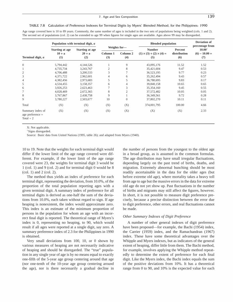
10 to 19. Note that the weights for each terminal digit woulddiffer if the lower limit of the age range covered were dif-ferent. For example, if the lower limit of the age rangecovered were 23, the weights for terminal digit 3 would be1 (col. 1) and 9 (col. 2) and for terminal digit 0 would be 8(col. 1) and 2 (col. 2).
The method thus yields an index of preference for eachterminal digit, representing the deviation, from 10.0%, of theproportion of the total population reporting ages with agiven terminal digit. A summary index of preference for allterminal digits is derived as one-half the sum of the devia-tions from 10.0%, each taken without regard to sign. If ageheaping is nonexistent, the index would approximate zero.This index is an estimate of the minimum proportion ofpersons in the population for whom an age with an incor-rect final digit is reported. The theoretical range of Myers’sindex is 0, representing no heaping, to 90, which wouldresult if all ages were reported at a single digit, say zero. Asummary preference index of 2.3 for the Philippines in 1990is obtained.
Very small deviations from 100, 10, or 0 shown byvarious measures of heaping are not necessarily indicativeof heaping and should be disregarded. The “true” popula-tion in any single year of age is by no means equal to exactlyone-fifth of the 5-year age group centering around that age(nor one-tenth of the 10-year age group centering around the age), nor is there necessarily a gradual decline in
the number of persons from the youngest to the oldest agein a broad group, as is assumed in the common formulas.The age distribution may have small irregular fluctuations,depending largely on the past trend of births, deaths, andmigration. Extremely abnormal bunching should be mostreadily ascertainable in the data for the older ages (butbefore extreme old age), where mortality takes a heavy tollfrom age to age but the massive errors in the data for extremeold age do not yet show up. Past fluctuations in the numberof births and migrants may still affect the figures, however.In short, it is not possible to measure digit preference pre-cisely, because a precise distinction between the error dueto digit preference, other errors, and real fluctuations cannotbe made.
Other Summary Indexes of Digit Preference
A number of other general indexes of digit preferencehave been proposed—for example, the Bachi (1954) index,the Carrier (1959) index, and the Ramachandran (1967)index. These have some theoretical advantages over theWhipple and Myers indexes, but as indicators of the generalextent of heaping, differ little from them. The Bachi method,for example, involves applying the Whipple method repeat-edly to determine the extent of preference for each finaldigit. Like the Myers index, the Bachi index equals the sumof the positive deviations from 10%. It has a theoreticalrange from 0 to 90, and 10% is the expected value for each
7. Age and Sex Composition 139
TABLE 7.8 Calculation of Preference Indexes for Terminal Digits by Myers’ Blended Method, for the Philippines: 1990
Age range covered here is 10 to 89 years. Commonly, the same number of ages is included in the two sets of populations being weighted (cols. 1 and 2).The second set of populations (col. 2) can be extended to age 99 when figures for single ages are available. Ages above 99 may be disregarded.
Deviation ofPopulation with terminal digit, a Blended populationpercentage from
Starting at age Starting at ageWeights for—
Number Percent 10.001
10 + a 20 + a Column 1 Column 2 (1) ¥ (3) + (2) ¥ (4) = distribution (6) - 10.00 =Terminal digit, a (1) (2) (3) (4) (5) (6) (7)
0 5,794,442 4,144,526 1 9 43,095,176 11.52 1.521 4,735,734 3,243,767 2 8 35,421,604 9.47 0.532 4,706,488 3,200,533 3 7 36,523,195 9.77 0.233 4,371,722 2,962,601 4 6 35,262,494 9.43 0.574 4,382,456 2,973,683 5 5 36,780,695 9.83 0.175 4,534,455 3,158,357 6 4 39,840,158 10.65 0.656 3,926,253 2,623,463 7 3 35,354,160 9.45 0.557 4,028,469 2,672,365 8 2 37,572,482 10.05 0.058 3,767,867 2,438,758 9 1 36,349,561 9.72 0.289 3,780,227 2,503,677 10 0 37,802,270 10.11 0.11
Total (X) (X) (X) (X) 374,001,795 100.00 4.66
Summary index of (X) (X) (X) (X) (X) (X) 2.33age preference =Total ∏ 2
X: Not applicable.1 Signs disregarded.Source: Basic data from United Nations (1995, table 26); and adapted from Myers (1940).

digit. The results obtained by the Bachi method resemblethose obtained by the Myers method. The U.S. CensusBureau (1994) has developed a spreadsheet program,SINGAGE, that calculates the Myers, Whipple, and Bachiindexes of digit preference.
Although not widely used, Siegel has proposed a methodof estimating digit preference that involves blending a seriesof estimates derived by osculatory interpolation. In hismethod, the average is taken of five different estimates of aparticular age that are obtained by rotating the five-year agegroups used in the interpolation. Siegel argues that it givesboth a measure of terminal digit preference and a measureof the preference for particular ages. (See U.S. Bureau of theCensus/Shryock, Siegel, and Associates, 1980, Vol. I., Table8.6, for an example).
Reduction of and Adjustment for Age and Digit Preference
In the preceding section, we were concerned primarilywith those measures that described an entire distribution oran important segment of it. We treat here those measures ofheaping and procedures for reducing or eliminating heapingthat are primarily applicable to individual ages. These meas-ures and procedures include modifying the census schedule,such as by varying the form of the question or questions usedto secure the data on age; and preparing alternative estimatesor carefully derived corrections for individual ages, such asby use of annual birth statistics or mathematical interpola-tion to subdivide the 5-year totals established by the censusand by calculation of refined age ratios for single ages. Insome situations, it is also desirable to consider handling theproblem by presenting only grouped data over part or all ofthe age distribution. In this case, the question of the optimumgrouping of ages for tabulation and publication arises.
Question on Date of Birth
At the enumeration stage, a question on date of birth maybe employed instead of a question on age, or both may beused in combination. When only a question on date of birthis used, the resulting pattern of age heaping is likely to be different, with preference for ages that correspond toyears of birth ending in 0 or 5. For example, such heapingoccurred in the 1970 and 1980 censuses of the United States,and both heaping on ages and on years of birth ending in 0and 5 were evident in the 1990 census of the United States.Although the heaping on a few ages may continue to be con-siderable, the evidence suggests that the use of a questionon date of birth, especially in combination with a questionon age, contributes to the accuracy of the age data obtained(Spencer, 1987). In many cases, an enumerator may not askboth questions, but derives the answer to one by calculationfrom the answer to the other; yet it is believed that havingboth questions on the schedule seems to make the enumer-
ator and the respondent more conscientious in the handlingof the questions on age. (The age question is also a usefulsource of an approximate answer when the respondent isunable or unwilling to estimate the date of birth.)
Calculation of Corrected Census Figures
Single-year-of-age data as reported may be “adjusted”following tabulation by developing alternative single-yearof-age figures directly. These alternative figures may replacethe census counts entirely or, as is more common, providea pattern by which the census totals for 5-year age groupsmay be redistributed by single years of age. There areseveral ways of developing the alternative estimates. Thesemay involve the relatively direct use of annual birth statis-tics, “surviving” annual births to the census date, use of lifetable populations, combining birth, death, and migration statistics to derive actual population estimates, and use ofvarious forms of mathematical interpolation.
The first procedure alluded to involves use of an annualseries of past births, in the cohorts corresponding to thecensus ages, for distributing the 5-year census totals. For thispurpose, annual birth statistics that have a fairly similardegree of completeness of registration over several years are required. The second procedure is quite similar, but the births employed are first reduced by deaths prior to thecensus date. A third procedure for replacing the tabulatedsingle-year-of-age figures involves use of the life table stationary population (Lx column) from an unabridged life table (i.e., one showing single ages). The specific stepsfor distributing the 5-year totals according to three specialsets of single-year-of-age estimates are illustrated for PuertoRico in Table 7.9.
The use of birth statistics or of the life table stationarypopulation to distribute 5-year census totals can easilyresult in discontinuity in the single ages at the junctions ofthe 5-year age groups, as may be seen by examining theage-to-age differences of the estimates in Table 7.9. Anumber of devices employing mathematical interpolation orgraduation can be used to subdivide the 5-year census totalsinto single years of age in such a way as to effect a smoothtransition from one age to another, while maintaining the5-year totals and removing erratic fluctuations in thenumbers (see last column in Table 7.9). In effect, thesedevices typically fit various mathematical curves to thetotals for several adjacent 5-year age groups in order toarrive at the constituent single ages for the central 5-yearage group in the set. The principal types of mathematicalcurves employed for this purpose are of the spline, oscula-tory, and polynomial form. In this method, various multi-pliers are ordinarily applied to the enumerated 5-year totalsto obtain the required figures directly. It is important to notethat each of the methods described also removes some truefluctuations implicit in the original single-year-of-agefigures—that is, fluctuations not due to errors in age
140 Hobbs
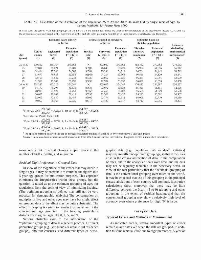
misreporting but to actual changes in past years in thenumber of births, deaths, and migration.
Residual Digit Preference in Grouped Data
In view of the magnitude of the errors that may occur insingle ages, it may be preferable to combine the figures into5-year age groups for publication purposes. This approacheliminates the irregularities within these groups, but thequestion is raised as to the optimum grouping of ages fortabulations from the point of view of minimizing heaping.(The optimum grouping so defined may still not be verypractical for demographic analysis.) The concentration onmultiples of five and other ages may have but slight effecton grouped data or the effect may be quite substantial. Theeffect of heaping is certain to remain to some extent in theconventional age grouping if the heaping particularly distorts the marginal ages like 0, 4, 5, and 9.
Serious obstacles exist to the introduction of the“optimum” grouping of data as a general practice. Differentpopulation groups (e.g., sex groups or urban-rural residencegroups), different censuses, and different types of demo-
graphic data (e.g., population data or death statistics) may require different optimum groupings, so that difficultiesarise in the cross-classification of data, in the computationof rates, and in the analysis of data over time; and the datamay not be regularly tabulated in the necessary detail. Inview of the fact particularly that the “decimal” grouping ofdata is the conventional grouping over much of the world,it may be expected that use of this grouping in the principalcensus tabulations of each country will continue. Illustrativecalculations show, moreover, that there may be little difference between the 0 to 4 (5 to 9) grouping and othergroupings in the extent of residual heaping and that the conventional grouping may show a relatively high level ofaccuracy even where preference for digit “0” is large.
Grouped Data
Types of Errors and Methods of Measurement
As indicated earlier, several important types of errorsremain in age data even when the data are grouped. In addi-tion to some residual error due to digit preference, 5-year or
7. Age and Sex Composition 141
TABLE 7.9 Calculation of the Distribution of the Population 25 to 29 and 30 to 34 Years Old by Single Years of Age, byVarious Methods, for Puerto Rico: 1990
In each case, the census totals for age groups 25–29 and 30–34 are maintained. These are taken as the numerators of the distribution factors F1, F2, and F3;the denominators are registered births, survivors of births, and life table stationary population in these groups, respectively. See footnotes.
Estimates based directly Estimates based on survivors Estimates based onon births of births life table population
EstimatesEstimated Estimated Life table Estimated derived by
Census Registered population Survival Survivors population stationary population mathematicalAge counts births F1
1 ¥ (2) = rate2 (2) ¥ (4) = F23 ¥ (5) = population2 F3
4 ¥ (7) = interpolation5
(years) (1) (2) (3) (4) (5) (6) (7) (8) (9)
25 to 29 270,562 385,367 270,562 (X) 372,099 270,562 482,762 270,562 270,56225 57,814 79,024 55,481 .96987 76,643 55,729 96,987 54,356 55,14226 54,404 77,746 54,585 .96784 75,246 54,713 96,784 54,242 54,72227 53,677 76,853 53,958 .96566 74,214 53,963 96,566 54,120 54,24128 52,758 75,842 53,248 .96335 73,062 53,125 96,335 53,991 53,59929 51,909 75,902 53,290 .96090 72,934 53,032 96,090 53,853 52,858
30 to 34 254,287 383,726 254,287 (X) 365,605 254,287 476,422 254,287 254,28730 54,170 75,204 49,836 .95835 72,072 50,128 95,835 51,151 52,19831 48,988 75,829 50,250 .95568 72,468 50,403 95,568 51,009 51,59832 50,067 76,083 50,419 .95293 72,502 50,427 95,293 50,862 50,93733 52,005 77,650 51,457 .95009 73,774 51,312 95,009 50,710 50,18034 49,057 78,960 52,325 .94717 74,789 52,017 94,717 50,555 49,374
1 F1 for 25–29 is ; F1 for 30–34 is .
2 Life table for Puerto Rico, 1990.
3 F2 for 25–29 is ; F2 for 30–34 is .
4 F3 for 25–29 is ; F3 for 30–34 is .
5 The specific method involved the use of Sprague osculatory multipliers applied to five consecutive 5-year age groups.Source: Basic data from official national sources and from U.S. Census Bureau, International Programs Center, unpublished tabulations.
254 287
476 42253374
,
,.=270 562
482 76256045
,
,.=
254 287
365 60569552
,
,.=270 562
372 09972712
,
,.=
254 287
383 72666268
,
,.=270 562
385 36770209
,
,.=
10-year data are affected by other types of age misreportingand by net underenumeration. Absolute net underenumera-tion would tend to cumulate as the age band widens. On theother hand, the percentage of net underenumeration wouldbe expected to vary fairly regularly over the age distribu-tion, fluctuating only moderately up and down. Absolute netage misreporting error and the percentage of net age misre-porting error should tend to take on positive and negativevalues alternately over the age scale, dropping to zero forthe total population of all ages combined. For the total pop-ulation, therefore, net census error and net underenumera-tion are identical. In general, as the age band widens, net agemisreporting tends to become less important and net under-enumeration tends to dominate as the type of error in agedata.
The particular form that these types of errors take variesfrom country to country and from census to census. We maycite some of the specific types of errors that have been iden-tified or described. Young children, particularly infants, andyoung adult males are omitted disproportionately in manycensuses. The liability for military service may be an impor-tant factor in connection with the understatement of youngadult males. It is possible that laws and practices relating to age for school attendance, child labor, voting, marriage,purchase of alcoholic beverages, and other such activitiesmay induce young people to overstate their age, so that they may share in the privileges accorded under the law topersons who have attained the higher age. Responses regard-ing age may also be affected by the social prestige accordedcertain members of a population, for example, the aged insome societies.
Ewbank (1981) identified several studies of age misre-porting patterns in developing countries, and separately dis-cussed such patterns for the age groups 0 to 14, 15 to 29,and 30 years and over. The ages of children tend to bereported more accurately than the ages of adults, althougheven children’s ages show decreasing accuracy with increas-ing age of the child. Enumerators may frequently distort the reporting of age for women 15 to 29, in particular, byestimating age on the basis of the physical maturity,union/marital status, or parity of the woman. For example,in some censuses and surveys, as in those of the countriesof tropical Africa, the number of females in their teens tendsto be understated and the number of females in the adult agegroups to be overstated. This bias has been attributed to atendency among interviewers systematically to “age” thosewomen who are already married or mothers on the assump-tion of a higher “typical” age of marriage than actually pre-vails (Brass et al., 1968, pp. 48–49). Among people aged 30years and over, the problems of heaping on digits ending in0 and 5 and age exaggeration are the most common types ofage misreporting problems.
It is quite difficult to measure the errors in grouped dataon age with any precision. It may be extremely difficult or
impossible, in fact, to determine the separate contribution ofeach of the types of errors affecting a given figure and toseparate the errors from real fluctuations (e.g., fluctuationsdue to migration) and, further, to identify the errors in rela-tion to their causes. Some of the measures of error for agegroups measure net age misreporting and net underenumer-ation separately, whereas others measure these types oferrors only in combination or measure only one of them.Some of the procedures provide only indexes of error forentire age distributions or only estimates of relative error forage groups (i.e., relative to the error in the same category inan earlier census or relative to another category in the samecensus), whereas other procedures provide estimates of theactual extent of error for age groups.
As in the case of measuring coverage of the total popu-lation, the methods for determining the existence of sucherrors and their approximate magnitude may be classifiedinto two broad types: first, case-by-case matching tech-niques employing data from reinterviews and independentlists or administrative records and, second, techniques ofdemographic analysis. The former techniques relate tostudies in which data collected in the census are matched ona case-by-case basis with data for a sample of personsobtained by reinterview or from independent records. Thelatter techniques involve (1) the development of estimatesof expected values for the population in age or other cate-gories, or for various population ratios, by use and manipu-lation of (a) data from the census itself or an earlier censusor censuses and (b) such data as birth, death, and migrationstatistics, and (2) the comparison of these expected valueswith the corresponding figures from the census. This methodmay also be extended to encompass comparison of aggre-gate administrative data with census counts.
Measurement by Reinterviews and Record Matching Studies
We consider first case-by-case checking techniques basedon reinterviews and matching against independent lists andadministrative records for the light they may throw on errorsin grouped data. Case-by-case matching studies permit theseparate measurement of the two components of net censuserror (or net census undercounts) in age data—net coverageerror (or net underenumeration) and net age misreporting.Furthermore, this type of study theoretically permits sepa-rating each of these components into its principal compo-nents—net coverage error into omissions and erroneousinclusions at each age, and net misreporting error into thevarious directional biases that affect each age group. Thus,the results of a reinterview study, or administrative recordsmay be cross-classified with the results of the original enumeration by 5-year, 10-year, or broader age groups, todetermine the number of persons who were omitted from,or erroneously included in, the census, for the same age
142 Hobbs
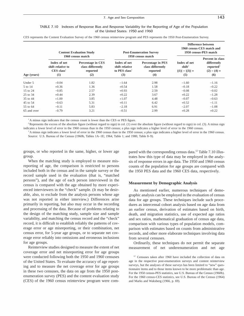
groups, or who reported in the same, higher, or lower agegroup.
When the matching study is employed to measure mis-reporting of age, the comparison is restricted to personsincluded both in the census and in the sample survey or therecord sample used in the evaluation (that is, “matchedpersons”), and the age of each person interviewed in thecensus is compared with the age obtained by more experi-enced interviewers in the “check” sample. (It may be desir-able, also, to exclude from the analysis persons whose agewas not reported in either interview.) Differences arise primarily in reporting, but also may occur in the recordingand processing of the data. Because of problems relating tothe design of the matching study, sample size and samplevariability, and matching the census record and the “check”record, it is difficult to establish reliably the patterns of cov-erage error or age misreporting, or their combination, netcensus error, for 5-year age groups, or to separate net cov-erage error reliably into omissions and erroneous inclusionsfor age groups.
Reinterview studies designed to measure the extent of netcoverage error and net misreporting error for age groupswere conducted following both the 1950 and 1960 censusesof the United States. To evaluate the accuracy of age report-ing and to measure the net coverage error for age groups in these two censuses, the data on age from the 1950 post-enumeration survey (PES) and the content evaluation study(CES) of the 1960 census reinterview program were com-
pared with the corresponding census data.12 Table 7.10 illus-trates how this type of data may be employed in the analy-sis of response errors in age data. The 1950 and 1960 censuscounts of the population for age groups are compared withthe 1950 PES data and the 1960 CES data, respectively.
Measurement by Demographic Analysis
As mentioned earlier, numerous techniques of demo-graphic analysis can be employed in the evaluation of censusdata for age groups. These techniques include such proce-dures as intercensal cohort analysis based on age data froman earlier census, derivation of estimates based on birth,death, and migration statistics, use of expected age ratiosand sex ratios, mathematical graduation of census age data,comparison with various types of population models, com-parison with estimates based on counts from administrativerecords, and other more elaborate techniques involving datafrom several censuses.
Ordinarily, these techniques do not permit the separatemeasurement of net underenumeration and net age
7. Age and Sex Composition 143
TABLE 7.10 Indexes of Response Bias and Response Variability for the Reporting of Age of the Population of the United States: 1950 and 1960
CES represents the Content Evaluation Survey of the 1960 census reinterview program and PES represents the 1950 Post-Enumeration Survey.
Difference between
Content Evaluation Study Post-Enumeration Survey1960 census-CES match and
1960 census match 1950 census match1950 census-PES match
Percent in classIndex of net Percentage in CES Index of net Percentage in PES Index of net differently
shift relative to class differently shift relative class differently shift2 reported3
CES class1 reported to PES class1 reported |(1)| - |(3)| = (2) - (4) =Age (years) (1) (2) (3) (4) (5) (6)
Under 5 -0.04 1.82 -1.64 2.98 -1.60 -1.165 to 14 +0.36 1.36 +0.54 1.58 -0.18 -0.2215 to 24 -0.85 2.57 +0.93 2.59 -0.08 -0.0225 to 34 +0.44 2.39 +0.22 3.67 +0.22 -1.2835 to 44 +1.00 3.85 +1.07 4.48 -0.07 -0.6345 to 54 -0.63 5.31 +0.11 6.42 +0.52 -1.1155 to 64 -0.11 5.83 -2.18 6.91 -2.07 -1.0865 and over -0.79 3.21 -0.51 2.99 +0.28 +0.22
1 A minus sign indicates that the census count is lower than the CES or PES figure.2 Represents the excess of the absolute figure (without regard to sign) in col. (1) over the absolute figure (without regard to sign) in col. (3). A minus sign
indicates a lower level of error in the 1960 census than in the 1950 census; a plus sign indicates a higher level of error in the 1960 census.3 A minus sign indicates a lower level of error in the 1960 census than in the 1950 census; a plus sign indicates a higher level of error in the 1960 census.Source: U.S. Bureau of the Census (1960b, Tables 1A–1E; 1964, Table 1; and 1980, Table 8–9).
12 Censuses taken after 1960 have included the collection of data onage in the respective post-enumeration surveys and content reinterviewsurveys, but the analyses of these surveys has been limited to “new” ques-tionnaire items and to those items known to be more problematic than age.For the 1950 census-PES statistics, see U.S. Bureau of the Census (1960b).For the 1960 census-CES statistics, see U.S. Bureau of the Census (1964)and Marks and Waksberg (1966, p. 69).

misreporting for any age group; these errors are measuredin combination as net census errors. Some of the techniquesmeasure net age misreporting primarily and net underenu-meration only secondarily or partly. Most of the techniquesof evaluating grouped age data do not provide absolute estimates of net census error by which census data can becorrected.
The methods of measuring net census error as such cangive some suggestive information regarding the nature andextent of net age misreporting, because, as we have previ-ously noted, net coverage error should tend to be in the samedirection from age to age and to vary rather regularly overthe age distribution. A division of net census error into thesetwo parts may also be possible by employing two or moremethods of evaluation in combination. An estimate of netcensus error is itself subject to error because the correspon-ding estimate of the corrected population contains errors.These result from, for example, net undercount of the censusfigure for an age cohort in a previous census, error in thereported or estimated number of births, underreporting andage misclassification in the death statistics, and omission,understatement, or overstatement of the allowance for netmigration.
The present discussion of the errors in grouped data onage by the methods of demographic analysis does not treatthe measurement and correction of errors separatelybecause, as we have noted, they are often two facets of thesame operation. We will, however, particularly note thosemethods that directly provide corrections of census figuresfor net undercounts. The latter methods will be illustratedprincipally by a review of recent U.S. studies of net under-counts using demographic analysis. First, however, we con-sider the basic methods under the headings of (1) intercensalcohort analysis, (2) comparisons with estimates based onbirth statistics, (3) age ratio analysis, (4) sex ratio analysis,(5) mathematical graduation of census data, and (6) com-parison with population models. We also consider briefly (7)comparison with aggregate administrative data.
Intercensal Cohort Analysis
In this procedure, the counts of one census are, in effect,employed to evaluate the counts at a later census. Ordinarily,the principal demographic factor at the national levelaccounting for the difference between the figures for thesame cohort at the two census dates is mortality. Migrationwill usually play a secondary, if not a minor, role, althougheven in this case the number of migrants may exceed thenumber of deaths at some of the younger ages. The figuresfrom both the earlier and later censuses are affected by netcensus undercounts. In addition, it is possible that the levelof migration and mortality may have been affected by suchspecial factors as movement of military forces into and outof a country, refugee movements, epidemic or famine, andwar deaths. The method of intercensal cohort analysis is
illustrated with data for the United States from 1980 to 1990.
Table 7.11 sets forth the steps by which estimates of theexpected population for age groups in April 1990 for theUnited States were derived. In this case, statistics on deaths,net civilian migration, and net movement of armed forcesby age are available and have been compiled in terms ofbirth cohorts for April 1980 through March 1990. Theexpected population in 1990, derived by combining the 1980census figures with the estimates of change for birth cohortsduring 1980 to 1990, is compared with the corresponding1990 census age counts.13 The results reflect the combinedeffect of underenumeration and age misreporting (i.e., neterrors) in the 1990 census, as well as the net errors in the1980 census and errors in the data on intercensal change,particularly age misreporting errors in death statistics andcoverage errors in the migration statistics. In more generalterms, the method measures relative net census error for abirth cohort at two successive censuses.
The 3% deficit at ages 25 to 29 in 1990 (col. 9) suggestsan underenumeration of persons of these ages in this censuson the principal assumption that children aged 15 to 19 wererather well enumerated in 1980 (col. 1). The error of closure(col. 9) for the population aged 10 to 14 in 1990—1.4% ofthe population expected in 1990—suggests an underenu-meration of the population aged 0 to 4 in 1980, perhaps com-bined with a coverage error in the migration statistics.
The method of intercensal cohort analysis may be appliedin another way to evaluate the consistency of the data on agein two successive censuses when net immigration or emi-gration is negligible and death statistics are lacking or defec-tive. Table 7.12 illustrates this method for South Korea forthe 1985 and 1995 censuses. For South Korea, adequatedeath statistics or a life table to measure mortality betweenthe censuses is not available; net migration is assumed to benegligible. First, the proportion surviving at each agebetween 1985 and 1995 (cols. 5 and 6) is calculated bydividing the 1995 population at a given age (terminal age)by the 1985 population 10 years younger (initial age). Forexample,
Second, the reasonableness of these proportions in them-selves or in comparison with an actual set or a model set oflife table survival rates is examined as a basis for judgingthe adequacy of the census data.
In the absence of net migration, proportions surviving in excess of 1.00 are unacceptable and suggest either netunderstatement in the 1985 census or net overstatement
P
Pm
m
20 241995
10 141985
2 238 0002 311 000
96857-
-= =
, ,, ,
.
144 Hobbs
13 For details on the estimation of the population for age groups usingbirth cohorts, see U.S. Census Bureau (1993b).
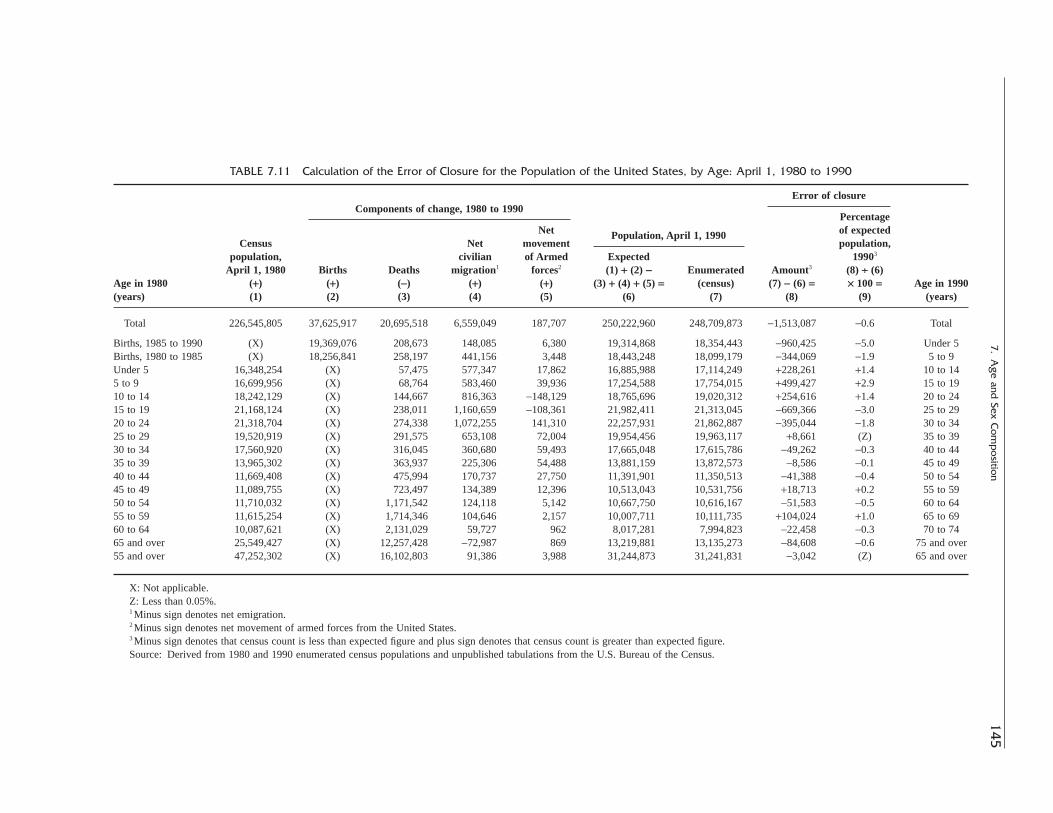
7.A
ge and
Sex Com
position
145
TABLE 7.11 Calculation of the Error of Closure for the Population of the United States, by Age: April 1, 1980 to 1990
Error of closureComponents of change, 1980 to 1990
PercentageNet Population, April 1, 1990 of expected
Census Net movement population,population, civilian of Armed Expected 19903
April 1, 1980 Births Deaths migration1 forces2 (1) + (2) - Enumerated Amount3 (8) ∏ (6)Age in 1980 (+) (+) (-) (+) (+) (3) + (4) + (5) = (census) (7) - (6) = ¥ 100 = Age in 1990(years) (1) (2) (3) (4) (5) (6) (7) (8) (9) (years)
Total 226,545,805 37,625,917 20,695,518 6,559,049 187,707 250,222,960 248,709,873 -1,513,087 -0.6 Total
Births, 1985 to 1990 (X) 19,369,076 208,673 148,085 6,380 19,314,868 18,354,443 -960,425 -5.0 Under 5Births, 1980 to 1985 (X) 18,256,841 258,197 441,156 3,448 18,443,248 18,099,179 -344,069 -1.9 5 to 9Under 5 16,348,254 (X) 57,475 577,347 17,862 16,885,988 17,114,249 +228,261 +1.4 10 to 145 to 9 16,699,956 (X) 68,764 583,460 39,936 17,254,588 17,754,015 +499,427 +2.9 15 to 1910 to 14 18,242,129 (X) 144,667 816,363 -148,129 18,765,696 19,020,312 +254,616 +1.4 20 to 2415 to 19 21,168,124 (X) 238,011 1,160,659 -108,361 21,982,411 21,313,045 -669,366 -3.0 25 to 2920 to 24 21,318,704 (X) 274,338 1,072,255 141,310 22,257,931 21,862,887 -395,044 -1.8 30 to 3425 to 29 19,520,919 (X) 291,575 653,108 72,004 19,954,456 19,963,117 +8,661 (Z) 35 to 3930 to 34 17,560,920 (X) 316,045 360,680 59,493 17,665,048 17,615,786 -49,262 -0.3 40 to 4435 to 39 13,965,302 (X) 363,937 225,306 54,488 13,881,159 13,872,573 -8,586 -0.1 45 to 4940 to 44 11,669,408 (X) 475,994 170,737 27,750 11,391,901 11,350,513 -41,388 -0.4 50 to 5445 to 49 11,089,755 (X) 723,497 134,389 12,396 10,513,043 10,531,756 +18,713 +0.2 55 to 5950 to 54 11,710,032 (X) 1,171,542 124,118 5,142 10,667,750 10,616,167 -51,583 -0.5 60 to 6455 to 59 11,615,254 (X) 1,714,346 104,646 2,157 10,007,711 10,111,735 +104,024 +1.0 65 to 6960 to 64 10,087,621 (X) 2,131,029 59,727 962 8,017,281 7,994,823 -22,458 -0.3 70 to 7465 and over 25,549,427 (X) 12,257,428 -72,987 869 13,219,881 13,135,273 -84,608 -0.6 75 and over55 and over 47,252,302 (X) 16,102,803 91,386 3,988 31,244,873 31,241,831 -3,042 (Z) 65 and over
X: Not applicable.Z: Less than 0.05%.1 Minus sign denotes net emigration.2 Minus sign denotes net movement of armed forces from the United States.3 Minus sign denotes that census count is less than expected figure and plus sign denotes that census count is greater than expected figure.Source: Derived from 1980 and 1990 enumerated census populations and unpublished tabulations from the U.S. Bureau of the Census.
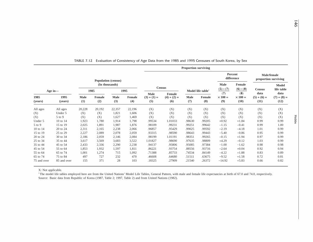
146H
obbs
TABLE 7.12 Evaluation of Consistency of Age Data from the 1985 and 1995 Censuses of South Korea, by Sex
Proportion surviving
Male/femalePercent
proportion survivingPopulation (census)difference
Model(In thousands)Census
Male Female
Census life tableAge in— 1985 1995Male Female
Model life table1
data data1985 1995 Male Female Male Female (3) ∏ (1) = (4) ∏ (2) = Male Female ¥ 100 = ¥ 100 = (5) ∏ (6) = (7) ∏ (8) =(years) (years) (1) (2) (3) (4) (5) (6) (7) (8) (9) (10) (11) (12)
All ages All ages 20,228 20,192 22,357 22,196 (X) (X) (X) (X) (X) (X) (X) (X)(X) Under 5 (X) (X) 1,821 1,606 (X) (X) (X) (X) (X) (X) (X) (X)(X) 5 to 9 (X) (X) 1,627 1,469 (X) (X) (X) (X) (X) (X) (X) (X)Under 5 10 to 14 1,923 1,780 1,914 1,798 .99534 1.01033 .98630 .99205 +0.92 +1.84 0.99 0.995 to 9 15 to 19 2,025 1,891 1,987 1,876 .98109 .99231 .99251 .99642 -1.15 -0.41 0.99 1.0010 to 14 20 to 24 2,311 2,165 2,238 2,066 .96857 .95429 .99025 .99592 -2.19 -4.18 1.01 0.9915 to 19 25 to 29 2,227 2,089 2,078 2,059 .93315 .98590 .98643 .99443 -5.40 -0.86 0.95 0.9920 to 24 30 to 34 2,186 2,059 2,146 2,084 .98199 1.01191 .98351 .99265 -0.15 +1.94 0.97 0.9925 to 34 35 to 44 3,617 3,569 3,683 3,522 1.01827 .98690 .97635 .98809 +4.29 -0.12 1.03 0.9935 to 44 45 to 54 2,433 2,336 2,290 2,238 .94137 .95806 .95085 .97384 -1.00 -1.62 0.98 0.9845 to 54 55 to 64 1,853 1,932 1,597 1,811 .86221 .93754 .88556 .93716 -2.64 +0.04 0.92 0.9455 to 64 65 to 74 1,001 1,274 715 1,092 .71388 .85733 .74534 .84149 -4.22 +1.88 0.83 0.8965 to 74 75 to 84 497 727 232 470 .46608 .64680 .51511 .63675 -9.52 +1.58 0.72 0.8175 and over 85 and over 155 371 28 103 .18325 .27909 .21540 .26372 -14.92 +5.83 0.66 0.82
X: Not applicable.1 The model life tables employed here are from the United Nations’ Model Life Tables, General Pattern, with male and female life expectancies at birth of 67.0 and 74.0, respectively.Source: Basic data from Republic of Korea (1987, Table 2; 1997, Table 2) and from United Nations (1982).
6 88
( ) ( )( )-5 7
7( ) ( )
( )-

(presumably due to age misreporting) in the 1995 census.This irregularity applies to the proportions for males withterminal ages 35 to 44 years, and to the proportions forfemales with terminal ages 10 to 14 and 30 to 34 years. Themale-female ratios of the proportion surviving for SouthKorea are generally reasonable. Very different proportionssurviving for males and females or higher proportions sur-viving for males than females except at the childbearingages, as is shown for terminal ages 20 to 24 and 35 to 44 inTable 7.12, are slightly suspect.
Comparison with Estimates Based on Birth Statistics
Estimates of net undercounts of children may be derivedby comparison of the census counts and estimates of children based on birth statistics, death statistics or life tablesurvival rates, and migration statistics. If possible, the birthand death statistics, particularly the former, should beadjusted to include an allowance for underregistration. Themethod was illustrated with U.S. data in Table 7.11. Birthstatistics for April 1, 1980, to April 1, 1985, and April 1,1985, to April 1, 1990, are combined with death and immi-gration statistics for the same cohorts to derive estimates of the expected population under 5 and 5 to 9 years old in 1990. The difference between the expected populationand the census count is then taken as the estimate of netundercount.
For the age group 0–4 in 1990,
(7.14)
(7.15)
where Pc represents the census count, Pe the expected pop-ulation, and E the estimated net undercount. The correspon-ding figures are
The census count of children under 5 years old,18,354,443, falls below the expected population,19,314,868, by about 960,000, or 5.0% of the expectedfigure. This difference is taken as the estimate of the netundercount of children under 5 in the census.
A special problem of calculation and interpretation of thedifference between the expected population and the censuscount of children exists when the birth statistics or the deathstatistics are incomplete. In the absence of immigration, thecomparison provides a minimum estimate of the net under-count of children when the expected population exceeds thecensus count (and a minimum estimate of the underregis-tration of births when the census figure exceeds the estimatebased on births). It may be desirable or even preferable inthis case to employ life table survival rates in lieu of deathstatistics because of the inadequacies of the reported deathstatistics or the convenience of using a life table.
19 369 076 208 673 154 465 19 314 868
18 354 443 19 314 868 960 425
, , , , , ,
, , , , ,
- + =- = -
P P Ec e0 4
19900 41990
0 41990
- - -- =
B D M Pe1985 1990 1985 1990 1985 19900 41990- - --- + =
The procedure is illustrated in Table 7.13, which com-pares the expected population under 10 years of age (singleyears under 5 and the age group 5 to 9) for males andfemales with the corresponding counts from the census ofPanama taken on May 13, 1990. Registered births (col. 1),tabulated by calendar year of occurrence, were first redis-tributed to conform to “census” years (i.e., May to May)on the assumption that the distribution is rectangular (i.e.,even) within each calendar year. Survival rates, represent-ing the probability of survival from birth to the age at thecensus date, were then calculated from an abridged lifetable for Panama for 1990. The expected populationexcluding the effect of immigration (col. 4) was thenderived as the product of the births in column 2 and thesurvival rates in column 3. The 4% deficit of the censuscount for children under 1 and the 1% deficit for children1 to 4 years old in comparison with the correspondingexpected populations may be taken as minimum estimatesof the net undercounts of these groups. The method sug-gests a net census overcount of children 5 to 9 years old(about 5%). However, the survival rates from the 1990 lifetable may be too high, and, hence, the estimate of survivorsmay be too high. Even allowing for this possibility and thepossibility of net emigration, the actual net undercountsmay be greater than those shown for the ages under 3 tothe extent that births are underregistered.
Age Ratio Analysis
The quality of the census returns for age groups may alsobe evaluated by comparing age ratios, calculated from thecensus data, with expected or standard values. An age ratiomay be defined as the ratio of the population in the givenage group to one-third of the sum of the populations in theage group itself and the preceding and following groups,times 100.14 The age ratio for a 5-year age group, 5Pa isdefined then as follows:
(7.16)
Barring extreme fluctuations in past births, deaths, ormigration, the three age groups should form a nearly linearseries. Age ratios should then approximate 100, even thoughactual historical variations in these factors would producedeviations from 100 in the age ratio for most ages. Inasmuchas, over a period of nearly a century, most countries haveexperienced not only minor fluctuations in populationchanges but also major upheavals, age ratios for some agesmay deviate substantially from 100 even where reporting of
5
13 5 5 5 5 5
100P
P P Pa
a a a- ++ +( )¥
7. Age and Sex Composition 147
14 Alternatively, age ratios have been defined as the ratio of the popu-lation in an age group to one-half the sum of the population in the preced-ing and subsequent groups, times 100. The definition given above ispreferred.
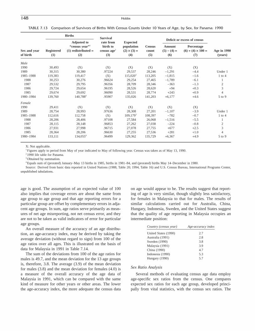
age is good. The assumption of an expected value of 100also implies that coverage errors are about the same fromage group to age group and that age reporting errors for aparticular group are offset by complementary errors in adja-cent age groups. In sum, age ratios serve primarily as meas-ures of net age misreporting, not net census error, and theyare not to be taken as valid indicators of error for particularage groups.
An overall measure of the accuracy of an age distribu-tion, an age-accuracy index, may be derived by taking theaverage deviation (without regard to sign) from 100 of theage ratios over all ages. This is illustrated on the basis ofdata for Malaysia in 1991 in Table 7.14.
The sum of the deviations from 100 of the age ratios formales is 49.7, and the mean deviation for the 13 age groupsis, therefore, 3.8. The average (3.9) of the mean deviationfor males (3.8) and the mean deviation for females (4.0) isa measure of the overall accuracy of the age data ofMalaysia in 1991, which can be compared with the samekind of measure for other years or other areas. The lowerthe age-accuracy index, the more adequate the census data
on age would appear to be. The results suggest that report-ing of age is very similar, though slightly less satisfactory,for females in Malaysia to that for males. The results ofsimilar calculations carried out for Australia, China,Hungary, Indonesia, Sweden, and the United States suggestthat the quality of age reporting in Malaysia occupies anintermediate position:
Country (census year) Age-accuracy index
United States (1990) 2.7Australia (1991) 2.8Sweden (1990) 3.8Malaysia (1991) 3.9China (1990) 4.7Indonesia (1990) 5.3Hungary (1990) 5.7
Sex Ratio Analysis
Several methods of evaluating census age data employage-specific sex ratios from the census. One comparesexpected sex ratios for each age group, developed princi-pally from vital statistics, with the census sex ratios. The
148 Hobbs
TABLE 7.13 Comparison of Survivors of Births With Census Counts Under 10 Years of Age, by Sex, for Panama: 1990
BirthsSurvival
Adjusted to rate from ExpectedDeficit or excess of census
“census year”1 birth to population Census Amount PercentageSex and year Registered (1) redistributed = census age2 (2) ¥ (3) = count (5) - (4) = (6) ∏ (4) ¥ 100 = Age in 1990of birth (1) (2) (3) (4) (5) (6) (7) (years)
Male1990 30,493 (X) (X) (X) (X) (X) (X)1989 30,315 30,380 .97224 29,537 28,246 -1,291 -4.4 Under 11985–1988 119,383 119,417 (X) 115,0203 113,205 -1,815 -1.6 1 to 4
1988 30,253 30,276 .96624 29,254 27,465 -1,789 -6.1 11987 29,532 29,795 .96356 28,709 28,346 -363 -1.3 21986 29,724 29,654 .96195 28,526 28,620 +94 +0.3 31985 29,674 29,692 .96090 28,531 28,774 +243 +0.9 4
1980–1984 139,760 140,7884 .95907 135,026 141,203 +6,177 +4.6 5 to 9
Female1990 29,411 (X) (X) (X) (X) (X) (X)1989 28,754 28,993 .97636 28,308 27,201 -1,107 -3.9 Under 11985–1988 112,616 112,758 (X) 109,1793 108,397 -782 -0.7 1 to 4
1988 28,206 28,406 .97108 27,584 26,068 -1,516 -5.5 11987 28,115 28,148 .96853 27,262 27,038 -224 -0.8 21986 27,931 27,998 .96715 27,078 27,755 +677 +2.5 31985 28,364 28,206 .96630 27,255 27,536 +281 +1.0 4
1980–1984 133,111 134,0554 .96499 129,362 135,729 +6,367 +4.9 5 to 9
X: Not applicable.1 Figures apply to period from May of year indicated to May of following year. Census was taken as of May 13, 1990.2 1990 life table for Panama.3 Obtained by summation.4 Equals sum of (prorated) January–May 13 births in 1985, births in 1981–84, and (prorated) births May 14–December in 1980.Source: Derived from basic data reported in United Nations (1988, Table 20; 1994, Table 16) and U.S. Census Bureau, International Programs Center,
unpublished tabulations.

expected figures may be carefully developed estimates ofthe actual sex ratios at each age or theoretical figures based on a population model. Another judges the censusage-specific sex ratios in terms of their age-to-age differences.
The first method involves developing estimates of theactual sex ratios at each age at a census date on the basis ofthe sex ratios of each of the components of change, partic-ularly the sex ratio of births and the sex ratios of survivalrates (i.e., the ratio of the male survival rate at a given ageto the corresponding female rate, derived from life tables).15
The basic calculations may be illustrated by the procedurefor deriving the expected sex ratios at ages 0 to 4 and 5 to9 at the census date. If the contribution of net migration isdisregarded, the expected sex ratio at ages 0 to 4 equals theproduct of the sex ratio of births in the 5 years preceding the
census date and the ratio of (a) the male survival rate from
birth to ages 0 to 4 to (b) the corresponding female
survival rate :16
(7.17)
where y designates a given year and y - 5 to y refers to the preceding 5 years. The expected sex ratio for the age
B
B
R
R
P
P
m
fy y
m
b y y
f
b y y
m
fy
ÊË
ˆ¯ ¥
( )( ) = Ê
ˈ¯
¢-
-
--
-
-
-5
0 4
50 4
5
0 4
0 4to
to
to
R f
b
0 4-( )Rm
b
0 4-( )
7. Age and Sex Composition 149
TABLE 7.14 Calculation of Age-Accuracy Index, for Malaysia: 1991
Analysis of age ratio
Male Female
Deviation DeviationPopulationfrom 100 from 100
Age Male Female Ratio1 (3) - 100 = Ratio1 (5) - 100 =(years) (1) (2) (3) (4) (5) (6)
Under 5 1,150,221 1,084,179 (X) (X) (X) (X)5 to 9 1,152,353 1,091,915 104.6 +4.6 104.5 +4.510 to 14 1,001,605 958,663 99.2 -0.8 98.5 -1.515 to 19 875,587 868,013 98.7 -1.3 99.6 -0.420 to 24 782,941 787,241 96.8 -3.2 97.4 -2.625 to 29 767,471 768,927 102.1 +2.1 102.5 +2.530 to 34 704,377 695,016 102.3 +2.3 102.1 +2.135 to 39 592,796 578,116 100.0 — 100.2 +0.240 to 44 480,353 458,341 101.4 +1.4 101.1 +1.145 to 49 348,407 323,888 91.9 -8.1 89.7 -10.350 to 54 309,147 300,766 105.2 +5.2 105.9 +5.955 to 59 223,745 227,042 93.9 -6.1 94.5 -5.560 to 64 181,569 193,340 104.4 +4.4 105.9 +5.965 to 69 116,527 127,572 89.9 -10.1 90.2 -9.870 to 74 90,846 103,230 (X) (X) (X) (X)
Total (irrespective (X) (X) (X) 49.7 (X) 52.1of sign)
Mean (X) (X) (X) 3.8 (X) 4.0
—: Represents zero.X: Not applicable.
1 The age ratio is defined as ¥ 100.
Source: Derived from enumerated census population as reported in U.S. Census Bureau (2000a, Table 4), www.census.gov/ipc/www/idbacc.html.
5
5 5 5 5 51 3
P
P P Pa
a a a- ++ +( )
15 Full development of the estimates of expected sex ratios of this typerequires a knowledge of the use of life tables and of techniques of popula-tion estimation. Both of these topics are treated in later chapters.
16 The expressions in parentheses are calculated as units or are treatedas single numbers in the calculations. For example, the sex ratio of birthsfor a given period, whether calculated on the basis of reported births orassumed on the basis of the sex ratio of births for a later period, is treatedas a single number in the “survival” calculations; and the sex ratio of thepopulation is derived as a direct result, without intermediate figures for theabsolute numbers of males and females.
group 5 to 9 would be derived theoretically as the jointproduct of the sex ratio of births 5 to 10 years earlier, thesex ratio of survival rates from birth to ages 0 to 4, 5 to 10years earlier, and the sex ratio of survival rates from ages 0 to 4 to ages 5 to 9 in the previous 5 years:
(7.18)
“Expected” sex ratios calculated in this way can then becompared to those calculated directly from the census data.An illustration of this procedure is presented in U.S. Bureauof the Census/Shryock, Siegel, and Associates, Vol. 1, Table8.14 (1980).
The results of the method are directly applicable forjudging the relative magnitude of the net census error of the counts of males and females; they do not indicate theabsolute level of net census error for either sex. If the resultsof this method are to be used to derive absolute estimates ofcorrected population for either sex or both sexes combined,an acceptable, independently determined set of estimates ofnet undercounts or corrected census figures by age for eithermales or females is required. For example, if correctedcensus figures for females are available, the expected sexratios would be applied to them to derive corrected figuresfor males. Because of the greater likelihood of deficienciesin the basic data and the greater dependence on the variousassumptions made as one goes back in time, the estimatesof expected sex ratios are subject to greater and greater erroras one goes up the age scale.
When the detailed data required to develop a set of esti-mated actual sex ratios (e.g., historical series of life tables,historical data on births of boys and girls, net immigrationor nativity of the population disaggregated by age and sex,war deaths) are not available or it is not practical to developthem, the expected pattern of sex ratios for age groups maybe approximated by employing a single current life table tomeasure survival from birth to each age, in conjunction withthe current reported or estimated sex ratio at birth. Thismethod, in effect, assumes that there has been no net migra-tion, either civilian or military, or excess mortality due towar or widespread epidemic. In addition, it assumes that thesex ratio of births and the differences in mortality betweenthe sexes at each age have remained unchanged. To theextent that these conditions prevail, the approximation to theactual sex ratios will be closer.
Expected sex ratios at the early childhood ages are notfar below the sex ratio at birth. Then, commonly, they fallgradually throughout life, not dipping below 100 until age40 or later. The decline is gentle at first but becomes steeperat the older ages. The general pattern described results from
B
B
R
R
R
R
P
P
m
fy y
m
b y y
f
b y y
m
y y
f
y y
m
fy
ÊË
ˆ¯ ¥
( )( ) ¥
( )( ) = Ê
ˈ¯
¢
- -
-
- --
- -
-
-
-
-
-
-
-
-10 5
0 4
10 50 4
10 5
0 4
5 9
5
0 4
5 9
5
5 9
5 9to
to
to
to
to
the usual small excess of boys among births and the usualexcess of male over female mortality.17
The regularity of the change in the expected sex ratiofrom age to age that we have just noted provides a basis forelaborating the age-accuracy index based solely on ageratios described earlier to incorporate some measure of theaccuracy of sex ratios. The United Nations (1952, 1955) hasproposed such an age-sex accuracy index. In this index, themean of the differences from age to age in reported sexratios, without regard to sign, is taken as a measure of theaccuracy of the observed sex ratios, on the assumption thatthese age-to-age changes should approximate zero. The UNage-sex accuracy index combines the sum of (1) the meandeviation of the age ratios for males from 100 (2) the meandeviation of the age ratios for females from 100, and (3)three times the mean of the age-to-age differences inreported sex ratios. In the UN procedure, an age ratio isdefined as the ratio of the population in a given age groupto one-half the sum of the populations in the preceding andfollowing groups. The calculation of the UN age-sex accu-racy index is illustrated in Table 7.15 for Turkey in 1990.The mean deviations of the age ratios for males and femalesare 5.5 and 5.5, respectively, and the mean age-to-age dif-ference in the sex ratios is 4.0. Applying the UN formula,we have: 5.5 + 5.5 + 3(4.0) = 23.0. Comparable indexes forTurkey and a few other countries are as follows:
Country (census year) U.N. age-sex accuracy index
Argentina (1991) 12.7United States (1990) 14.7Vietnam (1989) 22.9Turkey (1990) 23.0Hungary (1990) 26.0Indonesia (1990) 31.0India (1991) 39.6Tanzania (1988) 47.7
The U.S. Census Bureau (1994) has developed a spread-sheet program, AGESEX, that calculates the United Nationsage-sex accuracy index given the population in 5-year agegroups, for males and females, as input data. Census age-sex data are described by the United Nations as “accurate,”“inaccurate,” or “highly inaccurate” depending on whetherthe UN index is under 20, 20 to 40, or over 40.
The UN index has a number of questionable features as a summary measure for comparing the accuracy of theage-sex data of various countries. Among these are thefailure to take account of the expected decline in the sexratio with increasing age and of real irregularities in agedistribution due to migration, war, and epidemic as well as
150 Hobbs
17 The variations in the theoretical pattern of expected sex ratios by ageresulting solely from variations in the level of mortality, holding the sexratio at birth constant and excluding the effect of civilian migration andmilitary movements, may be shown by employing model life tables thathave very different levels of mortality, such as those given in Coale andDemeny (1983) and United Nations (1982).

normal fluctuations in births and deaths; the use of a definition of an age ratio that omits the central age groupand which, therefore, does not give it sufficient weight; andthe considerable weight given to the sex-ratio componentin the formula. In addition, the index is primarily a measureof net age misreporting and, for the most part, does not measure net underenumeration for age groups. Anallowance for the typical decline in the sex ratio fromchildhood to old age can be made by adjusting the meandifference of the census sex ratios downward by the meandifference between the expected sex ratio for ages under 5and, say, 70 to 74, derived from life tables. In spite of itslimitations, however, the UN index can be a useful measurefor making approximate distinctions between countrieswith respect to the accuracy of reporting age and sex incensuses.
Mathematical Graduation of Census Data
Mathematical graduation of census data can beemployed to derive figures for 5-year age groups that are
corrected primarily for net reporting error. What these graduation procedures do, essentially, is to “fit” differentcurves to the original 5- or 10-year totals, modifying theoriginal 5-year totals. Among the major graduation methodsare the Carrier-Farrag (1959) ratio method, Karup-King-Newton quadratic interpolation, cubic spline interpolation,Sprague or Beers osculatory methods, and methods devel-oped by the United Nations. The U.S. Census Bureau (1994)has developed a spreadsheet program, AGESMTH, thatsmooths the 5-year totals of a population using most of thesemethods.
Other mathematical graduation methods have beendeveloped that require more data than a distribution of thepopulation in 5-year age groups at a single census. Demenyand Shorter (1968) developed a procedure requiring the population in 5-year age groups from two censuses enu-merated 5 years apart (or a multiple thereof) and a set ofintercensal survivorship probabilities, and the UnitedNations (1983) developed a procedure of fitting a polyno-mial based on a single-year-of-age distribution.
7. Age and Sex Composition 151
TABLE 7.15 Calculation of the United Nations Age-Sex Accuracy Index, for Turkey: 1990
Analysis of age ratios
Analysis of sex ratios Male Female
Successive Deviation DeviationPopulationRatio differences from 100 from 100
Age Male Female [(1) ∏ (2)] ¥ 100 = Œ(3) = Ratio1 (5) - 100 = Ratio1 (7) - 100 =(years) (1) (2) (3) (4) (5) (6) (7) (8)
Under 5 3,052,255 2,902,489 105.16 (X) (X) (X) (X) (X)5 to 9 3,541,409 3,357,800 105.47 -0.31 107.10 +7.10 107.74 +7.7410 to 14 3,560,900 3,330,499 106.92 -1.45 106.19 +6.19 103.93 +3.9315 to 19 3,165,061 3,051,408 103.72 +3.19 103.06 +3.06 104.41 +4.4120 to 24 2,581,153 2,514,351 102.66 +1.07 92.17 -7.83 92.63 -7.3725 to 29 2,435,765 2,377,362 102.46 +0.20 104.14 +4.14 105.57 +5.5730 to 34 2,096,899 1,989,410 105.40 -2.95 99.38 -0.62 97.44 -2.5635 to 39 1,784,121 1,705,943 104.58 +0.82 101.49 +1.49 101.57 +1.5740 to 44 1,418,784 1,369,640 103.59 +0.99 98.01 -1.99 97.97 -2.0345 to 49 1,111,113 1,090,046 101.93 +1.66 92.64 -7.36 90.52 -9.4850 to 54 980,115 1,038,853 94.35 +7.59 93.14 -6.86 101.99 +1.9955 to 59 993,402 947,119 104.89 -10.54 113.62 +13.62 100.46 +.04660 to 64 768,547 846,746 90.76 +14.12 104.93 +4.93 115.30 +15.3065 to 69 471,479 521,608 90.39 +0.38 93.26 -6.74 90.69 -9.3170 to 74 242,572 303,519 79.92 +10.47 (X) (X) (X) (X)
Total (irrespective (X) (X) (X) 55.73 (X) 71.94 (X) 71.73of sign)
Mean (X) (X) (X) 3.98 (X) 5.53 (X) 5.52
Index = 3 times mean difference in sex ratios plus mean deviations of male and female age ratios.= 3 ¥ 3.98 + 5.53 + 5.52 = 22.99
X: Not applicable.
1 The age ratio is defined here as ¥ 100.
Source: Derived from enumerated census population as reported in U.S. Census Bureau (2000a, Table 4), www.census.gov/ipc/www/idbacc.html.
5
5 5 5 51 2
P
P Pa
a a- ++( )

Comparison with Population Models
Still another basis of evaluating the census data on age isto compare the actual percentage distribution of the popula-tion by age with an expected age distribution correspondingto various population models. One such model is the stablepopulation model. In the absence of migration, if fertilityand mortality remain constant over several decades; the age distribution of a population would assume a definiteunchanging form called stable. Such model age distributionsare pertinent in the consideration of actual age distributionsbecause nearly constant fertility and nearly constant or mod-erately declining mortality are characteristic of some lessdeveloped countries. The declines in mortality that haveoccurred in many populations affect the age distribution toonly a small extent. Such countries have a relatively stabledistribution (with constant mortality) or a quasi-stable agedistribution (with moderately declining mortality). The agedistributions of such countries may be represented ratherwell by the stable age distributions that would result fromthe persistence of their current fertility and mortality rates.The stable age distribution may then be used as a standardfor judging the adequacy of reported age distributions(Coale, 1963; van de Walle, 1966).
With the limitations implied, the inadequacies of the agedistribution in particular countries may be measured bycomparing the percentage age distributions in these coun-tries with the age distributions of the corresponding stable
populations. Specifically, for each age group an index maybe calculated by dividing the percentage in the age group ina given country by the corresponding percentage in thestable population. The choice of a stable age distribution tocompare with the enumerated population is discussed inChapter 22. The deviations of the indexes from 1.00 reflectthe extent to which a particular age group is relatively over-stated or understated as a result of net coverage error or agemisreporting. For example, the indexes shown in Table 7.16for Thailand in 1970 indicate a relatively high proportion of the male and female populations 5 to 14 years old andrelatively low proportions in the age range 20 to 29 years(U.S. Census Bureau, 1985).
Comparison with Aggregate Administrative Data
Finally, we note the use of various types of aggregate data,compiled primarily for administrative purposes, to evaluatecensus data in particular age groups. This procedure assumesthat the administrative records are free of the types of errorsof coverage and age reporting that characterize householdinquiries. It is assumed, for example, that a registration fromwhich the aggregate data are derived is complete and accu-rate (without omissions, duplications, or inactive records,i.e., records for persons who died or are no longer eligible orobligated to remain in the file) and contains accurate ageinformation, possibly involving formal proof of age. In thesecomparisons, no attempt is made at matching records for
152 Hobbs
TABLE 7.16 Comparison of the Enumerated Population of Thailand with a Stable Age Distribution, by Sex: 1970
Males Females
Enumerated Stable Enumerated StableAge population population1 Ratio population population1 Ratio(years) (1) (2) (3) = (1) ∏ (2) (4) (5) (6) = (4) ∏ (5)
All ages 100.0 100.0 — 100.0 100.0 —
0 to 4 16.7 17.3 0.97 16.2 17.0 0.955 to 9 15.7 14.4 1.09 15.1 14.2 1.0610 to 14 13.5 12.3 1.10 13.1 12.1 1.0815 to 19 10.7 10.5 1.02 10.9 10.3 1.0620 to 24 7.7 8.8 0.88 7.9 8.8 0.90
25 to 29 6.4 7.5 0.85 6.6 7.4 0.8930 to 34 6.1 6.3 0.97 6.2 6.2 1.0035 to 39 5.6 5.3 1.06 5.6 5.3 1.0640 to 44 4.5 4.4 1.02 4.4 4.4 1.0045 to 49 3.5 3.6 0.97 3.5 3.7 0.95
50 to 54 2.8 2.9 0.97 2.8 3.0 0.9355 to 59 2.3 2.3 1.00 2.3 2.4 0.9660 to 64 1.8 1.7 1.06 1.9 1.9 1.0065 to 69 1.3 1.2 1.08 1.4 1.4 1.0070 or older 1.5 1.5 1.00 2.0 1.9 1.05
1 Stable age distribution with “West” mortality, level 17, and r = .03.Note: See Chapter 22 for details on methods of selecting particular stable age distributions.Source: U.S. Bureau of the Census (1985, Figure 5-20).

individuals; only aggregates are employed. The aggregatesmay require a substantial amount of adjustment, however, toensure agreement with the intended census coverage. Thesedata may be a product of the Social Security system, the military registration system, the educational system, the vitalregistration system, immigration and naturalization pro-grams, and other such programs.
The U.S. Census Bureau has used aggregate administra-tive data to derive estimates of the total population and cor-responding estimates of net census undercounts, for theUnited States disaggregated by age, sex, and race in 1990,by the method of demographic analysis. The estimates of netcensus undercounts in 1990 by age and sex are shown inTable 7.17. The table indicates that most age-sex groups do in fact have net undercounts and that there is consider-able variation in the size of the undercounts over the age distribution.
Extreme Old Age and Centenarians
Census age distributions at advanced ages, say for those85 years old and over, suffer from serious reporting problems, with age exaggeration in older ages generallyconsidered to be common (Ewbank, 1981). The extent ofmisreporting of age of household members due to ignorance
of the true age on the part of the respondent in the house-hold may be considerable in this age range. The most seriousreporting problems have been found among reported ages of95 to 99 and 100 and over (Kestenbaum, 1992). There is anotable tendency, in particular, to report an age over 100 forpersons of very advanced age, in part generally attributableto a desire to share in the esteem generally accorded extremeold age or from a gross ignorance of the true age. The exag-geration of the number of centenarians in census statistics issuggested by several considerations. First, if death rates atthe later ages are projected to the end of life, the chance ofdeath at age 100 would be extremely high and few personswould remain alive past 100. For example, even thoughmortality has improved dramatically at the oldest ages, atage 100 the probability of death in one year is in the vicin-ity of 0.30 to 0.35 according to several life tables (e.g.,United States, 1989–1991; France, 1991–1995; Japan,1991–1995; and Sweden, 1996–1999).18 Second, the numberof survivors 100 years old and over at a given census date,of the population 90 years old and over at the earlier census,tends to be smaller than the current census count of the population 100 years old and over. For example, the 1990U.S. census count of the population 100 years old and over(37,306) exceeded the number expected on this basis by8%.19 Third, the number of centenarians is often dispropor-tionately greater for groups with lower overall levels of lifeexpectancy at birth. For example, about 16% of the 37,306persons reported at age 100 or over in the 1990 U.S. censuswere black whereas blacks made up only 12% of the totalpopulation and only 7% of the population 85 years old andover.
The census count of persons of extreme old age may alsobe evaluated by Vincent’s (1951) “method of extinct gener-ations.” The population 85 years old and over in a censustaken in 1970 would have almost completely died off by1990, so that it should be possible, by cumulating the appro-priate statistics of deaths in the period 1970–1990, to recon-struct the “true” population 85 years old and over in 1970.Using an extension of this method incorporating some pro-jected cohort deaths, Das Gupta (1991) estimated 15,236centenarians in the United States in 1980 compared with anenumerated total of 32,194. Siegel and Passel (1976) hadpreviously applied this method and other techniques ofdemographic analysis for 1950, 1960, and 1970, with similarresults. Another method for estimating the number of cen-tenarians and for evaluating the reported census count of thisgroup is through the use of administrative records data,
7. Age and Sex Composition 153
TABLE 7.17 Percentage Net Undercount of the Census of Population of the United States, by Age and Sex:
1980 and 1990
Percentages relate to the total resident population. Base of percentages isthe corrected population. Minus sign (-) denotes a net overcount in thecensus.
1980 1990
Age Both Both(years) sexes Male Female sexes Male Female
Total 1.2 2.2 0.3 1.8 2.8 0.9
Under 5 1.9 2.0 1.9 3.7 3.7 3.75 to 9 1.4 1.5 1.4 3.5 3.5 3.610 to 14 0.1 0.1 0.2 1.2 1.1 1.315 to 19 Z 0.3 -0.3 -1.7 -2.0 -1.320 to 24 1.9 3.3 0.5 Z 0.1 -0.225 to 29 2.6 4.3 0.9 4.1 5.6 2.530 to 34 1.5 3.2 -0.3 3.1 5.1 1.135 to 39 2.0 3.8 0.2 2.1 3.7 0.540 to 44 1.9 3.9 Z 1.0 2.4 -0.445 to 49 2.0 4.0 0.1 2.2 3.7 0.850 to 54 1.2 3.1 -0.7 2.1 3.8 0.655 to 59 0.8 2.6 -0.8 2.1 3.9 0.360 to 64 0.6 1.6 -0.2 1.5 3.3 -0.265 and over -0.1 -0.7 0.3 0.8 1.5 0.3
Z Less than 0.05 percent.Source: Robinson et al. (1991, appendix Table 2); and U.S. Census
Bureau, unpublished tabulations.
18 See United States 1989–1991 life tables produced by the U.S.National Center for Health Statistics (1997) and the Berkeley MortalityData Base, http://www.demog.berkeley.edu/wilmoth/mortality/.
19 A similar calculation is described in Myers (1966). Applying this cal-culation to 1980 census data results in an expected 34,480 centenarians in1990.

specifically Medicare records. Estimates of the centenarianpopulation using the Master Beneficiary Record File forMedicare also suggest that reported census totals of the pop-ulation 100 years old and over represent an overcount of thisgroup (Kestenbaum 1992, 1998).20
The thinness of the figures in the range 85 years old andover results in considerable fluctuation in rates based onthem. Preston, Elo, and Stewart (1997) determined thatseveral alternative patterns of age misreporting all led tounderestimates of mortality at the oldest ages. However, itis necessary to compute rates for ages until the end of thelife span for many purposes, such as to develop certainmeasures for the whole population or some particular age(e.g., computation of the value for life expectancy at birthor at age 40). Thus, even though in such cases the rates maynot be correct in themselves, they are necessary to developthe other measures. Moreover, there is a direct interest inmeasuring the increase in the number of very old personsbecause of higher public health costs for this growingnumber and because of possible indications of increase inhuman life span.
Age Not Reported
Age is not always reported in a census, even though theenumerator may be instructed to secure an estimate from therespondent or to estimate it as well as possible while enu-merating. In many national censuses, persons whose age isnot reported by the respondent are assigned an age on thebasis of an estimate made by the enumerator or on the basisof an estimate made in the processing of the census; or thecategory of “unknown” ages is distributed arithmeticallyprior to publication. As a result, census age distributions presented in recent UN Demographic Yearbooks often donot show a category of unknown age. The method used innational censuses to eliminate frequencies in this categoryis not always known, and hence it is not usually indicatedin the UN tables. About one-half of the census age distribu-tions (of about 75 countries with census age distributionsreported) shown in the 1997 Demographic Yearbook havefrequencies in a category of age not reported.
In population censuses of the United States since 1940,ages have been assigned to persons whose age was notreported on the basis of related information on the schedulefor the person and other members of the household, such asthe age of other members of the family (particularly thespouse) or marital status, and, for ages based on data fromthe long-form questionnaire, using information such asschool attendance and employment status. In censuses since1960, the allocation of age has been carried out by electroniccomputer on the basis of the record of an individual just pre-
viously enumerated in the census who had characteristicssimilar to those of the person whose age was not reported,whereas in 1950 and 1940 the allocation was made on thebasis of distributions derived from the same or previous censuses. Because the age allocations are based on actualage distributions of similar population groups or the actualcharacteristics of the same individuals, the resulting assign-ments of age should be reasonable and show relatively littleerror.
The proportion of the total population whose age was notreported in the field enumeration of the decennial censusesof the United States was quite low until 1960. In each censussince 1960, the assignment of age has been relatively morecommon, in part as a result of the shift of the census oper-ation to primarily a “mail-out, mail-back” procedure. Thereported percentages for each census since 1900 (with theseparate percentages allocated and substituted21 shown inparentheses, respectively) are as follows:
1900 0.3 1950 0.21910 0.2 1960 2.2 (= 1.7 + 0.5)1920 0.1 1970 5.0 (= 2.6 + 2.4)1930 0.1 1980 4.4 (= 2.9 + 1.5)1940 0.2 1990 3.0 (= 2.4 + 0.6)
The recent procedures used to handle unreported age inthe U.S. censuses are superior to those used generally in thecensuses before 1940, when the number of persons whoseage was not reported was shown in the published tables asa separate category, or in the 1880 census, when the“unknown ages” were distributed before printing in propor-tion to the ages reported. The pre-1940 procedure createsinconveniences in the use of the data, results in less accu-rate age data, and contributes to the cost of publication.Although simple prorating, like that in 1880, has its limita-tions (e.g., the results are subject to error and the procedurecan be applied to only a few principal age distributions), itis about the only method feasible for eliminating theunknown ages from the age distributions of the censusesbefore 1940. This elimination is desirable not only for thereasons previously stated but also for making comparisonsof the age statistics of two censuses.
To accomplish the arithmetic distribution of the unknownages, it may be assumed that those of unknown age have the same percentage distribution by age as those of knownage. The application of this assumption simply involves
154 Hobbs
20 For a discussion of the quality of U.S. census data on centenarians,also see Spencer (1986) and U.S. Census Bureau/Krach and Velkoff (1999).
21 In the 1990 census, for example, age was allocated for 2.4% of theenumerated population on the basis of other information regarding the sameperson, other persons in the household, or persons with similar character-istics reported on the census questionnaire. Age and all other populationcharacteristics were substituted for an additional 0.6% of the population.Recall that substitution occurs as a part of the process of providing char-acteristics for persons not tallied because of the failure to interview house-holds or because of mechanical failure in processing. The allocation ratioof 2.4% and the substitution rate of 0.6% combined imply that 3.0% of the1990 census population had a computer-generated age.

multiplying the number reported at each age by a factorequal to the ratio of the total population to the number whoseage was reported; that is,
(7.19)
where Pa represents the number reported at each age and Pu
the number whose age was not reported.22 Table 7.18 illus-
P P
PP
a u
x
a
x a
+¥
Â
Â0
0
trates this procedure for distributing unreported ages in thecase of the population of Zimbabwe in 1992. It may be moreappropriate to distribute the unknowns among adults only.Table 7.18 also illustrates the procedure for distributing theunreported ages among the population 20 years old and overfor the population of Zimbabwe in 1992.
The relative magnitude of this category reflects in arough way the quality of the data on age. The existence ofa very large proportion of persons of unknown age mayraise a question as to the validity of the reported age distribution, although, as stated, this situation is quiteuncommon.
ANALYSIS OF AGE COMPOSITION
General Techniques of Numerical andGraphic Analysis
Nature of Age Distributions
Data on age are most commonly tabulated and publishedin 5-year groups (0–4, 5–9, etc.). This detail is sufficient toprovide an indication of the form of the age distribution andto serve most analytic uses. For some types of analysis,however, data for single years may be needed. In some partsof the age range (i.e., the late teens, early twenties, latemiddle age) changes in some of the characteristics of thepopulation (i.e., labor force status, marital status, schoolenrollment status) are so rapid that single-year-of-age dataare required to present them adequately. For other analyticpurposes age data may be combined to obtain figures forvarious broader groups than 5-year groups. Age distributionsconsisting of combinations of 5-year age groups and 10-yearage groups, or 10-year age groups only, may sometimes bepublished so as to achieve consolidation of masses of dataand the reduction of sampling error, yet to provide sufficientdetail to indicate variations by age and permit alternativecombinations of age groups.
Further consolidation or special combinations are desir-able to represent special age groups. For fertility analysis thetotal number of women 15 to 44 or 15 to 49 years of age(the childbearing ages) is significant; the population 5 to 17(school ages) is important in educational research and plan-ning; and the group 18 to 24 as a whole roughly defines thetraditional college-age group, the group of prime militaryage, and the principal ages of labor force entry and marriage.For many purposes, the numbers of persons 18 and over and21 and over are useful.
A classification of the total population into several mutu-ally exclusive broad age groups having general functionalsignificance may be found useful for a wide variety of ana-lytic purposes. One such classification is as follows: under5 years, the preschool ages; 5 to 17 years, the school ages;18 to 44 years, the earlier working years, 45 to 64 years, the
7. Age and Sex Composition 155
TABLE 7.18 Procedure for Prorating Ages Not Reported,for Zimbabwe: 1992
Populationwith ages not
Population reportedwith ages not distributed
reported over agesPopulation distributed 20 years and over
as over all ages (1) ¥ f2 (ages 20Age enumerated (1) ¥ f1 = and over) =(years) (1) (2) (3)
Total 10,412,548 10,412,548 10,412,548
Under 5 1,584,691 1,589,880 1,584,6915 to 9 1,653,788 1,659,203 1,653,78810 to 14 1,456,751 1,461,521 1,456,75115 to 19 1,248,238 1,252,326 1,248,23820 to 24 989,897 993,139 997,48325 to 34 1,318,573 1,322,891 1,328,67635 to 44 852,690 855,482 859,22445 to 54 569,478 571,343 573,84255 to 64 361,165 362,348 363,93365 and over 343,291 344,415 345,922Age not reported 33,986 (X) (X)
Factors f1 and f2 are based on data in col. (1):
X: Not applicable.Source: Basic data from U.S. Census Bureau (2000a, Table 4),
www.census.gov/ipc/www/idbacc.html.
f
Population 20 years andover + unreported ages
Population 20 yearsand over
P P
Pa u
a2
4 469 080
4 435 0941 007662972= =
+( )= =Â
Â, ,
, ,.
fTotal population
Total populationof reported age
P P
Pa u
a1
10 412 548
10 378 5621 003274635= =
+( )= =Â
Â, ,
, ,.
22 The numbers so obtained are the same as the numbers obtained bythe longer procedure of computing the percentage distribution of personsof reported age, distributing the number of age not reported according tothis percentage distribution, and adding the two absolute distributionstogether.

later working years; 65 years and over, the period of retire-ment. Any grouping of the ages into working ages, schoolages, retirement ages, and so on is admittedly arbitrary andrequires some adaptation to the customs and institutionalpractices of different areas or some modifications as thesepractices change. For example, in the early 19th century inthe United States, the period of labor force participation wasconsiderably longer than today, extending back into thecurrent ages of compulsory school attendance and forwardinto the current ages of retirement.
Special interest also attaches to the numbers reachingcertain “threshold” ages in each year. These usually corre-spond to the initial ages of the functional groupingsdescribed in the previous paragraph. On reaching these ages,new social roles are assumed or new stages in the life cycleare begun (e.g. birth and reaching age 5 or 6, 18, 21, and 65in the western countries).
Percentage Distributions
In the simplest kind of analysis of age data, the magni-tude of the numbers relative to one another is examined. Ifthe absolute numbers distributed by 5-year age groups areconverted to percentages, a clearer indication of the relativemagnitudes of the numbers in the distribution is obtained.Conversion to percentages is necessary if the age distribu-tions of different countries of quite different population size are to be conveniently compared, either numerically or graphically. The percentage distribution by age of the population of Mexico in 1990, for example, was quite different from that of the United States:
Under 5 to 15 to 25 to 35 to 45 toTotal 5 14 24 34 44 64 65+
Mexico 100.0 12.6 25.9 21.7 14.6 10.0 11.0 4.2U.S. 100.0 7.4 14.2 14.8 17.4 15.1 18.6 12.6
Percentage Changes by Age
An important phase of the analysis of age data relates tothe measurement of changes over time. Most of the methodsof description and analysis of age data to be considered nextare applicable not only to the comparison of different pop-ulations but also to the comparison of the same populationat different dates.
The simplest measure of change by age is given by the amount and percentage of change at each age. Table 7.19 shows the amounts and percentages of change for theU.S. population for 5-year age groups between 1980 and1990.
Use of Indexes
Comparison between two percentage age distributions is facilitated by calculating indexes for each age group oroverall indexes for the distributions. Age distributions fordifferent areas, for population subgroups in a single area,and for the same area at different dates may be compared inthis way.
Index of Relative Difference
The magnitude of the differences between any two agedistributions, whether for different areas, dates, or popula-tion subgroups, may be summarized in single indexes from
156 Hobbs
TABLE 7.19 Population of the United States, 1980 and 1990, and Percentage Change, by Age, 1980 to 1990
Population Increase1
1990 1980 Amount PercentageAge (years) (1) (2) (1) - (2) = (3) [(3) ∏ (2)] ¥ 100 = (4)
Total 248,709,873 226,545,805 22,164,068 9.8
Under 5 18,354,443 16,348,254 2,006,189 12.35 to 9 18,099,179 16,699,956 1,399,223 8.410 to 14 17,114,249 18,242,129 -1,127,880 -6.215 to 19 17,754,015 21,168,124 -3,414,109 -16.120 to 24 19,020,312 21,318,704 -2,298,392 -10.825 to 29 21,313,045 19,520,919 1,792,126 9.230 to 34 21,862,887 17,560,920 4,301,967 24.535 to 44 37,578,903 25,634,710 11,944,193 46.645 to 54 25,223,086 22,799,787 2,423,299 10.655 to 64 21,147,923 21,702,875 -554,952 -2.665 and over 31,241,831 25,549,427 5,692,404 22.3
1 A minus (-) sign denotes a decrease.Source: Based on U.S. Census Bureau (1992, Table 14); and U.S. Bureau of the Census (1983, Table 43).

the individual age-specific proportions or indexes. Two suchindexes are the index of relative difference and the index ofdissimilarity. In the former procedure, (1) the deviations of the age-specific indexes from 100 are summed withoutregard to sign, (2) one-nth (n representing the number of agegroups) of the sum is taken to derive the mean of the per-centage differences at each age, and (3) the result in step 2is divided by 2 to obtain the index of relative difference. Theformula is
(7.20)IRD
rr
n
a
a= ¥¥Ê
ˈ¯ -Â
12
2
1
100 100
To reduce the likelihood of very large percent differencesat the oldest ages, which are given equal weight in theaverage, a broad terminal age group should be used. Theprocedure is illustrated in Table 7.20 with the calculation ofthe index of relative difference between the age distributionof the United States and those of Norway and Mexico in1990.
Index of Dissimilarity
Another summary measure of the difference between twoage distributions—the index of dissimilarity—is based onthe absolute differences between the percentages at each age.In this procedure, the differences between the percentages
7. Age and Sex Composition 157
TABLE 7.20 Calculation of Index of Relative Difference and Index of Dissimilarity of Age Distributions for Norway and MexicoCompared with the United States: 1990
NorwayUnited (1990) Mexico (1990)States
Difference from Difference from(1990)United States, United States,
Percentage Percentage Index 1990 Percent of Index 1990of total (r1a) of total (r2a) [(2) ∏ (1)] ¥ 100 = (2) - (1) = total (r2a) [(5) ∏ (1)] ¥ 100 = (5) - (1) =
Age (years) (1) (2) (3) (4) (5) (6) (7)
Total 100.00 100.00 100.00 — 100.00 100.00 —
Under 5 7.38 6.48 87.81 -0.90 12.62 171.07 +5.245 to 14 14.16 12.27 86.65 -1.89 25.94 183.24 +11.7915 to 24 14.79 15.25 103.15 +0.47 21.66 146.50 +6.8825 to 34 17.36 15.10 86.98 -2.26 14.60 84.11 -2.7635 to 44 15.11 14.66 97.03 -0.45 10.00 66.19 -5.1145 to 54 10.14 10.80 106.49 +0.66 6.64 65.51 -3.5055 to 64 8.50 8.95 105.25 +0.45 4.34 51.05 -4.1665 to 74 7.28 9.28 127.51 +2.00 2.49 34.20 -4.7975 and over 5.28 7.21 136.44 +1.92 1.69 32.03 -3.59
(1) Sum of percent 120.36 467.70differences withoutregard to sign =S|Index - 100|
(2) Mean percent 13.4 52.0difference =(S|Index - 100|) ∏ 9
(3) Index of relative 6.7 26.0difference = Halfof mean percentdifference = (2) ∏ 2
(4) Sum of absolute 11.00 47.81differences withoutregard to sign =S|r2a - r1a|
(5) Index of 5.5 23.9dissimilarity = Halfof sum of absolutedifferences =S|r2a - r1a| ∏ 2
— Represents zero.Source: Based on U.S. Census Bureau (1992, Table 14; 2000a, Table 4), www.census.gov/ipc/www/idbacc.html.
for corresponding age groups are determined, they aresummed without regard to sign, and one-half of the sum istaken (Duncan, 1959; Duncan and Duncan, 1955). (Takingone-half the sum of the absolute differences is equivalent totaking the sum of the positive differences or the sum of thenegative differences.) The general formula is then
(7.21)
As noted in Chapter 6 the magnitude of these indexes isaffected by the number of age classes in the distribution aswell as by the size of the differences and, hence, the resultsare of greatest value in comparison with similarly computedindexes for other populations.
A third summary measure of differences between age distributions (illustrated in Chapter 6) is the Theil Coeffi-cient (or Entropy Index). (See Reardon et al., 2000, pp.352–356.) It has the advantage that more than two distribu-tions may be compared in a single measure.
Median Age
The analysis of age distributions may be carried furtherby computing some measure of central tendency. The choiceof the measure of central tendency of a distribution depends,in general, on the logic of employing one or anothermeasure, the form of the distribution, the arithmetic pro-blems of applying one or another measure, and the extent towhich the measure is sensitive to variations in the distribu-tion. The most appropriate measure of central tendency foran age distribution is the median. The median age of an agedistribution may be defined as the age that divides the pop-ulation into two groups of equal-size, one of which isyounger and the other of which is older than the median. Itcorresponds to the 50-percentile mark in the distribution.The median age must not be thought of as a point of con-centration in age distributions of the population, however.
The arithmetic mean may also be considered as a measureof central tendency for age distributions. It is generallyviewed as less appropriate than the median for this purposebecause of the marked skewness of the age distribution ofthe general population. In addition, the calculation of thearithmetic mean is often complicated by the fact that manyage distributions end with broad open-ended intervals, suchas 65 and over or 75 and over. Because the calculation ofthe mean takes account of the entire distribution, however,it is more sensitive to variations in it.
Inasmuch as the general form of the age distribution of thegeneral population (i.e., reverse logistic and right skewness)appears also in many other important types of demographicdistributions (e.g., families by size, births and birthrates bybirth order, birthrates by age for married women, age of thepopulation enrolled in school, age of the single population),the median is commonly used as a summarizing measure ofcentral tendency in demographic analysis.
ID r ra a= -Â12 2 1
Because of the importance of the median in demographicanalysis, it is desirable to review here the method of com-puting it. The formula for computing the median age fromgrouped data, as well as for computing the median of anycontinuous quantitative variable from grouped data,23 maybe given as
(7.22)
where lMd = the lower limit of the class containing themiddle, or N/2th item; N = the sum of all the frequencies; Sfx
= the sum of the frequencies in all the classes preceding theclass containing the N/2th item; fMd = frequency of the classcontaining the N/2th item; and i = size of the class intervalcontaining the N/2th item. If there is a category of age notreported, N would exclude the frequencies of this class. Wemay illustrate the application of the formula by computingthe median age of the population of India in 1991, using thefollowing data:
Population PopulationAge (years) (in thousands) Age (years) (in thousands)
Total 838,568 55 to 59 21,4730 to 4 102,378 60 to 64 22,7495 to 9 111,295 65 to 69 12,85810 to 14 98,692 70 to 74 10,55415 to 19 79,035 75 to 79 4,14620 to 24 74,473 80 and over 6,37525 to 29 69,239 Age not reported 4,69530 to 34 58,40435 to 39 52,39940 to 44 42,55645 to 49 36,13450 to 54 31,114
Source: U.S. Census Bureau (2000a, Table 4).
The N/2th, or “middle,” person falls in the class interval20 to 24 years. The formula may be evaluated as follows:
Md = +-Ê
Ë
ÁÁÁ
ˆ
¯
˜˜˜
= + ÊË
ˆ¯
= + ( ) = +=
20 0
833 8732
391 400
74 4735
20 025 53774 473
5
20 0 3429 5 20 0 1 7
21 7
.
,,
,
.,,
. . . .
.
Md l
Nf
fiMd
x
Md
= +-Ê
Ë
ÁÁ
ˆ
¯
˜˜
Â2
158 Hobbs
23 A continuous quantitative variable is a quantitative variable that mayassume values at any point on the numerical scale within the whole rangeof the variable (e.g., age, income, birth weight). This type of variable shouldbe distinguished from discontinuous, or discrete, quantitative variables,which may assume only integral values within the range of the variable(e.g., size of family, order of birth, children ever born).

Medians are regularly shown for the principal age distri-butions published in the decennial census reports of the U.S.Census Bureau, but this is not common practice in nationalcensus volumes elsewhere. The United Nations also pres-ents median ages in its periodic reports on population pro-jections for the countries of the world.
Measures of Old and of Aging Populations
The median age is often used as a basis for describing apopulation as “young” or “old” or as “aging” or “younging”(i.e., “growing younger”). An examination of the medians fora wide variety of countries around 1990 suggests a currentrange from 16 years to 38 years (Table 7.21). Populationswith medians under 20 may be described as “young,” thosewith medians 30 or over as “old,” and those with medians 20 to 29 as of “intermediate” age. Kenya (15.9 years) andBangladesh (17.9) are in the first category; Sweden (38.5) andFrance (35.5) are in the second; and India (21.7), Thailand(25.1), and Chile (26.3) are in the third. The U.S. population,with a median age of 32.9 years in 1990, is among the popu-lations that are relatively “old”. When the median age rises,the population may be said to be “aging,” and when it falls,the population may be said to be “younging.”
The proportion of aged persons has also been regardedas an indicator of a young or old population and of a popu-lation that is aging or younging (Table 7.21). On this basis,populations with 10.0% or more 65 years old and over maybe said to be old (e.g., Japan, 12.1%, and Austria, 15.0%)and those with under 5.0% may be said to be young (e.g.,Zambia, 2.6%, and Bolivia, 4.3%). Chile had 6.6%, Indiahad only 4.1%, and Thailand only 4.6%. The examples ofIndia and Thailand reflect the fact that the degree of “youth”or “age” depends to some extent on the measure employedand the classification categories of that measure. A still dif-ferent indication of the degree to which a population is oldor young and is aging or younging is given by the propor-tion of people under age 15. Again, let us suggest somelimits for the proportion under 15 for characterizing a pop-ulation as young or old: under 25.0% as old (e.g., Spain,19.4%, and Belgium, 18.2%) and 35.0% and over as young(e.g., Bolivia, 41.4%, Uganda, 47.3%, and the Philippines,39.6%). South Korea (25.7%) and Brazil (34.7%) fall,respectively, just at the lower and upper limits of the inter-mediate category.
A fourth measure, the ratio of the number of elderlypersons to the number of children, or the aged-child ratio,takes into account the numbers and changes at both ends ofthe age distribution simultaneously. It may be representedby the following formula:
(7.23)P
P
65
0 14
100+
-¥
7. Age and Sex Composition 159
TABLE 7.21 Summary Measures of Age Composition forVarious Countries: Around 1990
Percentageof total
population
65 Ratio ofUnder years aged
Median 15 and persons toage years over children
Country and year (1) (2) (3) (per 100)
AfricaKenya (1989) 15.9 47.9 3.3 6.9South Africa (1991) 22.7 34.6 4.3 12.4Uganda (1991) 16.3 47.3 3.3 7.1Zambia (1990) 16.8 45.3 2.6 5.7Zimbabwe (1992) 17.0 45.2 3.3 7.3
North AmericaCanada (1991) na 20.9 11.6 55.7Mexico (1990) 19.8 38.6 4.2 10.8United States (1990) 32.9 21.5 12.6 58.3
South AmericaArgentina (1991) 27.2 30.6 8.9 29.0Bolivia (1992) 19.2 41.4 4.3 10.3Brazil (1991) 22.7 34.7 4.8 13.9Chile (1992) 26.3 29.4 6.6 22.3Ecuador (1990) 20.3 38.8 4.3 11.2Venezuela (1990) 21.1 37.2 4.0 10.8
AsiaBangladesh (1991) 17.9 45.1 3.2 7.2China (1990) 25.3 27.6 5.6 20.2India (1991) 21.7 37.5 4.1 10.9Indonesia (1990) 21.6 36.5 3.9 10.6Japan (1990) 37.5 18.2 12.1 66.2Malaysia (1991) 21.9 36.7 3.7 10.2Philippines (1990) 19.7 39.6 3.4 8.6South Korea (1990) 27.0 25.7 5.0 19.4Thailand (1990) 25.1 28.8 4.6 15.9Vietnam (1989) 20.2 39.0 4.7 12.2
EuropeAustria (1991) 35.6 17.4 15.0 86.0Belgium (1991) 36.5 18.2 18.5 101.7France (1990) 35.5 19.1 14.7 77.4Greece (1991) 36.1 19.2 13.7 71.1Hungary (1990) 36.3 20.5 13.2 64.5Portugal (1991) 34.5 20.0 13.6 68.1Russia (1989) 32.8 23.1 9.6 41.7Spain (1991) 33.9 19.4 13.8 71.3Sweden (1990) 38.5 17.8 17.9 100.6United Kingdom (1991) 36.3 19.1 16.0 83.8
OceaniaAustralia (1991) 32.4 22.3 11.3 50.6New Zealand (1991) 31.4 23.2 11.3 48.5
Source: Basic data from U.S. Census Bureau (2000a, Table 4),www.census.gov/ipc/www/idbacc.html.

For India in 1991, the value of this measure is
Populations with aged-child ratios under 15, like India’s,may be described as young (e.g., Kenya, 6.9, Bolivia, 10.3)and populations with aged-child ratios over 30 may bedescribed as old (e.g., France, 77.4, and Japan, 66.2). Manyless developed countries have so small a proportion ofpersons 65 and over and so large a proportion of childrenunder 15 that it seems desirable to broaden the range of thenumerator and narrow that of the denominator. If the agegroups under 10 and 50 and over are used for India in 1991,the value of this ratio is (109,268,000 ∏ 213,673,000) ¥ 100,or 51.1. In some more developed countries, the aging of thepopulation has progressed rather far, and the aged-child ratiomay approximate or even exceed 100. For example, theratios in Sweden (100.6) and Belgium (101.7) indicate thatthe number of aged persons exceeds the number of childrenunder 15. Of the summary indicators of aging we have mentioned—increase in median age, increase in proportionof aged persons, decrease in proportion of children, andincrease in ratio of aged persons to children—the lastmeasure, in one or another variant, is most sensitive to dif-ferences or changes in age composition and for some pur-poses may be considered the best index of population aging.
The four criteria of aging described may not give a con-sistent indication as to whether the population is aging ornot. Because changes in the median age over some perioddepend merely on the relative magnitude of the growth ratesof the total age segments above and below the initial medianage during the period, the median age may hardly changewhile the proportions of aged persons and of children mayboth increase or both decrease. Accordingly, a populationmay in some cases appear to be aging and younging at thesame time. A combination of a rise in the proportion 65 andover and a rise in the proportion under 15 would, of course,be accompanied by a decline in the proportion in the inter-mediate ages.
Aging of a population should be distinguished from theaging of individuals, an increase in the longevity of individ-uals, or an increase in the average length of life pertaining toa population. The latter two types of changes reflect declinesin mortality and result from improvements in the quality ofthe environment, life-style changes, improvements in publichealth practices, and medical advances among other factors.The aging of a population is a characteristic of an age distri-bution and is importantly affected by the trend of the birthrate as well as by the trend of mortality.
Age Dependency Ratios
The variations in the proportions of children, agedpersons, and persons of “working age” are taken account of
33 933 000312 365 000
100 10 9, ,, ,
.¥ =
jointly in the age dependency ratio (or its complement, thesupport ratio). The age dependency ratio represents the ratioof the combined child population and aged population to thepopulation of intermediate age. One formula for the agedependency ratio useful for international comparisonsrelates the number of persons under 15 and 65 and over tothe number 15 to 64:24
(7.24)
Applying the formula to the data for India in 1991, wehave
Separate calculation of the child-dependency ratio, or thecomponent of the age dependency ratio representing chil-dren under 15 (i.e., the ratio of children under 15 to persons15 to 64), and the old-age dependency ratio, or the compo-nent representing persons 65 and over (i.e., the ratio ofpersons 65 and over to persons 15 to 64), gives values of64.1 and 7.0 (Table 7.22). The corresponding figures for thetotal-, child-, and aged-dependency ratios for Portugal in1991 are 50.6, 30.1, and 20.5. As suggested by the figuresfor India and Portugal, differences (and changes) in agedependency ratios reflect primarily differences (andchanges) in the proportion of the population under 15 ratherthan in the proportion of the population 65 and over.
Age dependency ratios for a number of countries around1990 are shown in Table 7.22. In very young populations,ratios may exceed 100 (e.g., Uganda, 103; Kenya, 105);others are only about 50 (e.g., Canada, 48; France, 51).These figures reflect the great differences from country tocountry in the burden of dependency that the working-agepopulation must bear—differences that are principallyrelated to differences in the proportion of children and henceto differences in fertility rates. The figures for Northern andWestern Europe, however, show a more even influence ofthe two components of the dependency ratio.
Variations in the age dependency ratio reflect in a generalway the contribution of variations in age composition tovariations in economic dependency. The age dependencyratio is a measure of age composition, not of economicdependency, however. The economic dependency ratio may be defined as the ratio of the economically inactive
312 365 000 33 933 000487 575 000
100 71 0, , , ,
, ,.
+¥ =
P P
P0 14 65
15 64
100- +
-
+¥
160 Hobbs
24 An alternative formula employs the population under 18 for childdependents and the population 18 to 64 for adults of working age. Thisformula is more applicable to the more developed countries where entryinto the workforce typically comes relatively later than in less developedcountries. Still other formulas employ the population 60 and over for theadult dependents and the population 15 to 59 (or 20 to 59) for adults ofworking age, especially for the less developed countries.
population to the active population over all ages or of non-workers to workers (see Chapter 10).
Special Graphic Measures
This section describes two graphic measures that are par-ticularly applicable to the analysis of age composition, sup-plementing those previously illustrated in earlier chaptersapplicable to age data.
Time Series Charts
The first, called the one hundred percent stacked areachart, may be employed to depict temporal changes in per-centage age composition. Figure 7.1 shows the change in the percentage distribution of the population in broad agegroups for the United States from 1900 to 1990.
Population Pyramid
A very effective and quite widely used method of graph-ically depicting the age-sex composition of a population iscalled a population pyramid. A population pyramid isdesigned to give a detailed picture of the age-sex structureof a population, indicating either single ages, 5-year groups,or other age combinations. The basic pyramid form consistsof bars, representing age groups in ascending order from thelowest to the highest, pyramided horizontally on one another(see Figure 7.2). The bars for males are given on the left ofa central vertical axis, and the bars for females are given onthe right of the axis.
The number of males or females in the particular agegroup is indicated by the length of the bars from the centralaxis. The age scale is usually shown straddling the centralaxis, although it may be shown at the right or left of thepyramid only, or both on the right and left, perhaps in termsof both age and year of birth. In general, the age groups ina given pyramid must have the same class interval and mustbe represented by bars of equal thickness. Most commonly,pyramids show 5-year age groups.
A special problem is presented in the handling of theoldest age groups. If data are available for the oldest agegroups in the standard class interval (e.g., 5-year age groups)until the end of the life span, the upper section of thepyramid would have an elongated needlelike form andconvey little information for the space required. On the otherhand, the bar for a broad terminal group generally is not usedbecause it would not ordinarily be visually comparable withthe bars for the other age groups. For this reason, pyramidsare usually truncated at an open-ended age group where thedata begin to run thin (e.g., 75 years and over, or 80 yearsand over, or higher).
Pyramids may be constructed on the basis of eitherabsolute numbers or percentages. A special caution to beobserved in constructing a “percentage” pyramid is to be
7. Age and Sex Composition 161
TABLE 7.22 Age Dependency Ratios for Various Countries:Around 1990 (ratios per 100)
Total Child Ageddependency dependency dependency
ratio1 ratio2
Country and year (1) (2)
AfricaKenya (1989) 104.9 98.2 6.8South Africa (1991) 63.7 56.6 7.0Uganda (1991) 102.5 95.8 6.8Zambia (1990) 91.9 86.9 4.9Zimbabwe (1992) 94.4 87.9 6.4
North AmericaCanada (1991) 48.1 30.9 17.2Mexico (1990) 74.7 67.4 7.3United States (1990) 51.7 32.7 19.1
South AmericaArgentina (1991) 65.1 50.5 14.6Bolivia (1992) 84.0 76.1 7.8Brazil (1991) 65.4 57.5 8.0Chile (1992) 56.3 46.0 10.3Ecuador (1990) 75.7 68.1 7.6Venezuela (1990) 70.2 63.4 6.8
AsiaBangladesh (1991) 93.7 87.5 6.3China (1990) 49.7 41.3 8.3India (1991) 71.0 64.1 7.0Indonesia (1990) 67.7 61.2 6.5Japan (1990) 43.5 26.2 17.3Malaysia (1991) 67.8 61.5 6.3Philippines (1990) 75.5 69.5 6.0South Korea (1990) 44.2 37.0 7.2Thailand (1990) 50.1 43.2 6.9Vietnam (1989) 77.8 69.3 8.4
EuropeAustria (1991) 47.9 25.7 22.1Belgium (1991) 57.7 28.6 29.1France (1990) 51.0 28.8 22.3Greece (1991) 49.1 28.7 20.4Hungary (1990) 51.0 31.0 20.0Portugal (1991) 50.6 30.1 20.5Russia (1989) 48.7 34.4 14.3Spain (1991) 49.7 29.0 20.7Sweden (1990) 55.7 27.7 27.9United Kingdom (1991) 53.9 29.3 24.6
OceaniaAustralia (1991) 50.7 33.7 17.1New Zealand (1991) 52.6 35.5 17.2
1 Ratio of persons under 15 years of age and 65 years and over to persons15 to 64 years of age (per 100).
2 Ratio of persons under 15 years of age to persons 15 to 64 years ofage (per 100).
3 Ratio of persons 65 years and over to persons 15 to 64 years of age(per 100).
Source: Basic data from U.S. Census Bureau (2000a, Table 4),www.census.gov/ipc/www/idbacc.html.
sure to calculate the percentages on the basis of the grandtotal for the population, including both sexes and all ages(but excluding the population with age not reported). Apercentage pyramid is similar, in the geometric sense of the word, to the corresponding “absolute” pyramid. With an
appropriate selection of scales, the two pyramids are identi-cal. The choice of one or the other type of pyramid is moreimportant when pyramids for different dates, areas, or sub-populations are to be compared. Only absolute pyramids canshow the differences or changes in the overall size of thetotal population and in the numbers at each age. Percentagepyramids show the differences or changes in the propor-tional size of each age-sex group. In general, pyramids to becompared should be drawn with the same horizontal scaleand with bars of the same thickness.
Comparisons between pyramids for the same area at different dates and between pyramids for different areas orsubpopulations may be facilitated by superimposing onepyramid on another either entirely or partly. The pyramidsmay be distinguished by use of different colors or cross-hatching schemes. Occasionally in absolute pyramids andinvariably in percentage pyramids, the relative length of thebars in the two superimposed pyramids reverses at someages. The graphical representation then becomes more com-plicated. For example, if one pyramid is to be drawn exactlyover another and if the first pyramid is shown entirely in onecolor or cross-hatching scheme, then the parts of the bars in the second pyramid extending beyond the bars for the first pyramid would be shown in a second color or cross-hatching scheme, and the parts of the bars in the firstpyramid extending beyond the bars for the second pyramidwould be shown in a third color or cross-hatching scheme(Figure 7.3). An alternative design is to show the secondpyramid wholly or partly offset from the first one. In thisdesign, the first pyramid is presented in the conventional
162 Hobbs
0
10
20
30
40
50
60
70
80
90
100
1900 1910 1920 1930 1940 1950 1960 1970 1980 1990
Under 15
15-24
25-44
45-64
65 and over
Year
Percent
FIGURE 7.1 100–Percent Stacked Area Chart Showing Percent Distribution of the Population by Broad Age Groupsfor the United States: 1900 to 1990. Source: U.S. Census Bureau, census of population, 1900 to 2000.
6 5 4 3 2 1 0 1 2 3 4 5 6Population (millions)
85+
80− 8475− 7970− 74
65− 6960− 6455− 59
50− 5445− 4940− 4435− 39
30− 3425− 29
20− 2415− 1910− 14
5− 9under 5
Male Female
Age (years)
FIGURE 7.2 Population Pyramid for Japan: 1995. Source: U.S. CensusBureau (2000a).
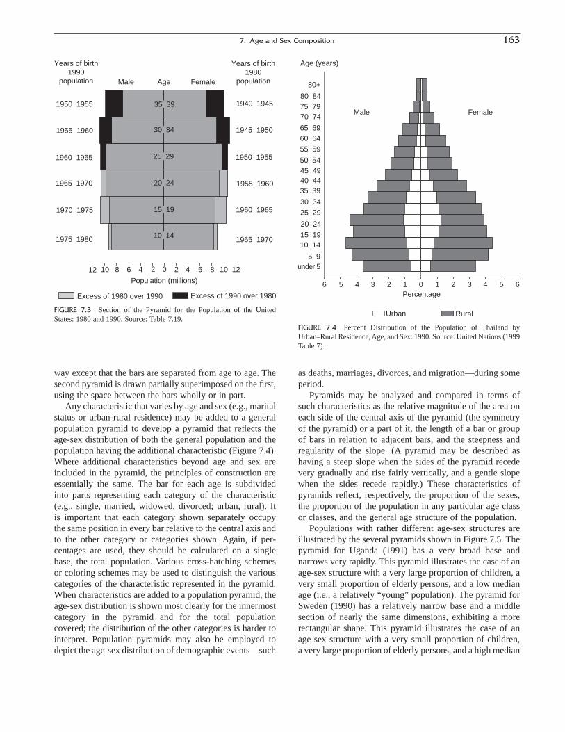
way except that the bars are separated from age to age. Thesecond pyramid is drawn partially superimposed on the first,using the space between the bars wholly or in part.
Any characteristic that varies by age and sex (e.g., maritalstatus or urban-rural residence) may be added to a generalpopulation pyramid to develop a pyramid that reflects theage-sex distribution of both the general population and thepopulation having the additional characteristic (Figure 7.4).Where additional characteristics beyond age and sex areincluded in the pyramid, the principles of construction areessentially the same. The bar for each age is subdivided into parts representing each category of the characteristic(e.g., single, married, widowed, divorced; urban, rural). It is important that each category shown separately occupy the same position in every bar relative to the central axis andto the other category or categories shown. Again, if per-centages are used, they should be calculated on a single base, the total population. Various cross-hatching schemesor coloring schemes may be used to distinguish the variouscategories of the characteristic represented in the pyramid.When characteristics are added to a population pyramid, theage-sex distribution is shown most clearly for the innermostcategory in the pyramid and for the total population covered; the distribution of the other categories is harder tointerpret. Population pyramids may also be employed todepict the age-sex distribution of demographic events—such
as deaths, marriages, divorces, and migration—during someperiod.
Pyramids may be analyzed and compared in terms ofsuch characteristics as the relative magnitude of the area oneach side of the central axis of the pyramid (the symmetryof the pyramid) or a part of it, the length of a bar or groupof bars in relation to adjacent bars, and the steepness andregularity of the slope. (A pyramid may be described ashaving a steep slope when the sides of the pyramid recedevery gradually and rise fairly vertically, and a gentle slopewhen the sides recede rapidly.) These characteristics of pyramids reflect, respectively, the proportion of the sexes,the proportion of the population in any particular age classor classes, and the general age structure of the population.
Populations with rather different age-sex structures areillustrated by the several pyramids shown in Figure 7.5. Thepyramid for Uganda (1991) has a very broad base andnarrows very rapidly. This pyramid illustrates the case of anage-sex structure with a very large proportion of children, avery small proportion of elderly persons, and a low medianage (i.e., a relatively “young” population). The pyramid forSweden (1990) has a relatively narrow base and a middlesection of nearly the same dimensions, exhibiting a morerectangular shape. This pyramid illustrates the case of anage-sex structure with a very small proportion of children,a very large proportion of elderly persons, and a high median
7. Age and Sex Composition 163
1975− 1980 1965− 1970
Years of birth1980
population
Years of birth1990
population AgeMale Female
1955− 1960
1945− 1950
1965− 1970
1955− 1960
1960− 1965
1950− 1955
1940− 19451950− 1955
1960− 1965
1970− 1975
12 10 8 6 4 2 0 2 4 6 8 10 12
Population (millions)
35− 39
30− 34
25− 29
20− 24
15− 19
10− 14
Excess of 1980 over 1990 Excess of 1990 over 1980
FIGURE 7.3 Section of the Pyramid for the Population of the UnitedStates: 1980 and 1990. Source: Table 7.19.
6 5 4 3 2 1 0 1 2 3 4 5 6Percentage
80+
80− 8475− 7970− 74
65− 6960− 6455− 59
50− 5445− 4940− 4435− 39
30− 3425− 29
20− 2415− 1910− 14
5− 9under 5
Male Female
Urban Rural
Age (years)
FIGURE 7.4 Percent Distribution of the Population of Thailand byUrban–Rural Residence, Age, and Sex: 1990. Source: United Nations (1999Table 7).

age (i.e., a relatively “old” population). The pyramids forArgentina (1991) and China (1990) illustrate configurationsintermediate between those for Uganda and Sweden. Thepyramid for the population of France given in Figure 7.6reflects various irregularities associated with that country’sspecial history.
The pyramids of geographically very small countries andof subgroups of national populations—geographic subdivi-sions or socioeconomic classes—may have quite differentconfigurations (i.e., they may vary considerably from therelatively smooth triangular and semi-elliptical shapes wehave identified). For example, the pyramid for Kuwait
164 Hobbs
80+75− 79
70− 74
65− 6960− 64
55− 59
50− 54
45− 49
40− 44
35− 39
30− 34
25− 29
20− 2415− 19
10− 14
5− 9
under 5
Male Female
10 9 8 7 6 5 4 3 2 1 0 1 2 3 4 5 6 7 8 9 10Percentage
Sweden, 1990
80+75− 79
70− 74
65− 6960− 64
55− 59
50− 54
45− 49
40− 44
35− 39
30− 34
25− 29
20− 2415− 19
10− 14
5− 9
under 5
Male Female
10 9 8 7 6 5 4 3 2 1 0 1 2 3 4 5 6 7 8 9 10Percentage
Argentina, 1991
80+75− 79
70− 74
65− 6960− 64
55− 59
50− 54
45− 49
40− 44
35− 39
30− 34
25− 29
20− 2415− 19
10− 14
5− 9
under 5
Male Female
10 9 8 7 6 5 4 3 2 1 0 1 2 3 4 5 6 7 8 9 10Percentage
Uganda, 1991
80+75− 79
70− 74
65− 6960− 64
55− 59
50− 54
45− 49
40− 44
35− 39
30− 34
25− 29
20− 2415− 19
10− 14
5− 9
under 5
Male Female
10 9 8 7 6 5 4 3 2 1 0 1 2 3 4 5 6 7 8 9 10Percentage
China, 1990
Age (years) Age (years)
FIGURE 7.5 Percent Distribution by Age and Sex of the Populations of Sweden, China, Argentina, and Uganda: Around1990. Source: U.S. Census Bureau (2000a).
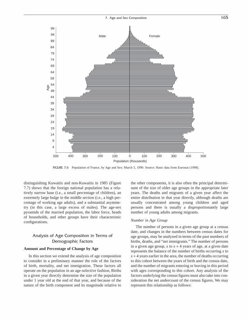
distinguishing Kuwaitis and non-Kuwaitis in 1985 (Figure7.7) shows that the foreign national population has a rela-tively narrow base (i.e., a small percentage of children), anextremely large bulge in the middle section (i.e., a high per-centage of working age adults), and a substantial asymme-try (in this case, a large excess of males). The age-sexpyramids of the married population, the labor force, headsof households, and other groups have their characteristicconfigurations.
Analysis of Age Composition in Terms ofDemographic Factors
Amount and Percentage of Change by Age
In this section we extend the analysis of age compositionto consider in a preliminary manner the role of the factorsof birth, mortality, and net immigration. These factors alloperate on the population in an age-selective fashion, Birthsin a given year directly determine the size of the populationunder 1 year old at the end of that year, and because of thenature of the birth component and its magnitude relative to
the other components, it is also often the principal determi-nant of the size of older age groups in the appropriate lateryears. The deaths and migrants of a given year affect theentire distribution in that year directly, although deaths areusually concentrated among young children and agedpersons and there is usually a disproportionately largenumber of young adults among migrants.
Number in Age Group
The number of persons in a given age group at a censusdate, and changes in the numbers between census dates forage groups, may be analyzed in terms of the past numbers ofbirths, deaths, and “net immigrants.” The number of personsin a given age group, x to x + 4 years of age, at a given daterepresents the balance of the number of births occurring x tox + 4 years earlier in the area, the number of deaths occurringto this cohort between the years of birth and the census date,and the number of migrants entering or leaving in this periodwith ages corresponding to this cohort. Any analysis of thefactors underlying the census figures must also take into con-sideration the net undercount of the census figures. We mayrepresent this relationship as follows:
7. Age and Sex Composition 165
Male Female
99
94
89
84
79
74
69
64
59
54
49
44
39
34
29
24
19
14
9
4
500 400 400300300 200 200100100 0
Population (thousands)
500
Age
FIGURE 7.6 Population of France, by Age and Sex: March 5, 1990. Source: Basic data from Eurostat (1998).

(7.25)
where Pa is the population in the age group; Bc, births in thecohort; Dc, deaths occurring to the cohort; Mc, net migrantsjoining the cohort; and Ea, net undercount in the censusfigure. For purposes of the present analysis, we shall assumethat there are no errors in the data on the components or thatthey have been satisfactorily corrected.
Generally, the younger the age group, the smaller theimpact of death and migration in determining the size of thegroup and the greater the relative importance of births. Thus,the size of the population under 5 years of age on April 1,1990, in the United States is very largely determined by thenumber of births occurring between April 1, 1985, and April1, 1990. This number is modified only by the relatively smallnumber of deaths occurring to these newborn childrenduring the period and by the relatively small number ofimmigrant children in this cohort entering the country in theperiod. The net undercount of the census figure increases thepotential gap between the births and the census figure some-what further. Similarly, the population 5 to 9 years old onApril 1, 1990, represents the births of April 1, 1980, to April1, 1985, modified by deaths and migration up to April 1,1990; the population 10 to 14 years old stems from the birthsof April 1, 1975, to April 1, 1980; and so forth.
P B D M Ea c c c a= - + -
The paramount importance of the past trend of births alsoapplies generally in interpreting short-term changes in thenumber of aged persons. For example, the increase of 5.3million, or 22%, in the population 65 years of age and overin the United States between 1980 and 1990 may beexplained largely in terms of the rise in the number of birthsbetween 1895–1905 and 1915–1925.25 Because the popula-tion aged 65 and over is largely made up of persons aged 65to 84, we have used these ages to determine the birth yearsof the two groups of cohorts and then eliminated the yearscommon to them. Once again, in spite of the considerableimportance of deaths in determining the number of agedpersons at each census date, the factor of mortality tends tobe relatively secondary in explaining the change in thenumber of aged persons over a period as short as 10 years.As stated earlier, both groups of cohorts being comparedhave been exposed to the risk of death for the same numberof years, albeit the considerable period of 65 to 84 years,and although some improvement in mortality may haveoccurred as the two groups of cohorts moved through lifefrom infancy to old age 10 calendar years apart, thisimprovement was much less important than the fact that thenumber of years of exposure was the same.
The contribution of migration to the change in the agedpopulation may be analyzed to some extent in the same wayas the contribution of mortality. The two groups of cohortshave been “exposed to the risk” of migration for the sameperiod of years (65 or more), but there may have beensudden shifts from year to year in the number of migrantsaffecting the two groups of cohorts.
A country’s age profile may be affected by the events ofwar and postwar demobilization, as well as by peacetimemobilization. A war may be directly responsible for a short-or long-term deficit of (primarily) males of military age inthe resident population, an increase in the death rate, a riseor fall in the birthrate, and the displacement of civilian pop-ulation. To the extent that there are battle losses of militarypersonnel, the deficit of males of military age will becomepermanent and may remain visible not only through the lifespan of the particular cohorts concerned but may also bereflected in later cohorts through the effect on the birthrate.26
To the extent that the civilian population is directly involvedin military activities and there are war losses of civilians(e.g., from bombing), the impact of a war will be moreevenly distributed over the age-sex classes.
166 Hobbs
80+
75− 79
70− 74
65− 69
60− 64
55− 59
50− 54
45− 49
40− 44
35− 39
30− 34
25− 29
20− 24
15− 19
10− 14
5− 9
<5
Male Female
150 125 100 75 50 25 0 25 50 75 100 125 150
Population (thousands)
Non-Kuwaiti Kuwaiti
Age (years)
FIGURE 7.7 Population by Age, Sex, and Nationality for Kuwait: 1985Source: Kuwait, Central Statistical Office (1986)
25 The reference here is specifically to the number of births rather thanto the birth rate. The absolute number of births may be rising while thebirthrate may be falling because the total population is growing. Forexample, the U.S. birthrate decreased generally in the period 1895 to 1925,but the number of births increased during this period. These are the cohortsthat entered the 65-and-over group during the 1960s, 1970s, and 1980s.
26 For such effects in the Soviet Union, see Pirozhkov and Safarova(1994). Also see Metropolitan Life Insurance Company (1940a) and Smithand Zopf (1970, pp. 160–162).

The nature and extent of the effect of a war on thebirthrate will depend in part on the duration and magnitudeof the war, the degree to which families are separated bymilitary service or destruction of civilian communities, andthe impact of the war on the economy.27 Although thebirthrate may rise or fall during wartime, it is especiallylikely to rise during the immediate postwar demobilizationperiod because of the reunion of married couples, a rise inthe number of marriages, and the postponement of births.The sharp fluctuations in the birthrate usually associatedwith war tend to produce marked variations in the size ofsuccessive age groups in a population. These “hollow” and“swollen” age groups will grow older with the passage oftime and reappear as hollow and swollen groups at succes-sively older ages at various subsequent dates, possibly fordecades to come (Figure 7.6).
As a direct result of war, the volume of ordinary civilianimmigration or emigration is likely to fall off to a meretrickle while movements of military personnel into and outof the country and of refugees and expellees may be volu-minous and erratic. With the end of the war, demobilizationof military personnel or displacements of population mayaccount for a tremendous rise in the volume of move-ment into or out of the belligerent countries. The changesdescribed may have a considerable impact on the age profileof the population as well as its sex composition.
Percentage of Change
We turn next to a formulation of the contribution of eachcomponent of change to the total percentage change in anage group between two dates. We may represent the popu-lation at a given age in an earlier (P0) and later (P1) censusin terms of its underlying components as follows:
(7.26)
(7.27)
Note that all the elements in each equation relate to thesame birth cohorts. (These equations are of the same formas Equation 7.25.) The relative contribution of each compo-nent to the total change in population is obtained by takingthe difference between these equations, grouping compo-nents, and dividing each side by P0
a:
(7.28)
Each term here, multiplied by 100, represents the contri-bution of a component in percentage points to the total per-centage change.
Table 7.23 illustrates the application of this formula inanalyzing the increase in the U.S. population for selected
P P
P
B B
P
D D
P
M M
P
E E
Pa a
a a a a
a a
a
1 0
0
1 0
0
1 0
0
1 0
0
1 0
0
-=
--
-+
--
-
P B D M Ea a1 1 1 1 1= - + -
P B D M Ea a0 0 0 0 0= - + -
age groups between 1980 and 1990. First, determine thenumbers of births, deaths, and net immigrants, as well as thenet undercount pertaining to each cohort (cols. 1 and 2);second, take the difference between the amounts for the twocohorts (col. 3); and third, divide the difference by the pop-ulation in the age group at the earlier census and multiplyby 100 (col. 6). According to this calculation, of the 12.3%increase in the 0-to-4 age group, the increase in births “con-tributed” 16.3 percentage points and the decrease in deaths“contributed” 0.3 percentage point, for a combined positivecontribution of 16.6 percentage points. The decrease in netmigration and the increase in net undercount had a combinednegative contribution of 4.3 percentage points, 0.4 percent-age point attributable to the migration component and 3.9percentage points to the change in undercount.
If only the contribution of births to total percentagechange is to be measured, or can be measured because dataon births alone can be developed, it is necessary simply to(1) determine the numbers of births corresponding to eachcohort from the registration data or by estimation, (2) sub-tract the births of each cohort from the corresponding censuscounts, to obtain estimates for all other components com-bined, including the net census undercount, and (3) proceedas before (see Table 7.23).
An alternative procedure for computing the contribu-tion of the components, which produces the same results,views the overall percentage change in the population as theweighted average of the percentage changes in the compo-nents. The percentage change in each component is shownin column 4 of Table 7.23. The weight attached to eachcomponent is derived by taking the ratio of a particularcomponent for the earlier cohort to the census population atthe earlier date. The weights are shown in column 5. Thecontribution of each component in percentage points (col.6) is obtained by taking the product of the percentages incolumn 4 and the weights in column 5. The weights forbirths and net immigration are positive, and the weights fordeaths and net undercount are negative. In the young ages,the component of births receives a relatively high weight incomparison with the other components. As one goes up theage scale, the relative weight of the birth component tendsto fall and the relative weight of the other components takentogether, particularly the death component, tends to rise. Forexample, at ages 0 to 4, the birth component has an absoluteweight of 1.022 and the other components combined aweight of (-).022; but at ages 55 to 59, the birth compo-nent has an absolute weight of 1.277 compared with aweight of (-).277 for the other components combined.These figures indicate relative weights for births of 98% and82%, respectively.28
7. Age and Sex Composition 167
27 For the effects of World War I on the birthrate in several Europeancountries, see Metropolitan Life Insurance Company (1940b).
28 The relative weight of births may be given by , where Wb
represents the absolute weight for births. The value of this function declineswith the rise in Wb.
W
Wb
b2 1-

Changes in Proportions by Age and in Overall Age-Sex Structure
We turn next to a brief consideration of the demographicfactors affecting the changes in the proportion of the popu-lation in a given age group between two dates or in the age-sex structure as a whole.
Changes in the proportion of the population in a givenage group between two dates depend on the relative rates ofgrowth of the age group in question and of the total popu-lation. In evaluating the role of natality in particular, it isuseful to compare the percentage difference between thenumbers of births corresponding to the two cohorts understudy with the percentage difference in the numbers of birthsduring the century or so prior to each of the two dates. For
example, the proportion of the population 30 to 34 years oldin the United States increased from 7.8% to 8.8% between1980 and 1990 largely because (1) the relative excess ofbirths occurring in 1955–1960 over births occurring in1945–1950 (21%) was greater than (2) the relative excess ofbirths in 1890–1990 over births in 1880–1980 (about 6%).The ratio of these ratios (1.21 ∏ 1.06) equals 1.14, suggest-ing a contribution of 14% due to births in the increase in theproportion of the population aged 30 to 34 between 1980and 1990; this proportion actually rose by 13%. The increasein the proportion of aged persons in the United Statesbetween 1980 and 1990 resulted in large part from (1) therelative excess of births between 1905 and 1925 over birthsbetween 1895 and 1915 (when most persons 65 and over in1990 and 1980, respectively, were born) in comparison with
168 Hobbs
TABLE 7.23 Calculation of the Contribution of the Components of Change to the Percentage Change for Selected Age Groupsin the Population of the United States between 1980 and 1990
Change Contribution ofeach component
Number (In thousands) Amount [(3) ∏ Pa80] ¥ 100
(In thousands) Percentage Weight or1980 1990 (2) - (1) = [(3) ∏ (1)] ¥ 100 = (1) ∏ Pa
80 = (4) ¥ (5) =Age and component (1) (2) (3) (4) (5) (6)
Under 5 years:Births 16,711 19,369 +2,658 +15.91 +1.022 +16.3Deaths1 (-)253 (-)209 +44 -17.39 -0.015 +0.3Net migration +213 +154 -59 -27.70 +0.013 -0.4Net undercount (-)324 (-)960 -636 +196.30 -0.020 -3.9Population or total change 16,348 18,354 +2,006 +12.27 (1.000) +12.3
5 to 9 years:Births 16,832 18,257 +1,425 +8.47 +1.008 +8.5Deaths1 (-)365 (-)258 +107 -29.32 -0.022 +0.6Net migration +484 +445 -39 -8.06 +0.029 -0.2Net undercount (-)251 (-)344 -93 +37.05 -0.015 -0.6Population or total change 16,700 18,099 +1,399 +8.38 (1.000) +8.4
15 to 19 years:Births 20,909 16,832 -4,077 -19.50 +0.988 -19.3Other components2 +259 +922 +663 +255.98 +0.012 +3.1Population or total change 21,168 17,754 -3,414 -16.13 (1.000) -16.1
25 to 29 years:Births 19,618 20,909 +1,291 +6.58 +1.005 +6.6Other components2 (-)97 +404 +501 -516.49 -0.005 +2.6Population or total change 19,521 21,313 +1,792 +9.18 (1.000) +9.2
35 to 39 years:Births 14,445 19,618 +5,173 +35.81 +1.034 +37.0Other components2 (-)480 +345 +825 -171.88 -0.034 +5.9Population or total change 13,965 19,963 +5,998 +42.95 (1.000) +43.0
55 to 59 years:Births 14,828 12,264 -2,564 -17.29 +1.277 -22.1Other components2 (-)3,213 (-)1,732 +1,481 -46.09 -0.277 +12.8Population or total change 11,615 10,532 -1,083 -9.32 (1.000) -9.3
1 As a negative component, “deaths” is assigned a negative sign. A positive amount of change in the number of deaths indicates a decrease in the numberof deaths or in effect an addition to the population.
2 “Other components” can have a positive or negative sign, depending on the combined contribution of deaths, net migration, and net coverage error.Source: Based on U.S. Census Bureau, unpublished tabulations.

(2) the slower average increase of births during the pastcentury, which is responsible for the moderate rate of growthof the total population in the 1980–1990 decade. Thus, thelongtime downward trend in the birthrate in the UnitedStates contributed to the increase in the proportion ofpersons in the older ages in recent decades.
A reduction in death rates contributes, as was statedearlier, to an increase in the number at an age group over a particular time interval (e.g., 10 years). Whether or notreductions in death rates contribute to an increase in the pro-portion of the population in any age group during such aperiod depends on the age pattern of improvements in deathrates. More specifically, the effect of mortality on changesin proportions by age depends on the difference between (1)the relative improvement in survival rates from birth up tothe specified age for the periods ending on each census date(e.g., 10 years apart) and (2) the relative improvement in sur-vival rates from birth to census age over all age cohortsincluded in the total population at the census dates. Ingeneral, if the savings in lives are confined to childhood, theproportion of children will tend to rise and the proportion ofolder persons to fall; if the savings in lives are confined toolder persons, the proportion of children will tend to fall andthe proportion of older persons to rise. In the experience ofthe United States as well as of many other countries beforeabout 1970, much more proportional improvement in mor-tality took place at the younger ages than at the older ages,and thus this factor contributed little or nothing to theincrease in the proportion of the aged.29 However, since thelast quarter of the last century, the age pattern of death ratesappears to have shifted in the United States and other lowmortality countries (Preston et al., 1989). To the extent thatcurrent and future changes in mortality are proportionallygreater at older ages, this factor may be expected to assumegreater weight, particularly in relatively “aged” countries(Caselli and Vallin, 1990).
The role of immigration can be analyzed in a similar way,but the specific impact on the age distribution may be quitedifferent from that of deaths because the migrants have theirown characteristic age pattern as well as a natural increase.Migrants change the prevailing age composition of the pop-ulation to the extent that their age composition plus theirnatural increase differs from that of the general population.Because immigrants tend to be relatively young on arrivaland may have a relatively higher natural increase, the usualshort-term effect of immigration is to reduce the proportionof older adults and aged persons in the population. This“younging” effect will continue if the volume of immigra-
tion is maintained and the new arrivals continue to have ayoung age distribution. The younging effect will tend todecline, however, if the volume of immigration falls off orif the new arrivals begin having an older age distribution, asoccurred generally in the United States in the first half of the20th century.
Because the median age is the 50-percentile mark in theage distribution, changes in the median age may be analyzedin much the same manner as changes in the proportion atsome age. The median age will rise during a period if thepopulation above the median age at the beginning of theperiod grows at a faster rate than the population below the median (or the total population), and the median age willfall under the opposite conditions. Here again, the factors ofmortality and migration have tended to be of considerablyless importance than the factor of fertility in explaining achange in the median age, but, as stated, in recent decadesin some countries the role of mortality has become moreimportant than fertility.
Analysis of Population Pyramids
It is possible to infer a good deal about the demographichistory of an area simply by examining the populationpyramid depicting its age-sex structure. Because a pyramiddoes not identify the specific demographic factors thatshaped it in a particular case, however, and because morethan one factor contributes to the determination of thenumber of persons at each age, it is not possible to stateexactly, especially without a knowledge of the history of thearea, how demographic factors operated to give a particularpyramid its special form.
A pyramid with a very broad base suggests a populationwith a relatively high birthrate, and if, in addition, thepyramid narrows rapidly from the base up—that is, has agenerally triangular shape with concave sides—a combina-tion of high birthrates and high death rates is suggested. Thepyramid for Uganda in 1991 shown in Figure 7.5 reflectssuch a demographic history. The beehive- or barrel-shapedpyramid for Sweden in 1990 shown in the same chart sug-gests a history of low fertility and low mortality. Irregularvariations in the lengths of the bars point to past sharp fluc-tuations in the number of births or in the volume of migra-tion, but they may also reflect a temporary rise in the numberof deaths resulting from war or epidemic. The pyramid forFrance in 1990 shown in Figure 7.6 has a number of irreg-ularities that may be explained on the basis of the fluctua-tions in the number of births and deaths caused by WorldWars I and II. The pyramid has been annotated to indicatethe age bands that were affected by military losses in WorldWars I and II, deficits of births during these wars, and thepost–World War II rise in births due to demobilization. If thebars for the youngest ages are shorter than those for the nexthigher ages, a recent decline in the number of births is sug-gested (Figure 7.2 for Japan in 1995), although some of such
7. Age and Sex Composition 169
29 Some earlier studies concerned with the theoretical and empiricalanalysis of the effect of mortality and natality trends on age compositionare Coale (1956, 1972), United Nations (1954), and Stolnitz (1956). Therelative contribution of fertility, mortality, and immigration to changes inthe age composition of the U.S. population between 1900 and 1960 is ana-lyzed in Valaoras (1950) and Hermalin (1966).

shortages may be due to relatively greater underenumerationof the youngest age groups.
Where the bars in the middle or the upper part of thepyramid are excessively long or short, heavy immigration oremigration of persons in these age groups in recent years, orof younger persons in the same age cohorts at an earlier date,is indicated. A pyramid with an asymmetrical shape in theprimary labor force ages (e.g., 25 to 54) generally representsa population that is characterized by heavy sex-selectivityof recent immigrants, such as the foreign national popula-tion of Kuwait in 1985 shown in Figure 7.7.
Analysis of Age-Sex Structure by Use of Population Models
Earlier we referred to the use of various models of pop-ulation structure in the evaluation and correction of censusdata on age-sex composition. These models are also usefulin the analysis of the age-sex structure of populations. Com-parisons of the structure of actual populations with the the-oretical structure generated by various constant or variableconditions of fertility and mortality represented by thesepopulation models permits a fuller understanding of the roleof these demographic conditions in age-sex structure. Thepyramids of these population models may also be used asgraphic standards for interpreting the pyramids of actualpopulations. Recall that the stable population model indi-cates the fixed age-sex structure of a population resultingfrom and consistent with constant birth and death rates (i.e.,a constant growth rate, positive or negative) and no migra-tion (a “closed population”). The quasi-stable populationmodel corresponds to the stable population model exceptthat mortality is assumed to be declining moderately. Thestationary population model, identified previously as aspecial case of the stable population model, assumes a zerogrowth rate (i.e., constant and equal numbers of births anddeaths each year and, hence, constant and equal birth anddeath rates each year). An alternative scenario for the stablepopulation model incorporates immigration at a constantlevel by age (Espenshade et al., 1982). The pyramids ofthese models are smooth and regular.
Populations with high and relatively unchanging birth-rates and with moderately high death rates, a type of popu-lation found in some less developed countries today, mostlyin sub-Saharan Africa, resemble the stable population modelwith a high growth rate (e.g., Figure 7.5, Uganda). Popula-tions with low birth and low death rates resemble the stablemodel with a low growth rate, or a stationary populationwith low birth and low death rates (e.g., Figure 7.5,Sweden). Low fertility-low mortality populations experi-encing a steady flow of immigration or emigration (with afixed age distribution) resemble a stationary populationmodel incorporating migration (not illustrated.) The devia-tions of the age-sex structure of actual populations from theclosely related models will give some indications of past
fluctuations in fertility and mortality, and the role of migra-tion and war mortality.
References
Bachi, R. 1954. “Measurement of the Tendency to Round off Age Returns.”Bulletin de l’Institut International de Statistique (Proceedings of the28th Session, Rome), 34(3): 129–138.
Brass, W., A. J. Coale, P. Demeny, D. Heisel, F. Lorimer, A. Romaniuk, andE. van de Walle. 1968. The Demography of Tropical Africa (pp. 13–52).Princeton, NJ: Princeton University Press.
Carrier, N. H. 1959. “A Note on the Measurement of Digital Preference inAge Recordings.” Journal of the Institute of Actuaries (Cambridge,England) 85: 71–85.
Carrier, N. H., and A. M. Farrag. 1959. “The Reduction of Errors in CensusPopulations for Statistically Underdeveloped Countries.” PopulationStudies (London) 12(3): 240–285.
Caselli, G., and J. Vallin. 1990. “Mortality and Aging.” European Journalof Population 6(1): 1–25.
Chahnazarian, A. 1988. “Determinants of the Sex Ratio at Birth: Reviewof Recent Literature.” Social Biology 35(3–4): 214–235.
China, State Council Population Census Office (Ed.). 2000. Di wu ciquanguo renkou pucha puchayuan shouce (Enumerator Handbook for the Fifth National Population Census), Beijing: China StatisticsPress.
Coale, A. J. 1956. “The Effects of Changes in Mortality and Fertility on Age Composition.” Milbank Memorial Fund Quarterly 34(1): 79–114.
Coale, A. J. 1963. “Estimates of Various Demographic Measures throughthe Quasi-Stable Age Distribution.” Emerging Techniques in Popula-tion Research, Milbank Memorial Fund, pp. 175–193.
Coale, A. J. 1972. The Growth and Structure of Human Populations: AMathematical Investigation. Princeton, NJ: Princeton University Press.
Coale, A. J., and J. Banister. 1994. “Five Decades of Missing Females inChina.” Demography 31(3): 459–479.
Coale, A. J., and P. Demeny. 1983. Regional Model Life Tables and StablePopulations, 2nd ed. with B. Vaughn. New York: Academic Press.
Das Gupta, M., and P. N. Mari Bhat. 1997. “Fertility Decline and IncreasedManifestation of Sex Bias in India.” Population Studies 51(3):307–315.
Das Gupta, P. 1991. “Reconstruction of the Age Distribution of the ExtremeAged in the 1980 Census by the Method of Extinct Generations.” 1990Proceedings of the Social Statistics Section. Washington, DC: American Statistical Association, pp. 154–159.
Davis, K., and P. van den Oever. 1982. “Demographic Foundations of New Sex Roles.” Population and Development Review 8(3): 495–511.
Demeny, P., and F. C. Shorter. 1968. “Estimating Turkish Mortality, Fertility, and Age Structure,” Statistics Institute Paper No. 2, IstanbulUniversity, Istanbul, Turkey.
Duncan, O. D. 1959. “Residential Segregation and Social Differentiation.”International Population Conference, International Union for the Scientific Study of Population, Vienna, pp. 571–572.
Duncan, O. D., and B. Duncan. 1955. “Residential Distribution and Occupational Stratification.” American Journal of Sociology 60(5):494.
ESCAP (United Nations Economic and Social Commission for Asia andthe Pacific). 1984. “Internal Migration in the Countries of the ESCAPRegion.” Third Asian and Pacific Population Conference: SelectedPapers. Asian Population Studies Series, No. 58, pp. 194–211.
Espenshade, T. J., L. F. Bouvier, and W. B. Arthur. 1982. “Immigration andthe Stable Population Model.” Demography 19(1): 125–134.
Ewbank, D. 1981. Age Misreporting and Age Selective Underenumeration:Sources, Patterns, and Consequences for Demographic Analysis.
170 Hobbs

Committee on Population and Demography. Report No. 4. Washington,DC.
France, Institut National de la Statistique et des Études Économiques. 1994.Recensement de la Population de 1990, Population Totale, Résultats duSondage au Quart, INSEE Resultats #301–302.
Gage, T. B. 1994. “Population Variation in Cause of Death: Level, Gender,and Period Effects.” Demography 31(2): 271–296.
Gregson, S., G. P. Garnett, and R. M. Anderson. 1994. “Assessing thePotential Impact of the HIV-1 Epidemic on Orphanhood and the Demo-graphic Structure of Populations in sub-Saharan Africa.” PopulationStudies 48(3): 435–458.
Hermalin, A. I. 1966. “The Effect of Changes in Mortality Rates on Popu-lation Growth and Age Distribution in the United States.” MilbankMemorial Fund Quarterly 44(4): 451–469, Part 1.
Hirschman, C., S. Preston, and V. M. Loi. 1995. “Vietnamese Casualtiesduring the American War: A New Estimate.” Population and Develop-ment Review 21(4): 783–812.
Kestenbaum, B. 1992. “A Description of the Extreme Aged PopulationBased on Improved Medicare Enrollment Data.” Demography 29(4):565–580.
Kestenbaum, B. 1998. “Recent Mortality of the Oldest Old from Medicare Data.” Social Security Adminstration, Working Paper. Baltimore, MD.
Kuwait Central Statistical Office. 1986. 1985 Census of Population. (inArabic).
Macmahon, B., and T. F. Pugh. 1953. “Influence of Birth Order and Maternal Age on the Human Sex Ratio at Birth.” British Journal of Preventive and Social Medicine 7(2): 83–86.
Marks, E. S., and J. Waksberg. 1966. “Evaluation of Coverage in the 1960Census of Population through Case-by-Case Checking.” Proceedingsof the Social Statistics Section. American Statistical Association. Washington, DC, pp. 62–70.
Martine, G. 1975. “Volume, Characteristics and Consequences of InternalMigration in Colombia.” Demography 12(2): 193–208.
McMahan, C. A. 1951. “An Empirical Test of Three Hypotheses Concern-ing the Human Sex Ratio at Birth in the United States, 1915–48.”Milbank Memorial Fund Quarterly 29(3): 273–293.
Metropolitan Life Insurance Company. 1940a. “The Cumulative Effect of Successive Wars on Age Composition of Population” Statistical Bulletin 21(4): 2–5.
Metropolitan Life Insurance Company. 1940b. “War and the Birth Rate,”Statistical Bulletin 21(3): 3–6.
Myers, R. J. 1940. “Errors and Bias in the Reporting of Ages in CensusData.” Transactions of the Actuarial Society of America 41: Part II(104): 395–415. (Reproduced in U.S. Bureau of the Census. 1951.Handbook of Statistical Methods for Demographers, pp. 115–125.)
Myers, R. J. 1954. “The Effect of Age of Mother and Birth Order on Sex Ratio at Birth.” Milbank Memorial Fund Quarterly 32(3): 275–281.
Myers, R. J. 1966. “Validity of Centenarian Data in the 1960 Census.”Demography 3(2): 470–476.
Park, C. B., and N. H. Cho. 1995. “Consequences of Son Preference in aLow-Fertility Society: Imbalance of the Sex Ratio at Birth in Korea.”Population and Development Review 21(1): 59–84.
Pirozhkov, S., and G. Safarova. 1994. “Demographic Regularities andIrregularities: The Population Age Structure.” In W. Lutz, S. Scherbov,and A. Volkov (Eds.), Demographic Trends and Patterns in the SovietUnion Before 1991. International Institute for Applied Systems Analysis(IIASA). Laxenburg, Austria.
Preston, S. H., C. Himes, and M. Eggers. 1989. “Demographic ConditionsResponsible for Population Aging.” Demography 26(4): 691–704.
Preston, S. H., I. T. Elo, and Q. Stewart. 1997. “Effects of Age Misre-porting on Mortality Estimates at Older Ages.” Population AgingResearch Center, University of Pennsylvania, Working Paper Series,No. 98–01.
Ramachandran, K. V. 1967. “An Index to Measure Digit Preference Errorin Age Data.” Summary in United Nations, World Population Confer-ence, 1965 (Belgrade), Vol. III, pp. 202–203.
Reardon, S. F., J. T. Yun, and T. M. Eitle. 2000. “The Changing Structureof School Segregation: Measurement and Evidence of Multiracial Metropolitan-Area School Segregation, 1989–1995.” Demography37(3): 351–364.
Republic of Korea, National Statistical Office. 1987. 1985 Population andHousing Census Report, Whole Country, Volume 1.
Republic of Korea, National Statistical Office. 1997. 1995 Population andHousing Census Report, Whole Country, Volume 1.
Robinson, J. G., B. Ahmed, P., Das Gupta, and K. A. Woodrow. 1991. “Esti-mating Coverage of the 1990 United States Census: DemographicAnalysis,” paper presented at the American Statistical Associationmeetings, Atlanta, GA.
Robinson, J. G., B. Ahmed, P., Das Gupta, and K. A. Woodrow. 1993. “Esti-mation of Coverage in the 1990 United States Census Based on Demo-graphic Analysis.” Journal of the American Statistical Association88(423): 1061–1071.
Ruder, A. 1985. “Paternal and Birth-Order Effect on the Human SecondarySex Ratio.” American Journal of Human Genetics 37(2): 362–372.
Saw, S. H. 1967. “Errors in Chinese Age Statistics.” Demography 4(2):859–875.
Siegel, J. S., and J. S. Passel. 1976. “New Estimates of the Number of Cen-tenarians in the United States.” Journal of the American StatisticalAssociation 71(355): 559–566.
Skeldon, R. 1986. “On Migration Patterns in India during the 1970s.” Pop-ulation and Development Review 12(4): 759–779.
Smith, T. L., and P. E. Zopf, Jr. 1970. Demography: Principles andMethods. Philadelphia: F. A. Davis.
South, S. J., and K. Trent. 1988. “Sex Ratios and Women’s Roles: ACross-National Analysis.” American Journal of Sociology 93(5): 1096–1115.
Spencer, G. 1986. “The Characteristics of Centenarians in the 1980Census.” Paper presented at the Population Association of Americameetings, San Francisco, CA.
Spencer, G. 1987. “Improvements in the Quality of Census Age Statisticsfor the Elderly.” Proceedings of the 1987 Public Health Conference onRecords and Statistics. Washington, DC.
Spencer, G., D. L. Word, and F. W. Hollmann. 1992. “Discontinuities inAge and Race Data from the 1990 Census,” Paper presented at theannual meeting of the Population Association of America, Denver, Colorado.
Stanecki, K. 2000. “The AIDS Pandemic in the 21st Century: The Demo-graphic Impact in Developing Countries.” Paper presented at the XIIIthInternational AIDS Conference. Durban, South Africa.
Stolnitz, G. J. 1956. “Mortality Declines and Age Distribution.” MilbankMemorial Fund Quarterly 34(2): 178–215.
Teitelbaum, M. S., and N. Mantel. 1971. “Socioeconomic Factors and theSex Ratio at Birth.” Journal of Biosocial Science 3: 23–41.
Trovato, F., and N. M. Lalu. 1996. “Narrowing Sex Differentials in LifeExpectancy in the Industrialized World: Early 1970’s to Early 1990’s.”Social Biology 43(1–2): 20–37.
United Nations. 1952. “Accuracy Tests for Census Age Distributions Tab-ulated in Five-Year and Ten-Year Groups.” Population Bulletin (2):59–79.
United Nations. 1954. “The Cause of the Aging of Populations: DecliningMortality or Declining Fertility.” Population Bulletin of the UnitedNations (4): 30–38.
United Nations. 1955. Chapter 3 in Methods of Appraisal of Quality of Basic Data for Population Estimates. Manuals on Methods of Estimating Population, Manual II. Series A, Population Studies, No. 23,pp. 31–54.
United Nations. 1958. Principles and Recommendations for National Pop-ulation Censuses, Statistical Papers, Series M, No. 27. New York.
7. Age and Sex Composition 171

United Nations. 1964. National Programmes of Analysis of PopulationCensus Data as an Aid to Planning and Policy-Making. PopulationStudies. Series A, No. 36.
United Nations. 1967. Principles and Recommendations for the 1970 Population Censuses, Statistical Papers, Series M, No. 44. New York.
United Nations. 1982. Model Life Tables for Developing Countries. Popu-lation Studies, No. 77. New York.
United Nations. 1983. Indirect Techniques for Demographic Estimation.Manual X, Population Studies, No. 81, Annex V.
United Nations. 1988. Demographic Yearbook 1986. New York: UnitedNations.
United Nations. 1994. Demographic Yearbook 1992. New York: UnitedNations.
United Nations. 1995. Demographic Yearbook 1993. New York: UnitedNations.
United Nations. 1998. Principles and Recommendations for Population andHousing Censuses, Revision 1. Statistical Papers, Series M, No. 67/Rev.1. New York: United Nations.
U.S. Bureau of the Census. 1960a. Historical Statistics of the United States:Colonial Times to 1957. Washington, DC.
U.S. Bureau of the Census. 1960b. The Post-Enumeration Survey: 1950.Technical Paper No. 4. Washington, DC.
U.S. Bureau of the Census. 1964. Accuracy of Data on Population Char-acteristics as Measured by Reinterviews. Evaluation and ResearchProgram U.S. Censuses of Population and Housing, 1960: ER 60, No.4.
U.S. Bureau of the Census. 1965. Historical Statistics of the United States:Continuation to 1962 and Revisions. Washington, DC.
U.S. Bureau of the Census. 1975. Historical Statistics of the United States:Colonial Times to 1970. Washington, DC.
U.S. Bureau of the Census. 1980. The Methods and Materials of Demog-raphy, by H. S. Shryock, J. S. Siegel, and Associates. Vols. 1 and 2,Fourth Printing (rev.). Washington, DC.
U.S. Bureau of the Census. 1983. General Population Characteristics,United States Summary, 1980. 1980 Census of Population. PC80-1-B1.Washington, DC.
U.S. Bureau of the Census. 1985. Evaluating Censuses of Population andHousing. Statistical Training Document, ISP-TR-5, Washington, DC.
U.S. Bureau of the Census. 1988. The Coverage of Population in the 1980Census, by R. E. Fay, J. S. Passel, and J. G. Robinson. 1980 Census ofPopulation and Housing. PHC80-E4. Washington, DC: U.S. Bureau ofthe Census.
U.S. Census Bureau. 1992. General Population Characteristics, UnitedStates, 1990. 1990 Census of Population. CP-1-1. Washington, DC.
U.S. Census Bureau. 1993a. The Foreign-Born Population in the UnitedStates, 1990. 1990 Census of Population. CP-3-1. Washington, DC.
U.S. Census Bureau. 1993b. “U.S. Population Estimates, by Age, Sex,Race, and Hispanic Origin: 1980 to 1991,” by F. W. Hollmann. CurrentPopulation Reports, P25–1095. Washington, DC.
U.S. Census Bureau. 1994. Population Analysis with Microcomputers, byE. E. Arriaga, with P. D. Johnson and E. Jamison (Associates). VolumesI and II.
U.S. Census Bureau. 1999. “Centenarians in the United States.” By C. A.Krach and V. A. Velkoff. Current Population Reports. P-23-199RV.Washington, DC.
U.S. Census Bureau. 2000a. International Data Base,www.census.gov/ipc/www/idbacc.html.
U.S. Census Bureau. 2000b. “Population Projections for the United Statesby Age, Sex, Race, Hispanic Origin, and Nativity: 1999 to 2100.”http://www.census.gov/population/www/projections/natproj.html.
U.S. National Center for Health Statistics. 1997. U.S. Decennial Life Tablesfor 1989–91. Vol. 1, Number 1, Hyattsville, MD.
Valaoras, V. G. 1950. “Patterns of Aging of Human Populations.” EasternStates Health Education Conference (1949). The Social and Biological
Challenge of Our Aging Population. New York: Columbia UniversityPress, pp. 67–85.
van de Walle, E. 1966. “Some Characteristic Features of Census Age Distributions in Illiterate Populations.” American Journal of Sociology71(5): 549–557.
Vincent, P. 1951. “La Mortalité des Viellards” (The mortality of the aged).Population 6(2): 181–204, Paris.
Waldron, I. 1993. “Recent Trends in Sex Mortality Ratios for Adults in Developed Countries.” Social Science and Medicine 36(4): 451–462.
Winston, S. 1931. “The Influence of Social Factors Upon the Sex Ratio atBirth.” American Journal of Sociology 37(l): 1–21.
Winston, S. 1932. “Birth Control and the Sex Ratio at Birth.” AmericanJournal of Sociology 38: 225–231.
Suggested Readings
Anderson, B. A., and B. D. Silver. 1985. “Estimating Census Undercountfrom School Enrollment Data: An Application to the Soviet Censusesof 1959 and 1970.” Demography 22(2): 289–308.
Bhat, P. N. Mari. 1990. “Estimating Transition Probabilities of Age Misstatement.” Demography 27(1): 149–163.
Budd, J. W., and T. Guinnane. 1991. “Intentional Age-Misreporting, Age-Heaping, and the 1908 Old Age Pensions Act in Ireland.” PopulationStudies 45(3): 497–518.
Caldwell, J. C. 1966. “Study of Age Misstatement Among Young Childrenin Ghana.” Demography 3(2): 477–490.
Chu, C. Y. C. 1997. “Age-Distribution Dynamics and Aging Indexes.”Demography 34(4): 551–563.
Coale, A. J. 1964. “How a Population Ages or Grows Younger.” In R. Freedman (Ed.), Population: The Vital Revolution (pp. 47–58).Garden City, NY: Doubleday-Anchor.
Coale, A. J. 1991. “Excess Female Mortality and the Balance of the Sexesin the Population: An Estimate of the Number of ‘Missing Females.’ ”Population and Development Review 17(3): 517–523.
Coale, A. J., and M. Zelnik. 1963. New Estimates of Fertility and Population in the United States. Princeton, NJ: Princeton UniversityPress.
Das-Gupta, A. 1955. “Accuracy Index of Census Age Distributions.” InUnited Nations, World Population Conference, 1954 (Rome), Vol. IV,pp. 63–74.
El Badry, M. A. 1955. “Some Demographic Measurements for Egypt Basedon the Stability of Census Age Distributions.” Milbank Memorial FundQuarterly 33(3): 268–305.
Eldridge, H. T., and J. S. Siegel, 1946. “The Changing Sex Ratio in theUnited States.” American Journal of Sociology 52(3): 224–234.
Ghana Census Office. 1964. 1960 Census of Ghana, Vol. V, AdministrativeReport, Post-Enumeration Survey, Part II, and Census Evaluation, PartIII, pp. 313–401. Accra.
Hull, T. 1990. “Recent Trends in Sex Ratios at Birth in China.” Populationand Development Review 16(1): 63–83.
James, W. H. 1987. “The Human Sex Ratio. Part 1: A Review of the Literature.” Human Biology 59(5): 721–752.
Lorimer, F. 1951. “Dynamics of Age Structure in a Population with Ini-tially High Fertility and Mortality.” Population Bulletin of the UnitedNations, 1: 31–41.
Mason, K. O., and L. G. Cope. 1987. “Sources of Age and Date-of-BirthMisreporting in the 1900 U.S. Census.” Demography 24(4): 563–573.
Myers, R. J. 1954. “Accuracy of Age Reporting in the 1950 United StatesCensus.” Journal of the American Statistical Association 49(268):826–831.
Norland, J. A. 1975. “Measuring Change in Sex Composition.” Demogra-phy 12(1): 81–88.
172 Hobbs

Notestein, F. W. 1960. “Mortality, Fertility, and Size—Age Distribution andthe Growth Rate.” In National Bureau of Economic Research, Demo-graphic and Economic Changes in Developed Countries, Princeton, NJ:Princeton University Press, pp. 261–289.
Preston, S., I. T. Elo, A. Foster, and H. Fu. 1998. “Reconstructing the Sizeof the African American Population by Age and Sex, 1930–1990.”Demography 35(1): 1–21.
Ramachandran, K. V., and V. A. Deshpande. 1964. “The Sex Ratio at Birthin India by Regions.” Milbank Memorial Fund Quarterly 42(2): Part 1,84–95.
Riley, M. W. 1987. “On the Significance of Age in Sociology.” AmericanSociological Review 52(1): 1–14.
Rosenwaike, I. 1979. “A New Evaluation of United States Census Data onthe Extreme Aged.” Demography 16(2): 279–288.
Rubin, E. 1967. “The Sex Ratio at Birth.” American Statistician 21(4):45–48.
Siegel, J. S. 1968. “Completeness of Coverage of the Nonwhite Populationin the 1960 Census and Current Estimates, and Some Implications.” InDavid M. Heer (Ed.), Social Statistics and the City (pp. 13–54). Cambridge, MA: Joint Center for Urban Studies of the MassachusettsInstitute of Technology and Harvard University.
Siegel, J. S. 1974. “Estimates of the Coverage of the Population by Sex,Race, and Age in the 1970 Census.” Demography 11(1): 1–23.
Tien, H. Y. 1980. “Age-Sex Statistics for China: What Do Recent NationalDisclosures and Local Figures Reveal?” Population and DevelopmentReview 6(4): 651–662.
United Nations. 1953. “Population Structure as a Factor in Manpower andDependency Problems of Underdeveloped Countries,” by John D.Durand. Population Bulletin of the United Nations (3): 1–8.
United Nations. 1956. The Aging of Populations and its Economic andSocial Implications. Series A, Population Studies, No. 26.
Valaoras, V. G. 1959. “Population Profiles as a Means for ReconstructingDemographic Histories.” In International Union for the Scientific Studyof Population, International Population Conference, 1959 (Vienna), pp.62–72.
Yerushalmy, J. 1943. “The Age-Sex Composition of the Population Result-ing from Natality and Mortality Conditions.” Milbank Memorial FundQuarterly 21(l): 37–63.
Yi, Z., T. Ping, G. Baochang, X. Yi, L. Bohua, and L. Yongpiing. 1993.“Causes and Implications of the Recent Increase in the Reported SexRatio at Birth in China.” Population and Development Review 19(2):283–302.
You, P. S. 1959. “Errors in Age Reporting in Statistically UnderdevelopedCountries.” Population Studies 13(2): 164–182.
Zelnik, M. 1961. “Age Heaping in the United States Census: 1880–1950.”Milbank Memorial Fund Quarterly 39(3): 540–573.
Zelnik, M. 1964. “Errors in the 1960 Census Enumeration of Native Whites.”Journal of the American Statistical Association 59(2): 437–459.
7. Age and Sex Composition 173

This Page Intentionally Left Blank

Few areas of demographic research have undergone asmuch change in the past 30 years as race and ethnicity.While race and ethnicity were largely overlooked in theofficial statistics of most nations for the better part of thepast century, the majority of the countries in the world today attempt to identify their populations by some type of racial or ethnic classification. These classifications and thepopulation they are intended to represent are of interest to national policy makers, businesses, marketers, andresearchers. Racial and ethnic groups frequently have dif-ferent geographic distributions, demographic characteris-tics, socioeconomic attributes, and political views andaffiliations. As more countries institute social and economicprograms designed to assist and improve the socioeconomicstanding of specific racial and ethnic groups, more completeand detailed statistics are likely to be developed.
In more than a few countries, programs have been created to address social and economic disadvantages thatcertain racial and ethnic groups have experienced. In theUnited States, for example, these programs include theEqual Employment Opportunity Act, Civil Rights Act,Voting Rights Act, Public Health Act, Fair Housing Act, Census Redistricting Act, and the Equal Credit OpportunityAct. To assist in the effective implementation of these andother social improvement programs, more detailed racialand ethnic statistics were developed through the programsof the Census Bureau and other federal, state, and localagencies.
There are, however, many areas in the world where racialand ethnic tensions make it politically and otherwise diffi-cult to collect and report race and ethnicity data. Even thedefinition and classifications of the term “race” in a givennation can be a source of conflict and disagreement. Severalcountries have had violent and long-running disputes amongracial or ethnic groups. If one group perceived that anotherethnic group was experiencing a faster rate of population
growth, this could lead to increased conflict among them.There are also cases where inequalities in the distribution ofresources within nations would be highlighted if completeracial and ethnic statistics were tabulated. Again, this couldlead to increased conflict.
Frequently, nations find that it is easier to avoid the issuesof racial definitions and characteristics than to establish racecategories and gather statistics. Mexico, for example, hasnot asked a race question on its census since 1921 (Sandar,1998). Recently, the representatives of 23 Caribbean,Central American, and South American countries and terri-tories met in Port of Spain to discuss issues concerning theyear 2000 round of censuses. While the conference covereda wide range of topics, from housing questions to the envi-ronment, any discussion of race and ethnic questions wasconspicuously absent (Latin American and CaribbeanDemographic Center, 1998).
RACIAL, ETHNIC, ANDNATIONALITY CHARACTERISTICS
The definitions of a “racial group” and an “ethnic group”are often muddled. Whereas two countries might use exactlythe same term to describe a given ethnic group within theirrespective borders, the actual definition of membershipcould vary rather substantially. Similarly, people with thesame racial background may be assigned different labelsfrom one country to another. For example, a person who isone-quarter black and three-quarters white would mostlikely be categorized as black in the United States (at leastprior to the 2000 census), while in Haiti he or she would becategorized as mulatto, and in Brazil as white (Murphy,1998). While there may be certain physical differencesamong various groups, race and ethnicity are primarilysocially defined constructs. Consequently, racial and ethnic
175
C H A P T E R
8
Racial and Ethnic Composition
JEROME N. McKIBBEN
The Methods and Materials of DemographyCopyright 2003, Elsevier Science (USA).
All rights reserved.

categories are less precise than many other demographicconcepts and less generalizable across nations.
In demographic research, race tends to be narrowlydefined. One useful definition is “a group that persons insideand outside the group decided to single out on the basis ofreal or alleged physical characteristics subjectively selected”(Feagin and Feagin, 1993). However, many nations, includ-ing the United States, depend on self-reporting in theircensuses. Given the limited number of racial categories that respondents are typically permitted to choose from in acensus, there tends to be a certain level of ambiguity in thedefinition of race. When respondents are given the freedomto choose multiple race categories (as was done in the UnitedStates for its 2000 census), the ambiguity increases.
The definition of “ethnic group” tends to be even moreambiguous than race, largely because it is used in both abroad and narrow context in demographic research. Someresearchers prefer a narrow definition of ethnicity, one thatis limited to groups distinguished primarily by nationality orgeographic characteristics; others use a much wider defini-tion, one that includes cultural factors such as religion andlanguage (Feagin and Feagin, 1993). Often, in the case of awider definition, several of these cultural characteristics arehighly correlated within one group. For example, in Nigeria,the Hausas tend to be Moslem and speak Hausa while theIbos are Christians and speak Ibo.
While nationality is sometimes closely related to ethnicity,it has a much more limited meaning. In regard to demo-graphic research there are two primary types: (1) country ofcurrent citizenship and (2) country of origin. Countries withsubstantial immigrant population will frequently havepersons who use both definitions to describe themselves. InCanada, for example, people may identify themselves as bothCanadian and as Dutch. There also are cases where the major-ity of a nationality lives in one nation, but is a distinct minor-ity. Examples of this are the Lapps in Finland, the Walloons inBelgium, the Sikhs in India, and the Basques in Spain. Inthese cases, members tend to use cultural factors, includinglanguage, to identify their nationality, as opposed to thecountry of citizenship. They suggest the distinction between“political nationality” and “ethnic nationality.”
RACE AND ETHNIC GROUPS
National Practices
Over the past 30 years, there has been a marked declinein the movement to develop a “standardized” definition forboth race and ethnicity that would be applicable acrossvarious cultures and nations. The United Nations (UN), forexample, provides recommendations on questions and theirwording, but the inclusion and scope of race and ethnic data
in national statistics is now seen as a mostly local issue(United Nations, 1998). Consequently, each nation tends todevelop a series of racial and ethnic definitions that reflectthat country’s cultural, social, and political system.
Because there is substantial variation in the racial andethnic definitions used from country to country, cross-national comparative analysis is difficult. Researchersundertaking multinational analysis need to conduct anextensive review of each nation’s racial and ethnic classifi-cation system to ensure that they are comparable. In addi-tion, caution must be used when examining a given nation’sracial and ethnic statistics over time because these defini-tions may have changed. Such has been the case for theUnited States over the past 50 years.
Racial Definitions in the United States
Until the 1970s, the racial classification and definitionsused by the U.S. Census Bureau had been essentially thesame for the preceding 40 years. Historically, the determi-nation of race on U.S. censuses was made by the enumera-tor on the basis of observation or, more recently, byself-identification. Unfortunately, not all state and federalagencies used the same definitions. This led to some confu-sion, particularly when many of the “affirmative action” pro-grams had to be implemented. To solve this problem, theOffice of Management and Budget (OMB) developed Sta-tistical Directive 15, Race and Ethnic Standards for FederalStatistics and Administrative Reporting (United StatesOffice of Management and Budget [OMB], 1978). Thisdirective was aimed at standardizing racial definitions forfederal as well as state government agencies. In it, OMBidentified four official race categories: (1) American Indianand Alaska Native, (2) Asian/Pacific Islander, (3) black, and(4) white.
Following the 1990 census, the OMB standards promul-gated in 1978 came under increasing criticism. The primarycomplaints were that they (1) did not reflect the increasingdiversity of the U.S. population, (2) used terms and conceptsthat did not have broad public acceptance, and (3) did notfacilitate respondent self-identification. To correct these andother perceived deficiencies, the OMB established the Inter-agency Committee for the Review of Racial and EthnicStandards in 1994. The members of the committee, whowere from more than 30 agencies, spent 4 years developingnew standards. In 1997, OMB (1997) released these newstandards in its report, Revisions to the Standards for theClassification of Federal Data on Race and Ethnicity. Thenew standards were used in the 2000 census and adopted byall federal programs as of January 1, 2003.
The minimum categories for data on race for federal sta-tistics, administrative reporting, and civil rights complianceare defined as follows:
176 McKibben

White. A person having origins in any of the originalpeoples of Europe, the Middle East, or North Africa.
Black or African American. A person having origins in anyof the black racial groups of Africa. Terms such as“Haitian” or “Negro” can also be used in addition to“Black or African-American.”
American Indian or Alaska Native. A person havingorigins of any of the original peoples of North or SouthAmerica (including Central America) and who main-tains tribal affiliation or community attachments.
Asian. A person having origins in any of the originalpeoples of the Far East, Southeast Asia, or the Indiansubcontinent including, for example, Cambodia, China,India, Japan, Korea, Malaysia, Pakistan, the PhilippineIslands, Thailand, and Vietnam.
Native Hawaiian or Other Pacific Islander. A personhaving origins in any of the original peoples of Hawaii,Guam, Samoa, or other Pacific Islands.
In a move that reflected a major change from the 1978standards, the new OMB 1997 specifications divided theformer Asian/Pacific Islander category into two groups. TheOMB felt that Native Hawaiians had presented a compellingargument that the racial categories needed to be amended inorder to describe their social and economic situation. In orderto identify Native Hawaiians separately in this new category,the choices of Guamanian (or Chamorro), Samoan, and “otherPacific Islander” were included in the 2000 census form.
It is important to note that the 1997 standards do notinclude an “other race” category. However, for the 2000census, the OMB granted the Census Bureau an exceptionto use a category called “Some Other Race.” The OMB(2000b) also granted a similar exception to the NationalCenter for Health statistics to include “Some Other Race”on the U.S. standard birth and death certificates to maintaincomparability between vital statistics data and those result-ing from the 2000 census.
The most important change in the 1997 standards was the decision to allow respondents the option of selectingmore than one racial category in responding to the questionon race. This policy change was implemented so that federal agencies could collect information that more accu-rately reflected the increasing racial diversity of the U.S.population.
However, allowing people of a multiracial background tocheck two or more racial categories has created additionalproblems for researchers wishing to use race as a variable.With five different racial categories and the option of listing“Some Other Race,” there are 63 different “combinations”(including single categories) of racial identification in the2000 census. One problem with this is that the majority ofthe racial combinations (i.e., all except the single categories)were not available prior to the 2000 census, thus making
comparisons over time difficult. A second problem is thatsmall geographic areas face a greater level of data suppres-sion because many of the 63 possible combinations haveinsufficient numbers of respondents to allow for publicationof the census results. While there is the option of collapsingall of the multiple race responses into a category called “Twoor More Races,” serious analytic problems remain. Provi-sional solutions to these issues provided by OMB will bediscussed in later sections.
Hispanics and Latinos
In the United States, “Hispanic,” is officially consideredan ethnic group and not a race. According to the 1997 OMBreporting standards all federal agencies must maintain,collect, and present Hispanic data along with racial data. An“Hispanic” person is defined as a person of Cuban, Mexican,Puerto Rican, South or Central American, or other Spanishcultural or origin, regardless of race. The term “Spanishorigin” can be used as an alternative to Hispanic, as can theterm “Latino”.
The primary goal of the new OMB standards is to estab-lish a common criterion for the classification of Hispanicpersons and to make the data consistent over time. However,problems will persist as long as there is disagreement andconfusion among Hispanic respondents regarding theirracial affiliation. In most cases, Hispanic respondents areclassified as white, and exceptions are so identified (e.g.,Hispanic-black, Hispanic-Asian). One issue that was ex-pected to change the racial distribution of the Hispanic pop-ulation in the 2000 census was the inclusion of South andCentral American Indians in the American Indian/AlaskaNative race category. Previous to this census, Hispanics whofelt that their primary racial background was Central orSouth American Indian descent did not have the option oflisting that as their race. Consequently, many of these peoplereported their race as “Other” on census forms.
The reporting of one’s race as “Other” is very commonamong respondents of Hispanic origin. The overwhelmingmajority of the “Other” population in the 1980 and 1990censuses were people of Hispanic origin. In 1980, 5.8million of the 6.8 million “Other” respondents wereHispanic. In the 1990 census, these numbers had grown to9.6 million out of 9.8 million (U.S. Census Bureau, 1991).As shown in Table 8.1, in the 2000 census, 14.9 millionHispanics, or 42.2% of the total U.S. Hispanic population,listed their race as “Other”. Conversely, only 47.9% of theHispanic population listed their race as white (U.S. CensusBureau, 2001). Thus, while most classification systemswould list the majority of Hispanics as white, less than halfof the U.S. Hispanic population identifies itself as white.
Because of refinements in census procedures and changesin the census questionnaire, data on the Hispanic population
8. Racial and Ethnic Composition 177

are not totally comparable across censuses. To address manyof the inconsistencies between censuses and between racialand Hispanic data, the OMB (1978) included severalchanges in its revised Statistical Directive 15 relating to theissues of Hispanic/Latino classification.
Immigration and Emigration Statistics
The U.S. Immigration and Naturalization Service (INS)does not collect race and ethnic information on personsimmigrating to the United States. Information on newarrivals is obtained from the U.S. Department of State’sform OF-155, “Immigrant Visa and Alien Registration,” andINS form I-181, “Memorandum of Creation of Record ofLawful Permanent Residence.” Some of the useful variablescollected on these forms include country of birth, country oflast residence, and nationality (U.S. INS, 1999). In someinstances, these can be used as proxies for ethnicity.However, researchers should use caution when using datafrom these two sources because there can be a notable dif-ference between the official perception of an immigrant’sracial/ethnic background, the immigrant’s self-identificationof race/ethnicity and country of birth and nationality.
Ancestry versus Ethnicity
The distinction between ancestry and ethnicity is oftenconfusing in official government statistics. Question 10 onthe U.S. 2000 census long form asks respondents to statetheir ancestry or ethnic origin. The Census Bureau definesancestry as a person’s ethnic origin, decent, heritage, orplace of birth, or the place of birth of the person’s parents(U.S. Census Bureau, 1990). Responses can range fromnational origins corresponding to the respondent’s surname
(no matter how many generations the family has lived in theUnited States) to a specific subnational ethnic group such asScotch, Ibo, or French Canadian. Further, the respondent hasthe option of listing more than one ancestry. Generally, onlythe first two responses were coded in 1990. If a responsewas in terms of a dual ancestry, such as Irish English, theperson was assigned two codes, in this case one for Irish andanother for English.
While ancestry and ethnic origin were asked on the 1980,1990, and 2000 censuses, the usefulness of these statisticsas descriptors of the ethnic composition of the population isquestionable. Given that individuals that are of multiethnicbackgrounds now constitute the majority of the nation’s pop-ulation, the accuracy of the census results is suspect at best.In most cases, the response given to the ancestry or ethnicorigin question on censuses is valid only for those who arefirst- or second-generation Americans by birth.
PROCEDURES FOR USING THE 1997OMB STANDARDS ON RACE AND
ETHNIC DATA
Formats for Collecting Data on Race andHispanic Ethnicity
The 1997 OMB standards provide for two formats thatmay be used for gathering information on race and Hispanicethnicity. The first format is that of self-reporting or self-identification using two separate questions. The OMB statesthat this is the preferred method for collecting data on raceand Hispanic ethnicity. This is the method that was used inthe 2000 census. When race and Hispanic ethnicity arecollected using this format, the OMB states that ethnicityshould be collected first. For this two-question format, theminimum race and ethnic categories recommended by theOMB are as follows.
RaceAmerican Indian or Alaska NativeAsianBlack or African AmericanNative Hawaiian or Other Pacific IslanderWhite
EthnicityHispanic or LatinoNot Hispanic or Latino
The second format is designed for situations where self-reporting is not feasible. In such a situation, a combinedrace/ethnic format may be used. Data on both race (includ-ing multiple responses) and Hispanic ethnicity should becollected when appropriate and feasible. If the combinedformat is used, the OMB recommends at least six categories,as follows:
178 McKibben
TABLE 8.1 Hispanic Population by Race for the UnitedStates, 2000
PercentageRace Number of total
Total 35,305,818 100.0
One race 33,081,736 93.7White 16,907,852 47.9Black or African American 710,353 2.0American Indian and Alaska Native 407,073 1.2Asian 119,829 0.3Native Hawaiian and Other Pacific 45,326 0.1
IslanderSome other race 14,891,303 42.2
Two or more races 2,224,082 6.3
Source: U.S. Census Bureau, Redistricting (P.L. 94–171) SummaryFile Tables PL1 and PL2.

American Indian or Alaska NativeAsianBlack or African AmericanHispanic or LatinoNative Hawaiian or Other Pacific IslanderWhite
Detailed instructions on the procedures for collectingrace and ethnic data are provided in Chapter 2 of the OMB’s(2000b) Provisional Guidance on the Implementation of the1997 Standards for Federal Data on Race and Ethnicity.
Processing Census 2000 Data Using the1997 Standards
As was the case for the 1990 census, the U.S. CensusBureau developed editing procedures for the 2000 census toimpute race and Hispanic origin for people who did notprovide this information (U.S. OMB, 2000b).
The editing and imputation procedures for race andHispanic origin used in the 2000 census are as follows:
1. Pre-editing. This procedure detects and corrects out-of-range values, ensures that no more than eight racecodes appear on the edited file, and resolves into onecode multiple responses given to the question onHispanic origin. (All original responses are preservedon the unedited files.)
2. Within-household imputation. When race or Hispanic-origin data are missing, responses are imputed from theresponses for others within the same household whohave reported race or Hispanic origin.
3. Between-household imputation. When data on race andHispanic origin are missing for all household members,origin and race are assigned from other census recordsin surrounding blocks (or nearby households) with“similar” characteristics (“hot-deck” procedure).
4. Substitution. Characteristics are assigned for membersof occupied housing units for which there is only acount of people and no characteristics are reported foranyone in the household (“hot-deck” procedure).
5. Group quarters editing. Characteristics are assigned topeople in group quarters.
Detailed instructions on the procedures for processingand allocating race and ethnic data are provided in Chapter2 of the OMB’s (2000b), Provisional Guidance on theImplementation of the 1997 Standards for Federal Data onRace and Ethnicity.
Confidentiality and Data Suppression
To maintain confidentiality of information about specificindividuals or households as required by law, the CensusBureau (and other federal agencies) use a “confidentiality
edit” to ensure that published data do not disclose suchinformation or make possible such disclosure. This proce-dure introduces a small amount of uncertainty into the datafor small geographic areas to prevent identification of spe-cific individuals or households. It was first implemented inthe 1990 census. However, disclosure of confidential infor-mation has become a more serious issue for the U.S. CensusBureau and other federal agencies using the 1997 OMBstandards, now that the number of race categories has beenexpanded to 63.
The OMB has instructed federal agencies to provide asmuch detail as possible while adhering to their own stan-dards of data quality and confidentiality. Under a typicaldata-quality standard, a table cell cannot be published if its relative standard error or other measure of reliability islarger than some value specified by the agency. Such a cellwould be suppressed—that is, withheld from publication.Under a confidentiality standard, a cell value must be sup-pressed if knowledge of the cell value might enable someoneto gain knowledge about one of the respondents contribut-ing data to the cell. If the cell is suppressed to preserve con-fidentiality, other cells must also be suppressed so that thecell value cannot be derived by subtraction. This procedureis called “complementary suppression.” In either situation,information on subgroups that cannot appear separately inthe table would be included in the appropriate subtotalsand/or in the total (U.S. OMB, 2000a).
Because of confidentiality concerns, the Census Bureauchose to suppress a large amount of the detailed race andethnic data gathered in the 2000 census. The March 2001Redistricting Files, for example, are the only 2000 censusproduct to report the total population for all 63 racecategories at the block level. Detailed information on thedefinition of sensitive cells and the selection of cells forsuppression is contained in Statistical Policy Working Paper22: Report on Statistical Disclosure Limitation Methodol-ogy (U.S. OMB, 1994).
Tabulation and Bridging Data
The OMB has also developed standards and proceduresfor tabulating race and ethnic data that would allow for the production of as much detailed information as possiblewhile adhering to the criteria for confidentiality and dataquality. While different tabulation procedures might berequired to meet the needs of different federal agencies,various agencies frequently need to compare race and ethnicdata. To facilitate such comparisons, some standardizationof tabulation procedures and categories is needed.
In addition to developing standards to establish consis-tency in tabulation procedures, the OMB has derivedstandards and procedures to govern the use of different“bridging” methodologies that have been developed for raceand ethnic data. Bridging procedures are to be used during
8. Racial and Ethnic Composition 179

the temporary period of time (roughly the first 5 years afterimplementation of the 1997 standards) when data users maywant to use different sets of race and ethnic data. The firstset would be the data resulting from the use of the new 1997definitions, and the second set would be a “bridging esti-mate” based on a method of predicting the responses thatwould have been obtained if the data had been collectedusing the 1978 definitions (U.S. OMB, 2000b). There aretwo principal purposes for using bridge estimates. The firstis to help the user understand the relationship between the1978 and 1997 definitions. The second is to provide consis-tent numerators and denominators for the transition period,before all data are available in the 1997 format.
Census data on the change in the distribution of the pop-ulation by race in the United States between 1990 and 2000are provided in Table 8.2.
The nine criteria that follow are designed to evaluate thetechnical merits of different bridging procedures. The firsttwo criteria are used in the selection of a specific bridgingmethod. The next six apply to both bridging and long-termtabulation decisions. The last criterion is of importance forthe future tabulation of data collected using the 1997 stan-dards. Researchers should consider each of these issues
carefully when making decisions concerning the bridgingand tabulation of race and ethnic data.
1. Measuring change over time. Differences between thenew distribution and the old distribution should reflectthe true change in the distribution itself as opposed to amethodologically induced change.
2. Minimize disruption to the single-race distribution.Ascertain how different the resulting bridge distributionis from the single-race distribution for detailed raceunder the 1997 standards. Differences should be kept toa minimum.
3. Range of applicability. Tabulation procedures that canbe used in a wide range of programs and variedcontexts are preferred.
4. Meet confidentiality and reliability standards. The tabu-lations must maintain confidentiality standards whilealso producing reliable estimates.
5. Statistically defensible. Tabulation procedures shouldfollow recognized statistical practices.
6. Ease of use. Because the tabulation procedures must becapable of easy replication by others, it is importantthat they can be implemented with a minimum ofdifficulty.
7. Skill required. Individuals with relatively little statisti-cal knowledge should be able to implement the tabula-tion procedures.
8. Understandability and communicability. The tabulationprocedures should be easily explainable to the public.
9. Congruence with respondent’s choice. Because of thechanges in the categories and the ability of the respon-dents to list more than one race, the tabulation proce-dure must reflect to the greatest extent possible the fulldetail of race reporting.
Detailed instructions, definitions, and guidelines fortabulation procedures as well as bridging methodology areprovided in Chapter 5 and Appendix C of the OMB (2000b)report, Provisional Guidance on the Implementation of the1997 Standards for Federal Data on Race and Ethnicity.
Aggregation, Allocation, and Presentation of Race and Ethnic Data Using
the 1997 Standards
Within the bounds of confidentiality and disclosurerestrictions, the results of the 2000 census should be reportedin as many different multiple race categories as possible. For agencies and organizations that collect and report race and ethnic data for civil rights and equal employmentopportunity (EEO) programs, different presentation guide-lines have been developed. OMB Bulletin No. 00-02 (U.S.OMB, 2000a) lists the governing rules for aggregating and allocating this type of data. An example is provided in Table 8.3.
180 McKibben
TABLE 8.2 United States Population by Race, 1990 and 2000
1990 2000
Percentage Percentageof total of total
Race Number population Number population
Total 248,709,873 100.0 281,421,906 100.0population
White 199,686,070 80.3 211,460,626 75.1
Black or 29,986,060 12.1 34,658,190 12.3AfricanAmerican
American 1,959,234 0.8 2,475,956 0.9Indian andAlaska Native
Asian 6,908,638 2.8 10,242,998 3.6
Native 365,024 0.1 398,835 0.1Hawaiian andOther PacificIslander
Some other 9,804,847 3.9 15,359,073 5.5race
Two or more X X 6,826,228 2.4races
X Not applicable.Source: U.S. Census Bureau; Redistricting (P.L. 94–171) Summary
File, Tables PL1 and 1990 Census.

The OMB guidelines state that a minimum of 10 racialcategories should be presented. They are the five single racegroups, four double race combinations, and one category to include the balance of individuals reporting more than one race. If applicable, in addition to these 10 categories,multiple-race combinations that constitute more than 1% ofthe populations of interest should also be included in theaggregation. The OMB allows responsible agencies to deter-mine which additional combinations meet the 1% thresholdfor the relevant jurisdictions based on data from the 2000census.
In terms of allocation of multiple-race responses for civilrights and EEO monitoring and enforcement, the OMBsuggests that the following rules should be used.
1. Responses in the five single-race categories are notallocated.
2. Responses that combine one minority race and whiteare allocated to the minority race.
3. Responses that include two or more minority races areallocated as follows:a. If the enforcement action is in response to a
complaint, allocate to the race of the allegeddiscrimination.
b. If the enforcement action requires assessing“disparate impact,” analyze the patterns based onalternative allocations to each of the minoritygroups.
It is important to note that the 1997 standards concern-ing the presentation of data on race and ethnicity underspecial circumstances are not to be invoked unilaterally byany federal agency or entity. If the standard categories arebelieved to be inappropriate, a special variance must be
requested from the OMB. In-depth instructions for thepresentation of race and ethnic data are provided in Chapter4 of the OMB (2000b).
Vital Statistics
Periodically, the U.S. National Center for Health Statis-tics (NCHS) revises the U.S Standard Certificates andReports, which set the standard on how race is reported onbirth and death certificates, and fetal death reports. The mostrecent revision, now being put in effect (2003), deals withthe timely implementation of the reporting classificationsput forth in OMB Statistical Directive 15 as revised.However, there have been other changes in the reporting ofrace in vital statistics over the past 20 years that have had amajor effect on the classification of a child’s race and thecomparability of vital statistics over time.
At no time have birth certificates included a question onthe race of the child. Prior to 1989, the NCHS assigned arace to the child solely for statistical purposes. Births weretabulated by this assigned race of the child, which wasinferred from information reported for the race of the parentson the birth certificate. When the parents were of the samerace, the child was assumed to be of the race of the parents.If the parents were of different races and one parent waswhite, the child was assigned the race of the parent who wasnot white. When the parents were of different races andneither parent was white, the child was assigned, for statis-tical purposes, the father’s race. The one exception to thisrule was that, if either parent was of Hawaiian descent, thechild was assigned as Hawaiian. If race was missing for oneparent, the child was assigned the race of the parent forwhom race was reported.
In 1989, the NCHS changed its editing procedures andbegan tabulating births according to the race of the mother.The primary reason for this change was the revision of thestandard birth certificate, which was introduced in that year.However, a second and equally important reason was toaddress problems relating to the large proportion of birthsfor which the father’s race was not reported. The largepercentage of births with the father’s race not reportedreflects the increase in the proportion of births to unmarriedwomen and the resulting frequent lack of information aboutthe father. Even before 1989, such births were assigned therace of the mother because there was no reasonable alterna-tive (U.S. NCHS, 1999). A third reason was the rapid growthof interracial births in the United States. Between 1978 and1992 the annual number of interracial births more thandoubled to 133,000 (Population Reference Bureau, 1995).By tabulating all births according to the race of the mother,there was a more uniform approach to the tabulation, replac-ing an arbitrary set of rules based on the races of the parents.
If the race of the mother is not identifiable and the raceof the father is known, the race of the father is assigned to
8. Racial and Ethnic Composition 181
TABLE 8.3 Guidance on Aggregation and Allocation ofMultiple-Race Responses for Use in Civil Rights Monitoring
and Enforcement in the United States
Rank Race
1 American Indian or Alaska Native2 Asian3 Black or African American4 Native Hawaiian or Other Pacific Islander5 White6 American Indian or Alaska Native and White7 Asian and White8 Black or African American and White9 American Indian or Alaska Native and Black or African
American10 >1%: Fill in if applicable11 >1%: Fill in if applicable12 Balance of individuals reporting more than one race13 Total
Note: See text for explanation.Source: United States Office of Management and Budget, 2000a.
the mother, whose race is then assigned to the child. If infor-mation on race is missing for both parents, the race of themother is imputed using a “hot-deck” approach, which usesinformation from a nearby record in which the mother’s raceis known.
It is important to note that in the public use microdatafiles produced and disseminated by the NCHS, both themother’s and father’s respective races are listed if they arereported on the birth certificate. Researchers may tabulatebirth data by the race of the mother, the father, or some com-bination of the two. However, if the research is to be basedon data from the birth certificate itself, it is suggested thatthe race of the child be assigned using the race of the mother.The NCHS, for example, has retabulated all of the annualbirth data since 1980 by the race of the mother. Tables foryears prior to 1980 show data by the race of the mother andby the race of the child using the previous algorithm ofNCHS. The presentation of both sets of tabulations allowsresearchers to make a distinction between the effects of thedefinitional changes of a child’s race from true changes in the data (U.S. NCHS, 1999). This precaution not-withstanding, particular vigilance should be used when conducting a long-term analysis of birth trends by race insubstate areas that historically have experienced largenumbers of multiracial births (McKibben et al., 1997).
The aforementioned changes in the designation of therace of a child at birth has had a major impact on the cal-culation of infant mortality rates by race. The immediateeffect of the 1989 revision was that a significant number ofbirths previously recorded in the nonwhite categories wasnow classified as white. This problem is partially addressedby the Linked Birth and Infant Death File (LBIDF) project,a cooperative project of state vital statistics offices and theNational Center for Health Statistics. With LBIDF data, it ispossible to use the mother’s race for both the numerator anddenominator in the calculation of infant mortality ratesbecause the mother’s race is shown on the birth certificate,which, in turn, is linked to the infant death certificate (Weed,1995). This data set notwithstanding, all analysis of deathstatistics by race over time should be conducted with greatcaution and researchers need to be sensitive to the variednumber of race definitions used over the past 40 years.
INTERNATIONAL RACE AND ETHNICCLASSIFICATIONS AND PRACTICES
Like the United States, many countries in the world counttheir citizens and collect vital statistics according to ethniccategories, but unlike the United States most countries donot compile data according to race. Apart from their demo-graphic uses, the procedures and practices of counting racialor ethnic groups are central in each group’s construction ofits identity, both for those within a given group and those
outside of it. Frequently, there is disagreement and conflictover the definitions used and their accuracy. Researchersneed to be keenly aware of the social, political, and eco-nomic concerns each country has incorporated into its raceand ethnic classifications.
The majority of Western nations today use the term “eth-nicity” as a basis for dividing people into groups as opposedto the term “race.” In many countries, ethnicity is regardedas being more scientifically defensible and politicallyacceptable than race. While there are some exceptions, manycountries have, in fact, completely discontinued using theterm “race” and instead use the term “ethnicity” alone intheir classification systems. If any additional criteria areincluded along with ethnicity, they are often somethingrelating to language or nationality (Kertzer and Arel, 2001).
In most countries, the definitions used in national cen-suses tend to make a person’s racial or ethnic identity “offi-cial” or recognized, whether it is an accurate definition ornot (Kertzer and Arel, 2001). In such cases, it is not uncom-mon for the self-perception of the respondent to differgreatly from the authoritative classification, leading to alarge degree of ambiguity. Further, while the inclusion of anethnic group into a nation’s census categories may helplegitimize a given group’s standing in that country, it mayalso be used to identify its members for exclusion from somepublic programs or civil rights.
There are no universally accepted race concepts, ethnicconcepts, or identities. Each nation develops and imple-ments definitions and terms that address its own statisticaland administrative needs. However, as we described inChapter 2, for more than 40 years the United Nations (UN)has promulgated guiding principles on how nations shouldconduct censuses and collect demographic and vital statis-tics data. The primary objectives of the recommendationsare to assist nations in planning the content of their censusesand to improve international comparability through harmo-nization of data, definitions, and the classification of topics.
The most recent edition of these recommendations wasdeveloped within the framework of the 2000 World Popula-tion and Housing Census Program adopted in 1995. The UNRecommendations for the 2000 round of censuses of popu-lation and housing (UN, 1998) does not mention the term“race” at all, and all questions on ethnic groups are regardedas noncore topics that is, useful topics for which interna-tional comparability is difficult to obtain. The UN regardsan ethnic group (or a national group) to be composed ofthose people who consider themselves as having a commonorigin or culture, which may be reflected in a language orreligion that differs from that of the rest of the population.Given this broad definition, the criteria for membership in aparticular ethnic group can vary greatly. A group of peoplemay believe that a certain characteristic identifies them asbelonging to a particular ethnic group, while nonmemberswho view the same characteristic of that group may tend not
182 McKibben

to assign them to that group, possibly assigning them to adifferent group.
Frequently, ethnic categories are constructed by nationalgovernments in response to public pressure. Where this has occurred, it has often been accompanied by tensionsbetween the needs of researchers and the public. In France,for example, the need for greater precision in categories ofanalysis to distinguish between different racial and ethnicgroups gave rise to passionate public debates over thecountry’s current immigration policy and past colonial prac-tices (Blum, 2001). As another example, Brazil has changedthe race definition used in each of its past three censuses,and the public’s perception of a race-free, nondiscriminatoryBrazilian society clashes with the views of many researcherswho try to demonstrate that there are social and economicdifferences based on racial and ethnic characteristics. Thus,over the past 30 years, the terms “race,” “color,” and“mixed” have had several different official meanings inBrazil (Nobles, 2001).
The issue of public pressure becomes even more complexwhen political influences from outside of the country affectwhat types of ethnic classification a nation uses. This is par-ticularly the case when an ethnic group is located in severaldifferent countries. Table 8.4 shows how the ethnic compo-sition of Macedonia was defined by four different nations in1889 through 1905. Each nation classified the population ina manner that was best suited for its own political agenda.In Israel, where the official policy is that there are no realethnic differences between Jews, the geographic area of theworld from which a respondent’s family has migrated isused in lieu of a direct ethnic classification (Goldscheider,2001).
External political events can also affect how people iden-tify themselves or how they want others to perceive them.During World War II, many Canadians of German descentlisted themselves as Dutch on the census. As a result, thatgroup’s percentage of the Canadian population was sub-stantially increased (Lieberson, 1993). More recently, many
Tutsi in Burundi identify themselves as some other ethnicgroup as they attempt to distance themselves from Hutuviolence in neighboring Rwanda (Uvin, 2001).
In an effort to create classifications systems that are sen-sitive to the self-identity concerns of their citizens, severalWestern nations have gone to great lengths to expand thenumber of ethnic categories used in their official statistics.In Canada, for example, the number of ethnic categories inthe 1996 census was increased over those used in 1991 toreflect the country’s increased ethnic diversity. SeveralAfrican groups such as Kenyans and Sudanese that had pre-viously been listed as “African Black” were listed separatelyin Canada’s 1996 census. In addition, many of the “OtherLatin” respondents of earlier Canadian censuses were ableto declare themselves as members of specific nationalgroups, such as Peruvian and Honduran (Canada, StatisticsCanada, 1996). While the expansion of ethnic categories inthe data published by many countries has aided demographicresearchers seeking to understand the interrelations of ethnicgroups, it has also created problems with data comparabil-ity and for time series analysis. Until a classification systemexists with little or no modification over several censuses,meaningful time series analysis and comparisons will bevery difficult.
As stated earlier, a growing number of countries stoppedusing the term “race” altogether in favor of terms like“ethnic” and “minority group.” Because of the politicalmisuses of the term “race” by Germany under NationalSocialism, the word acquired a strong negative connotation,particularly in Europe. Consequently, a combination ofelements of group identity, such as language, nationality,religion, and kinship, are increasingly used to designate anethnic group and there is a reduced tendency to use physi-cal characteristics to designate a “race.” The 1991 census ofthe United Kingdom used a coding framework of 34 differ-ent ethnic groups. However, the terms for these ethnicgroups ranged from commonly defined racial categories(e.g., white, black) to nationalities (e.g., Pakistani, Chinese)to geographic areas (e.g., Caribbean Islands, North Africa).Further, there were several separate categories for peoplewho considered themselves of “Mixed” or “Other” back-grounds (Bulmer, 1995).
Uses and Limitations
In countries with populations that are not racially or eth-nically homogeneous, statistics according to race or ethnicgroup are particularly useful for analyzing demographictrends, making population projections, and evaluating thequality of demographic statistics. In addition, government orprivate agencies seeking to target specific populations forsocial, economic, and health programs often have a keeninterest in race and ethnic composition. Further, there is alsoa great need to cross-classify a wide range of socioeconomic
8. Racial and Ethnic Composition 183
TABLE 8.4 Ethnic Designation by Source of Census Figures,Macedonia, 1889–1905 (Percent of total)
National group conducting the census
Ethnic group counted Bulgarian Serbian Greek Turkish
Bulgarians 52.3% 2.0% 19.3% 30.8%Serbians Z 71.4 0.0 3.4Greeks 10.1 7.0 37.9 10.6Albanians 5.7 5.8 Z ZTurks 22.1 8.1 36.8 51.8Others 9.7 5.9 6.1 3.4
Total 100.0 100.0 100.0 100.0
Z Less than 0.05 percent.Source: Kertzer and Arel, 2001.

and demographic characteristics by race and ethnicity:income, employment, education, immigration, age, and sex.The welfare of indigenous or minority groups is often ofspecial concern to national governments, and information on the size and characteristics of such groups is needed toformulate and implement appropriate policies and lans forservicing these groups.
MEASURES
There are not many measures that are specific to racial andethnic analysis. Simple percentage distributions are fre-quently used. The most commonly encountered measuresused in racial and ethnic analysis are those based on either theIndex of Dissimilarity or the “Segregation Index”, both ofwhich are discussed in Chapter 6. The Index of Dissimilaritycan be used to compare the distribution by race (or some othercharacteristic of interest) in two areas or two groups ofanother type or, conversely, the distribution of two racialgroups by some other characteristic, such as age or area.
Measures based on the Segregation Index deal with thegeographic distribution of groups of interest relative to oneanother. These groups can be defined by race, ethnicity,language, and so forth. As discussed in Chapter 6, there aremany variations of the “Segregation Index” because themeasures have different strengths and weaknesses andbecause they are based on the more general measures usedto describe the spatial distribution of populations.
Finally, because race and ethnicity are qualitativevariables, they can be analyzed using measures designedexpressly for use with qualitative variables—cluster analy-sis, discriminant analysis, and log-linear analysis, forexample (Kaufmann and Rousseeuw, 1990; Tabachnick andFidell, 1996).
COUNTRY OF BIRTH AND CITIZENSHIP
Place of birth is one of the most frequently asked ques-tions on population censuses. In most cases, it is asked ofall respondents, both citizens and noncitizens. Country ofbirth is also usually recorded on entry documents by mostimmigration and emigration agencies for both permanentand temporary residents. Further, country of birth is fre-quently listed on death certificates, while the country of birthof parents is often listed on a child’s birth certificate.
International Recommendations and Practices
“Country of birth” has been included on the UnitedNation’s recommended list of items for all the world census
programs from 1950 to 2000. A person’s country/place ofbirth is considered a core topic in the UN’s (1998) Re-commendations for the 2000 Censuses of Population andHousing. In these recommendations, place of birth is definedas the place of residence of the mother at the time of birth.For a person born outside the country, it is sufficient to askfor the country of residence of the mother at the time ofbirth. Information should be collected for all persons bornin the country where the census is conducted as well as forall persons born outside the country. The UN also recom-mends gathering information on the place of birth of parentsalthough this is considered a noncore topic. This informa-tion is essential to understanding the processes of integra-tion of immigrants and is particularly relevant in countrieswith high immigration rates or much concern about theintegration of their immigrants.
One of the key issues stressed by the UN is that a person’scountry of birth should be defined by current nationalboundaries and not the boundaries in place when that personwas born. For purposes of international comparability aswell as for internal use, it is recommended that the infor-mation on this topic be collected and coded in as detailed amanner as is feasible. The identification of the countriesshould be based on the three-digit alphabetical codes pre-sented in the international standard, ISO3166: Codes for the Representation of Names of Countries (InternationalOrganization for Standardization, 1993).
However, it is important to note that country of birth doesnot necessarily mean country of citizenship. With the largenumber of refugees and displaced persons in the worldtoday, it is not uncommon for a person to be born in onecountry and have citizenship in another. For example, manyPalestinians were born in Middle Eastern countries but donot hold citizenship in their country of birth. Further, giventhe large number of new countries that have recently becomeindependent—frequently due to the disintegration of othernation states—many persons’ reported country of birth maynot exist any longer.
An example of the distribution of a population by countryof birth is given for Canada in Table 8.5, which shows howthis distribution changed over three successive censusesbetween 1981 and 1996.
The UN (1998) recommendations list country of citizen-ship as a core topic that all nations should include in theircensuses. The UN suggests that citizenship be defined as theparticular legal bond between an individual and a nationstate, acquired by birth or naturalization. Naturalization may be acquired by declaration, option, marriage, or othermeans. Information on citizenship should be collected for allpersons and coded on the basis of the three-digit alphabeticcodes presented in the International Standard (InternationalOrganization for Standardization, 1993). The UN recom-mends that countries ask questions on the basis of acquiringcitizenship although this is considered a noncore topic.
184 McKibben

In regard to demographic research and analysis, theprimary concern for demographers is that country of birth or citizenship may not necessarily be a good indicator of aperson’s race or ethnicity. The most serious problem relatesto people who come from multiracial or multiethnic coun-tries. For example, a person who was born in Spain could consider his or her ethnic background to be Spanish,Basque, Catalan, or Galician. A person holding Mexicancitizenship could consider himself or herself to be white,black, American Indian, or of multiracial background.Consequently, country of birth/citizenship may have littlerelationship to a person’s racial or ethnic self-identification.
United States Practices
Because the United States was settled by immigrants andcontinues to be the recipient of large numbers of foreignmigrants, there has been strong and persistent interest in thecomposition of the nation’s population with respect to itsnativity, ethnicity, and national origin. Research interestsrange from the size, location, and rate of growth of variousimmigrant groups, to their demographic and economic char-acteristics. This interest has grown substantially since theliberalization of U.S. immigration laws in 1965. After therepeal of national “quota restrictions,” new waves of immi-grants began arriving in the country. However, unlike thegreat migrations of the late 1800s and early 1900s in whichthe vast majority of immigrants came from Europe, themajority making up the new waves has migrated from areasin the Western Hemisphere, Africa, and Asia (Easterlin et al., 1980).
Despite changes in the immigration laws (most recently,the Illegal Immigration Reform and Immigrant Responsi-bility Act of 1996), immigration trends in the United Stateshave remained fairly constant in both numbers and char-acteristics over the past 10 years. The Immigration andNaturalization Service (INS) produces an annual report pre-senting data on ethnicity and nationality of legal immigrantsinto the country. This report lists country of origin and theU.S. state of intended residence (U.S. INS, 2000).
The U.S. Census Bureau (or its predecessor agencies) hasasked for country of birth on census forms for more than150 years. In the 2000 census, question 12 on the long formasks a respondent born in one of the 50 states or the Districtof Columbia to enter that state, while all others, includingthose born in Puerto Rico, Guam, and other U.S. outlyingareas, are asked to list the country in which they were born.
The terms and definitions used by the Census Bureau andthe INS regarding a person’s country of birth have becomesimilar over the past 10 years. One of the more importantstandards that was set is to record a person’s country of birthon the basis of the accepted international boundaries of thatnation in the year that the information was gathered. In manyinstances this has resulted in a closer relation between thecountry-of-birth data and the person’s ancestry or ethnicbackground. For example, prior to 1991, a respondent whostated that he or she was born in the Soviet Union mostlikely would have identified Russian, Estonian, Armenian,or some other group as his or her ethnic background. Now,that person would identify the area in which he or she wasborn by its current name and boundaries. Thus, there is nowa strong probability that a person listing his or her countryof birth as Lithuania is actually a Lithuanian. This situationis also evident for people who have emigrated from the newcountries that constituted the former Yugoslavia and theformer Czechoslovakia.
In regard to data on the citizenship of residents of theUnited States, there are some notable differences betweenthe definitions used by the Census Bureau and the INS.Question 13 on the 2000 census long form asks respondentsif they are citizens of the United States. People respondingyes to this question may chose from one of four categories:(1) born the United States, (2) born in one of the U.S. terri-tories, (3) born abroad of an American parent or parents, and(4) citizen by naturalization. However, those who answer“no” are not asked their country of citizenship. While ques-tion 12 does ask a respondent’s country of birth, it cannotbe assumed that the country of birth is necessarily thecountry of citizenship.
The manifest focus of the INS is to ascertain who is acitizen and who is not. In this light, the INS is more con-cerned with the nation from which a person is emigratingthan the person’s racial and ethnic background. The laws anddefinitions on who is (and is not) a citizen established by the United States government are detailed and specific.
8. Racial and Ethnic Composition 185
TABLE 8.5 Foreign-Born Population by Country of Birth,Canada, Censuses of 1986, 1991, and 1996 (in thousands)
Country of birth 1986 1991 1996
United Kingdom 793.1 717.7 655.5Italy 366.8 351.6 332.1United States 282.0 249.1 244.7Hong Kong (China) 77.4 152.5 241.1India 130.1 173.7 235.9China 119.2 157.4 231.1Poland 156.8 184.7 193.4Philippines 82.2 123.3 184.6Germany 189.6 180.5 181.7Portugal 139.6 161.2 158.8Vietnam 82.8 113.6 139.3Netherlands 134.2 129.6 124.5Former Yugoslavia 87.8 88.8 122.0Jamaica 87.6 102.4 115.8Other and not stated 1178.9 1456.8 1810.6
Total 3908.0 4342.9 4971.1Percentage of total population 15.4 16.1 17.4
Source: Canada, Statistics Canada, 1996.

Consequently, the terms and definitions used by the INSregarding the country of emigration of a person are designedmainly to address questions of immigration law and policyrather than to provide data useful for conducting demo-graphic analyses of immigrants’ race and ethnic background.
The terms and definitions used by the INS to assign anation of origin to a U.S. immigrant are as follows (U.S.INS, 1999):
Country of birth. The country in which a person is bornCountry of chargeability. The independent country to
which an immigrant entering under the preferencesystem is accredited or charged
Country of citizenship. The country in which a person isborn (and for which he or she has not renounced or lostcitizenship) or naturalized, and to which that personowes allegiance and to whose protection he or she isentitled
Country of former allegiance. The previous country ofcitizenship of a naturalized United States citizen or of aperson who has derivative United States citizenship
Country of last residence. The country in which an alienhabitually resided prior to entering the United States
Country of nationality. The country of a person’s citizen-ship or the country of which the person is deemed to bea national. (Note that the country of nationality can bedifferent from the country of chargeability.)
Stateless person. A person having no nationality andunable to claim citizenship in any country
LANGUAGE
Language use or knowledge is a frequently asked ques-tion on national censuses and is recorded in many officialstatistics. Because language is a fundamental aspect of anyculture, it is often used as a proxy for identifying a person’snationality or ethnic origin. This culturally based concept ofnationality has become widely used in many countries overthe past 75 years. The use of language to define a culturalor ethnic community has forced several nations to recognizethe fact officially that many ethnic groups are not confinedto the boundaries of one nation (Arel, 2001). While therehas been a great expansion in the use and detail of languagestatistics, the classifications and function of these statisticsare often the results of political considerations. Conse-quently, like all other definitions of ethnicity, there is a greatvariation in the definition of “language used” by differentnations.
Three primary types of language inquires are made in censuses: (1) language first learned by the respondent, (2) language most commonly used by the respondent, and(3) knowledge of another officially recognized language(Arel, 2001). In countries with substantial multiethnic and
multilingual populations, such as Nigeria and India, the lan-guage first learned may be used to address social policyissues and to identify minority-majority language areas. Innations that receive large immigrant populations, such as theUnited States and Canada, information on the language mostcommonly used is helpful for ascertaining the rate of as-similation of foreign nationals. For nations with a substantialand varied indigenous population, such as Mexico andBrazil, the knowledge of various languages can helpmeasure the linguistic skills of a minority population.Because the manifest purpose of these language questionsmay be tied to specific political or economic issues, and areconstructed to address those issues, the resulting data maybe of limited use to researchers.
United States Practices
Except for 1950, there has been a language question on every United States census since 1890. However, theprimary purpose for the question in the United States hasbeen to measure assimilation, not to serve as a proxy for raceor ethnic background. Originally, the question was whetheror not the respondent could speak English. After 1930, the question was changed to determine instead the “mothertongue” of the foreign-born population (U.S. CensusBureau/Gibson and Lennon, 1999).
Since 1980, the language question on the decenial censusasks, “Does this person speak a language other than Englishat home?” (question 11 a, b, and c on the 2000 census form).If the answer is yes, the respondent is asked to record thename of the language. In addition, the respondent is asked,“How well do you speak English?” The listed responsers areone: very well, well, not well, not at all. While the resultsof the language question on U.S. censuses are of great inter-est and have been cross-tabulated with many other variables,they have limited use describing race and ethnicity. This isbecause in the United States, census-based language ques-tions have mainly been designed to gauge the level andextent of assimilation of first and second-generation im-migrants and not to codify a person’s national or ethnicbackground (or even to measure the country’s linguisticresources). Given the number and scope of race and ethnicquestions on U.S. censuses, there has never really been aneed to use language as a proxy measurement.
International Practices
Many nations of the world have avoided the use ofrace/ethnic questions in their official statistics. Even incountries that do have a race/ethnic classification system, the definitions used are frequently restrictive or biased.Consequently language information is often used wherereliable race and ethnic information is unavailable or ofdubious quality.
186 McKibben

This situation notwithstanding, language questions areconsidered to be noncore topics in the United Nations Rec-ommendations for the 2000 round of Censuses of Populationand Housing (1998). However, if a nation is going to collectdata on language use, the United Nations recommends fourquestions felt to be most relevant:
1. What is your mother tongue, defined as the first lan-guage spoken in early childhood?
2. What is your main language, defined as the languagethat you command best?
3. What language(s) is (are) currently spoken at home?4. Do you have knowledge of other language(s), defined
as the ability to speak and/or write one or moredesignated languages?
In these recommendations, the UN suggests asking atleast two questions, namely question 1 or 2 and question 3.It further suggests that for question 3, respondents should beallowed to list only one language.
In reality, the level and extent of language questions onnational questionnaires vary greatly, as does their quality.India’s 2001 census asks questions on the respondent’smother tongue and other languages known. The respondentcan list up to two other languages in order of proficiency(India, Office of the Registrar General, 2001). An exampleof language distribution is given for India in Figure 8.1.
New Zealand first introduced a language question in its1996 census. In its 2001 census, the language question offersa respondent the following five choices: English, Maori,Samoan, New Zealand Sign Language, and other. Therespondent is instructed to list as many languages as isapplicable (New Zealand, Statistics New Zealand, 2001).The reasons given by New Zealand for including a languagequestion in its census are as follows:
1. To determine the usage and distribution of languages inNew Zealand
2. To formulate and target policies and programs topromote the use of the Maori language
3. To assess the need for multilingual pamphlets andtranslation services
4. To determine the need for language-education programs
While this information has some usefulness to demogra-phers, the manifest purpose of the question is to aid in socialpolicy formation and not to ascertain race/ethnic classifica-tion (New Zealand, Statistics New Zealand, 1996).
The 1996 census of South Africa asks the following setof language-based questions: what language is spoken mostoften at home, does the respondent speak more than onelanguage at home, and if so, what is it? With the wide rangeof languages spoken in the nation (e.g., English, Afrikaans,Xhosa, Zulu, Hindi), the main focus of the question is toascertain the level and scope of multilingualism of residentsin the nation as opposed to identifying specific geographicareas where one language predominates (South AfricaCentral Statistical Service, 1996).
As widely used as language questions are in national sta-tistics, they are not found on all censuses, even in developedcountries. The United Kingdom, for example, conducts anextensive census; yet its 2001 census contains no languagequestion (United Kingdom Office of National Statistics,2001). The census of Belgium had a language question until1960, when Belgium dropped the language question. Thiswas because the question was used as a proxy for ethnicity.It was removed under pressure from the Flemish portion of Belgium’s population whose census counts showeddwindling numbers in the Brussels area, while substantialgains were shown for the Walloon portion of the population(Kertzer and Arel, 2001).
RELIGION
When considering a person’s ethnic and cultural back-ground, religion can be a useful identifier. The topic is ofextensive political and social interest as well as of wideresearch interest; and it can be of special use to demogra-phers. However, as was the case with languages, questionson religion are often used to address specific social andpolitical issues. Any use of these statistics for research pur-poses must include an in-depth examination of their validityand reliability as a substitute for race or ethnic variables.
There has never been a religion question on the UnitedStates census. Although there have been calls periodicallyto include one, appals to the principle of separation ofchurch and state have inevitably resulted in the exclusion ofsuch a question from official statistics. (One exception is aspecial survey conducted by the Census Bureau in the late1960s focusing on religion.) For the most part in the United
8. Racial and Ethnic Composition 187
Hindi
TeluguMarathi
Tamil
Bengali
Urdu
Gujarati
Otherlanguages
FIGURE 8.1 Distribution of the Population of India by Primary Language:1991Source: Census of India, 1997 (www.censusindia.net/datatable25/html)

States, information on the number and location of adherentsto a particular religion are collected by the individual reli-gious organization themselves or by private researchers.
International Practices
Religion is considered a noncore topic in the UN’sRecommendations for the 2000 round of Censuses ofPopulation and Housing (UN, 1998). If nations do chooseto collect information on religion, the three most relevantareas of inquiry concern the following:
1. Formal membership in a church or religiouscommunity
2. Participation in the life of a church or religiouscommunity
3. Religious belief
When only one question is asked, it is suggested that thedata be collected on “formal membership in a church or areligious community,” allowing for respondents to state“none.”
Examining a person’s membership in a church or reli-gious community fits into the concept of a cultural con-struction of identity and in many cases relates to the person’sethnic background. However, the connection between aperson’s religion and his or her ethnicity is one that a nationmay not want to make. In Uzbekistan, there has been a greatdebate on whether or not to include a question on religionon its census. Proponents argue that its inclusion would senda message of religious tolerance and pluralism. Opponentscharge that its inclusion could result in political tensionsfocusing on national and spiritual loyalties (Abramson,2001). In some nations, information on religion is used asthe primary distinction between different internal groups asopposed to ethnicity or nationality. Israel, for example,classifies non-Jewish residents inside its borders as Moslem,Christian, Druze, and other. Some maintain that the princi-pal purpose of this classification is to deny Arab groups anethnic or national identity. Thus, religion may be used as aproxy for ethnicity (Goldscheider, 2001). Figure 8.2provides an example of the distribution of a population byreligion with data for Australia.
Even in countries where a religion question is includedfor purely informational purposes, there has been a greatdeal of controversy over the usefulness of the question forresearchers. Throughout the late 1990s, the United Kingdomgrappled with the issue of including a religion question onits 2001 census. The arguments in favor included the needfor information by religious orders to plan their social andwelfare activities (Kosmin, 1999). One of the concernsvoiced by religious minority groups was that the resultscould be used to target members of their religions foradverse purposes. The fact that this information would beavailable to people who may want to single out members of
particular religious groups led some religious organizationsto strongly oppose the inclusion of any type of religion ques-tion (Weller and Andrews, 1998).
In 1999, it was decided to include the question “What is your religion” in the United Kingdom’s 2001 census.However, in a compromise move to appease opponents, thisquestion was made voluntary and is the only one that therespondent is not required to complete (United Kingdom,Office of National Statistics, 2001). Consequently, whilethere are now official government statistics on religiousmembership in the United Kingdom, there is also a greatdeal of concern about their completeness and accuracy.
The idea of allowing a respondent the option of answer-ing questions concerning religion is not without precedentin a census. South Africa’s census includes an optional ques-tion that allows the respondent to list the complete name ofhis or her religion, denomination, or belief. The NewZealand census form contains an extensive religion ques-tion, with detailed belief and denominational classifications,but the respondent again has the option of checking a boxlabeled “object to answering this question.” Australia hasasked an optional religion question on its censuses since1971. Despite the voluntary nature of the question, theresponse rate has been fairly high over the past 30 years. In1971, for example, 6.7% of the population did not state theirreligion and on the most recent (1996) census, that figurehad increased slightly to 8.8% (Newman, 1998).
References
Abramson, D. M. 2001. “The Soviet Legacy and the Census in Uzbekistan.”In D. Kertzer and D. Arel (Eds.), Census and Identity (pp. 137–155).Cambridge, UK: Cambridge University Press.
188 McKibben
Catholic
Anglican
Uniting Church
Other Christianreligion
No religion
Not stated
Otherreligions
IslamBuddhism
Judaism
FIGURE 8.2 Distribution of the Population of Australia by ReligionSource: 1996 Australia Census of Population
Arel, D. 2001. “Language and the Census.” In D. Kertzer and D. Arel(Eds.), Census and Identity (pp. 79–96). Cambridge, UK: CambridgeUniversity Press.
Blum, A. 2001. “The Debate on Resisting Identity Categorization inFrance.” In D. Kertzer and D. Arel (Eds.), Census and Identity (pp.97–117). Cambridge, UK: Cambridge University Press.
Bulmer, M. 1995. “The Ethnic Question in the 1991 Census of Population.”In D. Coleman and J. Salt (Eds.), Ethnicity in the 1991 Census, Vol. 1:General Demographic Characteristics of the Ethnic Minority Popula-tion (pp. 23–46). London, UK: Her Majesty’s Stationary Office.
Canada, Statistics Canada. 1996. “Comparison of Ethnic Origins collectedin 1996, 1991, and 1986.” 1996 Census Dictionary—Final Edition.Ottawa, Ontario: Statistics Canada.
Easterlin, R. A., D. Ward, W. S. Bernard, and R. Ueda. 1980. Immigration,Cambridge, MA: Belknap Press.
Feagin, J. R., and C. B. Feagin. 1993. Racial and Ethnic Relations. Engle-wood Cliffs, NJ: Prentice Hall.
Goldscheider, C. 2001. “Ethnic Categorization in Censuses.” In D. Kertzerand D. Arel (Eds.), Census and Identity (pp. 61–78). Cambridge, UK:Cambridge University Press.
India, Office of the Registrar General. 2001. Census of India 2001,Household Form. New Delhi, India: Office of the Registrar General ofIndia.
International Organization for Standardization. 1993. InternationalStandard ISO 3166: Codes for the Representation of Names ofCountries, 4th ed. Berlin, Germany: International Organization forStandardization.
Kaufman, L., and P. J. Rousseeuw. 1990. Finding Groups in Data. NewYork: John Wiley.
Kertzer, K., and D. Arel. 2001. “Censuses, Identity Formation and theStruggle for Political Power.” In D. Kertzer and D. Arel (Eds.), Censusand Identity (pp. 10–32). Cambridge, UK: Cambridge University Press.
Kosmin, B. 1999. Ethnic and Religious Questions in the 2001 UK Censusof Population: Policy Recommendations. London, UK: Institute ofJewish Policy Research.
Latin American and Caribbean Demographic Center. 1998. Report on theWorkshop on the Year 2000 Round of Population and Housing Cen-suses. Santiago, Chile: CELADE.
Lieberson, S. 1993. The Enumeration of Ethnic and Racial Groups in theCensus: Some Devilish Principles. In Challenges of Measuring anEthnic World. Washington, DC: U.S. Census Bureau.
McKibben, J., K. Faust, and M. Gann. 1997. “Birth and Cohort Dynamicsin the East South Central Region: Implications for Public Service Plan-ning.” Paper presented at the Population Association of America AnnualMeetings, Washington, DC.
Murphy, M. 1998. “Defining People: Race and Ethnicity in South AfricanDictionaries.” International Journal of Lexicography 11(1): 1–33.
Newman, G. 1998. “Census 96: Religion.” Research Note 27 1997–1998.Canberra, Australia: Parliament of Australia.
New Zealand, Statistics New Zealand. 1996. 1996 Census LanguageClassifications. Classification and Standards Section. Wellington, NZ:Statistics New Zealand.
New Zealand, Statistics New Zealand. 2001. New Zealand Census ofPopulation and Dwellings. Wellington, NZ: Statistics New Zealand.
Nobles, M. 2001. “Racial Categorization and Censuses.” In D. Kertzer andD. Arel (Eds.), Census and Identity (pp. 33–60). Cambridge, UK: Cam-bridge University Press.
Population Reference Bureau. 1995. “Multiracial Births Increase as U.S.Ponders Racial Definitions.” Population Today 23 (4). Washington, DC:Population Reference Bureau.
Sandar, G. 1998. “The Other Americans.” In M. Anderson and P. Collins(Eds.) Race, Class, and Gender, 3rd ed. (pp. 106–111). Belmont, CA:Wadsworth.
South Africa Central Statistical Service. 1996. Census Form—1996. Johan-nesburg, South Africa: South African Central Statistical Service.
Tabachnick, B., and L. Fidell. 1996. Using Multivariate Statistics, 3rd ed.New York: HarperCollins College Publishers.
United Kingdom Office of National Statistics. 2001. Census 2001, EnglandHousehold Form. London, England: Office of National Statistics.
United Nations. 1998. Principles and Recommendations for Population andHousing Censuses, Revision 1. Statistics Division, Series M, No. 67,Rev. 1. New York: United Nations.
United States Census Bureau. 1990. Population Variable Definitions 1990Census of Population, www.census.gov/td/stf3/append_b.html.
United States Census Bureau. 1991. 1990 Census Profile: Race and Hispanic Origin. Washington, DC: U.S. Government PrintingOffice.
United States Census Bureau. 1999. Historical Census Statistics on theForeign-born Population of the United States. By C. J. Gibson and E. Lennon. Population Division Working Paper No. 29. Washington,DC: U.S. Census Bureau.
United States Census Bureau. 2001. Census 2000 Brief: Overview of Raceand Hispanic Origin. Washington, DC: U.S. Government PrintingOffice.
United States Immigration and Naturalization Service. 1999. StatisticalYearbook of the Immigration and Naturalization Service, 1997.Washington, DC: U.S. Government Printing Office.
United States Immigration and Naturalization Service. 2000. StatisticalYearbook of the Immigration and Naturalization Service, 1998. Wash-ington, DC: U.S. Government Printing Office.
United States National Center for Health Statistics. 1999. Vital Statistics ofthe United States: Natality, 1997, Technical Appendix. Washington, DC:U.S. Government Printing Office.
United States Office of Management and Budget. 1978. Statistical Directive 15, Race and Ethnic Standards for Federal Statistics andadministrative Reporting. Washington, DC: U.S. Government PrintingOffice.
United States Office of Management and Budget. 1994. Statistical PolicyWorking Paper 22: Report on Statistical Disclosure Limitation Method-ology. Statistical Policy Office, Washington, DC: U.S. GovernmentPrinting Office.
United States Office of Management and Budget. 1997. Revisions to theStandards for the Classifications of Federal Data on Race and Ethnic-ity. Washington, DC: U.S. Government Printing Office.
United States Office of Management and Budget. 2000a. March BulletinNo. 00–02. Guidance on Aggregation and Allocation of Data for Usein Civil Rights Monitoring and Enforcement. Washington, DC: U.S.Government Printing Office.
United States Office of Management and Budget. 2000b. ProvisionalGuidelines on the Implementation of the 1997 Standards for FederalData on Race and Ethnicity. Washington, DC: U.S. Government Printing Office.
Uvin, P. 2001. “On Counting, Categorizing and Violence in Burundi andRwanda.” In D. Kertzer and D. Arel (Eds.), Census and Identity (pp.117–136). Cambridge, UK: Cambridge University Press.
Weed, J. A. 1995. “Vital Statistics in the United States: Preparing for theNext Century.” Population Index 61(4): 527–539.
Weller, P., and A. Andrews. 1998. “Counting Religion: Religion, Statisticsand the 2001 Census.” World Faiths Encounter 21 (November): 23–34.
8. Racial and Ethnic Composition 189

This Page Intentionally Left Blank

Marriage or a similar institution exists in all societies,albeit with varying forms and functions. Special variationsinclude consensual unions, common in many areas of LatinAmerica, same-sex marriages now legal in Denmark andSweden and among the Nandi of Kenya (woman-womanmarriages), and polygamous marriages frequently found in sub-Saharan Africa. Given the wide range of possiblemarital situations, it is imperative to define marriage in termsof the laws or customs of individual countries or areas.Unfortunately, the national or provincial nature of marriagelaws creates difficulties with respect to the internationalcomparability of the data. The first half of this chapter exam-ines the concepts and measures of marital status as well asthose of marriage and divorce.
The principal source of data on marriage and divorce isvital registration systems and population registers, but suchdata can also be obtained from censuses and surveys. Infor-mation pertaining to marital behavior is usually derivedfrom a civil registration system in the form of vital statis-tics. In nearly all areas of the world, marriages and divorcesare certified by governmental authorities. These records can provide demographic information on persons as theymove from one marital status to another. Censuses also mayprovide information that can be used to describe maritalevents and the resulting marital statuses. Data on maritalstatus and marital characteristics are derived principallyfrom censuses and surveys.
If registration data or census data on marriages are usedto analyze marital behavior, then the data are said to bedirect data. Conversely, if census data on marital status areused to estimate marital events, the data are said to be indi-rect. The data obtained from these two sources may relateto marital events within 1 year or other brief period oftime—so-called period data—or they may apply to a longperiod of time for a group of persons whose experience istracked over time—so-called cohort data for a birth cohort.
As the forms of marriage vary and change, so do the char-acteristics of households and family groups in which peoplelive. Types of households and families may vary from theindividual living alone to married couples (nuclear family)to extended families including related or unrelated individ-uals or subfamilies. The principal sources of statistical infor-mation on family groups are the same as those for maritalcharacteristics, namely, censuses, surveys, and populationregisters. Family groups and household characteristics arethe subjects of the second half of this chapter.
MARITAL STATUS
Concepts and Classifications
Basic Categories of Marital Status
In an effort to standardize the classification of maritalstatus, most countries conducting a population census usethe following general categories, which are applicable innearly every culture: (1) single (never married), (2) marriedand not legally separated, (3) widowed and not remarried,(4) divorced and not remarried, and (5) married but legallyseparated. Occasionally, an additional category, (6) remar-ried, is used. This is a subcategory of married and reflectsthe move from widowed or divorced to married. Countriesare requested by the United Nations to specify the minimumlegal age at which marriage with parental consent can occur.
Other categories of marital status, although not ascommon, may be needed in countries where there are suchspecial practices as concubinage, polygamy, levirate (marriage of her husband’s brother by a widow), sororate(marriage of his wife’s sister by a widower), and same-sexmarriages. All of these marriage practices can be crucial tothe understanding of the purpose of marriage. For example,
191
C H A P T E R
9
Marriage, Divorce, and Family Groups
KIMBERLY FAUST
The Methods and Materials of DemographyCopyright 2003, Elsevier Science (USA).
All rights reserved.

in Denmark and Sweden it is now legal for two partners ofthe same sex to marry for no other reason than their desireto be together. However, among the Nandi of Kenya (Obler,1980) and the Nuer of the Sudan (Burton, 1979), woman-woman marriages usually serve a more material purpose.Infertile women often become “female husbands” by mar-rying other women. The new wife then takes a male lover.The children that result from that union are said to belongto the biological mother and her female husband. Thereby,woman-woman marriages solve the problem of infertility aswell as provide a marriage for a fertile woman who may nothave been able to make a good marriage with a male becauseof a questionable history or status (Greene, 1998).
An annulment, or the rescision of a marriage, representsa special classification problem. Demographically it is akinto divorce and it is usually classified that way. Although onlya low percent of all divorces (including annulments) in theUnited States are actually annulments, in areas where annul-ment is more common, it is recommended that a specific cat-egory be established for them. Annulments can be of a civilor a religious nature. Currently, most annulments are civiland involve the fulfillment of legal requirements. To annula marriage, it is necessary to specify conditions that existedprior to the marriage that make the resulting marriage voidor voidable. The most common conditions are bigamy, con-sanguinity of marriage partners, fraud or misrepresentation,impotence, or insanity (Faust and McKibben, 1999). Con-versely, religious annulments must quality under churchdoctrine. Even though a religious annulment is secured, acivil annulment or a legal divorce also is necessary to endthe marriage legally.
By further delineating the classifications of marital status,important information can be culled from the data that mayfacilitate the study of marriage and the impact of the variousmarital statuses on the demographic processes of fertility,mortality, and migration.
The frequencies observed in any of the marital status cat-egories are highly dependent on the age-sex structure. Forexample, the decline in period marriage rates in the UnitedStates during the 1970s and 1980s appears to be inconsis-tent with the rise in median age at first marriage. However,during that period, the number of marriages per 1000 womenaged 15 and over (i.e., the general marriage rate) declinedat a faster pace than the number of marriages per 1000 totalpopulation (i.e., the crude marriage rate). The shifts in theU.S. population age structure were responsible for this phe-nomenon (Teachman, Polonko, and Scanzoni, 1999). As aresult of the “baby boom,” an increasing proportion of thepopulation moved into the most common marriage ages.This caused the crude marriage rate to remain high while thegeneral marriage rate fell. Likewise, the rates of marriagesand divorces can appear to be inconsistent. Obviously, mar-riage licenses are granted only to people who are currentlysingle (in the absence of polygamy), while divorce decrees
are granted only to people who are currently married. If thesize of one population changes in relation to the other, therates can rise and fall without any real change in mar-riage/divorce behavior.
Legal and cultural factors can also affect the frequenciesof the marital categories. The number of divorces and theease of remarriage are to an important degree culturallybased. Variations in these categories may also reflect thestrictness or laxity of the legal system.
Additional Marital Status Concepts
Marital status often is further distinguished by makingsubdivisions or combinations of the standard categories. Forexample, the category “ever married” is simply a combina-tion of “currently married” (including separated), widowed,and divorced. It is usually a counterpoint to “single” (i.e.,“never married”).
One variation in the development of family formation,cohabitation, has had a great impact on the classification ofmarital status. The practice of living together without a legalmarriage is widespread and is on the increase worldwide. Insome areas, it is a well-established practice; in other areas,it is fairly new. For example, in Bushbuckridge, a ruralregion of the Northern Province of South Africa, women areconsidered married when their male companions have paidthe labola (traditional bride price), regardless whether a reli-gious or civil ceremony was observed (Garenne, Tollman,Kahn, 2000). Given the large number of these type ofunions, the creation of a separate marital status for couplesliving together who are not legally married can only improveour understanding of the marital and family characteristicsof a population. Futhermore, important identifying infor-mation would be lost if they were combined with legallymarried couples.
The terminology used to describe these couples can varyand the individual terms carry different legal and culturalmeanings. The three most common terms used are cohabi-tation, consensual union, and common law. Whereas theseterms are often used interchangeably, caution is advised inmaking assumptions based on the terminology. For example,cohabitation is the term most frequently used in the UnitedStates. It specifies the sharing of a household by unmarriedpeople who have a marital relationship. In Canada, the sametype of union is referred to as a common-law union (Wu,1999). Neither country awards many rights to, or imposesmany obligations on, the couples participating in this typeof living arrangement. Currently, in the United States it isestimated that there are 4.2 million opposite-sex cohabitinghouseholds and 1.7 million same-sex cohabiting households(U.S. Census Bureau/Saluter and Lugaila, 1998a.) Histori-cally, cohabitation in the United States was most frequentamong the lower income groups. At present, cohabitationcrosses all income levels and is found in all “adult” age
192 Faust
groups. Statistics Canada has also documented the numberof Canadians in common-law unions (Wickens, 1997). In1995, nearly 2 million Canadians, representing 14% of allcouples, were living in common-law unions. Quebec has thelargest number and share of cohabiting couples, who con-stitute 64% of all couples under age 30.
Consensual union is the term, common in Latin America,used to categorize couples who consider themselves to bemarried but have never had a religious or civil marriage cer-emony. The legal meaning of this term can vary widely. Insome countries, a consensual union is accorded all the rights,and is bound by all the obligations that legally marriedcouples have; in other countries, the term is used to desig-nate couples who may consider themselves married but arenot legally married in the view of the government. Consen-sual unions are classified separately in most Latin Americancountries. In Puerto Rico, 12.8% of all women aged 15 to49 were in consensual unions during 1995–1996. Thesewomen represented 23% of all women who were in a union(Davila, Ramos, and Mattei, 1998).
Common law is a third way to describe couples who arecohabiting without a legal marriage ceremony. Typically, acommon-law union refers to cohabitation, as is the case inCanada. In the United States, a common-law marriage refersto a marriage that is recognized as legal although a legal ceremony was never preformed. Because there is no formaldocumentation of this type of marriage, a couple may beforced to prove the existence of their marriage if challenged.Currently, only eleven states in the United States (Alabama,Colorado, Iowa, Kansas, Montana, Oklahoma, Pennsylva-nia, Rhode Island, South Carolina, Texas, and Utah) plus theDistrict of Columbia recognize this type of marriage.Although the requirements vary slightly among the states,the essential conditions are the same. First, in all cases, thecouple must be free to marry legally; in other words, themembers must be of legal age, currently unmarried, and ofthe opposite sex. Most important, they must conduct them-selves in a way that leads to a reasonable belief that they aremarried. This may be accomplished by representing them-selves to others as married. This representation may includecohabitation, but cohabitation alone cannot determine alegalized common-law marriage. Once the union is recog-nized as legal and valid, the only way to end the relation-ship is by a legal divorce decree. Whereas a marriageceremony is not necessary, a formal divorce is necessary.
Recent changes worldwide in marriage and fertility prac-tices, such as cohabitation, out-of-wedlock childbearing,delayed marriages, divorce, and remarriage, have changedthe institution of marriage as well as the concepts embed-ded in marital status. Therefore, marital history can shed agreat deal of light on the current and future behavior ofmothers and children, including the timing of certain aspectsof that behavior. In research on children, it is especiallyimportant to be aware of the marital history of their parents.
Because more children are expected to experience thedivorce and remarriage of their parents as well as to spendsome time in a cohabitating or single-parent household, anexamination of the marital history of the parents may provevital in helping to explain the children’s current as well asfuture behavior.
Age at first marriage has been one of the most informa-tive facts about women’s marital history, especially for thestudy of their fertility. Because of the changing trends infamily formation, age at marriage is not as directly relatedto fertility as it was a few decades ago. Instead, age at firstunion may be a more appropriate measure. For example, theUnited States Census Bureau (U.S. Census Bureau/Lugaila,1998b) reported that in 1998 34.7% of all persons aged 25to 34 were never married and 53.4% of blacks in that agegroup were never married. At the same time, 40.3% of allchildren who lived with an unmarried mother lived withmothers who had never been married. Clearly, the increasein proportions remaining single has led to an increase in out-of-wedlock childbearing. More than 30% of all births occurto unmarried women (U.S. National Center for Health Statistics, 1997). It is also estimated that 30% of all non-marital births occur within cohabiting unions (Manning andLandale, 1996).
United States
Information on marital status has been published in thecensus reports of the United States for persons 15 years oldand over from 1890 to 1930, and 14 years and over since1940. At present, the Current Population Survey of the U. S. Census Bureau (1999) classifies persons by maritalstatus into one of four major categories: never married,including persons whose only marriage was annulled;married, that is, persons currently married, whether spouseis present or living separately; widowed, that is, widows andwidowers who have not remarried; and divorced, personslegally divorced and not remarried. The category “married”is further classified into (1) married, spouse present, (2) separated, (3) married, spouse absent. “Married, spousepresent,” includes everyone who shares a household with a spouse on a regular basis. Temporary absences, such asbusiness trips, hospital stays, and vacations, do not changethe classification. “Separated” includes everyone who hasobtained a legal separation from a spouse, is living apartwith the intention of securing a divorce, or is temporarilyseparated because of marital discord. The married, spouseabsent, category is designed for couples who are currentlymarried but are living in separate (nontemporary) resi-dences. This would include, but is not limited to, cases of military service, imprisonment, and employmentrelocations.
A new type of marital status is being created in somestates. The “covenant marriage” was first created in
9. Marriage, Divorce, and Family Groups 193

Louisiana in 1997. In this type of marriage the couple signsa legally enforceable document in which the participantsagree to undergo premarital counseling and predivorcecounseling, and wait 24 months for the right to divorcewithout spouse’s consent (Jeter, 1997).
Uses and Limitations
In spite of the changing nature of marriage, marriage,divorce, and marital status are useful and valid demographicvariables for study because marriage is an expected eventfor nearly all of the world’s population. To ignore marriagewould be to ignore a major life course event directly affect-ing fertility and indirectly affecting a host of demographicsocial, and economic characteristics. Study of marital statusallows us to examine the path to marriage by studying thecharacteristics of people never married as well as the char-acteristics of the newly married, and, of course, the study ofmarriage and divorce is directly linked to the study ofmarital status. We can study duration of marriage by com-paring marriage and divorce data for the same cohorts.Socioeconomic and other circumstances before and aftermarriages can be studied to illustrate the forces at work inthe processes of marital dissolution and remarriage.
Life course changes associated with marriage may becompared among racial, ethnic, and socioeconomic groupswithin and between countries. With the aid of marital statusdata, we may be able to ascertain the characteristics mostclosely associated with inequalities of income, education,employment, and longevity. By studying the movementsbetween marital statuses, we may be able to predict theimpact of changes in the legal system, the economy, and thesocial climate on families and children.
The use of marital status data does have some limitations.Census and survey responses on marital status are, for themost part, unvalidated responses. Respondents are rarelyasked to provide legal documentation when completingsurveys or censuses. The earlier discussion on cohabitation,consensual unions, and common-law marriages must be keptin mind when analyzing data classified by marital status.People reporting themselves as married may not be legallymarried. Although many cultural restrictions against cohab-itation have been eased in both “modern” and “traditional”societies, many respondents may hesitate to report theirstatus as cohabiting and report it as married instead. Alter-natively, many persons who are cohabiting or living incommon-law marriages may classify themselves as single,regardless of their real legal status and the guidelines of thecensus or survey.
Data on marriage and divorce obtained through a regis-tration system for vital events may be of creditable qualityand serve as numerators for marital rates of various kinds.Care must be taken in regard to the source of the data,however. Data on marriages may be compiled only for civil
marriages, although religious ceremonies also may be recognized legally. Conversely, church registers may be theonly source of data on marriages for some countries. In othercountries, population registers serve as the principal sourceof data on marriages and marital status.
The type of census that is conducted in a particularcountry or area affects the data obtained for the maritalstatus classes. A de facto enumeration may yield statisticson marital status (as well as on household characteristics)that do not reflect the usual situation of the persons concerned. Spouses may be temporarily absent for anynumber of reasons. This could cause the categories of“married, spouse present” to be understated and “married,spouse absent” to be overstated with respect to a de jureenumeration.
Quality of the Statistics
Response Bias
In reporting any type of personal information such asmarital status, respondents frequently introduce severaltypes of biases that tend to have a negative effect on thequality of the statistics. Interviewers and the processingoperations introduce other types of biases. The biases intro-duced by respondents usually result from the respondent’sunwillingness to admit marital difficulties, divorces, or sep-arations. In general, people prefer to report themselves asmarried rather than single or separated. They may also reportincorrect ages on marriage license forms in order to concealtheir true age, such as when marrying without parentalconsent or when marrying in order to legitimate a child’sbirth.
One way to detect the underreporting of the “separated”category is to compare the number of separated women withthe number of separated men. In a monogamous society, thenumbers should be quite similar after the marital status ofimmigrants and emigrants is taken into consideration. Asecond way to check the validity of data on marital status isto compare (1) an estimate of the marital distribution at thecensus date based on (a) the marital distribution at an earliercensus adjusted by (b) vital statistics data and immigrationdata with (2) the marital distribution at the current census.In general, the numbers of marriages and divorces should beconsistent with the number of people claiming each maritalstatus. The comparison of vital statistics and census statis-tics in the United States has become more difficult forresearchers since the mid-1990s. The U.S. Department ofHealth and Human Services (1995) announced that, begin-ning January 1, 1996, payments to states and other vital registration areas for the compilation of detailed data frommarriage and divorce certificates would be discontinued asa result of “tightened resource constraints,” and that detailedstatistics on marriages and divorces from individual states
194 Faust

would no longer be obtained. The federal agency suggestedthat the information on marriages and divorces formerlygathered from states could be replaced by surveys conductedby the National Center for Health Statistics and by theCurrent Population Survey of the Census Bureau. In anycase, estimates of marital groups from the Current Popula-tion Survey can be compared with corresponding data fromthe census.
Nonresponse and Inconsistent Responses
Nonresponse to questions on marital status and inconsis-tent responses involving marital status pose additional prob-lems. Unlike age, which can be deduced from date of birthand the current date, marital status cannot be assumed ordeduced readily from other answers of the respondent.Polygamy may cause confusion in the analysis of maritalstatus and may be associated with inconsistent and unac-ceptable responses. In sub-Saharan Africa, polygamy ratiosvary from 11.6% of married women in Burundi to 52.3% ofmarried women in Togo (Speizer and Yates, 1998). If theproportions of marital categories for men and women arecompared, more women than men should report beingmarried. Yet when husbands’ and wives’ marital statusresponses in the 1989 Kenya Demographic and HealthSurveys were matched, 6% of the husbands thought to bemonogamous actually reported having at least two wives,while 8% of the husbands thought to be polygynous actu-ally reported having only one wife (Ezeh, 1997). Likewise,if demographic variables such as mortality, fertility, orfamily planning are to be studied according to marital status,which wife should be used in the analysis? Should all of thewives be used, or the chronologically first wife, or a randomsample of the wives? The selection of a wife at random mayreduce the number of “incorrect” responses (Speizer andYates, 1998).
MEASURES AND ANALYSIS OF CHANGES
Age and Sex as Variables
In spite of the errors that may occur in reporting, maritalstatus classified by age and sex is useful in analyzing themarital and related behavior of males and females at variousages. By tracking marital status by age, it is possible to studythe timing of marriage as it relates to other life course eventssuch as education and employment. In addition, it allows forthe study of marriage customs, particularly as they mayaffect males differently from females. Age at first marriage,likelihood of remarriage, interval of time between divorceand remarriage, and other such measures may not be thesame for males and females. Furthermore, because of dif-fering life expectancies within societies and among them,
and differences in the age and sex structure of populations,age at first marriage and age and rates of widowhood, as wellas age and rates of remarriage, vary from one group toanother.
Usually, the overall number of married men is about thesame as the overall number of married women. However,great differences can be seen at each individual age group.In the United States and many other countries, the customis for women to marry men older than they are. When thatcustom is combined with the longer life expectancy ofwomen, great differences in marital status appear at theyoungest and oldest age groups. More young women aremarried than are young men and fewer elderly women aremarried than are elderly men. When the numbers of men andwomen eligible for marriage at the customary marrying agesare grossly unequal, the phenomenon is termed the marriagesqueeze. Given the customary gender difference in marriageages, sharp fluctuations in the number of births tend to giverise to a marriage squeeze, to the disadvantage of one or theother sex depending on the direction of the change in thenumber of births.
Table 9.1 shows the marital distribution of the male andfemale population for two age groups, for three selectedareas. The data presented illustrate the tendency towardearly marriage for females in India and the propensity for
9. Marriage, Divorce, and Family Groups 195
TABLE 9.1 Percentage Distribution of Males and FemalesAged 20–24 and 65 Years and over by Marital Status, for
Selected Areas: Selected Years, 1991 to 1998
Area, Year,20–24 years old 65–69 years old2
and Marital Status Male Female Male Female
India, 1991 100.0 100.0 100.0 100.0Married 39.6 81.8 84.3 51.0Divorced1 0.2 0.6 0.3 0.4Widowed 0.3 0.6 13.4 48.0Never married 59.9 17.0 2.0 0.6
West Bank and Gaza Strip, 1996 100.0 100.0 100.0 100.0Married 27.6 62.4 87.5 34.3Separated 0.1 0.3 0.2 1.1Divorced 0.3 1.0 z 0.7Widowed 0.0 0.3 11.6 61.1Never married 72.1 36.1 0.7 2.8
United States, 1998 100.0 100.0 100.0 100.0Married 15.9 27.8 80.4 55.9Separated 0.9 1.9 1.1 1.3Divorced 1.5 2.5 7.8 8.9Widowed 0.0 0.2 8.8 31.9Never married 83.4 70.3 4.1 4.3
z Less than 0.05.1 Includes separated.2 Ages 65–74 for the United States and 65 and over for the West Bank
and Gaza Strip.Sources: Palestinian Central Bureau of Statistics (1996); U.S. Census
Bureau/Lugaila (1998b); United Nations (1997a).

Indian females to marry older males. The data for the United States show a modest tendency for women to marry older men. It is interesting to note the differences inthe never-married category between the percentages forIndia and the United States. Indians, both males and females,are somewhat less likely to be never married, even at ages65 through 69, than are their counterparts in the UnitedStates.
The data on marital status for age-sex groups can reflectthe sex ratio of a country. As the reader may recall, the sexratio represents the number of males for each 100 femalesin the population. If the sex ratio in the population is dra-matically different from 100, the availability of marriagepartners may become a problem. As a result of the “one-child” policy in China, which legally limits couples to asingle child, and the preference of couples for sons, atremendous shortage of female children, dubbed “missinggirls,” has occurred in that country. Eventually, this willresult in a tremendous shortage of adult females, who maythen be dubbed “missing brides.” The imbalance in the age-specific sex ratios in China will greatly affect the marriagemarket and seriously skew the marital status distribution ateach age.
Measures of Marriage and Divorce
As is characteristic of other demographic variables, thereare many different measures of marriage and divorce. Someare easily confused and misinterpreted because they arerather similar in form and function. The most frequentlycited statistic is the absolute number of marriages each year.While this statistic is useful in measuring gross changes inthe number of marriages, it is not an analytically usefulnumber because it does not take into account variations inpopulation size or age structure. Increases (or decreases) in the number of marriages can result from a rise (or fall) inthe population or an increase (decrease) in the number ofyoung people in the population, such as resulted from theentry of the baby-boom cohorts into young adulthood in the1960s and 1970s. Often, analyses of marriage are limited tomen and women aged 15 and over. This is a rough way of“controlling” for age. By limiting the analysis to personsaged 15 and above, variations in the numbers at ages not eligible for marriage are excluded; persons under the age of 15 are at minimal risk of marriage.
Crude Marriage (Divorce) Rate
The simplest measure of marriage is the crude marriagerate, or the number of marriages in a year per 1000 popula-tion at midyear. Note that the crude marriage rate representsthe number of marriages, not the number of people gettingmarried. While this rate takes into account changes in the
size of the population, it is affected by segments of the population that are not at risk of marriage, such as minorsor those people currently married. Crude marriage rates areused most effectively for gross analyses in areas that maynot have the additional data to compute more refined meas-ures. If M is the total number marriages in one year, and Pis the average number of persons living in that year, then theformula for the crude marriage rate (CMR) is
(9.1)
This same type of formulation can be used to calculatethe crude divorce rate.
General Marriage (Divorce) Rate
In areas with more detailed data, a preferred measure is the general marriage rate (GMR). In this measure the population is restricted to persons of marriageable age. Mostcommonly the rate is expressed as the number of marriagesper 1000 women aged 15 and over. The formula is
(9.2)
where M is the number of marriages and Pf15+ is the number
of women aged 15 and older. A similar formula would beused to represent the general divorce rate.
Refined Divorce (Marriage) Rate
A common practice, employed especially by the newsmedia, is to compare the number of marriages in a givenyear with the number of divorces in the same year, and toinfer from this comparison the proportion of marriagesending in divorce. Although it is tempting to compare thenumbers for each event in this way, it is misleading becauseit fails to relate the event of divorce to the population at risk. A better way to express the divorce rate in a year is torelate the number of divorces in the year to the number of married women or men at the middle of the year, or tothe average number of married women and men. Currently,the U.S. National Center for Health Statistics uses thenumber of married women for such a computation. Theformula is
(9.3)
where D is the number of divorces and Pfmar is the number
of married females. This measure is a type of refined divorcerate. A similar measure could be formulated for a refinedmarriage rate, wherein the number of marriages in a year is
RDRD
Pmarf= ¥ 1000
GMRM
P f=15
1000+
¥
CMRM
P= ¥ 1000
196 Faust

related to the number of single, widowed, and divorcedwomen or men at the middle of the year.
Age-Sex-Specific Marriage (Divorce) Rates
It is often important to take account of the variations inthe age and sex composition of a population and computemarriage and divorce rates for age groups separately for menand women. By restricting the measure to one age group(and one sex) at a time, it is possible not only to examinethe rates for the individual age-sex groups but also to“control” for the size of the population in each age-sexgroup. Both marriage (ASMR) and divorce (ASDR) rates canbe calculated in this way. The formula for the divorce rateat age 39 is
(9.4)
where D f39 refers to the number of divorces of females
aged 39 in a year and Pf39 refers to the number of females
aged 39 at the middle of the year.It is useful to restrict the denominator of this measure to
the married population in the age-sex group. This modifica-tion provides a more refined measure in that it relates thenumber of divorces in the age-sex group to the populationexposed to the risk of divorce, namely, the number ofmarried males or females in the age group, rather than thetotal number of males or females in the age group. A similarmeasure may be formulated for age-specific marriage rateswherein the number of marriages of females at a given ageduring a year is related to the number of single, widowed,or divorced women at the age at midyear. Unfortunately, thenecessary data for computing these measures are not readilyavailable for most countries.
Order-Specific Marriage (Divorce) Rates
Currently, it is predicted that 70% of separated anddivorced Americans will remarry at some point (Faust andMcKibben, 1999). Where, as in the United States, there arehigh rates of divorce and remarriage, it is important to dis-tinguish between first marriage rates and remarriage rates.Remarriages, like first marriages, have a high probability ofending in divorce. Hence, there is interest in distinguishingbetween first divorces and second divorces. The residualcategories may be given as third and higher marriages andthird and higher divorces. Data on marriages and divorcesof specific orders allow for the calculation of marriage anddivorce rates of different orders. An order-specific marriagerate is defined as the number of marriages of a given orderduring a year per 1000 population 15 years and older at themiddle of the year. The formula for the first-marriage rate is
ASDRD
P
f
f= = ¥m39
39
39
1000
(9.5)
where M1 refers to the number of first marriages and Pnm15+
refers to the never-married population aged 15 years andolder. The formula for second marriages is
(9.6)
where M2 refers the number of second marriages and Pw+d
refers to the (first-order) widowed and divorced population.
Standardization and Method of Expected Cases
The simplest and commonest way of describing themarital status of a population is to present a percentage distribution of the population by marital categories, i.e., to calculate general marital status ratios (GMSR). This calculation is carried out by dividing the number of personsin each marital category by the total population 15 years and over and multiplying the result by 100. This type ofcomputation can be extended to each age-sex group. Per-centage distributions by age may also be computed for eachmarital category.
A serious shortcoming of the GMSR is its dependency onthe age structure of the population. If the general propor-tions in each marital class for two areas, or two differentdates for the same area, are compared, this comparisonwould be affected by the fact that an old population wouldtend to have more people in the widowed category than ayoung population, and a young population would tend tohave more people in the single category. A way to discountthe effect of differences in the age structures of populationsin such comparisons is to employ the same age distributionto weight the population at each age for the two populationsbeing compared (i.e., to standardize the general percentagesfor each marital class). This technique uses one age distri-bution as the “standard” and then calculates how manypersons would be in each marital class if all the populationsbeing compared had the same age structure as the standardpopulation. The choice of the standard population should becarefully considered. Any oddities in the age structure of the standard population will distort the comparison of themarital compositions of the populations under study.
Table 9.2 illustrates the procedure for standardizing thegeneral percentage single, married, widowed, and divorcedfor age. The table shows how to prepare the age-standardized general percent in each marital status for malesin 1890 by the direct method, using the number of males in1998 in each age group as the standard. Analogous steps arerequired to prepare the corresponding age-standardizedgeneral percentage in each marital status for females.
M
PW D
2 1000+
¥
M
Pnm
1
15 1000+ ¥
9. Marriage, Divorce, and Family Groups 197

1. List the number of males in each age group 15 yearsand over in 1998 (Pa) in column 1.
2. Calculate the proportion of males in each marital statusfor each age group in 1890 (ra) from the originalcensus data. The results are shown in columns 2 to 5.
3. Multiply columns 2 through 5 by the correspondingnumber of males in 1998 in column 1. The result is theexpected number in each marital status at each age(raPa). (The results for individual age groups are notdisplayed in the table.)
4. Sum the results in 3 for each column. These are thetotal expected numbers for each marital status (SraPa.).
5. Compute the general age-standardized percentagesingle, married, widowed, and divorced by dividingeach column total from step 4 by the total male popula-tion in 1998 (101,123). [(SraPa ∏ SPa) * 100.] Theseare the standardized percentages for each marital status.
The results in step 5 are interpreted as the percent ofmales 15 years and over who would have been in eachmarital status in 1890 if the age structure of the male popu-lation in 1890 were the same as the age structure of the malepopulation in 1998. Standardizing the general percents ineach marital status in 1890 by the 1998 age structure resultsin lowering the percentage of single men and raising thepercent married, widowed, and divorced. These adjustedpercents for 1890 may now be compared with the observedpercentages for 1998 (not shown) to reflect changes inmarital status unaffected by the changes in age structurebetween the 2 years.
Total Marriage Rate
This is a measure of the total number of marriages for aspecified cohort during its lifetime. The total marriage rate(TMR) for a synthetic cohort is calculated by summing theage-specific marriage rates over all age groups for other sexin a given year (compare with the total fertility rate). Thetotal population at each age is used in the denominator (i.e.,the denominator is not restricted to unmarried persons oronly those at risk of marriage). When the age-specific ratesare added in this way, they are weighted equally. In addi-tion, this measure is not adjusted for mortality. The formulais as follows:
(9.7)
where Mfa is the number of marriages of females aged a, and
Pfa is the total female population at age a.
A similar rate can be calculated for total first marriages(TFMR) by summing age-specific first marriage rates foreither males or females. The formula is as follows:
(9.8)
where Maf,1 is the number of first marriages to females aged
a, and Pfa is the total female population (including women in
all marital categories) at age a.1
TFMM
PR
f af
af
a
( ) = ¥=
•
Â,1
15
1000
TMRM
Pf a
f
af
a
( ) = ¥=
•
 100015
198 Faust
TABLE 9.2 Calculation of Percentage Distribution by Marital Status for Males 15 years and overin 1890, Standardized by Age with the 1998 Age Distribution as Standard, for the United States
Males, 19982
Distribution by marital status, 18901 (ra)
(In thousands) (Pa) Never married Married Widowed DivorcedAge (years) (1) (2) (3) (4) (5)
15 to 19 9,921 0.9957 0.0042 z z20 to 24 8,826 0.8081 0.1889 0.0025 0.000525 to 29 9,450 0.4607 0.5278 0.0099 0.001630 to 34 10,076 0.2655 0.7140 0.0181 0.002435 to 44 22,055 0.1537 0.8102 0.0327 0.003545 to 54 16,598 0.0915 0. 8440 0.0602 0.004355 to 64 10,673 0.0683 0.8245 0.1024 0.004865 and over 13,524 0.0561 0.7063 0.2335 0.0040Males, 15 years and over, 1998 (SPa) 101,123Expected number in marital status, 1890 (Sra*Pa) 30,435 64,117 6269 297Standardized percent in marital status, 1890 (Sra*Pa)/ (SPa) * 100 30.1 63.4 6.2 0.3Actual percentage in marital status, 1890 43.7 52.3 3.8 0.2
z Less than 0.00005.1 U.S. Census Bureau (1964).2 U.S. Census Bureau (1998d).
1 These measures were originally proposed by Siegel and illustrated inU.S. Bureau of the Census/Shyrock, Siegel, and associates (1971). SeeChapter 19.

Rates on a Probability Basis
Rates on a probability basis refer to a class of measuresthat indicate the probability that a marriage or divorce willoccur in a specified limited population in a specified briefperiod, such as year. For example, the rates can focus on thelikelihood of marriage for a person of a specific age, a spe-cific duration of divorce or widowhood, or other character-istic, or a combination of these. This type of rate may beapproximated by the central marriage rate at age a duringthe year (ASDR or ma). More precisely, we can allow formortality during the year. The formula is as follows:
(9.9)
where a is an age-specific probability of marriage at age aduring a year, ma is an age-specific central marriage rate andMa is the central death rate for persons aged a. A first mar-riage probability for a particular age during a year can bemeasured by
(9.9a)
where Psa represents the midyear single population at age
a, Das represents deaths of single persons at that age during
the year, and Mas represents marriages of single persons
at the age. First marriage probabilities could be computedfor the United States directly from the census of 1980 andseveral earlier censuses on the basis of the question on ageat first marriage.
Nuptiality Tables
A more complex analytic tool is the nuptiality table (i.e., amarriage formation table or a marriage dissolution table).Nuptiality tables are specialized types of life tables designedto measure and analyze marriage and divorce patterns. (SeeChapter 13, “The Life Table,” for a detailed treatment of theanatomy, construction, and uses of the life table.) These tablescan be constructed without regard to mortality (i.e., a grossnuptiality table) or with an allowance for mortality (i.e., a netnuptiality table.) In marriage formation tables (also calledattrition tables for the single population), age-specific firstmarriage rates are used to reduce an initial cohort over the agescale by estimates of first marriages. In a gross nuptialitytable, the persons who move to the next age are those males orfemales who did not marry in the age interval. In a net nup-tiality table, the persons who move to the next age are thosemales or females who neither married nor died. These singlesurvivors are then subject to the age-specific first marriagerates and mortality rates for the next age group.
Marriage formation tables also provide estimates of themedian age at first marriage, the proportion of the initialcohort who remain single at each age, the proportion of the
m m mam
a aS
aS
aS
aS
aS
aSM P D M M= ∏ + +( ) = ∏ + +( )1 1
21
2 2 2
m
mm
aa
a
=+2
2 m
initial cohort who never marry, the chance of ever marryingfrom each age forward, and other measures. (See Shryock,Siegel, and Stockwell, Methods and Materials of Demogra-phy: Condensed Edition, Academic Press, 1976, Chapter 19,for an exposition of a complete net nuptiality table, basedon probabilities of first marriage for 1958–1960 from the1960 census prepared by P. C. Click.)
Marriage dissolution tables are computed in much thesame way. Probabilities of divorce and death are used to calculate the number of marriages that dissolve. This typeof table can provide information on the probability of a mar-riage ever ending in either divorce or death and the averageduration in years of marriages.
Divorce Rates According to Marriage Duration
Because the length of marriage can affect the likelihoodof divorce, it is of interest to calculate divorce rates for“each” duration or length of the marriage. The formula fora divorce rate specific for duration of marriage is
(9.10)
where Di represents the number of divorces of persons in aspecific marriage-duration group (i), and Pm,i represents themidyear married population of the same marriage-durationgroup (i).
Average Age at First Marriage
The average age at first marriage has received consider-able attention as a means of describing and analyzing maritalbehavior. The measure has taken many specific forms, butthe most common variation is the median age at first marriage computed from grouped data. This statistic repre-sents the age below which and above which half of the population has married for the first time. In 1996, the esti-mated median age at first marriage in the United States was27.1 years for males and 24.8 years for females (U.S. CensusBureau/Saluter and Lugaila, 1998a). These figures areapproximately 4 years higher than the median age at firstmarriage for both males and females in 1970. The figure formales was at an historical high point. By 1997, the medianage at first marriage had slipped to 26.8 for males but hadrisen to 25.0 for females. Table 9.3 shows the median agesat first marriage for males and females in the United Statesand Poland for the years, 1985 to 1997. We note that thismeasure has changed very little over this period in Poland,but has shown a fairly steady increase in the United States.
As stated earlier, period data represent information relating to a given year or short span of years. For example,the median age at marriage for all persons who married in2001 is an example of a measure based on period data. A
D
Pi
m i,
¥ 1000
9. Marriage, Divorce, and Family Groups 199

key attribute of this measure is that the data all pertain tothe year 2001. Marriages during 2001 are arrayed accordingto age and the age above which and below which half of thenewlyweds marry is the median age at marriage. Anothermethod of ascertaining the median age at marriage is toreconstruct the marriage experience of persons born in eachprevious year or group of years from census data. This ispossible where the census asks for age or date of firstmariage, as was done in several U.S. censuses through 1980.
The median age at marriage can be calculated for allpersons who were born in some prior year, say 1950, usingcohort data. If the group of people born in 1950 is followedfrom birth to death, its cumulative marriage experiences canbe used to calculate the actual median age at marriage forthe birth cohort of 1950. The long period of time requiredfor the entire cohort to reach old age and the fuzzy referencedate make use of this measure problematic in spite of itsverisimilitude.
Estimate of Median Age at First Marriage by an Indirect Method
Median age at first marriage can be estimated indirectlyon the basis of census or survey data on marital status dis-aggregated by age and sex. The general method is asfollows:
1. The proportion of people who will ever marry must beestimated first. (About 90% of the population in mostcountries will marry at least once. The remaining 10%never marry.) To ascertain this figure more closely, it is necessary to identify the age group at which themaximum proportion of people are married. For
example, most people who will ever marry have beenmarried by the time they reach ages 45 to 54. There-fore, the proportion married at this age group (45 to 54)is often used as the upper limit. Above this age group,death begins to drive the proportion down and the mar-riage rate is quite low.
2. We next need to divide this proportion in half to deter-mine the proportion corresponding to the median age offirst marriage. Assuming that 90% of men or womenwill ever marry, the proportion ever married correspon-ding to the median age of first marriage is 45%.
3. Next, locate the exact age at which 45% of the popula-tion is married. In most countries, this age is locatedsomewhere between 25 and 29 years of age.
The procedure is illustrated here, first for single-year-of-age data and then for 5-year age group for U.S. 1996:
Step 1. For males, 95.53% of those aged 54 had evermarried. For females, the corresponding value was93.94%.
Step 2. One-half the value in step 1 is 47.76% for malesand 46.97% for females. Subtracting these values from100 yields 52.23% single for males and 53.03% singlefor females at the halfway mark. (This step is unneces-sary for deriving the median age, but it may be moremeaningful for those who interpret it as a measure ofthe attrition of the single population.)
Step 3. In Table 9.4, locate the ages at which 52.23% ofthe males are still single and the age at which 53.03%of the females are still single. It can be seen that themedian age at first marriage for males falls between
200 Faust
TABLE 9.3 Median Age at First Marriage, for Ever-Married Males and Females, 1985 to 1997,
for United States and Poland
United States Poland
Year Males Females Males Females
1985 25.5 23.3 25.0 22.61986 25.7 23.1 25.0 22.61987 25.8 23.6 25.0 22.51988 25.9 23.6 25.0 22.51989 26.2 23.8 24.8 22.91990 26.1 23.9 24.9 22.71991 26.3 24.1 24.6 22.21992 26.5 24.4 24.6 22.11993 26.5 24.5 24.7 22.21994 26.7 24.5 24.8 22.41995 26.9 24.5 24.9 22.51996 27.1 24.8 24.9 22.61997 26.8 25.0 25.1 22.9
Sources: U.S. Census Bureau/Saluter and Lugaila (1998a); UnitedNations Statistical Office (1998).
TABLE 9.4 Percentage Never Married by Single Years ofAge for Males and Females, United States, 1996
Age (years) Males Females
18 98.9 95.419 97.7 92.020 94.7 85.821 91.5 79.522 82.1 70.623 76.3 66.424 69.3 58.425 66.8 45.226 56.6 43.827 48.6 41.528 46.2 33.129 40.7 32.930 32.3 28.131 30.6 24.632 29.6 21.533 26.7 18.3
Source: U.S. Census Bureau/Saluter and Lugaila (1998a).

26.5 years, the midpoint of age 26 (where 56.6% of themales are still single) and 27.5 years, the midpoint ofage 27 (where 48.6% of the males are still single). Thetarget age is found among males at least 26.5 years butnot yet 27.5 years of age. Therefore, the “median inte-val” is 26.5–27.5 years of age. If we interpolate lin-early between these midpoint values to the proportionsnoted earlier, the median age at first marriage is deter-mined to be 27.0 years, slightly below the official figure.
Similarly, Table 9.4 shows that the median age for firstmarriage for females falls between age 24.5 (where 58.4%of the females are still single) and 25.5 years (where 45.2%of the females are still single). Again, using linear interpo-lation on the (cumulative) percents corresponding to thelimits of the median interval, 24.5 and 25.5, we find themedian age for females to be 24.9 years.
Table 9.5 shows the data in 5-year age groups corre-sponding to the single-year-of-age data in Table 9.4. Themedian age at first marriage can be estimated in the sameway as with the data for single years of age. For example,the median age at first marriage for males is known to fallsomewhere between the ages 20 to 24 and 25 to 29. Usingthe midpoints of each 5-year age group (22.5 and 27.5 years,respectively), we calculate the median age at first marriageto be 27.3 years for males and 25.2 for females by linearinterpolation. (Note that within a few decimal points theresults from single ages and grouped data are the same.)Care should be taken when using this procedure for popu-lations with rapid age changes or irregular age distributions;in this case a linear progression of the percentages singleover the five ages between the midpoints of the age groupsmay not be appropriate.
The median age at remarriage cannot confidently beestimated without specific data on marriages according toorder and age at remarriage. The most accurate way tomeasure the median age of higher-order marriages is to askthe relevant questions on marriage certificates or censusforms and to tabulate the data in the detail indicated.
Estimate of Mean Age at First Marriage by an Indirect Method
An indirect method may also be used to calculate themean age at first marriage. Called the “singulate mean ageat marriage,” the measure represents the mean age at firstmarriage of those in a hypothetical or synthetic cohort whoeventually marry by age 50 (Hajnal, 1953). A series of age-specific proportions of single persons for the age range 15to 54 is used to calculate the hypothetical cohort’s proba-bility of remaining single (Islam and Ahmed, 1998). Thebasic assumption of the calculation is that the change in theproportion single from age x to age x + 1 is a measure ofthe proportion of a birth cohort that married at that age.
Another assumption of this method is that no one diesbetween the 15th and 50th birthdays. An example of this calculation is shown for females of India using data in Table 9.6.
The procedure results in an estimate of the averagenumber of years lived in the single state by those who marrybefore age 50. The steps in the computations may be sum-marized as follows:
1. Sum the percentages single from age group 15 to 19 toage group 45 to 49 and multiply the sum by 5 (the useof 5 is required by the grouping into 5-year agegroups):
2. To this figure, add 1500 (15 ¥ 100), the years lived bythe cohort before the members’ 15th birthday:
3. Average the percentages for ages 45 to 49 and 50 to54:
12 0 73 0 76 0 74. . .+( ) =
449 25 1500 0 1949 25. . .+ =
89 85 5 449 25. .¥ =
9. Marriage, Divorce, and Family Groups 201
TABLE 9.5 Percentage Never Married by 5-Year AgeGroups for Males and Females, United States, 1996
Age Male Female
15–19 97.3 94.320–24 83.4 70.325–29 51.0 38.630–34 29.2 21.635–39 21.6 14.340–44 15.6 9.945–54 8.9 7.2
Source: U.S. Census Bureau/Saluter and Lugaila (1998a).
TABLE 9.6 Percentage Never-Married for Indian Women,by 50 Year Age Groups, 1991
Percentage Age (years) Total Never married never married
15–19 36,803,855 23,654,821 64.2720–24 36,958,481 6,280,927 16.9925–29 34,692,671 1,450,149 4.1830–34 28,486,719 505,122 1.7735–39 24,840,570 233,959 0.9440–44 19,714,094 191,862 0.9745–49 17,179,239 125,345 0.7350–54 14,208,702 107,651 0.76Sum, 15–49-years 89.85
Source: United Nations Statistical Office (1998). Demographic Year-book, Historical Supplement.
4. Multiply the results in step 3 by 50:
5. Subtract the result in step 4 from that in step 2:
6. Subtract the result in step 3 from 100:
7. Divide the result of step 5 by the result in step 6:
The number of years lived by those who did not marrybefore age 50 is calculated by multiplying the percent stillsingle (0.74) by 50. This number (37.00) is then subtractedfrom the total years of single life to age 50 (1949.25), toobtain the adjusted total (1912.25). This is then divided bythe percentage of women who have ever married (99.26).The result of the division is the singulate mean age at mar-riage. In the case of Indian women in 1991, the singulatemean age at marriage is 19.3 years.
Proportion Who Never Marry
The proportion of the population which never marries isof great interest in connection with the study of family struc-ture and changes, fertility, and population growth. Histori-cally, the terms bachelor and spinster were used for malesand females, respectively, who had not yet married by age35. Currently, we cannot safely assume that those who havenot married by age 35 will never marry, even though firstmarriage rates after age 35 have tended to be low. In 1998,13.6 million persons in the United States aged 25 to 34 yearshad never married. This represents 34.7% of all persons inthat age group (U.S. Census Bureau/Lugaila, 1998b). It isprojected that, by the year 2010, 28% of all persons aged 30to 34 will have never married, as compared to 25% in 1996(U.S. Census Bureau/Saluter and Lugaila, 1998a). As wesaw in Table 9.5, for the United States in 1996 at ages 45–54,only 7.2% of the women had never married. (However,compare the corresponding figure for India in 1991 in Table9.6—0.7%.)
It is not known whether those women will eventuallymarry or will choose to remain single. On the one hand, theleveling off in the age at first marriage may lead us to believethat they will marry at some time. On the other hand, thereare many social changes occurring in the United States, aswell as in other industrialized countries, that could lead toan increase in the proportion of persons who never marry.In these countries, out-of-wedlock childbearing is becomingmore accepted. This decline in the stigma attached to non-
1912 25 99 26 19 3. . .∏ =
100 00 0 74 99 26. . .- =
1949 25 37 00 1912 25. . .- =
0 74 50 37 00. .¥ =
marital births has been accompanied by an increase indivorce and cohabitation and an increase in the adoption ofchildren by unmarried women. Furthermore, the improve-ment in methods of birth control is contributing to a reduc-tion in the number of unwanted and unplanned pregnanciesand the number of “forced” marriages resulting from un-planned pregnancies and childbearing.
Changing gender roles and broadened educational andeconomic options for women have been associated withlower marriage rates. Being employed outside the homeintroduces people to spousal alternatives (i.e., a wider groupof friends, acquaintances, and coworkers). In addition,single women and men may feel that their independence andautonomy are threatened by marriage.
Group Variations
Understanding marital status as a demographic charac-teristic can be advanced by examining it in relation to otherdemographic and socioeconomic characteristics such as age,race, ethnicity, income, and education. It is known that theprobability of marriage, age at entry into marriage, durationof marriage, probability of divorce, and likelihood of remar-riage vary across social, racial, ethnic, and economic groups.For example, racial and ethnic groups in the United Statesdiffer in their tendency to marry early or late and in theirlifetime percentages who never marry. In 1998, for example,53.4% of blacks aged 25 to 34 had never married as com-pared to 35% for all persons in this age group (U.S. CensusBureau Lugaila, 1998b). Variations within ethnic groups areevidenced by marriage differences among the Hispanicgroups. Cuban-American women tend to postpone marriageand childbearing while Puerto Rican women are much morelikely to have children early and out of wedlock (Sanchez-Ayendez, 1988; Szapocznik and Hernandez, 1988).
FAMILY GROUPS
Historically, the United States census and other censuseshave used the designation “household” to mark units of enu-meration. Members of the household are not simply counted,however, but much data are also secured on the compositionand structure of households. The relationships of the peoplewithin the household can document broad societal trends.For example, analyses of household composition during the1990s showed an increasing proportion of children living in one-parent households as well as a large proportion ofgrandchildren living only with their grandparents. Likewise,the living arrangements of adults have been affected by soci-etal changes. For example, there has been an increase inunmarried-couple households and households maintained bysingle adults living alone, including young adults maintain-ing their own households.
202 Faust

United Nations Concepts and Classifications
In its continuing series of recommendations for popula-tion and housing censuses, the United Nations (1997b) hasrecently produced a document that addresses most, if not all,of the permutations of living arrangements. Place of usualresidence has been designated as the best method of associ-ating persons with a particular household and housing unitand of grouping persons in households. Households may besingle-person units or they may be multiperson units. Somecountries use the “housekeeping-unit” concept of a house-hold while others use the “household-dwelling unit”concept. The former concept focuses on the family rela-tionships within the housing unit such as married couples orsubfamilies, whereas the latter concept simply uses theaggregate number of persons occupying a housing unit. TheUnited Nations suggests that the housekeeping-unit defini-tion is more appropriate in areas where significant variationsin household structure are believed to occur. For a completelisting of household concepts and definitions, the originaldocument, Principles and Recommendations for Populationand Housing Censuses (United Nations, 1997b) should beconsulted.
Concepts Used in the United States
Households
According to concepts long used in the censuses and population surveys of the United States (U.S. CensusBureau, 1999),
A household consists of all the persons who occupy a housing unit.A house, an apartment or other group of rooms, or a single room isregarded as a housing unit when it is occupied or intended for occu-pancy as separate living quarters; that is, when the occupants do notlive and eat with any other people in the structure and there is either(1) direct access from the outside or through a common hall or (2) a kitchen or cooking equipment for the exclusive use of theoccupants.
This definition of household includes the related family members and all the unrelated people who share thehousing unit. The unrelated members include foster children, employees, and lodgers that share the housing unit.
Family and Nonfamily Households
Family households are households maintained by afamily (as will be defined later). Family households includeany unrelated people who may be residing in the samehousing unit. Nonfamily households consist of a personliving alone or a group of unrelated people sharing a housing
unit, such as partners or roomers. For example, a widowerliving alone is designated in this way.
Householder
A householder is defined as the person, or one of thepersons, in whose name the housing unit is owned or rented(also called the reference person). If the housing unit isjointly maintained (rented or owned) by a married couple,the householder or reference person may be either thehusband or the wife, whoever is named first. The designa-tion of the householder and the determination of eachperson’s relationship in the household are made at the timeof enumeration. The choice of the householder is importantin that the relationship status of all other persons in thehousehold is determined on the basis of their relationship tothe householder.
Beginning in 1980, the Census Bureau ended its practiceof automatically classifying the husband as the householderwhen the husband and wife jointly maintained the house-hold. Historically, the Census Bureau employed the desig-nation “head of household” or “head of family” for theperson now designated as the “householder.” Because of thegreater sharing of responsibilities among family members,it was felt that the term “head” was no longer appropriatenor was it appropriate simply to assign the classification ofhouseholder to the male or oldest person in the household.By allowing household members to designate their ownhouseholder, it was hoped to bring the census into line withgeneral social practice. However, self-designation does havedrawbacks in specifying family relationships, as will beshown in connection with the definition of a stepfamily pre-sented later.
Group Quarters
Groups quarters are the living arrangements of personsnot living in households. These may be institutions, otherrecognized quarters for groups, or structures housing groupsof 10 or more unrelated people. For example, a marriedcouple and their two children living with five other personsin the unit or structure owned by the householder would stillbe considered a private household but a structure housing amarried couple and nine other unrelated persons would be a group quarters. College dormitories and military barracksare also considered group quarters (regardless of the numberof persons in the unit), as are institutions such as prisons andnursing homes.
Family and Related Concepts
The terminology relating to the family currently used bythe Census Bureau was developed in 1947, and most of its
9. Marriage, Divorce, and Family Groups 203

categories have continued to be used to the present.However, it should be noted that specific changes in wordingand definition have been required as a result of general soci-etal changes such as the increases in cohabitation and non-marital parenthood.
Family
A family is a group of two or more persons in a house-hold (one of whom is the householder) who are related byblood, marriage, or adoption. According to this definition,married couples, single parents and children, grandparentsraising grandchildren, and two- or three-generation familiesare counted as one family if the members occupy the sameliving quarters.
Married couple
A married couple is defined as a husband and his wifeenumerated as members of the same household (with orwithout children under 18 years old in the household).
Spouse
A spouse is a person married to and living with a householder. Common-law marriages as well as formal marriages both result in a spousal status according to thisdefinition.
Subfamily
A subfamily is defined as a married couple (with orwithout children), or one parent with one or more ownnever-married children under 18 years old, in addition to thehouseholder.
Related Subfamily
A related subfamily is defined as a married couple withor without children, or one parent with one or more ownnever-married children under 18 years old, related to thehouseholder. An example is a married couple sharing thehome of the husband’s or wife’s parents. A related sub-family is counted as part of the family of the householder,as the subfamily does not maintain its own household.
Unrelated Subfamily
Formerly called a secondary family, an unrelated sub-family is defined as a married couple (with or without chil-dren), or one parent with one or more own never-marriedchildren under 18 years old, living in a household but notrelated to the householder. These are now excluded from thecount of families and the members are excluded from thecount of family members.
Secondary Individuals
These are persons residing in a household who are un-related to the householder. Those people residing in groupquarters are also classified as secondary individuals. Exam-
ples of secondary individuals are a roommate, a boarder, afoster child, and residents of a halfway house.
Stepfamily
A stepfamily is defined as a married couple with at leastone child under age 18 who is a stepchild of the householder.An accurate count of stepfamilies depends on the correctdesignation of the householder. For example, if the male isdesignated as the householder and he resides with his secondwife and his own child from his first marriage, the unit isnot counted as a stepfamily. However, if the wife is desig-nated as the householder, the fact that she resides with herhusband and his child from a former marriage would causethis family to be counted as a stepfamily.
Institutionalized Persons
Persons under authorized, supervised care or custody ina formal institution are designated institutionalized persons.All people living under these circumstances are classified aspatients or inmates regardless of the level of care, length ofstay, or reason for custody. Examples of such institutions arecorrectional facilities, nursing homes, psychiatric hospitals,and hospitals for the chronically ill, or physically handi-capped. Institutions differ from other groups quarters in thatpersons in institutions are generally restricted to the institu-tional buildings or grounds.
Unmarried Couple
Two unrelated adults of the opposite sex who share ahousehold (with or without the presence of children under18 years of age) are referred to as an unmarried couple.There can be only two adults per household in this category.
Unmarried Partner
An unmarried partner is an adult who is unrelated to thehouseholder but shares living quarters and has a close per-sonal relationship with the householder. This partner can beof the same sex or of the opposite sex of the householder.
Unrelated Individual
An unrelated individual is a person living in a householdwho is not related to the householder or members of thefamily or related subfamily of that household.
Limitations and Quality
As suggested earlier, international comparability ofhousehold data is affected by the country’s decision whetherto use the housekeeping-unit or household-housing-unitconcept of enumerating households and families. Even if wediscount the official definition planned for an area, the sta-tistics are also affected by how faithfully enumerators andrespondents observe it. Considering the United States alone,
204 Faust

changes in definition from one census to another limit com-parability. For example, prior to 1980, group quarters weredefined as living quarters containing six or more unrelatedpersons but, after that year, the definition was changed toinclude only groups of ten or more persons.
Analysis of Household and Family Statistics
Analyses of households and families are most often oriented in terms of family composition, characteristics ofthe householder, and characteristics of the other householdmembers. Often, it is important to study households andfamilies in terms of their characteristics as demographicunits (e.g., their size, their type, the number of generationswithin the household, and the number and ages of children).
Size of Household or Family
A distribution of households by size is a discrete (i.e., inintegers) distribution, beginning with one person as head ofhousehold living alone and continuing with each additionalrelated and unrelated member of the household. The distri-bution of families is also a discrete distribution, but it beginswith two (related) persons and continues with each addi-tional related member of the household. In 2000, the averagehousehold size for the United States was 2.59 persons whilethe average family size was 3.14 persons (U.S. CensusBureau, 2000). The inclusion of the large number of thesingle-person households in the household total results in alower average household size.
The pattern of the smaller (three to six persons on theaverage) nuclear family is not the norm in many societies ofsub-Saharan Africa, as suggested in Table 9.7. Because ofthe complex kinship systems and polygyny in the area, onefamily may live in various households located within a com-pound (Garenne, 2001). Given the cultural and legal varia-tions in marriage and residence rules, it is imperative tounderstand the composition of residences before assessingtheir size.
In computing the mean size of household, the numeratorshould be the total population located in households. Thiswould exclude persons located in group quarters. However,if these data are not available—which may be the case insome areas that do not collect data on the number of indi-viduals in households—the total population may be used.Therefore, the mean size of households may be computedby the following formulas:
(12)
In computing the median size of households or families,the midpoint of the median class is the (exact) number itself.For example, size class 3 has a range from 2.5 to 3.5 and itsmidpoint is 3.0. This assumption is required because the dis-tribution is discrete rather than continuous.
Number of Generations in a Family
Although the historical evidence on family size haspointed to smaller families, at least when the family isdefined as part of a single household (Goody, 1972; Laslett,1972), this may not be the case when families are defined interms of consanguinity and may be found in more than onehousehold. In many countries, including the United States,increased longevity has led to an increase in the proportionof “families” consisting of several generations, that is, to anincrease in the average number of generations per extendedfamily (Siegel, 1993). The “verticalization” of families sodefined has occurred as multiple generations survive. Thisprocess is slowed to the extent that average age at child-bearing, or the age of the mother when the first child is born,rises. At the same time, because of reduced fertility, fami-lies have fewer siblings, uncles, aunts, and cousins. Themany Demographic and Health surveys have documentedthe variety of structures within extended families.
Population in householdsNumber of households
orTotal population
Number of households
9. Marriage, Divorce, and Family Groups 205
TABLE 9.7 Percentage Distribution of Households, by Size, for Selected Countries: SelectedYears, 1996 to 2001
Percentage distribution by number of persons in household
Country Year Total households (thousands) Total 1 2 3 4 5+
Canada 1996 10,820 100.0 24.2 31.6 16.9 17.0 10.3Cyprus 2001 224 100.0 16.0 27.2 17.1 21.9 17.8Norway 2001 4,486 100.0 16.5 23.9 18.0 23.8 17.9South Africa 1996 9,060 100.0 16.4 17.6 14.6 15.2 36.4United States 2000 105,480 100.0 25.8 32.6 16.5 14.2 10.8
Sources: Canada (1996); Cyprus (2001); Norway (2001); South Africa (1996), United States Census Bureau (2000).

Characteristics of Households and Families as Socialand Economic Units
When studying families, it can be desirable to explore thesocial as well as economic characteristics of the householdor family members. In this case, all the members areassumed to share the same characteristic. For example,household income is the combined total income of thehouseholder and all other members 15 years old and over.This statistic would include the incomes of all subfamiliesor unrelated individuals in the household. Family income isthe total income of the related family members in the house-hold. It would not include the income of the subfamilies orunrelated individuals in the household. Care must be takenwhen using these kinds of aggregate statistics. If families areto be compared on the basis of total family income, it maybe necessary to consider the family type in the analysis. Afamily income of $43,000 per year earned by a single motherwith three children may mean quite different economic cir-cumstances than a family income of $43,000 per year earnedby three adults in the same family. Likewise, it is useful toexamine the differences between types of families andhouseholds by comparing them along racial, ethnic, andregional lines.
Characteristics of Persons by Characteristics of Their Household or Families
Conversely, it is sometimes beneficial to study individu-als within the context of their households or families. Thistype of analysis is useful in ascertaining the effects of livingarrangements on children’s behavior. For example, it iscommon to compare the juvenile delinquency rates of children in one-parent households as opposed to two-parenthouseholds.
Another application of the study of the individual withinthe context of the household or family is the cross-classification of data for the reference person with data forspouses on the same characteristic. Age at marriage, age atremarriage, and presence of children may be cross-classifiedfor the reference person and spouse. Other cross-tabulationson family or household status may include the following:marital status of adult children by the marital status ofparents, ages of children by type of household, livingarrangements of adult children by the marital status of theirparents and other selected characteristics of parents, themarital status of the householder and subfamily members,and marital characteristics of persons by metropolitan resi-dence and region of the household. These cross-tabulationsmay enable researchers to see the impact of family andhousehold living arrangements on the individual familymembers.
Dynamics of Households and Families
In the United States as well as other countries, the analy-ses of households and families have had to change in orderto adapt to the changes in marriage, divorce, household for-mation, and household dissolution. Studies can no longer belimited to the characteristics of the male householder andhouseholds headed by males, given the increase in single-parent female-headed families. They can no longer belimited to a couple’s own children, given the increase inremarriages with children and blended families. They can nolonger be limited to related family members, given the risein consensual unions and same-sex unions.
Changes in Numbers of Households and Families
A rise in the number of housing units and households maylead one to believe that there is a rise in population, butgrowth in housing units is not necessarily associated withpopulation growth. It may also be an indication of differentconfigurations of families within those households, leadingto a decline in average household size. Family types haveundergone significant changes in the last few decades in theUnited States. In 1998 there were approximately 71 millionfamily households and 32 million nonfamily households inthe United States and only 49% of all U.S. family house-holds contained children under age 18. At the same time,about 22 million adult children live with one or both of theirparents (U.S. Census Bureau/Casper and Bryson, 1998c.)The large number of adult children living with their parentsis matched by the large decline in young adults maintainingtheir own households. From 1990 to 1998, there was an 11%decrease in the number of 25-to-34-year-old Americansmaintaining their own households (U.S. Census Bureau/Lugaila, 1998b).
Historically, there had been a continuous decrease in theage at which children left their parental homes. Recently,however, that trend seems to be changing as adult childrenwait longer to leave home or return home after leaving forthe first time (Settersten, 1998). Many theories have beenput forth to explain the increasing trend of adult childrenliving in the parental home. Soaring costs of education aswell as inflated housing costs cause many adult children to remain at home while pursuing a college education (Setterson, 1998). Other researchers have suggested diffi-culty in finding employment, increased divorce rates, and alater age at marriage as factors contributing to this trend(DaVanzo and Goldscheider, 1990; Glick and Lin, 1986).
Often overlooked in demographic studies of householdsis the factor of housing stock, both its size and composition.If appropriate housing is neither available nor affordable,new households will not be established. Conversely, ifhousing is available and affordable, then the number ofhouseholds may increase quickly. Checking the availability
206 Faust

of housing is especially important when studying thechanges in households over time or when comparing thenumber of households from one country or region to another.In a study of household composition in Vietnam, Belanger(2000) found that recently married couples in the south weremuch more likely to live with parents than recently marriedcouples in the north. Belanger (2000) suggested that thismay be due to the creation of small housing units in the north when the socialist government took over large urbanhouses and formed small apartments to accommodate morefamilies. Because the apartments are much smaller in thenorthern region and financially manageable, it is moreadvantageous for newly married couples to procure theirown housing rather than share tight quarters with otherfamily members. An examination of the housing stock andhousing prices would be important in comparing the numberof households and families from area to area within theUnited States, given the wide range in the cost of living andin housing costs among regions. It is also important to con-sider the role of the housing stock in the growth or declinein the number of households in the United States.
Changes in Household and Family Composition
Dramatic changes in the rates of marriage, divorce,remarriage, marital and nonmarital childbearing, and sur-vival have caused the composition of families within house-holds to change as well.
Changes in Size of Household
One of the most obvious changes in household structureis the growing proportion of people living alone. Currently,
in the United States about 13% of all adults live alone (U.S.Census Bureau/Saluter and Lugaila, 1998a) and the numberof persons living alone is expected to increase for every agegroup (Figure 9.1). Of those adults living alone, 60% arefemale but the number of male householders living alone isalso substantial and increasing. A large share of the elderlypopulation of the United States consists of female house-holders living alone as a result of the premature deaths ofmen (or the greater longevity of women). Elderly marriedwomen are very likely to outlive their husbands. From aninternational perspective, this is generally true because lifeexpectancies of women exceed those of men in the greatmajority of countries. Whether the elderly surviving womenlive alone rather than with others is affected by culturalbeliefs regarding women’s living arrangements as well asthe availability of relatives and friends. Attention should begiven, therefore, to the gender roles in a society when study-ing the living arrangements of elderly women and men,especially elderly single householders.
Changes in Households with Children
In 1998, only about 68% of all children in the UnitedStates lived with two parents. Of the remaining children,28% lived with a single parent, as shown in Table 9.8.However, these figures may be misleading. For instance,“two parents” also includes stepparents. The single parentmay be a never-married parent, a widowed parent, or adivorced parent. These are important characteristics to noteas financial support of the children will vary according tothe legal status of the child (e.g., whether a foster child or astepchild) as well as the marital status of the parent.
9. Marriage, Divorce, and Family Groups 207
65− 74
55− 64
45− 54
35− 44
25− 34
15− 24
75+
Age
(ye
ars)
0 1 2 3 4
Number (millions)
5 6 7
2010
1995
FIGURE 9.1 Comparison of Number of Adult Persons Living Alone, by Age Groups, Current, 1996, and Projected,2000, for the United StatesSource: U.S. Census Bureau/Saluter and Lugaila, 1998a

Researchers tend to ignore the living arrangements ofchildren of single parents, focusing instead on the maritalstatus of the parents (Manning and Smock, 1997). In theUnited States, many children of single parents do not livealone with the parent. Often there may be other adults in the household such as grandparents, cohabiting partners, orother nonfamily members. Furthermore, the presence ofother adults in the household tends to be related to race andethnicity; nonwhites are much more likely to be living inhouseholds with other adults in addition to the single parentthan whites.
In conjunction with the decrease in two-parent house-holds, there has been an increase in the number of grand-parent-headed households. Legal changes begun in 1979 inthe United States encouraged the placement of foster chil-dren in next-of-kin care and this was the starting point for the increase (Fuller-Thompson and Minkler, 2000). Thelegal changes, coupled with personal problems of someyoung parents such as drug use, prison confinement, healthissues, and high unemployment rates, led to the need forgrandparents to provide a home for their grandchildren withor without the children’s parents. It is important to consideralso the age of the parents or grandparents in the household.Because parental age at first birth has been increasing overthe years, the likelihood that the children would be rearedin families with older parents or older grandparents also hasbeen increasing.
In the less developed countries also, the composition ofhouseholds with children is dramatically changing, espe-cially on the continent of Africa. As HIV/AIDS sweepsthrough many African countries and kills large numbers ofparents, children are being forced into households that maynot include family members. The number of children leftorphaned by disease has been growing sharply, and careshould be taken to examine the epidemiology of diseases inan area when looking for causes of changes in household composition.
The Life Cycle of the Family
It is apparent that family size and composition do notremain the same throughout the lives of the members. Afamily may experience the birth of children, their departurefrom the household, the return of adult children, divorces,remarriages, and widowhood, as well as other changes.These are so-called life cycle changes, the critical stagesthrough which families may pass. There are many aspectsof the life cycle of interest to analysts and service providers.Two periods of time in the life cycle of families are consid-ered the most critical for a divorce to occur—the first sevenyears of marriage and the period when couples have youngteenage children (Gottman and Levenson, 2000). A study inNorway (Villa, 2000) showed that the life stage of a familycould be used to explain rural-urban migration. Families in,or entering into, the phase of having young children weremuch more likely to migrate to rural areas because of a per-ception of safety. Simply knowing the life cycles of fami-lies may help uncover reasons for societal trends in familytransitions.
These illustrations suggest that the life cycle of the familycan be quite important when studying the demography offamilies and households. The impact of these stages is com-pounded by the fact that there are cultural differences in thetiming of the stages. In some cultures children are consid-ered adults at age 12, while in others children are not con-sidered adults until age 21. Researchers should thereforeascertain the variations in the life cycle of families from onesociety under study to another. In this way, explanations ofdemographic changes and characteristics, such as age atmarriage and living arrangements of children and grand-parents, may be more readily understood.
Illustrations of estimates of the principal parameters ofthe family life cycle for a series of birth cohorts are shownin Shryock, Siegel, and Stockwell, p. 175 (1976) and Siegel,p. 331 (1993). The stages are generally characterized by themedian age or the mean age of the wife when the criticalevent occurs. The specific critical events that may bedescribed in this way include age at first marriage, age atbirth of first child, age at birth of last child, age at death ofone spouse, and age at death of the second spouse. Othertypes of events characterize special types of life cycles.
References
Belanger, D. 2000. “Regional Differences in Household Composition andFamily Formation Patterns in Vietnam.” Journal of ComparativeFamily Studies 31(2): 171–196.
Burton, C. 1979. “Woman-Marriage in Africa: A Critical Study for Sex-Role Theory?” Australian and New Zealand Journal of Sociology15(2):65–71.
Canada. Statistics Canada. 1996. “Private Households by Size.” CanadaCensus of Population 1996.
208 Faust
TABLE 9.8 Distribution of Children under 18 Years of Age,by Presence of Parents, 1970 and 1998
Presence of parents 1970 1998
Children under 18 years, total (In thousands) 69,162 71,377Percentage living with:
Two parents 85.2 68.1One parent 11.9 27.7
Mother only 10.8 23.3Father only 1.1 4.4
Neither parent 2.9 4.1
Source: U.S. Census Bureau/Lugaila (1998b).

Cyprus. Republic of Cyprus Statistical Service. 2001. Census of Popula-tion 2001.
DaVanzo, J., and F. Goldscheider. 1990. “Coming Home Again: Returns tothe Parental Home of Young Adults.” Population Studies 44: 241–255.
Davila, A., G. Ramos, and H. Mattei. 1998. Encuesta de Salud Reproduc-tiva: Puerto Rico, 1995–96. Recinto de Ciencias Médicas. San Juan,Puerto Rico: Universidad de Puerto Rico.
Ezeh, A. 1997. “Polygyny and Reproductive Behavior in Sub-SaharanAfrica: A Contextual Analysis.” Demography 34(3): 355–368.
Faust, K., and J. McKibben. 1999. “Marital Dissolution: Divorce, Separa-tion, Annulment, and Widowhood.” In M. Sussman, S. Steinmetz, andG. Peterson (Eds.), Handbook of Marriage and Family, 2nd ed (pp.475–499). New York: Plenum Press.
Fuller-Thompson, E., and M. Minkler. 2000. “African American Grand-parents Raising Grandchildren: A National Profile of Demographic andHealth Characteristics.” Health and Social Work 25(2): 109–127.
Garenne, M. 2001. “Gender Asymmetry in Household Relationships in aBilinear Society: the Sereer of Senegal.” Paper presented for the virtualconference on African households: An exploration of census data. University of Pennsylvania, Center for Population Studies, November21–23, 2001.
Garenne, M., S. Tollman, and K. Kahn. 2000. “Premarital Fertility in RuralSouth Africa: A Challenge to Existing Population Policy.” Studies inFamily Planning 31(1): 47–60.
Glick, P., and S. Lin. 1986. “More Young Adults Are Living with TheirParents: Who Are They?” Journal of Marriage and the Family 48:107–112.
Goody, J. 1972. “The Evolution of the Family.” In P. Laslett (Ed.), House-hold and Family in Past Time. Cambridge: Cambridge University Press.
Gottman, J., and R. Levenson. 2000. “The Timing of Divorce: PredictingWhen a Couple Will Divorce Over a 14-Year Period.” Journal of Marriage and the Family 62(3): 737–746.
Greene, B. 1998. “The Institution of Woman Marriage in Africa: A CrossCultural Analysis.” Ethnology 37: 395–313.
Hajnal John, 1953. “Age of Marriage and Proportions Marrying.” Popula-tion Studies (London) 7(2): 111–136.
Islam, M., and A. Ahmed. 1998. “Age at First Marriage and Its Determi-nants in Bangladesh.” Asia-Pacific Population Journal 13(2): 73–92.
Jeter, J. 1997. “Covenant Marriages Tie the Knot Tightly.” The Washing-ton Post, p. A1.
Laslett. P., (Ed.). (1972) Household and Family in Past Time. Cambridge:Cambridge University Press.
Manning, W., and N. Landale. 1996. “Racial and Ethnic Differences in theRole of Cohabitation in Premarital Childbearing.” Journal of Marriageand the Family 58: 63–77.
Manning, W., and P. Smock. 1997. “Children’s Living Arrangements in Unmarried-Mother Families.” Journal of Family Issues 18(5):526–545.
Norway, Statistics Norway. 2001. “Persons in Private Households by Sizeof Household and Immigrant Population’s Country,” Table 3. NorwayCensus of Population 2001.
Obler, R. 1980. “Is the Female Husband a Man? Woman/Woman MarriageAmong the Nandi of Kenya.” Ethnology 19: 69–88.
Palestinian Central Bureau of Statistics. 1996. The Demographic Survey ofthe West Bank and Gaza Strip. Ramallah: PCBS, 1996.
Sanchez-Ayendez, M. 1988. “The Puerto Rican Family.” In C. J. Mindel,R. W. Habenstein, and R. Wright, Jr. (Eds.), Ethnic Families inAmerica: Patterns and Variations, 3rd ed. (pp. 173–198). New York:Elsevier.
Settersten, R., Jr. 1998. “A Time to Leave Home and a Time Never toReturn? Age Constraints on the Living Arrangements of Young Adults.”Social Forces 76 (4): 1373–1401.
Shryock, H. S., J. S. Siegel, and E. G. Stockwell. 1976. The Methods andMaterials of Demography: Condensed Edition. New York: AcademicPress.
Siegel, J. S. 1993. A Generation of Change: A Profile of America’s OlderPopulation. New York: Russell Sage Foundation.
South Africa, Statistics South Africa. 1996. “Census in Brief,” Table 3.3.South Africa Census of Population 1996.
Speizer, I., and A. Yates. 1998. “Polygyny and African Couple Research.”Population Research and Policy Review 17(6): 551–570.
Szapocznik, J., and R. Hernandez. 1988. “The Cuban American Family.”In C. J. Mindel, R. W. Habenstein, and R. Wright, Jr. (Eds.), EthnicFamilies in America: Patterns and Variations, 3rd ed. (pp. 160–172).New York: Elsevier.
Teachman, J., K. Polonko, and J. Scanzoni. 1999. “Demography and Fam-ilies.” In M. Sussman, S. Steinmetz, and G. Peterson (Eds.), Handbookof Marriage and Family, 2nd ed. (pp. 39–76). New York: Plenum Press.
United Nations Statistical Office. 1997a. Demographic Yearbook.United Nations Statistical Office. 1997b. Principles and Recommendations
for Population and Housing Censuses. Series M (67).United Nations Statistical Office. 1998. Demographic Yearbook, CD-ROM,
Historical Supplement.U.S. Bureau of the Census. 1964. “Characteristics of the Population, Part
1, United States Summary,” Table 177. U.S. Census of Population:1960, Vol. 1.
U.S. Bureau of the Census. 1971. The Methods and Materials of Demog-raphy, Vols. I–II. By H. S. Shyrock, J. S. Siegel, and Associates. Washington, DC: U.S. Government Printing Office.
U.S. Census Bureau. 1998a. “Marital Status and Living Arrangements:March 1996.” By A. Saluter and T. Lugaila. Current PopulationReports, Series p. 20–496.
U.S. Census Bureau. 1998b. “Marital Status and Living Arrangements:March 1998.” Update by T. Lugaila. Current Population Reports, Seriespp. 20–514.
U.S. Census Bureau. 1999. Definitions and Explanations of the CurrentPopulation Survey. Online athttp://www.census.gov/population/www/cps/cpsdef.html (accessed onJuly 9, 1999).
U.S. Census Bureau. 2000. online athttp://www.census.gov/population/www/census.
U.S. Department of Health and Human Services. 1995. “Change in the Marriage and Divorce Data Available from the National Center forHealth Statistics.” Federal Register 60(241): 66437–66438.
U.S. National Center for Health Statistics. 1997. “Advance Report of Natality Statistics, 1995.” Monthly Vital Statistics Report 45 (11, supplement).
Villa, M. 2000. “Rural Life Courses in Norway: Living within the Rural-Urban Complementarity.” History of the Family 5(4):473–491.
Wickens, B. 1997. “Shacking Up Now Respectable.” Maclean’s 110: 14.Wu, Z. 1999. “Premarital Cohabitation and the Timing of First Marriage.”
Canadian Review of Sociology and Anthropology 36: 109–128.
Suggested Readings
Ayad, M., B. Barrere, and J. Otto. 1997. “Demographic and SocioeconomicCharacteristics of Households.” Demographic and Health Surveys:Comparative Studies, no. 26. Calverton, MD. Macro International.
Goldscheider, F. K., and C. Goldscheider. 1993. Leaving Home before Mar-riage: Ethnicity, Familism, and Generational Relationships. Madison,WI: University of Wisconsin Press.
Shryock, H. S., Siegel, J. S., and E. G. Stockwell. 1976. The Methods andMaterials of Demography: Condensed Edition. Esp. Chapters 10 and19.
9. Marriage, Divorce, and Family Groups 209

Shorter, A. (1977). The Making of the Modern Family. New York: BasicBooks.
Sigle-Rushton, W., and S. McLanahan. 2002. “The Living Arrangementsof New Unmarried Mothers.” Demography 39(3): 415–434.
Smith, S., J. Nogle, and S. Cody. 2002. A Regression Approach to Esti-mating the Average Number of Persons per Household. Demography39(4): 697–712.
U.S. Census Bureau. 1998. “Household and Family Characteristics: March1998 (Update).” By L. M. Casper and K. Bryson. Current PopulationReports, p. 20–515.
U.S. Census Bureau. 1998c. “Growth in Single Fathers Outpaces Growthin Single Mothers, Census Reports.” By L. Casper and K. Bryson. PressRelease, December 11, 1998. U.S. Census Bureau. Online athttp://www.census.gov/Press-Release/cb98–228.html (accessed on February 21, 2001).
U.S. Census Bureau. 1998d. Current Population Reports, Series P-20,“Marital Status of Persons 15 Years and Over, by Age, Sex, Race, Hispanic Origin, Metropolitan Residence, and Region: March, 1998.”
210 Faust
Some readers may ask why educational and economiccharacteristics should be addressed in a book on demo-graphic methods and materials. There are several answers to this question. First, researchers routinely use educationaland economic measures in the examination of demographicevents and processes—particularly fertility, mortality, andmigration (Christenson and Johnson, 1995; Macunovich,1996; Rindfuss, Morgan, and Offutt, 1996; Rogers, 1992).Indeed, the underlying thesis of the demographic transi-tion—perhaps the most central demographic paradigm—links changes in fertility and mortality to economicdevelopment (Coale, 1974).
Moreover, educational and economic characteristics areoften the focus of demographic studies. For example, causesand consequences of differential educational attainment andthe poverty status of the population are standard topics fordemographers and demographic organizations, both in theUnited States and in other countries. Researchers trying tounderstand social structure and processes of stratificationroutinely use major demographic variables such as race,gender, and age to examine educational and economic differences.
Finally, the demography of educational and economiccharacteristics is fundamentally linked to public policy. For example, policy makers rely on such demographic infor-mation in the formation and evaluation of civil rights poli-cies, gender equity efforts, and antipoverty programs. Inaddition, the educational and economic characteristics ofstates and communities are routinely used in funding for-mulas to distribute public funds. In fact, many policygoals—such as a lower high school dropout rate or a lowerpoverty ratio—actually are demographic measures of edu-cational and economic characteristics. For example, coun-tries adopting the Declaration on the Survival, Protection
and Development of Children, announced at the 1990United Nations World Summit for Children, set the follow-ing as two of their major goals for 2000. First, they wantedto reduce the adult illiteracy ratio by half its 1990 level.Second, they called for universal access to basic educationand completion of primary education by at least 80% ofprimary school–age children.
In our efforts to update the original version of this pub-lication, we have focused more on new sources of data (thematerials of demography) rather than on new measures oranalytic techniques (the methods of demography). Thisfocus is based on our supposition that the sources of demo-graphic data in these two topic areas have expanded muchmore rapidly than the analytical tools used in these areas. Insome cases, new sources of educational and economic datahave led to the development of subtopics within these areasthat had received little attention in the past because of thescarcity of information. Recent work in the areas of wealthand poverty are examples of this development; these topicshave become much more widely studied with the availabil-ity of new data sources.
This chapter treats educational and economic character-istics as if they were relatively unrelated. In fact, they areclosely related in important ways. For example, an increasein education represents an increase in human capital; this inturn contributes to the productivity of the labor force; and arise in labor productivity affects wages and salaries, hoursof work, the demand for labor, and consumer behavior.
Under educational characteristics the principal topicscovered in this chapter are school enrollment, educationalprogression, literacy, and educational attainment. The maintopics considered under economic characteristics are eco-nomic activity and employment, income and poverty, andwealth.
211
C H A P T E R
10
Educational and Economic Characteristics
WILLIAM P. O’HARE, KELVIN M. POLLARD, AND AMY R. RITUALO
The Methods and Materials of DemographyCopyright 2003, Elsevier Science (USA).
All rights reserved.

EDUCATIONAL CHARACTERISTICS
School Enrollment
Perhaps the most fundamental educational characteristicis whether an individual is enrolled in an educational insti-tution. The share of individuals, especially those in youngerage groups, enrolled in school is a key indicator of asociety’s level of socioeconomic advancement. In moredeveloped societies, most young people are in school, whilea much smaller share of children and youth in less devel-oped countries are enrolled in school.
Concepts and Definitions
According to the United Nations (UN), school enrollmentrefers to enrollment in any regular accredited educationalinstitution, public or private, for systematic instruction atany level of education during a well-defined and recent timeperiod—either at the time of a census or during the mostrecent school year. For the purposes of the InternationalStandard Classification of Education, education includes all systematic activities designed to fulfill learning needs.Instruction in particular skills, which is not part of the rec-ognized educational structure of the country (e.g., in-servicetraining courses in factories), is not considered “schoolenrollment” for this purpose (United Nations, 1998). TheUnited States employs that concept, defining school enroll-ment as attendance in any institution designed to advance astudent toward a school diploma or collegiate degree (U.S.Census Bureau, 2000a). Where possible, the United Nationsrecommends that tabulations of school enrollment data bemade according to age, sex, geographic division, and levelof schooling.
In practice, the terms “school enrollment” and “schoolattendance” are often used interchangeably. Not everyoneenrolled in a school attends every day, but typically the dif-ference between enrollment and attendance is small and rel-atively stable over time. There may be situations, however,in which important distinctions are made between these twoterms. For example, in schools where a large number of chil-dren are used to harvest crops at certain times during theyear, enrollment and attendance figures for a given weekmay be quite different. In such situations it is important tobe clear about the whether the figures in question concernattendance or enrollment.
School enrollment statistics often distinguish betweenenrollment in public or private educational institutions,between full-time and part-time enrollment, and betweendifferent levels of schools (primary, secondary, and tertiary).It is also common to find statistics shown for various typesof educational institutions (e.g., college preparatory, voca-tional, teacher training) and by fields of study within a givenlevel (e.g., law, engineering, medicine, social sciences).
Consideration must be given to the time reference forenrollment questions. An important factor in this regard is the opening and closing dates of the school year. If the ques-tion is about current enrollment, it should be asked onlyduring a time when schools normally are in session and referto the current school year or term. If a question is asked duringa period when schools are not in session, it should refer to atime during the most recent school year. School enrollmentquestions should refer to a specific date or short period oftime. Use of a broader time reference—for example, the previous 12 months or calendar year—may result in two different school years being covered. On this basis, counts of enrollment will be higher than would be expected on a specific date or during any single school year.
An inquiry on school enrollment is usually directedtoward persons within certain age limits that must beselected carefully. If these age limits are narrow, it is likelythat many enrolled persons will be excluded. If, on the otherhand, the age limits are wide, the question on enrollmentwill be asked of many persons to whom it does not apply.Consequently, it is necessary to weigh the advantages anddisadvantages of questioning some age segments of the population among whom there are few enrollees in order to count all who are enrolled, as opposed to limiting theenrollment question to age groups having a substantialnumber enrolled and thereby limiting response, burden, and cost. Moreover, recent social changes, especially in Western societies, complicate the analysis of age-specifictrends in enrollment. Individuals often start school earlier in life (i.e., attending preschool before age 5) and continuegoing to school later in life than even a generation ago (i.e., returning to college or graduate school in their thirties).
Sources of Data
Most national censuses of population include some formof inquiry for measuring educational characteristics. A ques-tion on school enrollment has been included in the decen-nial census of the United States since 1840. There were noage limits for the enrollment questions in many of the cen-suses, but increasing emphasis in the tabulations was placedon the customary ages of school and university enrollment.In the censuses of 1950 and 1960, the question was confinedto persons under age 30 and persons between 5 and 34 yearsold, respectively.
Since 1970, there have been no age limits for this item,but most of the tabulations have emphasized the age rangefrom 3 through 34 years. Enrollment data are shown forfairly detailed age groups and are also cross-classified bylevel of school or grade enrolled (nursery school, kinder-garten, elementary, high school, college or university) andby type of control (public or private).
212 O’Hare, Pollard, and Ritualo

The U.S. Census Bureau has collected data on schoolenrollment in the Current Population Survey every Octobersince 1945. The resulting statistics are published in SeriesP20 of the Current Population Reports series. In addition,the U.S. Department of Education collects a standardized setof information known as the Common Core of Data (CCD),which is an annual survey that provides descriptive data forall public elementary and secondary schools in the UnitedStates. The CCD statistics are collected from educationdepartments in all 50 states, the District of Columbia,Department of Defense schools, and outlying areas (i.e.,Puerto Rico, the U.S. Virgin Islands, and Guam).
Internationally, the United Nations Educational, Scien-tific and Cultural Organization (UNESCO) collects schoolenrollment data from administrative agencies of UnitedNations member countries. It has published the data in anannual statistical yearbook since 1963. The UNESCO Sta-tistical Yearbook is arguably the most widely used sourcefor international education data, partly because it allows forcomparisons of countries with widely different educationalsystems. Another international organization that collectsschool enrollment and other educational data is the Organi-sation for Economic Cooperation and Development(OECD), a group of 29 industrialized countries that shareinformation used for formulating the public policies of theirgovernments.
Measures
Measures of school enrollment usually relate to an exactdate or a very short period of time. They may depend oneither census or survey data alone or on a combination ofthese data with statistics from educational systems.
Crude and General Enrollment Ratios
The first measure, the crude enrollment ratio (often mis-labeled a rate), may be expressed symbolically as
(10.1)
where E = Total enrollment at all levels and agesP = Total population
Because the constant multiplier employed with thevarious kinds of enrollment ratios is usually 100, the numer-ical results are usually labeled as percentages.
Preferably, the denominator of this ratio should be thepopulation eligible to be included in the numerator. Whetheror not an age limitation has been placed on the enrollmentquestion, the population in ages at which persons are cus-tomarily enrolled may be employed in the denominator. In
E
P¥ 100
this case, the measure calculated is called the general enroll-ment ratio. Using ages 5 to 34 as the age range in whichpeople are customarily enrolled in educational institutions,it may be expressed symbolically as
(10.2)
where E = Total enrollment at all levels and ages
= Population 5 to 34 years of age
Age-Specific and Level-Specific Enrollment Ratios
Comparisons based on crude or even general enrollmentratios may be misleading because age distributions differfrom one population to another. Caution must be exercisedin interpreting enrollment trends on the basis of crude andgeneral enrollment ratios because they may mask changesamong specific groups. That is, overall trends may changevery little while some changes in the population distributionamong age groups undergo significant change. A shifttoward a more youthful population can raise the crudeenrollment ratio by placing more persons in the typicalenrollment ages while age-specific enrollment ratios remainconstant.
Age-specific enrollment ratios are better measures ofeffective enrollment than crude or general enrollment ratiosbecause they focus on particular ages or age groups. Theage-specific enrollment ratio may be expressed as
(10.3)
where Ea = Enrollment at age aPa = Population at age a
The level-specific enrollment ratio may be expressed as
(10.4)
where El = Enrollment at school level lPa = Population in age group a corresponding to
school level in the numerator
In this measure, the numerator is not necessarily fullyincluded in the denominator. Although most personsenrolled in high school or secondary school, for example,may be in the age range of 14 to 17 years, some will bebelow and some above that age range. Furthermore, somepersons aged 14 to 17 may be enrolled in school but not atthe secondary level (see Table 10.1 for the United Statesfigures in 2000). An appropriate age range for the denomi-nator can be selected by examining cross-classifications ofage and school grade, and identifying the ages that are
E
Pl
a
¥ 100
E
Pa
a
¥ 100
Paa=Â
5
34
E
Paa=Â
¥
5
34 100
10. Educational and Economic Characteristics 213

214 O’Hare, Pollard, and Ritualo
1 The level-specific enrollment ratio is analogous to various measuresthat have different names, suggested by the United Nations: (1) total schoolenrollment ratio, which is the total enrollment in all schools below the thirdlevel as a percentage of the population aged 5 to 19; (2) primary schoolenrollment ratio, which is the total enrollment in schools at the first levelas a percentage of the population aged 5 to 14; and (3) secondary schoolenrollment ratio, which is the total enrollment in all schools at the secondlevel as a percentage of the population aged 15 to 19.
TABLE 10.1 School Enrollment Status of the Civilian Noninstitutional Population 3 Years Old andOver, by Age, Sex, and School Level: United States, October 2000 (Numbers in thousands)
Enrolled by school level
Nursery andAge (years) Population Total enrolled kindergarten Elementary High school College
Male3 and 4 4,046 2,157 2,157 — — —
5 and 6 4,270 4,064 2,211 1,853 — —
7 to 13 14,403 14,238 6 14,139 93 —
14 to 17 8,051 7,721 — 740 6,931 48
18 and 19 3,994 2,399 — 3 729 1,667
20 to 34 27,798 4,379 — 10 132 4,236
35 and older 63,240 1,024 — 14 57 953
Total, 3 and older 125,800 35,979 4,373 16,758 7,942 6,905
Female3 and 4 3,946 2,007 2,007 — — —
5 and 6 4,000 3,838 2,019 1,819 — —
7 to 13 13,753 13,610 6 13,461 143 —
14 to 17 7,663 7,388 — 505 6,809 74
18 and 19 3,908 2,515 — 6 506 2,003
20 to 34 28,409 4,963 — 8 125 4,831
35 and older 70,633 1,808 — 17 58 1,732
Total, 3 and older 132,311 36,130 4,032 15,815 7,642 8,641
— Represents less than 500.Source: U.S. Census Bureau, Current Population Reports, Series P20–521, “School Enrollment—Social and Economic Characteristics of Students:
October 1998 (Update),” by G. M. Martinez and A. E. Curry (September 1999): table 1. Accessed online at http://www.census.gov/population/www/socdemo/school/98tabs.html on June 21, 2000.
typical for the school grade or level in the numerator.1 Thelevel-specific enrollment ratio can be calculated for otherlevels of school in addition to the principal level at whichan age group is attending. (Sometimes the level-specificenrollment ratio is called the gross enrollment ratio.)
The next measure, the age-level-specific enrollment ratio,in effect, combines the specificity of both the level-specificenrollment ratio and the age-specific ratio. Sometimesreferred to as the net enrollment ratio, it can be computedwhen both enrollment classified by age and enrollment clas-sified by level are available. It may be expressed as
(10.5)
where Eal = Enrollment at age a and school level lPa = Population at age a
This ratio tells us the relative frequency for persons ageda to be enrolled at level l. For the most part, this ratio wouldbe computed for a particular age range in combination witha particular school level (e.g., elementary school level andages 7 to 13). (The selection of the age range follows thesame principle as for the level-specific enrollment ratio.) Itwould also be appropriate to compute ratios for a number ofdifferent grades, each in combination with a single age.
Age-Standardized or Age-Adjusted Ratio
What may appear to be differences or changes in enroll-ment participation when the general ratio is used may bepartly or wholly a function of differences or changes in thedistribution of the population by age within the age range
E
Pal
a
¥ 100

10. Educational and Economic Characteristics 215
for enrollment. For comparative purposes, therefore, it isoften desirable to have a single overall adjusted measure ofenrollment (rather than a number of specific measures) thatis based on a common age distribution, called the standardpopulation. To derive such a measure, the general enroll-ment ratio can be “standardized” to take into account thecommon age distribution of the population within the agerange for enrollment. In this way, the effect of the differentage structures is eliminated in comparing different groups atone date or the same group at different dates.
The age-standardized enrollment ratio may be expressedas
(10.6)
where Ea = Enrollment in age group aPa = Population in age group aPsa = Standard population in age group aPs = Total standard population
The standard population may be the age distribution ofone of the population groups being compared, an average of the age distributions of two or more population groupsbeing compared, or the distribution of a specially selected population (e.g., a national population when geographic subdivisions are being compared). Enrollment ratios can be standardized for additional factors, such as sex, ethnicgroup, or urban-rural residence, depending on the purposeof the comparison. (For a more detailed description of thestandardization procedure, including variations such as indi-rect standardization, see Chapter 12.)
Measurement of Enrollment Differentials
The concern with equality of educational opportunity hasled to many studies of disparities in school and collegeenrollments among population groups. Here it becomes nec-essary not only to obtain comparable measures of enrollmentfor various geographic, ethnic, and socioeconomic groups,and for the sexes, but also to define what constitutes widen-ing, stability, or narrowing of disparities. For instance, is anarrowing of disparities better indicated by a closing of thegap in absolute percentage points of enrollment or by areduction in the ratio of percentages enrolled?
Enrollment Projections
The process of deciding future educational needs—particularly for schools, classrooms, and teachers—makesprojections of future school enrollments very important tolocal and state agencies. Common projection methods, suchas the cohort-component and land-use methods, are oftenemployed in making such projections. Because publicacceptability of the projections is essential to future planning,the projection process often involves a team effort between
E P P
Pa a sa
s
( ) ¥¥Â
100
trained demographers and local school officials (Swanson et al., 1998). (Chapter 21 provides more detailed informationon the methods used in school enrollment projections.)
Uses and Limitations
Data on school enrollment are used to measure the extentof participation of an area’s population in the school system,as well as the relative participation of different segments of the population. Those involved in educational planningutilize enrollment statistics to measure the current (or projected) trend in school participation in both absolute andrelative terms. Most uses focus on changes over time, com-parisons across groups, or comparisons across geographicunits.
Educational statistics in most countries include morecomplete coverage of enrollment in regular, graded generalpublic educational institutions than of enrollment in spe-cialized, private, technical and vocational educational programs. As a consequence, they often understate the totalinvolvement of the population in the educational system.Differences in reporting of enrollment status limit interna-tional comparability of the statistics. The time reference ofthe census enrollment question not only varies from countryto country, but is not stated at all in many national publica-tions (United Nations, 1998). Enrollment is not alwayslimited to regular schools; for example, enrollment in com-mercial schools, dancing schools, or language schools maybe included in some countries but not in others. Variationsin the age range to which the enrollment question appliesalso may compromise comparisons. In addition, the numberof completed years of schooling that correspond to particu-lar levels of education varies across countries. In Austria, forexample, a student will complete his or her primary educa-tion after finishing the first 4 years of schooling; however, astudent in the Netherlands will complete his or her primaryeducation after finishing the first 8 years of schooling (U.S.National Center for Education Statistics, 1996).
Quality of Data
Enrollment data from school systems vary in qualitydepending on the attention given to statistical collection andreporting systems in the country (or in some cases, the schooldistrict) and the adequacy of the number and skills of per-sonnel assigned to amass the data. The quality of census andsurvey data on enrollment depends greatly on the complete-ness and accuracy of the census or survey as a whole and onthe attention devoted to refining the questions used to gatherthis information. Census and survey data usually are moreuniform across states or localities because they are collectedby a single agency assigned to compile the data. Before usingenrollment data, one should examine the questions used, thepopulation covered, the information provided to assist inter-viewers in asking the questions and in answering respon-

dents’ questions, the response rates to the questions, andother aspects of the data. As with other types of data collectedin censuses and surveys, much depends on the knowledgeand cooperation of the respondents.
Errors in population coverage and in age reporting areespecially important. They affect not only the count of thetotal persons enrolled for the age range covered but also theage-specific enrollment ratios.
Educational Progression
Measures of educational progression reflect how studentsmove through the educational system. For example, norma-tive expectations identify the following transition points inthe United States education system:
1. From preschool to elementary school2. From elementary school to middle school3. From middle school to high school4. From high school to college5. From undergraduate school to graduate school (or
professional school)
One can also examine progression through school, grade by grade. The proportions of students that make thetransitions just outlined provide useful information about the educational system in a country or about a populationsubgroup.
Concepts and Definitions
Data on educational progression provide a basis forunderstanding the extent to which population groups con-tinue in school and to what extent continuation in school isa reflection of normal grade progression. We are concernedhere with the concepts of school retention and dropout andof scholastic retardation and acceleration.
School retention refers to the continuation of personsenrolled in school from one school grade or level to anotheror from one age to an older age. Leaving school before gra-duation—typically referred to as “dropping out”—is themost commonly used basis for assessing academic retarda-tion. Dropping out of school can be viewed as the inverseof school retention. Dropping out is also related to the schoolenrollment measures discussed in the previous section.
Sources of Data
Administrative data from school systems provide onebasis for measures of school retention. The most frequentlyfound source of retention data are the reports of schoolsystems that give annual distributions of enrollment bygrade and annual statistics on the number graduating fromhigh school. Censuses are not very useful for measuring
school retention because they ordinarily are taken at 5- or10-year intervals. However, annual demographic surveysthat obtain data on school enrollment by grade or ageprovide the necessary statistics for the computation of retention measures. Longitudinal surveys, including panelstudies, that follow a cohort through time also are veryuseful in providing this kind of information.
Interpretation of these data is confounded by the fact thatstudents often move from one school or school system toanother during an academic year or between academic years.Consequently, annual changes in the number of studentsenrolled may be a product of migration more than educa-tional advancement. This is particularly problematic forsmaller geographic units where small changes can have abig impact on ratios and rates and where the effect of migra-tion may be pronounced.
Measures
The U.S. National Center for Education Statistics (1999)describes three types of dropout ratios, which we list next.While these ratios focus on United States high schools, theconcepts are easily transferred to other countries and otherschool levels. These measures provide important informa-tion about how effective educators are in keeping studentsenrolled in school.
The crude (central) dropout rate describes the “pro-portion” of students who leave school each year withouthaving completed a high school program. This measuretreats dropping out as a specific event that occurs during a specific period, usually one school year, and expresses thenumber of such events in relation to total enrollment.
The crude dropout rate may be expressed as
(10.7)
where Dy = Number of dropouts (events) in year yE = Total enrollment at the beginning or middle
of year y
The age-specific dropout ratio measures the total numberof dropouts among all young adults within a specified agerange. This measure reflects the status of a group of indi-viduals at a given date rather than the incidence of droppingout over a period of time. To reflect this fact, we may alsocall this measure the age-specific percent of dropouts. Itincludes all dropouts, regardless of the period when theperson last attended school. Because age-specific dropoutratios can reveal the extent of the dropout problem in theadult population, they also can be used to estimate the needfor further education and training.
The age-specific dropout ratio may be expressed as
(10.8)D
Pal
a
¥ 100
D
Ey ¥ 100
216 O’Hare, Pollard, and Ritualo

where Dal = Number of nonstudents in age group a whohave not completed educational level l
Pa = Population in age group a
The KIDS COUNT Data Book (published every year bythe Annie E. Casey Foundation in Baltimore, Maryland)includes a measure like this. The number of 16-to-19-year-olds who are not attending school and who have not gradu-ated from high school is expressed as a percentage of all16-to-19-year-olds and labeled the “high school dropoutrate.” For example, in 1999, the number of 16-to-19-year-olds in the state of New York that were not attending schooland were not high school graduates was 94,000. The totalnumber of 16-to-19-year-olds was 1,041,000. The dropoutratio (computed by using Formula 10.8) was 9.0% (AnnieE. Casey Foundation, 2002).
The cohort dropout rate represents the relative numberof dropouts occurring to a cohort of students over a periodof time, such as a single year or a few years. This rate is based on repeated measures of a group of students who start an educational level (such as high school) at thesame time and reveals how many students who started thatlevel drop out over time. Typically, cohort rates, which aredeveloped from longitudinal studies, provide more back-ground and contextual data on the students who drop outthan are available through more common data collectionsystems, such as the Current Population Survey or theCommon Core of Data. We have defined here a gradecohorts for analysis with respect to its experience in schoolretention.
The cohort dropout rate may be expressed as
(10.9)
where Dyc = Number of dropouts from cohort c in year y
or specified later yearsEc = Enrollment in cohort c at beginning of year y
Uses and Limitations
The statistics used in analyzing school retention aresubject to the same limitations as those used in analyzingschool enrollment. In addition, caution needs to be exercisedin measuring school retention to assure that the data for dif-ferent points in time are comparable and relate to the samecohort of persons. In analyzing retention in, or dropping outof, school, it is necessary to specify clearly the “populationat risk.” Is the interest in the number or in the proportion ofan age group that stays in or leaves school by an older age?Is it in the number or proportion of enrollees in a schoolgrade who continue on to a higher grade or drop out? Or isit some combination of these, such as the number or pro-
D
Ecy
c
 ¥ 100
portion of those in an age group who leave school beforeattaining a certain grade level? In areas experiencing highlevels of migration, one must take extra care in examiningcalculations of school retention to make sure the measuresreflect the population actually “at risk.”
It is important to recognize that a person can drop out ofschool, only to reenter at a later date. Such a person wouldshow up as a dropout event in the year he or she left school,even though the person ultimately returned. The personwould also be part of the dropout population in one year, butnot in the next.
Literacy
Measuring the literacy of a population has becomeincreasingly important as developed countries move fromlabor economies to information- and technology-basedeconomies. The literacy levels of industrialized countriescan be closely related to the country’s economic perform-ance. According to the Organisation for Economic Cooper-ation and Development (OECD), low literacy levels are “aserious threat to economic performance and social cohesion”(U.S. National Center for Education Statistics, 1998, p. 13).
Concepts and Definitions
The United Nations defines literacy as the ability both toread and write, with understanding, a short simple statementon everyday life (United Nations, 1998). A person whocannot meet this criterion is regarded as illiterate. An illit-erate person, therefore, may not read and write at all, or mayread and write only figures and his or her own name, or mayonly read and write a ritual phrase that has been memorized.The language (or languages) in which a person can read andwrite is not a factor in determining literacy. A resident ofEngland who can read and write in French but not in Englishwould still be considered literate.
The term “illiteracy,” as defined here, must be clearly distinguished from “functional illiteracy.” The latter termhas been used to refer to the completion of no more than afew years of primary schooling. For industrialized societiestoday, functional literacy would require several more years of schooling than a few years of primary schooling,although in the past, 4 years of primary schooling was often used to denote this level of literacy. Cross-tabulationsof literacy and years of schooling completed indicate that not all persons reported as illiterate lack formal school-ing, and not all persons without schooling are illiterate.While literacy is sometimes viewed as being differentiatedalong a continuum, it is usually treated as a dichotomousvariable.
The United Nations recommended that a question on lit-eracy be included in national censuses to be taken in 2000.
10. Educational and Economic Characteristics 217
It further recommended that data on illiteracy be collectedfor the population 10 years of age and older. Becausereading and writing ability ordinarily is not achieved untilone has had some schooling or has at least had time todevelop these skills, it is not useful to ask the question foryoung children. In some countries, including literacy datafor persons aged 10 to 14 years may overestimate the illit-erate population because persons in that age group still havethe potential to become literate through continued formalschooling. As a result, the United Nations recommends thatcross-national comparisons of literacy be limited to personsaged 15 and over (United Nations, 1998). The UnitedNations also recommends that data on illiteracy be tabulatedby age, sex, and major civil division (distinguishing urbanand rural areas within a division). When not classified byspecific age group, the tabulations on illiteracy should atleast distinguish between persons under 15 years of age andthose aged 15 and over.
The standard practice in obtaining literacy data is to askrespondents if they can read and write. Their answers to thisquestion are usually accepted at face value. Some countriesask separate questions about reading and writing ability,classifying persons as semiliterate if they can read but notwrite. Increasingly, efforts at collecting literacy-related datahave moved beyond the simple measurement of the person’sability to read and write, focusing instead on his or herability to use written information to function on the job andin society. In industrialized nations in particular, “adultstoday need a higher level of literacy to function well,because society has become more complex and low-skilljobs are disappearing. Inadequate levels of literacy in abroad section of the population may therefore have seriousimplications, even threatening a nation’s economic strengthand social cohesion” (U.S. National Center for EducationStatistics, 1998, p. 13).
Sources of Data
UNESCO’s Statistical Yearbook contains data on adultilliteracy. In addition, literacy is included in an internationaldatabase maintained by the International Programs Centerof the U.S. Census Bureau. For some countries, literacy dataare available for selected characteristics, such as age, sex,and urban-rural residence. Furthermore, nine governmentsand three intergovernmental organizations in North Americaand Europe participated in the first International Adult Literacy Survey (IALS) in the autumn of 1994.2
A question on literacy was included in the decennialcensus of the United States from 1840 through 1930. Thisquestion was dropped in the 1940 census in favor of themore informative item on educational attainment. Althoughthe Current Population Survey carried a question on illiter-acy intermittently through 1979, the U.S. Census Bureaudoes not use the concept any longer because only one-halfof 1% of the U.S. population reported in that survey thatthey could not read or write.
In 1985, the U.S. Department of Education revised thedefinition of literacy for its Young Adult Literacy Survey(YALS). This definition moved beyond the simple ability toread and write, focusing instead on the ability to use writteninformation to function in society. The department alsomeasured three domains of literacy—prose literacy, docu-ment literacy, and quantitative literacy—and reported datafor various levels of literacy within these three domains. The1992 National Adult Literacy Survey was modeled andimproved on the basis of the methodology used in the YALSto assess the literacy of the entire adult population in theUnited States.
The United Nations Children’s Fund (UNICEF) hasdeveloped the Multiple Indicator Cluster Survey (MICS) asa household survey tool for countries to measure andmonitor the goals set by the 1990 World Summit for Chil-dren. By 1996, more than 100 countries had conducted theMICS (including countries such as Albania, the DominicanRepublic, Mongolia, Lebanon, Côte d’Ivoire, Zambia,Senegal, and Somalia). In addition to collecting informa-tion on education, maternal mortality, contraceptive use, andHIV/AIDS, almost every survey includes a question on adult literacy of persons 15 years of age and older (UNICEF,2000).
Measures
General measures of illiteracy provide some indication of the educational status of the population, as well as an indication of the country’s socioeconomic level, with whichilliteracy is highly correlated. Illiteracy measures for subcategories of the population provide a basis for analyz-ing group differences and changes in literacy, particularly its spread from one segment of the population to another.Such measures also can illustrate social stratification in a community or a society. Two measures to be defined are the crude illiteracy ratio (often mislabeled a “rate”) and theage-specific illiteracy ratio.
The crude illiteracy ratio may be expressed as
(10.10)
where I = Number of illiterates in population coveredP = Total population covered
I
P¥ 100
218 O’Hare, Pollard, and Ritualo
2 Information on the development and methodology of the InternationalAdult Literacy Survey (IALS) can be found in U.S. National Center forEducation Statistics, 1998, Adult Literacy in OECD Countries: TechnicalReport on the First International Adult Literacy Survey, NCES 98-053, by T. S. Murray, I.S. Kirsch, and L.B. Jenkins (Washington, DC: U.S. Government Printing Office).
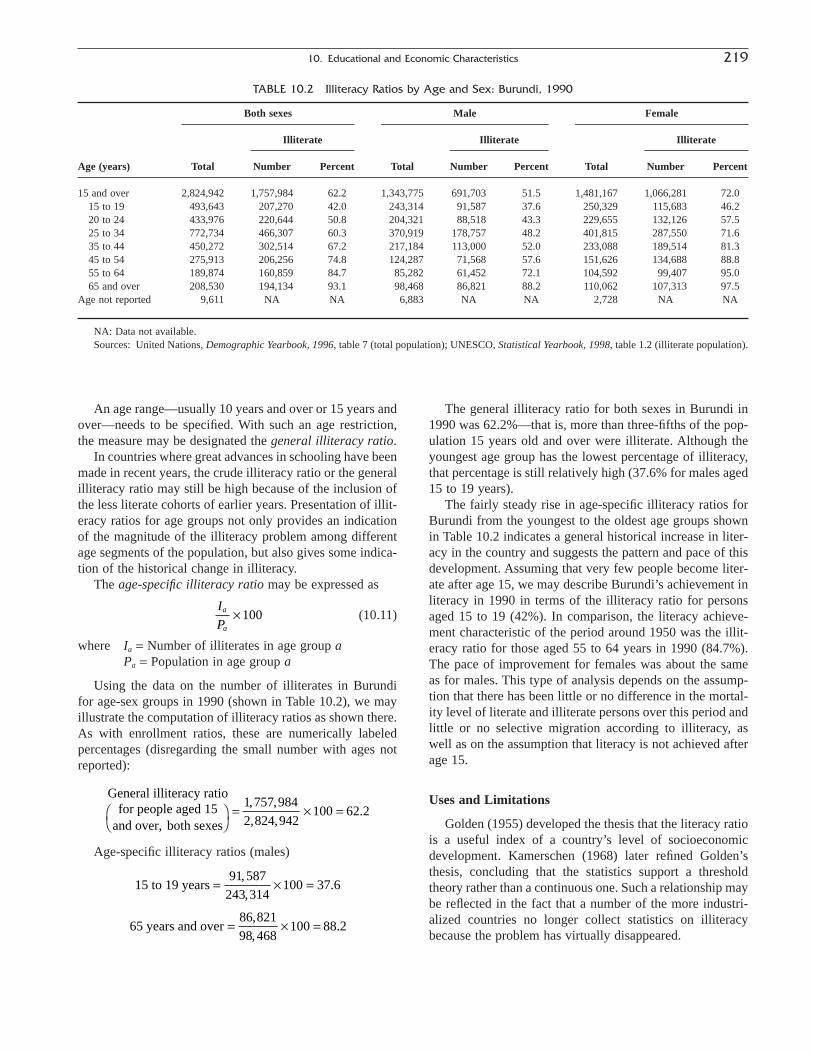
An age range—usually 10 years and over or 15 years andover—needs to be specified. With such an age restriction,the measure may be designated the general illiteracy ratio.
In countries where great advances in schooling have beenmade in recent years, the crude illiteracy ratio or the generalilliteracy ratio may still be high because of the inclusion ofthe less literate cohorts of earlier years. Presentation of illit-eracy ratios for age groups not only provides an indicationof the magnitude of the illiteracy problem among differentage segments of the population, but also gives some indica-tion of the historical change in illiteracy.
The age-specific illiteracy ratio may be expressed as
(10.11)
where Ia = Number of illiterates in age group aPa = Population in age group a
Using the data on the number of illiterates in Burundi for age-sex groups in 1990 (shown in Table 10.2), we mayillustrate the computation of illiteracy ratios as shown there.As with enrollment ratios, these are numerically labeled percentages (disregarding the small number with ages notreported):
Age-specific illiteracy ratios (males)
65 years and over = ¥ =86 82198 468
100 88 2,,
.
15 to 19 years = ¥ =91 587
243 314100 37 6
,,
.
General illiteracy ratiofor people aged 15
and over, both sexesÊË
ˆ¯
= ¥ =1 757 9842 824 942
100 62 2, ,, ,
.
I
Pa
a
¥ 100
The general illiteracy ratio for both sexes in Burundi in1990 was 62.2%—that is, more than three-fifths of the pop-ulation 15 years old and over were illiterate. Although theyoungest age group has the lowest percentage of illiteracy,that percentage is still relatively high (37.6% for males aged15 to 19 years).
The fairly steady rise in age-specific illiteracy ratios forBurundi from the youngest to the oldest age groups shownin Table 10.2 indicates a general historical increase in liter-acy in the country and suggests the pattern and pace of thisdevelopment. Assuming that very few people become liter-ate after age 15, we may describe Burundi’s achievement inliteracy in 1990 in terms of the illiteracy ratio for personsaged 15 to 19 (42%). In comparison, the literacy achieve-ment characteristic of the period around 1950 was the illit-eracy ratio for those aged 55 to 64 years in 1990 (84.7%).The pace of improvement for females was about the sameas for males. This type of analysis depends on the assump-tion that there has been little or no difference in the mortal-ity level of literate and illiterate persons over this period andlittle or no selective migration according to illiteracy, as well as on the assumption that literacy is not achieved afterage 15.
Uses and Limitations
Golden (1955) developed the thesis that the literacy ratiois a useful index of a country’s level of socioeconomicdevelopment. Kamerschen (1968) later refined Golden’sthesis, concluding that the statistics support a thresholdtheory rather than a continuous one. Such a relationship maybe reflected in the fact that a number of the more industri-alized countries no longer collect statistics on illiteracybecause the problem has virtually disappeared.
10. Educational and Economic Characteristics 219
TABLE 10.2 Illiteracy Ratios by Age and Sex: Burundi, 1990
Both sexes Male Female
Illiterate Illiterate Illiterate
Age (years) Total Number Percent Total Number Percent Total Number Percent
15 and over 2,824,942 1,757,984 62.2 1,343,775 691,703 51.5 1,481,167 1,066,281 72.015 to 19 493,643 207,270 42.0 243,314 91,587 37.6 250,329 115,683 46.220 to 24 433,976 220,644 50.8 204,321 88,518 43.3 229,655 132,126 57.525 to 34 772,734 466,307 60.3 370,919 178,757 48.2 401,815 287,550 71.635 to 44 450,272 302,514 67.2 217,184 113,000 52.0 233,088 189,514 81.345 to 54 275,913 206,256 74.8 124,287 71,568 57.6 151,626 134,688 88.855 to 64 189,874 160,859 84.7 85,282 61,452 72.1 104,592 99,407 95.065 and over 208,530 194,134 93.1 98,468 86,821 88.2 110,062 107,313 97.5
Age not reported 9,611 NA NA 6,883 NA NA 2,728 NA NA
NA: Data not available.Sources: United Nations, Demographic Yearbook, 1996, table 7 (total population); UNESCO, Statistical Yearbook, 1998, table 1.2 (illiterate population).

A question on the ability to read and write is obviouslysubject to a variety of interpretations, and the collection ofilliteracy data in a census may be handled with varyingdegrees of conscientiousness relative to any official stan-dard. In the case of educational level, an 8-year primary-school program in one country cannot always be comparedwith an 8-year primary-school program in another country.In sum, demographic statistics on education, apart frominadequacies of the data, reflect the effects of a variety ofcultural, social, and psychological factors that must be con-sidered when analyzing the data. All these considerationsnecessitate interpretation of published statistics on educationin only general terms.
For example, one might expect an understatement of illiteracy because some people are reluctant to admit they donot know how to read or write. However, in a country withhigh levels of illiteracy, there is presumably no real hesita-tion in classifying oneself as illiterate. On the other hand, ina country with a high level of literacy, people who are illiter-ate may be very hesitant to identify themselves as such.
Where tests of reading and writing ability have beenadministered in addition to a simple inquiry on illiteracy, thegeneral accuracy of the simple inquiry has been confirmed.3
Analysis of the reported illiteracy of age cohorts in asequence of censuses in the United States showed a highdegree of consistency from census to census (Folger and Nam, 1967). It would be helpful, however, to have more thorough and systematic evaluations of reported dataon illiteracy for a variety of countries.
Educational Attainment
Educational attainment is a critical measure of education,particularly in more developed countries. As the economiesof these countries became more technically sophisticated,their workforce needs moved beyond basic literacy. As a result, more detailed measures of educational perform-ance—measures that reflect what people get out of the educational system—have become more widely used.
According to the United Nations, educational attainmentis the highest level of education completed in the countrywhere the education was received (United Nations, 1998).It recommends that educational attainment be includedamong the basic areas of census inquiry and that data on the subject be collected for all persons 5 years of age andolder.
Typically, educational attainment is measured not by thenumber of calendar years that a person has spent in school,
but by the highest grade or level that he or she was able tocomplete. If the person was educated in the school systemof another country and not in his or her country of presentresidence, it is necessary to convert that schooling into theequivalent highest grade completed in the country of presentresidence.
The inclusion of a question on educational attainment in the United States census dates back to 1940. From 1950through 1980, the census asked respondents about thehighest grade of school they had ever attended, followed bya supplementary question on whether the respondent fin-ished that highest grade. Research has shown that the inclu-sion of this supplementary question reduced the tendency toreport an unfinished grade as the highest grade completedand thus corrected for the upward bias that may haveoccurred in statistics calculated without the use of such a question. However, questions measuring the number ofyears of school completed increasingly did not correspondwith the actual degree attained, particularly beyond the highschool level, and specific degrees such as an associate or amaster’s degree could not be identified from the “highestgrade completed” inquiry (Kominski and Siegel, 1987,1993).
As a result, the 1990 and 2000 censuses asked respon-dents about the highest level of education they have completed (see Table 10.3). The change is especially no-ticeable in the categories for high school completion andbeyond. Whereas the “old” census questions measured individual years of schooling (e.g., 13 years completed), the1990 census question focuses on specific levels of degreecompletion (e.g., some college but no degree, associatedegree, or bachelor’s degree). These developments haveimplications for several measures; for example, it is nolonger possible to calculate the mean and median years ofschool completed. This change in measuring educationalattainment was also reflected in the Current PopulationSurvey (CPS) questionnaire beginning in 1992. See, forexample Figure 10.1, displaying CPS data for 1995.
For a long time inquiries were made about educationalattainment in the Current Population Survey only at irregu-lar intervals. Since 1964, however, the U.S. Census Bureauhas published an annual report on the educational attainmentof the population (Current Population Reports Series P20,Population Characteristics). In comparing decennial censusand CPS statistics on enrollment and educational attainmentfor subdivisions of the country, it should be borne in mindthat in the census, college students are counted where theyactually live while attending college, whereas the CPScounts unmarried students at their parental homes (seeChapter 4).
Measures
The measures of educational attainment considered here are taken from publications of the U.S. Census Bureau
220 O’Hare, Pollard, and Ritualo
3 Discussion of the accuracy of reports on literacy as well as gradationsof literacy can be found in S. S. Zarkhovic, 1954, “Sampling Control ofLiteracy Data,” Journal of the American Statistical Association, 49(267):510–519; and C. Windle, 1959, “The Accuracy of Census Literacy Statis-tics in Iran,” Journal of the American Statistical Association 54 (287):578–581.
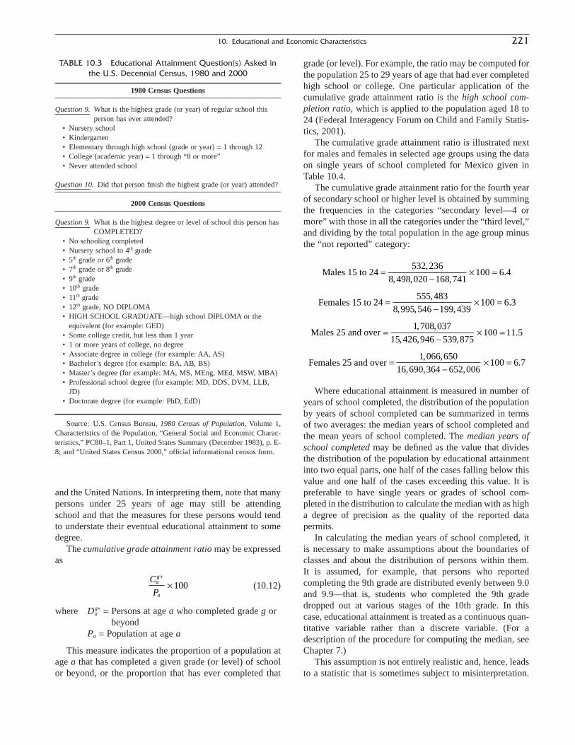
and the United Nations. In interpreting them, note that manypersons under 25 years of age may still be attending school and that the measures for these persons would tendto understate their eventual educational attainment to somedegree.
The cumulative grade attainment ratio may be expressedas
(10.12)
where Dag+ = Persons at age a who completed grade g or
beyondPa = Population at age a
This measure indicates the proportion of a population atage a that has completed a given grade (or level) of schoolor beyond, or the proportion that has ever completed that
C
Pag
a
+
¥ 100
grade (or level). For example, the ratio may be computed forthe population 25 to 29 years of age that had ever completedhigh school or college. One particular application of thecumulative grade attainment ratio is the high school com-pletion ratio, which is applied to the population aged 18 to24 (Federal Interagency Forum on Child and Family Statis-tics, 2001).
The cumulative grade attainment ratio is illustrated nextfor males and females in selected age groups using the dataon single years of school completed for Mexico given inTable 10.4.
The cumulative grade attainment ratio for the fourth yearof secondary school or higher level is obtained by summingthe frequencies in the categories “secondary level—4 ormore” with those in all the categories under the “third level,”and dividing by the total population in the age group minusthe “not reported” category:
Where educational attainment is measured in number ofyears of school completed, the distribution of the populationby years of school completed can be summarized in termsof two averages: the median years of school completed andthe mean years of school completed. The median years ofschool completed may be defined as the value that dividesthe distribution of the population by educational attainmentinto two equal parts, one half of the cases falling below thisvalue and one half of the cases exceeding this value. It ispreferable to have single years or grades of school com-pleted in the distribution to calculate the median with as higha degree of precision as the quality of the reported datapermits.
In calculating the median years of school completed, it is necessary to make assumptions about the boundaries ofclasses and about the distribution of persons within them. It is assumed, for example, that persons who reported completing the 9th grade are distributed evenly between 9.0and 9.9—that is, students who completed the 9th gradedropped out at various stages of the 10th grade. In this case, educational attainment is treated as a continuous quan-titative variable rather than a discrete variable. (For adescription of the procedure for computing the median, seeChapter 7.)
This assumption is not entirely realistic and, hence, leadsto a statistic that is sometimes subject to misinterpretation.
Females 25 and over =-
¥ =1 066 650
16 690 364 652 006100 6 7
, ,, , ,
.
Males 25 and over =-
¥ =1 708 037
15 426 946 539 875100 11 5
, ,, , ,
.
Females 15 to 24 =-
¥ =555 483
8 995 546 199 439100 6 3
,, , ,
.
Males 15 to 24 =-
¥ =532 236
8 498 020 168 741100 6 4
,, , ,
.
10. Educational and Economic Characteristics 221
TABLE 10.3 Educational Attainment Question(s) Asked inthe U.S. Decennial Census, 1980 and 2000
1980 Census Questions
Question 9. What is the highest grade (or year) of regular school thisperson has ever attended?
• Nursery school• Kindergarten• Elementary through high school (grade or year) = 1 through 12• College (academic year) = 1 through “8 or more”• Never attended school
Question 10. Did that person finish the highest grade (or year) attended?
2000 Census Questions
Question 9. What is the highest degree or level of school this person hasCOMPLETED?
• No schooling completed• Nursery school to 4th grade• 5th grade or 6th grade• 7th grade or 8th grade• 9th grade• 10th grade• 11th grade• 12th grade, NO DIPLOMA• HIGH SCHOOL GRADUATE—high school DIPLOMA or the
equivalent (for example: GED)• Some college credit, but less than 1 year• 1 or more years of college, no degree• Associate degree in college (for example: AA, AS)• Bachelor’s degree (for example: BA, AB, BS)• Master’s degree (for example: MA, MS, MEng, MEd, MSW, MBA)• Professional school degree (for example: MD, DDS, DVM, LLB,
JD)• Doctorate degree (for example: PhD, EdD)
Source: U.S. Census Bureau, 1980 Census of Population, Volume 1,Characteristics of the Population, “General Social and Economic Charac-teristics,” PC80–1, Part 1, United States Summary (December 1983), p. E-8; and “United States Census 2000,” official informational census form.
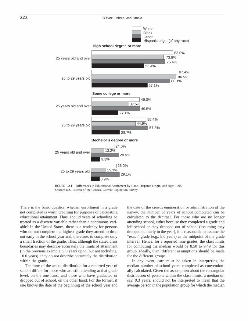
222 O’Hare, Pollard, and Ritualo
Hispanic origin (of any race)OtherBlackWhite
83.0%73.8%75.4%
53.4%
87.4%86.5%
80.1%57.1%
High school degree or more
Some college or more
Bechelor’s degree or more
25 years old and over
25 to 29 years old
25 years old and over
25 to 29 years old
25 years old and over
25 to 29 years old
49.0%
49.5%
55.4%44.9%
37.5%
27.1%
57.5%28.7%
24.0%13.2%
28.5%9.3%
26.0%15.3%
29.1%8.9%
FIGURE 10.1 Differences in Educational Attainment by Race, Hispanic Origin, and Age: 1995Source: U.S. Bureau of the Census, Current Population Survey
There is the basic question whether enrollment in a gradenot completed is worth crediting for purposes of calculatingeducational attainment. Thus, should years of schooling betreated as a discrete variable rather than a continuous vari-able? In the United States, there is a tendency for personswho do not complete the highest grade they attend to dropout early in the school year and, therefore, to complete onlya small fraction of the grade. Thus, although the stated classboundaries may describe accurately the limits of attainment(in the previous example, 9.0 years up to, but not including,10.0 years), they do not describe accurately the distributionwithin the grade.
The form of the actual distribution for a reported year ofschool differs for those who are still attending at that gradelevel, on the one hand, and those who have graduated ordropped out of school, on the other hand. For the former, ifone knows the date of the beginning of the school year and
the date of the census enumeration or administration of thesurvey, the number of years of school completed can be calculated to the decimal. For those who are no longerattending school, either because they completed a grade andleft school or they dropped out of school (assuming theydropped out early in the year), it is reasonable to assume the“exact” grade (e.g., 9.0 years) as the midpoint of the gradeinterval. Hence, for a reported nine grades, the class limitsfor computing the median would be 8.50 to 9.49 for thisgroup. Ideally, then, different assumptions should be madefor the different groups.
In any event, care must be taken in interpreting themedian number of school years completed as convention-ally calculated. Given the assumption about the rectangulardistribution of persons within the class limits, a median of,say, 9.3 years, should not be interpreted to mean that theaverage person in the population group for which the median
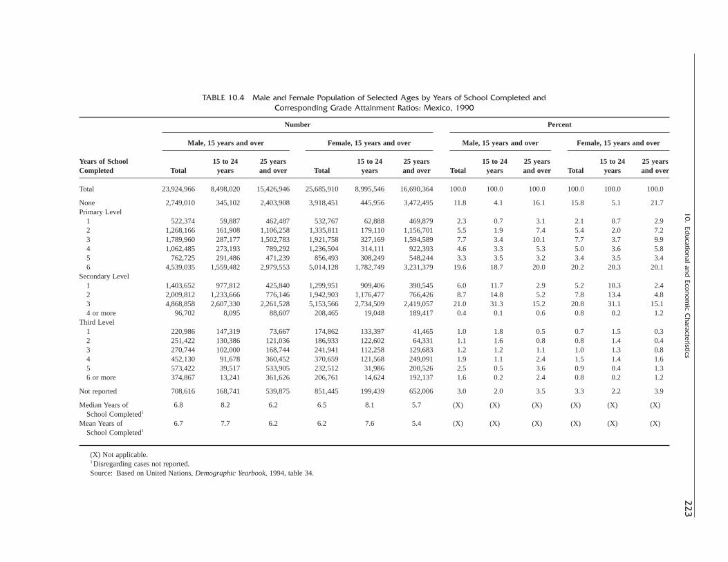
10.Ed
ucational and Econom
ic Characteristics
223
TABLE 10.4 Male and Female Population of Selected Ages by Years of School Completed andCorresponding Grade Attainment Ratios: Mexico, 1990
Number Percent
Male, 15 years and over Female, 15 years and over Male, 15 years and over Female, 15 years and over
Years of School 15 to 24 25 years 15 to 24 25 years 15 to 24 25 years 15 to 24 25 yearsCompleted Total years and over Total years and over Total years and over Total years and over
Total 23,924,966 8,498,020 15,426,946 25,685,910 8,995,546 16,690,364 100.0 100.0 100.0 100.0 100.0 100.0
None 2,749,010 345,102 2,403,908 3,918,451 445,956 3,472,495 11.8 4.1 16.1 15.8 5.1 21.7Primary Level
1 522,374 59,887 462,487 532,767 62,888 469,879 2.3 0.7 3.1 2.1 0.7 2.92 1,268,166 161,908 1,106,258 1,335,811 179,110 1,156,701 5.5 1.9 7.4 5.4 2.0 7.23 1,789,960 287,177 1,502,783 1,921,758 327,169 1,594,589 7.7 3.4 10.1 7.7 3.7 9.94 1,062,485 273,193 789,292 1,236,504 314,111 922,393 4.6 3.3 5.3 5.0 3.6 5.85 762,725 291,486 471,239 856,493 308,249 548,244 3.3 3.5 3.2 3.4 3.5 3.46 4,539,035 1,559,482 2,979,553 5,014,128 1,782,749 3,231,379 19.6 18.7 20.0 20.2 20.3 20.1
Secondary Level1 1,403,652 977,812 425,840 1,299,951 909,406 390,545 6.0 11.7 2.9 5.2 10.3 2.42 2,009,812 1,233,666 776,146 1,942,903 1,176,477 766,426 8.7 14.8 5.2 7.8 13.4 4.83 4,868,858 2,607,330 2,261,528 5,153,566 2,734,509 2,419,057 21.0 31.3 15.2 20.8 31.1 15.14 or more 96,702 8,095 88,607 208,465 19,048 189,417 0.4 0.1 0.6 0.8 0.2 1.2
Third Level1 220,986 147,319 73,667 174,862 133,397 41,465 1.0 1.8 0.5 0.7 1.5 0.32 251,422 130,386 121,036 186,933 122,602 64,331 1.1 1.6 0.8 0.8 1.4 0.43 270,744 102,000 168,744 241,941 112,258 129,683 1.2 1.2 1.1 1.0 1.3 0.84 452,130 91,678 360,452 370,659 121,568 249,091 1.9 1.1 2.4 1.5 1.4 1.65 573,422 39,517 533,905 232,512 31,986 200,526 2.5 0.5 3.6 0.9 0.4 1.36 or more 374,867 13,241 361,626 206,761 14,624 192,137 1.6 0.2 2.4 0.8 0.2 1.2
Not reported 708,616 168,741 539,875 851,445 199,439 652,006 3.0 2.0 3.5 3.3 2.2 3.9
Median Years of 6.8 8.2 6.2 6.5 8.1 5.7 (X) (X) (X) (X) (X) (X)School Completed1
Mean Years of 6.7 7.7 6.2 6.2 7.6 5.4 (X) (X) (X) (X) (X) (X)School Completed1
(X) Not applicable.1 Disregarding cases not reported.Source: Based on United Nations, Demographic Yearbook, 1994, table 34.
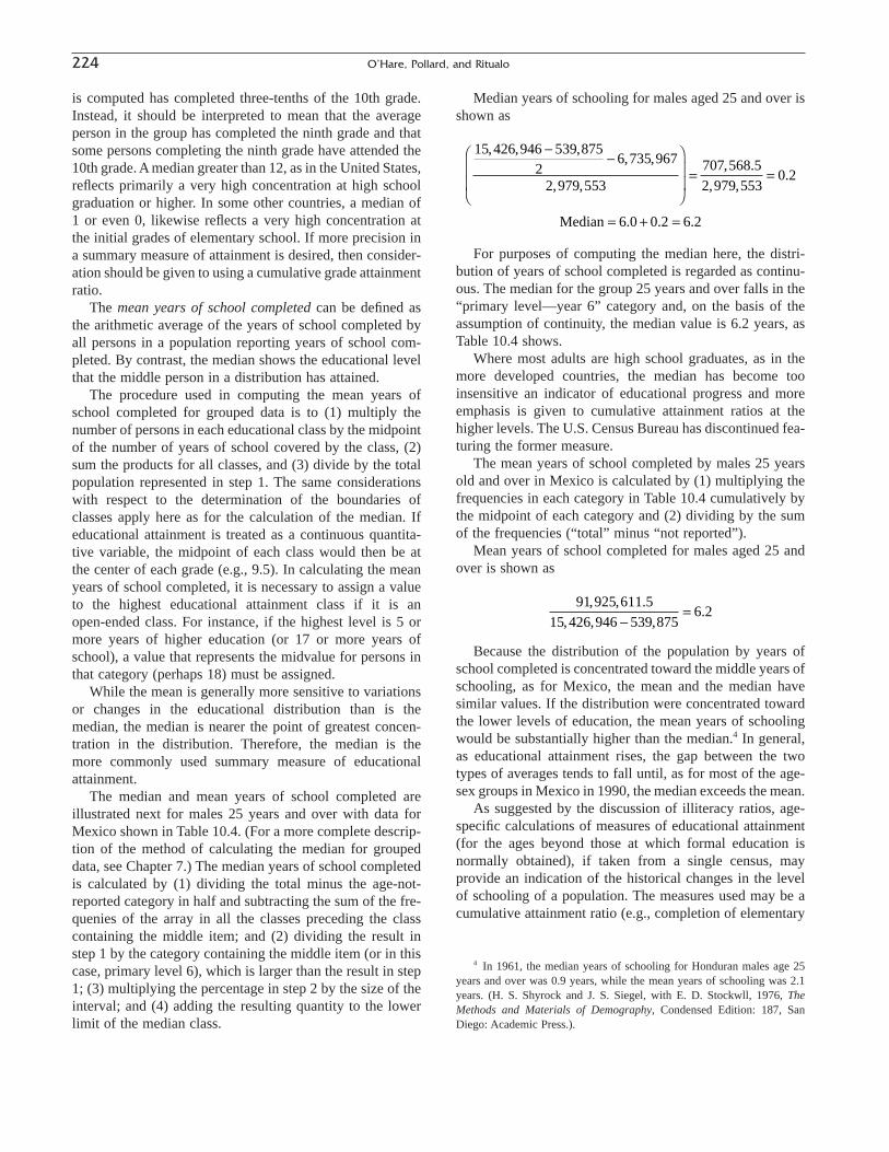
is computed has completed three-tenths of the 10th grade.Instead, it should be interpreted to mean that the averageperson in the group has completed the ninth grade and thatsome persons completing the ninth grade have attended the10th grade. A median greater than 12, as in the United States,reflects primarily a very high concentration at high schoolgraduation or higher. In some other countries, a median of1 or even 0, likewise reflects a very high concentration atthe initial grades of elementary school. If more precision ina summary measure of attainment is desired, then consider-ation should be given to using a cumulative grade attainmentratio.
The mean years of school completed can be defined asthe arithmetic average of the years of school completed byall persons in a population reporting years of school com-pleted. By contrast, the median shows the educational levelthat the middle person in a distribution has attained.
The procedure used in computing the mean years ofschool completed for grouped data is to (1) multiply thenumber of persons in each educational class by the midpointof the number of years of school covered by the class, (2)sum the products for all classes, and (3) divide by the totalpopulation represented in step 1. The same considerationswith respect to the determination of the boundaries ofclasses apply here as for the calculation of the median. Ifeducational attainment is treated as a continuous quantita-tive variable, the midpoint of each class would then be atthe center of each grade (e.g., 9.5). In calculating the meanyears of school completed, it is necessary to assign a valueto the highest educational attainment class if it is an open-ended class. For instance, if the highest level is 5 ormore years of higher education (or 17 or more years ofschool), a value that represents the midvalue for persons inthat category (perhaps 18) must be assigned.
While the mean is generally more sensitive to variationsor changes in the educational distribution than is themedian, the median is nearer the point of greatest concen-tration in the distribution. Therefore, the median is themore commonly used summary measure of educationalattainment.
The median and mean years of school completed areillustrated next for males 25 years and over with data forMexico shown in Table 10.4. (For a more complete descrip-tion of the method of calculating the median for groupeddata, see Chapter 7.) The median years of school completedis calculated by (1) dividing the total minus the age-not-reported category in half and subtracting the sum of the fre-quenies of the array in all the classes preceding the classcontaining the middle item; and (2) dividing the result instep 1 by the category containing the middle item (or in thiscase, primary level 6), which is larger than the result in step1; (3) multiplying the percentage in step 2 by the size of theinterval; and (4) adding the resulting quantity to the lowerlimit of the median class.
Median years of schooling for males aged 25 and over isshown as
For purposes of computing the median here, the distri-bution of years of school completed is regarded as continu-ous. The median for the group 25 years and over falls in the“primary level—year 6” category and, on the basis of theassumption of continuity, the median value is 6.2 years, asTable 10.4 shows.
Where most adults are high school graduates, as in themore developed countries, the median has become tooinsensitive an indicator of educational progress and moreemphasis is given to cumulative attainment ratios at thehigher levels. The U.S. Census Bureau has discontinued fea-turing the former measure.
The mean years of school completed by males 25 yearsold and over in Mexico is calculated by (1) multiplying thefrequencies in each category in Table 10.4 cumulatively bythe midpoint of each category and (2) dividing by the sumof the frequencies (“total” minus “not reported”).
Mean years of school completed for males aged 25 andover is shown as
Because the distribution of the population by years ofschool completed is concentrated toward the middle years ofschooling, as for Mexico, the mean and the median havesimilar values. If the distribution were concentrated towardthe lower levels of education, the mean years of schoolingwould be substantially higher than the median.4 In general,as educational attainment rises, the gap between the twotypes of averages tends to fall until, as for most of the age-sex groups in Mexico in 1990, the median exceeds the mean.
As suggested by the discussion of illiteracy ratios, age-specific calculations of measures of educational attainment(for the ages beyond those at which formal education isnormally obtained), if taken from a single census, mayprovide an indication of the historical changes in the levelof schooling of a population. The measures used may be acumulative attainment ratio (e.g., completion of elementary
91 925 611 515 426 946 539 875
6 2, , .
, , ,.
-=
Median = + =6 0 0 2 6 2. . .
15 426 946 539 8752
6 735 967
2 979 553707 568 52 979 553
0 2
, , ,, ,
, ,, .
, ,.
--Ê
Ë
ÁÁ
ˆ
¯
˜˜
= =
224 O’Hare, Pollard, and Ritualo
4 In 1961, the median years of schooling for Honduran males age 25years and over was 0.9 years, while the mean years of schooling was 2.1years. (H. S. Shyrock and J. S. Siegel, with E. D. Stockwll, 1976, TheMethods and Materials of Demography, Condensed Edition: 187, SanDiego: Academic Press.).
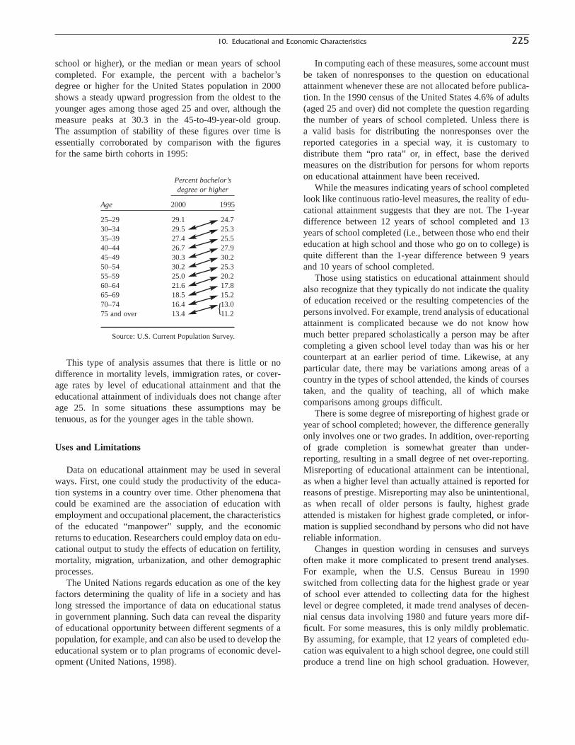
school or higher), or the median or mean years of schoolcompleted. For example, the percent with a bachelor’sdegree or higher for the United States population in 2000shows a steady upward progression from the oldest to theyounger ages among those aged 25 and over, although themeasure peaks at 30.3 in the 45-to-49-year-old group. The assumption of stability of these figures over time isessentially corroborated by comparison with the figures for the same birth cohorts in 1995:
In computing each of these measures, some account mustbe taken of nonresponses to the question on educationalattainment whenever these are not allocated before publica-tion. In the 1990 census of the United States 4.6% of adults(aged 25 and over) did not complete the question regardingthe number of years of school completed. Unless there is a valid basis for distributing the nonresponses over thereported categories in a special way, it is customary to distribute them “pro rata” or, in effect, base the derivedmeasures on the distribution for persons for whom reportson educational attainment have been received.
While the measures indicating years of school completedlook like continuous ratio-level measures, the reality of edu-cational attainment suggests that they are not. The 1-yeardifference between 12 years of school completed and 13years of school completed (i.e., between those who end theireducation at high school and those who go on to college) isquite different than the 1-year difference between 9 yearsand 10 years of school completed.
Those using statistics on educational attainment shouldalso recognize that they typically do not indicate the qualityof education received or the resulting competencies of thepersons involved. For example, trend analysis of educationalattainment is complicated because we do not know howmuch better prepared scholastically a person may be aftercompleting a given school level today than was his or hercounterpart at an earlier period of time. Likewise, at any particular date, there may be variations among areas of acountry in the types of school attended, the kinds of coursestaken, and the quality of teaching, all of which make comparisons among groups difficult.
There is some degree of misreporting of highest grade oryear of school completed; however, the difference generallyonly involves one or two grades. In addition, over-reportingof grade completion is somewhat greater than under-reporting, resulting in a small degree of net over-reporting.Misreporting of educational attainment can be intentional,as when a higher level than actually attained is reported forreasons of prestige. Misreporting may also be unintentional,as when recall of older persons is faulty, highest gradeattended is mistaken for highest grade completed, or infor-mation is supplied secondhand by persons who did not havereliable information.
Changes in question wording in censuses and surveysoften make it more complicated to present trend analyses.For example, when the U.S. Census Bureau in 1990switched from collecting data for the highest grade or yearof school ever attended to collecting data for the highestlevel or degree completed, it made trend analyses of decen-nial census data involving 1980 and future years more dif-ficult. For some measures, this is only mildly problematic.By assuming, for example, that 12 years of completed edu-cation was equivalent to a high school degree, one could stillproduce a trend line on high school graduation. However,
10. Educational and Economic Characteristics 225
Percent bachelor’s degree or higher
Age 2000 1995
25–29 29.1 24.730–34 29.5 25.335–39 27.4 25.540–44 26.7 27.945–49 30.3 30.250–54 30.2 25.355–59 25.0 20.260–64 21.6 17.865–69 18.5 15.270–74 16.4 13.075 and over 13.4 11.2
Source: U.S. Current Population Survey.
This type of analysis assumes that there is little or no difference in mortality levels, immigration rates, or cover-age rates by level of educational attainment and that the educational attainment of individuals does not change afterage 25. In some situations these assumptions may betenuous, as for the younger ages in the table shown.
Uses and Limitations
Data on educational attainment may be used in severalways. First, one could study the productivity of the educa-tion systems in a country over time. Other phenomena thatcould be examined are the association of education withemployment and occupational placement, the characteristicsof the educated “manpower” supply, and the economicreturns to education. Researchers could employ data on edu-cational output to study the effects of education on fertility,mortality, migration, urbanization, and other demographicprocesses.
The United Nations regards education as one of the keyfactors determining the quality of life in a society and haslong stressed the importance of data on educational status in government planning. Such data can reveal the disparityof educational opportunity between different segments of apopulation, for example, and can also be used to develop theeducational system or to plan programs of economic devel-opment (United Nations, 1998).
{

this is more difficult if one is trying to show trend data forreceipt of a post-high school degree, such as completion ofan associate’s degree. In the 1990 and 2000 censuses, datawere collected for persons who completed an associate’sdegree—a program that generally takes about 2 years ofschooling after completing high school. It is impossible,however, to identify associate’s degree holders using the1980 census data, because it is difficult to determine whetherpersons who completed 2 years of college education earnedan associate’s degree or completed the first 2 years of a bachelor’s degree program.
ECONOMIC CHARACTERISTICS
Economic Activity and Employment
Economic activity is vital to every society. How peopleorganize themselves around productive activity and thestratification processes that are associated with differentia-tion of labor are fundamental characteristics of a society.This section focuses on several dimensions of work and therewards of work (i.e., income and wealth).
Concepts and Definitions
Although all persons consume goods and services, onlypart of the population of a country is engaged in producingsuch goods and services. Most obviously, the youngest, theoldest, and the physically or mentally incapacitated do notengage in such economic activity because of an inability todo so. The manpower of a nation, then, is the totality ofpersons who could produce the goods and services if therewere a demand for their labors and they desired to partici-pate in such activity. The economically active (sometimesalso called the labor force or workforce) is that part of themanpower that actually is working or looking for work.5
At any given time, an economically active person may beeither employed or unemployed. (As we shall see, the dis-tinction is not always clear-cut; some of the employed maybe classified as underemployed.) Those not economicallyactive may be subdivided according to their major type ofactivity—for example, going to school or keeping house.The economically active also may be classified according to the nature of their current, last, or usual job (e.g., occupation, industry, status or class of worker, or place ofwork). Other characteristics relevant to the economicallyactive include the number of weeks worked in the past year,the number of hours worked in the past week or other
reference period, and, for the unemployed, the duration of unemployment.
The United Nations (1998) has recommended that censusinformation be collected that would allow persons to be classified according to type of activity—that is, either one’scurrent economic activity (as of a certain date) or one’susual economic activity (during an extended referenceperiod, such as the past 12 months). These data usually arecollected for persons at and above a minimum age, depend-ing on conditions in a specific country. For internationalcomparisons, the UN recommends that tabulations (at aminimum) distinguish between persons under age 15 andpersons aged 15 and older. In the United States, the monthlyCurrent Population Survey (CPS)—the major source of offi-cial statistics on the labor force—collects data on employ-ment for persons aged 15 and older. However, the officialUnited States definition of the labor force relates to ages 16and older.
Regardless of whether current or usual economic activ-ity is used, the United Nations (1998) has recommended thefollowing classification:
Economically active populationEmployedUnemployed
Not economically active populationStudentsHomemakersPension or capital income recipientsOthers
According to the International Labour Organisation’sCurrent International Recommendations on Labour Statis-tics (International Labour Organisation, 2000), the econo-mically active population “comprises all persons of eithersex who furnish the supply of labour for the production ofeconomic goods and services as defined by the UnitedNations system of national accounts and balances during aspecified time-reference period.” Included in this populationare persons in the civilian labor force and those who servein the armed forces. When compiling labor force data, somecountries (for example, the United States) show persons inthe armed forces in a separate category. In that way, armedforces personnel may be deducted from the total labor forcewhenever desirable for analytic purposes.
Within the economically active population, persons are categorized as either employed or unemployed. Theemployed population includes persons who either wereengaged in paid (wage and salary) employment or wereself-employed during the reference period. The employedalso include persons with a job or business enterprise, butwho were temporarily not at work due to illness, vacation,or some other specific reason. The unemployed population,by contrast, includes all persons who were without work butwere available for work, and had taken specific steps to seek
226 O’Hare, Pollard, and Ritualo
5 See also A. J. Jaffe and C. D. Stewart, 1951, Manpower Resourcesand Utilization, chapter 2, “Definitions and Concepts,” and chapter 3,“Socio-Economic Development and the Working Force” (New York: JohnWiley & Sons).

work during the reference period. (In many less developedcountries, the criterion of actively seeking work often isrelaxed to suit national circumstances.) Unemployedpersons include persons without work but who have madearrangements to work or become self-employed after the reference period, and they may include persons who havebeen temporarily laid off from their regular jobs. TheUnited Nations recommends that data on the unemployeddistinguish first-time job seekers and those persons onlayoff. It is important to recognize that those who arewithout a job, but are not seeking employment, are notincluded in the unemployed category under this definition.This latter group includes those who are sometimes referredto as “discouraged workers.”
The economically inactive population—those persons ofa minimum age not meeting any of the preceding charac-teristics during the reference period—consists of three maingroups plus a residual category. Students are persons whoattend any regular public or private institution for system-atic instruction toward a diploma or degree. Homemakersare persons (either male or female) who are responsible forhousehold duties in their own home. Pension or capitalincome recipients receive income from property, invest-ments, pensions, or royalties. These persons are oftenelderly. The residual, or “other” category, includes thosepersons receiving public assistance or private support, vol-unteers, and other economically inactive persons who do not fall into the other three categories. (Students, home-makers, and pension or capital income recipients may also be classified as economically active if they meet thecriteria for employed or unemployed during the referenceperiod.)
The Labor Force and the Usually Active Population
As mentioned earlier, the term economic activity can referto either the currently active population (indicated also bythe term “the labor force”) or the usually active population.The essence of all these terms involves the reference to time and the conduct of an activity from which the personderives, or attempts to derive, pay, profit, or family gain. Themeasurement of usual activity, based on a longer referenceperiod such as past 12 months, is most useful when tryingto include seasonal employment or in countries where alarge proportion of the population participates in subsistencefarming and cash cropping. The converse of the economi-cally active population and the usually active population arethe population not currently active and the population notusually active, respectively.
The collection procedures in the monthly Current Popu-lation Survey (CPS), the official source of U.S. labor forcestatistics, illustrate the labor force concept defined earlier.The CPS asks all persons aged 15 and over, excludinginmates of institutions and members of the armed forcesliving on a military installation, whether they worked for pay
or profit during a specified week. Those who did so are clas-sified as employed. Also classified as employed are thosepersons who had a job or business during the specified weekbut were absent from it because of vacation, illness, orrelated reasons. Persons who did not work for reasons otherthan those specified earlier were asked whether they soughtwork for pay or profit during the past four weeks and wereavailable to take a job if offered. Those who answered yesto both questions are classified as unemployed. Also classi-fied as unemployed are those persons who were on layofffrom their job and expecting recall—regardless of whetheror not they had actively sought work in the previous fourweeks. All persons not meeting the criteria for classificationas employed or unemployed are classified as not in the laborforce (U.S. Census Bureau, 1994).
It is easiest to determine economic activity in a countryor other area where practically everyone receives monetaryremuneration for his or her labors. In situations wheremoney does not change hands, such as in a subsistenceeconomy or for self-employed persons, it can often be verydifficult to decide who is and who is not economicallyactive.
Job Characteristics
Three items of information that describe the economi-cally active population are usually obtained when a censusor sample survey is conducted. These are occupation, indus-try, and status in employment (for example, employee oremployer).
According to the United Nations recommendations forpopulation and housing censuses, “occupation refers to thetype of work done during the time-reference period by the person employed (or the type of work done previously,if the person is unemployed), irrespective of the industry orthe status in employment in which the person should be clas-sified” (United Nations, 1998, p. 85). Examples of occupa-tions are economist, secretary, vegetable grower, lawyer,dentist, and garbage collector.
Specific occupations are frequently consolidated incensus and survey tabulations into conventionally definedbroad groups. This often happens in the presentation ofoccupation statistics where the number of cases is small, asin the case of data for small areas, cross-classifications withother economic, social, and demographic variables (such asrace and educational level), and data based on samplesurveys.
In the United States, the Standard Occupational Classifi-cation (SOC) system is the universal occupational classifi-cation system used by all federal government agencies thatcollect occupation data. While data on occupation has beencollected since the 1850 census of population, the SOC wasfirst introduced in 1977. The SOC has undergone periodicrevisions to accommodate new occupations—for example,computer software engineer, environmental engineer, and
10. Educational and Economic Characteristics 227
environmental scientist and specialist (including health). Itwas designed to cover all occupations for which work is performed for pay or profit, and to encourage all federalagencies (and private industries) to use one occupationalclassification system that would allow for comparabilityacross data collection systems. The most recent revision ofthe SOC occurred in 1998; the Census Bureau used this revi-sion to classify responses from the 2000 decennial census.Household surveys and other data collection systems beganusing the revised SOC system soon afterward (Levine,Salmon, and Weinberg, 1999).
The SOC has four hierarchical classification levels,designed to accommodate the ability and interest thatvarious data collection efforts have for collecting and report-ing occupational statistics.6 The major occupation classifi-cation consists of 23 categories. This major groupingincludes 98 minor classes, which can be disaggregated into452 broad occupations and 822 detailed occupations (U.S.Bureau of Labor Statistics, 1999). The 23 major occupa-tional groups of the revised SOC are as follows:
1. Management Occupations2. Business and Financial Operations Occupations3. Computer and Mathematical Occupations4. Architecture and Engineering Occupations5. Life, Physical, and Social Science Occupations6. Community and Social Services Occupations7. Legal Occupations8. Education, Training, and Library Occupations9. Arts, Design, Entertainment, Sports, and Media
Occupations10. Healthcare Practitioners and Technical Occupations11. Healthcare Support Occupations12. Protective Service Occupations13. Food Preparation and Serving Related Occupations14. Building and Grounds Cleaning and Maintenance
Occupations15. Personal Care and Service Occupations16. Sales and Related Occupations17. Office and Administrative Support Occupations18. Farming, Fishing, and Forestry Occupations19. Construction and Extraction Occupations20. Installation, Maintenance, and Repair Occupations21. Production Occupations22. Transportation and Material Moving Occupations23. Military Specific Occupations
For purposes of international comparisons, the UnitedNations recommends that countries compile their data inaccordance with the latest revision of the International Stan-dard Classification of Occupations (ISCO-88) from the
International Labour Organisation (ILO).7 The UN recog-nizes, however, that many countries will want to use occu-pational classification systems that they believe are moreuseful for national purposes. Because of this fact, the recommendation also suggests that countries using a system other than the ISCO attempt to determine the ISCO equivalent to the occupational group of the specificcountries (United Nations, 1998). Brazil, for example, uses a modified occupational coding list, ClassificaçãoBrasileira de Ocupações (CBO), which was created usingISCO-68 as a basis. For ease of international comparison,the Ministry of Labor provides the “crosswalk” between theCBO, ISCO-68, and ISCO-88 (Ministerio Do Trabalho,1996).
In addition to information on the individual’s occupation,it also is very important to know the person’s industry ofemployment (industry), or the kind of establishment wherethe person is employed. As defined by the United Nations,“Industry refers to the activity of the establishment in whichan employed person worked during the time referenceperiod established for data on economic characteristics (orlast worked, if unemployed)” (United Nations, 1998, p. 86).The term “activity of the establishment” means the kinds of goods produced or services rendered. Goods-producingestablishments include, for example, a petroleum refinery, a pulp and paper factory, and a fruit or vegetable canningplant. Examples of service-providing establishments are ahospital, a bread and breakfast inn, a railroad, an elementaryschool, and a grocery store.
For purposes of international comparability, the UnitedNations recommends that “countries prepare tabulationsinvolving the industrial characteristics of active personsaccording to the most recent revision of the InternationalStandard Industrial Classification of All Economic Activities(ISIC) available at the time of the census” (United Nations,1998, p. 86). As is the case with occupations, many countries use industrial classification systems that theybelieve are more useful for national purposes. The UN therefore recommends that these countries follow the same guidelines mentioned earlier with regard to occupations(United Nations, 1998). ISIC revision 3 is the most currentindustry classification system released by the ILO and consists of four levels of classification and 17 broad categories.
From the 1930s through the 1990s, U.S. national statis-tical agencies used the Standard Industrial Classification(SIC) as the classification system for industries. The SICwas revised periodically as the nation’s economy changed,most recently in 1987. Since 1997, however, the United
228 O’Hare, Pollard, and Ritualo
7 For more information, see International Labour Organisation, 1990,International Standard Classification of Occupations (ISCO-88), Geneva:International Labour Office.
6 More information on the SOC system is available at the followingwebsite: http://stats.bls.gov/soc/socguide.htm.

States has replaced the SIC with the North American Industrial Classification System (NAICS), which also will be used by Canada and Mexico (Saunders, 1999). As the economic structure of North American countriesevolved from one based primarily on manufacturing to oneincreasingly dependent on services, many analysts con-sidered the categories used in the SIC to be outdated. Theimplementation of the North American Free Trade Act,designed to create a single economic zone between theUnited States, Canada, and Mexico, also increased theattractiveness of a system that would be comparable for allthree countries.
The NAICS system groups establishments according toa production-based concept. In other words, industries usingsimilar processes to produce goods and services are classi-fied in a single category. For example, newspaper publish-ers, radio stations, and data processing services—each ofwhich would have been classified under a different sectorunder the SIC—are now classified into a single broad infor-mation category (U.S. Census Bureau, 2000b). The NAICSsystem lists 1170 specific industries in 20 different sectors.These sectors are as follows:
1. Agriculture, Forestry, Fishing, and Hunting2. Mining3. Utilities4. Construction5. Manufacturing6. Wholesale Trade7. Retail Trade8. Transportation and Warehousing9. Information
10. Finance and Insurance11. Real Estate and Leasing12. Professional, Scientific, and Technical Services13. Management of Companies and Enterprises14. Administrative and Support and Waste Management
and Remediation Services15. Educational Services16. Health Care and Social Assistance17. Arts, Entertainment, and Recreation18. Accommodation and Food Services19. Other Services (except Public Administration)20. Public Administration
According to the United Nations, “status in employment8
refers to the status of an economically active person withrespect to his or her employment, that is to say, the type ofexplicit or implicit contract of employment with otherpersons or organizations that the person has in his/her job”(United Nations, 1998, p. 87).
The international recommendations for classification ofthis economic characteristic and the definition of the cate-gories follow:
(a) An employee is a person who works in a paid employment job,that is to say, a job where the explicit or implicit contract ofemployment gives the incumbent a basic remuneration that is independent of the revenue of the unit for which he or sheworks.
(b) An employer is a person who, working on his or her own economic account or with one or a few partners, holds a self-employment job and, in this capacity, has engaged on a contin-uous basis (including the reference period) one or more personsto work for him/her as employees.
(c) An own-account worker is a person who, working on his own account or with one or a few partners, holds a self-employment job, and has not engaged on a continuous basis anyemployees.
(d) A contributing family worker is a person who holds a self-employment job in a market oriented establishment operated by a related person living in the same household, and who cannot be regarded as a partner.
(e) A member of producers’ cooperative is a person who holds aself-employment job in an establishment organized as a coop-erative, in which each member takes part on an equal footingwith other members in determining the organization of produc-tion, sales and/or other work.
(f) Persons not classifiable by status include those economicallyactive persons for whom insufficient information is available,and/or cannot be included.
The United States and other countries often combine“employer” and “own account worker.” In addition, they donot show “member of producers’ cooperative” separately.This category has been common in socialist countries, suchas the former Soviet Union and the Soviet bloc countries. Inthe United States in particular, few workers would fall underthe category labeled “producers’ cooperative.”
Other Economic Characteristics of Workers
In addition to the basic questions on economic activitysuch as occupation, industry, and status, which are almostalways included in population censuses and sample surveysthat deal with economic characteristics of individuals, alarge number of other economic characteristics have beenincluded in various household surveys. Generally, popula-tion censuses can only accommodate questions on a few, if any, additional economic characteristics. However, manycountries currently conduct special labor force samplesurveys or economic sample surveys that often obtain information on additional economic characteristics of individuals. Examples of the additional items that may beincluded are as follows:
Number of hours worked in reference weekNormal or scheduled hours (or days) of work per weekType of enterprise (household or nonhousehold)
10. Educational and Economic Characteristics 229
8 The term used in the United States is “class of worker.”

Type of employing establishment (business, government,etc.)
Number of employees (asked of employers only)Secondary occupationSeasonal variations in time worked (asked of persons
employed during the entire previous year)Reason for part-time work during the reference week (only
asked of persons who worked fewer than 35 hours orfewer than five days)
Whether respondent looked for more hours of work (onlyasked of persons who worked fewer than 35 hours orfewer than five days)
Whether respondent wanted more hours of work (onlyasked of persons who worked fewer than 35 hours orfewer than five days)
Kind of job sought (asked of unemployed persons)Duration of unemploymentMigration for employment
Some of these items are designed to elicit information onthe problem of underemployment. Though neither concep-tually clear-cut nor easy to measure, underemployment isoften a much more serious problem in underdeveloped countries than is unemployment.
Between “full” employment and complete lack ofemployment (i.e., unemployment) lies a continuum ofworking behavior. Any amount of work at any point on thiscontinuum can be called “underemployment” (i.e., less than“full” employment). The International Labour Organisation(ILO) has defined the term as follows: “underemployment is the difference between the amount of work performed bypersons in employment and the amount of work they wouldnormally be able and willing to perform” (InternationalLabour Organisation, 1957, p. 17).
Recent ILO conferences of labor statisticians haveattempted to make this definition more concrete. As a result,the ILO has subdivided underemployment into two majorcategories: (1) visible, when persons involuntarily work parttime or for shorter periods than usual, and (2) invisible,when persons work full time but the work is inadequatebecause earnings are too low or the job does not permit exercise of one’s fullest skills.9
Despite much research on the measurement of underem-ployment, it has not been possible to develop procedures asprecise as those used in measuring employment and unem-ployment. In large degree this difficulty stems from the factthat there is no uniquely correct measure or definition of“full” employment. For example, in the United States, 35hours of work is considered a “full” week, but other coun-
tries use different thresholds. It is also impossible to dis-cover a uniquely correct procedure for ascertaining invisi-ble underemployment. The degree to which work isadequate or inadequate does not lend itself to easy defini-tion and measurement.
Labor mobility is any change in a person’s status thatinvolves his or her economic activity or, more specifically,his or her job. The most common forms of labor mobilityare as follows:
Entering or leaving the labor forceShifting employment statusChanging occupationChanging industryChanging class of worker (status)Changing employerMoving from one geographic area to another (this topic
also is addressed in Chapter 19, “Internal Migration.”
Information on labor mobility can be obtained by askingpersons about their economic characteristics at some pre-vious date. They can be asked about their employmentstatus, occupation, industry, and so forth. By comparing theprevious and current activity, changes in economic activitycan be noted. Information on gross changes (i.e., all move-ments) is obtained by such direct questioning. However,problems of memory recall, among other issues, have pre-vented much use of these questions. In countries like theUnited States, with a well-developed market economy, thelabor force is not a static aggregate that changes only as the result of population growth. On the contrary, the laborforce is subject to very high turnover, even in the short run.
Sources of Data
Information on economic activity is collected fromhouseholds in population censuses or sample surveys, orfrom establishments through regular reporting in certainkinds of administrative programs or through special samplesurveys. The data from sources other than householdspertain to employment and unemployment but not to theeconomically inactive population.
Available national census statistics on the characteristicsof the economically active population have been summa-rized in the UN Demographic Yearbook, most recently in1994 (Tables 26 to 34). The ILO publishes labor force statistics from numerous sources, such as national laborforce surveys and other related household surveys, in theannual Yearbook of Labour Statistics. In 1999, the ILObegan a new publication series, Key Indicators of the LabourMarket, which presents data and analyses of core labormarket indicators at the country level (ILO, 2002a).
The United Nations has made efforts to select, arrange,and edit the statistics from member countries in order toincrease international comparability. However, the number
230 O’Hare, Pollard, and Ritualo
9 Also see International Labour Organisation, 2000, “Resolution Concerning the Measurement of Underemployment and InadequateEmployment Situations (October 1998),” data accessed online atwww.ilo.org/public/english/bureau/stat/res/underemp.htm (July 23).

and nature of the footnotes on the tables in the DemographicYearbook give one indication of the degree to which this objective could not readily be accomplished. Countriesvary in terms of definitions, populations covered, and categories tabulated. Countries that conduct sample house-hold surveys on a recurrent basis tend to use concepts
and procedures similar, but not identical, to the UN recom-mendations.
As early as 1820, the U.S. census attempted to collect sta-tistics on the economically active population. However, it was the 1870 population census that provided the firstbody of data adequate for a sophisticated profile of the
10. Educational and Economic Characteristics 231
TABLE 10.5 Selected Questions on Economic Activity Asked in the 2000 United States Decennial Census
Questions on Labor Force Status
Question 21. LAST WEEK, did this person do ANY work for either payor profit? (Mark the “Yes” box even if the person worked only 1 hour, orhelped without pay in a family business or farm for 15 hours or more, orwas on active duty in the Armed Forces.)
• Yes• No—Skip to 25a
Question 25a. LAST WEEK, was this person on layoff from a job?
• Yes—Skip to 25c• No
b. LAST WEEK, was this person TEMPORARILY absent from a jobor business?• Yes, on vacation, temporary illness, labor dispute, etc.—Skip to
26• No—Skip to 25d
c. Has this person been informed that he or she will be recalled towork within the next 6 months OR been given a date to return towork?• Yes—Skip to 25e• No
d. Has this person been looking for work during the last 4 weeks?• Yes• No—Skip to 26
e. LAST WEEK, could this person have started a job if offered one,or returned to work if recalled?• Yes, could have gone to work• No, because of own temporary illness• No, because of all other reasons (in school, etc.)
Question 26. When did this person last work, even for a few days?• 1995 to 2000• 1994 or earlizer, or never worked—Skip to 31
Questions on Industry, Occupation, and Work Status
Question 27. Industry or Employer (Describe clearly this person’s chiefjob activity or business last week. If this person had more than one job,describe the one at which this person worked the most hours. If thisperson had no job or business last week, give the information for his/herlast job or business since 1995.)
a. For whom did this person work? (If now on active duty in theArmed Forces, mark box and print the branch of the ArmedForces.)(Name of company, business or other employer)
b. What kind of business or industry was this? (Describe the activityat location where employed—for example: hospital, newspaperpublishing, mail order house, auto repair, shop, bank)
c. Is this mainly• Manufacturing?• Wholesale trade?• Retail trade?• Other (agriculture, construction, service, government, etc.)?
Question 28. Occupationa. What kind of work was this person doing? (For example:
registered nurse, personnel manager, supervisor of orderdepartment, auto mechanic, accountant)
b. What were this person’s most important activities or duties? (Forexample: patient care, directing hiring policies, supervising orderclerks, repairing automobiles, reconciling financial records)
Question 29. Was this person• Employee in a PRIVATE-FOR-PROFIT company or business or of
an individual, for wages, salary, or commissions• Employee in a PRIVATE, NOT-FOR-PROFIT, tax exempt, or
charitable organization• Local GOVERNMENT employee (city, county, etc.)• State GOVERNMENT employee• Federal GOVERNMENT employee• SELF-EMPLOYED in own NOT INCORPORATED business,
professional practice, or farm• SELF-EMPLOYED in own INCORPORATED business,
professional practice, or farm• Working WITHOUT PAY in family business or farm
Question on Activity in Previous Year
Question 30a. LAST YEAR, 1999, did this person work at a job or business at
any time?• Yes• No—Skip to 31
b. How many weeks did this person work in 1999? (Count paidvacation, sick leave, and military service)
c. During the weeks WORKED in 1999, how many hours did thisperson usually work each week?
Usual hours worked each week __________
Source: U.S. Census Bureau, “United States Census 2000,” informational census questionnaire.

232 O’Hare, Pollard, and Ritualo
TABLE 10.6 Employment Status of the Civilian Noninstitutional Population 16 Years of Age andOver: United States, 1995 to April 2000 (Numbers in thousands)
Civilian labor force
EmployedUnemployed
Civilian PercentYear and noninstitutional Percentage of In Nonagricultural of labor Not in laborMonth population Number population Number agriculture industries Number force force
ANNUAL AVERAGES1995 198,584 132,304 66.6 124,900 3,440 121,460 7,404 5.6 66,2801996 200,591 133,943 66.8 126,708 3,443 123,264 7,236 5.4 66,6471997 203,133 136,297 67.1 129,558 3,399 126,159 6,739 4.9 66,8371998 205,220 137,673 67.1 131,463 3,378 128,085 6,210 4.5 67,5471999 207,753 139,368 67.1 133,488 3,281 130,207 5,880 4.2 68,385
MONTHLY DATA, SEASONALLY ADJUSTED1999:
April 207,236 139,086 67.1 133,054 3,341 129,713 6,032 4.3 68,150May 207,427 139,013 67.0 133,190 3,290 129,900 5,823 4.2 68,414June 207,632 139,332 67.1 133,398 3,330 130,068 5,934 4.3 68,300July 207,828 139,336 67.0 133,399 3,278 130,121 5,927 4.3 68,492August 208,038 139,372 67.0 133,530 3,234 130,296 5,842 4.2 68,666September 208,265 139,475 67.0 133,650 3,179 130,471 5,825 4.2 68,790October 208,483 139,697 67.0 133,940 3,238 130,702 5,757 4.1 68,786November 208,666 139,834 67.0 134,098 3,310 130,788 5,736 4.1 68,832December 208,832 140,108 67.1 134,420 3,279 131,141 5,688 4.1 68,724
2000:January 208,782 140,910 67.5 135,221 3,371 131,850 5,689 4.0 67,872February 208,907 141,165 67.6 135,362 3,408 131,954 5,804 4.1 67,742March 209,053 140,867 67.4 135,159 3,359 131,801 5,708 4.1 68,187April 209,216 141,230 67.5 135,706 3,355 132,351 5,524 3.9 67,986
Source: U.S. Bureau of Labor Statistics, Employment and Earnings 47: 5 (May 2000): table A-1.
labor force. In the 1890 and 1910 censuses, substantial revisions were made in the collection and classification procedures so that it is difficult to construct a comparableseries prior to 1930. In the late 1930s, the Works ProgressAdministration developed a standard set of labor force concepts and procedures that were used in the 1940 and sub-sequent population censuses and also in the monthly samplesurveys. These surveys have been taken continuously sincethe 1940s.
In the population censuses from 1940 through 1960,persons aged 14 and over (except for inmates of institutions)were asked about their activities in the week preceding thecensus. Starting with the 1970 census, the Census Bureaubegan asking the employment question for persons aged 15and over—a practice maintained in the monthly CurrentPopulation Survey (CPS) to this day. Table 10.5 shows thekey labor force and employment questions asked in the 2000decennial census. These questions were also asked ofpersons aged 15 and over. However, it should be noted thatmany agencies, such as the U.S. Bureau of Labor Statistics(BLS), report labor force data only for persons aged 16 andover.
The labor force concepts in the CPS are discussed inseveral reports (e.g., U.S. Census Bureau, 1994). The CPSobtains more detailed information on labor force status thandoes the decennial census. Data collected in the CPS makeit possible to analyze several aspects of the work life of theemployed, including full-time/part-time status, reasons forworking part time (i.e., whether for economic or noneco-nomic reasons), and reasons for not working during the pre-vious week. Similarly, the unemployed can be classified bysuch factors as duration of unemployment, occupation andindustry of their last job (if they had worked before), classof work sought (full-time or part-time work), and reason forunemployment. Based on their reported activity, personswho are not in the labor force can be classified as home-makers, students, and other types (including retired, unableto work, etc.). Analysis of these categories is useful forstudying the labor reserve and for making labor force projections.
Table 10.6 shows some of the regular statistics on laborforce and employment status from the CPS. The annualfigures represent averages of the monthly figures in a givenyear. Many monthly figures, including the ones in this table,

10. Educational and Economic Characteristics 233
10 More information on the Current Employment Statistics program isavailable from the following website: www.bls.gov/ces.
TABLE 10.7 Occupation of Employed Persons 15 Years of Age and Over, by Sex and Marital Status: United States, 2001
Number in thousands Percent
Major Occupation Never NeverClass and Sex Total Married Married Widowed Divorced Total Married Married Widowed Divorced
Employed Males, 15 years 69,323 19,329 43,398 551 6,045 100.0 27.9 62.6 0.8 8.7and over
Executive, administrative, 10,007 1,557 7,586 104 759 100.0 15.6 75.8 1.0 7.6and managerial occupations
Professional specialty occupations 9,278 2,114 6,443 42 680 100.0 22.8 69.4 0.5 7.3Technical, sales, and 13,736 4,595 7,973 102 1,066 100.0 33.5 58.0 0.7 7.8
administrative supportoccupations
Service occupations 7,350 3,231 3,416 49 654 100.0 44.0 46.5 0.7 8.9Farming, forestry, and fishing 2,400 679 1,484 26 210 100.0 28.3 61.8 1.1 8.8
occupationsPrecision production, craft, 13,150 2,698 9,000 99 1,353 100.0 20.5 68.4 0.8 10.3
and repair occupationsOperators, fabricators, 13,402 4,452 7,496 129 1,324 100.0 33.2 55.9 1.0 9.9
and laborers
Employed Females, 61,089 15,827 35,504 2,071 7,687 100.0 25.9 58.1 3.4 12.615 years and over
Executive, administrative, 8,429 1,499 5,399 269 1,261 100.0 17.8 64.1 3.2 15.0and managerial occupations
Professional specialty occupations 10,716 2,368 6,914 253 1,181 100.0 22.1 64.5 2.4 11.0Technical, sales, and 24,988 6,837 14,324 828 2,999 100.0 27.4 57.3 3.3 12.0
administrative supportoccupations
Service occupations 10,800 3,704 5,254 493 1,349 100.0 34.3 48.6 4.6 12.5Farming, forestry, 588 103 414 27 44 100.0 17.5 70.4 4.6 7.5
and fishing occupationsPrecision production, craft, 1,146 209 731 30 177 100.0 18.2 63.8 2.6 15.4
and repair occupationsOperators, fabricators, 4,423 1,105 2,470 171 671 100.0 25.0 55.8 3.9 15.2
and laborers
Source: U.S. Census Bureau, March Current Population Survey, 1998.
are seasonally adjusted, because labor force statistics showsubstantial seasonal fluctuations.
In addition to the basic labor force statistics, the CensusBureau also reports labor force statistics that are cross-tabulated with a variety of demographic, social, and economic characteristics. Table 10.7, for example, showshow a key labor force characteristic (occupational category)can be used to study differentials in a demographic variable(marital status) among males and females.
Statistics from Establishments
The U.S. government compiles two major series ofemployment data from establishments. The CurrentEmployment Statistics program, a joint venture of the U.S.Bureau of Labor Statistics and state employment agencies,collects monthly employment, earnings, and payroll datafrom 400,000 establishments. The resulting data yield state
and national monthly totals on employment of nonfarmwage and salary workers.10
The other major series on employment comes from the Old Age and Survivors Insurance (OASI) records of the Social Security Administration (SSA). Each employercovered by Social Security provides quarterly informationabout each employee for the purpose of crediting theemployee’s pension fund. These records provide annual sta-tistics at the national, state, and county level on the numberof employees covered by the OASI. In addition, the SSAmaintains a Continuous Work History Sample of 1% ofcovered workers. Through this data source, it is possible foranalysts to study such issues as labor mobility (across estab-

234 O’Hare, Pollard, and Ritualo
lishments, industries, and geographic areas) and estimatedearnings over time.
Several other specialized series on employment are compiled. For example, the censuses of manufacturing,mining, and construction ask the respective establishmentsfor information on their employees. In addition, the U.S.Department of Agriculture collects data on farm labor. Probably the best known of the supplementary series is that of the unemployment insurance system. On a weeklybasis, each state reports the number of persons receivingunemployment insurance to the U.S. federal government.This arrangement provides regular information on thevolume of unemployment for counties, states, and thenation.
Establishment survey data typically differ from house-hold survey data in several ways. First, household surveyscover all persons aged 15 and over in the United States,while establishment surveys cover only a portion of thatpopulation. For example, the BLS’s Current EmploymentSeries program excludes the self-employed, unpaid familyworkers, and farmers; it also lacks good coverage forpersons employed in very small enterprises. Second, house-hold data on unemployment cover any persons who werelooking and available for work; the unemployment insur-ance series, by contrast, covers only persons who qualify forbenefits under the laws of their state.
Other differences concern the availability of demo-graphic and geographic information. In household surveys,for example, data are typically available for a variety of demographic and socioeconomic characteristics not generally available from establishment sources—age, sex, occupation, education, and so on. On the other hand, theestablishment reports contain intercensal data for small geographic areas while subnational data from the householdsurveys are limited in geographic detail. Certain types ofinformation—such as industry of employment, hoursworked, and earnings—may be obtained more accuratelyfrom the establishment reports than from the householdreports. Despite the differences, however, the two sources of statistics supplement each other enough so that the best analysis of employment trends can be made by the judicious use of data from both sources. Even so, the dataobtained from the population censuses and the Current Population Survey are generally sufficient for most analyticneeds, such as their use as benchmarks for labor force projections.
Measures
Economic Activity Ratios, Dependency Ratios, andReplacement Ratios
Many economic measures relate to the economicallyactive population, the labor force, or gainful workers,
depending on the type of data available; however, we willrefer to them generally as activity ratios. As with otherdemographic characteristics, crude, general, age-specific,and age-standardized ratios of economic activity may becomputed. It is customary to show most ratios separately formales and females.
The crude economic activity ratio (conventionally calleda “rate”) represents the number of economically activepersons as a percentage of the total population. It is alsoreferred to as the crude labor force participation ratio(“rate”) in countries where the labor force concept is appli-cable. For example, the crude economic activity ratio forSweden in 2000 is computed as follows:
Like all crude ratios, the age composition of the popula-tion greatly influences the crude activity age. This measureis useful primarily in comparisons where the analyst wishesto indicate simply the relative number of persons in a pop-ulation who are working, regardless of any other factorsinvolved. Examining changes in the crude economic activ-ity ratio over time allows analysts to highlight the effect ofdifferent levels of natural increase and migration on eco-nomic activity.
Unlike the crude activity ratio, the general economicactivity ratio is restricted to persons of working age. Morerefined than the crude ratio, this measure “controls” for the age structure of the population. We can calculate the generaleconomic activity ratio for persons aged 15 years and overin Sweden in 2000 as follows:
The minimum age for inclusion varies from country tocountry. For example, tabulations on economic activity havebeen shown for persons aged 12 and over in Uruguay andpersons aged 7 and over in Bolivia (United Nations, 1996).Because of this fact, analysts making cross-national com-parisons should consider the possibility that in many coun-tries, a large number of economically active children mightbe arbitrarily excluded from the enumerated labor forcebecause the minimal age may have been placed too high.Conversely, including an age group for whom the activityratio is very low—the activity ratio for persons aged 7 and8 in Bolivia was just 3.5% in 1990 (United Nations, 1996)—means a large number of economically inactive children willbe included in the denominator, which may distort the rate.
Both the crude and general activity ratios are usually cal-culated separately for males and females. When calculated
Populationeconomically active 15
Total population 15+
+¥ = ¥ =100
4 815 0007 201 000
100 66 9, ,, ,
.
Economicallyactive populationTotal population
¥ = ¥ =1004 815 0008 898 000
100 54 1, ,, ,
.
10. Educational and Economic Characteristics 235
in this fashion, they are termed sex-specific activity ratios.Sex-specific activity ratios are calculated for two differentreasons. First, the level of such ratios is usually much higherfor men than for women, although that usually is less so inmore developed countries. Second, variations in definitionsand operational procedures that most often affect measuresof economic activity have their greatest impact on figuresfor women because women’s attachment to the labor forceis more likely to be marginal and intermittent. Labor forceparticipation ratios for women vary much more than for men over time and across countries. Ratios for men are lesssubject to temporary or spurious variations than ratios forwomen, and international comparison of ratios for men areconsidered more valid by many analysts. However, thefemale labor force is quite often the most dynamic part ofthe labor force, as has been the case in the United Statessince the 1960s; therefore, researchers who restrict theiranalyses to the male labor force may be ignoring very impor-tant current and historical trends.
The same warning should be given to analysts whoconduct international and historical comparisons and restrictthemselves to figures on activities of men in the primeworking ages—20 to 59 years, for example. Just as withwomen, differences in definition and operating procedures(in the case of unpaid family workers or part-time workers,for example) often produce irregular or spurious variationsin activity ratios for the very young and the old. Althoughanalysts can make more valid comparisons by restrictingtheir comparisons to the prime working ages, they may be ignoring age groups that have experienced the majorchanges in economic activity.
For the reasons mentioned earlier, analysts usuallycompare activity ratios for specific age-sex groups. In fact,age-sex-specific activity ratios (called labor force participa-tion ratios when the labor force concept is used) are frequently the basic ratios that are studied in analyses of the economically active population. See for example, Figure 10.2.
An age-sex specific activity ratio is calculated using thefollowing formula:
(10.13)
where Peas = Economically active population in age-sex
group asPt
as = Total population in age-sex group as
For women 25 to 29 years of age in Canada in 1991, theratio is calculated as follows:
In addition to age and sex, one may calculate activityratios for population groups defined by various other
P
Pf
e
ft
25 29
25 29
884 8251 172 095
100 0 755 100 75 5-
-= ¥ = ¥ =
,, ,
. .
P
Pase
ast ¥ 100
characteristics, for example, educational attainment, maritalstatus, ethnicity, and economic level. The degree to whichthe activity ratios are made specific for such social and eco-nomic characteristics depends on two factors: the problemsbeing studied and the availability of adequate data.
An age-sex adjusted or standardized, activity ratio is theratio that would result for the “general” (i.e., adult) pop-ulation if the age-sex specific ratios for a given date or geographic area were weighted by a standard age-sex population distribution (see Chapter 12). Often the standardused is the national age-sex distribution for some specifieddate.
A common practice in demographic analysis is to calcu-late an age-dependency ratio from statistics on the age distribution of the population without regard to actual participation in economic activities. For example, the com-monly used age-dependency ratio (defined in Chapter 7),
(10.14)
considers all persons between ages 15 and 64 as producersand all persons under age 15 and over age 64 as dependents.This ratio is equivalent to the complement of the proportionof the total population 15 to 64 years old, a simple measureof age structure, but the term “dependency ratio” adds anaura of economic significance. This ratio is merely a measureof the role of age distribution in economic dependency.
The ratio of the economically inactive population to theeconomically active population is much more meaningful asa measure of economic dependency because it reflects notonly the area’s age-sex structure but also the economic activity participation ratios. Depending on which of thesemeasures one uses, the results can turn out to be quite dif-ferent, as data from Sweden’s 1990 census show. In the age-dependency ratio, the combined number of persons underage 15 and persons aged 65 and over (3,070,565) is dividedby the number of persons aged 15 to 64 (5,516,788), pro-ducing a ratio of 55.7 “age dependents” per 100 persons ofworking age. In the economic dependency ratio, by contrast,an economically inactive population (4,095,860), divided by the economically active population (4,491,493), yieldsthe economic dependency ratio of 91.2 inactive persons per100 active persons—more than one and one-half timeslarger than the age-dependency ratio.
The data in Table 10.8, which presents economic depend-ency ratios for selected countries, show how widely thismeasure can vary across countries. Several countries haveeconomic dependency ratios of less than 100—meaning thereare more economically active people than noneconomicallyactive people. Jordan, on the other hand, has an eco-nomic dependency ratio over 200. Even within the same economic/geographic class (for example, “developedeconomies”), nations often show enormous variation in thismeasure.
P P
P
t t
t
< +
-
+¥15 65
15 64
100

236 O’Hare, Pollard, and Ritualo
TABLE 10.8 Economic Dependency Ratios: Selected Countries, 2000
Economically Economically Economicinactive active dependency ratio
population population [(1)/(2)]*100 =Country and region (1) (2) (3)
DEVELOPED ECONOMIESFrance 22,335,514 17,574,760 127.1Spain 32,401,260 26,836,408 120.7Japan 58,727,298 68,369,016 85.9
TRANSITION ECONOMIESHungary 5,198,509 4,769,046 109.0Russian Federation 67,450,158 78,041,008 86.4Ukraine 24,294,341 25,273,826 96.1
ASIA AND THE PACIFICChina 512,190,491 762,942,375 67.1Indonesia 109,530,678 102,561,346 106.8Nepal 12,172,293 10,870,411 112.0
LATIN AMERICA AND THE CARIBBEANArgentina 22,035,369 14,996,445 146.9Brazil 91,159,608 79,246,672 115.0Jamaica 1,292,356 1,283,729 100.7
SUB-SAHARAN AFRICAEthiopia 35,127,261 27,780,527 126.4South Africa 25,280,845 18,028,352 140.2Tanzania 17,030,890 18,088,365 94.2
MIDDLE EAST AND NORTH AFRICAEgypt 42,094,707 25,789,769 163.2Jordan 3,346,903 1,566,212 213.7Morocco 18,098,596 11,779,807 153.6
Source: International Labour Organisation, 2002.
16 to 24 25 to 34 35 to 44 45 to 54 55 to 64 65 andolder
0
20
40
60
80
100
0
20
40
60
80
100Percent Percent
Men 1980Men 2000Women 1980Women 2000
Age
FIGURE 10.2 Labor force participation ratios for men and women. United States, 1980 and 2000Source: U.S. Bureau of Labor Statistics, Monthly Age Labor Review Nov. 2001, 26. Primary source is theCurrent Population Survey.
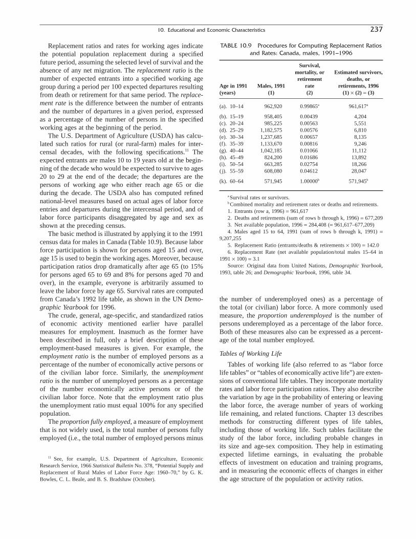
10. Educational and Economic Characteristics 237
Replacement ratios and rates for working ages indicatethe potential population replacement during a specifiedfuture period, assuming the selected level of survival and theabsence of any net migration. The replacement ratio is thenumber of expected entrants into a specified working agegroup during a period per 100 expected departures resultingfrom death or retirement for that same period. The replace-ment rate is the difference between the number of entrantsand the number of departures in a given period, expressedas a percentage of the number of persons in the specifiedworking ages at the beginning of the period.
The U.S. Department of Agriculture (USDA) has calcu-lated such ratios for rural (or rural-farm) males for inter-censal decades, with the following specifications.11 Theexpected entrants are males 10 to 19 years old at the begin-ning of the decade who would be expected to survive to ages20 to 29 at the end of the decade; the departures are thepersons of working age who either reach age 65 or dieduring the decade. The USDA also has computed refinednational-level measures based on actual ages of labor forceentries and departures during the intercensal period, and oflabor force participants disaggregated by age and sex asshown at the preceding census.
The basic method is illustrated by applying it to the 1991census data for males in Canada (Table 10.9). Because laborforce participation is shown for persons aged 15 and over,age 15 is used to begin the working ages. Moreover, becauseparticipation ratios drop dramatically after age 65 (to 15%for persons aged 65 to 69 and 8% for persons aged 70 andover), in the example, everyone is arbitrarily assumed toleave the labor force by age 65. Survival rates are computedfrom Canada’s 1992 life table, as shown in the UN Demo-graphic Yearbook for 1996.
The crude, general, age-specific, and standardized ratiosof economic activity mentioned earlier have parallel measures for employment. Inasmuch as the former havebeen described in full, only a brief description of theseemployment-based measures is given. For example, theemployment ratio is the number of employed persons as apercentage of the number of economically active persons orof the civilian labor force. Similarly, the unemployment ratio is the number of unemployed persons as a percentageof the number economically active persons or of the civilian labor force. Note that the employment ratio plus the unemployment ratio must equal 100% for any specifiedpopulation.
The proportion fully employed, a measure of employmentthat is not widely used, is the total number of persons fullyemployed (i.e., the total number of employed persons minus
the number of underemployed ones) as a percentage of the total (or civilian) labor force. A more commonly usedmeasure, the proportion underemployed is the number ofpersons underemployed as a percentage of the labor force.Both of these measures also can be expressed as a percent-age of the total number employed.
Tables of Working Life
Tables of working life (also referred to as “labor forcelife tables” or “tables of economically active life”) are exten-sions of conventional life tables. They incorporate mortalityrates and labor force participation ratios. They also describethe variation by age in the probability of entering or leavingthe labor force, the average number of years of working life remaining, and related functions. Chapter 13 describesmethods for constructing different types of life tables,including those of working life. Such tables facilitate thestudy of the labor force, including probable changes in its size and age-sex composition. They help in estimatingexpected lifetime earnings, in evaluating the probableeffects of investment on education and training programs,and in measuring the economic effects of changes in eitherthe age structure of the population or activity ratios.
TABLE 10.9 Procedures for Computing Replacement Ratiosand Rates: Canada, males, 1991–1996
Survival,mortality, or Estimated survivors,retirement deaths, or
Age in 1991 Males, 1991 rate retirements, 1996(years) (1) (2) (1) ¥ (2) = (3)
(a). 10–14 962,920 0.99865a 961,617a
(b). 15–19 958,405 0.00439 4,204(c). 20–24 985,225 0.00563 5,551(d). 25–29 1,182,575 0.00576 6,810(e). 30–34 1,237,685 0.00657 8,135(f). 35–39 1,133,670 0.00816 9,246(g). 40–44 1,042,185 0.01066 11,112(h). 45–49 824,200 0.01686 13,892(i). 50–54 663,285 0.02754 18,266(j). 55–59 608,080 0.04612 28,047
(k). 60–64 571,945 1.00000b 571,945b
a Survival rates or survivors.b Combined mortality and retirement rates or deaths and retirements.1. Entrants (row a, 1996) = 961,6172. Deaths and retirements (sum of rows b through k, 1996) = 677,2093. Net available population, 1996 = 284,408 (= 961,617–677,209)4. Males aged 15 to 64, 1991 (sum of rows b through k, 1991) =
9,207,2555. Replacement Ratio (entrants/deaths & retirements ¥ 100) = 142.06. Replacement Rate (net available population/total males 15–64 in
1991 ¥ 100) = 3.1Source: Original data from United Nations, Demographic Yearbook,
1993, table 26; and Demographic Yearbook, 1996, table 34.
11 See, for example, U.S. Department of Agriculture, EconomicResearch Service, 1966 Statistical Bulletin No. 378, “Potential Supply andReplacement of Rural Males of Labor Force Age: 1960–70,” by G. K.Bowles, C. L. Beale, and B. S. Bradshaw (October).

238 O’Hare, Pollard, and Ritualo
As mentioned, a measure that can be derived directlyfrom a table of working life is the expectation of activeworking life at birth or at any age. One may use workinglife tables to measure the aggregate number of entries into,as well as exits from, the labor force. Working life tablesalso measure the ages at which such events are likely to occur (Gendell, 1998; Gendell and Siegel, 1992). Theexpected active life at birth can be subtracted from lifeexpectancy at birth to give a measure of the expectation ofinactive life.
Factors in Analysis
In measuring economic activity and employment, thenature of the problem being studied determines the demo-graphic factors to be included. For almost any analysis,employment and unemployment data should be tabulatedand examined in age-sex detail. For specific problems, otherpopulation characteristics may be added.
For example, if the central problem is that of migrationof the labor force and the reasons behind the phenomenon,it would be necessary to consider labor force status andemployment status separately for migrants and nonmigrants.If the emphasis is on women in the labor force, then theanalysis could consider their marital status, the number andage of their children, the employment status and earnings ofthe husband, and such other population characteristics asmay seem relevant. If one were studying the relationship ofeducation to employment status and type of job, many of thecharacteristics already noted, plus school attendance andeducational attainment, would be relevant.
In countries containing both people living in a subsis-tence economy and those living in a market economy, it isimportant to distinguish the two sectors in the tabulations.This distinction may be approximated in terms of differentethnic groups, regions, urban-rural residence, or the majorcity compared with the balance of the country. In summary,many characteristics about which information is obtained ina census or sample household survey are useful in any analy-sis of economic activity. The primary problem toward whichthe study is directed will dictate the specific demographicand economic measures to be considered.
Projections of Economic Activity and Employment
Projections of economic activity (labor force) andemployment provide a very useful planning tool for busi-ness leaders and government officials. Projections allowemployers to gauge the future supply of and demand forlabor in their industry. This in turn allows them to makeinformed decisions for their enterprises. Government offi-cials also can use projections of labor force and employmentin making decisions. For example, if “demand” projectionsof the occupational distribution of the labor force show alarge expected increase in the need for technology-based
jobs in a country, educational administrators can tailor theircurriculum toward courses and programs that will prepareyoung people to take these jobs. Labor force projections alsohelp businesses and government to prepare for changes inthe composition of the workforce—for example, the changesin age, race, and education anticipated for the United Statespopulation in the first quarter of the 21st century.
Many international, national, and even some subnationalagencies prepare labor force and employment projections.The International Labor Organisation (ILO) periodicallyreleases world, regional, and national projections of the eco-nomically active population. In the United States, the U.S.Bureau of Labor Statistics (BLS) is the main source for suchprojections, preparing them every other year for the nation asa whole. BLS’s program also encompasses biennial pro-jections of employment with detail for industries and occu-pations. Using data from the BLS national projections, eachstate then produces its own occupational projections.
In the customary “prevalence ratio” method of projectingthe labor force, analysts need to project ratios of economicactivity (or labor force participation) as well as the size ofthe population. Specifically, projected age-sex–specificratios of labor force participation are applied to the corre-sponding figures on the age-sex distribution of the popula-tion. Analysts preparing projections for ethnically diversesocieties may wish to carry out the calculations for appro-priate race and ethnicity groups. The scope of the projec-tions is limited by the availability, detail, and quality ofcurrent estimates as well as the feasibility of projecting theseelements. (For more information about projections of thelabor force and employment, see Chapter 21.)
Uses and Limitations
Census and survey statistics on the economically activepopulation are especially useful in those countries that donot have a highly developed system of economic statisticsfrom establishment sources. Planning for economic devel-opment is an important use of such statistics, but it is onlyone of many uses. Labor force statistics provide much of thedescription of a nation’s or a region’s human resources. Statistics on occupational characteristics, particularly whencross-tabulated with educational attainment, provide aninventory of skills available among the people of a country.The UN Handbook on Social Indicators (United Nations,1989) describes these and other uses at various levels of economic development.
There are key definitional and methodological limitationsanalysts must consider when examining statistics on the economically active population. First, data on economiccharacteristics based on population censuses may not becomparable with data from household sample surveysbecause of differences in concepts, definitions, field proce-dures, and processing procedures such as editing rules. For
example, data from the U.S. decennial census differ slightlyfrom Current Population Survey data for reasons such as relative training of the interviewers, differences in the reference period, and sampling variability. In addition, suchdata from consecutive censuses, or even time series datafrom the same household survey, may not be comparable.Statistics from different sources or the same source but dif-ferent years may be affected by differences in definitions,question wording, coverage, time reference, and reportingerrors. Various reports from the U.S. Census Bureau (forexample, the P60 series of Current Population Reports) andthe U.S. Bureau of Labor Statistics (such as its monthlyjournal Employment and Earnings) contain considerableinformation about the strengths and limitations of the laborforce data.
The differences among countries in the definition of theeconomically active population may also adversely affectinternational comparisons on this subject. Countries vary intheir treatment of categories such as inmates of institutions,members of the armed forces, persons living in special areassuch as reservations, persons seeking work for the first time,persons engaged in part-time work, seasonal workers, andfamily workers. In some countries, all or parts of thesegroups are included among the inactive population, whileother countries treat persons in the same categories as partof the economically active population. Even in the samecountry, the treatment of these categories may have changedbetween censuses or may differ between a census and ahousehold sample survey, as alluded to earlier.
Generally, there are three major sources of noncompara-bility of census or survey data of which the analyst shouldbe aware. They concern variations in (1) the length of thetime period to which the questions on economic activityrefer, (2) the definition and inclusion of unpaid familyworkers, and (3) the lower age limit of persons covered byeconomic activity questions.
Variations in Length of Time Period
Some questions on economic activity refer to the employ-ment situation of the person on the day of the census orsurvey or during a brief period such as a specific week. In other cases, the question may refer to a longer period such as a month or year, whereas in still other cases (i.e.,under the gainful worker concept), the questions refer to theusual activity of the person without reference to any specifictime period. Such a variation in the time period affects the size of the economically active population, because more people would be considered as economically activeunder longer reference periods. The longer the referenceperiod, the more likely someone will have been economi-cally active at some point during the period. The length of a reference period also can affect the characteristics of the economically active population because a longer reference period is more likely to include marginal members
of the workforce (for example, seasonal workers, olderpersons, and full-time students). Such marginal members of the workforce are likely to have different demographicand socioeconomic characteristics from those of the “core”of the workforce, who would be included in a very short reference period.
Variation in Definition and Inclusion of Unpaid Family Workers
Another issue affecting comparability concerns variationin the classification of persons who are engaged in both economic activities and “noneconomic” activities (the latterincluding housekeeping or attending school). Perhaps themost important variation of this sort is the treatment ofunpaid family workers—that is, persons who work withoutpay in economic enterprises operated by other members oftheir households. The United Nations (1998) has recom-mended that unpaid family workers who contribute to anenterprise be included in the employed population on thesame basis as self-employed workers.
The question of receipt of money wages is a particularlyimportant factor affecting the classification of persons aseconomically active. In industrialized countries and in thelarge cities of most other countries, the large majority of the workers receive money, usually wages and salaries.However, in many parts of the world, particularly in the lessdeveloped countries, people engage in activities for theirown family’s consumption—such as subsistence agriculture,home improvement, milking animals, and processingfood—and do not work for money wages. Furthermore,because so many unpaid family workers (regardless of thetype of economy) are women, statistics on female laborforce participation are incomplete and often inaccurate(Anker, 1990). Variations in attitudes toward women andwork complicate the issue even more.
Variation in Age Group Covered by Statistics on Economic Activity
Countries differ in the age range of the population forwhich the questions on economic activity are to be asked.In almost every case, the variant is the lower age limit. Forexample, in the United States, Canada, and Chile, questionsof labor force participation are asked for persons 15 yearsof age and over (although in the United States tabulationsare often presented for persons 16 years of age and over),while in other countries, for example, Colombia, Costa Rica,Mexico, and Portugal, persons 12 years of age are askedabout their economic activity. In other countries such asBrazil, Indonesia, Namibia, and Pakistan, persons 10 yearsof age and over are asked about their economic activity, andin India the question is asked of persons 5 years of age andover (International Labour Office, 1990).
In order to permit international comparisons of data onthe economically active population, the United Nations
10. Educational and Economic Characteristics 239
recommends that “tabulations of economic characteristicsshould at least distinguish persons under 15 years of age andthose 15 years of age and over, and countries where theminimum school-leaving age is higher than 15 years andwhere there are economically active children below this ageshould endeavor to secure data on the economic character-istics of these children with a view to achieving internationalcomparability at least for persons 15 years of age and over”(United Nations, 1998, p. 79). In the United States, theminimum age for tabulation of decennial census data wasswitched from 14 years to 16 years in the 1970s, even thoughsupplementary labor force statistics were published for 14-and 15-year-olds for several years afterward.
Statistics on the workforce are subject to additional errors from various causes. Methods for measuring thesetypes of errors (described earlier in this book), such as comparisons of aggregate statistics, matching studies, andre-interview studies, are applicable to a population’s eco-nomic characteristics. Despite their limitations and theirerrors of measurement, labor force statistics have proven tobe highly useful. Even in less developed countries, errors in responses seem to be less of a problem than conceptualdifficulties.
Income, Wealth, and Poverty
Statistics on income, wealth, and poverty reflect the distribution of resources within a population or society.Although individual and family income have long been rec-ognized as having important relationships to many of thedemographic events and processes (such as mortality, fertil-ity, migration, and marriage), income as an item was onlyintroduced onto the U.S. population census schedules in1940. Income data are much more widely collected in peri-odic and regular household surveys. Wealth and poverty areeven more recent concepts. Measures of wealth havebecome useful because they often provide a more compre-hensive picture of economic well-being than income meas-ures do. As for poverty, few statistics were available beforethe 1960s, and data for international comparisons did notbecome available until the 1980s and 1990s.
Concepts and Definitions
Income is often meant to reflect the amount of resourcesreceived by individuals in a society. With regard to collect-ing data on it in censuses and surveys, the United Nationsstates, “income may be defined in terms of (a) monthlyincome in cash and/or in kind from work performed by eachactive person, or (b) the total annual income in cash and/orin kind of households regardless of source” (United Nations,1998, p. 88).
What actually does constitute income depends on theindividual society, however. In the United States, for
example, income includes salaries, wages, net earnings andprofits from one’s own business enterprise, and moneyearned from investments. Periodic payments received regu-larly from an inheritance or trust fund are also regarded asincome, as are the following: alimony, pensions, annuities,cash benefits (such as Social Security benefits, familyallowances, and unemployment benefits), sick pay, scholar-ships, and various other periodic receipts. On the other hand,the following items are usually not regarded as income:receipts from the sale of possessions, loan repayments,windfall gains, lump-sum inheritances, tax refunds, benefitson insurance policies, lump-sum compensation for injuryand other legal damages received, and related items. This isthe case even though the proceeds from these sources aresometimes spent on consumer goods and services.
Despite the lack of a universal standard regarding incomedata, there are some common principles that demographersshould be cognizant of when dealing with this subject. First, the reference period for income data could be an hour,a day, a week, a month, or a year. Each choice has costs and benefits. Hourly wages provide evidence of returns tolabor that may be masked by asking only about yearlyincome, but yearly income can overcome issues associatedwith seasonal work and provide a more realistic picture ofwell-being.
Second, to the extent that income is meant to reflectresources, cash, in-kind income, and noncash benefitsshould all be counted. However, in most contexts, only cashincome is included for practical reasons. The decision onwhether or not to include in-kind assistance or noncash ben-efits as money income can have important implications forcertain types of analysis. For example, most governmentmeans-tested assistance in the United States is provided asin-kind or noncash benefits, such as food stamps or medicalcoverage; therefore income measures that do not includenoncash benefits can overstate the level of poverty. Becausethe prevalence of noncash benefits varies between countries,one should make cross-national comparisons with caution(Blackburn, 1997).
There are three principal types of noncash benefits: thoseprovided by the government, those provided by an employer(such as health insurance and child care subsidies), and thoseobtained through “goods in exchange” (such as growingcrops for one’s personal consumption or obtaining goodsthrough barter). In subsistence economies, of course, practi-cally all income is in-kind income. Procedures for collectinginformation about income in these circumstances are neces-sarily very different from those used in cash economies. Inactual practice, censuses and surveys of many industrializedcountries ignore noncash income, because it is a small partof total income and very difficult to measure.
A third important decision regarding income measures iswhether to report pretax income or after-tax income. After-tax income is a better measure of disposable income (the
240 O’Hare, Pollard, and Ritualo

actual resources available to a family to purchase necessi-ties), but data on pretax income are much more readily avail-able. Because tax rates differ widely among countries, onemust be very careful in making cross-national comparisonsbased on pretax income.
It also is important to recognize the difference betweenearnings and income. Earnings represent money received inreturn for labor, but many types of income, such as interestfrom investments or government benefits, do not reflect areturn on work. Most of the income received by the elderly,for example, is not earned income.
Finally, the unit used to gather and report income isimportant. One can look at income of individuals, families,or households. According to U.S. Census Bureau definitions,there is more than one person in a family and sometimesmore than two generations in a household. Ideally, incomedata can be collected for each person in the household andthen added to produce totals and subtotals for units such ashouseholds, families, and married couples. A less satisfac-tory approach would be to obtain family or householdincome by asking directly for the total income received byall family (or household) members combined. Income ques-tions are rarely asked of children below working age, andadults living in certain types of group quarters, such as insti-tutions, are often excluded as well.
For international comparisons, statistics on the incomesof persons are most useful for males of working age and, toa lesser extent, for females of working age. The socioeco-nomic status of a dependent child or spouse is reflectedbetter by household and family income than by individualincome. Where the household contains one or more personsunrelated to the head of the household, income statistics forthe family are generally considered to be more useful thanthose for the entire household. However, this depends oncustoms and norms of the country involved; in largecomplex households it is often unclear how individualmembers of the household share income.
Wealth, typically measured as assets minus liabilities, rep-resents the resources available to a person or family. Theseresources can be invested to increase a person’s or family’seconomic well-being, for example, to purchase a house or tosend a child to college. They can also be drawn on in timesof need, for example, when family members experienceunemployment or prolonged illness. While there is often aclose association between income and wealth, the two con-cepts are very different. Wealth (or assets) is a more com-prehensive measure of economic well-being because itincludes resources not necessarily linked to current income.For example, wealth may include inheritance, savings, andappreciation of past investments that are unrelated to currentincome. In addition, wealth can reflect how much income hasbeen saved rather than spent over time.
Poverty status signals a lack of resources and a state of destitution that is usually associated with material hard-
ship. Poverty is often determined by comparing resources(usually income) with needs (often determined by familysize and composition), but it is sometimes determined as athreshold relative to the income distribution in a society. Forexample, families who earn less than half the median incomein a population are usually considered to be poor (Ruggles,1990).
Poverty is usually based on money income. The officialU.S. poverty threshold, established in the mid-1960s, com-pares the income of a family with a set of preestablishedthresholds based on family size and composition. The official definition of poverty in the United States is derivedby comparing the income for an individual or family to an assessment of needs based on family size and compo-sition. For example, the poverty income threshold in 2000 for a family of one adult under age 65 and two related children under age 18 was $13,874, while the threshold for a family of nine or more people including eight or morechildren was $33,291 (U.S. Census Bureau, 2001c). Someresearchers have argued that families or individuals may usesavings or borrow money to make purchases beyond theiryearly income and that consumption is a better gauge ofpoverty.
Sources of Data
Censuses and household surveys are the primary sourcesof income, wealth, and poverty data. However, data onincome may also be available from establishment records(e.g., payrolls), income tax returns, and Social Securityrecords. For example, the Statistics on Income (SOI) seriesfrom the U.S. Department of Treasury provides income datathat are based on tax returns.
Statistics from administrative records are of limited value to demographers, however, because few demographicand social characteristics are recorded in these sources, the entire population is not covered, and administrativerecords data do not cover all income sources. For example,there is generally a cutoff point for income below which a taxreturn does not have to be filed. Moreover, Social Securityrecords in the United States omit income above a legallyspecified amount and do not cover workers in certain indus-tries or types of establishments. Establishment payrolls are of value mainly as a source of information about hourly, weekly, or monthly earnings, and these data are generally available only in the form of averages. Income data from administrative records may be particularly usefulfor evaluating the quality of the data collected in householdinterviews.
Income data used for international comparisons are oftencollected through sample surveys and censuses. However,the United Nations (1998) has recognized the difficulty ofcollecting good income data in a census, especially data onin-kind benefits and income from self-employment and
10. Educational and Economic Characteristics 241
investments, and recommends that sample surveys be con-sidered for collecting this type of information. The dataarchives maintained by the Luxembourg Income Study(LIS) are derived from a set of such surveys. In 1980, theWorld Bank established the Living Standards MeasurementStudy, collecting detailed income and expenditure data inorder “to explore ways of improving the type and quality ofhousehold data collected by government statistical offices indeveloping countries” and “to develop new methods formonitoring progress in raising levels of living, to identifythe consequences for households of current and proposedgovernment policies, and to improve communicationsbetween survey statisticians, analysts, and policymakers”(Grosh and Glewwe, 1995, 1). Currently more than 40surveys have been completed, with additional surveys invarious stages of implementation.
The 1940 U.S. census was the first U.S. census to containa question on wage or salary income along with a questionon whether the person had received $50 or more from othersources in the preceding calendar year. Income from allsources was first collected in the 1950 census.
The 2000 decennial census form includes questions oneight possible sources of income:
1. Wages, salaries, commissions, bonuses or tips from alljobs
2. Self-employment income from own nonfarm businessesor farm businesses
3. Interest, dividends, net rental income, royalty income,or income from estates or trusts
4. Social Security or Railroad Retirement benefits5. Supplemental Security income6. Any public assistance or welfare payment from state or
local welfare offices7. Retirement, survivor, or disability pensions8. Any other sources of income received regularly such as
veteran’s payments, unemployment compensation, childsupport, or alimony
In the U.S. census, total income for a person, family, orhousehold is the sum of amounts reported for all of theseindividual sources, less any losses.
The U.S. Census Bureau’s Current Population Survey(CPS) first asked more detailed questions on income in 1945for the calendar year 1944. The income concepts used in theCPS agree very closely with those used in the contemporarydecennial census, although the CPS asks about many morespecific sources of income compared to the eight askedabout in the decennial census.
Family income and income of persons are associated witha variety of demographic, social, and economic characteris-tics. Table 10.10 presents the distribution of U.S. men andwomen according to age and income classes in 1998, as wellas the mean and median income for each age-sex combina-tion. The table shows that men have higher average incomes
than women at every age, and that average income increaseswith age until people reach the later working ages (with apeak at ages 45 to 54). Figure 10.3, also for the UnitedStates, shows how additional education enhances annualincome.
In general, data on wealth are scarce, mainly becauseacquiring this information requires a large series of rela-tively complex questions. To obtain accurate informationabout assets and debts requires a set of questions about manypossible sources of wealth. The accuracy of responses onthese types of questions is problematic because of the sen-sitive nature of this type of data, as well as the lack of knowl-edge or faulty recall on the part of respondents. For example,estimating the equity in a home owned by the respondentrequires that a person know (or estimate) the value of theproperty if it were to be sold and subtract the amount stillowed on the property.
The Survey of Income and Program Participation (SIPP)has provided estimates of wealth for American families forthe past 20 years. Reports can be found in the CensusBureau’s P70 series of Current Population Reports (“House-hold Economic Studies”). In addition, the ConsumerFinance Survey has provided some estimates of wealth.Private-sector vendors (e.g., Claritas) have provided someestimates of wealth for the United States based on statisti-cal models.
Poverty data typically come from surveys that collectdata on income, although they sometimes come from model-based estimates (i.e., estimates based on demographic or sta-tistical analysis) and surveys on expenditures. In the UnitedStates, major sources of poverty statistics are the decennialcensus, the CPS, and the SIPP. All three collect data that can be used for estimating poverty, but many other surveyscollect the information needed to construct measures ofpoverty. For example, both the National Survey ofAmerica’s Families and the Panel Study of Income Dynam-ics gather data to determine poverty status according to theofficial government definition.
Measures
Measures of income, wealth, and poverty depend on how the data have been collected and their availability toresearchers. Researchers who have access to exact dollaramounts from each respondent can easily construct manymeasures. Because of the sensitive nature of income data,however, such statistics often are gathered and reported interms of a set of income categories or ranges. Under thismethod, respondents are allowed to select an income rangerather than provide an exact amount. Generally, people aremore willing to provide information of this type than givetheir exact income. Moreover, respondents can usually esti-mate the range of their income accurately, even if they donot know the exact amount.
242 O’Hare, Pollard, and Ritualo
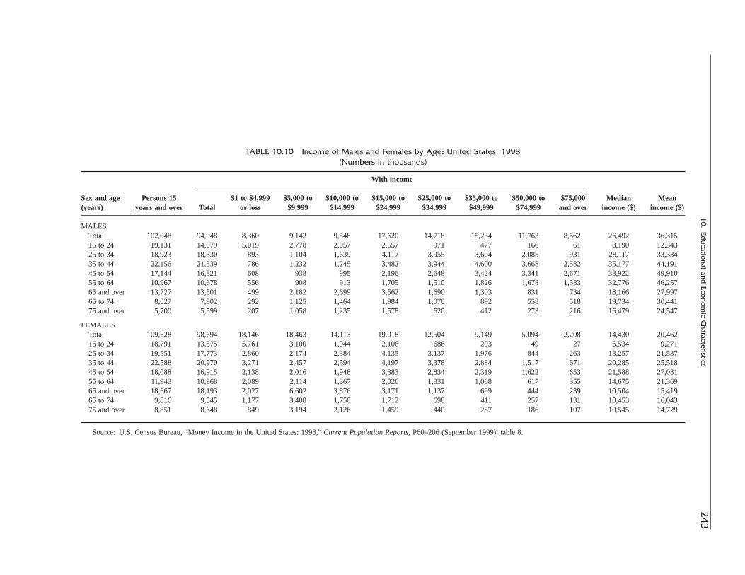
10.Ed
ucational and Econom
ic Characteristics
243
TABLE 10.10 Income of Males and Females by Age: United States, 1998(Numbers in thousands)
With income
Sex and age Persons 15 $1 to $4,999 $5,000 to $10,000 to $15,000 to $25,000 to $35,000 to $50,000 to $75,000 Median Mean(years) years and over Total or loss $9,999 $14,999 $24,999 $34,999 $49,999 $74,999 and over income ($) income ($)
MALESTotal 102,048 94,948 8,360 9,142 9,548 17,620 14,718 15,234 11,763 8,562 26,492 36,31515 to 24 19,131 14,079 5,019 2,778 2,057 2,557 971 477 160 61 8,190 12,34325 to 34 18,923 18,330 893 1,104 1,639 4,117 3,955 3,604 2,085 931 28,117 33,33435 to 44 22,156 21,539 786 1,232 1,245 3,482 3,944 4,600 3,668 2,582 35,177 44,19145 to 54 17,144 16,821 608 938 995 2,196 2,648 3,424 3,341 2,671 38,922 49,91055 to 64 10,967 10,678 556 908 913 1,705 1,510 1,826 1,678 1,583 32,776 46,25765 and over 13,727 13,501 499 2,182 2,699 3,562 1,690 1,303 831 734 18,166 27,99765 to 74 8,027 7,902 292 1,125 1,464 1,984 1,070 892 558 518 19,734 30,44175 and over 5,700 5,599 207 1,058 1,235 1,578 620 412 273 216 16,479 24,547
FEMALESTotal 109,628 98,694 18,146 18,463 14,113 19,018 12,504 9,149 5,094 2,208 14,430 20,46215 to 24 18,791 13,875 5,761 3,100 1,944 2,106 686 203 49 27 6,534 9,27125 to 34 19,551 17,773 2,860 2,174 2,384 4,135 3,137 1,976 844 263 18,257 21,53735 to 44 22,588 20,970 3,271 2,457 2,594 4,197 3,378 2,884 1,517 671 20,285 25,51845 to 54 18,088 16,915 2,138 2,016 1,948 3,383 2,834 2,319 1,622 653 21,588 27,08155 to 64 11,943 10,968 2,089 2,114 1,367 2,026 1,331 1,068 617 355 14,675 21,36965 and over 18,667 18,193 2,027 6,602 3,876 3,171 1,137 699 444 239 10,504 15,41965 to 74 9,816 9,545 1,177 3,408 1,750 1,712 698 411 257 131 10,453 16,04375 and over 8,851 8,648 849 3,194 2,126 1,459 440 287 186 107 10,545 14,729
Source: U.S. Census Bureau, “Money Income in the United States: 1998,” Current Population Reports, P60–206 (September 1999): table 8.
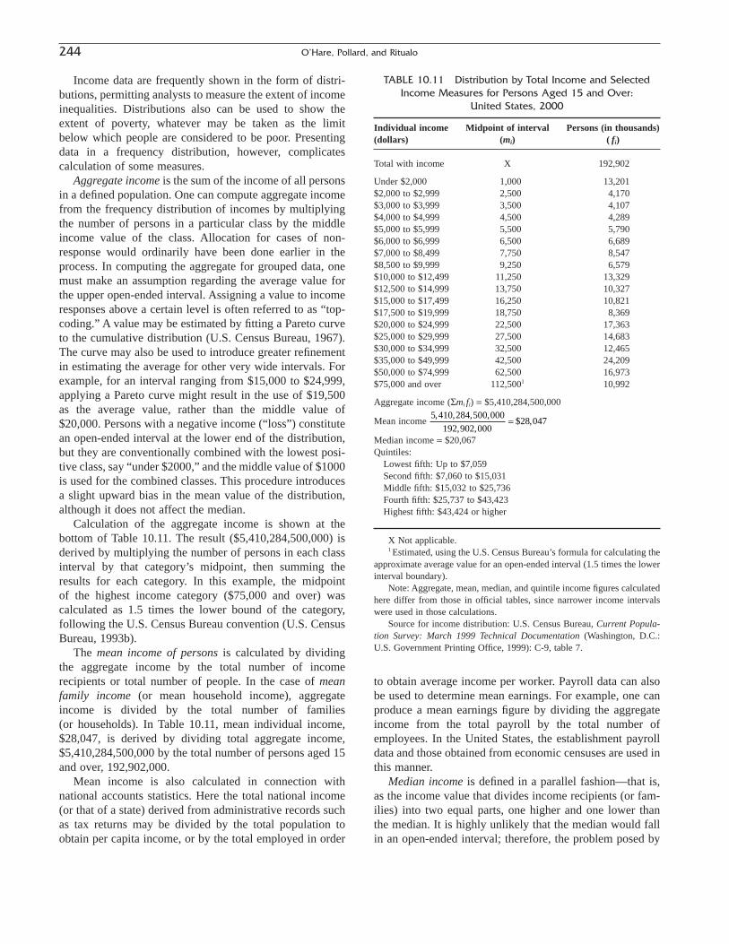
244 O’Hare, Pollard, and Ritualo
Income data are frequently shown in the form of distri-butions, permitting analysts to measure the extent of incomeinequalities. Distributions also can be used to show theextent of poverty, whatever may be taken as the limit below which people are considered to be poor. Presentingdata in a frequency distribution, however, complicates calculation of some measures.
Aggregate income is the sum of the income of all personsin a defined population. One can compute aggregate incomefrom the frequency distribution of incomes by multiplyingthe number of persons in a particular class by the middleincome value of the class. Allocation for cases of non-response would ordinarily have been done earlier in theprocess. In computing the aggregate for grouped data, onemust make an assumption regarding the average value forthe upper open-ended interval. Assigning a value to incomeresponses above a certain level is often referred to as “top-coding.” A value may be estimated by fitting a Pareto curveto the cumulative distribution (U.S. Census Bureau, 1967).The curve may also be used to introduce greater refinementin estimating the average for other very wide intervals. Forexample, for an interval ranging from $15,000 to $24,999,applying a Pareto curve might result in the use of $19,500as the average value, rather than the middle value of$20,000. Persons with a negative income (“loss”) constitutean open-ended interval at the lower end of the distribution,but they are conventionally combined with the lowest posi-tive class, say “under $2000,” and the middle value of $1000is used for the combined classes. This procedure introducesa slight upward bias in the mean value of the distribution,although it does not affect the median.
Calculation of the aggregate income is shown at thebottom of Table 10.11. The result ($5,410,284,500,000) isderived by multiplying the number of persons in each classinterval by that category’s midpoint, then summing theresults for each category. In this example, the midpoint of the highest income category ($75,000 and over) was calculated as 1.5 times the lower bound of the category, following the U.S. Census Bureau convention (U.S. CensusBureau, 1993b).
The mean income of persons is calculated by dividing the aggregate income by the total number of income recipients or total number of people. In the case of meanfamily income (or mean household income), aggregateincome is divided by the total number of families (or households). In Table 10.11, mean individual income,$28,047, is derived by dividing total aggregate income,$5,410,284,500,000 by the total number of persons aged 15and over, 192,902,000.
Mean income is also calculated in connection withnational accounts statistics. Here the total national income(or that of a state) derived from administrative records suchas tax returns may be divided by the total population toobtain per capita income, or by the total employed in order
TABLE 10.11 Distribution by Total Income and SelectedIncome Measures for Persons Aged 15 and Over:
United States, 2000
Individual income Midpoint of interval Persons (in thousands)(dollars) (mi) ( fi)
Total with income X 192,902
Under $2,000 1,000 13,201$2,000 to $2,999 2,500 4,170$3,000 to $3,999 3,500 4,107$4,000 to $4,999 4,500 4,289$5,000 to $5,999 5,500 5,790$6,000 to $6,999 6,500 6,689$7,000 to $8,499 7,750 8,547$8,500 to $9,999 9,250 6,579$10,000 to $12,499 11,250 13,329$12,500 to $14,999 13,750 10,327$15,000 to $17,499 16,250 10,821$17,500 to $19,999 18,750 8,369$20,000 to $24,999 22,500 17,363$25,000 to $29,999 27,500 14,683$30,000 to $34,999 32,500 12,465$35,000 to $49,999 42,500 24,209$50,000 to $74,999 62,500 16,973$75,000 and over 112,5001 10,992
Aggregate income (Smi fi) = $5,410,284,500,000
Mean income
Median income = $20,067Quintiles:
Lowest fifth: Up to $7,059Second fifth: $7,060 to $15,031Middle fifth: $15,032 to $25,736Fourth fifth: $25,737 to $43,423Highest fifth: $43,424 or higher
X Not applicable.1 Estimated, using the U.S. Census Bureau’s formula for calculating the
approximate average value for an open-ended interval (1.5 times the lowerinterval boundary).
Note: Aggregate, mean, median, and quintile income figures calculatedhere differ from those in official tables, since narrower income intervalswere used in those calculations.
Source for income distribution: U.S. Census Bureau, Current Popula-tion Survey: March 1999 Technical Documentation (Washington, D.C.:U.S. Government Printing Office, 1999): C-9, table 7.
5 410 284 500 000
192 902 00028 047
, , , ,
, ,$ ,=
to obtain average income per worker. Payroll data can alsobe used to determine mean earnings. For example, one canproduce a mean earnings figure by dividing the aggregateincome from the total payroll by the total number ofemployees. In the United States, the establishment payrolldata and those obtained from economic censuses are used inthis manner.
Median income is defined in a parallel fashion—that is,as the income value that divides income recipients (or fam-ilies) into two equal parts, one higher and one lower thanthe median. It is highly unlikely that the median would fallin an open-ended interval; therefore, the problem posed by

10. Educational and Economic Characteristics 245
the mean of assigning an average value for the open-endedinterval does not occur here. The median is often preferableto the mean for comparing population groups becauseextreme values do not affect the former, and it is closer tothe point of concentration of the distribution. (For furtherdetails on how to calculate the median from grouped data,see Chapter 7). Because income distributions are typicallyskewed toward higher values, there is often a marked dif-ference between the median income and the mean incomefor a group. For example, Table 10.11 shows that the medianincome of persons in the United States in 2000 was $20,067,while the mean income of persons for this group was$28,047.
When calculating the mean and the median, analysts mustdecide whether to use all persons or only those with income.Use of all persons provides a better assessment of the well-being of a population, but using only those with income pro-vides a better assessment of the rewards of working.
In addition to the preceding measures of central tendency,measures of dispersion can be used to describe an incomedistribution. Quintiles (fifths) have come to be used exten-sively in the description of family and household incomedistributions, partly because they offer a simple way ofdescribing income disparity. Quintiles provide informationfor groups on both the lower end and the upper end of theincome distribution, as well as on the groups in the middle.In the United States, analysts often focus attention on thelowest and highest fifths and the share of the nation’s aggre-gate income that each group receives. For example, U.S.Census Bureau data show that the top quintile of householdsreceived 49.7% of all money income in the United States in2000, while the bottom quintile received 3.6% (U.S. CensusBureau, 2001b).
The computation of the four values defining the quintilesis similar to that for computing the median. One-fifth, two-fifths, and so on, of the total number of persons are first com-puted, and then the income values corresponding to thesepoints are determined. Referring to Table 10.11, we note thatthe total number of persons is 192,902,000. We then proceedas follows:
to determine the number of persons in the lowest fifth.Adding cumulatively, we determine that 38,246,000 personshave income below $7000. (The next frequency,8,547,000—in the category $7000 to $8499—would put usover 38,580,400). The excess of persons at the first quintileposition over the cumulative frequency is
The number of additional people that we need from the$7000-to-$8499 category to bring the cumulative total to
38 580 400 38 246 000 334 400, , , , ,- =
192 902 0005
38 580 400, ,
, ,=
38,580,400 (in this case, 334,400) is divided by the fre-quency of the category to determine what proportion of theincome category must be added to the lower limit of the category.
The width of the interval containing the upper bound ofthe first quintile is $1500 ($8500 minus $7000). Hence, weapply this proportion to that value as shown in the equation:$1500 ¥ .0391 = $59. This step assumes that persons are distributed evenly across the entire income category. Theupper bound of the first quintile is then computed by addingthis value ($59) to the lower bound of the income range($7000).
This is the first quintile’s upper bound.The U.S. Census Bureau has traditionally used quintiles
to measure the extent of income inequality. It reports, forexample, that the share of the aggregate household incomethat was received by the households in the top quintileincreased from 43.8% in 1967 to 49.7% in 2000. During thesame period, the share of aggregate household incomereceived by the bottom quintile fell from 4% in 1967 to 3.6%in 2000 (U.S. Census Bureau, 2001b).
Both the Lorenz curve and the related Gini concentrationratio were described in Chapter 6 in connection with meas-uring the concentration of population in localities. They alsocan be used to measure the concentration of income, andthey have received considerable application in this field. TheGini ratio (or Gini index) is a single statistic that summa-rizes the dispersion of income across the entire income dis-tribution with a single number (U.S. Census Bureau, 2001b).It is a statistical measure of income inequality ranging from0 to 1. A measure of 1 indicates perfect inequality—oneperson has all the income and the rest have none. Con-versely, a measure of 0 indicates perfect equality—all peoplehave an equal share of income. The Census Bureau showsthat the Gini ratio for all U.S. households increased from.399 in 1967 to .460 in 2000 (U.S. Census Bureau, 2001b).These results are consistent with the findings on the sharesof the aggregate income going to the highest and lowestquintiles of income recipients.
When any of the previous income measures are used tostudy changes over time, allowances should be made forchanges in the cost of living. In the United States, forexample, the annual income reports of the Census Bureauinclude time series in constant dollars using the most recentreference year as the base. Table 10.12 shows that the seriesin current dollars gives an exaggerated impression of the rise in family income since 1975. Current dollars are con-
$ $ $7000 59 7059+ =
334 4008 547 000
0391,
, ,.=
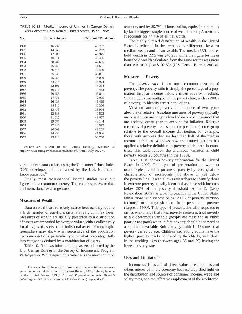
246 O’Hare, Pollard, and Ritualo
verted to constant dollars using the Consumer Prince Index(CPI) developed and maintained by the U.S. Bureau ofLabor statistics.12
Finally, most cross-national income studies must putfigures into a common currency. This requires access to dataon international exchange rates.
Measures of Wealth
Data on wealth are relatively scarce because they requirea large number of questions on a relatively complex topic.Measures of wealth are usually presented as a distributionof assets accompanied by average values, either collectivelyfor all types of assets or for individual assets. For example,researchers may show what percentage of the populationowns an asset of a particular type or what percentage fallsinto categories defined by a combination of assets.
Table 10.13 shows information on assets collected by theU.S. Census Bureau in the Survey of Income and ProgramParticipation. While equity in a vehicle is the most common
asset (owned by 85.7% of households), equity in a home isby far the biggest single source of wealth among Americans.It accounts for 44.4% of all net worth.
The highly skewed distribution of wealth in the UnitedStates is reflected in the tremendous differences betweenmedian wealth and mean wealth. The median U.S. house-hold wealth in 1995 was $40,200 while the figure for meanhousehold wealth calculated from the same source was morethan twice as high at $102,626 (U.S. Census Bureau, 2001a).
Measures of Poverty
The poverty ratio is the most common measure ofpoverty. The poverty ratio is simply the percentage of a pop-ulation that has income below a given poverty threshold.Some studies use multiples of the poverty line, such as 200%of poverty, to identify target populations.
Most measures of poverty fall into one of two types:absolute or relative. Absolute measures of poverty typicallyare based on an unchanging level of income or resources thatare updated every year to account for inflation. Relativemeasures of poverty are based on the position of some grouprelative to the overall income distribution, for example,those with incomes that are less than half of the medianincome. Table 10.14 shows how the United Nations hasapplied a relative definition of poverty to children in coun-tries. This table reflects the enormous variation in childpoverty across 23 countries in the 1990s.
Table 10.15 shows poverty information for the UnitedStates in 2000. This type of presentation allows data users to glean a fuller picture of poverty by looking at thecharacteristics of individuals just above or just below the poverty line. It also allows researchers to identify thosein extreme poverty, usually identified as those with incomesbelow 50% of the poverty threshold (Annie E. Casey Foundation, 2002). A growing practice in the United Stateslabels those with income below 200% of poverty as “low-income,” to distinguish them from persons in poverty(Loprest, 1999). This type of presentation also responds tocritics who charge that most poverty measures treat povertyas a dichotomous variable (people are classified as eitherpoor or not poor) when in fact poverty should be viewed asa continuous variable. Substantively, Table 10.15 shows thatpoverty varies by age. Children and young adults have thehighest poverty levels, followed by the elderly, with thosein the working ages (between ages 35 and 59) having thelowest poverty rates.
Uses and Limitations
Income statistics are of direct value to economists andothers interested in the economy because they shed light onthe distribution and sources of consumer income, wage andsalary rates, and the effective employment of the workforce.
TABLE 10.12 Median Income of Families in Current Dollarsand Constant 1998 Dollars: United States, 1975–1998
Year Current dollars Constant 1998 dollars
1998 46,737 46,7371997 44,568 45,2621996 42,300 43,9451995 40,611 43,4361994 38,782 42,6551993 36,959 41,6911992 36,573 42,4901991 35,939 43,0111990 35,353 44,0901989 34,213 44,9741988 32,191 44,3541987 30,970 44,4381986 29,458 43,8111985 27,735 42,0151984 26,433 41,4691983 24,580 40,2261982 23,433 39,9541981 22,388 40,5021980 21,023 41,6371979 19,587 43,1441978 17,640 42,5971977 16,009 41,2891976 14,958 41,0461975 13,719 39,790
Source: U.S. Bureau of the Census (online), available athttp://www.census.gov/hhes/income/histinc/f07.html (July 10, 2 ••.
12 For a concise explanation of how current income figures are con-verted to constant dollars, see U.S. Census Bureau, 1999, “Money Incomein the United States: 1998,” Current Population Reports P60–206 (Washington, DC: U.S. Government Printing Office): Appendix D.

10. Educational and Economic Characteristics 247
Income is one of the best measures of economic well-being,and it is often used in conjunction with educational attain-ment and occupation to measure the broader concept ofsocioeconomic status. Although the concept of total incomeis not difficult to relate to the experience of persons, fami-lies, and households in most countries, obtaining good dataon income is often a challenge. In many countries, one’sincome is a sensitive topic, while in other places the mix ofcash and noncash income makes it difficult to get a truepicture.
If one is considering primary data collection, conductinga small pilot study is often recommended to ascertain the possibility of obtaining reliable and valid information on income before any large-scale survey is undertaken.Income data obtained from household surveys should beverified against other available sources of such statistics. Inthe case of wage and salary income, such data can bechecked against employers’ records or establishment statis-tics when they are available. Unfortunately, for many othersources of income, there may be no means of verifying theresponses.
Income is often underreported in surveys, particularly,income from certain sources like public welfare programsor investments, and rates of nonresponse to questions onincome are often high because of its sensitive nature. One
TABLE 10.13 Ownership Ratios, Median Value of Asset Holdings, and the Distribution of Measured Net Worth by Asset Type: United States, 1993
Percent of households Median values of holdings Percent distribution ofAsset Type that own asset type for asset owners (dollars) measured net worth
ALL ASSETS X 37,587 100.0Interest-earning assets at financial institutions 71.1 2,999 11.4
Saving accounts 60.1 NA NAMoney market deposit accounts 12.6 NA NACertificates of deposit 16.0 NA NAInterest-earning checking 36.9 NA NA
Other interest-earning assets 8.6 12,998 4.0Money market funds 3.9 NA NAGovernment securities 2.1 NA NACorporate or municipal bonds 3.1 NA NAOther interest-earning assets 2.2 NA NA
Checking accounts 45.9 499 0.5Stocks and mutual fund shares 20.9 6,960 8.3Own home 64.3 46,669 44.4Rental property 8.4 29,300 6.7Other real estate 9.3 19,415 4.6Vehicles 85.7 5,140 6.4Business or profession 10.8 7,000 6.4U.S. savings bonds 18.5 775 0.8IRA or Keogh accounts 23.1 12,985 6.7Other financial investments 5.2 21,001 3.0
X Not applicable.NA Data not available.Source: U.S. Census Bureau, “Asset Ownership of Households: 1993,” by T. J. Eller and Wallace Fraser, Current Population Reports, Series P70–47
(1995): table A.
analysis of CPS data on income showed that the CPS under-reported real income by about 12% (U.S. Census Bureau,1993b). However, by comparing survey responses tonational accounts, it was revealed that, for some particularsources of income such as interest and dividends, less thanhalf the aggregate income was reported. In the 1990 decen-nial census, more than 13 million families did not providedata on income (U.S. Census Bureau, 1993a). This meansthat about 20% of all families had income data “imputed”by the Census Bureau because they either did not respondto income questions or did not fill out the census form appropriately.
Two groups that have posed major practical problems ofincome measurement are farmers and self-employed nona-gricultural workers. For example, the food that these personsraise and consume enhances their well-being and standardof living, yet that food is not money income. Sometimes the imputed value of such noncash items can be estimatedand added to cash profits to get total income figures for afarmer.
Data on income reported by the Census Bureau coveressenitially money income (excluding, for example, capitalgains) and exclude in-kind income, as previously stated. Thefact that some farm families receive part of their income inthe form of rent-free housing and goods produced and con-
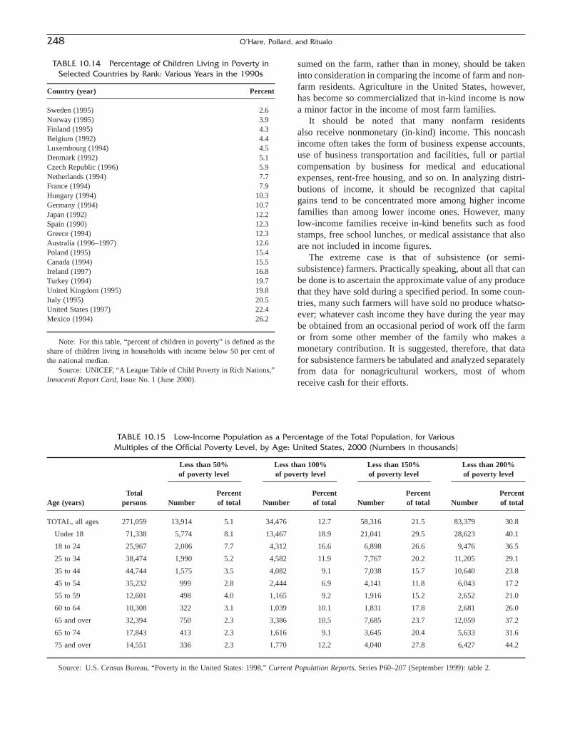
248 O’Hare, Pollard, and Ritualo
TABLE 10.15 Low-Income Population as a Percentage of the Total Population, for Various Multiples of the Official Poverty Level, by Age: United States, 2000 (Numbers in thousands)
Less than 50% Less than 100% Less than 150% Less than 200%of poverty level of poverty level of poverty level of poverty level
Total Percent Percent Percent PercentAge (years) persons Number of total Number of total Number of total Number of total
TOTAL, all ages 271,059 13,914 5.1 34,476 12.7 58,316 21.5 83,379 30.8
Under 18 71,338 5,774 8.1 13,467 18.9 21,041 29.5 28,623 40.1
18 to 24 25,967 2,006 7.7 4,312 16.6 6,898 26.6 9,476 36.5
25 to 34 38,474 1,990 5.2 4,582 11.9 7,767 20.2 11,205 29.1
35 to 44 44,744 1,575 3.5 4,082 9.1 7,038 15.7 10,640 23.8
45 to 54 35,232 999 2.8 2,444 6.9 4,141 11.8 6,043 17.2
55 to 59 12,601 498 4.0 1,165 9.2 1,916 15.2 2,652 21.0
60 to 64 10,308 322 3.1 1,039 10.1 1,831 17.8 2,681 26.0
65 and over 32,394 750 2.3 3,386 10.5 7,685 23.7 12,059 37.2
65 to 74 17,843 413 2.3 1,616 9.1 3,645 20.4 5,633 31.6
75 and over 14,551 336 2.3 1,770 12.2 4,040 27.8 6,427 44.2
Source: U.S. Census Bureau, “Poverty in the United States: 1998,” Current Population Reports, Series P60–207 (September 1999): table 2.
TABLE 10.14 Percentage of Children Living in Poverty inSelected Countries by Rank: Various Years in the 1990s
Country (year) Percent
Sweden (1995) 2.6Norway (1995) 3.9Finland (1995) 4.3Belgium (1992) 4.4Luxembourg (1994) 4.5Denmark (1992) 5.1Czech Republic (1996) 5.9Netherlands (1994) 7.7France (1994) 7.9Hungary (1994) 10.3Germany (1994) 10.7Japan (1992) 12.2Spain (1990) 12.3Greece (1994) 12.3Australia (1996–1997) 12.6Poland (1995) 15.4Canada (1994) 15.5Ireland (1997) 16.8Turkey (1994) 19.7United Kingdom (1995) 19.8Italy (1995) 20.5United States (1997) 22.4Mexico (1994) 26.2
Note: For this table, “percent of children in poverty” is defined as theshare of children living in households with income below 50 per cent ofthe national median.
Source: UNICEF, “A League Table of Child Poverty in Rich Nations,”Innocenti Report Card, Issue No. 1 (June 2000).
sumed on the farm, rather than in money, should be takeninto consideration in comparing the income of farm and non-farm residents. Agriculture in the United States, however,has become so commercialized that in-kind income is nowa minor factor in the income of most farm families.
It should be noted that many nonfarm residents also receive nonmonetary (in-kind) income. This noncashincome often takes the form of business expense accounts,use of business transportation and facilities, full or partialcompensation by business for medical and educationalexpenses, rent-free housing, and so on. In analyzing distri-butions of income, it should be recognized that capital gains tend to be concentrated more among higher incomefamilies than among lower income ones. However, manylow-income families receive in-kind benefits such as foodstamps, free school lunches, or medical assistance that alsoare not included in income figures.
The extreme case is that of subsistence (or semi-subsistence) farmers. Practically speaking, about all that canbe done is to ascertain the approximate value of any producethat they have sold during a specified period. In some coun-tries, many such farmers will have sold no produce whatso-ever; whatever cash income they have during the year maybe obtained from an occasional period of work off the farmor from some other member of the family who makes a monetary contribution. It is suggested, therefore, that datafor subsistence farmers be tabulated and analyzed separatelyfrom data for nonagricultural workers, most of whomreceive cash for their efforts.

The self-employed persons in nonagricultural pursuitsalso present a problem, inasmuch as the true income fromtheir work is the total amount of cash received minus thecost of doing business. Generally, the more developed theeconomy and the greater the amount of business performedby self-employed people, the more likely they are to haverecords that indicate the approximate cost of doing business,so that their true income is more accurately measured.
Because the amounts of income reported typically repre-sent income before deductions for personal taxes, SocialSecurity, savings bonds, and so on, it is not always an accurate measure of resources available to a family. Obtain-ing information on after-tax income is complicated,however. There are also large differences across countries in terms of taxes that must be considered in internationalcomparisons.
In many ongoing surveys, such as the CPS and the decen-nial census, the income statistics refer to receipts during the preceding calendar year while the characteristics of theperson, such as age, marital status, and labor force status,and the composition of the family refer to the survey date.Therefore, the income of the family does not include thoseamounts received by persons who were members of thefamily during all or part of the preceding calendar year butwho no longer resided with the family at the time of enu-meration. On the other hand, family income does includeamounts reported by related persons who did not reside withthe family last year but who were members of the family atthe time of enumeration.
Scholars use measures of wealth to gain a better under-standing of stratification within a population. Measures ofwealth can shed light on the economic position of a groupbeyond that provided by income data. For example, themedian income of elderly households in the United States(i.e., those with householders aged 65 years and over) is much less than the median for all households, but themedian wealth of elderly households is much higher than the median for all households. The median income of elderly households in 2000 was $23,048 compared to$42,148 for all households (U.S. Census Bureau, 2001b),while the median net worth (wealth) of elderly householdsin 1995 was $92,399 compared to $40,200 for all house-holds (U.S. Census Bureau, 2001a). In addition, examina-tion of data on wealth offers a more complete perspectiveon economic inequality (Oliver and Shapiro, 1995). Themedian income of black households in the United States($30,439) is 69% that of whites ($44,226), but the mediannet worth of households with a black householder ($7073)is just 14% that of whites ($49,030) (U.S. Census Bureau,2001a, 2001b).
Because the poor population is often a target of publicattention and public policies, data on poverty are usefulbecause they identify the number, geographic distribution,and characteristics of those at the bottom of the income dis-tribution. The U.S. Department of Education provides additional funds to schools on the basis of the number ofchildren in poverty (U.S. National Research Council, 1997).Figures on poverty can also be used to estimate the number
10. Educational and Economic Characteristics 249
0 10 20 30 40 50 60 70 80
$75,000 and over
$50,000 to $74,999
$25,000 to $49,999
$10,000 to $24,999
$1 to $9,999 or lossLess thanHigh School
High School
Some College orAssociate Degree
College Degree
Percent
EducationalLevel
38.9%27.0%
9.0%3.4%
1.9%
32.2%38.0%
36.9%22.3%
10.0%
17.5%22.1%
29.0%28.5%
16.9%
11.4%12.9%
25.1%45.7%
71.3%
FIGURE 10.3 Percent Distribution of Males 25 Years Old and Over by Educational Attainment, According to Income in 1998: United States, 1999Source: U.S. Bureau of the Census, “Money Income in the United States: 1998,” CurrentPopulation Reports, P60-206 (September 1999): table 8

of persons who are likely to be eligible for governmentmeans-tested programs.
References
Anker, R. 1990. “Female Labour Force Participation in Developing Countries: A Critique of Current Definitions and Data CollectionMethods.” In R. Turvey (Ed.), Developments in International Labour Statistics (pp. 126–140). Geneva: International Labour Organisation.
Annie E. Casey Foundation. 2002. KIDS COUNT Data Book: 2002, Balti-more, MD: Annie E. Casey Foundation.
Blackburn, M. L. 1997. Comparing Poverty: The United States and Other Industrial Nations. Washington, DC: American Enterprise Institute.
Brazil, Ministerio Do Trabalho. 1996. Trabua de Conversao CBO—IBGE—CIUO. Ministerio do Trabalho. Secretaria de Politicas de Emprego eSalario-SPES: Brasilia.
Christenson, B. A., and N. E. Johnson. 1995. “Educational Inequality inAdult Mortality: An Assessment with Death Certificate Data fromMichigan.” Demography 32: 215–229.
Coale, A. J. 1974. “The History of the Human Population.” In The HumanPopulation (pp. 15–25). San Francisco: Scientific American.
Federal Interagency Forum on Child and Family Statistics. 2001. America’sChildren: Key National Indicators of Well-Being, 2001. Federal Inter-agency Forum on Child and Family Statistics, Washington, DC: U.S.Government Printing Office.
Folger, J. K., and C. B. Nam. 1967. Education of the American Population.Washington, DC: U.S. Government Printing Office.
Gendell, M. 1998. “Trends in Retirement Age in Four Countries, 1965–95.”Monthly Labor Review 121: 8 (August): 20–30.
Gendell, M., and J. S. Siegel. 1992. “Trends in Retirement Age by Sex,1950–2005.” Monthly Labor Review 115: 7 (July): 22–29.
Golden, H. H. 1955. “Literacy and Social Change in UnderdevelopedCountries.” Rural Sociology 20(1): 1–7.
Grosh, M., and P. Glewwe. 1995. “A Guide to Living Standards Surveysand Their Data Sets.” LSMS Working Paper No. 120, The World Bank(updated on March 1, 1996).
International Labour Office. 1990. Statistical Sources and Methods. Vol. 3.Economically Active Population, Employment, Unemployment, andHours of Work (Household Surveys), 2nd ed. Geneva: InternationalLabour Office.
International Labour Office. 2002a. Key Indicators of the Labour Market:2002. Geneva: International Labour Office.
International Labour Office. 2002b. Yearbook of Labour Statistics: 2001.Geneva: International Labour Office.
International Labour Organization. 2000. Current International Recommendations on Labour Statistics. Geneva: International LabourOrganization.
International Labour Organisation. 1957. Measurement of Underemploy-ment. Ninth International Conference of Labour Statisticians. ReportNo. 4. Geneva: International Labour Organisation.
International Labour Organisation. 2002. Economically Active Population,1950–2000. Fourth Edition, Revision 2. Geneva: International LabourOrganisation.
Kamerschen, D. R. 1968. “Literacy and Socioeconomic Development.”Rural Sociology 33(2): 175–188.
Kominski, R., and P. M. Siegel. 1987. “Measuring Educational Attainmentin the 1990 Census.” Paper presented at the 1987 meeting of the Amer-ican Sociological Association (August 17).
Kominski, R., and P. M. Siegel. 1993. “Measuring Education in the Current Population Survey.” Monthly Labor Review 116: 9 (September):34–38.
Levine, C., L. Salmon, and D. H. Weinberg. 1999. “Revising the StandardOccupational Classification System.” Monthly Labor Review 122: 5(May): 36–45.
Loprest, P. 1999, How Families That Left Welfare Are Doing: A NationalPicture. New Federalism: National Survey of America’s Families,Series B, No. B-1 (August). Washington, DC: The Urban Institute.
Macunovich, D. J. 1996. “A Review of Recent Developments in the Economics of Fertility.” In P. L. Menchik (Ed.), Household and Family Economics (pp. 91–157). Dordrecht, Netherlands: Kluwer Academic.
Oliver, M. L., and T. M. Shapiro. 1995. Black Wealth, White Wealth: A NewPerspective on Racial Inequality. New York: Routledge.
Rindfuss, R. R., S. P. Morgan, and K. Offutt. 1996. “Education and theChanging Age Pattern of American Fertility: 1963–1989.” Demogra-phy 33: 277–290.
Rogers, R. G. 1992. “Living and Dying in the U.S.A.: SociodemographicDeterminants of Death among Blacks and Whites.” Demography 29:287–303.
Ruggles, P. 1990. Drawing the Line: Alternative Poverty Measures andTheir Implications for Public Policy. Washington, DC: The Urban Insti-tute Press.
Saunders, N. C. 1999. “The North American Industry ClassificationSystem: Change on the Horizon,” Occupational Outlook Quarterly(Fall).
Swanson, David A. et al. 1998. “K-12 Enrollment Forecasting: MergingMethods and Judgment.” ERS Spectrum (Fall): 24–31.
UNESCO. 1998. Statistical Yearbook, 1998. Paris: UNESCO.UNICEF. 2000. Monitoring Progress Toward the Goals of the World
Summit for Children: End-Decade Multiple Indicator Survey Manual.New York: UNICEF.
United Nations. 1989. Handbook on Social Indicators. Series F, Studies inMethods, No. 49. New York: United Nations.
United Nations. 1996. Demographic Yearbook, 1994. New York: UnitedNations.
United Nations. 1998. Principles and Recommendations for Population andHousing Census, Revision 1. Series M, Statistical Papers, No. 67. NewYork: United Nations.
U.S. Bureau of Labor Statistics. 1999. Revising the Standard OccupationalClassification System, Report 929. Washington, DC: U.S. GovernmentPrinting Office.
U.S. Census Bureau. 1967. Technical Paper No. 17. Trends in the Incomeof Families and Persons in the United States: 1947 to 1960. By M. F.Henson.
U.S. Census Bureau. 1993a. 1990 Census of Population, “Social and Eco-nomic Characteristics,” 1990 CP-2-1, United States. Washington, DC:U.S. Government Printing Office.
U.S. Census Bureau. 1993b. “Money Income of Households, Families, andPersons in the United States: 1992.” Current Population ReportsP60–184. Washington, DC: U.S. Government Printing Office.
U.S. Census Bureau. 1994. Current Population Survey, March 1994: Technical Documentation. Washington, DC: U.S. Government PrintingOffice.
U.S. Census Bureau. 2000a. Accessed online at www.census.gov/popula-tion/www/cps/cpsdef.html (July 17).
U.S. Census Bureau. 2000b. “North American Industry ClassificationSystem (NAICS).” Accessed online atwww.census.gov/epcd/www/naics.html (July 23).
U.S. Census Bureau. 2001a. “Household Net Worth and Asset Ownership:1995,” by M. E. Davern and P. J. Fisher. Current Population ReportsP70–71. Washington, DC: U.S. Government Printing Office.
U.S. Census Bureau. 2001b. “Money Income in the United States: 2000,”by C. DeNavas-Walt, R. W. Cleveland, and M. I. Roemer. Current Pop-ulation Reports P60–213. Washington, DC: U.S. Government PrintingOffice.
250 O’Hare, Pollard, and Ritualo

10. Educational and Economic Characteristics 251
U.S. Census Bureau. 2001c. “Poverty in the United States: 2000,” by J. Dalaker. Current Population Reports P60–214. Washington, DC:U.S. Government Printing Office.
U.S. National Center for Education Statistics. 1996. Education in Statesand Nations, 2nd ed., NCES 96-160, by R. P. Phelps, T. M. Smith, andN. Alsalam. Washington, DC: U.S. Government Printing Office.
U.S. National Center for Education Statistics. 1998. Adult Literacy inOECD Countries: Technical Report on the First International AdultLiteracy Survey, NCES 98-053, by T. S. Murray, I. S. Kirsch, and L. B.Jenkins. Washington, DC: U.S. Government Printing Office.
U.S. National Center for Education Statistics. 1999. Dropout Rates in theUnited States: 1997, NCES 1999-082, by P. Kaufman, S. Klein, and M.Frase. Washington, DC: U.S. Government Printing Office.
U.S. National Research Council. 1997. Small-Area Estimates of School-AgeChildren in Poverty. Washington, DC: National Academy Press.
Suggested Readings
Blackburn, M. L. 1997. Comparing Poverty: The United States and OtherIndustrial Nations. Washington, DC: American Enterprise Institute forPublic Policy Research.
International Labour Organization. 2000. Key Indicators of the LabourMarket: 1999. Geneva: International Labour Organization.
Levy, F. 1998. The New Dollars and Dreams: American Incomes and Eco-nomic Change. New York: Russell Sage Foundation.
National Research Council. 1995. Measuring Poverty: A New Approach,edited by C. F. Citro and R. T. Michael. Washington, DC: NationalAcademy Press.
Organisation for Economic Cooperation and Development. 2000. Educa-tion at a Glance: OECD Indicators 2000 Edition. Paris: OECD.
Ruggles, P. 1990. Drawing the Line: Alternative Poverty Measures andTheir Implications for Public Policy. Washington, DC: The Urban Insti-tute Press.
United Nations. 1998. Principles and Recommendations for Population andHousing Censuses: Revision 1. New York: United Nations.
U.S. Bureau of Economic Analysis. 1994. “Economic Concepts Incorpo-rated in the Standard Industrial Classification Industries of the United States.” Economic Classification Policy Committee Report No. 1(August).
U.S. Bureau of Economic Analysis. 1994. “The Heterogeneity Index: AQuantitative Tool to Support Industrial Classification.” Economic Clas-sification Policy Committee Report No. 2 (August).
U.S. Bureau of Labor Statistics. 1997. “Employment Projections.” In BLS Handbook of Methods, Chapter 13, Bulletin 2490 (April):122–129.
U.S. Bureau of Labor Statistics. 1999. “Revising the Standard OccupationalClassification System.” Report 929.
U.S. Census Bureau. 1998. “Measuring 50 Years of Economic ChangeUsing the March Current Population Survey.” Current PopulationReports P60–203. Washington, DC: U.S. Government Printing Office.
U.S. Census Bureau. 1999. “Experimental Poverty Measures: 1990 to1997,” by K. Short, T. Garner, D. Johnson, and P. Doyle. Current Pop-ulation Reports P60–205. Washington, DC: U.S. Government PrintingOffice.
U.S. National Center for Education Statistics. 1996. Education Indicators:An International Perspective, by N. Matheson, L. H. Salganik, R. P.Phelps, M. Perie, N. Alsalam, and T. M. Smith. NCES 96-003. Washington, DC: U.S. Government Printing Office.
U.S. National Center for Education Statistics. 1996. Education in Statesand Nations 2nd ed., by R. P. Phelps, T. M. Smith, and N. Alsalam.NCES 96-160. Washington, DC: U.S. Government Printing Office.
U.S. National Center for Education Statistics. 1998. Adult Literacy inOECD Countries: Technical Report on the First International Adult
Literacy Survey, by T. S. Murray, I. S. Kirsch, and L. B. Jenkins. NCES98-053. Washington, DC: U.S. Government Printing Office.
Selected websites
The following is a list of selected websites that have general informa-tion or statistics pertinent to educational and economic characteristics, supplementing those websites noted in the text and References.
Academy for Educational Development (AED)www.aed.orgAED is a nonprofit educational organization that addresses human devel-
opment needs in the United States and worldwide. The site includesinformation about publications and programs.
International Labour Organisation (ILO)www.ilo.org/public/english/index.htmThe International Labour Organisation is the United Nations’ specialized
agency that formulates international labor standards in the form of con-ventions and recommendations setting minimum standards of basiclabor rights.
National Center for Education Statistics (NCES) (U.S. Department ofEducation)
www.nces.ed.govNCES is the primary federal entity for collecting and analyzing data on
education in the United States and other nations.
Organisation for Economic Cooperation and Development (OECD)www.oecd.orgThe OECD groups 29 member countries in an organization that provides
governments a setting in which to discuss, develop, and improvenational and international economic and social policy.
U.S. Bureau of Economic Analysis (BAE) (U.S. Department of Commerce)
www.bea.govBAE is the principal federal agency responsible for analysing national and
regional economic data and reporting on the state of the economy.
U.S. Bureau of Labor Statistics (BLS) (U.S. Department of Labor)www.stats.bls.govThe BLS site provides information about the labor market in the United
States, including labor force statistics and other economic data, surveysand programs, publications, and regional information. Accessible publications online include the Occupational Outlook Handbook, Occu-pational Outlook Quarterly, and the Monthly Labor Review.
U.S. Social Security Administration (SSA)www.ssa.govSSA is the federal agency compiles data on covered workers, beneficiaries,
and benefits disbursed under the old-age security and disability programs.
United Nations Educational, Scientific and Cultural Organization(UNESCO)
www.unesco.orgSite contains several databases and selected statistics from the annual
UNESCO Statistical Yearbook.
The World Bankwww.worldbank.orgThis site includes information on recent, projects and publications as well
as an electronic media center, which lists products and services. Coversdeveloped countries as well as less developed countries.

This Page Intentionally Left Blank

DEFINITION AND TYPES
Directions of Change
Population change is measured as the difference betweenthe size of the population at different dates. Partly becauseof the prevailing trend of population in the countries of theworld, people often speak loosely of population “growth,”when actually increase or decrease is possible. In censusreports, increases are usually presented without a plus sign,while decreases are indicated by a minus sign.
Absolute and Percentage Change
One may obtain the absolute amount of change in thepopulation at different dates by subtracting the population atthe earlier date from the population at the later date. The per-centage change over the period is obtained by dividing theabsolute change by the population at the earlier date andmultiplying by 100. In presenting information about popu-lation change, many census tables include columns with thefollowing arrangement of captions:
Increase
Number Percent
Using the population at the earlier census as the base ofthe percentage of change is dictated partly by logic andpartly by convenience. It is logical in that such a measureanswers the basic question raised as to the rate of growthover an initial date. Many types of demographic rates arebased on the population at the beginning of the period (e.g.,survival rates and migration propensity rates). It is conven-ient in that this population is already at hand. While the cal-culation of vital rates uses the midperiod population, thisalternative base would have to be estimated.
PITFALLS IN MEASUREMENT
In measuring population change, it is essential that theelements that enter into measurement be comparable overtime. The geographic area to which the population refersshould be constant, the definition of the population shouldbe the same, and the completeness of coverage should notvary appreciably. This “rule” is not inviolable, however.There are cases, for example, where it is more realistic to measure changes for an expanding area, as explainedlater. Published population figures often refer to differentareas or reflect different kinds of enumerations over time.However, adjustments are rarely feasible, and change isusually computed with published counts or estimates.Nonetheless, knowledge of these differences is important foranalysis. Any attempt to measure population change mustconsider the following three pitfalls: (1) national or subna-tional areas may change, (2) definitions of the population tobe counted may change, and (3) the completeness of cover-age may vary.
Change in Territory
The national territory in which enumeration takes placemay change as the result of conquest, treaties, advancementof the frontiers of settlement, and similar events. Withinnational boundaries, water areas may be transformed intoland areas, and vice versa, as in the case of the AmazonRiver floodplain in Brazil. Often, it is possible to show thepopulation within constant boundaries and then to computethe change for this area. Ordinarily, it is the present territorythat is used when boundaries shift.
There are some cases when the use of an expanding areais preferable to that of a constant area. The total populationof the United States is a case in point. There is relativelylittle interest in the population growth of the United States
253
C H A P T E R
11
Population Change
STEPHEN G. PERZ
The Methods and Materials of DemographyCopyright 2003, Elsevier Science (USA).
All rights reserved.

within the territory of 1790. Fortunately, the territories pur-chased or annexed since that year contained few inhabitantsprior to their inclusion and first enumeration. In contrast, theterritorial shifts associated with the breakup of the SovietUnion created more complex problems for the examinationof population change because western portions of the formerUSSR have been settled for centuries.
Within many countries, there are changes in the bound-aries of states or provinces, secondary geographic sub-divisions, cities, and townships, and in boundaries of areas defined mainly for statistical purposes, such as urbanagglomerations or metropolitan areas. For example, ethnicconflicts within countries in Eastern Europe and CentralAsia may lead to new subnational divisions. Among citiesin any country, the change in the population may reflectannexations of territory. Because cities may grow by extend-ing their land areas as well as by becoming more denselysettled, the increase or decrease in the incorporated orexpanding area is perhaps of primary importance.
While recent U.S. census reports do not include statisticsfor populations in annexed areas, these publications doafford some assessment of the area annexed in growingurban centers. Table 11.1 presents data on 1980 and 1990populations and land areas of selected U.S. urbanized areas,ranked by percentage increase in land area during the 1980s(column 6). Columns 5 and 6 show that many areas withrapid population growth also experienced rapid growth inland area. In three cases, the geographic area grew as a resultof annexation of other cities (column 7). Thus, it is often dif-ficult to separate population growth from territorial annexa-tion when assessing urban population change. Populationgrowth in urban centers should always be treated withcaution because the estimates may be biased upward as aresult of increases in territory. There is often uncertainty ordisagreement as to whether fixed territory or changing ter-ritory is conceptually more appropriate when measuringchange in a particular situation. Given the importance of territorial annexation in growing urban areas, however,
254 Perz
TABLE 11.1 Growth of Population and Land Area, in Selected Urbanized Areasin 1980, United States, 1980–1990
(Urbanized areas consist of the central place or places and the surrounding urban fringe)
Population Area1 Percent Increase2
Annexed cities,1980 1990 1980 1990 Population Area 1980–1990
Urbanized area (1) (2) (3) (4) (5) (6) (7)
Norfolk-Portsmouth, VA 770,784 1,323,098 1,083 2,907 71.66 168.42 Hampton City,Newport NewsCity, SuffolkCity, VirginiaBeach City
Antioch-Pittsburgh, CA 86,435 153,768 67 168 77.90 150.30Austin, TX 379,560 563,008 364 726 48.33 99.31McAllen-Pharr-Edinburg, TX 157,423 263,192 163 323 67.19 97.98 MissionFort Pierce, FL 70,450 126,342 143 279 79.34 95.38Melbourne-Palm Bay, FL 212,917 305,978 433 845 43.71 95.15Bremerton, WA 64,536 112,977 91 177 75.06 94.29Lancaster, CA 56,328 187,190 118 215 232.32 81.86 PalmdaleRaleigh, NC 206,597 305,925 255 461 48.08 80.82Simi Valley, CA 79,921 128,043 69 123 60.21 78.12Sarasota-Bradenton, FL 305,431 444,385 389 664 45.49 70.69Killeen, TX 88,145 137,876 104 172 56.42 65.10Fort Collins, CO 78,287 105,809 90 145 35.16 60.67Fort Myers-Cape Coral, FL 140,958 220,552 247 388 56.47 56.92Laredo, TX 94,961 123,651 56 86 30.21 53.93Durham, NC 157,289 205,355 188 275 30.56 46.06San Diego, CA 1,704,352 2,348,417 1,582 2,298 37.79 45.25Palm Springs, CA 66,431 129,025 164 233 94.22 42.07Olympia, WA 68,616 95,471 110 151 39.14 37.55Orlando, FL 577,235 887,126 808 1,104 53.69 36.60
1 Land areas are in square kilometres.2 Base is 1980 population or area; expressed per 100 population or area.Sources: U.S. Bureau of the Census, 1983, Table 34, 1993a and 1993b, Table 1.

measurement of the part of the population change that isattributable to the change in territory demands attention.
Change in Definition
Populations may be defined in different ways, andchanges from one definition to another over time hinderassessments of population growth. Populations may be redefined from de jure counts, which include only usual residents, to de facto counts of both residents present andvisitors, or from de facto to de jure counts. A change froma de jure to a de facto basis in taking a census will not ordi-narily have a great effect on the intercensal change at thenational level, but it will often greatly affect the change inthe population of certain geographic subdivisions. In anystatistical area where substantial portions of the populationare nonresidents, such as military personnel, students, ortourists, de jure and de facto enumerations will yield differ-ent results. Where a nonresident population grows at a dif-ferent rate than that of residents, estimates of populationgrowth on the basis of de jure and de facto enumerationswill differ. Table 11.2 shows that the number of visitors inHawaii grew as a percentage of the de facto populationbetween 1980 and 1990. As a consequence, the increase ofthe de facto population was greater than that of the de jurepopulation. If we had only a de jure enumeration in 1980and a de facto enumeration in 1990, the percentage increasein the Hawaiian population would be 29.4%, much largerthan percentage increases in both the de jure and de factopopulations during the same period (i.e., 15% and 19%).
As another example of changing definitions of popula-tions, the 1950 U.S. census counted college students livingaway from “home” at their college residences. The changein definition of “usual residence” is reflected in Table 11.3,which presents census figures for the town of Chapel Hill,the seat of the University of North Carolina.
According to the U.S. Office of Education, 7419 studentswere enrolled in the university in the fall of 1949. If weassume that all of these students would not have beencounted under the old rule, we obtain an adjusted count of1758 for 1950. This indicates a population loss from 1940to 1950. In the light of our knowledge of the place and thetimes, however, this loss looks unreasonable. It is possiblethat we have overadjusted by subtracting students who alsohad their parental home in the town or who had no usualplace of residence elsewhere. It is also possible that a fairlylarge number of students lived in the outskirts of Chapel Hilland hence were properly not included in the 1950 total forthe town and that some of the university students living inthe town were missed in the 1950 census.
If we are examining the change in a particular subgroupof the population, we wish to be sure that the subgroup is
11. Population Change 255
TABLE 11.2 De Jure and De Facto Population Growth in Hawaii, 1980–1990 (Population in thousands)
Resident (de jure) Visitors Residents De facto population Percent visitorspopulation present absent (1) + (2) - (3) = (2) ∏ (4) =
Census date (1) (2) (3) (4) (5)
1980 (April 1) 964.7 97.6 9.6 1052.7 9.31990 (April 1) 1108.2 158.5 18.4 1248.4 12.7
Change, 1980–90Number 143.5 60.9 8.8 195.7 3.42
Percent1 14.9 62.4 91.7 18.6 X
X: Not applicable.1 Base of percent is 1980 population.2 Change in percentage points (= 12.7/9.3).Source: Based on Schmitt (1992), table 1.
TABLE 11.3 De Jure and De Facto Census Counts and Population Increase in Chapel Hill, NC, 1930 to 1990
(De jure counts, excluding students at the University of North Carolina)
Population Percentage increaseYear (1) (2)
1930 2,699 (X)1940 3,654 35.419501 9,177 151.11960 12,573 37.01970 26,199 108.41980 32,421 23.71990 37,604 16.0
X: Not applicable.1 De facto count that includes students attending the University of North
Carolina.Sources: U.S. Bureau of the Census, 1983, Table 34, and 1993b,
Table 1.
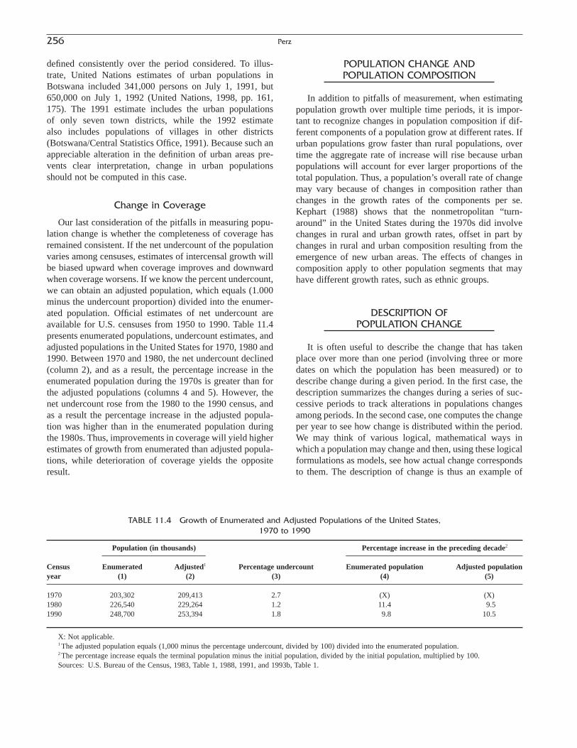
defined consistently over the period considered. To illus-trate, United Nations estimates of urban populations inBotswana included 341,000 persons on July 1, 1991, but650,000 on July 1, 1992 (United Nations, 1998, pp. 161,175). The 1991 estimate includes the urban populations of only seven town districts, while the 1992 estimate also includes populations of villages in other districts(Botswana/Central Statistics Office, 1991). Because such anappreciable alteration in the definition of urban areas pre-vents clear interpretation, change in urban populationsshould not be computed in this case.
Change in Coverage
Our last consideration of the pitfalls in measuring popu-lation change is whether the completeness of coverage hasremained consistent. If the net undercount of the populationvaries among censuses, estimates of intercensal growth willbe biased upward when coverage improves and downwardwhen coverage worsens. If we know the percent undercount,we can obtain an adjusted population, which equals (1.000minus the undercount proportion) divided into the enumer-ated population. Official estimates of net undercount areavailable for U.S. censuses from 1950 to 1990. Table 11.4presents enumerated populations, undercount estimates, andadjusted populations in the United States for 1970, 1980 and1990. Between 1970 and 1980, the net undercount declined(column 2), and as a result, the percentage increase in theenumerated population during the 1970s is greater than forthe adjusted populations (columns 4 and 5). However, thenet undercount rose from the 1980 to the 1990 census, andas a result the percentage increase in the adjusted popula-tion was higher than in the enumerated population duringthe 1980s. Thus, improvements in coverage will yield higherestimates of growth from enumerated than adjusted popula-tions, while deterioration of coverage yields the oppositeresult.
POPULATION CHANGE ANDPOPULATION COMPOSITION
In addition to pitfalls of measurement, when estimatingpopulation growth over multiple time periods, it is impor-tant to recognize changes in population composition if dif-ferent components of a population grow at different rates. Ifurban populations grow faster than rural populations, overtime the aggregate rate of increase will rise because urbanpopulations will account for ever larger proportions of thetotal population. Thus, a population’s overall rate of changemay vary because of changes in composition rather thanchanges in the growth rates of the components per se.Kephart (1988) shows that the nonmetropolitan “turn-around” in the United States during the 1970s did involvechanges in rural and urban growth rates, offset in part bychanges in rural and urban composition resulting from theemergence of new urban areas. The effects of changes incomposition apply to other population segments that mayhave different growth rates, such as ethnic groups.
DESCRIPTION OF POPULATION CHANGE
It is often useful to describe the change that has takenplace over more than one period (involving three or moredates on which the population has been measured) or todescribe change during a given period. In the first case, thedescription summarizes the changes during a series of suc-cessive periods to track alterations in populations changesamong periods. In the second case, one computes the changeper year to see how change is distributed within the period.We may think of various logical, mathematical ways inwhich a population may change and then, using these logicalformulations as models, see how actual change correspondsto them. The description of change is thus an example of
256 Perz
TABLE 11.4 Growth of Enumerated and Adjusted Populations of the United States, 1970 to 1990
Population (in thousands) Percentage increase in the preceding decade2
Census Enumerated Adjusted1 Percentage undercount Enumerated population Adjusted populationyear (1) (2) (3) (4) (5)
1970 203,302 209,413 2.7 (X) (X)1980 226,540 229,264 1.2 11.4 9.51990 248,700 253,394 1.8 9.8 10.5
X: Not applicable.1 The adjusted population equals (1,000 minus the percentage undercount, divided by 100) divided into the enumerated population.2 The percentage increase equals the terminal population minus the initial population, divided by the initial population, multiplied by 100.Sources: U.S. Bureau of the Census, 1983, Table 1, 1988, 1991, and 1993b, Table 1.

interpolation or curve-fitting to time-series data. The tech-niques used in such descriptions are similar to those used inmaking intercensal estimates and projections by purelymathematical means.
Linear Change
Computing the average amount of change during a yearor other interval of time is quite straightforward. One simplydivides the total change by the number of years or other unitof time. Suppose we want to compare the average annualamounts of population growth of a country where the inter-censal periods are of unequal length. Let us take the threemost recent censuses of Brazil as an example, shown inTable 11.5.
In computing the average amount of increase during aperiod, we implicitly make an assumption about how thegrowth is distributed over that period. For the moment, letus assume that the growth is linear, or follows an arithmeticprogression, which implies that there is a constant amountof increase per unit of time. While few demographic condi-tions cause populations to increase or decrease in an arith-metic progression, a straight line is frequently used not onlyto describe population growth in past periods but also toproject it into the future for short periods of time. Thegeneral equation for a straight line is
(11.1)
where y is the height of the line from zero, x is the horizontaldistance of the line from zero, a is the height of the line whenx equals zero, and b is the slope of the line, which indicatesthe amount of change in y for a unit change in x. In the caseof population change during a single period, we may expressthis as
(11.2)
where P0 is the initial population, Pn is the population at theend of the period (n years later), n is the time in years, andb is the annual amount of population change.
There are circumstances under which it is not particularlyproblematic to use a straight line in describing populationchange. When the time period between population enumer-
P P bnn = +0
y a bx= +
ations is short and the change relatively small, little errorcan be introduced by assuming that the population is chang-ing arithmetically. When monthly estimates are available,one may assume that population change within a monthfollows a straight line. Even over a 5-year period betweenquinquennial censuses, barring a major catastrophe such asa war, epidemic, or forced migration, this assumption maybe roughly applicable.
Rates of Change
More useful comparisons can be made with averageannual rates of population change. This raises the questionof how to express the rate, whether per unit, per 100, per 1000, or some other constant. For consistency, we willcontinue with the convention of expressing the rate as a percentage, or per 100.
Arithmetic Approximation to a Rate of Change
Let us continue with the Brazilian figures. We can use theaverage annual increase shown in column 4 in Table 11.5 toapproximate an average annual rate of change that is sim-plistic but convenient. The arithmetic rate of increase, incolumn 1 of Table 11.6, is calculated dividing the average
11. Population Change 257
TABLE 11.5 Linear Change of Population in Brazil, 1980–1991 and 1991–1996
Population Increase since preceding date Years since preceding date Average annual increase1, (2) ∏ (3) =Census date (1) (2) (3) (4)
1980 (September 1) 118,002,706 (X) (X) (X)1991 (September 1) 146,825,475 28,822,769 11.000 2,620,2521996 (August 31) 157,079,573 10,254,098 4.997 2,052,051
X: Not applicable.1 Equals the increase since the preceding census divided by the number of years elapsed since the preceding census.Source: Based on Brazil, Instituto Brasileiro de Geografia e Estatística (Brazilian Institute of Geography and Statistics (IBGE), 1998.
TABLE 11.6 Arithmetic Approximation of PopulationGrowth Rates in Brazil, 1980–1991 and 1991–1996
ArithmeticArithmetic approximation
rate of Average to the geometricIntercensal increase1 population2 rate of increase3
period (1) (2) (3)
1980 to 1991 2.22 132,414,091 1.981991 to 1996 1.40 151,952,524 1.35
1 Equals the average annual increase divided by the initial population,multiplied by 100. (Table 11.5, col. 4 ∏ col. 1 ¥ 100.)
2 Equals the mean of the initial and terminal populations of the period.3 Equals the average annual increase (Table 11.5, col. 4) divided by the
average population (col. 2), multiplied by 100.Source: Based on Table 11.5.

annual increase (column 4 in Table 11.5) by the popula-tion at the beginning of the intercensal period (column 1 inTable 11.5).
Arithmetic rates of increase are comparable only whenthe periods are of equal length. When the periods are ofunequal duration, the longer period tends to have the higherarithmetic rate. In the Brazilian example, the 1980 to 1991period is longer, and indicates a higher arithmetic growthrate than the 1991 to 1996 period. We must therefore choosea base for the rate that offsets the effects of unequal periods.To eliminate the bias due to unequal periods, an obviouschoice for the base is the mean of the populations at thebeginning and end of the periods. The average populationappears in column 2 of Table 11.6, and the new rate, derivedfrom this population and the average annual amount ofchange, is shown in column 3. When we compare columns1 and 3 in Table 11.6, we see that the excess of the earlierover the later average rate is reduced from 0.82 to 0.63. Notethat neither of these average annual rates, when appliedannually to the successive populations, will produce thepopulation at the end of the intercensal period. Nonethe-less, they represent fairly close approximations to genuineaverage annual rates, particularly the second of these measures.
Because from formula (2) we know
(11.3)
then the arithmetic approximation of the average rate isgiven by
(11.4)
Geometric Change
A geometric series is one in which the populationincreases or decreases at the same rate during each unit oftime, usually a year. If this constant rate of change is repre-sented by r and the initial population is represented by P0,then after n years the final population is given by
(11.5)
Suppose we observe the population at two dates and wishto find the annual rate of change on the assumption that the rate (rather than the change) is constant throughout theperiod. Let us return to our census data for Brazil. For the1991-to-1996 intercensal period, n = 4.997 years, P0 =146,825,475, and Pn = 157,079,573. Then
(11.6)
To solve the equation for r, take the natural logarithm ofeach side (ln), that is, the logarithm to the base e. The form
10
+ =r PP
nn
P P rnn= +( )0 1
¢ =+( )
¥rb
P Pn1 2100
0
bP P
nn=
- 0
e represents the base of the system of natural logarithms, itis a mathematical constant that equals 2.71828 . . . The baseof natural logarithms allows for computation of a constantrate of change, r, where the absolute amount of changevaries over time. The base e serves as a mathematically effi-cient alternative to the base 10, commonly used in earlieryears. To convert natural logarithms to ordinary numbers,use tables of natural logarithms or, more conveniently, apocket calculator or computer.
(11.7)
r = 0.013601, or about 1.36% per year
For population change in Brazil during the 1980 to 1991period, the assumption of geometric change yields a rate ofabout 2.01% per year.
If we had annual observations of the size of the popula-tion, and hence annual rates of population change, we couldfind the geometric mean of these annual rates:
(11.8)
Because the geometric rate is assumed to be constantthroughout the period, this geometric mean would be identical with the geometric rate of change figured from thepopulation at the beginning and end of the intercensalperiod.
Exponential Change
Geometric change is a type of change in which the com-pounding takes place at specified constant intervals, such asa year, and familiar to reader as “compound interest.”However, the annual compounding is arbitrary. Why notcompound semiannually or monthly? In an exponentialseries, the compounding takes place continuously (i.e., aconstant rate of change is applied at every infinitesimal unitof time). For a fixed period, an exponential growth curve canbe expressed as
(11.9)P P enrn= 0
rPP
PP
PP
PP
MGn
n
n nn= ¥ ¥ ¥ =-
1
0
2
1 1 0
. . .
1 1 013601+ =r .
ln 1 013510+( ) =r .
=.
.0675084 997
=ln .
.1 0698394 997
=
ÊË
ˆ¯ln
, ,, ,.
157 079 573146 825 475
4 997
lnln
1 0+( ) =
ÊË
ˆ¯
r
PP
n
n
258 Perz

Equation (11.9) allows for computation of change wherethe rate of change is compounded continuously. The term eis the base of natural logarithms. Solving for r, we get, first,
(11.10)
Then,
(11.11)
We will use Equation (11.11) to solve for the exponen-tial rate of growth, r, for Brazil in its last two intercensalperiods. For the 1980 to 1991 period, the computations areas follows:
= 0.019867, or 1.99% per year
For the 1991 to 1996 intercensal period, the averagegrowth rate, derived by continuous compounding, is 1.35%.Note that the average rate of growth when the compound-ing is continuous is always less than when the compound-ing is between longer time intervals such as a year.
We will close this subsection by recapitulating thevarious estimates of the average annual rate of growth thatwe have computed by various formulas for the last two inter-censal periods of Brazil. These estimates appear in Table11.7. The geometric method tends to yield the highest esti-mates of growth, followed by the exponential method, thenthe arithmetic approximation.
=0 218537
11.
=ln .1 244255
11
r =
ÊË
ˆ¯ln
, ,, ,
146 825 475118 002 706
11
r
PPn
n
=
ÊË
ˆ¯ln
0
eP
Prn n=
0
Population Change in Multiple Periods
The preceding section dealt with the computation of theaverage annual rate of change within a single period, specif-ically an intercensal period. Now we turn to the descriptionof change over a number of periods. Here, some of thecurves describing growth that we have already consideredcan also be applied, as can additional ones.
Describing the trend of population from a number ofobservations is usually a particular case of curve fitting, atopic that is dealt with more generally in Appendix C. Inchoosing the type of growth curve to fit to the populationdata, it is desirable both to examine the plotted points andto develop a demographic theory as to why populationshould be expected to change in the hypothesized way, givena particular set of historical conditions and in the light ofdemographic knowledge about the factors affecting the com-ponents of population change. The trend curve is of interestin its own right. It may also be used for purposes of inter-polation (that is, to find the trend value at a given date withinthe period of observation) or for purposes of extrapolation(that is, to find the trend value at a given date beyond theobservation period).
The Linear Trend
A straight line (that is, a polynomial of first degree) isrepresented by the following equation and can be fitted tothree or more observations by the method of least squares:
(11.12)
where t is the time in years elapsed between observations ofpopulation numbers.
Other Polynomial Trends
Population change is occasionally fairly well describedby a polynomial of second or higher degree. The equationof a second-degree polynomial (or parabola) is
(11.13)
and that of an nth degree polynomial is
(11.14)
Exponential Curves
The general equation for an exponential curve is
(11.15)
For population growth, this could be represented as
(11.16)
where Pt is the population at time t and r is the rate ofchange. The geometric growth equation, Pn = P0(1 + r)n, canbe seen to be a special case of Equation 11.16.
P a rtt= +( )1
y abx=
P a bt ct kttn= + + + +2 . . .
P a bt ctt = + + 2
P a btt = +
11. Population Change 259
TABLE 11.7 Arithmetic, Geometric, and Exponential Population Growth Rates in Brazil,
1980–1991 and 1991–1996
Growth rate
Formula 1980–1991 1991–1996
Arithmetic approximation1 1.98 1.35Geometric—Annual compounding 2.01 1.36Exponential—Continuous compounding 1.99 1.35
1 Arithmetic approximation employed the midperiod population as abase.
Source: Tables 11.5 and 11.6, and text.

When the rate of change is positive, the populationdescribed by such a curve would increase without any limit.Such a trend cannot continue indefinitely. An exponentialcurve may, however, describe population growth over a par-ticular period of time. Demographers sometimes speak ofsuch growth as “Malthusian growth” because of the well-known generalization by Malthus that population tends toincrease in a geometric progression.
The Logistic Curve
One of the best-known growth curves in demography isthe logistic curve. It was first derived by Verhulst around1838 but was rediscovered and popularized by Pearl andReed around 1920. Some species of animals and some bac-terial cultures have been observed to grow rapidly at firstwhen placed in a limited environment with ideal conditionsof food supply and space for their initially few numbers, andthen to grow slowly as the population experiences a pro-nounced scarcity of resources. There may be an upper limitto the numbers that can be maintained, whereupon the pop-ulation ceases to grow. Considerations such as these havegiven rise to attempts to predict what the upper limit wouldbe by fitting asymptotic growth curves to observed data. Theequation of this curve is
(11.17)
where Yc represents the computed value of Y, and k is thecarrying capacity of a region, measured as the maximumnumber of persons that can be supported per unit of area.1
Like other growth curves, the logistic is used for pro-jecting population growth as well as for describing its pastcourse. Some writers have criticized the logistic as being too mechanistic in its assumptions (e.g., for not allowing forvoluntary control over fertility or for migration) and forother reasons. The logistic cannot describe a population thatis decreasing.
The Time Required for a Population to Double
It is often of interest to know the time required for a pop-ulation to double in size if a given annual rate of increasewere to continue. This interest reflects the problems
Yk
ec a bx=
+ +1
confronting many rapidly growing countries, especially theeconomically underdeveloped ones.
For this purpose, we must return to Equation (11.9) for aconstant growth rate, continuously compounded:
where t is the length of the interval in years and Pt is thepopulation at the end of the interval. We want to find thenumber of years it will take for Pt to equal 2P0:
(11.18)
For an example, we can calculate population doublingtime in Brazil with the exponential growth rate for the 1991to 1996 period. To find t, we evaluate Equation 11.18. Thenatural logarithm of 2 equals 0.693417 . . . , and the annualrate of growth in Brazil between 1991 and 1996 was 1.35%.
Figure 11.1 shows the relationship between the annualrate of growth and the number of years for the populationto double, and Table 11.8 presents this relationship in tabularform.
Cyclical Change
Most of the foregoing discussion concerns the descrip-tion of secular trends in population size. In computing theaverage population change within an intercensal period, wewere, however, dealing with the combined effects of secularand cyclical movements. In recent years, studies of cyclicalpopulation change have proliferated. Easterlin (1968, 1987)argued that large birth cohorts in post-war United Statesexperienced lower incomes, resulting in later marriages andlower fertility. The large cohorts thus produced smallercohorts, which in turn earned higher incomes and tended tohave more children. These “Easterlin cycles” theoreticallygenerate cyclical changes in rates of population growthacross decades, though some authors have raised questionsabout their significance, particularly since 1980 (e.g.,Pampel and Peters, 1995; Wachter, 1991). Short-term fluc-tuations in the components of population growth havebecome the subject of historical demography. Lee (1981)analyzed monthly data on wheat prices, mortality, and fer-tility in England from the 1540s to the 1840s. By removingsecular trends, his analysis shows that cyclical rises in wheat
t = 51 4. years
t =0 693417
0 0135.
.
tr
=ln 2
ln 2 = rt
2 = ert
2 0 0P P ert=
P P etrt= 0
260 Perz
1 The logistic curve is very similar to the Gompertz curve. One differ-ence is that the growth increments of the logistic are symmetrical whenplotted, closely resembling a normal curve, whereas those of the Gompertzcurve are skewed. For the logistic curve, the differences between the recip-rocals of the population values decline by a constant percentage. See pages382–384 of the unabridged edition of The Methods and Methods of Demography, published, by the U.S. Census Bureau in 1980, for an illus-tration of the method of fitting a logistic curve.

cyclical effects of grain prices on mortality eroded by the19th century. Similar methods have also been applied to theless developed countries experiencing economic growth followed by debt crises during the 1980s. Tapinos, Mason,Bravo, and colleagues (1997) analyzed annual data in nineLatin American countries and showed some decreases innuptiality and increases in child mortality during years ofdeclines in gross domestic product or immediately follow-ing such declines. Work on cyclical fluctuations in the com-ponents of population growth tends to find weak effects, butmost authors admit to the need for refinement in the methodsemployed.
Seasonal Change
Because each of the components of population growth issubject to seasonal change, the growth of total population,especially the de facto population, may exhibit some degreeof seasonal fluctuation. To observe this, we need fairly accu-rate estimates of population on a monthly or at least a quar-terly basis. Data from the Consumer Confidence Survey ofFloridians reveal a pronounced seasonal fluctuation of pop-ulation in Florida due to temporary residents. Overall, 4.1%of Florida’s population consisted of temporary residents in1993. They numbered nearly 558,000 persons among thetotal for the state, estimated to be 13,609,000 on April 1,1993. In January, however, the percentage of temporary res-idents peaked at 7.3%, or about 991,000 people. The tem-porary population declined in subsequent months, reachinga trough in September of 1.1%, or 143,000 people. This
11. Population Change 261
0.0
10.0
20.0
30.0
40.0
50.0
60.0
70.0
80.0
90.0
100.0
110.0
120.0
130.0
140.0
150.0
0.0 0.5 1.0 1.5 2.0 2.5 3.0 3.5 4.0
Annual rate of growth (percentage)
Dou
blin
g tim
e (y
ears
)
FIGURE 11.1 Number of Years Necessary for the Population to Double According to Specified AnnualRates of Growth. Source: Table 11.8
TABLE 11.8 Population Doubling Time at Different AnnualRates of Growth
Annual rate Doubling Annual rate Doublingof growth time of growth time
0.1 693.1 2.1 33.00.2 346.6 2.2 31.50.3 231.0 2.3 30.10.4 173.3 2.4 28.90.5 138.6 2.5 27.70.6 115.5 2.6 26.70.7 99.0 2.7 25.70.8 86.6 2.8 24.80.9 77.0 2.9 23.91.0 69.3 3.0 23.11.1 63.0 3.1 22.41.2 57.8 3.2 21.71.3 53.3 3.3 21.01.4 49.5 3.4 20.41.5 46.2 3.5 19.81.6 43.3 3.6 19.31.7 40.8 3.7 18.71.8 38.5 3.8 18.21.9 36.5 3.9 17.82.0 34.7 4.0 17.3
Note: Computed by the formula for continuous compounding, Pt = P0ert,where t = ln 2 ∏ r.
prices led to rises in mortality along with declines in nuptiality, which reduced population growth for up to 36months. Related work (e.g., Galloway 1988) extended thesefindings to eight other European countries and showed that
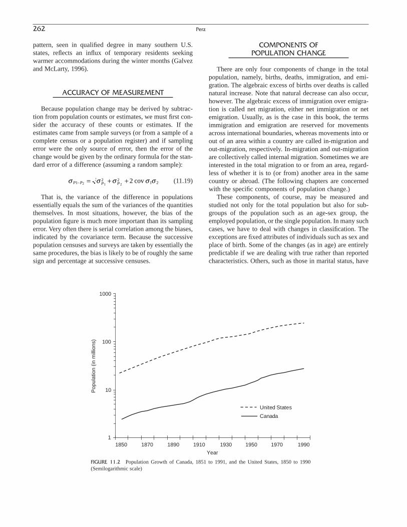
pattern, seen in qualified degree in many southern U.S.states, reflects an influx of temporary residents seekingwarmer accommodations during the winter months (Galvezand McLarty, 1996).
ACCURACY OF MEASUREMENT
Because population change may be derived by subtrac-tion from population counts or estimates, we must first con-sider the accuracy of these counts or estimates. If theestimates came from sample surveys (or from a sample of acomplete census or a population register) and if samplingerror were the only source of error, then the error of thechange would be given by the ordinary formula for the stan-dard error of a difference (assuming a random sample):
(11.19)
That is, the variance of the difference in populationsessentially equals the sum of the variances of the quantitiesthemselves. In most situations, however, the bias of the population figure is much more important than its samplingerror. Very often there is serial correlation among the biases,indicated by the covariance term. Because the successivepopulation censuses and surveys are taken by essentially thesame procedures, the bias is likely to be of roughly the samesign and percentage at successive censuses.
s s s s sP P P P12 2
1 22 1 22- = + + cov
COMPONENTS OF POPULATION CHANGE
There are only four components of change in the totalpopulation, namely, births, deaths, immigration, and emi-gration. The algebraic excess of births over deaths is callednatural increase. Note that natural decrease can also occur,however. The algebraic excess of immigration over emigra-tion is called net migration, either net immigration or netemigration. Usually, as is the case in this book, the termsimmigration and emigration are reserved for movementsacross international boundaries, whereas movements into orout of an area within a country are called in-migration andout-migration, respectively. In-migration and out-migrationare collectively called internal migration. Sometimes we areinterested in the total migration to or from an area, regard-less of whether it is to (or from) another area in the samecountry or abroad. (The following chapters are concernedwith the specific components of population change.)
These components, of course, may be measured andstudied not only for the total population but also for sub-groups of the population such as an age-sex group, theemployed population, or the single population. In many suchcases, we have to deal with changes in classification. Theexceptions are fixed attributes of individuals such as sex andplace of birth. Some of the changes (as in age) are entirelypredictable if we are dealing with true rather than reportedcharacteristics. Others, such as those in marital status, have
262 Perz
United States
Canada
1950 1970 199019301910189018701850
Year
1000
100
10
1
Pop
ulat
ion
(in m
illio
ns)
FIGURE 11.2 Population Growth of Canada, 1851 to 1991, and the United States, 1850 to 1990(Semilogarithmic scale)

restricted paths; for example, a change from single status isirreversible and the only possible change from widowed ordivorced is to married (excluding death). With some char-acteristics, however (e.g., occupation, income, or religion),it is theoretically possible to change from any category toany other category.
FACTORS IMPORTANT IN ANALYSIS
A great deal of demographic analysis is carried out interms of comparisons of population change among differentpolitical units, residence areas, and groups having variousdemographic, social, and economic characteristics. Com-parisons of percentage change are usually more meaningfulthan those of absolute change. If population changes in twocountries with intercensal periods of different lengths arebeing compared, annual average rates should be computed,preferably with the assumption of exponential growth.
If two areas, or groups, of radically different populationsize (e.g., the United States and Canada) are being comparedgraphically, a better indication of relative rates of change isgiven by a semilogarithmic graph (Figure 11.2) than by anarithmetic graph. Here population is plotted to a logarithmicscale on the vertical axis, whereas time is plotted to anarithmetic scale on the horizontal axis. Then equal verticaldistances will represent equal rates of change without regardto the size of the population. Further, on a semilogarithmicgraph, a population increasing at a constant rate is repre-sented by a straight line.
References
Botswana, Central Statistics Office. 1991. 1991 Population and HousingCensus: Administrative/Technical Report and National StatisticalTables. Gaborone, Botswana: Central Statistical Office.
Brazil, Instituto Brasileiro de Geografia e Estatística (Brazilian Institute ofGeography and Statistics, IBGE). 1998. Dados Históricos dos Censos—População, 1940–1996, http://www.ibge.org/informacoes/estat1.htm,available June 1998.
Easterlin, R. 1968. Population, Labor Force, and Long Swings in EconomicGrowth: The American Experience. New York: National Bureau of Eco-nomic Research.
Easterlin, R. 1987. Birth and Fortune: The Impact of Numbers on PersonalWelfare. Chicago: University of Chicago Press.
Galloway, P. R. 1988. “Basic Patterns in Annual Variations in Fertility, Nuptiality, Mortality, and Prices in Pre-Industrial Europe.” PopulationStudies 24(2): 275–302.
Galvez, J., and C. McLarty. 1996. “Measurement of Florida TemporaryResidents Using a Telephone Survey.” Journal of Social and EconomicMeasurement 22: 25–42.
Kephart, G. 1988. “Heterogeneity and the Implied Dynamics of RegionalGrowth Rates: Was the Nonmetropolitan Turnaround an Artifact ofAggregation?” Demography 25(1): 99–113.
Lee, R. D. 1981. “Short-Term Variation: Vital Rates, Prices, and Weather.”In E. A. Wrigley and R. S. Schofield (Eds.), The Population History ofEngland, 1541–1871 (pp. 356–401). Cambridge: Harvard UniversityPress.
Pampel, F. C., and H. E. Peters. 1995. “The Easterlin Effect.” AnnualReview of Sociology 21: 163–194.
Schmitt, R. C. 1992. “Estimating Hawaii’s De Facto Population.” AppliedDemography 7(2): 1–3.
Tapinos, G., A. Mason, and J. Bravo (Eds). 1997. Demographic Responsesto Economic Adjustment in Latin America. Oxford: Clarendon Press.
United Nations. 1998. Demographic Yearbook—1996. New York: UnitedNations.
U.S. Bureau of the Census. 1983. 1980 Census of Population, Character-istics of the Population, Chapter A: Number of Inhabitants, Part 1: USSummary, PC80-1-A1. Washington, DC: U.S. Government PrintingOffice.
U.S. Bureau of the Census. 1988. The Coverage of Population in the 1980Census. Report PHC80-E4. Washington, DC: U.S. Government Print-ing Office.
U.S. Bureau of the Census. 1991. “Refined 1990 Census Coverage Esti-mates.” Press release of 18 June, CB91-222. Washington, DC.
U.S. Bureau of the Census. 1993a. 1990 Census of Population and HousingSupplemental Reports: Urbanized Areas of the United States and PuertoRico, 1990 CPH-S-1-2. Washington, DC: U.S. Government PrintingOffice.
U.S. Bureau of the Census. 1993b. 1990 Census of Population: Social andEconomic Characteristics, United States, 1990 CP-2-1, Table 1. Washington, DC: U.S. Government Printing Office.
Wachter, K. W. 1991. “Elusive Cycles: Are There Dynamically PossibleLee-Easterlin Models for U.S. Births?” Population Studies 45:109–135.
11. Population Change 263

This Page Intentionally Left Blank

NATURE AND USES OF MORTALITY STATISTICS
Death is a principal “vital event” for which vital statis-tics are collected and compiled by the vital statistics regis-tration system; the others are live births, fetal deaths,marriages, and divorces. Adoptions, legitimations, annul-ments, and legal separations also may be included. The vitalstatistics system includes the legal registration, statisticalrecording and reporting of the occurrence of vital events,and the collection, compilation, analysis, presentation, anddistribution of vital statistics (United Nations, 1953, p. 4).The vital statistics system employs the registration methodof collecting the data on vital events, which typicallyinvolves the reporting to government officials of events asthey occur and the recording of the occurrence and the char-acteristics of these events.
Broadly speaking, death statistics are needed for demo-graphic studies and for public health administration. Themost important uses of death statistics include (1) the analy-sis of the present demographic status of the population aswell as its potential growth; (2) filling the administrative andresearch needs of public health agencies in connection withthe development, operation, and evaluation of public healthprograms; (3) the determination of administrative policy andaction in connection with the programs of government agen-cies other than those concerned with public health; and (4)filling the need for information on population changes inrelation to numerous professional and commercial activities.Death statistics are needed to make the analyses of past pop-ulation changes that are required for making projections ofpopulation and their demographic characteristics. The latterare employed in developing plans for housing and educa-tional facilities, managing the Social Security program, andproducing and providing services and commodities forvarious groups in the population. The analysis of mortality
statistics is essential to programs of disease control. Localhealth authorities use mortality statistics reports to deter-mine the administrative action needed to improve publichealth in local areas. All these uses are in addition to thedemands of individuals for documentary proof of death.
DEFINITION OF CONCEPTS:STATISTICAL LIFE AND DEATH
Adequate compilation and measurement of vital eventsrequire that the concepts of life and death be given formaldefinition, even though the meaning of these concepts mayappear obvious, at least in a physical sense, to most persons.Recent developments in the medical field have gone a longway to blur even the clinical distinction between life anddeath. When does life begin and end for statistical pur-poses—that is, for the counting of births and deaths? In fact,vital statistics systems identify three basic, complementary,and mutually exclusive categories: live births, deaths, andfetal deaths (i.e., fetal losses).
The United Nations and the World Health Organizationhave proposed the following definition of death: “Death is the permanent disappearance of all evidence of life at any time after birth has taken place (post-natal cessation ofvital functions without capability of resuscitation)” (UnitedNations, 1953, p. 6; World Health Organization, 1950, p. 17). A death can occur only after a live birth has occurred.The definition of a death can be understood, therefore, onlyin relation to the definition of a live birth (see Chapter 3 orChapter 15). For one thing, it excludes the entire categoryof fetal mortality, or pregnancy losses that occur prior to thecompletion of the birth process.
Although the definition of a “death” excludes losses prior to (live) births, these events are commonly called fetal deaths. A fetal death is formally defined as “death
265
C H A P T E R
12
Mortality
MARY A. MCGEHEE
The Methods and Materials of DemographyCopyright 2003, Elsevier Science (USA).
All rights reserved.

(disappearance of life) prior to the complete expulsion orextraction from its mother of a product of conception irre-spective of the duration of pregnancy; the death is indicatedby the fact that after such separation the fetus does notbreathe or show any other evidence of life, such as beatingof the heart, pulsation of the umbilical cord, or definitemovement of voluntary muscles” (WHO, 1950).
The term “fetal death” is employed in present demo-graphic practice to embrace the events variously called still-births, miscarriages, and abortions in popular medical orlegal usage. The term “stillbirth” is often used synony-mously with late fetal deaths, say a fetal death of 28 or morecompleted weeks of gestation, although the term is some-times employed to refer to all fetal deaths.
The term “miscarriage” is popularly employed to refer tospontaneous or accidental terminations of fetal life occur-ring early in pregnancy. The term “abortion” is defined asany termination of pregnancy before 28 weeks of gestation.There are two major categories of abortions: spontaneousand induced. Induced abortions are those initiated by delib-erate action undertaken with the intention of terminatingpregnancy; all other abortions are considered as sponta-neous. The recommendation of the United Nations and theWorld Health Organization is to group all of these events,miscarriages and abortions as well as stillbirths, under theheading “fetal death” and to classify them as early, inter-mediate, and late according to the months of gestation.
SOURCES OF DATA FOR MORTALITY STUDIES
The basic data on deaths for mortality studies, for the statistically developed areas, come from vital statistics registration systems and, less commonly, from national pop-ulation registers, as noted. The analysis of the death statis-tics from the vital statistics registration system depends onthe availability of appropriate population data from a censusor survey, or population estimates, to be used as bases forcomputing rates of various kinds. Dependence on a seconddata collection system is not necessary where an adequatenational population register system is in effect.
The vital statistics registration system is likely to be in-adequate in the underdeveloped countries; for these areas,other sources of data for measuring mortality have to be con-sidered. The principal alternative sources are (1) nationalcensuses and (2) national sample surveys. National censusesand sample surveys may provide (1) data on age composi-tion from which the level of recent mortality can be inferredand (2) direct data on mortality. The national sample surveysmay also provide additional detailed data permitting a morecomplete analysis of mortality. A sample survey may beemployed to follow up a sample of decedents reported in theregistration system. The inference regarding the level of
mortality is easier and firmer where two censuses are avail-able, but special techniques permit this inference with onlyone census in certain cases. Direct data on deaths are infre-quently obtained in censuses, but in recent decades samplesurveys have been used in a number of areas to measuremortality levels. The sample survey is not an acceptable sub-stitute for the registration system with respect to the legalaspects of registrations, however, since every vital eventshould be registered for legal purposes.
Vital statistics from civil registers are infrequently avail-able in Africa. The availability of vital statistics is onlyslightly greater for much of Asia and parts of Latin America.In these continents, coverage is uneven and the statisticsgenerally incomplete and unreliable. Estimated death ratesfor these areas, however, are becoming increasingly avail-able from sample surveys or from the analysis of censusreturns.
Mortality statistics are ordinarily presented in the statis-tical yearbooks of countries or in special volumes present-ing vital statistics. In the United States, a volume onmortality statistics was published each year from 1900 (theyear when the annual collection of mortality statistics for thedeath registration area began) to 1993 by the U.S. CensusBureau or the U.S. Public Health Service. In addition, provisional statistics as well as certain final data are pub-lished in brief reports in advance of the publication of the bound volumes. The United Nations’ DemographicYearbooks for 1957, 1961, 1966, 1967, 1974, 1980, and1985 emphasized tabulations of mortality. Other specialcompilations of mortality data include Annual Epidemio-logical and Vital Statistics, published by the World HealthOrganization since 1962, and the World Health StatisticsAnnual, published by the World Health Organization since1948.
QUALITY OF DEATH STATISTICS
We may consider the deficiencies of death statistics basedon vital statistics registration systems under three headings:(1) accuracy of the definition of death applied, (2) com-pleteness of registration, and (3) accuracy of allocation ofdeaths by place and time.
Application of Definition
Not all countries follow the definition of death recom-mended by the United Nations in obtaining a count ofdeaths. In some countries, infants who die within 24 hoursafter birth are classified not as deaths but as stillbirths or,failing provisions for this, are disregarded altogether (i.e., they are not classified as live births, deaths, or fetaldeaths). In other countries (e.g., Algeria, Martinique, andGuadeloupe), infants who are born alive but who die before
266 McGehee
the end of the registration period, which may last a fewmonths, are considered stillbirths or are excluded from alltabulations.
Completeness of Registration
Basis and Extent of Underregistration
The registration of deaths for a country may be incom-plete because of either (1) failure to cover the entire geo-graphic area of the country or all groups in the populationor (2) failure to register all or nearly all of the vital eventsin the established registration area. Typically, both of thesedeficiencies apply if the first is true. Many less developedcountries currently collect death statistics only in a desig-nated registration area (e.g., Indonesia, Ghana, Turkey,Brazil, Myanmar) or try to secure complete registration onlyin designated sample registration areas (e.g., India) for avariety of reasons. The registration area may exclude partsof the country where good registration is a practical impos-sibility in view of the country’s economic and social devel-opment and financial condition. Remote rural, mountainous,or desert areas in a country may not be serviced by regis-trars. The national government may not have completeadministrative control over certain parts of the territory itclaims as a result of civil disorder (e.g., former Burma) or a territorial dispute with another country (e.g., India. Pakistan). Nomadic and indigenous groups (e.g., nomadicIndians in Ecuador, jungle Indians in Venezuela, full-blooded aborigines in Australia), or particular ethnic orracial groups (Palestinian refugees in Syria, African popu-lation in former Bechuanaland, Bantus in South Africa) maybe excluded or hardly covered. Commonly, in underdevel-oped countries, babies who die before the end of the legalregistration period are registered neither as births nor deaths.In Taiwan, for example, deaths must be registered within 5days and births within 15 days. A sample test conductedabout 1965 showed that a large proportion of babies whodied within 15 days were not registered in any way at all.
The United Nations finds death registration to be sub-stantially incomplete for most countries of the world, in-cluding nearly all of those considered underdeveloped.According to an analysis of data that the United Nationscarried out for 1951–1955, only about 33% of the world’sdeaths were being registered: the percentage varied region-ally from 7% for East Asia to 100% in North America andEurope. Generally, a registration system that records 60% ormore of deaths is considered to be a useful source of mor-tality data. If completeness is below 60%, the value of thedata may be affected by nonrepresentativeness (Preston,1984). Carefully derived estimates of the completeness ofregistration are rarely, if ever, available. Several countrieshave provided estimates to the United Nations that are givenin its Demographic Yearbook. These estimates are typically
below 90%: even so, they probably overstate the actualextent of registration.
In the United States, the annual collection of mortalitystatistics began in 1900, when the registration area consistedof 10 states, the District of Columbia, and a number of cities,accounting for only 41% of the population of the UnitedStates. Complete geographic coverage of the United Stateswas not achieved until 1933, when the last state joined theregistration area. Currently, more than 99% of the deathsoccurring in the United States are believed to be registered.
Reporting of fetal “deaths” in the United States is lesscomplete. Even so, registration is believed to be relativelycomplete for fetal losses at 28 or more weeks of gestation.Statistical data on fetal losses include only those occurringat a stated or presumed gestation period of 20 or moreweeks.
Measurement of Underregistration
Several approaches are used to measure the complete-ness of death registration, none of which is highly satisfac-tory. The results of studies of underregistration of births, including birth registration tests and estimates made bydemographic analysis, have general implications for thecompleteness of death reporting. An appreciable underreg-istration of births suggests a substantial underregistration ofdeaths, even though the types of inducements to complywith the laws regarding registration differ for these events.
Chandra Sekar (now Chandrasekaran) and Deming havepresented a mathematical theory that, when applied to acomparison (i.e., matching) of individual entries on a regis-trar’s lists of deaths with the individual entries on the listsobtained in a house-to-house canvass, gives national unbi-ased estimates of the completeness of registration (ChandraSekar and Deming, 1949). The basic procedure is to dividethe area covered (either geographically or by a combinationof characteristics) into subgroups, each of which is highlyhomogeneous. (A highly homogeneous population isdefined as one in which each individual has an equal prob-ability of being enumerated.) Within such subgroups, thecorrelation between unregistered and unenumerated eventswould be very low. The percentage of “enumerated” deathsregistered in each subgroup is assumed, therefore, to applyto the unenumerated deaths that are registered in the sub-group to derive the total number of deaths that occurred inthe subgroup. An estimate of the total number of deaths (reg-istered and unregistered) in the area could then be derived by cumulating the total number of deaths corrected forunderregistration for subgroups. Relating the figures for registered deaths to this total nationally would then give anunbiased estimate of the completeness of registration.
This procedure represents one of the more promisingways of evaluating the reported number of deaths or deathrates, or of estimating them, particularly for the statistically
12. Mortality 267

underdeveloped areas. The various procedures for accom-plishing this include, in addition to the combined use of registration data and survey data represented by “popula-tion-growth—estimation studies,” the use of stable popula-tion models, repetitive and overlapping sample householdsurveys, the use of sample registration areas, and the analy-sis of statistics by age from successive censuses (Mauldin,1965, pp. 642–647).
Accuracy of Allocation by Place and Time
Accuracy of Allocation by Place
Part of the difficulty in the geographic allocation ofdeaths is due to the utilization of hospitals in large cities byresidents of the surrounding suburban and rural areas whosedeath in these hospitals results in an excessive allocation ofdeaths to the large cities. This bias is more likely to occurin the more industrialized countries where there is greateraccess to hospital facilities and a higher proportion of deaths occur in hospitals. However, many causes contributeto a patient’s moving to some area other than his or her usual place of residence; it cannot be assumed that the move-ment is always from rural or suburban areas to large cities.Deficiencies in the geographic allocation of deaths may also result from fatal accidents or unexpected deaths thatoccur away from the usual place of residence. This is morelikely to occur in the more industrialized areas wheremodern means of transportation have contributed to highpopulation mobility. A special problem relates to theassignment of residence of decedents who have lived in aninstitution outside their area of origin for a considerableperiod of time. In the United States, all deaths that occur ininstitutions of all types are allocated to the place of residencebefore entry into the institution, regardless of the length oftime the decedent spent in the institution. Because of diffi-culties in the allocation of deaths to the place of usual resi-dence of the decedent, even death statistics tabulated on ausual-residence basis often have a pronounced “occurrence”bias, particularly for central cities of large metropolitanareas.
Deaths tabulated by place of occurrence and place of res-idence are useful for different purposes, although the UnitedNations recommends that tabulations for geographic areaswithin countries should be made according to place of usualresidence. The occurrence data represent the “service load”;the residence data reflect the incidence of death in the population living in an area.
Accuracy of Allocation by Time
Most countries tabulate their death statistics in terms ofthe year the death occurred, reassigning the deaths from theyear of registration. Some countries, including a number of
underdeveloped ones, however, fail to make this reassign-ment. The death statistics published for these countries forany year relate to events that happened to be registered inthat year. The United Nations has recommended that theprincipal tabulations of deaths should be on a year-of-occurrence basis rather than on a year-of-registration basis.Few countries have tabulated the data in both ways so as toestablish the difference in the results. The death statistics forany year based on events registered in that year may belower or higher than the number that actually occurred inthe year because some events occurring in the year may notbe registered until many years have passed and the events registered during the year may include events of manyearlier years.
FACTORS IMPORTANT IN ANALYSIS
Mortality shows significant variations in relation tocertain characteristics of the decedent and certain character-istics of the event. These characteristics of the event and thedecedent define the principal characteristics that are impor-tant in the demographic analysis of mortality.
In view of the close relation between age and the risk of death, age may be considered the most important demographic variable in the analysis of mortality. No othergeneral characteristic of the decedent or of the event offersso definite a clue as to the risk of mortality. (This is true onlyfor the general population; for special population groups,other factors may be more important than age, e.g., durationof disability for disabled persons or cause of illness for thehospitalized population.) The other characteristics of thedecedent of primary importance include sex and usual placeof residence. Elements of primary importance characteriz-ing the event are the cause of death, place of death, and dateof occurrence and of registration of the death.
Other demographic characteristics of the decedent important in the analysis of mortality are marital status,socioeconomic status (e.g., occupation, literacy, educationalattainment), and urban-rural (or size-of-locality) residence.The United Nations also includes in its second-priority list the age of the surviving spouse (for married persons),industry and class of worker (as employer, employee, etc.) of the decedent, marital status of the parents (fordeceased infants), and number of children born (for femalesof childbearing age or older). The list can be extended tocover other factors that would permit analysis of the significant social and economic factors in mortality—forexample, the race or other ethnic characteristic of the dece-dent, such as nativity, country of birth, religion, language,or citizenship.
Mortality also varies by community and the immediatephysical environment. These characteristics include the climate, the altitude, the quality of health facilities, envi-
268 McGehee
ronmental conditions, such as the type of water supply,degree of air pollution, and the quantity and quality of foodavailable. We also could include here those characteristicspreviously cited relating to the place of death or usual place of residence of the decedent, such as the specific geographic subdivision, urban-rural residence, or size oflocality.
MEASURES BASED ON DEATH STATISTICS
Observed Rates
There are many measures of mortality based on death sta-tistics. They vary in the aspect of mortality they describe,their degree of refinement or elaboration, whether they aresummary measures or specific measures, and whether theyare measures of mortality per se or merely mortality-relatedmeasures. We can distinguish among the measures of mortality so-called observed rates from so-called adjustedrates. The distinction is only approximate. The observedrates are typically the simpler rates and are computeddirectly from actual data in a single brief calculation. Theadjusted rates are more complex both with respect to methodof calculation and to interpretation. They are often hypo-thetical representations of the level of mortality for a givenpopulation group, involving the use of various assumptionsto derive summary measures based on sets of specific deathrates.
Crude Death Rate
The simplest and most common measure of mortality isthe crude death rate. The crude death rate is defined as thenumber of deaths in a year per 1000 of the midyear popu-lation. That is,
(12.1)
The crude death rate for Costa Rica in 1994, for example,is calculated by dividing the count of deaths in Costa Ricain 1994 by the estimated population of Costa Rica on July1, 1994:
(12.2)
The midyear population is employed as an approxima-tion to the average population “exposed to risk” of deathduring the year. The midyear population may be approxi-mated by combining data on births, deaths, and immigrationfor the period between the census date and the estimate datewith the count from the previous census, as an arithmetic orgeometric mean of the population estimated directly on the
13 3143 266 000
1000 4 1,
, ,.¥ =
D
P¥ 1000
basis of these components for two successive January 1dates, and in other ways.
An array of crude death rates for a wide range of coun-tries around 1995 described as having rather complete deathregistration shows Costa Rica to have the lowest rate at 4.1.
Country and year Rate
Chile (1994) 5.4China (1995) 5.0Canada (1995) 7.1 Costa Rica (1994) 4.1 Cuba (1995) 7.1 Israel (1995) 7.4 Japan (1995) 7.4Mexico (1995) 4.8Puerto Rico (1994) 7.7Sweden (1995) 11.0United States (1995) 8.8Yugoslavia (1995) 10.2
Source: United Nations, Demographic Yearbook, 1996, table 24.
Other countries may have had slightly higher or lower ratesthan those shown here. The range of historical variation hasbeen much greater, however.
Crude death rates may be computed for any period, buttypically they are computed for the calendar year or the“fiscal” year (i.e., the 12-month period from July 1 to June30). In the latter case, the population figure should relate to January 1 of the fiscal year. Crude death rates are calcu-lated for 12-month periods such as calendar years or fiscal years so as to eliminate the effect of seasonal ormonthly variations on the comparability of the rates. In thecalculation of the crude death rate, as well as of other meas-ures of mortality, for the census year, the census counts ofpopulation are commonly employed, even though the censusmay have been taken as of some date in the year other thanJuly 1.
Sometimes an annual average crude death rate coveringdata for two or three years is computed in order to representthe longer period with a single figure or to add stability torates based on small numbers or intended for use in exten-sive comparative analysis. These annual average rates maybe computed in several different ways. Formulas are givenfor 3-year averages. In one procedure, crude rates are com-puted for each year and averaged—that is,
(12.3)
The average annual death rate for 1992–1994 for Mexicoaccording to this formula is
13
409 81489 538 000
1000416 335
91 261 0001000
419 07493 008 000
100013
4 58 4 56 4 51 4 6
,, ,
,, ,
,, ,
. . . .
¥ + ¥ÈÎÍ
+
¥ ˘˚̇
= + +( ) =
13
1000 1000 10001
1
2
2
3
3
D
P
D
P
D
P¥ + ¥ + ¥È
Î͢˚̇
12. Mortality 269

This procedure gives equal weight to the rates for the 3years.
In the second procedure, the average number of deaths isdivided by the average population:
(12.4)
The 1992–1994 rate for Mexico according to this formula is 4.5:
This procedure in effect weights the three annual crude deathrates in relation to the population in each year and, hence,may be viewed as more exact than the first procedure formeasuring mortality in the period.
In a third procedure, the average number of deaths for the3 years is divided by the midperiod population:
(12.5)
This is the most commonly used and most convenient pro-cedure and, in effect, assumes that P2 represents the averagepopulation exposed to risk of death in this period, or theaverage annual number of “person-years of life” lived in the period (Chapter 15). The assumption of an arithmetic progression in the population over the 3-year period is con-sistent with this general assumption. Normally, annual population figures are not available for small areas; there areonly the census counts. According to this formula, theaverage annual death rate for 1992–1994 for Mexico is
Note that all three formulas give essentially the sameresult to a single decimal in the present illustration. Similarresults may be expected from the three procedures unlessthere are sharp fluctuations in the size of the population.
The “crude death rate” has a specific and a generalmeaning. In its specific meaning, it refers to the generaldeath rate for the total population of an area, correspondingto the definition given earlier. More generally, however, itmay be used to refer to the general death rate for any popu-lation group in an area, such as the male population, thenative population, or the urban population. For example, thecrude death rate for the rural population of Chile in 1992 isrepresented by
D
Pr
r
¥ = ¥ =100011 170
2 207 9961000 5 1
,, ,
.
1 3 409 814 416 335 419 07491 261 000
1000
1 3 1 245 22391 261 000
1000415 074
91 261 0001000 4 5
, , ,, ,
, ,, ,
,, ,
.
+ +( )¥
=( )
¥ = ¥ =
1 310001 2 3
2
D D D
P
+ +( )¥
1 3 409 814 416 335 419 0741 3 89 538 000 91 261 000 93 008 000
1000
1 3 1 245 2231 3 273 807 000
1000415 074
91 269 0001000 4 5
, , ,, , , , , ,
, ,, ,
,, ,
.
+ +( )+ +( ) ¥
=( )
( ) ¥ = ¥ =
1 31 3
10001 2 3
1 2 3
D D D
P P P
+ +( )+ +( ) ¥
The formula calls for dividing the deaths in rural areasduring a year by the midyear population of rural areas. Inthis more general sense, the principal characteristic of a“crude” rate is that all ages are represented in the rate.
The crude death rate should be adjusted for underregis-tration of the deaths and for underenumeration of the popu-lation if satisfactory estimates of these errors are available,according to the following formula:
(12.6)
where Cd represents the percent completeness of registrationof deaths and Cp represents the percentage completeness ofthe census counts or population estimates (as decimals).Generally, in the underdeveloped countries or in the earlierstages of the development of a death registration system ina country, the extent of underreporting of deaths is muchgreater than the extent of underenumeration of the popula-tion in the census. In the statistically more developed situation, the registration of deaths has usually improved to the point where the completeness of death registrationexceeds the completeness of census enumeration. It may beprudent to correct neither the deaths nor the population whenthe percentage of completeness is believed to be about thesame for each. If only death corrections are available, it isadvisable to apply them only if they are much larger thanthe presumed understatement of the population figures, andthe same is true in the opposite situation.
Monthly Death Rate
There is an interest in examining variations in mortalityover periods shorter than a year. Monthly death rates com-puted directly would not be comparable from month tomonth, however, because of differences in the number ofdays. Ordinarily, therefore, monthly figures on deaths areconverted to an annual basis before rates are computed.Monthly deaths may be “annualized” by inflating thenumber of deaths for a given month (Dm) by the ratio of thetotal number of days in the year to the number in the par-ticular month (nm); the corresponding rate is then computedby dividing the annualized number of deaths by the popula-tion for the month:
(12.7)
The annualized death rate in the United States for January1990 is obtained as follows:
36531 216 654
248 143 0001000
2 550 926248 143 000
1000 10 3¥
¥ = ¥ =,
, ,, ,
, ,.
365
1000n m
m
mD
P
¥¥
D C
P Cd
p
∏∏
270 McGehee

Monthly death rates are also affected by seasonal variationand excess mortality due to epidemics. It is desirable toremove these influences from monthly data if the underlyingtrend of the death rate is to be ascertained. Instead, substituterates are calculated, serving as estimates of what might havebeen expected had epidemic conditions not intervened. Amonthly death rate adjusted for epidemic excess may befurther adjusted for seasonal variation by dividing theadjusted rate for the month by an appropriate seasonal adjust-ment factor for the month. The variations in the monthlycrude death rate due to seasonality result largely from largedifferences in seasonality by cause of death (Rosenwaike,1966). Several causes, such as certain diseases of earlyinfancy and motor vehicle accidents, exhibit seasonal pat-terns unlike that of the overall crude rate. Seasonal patterns ofmortality in countries other than the United States may varyaccording to their location and climactic conditions. Variousprocedures for calculating seasonal indexes are described inthe standard statistical texts, and particular procedures thatmay be used for calculating seasonal indexes for deaths aredescribed in various journal articles (Rosenberg, 1965, 1966;Rosenwaike, 1966; Sakamoto-Momigama, 1978). Note, inaddition, that seasonal patterns may themselves have a trend.
Another procedure that permits analysis of changes on amonthly basis involves direct calculation of annual deathrates. Rates are computed for successive 12-month periodsending in each successive month—that is, for example, fromJanuary 1996 to December 1996, from February 1996 toJanuary 1997, from March 1996 to February 1977, and soon. The deaths for each 12-month period are divided by thepopulation at the middle of the period to derive the deathrates. In this way, the monthly “trend” of the death rate canbe observed and analyzed on a current basis without distor-tion by seasonal variations and without need to apply sea-sonal adjustment factors. Rates of this kind based onprovisional data are published monthly with a lag of lessthan 2 months following the close of a particular 12-monthperiod by the U.S. National Center for Health Statistics forthe United States.
Year-to-year percentage changes in the death rate on acurrent basis can also be measured by comparing the rates forthe same month in successive years. Such rates do not requireadjustment for the number of days in the month (except forFebruary) or for seasonal variations. Annual relative changescan also be measured on a current basis by comparing cumu-lative rates covering all the months in a year to date with the corresponding period in the preceding year—that is, forexample, January to May 1997, and January to May 1996;January to June 1998, and January to June 1997.
Specific Death Ratios and Rates
The crude death rate gives only a very general indicationof the level of mortality and its changes. There is also a need
for measures that describe the specific components of theoverall number of deaths and the crude rate. Various typesof specific death ratios and rates are of interest both in them-selves and for their value in the analysis of the total numberof deaths and the crude rate.
Specific death ratios and rates refer to specific categoriesof deaths and population. These categories may be subdivi-sions of the population or deaths according to sex, age, occu-pation, educational level, ethnic group, cause of death, andso forth. We have already described the general (all ages)death rates for certain very broad classes of the populationas crude rates (e.g., crude rate for the male population, urbanpopulation, native population). These same general rates,however, may also be viewed as specific rates (e.g., sex-specific, urban-rural specific, nativity-specific, etc.). Exceptin the case of age, which always defines a rate as specific,there is, then, no clear dividing line between a crude rate anda specific rate. A rate is understood to be “crude” unlessspecifically indicated otherwise or unless it is specific withrespect to age.
Age-Specific Death Rates
As we have stated, age is the most important variable inthe analysis of mortality. Most tabulations of deaths requirecross-classification with age if they are to be useful. TheUnited Nations recommends tabulation of deaths by age,sex, and cause in the following age detail: Under 1, 1, 2, 3,4, 5-year age groups to 80–84, 85 and over, and not stated(United Nations, 1953). The United Nations also recom-mends tabulations of infant deaths by age (under 28 days,under 1 year, not stated) and month of occurrence; of infantdeaths by sex and detailed age (under 1 day, 1, 2, 3, 4, 5, 6days; 7 to 13, 14 to 20, 21 to 27, 28 days to under 2 months;2, 3, 4, . . . 11 months; not stated); and, as stated, of totalinfant deaths by cause of death.
The tabulations of deaths by age are subject to a numberof deficiencies. The principal ones, evident where the defi-ciencies are pronounced, include (1) substantial and variableunderregistration of deaths by age, (2) extensive misreport-ing of the age of the decedent, and (3) an excessive propor-tion of “age not stated.” Reporting of age of decedentsamong the extreme aged (say, 5-year age groups 85 andover) is believed to be quite inaccurate in most countries.The exact or even approximate age of most decedents atthese ages is not known to surviving relatives, friends, orneighbors, and their report tends to be a guess, with a ten-dency toward exaggeration of age. Because of serious errorsin the population at these ages also, observed death ratesamong the extreme aged are highly unreliable.
A distribution of deaths by age typically shows a bimodalpattern, as illustrated in Figure 12.1 and Table 12.1 withrecent data for several countries. The number and propor-tion of deaths are at a peak at age under 1 year; there are atrough at about ages 1 to 14 and a second peak at about ages
12. Mortality 271

65 to 74, after which the numbers fall off rapidly to the ter-minal ages of the life span.
The figures in Table 12.1 describe the relative importanceof deaths at each age, allowing jointly for the effect of thedistribution of the population by age and the variation indeath rates from age to age. In the absence of counts or esti-mates of population by age, calculation of the percentage
distribution of deaths by age serves as a simple way of ana-lyzing the role of age as a factor in mortality. To the extentthat deaths at each age have the same percentage net report-ing error, proportions of deaths by age are relatively free oferror and are valid for international comparisons.
The principal way of measuring the variation in mortal-ity by age, however, is in terms of age-specific death rates.
272 McGehee
0.0
5.0
10.0
15.0
20.0
25.0
30.0
35.0
40.0
Under 1year
1 to 4years
5 to 14years
15 to 24years
25 to 34years
35 to 44years
45 to 54years
55 to 64years
65 to 74years
75 to 84years
85 yearsand over
Age
Per
cen
t
JapanFinlandUnited StatesCanadaChina
FIGURE 12.1 Percent Distribution of Deaths by Age, for Selected Countries: Around 1990
TABLE 12.1 Percentage Distribution of Deaths by Age, for Various Countries: Around 1990
Age (years) Japan, 1990 Finland, 1990 United States, 1990 Canada, 1990 China,1 1989
Total 100.0 100.0 100.0 100.0 100.0Under 1 0.7 0.7 1.8 1.4 8.01 to 4 0.3 0.1 0.3 0.3 3.05 to 14 0.3 0.3 0.4 0.4 2.015 to 24 1.1 1.2 1.7 1.5 4.325 to 34 1.1 1.7 2.8 2.3 3.935 to 44 2.9 4.0 3.9 3.3 5.045 to 54 6.3 5.7 5.5 5.4 7.955 to 64 13.4 11.6 11.8 12.3 16.165 to 74 19.5 21.5 22.2 22.8 24.275 to 84 32.6 34.0 28.0 29.4 20.185 and over 21.7 19.1 21.6 20.8 5.6
1 Data from civil registers which are incomplete or of unknown completeness.Sources: United Nations, Demographic Yearbook, 1995, Table 18; and U.S. National Center for Health Statistics, Vital Statistics of the United States,
1990, Vol. II, Mortality, Part A, 1994, Table 1.27.
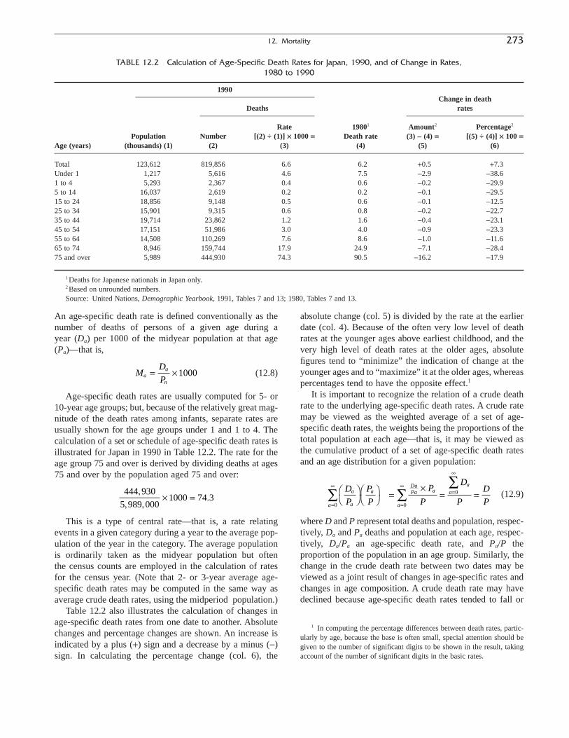
An age-specific death rate is defined conventionally as thenumber of deaths of persons of a given age during a year (Da) per 1000 of the midyear population at that age(Pa)—that is,
(12.8)
Age-specific death rates are usually computed for 5- or10-year age groups; but, because of the relatively great mag-nitude of the death rates among infants, separate rates areusually shown for the age groups under 1 and 1 to 4. Thecalculation of a set or schedule of age-specific death rates isillustrated for Japan in 1990 in Table 12.2. The rate for theage group 75 and over is derived by dividing deaths at ages75 and over by the population aged 75 and over:
This is a type of central rate—that is, a rate relatingevents in a given category during a year to the average pop-ulation of the year in the category. The average populationis ordinarily taken as the midyear population but often the census counts are employed in the calculation of ratesfor the census year. (Note that 2- or 3-year average age-specific death rates may be computed in the same way asaverage crude death rates, using the midperiod population.)
Table 12.2 also illustrates the calculation of changes inage-specific death rates from one date to another. Absolutechanges and percentage changes are shown. An increase isindicated by a plus (+) sign and a decrease by a minus (-)sign. In calculating the percentage change (col. 6), the
444 9305 989 000
1000 74 3,
, ,.¥ =
MD
Pa
a
n
= ¥ 1000
absolute change (col. 5) is divided by the rate at the earlierdate (col. 4). Because of the often very low level of deathrates at the younger ages above earliest childhood, and thevery high level of death rates at the older ages, absolutefigures tend to “minimize” the indication of change at theyounger ages and to “maximize” it at the older ages, whereaspercentages tend to have the opposite effect.1
It is important to recognize the relation of a crude deathrate to the underlying age-specific death rates. A crude ratemay be viewed as the weighted average of a set of age-specific death rates, the weights being the proportions of thetotal population at each age—that is, it may be viewed asthe cumulative product of a set of age-specific death ratesand an age distribution for a given population:
(12.9)
where D and P represent total deaths and population, respec-tively, Da and Pa deaths and population at each age, respec-tively, Da/Pa an age-specific death rate, and Pa/P theproportion of the population in an age group. Similarly, thechange in the crude death rate between two dates may beviewed as a joint result of changes in age-specific rates andchanges in age composition. A crude death rate may havedeclined because age-specific death rates tended to fall or
D
P
P
P
P
P
D
P
D
Pa
aa
aDaPa a
a
aaÊ
ˈ¯ÊË
ˆ¯ =
¥= =
=
•
=
•=
•
 ÂÂ
0 0
0
12. Mortality 273
1 In computing the percentage differences between death rates, partic-ularly by age, because the base is often small, special attention should begiven to the number of significant digits to be shown in the result, takingaccount of the number of significant digits in the basic rates.
TABLE 12.2 Calculation of Age-Specific Death Rates for Japan, 1990, and of Change in Rates,1980 to 1990
1990Change in death
Deaths rates
Rate 19801 Amount2 Percentage2
Population Number [(2) ÷ (1)] ¥ 1000 = Death rate (3) - (4) = [(5) ÷ (4)] ¥ 100 =Age (years) (thousands) (1) (2) (3) (4) (5) (6)
Total 123,612 819,856 6.6 6.2 +0.5 +7.3Under 1 1,217 5,616 4.6 7.5 -2.9 -38.61 to 4 5,293 2,367 0.4 0.6 -0.2 -29.95 to 14 16,037 2,619 0.2 0.2 -0.1 -29.515 to 24 18,856 9,148 0.5 0.6 -0.1 -12.525 to 34 15,901 9,315 0.6 0.8 -0.2 -22.735 to 44 19,714 23,862 1.2 1.6 -0.4 -23.145 to 54 17,151 51,986 3.0 4.0 -0.9 -23.355 to 64 14,508 110,269 7.6 8.6 -1.0 -11.665 to 74 8,946 159,744 17.9 24.9 -7.1 -28.475 and over 5,989 444,930 74.3 90.5 -16.2 -17.9
1 Deaths for Japanese nationals in Japan only. 2 Based on unrounded numbers.Source: United Nations, Demographic Yearbook, 1991, Tables 7 and 13; 1980, Tables 7 and 13.

because the proportion of the population in childhood andthe young adult ages, where age-specific death rates are low,increased.
Similarly, age-specific death rates may vary from countryto country in a quite different degree from the correspon-ding crude death rates. The various age-specific death ratesmay generally be much higher in one country than inanother, while the crude rates in the two countries may benearly the same or have an opposite relation.
Death rates may be made specific for sex and for othercharacteristics in combination with age. An age-sex specificdeath rate is defined as the number of deaths of males orfemales in a particular age group per 1000 males or femalesin the age group:
(12.10)
Next to age, sex may be considered the most importantvariable in the analysis of mortality. In fact, age-specificdeath rates are almost always sex-specific also. A compari-son of male and female death rates by age is given in theform of the percentage excess of the male rate over thefemale rate for a few countries in Table 12.3. Death rates ofmales show a marked excess over death rates for females inall or most age groups, particularly in areas of low mortal-ity. The lower the general level of mortality, the greater theexcess of male over female mortality tends to be. Thus, thegap between the rates for the sexes tends to be smaller inthe less developed countries. It may even be completelyerased (e.g., Bangladesh, Nepal, and Mali) or the femalerates may be higher only in older childhood or the repro-
D
P
D
Pam
am
af
af
¥ ¥1000 1000,
ductive ages (e.g., Sri Lanka, India, and Pakistan). Gener-ally, too, the time trends in the differences between male andfemale age-specific death rates have followed the precedingpatterns as mortality declined. A number of studies haveconsidered the causes of the sex differences in mortality(Rogers et al., 2000, Chapter 3; Wingard, 1982).
Death rates may be limited on the basis of other charac-teristics in addition to age and sex, for example, nativity,race, various socioeconomic characteristics, and cause ofdeath. Other types of specific death rates are considered inthe next sections.
Cause-Specific Death Ratios and Rates
An important aspect of the analysis of mortality relatesto the classification by cause of death. The classification ofdeaths according to cause employed by national govern-ments generally follows the International Classification ofDiseases as promulgated by the World Health Organization(WHO). The classification has regularly gone through adecennial revision under the auspices of the WHO or itspredecessor organizations in order that it may be consistentwith the latest diagnostic practice and with medicaladvances. The Ninth Revision of the International Classifi-cation was adopted by the World Health Organization in 1975 and has been used for compiling mortality data in the United States since 1979 (World Health Organization, 1977). The Eighth Revision of the Interna-tional Classification was adopted by the World Health Organization in 1965 and was first employed in modifiedform in the United States in 1968 (U.S. National Center forHealth Statistics, 2001; WHO, 1967). The Seventh Revision
274 McGehee
TABLE 12.3 Comparison of Male and Female Age-Specific Death Rates, for Various Countries:Around 1990
United States, 1990 El Salvador, 1992 Korea, 1994
Excess of Excess of Excess of male rate1 male rate1 male rate1
Male Female (2) - (1) = Male Female (4) - (5) = Male Female (7) - (8) =Age (years) (1) (2) (3) (4) (5) (6) (7) (8) (9)
All agesUnder 5 2.8 2.2 0.6 6.4 5.3 1.1 1.4 1.1 0.2Under 1 13.6 10.7 2.9 28.7 22.6 6.0 3.5 2.9 0.61 to 4 0.5 0.4 0.1 1.4 1.4 0.1 0.8 0.7 0.15 to 14 0.3 0.2 0.1 0.7 0.5 0.2 0.5 0.3 0.115 to 24 1.5 0.5 1.0 2.7 0.9 1.9 1.2 0.5 0.725 to 34 2.0 0.7 1.3 5.1 1.3 3.8 1.9 0.8 1.235 to 44 3.1 1.4 1.7 7.1 2.3 4.8 3.7 1.2 2.545 to 54 6.1 3.4 2.7 10.2 4.4 5.8 8.4 3.0 5.455 to 64 15.5 8.8 6.7 16.6 9.7 6.9 17.6 7.3 10.365 to 74 34.9 19.9 15.0 16.6 9.7 6.9 43.4 21.7 21.875 and over 98.8 74.0 24.7 78.0 66.2 11.7 203.0 178.3 24.7
1 Based on unrounded numbers.Source: U.S. National Center for Health Statistics, Vital Statistics of the United States, 1993, Vol. II, Mortality, Part A, Tables 1.27 and 1.4; and United
Nations, Demographic Yearbook.
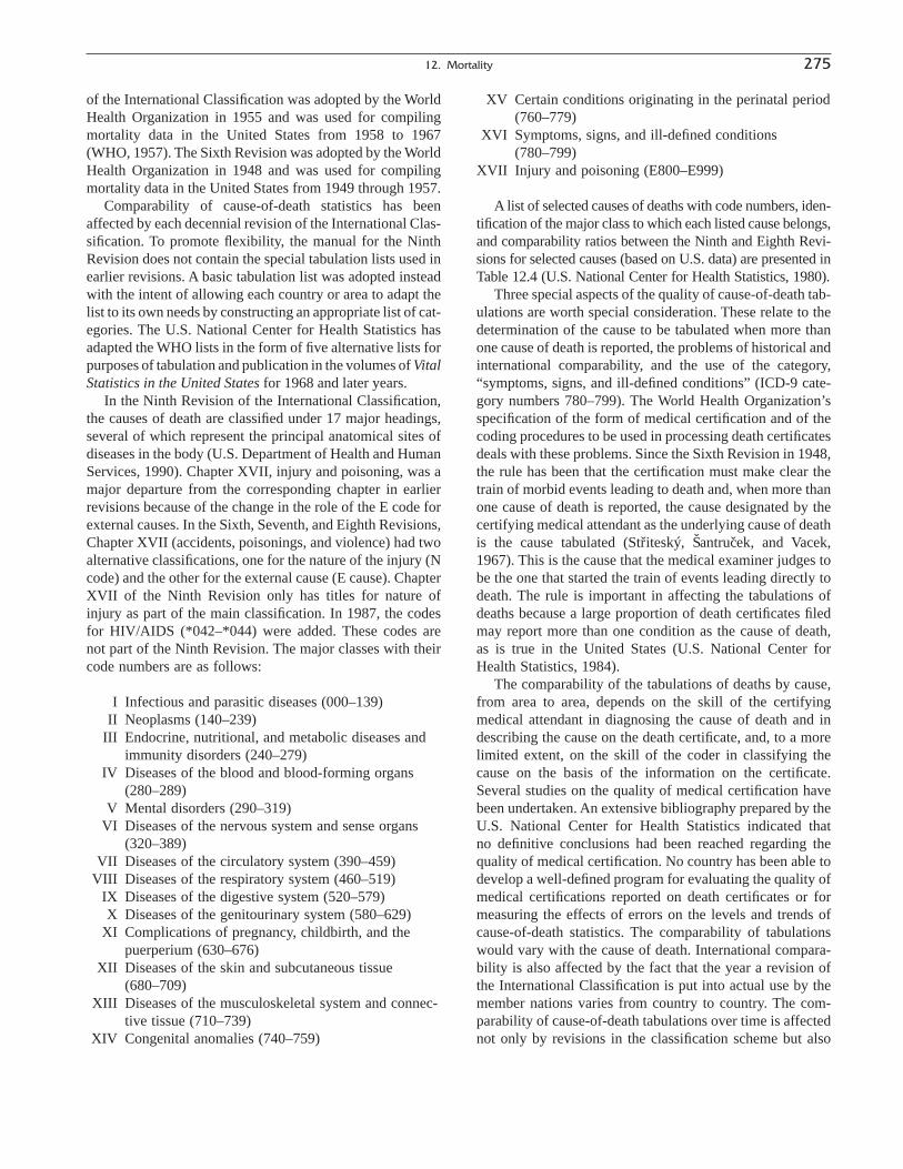
of the International Classification was adopted by the WorldHealth Organization in 1955 and was used for compilingmortality data in the United States from 1958 to 1967(WHO, 1957). The Sixth Revision was adopted by the WorldHealth Organization in 1948 and was used for compilingmortality data in the United States from 1949 through 1957.
Comparability of cause-of-death statistics has beenaffected by each decennial revision of the International Clas-sification. To promote flexibility, the manual for the NinthRevision does not contain the special tabulation lists used inearlier revisions. A basic tabulation list was adopted insteadwith the intent of allowing each country or area to adapt thelist to its own needs by constructing an appropriate list of cat-egories. The U.S. National Center for Health Statistics hasadapted the WHO lists in the form of five alternative lists forpurposes of tabulation and publication in the volumes of VitalStatistics in the United States for 1968 and later years.
In the Ninth Revision of the International Classification,the causes of death are classified under 17 major headings,several of which represent the principal anatomical sites ofdiseases in the body (U.S. Department of Health and HumanServices, 1990). Chapter XVII, injury and poisoning, was amajor departure from the corresponding chapter in earlierrevisions because of the change in the role of the E code forexternal causes. In the Sixth, Seventh, and Eighth Revisions,Chapter XVII (accidents, poisonings, and violence) had twoalternative classifications, one for the nature of the injury (Ncode) and the other for the external cause (E cause). ChapterXVII of the Ninth Revision only has titles for nature ofinjury as part of the main classification. In 1987, the codesfor HIV/AIDS (*042–*044) were added. These codes arenot part of the Ninth Revision. The major classes with theircode numbers are as follows:
I Infectious and parasitic diseases (000–139)II Neoplasms (140–239)
III Endocrine, nutritional, and metabolic diseases andimmunity disorders (240–279)
IV Diseases of the blood and blood-forming organs(280–289)
V Mental disorders (290–319)VI Diseases of the nervous system and sense organs
(320–389)VII Diseases of the circulatory system (390–459)
VIII Diseases of the respiratory system (460–519)IX Diseases of the digestive system (520–579)X Diseases of the genitourinary system (580–629)
XI Complications of pregnancy, childbirth, and thepuerperium (630–676)
XII Diseases of the skin and subcutaneous tissue(680–709)
XIII Diseases of the musculoskeletal system and connec-tive tissue (710–739)
XIV Congenital anomalies (740–759)
XV Certain conditions originating in the perinatal period(760–779)
XVI Symptoms, signs, and ill-defined conditions(780–799)
XVII Injury and poisoning (E800–E999)
A list of selected causes of deaths with code numbers, iden-tification of the major class to which each listed cause belongs,and comparability ratios between the Ninth and Eighth Revi-sions for selected causes (based on U.S. data) are presented inTable 12.4 (U.S. National Center for Health Statistics, 1980).
Three special aspects of the quality of cause-of-death tab-ulations are worth special consideration. These relate to thedetermination of the cause to be tabulated when more thanone cause of death is reported, the problems of historical andinternational comparability, and the use of the category,“symptoms, signs, and ill-defined conditions” (ICD-9 cate-gory numbers 780–799). The World Health Organization’sspecification of the form of medical certification and of thecoding procedures to be used in processing death certificatesdeals with these problems. Since the Sixth Revision in 1948,the rule has been that the certification must make clear thetrain of morbid events leading to death and, when more thanone cause of death is reported, the cause designated by thecertifying medical attendant as the underlying cause of deathis the cause tabulated (Střiteský, Šantruček, and Vacek,1967). This is the cause that the medical examiner judges tobe the one that started the train of events leading directly todeath. The rule is important in affecting the tabulations ofdeaths because a large proportion of death certificates filedmay report more than one condition as the cause of death,as is true in the United States (U.S. National Center forHealth Statistics, 1984).
The comparability of the tabulations of deaths by cause,from area to area, depends on the skill of the certifyingmedical attendant in diagnosing the cause of death and indescribing the cause on the death certificate, and, to a morelimited extent, on the skill of the coder in classifying thecause on the basis of the information on the certificate.Several studies on the quality of medical certification havebeen undertaken. An extensive bibliography prepared by theU.S. National Center for Health Statistics indicated that no definitive conclusions had been reached regarding thequality of medical certification. No country has been able todevelop a well-defined program for evaluating the quality ofmedical certifications reported on death certificates or formeasuring the effects of errors on the levels and trends ofcause-of-death statistics. The comparability of tabulationswould vary with the cause of death. International compara-bility is also affected by the fact that the year a revision ofthe International Classification is put into actual use by themember nations varies from country to country. The com-parability of cause-of-death tabulations over time is affectednot only by revisions in the classification scheme but also
12. Mortality 275
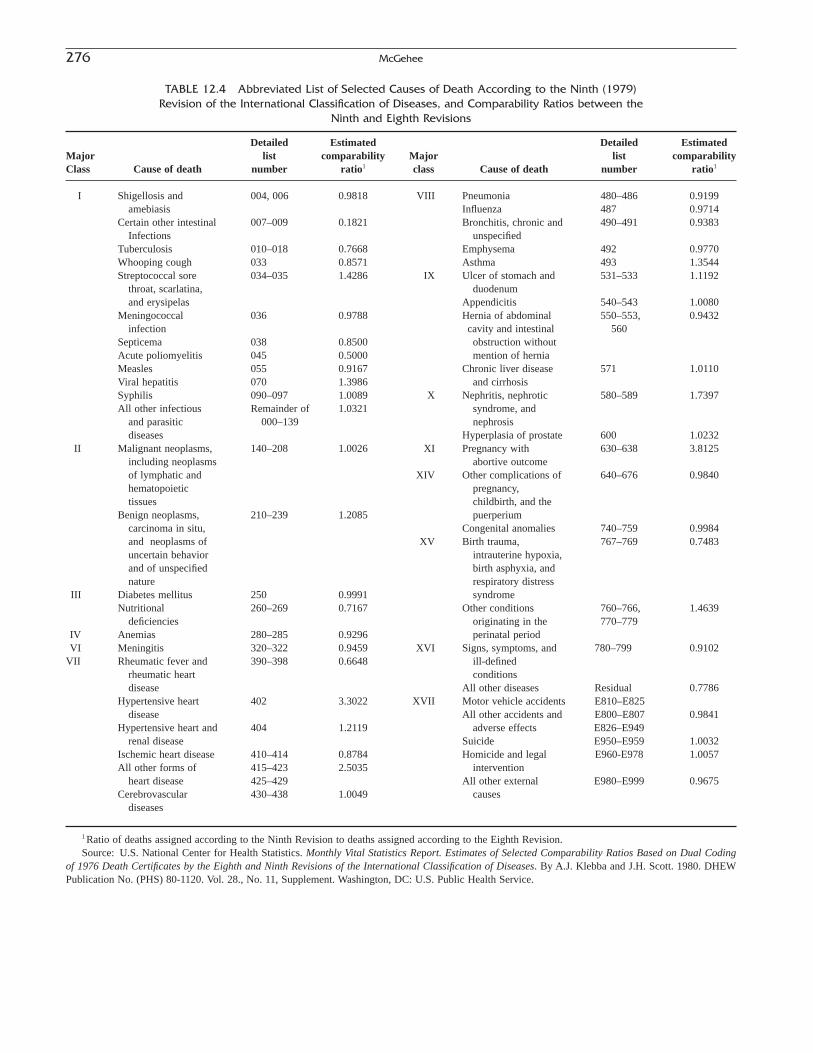
276 McGehee
TABLE 12.4 Abbreviated List of Selected Causes of Death According to the Ninth (1979) Revision of the International Classification of Diseases, and Comparability Ratios between the
Ninth and Eighth Revisions
Detailed Estimated Detailed EstimatedMajor list comparability Major list comparabilityClass Cause of death number ratio1 class Cause of death number ratio1
I Shigellosis and 004, 006 0.9818 VIII Pneumonia 480–486 0.9199amebiasis Influenza 487 0.9714
Certain other intestinal 007–009 0.1821 Bronchitis, chronic and 490–491 0.9383Infections unspecified
Tuberculosis 010–018 0.7668 Emphysema 492 0.9770Whooping cough 033 0.8571 Asthma 493 1.3544Streptococcal sore 034–035 1.4286 IX Ulcer of stomach and 531–533 1.1192
throat, scarlatina, duodenumand erysipelas Appendicitis 540–543 1.0080
Meningococcal 036 0.9788 Hernia of abdominal 550–553, 0.9432infection cavity and intestinal 560
Septicema 038 0.8500 obstruction withoutAcute poliomyelitis 045 0.5000 mention of herniaMeasles 055 0.9167 Chronic liver disease 571 1.0110Viral hepatitis 070 1.3986 and cirrhosisSyphilis 090–097 1.0089 X Nephritis, nephrotic 580–589 1.7397All other infectious Remainder of 1.0321 syndrome, and
and parasitic 000–139 nephrosisdiseases Hyperplasia of prostate 600 1.0232
II Malignant neoplasms, 140–208 1.0026 XI Pregnancy with 630–638 3.8125including neoplasms abortive outcomeof lymphatic and XIV Other complications of 640–676 0.9840hematopoietic pregnancy, tissues childbirth, and the
Benign neoplasms, 210–239 1.2085 puerperiumcarcinoma in situ, Congenital anomalies 740–759 0.9984and neoplasms of XV Birth trauma, 767–769 0.7483uncertain behavior intrauterine hypoxia,and of unspecified birth asphyxia, andnature respiratory distress
III Diabetes mellitus 250 0.9991 syndromeNutritional 260–269 0.7167 Other conditions 760–766, 1.4639
deficiencies originating in the 770–779IV Anemias 280–285 0.9296 perinatal periodVI Meningitis 320–322 0.9459 XVI Signs, symptoms, and 780–799 0.9102
VII Rheumatic fever and 390–398 0.6648 ill-definedrheumatic heart conditionsdisease All other diseases Residual 0.7786
Hypertensive heart 402 3.3022 XVII Motor vehicle accidents E810–E825disease All other accidents and E800–E807 0.9841
Hypertensive heart and 404 1.2119 adverse effects E826–E949renal disease Suicide E950–E959 1.0032
Ischemic heart disease 410–414 0.8784 Homicide and legal E960-E978 1.0057All other forms of 415–423 2.5035 intervention
heart disease 425–429 All other external E980–E999 0.9675Cerebrovascular 430–438 1.0049 causes
diseases
1 Ratio of deaths assigned according to the Ninth Revision to deaths assigned according to the Eighth Revision.Source: U.S. National Center for Health Statistics. Monthly Vital Statistics Report. Estimates of Selected Comparability Ratios Based on Dual Coding
of 1976 Death Certificates by the Eighth and Ninth Revisions of the International Classification of Diseases. By A.J. Klebba and J.H. Scott. 1980. DHEWPublication No. (PHS) 80-1120. Vol. 28., No. 11, Supplement. Washington, DC: U.S. Public Health Service.

by improved diagnosis and changing fashions in diagnosis.These last factors may account, in part, for the recent rise inmortality attributable to the chronic diseases of later life inthe less developed countries.
Although some deaths are extremely difficult to classify,care in the certification of cause of death keeps the numberof deaths of ill-defined or unknown cause to a minimum.The proportion of deaths assigned to “symptoms, senility,and ill-defined conditions” (Eighth Revision categorynumbers 780–796 and Ninth Revision category numbers780–799) may be employed as one measure of the qualityof reporting cause of death. For example, this categoryaccounts for less than 1% of the deaths in Australia (1994),slightly more than 1% in the United States (1993), but for21% in Egypt (1987) and 21% in South Africa (1993).Clearly, the cause-of-death tabulations for Egypt and SouthAfrica should be used with caution.
Mortality by cause of death may be analyzed in terms oftwo observed measures: death ratios specific for cause anddeath rates specific for cause. The former measure requiressimply a distribution of deaths by cause and hence can becomputed for intercensal years even when populationfigures are lacking.
A cause-specific death ratio represents the percentage ofall deaths due to a particular cause or group of causes. Thedeath ratio for cause C is
(12.11)D
Dc ¥ 100
where Dc, represents deaths from a particular cause or groupof causes, and D represents all deaths. Death ratios by causeare shown for several countries in Table 12.5. A set of deathratios readily permits comparisons from country to country,or from one year to another for the same country, of the rel-ative importance of a particular cause or group of causes ofdeath. For example, the death ratio for cerebrovasculardisease is considerably higher in Spain (13.0%) and Japan(14.9%) than in some other countries (e.g., 6.7% in theUnited States, 1990, and 4.5% in El Salvador, 1990). Thedeath ratio for tuberculosis is much higher in Zimbabwe(4.3% in 1990) than in the other countries.
The population exposed to risk of death from a particu-lar cause or group of causes may be directly taken accountof, in rough terms, by calculating “crude” cause-of-deathrates (Table 12.6). Separate death rates may be calculatedfor each cause or group of causes of death. A cause-specificdeath rate is conventionally defined as the number of deathsfrom a given cause or group of causes during a year per100,000 of the midyear population.
(12.12)
A cause-specific death rate employs a larger constant, or k,factor than a crude death rate or an age-specific death ratebecause there are relatively few deaths from many of thecauses.
It should be noted that a cause-specific death rate isunlike other types of death rates in one important respect—
D
Pc ¥ 100 000,
12. Mortality 277
TABLE 12.5 Deaths and Death Ratios Specific by Cause, for Various Countries: 1990 (Deaths areclassified according to the Ninth (1979) Revision of the International Statistical Classification ofDiseases, Injuries, and Causes of Death. Ratios are the number of deaths from each cause per
100 deaths from all causes.)
United States Zimbabwe2 El Salvador3 Spain Japan4
Cause of death1 Deaths Ratios Deaths Ratios Deaths Ratios Deaths Ratios Deaths Ratios
All causes 2,148,463 100.0 34,829 100.0 28,224 100.0 333,142 100.0 820,305 100.0Tuberculosis (010–018) 1,810 0.1 1,501 4.3 132 0.5 861 0.3 3,664 0.4Malignant neoplasm of female 43,391 2.0 100 0.3 38 0.1 5,398 1.6 5,848 0.7
breast (174)Diabetes mellitus (250) 47,664 2.2 349 1.0 347 1.2 8,989 2.7 9,470 1.2Cerebrovascular diseases (430–438) 144,088 6.7 1,175 3.4 1,256 4.5 43,263 13.0 121,944 14.9Atherosclerosis (440) 18,047 0.8 45 0.1 11 z 9,626 2.9 2,118 0.3Chronic liver disease and cirrhosis (571) 25,815 1.2 419 1.2 345 1.2 7,892 2.4 16,804 2.0Nephritis, nephrotic syndrome, and 20,764 1.0 461 1.3 282 1.0 5,632 1.7 17,140 2.1
nephrosis (580–589)Congenital anomalies (740–759) 13,085 0.6 485 1.4 214 0.8 1,382 0.4 3,571 0.4All other diseases 1,683,588 78.4 25,849 74.2 20,168 71.5 231,232 69.4 584,134 71.2Accidents, suicides, and homicides 150,211 7.0 4,445 12.8 5,431 19.2 18,867 5.7 55,612 6.8
(E810–E999)
z Less than 0.05.1 Numbers in parentheses represent the code numbers in the Ninth (1979) Revision of the International Classification.2 Data from incomplete registers.3 Includes deaths of foreigners temporarily in country.4 Japanese nationals only.Source: United Nations, Demographic Yearbook, 1995, Table 20.
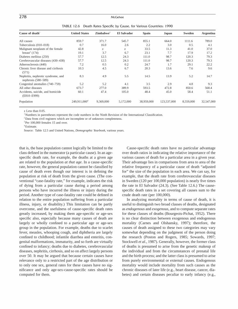
278 McGehee
TABLE 12.6 Death Rates Specific by Cause, for Various Countries: 1990
Cause of death1 United States Zimbabwe2 El Salvador Spain Japan Sweden Argentina
All causes 859.7 371.7 545.7 855.1 664.0 1111.6 789.0Tuberculosis (010–018) 0.7 16.0 2.6 2.2 3.0 0.5 4.1Malignant neoplasm of the female 42.8 z z 33.5 11.3 41.0 37.0
breast3 (174) 19.1 3.7 6.7 23.1 7.7 17.9 17.2Diabetes mellitus (250) 57.7 12.5 24.3 111.0 98.7 120.3 79.3Cerebrovascular diseases (430–438) 57.7 12.5 24.3 111.0 98.7 120.3 79.3Atherosclerosis (440) 7.2 0.5 0.2 24.7 1.7 29.1 22.2Chronic liver disease and cirrhosis 10.3 4.5 6.7 20.3 13.6 7.6 9.6
(571)Nephritis, nephrotic syndrome, and 8.3 4.9 5.5 14.5 13.9 5.2 14.7
nephrosis (580–589)Congenital anomalies (740–759) 5.2 5.2 4.1 3.5 2.9 4.8 9.3All other diseases 673.7 277.0 389.9 593.5 472.8 850.6 568.4Accidents, suicide, and homicide 60.1 47.4 105.0 48.4 45.0 58.4 51.1
(E810–E999)
Population 249,911,0004 9,369,000 5,172,000 38,959,000 123,537,000 8,559,000 32,547,000
z Less than 0.05.1 Numbers in parentheses represent the code numbers in the Ninth Revision of the International Classification.2 Data from civil registers which are incomplete or of unknown completeness.3 Per 100,000 females 15 and over.4 Estimate.Source: Table 12.5 and United Nations, Demographic Yearbook, various years.
that is, the base population cannot logically be limited to theclass defined in the numerator (a particular cause). In an age-specific death rate, for example, the deaths at a given ageare related to the population at that age. In a cause-specificrate, however, the general population cannot be classified bycause of death even though our interest is in defining thepopulation at risk of death from the given cause. (The con-ventional “case-fatality rate,” for example, indicates the riskof dying from a particular cause during a period amongpersons who have incurred the illness or injury during theperiod. Another type of case-fatality rate could be defined inrelation to the entire population suffering from a particularillness, injury, or disability.) This limitation can be partlyovercome, and the usefulness of cause-specific death ratesgreatly increased, by making them age-specific or age-sexspecific also, especially because many causes of death arelargely or wholly confined to a particular age or age-sexgroup in the population. For example, deaths due to scarletfever, measles, whooping cough, and diphtheria are largelyconfined to childhood; infantile diarrhea and enteritis, con-genital malformations, immaturity, and so forth are virtuallyconfined to infancy; deaths due to diabetes, cerebrovasculardiseases, nephritis, cirrhosis, and so on affect largely personsover 50. It may be argued that because certain causes haverelevance only to a restricted part of the age distribution orto only one sex, general rates for these causes have no sig-nificance and only age-sex-cause-specific rates should becomputed for them.
Cause-specific death rates have no particular advantageover death ratios in indicating the relative importance of thevarious causes of death for a particular area in a given year.Their advantage lies in comparisons from area to area of therelative frequency of a particular cause of death “adjustedfor” the size of the population in each area. We can say, forexample, that the death rate from cerebrovascular diseasesin Sweden (120 per 100,000 population) is nearly five timesthe rate in El Salvador (24.3). (See Table 12.6.) The cause-specific death rates in a set covering all causes sum to thecrude death rate (per 100,000).
In analyzing mortality in terms of cause of death, it isuseful to distinguish two broad classes of deaths, designatedas endogenous and exogenous, and to compute separate ratesfor these classes of deaths (Bourgeois-Pichat, 1952). Thereis no clear distinction between exogenous and endogenousmortality (Carnes and Olshansky, 1997); therefore, thecauses of death assigned to these two categories may varysomewhat depending on the judgment of the person doingthe research (Poston and Rogers, 1985; Sowards, 1997;Stockwell et al., 1987). Generally, however, the former classof deaths is presumed to arise from the genetic makeup ofthe individual and from the circumstances of prenatal lifeand the birth process; and the latter class is presumed to arisefrom purely environmental or external causes. Endogenousmortality would include mortality from such causes as thechronic diseases of later life (e.g., heart disease, cancer, dia-betes) and certain diseases peculiar to early infancy (e.g.,
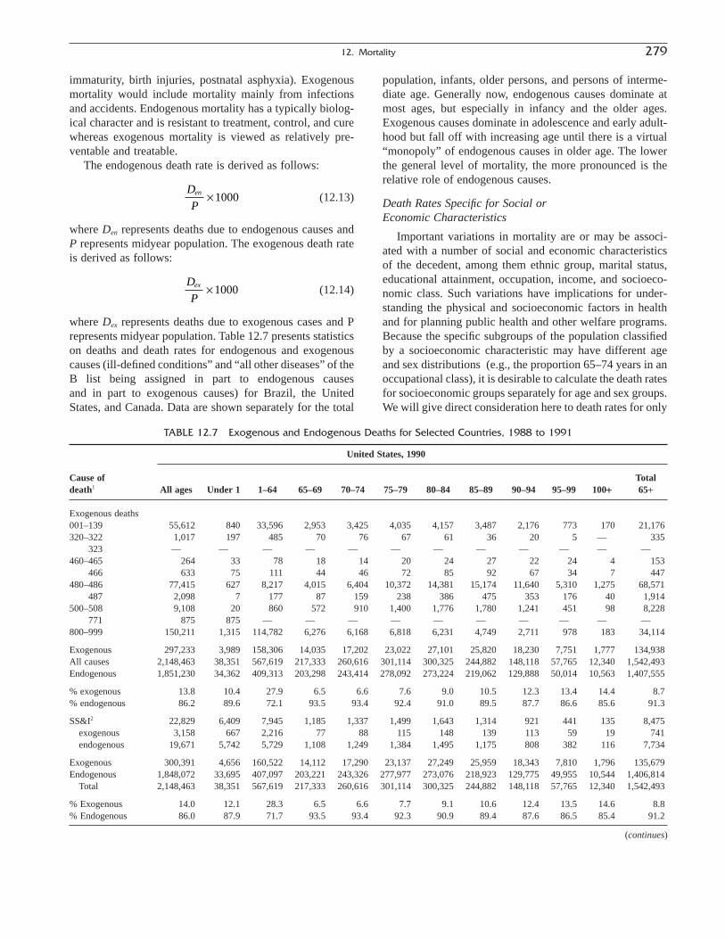
immaturity, birth injuries, postnatal asphyxia). Exogenousmortality would include mortality mainly from infectionsand accidents. Endogenous mortality has a typically biolog-ical character and is resistant to treatment, control, and curewhereas exogenous mortality is viewed as relatively pre-ventable and treatable.
The endogenous death rate is derived as follows:
(12.13)
where Den represents deaths due to endogenous causes andP represents midyear population. The exogenous death rateis derived as follows:
(12.14)
where Dex represents deaths due to exogenous cases and Prepresents midyear population. Table 12.7 presents statisticson deaths and death rates for endogenous and exogenouscauses (ill-defined conditions” and “all other diseases” of theB list being assigned in part to endogenous causes and in part to exogenous causes) for Brazil, the UnitedStates, and Canada. Data are shown separately for the total
D
Pex ¥ 1000
D
Pen ¥ 1000
population, infants, older persons, and persons of interme-diate age. Generally now, endogenous causes dominate atmost ages, but especially in infancy and the older ages.Exogenous causes dominate in adolescence and early adult-hood but fall off with increasing age until there is a virtual“monopoly” of endogenous causes in older age. The lowerthe general level of mortality, the more pronounced is therelative role of endogenous causes.
Death Rates Specific for Social or Economic Characteristics
Important variations in mortality are or may be associ-ated with a number of social and economic characteristicsof the decedent, among them ethnic group, marital status,educational attainment, occupation, income, and socioeco-nomic class. Such variations have implications for under-standing the physical and socioeconomic factors in healthand for planning public health and other welfare programs.Because the specific subgroups of the population classifiedby a socioeconomic characteristic may have different ageand sex distributions (e.g., the proportion 65–74 years in anoccupational class), it is desirable to calculate the death ratesfor socioeconomic groups separately for age and sex groups.We will give direct consideration here to death rates for only
12. Mortality 279
TABLE 12.7 Exogenous and Endogenous Deaths for Selected Countries, 1988 to 1991
United States, 1990
Cause of Totaldeath1 All ages Under 1 1–64 65–69 70–74 75–79 80–84 85–89 90–94 95–99 100+ 65+
Exogenous deaths001–139 55,612 840 33,596 2,953 3,425 4,035 4,157 3,487 2,176 773 170 21,176320–322 1,017 197 485 70 76 67 61 36 20 5 — 335
323 — — — — — — — — — — — —460–465 264 33 78 18 14 20 24 27 22 24 4 153
466 633 75 111 44 46 72 85 92 67 34 7 447480–486 77,415 627 8,217 4,015 6,404 10,372 14,381 15,174 11,640 5,310 1,275 68,571
487 2,098 7 177 87 159 238 386 475 353 176 40 1,914500–508 9,108 20 860 572 910 1,400 1,776 1,780 1,241 451 98 8,228
771 875 875 — — — — — — — — — —800–999 150,211 1,315 114,782 6,276 6,168 6,818 6,231 4,749 2,711 978 183 34,114
Exogenous 297,233 3,989 158,306 14,035 17,202 23,022 27,101 25,820 18,230 7,751 1,777 134,938All causes 2,148,463 38,351 567,619 217,333 260,616 301,114 300,325 244,882 148,118 57,765 12,340 1,542,493Endogenous 1,851,230 34,362 409,313 203,298 243,414 278,092 273,224 219,062 129,888 50,014 10,563 1,407,555
% exogenous 13.8 10.4 27.9 6.5 6.6 7.6 9.0 10.5 12.3 13.4 14.4 8.7% endogenous 86.2 89.6 72.1 93.5 93.4 92.4 91.0 89.5 87.7 86.6 85.6 91.3
SS&I2 22,829 6,409 7,945 1,185 1,337 1,499 1,643 1,314 921 441 135 8,475exogenous 3,158 667 2,216 77 88 115 148 139 113 59 19 741endogenous 19,671 5,742 5,729 1,108 1,249 1,384 1,495 1,175 808 382 116 7,734
Exogenous 300,391 4,656 160,522 14,112 17,290 23,137 27,249 25,959 18,343 7,810 1,796 135,679Endogenous 1,848,072 33,695 407,097 203,221 243,326 277,977 273,076 218,923 129,775 49,955 10,544 1,406,814
Total 2,148,463 38,351 567,619 217,333 260,616 301,114 300,325 244,882 148,118 57,765 12,340 1,542,493
% Exogenous 14.0 12.1 28.3 6.5 6.6 7.7 9.1 10.6 12.4 13.5 14.6 8.8% Endogenous 86.0 87.9 71.7 93.5 93.4 92.3 90.9 89.4 87.6 86.5 85.4 91.2
(continues)

TABLE 12.7 (continued)
Cause ofBrazil, 1988
death1 All ages Under 1 1–64 65–74 75+ 65+
Exogenous deaths001–139 47,829 19,075 22,376 2,953 3,425 6,378320–322 2,940 1,244 1,541 93 62 155
323 — — — — — —460–465 913 691 164 15 43 58
466 — — — — — —480–487 35,980 627 24,934 4,015 6,404 10,419
487 — — — — — —500–508 — — — — — —
771 — — — — — —E47–E53 53,311 910 46,762 2,699 2,940 5,639
E54 4,492 0 4,024 281 187 468E55 23,341 58 22,789 345 149 494E56 14,939 124 13,913 513 389 902
Exogenous 183,745 22,729 136,503 10,914 13,599 24,513All causes 833,369 119,792 378,453 136,834 198,290 335,124Endogenous 649,624 97,063 241,950 125,920 184,691 310,611
% exogenous 22.0 19.0 36.1 8.0 6.9 7.3% endogenous 78.0 81.0 63.9 92.0 93.1 92.7
SS&I2 157,812 26,406 56,290 25,178 49,938 75,116exogenous 34,795 5,010 24,351.87 2,008 3,425 5,433endogenous 123,017 21,396 31,938.13 23,170 46,513 69,683
Exogenous 218,540 27,739 160,855 12,922 17,024 29,946Endogenous 614,829 92,053 217,598 123,912 181,266 305,178
Total 833,369 119,792 378,453 136,834 198,290 335,124
% Exogenous 26.2 23.2 42.5 9.4 8.6 8.9% Endogenous 73.8 76.8 57.5 90.6 91.4 91.1
Cause ofCanada, 1991
death1 All ages Under 1 1–64 65–74 75+ 65+
Exogenous deaths001–139 1,454 26 413 332 683 1,015320–322 63 19 23 7 14 21
323 — — — — — —460–465 39 4 11 3 21 24
466 55 6 12 8 29 37480–487 6,776 34 514 837 5,391 6,228
487 — — — — — —500–508 — — — — — —
771 — — — — — —E47–E53 8,785 53 5,615 804 2,313 3,117
E54 3,593 — 3,146 277 170 447E55 622 12 567 24 19 43E56 237 6 194 22 15 37
Exogenous 21,624 160 10,495 2,314 8,655 10,969All causes 195,568 2,571 48,513 44,217 100,267 144,484Endogenous 173,944 2,411 38,018 41,903 91,612 133,515
— —
% exogenous 11.1 6.2 21.6 5.2 8.6 7.6% endogenous 88.9 93.8 78.4 94.8 91.4 92.4
SS&I2 3,682 437 1,259 596 1,390 1,986exogenous 407 27 272 31 120 151endogenous 3,275 410 987 565 1,270 1,835
Exogenous 22,031 187 10,723.75 2,345 8,775 11,120.17Endogenous 173,537 2,384 37,789.25 41,872 91,492 133,363.8
Total 195,568 2,571 48,513 44,217 100,267 144,484
% Exogenous 11.3 7.3 22.1 5.3 8.8 7.7% Endogenous 88.7 92.7 77.9 94.7 91.2 92.3
—zero.1 Ninth Revision of the International Classification of Diseases.2 “Symptoms, Signs, and ill-defined conditions.”Source: WHO, World Health Statistics Annual, 1993, 1994; and NCHS. 1990, Vital Statistics of the United States, Table 1.27.

a few of the possible characteristics, particularly maritalstatus, occupation, and socioeconomic status.
Death rates specific for marital status, age, and sex areuseful not only for the analysis of mortality patterns but alsofor the study of the dissolution of marriage. To compute suchrates, both death rates distributed by age, sex, and maritalstatus and population rates distributed by these characteris-tics are needed.
Such rates are affected by differences in the errors in, andby the comparability of, the information on marital status ondeath certificates and in the census. These are general prob-lems affecting vital rates for socioeconomic groupings of thepopulation since the numerator of the rate comes from the vital statistics system and the denominator comes fromthe census.
Little data are available of a satisfactory quality on deathsfor occupations and socioeconomic status. The principal tab-ulations of deaths for occupational categories have beenmade for the United States and the United Kingdom,although several other countries have compiled such data.National mortality data on occupations have appeareddecennially from 1851 to-date for England and Wales, withthe latest report covering the years 1979–1980 and 1982–1990. Canada also has produced a major report describingmortality on occupations in British Columbia with data cov-ering 1950 through 1984 (Gallagher et al., 1989). The firstreport describing occupational mortality in the United Stateswas published for scattered years beginning in 1890.
Death statistics and death rates for occupations are subjectto a number of important types of errors. They are subject to the errors of death statistics in general and to errors in thereporting, coding, and classification of occupation. When-ever a high proportion of deaths is unclassified or not clearlyclassified by occupation, the quality of the statistics on deaths is in question. Like death rates for marital status, death rates for occupations are affected by differences in thenature and accuracy of the information returned on the deathcertificate as compared with that returned in the populationcensus. The problem of disagreement between the reportingof occupations in the two sources can be sharply reduced bycombining occupations into major groups.
In the United States, the lack of correspondence betweennumerator and denominator of the death rate is chiefly aresult of the large proportion of decedents reported as “not in the labor force” or “retired” in the census (currentactivity) for whom a report of usual occupation is given on the death certificate. This problem can largely be elimi-nated by limiting the tabulations to the age range 20 to 59 or 20 to 64, although this excludes the majority of deaths.
In 1997, the United States published a study thatdescribed mortality by occupation, industry, and cause ofdeath using data from 24 reporting states for the years 1984to 1988 (U.S. NIOSH/Burnett, Maurer, and Dosemeci,1997). The report included an analysis for all white and
12. Mortality 281
Death rate fromNumber of tuberculosis, all
white miners working malesAge (years) pa Ma
20–24 74,598 .000122625–29 85,077 .000161230–34 80,845 .000215435–44 148,870 .000339645–54 102,649 .000568255–59 42,494 .000752360–64 30,037 .0008237
Total, 20–64 564,570 .0009565
1 Expected deaths from tuberculosis for white miners = SMapa =S column (1) ¥ column (2) = 2062 Tabulated deaths from tuberculosis for white miners = d = 5403 Standardized mortality ratio =
d
M p
m p
M pa a
a a
a aÂÂÂ
¥ ¥ = ¥ =100 100540
206100 263or
black males and females aged 20 and older. Women listedin the census as “housewives, homemakers” were excludedfrom both the occupation and industry analysis. This was thefirst report of its kind since 1962 when a study describingthe variation of mortality by occupation and industry amongmen 20 to 64 years of age in the United States in 1950resulted in the publication of a number of study on thissubject. In the 1962 report, for example, death rates (per100,000 population) were presented for specific occupa-tions, by age and color of decedent, and for specific indus-try groups, by age of decedent (U.S. NIOSH/Burnett et al.,1997). Standardized mortality ratios were presented for spe-cific occupations by color, for major occupation groups byselected causes of death and color, and for specific occupa-tions and industries by selected causes of death.
A standardized mortality ratio (SMR) for a particularoccupation or industry among males compares the tabulatednumbers of deaths in that occupation or industry with thenumber to be expected had the age-specific death rates forthe total male population with work experience prevailed inthat occupation or industry. The method of calculation usedin the 1962 publication is illustrated with data on deathsfrom tuberculosis of white miners in the United States in1950 (U.S. National Office of Vital Statistics, 1950b).
In this calculation, the age-specific death rates for allworking males (col. 2) are assumed to apply to white miners(col. 1) in order to derive the expected number of deathsfrom tuberculosis for white miners. The standardized mor-tality ratio represents the ratio of the number of actual deathsfrom tuberculosis for white miners, 540, to the expectednumber, 206, expressed as an index (i.e., per 100). As laterformulas show, the standardized mortality ratio is equivalent

to the relative mortality of an occupation group computedby the method of “indirect standardization.” Like allsummary measures of this kind, the standardized ratios maymask differences found in the underlying age-specific rates(Silcock, 1959, pp. 183–192).
The 1997 report uses age-standardized proportionatemortality ratios (PMR) for the four race-sex groups, by age(age 20 and over, 20 to 64 years of age, and 65 and over),for 325 occupation categories and 235 industry categoriesand for selected causes of death (188 causes for females and192 causes for males) as a measure of comparison. The pro-portionate mortality rate allows one to determine whetherthe proportion of deaths from a certain cause of death for acertain occupation is higher (greater than 100) or lower (lessthan 100) than the corresponding proportion for all occupa-tions combined (U.S. NIOSH/Burnett et al., 1997). A PMRgreater than 100 is an indication of a higher relative risk ofmortality. For example, a PMR of 156 for white male truckdrivers aged 20 years and older (occupation code 804) who died as a result of a motor vehicle accident (E810–E825, E929.0) means that the proportion of deaths from this cause for white male truck drivers was 56% higher than that for all males in all occupations combined for thiscause.
An advantage of the PMR is that it does not require thepopulation data needed for population-based measures suchas the SMR (U.S. National Center for Health Statistics/Rosenberg et al., 1993). However, the PMR has certain lim-itations as an indicator of relative mortality risk. First, it isa ratio, not a death rate, because total deaths instead of thepopulation at risk are used in its calculation (Dever, 1991).Second, PMRs can overstate the risk of mortality if the riskof death for all causes for an occupation or industry is low.Conversely, the PMR can understate mortality risk if theoverall risk of death is high (Decoufle, Thomas, and Pickle,1980). Third, abnormally high mortality in any of the majorcauses of death can distort the PMR. This is illustrated bythe case of a low PMR resulting from a disproportionately or unusually high number of deaths from a major cause ofdeath and vice versa. Finally, having a category of unre-ported occupations that are not distributed proportionatelycan affect the PMR (Zeighami and Morris, 1983). Theformula given in the 1997 report for calculating age-adjustedproportionate mortality rates is as follows (U.S. NIOSH/Burnett et al., 1997):
Cause of death
Occupation causes Cause X Other causes All
Occupation Y Ai Bi Nli
Other occupations Ci Di N2i
All occupations M1i M2i Ti
i = ith age group (5-year age groups 20–24, 25–29, etc.)Ai = observed number of deaths for a specific occupation (industry) and
cause-of-death combination for the ith age group
where E(Ai) = expected number of deaths for a specific occu-pation (industry) and cause-of-death combination for the ithage group.
(12.15)
The association between causes of death and occupationand industry of a decedent may be explained by several factors, such as the level of health required for certain occupations (e.g., firefighter), the attraction of certain ethnicgroups to particular types of occupations, and the socioeco-nomic status (income, educational attainment, etc.) of thedecedent that encourages a lifestyle or behavior (e.g., smoking,alcohol consumption) that may be more strongly associatedwith mortality than the occupations themselves (U.S. NationalCenter for Health Statistics/Rosenberg et al., 1993).
In 1992, a rather comprehensive study of the effect ofdemographic, social, and economic factors on mortality waspublished by the U.S. National Institutes of Health/Rogot,Sorlie, Johnson, and Schmitt, 1992. Data for the study camefrom the 1979–1985 follow-up of the U.S. National Longi-tudinal Mortality Study (NLMS). The NLMS is a long-termprospective study of mortality that is used mainly to examinesocioeconomic, demographic, and occupational mortalitydifferentials in the United States. The results of the 1992study were published in a book titled, A Mortality Study of 1.3 Million Persons: By Demographic, Social, and Economic Factors: 1979–1985 Follow-up, which was thesecond in a series of data books containing information fromthe NLMS. The first data book was published in 1988 andincluded data for 1979 to 1981. Standardized mortality ratios(SMRs) were calculated for 16 characteristics (e.g., nativity,education, income, marital status, employment status, etc.),by age, sex, and race, for the leading causes of death.
Adjusted Rates
Rates Adjusted to a Probability Basis
In general, the rates we have considered so far may bedescribed as “central rates.” Although they give a satisfac-tory indication of the relative frequency of the event ofdeath, they do not describe precisely the risk of dying forany actual cohort (i.e., they are not true probabilities). Suchprobabilities express the chance that death will occur duringa particular period to a person in a particular populationgroup alive at the beginning of the period. When the prob-ability is expressed as a ratio, the denominator represents theinitial population “exposed to risk” and the numerator thefrequency with which the event of death occurs in this par-ticular population over the period. The most commonlycomputed probabilities of death are specific by age and
PMRA
E A
i
i
=( )
¥Â 100
E AM N
Ti
i i
i
( ) = 1 1
282 McGehee

relate to a 1-year period. An age-specific probability ofdying might answer the question, for example, what is thechance that a newborn child will die before it reaches its firstbirthday? Such probabilities are referred to as “mortalityrates” to distinguish them from the “central death rates” or“death rates” that we have previously described.
Conventional Infant Mortality Rate
Analysis of infant mortality has commonly been carriedout in terms of the “infant mortality rate” rather than theinfant death rate to approximate the probability of deathamong infants in a given year. The accuracy of the approx-imation varies from one situation to another but depends ingeneral on the annual fluctuations in the number of births.We shall refer to this rate as the “conventional infant mor-tality rate” to distinguish it from certain other types of infantmortality rates, to be described, which are more akin to trueprobabilities. The conventional infant mortality rate isdefined as the number of infant deaths per year per 1000 livebirths during the year:
(12.16)
where Do represents deaths of infants during a year and Brepresents live births during the same year.
Infant mortality rates vary in the following array for 1990from 3.9 in Finland to 101.9 in Pakistan (United Nations,1995).
Country Rate Country Rate
Australia 5.7 Finland 3.9Turkey 44.4 Portugal 7.5Chile 11.1 Sweden 3.7Costa Rica 13.2 India 74.0Argentina 22.2 Thailand1 32.0United Kingdom 6.2 France 4.6Japan 4.3 United States 7.5Pakistan1 101.9 Venezuela 21.0Peru 81.0 Yugoslavia 16.4
1 1993.
Ordinarily, the conventional infant mortality rate gives asufficiently close approximation to the chance of dyingbetween birth and attainment of the first birthday for the yearto which the basic data on deaths relate. It has been widelyused as an indicator of the health conditions of a commu-nity and, hence, of its level of living, although it may not be particularly appropriate for this purpose in developedareas.
Because of the very high level of mortality in the firsthours, days, and weeks of life and the difference in thecauses accounting for infant deaths at the earlier and laterages of infancy, the conventional infant mortality rate mayusefully be “broken up” into a rate covering the first monthor so and a rate for the remainder of the year. The rate for
D
Bo ¥ 1000
the first period is called the neonatal mortality rate, and therate for the second period is called the post-neonatal mor-tality rate. The neonatal mortality rate is defined as thenumber of deaths of infants under 4 weeks of age (28 days)or under 1 month of age during a year per 1000 live birthsduring the year:
(12.17)
Because nearly all (over 95%) deaths of infants under 1month of age occur to babies born in the same year, theresulting neonatal mortality rate is close to a probability ofneonatal death. The post-neonatal mortality is defined as thenumber of infant deaths at 4 through 51 weeks of age or 1through 11 months of age during a year per 1000 live birthsduring the year:
(12.18)
The formula for the post-neonatal mortality rate is quitefar from expressing a true probability because more than athird of the infant deaths over 1 month of age in a year mayoccur to births of the previous year.
Adjusted Infant Mortality Rates
The conventional infant mortality rate is not a true prob-ability, as has been noted. We can recognize this immedi-ately by noting that not all of the infant deaths in a givenyear occurred to births in the same year; some occurred tobirths of the previous year. Consider, for example, the yearof birth of the older infants (e.g., 10 months old) dyingtoward the beginning of the calendar year (e.g., February)as compared with the younger infants (e.g., 2 months old)dying toward the end of the year (e.g., October). If thenumber of births does not fluctuate much from year to year,the conventional infant mortality rate for a year will repre-sent rather well the probability of an infant dying during theyear. If there are sharp fluctuations in the number of birthsbetween years and within years, however, the conventionalinfant mortality rate will give a distorted indication of thelevel and trend of infant mortality (U.S. Bureau of theCensus/Moriyama and Greville, 1944). It is desirable thento adjust the conventional rate to allow for the true popula-tion exposed to risk. Three alternative ways of calculatingadjusted infant mortality rates are described next.
First, it is useful to consider the following diagram, whichschematically shows the relationship among births in 3 successive years (y - 1, y, and y + 1), deaths under 1 in these
Post -neonatal mortality rate
or
= ¥
¥
-
-
D
BD
B
weeks
months
4 51
1 11
1000
1000
Neonatal mortality rate
or
= ¥
¥
-
<
D
BD
B
weeks
month
0 3
1
1000
1000
12. Mortality 283

years, and the number of survivors reaching their first birth-day in these years (l1).
deaths according to birth cohort—must be estimated or,more commonly, assumed on the basis of statistics for othercountries.
In the first procedure for calculating an “adjusted infantmortality rate” (Formula A in the table), the portion of deathsunder 1 in year y and the portion of deaths under 1 in yeary + 1 occurring to births in year y are combined and dividedby the births in year y. Deaths in 1995 and 1996 are relatedto births in 1995 for Japan:
Formula A:
(12.19)
In the next procedure (Formula B), each portion of the infant deaths occurring in a given year is related to the births in the appropriate year and cohort. The formula isillustrated with deaths in 1995 and births in 1995 and 1994for Japan:
Formula B:
(12.20)
In the third procedure for calculating an adjusted infantmortality rate for a particular year (Formula C), infant deathsin year y are divided by a weighted average of births in yearsy and y - l. The weights may be taken as the same (separa-
¢+
¢¢ÊË
ˆ¯ ¥ +Ê
ˈ¯
¥ = +( ) ¥ =-
D
B
D
By
y
y
y 1
10003946
1 187 0641108
1 238 328
1000 00332 00089 1000 4 2
or, , , ,
. . .
¢ + ¢¢¥
+¥ =+D D
By y
y
1 10003946 9481 187 064
1000 4 1or, ,
.
284 McGehee
By-1 By By+1
D¢y-1 D¢y D¢y+1
D≤y-1 D≤y D≤y+1
l1y-1 l1
y l1y+1
D¢y and D≤y together make up infant deaths in year y; D¢y isthe portion occurring to births in year y (By) and D≤y is theportion occurring to births of the previous year (By-1). Thecohort of births in year y (By) loses D¢y members throughdeath in year y and D≤y+1 members through death in year y + 1 while moving toward its first birthday (l1
y+1).Table 12.8 illustrates the calculation of the adjusted infant
mortality rate with data for Japan from 1995 to 1997 byseveral procedures. All the procedures allow for the fact thatsome of the infant deaths in a year occur to births of thesame year and some occur to births of the previous year or,conversely, that some of the babies born in a given year whodie before their first birthday die in the same year as the yearof birth and some die in the following year. The separationof the deaths by birth cohort is readily possible in the caseof Japan because the deaths are tabulated by year of birth.Normally, this is not the case, and the separation factorsfor infant deaths—that is, the proportions for dividing the
TABLE 12.8 Calculation of Conventional and Adjusted Infant Mortality Rates, for Japan:1995–1997
Year (y)
Item Symbols and fomulas 1994 1995 1996 1997
Births B 1,238,328 1,187,064 1,206,555 1,191,665Infant deathsDy≤ (X) (X) 1,108 948 914Dy¢ (X) (X) 3,946 3,598 3,489
Conventional infant mortality rate. (X) 4.3 3.8 3.7
Adjusted Infant Mortality rates:
A (X) 4.1 3.7 (X)
B (X) 4.2 3.8 3.7
C (X) 4.2 3.8 3.7
X: Not applicable.
1 Separation factor ( f ¢) = . Factors: 1995, .7808; 1996, .7915; 1997, .7924.
Basic data from Japan, Ministry of Health and Welfare.
¢¢ + ¢¢D
D Dy
y y
D
f B f By
y y¢ + - ¢( ) -1 1
¢+
¢¢ÈÎÍ
˘˚̇
¥-
D
B
D
By
y
y
y 1
1 000,
¢ + ¢¢¥+D D
By y
y
1 1 000,
¢ + ¢¢¥D D
By y
y
1 000,
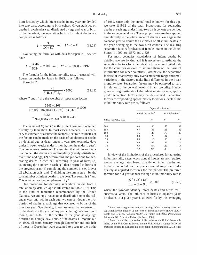
of 1989, since only the annual total is known for this age,we take 11.5/12 of the total. Proportions for separatingdeaths at each age under 1 into two birth cohorts are derivedin the same general way. These proportions are then appliedcumulatively to the total number of deaths at each age in thecalendar year to derive the estimates of all infant deaths inthe year belonging to the two birth cohorts. The resultingseparation factors for deaths of female infants in the UnitedStates in 1990 are .8672 and .1328.
For most countries, tabulations of infant deaths bydetailed age are lacking and it is necessary to estimate theseparation factors for infant deaths from more limited datafor the countries or even to assume them on the basis ofinformation for other countries. Fortunately, the separationfactors for infants vary only over a moderate range and smallvariations in the factors make little difference in the infantmortality rate. Separation factors may be observed to varyin relation to the general level of infant mortality. Hence,given a rough estimate of the infant mortality rate, appro-priate separation factors may be determined. Separationfactors corresponding approximately to various levels of theinfant mortality rate are as follows:
Separation factors
model life tables2 U.S. life tables3
Infant mortality rate f ¢ f ≤ f ¢ f ≤
200 .60 .40 .68 .32150 .67 .33 .68 .32100 .75 .25 .75 .2550 .80 .20 .84 .1625 .85 .15 .86 .1415 .95 .05 .86 .1410 NA NA .86 .145 NA NA .88 .12
In view of the limitations of the procedures for adjustinginfant mortality rates, when annual figures are not requiredannual average rates based directly on infant deaths andbirths as reported for the years covered may serve ade-quately as adjusted measures for this period. The preferredformula for a 3-year annual average infant mortality rate is
(12.23)
where the symbols identify infant deaths and births for 3successive years. The influence of births in adjacent yearson deaths of a given year is allowed for by this averaging
D D D
B B B
y y y
y y y
01
0 01
1 1
1000- +
- -
+ ++ +
¥
12. Mortality 285
tion) factors by which infant deaths in any year are dividedinto two parts according to birth cohort. Given statistics ondeaths in a calendar year distributed by age and year of birthof the decedent, the separation factors for infant deaths arecomputed as follows:
(12.21)
Evaluating the formulas with data for Japan in 1995, wehave
The formula for the infant mortality rate, illustrated withfigures on deaths for Japan in 1995, is as follows:
Formula C:
(12.22)
where f ¢ and f ≤ are the weights or separation factors:
The values of D¢y and D≤y in the present case were obtaineddirectly by tabulation. In most cases, however, it is neces-sary to estimate or assume the factors. Accurate estimates ofthe factors can be made on the basis of tabulations of deathsby detailed age at death under 1 year (for example, daysunder 1 week, weeks under 1 month, months under 1 year).The procedure consists of (1) assuming that within each tab-ulation cell the deaths are rectangularly (evenly) distributedover time and age, (2) determining the proportions for sep-arating deaths in each cell according to year of birth, (3)estimating the number in each cell that occurred to births ofthe previous year, (4) cumulating the numbers in step 3 overall tabulation cells, and (5) dividing the sum in step 4 by thetotal number of infant deaths in the year. The result is f ≤ andf ¢ is obtained as the complement of f ≤.
One procedure for deriving separation factors from a tabulation by detailed age is illustrated in Table 12.9. Thisis the kind of tabulation recommended by the UnitedNations. Assuming a rectangular distribution over the cal-endar year and within each age, we can set down the pro-portion of deaths at each age that occurred to births of theprevious year. Specifically, it was assumed that one-twelfthof the deaths in the year at any particular age occurred in amonth, and 1/365 of the deaths in the year at any ageoccurred in a single day. Thus, of the deaths 11 months oldin 1990, all from January through November and one-halfof those in December were assumed to occur to the births
3946 11087808 1 187 064 2192 1 238 328
1000
5054926 860 271 441
1000 4 2
+( ) + ( ) ¥
=+
¥ =
. , , . , ,
, ,.
D
f B f By
y y¢ + ¢¢¥
-1
1000
¢ = = ¢¢ = - =f f39465054
7808 1 7808 2192. . .and
¢ =¢
¢ + ¢¢¢¢ = - ¢f
D
D Df fy
y y
and 1
2 Based on a regression analysis relating infant mortality rates and separation factors implicit in the series of model life tables shown in A. J.Coale and Demeny, Regional Model Life Tables and Stable Populations,Princeton, NJ, Princeton University Press, 1966.
3 Based on the historical series of life tables for the United States pub-lished by the U.S. Census Bureau and the U.S. National Center for HealthStatistics and made available in a personal memorandum from J. S. Siegel.

TABLE 12.9 Calculation of Separation Factors for Deaths of Female Infants on the Basis ofAnnual Data on Deaths by Detailed Age, for the United States: 1990 (One-twelfth of the annual
total of deaths is assumed to occur in each month.)
Infant deaths
Assumed proportion born in previous year Total Born in 1989 (1) ¥ (2) = Born in 1990 (2) - (3) =Age at death (1) (2) (3) (4)
Total (X) 38,351 5,093 33,258
11 months 347 333 14
10 months 346 303 43
9 months 430 340 90
8 months 499 353 146
7 months 635 397 238
6 months 772 418 354
5 months 1,040 477 563
4 months 1,536 576 960
3 months 2,126 620 1506
2 months 2,910 606 2304
28 to 59 days1 3,401 425 2,976
21 to 27 days 966 65 901
14 to 20 days 1,308 63 1,245
7 to 13 days 2,015 58 1,957
6 days 376 7 369
5 days 444 7 437
4 days 574 7 567
3 days 813 8 805
2 days 1,340 9 1,331
1 day 1,846 8 1,838
1 to 23 hours2 10,265 14 10,251
Under 1 hour2 4,362 — 4,362
Separation factors:
f¢
f≤
1 Treated as deaths of one month of age. All of the January (or initial month) deaths and one-half of the February (or second-month) deaths of this agewere assumed to occur to births of the previous calendar (or fiscal) year.
2 8760 represents the number of hours in the year.Source: Basic data from U.S. National Center for Health Statistics, Vital Statistics of the United States, 1990, Vol. II, Mortality, Part A, 1994, Table 2.12.
¢¢¢ + ¢¢
= =D
D D
5 093
38 3511328
,,
.
¢¢ + ¢¢
= =D
D D
33 258
38 3518672
,,
.
1
2
1
8 760
1
17 5200007 0+ = = @
, ,.
1
8 760
1
2
23
8 760
25
17 5200014
, , ,.+ Ê
ËÁˆ¯̃ = =
1
365
1
2
1
365
3
7300041+ Ê
ˈ¯ = = .
2
365
1
2
1
365
5
7300068+ Ê
ˈ¯ = = .
3
365
1
2
1
365
7
7300096+ Ê
ˈ¯ = = .
4
365
1
2
1
365
9
7300123+ Ê
ˈ¯ = = .
5
365
1
2
1
365
11
7300151+ Ê
ˈ¯ = = .
6
365
1
2
1
365
13
7300178+ Ê
ˈ¯ = = .
7
365
1
2
7
365
21
7300288+ Ê
ˈ¯ = = .
14
365
1
2
7
365
35
7300479+ Ê
ˈ¯ = = .
21
365
1
2
7
365
49
7300671+ Ê
ˈ¯ = = .
1 5
121250
..=
2 5
122083
..=
3 5
122917
..=
4 5
123750
..=
5 5
124583
..=
6 5
125417
..=
7 5
126250
..=
8 5
127083
..=
9 5
127916
..=
10 5
128750
..=
11 5
129583
..=

formula except at the fringes of the period. The relative errorfrom this formula is small unless there are extremely sharpchanges in the annual numbers of births.
Mortality Rates at Ages above Infancy
Death rates at the ages above infancy can also be adjustedto a probability basis (i.e., expressed as mortality rates). Letus consider the problem first in terms of single ages. Forthose few countries (e.g., Japan, Venezuela) for which tabulations of deaths by single ages and years of birth areavailable, the task is simple. One can immediately adapt any of the formulas given for deriving infant mortality rates.Tables 12.10 and 12.11 indicate two ways of calculatingmortality rates in single ages, allowing for the fact that deaths at a given age during a year belong to two dif-
ferent birth cohorts or, conversely, that a single birth cohortmay experience deaths at two ages during a year. The dataare for children under 10 years and persons 60 to 69 yearsin Japan in 1996, and mortality rates are calculated accord-ing to formulas of type A and B for the former and type Bfor the latter. (Other procedures, employed in the construc-tion of life tables, are described in the Chapter 13.) Adapt-ing Formula A or 12.19 for use with population figures, wehave
(12.24)
where D≤a and D¢a+1, represent deaths at age a and deaths atage a + 1 in a given year, respectively, to the population ageda at the beginning of the year, and P¢a represents the
¢¢+ ¢¢
¥+D D
Pa a
a
1 1000
12. Mortality 287
TABLE 12.10 Calculation of Mortality Rates for the Population under 10 Years of Age byFormula A, for Japan: 1996
Population Mortality rate
January 1, ¥ 1000
Age on Deaths 1996 Da 19961 Pa¢ [(1) ÷ (2)] ¥ 1000 =January 1, 1996 Year of Birth Age at death (1) (2) (3)
Under 1 and 1 1345Under 1 year 1995 Under 1 948 1,182,522 1.1
1 3971 and 2 585
1 year 1994 1 375 1,187,421 0.52 210
2 and 3 3652 years 1993 2 225 1,179,977 0.3
3 1403 and 4 273
3 years 1992 3 156 1,193,449 0.24 117
4 and 5 2674 years 1991 4 144 1,200,349 0.2
5 1235 and 6 187
5 years 1990 5 103 1,216,619 0.26 84
6 and 7 2016 years 1989 6 111 1,250,690 0.2
7 907 and 8 202
7 years 1988 7 115 1,291,536 0.28 87
8 and 9 1478 years 1987 8 71 1,331,085 0.1
9 769 and 10 152
9 years 1986 9 74 1,362,403 0.110 78
1 Equals three-fourths of the population estimate for October 1, 1995, plus one-fourth of the population estimate for October 1, 1996.Source Basic data from Japan, Ministry of Health and Welfare, Vital Statistics, 1996, Japan, Vol. I, Table 5; and Japan, Statistics and Information Depart-
ment, Population Estimates by Age and Sex as of October 1, 1996, Tables 1 and 4.
¢¢+ ¢¢
D D
Pa a +1
a
{{{{{{{{{{
}}}}}}}}}}
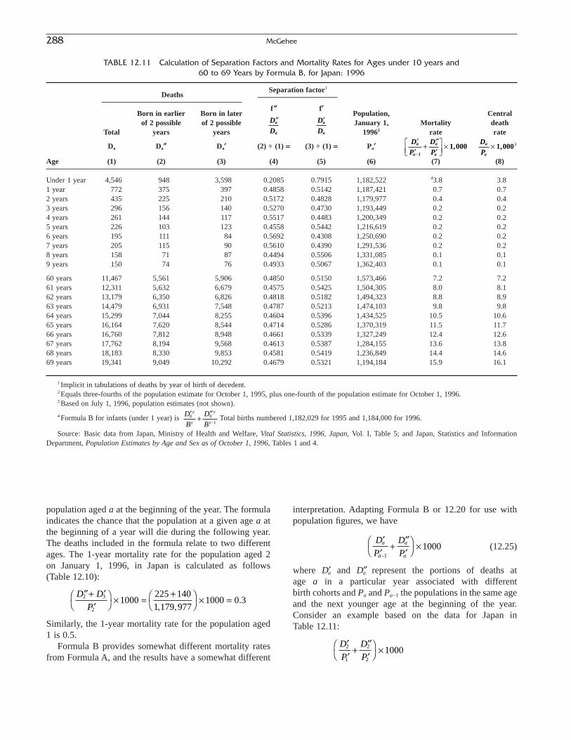
TABLE 12.11 Calculation of Separation Factors and Mortality Rates for Ages under 10 years and60 to 69 Years by Formula B, for Japan: 1996
DeathsSeparation factor1
Born in earlier Born in laterf≤ f¢
Population, Centralof 2 possible of 2 possible January 1, Mortality death
Total years years 19962 rate rate
Da Da≤ Da¢ (2) ÷ (1) = (3) ÷ (1) = Pa¢
Age (1) (2) (3) (4) (5) (6) (7) (8)
Under 1 year 4,546 948 3,598 0.2085 0.7915 1,182,522 43.8 3.81 year 772 375 397 0.4858 0.5142 1,187,421 0.7 0.72 years 435 225 210 0.5172 0.4828 1,179,977 0.4 0.43 years 296 156 140 0.5270 0.4730 1,193,449 0.2 0.24 years 261 144 117 0.5517 0.4483 1,200,349 0.2 0.25 years 226 103 123 0.4558 0.5442 1,216,619 0.2 0.26 years 195 111 84 0.5692 0.4308 1,250,690 0.2 0.27 years 205 115 90 0.5610 0.4390 1,291,536 0.2 0.28 years 158 71 87 0.4494 0.5506 1,331,085 0.1 0.19 years 150 74 76 0.4933 0.5067 1,362,403 0.1 0.1
60 years 11,467 5,561 5,906 0.4850 0.5150 1,573,466 7.2 7.261 years 12,311 5,632 6,679 0.4575 0.5425 1,504,305 8.0 8.162 years 13,179 6,350 6,826 0.4818 0.5182 1,494,323 8.8 8.963 years 14,479 6,931 7,548 0.4787 0.5213 1,474,103 9.8 9.864 years 15,299 7,044 8,255 0.4604 0.5396 1,434,525 10.5 10.665 years 16,164 7,620 8,544 0.4714 0.5286 1,370,319 11.5 11.766 years 16,760 7,812 8,948 0.4661 0.5339 1,327,249 12.4 12.667 years 17,762 8,194 9,568 0.4613 0.5387 1,284,155 13.6 13.868 years 18,183 8,330 9,853 0.4581 0.5419 1,236,849 14.4 14.669 years 19,341 9,049 10,292 0.4679 0.5321 1,194,184 15.9 16.1
1 Implicit in tabulations of deaths by year of birth of decedent.2 Equals three-fourths of the population estimate for October 1, 1995, plus one-fourth of the population estimate for October 1, 1996.3 Based on July 1, 1996, population estimates (not shown).
4 Formula B for infants (under 1 year) is Total births numbered 1,182,029 for 1995 and 1,184,000 for 1996.
Source: Basic data from Japan, Ministry of Health and Welfare, Vital Statistics, 1996, Japan, Vol. I, Table 5; and Japan, Statistics and Information Department, Population Estimates by Age and Sex as of October 1, 1996, Tables 1 and 4.
¢ + ¢¢-
D
B
D
B
y
y
y
y0 0
1
D
Pa
a
¥ 1,0003¢¢
+ ¢¢¢
ÈÎÍ
˘˚̇
¥-
D
P
D
Pa
a 1
a
a
1,000
¢D
Da
a
¢¢D
Da
a
population aged a at the beginning of the year. The formulaindicates the chance that the population at a given age a atthe beginning of a year will die during the following year.The deaths included in the formula relate to two differentages. The 1-year mortality rate for the population aged 2 on January 1, 1996, in Japan is calculated as follows (Table 12.10):
Similarly, the 1-year mortality rate for the population aged1 is 0.5.
Formula B provides somewhat different mortality ratesfrom Formula A, and the results have a somewhat different
¢¢+ ¢¢
ÊË
ˆ¯ ¥ =
+ÊË
ˆ¯ ¥ =
D D
P2 3
2
1000225 1401 179 977
1000 0 3, ,
.
interpretation. Adapting Formula B or 12.20 for use with population figures, we have
(12.25)
where D¢a and D≤a represent the portions of deaths at age a in a particular year associated with different birth cohorts and Pa and Pa-1 the populations in the same ageand the next younger age at the beginning of the year. Consider an example based on the data for Japan in Table 12.11:
¢¢
+¢¢¢
ÊË
ˆ¯ ¥
D
P
D
P2
1
2
2
1000
¢¢
+¢¢¢
ÊË
ˆ¯ ¥
-
D
P
D
Pa
a
a
a1
1000
288 McGehee

Such a formula tells the chance of dying at age 2—thatis, between one’s second birthday and one’s third birthday.The chance of dying at age 1—that is, between one’s firstbirthday and one’s second birthday—is represented by
The mortality rate of 0.4 at age 2 compares with a centraldeath rate at age 2 of 0.4 (Table 12.11). In general, however,central death rates tend to be higher than mortality ratesbecause, barring net immigration and changes in numbers of births, the midyear population in an age cohort will besmaller than the population at the beginning of the year. Thisis suggested by the differences between the mortality ratesand central death rates for ages 60 to 69 years shown inTable 12.11.
The rate of 0.5, obtained with Formula A as the mortal-ity rate of the population initially 1 year of age, is inter-mediate to the mortality rates for ages 1 and 2 shown byFormula B, 0.7 and 0.4, respectively. In general, the resultsfrom Formula A fall between the results from Formula B forsuccessive ages. This relationship corresponds to the ages ofthe deaths reflected in each formula.
The considerable deviation of the separation factors from.50–.50 in infancy reflects the fact that infant deaths tend to be concentrated at the earliest ages of infancy—that is,near the time of birth. This concentration results from the predominant role of the endogenous causes of mortality atthis age. The greater risk of dying in the first part of an age would also be expected to apply to some of the agesabove infancy, but the available data show that this phe-nomenon tends to disappear quite quickly and is hardlyevident once the first year of life has passed. Table 12.11presents the separation factors for deaths by single agesunder 10 implied by the tabulations of deaths by age andyear of birth for Japan in 1996. Although there are smallfluctuations in the separation factors, they converge rapidlyto about .50–.50. Even the separation factors for deaths atages 1 and 2 are close to these values. At the higher ages oflife also, where mortality rates are rising rapidly, the sepa-ration factors implied by the tabulated data for Japanapproximate .50–.50 and show no particular trend withincreasing age even though such a trend would be expected.Illustrative data for ages 60 to 69 for Japan in 1996 areshown in Table 12.11.
There are neither tabulations of death statistics by age andyear of birth nor tabulations of deaths by subdivisions ofsingle years of age above infancy for the United States. Theseparation factors needed to compute mortality rates for ages above infancy in the United States cannot be derived from these sources, therefore. The only study intended to
¢¢
+¢¢¢
ÊË
ˆ¯ ¥
D
P
D
P1
0
1
1
1000
2101 187 421
2251 179 977
1000 0 4, , , ,
.+ÊË
ˆ¯ ¥ =
establish the separation factors for ages above infancy in theUnited States was based on a 10% sample of deaths at ages1 to 4 in 1944, 1945, and 1946 (U.S. National Office of VitalStatistics, 1950a). The tabulation of these deaths by year ofbirth indicated separation factors rather close to .50–.50 foreach age. Since a moderate variation in the separation factorhas only a slight effect on the mortality rate, it seems bestto employ a separation factor of 0.50 for splitting deathsaccording to birth cohort at the ages above infancy and forcalculating 1-year mortality rates at these ages.
The discussion so far has been confined to mortality ratesfor single ages in a single year. Mortality rates for longerperiods of time and for age groups may also be calculated.Such rates may be constructed from observed data over anumber of calendar years and represent a real cohort, or theymay be constructed from observed data for a single calen-dar year and represent a synthetic cohort.
For example, it is possible to calculate the risk of dying fora 5-year old in a 5-year period from the appropriate probabil-ities for this 5-year period. The probabilities at successiveages in successive calendar years would be used. A syntheticprobability of this kind could be derived by combining theappropriate single-year-of-age probabilities for a single cal-endar year. The formula would take the following form:
(12.26)
where q5¢ represents the 1-year mortality rate between ages5 and 6, and 5q5 the risk of a 5-year old dying in the next 5years. Ordinarily, single-year-of-age tabulations of deathstatistics are not available or are too inaccurate to serve asa basis for the calculation of death rates and mortality ratesfor single years of age. Adjusted estimates of deaths anddeath rates in single ages may be derived by various typesof interpolation procedures from 5-year age data.
A rough estimate of the annual mortality rate for a 5-yearage group may be derived as follows:
1. Set down total deaths in a given age group during theyear.
2. Set down the population in this age group at the middleof the year.
3. Add one-half of the deaths in step 1 to the populationin step 2. (This is the base population for the rate, i.e.,the population at the beginning of the year that wouldbe in this age group at the middle of the year.)
4. Divide the figure in step 1 by the result in step 3.
This procedure disregards the effect of net immigration ondeaths and population during the year.
For the probability that a person aged 60 to 64 years ofage would die within one year, according to experience inthe United States in 1990, the corresponding figures are
yxy
a a aq D P D+ = ∏ +ÊË
ˆ¯
15 5 5
12
5 5 5 6 7 8 91 1 1 1 1 1¢ = - - ¢( ) - ¢( ) - ¢( ) - ¢( ) - ¢( )q q q q q q
12. Mortality 289

1. Deaths = 154,8312. Population on July 1, 1990 = 10,619,0003. Base population 10,619,000 + 1/2(154,831) = 10,696,4164. Rate = 154,831/10,696,416 = .01448 or 14.5 per 1000
Cause-Specific Mortality Rates
Measures giving the chance of dying from a particularcause at a particular age in a year or 5-year period, or ofeventually dying from this cause, have been developed,principally in connection with the preparation of life tablesby cause of death (Chapter 15). Cause-specific probabilitiesof death can be computed in a manner paralleling the cal-culation of general probabilities of dying. In the case ofgeneral cause-specific probabilities for single ages for singlecalendar years, the deaths from a particular cause or groupof causes at a particular age (a) for a given calendar yearmay be divided by the population at age a at the middle ofthe year plus one-half of all deaths at age a during the year.(The base population may alternatively be estimated as themean of the population at age a and the population at thenext younger age (a - 1) at the beginning of the year, or the mean of the population at age a at the middle of the yearand age a - 1 at the middle of the previous year.) Therequired data on deaths would normally be obtained byinterpolation from 5-year age data. As before, this proceduredisregards the net migration occurring during the year of theestimate. A 1-year cause-of-death probability for a 5-yearage group may be derived as follows:
1. Set down (a) total deaths in the given age group, (b)deaths from the particular cause in this age groupduring the year, and (c) the population in this agegroup at the middle of the year.
2. Add one-half of all deaths at these ages (item la) to thefigure in item1c. (This is the base population for therate—that is, the population at the beginning of theyear that would be 60 to 64 at the middle of the year.)
3. Divide the figure in item 1b by the result in step 2.
For calculating the risk of death from heart disease in theUnited States at ages 60 to 64 in 1990, the correspondingfigures are as follows:
1. All deaths, 154,831; deaths due to heart disease,48,449; and population, July 1, 1990, 10,619,000
2. Base population = 10,619,000 + 1/2(154,831) =10,696,416
3. Rate = 48,449 ÷ 10,696,416 = .004529 or 452.9 per100,000
Cause-specific probabilities for 5-year time periods,whether for single ages or 5-year age groups, particularlythose derived “synthetically” on the basis of data for a single calendar year, are, as suggested earlier, akin to the
measures developed in connection with life tables (seeChapter 13).
The conventional infant mortality rate, previouslydescribed as an approximate measure of the risk of dying in infancy, may be viewed as the sum of a series of rateseach of which represents the chance of dying in infancy froma particular cause. In analyzing differences in overall infantmortality rates, it is useful to separate the infant deaths bycause into the two broad classes, endogenous and exoge-nous, described earlier, and to compute separate rates. Theformula for the endogenous infant mortality rate is
(12.27)
and the formula for the exogenous infant mortality rate is
(12.28)
As suggested earlier, the endogenous set of causes isrelated to the genetic makeup of the infant, the circum-stances of life in utero, and the conditions of labor. Theexogenous set of causes is related to the contact of the infantwith the external world. Endogenous infant mortalityincludes mainly mortality from congenital anomalies, imma-turity, birth injuries, postnatal asphyxia, and so on (i.e., con-ditions that are difficult to prevent or treat in the present stateof knowledge). Exogenous infant mortality includes mainlyinfections and post-natal accidents (i.e., conditions that arerelatively preventable or treatable). The endogenous infantmortality rate is estimated at 18.3 in the United States in1966 and at 14.4 in Norway in 1959. About one-quarter ofthe infant deaths in these countries are exogenous, whereasin Costa Rica over 60% are in this category (Table 12.7). Asa result, in Costa Rica the exogenous infant mortality rate iswell above the endogenous rate. This type of comparativeinternational analysis of the infant mortality rate in terms ofendogenous and exogenous causes is useful in determiningthe extent to which the rate can reasonably be reduced in thepresent state of knowledge.
The maternal mortality rate is a widely used type ofcause-specific mortality rate representing approximately the risk of dying as a result of “complications of pregnancy,childbirth, and the puerperium” (ICD-9 category numbers630–676). This rate is conventionally defined as the numberof deaths due to puerperal causes per 10,000 or 100,000births. With a constant of 100,000, the formula is
(12.29)
where Dp represents deaths due to puerperal causes. Mater-nal mortality rate vary widely around the world.
Some illustrature figures relating to the years around1995 are 8 (per 100,000 births) for Israel 12 for Japan, 65for Mexico, 260 for Brazil, 590 for Cambodia, and 830 forNepal (Population Reference Bureau, 2002).
D
B
p
¥ 100 000,
D
Boex
¥ 1000
D
Boen
¥ 1000
290 McGehee

The figures suggest the range and variation in thismeasure for the countries of the world in recent years. In theformula the number of births is employed as an approxima-tion to the number of women exposed to the risk of dyingfrom puerperal causes.
Rates Adjusted for Population Composition
The level of an observed death rate, like that of otherobserved rates, is affected by the demographic compositionof the population for which the rate is calculated. The agecomposition of the population, in particular, is a key factoraffecting the level of the crude death rate. For purposes ofcomparing death rates over time or from area to area, it isuseful to determine the difference between the rates on theassumption that there are no differences in age composition.It is particularly important to eliminate the effect of the dif-ferences in age structure of two populations being comparedif one is trying to compare their health conditions. Crudedeath rates are especially unsatisfactory for this purpose. Acrude death rate of a population may be relatively highmerely because the population has a large proportion ofpersons in the older ages, where death rates are high; or itmay be relatively low because the population has a largeproportion of children and young adults, where death ratesare low. The crude death rate of a country may actually riseeven though death rates at each age remain stationary, if thepopulation is getting older.
The procedure of adjustment of the crude rates to elimi-nate from them the effect of differences in population com-position with respect to age and other variables is sometimescalled standardization. Often, death rates are adjusted orstandardized for both age and sex. Other variables for whichdeath rates may be adjusted or standardized are racial com-position, nativity composition, urban-rural composition, andso on. We shall confine our discussion largely to standardi-zation for age since this is the most important and mostcommon variable for which the standardization of deathrates is carried out.
Age-adjusted rates can be interpreted as the hypotheticaldeath rate that would have occurred if the observed age-specific rates were associated with a population whose age distribution equalled that of the standard population. How-ever, it is important to recognize that age-adjusted or age-standardized rates have no direct meaning in themselves. Theyare meaningful only in comparison with other similarly com-puted rates. Since they are useful only for comparison, thecommonest application of the procedure is to compute suchrates for the areas or population groups whose mortality is tobe compared and to calculate the relative differences of theresulting rates. The meaningful measure then is a ratio, index,or percentage difference between rates similarly adjusted.
A number of methods have been developed for adjustingdeath rates for age composition or for deriving indexes or
relative measures of age-adjusted mortality. We shall con-sider four principal methods. The measures are the age-adjusted or age-standardized death rate calculated by thedirect method, the age-adjusted or age-standardized deathrate calculated by the indirect method, the comparative mor-tality index, and the life table death rate.
Direct Standardization
The simplest and most straightforward measure is theage-adjusted death rate derived by the direct method. Formost comparisons, this is the preferred procedure and it pro-vides the best basis for determining the relative differencebetween mortality in two areas or at two dates. In thismethod, a “standard” population is selected and employedin deriving all the age-adjusted rates in a set to be compared.If the same standard population is employed, as required, allthe rates are directly comparable. The formula calls for computing the weighted average of the age-specific deathrates in a given area, using as weights the age distributionof the standard population. The formula for direct standard-ization is
(12.30)
where = age-specific death rate in the given
area, Pa represents the standard population at each age, andP or SPa represents the total of the standard population.(Capital letters are used here to identify the elements of thestandard population, and lowercase letters are used to iden-tify the elements of the populations under study.) Each age-specific rate is multiplied, in effect, by the proportion of thestandard population in each age group. (In standardizing adeath rate for age and sex jointly, each age-sex-specificdeath rate is multiplied by the proportion of the total standard population in that age-sex group.) The age-standardized death rate for the standard population is thesame as its own crude death rate, since the age-specific deathrates for the standard population would be weighted by itsown population. The relative mortality of the given area isderived by dividing the age-standardized rate for the area bythe crude death rate of the standard population.
Illustrative calculations are shown for a group of coun-tries around 1990 in Table 12.12. The population of theUnited States is employed as a standard population to cal-culate the age-standardized death rate for Czechoslavakia(1990), Ecuador (1990), Finland (1990), and Japan (1990).The steps in calculating the age-adjusted death rate by thedirect method for Japan are as follows:
RMm P
PM
m P
M P
a a a a
a a1 = ∏ =Â Â
Â
md
pa
a
a
=
mm P
Pm
P
Pa a
aa
1 1000 1000= ¥ ¥Â Âor
12. Mortality 291

1. Record the population in each age group for the UnitedStates (standard population).
2. Record the age-specific death rates for Czechoslovakia.3. Compute the cumulative product of the population
figures in step 1 and the death rates in step 2(3,163,087).
4. Divide the result in step 3 (3,163,087) by the total population of the United States (248,710,000). Theresult is 12.7 per 1000.
The crude death rate in Czechoslovakia, 11.6 per 1000population, is 36% greater than the crude death rate in theUnited States, 8.6 (Table 12.12). The adjustment of the cruderate in Czechoslovakia raised it to 12.7, reflecting the factthat the age composition of Czechoslovakia’s population is more favorable for a low crude death rate than that of the United States. Equating the age distributions raises therelative excess of the Czechoslovakia rate to a relative ex-cess of 48%. Note that (direct) standardization caused a
rise in the death rate for Ecuador and Japan also. Both the crude and adjusted death rates for Ecuador and Japanindicate that these countries have populations with lowermortality than that for the United States.
Two basic types of standard populations are used tocompute the age-adjusted death rate by the direct method:internal and external. The internal standard selected may be the age distribution of one of the areas or dates (e.g., earliest, middle, or latest in a series) being compared, or the sum or average of the age distributions for the areas ordates being compared. The external standard is a real or the-oretical distribution of some sort. Different results for therelative differences between adjusted rates will be obtaineddepending on the age distribution selected as a standard. Infact, the choice of standard may even affect the direction ofthe difference between the rates for the populations beingcompared. Hence, it is desirable to select the standard population carefully. The general rule is to select as a standard an age distribution that is similar to the age
292 McGehee
TABLE 12.12 Calculation of Age-Standardized Death Rates by the Direct Method, for Several Countries: 1990
Standard population Age-specific death rates(in thousands) (ma)
(Pa)United States, Czechoslovakia, Ecuador, Finland, Japan,
Age 1990 1990 1990 1990 1990
Under 1 year 3,217 11.4 33.1 5.7 4.61 to 4 years 15,137 0.4 3.3 0.3 0.45 to 9 years 18,099 0.3 0.7 0.2 0.210 to 14 years 17,114 0.2 0.7 0.2 0.115 to 19 years 17,754 0.6 1.2 0.8 0.420 to 24 years 19,020 0.8 1.7 1.1 0.525 to 29 years 21,313 0.9 1.8 0.9 0.530 to 34 years 21,863 1.3 2.2 1.4 0.635 to 39 years 19,963 2.1 2.7 1.9 0.940 to 44 years 17,616 3.4 3.4 2.8 1.445 to 49 years 13,873 5.7 4.7 3.8 2.450 to 54 years 11,351 9.0 6.4 6.0 3.755 to 59 years 10,532 13.8 9.5 8.8 6.160 to 64 years 10,616 21.4 13.0 14.0 9.365 to 69 years 10,112 32.9 20.8 21.9 13.770 to 74 years 7,995 49.3 31.2 35.3 23.575 to 79 years 6,121 80.2 50.3 58.1 42.180 to 84 years 3,934 127.0 71.8 96.3 75.985 years and over 3,080 216.7 166.0 184.2 158.1
(1) Total standard population = SPa = P 248,710 (X) (X) (X) (X)(2) Expected deaths = SmaPa (X) 3,163,087 1,365,663 2367,408 1723,156
(3) Age-adjusted death rate = 8.6 12.7 5.5 9.5 6.9
(4) Percentage difference from U.S. rate [(3) - 8.6] ∏ 8.6 (X) +47.9 -36.2 +10.7 -19.4(5) Crude death rate (CDR) 8.6 11.7 5.2 10.0 6.6(6) Percentage difference or CDR from U.S. (X) +36.0 -39.5 +16.3 -23.3
rate [(5) - 8.6] ∏ 8.6
X: Not applicable.Sources: Basic data from United Nations, Demographic Yearbook (various dates).
Sm P
Pa a = ( )
( )2
1
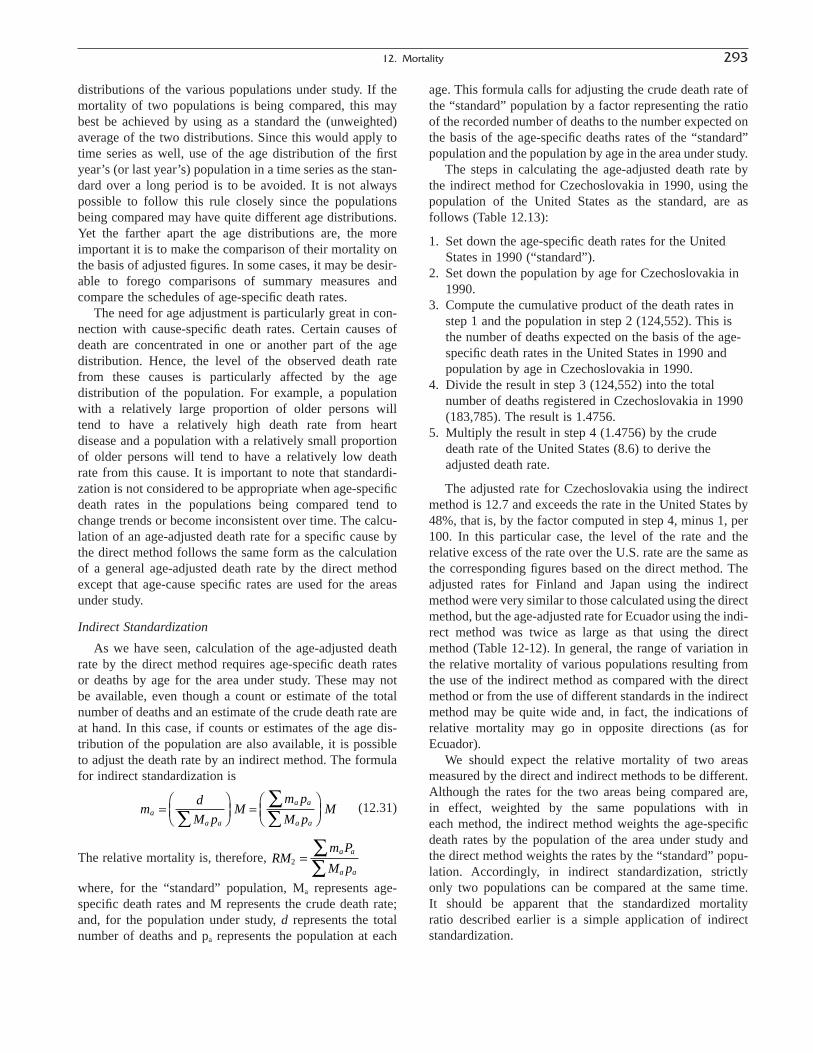
distributions of the various populations under study. If themortality of two populations is being compared, this maybest be achieved by using as a standard the (unweighted)average of the two distributions. Since this would apply totime series as well, use of the age distribution of the firstyear’s (or last year’s) population in a time series as the stan-dard over a long period is to be avoided. It is not alwayspossible to follow this rule closely since the populationsbeing compared may have quite different age distributions.Yet the farther apart the age distributions are, the moreimportant it is to make the comparison of their mortality onthe basis of adjusted figures. In some cases, it may be desir-able to forego comparisons of summary measures andcompare the schedules of age-specific death rates.
The need for age adjustment is particularly great in con-nection with cause-specific death rates. Certain causes ofdeath are concentrated in one or another part of the age distribution. Hence, the level of the observed death rate from these causes is particularly affected by the age distribution of the population. For example, a populationwith a relatively large proportion of older persons will tend to have a relatively high death rate from heart disease and a population with a relatively small proportionof older persons will tend to have a relatively low death rate from this cause. It is important to note that standardi-zation is not considered to be appropriate when age-specificdeath rates in the populations being compared tend tochange trends or become inconsistent over time. The calcu-lation of an age-adjusted death rate for a specific cause bythe direct method follows the same form as the calculationof a general age-adjusted death rate by the direct methodexcept that age-cause specific rates are used for the areasunder study.
Indirect Standardization
As we have seen, calculation of the age-adjusted deathrate by the direct method requires age-specific death rates or deaths by age for the area under study. These may not be available, even though a count or estimate of the totalnumber of deaths and an estimate of the crude death rate areat hand. In this case, if counts or estimates of the age dis-tribution of the population are also available, it is possibleto adjust the death rate by an indirect method. The formulafor indirect standardization is
(12.31)
The relative mortality is, therefore,
where, for the “standard” population, Ma represents age-specific death rates and M represents the crude death rate;and, for the population under study, d represents the totalnumber of deaths and pa represents the population at each
RMm P
M p
a a
a a2 = Â
Â
md
M pM
m p
M pMa
a a
a a
a a
=ÊËÁ
ˆ¯̃
=ÊËÁ
ˆ¯̃Â
ÂÂ
age. This formula calls for adjusting the crude death rate ofthe “standard” population by a factor representing the ratioof the recorded number of deaths to the number expected onthe basis of the age-specific deaths rates of the “standard”population and the population by age in the area under study.
The steps in calculating the age-adjusted death rate by the indirect method for Czechoslovakia in 1990, using thepopulation of the United States as the standard, are asfollows (Table 12.13):
1. Set down the age-specific death rates for the UnitedStates in 1990 (“standard”).
2. Set down the population by age for Czechoslovakia in1990.
3. Compute the cumulative product of the death rates instep 1 and the population in step 2 (124,552). This isthe number of deaths expected on the basis of the age-specific death rates in the United States in 1990 andpopulation by age in Czechoslovakia in 1990.
4. Divide the result in step 3 (124,552) into the totalnumber of deaths registered in Czechoslovakia in 1990(183,785). The result is 1.4756.
5. Multiply the result in step 4 (1.4756) by the crudedeath rate of the United States (8.6) to derive theadjusted death rate.
The adjusted rate for Czechoslovakia using the indirectmethod is 12.7 and exceeds the rate in the United States by48%, that is, by the factor computed in step 4, minus 1, per100. In this particular case, the level of the rate and the relative excess of the rate over the U.S. rate are the same as the corresponding figures based on the direct method. Theadjusted rates for Finland and Japan using the indirectmethod were very similar to those calculated using the directmethod, but the age-adjusted rate for Ecuador using the indi-rect method was twice as large as that using the directmethod (Table 12-12). In general, the range of variation inthe relative mortality of various populations resulting fromthe use of the indirect method as compared with the directmethod or from the use of different standards in the indirectmethod may be quite wide and, in fact, the indications ofrelative mortality may go in opposite directions (as forEcuador).
We should expect the relative mortality of two areasmeasured by the direct and indirect methods to be different.Although the rates for the two areas being compared are, in effect, weighted by the same populations with in each method, the indirect method weights the age-specificdeath rates by the population of the area under study and the direct method weights the rates by the “standard” popu-lation. Accordingly, in indirect standardization, strictly only two populations can be compared at the same time. It should be apparent that the standardized mortality ratio described earlier is a simple application of indirectstandardization.
12. Mortality 293

Comparative Mortality Index
The comparative mortality index (CMI) is a measure ofrelative mortality, usually employed to indicate changesover time in the overall mortality of an area. It uses a shift-ing pattern of population weights, designated to overcomethe problems of prolonged use of a single standard age dis-tribution. The formula is
(12.32)
where Ma represents the age-specific death rates in the stan-dard or initial year, ma, represents the age-specific deathrates in later years, and
where Pa and Pare populations of the standard or initial year andpa and p are populations of each later years being calculated.
The formula calls for taking a ratio of (1) the weightedsum of age-specific death rates in each year to (2) the similarly weighted sum of age-specific death rates of the
wP
P
p
pa
a a= +ÊË
ˆ¯
12
CMIw m
w M
a a
a a
= ÂÂ
initial year. The weights are the average of (1) the propor-tion of the total population in the age group in the initial yearand (2) the corresponding proportion in each later year.
Life Table Death Rate
The life table death rate, the fourth type of age-adjustedrate considered here, is the most difficult one to derive,requiring the construction of a life table from the observedage-specific death rates for each population examined. It isalso the most difficult to interpret. The subject of life tablesis treated separately and in detail in the next chapter. We maynote here that the assumption of a constant annual numberof births and a constant set of age-specific death rates cor-responding to the observed age-specific death rates of anarea in a given year or period generates a population withan unchanging total size and age distribution, called the“life-table stationary population,” which has its own crudebirth and death rates. The crude death rate of this populationis called the “life table death rate.” In effect, the life tabledeath rate may be viewed as an age-adjusted death rateresulting from the weighting of age-specific death rates bythe life table stationary population.
294 McGehee
TABLE 12.13 Calculation of Age-Standardized Death Rates by the Indirect Method, for SeveralCountries: 1990
Age-specificdeath rates (Ma) Population (in thousands)
United States,Age 1990 Czechoslovakia Ecuador (pa) Finland Japan1
All ages 8.6 15,660 9,649 4,998 123,612Under 1 year 9.7 207 241 65 12171 to 4 years 0.5 856 1012 247 5,2935 to 9 years 0.2 1,144 1,262 327 7,48710 to 14 years 0.3 1,354 1,224 325 8,55015 to 19 years 0.9 1,276 1,039 303 10,03320 to 24 years 1.1 1,061 917 344 8,82325 to 29 years 1.2 1,084 790 377 8,09230 to 34 years 1.5 1,134 666 383 7,80935 to 39 years 2.0 1,252 563 405 9,02840 to 44 years 2.5 1,185 448 441 10,686
45 to 49 years 3.8 949 351 325 9,04250 to 54 years 5.9 764 295 275 8,10955 to 59 years 9.3 780 226 252 7,74560 to 64 years 14.6 772 203 255 6,76365 to 69 years 21.6 723 140 223 5,11870 to 74 years 32.7 353 109 167 3,82875 to 79 years 49.3 404 75 140 3,02680 to 84 years 76.8 242 52 92 1,83885 years and over 153.3 120 36 52 1125
(1) Expected deaths = SMapa (X) 124,552 37,538 45,648 1,054,925(2) Registered deaths (d) 2,148,463 183,785 50,217 50,058 820,305
(3) Ratio, (X) 1.4756 1.3378 1.0966 0.7776
(4) Age-adjusted death rate = 8.6 x (3) 8.6 12.7 11.5 9.4 6.7(5) Percent difference from U.S. rate2 = [(4) - 8.6] ∏ 8.6 (X) +47.6 +33.8 +9.7 -22.2
(X): Not applicable.1 Population with age not reported distributed on the basis of reported distribution. 2 also = [1 - (3)] ¥ 100.
Registered deaths
Expected deaths= = ( )
( )Âd
M pa a
2
1
Summary Note on Age-Adjustment
We have considered a number of ways of calculating age-adjusted death rates. This discussion suggests that there isno perfect method of removing the effects of age composi-tion when the mortality experiences of different populationsare being compared. The direct method of standardizationemploys a common standard population for all the areas ordates being compared, but the results are affected by thechoice of standard population and the standard may beunreasonable for widely different populations or over longperiods of time. In the indirect method of standardizationand in the calculation of the comparative mortality index,the comparability of results is affected by the use of a dif-ferent standard population for each area or date for whichcomparative measures are derived. The calculation of lifetable death rates avoids the problem of the arbitrary choiceof a standard population, since life table death rates are generated entirely from the age schedules of age-specificdeath rates; in effect, however, each set of age-specific ratesis weighted by a different population, derived from thosevery age-specific rates. For a complete analysis of mortality, it is desirable to examine the differences in theindividual age-specific rates.
Measures of Pregnancy Losses
Much loss of potential life occurs as a result of fetallosses, and there is a close relationship between fetal andneonatal mortality.
Fetal Mortality
As we have seen, the definition of fetal “death” comple-ments the definitions of live birth and death. In some coun-tries, however, the definition employed differs from theinternational recommendations: live-born children dyingearly in life (e.g., before registration of birth or within 24hours of birth) may be classed with fetal deaths. A moreimportant problem is the incompleteness and irregularity ofreporting of fetal deaths. This limitation applies to the datafor most countries of the world. The duration of pregnancyrequired for registration varies widely. Reporting of earlyfetal deaths may be seriously incomplete even whererequired by law. When registration of all fetal deaths is notmandatory, countries differ as to what is to be registered asa late fetal death; 28 weeks is most frequently specified asthe minimum period. As a result, international comparabil-ity is far greater for the late fetal deaths than for all fetaldeaths taken together.
In view of this situation, the United Nations has recom-mended that fetal deaths be tabulated by period of gestationinto four classes: under 20 completed weeks, 20 to 27 com-pleted weeks, 28 to 36 completed weeks, and 37 completedweeks and over (and not stated). It has designated fetaldeaths of at least 28 weeks of gestation, combined with fetal
deaths of unknown gestational age, as “late” fetal deaths;fetal deaths under 20 weeks’ gestation as “early” fetaldeaths; and fetal deaths of 20 to 27 weeks’ gestation as“intermediate” fetal deaths. Gestational age reported inmonths should be allocated to the corresponding intervals inweeks. The data on late fetal deaths are subject to sub-stantial error introduced by incorrect reporting of gestationalage. The determination of age is often difficult and compa-rability of the tabulations is affected by the differences in the skill of the medical attendant in making this determination.
The loss through fetal deaths may be measured by thefetal death ratio or the fetal death rate. The fetal death ratiois defined as the number of fetal deaths reported in a yearper 1000 live births in the same year, or
where Df represents either all fetal losses or late fetal losses.Because of the variability in coverage of the early and inter-mediate fetal losses mentioned earlier, it is preferable fromthe point of view of international comparability to computethe fetal death ratio on the basis of late fetal losses only. Thefetal death rate relates the fetal losses more closely to thepopulation at risk than the fetal death ratio (i.e., it is moreakin to a probability). The formula includes the fetal lossesin the denominator as well as in the numerator:
This rate should also be calculated with late fetal losses only.In spite of the theoretical advantage of the fetal death rate,
the fetal death ratio may be considered preferable for inter-national comparisons. The registration of fetal losses isirregular, and the effect of this irregularity is compoundedwhen fetal losses are included with the births in the base of the fetal death rate. Because of the likelihood that poorregistration of fetal losses will occur in association with poorregistration of births and hence that errors in each compo-nent will offset one another to some extent, fetal death ratiosmay sometimes be of satisfactory quality even where thebasic data are questionable.
Specific fetal death ratios may be calculated in terms ofperiod of gestation of the fetus or in terms of the age of themother (requiring data on the age of mother for births andfetal deaths). Other characteristics of principal importancein the analysis of fetal losses are the marital status of themother (legitimacy of the fetus), the sex of the fetus, the number of children previously born to the mother, andthe type of birth (single or plural issue). Other factorsinclude the cause of fetal death, hospitalization, age offather, date of marriage (for legitimate pregnancies), levelof education of parents, and the occupational characteristicsof the parents.
D
B D
f
f+¥ 1000
D
B
f
¥ 1000
12. Mortality 295

Perinatal Mortality
The causes of death in early infancy are believed to beso akin to those accounting for late fetal losses that variousmeasures of mortality combining fetal losses and deaths ofearly infancy have been proposed. The combination of thesedeaths is also intended to eliminate the errors resulting fromdeliberate and inadvertent misclassification as between fetallosses, births, and neonatal deaths. The combined risk ofdying during the period near parturition (i.e., just before,during, and just after birth) is measured by various so-calledperinatal mortality ratios and rates. The formulas differ withrespect to the age limits of the infant deaths and the gesta-tional age of fetal losses to be included, and with respect towhether fetal losses are included in or excluded from thebase of the ratios. Neonatal deaths, deaths under 1 week, ordeaths under 3 days, in combination with all fetal losses orlate fetal losses, are possible ways of operationally definingperinatal deaths. In view of the general lack of tabulated dataon infant deaths under 3 days, this coverage is not veryuseful for international comparisons. The World HealthOrganization defines the perinatal period as extending fromthe 28th week of gestation to the seventh day of life. Forcomputational purposes, the lower limit of viability is takenas 28 complete weeks of gestation and the early part ofextra-uterine life is taken to be the first 7 days of life.
One formula for the perinatal mortality ratio is, then, thenumber of deaths under 1 week of age and late fetal lossesper 1000 live births in a year:
where Dz represents deaths under 1 week, Df represents latefetal losses, and B represents births. Another formula is thenumber of neonatal and late fetal deaths per 1000 live birthsin a year:
where Dn represents neonatal deaths.The corresponding perinatal mortality rate differs by
including late fetal losses in the denominator, thus approximating a probability more closely. It is consideredthe preferred measure because the denominator is more representative of the population at risk (Hoyert, 1994). The perinatal mortality rate can be defined as the number of perinatal deaths per 1000 live births and fetal losses as illustrated in the following formula:
where the symbols have the same meaning as they did previously.
D D
B D
D D
B D
z f
f
n f
f
++
¥+
+¥1000 1000or
D D
B D
n f
f
++
¥ 1000
D D
B
z f+¥ 1000
These various measures give essentially the same indi-cations of international differences. The perinatal mortalityrate has a small theoretical advantage over the perinatal mor-tality ratio, but the perinatal mortality ratio is probably morestable for international comparison. In the United States,there is little numerical difference between the perinatalratios and rates, and the difference becomes smaller as peri-natal mortality decreases (U.S. NCHS, 1989).
For a fuller discussion of these measures, with illustra-tions, see Chapter 14.
References
Bourgeois-Pichat, J. 1952, July–Sept. “Essai sur la mortalité ‘biologique’de l’homme” [Essay on the “Biological” Mortality of Man]. Population(Paris) 7(3): 381–394.
Carnes, B. A., and S. J. Olshansky. 1997. “A Biologically Motivated Partitioning of Mortality.” Experimental Gerontology 32: 615–631.
Chandra Sekar, C. C., and W. E. Deming. 1949. “On a Method of Esti-mating Birth and Death Rates and the Extent of Registration.” Journalof the American Statistical Association 44: 101–115.
Decoufle, P., T. L. Thomas, and L. W. Pickle. 1980. “Comparison of theProportionate Mortality Ratio and Standardized Mortality Ratio RiskMeasures.” American Journal of Epidemiology 111: 263–269.
Dever, G. E. A. 1991. Community Health Analysis: Global Awareness atthe Local Level. 2nd ed. Gaithersburg, MD: Aspen.
Gallagher, R. P., W. J. Threlfall, P. R. Band, and J. J. Spinelli. 1989. Occu-pational Mortality in British Columbia: 1950–1984. Vancouver, BC:Cancer Control Agency of British Columbia.
Mauldin, W. P. 1965. “Estimating Rates of Population Growth.” In FamilyPlanning and Population Programs: A Review of World Developments(pp. 642–647). Proceedings of the International Conference of FamilyPlanning Programs, Geneva. Chicago: University of Chicago Press.
NIOSH. 1997. Mortality by Occupation, Industry, and Cause of Death: 24 Reporting States, 1984–1988. By C. Burnett, J. Maurer, and M.Dosemeci. DHHS (NIOSH) publication 97–114.
Population Reference Bureau. 2002. 2000 Women of the World. By JustineSass and Lori Ashford. Wall Chant. Washington, DC: Population Reference Bureau.
Poston, Dudley L., and R. G. Rogers. 1985. “Toward a Reformulation ofthe Neonatal Mortality Rate.” Social Biology 32: 1–12.
Preston, S. H. 1984. “Use of Direct and Indirect Techniques for Estimat-ing the Completeness of Death Registration Systems.” In Data Basesfor Mortality Measurement (pp. 66–90). Papers of the Meeting of the United Nations/World Health Organization Working Group on Data Bases for Measurement of Levels, Trends and Differentials inMortality, Bangkok, 20–23, October 1981. New York: United Nations.
Rogers, R. G., R. A. Hummer, and C. B. Narn. 2000. Living and Dying inthe U.S.A. San Diego: Academic Press.
Rosenberg, H. M. 1966. “Recent Developments in Seasonally AdjustingVital Statistics.” Demography 3(2): 305–318.
Rosenwaike, I. 1966. “Seasonal Variation of Deaths in the United States,1951–60.” Journal of the American Statistical Assocation 61(315):706–719.
Sakamoto-Momiyama, M. 1978. “Changes in the Seasonality of HumanMortality: A Medico-Geographical Study.” Social Science and Medi-cine 12: 29–42.
Silcock, H. 1959, September. “The Comparison of Occupational MortalityRates.” Population Studies (London) 13(2): 183–192.
Sowards, K. A. 1997. “Premature Birth and the Changing Composition ofNewborn Infectious Disease Mortality: Reconsidering ‘Exogenous’Mortality.” Demography 34: 399–409.
296 McGehee

Stockwell, E. G., D. A. Swanson, and J. W. Wicks. 1987. “The Age-CauseProxy Relationship in Infant Mortality.” Social Biology 34: 249–253.
Střiteský, M. S., M. Šantruček, and M. Vacek. 1967. Summary of “The Train of Morbid Events Leading Directly to Death—A Practical and Methodological Problem.” In United Nations, Proceedings of theWorld Population Conference 1965 (Belgrade) (pp. 453–454). Vol. II. New York.
United Nations. 1953. Principles for a Vital Statistics System. StatisticalPapers, Series M, No. 19.
United Nations. Various years. Demographic Yearbook.U.S. Bureau of the Census. 1944. “Effect of Changing Birth Rates upon
Infant Mortality Rates.” By I. Moriyama and T. N. E. Greville. VitalStatistics—Special Reports, Vol. 19, No. 21. pp. 401–412.
U.S. Department of Health and Human Services. 1990. International Clas-sification of Diseases, Vol. 1, 9th revision, 3rd ed. DHHS Publication89-1260. Washington, DC: U.S. Government Printing Office.
U.S. National Center for Health Statistics (NCHS). 1980. Monthly Vital Sta-tistics Report. “Estimates of Selected Comparability Ratios Based onDual Coding of 1976 Death Certificates by the Eighth and Ninth Revi-sions of the International Classification of Diseases.” By A. J. Klebbaand J. H. Scott. DHEW Publication No. (PHS) 80-1120, Vol. 28, No.11, Supplement. Rockville, MD: Public Health Service. .
U.S. National Center for Health Statistics. 1984. Monthly Vital StatisticsReport. “Multiple Causes of Death in the United States,” Vol. 32(10),Supplement(2). Washington, DC: U.S. Government Printing Office.
U.S. National Center for Health Statistics. 1989. Monthly Vital StatisticsReport (Provisional Statistics), “Births, Marriages, Divorces, andDeaths for [month, year]. Washington, DC: Public Health Service.
U.S. National Center for Health Statistics. 1993. “Mortality by Occupation,Industry, and Cause of Death: 12 Reporting States, 1984.” By H. M.Rosenberg, C. Burnett, J. Maurer, and R. Spirtas. Monthly Vital StatisticsReport 42(4) Supplement. Hyattsville, MD: Public Health Service.
U.S. National Center for Health Statistics. 2001. “Comparability of Causeof Death between ICD-9 and ICD-10: Pretimenary Estimates.” By R. N. Anderson, A. M. Miniño, D. L. Hoyert, and H. M. Rosenberg.Monthly Vital Statistics Reports 49(2).
U.S. National Institutes of Health. 1992. A Mortality Study of 1.3 MillionPersons; by Demographic, Social, and Economic Factors: 1979–1985Follow-Up. By E. Rogot, P. D. Sorlie, N. J. Johnson, and C. Schmitt.NIH Pub No. 92-3297.
U.S. National Institutes of Occupational Safety and Health (NIOSH). 1997.“Mortality by Occupation, Industry, and Cause of Death: 24 ReportingStates, 1984–1988,” by C. Burnett, J. Maurer, and M. Dosemeci. DHHS(NIOSH) publication 97–114.
U.S. National Office of Vital Statistics. 1950a. “Investigations of Separa-tion Factors at Ages 1–4 Based on 10 Percent Mortality Sample.” ByT. N. E. Greville. In Vital Statistics—Special Reports, Selected Studies,Vol. 33, No. 7.
U.S. National Office of Vital Statistics. 1950b. Vital Statistics-SpecialReports, Vol. 53(2).
U.S. Public Health Service. 1965. “Seasonal Adjustment of Vital Statisticsby Electronic Computer.” By H. M. Rosenberg (pp. 201–210). PublicHealth Reports, Vol. 80, No. 3.
Wingard, D. L. 1982. “The Sex Differential in Mortality Rates: Demo-graphic and Behavioral Factors.” American Journal of Epidemiology115: 205–216.
World Health Organization. 1950, December. Official Records of the WorldHealth Organization, No. 28, Third World Health Assembly, Geneva, 8to 27 May 1950.
World Health Organization. 1957. Manual of the International StatisticalClassification of Diseases, Injuries, and Causes of Death, 1965 Revi-sion, Vol. I.
World Health Organization. 1967. Manual of the International StatisticalClassification of Diseases, Injuries, and Causes of Death, 1965 Revi-sion, Vols. I and II.
World Health Organization. 1977. International Classification of Disease.Manual of the International Statistical Classification of Diseases,Injuries, and Causes of Death. Based on the recommendations of theWorld Health Assembly. Volume 1, Geneva.
Zeighami, E. A., and M. D. Morris. 1983. “The Measurement and Inter-pretation of Proportionate Mortality.” American Journal of Epidemiol-ogy 117: 90–97.
Suggested Readings
Bourgeois-Pichat, J. 1952, July–September. “Essai sur la mortalité‘biologique’ de l’homme” (Essay on the “Biological” Mortality ofMan). Population (Paris), 7(3): 381–394.
Chandra Sekar, C., and W. E. Deming. 1949, March. “On a Method of Esti-mating Birth and Death Rates and the Extent of Registration.” Journalof the American Statistical Association 44(245): 101–115.
Comstock, G. W., and R. E. Markush. 1986. “Further Comments on Prob-lems in Death Certification.” American Journal of Epidemiology 124:180–181.
Crimmins, E. M. 1981. “The Changing Pattern of American MortalityDecline, 1940–77, and Its Implications for the Future.” Population andDevelopment Review 7: 229–253.
Dever, G. E. A. 1991. Community Health Analysis: Global Awareness atthe Local Level. 2nd ed. Gaitherberg, MD: Aspen.
Dorn, H. F. 1966. “Underlying and Contributory Causes of Death.” In W.Haenszel (Ed.), U.S. Public Health Service, EpidemiologicalApproaches to the Study of Cancer and Other Chronic Diseases (pp.421–430), National Cancer Institute Monograph 19.
Fletcher, B. 1988. “Occupation, Marriage and Disease-Specific MortalityConcordance.” Social Science and Medicine 27(6): 615–622.
Forbes, D., and W. P. Frisbie. 1991. “Spanish Surname and Anglo InfantMortality: Differentials over a Half Century.” Demography 28:639–660.
Frisbie, W. P., D. Forbes, and R. G. Rogers. 1992. “Neonatal and Post-neonatal Mortality as Proxies for Cause of Death: Evidence from Ethnic and Longitudinal Comparisons.” Social Science Quarterly 73:535–549.
Gregorio, D. I., S. J. Walsh, and D. Paturzo. 1997. “The Effects of Occupation-Based Social Position on Mortality in a Large American Cohort.” American Journal of Public Health 87: 1472–1475.
Guest, A. M., G. Almgren, and J. M. Hussey. 1998. “The Ecology of Raceand Socioeconomic Distress: Infant and Working-Age Mortality inChicago.” Demography 35: 23–34.
Hammond, E. I. 1965. July. “Studies in Fetal and Infant Mortality. I. AMethodological Approach to the Definition of Perinatal Mortality.”American Journal of Public Health 55(7): 1012–1023.
Horiuchi, S., and J. R. Wilmoth. 1998. “Deceleration in the Age Pattern ofMortality at Older Ages.” Demography 35: 391–412.
Hummer, R. A. 1996. “Black-White Differences in Health and Mortality: AReview and Conceptual Model.” Sociological Quarterly 37: 105–125.
Kannisto, V. 1957. “The Value of Certain Refinements of the Infant Mor-tality Rate.” Bulletin of the World Health Organization 16(4): 763–782.
Kaplan, G. A., E. R. Pamuk, J. W. Lynch, R. D. Cohen, and J. L. Balfour.1996. “Inequality in Income and Mortality in the United States: Analy-sis of Mortality and Potential Pathways.” British Medical Journal 312:999–1003.
Kawachi, I., B. P. Kennedy, K. Lochner, and D. Prothrow-Smith. 1997.“Social Capital, Income Inequality, and Mortality.” American Journalof Public Health 87: 1491–1498.
Kilpatrick, S. J. 1962, November. “Occupational Mortality Indices.” Pop-ulation Studies (London) 16(2): 175–187.
Kitigawa, E. M. 1966, September. “Theoretical Considerations in the Selec-tion of a Mortality Index, and Some Empirical Comparisons.” HumanBiology 38(3): 293–308.
12. Mortality 297
Kitigawa, E. M., and P. M. Hauser. 1973. Differential Mortality in the UnitedStates: A Study of Socioeconomic Epidemiology. Vital and Health Statis-tics Monographs. Cambridge, MA: Harvard University Press.
Kitigawa, E. M., and P. M. Hauser. 1977. “On Mortality.” Demography 14:381–389.
Koskinen, S., and T. Martelin. 1994. “Why Are Socioeconomic MortalityDifferences Smaller Among Women than among Men?” Social Scienceand Medicine 38: 1385–1396.
Kpedekpo, G. M. K. 1968. “Evaluation and Adjustment of Vital Registra-tion Data for the Compulsory Registration Areas of Ghana.” Demog-raphy 5(1): 86–92.
Krueger, D. E. 1966, January. “New Numerators for Old Denominators—Multiple Causes of Death.” In W. Haenszel (Ed.), U.S. Public HealthService, Epidemiological Approaches to the Study of Cancer and OtherChronic Diseases (pp. 431–442). National Cancer Institute Monograph19.
Legaré, J. M. 1966, September–October. “Quelques considérations sur lestables de mortalité de génération. Application à l’Angleterre et au Paysde Galles” (Some Considerations Relating to Generation Life Tables.Application to England and Wales). Population (Paris) 21(5): 915–938.
Logan, W. P. D. 1953. “The Measurement of Infant Mortality.” PopulationBulletin of the United Nations, No. 3, pp. 30–67.
Lopez, A. D., G. Caselli, and T. Valkonen. 1995. Adult Mortality in Devel-oped Countries: From Description to Explanation. Oxford: ClarendonPress.
Madigan, F. C. 1957, April. “Are Sex Mortality Differentials Biolog-ically Caused?” Milibank Memorial Fund Quarterly 35(2): 202–223.
Manton, K. B. 1980. “Sex and Race Specific Mortality Differentials in Mul-tiple Cause of Death Data.” Gerontologist 20: 480–493.
Martin, W. J. 1951. “A Comparison of the Trends of Male and Female Mor-tality.” Journal of the Royal Statistical Society. Series A (General),114(3): 287–306.
Moriyama, I. M., and L. Guralnick. 1956. “Occupational and Social ClassDifferences in Mortality” (pp. 61–73). In Trends and Differential in Mor-tality. 1955 Annual Conference, Milibank Memorial Fund, New York.
Olshansky, S. J., and B. A. Carnes. 1994. “Demographic Perspectives onHuman Senescence.” Population and Development Review 20: 57–80.
Olshansky, S. J., and B. A. Carnes. 1997. “Ever Since Gompertz.” Demog-raphy 34: 1–15.
Polednak, A. P. 1997. Segregation, Poverty, and Mortality in Urban AfricanAmericans. New York: Oxford University Press.
Poston, D. L., and R. G. Rogers. “Toward a Reformulation of the Neo-natal Mortality Rate.” Social Biology 32: 1–12.
Preston, S. H., and M. R. Haines. 1991. Fatal Years: Child Mortality inLate Nineteenth-Century America. Princeton, NJ: Princeton UniversityPress.
Rogers, R. G., and R. Hackenberg. 1987. “Extending EpidemiologicTheory: A New Stage.” Social Biology 34: 234–241.
Rogers, R. G., R. A. Hummer, and C. B. Narn. 2000. Living and Dying inthe U.S.A. San Diego: Academic Press.
Rosenberg, H. M. 1966. “Recent Developments in Seasonally AdjustingVital Statistics.” Demography 3(2): 305–318.
Schofield, R., D. Reher, and A. Bideau. 1991. The Decline of Mortality inEurope. Oxford: Clarendon Press.
Silcock, H. 1959, November. “The Comparison of Occupational MortalityRates.” Population Studies (London) 13(2): 183–192.
Sorlie, P. D., E. Backlund, and J. B. Keller. 1995. “U.S. Mortality by Eco-nomic, Demographic, and Social Characteristics: The National Longitu-dinal Mortality Study.” American Journal of Public Health 85: 949–956.
Sowards, K. A. 1997. “Premature Birth and the Changing Composition ofNewborn Infectious Disease Mortality: Reconsidering ‘Exogenous’Mortality.” Demography 34: 399–409.
Sowder, W. T. 1954, September. “Why Is the Sex Difference in MortalityIncreasing?” In U.S. Public Health Service Public Health Reports, Vol.69, No. 9, pp. 860–864.
Spiegelman, M., and H. H. Marks. 1966, September. “Empirical Testing ofStandards for the Age Adjustment of Death Rates by the DirectMethod.” Human Biology 38(3): 280–292.
U.S. National Center for Health Statistics. 1969. “Comparability of MaritalStatus, Race, Nativity, and Country of Origin on the Death Certificateand Matching Census Record, United States, May–Aug. 1960.” Vitaland Health Statistics, Series 2. No. 34.
U.S. National Center for Health Statistics. 1968. Vital Statistics Rates inthe United States, 1940–1960. By Robert D. Grove and Alice M. Hetzel.PHS Pub. 1677, Chapter 2.
U.S. National Center for Health Statistics. 1968. “Comparability of Age onthe Death Certificate and Matching Census Record, United States,May–Aug. 1960.” Vital Statistics Rates in the United States, Series 2,No. 29.
U.S. National Center for Health Statistics. 1992. International Collabora-tive Effort on Perinatal and Infant Mortality. Proceedings. By R. Hartford. Hyattsville, MD: National Center for Health Statistics.
U.S. National Center for Health Statistics. 1994. “Effect on Mortality Ratesof the 1989 Change in Tabulating Race.” By D. L. Hoyert, Vital HealthStatistics 20(25). Washington DC: U.S. Government Printing Office.
U.S. National Office of Vital Statistics. 1951. “Mortality, Occupation, andSocio-Economic Status.” By Jean Daric. Vital Statistics-SpecialReports, Selected Studies, Vol. 33, No. 10. pp. 175–187. Sept. 21, 1951.(Translation of “Mortalité, profession, et situation sociale,” Population(Paris), 4(4): 672–694, Oct.–Dec. 1949.)
Vallin, J., S. D’Souza, and A. Palloni. 1990. Measurement and Analysis ofMortality: New Approaches. Oxford: Clarendon Press.
Wilkinson, R. G. 1989. “Class Mortality Differentials, Income Distribution,and Trends in Poverty 1921–1981.” Journal of Social Policy 18: 307–335.
Williams, D. R., R. Lavizzo-Mourey, and R. C. Warren. 1994. “The Conceptof Race and Health Status in America.” Public Health Reports 109:26–41.
Wingard, D. L. 1982. “The Sex Differential in Mortality Rates: Demo-graphic and Behavioral Factors.” American Journal of Epidemiology115: 205–216.
Wolfenden, H. H. 1962, November. “On the Theoretical and Practical Con-siderations Underlying the Direct and Indirect Standardization of DeathRates.” Population Studies (London), 16(2): 188–190.
World Health Organization. 1977. Manual of Mortality Analysis, Geneva:World Health Organization.
Yanagishita, M., and J. M. Guralnik. 1988. “Changing Mortality Patternsthat Led Life Expectancy in Japan to Surpass Sweden’s.” Demography25: 611–624.
Yerushalmy, J. 1951, August. “A Mortality Index for Use in Place of the Age-Adjusted Death Rate.” American Journal of Public Health 41: 907–922.
Zenger, E. 1993. “Siblings’ Neonatal Mortality Risks and Birth Spacing inBangladesh.” Demography 30: 477–488.
APPENDIX 12.A1. NOTES ONMAJOR RECENT DEVELOPMENTS IN
U.S. MORTALITY STATISTICS*
Tenth Revision of International Classification of Diseases
The Tenth Revision (ICD-10) of the International Classification of Dis-eases was promulgated by the World Health Organization in 1992–1994 andimplemented in the United States beginning with deaths in 1999. It replacesthe Ninth Revision of the International Classification of Diseases (ICD-9),which was implemented in the United States with 1979 mortality data. ICD-
298 McGehee
* Prepared by Jacob S. Siegel.
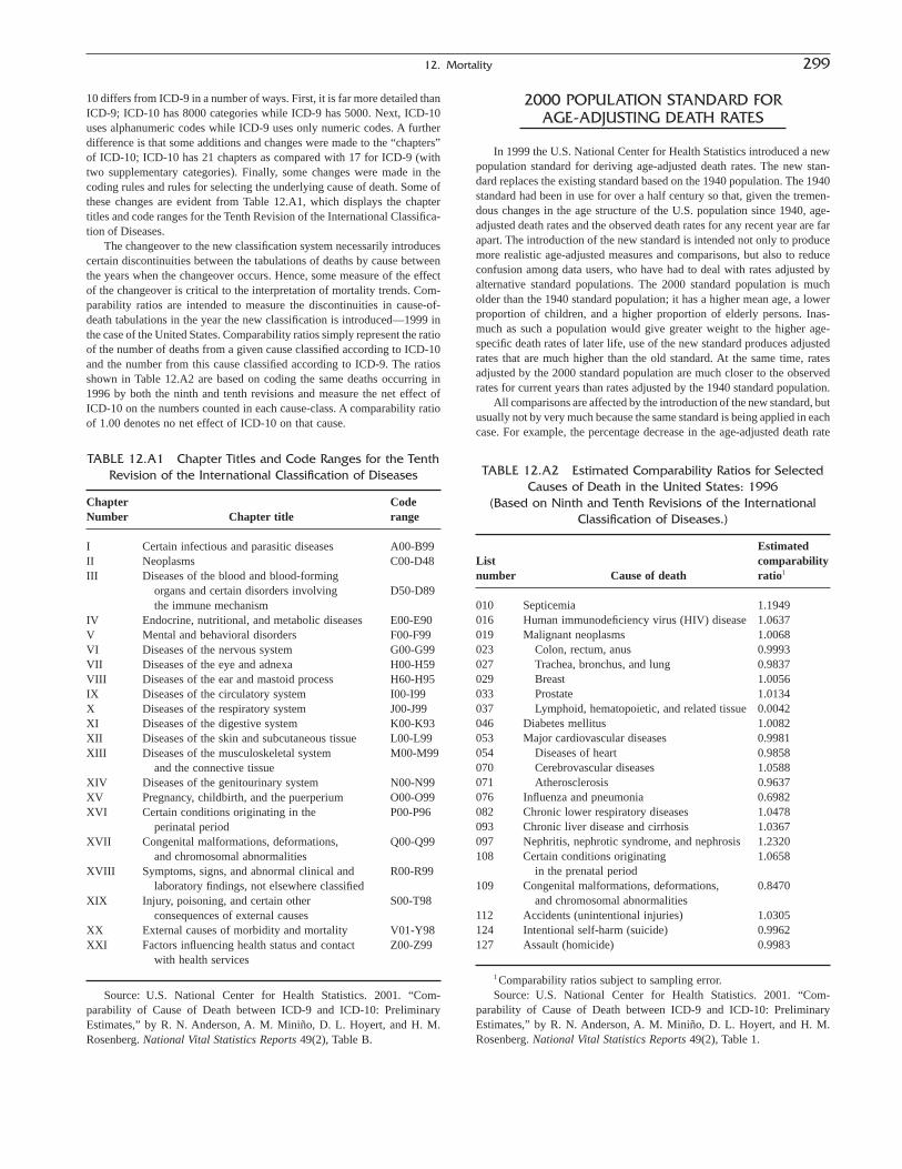
12. Mortality 299
2000 POPULATION STANDARD FORAGE-ADJUSTING DEATH RATES
In 1999 the U.S. National Center for Health Statistics introduced a newpopulation standard for deriving age-adjusted death rates. The new stan-dard replaces the existing standard based on the 1940 population. The 1940standard had been in use for over a half century so that, given the tremen-dous changes in the age structure of the U.S. population since 1940, age-adjusted death rates and the observed death rates for any recent year are farapart. The introduction of the new standard is intended not only to producemore realistic age-adjusted measures and comparisons, but also to reduceconfusion among data users, who have had to deal with rates adjusted byalternative standard populations. The 2000 standard population is mucholder than the 1940 standard population; it has a higher mean age, a lowerproportion of children, and a higher proportion of elderly persons. Inas-much as such a population would give greater weight to the higher age-specific death rates of later life, use of the new standard produces adjustedrates that are much higher than the old standard. At the same time, ratesadjusted by the 2000 standard population are much closer to the observedrates for current years than rates adjusted by the 1940 standard population.
All comparisons are affected by the introduction of the new standard, butusually not by very much because the same standard is being applied in eachcase. For example, the percentage decrease in the age-adjusted death rate
10 differs from ICD-9 in a number of ways. First, it is far more detailed thanICD-9; ICD-10 has 8000 categories while ICD-9 has 5000. Next, ICD-10uses alphanumeric codes while ICD-9 uses only numeric codes. A furtherdifference is that some additions and changes were made to the “chapters”of ICD-10; ICD-10 has 21 chapters as compared with 17 for ICD-9 (withtwo supplementary categories). Finally, some changes were made in thecoding rules and rules for selecting the underlying cause of death. Some ofthese changes are evident from Table 12.A1, which displays the chaptertitles and code ranges for the Tenth Revision of the International Classifica-tion of Diseases.
The changeover to the new classification system necessarily introducescertain discontinuities between the tabulations of deaths by cause betweenthe years when the changeover occurs. Hence, some measure of the effectof the changeover is critical to the interpretation of mortality trends. Com-parability ratios are intended to measure the discontinuities in cause-of-death tabulations in the year the new classification is introduced—1999 inthe case of the United States. Comparability ratios simply represent the ratioof the number of deaths from a given cause classified according to ICD-10and the number from this cause classified according to ICD-9. The ratiosshown in Table 12.A2 are based on coding the same deaths occurring in1996 by both the ninth and tenth revisions and measure the net effect ofICD-10 on the numbers counted in each cause-class. A comparability ratioof 1.00 denotes no net effect of ICD-10 on that cause.
TABLE 12.A1 Chapter Titles and Code Ranges for the TenthRevision of the International Classification of Diseases
Chapter Code Number Chapter title range
I Certain infectious and parasitic diseases A00-B99II Neoplasms C00-D48III Diseases of the blood and blood-forming
organs and certain disorders involving D50-D89the immune mechanism
IV Endocrine, nutritional, and metabolic diseases E00-E90V Mental and behavioral disorders F00-F99VI Diseases of the nervous system G00-G99VII Diseases of the eye and adnexa H00-H59VIII Diseases of the ear and mastoid process H60-H95IX Diseases of the circulatory system I00-I99X Diseases of the respiratory system J00-J99XI Diseases of the digestive system K00-K93XII Diseases of the skin and subcutaneous tissue L00-L99XIII Diseases of the musculoskeletal system M00-M99
and the connective tissueXIV Diseases of the genitourinary system N00-N99XV Pregnancy, childbirth, and the puerperium O00-O99XVI Certain conditions originating in the P00-P96
perinatal periodXVII Congenital malformations, deformations, Q00-Q99
and chromosomal abnormalitiesXVIII Symptoms, signs, and abnormal clinical and R00-R99
laboratory findings, not elsewhere classifiedXIX Injury, poisoning, and certain other S00-T98
consequences of external causesXX External causes of morbidity and mortality V01-Y98XXI Factors influencing health status and contact Z00-Z99
with health services
Source: U.S. National Center for Health Statistics. 2001. “Com-parability of Cause of Death between ICD-9 and ICD-10: Preliminary Estimates,” by R. N. Anderson, A. M. Miniño, D. L. Hoyert, and H. M.Rosenberg. National Vital Statistics Reports 49(2), Table B.
TABLE 12.A2 Estimated Comparability Ratios for SelectedCauses of Death in the United States: 1996
(Based on Ninth and Tenth Revisions of the InternationalClassification of Diseases.)
EstimatedList comparabilitynumber Cause of death ratio1
010 Septicemia 1.1949016 Human immunodeficiency virus (HIV) disease 1.0637019 Malignant neoplasms 1.0068023 Colon, rectum, anus 0.9993027 Trachea, bronchus, and lung 0.9837029 Breast 1.0056033 Prostate 1.0134037 Lymphoid, hematopoietic, and related tissue 0.0042046 Diabetes mellitus 1.0082053 Major cardiovascular diseases 0.9981054 Diseases of heart 0.9858070 Cerebrovascular diseases 1.0588071 Atherosclerosis 0.9637076 Influenza and pneumonia 0.6982082 Chronic lower respiratory diseases 1.0478093 Chronic liver disease and cirrhosis 1.0367097 Nephritis, nephrotic syndrome, and nephrosis 1.2320108 Certain conditions originating 1.0658
in the prenatal period109 Congenital malformations, deformations, 0.8470
and chromosomal abnormalities112 Accidents (unintentional injuries) 1.0305124 Intentional self-harm (suicide) 0.9962127 Assault (homicide) 0.9983
1 Comparability ratios subject to sampling error.Source: U.S. National Center for Health Statistics. 2001. “Com-
parability of Cause of Death between ICD-9 and ICD-10: Preliminary Estimates,” by R. N. Anderson, A. M. Miniño, D. L. Hoyert, and H. M.Rosenberg. National Vital Statistics Reports 49(2), Table 1.
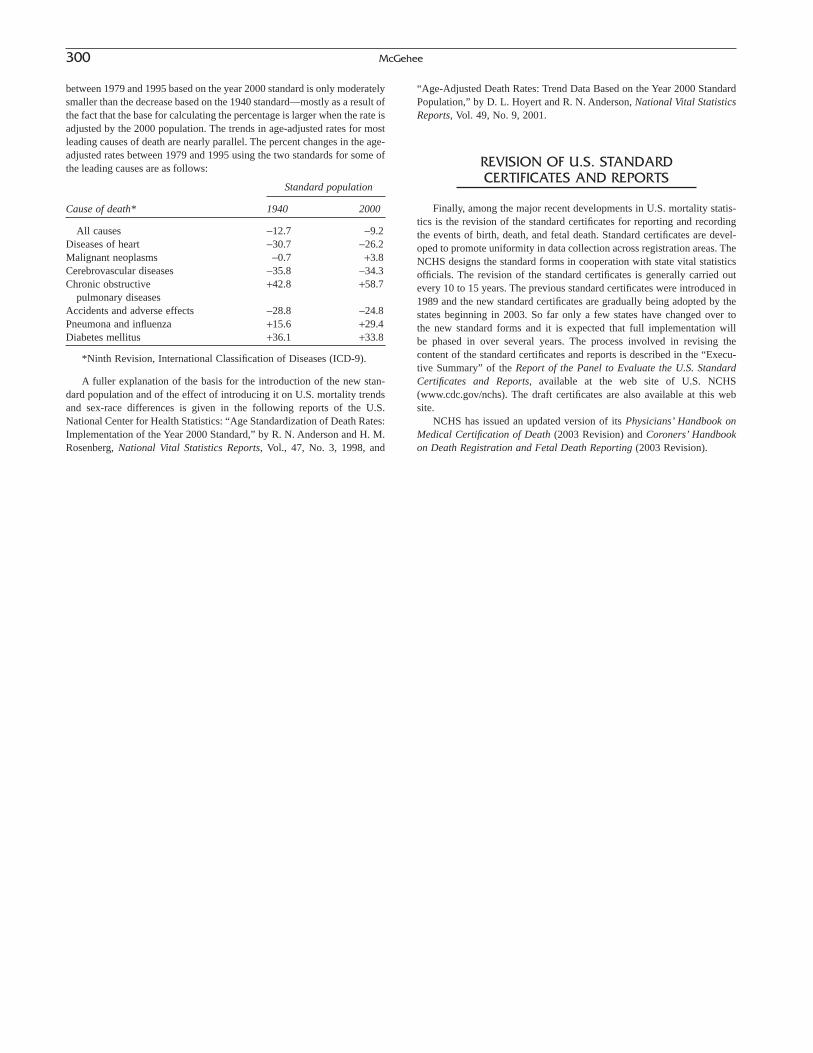
between 1979 and 1995 based on the year 2000 standard is only moderatelysmaller than the decrease based on the 1940 standard—mostly as a result ofthe fact that the base for calculating the percentage is larger when the rate isadjusted by the 2000 population. The trends in age-adjusted rates for mostleading causes of death are nearly parallel. The percent changes in the age-adjusted rates between 1979 and 1995 using the two standards for some ofthe leading causes are as follows:
Standard population
Cause of death* 1940 2000
All causes -12.7 -9.2Diseases of heart -30.7 -26.2Malignant neoplasms -0.7 +3.8Cerebrovascular diseases -35.8 -34.3Chronic obstructive +42.8 +58.7
pulmonary diseasesAccidents and adverse effects -28.8 -24.8Pneumona and influenza +15.6 +29.4Diabetes mellitus +36.1 +33.8
*Ninth Revision, International Classification of Diseases (ICD-9).
A fuller explanation of the basis for the introduction of the new stan-dard population and of the effect of introducing it on U.S. mortality trendsand sex-race differences is given in the following reports of the U.S.National Center for Health Statistics: “Age Standardization of Death Rates:Implementation of the Year 2000 Standard,” by R. N. Anderson and H. M.Rosenberg, National Vital Statistics Reports, Vol., 47, No. 3, 1998, and
“Age-Adjusted Death Rates: Trend Data Based on the Year 2000 StandardPopulation,” by D. L. Hoyert and R. N. Anderson, National Vital StatisticsReports, Vol. 49, No. 9, 2001.
REVISION OF U.S. STANDARDCERTIFICATES AND REPORTS
Finally, among the major recent developments in U.S. mortality statis-tics is the revision of the standard certificates for reporting and recordingthe events of birth, death, and fetal death. Standard certificates are devel-oped to promote uniformity in data collection across registration areas. TheNCHS designs the standard forms in cooperation with state vital statisticsofficials. The revision of the standard certificates is generally carried outevery 10 to 15 years. The previous standard certificates were introduced in1989 and the new standard certificates are gradually being adopted by thestates beginning in 2003. So far only a few states have changed over to the new standard forms and it is expected that full implementation will be phased in over several years. The process involved in revising the content of the standard certificates and reports is described in the “Execu-tive Summary” of the Report of the Panel to Evaluate the U.S. StandardCertificates and Reports, available at the web site of U.S. NCHS(www.cdc.gov/nchs). The draft certificates are also available at this website.
NCHS has issued an updated version of its Physicians’ Handbook onMedical Certification of Death (2003 Revision) and Coroners’ Handbookon Death Registration and Fetal Death Reporting (2003 Revision).
300 McGehee

NATURE AND USE OF LIFE TABLES
Some of the measures of mortality discussed in Chapter12 are associated with a statistical model known as a lifetable. A life table is designed essentially to measure mortal-ity, but various specialists employ it in a variety of ways.Public health workers, demographers, actuaries, economists,and many others use life tables in studies of longevity, fer-tility, migration, and population growth, as well as in makingprojections of population size and characteristics and instudies of widowhood, orphanhood, length of married life,length of working life, and length of disability-free life. Inits simplest form, an entire life table is generated from age-specific mortality rates, and the resulting values are used tomeasure mortality, survivorship, and life expectation. Inother applications, the mortality rates in the life table arecombined with other demographic data into a more complexmodel that measures the combined effect of mortality andchanges in one or more socioeconomic characteristics (e.g.,a table of working life, which combines mortality rates andlabor force participation ratios and measures their combinedeffect on working life).
Life tables are, in essence, one form of combining mortality rates of a population at different ages into a singlestatistical model. They are principally used to measure the level of mortality of the population involved. One oftheir main advantages over other methods of measuringmortality is that they do not reflect the effects of the age distribution of an actual population and do not require theadoption of a standard population for acceptable compar-isons of levels of mortality in different populations. Anotheris that a life table readily permits making mortalityallowances for age cohorts, eliminating the burdensome task of compiling death statistics for age cohorts fromannual death statistics by age, even when the latter are available.
TYPES OF LIFE TABLES
Life tables differ in several ways, including the referenceyear of the table, the age detail, and the number of factorscomprehended by the table. We may distinguish two typesof life tables according to the reference year of the table: thecurrent or period life table and the generation or cohort lifetable. The first type of table is based on the experience overa short period of time, such as 1 year, 3 years, or an inter-censal period, in which mortality has remained substantiallythe same. Commonly, the death statistics used for a currentlife table relate to a period of 1 to 3 years, and the popula-tion data used relate to the middle of that period (usuallyclose to the date of a census). This type of table, therefore,represents the combined mortality experience by age of thepopulation in a particular short period of time (treated syn-thetically or viewed cross-sectionally); it does not representthe mortality experience of an actual cohort. Instead, itassumes a hypothetical cohort that is subject to the age-specific death rates observed in the particular period. There-fore, a current life table may be viewed as a snapshot ofcurrent mortality. It is an excellent summary description ofmortality in a year or a short period.
The second type of life table, the generation life table, isbased on the mortality rates experienced by a particular birthcohort (e.g., all persons born in the year 1900). Accordingto this type of table, the mortality experience of the personsin the cohort would be observed from their moment of birththrough each consecutive age in successive calendar yearsuntil all of them die. Obviously, data over a long period ofyears are needed to complete a single table, and it is not pos-sible wholly on the basis of actual data to construct genera-tion tables for cohorts born in the 20th century. This type oftable is useful for projections of mortality, for studies ofmortality trends, and for the measurement of fertility andreproductivity. In general, unless otherwise specified, the
301
C H A P T E R
13
The Life Table
HALLIE J. KINTNER
The Methods and Materials of DemographyCopyright 2003, Elsevier Science (USA).
All rights reserved.

term “life table” is used in this chapter to refer to a currentlife table.
Life tables are also classified into two types—complete(or unabridged) and abridged—according to the length of theage interval in which the data are presented. A complete lifetable contains data for every single year of age from birth tothe last applicable age. An abridged life table contains dataat intervals of 5 or 10 years of age for most of the age range.Demographers usually prepare the simpler abridged life tablerather than the more elaborate complete life table. Tableswith values for 5- or 10-year intervals are sufficientlydetailed for most purposes, and the abridged table is less burdensome to prepare. Moreover, it is often more conven-ient to use. Tables 13.1 and 13.2 are illustrations of completeand abridged life tables, respectively. Occasionally, the basicvalues from a complete life table are presented only for everyfifth age in order to economize on space.
We may also distinguish a conventional life table, which isconcerned only with the general mortality experience of acohort by age, from a multiple decrement table, whichdescribes the separate and combined effects of more than onefactor. Mortality is always involved. Multiple decrementtables are of several forms. The mortality factor may beapplied in terms of component death rates (e.g., for causes ofdeath), or mortality may be combined with changes in one ormore socioeconomic characteristic(s) of the population. Mul-tiple decrement tables describe the diminution of an originalcohort through these factors (e.g., the attrition of the singlepopulation through mortality and marriage). Increment-decrement tables and multistate tables, elaborations of multi-ple decrement tables, describe the effect of accession to andwithdrawal from the original cohort at various stages in its lifehistory. Examples include a table of working life (which com-bines mortality rates and labor force participation ratios) anda nuptiality table (which combines mortality rates and data onthe prevalence or incidence of marriage and divorce).
AVAILABILITY OF LIFE TABLES
The first recognized life table was published in 1693 byHalley. It was based on birth and death registration data forthe city of Breslau during the years 1687 to 1691. Theassumption adopted in the preparation of this table that thepopulation of Breslau had remained stationary (i.e., that thetotal population and the numbers in each age and sex groupdid not change over many decades) was not entirely correctand, therefore, the resulting life table could not be regardedas being correct. Other life tables were prepared in the 17thand 18th centuries on the basis of limited data, but they weresubject to necessary simplifying assumptions that renderedthem inexact.
The first scientifically correct life table based on bothpopulation and death data classified by age was prepared by
Milne and published in 1815. It was based on the mortalityexperience in two parishes of Carlisle, England, during the period 1779–1787. A large number of life tables havebeen published since then. In the early years, most of these pertained to European countries, particularly Scandinavian countries, but life tables are now available formost countries of the world and every continent is represented.
In the United States, official complete life tables havebeen prepared since 1900–1902 in connection with thedecennial censuses of population. These tables are based onthe registered deaths in the expanding death registration area(continental United States first being covered for the1929–1931 table) in the 3-year period containing the censusyear. Hence, there is an unbroken decennial series of com-plete life tables covering the 20th century (U.S. Bureau ofthe Census, 1921, 1936, 1946; U.S. National Office of VitalStatistics, 1954; U.S. National Center for Health Statistics,1964, 1975, 1985a, 1997a). There are some tables also forintercensal periods, as for 1901–1910, 1920–1929, and1930–1939. An annual series of abridged life tables wasstarted in 1945 and continued to the end of the 20th century.They are now published on a provisional basis for a givenyear just after the close of the year and on a revised basis inthe annual volume on mortality statistics for the year or incurrent reports. These annual tables are based on the annualdeath registration and on postcensal estimates of population.
In addition to national tables, tables have been preparedfrom time to time for geographic areas varying in size fromspecific cities to geographic divisions and regions. Sets oflife tables for all states have now been published in con-nection with the censuses of 1930 (whites only), 1940(whites only), 1950 (nonwhite tables for states in the Southregion only), 1960 (race/ethnic group for selected states),1970, 1980, and 1990 (U.S. National Office of Vital Sta-tistics, 1948, 1956a; U.S. National Center for Health Statistics, 1966, 1977, 1990, 1998). Life tables for geo-graphic divisions or regions corresponding to these statetables have also been published (U.S. National Office ofVital Statistics, 1956b; U.S. National Center for Health Sta-tistics, 1965). For the first time, life tables for metropolitanand nonmetropolitan areas as a whole were published for1959–1961 (U.S. National Center for Health Statistics,1967). For some periods prior to 1940, separate tables werepublished for the urban and rural populations.
Special compilations of life tables or analytic studies oflife tables were published in connection with the 1900, 1910,1930, and 1940 censuses. The life tables included in thesevolumes covered the death registration states or the UnitedStates as a whole, specified individual states and cities, andthe urban and rural parts of the death registration states insome cases. A general guide to the U.S. life tables for 1900to 1959 has been published (U.S. National Center for HealthStatistics, 1963).
302 Kintner

13.The Life Table
303
TABLE 13.1 Complete Life Table for the Total Population of the United States: 1989–1991
Average AverageProportion remaining Proportion remaining
dying lifetime dying lifetime
Proportion Average Period AverageAge of persons Of 100,000 number of Age of persons Of 100,000 numberInterval alive at born alive Stationary population years of interval alive at born alive Stationary population of years
beginning life beginning of lifePeriod of age Number Number In this and remaining Period of age Number Number In this and remainingof life interval living at dying all at of life interval living at dying all atbetween dying beginning during In the subsequent beginning between dying beginning during In the subsequent beginningtwo exact during of age age age age of age two during of age age age age of ageages interval interval interval interval intervals interval ages interval interval interval interval intervals interval(1) (2) (3) (4) (5) (6) (7) (1) (2) (3) (4) (5) (6) (7)x to x tox + 1 x + 1(years) qx lx dx Lx Tx ex (years) qx lx dx Lx Tx ex
0–1 0.00936 100,000 936 99,258 7,536,614 75.371–2 0.00073 99,064 72 99,028 7,437,356 75.082–3 0.00048 98,992 48 98,968 7,338,328 74.133–4 0.00037 98,944 37 98,926 7,239,360 73.174–5 0.00030 98,907 30 98,892 7,140,434 72.195–6 0.00027 98,877 27 98,863 7,041,542 71.226–7 0.00025 98,850 25 98,838 6,942,634 70.237–8 0.00023 98,825 23 98,814 6,843,796 69.258–9 0.00020 98,802 20 98,792 6,744,983 68.279–10 0.00018 98,782 18 98,773 6,646,191 67.28
10–11 0.00016 98,764 16 98,756 6,547,418 66.2911–12 0.00016 98,748 16 98,740 6,448,662 65.3012–13 0.00022 98,732 22 98,721 6,349,922 64.3113–14 0.00032 98,710 32 98,694 6,251,201 63.3314–15 0.00047 98,678 46 98,655 6,152,507 62.3515–16 0.00063 98,632 62 98,601 6,053,852 61.3816–17 0.00077 98,570 76 98,532 5,955,251 60.4217–18 0.00089 98,494 88 98,450 5,856,719 59.4618–19 0.00096 98,406 94 98,359 5,758,269 58.5219–20 0.00101 98,312 99 98,263 5,659,910 57.5720–21 0.00104 98,213 102 98,162 5,561,647 56.6321–22 0.00109 98,111 107 98,058 5,463,485 55.6922–23 0.00112 98,004 110 97,949 5,365,428 54.7523–24 0.00114 97,894 112 97,838 5,267,479 53.8124–25 0.00116 97,782 113 97,726 5,169,641 52.8725–26 0.00117 97,669 114 97,612 5,071,915 51.9326–27 0.00119 97,555 116 97,497 4,974,303 50.9927–28 0.00121 97,439 118 97,380 4,876,806 50.05
(continues)
28–29 0.00126 97,321 123 97,260 4,779,426 49.1129–30 0.00133 97,198 129 97,134 4,682,167 48.1730–31 0.00140 97,069 136 97,001 4,585,033 47.2331–32 0.00147 96,933 142 96,862 4,488,032 46.3032–33 0.00154 96,791 149 96,717 4,391,170 45.3733–34 0.00162 96,642 157 96,564 4,294,454 44.4434–35 0.00170 96,485 164 96,403 4,197,890 43.5135–36 0.00178 96,321 171 96,236 4,101,487 42.5836–37 0.00188 96,150 181 96,060 4,005,252 41.6637–38 0.00198 95,969 190 95,874 3,909,192 40.7338–39 0.00207 95,779 198 95,680 3,813,318 39.8139–40 0.00217 95,581 207 95,478 3,717,638 38.9040–41 0.00228 95,374 217 95,266 3,622,161 37.9841–42 0.00240 95,157 228 95,043 3,526,895 37.0642–43 0.00254 94,929 241 94,809 3,431,852 36.1543–44 0.00271 94,688 257 94,560 3,337,044 35.2444–45 0.00292 94,431 276 94,293 3,242,484 34.3445–46 0.00318 94,155 299 94,006 3,148,191 33.4446–47 0.00348 93,856 327 93,693 3,054,186 32.5447–48 0.00380 93,529 355 93,352 2,960,493 31.6548–49 0.00414 93,174 386 92,981 2,867,142 30.7749–50 0.00449 92,788 417 92,580 2,774,161 29.9050–51 0.00490 92,371 453 92,145 2,681,581 29.0351–52 0.00537 91,918 494 91,671 2,589,437 28.1752–53 0.00590 91,424 539 91,155 2,497,766 27.3253–54 0.00647 90,885 588 90,591 2,406,611 26.4854–55 0.00708 90,297 639 89,978 2,316,020 25.6555–56 0.00773 89,658 693 89,312 2,226,043 24.83

304K
intnerTABLE 13.1 (continued)
Average AverageProportion remaining Proportion remaining
dying lifetime dying lifetime
Proportion Average Period AverageAge of persons Of 100,000 number of Age of persons Of 100,000 numberInterval alive at born alive Stationary population years of interval alive at born alive Stationary population of years
beginning life beginning of lifePeriod of age Number Number In this and remaining Period of age Number Number In this and remainingof life interval living at dying all at of life interval living at dying all atbetween dying beginning during In the subsequent beginning between dying beginning during In the subsequent beginningtwo exact during of age age age age of age two during of age age age age of ageages interval interval interval interval intervals interval ages interval interval interval interval intervals interval(1) (2) (3) (4) (5) (6) (7) (1) (2) (3) (4) (5) (6) (7)x to x tox + 1 x + n(years) qx lx dx Lx Tx ex (years) qx lx dx Lx Tx ex
83–84 0.08207 37,995 3,118 36,436 267,631 7.0484–85 0.08907 34,877 3,106 33,324 231,195 6.6385–86 0.09705 31,771 3,083 30,230 197,871 6.2386–87 0.10627 28,688 3,049 27,164 167,642 5.8487–88 0.11625 25,639 2,981 24,149 140,478 5.4888–89 0.12688 22,658 2,875 21,221 116,330 5.1389–90 0.13834 19,783 2,737 18,415 95,109 4.8190–91 0.15135 17,046 2,580 15,756 76,695 4.5091–92 0.16591 14,466 2,400 13,266 60,939 4.2192–91 0.18088 12,066 2,182 10,975 47,673 3.9593–94 0.19552 9,884 1,933 8,918 36,698 3.7194–95 0.21000 7,951 1,670 7,116 27,780 3.4995–96 0.22502 6,281 1,413 5,575 20,664 3.2996–97 0.24126 4,868 1,174 4,281 15,090 3.1097–98 0.25689 3,694 949 3,220 10,809 2.9398–99 0.27175 2,745 746 2,372 7,589 2.7699–100 0.28751 1,999 575 1,712 5,217 2.61
100–101 0.30418 1,424 433 1,208 3,506 2.46101–102 0.32182 991 319 832 2,298 2.32102–103 0.34049 672 229 558 1,467 2.18103–104 0.36024 443 160 363 909 2.05104–105 0.38113 283 108 229 546 1.93105–106 0.40324 175 71 140 317 1.81106–107 0.42663 104 44 82 178 1.71107–108 0.45137 60 27 47 96 1.59108–109 0.47755 33 16 25 49 1.48109–110 0.50525 17 9 9 24 1.39
Source: U.S. National Center for Health Statistics. 1997. U.S. Decennial Life Tables for 1989–91. Vol. 1, no. 1, pp. 6–7.
56–57 0.00844 88,965 751 88,590 2,136,731 24.0257–58 0.00926 88,214 817 87,806 2,048,142 23.2258–59 0.01019 87,397 891 86,952 1,960,336 22.4359–60 0.01120 86,506 969 86,022 1,873,385 21.6660–61 0.01223 85,537 1,046 85,014 1,787,363 20.9061–62 0.01328 84,491 1,122 83,930 1,702,349 20.1562–63 0.01439 83,369 1,200 82,769 1,618,419 19.4163–64 0.01560 82,169 1,282 81,528 1,535,650 18.6964–65 0.01691 80,887 1,368 80,203 1,454,122 17.9865–66 0.01827 79,519 1,453 78,793 1,373,919 17.2866–67 0.01967 78,066 1,536 77,298 1,295,127 16.5967–68 0.02121 76,530 1,623 75,719 1,217,829 15.9168–69 0.02297 74,907 1,721 74,047 1,142,110 15.2569–70 0.02499 73,186 1,829 72,272 1,068,064 14.5970–71 0.02727 71,357 1,946 70,384 995,792 13.9671–72 0.02979 69,411 2,068 68,377 925,408 13.3372–73 0.03251 67,343 2,189 66,249 857,031 12.7373–74 0.03534 65,154 2,303 64,003 790,783 12.1474–75 0.03824 62,851 2,403 61,650 726,780 11.5675–76 0.04126 60,448 2,494 59,201 665,131 11.0076–77 0.04455 57,954 2,582 56,663 605,930 10.4677–78 0.04819 55,372 2,668 54,038 549,267 9.9278–79 0.05239 52,704 2,761 51,324 495,229 9.4079–80 0.05723 49,943 2,858 48,514 443,905 8.8980–81 0.06277 47,085 2,956 45,607 395,391 8.4081–82 0.06885 44,129 3,038 42,610 349,784 7.9382–83 0.07535 41,091 3,096 39,543 307,174 7.48
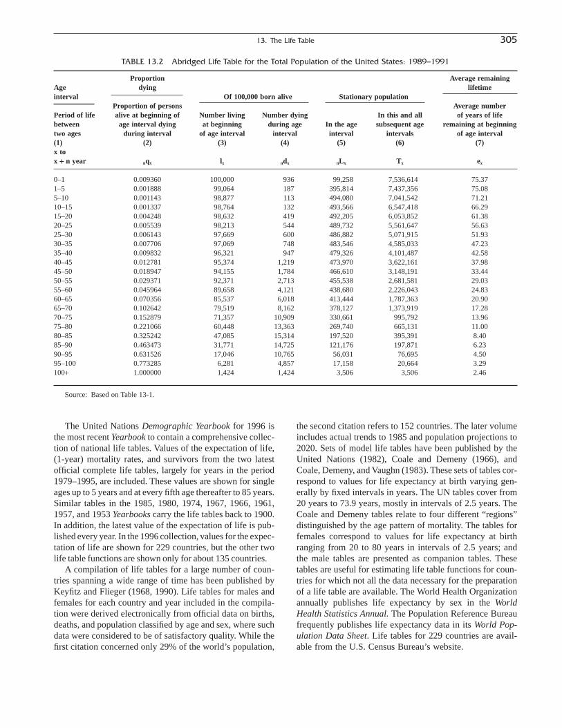
13. The Life Table 305
The United Nations Demographic Yearbook for 1996 isthe most recent Yearbook to contain a comprehensive collec-tion of national life tables. Values of the expectation of life,(1-year) mortality rates, and survivors from the two latestofficial complete life tables, largely for years in the period1979–1995, are included. These values are shown for singleages up to 5 years and at every fifth age thereafter to 85 years.Similar tables in the 1985, 1980, 1974, 1967, 1966, 1961,1957, and 1953 Yearbooks carry the life tables back to 1900.In addition, the latest value of the expectation of life is pub-lished every year. In the 1996 collection, values for the expec-tation of life are shown for 229 countries, but the other twolife table functions are shown only for about 135 countries.
A compilation of life tables for a large number of coun-tries spanning a wide range of time has been published byKeyfitz and Flieger (1968, 1990). Life tables for males andfemales for each country and year included in the compila-tion were derived electronically from official data on births,deaths, and population classified by age and sex, where suchdata were considered to be of satisfactory quality. While thefirst citation concerned only 29% of the world’s population,
the second citation refers to 152 countries. The later volumeincludes actual trends to 1985 and population projections to2020. Sets of model life tables have been published by theUnited Nations (1982), Coale and Demeny (1966), andCoale, Demeny, and Vaughn (1983). These sets of tables cor-respond to values for life expectancy at birth varying gen-erally by fixed intervals in years. The UN tables cover from20 years to 73.9 years, mostly in intervals of 2.5 years. TheCoale and Demeny tables relate to four different “regions”distinguished by the age pattern of mortality. The tables forfemales correspond to values for life expectancy at birthranging from 20 to 80 years in intervals of 2.5 years; andthe male tables are presented as companion tables. Thesetables are useful for estimating life table functions for coun-tries for which not all the data necessary for the preparationof a life table are available. The World Health Organizationannually publishes life expectancy by sex in the WorldHealth Statistics Annual. The Population Reference Bureaufrequently publishes life expectancy data in its World Pop-ulation Data Sheet. Life tables for 229 countries are avail-able from the U.S. Census Bureau’s website.
TABLE 13.2 Abridged Life Table for the Total Population of the United States: 1989–1991
AgeProportion Average remaining
intervaldying
Of 100,000 born alive Stationary populationlifetime
Proportion of persons Average numberPeriod of life alive at beginning of Number living Number dying In this and all of years of lifebetween age interval dying at beginning during age In the age subsequent age remaining at beginningtwo ages during interval of age interval interval interval intervals of age interval(1) (2) (3) (4) (5) (6) (7)x tox + n year nqx lx ndx nLx Tx ex
0–1 0.009360 100,000 936 99,258 7,536,614 75.371–5 0.001888 99,064 187 395,814 7,437,356 75.085–10 0.001143 98,877 113 494,080 7,041,542 71.2110–15 0.001337 98,764 132 493,566 6,547,418 66.2915–20 0.004248 98,632 419 492,205 6,053,852 61.3820–25 0.005539 98,213 544 489,732 5,561,647 56.6325–30 0.006143 97,669 600 486,882 5,071,915 51.9330–35 0.007706 97,069 748 483,546 4,585,033 47.2335–40 0.009832 96,321 947 479,326 4,101,487 42.5840–45 0.012781 95,374 1,219 473,970 3,622,161 37.9845–50 0.018947 94,155 1,784 466,610 3,148,191 33.4450–55 0.029371 92,371 2,713 455,538 2,681,581 29.0355–60 0.045964 89,658 4,121 438,680 2,226,043 24.8360–65 0.070356 85,537 6,018 413,444 1,787,363 20.9065–70 0.102642 79,519 8,162 378,127 1,373,919 17.2870–75 0.152879 71,357 10,909 330,661 995,792 13.9675–80 0.221066 60,448 13,363 269,740 665,131 11.0080–85 0.325242 47,085 15,314 197,520 395,391 8.4085–90 0.463473 31,771 14,725 121,176 197,871 6.2390–95 0.631526 17,046 10,765 56,031 76,695 4.5095–100 0.773285 6,281 4,857 17,158 20,664 3.29100+ 1.000000 1,424 1,424 3,506 3,506 2.46
Source: Based on Table 13-1.

ANATOMY OF THE LIFE TABLE
Life Table Functions
The basic life tables functions—nqx, lx, ndx, nLx, Tx, andex—can be observed in Tables 13.1 and 13.2. These sixcolumns are generally calculated and published for everylife table. However, in some cases, because of limitations ofspace, columns may be omitted. (For example, the UnitedNations publishes only qx, lx, and ex in the DemographicYearbook.) This is done without a significant loss of infor-mation because the functions are interrelated and some canbe directly calculated from the others. In general, the mor-tality rate (nqx) is the basic function in the table (i.e., theinitial function from which all other life table functions arederived).
Alternative Interpretations
Life table functions are subject to two different interpre-tations depending on the interpretation given to the life tableas a whole. In the more common interpretation, the life tableis viewed as depicting the lifetime mortality experience ofa single cohort of newborn babies, who are subject to theage-specific mortality rates on which the table is based. Inthe second interpretation, the life table is viewed as a sta-tionary population resulting from the (unchanging) scheduleof age-specific mortality rates shown and a constant annualnumber of births.
The Life Table as the Mortality Experience of a Cohort
Under the first interpretation, the life table model con-ceptually traces a cohort of newborn babies through theirentire life under the assumption that they are subject to thecurrent observed schedule of age-specific mortality rates.The cohort of newborn babies, called the radix of the table,is usually assumed to number 100,000. In this case, the inter-pretation of the life table functions in an abridged tablewould be as follows:
x to x + n The period of life between two exact ages. Forinstance, “20–25” means the 5-year interval betweenthe 20th and 25th birthdays.
nqx The proportion of the persons in the cohort alive at thebeginning of an indicated age interval (x) who will diebefore reaching the end of that age interval (x + n). Forexample, according to Table 13.2, the proportion dyingin the age interval 20–25 is 0.005539—that is, out ofevery 100,000 persons alive and exactly 20 years old,554 will die before reaching their 25th birthday. Inother words, the nqx values represent the probability thata person at his or her xth birthday will die before reach-ing his or her x + nth birthday.
lx The number of persons living at the beginning of theindicated age interval (x) out of the total number ofbirths assumed as the radix of the table. Again, accord-ing to Table 13.2, out of 100,000 newborn babies,98,213 persons would survive to exact age 20.
ndx The number of persons who would die within the indi-cated age interval (x to x + n) out of the total numberof births assumed in the table. Thus, according to Table13.2, there would be 544 deaths between exact ages 20and 25 to the initial cohort of 100,000 newborn babies.
nLx The number of person-years that would be lived withinthe indicated age interval (x to x + n) by the cohort of100,000 births assumed. Thus, according to Table 13.2,the 100,000 newborn babies would live 489,732person-years between exact ages 20 and 25. Of the98,213 persons who reach age 20, the 97,669 whosurvive to age 25 would live 5 years each (97,669 ¥ 5= 488,345 person-years) and the 544 who die wouldeach live varying periods of time less than 5 years,averaging about 21/2 years
Tx The total number of person-years that would be livedafter the beginning of the indicated age interval by thecohort of 100,000 births assumed. Thus, according toTable 13.2, the 100,000 newborn babies would live5,561,647 person-years after their 20th birthday.
ex The average remaining lifetime (in years) for a personwho survives to the beginning of the indicated ageinterval. This function is also called the completeexpectation of life or, simply, life expectancy. Thus,according to Table 13.2, a person who reaches his orher 20th birthday should expect to live 56.63 yearsmore, on the average.
The interpretation of the functions in a complete lifetable is the same as in the abridged table except that theqx, dx, and Lx values relate to single-age intervals. Thelx, Tx, and ex values have the same interpretation as inthe abridged table because they are not “interval”values but pertain to exact age x.
The Life Table as a Stationary Population
An alternate interpretation of the life table is the one asso-ciated with the concept of a stationary population. A station-ary population is defined as a population whose total numberand distribution by age do not change with time. Such a hypo-thetical population would result if the number of births peryear remained constant (usually assumed at 100,000) for along period of time and each cohort of births experienced thecurrent observed mortality rates throughout life. The annualnumber of deaths would thus equal 100,000 also, and therewould be no change in the size of the population.
544 2 55 1387¥ =. person-years
306 Kintner
In this case, the interpretation of x to x + n, nqx and ex
would be as previously indicated, but, given that births areconstant at 100,000 per year and that the observed deathrates at each age remain in effect for the life of the cohort,for the other life table functions, it would be as follows:
lx The number of persons who reach the beginning of theage interval each year. According to Table 13.2, therewould be 98,213 persons reaching exact age 20 everyyear.
ndx The number of persons that die each year within theindicated age interval. According to Table 13.2, therewould be 544 deaths between exact ages 20 and 25every year.
nLx The number of persons in the population who at anymoment are living within the indicated age interval.According to Table 13.2, there would be 489,732persons living between exact ages 20 and 25 in thepopulation at any time.
Tx The number of persons in the population who at anymoment are living within the indicated age interval andall higher age intervals. According to Table 13.2, therewould be 5,561,647 persons over exact age 20 living inthe population at any time.
Each interpretation has its particular applications. Forexample, the interpretation of the life table as the history ofa cohort is applied in public health studies and mortalityanalysis, and in the calculation of survival rates for estimat-ing population, net migration, fertility, and reproductivity.The interpretation of the life table as a stationary populationis used in the comparative measurement of mortality and instudies of population structure.
Life Span and Life Expectancy
In measuring longevity, two concepts should be distin-guished: life span and life expectancy. The first concept triesto establish numerically the age limit of human life (i.e., theage that human beings as a species could reach underoptimum conditions). There is no known exact figure for thelife span of human beings or any other species (Carey,1997). However, by using the verified age of the longestlived individual, one operational definition of life span for aspecies can be constructed, namely, the maximum recordedage at death. Using this operational definition, the life spanfor humans appears to be just over 120 years (Olshansky,Carnes, and Cassel, 1990).
Life expectancy is the expected number of years to belived, on the average, by a particular population at a partic-ular time. Sufficiently accurate records have been availablefor some time for many countries from which estimates havebeen prepared. These estimates have generally come from acurrent life table, although in some instances they have beenprepared from more limited data.
CONSTRUCTION OFCONVENTIONAL LIFE TABLES
General Considerations
The main concern in this section is with methods of con-structing life tables where satisfactory data on births, deaths,and population are available. (Model life tables and indirecttechniques of life table construction are often employed for statistically underdeveloped countries, as discussed inChapter 22 and Appendix B.) Mathematical formulas anddemographic procedures are discussed in detail, and tech-niques for manipulating the mortality data are presented. Itshould be observed that in every instance underlying theseprocedures, formulas, and techniques, there is an assump-tion that the data on births, deaths, and population are fullyaccurate. It is well known, however, that one of the mostimportant aspects of the preparation of a life table is thetesting of the data for possible biases and other errors. Mostof the procedures used to check on the accuracy of the datahave been discussed in previous chapters and will not be dis-cussed again here. It suffices that the level of inaccuracy thatcan be tolerated depends mostly on the intended use of thelife table.
One factor that is usually involved in the selection of themethod to be used in the construction of a life table is thedegree of adherence to the observed data that is desired. Fulladherence to the observed values implies that the final lifetable functions will exhibit all the fluctuations in theobserved data, whether these are due to real variations or to errors in the data. On the other hand, overgraduation (i.e., excessive “smoothing” of the data by mathematicalmethods) will eliminate or reduce true variations in the age pattern of mortality rates. Therefore, it must be decidedwhether the emphasis in the life table should be on its close-ness to the actual data or on its presentation of the underly-ing mortality picture after fluctuations have been removed.In the statistically developed countries, as the quality andquantity of data have improved with the passage of time,fewer irregular fluctuations have been noticed in theobserved mortality rates. Therefore, the tendency has beento place stronger emphasis on adherence to the data and lessemphasis on eliminating or reducing the fluctuations.
The Complete Life Table
As was indicated before, a complete life table is a lifetable in which the values of the functions are shown forsingle years of age. This type of table either can be com-puted directly from the observed data or can be obtained bysuitable interpolation of an abridged life table. In manyinstances, even when a complete life table is being con-structed, the observed data are combined into age groups andthen interpolated to obtain the single-year values. This pro-
13. The Life Table 307

308 Kintner
cedure is generally used to smooth out artificial fluctuationsin the data or to adjust for what are believed to be inconsis-tencies or errors in the data.
Basic Construction Problems
The construction of complete life tables can be consid-ered in terms of three broad phases. First, the basic data ondeaths, population, and births are checked for inconsisten-cies, biases, and other errors, and adjustments are madewhere necessary. Second, the death rates and mortality rates are computed and graduated (i.e., mathematicallysmoothed). Third, the remaining functions of the life tableare calculated. As indicated previously, this chapter empha-sizes the second and third steps.
Life tables are based on probabilities of dying, the prob-ability that an individual alive at age x dies before reachinghis or her next birthday (age x + 1). The Lexis diagram(Figure 13.1) shows the relation of the number attaining agex, the population in age x, and the deaths at age x. Individ-ual lives move along diagonal lines from the origin up andto the right. In general, then,
Dzx The number of deaths that occur during calendar year zamong persons who have attained age x at last birthday(the area encompassed by points ABCD in Figure13.1).
aDzx The number of persons who attained age x in the cal-endar year z and died before the end of the calendaryear (the area encompassed by points ABC).
dDzx The number of persons alive at the beginning of cal-endar year z who were x years old last birthday anddied before attaining age x + 1 (the area encompassedby points ADC).
Pzx The number of persons alive at the beginning of calen-
dar year z who are x years old last birthday (the linefrom point A to point D).
Ezx The number of persons attaining age x in year z (the
line from point A to point B).Note that aDz
x + dDzx = Dz
x and Ezx+1 = Pz
x - dDzx.
There are several alternative ways to compute mortalityrates, qx, from vital statistics and census data. One approachrelates deaths in the parallelogram ABCE to lines connect-ing AB. Under the assumption of no migration, the mortal-ity rate for ages above 1 would be
(13.1)
The corresponding mortality rate for the first year of lifewould replace the denominator with the number of births inyear z. However, these formulas involve the partial mortal-ity experience of 2 consecutive calendar years rather thanthe experience of a single calendar year.
Another approach concerns deaths in ABCD and relatesaDz
x to lines connecting AB and dDzx to lines connecting AD.
For ages above 1
(13.2)
The mortality rates could be based on the experience ofa single calendar year if it is assumed that there is littlechange in mortality or in the seasonal birth pattern betweenthe 2 years. In that case, the formulas for ages above 1 andfor infants would be
(13.3)
(13.4)
These formulas directly employ deaths in the single yearz only, although deaths for prior years are required to deter-mine the population at the beginning of the year at age under1, or Pz
x in general.It should be noted that these formulas require the regis-
tered deaths in every calendar year to be separated accord-ing to whether they occurred before or after the birthdayanniversary in that year. When the death statistics are notavailable in this form, the usual approach is to estimate sep-aration factors fx from other sources or to assume that thoseobserved in other populations apply in the present case.
Generally, separation factors above age 1 are assumed tobe 0.5. Deaths under age 1 are concentrated at the beginningof the interval; about half of infant deaths in the UnitedStates occur in the first week of life and 65% happen withinthe first month. The average age at death for infants riseswith increasing infant mortality levels. Preston, Keyfitz, andSchoen (1972) suggested the following approximation forthe separation factor for those less than 1 year of age:
(13.5)1 0 1 00 07 1 7a m= + ◊. .
qP
B
E
P
z
z
z
z00
11
0
1= - ◊+
qP
E
E
Px
xz
xz
xz
xz
= - ◊+
+11
1
qD
E
D
Px
xz
xz
xz
xz
= - -ÊËÁ
ˆ¯̃◊ -Ê
ËÁˆ¯̃1 1 1
a d
qD D
Ex
xz
xz
xz
=+ +a d 1
Dx
Dx
Px+1
Ex+1
Ex Ex
Px
Dx+1
Dx
DxdDz
aDz
Px Dx
Pz
Ez
Ez Ez+1
Pz Pz+1
dDz+1
Dz
Dz+1Dz
FIGURE 13.1 ••

Given the separation factors, to calculate the qx the deathswould be estimated as follows:
(13.6)
(13.7)
The separation factor fx¢ represents the proportion ofdeaths at a given age in a given year that occurred after thebirthday anniversary in that year. In the case of infant deaths,fx¢ represents the proportion of all infant death in a year thatoccurred to babies born in the year. Small errors in the sep-aration factors do not materially affect estimates.
In the computation and graduation of the mortality rates, three different age segments are recognized as havingpeculiar problems and are treated separately. The first is theyoungest age segment, which generally includes ages under5. Where the quality of data is sufficiently good and the levelof mortality is low, the first segment can be limited to thefirst year of life. The second segment generally covers thebulk of the table, from age 5 to age 85, where the most reli-able data are found. The third segment covers the oldestages, 85 years and older, and usually contains the data ofhighest uncertainty. It should be observed that these aresomewhat arbitrary divisions. It is entirely possible or evenadvisable in some cases, depending on the nature of theobserved data, further to subdivide some of these segments.The number of segments and their age limits should bedetermined based on an analysis of the data available.
Mortality at Ages Under 5 Years
The methods used to compute mortality risks at ages lessthan 5 years must necessarily be adapted to the type andquality of data available. As the quality and quantity of dataimprove, it is feasible to extend to ages 1 to 4 years themethods used in the main body of the life table. Owing tothe distinct peculiarities of mortality during the first year oflife, however, special procedures must be used to computethe death rates at ages less than 1 year.
On many occasions, the census counts are particularlyinaccurate at the younger ages. It may be desirable or neces-sary, then, to design formulas or procedures to obtain the mor-tality rates at ages under 5 years on the basis of recorded birthsrather than on population counts. The most frequently usedprocedure employs the registered birth and death statistics.For the United States 1989–1991 decennial life table, mortal-ity rates for those under 2 years were based on registeredbirths and deaths while the companion rates for those 2 yearsand over were based on registered deaths and populationcounts (U.S. National Center for Health Statistics, 1997b).
The calendar-year infant mortality rate is often used torepresent the mortality risk for the first year of life. This procedure partially substitutes cohort for period data. Theconventional infant mortality rate is the number of deaths in
aD f D f Dxz
x xz
xz= - ¢¢( ) = ¢1
dD f Dxz
x xz= ¢¢
infancy to a group of persons born in the same year. The cal-endar-year infant mortality rate is computed as the ratio of the number of deaths of those less than 1 year (in that year) tothe number of live births in that year. So deaths in year z + 1 ofinfants born late in the year z are represented by deaths in yearz to those born late in year z - 1.
If the vital statistics tabulations are sufficiently detailed, itis possible to use days, weeks, months, or quarter-years asunits for constructing qx for young ages. The United States1989–1991 decennial life tables, for example, used 0 to 1 day,1 to 7 days, 7 to 28 days, 28 to 365 days, and 1 to 2 years. Theprocedure assumes that births are uniformly distributedwithin these intervals.
It is not necessary to begin with mortality rates. At agesunder 2 years, the United States decennial life tables did notbegin with mortality rates but rather with observed and lifetable deaths. For each age interval 0 to 1 day, 1 to 7 days, 7to 28 days, 28 to 365 days, and 1 to 2 years, the formula was
where tDx denotes the number of deaths occurring in1989–1991 between exact ages x and x + t, and tEx is aweighted count of births during 1987–1991. The denomina-tor assumes that births are uniformly distributed over theyear. The values of tdx were then used to calculate values oflx up to age 2 years by successive application of the formulalx+t = lx - dx.
For ages 1 to 4, other approximations of the mortalityrates may be used when the census data are considered tobe of acceptable accuracy and the death rates are low. Acentral death rate, mx, is calculated from the observed deaths,Dx, and the census count, Px, using the formula
(13.8)
In some instances, this formula is modified to improve itsreliability by using an average population derived from thepopulations at three adjacent ages, as follows:
where Dx denotes the number of deaths to those aged x. Thepopulation at risk of dying at age x during the 3-year periodincludes mainly members of three adjacent annual birthcohorts; hence the denominator sums the populations agedx - 1, x, and x + 1. This approach was used for the UnitedStates 1989–1991 decennial life table for ages 2 to 4. Forexample, deaths at age 2 during 1989–1991 were divided bythe sum of the populations at ages 1, 2, and 3.
The central death rates are then converted to the neededmortality rates, or probabilities, by means of the formula
mD
P P Px
x
x x x
=+ +- +
3
1 1
mD
Px
x
x
=
t xt x
t x
dl D
E= 0
13. The Life Table 309

(13.9)
This formula is based on the assumption that deathsbetween exact ages x and x + 1 occur, on the average, at age x + 1–
2, as, for example, when deaths at age x in a given year
are rectangularly distributed by age and time interval. Theformula for qx shown may be derived from the basic formula for mx and expresses this assumption more explicitly:
(13.10)
Then, dividing numerator and denominator by Px,
Mortality at Ages 5 to 84
The main segment of a life table is that covering ages 5 to84. For this range we usually have the most accurate data onobserved mortality. The goal is to obtain a smooth curve ofdeath rates by age that joins age 5 with the previously com-puted rates for ages below 5. The death statistics and popula-tion data are combined into the conventional 5-year agegroups: 5 to 9, 10 to 14, and so on. Grouping eliminates mostof the problems associated with digit preference in age report-ing and accomplishes part of the desired graduation, and thisparticular grouping has been found especially satisfactory.The death statistics employed would be the total of the deathsrecorded in the observation period; usually 1, 2, or 3 years, andthe population data would refer to the middle of the period.
There are two main approaches to obtaining mortalityrates for single-year ages. One approach is to interpolate thepopulation counts and registered deaths from the aggregateddata to the corresponding single-year-of-age intervals. Then,qx is calculated using
(13.11)
The U.S. decennial life table for 1989–1991 used thisapproach for ages 5 to 94 (U.S. National Center for HealthStatistics, 1997b).
The other main approach is to obtain central age-specificdeath rates from the grouped data using Equation (13.11),test for data anomalies and adjust the rates if necessary, cal-culate, nqx, and then graduate them to obtain single-yearrates. Any abrupt change in the mortality curve is regardedas reflecting a possible anomaly in the data. Each possibleanomaly is investigated in detail and, if necessary, adjust-ment procedures are developed for the data. These adjust-ment procedures vary considerably in detail; they are notgenerally subject to broad generalization because each setof data has it own peculiarities.
qD
P Dx
x
x x
=+ ◊.5
qm
m
m
mx
x
x
x
x
=+
=+1 52
2.
mD
Pq
D
P Dx
x
xx
x
x x
= =+
and.5
qm
mx
x
x
=+2
2
Graduation of Mortality Rates
Once the data have been adjusted, the calculation of themortality rates for single years of age becomes an exercisein graduation techniques. A large number of graduationmethods have been used in the past, and new ones are con-stantly being devised. However, it is important that theanalyst select the method most appropriate for the datainvolved, taking into account limitations in time, personnel,mathematical skill, and possible use of the final life table.The selection of the interpolation formula to be useddepends mostly on the desired balance between smoothnessand closeness of fit to the data. In general, an improvementin smoothness can only be made at the expense of closenessof fit. The analyst must judge, according to his or her expe-rience, the relative importance that should be given to eachof the two opposing considerations.
The three most commonly used interpolation techniques tocompute single-year qx values from grouped (interval) valuesare (1) Sprague multipliers, (2) Beers multipliers, and (3)Karup-King multipliers. All three of these techniques weredesigned so that the sum of the interpolated single-year valuesfor “countable items” (e.g., deaths) is consistent with the totalnumber of countable items for the group (interval) as a whole.The U.S. decennial life tables for 1989–1991 used Beers mul-tipliers (U.S. National Center for Health Statistics, 1997b).
Mortality at Ages 85 and Over
Population and death data at the oldest ages have alwaysbeen considered to be of low accuracy. In most life tables pre-pared in the past, the statistics at these ages have been disregarded because of the low credibility that most demographers and actuaries assign to the basic registrationand census data. Because the quality of these data has beenimproving, however, the tendency now is to retain as muchof them as possible for constructing the life table. This canbe done either by basing the final rates partially on therecorded data or by extending the range of the main portionof the life table beyond age 84—say to age 89 or 94.
In practice, it has been found that, regardless of the totalvolume of data and their accuracy, there is some point at theolder ages beyond which arbitrary methods must be applied.At those very old ages, the data become either too scanty tobe statistically reliable or they are regarded as invalidbecause of errors in age reporting and coverage in the censusor death statistics. For practical purposes, any reasonablemethod can be used because the effect of the choice of rates at these ages on the life table functions at the youngerages would be relatively minor. The method selected,however, should produce a smooth juncture with the mor-tality rates in the main portion of the life table. It should alsoproduce mortality rates that increase smoothly with advanc-ing age.
310 Kintner

One method used is to assume that mortality rates increaseat the oldest ages by about the same percentage as, or, morerealistically, a decreasing percentage of that found at the endof the main portion of the life table. Empirically, in the lowmortality countries, the percentage of increase at the later ageshas been found to be about 10% per year of age. This meansthat every mortality rate at the oldest ages would be 10%higher than the rate at the next previous age or a decliningfunction of 10%. Asecond method is to fit a third degree poly-nomial to the last three acceptable mortality rates and to anassumed rate of unity at a very high age chosen arbitrarily(e.g., age 110). A third method is to fit a Gompertz-Makehamcurve to the end values of the main portion of the life table.
Afourth method is to adopt a series of rates, based on mor-tality experience in other populations, that are believed to beacceptably accurate. In the 1989–1991 United States decen-nial life tables, death rates at ages 85 and over were based, atleast in part, on the experience of the Medicare program (U.S.National Center for Health Statistics, 1997b). Medicare datawere considered more accurate than conventional death rates,already described as suffering from age misreporting amongthe extreme elderly. Medicare death rates at ages 85 to 94were blended with those based on census populations andregistered deaths; rates for older ages were based entirely onMedicare data. The Medicare rates were based directly ondata on deaths and Medicare enrollments for ages 66 to 105.The rates were then smoothed or graduated (see Appendix Cfor a discussion of “smoothing”). Graduated rates at theoldest ages were replaced by rates obtained by a method ofextrapolation set forth in the Annual Social Security TrusteesReports. In this method for each sex, a minimum percentageincrease from qx-1 to qx was required. The level of qx forfemales was not allowed to rise to a level higher than that formales of the same age and race/ethnic group.
Derivation of Other Life Table Functions
The other life table functions are calculated using stan-dard procedures, once the single-year qx’s have been deter-mined. The first values to be computed are the series of lx’s or number of survivors for single years of age. Thesevalues are obtained using the formula
(13.12)
According to this formula, the number of survivors to agiven age, lx, equals the number reaching the previous age, lx-1, times the probability of surviving from that age to thenext, (1-qx-1). The calculations for lx can be “set in motion” byuse of the radix of 100,000 for l0. As examples, the calcula-tions for Table 13.1 at ages 1, 2, and 37 would be as follows:
l q l
l q l
l q l
1 0 0
2 1 1
37 36 36
1 1 00936 100 000 99 064
1 1 00073 99 064 98 992
1 1 00188 96 150 95 969
= -( )◊ = -( )◊ =
= -( )◊ = -( )◊ =
= -( )◊ = -( )◊ =
. , ,
. , ,
. , ,
l q lx x x= -( )- -1 1 1
The dx’s or deaths are the second series of values to becalculated. These follow the formula
(13.13)
This means that the number of deaths at a given age equalsthe difference between the number surviving to that age andthe number surviving to the subsequent age. The calculationsfor Table 13.1 at ages under 1, 1, and 36 would be as follows:
The third series is the Lx’s, the number of person-yearslived by the cohort at a given age. These are computed usingthe approximation
(13.14)
With the exception of age under 1, the Lx’s are the averageof lx and lx+1. The calculations for Table 13.1 at ages under1, 1, and 36 would be as follows:
The fourth series of values, the Tx’s, the total number ofperson-years lived by the cohort after reaching age x, is com-puted by summing the Lx’s for ages x and over to the end ofthe life table. Algebraically, we have
(13.15)
where w is the last age in the life table. For example, T85 isthe sum of all the Lx’s from L85 to L109 in the calculations for Table 13.1: T85 = L85 + L86 + L87 + . . . + L108 + L109 = 30,230+ 27,164 + 24,149 + . . . + 25 + 9 = 197,871. T0 is the sumof the entire column of Lx’s and represents the total numberof person-years lived by the cohort in its lifetime.
The final series of values, ex, expectation of future life, is computed using the formula
(13.16)
The calculations for Table 13.1 at ages 0 and 36 wouldbe as follows:
(Hence, expectation of life at birth can be determined byinspection of T0, with a shift of the decimal.)
eT
l36
36
36
4 005 25296 150
41 66= = =, ,
,.
eT
l0
0
0
7 536 614100 000
75 37= = =, ,
,.
eT
lx
x
x
=
T Lx yy x
y
==
=
Âw
L l l
L l l
L l l
0 0 1
1 1 2
36 36 37
207 793 207 100 000 793 99 064 99 258
0 5 0 5 0 5 99 064 0 5 98 992 99 028
0 5 0 5 0 5 96 150 0 5 95 969 96 060
= + = ( ) + ( ) =
= + = ( ) + ( ) =
= + = ( ) + ( ) =
. . . , . , ,
. . . , . , ,
. . . , . , ,
L f l f l f l f lx x x x x x x x x= ¢¢ + ¢ = ¢¢ + - ¢¢( )+ +1 11
d l l
d l l
d l l
0 0 1
1 1 2
36 36 37
100 000 99 064 936
99 064 98 992 72
96 150 95 969 181
= - = - =
= - = - =
= - = - =
, ,
, ,
, ,
d l lx x x= - +1
13. The Life Table 311

312 Kintner
The Abridged Life Table
Specific Short-Cut Methods
The most fundamental step in life table construction is to convert the observed age-specific death rates into theircorresponding mortality rates, or probabilities of dying. Aswe have seen, in a complete life table, the basic formula forthis transformation is
(13.17)
where mx is the observed death rate at a given age and qx isthe corresponding probability of dying. As stated earlier, thisformula is based on the assumption that deaths betweenexact ages x and x + 1 are rectangularly distributed by ageand time interval. One of the key features of the variousshortcut methods described below is the procedure formaking this basic transformation from nmx to nqx when thedata are grouped. Another difference in the methods is in theway the stationary population is derived. We will describefour shortcut methods here: the Reed-Merrell method, theGreville method, the Keyfitz-Frauenthal method, and themethod of reference to a standard table.
The Reed-Merrell Method
Although it has now largely been replaced by othermethods, the Reed-Merrell (Reed and Merrell, 1939)method was for many years one of the most frequently usedshortcut procedures for calculating an abridged life table. Inthis method the mortality rates are read off from a set ofstandard conversion tables showing the mortality rates asso-ciated with various observed central death rates. The stan-dard tables for 3m2, 5mx, and 10mx were prepared on theassumption that the following exponential equation holds:
(13.18)
where n is size of the age interval, nmx is the central deathrate, a is a constant, and e is the base of the system of naturallogarithms. Reed and Merrell found that a value of a = 0.008would produce acceptable results. The conversion of nmx’sto nqx’s by use of the Reed-Merrell tables is usually appliedto 5-year or 10-year data, but special age groups areemployed at both ends of the life table. At the younger agesthe most frequently used groupings are (1) ages under 1, 1,and 2 to 4 or (2) ages under 1 and 1 to 4. Conversion tablesfor these ages or age groups, as well as for 5mx and 10mx wereworked out by Reed and Merrell; they are reproduced inAppendix A.
For example, the death rate for the age group 55 to 59(5m55) observed in the United States in 1991, .009263, wouldbe converted to the 5-year mortality rate (5q55), .04534, byusing the Reed-Merrell table of values of 5qx associated with5mx. We look up .009263 in the 5mx column, read off the cor-
n xn m an mq e n nx x= - - ◊ -1
3 2
qm
mx
x
x
=+2
2
responding 5q55 value, interpolating as required. The con-version tables are used to derive 5qx from 5mx for all 5-yearage groups from 5 to 9 on. At the higher ages, the mortalityrate for the open-end group (e.g., 85 years old and over) isevidently equal to one because the life table ends at the agewhere there are no more survivors.
Once the mortality rates have been calculated, the con-struction of the abridged life table continues with the com-putation of each entry in the survivor column, lx, and thedeath column, ndx, along standard lines, using the formulas
(13.19)
(13.20)
All three shortcut methods described in this sectionfollow the same procedure in deriving lx and ndx.
In the calculation of the next life table function, nLx, eachof the three methods to be discussed follows a different pro-cedure. In the Reed-Merrell method, Tx values are directlydetermined from the lx’s for ages 10 and over, or 5 and over,by use of the following equations:
(13.21)
if the age intervals in the table are 5-year intervals, and
(13.22)
if the age intervals in the table are 10-year intervals. Theseequations are based on the assumption that the area underthe lx curve between any two ordinates is approximated bythe area under a parabola through these two ordinates andthe preceding and following ordinates (Formula 13.21) orthe following ordinate only (Formula 13.22).
For the ages under 10, Reed and Merrell note that Lx maybe determined directly from the following linear equations:
(13.23)
(13.24)
(13.25)
(13.26)
(13.27)
L0 should be determined from lo and l1 by use of separationfactors appropriate for each situation, however. nLx for ages10 and over may be derived by taking the differencesbetween the Tx’s, and ex is computed as the ratio of Tx
to lx.An illustration of the application of the Reed-Merrell
method is given in Table 13.3, which shows the calculation
5 5 0 5 10003 2 242 2 761L l l l= - + +. . .
3 2 0 2 5021 1 384 1 637L l l l= - + +. . .
4 1 0 1 5034 1 184 2 782L l l l= + +. . .
L l l1 1 2410 590= +. .
L l l0 0 1276 724= +. .
T l l lx x x x= + ++ +=
•
Â4 16667 8333 1010 101
. . aa
T l l l lx x x x x= - + + +- + +=
•
Â. . .20833 2 5 20833 55 5 51
aa
n x x x nd l l= - +
l q lx n n x x+ = -( )1

13. The Life Table 313
of an abridged life table for urban Colombia in 5-year ageintervals for 1993 from the observed central death rates fromthe United Nations’ Demographic Yearbook. In this case, theconversion tables are employed to obtain nqx at all ages anduse is made of the tables for m0, 4m1, and 5mx. The steps areas follows:
1. Read off nqx values corresponding to nmx values fromthe appropriate conversion table in Appendix A.
2. Derive the lx and ndx columns by the following steps:a. Multiply q0 (.025485) by the radix l0 (100,000) toobtain d0 (2,549).b. Subtract d0 from l0 to get l1 (97,451).c. Continue multiplying the successive values of lx bythe corresponding nqx values to get ndx and subtractingthe successive values of ndx from lx to get lx+n.
3. Sum the values of lx from the end of life to age x.
4. Substitute these sums and the indicated lx values inequation (13.21) to get Tx. For example, T25 is obtainedfrom Equation (13.21) as follows:
=ÊËÁ
ˆ¯̃+
=
•
 lx 50
aa
5. Derive nLx for the ages under 10 years by use of Equa-tions (13.23), (13.25), and (13.27). The separationfactors given in Equation (13.23) have been used forconvenience although 0.15 and 0.85 would have beenmore realistic choices.
Greville’s Method
A method suggested by T. N. E. Greville (1943) convertsthe observed central death rates to the needed mortality ratesby the use of the formula
(13.28)
where c comes from an assumption that the nmx valuesfollow an exponential curve. Logec could be assumed to beabout 0.095. Using this method with the observed death rateof .009263 for 5m55 (United States, 1991) cited in the pre-ceding page, would also lead to a mortality rate of .045341as follows:
n xn x
n x n x e
qm
nm
nm c
=+ + -( )È
Î͢˚̇
1 12 12
log
T25 20833 94 487 2 5 91 737 20833 89 201
5 784 866 4 152 571
= - ( ) + ( ) + ( )
+ ( ) =. , . , . ,
, , ,
TABLE 13.3 Calculation of Abridged Life Table for Males in Urban Colombia, 1993, by the Reed-Merrell Method
Age interval(exact ages, x to x + n) nmx nqx ndx lx Tx nLx ex
0–12 0.0275 0.025485 2,549 100,000 1 6,548,117 98,1552 65.51–5 0.0015 0.005848 570 97,451 1 6,449,962 388,3053 66.25–10 0.0006 0.002996 290 96,881 1 6,061,657 483,5954 62.610–15 0.0007 0.003494 338 96,591 1,163,934 5,578,062 482,418 57.715–20 0.0037 0.018343 1,766 96,253 1,067,343 5,095,644 477,352 52.920–25 0.0059 0.029103 2,750 94,487 971,090 4,615,292 465,721 48.925–30 0.0056 0.027642 2,536 91,737 876,603 4,152,571 452,249 45.330–35 0.0052 0.025691 2,292 89,201 784,866 3,700,322 440,239 41.535–40 0.0055 0.027155 2,360 86,909 695,665 3,260,083 428,637 37.540–45 0.0054 0.026667 2,255 84,549 608,756 2,831,446 417,181 33.545–50 0.0067 0.032988 2,715 82,294 524,207 2,414,265 404,928 29.350–55 0.0088 0.043120 3,431 79,579 441,913 2,009,337 389,820 25.255–60 0.0139 0.067320 5,126 76,148 362,334 1,619,517 368,711 21.360–65 0.0213 0.101433 7,204 71,022 286,186 1,250,806 338,112 17.665–70 0.0338 0.156455 9,985 63,818 215,164 412,694 295,191 14.370–75 0.0514 0.228672 12,310 53,833 151,346 617,503 239,142 11.575–80 0.0781 0.327397 13,594 41,523 97,513 378,361 173,617 9.180–85 0.1129 0.438558 12,248 27,929 55,990 204,744 106,307 7.385 and over 0.1593 1.000000 15,681 15,681 28,0615 98,4376 98,437 6.3
1 Entries not required for the calculations desired.2
1L0 = .276 l0 + .724 l13
4 L1 = .034 l0 + 1.184 l1 + 2.782 l54
5 L5 = -.003 l0 + 2.242 l5 + 2.761 l105 Includes an estimate for l90, l95, and l100 (=12,380)6 T85 = •L85 = lx/•mx (= 15681/0.1593)Source: Observed age-specific death rates from United Nations, Demographic Yearbook, 1996, Table 26.
lx+=
•
 5aa 0
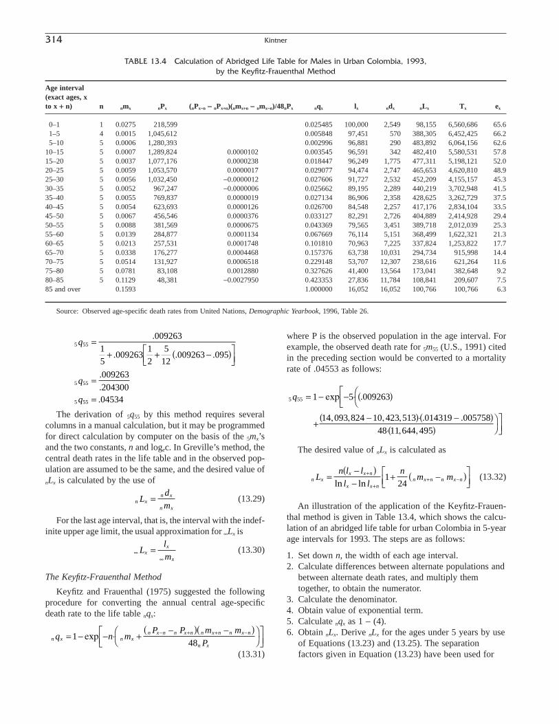
314 Kintner
The derivation of 5q55 by this method requires severalcolumns in a manual calculation, but it may be programmedfor direct calculation by computer on the basis of the 5mx’sand the two constants, n and logec. In Greville’s method, thecentral death rates in the life table and in the observed pop-ulation are assumed to be the same, and the desired value ofnLx is calculated by the use of
(13.29)
For the last age interval, that is, the interval with the indef-inite upper age limit, the usual approximation for •Lx is
(13.30)
The Keyfitz-Frauenthal Method
Keyfitz and Frauenthal (1975) suggested the followingprocedure for converting the annual central age-specificdeath rate to the life table nqx:
(13.31)
n x n xn x n n x n n x n n x n
n x
q n mP P m m
P= - - ◊ +
-( ) -( )ÊË
ˆ¯
ÈÎÍ
˘˚̇
- + + -148
exp
••
=Ll
mx
x
x
n xn x
n x
Ld
m=
5 55
5 55
5 55
00926315
00926312
512
009263 095
00926320430004534
q
q
q
=+ + -( )È
Î͢˚̇
=
=
.
. . .
.
..
where P is the observed population in the age interval. Forexample, the observed death rate for 5m55 (U.S., 1991) citedin the preceding section would be converted to a mortalityrate of .04553 as follows:
The desired value of nLx is calculated as
(13.32)
An illustration of the application of the Keyfitz-Frauen-thal method is given in Table 13.4, which shows the calcu-lation of an abridged life table for urban Colombia in 5-yearage intervals for 1993. The steps are as follows:
1. Set down n, the width of each age interval.2. Calculate differences between alternate populations and
between alternate death rates, and multiply themtogether, to obtain the numerator.
3. Calculate the denominator.4. Obtain value of exponential term.5. Calculate nqx as 1 - (4).6. Obtain nLx. Derive nLx for the ages under 5 years by use
of Equations (13.23) and (13.25). The separationfactors given in Equation (13.23) have been used for
n xx x n
x x nn x n n x nL
n l l
l l
nm m=
-( )-
+ -( )ÈÎÍ
˘˚̇
+
++ -ln ln
124
5 55 1 5 009263
14 093 824 10 423 513 014319 00575848 11 644 495
q = - - ◊ ( )ÊË
ÈÎÍ
+-( )◊ -( )
◊( )ˆ¯
˘˚̇
exp .
, , , , . ., ,
TABLE 13.4 Calculation of Abridged Life Table for Males in Urban Colombia, 1993, by the Keyfitz-Frauenthal Method
Age interval(exact ages, xto x + n) n nmx nPx (nPx-n - nPx+n)(nmx+n - nmx-n)/48nPx nqx lx ndx nLx Tx ex
0–1 1 0.0275 218,599 0.025485 100,000 2,549 98,155 6,560,686 65.61–5 4 0.0015 1,045,612 0.005848 97,451 570 388,305 6,452,425 66.25–10 5 0.0006 1,280,393 0.002996 96,881 290 483,892 6,064,156 62.6
10–15 5 0.0007 1,289,824 0.0000102 0.003545 96,591 342 482,410 5,580,531 57.815–20 5 0.0037 1,077,176 0.0000238 0.018447 96,249 1,775 477,311 5,198,121 52.020–25 5 0.0059 1,053,570 0.0000017 0.029077 94,474 2,747 465,653 4,620,810 48.925–30 5 0.0056 1,032,450 -0.0000012 0.027606 91,727 2,532 452,209 4,155,157 45.330–35 5 0.0052 967,247 -0.0000006 0.025662 89,195 2,289 440,219 3,702,948 41.535–40 5 0.0055 769,837 0.0000019 0.027134 86,906 2,358 428,625 3,262,729 37.540–45 5 0.0054 623,693 0.0000126 0.026700 84,548 2,257 417,176 2,834,104 33.545–50 5 0.0067 456,546 0.0000376 0.033127 82,291 2,726 404,889 2,414,928 29.450–55 5 0.0088 381,569 0.0000675 0.043369 79,565 3,451 389,718 2,012,039 25.355–60 5 0.0139 284,877 0.0001134 0.067669 76,114 5,151 368,499 1,622,321 21.360–65 5 0.0213 257,531 0.0001748 0.101810 70,963 7,225 337,824 1,253,822 17.765–70 5 0.0338 176,277 0.0004468 0.157376 63,738 10,031 294,734 915,998 14.470–75 5 0.0514 131,927 0.0006518 0.229148 53,707 12,307 238,616 621,264 11.675–80 5 0.0781 83,108 0.0012880 0.327626 41,400 13,564 173,041 382,648 9.280–85 5 0.1129 48,381 -0.0027950 0.423353 27,836 11,784 108,841 209,607 7.585 and over 0.1593 1.000000 16,052 16,052 100,766 100,766 6.3
Source: Observed age-specific death rates from United Nations, Demographic Yearbook, 1996, Table 26.
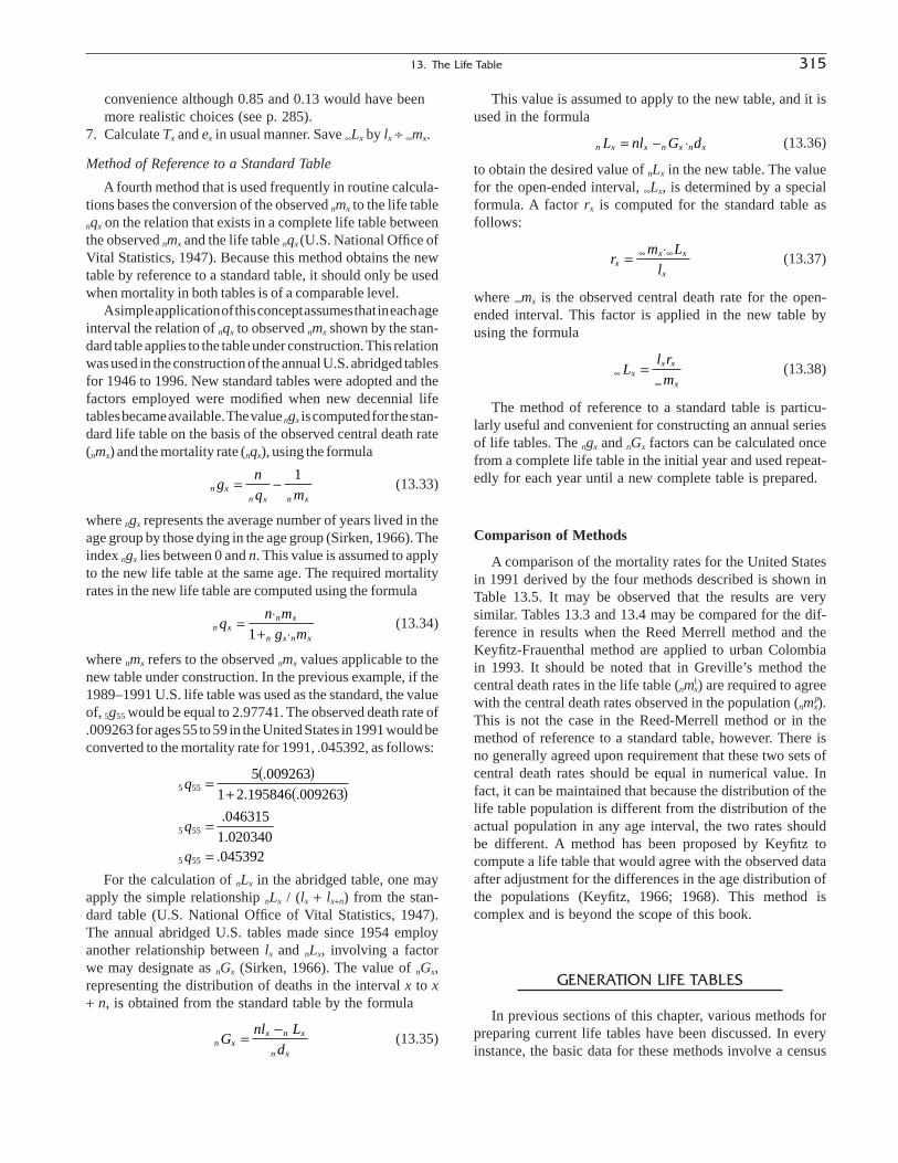
This value is assumed to apply to the new table, and it isused in the formula
(13.36)
to obtain the desired value of nLx in the new table. The valuefor the open-ended interval, •Lx, is determined by a specialformula. A factor rx is computed for the standard table asfollows:
(13.37)
where •mx is the observed central death rate for the open-ended interval. This factor is applied in the new table byusing the formula
(13.38)
The method of reference to a standard table is particu-larly useful and convenient for constructing an annual seriesof life tables. The ngx and nGx factors can be calculated oncefrom a complete life table in the initial year and used repeat-edly for each year until a new complete table is prepared.
Comparison of Methods
A comparison of the mortality rates for the United Statesin 1991 derived by the four methods described is shown inTable 13.5. It may be observed that the results are verysimilar. Tables 13.3 and 13.4 may be compared for the dif-ference in results when the Reed Merrell method and theKeyfitz-Frauenthal method are applied to urban Colombiain 1993. It should be noted that in Greville’s method thecentral death rates in the life table (nml
x) are required to agreewith the central death rates observed in the population (nmp
x).This is not the case in the Reed-Merrell method or in themethod of reference to a standard table, however. There isno generally agreed upon requirement that these two sets ofcentral death rates should be equal in numerical value. Infact, it can be maintained that because the distribution of thelife table population is different from the distribution of theactual population in any age interval, the two rates shouldbe different. A method has been proposed by Keyfitz tocompute a life table that would agree with the observed dataafter adjustment for the differences in the age distribution ofthe populations (Keyfitz, 1966; 1968). This method iscomplex and is beyond the scope of this book.
GENERATION LIFE TABLES
In previous sections of this chapter, various methods forpreparing current life tables have been discussed. In everyinstance, the basic data for these methods involve a census
••
=Ll r
mx
x x
x
rm L
lx
x x
x
=◊• •
n x x n x n xL nl G d= - ◊
13. The Life Table 315
convenience although 0.85 and 0.13 would have beenmore realistic choices (see p. 285).
7. Calculate Tx and ex in usual manner. Save •Lx by lx ∏ •mx.
Method of Reference to a Standard Table
A fourth method that is used frequently in routine calcula-tions bases the conversion of the observed nmx to the life tablenqx on the relation that exists in a complete life table betweenthe observed nmx and the life table nqx (U.S. National Office ofVital Statistics, 1947). Because this method obtains the newtable by reference to a standard table, it should only be usedwhen mortality in both tables is of a comparable level.
Asimple application of this concept assumes that in each ageinterval the relation of nqx to observed nmx shown by the stan-dard table applies to the table under construction. This relationwas used in the construction of the annual U.S. abridged tablesfor 1946 to 1996. New standard tables were adopted and thefactors employed were modified when new decennial lifetables became available. The value ngx is computed for the stan-dard life table on the basis of the observed central death rate(nmx) and the mortality rate (nqx), using the formula
(13.33)
where ngx represents the average number of years lived in theage group by those dying in the age group (Sirken, 1966). Theindex ngx lies between 0 and n. This value is assumed to applyto the new life table at the same age. The required mortalityrates in the new life table are computed using the formula
(13.34)
where nmx refers to the observed nmx values applicable to thenew table under construction. In the previous example, if the1989–1991 U.S. life table was used as the standard, the valueof, 5g55 would be equal to 2.97741. The observed death rate of.009263 for ages 55 to 59 in the United States in 1991 would beconverted to the mortality rate for 1991, .045392, as follows:
For the calculation of nLx in the abridged table, one mayapply the simple relationship nLx / (lx + lx+n) from the stan-dard table (U.S. National Office of Vital Statistics, 1947).The annual abridged U.S. tables made since 1954 employanother relationship between lx and nLx, involving a factorwe may designate as nGx (Sirken, 1966). The value of nGx,representing the distribution of deaths in the interval x to x+ n, is obtained from the standard table by the formula
(13.35)n xx n x
n x
Gnl L
d=
-
5 55
5 55
5 55
5 0092631 2 195846 009263
0463151 020340045392
q
q
q
=( )
+ ( )
=
=
.. .
..
.
n xn x
n x n x
qn m
g m=
◊+ ◊1
n xn x n x
gn
q m= -
1

316 Kintner
of the population (or accurate estimates of the populationdistributed by age and sex), the deaths recorded in the yearof the census or in a number of years around the census year,and the births in a few years just prior to the census year.Life tables prepared from these data portray the mortalityexperience of the population observed during the relativelyshort period to which the data on deaths apply.
Because life tables are mathematical models that trace acohort of lives from birth to death according to an assumedseries of mortality rates, it would be logical to try to basethe life table on the mortality rates experienced by an actualbirth cohort. For this purpose, it is necessary to have col-lected data on an annual basis for many years before a lifetable could be prepared. For example, a generation life tablefor the birth cohort of 1900 would employ the observeddeath or mortality rates for infancy in 1900, for age 1 in1901, for age 2 in 1902, and so on until the latest availablerates at the highest ages are obtained; the remaining rateswould have to be obtained by projection. Table 13.6 pres-ents selected values from a generation life table for thecohort of white females born in 1900 in the United States,prepared by Bell, Wade, and Goss (1992).
A sufficient period of time has elapsed since mortalitydata have been systematically recorded for a number of generation life tables to have been prepared. For example,Jacobson (1964) prepared life tables for white males andfemales born in the United States in 1840 and every 10th year
thereafter through 1960, on the basis of the mortality ratesexperienced in each year of the life of these cohorts and pro-jected mortality rates. Earlier, Dublin and Spiegelman(1941), Dublin, Lotka, and Spiegelman (1949), and Spiegel-man (1957) developed or described such tables. Generationlife tables can be used to compute generation reproductionrates, to study life expectancy historically, to project mortal-ity, and to make estimates of orphanhood (Gregory, 1965).A series of such tables could represent the development ofmortality and life expectancy of real cohorts over time andimprove the basis for analyzing the relation between theearlier mortality of a cohort and its later experience. In viewof the general tendency for mortality to fall, the expectationof life at birth in a generation life table tends to be higher thanin the current table for the starting year of the generation lifetable. A comparison of life expectations at birth in two suchtables reflects the average improvement in mortality for theactual cohort over its lifetime. Conversely, current life tablestypically understate the probable life expectancy to beobserved in the future for persons at a given age becausemortality is expected to continue declining. The generationlife table for the cohort of U.S females born in 1900, forexample, shows a life expectation at birth of 58.3 years (Bellet al., 1992). In contrast, the current life table for 1900 showsa life expectation at birth of 49.0 years. The actual experienceof the 1900 cohort added nearly 10 years to its life expecta-tion at birth.
TABLE 13.5 Comparison of Mortality Rates for the Total United States Population, 1991, Com-puted by Four Different Abridged Life Table Methods
Age intervalComputed nqx
(exact ages, ngx nmx Reference tox to x + n) Standard1 Observed2 Reed- Merrell Greville standard table Keyfitz-Frauenthal
1–5 422.203800 0.000474 0.001856 0.001894 0.0019755–10 -103.093000 0.000215 0.001074 0.001074 0.001099
10–15 -45.045000 0.000258 0.001289 0.001289 0.001305 0.00129315–20 8.575279 0.000890 0.004441 0.004441 0.004416 0.00443220–25 3.345601 0.001101 0.005491 0.005491 0.005485 0.00548325–30 4.249223 0.001230 0.006133 0.006133 0.006118 0.00612530–35 -1.625560 0.001541 0.007678 0.007678 0.007724 0.00767635–40 0.308471 0.001977 0.009840 0.009840 0.009879 0.00985340–45 3.585178 0.002536 0.012606 0.012606 0.012566 0.01266445–50 1.963739 0.003805 0.018859 0.018859 0.018884 0.01901150–55 2.246376 0.005758 0.028412 0.028411 0.028422 0.02855455–60 2.195846 0.009263 0.045341 0.045340 0.045392 0.04552760–65 2.278723 0.014319 0.069283 0.069282 0.069333 0.06913565–70 2.294695 0.021368 0.101741 0.101739 0.101846 0.10171770–75 2.352904 0.032051 0.148948 0.148946 0.149017 0.14915375–80 2.421006 0.048068 0.215454 0.215461 0.215286 0.21603480–85 2.497600 0.075754 0.319215 0.319274 0.318507 0.320953
1 Computed from the life table for the United States, 1981, total population, which is used as the standard table. The ngx factors at ages below 50 seemirregular and would be expected to approximate 2.5. However, where death rates are low, the computed nqx is relatively insensitive to large variations in ngx.
2 Ratio of deaths to population observed in the United States in 1991.
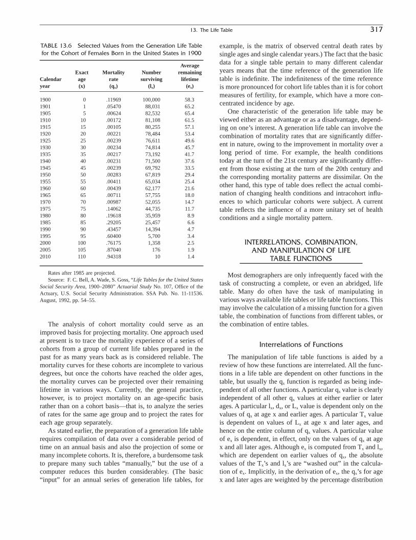
example, is the matrix of observed central death rates bysingle ages and single calendar years.) The fact that the basicdata for a single table pertain to many different calendaryears means that the time reference of the generation lifetable is indefinite. The indefiniteness of the time referenceis more pronounced for cohort life tables than it is for cohortmeasures of fertility, for example, which have a more con-centrated incidence by age.
One characteristic of the generation life table may beviewed either as an advantage or as a disadvantage, depend-ing on one’s interest. A generation life table can involve thecombination of mortality rates that are significantly differ-ent in nature, owing to the improvement in mortality over along period of time. For example, the health conditionstoday at the turn of the 21st century are significantly differ-ent from those existing at the turn of the 20th century andthe corresponding mortality patterns are dissimilar. On theother hand, this type of table does reflect the actual combi-nation of changing health conditions and intracohort influ-ences to which particular cohorts were subject. A currenttable reflects the influence of a more unitary set of healthconditions and a single mortality pattern.
INTERRELATIONS, COMBINATION,AND MANIPULATION OF LIFE
TABLE FUNCTIONS
Most demographers are only infrequently faced with thetask of constructing a complete, or even an abridged, lifetable. Many do often have the task of manipulating invarious ways available life tables or life table functions. Thismay involve the calculation of a missing function for a giventable, the combination of functions from different tables, orthe combination of entire tables.
Interrelations of Functions
The manipulation of life table functions is aided by areview of how these functions are interrelated. All the func-tions in a life table are dependent on other functions in thetable, but usually the qx function is regarded as being inde-pendent of all other functions. A particular qx value is clearlyindependent of all other qx values at either earlier or laterages. A particular lx, dx, or Lx value is dependent only on thevalues of qx at age x and earlier ages. A particular Tx valueis dependent on values of Lx at age x and later ages, andhence on the entire column of qx values. A particular valueof ex is dependent, in effect, only on the values of qx at agex and all later ages. Although ex is computed from Tx and lx,which are dependent on earlier values of qx, the absolutevalues of the Tx’s and lx’s are “washed out” in the calcula-tion of ex. Implicitly, in the derivation of ex, the qx’s for agex and later ages are weighted by the percentage distribution
13. The Life Table 317
The analysis of cohort mortality could serve as animproved basis for projecting mortality. One approach usedat present is to trace the mortality experience of a series ofcohorts from a group of current life tables prepared in thepast for as many years back as is considered reliable. Themortality curves for these cohorts are incomplete to variousdegrees, but once the cohorts have reached the older ages,the mortality curves can be projected over their remaininglifetime in various ways. Currently, the general practice,however, is to project mortality on an age-specific basisrather than on a cohort basis—that is, to analyze the seriesof rates for the same age group and to project the rates foreach age group separately.
As stated earlier, the preparation of a generation life tablerequires compilation of data over a considerable period oftime on an annual basis and also the projection of some ormany incomplete cohorts. It is, therefore, a burdensome taskto prepare many such tables “manually,” but the use of acomputer reduces this burden considerabley. (The basic“input” for an annual series of generation life tables, for
TABLE 13.6 Selected Values from the Generation Life Tablefor the Cohort of Females Born in the United States in 1900
Average Exact Mortality Number remaining
Calendar age rate surviving lifetime year (x) (qx) (lx) (ex)
1900 0 .11969 100,000 58.31901 1 .05470 88,031 65.21905 5 .00624 82,532 65.41910 10 .00172 81,108 61.51915 15 .00105 80,255 57.11920 20 .00221 78,484 53.41925 25 .00239 76,611 49.61930 30 .00234 74,814 45.71935 35 .00217 73,192 41.71940 40 .00231 71,500 37.61945 45 .00239 69,792 33.51950 50 .00283 67,819 29.41955 55 .00411 65,034 25.41960 60 .00439 62,177 21.61965 65 .00711 57,755 18.01970 70 .00987 52,055 14.71975 75 .14062 44,735 11.71980 80 .19618 35,959 8.91985 85 .29205 25,457 6.61990 90 .43457 14,394 4.71995 95 .60400 5,700 3.42000 100 .76175 1,358 2.52005 105 .87040 176 1.92010 110 .94318 10 1.4
Rates after 1985 are projected.Source: F. C. Bell, A. Wade, S. Goss, “Life Tables for the United States
Social Security Area, 1900–2080” Actuarial Study No. 107, Office of theActuary, U.S. Social Security Administration. SSA Pub. No. 11-11536.August, 1992, pp. 54–55.

of the L’s that they generate. Because of the sharp drop fromq0 to q1, e1 is commonly higher than e0; thereafter, ex tendsto fall steadily. At low levels of q0, e0 begins to exceed e1.
In some cases, values are presented for only some of thelife table functions. Some or all of the others may be desired.Let us consider the case where, as in the UN DemographicYearbook, we are given 1-year values of qx, lx, and ex at everyfifth age and we want 5Lx values for computing 5-year sur-vival rates (ratios of 5Lx’s; see later). We apply the follow-ing relationships:
The 5qx’s corresponding to the lx values at every fifth age
are calculated by and the 5dx’s corresponding to the
lx values are calculated by lx - lx+5.Given the same basic information as just noted, we may
wish to secure the values for the individual ages of somefunction. In that case, any of the standard interpolation for-mulas may be applied. We may interpolate qx or lx to singleages and obtain single values of dx as a by-product. Or wemay derive Tx at every fifth age as described in the preced-ing paragraph and then apply one of the interpolation for-mulas to secure Tx at single ages. Single values for ex maybe secured by direct interpolation or by interpolating the lx
function to single ages and completing the table. (Interpola-tion procedures are discussed more fully in Appendix C.)
Combination of Tables and Functions
First, let us consider the case where life tables for twopopulations are available and we should like to have a singlelife table for the combined population. Suppose, forexample, we want to derive a single table for the generalpopulation from separate life tables for the male and femalepopulations. This can be done by weighting the qx’s fromthe male and female tables in accordance with the distribu-tion of the population by sex at each age. A new table maynow be recomputed from the combined qx’s and an assumedradix of 100,000. If only one of the other functions iswanted, the values from the separate tables may be com-bined on the basis of population weights in only a few scat-tered ages because the shifts from age to age in thedistribution of the population by sex could introduce unac-ceptable fluctuations by age in these functions for the com-bined population, and the resulting values for differentfunctions may not be consistent with one another. (Note thatthese functions would not all receive the same populationweights, e.g., lx would be weighted by the population at agex, and Tx and ex would be weighted by the population for
1 5- +l
lx
x
eT
l
T e l
L T T
xx
x
x x x
x x x
=
\ == - +and 5 5
ages x and over, the weights in each case reflecting the agescovered by the measure.) Only the use of a constant weight-ing factor over all ages can prevent fluctuations by age inthe values of a function. If an entire column for a functionis wanted, therefore, it is best to recompute the values forthe function by starting with the weighted qx’s.
A different problem is represented by the need for sepa-rate male and female life tables whose values bear a realis-tic absolute relation to one another. The tables for males andfemales as originally computed do not bear a consistent“additive” relationship to one another because births of boysand girls do not occur in equal numbers, as is implied by theradixes of the separate life tables for males and females. Tomake the tables additive, it is necessary to inflate the lx, dx,Lx, and Tx values of the male life table by the sex ratio atbirth in the actual population. Thus, the stationary male population at each age adjusted for absolute comparabilitywith the female stationary population is derived by
(13.39)
and the stationary male population of all ages, adjusted forcombination with the total female stationary population, isobtained by
(13.40)
The birthrate (and also the death rate) for the male andfemale life tables taken in combination is given by
(13.41)
The ratio of children under 5 to women of childbearingage in the stationary population, a measure known as thereplacement quota, is obtained by
(13.42)
We have been describing the procedures by which wemay arrive at life table values for a total population consis-tent in absolute level with the life table values for the sepa-rate component male and female populations. Even if thestationary populations are properly combined and reducedto the level of a single table with a radix of 100,000 byapplying the factor
(13.43)100 000
100 000 100 000
,
, ,B
B
m
f+
B
BL L
L
m
fm f
f
◊ +- -
-
0 4 0 4
15 49
B
Bl l
B
BT T
m
f
m
fm f
0 0
0 0
+
+
B
BT
m
fm◊ 0
B
BL
m
f xm◊
318 Kintner
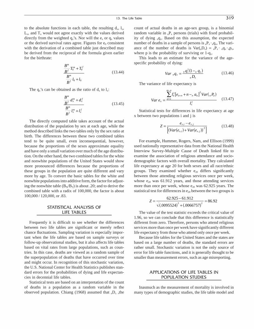
to the absolute functions in each table, the resulting dx, lx,Lx, and Tx would not agree exactly with the values deriveddirectly from the weighted qx’s. Nor will the ex or qx valuesor the derived survival rates agree. Figures for e0 consistentwith the derivation of a combined table just described maybe derived from the reciprocal of the formula given earlierfor the birthrate:
(13.44)
The qx’s can be obtained as the ratio of dx to lx:
(13.45)
The directly computed table takes account of the actualdistribution of the population by sex at each age, while themethod described links the two tables only by the sex ratio atbirth. The differences between these two combined tablestend to be quite small, even inconsequential, however,because the proportions of the sexes approximate equalityand have only a small variation over much of the age distribu-tion. On the other hand, the two combined tables for the whiteand nonwhite populations of the United States would showmore pronounced differences because the proportions ofthese groups in the population are quite different and varymore by age. To convert the basic tables for the white andnonwhite populations into additive form, the factor for adjust-ing the nonwhite table (BN/BT) is about .20; and to derive thecombined table with a radix of 100,000, the factor is about100,000 / 120,000, or .83.
STATISTICAL ANALYSIS OF LIFE TABLES
Frequently it is difficult to see whether the differencesbetween two life tables are significant or merely reflectchance fluctuations. Sampling variation is especially impor-tant when the life tables are based on sample surveys orfollow-up observational studies, but it also affects life tablesbased on vital rates from large populations, such as coun-tries. In this case, deaths are viewed as a random sample ofthe superpopulation of deaths that have occurred over timeand might occur. In recognition of this stochastic variation,the U.S. National Center for Health Statistics publishes stan-dard errors for the probabilities of dying and life expectan-cies in decennial life tables.
Statistical tests are based on an interpretation of the countof deaths in a population as a random variable in theobserved population. Chiang (1968) assumed that nDx ,the
B
Bd d
B
Bl l
m
f xm
xf
m
f xm
xf
+
+
B
BT T
B
Bl l
m
fm f
m
f
0 0
0 0
+
+
count of actual deaths in an age-sex group, is a binomialrandom variable in nPx persons (trials) with fixed probabil-ity of dying nqx. Based on this assumption, the expectednumber of deaths in a sample of persons is nPx · nqx, The vari-ance of the number of deaths is Var(nDx) = nPx · nqx · npx,where p is the probability of surviving or 1-qx.
This leads to an estimate for the variance of the age-specific probability of dying:
(13.46)
The variance of life expectancy is
(13.47)
Statistical tests for differences in life expectancy at agex between two populations i and j is
(13.48)
For example, Hummer, Rogers, Nam, and Ellison (1999)used nationally representative data from the National HealthInterview Survey-Multiple Cause of Death linked file toexamine the association of religious attendance and socio-demographic factors with overall mortality. They calculatedlife expectancy at age 20 for both sexes and all race/ethnicgroups. They examined whether e20 differs significantlybetween those attending religious services once per week,whose e20 was 61.912 years, and those attending servicesmore than once per week, whose e20 was 62.925 years. Thestatistical test for differences in e20 between the two groups is
The value of the test statistic exceeds the critical value of1.96, so we can conclude that this difference is statisticallydifferent from zero. Therefore, persons who attend religiousservices more than once per week have significantly differentlife expectancy from those who attend only once per week.
Because life tables for the United States and the states arebased on a large number of deaths, the standard errors arerather small. Stochastic variation is not the only source oferror for life table functions, and it is generally thought to besmaller than measurement errors, such as age misreporting.
APPLICATIONS OF LIFE TABLES INPOPULATION STUDIES
Inasmuch as the measurement of mortality is involved inmany types of demographic studies, the life table model and
Z =-
( ) + ( )=
62 925 61 912
0095524 006675786 92
2 2
. .
. ..
Ze e
Var e Var e
x i x j
x i x j
=-
( ) + ( )( )[ ], ,
, ,.5
Var el e n a Var P
lx
a a n n a n aa x
n
x
=+ -[ ] ( )+
=
-
 2 2
2
w
Var qq q
Dn x
n x n x
n x
=-( )2 1
13. The Life Table 319
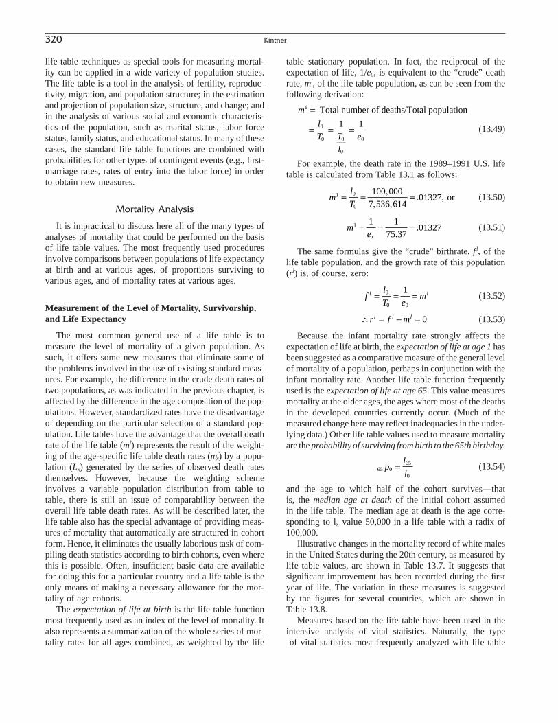
life table techniques as special tools for measuring mortal-ity can be applied in a wide variety of population studies.The life table is a tool in the analysis of fertility, reproduc-tivity, migration, and population structure; in the estimationand projection of population size, structure, and change; andin the analysis of various social and economic characteris-tics of the population, such as marital status, labor forcestatus, family status, and educational status. In many of thesecases, the standard life table functions are combined withprobabilities for other types of contingent events (e.g., first-marriage rates, rates of entry into the labor force) in orderto obtain new measures.
Mortality Analysis
It is impractical to discuss here all of the many types ofanalyses of mortality that could be performed on the basisof life table values. The most frequently used proceduresinvolve comparisons between populations of life expectancyat birth and at various ages, of proportions surviving tovarious ages, and of mortality rates at various ages.
Measurement of the Level of Mortality, Survivorship,and Life Expectancy
The most common general use of a life table is tomeasure the level of mortality of a given population. Assuch, it offers some new measures that eliminate some ofthe problems involved in the use of existing standard meas-ures. For example, the difference in the crude death rates oftwo populations, as was indicated in the previous chapter, isaffected by the difference in the age composition of the pop-ulations. However, standardized rates have the disadvantageof depending on the particular selection of a standard pop-ulation. Life tables have the advantage that the overall deathrate of the life table (ml) represents the result of the weight-ing of the age-specific life table death rates (ml
x) by a popu-lation (Lx) generated by the series of observed death ratesthemselves. However, because the weighting schemeinvolves a variable population distribution from table totable, there is still an issue of comparability between theoverall life table death rates. As will be described later, thelife table also has the special advantage of providing meas-ures of mortality that automatically are structured in cohortform. Hence, it eliminates the usually laborious task of com-piling death statistics according to birth cohorts, even wherethis is possible. Often, insufficient basic data are availablefor doing this for a particular country and a life table is theonly means of making a necessary allowance for the mor-tality of age cohorts.
The expectation of life at birth is the life table functionmost frequently used as an index of the level of mortality. Italso represents a summarization of the whole series of mor-tality rates for all ages combined, as weighted by the life
table stationary population. In fact, the reciprocal of theexpectation of life, 1/e0, is equivalent to the “crude” deathrate, ml, of the life table population, as can be seen from thefollowing derivation:
(13.49)
For example, the death rate in the 1989–1991 U.S. lifetable is calculated from Table 13.1 as follows:
(13.50)
(13.51)
The same formulas give the “crude” birthrate, f l, of thelife table population, and the growth rate of this population(rl) is, of course, zero:
(13.52)
(13.53)
Because the infant mortality rate strongly affects theexpectation of life at birth, the expectation of life at age 1 hasbeen suggested as a comparative measure of the general levelof mortality of a population, perhaps in conjunction with theinfant mortality rate. Another life table function frequentlyused is the expectation of life at age 65. This value measuresmortality at the older ages, the ages where most of the deathsin the developed countries currently occur. (Much of themeasured change here may reflect inadequacies in the under-lying data.) Other life table values used to measure mortalityare the probability of surviving from birth to the 65th birthday.
(13.54)
and the age to which half of the cohort survives—that is, the median age at death of the initial cohort assumed in the life table. The median age at death is the age corre-sponding to lx value 50,000 in a life table with a radix of100,000.
Illustrative changes in the mortality record of white malesin the United States during the 20th century, as measured bylife table values, are shown in Table 13.7. It suggests thatsignificant improvement has been recorded during the firstyear of life. The variation in these measures is suggested by the figures for several countries, which are shown inTable 13.8.
Measures based on the life table have been used in theintensive analysis of vital statistics. Naturally, the typeof vital statistics most frequently analyzed with life table
65 065
0
pl
l=
\ = - =r f ml l l 0
fl
T eml l= = =0
0 0
1
mex
1 1 175 37
01327= = =.
.
ml
T1 0
0
100 0007 536 614
01327= = =,
, ,. , or
m
l
T Tl
e
1
0
0 0
0
0
1 1
=
= = =
Total number of deaths/Total population
320 Kintner

13. The Life Table 321
measures is mortality because these measures were origi-nally designed for precisely that application, and that appli-cation is usually the simplest. The analysis of mortalitycould cover variations in time and between populationgroups by age, sex, ethnic group, race, marital status, geographic residence, and other demographic characteristicsthat may be regarded as being associated with the overalllevel of mortality. Table 13.9 shows, for example, the vari-
ation in time, by age, of the relative mortality of white malesand females in the United States in terms of life table mor-tality rates. Although mortality of white males has improvedtremendously during the 20th century in the United States(Table 13.7), the improvement has been greater for whitefemales (Table 13.9).
Model life tables may be used to evaluate the quality ofmortality data for statistically underdeveloped populationsand to establish the validity of recorded differences in thepatterns of mortality of these populations. The mortality data
TABLE 13.7 Change in the Mortality of White Males in the United States According to VariousLife Table Measures: 1900 to 1996 [Life tables for periods before 1929–31 relate to the Death
Registration States]
Probability of Median age atExpectation of Expectation of Expectation of surviving from death of initial
Period life at birth life at age 1 life at age 65 birth to age 65 cohort
1900–02 48.23 54.61 11.51 .392 57.21909–11 50.23 56.26 11.25 .409 59.31919–21 56.34 60.24 12.21 .507 65.41929–31 59.12 62.04 11.77 .530 66.41939–41 62.81 64.98 12.07 .583 68.71949–51 66.31 67.41 12.75 .635 70.71959–61 67.55 68.34 12.97 .658 71.41969–71 67.94 68.33 13.02 .663 71.51979–81 70.82 70.70 14.26 .724 74.21989–91 72.72 72.35 15.24 .760 76.11996 73.90 73.40 15.80 .779 77.2
Increase, 1900–2 to 1996 25.67 18.79 4.29 .387 20.0Increase, 1949–51 to 1996 7.59 5.99 3.05 .144 6.5
Source: Various official United States life tables.
TABLE 13.8 Mortality of Females According to Various LifeTable Measures, for Selected Countries: Around 1990
Probability Median ageof surviving at death
Country Expectation of life at-
from birth of initial and year Birth Age 1 Age 65 to age 65 cohort
Argentina, 75.59 76.30 17.26 .826 80.31990–2
Bangladesh, 1988 55.97 61.50 11.98 .566 68.6Canada, 1992 80.89 80.36 19.88 .886 83.8China, 1990 70.49 71.92 14.74 .756 75.8Egypt, 1991 66.39 58.65 12.87 .702 72.6India, 1986–90 58.90 62.60 12.90 .572 68.6Japan, 1994 82.98 82.29 20.97 .919 >85Moldova, 1994 69.79 70.18 13.19 .717 73.6Peru, 1990–95 66.55 70.65 14.59 .727 77.3Philippines, 1991 66.70 68.70 13.70 .692 73.6Russian 71.18 71.29 14.58 .741 75.4
Federation,1994
Zimbabwe, 1990 62.00 65.10 13.30 .613 70.7
Source: United Nations Demographic Yearbook, 1996, Tables 32 and33.
TABLE 13.9 Mortality Rate of White Females as Percent ofthe Mortality Rates of White Males in the United States for
Selected Ages, as shown by various life tables: 1900 to1996 [Life tables for periods before 1929–31 relate to the
Death Registration States]
Exact age
Period 0 1 10 20 30 40 50 60 70 80
1900–02 83 90 90 93 97 88 87 88 91 911909–11 83 92 87 86 91 79 81 84 91 931919–21 80 90 85 101 105 90 91 88 92 951929–31 80 89 77 87 91 78 75 78 84 901939–41 79 89 70 68 79 72 66 67 78 871949–51 77 89 67 45 63 62 55 56 68 821959–61 76 88 67 35 54 57 50 48 58 771969–71 76 87 73 34 49 57 52 45 51 681979–81 78 84 89 32 39 55 53 50 50 611989–91 77 89 88 36 35 45 57 56 56 611996 82 77 66 33 41 49 59 60 63 72
Note: Ratios of qx per 100.Source: Various official United States life tables.
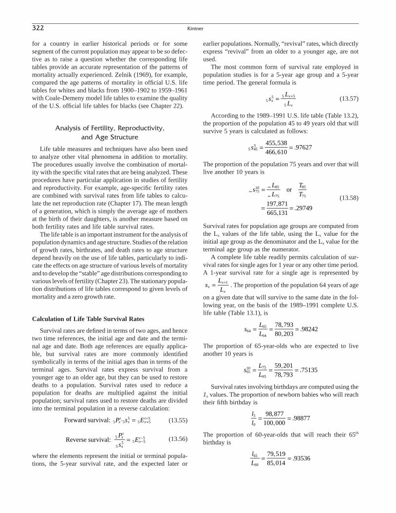
322 Kintner
for a country in earlier historical periods or for somesegment of the current population may appear to be so defec-tive as to raise a question whether the corresponding lifetables provide an accurate representation of the patterns ofmortality actually experienced. Zelnik (1969), for example,compared the age patterns of mortality in official U.S. lifetables for whites and blacks from 1900–1902 to 1959–1961with Coale-Demeny model life tables to examine the qualityof the U.S. official life tables for blacks (see Chapter 22).
Analysis of Fertility, Reproductivity, and Age Structure
Life table measures and techniques have also been usedto analyze other vital phenomena in addition to mortality.The procedures usually involve the combination of mortal-ity with the specific vital rates that are being analyzed. Theseprocedures have particular application in studies of fertilityand reproductivity. For example, age-specific fertility ratesare combined with survival rates from life tables to calcu-late the net reproduction rate (Chapter 17). The mean lengthof a generation, which is simply the average age of mothersat the birth of their daughters, is another measure based onboth fertility rates and life table survival rates.
The life table is an important instrument for the analysis ofpopulation dynamics and age structure. Studies of the relationof growth rates, birthrates, and death rates to age structuredepend heavily on the use of life tables, particularly to indi-cate the effects on age structure of various levels of mortalityand to develop the “stable” age distributions corresponding tovarious levels of fertility (Chapter 23). The stationary popula-tion distributions of life tables correspond to given levels ofmortality and a zero growth rate.
Calculation of Life Table Survival Rates
Survival rates are defined in terms of two ages, and hencetwo time references, the initial age and date and the termi-nal age and date. Both age references are equally applica-ble, but survival rates are more commonly identifiedsymbolically in terms of the initial ages than in terms of theterminal ages. Survival rates express survival from ayounger age to an older age, but they can be used to restoredeaths to a population. Survival rates used to reduce a population for deaths are multiplied against the initial population; survival rates used to restore deaths are dividedinto the terminal population in a reverse calculation:
(13.55)
(13.56)
where the elements represent the initial or terminal popula-tions, the 5-year survival rate, and the expected later or
Reverse survival: 5 P
sEx
t
xxt
55 5 5
5= --
Forward survival: 5 55
5 55P s Ex
tx x
t◊ = ++
earlier populations. Normally, “revival” rates, which directlyexpress “revival” from an older to a younger age, are notused.
The most common form of survival rate employed inpopulation studies is for a 5-year age group and a 5-yeartime period. The general formula is
(13.57)
According to the 1989–1991 U.S. life table (Table 13.2),the proportion of the population 45 to 49 years old that willsurvive 5 years is calculated as follows:
The proportion of the population 75 years and over that willlive another 10 years is
(13.58)
Survival rates for population age groups are computed fromthe Lx values of the life table, using the Lx value for theinitial age group as the denominator and the Lx value for theterminal age group as the numerator.
A complete life table readily permits calculation of sur-vival rates for single ages for 1 year or any other time period. A 1-year survival rate for a single age is represented by
. The proportion of the population 64 years of age
on a given date that will survive to the same date in the fol-lowing year, on the basis of the 1989–1991 complete U.S.life table (Table 13.1), is
The proportion of 65-year-olds who are expected to liveanother 10 years is
Survival rates involving birthdays are computed using the1x values. The proportion of newborn babies who will reachtheir fifth birthday is
The proportion of 60-year-olds that will reach their 65th
birthday is
l
L65
60
79 51985 014
93536= =,,
.
l
l5
0
98 877100 000
98877= =,,
.
sL
L6510 75
65
59 20178 793
75135= = =,,
.
sL
L64
65
64
78 79380 203
98242= = =,,
.
sL
Lx
x
x
= +1
••
•=
= =
sL
L
T
T7510 85
75
85
75
197 871665 131
29749
or
,,
.
5 455 455 538
466 61097627s = =
,,
.
55 5 5
5
sL
Lx
x
x
= +

13. The Life Table 323
The proportion of infants born in a year who will survive tothe end of that year (when the cohort is under 1 year of age) is
while the proportion of the newborn infants who will reachtheir first birthday is
If survival from birth to a given age interval is wanted,
then the survival rate is or, for a 5-year age group,
. Here n, or 5, cohorts of 100,000 births are at risk.
For survival from birth to age interval 30 to 34, we have
Survival rates involving 5-year age groups may also becomputed using values of Lx or lx for the midpoint age. Thesurvival rate from birth to age interval 30 to 34 may beapproximated by
This approximation has little effect on the survival rate, par-ticularly in the ages up through young adulthood.
Survival rates for parts of a calendar year may be calcu-lated by interpolating between the Lx’s. A 3–4-year survival ratefrom a complete life table is computed as follows (except atage under 1):
(13.59)
For age 45,
For ages under 1, life tables giving Lx values by monthsof age or other subdivisions of age under 1 should be used.Alternatively, special factors may be derived from statisticsfor infant deaths in a manner similar to the way the separa-tion factors for all infant deaths were derived.
Use of Life Table Survival Rates
In the use of life table survival rates in population studies,decisions have to be made regarding the selection of the life
14
94 00634
93 693
94 0069975
, ,
,.
( ) + ( )=
14
34 1L L
L
x x
x
+ +
l
l
L
l32 5
0
32
0
96 717100 000
96717. ,,
.= = =
483 546500 000
96709,,
.=
5
05L
lx
n xL
nl0
l
l1
0
99 064100 000
99064= =,,
.
L
l0
0
99 258100 000
99258= =,,
.
table and life table survival rates most appropriate for a par-ticular problem. Where a life table is not available for theparticular year or period, but for prior and subsequent yearsor for the initial and terminal years of the period, special survival rates may have to be computed on the basis of the available life tables. Commonly, for example, life tablesare available for the census years, but we are interested in measuring population changes or net migration for theintercensal period. Survival rates appropriate for thispurpose may be derived by (1) calculating the required sur-vival rates from each of the two tables and (2) averagingthem. This assumes that mortality changes occurred evenly over the intercensal period. We should also considerwhether they were sufficiently great to justify the additionalcalculations.
In other cases, there may be a question of adjusting ratesfor various geographic, racial, ethnic, or other socioeco-nomic categories. Differences in age-specific death rates forvarious geographic, ethnic, or socioeconomic categoriesshould be examined, when they can be computed, to deter-mine whether life table survival rates for the general popu-lation should be adjusted for these differences. For example,the convergence of state mortality for each sex-race in theUnited States group to the national level has been so pronounced over the past several decades that, for most purposes, it is not necessary to employ separate life tables for each state in making population projections forstates. National life tables for each sex-race group are adequate.
Survival rates for the general population can be adjusteddirectly for geographic or socioeconomic variations by useof observed central death rates for the various categories, asfollows: (1) take the complement of the general survivalrate; (2) calculate an adjustment factor for the particular geo-graphic or socioeconomic category in terms of central deathrates, (3) multiply the adjustment factor by the complementof the general survival rate, and (4) take the complement ofthe result in step 3. For example, if 5s5
x is a 5-year survivalrate for ages x to x + 4 and 5mx is a central death rate at agesx to x + 4 for the general population, we may develop sur-vival rates for the single population as follows:
(1) 1 - 5sx5 (a type of 5-year mortality rate)
(2) (5mx + 5mx+5) for the single population ∏(5mx + 5mx+5) for the general population
(3) = (1) · (2)(4) = (1) - (3)
Sometimes the evidence will not justify making this type ofadjustment in the general rates or suggest that it is unnecessory.
Migration may be a troublesome element in making acorrect estimate of deaths by means of life table survivalrates for populations that are not closed (i.e., affected bymigration). Application of survival rates to the initial popu-lation tends to understate deaths for a population with netin-migration and to overstate deaths for a population with

net out-migration. A reverse procedure for applying the sur-vival rates has the opposite effect (Chapters 18 and 19).
In many cases, official life tables are available but theyare based on seriously incomplete statistics on deaths and are not satisfactory for most uses. In these cases, and in others where life tables are not available for thecountry, one may have to decide whether to construct a life table, “borrow” a life table from another country, oremploy a model life table. Commonly, the countries thatlack life tables simply do not have adequate death statisticsfor constructing such tables. In some cases, one may con-struct a table by use of population census data and “stablepopulation techniques,” but it is more practical and conve-nient to “borrow” another country’s table or, preferably, toadopt a model table appropriate to the population understudy. The selection of a model table and use of stable pop-ulation techniques are discussed in Chapter 22 and Appendix B.
The estimates of survivors will differ depending on theage interval employed in computing the survival rates. (Weconsider this question apart from the age detail required inthe estimates of survivors.) With few exceptions, 5-year survival rates are sufficiently detailed to take account of the important variations in the estimates of survivors. Formost calculations, 10-year age intervals will be adequate,however. The use of survival rates with a given age intervalimplies that the actual population has the same distributionby age as the life table population in this interval. For thisreason, survival rates for very broad age spans should beavoided except in rough calculations. Hence, the terminalopen-ended interval should relate to a relatively limited agespan containing only a small percentage of the total popu-lation. Terminal group 65 and over is to be avoided exceptfor very “young” populations (e.g., Syria, Guatemala). Onthe other hand, for countries with relatively old populations(e.g., France, Great Britain), a terminal group of 75 and overmay be unsatisfactory.
While life table survival rates represent the ratio of lx orLx values to one another, the actual level of survival rates isaffected only by the qx’s in the age range to which the sur-vival rates apply. Hence, life table survival rates for variouspopulations may properly be combined on the basis of thepopulation distribution at these ages. For example, 5-yearsurvival rates with initial ages 40 to 44, for the white andnonwhite populations of the United States, would be com-bined on the basis of the distribution of the population inthese race groups at ages 40 to 44 in order to obtain a sur-vival rate for both populations combined.
National Census Survival Rates
Another means of allowing for mortality, national censussurvival rates, employs life table concepts but does notinvolve the actual use of life tables. National census survival
rates are particularly applicable in the measurement of inter-nal net migration, but they are also used in measuring orevaluating the level of mortality and in constructing lifetables, especially for countries lacking adequate vital statis-tics. National census survival rates essentially represent theratio of the population in a given age group in one censusto the population in the same birth cohort at the previouscensus. Normally, then, census survival rates pertaining tothe children born in the decade are not computed. An illus-tration of the method of computation of census survival ratesfor several countries and a comparison with life table sur-vival rates are presented in Table 13.10. National censussurvival rates measure mortality essentially, but they areaffected by the relative accuracy of the two census countsemployed in deriving them. Underlying their use are certainbasic assumptions. They are that the population is a closedone (i.e., that there was no migration during the intercensalperiod) and that there has been no abnormal influence onmortality (e.g., war). Census survival rates may be ratherirregular, often fluctuating up and down throughout the agescale and exceeding unity in some ages. Note particularlythe rates for Botswana in Table 13.11. The more inconsis-tent in accuracy are the data from the two censuses, the moreerratic the census survival rates are.
In the use of national census survival rates to measureinternal net migration for geographic subdivisions of coun-tries, the fact that the rates incorporate both the effect ofmortality and relative net census error is considered anadvantage. The reasoning is that because net migration isobtained as a residual and the census survival rates “incor-porate” the effect of the relative accuracy of the censuscounts in addition to mortality, the estimates of net migra-tion are unaffected by the errors in the census data. Nationalcensus survival rates for the United States have been usedboth in the estimation of net migration of age, sex, and racegroups, for states and counties in historical studies, and inthe evaluation of the levels of mortality shown in the offi-cial life tables.
LIFE TABLES WITH MULTIPLEDECREMENTS
Conventional life tables represent the reduction of the lifetable cohort by mortality alone. Life tables with multipledecrements describe how attrition from more than one factorreduces the life table cohort. A double decrement table is atype of multiple decrement life table in which there are twoforms of exit from the initial cohort, one of which is mortalityand the other is some change in social or economic status.One example is a nuptiality (marriage formation) table, whichfollows a cohort of never-married persons as they are exposedto marriage rates and death rates. Another example of adouble decrement table is one that follows a cohort of first
324 Kintner
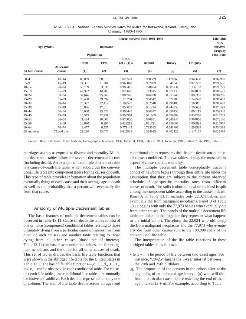
13. The Life Table 325
TABLE 13.10 National Census Survival Rates for Males for Botswana, Ireland, Turkey, andUruguay, 1980–1990
Census survival rate, 1980–1990
Age (years) Botswana
Population 1984–1986Rate.
At second1980 1990 (2) ∏ (1) = Ireland Turkey Uruguay
At first census census (1) (2) (3) (4) (5) (6) (7)
0–4 10–14 86,069 88,615 1.029581 0.988389 1.178368 0.949638 0.9629005–9 15–19 74,301 71,704 0.965048 0.957009 1.041048 0.975587 0.995636
10–14 20–24 58,709 53,038 0.903405 0.778674 0.905234 1.137193 0.99322915–19 25–29 42,972 44,203 1.028647 0.723915 0.971136 1.041833 0.98952720–24 30–34 32,646 35,568 1.089506 0.876978 0.953246 1.000395 0.98729625–29 35–39 26,498 29,592 1.116764 0.954542 1.022280 1.147528 0.98549230–34 40–44 20,327 22,412 1.102573 0.962540 0.996185 1.16505 0.98069335–39 45–49 16,826 17,813 1.058659 0.961294 0.944353 1.103631 0.97059940–44 50–54 15,600 15,529 0.995449 0.936017 0.896453 1.006115 0.95233345–49 55–59 13,575 12,231 0.900994 0.921369 0.896584 0.932286 0.91922250–54 60–64 11,424 10,008 0.876050 0.870831 0.840947 0.904868 0.87316655–59 65–69 10,090 8,297 0.822299 0.831721 0.759667 1.068891 0.81596760–64 70–74 8,477 6,537 0.771145 0.723513 0.641406 1.203539 0.73439365 and over 75 and over 21,220 13,070 0.615928 0.384943 0.402123 1.147139 0.625499
Source: Basic data from United Nations, Demographic Yearbook, 1996, Table 34; 1994, Table 7; 1993, Table 26; 1988, Tables 7, 26; 1983, Table 7.
marriages as they as exposed to divorce and mortality. Multi-ple decrement tables allow for several decremental factors(including death). An example of a multiple decrement tableis a cause-of-death life table, which subdivides the conven-tional life table into component tables for the causes of death.This type of table provides information about the populationeventually dying of each cause and their average age at deathas well as the probability that a person will eventually diefrom that cause.
Anatomy of Multiple Decrement Tables
The basic features of multiple decrement tables can beobserved in Table 13.11. Cause-of-death life tables consist ofone or more (component) conditional tables relating to thoseultimately dying from a particular cause of interest (or from a set of such causes) and another table relating to those dying from all other causes (those not of interest). Table 13.11 consists of two conditional tables, one for malig-nant neoplasms and the other for all other causes of death.This set of tables divides the basic life table functions thatwere shown in the abridged life table for the United States inTable 13.2. The basic life table functions—nqx, lx, ndx, nLx, Tx,and ex—can be observed in each conditional table. For cause-of-death life tables, the conditional life tables are mutuallyexclusive and additive. Each death is represented in only onedx column. The sum of life table deaths across all ages and
conditional tables represents the life table deaths attributed toall causes combined. The two tables display the most salientaspect of cause-specific mortality.
The multiple decrement table conceptually traces acohort of newborn babies through their entire life under theassumption that they are subject to the current observedschedule of age-specific mortality rates from differentcauses of death. The radix (cohort of newborn babies) is splitamong the component tables according to the cause of death.Panel A of Table 13.11 includes only 22,024 babies whoeventually die from malignant neoplasms. Panel B of Table13.11 begins with only the 77,973 babies who eventually diefrom other causes. The panels of the multiple decrement lifetable are linked in that together they represent what happensto the initial cohort. Therefore, the 22,024 who ultimatelydie from malignant neoplasms and the 77,973 who eventu-ally die from other causes sum to the 100,000 radix of theconventional life table.
The interpretation of the life table functions in theseabridged tables is as follows:
x to x + n The period of life between two exact ages. Forinstance, “20–25” means the 5-year interval betweenthe 20th and 25th birthdays.
nqx The proportion of the persons in the cohort alive at thebeginning of an indicated age interval (x) who will diefrom a particular cause before reaching the end of thatage interval (x + n). For example, according to Table
rate,survivalUruguay
Life table

326 Kintner
TABLE 13.11 Multiple Decrement Life Table for Malignant Neoplasms and Other Causes, United States 1989–91
Of 100,000 born alive who
eventuallyOf 100,000 born alive Stationary population die from
Proportion of Average number of cause cpersons alive at Number living Number Population years of life remaining
Period beginning of at beginning of dying in this In this at beginning of Numberbetween two age interval dying age interval who during age age interval who and all age interval for those living atexact ages, x during interval eventually die interval from will eventclly subsequent who will eventually beginningto x+n (years) from cause c from cause c cause c die from cause age intervals die from cause c of age interval
A. Malignant Neoplasms
nqx,neoplasms lx, neoplasms ndx,neoplasms nLx,neoplasms nTx, neoplasms ex,neoplasms l*x,neoplasms
0–1 0.00002 22,024 2 22,022 1,587,922 72.10 100,0001–5 0.00014 22,021 13 88,053 1,565,900 71.11 99,9905–10 0.00017 22,008 16 109,999 1,477,847 67.15 99,929
10–15 0.00016 21,992 15 109,919 1,367,849 62.20 99,85415–20 0.00021 21,976 20 109,830 1,257,929 57.24 99,78520–25 0.00028 21,956 28 109,710 1,148,099 52.29 99,69225–30 0.00043 21,928 42 109,534 1,038,389 47.35 99,56630–35 0.00080 21,886 77 109,235 928,855 42.44 99,37435–40 0.00152 21,808 146 108,677 819,620 37.58 99,02240–45 0.00291 21,662 277 107,618 710,943 32.82 98,36045–50 0.00572 21,385 539 105,578 603,325 28.21 97,10050–55 0.01046 20,846 966 101,816 497,748 23.88 94,65455–60 0.01732 19,880 1,553 95,519 395,932 19.92 90,26760–65 0.02628 18,327 2,248 86,017 300,413 16.39 83,21765–70 0.03600 16,079 2,863 73,239 214,397 13.33 73,00970–75 0.04728 13,217 3,374 57,648 141,157 10.68 60,01175–80 0.05613 9,843 3,393 40,731 83,510 8.48 44,69180–85 0.06310 6,450 2,971 24,822 42,778 6.63 29,28685–90 0.06504 3,479 2,066 12,228 17,957 5.16 15,79690–95 0.06054 1,412 1,032 4,482 5,729 4.06 6,41395–100 0.05107 380 321 1,100 1,247 3.28 1,727
100+ 1.00000 60 60 147 147 2.46 271
B. Other Causes
nqx,other lx, other ndx,other nLx,other nTx, other ex,other l*x,other
0–1 0.0093400 77,973 934 77,156 5,947,292 76.27 100,0001–5 0.0017400 77,039 174 307,738 5,870,136 76.20 98,8025–10 0.0009700 76,865 97 384,083 5,562,398 72.37 98,579
10–15 0.0011700 76,768 117 383,548 5,178,315 67.45 98,45515–20 0.0039900 76,651 399 382,258 4,794,768 62.55 98,30520–25 0.0051600 76,252 516 379,970 4,412,510 57.87 97,79325–30 0.0055800 75,736 558 377,285 4,032,540 53.24 97,13130–35 0.0067100 75,178 671 374,213 3,655,255 48.62 96,41535–40 0.0080100 74,507 801 370,533 3,281,043 44.04 95,55540–45 0.0094100 73,706 941 366,178 2,910,510 39.49 94,52845–50 0.0124500 72,765 1,245 360,713 2,544,333 34.97 93,32150–55 0.0174700 71,520 1,747 353,233 2,183,620 30.53 91,72455–60 0.0256800 69,773 2,568 342,445 1,830,388 26.23 89,48460–65 0.0376900 67,205 3,769 326,603 1,487,943 22.14 86,19065–70 0.0529900 63,436 5,299 303,933 1,161,340 18.31 81,35670–75 0.0753400 58,137 7,534 271,850 857,408 14.75 74,56075–80 0.0997000 50,603 9,970 228,090 585,558 11.57 64,89880–85 0.1234200 40,633 12,342 172,310 357,468 8.80 52,11285–90 0.1265800 28,291 12,658 109,810 185,158 6.54 36,28390–95 0.0973300 15,633 9,733 53,833 75,348 4.82 20,04995–100 0.0453600 5,900 4,536 18,160 21,515 3.65 7,567
100+ 1.0000000 1,364 1,364 3,355 3,355 2.46 1,749
Source: U.S. National Center for Health Statistics, 1999.

13.11 panel A, the proportion dying from malignantneoplasms in the age interval 20 to 25 is 0.00028. That is, out of every 100,000 persons alive and exactly20 years old, 28 will die from malignant neoplasmsbefore reaching their 25th birthday. In other words, thenqx values represent the probability that a person at hisxth birthday will die from malignant neoplasms beforereaching his or her x + nth birthday.
lx The number of persons living at the beginning of theindicated age interval (x) out of the total number ofbirths assumed as the radix of the table who will ulti-mately die from a particular cause. Again, according toTable 13.11, out of 22,024 newborn babies who eventu-ally die from malignant neoplasms, 21,956 personswould survive to exact age 20.
ndx The number of persons who would die from a particularcause within the indicated age interval (x to x + n) out ofthe 100,000 births assumed in the combined tables. Thus,according to Table 13.11, there would be 28 deaths frommalignant neoplasms between exact ages 20 and 25 to theinitial cohort of 100,000 newborn babies.
nLx The number of person-years that would be lived withinthe indicated age interval (x to x + n) by the cohort who
will ultimately die from malignant neoplasms. Thus,according to Table 13.11, the 100,000 newborn babieswould live 109,710 person-years between exact ages 20and 25. Of the 21,956 persons who reach age 20 beforeeventually dying from malignant neoplasms, the 21,928who survive to age 25 would live 5 years each (21,928 ¥5 = 109,640 person-years) and the 28 who die would eachlive varying periods of time less than 5 years, averagingabout 21–2 years (28 ¥ 2.5 = 70 person-years)
Tx The total number of person-years that would be livedafter the beginning of the indicated age interval by thecohort of those who eventually die from malignant neo-plasms. Thus, according to Table 13.11, the 22,024newborn babies who ultimately die from malignant neo-plasms would live 1,148,099 person-years after their 20thbirthday.
ex The average remaining lifetime (in years) for a personwho survives to the beginning of the indicated ageinterval for those ultimately dying from a particularcause. Thus, according to Table 13.11, persons whoreach their 20th birthday and who eventually die frommalignant neoplasms should expect to live 52.29 yearsmore, on the average.
13. The Life Table 327
TABLE 13.12 Actual Deaths and Life Table Deaths for Malignant Neoplasms and Other Causes,United States: 1989–1991
Actual deaths Life table deaths
Exact Total Neoplasms All other causes Total Neoplasms All other causesages nDx nDx, neoplasms nDx,other ndx ndx, neoplasms ndx,other
0–1 114,810 274 114,536 936 2 9341–5 21,444 1,545 19,899 187 13 1745–10 12,238 1,774 10,463 113 16 97
10–15 13,599 1,581 12,018 132 15 11715–20 46,609 2,258 44,351 419 20 39920–25 63,099 3,226 59,873 544 28 51625–30 79,018 5,578 73,440 600 42 55830–35 101,279 10,482 90,797 748 77 67135–40 117,550 18,118 99,432 947 146 80140–45 135,123 30,758 104,364 1,219 277 94245–50 156,378 47,214 109,164 1,784 539 1,24550–55 201,256 71,674 129,582 2,713 966 1,74755–60 295,958 111,499 184,459 4,121 1,553 2,56860–65 465,044 173,739 291,305 6,018 2,248 3,77065–70 651,048 228,339 422,709 8,162 2,863 5,29970–75 787,101 243,437 543,664 10,909 3,374 7,53575–80 904,394 229,612 674,782 13,363 3,393 9,97080–85 904,222 175,431 728,791 15,314 2,971 12,34385–90 737,820 103,545 634,276 14,725 2,066 12,65990–95 447,208 42,868 404,340 10,765 1,032 9,73395–100 175,745 11,607 164,138 4,857 321 4,536
100+ 37,506 1,571 35,935 1,424 60 1,364Total, all ages 100,000 22,024 77,976
Source: Published and unpublished data from the U.S. National Center for Health Statistics.

The multiple decrement table is a way to partition the con-ventional life tables into conditional tables for each cause ofdeath. The conditional tables are linked to the conventionallife table by several relationships. At all ages, the number ofsurvivors and person-years in the conventional life table is therespective sum over the conditional tables. That is,
Furthermore, the life expectancy for a population is theaverage of the multiple decrement life expectancies for theseparate causes of death, weighted by the proportions dyingof each cause:
For example, life expectancy at birth in Table 13.2 is75.37, which is the weighted sum of life expectancy at birthfor those who eventually die from malignant neoplasms(72.10) and those who eventually die from other causes(76.27), where the weights are the proportions of the100,000 births who eventually die from each cause. So
Table 13.11 shows life table deaths for malignant neo-plasms and other causes for the United States in 1989–1991,using the life table deaths by cause (ndx,c) series of Table 13.12.We have added the column lx*, which rescales the lx series tothe radix 100,000. The rescaling is not necessary but simpli-fies comparison of rates of population attrition for each cause.
Construction of Multiple Decrement Tables
Double-decrement and multiple-decrement tables may beconstructed either on the basis of age-specific probabilitiesof the occurrence of the events (occurrence/exposure rates)or on the basis of prevalence ratios, obtained usually fromcensuses or surveys. When prevalence ratios are used, thelife table stationary population is distributed into differentstatuses according to the prevalence of those statuses in theactual observed population.
The construction of multiple decrement tables isdescribed in terms of cause-of-death life tables. As men-tioned, multiple decrement cause-of-death life tables subdi-vide total life table deaths into the different causes or groupsof causes of death. In constructing a multiple decrementtable, one first constructs a conventional life table using age-specific probabilities of dying for all causes combined.Then, from the counts of actual deaths by cause, the pro-portion of deaths due to each cause is computed. Next, ndx,life table deaths between ages x and x + n, are separated intoc cause-of-death subcategories ndx,1, ndx,2, ... ndx,c. This sub-
e022 024
100 00072 10
77 976100 000
76 27= ÊË
ˆ¯◊ + Ê
ˈ¯◊
,,
.,,
.
el e
lx
x c x c
x
=( )Â , ,
l l L Lx x cc
n x n x cc
= =Â Â, ,and
division of life table deaths by cause is made on the basisof the actual distribution of deaths by cause at each age:
(13.60)
Table 13.12 shows the actual deaths and life table deathsfor the 1989–1991 U.S. life table. Total deaths have beendivided into two subcategories, malignant neoplasms andother causes. The actual deaths are the averages from 1989to 1991. The column for total life table deaths comes fromTable 13.2. Beginning at age under 1 year, we allocate totallife table deaths into life table deaths by cause proportion-ally based on the actual deaths:
All life table deaths are included in the allocation. Forexample, the life table deaths at age under 1 by cause sumto the total life table deaths for age under 1 (934 + 2 = 936).
The life table deaths partitioned by cause are used to con-struct life tables conditional on dying from that cause. Thendx,c series can be used to construct the conditional life table showing the survival distribution for individuals whoeventually die of one cause by defining the initial populationl0,c to be
(13.61)
The sum of the ndx,c terms across all ages represents alllife table deaths for the cth cause. Table 13.11 indicates thatthe sum of all life table deaths from malignant neoplasms is22,024; this becomes the radix for the conditional life tablefor malignant neoplasms.
Table 13.12 shows the summations of the ndx,c terms,which yield the totals, l0,neoplasms = 22,024 and l0,other = 77,976.The reader can confirm that wd0 = l0 = 100,000 = sum of l0,c.The l0,c estimates tell us that, of 100,000 persons born, 22%would eventually die from malignant neoplasms and 78%would die from other causes, at the 1989–1991 survival probabilities.
We estimate the number of survivors for the cause at subsequent ages, lx,c, by subtraction of the ndx,c terms. Thatis,
(13.62)
The lx,c series is exactly the lx series of the conventional lifetable, except that it describes the survival experience ofpersons eventually dying of a particular cause c.
The life table deaths for each cause and age group areused to calculate the cause-specific probability of dying.These are also called probabilities of death from specified
l l dx n c x c n x c+ = -, , ,
l d dc c n x cx
n
0 00
, , ,= ==
-
Âw
w
d dD
D
d dD
D
neoplasmsneoplasms
otherother
0 00
0
0 00
0
936274
114 8102
936114 536114 810
934
,,
,,
,,,
= ◊ = ◊Êˈ¯ =
= ◊ = ◊Êˈ¯ =
n x c n xn x c
n x
d dD
D,
,= ÊË
ˆ¯
328 Kintner

viduals saved would be immediately subject to the deathrates from other causes, usually major causes in later life.This phenomenon is called “competing risks.” Becausedeath from the cause eliminated would often have occurredat the older ages, few additional years would be added if theindividual survived and died shortly after from anothercause. The various causes of decrement are assumed to actindependently of each other in the present case. If the causesare assumed not to be independent, it is still possible todevelop a cause-eliminated life table if the interconnect-edness can be modeled explicitly (Manton and Stallard,1984).
Anatomy of Cause-Elimination Life Tables
Table 13.13 presents an abridged life table for the totalpopulation of the United States in 1989–1991, prepared onthe assumption that malignant neoplasms (cancer) are elim-inated as a cause of death. A series of such life tables, con-sidered in comparison with a life table for all causescombined, provides various measures of the relative impor-tance of the different causes of death. The cause-eliminationlife table includes the basic life table functions—nqx, lx, ndx,nLx, Tx, and ex, as well as three additional functions.
The interpretation of the life table functions in anabridged life table would be as follows:
x to x + n The period of life between two exact agesnqx
(-i) The proportion of the persons in the cohort alive at thebeginning of an indicated age interval (x) who will diebefore reaching the end of that age interval (x + n) assum-ing that malignant neoplasms have been eliminated as acause of death. Comparison of Tables 13.13 and 13.2indicates that when malignant neoplasms have been elim-inated as a cause of death, the proportion dying in the ageinterval 20 to 25 falls from .00554 to .00526.
lx(-i) The number of persons living at the beginning of the
indicated age interval (x) out of the total number ofbirths posited as the radix of the table, assuming thatmalignant neoplasms have been eliminated. Accordingto Table 13.13, out of 100,000 newborn babies, 98,282persons would survive to exact age 20 assuming thatmalignant neoplasms have been eliminated. Note thatthe number of survivors to age 20 is higher in Table13.13 (which assumes that no one dies from malignantneoplasms), than in Table 13.2, (which assumes that nocauses of death have been eliminated).
ndx(-i) The number of persons who would die within the indicated age interval (x to x + n) out of the 100,000births, assuming no deaths from neoplasms. Of the 98,282survivors to age 20, 517 are expected to die before age 25.Again comparing Tables 13.2 and 13.13, the number ofdeaths between exact ages 20 and 25 to the initial cohortof 100,000 newborn babies would fall from 544 to 517 ifmalignant neoplasms were eliminated.
13. The Life Table 329
causes and represent the probability that an individual willdie of cause c after surviving to age x but before reachingage x + n.
(13.63)
For example, the probability that an individual aged 20 willdie from malignant neoplasms before age 25 is
The sum of the life table deaths for cause c is the numberwho eventually die of cause c from among the births thatbegin the life table (l0). The probability that an individualeventually dies of the cth cause is
(13.64)
Life expectancy for each conditional table is constructedaccording to the formulas for constructing abridged lifetables with the substitution of the conditional terms nlx,c andnLx,c for the conventional life table quantities nlx and nLx.
Cause-Elimination Life Tables
Life tables have been computed under the assumption thata specific decrement (for instance, a cause of death or groupof causes of death) is eliminated, that is, that it is impossibleto die from the eliminated cause (Greville, 1948; U.S.National Center for Health Statistics, 1968, 1985b, 1999).Such cause-elimination life tables describe the hypotheticalsituation that a cause of decrement has been eliminated. Thisis the same as assuming that the probability of dying from thatcause is zero (or the probability of surviving form it is 1.0).Note that while deaths from a cause are assumed to disappear,the disease itself is not assumed to go away.
Two important cautions must be observed in interpretingcause-elimination life tables. First, they provide no informa-tion about future longevity even though they can be useful informulating assumptions about future longevity. They simplygive us additional insight into the current cause pattern ofmortality. Second, they are theoretical constructs in that theyhypothesize shifts in mortality that do not occur independ-ently and hence do not realistically represent the actual gainsfrom eliminating a cause. It is likely that the gains from elim-inating a cause would, in actual experience, be much smallerthan shown in the table, as explained below.
Cause-elimination life tables are usually based on theassumption that eliminating one cause of death has no effecton the risk of dying from the remaining causes. The poten-tial gain in life expectation as measured by cause-elimination life tables is constrained by the fact that indi-
ww
w
qd
l
d
lc
n a c c
a
n
00
0
00,
, ,= ==
-
Â
5 2028
98 213000285q neoplasms, ,
.= =
n x cn x c
x
qd
l,
,=

330 Kintner
nLx(-i) The number of person-years that would be livedwithin the indicated age interval (x to x + n) by thecohort. Thus, according to Table 13.13, the 100,000newborn babies would live 490,144 person yearsbetween exact ages 20 and 25.
Tx(-i) The total number of person-years lived after the
beginning of the indicated age interval. Thus, accordingto Table 13.13, the 100,000 newborn babies would live5,896,816 person-years after their 20th birthday.
ex(-i) The average remaining lifetime (in years) for a person
who survives to the beginning of the indicated ageinterval, assuming that malignant neoplasm has beeneliminated as a cause of death. Thus, according toTable 13.13, a person who reaches his or her 20thbirthday should expect to live, on average, 60 moreyears.
Yi The probability of eventually dying of the specific cause,malignant neoplasms in this case. According to Table13.13, 22% of live births would die from malignant neo-plasms. Note that this type of probability was discussedpreviously with multiple decrement life tables.
g(-i) The gain in life expectancy from eliminating a speci-fied cause. If malignant neoplasms were eliminated as acause of death, then 3.36 years would be added to lifeexpectancy at birth for the total U.S. population in1989–1991. This column represents the difference in e0
between Tables 13.13 and 13.2.g (-i) The gain in life expectancy for those who would have
died if the cause not been hypothetically eliminated.According to Table 13.13, those who would have diedfrom malignant neoplasms can expect to live, onaverage, 15.25 additional years at birth.
TABLE 13.13 Abridged Life Table Eliminating Malignant Neoplasms as a Cause of Death, for the Total Population of the UnitedStates: 1989–1991
Ageinterval Proportion Average remaining lifetime
Period ofdying
Of 100,000 born Stationary Averagelife Proportion alive population number ofbetween of persons years of life Probability Gain in Gain intwo alive at Number In this and remaining of life lifeexact beginning of Number dying all at eventually expectancy expectancyages age interval living at during In subsequent beginning dying eliminating for thosestated dying during beginning of age this age age of age of specified specified who wouldin years interval age interval interval interval intervals interval cause cause have died
x to nqx(-i) lx
(-i) dx(-i)
nLx(-i) Tx
(-i) ex(-i) yx
i gx(-i) gx
(-i)
x + n0–1 0.00934 100,000 934 99,260 7,872,401 78.72 0.22023 3.36 15.251–5 0.00175 99,066 174 395,855 7,773,142 78.46 0.22229 3.39 15.245–10 0.00096 98,893 95 494,206 7,377,287 74.60 0.22257 3.38 15.20
10–15 0.00117 98,798 116 493,766 6,883,081 69.67 0.22266 3.38 15.1615–20 0.00405 98,682 400 492,499 6,389,315 64.75 0.22280 3.37 15.1320–25 0.00526 98,282 517 490,144 5,896,816 60.00 0.22355 3.37 15.0825–30 0.00572 97,765 559 487,464 5,406,672 55.30 0.22451 3.37 15.0330–35 0.00691 97,206 672 484,413 4,919,208 50.61 0.22546 3.37 14.9535–40 0.00834 96,534 805 480,736 4,434,795 45.94 0.22641 3.36 14.8440–45 0.00989 95,729 946 476,396 3,954,059 41.30 0.22713 3.33 14.6445–50 0.01327 94,783 1,257 470,980 3,477,663 36.69 0.22712 3.25 14.3350–55 0.01900 93,526 1,777 463,492 3,006,684 32.15 0.22568 3.12 13.8155–60 0.02890 91,748 2,652 452,556 2,543,192 27.72 0.22173 2.89 13.0460–65 0.04467 89,097 3,980 436,062 2,090,636 23.46 0.21426 2.57 11.9965–70 0.06790 85,117 5,780 411,798 1,654,573 19.44 0.20221 2.16 10.6970–75 0.10827 79,337 8,590 376,115 1,242,775 15.66 0.18522 1.71 9.2375–80 0.17008 70,747 12,033 324,472 866,659 12.25 0.16283 1.25 7.6680–85 0.27173 58,714 15,954 254,085 542,187 9.23 0.13699 0.84 6.1185–90 0.41446 42,760 17,722 168,451 288,102 6.74 0.10950 0.51 4.6590–95 0.59446 25,037 14,884 84,814 119,651 4.78 0.08285 0.28 3.3795–100 0.74997 10,154 7,615 28,428 34,836 3.43 0.06057 0.14 2.33
100+ 1.00000 2,539 2,539 6,408 6,408 2.52 0.04189 0.06 1.45
Source: U.S. National Center for Health Statistics. R. N. Anderson, 1999. “United States Life Tables Eliminating Certain Causes of Death.” U.S. Decen-nial Life Tables for 1989–91, vol. 1, no. 4. Hyattsville, MD: U.S. National Center for Health Statistics.
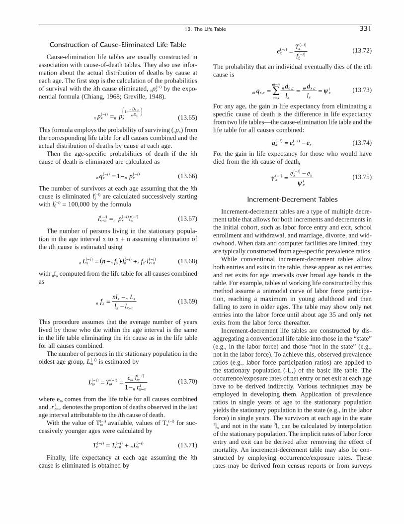
Construction of Cause-Eliminated Life Table
Cause-elimination life tables are usually constructed inassociation with cause-of-death tables. They also use infor-mation about the actual distribution of deaths by cause ateach age. The first step is the calculation of the probabilitiesof survival with the ith cause eliminated, npx
(-i) by the expo-nential formula (Chiang, 1968; Greville, 1948).
(13.65)
This formula employs the probability of surviving (npx) fromthe corresponding life table for all causes combined and theactual distribution of deaths by cause at each age.
Then the age-specific probabilities of death if the ithcause of death is eliminated are calculated as
(13.66)
The number of survivors at each age assuming that the ithcause is eliminated lx
(-i) are calculated successively startingwith l0
(-i) = 100,000 by the formula
(13.67)
The number of persons living in the stationary popula-tion in the age interval x to x + n assuming elimination ofthe ith cause is estimated using
(13.68)
with nfx computed from the life table for all causes combinedas
(13.69)
This procedure assumes that the average number of yearslived by those who die within the age interval is the samein the life table eliminating the ith cause as in the life tablefor all causes combined.
The number of persons in the stationary population in theoldest age group, Lw
(-i) is estimated by
(13.70)
where ew comes from the life table for all causes combinedand nr i
w-n denotes the proportion of deaths observed in the lastage interval attributable to the ith cause of death.
With the value of Tw(-i) available, values of Tx
(-i) for suc-cessively younger ages were calculated by
(13.71)
Finally, life expectancy at each age assuming the ithcause is eliminated is obtained by
T T Lxi
x ni
n xi-( )
+-( ) -( )= +
L Te l
ri i
i
n niw w
w w
w
-( ) -( )-( )
-= =
◊-1
n xx n x
x x n
fnl L
l l=
-- +
n xi
n x ni
n x x niL n f l f l-( ) -( )
+-( )= -( )◊ + ◊
l p lx ni
n xi
xi
+-( ) -( ) -( )=
n xi
n xiq p-( ) -( )= -1
n xi
n x
DDp p
n x c
n x-( ) -ÊËÁ
ˆ¯̃=
1 ,
(13.72)
The probability that an individual eventually dies of the cthcause is
(13.73)
For any age, the gain in life expectancy from eliminating aspecific cause of death is the difference in life expectancyfrom two life tables—the cause-elimination life table and thelife table for all causes combined:
(13.74)
For the gain in life expectancy for those who would havedied from the ith cause of death,
(13.75)
Increment-Decrement Tables
Increment-decrement tables are a type of multiple decre-ment table that allows for both increments and decrements inthe initial cohort, such as labor force entry and exit, schoolenrollment and withdrawal, and marriage, divorce, and wid-owhood. When data and computer facilities are limited, theyare typically constructed from age-specific prevalence ratios.
While conventional increment-decrement tables allowboth entries and exits in the table, these appear as net entriesand net exits for age intervals over broad age bands in thetable. For example, tables of working life constructed by thismethod assume a unimodal curve of labor force participa-tion, reaching a maximum in young adulthood and thenfalling to zero in older ages. The table may show only netentries into the labor force until about age 35 and only netexits from the labor force thereafter.
Increment-decrement life tables are constructed by dis-aggregating a conventional life table into those in the “state”(e.g., in the labor force) and those “not in the state” (e.g.,not in the labor force). To achieve this, observed prevalenceratios (e.g., labor force participation ratios) are applied tothe stationary population (nLx) of the basic life table. Theoccurrence/exposure rates of net entry or net exit at each agehave to be derived indirectly. Various techniques may beemployed in developing them. Application of prevalenceratios in single years of age to the stationary populationyields the stationary population in the state (e.g., in the laborforce) in single years. The survivors at each age in the state1lx and not in the state 0lx can be calculated by interpolationof the stationary population. The implicit rates of labor forceentry and exit can be derived after removing the effect ofmortality. An increment-decrement table may also be con-structed by employing occurrence/exposure rates. Theserates may be derived from census reports or from surveys
gyx
i xi
x
xi
e e-( )-( )
=-
g e exi
xi
x-( ) -( )= -
ww
w
yqd
l
d
lx c
n a c
x
x c
xa x
n
xi
,, ,= = =
=
-
Â
eT
lx
i xi
xi
-( )-( )
-( )=
13. The Life Table 331

332 Kintner
on current status and status at an earlier date. Cross-sectionaldata from a single census measuring the changes in the pro-portions over single ages can also be used to derive the rates.
Increment-decrement tables provide some types of infor-mation not available from conventional tables and double-decrement tables. Using tables of working life as illustration,we can obtain such measures as the proportion of the cohortever entering the labor force, the average remaining yearsof active life, the rate of accessions to the labor force andretirements at each age, and the mean ages of entry into thelabor force and retirement.
Increment-decrement tables are limited because theycannot model all possible transitions between the statesunder consideration. For this reason, multistate tables have largely replaced increment-decrement tables. Unlike increment-decrement tables, multistate tables of workinglife are not limited to a unimodal curve of labor force par-ticipation and can handle those individuals who enter thelabor the force, exit, and then reenter it.
MULTISTATE LIFE TABLES
Multistate life tables are a major extension of life tables.Both conventional life tables and multiple decrement lifetables model departures, over time, from a cohort of livebirths. Conventional life tables concern two states—life anddeath—while multiple decrement models allow for more thantwo states—life and various causes of death, for example.Multistate models, in contrast, allow not only for movementsbetween life (an active state) and death (an absorbing state)but also for all possible movements among various types ofactive states. For example, a multistate nuptiality modelallows individuals to move from being unmarried to married,from married to divorced, from divorced to remarried, andfrom remarried to divorced. Because of this flexibility, multi-state models have had a broad range of applications, includ-ing marital status, labor force behavior, interregionalmigration, and health status.
Multistate models relate to “states”, which typicallyinclude death and various categories for the living. Statesare mutually exclusive and discrete. There are several typesof states. Absorbing states (like death) only permit entries.Transient states allow both entries and exits. In addition,some states (like never married) permit only exits. Together,the states are the elements of the “state space.”
Mathematically, multistate models are a type of Markovprocess. Markov processes assume that transition probabil-ities depend only on age (or duration in state) and currentstate. Furthermore, the probabilities are assumed independ-ent of the previous state.
Anatomy of Multistate Models
Unlike conventional tables or multiple decrement tables,multistate models do not have a standard table format with
a small set of measures shown in every analysis. Instead,measures are selectively presented according to the require-ments of the analysis. Many measures have counterparts inconventional and multiple decrement life tables. Outputmeasures include lifetime transition probabilities, propor-tion of the population dying while in each state, expectedduration of stay in each state (e.g., marriage), and numberof transitions to each state per person.
Construction of Multistate Models
Multistate life tables are constructed from transitionprobabilities between the states analyzed in the table. Thereare different ways of deriving the basic transition probabil-ities. They may be obtained from a survey with a retrospec-tive question on the previous year’s status. Alternatively, theappropriate transitions, including deaths, may be securedfrom a longitudinal (panel) survey. The panel data for twodates can be used both to validate retrospective data from asingle survey and to provide the matrix of required transi-tion data. The appropriate transitions can also be calculatedfrom census population counts and vital statistics. The con-struction of a multistate table is illustrated in this chapterwith a table of working life.
Working-Life Tables
Working-life tables model the worklife history of a hypothetical cohort assumed to experience currently prevail-ing labor force ratios. Multistate models of working lifedescribe labor force attachment as a dynamic process.Members of the population are viewed as entering and leavingthe labor market repeatedly during their lifetimes, with nearlyall participating for some period during their lives. Tables ofworking life are useful in understanding the mechanisms andimplications of changes in the labor force. These tablesprovide an indication of the average number of working yearsto be expected after a given age by all persons or by persons inthe labor force attaining that age. In addition, the tables provideinformation on age-specific rates of accession to, and separa-tion from, the labor force. These measures are used in legalproceedings to estimate work years lost and earnings foregoneby individuals whose careers have been truncated by death.They are often used by governments for estimating manpowerreplacement needs for industry and assessing the economicimplications of changes in economic activity ratios and theage-structure of the population.
The construction of a working-life table for U.S. malesin 1979–1980, developed by Smith (1982, 1986), is shownas Table 13.14. The major source of data for constructingthis table is the Current Population Survey (CPS), thenationwide monthly household survey sponsored by theU.S. Bureau of Labor Statistics. Because individuals areinterviewed during each of four successive months and

13. The Life Table 333
again in the same 4 months of the following year, CPSrecords can be matched so that each person’s status at thebeginning and end of a 12-month interval can be compared.To construct the table of working life shown as Table 13.14,individuals’ labor force status in a given month of 1979 was matched to that information in the same month of 1980. If labor force status changed between the two reference dates, then labor force transitions were registered.Surviving respondents were classified as “active” or “inac-tive” if their status was identical at both dates, and as“entrants” or “exits” if their status changed. The state space of this multistate model consists of three states: twolabor force states (active and inactive) and death. Four tran-sitions among the states are possible, two between the laborforce statuses and two between each of these and death. Lifetable calculations are carried out on single-year-of-age data. Life table calculations are based on exact ages, but the survey data have a slightly different age reference. In the survey, when the average person claims to have a certain age x, that person’s age is actually halfway betweenexact age x and exact age x + 1. Therefore, the survey datahave to be recentered to exact ages before developing thelife table functions. Mortality rates were assumed to be identical for all persons of a given age, regardless of laborforce status. The number of persons expected to die betweeninterviews was estimated using a standard mortality schedule.
As an example of the process involved in constructing a working life table, we first calculate a transition matrix for each age by setting up a 2 ¥ 2 contingency table of labor force status in 1980 by labor force status in 1979, as shown in Figure 13.2. Age-specific transition probabilities(px, shown in columns 2 to 6 in Table 13.14) indicate the likelihood that an individual of a given exact age and laborforce status will be in each of three possible states (active,inactive, or dead) 1 year later. For each age and labor forcestatus, the transition probabilities sum to 1. For example, atage 16,
p p pxd i
xi i
xa+ + = + + =. . . .00130 70257 29613 1 00000
For each combination of age and labor force status, thetransition probabilities are computed as row percentagesfrom tables, such as is shown in Figure 13.2. For example,the probability of exiting the labor force beginning at age x is
(13.76)
where p is the transition probability, the prefixed superscripta refers to the state at time 1, the suffixed superscript i refersto the state at time 2, and Group Ax refers to the row totalfrom Figure 13.2.
Age-specific rates of transfer between statuses mx
(columns 7 to 9 in Table 13.14) are the number of transfersfrom state 1 to state 2 between exact ages x and x + 1 perthousand cohort members age x in the stationary population.These transfer rates allow for multiple status changes byindividuals during the year. Transfer rates are computedfrom transition probabilities as follows:
(13.77)
For example, the rate of separation from the labor forceat age 17 is
The probability of moving into and out of the labor forceis relatively high at some ages, such as 16 and 17, whenmany start their careers with temporary summer jobs.Although some individuals will make changes repeatedlyduring the year, only their final transition is included in theyear-to-year comparisons. Their other changes are lost.
The survivors from an initial cohort of 100,000 births, lx,are in column 10 of Table 13.14. They are calculated fromthe survivors in the preceding age x - 1 and the probabilityof surviving from age x + 1 to age x:
axi
axi
axa i
xi a
xi i
xa
mp
p p p p=
◊+( ) +( ) - ◊( )
=◊
+( )◊ +( ) - ◊( ) =
4
1 1
4 220431 77808 1 61255 22043 38597
31692.
. . . ..
axi
axi
axa i
xi a
xi i
xa
mp
p p p p=
◊+( ) +( ) - ◊( )
4
1 1
axi x
x
pExits
Group A=
State at time 1,age x State at time 2, age x+1
Total In labor force Not in labor force
Dead
In labor force Group A Actives Exits Deaths ofactives
Not in labor force Group B Entrants Inactives Deaths ofinactives
FIGURE 13.2 Labor force flows for the 1979–1980 Tables of Working Life
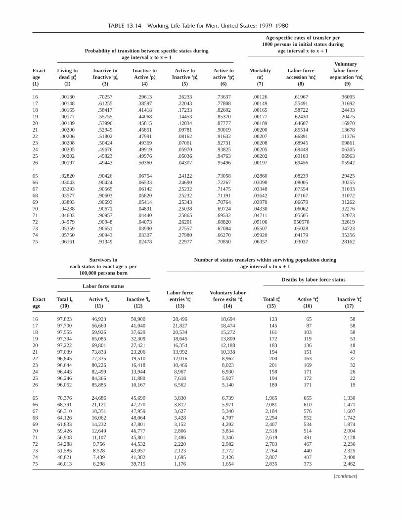
TABLE 13.14 Working-Life Table for Men, United States: 1979–1980
Age-specific rates of transfer per
Probability of transition between specific states during1000 persons in initial status during
age interval x to x + 1age interval x to x + 1
VoluntaryExact Living to Inactive to Inactive to Active to Active to Mortality Labor force labor forceage dead pd
x Inactive ipix Active ipa
x Inactive apix active apa
x mdx accession ima
x separation amix
(1) (2) (3) (4) (5) (6) (7) (8) (9)
16 .00130 .70257 .29613 .26233 .73637 .00126 .61967 .3609517 .00148 .61255 .38597 .22043 .77808 .00149 .55491 .3169218 .00165 .58417 .41418 .17233 .82602 .00165 .58722 .2443319 .00177 .55755 .44068 .14453 .85370 .00177 .62430 .2047520 .00189 .53996 .45815 .12034 .87777 .00189 .64607 .1697021 .00200 .52949 .45851 .09781 .90019 .00200 .85514 .1367822 .00206 .51802 .47991 .08162 .91632 .00207 .66891 .1137623 .00208 .50424 .49369 .07061 .92731 .00208 .68945 .0986124 .00205 .49676 .49919 .05970 .93825 .00205 .69448 .0630525 .00202 .49823 .49976 .05036 .94763 .00202 .69103 .0696326 .00197 .49443 .50360 .04307 .95496 .00197 .69456 .05942�
65 .02820 .90426 .06754 .24122 .73058 .02860 .08239 .2942566 .03043 .90424 .06533 .24690 .72267 .03090 .08005 .3025567 .03293 .90565 .06142 .25232 .71475 .03348 .07554 .3103368 .03577 .90603 .05820 .25232 .71191 .03642 .07167 .3107269 .03893 .90693 .05414 .25343 .70764 .03970 .06679 .3126270 .04238 .90671 .04891 .25038 .69724 .04330 .06062 .3227671 .04603 .90957 .04440 .25865 .69532 .04711 .05505 .3207372 .04979 .90948 .04073 .26201 .68820 .05106 .050570 .3261973 .05359 .90651 .03990 .27557 .67084 .05507 .05028 .3472374 .05750 .90943 .03307 .27980 .66270 .05920 .04179 .3535675 .06161 .91349 .02478 .22977 .70850 .06357 .03037 .28162
Survivors ineach status to exact age x per
Number of status transfers within surviving population during
100,000 persons bornage interval x to x + 1
Labor force statusDeaths by labor force status
Labor force Voluntary laborExact Total lx Active alx Inactive ilx entries ita
x force exits atix Total td
x Active atdx Inactive itd
x
age (10) (11) (12) (13) (14) (15) (16) (17)
16 97,823 46,923 50,900 28,496 18,694 123 65 5817 97,700 56,660 41,040 21,827 18,474 145 87 5818 97,555 59,926 37,629 20,534 15,272 161 103 5819 97,394 65,085 32,309 18,645 13,809 172 119 5320 97,222 69,801 27,421 16,354 12,188 183 136 4821 97,039 73,833 23,206 13,992 10,338 194 151 4322 96,845 77,335 19,510 12,016 8,962 200 163 3723 96,644 80,226 16,418 10,466 8,023 201 169 3224 96,443 82,499 13,944 8,967 6,930 198 171 2625 96,246 84,366 11,880 7,618 5,927 194 172 2226 96,052 85,885 10,167 6,562 5,140 189 171 19�
65 70,376 24,686 45,690 3,830 6,739 1,965 655 1,33066 68,391 21,121 47,270 3,812 5,971 2,081 610 1,47167 66,310 18,351 47,959 3,627 5,340 2,184 576 1,60768 64,126 16,062 48,064 3,428 4,707 2,294 552 1,74269 61,833 14,232 47,801 3,152 4,202 2,407 534 1,87470 59,426 12,649 46,777 2,806 3,834 2,518 514 2,00471 56,908 11,107 45,801 2,486 3,346 2,619 491 2,12872 54,288 9,756 44,532 2,220 2,982 2,703 467 2,23673 51,585 8,528 43,057 2,123 2,772 2,764 440 2,32574 48,821 7,439 41,382 1,695 2,426 2,807 407 2,40075 46,013 6,298 39,715 1,176 1,654 2,835 373 2,462
(continues)
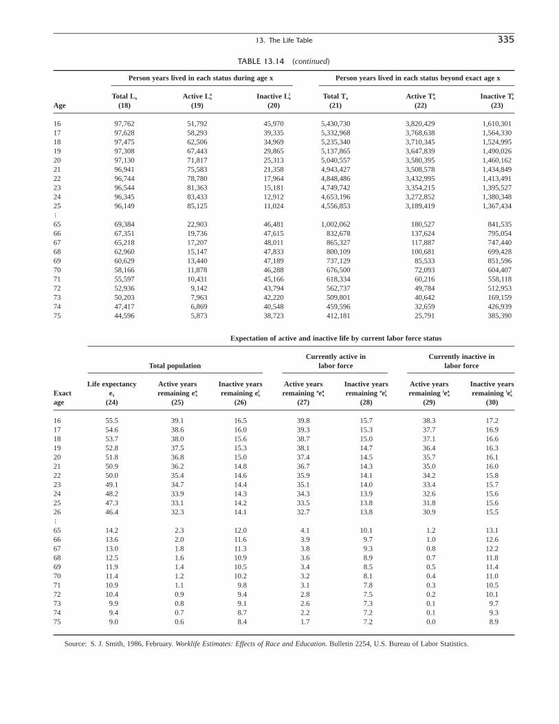
13. The Life Table 335
TABLE 13.14 (continued)
Person years lived in each status during age x Person years lived in each status beyond exact age x
Total Lx Active Lax Inactive Li
x Total Tx Active Tax Inactive Ti
x
Age (18) (19) (20) (21) (22) (23)
16 97,762 51,792 45,970 5,430,730 3,820,429 1,610,30117 97,628 58,293 39,335 5,332,968 3,768,638 1,564,33018 97,475 62,506 34,969 5,235,340 3,710,345 1,524,99519 97,308 67,443 29,865 5,137,865 3,647,839 1,490,02620 97,130 71,817 25,313 5,040,557 3,580,395 1,460,16221 96,941 75,583 21,358 4,943,427 3,508,578 1,434,84922 96,744 78,780 17,964 4,848,486 3,432,995 1,413,49123 96,544 81,363 15,181 4,749,742 3,354,215 1,395,52724 96,345 83,433 12,912 4,653,196 3,272,852 1,380,34825 96,149 85,125 11,024 4,556,853 3,189,419 1,367,434�
65 69,384 22,903 46,481 1,002,062 180,527 841,53566 67,351 19,736 47,615 832,678 137,624 795,05467 65,218 17,207 48,011 865,327 117,887 747,44068 62,960 15,147 47,833 800,109 100,681 699,42869 60,629 13,440 47,189 737,129 85,533 851,59670 58,166 11,878 46,288 676,500 72,093 604,40771 55,597 10,431 45,166 618,334 60,216 558,11872 52,936 9,142 43,794 562,737 49,784 512,95373 50,203 7,963 42,220 509,801 40,642 169,15974 47,417 6,869 40,548 459,596 32,659 426,93975 44,596 5,873 38,723 412,181 25,791 385,390
Expectation of active and inactive life by current labor force status
Currently active in Currently inactive inTotal population labor force labor force
Life expectancy Active years Inactive years Active years Inactive years Active years Inactive yearsExact ex remaining ea
x remaining eix remaining aea
x remaining aeix remaining iea
x remaining ieix
age (24) (25) (26) (27) (28) (29) (30)
16 55.5 39.1 16.5 39.8 15.7 38.3 17.217 54.6 38.6 16.0 39.3 15.3 37.7 16.918 53.7 38.0 15.6 38.7 15.0 37.1 16.619 52.8 37.5 15.3 38.1 14.7 36.4 16.320 51.8 36.8 15.0 37.4 14.5 35.7 16.121 50.9 36.2 14.8 36.7 14.3 35.0 16.022 50.0 35.4 14.6 35.9 14.1 34.2 15.823 49.1 34.7 14.4 35.1 14.0 33.4 15.724 48.2 33.9 14.3 34.3 13.9 32.6 15.625 47.3 33.1 14.2 33.5 13.8 31.8 15.626 46.4 32.3 14.1 32.7 13.8 30.9 15.5�
65 14.2 2.3 12.0 4.1 10.1 1.2 13.166 13.6 2.0 11.6 3.9 9.7 1.0 12.667 13.0 1.8 11.3 3.8 9.3 0.8 12.268 12.5 1.6 10.9 3.6 8.9 0.7 11.869 11.9 1.4 10.5 3.4 8.5 0.5 11.470 11.4 1.2 10.2 3.2 8.1 0.4 11.071 10.9 1.1 9.8 3.1 7.8 0.3 10.572 10.4 0.9 9.4 2.8 7.5 0.2 10.173 9.9 0.8 9.1 2.6 7.3 0.1 9.774 9.4 0.7 8.7 2.2 7.2 0.1 9.375 9.0 0.6 8.4 1.7 7.2 0.0 8.9
Source: S. J. Smith, 1986, February. Worklife Estimates: Effects of Race and Education. Bulletin 2254, U.S. Bureau of Labor Statistics.

(13.78)
Columns 11 and 12 in Table 13.14 represent the numberof survivors from the initial cohort remaining in a labor forcestatus for each age. Survivors are allocated between statesusing the transfer rates. The number of survivors in eachstate at age x is the number in that state at the previous agex - 1 plus persons entering that state minus those exitingthat state and those who died while in the state of interest.For example, the number of inactives at age x is
(13.79)
The number of survivors in each state at age x can berestated in terms of the number of survivors from the previ-ous age and the number of transfers among states, shown incolumns 13 through 17 in Table 13.14. Continuing with theexample of the number of inactives at age x,
(13.80)
For example, the number of inactives at age 20 is
Assuming that deaths and labor force entries and exits areevenly distributed throughout the year, the total number inthe stationary population alive at midyear is half of the sumof the stationary population at the beginning and end of thatinterval:
The number in each state at midyear, computed in thisway, is shown in columns 18 through 20 of Table 13.14. Thisfigure is also known as the number of person-years lived bythe group in any state as it passes through a given age.
Columns 21 through 23 in Table 13.14 are the sum of theperson years (of total life, active life, inactive life) from agex to the end of the table. For example, the sum of the person-years lived in inactive status from age x to the end of thetable is
Columns 24 through 30 of Table 13.14 show many mea-sures of the expectation of life for the total population. Thepopulation-based expectancy of working life is the averagenumber of years to be spent in the labor force above exactage x for each person reaching that age. This is an overallmeasure for the total cohort and can be derived for everyage. The average working life expectancy for the total pop-ulation at age x is
T Lxi
xi
x x
x
==
=
Âw
Ll l
Ll l
Ll l
xx x
xi
ix
ix
xa
ax
ax=
+=
+=
++ + +1 1 1
2 2 2, , or
i i a i i a i dl l l l l20 19 19 19 19
32 309 13 809 18 645 53 27 421
= + - -= + - - =, , , ,
ix
ix
axi i
xa i
xdl l t t t= + - -- - - -1 1 1 1
ix
ix
ax
axi i
xi
xa i
xi
xdl l L m L m L m= + ◊( ) - ◊( ) - ◊( )- - - - - - -1 1 1 1 1 1 1
l l px x xd= ◊ -( )- -1 11
For example, the average working life expectancy for thetotal population at age 66 is
Other life expectancies also can be calculated, but Table13.14 does not present all the information that is required.The labor force-based expectancy of working life refers tothe average number of years to be spent in the labor forceabove a given exact age for each person in the labor forceat that age. It is the ratio of total number of years in the laborforce from age x onward to the number of survivors in thelabor force at age x. For example, the average working lifeexpectancy for those currently working is
However, aTax is not shown in Table 13.14, which follows
a cohort of individuals through a lifetime of labor forceentries and exits to estimate average remaining working lifefor all persons in the cohort. It is possible to follow other,more specific cohorts through their lifetime using the samegeneral procedure. First, a cohort is identified, such as thosewho entered the labor force at a specific age. Then, survivorsof the original cohort are subjected to the transfer ratesappropriate to their current age and status to derive the sur-vivors at each age over the lifetime. This set of survivors byage is converted into person-years of activity and inactivityin the labor force for that group during the age interval. Theperson-years are then summed across all ages and then aver-aged over persons alive and in the given status at the initialage. Figure 13.3 demonstrates some of these calculations byfollowing a cohort of men at initial age 16.
Because of the high variances of the transition probabil-ities, resulting mainly from the detailed cross-classificationof the sample data, and because of the problems of hetero-geneity and age dependency, multivariate analysis may beused to improve the stability and other qualities of the data(i.e., regression analysis with covariates may be applied tothe original rates).
THE LIFE TABLE IN CONTINUOUS NOTATION
Up to this point, this chapter has presented life tablesusing discrete notation, both because it is easier for mostpeople to grasp and because it facilitates applications. Thissection introduces the life table in continuous notationbecause much of demographic theory rests on the use of thisnotation in life table analysis.
axa
axa
ax
eT
l=
eT
la
a
6666
66
137 62468 391
2 0= = =,,
.
eT
lxa x
a
x
=
336 Kintner
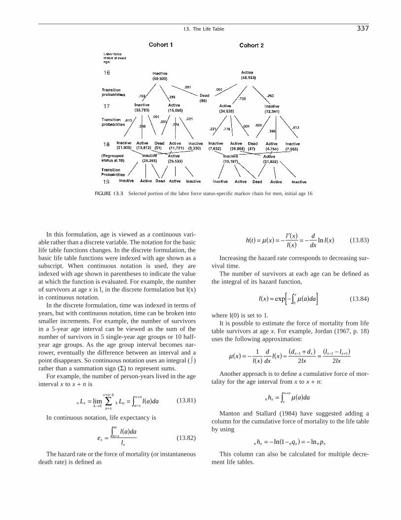
In this formulation, age is viewed as a continuous vari-able rather than a discrete variable. The notation for the basiclife table functions changes. In the discrete formulation, thebasic life table functions were indexed with age shown as asubscript. When continuous notation is used, they areindexed with age shown in parentheses to indicate the valueat which the function is evaluated. For example, the numberof survivors at age x is lx in the discrete formulation but l(x)in continuous notation.
In the discrete formulation, time was indexed in terms ofyears, but with continuous notation, time can be broken intosmaller increments. For example, the number of survivorsin a 5-year age interval can be viewed as the sum of thenumber of survivors in 5 single-year age groups or 10 half-year age groups. As the age group interval becomes nar-rower, eventually the difference between an interval and apoint disappears. So continuous notation uses an integral ( Ú )rather than a summation sign (S) to represent sums.
For example, the number of person-years lived in the ageinterval x to x + n is
(13.81)
In continuous notation, life expectancy is
(13.82)
The hazard rate or the force of mortality (or instantaneousdeath rate) is defined as
el a da
lx
a x
x
=( )
=Úw
n xk
k aa x
x n
a x
x n k
L L l a da= = ( )Æ =
+
=
+ -
ÚÂlim0
(13.83)
Increasing the hazard rate corresponds to decreasing sur-vival time.
The number of survivors at each age can be defined asthe integral of its hazard function,
(13.84)
where l(0) is set to 1.It is possible to estimate the force of mortality from life
table survivors at age x. For example, Jordan (1967, p. 18)uses the following approximation:
Another approach is to define a cumulative force of mor-tality for the age interval from x to x + n:
Manton and Stallard (1984) have suggested adding acolumn for the cumulative force of mortality to the life tableby using
This column can also be calculated for multiple decre-ment life tables.
n x n x n xh q p= - -( ) = -ln ln1
n xx
x nh a da= ( )
+
Ú m
m xl x
d
dxl x
d d
lx
l l
lxx x x x( ) = - ( ) ( ) ª
+( )=
-( )- - +12 21 1 1
l x a dax
( ) = - ( )[ ]Úexp m0
h t xl x
l x
d
dxl x( ) = ( ) = -
¢( )( ) = - ( )m ln
13. The Life Table 337
FIGURE 13.3 Selected portion of the labor force status-specific markov chain for men, initial age 16

Figure 13.4 compares the survival function lx to thehazard function hx for the U.S. abridged life table shown inTable 13.2. The number of survivors falls with increasingage, while the mortality hazard increases with age. Note that
this graph uses the approximation
References
Bell, F., A. Wade, and S. Goss. 1992. Life Tables for the United States SocialSecurity Area 1900–2080. Actuarial Study, No. 107. Office of theActuary, U.S. Social Security Administration. SSA Pub. No. 11-11536.
Carey, J. R. 1997. “What Demographers Can Learn from Fruit Fly Actu-arial Models and Biology.” Demography 34: 17–50.
Chiang, C. L. 1968. Introduction to Stochastic Processes in Biostatistics.New York: John Wiley and Sons.
Coale, A., and P. Demeny. 1966. Regional Model Life Tables and StablePopulations. Princeton, NJ: Princeton University Press.
Coale, A., P. Demeny, and B. Vaughn. 1983. Regional Model Life Tablesand Stable Populations. New York: Academic Press.
Dublin, L. I., A. J. Lotka, and M. Spiegelman. 1949. Length of Life. Rev.ed. New York: Ronald Press.
Dublin, L. I., and M. Spiegelman. 1941. “Current Versus Generation LifeTables, Human Biology, 13: 439–458.
Gregory, I. 1965. “Retrospective Estimates of Orphanhood from Genera-tion Life Tables.” Milbank Memorial Fund Quarterly 43(3): 323–348.
Greville, T. N. E. 1943. “Short Methods of Constructing Abridged LifeTables,” Record of the American Institute of Actuaries, 32(65): 29–42.
Greville, T. N. E. 1948. “Mortality Tables Analyzed by Cause of Death.”The Record, American Institute of Actuaries, Vol. 37, Part II, No. 76.
Hummer, R., R. Rogers, C. B. Nam, and C. G. Ellison. 1999. “ReligiousInvolvement and U.S. Adult Mortality.” Demography 36: 273–285.
Jacobson, P. H. 1964. “Cohort Survival for Generations Since 1840.”Milbank Memorial Fund Quarterly 42(3): 36–51.
m x hx+ÊË
ˆ¯ =
12
.
Jordan, C. W. 1967. Life Contingencies. Chicago: Society of Actuaries.Keyfitz, N. 1966. “A Life Table That Agrees with the Data.” Journal of the
American Statistical Association 61(314): 305–311.Keyfitz, N. 1968. “A Life Table That Agrees with the Data: II.” Journal of
the American Statistical Association 63(324): 1253–1268.Keyfitz, N., and W. Flieger. 1968. World Population: An Analysis of Vital
Data. Chicago: University of Chicago Press.Keyfitz, N., and W. Flieger. 1990. World Population Growth and Aging:
Demographic Trends in the Late 20th Century. Chicago: University ofChicago Press.
Keyfitz, N., and J. Frauenthal. 1975. “An Improved Life Table Method.”Biometrics, 31: 889–899.
Manton, K., and E. Stallard. 1984. Recent Trends in Mortality Analysis.Orlando, FL: Academic Press.
Olshansky, J., B. Carnes, and C. Cassell. 1990. “In Search of Methuselah:Estimating the Upper Limits to Human Longevity.” Science 250:634–640.
Preston, S., N. Keyfitz, and R. Schoen. 1972. Causes of Death: Life Tablesfor National Populations. New York: Seminar Press.
Reed, L. J., and M. Merrell. 1939. “A Short Method for Constructing an Abridged Life Table.” American Journal of Hygiene 30(2): 33–62.
Sirken, M. G. 1966. “Comparison of Two Methods of ConstructingAbridged Life Tables by Reference to a ‘Standard’ Table” (pp. 1–11).U.S. National Center for Health Statistics. Vital and Health Statistics,Series 2, No. 4 Revised.
Smith, S. 1982. Tables of Working Life: The Increment-Decrement Model. U.S. Bureau of Labor Statistics, Bulletin 2135.
Smith, S. 1986. Worklife Estimates: Effects of Race and Education. U.S.Bureau of Labor Statistics, Bulletin 2254.
Spiegelman. M. 1957. “The Versatility of the Life Table,” AmericanJournal of Public Health 47(3): 297–304.
United Nations. 1982. Model Life Tables for Developing Countries.ST/ESA/SerA/77. New York: United Nations.
U.S. Bureau of the Census. 1921. United States Life Tables, 1890, 1901,1910, and 1901–10. Washington, DC: Government Printing Office.
U.S. Bureau of the Census. 1936. United States Life Tables, 1930.
338 Kintner
FIGURE 13.4 Survivors of 100,000 births and force of mortality by age in life table for total United States, 1989–91
Suggested Readings
Part A Theory and Construction of Life Tables
Armstrong, R. J. 1998. “Methodology of the National and State Life Tables:1989–1991.” U.S. Decennial Life Tables for 1989–1991, vol. 1, no. 2.National Center for Health Statistics. Hyattsville, MD. DHHS Pub.PHS-98-1150-2.
Batten, R. W. 1978. Mortality Table Construction. Englewood Cliffs, NJ:Prentice-Hall.
Chiang, C. L. 1968. Introduction to Stochastic Processes in Biostatistics(Chapters 9–12). New York: John Wiley and Sons.
Chiang, C. L. 1984. The Life Table and Its Applications. Malabar, FL:Krieger.
Jacobson, P. H. 1964. “Cohort Survival for Generations Since 1840.”Milbank Memorial Fund Quarterly 42(3): 36–51.
Jordan, C. W. 1967. Life Contingencies. (Chapters 14 and 15). Chicago, IL:Society of Actuaries.
Keyfitz, N. 1966. “A Life Table That Agrees with the Data.” Journal of theAmerican Statistical Association 61(314): 305, 311.
Keyfitz, N. 1977. Introduction to the Mathematics of Population with Revi-sions. Part 1, “The Life Table.” Reading, MA: Addison-Wesley.
Keyfitz, N. 1968. “A Life Table That Agrees with the Data: II.” Journal ofthe American Statistical Association 63(324): 1253–1268.
Keyfitz, N. 1985. Applied Mathematical Demography, 2nd ed. New York:Springer Verlag.
Namboodiri, N. K., and C. M. Suchindran. 1987. Life Table Techniques andTheir Applications. Orlando, FL: Academic Press.
Preston, S., N. Keyfitz, and R. Schoen. 1972. Causes of Death: Life Tablesfor National Populations (Chapter 2). New York: Seminar Press.
Schoen, R. 1978. “Calculating Life Tables by Estimating Chiang’s a fromObserved Rates.” Demography 15: 625–635.
Sirken, M.G. 1966. “Comparison of Two Methods of ConstructingAbridged Life Tables by Reference to a ‘Standard’ Table.” U.S.National Center for Health Statistics. Vital and Health Statistics (pp.1–11), Series 2, No. 4 Revised.
Part B Applications, Multiple Decrement Tables,Cause-Elimination Tables, and Multistate Tables
Arriaga, E. E. 1984. “Measuring and Explaining the Change in LifeExpectancies.” Demography 21: 83–96.
Bongaarts, J. 1987. “The Projection of Family Composition over the LifeCourse with Family Status Life Tables. In J. Bongaarts, T. Burch, andK. Wachter (Eds.), Family Demography: Methods and Their Applica-tion (pp. 189–212). New York: Oxford University Press.
Hayward, M., W. R. Grady, and S. D. McLaughlin. 1988. “Recent Changesin Mortality and Labor Force Behavior among Older Americans: Con-sequences for Nonworking Life Expectancy.” Journal of Gerontology:Social Sciences 43: S194–S199.
Hoem, J. 1978. “A Markov Chain Model of Working Life Tables,” Scan-dinavian Actuarial Journal: 1: 1–20.
Ishikawa, A. 1994. “Abridged Working Life Tables for Japanese Men andWomen: 1990.” Jinko Mondai Kenkyu/Journal of Population Problems49: 57–70.
Keyfitz, N. 1977. “What Difference Would It Make If Cancer Were Erad-icated? An Examination of the Taeuber Paradox.” Demography, 14:411–418.
Kochanek, K. D., J. D. Maurer, and H. M. Rosenberg. 1994. “Causes ofDeath Contributing to Changes in Life Expectancy: United States,1984–1989,” Vital and Health Statistics 20(23). Hyattsville, MD: U.S.National Center for Health Statistics.
13. The Life Table 339
U.S. Bureau of the Census. 1946. United States Life Tables and ActuarialTables, 1939–41.
U.S. National Center for Health Statistics. 1963. Guide to United StatesLife Tables, 1900–59.
U.S. National Center for Health Statistics. 1964. U.S. Life Tables: 1959–61,vol. 1, no. 1.
U.S. National Center for Health Statistics. 1965. Life Tables: 1959–61, vol.1, no. 3, “Life Tables for the Geographic Divisions of the United States,1959–61.”
U.S. National Center for Health Statistics. 1966. U.S. Life Tables: 1959-61,vol. 2, nos. 1–51, State Life Tables. Hyattsville, MD: National Centerfor Health Statistics.
U.S. National Center for Health Statistics. 1967. U.S. Life Tables: 1959–61,vol. 1, no. 5. “Life Tables for Metropolitan and Nonmetropolitan Areasof the United States: 1959–6l.”
U.S. National Center for Health Statistics. 1968. U.S. Life Tables: 1959–61,vol. 1, no. 6, “United States Life Tables by Causes of Death, 1959–6l.”
U.S. National Center for Health Statistics. 1975. U. S. Decennial Life Tablesfor 1969–71, vol. 1, no. 1, U.S. Decennial Life Tables. DHEW Pub. No.HRA 75-1150.
U.S. National Center for Health Statistics. 1977. U.S. Decennial Life Tablesfor 1969–71, vol. 2, nos. 1–51, State Life Tables. Hyattsville, MD:National Center for Health Statistics.
U.S. National Center for Health Statistics. 1985a. U.S. Decennial LifeTables for 1979–81, vol. 1, no. 1, U.S. Decennial Life Tables. DHHSPub. No. PHS 85-1150-1. Washington, DC: U.S. Government PrintingOffice.
U.S. National Center for Health Statistics. 1985b. U.S. Decennial Life Tablesfor 1979–81, vol. 1, no. 2, “U.S. Life Tables Eliminating Certain Causesof Death”. By L. Curtin and R. Armstrong. DHHS Pub. No. PHS 86-1150-2. Washington, DC: U.S. Government Printing Office.
U.S. National Center for Health Statistics. 1990. U.S. Decennial Life Tablesfor 1979–81, vol. 2, nos. 1–51, “State Life Tables.” Hyattsville, MD:National Center for Health Statistics.
U.S. National Center for Health Statistics. 1997a. United States DecennialLife Tables for 1989–91, vol. 1, no. 1. “U.S. Life Tables.” DHHS Pub.No. PHS-98-1150-1. Hyattsville, MD.
U.S. National Center for Health Statistics. 1997b. United States DecennialLife Tables for 1989–91, vol. 1, no. 2. “Methodology of the Nationaland State Life Tables.” DHHS Pub. No. PHS-98-1150-2. Hyattsville,MD.
U.S. National Center for Health Statistics. 1998. U.S. Decennial Life Tablesfor 1989–91, vol. 2, nos. 1–51, “State Life Tables.” Hyattsville, MD:National Center for Health Statistics.
U.S. National Center for Health Statistics. 1999. U.S. Decennial Life Tablesfor 1989–91, vol. 1, no. 4, “U.S. Life Tables Eliminating Certain Causesof Death.” Hyattsville, MD: National Center for Health Statistics.
U.S. National Office of Vital Statistics, 1947. Vital Statistics-SpecialReports, Selected Studies, vol. 23, no. 11, “U.S. Abridged Life Tables,1945.”
U.S. National Office of Vital Statistics. 1948. State and Regional LifeTables, 1939–41.
U.S. National Office of Vital Statistics, 1954. Vital Statistics-SpecialReports, Life Tables for 1949–51, vol. 41, no. 1, “United States LifeTables, 1949–51.”
U.S. National Office of Vital Statistics, 1956a. Vital Statistics-SpecialReports, vol. 41, Supplement, State Life Tables: 1949–51.
U.S. National Office of Vital Statistics. 1956b. Vital Statistics-SpecialReports, Life Tables for 1949–51, vol. 41, no. 4, “Life Tables for theGeographic Divisions of the United States. 1949–51.”
Zelnik, M. 1969. “Age Patterns of Mortality of American Negroes:1900–02 to 1959–61,” Journal of the American Statistical Association64(326): 433–434.

Land, K., J. Guralnik, and D. Blazer. 1994. “Estimating Increment-Decrement Life Tables with Multiple Covariates from Panel Data: TheCase of Active Life Expectancy.” Demography 31: 297–319.
Land, K., G. Hough, and M. McMillen. 1986. “Voting Status Life Tablesof the United States, 1968–1980.” Demography, 23: 381–402.
Lee, E. S., and G. K. Bowles. 1954. “Selection and Use of Survival Ratiosin Population Studies.” Agricultural Economics Research 6(4):120–125.
Long, L. H. 1973. “New Estimates of Migration Expectancy in the UnitedStates.” Journal of the American Statistical Association 68(341): 37–43.
Manton, K., and E. Stallard, 1984. Recent Trends in Mortality Analysis.Orlando, FL: Academic Press.
Namboodiri, N. K., and C. M. Suchindran. 1987. Life Table Techniques andTheir Applications (Chapters 6–9). Orlando, FL: Academic Press.
Pollard, J. H. 1988. “On the Decomposition of Changes in Expectation ofLife and Differentials in Life Expectancy.” Demography 25: 265–276.
Rogers, A. 1995. Multiregional Demography: Principles, Methods andExtensions. New York: J. Wiley and Sons.
Rogers, R., A. Rogers, and A. Belanger. 1989. “Active Life among theElderly in the United States: Multistate Life table Estimates and Popu-lation Projections.” The Milbank Quarterly 67: 370–411.
Schmertmann, C. P., A. Amankwaa, and R. Long. 1998. “Three Strikes andYou’re Out: Demographic Analysis of Mandatory Prison Sentencing.”Demography 35: 445–463.
Siegel, J. S. 2002. Applied Demography: Applications to Business, Gov-ernment, Law, and Public Policy (Chapters 7, 8, and 13). San Diego:Academic Press.
Stockwell, E. G., and C. B. Nam. 1963. “Illustrative Tables of School Life.”Journal of the American Statistical Association 58(304): 1113–1124.
Willekens, F. 1987. “The Marital Status Life Table.” In J. Bongaarts, T.Burch, and K. Wachter (Eds.), Family Demography: Methods and TheirApplication, (pp. 125–149). New York: Oxford University Press.
Wolf, D. A. 1988. “The Multi-State Life Table with Duration Dependence.Mathematical Population Studies, 1: 217–245.
Wood, J., D. Holman, A. Yashin, R. Peterson, M. Weinstein, and M. Chang.1994. “A Multi-state Model of Fecundability and Sterility.” Demogra-phy 31: 403–426.
Yashin, A., I. Iachine, K. Andreev, and U. Larsen. 1998. “Multistate Modelsof Postpartum Infecundity, Fecundability and Sterility by Age andParity: Methodological Issues.” Mathematical Population Studies, 7:51–78, 109–110.
340 Kintner

NATURE AND USES OF HEALTH STATISTICS
Health is a leading characteristic of the members of a population, akin to other demographic and socioeconomiccharacteristics. It is an important correlate of other demo-graphic and socioeconomic characteristics as well. Forexample, health statistics are often used in interpretingtrends in mortality and in designing assumptions for makingprojections of mortality. Moreover, health has often been thesubject of inquiry in population surveys and censuses.
In recent decades, the conceptualization of populationhealth has extended beyond measures of mortality (e.g., life expectancy, infant mortality) to include specific healthmeasures such as the incidence or prevalence of morbid con-ditions, or summary measures of health such as healthy lifeexpectancy and health-related quality of life. This extensionof population health is due in part to secular trends ofincreased life expectancy, which has shifted the focus of population health from the quantity of life to the qualityof life, defined in a number of different ways. The WorldHealth Organization (WHO) and various research organiza-tions have worked to develop and promote summary mea-sures of population health that combine measures ofmortality and measures of health conditions to represent thestate of a population’s health in a single number. Summarymeasures of population health are important because of thevarious types of potential applications, as enumerated byMurray, Salomon, and Mathers (1999, pp. 3–4):
1. Comparing the health of one population with the healthof another population
2. Comparing the health of the same population at differ-ent points in time
3. Identifying and quantifying health inequalities withinpopulations
4. Providing appropriate and balanced attention to theeffects of nonfatal health conditions on overall popula-tion health
5. Informing debates on priorities for health service delivery and planning
6. Informing debates on priorities for research and devel-opment in the health sector
7. Improving professional training curricula in publichealth
8. Analyzing the benefits of health interventions for use incost-effectiveness analyses
In addition, the WHO has initiated a new global healthpolicy that aims to meet the major health problems andissues in the new century. The health policy initiative,“Health for All in the 21st Century” (HFA), was establishedto improve global health and reduce health inequities within and between countries through the development ofhealth priorities and targets for the first two decades of the21st century. Member countries have been encouraged to settheir own goals in relation to the HFA goals. In the UnitedStates, “Healthy People 2010” has been launched to meettwo overarching goals: to increase the quality of the yearslived and years of healthy life, and to eliminate health dis-parities (U.S. Department of Health and Human Services,2000a, p. 2).
U.S. goals target leading health indicators, includingthose for morbid conditions, lifestyle habits, and access tohealth care. The measurement of the incidence and preva-lence of morbid conditions, particularly chronic/degen-erative diseases, age at onset, case-fatality rates, and thephysical and emotional effects of health conditions havebecome increasingly important concerns in understandingpopulation health. Thus, there is a need for a broader arrayof health statistics to represent the occurrence and distribu-tion of health conditions to characterize population health.
341
C H A P T E R
14
Health Demography
VICKI L. LAMB AND JACOB S. SIEGEL
The Methods and Materials of DemographyCopyright 2003, Elsevier Science (USA).
All rights reserved.
DEFINITION OF CONCEPTS
Health
It is difficult to define health in operational terms becausehealth is multidimensional and, in part, socially defined. TheWorld Health Organization gave health a positive definitionin its Constitution in 1946: “Health is a state of completephysical, mental, and social well-being and not merely theabsence of disease or infirmity.” The definition of health hasbeen both broadened (Mahler, 1981) and sharply narrowed(Dubos, 1968, Chapter 4). The latter defined health as “amodus vivendi enabling imperfect men to achieve a reward-ing and not too painful existence while they cope with animperfect world.” In spite of efforts to quantify health status,for the most part health is measured in terms of its converse,such as disease, disability, and death.
Health Conditions
Several general terms are employed to indicate a lack ofgood health, such as disease, illness, health condition, andmorbid condition, and the definitions overlap. Disease refersto the biophysical state of ill health, whereas illness is thesocial experience of being sick or diseased. Morbidityis a broad term for any health condition. As such, mor-bidity encompasses diseases, injuries, and impairments.More specifically, morbidity encompasses acute conditions(including acute illnesses and injuries) and chronic condi-tions (including chronic illnesses and impairments). Theterms acute and chronic do not have precise definitions butare distinguished on the basis of the duration and the typeof health condition considered. An acute condition typicallyhas a rapid onset, has a relatively short duration, and usuallyends with either recovery or death. A chronic conditionusually involves a lengthy period of evolution and progres-sion, has a long duration, and is considered relativelyintractable to treatment. Infectious diseases, for example, areusually classified as acute, while cardiovascular diseases areclassified as chronic. Impairments are chronic conditionsinvolving abnormalities of body structure and appearance,the most common being chronic sensory and musculoskele-tal conditions. Comorbidity is a term referring to multiplechronic conditions in one individual.
The classification of morbid conditions used by nationalgovernments follows the same classifications recommendedabout every 10 to 20 years by the World Health Organiza-tion for the classification of causes of death. The tenth revision of the International Statistical Classification of Diseases and Related Problems (ICD-10) was published bythe WHO in 1992–1994. The ninth revision remained gen-erally in effect in 1998, however. The United States shiftedto the new classification beginning in 1999. Major changesbetween ICD-9 and ICD-10 are that ICD-10 (1) includes
more detailed categories (8000 versus 5000), (2) usesalphanumeric rather than numeric codes, and (3) changessome of the rules for coding and for the classification ofunderlying cause of death (U.S. National Center for HealthStatistics/Anderson et al., 2001a).
The ICD includes classifications for mental illnesses aswell as physical illnesses. Chapter V of ICD-10, “Mentaland Behavioral Disorders,” provides clinical descriptions inaddition to diagnostic guidelines. In the United States a sep-arate publication, The Diagnostic and Statistical Manual ofMental Disorders (DSM-IV, American Psychiatric Associa-tion, 1994), also gives a classification of mental illnesses.The codes and terms provided in DSM-IV are fully compat-ible with ICD-10. According to Mausner and Kramer (1985,p. 25), in the system of classification of mental disorders,the clinician assigns a category on the basis of observationsrelating to clinical syndromes, personal disorders, physicaldisorders and conditions, severity of psychosocial stressors,and highest level of adaptive functioning during the previ-ous year.
A disability refers to an acute or chronic condition thataffects an individual’s ability to function and carry out hisor her activities. The U.S. National Health Interview Surveydefines disability as “any temporary or long-term reductionof a person’s activity as a result of an acute or chronic con-dition.” It refers, therefore, to the consequences of healthconditions. It is useful to distinguish those disabilities thatcan be managed in part or on the whole by technologicaldevices and structural changes in the community and thosethat cannot. Such a distinction can aid in defining degreesof disability, from slight to moderate to severe.
In 1980 the World Health Organization issued the International Classification of Impairments, Disabilities,and Handicaps (ICIDH). It was developed to model andstandardize concepts in the disablement process. Becausedisability is viewed as a consequence of disease, and theidentification of a disease does not adequately portray thefull consequences of the condition, the ICIDH was to be anextension of the ICD scheme. In the ICIDH scheme, animpairment refers to a loss or abnormality of psychologicalfunction or physiological or anatomical structure or func-tion; a disability is a restriction or inability to perform anactivity in the range considered normal for a person; and ahandicap is a limitation or inability to perform one’s socialrole(s) due to an impairment or disability (World HealthOrganization, 1980).
The current ICIDH scheme has been difficult to use fora number of reasons: (1) the overlaps between the variousconcepts, especially between disability and handicap, (2) thelack of clarity about the specific meanings associated withthe categories, (3) the difficulty in applying the classifica-tion scheme to various theories and models of disablement,(4) the difficulty in adapting currently collected health datato conform with the ICIDH framework, and (5) the failure
342 Lamb and Siegel

of the ICIDH scheme to encompass the possibility for rever-sals, reductions in severity, or recovery.
Since 1995 there have been efforts to revise the ICIDHframework and definitions. A new version of the ICIDH,renamed the International Classification of Functioning,Disability and Health (WHO, 2001), has been published.The new ICF is restructured to capture both the positive and negative aspects of functioning and focuses on (1) bodyfunctions and body structures, (2) activities performed by anindividual, and (3) participation in, and classification of, theareas of life in which an individual is involved. In addition,environmental factors are also part of the new classificationscheme. “Environmental factors” is broadly defined andencompasses “assistive” products and technologies, thenatural environment and human changes to the environment,support and relationships provided by people and animals,attitudes and beliefs, and formal services, governmentalsystems, and policies that affect the disabled.
SOURCES OF DATA FOR HEALTHSTUDIES AND QUALITY OF
HEALTH STATISTICS
Health data can be obtained both from the general sourcesfor demographic data, such as censuses, vital statistics reg-istrations, and general sample surveys, and from specializedsources, such as sample surveys on health, administrativerecords on health (e.g., disease registries), epidemiologicalstudies, and clinical trials. These sources all provide quan-titative data on health. We consider each of these in turn andthen comment briefly on qualitative sources of informationon health. The U.S. Department of Health and Human Services periodically publishes an International HealthData Reference Guide (e.g., U.S. Department of Health andHuman Services, 2000b), which presents an overview ofinternational health data from vital statistics, hospital sta-tistics, health personnel statistics, and population-basedsurveys. The purpose of the guide is to provide informationabout sources of health data around the world useful for sup-porting international studies and comparisons of populationhealth.
Censuses
Periodically, population censuses have obtained informa-tion regarding conditions that we now term sensory, physi-cal, and mental impairments. The 1830 U.S. census was thefirst U.S. census to contain questions intended to determinethe number of persons who were “deaf, dumb, or blind.” The 1840 U.S. census added the category of “insanity.”Recent censuses of the United States (1980, 1990, and 2000) have had questions on activity limitations with re-spect to work, use of transportation, or personal care. The
2000 U.S. census, for example, asked the following yes/noquestions:
Does this person have any of the following long-lastingconditions:
a. Blindness, deafness, or a severe vision or hearingimpairment?
b. A condition that substantially limits one or morebasic physical activities such as walking, climbingstairs, reaching, lifting, or carrying?
Because of a physical, mental, or emotional conditionlasting 6 months or more, does this person have any diffi-culty in doing any of the following activities:
a. Learning, remembering, or concentrating?b. Dressing, bathing, or getting around inside the
home?c. (Answer if this person is 16 years old or over.)
Going outside the home alone to shop or visit adoctor’s office?
d. (Answer if this person is 16 years old or over.)Working at a job or business?
Demographers have used both historic (Costa, 2000;Elman and Myers, 1997, 1999) and recent (Geronimus et al.,2001; Hayward and Heron, 1999) U.S. census data toexamine trends in health and health expectancy in the UnitedStates.
Vital Statistics and Administrative Records
The various registration systems constituting the totalvital registration system for a country produce several setsof data directly or indirectly related to health, including dataon births and deaths, and possibly fetal losses, induced terminations of pregnancy, the health conditions associatedwith these events, marriages, and divorces.
Administrative records may be maintained as a surveil-lance device for health conditions or use of health care serv-ices. Such records include disease registries and health careutilization records. State and provincial health departments,and public and private research organizations, often main-tain files on communicable diseases and selected chronicconditions. For example, the U.S. National Cancer Institutesupports a cancer registry, and the U.S. National Heart,Lung, and Blood Institute supports a pediatric cardiomy-opathy registry. The latter is a national registry of childrenwith different forms of cardiomyopathy and is designed tomeasure the relative frequency of the disease, to describe thesurvival experience of the patients, to advance knowledgeof its causes, and to identify new diagnostic and therapeuticprocedures (New England Research Institute, 1996).
Health care utilization records are usually maintained bythe agencies that administer health programs. The Centersfor Medicare and Medicaid Services (formerly the HealthCare Financing Administration) in the United States
14. Health Demography 343

maintains complete records of conditions reported forMedicare claims and State Departments of Health maintainrecords for Medicaid claims. The former is the program ofnational health insurance for the elderly, and the latter is theprogram of public medical care for the indigent.
General Sample Surveys and National Health Surveys
General sample surveys not specifically designed ashealth surveys, such as the Current Population Survey andthe Survey of Income and Program Participation in theUnited States, occasionally carry questions on health, suchas on work disability or functional status, to accompany theprincipal questions on labor force participation and income.
An increasing number of countries conduct periodicsurveys specifically devoted to health. Examples of population-based health surveys are the National HealthInterview Survey of the United States, the National HealthInterview Survey in the Netherlands, the Götebörg Study inSweden, and the Health Survey for England. These surveyssecure their data by interviewing the general population,conducting actual physical tests, or reviewing medicalrecords.
The U.S. Agency for International Development hasfunded a set of Demographic and Health Surveys (DHS) in less developed countries. ORC Macro conducts thesesurveys. Since 1985, more than 100 surveys have been con-ducted in Africa, Asia, the Near East, Latin America, and theCaribbean (see Table 14.1). Typically, a DHS is a nationallyrepresentative sample of between 5000 and 30,000 house-holds, with a focus on women between the ages of 15 and49. These surveys deal with subjects such as contraceptivepractices, breast-feeding, lifetime reproductive behavior,HIV/AIDS and other sexually transmitted diseases (STDs),health characteristics of children (e.g., height, weight,immunization, diarrhea, fever), women’s work history, andbackground information about the husband. These data areused to provide information and analyses of the state ofhealth of women and children in less developed countries.
The World Health Organization, the United Nations, andU.S. National Institutes of Health have sponsored numeroushealth surveys in less developed countries. These surveysare cross-sectional, secure data by self-reports, and usuallyrelate to specific diseases and the elderly.
Epidemiological Studies
Epidemiological studies are concerned with the distribu-tion of diseases, injuries, and impairments in human popu-lations and the possible risk factors associated with them.The goal is to identify the determinants of the diseases andto devise programs of disease prevention and control. Epi-demiological studies are a principal tool of community
or population medicine, which has the community as itsprimary object of concern.
There are several different types of epidemiologicalstudies, each with many variants. In case-control studies, agroup of patients with a disease under study is matched bya group of healthy persons (the controls) on the basis of avariety of criteria including age, sex, race, and socioeco-nomic characteristics. Such studies try to identify other char-acteristics that distinguish the two groups. In longitudinalstudies, a group that does not have the particular disease is selected for the study of the disease; base data on demographic, socioeconomic, and health characteristics aresecured; and the group is followed up to see who developsthe disease being studied and to ascertain their distin-guishing characteristics. When the same individuals are canvassed over time, the study is designated a panel study.When the same population is canvassed, the study is desig-nated a cohort study. Some studies mix features of case-control studies and longitudinal studies.
In community studies, random samples of a populationor population groups may be studied alone or as paired units(one being a control). Schools or even cities may be the pop-ulation units sampled. The sample in one city may be sub-jected to the health program being tested, while the samplein another city is not. A sample of schools in a city may bedivided into schools subject to the treatment program and
344 Lamb and Siegel
TABLE 14.1 Demographic and Health Surveys Conductedby Macro International, Inc., and National Agencies with
Support of the U.S. Agency for International Development:1985 to 2001
Number of Number ofContinent and region countries surveys
All areas 66 118
Africa 35 60Western Africa 121 22Middle Africa 4 5Eastern Africa 14 24Southern Africa 2 2North Africa 3 7
Asia 18 30West Asia 4 7Central Asia 4 5South Asia 5 9Southeast Asia 5 9
Latin America and Caribbean 13 28Caribbean 3 6Central America2 4 6South America3 6 16
1 One from Ondo State, 1986.2 Includes Mexico, 1987.3 Includes Northeast Region of Brazil, 1991.Source: ORC Macro, 2002.

those used as controls. Alternatively, all schools in a citymay be included in a study, with a sample of students in eachschool subject to the program and another sample in thatschool carried as controls. In another variation, a singlesample of the population may be followed longitudinallyand examined before and after a health program is put intoeffect. In designing health surveys, the investigator shouldplan to inquire about a basic set of descriptive variables,such as age, sex, race, and socioeconomic status, and a morespecialized set of variables relevant to the specific study.
Clinical Trials
The purpose of clinical trials is to evaluate the efficacyof a treatment protocol for humans compared with no treat-ment or an alternative treatment. Clinical trials accompanythe practice of clinical medicine, which deals with themedical care of individuals. Clinical medicine contrasts withbasic research in a laboratory on animals, and with commu-nity medicine, which as noted earlier, oversees the health ofcommunities.
A clinical trial must be carefully controlled for the resultsto be valid. The method normally uses double-blind ran-domized samples to compare medical treatments. In thisdesign, called randomized clinical trials, one experimentalgroup receives the treatment being tested and anothercontrol group receives a placebo or dummy treatment, andneither the subjects nor the researchers know who is in theexperimental group and who is in the control group.
One type of clinical trial, called an interventional trialwith sequential design, in which the responses have a binaryoutcome, uses data for pairs of patients, each receiving one of the two treatments (e.g., drugs) being compared. Discordant pairs, where the treatment effect differs for themembers of the pair, provide the basis for preferring onetreatment to the other. In this methodology, a relatively smallnumber of examinations of the data are made during thecourse of the trial and repeated significance testing is carriedout. The investigator may discontinue the trial use of thetreatment (i.e., a drug) or give it to all subjects if a suffi-ciently large difference is observed during the course of thetrial.
Qualitative Sources
Quantitative methods provide most of the data and ana-lytic information about health, but qualitative methods areused in a variety of ways to support quantitative research.Specifically, qualitative methods may be used to plan quan-titative studies, either to develop the questionnaire or todevelop hypotheses about the relevant factors, and to inter-pret the results of the quantitative analysis. Case studies andfocus-group discussions represent two widely used qualita-tive methods employed in health studies.
Ethnographic research, another qualitative method, canbe used to construct models of “regional” (i.e., geographic,ethnic, class) illnesses, including their symptoms and etiol-ogy, by gathering data about the terminology used for dif-ferent conditions and about folk methods of prevention,diagnosis, and treatment. Measures of self-assessed healthcan be greatly improved by developing questionnaires andinstructional material that take into account regional viewsas to good health, by educating health providers in the mostaccurate ways of reporting illness, and by educating indi-viduals in the community about health matters (Obermeyer,1996).
PROBLEMS WITH HEALTH DATA SOURCES
Census and Survey Data, Vital Statistics, and Administrative Records
Census data, as is true of all survey data, are subject toerrors of coverage and errors of classification. The under-counting of certain groups, such as particular age groups,some racial minorities, economically disadvantaged per-sons, and certain types of households particularly affectcensus data. Similarly, vital statistics and administrativerecords may sometimes be seriously incomplete and inade-quate in other ways, particularly in less developed countries.In deference to using inadequate records, other sources ofdata should be employed to measure health outcomes andservices, or the sources should be adjusted, to the extent pos-sible, to allow for statistical deficiencies.
Information gathered via survey methods, whether theyare general, health, or epidemiological surveys, share anumber of problems. The health-related information is gath-ered via self-reports, and the data may be biased for anumber of reasons. These biases may vary for gender, race,education, social status, and the availability of health insur-ance. In addition, the data on health conditions are typicallyobtained via probes for the specific conditions, and someconditions may not be documented.
Another aspect of unreliable reporting by respondents,particularly persons with little education, is that they maygive overly favorable reports of their current health status ormay not recall previous health conditions accurately. Moreeducation is associated with greater awareness of healthproblems, higher utilization of health services, and, as aresult, possibly higher reporting of morbidity. A problemcommon to all morbidity studies is the discrepancy betweenobjective indicators of health and subjective reports. If adisease is not life threatening, it may be considered of littleimportance from a medical point of view but consideredquite disabling by the individual in a self-assessment ofhealth. Moreover, respondents tend to interpret their health
14. Health Demography 345

status in relation to their own view of normal health andwell-being. The respondent may be too accepting of painand dysfunction, or the opposite.
These problems are particularly evident in the area ofreproductive morbidity (discussed more fully later in thischapter). The problem of consistency between objectiveindicators and subjective reporting of health is aggravatedby the gap between the understanding of illnesses in somenon-Western countries and the biomedical categories of dis-eases. It is not uncommon for views of an illness in thesecountries and the biomedical categories for the illness to beat odds.
Missing reports present another problem in that suchreports are not well represented by the actual reportsreceived. Persons who do not report their health status aremore likely to be suffering from a health condition, or amore severe health condition, than those who do report theircondition, or to be disabled, or more severely disabled, thanthose who do report their condition. It is better, therefore, touse methods of imputing the missing data on the basis ofsample follow-up studies and other data than to assume thatthe missing data are randomly distributed or distributed likethe reported cases.
Multicollinearity (i.e., correlation of risk factors) mayconfound the results of analyses. If a factor is being testedand it is correlated with another factor that may truly beexerting a cause-effect influence, the effect may erroneouslybe attributed to the factor being tested. A study may be inter-preted to show that eating green vegetables reduces the riskof heart disease, but people who eat green vegetables mayalso exercise regularly and be more health conscious. Hence,the cause of the reduction in heart disease may be eatinggreen vegetables, exercising frequently, being health con-scious, or all in combination.
Epidemiological Studies and Clinical Trials
Epidemiological studies have important limitations orpotential limitations. They cannot definitively prove a cause-effect relation between so-called risk factors and the disease;at best, they show a probable cause-effect relation. Riskassessment in epidemiological studies is more likely to bevalid if the association is strong (e.g., smoking and lungcancer) than when it is weak. Moreover, the sample may bebiased and not representative of the universe from which itwas drawn (e.g., based only on listed telephone subscribers)or may not represent the larger population (e.g., based onlyon adult white males).
The problem of censoring is usually present in epidemi-ological studies. It arises from the fact that the actual dateof the onset of a health condition cannot be known, only theprior examination date and the date when the health condi-tion was identified. For example, an epidemiological study
may seek to identify risk factors for infection and the pro-gression from infection to clinical disease. In HIV, the exacttime of infection is not known, but it could be set as fallingin the interval between the last negative blood test and thefirst positive blood test. The data for this period aredescribed as interval censored, and the data for the infectiontime are described as left censored. Some subjects who willget the disease (AIDS) would not have been diagnosed withit at the time it occurred or at the time of the study; the datafor them are right censored. Similarly, the period betweenthe actual time of infection and the actual time of onset ofdisease, the latency period, cannot be fixed closely becauseneither the first date nor the last date is known. Data for thelatency period are censored both on the left and the right, ordoubly censored. It is often the case that a study does notrun long enough to reveal the full effects of a factor on allparticipants (e.g., the effect of low consumption of calciumin the diet on osteoporosis).
Clinical trials have their limitations or potential limita-tions. In clinical trials, as in epidemiological studies, thesample is often limited to a particular segment of the popu-lation (e.g., middle-aged white males, nurses), and underthese conditions, the results cannot safely be generalized tothe whole population.
MEASURES OF HEALTH STATUS,FUNCTIONING, AND USE OF
HEALTH SERVICES
Measures of Health Status
Measures of health may be based on either subjectiveinformation on health conditions or objective information.For example, the percentage of respondents assessing theirhealth as poor, fair, good, or excellent is a commonly usedsubjective measure. However, many health measures arebased on respondents’ self-reports of actual health condi-tions, after a diagnosis by a health professional.
Prevalence Ratios and Incidence Rates
The measures differ also as to whether they refer to thehealth status of a population group at some date or to healthevents occurring to an exposed population over a year orsimilar period. The former are called measures of preva-lence, and the latter are called measures of incidence.
When data are available, we can compute prevalenceratios for acute illnesses, chronic illnesses, injuries, orimpairments, or these conditions can be incorporated into ageneral prevalence ratio for acute conditions (acute illnessesand injuries) and a general prevalence ratio for chronic conditions (chronic conditions and impairments). The
346 Lamb and Siegel

prevalence ratio for an acute disease is the percentage ofpersons with the acute disease at a specific date. Table 14.2shows prevalence ratios for two acute childhood conditionsfor most countries of sub-Saharan Africa for various yearsfrom 1991 to 2000. In addition to measures for the total pop-ulation, measures for the noninstitutional population and the institutional population are often computed separatelybecause of the difference in the sources of the data and thenotably different levels of the measures.
Incidence rates for specific conditions may be computedas the number of persons incurring a particular health
condition during a year, or the number of particular healthconditions incurred during a year, per 100,000 persons. Incidence measures roughly parallel the various types ofprevalence measures. The most common measures are theincidence rate for acute illnesses, either the number ofpersons incurring an acute illness during a year or thenumber of acute illnesses incurred during a year, per100,000 persons, and the incidence rate for chronic ill-nesses, either the number of persons incurring a chronicillness during a year or the number of chronic illnessesincurred during a year, per 100,000 persons. Separate ratescan be computed for acute illness, injury, chronic illness, andimpairments. For example, we may compute the number ofpersons incurring an injury during a year, or the number ofinjuries in a year, per 100,000 persons. The latter measureis also labeled the number of episodes of injuries during ayear per 100,000 persons. The incidence rate for an acute orchronic condition is calculated simply by
(14.1)
where Ic represents the number of acute or chronic condi-tions occurring during the year and P the number of personsin the population. Table 14.3 shows incidence rates forseveral types of cancers for six countries in East Asia for2000.
The average duration of illness refers to the period oftime that a condition lasts. The relation between an inci-dence rate and a prevalence ratio for a given year may berepresented roughly by
(14.2a)
(14.2b)
For example, if the incidence rate of an illness is 200 per100,000 population and the prevalence ratio equals 1000 per100,000 population, then the average duration of the illnessis roughly 5 years. The precise relation is affected by theannual fluctuations in the incidence rate and by the survivalrate of those who have incurred the condition—the case-fatality rate (explained below)—in the several years prior tothe year of reference.
Age-Specific and Cause-Specific Prevalence Ratios andIncidence Rates
A type of cause-specific measure, the case-fatality rate,determines, on a cross-sectional basis, what proportion ofpersons having a disease or injury die from it during a year.It is the ratio per 100 of the deaths from the disease or injuryduring the year to the persons who have the disease or injuryat the middle of the year:
Average duration of illness
prevalence ratio/ incidence rateª
Prevalence ratio
incidence rate average duration of illnessª *
IR I PC C= ∏( ) *100 000,
14. Health Demography 347
TABLE 14.2 Prevalence Ratios for Two Infectious Conditionsof Children Under Age 5 in Most Countries of Sub-Saharan
Africa: Selected Years, 1991 to 2000 (Percentage of childrenunder age 5 reported as having the health condition at the
time of the survey.)
Acute respiratoryCountry and year tract infection Diarrhea
Benin, 1996 15.7 26.1Botswana, 2000 38.5 6.5Burkina Faso, 1999 13.5 20.01
Cameroon, 2000 7.0 18.92
Central African Republic, 1995 28.2 26.51
Chad, 2000 12.5 31.2Comoros, 2000 10.1 18.3Cote d’Ivoire, 2000 3.7 20.1Eritrea, 1995 23.0 23.6Ethiopia, 2000 24.4 23.6Gambia, 2000 7.7 21.5Ghana, 1998 13.8 17.9Guinea Bissau, 2000 10.1 31.5Guinea, 1999 15.9 21.2Kenya, 1998 20.1 17.1Madagascar, 2000 10.5 12.8Malawi, 1996 12.3 16.1Mali, 1996 15.3 25.3Mauritania, 1991 12.0 28.61
Mozambique, 1997 11.8 20.7Namibia, 1992 18.0 20.6Niger, 2000 11.8 40.0Nigeria, 1999 11.3 15.3Rwanda, 1992 32.6 21.8Senegal, 2000 6.6 21.31
Sierra Leone, 2000 8.7 25.3Tanzania, 1999 13.9 12.4Togo, 1998 20.2 31.1Uganda, 1995 27.1 23.5Zambia, 1996 12.7 23.5Zimbabwe, 1999 15.8 13.9
1 For 1996.2 For 1998.Note: The prevalence of acute respiratory tract infection and diarrhea
often varies by season. Country surveys were administered at differenttimes and, hence, the prevalence data are not fully comparable across countries.
Source: UNICEF, 2001.

(14.3)
where Dc represents the number of deaths from the causeand Pc is the number of persons having the same health con-dition. A study of the “Global Burden of Tuberculosis” (Dyeet al., 1999) estimated the global case-fatality rate for tuber-culosis as 23. However, the case-fatality rate exceeded 50 in African countries with high rates of HIV infection. Thismeasure can be restructured in cohort form as the propor-tion of persons having a disease or injury at the beginningof a year who die from that disease or injury during the subsequent year. A reduction in the case-fatality rate of adisease or injury would tend to increase the prevalence ofthe disease, and this effect would also occur if there was anincrease in the average duration of the condition. Such rela-tions have important implications for the analysis of the relative costs of death and illness and hence the costs of adisease-prevention program.
All of these measures can be calculated for the entire population or a particular segment of it, such as an agegroup. Hence, we can calculate age-cause-specific preva-lence ratios and age-cause-specific incidence rates:
(14.4)
where IR represents the incidence rate, cr is respiratorycancer, sa is the sex-age group, and P is the population. Forexample, the incidence rate for cancer of the respiratorysystem in 1999, for U.S. males aged 60 to 64, was 291.4 per100,000 (NAACCR, 2001). Thus,
Age-Adjusted Measures and Probabilities
Just as there are age-adjusted or age-standardized measures of mortality, there are age-adjusted measures of
cr mIR , – , , , .60 64 7685 2 637 268 100 000 291 4= ∏( ){ } * =
cr sa cr sa saIR I P= ∏( ) *100 000,
CFR D Pc c= ∏( )*100 morbidity. These are summary measures representing theweighted combination of age-specific ratios or rates ofillness, injury, and impairment, employing common age distributions as weights for the populations being compared.We can calculate morbidity ratios and morbidity ratesadjusted for age following the procedures given in Chapter 12.
Central age-specific rates may be converted to probabil-ities of incurring an illness, injury, or impairment during ayear. For single ages,
(14.5a)
or, more exactly,
(14.5b)
where c and nc refer, respectively, to persons having thehealth condition and those not having it. Central age-specific measures may also be converted to transition prob-abilities for use in constructing tables of healthy life (see thediscussion that follows). Such probabilities represent theproportion of the population in each health status at a givendate that will be located in the same or another health statusat some subsequent date (e.g., a year later) or die during theperiod.
Measures of Functioning
There are numerous measures of health that focus onwhat one cannot do or has difficulty doing because of healthconditions. As noted previously, a health condition thatlimits functioning is termed a disability. Early measures ofdisability were based on questions about limitations in performing one’s “major activity” due to health reasons insurveys such as the U.S. National Health Interview Survey
c a nc a nc a c aI P D I∏ + +( ){ } *12
12 100
c ap
c a a aIR I P D= ∏ +( ){ }12 100*
348 Lamb and Siegel
TABLE 14.3 Incidence Rates for Specified Types of Cancer, by Sex, for Eastern Asian Countries:2000 (Incidence rates represent the number of new cases of the health condition reported during
the year per 100,000 persons.)
Country and sex Melanoma Colon/Rectal Stomach Lung Leukemia
MalesChina, People’s Republic of 0.21 12.24 33.25 35.06 4.07China, Hong Kong 1.16 43.01 23.95 91.62 6.80Japan 0.63 77.74 124.63 76.78 7.75Korea, Democratic People’s Republic of 0.28 10.23 48.25 31.08 4.66Korea, Republic of 0.33 13.01 61.09 40.32 4.92Mongolia 0.45 2.47 22.54 16.63 3.16
FemalesChina, People’s Republic of 0.17 10.12 17.90 16.04 3.17China, Hong Kong 1.06 39.48 14.16 46.07 5.16Japan 0.49 54.06 58.66 27.17 5.20Korea, Democratic People’s Republic of 0.23 9.34 24.17 11.36 3.42Korea, Republic of 0.26 11.48 29.33 13.91 3.56Mongolia 0.38 2.11 15.30 7.16 3.27
Source: Ferlay et al., 2001.
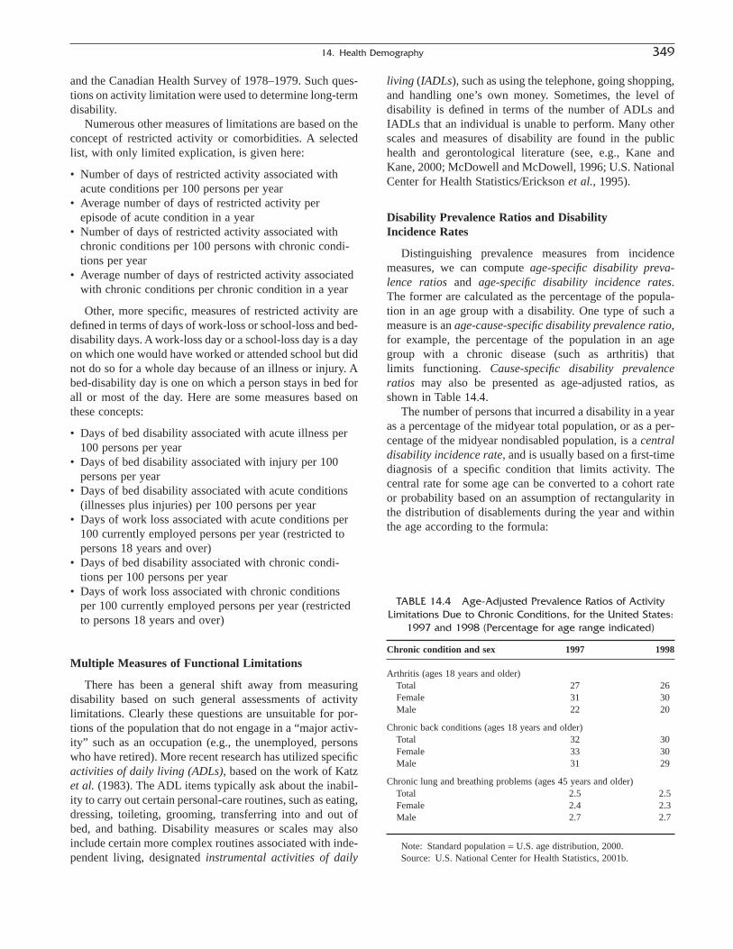
and the Canadian Health Survey of 1978–1979. Such ques-tions on activity limitation were used to determine long-termdisability.
Numerous other measures of limitations are based on theconcept of restricted activity or comorbidities. A selectedlist, with only limited explication, is given here:
• Number of days of restricted activity associated withacute conditions per 100 persons per year
• Average number of days of restricted activity perepisode of acute condition in a year
• Number of days of restricted activity associated withchronic conditions per 100 persons with chronic condi-tions per year
• Average number of days of restricted activity associatedwith chronic conditions per chronic condition in a year
Other, more specific, measures of restricted activity aredefined in terms of days of work-loss or school-loss and bed-disability days. A work-loss day or a school-loss day is a dayon which one would have worked or attended school but didnot do so for a whole day because of an illness or injury. Abed-disability day is one on which a person stays in bed forall or most of the day. Here are some measures based onthese concepts:
• Days of bed disability associated with acute illness per100 persons per year
• Days of bed disability associated with injury per 100persons per year
• Days of bed disability associated with acute conditions(illnesses plus injuries) per 100 persons per year
• Days of work loss associated with acute conditions per100 currently employed persons per year (restricted topersons 18 years and over)
• Days of bed disability associated with chronic condi-tions per 100 persons per year
• Days of work loss associated with chronic conditionsper 100 currently employed persons per year (restrictedto persons 18 years and over)
Multiple Measures of Functional Limitations
There has been a general shift away from measuring disability based on such general assessments of activity limitations. Clearly these questions are unsuitable for por-tions of the population that do not engage in a “major activ-ity” such as an occupation (e.g., the unemployed, personswho have retired). More recent research has utilized specificactivities of daily living (ADLs), based on the work of Katzet al. (1983). The ADL items typically ask about the inabil-ity to carry out certain personal-care routines, such as eating,dressing, toileting, grooming, transferring into and out ofbed, and bathing. Disability measures or scales may alsoinclude certain more complex routines associated with inde-pendent living, designated instrumental activities of daily
living (IADLs), such as using the telephone, going shopping,and handling one’s own money. Sometimes, the level of disability is defined in terms of the number of ADLs andIADLs that an individual is unable to perform. Many otherscales and measures of disability are found in the publichealth and gerontological literature (see, e.g., Kane andKane, 2000; McDowell and McDowell, 1996; U.S. NationalCenter for Health Statistics/Erickson et al., 1995).
Disability Prevalence Ratios and Disability Incidence Rates
Distinguishing prevalence measures from incidencemeasures, we can compute age-specific disability preva-lence ratios and age-specific disability incidence rates. The former are calculated as the percentage of the popula-tion in an age group with a disability. One type of such ameasure is an age-cause-specific disability prevalence ratio,for example, the percentage of the population in an agegroup with a chronic disease (such as arthritis) that limits functioning. Cause-specific disability prevalenceratios may also be presented as age-adjusted ratios, asshown in Table 14.4.
The number of persons that incurred a disability in a yearas a percentage of the midyear total population, or as a per-centage of the midyear nondisabled population, is a centraldisability incidence rate, and is usually based on a first-timediagnosis of a specific condition that limits activity. Thecentral rate for some age can be converted to a cohort rateor probability based on an assumption of rectangularity inthe distribution of disablements during the year and withinthe age according to the formula:
14. Health Demography 349
TABLE 14.4 Age-Adjusted Prevalence Ratios of ActivityLimitations Due to Chronic Conditions, for the United States:
1997 and 1998 (Percentage for age range indicated)
Chronic condition and sex 1997 1998
Arthritis (ages 18 years and older)Total 27 26Female 31 30Male 22 20
Chronic back conditions (ages 18 years and older)Total 32 30Female 33 30Male 31 29
Chronic lung and breathing problems (ages 45 years and older)Total 2.5 2.5Female 2.4 2.3Male 2.7 2.7
Note: Standard population = U.S. age distribution, 2000.Source: U.S. National Center for Health Statistics, 2001b.

(14.6a)
or, more exactly,
(14.6b)
where all elements refer to specific age x, DiRp representsthe probability of incurring a disability during the year, Didisablements during the year, Pnd the midyear nondisabledpopulation, and Dnd deaths of nondisabled persons during theyear. The formula expresses the probability of a nondisabledperson at exact age x becoming disabled between exact agex and exact age x+1 during a year.
Other Health-Related Measures
The concepts of dependence and long-term care relate tophysical dependence on others for care. Long-term care isgenerally defined as the provision of health, personal care,and social services over time to individuals who have functional limitations. It encompasses home care, com-munity services, and institutional care. Most persons in long-term care settings in the United States reside in nursinghomes, although the rate of nursing home residency has beendeclining. Both prevalence and incidence measures can becalculated for these dependent statuses. For example, note the very different values for the “stock” (prevalence)and “flow” (incidence) measures of residence in nursinghomes at ages 65 and over in the United States: At any given time, about 5% of the population 65 and over residesin nursing homes; in the course of a year, some 8% of theelderly population enter nursing homes; and over the courseof their lives, 33 to 50% of the elderly will enter a nursinghome.
Measures of Use of Health Services andAvailability of Support
There are several commonly used measures of the use ofhealth services that provide formal support to ill persons and of kinship networks that provide informal support tothem:
• Number of physician visits per 100 persons in a year• Number of dental visits per 100 persons in a year• Number of hospital stays (discharges) per 100 persons
in a year• Percentage of persons aged 65 years and over who have
living children• Percentage of persons aged 50 years and over who have
living parents 65 years and over• Number of days of care delivered per week by care-
givers per 100 dependent persons• Average number of days of care delivered per week by
each caregiver
Di P D Dind nd∏ + +( )12
12
DiR Di P Dp = ∏ +( )12
MEASUREMENT OF REPRODUCTIVE HEALTH
Definition and Sources of Data
In the United Nations 1994 World Plan of Action, repro-ductive health is defined as “a state of complete physical,mental, and social well-being . . . in all matters relating tothe reproductive system and to its functions and processes”(United Nations, 1994). Accordingly, reproductive health isconcerned with the health correlates of reproductive events(i.e., conception, pregnancy, birth, and the postpartumperiod) and the ability to bear healthy children and avoidpregnancy loss, to regulate fertility, and to engage in satis-fying sexual behavior without fear of disease or unwantedpregnancy. This definition goes well beyond the provisionof family planning services. For example, it encompassesthe measurement of sexuality, including the study of patternsof sexual behavior. These patterns are important in affectingthe exposure to sexually transmitted diseases and reproduc-tive tract infections, the choice of contraceptive methods,and other health aspects of reproductive events.
The organizations that have provided information aboutreproductive health include the World Health Organization(e.g., maternal mortality, social factors in contraceptive use),Family Health International (e.g., maternal mortality, repro-ductive morbidity, and sexually transmitted diseases), theInternational Women’s Health Coalition (e.g., reproductivetract infections), ORC Macro (e.g., demographic and healthsurveys, obstetric morbidity in the Philippines), the LondonMaternal and Child Epidemiology Unit (e.g., various proj-ects in less developed countries), and the Population Council(e.g., numerous community studies relating to reproductivehealth). The U.S. Agency for International Developmentfunds some of these organizations in whole or in part.
Measuring reproductive health presents special problemsbecause of the possible inconsistency between the results ofdifferent measures, the fact that many conditions can beasymptomatic or result from clandestine behavior, and theoften frivolous view of reproductive conditions taken by thecommunity and physicians (Obermeyer, 1996; Stewart et al.,1996; WHO, 1989). The discrepancy between objective andsubjective information is especially problematic for repro-ductive health.
Reproductive health is measured by a combination ofself-reports, clinical examinations, and laboratory analyses.Respondents’ perceptions of what is healthy and unhealthyaffect the nature and consistency of the measures when acondition is reported. In fact, a “culture of silence” heavilyinfluences the reporting of reproductive morbidity becausewomen’s problems are not viewed with much seriousness inmany countries. Many of these conditions are not consid-ered serious from a medical point of view, and women tol-erate them as part of reproductive functioning. This is true
350 Lamb and Siegel

even though these conditions do affect a woman’s generalfunctioning and can be measured by functional criteria.Because access to medical services is limited in many lessdeveloped countries (LDCs), many women are unaware thatthey really have a definite illness. For example, in manyIslamic and Hindu communities, the practice of Purdahforbids women from being seen in a hospital or clinic unlessthe husband’s permission is obtained.
Studies of reproductive morbidity can be hospital basedor community based. However, most of the available studieson maternal mortality are hospital based, not communitybased, even though such studies do not give a representativedescription of the extent of maternal mortality in the com-munity. Studies of reproductive morbidity in the communityare almost rare in LDCs (Zurayk et al., 1993).
Reproductive morbidity studies can deal with specificmorbid conditions or a wide range of such conditions.Because of the special difficulties of interpreting the resultsof morbidity research, the research method and scope ofeach morbidity study need to be fully described in theanalyst’s report. This requirement is not usually met (WHO,1989). The validation of indicators, such as by clinicalexamination, is rare although some studies do compare self-reports of health conditions and actual medical diagnoses(Zurayk et al., 1993). The geographic focus is uneven, as isthe focus on particular morbid conditions. Only a handful ofcountries have received attention (e.g., Nigeria, Ghana,Gambia, India, Singapore, and Bangladesh).
Morbidity studies involving interviews pose difficultproblems of (1) how to design studies, (2) how to access thewomen respondents, (3) how to ask the appropriate ques-tions, and (4) how to interpret the responses. For example,the role of the interviewer is critical. Whether the intervieweris a male or female, of the same or different social class, aphysician or not, or a stranger or not can affect the quality ofthe data collected. Recall bias is a serious problem as well.
The risk factors for reproductive health include bothproximate and contextual variables (Obermeyer, 1996).Some variables, such as age, parity, pregnancy history, useof health services, and medical history can be measuredquantitatively with some precision. Other variables, such asthe use of contraceptive methods, sexual practices, and prac-tices relating to personal hygiene, are also quantifiable butare difficult to measure. Still others deal with perceptions,motivations, attitudes, and psychological contextual factors,such as religiosity, feelings of control, and interpretations ofmorbid conditions.
Maternal Health
Measures
Maternal mortality is conventionally measured by thematernal mortality ratio, representing the risk of a woman’s
dying from complications of pregnancy, childbirth, or thepuerperium. According to the Tenth International Classifi-cation of Diseases, maternal death is the death of a woman“while pregnant, or within 42 days of termination of preg-nancy, irrespective of the duration and the site of the preg-nancy, from any cause related to or aggravated by thepregnancy or its management, but not from accidental orincidental causes” (ICD-10, Class XV, codes O00–O99).According to the ninth revision, maternal deaths are the sumof deaths due to abortion (code AM 42), direct obstetriccauses (code AM 43), and indirect obstetric causes (codeAM 44).
The WHO defines two other concepts related to maternaldeaths, namely late maternal deaths and pregnancy-relateddeaths. As suggested, the WHO also distinguishes directobstetric deaths from indirect obstetric deaths. A late mater-nal death is a death more than 42 days and less than 1 year after termination of pregnancy from any cause relatedto or aggravated by the pregnancy. Direct obstetric deathsresult from obstetric complications of the pregnant state(pregnancy, labor, and puerperium), from interventions,omissions, incorrect treatment, or from a chain of eventsresulting from any of these causes. Indirect obstetric deathsare those resulting from previously existing disease ordisease that develops during pregnancy, and are not due to direct obstetric causes but were aggravated by the physiological effect of pregnancy. A pregnancy-relateddeath is a death of a woman while pregnant or within 42days of the termination of pregnancy irrespective of thecause of death.
The maternal mortality ratio is now generally defined asthe number of deaths due to puerperal causes per 100,000births. The formula is
(14.7)
where Dp represents deaths due to puerperal causes. For-merly, when maternal deaths were more numerous, a con-stant multiplier of 10,000 was commonly used, and it maybe reasonably used today for groups of countries with rela-tively high maternal mortality.
The maternal mortality ratio varies widely. The WHOwith UNICEF (WHO, 1996) published country-by-countryestimates of maternal mortality ratios for 1990. The globalestimate was 430 deaths per 100,000 births. The highestrates occurred primarily in the less developed regions. Interms of world regions, maternal deaths ranged from 11 per100,000 births for North America to 1060 per 100,000 birthsin East Africa in 1990.
In the formula for estimating the maternal mortality ratio,the number of births is employed as an approximation to thenumber of women exposed to the risk of dying from puer-peral causes. A refinement of the maternal mortality ratio, thematernal mortality rate, broadens the denominator to includelate fetal losses and induced terminations of pregnancy:
MMR D Bp1 100 000= ∏( ) * ,
14. Health Demography 351

(14.8)
where Llf represents late fetal losses and A (induced) abortions.
Another measure, which reflects both the risk of deathper pregnancy and the number of pregnancies, is the lifetimerisk of maternal death. It is calculated by the formula
(14.9)
where MMR is the maternal mortality ratio, which isexpressed as a decimal, TFR is the total fertility rate (seeChapter 15), and 1.2 is a multiplier to adjust for pregnanciesnot ending in live births (Tinker and Koblinsky, 1993). Asshown in Table 14.5, in 1988 the lifetime risk of maternaldeath for women in the more developed countries is about1 in 150 whereas the risk for women in the less developedcountries is about 1 in 50.
Among the factors important in the analysis of maternalmortality are the woman’s age and parity. Rates are higher for very young women, high-parity women, olderwomen, and women with short birth intervals. Underlyingthese demographic phenomena are such conditions aschronic disease and malnutrition, poverty, unwanted
LRMD MMRTFR= - -( )1 1
1 2.
MMR D B L Ap lf2 100 000= ∏ + +( ){ } * , pregnancies, inadequate prenatal and obstetric care, and lack
of access to a hospital. In addition, there are the direct causesof maternal deaths—obstetric complications and unsafeabortions.
Measures of Pregnancy Losses
Much loss of potential life occurs because of lossesduring pregnancy, so-called fetal mortality. There is a closerelation between fetal losses and neonatal mortality. Hence,we cover fetal losses and perinatal mortality (i.e., the com-bination of late fetal losses and early infant mortality)together in this section. According to the WHO (1992), aswe may recall from Chapter 12, neonatal deaths are deathsamong live births during the first 28 completed days of life.Those neonatal deaths occurring during the first seven completed days of life are designated early neonatal deaths; deaths during the remainder of the period (from the8th day through the 28th day) are designated late neonataldeaths.
Pregnancy Losses and Fetal Losses
The WHO-recommended definition of fetal “death” com-plements the definition of (live) birth and death. In 1950 theWorld Health Organization recommended the following definition of fetal “death” for international use: “Death priorto the complete expulsion or extraction from its mother of aproduct of conception, irrespective of the duration of preg-nancy; the death is indicated by the fact that after such separation, the fetus does not breathe or show any other evi-dence of life such as beating of the heart, pulsation of theumbilical cord, or definite movement of involuntarymuscles” (U.S. National Office of Vital Statistics, 1950).The WHO maintained this recommendation in the tenthrevision in 1992.
In some countries, however, the definition employeddiffers from the international recommendation: Live-bornchildren dying early in life (e.g., before registration of birthor within 24 hours of birth) may be classed with fetal deaths.A more important problem is the incompleteness and irregularity of reporting of fetal deaths. This limitationapplies to the data for most countries of the world. The duration of pregnancy required for registration varieswidely. Reporting of early fetal deaths may be seriouslyincomplete even where required by law. When registrationof only late fetal deaths (rather than all fetal deaths) ismandatory, countries differ as to what is to be registered asa late fetal death: 28 weeks of gestation is most frequentlyspecified as the minimum period. On balance, internationalcomparability is far greater for late fetal deaths than for allfetal deaths taken together (Casterline, 1989).
The World Health Organization has recommended theterm fetal deaths as the generic term for all pregnancy
352 Lamb and Siegel
TABLE 14.5 Lifetime Risk of Maternal Death, by Region andSubregion: 1988
Maternity Total Lifetime riskmortality fertility 1 - [1 -
ratio, 1988 rate, 1991 (1)]1.2*(2) =Continent and region (1) (2) (3)
World 0.0037 3.4 0.015
More developed 0.0003 1.9 0.007countries
Less developed 0.0042 3.9 0.020countries
Africa 0.0063 6.1 0.045North 0.0036 5.0 0.021East 0.0068 6.8 0.054Middle 0.0071 6.0 0.050West 0.0076 6.4 0.057South 0.0027 4.6 0.015
Asia 0.0038 3.9 0.018East 0.0012 2.2 0.003Southeast 0.0034 3.4 0.014South 0.0057 4.4 0.030West 0.0028 4.9 0.016
South America 0.0022 3.3 0.009
North America 0.0001 2.6 —
Europe 0.0002 1.7 —
Oceania 0.0060 2.6 0.019
Note: — Rounds to zero.Source: Tinker and Koblinsky, 1993, Table 1.1. © 1993, The World
Bank. Reprinted by permission.

losses. Accordingly, fetal deaths encompass those pregnancylosses known by other names, such as miscarriages, abor-tions, and stillbirths. Granting that there is an advantage ina general term for this class of events for statistical purposes,a preferred term is pregnancy losses rather than fetal deaths.A term is also needed for pregnancy losses excludinginduced terminations of pregnancy—that is, for spontaneousterminations of pregnancy—and for this the term fetal lossesis suggested. This is the usage of the U.S. National Centerfor Health Statistics. The term abortion may be used in itsrestricted sense for induced terminations of pregnancy. Themain reason for replacing the term fetal deaths with theterms pregnancy losses and fetal losses is that in the UN sta-tistical system, “death” can occur only after a live birth. Inaddition, a general term is needed for all losses during preg-nancy, and a restricted term is needed for losses that exclude(induced) abortions.
The WHO also recommended that “fetal deaths” shouldbe distinguished by length of gestation period as early (lessthan 20 completed weeks of gestation), intermediate (20completed weeks but less than 28), and late (28 completedweeks and over). Gestational ages reported in months shouldbe allocated to the corresponding interval in weeks. Thedetermination of age is often difficult, and comparability ofthe tabulations is affected by the difference in the skill ofthe medical attendant in making this determination. Even thedata on late fetal losses are subject to substantial error intro-duced by incorrect reporting of gestational age. In view ofthe very poor reporting of early fetal losses and the varia-tion from one reporting jurisdiction to another of theminimum period for which fetal loss reporting is required,fetal loss rates in official sources are normally limited tofetal losses with 20 weeks or more, or 28 weeks or more, ofgestation. Where the gestation period is not stated, as is oftenthe case, some assumption has to be made regarding theperiod of gestation. The World Health Organization classi-fies these “unstated” cases in a fourth class.
In the United States, a separate U.S. Standard Report ofStillbirth (later Fetal Death) was introduced in 1939,although state vital statistics laws dictate the exact form andcontent of the certificates used for each state. Reporting isrequired for fetal losses of 20 weeks or more in all report-ing areas (with some variation by birth weight) but severalstates require reporting of all fetal losses. Where reportingis required only for fetal losses of 20 weeks or more, theU.S. National Center for Health Statistics assigns “unstated”cases to the period 20 weeks or more (U.S. National Centerfor Health Statistics, 1991, pp. 14–15).
Fetal losses may be measured by the fetal loss ratio orthe fetal loss rate. The fetal loss ratio is defined as thenumber of fetal losses reported in a year per 1000 live birthsin the same year, or
(14.10)FLR L Blf= ∏( ) *1000
where Llf represents all fetal losses or late fetal losses.Because of the variability of coverage of the early and inter-mediate fetal losses mentioned earlier, it is preferable fromthe point of international comparability to compute the fetalloss ratio on the basis of late fetal losses only. The same datarequired to compute the fetal loss ratio can be used tocompute the more precise fetal loss rate. The fetal loss raterelates fetal losses more closely to the population at risk thanthe fetal loss ratio. The formula includes the fetal losses inthe denominator as well as in the numerator:
(14.11)
For the reason stated, this measure also should best becalculated with late fetal losses only. In this case, the de-nominator represents pregnancies carried to term or nearlycarried to term. Late fetal loss ratios and late fetal loss ratesfor a number of countries are presented in Table 14.6.
In spite of the theoretical advantage of the fetal loss rate,the fetal loss ratio may be considered preferable for inter-national comparisons. The registration of fetal losses isirregular, and the effect of this irregularity is compoundedwhen fetal losses are included with the births in the base of the fetal loss rate. Because of the likelihood that poor registration of fetal losses will occur in association with poor registration of births and, hence, that the errors in eachcomponent will offset one another to some extent, fetal lossratios may sometimes be of satisfactory quality even wherethe basic data are questionable.
Specific fetal loss ratios and fetal loss rates may be cal-culated in terms of the period of gestation of the fetus or interms of the age of mother (requiring data on the date of termination of pregnancy for fetal losses and on the age of mother for births, respectively). Other characteristics ofimportance in the analysis of fetal losses are marital statusof mother (distinguishing marital from nonmarital pregnan-cies), sex of the fetus, total birth order (counting live births
FLR L B Lp lf lf= ∏ +( ){ } *1000
14. Health Demography 353
TABLE 14.6 Fetal Loss Ratios and Fetal Loss Rates, forSelected Countries: 1991
Ratio RateFetal Births [(1) / (2)] [(1) / [(2) + (1)]]
Country losses ¥ 1000 = ¥ 1000 =(1) (2) (3) (4)
Cuba 1,891 173,896 10.87 10.76Chile 1,754 299,456 5.86 5.82Italy 2,887 562,787 5.13 5.10Japan 4,376 1,223,245 3.58 3.56Australia 1,150 257,247 4.47 4.45Tunisia 2,116 207,455 10.20 10.10Spain 1,564 395,989 3.95 3.93
Source: United Nations, 1995, Tables 9 and 12.
plus fetal losses and abortions), birth weight, and pluralityof fetus. Other factors include the cause of fetal loss, hospi-talization, age of father, date of marriage (for marital preg-nancies), level of education of parents, and the occupationalcharacteristics of the parents.
Pregnancy losses include so-called abortions. The latterterm is not commonly used in international statistical com-pilations because it tends to have legal, programmatic, andethical implications that are not desirable in a statisticalconcept. In theory, the term encompasses both spontaneousand induced terminations of pregnancy. Spontaneous abor-tions, or spontaneous terminations of pregnancy, correspondroughly to what in popular usage are designated as miscar-riages. Stillbirth is another popular as well as legal term forspontaneous abortions, usually those with longer periods ofgestation. Its legal definition varies according to the par-ticular political jurisdiction. Spontaneous abortions are farmore common than induced abortions (James, 1970).Induced abortions may be legal or illegal depending on thelaws of the particular jurisdiction. In practice, the term“abortion” is usually limited to induced abortions, whichmay be defined as induced terminations of pregnancy beforethe fetus has became capable of surviving, with appropriatesupport, to the neonatal period and eventually maintainingan independent life outside the uterus of the mother (WHO,1970).
Information on abortions comes from the official statis-tics of countries where abortion has been made legalalthough the data may be compiled by private organizations,as in the United States. The data may come from hospitalrecords or survey responses. In 1970, the U.S. NationalCenter for Health Statistics began to separate reports of(induced) abortions from other fetal losses. To improve com-parability of data on (induced) abortions, they have to bepurged of reports of spontaneous abortions. There are noreliable statistics on illegal abortions.
There are several measures of abortions (i.e., legalinduced terminations of pregnancy) in common use. Theyparallel those for fetal losses defined in the narrower sensegiven here. The general abortion rate can be defined as thenumber of legal, induced pregnancy terminations in a cal-endar year per 1000 women 15 to 44 or 15 to 49 at midyear.The age range of the women may be selected to allow fortheir ages at the time of the pregnancy termination.
The abortion ratio is the number of legal, induced preg-nancy terminations in a year per 1000 births, or alternatively,terminations in a calendar year per 1000 births in the yearfrom July 1 of the year to June 30 of the following year. Theabortion rate (approximating a probability of abortion) isthe number of legal, induced pregnancy terminations in ayear per 1000 births, late fetal losses, and legal, inducedpregnancy terminations. The births are taken from July 1 ofthe year to June 30 of the following year to match the timeof conception with the time of abortion. The restriction to
legal, induced abortions and late fetal losses is intended tolend stability and comparability to the measures by exclud-ing the inadequately recorded illegal abortions and early andintermediate fetal losses. Analysis of these measuresemploys such variables as the woman’s age, total number ofprior births, and the marital status of the woman.
With appropriate adjustments in the data, it is possible todevelop an estimate of the pregnancies exposed to the riskof abortion during a year. Total pregnancies may be repre-sented by the sum of births, abortions, and fetal losses. A general pregnancy rate, and a set of consistent, albeitapproximate, rates for these components may be calculatedas the number for each of them in a year per 1000 women 15–44 years of age at the middle of the year. Forexample, in the United States in 1997, the general pregnancyrate was 103.7, the general fertility rate was 65.0, the generalabortion rate was 22.2, and the general fetal loss rate was16.5 (U.S. National Center for Health Statistics/Ventura etal., 2001c). A more exact general pregnancy rate for a givenyear may be calculated by employing births from July 1 ofthe year to July 1 of the following year. The number of pre-gnant women at a particular date can be estimated bysumming births in the following 9 months, abortions in thenext 6 months, and fetal losses of 20 weeks or more in thenext 20 weeks.
Perinatal Mortality
The causes of death in early infancy are believed to beso akin to those accounting for fetal losses that variousmeasures combining fetal losses and deaths of early infancyhave been devised. The combination of these events is alsointended to eliminate the errors resulting from deliberate andinadvertent misclassification among fetal losses, births, and neonatal deaths. The combined risk of dying during the period near parturition (i.e., just before, during, and after birth) is measured by various so-called perinatal deathratios and perinatal mortality rates. The formulas differ withrespect to the age limits of the infant deaths and the gesta-tional age of fetal losses to be included, and with respect towhether fetal losses are included in or excluded from thebase of the measures. Neonatal deaths, deaths under 1 week,and deaths under 3 days, in combination with intermediateand late fetal losses, or with late fetal losses only, are pos-sible ways of operationally defining perinatal deaths. Inview of the general lack of tabulated data on infant deathsunder 3 days, the use of this period is not very useful forinternational comparisons.
The World Health Organization defines the perinatalperiod as the period of prenatal existence after viability ofthe fetus is reached, the duration of labor, and the early partof extra-uterine life. The WHO recommends in ICD-9 that“countries should present, solely for international compar-isons, ‘standard perinatal statistics’ in which the numerator
354 Lamb and Siegel

and denominator of all rates are restricted to fetuses andinfants weighing 1000 grams or more or, where birth weightis unavailable, [having] the corresponding gestational age(28 weeks) or body length (35cm crown-heel)” (UnitedNations, 1994, p. 27; WHO, 1992). According to the tenthrevision, the perinatal period commences at 22 completedweeks (154 days) of gestation (the time when birth weightis normally 500 grams) and ends at seven completed daysafter birth.
Because birth weight and gestational age are not recordedon the death certificate in the United States, the NationalCenter for Health Statistics was unable to adopt these defi-nitions. The NCHS uses three definitions, designated I, II,and III. In definition I, the one generally used for interna-tional comparisons, the lower “age” limit of fetal loss istaken as 28 completed weeks of gestation and the early partof extra-uterine life is taken to be the first 7 days of life. Thecorresponding formula for the perinatal death ratio is, then,the number of deaths under 1 week of age and late fetallosses per 1000 live births in a year:
(14.12)
where Dz represents deaths less than 1 week, Llf representslate fetal losses, and B represents births. The formula underdefinition III is the number of infant deaths under 1 weekand fetal losses of 20 weeks’ gestation or more per 1000 livebirths in a year:
(14.13)
where Llf represents fetal losses of 20 weeks gestation ormore.
The corresponding perinatal mortality rate differs byincluding late fetal losses, or intermediate and late fetallosses, in the base of the ratio, thus approximating a proba-bility more closely. Specifically, the perinatal mortality rateis defined as
(14.14)
or
PDR D L B Lap z lf lf= +( ) ∏ +( ){ } *1000
PDR D L Bbz lf= +( ) ∏{ } *1000
PDR D L Baz lf= +( ) ∏{ } *1000
(14.15)
where the symbols have the same meaning as in formulasPDRa and PDRb in the previous equations. These two meas-ures give essentially the same indications of internationaldifferences, as can be noted in Table 14.7. The perinatalmortality rate has a small theoretical advantage over theperinatal death ratio, but the perinatal death ratio is proba-bly more stable for international comparisons.
Other measures of perinatal mortality have been pro-posed. The feto-infant mortality rate is one such measureand it was proposed by the International Collaborative Efforton Perinatal and Infant Mortality. It extends the concept ofperinatal mortality to include the entire infant period andincludes fetal losses of 28 or more weeks of gestation in boththe numerator and denominator of the rate. The feto-infantmortality rate has two advantages over the traditional infantmortality rates. First, it eliminates the problem of having tomake the distinction between a fetal “death” and a birth, aproblem that has made international comparisons difficult.Second, it is a more encompassing measure of pregnancyperformance (U.S. National Center for Health Statistics/Hartford, 1992).
Contraception
Effectiveness of contraception may be considered inthree dimensions: clinical effectiveness, use effectiveness,and demographic effectiveness. Clinical effectiveness refersto the effectiveness of a contraceptive method under idealconditions (i.e., when the method is used consistently andas instructed). Use effectiveness refers to the actual experi-ence of couples using a method in terms of periods of pro-tection provided. Demographic effectiveness refers to theeffect on population growth of the use of the method interms of births averted. Demographic effectiveness is moredifficult to measure than use effectiveness. A contraceptiveaverts births by delaying conception when a woman is in a
PDR D L B Lbp z lf lf= +( ) ∏ +( ){ } *1000
14. Health Demography 355
TABLE 14.7 Perinatal Death Ratios and Perinatal Death Rates, for Selected Countries: VariousYears: 1991 to 1994
Ratio RatePDRa = {[(1) + (2)] / PDRp
a = {[(1) + (2)] /Late fetal losses1 Deaths under 1 week Births (3)} ¥ 1000 = [(3) + (1)]} ¥ 1000 =
Country, year (1) (2) (3) (4) (5)
Cuba, 1991 1,891 811 173,896 15.54 15.37Chile, 1994 1,321 1,496 288,175 9.78 9.73Italy, 1992 2,546 2,350 567,841 8.62 8.58Japan, 1994 4,048 2,086 1,238,328 4.95 4.94Australia, 1994 898 830 258,051 6.70 6.67Spain, 1991 1,564 1,314 395,989 7.27 7.24
1 Fetal losses of 28 weeks or more of gestational age.Source: United Nations, 1995, Tables 9 and 12.
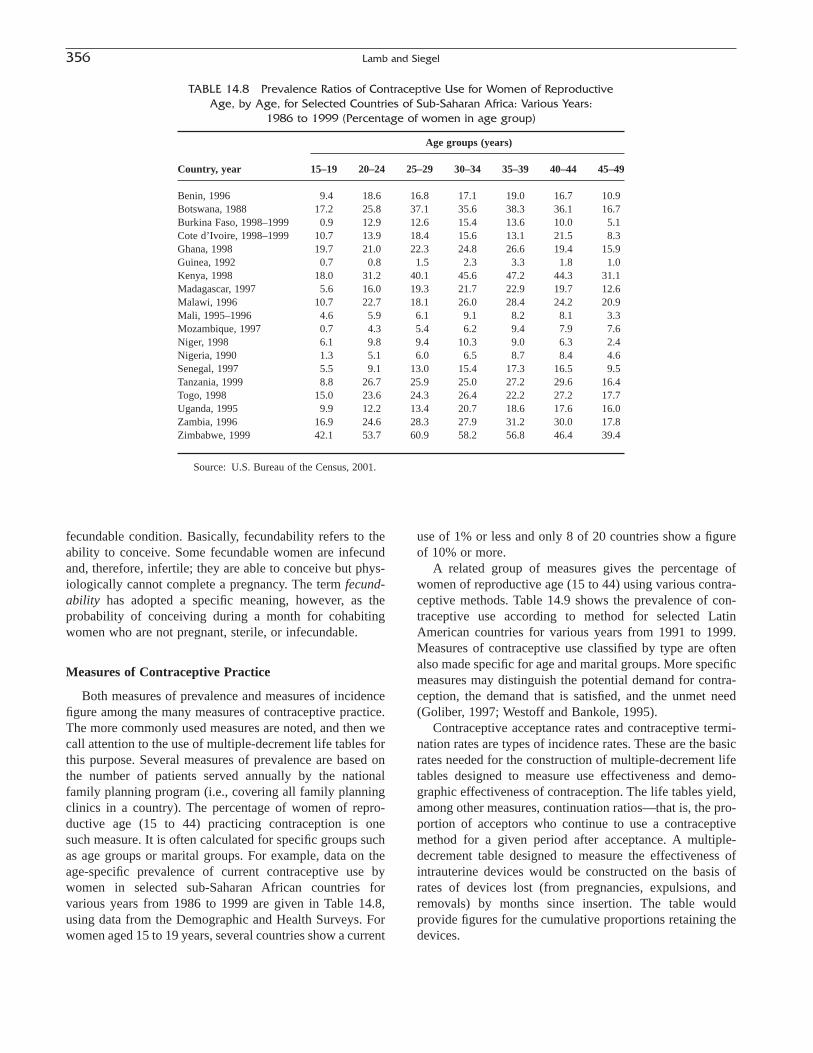
fecundable condition. Basically, fecundability refers to theability to conceive. Some fecundable women are infecundand, therefore, infertile; they are able to conceive but phys-iologically cannot complete a pregnancy. The term fecund-ability has adopted a specific meaning, however, as theprobability of conceiving during a month for cohabitingwomen who are not pregnant, sterile, or infecundable.
Measures of Contraceptive Practice
Both measures of prevalence and measures of incidencefigure among the many measures of contraceptive practice.The more commonly used measures are noted, and then wecall attention to the use of multiple-decrement life tables forthis purpose. Several measures of prevalence are based onthe number of patients served annually by the nationalfamily planning program (i.e., covering all family planningclinics in a country). The percentage of women of repro-ductive age (15 to 44) practicing contraception is one such measure. It is often calculated for specific groups suchas age groups or marital groups. For example, data on theage-specific prevalence of current contraceptive use bywomen in selected sub-Saharan African countries forvarious years from 1986 to 1999 are given in Table 14.8,using data from the Demographic and Health Surveys. Forwomen aged 15 to 19 years, several countries show a current
use of 1% or less and only 8 of 20 countries show a figureof 10% or more.
A related group of measures gives the percentage ofwomen of reproductive age (15 to 44) using various contra-ceptive methods. Table 14.9 shows the prevalence of con-traceptive use according to method for selected LatinAmerican countries for various years from 1991 to 1999.Measures of contraceptive use classified by type are oftenalso made specific for age and marital groups. More specificmeasures may distinguish the potential demand for contra-ception, the demand that is satisfied, and the unmet need(Goliber, 1997; Westoff and Bankole, 1995).
Contraceptive acceptance rates and contraceptive termi-nation rates are types of incidence rates. These are the basicrates needed for the construction of multiple-decrement lifetables designed to measure use effectiveness and demo-graphic effectiveness of contraception. The life tables yield,among other measures, continuation ratios—that is, the pro-portion of acceptors who continue to use a contraceptivemethod for a given period after acceptance. A multiple-decrement table designed to measure the effectiveness ofintrauterine devices would be constructed on the basis ofrates of devices lost (from pregnancies, expulsions, andremovals) by months since insertion. The table wouldprovide figures for the cumulative proportions retaining thedevices.
356 Lamb and Siegel
TABLE 14.8 Prevalence Ratios of Contraceptive Use for Women of ReproductiveAge, by Age, for Selected Countries of Sub-Saharan Africa: Various Years:
1986 to 1999 (Percentage of women in age group)
Age groups (years)
Country, year 15–19 20–24 25–29 30–34 35–39 40–44 45–49
Benin, 1996 9.4 18.6 16.8 17.1 19.0 16.7 10.9Botswana, 1988 17.2 25.8 37.1 35.6 38.3 36.1 16.7Burkina Faso, 1998–1999 0.9 12.9 12.6 15.4 13.6 10.0 5.1Cote d’Ivoire, 1998–1999 10.7 13.9 18.4 15.6 13.1 21.5 8.3Ghana, 1998 19.7 21.0 22.3 24.8 26.6 19.4 15.9Guinea, 1992 0.7 0.8 1.5 2.3 3.3 1.8 1.0Kenya, 1998 18.0 31.2 40.1 45.6 47.2 44.3 31.1Madagascar, 1997 5.6 16.0 19.3 21.7 22.9 19.7 12.6Malawi, 1996 10.7 22.7 18.1 26.0 28.4 24.2 20.9Mali, 1995–1996 4.6 5.9 6.1 9.1 8.2 8.1 3.3Mozambique, 1997 0.7 4.3 5.4 6.2 9.4 7.9 7.6Niger, 1998 6.1 9.8 9.4 10.3 9.0 6.3 2.4Nigeria, 1990 1.3 5.1 6.0 6.5 8.7 8.4 4.6Senegal, 1997 5.5 9.1 13.0 15.4 17.3 16.5 9.5Tanzania, 1999 8.8 26.7 25.9 25.0 27.2 29.6 16.4Togo, 1998 15.0 23.6 24.3 26.4 22.2 27.2 17.7Uganda, 1995 9.9 12.2 13.4 20.7 18.6 17.6 16.0Zambia, 1996 16.9 24.6 28.3 27.9 31.2 30.0 17.8Zimbabwe, 1999 42.1 53.7 60.9 58.2 56.8 46.4 39.4
Source: U.S. Bureau of the Census, 2001.

MEASURES LINKING MORTALITYAND MORBIDITY
The Relation between Changes in Mortalityand Changes in Morbidity
After the turn of the 20th century in the more developedcountries, and after World War II in the less developed coun-tries, there has been a pronounced shift in the pattern of thecauses of morbidity, as with the causes of mortality, from apredominance of acute, infectious, and parasitic diseases toa predominance of chronic, endogenous, accident-related,and self-imposed conditions (Olshansky et al., 1997). Thecategory endogenous diseases includes such diseases as cardiovascular diseases, cancer, diabetes, kidney diseases,arthritis and rheumatism, emphysema, and certain diseasesof early infancy. However, the exact scope of endogenousdiseases is arbitrary, particularly with respect to the inclu-sion or exclusion of respiratory illnesses.
The change in the pattern of morbidity has been termedthe epidemiologic transition (Omran, 1971, 1977). Epi-demiologic transition theory has directed attention to theshifts in disease patterns and causes of mortality, and theresulting impacts on life expectation and population growth.A major premise of epidemiologic transition theory is thatmortality is the fundamental factor in population dynamics.
Measurement of the relation between changes in mor-bidity and changes in mortality is complex, partly becausethe relation varies over the age scale, over time, and betweenbirth cohorts. The initial assumptions regarding mortalityand morbidity trends have been that the two were closelyrelated and therefore followed close trajectories over time.
Thus, if mortality declines, then morbidity also declines.Alter and Riley (1989; Riley and Alter, 1996) have demon-strated, using historical data sources, that morbidity levelstended to rise after mortality declines, rather than thereverse. This does not reflect increases in incidence, butrather improvements in case fatality rates and rising preva-lence levels.
As countries progress through the later stages of the epi-demiologic transition, the traditional indicators of popula-tion health, based on mortality rates alone, are expected tochange little. Therefore, the incidence, prevalence, and dura-tion of morbid conditions, case-fatality rates, and the dis-abling effects of morbid conditions are increasinglyimportant concerns in the examination of population health.Various scholars, including some at the World Health Orga-nization, have graphically modeled the relation betweenmortality, disability, and morbidity survival curves. A gen-eralized diagram of these relations over the age scale isshown in Figure 14.1 (WHO, 1984). Much of the analysisof the relation between mortality and disability or morbid-ity in recent years has been carried out in terms of tables ofactive or healthy life. We turn next to a discussion of thismeasurement tool.
Measurement of Active (Healthy,Independent) Life Expectancy
Tables of active (healthy, independent) life can be con-structed to elucidate the relation between morbidity andmortality quantitatively. A method for estimating active lifeexpectancy was outlined by Sullivan (1971). The so-calledSullivan method employs age-specific prevalence ratios of
14. Health Demography 357
TABLE 14.9 Prevalence Ratios of Contraceptive Use by Women of Reproductive Age, 15 to 49Years, by Method for Selected Latin American Countries: Various Years: 1991 to 1999 (Percent-
age of women 15–49 years of age)
No AnySterilization
OtherCountry, year method method1 Pill IUD Total Female Condom modern Traditional
Belize, 1991 53.3 46.7 14.9 1.9 NA 18.7 1.9 6.7 2.5Bolivia, 1998 51.7 48.3 3.8 11.1 NA 6.5 2.6 1.1 23.1Brazil, 1996 23.3 76.7 20.7 1.1 42.7 40.1 4.4 1.3 6.4Columbia, 1995 27.8 72.2 12.9 11.1 26.4 25.7 4.3 4.6 12.9Costa Rica, 1992–1993 25.0 75.0 18.0 9.0 21.0 20.0 16.0 1.0 10.0Ecuador, 1994 43.2 56.8 10.2 11.8 NA 19.8 2.6 1.6 10.8El Salvador, 1998 40.2 59.8 8.1 1.5 NA 32.5 2.6 9.6 5.6Guatemala, 1998–1999 61.8 38.2 5.0 2.2 17.5 16.7 2.3 3.9 7.3Honduras, 1987 59.4 40.6 13.4 4.3 12.8 12.6 1.8 0.6 7.6Mexico, 1995 33.0 67.0 8.0 15.0 27.0 NA 4.0 4.0 9.0Nicaragua, 1998 39.7 60.3 13.9 9.1 26.6 26.1 2.6 5.2 2.5Paraguay, 1998 37.7 62.1 13.1 11.1 NA 8.0 7.3 8.0 14.6Peru, 1996 35.8 64.2 6.2 12.0 9.7 9.5 4.4 9.0 22.9
Note: NA: Not available.1 Excludes percentage for female sterilization where figures are given for both sexes.Source: U.S. Bureau of the Census, 2001.

disability (i.e., the percentages of persons in each age inter-val who are disabled) and current basic life tables to produceestimates of active life expectancy. In most cases, the age-specific disability ratios are derived from sample surveys.
The disability prevalence ratios are used to calculate theperson-years of life lived in health (i.e., nondisabled condi-tion) for the age intervals using the Lx life table function (seeChapter 13 for a more detailed explanation of the life tablefunctions):
(14.16)
where healthy status is denoted by hs and DPR is the age-specific disability prevalence ratio. The person-years ofhealth for each age interval (Lx(hs)) are summed from age xforward to the end of the table to obtain the total person-years that are healthy, or active (i.e., nondisabled), life:
(14.17)
The healthy, or active, life expectancy values areobtained by dividing total healthy person-years at each ageby the lx value at that age from the basic life table:
(14.18)
The prevalence-ratio method of life table constructionhas serious limitations. In particular, it does not allow for atransition from disabled status to nondisabled status. Theprevalence-ratio method may be considered as following themodel of double-decrement tables in that two factors operateto reduce the original cohort, death and dependency, but theprobabilities of becoming dependent and of dying are only
e T lx hs x hs x( ) ( )= ∏
T Lx hs x hs ax a( )•
( )=[ ]== Â
L DPR Lx hs x( ) = -( ) *1
implicit or derivable indirectly. Thus, the estimates are onlya rough reflection of the health levels of a population at aparticular time (Crimmins, Saito, and Hayward, 1993).
Multistate Method
With the availability of several sample health surveysproviding longitudinal data on changes in health status and the development of new techniques of life table con-struction, analysts began to employ the multiple-decrementmethod and its logical extension, the increment-decrementmethod, and the multistate method. Tables constructed bythe first method explicitly measure the shift from independ-ence to dependence and from these states to death, but theyfail to make an explicit allowance for returns to independ-ence (Katz et al., 1983). Tables constructed by the secondmethod have the advantage that the model explicitly meas-ures the shift from dependence to independence as well asfrom independence to dependence, but the disadvantage isthat this can be done only on a net basis within each agegroup. That is to say, shifts in both directions cannot bemeasured for the same age span.
Further advances in mathematical demography led to theapplication of the more flexible multistate life table modelto measure changes in health status (Rogers, Rogers, andBranch, 1989; Rogers, Rogers, and Belanger, 1989, 1990).The multistate model permits two or more radices (i.e., mul-tiple starting states—e.g., the initially independent popula-tion and the initially dependent population) and followsthese populations as they age, shift to a dependent status,return to an independent status, and die. The multistate
358 Lamb and Siegel
0
20
40
60
80
100
0 10 20 30 40 50 60 70 80 90 100 110Age
Morbidity (1)
Mortality (3)
Disability (2)
Per
cent
age
surv
ivin
g
FIGURE 14.1 Stylized Representation of the Relation between the Age Curves for Morbidity, Disability, and Mortality (Percentage of the initial birth cohort who survive to the indicated ages (1) without a (chronic) disease or (major) disability, (2) without a (major) disability but with at least one (chronic) disease, or (3) with at least
one (major) disability resulting from at least one (chronic) disease at the higher ages.)
model can be used to analyze changes in degrees of health(e.g., no functioning problems, some functioning problems,unable to manage independent living, and unable to managepersonal care) within each age group and over the age scale(see, e.g., Crimmins, Hayward, and Saito, 1994, 1996; Land,Guralnik, and Blazer, 1994; Rogers, Rogers, and Balanger,1989). Thus, the multistate model can deal with multipleexits from and entries to the same state within each age inter-val. Moreover, it can handle the use of separate age sched-ules of mortality for each health status rather than a singleaverage level of mortality.
The results on expectation of healthy years from preva-lence-ratio tables, multiple increment-decrement tables, andmultistate tables are not comparable because of differencesin the data, methods, and assumptions employed (Rogers etal., 1990). While the results from the multistate tables areviewed as more realistic and valid, the data on mortality andhealth transitions may be unstable because of the smallernumber of incidence cases than prevalence cases and thegreater disaggregation of the data. Hence, even the estimatesof healthy life expectancy at particular dates from multistatetables should be viewed with caution.
The basic data for the construction of a table of active,healthy, or disability-free life come from longitudinal(panel) health surveys providing observations of the healthstatus of a person at two or more points in time (e.g., a yearapart). A single health survey inquiring about current andprior health status could provide the data, but the retrospec-tive reports would patently be less accurate than currentreports. In the United States, the list of recent national healthsurveys include the Longitudinal Study of Aging (LSOA),the National Long Term Care Survey (NLTCS), the Healthand Retirement Study (HRS), and the Established Popula-tions for Epidemiologic Studies of the Elderly (EPESE). In addition to providing the health data, these surveysprovide the basis for measuring differential mortalityaccording to health status. Inasmuch as the sample sizes maybe quite small for some groups, the observed mortality ratesmay be quite irregular and considerable smoothing of therates may be necessary before constructing life tables. Theresults must also be evaluated for the possible effect oflosses to the sample between waves that differ according tohealth status.
Multistate tables of disability-free or healthy life can beconstructed in several ways. Only a few approaches arementioned here, without attempting a full exposition of thiscomplex subject. A more detailed presentation of a methodfor developing a multistate life table is given in Chapter 13,“The Life Table.” The order and form of the computationsgiven here may differ somewhat from those described inChapter 13. Because of the number and complexity of thecalculations, the construction of multistate life tables isnormally carried out with matrix operations by computer.
A basic step in the construction of a multistate table ofactive life is the determination of the health transitions
according to age between survey dates, such as from anindependent state to a dependent state or from a dependentstate to an independent state. The observed transition ratesfrom state i to state j in the age interval x to x+n can be inthe form of central transfer rates (Mx) (i.e., the ratio of trans-fers to the midperiod population). Because of irregularitiesin their age pattern, the rates may require smoothing. A log-linear regression equation may be used for this purpose(Crimmins, Hayward, and Saito, 1994; Rogers, Rogers, andBelanger, 1990):
(14.19)
This model assumes that the transition process dependsonly on age, but if the transition rates do not vary by age, adifferent equation may have to be used for smoothing. Ifthere are only two origin states and two destination states(excluding death), two regression equations have to besolved for two sets of coefficients. With three origin and des-tination states (excluding death), four regression equationshave to be solved for four sets of coefficients.
The smoothed central transfer rates, represented in matrixform by M(x,n), next have to be converted to a transitionprobability matrix, P(x,n). The elements in this matrix, iPj
x,represent the probability that a person at exact age x and instate i at the beginning of an interval will be in state j at theend of the interval (e.g., 1 year later) at exact age x + n. Thefollowing numerical approximation has been proposed forthis conversion (Crimmins et al., 1994; Rogers and Ledent,1976; Schoen, 1988, P. 70; Willikens et al., 1982):
(14.20)
where P(x,n) is the transition-probability matrix, M(x,n) isthe matrix of transition rates, and I is the identity matrix.
In the simplest situation relating to the multistate analy-sis of health status, there are two origin states and three des-tination states, including death, representing three states,four possible transitions across states, and six transitions intotal, including “transitions” from a state to the same state,as indicated by the following paradigm:
Transition probabilitiesState of origin,exact age x State of destination, exact age x+1
Independent Dependent Death (d) Totallife (a) life (i)
Independent X X X 1.000life (a)
Dependent X X X 1.000life (i)
The survivors at exact age x and the person-years livedbetween exact age x and exact age x + 1 (or x + n), in eachhealth state, may be calculated by the matrix formulas:
(14.21)l l Px n x x n+( ) = ( ) ( )* ,
P I M I Mx n n x n n x n, , ,( ) = + ( )[ ] - ( )[ ]-2 2
1
M exx= +( )a b
14. Health Demography 359

(14.22)
The second equation assumes that l(x) changes linearlywithin the interval and that the transfers are distributed rectangularly in the interval. An element in the matrix l(x+n) is ilj(x+n) and an element in the matrix L(x,n) is Lj (x, x+n).
We can obtain the absolute number of life table transfersbetween health states of each type, D(x,n), by the formula
(14.23)
Finally, the expectation of life for each health state ateach exact age may be derived by the usual formulas. Forexample,
(14.24)
or (14.25)
or (14.26)
where Tix is the number of person-years lived in state i
beyond age x, derived by summing the L ix values in a given
state, and lx is the number of survivors to age x. The firstformula, the so-called population-based value, gives theaverage years of dependent life of all survivors at exact agex, while the second and third formulas, the so-called status-based values, give the average years of dependent life at agex of survivors in the dependent state and survivors in theindependent state. Corresponding formulas can be used toderive the life expectancy values for the independent state.To estimate these measures, separate survival populationsaccording to health state must be carried forward. One pos-sibility is to disaggregate the radix of the life table, at someage above birth, according to the observed prevalence ineach of the health states in the actual population.
Alternatively, the change between l(x) and l(x+1) may bederived from the formulas:
(14.27)
(14.28)
(14.29)
M(x), representing the ratio of transfers D(x) to the lifetable stationary population L(x), is known from the observedpopulation, but we do not know L(x) at this point becausewe do not know the l(x)s. We can estimate l(x), L(x), andd(x) by successive approximation through an iterative tech-nique: First, the changes in l(x)—that is, d(x)—are approx-imated as the product of l(x) and M(x). Next, we use theseestimates of d(x) to derive first estimates of l(x+1) and L(x).Now we multiply M(x) by these first estimates of L(x) toderive second estimates of l(x+1), d(x), and L(x). Thisprocess can be repeated if necessary.
i i a i i a i dl x l x t x t x t x+( ) = ( ) + ( ) - ( ) - ( )1
i i a a i
i i a i i d
l x l x L x m x
L x m x L x m x
+( ) = ( ) + ( )* ( )[ ]- ( )* ( )[ ] - ( )* ( )[ ]
1
l x l x L x M x+( ) = ( ) - ( ) ( )1
a i i ae x T x l x( ) = ( ) ∏ ( )
i i i ie x T x l x( ) = ( ) ∏ ( )e x T x l xi i( ) = ( ) ∏ ( )
D L Mx n x n x n, , ,( ) = ( ) * ( )
L l lx n n x x n,( ) = ( ) + +( )[ ]2 In a different approach, the number of survivors at thebeginning of an age interval may be derived from thenumber of survivors at the beginning of the previous ageinterval with transition probabilities calculated directly fromthe survey. For example, the number of independent personsdying and the number transferring from the independentpopulation to the dependent population are subtracted fromthe independent population, and those transferring from thedependent population to the independent population areadded to the latter:
(14.30)
(14.31)
where a, i, and d represent independence, dependence, and death, respectively. Similarly, for the dependent population:
(14.32)
As we saw in Chapter 13, the m(x), the central transferrates, can then be derived from the transition probabilities(Formula 13.77).
Tables of healthy (disability-free) life by the multistatemethod have been calculated for only a few countries,including United States, Canada, Japan, the Netherlands,and France, but more than two dozen countries, includingseveral in Africa and Asia, have prepared tables of disabil-ity-free life by the simpler methods. An illustration of theresults from applying multistate life table methods tomeasure life expectancy according to health status is pre-sented in Table 14.10. This table shows, for example, thatwhile women at age 70 in the United States have a sub-stantially greater total life expectancy than men, the inde-pendent active life expectancy of the two sexes is muchcloser.
Most tables constructed so far have tended to defineactive or healthy life, or to conceptualize morbidity, in termsof dependency (i.e., having ADL and/or IADL limitations).They can then be used to measure the lifetime chances ofbecoming dependent, expectancies of independent anddependent life at each age, the shares of the remaining lifethat will be independent and dependent at each age, averageduration of dependency before recovery and before death,the probability of dying in independent and dependentstates, and the mean age of dependent persons. Combina-tions of tables of disability-free life for the sexes and for asuccession of years can answer such questions as the fol-lowing: Are the extra years of life expectancy of womenover those of men years of dependent life or independentlife? What is the comparative proportion of life spent freeof disability for men and women? Has health statusimproved among the elderly? Has health status improved intandem with life expectancy? By simulation, these questionscan be answered: What is the relative effect of shifts in mor-
ix
ix
ix
ixd i
xi
xa a
xa
xil l l p l p l p+ = - *( ) - *( ) + *( )1
ax
ax
ax
axd a
xa
xi i
xi
xal l l p l p l p+ = - *( ) - *( ) + *( )1
l l px x xd
+ = * -( )1 1
360 Lamb and Siegel

tality and morbidity on the size and life expectation of thedependent population? What is the effect of a change of ageat onset of dependency on the size and life expectation ofthe dependent population?
Tables measuring life expectancy of persons who haveincurred certain chronic illnesses (e.g., diabetes, arthritis)can also be constructed. For this purpose, one needs information on age-specific rates of occurrence, rates of“recovery,” and differences in death rates of those with thechronic disease and those without it. Such tables are espe-cially useful in elucidating the impact on health of variousinterventions. They can answer such questions as the fol-lowing: What is the expectation of life spent free of thedisease? What is the proportion of life spent free of thedisease? Has the age of onset of the disease been changing?Has the age of disability changed, assuming a fixed age ofonset of the disease? What is the effect of a change in theage at onset of the disease on the period of disability?
Measures of Overall Health Status
Relative Index of Overall Physical Health
Many proposals have been made for constructing a healthindex. To derive a relative index of overall physical health,one may consider calculating the average of a variety ofphysiological biomarkers and measures of performance ateach age and then deriving an index of health at each age by comparing these summary measures with the corre-sponding value for some band of young ages, such as 25 to34, taken as standard. Because of the great variability in thebiomarkers and in the performance of individuals at givenages, this approach has been considered futile. It should beuseful, however, in showing the general shift in health over the age scale, even if it cannot serve as a standard forindividuals.
Quality-Adjusted Life Years and Disability-AdjustedLife Years
The so-called quality-adjusted life year (QALY) is ameasure that combines the impact of premature death anddisability into a single measure. There are many variants ofthe measure. To implement it, a single currency—that is,measurement unit—is required. Time can serve this purpose,and the measure can take the form of the sum of the yearslost to premature death and the years lived with a disability.
An internationally standardized measure is needed thatincorporates health conditions, not just mortality, intoassessments of health status; evaluates the burden of particular health conditions in a demographically plausibleway; and measures the burden of disease and injury in ameasurement unit that can also be used to measure the cost-effectiveness of interventions (i.e., the cost per unit ofdisease burden averted). The measure, known as the disability-adjusted life year (DALY), an internationallystandardized form of the QALY, is designed to meet theserequirements. In brief, one DALY is 1 lost year of healthylife. The measure was developed in connection with theWHO project on the Global Burden of Disease (GBD, seeMurray and Lopez, 1996).
The DALY combines years of life lost to premature deathand years of healthy life lost to disability of a specifiedseverity and duration. A premature death as defined here isa death that occurs before the age to which the decedentwould have been expected to live on the basis of his or herage and sex and the current life table for Japan, the tablewith the highest current life expectation (82.5 years forwomen and 80.0 years for men). DALYs are calculated foreach health condition in a population and then summed overall conditions. To calculate the DALYs for a particular con-dition, estimates are made for years of life lost and yearslived with a disability of specified severity and duration forthe condition.
14. Health Demography 361
TABLE 14.10 Years of Expected Life by Functioning Status for U.S. Females and Males at Ages70, 80, and 90: 1984–1990
Expected active life Expected inactive life
Some Unable to manageTotal No functioning functioning independent Unable to manage Percentage
Age and sex expected life Total problems problems Total living personal care inactive
Female70 years 13.9 11.1 4.3 6.8 2.8 1.0 1.8 20.180 years 8.4 5.5 1.6 3.9 2.9 1.0 1.9 34.590 years 4.8 1.8 0.3 1.5 2.9 0.9 2.0 60.4
Male70 years 10.3 8.9 4.1 4.8 1.4 0.6 0.8 13.680 years 6.0 4.4 1.6 2.8 1.6 0.7 0.9 26.790 years 3.3 1.6 0.4 1.2 1.8 0.7 1.1 54.5
Source: Crimmins, Hayward, and Saito, 1996, Table 3. © 1996 Gerontological Society of America. Reprinted by permission.
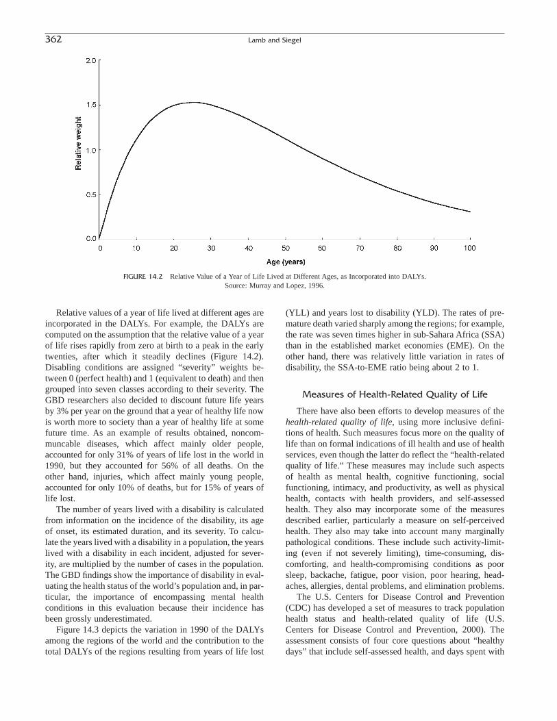
Relative values of a year of life lived at different ages areincorporated in the DALYs. For example, the DALYs arecomputed on the assumption that the relative value of a yearof life rises rapidly from zero at birth to a peak in the earlytwenties, after which it steadily declines (Figure 14.2). Disabling conditions are assigned “severity” weights be-tween 0 (perfect health) and 1 (equivalent to death) and thengrouped into seven classes according to their severity. TheGBD researchers also decided to discount future life yearsby 3% per year on the ground that a year of healthy life nowis worth more to society than a year of healthy life at somefuture time. As an example of results obtained, noncom-muncable diseases, which affect mainly older people,accounted for only 31% of years of life lost in the world in1990, but they accounted for 56% of all deaths. On the other hand, injuries, which affect mainly young people,accounted for only 10% of deaths, but for 15% of years oflife lost.
The number of years lived with a disability is calculatedfrom information on the incidence of the disability, its ageof onset, its estimated duration, and its severity. To calcu-late the years lived with a disability in a population, the yearslived with a disability in each incident, adjusted for sever-ity, are multiplied by the number of cases in the population.The GBD findings show the importance of disability in eval-uating the health status of the world’s population and, in par-ticular, the importance of encompassing mental healthconditions in this evaluation because their incidence hasbeen grossly underestimated.
Figure 14.3 depicts the variation in 1990 of the DALYsamong the regions of the world and the contribution to thetotal DALYs of the regions resulting from years of life lost
(YLL) and years lost to disability (YLD). The rates of pre-mature death varied sharply among the regions; for example,the rate was seven times higher in sub-Sahara Africa (SSA)than in the established market economies (EME). On theother hand, there was relatively little variation in rates ofdisability, the SSA-to-EME ratio being about 2 to 1.
Measures of Health-Related Quality of Life
There have also been efforts to develop measures of thehealth-related quality of life, using more inclusive defini-tions of health. Such measures focus more on the quality oflife than on formal indications of ill health and use of healthservices, even though the latter do reflect the “health-relatedquality of life.” These measures may include such aspectsof health as mental health, cognitive functioning, socialfunctioning, intimacy, and productivity, as well as physicalhealth, contacts with health providers, and self-assessedhealth. They also may incorporate some of the measuresdescribed earlier, particularly a measure on self-perceivedhealth. They also may take into account many marginallypathological conditions. These include such activity-limit-ing (even if not severely limiting), time-consuming, dis-comforting, and health-compromising conditions as poorsleep, backache, fatigue, poor vision, poor hearing, head-aches, allergies, dental problems, and elimination problems.
The U.S. Centers for Disease Control and Prevention(CDC) has developed a set of measures to track populationhealth status and health-related quality of life (U.S. Centers for Disease Control and Prevention, 2000). Theassessment consists of four core questions about “healthydays” that include self-assessed health, and days spent with
362 Lamb and Siegel
FIGURE 14.2 Relative Value of a Year of Life Lived at Different Ages, as Incorporated into DALYs.Source: Murray and Lopez, 1996.

physical illness, mental problems, or the inability to pursue one’s usual activities. These four items are used tocreate a summary index of unhealthy days within the past30 days. An additional ten questions can be included with the four core questions to ascertain more detailed information about healthy days. These additional questionsask about any activity limitations, or days with pain, depres-sion, anxiety, sleeplessness, or lack of vitality (U.S. Centersfor Disease Control and Prevention, 2000).
Other efforts to measure health and quality of life includethe Medical Outcomes Study Short Forms (SF-12 and SF-36), which also include self-assessments of general healthand questions about activities and functional limitations,physical and emotional problems, and pain (e.g., Ware,Kosinski, and Dewey, 2000). Additional measures have beenproposed. (See, e.g., U.S. National Center for Health Statis-tics/Erickson et al., 1995.) Thus, the definition and meas-urement of the health quality of life continue to be areas ofdebate among the experts.
GENERAL ANALYTIC DEVICES ANDHEALTH PROJECTION MODELS
General Analytic Devices
We consider next several analytical techniques that arewidely used in research on health demography. They areecological analysis, cohort analysis, multivariate logisticregression models, proportional hazards models, and gradeof membership analysis. We briefly mention also the ran-
domized response technique and meta-analysis, which thereader may occasionally encounter in studies on healthresearch.
Ecological Analysis
Numerous epidemiological studies have used ecologicalanalysis as a method of demonstrating a relation between ahealth characteristic and certain explanatory variables. Inecological analysis, the units of observation are small geo-graphic areas composing the total area under considerationrather than individuals. The correlation between the measuresof health characteristics and the explanatory variables, bothcalculated for these small geographic units, is typically inter-preted to represent the correlation between the variables forindividuals. The “area” method rather than the “individual”method may be employed both for reasons of convenienceand necessity; the data to be managed may be vastly reducedor they may be unavailable for individual respondents.
Because of this extension of the conclusions from areasto individuals, the validity of ecological correlation has beenquestioned. To the extent that the areas are small, numerous,and internally homogenous in the relevant characteristics,the extension should be more valid. Further improvementwould result if the area data were weighted according to thesize of the population in the geographic areas.
Cohort Analysis
Cohort analysis has been widely applied in health studiesto reflect the changes over the life course in health
14. Health Demography 363
RegionsEME. Established Market EconomiesFSE. Formerly Socialist EconomiesCHN. ChinaLAC. Latin America CaribbeanOAI. Other Asia and IslandsMEC. Middle Eastern CrescentIND. IndiaSSA. Sub-Saharan Africa
FIGURE 14.3 Disability-Adjusted Life Years per 1000 population by World Region and Years of Life Lost (YLL)and Years Lost to Disability (YLD): 1990
Source: Murray and Lopez, 1996, Figure 12. © 1996. World Health Organization; reprinted with permission.

conditions and to obviate the possible misinterpretation ofthe explanatory factors in health outcomes that could result from cross-sectional analysis. The changes in a specific typeof health experience over the age scale for a birth cohortmay not be reflected accurately in the record of health expe-rience over the age scale in a particular year or short spanof years.
Cohorts differ in their health experiences and potentialfor longevity mainly because of the differing influences ofgenetic and environmental factors, particularly the latter.Environmental factors, broadly conceived, include all influ-ences that are not genetic, such as lifestyle, behavior, occu-pation, education, income, and access to health care, as wellas the demographic characteristics of the person and thecharacteristics of the physical environment. A third factor,stochastic influences, or chance, also contributes to variationamong cohorts. The composition of cohorts, especially theirsocial and economic characteristics, may change in uniqueways from cohort to cohort, with the result that considerablecomplexity is introduced into the analysis of cohort trends.There are pronounced cohort differences in the prevalenceof specific chronic diseases such as heart disease, lungcancer, or stomach cancer. In the United States, cohorts bornin the 1920s and 1930s have high levels of risk for lung andstomach cancer. Cohorts born in later decades have decreas-ing levels of risk for these conditions because of decreasinglevels of cigarette use (Manton and Myers, 1987; Mantonand Stallard, 1982; Patrick et al., 1982).
Cohort analysis also allows for the measurement of theshifting influence of unobserved heterogeneity of risk andexposure in each cohort. Each cohort includes individuals ofdiffering health and survival potential, so that the composi-tion of the cohort with respect to its health potential changesas the cohort ages. Weaker individuals drop out of the cohortwhile the stronger members remain, with the result that theaverage health status and mortality potential of the cohortcontinually change (Keyfitz and Litman, 1979; Manton andStallard, 1984).
Multivariate Logistic Regression
In regression analysis the dependent variable may beeither an unrestricted absolute variable or a polytomous(usually dichotomous) variable that may be related to one or more independent variables. In health studies, the dependent variable is often expressed as a dichotomous vari-able—that is, as the probability of the occurrence of anevent. If we let P(t) be the probability that an individualexperiences an event at time t, given that the individual isat risk of experiencing the event at time t, and if we let x1
and x2 be two explanatory variables, in a first approximationwe can express P(t) as a linear function of the explanatoryvariables,
(14.33)P t a b x b x( ) = + +1 1 2 2
For example, P(t) could be the probability of entering ahospital at time t = 1, 2, 3, 4, and so forth, x1 could be age,and x2 could be the number of chronic health conditionsamong a specified list. This equation has the limitation thatP(t) can in fact take on values only between 0 and 1, whilethe equation can produce any real number for P(t). To dealwith this problem, we can make a logit transformation ofP(t),
(14.34)
A logit transformation takes the natural logarithm of theratio of a proportion to the complement of the proportion. Itexpresses the odds ratio in terms of the natural logarithmsrather than the natural numbers. Because P(t) varies between0 and 1, logit P(t) varies between minus infinity and plus infinity (see Appendix C for further explanation; alsosee Halli and Rao, 1992, pp. 103–104.
The multivariate logistic regression equation presentedas (14.34) is one in which the natural logarithm of the oddsof the dependent variable is predicted by a linear functionof the independent variables. The regression coefficients b1
and b2 give the change in the logit, or “log odds,” for eachunit increase in x1 and x2, respectively, holding the otherfactor constant. The logistic equation can be generalized toinclude k explanatory variables:
(14.35)
or in exponential form
(14.36)
Proportional Hazards Models
Many mathematical functions have been applied todescribe the age variations of chronic disease and the rela-tion between a disease and other variables. We consider herea selected group of these functions. We define P(t, t + s) asthe probability that an individual experiences an event in theinterval from t to t + s, given that the individual is at risk ofexperiencing the event at time t. This is called the discretetime hazard rate. In relating the hazard rate to one or moreexplanatory variables, it is conventional to calculate thenatural logarithm of the hazard rate. Three multivariatemodels—the exponential, Weibull, and Gompertz—arecommonly used for this purpose (Allison, 1984).
In the exponential function, with two explanatory vari-ables, the natural logarithm of h(t) is set equal to a linearfunction of the explanatory variables,
(14.37)
where a, b1, and b2 are constants to be estimated. In this casethe hazard function is constant over time. Such a model is useful for relating health characteristics to explanatoryvariables at some particular instance in time. It is unrealis-
ln h t a b x b x( ) = + +1 1 2 2
P t P t a b x b x b xk k( ) - ( )[ ] = + + + +( )1 1 1 2 2exp . . .
ln . . .P t P t a b x b x b xk k( ) - ( )[ ] = + + + +1 1 1 2 2
ln P t P t a b x b x( ) - ( )[ ] = + +1 1 1 2 2
364 Lamb and Siegel

tic, however, for analyzing morbidity over time or over theage scale because the hazard rate would change with timeor age.
If the logarithm of the hazard rate increases or decreaseslinearly with the logarithm of time, we can express this rela-tion in a regression equation based on the Weibull model:
(14.38)
where c is a constant greater than -1. Another function thatallows the hazard rate to change with time (or age) is theGompertz function. The regression equation is
(14.39)
where c is a constant that may be either positive or negative. The exponential model is a special case of theGompertz and Weibull models. These models are solved bymaximum likelihood procedures.
Proportional hazards models are ways of applyingregression analysis to time-dependent variables. The expo-nential, Gompertz, and Weibull models are forms of pro-portional hazards models. The proportional hazards modeldescribing two time-constant variables, may be written as
(14.40)
where h(t) is the hazard rate and a(t) is any function of time.This model is called the proportional hazards model becausefor any two individuals at any particular time the ratio oftheir hazard rates is a constant, although it may vary for theexplanatory variables. That is,
(14.41)
where i and j refer to different individuals and c does notdepend on time but may depend on the explanatory variable.Although the hazard rates are no longer proportional whentime-varying explanatory variables are introduced, themodel is still called proportional hazards.
Cox (1972) proposed the method of partial likelihood asa way of solving the model. Partial likelihood solves for thecoefficients b1 and b2, discarding the information about thefunction a(t) and treating the information about b1 and b2 asif the model was an ordinary likelihood function. The Coxmethod is widely applied in estimating regression modelswith continuous time data (Allison, 1984).
Grade of Membership Analysis
Grade of membership (GoM) procedures are multi-variate classification techniques based on “fuzzy” data sets. Fuzzy data sets are groupings of data based on criteriathat are partly ambiguous or incomplete. An example of afuzzy classification is the classification of persons accord-ing to race in the United States. Many individuals are ofmixed race, but they choose to assign themselves (in self-enumeration) to a single racial category or are assigned to a
h t h t ci j( ) ( ) =
ln h t a t b x b x( ) = ( ) + +1 1 2 2
ln h t a b x b x ct( ) = + + +1 1 2 2
ln lnh t a b x b x c t( ) = + + +1 1 2 2
single racial category by the enumerator or investigator.Disability is another characteristic of individuals that isassociated with or composed of several fuzzy data sets. Ingrade of membership analysis the individual is “split up”into several classes, with weights or scores, based on the“components” of the fuzzy data set (e.g., races in the mixtureor types of disability). The scores for each individual rangefrom 0 to 1 and sum to 1. Such scores or proportions are thegrades of membership. A grade of membership is, therefore,a measure of the degree to which an individual is a memberof a particular fuzzy set. The grade of membership proce-dure determines, at the same time, both the identity of thefuzzy subgroups in the population and the profile of attrib-utes that defines the subgroups.
The method calls for a number of grade of membershipruns. For each run, the number of pure types (K) is pre-determined by the analyst. The procedure is applied itera-tively until the model converges. The parameters of thegrade of membership function are estimated by maximizinga multinomial likelihood function. The choice of K, K + 1,or K - 1 groups is based on the goal of minimizing the heterogeneity, and maximizing the homogeneity, withingroups. At convergence the solution for the values of thevariables represents the maximization of the within-grouphomogeneity and the minimization of the between-grouphomogeneity.
Woodbury and Clive (1974) introduced the grade ofmembership procedure as a way to study symptoms of clinical conditions. Portrait, Lindeboom, and Deeg (2001),applying this method to the concept of health status, con-clude that underlying health status can be described by sixhealth dimensions (“pure types”). They used estimates of thedimensions of health derived by the GoM method to appor-tion total life expectancy at selected older ages into compo-nents denoted as “health expectancies,” similar to active lifeexpectancies discussed previously in this chapter. Theresults indicate that at age 65, males are expected to liveanother 14.95 years, whereas females are expected to live20.29 years. Of the total life expectancy, each sex isexpected to live about 7 healthy years, and the additionalyears females “enjoy” are very likely to be unhealthy years.In Manton and Stallard (1991), the GoM method is used to develop multidimensional distinctions among disabilitylevels and to decompose life expectancy at the older agesinto eight disability types.
Randomized Response Technique
In research on population health involving surveys, it isoften necessary to secure information on sensitive subjects,such as having had an abortion, using illegal drugs, ordriving while intoxicated. In such cases, it may not be wiseto ask a direct question, even if self-enumeration is themethod of data collection. The randomized response
14. Health Demography 365

technique is designed to secure more complete and accurateresponses on sensitive subjects. The technique has more than one variation. Commonly, the sensitive question isasked in conjunction with another innocuous question, andthe respondent determines which question he or sheanswers, using some probability device under his or hercontrol. For example, if the probability device is the toss ofa coin, heads could mean that the respondent should answerthe sensitive question. The enumerator would not know thechoice in the individual case, but the probability of pickingthe sensitive or the innocuous question over all respondentsis known. Finally, the reader is cautioned that, in less devel-oped countries particularly, this device for obtaining sensi-tive information may have no advantage over simpler andmore direct methods (Mensch, Hewitt, and Erulkar, 2003).1
Meta-Analysis
Meta-analysis is the statistical analysis of the results of agroup of studies, all designed to test a given hypothesis ortreatment, for the purpose of arriving at an integrated con-clusion. In meta-analysis, each study is a unit of observa-tion. Combined analysis of the primary results adds to thepower of the findings (e.g., the ability to identify the statis-tical significance of the differences) and aims to interpret orreconcile conflicting conclusions, even when the primaryresults do not permit firm conclusions. For example, theNew England Research Institute (1994) conducted a meta-analysis of the protective effects of hormone replacementagainst coronary heart disease in women and found aninsignificant association between estrogen therapy and heartdisease mortality/morbidity, once major methodological differences in the various studies were controlled. Meta-analysis cannot overcome the defects of poorly designedstudies or eliminate response bias, and if the individualstudies show marginally significant results, meta-analysiswill not necessarily provide statistically significant results.
Health Projection Models
In preparing projections of health status, demographicfactors are usually treated as exogenous, while health con-ditions are generally treated as endogenous. Because healthis most commonly compromised and most costly at the olderages, it is important to carry out the computations in con-siderable age detail and cover a wide range of ages. Figuresat least up to ages 85 years and over are necessary. Anotherguideline is applicable, especially because we are dealing
with projections. It is desirable to compute some type ofmeasure(s) of uncertainty. This could be done by derivingalternative reasonable series with different assumptions forbasic components, modeling the effect of different inde-pendent factors or methods, or possibly measuring confi-dence limits stochastically.
There are a variety of models of projection procedures,not always distinguishable. Manton, Singer, and Suzman(1993) enumerated the following types: (1) actuarial models,(2) demographic forecasts, (3) economic forecasts, (4) epi-demiological forecasts, and (5) health and functional fore-casts. The actuarial model and the demographic model arerather similar. They are typically based on life tables, andassumptions regarding health conditions are imposed onpopulation projections disaggregated by age and sex. This isan application of the ratio method, given basic populationprojections derived by the cohort-survival method. The actu-arial models tend to project selected populations (e.g., thoseto be insured), whereas demographic projections tend to begeneral-purpose projections. Both the actuarial model andthe demographic model assess the statistical uncertainty ofthe projections by presenting alternative series with varyingassumptions on the components. Both actuarial and demo-graphic projections have been criticized because they do notassess the statistical uncertainty of the series by the mostinstructive methods (Manton et al., 1993; Preston, 1993;Tolley, Hickman, and Lew, 1993).
In the econometric model, a system of simultaneouslinear equations links health changes and relevant factors,and a least-squares solution is used to establish the rela-tionship and project health changes. Epidemiological fore-casts use prevalence ratios for diseases and data fromepidemiological investigations to estimate the populationimpact of a disease or health condition. Forecasts are basedon longitudinal data on the physiological status of individ-uals. In the health process model, the projections of healthstates are antecedent to and determine the projections ofmortality. Disease risks are described as a multivariate stochastic process of physiological change (Manton andStallard, 1992; Woodbury and Manton, 1983). This ap-proach contrasts with the first four methods, which are dis-crete-state and discrete-time models of projections.
References
Allison, P. 1984. Event History Analysis: Regression for Longitudinal EventData. Beverly Hills, CA: Sage.
Alter, G. C., and J. Riley. 1989. “Frailty, Sickness and Death: Models ofMorbidity and Mortality in Historical Populations.” Population Studies43: 25–45.
American Psychiatric Association. 1994. Diagnostic and Statistical Manualof Mental Disorders, DSM-IV. Washington, DC: American PsychiatricAssociation.
Casterline, J. B. 1989. “Collecting Data on Pregnancy Loss: A Review ofEvidence from the World Fertility Survey.” Studies in Family Planning20: 81–95.
366 Lamb and Siegel
1 It is pertinent to mention here a very different survey device, namelymultiplicity (or network) sampling in which the respondent householdsprovide information not only about themselves but also about close rela-tives (e.g., parents, children, siblings) not in the households. By stretchingthe size of the sample in effect, this device is particularly applicable forsurveying the prevalence of rare diseases.

Costa, D. 2000. “Understanding the Twentieth-Century Decline in ChronicConditions Among Older Men.” Demography 37: 53–72.
Cox, D. R. 1972. “Regression Models and Life Tables.” Journal of theRoyal Statistical Society, Series B34: 187–202.
Crimmins, E. M., M. D. Hayward, and Y. Saito. 1994. “Changing Mortal-ity and Morbidity Rates and the Health Status and Life Expectancy ofthe Older Population.” Demography 31: 150–175.
Crimmins, E. M., M. D. Hayward, and Y. Saito. 1996. “Differentials inActive Life Expectancy in the Older Population of the United States.”Journal of Gerontology: Social Sciences 51B: S111–S120.
Crimmins, E. M., Y. Saito, and M. D. Hayward. 1993. “Sullivan and Mul-tistate Methods of Estimating Active Life Expectancy: Two Methods,Two Answers.” In J. M. Robine, C. D. Mathers, M. R. Bone, and I.Romieu, Calculation of Health Expectancies: Harmonization, Consen-sus Achieved and Future Perspectives (pp. 155–160). Montrouge: JohnLibbey Eurotext.
Dubos, R. 1968. Man, Medicine and Environment. New York: Frederick A.Praeger.
Dye, C., S. Scheele, P. Dolin, V. Pathania, and M. C. Raviglione. 1999.“Global Burden of Tuberculosis: Estimated Incidence, Prevalence, andMortality by Country.” Journal of the American Medical Association282: 677–686.
Elman, C., and G. C. Myers. 1997. “Age and Sex-Differentials in Morbid-ity at the Start of an Epidemiological Transition: Returns from the 1880U.S. Census.” Social Science & Medicine 45: 943–956.
Elman, C., and G. C. Myers. 1999. “Geographic Morbidity Differentials inthe Late Nineteenth-Century United States.” Demography 36: 429–443.
Ferlay, J., F. Bray, P. Pisani, and D. M. Parkin. 2001. GLOBOCAN 2000:Cancer Incidence, Mortality and Prevalence Worldwide, Version 1.0.IARC [International Association of Cancer Registries] CancerBase No. 5. Lyon, France: IARCPress. Limited version available online atwww-dep.iarc.fr/globocan/globocan.htm.
Geronimus, A. T., J. Bound, T. A. Waidmann, C. G. Colen, and D. Steffick.2001. “Inequalities in Life Expectancy, Functional Status, and ActiveLife Expectancy Across Selected Black and White Populations in theUnited States.” Demography 38: 227–251.
Goliber, T. J. 1997. “Population and Reproductive Health in Sub-SaharanAfrica.” Population Bulletin 52(4): 1–44. Washington, DC: PopulationReference Bureau.
Halli, S. S., and K. V. Rao. 1992. Advanced Techniques of PopulationAnalysis. New York: Plenum.
Hayward, M. D., and M. Heron. 1999. “Racial Inequality in Active LifeAmong Adult Americans.” Demography 36: 77–91.
James, W. H. 1970. “The Incidence of Spontaneous Abortion.” PopulationStudies 24: 241–245.
Kane, R. L., and R. A. Kane (Eds). 2000. Assessing Older Persons: Mea-sures, Meaning, and Practical Applications. New York: Oxford Uni-versity Press.
Katz, S., L. G. Branch, M. H. Branson, J. A. Papsidero, J. C. Beck, and D. S. Greer. 1983. “Active Life Expectancy.” New England Journal ofMedicine 309: 1218–1223.
Keyfitz, N., and G. Litman. 1979. “Mortality in a Heterogeneous Popula-tion.” Population Studies 33: 333–343.
Land, K. C., J. M. Guralnik, and D. G. Blazer. 1994. “Estimating Increment-Decrement Life Tables with Multiple Covariates from PanelData: The Case of Active Life Expectancy.” Demography 31: 297–319.
Mahler, H. 1981, February/March. “Health for All by the Year 2000.” WorldHealth Statistics.
Manton, K. G., and G. C. Myers. 1987. “Recent Trends in Multiple-CausedMortality 1968 to 1982: Age and Cohort Components.” PopulationResearch and Policy Review 6: 161–176.
Manton, K. G., B. H. Singer, and R. M. Suzman. 1993. “The Scientific andPolicy Needs for Improved Health Forecasting Models for Elderly Populations.” In K. G. Manton, B. H. Singer, and R. M. Suzman (Eds.),
Forecasting the Health of Elderly Populations (pp. 3–35). New York:Springer-Verlag.
Manton, K. G., and E. Stallard. 1982. “A Cohort Analysis of U. S. StomachCancer Mortality: 1950 to 1977.” International Journal of Epidemiol-ogy 11: 49–61.
Manton, K. G., and E. Stallard. 1984. “Heterogeneity and Its Effect on Mortality Measurement.” Proceedings, Seminar on Methodology andData Collection in Mortality Studies, July 7–10, 1981. Dakar, Senegal:International Union for the Scientific Study of Population.
Manton, K. G., and E. Stallard. 1991. “Cross-Sectional Estimates of ActiveLife Expectancy for the U.S. Elderly and the Oldest-Old Populations.”Journal of Gerontology: Social Sciences 46: 170–182.
Manton, K. G., and E. Stallard. 1992. “Projecting the Future Size andHealth Status of the U.S. Elderly Population.” International Journal ofForecasting 8: 433–458.
Mausner, J. S., and S. Kramer. 1985. Epidemiology: An Introductory Text.Philadelphia: W. B. Saunders.
McDowell, I., and C. McDowell. 1996. Measuring Health: A Guide toRating Scales and Questionnaires. New York: Oxford University Press.
Mensch, B. S., P. C. Hewitt, and A. S. Erulkar. 2003. “The Reporting ofSensitive Behavior by Adolescents: A Methodological Experiment inKonya.” Demography 40(2): 247–268.
Murray, C. J. L., and A. D. Lopez (Eds.). 1996. The Global Burden ofDisease: A Comprehensive Assessment of Mortality and Disability fromDiseases, Injuries, and Risk Factors in 1990 and Projected to 2020.Summary. Cambridge, MA: Harvard University Press.
Murray, C. J. L., J. Salomon, and C. Mathers. 1999. “A Critical Examina-tion of Summary Measures of Population Health.” WHO Global Programme on Evidence for Health Policy, Discussion Paper No. 2.Geneva: World Health Organization.
New England Research Institute. 1994, Summer/Fall. Network.New England Research Institute. 1996, Spring/Summer. Network.North American Association of Central Cancer Registries (NAACCR).
2001. CiNA+ [Cancer in North America]. Available online at www.naaccr.org/cinap/index.htm.
Obermeyer, C. M. 1996, January. “A Research Agenda for ReproductiveHealth.” IUSSP Newsletter 54: 10–19.
Olshansky, S. J., B. Carnes, R. G. Rogers, and L. Smith. 1997. “InfectiousDiseases: New and Ancient Threats to World Health.” Population Bulletin 52(2). Washington, DC: Population Reference Bureau.
Omran, A. R. 1971. “The Epidemiologic Transition: A Theory of the Epi-demiology of Population Change.” Milbank Memorial Fund Quarterly49: 509–538.
Omran, A. R. 1977. “Epidemiologic Transition in the United States: The Health Factor in Population Change.” Population Bulletin 32(2).Washington, DC: Population Reference Bureau.
ORC Macro. 2002. www.measuredhs.com.Patrick, C. H., Y. Y. Palesch, M. Feinleib, and J. A. Brody. 1982. “Sex-
Differences in Declining Cohort Death Rates from Heart Disease.”American Journal of Public Health 72: 161–166.
Portrait, F., M. Lindeboom, and D. Deeg. 2001. “Life Expectancies in Specific Health States: Results from a Joint Model of Health Status andMortality of Older Persons.” Demography 38: 525–536.
Preston, S. H. 1993. “Demographic Change in the United States,1970–2050.” In K. G. Manton, B. H. Singer, and R. M. Suzman (Eds.),Forecasting the Health of Elderly Populations (pp. 51–77). New York:Springer-Verlag.
Riley, J. C., and G. Alter. 1996. “The Sick and the Well: Adult Health inBritain During the Health Transition.” Health Transition Review 6:19–44.
Rogers, A., and J. Ledent 1976. “Increment-Decrement Life Tables: ACommont.” Demography 13: 287–290.
Rogers, A., R. G. Rogers, and A. Belanger. 1990. “Longer Life but Worsening Health? Measurement and Dynamics.” Gerontologist 30:640–649.
14. Health Demography 367

Rogers, A., R. G. Rogers, and L. Branch. 1989. “A Multistate Analysis ofActive Life Expectancy.” Public Health Reports 104: 222–226.
Rogers, R., A. Rogers, and A. Belanger. 1989. “Active Life Among theElderly in the United States: Multistate Life Table Estimates and Population Projections.” Milbank Memorial Fund Quarterly 67: 370–411.
Schoen, R. 1988. Modeling Multigroup Populations. New York: PlenumPress.
Stewart, M. K., C. K. Stanton, M. Festin, and N. Jacobson. 1996. “Issuesin Measuring Maternal Morbidity: Lessons from the Philippines Safe Motherhood Survey Project.” Studies in Family Planning 27:29–36.
Sullivan, D. F. 1971. “A Single Index of Mortality and Morbidity.” HealthReports 86: 347–354.
Tinker, A., and M. A. Kolinsky, 1993. “Making Motherhood Safe.” WorldBank Discussion Papers No, 202. Washington, DC: The World Bank.
Tolley, H. D., J. C. Hickman, and E. A. Lew. 1993. “Actuarial and Demo-graphic Forecasting Methods.” In K. G. Manton, B. H. Singer, and R. M. Suzman (Eds.), Forecasting the Health of Elderly Populations(pp. 39–49). New York: Springer-Verlag.
UNICEF. 2001. The State of the World’s Children 2000. Geneva: UNICEF.Available online at www.unicef.org.
United Nations. 1994. World Plan of Action Conference Document. Inter-national Conference for Population and Development. Cairo, Egypt:United Nations.
United Nations. 1995. Demographic Yearbook. New York: United Nations.U.S. Bureau of the Census. 2001. International Database. Available online
at www.census.gov/ipc/www/idbnew.html.U.S. Centers for Disease Control and Prevention. 2000. Measuring Healthy
Days. Atlanta, GA: Centers for Disease Control and Prevention.U.S. Department of Health and Human Services. 2000a. Healthy People
2010: Understanding and Improving Health, 2nd ed. Washington, DC:U.S. Government Printing Office.
U.S. Department of Health and Human Services. 2000b. InternationalHealth Data Reference Guide, 1999. DHHS Publication No. (PHS)2000-1007.
U.S. National Center for Health Statistics. 1991. Vital Statistics of theUnited States: Vol. II, Mortality, Part A. Washington, DC: U.S. Govern-ment Printing Office.
U.S. National Center for Health Statistics. 1992. International Collabora-tive Effort on Perinatal and Infant Mortality. Proceedings. By R. Hartford. Hyattsville, MD: National Center for Health Statistics.
U.S. National Center for Health Statistics. 1995. “Years of Healthy Life,”by P. Erickson, R. Wilson, and I. Shannon. Healthy People 2000: Statistical Notes, No. 7.
U.S. National Center for Health Statistics. 2001a. “Comparability of Causeof Death Between ICD-9 and ICD-10: Preliminary Estimates,” by R. N. Anderson, A. M. Miniño, D. A. Hoyart, and H. M. Rosenberg.National Vital Statistics Reports 49(2).
U.S. National Center for Health Statistics. 2001b. DATA2010: The Healthy People 2010 Database. Available online atWONDER.CDC.GOV/DATA2010.
U.S. National Center for Health Statistics. 2001c. “Trends in PregnancyRates for the United States, 1976–97: An Update,” by S. J. Ventura, W. D. Mosher, S. C. Curtin, J. C. Abma, and S. Henshaw. National VitalStatistics Reports 49(4).
U.S. National Office of Vital Statistics. 1950. “International Recommen-dations on Definitions of Live Birth and Fetal Death.” Washington, DC:U.S. Public Health Service.
Ware, J. E., M. Kosinski, and J. E. Dewey. 2000. How to Score Version 2of SF-36® Health Survey. Lincoln, RI: QualityMetric.
Westoff, C. F., and A. Bankole. 1995. Unmet Need: 1990–1994. DHS Com-parative Studies, No. 16. Calverton, MD: ORC Macro.
Willekens, F. J., I. Shah, J. M. Shah, and P. Ramachandran. 1982. “Multi-state Analysis of Marital Status Life Tables: Theory and Application.”Population Studies 36: 129–144.
Woodbury, M. A., and J. Clive. 1974. “Clinical Pure Types as a Fuzzy Partition.” Journal of Cybernetics 4: 111–121.
Woodbury, M. A., and K. G. Manton. 1983. “A New Procedure for Analy-sis of Medical Classification.” Methods of Information in Medicine 21:210–220.
World Health Organization. 1970. “Spontaneous and Induced Abortion.”Technical Report Series No. 461.
World Health Organization. 1980. International Classification of Im-pairments, Disabilities, and Handicaps: A Manual of ClassificationRelating to the Consequences of Disease. Geneva: World Health Organization.
World Health Organization. 1984. The Uses of Epidemiology in the Studyof the Elderly: Report of a Scientific Group on the Epidemiology of Aging, Technical Report Series 706. Geneva: World Health Organization.
World Health Organization. 1989. Measuring Reproductive Morbidity,Report of a Technical Working Group, Geneva, August 30–September 1.
World Health Organization. 1992, 1993, 1994. International StatisticalClassification of Diseases and Related Problems. Volume I: ICD-10,Tabular List. (1992); Volume II: Instructional Manual. (1993); VolumeIII: Alphabetical Index. (1994). Geneva: World Health Organization.
World Health Organization. 1996. Revised 1990 Estimates of MaternalMortality: A New Approach by WHO and UNICEF. Geneva: WorldHealth Organization.
World Health Organization. 2001. International Classification of Func-tioning, Disability, and Health. Geneva: World Health Organization.
Zurayk, H., H. Khattab, N. Younis, M. El Mouelhy, and M. Faddle. 1993.“Concepts and Measures of Reproductive Morbidity.” Health Transi-tion Review 3: 17–40.
Suggested Readings
General Methods of Analysis
Allison, P. D. 1984. Event History Analysis: Regression for LongitudinalEvent Data. Quantitative Applications in the Social Sciences. Paper No.07-046. Beverly Hills, CA: Sage.
Armstrong, B. K., E. White, and R. Saracci. 1992. Principles of ExposureMeasurement in Epidemiology. New York: Oxford University Press.
Dever, G. E. A. 1991. Community Health Analysis: Global Awareness atthe Local Level. 2nd ed. Gaithersburg, MD: Aspen.
Manton, K. G., and E. Stallard. 1992. “Demographics (1950–1987) ofBreast Cancer in Birth Cohorts of Older Women.” Journals of Geron-tology 47: 32–42.
Manton, K. G., M. A. Woodbury, and H. D. Tolley. 1994. Statistical Appli-cations Using Fuzzy Sets. New York: John Wiley & Sons.
Omran, A. 1977. “Epidemiologic Transition in the United States: TheHealth Factor in Population Change.” Population Bulletin 32(2). Washington, DC: Population Reference Bureau.
Pol, L. G., and R. K. Thomas. 2001. The Demography of Health and HealthCare, 2nd ed. New York: Plenum.
Rockett, I. 1994. “Population and Health: An Introduction to Epidemiol-ogy.” Population Bulletin 49(3). Washington, DC: Population Refer-ence Bureau.
Susser, M. 1987. “Epidemiology in the United States after World War II:The Evolution of Technique.” Epidemiologic Review 7: 147–177.
Wallace, R., and A. Herzog. 1995. “Overview of the Health Measures inthe Health and Retirement Study: Background and Overview.” Journalof Human Resources 30 (Supp.): S84–107.
World Health Organization, Regional Office for Europe. 1996. HealthInterview Surveys: Toward International Harmonization of Methodsand Instruments. Edited by A. de Bruim, H. S. J. Pivacet, and A. Nossikov. WHO Regional Publications, European Series, No. 58.
Williams, D. R., R. Lavizzo-Mourey, and R. C. Warren. 1994. “TheConcept of Race and Health Status in America.” Public Health Reports109: 26–41.
368 Lamb and Siegel

Health and Mortality
Cohen, J., 1984. “Demography and Morbidity: A Survey of Some Interac-tions.” In Nathan Keyfitz (Ed.), Population and Biology: Bridgebetween Disciplines (pp. 199–220). Proceedings of a Conference.Liège, Belgium: Ordina Editions.
Freedman, V. L., and B. J. Soldo (Eds.). 1994. Trends in Disability at OlderAges: Summary of a Workshop. Washington, DC: National AcademyPress.
Fries, J. 1980. “Aging, Natural Death, and the Compression of Morbidity.”New England Journal of Medicine 303: 130–135.
Gribble, J., and S. Preston (Eds.). 1993. The Epidemiological Transition:Policy and Planning Implications for Developing Countries. Washington, DC: National Academy Press.
Hummer, R. A. 1996. “Black-White Differences in Health and Mortality:A Review and Conceptual Model.” Sociological Quarterly 37:105–125.
Ingram, D., S. Stoll, and G. Baker. 1995. “Is Attempting to Assess Biolog-ical Age Worth the Effort?” Gerontologist 35(5): 707.
Johansson, S. 1991. “The Health Transition: The Cultural Inflation of Mor-bidity during the Decline of Mortality.” Health Transition Review 1(1):39–68.
Nusselder, W. J. 1998. Compression or Expansion of Morbidity? A LifeTable Approach. Amsterdam: Thesis Publications.
Olshansky, S. J., and B. Carnes. 1994. “Demographic Perspectives onHuman Senescence.” Population and Development Review 20(1):57–80.
Olshansky, S. J., B. Carnes, R. G. Rogers, and L. Smith. 1997. “InfectiousDiseases: New and Ancient Threats to World Health.” Population Bul-letin 52(2). Washington, DC: Population Reference Bureau.
Riley, J. 1990. “The Risk of Being Sick: Morbidity Trends in Four Coun-tries.” Population and Development Review 16(3): 403–431.
Riley, J. 1992. “From a High Mortality Regime to a High MorbidityRegime: Is Culture Everything in Sickness?” Health Transition Review2(1): 71–78.
Schneider, E., and J. Brody. 1983. “Aging, Natural Death, and the Com-pression of Morbidity: Another View.” New England Journal of Medi-cine 309: 854–856.
Verbrugge, L., and A. Jette. 1994. “The Diablement Process.” SocialScience and Medicine 38(1): 1–14.
Wolinsky, F., and R. Johnson. 1992. “Perceived Health Status and Mortal-ity among Older Men and Women.” Journal of Gerontology: Social Sciences 47(6): S304–S312.
Tables of Healthy Life
Crimmins, E., M. Hayward, and Y. Saito. 1994. “Changing Mortality andMorbidity Rates and the Health Status and Life Expectancy of the OlderPopulation.” Demography 31(1): 159–175.
Crimmins, E., Y. Saito, and D. Ingegneri. 1989. “Changes in LifeExpectancy and Disability-Free Life Expectancy in the United States.”Population and Development Review 15(2): 235–267.
Manton, K., and E. Stallard. 1991. “Cross-Sectional Estimates of ActiveLife Expectancy for the U.S. Elderly and Oldest-Old Population.”Journal of Gerontology: Social Sciences 46(3): S170–S182.
Manton, K., E. Stallard, and L. Corder. 1995. “Changes in Morbidity andChronic Disability in the U.S. Elderly Population: Evidence from the1982, 1984, and 1989 National Long-Term Survey.” Journal of Geron-tology: Social Sciences 50B(4): S194–S204.
Mathers, C. D., J. McCallum, and J-M. Robine (eds). 1994. Advances inHealth Expectancies. Canberra: Australian Institute of Health and Welfare.
Robine, J-M., C. D. Mathers, M. R. Bone, and I. Romieu. 1992. Calcula-tion of Health Expectancies: Harmonization, Consensus Achieved, andFuture Perspectives. Montrouge, France: John Libbey Eurotext.
Robine, J-M., and K. Ritchie. 1991. “Healthy Life Expectancy: Evaluationof a New Global Indicator for Change in Population Health.” BritishMedical Journal 302: 457–460.
Rogers, A., R. Rogers, and A. Belanger. 1989. “Active Life among the Elderly in the United States: Multistate Life Table Estimates andProjections.” Milbank Memorial Fund Quarterly 67(3–4): 370–411.
Wilkins, R., and Adams, O. 1983. Healthfulness of Life: A Unified View ofMortality, Institutionalization, and Non-Institutionalized Disability inCanada, 1978. Montréal: Institute for Research on Public Policy.
Reproductive Health
AbouZahr, C., and E. Royston, 1991. Maternal Mortality: A Global FactBook. Geneva: World Health Organization.
Anderson, B., K. Katus, A. Puur, and B. Silver. 1994. “The Validity ofSurvey Responses on Abortion: Evidence from Estonia.” Demography31(1): 115–132.
Casterline, J. B. 1989. “Collecting Data on Pregnancy Loss: A Review ofEvidence from the World Fertility Survey.” Studies in Family Planning20(2): 81–85.
Coeytaux, F., A. Leonard, and E. Royston (Eds.). 1989. MethodologicalIssues in Abortion Research. New York: The Population Council.
Fathalla, M. 1988. “Reproductive Health: A Global Overview.” Annals ofthe New York Academy of Sciences 626: 1–10.
Goliber, T. J. 1997. “Population and Reproductive Health.” Population Bulletin 52(4) Washington, DC: Population Reference Bureau.
Graham, W., and O. Campbell. 1990. Measuring Maternal Health: Defin-ing the Issues. London: Maternal and Child Epidemiology Unit, LondonSchool of Hygiene and Tropical Medicine.
Hammond, E. I. 1965. “Studies in Fetal and Infant Mortality. I. A Method-ological Approach to the Definition of Perinatal Mortality,” AmericanJournal of Public Health 55(7): 1012–1023.
Henshaw, S. K., and J. Van Vort (Eds.). 1992. Abortion Handbook: Read-ings, Trends, and State and Local Data to 1988. 1992 Edition. NewYork: The Alan Guttmacher Institute.
IUSSP. 1975. Measuring the Effect of Family Planning Programs on Fertility. Liège, Belgium: Ordina Editions.
IUSSP. 1984. Survey Analysis for the Guidance of Family Planning Programs. Liège, Belgium: Ordina Editions.
IUSSP. 1992. Measurement of Maternal and Child Mortality, Morbidityand Health Care: Interdisciplinary Approaches. Liège, Belgium:Ordina Editions.
Obermeyer, C. 1996. “A Research Agenda for Reproductive Health.”Newsletter 54. International Union for the Scientific Study of Population.
Potter, R. 1967. “The Multiple Decrement Life Table as an Approach to theMeasurement of the Use-Effectiveness and Demographic Effectivenessof Contraception.” Proceedings of the Conference of the InternationalUnion for the Scientific Study of Population, Sydney, Australia.
Singh, S., and D. Wulf. 1994. “Estimated Levels of Induced Abortion inSix Latin American Countries.” International Family Planning Per-spectives 20(1): 4–13.
Stecklov, G. 1995. “Maternal Mortality Estimation: Separating Pregnancy-Related and Non-Pregnancy-Related Risks.” Studies in Family Planning 26(1): 33–38.
Stewart, M. K., C. K. Stanton, M. Festin, and N. Jacobson. 1996. “Issuesin Measuring Maternal Morbidity: Lessons from the Philippines SafeMotherhood Survey Project.” Studies in Family Planning 27(1): 29–36.
World Health Organization. 1990. Measuring Reproductive Morbidity.Report of a Technical Working Group, Geneva, August 30–September1, 1989. WHO/MCH/90.4.
Younis, N., H. Khattab, H. Zurayk, M. El-Mouelhy, M. F. Amin, and A. F.Farag. 1993. “A Community Study of Gynecological and Related Mor-bidities in Rural Egypt.” Studies in Family Planning 24(3): 175–186.
14. Health Demography 369

Zurayk, H., H. Khattab, N. Younis, M. El-Mouelhy, and M. Fadle Amin.1993. “Concepts and Measures of Reproductive Morbidity.” HealthTransition Review 3(1): 17–40.
Projections of Health Status
Kunkel, S., and R. Applebaum. 1992. “Estimating Prevalence of Long-Term Disability for an Aging Society.” Journal of Gerontology: SocialSciences 47(5): S273–S260.
Manton, K. G. 1984. “The Application of Disease-Specific Models forHealth Trend Projections.” World Health Statistics Quarterly, No. 3.
Manton, K. G., B. Singer, and R. Suzman (Eds.). 1993. Forecasting theHealth of Elderly Populations. New York: Springer-Verlag.
Manton, K. G., and E. Stallard. 1993. “Projecting Morbidity and Mortalityin Developing Countries during Adulthood.” In J. Gribble and S.Preston (Eds.), The Epidemiological Transition: Policy and PlanningImplications for Developing Countries (pp. 101–125). Washington, DC:National Academy Press.
Manton, K. G., E. Stallard, and B. Singer. 1992. “Projecting the Future Sizeand Health Status of the U.S. Elderly Population.” InternationalJournal of Forecasting. Special Issue 8(3): 433–458.
Stoto, M., and J. Durch. 1993. “Forecasting Survival, Health, and Disabil-ity: Report of a Workshop.” Population and Development Review 19(3):556–581.
370 Lamb and Siegel

CONCEPTS
We employ “natality” here as a general term represent-ing the role of births in population change and human reproduction. There are also the terms “fertility” and“births.” The three terms have alternative and overlappingmeanings, and convention has, in fact, often established aparticular choice of term to be used in a particular context.In one sense, the term “fertility” is synonymous with natality in referring to the birth factor in population changein the broadest sense. Accordingly, we may speak either of natality statistics, measures, studies, and so forth, or of fertility statistics, measures, studies, and so forth. In a more restricted sense and more commonly, the term “fertility” refers to the more refined analysis of natality and to certain more or less refined measures of natality. It is because this usage of the term “fertility” is so commonthat we have preferred to use the less committed term “natal-ity” to identify the subjects treated in this and the nextchapter.
“Birth statistics” and “birthrates” tend to have a morenarrow reference than “natality statistics” and “natalityrates” because the former commonly refer to birth statisticsper se from the registration system and generally excludethose types of natality statistics that are derived from cen-suses and surveys. Typically, “fertility statistics” come fromeither source. In this chapter and the next two chapters, wehave tried to maintain the distinction between birthrates andfertility rates in terms of the source of the data and the com-plexity of the measures. At the same time, we have tried torecognize the conventions in terminology that have alreadybeen established.
“Fertility” refers to actual birth performance, as com-pared with “fecundity,” which refers to the physiologicalcapacity to reproduce (International Union for the Scientific
Study of Population 1982, pp. 78–79).1 One’s fertility islimited by one’s fecundity and is usually far below it. Infe-cund persons are also described as sterile. The termfecundibility refers to a special aspect of fecundity, namelythe probability of conceiving measured on a monthly basis.
The terms “natality,” “fertility,” and “births” may relateto total births, including live births and “stillbirths,” but theyhave come increasingly to refer to live births only. We willuse the word “births” to mean “live births” only, unless otherwise specified. We cite again, as given in Chapter 3,the statistical definition of a live birth that is recommendedby the World Health Organization (1950, p. 17) and theUnited Nations (1991a, p. 17):
Live birth is the complete expulsion or extraction from its motherof a product of conception, irrespective of the duration of preg-nancy, which, after such separation, breathes or shows any otherevidence of life such as beating of the heart, pulsation of the umbil-ical cord, or definite movement of voluntary muscles, whether ornot the umbilical cord has been cut or the placenta is attached; eachproduct of such a birth is considered live-born.
According to this definition, the period of gestation, or thestate of life or death at the time of registration, is not relevant.The U.S. standard contains this definition plus a statementrecommended by the American College of Obstetricians andGynecologists to assist in the determination of what should beconsidered a live birth: “Heartbeats are to be distinguishedfrom transient cardiac contractions; respirations are to be
371
C H A P T E R
15
NatalityMeasures Based on Vital Statistics
SHARON ESTEE
The Methods and Materials of DemographyCopyright 2003, Elsevier Science (USA).
All rights reserved.
1 In the Romance languages, the cognate words have opposite mean-ings. For example, fécondité in French means fertility in English. The termsshould be paired in terms of their meanings as follows:
English French Spanish
Fertility Fécondité FecundidadFecundity Fertilité Fertilidad

distinguished from fleeting respiratory efforts or gasps” (U.S.National Center for Health Statistics, 1997a, p. 2). The defini-tion of death, also given in Chapter 3, complements that oflive birth, because death is “the permanent disappearance of all evidence of life at any time after live birth has takenplace.” “Fetal deaths” are excluded from both “live births”and “deaths,” because fetal death refers to the disappearanceof life prior to the expulsion or extraction from its mother of aproduct of conception. Stillbirths, miscarriages, and abor-tions are types of fetal deaths and, hence, are excluded fromlive births (United Nations, 1991a, p. 17).
BASIC DATA FOR NATALITY STUDIES
The basic data for natality studies come from (1) the vitalstatistics registration system, (2) national censuses, and (3)national sample surveys. In several countries in which thevital statistics registration system has been incorporated intoa national population register system, the latter is then thesource of natality data. The first source, the registrationsystem, provides birth statistics principally. The secondsource, national censuses, provides (1) data on the age com-position of the population from which the level of recent fer-tility can be inferred, (2) direct data on births and fertility,(3) statistics on children by the family status of their parents,(4) population data on fertility-related variables, and (5)population bases for calculating various types of fertilityrates. The national sample surveys may provide (1) the sametypes of data as a census (national data) and (2) additionaldetailed data permitting a more complete analysis of fertil-ity, including data on special aspects of fertility notamenable to collection in a census and data on the numberand timing of marriages, pregnancies, and births.
The types of data and the analytic measures based prin-cipally on the birth registration system are sufficiently different from those derived from censuses or surveys tosuggest separate detailed treatment of these topics. There-fore, two chapters are devoted to natality in this volume, dis-tinguished in terms of the collection system furnishing thedata. This, the first, relates to natality as measured by birthstatistics from a registration system, and the second (Chapter16) examines natality as measured by censuses and surveys.A final note on natality data and measures based on nationalpopulation registers is included in this chapter because thepopulation register system is viewed as closely akin to andas an extension of the registration system.
QUALITY OF BIRTH STATISTICS
Birth statistics suffer from a number of deficienciessimilar to those characteristic of death statistics. We can consider the types of deficiencies under five headings: (1)
accuracy of the definition employed and of its application,(2) completeness of registration, (3) accuracy of allocationby place, (4) accuracy of allocation by time, and (5) accu-racy of the classification of the births in terms of demo-graphic, socioeconomic, and medical characteristics. For themore developed countries, the deficiencies in (1), (2), and(4) have largely been overcome and the concern is prima-rily with the problems in (3) and (5). For the statisticallyunderdeveloped areas, all of these deficiencies are impor-tant, but the problem in (2) looms largest.
Application of Definition
To meet the requirements of the definition recommendedby the United Nations, the count of births must include alllive-born products of pregnancy and exclude pregnanciesnot terminating in a live birth, (i.e., fetal losses). Onecommon problem is the failure to register the birth of a childwho dies very shortly after birth or who dies before theparents have registered the birth. Depending on nationallaws and practices, the registration period may vary from afew days to a few years following the date of birth (UnitedNations, 1985, pp. 26–27). In some cases (e.g., Zaire,Poland) newborn infants who die within 24 hours after birthare excluded from the tabulations of live births (UnitedNations, 1985, pp. 66 and 71). In others (e.g., Algeria,French Guiana, and Malaysia), registration of the birth ofthe infant is not required if the infant dies before the estab-lished registration period ends (United Nations, 1998a). Thecountries that were formerly part of the Union of SovietSocialist Republics (e.g., Azerbaijan, Belarus, Kazakhstan,the Russian Federation) exclude infants which die within 7days of birth if gestation is less than 28 weeks, birthweightis less than 1000 grams, and length is less than 35 centime-ters (United Nations, 1998a).
Completeness of Registration
As in the discussion of mortality in Chapter 12, to whichreference should be made, we may distinguish two aspectsof the incompleteness of registration of birth statistics: (1)the failure to cover the entire geographic area of a countryor all groups in the population and (2) the failure to registerall the vital events in the established registration area. In thepast, some less developed countries registered births only in designated registration areas (e.g., Nigeria, Indonesia,Ghana).2 Nomadic and indigenous groups (e.g., nomadicIndians in Ecuador; jungle Indians in Brazil, Peru, orVenezuela) or particular ethnic or racial groups (Vietnamese
372 Estee
2 According to a report on the progress of civil registration and vitalstatistics, those efforts that focused on the development of civil registrationsystems in demonstration areas usually have failed to produce the desiredresult of nationwide systems (United Nations, 1991b, p. 8).
refugees in Hong Kong) may be excluded from the groupscovered. Special groups (e.g., alien armed forces, nonresi-dent foreigners, all foreigners) may be excluded in somecases (United Nations, 1999, p. 301). Sample registrationschemes are used in some countries (e.g., India, Pakistan,and Bangladesh) to produce fertility measures and popula-tion growth rates, but these schemes do not provide adequatecivil registration systems for legal, administrative, and otherstatistical purposes (United Nations 1991b, p. 9).
The United Nations finds birth registration to be sub-stantially incomplete for many countries of the world, par-ticularly those considered underdeveloped. Nearly one-thirdof all births, about 40 million infants, fail to be registeredeach year according to estimates by UNICEF (1998). TheUnited Nations classifies a country’s registration of births as being relatively complete if at least 90% of the births areregistered. Fifty-two percent of 217 countries listed in the1997 Demographic Yearbook (United Nations, 1999) metthis criterion. The highest proportion of countries achievingthis level of coverage occurs in Europe (44 out of 47 coun-tries) and the lowest in Africa (8 out of 57).
Measurement by Match Studies
The United Nations (1991a) recommends that civil reg-istration systems should be evaluated regularly regardingcompleteness of coverage and accuracy of reporting. Directmethods for assessing the degree of coverage involve match-ing birth records to such independent data sources as gov-ernment and private administrative systems (e.g., infantdeath certificates, school enrollment records, hospitalrecords) and lists generated from population censuses andsurveys. A dual-record system in which information onbirths is collected from two independent sources—a civilregistration system, sometimes in specified sample registra-tion areas, and a survey—has been used to determine theapparent coverage of the registration system and to estimatethe number of vital events. A number of countries (e.g.,India, Pakistan, Ghana, Iraq, Indonesia) have adopted thisapproach since the 1970s to assess the coverage of their reg-istration systems (United Nations, 1991a, pp. 49–50). Birthregistration is often found to vary sharply between regionsof a country. For example, in Pakistan’s Punjab Province88% of all births are registered compared to 46% in itsNorth-West Frontier Province; in Turkey’s western region,84% are registered compared to 54% in its eastern region(UNICEF, 1998).
In the United States, when the birth registration area wasinitially established in 1915, it covered the District ofColumbia and 10 Northeastern and North Central states andencompassed only 31% of the population. Complete geo-graphic coverage of the United States was not achieved until1933, when the last state joined the registration area. Evenso, registration of births in the U.S. birth registration area
was not complete. In fact, only 90% completeness of registration in a state was a condition for joining the registra-tion area, and the testing procedure was quite crude(Shapiro, 1950).
Three systematic national tests of the completeness ofbirth registration in the United States have been conducted,one in 1940, a second in 1950, and a third in 1969–1970.The 1969–1970 test was based on a match of listings of chil-dren under 5, made over a 9-month period in the NationalHealth Survey-Health Interview Survey sample and in partof the Current Population Survey sample, with birth certifi-cates on file. No attempt was made to determine whethercertificates were filed for children who died. The study was intended to provide only national estimates of the completeness of birth registration, by color, in the period1964–1968. The tests of 1940 and 1950 had similar method-ological designs; all children under 3 or 4 months of ageenumerated in the 1940 and 1950 censuses, respectively,were matched with births registered during the 3 or 4 monthspreceding the censuses. A special enumeration form wascompleted for each infant to secure the information neededto locate the birth certificate and to carry out an analysis ofthe extent of underregistration. The matching study of 1950was conducted by the U.S. National Office of Vital Statis-tics, and that of 1969–1970 was conducted by the U.S.Bureau of the Census in cooperation with the U.S. NationalCenter for Health Statistics.
The overall test results indicated a completeness of birthregistration of 92.5% in 1940, 97.9% in 1950, and 99.2% in1964–1968. The most impressive differences in each yearwere found between whites and nonwhites and betweenbirths in hospitals and births outside hospitals (Schachter,1962; U.S. National Center for Health Statistics, 1997b).
Measurement by Aggregate Methods
Given the amount of time and resources required tomatch birth records to other data sources and to implementdual-record systems, aggregate methods are also recom-mended by the United Nations (1991a) to assess the com-pleteness and accuracy of birth registration systems. Fertilitystatistics derived from a census or a survey can be comparedto measures derived from a country’s registration system.Each of these sources of fertility measurement is subject todifferent types of errors that must be taken into accountwhen making these comparisons. In all three systems, birthsof children who are no longer living tend to be under-reported, but surveys and censuses are more prone to errorscaused by the difficulty, especially among older women, inrecalling the timing of births or ages of children. Disentan-gling these possible sources of error and determining theireffects on estimated fertility trends and measures of currentand completed fertility is not an easy matter, as shown in anevaluation of the birth history data collected in a national
15. Natality 373

fertility survey in India (Bhat, 1995). In this instance, birthstatistics from the country’s Sample Registration System, its1981 census, and several surveys were used to help assessthe accuracy of statistics derived from birth histories gath-ered in a recent National Family Health Survey.
Accuracy of Characteristics of Births
The tabulations of births may suffer from inaccuracies ordeficiencies with respect to the geographic allocation of thebirth, the allocation to the year of occurrence, and specificdemographic and social characteristics of the births, theinfants, and the parents (age of mother or father, order ofbirth of child, education of mother or father, etc.). Of themany possible characteristics that may be useful for prepar-ing birth statistics, the United Nations (1973, pp. 20–22) rec-ommends that priority be placed on gathering the following12 items: attendant at birth, date of occurrence, date of reg-istration, place of occurrence, type of birth (i.e., single ormultiple issue), legitimacy status,3 sex, weight at birth, age(or date of birth) of mother, date (or duration) of marriage formarried parents, number of children born alive to the mother,and the usual place of residence of the mother. The UnitedNations lists an additional 25 items that are also desirable,including gestational age of infant; the nationality, ethnicity,education, occupation, and place of birth of both parents; theusual place of residence of the father; and information aboutprior births and fetal deaths for the mother. In a survey ofnational practices, the United Nations (1985, pp. 36–37)found that all 88 countries that replied to the survey collectedthe date of birth and sex of the infant and % or more gathereddate and place of birth, date of registration, the age (or dateof birth) of the mother, the usual place of residence of themother, and the occupation of the father.
The United States Standard Certificate of Live Birth con-tains the items recommended by the United Nations plusother medical, social, and behavioral items identified by anational committee as important for examining maternal andchild health. Each state, in turn, adopts all or part of thenational standard and may add items of its own. Since theearly 1900s, when the first U.S. standard for births wasdeveloped, it has been revised periodically (U.S. NationalCenter for Health Statistics, 1996, technical appendix, p. 2).The revision adopted in 1989 required the collection of moreextensive medical information than previously gathered,including more details on the woman’s pregnancy history,
prenatal care, method of delivery, obstetric practices,medical risks, and birth outcomes (e.g., congenital anom-alies). The expanded content was made possible by the useof check boxes in place of open-ended questions and by theextensive use of automation in many states. By 1995, nearly70% of all births in the United States were registered viaelectronic birth certificate systems (U.S. National Center forHealth Statistics, 1997b).
Accuracy of Allocation by Place
Deficiencies in the geographic allocation of births usuallytake the form of excessive allocation of births to cities at the expense of the surrounding unincorporated suburban andrural areas. In the United States, this appears to result fromthe classification of city of residence from postal informa-tion. Although the question “Inside city limits?” is posed onthe U.S. Standard Certificate of Live Births in an effort todifferentiate between mothers who live within city bound-aries and those who do not, it appears that this question isinappropriately answered as yes by many mothers or by hos-pital staff who do not bother to confirm the residence of themother. One means to avoid this erroneous allocation ofbirths would be to assign municipal location based on themother’s actual address using available computer software.Not only would the allocation of births according to politi-cal units such as county and city be improved by using thismethod, but the allocation to many other types of geographicunits (e.g., school districts, census tracts) would be possibleas well.
The United Nations recommends that the principal tabu-lations of birth statistics for geographic areas within coun-tries be made according to place of usual residence ratherthan according to place of occurrence (United Nations,1991a, p. 47). Both types of figures are useful for differentpurposes. The occurrence data represent the true “service”load (i.e., requirements for maternity services). The resi-dence data are more appropriate for measuring the fertilityof the resident population and the relation of the social andeconomic characteristics of the population to the level of fer-tility. When the population data from the census are in termsof usual residence, the birth statistics should preferably betabulated on the same basis, so that the two series will becomparable. Even if a census has been taken on a de factobasis, birth statistics by residence are probably more usefulthan birth statistics by occurrence (e.g., in the measurementof net migration).
On a national level, the United Nations recommends thatbirth statistics be tabulated on a de facto or present-in-areabasis (United Nations, 1991a, p. 47). These statistics are cus-tomarily treated as a good approximation of births to resi-dents for most countries because the national differencebetween the de facto and the de jure (resident) populationstends to be negligible.
374 Estee
3 A group of experts convened in New York by the United Nations Statistics Division in November 1998 to revise the Draft Principles andRecommendations for a Vital Statistics System recommended that the term“legitimacy” should not appear in birth records for individuals to help eliminate stigma that may be associated with the term. The concept of legitimacy, however, is considered technically accurate and may be used in statistical reports on the incidence of marital and nonmarital fertility(Gonzolez, 1998).
Accuracy of Allocation by Time
About three out of four countries tabulate their birth statistics in terms of the year of occurrence of the birth, reassigning the births from the year of registration, as recommended by the United Nations (1991a, pp. 46–47).Most of those that fail to make the reassignment to date ofoccurrence are generally less developed (e.g., Seychelles,Nicaragua) (United Nations 1985, pp. 76–78). The birth sta-tistics published for these countries for any year relate toevents that were registered in that year. Inasmuch as the lawsrequiring early registration are often not observed and arerarely enforced, and the social pressures to register a birthmay be few and weak or apply at some late date (e.g., onentering school), many births are not registered for sometime, even years, after the birth has occurred (UNICEF,1998). The differences between birth statistics tabulated byyear of occurrence and year of registration are minimal inthe more developed areas because of the strict requirementsfor early registration and the general compliance with them.In Belgium and the Netherlands, for example, birth certifi-cates must be filed within 3 days of the birth; in the UnitedStates, state requirements vary, but all states require filingwithin 3 to 10 days of the birth; birth certificates have to befiled within 14 days in Japan and within 4 weeks in Norway(United Nations, 1985, pp. 60–63). Even so, in these coun-tries the births are allocated to the actual year and month ofoccurrence. However, the consistent lag tends to reduce theextent of the problem. Because of the considerable delays inregistration and the failure to reallocate the births in manycountries, the net overstatement or understatement of birthsin any year may be substantial. Because of the greater pres-sures to register a death promptly, the difference between thenumbers of births on the two bases is likely to be muchgreater than between the numbers of deaths.
There may also be some error in regard to the year forwhich a birth is reported if a specific year is regarded as favor-able or unfavorable. For example, when the year of the horsestarts a new cycle in the Oriental countries, it tends to showlow birthrates, apparently because of an effort to avoid regis-tration as of that year insofar as possible (Azumi, 1968).
Accuracy of Classification by Demographic,Socioeconomic, and Medical Characteristics
Errors may occur in the tabulations of the demographicand social characteristics of births and in the correspondingtabulations of the population employed to calculate birth andfertility rates. These errors may take the form of differentialunderregistration of births in certain categories, biases inreporting the characteristics of the births or of the parents of the newborn children, and errors of these kinds in the corresponding populations. To evaluate the degree of error,information from birth certificates has been compared to
information gathered from independent sources such assurveys of recent mothers (Fingerhut and Kleinman, 1985)or from the related medical records of hospitals and clinics(e.g., in Brazil; see Jorge et al., 1993; in the United States,see Piper et al., 1993). Basic demographic characteristicssuch as the age of the mother tend to be more accuratelyreported than social traits such as education. Informationabout the mother is more accurate and complete than thatfor the father; and medical information about the birth or thenewborn appears to be the least adequately reported of all.
GENERAL ASPECTS OF THEANALYSIS OF NATALITY STATISTICS
Problems in Analysis of Natality Statistics
The analysis of natality is, in several ways, more com-plicated than the analysis of mortality. Even the statisticaldefinition of birth is more problematic than the definition ofdeath. The differences in the complexity of measurement ofnatality result from the special and, to some extent, uniquecharacteristics of natality and of the factors affecting child-bearing. These special characteristics give rise to a varietyof measures, which may be quite different and which maygive inconsistent results.
We may enumerate six such characteristics. First, theentire population is not subject to the risk of having a child.Motherhood is largely restricted to women of childbearingage, while fatherhood, even though less constrained by aman’s physiology, usually occurs within a somewhat limitedrange of ages. Second, natality may be measured in relationto fathers as well as mothers, or even couples. Two parents,with different demographic, socioeconomic, and other characteristics, are involved in each birth. Third, the eventof birth in a sense occurs to both a child and a parent (orparents) and, in measuring natality, the characteristics ofboth the child and the parent have to be considered jointly.Death, however, occurs to an individual only. Fourth, thesame adult can have more than one birth in a lifetime andmay be more or less continuously exposed to the risk of par-enthood even after having a child. In fact, parenthood mayoccur twice to the same individual in a single year and, even,in the form of multiple births, twice or more to the sameindividual at the same hour. Death can occur but once,however, just as birth can occur but once to the newbornchild.
Fifth, the time period of reference in relation to the pop-ulation at risk is quite important because of the possibilityof large annual fluctuations in fertility and large differencesbetween annual levels of fertility and the levels of fertilityperformance of individuals and couples over a lifetime. Furthermore, changes in fertility over time as represented by period measures may reflect not only changes in the
15. Natality 375

quantity (or quantum) of births but also shifts in the timing(or tempo) of births. Although it is well established thatchanges in the timing of first and subsequent births can causeannual fluctuations in the number of births (Hajnal, 1947;Ryder, 1956, 1980), those shifts in timing often occur simul-taneously for women of many cohorts, suggesting that theshifts may be due to events unique to the period rather thanto events peculiar to given cohorts (Ní Bhrolchaín, 1992).The challenge is to create accurate period and cohort meas-ures of fertility and to interpret them appropriately in termsof causes of temporal shifts and consequences for popula-tion growth. To improve the accuracy of period measuresand conclusions that may be drawn from these measures,refinements have been suggested based on age, parity(defined below), birth order, and length of time since lastbirth (Bongaarts and Feeney, 1998; Ní Bhrolchaín, 1992).
Finally, changes in fertility are strongly affected by per-sonal attitudes, preferences, and motivations of women andtheir partners as shaped by the social and economic contextswithin which they live. Shifts in childbearing have takenplace in some highly industrialized countries like the UnitedStates and Sweden within the context of even more profoundchanges in the way in which individuals form relationshipsand establish families. It is no longer sufficient to analyze fertility within the bounds of traditional marriages; in manycountries, it is necessary to explore the growing tendency tohave children in nonmarital unions or independently of eitherlegal or nonmarital unions. Such complexity requires the col-lection of extensive data, care in measurement, and the devel-opment of often elaborate theoretical frameworks.
In certain respects, the handling of birth statistics issomewhat simpler than the handling of death statistics. Forinstance, the analysis of births does not present the com-plexities faced in classifying deaths by cause. Furthermore,as a component of change in the estimation of age distribu-tions, births during any period affect only the initial ages ofthe distribution and, by their nature, define particular “birthscohorts” to which deaths and migrants must be assigned.Deaths during the period affect the entire age distributionand, as ordinarily tabulated, must be redistributed by age tocorrespond to the distribution of the population by birthcohorts at the particular date and with the population bornduring the period.
Factors Important in Analysis
The special characteristics of births and birth statisticsjust described suggest many of the variables that are impor-tant or useful in the measurement and analysis of natality.The variables of prime importance are the age of the child’smother and father and the age-sex distribution of the popu-lation. For many years, marriage was nearly as important aswas one’s age in ascertaining the risk of childbearing. Theincrease in the proportion of births outside of marriage in
countries throughout the world, however, has contributed to an increased complexity in analyzing natality relative tomarital status. The complexity includes difficulties in acquir-ing information about fathers who are not legally tied to thechild in vital registration systems, lack of information on theformation or duration of nonmarital unions, and a failure to understand how childbearing patterns may change in thefuture in the increasingly diverse process of family forma-tion. Although it is still necessary to examine variables associated with childbearing within marriage such as age atmarriage, interval since marriage, and duration of marriage,it is also important to try to examine similar characteristicsof extramarital relationships.
Other variables of considerable theoretical importancethat reflect sharp differences in fertility are parity of mother(that is, the number of children born to the woman), orderof birth of the child, and interval since previous birth, mar-riage, or formation of a nonmarital union; but there are fewdata on these subjects from the vital statistics tabulationsthat can be related to population data from a census orsurvey. Furthermore, although there is considerable interestin examining these characteristics for fathers as well as formothers, such information is generally not gathered forfathers in vital registration systems. Some characteristics ofinterest in the analysis of natality relate essentially to thebirths, such as sex, month of occurrence, and place of occur-rence in terms of urban-rural residence, metropolitan-nonmetropolitan residence, or size of place. Others relate tothe ethnic or socioeconomic characteristics or status of theparents, such as color, race, or ethnic affiliation, occupation,educational attainment, religion, and income. Data on thesetopics provide information on variations in fertility withrespect to the demographic and socioeconomic characteris-tics of the parents, but here too, few data are available onmany of them from registration sources.
MEASURES BASED ON BIRTH STATISTICS
A great number of measures of natality are based on birthstatistics. These vary with the aspect of fertility that they are describing, their degree of refinement or elaboration,whether they are summary measures or specific measures,and whether they are measures of fertility per se or merely fer-tility-related measures. As in the case of measures of mortal-ity, our outline of measures of fertility distinguishes, first,observed rates from adjusted rates. The distinction is onlyapproximate. The observed rates tend to be the simpler ratesand to be computed directly from actual data (i.e., theymeasure the phenomenon described, without assumption ofhypothetical conditions), whereas the adjusted rates are morecomplex both with respect to method of calculation and tointerpretation. The latter are often hypothetical representa-
376 Estee
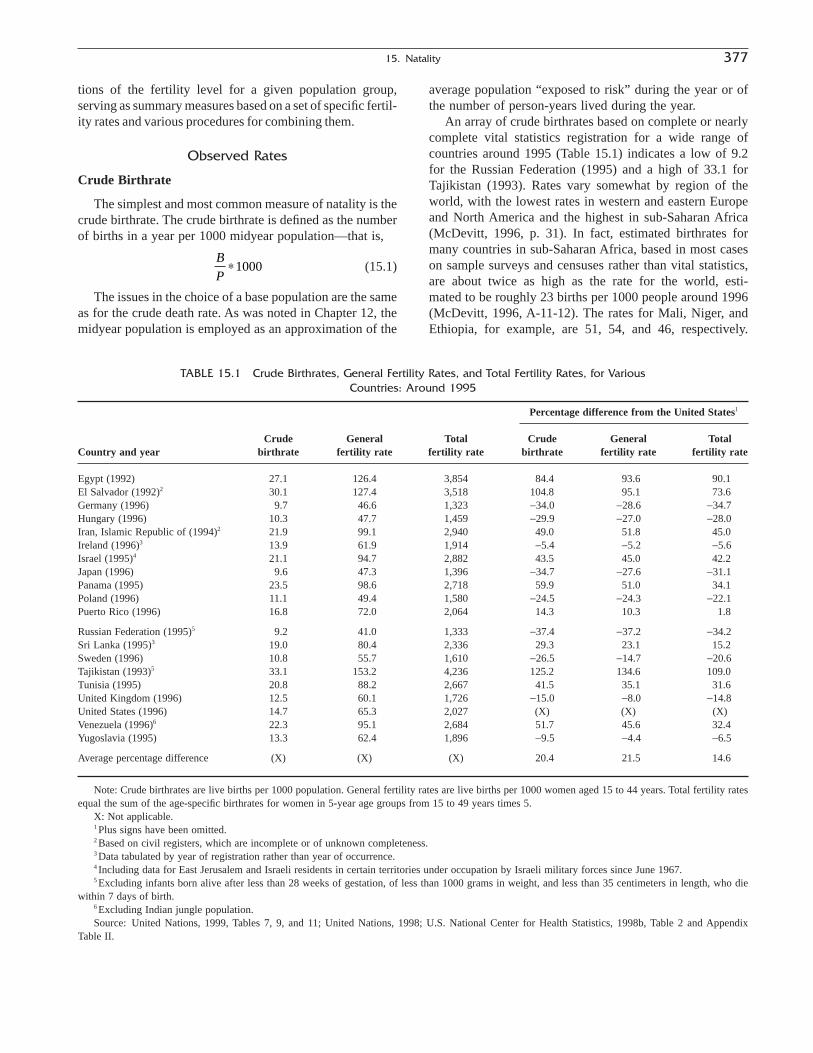
tions of the fertility level for a given population group,serving as summary measures based on a set of specific fertil-ity rates and various procedures for combining them.
Observed Rates
Crude Birthrate
The simplest and most common measure of natality is thecrude birthrate. The crude birthrate is defined as the numberof births in a year per 1000 midyear population—that is,
(15.1)
The issues in the choice of a base population are the sameas for the crude death rate. As was noted in Chapter 12, themidyear population is employed as an approximation of the
B
P*1000
average population “exposed to risk” during the year or ofthe number of person-years lived during the year.
An array of crude birthrates based on complete or nearlycomplete vital statistics registration for a wide range ofcountries around 1995 (Table 15.1) indicates a low of 9.2for the Russian Federation (1995) and a high of 33.1 forTajikistan (1993). Rates vary somewhat by region of theworld, with the lowest rates in western and eastern Europeand North America and the highest in sub-Saharan Africa(McDevitt, 1996, p. 31). In fact, estimated birthrates formany countries in sub-Saharan Africa, based in most caseson sample surveys and censuses rather than vital statistics,are about twice as high as the rate for the world, esti-mated to be roughly 23 births per 1000 people around 1996(McDevitt, 1996, A-11-12). The rates for Mali, Niger, andEthiopia, for example, are 51, 54, and 46, respectively.
15. Natality 377
TABLE 15.1 Crude Birthrates, General Fertility Rates, and Total Fertility Rates, for Various Countries: Around 1995
Percentage difference from the United States1
Crude General Total Crude General TotalCountry and year birthrate fertility rate fertility rate birthrate fertility rate fertility rate
Egypt (1992) 27.1 126.4 3,854 84.4 93.6 90.1El Salvador (1992)2 30.1 127.4 3,518 104.8 95.1 73.6Germany (1996) 9.7 46.6 1,323 -34.0 -28.6 -34.7Hungary (1996) 10.3 47.7 1,459 -29.9 -27.0 -28.0Iran, Islamic Republic of (1994)2 21.9 99.1 2,940 49.0 51.8 45.0Ireland (1996)3 13.9 61.9 1,914 -5.4 -5.2 -5.6Israel (1995)4 21.1 94.7 2,882 43.5 45.0 42.2Japan (1996) 9.6 47.3 1,396 -34.7 -27.6 -31.1Panama (1995) 23.5 98.6 2,718 59.9 51.0 34.1Poland (1996) 11.1 49.4 1,580 -24.5 -24.3 -22.1Puerto Rico (1996) 16.8 72.0 2,064 14.3 10.3 1.8
Russian Federation (1995)5 9.2 41.0 1,333 -37.4 -37.2 -34.2Sri Lanka (1995)3 19.0 80.4 2,336 29.3 23.1 15.2Sweden (1996) 10.8 55.7 1,610 -26.5 -14.7 -20.6Tajikistan (1993)5 33.1 153.2 4,236 125.2 134.6 109.0Tunisia (1995) 20.8 88.2 2,667 41.5 35.1 31.6United Kingdom (1996) 12.5 60.1 1,726 -15.0 -8.0 -14.8United States (1996) 14.7 65.3 2,027 (X) (X) (X)Venezuela (1996)6 22.3 95.1 2,684 51.7 45.6 32.4Yugoslavia (1995) 13.3 62.4 1,896 -9.5 -4.4 -6.5
Average percentage difference (X) (X) (X) 20.4 21.5 14.6
Note: Crude birthrates are live births per 1000 population. General fertility rates are live births per 1000 women aged 15 to 44 years. Total fertility ratesequal the sum of the age-specific birthrates for women in 5-year age groups from 15 to 49 years times 5.
X: Not applicable.1 Plus signs have been omitted.2 Based on civil registers, which are incomplete or of unknown completeness.3 Data tabulated by year of registration rather than year of occurrence.4 Including data for East Jerusalem and Israeli residents in certain territories under occupation by Israeli military forces since June 1967.5 Excluding infants born alive after less than 28 weeks of gestation, of less than 1000 grams in weight, and less than 35 centimeters in length, who die
within 7 days of birth.6 Excluding Indian jungle population.Source: United Nations, 1999, Tables 7, 9, and 11; United Nations, 1998; U.S. National Center for Health Statistics, 1998b, Table 2 and Appendix
Table II.

378 Estee
Current geographic variation may also encompass reason-ably well the range of historical variation. For example, thecrude birthrate in the United States appears to have approx-imated 50 around 1800 (Grabill, Kiser, and Whelpton 1958,p. 5), and it declined to 15 in 1996. Natural fertility, or fer-tility uncontrolled in any way, would be higher than hasactually been experienced by any country’s population. Onthe basis of an analysis made by Henry (1961) of fertility ina number of populations where little or no fertility controlis practiced, we may estimate a crude birthrate of about 60as corresponding to conditions of natural fertility.
In computing the crude birthrate for geographic subdivi-sions of countries, it is preferable to employ births allocatedby place of usual residence, particularly if the populationdata are distributed in terms of place of usual residence. Sat-isfactory birthrates by residence may often be computed,however, on the basis of population data tabulated on a defacto basis. The use of residence data for births is moreimportant for the smaller geographic units than for the largerones, because the smaller the area, the more likely the rateis to be affected by the movement of mothers to hospitals tohave their babies. Rates by residence more truly reflect thepropensity of the population living in an area to have birthsthan rates by occurrence. In computing rates with births byoccurrence, some freedom in the choice of type of popula-tion is often possible, although use of de facto populationfigures is preferable.
As with the crude death rate, sometimes an annualaverage crude birthrate covering data for 2 or 3 years is com-puted in order to describe the longer period or to add sta-bility to the rates. As was noted in Chapter 12, these annualaverage rates may be computed in a number of ways, all ofwhich give essentially the same results. The crude rates maybe computed for each year and averaged, the annual averagenumber of births may be divided by the annual average population, or the average number of births for the 3 yearsmay be divided by the midperiod population. The last
(15.2)
is the most commonly used procedure.Like the term “crude death rate,” the term “crude
birthrate” when unqualified means the crude birthrate for thetotal population of an area, but one may also speak of thecrude birthrate of a particular population group in the area,such as a race, nativity, residence, or occupation group. Forexample, the crude birthrate for the black population of theUnited States in 1996 is represented by
In this more general sense the principal characteristic ofa “crude” birthrate is that all ages and both sexes are repre-sented in the rate.
B
Pb
b
* = * =1000594 781
33 503 4351000 17 8
,, ,
.
1 310001 2 3
2
B B B
P
+ +( )*
The birthrate should be adjusted for underregistration ofthe births and for underenumeration of the population if sat-isfactory estimates of these errors are available, accordingto the following formula:
(15.3)
where Cb represents the percentage completeness of registration of births and Cp represents the percentage com-pleteness of the census counts or population estimates.
Official national birthrates for the United States are nowbased on the uncorrected figures. The U.S. National Centerfor Health Statistics has followed this practice since 1959,on the ground that the underregistration of births is rathersmall and has presumably become smaller than the under-statement of the population. It has published an officialseries of birthrates for the years 1909 to 1959 employingbirths adjusted for underregistration; during all or most ofthis period, births were presumed to be less completelyreported than the census population.
Monthly Birthrate
For births, as for deaths, there is an interest in examiningvariations over periods shorter than a year. We note onlyvery briefly here the measures of the monthly variation inthe birthrate, corresponding to those described for the deathrate in Chapter 12. The monthly birth rate may be “annual-ized” by inflating the number of births for a given month bythe ratio of the total number of days in the year to the numberin the particular month and then dividing by the populationfor the month. The annualized birthrate in the United Statesfor November 1997, adjusted for underregistration, isobtained as follows:
For births, as for deaths, analysis of monthly changes maybe carried out on the basis of rates computed for successive12-month periods ending in each successive month. Rates ofthis kind for the United States, based on provisional data, arepublished with a lag of about 6 months by the U.S. NationalCenter for Health Statistics (1998a). Year-to-year changes inthe birthrate on a current basis can also be measured by com-paring the rates for the same month in successive years. Therates in this comparison do not require adjustment for thenumber of days in the month or for seasonal variations(except for February in leap year). Annual relative changescan also be measured on a current basis by comparing cumu-lative rates covering all the months in a year to date with the
36530
36530
302 000
268 592 0001000
3 674 333268 592 000
1000 13 7
*=
**
= * =
B
P
November 1997
November 1997
,
, ,, ,, ,
.
B C
P Cb
p
∏∏
*1000
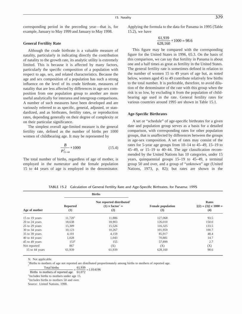
corresponding period in the preceding year—that is, forexample, January to May 1999 and January to May 1998.
General Fertility Rate
Although the crude birthrate is a valuable measure ofnatality, particularly in indicating directly the contributionof natality to the growth rate, its analytic utility is extremelylimited. This is because it is affected by many factors, particularly the specific composition of a population withrespect to age, sex, and related characteristics. Because theage and sex composition of a population has such a stronginfluence on the level of its crude birthrate, measures ofnatality that are less affected by differences in age-sex com-position from one population group to another are moreuseful analytically for interarea and intergroup comparisons.A number of such measures have been developed and arevariously referred to as specific, general, adjusted, or stan-dardized, and as birthrates, fertility rates, or reproductionrates, depending generally on their degree of complexity oron their particular significance.
The simplest overall age-limited measure is the generalfertility rate, defined as the number of births per 1000women of childbearing age. It may be represented by
(15.4)
The total number of births, regardless of age of mother, isemployed in the numerator and the female population 15 to 44 years of age is employed in the denominator.
B
P f15 44
1000-
*
Applying the formula to the data for Panama in 1995 (Table15.2), we have
This figure may be compared with the correspondingfigure for the United States in 1996, 65.3. On the basis ofthis comparison, we can say that fertility in Panama is aboutone and a half times as great as fertility in the United States.The general fertility rate is sometimes defined in relation tothe number of women 15 to 49 years of age but, as notedbelow, women aged 45 to 49 contribute relatively few birthsto the total number. It is preferable, therefore, to avoid dilu-tion of the denominator of the rate with this group when therisk is so low, by excluding it from the population of child-bearing age used in the rate. General fertility rates forvarious countries around 1995 are shown in Table 15.1.
Age-Specific Birthrates
A set or “schedule” of age-specific birthrates for a givendate and population group serves as a basis for a detailedcomparison, with corresponding rates for other populationgroups, that is unaffected by differences between the groupsin age-sex composition. A set of rates may consist of therates for 5-year age groups from 10–14 to 45–49, 15–19 to45–49, or 15–19 to 40–44. The age classification recom-mended by the United Nations has 10 categories, under 15years, quinquennial groups 15–19 to 45–49, a terminalgroup 50 and over, and a group of “unknown” age (UnitedNations, 1973, p. 82); but rates are shown in the
61 939628 160
1000 98 6,,
.* =
15. Natality 379
TABLE 15.2 Calculation of General Fertility Rate and Age-Specific Birthrates, for Panama: 1995
Births
Not reported distributed1 RatesReported (1) ¥ factor2 = Female population [(2) ∏ (3)] ¥ 1000 =
Age of mother (1) (2) (3) (4)
15 to 19 years 11,7203 11,886 127,068 93.520 to 24 years 18,638 18,903 126,010 150.025 to 29 years 15,309 15,526 116,325 133.530 to 34 years 10,123 10,267 101,959 100.735 to 39 years 4,101 4,159 85,917 48.440 to 44 years 1,028 1,043 70,881 14.745 to 49 years 1534 155 57,899 2.7Not reported 867 (X) (X) (X)
15 to 44 years 61,939 61,939 628,160 98.6
X: Not applicable.1 Births to mothers of age not reported are distributed proportionately among births to mothers of reported age.2
3 Includes births to mothers under age 15.4 Includes births to mothers 50 and over.Source: United Nations, 1998.
Total births
Births to mothers of reported age= =61 939
61 0721 014196
,
,.

380 Estee
Demographic Yearbook for the group under 20, and a ter-minal group 45 and over (United Nations, 1999, Table 11).
An age-specific birthrate is defined as the number ofbirths to women of a given age group per 1000 women inthat age group:
(15.5)
The formula for the birthrate at ages 20 to 24 is
(15.6)
Age-specific birthrates as here defined are a type of“central” rate, in somewhat the same sense that age-specificdeath rates are central rates. The corresponding probabilitiesare discussed later. The rate for women 20 to 24 years oldin Panama (1995) is, therefore (Table 15.2),
Table 15.3 presents schedules of age-specific birthratesfor a number of countries around 1995, and Figure 15.1 dis-plays these rates graphically. The lines approximate normalcurves moderately skewed to the right. Despite the general
18 903126 010
1000 150 0,,
.* =
fB
P f20 2420 24
20 24
1000--
-
= *
fB
Pa
a
af
= *1000
similarity of these curves from one country to another, thereare interesting differences as well. For example, birthratespeak for women in their early twenties (20 to 24 age group)in several countries (e.g., Tajikistan, El Salvador), while, inother countries (e.g., Iran, United States), the rates are highand nearly equal in the two 5-year age groups for women intheir twenties. Birth rates for women 15 to 19 years of agevary considerably from a low of 4 per 1000 in Japan to ahigh of 109 per 1000 in El Salvador. The relative magni-tudes of the age-specific birth rates are more evident whenthe schedules of rates are converted into percent distribu-tions, as is shown in Table 15.4. The rates for ages 45 to 49are of little absolute or relative importance, and the rates forages 40 to 44 usually fall below those for ages 15 to 19.Most births—from 94 to 99% depending on the country—occur to women between 15 and 39 years of age. Births inthe peak childbearing years, those between ages 20 and 29,account for a low of 42% of births in Ireland to a high of67% of births in Russia.
Differences in the age pattern of childbearing may alsobe measured in terms of the median age of childbearing(median age of mother) or the mean age of childbearing(mean age of mother). Both measures are used but under different circumstances. Calculating these measures on thebasis of age-specific birthrates rather than numbers of births
TABLE 15.3 Age-Specific Birthrates and Median Age of Mother, for Various Countries: Around 1995 (Birthrates are live births per 1000 women in specified group.)
Birthrates by age of woman
15 to 19 20 to 24 25 to 29 30 to 34 35 to 39 40 to 44 45 to 49 Median ageCountry and year years1 years years years years years years2 of mother
Egypt (1992) 13.3 150.9 252.9 180.4 120.5 39.2 13.6 28.4El Salvador (1992) 108.7 192.3 166.1 116.8 75.4 33.8 10.5 26.5Germany (1996) 9.6 55.4 90.2 75.8 28.4 4.9 0.2 28.7Hungary (1996) 29.9 92.6 100.0 48.9 16.9 3.4 0.1 26.2Iran (1994) 46.2 147.0 151.7 113.4 74.6 36.4 18.7 28.3Ireland (1996)3 16.1 52.2 108.0 129.4 64.2 12.2 0.6 30.6Israel (1995) 18.2 121.8 188.3 150.6 78.2 17.9 1.5 28.9Japan (1996) 3.9 39.7 109.9 95.4 27.4 2.9 0.1 29.4Mexico (1995) 85.2 172.1 166.1 123.7 70.9 26.6 7.6 27.1Panama (1995) 93.5 150.0 133.5 100.7 48.4 14.7 2.7 26.1Russian Federation (1995) 44.7 112.8 66.7 29.5 10.6 2.2 0.1 23.9Sri Lanka (1995)3 29.6 95.1 132.5 113.0 72.7 21.8 2.6 29.1Sweden (1996) 7.8 59.2 116.4 92.3 38.9 7.0 0.3 29.0Tajikistan (1993) 53.9 271.9 225.5 159.6 93.6 35.7 6.9 27.2Tunisia (1995) 13.6 93.0 151.6 144.2 89.7 33.5 7.7 30.3United Kingdom (1996) 29.7 76.2 106.8 88.6 36.9 6.8 0.3 28.1United States (1996) 55.6 110.4 113.1 83.9 35.3 6.8 0.3 26.6Venezuela (1996) 88.1 147.8 130.0 93.1 54.6 19.0 4.0 26.2Yugoslavia (1995) 32.6 126.6 121.6 69.1 24.1 4.7 0.5 26.3
1 Includes births to women under age 15. Base is the female population 15 to 19 years of age.2 Includes births to women age 50 and over. Base is the female population 45 to 49 years of age.3 Data tabulated by year of registration rather than year of occurrence.Source: Based on United Nations, 1999, Table 11; U.S. National Center for Health Statistics 1998b, Table 3.

15. Natality 381
FIGURE 15.1 Age-Specific Birthrates for Various Countries: Around 1995 Note: Points are plotted at midpoint of age intervals.
Source: Table 15.3
TABLE 15.4 Percentage Distribution of Age-Specific Birthrates by Age of Mother, for VariousCountries: Around 1995
15 to 19 20 to 24 25 to 29 30 to 34 35 to 39 40 to 44 45 to 49Country and year All ages years1 years years years years years years2
Egypt (1992) 100.0 1.7 19.6 32.8 23.4 15.6 5.1 1.8El Salvador (1992) 100.0 15.4 27.3 23.6 16.6 10.7 4.8 1.5Germany (1996) 100.0 3.6 20.9 34.1 28.7 10.7 1.9 0.1Hungary (1996) 100.0 10.3 31.7 34.3 16.8 5.8 1.1 0.0Iran (1994) 100.0 7.9 25.0 25.8 19.3 12.7 6.2 3.2Ireland (1996)3 100.0 4.2 13.6 28.2 33.8 16.8 3.2 0.2Israel (1995) 100.0 3.2 21.1 32.7 26.1 13.6 3.1 0.3Japan (1996) 100.0 1.4 14.2 39.3 34.2 9.8 1.0 0.0Mexico (1995) 100.0 13.1 26.4 25.5 19.0 10.9 4.1 1.2Panama (1995) 100.0 17.2 27.6 24.6 18.5 8.9 2.7 0.5Russian Federation (1995) 100.0 16.8 42.3 25.0 11.1 4.0 0.8 0.0Sri Lanka (1995)3 100.0 6.3 20.3 28.4 24.2 15.6 4.7 0.6Sweden (1996) 100.0 2.4 18.4 36.2 28.7 12.1 2.2 0.1Tunisia (1995) 100.0 2.6 17.4 28.4 27.0 16.8 6.3 1.4United Kingdom (1996) 100.0 8.6 22.1 30.9 25.7 10.7 2.0 0.1United States (1996) 100.0 13.7 27.2 27.9 20.7 8.7 1.7 0.1Venezuela (1996) 100.0 16.4 27.5 24.2 17.3 10.2 3.5 0.7Yugoslavia (1995) 100.0 8.6 33.4 32.1 18.2 6.4 1.2 0.1
1 Includes births to women under age 15. Base is the female population 15 to 19 years of age.2 Includes births to women aged 50 and over. Base is the female population 45 to 49 years of age.3 Data tabulated by year of registration rather than year of occurrence.Source: United Nations, 1999, Table 11; U.S. National Center for Health Statistics, 1998b, Table 3.

eliminates the effect of differences in the age-sex composi-tion of the populations being compared. They may be inter-preted then as describing the age pattern of childbearing ofa synthetic cohort of women—that is, a hypothetical groupof women who are viewed as having in their lifetime the(fertility) experience recorded in a single calendar year.
Both the median age and the mean age are ordinarilycomputed from data compiled for 5-year age groups. Themean age of a distribution of birthrates is computed accord-ing to the following formula:
(15.7)
where a represents the midpoint of each age interval (17.5,22.5, etc.) and fa represents an age-specific birthrate for a 5-year age group. (The formula follows the form of aweighted average of ages, the weights being the age-specificbirthrates.)
The considerable similarity of the age distributions ofbirth rates suggests that the median age would vary onlylittle. For the array of countries shown in Table 15.3, thehighest and lowest median ages vary by 6.7 years out of arange of about 35 years of reproductive life, but if the twoextreme cases of the Russian Federation (23.9) and Ireland(30.6) are excluded, the difference falls to only 4.2 years.These differences tend to distinguish populations that havetheir children relatively early in the childbearing period andthose that have them relatively late. On this basis, child-bearing occurs relatively early in the Russian Federation and relatively late in Ireland. These differences may beaccounted for in terms of the differences in the median ageat first birth and in the median interval between births. Tothe extent that marriage is a precursor of childbearing, theage at marriage and the interval between marriage and thefirst birth may also account for these differences.
Fertility Rates Specific for Order of Birth
Another dimension for analyzing fertility, in addition tothe age of the mother, is the order of birth of the child. Orderof birth refers to the number or sequence of the child amongthe live births of the mother, including the present child. Thesimplest way of analyzing births classified by order of birthconsists of calculating the proportional distribution of thebirths by order. Such a percentage distribution of births byorder is much less affected by underregistration of birthsthan are rates and can be computed without use of popula-tion data; but at the same time, the percentages are affectedby such factors as the distribution of the female populationby age. As illustrated by data for several countries, thosewith the lowest levels of fertility have proportionately more
aaf
f
aa
aa
=ÂÂ
births of first or second order than those with higher levelsof fertility:
382 Estee
Egypt, Japan, Panama, United States,Birth order 1992 1996 1995 1996
Total 100.0 100.0 100.0 100.0First 34.7 47.6 34.1 40.8Second 22.9 36.8 25.3 32.2Third 16.1 12.8 16.2 16.1Fourth 10.9 2.2 8.8 6.2Fifth 6.9 0.4 5.2 2.3Sixth 4.3 0.1 3.3 1.0Seventh 2.3 — 2.3 0.4Eighth and over 2.0 — 3.7 0.5Not reported — — 1.1 0.6
—: Zero or rounds to zero.
General fertility rates may be computed for each order ofbirth without reference to age of the mother. A generalorder-specific fertility rate is defined as the number of birthsof a given order per 1000 women of childbearing age:
(15.8)
where Bi represents births of a given order and Pf15–44 the
number of women 15 to 44 years of age. Thus, the generalsecond-order fertility rate is
(15.9)
where B2 refers to births of the second order. This formulais evaluated for Panama in 1995 as follows (Table 15.5):
Note that the sum of the general order-specific rates overall orders equals the general fertility rate, that is
(15.10)
Usually, there is a category of births of order not reported.This category may be treated separately or distributed overthe births of reported order pro rata.
Variations in order-specific birthrates by age may be analyzed in terms of age-order-specific rates. A rate of thistype is represented by the formula:
(15.11)
where Bai represents births of a given order to women of a
given age group and Paf relates to all the women in a partic-
ular age group, without regard to the number of children
fB
Pai a
i
af
= *1000
B
P
B
Pi
fi
f15 441 15 44-=
•
-Â =
15 698628 160
1000 25 0,,
.* =
B
P f
2
15 44
1000-
*
B
Pi
f15 44
1000-
*

they have had. This is a type of central rate, as we havedefined it. For example, the second-order birthrate forwomen 20 to 24 years old in Panama (1995) is (Table 15.5):
The sum of age-order-specific rates over all orders for a particular age group equals the general age-specific birthratefor that age group (the rates being additive because thedenominators are the same)—that is,
(15.12)
The age-order-specific rates cannot be added for a par-ticular order over all ages to derive the general fertility ratefor that order, however, because the denominators of therates are all different.
In the calculation of age-order-specific birthrates, it isdesirable to dispose both of births of “unknown” age and ofbirths of “unknown” order, both of which ordinarily appear in the basic tabulations. This can be done satisfactorily by(1) prorating the “unknown ages” for each order among the“known ages” for each order and then (2) prorating the“unknown orders” for each age group among the “knownorders” for each age group, or vice versa.
B
P
B
Pai
af
i
a
af
=
•
 * = *1
1000 1000
B
P f
20 242
20 24
10005 975
126 0101000 47 4-
-
* = * =,,
.
Median ages of childbearing may be computed for each order of birth from age-order-specific birthrates, asshown in Table 15.6. These values give an indication of the “typical” age at which mothers have their first, second,or later child. Differences between values for consecutiveorders give a rough idea of the spacing intervals betweenbirths. The median age for first births suggests the typicalage of starting families, and by determining the averagenumber of children per woman by other methods, we canidentify by interpolation the typical age of completing fam-ilies. For example, the typical age of starting families inPanama in 1995 is estimated at 21.6 years, the median ageof first births. The annual “total fertility rate,” discussedlater, of 2.7 children corresponds in Table 15.6 to a medianage of about 27 years, which may be taken as the typical ageof completing families in Panama. Each child tends tofollow the previous child after an interval of about 2.5 to 3.3years, with a total average interval of about 6 years from thebirth of the first child to the birth of the third, and normallylast, child. For women who have more than three childrenin Panama, the average time between each successive laterbirth tends to be about 1.5 to 2.5 years.
Marital and Nonmarital Fertility Rates
Observed fertility rates may be further refined by takingmarital status into account in classifying births and defining
15. Natality 383
TABLE 15.5 Calculation of General Order-Specific Birthrates and Order-Specific Birthrates forWomen 20 to 24 Years of Age, for Panama: 1995
Ages 20 to 24 RatesBirths including age
All ages Ages 20 to 24Ages 20 to 24 Age
not reported1
(1) ∏ female (4) ∏ femaleAll ages reported not reported pop. 15 to 442 = pop. 20 to 243 =
Birth order (1) (2) (3) (4) (5) (6)
All orders 61,939 18,638 867 18,8734 98.6 149.84
First 21,101 7,368 128 7,413 33.6 58.8Second 15,698 5,934 108 5,975 25.0 47.4Third 10,051 3,419 85 3,448 16.0 27.4Fourth 5,468 1,337 47 1,349 8.7 10.7Fifth 3,211 382 33 386 5.1 3.1Sixth 2,072 88 28 89 3.3 0.7Seventh 1,407 18 21 18 2.2 0.1Eighth and over 2,262 13 39 13 3.6 0.1Not reported 669 79 378 182 1.1 1.4
Median order of birth (X) (X) (X) (X) 2.1 1.8
X: Not applicable.1 Births to mothers with age not reported are distributed proportionately among births to mothers with age reported.2 Female population 15 to 44 years of age = 628,160.3 Female population 20 to 24 years of age = 126,010.4 Number of births obtained by summation of figures for each order; numbers and rates differ from figures obtained by distributing ages not reported
without regard to order of birth (18,903 and 150.0).Source: United Nations Statistics Division, 1998.
11 3
2( )
( ) - ( )*( ) =

the base population. In many countries, births still occur pri-marily within marriage, but in a number of countries, theproportion of births occurring outside marital unions hasbecome significant (United Nations, 1998b, pp. 54–55). Inthe past, marital fertility measures have used labels derivedfrom the concept of the legitimacy status of the child at birth.The United Nations defines legitimate live births as thosethat occur to parents who are married at the time of birthaccording to the prevailing civil laws of the area. Birthsoccurring within nonmarital unions have usually been clas-sified as illegitimate. To avoid stigmatizing a child, the useof such labels on a child’s birth certificate is no longer recommended, even though the concept of legitimacy maycontinue to be used for technical and statistical purposes bythe United Nations and some countries (see footnote 3). Wehave chosen to use the terms “marital” and “nonmarital” inplace of “legitimate” and “illegitimate” in labeling variousfertility measures, thereby classifying the birth in terms ofthe marital status of the parents rather than the apparent legal
status of the child. Except as noted later, this change merelyaffects the label of the measure and not the way in which itis calculated.
General and Age-Specific Marital and Nonmarital Fertility Rates
The general marital fertility rate and the general non-marital fertility rate relate live births to married women andlive births to unmarried women, respectively. The generalmarital fertility rate (formerly, general legitimate fertilityrate) is defined as the number of live births occurring tomarried women in a year per 1000 married women 15 to 44years of age at the middle of the year:
(15.13)
where Bm represents live births to women who were legallymarried at the time of birth and Pfm
15–44 represents marriedwomen (including those who are separated but not yet
B
P
m
fm15 44
1000-
*
384 Estee
TABLE 15.6 Age-Order-Specific Birthrates, for the United States, 1996, and Panama, 1995
Age of mother1
Country, year, and General 15 to 19 20 to 24 25 to 29 30 to 34 35 to 39 40 to 44 45 to 49 Median age order of birth fertility rate2 years3 years years years years years years4 of mother
United States (1996)All orders5 65.3 55.6 110.4 113.1 83.9 35.3 6.8 0.3 26.5First 26.8 43.7 52.0 42.7 23.4 7.8 1.4 0.1 24.0Second 21.1 9.9 37.4 39.5 30.5 11.4 1.9 0.1 27.3Third 10.5 1.7 14.8 19.7 17.8 8.2 1.4 0.1 28.9Fourth 4.1 0.2 4.5 7.2 7.2 4.1 0.9 — 30.1Fifth 1.5 — 1.2 2.5 2.8 1.8 0.5 — 31.2Sixth 0.6 — 0.3 0.9 1.2 0.9 0.3 — 32.5Seventh 0.3 — 0.1 0.4 0.6 0.5 0.2 — 33.3Eighth and over 0.3 — — 0.2 0.5 0.6 0.3 — 35.8
Median order of birth 1.8 1.1 1.6 1.9 2.1 2.4 2.6 3.0 (X)
Panama (1995)All orders5 98.6 93.0 149.8 133.7 101.0 48.7 14.8 2.7 26.1First 34.0 68.1 59.4 29.8 12.8 3.4 1.1 0.1 21.6Second 25.3 20.6 47.9 36.9 21.9 7.0 1.1 0.2 24.9Third 16.2 3.9 27.6 28.1 20.6 8.4 1.3 0.1 27.4Fourth 8.8 0.4 10.8 18.1 14.2 5.7 1.0 0.2 28.9Fifth 5.2 0.1 3.1 11.5 9.9 4.9 1.0 0.3 30.4Sixth 3.3 — 0.7 5.8 8.2 4.6 1.3 0.1 31.4Seventh 2.3 — 0.1 2.3 6.4 4.3 1.6 0.2 33.9Eighth and over 3.6 — 0.1 1.2 7.0 10.3 6.4 1.5 36.8
Median order of birth 2.1 1.2 1.8 2.5 3.3 4.5 6.9 7.6 (X)
—: Represents zero or rounds to zero.X: Not applicable.1 Births to mothers of age not reported are distributed proportionately among births to mothers of reported age.2 General fertility rates are live births per 1000 women aged 15 to 44 years.3 Includes births to mothers under 15 years of age.4 Includes births to mothers 50 years of age and over.5 Births of order not reported are distributed proportionately among births of reported birth order.Source: United Nations Statistics Division, 1998; U.S. National Center for Health Statistics, 1998b, Tables 2 and 3.

divorced) who are 15 to 44 years of age.4 An array of generalmarital fertility rates for years around 1995 is shown inTable 15.7. The rates given here range from 68.7 forHungary to 110.4 for Ireland. The general nonmarital fer-tility rate (formerly, the illegitimacy rate) is defined as thenumber of live births to unmarried women in a year, regard-less of the age of the mother, per 1000 unmarried women 15to 44 years old at the middle of the year:
(15.14)B
P
u
fu15 44
1000-
*
where Bu represents live births to women who were notlegally married at the time of birth and Pu
15–44 representsunmarried women (i.e., single, widowed, divorced, or co-habiting partner) who are 15 to 44 years of age. An array ofgeneral nonmarital fertility rates for years around 1995 is shown in Table 15.7. The rates given here range from 12.6 for Poland to 65.6 for Chile, a country in which nearly7% of the women of childbearing ages are living in consensual unions (United Nations, 1998).
Age-specific marital birthrates and age-specific nonmar-ital birthrates may also be computed for women in specificage categories—that is,
(15.15)
and
(15.16)B
Pau
afu
*1000
B
Pam
afm
*1000
15. Natality 385
TABLE 15.7 General Marital and Nonmarital Fertility Rates and Age-Specific Birthrates by MaritalStatus, for Various Countries: Around 1995
Age-specific birthrates by marital status
Marital status, General marital or 15 to 19 20 to 24 25 to 29 30 to 34 35 to 39 40 to 44 45 to 49country, and year nonmarital fertility rate years1 years years years years years years2
Married 3
Australia (1994) 90.9 162.8 179.7 186.4 126.8 44.9 6.7 0.3Chile (1992) 102.7 230.3 198.1 150.6 98.3 49.0 12.5 1.0Hungary (1996) 68.7 394.4 214.7 128.1 52.6 16.8 3.2 0.1Ireland (1996)4,5 110.4 376.8 266.7 216.3 171.6 77.9 13.7 0.7Poland (1996) 73.9 601.7 254.8 131.0 61.8 25.0 5.7 0.3Sweden (1996) 75.2 304.3 249.6 193.0 109.8 39.3 6.6 0.3United States (1996) 83.7 346.3 209.1 157.0 102.4 41.1 8.0 (X)
Unmarried 6
Australia (1994) 33.3 18.6 40.7 52.1 49.5 28.8 6.9 0.2Chile (1992) 65.6 47.4 82.5 87.8 83.3 62.6 20.1 1.6Hungary (1996) 23.3 16.9 30.3 42.6 37.5 17.0 3.7 0.1Ireland (1996)4,7 26.0 15.5 37.8 33.7 32.5 19.1 5.6 0.3Poland (1996) 12.6 7.8 17.2 21.0 22.0 15.8 4.5 0.2Sweden (1996) 45.6 6.4 45.0 88.3 77.5 38.5 7.8 0.3United States (1996) 44.8 44.1 70.7 56.8 41.1 20.1 4.8 (X)
Note: General marital or nonmarital fertility rates are total live births to women in a given marital status per 1000 women 15 to 44 years of age in thesame marital status. Age-specific birthrates by marital status are live births to women of a given marital status and age group per 1000 women in the spec-ified group.
X: Not available1 Includes births to women under age 15; the base is women 15 to 19 years of age.2 Includes births to women age 50 and over; the base is women 45 to 49 years of age.3 Includes births to women who are separated.4 Data tabulated by year of registration rather than year of occurrence.5 Includes births to women who are “consensually” married but not for those who are separated.6 Includes births to women who are single, “consensually” married, widowed, or divorced.7 Includes births to women who are separated but not for those who are “consensually” married.Source: United Nations, 1998c; U.S. National Center for Health Statistics, 1998b, Tables 1, 17 and supplementary table, “Female Population by Marital
Status, Age, Race and Hispanic Origin: United States, 1996.”
4 The term “general marital fertility rate” was formerly used to repre-sent the total number of live births in a year, regardless of the age andmarital status of the mother, per 1000 married women 15 to 44 year of ageat the middle of the year (Shryock, Siegel, and Stockwell, 1976, p. 281).This particular measurement of all births relative to only married womenis no longer as useful as it once was, given the increasing number of birthsto women who are unmarried. As a result, this measure is not included hereand the term “general marital fertility rate” is reserved for births to marriedwomen per 1000 married women 15 to 44 years of age.

The nonmarital birth ratio (formerly, the illegitimacyratio) is defined as the number of live births to unmarriedwomen per 1000 total live births:
(15.17)
where Bu represents births to unmarried women and B totalbirths. This ratio may be subject to considerable under-statement because extramarital births are more likely to go unregistered than births occurring within marriage andbecause unmarried parents may report themselves asmarried to avoid social stigma for their child. The nonmar-ital birth ratio has an extremely wide range depending onthe situation in a given area: it may vary from nearly 0 tomore than 500 per 1000 live births:
Country and year Nonmarital birth ratio
Australia (1994) 256.1Chile (1992) 368.1Costa Rica (1995) 465.9Cyprus (1996) 14.9France (1994) 361.0Japan (1996) 12.8Kazakhstan (1996) 176.0Poland (1996) 101.7Spain (1995) 110.9Sri Lanka (1995) 15.4Sweden (1996) 538.9United States (1996) 323.9
The nonmarital birth ratio is strongly affected by the rel-ative frequency of nonmarital unions. The rise in cohabita-tion in many developed countries, particularly in WesternEurope, the United States, and Australia, has resulted inratios between 250 and 550. The highest ratio, 539 inSweden, indicates that over half of the births are to womenwho are not married at the time of the birth even though they are likely to be living with the father of the child. Latin American countries, with long-standing traditions of consensual unions, exhibit nonmarital birth ratios be-tween 350 and 500, as exemplified by the ratios for Chileand Costa Rica, which equal 368 and 466, respectively. Incountries where nonmarital unions are uncommon, the non-marital birth ratio tends to be rather low, as occurs in Asian and Southern European countries. In Japan, for ex-ample, only 13 out of 1000 live births occur to unmarried women.
Duration-Specific Marital Fertility Rates
For those births occurring to married couples, fertilityvaries as sharply with the duration of the marriage as withthe age of the parents. Tabulations of births by duration ofmarriage are rendered more useful for analysis if they arecross-tabulated by age of mother and order of birth. With the
B
B
u
*1000
increase in the number of births occurring outside marriage,information about nonmarital unions including their dura-tion would be useful. Vital records systems usually docu-ment a mother’s marital status but rarely gathers informationabout the duration of the marriage and never about the lengthof nonmarital unions. Population registers tend to be a goodsource of information about the duration of marriages but, like vital records, do not gather comparable data on“consensual” living arrangements. As a result, informationabout the duration of either marital or nonmarital unions isgenerally obtained from surveys or censuses.
The simplest measure, the duration-specific marital birthratio, is merely the percentage distribution of births tomarried women by duration of married life. In most coun-tries, the highest proportion of births to married womentends to occur in the first 5 years of marriage, as seen inTable 15.8. The concentration of births within the first 12months of marriage is noticeably high in Japan and Panama,two rather different countries; the first has a much higherproportion of births occurring within marriage than thelatter. Ireland exemplifies the other extreme with relativelyfew births to married women occurring within the first 12months of marriage.
Availability of the number of married women distributedby duration of married life makes it possible to computeduration-specific marital fertility rates. A duration-specificmarital fertility rate is defined as the number of live birthsto women married for a specific number of years per 1000women 15 to 44 (or 15 to 49) years of age married for thisnumber of years—that is,
(15.18)
where Bmt represents live births to women married t years
and Pfm15–44t represents women 15 to 44 years of age married
t years. Unfortunately, reliable estimates of the distributionof the female population by marital duration suitable for use in computing fertility rates have become increasinglydifficult to obtain. European countries that calculated these rates in the past no longer do so. As a result, duration-specific marital fertility rates are shown for only onecountry, Sweden. The usefulness of these rates is limited because slightly less than half of the births inSweden occur to women who are married at the time of thebirth.
For classifying the births, duration of married life is thenumber of completed years elapsed between the date of mar-riage and date of birth of the child. In the absence of infor-mation on the exact date of marriage, duration may be basedon the difference between the year of marriage and the yearof the birth. This procedure introduces an upward bias in thefrequencies for all durations except the category under-
B
Ptm
fmt15 44
1000-
*
386 Estee
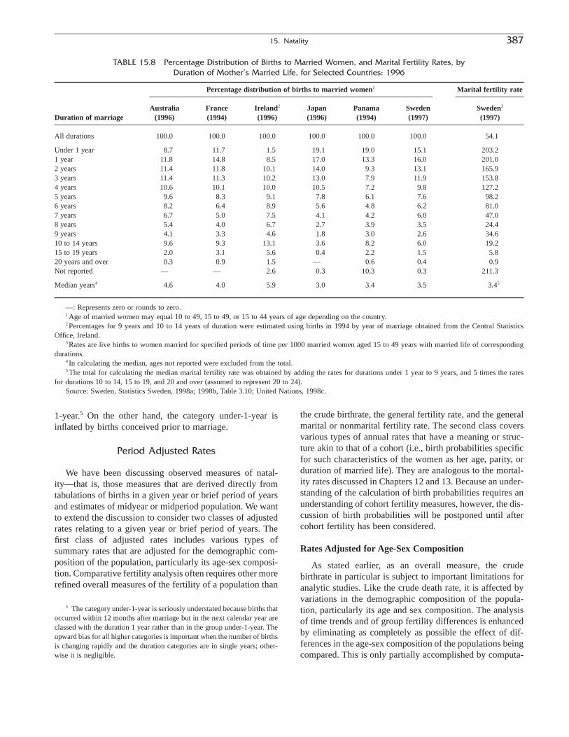
1-year.5 On the other hand, the category under-1-year isinflated by births conceived prior to marriage.
Period Adjusted Rates
We have been discussing observed measures of natal-ity—that is, those measures that are derived directly fromtabulations of births in a given year or brief period of yearsand estimates of midyear or midperiod population. We wantto extend the discussion to consider two classes of adjustedrates relating to a given year or brief period of years. Thefirst class of adjusted rates includes various types ofsummary rates that are adjusted for the demographic com-position of the population, particularly its age-sex composi-tion. Comparative fertility analysis often requires other morerefined overall measures of the fertility of a population than
the crude birthrate, the general fertility rate, and the generalmarital or nonmarital fertility rate. The second class coversvarious types of annual rates that have a meaning or struc-ture akin to that of a cohort (i.e., birth probabilities specificfor such characteristics of the women as her age, parity, orduration of married life). They are analogous to the mortal-ity rates discussed in Chapters 12 and 13. Because an under-standing of the calculation of birth probabilities requires anunderstanding of cohort fertility measures, however, the dis-cussion of birth probabilities will be postponed until aftercohort fertility has been considered.
Rates Adjusted for Age-Sex Composition
As stated earlier, as an overall measure, the crudebirthrate in particular is subject to important limitations foranalytic studies. Like the crude death rate, it is affected byvariations in the demographic composition of the popula-tion, particularly its age and sex composition. The analysisof time trends and of group fertility differences is enhancedby eliminating as completely as possible the effect of dif-ferences in the age-sex composition of the populations beingcompared. This is only partially accomplished by computa-
15. Natality 387
TABLE 15.8 Percentage Distribution of Births to Married Women, and Marital Fertility Rates, byDuration of Mother’s Married Life, for Selected Countries: 1996
Percentage distribution of births to married women1 Marital fertility rate
Australia France Ireland2 Japan Panama Sweden Sweden3
Duration of marriage (1996) (1994) (1996) (1996) (1994) (1997) (1997)
All durations 100.0 100.0 100.0 100.0 100.0 100.0 54.1
Under 1 year 8.7 11.7 1.5 19.1 19.0 15.1 203.21 year 11.8 14.8 8.5 17.0 13.3 16.0 201.02 years 11.4 11.8 10.1 14.0 9.3 13.1 165.93 years 11.4 11.3 10.2 13.0 7.9 11.9 153.84 years 10.6 10.1 10.0 10.5 7.2 9.8 127.25 years 9.6 8.3 9.1 7.8 6.1 7.6 98.26 years 8.2 6.4 8.9 5.6 4.8 6.2 81.07 years 6.7 5.0 7.5 4.1 4.2 6.0 47.08 years 5.4 4.0 6.7 2.7 3.9 3.5 24.49 years 4.1 3.3 4.6 1.8 3.0 2.6 34.610 to 14 years 9.6 9.3 13.1 3.6 8.2 6.0 19.215 to 19 years 2.0 3.1 5.6 0.4 2.2 1.5 5.820 years and over 0.3 0.9 1.5 — 0.6 0.4 0.9Not reported — — 2.6 0.3 10.3 0.3 211.3
Median years4 4.6 4.0 5.9 3.0 3.4 3.5 3.45
—: Represents zero or rounds to zero.1 Age of married women may equal 10 to 49, 15 to 49, or 15 to 44 years of age depending on the country.2 Percentages for 9 years and 10 to 14 years of duration were estimated using births in 1994 by year of marriage obtained from the Central Statistics
Office, Ireland.3 Rates are live births to women married for specified periods of time per 1000 married women aged 15 to 49 years with married life of corresponding
durations.4 In calculating the median, ages not reported were excluded from the total. 5 The total for calculating the median marital fertility rate was obtained by adding the rates for durations under 1 year to 9 years, and 5 times the rates
for durations 10 to 14, 15 to 19, and 20 and over (assumed to represent 20 to 24).Source: Sweden, Statistics Sweden, 1998a; 1998b, Table 3.10; United Nations, 1998c.
5 The category under-1-year is seriously understated because births thatoccurred within 12 months after marriage but in the next calendar year areclassed with the duration 1 year rather than in the group under-1-year. Theupward bias for all higher categories is important when the number of birthsis changing rapidly and the duration categories are in single years; other-wise it is negligible.
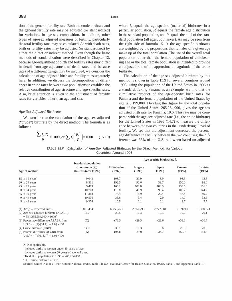
tion of the general fertility rate. Both the crude birthrate andthe general fertility rate may be adjusted (or standardized)for variations in age-sex composition. In addition, othertypes of age-sex adjusted measures of fertility, particularlythe total fertility rate, may be calculated. As with death rates,birth or fertility rates may be adjusted (or standardized) byeither the direct or indirect method. Even though the basicmethods of standardization were described in Chapter 12,because age-adjustment of birth and fertility rates may differin detail from age-adjustment of death rates and becauserates of a different design may be involved, we consider thecalculation of age-adjusted birth and fertility rates separatelyhere. In addition, we discuss the decomposition of differ-ences in crude rates between two populations to establish therelative contribution of age structure and age-specific rates.Also, brief attention is given to the adjustment of fertilityrates for variables other than age and sex.
Age-Sex Adjusted Birthrate
We turn first to the calculation of the age-sex adjusted(“crude”) birthrate by the direct method. The formula is asfollows:
(15.19)f P
Pf
P
Pa a
f
aaf Â* Ê
ËÁˆ¯̃ *1000 1000, or
where fa equals the age-specific (maternal) birthrates in aparticular population, Pf
a equals the female age distributionin the standard population, and P equals the total of the stan-dard population (all ages, both sexes). As may be seen fromthe right side of formula 15.19, the age-specific birthratesare weighted by the proportions that females of a given agemake up of the total population. The use of the overall totalpopulation rather than the female population of childbear-ing age or the total female population is intended to providean adjusted rate of the approximate magnitude of the crudebirthrate.
The calculation of the age-sex adjusted birthrate by thismethod is shown in Table 15.9 for several countries around1995, using the population of the United States in 1996 asa standard. Taking Panama as an example, we find that thecumulative product of the age-specific birth rates forPanama and the female population of the United States byage is 5,199,800. Dividing this figure by the total popula-tion of the United States, 265,284,000, gives the age-sexadjusted birth rate for Panama, 19.6. This rate may be com-pared with the age-sex adjusted rate (i.e., the crude birthrate)for the United States in 1996 (14.7) to measure the differ-ence between the two countries in the “underlying” level offertility. We see that the adjustment decreased the percent-age difference in fertility between the two countries; the dif-ference was 33% of the U.S. rate when based on adjusted
388 Estee
TABLE 15.9 Calculation of Age-Sex Adjusted Birthrates by the Direct Method, for Various Countries: Around 1995
Standard populationAge-specific birthrates, fa
(thousands) (Pfa) El Salvador Hungary Japan Panama Tunisia
Age of mother United States (1996) (1992) (1996) (1996) (1995) (1995)
15 to 19 years1 9,043 108.7 29.9 3.9 93.5 13.620 to 24 years 8,561 192.3 92.6 39.7 150.0 93.025 to 29 years 9,469 166.1 100.0 109.9 133.5 151.630 to 34 years 10,708 116.8 48.9 95.4 100.7 144.235 to 39 years 11,318 75.4 16.9 27.4 48.4 89.740 to 44 years 10,506 33.8 3.4 2.9 14.7 33.545 to 49 years2 9,376 10.5 0.1 0.1 2.7 7.7
(1) SPfafa = expected births 3,891,494 6,759,763 2,761,298 2,777,981 5,199,800 5,338,123
(2) Age-sex adjusted birthrate (ASABR) 14.7 25.5 10.4 10.5 19.6 20.1= [(1)/265,284,000] *10003
(3) Percentage difference ASABR from (X) +73.5 -29.3 -28.6 +33.3 +36.7U.S.4 = {[(2)/(14.7)] - 1.0}*100
(4) Crude birthrate (CBR) 14.7 30.1 10.3 9.6 23.5 20.8(5) Percent difference of CBR from (X) +104.8 -29.9 -34.7 +59.9 +41.5
U.S.4 = {[(4)/(14.7)] - 1.0}*100
X: Not applicable.1 Includes births to women under 15 years of age.2 Includes births to women 50 years of age and over.3 Total U.S. population in 1996 = 265,284,000.4 U.S. crude birthrate = 14.7.Source: United Nations, 1999; United Nations, 1998c, Table 11; U.S. National Center for Health Statistics, 1998b, Table 1 and Appendix Table II.

rates but 60% when based on crude rates. It is implied thatthe age-sex composition of Panama’s population is morefavorable for a high level of fertility than that of the UnitedStates. Subtracting the difference in age-adjusted fertilityrates (4.9) from the total difference between the crude rates(8.8) yields an estimate of the effect of the difference in agecomposition (3.9) on the difference between the crude rates.Because these results are affected by the choice of the pop-ulation used as a standard, we consider this decompositionof the difference in the crude rates preliminary and considerthe more refined calculation that follows.
The general fertility rate may also be further adjusted forage-sex composition by the direct method by applying thefollowing formula:
(15.20)
This formula is like the formula for the age-sex adjustedbirthrate, except that the divisor here is the female populationof childbearing age rather than the total population. Hence,age-sex adjusted general fertility rates are of the same orderof magnitude as unadjusted general fertility rates. Relativevariations in age-sex adjusted general fertility rates are thesame as those in age-sex adjusted “crude” birthrates; hence,the former type of rate is infrequently used.
The crude birthrate may also be adjusted for age-sex com-position by the indirect method when age-specific birthratesfor the particular population are lacking or defective. Theconventional calculation by this method follows the formula:
(15.21)
where the symbols have the following meaning:
For the particular population:b = total birthspf
a = female population by ageFor the “standard” population:
Fa = age-specific birthratesF = crude birthrate
b
F pF
a af * *1000
f P
P
a af
af
ÂÂ *1000
Note that this formula may be restated as
(15.22)
that is to say, the relative difference in adjusted fertilitybetween the two areas is equivalent to direct standardizationin which the population distribution of the particular popula-tion under study is the standard population. In effect, then, in“indirect standardization” the age-specific pattern of fertilityis borrowed for the population under study and the standardpopulation is the age-sex distribution of the study population.
The calculation of age-sex adjusted rates using the indi-rect method is illustrated in Table 15.10 for several coun-tries using the age-specific birthrates of the United States in1996 as the pattern for fertility and the population of Panamaas the standard population. For example, for Panama in1995, we proceed as follows: First, we compute the cumu-lative product of the age-specific rates for the United States(the standard weights) and the number of women in Panamain each age group. The result, 46,186, represents the numberof births that Panama would have had in 1995 if its age-specific birthrates were equal to those of the United Statesin 1996. The ratio of the actual number of births in Panamain 1995, 61,939, to the expected number equals 1.3411. Mul-tiplying this ratio times the crude birthrate of the UnitedStates (14.7) gives a sex-age adjusted birthrate per 1000population of 19.7 for Panama. Before the adjustment of the crude birthrate, fertility in Panama appeared to be 60% greater than in the United States (23.5/14.7), as shownin Table 15.9; following the adjustment, the differenceappeared to be only 34% (19.7/14.7). The result suggeststhat a difference in age-sex composition accounts for a con-siderable part of the difference in crude birthrates.
The age-sex adjusted birthrates derived from indirectstandardization were similar to those produced throughdirect standardization for all of the countries considered hereexcept Tunisia, as illustrated by the following summary ofrates and percentage differences from the crude birthrate ofthe United States:
f p
F pF
a af
a af
ÂÂ * *1000
15. Natality 389
Adjusted birthrate Percentage difference from U.S. rate
Country and year Crude birthrate Directa Indirectb Crude Directa Indirectb
El Salvador (1992) 30.1 25.5 25.2 +104.8 +73.5 +71.4Hungary (1996) 10.3 10.4 10.7 -29.9 -29.3 -27.2Japan (1996) 9.6 10.5 10.0 -34.7 -28.6 -32.0Panama (1995) 23.5 19.6 19.7 +59.9 +33.3 +34.0Tunisia (1995) 20.8 20.1 17.6 +41.5 +36.7 +19.7United States (1996) 14.7 14.7 14.7 (X) (X) (X)
X: Not applicablea The standard population is the U.S. population in 1996.b The pattern of age-specific birthrates for the United States in 1996 is assumed to apply to each country, but the standard population implied for each
country’s calculation is the population of that country.

As suggested by the discussion of age-adjustment ofdeath rates in Chapter 12, the magnitude of the discrepancybetween the age-adjusted rates obtained from these twomethods can be related to the general magnitude of the dif-ference in the age composition of the countries being com-pared. Moreover, the rates adjusted by the indirect methodfor different countries are, in effect, based on different pop-ulation weighting schemes. Because of the more limitedcomparability of a set of rates calculated by the indirectmethod of age-adjustment and its use of borrowed patternsof age-specific fertility, the direct method is the preferredmethod of calculation.
The age-sex adjustment using the indirect approach isparticularly applicable to some statistically underdevelopedcountries because only data on the total number of births andthe population distribution by age and sex are required forthe calculation. This may be the case in a country such asTunisia, where the age-specific birthrates used in the directmethod of standardization included 26,453 births (14.2% ofthe total) for which the mother’s age had not been recordedon the birth certificate. To the extent that these births maynot be distributed proportionately to those in which themother’s age is reported (the assumption used in allocatingthe births with unreported age of mother), the age-specificrates may be distorted and could produce less reliable age-adjusted rates in the direct method.
Decomposition of Difference between Rates
It is of interest to measure precisely the degree to whichthe difference between the crude birthrates of two popula-tions can be attributed to differences in age-specific rates rel-ative to the age-sex structures of the two populations. Themethod of decomposition used for this purpose relies ondirect standardization and can be used to determine the rel-ative contribution of a number of different factors that com-prise a rate change. To demonstrate the usefulness of thismethod, we will consider the relatively simple example ofthe crude birthrate expressed as the product of age-specificbirthrates and the proportion of women in specific age categories relative to the total population, as shown in thefollowing equation:
(15.23)
where B equals total births, Ba represents births to womenof a given age group, Pf
a equals the female population in agegroups, and P is the total population. As described earlier,by using standardization, one may first determine what thedifference in the crude birthrates of two populations wouldbe if the age-specific birthrates of the two populations dif-fered but the population structures were the same. Theresulting birthrates for each population would be adjusted
B
P
B
P
P
Pa
af
a
af
* =*
*Â10001000
390 Estee
TABLE 15.10 Calculation of Age-Sex Adjusted Birthrates by the Indirect Method, for Various Countries: Around 1995
Age-specificFemale population (thousands), p f
a
birthrates (Fa) El Salvador Hungary Japan Panama TunisiaAge of mother United States (1996) (1992) (1996) (1996) (1995) (1995)
15 to 19 years1 55.6 301 386 4,016 127 46920 to 24 years 110.4 260 403 4,804 126 41425 to 29 years 113.1 212 344 4,593 116 38830 to 34 years 83.9 173 299 3,955 102 33735 to 39 years 35.3 142 347 3,848 86 28440 to 44 years 6.8 120 428 4,274 71 22245 to 49 years2 0.3 97 376 5,576 58 160
(1) SFap fa = expected births (X) 89,792 145,227 1,771,653 46,186 155,526
(2) Actual births 3,891,494 154,014 105,272 1,206,555 61,939 186,416(3) Ratio, actual births/expected (X) 1.7152 0.7249 0.6810 1.3411 1.1986
births = (2)/(1)(4) Age-adjusted birthrate = (3) *14.73 14.7 25.2 10.7 10.0 19.7 17.6(5) Percentage difference from the
United States, 1996 = {[(4)/ (X) +71.4 -27.2 -32.0 +34.0 +19.7(14.7)] - 1.0}*100
X: Not applicable.1 Includes births to women under 15 years of age.2 Includes births to women 50 years of age and over.3 U.S. crude birthrate = 14.7.Source: United Nations, 1999, Tables 7 and 9; United Nations, 1998c; U.S. National Center for Health Statistics, 1998b, Tables 2 and 3.
for the difference in age-sex structure, and the differencebetween the age-sex adjusted rates would provide a measureof the effect due to the age-specific rates, called the rateeffect. Next, to determine the effect of the differences in theage-sex structures, called the compositional effect, onewould produce adjusted birthrates in which the age-specificrates were held constant and the proportion of women ineach age group was allowed to vary.
In a more refined calculation, when computing the rateand compositional effects that account for observed differ-ences in crude birthrates between two populations, the stan-dards to be used for the age-sex structure and age-specificrates, respectively, should be the average for each of thesefactors in the two populations (Kitagawa, 1995). By usingthe average as the standard, one may eliminate an interac-tion effect that may occur when one uses other standards.The interaction effect results from the fact that the rate effectdepends on the choice of population standard and the com-positional effect depends on the choice of rates used in thecalculations.
For example, the first step in calculating the rate effectfor two populations, labeled populations 1 and 2, would beto compute the age-sex adjusted birthrate in each popula-tion. The equation for population 1 would be
(15.24)
where the symbols have the following meaning for popula-tion 1:
p fla = females by age group
P1 = total populationB1a = births to females by age group
with corresponding terms for population 2. This equationmay also be written as
(15.25)
in which the age-sex adjusted rate for population 1 using thestructure of population 2 as a standard is added to the crudebirthrate of population 1 and the resulting sum is divided by2. The results of such calculations can be seen in Table15.11, in which the United States (1996) is shown as popu-lation 1 and Panama (1995) as population 2. For the UnitedStates, the age-sex adjusted birthrate equals 16.12, which is one-half of the sum (32.24) of the United States’ crudebirthrate (14.67) and its adjusted rate (17.57) whenPanama’s population structure serves as a standard. Usingsimilar calculations, Panama’s age-sex adjusted rate equals
pP
B
p
pP
B
pa
fa
af
af
a
af
2
2
1
1
1
1
1
1
2
* + *ÂÂ
B
p
pP
pPa
af
af
af
1
1
2
2
1
1
2*
+Ê
Ë
ÁÁÁ
ˆ
¯
˜˜˜
Â
21.57. The rate effect, which is the difference between theage-sex standardized rates of the two populations, equals21.57 - 16.12, or 5.45. The compositional effect (the dif-ference between the age-specific-rate-standardized “crude”rates) equals 3.42. The overall difference between the crudebirthrates of Panama and the United States (8.87) equals thesum of the rate effect (5.45) and the compositional effect(3.42). Calculating the percentage of each of these effectsrelative to the total, we see that the difference in the age-specific rates of the two countries (the rate effect) accountsfor 61.5%, while the difference in their age-sex structures(the compositional effect) accounts for 38.5% of the overalldifference in the crude birthrates of Panama and the UnitedStates. This process can be extended to more variables andto more complex functional relations among the variablesthat comprise a rate, as shown in detail in Das Gupta (1993).
Total Fertility Rate
The total fertility rate (TFR) is another age-sex adjustedmeasure of fertility that takes account of age detail within thechildbearing ages, but it is of a quite different order of magni-tude. Once again we begin, in the direct method of computa-tion, with a set of age-specific maternal birthrates for thepopulation under study. In theory, the total fertility rate repre-sents simply the sum of the age-specific birthrates over allages of the childbearing period. Hence, the age-specific ratesare given equal weight and the resulting measure of fertility isof the approximate magnitude of “completed family size”—that is, the total number of children 1000 women will bear intheir lifetime (see the following and Chapter 17). If the actualrates are for single years of age, then they each receive aweight of 1; if the actual rates are for 5-year age groups, as isthe usual case, then they each receive a weight of 5. In thelatter case, the calculation is simply carried out by summingthe rates and multiplying the total by 5:
(15.26)
An array of total fertility rates based on data for 5-yeargroups was given in Table 15.1. The rate for El Salvador, forexample, was obtained by summing the age-specific birth-rates (per 1000) shown in Table 15.3 and multiplying by 5:
The rate for ages 15 to 19 includes the few births towomen under 15. The total fertility rates shown in Table 15.1vary from 1323 for Germany, 1996, to 4236 for Tajikistan,1993; that is, the highest fertility shown is over three timesas great as the lowest fertility shown.
The total fertility rate is recommended as an easy-to-compute and effective measure of age-sex adjusted fertility
5
5 108 7 192 3 166 1 116 8 75 4 33 8 10 5
5 703 6 3 518
15 19 20 24 25 29 30 34 35 39 40 44 45 49f f f f f f f- - - - - - -+ + + + + +( )= + + + + + +( )= ( ) =
. . . . . . .
. ,
5 100015 19
45 49
faa
a
*= -
= -
Â
15. Natality 391

for year-to-year or area-to-area comparisons. Because theweighting pattern of the age-specific birthrates is always thesame in computing total fertility rates by the direct methodand the weighting pattern is a generally reasonable one,there is little question regarding the comparability of a setof total fertility rates computed in this way. The relative levelof fertility between two populations, measured by compar-ing total fertility rates, will be very similar to that shown byage-sex adjusted birthrates (direct method) because there areroughly the same numbers of women in each of the child-bearing ages.
Because the total fertility rate combines the birth ratesover all childbearing ages in a given year, it may also beviewed as representing the completed fertility of a syntheticcohort of women. For example, the total fertility rate of 3518for El Salvador in 1992 may be interpreted to mean that acohort of 1000 women would have 3518 children in theirlifetime on the average, assuming that they bear children ateach age at the rates prevailing in El Salvador in 1992 andthat none of the women die before reaching the end of the
childbearing period. Under corresponding assumptions,1000 women living in Germany would have only 1323 chil-dren in their lifetime, fewer than the number required toreplace their parents.
When only a count of total births is available and a tab-ulation of births by age of mother is lacking, the indirectmethod of deriving the total fertility rate may be used. Theformula is
(15.27)
where Fa refers to the “standard” set of age-specific birthratesand, hence, 5SFa represents the total fertility rate correspon-ding to this standard set of rates; b and pa refer to total birthsand the population by age for the area or group under study,respectively. In this formula, the total fertility rate based onthe standard set of age-specific birthrates (5SFa) is adjustedupward or downward by the ratio of reported total births forthe particular population (b) to the number of births expectedin the particular population on the basis of the standard set of
b
F pF
a af a Â* *5 1000
392 Estee
TABLE 15.11 Standardization and Decomposition of Crude Birthrates as a Function of Age-Specific Birthrates and Age Composition of the Female Population, for the United States
1996 and Panama 1995
Proportion of females in the
Age-specific birthrates population by age group
United States (1996) Panama (1995) United States (1996) Panama (1995)Age groups (a) Population 1 ( f1a) Population 2 ( f2a) Population 1 (p1a/P1) Population 2 (p2a/P2)
15 to 191 55.6 93.5 0.034088 0.04829620 to 24 110.4 150.0 0.032271 0.04789425 to 29 113.1 133.5 0.035693 0.04421330 to 34 83.9 100.7 0.040365 0.03875335 to 39 35.3 48.4 0.042665 0.03265540 to 44 6.8 14.7 0.039604 0.02694145 to 492 0.3 2.7 0.035343 0.022006
Crude birthrate (CBR) = 14.67 23.54 (X) (X)
Standardization Decomposition
Panama (1995) United States (1996) Percent distribution Birthrates Population 2 Population 1 Difference (effects) of effects
Age-sex-population-standardized 21.57 16.12 Rate effect: 5.45 61.5crude birthrates
Age-specific-rate-standardized crude 20.56 17.14 Compositional effect: 3.42 38.5birthrates
Crude birthrate (CBR) 23.54 14.67 Total effect: 8.87 100.0
X: Not applicable.1 Includes births to women under 15 years of age.2 Includes births to women 50 years of age and over.Source: United Nations, 1999, Tables 7 and 11; United Nations, 1998c; U.S. National Center for Health Statistics, 1998b, Table 3 and Appendix
Table II.
B
P*1000
P
PafB
Pa
af
*1000

15. Natality 393
age-specific birthrates (SFap fa). It will be noted that this
formula parallels that for the calculation of the age-sexadjusted (“crude”) birthrate by the indirect method:
(15.28)
The application of this procedure is illustrated in the fol-lowing tabular display, where the total fertility rate for Egyptin 1996 is obtained from a set of age-specific rates for 1992,estimates of the female population by age in 1996, and anestimate of total births in 1996 (McDevitt, 1996, Table A.5;United Nations, 1998c):
Age-specific birthrates, Female population,1992 (Fa) 1996 (pf
a)Age (years) (1) (2)
15 to 19 13.3 3,042,00020 to 24 150.9 2,651,00025 to 29 252.9 2,312,00030 to 34 180.4 2,001,00035 to 39 120.5 1,726,00040 to 44 39.2 1,481,00045 to 49 13.6 1,257,000
(1) Expected births, 1996 = SFap fa 1,669,503
(2) Reported births, 1996 = b 1,792,000(3) Factor = (2) ∏ (1) 1.07337(4) TFR, 1992 = 5SFa 3,854(5) TFR, 1996 = TFR, 1992 * Factor = (4)*(3) 4,137
First, the age-specific birthrates in Egypt in 1992 fromages 15 to 19 to 45 to 49 are set down (col. 1). The rate forages 15 to 19 includes the few births to women under 15,and the rate for ages 45 to 49 includes the few births towomen 50 and over—that is,
(15.29)
Next, the total fertility rate for Egypt in 1992 (standard TFR)is calculated as five times the sum of the age-specificbirthrates in 1992—that is, 5 ¥ 770.8 = 3854. The“expected” number of births is obtained as the cumulativeproduct of the rates (on a unit basis) in column 1 and thefemale population by age for Egypt in 1996 in column 2.This product is 1,669,503. The estimated number of birthsin 1996 for Egypt is 1,792,000. Dividing the estimatednumber of births (1,792,000) by the expected number(1,669,503) gives the factor (1.07337) for adjusting the standard total fertility rate. Accordingly, the estimated totalfertility rate for 1996 is 1.07337 ¥ 3854, or 4137.
This procedure is particularly applicable for providingestimates when tabulations of births by age of mother arenot readily available. Thus, in the case of Egypt, the UnitedNations database contains births by age of mother for 1992and estimates of the female population for 1992 and 1996.Using an estimate of the total number of births in Egypt for
B
P
B
Pf f
<
-
+
-
20
15 19
45
45 49
and
b
F pF
a af * *1000
1996 prepared by the U.S. Bureau of the Census (McDevitt,1996, Table A.5), this method provided a means for esti-mating Egypt’s total fertility rate for the more recent year.The technique is also useful for updating a time series oftotal fertility rates when the total number of births is knownfor a given year, but births have not yet been tabulated byage of mother. An early estimate of the total fertility ratemay be obtained by using the age-specific birthrates of thepreceding year.
Separate total fertility rates may readily be derived forsignificant categories of the population or of births. Twotypes of examples may be given. The total fertility rate maybe calculated for geographic, residence, race or ethnicgroups, or other subdivisions of the population of a country.In these calculations, the births and the women both relateto the same geographic, residence, or race or ethnic group.The resulting figures for various categories of a classifica-tion (e.g., Hispanic, non-Hispanic) are independent andcannot be combined. The total fertility rate for each birthorder may be obtained by summing the (5-year) age-specificrates for each order over all ages of childbearing and multi-plying by 5. Thus, the rate for first births may be obtainedby summing first birthrates over all ages (5Sf 1
a), the rate forsecond births may be obtained by summing secondbirthrates over all ages (5Sf 2
a), and so on. The sum of order-specific total fertility rates over all orders equals the overalltotal fertility rate.
Rates Adjusted for Marital Status
Birth and fertility rates may be adjusted or standardizedfor other population characteristics in addition to age andsex, such as urban-rural residence, race or ethnic group,marital status, and duration of marriage. Standardization formarital status, age, and sex, for example, goes beyond therefinement in general marital or nonmarital fertility rates bytaking account of marital and nonmarital fertility by agewithin the childbearing period. Crude birthrates and generalfertility rates may be adjusted for age, sex, and marital statusby an extension of the procedures for direct standardizationdescribed earlier. Age-specific marital fertility rates (birthsto married women per 1000 married women) and age-specific nonmarital fertility rates (births to single, widowed,or divorced women per 1000 unmarried women) are com-bined on the basis of a standard distribution by age, sex, andmarital status. If the expected births are divided by the totalpopulation, an age-sex-marital-status adjusted (crude)birthrate is derived:
(15.30)
where f am and f u
a represent the age-specific fertility rates ofmarried and unmarried women, respectively, P represents
f P f P
P
am
afm
au
afu
aa
+ ÂÂ

the total population, and Pafm and Pa
fu represent the number of females by age in the standard population who aremarried and unmarried, respectively. If the expected number is divided by the number of women of childbearingage, we obtain the general fertility rate adjusted for thesefactors:
(15.31)
A change in the crude birthrate, the general fertility rate,and the general marital fertility rate may be considered asresulting jointly from changes in the proportions of married(or unmarried) women at each age and from changes in age-sex-specific marital (and nonmarital) fertility. Comparisonof the unadjusted rates and the adjusted rates is useful inidentifying the separate contribution of each of these factorsto the total change in the unadjusted rates.
Cohort Fertility Measures
We have already considered the calculation and interpreta-tion of schedules of age-specific central birthrates and of totalfertility rates for a particular year. As we have noted, suchschedules of birthrates and their sums can be considered asapplying to a synthetic cohort. Rates for different calendaryears may be combined to derive various measures describ-ing the fertility of true birth or marriage cohorts of women.
Fertility of Birth Cohorts
Consider an array of age-specific central birthrates, for acurrent year and a series of earlier years, for each age 14 to49 identified in terms of year of birth of the mother. Table15.12 shows a portion of such an array (i.e., age-specificrates for ages 14 to 18 from 1992 to 1996 for the UnitedStates). The age-specific birthrates for successive singleages from age 14 on, in successive years, may now be com-bined to derive cumulative fertility rates (per 1000 women)to any given age to any given year for any particular cohort.For example, the cumulative fertility rate for the birth cohortof 1977–1978 to exact age 19 on January 1, 1997, is derivedas the sum of the following age-specific birthrates:6
f P f P
P
am
afm
au
afu
aaf
+ ÂÂ-15 44
(15.32)
Using the data for the United States given in Table 15.12,we have (per 1000 women)
The rates pertaining to any particular cohort fall alongdiagonal cells in the array. The cumulative fertility rate forthe birth cohort of 1978–1979 to exact age 18 on January 1,1997, is derived as the sum of the following age-specificbirthrates:
(15.33)
The U.S. figures are
Cumulative and Completed Fertility Rates
By deriving a set of cumulative fertility rates showingfertility up to each successive age, one can follow the fer-tility progress of a birth cohort through the childbearingages. The fertility history of the 1946–1947 birth cohort,illustrated with data for the United States, is described asfollows:
8 0 20 7 37 1 55 7 121 5. . . . .+ + + =
f f f f141993
151994
161995
171996+ + +
7 9 20 8 38 5 58 9 78 3 204 4. . . . . .+ + + + =
f f f f f141992
151993
161994
171995
181996+ + + +
394 Estee
6 The cohorts of mothers are defined in terms of July 1-to-June 30 yearsof birth. A group of persons born in July 1-to-June 30 12-month periodswould have conventional completed ages on July 1 and assumed to haveexact ages on January 1 in subsequent years. Cumulative fertility up to agiven exact age on a January 1 date combines the rates for all prior agesand calendar years in the cohort’s experience. For example, the cohort ofwomen born in 1977–1978 (July 1 to June 30) was under 1 (0) years of age(in completed years) on July 1, 1978, and 18 years of age on July 1, 1996(=1996–1978). It is assumed to be of exact age 19 on January 1, 1997. Thecohort’s cumulative fertility on January 1, 1997, when it was of exact age19, combines birthrates for ages 14, 15, 16, 17, and 18 through 1996.
Age-specificCumulative fertility rate birthrates
Rate Percentcumulated
per of Referencethrough-
Age 1000 completed date Calendarcovered women rate (Jan.1) Age year
Up to age 20 346.5 16.0 1967 19 1966Up to age 25 1,136.5 52.4 1972 24 1971Up to age 30 1,734.5 80.0 1977 29 1976Up to age 35 2,031.1 93.7 1982 34 1981Up to age 40 2,143.2 98.8 1987 39 1986Up to age 45 2,167.3 100.0 1992 44 1991Up to age 50 2,168.3 100.0 1997 49 1996
If central birthrates over all ages of childbearing for agiven birth cohort are combined in the manner described,then the completed fertility rate for this cohort is obtained:
(15.34)
where y refers to the calendar year when the cohort is 14years of age. For example, the completed fertility rate forthe cohort born in 1946–1947 (exact age of 50 on January1, 1997) is computed as follows:
(15.35)f f f f f f141961
151962
161963
471994
481995
491996+ + + + +. . .
f f f f f fy y y y y y14 15
116
247
3348
3449
36+ + + + ++ + + + +. . .

15. Natality 395
TABLE 15.12 Central Birthrates, 1992 to 1996, and Cumulative Fertility Rates, 1993 to 1997, byAge of Mother, for Each Birth Cohort from 1973–1974 to 1981–1982, for the United States
Age 1992 1993 1994 1995 1996 Birth cohort
Current age:
14 years 7.9 8.0 8.0 7.6 7.0
15 years 20.9 20.8 20.7 19.8 18.4
16 years 38.8 38.8 38.5 37.1 34.7
17 years 61.7 61.1 60.8 58.9 55.7
18 years 85.6 84.4 83.8 81.6 78.3
Age 1993 1994 1995 1996 1997 Birth cohort
Exact age:
15 years 7.9 8.0 8.0 7.6 7.0
16 years (1) 28.7 28.7 27.8 26.0
17 years (1) (1) 67.2 65.8 62.5
18 years (1) (1) (1) 126.1 121.5
19 year (1) (1) (1) (1) 204.4
Note: Birth cohort is identified by years shown in margins between the diagonal lines. Central birthrates relate to calendar years indicated. Cumulativerates relate to January 1 of years indicated. Rates are per 1000 women.
1 Cumulative rates cannot be derived on the basis of the annual rates given.Source: U.S. National Center for Health Statistics, 1996, Tables 1-19 and 1-20; 1998c, Tables 201-202.
1981–82
1980–81
1979–80
1978–79
1977–78
1976–771975–76
1974–751973–74
1981–82
1980–81
1979–80
1978–79
1977–781976–771975–76
1974–75
1973–74
Central rates
Cumulative rates

The completed fertility rate is attained by some age in thelate forties. As is suggested by a comparison of the cumu-lative rates from age 45 on, very little change occurs afterthe cohort reaches age 45. The cumulation can, in fact, beterminated with the age-specific birthrate at age 44, or con-tinued to higher ages up through the rate for age 49 if thenecessary data are available.
We have illustrated the procedure for deriving cumula-tive fertility rates to each age of childbearing for a currentor a past year. Cumulative fertility rates for births of a par-ticular order (first, second, etc.) may be derived in a similarmanner from an array of age-order-specific rates, except thatthe rates for first births only, second births only, and so onfor each birth cohort, are combined. These rates state thetotal number of first births, second births, and later birthsthat 1000 women have had by the age and date indicated.Table 15.13 illustrates cumulative rates to exact ages 15 to24 as of January 1, 1996 (corresponding to the birth cohortsof 1971–1972 to 1980–1981) for individual birth orders, for
396 Estee
TABLE 15.13 Cumulative Fertility Rates, by Exact Age of Mother and Birth Order, for Women in Each Birth Cohort from 1971–1972 to 1980–1981, January 1, 1996, and for Women in Each Birth Cohort from 1971–1972 to 1976–1977, January 1, 1997, for the United States
(Rates are per 1000 women.)
Birth order
Birth cohort1 Age of woman Total 1 2 3 4 5 6 7 8 and over
Cumulative fertility rate by exact age, January 1, 19961980–81 15 years 7.6 7.6 — — — — — — —1979–80 16 years 27.8 26.3 1.4 0.1 — — — — —1978–79 17 years 65.8 59.6 5.7 0.5 — — — — —1977–78 18 years 126.1 108.7 15.4 1.9 0.1 — — — —1976–77 19 years 210.1 170.7 33.3 5.4 0.7 — — — —1975–76 20 years 310.9 237.2 59.7 12.0 2.0 — — — —1974–75 21 years 422.9 301.0 93.7 22.8 4.8 0.5 0.1 — —1973–74 22 years 537.9 357.9 132.0 37.2 8.9 1.6 0.3 — —1972–73 23 years 648.1 405.3 171.0 53.8 14.2 3.1 0.6 0.1 —1971–72 24 years 753.1 446.9 208.4 71.2 20.2 5.0 1.2 0.2 —
Central birthrates by current age, calendar year 19961976–77 19 years 95.8 64.2 24.6 5.9 1.1 — — — —1975–76 20 years 106.6 62.8 31.7 9.4 2.2 0.4 0.1 — —1974–75 21 years 110.8 56.7 36.6 12.9 3.5 0.9 0.2 — —1973–74 22 years 112.5 51.2 39.0 15.8 4.8 1.3 0.3 0.1 —1972–73 23 years 112.5 47.2 39.6 17.6 5.8 1.7 0.5 0.1 —1971–72 24 years 112.0 45.0 39.2 18.5 6.4 2.0 0.6 0.2 0.1
Cumulative fertility rate by exact age, January 1, 19971976–77 20 years 305.9 234.9 57.9 11.3 1.8 — — — —1975–76 21 years 417.5 300.0 91.4 21.4 4.2 0.4 0.1 — —1974–75 22 years 533.7 357.7 130.3 35.7 8.3 1.4 0.3 — —1973–74 23 years 650.4 409.1 171.0 53.0 13.7 2.9 0.6 0.1 —1972–73 24 years 760.6 452.5 210.6 71.4 20.0 4.8 1.1 0.2 —1971–72 25 years 865.1 491.9 247.6 89.7 26.6 7.0 1.8 0.4 0.1
—: Represents zero or rounds to zero.1 Period from July 1 of initial year to June 30 of terminal year.Source: U.S. National Center for Health Statistics, 1998c, Tables 201 and 202 for 1995 and 1996.
the United States. For example, by this date, the cohort bornin 1972–1973 and of exact age 23 years, has had 405.3 firstbirths, 171.0 second births, 53.8 third births, and so on (per1000 women).
The updating of these cumulative rates to January 1,1997, is achieved by combining them with the centralbirthrates, by age and birth order, for 1996. Central birthratesfor ages 19 to 24 and cumulative rates by birth order as ofJanuary 1, 1997, for exact ages 20 to 25 are shown in Table15.13. For example, the cohort of 1972–1973, which had405.3 first births (per 1000 women) by January 1, 1996,when it was at exact age 23, had 47.2 additional first birthsin 1996, when it was 23 years of age, and hence a cumula-tive rate of 452.5 first births by January 1, 1997, when it wasat exact age 24.
The cumulative or completed fertility rates for severalconsecutive birth cohorts or ages for a given date may beaveraged to represent the cumulative or completed fertilityrate for these birth cohorts or ages as a group. The cumulative

rates for exact ages 20 to 24 as of January 1, 1997, shown inTable 15.14 were derived by averaging the cumulative ratesfor ages 20 to 24, respectively, shown in Table 15.13.
It should be evident that, because childbearing is spreadover more than 30 years of life, the completed fertility ratefor any given cohort cannot be assigned to any particularcalendar year as a measure of fertility in that year. The ratecertainly does not reflect fertility in the year of birth of thecohort, and it tells us little or nothing about fertility in theyear the cohort reached childbearing age (age 14, say) or inthe year the cohort completed childbearing (age 45, say).Inasmuch as fertility is concentrated at the ages 20 to 29, the completed fertility rate for a particular cohort may beassigned roughly to the decade when the cohort movedthrough the ages 20 to 29. To simplify our historical analy-sis, we may choose to assign it arbitrarily to the single calendar year when the cohort was at the mean age of childbearing. Inasmuch as the mean age of childbearingvaries from birth cohort to birth cohort for a given popula-tion and from population to population, when we are dealingwith many cohorts, we may make a rough general assign-ment of the completed fertility rate to the year when thecohorts were 25 years of age.
Timing of Childbearing for Cohorts
Measures of “timing” or “spacing” of births for actualbirth cohorts give a more realistic indication of the timingor spacing of births than those calculated from births in asingle calendar year. The measures include the mean age ofmother (mean age of childbearing), median age of mother,cumulative fertility in percentages, and mean and medianintervals between births.7 The median age of mother indi-
cates whether a cohort tends to have its children relativelyearly or relatively late in the childbearing period, particu-larly in comparison with earlier or later cohorts. For birthsoccurring within marriage, it is affected both by the timingof marriage, as measured, say, by the median age at first mar-riage and by spacing of births within marriage. Other eventssuch as completion of schooling, obtaining a job, or gettinga promotion may also affect the timing of births, regardlessof the marital status of the woman. The basic data for thecalculation consist of a distribution of age-specific birthratesfor single ages and single calendar years, for a single birthcohort of women, or of age-specific birthrates for 5-year agegroups at 5-year time intervals, for a 5-year group of birthcohorts. That is, the median is based on
(15.36)
(15.37)
where y represents the calendar year when the cohort was14 or the cohorts were 15 to 19 and where the rates for ages15 to 19 and 40 to 44 include any births for the ages under15 and over 44, respectively. The resulting median age isidentified as the median age of births for this particular birthcohort or group of birth cohorts. The terms “median age ofbirths,” “median age of childbearing,” and median age ofmother” are used interchangeably in this context.
Another general indication of the spacing of a cohort’sbirths is obtained by converting the set of cumulative
f f f f f fy y y y y y15 19 20 24
525 29
1030 34
1535 39
2040 44
25- -
+-
+-
+-
+-
+, , , , ,
f f f f f fy y y y y y14 15
116
247
3348
3449
36, , . . . , , ,+ + + + +
15. Natality 397
TABLE 15.14 Cumulative Fertility Rates, by Exact Age of Mother and Birth Order, for Women inGroups of Birth Cohorts from 1942–1947 to 1977–1982, for the United States: January 1, 1997
(Rates are averages of the rates per 1000 women for single cohorts.)
Birth Exact age of motherBirth order
cohorts1 on January 1, 1997 Total 1 2 3 4 5 6 7 8 and over
1977–82 15 to 19 years 84.3 72.2 10.6 1.4 0.1 — — — —1972–77 20 to 24 years 533.6 350.8 132.2 38.6 9.6 1.9 0.4 0.1 —1967–72 25 to 29 years 1,068.0 565.0 319.4 126.3 40.2 12.0 3.7 1.0 0.41962–67 30 to 34 years 1,576.0 738.4 504.8 219.0 74.9 24.7 8.9 3.3 2.01957–62 35 to 39 years 1,878.7 815.7 618.1 284.3 101.2 35.2 13.8 5.7 4.71952–57 40 to 44 years 1,969.8 834.3 649.8 301.8 111.2 40.8 17.0 7.5 7.41947–52 45 to 49 years 2,047.7 851.1 672.7 316.3 122.1 46.6 20.0 9.2 9.71942–47 50 to 54 years 2,302.6 875.3 723.8 388.9 174.3 74.7 33.9 15.8 15.9
—: Represents zero or rounds to zero.1 Period from July 1 of initial year to June 30 of terminal year.Source: U.S. National Center for Health Statistics, 1998c, Table 202, 1997.
7 Cohort fertility measures are typically derived for women, but com-parable measures for men could be created if information were available
for a sufficient number of fathers. Vital registration systems, however, typ-ically gather information about the mother’s pregnancy and childbearinghistory and not about the father’s. With an increase in marital dissolutionand nonmarital childbearing, information about the father’s history is evenless likely to be acquired through vital statistics than ever before.

fertility rates to each successive age for the cohort into per-cents of the completed fertility rate. An illustration wasgiven in the tabular display at the beginning of this section.A more specific indication of spacing, relating to particularbirth intervals, may be obtained from an analysis of order-specific rates for birth cohorts. This type of analysis is par-allel to that described earlier in connection with calendaryear data. The median age for first births occurring to thecohort reflects the typical age of initiating childbearing. Asbefore, birth intervals may be approximated by taking thedifference between the median ages for successive orders.
Parity Distribution of Women
Cumulative fertility rates by live birth order and exact ageof mother, for women in single-year birth cohorts or groups ofbirth cohorts, at a particular date, provide the basis for deriv-ing the distribution of all women by parity at a particular ageor age range (corresponding also to a particular birth cohort orcohorts) at this date. Parity refers to the number of childrenpreviously born alive to a woman. Zero-parity women arewomen who have never had a child, 1-parity women arewomen who have had only one child, and so forth. A paritydistribution of women can be computed for each age and date(i.e., each birth cohort observed on a particular date) forwhich cumulative fertility rates have been developed.
Note, first, that the cumulative rate for first births per1000 women to any date and age represents the number ofwomen who have had one or more children. These womenare all different because no woman could have had morethan one first birth; but it includes women who have hadtwo, three, four, or more children. The percentage of zero-parity or childless women is obtained, therefore, by sub-tracting the cumulative first birthrate from 1000 (yieldingthe number of zero-parity women per 1000 women) anddividing by 10 (yielding the percentage of zero-paritywomen). For example, the percentage of zero-parity women
aged 40 to 44 on January 1, 1997 (birth cohorts of1952–1953 to 1956–1957) in the United States (16.6% inTable 15.15) is derived as follows from the data in Table15.14:
The proportions of women at individual parities one andover can be obtained by taking the difference between cumulative fertility rates for successive orders (yielding thenumber of n-parity women per 1000) and dividing by 10(yielding the percentage of n-parity women):
(15.38)
For example, the percentage of second-parity womenaged 40 to 44 on January 1, 1997 (birth cohorts of1952–1953 to 1956–1957) given in Table 15.15 is calculatedon the basis of data in Table 15.14 as follows:
The percentage of women in a terminal (open-ended)parity group is found by dividing the cumulative rate for thelowest parity included in the terminal group by 10. Forexample, the percentage of 40 to 44-year-old women in 1997at seventh and higher parity is found by dividing the cumu-lative rate for seventh-order births by 10:
The percentage of zero-parity women at ages 45 to 49(15% in Table 15.15) reflects approximately the extent to
7 510
0 8.
. %=
649 8 301 810
348 010
34 8. . .
. %-
= =
Percent at parity =
Cumulative rate, order Cumulative rate, order +1
10n
nn
-ÊËÁ
ˆ¯̃
1000 834 310
165 710
16 6-
= =. .
. %
398 Estee
TABLE 15.15 Percentage Distribution of Women by Parity, by Exact Age, in Groups of BirthCohorts from 1947–1952 to 1977–1982, for the United States: January 1, 1997
Birth Exact age of womenBirth order
cohorts1 on January 1, 1997 Total 0 1 2 3 4 5 6 7 and over
1977–82 15 to 19 years 100.0 92.8 6.2 0.9 0.1 — — — —1972–77 20 to 24 years 100.0 64.9 21.9 9.4 2.9 0.8 0.2 — —1967–72 25 to 29 years 100.0 43.5 24.6 19.3 8.6 2.8 0.8 0.3 0.11962–67 30 to 34 years 100.0 26.2 23.4 28.6 14.4 5.0 1.6 0.6 0.31957–62 35 to 39 years 100.0 18.4 19.8 33.4 18.3 6.6 2.1 0.8 0.61952–57 40 to 44 years 100.0 16.6 18.5 34.8 19.1 7.0 2.4 1.0 0.81947–52 45 to 49 years 100.0 14.9 17.8 35.6 19.4 7.6 2.7 1.1 0.9
—: Represents zero or rounds to zero.1 Period from July 1 of initial year to June 30 of terminal year.Source: Table 15.14.

which the women in a population have been remainingchildless, both outside marriage and within marriage (frominfecundity or voluntary choice). This percentage is differ-ent for each new cohort completing the childbearing periodand may be higher or lower for cohorts completing child-bearing in the future. It represents the maximum estimate ofthe extent of infecundity for a given cohort. If we subtractfrom the proportion of zero-parity women at ages 45 to 49the proportion of women at these ages who have nevermarried and have never had a child, as shown by the censusor national sample surveys (about 6% for U.S. women in1995),8 we obtain an estimate of the proportion of ever-married women who are childless. Where voluntary child-lessness is small, this adjusted percentage (9%) serves as arough estimate of the extent of infecundity of marriedwomen.
Birth Probabilities
Birth probabilities represent the probability that a birthwill occur over some time period to a woman with a givenset of demographic characteristics, such as age, parity, age-parity, parity-birth interval, or duration of marriage, and soon, at the beginning of the period. The probabilities areusually expressed as the number of births in a year per 1000women in the class at the beginning of the year.
Birth probabilities specific by age indicate the chance thata woman of a given exact age at the beginning of the yearwill have a birth during the year. An age-specific probabil-ity may be represented by a. A value of a may be approx-imated by fa, the central birthrate at age a during the year.For example, the 1-year birth probability for a cohort ofwomen of exact age 20 on January 1, 1996, in the UnitedStates is 107 per 1000 (Table 15.13).9 A similar relationbetween a and fa may be assumed for grouped data—thatis, n a, the probability that a cohort of women of exact agesa to a + n at the beginning of a year will have a birth duringthe year—may be approximated by n fa the central birthratefor ages a to a + n, or n a � n fa. For example, the 1-yearbirth probability for cohorts of women of exact ages 20 to24 on January 1, 1996, in the United States is represented
p
pp
pp
simply by the central birthrate for women 20 to 24 years ofage in 1996, 110.9 births per 1000 women (computed fromTable 15.13).
Birth probabilities specific by parity indicate the chancesthat a woman of a given parity at the beginning of the yearwill have a child during the year (and attain the next parity).Such rates would only be meaningful for women of child-bearing age, so that normally the probabilities are made spe-cific with respect to both age and parity. Age-parity-specificbirth probabilities indicate the chances that a woman of agiven parity and exact age at the beginning of a year willhave a child during the year (i.e., will attain the next paritybefore her next birthday). In general, an age-parity-specificbirth probability is calculated from central birthrates andcumulative fertility rates by order. The general formula foran age-parity-specific birth probability is
(15.39)
where n ia represents the probability that a cohort of women
of exact ages a to a + n and of parity i at the beginning of a yearwill have an i + 1th child during the calendar year, and
n f ai+1 = i + 1th order birth rate for women of completed age
a to a + n years in the calendar year
For example, the birth probability of first-parity womenaged 20 to 24 in 1996 in the United States is calculated fromthe second-order birthrate in 1996 for the cohort aged 20 to24 in 1996 (37.2), the cumulative fertility rate for the first-order births to this cohort by the beginning of 1996 (349.7),and the cumulative rate for second-order births by the begin-ning of 1996 (133.0). Each of these values is derived fromTable 15.13 by averaging the corresponding rates for thesingle ages 20 to 24. Each of the cumulative rates includessome women who also had higher-order births. The differ-ence between the cumulative rates represents the rate forwomen who have had births of first order only. Thus, thebirth probability of first-parity women aged 20 to 24 in 1996in the United States is calculated as follows:
The birth probability of zero-parity women aged 20 to 24in 1996 is calculated from the first-order birthrate in 1996for the cohort 20 to 24 in 1996 (52.6) and the cumulative
37 2349 7 133 0
1000 172.
. .-* =
n ai
a n
f
ages
++
 =1
1
1w
cumulative fertility rate of order + tobeginning
of next
year for a cohort of exact
to +
i
a a n
n ai
a n
f i
a a nw1
+
 = cumulative fertility rate of order to beginning of year for a cohort of women of exact ages
to +
p
n ai n a
i
n ai
n ai
a na np
f
f f
=-
*+
+++
ÂÂ
1
1
11
1000
ww
15. Natality 399
8 According to the 1995 Current Population Survey (Bachu, 1997),65.9% of the 992,000 never-married women ages 40 to 44 had never hada child. This suggests that 654,000, or 6.4%, of the estimated 10,244,000women in their early 40s were never married and at zero parity.
9 Equating the age-specific birth probability for age a and the centralbirth rate for age a implies that no deaths occur to the women in the halfyear between the beginning and middle of the year, or between exact agea and completed age a—that is,
Mortality over a half year tends to be rather low for women in the child-bearing ages, especially in countries where mortality is generally low, sothat the assumption has only negligible effect.
pB
p D
B
Pfa
a
af
af
a
af a=
+= =1
2
˙
fertility rate for first-order births to this cohort by the begin-ning of 1996 (349.7):
The calculation for the terminal (open-ended) paritygroup may be illustrated with the calculation of the proba-bility that seventh-and-higher parity women of exact age 25 to 29 on January 1, 1996, will have another (eighth-and-higher order) child during 1996 (data not shown in tables).The central birthrate for eighth-and-over births in 1996, 0.2,is divided by the cumulative rate to January 1, 1996, forwomen of exact age 25 to 29 who have had 7 children—thatis, the difference between the cumulative rate for 7 or more(1.1) and the cumulative rate for 8 or more (0.5):
Parity-specific probabilities can also be calculated torefer only to married women. One procedure is to developprobabilities of first marriage among all women by age first,then the probability of first births among zero-parity marriedwomen, then the probability of second births among 1-paritywomen, and so on. A substitute for, or addition to, the usualdetail by age would be duration of married life or birth interval. Further refinements would, therefore, develop theprobabilities separately by the interval in months betweenmarriage and first births, and between births of successiveorders. The age variable may be included only in terms ofage at marriage in the first marriage probabilities or it maybe included throughout the whole set of figures.
Parity-Progression Ratios
Parity-progression ratios ( probabilité d’agrandissement)developed by Henry may be computed as an extension ofthe study of birth histories (Henry, 1953; Wunsch andTermote, 1978, Chap. 5). In general, they represent the prob-ability, on a retrospective basis, of having an n + 1th childamong those that have had an nth child. Parity-progressionratios may be defined in several ways depending on the dataavailable and the degree of refinement sought. They may bebased on birth statistics or survey/census data on fertility,and on birth cohorts, marriage cohorts, the married popula-tion within birth cohorts, or the corresponding period data.
In their simplest form, parity-progression ratios may becomputed as ratios of the number of births of adjacent ordersin a current year. The formula may then be given simply asfollows:
(15.40)
where Bi represents births of a given order in some year andBi+1 are births of the next higher order in the same year. In
aB
Bi
i
i
= +1
0 21 1 0 5
10000 20 6
1000 333.
. ...-
* = * =
52 61000 349 7
1000 81.
.-* =
a more refined form, parity progression ratios may be computed for birth cohorts and may make allowances formarriage and the different intervals between the births of different parities. In another form, the rates are based on theproportions of married women who have had children of aparticular order and above. The parity-progression ratio ai
would then be defined as follows:
(15.41)
(15.42)
(15.43)
where m1+, m2+, . . . , mi+ are the percents of married womenin a given year who have had 1 or more, 2 or more, . . . i +1 or more children and where a0, a1, . . . , ai are the “proba-bilités d’agrandissement” of the families with 0 (withoutchildren), 1 child, . . . , i children, or, in general, the proba-bilities that a family will be enlarged by an additional childeach year. These probabilities are calculated only for cohortsof women who have reached the end of the childbearingperiod.
Fertility of Marriage Cohorts
Women who marry in a certain year (i.e., a marriagecohort) share a common experience in relation to the polit-ical, social, and economic conditions at the time of marriageand at successive years of married life. This experience mayencompass such specific aspects of living as housing condi-tions, life style, and tastes. Insofar as these factors influencefertility behavior, it is of interest to study the fertility of mar-riage cohorts. We have already made reference to the rela-tion of marriage duration to fertility (see the earlier section,“Duration-Specific Marital Fertility Rates”).
A central marital birthrate specific for duration of marriage for a given calendar year has been defined, ineffect, as the number of births occurring to women of a givenmarriage duration (i.e., a given marriage cohort) in the yearper 1000 married women of that “duration” (i.e., marriagecohort) at the middle of the year:
(15.44)
where y defines the calendar year, t the number of yearssince marriage, and Bfm and Pfm represent births to marriedwomen and the number of married women, respectively. Toderive cohort fertility tables for marriage cohorts, we needsuch rates annually. However, annual estimates of the sizeof a given marriage cohort, which constitute the denomina-tors of the rates, are rarely computed, because census dataon marital status by years since marriage (or age at first
B
Py tfm
y tfm
,
,
*1000
am
mi
i
i
= + +
+
1
am
m1
2
1
= +
+
a m0 1= +
400 Estee

marriage), and data on death, divorces, immigration, andemigration by marital status and year of marriage are rarelyavailable. For this reason, the denominator used in comput-ing rates for marriage cohorts is usually the original size ofeach marriage cohort.10 Computed in this way, however,duration-specific birthrates tend to be increasingly under-stated as the duration of marriage grows, because thedenominator tends progressively to overstate the current sizeof the marriage cohort. The usefulness of such measures forunderstanding natality within a population as a whole isfurther weakened as more and more births occur outside ofmarriage, and comparable information about the formationof nonmarital unions is not gathered in vital registrationsystems or censuses and may be available only throughsurveys.
Paternal Rates
As stated earlier, fertility measures are commonly com-puted with reference to the female population, but they mayequally well be computed with reference to the male popu-lation. The historical tendency to study fertility almostexclusively in terms of women’s attitudes, behaviors, andcharacteristics without adequate reference to the correspon-ding attributes of men has been challenged (e.g., Bianchi,1998; Goldscheider and Kaufman, 1996). Research basedlargely on survey data has demonstrated the importance ofinvestigating the role of men in reproductive planning, theiruse of contraceptives, and the degree of agreement betweenpartners about childbearing goals (e.g., Dodoo, 1998;Thomson, 1997).
Investigation of paternal fertility using vital records issometimes hampered by the absence of information aboutthe biological father, particularly for births occurring outsidemarriage. For example, the age of the father was not statedon over 15% of the birth certificates for the United States in 1996 (U.S. National Center for Health Statistics, 1998b).Tabulations of births by such basic characteristics as father’sage requires the allocation of “unknowns.” The UnitedNations recommends that births for which the father’s ageis not reported should be distributed proportionately to those for which the age is reported (United Nations, 1988). TheNational Center for Health Statistics recommends a furtherrefinement of this allocation such that the mother’s age istaken into account as well because the records on which the father’s age are not stated are more likely to be those of younger women, particularly teenagers (U.S. NationalCenter for Health Statistics, 1998b).
The general paternal fertility rate is defined as the numberof births, regardless of age of father, per 1000 males 15 to54 years of age; that is11
(15.45)
For Poland in 1996, we have
The different choice of ages for males from that for femalesresults from the longer span of the reproductive years formales.
An age-specific paternal birthrate is defined as thenumber of births to men of a given age group per 1000 menin that age group:
(15.46)
As in the general fertility rate, age-specific birthrates formen are defined for a broader range of age categories thanfor women, with the upper interval typically encompassingbirths to men of ages 55 years or more relative to men 55 to59 years of age or 55 to 64 years of age. The age-specificpaternal birthrates shown in Table 15.16 depict a consider-able degree of diversity between countries. In some coun-tries, notably Egypt and several countries in Latin America,relatively high age-specific rates are shown for men in theirfifties. The United Nations (1988, p. 99) cautions that inter-national comparability may be affected by national registra-tion practices and specifically notes that the birthrates formen at ages 55 or more may be affected by the delay in reg-istration until a certificate is needed for acquiring specificbenefits for the child. As a result principally of the generallyhigher age of marriage of males than females and the greaterlength of the male reproductive age span, the characteristicage span of male fertility is different from that of females.Furthermore, the median age of fathers tends to be a fewyears higher than the median age of mothers. When the age-specific rates for men are compared with those for womenshown in Table 15.3, a general pattern observed is that theage-specific maternal birthrates tend to be somewhat higherat the younger ages while the reverse is true at the higherages.
Because of the use of a broader age group of the popu-lation in the base, the general fertility rate for men tends to
fB
Pam a
m
am
= *1000
428 20311 098 941
1000 38 6,
, ,.* =
GFRB
Pm m
= *-15 54
1000
15. Natality 401
10 The marriages corresponding to births in a calendar year shouldproperly be the marriages for 12-month periods, July 1 to June 30. For example, marriages of 1990–1991 correspond to women married 5years on July 1, 1996 and to births in 1996 occurring to women married 5years.
11 In calculating the general paternal fertility rate, the United Nations(1988, p. 99) uses males aged 15 to 64 years as the base, but it acknowl-edges in its technical notes that the upper limit, 64, is higher than the morecommonly used limits of 54 or 59. The age range, 15 to 54, was adoptedhere for consistency with practices of the U.S. National Center for HealthStatistics and because of the relatively low frequency of births reported formen aged 55 or over in most countries.

run somewhat lower than the general fertility rate for women(Table 15.17). Unlike the general fertility rate, the total fer-tility rate for males tends to run somewhat higher than thecorresponding rate for females (Table 15.17). This is primarily because of the greater length of the reproductive
period, the higher age of fathers, and the less stringent physiological limitations on the number of children born tomen. The proportions of the sexes have an indirect effect onmaternal and paternal total fertility rates, because this factoraffects the proportions who form marital or nonmaritalunions. Births typically occur at older ages for fathers thanfor mothers and, therefore, at ages with fewer persons. Atthese higher ages there is typically a smaller proportion ofmen than women, and, as a result, a higher proportion ofmen in marriages or cohabiting living arrangements.
Whether the measure is the general fertility rate or thetotal fertility rate, paternal and maternal rates give about thesame indications of changes over time for a given area or ofdifferences from area to area. For the 10 countries listed inTable 15.17, the male and female total fertility rates havethe extremely high correlation coefficient of .99. Paternalfertility rates are generally considered less satisfactory thanmaternal rates, however, because of the longer and lessclearly defined reproductive period and the greater defi-ciency in the reporting of the characteristics of the father onthe birth certificate.
Measures Based on Population Registers
In Chapter 2, we considered the population register as ageneral source of population data comprehending within itsscope the functions of both a registration system for birthsand deaths and a registration system for international andinternal migration. In the system as it operates in Sweden,for example, a personal record is created at birth on the basis
402 Estee
TABLE 15.16 Age-Specific Paternal Birthrates, for Various Countries: Around 1995 (Birthrates are live births per 1000 men in specified group.)
Birthrates by age of father1
15–19 20–24 25–29 30–34 35–39 40–44 45–49 50–54 55 andCountry and year years2 years years years years years years years over3
Cuba (1995) 11.7 65.1 83.2 66.7 38.8 17.8 8.2 3.3 3.0Egypt (1992) 1.1 31.2 168.0 238.5 194.1 114.3 61.5 32.9 37.7Hungary (1996)4 4.9 51.9 111.4 75.4 32.1 12.7 3.9 1.3 0.6Israel (1995) 1.4 50.0 163.0 186.2 125.2 56.0 16.2 6.8 5.3Panama (1995) 20.6 111.7 142.4 128.5 87.1 57.6 34.1 18.1 15.0Poland (1996) 3.8 63.6 113.4 75.1 35.8 14.0 4.2 1.2 0.5Puerto Rico (1996) 32.1 108.1 124.4 93.7 51.0 24.3 11.0 5.9 4.8United States (1996)4,5 23.0 84.4 107.7 94.3 51.5 20.4 6.9 2.5 0.3Venezuela (1996) 23.9 110.6 137.8 117.1 88.0 55.1 31.0 19.36
Yugoslavia (1995)4 3.1 57.7 127.5 107.2 52.7 17.4 5.4 1.46
1 Births with unreported fathers’ ages are distributed in proportion to births of reported fathers’ ages regardless of age of mother unless otherwise noted.2 Includes births to men under age 15. Base is the male population 15 to 19 years of age.3 Includes births to men aged 55 and over. Base is the male population 55 to 59 years of age.4 Rates based on age distributions in which births to fathers of age unreported exceeded 10% of total.5 Births with unreported father’s age are distributed in proportion to births of reported father’s age within each 5-year age category of the mother.6 Includes births to men aged 50 and over. Base is the male population 50 to 59 years of age.Source: United Nations Statistics Division, 1998; U.S. National Center for Health Statistics 1998b, Table 20.
TABLE 15.17 Comparison of Paternal and Maternal FertilityMeasures, for Various Countries: Around 1995
Ratio, paternal to
Excess ofmaternal rate
paternal General Totalmedian age fertility fertility
Country and year (years) rate rate
Cuba (1995) 4.5 0.811 1.002Egypt (1992) 5.6 0.813 1.141Hungary (1996) 2.9 0.758 1.008Israel (1995) 3.5 0.822 1.059Panama (1995) 5.2 0.843 1.132Poland (1996) 2.5 0.781 0.986Puerto Rico (1996) 3.2 0.862 1.103United States (1996) 2.5 0.783 0.964Venezuela (1996) 4.6 0.840 1.122Yugoslavia (1995) 3.7 0.770 0.986Average 3.8 0.808 1.050
Note: General paternal fertility rates are live births per 1000 men aged15 to 54 years. General maternal fertility rates are live births per 1000women aged 15 to 44 years. Total fertility rates equal 5 times the sum ofthe age-specific birthrates in 5-year intervals ranging from 15 to 49 forwomen and from 15 to 59 for men.
Source: Tables 15.1, 15.3, and 15.16; United Nations, 1998c.

of notification of the birth to the local registrar, and of theevents subsequently affecting the individual (i.e., marriage,divorce, change of residence, and death) are entered into an automated information system (Andersson, 1997). Theresulting database contains detailed information about theparents and the birth that is useful for examining fertility. Asin vital registration systems, however, population registerscontain details about the father only if the parents aremarried to one another. Using data from the population register of Finland during the mid-1980s, for example, Lutz(1989) was able to examine the relationship between severaldemographic dimensions of fertility, including age, parity,duration of marriage, and time span between births fornearly all mothers and all but about 6% of the fathers.
Because the population register system calls for the noti-fication of government authorities by householders, on theoccasion of a birth, rather than periodic reporting of birthsoccurring over a particular past period, this basis of collec-tion is more akin to the registration method than to thecensus or survey method. We consider here, then, the specialproblems and potentialities of analysis of natality statisticsderived from population registers.
Population registers constitute an extremely valuablesource of data for natality analysis. As a self-containedsystem, the population register system theoretically providesboth the births on a residence basis for any period and theresident population at any required date, both nationally andfor geographic subdivisions. As operated in some countries,the system ensures correct allocation of births to the munic-ipality of residence of the mother. Where the population register system is fully developed, registration of births isbelieved by national authorities to be virtually 100% complete.
The system permits calculation of birthrates for smallgeographic units in a country on a regular monthly andannual basis with extremely short time lags. Births bymarital status of the mother and the father provided by thesystem can be related to national estimates of population byage, sex, and marital status. In some cases, the register mayprovide data on other socioeconomic characteristics of thepopulation (e.g., occupation), albeit not regularly updated,which may be employed in the calculation of fertility ratesfor the corresponding socioeconomic groups. Annual age-parity-specific birth probabilities, cumulative fertility ratesby order of birth, and parity distributions of women and menmay be developed wholly from the system after it has beenoperating for a number of years.
The registers may provide data on the mothers or fathersof the newborn children supplementing the information onthe individual forms for births. The population registersreadily permit the selection of a sample of births or of theirparents in a given period. The provincial and local govern-ments can utilize the population registers for the analysis ofthe local fertility situation; and, if the data are insufficient,
they can be extended by field surveys in the area, using theentries in the register as the sampling frame. Finally, the reg-ister data may be supplemented by the results of a census or national sample survey that provides information on thesocioeconomic characteristics of the population for use inthe calculation of the corresponding types of vital rates.
References
Andersson, G. 1997. “Childbearing Trends in Sweden 1961–1995.” Stock-holm Research Reports in Demography No. 117. Stockholm University,Demography Unit.
Azumi, K. 1968. “The Mysterious Drop in Japan’s Birthrate.” Transaction5(6): 46–48.
Bachu, A. 1997. “Fertility of American Women: June 1995 (Update).”Current Population Reports Series P20-499, www.census.gov/prod/3/97pubs/p20–499.pdf.
Bhat, M. 1995. “On the Quality of Birth History Data Collected in NationalFamily Health Survey, 1992–92.” Demography India 24(2): 245–258.
Bianchi, S. M. (Ed.) 1998. “Special Issue: Men in Families.” Demography35(2): 133–258.
Bongaarts, J., and G. Feeney. 1998. “On the Quantum and Tempo of Fertility.” Population and Development Review 24(2): 271–291.
Das Gupta, P. 1993. Standardization and Decomposition of Rates: A User’sManual. U.S. Bureau of the Census. Current Population Reports, SeriesP23-186. Washington, DC: U.S. Government Printing Office.
Dodoo, F. N. 1998. “Men Matter: Additive and Interactive Gendered Pref-erences and Reproductive Behavior in Kenya.” Demography 35(2):229–242.
Fingerhut, L. A., and J. C. Kleinman. 1985. “Comparability of Reportingbetween the Birth Certificate and the 1980 National Natality Survey.”Vital and Health Statistics. Series 2, No. 99. U.S. National Center forHealth Statistics.
Goldscheider, F. K., and G. Kaufman. 1996. “Fertility and Commitment:Bringing Men Back In.” In J. B. Casterline, R. D. Lee, and K. A. Foote(Eds.), Fertility in the United States: New Patterns, New Theories (pp.87–99). Population and Development Review 22 Supp.
Gonzolez, V. 1998. United Nations, Statistics Division. Personal communication.
Grabill, W. H., C. V. Kiser, and P. K. Whelpton. 1958. The Fertility of American Women. New York: John Wiley & Sons.
Hajnal, J. 1947. “The Analysis of Birth Statistics in the Light of the RecentInternational Recovery of the Birth Rate.” Population Studies I(2):137–164.
Henry, L. 1953. Fécondité des Mariages: Nouvelle Méthode de Mesure(Fertility of Marriages: A New Method of Measurement). Travaux et Documents, Cahier No. 16. Institut National d’Études Démo-graphiques. Paris: Presses Universitaires de France. English translation:UN/ESCAP Population Translation Series No. 3 (1980).
Henry, L. 1961. “La fécondité naturelle. Observation, théorie, résultats.”Population 16(4): 625–636.
International Union for the Scientific Study of Population (IUSSP). 1982.Multilingual Demographic Dictionary, 2nd ed., English Section.Adapted by Etienne van de Walle from the French Section by LouisHenry. Liège, Belgium: Ordina Editions.
Jorge, M. H. P. de Mello, S. L. D. Gotlieb, M. L. M. S. Soboll, M. F. deAlmeida, and M. do R. D. O. Latorre. 1993. “Evaluation of the Infor-mation System on Live Births and of the Use of Its Data in Epidemi-ology and Health Statistics” [“Avaliação do Sistema de InformaçãoSobre Nascidos Vivos e o Uso de Seus Dados em Epidemiologia eEstatísticas de Saúde”]. Revista de Saúde Pública 27(6 Supp.): 2–46.
Kitagawa, E. M. 1995. “Components of a Difference between Two Rates.”Journal of the American Statistical Association 50(272): 1168–1194.
15. Natality 403

Lutz, W. 1989. Distributional Aspects of Human Fertility: A Global Comparative Study. A volume in the series Studies in Population. H. H. Winsborough (Ed.). London: Academic Press.
McDevitt, T. M. 1996. World Population Profile: 1996. U.S. Bureau of theCensus, Report WP/96. Washington, DC: U.S. Government PrintingOffice.
Ní Bhrolchaín, M. 1992. “Period Paramount? A Critique of the CohortApproach to Fertility.” Population and Development Review 18(4):599–629.
Piper, J. M., E. F. Mitchel, Jr., M. Snowden, C. Hall, M. Adams, and P.Taylor. 1993. “Validation of 1989 Tennessee Birth Certificates usingMaternal and Newborn Hospital Records.” American Journal of Epidemiology 137(7): 758–768.
Ryder, N. B. 1956. “Problems of Trend Determination During a Transitionin Fertility.” Milbank Memorial Fund Quarterly 34(1): 5–21.
Ryder, N. B. 1980. “Components of Temporal Variations in American Fertility.” In R. W. Hiorns (Ed.), Demographic Patterns in DevelopedSocieties (pp. 15–54). London: Taylor and Francis.
Schachter, J. 1962. “Matched Record Comparison of Birth Certificate andCensus Information: United States, 1950.” Vital Statistics—SpecialReports 47(12). U.S. National Vital Statistics Division, Public HealthService.
Shapiro, S. 1950. “Development of Birth Registration and Birth Statisticsin the United States.” Population Studies 4(1): 86–111.
Shryock, H. S., J. S. Siegel, and E. G. Stockwell. 1976. The Methods andMaterials of Demography. Condensed edition. San Diego, CA: Acade-mic Press.
Sweden, Statistics Sweden. 1998a. “Married Women by Year of Marriage.”Unpublished table.
Sweden, Statistics Sweden. 1998b. “Vital Statistics.” Population Statistics,1997. Part 4.
Thomson, E. 1997. “Couple Childbearing Desires, Intentions, and Births.”Demography 34(3): 343–354.
UNICEF. 1998. “Civil Rights League Table: Birth Registration.” Progressof Nations, 1998.
United Nations. 1973. Principles and Recommendations for a Vital Statis-tics System. Statistical Papers, Series M, No. 19, Rev. 1.
United Nations. 1985. Handbook of Vital Statistics Systems and Methods,Vol. II, Review of National Practices. Studies in Methods, Series F, No.35.
United Nations. 1988. Demographic Yearbook, 1986.United Nations. 1991a. Handbook of Vital Statistics Systems and Methods,
Vol. I, Legal, Organizational and Technical Aspects. Studies inMethods, Series F, No. 35.
United Nations. 1991b. Progress Report on Civil Registration and Vital Sta-tistics, Report of the Secretary-General. Economic and Social Council,January 2.
United Nations. 1998a. “Data Available as of 1 July 1998.” Population andVital Statistics Report. Statistical Papers, Series A, Vol. L, No. 3.
United Nations. 1998b. World Population Monitoring: Selected Aspects ofReproductive Rights and Reproductive Health.
United Nations. 1998c. United Nations Economic and Social InformationSystem, Demographic Yearbook Database.
United Nations. 1999. Demographic Yearbook, 1997.U.S. National Center for Health Statistics. 1996. Vital Statistics of the
United States, 1992, Vol. I, Natality.U.S. National Center for Health Statistics. 1997a. State Definitions and
Reporting Requirements for Live Births, Fetal Deaths, and Induced Terminations of Pregnancies, 1997 Revision.
U.S. National Center for Health Statistics. 1997b. U.S. Vital StatisticsSystem: Major Activities and Developments, 1950–95.
U.S. National Center for Health Statistics. 1998a. “Births, Marriages,Divorces, and Death for November 1997.” Monthly Vital StatisticsReport 46(11).
U.S. National Center for Health Statistics. 1998b. “Report of Final Natal-ity Statistics, 1996.” Monthly Vital Statistics Report 46(11) Supplement.
U.S. National Center for Health Statistics. 1998c. Vital Statistics of theUnited States. Unpublished tables by year, 1993 through 1997.
World Health Organization. 1950. Official Records of the World HealthOrganization. No. 28. Third World Health Assembly, Geneva, 8 to 27May 1950.
Wunsch, G. G., and M. G. Termote. 1978. Introduction to DemographicAnalysis: Principles and Methods. New York: Plenum Press.
Suggested Readings
Barkalov, N. B., and J. Dorbritz. 1996. “Measuring Period Parity-Progression Ratios with Competing Techniques: An Application to East Germany.” Zeitschrift für Bevölkerungswissenschaft 21(4): 459–505.
Brass, W. 1990. “Cohort and Time Period Measures of Quantum Fertility:Concepts and Methodology.” In H. A. Becker (Ed.), Life Histories andGenerations (Vol. II, pp. 455–476). Utrecht: University of Utrecht,ISOR.
Bulatao, R. A., and R. D. Lee (Eds). 1983. Determinants of Fertility inDeveloping Countries. 2 vols. New York: Academic Press.
Calot, G. 1993. “Relationships between Cohort and Period DemographicIndicators: The Translation Problem Revisited.” Population 5:183–221.
Casterline, J. B., R. D. Lee, and K. A. Foote (Eds). 1996. Fertility in theUnited States: New Patterns, New Theories. Population and Develop-ment Review 22 Supp.
Chandra Sekar, C., and E. W. Deming. 1949. “On a Method of EstimatingBirth and Death Rates and the Extent of Registration.” Journal of theAmerican Statistical Association 44(245): 101–115.
Chen, R., and S. P. Morgan. 1991. “Recent Trends in the Timing of FirstBirths in the United States.” Demography 28(4): 513–533.
Coale, A. J., and M. Zelnik. 1963. New Estimates of Fertility and Popula-tion in the United States. Princeton, NJ: Princeton University Press.
Davis, K., M. S. Bernstam, R. Ricardo-Campbell (Eds). 1996. Below-Replacement Fertility in Industrial Societies: Causes, Consequences,Policies. Population and Development Review 12 Supp.
Easterlin, R. A. 1975. “An Economic Framework for Fertility Analysis.”Studies in Family Planning 6: 54–63.
Ewbank, D. 1993. “Coarse and Refined Methods for Studying the FertilityTransition in Historical Populations.” In D. S. Reher and R. Schofield(Eds.), Old and New Methods in Historical Demography (pp. 345–360).Oxford: Clarendon Press.
Feeney, G. 1983. “Population Dynamics Based on Birth Intervals and ParityProgression.” Population Studies 37: 75–89.
Feeney, G. 1991. “Fertility Decline in Taiwan: A Study Using Parity Pro-gression Ratios.” Demography 28(3): 467–479.
Foster, A. 1990. “Cohort Analysis and Demographic Translation: A Com-parative Study of Recent Trends in Age-Specific Fertility Rates fromEurope and North America.” Population Studies 44: 287–315.
Hajnal, J. 1950. “Births, Marriages, and Reproductivity, England andWales, 1938–47.” Reports and Selected Papers of the Statistics Com-mittee, Vol. 2. United Kingdom, Royal Commission on Population.London: H. M. Stationary Office.
Henry, L. 1961. “Some Data on Natural Fertility.” Eugenics Quarterly 8(2):81–91.
Henry, L. 1972. On the Measurement of Human Fertility: Selected Writ-ings, translated and edited by M. C. Sheps and E. Lapierre-Adamcyk.Amsterdam: Elsevier Publishing Company.
Heuser, R. L. 1976. Fertility Tables for Birth Cohorts by Color: UnitedStates, 1917–73. U.S. National Center for Health Statistics.
Hobcraft, J. 1996. “Fertility in England and Wales: A Fifty-Year Perspec-tive.” Population Studies 50: 485–524.
404 Estee
Hobcraft, J., J. Menken, and S. Preston. 1982. “Age, Period and CohortEffects in Demography: A Review.” Population Index 48(1): 4–43.
Knudsen, L. B. 1993. Fertility Trends in Denmark in the 1980s: A Regis-ter Based Socio-Demographic Analysis of Fertility Trends. No. 44. Danmarks Statistik.
Kuczynski, R. R. 1932. Fertility and Reproduction: Methods of Measuringthe Balance of Births and Deaths. New York: Falcon Press.
Leete, R., and A. Iqbal (Eds.). 1993. The Revolution in Asian Fertility:Dimensions, Causes, and Implications. Oxford: Clarendon Press.
Lewis, R. A., and R. H. Rowland. 1995. “Regional Trends in Crude Birth,Death, and Natural Increase Rates in Russia and the USSR: 1897–1989.” Post-Soviet Geography 36(10): 617–643.
Luke, B., and L.G. Keith. 1991. “The United States Standard Certificate ofLive Birth: A Critical Commentary.” Journal of Reproductive Medicine36(8): 587–591.
Lutz, W., S. Scherbov, and A. Volkov (Eds.). 1994. Demographic Trendsand Patterns in the Soviet Union Before 1991. London and New York:Routledge. Laxenburg, Austria: International Institute for AppliedSystems Analysis [IIASA].
Morgan, S., and Renbao Chen. 1992. “Predicting Childlessness for RecentCohorts of American Women.” International Journal of Forecasting 8:477–493.
Namboodiri, N. K. 1981. “On Factors Affecting Fertility at Different Stagesin the Reproductive History: An Exercise in Cohort Analysis.” SocialForces 59: 1114–1129.
Ní Bhrolchaín, M. 1987. “Period Parity Progression Ratios and Births Intervals in England and Wales, 1941–1971.” Population Studies 41:103–125.
Pandey, A., and C. M. Suchindran. 1997. “Estimation of Birth Intervals andParity Progression Ratios from Vital Rates.” Sankhya: Indian Journalof Statistics, Series B, 59(1): 108–122.
Potter, R. G., Jr. 1963. “Birth Intervals: Structure and Change.” PopulationStudies (London) 17(2): 155–166.
Pullum, T. W. 1980. “Separating Age, Period and Cohort Effects in WhiteUS Fertility: 1920–1970.” Social Science Research 9: 225–244.
Rallu, Jean-Louis, and L. Toulemon. 1994. “Period Fertility Measures: TheConstruction of Different Indices and their Application to France,1946–89.” Population. English Selection. 6: 59–130.
Rindfuss, R. R., S. P. Morgan, and K. Offutt. 1996. “Education and theChanging Pattern of American Fertility.” Demography 33: 277–290.
Rindfuss, R. R., S. P. Morgan, and G. Swicegood. 1988. First Births inAmerica: Changes in the Timing of Parenthood. Berkeley, CA: Uni-versity of California Press.
Rindfuss, R. R., and A. M. Parnell. 1989. “The Varying ConnectionBetween Marital Status and Childbearing in the United States.” Popu-lation and Development Review 15: 447–470.
Ryder, N. B. 1986. “Observations on the History of Cohort Fertility in theUnited States.” Population and Development Review 12: 617–643.
Ryder, N. B. 1990. “What Is Going to Happen to American Fertility?” Population and Development Review 16: 433–454.
Smith, H. L., S. P. Morgan, and T. Koropeckyj-Cox. 1996. “A Decompo-sition of Trends in the Nonmarital Fertility Ratios of Blacks and Whitesin the United States, 1960–1992.” Demography 33(2): 141–151.
Zakharov, S. V., and E. I. Ivanova. 1996. “Fertility Decline and RecentChanges in Russia: On the Threshold of the Second Demographic Transition.” In J. Davanzo (Ed.), Russia’s Demographic “Crisis”(pp.36–83). Rand Conference Proceedings. Santa Monica, CA: RandCenter For Russian and Eurasian Studies.
Zhu, J. 1994. “A Model of the Age Patterns of Births by Parity in NaturalFertility Populations.” Mathematical Population Studies 4(3): 153–173.
15. Natality 405

This Page Intentionally Left Blank

The previous chapter discussed the use of vital statisticsto measure natality, especially for areas with established andrelatively complete vital registration systems. This chaptercontinues the discussion of natality, but by use of census andsample survey data. Methods and issues particularly relevantto the measurement of natality in statistically less developedareas will be the subject of Chapter 22. Reproductivity, inwhich survivorship is combined with fertility, is the topic ofChapter 17. Some measures are discussed in more than oneof these chapters because they can be estimated from varioussources or are conceptually closely related. This chapterfocuses on how to obtain fertility measures from a censusor survey data, even if the measures can also be calculatedfrom vital statistics data. When useful, comparisons will bemade with a wider range of measures.
Some examples will illustrate the nature of the overlapamong these chapters. The classical estimate of the crudebirthrate (CBR) uses vital statistics data for the numeratorand census data for the denominator, combining generictypes of data from both Chapters 15 and 4. As we will see,it is also possible to estimate the CBR entirely from a fer-tility survey if it includes a household roster. Thus, there issome discussion of the CBR here, as well as in Chapter 15.The total fertility rate (TFR) can be calculated completelywith survey data and is similar to the gross reproduction rate(GRR) and the net reproduction rate (NRR), measures ofreproductivity discussed in Chapter 17.
Most of the measures in Chapters 15, 16, and 17 can beclassified into three types, according to their numerators anddenominators. Birthrates have both male and female birthsin the numerators and both males and females in the denom-inator. The crude birth rate (CBR) is an example of abirthrate; indeed, it is the only measure of natality consis-tently labeled a birth rate. By contrast, fertility rates haveboth male and female births in the numerators, but just onesex in the denominator, usually females because fertility has
traditionally been considered to be an attribute of women,and most data sources for births provide more informationabout the mother than about the father. The general fertilityrate (GFR) and TFR are the most common examples of fer-tility rates. Third, a reproduction rate is limited to femalebirths in the numerator as well as females in the denomina-tor, and describes the replacement of females by females (ormales by males). The GRR and NRR are the best knownexamples of reproduction rates.1
The distinction between birth, fertility, and reproductionrates is didactically useful and the computational relationsbetween them can be seen as simple. For example, the GFRcan be calculated by dividing the CBR by the proportion of thetotal population who are women aged 15 to 44. The GRR canbe calculated by multiplying the TFR by the proportion of allbirths that are girls (assuming that the proportion of births thatare girls does not greatly depend on the age of the mother).
Recent decades have seen a major transformation in the kinds of data available for demographic estimation, particularly related to natality. When this book originallyappeared, it made only limited reference to fertility surveysand the birth rosters they contain. Most examples in the original chapter were based on census data. Since that time,there has been a complete reversal in the relative importanceof censuses and surveys for measuring fertility. In the UnitedStates, the National Center for Health Statistics has con-ducted several rounds of the National Survey of FamilyGrowth (often referred to as “NSFG”). Internationally, withprimary sponsorship by the U.S. Agency for InternationalDevelopment, nearly two hundred fertility surveys havebeen conducted by the World Fertility Survey (WFS,1973–1984) and the Demographic and Health Surveys
407
C H A P T E R
16
NatalityMeasures Based on Censuses and Surveys
THOMAS W. PULLUM
The Methods and Materials of DemographyCopyright 2003, Elsevier Science (USA).
All rights reserved.
1 This classification differs from common usage and the terminologyof the IUSSP’s Multilingual Demographic Dictionary, which uses “birth”and “fertility” interchangeably for some natality measures, particularityage-specific and order-specific rates and probabilities.

(DHS, since 1985). Many other surveys have been carriedout with support from the U.S. Centers for Disease Controland Prevention (CDC) or under other auspices.
Along with this revolution in data availability, recentdecades have seen a shift from aggregates to individuals asthe units of analysis, and the corresponding adaptation ofstatistical tools to the analysis of demographic data. Statis-tical methods themselves have expanded enormously inrecent decades because of a contemporaneous growth ofcomputing capacity. Thirty years ago, for example, Poissonregression, logit regression, and hazard models, all of whichare particularly appropriate for demographic analysis, wereunavailable. For these reasons, this revised chapter differsdramatically from the original version.
We will present the measurement of fertility as funda-mentally a description of an individual-level process. Whenat all possible, fertility measures are now generated withindividual-level data—a fertility survey or a public-usesample from a census—rather than the tabulated informa-tion in a full census. The most useful measures of fertility,and indeed most of the traditional measures, can be inter-preted in one or the other of the following two ways: (1) asthe average or expected number (in the statistical sense) ofbirths that a woman has in an interval of time, “controlling”for such characteristics as her age, marital duration, andparity, or (2) as the probability that a woman has a birth inan interval of time, controlling for such characteristics as herage, marital duration, and parity.
Otherwise, these measures differ from one another onlyin terms of the reference interval of time, what they“control” for, how they control for it, and whether they arecohort or synthetic cohort measures. When calculated froma sample, each measure has a standard error (sometimes dif-ficult to estimate) that can be used to construct confidenceintervals or test hypotheses. Most have the potential to beincluded in some form of multivariate analysis.
TYPES OF DATA AVAILABLE IN ACENSUS OR SURVEY
Census Data
Censuses have long been effectively employed in themore developed countries in the measurement and analysisof fertility, especially in the “dimensions of time and space.”Census data on children ever born and the age-sex distribu-tion have been used to track and analyze historical changesin fertility, including the years before vital registration wasinitiated or adequately developed for demographic applica-tions. For example, the U.S. census data on children everborn, as reported for elderly women, have been employedto analyze the historical shifts in the familial support avail-able to them. In addition, censuses have been used todescribe and analyze geographic variations in fertility within
countries, both currently and historically. Censuses provid-ing retrospective data on fertility, released as public usemicrodata samples, permit manipulation of individual-leveldata that can be linked to other demographic and socioeco-nomic variables for current and historical fertility analysis.For a further discussion of measures of fertility based onaggregated census data, refer to Chapter 22 of this volume(statistically less developed areas) and to Chapter 17 of thefirst edition of this book (H. S. Shryock, J. S. Siegel, and E. G. Stockwell, 1976) (more developed areas).
As described elsewhere (see, for example, Chapter 2),many countries of the world conduct a census every 10years, and some do so every 5 years. Prior to the 1970s, acensus typically provided the best available data for esti-mating fertility, particularly in a less developed country.Vital registration systems were (and often continue to be)seriously incomplete, and only a few countries had con-ducted large-scale fertility surveys. This data deficiency ledto creative ways to estimate fertility indirectly using onecensus or, even better, two successive censuses.
Some censuses include information on the number ofchildren ever born (CEB). For example, this was a standarditem for U.S. censuses from 1900 through 1990, but it is nolonger collected in the U.S. census. This item is useful butsays nothing about the timing of the births, apart from infer-ences based on the woman’s age or the ages of children inthe household.
Prior to the widespread use of fertility surveys, the inadequacy of vital registration systems in less developedcountries led to the inclusion of fertility-related questions oncensus forms. This occurred notably in Africa, where WilliamBrass of the London School of Hygiene and Tropical Medicine advised several central statistical offices, but also in Latin America and Asia. Such questions may ask whether a child was born in the last year (or another reference period),the number of children born in the previous 5 years (oranother reference period), or the length of time since the most recent birth. The value of such data depends on a correctinterpretation of reference periods and time intervals.
As a minimum, every census produces an age distribu-tion. This contains information about fertility because thepeople observed to be age a at last birthday are the survivorsof persons born exactly a to a + 1 years before the census.For example, infants, who are under one year of age (agedzero) at last birthday, are the survivors of the births duringthe previous elapsed year (not calendar year). The numberof surviving children is less than the number of births(assuming no net immigration), so it is necessary in esti-mating the number of births with such data to use a reversesurvival method, requiring assumptions about mortality.Many censuses in East and Southeast Asia include informa-tion to identify the children who were born to a specificwoman in the household. With a plausible life table thatspans the ages of the children, and also the mothers, it is
408 Pullum
possible to use the “own-children” method to estimate age-specific fertility rates during the 15 or so years before thecensus. This method falls within the rubric of indirect esti-mation, which is discussed elsewhere, including Chapter 22and Appendix C.
The original version of this chapter devoted substantialspace to the child-woman ratio (CWR), that is, the ratio ofthe number of children aged 0 to 4 to the number of womenaged 15 to 49 reported in a census. The CWR is calculatedfrom an age-sex distribution. If mortality is ignored, it isapproximately five times the general fertility rate (discus-sion follows). In view of the current availability of moreappropriate data, we have less need for the CWR as ameasure of fertility and will discuss it only briefly.
In summary, census data alone are not as well suited forfertility measurement and analysis as survey data and noware infrequently used for this purpose, apart from the own-children method. Censuses provide population counts, or arethe basis for intercensal and postcensal estimates of popu-lation, that can serve as the denominators of some rates; butthey generally provide useful information about numbers ofbirths only if supplemented with estimates of survivorship.
Survey Data
Special surveys on fertility, contraceptive use, and relatedtopics are now the primary source of data for fertility analy-sis. Prior to the early 1970s, when the World Fertility Survey(WFS) began, most surveys of this genre were oriented pri-marily around the estimation of contraceptive prevalence.When WFS was launched, there was considerable skepticismthat reliable retrospective birth histories could be collected in the less developed countries. Many experts believed thatthe reported birth histories would be incomplete becauserespondents would omit children who had died or were bornlong ago, and birth dates would often be unknown or erro-neously reported. The WFS surveys soon demonstrated thatreliable birth histories could indeed be collected.
In a typical fertility survey, a female respondent is firstasked how many children she ever had, and how many arestill alive, and then she is asked a series of questions (mainlydate, sex, and survivorship) about each birth, beginning withthe most recent one and working backward. (Some surveysbegin with the earliest birth and work toward the present.)In addition, fertility surveys include the woman’s own dateof birth and a marriage history, giving dates of marriage and of marital dissolution. The definition of marriage is generally flexible and includes cohabitation. Many of theearly surveys defined eligible respondents to be ever-married women aged 15 to 49, but it is now more commonto include all women 15 to 49 (occasionally 15 to 44),regardless of marital status. Most surveys include a house-hold roster that lists all persons in the household (with somecharacteristics, such as age, sex, and relation to head),
including households that have no eligible respondents. Thisroster is especially important for calculating all-women fertility rates if the eligible respondents are limited to ever-married women.
The information in the birth history is coded onto a com-puter record, or set of records, for each case. To facilitatecalculations, dates consisting of a month field and year fieldare typically converted into century month codes (cmc’s),which begin with cmc = 1 for January 1900. Thus, forexample, the cmc for August 1999 would be 8 + 99*12 =1196, because August is the eighth month of the year and ayear contains 12 months. It seems likely that cmc’s will con-tinue to originate with January 1900 well into the 21stcentury. The date of interview is also converted to a centurymonth code. This date will vary over the interval of data col-lection, usually several months. Care must be taken with thecalculation of rates that extend into these months, becauserespondents provide incomplete information about the inter-val of data collection. Days of the month are ignored; in calculations it is necessary to make some arbitrary but consistent assumptions, for example, that events alwaysoccur on the first day of a month.
A birth history, sometimes requiring reference to thewoman’s birth date, marriage history, and date of interview,thus provides the following kinds of information for eachrespondent:
Children ever born and children still living (forced tomatch the responses to the direct questions on thesetotals)
Number of births in a window (interval) of age, calendartime, time since survey, or marital duration (elapsedtime since first marriage), or an intersection of suchwindows
A classification of these numbers of births into whetherthey were marital, premaritally conceived, or premari-tally born, using either the “ever-married” or “currentlymarried” criterion for marital status
Length of intervals between births, including the intervalfrom first marriage to first birth (closed intervals) andfrom first marriage (if no birth has occurred) or latestbirth to date of interview (the “open” interval)
Exposure to risk of an event, as described in the nextsection
The respondents can also be classified according to othercovariates for which data may be available, such as educa-tion. With this information it is possible to calculate rateswithin subgroups or to use a multivariate method.
This chapter includes examples from a specific Demo-graphic and Health Survey, the 1998 National Demographicand Health Survey of the Philippines, the main results ofwhich were published in January 1999 (Philippines NationalStatistics Office and Department of Health, and Macro Inter-national, 1999). It is subsequently referred to as “Philippines
16. Natality 409

NDHS Report, 1999”. The fieldwork for this survey wasconducted from early March through early May 1998 andincluded interviews with 13,983 women. The rates givenhere differ somewhat from those in that report, mainlybecause we simplify the illustrative calculations by not usingweights. A substantive analysis of this survey should useweights, as in the published report.
MEASURES OF FERTILITY IN AN INTERVAL OF AGE OR MARITAL DURATION
This section discusses the most common of the specificfertility rates and birth probabilities. All calculations arebased on individual-level data from a survey.
Terminology
In fertility analysis, as in the analysis of mortality, migra-tion, or other demographic events, exposure to risk is a keyconcept. This term refers to the time during which a personis at risk of experiencing an event, whether or not the eventactually occurred. For example, the age-period-specific fer-tility rate for ages 20 to 24 in 1990–1994 is estimated fromwomen who were in at least part of the age interval 20 to 24during at least part of the time interval 1990–1994. A par-ticular woman’s exposure to risk is the amount of time thatshe was in this state.
When aggregated data are used to calculate rates, expo-sure to risk is approximated with a midpoint count (or esti-mate) of the number of persons at risk. Thus, the definitionsof fertility rates in Chapter 15 gave counts or estimates ofwomen for the denominators. Individual-level data allow thecalculation of exposure to risk on a case-by-case basis.
An interval of age has a clear meaning and is generallyeither a single year or a standard 5-year interval. An inter-val of time, or a period, can have two possible interpreta-tions. The first is calendar time. A rate that is calculated fora calendar year, such as 1998, or a 5-year interval, such as1995–1999, is easily compared with rates from other datasources.
Another possibility is to interpret time as elapsed timebefore the interview—for example, the year (12 months)prior to the month of interview (perhaps ignoring the actualmonth of interview, because it has incomplete exposure). Anadvantage of this interpretation of time is that there is com-plete exposure for every case, regardless of the date of inter-view. A disadvantage is that comparisons with other sourcesare blurred, because the start and end dates of intervals arelinked to the dates of fieldwork.
An interval of marital duration refers to the length oftime since the date of first marriage. Like age, it is gener-ally given in single completed years, beginning with dura-tion zero, or in standard 5-year intervals. For example,marital duration 10 to 14 years begins exactly 10 years after
the date of first marriage and ends exactly 15 years after thedate of first marriage. It is customary not to re-initializemarital duration if a woman is widowed or divorced orremarries. It is also customary not to make any deductionsfor time between marriages or to label births between mar-riages as nonmarital. Such elaborations are possible, if amarital history can be consulted, but are rarely worth thetrouble unless there is a specific interest in the measurementof fertility outside of marriage.
The term “window” will refer to an interval of time,stated in century month codes, extending from the beginningto the ending month. A window may be restricted by therequirement that a woman have a specific age or maritalduration (in which case it can be thought of as an intervalof age or marital duration). A window may be truncated onthe left by the date of first marriage, or it may be truncatedon the right by the month of interview.
Assume that we know the following for each woman, bycalendar month and year:
Her date of birth (needed for the calculation of age)Her date of first marriage (needed for the calculation of
marital duration)The dates of birth of all her live birthsThe date of interview
The following kinds of measures are commonly calcu-lated from such data:2
Age-period-specific fertility ratesAge-period-specific marital fertility ratesMarital duration-period-specific marital fertility ratesOrder-period-specific fertility ratesPeriod-specific-birth probabilities
All such measures are specific for a time period, typically5-year intervals of calendar years or of years before theinterview month. Our examples will assume 5-year intervalsof calendar years, as well as 5-year intervals of age andmarital duration. The measures designated as rates in thislist fall in the class of “central” rates when calculated fromaggregrate data.
To calculate fertility measures from survey data, it isdesirable to have a survey that includes all women, not justever-married women. We shall assume that the data includeall women, but will describe the modifications to estimaterates using only ever-married women.
Period Rates
Age-Specific Fertility Rates
We now turn to the most common kinds of specific fer-tility rates. These rates all have the form of the average or
410 Pullum
2 Conventionally, the names of these measures do not incorporate a ref-erence to the fact that they are period-specific, but this is done here todescribe them more fully and to elucidate the method of derivation.
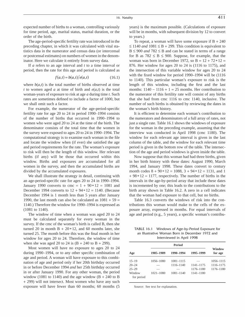
expected number of births to a woman, controlling variouslyfor time period, age, marital status, marital duration, or theorder of the birth.
The age-period-specific fertility rate was introduced in thepreceding chapter, in which it was calculated with vital sta-tistics data in the numerator and census data (or intercensalor postcensal estimates) on numbers of women in the denom-inator. Here we calculate it entirely from survey data.
If a refers to an age interval and t to a time interval orperiod, then the rate for this age and period is calculated as
(16.1)
where b(a,t) is the total number of births observed at time t to women aged a at time of birth and e(a,t) is the totalwoman-years of exposure to risk at age a during time t. Suchrates are sometimes defined to include a factor of 1000, butwe shall omit such a factor.
For example, the numerator of the age-period-specificfertility rate for age 20 to 24 in period 1990–1994 consistsof the number of births that occurred in 1990–1994 towomen who were aged 20 to 24 at the time of the birth. Thedenominator consists of the total time that the women in the survey were exposed to ages 20 to 24 in 1990–1994. Thecomputational strategy is to examine each woman in the fileand locate the window when (if ever) she satisfied the ageand period requirements for the rate. The woman’s exposureto risk will then be the length of this window. Her relevantbirths (if any) will be those that occurred within thiswindow. Births and exposures are accumulated for allwomen in the survey, and then the accumulated births aredivided by the accumulated exposures.
We shall illustrate the strategy in detail, continuing withan age-period-specific rate for ages 20 to 24 in 1990–1994.January 1990 converts to cmc = 1 + 90*12 = 1081 andDecember 1994 converts to 12 + 94*12 = 1140. (BecauseDecember 1994 is 1 month less than 5 years after January1990, the last month can also be calculated as 1081 + 59 =1140.) Therefore the window for 1990–1994 is expressed as(1081 to 1140).
The window of time when a woman was aged 20 to 24must be calculated separately for every woman in thesurvey. If the cmc of the woman’s birth is called B, then sheturned 20 in month B + 20*12, and 60 months later, sheturned 25. The month before this was the final month in herwindow for ages 20 to 24. Therefore, the window of timewhen she was aged 20 to 24 is (B + 240 to B + 299).
Most women will have no exposure to ages 20 to 24during 1990–1994, or to any other specific combination ofage and period. A woman will have exposure to this combi-nation of age and period only if her 20th birthday occurredin or before December 1994 and her 25th birthday occurredin or after January 1990. For any other woman, the periodwindow (1081 to 1140) and the age window (B + 240 to B+ 299) will not intersect. Most women who have any suchexposure will have fewer than 60 months; 60 months (5
f a t b a t e a t, , ,( ) = ( ) ( )
years) is the maximum possible. (Calculations of exposurewill be in months, with subsequent division by 12 to convertto years.)
To repeat, a woman will have some exposure if B + 240£ 1140 and 1081 £ B + 299. This condition is equivalent toB £ 900 and 782 £ B and can be stated in terms of a rangefor B as 782 £ B £ 900. Suppose, for example, that thewoman was born in December 1972, so B = 12 + 72*12 =876. Her window for ages 20 to 24 is (1116 to 1175), andthe intersection of this variable window for ages 20 to 24with the fixed window for period 1990–1994 will be (1116to 1140). This particular woman’s exposure to risk is thelength of this window, including the first and the lastmonths: 1140 - 1116 + 1 = 25 months. Her contribution tothe numerator of this fertility rate will consist of any birthsthat she had from cmc 1116 to cmc 1140, inclusive. Thenumber of such births is obtained by reviewing the dates inthe woman’s birth history.
It is efficient to determine each woman’s contribution tothe numerators and denominators of a full array of rates, notjust a single rate. Table 16.1 shows the windows of exposurefor the woman in the preceding example, assuming that theinterview was conducted in April 1998 (cmc 1180). Thewindow for each relevant age interval is given in the lastcolumn of the table, and the window for each relevant timeperiod is given in the bottom row of the table. The intersec-tion of the age and period windows is given inside the table.
Now suppose that this woman had had three births, givenin her birth history with these dates: August 1990, March1994, and January 1998. These dates convert to centurymonth codes 8 + 90*12 = 1088, 3 + 94*12 = 1131, and 1+ 98*12 = 1177, respectively. The number of births in theintervals in the age-by-period array that include these datesis incremented by one; this leads to the contributions to thebirth array shown in Table 16.2. A zero in a cell indicatesthat the woman had exposure to that cell, but no births.
Table 16.3 converts the windows of risk into the con-tributions this woman would make to the cells of the ex-posure array, expressed in months. For equal intervals of age and period (e.g., 5 years), a specific woman’s contribu-
16. Natality 411
TABLE 16.1 Windows of Age-by-Period Exposure for an Illustrative Woman Born in December 1972 and
Interviewed in April 1998
PeriodWindow
Age 1985–1989 1990–1994 1995–1999 for age
15–19 1056–1080 1081–1115 — 1056–111520–24 — 1116–1140 1141–1175 1116–117525–29 — — 1176–1180 1176–1180Window 1021–1080 1081–1140 1141–1180
for period
Source: See text for explanation.

tion to the arrays of exposures (and births) will always belocated on two adjacent diagonals going from the upper leftto the lower right. We give half a month of exposure to themonth of interview (and include any births reported in thatmonth).
Three rows and three columns are shown for this respon-dent’s age-by-period array, but they are extracted from alarger array that would extend to ages 45 to 49 and to periodsgoing back as far as desired, up to 35 years (if the age rangeof eligible respondents is 50 - 15 = 35 years). In practicethis kind of array is often taken back no more than 10 years.The further back it goes, the greater the chance of reportingerror. If maternal mortality is high, there is omission of thehigher-fertility women who have died, along with theirbirths, so that the more remote rates are biased downward.A comparison of the more remote rates with those obtained
from an earlier survey can help to identify patterns of report-ing error and selectivity.
These steps are repeated for every woman in the survey,until a full array of exposures and a corresponding full arrayof rates are obtained. Exposures are converted to years bydividing the months of exposure by 12, and the total birthsare divided by total exposure, cell by cell, to give the age-period specific fertility rates.
Because there is a cutoff age in a fertility survey (usuallyage 49), the array of rates will be empty in the lower left ofthe table. If we go back more than five years, we have noinformation about women aged 45 and over; if we go backmore than 10 years, we have no information about womenaged 40 and over; and so on.
Tables 16.4 through 16.6 give the numbers of births,months of exposure, and age-period-specific fertility ratesfor the 1998 NDHS of the Philippines. The last time inter-val is labeled “1995–1999”, but the data for that intervalshould be understood to extend only to the fieldwork in1998. In these and later tables, cells with zeros or dashesshould be interpreted to be outside the time and age (or dura-tion) range of the survey.
How would these rates be estimated if the survey waslimited to ever-married women? The answer is relativelysimple if there is an accompanying household roster thatindicates which women were selected for the interviews, and if there is a negligible amount of childbearing by never-married women. Assume that these two conditions are true.
The birth array would be calculated exactly as shownearlier, but would necessarily be limited to the birth histo-ries of the ever-married women. The exposure array,however, would be calculated from all the women in thehousehold roster who were in the age range of the eligiblerespondents at the time of the survey, usually 15 to 49, andwould not be limited to the ever-married women in thesurvey. The rates would again be calculated by dividing thebirth array by the exposure array, cell by cell.
If the researcher wishes to calculate age-period-specificrates within socioeconomic categories, using a survey
412 Pullum
TABLE 16.2 Contributions of the Illustrative Woman to theNumerators of Age-Period-Specific Fertility Rates
Period
Age 1985–1989 1990–1994 1995–1999
15–19 0 1 —20–24 — 1 025–29 — — 1
Source: See text for explanation.
TABLE 16.3 Months of Age-by-Period Exposure for theIllustrative Woman
Period
Age 1985–1989 1990–1994 1995–1999
15–19 25 months 35 months 0 months20–24 0 months 25 months 35 months25–29 0 months 0 months 4.5 months
Source: See text for explanation.
TABLE 16.4 Numerators of Age-Period-Specific Fertility Rates (numbers of births): Philippines, 1998
Age 1965–1969 1970–1974 1975–1979 1980–1984 1985–1989 1990–1994 1995–1999
15–19 309 572 732 765 745 710 46320–24 75 1104 1709 2101 2231 2186 134225–29 0 82 1338 1791 2173 2370 149530–34 0 0 107 1062 1395 1754 109835–39 0 0 0 67 689 882 67640–44 0 0 0 0 32 315 21145–49 0 0 0 0 0 5 24
Source: Based on the 1998 National Demographic and Health Survey (NDHS) of the Philippines (Philippines National Statistics Office, Department ofHealth, and Macro International, 1999).

limited to ever-married women, this will be possible onlyfor categories specified for the women in the householdsurvey. Region, type of residence, and education are usuallyavailable in the household survey, but not much more. In anall-women survey, rates can be made specific for any char-acteristics of the respondents. Rates that are defined only forever-married women, such as the marital fertility rates to bediscussed next, are obviously unaffected by the restrictionof eligibility to ever-married women.
Age-Specific Marital Fertility Rates
Marital fertility rates are restricted according to maritalstatus, but otherwise they are calculated in the same way asrates that do not refer to marital status. The marital fertilityrate for age a and period t is
(16.2)
where mb(a,t) is the total marital births observed at time t to women aged a at time of birth and me(a,t) is thetotal woman-years of marital exposure to risk at age a attime t.
This type of rate is limited to births and exposure thatoccur after first marriage. As stated earlier, the marriagehistory is typically not consulted for any dates other than thedate of first marriage (or when the couple first lived togetheras “married”). If M is the month of first marriage, then any
mf a t mb a t me a t, , ,( ) = ( ) ( )
window will omit exposure and births prior to M. Forexample, if the respondent in the previous example wasmarried in February 1993 (i.e., M = 2 + 93*12 = 1118), thenthe window (1116–1140) will be reduced to (1118–1140); thiswill be the respondent’s window of exposure to marital fertil-ity while at ages 20 to 24 in period 1990–1994; the exposureto risk will be 1140 - 1118 + 1 = 23 months. Births prior tomonth 1118 will be ignored, leaving two marital births, inmonths 1131 and 1171. After the window in which the firstmarriage occurred, there will be no difference between awoman’s contributions to the numerator and denominator ofthe marital rate and the overall rate. The windows of risk,marital births, and marital exposure for the illustrativewoman are given in Tables 16.7 through 16.9.
16. Natality 413
TABLE 16.5 Denominators of Age-Period-Specific Fertility Rates (years of exposure): Philippines, 1998
Age 1965–1969 1970–1974 1975–1979 1980–1984 1985–1989 1990–1994 1995–1999
15–19 4,789.58 7,184.83 9,040.25 10,204.92 10,753.75 11,145.50 8,717.0420–24 364.58 4,789.58 7,184.83 9,040.25 10,204.92 10,753.75 7,091.2125–29 0 364.58 4,789.58 7,184.83 9,040.25 10,204.92 6,926.5030–34 0 0 364.58 4,789.58 7,184.83 9,040.25 6,589.4235–39 0 0 0 364.58 4,789.58 7,184.83 5,646.6740–44 0 0 0 0 364.58 4,789.58 4,469.6745–49 0 0 0 0 0 364.58 2,626.13
Source: Based on the 1998 NDHS of the Philippines (Philippines National Statistics Office, Department of Health, and Macro International, 1999).
TABLE 16.6 Age-Period-Specific Fertility Rates (births per year); Philippines, 1998
Age 1965–1969 1970–1974 1975–1979 1980–1984 1985–1989 1990–1994 1995–1999
15–19 .0645 .0796 .0810 .0750 .0693 .0637 .053120–24 .2057 .2305 .2379 .2324 .2186 .2033 .189225–29 — .2249 .2794 .2493 .2404 .2322 .215830–34 — — .2935 .2217 .1942 .1940 .166635–39 — — — .1838 .1439 .1228 .119740–44 — — — — .0878 .0658 .047245–49 — — — — — .0137 .0091
Source: Tables 16.4 and 16.5.
TABLE 16.7 Windows of Age-by-Period Marital Exposurefor the Illustrative Woman
Period
Age 1990–1994 1995–1999 Window for Age
15–19 — — 1056–111520–24 1118–1140 1141–1175 1116–117525–29 — 1176–1180 1176–1180Window for period 1081–1140 1141–1180
Source: See text for explanation.

414 Pullum
TABLE 16.8 Marital Births for the Illustrative Woman
Period
Age 1990–1994 1995–1999
15–19 0 —20–24 1 025–29 — 1
Source: See text for explanation.
TABLE 16.9 Months of Age-by-Period Marital Exposure for the Illustrative Woman
Period
Age 1990–1994 1995–1999
15–19 0 months 0 months20–24 23 months 35 months25–29 0 months 4.5 months
Source: See text for explanation.
Working from a data file, each respondent’s contributionsto the arrays for marital births and marital exposures are cal-culated; months of marital exposure are converted to years;and the rates are calculated by dividing births by exposure,cell by cell. Tables 16.10 through 16.12 give the numbers ofmarital births, months of marital exposure, and age-period-specific marital fertility rates for the 1998 NDHS of thePhilippines.
Marital Duration-Specific Marital Fertility Rates
Marital fertility can be referenced by the woman’s dateof marriage rather than her date of birth. The marital fertil-ity rate for duration d and period t is
(16.3)mf d t mb d t me d t, , ,( ) = ( ) ( )
TABLE 16.10 Numerators of Marital-Age-Period-Specific Fertility Rates (births): Philippines, 1998
Age 1965–1969 1970–1974 1975–1979 1980–1984 1985–1989 1990–1994 1995–1999
15–19 299 544 698 727 707 681 43220–24 73 1081 1681 2069 2194 2142 131225–29 0 79 1317 1782 2155 2342 148130–34 0 0 105 1058 1391 1749 109735–39 0 0 0 67 685 880 67440–44 0 0 0 0 31 315 21145–49 0 0 0 0 0 5 24
Source: Based on 1998 NDHS of the Philippines (Philippines National Statistics Office, Department of Health, and Macro International, 1999).
TABLE 16.11 Denominators of Marital-Age-Period-Specific Fertility Rates (years of exposure):Philippines, 1998
Age 1965–1969 1970–1974 1975–1979 1980–1984 1985–1989 1990–1994 1995–1999
15–19 747.75 1374.92 1655.92 1756.83 1710.50 1625.83 965.3820–24 153.00 2601.42 4229.58 5170.42 5625.50 5649.92 3511.4225–29 0 253.58 3809.92 5945.92 7223.08 8134.33 5472.1330–34 0 0 314.58 4316.83 6498.42 8101.58 5954.8335–39 0 0 0 329.75 4446.33 6682.25 5250.6340–44 0 0 0 0 336.42 4498.42 4240.1745–49 0 0 0 0 0 338 2507.29
Source: Based on 1998 NDHS of the Philippines (Philippines National Statistics Office, Department of Health, and Macro International, 1999).
where mb(d,t) is the total marital births observed at time t to women with duration d at time of birth and me(d,t) isthe total woman-years of marital exposure to risk at dura-tion d at time t.
For example, if the illustrative woman was married inmonth M = 1118, then she had marital duration 0 to 4 yearsin the window (M to M + 59)—that is, (1118 to 1177), andso on. Her windows of exposure, marital births, and monthsof exposure for the marital duration rates are given in Tables16.13 through 16.15.
The marital duration-period-specific rates are calculated,as shown earlier, by dividing the accumulated array of birthsby the accumulated array of exposures (converted to years).Tables 16.16 through 16.18 give the numbers of maritalbirths, the months of marital exposure, and marital duration-
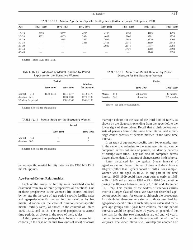
period-specific marital fertility rates for the 1998 NDHS ofthe Philippines.
Age-Period-Cohort Relationships
Each of the arrays of fertility rates described can beexamined from any of three perspectives or directions. Oneof these perspectives is the woman’s life course, indicatedby her age (in the case of age-period-specific fertility ratesand age-period-specific marital fertility rates) or by hermarital duration (in the case of duration-period-specificmarital fertility rates), as shown in the columns of Tables16.6, 16.12, and 16.18. The second perspective is acrosstime periods, as shown in the rows of these tables.
A third perspective, perhaps less obvious, is across birthcohorts (in the case of the first two kinds of rates) or across
marriage cohorts (in the case of the third kind of rates), asshown by the diagonals extending from the upper left to thelower right of these tables. Recall that a birth cohort con-sists of persons born in the same time interval and a mar-riage cohort consists of persons married in the same timeinterval.
In an array of age-period-specific rates, for example, ratesin the same row, referring to the same age interval, can becompared across columns or periods, to identify patterns of change over time. They can also be compared across diagonals, to identify patterns of change across birth cohorts.
Rates calculated for the typical 5-year interval ofage/duration and 5-year interval of time will draw from a10-year (rather than 5-year) cohort of births. For example,women who are aged 25 to 29 in any part of the time interval 1995–1999 could have been born as early as 1995- 30 = 1965 and as late as 1999 - 25 = 1974 (i.e., anytimeduring the 10 years between January 1, 1965 and December31, 1974). This feature of the widths of intervals carries over to a larger class of rates. We have not described age-cohort-specific rates, for example, although the proceduresfor calculating them are very similar to those described forage-period-specific rates. If such rates were calculated for 5-year age groups and 5-year birth cohorts, then the periodintervals would be spread over 10 years. In general, if theintervals for the first two dimensions are w1 and w2 years,then an interval for the third dimension will be w3 = w1 +w2 years. The wider intervals will overlap one another. For
16. Natality 415
TABLE 16.12 Marital-Age-Period-Specific Fertility Rates (births per year): Philippines, 1998
Age 1965–1969 1970–1974 1975–1979 1980–1984 1985–1989 1990–1994 1995–1999
15–19 .3999 .3957 .4215 .4138 .4133 .4189 .447520–24 .4771 .4155 .3974 .4002 .3900 .3791 .373625–29 — .3115 .3457 .2997 .2983 .2879 .270630–34 — — .3338 .2451 .2141 .2159 .184235–39 — — — .2032 .1541 .1317 .128440–44 — — — — .0921 .0700 .049845–49 — — — — — .0148 .0096
Source: Tables 16.10 and 16.11.
TABLE 16.13 Windows of Marital Duration-by-Period Exposure for the Illustrative Woman
PeriodWindow
1990–1994 1995–1999 for duration
Marital 0–4 1118–1140 1141–1177 1118–1177duration 5–9 — 1178–1180 1178–1180Window for period 1081–1140 1141–1180
Source: See text for explanation.
TABLE 16.14 Marital Births for the Illustrative Woman
Period
1990–1994 1995–1999
Marital 0–4 1 1duration 5–9 — 0
Source: See text for explanation.
TABLE 16.15 Months of Marital Duration-by-Period Exposure for the Illustrative Woman
Period
1990–1994 1995–1999
Marital 0–4 23 months 37 monthsduration 5–9 0 months 2.5 months
Source: See text for explanation.

example, cohorts described with the diagonals of the usualage-period-specific rates will refer to birth dates such as1950–1959, 1955–1964, 1960–1969, 1965–1974, and so on.This blurring in the third dimension, so to speak, has theeffect of suppressing some of the variation in that dimen-sion in the same way that a moving average does. The link-ages between age/duration, period, and cohort are relevantto all demographic and sociocenomic variables that have anage dimension (e.g., mortality, labor force).
Order-Specific Fertility Rates
As may be recalled from Chapter 15, a woman’s parity is the number of live births that she has had. Any of the pre-
ceding rates can also be made specific for the parity of themother or, equivalently, the birth order of the latest child.Such rates are sometimes called parity-specific, with refer-ence to the mother, and sometimes called order-specific, withreference to the child; we shall describe them as order-specific. These rates were introduced in Chapter 15, but theirconstruction will be briefly reviewed in the present context.
It is easiest to clarify the labeling with an example. Anage-period-order-specific rate is specific for order two if itmeasures the rate of childbearing of second births forwomen in each combination of age and period. When asecond birth occurs, the woman moves from parity one toparity two. Thus the rate is indexed by the birth that closesthe interval.
416 Pullum
TABLE 16.16 Numerators of Marital Duration-Period-Specific Fertility Rates (births): Philippines, 1998
Age 1965–1969 1970–1974 1975–1979 1980–1984 1985–1989 1990–1994 1995–1999
0–4 348 1372 2374 3065 3346 3511 23345–9 24 319 1126 1649 1982 2148 1292
10–14 0 13 283 783 1170 1306 80815–19 0 0 18 187 530 766 50520–24 0 0 0 19 130 346 23525–29 0 0 0 0 5 36 5630–34 0 0 0 0 0 1 1
Source: Based on 1998 NDHS of the Philippines (Philippines National Statistics Office, Department of Health, and Macro International, 1999).
TABLE 16.17 Denominators of Marital Duration-Period-Specific Fertility Rates (years of exposure): Philippines, 1998
Age 1965–1969 1970–1974 1975–1979 1980–1984 1985–1989 1990–1994 1995–1999
0–4 838.17 3272.25 5700.58 7432.00 8218.42 9116.92 6200.215–9 62.58 895.08 3347.92 5778.33 7531.58 8290.67 5862.58
10–14 0 62.58 898.92 3347.92 5780.83 7532.50 5260.2915–19 0 0 62.58 898.92 3347.92 5780.83 4802.7520–24 0 0 0 62.58 898.92 3347.92 3500.9625–29 0 0 0 0 62.58 898.92 1870.4230–34 0 0 0 0 0 62.58 389.88
Source: Based on 1998 NDHS of the Philippines (Philippines National Statistics Office, Department of Health, and Macro International, 1999).
TABLE 16.18 Marital Duration-Period-Specific Fertility Rates (births per year): Philippines, 1998
Age 1965–1969 1970–1974 1975–1979 1980–1984 1985–1989 1990–1994 1995–1999
0–4 .4152 .4193 .4164 .4124 .4071 .3851 .37645–9 .3835 .3564 .3363 .2854 .2632 .2591 .2204
10–14 — .2077 .3148 .2339 .2024 .1734 .153615–19 — — .2876 .2080 .1583 .1325 .105120–24 — — — .3036 .1446 .1033 .067125–29 — — — — .0799 .0400 .029930–34 — — — — — .0160 .0026
Source: Tables 16.16 and 16.17.
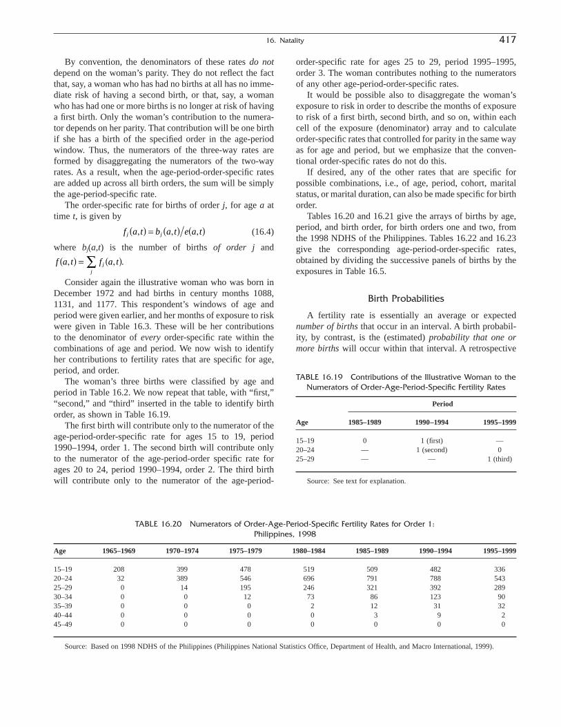
By convention, the denominators of these rates do notdepend on the woman’s parity. They do not reflect the factthat, say, a woman who has had no births at all has no imme-diate risk of having a second birth, or that, say, a womanwho has had one or more births is no longer at risk of havinga first birth. Only the woman’s contribution to the numera-tor depends on her parity. That contribution will be one birthif she has a birth of the specified order in the age-periodwindow. Thus, the numerators of the three-way rates areformed by disaggregating the numerators of the two-wayrates. As a result, when the age-period-order-specific ratesare added up across all birth orders, the sum will be simplythe age-period-specific rate.
The order-specific rate for births of order j, for age a attime t, is given by
(16.4)
where bj(a,t) is the number of births of order j and
Consider again the illustrative woman who was born inDecember 1972 and had births in century months 1088,1131, and 1177. This respondent’s windows of age andperiod were given earlier, and her months of exposure to riskwere given in Table 16.3. These will be her contributions to the denominator of every order-specific rate within thecombinations of age and period. We now wish to identifyher contributions to fertility rates that are specific for age,period, and order.
The woman’s three births were classified by age andperiod in Table 16.2. We now repeat that table, with “first,”“second,” and “third” inserted in the table to identify birthorder, as shown in Table 16.19.
The first birth will contribute only to the numerator of theage-period-order-specific rate for ages 15 to 19, period1990–1994, order 1. The second birth will contribute onlyto the numerator of the age-period-order specific rate forages 20 to 24, period 1990–1994, order 2. The third birthwill contribute only to the numerator of the age-period-
f a t f a tjj
, , .( ) = ( )Â
f a t b a t e a tj j, , ,( ) = ( ) ( )
order-specific rate for ages 25 to 29, period 1995–1995,order 3. The woman contributes nothing to the numeratorsof any other age-period-order-specific rates.
It would be possible also to disaggregate the woman’sexposure to risk in order to describe the months of exposureto risk of a first birth, second birth, and so on, within eachcell of the exposure (denominator) array and to calculateorder-specific rates that controlled for parity in the same wayas for age and period, but we emphasize that the conven-tional order-specific rates do not do this.
If desired, any of the other rates that are specific for possible combinations, i.e., of age, period, cohort, maritalstatus, or marital duration, can also be made specific for birthorder.
Tables 16.20 and 16.21 give the arrays of births by age,period, and birth order, for birth orders one and two, fromthe 1998 NDHS of the Philippines. Tables 16.22 and 16.23give the corresponding age-period-order-specific rates,obtained by dividing the successive panels of births by theexposures in Table 16.5.
Birth Probabilities
A fertility rate is essentially an average or expectednumber of births that occur in an interval. A birth probabil-ity, by contrast, is the (estimated) probability that one ormore births will occur within that interval. A retrospective
16. Natality 417
TABLE 16.19 Contributions of the Illustrative Woman to theNumerators of Order-Age-Period-Specific Fertility Rates
Period
Age 1985–1989 1990–1994 1995–1999
15–19 0 1 (first) —20–24 — 1 (second) 025–29 — — 1 (third)
Source: See text for explanation.
TABLE 16.20 Numerators of Order-Age-Period-Specific Fertility Rates for Order 1: Philippines, 1998
Age 1965–1969 1970–1974 1975–1979 1980–1984 1985–1989 1990–1994 1995–1999
15–19 208 399 478 519 509 482 33620–24 32 389 546 696 791 788 54325–29 0 14 195 246 321 392 28930–34 0 0 12 73 86 123 9035–39 0 0 0 2 12 31 3240–44 0 0 0 0 3 9 245–49 0 0 0 0 0 0 0
Source: Based on 1998 NDHS of the Philippines (Philippines National Statistics Office, Department of Health, and Macro International, 1999).
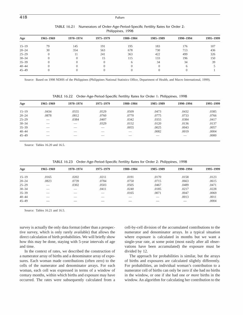
418 Pullum
TABLE 16.21 Numerators of Order-Age-Period-Specific Fertility Rates for Order 2: Philippines, 1998
Age 1965–1969 1970–1974 1975–1979 1980–1984 1985–1989 1990–1994 1995–1999
15–19 79 145 191 195 183 176 10720–24 30 354 563 678 730 713 43625–29 0 11 241 363 422 499 32630–34 0 0 15 115 133 196 15035–39 0 0 0 6 34 34 3940–44 0 0 0 0 0 6 545–49 0 0 0 0 0 0 1
Source: Based on 1998 NDHS of the Philippines (Philippines National Statistics Office, Department of Health, and Macro International, 1999).
TABLE 16.22 Order-Age-Period-Specific Fertility Rates for Order 1: Philippines, 1998
Age 1965–1969 1970–1974 1975–1979 1980–1984 1985–1989 1990–1994 1995–1999
15–19 .0434 .0555 .0529 .0509 .0473 .0432 .038520–24 .0878 .0812 .0760 .0770 .0775 .0733 .076625–29 — .0384 .0407 .0342 .0355 .0384 .041730–34 — — .0329 .0152 .0120 .0136 .013735–39 — — — .0055 .0025 .0043 .005740–44 — — — — .0082 .0019 .000445–49 — — — — — — .0000
Source: Tables 16.20 and 16.5.
TABLE 16.23 Order-Age-Period-Specific Fertility Rates for Order 2: Philippines, 1998
Age 1965–1969 1970–1974 1975–1979 1980–1984 1985–1989 1990–1994 1995–1999
15–19 .0165 .0202 .0211 .0191 .0170 .0158 .012320–24 .0823 .0739 .0784 .0750 .0715 .0663 .061525–29 — .0302 .0503 .0505 .0467 .0489 .047130–34 — — .0411 .0240 .0185 .0217 .022835–39 — — — .0165 .0071 .0047 .006940–44 — — — — — .0013 .001145–49 — — — — — — .0004
Source: Tables 16.21 and 16.5.
survey is actually the only data format (other than a prospec-tive survey, which is only rarely available) that allows thedirect calculation of birth probabilities. We will briefly showhow this may be done, staying with 5-year intervals of ageand time.
In the context of rates, we described the construction ofa numerator array of births and a denominator array of expo-sures. Each woman made contributions (often zero) to thecells of the numerator and denominator arrays. For eachwoman, each cell was expressed in terms of a window ofcentury months, within which births and exposure may haveoccurred. The rates were subsequently calculated from a
cell-by-cell division of the accumulated contributions to thenumerator and denominator arrays. In a typical situationwhere exposure is calculated in months but we want asingle-year rate, at some point (most easily after all obser-vations have been accumulated) the exposure must bedivided by 12.
The approach for probabilities is similar, but the arraysof births and exposures are calculated slightly differently.For probabilities, an individual woman’s contribution to anumerator cell of births can only be zero if she had no birthsin the window, or one if she had one or more births in thewindow. An algorithm for calculating her contribution to the

numerator of a rate needs only to be altered by recoding anypositive number of births into just one birth. A woman’s con-tribution to the corresponding denominator cell of exposurewill depend in part on whether she actually had a birthduring the window of observation. This may seem counter-intuitive and calls for some justification.
Consider the probability that a woman will have a birthwhile aged 20 to 24, which is to be estimated with births and exposure observed within that age interval during1990–1994. The outcome is binary: Either a birth occurs, inwhich case a code of 1 is assigned, or no birth occurs, inwhich case a code of 0 is assigned.
The classical example of a trial with a binary outcome isthe toss of a coin. We toss a coin once, and assign code 1 toa success, say a head, and code 0 to a failure, a tail. Thenumerator or outcome can be 0 or 1, interpreted as the (pos-sible) number of heads or successes when the number oftrials—the denominator—is 1. If we tossed n independentbut identical coins, the number of successes could be anyinteger k between 0 and n, inclusive, and k would have abinomial distribution with denominator n.
This familiar model may clarify the requirement that ifthe outcome takes the values 0 or 1, then the denominator,or degree of risk associated with the outcome, must neverbe less than the value of the numerator. If the denominatorcould be less than 1 when the numerator is 1, we would havethe potential to produce an estimated probability greater than1, which is not allowed.
The relevant data in a window of age and time are gen-erally censored on either the left or the right, and sometimes(if the interview occurred within the time interval) on boththe left and the right. There are three possibilities.
If the observation is not censored, and the woman had afull 60 months of exposure to the window, then her contri-bution to the denominator will be 1 (the number of monthsin the window divided by 60).
If the observation is censored, and no birth occurred inthe window, then her contribution to the denominator willbe the fraction of the full 5-year or 60-month interval forwhich she was observed—that is, the number of months inthe window divided by 60. This fraction indicates that theobservation is only partial.
The remaining possibility is that the observation is cen-sored but a birth does occur. This is where the coin-tossinganalogy becomes relevant. If a birth occurred, then it doesnot matter that there was less than full observation of thewoman, and we credit the case with a contribution of 1 tothe denominator. Indeed, we must credit her with 1 to avoidhaving a contribution to the denominator that is less than thecontribution to the numerator.
To summarize,
• If there was no censoring within the cell, then exposurefor the probability equals the exposure for the rate.
• If there was censoring and no birth, then exposure forthe probability equals the exposure for the rate.
• If there was censoring and a birth (one or more), thenexposure must be augmented to reach the length itwould have had in the absence of censoring (e.g., 60 months).
• After the exposure in a cell has been accumulated acrossall respondents, the sum must be normalized to amaximum of one unit per woman (e.g., by dividing thetotal months by 60).
These rules are consistent with an assumption that theprobability of having a birth is uniform within the intervalof age and time (or intervals of other dimensions, depend-ing on the specific rate). If this assumption is not plausible,then (as with a rate) the researcher may choose to adoptshorter intervals, within which the assumption is safer.
Reconsider the illustrative woman born in December1972, with births in century-months 1088, 1131, and 1177.We described in detail the calculation of this woman’s contributions to the numerator and denominator arrays ofage-period-specific fertility rates. How would these contri-butions differ for age-period-specific birth probabilities?
First consider the numerator array. Cells with no birthswill continue to make a contribution of zero. Because thewoman’s births occurred in different cells of the age-by-period array, the three cells with a contribution of one birthto the numerator of a rate also contribute one birth to thenumerator of a probability. The numerator array will thus beexactly the same as Table 16.3 and need not be repeated.
The contributions to the denominator array will remainunchanged for those cells in which no births occurred. In thethree cells in which a birth occurred, the months of expo-sure must be increased to 60. After the accumulation of allexposures, we emphasize that the total in each cell must be normalized by dividing by 60 months, rather than 12months, and that the probability extends across a 5-yearrange, whereas the rate is interpreted in terms of a singleyear. The denominator contributions are given in Table 16.24, prior to the division by 60.
Tables 16.25 through 16.27 give the births, exposures,and age-period-specific birth probabilities for the 1998
16. Natality 419
TABLE 16.24 The Illustrative Woman’s Contributions to Riskfor the Age-Period-Specific Birth Probabilities
Period
Age 1985–1989 1990–1994 1995–1999
15–19 25 months 60 months 0 months20–24 0 months 60 months 35 months25–29 0 months 0 months 60 months
Source: See text for explanation.
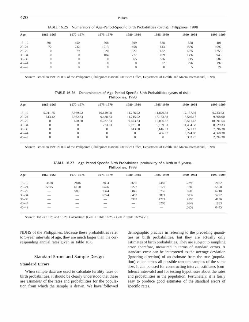
420 Pullum
TABLE 16.25 Numerators of Age-Period-Specific Birth Probabilities (births): Philippines: 1998
Age 1965–1969 1970–1974 1975–1979 1980–1984 1985–1989 1990–1994 1995–1999
15–19 391 450 568 599 588 558 40120–24 72 732 1213 1458 1613 1566 109725–29 0 79 920 1327 1622 1785 125530–34 0 0 104 777 1079 1336 94535–39 0 0 0 65 536 715 58740–44 0 0 0 0 32 276 19745–49 0 0 0 0 0 5 24
Source: Based on 1998 NDHS of the Philippines (Philippines National Statistics Office, Department of Health, and Macro International, 1999).
TABLE 16.26 Denominators of Age-Period-Specific Birth Probabilities (years of risk): Philippines, 1998
Age 1965–1969 1970–1974 1975–1979 1980–1984 1985–1989 1990–1994 1995–1999
15–19 5,041.75 7,989.92 10,129.08 11,276.92 11,820.58 12,157.92 9,723.6320–24 643.42 5,932.33 9,438.33 11,715.92 13,163.58 13,546.17 9,868.0025–29 0 670.50 6,237.83 9,693.83 12,006.67 13,511.42 10,091.5430–34 0 0 773.33 6,021.58 9,189.33 11,454.58 8,929.3335–39 0 0 0 613.00 5,616.83 8,521.17 7,096.3840–44 0 0 0 0 486.67 5,224.08 4,968.3845–49 0 0 0 0 0 383.25 2,694.38
Source: Based on 1998 NDHS of the Philippines (Philippines National Statistics Office, Department of Health, and Macro International, 1999).
TABLE 16.27 Age-Period-Specific Birth Probabilities (probability of a birth in 5 years): Philippines, 1998
Age 1965–1969 1970–1974 1975–1979 1980–1984 1985–1989 1990–1994 1995–1999
15–19 .3878 .2816 .2804 .2656 .2487 .2295 .206220–24 .5595 .6170 .6426 .6222 .6127 .5780 .555825–29 — .5891 .7374 .6845 .6755 .6606 .621830–34 — — .6724 .6452 .5871 .5832 .529235–39 — — — .5302 .4771 .4195 .413640–44 — — — — .3288 .2642 .198345–49 — — — — — .0652 .0445
Source: Tables 16.25 and 16.26. Calculation: (Cell in Table 16.25 ∏ Cell in Table 16.25) ¥ 5.
NDHS of the Philippines. Because these probabilities referto 5-year intervals of age, they are much larger than the cor-responding annual rates given in Table 16.6.
Standard Errors and Sample Design
Standard Errors
When sample data are used to calculate fertility rates orbirth probabilities, it should be clearly understood that theseare estimates of the rates and probabilities for the popula-tion from which the sample is drawn. We have followed
demographic practice in referring to the preceding quanti-ties as birth probabilities, but they are actually only estimates of birth probabilities. They are subject to samplingerror, therefore, measured in terms of standard errors. Astandard error can be interpreted as the average deviation(ignoring direction) of an estimate from the true (popula-tion) value across all possible random samples of the samesize. It can be used for constructing interval estimates (con-fidence intervals) and for testing hypotheses about the ratesand probabilities in the population. Fortunately, it is fairlyeasy to produce good estimates of the standard errors of specific rates.

The generic form for a specific rate is r = b/e, where r isthe rate (ignoring any multipliers such as 1000), b is a countor frequency of births, and e is a measure of exposure inwoman-years. Let s.e.(r) denote the estimated standard errorof the rate.
As a good first approximation, for a fixed amount ofexposure, the number of births has a Poisson distribution. Auseful property of a Poisson distribution is that its mean andvariance are equal. The observed number of births will bethe maximum likelihood estimate of both the mean and thevariance of the distribution. Therefore,
(16.5)
Any of the three forms on the right-hand side of thisequation can be used. Suppose, for example, that an age-specific rate for ages 30 to 34 is .100 births per woman peryear, and the numerator of this rate included 400 births. Thenthe estimated standard error of the rate would be
Another useful property of a Poisson sampling distribu-tion for a birth count is that it is well approximated by anormal distribution having the same mean and standarddeviation, especially for large samples. Adapting the usualformulas for confidence intervals for parameters whoseestimates have asymptotically normal sampling distribu-tions, a 95% confidence interval for the underlying true ratewill be r ± 1.96r/ . The 95% confidence interval for therate estimated in the preceding paragraph would thus rangefrom .090 to .110.
Suppose there are two independent estimates r1 and r2 ofthe true rates for two subpopulations (or two time periods,two age groups, etc.). Then the test statistic for a nullhypothesis that the underlying rates are equal will be
(16.6)
For example, a two-sided null hypothesis will be rejectedat the .05 level if the calculated test statistic is greater than1.96 or less than -1.96.
The standard error for an estimated birth probability isestimated by drawing on statistical theory for a binomial dis-tribution. Say that the estimated probability is p = b/e, whereboth b and e are different from the preceding discussion ofrates; here b is the total relevant birth count limited to 0’sand 1’s, and e is the total exposure, scaled to be 1 if a birthoccurred or there was no censoring, or the appropriate frac-tion if no birth occurred and there was censoring. Then thestandard error of p is estimated to be
(16.7)
The standard error of p is similar to the standard error ofr, particularly when p (or r) is small. Formulas for con-
s e p p p e p b p. . .( ) = -( ) = ( ) -( )1 1
z r r r b r b= -( ) ( ) + ( )1 2 12
1 22
2 .
b
s e r r b. . . .( ) = = =100 400 005
s e r b e r e r b. . .( ) = = =
fidence intervals and test statistics using estimated proba-bilities and standard errors can be found in statistics texts.
Sample Design
In a simple random sample, every case in the populationhas the same probability of appearing in the sample and thisprobability is independent of whether another case appears.Statistical theory is based on such a model, but virtually nofertility survey follows these criteria. Most surveys have astratified cluster design, in which relatively small subpopu-lations are oversampled and relatively large subpopulationsare undersampled. Census enumeration districts or othersuch administrative areas comprise the primary samplingunits, within which households and individuals are selected.These departures from the model of a simple random samplehave two important implications.
First there is the issue of sampling weights, which com-pensate for oversampling and undersampling. Such weightsare inversely proportional to the probability that a case inthe sample would have been selected from the population.If a case was oversampled, for example, the weight wouldbe relatively small, and if it was undersampled, the weightwould be relatively large. If needed, weights are calculatedby the survey organization and included on each computerrecord, generally near the case identification codes. They aregenerally constructed so that (if the decimal point is prop-erly located) the average value of the weights is 1.0, and thetotal of the weights, across the entire sample, is equal to thenumber of cases in the sample.
If weights are provided, we recommend that they be usedin the calculation of the descriptive measures given in thischapter (even though we did not follow that practice for theillustrations with data from the Philippines). Otherwise, themeasures will be biased toward the oversampled subpopu-lations. The weights compensate for this bias. Statisticalcomputer packages generally have a weight option. Theresearcher simply invokes that option and identifies theweight variable. If xi is the value of a variable for case i, andwi is the weight for case i, then the main effect of the weightoption is to replace xi by wixi, to replace xi
2 by wixi2, and so
on. In the calculation of mean CEB, for example, if xi is the
CEB for woman i, the mean CEB would be .
The weight wi appears in the denominator in place of animplied count of 1 for case i. An unweighted estimate has aslightly smaller standard error than a weighted estimate—which is one reason why some researchers do not useweights.
There is uniform agreement that for the calculation ofstandard errors, every real case in the sample should begiven equal importance. This practice means that parallelcomputer runs are often required: one with weights for estimation and one without weights to get standard errors
w x wii
i ii
 Â
16. Natality 421

for the construction of confidence intervals or tests ofhypotheses.
Thus, the recommended practice with respect to weightsis as follows:
• Use sampling weights when unbiased descriptive estimates are desired.
• Use sampling weights in multivariate models unless themodel includes all the stratifying variables or you areconfident that the model is fully specified.
• Omit sampling weights for the estimation of standarderrors or use software that gives “robust” weighted estimates.
The second issue for the analysis of complex samplingdesigns comes from the use of sample clusters. The cases inthese clusters are not independent, but overlap in the infor-mation they provide. The degree of overlap is reflected inthe intraclass correlation. This is not easily calculated andvaries from one variable to another. The lack of independ-ence will not alter the estimates of summary statistics, rates,probabilities, and coefficients, but it will affect standarderrors. If the clustering is not taken into account, the esti-mated standard errors will tend to be too small, and as aresult, the p-values in hypothesis tests will be understatedand confidence intervals will be too narrow. If possible, themagnitude of these effects should be assessed with a com-puter package.
MEASURES OF OVERALL FERTILITY
Overall fertility refers to the total number of births rela-tive to the total number of persons or women in the popu-lation. Age and marital duration are ignored, except wherewomen are restricted to the range of the childbearing ages.These measures are described after the specific rates, ratherthan before them, because they involve some concepts intro-duced in connection with the specific rates.
Crude Birthrate
The crude birthrate (CBR) was defined in Chapter 15 tobe the number of births in a fixed reference period, gener-ally a year, divided by the (total) population at the midpointof the reference period, multiplied by 1000. Typically, thenumerator comes from vital statistics and the denominatorcomes from a census or is estimated from census data.
It is possible to estimate the CBR entirely from surveydata if the survey includes a roster for all the sample house-holds, including the households that had no eligible respon-dents. The household sample then represents the generalpopulation at the time of data collection. The birth historiesprovide a count of the number of births during a recent timeinterval for the sample, giving the numerator of the CBR.The total household count can serve as the denominator of
the CBR for recent time periods. Because of the generalinterest in the CBR, we will go into some detail on the issuesraised when it is estimated with such data.
The fieldwork for the 1998 NDHS of the Philippines wasconducted entirely in 1998, so the survey could be used toestimate the CBR in 1997. The numerator would consist ofall births observed in the birth histories for 1997, namely1586 births (Philippines NDHS Report, 1999, Table C4). Anapproximation for the denominator would be the totalnumber of persons in the household survey, namely 60,349persons (Philippines NDHS Report, 1999, Table C1). Theratio, multiplied by 1000, is (1586/60,349) ¥ 1000 = 26.3.In this illustration, the numerator and denominator areunweighted. The weighted estimate of the CBR for the 36months before the survey is 28.0 (Philippines NDHS Report,1999, Table 3.1).
The standard error of the unweighted estimate of the CBRfor 1997 is ( /60,349) ¥ 1000 = .66, so that a 95% con-fidence interval for the estimated rate (unweighted) wouldrange from 25.0 to 27.6 (= 26.3 ± 1.96 times .66). Follow-ing the practice of ignoring weights for the calculation ofstandard errors, we could also use .66 to construct a confi-dence interval for the weighted CBR, so that a 95% confi-dence interval for the weighted estimate would range from26.7 to 29.3 (= 28.0 ± 1.96 times .66).
The median date of the 1998 NDHS fieldwork was approximately April 1, 1998; the midpoint of 1997 was July 1, 1997. One might argue that a denominator at the time of the survey is too large and could be improved by projectingthe household population back nine months, or .75 of a year,using the Philippines’ estimated annual growth rate of 2.0%.We would not advocate such an adjustment because it ignoresan inherent linkage between the numerator and denominatordata. If we deflated the denominator population, then to beconsistent we should also deflate the number of women whoproduced the births, and this in turn would deflate the numberof births. The same adjustments would be made to both thenumerator and the denominator and they would cancel out(assuming no change in the birth rate in this period).
Another way to improve the denominator would be to usethe household survey to calculate person-years lived by allhousehold members during 1997. Although this step wouldbe an improvement, such a denominator would ignoreanyone who had died between the beginning of 1997 andthe date of the survey, and would be somewhat too small.Whatever adjustments to the denominator one might makefor a recent time interval, they are unlikely to be outside therange of sampling error.
Compared with the traditional definition, the numeratordescribed earlier omits births to women who had a birthduring the reference window of time but died between thebirth and the interview. Such women and their births areomitted from the survey. This effect is small unless adultfemale mortality is extremely high. The numerator also
1586
422 Pullum
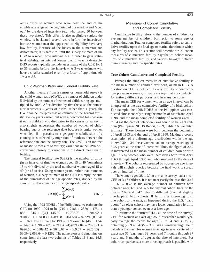
omits births to women who were near the end of the eligible age range at the beginning of the window and “agedout” by the date of interview (e.g. who turned 50 betweenthese two dates). This effect is also negligible (unless thewindow is backdated several years before the interviews)because women near the upper end of eligibility have verylow fertility. Because of the biases in the numerator anddenominator, it is safest to limit the survey estimate of theCBR to a recent time interval, but in order to gain statis-tical stability, an interval longer than 1 year is desirable.DHS reports typically include an estimate of the CBR for 1to 36 months before the interview. A 3-year estimate willhave a smaller standard error, by a factor of approximately1/ = .58.
Child-Woman Ratio and General Fertility Rate
Another measure from a census or household survey isthe child-woman ratio (CWR), the number of children under5 divided by the number of women of childbearing age, mul-tiplied by 1000. After division by five (because the numer-ator represents 5 years of births, rather than 1 year), theCWR can be interpreted as an estimate of the general fertil-ity rate 21/2 years earlier, but with a downward bias becauseit omits children who died prior to the census or survey. Italso slightly understates the number of women of child-bearing age at the reference date because it omits womenwho died. If it pertains to a geographic subdivision of acountry, it is affected by migration of mothers between thereference date and the survey date. The CWR is an indirector substitute measure of fertility; variations in the CWR willcorrespond closely to variations in the direct measures offertility.
The general fertility rate (GFR) is the number of births(in an interval of time) to women aged 15 to 49 (sometimes15 to 44), divided by the total number of women aged 15 to49 (or 15 to 44). Using woman-years, rather than numbersof women, a survey estimate of the GFR is simply the sumof the numerators of the age-specific rates, divided by thesum of the denominators of the age-specific rates:
(16.8)
Using the 1998 NDHS of the Philippines, we estimate theGFR for 1990–1994 to be (710 + 2186 + 2370 + 1754 +882 + 315 + 5)/(11,145.50 + 10,753.75 + 10,204.92 +9040.25 + 7184.83 + 4789.58 + 364.58) = 8222/43,803.41= 0.1877. The estimate for 1995–1999 would be (463 + 1342+ 1495 + 1098 + 676 + 211 + 24)/(8717.04 + 7091.21 +6926.50 + 6589.42 + 5646.67 + 4469.67 + 2626.13) =5309/42,066.64 = 0.1262. The numerators and denominatorscome from the last two columns of Tables 16.4 and 16.5,respectively.
GFR tb a t
e a ta
a
( ) =( )
( )
ÂÂ
,
,
3
Measures of Cohort Cumulative and Completed Fertility
Cumulative fertility refers to the number of children, oraverage number of children, born prior to some age ormarital duration. Total or completed fertility refers to cumu-lative fertility up to the final age or marital duration in whichany fertility occurs. This section will describe “true” cohortmeasures of cumulative fertility, “synthetic” cohort meas-ures of cumulative fertility, and various linkages betweenthese measures and the specific rates.
True Cohort Cumulative and Completed Fertility
Perhaps the simplest measure of cumulative fertility isthe mean number of children ever born, or mean CEB. Aquestion on CEB is included in every fertility or contracep-tive prevalence survey, in many surveys that are conductedfor entirely different purposes, and in many censuses.
The mean CEB for women within an age interval can beinterpreted as the true cumulative fertility of a birth cohort.For example, the 1998 NDHS of the Philippines was con-ducted almost entirely during the months of March and April1998, and the mean completed fertility of women aged 30to 34 (at the date of interview) was found to be 2.69 chil-dren (Philippines NDHS Report, 1999, Table 3.6; weightedestimate). These women were born between the beginningof April 1963 and the end of April 1968. Making a coarseassumption of a uniform age distribution within the ageinterval 30 to 34, these women had an average exact age of32.5 years at the date of interview. Thus, the figure of 2.69is interpreted as the mean number of children born prior toage 32.5 by women who were themselves born from April1963 through April 1968 and who survived to the date ofinterview. The cohorts represented by successive age inter-vals will slightly overlap because the field work is spreadover an interval of time.
The women aged 35 to 39 in the same survey had a meanCEB of 3.47 children. It is not necessarily the case that 3.47- 2.69 = 0.78 is the average number of children bornbetween ages 32.5 and 37.5 for any real cohort, because themeans 2.69 and 3.47 refer to different (even if slightly overlapping) birth cohorts. If fertility is increasing from one cohort to the next, as happened during the U.S. “babyboom,” an older cohort may have lower cumulative fertilitythan a younger cohort, even at a later age.
To estimate the “current” (i.e., at the time of the survey)CEB for women at exact age 35, a researcher would typi-cally average the means for ages 30 to 34 and 35 to 39,obtaining (2.69 + 3.47)/2 = 3.08. An alternative might be tocalculate the mean for women in an age interval centered onexact age 35 (e.g., ages 32 years and 7 months through 37years and 6 months of age) at the date of interview. Forcohort comparisons, a more direct approach is possible with
16. Natality 423

survey data. For the cohort born during 1960–1964, forexample, exact age 35 was reached before the 1998 surveydescribed earlier; so the birth histories could be used to cal-culate each woman’s CEB at the beginning of the monthwhen she had her 35th birthday. The average of these CEBswould be the average CEB at exact age 35 for this birthcohort. Birth cohorts above exact age 35 (at the survey date)could be compared in terms of the mean number of childrenthey had had by exact age 35.
The CEB can be interpreted as completed fertility forwomen aged 45 to 49 or greater, but may actually underes-timate completed fertility because of underreporting of thefertility of older cohorts. Women may omit children whowere born long ago and died while young. Moreover,women who have had numerous children have a higher riskof dying from maternal or related causes. After the first birth,which is the most hazardous, the risk of maternal mortalityis roughly proportional to the number of children. Womenwho died from such causes will be omitted from a census orsurvey, with the result that the mean CEB is biased down-ward. Thus, it is common in a less developed country for themean CEB to reach a maximum for women aged about 45to 49 and to decline steadily for older women, contrary tohistorical information about fertility trends.
An overall mean CEB calculated for women 15 to 49 willbe sensitive to the age distribution within that age range. Many observed age distributions, particularly in the lessdeveloped countries, have more women in their twenties thanin their thirties, and more in their thirties than in their forties.Amean will thus be weighted toward younger women, partic-ularly if the population was growing rapidly when thesewomen were born. A mean CEB calculated for a very broadage interval, or an overall mean CEB, is largely descriptiveand has serious limitations for comparisons across groups ortime periods. Direct standardization on some standard agedistribution will slightly improve the usefulness of the CEBfor making comparisons. In the absence of an obvious stan-dard, a uniform age distribution can be used; in this case thestandardized mean CEB will simply be the unweightedaverage of the mean CEBs in all the age intervals.
Synthetic Cumulative and Total Fertility
As a generalization, synthetic measures are constructedby interpreting period data as if they referred to a cohort.The best-known example is in the context of mortality (see,for example, Chapter 13), in which period data on the mortality of persons aged 0, 1–4, 5–9, . . . , 85+ are used toprepare an abridged life table. The survivorship column ofthe life table is interpreted as a description of a hypotheti-cal or synthetic birth cohort as it passes from birth to exactages 1, 5, 10, . . . , 85, even though the data for these ageintervals actually come from different birth cohorts. The survivorship column of the life table provides a synthetic
answer to a hypothetical “what if” question, namely “Whatis the chance of surviving to each exact age a if a cohort ofwomen experiences throughout their lives the mortalityobserved in a recent interval of time?”
The concept of a synthetic cohort is easily extended tothe measurement of fertility. (See, for example, Chapter 15.)Corresponding to the three period-specific fertility ratesdescribed earlier, for 5-year intervals of time and either ageor marital duration, there are three cumulative totals for timeperiod t, given as follows:
• CFR(x,t) is five times the sum of the age-period-specificrates up to exact age x.
• CMFR(x,t) is five times the sum of the age-period-specific marital rates up to exact age x.
• CMDFR(x,t) is five times the sum of the marriage-duration-period-specific rates up to exact duration x
Thus,
(16.9)
This cumulative fertility rate at time t can be interpretedas the number of children that a woman would be expectedto have (i.e., would have on average) if she experienced thetime t rate for ages 15 to 19 for 5 years, the time t rate forages 20 to 24 for 5 years, and so on, up to the age intervalthat extended from exact age x-5 to exact age x. In short, itis the expected number of births prior to age x, based on thefertility observed for different age intervals during timeinterval t. It is implicit that the woman survives to age x;possible mortality is ignored.
Similarly,
(16.10)
is the cumulative marital fertility up to age x, with the addi-tional assumption that the woman is married from the earli-est age in the summation, usually age 15. This cumulativerate can be very high because age-specific marital fertilityrates are higher than age-specific fertility rates, especially inthe younger ages where fewer women are married. It ispreferable to apply a synthetic cohort interpretation to theduration-period-specific marital rates, in which case thecohorts are indexed by marital duration, rather than age.Thus, the cumulative marital duration fertility rate,
(16.11)
gives the expected (or average) number of births in the firstx years of marriage, without any reference, implicit orexplicit, to age at marriage.
As described earlier, retrospective rates produced by asurvey will be right-censored for earlier time periods, so thatthe full range of ages and marital durations will usually beavailable only for the most recent 5-year time period. For
CMDFR x t mf d td x
, ,( ) = ( )<Â5
CMFR x t mf a ta x
, ,( ) = ( )<Â5
CFR x t f a ta x
, ,( ) = ( )<Â5
424 Pullum

that time period, at least, the age-specific rates can be calculated out to ages 45 to 49 and the duration-specific ratesout to duration 30 to 34. The cumulative fertility rate out toexact age 50 is the well-known total fertility rate, or TFR—that is,
(16.12)
and the cumulative marital duration fertility rate out to exactduration 35 is known as the total marital duration fertilityrate or TMDFR—that is,
(16.13)
There is no need to duplicate here the discussion of theserates and their interpretation given in Chapter 15. Also seeChapter 17 for modifications to limit the births to daughtersand to take account of survivorship, leading to the grossreproduction rate and the net reproduction rate. Our purposehere is simply to indicate how the cumulative fertility rates,total fertility rates, and reproduction rates can be built upfrom specific rates derived from survey data.
Adding up the rates in the final columns of Tables 16.6 and 16.18, respectively, and multiplying by 5, we obtain an unweighted TFR for the Philippines in 1995–1999 of(0.0531 + 0.1892 + 0.2158 + 0.1666 + 0.1197 + 0.0472 +0.0091) ¥ 5 = 4.00. This number can be interpreted as themean number of children that a woman would eventuallyhave if she survived to the end of the childbearing ages andexperienced the age-specific fertility rates observed during1995–1999. The TMDFR for 1995–1999 is (0.3764 + 0.2204+ 0.1536 + 0.1051 + 0.0671 + 0.0299 + 0.0026) ¥ 5 = 4.78.This number can be interpreted as the mean number of chil-dren that a woman would eventually have if she ever married,survived to the end of the childbearing ages, and experiencedthe observed duration-specific marital fertility rates.
The total marital fertility rate (TMFR) for 1995–1999,calculated from the final column of Table 16.12, would be(0.4475 + 0.3736 + 0.2706 + 0.1842 + 0.1284 + 0.0498 +0.0096) ¥ 5 = 7.32. This number can be interpreted as themean number of children that a woman would eventuallyhave if she married at age 15, survived to the end of thechildbearing period, and experienced the observed age-specific marital fertility rates. The TMFR is required for theBongaarts decomposition procedure (see Chapter 22). Itshould be interpreted cautiously because of its sensitivity tothe high fertility of the early age intervals, even if very fewwomen of those ages are actually married.
It is also possible to cumulate order-specific rates toobtain a total fertility rate TFRj for each birth order j. Forexample, if the age-order-specific rates for order 1 are addedacross age (and multiplied by five if the age intervals are 5years wide), we obtain TFR1, which can be interpreted as theproportion of women who will ever have a first birth in a
TMDFR t mf d td
( ) = ( )<Â5
35
,
TFR t f a ta
( ) = ( )<Â5
50
,
synthetic cohort subject to the observed period rates. It ispossible for such a sum to exceed 1.0 if, say, the real cohortstended to time their first births to occur during the observedperiod. For a real cohort followed over time, it would ofcourse be impossible for the proportion to exceed one, so the interpretation must be modified if this happens to the synthetic measure. Similarly for higher birth orders. Asnoted earlier, if the age-order-specific rates are added acrossbirth orders, we get the age-specific rates. Therefore, thesum of the order-specific total fertility rates, across birthorders j, will be the overall TFR—that is,
(16.14)
and
(16.15)
For 1995–1999, the order-specific rates for the illustra-tive data set are obtained from the last column of Tables 16.22 and 16.23 by adding the order-specific rates and multiplying the sums by five. They are as follows, for birthorders 1 to 4: TFR1 = 0.88, TFR2 = 0.61, TFR3 = 0.62, andTFR4 = 0.47. (Tables 16.22 and 16.23 give the order-specificrates for orders 1 and 2 only.) Calculated as a residual, TFR5+
= 4.00 - 0.88 - 0.61 - 0.62 - 0.47 = 1.42. For a syntheticcohort interpretation, about 88% of women would eventu-ally have a first birth, about 61% would eventually have asecond birth, about 62% would eventually have a third birth,and about 47% would eventually have a fourth birth. Thiskind of interpretation could be extended to individual birthorders five, six, and so forth, but not to an aggregation suchas five or more.
Parity-Progression Ratios
Chapter 15 defined parity-progression ratios and showedhow they can be calculated with vital statistics data. Thebirth histories in a fertility survey are a much more directsource of information about parity progression. The progression from parity j to parity j + 1 is the closure of a birth interval, and birth histories contain information aboutboth the beginnings and ends of birth intervals. The pro-bability of making such a transition, given that parity j wasreached (i.e., the parity-progression ratio) will be labeledPPRj.
There are some important distinctions between order-specific fertility rates and parity-progression ratios, in termsof data requirements and interpretation, despite a superficialsimilarity in their names. Parity-progression ratios areindexed by the order of the birth that begins a birth interval(with a woman beginning at zero), whereas order-specificrates are indexed by the order of the birth that closes a birthinterval. As another distinction, order-specific rates are
TFR t TFR tjj
( ) = ( )Â
TFR t f x tj jx
( ) = ( )<Â5
50
,
16. Natality 425

typically calculated for specific ages (or marital durations)and periods; parity-progression ratios are typically calcu-lated for cohorts or periods, but not for specific ages (ordurations). Most important, parity-progression ratios areactually (estimated) conditional probabilities, rather than(central) rates, limited to the subpopulation at risk of makingeach successive transition to a higher parity.
True-Parity Progression Ratios
The following discussion draws on Hinde (1998, Chapter9). If we follow a real cohort of women (that is, look retro-spectively at the completed birth histories of the survivorsof a real cohort), the probability that a woman who reachedorder j would go on to parity j + 1 could be readily estimatedby dividing the number of women who ever reached parityj + 1 by the number of women who ever reached parity j. Ifnk is the number of women who eventually had exactly kbirths, then
(16.16)
Such an estimate can be seriously deficient if the cohorthas not yet reached the end of the childbearing ages, becauseof two possible sources of bias. The first problem may bedescribed as right-censoring. Some of the women who havereached parity j will eventually go on to parity j + 1, but theyhave not been observed long enough for this to be witnessed.Right-censoring always produces an underestimate of the cohort’s eventual parity progression ratio. The secondproblem is left-censoring: some women have not yet evenreached parity j, so the estimate will be biased towardwomen who reached parity j earlier, rather than later, in thelife course. Women who reach a given parity early will tendto have larger completed families, so left-censoring tends toproduce an overestimate of the cohort’s eventual parity progression ratio.
Instead of regarding the parity-progression ratio as a characteristic of a birth cohort, with the attendant difficulty
PPR n nj kk j
kk j
= ÊËÁ
ˆ¯̃
ÊËÁ
ˆ¯̃> ≥
 Â
of making estimates before the cohort has completed itschildbearing, we can shift to a period-specific definitionfrom the birth-cohort definition, and try to estimate the prob-ability of making a transition from parity j to parity j + 1,for all birth cohorts or age groups pooled, within an inter-val of time.
Suppose, for example, that we used the 1998 survey toestimate the progression from parity one to parity two.Pooling all age groups, we could identify women who hada first birth in 1990, say, and determine the proportion ofthem who had a second birth in 1990 or later. (It is possibleto have two births in the same year, and we include the pos-sibility of twins or other multiple births.) Then these womenwould have had nine calendar years (1990 to 1998; 1998 isonly partially observed) in which to have a second birth.Since very few completed intervals are longer than this, theestimated PPR1 could be interpreted as only a slight under-estimate of the true probability that a woman who had a firstbirth in 1990 would eventually have a second birth.
Continuing to think of the transition from parity one toparity two, in order to keep the notation as simple as possi-ble, let N1990 be the number of women who had a first birthin 1990, and of those women, let nt be the number of womenwho had a second birth in t = 1990, . . . , 1997. Then
(16.17)
The number of years following the reference year (in thiscase the reference year is 1990) is arbitrary, so long as itincludes “virtually all” of the next-order births. To keep theright-censoring effect the same for a series of estimates, onecould use 1980 through 1990, for example, as the referenceyears for the first birth and a 9-year interval (including thereference years) as the interval in which the second birthcould have occurred.
Tables 16.28 and 16.29, from the 1998 NDHS of thePhilippines, illustrate the necessary intermediate calcula-tions. Table 16.28 shows that 337 women had a first birth in1990. Table 16.29 gives the number of women who had a
PPR n Nkk
1 19900
8
1990= ÊËÁ
ˆ¯̃+
=Â
426 Pullum
TABLE 16.28 Births by Order and Calendar Year, 1990 to 1998: Philippines, 1998
Order 1990 1991 1992 1993 1994 1995 1996 1997 1998
1 337 366 402 331 389 385 406 416 852 327 323 341 339 294 301 346 339 783 268 270 268 292 259 263 237 273 684 221 214 212 216 191 202 187 186 425 173 133 157 156 154 147 133 144 366 108 99 124 108 105 111 94 118 257 80 68 75 57 80 82 76 65 238 59 58 56 37 50 52 50 54 11
Source: Based on 1998 NDHS of the Philippines (Philippines National Statistics Office, Departmentof Health, and Macro International, 1999).

first birth in 1990 (or other calendar years) and had a secondbirth in a later year. The number of women shown for asecond birth in years 1990 through 1998 is 0 + 79 + 126 +55 + 20 + 9 + 10 + 8 + 1 = 308. Therefore the estimate ofPPR1 for reference year 1990 is 308/337 = 0.91. (This isprobably an underestimate, since for earlier years weobserve some longer gaps between first and second births.)Tables analogous to Table 16.29, describing transitions froma second to a third birth, from a third to a fourth birth, andso on, are also possible but are not presented here.
There is progressive left-censoring (omission of womenwho never had a first birth) in the estimates just described.It increases as we push the starting year backward in timebecause a fertility survey omits women over age 49 at thetime of the survey. The 1990 estimate given earlier, forexample, omits women who were over age 49 in 1998 (i.e.,over age 41 in 1990) so the denominator of PPR1 for 1990is limited to women who had their first birth by age 41. Thesynthetic measures discussed here will reduce that problem.
Continuing to think of the transition from parity one toparity two, and retaining the previous notation for referenceyear 1990, the “true” probability of progressing from parityone to parity two,
is algebraically equivalent to
(16.18)
where
a0 = n1990/N1990
a1 = n1991/(N1990 - n1990)a2 = n1992/(N1990 - n1990 - n1991) and so on, and in general
a n N nj j kk
j
= -ÊËÁ
ˆ¯̃+ +
=Â1990 1990 1990
0
PPR a a a1 0 1 81 1 1 1= - -( ) -( ) -( ). . .
PPR n Nkk
1 19900
8
1990= ÊËÁ
ˆ¯̃+
=Â
Here aj is analogous to qx in the construction of a lifetable. It is the estimated probability of changing state (parity,rather than survivorship status) in an interval of time or age.
In words, the probability of not going on to a second birth(within 9 years of 1990, inclusive) is the probability of notgoing on to a second birth in the same year, times the prob-ability of not doing so a year later (given that the womandid not already go on), times the probability of not doing soa year after that (given that the woman did not already goon), and so on, until “virtually all” transitions have occurred.Repeating the calculation of PPR1 for reference year 1990,just described, this procedure would require the followingintermediate steps:
a0 = 0/337, 1 - a0 = 337/337a1 = 79/(337 - 0) = 79/337, 1 - a1 = 258/337a2 = 126/(337 - 79) = 126/258, 1 - a2 = 132/258a3 = 55/(258 - 126) = 55/132, 1 - a3 = 77/132a4 = 20/(132 - 55) = 20/77, 1 - a4 = 57/77a5 = 9/(77 - 20) = 9/57, 1 - a5 = 48/57a6 = 10/(57 - 9) = 10/48, 1 - a6 = 38/48a7 = 8/(48 - 10) = 8/38, 1 - a7 = 30/38a8 = 1/(38 - 8) = 1/30, 1 - a8 = 29/30
and
Note that this result is identical to the one obtained earlier.
Synthetic Parity-Progression Ratios
To construct a synthetic analog, we will index themeasure by the year in which the second birth occurred andborrow the successive year-specific aj measures from
PPR1 1 337 337 258 337 132 258
77 132 57 77 48 57 38 48 30 38 29 30
1 29 337 308 337 0 91
= - ( )( )( )( )( )( )( )( )( )
= - ( ) = = .
16. Natality 427
TABLE 16.29 Number of Women With a Birth of Order 1 in Row Year and a Birth ofOrder 2 in Column Year, 1990 to 1998: Philippines, 1998
Year ofYear of order 2 birth
order 1 birth 1990 1991 1992 1993 1994 1995 1996 1997 1998
1990 0 79 126 55 20 9 10 8 11991 0 0 101 121 40 25 18 12 11992 0 0 2 102 127 56 20 20 31993 0 0 0 7 65 107 50 22 81994 0 0 0 0 2 87 134 51 61995 0 0 0 0 0 1 93 119 171996 0 0 0 0 0 0 4 90 351997 0 0 0 0 0 0 0 5 51998 0 0 0 0 0 0 0 0 1
Source: Based on 1998 NDHS of the Philippines (Philippines National Statistics Office, Departmentof Health, and Macro International, 1999).

successive cohorts (indexed by the second birth) rather thanfrom the same cohort (indexed by the first birth). As before,let Nt be the number of first births in year t. Expand the previous notation by replacing nt with nt1,t2, where t1 is theyear when the first birth occurred and t2 is the year whenthe second birth occurred. Thus, the previous symbol n1991,for example, would become n1990,1991. The synthetic measurefor 1997, the year of the second birth, would be
(16.19)
where again we cover a span of 9 years, inclusive, and
a0* = n1997,1997/N1997,a1* = n1996,1997/(N1996 - n1996,1996)a2* = n1995,1997/(N1995 - n1995,1995 - n1995,1996) and so on, and in
general
Tables 16.28 and 16.29 also include the necessary datafrom the Philippines’1998 NDHS to estimate PPR 1* for 1997(indexed by the year in which the second birth occurred,rather than first). It requires these intermediate steps:
a0* = 5/416 = 0.0120a1* = 90/(406 - 4) = 0.2239a2* = 119/(385 - 1 - 93) = 0.4089a3* = 51/(389 - 2 - 87 - 134) = 0.3072a4* = 22/(331 - 7 - 65 - 107 - 50) = 0.2157a5* = 20/(402 - 2 - 102 - 127 - 56 - 20) = 0.2105a6* = 12/(366 - 101 - 121 - 40 - 25 - 18) = 0.1967a7* = 8/(337 - 79 - 126 - 55 - 20 - 9 - 10) = 0.2105a8* = 1/(373 - 1 - 96 - 130 - 52 - 26 - 23 - 3 - 5)
= 0.0270
This synthetic analog of the cohort estimate of PPR1
is also biased downward somewhat because a few of thesecond births in 1997 were preceded by birth intervalslonger than 8 years. Nevertheless, it is close to the truecohort estimate for first births in 1990, which was 0.91.
FINAL NOTE
The main goal of this chapter has been to describe indetail the manner in which a wide range of fertility meas-ures can be calculated from survey microdata data. Nearlyall of these measures were developed prior to the availabil-ity of fertility surveys and were originally defined in termsof vital statistics data for numerators and census data for
PPR1 1 1 0 0120 1 0 2239 1 0 4089 1 0 3072
1 0 2157 1 0 2105 1 0 1967 1 0 2105
0 88
= - -( ) -( ) -( ) -( )-( ) -( ) -( ) -( )
=
. . . .
. . . .
.
a n N nj j j j j ik
j
* ., ,= -ÊËÁ
ˆ¯̃- - - - +
=Â1997 1997 1997 1997 1997
0
PPR a a a1 0 1 81 1 1 1* ( *)( *) . . . ( *)= - - - -
denominators, as described in Chapter 15. The original def-initions were appropriate for the available data sources,but—apart from limitations of sample size—retrospectivesurveys can be a superior source. When individual-level data are available, it is natural to see fertility as a stochasticcharacteristic of individuals (rather than as a deterministiccharacteristic of aggregates) to be expressed in terms of esti-mated expected values and estimated probabilities, condi-tional on a range of other characteristics. The essentialingredients are whether a birth (or a number of births)occurred in an interval, together with a measure of exposureto risk, such as the length of the interval or the amount ofthe interval spent in a given state (such as an age or maritalstatus). Retrospective surveys fall short of a continuous pop-ulation register, but they are much closer to the process thanthe traditional sources of data.
The individual-level components can be cumulated intonumerators and denominators and manipulated to describean aggregate, as in this chapter. They can also be used inmultivariate statistical analyses that involve a wide range ofrisk factors, partitioning according to proximate determi-nants, and related variables and models. Poisson regression,logit regression, and hazard modeling are possible with theindividual-level components, but these do not fall within thescope of this chapter.
References
Hinde, A. 1998. Demographic Methods (Chapters 8–11). London: Arnold.International Union for the Scientific Study of Population (IUSSP). 1982.
Multilingual Domographic Dictionary, English Setion. Second editionadapted by Etienne van de Walle. Liège, Belgium, Ordina Editions.
Philippines National Statistics Office (NSO) and Department of Health(DOH), and Macro International, Inc. (MI). 1999. National Demo-graphic and Health Survey 1998. Manila: NSO and MI.
Shryock, H. S., J. S. Siegel, and E. G. Stockwell, 1976. The Methods andMaterials of Demography. Condensed Edition. New York: AcademicPress.
Suggested Readings
Bulatao, Rudolfo, A., and J. B. Casterling. (eds.). 2001. Global FertilityTransition. A Supplement to Vol. 27, 2001, Population and Develop-ment Review. New York: The Population Council.
Casterline, J. B., R. D. Lee, and K. A. Foote (Eds.). 1996. Fertility in theUnited States: New Patterns, New Theories. A Supplement to Vol. 22,1996, Population and Development Review. New York: PopulationCouncil.
Cleland, J., and C. Scott (Eds.). 1987. The World Fertility Survey: AnAssessment of Its Contribution. London: Oxford University Press.
Kiser, C. V., W. H. Grabill, and A. A. Campbell. 1968. Trends and Variations in Fertility in the United States. Cambridge, MA: HarvardUniversity Press. Esp. pp. 297–310.
Whelpton, P. K., A. A. Campbell, and J. E. Patterson. 1966. Fertility and Family Planning in the United States. Princeton, NJ: Princeton University Press. Esp. pp. 1–31, 416–419.
428 Pullum

The study of reproductivity is concerned with the extentto which a group is replacing its own numbers by naturalprocesses. Measures of reproductivity or population replace-ment are thus essentially measures of natural increaseexpressed in terms of a generation rather than a year or otherbrief period of time. The group may be a true or a syntheticbirth cohort, or a true or a synthetic marriage cohort. Theanalysis of reproductivity has led mathematical demogra-phers to the concept of the stable population and of its vitalmeasures. Originally viewed as indicating the intrinsic orultimate results of current fertility and mortality, these con-cepts have been found to have much wider applications inthe estimation of current vital measures and populationstructure and in many types of demographic analysis.
Certain measures describing annual, instead of genera-tional experience, are sometimes considered simple meas-ures of reproductivity. Among these are the crude rate ofnatural increase and the vital index. Natural increase wasdefined in Chapter 11 as the difference between the numberof births and the number of deaths. The crude rate of naturalincrease is thus the (algebraic) excess of births over deathsper 1000 of the population, or the difference between thecrude birthrate and the crude death rate. This rate can beexpressed as
(17.1)
(17.2)where rn = rate of natural increase, B = births during a calendar year, D = deaths during a calendar year, P =midyear population, b = the birthrate, and d = the death rate.
The vital index (VI) is the ratio of the number of birthsin a year to the number of deaths in the year, times 100. Inother words,
(17.3)VIB
D= ¥ 100
= -b d
rB D
Pn =
-¥ 1000
One of the few virtues of this index is that it can be com-puted for an area for which postcensal population estimatesare not available. It indicates crudely the extent to which theforce of natality exceeds that of mortality in a given year.
The rate of natural increase is the most direct indicationof how rapidly a given population actually grew during agiven year as the result of vital processes. If births exceeddeaths, there is growth and the rate is positive. If deaths outnumber births, the population fails to increase during the year, and the rate is negative. The crude rate of naturalincrease, like its two components, is influenced by thecurrent age structure. If, for example, a relatively large pro-portion of a population is in adolescence and early adult-hood, the population tends to have a relatively high birthrateand a relatively low death rate; these result in a high cruderate of natural increase. If, however, a relatively small pro-portion of the population is within these ages, its rate ofnatural increase tends to be relatively low. For example,after a devastating war, the sex ratio of the population in thereproductive ages may be abnormally low so that the cruderate of natural increase will be depressed for some yearsthereafter. Because the age and sex composition of a popu-lation at a given time is determined by the previous trend ofits birth and death rates and by its migration history duringthe same time span, any measure of reproductivity that failsto take account of the actual age and sex composition of thepopulation is an inadequate measure of the long-termreplacement tendencies in that population.
The actual experience of a generation may be observedover a period of some 30 years, or the experience may besynthesized from current data. For many years, reproductionrates were computed only from current vital statisticsbecause it was thought that the fertility of women in, say, 30successive years of age in the childbearing period in a singlecalendar year could be combined to approximate the fertil-ity and reproductivity of an actual cohort of women passing
429
C H A P T E R
17
Reproductivity
A. DHARMALINGAM
The Methods and Materials of DemographyCopyright 2003, Elsevier Science (USA).
All rights reserved.
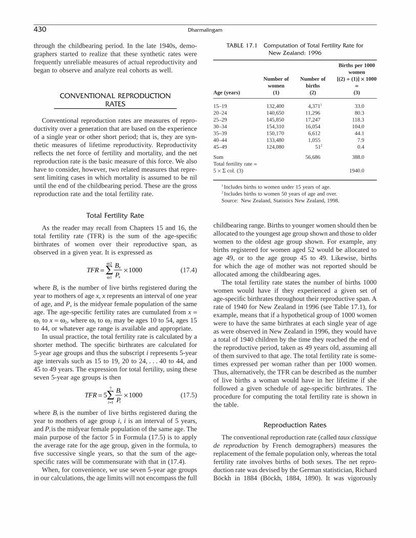
through the childbearing period. In the late 1940s, demo-graphers started to realize that these synthetic rates were frequently unreliable measures of actual reproductivity andbegan to observe and analyze real cohorts as well.
CONVENTIONAL REPRODUCTIONRATES
Conventional reproduction rates are measures of repro-ductivity over a generation that are based on the experienceof a single year or other short period; that is, they are syn-thetic measures of lifetime reproductivity. Reproductivityreflects the net force of fertility and mortality, and the netreproduction rate is the basic measure of this force. We alsohave to consider, however, two related measures that repre-sent limiting cases in which mortality is assumed to be niluntil the end of the childbearing period. These are the grossreproduction rate and the total fertility rate.
Total Fertility Rate
As the reader may recall from Chapters 15 and 16, thetotal fertility rate (TFR) is the sum of the age-specificbirthrates of women over their reproductive span, asobserved in a given year. It is expressed as
(17.4)
where Bx is the number of live births registered during theyear to mothers of age x, x represents an interval of one yearof age, and Px is the midyear female population of the sameage. The age-specific fertility rates are cumulated from x =w1 to x = w2, where w1 to w2 may be ages 10 to 54, ages 15to 44, or whatever age range is available and appropriate.
In usual practice, the total fertility rate is calculated by ashorter method. The specific birthrates are calculated for 5-year age groups and thus the subscript i represents 5-yearage intervals such as 15 to 19, 20 to 24, . . . 40 to 44, and 45 to 49 years. The expression for total fertility, using theseseven 5-year age groups is then
(17.5)
where Bi is the number of live births registered during theyear to mothers of age group i, i is an interval of 5 years,and Pi is the midyear female population of the same age. Themain purpose of the factor 5 in Formula (17.5) is to applythe average rate for the age group, given in the formula, tofive successive single years, so that the sum of the age-specific rates will be commensurate with that in (17.4).
When, for convenience, we use seven 5-year age groupsin our calculations, the age limits will not encompass the full
TFRB
Pi
ii
= ¥=Â5 1000
1
7
TFRB
Px
x
= ¥Â 10001
2
w
w
childbearing range. Births to younger women should then beallocated to the youngest age group shown and those to olderwomen to the oldest age group shown. For example, anybirths registered for women aged 52 would be allocated toage 49, or to the age group 45 to 49. Likewise, births for which the age of mother was not reported should be allocated among the childbearing ages.
The total fertility rate states the number of births 1000women would have if they experienced a given set of age-specific birthrates throughout their reproductive span. Arate of 1940 for New Zealand in 1996 (see Table 17.1), forexample, means that if a hypothetical group of 1000 womenwere to have the same birthrates at each single year of ageas were observed in New Zealand in 1996, they would havea total of 1940 children by the time they reached the end ofthe reproductive period, taken as 49 years old, assuming allof them survived to that age. The total fertility rate is some-times expressed per woman rather than per 1000 women.Thus, alternatively, the TFR can be described as the numberof live births a woman would have in her lifetime if she followed a given schedule of age-specific birthrates. Theprocedure for computing the total fertility rate is shown inthe table.
Reproduction Rates
The conventional reproduction rate (called taux classiquede reproduction by French demographers) measures thereplacement of the female population only, whereas the totalfertility rate involves births of both sexes. The net repro-duction rate was devised by the German statistician, RichardBöckh in 1884 (Böckh, 1884, 1890). It was vigorously
430 Dharmalingam
TABLE 17.1 Computation of Total Fertility Rate for New Zealand: 1996
Births per 1000women
Number of Number of [(2) ∏ (1)] ¥ 1000women births =
Age (years) (1) (2) (3)
15–19 132,400 4,3711 33.020–24 140,650 11,296 80.325–29 145,850 17,247 118.330–34 154,310 16,054 104.035–39 150,170 6,612 44.140–44 133,480 1,055 7.945–49 124,080 512 0.4
Sum 56,686 388.0Total fertility rate =5 ¥ S col. (3) 1940.0
1 Includes births to women under 15 years of age.2 Includes births to women 50 years of age and over.Source: New Zealand, Statistics New Zealand, 1998.
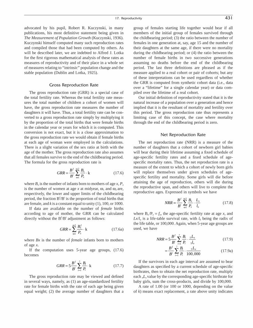
advocated by his pupil, Robert R. Kuczynski, in many publications, his most definitive statement being given inThe Measurement of Population Growth (Kuczynski, 1936).Kuczynski himself computed many such reproduction ratesand compiled those that had been computed by others. Aswill be described later, we are indebted to Alfred J. Lotkafor the first rigorous mathematical analysis of these rates asmeasures of reproductivity and of their place in a whole setof measures relating to “intrinsic” population change and thestable population (Dublin and Lotka, 1925).
Gross Reproduction Rate
The gross reproduction rate (GRR) is a special case ofthe total fertility rate. Whereas the total fertility rate meas-ures the total number of children a cohort of women willhave, the gross reproduction rate measures the number ofdaughters it will have. Thus, a total fertility rate can be con-verted to a gross reproduction rate simply by multiplying itby the proportion of the total births that were female birthsin the calendar year or years for which it is computed. Thisconversion is not exact, but it is a close approximation tothe gross reproduction rate we would obtain if female birthsat each age of woman were employed in the calculations.There is a slight variation of the sex ratio at birth with theage of the mother. The gross reproduction rate also assumesthat all females survive to the end of the childbearing period.The formula for the gross reproduction rate is
(17.6)
where Bx is the number of infants born to mothers of age x, Px
is the number of women at age x at midyear, w1 and w2 are,respectively, the lower and upper limits of the childbearingperiod, the fraction Bf/Bt is the proportion of total births thatare female, and k is a constant equal to unity (1), 100, or 1000.
If data are available on the number of female birthsaccording to age of mother, the GRR can be calculateddirectly without the Bf/Bt adjustment as follows:
(17.6a)
where Bx is the number of female infants born to mothersof age x.
If the computation uses 5-year age groups, (17.6)becomes
(17.7)
The gross reproduction rate may be viewed and definedin several ways, namely, as (1) an age-standardized fertilityrate for female births with the rate of each age being givenequal weight; (2) the average number of daughters that a
GRRB
B
B
P
f
t
i
ii
= ◊=Â5
1
7
k
GRRB
Pxf
x
= ◊ kw
w
1
2
GRRB
B
B
P
f
t
x
x
= ◊ kw
w
1
2
group of females starting life together would bear if allmembers of the initial group of females survived through the childbearing period; (3) the ratio between the number offemales in one generation at, say, age 15 and the number oftheir daughters at the same age, if there were no mortalityduring the childbearing period; or (4) the ratio between thenumber of female births in two successive generationsassuming no deaths before the end of the childbearingperiod. The last three definitions are phrased as if themeasure applied to a real cohort or pair of cohorts; but anyof these interpretations can be used regardless of whetherthe GRR is computed from synthetic cohort data (i.e., dataover a “lifetime” for a single calendar year) or data com-piled over the lifetime of a real cohort.
Our initial definition of reproductivity stated that it is thenatural increase of a population over a generation and henceimplied that it is the resultant of mortality and fertility overthis period. The gross reproduction rate thus represents alimiting case of this concept, the case where mortalitythrough the end of the childbearing period is zero.
Net Reproduction Rate
The net reproduction rate (NRR) is a measure of thenumber of daughters that a cohort of newborn girl babieswill bear during their lifetime assuming a fixed schedule ofage-specific fertility rates and a fixed schedule of age-specific mortality rates. Thus, the net reproduction rate is ameasure of the extent to which a cohort of newly born girlswill replace themselves under given schedules of age-specific fertility and mortality. Some girls will die beforeattaining the age of reproduction, others will die during the reproductive span, and others will live to complete thereproductive ages. Expressed in symbols we have
(17.8)
where Bx /Px = fx, the age-specific fertility rate at age x, andLx/lo is a life-table survival rate, with l0 being the radix ofthe life table, or 100,000. Again, when 5-year age groups areused, we have
(17.9)
(17.9a)
If the survivors in each age interval are assumed to beardaughters as specified by a current schedule of age-specificbirthrates, then to obtain the net reproduction rate, multiplyeach nLx value by the corresponding age-specific birthrate forbaby girls, sum the cross-products, and divide by 100,000.
A rate of 1.00 (or 100 or 1000, depending on the valueof k) means exact replacement, a rate above unity indicates
= ◊=ÂB
B
B
P
Lf
t
i
i
x
i
5
1
7
100 000,
NRRB
B
B
P
L
l
f
t
i
i
x
oi
= ◊=Â5 5
51
7
NRRB
B
B
P
L
l
f
t
x
x
x
o
= ◊Âw
w
1
2
17. Reproductivity 431

that the population is more than replacing itself, and a ratebelow unity means that the population is not replacing itself.The interpretations corresponding to those given for thegross rate are (1) an age-standardized “mortality-adjusted”fertility rate with each age being given an equal weight; (2)the average number of daughters born to a group of femalesstarting life together, (3) the ratio between the number offemales in one generation at, say, age 15, and the number oftheir daughters at the same age, and (4) the ratio betweenfemale births in two successive generations. All these inter-pretations include allowance for mortality up through thechildbearing period. As previously indicated, the net repro-duction rate is frequently abbreviated NRR, but the usualsymbol in mathematical demography is Lotka’s R0. Therationale of R0 is made clear in the next section.
The procedure for computing the gross and net repro-duction rates is shown in Table 17.2. From statistics onbirths and population, we have computed age-specificbirthrates for New Zealand in 1996. For convenience, theage-specific rates are computed from births of both sexes,so we use the symbol 5 f T
x. The transition to female birthsonly is made later, in a single step, by applying the propor-tion of all births that are female. Also for convenience, wehave grouped our data in 5-year age groups. In this form thefigures in column 2 do not look like survival rates becausethe survival rates have been cumulated over 5 years. We
could have used instead the female survival rate to the
midpoint of each age interval , , and so on. For
example, the survival rate to age 17.5 is = 0.98904.
In this approach, the sum of column 3 would need to be mul-tiplied by 5 to produce the net reproduction rate. From thefemale life table for 1996, we read off, or sum, the valuesof 5Lx for x taken successively at ages 15, 20, 25, . . . 45.Because these are for 100,000 women, we divide them by100,000 to obtain values per woman (the 4.94560 years forthe age group 15 to 19 is equivalent to 494,560 years livedby a cohort of females who number 100,000 at birth).
The specific steps are as follows:
Step 1. Compute the age-specific birthrate per female, andenter it in column 1.
Step 2. From an appropriate life table, find the number ofyears lived by females in the stationary population foreach interval of age. In an abridged life table, 5Lx willbe given directly. (In a life table with single years ofage, 5Lx can be obtained by summing five successivevalues of Lx or by subtracting Tx+5 from T5.)
Step 3. Divide 5Lx by 100,000, and enter the result incolumn 2.
Step 4. Multiply each entry of column 2 by the cor-responding entry of column 1 and enter the result incolumn 3.
Step 5. To obtain the gross reproduction rate, multiply thesum of the entries in column 1 by the proportion ofbirths that are female (.48551) and then by the factor 5.
Step 6. To obtain the net reproduction rate, apply thefactor .48551 to the sum of column 3.
These rates are expressed per woman, but they could alsohave been expressed per 100 women or per 1000 women. Itis important to note that in the conventional reproductionrates, the age-specific fertility and mortality rates all refer tothe same fixed period of time, say a given calendar year orthe average of a few years. Moreover, if a life table is notavailable for exactly the same year as that of the fertilityschedule, approximate reproduction rates for that year maybe obtained by using a life table for an adjacent year oryears. In general, it is more important for the fertility datato relate to the reference year than the mortality data, whichare not likely to vary much over a few years and would have less effect than the fertility rates on the level of reproductivity.
These reproduction rates are defined in terms of thefemale population, but analogous rates can also be computedfor both sexes combined or for the male population only.(See the section on “Reproduction of the Male Population”presented later in this chapter.) Reproductivity is usuallystudied in terms of mothers and daughters because thefecund period for females is shorter than it is for males and
98 904100 000
,,
l
l22 5
0
.l
l17 5
0
.
432 Dharmalingam
TABLE 17.2 Computation of Gross and Net ReproductionRates for New Zealand: 1996
Number of
Age-specific birth Survival rate1
births
Age of rate per femalemother 5 f T
x (1) ¥ (2) =(years) (1) (2) (3)
15–19 0.03301 4.94560 0.1632720–24 0.08031 4.93198 0.3961025–29 0.11825 4.91951 0.5817430–34 0.10404 4.90505 0.5103135–39 0.04403 4.88659 0.2151640–44 0.00790 4.86117 0.0384245–49 0.00041 4.81951 0.00198
Sum 0.38796 X 1.90698
X Not applicable.1 Also allows for 5-year grouping of ages. Source: Based on Table 17.1. The life tables used here were taken from
Cheung, 1999.
NRR or RB
Bf
L
B
Bf
L
F
T xT x
F
F
F
T xT x
F
F
,
. . .
05
05
5
05
55
48551 1 90698 0 92586
= ◊◊
= ◊ ◊
= ( )( ) =
Â
Âl
l
GRRB
Bf
F
T xT= = ( )( ) =Â5 5 48551 0 38796 0 94179
5. . .
5
0
LxF
F�
5s
0
fL
XT x
F
F◊
�

because demographic and other characteristics (age, maritalstatus, and so on) are much more likely to be known formothers than for fathers, especially in the case of non-marital births.
The ratio of the net reproduction rate to the gross repro-duction rate is called the reproduction-survival ratio. It isthe proportion of potential reproductivity that survives theeffects of mortality.
THE STABLE POPULATION: ITS VITAL RATES AND
OTHER CHARACTERISTICS
The assumption of the constancy of age-specificbirthrates and death rates for a generation, which is made inthe calculation of the gross reproduction rate and the netreproduction rate, defines the basic conditions of a generaltheoretical model. Lotka developed a model that describedthe age composition implied by the given sets of vital ratesand expressed reproductivity on an annual as well as on ageneration basis. This model is designated the “stable pop-ulation” model. Lotka demonstrated in 1907 that if a popu-lation is subject to a fixed schedule of age-specific fertilityrates and a fixed schedule of age-specific mortality rates foran indefinite period of time and if meanwhile there is nomigration, ultimately the age composition of the populationwould assume a fixed characteristic distribution (Lotka,1907). Coale (1968) has investigated the time required for apopulation with a given age structure and given age-specific fertility and mortality schedules to approach its ultimatestable form.
In 1925, Lotka proved that a closed population (i.e., apopulation without immigration) with constant age-specificfertility and mortality schedules would eventually have aconstant rate of natural increase (Dublin and Lotka, 1925).Lotka called this rate the true rate of natural increase. It hasalso been called the intrinsic rate of natural increase. (Thelife table stationary population can be viewed as a stablepopulation with a zero rate of natural increase.)
Intrinsic Rate of Natural Increase
Lotka computed the true rate of natural increase bysolving the integral equation
(17.10)
where p(x) is the probability of surviving from birth to agex, r is the intrinsic rate of increase per person per year, andf(x) is the number of live female births per year to eachwoman of age x. Note that p(x) is the Lx of the life tabledivided by lo. Because f(x) is zero outside the childbearing
e f x p x dxrx-•
Ú ( ) ( ) =0
1
period, we could substitute the limits w1 and w2, or approx-imately 15 to 49, as the limits of the definite integral.
In practice, a very close approximation to the real root ofEquation (17.10) is given by the quadratic equation
(17.11)
where
(17.12)
(17.13)
where ln represents a logarithm to the base e, R0 is the net reproduction rate, and R1 and R2 are the first and secondmoments of the curve representing the age schedule of netreproductivity. The general equation for these moments isgiven by
(17.14)
The intrinsic measures that are presented here as rela-tively exact employ at most the second moments. Fortu-nately, the terms involving the higher moments convergequite rapidly toward zero.
Solving the quadratic Equation (17.11) for r, we obtain,for the positive radical, which corresponds to the real root:
(17.15)
and substituting for a and b in terms of R0, R1, and R2, weobtain, as given by Kuczynski (1932, p. 59)
(17.16)
As we see from the computations for Table 17.3, thisform enables us to evaluate r, because R0 was derived inTable 17.2, and R1 and R2 can also be derived from the samebasic statistics.
Mean Length of Generation
The mean length of generation is defined as the mean ageof mothers at the birth of their daughters. Because the stablepopulation is growing at the annual rate r, compounded continuously, and the net reproduction rate, R0, is its rate of growth in one generation, T years, we may write in anapproximate formulation
(17.17)R erT0 =
r
RR
RR
RR
RR
R
RR
RR
o oo
o o
=- Ê
ˈ¯ - - Ê
ˈ¯
È
ÎÍ
˘
˚˙
- ÊË
ˆ¯
1 12
2
0
1
0
2
2 12
2 ln
rRo=
- + +a a bb
2 2 ln
R x f x p x dxnn
o= ( ) ( )
•
Ú
b a= - = ÊË
ˆ¯ -2 2 1
22R
R
R
R
R
Ro o o
a =R
Ro
1
12
020b ar r R+ - =ln
17. Reproductivity 433

Note the similarity to the formula for population growth,Pt/P0 = ert.
(17.18)
Because from (17.11),
(17.19)
(17.20)
Because every year the stable population is (1 + r)times larger than the year before, at the end of a genera-tion, it will be larger by a factor equal to the net repro-duction rate. Of course, if r is negative, R0 will be less thanone.
Intrinsic Birthrate
The true or intrinsic birthrate is the birthrate that wouldeventually be reached in a population subject to fixed fertil-ity and mortality schedules. Thus, it is the birthrate of the
T r= +a b12
ln R r ro = +12
2b a
Tr
Ro=1
ln
stable population. The intrinsic birthrate may be expressedby the equation
(17.21)
where b is the birthrate per person per year and the integralrepresents the total female stable population. This transcen-dental equation can be solved directly for b in a mannersimilar to that used for solving (17.10) for r; or, if we firstdetermine the arithmetic value of r, we can substitute it in(17.21) and evaluate the definite integral.
A satisfactory approximation to Equation (17.21) may beobtained from
(17.22)
Intrinsic Death Rate
The true, or intrinsic, death rate is the death rate thatwould eventually be reached in a population subject to fixed
be
Ll
r x x
oo
=◊- +( )•
Ú1
1 2
be p x dxrx
o
=( )-•
Ú1
434 Dharmalingam
TABLE 17.3 Calculation of Intrinsic Rate of Increase (r), New Zealand: 1996
Products
Annual births Zero Firstof daughters Pivotal moment moment Second moment
Age of mother per female (midpoint) age (R0) (R1) (R2)x to x + 4 5Fx (x + 21/2) (1) ¥ (3) = (2) ¥ (4) = (2) ¥ (5) =(years) (1) (2) (3) (4) (5) (6)
15–19 .01603 17.5 4.94560 .07927 1.38723 24.2765020–24 .03899 22.5 4.93198 .19231 4.32700 97.3575125–29 .05741 27.5 4.91951 .28244 7.76712 213.595730–34 .05051 32.5 4.90505 .24776 8.05219 261.696335–39 .02138 37.5 4.88659 .10446 3.91728 146.898140–44 .00384 42.5 4.86117 .01865 0.79280 33.6940445–49 .00020 47.5 4.81951 .00096 0.04568 2.16999
Sum .18836 (X) (X) .92586 26.28931 779.6882
Substituting the values for R0, R1, and R2 in equation (17.16), we obtain
r = -.00271
X: Not applicable.Source: Table 17.2.Note: Inconsequential discrepancies from the handling of decimals may be disregarded.
GRR
NRR R
R
R
R
R
R
R
Re
= ( ) = ¥ =
= = ( ) =
= ( ) =
= ( ) =
= =
= - = -
= -
ÂÂ
ÂÂ
5 1 5 18836 0 94179
4 0 92586
5 26 28931
6 779 6882
28 39451
35 8761
07703
0
1
2
1
0
2 2
0
0
col.
col.
col.
col.
. .
.
.
.
.
.
log .
a
b a
5
0
LxF
�
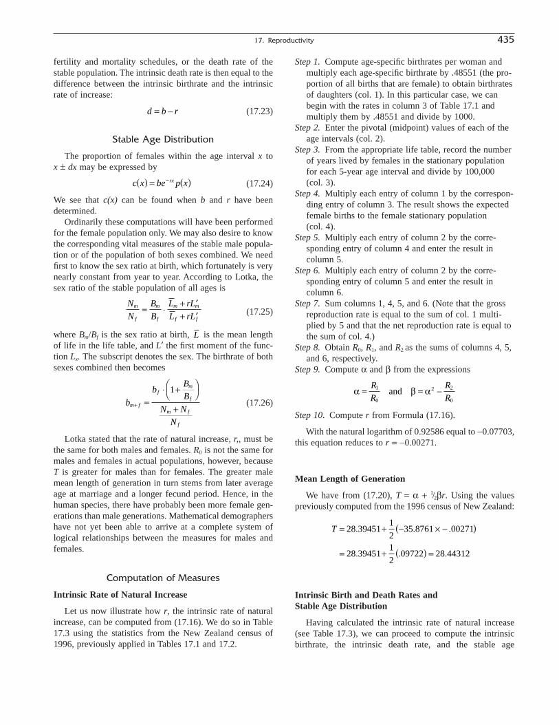
fertility and mortality schedules, or the death rate of thestable population. The intrinsic death rate is then equal to thedifference between the intrinsic birthrate and the intrinsicrate of increase:
(17.23)
Stable Age Distribution
The proportion of females within the age interval x to x ± dx may be expressed by
(17.24)
We see that c(x) can be found when b and r have been determined.
Ordinarily these computations will have been performedfor the female population only. We may also desire to knowthe corresponding vital measures of the stable male popula-tion or of the population of both sexes combined. We needfirst to know the sex ratio at birth, which fortunately is verynearly constant from year to year. According to Lotka, thesex ratio of the stable population of all ages is
(17.25)
where Bm/Bf is the sex ratio at birth, is the mean lengthof life in the life table, and L¢ the first moment of the func-tion Lx. The subscript denotes the sex. The birthrate of bothsexes combined then becomes
(17.26)
Lotka stated that the rate of natural increase, r,, must bethe same for both males and females. R0 is not the same formales and females in actual populations, however, becauseT is greater for males than for females. The greater malemean length of generation in turn stems from later averageage at marriage and a longer fecund period. Hence, in thehuman species, there have probably been more female gen-erations than male generations. Mathematical demographershave not yet been able to arrive at a complete system oflogical relationships between the measures for males andfemales.
Computation of Measures
Intrinsic Rate of Natural Increase
Let us now illustrate how r, the intrinsic rate of naturalincrease, can be computed from (17.16). We do so in Table17.3 using the statistics from the New Zealand census of1996, previously applied in Tables 17.1 and 17.2.
b
bBB
N NN
m f
fm
f
m f
f
+ =◊ +ÊË
ˆ¯
+
1
Lf
N
N
B
B
L rL
L rLm
f
m
f
m m
f f
= ◊+ ¢+ ¢
c x be p xrx( ) = ( )-
d b r= -
Step 1. Compute age-specific birthrates per woman andmultiply each age-specific birthrate by .48551 (the pro-portion of all births that are female) to obtain birthratesof daughters (col. 1). In this particular case, we canbegin with the rates in column 3 of Table 17.1 andmultiply them by .48551 and divide by 1000.
Step 2. Enter the pivotal (midpoint) values of each of theage intervals (col. 2).
Step 3. From the appropriate life table, record the numberof years lived by females in the stationary populationfor each 5-year age interval and divide by 100,000 (col. 3).
Step 4. Multiply each entry of column 1 by the correspon-ding entry of column 3. The result shows the expectedfemale births to the female stationary population (col. 4).
Step 5. Multiply each entry of column 2 by the corre-sponding entry of column 4 and enter the result incolumn 5.
Step 6. Multiply each entry of column 2 by the corre-sponding entry of column 5 and enter the result incolumn 6.
Step 7. Sum columns 1, 4, 5, and 6. (Note that the grossreproduction rate is equal to the sum of col. 1 multi-plied by 5 and that the net reproduction rate is equal tothe sum of col. 4.)
Step 8. Obtain R0, R1, and R2 as the sums of columns 4, 5,and 6, respectively.
Step 9. Compute a and b from the expressions
Step 10. Compute r from Formula (17.16).
With the natural logarithm of 0.92586 equal to -0.07703,this equation reduces to r = -0.00271.
Mean Length of Generation
We have from (17.20), T = a + 1/2br. Using the valuespreviously computed from the 1996 census of New Zealand:
Intrinsic Birth and Death Rates and Stable Age Distribution
Having calculated the intrinsic rate of natural increase(see Table 17.3), we can proceed to compute the intrinsicbirthrate, the intrinsic death rate, and the stable age
T = + - ¥ -( )
= + ( ) =
28 3945112
35 8761 00271
28 3945112
09722 28 44312
. . .
. . .
a b a= = -R
R
R
R1
0
2 2
0
and
17. Reproductivity 435

distributions of the female and male populations. The com-putations are set forth in Table 17.4.
Step 1. Set down the midpoint of the age intervals (col. 1).
Step 2. Multiply each midpoint of column 1 by -0.00271,the value of r. Enter the result in column 2.
Step 3. Compute the value . Since r is negative,
the entries in column 3 all exceed 1.000. If r were posi-tive, they would all fall between zero and one.
Step 4. From the female life table, record the averagenumber of years one woman would live during eachage interval. This is obtained by dividing 5Lx for theappropriate interval of the female stationary populationby 100,000. Record the results in column 4.
Step 5. Multiply each entry in column 4 by the correspon-ding entry in column 3. Record the products in column5. Sum these entries and record the result at the bottomof column 5.
12 5er x+( ).
Step 6. From the corresponding male life table, multiplythe average number of years each male would liveduring each age interval by the sex ratio at birth andrecord the product in column 6.
Step 7. Multiply each entry in column 6 by the correspon-ding entry in column 3, and record the products incolumn 7. Sum these entries, and record the result atthe bottom of column 7.
Step 8. Compute the intrinsic birth and death rates. Thetotal number of female person-years is the total ofcolumn 5, or 89.24075. There is 1 female birth. (The radix of the female life table is 100,000 births, but we have changed it to 1 in the calculations shownin Table 17.4.) Therefore, to obtain the female birthrate
per person, we use the fraction , which is
0.01121. The intrinsic birthrate per 1000 of the femalepopulation—the conventional form—is, therefore,11.21. The birthrate for the entire stable population(both sexes) is
189 24075.
436 Dharmalingam
TABLE 17.4 Computation of the Intrinsic Birth and Death Rates, and the Age Distribution, of the Stable Population, for New Zealand: 1996
Stable population
r(x + 2.5) e-r(x+2.5)Female stable Male stable
Female Maleor or population population
Age interval Midpoint -.00271(x + 2.5) derivative derivative(x to x + 4, (x + 2.5) -.00271 ¥ (1) = (3) ¥ (4) = (3) ¥ (6) =in years) (1) (2) (3) (4) (5) (6) (7) (8) (9)
0–4 2.5 -.00677 1.00679 4.96599 4.99972 5.25703 5.29274 2,827 2,9925–9 7.5 -.02031 1.02052 4.95905 5.06080 5.24730 5.35496 2,861 3,027
10–14 12.5 -.03385 1.03443 4.95513 5.12573 5.24128 5.42173 2,898 3,06515–19 17.5 -.04739 1.04853 4.94560 5.18561 5.22453 5.47808 2,932 3,09720–24 22.5 -.06093 1.06282 4.93198 5.24183 5.18664 5.51249 2,963 3,11625–29 27.5 -.07447 1.07731 4.91951 5.29985 5.14570 5.54353 2,996 3,13430–34 32.5 -.08801 1.09200 4.90505 5.35631 5.10912 5.57915 3,028 3,15435–39 37.5 -.10155 1.10689 4.88659 5.40889 5.07400 5.61634 3,058 3,17540–44 42.5 -.11509 1.12197 4.86117 5.45411 5.03314 5.64705 3,083 3,19345–49 47.5 -.12863 1.13727 4.81951 5.48108 4.97399 5.65677 3,099 3,19850–54 52.5 -.14217 1.15277 4.74775 5.47308 4.87195 5.61625 3,094 3,17555–59 57.5 -.15571 1.16849 4.63715 5.41845 4.70608 5.49899 3,063 3,10960–64 62.5 -.16925 1.18442 4.47209 5.29682 4.44116 5.26018 2,995 2,97465–69 67.5 -.18279 1.20056 4.22438 5.07163 4.02992 4.83817 2,867 2,73570–74 72.5 -.19633 1.21693 3.85871 4.69577 3.44902 4.19721 2,655 2,37375–79 77.5 -.20987 1.23352 3.33681 4.11601 2.67425 3.29873 2,327 1,86580–84 82.5 -.22341 1.25033 2.58634 3.23379 1.75868 2.19894 1,828 1,24385–89 87.5 -.23695 1.26738 1.64461 2.08434 0.89992 1.14054 1,178 64590 and over 95.0 -.25726 1.29338 0.95634 1.23691 0.37955 0.49090 699 278
Sum 89.24075 (X) 87.64277 50,452 49,548
Source: Table 17.3 and Cheung, 1999.
b 01164 d 01435T T= . = . r = -.00271
b 01121 d 01392 b 01209 d .01480F F M M= . = . = . =
7100,0005 7
( )( ) ( )ÂÂ
¥+
5100,0005 7
( )( ) ( )ÂÂ
¥+
5
0
(Sex ratio
at birth,
1.05969
LxM
m�◊
)
5
0
LxF
F�
12.5er x+( )

or 11.64 per 1000. The intrinsic death rate equals theintrinsic birthrate minus the intrinsic rate of naturalincrease, or 11.64 - (-2.71), which equals 14.35 per 1000.
Step 9. To compute the distribution of the stable popula-tion by age and sex, we add the sums of columns 5 and7, obtaining 176.88352, which is the total stable popu-lation derivative of both sexes. To express the distribu-tion per 100,000 of the total population, divide 100,000by this total and multiply each value in columns 5 and7 by this constant factor. Post the results in columns 8and 9, respectively.
Formula (17.24) gives the age distribution per unit for agiven sex. Because the number of female births is 1, thenthe female birthrate is, as in formulas (17.21)
or, in our table, the reciprocal of the total of the entries incolumn 5 as in Formula (17.22). In the actual computationsin our worksheet, the value of b does not appear explicitly.
The results obtained give a stable population consistingof 100,000 persons with the appropriate numbers of malesand females in accordance with the sex ratio at birth. Oftenthe distribution is wanted for the female (or male) popula-tion only. Then we use the sum of column 5—or column 7—alone rather than the total of the two sums. For example, forfemales under 5 years old, the percentage is:
Some Approximations
The amount of calculation required for some of thesemeasures can be reduced appreciably by using shortcut formulas described by Coale. These appear in two separatearticles. We will describe first his earlier proposal forapproximating the intrinsic rate of natural increase (Coale,1955). Coale’s calculations involve two relationships:
(17.27)
(17.28)
where NRR is the net reproduction rate, GRR is the grossreproduction rate, r is the intrinsic rate of natural increase,
T is the mean length of a female generation, and is the
probability of a female’s surviving to age T.
l
lT
0
NRR
GRR
l
lT
o
ª
NRR erT=
4 9997289 24075
100 5 603..
. %¥ =
1
e p xrx- ( )Â
1 1 0596989 24075 87 64277
2 05969176 88352
01164+
+= =
.. .
..
.The intrinsic rate of natural increase can be estimated by
determining T from the approximate relationship (17.27),Thus
(17.29)
and calculating r from (17.27), using natural logarithms (ln),we obtain
(17.30)
Because r and T are reciprocally related, the percentageerror in estimating r varies inversely with that in estimatingT. Coale tested the accuracy of the approximation by com-paring the results it yields with the results of exact compu-tations of T for 17 different countries. The root mean squareerror was about 1.8% of the average value of T. Coale (1955,p. 96) also gave an approximation, first suggested by Lotka,for b, the intrinsic birthrate.)
Let us use this approximation to estimate r and comparethe result with the closer estimate of Table 17.3. We take thevalues of NRR and GRR from that table:
Consulting the New Zealand life table for 1996 and inter-polating, we find that this value of lT corresponds to a T of29.02 years. Substituting in (17.31) we have
which compares well with the -.00271 found by the moreexact method.
The shortcut method is very close. There are other possibleapproximations, however. Because T = a + 1/2br, it can be seenthat the second term can be ignored when r is small. Then
(17.31)
From Table 17.3, T = = 28.394 years:
(17.32)
f(x) being the fertility rate at age x and p(x) the survival rateto age x. This can be seen as a weighted age (x) in whichthe weights are the rates of age-specific survivors of births.
We may then substitute this new estimate of T in theequation R0 = erT, obtaining
r =-
= -0 0770328 394
00271..
.
R
R
xf x p x
f x p x1
0
=( ) ( )( ) ( )
ÂÂ
26 289310 92586
..
TR
Ro
@ =a 1
r = =-
= -ln .
..
..
0 9258629 02
0770329 02
0 00265
lT = ¥ =0 925860 94179
100 000 98 308..
, ,
rNRR
T=
ln
l lNRR
GRRT o@
17. Reproductivity 437

This is the same as that obtained through the exactmethod illustrated earlier.
In a later article, Coale gave still another way of approx-imating r. This method (Coale, 1957) involves using 29years as an estimate of T and getting r1, as a first approxi-mation to the value of r, which is then adjusted according tothe extent to which
(17.33)
The excess of the estimate from 1 is designated d and theadjusted value of r becomes
(17.33a)
Coale regarded this approximation as better than that basedon (17.28).
Relation between Actual and Intrinsic Rates of Increase
Preston and Coale (1982) demonstrated that there is anecessary link between the actual rate of increase of a pop-ulation and the intrinsic rate of increase of the correspon-ding stable population. Specifically, Preston (1986) showedthat the mean age-specific growth rate up to age T, the meanlength of generation, is a close approximation to Lotka’sintrinsic rate of increase. In other words,
(17.34)
where r is the intrinsic rate of increase, T the mean lengthof generation, and r(x) the age-specific growth rates. T isusually close to the mean age of childbearing, say, A*. Thus,alternatively, one can derive (A*)—the mean growth rateof the population segment below the mean age at child-bearing. However, it is found that the intrinsic rate ofincrease is better approximated by (T) than by (A*).
The preceding relation between the rate of increase of apopulation below age T and the intrinsic rate of increase has important implications for population momentum. If an intrinsic growth rate of zero (i.e., R0 = 1) is attained andmaintained in a population, then the population below ageT will remain approximately constant in size from the timeat which it is attained. But we know from the experiencesof the more developed and some less developed countriesthat a population continues to grow in size even after attain-ing replacement-level fertility. It thus follows that thegrowth momentum must occur above age T. “The momen-tum results from projecting into higher ages the largercohorts of persons already born, and not from projectinggrowth into the reproductive [or young adult] ages of thebirths still to occur” (Preston, 1986, p. 350).
rr
r
r rT
r x dxT
ª = ( )Ú1
0
r
r
1
1
29+
-
dd
e f x p x dxr x- ( ) ( )Ú 1
1
2
w
wfails to equal 1.
REPRODUCTIVITY ESTIMATED FROMCENSUS STATISTICS
In the absence of adequate birth statistics, attempts havebeen made to compute measures of reproductivity whollyfrom census statistics or from census statistics and lifetables. The methods described in this section are applicableto many countries with good age-sex statistics from censusesbut with inadequate birth statistics, including many lessdeveloped countries. It is often desirable, however, to makesome kind of correction for undercounting young children,or otherwise to adjust the age-sex distribution, when meas-uring reproductivity from census data.1
Measures Based on Age-Sex Distributions:The Replacement Index
The replacement index is computed on the basis of theage distribution of the actual female population and a femalelife table for the same period. The calculation involvesdividing the ratio of children under five years of age tofemales in the reproductive ages in the actual population, bythe corresponding ratio in the life table stationary popula-tion. Thus defined, this measure relates to reproductivity inthe 5 years preceding the reference date of the observed agedistribution. We may exercise a choice in the age groups forchildren and women employed in the measures, just as wedo in the case of the general fertility ratio.
In his 1920 census monograph, Thompson (1931)devised several types of measures that he called replacementindexes. Of these, his permanent replacement index corre-sponded to the index just described. (Net replacementindexes similar to those defined by Thompson were com-puted for many countries of the world as part of the com-puter program devised by Keyfitz and Flieger (1968).)
Subsequently Lotka gave a generalized mathematicaltreatment of replacement indexes and showed how a re-placement index is related to the intrinsic rate of naturalincrease (Lotka, 1936). He defined the index J in the sameway as Thompson’s permanent replacement index, namely,as the quotient of two ratios, the numerator, the ratio of chil-dren under a given age to women in the childbearing ages
438 Dharmalingam
1 The general approach is similar to that in estimating fertility mea-sures from survey data described in Chapter 16. In the United States, repro-duction rates, like other fertility measures, were first based on census data,for several reasons: (a) the failure of the Birth Registration Area to coverthe entire United States until 1933; (b) the lack of national statistics on res-ident births until 1937; and (c) the fact that fertility data on some charac-teristics (such as farm-nonfarm residence) are available from the census butnot from the registration system. The last of these reasons is still an impor-tant one. On the other hand, we must recognize that undercounting of youngchildren in the United States has become more serious than underregistra-tion of births but that we have little information on current geographic vari-ation of either of these types of errors.

in the actual population and, the denominator, the same ratioin the life table population. Thus, in integral notation,
(17.35)
where c(a) is a segment of the age distribution in the actualpopulation and p(a) is the probability at birth of surviving toage a; p and q are the lower and upper limits, respectively, ofthe younger age group of both sexes, and u and v are the lowerand upper limits, respectively, of the age groups of women in the reproductive ages. The symbol b0 denotes the birthrateper person in the life table population in which
(17.36)
In the more conventional demographic notation, this is
(17.37)
Note that in deriving the total number of children in the lifetable population, it is necessary to combine the number ofboys and girls from their respective life tables, inflating thenumber of boys by the sex ratio of births.
The replacement index, then, gives us a method forapproximating the net reproduction rate in the absence ofvital statistics. Table 17.5 illustrates the computation of the J index with 1996 statistics for New Zealand consistentwith those used in Tables 17.3 and 17.4. We have used the simpler statistical notation instead of Lotka’s integralequation:
(17.38)
where ln represents a natural logarithm and a2 and a1 aredefined in Table 17.5.
The value of J(0.98179) greatly exceeds the value ofR0(.92586) in Table 17.3, and the value of r(-.00062) is con-siderably less than that of r(-.00271) in Table 17.3. Thiscould arise from the extent to which the 1996 population ofNew Zealand was not of stable form, the use of very differ-ent data systems, and the difference in the reference date andsexes (of children) of the two calculations.
Reproduction Rate Estimated from Women’sOwn Children Under 5
Up to this point in our discussion of the use of censusdata to approximate net reproductivity, we have dealt onlywith the data obtainable from age-sex distributions. Becauseit was not until the 1940 census of the United States thatdata were tabulated and published on the distribution of
¢ =-
rJln
a a2 1
JP
P
LBB
L
Lf
f m
f
m
f= ∏
+-
-
- -
-
0 4
15 49
0 4 0 4
15 49
c a b p a( ) = ( )0
Jc a da
c a da
b p a da
b p a da
p
q
u
v
op
q
ou
v=
( )
( )∏
( )
( )
ÚÚ
ÚÚ
women by the number of their own children under 5 yearsold in the household, it is not surprising that no attentionwas paid by demographers to the computation of reproduc-tion rates from such data. In 1942, Grabill developed amethod for calculating gross and net reproduction rates fromdata on own children under 5 years, of women of child-bearing age, which was most completely described in anarticle by Grabill and Cho (1965).
They began by estimating the age-specific birthrates cor-responding to the ratios of own children to women by age.Let Bf
x denote the number of daughters born to women ofage x and Pf
x the number of women of age x; then
(17.39)
is the age-specific birthrate.Let sX be the life table probability of survival from
birth to age x, or the probability that daughters will live totheir mother’s age. Thus, using life table probabilities, onecan expect that a census or survey taken i years after the
FB
Px
xf
xf
=
17. Reproductivity 439
TABLE 17.5 Computation of Replacement Index (J) and Substitute Intrinsic Rate of Natural Increase for
New Zealand: 1996
Steps Calculation
1. Ratio, children 0–4 to women 15–49 years: census populationa. PT
0–4 279,606b. PF
15–49 954,675c. Ratio (a) ∏ (b) .29288
2. Ratio, children 0–4 to women 15–49 years: life table populationa. LM
0–4 496,091b. LF
0–4 496,599c. LF
15–49 3,426,941
d. .29831
3. Replacement Index (J) = (l,c) ∏ (2,d) .98179
4. Rate of Increase
a. ln J -.01838b. a1 = Mean age of children 0–4 in life table
population1 2.69c. a2 = Mean age of women 15–49 in life table
population2 32.42d. a2 - a1 29.73e. r¢ = (a) ∏ (d) -.00062
1 The mean age for each sex was based on values for L0 and L1–4 in theabridged life table for New Zealand, and midpoints of 0.5 and 3.0, respec-tively, were assumed for these age groups. The resulting mean ages formales and females were then weighted in proportion to the assumed dis-tributions of births by sex in New Zealand.
2 Computed on the basis of the life table population in 5-year age groupsand the midpoints of these age intervals.
Source: Statistics New Zealand, 1998.
¢ =-
rln J
a a2 1
1 05969. a b
c
( ) + ( )( )

birth of the daughters will show BfxSi surviving daughters of
age i. Similarly, the survivorship among women “x” to age
“x + i” would be . The ratio of surviving daughters
born to surviving women would be
(17.40)
Given , Bfx = FxPf
x. Substituting FxPfx for Bf
x in
(17.40), we get
(17.41)
and
(17.42)
Replacing the Fx values in the conventional formulas forgross and net reproduction rates with the mathematically
identical values yields
(17.43)
because si is a constant
(17.44)
The summation in (17.43) and (17.44) is to be taken overall ages for which Rx+i > 0.
Using a life table notation and daughters under 5 yearsold, we may write
(17.45)
where is the female life table stationary population
under 5 years old expressed on a unit-radix basis, A is the age of women at the census date, RA
0-4 is the ratio ofdaughters under 5 years old to women aged A, and LA is thefemale life table stationary population age A, expressed ona unit-radix basis. Using a specific survival-rate notation,5sA, or 5s¢x if we understand x to cover the childbearing ages,we have
(17.46)
Similarly, the gross reproduction rate is
NRRs
R sx x= ◊ ¢Â1
5 05 5
Lx0
4
Â
NRR
L
R L
x
A A= ◊ ◊
ÂÂ -1
0
40 4
NRR Rs
s ss
sR sx i
x i
x ix
ix i x i= Ê
ˈ¯ ◊È
Î͢˚̇
= ◊++
+ +Â Â1
GRR Rs
s s sR
s
sx i
x i
x i ix i
x i
x
= ◊ = ◊++
++Â Â1
RS
S Sx i
x i
x i+
+ÈÎÍ
˘˚̇
F Rs
s sx x i
x i
x i
= ÈÎÍ
˘˚̇+
+
RF s s
Sx i
x x i
x i+
+=
FB
Px
xf
xf
=
RB s
PSS
x ixf
i
xf x i
x
++
=ÊË
ˆ¯
Ps
sxf x i
x
+ÊË
ˆ¯
(17.47)
It is assumed in expression (17.47) that women age A atthe census date were, on the average, 21/2 years younger atthe time their daughters under 5 years old were born. Thisassumption is not very reasonable for females near thebeginning or end of the childbearing period, but the errorstend to cancel so that the overall effect on the GRR is slight.
Again, in our survival rate notation, we have
(17.48)
where 5s¢x is the survival rate of women from birth to exactages x to x + 5, and 5s≤x is the survival rate to exact ages x -2.5 to x + 2.5.
One important consideration in the use of age-specificratios of own children to compute reproduction rates has notyet been brought out, however—namely, that “own chil-dren” fail to account for all children under 5 years (or under1, etc.). The obvious remedy is to make a correction on thebasis of the total number of children in the population. Thiscan be an overall correction, not taking account of variationswith age of mother because these do not have much effecton a reproduction rate, which is a sum over all ages.
Our illustration comes from The Gambia. The methodhas also been applied to several other less developed coun-tries (e.g., Sri Lanka, Korea).
In Table 17.6, we have translated the LA’s and LX’s intosurvival rates for convenience of manipulation. In summingcolumns 4 and 6, we would ordinarily multiply by 5 becausewe are dealing with 5-year age groups of women, and therates are averages for the 5 years. On the other hand, thechildren under 5 in the numerator of column 1 are survivorsof births over a 5-year period, and they need to be reducedto annual births. Hence, the 5’s cancel.
This method can be applied as well to geographic subdi-vision of countries, including the more developed countries,for which vital statistics may not be available, such as type-of-residence areas (e.g., rural-form population, urbanizedareas). This method can be applied also to a country forwhich there are no census or survey data on own childrenby age of mother. The application requires a form of indi-rect standardization to estimate the schedule of age-specificratios of children to women.2 Grabill and Cho (1965, p. 59)
GRRs
R s
sx x
x
=◊ ¢¢¢-
Â1
0 4
5 5
5
GRR
L
RL
Lx
AA
A
= ◊
ÂÂ -
-
500 000
0
40 4
2 5
,
.
440 Dharmalingam
2 Inasmuch as we know the total number of girls under age 5 and thenumber of women according to age, we use the schedule of age-specificratios of own female children under 5 per 1000 women for another countryfor which such ratios are available (“the standard”), to derive the“expected” number of children under 5 in the country of interest. We thendivide this number into the total number of girls under 5 to obtain an adjust-ment factor. The factor is then applied to the standard schedule of ratios to obtain an estimated schedule of ratios for the country of interest. Theremaining steps would then be the same as before with the use of an appro-priate life table.
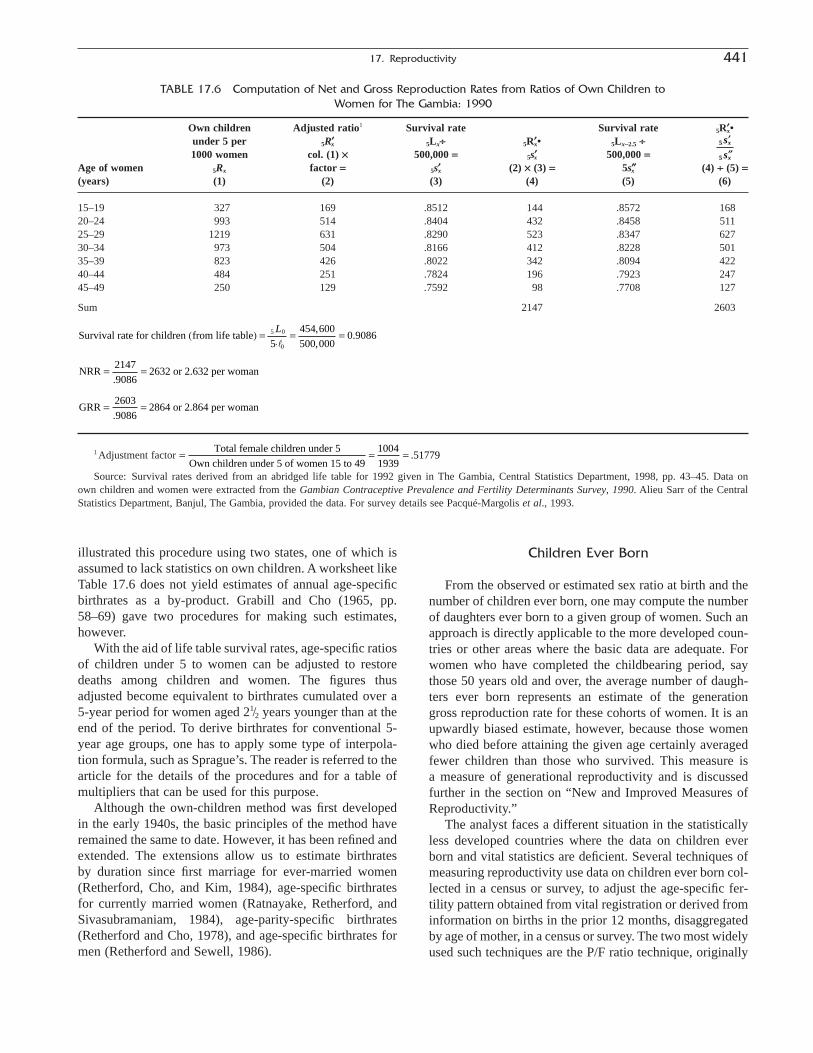
illustrated this procedure using two states, one of which isassumed to lack statistics on own children. A worksheet likeTable 17.6 does not yield estimates of annual age-specificbirthrates as a by-product. Grabill and Cho (1965, pp.58–69) gave two procedures for making such estimates,however.
With the aid of life table survival rates, age-specific ratiosof children under 5 to women can be adjusted to restoredeaths among children and women. The figures thusadjusted become equivalent to birthrates cumulated over a5-year period for women aged 21/2 years younger than at theend of the period. To derive birthrates for conventional 5-year age groups, one has to apply some type of interpola-tion formula, such as Sprague’s. The reader is referred to thearticle for the details of the procedures and for a table ofmultipliers that can be used for this purpose.
Although the own-children method was first developedin the early 1940s, the basic principles of the method haveremained the same to date. However, it has been refined andextended. The extensions allow us to estimate birthrates by duration since first marriage for ever-married women(Retherford, Cho, and Kim, 1984), age-specific birthratesfor currently married women (Ratnayake, Retherford, andSivasubramaniam, 1984), age-parity-specific birthrates(Retherford and Cho, 1978), and age-specific birthrates formen (Retherford and Sewell, 1986).
Children Ever Born
From the observed or estimated sex ratio at birth and thenumber of children ever born, one may compute the numberof daughters ever born to a given group of women. Such anapproach is directly applicable to the more developed coun-tries or other areas where the basic data are adequate. Forwomen who have completed the childbearing period, saythose 50 years old and over, the average number of daugh-ters ever born represents an estimate of the generation gross reproduction rate for these cohorts of women. It is anupwardly biased estimate, however, because those womenwho died before attaining the given age certainly averagedfewer children than those who survived. This measure is a measure of generational reproductivity and is discussedfurther in the section on “New and Improved Measures ofReproductivity.”
The analyst faces a different situation in the statisticallyless developed countries where the data on children everborn and vital statistics are deficient. Several techniques ofmeasuring reproductivity use data on children ever born col-lected in a census or survey, to adjust the age-specific fer-tility pattern obtained from vital registration or derived frominformation on births in the prior 12 months, disaggregatedby age of mother, in a census or survey. The two most widelyused such techniques are the P/F ratio technique, originally
17. Reproductivity 441
TABLE 17.6 Computation of Net and Gross Reproduction Rates from Ratios of Own Children toWomen for The Gambia: 1990
Own children Adjusted ratio1 Survival rate Survival rate 5R¢x•under 5 per 5R¢x 5Lx∏ 5R¢x• 5Lx-2.5 ∏1000 women col. (1) ¥ 500,000 = 5s¢x 500,000 =
Age of women 5Rx factor = 5s¢x (2) ¥ (3) = 5s≤x (4) ∏ (5) =(years) (1) (2) (3) (4) (5) (6)
15–19 327 169 .8512 144 .8572 16820–24 993 514 .8404 432 .8458 51125–29 1219 631 .8290 523 .8347 62730–34 973 504 .8166 412 .8228 50135–39 823 426 .8022 342 .8094 42240–44 484 251 .7824 196 .7923 24745–49 250 129 .7592 98 .7708 127
Sum 2147 2603
1 Adjustment factor
Source: Survival rates derived from an abridged life table for 1992 given in The Gambia, Central Statistics Department, 1998, pp. 43–45. Data on own children and women were extracted from the Gambian Contraceptive Prevalence and Fertility Determinants Survey, 1990. Alieu Sarr of the CentralStatistics Department, Banjul, The Gambia, provided the data. For survey details see Pacqué-Margolis et al., 1993.
= = =Total female children under 5
Own children under 5 of women 15 to 49
1004
193951779.
GRR2603
.90862864 or 2.864 per woman= =
NRR2147
.90862632 or 2.632 per woman= =
Survival rate for children from life table( ) =◊
= =5 0
05
454 600
500 0000 9086
L
l
,
,.
5
5
¢¢¢
s
sx
x
developed by Brass, and the Arriaga technique. A major dif-ference between these two techniques relates to the assump-tion about past fertility. While Brass’s technique is based on the assumption that fertility has been constant during acertain period, say the past 10 or 15 years, the Arriaga tech-nique requires no such assumption. As the fertility transitionhas been under way in almost all less developed countries,the potential for the application of the Brass technique hasbecome limited. Readers interested in Brass’s P/F techniqueand in the Arriaga technique are referred to the standardsource for indirect estimation techniques (United Nations,1983) and to Chapter 22.
MISINTERPRETATIONS ANDSHORTCOMINGS OF
CONVENTIONAL MEASURES
Interpretation of Conventional Rates
During the 1920s and 1930s, Dublin, Lotka, Lorimer,Osborn, Notestein, and other prominent demographersstated explicitly that the net reproduction rate and othermeasures of the stable population merely described whatwould happen if the fertility and mortality schedules of a given period continued unchanged sufficiently long in aclosed population. These measures did not represent adescription of what was happening or forecasts of whatwould eventually happen to the given population. It was rec-ognized that both fertility and mortality were indeed chang-ing in many of the populations studied.
Because the general trend in fertility had been downwardfor many decades, however, the reproduction rates came tobe regarded as conservative indicators of how far reproduc-tivity would eventually fall. It was frequently stated that thecurrent levels of the crude rate of natural increase were dueto transitory favorable age distributions (resulting from pastbirths, deaths, and migration) and could not be maintained.When the net reproduction rate of the United States fellbelow unity in the 1930s, some demographers wrote that ourpopulation was no longer replacing itself.
Then, after the end of World War II, a sudden, very fun-damental change took place. The sharp upturn of age-specific fertility rates led some demographers to challengethe inevitability of a decline in the population, and at thesame time the interpretation of the classical reproductionrates was profoundly modified and their utility was seen tobe much less than had been thought (Dorn, 1950). Since theend of the “baby boom” in the mid-1960s, most Westerncountries have been experiencing below-replacement-levelfertility. This has again raised concerns about possible pop-ulation decline in these countries (Bongaarts and Feeney,1998; Lesthaghe and Willems, 1999). The situation has alsosuggested, however, the possible relevance of the classical
reproduction rates to Western populations that wereapproaching or approximating a stationary condition, that is,a stable condition with a zero rate of increase.
Let us try to see how the misinterpretation of the earlierreproduction rates came about. One of the ingredients inreproduction rates is a schedule of age-specific fertility ratesfor a given year or other short period of time. This scheduleis treated as if it represented the performance of a cohort of women as they pass through the successive ages of thechildbearing period. Likewise, the mortality schedule istreated as if it could be used to describe the proportion ofwomen in a given cohort who survive from birth to succes-sive ages of the childbearing period. The conventional lifetable is the same kind of “synthetic” cohort. The usefulnessof these “synthetic” measures depends, in large degree, onthe extent to which they describe the fertility, mortality, or reproductivity of some past or future period, or, fromanother viewpoint, on whether actual cohorts have had thisexperience or could have had this experience.
It is obvious that the conventional rates assume that thefertility rate at one age is independent of the rates at earlierages for the same group of women. Suppose in a given year,t, women aged 25 had a fertility rate f t
25 and those aged 35had a fertility rate f t
35. Then, 10 years later would f 25t+10 for
the younger cohort be likely to equal f t35 for the older cohort,
if at prior ages they had had very different fertility rates?One cohort may have lived through ages 20 to 24 in adepression, the other in prosperity (or one in wartime, theother in peacetime). Their distribution by age at marriagemay have been very different. The proportions marrying bydifferent ages may also have been different, perhaps becausethere was a great shortage of marriageable men arising from war losses. Marriages and births are believed to bepostponed or advanced because of the prevailing economicand sociopsychological conditions. In the 1930s and 1940s,most of the reproduction rates that were available to demog-raphers were for the interwar period for countries that werebelligerents in World War I and had suffered from the Great Depression of the 1930s. In fact, relatively few repro-duction rates then available applied to populations that had spent their reproductive lives in periods of stability or gradual social change. More generally, there was a tend-ency to extrapolate short-run conditions into long-run consequences.
Other Limitations of ConventionalReproduction Rates
The conventional reproduction rates may also implyimpossible values by order of birth, and corresponding male and female rates may be very different. Some of theshortcomings have been remedied by refinements that aredescribed in the next major section.
442 Dharmalingam

Impossible Reproduction Rates by Order of Birth
Reproduction rates can be computed separately for eachorder of birth. Working with American fertility data for theyears during World War II, Whelpton (1946) noticed somelogical absurdities. When he added the first birthrates overall ages from 15 through 49 for native white women in 1942,he obtained a rate of 1084. In other words, it was impliedthat 1000 women living through the childbearing periodwould have 1084 first births! In view of the existence ofsome involuntary sterility and spinsterhood, even 1000 firstbirths would be impossible for a real cohort.
The explanation of this paradox lies in the facts that manywomen in their thirties had their first child in 1942 afterpostponing marriage and childbearing during the depressionand many younger women were marrying and beginningchildbearing relatively early as the result of the psychologyof the prosperous wartime period. This combination ofevents could not occur in the lifetime of a real cohort ofwomen. This analysis brings out clearly the fact that thechanges in the timing of childbearing make fertility at oneage not independent of fertility at earlier ages. In the Westernmore developed countries, indicators of period fertility haveshown substantial declines since the mid-1960s. It is arguedthat part of the decline was due to postponement of child-bearing to later ages. It is possible that a stop to postpone-ment could lead to a substantial increase in period totalfertility rates.
Inconsistent Male and Female Reproduction Rates
Although reproduction rates are usually computed onlyfor the female population, rates for the male population canalso be computed. The calculation of reproduction rates formales and females has shown that they are not compatible,however.
Kuczynski (1932), for example, calculated a net repro-duction rate of only 977 per 1000 French females in1920–1923 but one of 1194 per 1000 French males. Heattributed the inconsistency to a lack of balance between thesexes in the reproductive ages, arising from deaths of menin World War I. A lack of balance could also arise in somecountries from the greater international migration of menthan of women. In monogamous societies, persons of the sexin short supply in the reproductive ages would be expectedto have the higher reproduction rate because a greater proportion of them would be able to find marital partners.Apparent values of the conventional reproduction rates areaffected by underenumeration and misstatements of age inthe population, underregistration of births, and errors in cov-erage and age-reporting of deaths. Differences in the calcu-lated rates for the two sexes are affected only by the sexdifferences in the quality of the basic data and in populationcomposition, however.
Differences between male and female reproduction ratesmay lead to different conclusions regarding populationreplacement. Could the female sub-replacement net repro-duction rates, especially prevalent in Western Europe duringthe 1930s, validly have been interpreted as foreshadowingfailure of the population to reproduce itself when corre-sponding male reproduction rates were well above unity?Part of the rise in German fertility during the early years ofrule under National Socialism (1920s) may have reflectedan increasingly favorable balance of the sexes as men tooyoung to have fought in World War I attained marriageableage. Hence, some of the increase in female reproductionrates appeared to represent the passing of a temporary short-age of husbands rather than any fundamental change in thefertility of married couples. On the other hand, war lossesof men in World War I were not the only cause of decliningreproduction rates during the interwar period. This is sug-gested by the fact that reproductivity also declined in theneutral Scandinavian countries.
Thorough analyses of the theoretical relationshipsbetween male and female reproduction rates were madeindependently but about the same time by Vincent (1946)and Karmel (1948a and 1948b).
We have discussed the problem of the consistency at maleand female reproduction rates in the context of the conven-tional (period or synthetic) reproduction rates. It is neces-sary, however, to point out that these inconsistencies do notdisappear when the improvements to be discussed in thenext section—including rates for real cohorts—are intro-duced. (Reproduction rates for the male population are discussed in a separate section of the chapter.)
NEW AND IMPROVED MEASURESOF REPRODUCTIVITY
Adjusted Period Rates
Whelpton’s Adjustment
Much of the criticism of the conventional reproductionrates that has just been summarized is mingled with sug-gestions for improving them. In the United States, theattempts at improvement first took the form of continuing to use period data but taking account of additional demo-graphic factors.
Such an approach was taken by Whelpton shortly afterthe end of World War II. As mentioned in the precedingsection of this chapter, Whelpton (1946) showed that theconventional reproduction rates could lead to absurd resultswhen dissected into their components with respect to order of birth. This conclusion led him to develop a “lifetable” procedure for the computation of age and parity-specific rates.
17. Reproductivity 443

Birth statistics disaggregated by order of birth and by age of mother were readily available for the United States;and there were also population data giving the distributionof women by age and parity for selected periods. Whelptonused the distributions for 1940 and 1910 published in the 1940 census reports. To obtain such distributions for intermediate and later years, a large amount of compu-tation and some fairly broad assumptions were obviouslyrequired.
Starting with a hypothetical cohort of women, Whelptonallowed for mortality and parity by subtracting deaths andsuccessive numbers who bore a first child, second child, andso on. His allowance for fecundity and marriage representsan attempt to confine the specific rates to women at risk in the actuarial sense. On the basis of the meager evidencethen available, Whelpton assumed that 10% of women were “sterile” (i.e., involuntarily childless) and that an additional 10% would not marry before the end of the child-bearing period. This method of allowing for marital statusis more limited than the computation of nuptial reproduc-tion rates, which introduces marital status as another spe-cific characteristic in the rates.
For the years from 1920 to 1944, Whelpton found thatnet reproduction rates adjusted for age-parity-marriage-fecundity were lower than the conventional reproductionrates for every year except 1921, for which the rates werethe same. The differences, however, were not large.Although the “life table” procedure used by Whelpton to“standardize” the total fertility rate (TFR) for parity didproduce meaningful results, it did not deal directly with dis-tortions created by timing changes. Changes in the numbersof birth during a period due to delay or recovery in child-bearing affect not only ordinary age-specific rates and thetotal fertility rate but also life table rates (i.e., rates adjustedfor parity, marriage, and fecundity).
Ryder’s Translation Equation
In a 1956 article, Norman Ryder proposed a translationequation to adjust the period measures of fertility forchanges in the tempo or timing of childbearing. In a numberof articles, Ryder showed how the TFR was influenced bychanges in the timing of childbearing among cohorts ofwomen in the United States (e.g., Ryder, 1956, 1959, 1964,1986). In Ryder’s equation, the TFR is linked to the com-pleted fertility rate (CFR) of a cohort and changes in themean age at childbearing per cohort, say (c years):
(17.49)
If there was no change in mean age at childbearing fromone cohort to the next, then Equation (17.49) becomes TFR= CFR. If the mean age at childbearing increases by, say,0.05 year per cohort (e.g., from 29.00 years for one cohortto 29.05 for the next, etc.), then substitution in Equation
TFR CFR c= ¥ -( )1
(17.60) gives TFR = CFR ¥ (1 - 0.05). That is, an increaseof 0.05 year in the mean age at childbearing per cohortwould result in a TFR that is 5% less than the correspondingCFR. Similarly, if the mean age at childbearing decreasesby, say, 05 year for successive cohorts, then the TFR wouldbe greater than the corresponding CFR by 10%.
Despite being simple and responsive to the changes intiming on the TFR, Ryder’s equation has not been widelyapplied in empirical studies. This is due to two main reasons(Bongaarts and Feeney, 1998): (1) Ryder assumes thatchanges in period fertility are due to changes in the tempoand quantum of cohort fertility; however, the writings onthis issue do not seem to support this assumption (e.g.,Brass, 1974; Ní Bhrolcháin, 1992; Pullum, 1980); and (2)changes in mean age at childbearing of aggregate cohortsmay not necessarily result from changes in tempo or timing.In other words, mean age at childbearing for all births couldchange as a result of declines in higher order births whilethe timing of individual births may not change. AlthoughRyder noted that this problem could be solved by applyingthe translation formula to each birth order separately, he didnot follow this idea up in his later work.
Bongaarts-Feeney Method
As mentioned earlier, changes in the TFR can arise as aresult of changes in its quantum component or in its tempoor timing component or as a result of changes in both com-ponents. To overcome the problems inherent in the methodsof Welpton, Ryder, and others, Bongaarts and Feeney (1998)developed a method to adjust the TFR for changes in tempoof childbearing. Application of this method gives a tempo-adjusted TFR.
The principle behind the method is simple, and the deri-vation of the formula is straightforward. If the mean age ofmothers at childbearing of any birth order i changes by anamount r per annum (ri), then the observed number of birthsof order i (Bi,obs) may be expressed as 1 - ri times the numberof births had there been no change in their timing (Bi,adjs). Inother words,
(17.50)
Extending the preceding formula for birth-order-specifictotal fertility rates, we get
(17.51)
where TFRi,obs is the observed total fertility rate for order i,TFRi,adj is the total fertility rate for order i if there had beenno changes in the timing of i-order births, and ri is the annualchange in the mean age at childbearing for order i. Summingover i, we get the adjusted total fertility rate:
TFRTFR
ri adj
i obs
i,
,=-( )1
BB
ri adj
i obs
i,
,=-( )1
444 Dharmalingam

(17.52)
Application of this method depends on the availability ofage-order-specific fertility rates for at least two points oftime, say, t and t - n. Using the age-order-specific fertilityrates, order-specific total fertility rates (TFRis) and order-specific mean ages at childbearing (MACis) can be derived.The annual change in mean age at childbearing for birthorder i is obtained as
(17.53)
where MACi,t is the mean age at childbearing for birth orderi for the end period t, MACi,t-n is the mean age of child-bearing for birth order i for the initial period t-n, and n isthe number of years between the initial and end periods.
An illustrative calculation and results from an applicationof the Bongaarts-Feeney method to Italy, Belgium, andFrance are given in Table 17.7. As the figures in the lastcolumn indicate, tempo-adjusted total fertility rates for allthree countries for calendar years 1988–1990 are greaterthan the observed TFRs. Bongaarts and Feeney (1998)applied their method to the United States and Taiwan, andthey concluded that tempo-adjusted fertility measures arepreferable to unadjusted period measures to reflect changesin real cohort fertility. A comparison of (1) completed cohortfertility rates for U.S. women born in 1904 through 1941with weighted averages of (2) adjusted TFRs and (3)observed TFRs, over the years during which the cohorts in(1) were in the main childbearing ages, showed that com-
rMAC MAC
ni
i t i t n=- -, ,
TFR TFRadj i adji
n
==Â ,
1
pleted cohort fertility rates estimated from adjusted TFRsprovided a far closer approximation to the correspondingobserved cohort fertility rates than those estimated fromunadjusted TFRs.
Reproduction rates for cohorts born in a given yearshould be compared with the conventional (i.e., synthetic)rates 28 or so years later (i.e., at the time when the cohortwas near its average age of childbearing). Females born ina given year or period were not at the beginning of theirchildbearing period until about 15 years later, at the averageage of childbearing until about 25 to 30 years later, and atthe end thereof until about 50 years later. Any of these lagsare more reasonable than a comparison in the year of birthof the cohort. As was said in Chapter 16, however, there isno one-to-one correspondence between the fertility of a birthcohort and that of any particular year or short period. In anycase, note that the fluctuations in the period rates are muchgreater than those in the generation rates. Generations thatexhibited fertility well below average in some periods madeup the deficit by fertility well above average in other periods.
Generation Reproduction Rates
So far, the improved measures of reproductivity that wehave described have simply been annual, or period, reproduc-tion rates computed from fertility rates specific for other demographic variables in addition to age. In consideringgeneration reproduction rates, we are moving to measures ofreproductivity that are based on the fertility and mortalityexperience of an actual cohort of women during its reproduc-tive years and not on the experience of one calendar year or
17. Reproductivity 445
TABLE 17.7 Birth-Order-Specific Period Total Fertility Rates (TFRi ), Birth-Order-Specific MeanAges at Childbearing (MACi), Observed Period Total Fertility Rates (TFRobs), and Period Total
Fertility Rates Adjusted for Tempo Shifts (TFRadj): Italy, Belgium, and France, 1980 and ca. 1989
Birth order 1 Birth order 2 Birth order 3 Birth order 4+TFRobs TFRadj
Country (year) TFR1 MAC1 TFR2 MAC2 TFR3 MAC3 TFR4+ MAC4+ (all orders) (all orders)
Italy1980 .771 24.6 .581 27.6 .210 30.2 .080 34.0 1.64 1.641
1990 .628 26.4 .466 29.3 .160 31.8 .080 34.7 1.33 1.602
ri(1980–1990) +.18 +.17 +.16 +.07 -.31 -.04Belgium
1980 .80 24.8 .54 27.1 .21 29.4 .12 31.8 1.67 1.671
1988 .74 26.2 .51 28.1 .21 30.1 .11 30.6 1.57 1.81ri(1980–1988) +.175 +.125 +.088 -.15 -.10 +.14
France1980 .82 24.6 .68 27.2 .31 29.2 .14 32.4 1.95 1.951
1989 .77 26.2 .59 28.5 .30 30.4 .13 33.3 1.79 2.01ri(1980–1989) +.178 +.144 +.133 +.10 -.16 +.06
1 Adjusted TFR set equal to Observed TFR in initial years.
2 Illustrative calculation:
Source: Adapted from Lesthaeghe and Willems, 1999, p. 214.
1 60628
1 18
466
1 17
160
1 16
080
1 07.
.
.
.
.
.
.
.
.=
-( )+
-( )+
-( )+
-( )

other short period cumulated over all the reproductive ages.With this very important difference, the generation gross andnet reproduction rates are defined just as they are in the caseof the conventional, or “classical,” reproduction rates.
Generation rates can be derived in several ways. We willconsider, first, generation rates that can be obtained fromvital statistics and then rates that can be obtained fromcensus or survey statistics on children ever born.
Generation Rates from Vital Statistics
A direct method of computing a generation net repro-duction rate would be to start with female births of a givenyear, say 1950. The female births to native women of thesame cohort would be added throughout its childbearingperiod. Thus, we would add the births in 1965 to girls 15years old, the births in 1966 to girls 16 years old, the birthsin 1967 to girls 17 years old, and so on through the birthsin 1999 to women 49 years old. Mortality of the mothers(earlier generation) is introduced at each successive age sothat no survival rates are required. The sum of these suc-cessive female births divided by the initial size of the cohortof mothers is the net reproduction rate for the cohort of 1950.This method would not be appropriate for countries of heavyimmigration or emigration. Earlier in the chapter, we dis-cussed approximate methods of computing conventionalrates from census data in the absence of adequate birth statistics. We now have shown that, given adequate vital statistics, it is possible to compute generation reproductionrates without population data from censuses.
Generation reproduction rates were first computed byPierre Depoid (1941) for France. The first American gener-ation rates were computed by Thomas Woofter (1947).
Depoid’s Method
Depoid (1941) calculated the conventional age-specificfertility rates (15 to 19 through 45 to 49 years) for 5-yearcohorts beginning with 1826 to 1830 and ending with 1900to 1905. Multiplying the sum of these fertility rates (daugh-ters only) for a cohort by 5 gives the gross reproduction rate.For the same cohorts, he computed the probability of sur-vival from birth to various ages up to 50 for females. Thesummed products of the fertility rates and the survival ratesgave the generation net reproduction rate. All reproductionrates were for women who had completed their childbear-ing period.
Woofter’s Method
To obtain generation reproduction rates, Woofter (1947)computed the number of daughters surviving to the exactages of mothers at the time when their daughters were born.More precisely, the age-specific fertility rates used werethose of the calendar years when the cohort of womenattained specific ages. Woofter originally named the cohorts
according to the calendar year when they were 15, notaccording to the calendar years of their birth. Thus, theywere identified by the year when they entered the child-bearing period. For his “1915” cohort, for example, hecumulated the age-specific fertility rate of 15-year-oldfemales in 1915, the rate of 16-year-olds in 1916, and so onthrough the rate of 44-year-olds in 1944. The sum is his gen-eration gross reproduction rate. Applying to each cohort of daughters the mortality rates appropriate to the calendaryears through which they must survive and summing theproducts of the appropriate fertility and survival rates,Woofter obtained the generation net reproduction rate.
Woofter’s method of computing generation reproductionrates mixes two generations. In other words, the mortalityused for the computation of his generation reproduction rateis not that to which a single generation of women has beenexposed but is made up, in varying proportions, of the mortality to which the mothers have been exposed and the mortality to which their daughters have been exposed.This method requires the projection of mortality rates intofuture years even when we are concerned with fertility thatwas completed in the recent past (Lotka, 1949).
Whelpton’s Method
The preparation of cumulative and completed fertilityrates for cohorts was discussed in Chapter 15. When suchcompleted fertility rates are multiplied by the proportion of births that are female, we have generation gross repro-duction rates. In the United States, Whelpton (1954) haddone pioneering work on assembly of the vital statistics dataand their adjustment and on the methodology of calculatingthe measures. This work was extended by Whelpton andCampbell (1960) for the U.S. National Office of Vital Statistics (predecessor to the National Center for Health Statistics).
Most of the complications in the methodology stem frominadequacies in the underlying vital statistics and populationstatistics, particularly for earlier years. Generation grossreproduction rates for more recent years can be readily com-puted from completed fertility rates for annual birth cohortsof women by current age of woman and live birth order.
Ideally, one would develop a generation life table for thesame cohort of females or, what amounts to the same thing,apply an annual survival rate for each year that comes fromthe life table of that year. This procedure would involve agreat deal of work but probably less than is devoted to esti-mating cumulative fertility. A shortcut would be to use a lifetable applying to the date at which the cohort had completedroughly half of its childbearing. This age tends to be fairlyconstant.
Whelpton (1954) paid some attention to this problem inthe mid-fifties. In the European context, Pressat (1966)devoted some space in his text to methods of computing bothnet and gross reproduction rates for actual cohorts.
446 Dharmalingam

Generation Rates from Children Ever Born
It has already been mentioned that the derivation of thegross reproduction rate from data on children ever born towomen of completed fertility is quite direct. For example,the number of children ever born per 1000 women 45 to 49years old as reported in Chile in 1960 was 3621. Multiply-ing this rate by the proportion of female births in 1960,0.49166, gives 1780. This is a generation gross reproductionrate, albeit one that has been affected by any selective mor-tality and net immigration among the women of this cohort.To approximate the generation net reproduction rate, we
multiply by the survival rate from a Chilean life table
for 1940, when this cohort was roughly at its average age ofchildbearing. Numerically, 1780 times 0.63623 gives 1115,or NRR = 1.115.
Another approximate method was utilized in a reportbased on statistics for 1964 from the Current PopulationSurvey (U.S. Bureau of the Census, 1966). This approxi-mation is based on a “replacement quota.” This quota iscomputed as follows:
1. From the sex ratio at birth, compute the total number ofbirths corresponding to 1000 female births (e.g., for asex ratio of 1050, this would be 2050). This is thenumber of births required for a cohort of 1000 womento replace itself if all of them survived through thechildbearing period.
2. Divide this “gross” quota by the survival rate ofwomen to the average age of childbearing. The quotientis the replacement quota. In the report cited, theaverage age of childbearing was taken as 27 and thesurvival rate as .963, so that the replacement quota is2130 (= .2050 ∏ .963) births.
The survival rate used was based on a current life table;and again, as a refinement, a life table corresponding to theyear when the cohort was 27 years old could be used instead.This would be about 20 years earlier, or 1944. The numberof children ever born reported by women 45-to-49-years oldin 1964 was 2437. This is 1.144 times the quota, indicatingan approximate generation net reproduction rate of 1.144 forthese women. An alternative calculation is 2437 (CEB) *.4878 (proportion female) * .963 (survival rate) = 1144, or1.144 per woman.
OTHER TYPES OF REPRODUCTIVITY MEASURES
Incomplete Reproductivity of Cohorts
Very little of recent fertility is reflected in the reproduc-tivity of cohorts that have completely passed through thechildbearing age. It is usually this recent fertility that is ofgreatest interest, however, because we wish to get some clue
L
l27
0
concerning the effect of recent events upon the eventual sizeof completed families. Much can be learned by comparingthe cumulative reproductivity of cohorts still in the midst ofthe childbearing period with that of earlier cohorts whenthese latter were at the same age.
We may then want to extrapolate, by some method orother, the net reproductivity of the cohort to the end of itschildbearing period. Shortly after they began studying cohortreproductivity, both Woofter (1949) and Whelpton (1946)addressed this problem. Since that time, demographers havestudied the problem of extrapolating the incomplete fertilityof cohorts; but they have paid very little attention to adjust-ing the cumulative fertility to take account of future changesin mortality. This situation may reflect the fact that, in theUnited States and other Western countries, survival rates arehigh and fairly stable at the ages concerned. Moreover, inmaking population projections, demographers customarilytreat future fertility and future mortality separately and arenot explicitly concerned with reproductivity.
Nuptial Reproduction Rates
To the analysis of the possibilities latent in constant age-specific fertility and mortality rates Wicksell (1931), Charles(1938–1939), and other demographers have added constantage-specific first-marriage rates. The results are called thenuptial gross reproduction rate and the nuptial net repro-duction rate. The nuptial gross reproduction rate is obtainedby applying current marital fertility rates to the proportionsof married women at each age that would result from currentmarriage rates. Charles (1938–1939, p. 681) defined this rateas “the number of girls who would be born on the averageto each woman passing though the childbearing period if the specific fertility rates of single and married women andthe marriage rate at each age for a given year were all toremain constant.” The nuptial net reproduction rate is thenumber of girls who would be born on the average to a birthcohort of females if, in their lifetime, they were subject ateach age to the specific fertility rates of single and ever-married women, the marriage rate, and the mortality for agiven year.
An age-specific fertility rate may be viewed as a weightedaverage of rates specific for additional demographic vari-ables such as duration of marriage and parity (Stolnitz andRyder, 1949). The conventional reproduction rates are thenimplicitly a function of the existing composition by maritalstatus, marital duration, parity, and other variables. Conse-quently, conventional net reproduction rates do not effec-tively remove the influence of the current population’sdemographic history. However, net rates adjusted for dura-tion of marriage, parity, and so on may be strikingly differ-ent from unadjusted ones.
Spiegelman (1968, p. 286) expressed the nuptial netreproduction rate by the formula
17. Reproductivity 447

(17.54)
where f lx is the survival rate of women to age x, f nx is thecorresponding age-specific proportion of married women inthe current population, and fi¢x and fi≤x are the fertility rates ofmarried and unmarried women, respectively, at age x. Thetwo terms represent marital and nonmarital reproductivity,respectively. In this formulation, the conventional net reproduction rate has simply been divided into these twocomponents without any effect on the total.
A nuptial reproduction rate may also be computed by theuse of a hypothetical standard population of women disag-gregated by marital status, age, and duration of marriage.The standard population is developed by life table tech-niques (“multiple decrement” procedure) from an initialgroup of 100,000 single women who are then reduced bydeath rates, marriage rates, and rates of dissolution of mar-riage in a given period. The standard population gives thenumber of women at each age who are unmarried and,further, the number of married women at each age distrib-uted by duration. We apply age-specific birthrates of unmar-ried women to the unmarried women of the standardpopulation and birthrates of married women at each age andmarriage duration to the married women of the standardpopulation. The resulting cumulative product represents thetotal number of births that would be born to a cohort ofwomen with the fertility rates of the country and year underexamination and the marriage and mortality rates of the stan-dard population.
Reproductivity of Marriage Cohorts
Another approach to reproductivity is to deal withcohorts of marriages (i.e., with the subsequent fertility andmortality of couples marrying in a given year). If this analy-sis is to be brought to bear on population replacement,however, one must go on to consider the proportion of eachsex that eventually marries, age at marriage, dissolution ofmarriage by death or divorce, remarriage, and nonmaritalfertility. Most of the computations of reproductivity for mar-riage cohorts have been confined to gross reproduction ratesand have not been extended to net reproduction rates.
Using data collected in the 1946 Family Census in GreatBritain, Glass and Grebenik (1954, pp. 136–137) estimatedthe net fertility of specific marriage cohorts as follows:
1. They constructed generation life tables for males andfemales.
2. For three marriage periods, they distributed marriagesjointly by age of bride and by age of groom, using 5-and 10-year age groups, respectively.
3. For these joint age groups, they computed joint survival rates from the generation life tables.
¢¢ = ¢ + ¢ -( )Â ÂRfl
fi fn flfl
fi fn floo
x x x x x x1 1
11
2
0 1
2
w
w
w
w 4. The joint survival rates were applied to the corresponding duration-specific fertility rates from thefamily census tabulations.
5. These results were weighted by the age distribution ofmarriages for the corresponding cohort, so as to obtainthe overall net fertility of that marriage cohort.
These calculations were regarded as a sort of exercise byGlass and Grebenik; they regarded their estimates of gener-ation replacement rates based on birth cohorts as being moreuseful. “To go beyond these estimates of net marital fertil-ity and to apply the concept of replacement means intro-ducing the missing factors into the calculations—in thiscase, premarital mortality, the probability of first marriage,the chances of dissolution of marriage by divorce as well asdeath, the likelihood of remarriage, and the contribution of illegitimacy” (Glass and Grebenik, 1954, p. 278). Eventhough Glass and Grebenik did not then undertake thesefurther calculations, their work called for very detailed tabulations, exceedingly complex calculations, and manyassumptions. This major reliance on date of marriage ratherthan on the mother’s date of birth arose, in part, from thefact that the latter item was not included on the birth cer-tificate in England and Wales until 1938. Nonetheless, takingaccount of these factors regarding marriage has enriched theanalysis of fertility trends and may have provided a betterbasis for projecting fertility into the future.
The use of marriage cohorts is one way of avoidinginconsistent male and female reproduction rates. Theseinconsistencies were discussed earlier, and the next sectionreturns to this issue in dealing explicitly with male reproductivity.
Reproduction of the Male Population
Although both a mother and a father are involved in everybirth, it has been customary to disregard this biological fact,and to measure fertility and reproduction primarily forfemales and only secondarily for males and the total popu-lation. Paternal rates could be used as easily as maternalrates, however, if adequate data were collected; and, in fact,reproduction rates have been calculated directly for males(Hopkin and Hajnal, 1947; Kuczynski, 1932; Tietze, 1939).A male reproduction rate, in terms of the number of sonssired by a “synthetic cohort” of males starting life together,was first published by Kuczynski (1932, pp. 36–38). Thefirst male reproduction rates based on American data werepublished by Myers (1941).
Paternal reproduction rates are particularly useful inmeasuring the replacement of various social and economicgroups defined by a characteristic of the father, such as occupation. To obtain the necessary fertility data for suchcharacteristics of the father, census or survey data on mendistributed by the number of their children are usuallyneeded.
448 Dharmalingam

A previous section discussed the conventional replace-ment indexes, using all children and women. The numera-tor in Formula (17.37) could have been restricted to girls.Here we will illustrate formulas for replacement indexes formales and for both sexes combined. For males, then, theformula may be written
(17.55)
where the two ratios are for the actual and life table malepopulations, respectively. Similarly, for both sexes, we maywrite
(17.56)
These indexes are easy to compute because they call onlyfor the age distribution and a life table; they are especiallyuseful for countries where adequate birth registration doesnot exist. If only separate-sex life tables are available, thelife table elements will have to be combined by weightingwith sex ratios of births, when calculating the measure forboth sexes.
The reproduction rate for men can also be computedusing an extension of the own-children method presented ina previous section. The extension of the method requiresmatching children to fathers instead of mothers. The results,however, tend to be less precise than those for mothers, fortwo reasons. First, censuses normally do not ask men for thenumber of children they have fathered and the number stillliving. As this information is used for matching children toparent, the absence of it for fathers can increase the match-ing errors. Second, when a union is dissolved, children generally accompany the mother rather than the father. Theown-children methodology can match such children to themother but not to the (correct) father. This results in a largervolume of unmatched children. For these reasons, the own-children method produces fertility estimates that are lessaccurate for men than for women (Cho, Retherford, andChoe, 1986; Retherford and Sewell, 1986).
The procedure and equations for computing fertility esti-mates for men are the same as those for women given inEquations (17.45) to (17.48). However, men are substitutedfor women in the equations and the reproductive age rangeis extended by 5 years to age 54.
RELATIONSHIPS BETWEEN VITALRATES AND AGE STRUCTURE IN
ACTUAL AND STABLEPOPULATIONS
The stable population model has been used (1) to assistin analyzing implications of vital rates, (2) to show themanner in which population would grow over time under
RIP
P
L
Lt
t
t
t
t= ∏-
-
-
-
0 4
15 54
0 4
15 54
RIP
P
L
Lm
m
m
m
m= ∏-
-
-
-
0 4
15 54
0 4
15 54
specified conditions, (3) to estimate vital rates of popula-tions of statistically underdeveloped countries, and (4) toevaluate, estimate, or correct age distributions of such coun-tries. The first two uses of the stable population model areconnected with its use in projections of populations for themore developed countries and also with studies of pasttrends designed to measure the relative contribution of thecomponents of population growth to total growth, especiallyfor age groups.
A fundamental kind of demographic analysis is the analy-sis of the relationship between changes in the componentsof population change and changes in age-sex structure. Thetypes of analysis undertaken have been both historical andtheoretical. The empirical, historical analysis has reachedsome surprising conclusions, upsetting, for example, intu-itive beliefs concerning the relative importance of fertilityand mortality in the aging of Western populations since thestart of the 20th century. The basic approach, designed toisolate the contribution of each component to changes in age structure, is to “hold constant” one component at a time and to use the actual historical values of the other components.
First, demographic and mathematical analysis (Coale,1956; Hermalin, 1966; Siegel, 1993; pp. 330–334) hasshown, as Hermalin stated (pp. 451–452), that
1. The measure of mortality that [directly] determines the effect ofchanges in mortality on age composition and growth is the rel-ative change in survival rates, rather than the relative change inthe corresponding mortality rates.
2. Improvements in mortality can be made that have no effect at allon the age distribution. Specifically, a proportional increase inthe probability of surviving a fixed number of years, which wasthe same at all ages, would leave the age distribution unaffectedthough it would increase the growth rate.
3. The effect of mortality improvement on the growth rate varieswith the initial level of mortality as well as the magnitude of thechange. A change in expectation of life at birth from 30 to 40years, for example, will produce a higher growth rate than achange from 60 to 70 years, for a given level of fertility.
An analysis of changes in the American population byHermalin (1966) reached conclusions that seem to apply tomany other Western countries. He extended and refined thework of Valaoras (1950) and Lorimer (1951). Hermalinfound that, for the first six decades of the 20th century in theUnited States,
1. Immigration had little effect on age composition andthis effect was to make the population younger.
2. Changes in fertility have been the dominant influencein the age composition of the population, leading to amarked aging of the population.
3. Whether declining mortality rates have served to “age”or “young” the population depends on the measure onewishes to employ. On balance, however, declining mor-tality led to a somewhat younger population.
17. Reproductivity 449
Coale (1956) had shown earlier that the reason whydeclining mortality had had so little effect on age structurelay in the U-shaped or J-shaped age pattern of historicalimprovements in survival rates. The reduction of mortalityhas had a considerable effect on population growth,however; the 1960 population of the United States is esti-mated to have been about one-third larger as the result ofimprovements in survival rates since 1900. Further improve-ments in mortality have had a smaller effect on overall population growth after 1960, and fertility and immigrationhave been the chief determinants of population growth.However, the effect of mortality on the aging of the popu-lation appears to have exceeded that of fertility in this laterperiod (Preston, Himes, and Eggers, 1989).
Hornseth (1953) examined the contributions of thesefactors to the increase of the population 65 years old andover in the United States. He was interested in the absolutesize of the elderly population rather than in the proportionof elderly persons in the total population. Hornseth con-cluded that the most important element in the sharp increasein the aged population during the first 50 years of the 20thcentury had been the rapid increase in births in the last halfof the 19th century, and that the large immigration in the firstquarter of the 20th century and the reduction in mortalityranked much lower and in that order. The role of thesefactors in the growth of the elderly population in the secondhalf of the century appears to have been reversed.
Keyfitz (1968) made a number of important theoreticalcontribution in this area. We recall that Coale (1956) hadshown that the effect of declines in mortality rates on agestructure depends on the age-pattern of these declines.According to Keyfitz “a neutral change in mortality may bedefined as one that is either constant at all ages or, withoutbeing constant, has an incidence such that the age distribu-tion of the population, or at least its mean age, is unaffected.If the incidence of improved mortality is, on balance, atyounger ages, then the age distribution becomes younger,and vice versa” (Keyfitz, 1968, p. 237). He derived an index,or set of weights, that tells us whether the change is neutral,and, if not, whether it falls on the younger or the older sideof neutrality. Keyfitz also gave expressions for decompos-ing changes in the intrinsic rate of natural increase and thenet reproduction rate into component factors. (e.g., intrinsicbirth and death rates).
Although the stable population model has been valuablein understanding the long-term changes in the age structure,Preston, Himes, and Eggers (1989) have demonstrated thatthe stable model has only limited practical utility for figur-ing out what specific demographic conditions contribute toa population’s growing older or younger at a particular time.Preston et al. studied aging in the United States and Swedenduring 1980–1985 by using an alternative accounting systemthat views aging as a function of age-specific growth rates.Their analysis showed that declining mortality was the
principal source of aging in both Sweden and the UnitedStates during 1980–1985. Migration has also played animportant role in both countries. Recent trends in fertilityhave made a relatively small contribution to current trendsin aging. Preston et al. (1989, p. 699) inferred that “theUnited States is currently an aging population not mainlybecause fertility has fallen from its historic levels . . . butbecause mortality has declined in the course of the 20thcentury in such a way as to increase the growth rate of theolder population.”
Preston and Coale (1982) and Preston (1986) also madesome further important theoretical contributions. They havedemonstrated that the equations that describe the relation-ships among demographic parameters in a stable populationare a special case of a set of similar equations that appliesto a closed population (Preston and Coale, 1982). Buildingon the earlier related works (Bennett and Horiuchi, 1981;Hoppensteadt, 1975; Langhaar, 1972; Trucco, 1965; VonFoerster 1959), Preston and Coale pointed out that there isa necessary relation in a closed population between a popu-lation’s age structure at time t, its age-specific force of mor-tality at time t, and its set of age-specific growth rates at timet. The value of the new synthesis seems to lie in its powerto illuminate the specific demographic conditions respon-sible for population aging (Preston et al., 1989) and the legacy of past population dynamics (Horiuchi, 1995;Horiuchi and Preston, 1988). As indicated in a previoussection, Preston used the new synthesis to show also that theintrinsic growth rate of a population is closely approximatedby the average of age-specific growth rates below the agerepresented by T, the mean length of generation (Preston,1986). An implication of the relation between the actual andintrinsic growth rates is that any disparity between the twomust be primarily due to an unusual population growthpattern at ages above T.
Finally, some analysts have shown that the “no migra-tion” assumption that restricts the application of stable/stationary population theory is not necessary (Espenshade,Bouvier, and Arthur, 1982). Under certain conditions of net immigration and fertility, the theory can incorporatemigration. As long as fertility is below replacement, con-clude Espenshade et al., a constant number and age distri-bution of immigrants (with fixed fertility and mortalityschedules) lead to a stationary population. Neither the levelof the net reproduction rate nor the size of the annual immi-gration affect the emergence of a stationary population.
FINAL NOTE
We round out the involved discussion on reproductivityin this chapter with some general observations.
1. The conventional reproduction rates may be easilyand readily computed if the necessary statistics are avail-able, but they must be interpreted with considerable caution
450 Dharmalingam

since they are hypothetical constructs involving manyassumptions.
2. In areas of fertility decline or increase, statistics forreal cohorts are required to answer the question whether thepopulation is actually reproducing itself.
3. Stable population concepts have been found to havemany useful applications. For example, in the less developedcountries with an actual population that is roughly stable (con-stant fertility and mortality) or quasi-stable (constant fertilitybut moderately declining mortality), the model can be used toapproximate the age structure and its basic demographicparameters. For the more developed countries, expeciallythose with little or no immigration/emigration, the stable pop-ulation model, particularly in its stationary form, provides auseful generalized model of age structure of such a populationand its basic demographic parameters.
4. Analysis of reproductivity now includes not only thecomputation and interpretation of the conventional meas-ures, but measures adjusted for a variety of demographicfactors, disaggregation of the rates for marital status, dura-tion of marriage, order of birth, and other factors, measuresfor real birth cohorts and marriage cohorts, and measures ofpaternal reproductivity.
5. The electronic computer has opened up new possibil-ities for processing detailed input data on reproductivity andfor deriving a wide variety of measures relating to replace-ment and to the stable population.
6. If the appropriate data on fertility are collected in acensus or sample survey and public-use microdata files areprepared, whether for a more developed or less developedcountry, the methods of Chapter 16 may be applied to derivethe measures of reproductivity described in this chapter.Measures based on aggregate data may also be derived fromeither the census or sample survey, as explained in thischapter.
References
Bennett, N. G., and S. Horiuchi. 1981. “Estimating the Completeness ofDeath Registration in a Closed Population.” Population Index 42:207–221.
Bongaarts, J., and G. Feeney. 1998. “On the Quantum and Tempo of Fertility.” Population and Development Review 24: 271–291.
Böckh, R. 1884. Statistisches Jahrbuch der Stadt Berlin. (pp. 30–34).Böckh, R. 1890. “Die Statistische Messung der Ehelichen Fruchtbarkeit.”
Bulletin de l’Institut International de Statistique. Volume V, FirstSection, pp. 165–166.
Brass, W. 1974. “Perspectives in Population Prediction: Illustrated by theStatistics of England and Wales.” Journal of the Royal StatisticalSociety A 137: 55–72.
Charles, E. 1938–1939. “Differential Fertility in Scotland, 1911–1931.”Transactions of the Royal Society of Edinburgh 59: 673–686.
Cheung, M-J. 1999. Mortality, Morbidity and Population Health Dynam-ics. Unpublished PhD thesis, Population Studies Centre, University ofWaikato, Hamilton, NZ.
Cho, L-J., R. D. Retherford, and M. K. Choe. 1986. The Own-ChildrenMethod of Fertility Estimation. Honolulu: East-West Center.
Coale, A.J. 1955. “The Calculation of Approximate Intrinsic Rates.” Pop-ulation Index 21(2): 94–97.
Coale, A. J. 1956. “The Effect of Declines in Mortality on Age Distribu-tion” (pp. 125–132). In Trends and Differentials in Mortality. NewYork: Milbank Memorial Fund.
Coale, A. J. 1957. “A New Method for Calculating Lotka’s r—The Intrin-sic Rate of Growth in a Stable Population.” Population Studies 1:92–94.
Coale, A. J. 1968. “Convergence of a Human Population to Stable Form.”Journal of the American Statistical Association 63: 395–435.
Depoid, P. 1941. “Reproduction nette en Europe depuis l’origine de statis-tiques de l’état civile.” Etudes démographiques, No. 1. Statistiquegénérale de la France, Imprimerie nationale.
Dorn, H. F. 1950. “Pitfalls in Population Forecasts and Projections.”Journal of the American Statistical Association, 45: 320–322.
Dublin, L. I., and A. J. Lotka. 1925. “On the True Rate of Natural Increase.” Journal of the American Statistical Association. 20:305–339.
Espenshade, T. J., L. F. Bouvier, and W. B. Arthur. 1982. “Immigration andthe Stable Population Model.” Demography 19(1): 125–134.
Gambia, Central Statistics Department. 1998. Population and Housing Census 1993. Mortality Analysis and Evaluation. Volume 3,Department of State for Finance and Economic Affairs. Banjul, TheGambia.
Glass, D. V., and E. Grebenik. 1954. “The Trend and Pattern of Fertility in Great Britain.” In Papers of the Royal Commission on Population,Vol. VI, Part I, Report. Appendix 2 to Chapter 6, pp. 136–137.
Grabill, W. H., and L. J. Cho. 1965. “Methodology for the Measurementof Current Fertility from Population Data on Young Children.” Demog-raphy 2: 50–73.
Hermalin, A. I. 1966. “The Effect of Changes in Mortality Rates on Popu-lation Growth and Age Distribution in the United States.” MilbankMemorial Fund Quarterly, 44: 451–469.
Hopkin, W. A. B., and J. Hajnal. 1947. “Analysis of the Births in Englandand Wales, 1939, by Father’s Occupation.” (2 parts) Population Studies1(2): 187–203, and l(3): 275–300.
Hoppensteadt, F. 1975. Mathematical Theories of Populations: Demo-graphics, Genetics, and Epidemics. Philadelphia: Society for Industrialand Applied Mathematics.
Horiuchi, S. 1995. “The Cohort Approach to Population Growth: A Retro-spective Decomposition of Growth Rates for Sweden.” PopulationStudies 49: 147–163.
Horiuchi, S., and S. H. Preston. 1988. “Age-Specific Growth Rates: The Legacy of Past Population Dynamics.” Demography 25: 429–442.
Hornseth, R. A. 1953. “Factors on the Size of the Population 65 Years and Older.” Unpublished paper summarised in Population Index 19:181–182.
Karmel, P. H. 1948a. “An Analysis of the Sources and Magnitudes of Incon-sistencies Between Male and Female Net Reproduction Rates in ActualPopulations.” Population Studies 2: 240–273.
Karmel, P. H. 1948b. “The Relations between Male and Female Nuptialityin a Stable Population.” Population Studies 1: 353–387.
Keyfitz, N. 1968. “Changing Vital Rates and Age Distributions.” Popula-tion Studies 22: 235–251.
Keyfitz, N., and W. Flieger. 1968. World Population: An Analysis of VitalData. Chicago: University of Chicago Press.
Kuczynski, R. R. 1932. Fertility and Reproduction. New York: FalconPress.
Kuczynski, R. R. 1936. The Measurement of Population Growth. NewYork: Oxford University Press.
Langhaar, H. L. 1992. “General Population Theory in the Age-Time Con-tinuum.” Journal of the Franklin Institute 293: 199–214.
Lesthaeghe, R., and P. Willems. 1999. “Is Low Fertility a Temporary Phe-nomenon in the European Union?” Population and DevelopmentReview 25: 211–228.
17. Reproductivity 451

Lorimer, F. 1951. “Dynamics of Age Structure in a Population with Ini-tially High Fertility and Mortality.” In United Nations, Population Bulletin, No. 1, pp. 31–41.
Lotka, A. J. 1907. “Relation between Birth Rates and Death Rates.” Science(New Series) 26(653): 21–22.
Lotka, A. J. 1936. “The Geographic Distribution of Intrinsic NaturalIncrease in the United States, and an Examination of the Relationbetween Several Measures of Net Reproductivity.” Journal of the American Statistical Association 31: 273–294.
Lotka, A. J. 1949. “Critique de certains indices de reproductivité. “Unpub-lished paper presented at the International Union for the Scientific Studyof Population, Geneva.
Myers, R. J. 1941. “The Validity and Significance of Male Net Reproduc-tion Rates.” Journal of the American Statistical Association 36:275–282.
New Zealand, Statistics New Zealand. 1998. Demographic Trends 1997.Wellington: Statistics New Zealand.
Ní Bhrolcháin, M. 1992. “Period Paramount? A Critique of the CohortApproach to Fertility.” Population and Development Review 18:599–629.
Pacqué-Margollis, S., M. Guèye, M. George, and M. Thomé. 1993.Gambian Contraceptive Prevalence and Fertility Determinants Survey.Center for Applied Research on Population and Development, SahelInstitute, Bamako, Mali; Medical and Health Services Department andNational Population Commission, Banjul, The Gambia; The PopulationCouncil, Bamao, Mali.
Pressat, R. 1966. Principes d’analyse: cours d’analyse démographique de l’Institut démographie de l’Université de Paris. Editions de l’Insti-tut national d’études démographiques, Paris (pp. 51–59 and 113–123).
Preston, S. H. 1986. “The Relation between Actual and Intrinsic GrowthRates.” Population Studies 40: 343–351.
Preston, S. H., and A. J. Coale. 1982. “Age Structure Growth, Attrition, andAccession: A New Synthesis.” Population Index 48: 215–259.
Preston, S. H., C. Himes, and M. Eggers. 1989. “Demographic ConditionsResponsible for Population Aging.” Demography 26: 691–704.
Pullum, T. W. 1980. “Separating Age, Period and Cohort Effects in WhiteU.S. Fertility, 1920–70.” Social Science Research 9: 225–244.
Ratnayake, K., R. D. Retherford, and S. Sivasubramaniam. 1984. FertilityEstimates for Sri Lanka Derived from the 1981 Census. Matara, SriLanka: Department of Geography, Ruhuna University; Honolulu: East-West Population Institute, East-West Center.
Retherford, R. D., and L-J. Cho. 1978. “Age-Parity-Specific Birth Ratesand Birth Probabilities from Census or Survey Data on Own Children.”Population Studies 32: 567–81.
Retherford, R. D., L-J. Cho, and N. Kim. 1984. “Census-Derived Estimatesof Fertility by Duration Since First Marriage in the Republic of Korea.”Demography 38: 537–74.
Retherford, R. D., and W. H. Sewell. 1986. “Intelligence and Family SizeReconsidered.” Paper presented at the Annual Meeting of the Popula-tion Association of America, San Francisco.
Ryder, N. 1956. “Problems of Trend Determination during a Transition inFertility.” Milbank Memorial Fund Quarterly 34: 5–21.
Ryder, N. 1959. “An Appraisal of Fertility Trends in the United States.” InThirty Years of Research in Human Fertility: Retrospect and Prospect(pp. 38–49). New York: Milbank Memorial Fund.
Ryder, N. 1964. “The Process of Demographic Translation.” Demography1: 74–82.
Ryder, N. 1986. “Observations on the History of Cohort Fertility in theUnited States.” Population and Development Review 12: 617–643.
Siegel, J. S. 1993. A Generation of Change: A Profile of America’s OlderPopulation. New York: Russell Sage Foundation.
Spiegelman, M. 1968. Introduction to Demography, Rev. ed. (pp.283–292). Cambridge, MA.: Harvard University Press.
Stolnitz, G. J., and N. B. Ryder. 1949. “Recent Discussion of the Net Repro-duction Rate.” Population Index 15: 114–128.
Thompson, W. S. 1931. Ratio of Children to Women: 1920. Census Mono-graph XI (pp. 157–174). Washington, DC: U.S. Bureau of the Census.
Tietze, C. 1939. “Differential Reproduction in England.” Milbank Memor-ial Fund Quarterly 17: 288–293.
Trucco, E. 1965. “Mathematical Models for Cellular Systems; The vonFoerster Equation.” Parts I and II. Bulletin of Mathematical Biophysics27: 285–304 and 449–470.
United Kingdom. 1949. Royal Commission on Population. Report (pp.60–63 and 241–258). London: H. M. Stationery Office.
United Nations. 1983. Indirect Techniques for Demographic Estimation.Manual X. Population Studies No. 81, Department of International Economic and Social Affairs. New York: United Nations.
U.S. Bureau of the Census. 1966. “Fertility of the Population: June 1964 and March 1962.” Current Population Reports. Series P-20, No. 147.
Valaoras, V. G. 1950. “Patterns of Aging of Human Populations.” TheSocial and Biological Challenge of Our Aging Population. Proceedingsof the Eastern States Health Education Conference, March 31-April 1,1949 (pp. 67–85). New York: Columbia University Press.
Vincent, P. 1946. “De la mesure du taux intrinsique d’accroissement natureldans les populations monogames.” Population (Paris) 1: 699–712.
von Foerster, H. 1959. “Some Remarks on Changing Populations.” Pp.382–407 in F. Stohlman (Ed.), The Kinetics of Cellular Proliferation.New York: Green and Stratton.
Whelpton, P. K. 1946. “Reproduction Rates Adjusted for Age, Parity,Fecundity, and Marriage.” Journal of the American Statistical Associ-ation. 41: 501–516.
Whelpton, P. K. 1954. Cohort Fertility: Native White Women in the UnitedStates (pp. 480–492). Princeton, NJ: Princeton University Press.
Whelpton, P. K., and A. A. Campbell. 1960. Fertility Tables for BirthCohorts of American Women. In Vital Statistics Special Re-ports. Selected Studies. Vol. 51, Part I, U.S. National Office of VitalStatistics.
Wicksell, S. D. 1931. “Nuptiality, Fertility, and Reproductivity.” Scandi-navisk Aktuarietidskrift. 14: 125–157.
Woofter, T. J. 1947. “Completed Generation Reproduction Rates.” HumanBiology 19(3): 133–153.
Woofter, T. J. 1949. “The Relation of the Net Reproduction Rate to OtherFertility Measures.” Journal of the American Statistical Association 44:50l–517.
Suggested Readings
Arthur, W. B., and J. W. Vaupel. 1984. “Some General Relationships inPopulation Dynamics.” Population Index 50: 214–226.
Coale, A. J. 1957. “How the Age Distribution of a Human Population IsDetermined.” Cold Spring Harbor Symposia on Quantitative Biology22: 83–89.
Coale, A. J. 1972. The Growth and Structure of Human Populations,Princeton, NJ: Princeton University Press.
Coale, A. J. 1985. “An Extension and Simplification of a New Synthesisof Age Structure and Growth.” Asian and Pacific Census Forum 12:5–8.
Espenshade, T. J., L. Bouvier, and W. B. Arthur. 1982. “Immigration andthe Stable Population Model.” Demography 19(1): 125–134.
Foster, A. 1990. “Cohort Analysis and Demographic Translation: A Com-parative Study of Recent Trends in Age-Specific Fertility Rates fromEurope and North America.” Population Studies 44: 287–315.
Glass, D. V. 1940. Population Policies and Movements (pp. 383–415). NewYork: Oxford University Press.
452 Dharmalingam

Grabill, W. H., and L. J. Cho. 1965. “Methodology for the Measurementof Current Fertility from Population Data on Young Children.” Demog-raphy 2: 50–73.
Hajnal, J. 1947. “The Analysis of Birth Statistics in the Light of the RecentInternational Recovery of the Birth-Rate.” Population Studies l(2):137–164.
Hajnal, J. 1950. “Births, Marriages, and Reproductivity, England andWales, 1938–1947.” In Papers of the Royal Commission on Population,Vol. II, Reports and Selected Papers of the Statistics Committee (pp.303–400). London, H. M. Stationery Office.
Hajnal, J, 1959. “The Study of Fertility and Reproductivity: A Survey ofThirty Years.” pp. 11–37 in Thirty Years of Research in Human Fertil-ity: Retrospect and Prospect. Papers presented at the 1958 Annual Con-ference, October 22–23, 1958, Part II. New York: Milbank MemorialFund.
Hermalin, A. I. 1966. “The Effect of Changes in Mortality Rates on Popu-lation Growth and Age distribution in the United States.” MilbankMemorial Fund Quarterly 44(4): 451–469, Part I.
Horiuchi, S. 1995. “The Cohort Approach to Population Growth: A Retro-spective Decomposition of Growth Rates for Sweden.” PopulationStudies 49: 147–163.
Hyrenius, H. 1948. “La mesure de la reproduction et de la accroissementnaturel.” Population (Paris)3: 271–292.
Karmel, P. H. 1947. “The Relations between Male and Female Reproduc-tion Rates.” Population Studies l: 249–274.
Lam, D. 1984. “The Variance of Population Characteristics in Stable Pop-ulations, with Applications to the Distribution of Income.” PopulationStudies 38: 117–127.
Lotka, A. J. 1936. “The Geographic Distribution of Intrinsic NaturalIncrease in the United States, and an Examination of the RelationBetween Several Measures of Net Reproductivity.” Journal of theAmerican Statistical Association 31(194): 273–294.
Ní Bhrolcháin, M. 1987. “Period Parity Progression Ratios and Birth Inter-vals in England and Wales, 1941–1971: A Synthetic Life Table Analy-sis.” Population Studies 41: 103–125.
Preston, S. H., C. Himes, and M. Eggers. 1989. “Demographic Con-ditions Responsible for Population Aging.” Demography 26: 696–704.
United Nations. 1954. “The Cause of the Aging of Populations: DecliningMortality or Declining Fertility?” Population Bulletin, No. 4, pp.30–38.
U. S. Bureau of the Census. 1944. Sixteenth Census of the United States:1940. Population. Differential Fertility: 1940 and 1910. StandardizedFertility Rates and Reproduction Rates. Pp. 3–5; 39–40.
Wachter, K. W. 1988. “Age Group Growth Rates and Population Momen-tum.” Population Studies 42: 487–494.
Whelpton, P. K. 1946. “Reproduction Rates Adjusted for Age, Parity,Fecundity, and Marriage.” Journal of the American Statistical Associ-ation 41(236): 501–516.
Woofter, T. J. 1947. “Completed Generation Reproduction Rates.” HumanBiology 19(3): 133–153.
17. Reproductivity 453

This Page Intentionally Left Blank

Migration is the third basic factor affecting change in the population of an area; the other two factors, births anddeaths, have been treated in earlier chapters. The importanceof migration in affecting the growth and decline of popula-tions and in modifying the demographic characteristics ofthe areas of origin and the areas of destination has long beenrecognized.
In particular, migration is an important element in thegrowth of the population and the labor force of an area. Knowledge of the number and characteristics ofpersons entering or leaving an area is required, together with census data on population size and vital statistics, to analyze the changes in the structure of the population and labor force of an area. The measurement and analysisof migration are important in the preparation of populationestimates and projections for a nation or parts of a nation.Data on such factors as the sex, age, citizenship, mothertongue, duration of residence, occupation, and education of the immigrant facilitate an understanding of the natureand magnitude of the problem of social and cultural integration that occurs in areas affected by heavy immigration.
The sociologist is concerned with the social and psycho-logical effects of migration on the migrant and on the populations of the receiving and sending areas and the acculturation and adjustment of migrant populations. The economist is interested in the relation of migration to the business cycle, the supply of skilled and unskilled labor,the growth of industry, and the occupational and employ-ment status of the migrant. The legislator and political sci-entist are concerned with the formulation of policies andlaws regarding immigration and, to a lesser extent, internalmigration, and the enfranchisement and voting behavior ofmigrants.
CONCEPTS AND DEFINITIONS
Migration is a form of geographic or spatial mobilityinvolving a change of usual residence between clearlydefined geographic units. Some changes of residence,however, are temporary or short term, and do not involvechanges in usual residence; these are usually excluded fromthe statistics on migration. They include brief excursions forvisiting, vacation, or business, even across national bound-aries. Other changes in residence, although permanent, areshort-distance movements and, hence, are also excludedfrom the data on migration. In practice, such short-distancemovements affect the scope of internal but not internationalmigration. Thus, the term “migration” has in general usagebeen restricted to relatively permanent changes in residencebetween specifically designated political or statistical areasor between type-of-residence areas (for example, rural-to-urban movement).
For demographic purposes, two broad types of migrationare identified: international migration and internal migra-tion. The former refers to movement across national bound-aries. It is designated as emigration from the standpoint ofthe nation from which the movement occurs and as immi-gration from that of the receiving nation. The term “internalmigration” refers to migration within the boundaries of agiven country.
The distinction between international and internal migra-tion is not always clear because non-self-governing ter-ritories have some but not all of the characteristics ofindependent states. Depending on the purpose of the statis-tics and on the time of the migration and the characteristicsof the migrant, such movements as those between the formeroccupied zones of postwar Germany, between Puerto Ricoand the United States, or between France and the former
455
C H A P T E R
18
International Migration
BARRY EDMONSTON AND MARGARET MICHALOWSKI
The Methods and Materials of DemographyCopyright 2003, Elsevier Science (USA).
All rights reserved.

Algeria might be classified as either internal or internationalmigration. A historical series for a country may include anarea for part of the series that later becomes independent,and it may not be possible to reconstruct the figures frominternal to international migration. For example, the migra-tion statistics of the United Kingdom include the IrishRepublic prior to April 1, 1923, and immigration statisticsfor Canada do not include Newfoundland prior to its con-federation with Canada on March 31, 1949.1
The sources of data, the types of data available, and thetechniques of estimation and analysis are sufficiently differ-ent for international and internal migration, however, towarrant separate treatment of these two types of migration.Therefore, two chapters are devoted to migration in thisvolume, the first to international migration and the secondto internal migration.
Recognizing the importance of international migrationand the need for statistics that would be comparable acrosscountries, the United Nations developed a set of recom-mendations for the collection of such data.2 A recommendedgeneral definition is that an international migrant is a personwho changes his or her country of abode. A person’s countryof abode is “the country where that person spends most of his or her daily night rest over a period of a year.” Tofacilitate the use of this definition in organizing national statistics, the United Nations also developed a taxonomy ofinternational inflows and outflows of people. (See thesection on data collection systems.)
Refugees represent a special class of immigrants who areadmitted under special dispensation of the host country,ostensibly because they are victims of political persecutionin their home country. Economic distress in the country oforigin is not usually viewed as an acceptable basis of refugeestatus, although this and cultural pressures have been rec-ognized at times. The 1967 United Nations Protocol onRefugees defined a refugee as any person who is outside thecountry of his or her nationality, is unable or unwilling toreturn to that country because of persecution or a well-founded fear of persecution, and is unable or unwilling toavail himself or herself of the protection of his or her owngovernment. Claims of persecution may be based on theperson’s race, religion, nationality, or political opinion.
Other governmental entities and nongovernmental organ-izations may use the same definition, a more restrictive
definition, or a broader definition. The U.S. definition ofrefugees set forth in the Refugee Act of 1980 conforms tothe UN definition. The U.S. Committee for Refugees, whichpublishes an annual refugee survey, excludes persons asrefugees who have opportunities for permanent settlementin their countries of asylum or elsewhere, even if they cannotreturn to their homelands because of continued fear of per-secution. This describes the large groups of “refugees” whohave settled in the United States, Canada, Western Europe,and Australia. In practice, because of the many instances offamine and civil war, the United Nations employs a moreinclusive definition of refugee status than set forth in the1967 protocol, one which does not require location outsidethe home country and a “well-founded fear of persecution.”The United Nations, as well as many other organizations,refer to the large numbers of persons who have beenuprooted but who remain within the borders of their owncountry as refugees, although they are more properly labeledinternally displaced persons. The widening of the appli-cation of refugee status to include economic hardship,however, has tended to confound the concept and make it extremely difficult to assign numbers to this group. Themore developed countries tend to combine refugees andasylees, the latter being those who are already in the hostcountry and whose claim to refugee status has not yet beenadjudicated.
Many countries are reluctant hosts (and a few are willinghosts) to a large number of illegal immigrants (also called illegal aliens and undocumented immigrants). Theprincipal causes for their entry into the host country relate generally to more favorable economic and social con-ditions in the country of destination than in the country oforigin. Some illegal immigrants have entered the hostcountry by illegal entry (illegal border crossings that involveentrance without inspection). In the United States, thesepersons are referred to as EWIs (entrants without inspec-tion). Others have entered with proper documents as visitors(e.g., tourists, students, and other temporary visitors) butstay beyond the approved period or otherwise violate theterms of their admission; these are referred to as visa overstayers in the United States. Finally, still other illegalimmigrants, entrants with false documents, have enteredwith counterfeit, altered, or borrowed immigration docu-ments. The members of the first group do not appear in anyreports of the immigration service unless they are appre-hended. Members of the second group are listed in therecords of the immigration service; hence, it is possible toestimate their numbers approximately, if a nation’s interna-tional statistics can provide an estimate of the number oftemporary visitors who exit the country. Generally, it shouldbe possible to make more accurate estimates for the secondgroup than for the first group. The third group is similar tothe first in being essentially absent from official records.
456 Edmonston and Michalowski
1 Great Britain, The Registrar General’s Statistical Review of Englandand Wales, the Year 1963, Part 11. Tables, Population, 1965. p. vi and tableS. Canada, Statistics Canada, “Population Growth in Canada”, by M. V.George, 1971 Census of Canada Profile Studies, Catalogue 99–701,Ottawa: Statistics Canada.
2 United Nations, Recommendations on Statistics of InternationalMigration. Revision 1. ST/ESA/STAT/SER.M/58/REV.1., 1998; UnitedNations. Recommendations on Statistics of International Migration. Statis-tical Papers, Series M, No. 58, 1980.

The illegal border crossers and visa overstayers haveaccounted for most illegal immigrants in the United Statesin recent decades. Illegal border crossers make up about60% of the total illegal immigrant population; visa over-stayers contribute the remaining 40%.3 Illegal immigrationhas figured prominently as a public issue in some Westerncountries in recent decades (Bean et al., 1990), particularlythe United States, France, and Germany. Hence, estimatingtheir numbers and annual flows has also become an impor-tant task for the formulation of public policy relating toimmigration into these countries. Estimates are also requiredfor the purpose of preparing postcensal estimates and pro-jections of each affected country and for the purpose ofevaluating the completeness of census coverage. Govern-ments also need to know the number of illegal immigrantsin order to measure their economic effects and to adminis-ter various public programs in which they participate.
Temporary international migration has become a moreimportant topic in recent years. Although temporary fromthe legal point of view, the movement plays an importantrole in international business and education. First, tempo-rary migration is gaining importance as international orglobal business evolves. Managers increasingly look to aglobal labor market for persons with many of the skills andqualifications needed for their firms to compete successfullyin the current business environment. Second, temporarymigration is frequently of substantial duration, resemblingmore permanent migration, especially for migrants who staylonger than a “typical” period of time (i.e., 1 year forworkers and a period of several years for students). In somecases, while living in a country, migrants are permitted toadjust their temporary status to a permanent one and thentake up citizenship in their new country of residence. In the1995–1996 fiscal year in the United States, 255,000 for-merly temporary migrants became permanent residents—28% of the 916,000 who became permanent residents.4
The major contributing factors that have influenced thedevelopment of temporary flows between Canada and theUnited States are the provision with 1989 Free Trade Agree-ment (FTA) for facilitating the migration of technical and managerial personnel in connection with cross-borderinvestment and a long tradition of post-secondary educationexchanges. An expansion of this agreement to includeMexico and the creation in 1994 of the new trade zone basedon the North American Free Trade Agreement (NAFTA)further spurred labor migration among North Americancountries. NAFTA permits movement of people between the
three countries to participate in business, trade, and invest-ment activities and to provide professional services andexpertise.
Following the official terminology of particular coun-tries, people participating in this type of migration are callednonimmigrants (in the United States), nonpermanent resi-dents (in Canada), and temporary residents (in Australia).
U.S. nonimmigrants are aliens admitted to the country fora specified purpose and temporary period but not for per-manent stay. Tourists, who visit from a few days to severalmonths, are the most numerous group of nonimmigrants tothe United States. Second in volume are business personscoming to the United States to engage in commercial trans-actions. Other categories, much smaller in size, are foreignstudents and temporary workers.
Canadian nonpermanent residents are aliens with work or student permits and those who were admitted into thecountry on the basis of a special Minister of Citizenship and Immigration permit, which is issued for humanitarianreasons. The category also includes asylum seekers inCanada. Their share of the total group of nonpermanent residents ranged between 30 and 40% in the mid-1990s.5
Although they have a different legal status, many asylumseekers in Canada are part of the foreign student populationand labor force.
Australian temporary residents are people approved fornonpermanent stay in Australia for specific purposes thatresult in some benefit to Australia.6 This definition directlyrelates entry of temporary migrants to benefits gained byAustralia. The focus of approval is based on needs for skilledemployment, the social and cultural situation, and inter-national relations. This category includes top managers,executives, specialists, and technical workers, as well asdiplomats and other personnel of foreign governments, long-stay temporary business entrants, temporary workers whocan remain with one employer up to 3 months and a total ofup to 1 year (“working holiday makers”). These employedforeigners are generally sponsored by an Australian businessor other organization to work in Australia as a skilled, paidemployee. Australia has a separate category for studentswho are admitted into the country to undertake formal orinformal study. In 1998, foreign students were slightly morenumerous than temporary residents.
Later in this chapter, we provide some numerical evi-dence of the importance of temporary migrants in selectedcountries. We limit here the concept of temporary migrantto those foreigners who are in a country legally on a tem-porary basis but who have limited rights to work or study.
18. International Migration 457
3 U.S. Immigration and Naturalization Service, Statistical Yearbook ofthe Immigration and Naturalization Service, 1997. Washington, DC: U.S.Government Printing Office, 1999, p. 199.
4 U.S. Immigration and Naturalization Service. Statistical Yearbook ofthe Immigration and Naturalization Service, 1996. Washington, DC: U.S.Government Printing Office, 1997.
5 Canada, Statistics Canada, Demography Division, unpublished estimates.
6 Australia, Department of Immigration and Multicultural Affairs. Statistical Report: Temporary Entrants, 1997–1998. Australia, 1999.

TYPES OF INTERNATIONALMIGRATION
International migratory movements may be variouslyclassified as temporary or permanent movements, move-ments of individuals and families or movements of wholenations or tribes, movements of citizens or aliens, voluntaryor forced movements, peaceful or nonpeaceful movements,movements of civilians or military personnel, and move-ments for work, study, or other purposes.7 A common basisof classification of immigration statistics, important becauseof its relation to the collection systems often employed, isthe mode of travel or type of entry or departure point (i.e.,sea, air, or land).
More permanent movements are generally made as aresult of racial, ethnic, religious, political, or economic pres-sures, or a combination of these, in the area of emigration,and corresponding attractive influences in the area of immi-gration. Of the persons who enter or leave any country in agiven period, only a portion may be permanent immigrantsor emigrants. At the present time, much of the internationalmobility of labor, although of economic significance, is of a temporary nature. This movement would not properly beincluded in the statistics of (permanent) migration but inthose of temporary movements: yet as noted previously,there is strong interest in such figures. This is particularlytrue on the European continent, where daily, weekly, or sea-sonal movements over national boundaries occur on a con-siderable scale. On the American continent, a similar casemay be seen in the seasonal traffic across the border betweenMexico and the United States and the daily commutingbetween Canada and the United States (e.g., between Detroitand Windsor) from home to factory or office.
Conquest, invasion, colonization, forced populationtransfers, and refugee movements represent types of massmovements. Conquest and invasion illustrate types of non-peaceful mass movements of a tribe or nation (e.g., the inva-sion of Poland by the Germans in 1939, the invasion of Kuwait by the Iraqis in 1990). The racial and nationalis-tic ideologies of countries have been major factors in forcedmigrations of ethnic groups, tribes, or nations (e.g., theimportation of black slaves into the Western Hemisphereduring the 18th century and the transfer of millions of Jewsto concentration camps in German-occupied territoriesduring World War II). War and other political upheavalshave resulted in numerous forced population transfers andrefugee movements (e.g., the exchange of millions ofpersons between India and Pakistan after the partition ofIndia in 1947, the exchange of population between Greece
and Turkey in the early 1920s, and the movement of Palestinian refugees to Jordan and the West Bank after theestablishment of the state of Israel in 1948). The shipmentof troops under military orders may be considered a type offorced migration.
Colonization is a movement of a tribe or nation, or ofindividuals and families for the purpose of settling in a relatively uninhabited area discovered or conquered by the“mother” country (e.g., the movement to the Western Hemi-sphere by Europeans during the colonial period and themovement to Australia by the British in the early part of the20th century). Historically, another important type of inter-national movement associated with colonization was themovement related to the coolie contract system, which wastheoretically voluntary and often led to permanent settle-ment. It flourished in the 19th century on the initiative of thecolonial powers, especially Great Britain, France, and theUnited States. For example, Britain recruited Asian Indiansfor labor on plantations and in mines in Burma, Ceylon, Fiji,East Africa, and various Caribbean Islands. France recruitedIndochinese for New Caledonia. The United States recruitedChinese, Japanese, Filipinos, and other Asian nationals forwork in Hawaii and continental United States, and Mexicansfor work in the southwestern states.
COLLECTION SYSTEMS
Data on international migration may be derived from avariety of sources.8 We distinguish five classes of migrationdata corresponding to these several sources:
1. Statistics collected on the occasion of the movement of people across international borders, mostly as by-products of the administrative operations of bordercontrol, and “passenger statistics” obtained from lists of passengers on sea or air transport manifests.
2. Statistics of passports and of applications for passports,visas, work permits, and other documents for interna-tional migration.
3. Statistics obtained in connection with population registers.
4. Statistics obtained in censuses or periodic national population surveys through inquiries regarding previousresidence, place of birth, nationality, or citizenship.
5. Statistics collected in special or periodic inquiriesregarding migration, such as a registration of aliens ora count of citizens overseas.
In addition, estimates of total net migration or net mi-gration of particular groups (foreign born, aliens, civilian
458 Edmonston and Michalowski
7 For a general typology of migration, see William Petersen, Popula-tion, 2nd ed., Collier-MacMillan Limited. Toronto, 1969, pp. 289–300; andWilliam Petersen, “A General Typology of Migration,” in Charles B. Nam(Ed.), Population and Society, Houghton-Mifflin, pp. 288–297.
8 We are concerned here principally with sources of data relating to thevolume of immigration and emigration. Vital statistics provide some infor-mation on international migration through questions on country of birth andcitizenship asked of parents of newborn infants and for decadents.

citizens, armed forces) for particular past periods may bemade on the basis of these or other statistics. For example,estimates of net migration of citizens of the country, includ-ing armed forces, may be made in some cases on the basis ofcounts or estimates of the citizens overseas. The variousways of estimating net migration by indirect methods will betreated in a subsequent section. In this section we treat thedirect sources of migration statistics, describe the kinds ofstatistics provided, and consider their relation to one another.
The data collection systems listed do not usually provideadequate data for four special categories of inter-nationalmigrants—temporary immigrants, refugees, emigrants, andillegal immigrants. In the final part of this section, we con-sider the availability of data for two of these migrant groups.Problems of estimating emigration and illegal immigrationand are discussed in a later section.
Border Control Data and Administrative Data Sources
We consider here the first two of the sources of migra-tion statistics listed earlier. Border control data are the mostimportant source for the direct measurement of migration, ifnot the most frequently available of the various sources, andhence, this source is given most detailed consideration inthis chapter. Statistics from the operations of border controlrelate to any of several systems of collecting migration sta-tistics at the point of actual movement across internationalborders. These collection systems may distinguish “landborder control statistics,” which relate particularly to move-ment across land borders, from “port control statistics,”which relate particularly to movement into and out of acountry via its airports and seaports. The collection of infor-mation at land borders is much more difficult than at ports.This is due in large part to the heavier traffic, with only asmall proportion of all travelers being classified as migrants.Declaration forms are not commonly used at land bordersand, hence, types of travelers are not distinguished. Somenational systems employ coupons detachable at points ofdeparture and arrival from special identity documents issuedto migrants by their own governments. They cover both landand port movement.
Collection of migration statistics on the basis of traveldocuments or special forms requires that the agency respon-sible for the operation have agents at the border points whoare authorized to request the desired statistical informationfrom international travelers. Passports and work permitscarried by travelers crossing the borders may be used tofacilitate obtaining data on some classes of travelers.
Normally a distinction is made between permanent andtemporary migrants, on the one hand, and border traffic, on the other. Persons residing in border areas may make frequent moves across the border and employ special sim-
plified travel documents (border crossing cards). Bordertraffic is then usually omitted from the principal tabulationson migration.
The types of administrative organization for collectingand compiling immigration statistics vary from that wherethe data are collected and published by a single immigrationagency to that where several administrative agencies areinvolved in the collection of the migration data, with publi-cation by each of them, one of them, or a central statisticaloffice. The organization adopted varies with the situation in each country. Questionnaires may be required from travelers and migrants by such departments as immigration,police, customs, exchange control, or public health. Theinformation obtained on these forms by the various author-ities participating in border control activities may or may notbe used for statistical purposes. It is still a major problem inmany countries to eliminate duplication between the itemsof information collected and published by the differentagencies and to ensure that these items cover the fieldwithout leaving serious gaps.
Instead of or in addition to statistics based on varioustravel documents or special report forms, the country maycollect “passenger statistics,” or “statistics of sea and trans-port manifests.” Tabulations of “passenger statistics” arebased on counts of names on copies of passenger lists fur-nished by steamship companies and airlines, or statisticalreturns compiled from them by the transportation compa-nies. Migrants cannot usually be distinguished from othertravelers (unless the ship or plane on which they are travel-ing is specifically an “emigrant transport”), and the classifi-cation of passengers in terms of previous country of usualresidence or intended country of usual residence is notprecise. Emigrants do not necessarily embark from theircountry of last usual residence or disembark at their countryof intended usual residence. Often, transport manifests arechecked in the border control operations against the identitypapers of the travelers. This type of collection system is notapplicable to land border movement.
Availability of Data
Statistics of international migration are now available formany immigration-receiving countries. For the most part,those countries collecting such data normally collect onlythe data they need for their own administrative purposes. For many countries, detailed statistics on migration are scattered through the publications of several national age-ncies. To facilitate use of these data, the United Nations assembled and published a bibliography of statistics oninternational travelers and migrants covering 24 selectedcountries over the 1925–1950 period.9 Statistics for the
18. International Migration 459
9 United Nations, Analytical Bibliography of Statistics on InternationalMigration, 1925–1950, Population Studies, Series A, No. 24, 1955.
period 1918–1947 are available in another United Nationspublication.10
International compilations of migration data for thepost–World War II period are available in various issues of the United Nations’ Demographic Yearbook beginning with its 1949/1950 volume, the current frequency beingbiennial (even years). During the 1950-to-1970 period, theYearbook occasionally presented national data on interna-tional arrivals and departures classified by major categories,long-term immigrants and emigrants according to age andsex, and country/area of intended residence, together withextensive explanations for the lack of comparability. Since1970, the United Nations has compiled only national dataon long-term immigrants and emigrants classified by ageand sex. In addition, the United Nations recommends that it would be preferable for each country to present its migra-tion statistics in a single, easily available publication. Pub-lications of the Organisation for Economic Co-operation and Development (OECD) in Paris, particularly its annualTrends in International Migration, are useful sources ofcomparative information for its industrialized member countries.11
Collection of Border Control Data in the United States
Immigration data for the United States are available ormay be developed from several sources. As indicated inChapter 2, the principal source of data on immigration for the United States is the tabulations of the Immigrationand Naturalization Service, resulting from the administra-tive operations of border control. One collection systemsecures tabulations of aliens on the basis of visas or otherdocuments surrendered at ports of entry; these cover legalor “documented” movements. The Immigration and Natu-ralization Service also compiles data on passengers on airand seagoing vessels, “border-crossers,” and crewmen.Several other federal agencies compile statistics of inci-dental use in the measurement of international movements(e.g., U.S. Census Bureau statistics on the volume of immi-gration reported in decennial censuses and Current Popula-tion Surveys). Finally, limited comparative or supplementarydata for the United States may be obtained from the reportson immigration of various foreign countries.
History of Collection of Migration Data
Official records of immigration to the United States havebeen kept by a federal agency since 1820; official records ofemigration have been kept only since 1908 and were dis-
continued in 1957. The Department of State, the Departmentof Labor, and other departments compiled the statisticsbefore this work was shifted from the Department of Labor to the Justice Department in 1944, where it is nowlocated.
The immigration office has issued a report on immigra-tion each year since it was established in 1820, except forthe years from 1933 to 1942, when the report appeared onlyin abbreviated form or was not published at all. Althoughthese reports have been designed primarily to describe the administrative operations of the immigration office, anextensive body of statistical data on immigration has beenincluded in them. The immigration statistics of the Immi-gration and Naturalization Service are now published in theannual Statistical Yearbook of the Immigration and Natu-ralization Service—replacing the earlier Annual Report ofthe Immigration and Naturalization Service and the I and NReporter (a monthly or quarterly report). The yearbook ispublished with a lag of approximately 2 years following theclose of the fiscal year (beginning October 1 and ending the following September 30) to which the figures relate; theyearbook is also available on the Immigration and Natural-ization Service’s website.
Since 1820, the official immigration statistics havechanged considerably in completeness and in the basis ofreporting. Reports for Pacific ports were not included until1850. Entries of Canadians and Mexicans over the landborders first began to be reported in 1906. Until 1904 onlythird-class passengers were counted as immigrants; first-and second-class passengers were omitted. The currentseries on “immigrant aliens admitted” (i.e., aliens admittedfor permanent residence in the United States) began in 1892(except during 1895 to 1897); earlier, the figures related to“immigrant aliens arrived” or “alien passengers.” HistoricalU.S. immigration statistics also include varying reports foraliens “admitted” (i.e., immigrants receiving permission toimmigrate, although not necessarily arriving in the UnitedStates) and aliens “arrived” (i.e., immigrants actually dis-embarking in the United States).
Principal Collection Systems
The data on migration of the Immigration and Natural-ization Service do not fit any simple classification schemeand, in fact, because of the complexity and variety of thedata, more than one classification scheme is required topresent them. We may identify two principal collectionsystems and a few subsidiary and supplementary ones. Thefirst is confined to aliens and is based on visa forms surren-dered by aliens at ports of entry and visas issued to aliensadjusting their status in the country to permanent residence.We will refer to the resulting data as “admission statistics.”This system covers only a small part of the movement acrossthe United States borders. The second principal collectionsystem is more inclusive than the first and, in general, covers
460 Edmonston and Michalowski
10 United Nations, Sex and Age of International Migrants for SelectedCountries, 1918–1947, Population Studies, Series A, No. 11, 1953.
11 Organisation for Economic Co-operation and Development, Trendsin International Migration—1999 Edition, Paris: Organisation for Eco-nomic Co-operation and Development, 1999.
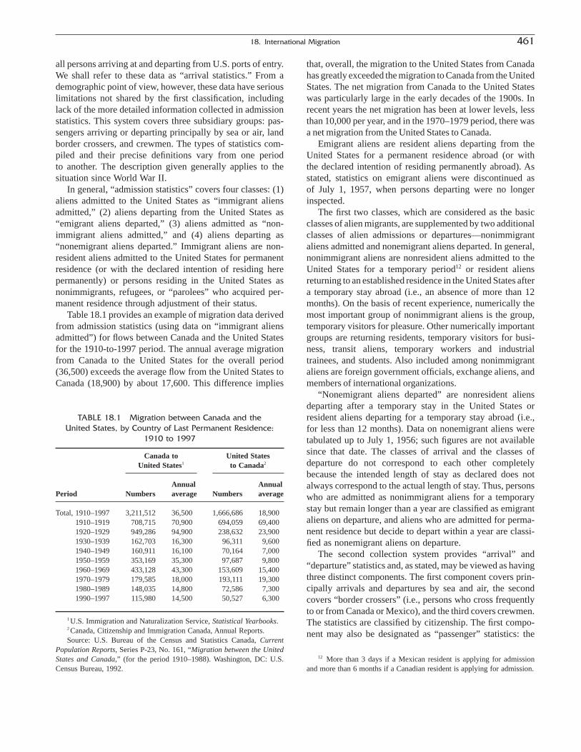
all persons arriving at and departing from U.S. ports of entry.We shall refer to these data as “arrival statistics.” From ademographic point of view, however, these data have seriouslimitations not shared by the first classification, includinglack of the more detailed information collected in admissionstatistics. This system covers three subsidiary groups: pas-sengers arriving or departing principally by sea or air, landborder crossers, and crewmen. The types of statistics com-piled and their precise definitions vary from one period to another. The description given generally applies to the situation since World War II.
In general, “admission statistics” covers four classes: (1)aliens admitted to the United States as “immigrant aliensadmitted,” (2) aliens departing from the United States as“emigrant aliens departed,” (3) aliens admitted as “non-immigrant aliens admitted,” and (4) aliens departing as“nonemigrant aliens departed.” Immigrant aliens are non-resident aliens admitted to the United States for permanentresidence (or with the declared intention of residing herepermanently) or persons residing in the United States asnonimmigrants, refugees, or “parolees” who acquired per-manent residence through adjustment of their status.
Table 18.1 provides an example of migration data derivedfrom admission statistics (using data on “immigrant aliensadmitted”) for flows between Canada and the United Statesfor the 1910-to-1997 period. The annual average migrationfrom Canada to the United States for the overall period(36,500) exceeds the average flow from the United States toCanada (18,900) by about 17,600. This difference implies
that, overall, the migration to the United States from Canadahas greatly exceeded the migration to Canada from the UnitedStates. The net migration from Canada to the United Stateswas particularly large in the early decades of the 1900s. Inrecent years the net migration has been at lower levels, lessthan 10,000 per year, and in the 1970–1979 period, there wasa net migration from the United States to Canada.
Emigrant aliens are resident aliens departing from theUnited States for a permanent residence abroad (or with the declared intention of residing permanently abroad). Asstated, statistics on emigrant aliens were discontinued as of July 1, 1957, when persons departing were no longerinspected.
The first two classes, which are considered as the basicclasses of alien migrants, are supplemented by two additionalclasses of alien admissions or departures—nonimmigrantaliens admitted and nonemigrant aliens departed. In general,nonimmigrant aliens are nonresident aliens admitted to theUnited States for a temporary period12 or resident aliensreturning to an established residence in the United States aftera temporary stay abroad (i.e., an absence of more than 12months). On the basis of recent experience, numerically themost important group of nonimmigrant aliens is the group,temporary visitors for pleasure. Other numerically importantgroups are returning residents, temporary visitors for busi-ness, transit aliens, temporary workers and industrialtrainees, and students. Also included among nonimmigrantaliens are foreign government officials, exchange aliens, andmembers of international organizations.
“Nonemigrant aliens departed” are nonresident aliensdeparting after a temporary stay in the United States or resident aliens departing for a temporary stay abroad (i.e.,for less than 12 months). Data on nonemigrant aliens weretabulated up to July 1, 1956; such figures are not availablesince that date. The classes of arrival and the classes ofdeparture do not correspond to each other completelybecause the intended length of stay as declared does notalways correspond to the actual length of stay. Thus, personswho are admitted as nonimmigrant aliens for a temporarystay but remain longer than a year are classified as emigrantaliens on departure, and aliens who are admitted for perma-nent residence but decide to depart within a year are classi-fied as nonemigrant aliens on departure.
The second collection system provides “arrival” and“departure” statistics and, as stated, may be viewed as havingthree distinct components. The first component covers prin-cipally arrivals and departures by sea and air, the secondcovers “border crossers” (i.e., persons who cross frequentlyto or from Canada or Mexico), and the third covers crewmen.The statistics are classified by citizenship. The first compo-nent may also be designated as “passenger” statistics: the
18. International Migration 461
TABLE 18.1 Migration between Canada and the United States, by Country of Last Permanent Residence:
1910 to 1997
Canada to United States United States1 to Canada2
Annual Annual Period Numbers average Numbers average
Total, 1910–1997 3,211,512 36,500 1,666,686 18,9001910–1919 708,715 70,900 694,059 69,4001920–1929 949,286 94,900 238,632 23,9001930–1939 162,703 16,300 96,311 9,6001940–1949 160,911 16,100 70,164 7,0001950–1959 353,169 35,300 97,687 9,8001960–1969 433,128 43,300 153,609 15,4001970–1979 179,585 18,000 193,111 19,3001980–1989 148,035 14,800 72,586 7,3001990–1997 115,980 14,500 50,527 6,300
1 U.S. Immigration and Naturalization Service, Statistical Yearbooks.2 Canada, Citizenship and Immigration Canada, Annual Reports.Source: U.S. Bureau of the Census and Statistics Canada, Current
Population Reports, Series P-23, No. 161, “Migration between the UnitedStates and Canada,” (for the period 1910–1988). Washington, DC: U.S.Census Bureau, 1992.
12 More than 3 days if a Mexican resident is applying for admissionand more than 6 months if a Canadian resident is applying for admission.

count is derived from lists of names on passenger manifestsprepared by the airlines and steamship companies.
The second component, border crossers, represents prin-cipally a count, made by immigration inspectors at estab-lished points of entry, of persons entering the United Statesover its land borders with Canada and Mexico. It is a countof crossings; hence, the same persons may be counted morethan once.
As mentioned earlier, in addition to the two basic classesof international migrants (immigrants or “new permanentarrivals” and emigrants departing or “permanent residentdepartures”), some statistical information is secured forseveral other groups of persons who cross the borders of theUnited States. Some account should be taken of these othergroups in any assessment of the impact of immigration on thepopulation, especially the de facto population: Particularattention should be given to the following categories:
1. Nonimmigrant aliens. Most nonimmigrants are touristswhose visits range from a few days to a few months. Alarge number of other nonimmigrants are businesspersons who stay typically for less than a few weeks.Nonimmigrants, however, also include several groupswho usually stay in the United States for severalmonths or more. Among them are government officials,students, and temporary workers as well as theirspouses and children. In recent years, about 1 millionnonimmigrants entered the United States annually.13
2. Aliens paroled into the United States. From time totime, special legislation allows political refugees to enter and remain in the United States outside therequirements of the Immigration Act. Refugees fromHungary after the supression of the revolution in 1956,refugees from the Communist regime in Cuba in the1960s, and El Salvadorian refugees after the civil warin the 1990s were granted asylum by special legislation.
3. Arrivals from and departures to the outlying areas ofthe United States. In the basic tabulations on admis-sions, the United States and its outlying areas aretreated as a unit. Data on movement between theUnited States and Puerto Rico are currently available,however, in the form of passenger statistics compiledby Puerto Rican authorities.
4. U.S. government employees and dependents. Directdata are not available for military personnel, but theirnumber may be estimated from data on the number ofU.S. military personnel overseas given in censusreports and reports of the U.S. Department of Defense.Estimates for other Federal employees and theirdependents may be made by a similar method usingdata from the Office of Personnel Management.
5. Illegal entrants and unrecorded departures.6. Aliens deported from the United States or departing
voluntarily under deportation proceedings. During1997, 1,537,000 deportable aliens were located. Almostall deportees had entered the United States withoutinspection and were removed under conditions of voluntary departure.
Except for daily commuting, all of the movement acrossa country’s borders, however temporary, should be consid-ered demographically significant in relation to a de factocount of the population. The groups of migrants who wouldbe considered consistent with a de jure count of the popu-lation would be much more restricted. In the case of theUnited States, these include members of the armed forceswho are transferred into and out of the United States, all“immigrant aliens admitted” and “emigrant aliens departed,”certain classes of “nonimmigrant aliens admitted” and “non-emigrant aliens departed” (such as students, resident aliensarriving and departing, some temporary visitors for busi-ness, and temporary workers and industrial trainees),“refugees” and “parolees” who enter under special legisla-tion and may later have their status adjusted to that of permanent residents, and citizens who change their usualresidence (i.e., move to or from outlying areas and foreigncountries). The discontinuance of data collection for certainof these categories (emigrant and nonemigrant aliensdeparted) and the volatility of the figures for passengermovement (citizens arriving and departing, aliens departing)present a challenge in estimation of additions through immi-gration to both the de jure and the de facto populations. Procedures used currently by the U.S. Census Bureau are described further in the section on estimation of netmigration.14
Quality of Statistics
The quality of data on international migration based onfrontier control operations is generally much poorer thanthat of census counts or birth and death statistics. Such datatend to suffer from serious problems of completeness andinternational comparability. There are several reasons for thepoor quality of the data. First, there are many forms of inter-national movement, and they are not easy to define or clas-sify. Second, the classification based on duration of stay or
462 Edmonston and Michalowski
13 B. L. Lowell (Ed.), Temporary migrants in the United States, U.S.Commission on Immigration Reform, Washington, DC, 1996.
14 For other discussions of U.S. immigration statistics and populationestimates, see U.S. Immigration and Naturalization Service and U.S.Bureau of International Labor Affairs, 1999, The Triennial ComprehensiveReport on Immigration; B. Edmonston (Ed.), 1996, Statistics on U.S. Immi-gration: An Assessment of Data Needs for Future Research. Washington,DC: National Academy Press; U.S. Census Bureau, “National and StatePopulation Estimates: 1990 to 1994,” by E. Byerly and K. Deardoff. 1995,Current Population Reports, P25–1127. Washington, DC: U.S. CensusBureau.

purpose of migration depends on statements of intentions,and the actual movements may not correspond to these state-ments of intentions. Next, the mere counting of persons onthe move is extremely difficult, especially when a countryhas a very long boundary that is poorly patrolled. It is certainthat many international migrants enter or leave a countryunrecorded under these conditions. Controls over departuresare usually less strict than over arrivals so that statistics ofemigration are more difficult to collect and less accurate thanstatistics of immigration. This type of problem is illustratedby unrecorded movement over the Mexican border to theUnited States. Between 1990 and 1997, 9.8 million alienswere apprehended for being in the United States illegally:more than 90% of these were Mexicans who were appre-hended by district offices along the Mexican border. Mostof those apprehended, however, had been in the UnitedStates for less than a few weeks.15
The complexity and diversity of definitions and classifi-cation systems used in different countries also seriouslyimpede international comparability of migration statistics. Inthe recent review of different data collection systems, theUnited Nations concluded that, where available, data frompopulation registers are most satisfactory for the measure-ment of international migration.16 Border collection data,which have been traditionally considered a major source ofinformation on migration flows and which in the past formeda base model for the United Nations recommendations on international migration statistics, are judged rarely toprovide the best measures of international migration flows.Nevertheless, the United Nations advises that this sourceshould be explored by individual countries inasmuch asvarious data sources present different opportunities for theimplementation of the definitions of long-term and short-term migrants that the United Nations recommends.
Data from Population Registers
A fully developed system of national population account-ing would cover movement into and out of a country as well as births, deaths, and internal movements. Under thissystem, international movement, including arrivals into thecountry and departures from it, is simply a special type of change of residence that must be reported to the local registrar. Reporting of change of residence is generallyexempted from declaration if the duration of absence isshort. At present, this is a relatively uncommon source ofmigration statistics. Few countries in the world, mainlycountries of western and northern Europe, have a system ofcontinuous population registration from which it is possible
to derive satisfactory immigration and emigration statis-tics. These include Austria, Belgium, Denmark, Finland,Germany, Iceland, Israel, Italy, Japan, Liechtenstein, Luxembourg, the Netherlands, Norway, Spain, Sweden,Switzerland, and Taiwan.17 In addition, Eastern and CentralEuropean countries as well as those of the Commonwealthof Independent States (the successor states of the formerUnion of Soviet Socialist Republics) are reviewing theirpopulation registers with the goal of improving the possi-bilities of collecting adequate statistics on internationalmigration through that data source.
Census or Survey Data
Censuses and national surveys offer useful data on avariety of important aspects of international migration. Inthe United States, the decennial census and the Current Pop-ulation Survey contain limited direct information on thevolume of immigration. Combined with other data, thisinformation, serves as a basis for making estimates of netimmigration for intercensal periods.18 Limited data for theUnited States may also be obtained from the censuses ofvarious foreign countries. We consider, first, data on priorresidence and nativity, giving attention to data on the yearof arrival for the foreign-born population.
Residence Abroad at a Previous Date
Censuses or national sample surveys may, in effect,provide information on immigration during a fixed periodprior to the census or survey date. From a theoretical pointof view, the type of immigration data obtained in a censusor survey differs in several respects from data compiled in connection with the administrative operations of bordercontrol. The latter represent counts of arrivals and departuresduring a given period. The former represent a classificationof the population living in the country at a particular dateaccording to residence inside or outside the country at someprevious specified date. The census data on migration coveronly persons who were alive both at the census date and atthe previous specified date. Hence, the number of “immi-grants” reported in the census or survey is deficient. A countof immigrants during the period between the previous date
18. International Migration 463
15 Pages 164–165, Table 61, in U.S. Immigration and NaturalizationService, Statistical Yearbook of the Immigration and NaturalizationService, 1997, Washington, DC: U.S. Government Printing Office 1999.
16 See footnote 2.
17 R. E. Bilsborrow, G. Hugo, A. S. Oberai, and H. Zlotnik, Interna-tional Migration Statistics: Guidelines for Improving Data CollectionSystems, Geneva, Switzerland; International Labour Office, 1997; MichelPoulain, “Confrontation des statistiques de migrations intra-européenes:vers plus d’harmonisation,” European Journal of Population 9:353–3.
18 A description of the census concepts and definitions and selecteddecennial census data on the foreign-born population of the United Statescan be found in C. Gibson and E. Lennon, “Historical Census Statistics onthe Foreign-Born Population of the United States: 1850 to 1990,” Popula-tion Division Working Paper No. 29, Washington, DC: U.S. Bureau of theCensus, 1999. www.census.gov.

and the census date does not include the number of childrenborn abroad during this period who immigrated into thecountry, immigrants who died (in the country of immigra-tion), or immigrants who departed during the period (e.g.,returned to the country of origin). Even though the censusor survey figures exclude the departures of those whoarrived during the migration found, they cannot properly beviewed as estimates of net immigration because they fail toallow for the departure of persons who were living in thecountry prior to the migration period. For example, U.S.census data usually represent immigration for the 5 yearsprior to the census; hence they relate only to “survivors” 5years old and over at the census date. Censuses or surveyscannot readily provide any separate information on emigra-tion for a country.
Data on prior residence abroad are available only for thebrief periods before each census or survey in which a ques-tion on “previous residence” is asked. On the other hand, thecensus or survey data on immigration are likely to providecomprehensive information for certain types of migrants(e.g., aliens and citizens, civilians and military personnel). Inaddition, certain demographic characteristics of the “immi-grants” (especially age, sex, and marital status) and theirsocioeconomic characteristics may be readily tabulated.
In spite of the simplicity of the question and its value inproviding data on the volume of immigration and the char-acteristics of immigrants, these types of data are availablefor few countries. These data are illustrated in Table 18.2,using Canada and the United States as examples. Data relat-ing to the volume of immigration and the characteristics of
immigrants, based on a question relating to previous resi-dence, are given in the reports on internal migration derivedfrom the census. A category of “persons abroad” is shownin the published tables as one of three major categories ofmigration status (namely, nonmigrant, internal migrant, andimmigrant). This category refers to persons living in thecountry at the census date who reported that their place ofresidence at a specified previous date was in a foreigncountry (or in an outlying area for the United States).
Nativity
Census data on nativity, particularly on the foreign born,serve both as direct indicators of the volume and character-istics of immigrants and as a basis for estimating them. Dataon the foreign born are especially valuable for measuringmigration when “border control” data on migration arelacking, are of poor or questionable quality, or are irregu-larly compiled. Some important kinds of classifications may not be available in the regular immigration tabulations,but may appear in the census data. Hence, measurement ofthe volume of immigration of certain groups or of certaincharacteristics of immigrants may be possible only fromcensus data. Where similar material is available from bothsources, the census data may aid in validating the indica-tions of the “regular” immigration data. For most countries,including the United States, the body of census informationrelating to the foreign-born population is more extensive anddetailed than the immigration data collected at time ofarrival.
464 Edmonston and Michalowski
TABLE 18.2 Number of Persons 5 Years of Age and Older Abroad 5 Years Prior to the Census,as Reported in the Censuses of Population for Canada and the United States:
Around 1980 and 1990
Reported immigrationCountry Date of census Number abroad Total population1 Percentage abroad during period2
Canada3
May 14, 1996 928,700 28,846,800 3.2 1,176,100June 4, 1991 913,300 27,296,900 3.3 873,800June 3, 1986 463,900 25,309,300 1.8 499,800June 3, 1981 556,200 24,343,200 2.3 590,400
United StatesApril 1, 1990 4,821,100 230,445,800 2.1 2,927,000April 1, 1980 3,931,800 210,232,300 1.9 2,496,000
1 Population 5 years of age and older.2 Reported immigration for 5-year period preceding the census.3 Total population data collected on a 100% basis.Source: Canada: Statistics Canada, “Interprovincial and International Migration in Canada” (91-208); “Mobility Status and Interprovincial Migration,”
Census 1986 (93-108); “Mobility and Migration,” Census 1991 (93–322); www.statcan.ca/english/census96/apr14/mobil.htm. United States: Immigration andNaturalization Service, Immigration and Naturalization Service Yearbook, 1975 to 1990, Washington, DC: INS. Bureau of the Census, 1980 Census of Population, Volume 1, Characteristics of the Population, PC 80-1-C1., U.S. Summary, Table 80, Washington, DC: Bureau of the Census, 1981. Bureau of the Census, 1990 Census of Population, Social and Economic Characteristics, United States, 1990 CP-2-1, Table 18, Washington, DC: Bureau of theCensus, 1993.

A classification of the U.S. population by nativity hasbeen made since 1850 in connection with the census ques-tion on “State or country of birth.” The number of scheduleinquiries relating to the foreign-born population increasedwith each succeeding census after 1850 until the peak in1920, when there were questions, among others, on countryof birth, mother tongue, and year of immigration. In eachyear since 1850, the foreign born were tabulated at least byage and sex.
Volume of Immigration
Census tabulations of the foreign-born populationprovide information on “net lifetime immigration” of theforeign-born (i.e., net immigration over the lifetime of thepresent population). Census data on the foreign born do notprovide an indication of the volume of immigration duringany particular past period of time. Moreover, even if the dataare tabulated by year or period of immigration, foreign-born persons who returned to live abroad or who died priorto the census date are excluded. At the older ages, both ofthese factors may have an important impact in reducing thenumbers of foreign born far below the numbers of immi-grants who may have originally entered the country. Sur-viving immigrants are counted only once, even though theymay have moved to the country in question more than oncein a lifetime.
In sum, the census figures provide information specifi-cally on the balance of immigration and emigration offoreign-born persons during the last century, diminished bythe number of deaths of immigrants in the country prior tothe census date. Thus,
(18.1)
(18.2)
where PF refers to the foreign-born population, IF and EF
refer to immigrants and emigrants born abroad, respectively,and DF refers to deaths of foreign-born persons in thecountry. It should be particularly noted that the quantity IF
- EF does not represent net migration in the usual sense,because the emigrants here consist solely of former immi-grants (“return migrants”), and movement of native personsis entirely excluded.
Characteristics of Immigrants
Much information regarding the geographic and resi-dence distribution and the demographic, social, and eco-nomic characteristics of immigrants can be obtained fromcensus data on the nativity of the population. The charac-teristics of the surviving immigrants are reflected in thecurrent composition of the foreign-born population withrespect to such variables as age, sex, country of birth, mothertongue, occupation, and educational attainment. Some ofthese characteristics (e.g., place of residence or occupation)
I E P DF F F F-( ) = +
P I E DF F F F= -( ) -
undergo changes after the date of arrival, others (e.g.,country of birth, year of immigration, or mother tongue)should not change at all, and still others change in measur-able ways (age) or may change little or not at all (educa-tional attainment for adults). However, the distributions areaffected by differences in the emigration and mortality ofimmigrants in different categories as well as errors of report-ing and coverage. Hence, the adequacy of the foreign-borndata in reflecting the characteristics of immigrants varieswith the characteristic.
The distinctive geographic distribution of immigrantsand the influence of immigration on the geographic distri-bution of the general population may be inferred from acomparison of the geographic distribution of the native,foreign-born, and total populations of a country.
Differences in the fertility level of immigrants and thenonimmigrant population may be ascertained from differ-ences between the foreign-born and the native populationsin the general fertility rate or in the average number of chil-dren ever born.
For studies of the impact of immigration on a country’ssocial and economic structure, census data on the foreignborn are particularly valuable. Census data giving detailedtabulations of the foreign-born population by area of pre-sent residence and country of birth permit the calculation of indexes of the relative concentration of various ethnicgroups among the immigrants in various parts of a country.19
Census data on the detailed occupation and country of birthof the foreign born provide the basis for measuring the ten-dency of various ethnic groups among the immigrants toconcentrate in certain lines of work. Census data on the proportion of foreign born in the labor force, classified byoccupation and industry, are also useful in measuring theminimal impact of immigration on a country’s labor forceand economy over a broad period of time.20
Studies of the changes in the social and economic statusof immigrants and of the cultural assimilation of immigrantsinvolve comparisons of the characteristics of the immigrantsand the general population and observation of changes in theimmigrants over time. The use of census data is necessaryor preferable in such studies over the use of border controlstatistics. Census data must also be employed where theimmigrants are to be classified according to their status withrespect to characteristics that necessarily change or that may change after immigration (e.g., citizenship, employ-ment status, occupation, language spoken), or where theimmigration data are not tabulated in terms of the charac-teristic (e.g., educational attainment). Greater comparability
18. International Migration 465
19 See Table 14 in E. P. Hutchinson, Immigrants and Their Children,1850–1950, 1950 Census Monograph, New York. John Wiley & Sons,1956.
20 J. P. Smith and B. Edmonston (Eds.), The New Americans: Eco-nomic, Demographic, and Fiscal Effects of Immigration, Washington, DC:National Academy Press, Chapters 4 and 5, 1997.
in the classification is probably achieved by use of censusdata, even where these conditions do not apply.21
Timing of Immigration
There is specific interest in the timing of immigration.Knowledge solely of the number and characteristics ofimmigrants over the indeterminate past is of limited practi-cal value in migration analysis. How long the immigrant hasbeen in the host country is relevant to the immigrant’s assim-ilation, including the immigrant’s opportunities for acquir-ing citizenship there or learning the language of the hostcountry. We should like to know the number and character-istics of immigrants at least for intercensal periods. Inferences regarding intercensal trends in the volume ofmigration or the characteristics of migrants cannot safely bemade directly from a series of census figures for the totalnumber of foreign-born persons or from a series of derivedmeasures based on statistics for the foreign born.
Tabulations by year of immigration would indicatedirectly the volume of immigration (for surviving immi-grants who had not emigrated) for particular past periods.Such statistics are useful in refining migration analysesbased on date or place of birth. Each immigrant would beasked the date of arrival in the country of present residenceor the date of departure from the country of birth. Thismethod requires an additional question relating to date ofmigration on the questionnaire. The data may be tabulatedin terms of year or period of immigration or duration of residence in the country of immigration.
A question on year of immigration or number of years ofresidence of the foreign-born population was asked in thedecennial censuses of the United States from 1890 to 1930,omitted from the censuses of 1940 to 1960, and then restoredto the questionnaire in 1970.22
Miscellaneous Other Sources
Other sources of immigration data are given brief treat-ment here because they are relatively uncommon. These
include special surveys, registrations of aliens, tabulationsof permits for work abroad, and tabulations of passports andvisas issued.
The occasional special surveys may involve inquiriesrelating to the nativity, previous residence, or citizenship of the resident population. Surveys may be taken of thecountry’s citizens living abroad. The figures obtained fromsuch a survey would represent net lifetime emigration of acountry’s citizens including the natural increase of theseemigrants but excluding former citizens who had becomenaturalized in the countries of emigration.
Occasional, periodic, or continuous special registrationsof aliens may be carried out. In several countries (e.g., theUnited States until 1981, Japan, and New Zealand), aliensare required to register annually. The count of alien regis-trants in a single registration may be interpreted as repre-senting lifetime net surviving alien immigrants, that is, totalimmigration of aliens, less deaths, emigration, and natural-izations of aliens prior to the record date. Obviously, suchdata tell us nothing about the timing of migration withouttabulations by year of entry (or duration of residence) or age. Typically, country of nationality is obtained rather thancountry of last permanent residence. A registration of alienswas conducted in the United States in 1940 by the Immi-gration and Naturalization Service in accordance with therequirements of the Alien Registration Act of 1940, and anannual registration was conducted between 1951 and 1981in accordance with the requirements of the Internal SecurityAct of 1950 and the Immigration and Nationality Act of1952.23
Foreign workers may have the obligation to secure awork permit, as in most European countries, the UnitedStates, Canada, and Australia. As measures of immigration,the data are compromised by emigration and by the fact thatnot all permits are used. Moreover, the procedure followedin renewing permits may be ill adapted to the recording ofinternational movements. The statistics of alien identitycards also have this defect.
Counts of passports and visas issued by a particularcountry relate to citizens and aliens, respectively. There isno way of knowing exactly what percentages of passportsand visas are actually used, or if used, when the travelerdeparts or returns and how many trips the traveler makes.Tabulation of the number of travelers listed on a passport orvisa is required to determine the possible number of travel-
466 Edmonston and Michalowski
21 Examples of the use of census tabulations on the foreign born in thestudy of cultural and ethnic assimilation of immigrants are given in: R. D.Alba, J. R. Logan, B. J. Stults, G. Marzan, and W. Zhang, “ImmigationGroups in the Suburbs: a Reexamination of Suburbanization and SpatialAssimilation,” American Sociological Review 64(3): 446–460, June 1999;J. E. Coughlan, D. J. McNamara, Asians in Australia: Patterns of Migra-tion and Settlement, South Melbourne, Australia: MacMillan Education,1997; S. M. Lee, “Do Foreign Birth and Asian Minority Status Lower Canadian Women’s earnings,” Canadian Studies in Population 26(2): 159–182, 1999; D. Myers and S. W. Lee, “Immigration Cohorts and Residen-tial Overcrowding in Southern California,” Demography 33(1): 51–65,February 1996; and E. Ng and F. Nault, “Fertility among Recent ImmigrantWomen to Canada, 1991: an Examination of the Disruption Hypothesis,”International Migration Review 35(4): 559–578, 1999.
22 In the 1890 and 1900 censuses, the question was the number of yearsof residence of the foreign born in the United States. The tabulation in 1890was limited to alien males 21 years old and over.
23 Each alien, regardless of date of immigration or length of stay, wasrequired to register in January of each year and provide information regard-ing his or her address, sex, date of birth, country of birth, citizenship, dateof entry into the United States, permanent or temporary status, and currentoccupation. Tabulations of aliens who reported under the Alien AddressProgram were shown in the Annual Report of the Immigration and Natu-ralization Service and the I and N Reporter. They distinguished permanentresidents from nonpermanent residents and showed numbers of aliens bynationality and state of current residence.

ers involved. Although passports and visas have severe lim-itations for measuring the actual volume of internationalmigration, they may be useful in evaluating data or estimatesfrom other sources.
Special Categories of International Migrants
We consider next mainly two types of internationalmigrants—temporary immigrants and refugees—that werenot fully described in the data collection systems discussedearlier.
Temporary Immigrants
Census data on the foreign born should not be perceivedas information on immigration flows into the country. Theforeign-born population in the census includes a variety ofcategories of international migrants such as persons who donot have a legal status (e.g., illegal, undocumented, or irreg-ular-status immigrants), legal permanent residents, humani-tarian admissions (e.g., refugees and asylees), and personswho have a right to residence for a limited period only (e.g.,temporary immigrants). The 1990 census data for the UnitedStates show that there were 19.7 million foreign-bornpersons in the country (8% of the total population). Thecensus does not provide data on the different categories ofimmigrants. However, estimates produced using the censusdata demonstrate that the great majority of them, 17.8million or over 85%, were living in the country legally.24
Among legal residents, 38% were naturalized citizens, and 45% were permanent resident aliens. The remaining 1.9 million were persons admitted to the country on a
humanitarian basis (who can, after 1 year, adjust their status to permanent residence) or as temporary immigrants(e.g., students, business persons, teachers, and otherworkers). Depending on the category, foreign-born personshave different access to labor markets. Access to employ-ment can range from unrestricted to limited-to-nongovern-ment jobs only (e.g., noncitizens), and from permission tobe with a designated employer (e.g., some temporary immi-grants) to lack of right to employment (e.g., spouses of some temporary immigrants). Foreign-born persons alsohave different access to services in the area of health andsocial assistance. For these reasons, conclusions drawn fromthe research based on the census data on the foreign bornrequire attention to the internal diversity of this population.
In the United States, it is estimated that the number of tem-porary immigrants exceeded one-half million in 1990 (seeTable 18.3). They represented almost 3% of the foreign-bornpopulation and 0.2% of the total population. In comparison,in Canada, the temporary immigrant population was only halfthe size of the U.S. temporary immigrant population but rela-tively more important, representing almost 5% of Canada’sforeign-born population. Canada’s temporary immigrants asa share of the foreign-born population decreased to just over3% in 1996. In Australia, the temporary immigrant popula-tion was about 200,000 in 1998, accounting for nearly 5% ofAustralia’s foreign-born population.
Apart from being a selective population in terms of skills,temporary immigrants are also different from recent “tradi-tional” (i.e., permanent) immigrants in their geographicalorigins. Census data from the United States and Canada
18. International Migration 467
TABLE 18.3 Temporary Immigrants in Australia, Canada, and the United States for Various Years
Percentage of
Temporary Foreign-born Foreign-bornCountry immigrants population Total population population Total population
AustraliaJune 1998 196,7001 4,322,6002 18,532,2002 4.6 1.1
CanadaJune 1991 223,400 4,566,300 26,994,000 4.9 0.8May 1996 166,700 5,137,800 28,528,100 3.2 0.6
United StatesApril 1990 537,900 19,767,300 248,709,900 2.7 0.2
1 Total includes 93,986 foreigners in Australia for temporary work-related stay and 102,689 foreign students.2 Estimated as of June 1997.Source: United States: Bureau of Census, unpublished data. Gibson, C. J. and E. Lennon, “Historical Census Statistics on the Foreign-born Population
of the United States: 1850 to 1990,” Population Division Working Paper, No. 29. Washington, DC: U.S. Bureau of the Census, 1999. Statistics Canada,“Immigration and Citizenship,” Ottawa: Supply and Services Canada, 1992, 1991 Census of Canada, Catalogue number 95-316.; and unpublished data.Department of Immigration and Multicultural Affairs, Statistical Report: Temporary Entrants, 1997–1998, 1999. Australian Bureau of Statistics, EstimatedResident Population by Country of Birth, Age and Sex, Australia, Catalogue 3221.0.
24 M. Fix and J. S. Passel, 1994, Immigration and Immigrants: Settingthe Record Straight. Washington, DC: The Urban Institute.

provide evidence of these differences (see Table 18.4). Morethan half of the 500,000 temporary immigrants in the UnitedStates were born in 10 countries. Recent permanent andillegal immigrants (i.e., those who came to stay during the3-year period prior to the census) are even more concen-trated in terms of their origins. Over 60% were born in the10 top countries of birth. The same countries are major coun-tries of origin for temporary, permanent, and illegal immi-grants. Their relative numerical importance, however, withinthe top 10 countries differs. Mexico ranks tenth among thecountries of origin for temporary immigrants and ranks firstamong permanent and illegal immigrants. Philippines is the
ninth country among the 10 top origins for temporary immi-grants but the second for permanent and illegal immigrants.The other difference between geographical origins of thetwo immigrant categories is the importance of the “moredeveloped” countries as their origins. There were four suchcountries among the major countries of origin for temporaryimmigrants to the United States—Japan, Taiwan, Canada,and United Kingdom—but none are among the top 10 forthe permanent or illegal immigrants.
Canada’s temporary immigrants are more diversified than those in the United States. Less than 50% of Canada’stemporary immigrants are from the 10 top countries of
468 Edmonston and Michalowski
TABLE 18.4 Top 10 Countries of Temporary Immigrants and Recent Permanent Immigrants to the United States and Canada: 1990 and 1991
United States:
Temporary immigrants1 Recent permanent and illegal immigrants 1987–1991
Rank Place of birth Number Percentage Rank Place of birth Number Percentage
1 Japan 62,800 12.2 1 Mexico 729,400 31.82 People’s Republic of China 31,600 6.1 2 Philippines 113,700 5.03 Korea 27,800 5.4 3 El Salvador 89,800 3.94 India 24,900 4.8 4 Korea 76,900 3.45 Taiwan 23,400 4.6 5 People’s Republic of China 74,200 3.26 Canada 22,400 4.4 6 Viet Nam 70,600 3.17 U.S.S.R. 21,500 4.2 7 U.S.S.R. 67,900 3.08 United Kingdom 19,300 3.8 8 India 59,600 2.69 Philippines 17,100 3.3 9 Dominican Republic 54,100 2.4
10 Mexico 16,800 3.3 10 Nicaragua 52,100 2.3Subtotal (10 countries) 267,600 52.0 Subtotal (10 countries) 1,388,300 60.6Other countries 246,600 48.0 Other countries 902,600 39.4Total 514,200 100.0 Total 2,290,900 100.0
Canada:
Temporary immigrants Recent permanent immigrants 1988–1991
Rank Place of birth Number Percentage Rank Place of birth Number Percentage
1 United States 18,200 8.1 1 Hong Kong 60,900 10.32 Philippines 15,100 6.8 2 Poland 41,200 6.93 Sri Lanka 12,700 5.7 3 People’s Republic of China 38,600 6.54 Hong Kong 11,000 4.9 4 Philippines 35,400 6.05 People’s Republic of China 10,900 4.9 5 India 31,700 5.36 United Kingdom 9,300 4.2 6 Lebanon 23,900 4.07 Iran 8,200 3.7 7 Viet Nam 22,700 3.88 Trinidad and Tobago 7,000 3.1 8 United Kingdom 22,700 3.89 Japan 6,800 3.0 9 Portugal 18,400 3.1
10 India 5,800 2.6 10 United States 18,300 3.1Subtotal (10 countries) 105,000 47.0 Subtotal (10 countries) 313,800 52.9Other countries 118,400 53.0 Other countries 279,200 47.1Total 223,400 100.0 Total 593,000 100.0
1 Persons who “came to stay” in the United States in 1987 or later.Source: Statistics Canada, 1991 Canadian Census of Population unpublished data; United States Bureau of Census estimates based on the 1990 U.S.
Census of Population and unpublished data.
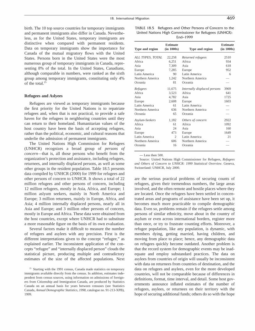
birth. The 10 top source countries for temporary immigrantsand permanent immigrants also differ in Canada. Neverthe-less, as for the United States, temporary immigrants are distinctive when compared with permanent residents. Data on temporary immigrants show the importance forCanada of the mutual migratory flows with the UnitedStates. Persons born in the United States were the mostnumerous group of temporary immigrants in Canada, repre-senting 8% of the total. In the United States, Canadians,although comparable in numbers, were ranked as the sixthgroup among temporary immigrants, constituting only 4%of the total.25
Refugees and Aslyees
Refugees are viewed as temporary immigrants becausethe first priority for the United Nations is to repatriaterefugees and, when that is not practical, to provide a safehaven for the refugees in neighboring countries until theycan return to their homeland. Humanitarian values of thehost country have been the basis of accepting refugees,rather than the political, economic, and cultural reasons thatunderlie the admission of permanent immigrants.
The United Nations High Commission for Refugees(UNHCR) recognizes a broad group of persons ofconcern—that is, all those persons who benefit from theorganization’s protection and assistance, including refugees,returnees, and internally displaced persons, as well as someother groups in the resident population. Table 18.5 presentsdata compiled by UNHCR (2000) for 1999 for refugees andother persons of concern to UNHCR. It shows a total of 22million refugees and other persons of concern, including 12 million refugees, mostly in Asia, Africa, and Europe; 1million aslyum seekers, mainly in North America andEurope; 3 million returnees, mainly in Europe, Africa, andAsia; 4 million internally displaced persons, nearly all inAsia and Europe; and 3 million other persons of concern,mostly in Europe and Africa. These data were obtained fromthe host countries, except where UNHCR had to substitutea more reasonable figure on the basis of its own evaluation.
Several factors make it difficult to measure the numberof refugees and asylees with any precision. First is the different interpretations given to the concept “refugee,” asexplained earlier. The inconsistent application of the con-cepts “refugee” and “internally displaced person” clouds thestatistical picture, producing multiple and contradictoryestimates of the size of the affected populations. Next
are the serious practical problems of securing counts ofrefugees, given their tremendous numbers, the large areasinvolved, and the often remote and hostile places where theyare located. Once the refugees have been settled in concen-trated areas and programs of assistance have been set up, itbecomes much more practicable to compile demographicdata. Even so, problems remain if the refugees settle amongpersons of similar ethnicity, move about in the country ofasylum or even across international borders, register morethan once, or try to frustrate counting efforts. Moreover, arefugee population, like any population, is dynamic, withmembers dying, getting married, having children, andmoving from place to place; hence, any demographic dataon refugees quickly become outdated. Another problem isthat the record system for demographic events may be inad-equate and employ substandard practices. The data onasylees from countries of origin will usually be inconsistentwith data on returnees from countries of destination, and thedata on refugees and asylees, even for the more developedcountries, will not be comparable because of differences indefinitions, format, time interval, and detail. Some host gov-ernments announce inflated estimates of the number ofrefugees, asylees, or returnees on their territory with thehope of securing additional funds; others do so with the hope
18. International Migration 469
TABLE 18.5 Refugees and Other Persons of Concern to theUnited Nations High Commissioner for Refugees (UNHCR):
End–1999
Estimate EstimateType and region (in 1000s) Type and region (in 1000s)
ALL TYPES, TOTAL 22,258 Returned refugees 2510Africa 6,251 Africa 934Asia 7,309 Asia 618Europe 7,285 Europe 952Latin America 90 Latin America 6Northern America 1,242 Northern America —Oceania 81 Oceania —
Refugees 11,675 Internally displaced persons 3969Africa 3,523 Africa 641Asia 4,782 Asia 1725Europe 2,608 Europe 1603Latin America 61 Latin America —Northern America 636 Northern America —Oceania 65 Oceania —
Asylum-Seekers 1,182 Others of concern 2922Africa 61 Africa 1092Asia 24 Asia 160Europe 473 Europe 1649Latin America 2 Latin America 21Northern America 606 Northern America —Oceania 16 Oceania —
— Less then 500.Source: United Nations High Commissioner for Refugees, Refugees
and Others of Concern to UNHCR: 1999 Statistical Overview. Geneva,Switzerland: UNHCR, July 2000.
25 Starting with the 1991 census, Canada made statistics on temporaryimmigrants available directly from the census. In addition, estimates inde-pendent from census sources, using information on admissions of foreign-ers from Citizenship and Immigration Canada, are produced by StatisticsCanada on an annual basis for years between censuses (see StatisticsCanada, Annual Demographic Statistics, 1998, catalogue no. 91-213-XPB),1999.

of winning public support for reducing the number ofrefugees and asylees admitted. As a result, the barriers to thecompilation of good refugee statistics are considerable andthe quality of the data varies greatly.
Estimates of the number of refugees have been based onvisual assessment, extrapolations of health surveys, andspecial registration systems. If resources are adequate, con-ditions of stability prevail, and there is support from the hostgovernment, UNHCR can secure detailed information ofgood quality about refugees. Under conditions of stability, a registration or census (or sample survey of the total population) can be attempted in such camp settlements. An important parameter critical for evaluating refugee conditions is an estimate of mortality. Retrospective surveysof surviving family members are a possible tool for meas-uring population size and mortality, but are subject to recallbias. The major limitation for the measurement of mortalitywith retrospective surveys in refugee populations, however,is the selective mortality of whole villages and families,leaving no members behind to report on the deaths thatoccurred. Even surveys that attempt to collect mortality data for relatives, however, may fail to uncover mortality to distant relatives or villages if there are no survivingmembers.
Many notable refugee movements have occurred in thepast few centuries, some being massive exoduses to neigh-boring countries as a result of wars. We note in particularthe vast refugee movements associated with and followingWorld War II; and the large displacements of tribal popula-tions in sub-Saharan Africa in the 1990s, particularly fromRwanda to Zaire; the forced movements of Serbs, Croats,and Bosnians within former Yugoslavia and from it toseveral other European countries such as Italy, Sweden, andGermany; and of Afghans to Pakistan and Iran. Secession-ist movements, insurgencies, civil wars, and domestic unrestwere widespread in the last decade of the 20th century.Many nations (e.g., France, Canada, United Kingdom,Spain, Sri Lanka, Sudan, Burundi, Turkey, and Iraq) containethnic or religious groups seeking independence, and somecitizens have already left these countries claiming refugeestatus. It is extremely difficult to quantify most of these population movements.
The United States admits persons as refugees undernumerical ceilings for specific regions of origin, set by lawand administrative regulations, with the possibility for therefugees to secure adjustment to permanent resident statusafter 1 year. The United States covers most refugee admis-sions by separate legislation. Since World War II, largegroups of refugees have been admitted to the United Statesfrom Hungary and other former Soviet bloc countries, Cuba, the former Soviet Union, Vietnam and other countriesof Indochina, Iraq, and Bosnia. The admission ceiling for1997, set by President Clinton in consultation with the Con-gress, was 78,000. In fiscal year 1996–1997, about 69,000
refugees arrived in the United States and, in addition, about10,000 persons were granted asylum. A small additionalgroup was admitted as parolees, temporary admissionswhose entry is deemed to be in the public interest or justi-fied on humanitarian groups although they may appear to beinadmissible.
COMBINATION, EVALUATION, ANDESTIMATION OF INTERNATIONAL
MIGRATION STATISTICS
As we have suggested, adequate data on immigration,emigration, or net migration are often not available for acountry, even though a number of direct sources of databearing on international migration for that country mayexist. One method of expanding the quantity of informationon migration for a given country is to refer to the migrationstatistics for other countries furnishing or receiving migrantsfrom the country under study. This approach depends on the fact that any international movement involves two countries—the country of immigration and the country ofemigration—and therefore may be reported by two coun-tries. Because overlapping as well as complementary information may be available, this approach also serves asa basis of evaluation of migration data. Let us imagine twoarrays presenting statistics of migration between all the pairsof countries in the world. One such array would give the statistics reported by the country of immigration, and thesecond would give the statistics reported by the country ofemigration. If immigration and emigration were completelyand consistently reported for all the countries of the world,the two arrays would agree or nearly agree. For example,the total immigration reported for a given country wouldcoincide with the emigration reported by all the other coun-tries that furnish emigrants to the country in question. Like-wise, the total emigration reported for a given country wouldcoincide with the immigration received by all other coun-tries from the country under consideration.
In practice, of course, migration statistics are lacking formany countries and the statistics available are often incom-plete and inconsistent. The lack of comparability of themigration statistics from one country to another is a majorproblem. The types of movement counted as migration andthe categories of persons classed as migrants will differ fromcountry to country, partly because there are many differentways of defining a migrant and the categories of migrationand because there are many different systems for collectingthe data. A small part of the difference in the counts ofmigrants reported by different countries for a given year mayresult from the fact that there is a gap in time between departure from one country and arrival in another. Sometravelers may change their destination or not be admitted to a country; moreover, births and deaths may occur during
470 Edmonston and Michalowski

the moves. There is also a problem in the statistical identi-fication of the country of origin as well as destination.Although the statistics usually relate to country of last per-manent residence, in some cases they relate to country ofbirth, country of last previous residence, or country of citi-zenship and these may differ from one another.
In spite of the limitations mentioned, the binationalreporting of international migration provides a useful, if notalways fully adequate, basis for evaluating the accuracy ofmigration data for a country or for filling in missing data,particularly on emigration.
The possibility of combining and comparing statisticsfrom different countries applies to census statistics as wellas to statistics of border control. Suppose we are trying toestimate the net total movement to or from a country or aparticular stream and its counterstream. We can approximatethe true “net lifetime immigration” for a country somewhatmore closely, for example, if we try to “balance” the censuscount of the foreign-born population in the country with the census count of persons in other countries who had been born in the country in question. In practice, it is usuallypossible to identify at least those few countries that are principal destinations of the emigrants of some country orthat are the principal origins of the immigrants of thatcountry. Many national censuses identify a long list of countries of origin for their foreign born. If the principalmovement from a country is to one or two countries only,examination of the census reports of only these few coun-tries is required to measure net migration for the country ofemigration. For example, 744,830 persons living in theUnited States in 1990 were born in Canada, and 249,080persons living in Canada in 1991 were born in the UnitedStates; these figures indicate a “net surviving emigration” ofapproximately 496,000 persons from Canada to the UnitedStates up to 1990. With census statistics as with regularimmigration statistics, there may be a serious problem ofcomparability resulting from differences in the nature of thecensus questions, the type of census (de facto or de jure),and the dates of the two censuses.
Estimation and Evaluation of Net Migration
In view of the lack of adequate statistics on migration formany countries and many periods, it is often necessary toestimate the volume of migration. Although there is interestin separate figures on immigration and emigration, the avail-able methods do not permit making adequate estimates ofimmigration or emigration separately; only the balance ofmigration can be satisfactorily estimated by these methods.For the most part, the same methods are useful in evaluat-ing the reported migration data as for deriving alternativeestimates of net migration. Accordingly, we treat the proce-dures for the estimation and evaluation of net migrationjointly in the present section.
Intercensal Component Method for the Total Population
Approximate estimates of net immigration can often bederived for intercensal periods by use of census data on thetotal population. The general formula for estimating the totalvolume of net immigration in an intercensal period involvesa rearrangement of the elements of the standard intercensalcomponent equation:
(18.3)
Net immigration is derived as a residual; as previouslystated, estimates of immigration and emigration cannot beobtained separately. The method simply involves subtract-ing an estimate of natural increase (B - D) during the periodfrom the net change in population during the period (P1 -P0). If the data used to arrive at the estimate are exact, anexact estimate of the balance of all in-movements and out-movements is obtained. Because, however, the censuscounts and vital statistics as recorded are subject to unknowndegrees of error, the residual estimates of net immigrationmay be in substantial error. In addition, the relative error ofnet immigration may be considerable when the amount ofmigration is small.
Estimates of intercensal net migration for Canada and theUnited States derived by the residual method are shown inTable 18.6. For the United States during the 1980–1990period, population increase amounted to 22,164,000 (i.e.,248,710,000 minus 226,546,000) and natural increaseamounted to 17,205,000; hence, the estimated net migrationwas 4,959,000 (i.e., 22,164,000 minus 17,205,000). ForCanada during the 1981-to-1991 period, population increaseamounted to 3,220,100 (i.e., 28,120,100 minus 24,900,000)and natural increase amounted to 1,975,000; hence, the estimated net migration was 1,245,000 (i.e., 3,220,000minus 1,975,000). Estimated net migration into eitherCanada or the United States is less than recorded arrivalsbecause of emigration.26
Intercensal Cohort-Component Method
The cohort-component method is applicable to the esti-mation of net migration, for age (birth) cohorts, for the totalpopulation and for segments of the population that are fixedover time (e.g., sex, race, and country of birth) or relativelyfixed over time (e.g., mother tongue and religion). This pro-cedure involves the calculation of estimates for age cohortson the basis of separate allowances for the components ofpopulation change (deaths only for all age groups born by
I E P P B D-( ) = -( ) - -( )1 0
18. International Migration 471
26 In the United States, recorded arrivals are inflated in the 1980–1990period by IRCA legalizations: some are recorded as new permanent resi-dents in the period although they may have entered the United States priorto 1980 and, therefore, may have been counted in the 1980 census.

the starting date and births and deaths for the newborncohorts). The compilation of death statistics for birth cohortsto allow for the mortality component is so laborious,however, even where the basic statistics on death are avail-able, that survival rates are normally used instead. The sur-vival rates may be life-table survival rates or so-callednational census survival rates. (Census survival rates are discussed in Chapters 13 and 19).
One formula for this purpose covering age (birth) cohortsother than those born during the intercensal period is
(18.4)
where Ia and Ea represent immigrants and emigrants in acohort defined by age a at the end of the period, P1
a the pop-ulation at this age in the second census, P0
a-t the populationt years younger at the first census, and s the survival rate forthis age cohort for an intercensal period of t years. That is,s is a simplified representation of nSt
a-t for the cohort aged ato a + n years at the end of period t. For the newborn cohorts,the formula is
(18.5)
where B represents the births that occurred in the intercensalperiod.
I E P sBa a a-( ) = -1
I E P sPa a a a t-( ) = - -1 0
Table 18.7 illustrates the procedure for estimating the intercensal net migration of males between 1980 and1990 for age cohorts for the United States by use of life-table survival rates. Ten-year survival rates for 5-year agegroups are first computed from the 1985 U.S. life table bythe formula:
(18.6)
where 5Sx10 represents the probability of survival from
age x to x + 5 for a 10-year period. These rates (col. 3) are applied to the population at the first census (col. 1) toderive an estimate of the expected survivors 10 years olderat the later census date. The difference (col. 4) between thepopulation at the second census (col. 2) and the expectedpopulation (col. 1 ¥ col. 3) is an estimate of net migration.
These calculations represent an application of the con-ventional survival-rate procedure. One defect of this methodis that it has a tendency to understate or overstate the numberof (implied) deaths during the intercensal period. In an “emigration” country, the initial population in an age cohortoverstates the average population exposed to risk during thefollowing intercensal period, and the terminal populationunderstates the average population exposed to risk, becausesome persons emigrate. A more satisfactory estimate of(implied) deaths and net migration may be made by adjust-ing for the mortality of migrants during the reference period.This adjustment is carried out in two ways in Table 18.7. Inthe first method, we proceed by (1) “surviving” the initialpopulation to the date of the second census (col. 1 ¥ col. 3),(2) calculating the corresponding “forward” estimate of netmigration (col. 4 = col. 2 - (col. 1 ¥ col. 3)), (3) “reversesurviving” or “younging” the population at the secondcensus to the data of the first census by dividing it by thesurvival rate (col. 2 / col. 3), (4) calculating the correspon-ding “reverse” estimate of net migration from the “younged”population (col. 5 = col. 2 / col. 3 - col. 1), and (5) averag-ing the two estimates of net migration in cols. 4 and 5.27 Theformulas are
Forward estimate: (18.7a)
Reverse estimate: (18.7b)
Average estimate: (18.7c)MM M
31 2
2=
+
M I EP
sPa a
aa t2 2
10= -( ) = - -
M I E P sPa a a a t1 11 0= -( ) = - -
510 5 10
5
SL
Lx
x
x
= +
472 Edmonston and Michalowski
TABLE 18.6 Calculation of the Estimated Intercensal NetMigration by the Residual Method, for Selected Countries:
About 1980 to 1990
Item Canada1 United States
(1) First census date July 1, 1981 April 1, 1980(2) First census population 24,900,000 226,546,000(3) Second census date July 1, 1991 April 1, 1990(4) Second census population 28,120,000 248,710,000(5) Net change, (4)-(2) 3,220,000 22,164,000(6) Births 3,806,000 38,032,000(7) Deaths 1,831,000 20,827,000(8) Natural increase, (6)-(7) 1,975,000 17,205,000
Estimated net migration:(9) Residual method, (5)-(8) 1,245,000 4,959,000
Recorded migration(10) Gross arrivals based on 1,381,000 5,808,000
migration records
1 The July 1 population is a population estimate using the census countof population adjusted to July 1 and for net census undercoverage.
Source: Canada: Statistics Canada, Annual Demographic Statistics,1994, Ottawa: Statistics Canada, 1995, Tables 1.1, 3.3, 3.4, and 4.1.
United States: U.S. Census Bureau, “U.S. Population Estimates by Age,Sex, Race, and Hispanic Origin: 1980 to 1991,” Current PopulationReports, P25-1095, Tables 1 and 2, Washington, DC: U.S. GovernmentPrinting Office, 1993. Immigration and Naturalization Service, StatisticalYearbook of the Immigration and Naturalization Service, annual reports from 1980 to 1990, Washington, DC: Immigration and Naturaliza-tion Service, 1982 to 1993.
27 The bias in the estimates of net migration derived by the life-table survival-rate method was first described by J. S. Siegel and C. H.Hamilton, who proposed averaging the forward and reverse methods as a solution for the problem. See their paper “Some Considerations in theUse of the Residual Method of Estimating Net Migration,” Journal of theAmerican Statistical Association 47(259): 475–500, Sept. 1952.
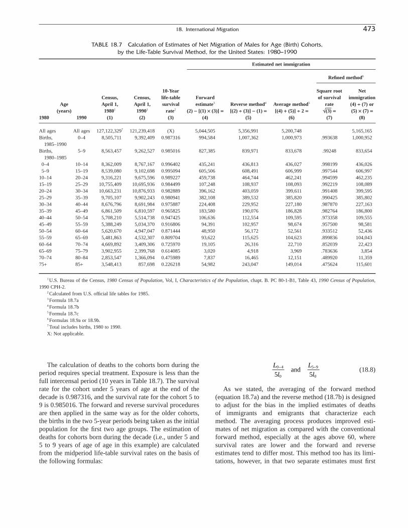
The calculation of deaths to the cohorts born during theperiod requires special treatment. Exposure is less than thefull intercensal period (10 years in Table 18.7). The survivalrate for the cohort under 5 years of age at the end of thedecade is 0.987316, and the survival rate for the cohort 5 to9 is 0.985016. The forward and reverse survival proceduresare then applied in the same way as for the older cohorts,the births in the two 5-year periods being taken as the initialpopulation for the first two age groups. The estimation ofdeaths for cohorts born during the decade (i.e., under 5 and5 to 9 years of age of age in this example) are calculatedfrom the midperiod life-table survival rates on the basis ofthe following formulas:
(18.8)
As we stated, the averaging of the forward method (equation 18.7a) and the reverse method (18.7b) is designedto adjust for the bias in the implied estimates of deaths of immigrants and emigrants that characterize each method. The averaging process produces improved esti-mates of net migration as compared with the conventionalforward method, especially at the ages above 60, where survival rates are lower and the forward and reverse estimates tend to differ most. This method too has its limi-tations, however, in that two separate estimates must first
L
l
L
l0 4
0
5 9
05 5- -and
18. International Migration 473
TABLE 18.7 Calculation of Estimates of Net Migration of Males for Age (Birth) Cohorts, by the Life-Table Survival Method, for the United States: 1980–1990
Estimated net immigration
Refined method6
10-Year Square root Net Census, Census, life-table Forward of survival immigration
Age April 1, April 1, survival estimate3 Reverse method4 Average method5 rate (4) ∏ (7) or(years) 19801 19901 rate2 (2) - [(1) ¥ (3)] = [(2) ∏ (3)] - (1) = [(4) + (5)] ∏ 2 = ÷(3) = (5) ¥ (7) =
1980 1990 (1) (2) (3) (4) (5) (6) (7) (8)
All ages All ages 127,122,3297 121,239,418 (X) 5,044,505 5,356,991 5,200,748 5,165,165Births, 0–4 8,505,711 9,392,409 0.987316 994,584 1,007,362 1,000,973 .993638 1,000,952
1985–1990Births, 5–9 8,563,457 9,262,527 0.985016 827,385 839,971 833,678 .99248 833,654
1980–19850–4 10–14 8,362,009 8,767,167 0.996402 435,241 436,813 436,027 .998199 436,0265–9 15–19 8,539,080 9,102,698 0.995094 605,506 608,491 606,999 .997544 606,997
10–14 20–24 9,316,221 9,675,596 0.989227 459,738 464,744 462,241 .994599 462,23515–19 25–29 10,755,409 10,695,936 0.984499 107,248 108,937 108,093 .992219 108,08920–24 30–34 10,663,231 10,876,933 0.982889 396,162 403,059 399,611 .991408 399,59525–29 35–39 9,705,107 9,902,243 0.980941 382,108 389,532 385,820 .990425 385,80230–34 40–44 8,676,796 8,691,984 0.975887 224,408 229,952 227,180 .987870 227,16335–39 45–49 6,861,509 6,810,597 0.965825 183,580 190,076 186,828 .982764 186,80040–44 50–54 5,708,210 5,514,738 0.947425 106,636 112,554 109,595 .973358 109,55545–49 55–59 5,388,249 5,034,370 0.916806 94,391 102,957 98,674 .957500 98,58150–54 60–64 5,620,670 4,947,047 0.871444 48,950 56,172 52,561 .933512 52,43655–59 65–69 5,481,863 4,532,307 0.809704 93,622 115,625 104,623 .899836 104,04360–64 70–74 4,669,892 3,409,306 0.725970 19,105 26,316 22,710 .852039 22,42365–69 75–79 3,902,955 2,399,768 0.614085 3,020 4,918 3,969 .783636 3,85470–74 80–84 2,853,547 1,366,094 0.475989 7,837 16,465 12,151 .489920 11,35975+ 85+ 3,548,413 857,698 0.226218 54,982 243,047 149,014 .475624 115,601
1 U.S. Bureau of the Census, 1980 Census of Population, Vol, I, Characteristics of the Population, chapt. B. PC 80-1-B1, Table 43, 1990 Census of Population,1990 CPH-2.
2 Calculated from U.S. official life tables for 1985.3 Formula 18.7a4 Formula 18.7b5 Formula 18.7c6 Formulas 18.9a or 18.9b.7 Total includes births, 1980 to 1990.X: Not applicable.

be computed and the weighting of the two estimates is arbitrary.
The second method of estimating net migration dealswith these limitations. A single equation will be used toderive the estimates, and for this the forward equation andthe reverse equation are equally satisfactory. The methodinvolves an adjustment of either the forward or the reverseestimates by the square root of the survival rate, represent-ing survival for approximately one half the period.28
(18.9a)
(18.9b)
(18.9c)
Table 18.7 shows the calculation of estimates of netimmigration to the United States, for birth cohorts of malesbetween 1980 and 1990 by this method. They can be derivedeither by dividing the forward estimate (col. 4), or by mul-tiplying the reverse estimate (col. 5), by the square root ofthe survival rate (col. 7). For this population, the averageestimates and the refined estimates are very close over muchof the age span but begin to diverge at the older ages wherethe survival rates are relatively low.
Intercensal Component Method for the Foreign-Born Population
Intercensal changes in the volume of immigration areobscured in a historical series on the number of foreign-bornpersons. Combined use of such data at successive censusesin some form may serve as a basis for estimating intercensalnet immigration.
The intercensal change in the foreign-born populationunderstates the net immigration of foreign-born personsduring an intercensal period by the number of deaths offoreign-born persons in the area during the period. Thus,solving the intercensal component equation for the foreign-born population for IF - EF, we have
(18.10)
(18.11)
where P0F and P1
F represent the foreign-born population at thefirst and second censuses, respectively, IF and EF representpersons born abroad entering and leaving the area during theintercensal period, respectively, and DF represents the
I E P P DF F F F F-( ) = - +1 0
P P I E DF F F F F1 0= + - -
M M I EF R a a= = -
M I E P s P sR a a R a a t= -( ) = ∏( ) -[ ] ¥-1 0
M I EP sP
sF a a F
a a t= -( ) =- -
1 0
number of deaths of foreign-born persons in the area duringthe intercensal period. The factor of births does not figureamong the components of change of the foreign-born pop-ulation. As suggested earlier, total (gross) immigration (oremigration) of the foreign born cannot be estimated by thisresidual procedure, only the net numbers of foreign-bornpersons arriving (or departing).
The number of deaths may be quite large and have a con-siderable effect on the estimate of net immigration, particu-larly if large numbers of immigrants arrived in precedingdecades and are now of advanced age. The difference in the number of foreign-born persons may even suggest netemigration when net immigration actually occurred. Forexample, the figure for the United States for the 1950–1960decade (-693,000) suggests a substantial net emigration,whereas frontier control data show a substantial net immi-gration of aliens during this period (2,238,000). WhenFormula (18.11) is used to estimate net migration to theUnited States, 1950–1960 (i.e., when an allowance for thedeaths of the foreign born is made), the resulting figuresshow a substantial net immigration of foreign-born persons:
Central age-specific death rates applied to midperiod 1,736,000population
Life table survival-rate method 1,805,000Census survival-rate method 1,450,000
The estimates of net immigration vary between 1.4 and1.8 million. Each of the estimates, however, is much higherthan the estimate of -693,000 that ignores deaths to theforeign-born population.
The allowance for the deaths of the foreign-born popula-tion during the intercensal period can be made by use of sta-tistics of deaths or by estimating deaths on the basis of deathrates or survival rates. Illustrations will be given here ofseveral procedures. The calculations are quite simple whenonly an estimate of total net immigration is wanted and bothpopulation and deaths are tabulated by nativity. As Formula(18.11) shows, it is merely necessary to take the differencebetween the counts of the foreign-born population in the twocensuses and add the number of deaths of the foreign-born.(This method corresponds to the “vital statistics” method ofestimating net migration described in Chapter 19.)
In the event that statistics of deaths of foreign-bornpersons are lacking, as is the common situation, the numbermay be estimated by applying appropriate central age-specific death rates to the midperiod foreign-born population. This procedure has been worked out for theforeign-born population of the United States for 1980–1990.The specific steps consist of (1) cumulatively multiplyingcentral age-sex specific death rates for the general popula-tion by the estimated foreign-born population distributed byage and sex for 1985 (i.e., an average of the foreign-bornpopulations in 1980 and 1990), to determine the averageannual number of deaths of foreign-born persons, and (2)
474 Edmonston and Michalowski
28 J. S. Siegel developed this refined method of adjusting for the biasin the estimate of deaths to migrants. See J. S. Siegel, Applied Demogra-phy: Applications to Business, Government, Law, and Public Policy, SanDiego: Academic Press, 2002, pp. 22–23. It was originally applied in theestimation of retirements by the life-table residual method. See M. Gendelland J. S. Siegel, “Trends in Retirement Age by Sex, 1950–2005, MonthlyLabor Review 115(7): 22–29, July 1992.
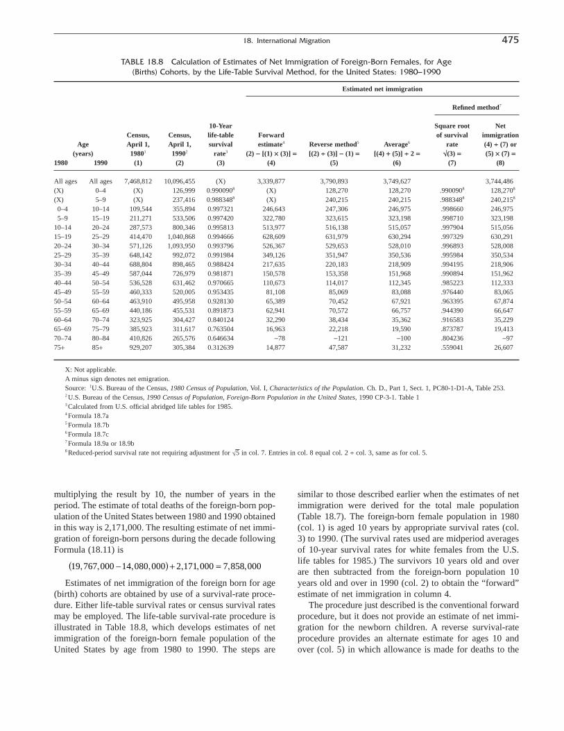
multiplying the result by 10, the number of years in theperiod. The estimate of total deaths of the foreign-born pop-ulation of the United States between 1980 and 1990 obtainedin this way is 2,171,000. The resulting estimate of net immi-gration of foreign-born persons during the decade followingFormula (18.11) is
Estimates of net immigration of the foreign born for age(birth) cohorts are obtained by use of a survival-rate proce-dure. Either life-table survival rates or census survival ratesmay be employed. The life-table survival-rate procedure isillustrated in Table 18.8, which develops estimates of netimmigration of the foreign-born female population of theUnited States by age from 1980 to 1990. The steps are
19 767 000 14 080 000 2 171 000 7 858 000, , , , , , , ,-( ) + =
similar to those described earlier when the estimates of netimmigration were derived for the total male population(Table 18.7). The foreign-born female population in 1980(col. 1) is aged 10 years by appropriate survival rates (col.3) to 1990. (The survival rates used are midperiod averagesof 10-year survival rates for white females from the U.S. life tables for 1985.) The survivors 10 years old and overare then subtracted from the foreign-born population 10years old and over in 1990 (col. 2) to obtain the “forward”estimate of net immigration in column 4.
The procedure just described is the conventional forwardprocedure, but it does not provide an estimate of net immi-gration for the newborn children. A reverse survival-rateprocedure provides an alternate estimate for ages 10 andover (col. 5) in which allowance is made for deaths to the
18. International Migration 475
TABLE 18.8 Calculation of Estimates of Net Immigration of Foreign-Born Females, for Age(Births) Cohorts, by the Life-Table Survival Method, for the United States: 1980–1990
Estimated net immigration
Refined method7
10-Year Square root Net Census, Census, life-table Forward of survival immigration
Age April 1, April 1, survival estimate4 Reverse method5 Average6 rate (4) ∏ (7) or(years) 19801 19902 rate3 (2) - [(1) ¥ (3)] = [(2) ∏ (3)] - (1) = [(4) + (5)] ∏ 2 = ÷(3) = (5) ¥ (7) =
1980 1990 (1) (2) (3) (4) (5) (6) (7) (8)
All ages All ages 7,468,812 10,096,455 (X) 3,339,877 3,790,893 3,749,627 3,744,486(X) 0–4 (X) 126,999 0.9900908 (X) 128,270 128,270 .9900908 128,2708
(X) 5–9 (X) 237,416 0.9883488 (X) 240,215 240,215 .9883488 240,2158
0–4 10–14 109,544 355,894 0.997321 246,643 247,306 246,975 .998660 246,9755–9 15–19 211,271 533,506 0.997420 322,780 323,615 323,198 .998710 323,198
10–14 20–24 287,573 800,346 0.995813 513,977 516,138 515,057 .997904 515,05615–19 25–29 414,470 1,040,868 0.994666 628,609 631,979 630,294 .997329 630,29120–24 30–34 571,126 1,093,950 0.993796 526,367 529,653 528,010 .996893 528,00825–29 35–39 648,142 992,072 0.991984 349,126 351,947 350,536 .995984 350,53430–34 40–44 688,804 898,465 0.988424 217,635 220,183 218,909 .994195 218,90635–39 45–49 587,044 726,979 0.981871 150,578 153,358 151,968 .990894 151,96240–44 50–54 536,528 631,462 0.970665 110,673 114,017 112,345 .985223 112,33345–49 55–59 460,333 520,005 0.953435 81,108 85,069 83,088 .976440 83,06550–54 60–64 463,910 495,958 0.928130 65,389 70,452 67,921 .963395 67,87455–59 65–69 440,186 455,531 0.891873 62,941 70,572 66,757 .944390 66,64760–64 70–74 323,925 304,427 0.840124 32,290 38,434 35,362 .916583 35,22965–69 75–79 385,923 311,617 0.763504 16,963 22,218 19,590 .873787 19,41370–74 80–84 410,826 265,576 0.646634 -78 -121 -100 .804236 -9775+ 85+ 929,207 305,384 0.312639 14,877 47,587 31,232 .559041 26,607
X: Not applicable.A minus sign denotes net emigration.Source: 1U.S. Bureau of the Census, 1980 Census of Population, Vol. I, Characteristics of the Population. Ch. D., Part 1, Sect. 1, PC80-1-D1-A, Table 253.2 U.S. Bureau of the Census, 1990 Census of Population, Foreign-Born Population in the United States, 1990 CP-3-1. Table 13 Calculated from U.S. official abridged life tables for 1985.4 Formula 18.7a5 Formula 18.7b6 Formula 18.7c7 Formula 18.9a or 18.9b8 Reduced-period survival rate not requiring adjustment for ÷5 in col. 7. Entries in col. 8 equal col. 2 ∏ col. 3, same as for col. 5.

476 Edmonston and Michalowski
population during the decade, and makes possible the cal-culation of estimates of net immigration of children bornduring the intercensal period. The two sets of estimates ofnet immigration are then averaged (col. 6) to derive “Con-ventional” average estimates of net immigration of foreign-born females to the United States, 1980–1990 ([(col. 4) +(col. 5)] / 2). To reduce the calculations, estimates for thechildren born during the period derived by the reversemethod may be combined with estimates for the other agegroups derived by the forward method. The result in thiscase is 3,708,000 as compared with the 3,750,000 obtainedby the average method. Once again the calculations relate toage cohorts, so that age groups 10 years apart are paired inthe two censuses; all the calculations for the same agecohorts are shown on the same line of the table.
Here again, it is desirable to adjust the results to allowmore precisely for the bias in the estimates of deaths and netimmigrants. Table 18.8 shows the adjusted results, obtainedby dividing the forward estimates of net migration by thesquare root of the survival rate (col. 8 = col. 4 ∏ col. 7).
The estimation of deaths for the cohorts born abroad inthe intercensal period (i.e., under 5 and 5 to 9 years of ageat end of period) requires special treatment because thesegroups are exposed to the risk of death in the United Statesfor much less than 10 years as a result both of recent birthabroad and of the staggered timing of immigration. Forexample, the population under 5 years old in 1990 has beenat risk for only 1.25 years on the average (2.5 ¥ 0.5 years),and the population 5 to 9 years old in 1990 has been at riskfor only 3.75 years on the average (7.5 ¥ 0.5 years). The firstfactors (i.e., 2.5 and 7.5) represent the average period of timebetween birth and the 1990 census, and the second factor(i.e., 0.5) reflects the fact that the migrants entered thecountry or departed at various times during the periodbetween birth and the census, with an assumed average residence in the area of one-half the period. Therefore, thesurvival rates for the two age groups, under 5 and 5 to 9,respectively, in exact ages, are as follows:
As was stated earlier, alternative estimates of net immigration of the foreign-born population employing thesurvival-rate procedure may be derived by use of national census survival rates instead of life-table survivalrates. It may be recalled from Chapter 13 that census survival rates represent the ratios of the population in a given age at one census to the population in the same age cohort at an earlier census and are usually computed for the native population to exclude the effects of interna-tional migration from the rates. They are intended to repre-sent the combined effect of mortality and the relative changefrom one census to the next in the percent (net) error in
L
l L
L
L0 5
0 0 3 75
5 10
1 25 6 251 25-
-
-
-+. . . .and
census coverage for a given age cohort. Their presumedadvantage is that the estimates of net migration resultingfrom their use may be more accurate than when life-tablesurvival rates are used, because errors in census enumerationare incorporated in the census survival rates rather than in the(residual) estimates of net migration, as in the case when life-table survival rates are used. In both instances, for the censussurvival-rate method and the life-table survival-rate method,the assumption is made that the mortality levels of theforeign-born and the total populations are the same.
The steps are the same as with life-table survival rates,once the census survival rates have been calculated. Thecohorts born during the intercensal period once again requirespecial treatment. For the computations relating to the U.S.foreign-born population, as before, the populations under 5and 5 to 9 years old in 1990 have to be “younged” to theestimated date of arrival in the United States, not to the dateof birth; and only a reverse estimate of net migration is possible.
The general procedure just described may be extended to derive estimates of net immigration, by age and sex,according to race, country of birth, mother tongue, or other“ascribed” or fixed demographic characteristic, or combina-tion of them. Table 18.9 presents the calculation of estimatesof the net migration of males and females, born in the Philippines, to the United States between 1980 and 1990,based on U.S. census statistics on country of birth. A(forward) estimate of net immigration to the United Statesof males and females born in the Philippines is made by carrying the population of the United States born in thePhilippines, for 1980, forward to 1990, by the use of 10-yearcensus survival rates and 10-year life-table survival rates,and comparing the survivors with the corresponding 1990census figures. Reverse estimates of net immigration of chil-dren under 10 are prepared by “younging” the 1990 censusfigures back to the average date of immigration. The overallestimate of net immigration of Filipinos to the United States,for males (239,000) and females (311,000) combined,derived by the census survival-rate method, is 550,000. Bythe life-table survival-rate method, the combined estimate ofnet immigration for both sexes is 530,000. This estimatemay be compared with the estimate of 516,000 Philippine-born immigrants coming to the United States during thedecade and surviving to 1990, based on visa data and sur-vival calculations. The percentage differences between thecensus and life-table survival-rate methods are small formost ages but become rather large among some adult ages,especially for males aged 35 to 44 years. Table 18.9 alsoshows a comparison of estimates of the net migration of theforeign born based on the census survival-rate method andestimates of immigration based on visa data. The differencesare quite large for most adult ages. It is apparent that theU.S. censuses and the visa data reflect quite different levelsof immigration.

TABLE 18.9. Comparison of Estimates of Net Migration of the Philippine-Born Population, forSex and Age (Birth) Cohorts, by the Census and Life-Table Survival-Rate Methods, for the United
States: 1980–1990
Estimates of net immigration Percentage difference from census survival-rate method
Census survival-rate Life-table survival-rate Life-table survival-rate method Visa data
Agemethod method Visa data
Male Female Male Femalein 1990 Male Female Male Female Male Female 100x {(3) - (1)}/ 100x {(4) - (2)}/ 100x {(5) - (1)}/ 100x {(6) - (2)}/(years) (1) (2) (3) (4) (5) (6) (1) = (7) (2) = (8) (1) = (9) (2) = (10)
All ages 239,372 310,692 230,621 300,464 202,399 314,051 -3.7 -3.3 -15.4 +1.1
Under 5 3,190 2,369 3,110 2,306 2,789 2,793 -2.5 -2.6 -12.6 +17.9
5–14 24,156 24,653 24,155 24,741 27,182 26,821 — +0.4 +12.5 +8.8
15–24 28,453 30,252 28,465 30,299 45,694 50,534 — +0.2 +60.6 +67.0
25–34 36,984 39,308 34,847 37,417 33,717 75,911 -5.8 -4.8 -8.8 +93.1
35–44 42,097 57,213 37,751 53,160 38,420 68,668 -10.3 -7.1 -8.7 +20.0
45–54 46,087 77,236 43,289 74,430 22,907 33,333 -6.1 -3.6 -50.3 -56.8
55–64 41,898 72,141 41,382 71,168 15,452 26,619 -1.2 -1.3 -63.1 -63.1
65 and over 16,507 7,521 17,622 6,943 16,237 29,371 +6.8 -7.7 -1.6 +290.5
Notes: Visa data are numbers of legal immigrants, by age and sex, “survived” from the year of entry to 1990, using life-table survival rates.The survival-rate estimates are based on the forward method.—Less than 0.05 percent.

Table 18.10 illustrates the calculation of estimates of thenet movement of population between two areas on the basisof place-of-birth data from the census of the destinationcountry. The illustration relates to the movement of thefemale population between Hong Kong and Canada in the1991–1996 period. The basic procedure is the same as in the illustration in Table 18.8, but here account is taken ofthe movements over a 5-year period. The net movement ofHong Kong–born females is estimated by “surviving” theCanadian female population born in Hong Kong (col. 1)forward to 1996 (col. 4), by use of 5-year life-table survivalrates (based on 1996 life tables), shown in col. 3. The esti-mated survivors are subtracted from the 1996 female popu-lation of Canada born in Hong Kong (col. 2) to obtain thepreliminary estimates of net migration from Hong Kong toCanada for females for age cohorts during the 1991-to-1996period (col. 5). Then the final estimates (col. 6) are obtainedby dividing the estimates in col. 5 by (i.e., square rootof col. 3).
Changes in Alien Population
The same types of procedures as described in the previ-ous section may be employed in connection with census
s
counts of aliens, where available. The change in the numberof aliens between two dates is affected by naturalizations aswell as by net immigration and deaths:
(18.12)
(18.13)
where A refers to aliens and N refers to naturalizations.Hence the net immigration of aliens is estimated as the sumof the net change in the number of aliens, deaths of aliens,and naturalizations.
Data on Nationals Abroad
Estimates of the net migration of nationals or a par-ticular segment of them (e.g., employees of the national government and their dependents, armed forces) during someperiod, complementing the estimates for the foreign born oraliens, may be derived by a similar method from statistics orestimates of these groups living outside the country at thebeginning and end of the period. The formula may be arrivedat by solving the component equation relating to this specialpopulation for the net migration component:
I E P P D NA A A A A-( ) = - + +1 0
P P I E D NA A A A A1 0= + - - -
478 Edmonston and Michalowski
TABLE 18.10 Calculation of Estimates of Net Immigration of Females from Hong Kong toCanada, by Age (Birth) Cohorts, by the Life-Table Survival-Rate Method: 1991–1996
Canadian females bornin Hong Kong
5-year life-Net migration
Census, Census, table Forward AdjustedAge June 1, May 14, survival Survivors estimate estimate
(years) 1991 1996 rate (1) ¥ (3) = (2) - (4) = (4) ∏ ÷––––(3) =
1991 1996 (1) (2) (3) (4) (5) (6)
All ages All ages 77,325 124,315 (X) 77,792 47,766 47,963(X) Under 5 X 1,240 0.9987 1,2421 1,2421 1,2421
Under 5 5–9 1,470 4,245 0.9989 1,468 2,777 2,7795–9 10–14 3,700 7,590 0.9993 3,697 3,893 3,894
10–14 15–19 4,590 10,400 0.9988 4,585 5,815 5,81815–19 20–24 5,860 10,705 0.9984 5,850 4,855 4,85920–24 25–29 5,955 9,765 0.9983 5,945 3,820 3,82325–29 30–34 9,140 15,060 0.9978 9,120 5,940 5,94730–34 35–39 13,480 19,330 0.9968 13,437 5,893 5,90235–39 40–44 13,090 17,975 0.9949 13,023 4,952 4,96540–44 45–49 9,385 12,795 0.9922 9,311 3,484 3,49845–49 50–54 2,890 3,910 0.9880 2,855 1,055 1,06150–54 55–59 2,715 3,865 0.9804 2,662 1,203 1,21555–59 60–64 1,730 2,985 0.9691 1,677 1,308 1,32960–64 65–69 1,210 1,810 0.9516 1,151 659 67665–69 70–74 880 1,400 0.9232 812 588 61270–74 75–79 735 725 0.8759 644 81 8775+ 80+ 495 515 0.6309 312 203 256
X: Not applicable.1 Reverse estimate.Source: 1991 and 1996 Canadian Census of Population unpublished data; 1996 Abridged Life Tables, Statistics Canada unpublished data.

(18.14)
where 00 and 01 represent the country’s overseas populationat the initial and terminal date in the period, respectively, B0
represents births to the country’s overseas population, D0
represents deaths to the country’s overseas population, andM0 represents net movement overseas. The sign of the resultis then changed so that it will refer to movement vis-à-visthe country in question, not the country’s population abroad.Net movement into the country of its nationals from over-seas equals -M0, therefore.
United States Procedure of Estimating Net Migration
The estimates of net civilian immigration to the UnitedStates currently employed by the U.S. Census Bureau in itspopulation estimates illustrate the composite use of severalof the sources and methods that have been described. Thestatistics of net civilian immigration for the United States inrecent decades cover the following categories:
1. Immigrant aliens2. Refugee aliens3. Permanent emigration of legal residents4. Net migration of illegal immigrants5. Net migration of nonrefugee temporary residents
(mainly foreign students and temporary workers)6. Net migration from Puerto Rico and other outlying
areas under U.S. jurisdiction7. Net movement of civilian citizens affiliated with the
U.S. government (federal government employees anddependents, including military dependents)
Categories 1, 2, and 5, represent “frontier control” sta-tistics compiled by the U.S. Immigration and NaturalizationService. Categories 3 and 4 are numerically substantial butlack reliable data; they are estimates prepared by the U.S.Census Bureau. Category 6 is based on passenger statisticscompiled by the Planning Board of the Commonwealth ofPuerto Rico. Category 7 represents estimates prepared bythe U.S. Census Bureau, and derived from data on the over-seas population provided by the U.S. Department of Defenseand the U.S. Office of Personnel Management.
Estimating Illegal Immigration
It is impossible to estimate the number of illegal immi-grants in a country with a small relative error. This is sobecause illegal movements are clandestine and the status ofillegal immigrants is not a matter of public record, or readilyor accurately ascertained by direct enquiry. If illegal immi-grants constitute several million in a population of a fewhundred million, however, as appears to be the case for theUnited States, we should be able to detect their presence bymanipulating available demographic data, including cen-suses, large national surveys, vital statistics, and immigra-
M O O B D0 1 0 0 0= -( ) - -( ) tion data. We should be able to measure the number of illegalimmigrants with less than a 50% relative error, if not by lessthan a 25% relative error, by demographic analyses and acombination of data from several record systems.
The data to be used in measuring illegal immigrationinclude census data, sample survey data, Social Security andother administrative data, and immigration data. The immi-gration records could include records of persons listed inalien registrations, records of immigrant aliens admittedlegally, records of visitors and other short-term “nonimmi-grants,” and records of aliens held for deportation (includ-ing illegal immigrants apprehended at the border). Althougha great variety of methods as well as data can be employedto estimate illegal immigrants, none are robust and allrequire broad and sometimes extensive assumptions. Inpractice, these methods are combined and different methodsmay be applied in estimating the different types of illegalimmigrants. Moreover, it is useful to analyze the data interms of the principal countries of origin. Among the generaltypes of studies are the following:
1. A special household survey of foreign-born personscovering selected subnational areas where foreign-bornpersons are concentrated
2. Comparative analysis of aggregate administrative dataand census and/or national sample survey data (e.g.,employment data from Social Security or other admin-istrative records and from census records)
3. Demographic analysis of census and survey data (e.g.,analysis of the regional variation or trend of death ratesor sex ratios, component analysis of changes in succes-sive national sample surveys or censuses, and com-parative analysis of census data on population and thelabor force in paired principal countries of origin anddestination)
4. Case-by-case matching of two or more, preferablyindependent, collection systems (e.g., census, post-enumeration surveys, or Social Security records, taxfiles, or other administrative records)
5. Historical analysis of the records of border apprehen-sions and year-to-year matching of these records inorder to measure those entering without inspection
6. Matching of visas of arriving temporary visitors withvisas of departing temporary visitors in subsequentyears in order to measure visa overstayers
7. Intensive checks at selected official border crossingpoints in order to measure persons attempting to enterwith fraudulent documents
Matching border apprehensions and Social Security filesshould provide useful information on the socioeconomiccharacteristics of illegal entrants who have been apprehended.
Some more specific methods of measuring illegal immi-gration are described in the following sections.
18. International Migration 479

Use of Immigrant Records Only
An analysis of historical data on border apprehensionsand the characteristics of those apprehended could providea basis for rough estimates of the number of illegal entrants,especially if multiple apprehensions are identified by recordmatching. This might involve imputing ratios of illegalentrants to apprehensions for sections of the national border.Alternatively, the records of temporary aliens admitted andthe records of temporary aliens departing within a specifiedperiod could be matched to identify those who had failed toleave the country within a reasonable time of their requireddeparture date.29
Demographic Analysis
In one application of demographic analysis, we cancompare the trend of death rates according to age and sexover a series of years for a particular part of the country inwhich aliens are concentrated with the trends of death ratesin the balance of the country. For this purpose, the assump-tions are made that only a small portion of the illegal population is enumerated in the censuses or is included inthe postcensal population estimates on which the death rates are based but that all or nearly all of the deaths ofillegal immigrants are included in the death statistics. If the illegal population has increased greatly over the obser-vation period in the designated geographic area, then thedeath rates at the young adult ages in this area would showsubstantially larger increases or substantially smallerdecreases than in the balance of the country at these agesduring the period.30
One of the common observations made about illegalimmigration is that young adult males predominate in themovement. A substantial drop in the sex ratio of an agecohort over a decade for a country of origin and a substan-tial rise in the sex ratio for the country of destination duringthe same period for the same cohort might indicate thatmany more males than females emigrated from the firstcountry to the second country during the period. The ques-tion still arises whether this shift is more extreme than couldbe accounted for by reported migration of the sexes from thecountry of origin to the country of destination.31
Demographic Analysis Linking Survey andImmigration Data
Net illegal immigration can be estimated as a residual bydecomposing the change in the foreign-born population orthe population born in one or more of the countries of prin-cipal origin of immigrants on the basis of census counts orsurvey estimates of the foreign-born population at two datesand data on the components of change. For this purpose,census or sample survey data on the total foreign-born pop-ulation at one date are combined with data on legal immi-gration and estimates of deaths and emigration of legalimmigrants, and then compared with data on the totalforeign-born population at a later date.32
When data on country of origin are available in censusesor surveys, they can be used to prepare separate estimatesof illegal immigration.33 For analysis of illegal immigrationfor specific countries of origin, the data should preferablybe tabulated by age and sex because allowance has to bemade for mortality by use of life tables. Analysis by countryof origin requires data on legal immigration and emigrationof legal immigrants. In the United States data on legal im-migration can be obtained from the U.S. Immigration and Naturalization Service. Different life tables and differentallowances for emigration of legal immigrants can be usedto provide alternative estimates. A complementary type ofstudy can be carried out using two consecutive censuses ofthe country of emigration (e.g., Mexico) and again makingalternative allowances for mortality and emigration of legalimmigrants.
Estimates of the number of illegal immigrants residing ina country, for different countries of origin, can be made bycomparing the number of legally resident immigrants froman alien registration and a census count of the total numberof foreign born.34 This approach can be extended to make
480 Edmonston and Michalowski
29 For an example of studies using immigrant records, see R. Warren,“Annual Estimates of Nonimmigrant Overstays in the United States: 1985to 1988,” in F. D. Bean, B. Edmonston, and J. S. Passel (Eds.), Undocu-mented Migration to the United States: IRCA and the Experience of the1980s, Washington, DC: Urban Institute Press, 1990.
30 The use of this method is illustrated in J. G. Robinson, “Estimatingthe Approximate Size of the Illegal Alien Population in the United States by the Comparative Trend Analysis of Age-Specific Death Rates,”Demography 17: 159–176, 1980.
31 For an illustration of the use of this method to estimate the flow ofillegal immigrants from Mexico to the United States, see F. D. Bean, A. G.King, and J. S. Passel, “The Number of Illegal Migrants of Mexican Originin the United States: Sex-Ratio Based Estimates for 1980. Demography20(1): 99–106, 1983.
32 An example of the application of this approach is given in K. Woodrow and J. S. Passel, “Post-IRCA Undocumented Immigration to the United States: An Assessment Based on the June 1988 Current Population Survey,” Chapter 2 in F. D. Bean, B. Edmonston, and J. S. Passel (Eds.), Undocumented Migration to the United States: IRCA andthe Experience of the 1980s, Washington, DC: Urban Institute Press, 1990.
33 For country-of-origin estimates, for example, estimates of theMexican-born population of the United States, J. S. Passel and K. Woodrowanalyzed the Current Population Surveys conducted in 1979 and 1983 inorder to estimate illegal immigation from Mexico to the United Statesbetween these years. See their paper, “Change in the Undocumented AlienPopulation in the United States, 1979–1983, International MigrationReview 21(4): 303–334, 1987.
34 Minimal estimates of illegally present immigrants in 1980 in the United States, for selected countries of birth, were derived by R. Warren and J. S. Passel by subtracting the number of legally resident immigrants based on an alien registration from the census count of immi-grants (modified to account for deficiencies in the data). See their paper,“A Count of the Uncountable: Estimates of the Undocumented AliensCounted in the United Stated Census,” Demography 24: 375–393, August1987.

separate estimates of the illegal immigrant population forsubnational areas.35
Comparison of Aggregate Administrative Records
Comparison of two data series, one of which is likely to include all or most illegal immigrants in a country and the other of which is likely to exclude all or most of them, represents another possible avenue of estimation. Two general illustrations may be given. The first compares two national data series on employment in the United Statesover a decade or so, one based on household reporting ofemployment status and the other based on establishmentreporting of the numbers of employees. Any sharp changein the number of illegal immigrants over the observationperiod should be evident from a comparison of changes inthe differences between these two series. A second compar-ison can be carried out between census figures on schoolenrollment for states and administrative data on enrollmentfor states. The differences between the two sets of datawould be attributed to illegal residents of school age. We areassuming that the latter series includes many, if not most,illegal residents while the former includes few or none ofthem. At best such comparisons can provide minimal estimates of employed illegal residents or of school-age children of illegal immigrants.
Dual Systems Analysis
A potentially more productive, but also more costly,approach is to match individual records in various censuses,surveys, and administrative record files such as Social Secu-rity records and national income tax returns. For example,in 1977 the U.S. Social Security Administration developedan estimate of the number of illegal residents aged 18 to 44years in the United States in 1973 on the basis of a matchof the Current Population Survey, Social Security records,and federal income tax returns. The estimate obtained was3.9 million, with a subjective 68% confidence intervalranging from 2.9 to 5.7 million.36
Sample Survey
It is theoretically possible to obtain an estimate of thenumber of illegal residents and their demographic andsocioeconomic characteristics by direct inquiry in a survey.
The survey could be framed as a sample survey of theforeign-born population and can be restricted to the areas ina country where the foreign-born population is concentrated.Intensive probing could be used to determine the circum-stances of entry and the residence of the survey respondentsand the members of their households. Such a survey,however, presents great difficulties because of the illegalstatus of the respondents or their household members. Itwould generally be seen as threatening to the respondents,once they learn the purpose of the survey. At best, such asurvey would yield a minimal estimate of the number ofillegal immigrants.
Estimating Emigration
Earlier we mentioned that few countries collect dataspecifically on emigrants. Relatively fewer countries collectcomprehensive emigration statistics that cover all groups ofemigrants. Countries where emigration is measured on aregular basis, usually by a central statistical agency, employa combination of different data sources and methods. TheUnited States, Canada, and Australia are good examples ofvaried approaches taken by different countries.
Because, as noted previously, the collection of statisticson emigration for the United States was discontinued in 1957and no direct measure of emigration has been available sincethen, estimates have had to be prepared. The U.S. CensusBureau estimates emigration of foreign-born and the U.S.-born legal, permanent residents separately. These statisticsexclude emigration of citizens affiliated with the federal government (civilians and members of armed forces andtheir dependents). No attempt is made to estimate emigrationof other groups of residents in the country that are includedin the international migration component of populationchange: i.e., Puerto Ricans, non-refugee temporary residents,and illegal residents in addition to federally affiliated citi-zens. Only data on net migration are available for thosegroups.
Estimates of emigration of the U.S. born and foreign-born permanent residents are developed by demographicanalysis using a variety of administrative sources and thecensus. Since 1997, for the foreign born, an assumption ismade that the trend in emigration follows the trend in thesize of the foreign-born population according to country ofbirth. Ahmed and Robinson applied crude rates of emigra-tion for countries, in a residual technique with the cohort survival method, to the 1980 and 1990 census data on theforeign born tabulated by detailed demographic characteris-tics (sex, age, period of immigration, and country of birth).37
For emigration of the U.S.-born population, the U.S. CensusBureau makes an annual allowance of 48,000, based on
18. International Migration 481
35 Extensions of the country-of-birth approach have been made byPassel and Woodrow to illustrate the use of the method for making esti-mates of the illegal immigrants for states of the United States. See J. S.Passel and K. Woodrow, “Geographic Distribution of Undocumented Immi-grants: Estimates of Undocumented Aliens Counted in the 1980 Census byState,” International Migration Review 18: 642–671, Fall 1984.
36 Social Security Administration, unpublished paper, “Estimates of theIllegal Immigrant Population of the United States,” Washington, DC: SocialSecurity Administration, 1977.
37 For more details, see B. Ahmed and J. G. Robinson, “Estimates ofthe Foreign-Born Population: 1980–1990,” Population Division WorkingPaper No. 9, U.S. Bureau of Census, 1994, www.\\census.gov.

research by Fernandez.38 This estimate is composed of twoelements. The first component is calculated by applying thecohort-survival method to the census data of selected foreigncountries on the U.S.-born persons living in these countries.The second component is based on the U.S. State Depart-ment data on registrations of U.S. citizens living abroad. Itcovers countries for which foreign-country census data onU.S.-born persons are not available or are of poor quality.
Since 1999, Canada’s statistical agency, StatisticsCanada, measures total emigration through three compo-nents: emigration of Canadian citizens and alien permanentresidents, return of emigrants, and net emigration of Cana-dian residents temporarily abroad.39 Although published datareflect total emigration, data on the individual componentsare provided on request. Aliens with temporary status inCanada (nonpermanent residents) are also included as acomponent of international migration, but only their netmigration is measured.
The first two components are estimated using a modelbased on administrative data. These data are extracted by theCanada Customs and Revenue Agency from the federallyadministrated Child Tax Benefit program and provide infor-mation only on children whose families are entitled to thebenefit (the entitlement is established by the presence ofchildren under age 18 and the prescribed family income). In addition, the estimate of emigration uses data collectedby the U.S. Immigration and Naturalization Service on Canadian residents admitted to the United States for per-manent residence. The model accounts for the differentpropensity to emigrate and return, respectively, betweenthose receiving and not receiving the benefit.40 The thirdcomponent, Canadians temporarily abroad, is measuredfrom the estimated trend in the size of the Canadian popu-lation residing temporarily outside the country. The trend isestimated on the basis of the results of the Reverse RecordCheck conducted in 1991 and 1996, which is the majorsurvey for estimation of the coverage error in the Canadiancensus.41
In Australia, all international arrival and departure statis-tics are derived from a combination of “100%” bordercontrol statistics and sampling at the borders. All permanentmovement (arrivals and departures) and all temporary move-ments with a duration of stay in the country or abroad of 1year or more are fully registered. Measurement of tempo-rary movements with a duration of stay of less than 1 yearare based on a sample of these movements. Passenger cardsare the source of these statistics, with the addition of infor-mation on passport and visa data. Australia distinguishesbetween movements of Australian residents, settlers (for-eigners who hold immigrant visas and New Zealand citizenswho indicate intention to settle), and visitors.
Currently, the Australian Bureau of Statistics calculatesnet international migration as the difference between per-manent and long-term arrivals and permanent and long-termdepartures. There is also a special component of “categoryjumping.” This component is a measure of the net effect of changes in travel intentions from short term to permanent/long term or vice versa.42 In Australian practice,therefore, emigration includes departures of Australian res-idents (citizens and aliens with permanent residence status)who on departure state that they are departing permanentlyor intend to stay abroad for more than 12 months, and depar-tures of visitors who had stayed in Australia for 12 monthsor more. Although not used for preparing population esti-mates, the data on short-term departure of Australian resi-dents and overseas visitors are also published.
The preceding discussion demonstrates that for estimat-ing emigration, the United States relies primarily on censusdata, Canada uses administrative data other than bordercontrol data predominately, and Australia employs bordercontrol data, with an explicit reference to permanent andtemporary movement as measured by the duration of residence.
So far the direct method of measuring emigration knownas multiplicity or network sampling has not been considered.This method involves inquiring of members of the originalsample households in a survey and members of householdsof close relatives (within a specified degree of consanguin-ity, e.g., siblings, parents, and children) about members ofthe households who have gone “abroad” to live during aspecified past period. There are issues here of the omissionof single-person or even family households all of whosemembers have moved “overseas” and of the sample weight-ing. No country has made a serious effort to fully exploitthis method, but it remains a serious possibility.
482 Edmonston and Michalowski
38 For more details, see E. W. Fernandez, “Estimation of the AnnualEmigration of U.S. Born Persons by Using Foreign Censuses and SelectedAdministrative Data: Circa 1980,” Population Division Working Paper, No.10, U.S. Bureau of Census, 1995. www.census.gov.
39 For the data and a brief description of the methodology, see Statis-tics Canada, “Annual Demographic Statistics, 1999,” Ottawa, Ontario: Statistics Canada, 2000.
40 For more details on the research leading to development of themethod, see D. Morissette, “Estimation of Emigration,” Demography Divi-sion, Ottawa, Ontario: Statistics Canada, 1999; and D. Morissette, “Estima-tion of Returning Canadians,” Demography Division, Ottawa: StatisticsCanada, 1999, www.dissemination.statcan.ca/english/concepts/demog/index.htm.
41 For more details on the research leading to development of themethod, see M. Michalowski, “Canadians Residing Temporarily Abroad:Numbers, Characteristics and Estimation Methods,” Demography Division,Ottawa: Statistics Canada, 1999, www.dissemination.statcan.ca/english/concepts/demog/index.htm.
42 For a description of the categories and procedures, see AustralianBureau of Statistics, “Australian Demographic Statistics, December 1994,”1995; and Australian Bureau of Statistics, “Statistical Concepts Library,”catalogue 3228.0, www.abs.gov.au/websitedbs.
TECHNIQUES OF ANALYSIS
Few specialized demographic techniques have beendevised for the analysis of international migration. Many ofthe techniques of analysis used in other demographic fields,especially for internal migration, apply equally to interna-tional migration. We will, accordingly, touch on this subjectonly briefly in this chapter, leaving the more complete dis-cussion to the chapter on internal migration.
General Aspects of Migration Analysis andDemographic Factors Important in Analysis
Analysis of international migration presents certain com-plexities arising from the special characteristics that distin-guish it from, say, mortality analysis and natality analysis.The conceptual difficulties in defining a migrant are muchgreater than in defining a birth or a death. These difficultiesare associated with the variety of definitions in a givencountry and between countries and with the variety of col-lection systems, and they result in serious problems of inter-national comparability. Unlike the events of birth or death,migration necessarily involves two areas: the area of originand the area of destination. This fact leads to interest in par-ticular migration streams and counterstreams as well as intotal migration to an area; to the need to analyze immigra-tion, emigration, and net migration jointly; and to difficul-ties in formulating measures of analysis, particularly rates.Formulation of migration rates involves practical and theo-retical problems. Immigration cannot be viewed as a risk towhich the members of the receiving population are subjectin the same sense that this population is subject to the riskof death or bearing children, because the migrants comefrom outside the population. On the other hand, one canview emigration as a risk associated with the population ofthe area of origin. Analysis in terms of net migration, whichis often necessary because of the lack of adequate statisticson immigration and emigration, presents special arithmeticand logical problems because net migration may be a posi-tive or negative quantity and may differ considerably inmagnitude from the gross volume of movement into or outof the country.
Unlike death, but like bearing a child, the event of migra-tion may occur repeatedly to the same person or may notoccur at all to an individual in his or her lifetime. Hence,there is need to differentiate migration (i.e., number ofmoves) from migrants (i.e., number of persons who havemoved) and to specify precisely the geographic areas andthe time period for which migration status (e.g., migrant,nonmigrant) is defined. The time period must be chosencarefully because it introduces one of the main complica-tions in defining migration rates.
Analysis of international migration involves some of thesame factors found to be important in other fields of demo-
graphic analysis as well as other factors especially pertinentto this subject. Analysis of international migration streamscalls for data on country of last permanent residence ofimmigrants and country of next permanent residence ofemigrants. Country of birth or citizenship may serve as asubstitute for previous permanent residence or as a supple-ment to it. For both administrative and demographic uses, itis important to have data on citizenship, type of migration(e.g., permanent, temporary, and “commuters” or “bordercrossers”), and the legal basis of entry of aliens.
Tabulations on type of migration and legal basis of entrymay also provide general or detailed information on causesof migration—that is, whether the migrant intends to settlepermanently, study, tour, or work temporarily. There is inter-est in the demographic, social, and economic characteristicsof migrants. In recommending a program to improve inter-national migration statistics, the U N Population Commis-sion at its third Session in May 1958 urged the “provisionof statistics most relevant to the study of demographic trendsand their relation to economic and social factors, includingstatistics on age, sex, marital condition, family size, occu-pation and wages of migrants.”43 The variation of rates ofmigration by age and sex may be quite pronounced and isimportant for its effect on the composition of the populationof the sending and receiving countries. It is also of value tohave data on major occupation groups and industrial classes,particularly in connection with an analysis of the impact of migration on the sending and receiving countries’economies. Data on the mother tongue, ethnic origin or race,education, marital status, and family composition of theimmigrants are useful in the analysis of the assimilation ofimmigrants. Tabulations on state or province of intendedfuture residence for immigrants and on state of last perma-nent residence for emigrants are useful for making currentestimates of population for such subdivisions.
Some analysts of international migration also take intoaccount various nondemographic factors, such as changes inlegislation regarding immigration and emigration, programsto assist immigrants, modes and costs of travel, and eco-nomic and social conditions at origin and destination,including wars, sociolegal status of minorities, businesscycles, adequacy of harvests, and many other social and economic factors that are not necessarily measured by thepopulation census or immigration statistics.
Net Migration, Gross Migration, and Migration Ratios
Movement into a country, previously referred to as immi-gration, may also be referred to as gross immigration. Sim-ilarly, movement out of a country, previously referred to as
18. International Migration 483
43 United Nations, Problems of Migration Statistics, Series A, Popula-tion Studies 5: 2, 1958.

emigration, may also be referred to as gross emigration. The balance of gross immigration and gross emigration for a given country is referred to as net immigration or net emigration, depending on whether immigration or emigration is larger. A series of figures on gross immigra-tion or emigration for several countries constituting somebroader geographic area, say a continent, cannot be com-bined by addition to obtain the corresponding figures ongross immigration or emigration for the broader area,because some of the movement may have occurred betweenthe constituent countries and hence would balance out in themeasurement of immigration to or emigration from the areaas a whole.
Net migration figures, however, can be added together to obtain totals for broader areas or subtracted from oneanother to obtain figures for constituent areas. The latterrelation may be seen either by an algebraic or a graphic pres-entation. If we consider the movement affecting two coun-tries, then we may diagram this movement as follows:
the absence of all movement. There is interest, then, in the basic immigration and emigration figures even when thenet movement is known. In analyzing the differencesbetween the total movement and the net movement, a usefulconcept is that of gross migration, the sum of immigrationand emigration. This figure may also be called migrationturnover. It is intended to represent the total movementacross the borders of an area during a period. For example,the net immigration of 949,700 into Canada during the1991–1996 period represents the balance of an immigrationof 1,178,800 and an emigration of 229,100. In total,1,407,900 (i.e., 1,178,800 plus 229,100) moves occurredacross the Canadian borders during that period (Table 18.11).
Various types of ratios may be computed to indicate therelative magnitude of immigration (I), emigration (E), netmigration (I - E, or M), and gross migration (I + E), to orfrom a country:
(18.15)
(18.16)
(18.17)
(18.18)
(18.19)
(18.20)
The ratio to be selected for some particular analytic studydepends on the type of analysis being made and the migra-tion characteristics of the area under study. For an area char-acterized by immigration, the ratio of net immigration togross immigration may be used to measure the proportionof (gross) immigration that is effectively added to the pop-ulation (i.e., the proportion that is uncompensated by emi-gration). Similarly, for an area characterized by emigration,the ratio of net emigration to (gross) emigration may be usedto measure the proportion of the (gross) emigration that iseffectively lost (i.e., the proportion that is uncompensatedby immigration). Table 18.11 illustrates the computation ofthese measures on the basis of data for Canada for the 10-year periods from 1861–1871 to 1891–1901, for the 5-yearperiods from 1976–1981 to 1991–1996, and for the1996–1999 period. At the end of the 19th century, Canadawas a country of large-scale immigration and emigration,with an overall net emigration. In the mid-1970s to the mid-1980s, the volume of emigration was approximately 50% of
Net migrationGross migration
=-+
I E
I E
EmigrationGross migration
=+E
I E
ImmigrationGross migration
=+I
I E
Net emigrationImmigration
where =-
>E I
EE I
Net immigrationImmigration
where =-
>I E
II E
EmigrationImmigration
=E
I
484 Edmonston and Michalowski
Area 1 Area 2
B E D
A F C
Thus, we have the following relationships:
(1) = Immigration to areas 1 and 2 as a unit, excludingmovement between areas 1 and 2 = A + C.
(2) = Emigration from areas 1 and 2 as a unit, excludingmovement between areas 1 and 2 = B + D.
(3) = (1) - (2) = net immigration to areas 1 and 2 as aunit, calculated directly = (A + C) - (B + D).
(4) = Net immigration, area 1, taken separately = (A + E)- (B + F).
(5) = Net immigration, area 2, taken separately = (C + F)- (D + E).
(6) = (4) + (5) = Net immigration, areas 1 and 2 as a unit,calculated by summing net migration for the compo-nent areas = (A + C) - (B + D).
Note that the results in (3) and (6) are the same. They canbe extended to cover n areas, in fact, the entire world. At theglobal level, we know that only births and deaths affect pop-ulation growth. If comparable international migration datawere available for every country for the same period, apurely hypothetical situation at present, the sum of the netimmigration or net emigration figures for the various coun-tries would therefore have to be zero.
It should be evident that any one of many very differentamounts of immigration and emigration may underlie anygiven net figure. A net figure of zero may represent the balance of two equally large migration currents or

18. International Migration 485
the volume of immigration, with net immigration rangingfrom 44 to 53% of the level of immigration. Since then,immigration has increased and emigration has decreased, sothat the current level of net immigration is a still higher pro-portion of the level of immigration. At the beginning of the1990s, 80% of Canadian immigration was effectively addedto the growth to the country’s population.
Another measure, the ratio of net migration to grossmigration, or net migration to migration turnover (Formula18.20), is a measure of migration effectiveness. It measuresthe relative difference between the effective addition or lossthrough migration and the overall gross movement. The ratiovaries from negative one to positive one, the higher (orlower) the ratio from zero, the fewer the moves required toproduce a given net gain (or loss) in population for a par-ticular country.
The logic of the interpretation of migration ratios, wherenegative values appear in the numerator or where the numer-ator or denominator is very small, should be considered. Anegative sign may simply be taken to indicate that emigra-tion exceeds immigration. Extremely large ratios resultingfrom very small denominators must ordinarily be interpretedwith special care. Extremely small ratios resulting from verysmall numerators simply indicate that the effective additionor loss is small in relation to gross migration or migrationturnover.
Migration Rates
Only limited use has been made of migration rates in theanalysis of international migration or national population
growth. In fact, no particular set of rates has yet becomestandard. Theoretically, the analogues of some of the typesof rates used in natality or mortality analysis could beemployed here. The logical difficulties of determining theform of migration rates and of interpreting them are proba-bly greater for the reasons suggested earlier. The analyticmeasures used could also follow the form of those used ininternal migration analysis because many of the problems ofanalysis are the same (Chapter 19).
Several crude rates may be constructed on the basis ofseparate figures on immigration and emigration. These ratesrepresent the amount of immigration, emigration, net migra-tion, or gross migration per 1000 of the midyear populationof a country and may be symbolized as follows:
(18.21)
(18.22)
(18.23)
(18.24)
We illustrate the application of the various formulas bycomputing the rates for the United Kingdom in 1995. Thenumber of immigrants during 1995 was 245,452, the number
Crude gross migration rate =+
¥I E
P1000
Crude net migration (i.e., net immigration
or net emigration) rate =-
¥I E
P1000
Crude emigration rate = ¥E
P1000
Crude immigration rate = ¥I
P1000
TABLE 18.11 Amounts and Ratios of Net and Gross Migration, for Canada, 1861 to 1901 and 1976 to 1999
Ratio, net migrationto immigrationor emigration4 Ratio, net migration
Net migration Gross migration (3) ∏ (1) or to gross migrationImmigration2 Emigration3 (1) - (2) = (1) + (2) = (3) ∏ (2) = (3) ∏ (4) =
Period1 (1) (2) (3) (4) (5) (6)
1861–1871 260,000 410,000 -150,000 670,000 -0.3659 -0.22391871–1881 350,000 404,000 -54,000 754,000 -0.1337 -0.07161881–1891 680,000 826,000 -146,000 1,506,000 -0.1768 -0.09691891–1901 250,000 380,000 -130,000 630,000 -0.3421 -0.20631976–1981 587,000 278,200 308,800 865,200 0.5261 0.35691981–1986 497,000 277,600 219,400 774,600 0.4414 0.28321986–1991 883,600 212,500 671,100 1,096,100 0.7595 0.61231991–1996 1,178,800 229,100 949,700 1,407,900 0.8056 0.67461996–1999 592,300 164,100 428,200 756,400 0.7229 0.5661
1 Periods based on census years, which refer to the periods beginning July 1 and ending June 30.2 Citizenship and Immigration Canada data.3 Demography Division, Statistics Canada estimates.4 Ratio is based on emigration when net migration is negative and on immigration when net migration is positive.Source: Statistics Canada, Profile Studies, Cat. 99–701 vol. v, Part. 1, 1976. Demography Division, Statistics Canada (for the 1976 to 1999 period).

of emigrants during that year was 191,570, and the estimatedpopulation on July 1, 1995 was 58,606,000. Substituting thefirst and third values in the formula for the crude immigra-tion rate, we have (245,452/58,606,000) ¥ 1000, or 4.2. Thecrude emigration rate is (191,570/58,606,000) ¥ 1000 or 3.3.The difference between the crude immigration rate and thecrude emigration rate equals the crude net immigration rate(0.9), and the sum of the two rates equals the crude grossmigration rate (7.5). The net migration rate may be either acrude net immigration rate or a crude net emigration rate.The gross migration rate is a measure of the relative mag-nitude of migration turnover and the population that itaffects. Additional illustrative computations are given inTable 18.12.
Various kinds of specific rates may also be computed.The rates may be specific for age, sex, race, or other char-acteristics of the migrants. An age-specific net migration rateis computed as the amount of net migration (net immigra-tion or net emigration) at a given age per 1000 of themidyear population at this age:
(18.25)
where Ia and Ea represent immigration and emigration at agea, respectively, and Pa represents the midyear population atage a.
The most appropriate general base for the calculation ofrates describing the relative frequency of migration for acountry during a period is the population of that area at themiddle of the period. This is particularly the case where themigration data are frontier control data, or visa data, whichcover all movements into and out of the country during the period. The midperiod population represents here theaverage population “at risk” of sending out emigrants orreceiving immigrants during the migration period. The midperiod population can serve as a common base for thecalculation of rates of immigration, emigration, net immigration, and net emigration.
When the migration data come from a census or survey,they are ordinarily restricted to the cohorts of persons livingboth at the beginning and at the end of the migration period(i.e., excluding immigrants who were born, died, or emi-grated during the period). In this case, use of a midperiodpopulation may be less appropriate and less convenient, par-ticularly for migration periods of more than 1 year, andusually practical substitutes are used. Because populationdata corresponding to these immigration data are readilyavailable in the census or survey, it is common to use thecensus population as a base. Census or survey data on thenumber of persons resident in the country who are livingabroad at a particular previous date (e.g., t years earlier) aretypically expressed as a percentage of the census or surveypopulation t years old and over. These rates may loosely be
I E
Pa a
a
-¥ 1000
interpreted as the rates of immigration for the area duringthe period or, more exactly, the proportion of immigrants in the population at the census or survey date (since thenumbers of immigrants are diminished by deaths and emi-grants between the date of arrival and the census date).
The current census population may also be used as a basewhere rates of net immigration are computed from censusdata on nativity. As may be recalled, data on the foreign bornrepresent lifetime immigration excluding immigrants whosubsequently died or emigrated. For example, the rate oflifetime net immigration may be computed from the data onnativity in a single census as the percentage (or per thou-sand) that the population living in the country, but bornoutside the country, constitutes of the total population livingin the country.
The various types of rates we have been discussing canall be computed on an age-specific basis provided the migra-tion data and the population data have been tabulated by age.Some are central rates in the same sense as crude death ratesand age-specific death rates, others are “reverse cohort”rates, as when the terminal population in the same cohort asthe migrants is used as a base. They are not “true” rates orprobabilities of migration—that is, they do not represent thechance that a person observed at some date will migrate intoor out of an area during a specified subsequent period.
Normally, probabilities are expressed for relatively re-stricted categories of the population, such as an age group,but we can extend the term loosely here to relate to generalpopulations. If probabilities of migration are to be com-puted, it is not always apparent what population should beused in the denominator. The population in a country at thebeginning of the specified migration period (plus one-halfthe immigrants and one-half the births during the period)represent the approximate population exposed to the risk oflosing members through emigration during the subsequentperiod. In an age-specific rate for a 1-year period, this pop-ulation can be approximated by the midperiod population atsome age plus one-half the deaths and emigrants at that ageduring the year. An annual age-specific probability of emi-gration between exact ages a and a + 1 is
(18.26)
where Ea represents emigrants at a given age during the year,Pa represents the midyear population at age a, and Da
represents deaths during the year at age a. The immigrantsat age a who arrive during the year and who are at risk ofemigration during the year are already included in the midperiod population figure (Pa).
Probabilities of immigration cannot be based on theinitial population of an area. Immigration to an area duringa period is not a risk to which the population of the area at
eaa
a a a
E
P D E=
+ +12
12
486 Edmonston and Michalowski

the beginning of the period is subject because the immi-grants are not a part of this initial population. The numberof immigrants entering a country is logically related to thepopulation at the beginning of the period in all the othercountries of the world, or at least those countries where the
immigrants originate. An immigration rate computed on thisbase would have only theoretical interest and would be oflittle or no practical value in analyzing population growth ina particular country. Inasmuch as probabilities of immigra-tion cannot be computed, the substitute procedure of com-
18. International Migration 487
TABLE 18.12 Various Rates of Migration for Selected Countries, around 1995
Country Immigration Emigration Net migration Gross migrationand year Population2 rate rate rate rate(1995 unless Immigration1 Emigration1 (in thousands) (1) ∏ (3) ¥ (2) ∏ (3) ¥ [(1) - (2)] ∏ (3) ¥ [(1) + (2)] ∏ (3) ¥noted otherwise) (1) (2) (3) 1,000 = (4) 1,000 = (5) 1,000 = (6) 1,000 = (7)
AfricaSouth Africa 5,064 8,725 41,244 0.1 0.2 -0.1 0.3Zimbabwe 2,901 3,282 11,526 0.3 0.3 — 0.5
North AmericaCanada 300,313 165,725 29,615 10.1 5.6 +4.5 15.7Dominican Republic, 984,557 1,044,806 7,769 126.7 134.5 -7.8 261.2
1994United States3 878,288 263,232 262,765 3.3 1.0 +2.3 4.3
South AmericaEcuador, 1994 471,961 348,845 11,221 42.1 31.1 +11.0 73.1Venezuela, 1991 62,482 77,388 19,787 3.2 3.9 -0.8 7.1
AsiaIndonesia 218,952 57,096 194,755 1.1 0.3 +0.8 1.4Israel, 1990 197,533 14,191 4,660 42.4 3.0 +39.3 45.4Japan 87,822 72,377 125,197 0.7 0.6 +0.1 1.3Kazakhstan, 1994 400,925 811,312 16,740 24.0 48.5 -24.5 72.4Republic of Korea 101,612 403,522 45,093 2.3 8.9 -6.7 11.2
EuropeBelarus 206,839 207,044 10,281 20.1 20.1 — 40.3Belgium 62,950 36,044 10,137 6.2 3.6 +2.7 9.8Czech Republic, 1994 10,207 265 10,336 1.0 0.0 +1.0 1.0Finland 12,222 8,957 5,108 2.4 1.8 +0.6 4.1Germany 1,096,048 698,113 81,661 13.4 8.5 +4.9 22.0Iceland 2,867 4,285 267 10.7 16.0 -5.3 26.8Italy, 1994 99,105 65,548 57,204 1.7 1.1 +0.6 2.9Latvia, 1994 3,046 21,856 2,548 1.2 8.6 -7.4 9.8Netherlands 96,099 63,321 15,459 6.2 4.1 +2.1 10.3Norway 26,678 19,311 4,360 6.1 4.4 +1.7 10.5Poland, 1994 6,907 25,904 38,544 0.2 0.7 -0.5 0.9Russian Federation, 1,146,735 337,121 147,968 7.7 2.3 +5.5 10.0
1994Sweden 45,887 33,984 8,831 5.2 3.8 +1.3 9.0Switzerland 90,957 69,357 7,041 12.9 9.9 +3.1 22.8United Kingdom 245,452 191,570 58,606 4.2 3.3 +0.9 7.5
OceaniaAustralia 253,940 149,360 18,049 14.1 8.3 +5.8 22.3
—Less than 0.05.1 Long-term immigrants: Nonresidents, or persons who have not continuously lived in the country for more than 1 year, arriving for a length of stay of
more than 1 year.Long-term emigrants: Residents, or persons who have resided continuously in the country for more than 1 year, who are departing to take up residence
abroad for more than 1 year.2 Estimated midperiod population.3 U.S. Bureau of Census estimate: Immigration includes refugees and illegal entrants as well as legal permanent residents; emigration includes departures
of legal foreign-born and native residents.Source: United Nations, Demographic Yearbook, 1996, Tables 5, 35, and 36.

puting the “probability” that an area will receive immigrantsis employed; this “probability” is based on the population ofthe area at the end of the migration period.
We can consider computing probabilities of net immi-gration or net emigration by employing the fiction that theyare gross immigration or gross emigration rates, respec-tively. Net emigration can reasonably be related to the population at the beginning of the migration period, but,again, there is no simple, logical base for computing a netimmigration rate. It would also be confusing to have a different base for different rates in a time series or in an array of rates for various countries. Under these circum-stances, we must abandon our effort to compute actual probabilities of net migration, and accept the midpoint population as the best compromise. When this choice isinconvenient, as is often the case, we would fall back on thecensus or survey population, which is normally the terminalpopulation.
Immigration and Population Growth
We next consider certain aspects of the measurement ofimmigration in relation to the other components of popula-tion growth and to overall population growth.
Immigration as a Component of Population Growth
It may be desired to express the relative importance ofmigration as a component of national population growthduring a period in terms of the percentage that each com-ponent of population change contributes to the total increaseor decrease during the period. For this purpose, becausesome components are positive (births and immigration) andothers negative (deaths and emigration), it is best to combinethem so that logically related items in the distribution havea common sign for the calculation of the percentages. Wecan compute the percentages that net immigration (+) andnatural increase (+) constitute of the total increase, or netemigration (-) and natural decrease (-) constitute of the totaldecrease, but not the percentages that the individual com-ponents constitute of total increase or total decrease.
The importance of net immigration or net emigration inrelation to population growth for a country may be more sensitively measured by the ratio of net immigration (M) ornet emigration to natural increase (births minus deaths, or B - D) during the period. These ratios express the amountof net migration as a “percentage” of the amount of naturalincrease:
(18.27)
Other measures of the relation of migration to populationchange may be developed on the basis of the concepts of
M
B D-¥ 100
migration turnover (i.e., the sum of immigration and emi-gration), natural turnover (i.e., births plus deaths), and population turnover (i.e., the sum of the four components).These values may be related to one another and to the totalpopulation in order to measure the magnitude of the basicdemographic changes that a population experiences and hasto deal with over a year or longer period.
Total Contribution of Migration to Population Change
It is sometimes desirable to measure not simply net immi-gration or emigration during a period for a country but thetotal effective contribution of immigration or emigration tothe country’s population growth or loss during the period.Estimation of the “net population change attributable tomigration” involves adjusting net immigration or emigra-tion, as reported, to allow for the natural increase of themigrants, or involves estimating net migration in a specialway so as to incorporate its own natural increase. In general,net immigration or net emigration during a period must bereduced for the deaths of the migrants and increased for thebirths occurring to them during the period. The estimate ofpopulation loss attributable to emigration must include thenatural increase of the emigrants after emigration becausethis natural increase as well as the emigrants themselves waslost to the population. Inasmuch as all the descendants of themigrants during a period represent gains or losses due tomigration during the period, births occurring to the (native)children of the migrants will also have to be taken intoaccount in a long period of observation. All of these adjust-ments must be estimated because statistics on the deaths ofmigrants and on births to migrant women are not normallyavailable.
An estimate of the net population gain due to net immi-gration or net loss due to net emigration for one or moreintercensal periods may be derived by (1) aging to a latercensus date the initial census population and estimated birthsoccurring to the initial population during the intercensalperiod and (2) subtracting the resulting estimates ofexpected survivors from the later census counts. The aging of the population may be accomplished by means oflife-table survival rates or national census survival rates.Death statistics should not be used because deaths occurringto the initial population are required, not deaths occurring to the average resident population. The procedure for estimating net gain or loss due to migration is illustrated bythe material in Table 18.13 relating to age cohorts of themale and female populations of Canada for the period1986–1991.
For the cohorts already born by the initial date, simplercalculations can be employed than when one is estimatingnet immigration or emigration for birth cohorts as a resid-ual. It is necessary neither to compile death statistics forthese cohorts nor to estimate their deaths with survival rates
488 Edmonston and Michalowski

18. International Migration 489
by a special procedure as before. The conventional forwardsurvival procedure usually suffices. On the other hand, thecalculation of births occurring to the initial population presents a special problem. In the present case, this was done by (1) computing age-specific fertility rates for the1986–1991 period for the general population and (2) apply-ing these rates to the survivors of the initial female popula-tion for each year. In step 1, annual intercensal estimates ofthe population by age and sex are required. For Canada, theofficial estimates for July 1, 1986, adjusted for census under-coverage, were employed. In step 2, annual figures for theexpected female survivors 15 to 44 years of age werederived by “aging” the 1986 census-based population esti-mates from 1986 to 1991 by use of life-table survival ratesand then interpolating the figures for 1986 and 1991 linearlyto individual years. The fertility rates were then applied.
The resulting births were then “aged” to 1991, like theinitial population, using life-table survival rates. The esti-mated net gain due to net immigration is then obtained asthe difference between the observed 1991 population and thesurviving population.
The top panel of Table 18.13 shows the calculation fortotal net gain due to net immigration (row 5) as the differ-ence between the observed population and the expected
1991 population (row 4–row 3). The expected 1991 popu-lation assumes no net immigration and is the sum of the1991 survivors of the initial 1986 population and the sur-vivors of the births to the initial population (row 2).
The lower panel of Table 18.13 displays the componentsof the estimate of total net gain due to net immigration. Step 1 shows the calculation of net immigration during1986–1991 as a residual, obtained by subtracting births (1c)from and adding deaths (1d) to net population change (1b -1a). Net immigration for the 1986–1991 period in Canada isestimated as 928,000. Step 2 involves the calculation ofbirths to net immigrants as the difference between birthsreported for the 1986–1991 period (2a) and births estimatedas occurring to the initial 1986 population (2b, taking survivorship into account), or 45,000 births. Step 3 is thecalculation of deaths to net immigrants as the differencebetween deaths reported for the 1986–1991 period (3a) and the sum of deaths to the initial population (3b) anddeaths to the initial population’s births (3c), or 12,000deaths. Step 4 presents the calculation of net population gaindue to net immigration as net immigration (1), plus births tonet immigrants (2), minus deaths to net immigrants (3), or962,000. Canada’s total population gain for the 1986–1991period was 1,916,300, so that its net gain due to immi-gration accounted for more than 50% (6) of net populationgain.
The reported net immigration for the period was 671,000(7); but this figure represents the balance between legalimmigration and emigration. The estimated net gain due tonet immigration includes the effect of births and deaths tonet migrants, as well as the combined effects of populationchange due to immigration, emigration, net internationalflows of Canadian residents, net international flows of nonpermanent residents, and miscellaneous categories ofpersons moving in and out of Canada from July 1, 1986 toJune 30, 1991.
Births to net migrants are obtained as the differencebetween (1) births as reported and (2) births as estimated forthe initial population. Deaths of net migrants may be derivedas the difference between (1) the reported deaths and (2) thedeaths occurring to the initial population and its births. Thelatter figure is the difference between (1) the initial popula-tion and its births and (2) their survivors.
Another procedure for estimating the net gain or loss inpopulation due to international migration consists of apply-ing life-table survival rates to the reported net migrationfigures, distributed by age and sex, for a period (e.g., 5 or10 years) to obtain estimates of surviving “net migrants” atthe end of the period and then of applying general fertilityrates, age-adjusted birthrates, or age-specific birthrates to“net migrant” women in age groups (estimated for themiddate of the period) to obtain estimates of births for thewhole period. In each case, the required rates must ordinar-ily be borrowed, possibly from the general population.
TABLE 18.13 Calculation of Total Net Gain Due to NetImmigration, and the Components of Net Gain,
for Canada: 1986–1991
Total net gain(1) Population, July 1, 1986 26,203,800(2) Births to initial population 1,888,560(3) Survivors, July 1, 1991, assuming no net immigration 27,157,603(4) Population, July 1, 1991 28,120,100(5) Estimated net gain due to net immigration 961,669(6) Reported net immigration 671,075
Components of estimate of total net gain due to net immigration(1) Net immigration estimated as a residual, 928,976
(1b) - (1a) - (1c) + (1d) =(a) Population, July 1, 1986 26,203,800(b) Population, July 1, 1991 28,120,100(c) Births as reported 1,933,293(d) Deaths as reported 945,969
(2) Births to net migrants, (2a) - (2b) = 44,733(a) Births as reported 1,933,293(b) Births to initial population 1,888,560
(3) Deaths to net migrants, (3a) - (3b) - 3(c) = 12,040(a) Deaths as reported 945,969(b) Deaths to initial population 880,505(c) Deaths to initial population’s births 53,424
(4) Net gain due to net immigration, (1) + (2) - (3) = 961,669(5) Net population gain, (1b) - (1a) = 1,916,300(6) Proportion of net population gain due to net 0.5018
immigration, (4)/(5) =(7) Reported net immigration, (7a) - (7b) = 671,075
(a) Reported immigration 883,607(b) Reported emigration 212,532
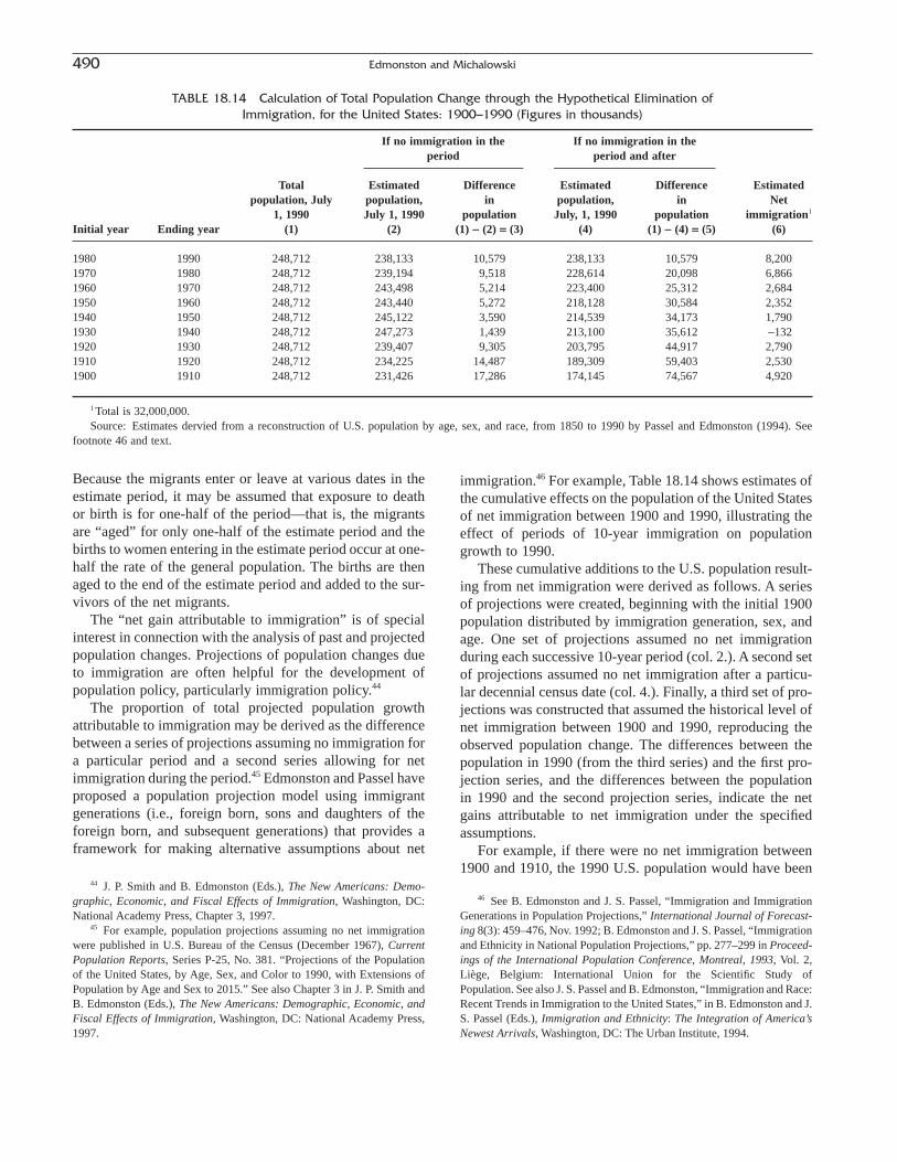
Because the migrants enter or leave at various dates in theestimate period, it may be assumed that exposure to deathor birth is for one-half of the period—that is, the migrantsare “aged” for only one-half of the estimate period and thebirths to women entering in the estimate period occur at one-half the rate of the general population. The births are thenaged to the end of the estimate period and added to the sur-vivors of the net migrants.
The “net gain attributable to immigration” is of specialinterest in connection with the analysis of past and projectedpopulation changes. Projections of population changes dueto immigration are often helpful for the development of population policy, particularly immigration policy.44
The proportion of total projected population growthattributable to immigration may be derived as the differencebetween a series of projections assuming no immigration fora particular period and a second series allowing for netimmigration during the period.45 Edmonston and Passel haveproposed a population projection model using immigrantgenerations (i.e., foreign born, sons and daughters of theforeign born, and subsequent generations) that provides aframework for making alternative assumptions about net
immigration.46 For example, Table 18.14 shows estimates ofthe cumulative effects on the population of the United Statesof net immigration between 1900 and 1990, illustrating theeffect of periods of 10-year immigration on populationgrowth to 1990.
These cumulative additions to the U.S. population result-ing from net immigration were derived as follows. A seriesof projections were created, beginning with the initial 1900population distributed by immigration generation, sex, andage. One set of projections assumed no net immigrationduring each successive 10-year period (col. 2.). A second setof projections assumed no net immigration after a particu-lar decennial census date (col. 4.). Finally, a third set of pro-jections was constructed that assumed the historical level ofnet immigration between 1900 and 1990, reproducing theobserved population change. The differences between thepopulation in 1990 (from the third series) and the first pro-jection series, and the differences between the population in 1990 and the second projection series, indicate the netgains attributable to net immigration under the specifiedassumptions.
For example, if there were no net immigration between1900 and 1910, the 1990 U.S. population would have been
490 Edmonston and Michalowski
44 J. P. Smith and B. Edmonston (Eds.), The New Americans: Demo-graphic, Economic, and Fiscal Effects of Immigration, Washington, DC:National Academy Press, Chapter 3, 1997.
45 For example, population projections assuming no net immigrationwere published in U.S. Bureau of the Census (December 1967), CurrentPopulation Reports, Series P-25, No. 381. “Projections of the Populationof the United States, by Age, Sex, and Color to 1990, with Extensions ofPopulation by Age and Sex to 2015.” See also Chapter 3 in J. P. Smith andB. Edmonston (Eds.), The New Americans: Demographic, Economic, andFiscal Effects of Immigration, Washington, DC: National Academy Press,1997.
TABLE 18.14 Calculation of Total Population Change through the Hypothetical Elimination ofImmigration, for the United States: 1900–1990 (Figures in thousands)
If no immigration in the If no immigration in theperiod period and after
Total Estimated Difference Estimated Difference Estimatedpopulation, July population, in population, in Net
1, 1990 July 1, 1990 population July, 1, 1990 population immigration1
Initial year Ending year (1) (2) (1) - (2) = (3) (4) (1) - (4) = (5) (6)
1980 1990 248,712 238,133 10,579 238,133 10,579 8,2001970 1980 248,712 239,194 9,518 228,614 20,098 6,8661960 1970 248,712 243,498 5,214 223,400 25,312 2,6841950 1960 248,712 243,440 5,272 218,128 30,584 2,3521940 1950 248,712 245,122 3,590 214,539 34,173 1,7901930 1940 248,712 247,273 1,439 213,100 35,612 -1321920 1930 248,712 239,407 9,305 203,795 44,917 2,7901910 1920 248,712 234,225 14,487 189,309 59,403 2,5301900 1910 248,712 231,426 17,286 174,145 74,567 4,920
1 Total is 32,000,000.Source: Estimates dervied from a reconstruction of U.S. population by age, sex, and race, from 1850 to 1990 by Passel and Edmonston (1994). See
footnote 46 and text.
46 See B. Edmonston and J. S. Passel, “Immigration and ImmigrationGenerations in Population Projections,” International Journal of Forecast-ing 8(3): 459–476, Nov. 1992; B. Edmonston and J. S. Passel, “Immigrationand Ethnicity in National Population Projections,” pp. 277–299 in Proceed-ings of the International Population Conference, Montreal, 1993, Vol. 2,Liège, Belgium: International Union for the Scientific Study of Population. See also J. S. Passel and B. Edmonston, “Immigration and Race:Recent Trends in Immigration to the United States,” in B. Edmonston and J.S. Passel (Eds.), Immigration and Ethnicity: The Integration of America’sNewest Arrivals, Washington, DC: The Urban Institute, 1994.
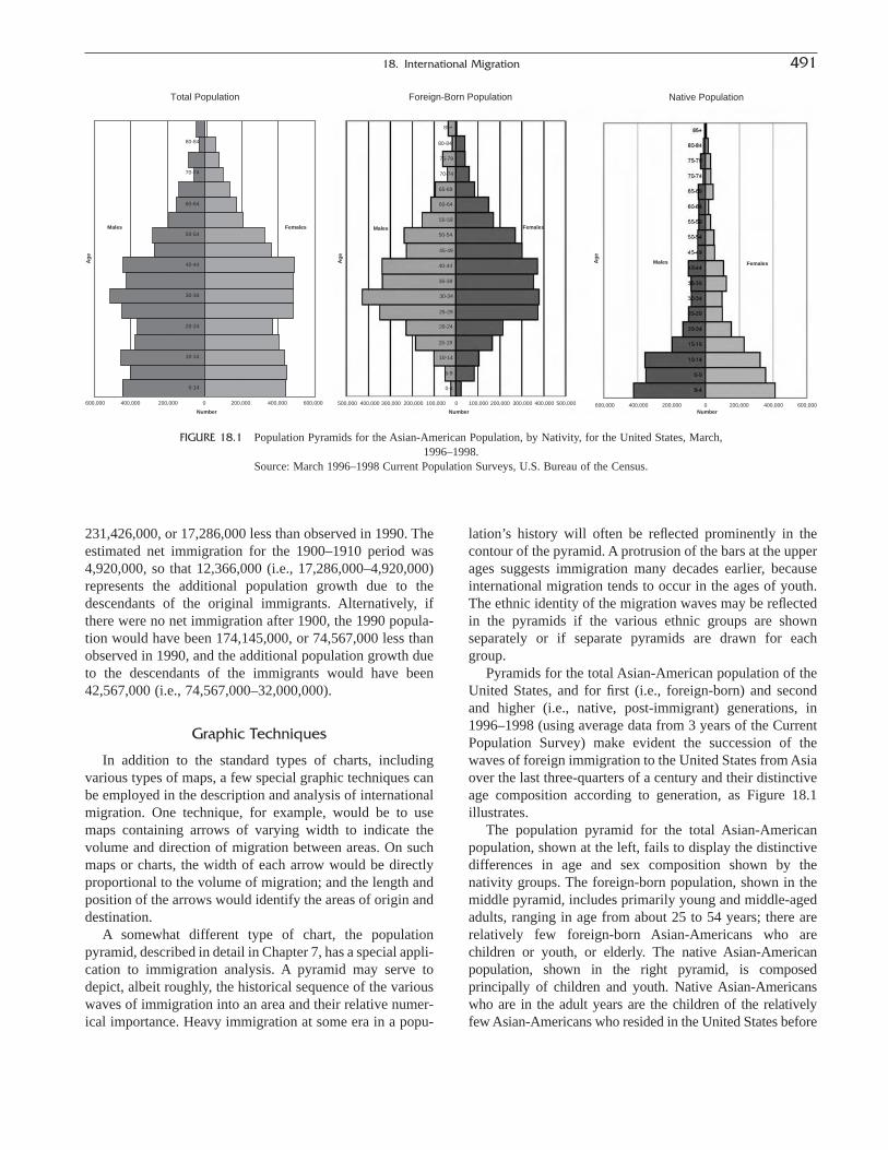
18. International Migration 491
Ag
e
Ag
e
FemalesMales
Males
NumberNumber Number
Females
85+
80-84
75-79
70-74
65-69
60-64
55-59
50-54
45-49
40-44
35-39
30-34
25-29
20-24
15-19
10-14
500,000 500,000 600,000 600,000400,000 400,000200,000 200,000400,000 400,000300,000 300,000200,000 200,000100,000 0 0100,000
5-9
0-4
Males Females
80-84
70-74
60-64
50-54
40-44
30-34
20-24
10-14
0-14
400,000400,000 200,000200,000 0 600,000600,000
Foreign-Born PopulationTotal Population Native PopulationA
ge
FIGURE 18.1 Population Pyramids for the Asian-American Population, by Nativity, for the United States, March,1996–1998.
Source: March 1996–1998 Current Population Surveys, U.S. Bureau of the Census.
231,426,000, or 17,286,000 less than observed in 1990. Theestimated net immigration for the 1900–1910 period was4,920,000, so that 12,366,000 (i.e., 17,286,000–4,920,000)represents the additional population growth due to thedescendants of the original immigrants. Alternatively, ifthere were no net immigration after 1900, the 1990 popula-tion would have been 174,145,000, or 74,567,000 less thanobserved in 1990, and the additional population growth dueto the descendants of the immigrants would have been42,567,000 (i.e., 74,567,000–32,000,000).
Graphic Techniques
In addition to the standard types of charts, includingvarious types of maps, a few special graphic techniques canbe employed in the description and analysis of internationalmigration. One technique, for example, would be to usemaps containing arrows of varying width to indicate thevolume and direction of migration between areas. On suchmaps or charts, the width of each arrow would be directlyproportional to the volume of migration; and the length andposition of the arrows would identify the areas of origin anddestination.
A somewhat different type of chart, the populationpyramid, described in detail in Chapter 7, has a special appli-cation to immigration analysis. A pyramid may serve todepict, albeit roughly, the historical sequence of the variouswaves of immigration into an area and their relative numer-ical importance. Heavy immigration at some era in a popu-
lation’s history will often be reflected prominently in thecontour of the pyramid. A protrusion of the bars at the upperages suggests immigration many decades earlier, becauseinternational migration tends to occur in the ages of youth.The ethnic identity of the migration waves may be reflectedin the pyramids if the various ethnic groups are shown separately or if separate pyramids are drawn for each group.
Pyramids for the total Asian-American population of theUnited States, and for first (i.e., foreign-born) and secondand higher (i.e., native, post-immigrant) generations, in1996–1998 (using average data from 3 years of the CurrentPopulation Survey) make evident the succession of thewaves of foreign immigration to the United States from Asiaover the last three-quarters of a century and their distinctiveage composition according to generation, as Figure 18.1illustrates.
The population pyramid for the total Asian-Americanpopulation, shown at the left, fails to display the distinctivedifferences in age and sex composition shown by the nativity groups. The foreign-born population, shown in themiddle pyramid, includes primarily young and middle-agedadults, ranging in age from about 25 to 54 years; there arerelatively few foreign-born Asian-Americans who are children or youth, or elderly. The native Asian-American population, shown in the right pyramid, is composed principally of children and youth. Native Asian-Americanswho are in the adult years are the children of the relativelyfew Asian-Americans who resided in the United States before

492 Edmonston and Michalowski
about 1960. There are very few elderly Asian Americans; theyare either the children or grandchildren of Asian immigrantswho came to the United States prior to World War II.
Suggested Readings
Akers, D. S. 1967. “Immigration Data and National Population Estimatesfor the United States.” Demography 4(l): 262–272.
Badets, J., and T. Chui. 1994. “Canada’s Changing Immigrant Population”Focus on Canada series. Ottawa, Ontario: Statistics Canada.
Battistella, G., and A. Paganoni (Eds.). 1996. Asian Women in Migration.Manilla, Philippines: Scalabrini Migration Center.
Bean, F., T. J. Espenshade, M. J. White, and R. F. Dymowski. 1990. “Post-IRCA Changes in the Volume and Composition of UndocumentedMigration to the United States: An Assessment Based on ApprehensionsData.” In F. D. Bean, B. Edmonston, and J. S. Passel (Eds.), Undocu-mented Migration to the United States: IRCA and the Experience of the1980s (pp. 111–158). Washington, DC: The Urban Institute.
Bilsborrow, R. E., G. Hugo, A. S. Oberai, and H. Zlotnik. 1997. Interna-tional Migration Statistics: Guidelines for Improving Data CollectionSystems. Geneva, Switzerland: International Labour Office.
Borjas, G. J., and R. B. Freeman (Eds.). 1996. Immigrants and the WorkForce. Chicago: University of Chicago Press.
Bouvier, L. F., and D. Simcox. 1995. “Foreign-Born Professionals in theUnited States.” Population and Environment 16(5): 429–444.
Boyd, M., and M. Vickers. 2000. “100 Years of Immigration in Canada.” Canadian Social Trends 58: 2–12. Ottawa, Ontario: StatisticsCanada.
Bratsberg, B., and D. Terrell. 1996. “Where Do Americans Live Abroad?”International Migration Review 30(3): 788-8-2.
Chiswick, B. R. (Ed.). 1992. Immigration, Language, and Ethnicity. Washington, DC: AEI Press.
Cornelius W. A., P. L. Martin, and J. F. Hollifield (Eds.). 1994. ControllingImmigration. A Global Perspective. Palo Alto, CA: Stanford UniversityPress.
Edmonston, B. (Ed.). 1996. Statistics on U.S. Immigration: An Assessmentof Data Needs for Future Research. Washington, DC: NationalAcademy Press.
Ellis, M., and R. Wright. 1998. “When Immigrants Are Not Migrants:Counting Arrivals of Foreign-Born Using the U.S. Census.” Interna-tional Migration Review 32(1): 127–144.
Espenshade, T. J. 1990. “Undocumented Migration to the United States:Evidence from a Repeated Trials Model.” In F. D. Bean, B. Edmonston,and J. S. Passel (Eds.), Undocumented Migration to the United States:IRCA and the Experience of the 1980s (pp. 159–182). Washington, DC:The Urban Institute.
Fix, M., and J. S. Passel. 1994. Immigration and Immigrants. Setting theRecord Straight. Washington, DC: The Urban Institute.
Gibson, C. J., and E. Lennon. 1999. Historical Census Statistics on theForeign-Born Population of the United States: 1850 to 1990. Popula-tion Division Working Paper No. 29. Washington, DC: U.S. Bureau ofthe Census.
Halli, S. S., and L. Driedger (Eds.). 1999. Immigrant Canada: Demo-graphic, Economic and Social Challenges. Toronto, Ontario: Univer-sity of Toronto Press.
Hill, K. 1985. “Indirect Approaches to Assessing Stocks and Flows ofMigrants.” In D. B. Levine, K. Hill, and R. Warren (Eds.), ImmigrationStatistics: A Story of Neglect (pp. 205–224). Washington, DC: NationalAcademy Press.
Jasso, G., and M. Rosenzweig. 1990. The Chosen People: Immigrants inthe United States. New York: Russell Sage Foundation.
Kritz, M. M., L. L. Lim, and H. Zlotnik. 1992. “International MigrationSystem—A Global Approach.” Oxford, UK: Oxford University Press.
Lee, S. M. 1998. “Asian-Americans: Diverse and Growing.” PopulationBulletin 53(2), June. Washington, DC: Population Reference Bureau.
Lowell, B. L. (Ed.). 1996. Temporary Migrants in the United States. Washington, DC: U.S Commission on Immigration Reform.
Martin, P. L., and E. Midgley. 1999. “Immigration to the United States,”Population Bulletin 54(2), June. Washington, DC: Population Refer-ence Bureau.
Massey, D., D. Arango, G. Hugo, A. Kouaouci, A. Pellegrino, and J. E.Toylor. 1993. “Theories of International Migration: A Review andAppraisal.” Population and Development Review 19(3): 431–465.
Michalowski, M. 1992. “The Dynamics of Recent South-North Flows of Temporary Workers: A Canadian Case Study.” In Peopling of theAmericas (vol. 2, pp. 255–277). IUSSP, Vera Cruz, Mexico.
Michalowski, M. 1996. “Visitors and Visa Workers: Old Wine in NewBottles?” In A. B. Simmons (Ed.), International Migration, RefugeeFlows and Human Rights in North America—The Impact of Trade andRestructuring. New York: Center for Migration Studies.
Organisation for Economic Co-operation and Development. 1997. Trendsin International Migration: Continuous Reporting System on Migra-tion, Annual Report 1996. Paris: OECD.
Portes, A. 1997. “Immigration Theory for a New Century: Some Problemsand Opportunities.” International Migration Review 31(4): 799–825.
Rudolph, C. W. 1999. (Ed.). “Reconsidering Immigration in an IntegratingWorld.” Journal of International Law and Foreign Affairs 3(2).
Sloan, J., and S. Kennedy. 1992. Temporary Movements of People to andfrom Australia. Canberra, Australia: Bureau of Immigration Research.
Simmons, A. B. (Ed.). 1996. International Migration, Refugee Flows andHuman Rights in North America: The Impact of Free Trade andRestructuring. New York: Center for Migration Studies.
United Nations. 1998. Population Distribution and Migration.ST/ESA/SER.R/133. New York: United Nations.
United Nations. 1998. Recommendations on Statistics of InternationalMigration. Revision 1, ST/ESA/STAT/SER.M/58/REV.1. New York:United Nations.
United Nations. 1998. World Population Monitoring 1997. Inter-national Migration and Development. Population Division(ST/ESA/SER.A/169). New York: United Nations.
United Nations High Commission for Refugees (UNHCR). 2000. The Stateof the World’s Refugees. London: Oxford University Press.
U.S. Bureau of the Census and Statistics Canada. 1992. “Migration betweenthe United States and Canada.” Current Population Reports, P-23, No.161. Washington, DC: U.S. Bureau of the Census.
U.S. Immigration and Naturalization Service. 2000. Statistical Yearbook ofthe Immigration and Naturalization Service, 1998. Washington, DC:U.S. Government Printing Office.
U.S. Immigration and Naturalization Service and U.S. Department ofLabor. 1999. The Triennial Comprehensive Report on Immigration.Washington, DC: U.S. Government Printing Office.
Woodrow, K., and J. S. Passel. 1987. “Preliminary Estimates of the Undoc-umented Immigration to the United States, 1980–1986: Analysis of theJune 1986 Current Population Survey.” Proceedings of the Social Sta-tistics Section, American Statistical Association, San Francisco, CA.
Zlotnik, H. 1996. “Migration to and from Developing Countries: A Reviewof Past Trends.” In W. Lutz (Ed.), The Future Population of the World:What Can We Assume Today? (pp. 229–335). Laxenburg, Austria:IIASA.

Population movement—migratory or local—usually isdeliberate. That makes the presence (or absence) of moversin a place a matter of choice, not chance. The voluntarymovement of people selects distinct types of individualsfrom their origins. Consequently, migration and mobilitytypically affect more than just total numbers of inhabitants.Over time, a population may be changed or transformed aspeople realize their intentions to enter or leave an area. Apopulation’s composition may be altered with respect to age,sex, race, ethnicity, income, education, and other socio-economic characteristics. In California, for example, non-Hispanic whites constituted nearly 80% of the population in1970 but only 50% by 2000, as Hispanics and nonwhitesmigrated in. Primarily through foreign immigration, the Hispanic population rose from 12% of the total populationof the state in 1970 to 31% by 2000; the Asian populationrose from 3% to 12% (see, for example, Gober, 1993). InFlorida, persons 65 years and older rose from 8.6% of thetotal population in 1950 to 17.6% in 2000, principallythrough an ongoing influx of retirees into the state (Smith,Tayman, and Swanson, 2001, p. 135). Sustained out-movement—migration or local residential mobility—candrain away the more youthful, educated, and skilledmembers of the population and leave behind older, undere-ducated, and unskilled adults in an entire subregion like theMississippi Delta or a particular city like St. Louis.
Now as in the past, people continue to migrate for reasonsthat are connected with the workings of national economicand social systems. A characteristic of modern economies isthe quick exploitation of newly developed resources or
knowledge, a process that requires the abandonment of oldenterprises along with the development of new ones. Sucheconomies depend on migration to alter the labor forces oflocalities more quickly than could be accomplished throughnatural increase alone.
Within a nation, mobility rates and migration patterns canvary widely among areas. Wide differences in mobility ratesand migration patterns, and their potential for rapid change,underscore the importance of measuring migration accu-rately and understanding its operation. Data limitations,though, make this a daunting task. The populations of someareas remain stable for long periods, while those of otherschange dramatically. Some places look much as they did ageneration ago, while others have apartment complexesspringing up seemingly overnight in what once were straw-berry fields.
CONCEPTS OF MOBILITY AND MIGRATION
The demographic concept of “mobility” refers to spatial,physical, or geographic movement (as distinct from the sociological concept, which refers to a change in status, e.g.,of occupation). This chapter deals with geographic forms of mobility, not “social mobility.” The term “migration,” asused by demographers, refers to mobility across a relevantpolitical or administrative boundary—a region, state, orcounty, for example—distinguishing it from the more localform of mobility (often termed “residential mobility”)within a particular community. The intended distinction hereis one of both distance and type: Migration refers to movesfrom one “community” to another or, more broadly, long-distance (instead of short-distance) moves (Long, Tucker,and Urton, 1988b).
Although conceptually distinct, migration and localmobility are imperfectly distinguished empirically. “Local
493
C H A P T E R
19
Internal Migration and Short-Distance Mobility1
PETER A. MORRISON, THOMAS M. BRYAN, AND DAVID A. SWANSON
The Methods and Materials of DemographyCopyright 2003, Elsevier Science (USA).
All rights reserved.
1 This chapter contains adaptations of material from Morrison (1975,1977, and 1980), Morrison and Wheeler (1976), and Smith, Tayman, andSwanson (2001), as well as from Shryock, Siegel, and Stockwell (1976).Additional materials were provided by Michael Greenwood and LarryLong.

community” has no precise definition (Zax, 1994). Opera-tionally, moves across state or county lines are almost uni-versally deemed to be migratory, although they may coververy short distances for people living near those lines. Intra-county moves are even more difficult to classify. If a personmoves from one town to another within the same county, orfrom one neighborhood to another within the same town,does that move reflect migration or local mobility? The deci-sion may be made on practical statistical grounds or be arbi-trary. Distinctions between migration and local mobility arecritical for some types of analyses, but not for others (Zax,1994). If, for example, one is developing migration data foruse in a set of population projections, then all moves into orout of the geographic areas to be projected would be definedas migration, regardless of the distance moved, the degreeof change in the living environment, or the size of the area.
In the United States, a change in one’s usual place of re-sidence must involve crossing a county boundary to qualifyas migration. Alternatives such as commuting, or the diurnalmovement between home and workplace, or between homeand school and so on do not qualify as migration. Further, adistinction between international migration and internalmigration is made, as was explained in Chapter 18.
Place of Residence
As noted by Smith et al. (2001, p. 98), the simple ques-tion, “Where do you live?” defies an equally simple answer.In the United States, for example, many retirees are seasonalresidents of several places; itinerant farm workers follow theharvest seasonally from place to place. Further complicat-ing matters, a dual-career couple may consider themselvesa single family but they are really two households if thespouses live and work in different cities, joining each otheronly on weekends. Children of divorced couples may spendalternating weeks or months with each parent. College stu-dents whose parental home is, say, Chicago may reside formost of the school year in Boston, living “away from home.”Itinerant professional baseball players spend much of theyear “moving” from city to city. Where, can we say, do thesepeople live? Moreover, for the places involved (be they aseasonal resort community or a college town), how manyinhabitants are there?
The answers here are consequential because mobility andmigration typically refer to changes in a person’s place ofusual residence (Smith et al., 2001, pp. 99–100). Because ofthis focus on changes in usual residence, traditional meas-ures of geographic mobility and migration miss commontypes of temporary population movements such as dailycommuting to work, movements between weekday homesand weekend homes, seasonal migration, business trips,vacations, and the sometimes itinerant life on the road ofretired couples in recreational vehicles. Such nonpermanentmoves are numerous but may go uncounted, despite sub-
stantial impacts on both the sending and receiving regions(Behr and Gober, 1982; McHugh, Hogan, and Happel, 1995;Smith, 1989). Because the focus here is on changes in one’splace of usual residence, temporary and seasonal mobility,although important, lies beyond the scope of this chapter.
Alternatively, some minimum-distance threshold mightdefine those moves to be classified as “migration,” but otherdifficulties may then arise. Respondents may err in report-ing the distance of their moves; or the distance assigned toa move may require information on longitudes and latitudes.In any case, distance alone is an imperfect metric for distinguishing migratory moves. Permanently migrating 60 miles from one community in Rhode Island to anothercommunity in Massachusetts may differ altogether fromdaily commuting 60 miles each way from home to workwithin Los Angeles County, California.
As a practical matter, the migrant is defined operationallyas a mover who changes her or his administrative area ofusual residence. The area may be the primary, secondary, oreven tertiary division in a country. The name of the specificadministrative area of prior residence usually is recorded aswell. With this information, migrants can be characterizedaccording to whether or not the move was also betweenhigher levels of administrative (or statistical) areas. Forexample, if migrants in India are defined as movers betweendifferent districts, interstate migrants and interregionalmigrants can also be distinguished (the latter being definedas migrants between two natural regions).
Defining a migrant as a mover between two administra-tive areas honors the concept of a change in environment ormilieu, albeit crudely. One administrative area or region maydiffer culturally from another, as in India, where states aredistinguished primarily by the different languages theirinhabitants speak.
Length of Migration Interval
Given the basic definition of a migrant as a person whosecurrent place of residence is different from an earlier placeof residence, some choice has to be made as to the length ofthe time interval for which the change in residence isreported. National statistical offices traditionally use either1- or 5-year intervals for developing migration statistics (U. S. Census Bureau/Long and Boertlein, 1990a). Migra-tion data covering different intervals simply reflect differentaspects of the migration process and the actual sequences of moves people undertake (elaborated in DaVanzo andMorrison, 1981, 1982; DaVanzo, 1983). Consider a 1995resident of Dallas, Texas, who moved to Houston in 1996,then to Boston in 1998, then back to Houston in 1999. With annual surveys, a succession of short (e.g., annual)migration intervals would discern all three moves. However,the response to the retrospective question, “Where did youlive five years ago?” asked in 2000 in Houston would
494 Morrison, Bryan, and Swanson
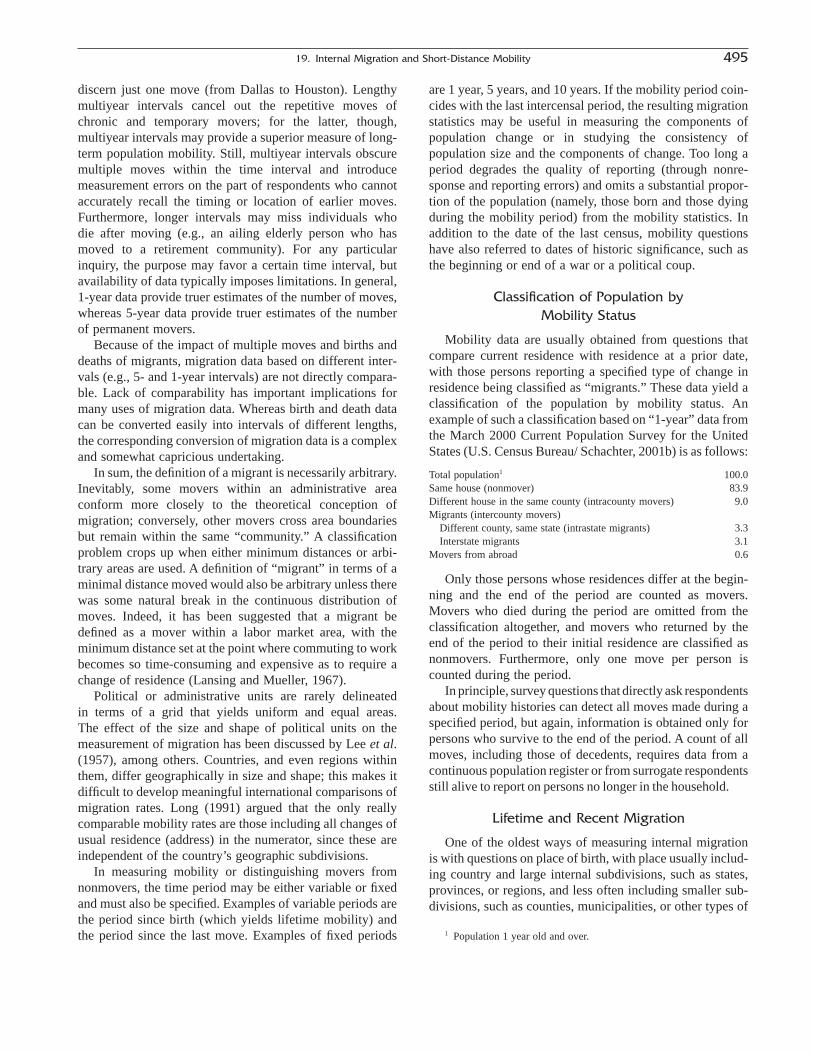
discern just one move (from Dallas to Houston). Lengthymultiyear intervals cancel out the repetitive moves ofchronic and temporary movers; for the latter, though, multiyear intervals may provide a superior measure of long-term population mobility. Still, multiyear intervals obscuremultiple moves within the time interval and introduce measurement errors on the part of respondents who cannotaccurately recall the timing or location of earlier moves. Furthermore, longer intervals may miss individuals who die after moving (e.g., an ailing elderly person who hasmoved to a retirement community). For any particularinquiry, the purpose may favor a certain time interval, butavailability of data typically imposes limitations. In general,1-year data provide truer estimates of the number of moves,whereas 5-year data provide truer estimates of the numberof permanent movers.
Because of the impact of multiple moves and births anddeaths of migrants, migration data based on different inter-vals (e.g., 5- and 1-year intervals) are not directly compara-ble. Lack of comparability has important implications formany uses of migration data. Whereas birth and death datacan be converted easily into intervals of different lengths,the corresponding conversion of migration data is a complexand somewhat capricious undertaking.
In sum, the definition of a migrant is necessarily arbitrary.Inevitably, some movers within an administrative areaconform more closely to the theoretical conception of migration; conversely, other movers cross area boundariesbut remain within the same “community.” A classificationproblem crops up when either minimum distances or arbi-trary areas are used. A definition of “migrant” in terms of aminimal distance moved would also be arbitrary unless therewas some natural break in the continuous distribution ofmoves. Indeed, it has been suggested that a migrant bedefined as a mover within a labor market area, with theminimum distance set at the point where commuting to workbecomes so time-consuming and expensive as to require achange of residence (Lansing and Mueller, 1967).
Political or administrative units are rarely delineated in terms of a grid that yields uniform and equal areas. The effect of the size and shape of political units on themeasurement of migration has been discussed by Lee et al.(1957), among others. Countries, and even regions withinthem, differ geographically in size and shape; this makes itdifficult to develop meaningful international comparisons ofmigration rates. Long (1991) argued that the only reallycomparable mobility rates are those including all changes ofusual residence (address) in the numerator, since these areindependent of the country’s geographic subdivisions.
In measuring mobility or distinguishing movers fromnonmovers, the time period may be either variable or fixedand must also be specified. Examples of variable periods arethe period since birth (which yields lifetime mobility) andthe period since the last move. Examples of fixed periods
are 1 year, 5 years, and 10 years. If the mobility period coin-cides with the last intercensal period, the resulting migrationstatistics may be useful in measuring the components ofpopulation change or in studying the consistency of population size and the components of change. Too long aperiod degrades the quality of reporting (through nonre-sponse and reporting errors) and omits a substantial propor-tion of the population (namely, those born and those dyingduring the mobility period) from the mobility statistics. Inaddition to the date of the last census, mobility questionshave also referred to dates of historic significance, such asthe beginning or end of a war or a political coup.
Classification of Population by Mobility Status
Mobility data are usually obtained from questions thatcompare current residence with residence at a prior date,with those persons reporting a specified type of change inresidence being classified as “migrants.” These data yield aclassification of the population by mobility status. Anexample of such a classification based on “1-year” data fromthe March 2000 Current Population Survey for the UnitedStates (U.S. Census Bureau/ Schachter, 2001b) is as follows:
Total population1 100.0Same house (nonmover) 83.9Different house in the same county (intracounty movers) 9.0Migrants (intercounty movers)
Different county, same state (intrastate migrants) 3.3Interstate migrants 3.1
Movers from abroad 0.6
Only those persons whose residences differ at the begin-ning and the end of the period are counted as movers.Movers who died during the period are omitted from theclassification altogether, and movers who returned by theend of the period to their initial residence are classified asnonmovers. Furthermore, only one move per person iscounted during the period.
In principle, survey questions that directly ask respondentsabout mobility histories can detect all moves made during aspecified period, but again, information is obtained only forpersons who survive to the end of the period. A count of allmoves, including those of decedents, requires data from acontinuous population register or from surrogate respondentsstill alive to report on persons no longer in the household.
Lifetime and Recent Migration
One of the oldest ways of measuring internal migrationis with questions on place of birth, with place usually includ-ing country and large internal subdivisions, such as states,provinces, or regions, and less often including smaller sub-divisions, such as counties, municipalities, or other types of
19. Internal Migration and Short-Distance Mobility 495
1 Population 1 year old and over.

localities. Such questions were originally asked in censusesbut sometimes are included in surveys. They are said to offermeasures of “lifetime” mobility because they enable theanalyst to determine the difference between the place wherepeople were born and the place where they lived at the time of the census or survey. Since the questions usuallyrefer to large geographical areas, the resulting data reflectmoves that cover considerable distances.
Surveys often focus on more recent moves, asking “Didyou live at this street address on this date 1 year ago?” (or5 years ago or some other interval). Those answering no areasked whether the move crossed some significant boundary(e.g., a county or state line) or to name the locality of resi-dence 1 year earlier. Although survey sample sizes are rarelylarge enough to show gross flows for any but the most populous geographical units, knowing locality of residenceat the survey date and 1 year earlier can reveal the distancemoved or the type of move (e.g., rural to urban, metropoli-tan to nonmetropolitan, central city to suburbs).
Table 19.1 illustrates both types of data, as derived fromthe Census 2000 Supplementary Survey for the UnitedStates. Column 1 shows the percentage of the population ofeach state living in their state of birth. The percentage notliving in their state of birth includes people born in anotherU.S. state or the District of Columbia, or born outside the50 states and the District of Columbia. Column 2 from thesame survey shows the percentage of each state’s popula-tion living in a different residence at the time of the surveythan 1 year earlier. The illustration in column 2 of recent,mostly local, moves contrasts with the measure in column 1of “lifetime” moves from one state to another—usually, butnot always, over significant distances.
States vary more on the born-in-state-of-residencemeasure than on the residential mobility rate. The percent-age of the population not living in their state of birth variedby a factor greater than three and a half (from a high of77.0% in Nevada to a low of 21.6% in Louisiana). One-yearresidential mobility rates varied by a factor of just over 2(from 23.7% in Nevada to 11.1% in New York). Movingfrom one dwelling to another in a year’s time occurs rou-tinely everywhere, whereas departing from one’s state ofbirth may vary widely across states. Lifetime interstatemigration, measured in this way, represents a longer andmore difficult move than simply changing residence locally,although some interstate moves, especially when a metro-politan area overlaps state boundaries, cover short distancesand in reality constitute “residential mobility.”
The percentage of a state’s population that was born inthat state reflects the proclivity of natives of the state to leaveit and the propensity of non-natives of the state to move intoit. States like Louisiana and Pennsylvania, a high percent-age of whose residents live in their state of birth, typicallyhave experienced significant outmigration of youth and“aging in place” of the population that remained. By
496 Morrison, Bryan, and Swanson
TABLE 19.1 U.S. States Ranked by Percentage of Popula-tion Living in State of Birth, and Percentage Not Living in
Same Residence as 12 Months Earlier: 2000
Percentage of Percentage (agedpopulation 1+) who changed
living in state residence inState of birth past 12 months
Louisiana 78.4 16.1Pennsylvania 78.3 11.6Michigan 74.6 14.7Mississippi 74.3 15.9Ohio 74.2 14.4Iowa 74.0 15.6Alabama 73.9 15.1West Virginia 73.7 12.8Kentucky 73.5 15.3North Dakota 72.6 16.0Indiana 71.7 16.2Wisconsin 71.6 15.6Minnesota 69.9 13.4Maine 67.8 12.8Nebraska 67.4 17.8South Dakota 66.6 15.9Missouri 66.2 17.9Illinois 65.8 15.5New York 65.6 11.1Massachusetts 65.5 13.1North Carolina 63.5 16.7Utah 63.3 18.2Tennessee 63.0 17.6Rhode Island 62.6 12.9Oklahoma 62.3 18.3Arkansas 61.4 17.8Kansas 61.3 17.0Texas 61.3 18.7South Carolina 59.2 15.7Georgia 58.9 17.8Connecticut 57.1 13.7Montana 56.8 15.9Hawaii 56.6 16.8Vermont 55.3 14.3New Jersey 52.9 12.1New Mexico 51.3 17.5Virginia 50.8 14.3California 50.6 16.6Delaware 50.0 15.2Idaho 49.9 17.5Maryland 49.0 15.0Washington 47.5 20.1Oregon 45.8 20.9Dist. Of Columbia 43.5 17.6New Hampshire 43.4 14.9Wyoming 41.4 19.5Colorado 41.1 21.1Alaska 37.6 22.1Arizona 33.9 21.3Nevada 23.0 23.7
Source: U.S. Census Bureau, Census 2000 Supplementary Survey,available at www.census.gov.

contrast, states like Nevada, Arizona, and Alaska, with lowpercentages of the resident population born in the state, typ-ically have experienced considerable inmigration. Thatinflux often consists of younger people leaving their state ofbirth but may also include retirees attracted by a favorableclimate or other amenities.
States also vary considerably according to the othermeasure—the percentage who move from one dwelling unitto another in the 12 months prior to answering the ques-tionnaire. We mentioned above the 2-to-1 ratio of Nevada’s12-month residential mobility rate to New York’s rate. Ingeneral, the states with the lowest percentage of populationliving in its state of birth exhibited high rates of residentialmobility (i.e., moves in the preceding 12 months), so thatsome association exists between the two measures on thestate level. The association is not perfect, however. NewYork State, the state with the lowest rate of residentialmobility, ranked 19th according to the percentage living instate of birth. Louisiana, the state with the highest percent-age of residents born in the state, had a residential mobilityrate that exceeded the rates in many other states.
The two measures in the table illustrate “long term” and“recent” conceptualizations of internal migration. When bothmeasures are derived from the same data set (e.g., a particu-lar census), their utility can be expanded by combining themto show recent flows that represent people (1) leaving theirstate of birth, (2) returning to their state of birth, and (3)making repeat (or onward) moves, as represented by peoplewho moved from one state to another in the most recentperiod but were neither moving to nor from their state ofbirth. This approach has most often been applied with censusdata on state or province of birth and state or province of residence 5 years previously, but on occasion 1-year datahave been used as well (Newbold, 1997).
International Comparisons of Spatial Mobility
Analyses of most demographic subjects have featuredinternational comparisons, and sustained efforts have been made to achieve greater international comparability inmeasures of analysis. In contrast, comparisons of countriesin terms of “mobility propensity” have been rare. Measur-ing movement across spatial units of different sizes createsinsurmountable problems of translating one country’smigration-defining geographic units into another’s—forexample, U.S. counties into Swiss cantons or Japanese prefectures.
An alternative to developing such a conversion algorithmis to focus on the second measure shown in Table 19.1, themeasure of residential mobility. The percentage of the popu-lation that changes usual residence in 1 year is insensitiveto the spatial differences in migration-defining units and thuscan provide a measure of total mobility that is internation-ally comparable, as is shown in Table 19.2.
Table 19.2 reveals considerable variability in residentialmobility rates among the 14 countries shown, ranging fromannual rates of 6.1% in Ireland to 17 to 18% in Australia,the United States, and Canada. These differences tend toprevail among large geographic areas within each of thecountries (Long, 1991). That is, the differences cannot beattributed to very rapidly growing areas with high popula-tion turnover. (See the rates for Nevada in Table 19.1.)
Nor can the differences be attributed to varying age composition. Because mobility rates are high among youngadults, countries with older populations might be expectedto have lower rates of moving (U.S. Census Bureau/Schachter, 2001a). The differences revealed in Table 19.2tend to persist across age groups, although differences aresomewhat greater at young-adult ages and less at the oldestage categories (Long, 1992). The diminished differences inresidential mobility of the very old reflects the fact that atthese age groups increasing frailty and moves to children’shomes or group homes account for considerable mobilityand are fairly uniform forces among the developed countriesshown in Table 19.2.
The greater differences among countries in the residen-tial mobility rates of young adults presumably reflect greatervariability in the life cycle events that typically govern thetiming of leaving home, progress in school attainment ortraining beyond the compulsory ages, and opportunities toenter the labor force and set up independent households. Dif-ferent rates of moving at other age groups may reflect theliquidity and fluidity in labor and housing markets and othercountry-specific conditions. The differences shown in Table19.2 appear to reflect national policies, practices, andperhaps customs that constitute pervasive influences on theoverall rates of moving. Data for earlier years suggest strongpersistence of differences among countries in rates of resi-dential mobility (Long, 1991). Other evidence, too, suggests
19. Internal Migration and Short-Distance Mobility 497
TABLE 19.2 Percentage of the Population Changing UsualResidence in 1 Year, for Selected Countries: Around 1981
Country Percentage who moved
Ireland 6.1Belgium 7.3Austria 7.6Netherlands 7.7France 9.4Japan 9.5Sweden 9.5Great Britain 9.6Israel 11.3Switzerland 13.7Hong Kong 14.6Australia 17.0United States 17.5Canada 18.0
Source: Official documents identified in Long (1991).

relative stability of annual rates of residential mobility, withonly limited sensitivity to relatively modest business-cyclechanges (Long, 1988).
The residential mobility concept lumps internal migra-tion with short-distance mobility. There is no direct way ofseparating the two in a way that permits international com-parisons except by measuring distance moved. This can beaccomplished by asking people how far they move or bymeasuring the distance from very small areas like postaldelivery zones. The United States has used the formerapproach, finding relatively modest rounding of distancesmoved. Britain has used the latter approach, and a few othercountries have calculated distance moved for moversbetween localities by employing centroids of locality oforigin and locality of destination. There is some evidencethat differences among countries are greater among “localmovers” than at longer distances (Long, Tucker, and Urton,1988a).
Gross and Net Migration
Gross migration is the movement of people into and out of an area; net migration is the difference between thetwo. For a nation as a whole, disregarding immigration,inmigration equals outmigration, so net internal migration iszero. The distinction between gross and net migration hasincreasing analytic and practical significance at more locallevels, for several reasons.
First, there are no “net migrants,” only people who move.To understand, for example, New York’s level of net out-migration between 1985 and 1990 of 0.8 million meansaccounting for the decisions behind the moves of 2.3 millionpeople coming to or moving away from that state during thisperiod (U.S. Census Bureau, 1995). Sometimes, the volumeof net migration is deceptively small, as with metropolitanAlbuquerque, New Mexico, during the 1960s. This metro-politan area’s 1970 population of about a third of a millionincluded a gain of just 22 “net migrants” since 1960. Thisnet figure reveals little or nothing of what went on in Albu-querque: In a typical year throughout the decade, some 44thousand people—more than one-sixth of the population—moved to the metropolitan area, replacing about the samenumber who left for other areas (Morrison and Wheeler,1976).
Second, whatever level of net migration an area registers,the larger gross migratory exchange of individuals involvedmay well reshape the composition of its resident population.At one extreme, for example, is the 1970s genre of energyboom towns in the Rocky Mountain and Northern GreatPlains states (e.g., Gillette, Wyoming, or Colstrip, Montana).Such “instant cities” typically attracted a largely male pop-ulation motivated by personal gain to sites possessing fewof the standard prerequisites for urban greatness (Morrison,1977).
As another example, in the early 1990s, data on California’s driver’s license-address-change program sug-gested an increasing migratory exodus from the state and adeclining influx of newcomers, making California a netexporter of population to other states. These gross comingsand goings signaled, however, that a fundamental, perhapsnecessary, generational change was under way that wasreshaping the state’s workforce. Nearly one of every twoadults moving to California from another state was underage 30, whereas one of every four adults moving out of statewas over age 45. These contrasting age profiles of arrivingand departing migrants are no accident. They reveal in parta rebalancing of labor supply with demand, as aerospacemanufacturing waned and the state adapted to a changingfuture tied partly to its Pacific Rim access. They may alsoreflect the effect of “white flight” as many white native Californians decided to abandon their homes before the“invasion” by foreign migrants.
Third, the distinction between gross and net migrationhas important practical implications, especially in newlygrowing areas. Nineteenth-century Oregonians were said tooffer an occasional prayer: “We thank the goodness and thegrace / That brought us to this lovely place/And now withall our hearts we pray/ That other folks will stay away.” Acentury later, affected communities sought to impose localpopulation “ceilings” or enact other measures to controlmigratory influx. In attempting to control its growth, does acommunity abridge the freedom of outsiders to move in if,indeed, a continuing procession of people come and go? Itmay be argued that zero net migration, even if deliberatelyinduced, does not necessarily abridge the right of access to a community so long as residents continually depart(Morrison, 1977).
Table 19.3 shows in-, out-, and net migration for everystate and the District of Columbia between 1985 and 1990.These numbers refer strictly to internal migrants, or peoplemoving from one state to another within the United States.Although the decennial census also collects data on immi-gration from abroad, it does not collect data on emigrationto foreign countries. This precludes the possibility of calcu-lating overall net migration estimates for states (or any otherregions), reflecting both internal and international migration,on the basis of decennial census data only.
International and Internal Migration
As noted in Chapter 18, it is useful to distinguish inter-national (or foreign) and internal (or domestic) migration.International migration refers to moves from one country toanother, whereas internal migration refers to moves fromone place to another within a particular country. The datashown in Table 19.3 refer solely to internal migrants.Although internal migration typically is the more dominantof the two types of movement in subnational population
498 Morrison, Bryan, and Swanson
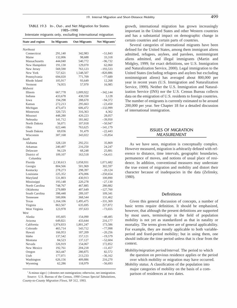
growth, international migration has grown increasinglyimportant in the United States and other Western countriesand has a substantial impact on demographic change incertain countries and certain parts of countries.
Several categories of international migrants have beendefined for the United States, among them immigrant aliensadmitted, refugees, asylees, and parolees, nonimmigrantaliens admitted, and illegal immigrants (Martin andMidgley, 1999; for exact definitions, see U.S. Immigrationand Naturalization Service, 2000). Legal immigration to theUnited States (including refugees and asylees but excludingnonimmigrant aliens) has averaged about 800,000 per year in recent years (U.S. Immigration and NaturalizationService, 1999). Neither the U.S. Immigration and Natural-ization Service (INS) nor the U.S. Census Bureau collectsdata on the emigration of U.S. residents to foreign countries.The number of emigrants is currently estimated to be around200,000 per year. See Chapter 18 for a detailed discussionof international immigration.
ISSUES OF MIGRATIONMEASUREMENT
As we have seen, migration is conceptually complex.However measured, migration is arbitrarily defined with ref-erence to distance, time intervals, geographic boundaries,permanence of moves, and notions of usual place of resi-dence. In addition, conventional measures may understatethe true extent of migration and mobility and distort theircharacter because of inadequacies in the data (Zelinsky,1980).
Definitions
Given this general discussion of concepts, a number ofbasic terms require definition. It should be emphasized,however, that although the present definitions are supportedby most users, terminology in the field of population mobility is not yet as standardized as that in natality or mortality. The terms given here are of general applicability.For example, they are mostly applicable to both variable-period and fixed-period mobility; but in using them, oneshould indicate the time period unless that is clear from thecontext.
Mobility/migration period/interval. The period to whichthe question on previous residence applies or the periodover which mobility or migration may have occurred.
Mobility status. A classification of the population intomajor categories of mobility on the basis of a com-parison of residences at two dates.
19. Internal Migration and Short-Distance Mobility 499
TABLE 19.3 In-, Out-, and Net Migration for States:1985–1990
Interstate migrants only, excluding international migration
State and region In-Migrants Out-Migrants Net Migrants1
NortheastConnecticut 291,140 342,983 -51,843Maine 132,006 98,688 33,318Massachusetts 444,040 540,772 -96,732New Hampshire 191,130 129,070 62,060New Jersey 569,590 763,123 -193,533New York 727,621 1,548,507 -820,886Pennsylvania 694,020 771,709 -77,689Rhode Island 105,917 93,649 12,268Vermont 74,955 57,970 16,985
MidwestIllinois 667,778 1,009,922 -342,144Indiana 433,678 430,550 3,128Iowa 194,298 288,670 -94,372Kansas 272,213 295,663 -23,450Michigan 473,473 606,472 -132,999Minnesota 320,725 316,363 4,362Missouri 448,280 420,223 28,057Nebraska 141,712 181,662 -39,950North Dakota 56,071 107,018 -50,947Ohio 622,446 763,625 -141,179South Dakota 69,036 91,479 -22,443Wisconsin 307,168 343,022 -35,854
SouthAlabama 328,120 292,251 35,869Arkansas 240,497 216,250 24,247Delaware 94,129 68,248 25,881District of 109,107 163,518 -54,411
ColumbiaFlorida 2,130,613 1,058,931 1,071,682Georgia 804,566 501,969 302,597Kentucky 278,273 298,397 -20,124Louisiana 225,352 476,006 -250,654Maryland 531,803 430,913 100,890Mississippi 193,148 220,278 -27,130North Carolina 748,767 467,885 280,882Oklahoma 279,889 407,649 -127,760South Carolina 398,448 289,107 109,341Tennessee 500,006 368,544 131,462Texas 1,164,106 1,495,475 -331,369Virginia 863,567 635,695 227,872West Virginia 123,978 197,633 -73,655
WestAlaska 105,605 154,090 -48,485Arizona 649,821 433,644 216,177California 1,974,833 1,801,247 173,586Colorado 465,714 543,712 -77,998Hawaii 166,953 187,209 -20,256Idaho 137,542 157,121 -19,579Montana 84,523 137,127 -52,604Nevada 326,919 154,067 172,852New Mexico 192,761 204,218 -11,457Oregon 363,447 280,875 82,572Utah 177,071 213,233 -36,162Washington 626,156 409,886 216,270Wyoming 62,286 118,979 -56,693
1 A minus sign (-) denotes net outmigration; otherwise, net inmigration.Source: U.S. Bureau of the Census, 1990 Census Special Tabulations,
County-to-County Migration Flows, SP 312, 1993.
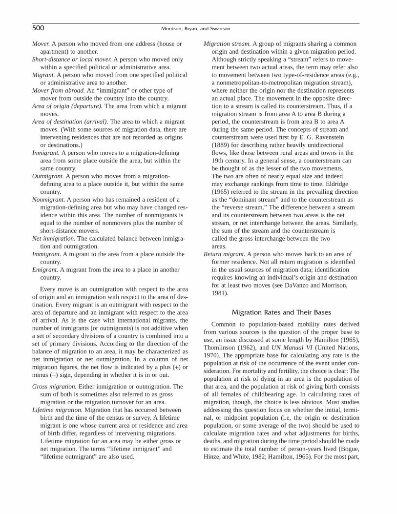
Mover. A person who moved from one address (house orapartment) to another.
Short-distance or local mover. A person who moved onlywithin a specified political or administrative area.
Migrant. A person who moved from one specified politicalor administrative area to another.
Mover from abroad. An “immigrant” or other type ofmover from outside the country into the country.
Area of origin (departure). The area from which a migrantmoves.
Area of destination (arrival). The area to which a migrantmoves. (With some sources of migration data, there areintervening residences that are not recorded as originsor destinations.)
Inmigrant. A person who moves to a migration-definingarea from some place outside the area, but within thesame country.
Outmigrant. A person who moves from a migration-defining area to a place outside it, but within the samecountry.
Nonmigrant. A person who has remained a resident of amigration-defining area but who may have changed res-idence within this area. The number of nonmigrants isequal to the number of nonmovers plus the number ofshort-distance movers.
Net inmigration. The calculated balance between inmigra-tion and outmigration.
Immigrant. A migrant to the area from a place outside thecountry.
Emigrant. A migrant from the area to a place in anothercountry.
Every move is an outmigration with respect to the areaof origin and an inmigration with respect to the area of des-tination. Every migrant is an outmigrant with respect to thearea of departure and an inmigrant with respect to the areaof arrival. As is the case with international migrants, thenumber of inmigrants (or outmigrants) is not additive whena set of secondary divisions of a country is combined into aset of primary divisions. According to the direction of thebalance of migration to an area, it may be characterized asnet inmigration or net outmigration. In a column of netmigration figures, the net flow is indicated by a plus (+) orminus (-) sign, depending in whether it is in or out.
Gross migration. Either inmigration or outmigration. Thesum of both is sometimes also referred to as grossmigration or the migration turnover for an area.
Lifetime migration. Migration that has occurred betweenbirth and the time of the census or survey. A lifetimemigrant is one whose current area of residence and areaof birth differ, regardless of intervening migrations.Lifetime migration for an area may be either gross ornet migration. The terms “lifetime inmigrant” and “lifetime outmigrant” are also used.
Migration stream. A group of migrants sharing a commonorigin and destination within a given migration period.Although strictly speaking a “stream” refers to move-ment between two actual areas, the term may refer alsoto movement between two type-of-residence areas (e.g.,a nonmetropolitan-to-metropolitan migration stream),where neither the origin nor the destination representsan actual place. The movement in the opposite direc-tion to a stream is called its counterstream. Thus, if amigration stream is from area A to area B during aperiod, the counterstream is from area B to area Aduring the same period. The concepts of stream andcounterstream were used first by E. G. Ravenstein(1889) for describing rather heavily unidirectionalflows, like those between rural areas and towns in the19th century. In a general sense, a counterstream can be thought of as the lesser of the two movements. The two are often of nearly equal size and indeed may exchange rankings from time to time. Eldridge(1965) referred to the stream in the prevailing directionas the “dominant stream” and to the counterstream asthe “reverse stream.” The difference between a streamand its counterstream between two areas is the netstream, or net interchange between the areas. Similarly,the sum of the stream and the counterstream is called the gross interchange between the two areas.
Return migrant. A person who moves back to an area offormer residence. Not all return migration is identifiedin the usual sources of migration data; identificationrequires knowing an individual’s origin and destinationfor at least two moves (see DaVanzo and Morrison,1981).
Migration Rates and Their Bases
Common to population-based mobility rates derivedfrom various sources is the question of the proper base touse, an issue discussed at some length by Hamilton (1965),Thomlinson (1962), and UN Manual VI (United Nations,1970). The appropriate base for calculating any rate is thepopulation at risk of the occurrence of the event under con-sideration. For mortality and fertility, the choice is clear: Thepopulation at risk of dying in an area is the population ofthat area, and the population at risk of giving birth consistsof all females of childbearing age. In calculating rates ofmigration, though, the choice is less obvious. Most studiesaddressing this question focus on whether the initial, termi-nal, or midpoint population (i.e, the origin or destinationpopulation, or some average of the two) should be used tocalculate migration rates and what adjustments for births,deaths, and migration during the time period should be madeto estimate the total number of person-years lived (Bogue,Hinze, and White, 1982; Hamilton, 1965). For the most part,
500 Morrison, Bryan, and Swanson

measures of mobility that involve population bases and rates are discussed in the subsection on “Measures Used inAnalysis.”
A measure of the rate of mobility, or the ratio of thenumber of movers in an interval of time to the population atrisk during that interval, is
(19.1)
where
m = the mobility rateM = the number of moversP = the population at riskk = a constant, such as 100 or 1000
For mobility and movers, the more specific terms “migra-tion” and “migrants” may be substituted.
For the country as a whole, this rate measures the overalllevel of mobility or migration. In the case of migration, threeanalogous rates are those of inmigration, outmigration, andnet migration, which are given respectively by
(19.2)
(19.3)
(19.4)
where I and O are the numbers of inmigrants and outmi-grants, respectively. If the migration interval is short, say ayear or less, the initial, final, or average populations all yieldabout the same rates. For a 5-year period, there can be con-siderable difference.
The next choice concerns the area to be used as a base.For outmigration from an area, the population at risk isclearly that of the area itself. For inmigration, however, thepopulation at risk is that of the balance of the country. Thisbase is rarely used, but see Shryock (1964) for illustrations.Mainly as a practical matter, inmigration rates and outmi-gration rates are both based on the destination population.Net migration rates preferably should be the differencebetween in- and outmigration rates that have the same population base. This goal can be achieved also by use ofan average of the origin and destination populations, wherethis is practical, or as suggested later, where lifetime migra-tion is concerned, by an average of the population born inthe state and the population resident in the state.
SOURCES OF DATA AND STATISTICS
Whereas birth and death data are readily available for themore developed countries lacking a continuous populationregister, the same cannot be said for migration data. Theideal migration data set for an area would include data on at least the following (U.S. Census Bureau/Wetrogan andLong, 1990b):
m I O P kn = -( )( )*
m O P ko = ( )*
m I P ki = ( )*
m M P k= ( )*
Origins and destinations of migrantsData available in 1-year age groups and sexData available on an annual basis for a variety of time
periodsData available for a number of geographic levelsData consistent with the relevant population base for cal-
culating migration rates
Ideally, these data would be available for states, counties,and a variety of subcounty areas (Smith et al., 2001, p. 112).Unfortunately, no single data set even comes close tomeeting all of these criteria. In fact, no federal agency in the United States directly tracks population movements,although various European countries with population regis-ters do.
Population Registers
A continuous population register system requires everyperson to transfer his or her record from one local registryoffice to another when moving. Migration statistics are com-piled from these changes of residence. Such statistics havebeen published for many years by the Nordic countries anda few other western European countries, and more recentlyby eastern European and Asian countries as well. Amongsuch countries are Belgium, Denmark, Finland, Hungary,Iceland, Israel, Italy, Japan, Netherlands, Norway, Poland,Singapore, Spain, and Sweden.
Censuses and Surveys
Mobility data derived from censuses and surveys are oftwo broad types. The first type consists of those tabulatedfrom direct questions about mobility or about prior resi-dence—place of birth, place of residence at a fixed past date,duration of residence, last prior residence, mobility history,number of moves, and so on. The second type consists ofestimates of net migration derived from (1) counts of totalpopulation or population disaggregated by age and sex, attwo censuses, and (2) natural increase (births minus deaths)or intercensal survival rates, which are derived in turn from(a) life tables or (b) comparison of the age distributions of countries not experiencing immigration or emigration in successive censuses. The difference between the totalchange in population during an intercensal period and thechange due to natural increase is imputed to net migration.Usually, however, this difference also includes net immi-gration from abroad. These estimates are derived by a resid-ual method and hence are called residual estimates.
Censuses
The most common source of migration data is a regularcensus. Fixed-period-migration data have been collected in every U.S. decennial census since 1940, and lifetime-
19. Internal Migration and Short-Distance Mobility 501

migration data in every U.S. decennial census since 1850.The former data are based on responses to a question askingplace of residence 5 years earlier (except for the 1950census, which asked place of residence 1 year earlier). TheU.S. Census Bureau tabulates in- and outmigration data dis-aggegated by age, sex, and race for all states and counties.
Numerous problems plague migration data from the U.S.decennial census, as described by Smith et al. (2001, p. 113).First, the data cannot gauge the effects of multiple movesduring the 5-year period. For example, a person may havelived in an apartment in Chicago in 1995, moved to a housein the suburbs in 1996, been transferred to a job in Atlantain 1998, and retired to Sarasota in January 2000. Censusmigration data would show only the move from Chicago toSarasota, completely missing the other moves. Data from the decennial census substantially understate the full extentof mobility and migration during a 5-year period (seeDaVanzo and Morrison, 1981; U.S. Census Bureau/Longand Boertlein, 1990a).
A second problem is that the question regarding residence5 years earlier is included only in the long form of the U.S.census questionnaire, which was sent to 15 to 25% of house-holds in the United States (with the proportion varying fromone census to another). This creates problems of data relia-bility, especially for small places and for detailed categoriessuch as age, sex, and race/ethnicity groups (Isserman, Plane,and McMillen, 1982). Reliability of the data is also affectedby the respondent’s lack of knowledge regarding geographicboundaries or inability to remember accurately his or herplace of residence 5 years earlier (U.S. Census Bureau/Wetrogan and Long, 1990b).
A third problem with migration data from the census isthat data covering both in- and outmigration are not avail-able below the county level. Outmigration data present aneven greater problem than inmigration data, because theymust be compiled from questionnaires filled out by ex-residents throughout the country.
Other problems noted by Smith et al. (2001, p. 114)include (1) the inevitable failure of the U.S. decennialcensus to cover emigration to foreign countries, (2) censusundercount problems, and (3) problems of assigning datesto any moves.
Sample Surveys
Considering only sample surveys, the most commonsource of U.S. migration data is the Current PopulationSurvey (CPS). The reader is already familiar with the factthat this survey is conducted by the Census Bureau, coverssome 50,000 households, and is designed primarily to obtainlabor force information. Every March, supplementary ques-tions are asked that include migration. The survey collectsdata on geographic mobility for the United States and itsregions, including data on the characteristics of migrants.
Other federally sponsored surveys that have been used tostudy mobility and migration include the American HousingSurvey (AHS), the Survey of Income and Program Partici-pation (SIPP), and the National Longitudinal Surveys(NLS). These surveys provide data that are useful for manytypes of migration analyses, but generally do not serve as asufficient basis for measuring and analyzing state and localmigration because of small sample sizes and the sampledesigns.
As the reader may also recall, the American CommunitySurvey collects monthly data from a large rolling sample ofhouseholds. Initiated in 1996, as now envisioned it eventu-ally will cover every place in the United States, providingusable data for small places over a 5-year period. Migrationdata in this survey are based on place of residence 1 yearearlier rather than 5 years earlier, with the effect of compli-cating comparisons with migration data from the decennialcensus.
Migration Histories
Almost all specialized types of questions for gatheringmobility data have been limited to surveys. The mostcommon type is the mobility or migration history—a rosterof previous usual residences with the dates of moves. Sucha history may be accompanied by a similar listing of all jobsfor persons of working age. From such histories it is possi-ble to summarize the number of lifetime moves or thenumber of moves in a given period. Such data are sometimesobtained by a simple, direct question, however. Likewise,instead of determining occupation, employment status,marital status, and so on, at a fixed past date from a more-or-less complete history, a direct question referring to thepast date that is central to the study may be employed. Othertopics include permanence of migration, number of house-hold members who moved together, month of migration,reasons for moving, migration plans or intentions, and costof moving.
Migration histories are not limited to national samplesurveys but may come from surveys of specific areas. Sincea relatively small proportion of the population moves fre-quently and repeatedly, the surveys do not usually attemptto record all former residences (or all moves) but only thelast “k” residences and perhaps also the residence at birth.Furthermore, the exact address is usually not recorded butonly the area of residence, and there may be other restric-tions on the information recorded.
Such histories are typically easier to trace in countrieswith population registration systems, such as the Nether-lands. The population statistics of the Netherlands are basedon automated municipal population registers and are com-piled by Statistics Netherlands. Each inhabitant has a uniqueidentification number and is registered in the municipalitywhere he or she lives. When a person dies or emigrates, the
502 Morrison, Bryan, and Swanson

data about them are kept by the municipality of last resi-dence. No data are erased from the system. For example, ifa person moves, the new address is added to the informa-tion already available. The old address is kept as well, butin a historic portion of the personal file (Netherlands, Sta-tistics Netherlands, 1998). This procedure is followed inother population registration systems as well.
Status at Prior Date
To obtain a person’s current characteristics, theresearcher may make use of questions that are a regular partof a general purpose survey. To obtain the characteristics ata past date (i.e., retrospectively), such surveys increasinglyinclude additional questions to elicit that information(DaVanzo, 1982). Recording the respondent’s status prior tomigration provides a basis for measuring differential pro-pensities to migrate and for describing temporal sequences.Pinning down the temporal sequence of events can clarifycausal relationships and help to answer such questions as,did the unemployment of a given worker precede (hencepossibly cause) a recorded move? Or, did a previouslyemployed worker end up jobless after migrating?
One weakness of such retrospective data is the inevitab-ility of response error. Respondents never recollect eventsand their timing with perfect accuracy, and recall accuracydiminishes as elapsed time increases. Recent tests in theUnited States indicate that the number of changes in statusas measured by retrospective questions is considerablyunderestimated. Comparisons of current survey reports withreports of matched persons secured in a decennial census 6years later indicated that the number of shifts in occupationreported in the census was considerably understated. As acorollary, the retrospective description of jobs 6 years earliermust have been subject to considerable response error. Pre-sumably, errors of recall would be fewer for a 1-year period,however. With the advent of large-scale continuous meas-urement devices, such as the American Community Survey,these errors should be reduced and more timely informationon migration patterns produced.
Other facets of mobility covered in surveys includerespondents’ expectations, intentions, or desires to move.Questions on these attitudinal facets of behavior may beevaluated by checking at the end of the reference period todetermine whether or not the respondent who expressed anexpectation, intention, or desire to move in fact did so (i.e.,actually left the former address). In the case of migration (asopposed to merely moving), it would also be necessary toascertain whether the person had also left the county, munic-ipality, and so on. Securing this additional information (byinterviewing other members of the household or neighbors,obtaining postal change-of-address files, etc.) may be feasi-ble but costly.
Residual Estimates
As shown in Table 19.3, estimates of net migration canbe derived from gross migration data by subtracting thenumber of outmigrants from the number of inmigrants.However, gross migration data are not always available. Insuch cases, net migration can be estimated indirectly “dif-ferenary” them as a residual by comparing an area’s popu-lation at two dates, them “differenary”, and removing,allowing for the change due to natural increase. The resid-ual is attributed to net migration. This approach is known asthe indirect or residual method.
Residual estimates require no special questions and maybe computed from population counts disaggregated by age and sex, or even from population totals. The indirectmethods to be discussed in this section are (1) the nationalgrowth-rate method and (2) the residual method comprising(a) the vital statistics method and (b) the survival-ratemethod. The use of place-of-birth statistics is sometimesconsidered an indirect method, but since it requires a specialquestion and since there are some direct measures derivablefrom the data, it will be treated separately in the next majorsection.
National Growth-Rate Method
This is a crude method in which the estimated migrationrate, mi, for area i is given by
(19.5a)
where P1t and P0
t represent the national population at thebeginning and end of the intercensal period, respectively, P0
i
represents the populations of the geographic subdivisions atthe beginning of the period, and P1
i represents their popula-tions at the end of the period.
This rate is customarily multiplied by a constant, such as 100 or 1000. Thus, for a geographic division, a rate ofgrowth greater than the national average is interpreted as netinmigration and a rate less than the national average as netoutmigration. The same procedure can be applied to specificage-sex groups to derive estimates of net migration for birthcohorts. This method yields an estimate of the rate of inter-nal migration for geographic subdivisions on the assumptionthat rates of natural increase and of net immigration fromabroad are the same for all parts of the country. It requiresno vital statistics.
Vital Statistics Method
A simple variant of the preceding method may be usedto obtain a rough indication of the extent of net migrationfor geographic subdivisions by comparing the rate of growth
m P P P P P P ki i i i i t t= -( )[ ] - -( )[ ]{ }*1 0 0 1 0 0
19. Internal Migration and Short-Distance Mobility 503

of each area with the rate of natural increase of the nation.This method assumes that the rate of natural increase is thesame throughout the country.
(19.5b)
where P1i represents the populations of the geographic sub-
divisions at the end of the intercensal period, P0i is the pop-
ulations of the geographic subdivisions at the beginning ofthe period, Bt is the number of births nationally during theintercensal period, and Dt is the number of deaths nationallyduring the intercensal period, so that [(Bt - Dt)/ P0
t ] equalsthe national natural rate of increase during the intercensalperiod.
This formula yields an estimate of the total rate of netmigration, including international migration, rather than thenet internal migration rate. Where net immigration is negli-gible, Formulas (19.5a) and (19.5b) yield the same results(provided the census counts and the vital statistics are consistent).
If a country has reasonably complete vital statistics andif the two successive censuses are about equally complete,then a more refined application of the vital statistics methodis possible. Then the vital statistics method is almost alwaysused to estimate net migration for the total population (i.e.,all age-sex groups combined) of an area within a country.As before, the intercensal component equation is the meansof estimating net migration as a residual with vital statisticsfor each area.
(19.6)
where Mi represents the amount of net migration for area iand the other symbols also refer to area i.
The result is the difference between the total number ofpersons moving into an area during a given intercensalperiod and the number moving out. This estimate of netmigration reflects both the inmigrants and outmigrants whodied before the second census (Siegel and Hamilton, 1952).The net migration obtained for a given area is that withrespect to all other areas and thus represents net internationalmigration combined with net internal migration. Thismethod may be used to estimate net migration for a sex,race, nativity group, or any other group defined by a char-acteristic that is invariant over time, provided that the pop-ulation and vital statistics are available for the characteristic.The main issue concerning the method is not the theoreticalvalidity of Equation (19.6), which represents what Siegeland Hamilton (1952) call “exact net migration,” but ratherthe effect of errors in the terms on the right-hand side of theequation upon the accuracy of the estimate. A further issueis the accuracy of this method as applied to actual statisticsin comparison with that of other methods, such as the survival-rate method (Hamilton, 1966; Siegel and Hamilton,1952; Stone, 1967).
M P P B Di i i i i= -( ) - -( )1 0
m P P P B D P ki i i i t t t= -( )[ ] - -( )[ ]{ }*1 0 0 0
Changes in Area Boundaries
One possible source of error in residual estimates of netmigration is a change in the boundaries of the geographicarea or areas in question. Unless the population figures andthose on natural increase can be adjusted to represent a con-stant area (ordinarily the present rather than the originalarea), the estimates will reflect the population in the trans-ferred territory as well as net migration. If the territory transferred is an entire administrative unit of some sort (for example, a municipality that is transferred from oneprovince to another), the requisite statistics will usually bereadily available. Often, however, the transferred territorydoes not follow any previous legal boundaries. In that case,rough estimates will have to be made, for example, on thebasis of new and old maps, using the land areas involved asa rough indicator of the proportions of an old administrativeunit’s population and vital events that are to be attributed to the new units. The transfer will usually occur during the intercensal period. Vital events for the years after thetransfer will often be on the new geographic basis and willrequire no adjustment. There may be a lag in the geographicassignment of vital events, however. In any case, if the trans-fer occurred during a year and the vital statistics are avail-able for whole years only, a special proration must be madefor the year of transfer.
Exclusion of International Migration
As previously mentioned, any variant of the residualmethod includes in its estimate of net migration the netimmigration from abroad (unless a specific effort is made toremove that component). One approach is to confine thecomputations to the native population. In the case of the vitalstatistics method, this approach requires that the native pop-ulation be available separately from the two censuses andthat deaths also be tabulated by nativity. The inputs andmethod of this approach for calculating net internal migra-tion for a state may be described as follows:
(1) Native population of state at second census(2) Native population of state at first census(3) Total births in intercensal period(4) Deaths of natives in intercensal period
Estimated net migration of the native population to the statefrom other states is given by (1) - (2) - (3) + (4). Asexplained in Chapter 8, “native” means born in the country,not just born in the state. Births are all native by definition,and babies born during the intercensal period are includedin the native population counted at the end of the period(unless they emigrated or died).
The other approach to estimating net internal migrationis to allow directly for net immigration from abroad (by sub-traction). For this purpose, of course, one must know notonly the total immigration but also the area (state, province,
504 Morrison, Bryan, and Swanson

etc.) of intended residence of the immigrants and the area oflast residence of the emigrants. One must assume that immi-grants went to their announced area of destination and thatemigrants departed for abroad from their reported area oflast residence. Note that direct data on emigration are notavailable for the United States and its states and this com-ponent must be estimated.
Other Issues
Because the estimates of net migration represent a re-sidual obtained by subtraction, relatively moderate errors inpopulation counts or in statistics of births or deaths producemuch larger percentage errors in the migration estimates.Fortunately, these errors sometimes offset one another tosome degree. For example, the population counts at the twosuccessive censuses may represent about the same amountof net underenumeration. For the same percentage error,errors in the population statistics have more effect on the estimates of net migration than do errors in the vital statistics.
Although the vital statistics method is adaptable tomaking estimates of net migration for age groups, it is rarelyused for this purpose, mainly because of the effort involvedin both data compilation and calculations. The advent ofcomputer-intensive methods now makes it much more fea-sible to produce estimates in this detail. A detailed accountand evaluation of this method is provided by Hamilton(1967).
Survival-Rate Method
The survival-rate method is the favored variant for sta-tistically less developed countries because it does not requireaccurate vital statistics, which are usually unavailable inthese countries. It is commonly used elsewhere as well,since it is easily implemented and yields estimates of netmigration for age and sex groups without the use of deathsstatistics in this detail. Equation (19.7) provides the basicformula for estimating net migration (Mx
x+t¢) using the survival-rate method.
(19.7)
where Px0 and Pt
x+t represents the population figures at thebeginning and end of the period, respectively, for the cohort,s the survival rate for the cohort, and (the square root of the survival rate) an adjustment for deaths of migrantsduring the period (Siegel, 2002, p. 22).
Two main types of survival rates are used, those from lifetables and those from censuses. The former are derived froma life table, if possible for the same geographic area and timeperiod to which the estimate of net migration applies.Usually, however, for a county or city without an appropriatelife table, one could use a recent life table for its province,its region, or the national population, making the choice on
s
M P sP sxx t
x tt
x+ ¢
+= -( ) ∏0
the basis of available information as to comparative mortal-ity. For a city, for example, the life table for a group of highlyurbanized states might be most appropriate. The census survival rate represents the ratio of the numbers in the samenational cohort at successive censuses. The objective instructuring this rate is to approximate a closed population.This method requires no life table and no vital statistics andhas the advantage of eliminating the effects of some of the errors in the population statistics from the migration estimates.
Like the vital statistics method, the life-table variants ofthe survival-rate method are designed to measure net migra-tion exactly, assuming that there are no errors in the under-lying population and vital statistics and that population andmigrants have the same level of mortality. To close the the-oretical gap between the vital statistics method and the life-table survival-rate method, an allowance has to be made, inthe equation for the latter method, for the deaths of migrantsin the area during the period (deaths of inmigrants afterimmigration and deaths of “outmigrants” before possibleoutmigration). In other words, an adjustment is necessary tomake the number of deaths to residents of a given areaduring a given period from the survival method approxi-mately equivalent to the number of “recorded” deaths—thatis, deaths to “nonmigrants” plus deaths to inmigrants. Thatis the function of the element in the equation.
There are two ways of applying life-table survival rates.In one method, called the forward survival-rate method, theestimate of net migration is obtained as in Equation (19.7).Another way, called the reverse survival-rate method, carriesout the calculations in reverse. Here the survival rate isdivided into the number in the age group at the end of theintercensal period. Thus,
(19.8)
where the symbols have the same meaning as for the forwardequation (Siegel, 2002, p. 22). It can be shown that the two methods give identical results and that the distinctionbetween the two methods is unnecessary—that is, M¢ = M≤:
(19.9)
In practice, the analyst can simply apply the forward formula(Siegel, 2001, p. 22).
In an earlier design of the survival-rate formulas (i.e.,excluding the element ), the forward formula and thereverse formula gave different results because they did notallow exactly for the deaths of migrants during the period,either including deaths of inmigrants over the whole periodor deaths of outmigrants over the whole period (Siegel andHamilton, 1952). It was considered expedient under thesecircumstances to average the results of the two formulas.
s
P sP s
P s s s P s s
P s P s
x tt
x
x tt
x
x tt
x
+
+
+
-( ) ∏= ∏( ) - ∏( ){ } ∏ ∏( )= ∏( ) -{ }
0
0
0
M P s P sxx t
x tt
x0+ ¢¢
+= ∏( ) -{ }
s
19. Internal Migration and Short-Distance Mobility 505
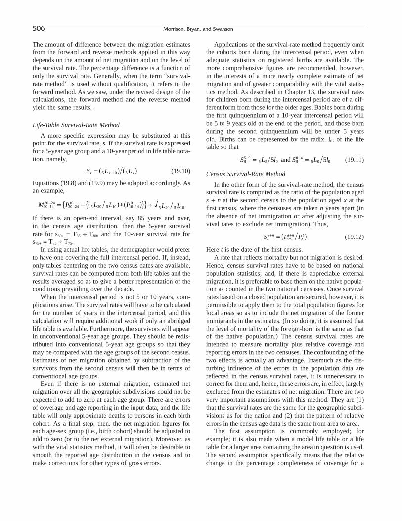
The amount of difference between the migration estimatesfrom the forward and reverse methods applied in this waydepends on the amount of net migration and on the level ofthe survival rate. The percentage difference is a function ofonly the survival rate. Generally, when the term “survival-rate method” is used without qualification, it refers to theforward method. As we saw, under the revised design of thecalculations, the forward method and the reverse methodyield the same results.
Life-Table Survival-Rate Method
A more specific expression may be substituted at thispoint for the survival rate, s. If the survival rate is expressedfor a 5-year age group and a 10-year period in life table nota-tion, namely,
(19.10)
Equations (19.8) and (19.9) may be adapted accordingly. Asan example,
If there is an open-end interval, say 85 years and over, in the census age distribution, then the 5-year survival rate for s80+ = T85 ∏ T80, and the 10-year survival rate for s75+ = T85 ∏ T75.
In using actual life tables, the demographer would preferto have one covering the full intercensal period. If, instead,only tables centering on the two census dates are available,survival rates can be computed from both life tables and theresults averaged so as to give a better representation of theconditions prevailing over the decade.
When the intercensal period is not 5 or 10 years, com-plications arise. The survival rates will have to be calculatedfor the number of years in the intercensal period, and thiscalculation will require additional work if only an abridgedlife table is available. Furthermore, the survivors will appearin unconventional 5-year age groups. They should be redis-tributed into conventional 5-year age groups so that theymay be compared with the age groups of the second census.Estimates of net migration obtained by subtraction of thesurvivors from the second census will then be in terms ofconventional age groups.
Even if there is no external migration, estimated netmigration over all the geographic subdivisions could not beexpected to add to zero at each age group. There are errorsof coverage and age reporting in the input data, and the lifetable will only approximate deaths to persons in each birthcohort. As a final step, then, the net migration figures foreach age-sex group (i.e., birth cohort) should be adjusted toadd to zero (or to the net external migration). Moreover, aswith the vital statistics method, it will often be desirable tosmooth the reported age distribution in the census and tomake corrections for other types of gross errors.
M P L L P L L10 1420 24
20 2410
5 20 5 10 10 140
5 20 5 10--
- -= - ( )*( ){ }{ } ∏
S L Lx x x= ( ) ( )+5 10 5
Applications of the survival-rate method frequently omitthe cohorts born during the intercensal period, even whenadequate statistics on registered births are available. Themore comprehensive figures are recommended, however, in the interests of a more nearly complete estimate of netmigration and of greater comparability with the vital statis-tics method. As described in Chapter 13, the survival ratesfor children born during the intercensal period are of a dif-ferent form from those for the older ages. Babies born duringthe first quinquennium of a 10-year intercensal period willbe 5 to 9 years old at the end of the period, and those bornduring the second quinquennium will be under 5 years old. Births can be represented by the radix, l0, of the lifetable so that
(19.11)
Census Survival-Rate Method
In the other form of the survival-rate method, the censussurvival rate is computed as the ratio of the population agedx + n at the second census to the population aged x at thefirst census, where the censuses are taken n years apart (inthe absence of net immigration or after adjusting the sur-vival rates to exclude net immigration). Thus,
(19.12)
Here t is the date of the first census. A rate that reflects mortality but not migration is desired.
Hence, census survival rates have to be based on nationalpopulation statistics; and, if there is appreciable externalmigration, it is preferable to base them on the native popula-tion as counted in the two national censuses. Once survivalrates based on a closed population are secured, however, it ispermissible to apply them to the total population figures forlocal areas so as to include the net migration of the formerimmigrants in the estimates. (In so doing, it is assumed thatthe level of mortality of the foreign-born is the same as thatof the native population.) The census survival rates areintended to measure mortality plus relative coverage andreporting errors in the two censuses. The confounding of thetwo effects is actually an advantage. Inasmuch as the dis-turbing influence of the errors in the population data arereflected in the census survival rates, it is unnecessary tocorrect for them and, hence, these errors are, in effect, largelyexcluded from the estimates of net migration. There are twovery important assumptions with this method. They are (1)that the survival rates are the same for the geographic subdi-visions as for the nation and (2) that the pattern of relativeerrors in the census age data is the same from area to area.
The first assumption is commonly employed; forexample; it is also made when a model life table or a lifetable for a larger area containing the area in question is used.The second assumption specifically means that the relativechange in the percentage completeness of coverage for a
S P Pxx n
x nt n
xt+
++= ( )
S L l S L lB B and 5 95 5 0
0 45 0 05 5- -= =
506 Morrison, Bryan, and Swanson
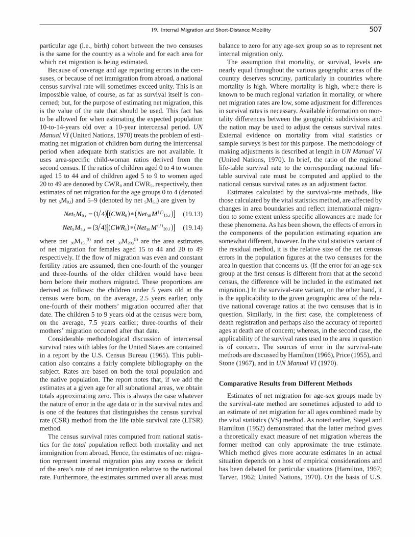
particular age (i.e., birth) cohort between the two censusesis the same for the country as a whole and for each area forwhich net migration is being estimated.
Because of coverage and age reporting errors in the cen-suses, or because of net immigration from abroad, a nationalcensus survival rate will sometimes exceed unity. This is animpossible value, of course, as far as survival itself is con-cerned; but, for the purpose of estimating net migration, thisis the value of the rate that should be used. This fact has to be allowed for when estimating the expected population10-to-14-years old over a 10-year intercensal period. UNManual VI (United Nations, 1970) treats the problem of esti-mating net migration of children born during the intercensalperiod when adequate birth statistics are not available. Ituses area-specific child-woman ratios derived from thesecond census. If the ratios of children aged 0 to 4 to womenaged 15 to 44 and of children aged 5 to 9 to women aged20 to 49 are denoted by CWR0 and CWR5, respectively, thenestimates of net migration for the age groups 0 to 4 (denotedby net 5M0,i) and 5–9 (denoted by net 5M5,i) are given by
(19.13)
(19.14)
where net 30M15,i(f) and net 30M20,i
(f) are the area estimates of net migration for females aged 15 to 44 and 20 to 49respectively. If the flow of migration was even and constantfertility ratios are assumed, then one-fourth of the youngerand three-fourths of the older children would have been born before their mothers migrated. These proportions arederived as follows: the children under 5 years old at thecensus were born, on the average, 2.5 years earlier; onlyone-fourth of their mothers’ migration occurred after thatdate. The children 5 to 9 years old at the census were born,on the average, 7.5 years earlier; three-fourths of theirmothers’ migration occurred after that date.
Considerable methodological discussion of intercensalsurvival rates with tables for the United States are containedin a report by the U.S. Census Bureau (1965). This publi-cation also contains a fairly complete bibliography on thesubject. Rates are based on both the total population and the native population. The report notes that, if we add theestimates at a given age for all subnational areas, we obtaintotals approximating zero. This is always the case whateverthe nature of error in the age data or in the survival rates andis one of the features that distinguishes the census survivalrate (CSR) method from the life table survival rate (LTSR)method.
The census survival rates computed from national statis-tics for the total population reflect both mortality and netimmigration from abroad. Hence, the estimates of net migra-tion represent internal migration plus any excess or deficitof the area’s rate of net immigration relative to the nationalrate. Furthermore, the estimates summed over all areas must
Net M CWR Net Mif
i5 5 5 30 203 4, ,= ( ) ( )*( )[ ]( )
Net M CWR Net Mif
i5 0 0 30 151 4, ,= ( ) ( )*( )[ ]( )
balance to zero for any age-sex group so as to represent netinternal migration only.
The assumption that mortality, or survival, levels arenearly equal throughout the various geographic areas of thecountry deserves scrutiny, particularly in countries wheremortality is high. Where mortality is high, where there isknown to be much regional variation in mortality, or wherenet migration rates are low, some adjustment for differencesin survival rates is necessary. Available information on mor-tality differences between the geographic subdivisions andthe nation may be used to adjust the census survival rates.External evidence on mortality from vital statistics orsample surveys is best for this purpose. The methodology ofmaking adjustments is described at length in UN Manual VI(United Nations, 1970). In brief, the ratio of the regionallife-table survival rate to the corresponding national life-table survival rate must be computed and applied to thenational census survival rates as an adjustment factor.
Estimates calculated by the survival-rate methods, likethose calculated by the vital statistics method, are affected bychanges in area boundaries and reflect international migra-tion to some extent unless specific allowances are made forthese phenomena. As has been shown, the effects of errors inthe components of the population estimating equation aresomewhat different, however. In the vital statistics variant ofthe residual method, it is the relative size of the net censuserrors in the population figures at the two censuses for thearea in question that concerns us. (If the error for an age-sexgroup at the first census is different from that at the secondcensus, the difference will be included in the estimated netmigration.) In the survival-rate variant, on the other hand, itis the applicability to the given geographic area of the rela-tive national coverage ratios at the two censuses that is inquestion. Similarly, in the first case, the completeness ofdeath registration and perhaps also the accuracy of reportedages at death are of concern; whereas, in the second case, theapplicability of the survival rates used to the area in questionis of concern. The sources of error in the survival-ratemethods are discussed by Hamilton (1966), Price (1955), andStone (1967), and in UN Manual VI (1970).
Comparative Results from Different Methods
Estimates of net migration for age-sex groups made bythe survival-rate method are sometimes adjusted to add toan estimate of net migration for all ages combined made bythe vital statistics (VS) method. As noted earlier, Siegel andHamilton (1952) demonstrated that the latter method givesa theoretically exact measure of net migration whereas theformer method can only approximate the true estimate.Which method gives more accurate estimates in an actualsituation depends on a host of empirical considerations andhas been debated for particular situations (Hamilton, 1967;Tarver, 1962; United Nations, 1970). On the basis of U.S.
19. Internal Migration and Short-Distance Mobility 507

data, Hamilton (1967) and Tarver (1962) found that theforward census survival-rate method tends to give (alge-braically) lower estimates of net migration than the vital sta-tistics method. The authors of UN Manual VI (1970) statedthat “Since the number of deaths is likely to be larger in thelarger of the two components of net migration (inmigrationand outmigration), CSR estimates obtained by the forwardmethod will generally be smaller than those obtained by theVS method.” They concluded, however, that it is difficult tomake a general statement regarding the relative accuracy ofthe two methods for the net migration of all ages combined.No research has been reported comparing the vital statisticsmethod and the survival-rate method applied according tothe new design described here (i.e., adjusting by for thebias in the measurement of deaths and net migration).
Uses and Limitations
In summary, the residual method cannot be used to estimate gross inmigration or outmigration or migrationstreams. The migration period must be the intercensal orsimilar period. In any of its variations, this method can beused to estimate net migration for a fixed area, for a groupdefined by an unchanging characteristic (e.g., sex, race,nativity), or for a group defined by a characteristic thatchanges in a fixed way with time (age).
The residual method cannot ordinarily be used for socialand economic groups, mainly because the correspondingcharacteristics (e.g., marital status, occupation, income)change frequently and unpredictably during the intercensalperiod. In most countries, educational level changes soseldom for adults, however, that net migration according toeducational attainment could probably be estimated fairlywell for the adult population.
Rural-urban migration is such an important element ininternal migration, particularly in the less developed coun-tries, that there is great interest in measuring it by somemeans. This may be accomplished, but as with othermethods, the residual method has many pitfalls in this appli-cation. Other things being equal, the method works bestwhen the urban and rural areas are defined in terms of wholeadministrative units and changes in classification are rarelymade. Here one may obtain constant territories over theintercensal period by reassigning whole localities that havebeen shifted from the rural to the urban classification or vice versa. When, however, the reclassification of territoryinvolves annexations and retrocessions or a radically differ-ent set of boundaries for the units in question, there areserious problems in adjusting the statistics and these may beinsurmountable. The UN Manual VI (1970) describes someof the devices that can be used to handle these difficulties.
As previously stated, normally census errors in classifi-cation as well as in coverage will be reflected as errors inthe estimated net migration. Furthermore, death statistics are
s
not available separately for all the areas or groups in ques-tion, and life tables for larger populations will be inappro-priate in varying degrees.
The major advantage of indirect methods of estimatingnet migration is that they can be applied when no direct dataon in- and outmigration are available. Consequently, theyare particularly useful for small areas. However, the accu-racy of these estimates depends heavily on the accuracy ofthe underlying population estimates (or counts) and the vitalstatistics or survival rates. Vital statistics and the associatedsurvival-rates in the United States are generally quite accu-rate, but the accuracy of population estimates and censuscounts varies over time and from place to place. In particu-lar, since net migration is often estimated for decades,changes in the coverage from one census to another maycause estimates of net migration to be too high or too low.Changes in geographic boundaries over time may also affectnet migration estimates. This generally is not a problem forstates and counties, but may be significant for cities, censustracts, zip code areas, and other subcounty areas.
Estimates of net migration disaggregated by age, sex, andrace for states in the United States were produced for eachdecade from 1870 to 1950 (Lee et al., 1957) and wereextended to counties in the 1950s, 1960s, and 1970s (White,Meuser, and Tierney, 1987). Estimates of total net migrationfor states and counties for the 1980s and 1990s have beenproduced by the Census Bureau and are available on theInternet. To our knowledge, however, no further disaggre-gation of these estimates by age, sex, and race have beenproduced for all states and counties in the United States.Analysts choosing to use data on net migration may have toproduce the data themselves.
Miscellaneous Sources
In many countries, administrative records gathered forpurposes other than measuring internal spatial movementshave been adapted to measure place-to-place flows ofpeople. The records most commonly used for migration estimates on a continuing basis in the United States comefrom the Internal Revenue Service (IRS), the federal agencyresponsible for collecting taxes. Income tax returns are to be filed as of April 15 each year, and the Census Bureaumatches the returns from year to year according to the tax-payer’s Social Security number. Each tax return used for this purpose includes the number of “dependents” (otherfamily members) and the street address from which the formis filed. Year-to-year matches provide annual estimates ofgross flows for states and counties that are available on theIRS’s website (www.irs.gov). No information on individualsor individual households is released—just gross flows.
As explained in Chapters 2 and 18, the Immigration andNaturalization Service (INS) within the U.S. Department of Justice is the major source of international migration
508 Morrison, Bryan, and Swanson

statistics in the United States. The INS produces annual sta-tistics on the number of legal immigrants according to type,country of origin, state of intended residence, age, sex,marital status, occupation, and several other characteristics.See Chapters 2 and 18 and Immigration and NaturalizationService (1999, 2000) for further information regarding theINS data.
In other countries, similar tracking systems can provideinformation on spatial movements. A system of nationalhealth care can record an individual’s successive move-ments, at least insofar as these involve seeking health care.A rich source of statistics on internal movements is a fullydeveloped national information system that involves notingthe changing locations where individuals receive govern-ment services of varying types.
Some of the partial population registers (i.e., registers of a population subgroup) have been, or could be, used toestimate the migration of particular population subgroups.By various assumptions, migration rates for a subgroupcould be extended to the general population; or the data maysimply be used to describe and analyze migration differen-tials among classes within the subgroup. Several illustra-tions follow.
In the United States, the national social insurance schemethat provides pensions to retired workers and their surviv-ing dependents, the Old Age and Survivors Insurance systemoperated by the U.S. Social Security Administration, is thebasis for a 1% continuous work history sample. The samplegives the age, sex, and place of employment of workerscovered by the program. Migration can be approximated bycomparing successive places of employment of individualworkers at yearly intervals. The chief shortcomings of theprocedure include (1) a lack of correspondence between areaof employment and area of residence, (2) incompleteness ofcoverage (for example, in the past some industries have notbeen covered), and (3) sampling error. These data are bestsuited, therefore, for making estimates for large areas likestates. A pioneering study with this material for two stateswas carried out by Bogue (1952), who tried to measure jobmobility as well as geographic mobility. An example of asubsequent study using this source and exploring its appli-cability is provided by Morrison and Relles (1975).
Another source involving use of administrative recordsto gauge migration flows and patterns is files of drivers’license address changes (DLAC). One such application hasbeen made by the state of California in preparing its annualofficial population estimates for counties. California reportschanges in interstate driver’s license addresses annually.When a person with a driver’s license from another stateapplies for a California driver’s license, that person isrequired to relinquish the license from his or her previousstate of residence. The information is recorded and thedriver’s license is returned to the previous state of residence.Similarly, other states return California drivers’ licenses to
the California authorities when former California driversapply there for new licenses. The DLAC data provide anannual measure of the volume and directions of gross migra-tion of the adults licensed to drive, for the counties of California. These estimates, in turn, can be extended to theentire population, based on the further estimate that onechange of a driver’s license address corresponds to 1.5actual moves. Despite important limitations, the DLAC datahave proven sufficiently useful to be incorporated into themethodology by which the state prepares its official popu-lation estimates (Johnson and Lovelady, 1995).
In Canada, the Family Allowance System provides estimates of both monthly and annual flows; place-to-placemigration data are available for sex and age groups as wellas socioeconomic characteristics. Croze (1956) estimatedthe net migration in France for the period 1950–1952 for departments, using electoral lists. Registers of electors(voters) are maintained and updated locally, and changes inregistrations for each community are reported annually.Comparisons of a sample of the names in the alphabeticallistings of successive city directories, with allowances fordeath and the attainment of adulthood (usually age 18 in thedirectories), identify persons who have entered or left thearea. Goldstein (1958) made the classic study of this typefor Norristown, Pennsylvania. It gives a detailed account ofthe validity of this type of data and methodology.
ANALYSIS OF DIRECT DATA
Place of Birth
Uses and Limitations
The traditional item that represents a direct questionrelating to migration is place of birth. This item has longbeen included in national censuses, and it is occasionallyfound in sample surveys. The first national census to containsuch an item was that of England and Wales in 1841. Asexplained in Chapters 8 and 18, two kinds of specificity areusually called for: (1) in the case of the foreign born, thecountry of birth; and (2) in the case of the native population,the primary geographic subdivision (i.e., state, province,etc.) or, often also , the secondary subdivision, such as thedistrict in India or Pakistan. “Native” may be defined some-times to include persons born in the outlying territories ofthe country and not covered by the census in question.Usually those natives are separately identified, however.
Several examples will be given of the treatment of dataon internal migration from the question on birthplace innational population censuses. The most detailed and basicstatistics, from which various summary statistics arederived, are given in the cross-classification of residence atbirth by residence at the time of the census. Some countriesshow such cross-classifications, or consolidations thereof,
19. Internal Migration and Short-Distance Mobility 509

for secondary divisions (Taeuber, 1958). Changes of resi-dence in these cross-classified statistics may be viewed asrepresenting migration streams between the time of birth andthe time of enumeration.
Frequently the statistics of streams are consolidated intocategories like “living in given state, born in different state”and “born in given state, living in different state.” These datamay be viewed as representing lifetime inmigrants and life-time outmigrants for each state, respectively.
Characteristics (e.g., age and socioeconomic characteris-tics) of lifetime migrants are usually shown in terms of theseconsolidated categories (e.g., whether or not born in area ofenumeration), because the full detail would be voluminous;but they are sometimes shown for migration streams.
In the United States, data on the state of birth of the nativepopulation have been collected at every census from 1850onward. A cross-classification of each state of residence atthe time of the census with each state, territory, and posses-sion at time of birth has been shown in full detail. In addi-tion, the state of birth has been shown in some reports forthe urban, rural-nonfarm, and rural-farm parts of states andfor individual cities of varying minimal size. The censusinquiry does not provide information on urban-rural resi-dence, or city of residence, at birth.
The accuracy or quality of the statistics on place of birthof the native population is not of concern here except insofaras they pertain to internal migration. On the assumption thatthe statistics are accurate, what would they actually measure,and how useful are these measures to the demographer?
Unlike the estimates of migration derived by the residualmethod, which are limited to net movements, place-of-birthdata can represent inmigrants, outmigrants, and specificstreams. The statistics often reveal nothing about intrastatemigration, and even when secondary subdivisions are spec-ified in the recording of birthplace, intra-area mobility(short-distance movement) is not covered. Moreover, thestatistics do not take account of intermediate movementsbetween the time of birth and the time of the census, andpersons who have returned to live in their area of birthappear as nonmigrants. In sum, these statistics do not indi-cate the total number of persons who have moved from thearea in which they were born to other areas, or to any spe-cific area, during any given period of time.
The question of time reference deserves particular atten-tion. Unless the statistics from one census were tabulated byage, they tell us nothing about when the move occurred.With a tabulation by age, the only specification is that givenby age itself; for example, a migrant 35 years old must havemoved within the 35 years preceding the census. Thus, theolder the migrant, the less is known about the date of themove and the greater the likelihood of intervening movesbetween other areas of the same class. Even statistics tabu-lated by age for two successive censuses are not fully adequate for measuring migration in an intercensal period,
although they do greatly enhance the value of the data. Also,inasmuch as the statistics on state, province, and so on ofbirth are limited to the native population of the country, theinternal migration of the foreign-born population subsequentto its immigration is not included.
There is little quantitative evidence of the accuracy withwhich birthplace is reported. The fact that birthplace is aconstant in a person’s life should strengthen recall. Since,however, for everybody except young children, it relates toa more remote date than does the migration question regard-ing residence at a fixed past date, recall on the part of respon-dents will likely fade over time and the responses will beless accurate for persons about whom the information isprovided by others.
Statistics on place of birth are subject to the types oferrors of reporting and data processing that affect the gen-erality of demographic characteristics; in addition, they havesome sources of error that are sui generis. These includeuncertainties about area boundaries at the time of birth andabout the reporting of birthplace for babies who were notborn at the usual residence of their parents. There have beenseveral attempts to measure the gross and net effects of thesesources of error by such methods as re-interviews or match-ing studies of a sample of the original records. For the 1980and 1990 U.S. censuses, there was, overall, little inconsis-tency between the census responses on place of birth and the reinterview responses (U.S. Census Bureau, 1995, p. 19).Thus, it appears that the census responses accurately reflectthe actual state or foreign country of birth. The introductionof automated coding in 1990 contributed to the consistencyof the data.
From the standpoint of measuring internal migration, itwould be ideal if birthplace were reported in terms of presentboundaries. (Otherwise, a person who lived in a part of stateA that was transferred to state B is automatically classifiedas a migrant whether he moved or not.) Rarely, however, areinstructions provided in the census on this point. This is a problem with other migration questions as well, but the chances are greater that a boundary change occurred if lifetimes are being considered. In the United States, WestVirginia was detached from Virginia and became a separatestate in 1863. It is evident from the subsequent statistics for many decades thereafter that some respondents born inWest Virginia before 1863 gave Virginia as their birthplacewhereas others gave West Virginia. In adapting to this situation, the analysts at the University of Pennsylvaniacombined these two states as one birthplace for 1870 in theirmonumental study of population redistribution in the UnitedStates from 1870 to 1950 (Lee et al., 1957).
In statistically developed countries, a very high propor-tion of births take place at hospitals rather than in the home.The two places may be located in different areas; thus, someambiguity is introduced in the question on birthplace. Fromwhat was said earlier about the desirability of measuring
510 Morrison, Bryan, and Swanson
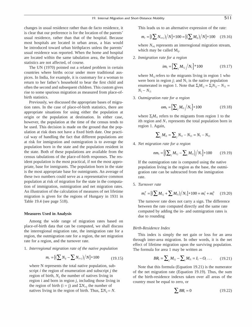
changes in usual residence rather than de facto residence, itis clear that our preference is for the location of the parents’usual residence, rather than that of the hospital. Becausemost hospitals are located in urban areas, a bias would be introduced toward urban birthplaces unless the parents’usual residence was reported. When the home and hospitalare located within the same tabulation area, the birthplacestatistics are not affected, of course.
The UN (1970) pointed out a related problem in certaincountries where births occur under more traditional aus-pices. In India, for example, it is customary for a woman toreturn to her father’s household to bear the first child andoften the second and subsequent children. This custom givesrise to some spurious migration as measured from place-of-birth statistics.
Previously, we discussed the appropriate bases of migra-tion rates. In the case of place-of-birth statistics, there areappropriate situations for using either the population atorigin or the population at destination. In either case,however, the population at the time of the census tends tobe used. This decision is made on the ground that the pop-ulation at risk does not have a fixed birth date. One practi-cal way of handling the fact that different populations are at risk for inmigration and outmigration is to average thepopulation born in the state and the population resident inthe state. Both of these populations are available from thecensus tabulations of the place-of-birth responses. The res-ident population is the most practical, if not the most appro-priate, base for inmigrants. The population born in the stateis the most appropriate base for outmigrants. An average ofthese two numbers could serve as a representative commonpopulation at risk of migration for the state in the computa-tion of immigration, outmigration and net migration rates. An illustration of the calculation of measures of net lifetimemigration is given for the regions of Hungary in 1931 inTable 19.4 (see page 518).
Measures Used in Analysis
Among the wide range of migration rates based on place-of-birth data that can be computed, we shall discussthe interregional migration rate, the inmigration rate for aregion, the outmigration rate for a region, the net migrationrate for a region, and the turnover rate.
1. Interregional migration rate of the native population
(19.15)
where N represents the total native population, sub-script i the region of enumeration and subscript j theregion of birth, Nij the number of natives living inregion i and born in region j, including those living inthe region of birth (i = j) and SNi=j the number ofnatives living in the region of birth. Thus, SNij = N.
m N N Nr ij i j= -( )[ ]*Â Â = 100
This leads us to an alternative expression of the rate:
(19.16)
where Niπj represents an interregional migration stream,which may be called Mij.
2. Inmigration rate for a region
(19.17)
where M1j refers to the migrants living in region 1 whowere born in region j; and N1 is the native populationenumerated in region 1. Note that SjM1j = SjN1j - N11 =N1 - N11
3. Outmigration rate for a region
(19.18)
where SjMi1 refers to the migrants from region 1 to theith region and N1 represents the total population born inregion 1. Again,
4. Net migration rate for a region
(19.19)
If the outmigration rate is computed using the nativepopulation living in the region as the base, the outmi-gration rate can be subtracted from the inmigrationrate.
5. Turnover rate
(19.20)
The turnover rate does not carry a sign. The differencebetween the rate computed directly and the same ratecomputed by adding the in- and outmigration rates isdue to rounding
Birth-Residence Index
This index is simply the net gain or loss for an areathrough inter-area migration. In other words, it is the neteffect of lifetime migration upon the surviving population.The formula for area 1 may be written as
(19.21)
Note that this formula (Equation 19.21) is the numeratorof the net migration rate (Equation 19.19). Thus, the sum of the birth-residence indexes taken over all areas of thecountry must be equal to zero, or
(19.22)BRi =Â 0
BR M M I Ojj ii1 1 1 1 1= - = -Â Â . . .
m M M N m mTj i
I1 1 1 1 1 1
0100= +( )[ ]* = +Â Â
nm M M Njj ii i1 1 100= -( )[ ]*Â Â 1
M N N N Nij ij1 1 11 1 11Â Â= - = -
om M Nij1 1 1 100= [ ]*Â
im M Njj1 1 1 100= [ ]Â *
m N N M Nr i j ij= ( )[ ]* = ( )[ ]*π Â100 100
19. Internal Migration and Short-Distance Mobility 511
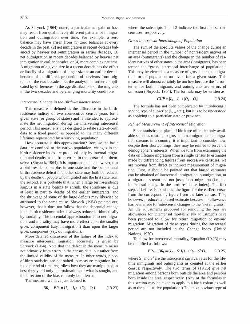
As Shryock (1964) noted, a particular net gain or lossmay result from qualitatively different patterns of inmigra-tion and outmigration over time. For example, a zerobalance may have arisen from (1) zero balances at everydecade in the past, (2) net inmigration in recent decades bal-anced by heavier net outmigration in earlier decades, (3) net outmigration in recent decades balanced by heavier netinmigration in earlier decades, or (4) more complex patterns.A migration of a given size in a recent decade has the effectordinarily of a migration of larger size at an earlier decadebecause of the different proportion of survivors from mig-rants of the two decades, but the analysis is further compli-cated by differences in the age distributions of the migrantsin the two decades and by changing mortality conditions.
Intercensal Change in the Birth-Residence Index
This measure is defined as the difference in the birth-residence indices of two consecutive census years for agiven state (or group of states) and is intended to approxi-mate the net migration during the intervening intercensalperiod. This measure is thus designed to relate state-of-birthdata to a fixed period as opposed to the many different lifetimes represented by a surviving population.
How accurate is this approximation? Because the basicdata are confined to the native population, changes in thebirth residence index are produced only by internal migra-tion and deaths, aside from errors in the census data them-selves (Shryock, 1964). It is important to note, however, thata birth-residence surplus in one state and the coincidentalbirth-residence deficit in another state may both be reducedby the deaths of people who migrated into the first state fromthe second. It is probable that, when a large birth-residencesurplus in a state begins to shrink, the shrinkage is due at least in part to deaths of the earlier inmigrants, and the shrinkage of some of the large deficits may likewise beattributed to the same cause. Shryock (1964) pointed out,however, that it does not follow that the decennial changein the birth residence index is always reduced arithmeticallyby mortality. The decennial approximation is to net migra-tion, and mortality may have more effect upon the smallergross component (say, inmigration) than upon the largergross component (say, outmigration).
More detailed discussion of the failure of the index tomeasure intercensal migration accurately is given byShryock (1964). Note that the defect in the measure arisesnot primarily from errors in the census data, but rather fromthe limited validity of the measure. In other words, place-of-birth statistics are not suited to measure migration in afixed period of time regardless how they are manipulated; atbest they yield only approximations to what is sought, andthe direction of the bias can only be inferred.
The measure we have just defined is
(19.23)BR BR I I O O2 1 2 1 2 1- = -( ) - -( )
where the subscripts 1 and 2 indicate the first and secondcensuses, respectively.
Gross Intercensal Interchange of Population
The sum of the absolute values of the change during anintercensal period in the number of nonresident natives ofan area (outmigrants) and the change in the number of res-ident natives of other states in the area (inmigrants) has beentermed the “gross intercensal interchange of population.”This may be viewed as a measure of gross interstate migra-tion, or of population turnover, for a given state. Thismeasure will almost certainly be too low because the “error”terms for both inmigrants and outmigrants are errors ofomission (Shryock, 1964). The formula may be written as
(19.24)
The formula has not been complicated by introducing asecond type of subscript (Ii, t, etc.), but it is to be understoodas applying to a particular state or province.
Refined Measurement of Intercensal Migration
Since statistics on place of birth are often the only avail-able statistics relating to gross internal migration and migra-tion streams in a country, it is important to consider how,despite their shortcomings, they may be refined to serve thedemographer’s interests. When we turn from examining thedata on lifetime migration from a single census to estimatesmade by differencing figures from successive censuses, weare moving from direct to indirect measurement of migra-tion. First, it should be pointed out that biased estimates can be obtained of intercensal inmigration, outmigration, ora migration stream and not just of net migration (i.e., theintercensal change in the birth-residence index). The firststep, as before, is to subtract the figure for the earlier censusfrom the corresponding figure from the later census. This,however, produces a biased estimate because no allowancehas been made for intercensal changes to the “net migrants.”All the adjustments proposed for removing the bias areallowances for intercensal mortality. No adjustments havebeen proposed to allow for return migration or onwardmigration. Migration of these types during the intercensalperiod are not included in the Change Index (UnitedNations, 1970).
To allow for intercensal mortality, Equation (19.23) maybe modified as follows:
(19.25)
where S1 and S0 are the intercensal survival rates for the life-time inmigrants and outmigrants as counted at the earliercensus, respectively. The two terms of (19.25) give netmigration among persons born outside the area and personsborn inside the area, respectively. (Any of the formulas inthis section may be taken to apply to a birth cohort as wellas to the total native population.) The most obvious type of
BR BR I S I O S OI O2 1 2 1 2 1- = -( ) - -( )
GIIP I I O O= - + -2 1 2 1
512 Morrison, Bryan, and Swanson

survival rate to use is an intercensal survival rate, and thisrequires that the place-of-birth data be tabulated by age atboth censuses.
UN Manual VI (United Nations, 1970) gives proceduresfor three situations, namely, where place of birth has beentabulated by age for neither of two successive censuses, forone but not the other, and for both. In the first situation, itis possible to use only an overall life-table survival rate (e.g.,T10/T0), thus assuming that migrants had the age distribu-tions and age-specific mortality rates of the life-table popu-lation. Unrealistic as this assumption is, this adjustment isbetter than not allowing for mortality at all.
When age is cross-tabulated at only one census, thatcensus is very likely to be the later one. This circumstanceis preferred because the intercensal survival rate for a periodof k years can then be computed as the ratio of the popula-tion k years old and over at the second census to the popu-lation of all ages at the first census. Because the populationborn in a given state or province is a closed population justlike the total native population of the country (neglectingreturn immigration of natives and emigration of nativesabroad), a forward intercensal survival rate can be calculatedfor any tabulated area of birth (Nj, a+k
t+k ∏ Nj,at ).
The third procedure—that applicable where state of birth is tabulated by age for two censuses—is similar in itsstrategy to the second, but the computations are much more detailed. The computations are carried out separatelyfor each age (birth) cohort.
Residence at a Fixed Past Date
Fixed-period migration can be obtained by a question ofthe form, “Where did you live on [date]” or “Where did youlive 5 years ago?” Often, however, the question is in severalparts, with the parts specifying the levels of area detailrequired. In many ways, this is the best single item on pop-ulation mobility. It counts the migrants over a definite pastperiod of time associated with the current population andprovides gross as well as net migration statistics. Thesegross statistics do not, however, include all of the movesduring the period or even all of the persons who have movedduring the period. So-called gross migration from the fixed-period question is partly a net measure because circularmigrants during the migration period are counted only once,and migrants who died during the migration period and chil-dren born after the reference date are not included in the statistics. With regard to the last of these categories, the con-vention of assigning the residence of the mother to the chil-dren born during the migration period was employed in afew Current Population Surveys in the United States. Likeother migration questions in censuses, this question is notvery well suited to a de facto census. In spite of these limi-tations, a wide range of useful measures can be derived from
the absolute figures, and useful analyses of geographic pat-terns, time series, differentials, and so forth can be based onthese measures.
The United States census of 1940 was the first to includea question of this type, relating to a 5-year period. Such a 5-year question has been included in each decennial census(except 1950) since that year. The census 2000 question wasessentially the same as that of 1940. The inclusion of a fixed-period migration question in national sample surveys hasalso become more prevalent. United States is one of thecountries that includes a fixed-period migration question ona regular basis. After experimenting with a variety of migra-tion intervals, the U.S. Census Bureau settled on a 1-yearinterval for its survey of April 1948 and with a few excep-tions has continued with a 1-year interval to the present.
Choice of Mobility Period
In choosing the reference date for the mobility question,considerations of usefulness and of accuracy may conflict toan extent. From the standpoint of demographic analysis, thedate of the previous census has many advantages, since thecomponents of population change can then readily bestudied for the intercensal period. If the intercensal periodis 10 years rather than 5 years, however, errors of memoryand lack of knowledge may be excessive in reporting prior residence. Anthropologists have found that otherevents are remembered relatively well if they are tied in withsome event of historical significance, such as the outbreakof a war or the achievement of national independence; butthe irregular time intervals thus defined do not lend them-selves very well to time series or to demographic analysisin general.
The longer the migration interval, the greater the numberof children that will be omitted from the coverage of thequestion, and the less will characteristics such as age andmarital status recorded in the census correspond to those atthe time of the move. On the other hand, a very short period(i.e., 1 year or less) may not yield enough migrants fordetailed analysis of migration streams. Furthermore, onemust consider the representativeness of the 1-year period or,to a lesser extent, any period shorter than the intercensalperiod. The U.S. Census Bureau (concurring with manyexperts in the field) judges a 5-year mobility period, onbalance, to be optimal for a census, even though a 1-yearperiod may be highly useful in an annual sample survey.
Average Annual Movers
Another problem arises in the computation of averageannual numbers or rates. If the number of moves has beencompiled from a population register over a period of years,it is quite appropriate to obtain such averages by dividingthe number of moves by the number of years. When,
19. Internal Migration and Short-Distance Mobility 513

however, the number of movers is defined by the number ofpersons whose residence at the beginning of a fixed periodis different from that at the census or survey date, then thecalculation produces an estimate with a downward bias andthe longer the interval the greater the bias.
The reasons for this bias are as follows:
1. A larger proportion of movers will have died over thelonger period than over the shorter period. Emigrationfrom the country has the same directional bias in itseffect on the migration statistics as deaths.
2. A mover has a greater opportunity to return to his orher original residence over a longer period than over ashorter period. Hence, the number of persons per yearappearing to be movers will be smaller for the longerperiod.
3. Since a mover is counted as such only once, regardlessof the number of times he or she moves, the proportionof movers in any one of five 1-year periods is expectedto be larger than one-fifth the proportion over a 5-yearperiod—given a constant proportion of movers peryear.
4. When children born after the base date are not coveredby the mobility questions, fewer movers are countedfor the longer period. Children born during the mobilityinterval are then excluded from the base population.The effect on the overall rate also depends on the age-specific mobility rates. Young children tend to be moremobile than the average for the population of all ages(U.S. Census Bureau/Schachter, 2001b).
Nonetheless, averages computed for periods of unequallength can be used with appropriate caution in the analysis.If the apparent average was greater for the longer period thanfor the shorter period, then the true difference was in thesame direction and at least as large. This bias also affectsannual estimates computed from the “intercensal change inthe birth-residence index” and estimates of net migrationmade by the survival-rate method.
Quality of the Data and Statistics
The data obtained by the question on residence at a fixedpast date are subject to essentially the same types of errorsof reporting and tabulation in censuses and surveys as areother demographic, social, and economic characteristics. Inaddition, the reporting of this item is affected by the typesof errors that are peculiar to reporting past events and theirplacement in time.
Data secured from a sample survey are, of course, subjectto sampling error as well as nonsampling error. The ContentReinterview Surveys of the 1980 and 1990 U.S. censusesdid not secure information on the accuracy of reporting res-idence 5 years prior to the census. The share of persons forwhom prior residence was allocated in the 1990 census was6.4%; the percentage not reporting prior residence in cen-
suses has been rising. Among persons in households inter-viewed in the Current Population Survey, the proportionfailing to answer the question on residence 1 year earlier isquite low—on the order of a fraction of 1%. These omis-sions are now filled by computerized allocations. Of house-holds eligible for interview, however, about 4 to 5% are notinterviewed at all in an average month. The members ofthese households are also nonrespondents on the migrationquestions, of course. Inflating the sample data to “control”totals (that is, independent estimates of total population dis-aggregated by age, sex, race, and Hispanic origin) givesthese nonrespondents the same characteristics as thosepersons in the specific age-sex-race-Hispanic-origin groupthat reported, although actually they may have had a some-what different distribution on such a characteristic as mobil-ity. This weighting partially corrects for bias due toundercoverage. Because of the allocations and adjustments,the published statistics do not show any cases “not reported”on migration.
A recurring difficulty in both censuses and samplesurveys of the United States has been the biased reports ofthe urban or rural origin of movers. This difficulty arisespartly from the rather complex urban-rural definition now inuse and partly from a strong tendency for persons livingoutside a city but in its suburbs to give the city as their res-idence. This tendency leads to an overstatement of outmi-gration from urban areas and an understatement of that fromrural areas. As a result, the United States has had to discon-tinue the direct measurement of rural-urban migration. Incountries where the areas classified as urban have relativelypermanent boundaries, this problem may be less acute.
Measures Used in Analysis
Many of the measures used in analyzing fixed-periodmobility are identical or similar to those used with the kindsof mobility data that were discussed previously. There arealso similar problems regarding the choice of populationbase, annual averages, and so on.
Mobility or Migration Status
To analyze mobility or migration status, the simplest typeof derived figures is the percentage distribution by mobilitystatus. For some purposes (e.g., comparisons of two statesin the same country), it would be better to base the percent-age distribution on the total excluding the “not reported”cases. For some countries, the “unknowns” shown are onlypartial unknowns since the nonresponses had been partlyallocated. The percentages for various types of mobility canalso be regarded as mobility rates per 100 of the residentpopulation.
In a distribution for a particular geographic subdivision,some of the figures also represent inmigration rates, forexample, the category “different county” in the distributionby mobility status for a county. Of necessity, such a distri-
514 Morrison, Bryan, and Swanson

bution excludes outmigrants. Such “status rates” includeinmigrants to the area during the “migration” period, butexclude outmigrants during the migration period. (The elements in the percent distribution of the population bymigration are being called “status rates,” although this nameis quite clearly a demographic oxymoron. “Rates” measurechange over a period, and “status” refers to the condition ata particular date. Here, the participation of the survivingpopulation in the event of mobility over a prior 1-year or 5-year period is ascertained at a particular time.) In the case of fixed-period migration, the population at the begin-ning of the period rather than the end of the period (i.e., thepopulation at the end plus a portion of the outmigrantsduring the period minus a portion of the inmigrants duringthe period) more nearly represents the population “at risk”of outmigration (disregarding births and deaths during theperiod). This population is usually available or can be estimated.
The choice of a population base for the rates is signifi-cant not so much for its effect on the size of the base as forits effect on the number of migrants. Persons who areexcluded or included (preferably in part) to approximate thepopulation at the beginning of the period have a 100%migration rate, and their number must be deducted from oradded to the number of migrants as well as the base. If amigration rate is to be based on the initial population, theinmigrants from outside the region should be removed fromthe resident migrants in each region and the outmigrants toother regions should be restored in order to include just thosemigrants who lived in the region earlier.
In-, Out-, and Net Migration Rates
In-, out-, and net migration rates may be expressed byformulas analogous to those shown earlier for place-of-birthstatistics. Again, it is possible to base the rate on the popu-lation at the beginning or end of the period or on the mid-period population.
A partial migration rate is defined as the number ofmigrants to an area from a particular origin, or from an areato a particular destination, per 1000 or per 100 of the pop-ulation at either origin or destination. The partial outmi-gration rate can be expressed as
(19.26)
where Mji is the stream from area i to area j. For the streamfrom j to i, the partial outmigration rate is
(19.27)
The gross rate of population interchange may be defined as
(19.28)
The net rate of population interchange is then
(19.29)NRI M M P Pi j ij ji i j´ = -( ) +( )[ ]*1000
GRI M M P Pi j ij ji i j´ = +( ) +( )[ ]*1000
m M PijI
ij i= ( )*1000
m M Pji ji i0 1000= ( )*
The “effectiveness” of internal migration may be meas-ured by the ratio of net migration to turnover—a measureproposed by Shryock (1959). The higher the ratios for a setof areas, the fewer the moves that are required to effect agiven amount of population redistribution among them.There are patently other important aspects of the effective-ness of migration that are not comprehended in this measure.This ratio ranges from 0 to 100. The effectiveness of astream and its counterstream may also be measured in thisfashion. Often the counterstream is as large as the stream,so that there is little net migration and a low ratio of effectiveness.
Migration Preference Index
The Migration Preference Index is another measure offixed-period mobility. This measure, first suggested byBachi (1957), is defined as the ratio (times a constant) of theactual to the expected number of migrants in a stream whenthe expected number is directly proportionate to both thepopulation at origin and the population at destination.
This measure indicates, then, whether streams are greater or smallerthan would be expected from considerations of population sizealone. It does not include any assumption about the expected effectof distance, but we can compare measures for different streams inthe light of our knowledge of contiguity and of mileage and, in fact,in the light of knowledge that we may have about the relative attrac-tiveness of the areas. (Shryock, 1964)
This index can be computed in several ways. The mostuseful one, however, relates to interarea migrants only—thatis, the Preference Index for a state relates to interstate migra-tion only. To compute the index, interstate migrants areassumed to be distributed proportionately to the populationat origin and the population at destination. Take the nationalrate of interarea (interprovincial, interregional, etc.) migra-tion. Assume that it is uniformly the outmigration rate forall areas of the given class. Compute the expected totalnumber of outmigrants from a given area to all destinations.Distribute these among the other areas in proportion to theirpopulation, to obtain the expected number of migrants ineach stream. The Preference Index is then given by
(19.30)
where MOD = actual number of migrants from 0 to DP0 = population at origin 0PD = population at destination DSPi = national populationm = proportion of interarea migrants in the
national populationThis index may vary from 0 to •. The total number
of expected inmigrants can be obtained by summing theexpected numbers in all the inmigration streams, but theindices themselves are not additive (Shryock, 1964). For anillustration of the computation of the migration preference
P I M P P mP POD i D. . = -( ) ( )[ ]*Â 0 0 100
19. Internal Migration and Short-Distance Mobility 515

index, see Tables 21.12 and 21.13 in Shryock, Siegel, andStockwell (1976).
Distance of Move
A very different way of reducing the data is to computethe distance (in kilometers or miles) between the points oforigin and destination. Actually, instead of points (i.e.,addresses), it would be practical to start with statistics onorigin and destination grouped in tabulation areas, and esti-mate the distance between the centers of the areas of originand destination.
Duration of Residence and Last Prior Residence
The typical question on duration of residence has theform, “How long has subject person been living in thisarea?” (i.e., the area of usual residence). The logical com-panion question, and that recommended by the UnitedNations, is one concerning the name of the previous area ofresidence; but in national censuses most countries asking thequestion on duration of residence have been content to askonly for place of birth. There are two ways of defining amigrant from such data:
1. A person who had moved into the area at any time inthe past and was still resident there. This categorywould include primary, secondary (or progressive), and return migrants. By this definition, the number ofmigrants would exceed that of lifetime migrants.
2. A person who had moved into the area since a givendate—1 year ago, 2 years ago, and so forth. Again thismight be a person who had migrated only once sincehis or her birth, a secondary migrant, or a returnmigrant. The areas referred to earlier are those areas,such as municipalities, counties, and so on, that are“migration-defining” for the particular country.
The item on duration of residence in national censuseshas been especially popular in the Americas, and a numberof countries have also asked for previous area of residence.In the United States, a question on year moved to presentresidence was included in the census of 2000 and severalearlier censuses. Since, however, the year of the move intothe county of residence has not been determined, this itemhas not yielded any migration statistics for the United States.It was a part of the Housing Census in each case and demog-raphers have made little use of the data.
If only the last previous place of residence has beenobtained or tabulated, the resulting statistics, like those from the item on place of birth, have an indefinite time ref-erence. However, these statistics describe direct moveswhereas the place-of-birth statistics may conceal interven-ing moves.
The chief virtue of the question on duration of residence(or on year of last move) is that it gives the distribution oflifetime movers by date of latest move. If the previous placeof residence has also been ascertained, then the time is alsofixed for streams of migration. Such statistics describe theinmigrants now living in an area, but they do not produce avery useful time series. Since only the latest move isrecorded, the number of moves in the earlier years will beseriously understated because of multiple moves and deaths.Origin-destination tabulations for the most recent migrationinterval will yield data approximating those from the fixed-period item for the same interval; the shorter the interval,the closer the approximation. Furthermore, percentage dis-tributions by duration of residence enable us to distinguishthose parts of the country to which migrants have gone inrelatively recent years.
A number of countries have cross-tabulated duration ofresidence in a place by place of birth or by place of last pre-vious residence. From such statistics on migration streams,the volume of in-, out-, and net migration, and median dura-tion of residence can be computed, as well as the corre-sponding rates using the current population as the base. Foran illustration of the calculation of median duration of resi-dence from data on duration of residence of inmigrants to astate cross-classified by state of last residence, see Table21.15 in Shryock, Siegel, and Stockwell (1976). As with sta-tistics on place of birth, it is not possible to compute“propensity” rates (using as a base the origin population ata fixed past date), however.
The statistics on duration of residence and area of previ-ous residence are subject to the usual types of reportingerrors that have been discussed for other migration ques-tions. In addition, there is the likelihood of preferences forround numbers in the reporting of duration in years.
Few additional measures have been proposed for thissubject. In addition to the percentage distribution by dura-tion of residence and the median duration of residence, ameasure of dispersion, like the interquartile range, couldalso be computed. There is a high positive correlationbetween duration of residence and age, and tables giving across-classification by age are a prerequisite for adequateanalysis. When the same tabulation is available for succes-sive censuses, there are opportunities for more complexmethods and measures. The UN Manual VI (United Nations,1970, Table B.15) carries a dummy table illustrating thecomputation for an intercensal period.
Measures Derived from Microdata
The increasing availability of microdata, especially lon-gitudinal microdata, since the 1970s has fostered significantadvances in measuring people’s mobility and, as a conse-quence, refined conceptualizations of the process itself. ThePublic Use Microdata Sample (PUMS) from the U.S. decen-
516 Morrison, Bryan, and Swanson
nial census is one such source. Although cross-sectional, itaffords considerable latitude in tailoring the definition ofparticular population segments for which census migrationmeasures are calculated—for example, persons classified bymultiple variables simultaneously, such as current area ofresidence, household or family type, occupation, race, andso forth.
More significant, perhaps, has been the proliferation of longitudinal microdata sources, which have greatlyexpanded the frontiers of migration research during the1980s and 1990s. These data sets afforded researchers newand more exact approaches to defining and studying themigration sequences formed by individual moves (seeDaVanzo and Morrison, 1981, 1982). Noteworthy datasources used for migration research include the Universityof Michigan’s Panel Study of Income Dynamics (PSID), theNational Longitudinal Surveys (NLS), and High School andBeyond (HS&B).
The wealth of new data on migration, and the sequencesof moves that became discernible, demanded new concep-tualizations and measures. The act of migration came to beseen as more than an isolated once-and-for-all event. Usinglongitudinal microdata, researchers demonstrated that themajority of moves that people make are not first moves, butrepeat moves that form sequences of migration. The possi-bility of delineating those sequences empirically invited new measures of the types of migration sequences that arose,new theoretical conceptualizations for explaining suchsequences, and new insights into the consequences suchsequences may have for the populations at origin and destination.
Multistate Life Tables of Interregional Transfers
In earlier chapters we noted the application of multistatemethods to life tables. Such an extension of life tablemethods has led to the development of tables of workinglife, nuptiality tables, tables of healthy life, and so on, whichprovide measures of average years of working life, singlelife, and healthy life, respectively, and other related meas-ures. These methods may also be applied to the measure-ment of interregional migration (Willekens and Rogers,1978), but a full explanation of the construction and use oftables of interregional transference is beyond the scope ofthis chapter. Here we only present a brief outline and referthe reader to Namboodiri (1993), who provided an empiri-cal example using Yugoslavia and Slovenia. The fourgeneral steps in the derivation of a multistate table for inter-regional migration are as follows:
1. Calculate central age-specific migration rates and deathrates.
2. Use the central rates in step 1 as estimates of the corre-sponding transition intensities.
3. Convert the transition intensities in step 2 into transi-tion probabilities.
4. Use the transition probabilities in step 3, in combina-tion with an assumed radix for the number of births ineach region to construct the table.
The population distribution at the end of a given periodis derived as a matrix product of the initial matrix and thetransition probabilities for the period. The results correspondto the lx function and the ndx function of the conventionallife table. From such a table we can provide information onthe proportion of persons ever moving between the tworegions, the time that will be spent in each region in any yearor in a lifetime, the numbers dying in each region, andrelated measures.
A table of migration expectancy, without reference toorigin and destination, that provides estimates of averagemoves per person may be calculated by a more conventionalmethod—that is, a double-decrement table based on theprobability of dying and the probability of moving in eachyear, or only the probability of moving, omitting theallowance for mortality (Long, 1973).
DETERMINANTS ANDCONSEQUENCES OF MIGRATION
What causes change in an area’s migration patterns over time? Here we can only touch on the major themes thatstand out from the immense research literature that hasaddressed the question over the decades. More extensivediscussions on the determinants of migration may be foundin DaVanzo and Morrison (1981), Greenwood (1997); Long (1988); Mohlo (1986), Morrison (1975), U.S. CensusBureau/Schachter (2001b), and Zelinsky (1980).
Sample Survey Data
Questions on reasons for moving are among the morepopular items in sample surveys on internal migration.These questions represent an attempt to determine motiva-tion by asking movers why they moved. This approach isquite different from trying to draw inferences on causes ofmigration from data on migration differentials or on thecomparative characteristics of sending and receiving areas.In the survey approach, there are no attempts to establish a“control group” of nonmigrants by seeking to measure theprevalence among them of the conditions cited by moversas reasons for moving. Thus, we cannot say, for example,whether unsatisfactory housing conditions are more preva-lent among migrants in a given period than among those who
19. Internal Migration and Short-Distance Mobility 517

did not migrate. “Push-pull” theories are seldom testedexplicitly, for example by asking the respondent to comparehis or her attitudes toward the areas of origin and destina-tion. On the other hand, studies that ask reasons for movingprobably do measure the subjective importance of the con-ditions cited as a reason for leaving.
The main problems of measurement for this topic seemto be the choice of a reasonable number of predesignatedreasons that are mutually exclusive and the choice of ana-lytically relevant classifications of reasons. There has beenlittle standardization of categories or reasons among thevarious surveys that have investigated this topic. Therespondent is often allowed to give more than one reason sothat the sum of reasons given may exceed the number ofpersons reporting.
There is frequently an attempt, either in the questionsthemselves or in the tabular classification of the replies, todistinguish job-related from personal or social reasons. Thesurvey results support this distinction because job-relatedreasons are relatively much more frequent among themigrants than among the short-distance movers. In theMarch 2000 Current Population Survey of the United States,for example, only 5.6% of the intracounty movers gavework-related reasons, while 31% of the intercounty moversgave such reasons (Table 19.5). Most moves are for housing-related reasons; they accounted for 52% of all the moves and65% of the intracounty moves.
General Theory of Migration
In the highly industrialized countries, the population of almost every region and locale is continuously re-composed over time by a gradual procession of migrantscoming and going, for the most part by choice. The pur-posefulness of migration makes it a largely autonomousprocess and one that is indicative of opportunity seeking.The view that personal success is as readily achievablebeyond as within one’s native region is a distinctive anddeeply ingrained element of the cultures of industrializedsocieties. It is the product of the persistent pull of economicopportunities in other places that enables individuals alert to opportunity to exploit newly developed resources orknowledge quickly.
The national and regional economies benefit frompeople’s readiness to migrate and from the resulting eco-nomic and social realignments, as a freely-mobile popula-tion rearranges itself in space to answer the changing needsof the economy. The economies of rapidly growing regions,like huge parabolic mirrors, gather migrants extensivelyfrom many origins and direct them to locales of expandingemployment growth. Without a tradition of migration, whichmoves people from areas where jobs are dwindling to placeswhere workers are needed, national economic developmentwould be more sluggish and less efficient than is actuallythe case.
518 Morrison, Bryan, and Swanson
TABLE 19.4 Calculation of Net Lifetime Migration Rates for the Regions of Hungary: 1931 (Figures relate to the Trianon area of Hungary. Numbers in thousands.)
Item Hungary Transdanubia Great Plain1 Budapest North
Born in specified region(1) Total 80722 2819 3560 550 1128(2) Living in other regions 896 327 267 170 132(3) = (2)/(1) Rate of outmigration3 11.1 11.6 7.5 30.9 11.7
Living in specified region(4) Total 80722 2600 3611 793 1064(5) Born in other regions 896 91 325 414 66(6) = (5)/(4) Rate of inmigration4 11.1 3.5 9.0 52.2 6.2
Net gain (+) or loss (-) of survivors through interregional migration(7) = (5) - (2) Net migration — -236 +58 +244 -66(8) = [(2) + (5)]/2 Average of populations
born in region and living in region 80722 2710 3586 672 1096(9) = (7)/(8) Net migration rate5 — -8.7 +1.6 +36.3 -6.0
(10) = Rate with variable base6 — -8.4 +1.6 +30.8 -5.9
1 Excludes Budapest.2 Discrepancy between figure for total Hungary and sum of figures for the four regions is a result of rounding.3 Percent of population born in specified region.4 Percent of population living in specified region.5 Percent of the average of the populations born in the region and living in the region.6 Base varies depending on direction of net migration.Source: Based on Siegel (1958), Table IV-H.

In the final analysis, migration is a process whose con-sequences flow from the inherent selectivity of the act itselfand from the resulting growth or decline bestowed onregions and places. Accordingly, migration tends to selectdistinct types of individuals according to an array of char-acteristics (Morrison and DaVanzo, 1986; see also Blau andDuncan, 1967). For example, migrants tend to be moreyouthful, more educated, and more trained or experiencedin professional lines of work, than their counterparts who donot migrate. Those who migrate are also inclined to migraterepeatedly. Beyond such readily observable attributes, theelement of deliberate choice in most moves sharply differ-entiates persons by motive. Owing to its selectivity, migra-tion is noteworthy as a sorting mechanism, filtering andsifting the population as some of its members move aboutwhile others stay put. A place that grows by net migrationof 1000 has gained 1000 people who are there essentiallybecause they want to be there. Natural increase does not contribute deliberate residents; it only adds to populationnumbers by the lottery of birth and death.
The influx of self-selected persons has repercussions forplaces. For example, heavy migration had left a powerfuldemographic legacy in metropolitan San Jose, California, by1970. Its population became both youthful and noticeably
hypermobile (that is, prone to further onward migration).About 21 migrants per 100 residents entered the populationand 17 per 100 residents departed each year. Conversely, thecity of St. Louis illustrates how heavy and prolonged out-migration from a place can alter the age structure of theremaining population, drawing away potential parents andleaving behind an elderly population that no longer canreplace itself. Natural decrease results, that is, the numberof people dying exceeds the number being born, and popu-lation decline acquires its own dynamic (Morrison, 1974).
References
Bachi, R. 1957. “Statistical Analysis of Demographic Series.” Bulletin del’institut international de statistique 36(2): 234–235. Proceedings of the30th meeting of the Institute. Stockholm.
Behr, M., and P. Gober. 1982. “When a Residence Is Not a House: Examining Residence-Based Migration Definitions.” ProfessionalGeographer 34: 178–184.
Blau, P., and O. D. Duncan. 1967. The American Occupational Structure.New York: John Wiley & Sons.
Bogue, D. 1952. A Methodological Study of Migration and Labor Mobil-ity in Michigan and Ohio in 1947. Scripps Foundation Studies in Population Distribution, No. 4. Miami, OH: Scripps Foundation forResearch in Population Problems.
19. Internal Migration and Short-Distance Mobility 519
TABLE 19.5 Percentage Distribution of Movers within the United States by Main Reason for Moving and Type of Move: March 1999 to March 2000
(movers aged 1 and over)
Reason for moving Total Intracounty Intercounty
Total movers (in 1000s) 41,642 24,399 17,243Percentage 100.0 100.0 100.0Family-related reasons 26.3 25.9 26.9
Change in marital status 6.2 6.2 6.2To establish own household 7.4 9.3 4.7Other family reasons 12.7 10.4 16.0
Work-related reasons 16.2 5.6 31.1New job/job transfer 9.7 1.4 21.6To look for work/lost job 1.3 0.5 2.4Closer to work/easier commute 3.5 3.0 4.2Retired 0.4 0.1 0.9Other job-related reason 1.2 0.6 2.0
Housing-related reasons 51.6 65.4 31.9Wanted to own home/not rent 11.5 14.3 7.5New/better house/apartment 18.5 24.2 10.3Better neighborhood/less crime 4.4 4.8 3.9Cheaper housing 5.5 7.5 2.8Other housing reason 11.7 14.7 7.4
Other reasons 6.0 3.0 10.1Attend/leave college 2.3 0.7 4.4Change of climate 0.7 0.2 1.6Health reasons 1.1 0.8 1.6Other reason 1.8 1.3 2.5
Source: U.S. Census Bureau/Schachter (2001a). Primary source is the Current Population Survey,March 2000.
Bogue, D., K. Hinze, and M. White. 1982. Techniques for Estimating NetMigration. Chicago: University of Chicago Press.
Croze, M. 1956. Un instrument d’étude des migrations intérieures: Lesmigrations d’électeurs (An instrument for studying internal migration:the migration of electors). Population 11(2): 235–260.
DaVanzo, J. 1982. “Techniques for Analysis of Migration-History Data.”RAND N-1842-AID/NICHD. Santa Monica, CA: RAND Corporation.
DaVanzo, J. 1983. “Repeat Migration in the United States: Who MovesBack and Who Moves On?” Review of Economics and Statistics 65:552–559.
DaVanzo, J., and P. Morrison. 1981. “Return and Other Sequences ofMigration in the United States.” Demography 18: 85–101.
DaVanzo, J., and P. Morrison. 1982. “Migration Sequences: Who MovesBack and Who Moves On?” RAND R-2548-NICHD. Santa Monica,CA: RAND Corporation.
Eldridge, H. T. 1965. “Primary, Secondary, and Return Migration in theUnited States, 1955–60.” Demography 2: 445.
Gober, P. 1993. “Americans on the Move.” Population Bulletin 48(3).Washington, DC: Population Reference Bureau.
Goldstein, S. 1958. Patterns of Mobility, 1910–1950: The NorristownStudy. Philadelphia, PA: University of Pennsylvania Press.
Greenwood, M. 1997. “Internal Migration in Developed Countries. In M.Rosenzweig and O. Stark (Eds.), Handbook of Population and FamilyEconomics (pp. 647–720). Amsterdam, Holland: Elsevier Science.
Hamilton, C. H. 1965. “Practical and Mathematical Considerations in theFormulation and Selection of Migration Rates.” Demography 2:429–443.
Hamilton, C. H. 1966. “Effect of Census Errors on the Measurement of NetMigration.” Demography 3: 393–415.
Hamilton, C. H. 1967. “The Vital Statistics Method of Estimating NetMigration by Age Cohorts.” Demography 4: 464–478.
Isserman, A., D. Plane, and D. McMillen. 1982. “Internal Migration in theUnited States: An Evaluation of Federal Data.” Review of Public DataUse 10: 285–311.
Johnson, H., and R. Lovelady. 1995. Migration between California andOther States: 1985–1994. Sacramento, CA: Demographic ResearchUnit, California Department of Finance.
Lansing, J. B., and E. Mueller. 1967. The Geographic Mobility of Labor.Ann Arbor, MI: Survey Research Center, University of Michigan.
Lee, E., A. Miller, C. Brainerd, and R. Easterlin. 1957. “MethodologicalConsiderations and Reference Tables.” In S. Kuznets and D. Thomas(Eds.), Population Redistribution and Economic Growth: United States,1870–1950 (pp. 15–56). Philadelphia: The American PhilosophicalSociety.
Long, L. 1973. “New Estimates of Migration Expectancy in the UnitedStates.” Journal of the American Statistical Association 68(341):37–43.
Long, L. 1988. Migration and Residential Mobility in the United States.New York: Russell Sage Foundation.
Long, L. 1991. “Residential Mobility Differences among Developed Coun-tries.” International Regional Science Review 14: 133–147.
Long, L. 1992. “Changing Residence: Comparative Perspectives on ItsRelationship to Age, Sex, and Marital Status.” Population Studies 46:141–158.
Long, L., C. Tucker, and W. Urton. 1988a. “Measuring Migration Dis-tances: Self-Reporting and Indirect Methods.” Journal of the AmericanStatistical Association 83: 674–678.
Long, L., C. Tucker, and W. Urton. 1988b. “Migration Distances: An Inter-national Comparison.” Demography 25: 633–640.
Martin, P., and E. Midgley. 1999. “Immigration to the United States.” Population Bulletin 54. Washington, DC: Population Reference Bureau.
McHugh, K., T. Hogan, and S. Happel. 1995. “Multiple Residence andCyclical Migration: A Life Course Perspective.” Professional Geogra-pher 47: 251–267.
Mohlo, I. 1986. “Theories of Migration: A Review.” Scottish Journal ofPolitical Economy 33: 396–419.
Morrison, P. 1974. “Urban Growth and Decline: San Jose and St. Louis inthe 1960s.” Science 185: 757–762.
Morrison, P. 1975. “Toward a Policy Planner’s View of the Urban Settle-ment System.” RAND P-5357. Santa Monica, CA: RAND Corporation.
Morrison, P. 1977. “Migration and Rights of Access: New Public Concerns of the 1970s.” RAND P-5785. Santa Monica, CA: RANDCorporation.
Morrison, P. 1980. “Current Demographic Change in Regions of the UnitedStates.” In V. Arnold (Ed.), Alternatives to Confrontation: A NationalPolicy Toward Regional Change (pp. 63–94). Lexington, MA: D.C.Heath & Co.
Morrison, P., and J. DaVanzo. 1986. “The Prism of Migration: Dissimilar-ities between Return and Onward Movers. Social Science Quarterly 67:504–516.
Morrison, P., and D. Relles. 1975. “Recent Research Insights into Local Migration Flows.” RAND P-5379. Santa Monica, CA: RANDCorporation.
Morrison, P., and J. Wheeler. 1976. “The Image of Elsewhere in the American Tradition of Migration. RAND Document P-5729. SantaMonica: RAND Corporation.
Namboodiri, K. 1993. Demographic Analysis: A Stochastic Approach. SanDiego, CA: Academic Press.
Netherlands, Statistics Netherlands. 1998. “Statistics of the Population witha Foreign Background, Based on Population Register Data.” WorkingPaper 6, ECE Work Session on Migration Statistics at the Conferenceof European Statisticians Geneva, March 25–27, 1998.
Newbold, K. 1997. “Race and Primary, Return and Onward InterstateMigration.” Professional Geographer 49: 1–14.
Price, D. 1955. “Examination of Two Sources of Error in the Estimation ofNet Internal Migration.” Journal of the American Statistical Associa-tion 50: 689–700.
Ravenstein, E. 1889. “The Laws of Migration.” The Journal of the RoyalStatistical Society, LII, 241–301.
Shryock, H. S. 1959. “The Efficiency of Internal Migration in the UnitedStates.” International Population Conference, Vienna, 1959. Vienna:The Working Committee of the Conference.
Shryock, H. S. 1964. Population Mobility within the United States.Chicago: Community and Family Study Center, University of Chicago.
Shryock, H. S., J. S. Siegel, and E. G. Stockwell. 1976. The Methods andMaterials of Demography, condensed ed. San Diego, CA: AcademicPress.
Siegel, J. S. 1958. The Population of Hungary, International PopulationStatistics Reports, Series P-90, No. 9. Washington, DC: U.S. Bureau ofthe Census.
Siegel, J. S. 2001. Applied Demography: Applications to Business, Gov-ernment, Law, and Public Policy. San Diego, CA: Academic Press.
Siegel, J., and C. H. Hamilton. 1952. “Some Considerations in the Use ofthe Residual Method of Estimating Net Migration.” Journal of theAmerican Statistical Association 47: 480–481.
Smith, S. 1989. “Toward a Methodology for Estimating Temporary Residents.” Journal of the American Statistical Association 84:430–436.
Smith, S. K., J. Tayman, and D. A. Swanson. 2001. State and Local Population Projections: Methodology and Analysis. New York: PlenumPress/Kluwer Academic.
Stone, L. 1967. “Evaluating the Relative Accuracy and Significance of NetMigration Estimates.” Demography 4: 310–330.
Taeuber, I. 1958. The Population of Japan. Princeton, NJ: Princeton University Press.
Tarver, J. 1962. “Evaluation of Census Survival Rates in Estimating Intercensal State Net Migration.” Journal of the American StatisticalAssociation 57: 841–862.
520 Morrison, Bryan, and Swanson

Thomlinson, R. 1962. “The Determination of a Base Population for Computing Migration Rates.” Milbank Memorial Fund Quarterly 40:356–366.
United Nations, 1970. Methods of Measuring Internal Migration. Manual VI, Methods of Estimating Population. New York: UnitedNations.
U.S. Census Bureau. 1965. “National Census Survival Rates, by Color andSex, for 1950 to 1960.” By D. S. Akers and J. S. Siegel. Current Pop-ulation Reports, Series P-23, No. 15.
U.S. Census Bureau. 1990a. “Comparing Migration Measures Having Different Intervals.” By L. Long and C. Boertlein. Current PopulationReports, P-23, No. 166.
U.S. Census Bureau. 1990b. “Creating Annual State-to-State MigrationFlows with Demographic Data.” By S. Wetrogan and J. Long. CurrentPopulation Reports, P-23, No. 166.
U.S. Census Bureau. 1995. “Selected Place of Birth and Migration Statis-tics: 1990.” CPH-L-121.
U.S. Census Bureau. 2001a. “Geographic Mobility: March 1999 to March2000.” By J. Schachter. Current Population Reports P20-538.
U.S. Census Bureau. 2001b. “Why People Move: Exploring the March2000 Current Population Survey. By J. Schachter. Current PopulationReports P23-204.
U.S. Immigration and Naturalization Service. 1999. Statistical Year-book of the Immigration and Naturalization Service: 1997.
U.S. Immigration and Naturalization Service. 2000. Statistical Yearbook of the Immigration and Naturalization Service. Online atwww.ins.usdoj.gov/graphics/aboutins/statistics/Immigs.htm.
White, M., P. Meuser, and J. Tierney. 1987. “Net Migration of the Popula-tion of the United States by Age, Race, and Sex: 1970–1980.” AnnArbor, MI: Inter-University Consortium for Political and SocialResearch.
Willekens, F., and A. Rogers. 1978. Spatial Population Analysis: Methodsand Computer Programs. Laxenburg, Austria: International Institute forApplied Systems Analysis.
Zax, J. 1994. “When Is a Move a Migration?” Regional Science and UrbanEconomics 24: 341–360.
Zelinsky, W. 1980. “The Impasse in Migration Theory: A Sketch Map forPotential Escapees.” In P. Morrison (Ed.), Population Movements:Their Forms and Functions in Urbanization and Development(pp. 19–46). Liège, France: Orlina Editions.
Suggested Readings
Clark, D., and W. Hunter. 1992. “The Impact of Economic Opportunity,Amenities and Fiscal Factors on Age-Specific Migration Rates.”Journal of Regional Science 32: 349–365.
Clark, D., T. Knapp, and N. White. 1996. “Personal and Location-SpecificCharacteristics and Elderly Interstate Migration.” Growth and Change27: 327–351.
Clark, W. A. V. 1986. Human Migration. Volume 7, Scientific GeographySeries. Beverly Hills, CA: Sage.
DaVanzo, J. 1978. “Does Unemployment Affect Migration? Evidence from Micro-data.” Review of Economics and Statistics 60: 504–514.
Engels, R., and M. Healy. 1981. “Measuring Interstate Migration Flows:An Origin-Destination Network Based on Internal Revenue ServiceRecords.” Environment and Planning A 13: 1345–1360.
Fischer, M., and P. Nijkamp (Eds.). 1987. Regional Labour Markets: Analytical Contributions and Cross-national Comparisons.Amsterdam: North-Holland.
Goldscheider, C. 1987. “Migration and Social Structure: Analytic Issuesand Comparative Perspectives in Developing Nations.” SociologicalForum 2: 674–696.
Goldscheider, C., and F. Goldscheider. 1994. “Leaving and ReturningHome in 20th Century America.” Population Bulletin 48(4). Washington, DC: Population Reference Bureau.
Graves, P., and P. Linneman. 1979. “Household Migration: Theoretical andEmpirical Results.” Journal of Urban Economics 6: 383–404.
Greenwood, M. 1981. Migration and Economic Growth in the UnitedStates: National, Regional and Metropolitan Perspectives. New York:Academic Press.
Greenwood, M. 1985. “Human Migration: Theory, Models, and EmpiricalStudies.” Journal of Regional Science 25: 521–544.
Greenwood, M., G. Hunt, and J. McDowell. 1986. “Migration and Employ-ment Change: Empirical Evidence on the Spatial and Temporal Dimen-sions of the Linkages.” Journal of Regional Science 26: 223–234.
Greenwood, M., G. Hunt, D. Rickman, and G. Treyz. 1991. “Migration,Regional Equilibrium, and the Estimation of Compensating Differen-tials.” American Economic Review 81: 1382–1390.
Kintner, H., and D. Swanson. 1993. “Towards Measuring Uncertainty inEstimates of Intercensal Net Migration.” Canadian Studies in Popula-tion 20: 153–191.
Kulkarni, M., and L. Pol. 1994. “Migration Expectancy Revisited: Resultsfor the 1970s, 1980s and 1990s.” Population Research and PolicyReview 13: 195–202.
McHugh, K. 1985. “Reasons for Migrating or Not.” Sociology and SocialResearch 69: 585–588.
Meuser, P., and M. White. 1989. “Explaining the Association between Ratesof In-migration and Out-migration.” Papers of the Regional ScienceAssociation 67: 121–134.
Morrison, P. 1971. “Chronic Movers and the Future Redistribution of Population: A Longitudinal Analysis.” Demography 8: 171–184.
Morrison, P., and J. DaVanzo. 1986. “The Prism of Migration: Dissimilar-ities between Return and Onward Movers. Social Science Quarterly 67:504–516.
Nam, C., W. Serow, and D. Sly (Eds.). 1990. International Handbook onInternal Migration. New York: Greenwood Press.
Plane, D. 1993. “Demographic Influences on Migration.” Demography 27:375–383.
Rees, P. 1977. “The Measurement of Migration from Census Data andOther Sources.” Environment and Planning A 9: 247–272.
Rogers, A. (Ed.). 1984. Migration, Urbanization and Spatial PopulationDynamics. Boulder, CO: Westview Press.
Rogers, A. 1990. “Requiem for the Net Migrant.” Geographical Analysis22: 283–300.
Smith, S., and D. A. Swanson. 1998. “In Defense of the Net Migrant.”Journal of Economic and Social Measurement 24: 249–264.
Zachariah, K. C. 1962. “Method of Estimating Net Migration.” Journal ofthe American Statistical Association 57: 175–183.
19. Internal Migration and Short-Distance Mobility 521

This Page Intentionally Left Blank

THE NATURE AND USE OFPOPULATION ESTIMATES
Currently, the most complete and reliable source of infor-mation on the population of countries and their geographicsubdivisions is a census based on house-to-house enumera-tion. However, populations change constantly and sometimesquite rapidly, making census statistics for every tenth year,even every fifth year, inadequate for most purposes. Althoughstate, provincial, and even local governments sometimesconduct special censuses, these sparse data rarely meet allpublic needs. Moreover, the method of complete enumerationis expensive, laborious, and time-consuming, and it is notapplicable to past and future dates. Population estimates areused by government officials, market research analysts,public and private planners, and others for determiningnational and subnational allocations of funds (Martin &Serow, 1979), calculating denominators for vital rates and percapita time series, establishing survey “controls”, guidingadministrative planning, developing market indicators, andpreparing descriptive and analytical studies (Long, 1993).
To meet the need for up-to-date population figures, awide variety of estimating techniques, including the use ofsample surveys, have been developed. Like a census, samplesurveys are rather expensive and cannot provide data forpast or future dates. However, nonsurvey or analytic tech-niques involving the use of vital statistics, immigration, andother data symptomatic of population change, as well asmathematical methods, are relatively inexpensive to applyand can be used to prepare estimates for past and future datesas well as for current dates.
TYPES OF POPULATION ESTIMATES
Estimates can be broadly divided into three types on thebasis of their time reference and method of derivation. These
types, which pose different methodological problems andare associated with different levels of reliability, are (1)intercensal estimates, which relate to a date intermediate totwo censuses and take the results of these censuses intoaccount; (2) postcensal estimates, which relate to a past orcurrent date following a census and take that census and pos-sibly earlier censuses into account, but not later censuses;and (3) projections, which are conditional “estimates” ofpopulation at future dates (Davis 1995).1 Both postcensalestimates and projections can be regarded as extrapolations,and intercensal estimates as interpolations. Though extrap-olative techniques may be used in making both populationestimates and projections, estimates are most commonlymade with the addition of “symptomatic” data, and projec-tions encompass many considerations not encountered inmaking estimates. Therefore, detailed coverage of popula-tion projections is left entirely to the following chapter. Itshould also be noted that estimates must frequently be madefor areas that have never had an accurate census; hence theremay be no base on which to extrapolate or interpolate esti-mates and they must be generated from alternate datasources and by alternate techniques.
Estimates vary in several other respects: the geographicareas of reference, the segments of the population they dis-tinguish, and whether they refer to people physically present(e.g., daytime or nighttime population) or usual residents.Areas may be a whole country, the major geographic subdi-visions of a country, or broad classes of areas within thecountry (e.g., urban and rural areas, city-size classes). Esti-mates may be made of the total population of an area or ofparticular classes of the population, such as age, sex, race,nativity, family and marital status, educational attainment,
523
C H A P T E R
20
Population Estimates
THOMAS BRYAN
The Methods and Materials of DemographyCopyright 2003, Elsevier Science (USA).
All rights reserved.
1 The term “estimate” is generally used by demographers to refer toapproximations of population size for current or past dates white “projec-tion” refers to approximations for a future date.

employment status, and so forth. An important aspect of thetype of population estimates to be made relates to the defi-nition of population employed for the estimate. Estimates,like census counts, vary as to whether they refer to the dejure (usual resident) population or the de facto (physicallypresent) population. Countries tend to employ the same typeof population in their estimates as in their previous censuses.Another dimension of the problem of definition relates to coverage of armed forces, both at home and abroad, andcoverage of nationals abroad.
INTERNATIONAL AND NATIONAL PROGRAMS OFPOPULATION ESTIMATES
In planning a national population estimates program, theresponsible agency in the national government determineswhich estimates it will make according to the demand orneed for various kinds of figures, the availability and qualityof basic data, the effort necessary to produce the estimates,and the resources (i.e., funds, personnel, and time) available.On this basis, it is likely to recommend that estimates of thetotal population and of the population classified accordingto age and sex, for a nation, are most important, followedby estimates for the nation’s primary political subdivisions,first of the total population, then of age, sex, and other char-acteristics. Estimates of total population for secondary geo-graphic subdivisions (e.g., counties in the United States)would be of next importance in a national program.
Estimates of the total population, age, race, sex, and eth-nicity are generally obtained with analytic techniques. Esti-mates encompassing further population detail, such asmarital status, educational attainment, literacy, employmentstatus, broad occupation and industry groups, are important,but normally are best obtained from continuing or periodicnational sample surveys. These characteristics presentspecial problems of estimation because they may changeduring the lifetime of individuals (e.g., a change frommarried to divorced) and the requisite data on the compo-nents of change are frequently unavailable or cannot be estimated satisfactorily.
The best sources for the national population data are typically the national governments themselves. The figurescharacteristically appear in national statistical yearbooksand also in special reports, both of which are commonlyprinted but are increasingly found in electronic format andon the Internet (see Chapter 2). National estimates usuallyfail to include adjustments for deficits in census coverage orother census errors and may lack comparability with esti-mates from other countries because of differences in the cat-egories of the population represented. The scope of nationalpopulation estimates programs varies enormously withrespect to the resources devoted to it, the frequency and
detail of the estimates, as well as the type of publication.The extent to which the methodology is explained and theresults are analyzed also varies substantially. The discussionof the methodology will show wide differences in themethods employed and the quality of the results, dependingon the resources and data available.
United Nations Program
The United Nations conducts the most comprehensiveinternational population estimates and publication programin the world. Its publication Demographic Yearbook (seeChapter 2) presents for each country of the world, sovereignand nonsovereign, estimates of population with about a 2-year lag (United Nations, 1999). Currently, 229 “countries”are reported. Other estimates published regularly in theYearbook include an annual table showing aggregates ofpopulation for the world, continents, and regions, both atdecennial intervals and for the current year; estimates for thetotal population by age and sex for selected countries; andestimates of the total population of capital cities and of eachcity that had 100,000 or more inhabitants according to thelatest available data. Data on population components, suchas mortality and natality, are generally reported for the 5most recent years.
Generally, the estimates displayed in the Yearbook areofficial figures that are consistent with the results of nationalcensuses or sample surveys taken in the period. Thus, theyhave been revised by the national government or by theUnited Nations on the basis of a census or survey where discontinuities appeared to exist, so as to form a consistentseries. They refer to July 1 of the estimate year, but mayhave been computed by the United Nations as the mean oftwo year-end official estimates. When an acceptable officialestimate of population is not available for a given year, theUnited Nations prepares its own estimate. These estimatesmay take into account available information on the reliabil-ity of census and survey results and data on natural increaseand net migration, so as to produce estimates for variouspostcensal and intercensal years comparable to one anotherand to the figures for the census date. The methodology andquality of the estimates are indicated by a type-of-estimatecode accompanying each estimate. The code is composed of four parts, identifying the nature of the basic data, theirrecency, the nature of the adjustment since the base date, andthe quality of this adjustment.
United States
The official population estimates for the United Statesprepared by the U.S. Census Bureau relate to the populationon a de jure basis (usual residence) rather than the de facto(actually present) population, just as with the decennialcensus. This agency regularly publishes a wide variety ofpopulation estimates for the nation as a whole as well as
524 Bryan

states, counties, places and other county subdivisions, andmetropolitan areas. Four types of population estimates areregularly prepared for the United States as a whole: (1) thetotal population residing in the United States (that is, thepopulation as usually defined in the decennial census), (2)the total population including armed forces overseas (that is,the total population resident in the United States plus armedforces of the United States stationed overseas), (3) the civil-ian population (that is, the total resident population minusarmed forces stationed in the United States), and (4) thecivilian noninstitutional population (that is, civilian popula-tion minus persons residing in institutional group quarters).2
The civilian noninstitutional population is important, as itrepresents the universe for many demographic surveys,including the U.S. Census Bureau’s Current PopulationSurvey (CPS). Because in previous decennial censuses indi-viduals were assigned geographically according to theirusual place of residence and because the armed forces over-seas were not allocated to a residence in the United States,only the first and third types of population estimates havebeen prepared for subdivisions of the United States.
Monthly estimates for the period April 1, 2000, andforward are postcensal estimates, based primarily on the2000 decennial census enumeration and estimates of thepopulation change from the census date to the referencedates of the estimates. Estimates of the United States resi-dent population include persons resident in the 50 states andthe District of Columbia. They exclude residents of the com-monwealth of Puerto Rico and residents of the outlyingareas under United States sovereignty or jurisdiction, whoare estimated separately. The definition of residence con-forms to the criterion used in the 2000 census, which definesa resident of a specified area as a person “usually resident”in that area.
For the United States as a whole, postcensal and inter-censal estimates are released in five broad tables and maybe found on the Internet (census.gov/population/www/estimates/uspop.html). Therein, can be found present total
monthly population estimates statistics for the resident pop-ulation, resident population plus armed forces overseas,civilian population, and civilian noninstitutional population.Also presented are annual population estimates for agegroups and sex, with totals, medians, means, and 5-year agegroup summaries by sex, annual population estimates bysex, race, and Hispanic origin, selected years, with totals,median, and mean ages. Additional details may be found onthis site on monthly postcensal resident population, residentpopulation plus armed forces overseas, civilian population,and civilian noninstitutional population, for single years ofage, sex, race, and Hispanic origin, quarterly estimates ofmonthly postcensal resident population, resident populationplus armed forces overseas, civilian population, and civiliannoninstitutional population.
For states, postcensal and intercensal estimates of totalpopulation are published for each midyear date and may alsobe found on the Internet (census.gov/population/www/estimates/statepop.html). The Census Bureau produces totalpopulation, estimates by age and sex, and estimates by raceand Hispanic origin. Tables released include total state pop-ulation estimates and demographic components of change,annual time series of state population estimates by age andsex, and annual time series of state population estimates byrace and Hispanic origin.
The U.S. Census Bureau is also responsible for generat-ing subcounty estimates for general purpose governmentalunits, which are those that have elected officials who canprovide services and raise revenue. These include all incor-porated places and functioning minor civil divisions(MCDs). Subcounty population totals are produced annuallyand may be found on the Internet (census.gov/population/www/estimates/popest.html). Estimates of metropolitanareas (MAs) based on subcounty estimates may also be found on the Internet (census.gov/population/www/estimates/metropop.html).
The Census Bureau works closely with state representa-tives in the Federal State Cooperative for Population Estimates (FSCPE) to create these estimates. Informal cooperation between the U.S. federal government and thestates in the area of local population estimates existed asearly as 1953. In 1966, the National Governor’s Conference,in cooperation with the Council of State Governments, ini-tiated and sponsored the First National Conference on Com-parative Statistics held in Washington, D.C. This conferencegave national recognition to the increasing demand for subnational population estimates. Between 1967 and 1973,a group of Census Bureau and state employees, charged with developing annual subnational population estimates,formally established the Federal State Cooperative Programfor Population Estimates (census.gov/population/www/coop/history.html).
In addition to the release of actual estimates, the CensusBureau’s program of population estimates includes the occa-
20. Population Estimates 525
2 Institutionalized persons include persons under formally authorized,supervised care or custody in institutions. Such persons are classified as“patients” or “inmates” of an institution regardless of the availability ofnursing or medical care, length of stay, or the number of persons in theinstitution. Generally, institutionalized persons are restricted to the institu-tional buildings and grounds and thus have limited interaction with the surrounding community. These institutions include correctional facilities,nursing homes, mental hospitals, and juvenile institutions. Noninstitution-alized persons include all persons who live in group quarters other thaninstitutions and in households. Persons living in the following places areclassified as “other persons in group quarters” when there are 10 or moreunrelated persons living in the unit: rooming houses, group homes, reli-gious group quarters, college quarters, agricultural and other workers’ dor-mitories, emergency shelters, and hospital dormitories. Otherwise, theseliving quarters are classified as housing units (U.S. Census Bureau, 1990b).

sional publication of reports explicating methods of makingstate or county population estimates for use by local techni-cians. Population estimates for states, counties, and cities arealso published by many state and local government agenciesand by private organizations. Population estimates for a stateand its counties may appear in the reports of the state healthdepartment, a state planning agency, the business or socialresearch bureau at the state university, or the budget officeor equivalent (Illinois Department of Public Health, 1999).The reports of many local planning commissions containcurrent estimates for local areas.
METHODOLOGY
General Considerations
Choice of Data and Method
The most important factor determining the choice of the method to be used in preparing a population estimate is the type and quality of data available for this purpose. If,for example, an estimate of the total population of an areais wanted and the only relevant information at hand is thetotal size of the population at two or more census dates, thena purely mathematical or graphic approach may have to beused. The level of accuracy required and the amount of time,funds, and trained personnel available are other importantconsiderations in determining the choice of method.
The data on which a population estimate may be basedcan be divided roughly into two categories: (1) “direct” dataand (2) “indirect” symptomatic data, which apply to the basedate and data for the period between the base date and theestimate date. The classification depends on the specific kindof data and their use in a given method. Direct data are thoseobtained from censuses, population registers, and specialcompulsory or quasi-compulsory registrations as well asrecorded data on the components of population change (i.e.,statistics on births, deaths, and migration) when these dataare used to measure these phenomena themselves.
Indirect data, on the other hand, are those that are usedto produce estimates of certain parameters on the basis ofinformation that is only indirectly related to or “symp-tomatic” of its actual value. Examples of indirect data areschool enrollment and school census data, income taxreturns, statistics on gas and electric meter installations,employment statistics, statistics on voter registrations, birthand death statistics (when used to reflect total populationchange directly rather than to measure natural increase), andstatistics on housing construction, conversion, and demoli-tion. Most often, estimation techniques utilizing indirectdata are used when direct data are unavailable or partiallycomplete.
It should be apparent that data of a given type may bedirect for one kind of estimate and indirect for another and
that there is no rigid dividing line between the two classesof data. Data on registrations for military service representindirect data if they are being employed symptomatically toestimate the total male population as such and direct data ifthey are being employed to estimate the male population ofregistration age directly. Both direct and indirect data maybe used in combination in preparing a given population estimate. To complete an estimate, the available direct andindirect data may have to be manipulated on the basis ofhypotheses or assumptions. These hypotheses or assump-tions may involve the use of a mathematical formula or itsequivalent, such as a graph. Estimation by use of assump-tions or a mathematical formula is required to make effec-tive use of indirect data. If the analyst lacks reliable data ofboth the direct and indirect types, mathematical models arerequired (i.e., some assumptions must be made as to thetrend of population change following the base date andexpressed in terms of some mathematical formula or graphicdevice).
The usefulness of indirect data for population estimationdepends on the extent to which factors other than popula-tion size and distribution influence them. Changes in thenumber of children attending school may result fromchanges in the laws relating to attendance and in theirenforcement and in the availability of school facilities, aswell as from changes in the number of children of schoolage. In addition, the prevalence of private schools and home schooling in an area may confound enrollment data collection. Employment, housing construction, and thenumber of public utility customers change with economicconditions as well as with population and households. Thenumber of deaths varies not only with the size of the popu-lation but with the “force of mortality,” which sometimesshows sharp fluctuations, for example as the result of an epidemic. It is apparent that the usefulness of indirect dataas symptomatic indicators of population change will varywith the particular situation and that many of them will be of little or no value in preparing estimates for the lessdeveloped areas.
In general, the data to be used should be carefully eval-uated according to the requirements set forth in previouschapters. The coverage of the latest census is especiallyimportant. A detailed understanding of definitions and col-lection procedures may be important in a particular case.The method used in collecting the data may give importantindications as to the consistency of a series and the likeli-hood of over- or undercounting.
Some Estimating Principles
Some principles of population estimation may serve as rough guides (with numerous exceptions) of the assumptions and decisions made in an official estimatesprogram:
526 Bryan

1. Greater accuracy can generally be achieved for anentire country than for its geographic subdivisions. Thenational population is much more likely to be a closed popu-lation than is that of a subdivision of the country. Moreover,when there is immigration, it is likely to be registered foradministrative reasons while internal migration will gounrecorded. In general, more direct data, data of betterquality, and more information on how to adjust these datafor deficiencies are available for the larger areas, particularlyfor entire countries, than for the smaller areas. Furthermore,the size of small populations may fluctuate widely, with the result that accurate estimation is extremely difficult orimpossible. Depressed economic opportunities in one regionof a country would have little discernible effect on the sizeof the population of the country but a particular state orprovince in this region might be sharply affected. A singlefactory closing would have little or no effect on the size ofthe population of a state, but it might cause the populationof a small county in the state to be reduced sharply. It isusually advisable, therefore, to consider the sum of all geo-graphic subareas (when available) in relation to an inde-pendently estimated area total to help determine relativeaccuracy and the potential need for adjustment. Forexample, the sum of estimates for provinces should be com-pared to the national total.
2. More accurate estimates can generally be made for thetotal population than for the demographic characteristics ofthe population of the area. Fewer data and data of poorerquality are usually available for making estimates of thepopulation of a given area classified by age, race, sex, andother characteristics than of the total population of the area.It is usually advisable, therefore, to adjust estimates for suchclasses to the area total for the characteristic (e.g., estimatesfor age classes in the population of a province should beadjusted to the estimated total of all ages for the province).
3. In general, assuming that the available data are ofgood quality, direct data are to be preferred to indirect data.The more nearly the basic data approximate an exact countof the population being estimated or reflect actual change inthat population since some base date (when the populationfigure is closely known), and the less adjustment or mani-pulation of the data required, the smaller the error to beexpected in the resulting estimate. In actual practice, allow-ing that the direct or indirect data may in fact be defective,the choice may be determined by the accuracy, complete-ness, internal consistency, and recency of the data. In meas-uring population change, use of data that reflect actualpopulation change (i.e., direct data, such as births, anddeaths, etc.) and of methods whose steps parallel actualdemographic processes (e.g., aging) may be expected, on theaverage, to produce more accurate estimates than the use ofdata and methods that are indirect. Again assuming that theavailable data are of good quality, this principle suggests,first, the use of direct data before use of indirect data in the
preparation of a particular estimate and the use of both directand indirect data before mathematical methods are resortedto as a main procedure. The principle suggests, second, thedesirability of employing a “cohort” approach, where pos-sible, because such procedures by their very nature followactual demographic changes. The most common applicationof a cohort approach is in the preparation of estimates of agegroups.
4. An estimate may be cross-checked against anotherestimate derived by an equally accurate, or more accurate,method using different data and assumptions. Two or moreindependent estimates based in whole or part on differentdata or different methods, each considered highly accurate,can sometimes be worked out. If the estimates differ con-siderably from one another, doubt is cast on both; if they arequite similar, one may have greater confidence in each.
5. The quality of the base data, the quality of the dataused to allow for change since the base date, and the periodof time that has elapsed since the base date all have a majoreffect on the accuracy of the final estimate. It is reasonableto assume that the poorer the quality of the data and thelonger the estimating period, the less reliable resulting population estimates will be.
6. The averaging of methods may be employed as a basisfor improving the accuracy of population estimates. Themethods to be averaged should employ different indicatorsor essentially different procedures and assumptions. Aver-aging may affect the accuracy of population estimates in twoways. It may reduce the risk of an extreme error and it maypartly offset opposite biases characteristic of the two typesof estimates being averaged. The methods to be averagedmay be selected subjectively or on the basis of various quantitative indications given by studies of the accuracy ofthe methods (discussed later). For example, two methodsthat have relatively low average errors but that have oppo-site biases may be considered good candidates for averag-ing. The existence of opposite biases is indicated by anegative correlation between the percentage errors for thegeographic units in a distribution (e.g., states) according tothe two methods. The methods to be averaged may be giventhe same weights or different weights, which may be deter-mined subjectively or quantitatively on the basis of evalua-tion studies. However, it is important to note that theassumptions on which any weights are assigned must bewell specified, as the optimal weights for one place or timeperiod may not be appropriate for another place or timeperiod.
In developing population estimates, four broad categoriesof procedures may be used (Siegel, 2002, p. 404):
1. Mathematical extrapolation (e.g. exponential trends; linear interpolation)
2. Censal-ratio methods (e.g., housing-unit methodto vital-rates method)
20. Population Estimates 527

528 Bryan
3. Component methods (e.g., component methods I and II)
4. Statistical methods (e.g., ratio-correlation)
Each of these procedures may be applied more or lesssuccessfully based on the principles defined, as well as thegeographic level being estimated and quality of data available.
NATIONAL ESTIMATES
Three decisions must be made before devising nationalpopulation estimates: (1) the methodology, (2) the datasources, and (3) a program of evaluation. The type of esti-mates being made then determines in large part the fre-quency, the extent of revision, and the need for adjustment.Typically, total population estimates are made with greaterfrequency than estimates of components of populationchange or estimates at subnational geographic levels.Usually, a set of estimates is released in preliminary, inter-mediate, and final stages. Oftentimes, these stages are neces-sitated by the slow process of collecting the supporting dataand evaluating them. Finally, estimates are typicallyadjusted periodically so that they agree with the census or apopulation register.
In consideration of these decisions and determinations,this discussion is structured to consider estimates of nationalpopulation first and then estimates of the geographic subdi-visions of countries. Under each of these headings, postcen-sal estimates will first be considered for the total population,then for the two most basic demographic characteristics, ageand sex—which are the most easily measured. Naturally,other characteristics of the population (such as race or eth-nicity) are possible with these techniques if supporting dataare available. However, estimates of these “subgroup” vari-ables are subject to considerable error as their definitionsoften vary or the classification may in fact be self-reported.Both the national and subnational sections and the total and“subgroup” sections will be concluded with a discussion ofintercensal adjustment. In presenting the techniques that areapplicable for a given area, techniques using direct data willbe described first, then techniques depending on both directand indirect data or on indirect data only, then those involv-ing principally mathematical assumptions.
National Population, Postcensal
Several methods are available for making postcensalestimates of a nation’s population, each applicable under dif-ferent circumstances. It is preferable, when possible, toprepare postcensal estimates on the basis of census countsand direct data on postcensal changes from registration
systems or administrative records. From time to time, aspecial national registration may be taken that may serve asa basis for an estimate of national population or for evalu-ating an estimate of national population derived by othermethods. The nature and function of population registershave been described in previous chapters. The data from theregister may be employed to update the count from the pre-vious census, rather than to provide the current estimatesdirectly. The register may differ slightly from the censusinsofar as it may use different definitions and geographicboundaries. Typically the information from the register atthe census date is evaluated, on the basis of the censusreturns, and the register is adjusted to agree with the census.Adequate postcensal estimates may also be derived byupdating the results of a national sample survey or a nationalregistration to the estimate date, on the basis of the balanceof births, deaths, and migration.
Another important consideration in making national esti-mates is the universe to be estimated. In certain instances,estimates are desired simply for the national resident popu-lation, while other programs stipulate additional informationon the population overseas, armed forces personnel, andinstitutionalized populations. Each of these characteristicsrequires additional data and methodological refinements.
While most planning and national reporting requirementscontinue to involve only estimates of total population, agrowing number are beginning to require estimates forvarious population subgroups, such as age, sex, race, andsex. While the demand for more and greater detail on char-acteristics in population estimates is clearly growing, thesupply of high-quality detailed estimates has been slow toexpand (Rives and Serow, 1984, p. 64). This has been dueto both the dramatically greater resources required by sucha program, as well as the reduced accuracy that inevitablycharacterizes estimates of subgroups.
As with estimating the total national population, it is im-portant to consider what the most appropriate “base” popu-lation is. In most methods, a decennial census number orsequential combinations thereof are used as part of theprocess. Oftentimes, the results of decennial censuses areadjusted or differ in the results on the basis of whethersample or 100% data are used. In general, as errors or under-counts may usually be attributable to a particular componentof the total population, it is advised that the 100% data beused (where possible) and that the most recent count reso-lutions and undercount adjustments be utilized.
Component Methods
A simple component method may be used for estimatingthe total national population when a satisfactory censuscount and satisfactory administrative records on births,deaths, and migration are available. The method consistsessentially of adding natural increase and net immigration

for the period since the previous census to the latest censuscount or the latest previous estimate. The basic estimatingequation is as follows:
(20.1)
where Pt represents the current population, P0 represents the base resident population, B represents births to residentwomen, D represents deaths of residents, I represents immi-grants, and E represents emigrants. A fictitious example isas follows:
Estimated population, July 1, 1998: P0 47,566,235Events for July 1, 1998, to June 30, 1999
Live births B +932,476Deaths D -455,238
Natural increase +477,238Entries I +396,876Exits E -377,895
Entries minus exits +18,981Net population increase +496,219
Estimated population, July 1, 1999 P1 48,062,454
If an estimate including the country’s armed forces over-seas is required, P0 should include the armed forces over-seas and D should include the military deaths overseas. If an estimate of the resident population of a country isrequired, one procedure is to carry the resident populationat the census date forward by adding resident births, sub-tracting resident deaths (only), and adding net immigrationincluding movements of the armed forces into and out of thecountry. Table 20.1 presents an example. Another possibil-ity is to subtract the armed forces overseas on the estimatedate from an estimate of population including armed forcesoverseas.
P P B D I Et = + - + -0
The data used to implement the component method aregenerally found in national administrative records. Birth anddeath data are collected regularly in most nations. Data on immigration and (less commonly) emigration are alsogenerally collected, though they are often confounded byillegal migration, failure of migrants to officially report their entry and exit, and errors in migration records. SeeChapters 2 and 18 for further information on national datasources regarding immigration and emigration.
Cohort-Component Method
The component method may be modified for use in esti-mating components of the population. Typically, the modi-fied component method is used for estimating age and sexand is known as the “cohort-component” method. The basicestimating equation for the cohort-component method issimilar to that for the component method as applied to thetotal population, except that the component equation mustbe evaluated for each age group and the birth component isincluded only at the very youngest ages. While births aretypically easily derived at the national level, a specialproblem in making age estimates relates to the determina-tion of the number of deaths and migrants that belong to aparticular cohort. Addressing this problem ordinarilyinvolves subdividing both the reported data on deaths andnet migrants into age (birth) cohorts using separationfactors. For example, at age 0, the distribution of deathswithin the year of age is sufficiently uneven to require theuse of special separation factors. To subdivide the deaths bycohorts, proportions may be derived from tabulations ofdeaths by year of birth (see Chapter 13).
Any separation factor may be derived on the basis ofexpert opinion or local area evidence of specific mortalitylevels. Generally in the more developed countries a separa-tion factor of approximately .9 for deaths of infants andapproximately .6 for those 1 year of age is obtained. Hence,the number of deaths corresponding to the cohort under 1on the beginning estimate date is .90 D0 (where D0 repre-sents infant deaths between the beginning and ending esti-mate dates), and to the cohort aged 1, .60 D0 + .40 D1.Henceforth, all cohorts would receive a “rectangular” sepa-ration factor, which is expressed as .50 D1 +.50 D2 and soon. It should be noted that a rectangular assumption disregards any available information regarding monthlyvariations in the number of deaths.
Another approach may be illustrated with estimates forsingle ages in Canada, as shown in Table 20.2. Rather thanusing separation factors, Statistics Canada attributes eventsof a given age directly to the population of that age on July1, 1998. This is because the age is calculated not as of theevent but as of July 1, 1998. Suppose that estimates forsingle years of age on July 1, 1999, are desired, given esti-
20. Population Estimates 529
TABLE 20.1 Calculation of Annual Intercensal Estimates of the Resident Population of the United States: April 1,
1980, to April 1, 1990
Postcensal Intercensalpopulation Intercensal population
estimate adjustment estimates Date (1) (2) (1) + (2) =
April 1, 1980 226,545,805 — 226,545,805July 1, 1980 227,048,628 -33,926 227,014,702July 1, 1981 229,419,923 -171,724 229,248,199July 1, 1982 231,765,518 -312,233 231,453,285July 1, 1983 234,042,411 -455,328 233,587,083July 1, 1984 236,224,876 -601,209 235,623,667July 1, 1985 238,469,164 -749,441 237,719,723July 1, 1986 240,829,869 -900,696 239,929,173July 1, 1987 243,143,690 -1,054,465 242,089,225July 1, 1988 245,494,110 -1,211,588 244,282,522July 1, 1989 247,961,185 -1,371,675 246,589,510April 1, 1990 250,204,514 -1,494,641 248,709,873
Source: Internal U.S. Census Bureau document.

mates of this kind for July 1, 1998. The basic equations, representing estimates for single years of age over a 1-yearperiod are
For the population under 1: (20.2)
For the population aged 1 and higher:(20.3)
where P = the estimated populationB = birthsD = deathsE = number of emigrantsI = number of immigrantso = infantsa = the age of the event as of July 1, 1998.
1. First, the base population must be set down in singleyears of age according to ages on July 1, 1998 (col. 1).
2. Births during the 12-month period July 1, 1998, to July1, 1999, are set down at the head of column 1. Theevents for the age “-1” are events that relate to thebirths between July 1, 1998 and July 1, 1999. Hence, toderive the population aged 0 in 1999, the events to thepopulation aged “-1” are added to or subtracted fromthe births.
P P D I Eat
at
a a a++ = - + -1
1
P B D I Et0
11 1 1
+- - -= - + -
3. Next, an estimate of the number of deaths occurring toeach age during July 1, 1998, to July 1, 1999 (distrib-uted by age as of July 1, 1998) is needed. These areshown in column 2.
4. The immigration (col. 3) and emigration (col. 4) com-ponents require recording of age as of July 1, 1998. Ifsingle-year-of-age data are not available, the readermay refer to techniques in described in Appendix C.
5. The final estimates (col. 5) for the following age areobtained by subtracting the difference between deathsand net international migrants, from the initial popula-tion (col. 1). For 5-year groups, for example, the cumu-lation on line 0–4 yields the estimate for ages 1–5.
A set of annual midyear postcensal estimates by age nor-mally has to be built up from the census counts in singleyears of age, which may require adjustment for various typesof reporting errors, such as underenumeration and age misreporting, particularly age heaping. The census figureswould usually also have to be carried forward to the middateof the first postcensal year.
As mentioned earlier, the base population on which post-censal estimates of population change are built is veryimportant. Oftentimes, in a census, problems may arise fromunderenumeration, and occasionally overenumeration, but
530 Bryan
TABLE 20.2 Estimation of the Permanent Male Population of Canada, for Selected Ages: 1999
Population Deaths Immigrants Emigrants1 PopulationAll July 1, 1998 July 1, 1998–1999 July 1, 1998–1999 July 1, 1998–1999 July 1, 1999ages (1) (2) (3) (4) (5)
Total 30,011,4352 222,425 173,011 58,787 30,244,125Births3 340,891 1,817 591 800 344,500 297 2,853 195 339,5851 358,510 150 2,320 463 346,8612 385,712 97 2,381 611 360,2173 390,091 88 2,419 734 387,3854 393,430 67 2,573 828 391,6880–4 1,872,243 699 12,546 2,831 1,825,7365 401,526 59 2,605 898 395,1086 412,364 68 2,604 946 403,1747 416,686 50 2,581 977 413,9548 418,373 55 2,820 990 418,2409 404,160 62 2,862 979 420,1485–9 2,053,109 294 13,472 4,790 2,050,624...85 69,137 6,550 43 19 72,66686 58,313 6,156 21 15 62,61187 49,835 5,838 18 14 52,16388 41,967 5,332 18 14 44,00189 34,795 4,998 16 12 36,63985–89 254,047 28,874 116 74 268,08090+ 121,093 24,015 43 69 126,853
1 Emigrants represent the emigrants net of returning Canadians who emigrated from Canada but subsequently returned.2 Total excludes births during the period.3 The events for the births (age “-1”) are events that relate to births July 1, 1998–1999.Source: Estimates Branch, Statistics Canada.

also from age misreporting. Official adjustments for under-enumeration and age misreporting are often made after acensus is completed, and a number of courses can be takenwith these adjustments with respect to the estimates. Theunchanged census counts may be employed on the putativeground that the postcensal estimates by age should be com-parable with the official census counts or that the correctionfactors are subject to too much error to be used with confi-dence. The corrections may simply be applied and carriedforward. Alternatively, one may “inflate” the census counts,carry these corrected figures forward by age cohorts to anolder age, then “deflate” the results to census level by useof the corrections at the last census applicable at the olderage group. Note in the following formula that the “deflation”factor (ca+5) differs from the “inflation” factor (ca) because a different age group is involved at the different dates, Prepresents the population, D represents deaths, and M represents migration:
(20.4)
The resulting estimates are at a level comparable to theofficial census counts and should be related to these in meas-uring changes by age in the postcensal period. Often annualestimates of the population in the conventional 5-year agegroups are all that is desired. Even so, it is probably moreefficient to carry out most of the calculations in single yearsof age because of the changing identity of the cohorts in theestimate for any 5-year age group.
Limited Cohort-Component Method
The cohort-component method may be applied in a morelimited way than described here—that is, in less detailed orprecise form, at less frequent intervals, or in combinationwith mathematical or other procedures not employing com-ponents. One variation, described later, is particularly appli-cable to a country that has reliable birth statistics by year,death statistics by age, and a negligible volume of net immi-gration. The method consists simply of carrying forward thepopulation by 5-year age groups, as enumerated at the pre-vious census, for 5 years by the use of life-table survivalrates. Annual estimates of population by age may then besecured by interpolating to each calendar year between thecensus counts and the estimates 5 years later by age. Thisinterpolation may be applied to the absolute numbers or thepercentage distributions by age, but in each case the inter-polated figures should be tied in with the preestablished totalpopulation figure.
This method of deriving estimates at quinquennial andannual intervals is illustrated with data for the Republic ofSlovenia in Table 20.3. Census counts by age and sex forMarch 31, 1991, as enumerated (cols. 1 and 2) are carriedforward to March 31, 1996 (col. 5) by use of survival rates
5 55
5
Pc P D M
ca
a a
a+
+=
( ) - +*
from a current life table (cols. 3 and 4). The survival ratesused are derived from the Abridged Life Table by Sex,Republic of Slovenia, 1991–1992. The survival calculationsare carried out separately for males and females because thesurvival rates come separately for each sex, but only the sur-vivors for both sexes combined need to be recorded.
Table 20.3 goes on to illustrate the calculation of esti-mates of population for ages for July 1, 1993. Having estab-lished the age distribution in 1996 by a cohort method,relatively simple mathematical procedures will give a closeapproximation to consistent age estimates for prior dates.First approximations are obtained by linear interpolation ofthe absolute numbers for each age group in 1991 and 1996:
(20.5)
where m0 and m1 represent the interpolation multipliers. Inthis example, the interpolation multipliers are based on thefollowing fractions:
March 31, 1991–July 1 1993 = 824 days/1828 days = .451
March 31, 1991–March 31, 1996
July 1, 1993–March 31, 1996 = 1004 days/1828 days = .549
March 31, 1991–March 31, 1996
These multipliers are the proportions of the (5-year)intercensal period before (.451) and after (.549) the estimatedate, and they are applied in reverse order.
(20.6)
The resulting initial total for July 1, 1993 (1,883,629) isderived on the basis of the assumption of a linear growth“rate” between 1986 and 1991. The assumption of a lineargrowth “rate” is oftentimes tenuous, as it does not directlyconsider current events that could move the populationhigher or lower, or perhaps even in the opposite direction ofthis type of estimate. These considerations aside, the lineargrowth rate over short periods of time is conservative andsimple, and is justifiable particularly when used for interpo-lation between established figures.
Interpolation of age groups to single calendar years bycohorts would be undesirable for several reasons. Cohortinterpolation of 5- or 10-year age groups to some intermedi-ate date within a 5-year time period would initially produceestimates in “odd” 5-year age groups that would then requireredistribution into the conventional ages. Such calculationswould be more numerous, and not necessarily more exact orconsistent with the initial figures, than the calculations forlinear interpolation at the same ages. Under these circum-stances, it is preferable to interpolate between figures for thesame 5- or 10-year age groups; this procedure does notrequire the redistribution of the interpolated figures by age.
Mathematical Extrapolation
For countries lacking current administrative records onthe components of population changes—and this includes
P P Pa a a1993 1991 1996549 451= +. .
P m P m Pat
a a= +00
11
20. Population Estimates 531

many countries in the world—the figure for the base year istypically updated by use of an assumed rate of populationincrease. When making estimates, geometric extrapolation(reflecting exponential increase), linear, and quadratic func-tions are all possible. The application of mathematicalextrapolation is undertaken in a four-step procedure: (1)observations are plotted on a graph, (2) all extrapolativefunctions are graphed for comparison, (3) the extrapolativefunction that conforms to the most general judgment regard-ing the most likely future behavior of the series and lowestpotential error is selected, and (4) the value of the selectedfunction is calculated for the projection date (Davis, 1995,p. 31).
The rate of change assumed for the postcensal period maytake several forms, including the average annual rate ofchange in the previous intercensal period, an extrapolationof the rates for the two previous intercensal periods, or a rateassumed when only one or no census was taken. The methodof updating the latest census figure or other base figureimplies, of course, that the population has been changing at
a more or less constant rate since the base date. The specificsteps for projecting a population by use of an exponentialrate of increase may be illustrated with data for Latvia (Lativia, Central Statistical Bureau, 1999).
If the average annual growth rate between July 1, 1980,and July 1, 1990 (i.e., the last intercensal period), is assumedto continue to 1998, the estimated population of Latvia onJuly 1, 1998, may be determined as follows: From thegeneral formula for population growth:
(20.7)
(or Pt = P0ert where Pt represents the current year popula-tion, P0 represents the base year population, r represents theexponential rate, and t represents years). Thus:
Solving for rt
P P
r
t: ln
ln, ,, ,
.
1
110
2 671 7092 525 189
00564
0( )
= ÊË
ˆ¯ =
P
Pet rt
0
=
532 Bryan
TABLE 20.3 Estimation of the Population of the Republic of Slovenia, by Age, for 1996 and1993, by the Survival-Rate Method
Census population,Estimated population
March 31, 19911 Survival rate Survivors (both sexes)July 1, 19932
Age (years) March 31, 1996 AdjustedMale2 Female2 Male Female [(1) * (3)] Initial4 (6) * 1.067755
1991 1996 (1) (2) (3) (4) + [(2) * (4)] = (5)3 (6) (7)
All ages All ages 892,4996 954,5056 X X 1,928,2146 1,883,6296 2,011,2416
Births, 1991–1996 Under 5 68,538 65,176 0.990 0.993 132,572 X XUnder 5 5 to 9 77,788 73,331 0.998 0.999 150,893 142,754 152,4255 to 9 10 to 14 75,752 71,846 0.999 0.999 147,462 149,084 159,184
10 to 14 15 to 19 72,173 70,197 0.999 0.999 142,219 144,667 154,46715 to 19 20 to 24 76,148 76,919 0.995 0.998 152,573 148,175 158,21320 to 24 25 to 29 79,962 79,612 0.991 0.998 158,735 156,416 167,01325 to 29 30 to 34 87,769 82,190 0.993 0.998 169,128 164,897 176,06830 to 34 35 to 39 79,730 74,363 0.990 0.997 153,116 160,874 171,77335 to 39 40 to 44 61,587 58,887 0.985 0.995 119,235 135,196 144,35540 to 44 45 to 49 62,593 60,436 0.980 0.992 121,267 121,318 129,53745 to 49 50 to 54 58,968 61,663 0.969 0.985 117,856 120,918 129,11050 to 54 55 to 59 52,420 61,335 0.952 0.978 109,902 115,604 123,43655 to 59 60 to 64 35,845 56,301 0.920 0.969 87,536 100,154 106,93960 to 64 65 to 69 20,491 32,768 0.877 0.950 49,113 68,718 73,37365 to 69 70 to 74 22,312 35,867 0.830 0.923 51,605 54,090 57,75570 to 74 75 to 79 17,270 30,891 0.764 0.864 39,900 49,714 53,08275 to 79 80 to 84 8,134 18,072 0.645 0.759 18,968 32,382 34,57680 to 84 85 to 89 2,883 7,572 0.498 0.620 6,134 14,295 15,26385 to 89 90 to 94 674 2,255 0.370 0.504 1,3867 4,3758 4,6718
X: Not applicable.1 Source: Slovenia, Statistical Office of the Republic of Slovenia, Results of Surveys, 1994, Tables 3.1 and 10.29.2 Ages of 1991.3 Ages of 1996.4 Obtained by linear interpolation: .549P1991 + .451P1996.5 Factor obtained by dividing the independent estimate (2,011,241) by the initial estimate resulting from linear interpolation (1,883,629).6 Ages under 90 years.7 Ages 90 to 94 years.8 Ages 85–89 years.

To estimate the population 8 years from base, r (.00564)is multiplied by 8 to get ert = 1.04512. This factor is thenmultiplied by the 1990 population of 2,671,709 to get a 1998population of 2,792,000. If annual population estimates arerequired, the extrapolated rate can be determined for eachyear of the period. This extrapolation also can be easily per-formed using many of today’s spreadsheet programs. Asmentioned, other forms are possible, affording the analyst arange of choices of mathematical functions to use. Asdescribed in the “Evaluation” section of this chapter, whendata are available, one of the best guides for selecting a func-tion is to fit the curves to observed growth patterns andcompare results with a census in an “ex-post” style of test(Davis, 1995, pp. 29–30).
It should also be noted that most projections using expo-nential growth functions trace growth paths without anyknown upper limits. Obviously, exponential growth cannotoccur indefinitely. In recognizing this, a modified exponen-tial equation may be considered. This differs from the expo-nential equation in that there is an established upper andlower bound to the rate of population change. Over time, thepopulation is assumed to approach this bound asymptoti-cally. This may be the case when population estimates arebeing made for an area with administrative boundaries,
which, when reached, significantly constrain further popu-lation growth. The modified exponential may be written as
(20.8)
This Equation (20.8) basically resembles the form of theexponential equation, except for the addition of the constantc (Davis, 1995, p. 25).
Extrapolative techniques may also be used in preparingpostcensal estimates of population components. However, these procedures give relatively crude results and are to beused only when lack of suitable information on births,deaths, and migration make it impractical to use some typeof cohort-component method.
Two types of mathematical procedures, both employinga single independently determined estimate of the currenttotal population, are illustrated in Table 20.4. In thisexample, estimates have been made for broad age groups forthe Philippines on July 1, 1998, by (1) linear extrapolationof the absolute census counts by age for 1980 and 1990 and(2) linear extrapolation of the percentage of the populationin each age group at the two censuses. In both instances, the population is “controlled” to a national total. This“control” total may be derived from conventional geomet-ric extrapolation, another type of extrapolation, or by other
y ab cx= +
20. Population Estimates 533
TABLE 20.4 Estimation of the Population of the Philippines by Age, for July 1, 1998, by Linear Extrapolation of Numbers and Percentages
Linear extrapolation ofCensus percentage
Linear extrapolation of
Census populationnumbers, July 1, 1998
distributionpercentages, July 1, 1998
Initial Adjusted PopulationMay 1, 1980 May 1, 1990 estimates estimates May 1, 1980 May 1, 1990 Percentages estimates
Age (years) (1) (2) (3) (4) (5) (6) (7) (8)
All ages 48,098,460 60,559,116 70,783,719 73,097,1251 100.00 100.00 100.00 73,097,1251
Under 5 7,666,197 8,466,973 9,072,175 9,368,678 15.94 13.98 12.38 9,051,3675 to 9 6,605,446 8,061,008 9,261,847 9,564,549 13.73 13.31 12.97 9,477,856
10 to 14 5,949,904 7,465,732 8,716,290 9,001,162 12.37 12.33 12.29 8,986,19115 to 19 5,255,641 6,640,651 7,783,284 8,037,663 10.93 10.97 11.00 8,038,63920 to 24 4,588,224 5,768,325 6,741,908 6,962,252 9.54 9.53 9.51 6,954,15525 to 29 3,854,164 4,945,251 5,845,398 6,036,441 8.01 8.17 8.29 6,060,40630 to 34 2,998,581 4,201,026 5,193,043 5,362,766 6.23 6.94 7.51 5,490,42135 to 39 2,419,171 3,501,621 4,394,642 4,538,271 5.03 5.78 6.40 4,675,89940 to 44 2,077,506 2,753,843 3,311,821 3,420,060 4.32 4.55 4.73 3,460,17445 to 49 1,660,486 2,221,488 2,684,315 2,772,045 3.45 3.67 3.84 2,810,40550 to 54 1,386,743 1,905,828 2,334,073 2,410,357 2.88 3.15 3.36 2,457,98455 to 59 1,094,560 1,439,403 1,723,898 1,780,240 2.28 2.38 2.46 1,797,83160 to 64 905,496 1,127,881 1,311,349 1,354,207 1.88 1.86 1.85 1,349,36965 to 69 718,336 807,620 881,279 910,082 1.49 1.33 1.20 879,37870 to 74 440,304 565,339 668,493 690,341 0.92 0.93 0.95 693,19875 to 79 283,810 385,644 469,657 485,007 0.59 0.64 0.67 493,39780+ 193,891 301,483 390,246 403,001 0.40 0.50 0.58 420,455
Source: Republic of the Philippines 1980 Census of Population and Housing, Volume 2, National Summary.Republic of the Philippines 1990 Census of Population and Housing, Report No. 3, Socio-Economic and Demographic Characteristics.Republic of the Philippines 1991 Philippine Statistical Yearbook.
1 Independent estimate, derived by geometric extrapolation.
methods, such as a national estimate based on populationregisters.
The preliminary estimates are derived at each age bylinear extrapolation. Given an all-ages control, they receivea further proportional adjustment to the assigned figure forthe total population. In this instance, the independentnational population estimate 73,097,125 (col. 4) was madeby geometric extrapolation. The resulting adjustment isapproximately 3.3%.
In the second procedure, the estimates are calculated by the linear extrapolation of the percentage distribution.First, the percentage distributions by age in 1980 and 1990are computed (cols. 5 and 6). Second, estimates of this distribution on July 1, 1998, are again derived by linearextrapolation, employing the same multipliers as for linearextrapolation of the absolute census counts (col. 7). The extrapolated percentages will automatically add to100%. The extrapolated percentages are then multiplied bythe independent estimate for the total population for July 1,1998 (73,097,125), to secure the population estimates forage groups on that date.
Other Methods
Most nations are statistically well developed enough to utilize either component methods or extrapolative tech-niques for making population estimates. However, in manystatistically underdeveloped countries, the data necessary forutilizing these methods are frequently limited. In these sit-uations, an effective estimates system must be developedfrom a known base population at a specific date, thenadjusted on the basis of ratios to what is known about thenation’s rate of growth or other data symptomatic of change.In statistically undeveloped countries, there are potentialhindrances to both determining a base population, as well asto the collection of numerator data for ratios and other symp-tomatic data necessary for developing estimates (seeChapter 22).
There are several types of situations for which the basepopulation for estimates must be derived from extremelylimited data, such as when there is an incomplete or poorcensus or censuses or when only one census has been taken.Estimates based on incomplete censuses include estimatesbased on censuses covering a minority of the population orconducted over an extended period of time. This categoryalso includes estimates based on partial sample surveys andestimates based on counts of selected groups in the popula-tion, such as those covered in agricultural, school, or othercensuses, and those listed in various types of special regis-ters, such as lists of taxpayers or voters. With a partialcensus, sample survey, or registration of individuals, theerror in the total population figure is compounded by errorsin the partial count. Poorly conducted censuses suffer pri-marily from two shortcomings: the failure to enumerate the
relevant population (nearly always with differential cover-age) and poor age reporting by the population canvassed.This leads to a population base on which it is very difficultto calculate rates and ratios, which again compound errorsin population estimates and components.
Even estimates based on one census are difficult toprepare; however, the estimating situation is vastly im-proved from having no census at all. Standard mathemati-cal formulas are not directly usable, and estimates can onlybe made under these circumstances by the use of rather arbitrary assumptions. The most common principle is the“estimating ratio,” which is the relation of the total popula-tion to the unit of measurement or the “indicator” data. Ascompared with a partial or incomplete census, or no censuswhatsoever, one has a firm base to which an estimate of post-censal change can be added; or it allows for the computa-tion of a firm estimating ratio by which the total populationcan be estimated from the indicator data.
If there is a base population upon which to developcurrent estimates (though perhaps not totally reliable), theremay be an ongoing population register or survey that willmake possible rough estimates of the current population andits demographic characteristics. More commonly, there areno direct measures of the demographic parameters and theymust be estimated indirectly. There are two main types ofindirect estimation techniques. The first type includesmethods for adjusting data that have been collected by thetraditional systems (such as a method designed to estimatea death rate from vital-registration data of uncertain accu-racy). The second includes methods based on questions that can be answered with reasonable accuracy and thatprovide data that permit indirect estimation (such as usinginformation on the incidence of orphanhood to estimateadult mortality). The reliance on special questions has ledthe second method to be most commonly associated withspecial sample surveys or censuses (United Nations, 1983,pp. 2–3).
Where the whole population or an important part of it hasnot been counted, and there is no possibility of estimatingdemographic parameters, population estimates have to bebased on “conjectures.” A conjectural estimate is one basedon numerical data not relating to the population itself. Conjectural procedures vary from guessing to conversionsof data on inhabited land area, tax revenues, or total pro-duction or consumption of a staple commodity, to a popula-tion estimate by applying a factor representing the ratio ofpopulation to the unit of measurement. Conjectural esti-mates are commonly subject to a very wide margin of error.
The need to evaluate and correct the basic data for pop-ulation estimates is all the more important in the case ofthose statistically underdeveloped countries that have little experience in census taking or systematic collection of vital statistics (e.g., countries with only one census ornone).
534 Bryan

An evaluation of such data, and their correction wherenecessary, are essential steps in making reliable populationestimates and in determining the confidence limits of theestimates made. Refer to Chapter 22 (Methods for Statisti-cally Undeveloped Areas) for a detailed discussion of thesemethods. For a detailed discussion of mathematical tech-niques for making population estimates based on limiteddata, refer to the United Nations publication Manual X: Indi-rect Techniques for Population Estimation (1983). Furtherinformation on estimating demographic components may befound in Brass (1975) and Arriaga et al. (1994).
National Population, Intercensal
Intercensal and postcensal procedures serve different pur-poses with respect to the validation of estimates results. Ifthe aim is to optimize estimates of total population in serieslonger than an intercensal period, intercensal estimates areof value because census enumerations act as a “hedge”against cumulative error in the measurement of change (U.S.Census Bureau, 1992, p. xiv). Intercensal estimates are pro-duced following each census in order to reconcile postcen-sal estimates with census counts, thus ensuring the internalconsistency of the estimates system (Statistics Canada,1987, p. 35).
While providing necessary adjustments for consistency,intercensal estimates present the additional problem ofallowing for the difference between the “expected” numberat the later census date (P¢1) and the number enumerated (P1),the so-called error of closure. This difference represents thebalance of errors in the elements of the estimating equation(including the population counts from the earlier and latercensuses). The error of closure can be accounted for by threesources: (1) in estimating the postcensal change in popula-tion during the decade, faulty or incomplete data or dis-crepancies between the universe of the base population andthe universe to which each of the components applies; (2) differential completeness of coverage in the two cen-suses, producing error in the estimate of intercensal change;and (3) for population subgroups, misclassification amongthe first census, the second census, and the various sourcesfor the measurement of change (U.S. Census Bureau, 1992,p. xv). The use of “adjusted” or “unadjusted” census resultsmust be considered as well. If and when intercensal nationalestimates are made, it is important to maintain consistencybetween the initial and second censuses.
Assuming that the census counts between which theintercensal estimates are to be made are maintained withoutchange, there are several methods to allocate the total errorto each respective intercensal year. One simple arithmeticdevice assumes that the adjustment for the error of closureis purely a function of time elapsed since the first census;hence, the correction for each year is derived by interpolat-
ing between zero at the earlier census date and the error ofclosure assigned to the later census date. These interpolatedcorrections may then be combined with the original post-censal population estimates. More sophisticated techniquesdistribute the error of closure over the intercensal period inproportion to the postcensal population, total populationchange, or one or more of the components of change. Lessrefined methods are satisfactory for the calculation of inter-censal estimates, but as noted, to make full use of the avail-able data, the special problem of the error of closure mustbe dealt with.
Making intercensal estimates by components of popula-tion change is confounded by the need to adjust for the error of closure by age and other segments. Not all of the difference between the census count for age and thecount for the same cohort at the later census can beaccounted for by errors in the available estimates of netchange due to deaths and net migration (and births foryoungest age groups). Part of the discrepancy may be a con-sequence of the difference between the net undercounts inthe two censuses for the age groups in the same cohort. Thisirregularity cannot reasonably be attributed entirely to errorsin the independent estimates of net change. Several alterna-tive procedures for handling the error of closure in connec-tion with adjusting postcensal estimates by age made by thecohort-survival method may be considered first. In addition,input data may need to be adjusted to conform to changesin definitions—not only in the data themselves but in censusdefinitions as well. These methods produce estimates thatare in one way or another comparable with the censuscounts.
Deriving total national intercensal estimates is a rela-tively easy affair, typically arrived at by associating eachestimated annual change with a portion of the adjustmentnecessary for the estimate and the second census to agree.An illustration of the adjustment for error of closure in thetotal United States population estimates between 1980 and1990 is shown in Table 20.5.
The intercensal estimates between 1980 and 1990 arederived as follows:
(20.9)
where t is expressed in years since the first census, Pt is theintercensal estimate at time t, Qt is the postcensal estimateat time t, P10 is the April 1, 1990, census count, Q10 is theApril 1, 1990, postcensal estimate, and Q0 is the April 1,1980, census count. This equation takes into account boththe length of time from the previous census and the size ofthe postcensal population estimates (U.S. Census Bureau,1987). Note that t may be fractional if the estimate date isnot April 1. For example, t would equal .25 for July 1, 1980.Numerous other linear and exponential methods are avail-
P Qt Q tP
Qt t=
-( ) +[ ]1010
10 10
10
20. Population Estimates 535

able for generating intercensal estimates, but they frequentlygenerate very similar results unless there has been a verydramatic shift in population in a very short period of time.
As discussed, attributing intercensal adjustments to com-ponents of the population is a considerably more difficulttask. Derivations of the extrapolative technique and compo-nent technique may be used most effectively to make esti-mates of the components of the national population.
Component Methods
When the cohort-component method is used to developpostcensal national population estimates, distortions mayoccur that become magnified over the length of the post-censal period. Typically, these distortions are caused byreporting errors and undercounts in the census populationfrom which the estimates are developed. This distortion iscompounded by the possibility that the net undercount ratemay change significantly over time from one age group toanother. Furthermore, the growth rate of a cohort from thecensus date to the estimate date may be significantly differ-ent from the corresponding growth rate based on populationsadjusted for net undercounts (U.S. Census Bureau/DasGupta and Passel, 1987).
To counter these distortions, the U.S. Census Bureau hasused the “inflation-deflation method” since the 1970 census.The inflation-deflation procedure combines the use of post-censal estimates by the cohort-component method, cohortadjustment for the error of closure in single ages, andallowance for net census undercounts (U.S. Census Bureau,1992, pp. xvii–xviii).
The cohort method ideally requires a base free of netundercounts. It is desirable to have a set of estimates by ageon the initial census date that have been corrected for netundercounts. To these the estimates of net cohort change areadded. For example, the April 1, 1980, U.S. census popula-tion, including armed forces overseas, is “inflated” for esti-mated net census undercounts by age, sex, and race. Theresulting estimates are carried forward by age to July 1 ofeach subsequent year by adding births, subtracting deaths,and adding net migration. The net estimates are then“deflated” to reflect estimated percentage net census under-counts by age, sex and race. A pro rata adjustment is thenmade to bring the estimates into agreement with the totalpopulation in each sex-age group obtained by carryingforward the census population with information on subse-quent births, deaths, and immigration without regard to age.This calculation provides “true” intercensal estimates by ageand, when continued to April 1, 1990, provides a “true” po-pulation in each year from 1980 to 1990. The differencebetween the “true” population in 1980 and 1990 and thecensus counts represents tentative estimates of net under-counts by age in these years.
Mathematical Extrapolation
An intercensal estimate generated by this technique is technically defined as interpolation. Interpolation considers what is known at a base date (initial census) as well as at a later date (second census) and makes assump-tions, possibly taking other information into account, todetermine what is known about intermediate dates. Numer-ous methods, ranging from very simplistic to extremelycomplex ones, are available for interpolation, though itshould be noted that complexity is not always correlatedwith accuracy. In fact, many of the most complex inter-polative functions will generate results that are nearly identical to simple ones, in making intercensal estimates.This often minimizes the debate about which method to use, whether a simple or complex method, rather than about which exact method. Further consideration must be made as to whether to interpolate by age group (e.g., 20to 24 in 1990 and 20 to 24 in 2000) or by cohort (e.g., 20 to 24 in 1990 and 30 to 34 in 2000). In interpolating byage group, the assumption is that mortality is accounted for by the difference between the initial and second censusvalues by age group. In interpolating by cohort, survivalrates for each cohort must be considered. The most sim-plistic method may be classified as a linear model, which may be applied either by interpolating a population(or proportion of the population) to dates intermediatebeween two censuses or by the forward-reverse survival-rateprocedure.
536 Bryan
TABLE 20.5 Calculation of Annual Intercensal Estimates of the Resident Population of the United States: July 1, 1980
to July 1, 1989
Postcensal Intercensal population Intercensal population
estimate adjustment estimates Date (1) (2) (1) + (2) = (3)
April 1, 1980 226,545,805 — 226,545,805July 1, 1980 227,048,628 -33,926 227,014,702July 1, 1981 229,419,923 -171,724 229,248,199July 1, 1982 231,765,518 -312,233 231,453,285July 1, 1983 234,042,411 -455,328 233,587,083July 1, 1984 236,224,876 -601,209 235,623,667July 1, 1985 238,469,164 -749,441 237,719,723July 1, 1986 240,829,869 -900,696 239,929,173July 1, 1987 243,143,690 -1,054,465 242,089,225July 1, 1988 245,494,110 -1,211,588 244,282,522July 1, 1989 247,961,185 -1,371,675 246,589,510April 1, 1990 250,204,514 -1,494,641 248,709,873
Source: Internal U.S. Census Bureau document.

Two examples of linear interpolation by age group areillustrated in Table 20.6. Estimates have been made forbroad age groups for the Philippines on July 1, 1988, on thebasis of the 1980 and 1990 census counts by (1) linear inter-polation of the absolute census counts and (2) linear inter-polation of the percentages of the population in each agegroup at the two censuses.
In the first procedure, the preliminary estimates must beadjusted pro rata to the assigned total population (which inthis instance is obtained by geometric interpolation). In thesecond procedure, the interpolated percentages will auto-matically add to 100% for all ages. The specific steps in the calculation of estimates by the method of linear inter-polation are as follows. First, the linear interpolation is calculated:
May 1, 1980–July 1, 1988: 2984 days/3653 days = .817July 1, 1988–May 1, 1990: 669 days/3653 days = .183
These multipliers are the proportions of the (10-year)intercensal period before (.817) and after (.183) the estimatedate, and are applied in reverse order. Substituting as follows:
(20.10)P P Pa a a7 1 1988 5 1 1980 5 1 1990183 817= +. .
The initial estimates are then “controlled” to the independent total population for July 1, 1988 (58,057,316),obtained by geometric interpolation of the census counts, asshown here:
(20.11)
This results in an adjustment of about -0.4%. Final estimates based on census percentage distributions are thencalculated by applying the interpolated percentage to theindependent national estimate (58,057,316).
The forward-reverse survival-rate procedure “survives”cohorts forward and backward to interpolate population estimates. An example is illustrated for the Philippines onFebruary 1, 1985 (Table 20.7). The procedure involves thecalculation of two preliminary estimates, one by aging thefirst census (cols. 1 to 6) forward in time and the second by“younging” the second census (cols. 7 to 12) backward intime; and then averaging the two estimates (cols. 13 to 14).First, the May 1, 1980, census population was aged to May1, 1985, by use of the UN model life tables (United Nations,
X XX
X7 1 1988 5 1 1980
5 1 1990
5 1 1980
29843653
= ÊËÁ
ˆ¯̃*
20. Population Estimates 537
TABLE 20.6 Calculation of Intercensal Estimates of the Population of the Philippines by Age, for July 1, 1988, by Linear Interpolation of Numbers and Percentages
Linear interpolation ofCensus
Linear interpolation of
Census populationnumbers, July 1, 1988
percentage distributionpercentages July 1, 1988
Initial Adjusted PopulationMay 1, 1980 May 1, 1990 estimates1 estimates May 1, 1980 May 1, 1990 Percents estimates
Age (years) (1) (2) (3) (4) (5) (6) (7) (8)
All ages 48,098,460 60,559,116 58,278,816 58,057,3162 100.00 100.00 100.00 58,057,3161
Under 5 7,666,197 8,466,973 8,320,431 8,288,808 15.94 13.98 14.34 8,325,1325 to 9 6,605,446 8,061,008 7,794,640 7,765,015 13.73 13.31 13.39 7,772,851
10 to 14 5,949,904 7,465,732 7,188,335 7,161,015 12.37 12.33 12.34 7,161,79915 to 19 5,255,641 6,640,651 6,387,194 6,362,918 10.93 10.97 10.96 6,362,20020 to 24 4,588,224 5,768,325 5,552,367 5,531,264 9.54 9.53 9.53 5,531,52625 to 29 3,854,164 4,945,251 4,745,582 4,727,546 8.01 8.17 8.14 4,724,70830 to 34 2,998,581 4,201,026 3,980,979 3,965,848 6.23 6.94 6.81 3,952,80435 to 39 2,419,171 3,501,621 3,303,533 3,290,977 5.03 5.78 5.64 3,277,01140 to 44 2,077,506 2,753,843 2,630,073 2,620,077 4.32 4.55 4.51 2,615,84445 to 49 1,660,486 2,221,488 2,118,825 2,110,772 3.45 3.67 3.63 2,106,76250 to 54 1,386,743 1,905,828 1,810,835 1,803,953 2.88 3.15 3.10 1,799,05555 to 59 1,094,560 1,439,403 1,376,297 1,371,066 2.28 2.38 2.36 1,369,18860 to 64 905,496 1,127,881 1,087,185 1,083,052 1.88 1.86 1.87 1,083,42665 to 69 718,336 807,620 791,281 788,274 1.49 1.33 1.36 791,24170 to 74 440,304 565,339 542,458 540,396 0.92 0.93 0.93 540,06075 to 79 283,810 385,644 367,008 365,613 0.59 0.64 0.63 364,74680+ 193,891 301,483 281,794 280,723 0.40 0.50 0.48 278,965
Source: Republic of the Philippines 1980 Census of Population and Housing, Volume 2, National Summary.Republic of the Philippines 1990 Census of Population and Housing, Report No. 3, Socio-Economic and Demographic Characteristics.Republic of the Philippines 1991 Philippine Statistical Yearbook.
1 Interpolation factors are .183 and .817.2 Independent estimate derived by geometric interpolation.

1982, pp. 266–267). The tables used correspond to the SouthAsia Pattern and were selected on the basis of Philippinemale and female life expectancy (Philippines, National Sta-tistical Coordination Board, 1991) in 1980 (for the forwardportion) and 1990 (for the reverse portion). It was assumedthat net immigration equaled or approximated zero (thoughthis assumption is often incorrect and must be consideredseriously). The “forward” estimates of the population forFebruary 1, 1985 (col. 6), were derived by linear interpola-tion, at each age, between the census counts for May 1,1980, and the survivors on May 1, 1985. The equationemployed for this purpose, expressing the calculations interms of multipliers, is
(20.12)
The multipliers are the proportions of the (5-year) inter-censal period before (.951) and after (.049) the estimate date,and are applied in reverse order:
(May 1, 1980–February 1, 1985) ∏ (May 1, 1980-May 1, 1985) = 1738 days/1827 days = .951
(February 1, 1985–May 1, 1985) ∏ (May 1, 1980-May 1, 1985) = 89 days/1827 days = .049
A second set of preliminary estimates for February 1,1985, was prepared by the “reverse” procedure. The May 1,1990, census counts were “younged” to May 1, 1985, by useof the UN model life tables. Estimates of population for February 1, 1985, were then made by interpolating betweenthese estimates for May 1, 1985, and the census counts for1980 at each age. The equation expressing the latter calcu-lation in terms of multipliers is identical to that given earlierin connection with the forward estimates of the populationfor May 1, 1985.
The differences between the forward and reverse esti-mates are principally a reflection of differences in census netundercounts for a given cohort at the two censuses, but theyalso reflect any net immigration during the intercensalperiod. The final estimates are derived by averaging theforward and reverse estimates, with weights in reverse rela-tion to the time lapse from the census dates (col. 13), asfollows:
(May 1, 1980–February 1, 1985) ∏ (May 1, 1980-May 1, 1990) = 1738 days/3653 days = .475
(February 1, 1985–May 1, 1990) ∏ (May 1, 1980-May 1, 1990) = 1915 days/3653 days = .525
These multipliers are the proportions of the (10-year) inter-censal period before (.475) and after (.525) the estimate dateand are applied in reverse order. Substituting as follows:
(20.13)
The preliminary estimates for 1985 are thus averagedwith weights of .525 for the forward estimate and .475 for
P P Pa a a2 1 1985 5 1 1980 5 1 1990525 475= +. .
P P Pa a a2 1 1985 5 1 1980 5 1 1985049 951= +. .
the reverse estimate. These results are then adjusted pro ratato the independent estimate of the total population on Feb-ruary 1, 1985, derived by geometric interpolation of thecensus counts for 1980 and 1990 (col. 14). The independentestimate is derived by the following equation:
(20.14)
where 1738 equals the number of days from May 1, 1980,to the estimate date of February 1, 1985. The factor foradjusting the weighted estimates to the independentlyderived estimate of the total for February 1, 1985, is(53,669,990 / 53,373,706) or 1.00555.
The difficulty with linear interpolation, especially whenpopulations are rapidly changing, is that there are often sig-nificant deviations in values where two interpolation curvesmeet. Various methods have been employed to effect asmooth junction of the interpolations made for one range ofdata with the interpolations made for the next (adjacent)range. Osculatory interpolation is a method that accom-plishes that purpose. It involves combining two overlappingpolynomials into one equation. Although osculatory inter-polation encompasses a wide variety of possible equations,only a few are used for interpolating population estimates.These include Sprague’s fifth-difference equation, Karup-King’s third-difference equation, and Beer’s six-term ordi-nary and modified formula. These techniques are discussedin detail in Appendix C.
Final Considerations
It is important to note, especially for estimates of thecomponents of a national population, that it is the totalhousehold and nonhousehold population that is being considered. Generally, no special adjustments are necessaryat this geographic level to account for nonhousehold or“group quarters” population. Consideration must be madefor this population, however, if it constitutes an unusuallylarge portion of the total population or if the number or pro-portion has changed significantly since the most recentcensus (Land and Hough, 1986). In this situation, it is nec-essary to obtain group-quarters figures in the same level ofdemographic detail as the household population used in theselected estimation procedure (Rives and Serow, 1984, 74).
SUBNATIONAL ESTIMATES
Subnational Population, Postcensal
Estimating the population of geographic subdivisions of a country, such as states, provinces, counties, and cities,generally requires a somewhat different approach than
X XX
X2 1 1988 5 1 1980
5 1 1990
5 1 1980
17383653
= ÊËÁ
ˆ¯̃*
538 Bryan

TABLE 20.7 Calculation of the Intercensal Estimates of the Population of the Philippines by Age, for July 1, 1985, by the Forward-Reverse Survival-Rate Method
Weighted populationCensus population, May 1,
Survivors (both Preliminary populationestimates, February 1,
Age1980 Survival rate
sexes) May 1, 1985 estimate, February 1,1985 prel.1
Male Female Male Female [(1) * (3) + [(2)* (4)] = 19851 Initial1980 1985 (1) (2) (3) (4) (5) (6) (13)
All ages All ages 24,128,755 23,969,705 X X 53,397,0442 53,137,4132 53,373,7062
Births, 1980–1985 Under 5 years 3,831,113 3,544,100 0.8945 0.9037 6,629,734 6,680,520 7,346,698Under 5 5 to 9 3,932,770 3,733,427 0.9669 0.9702 7,424,766 7,384,619 7,415,6745 to 9 10 to 14 3,396,682 3,208,764 0.9924 0.9936 6,559,095 6,529,245 6,580,10010 to 14 15 to 19 3,036,022 2,913,882 0.9949 0.9955 5,921,308 5,888,690 5,834,25115 to 19 20 to 24 2,566,848 2,688,793 0.9938 0.9942 5,224,132 5,192,972 5,082,39520 to 24 25 to 29 2,210,308 2,377,916 0.9924 0.9932 4,555,256 4,520,902 4,378,13425 to 29 30 to 34 1,918,288 1,935,876 0.9907 0.9919 3,820,643 3,780,362 3,657,12330 to 34 35 to 39 1,521,082 1,477,499 0.9877 0.9897 2,964,653 2,937,925 2,867,69335 to 39 40 to 44 1,227,966 1,191,205 0.9819 0.9862 2,380,506 2,365,659 2,326,57740 to 44 45 to 49 1,046,208 1,031,298 0.9724 0.9807 2,028,727 2,010,683 2,001,58645 to 49 50 to 54 825,018 835,468 0.9563 0.9702 1,599,536 1,589,109 1,575,18350 to 54 55 to 59 682,996 703,747 0.9320 0.9514 1,306,097 1,295,732 1,290,56355 to 59 60 to 64 528,491 566,069 0.8950 0.9207 994,179 989,834 992,82760 to 64 65 to 69 441,026 464,470 0.8418 0.8746 777,481 774,583 777,81265 to 69 70 to 74 349,270 369,066 0.7716 0.8082 567,776 584,937 610,37970+ 75+ 445,780 472,225 0.6845 0.7158 643,155 611,640 636,711
Weighted population
“Younged” population,estimates, February 1,
Census population, May 1May 1, 1985 (both Preliminary population
1985 final
Age1990 Survival rate
sexes) estimate, February 1, (53,669,990/53,373,706) *Male Female Male Female [(7) ∏ (9)] + [(8)∏ (10)] = 19851 (13) = 1.00555* (13) =
1990 1985 (7) (8) (9) (10) (11) (12) (14)
All ages All ages 30,443,187 30,115,929 X X 53,920,1332 53,634,8712 53,669,9903
Under 5 X 4,342,516 4,124,457 0.9747 0.9776 X X X5 to 9 Under 5 4,125,409 3,935,599 0.9941 0.9952 8,104,474 8,082,999 7,387,48010 to 14 5 to 9 3,799,408 3,666,324 0.9959 0.9967 7,493,513 7,449,997 7,456,83915 to 19 10 to 14 3,320,861 3,319,790 0.9950 0.9957 6,671,675 6,636,309 6,616,62720 to 24 15 to 19 2,866,207 2,902,118 0.9939 0.9949 5,800,793 5,774,080 5,866,63725 to 29 20 to 24 2,459,263 2,485,988 0.9925 0.9938 4,979,344 4,960,179 5,110,60830 to 34 25 to 29 2,110,791 2,090,235 0.9900 0.9920 4,239,204 4,220,337 4,402,43735 to 39 30 to 34 1,768,532 1,733,089 0.9851 0.9889 3,547,824 3,520,911 3,677,42440 to 44 35 to 39 1,389,855 1,363,988 0.9767 0.9840 2,809,178 2,790,067 2,883,61145 to 49 40 to 44 1,113,345 1,108,143 0.9622 0.9747 2,293,989 2,283,382 2,339,49350 to 54 45 to 49 944,837 960,991 0.9397 0.9580 2,008,589 1,991,532 2,012,69755 to 59 50 to 54 705,646 733,757 0.9048 0.9302 1,568,708 1,559,792 1,583,92760 to 64 55 to 59 547,008 580,873 0.8545 0.8875 1,294,655 1,284,850 1,297,72765 to 69 60 to 64 376,777 430,843 0.7874 0.8249 1,000,805 996,135 998,33870 to 74 65 to 69 264,981 300,358 0.7026 0.7371 784,630 781,381 782,13075 to 79 70 to 74 176,680 208,964 0.6083 0.6263 624,097 638,499 613,76780+ 75+ 131,071 170,412 0.4403 0.4250 698,655 664,421 640,246
Source: Republic of the Philippines 1980 Census of Population and Housing, Volume 2, National Summary.Republic of the Philippines 1990 Census of Population and Housing, Report No. 3, Socio-Economic and Demographic Characteristics.Republic of the Philippines 1991 Philippine Statistical Yearbook.United Nations, 1982. Model Life Tables for Developing Countries, Population Studies Series A, No. 77. South Asia Pattern, Males, p. 266, Females p. 267.
X Not applicable. 1 Obtained by linear interpolation or weighting factors. See text for explanation. 2 Obtained by summation. 3 Independent estimate desived by geometric interpolation.

estimating the total population for a nation. There areusually fewer data, and these are generally of poorer quality,than data available for a nation as a whole. When data froma population register are available, they may be used for esti-mates, though they may be subject to intercensal revisionfollowing censuses. In considering the requirements of a tra-ditional component method, births and deaths for subna-tional areas are available for many countries on a regularbasis. When direct information on the volume of immigra-tion and emigration (as well as the movement of domesticin- and out-movers) is not available, net migration must be estimated indirectly to apply traditional componentmethods. Regression-based techniques are possible depend-ing on the level and availability of input data. One of themost commonly used methods of making subnational pop-ulation estimates is the housing unit method; it is based onthe number of housing units, the occupancy rate, and theaverage number of occupants in each housing unit in the areabeing estimated. Finally, a composite method may be usedwhen the same data are not available or the same methodscannot be used for a set of subnational estimates at a givengeographic level.
Data from population registers, registration data, and citydirectories may be used to develop population estimates forsmall geographic areas for occasional dates or on a regularbasis. The registration must be compulsory (e.g., a militaryregistration) or quasi-compulsory (i.e., voluntary but sup-ported by strong pressures to participate, as, for example,registration for food ration books) to ensure reasonably com-plete coverage of the population. Registration data may haveto be adjusted to include certain segments of the populationnot required to register and to exclude others required to reg-ister but not encompassed in the population for which esti-mates are being prepared. Military registration data are oflimited usefulness for making population estimates, prima-rily because they usually cover only a narrow range of theage distribution and are likely to be incompatible withcensus data.
Delayed registrations obviously create a special problem.Because they may be numerous, it is desirable to includeregistrations for a short period following the initial registra-tion date. On the other hand, it is hazardous to use a countof registrants for a date far removed from the date of theinitial registration because the registration lists may not beadjusted to exclude persons who died or left the area afterthe initial registration date or to include persons whomigrated into the area during this period.
Component Methods
As with national programs, estimates of regional andlocal population may be prepared for current dates by a component method if satisfactory data on births, deaths,
and migration are available. For statistically developedcountries, the required birth and death statistics or estimatesare generally available with only a brief time lag. Subna-tional migration data, however, present a special problem.Not only must immigration and emigration be considered,but also in- and out-movers. Further, adequate data onmigration for local areas for current years, particularly on acontinuing basis, are rare. Migration data may be securedfor geographic subdivisions of a country on a current basisfrom continuing national sample surveys, surveys on inter-nal migration, population registers or registrations, specialtabulations from appropriate administrative records such astax returns and records of a family allowance system orsocial security system. Typically, the migration data fromsample surveys fail to include those migrants who diedduring the reference period. The deaths of in-migrants mustbe included in the data on in-migrants just as they areincluded in the reported death statistics.
The inclusion of a migration question (i.e., residence atfixed previous date) on the census schedule makes possiblethe preparation of estimates for a specific precensal date bya component method involving direct measurement ofmigration. The general equations are
(20.15)
or
(20.16)
where Pt-x is the estimated total population at a particulardate x years before the census (i.e., 1 year, 5 years, etc.), Pt
is the census population, Dx is the number of deaths in theperiod of x years between the estimate date and the censusdate, Bx is the number of births during the period, and Mx isthe number of (net) migrants during the period. The formulamay take two forms. The elements may relate to (a) all agesor (b) the cohorts x years of age and over at the census date.In the former case, Pt and Pt-x relate to the total populationat the census date and the estimate date, respectively, andDx, Bx, and Mx relate to total deaths, births, and (net)migrants, respectively. In the latter case, Pt-x is the estimatedtotal population at the estimate date, Pt
c is the census popu-lation aged x and over (1 and over, 5 and over, etc.), Dx
c isthe number of deaths to the cohorts aged x and over on thecensus date, and Mx
c is the number of (net) migrants affect-ing these cohorts.
In the absence of actual data on internal migration, thiscomponent may be estimated with “symptomatic” data. Toserve this purpose, the symptomatic data on internal migra-tion must be available on a continuing current basis, mustrelate to a substantial segment of the population, must beinternally comparable from year to year, and must fluctuateprincipally in response to changes in population. Manyseries of administrative data may be considered for this
P P D Mt xct
cx
cx- = + -
P P D B Mt x t x x x- = + - -
540 Bryan

purpose, such as the population covered by tax returns ordata on school enrollment. The derivation of migration datafrom these systems for the principal and secondary politicalunits of a country as a set may be quite complex and involvemodifications of the basic reporting form, the need forspecial tabulations, difficult problems of assigning resi-dence, and other such concerns.
The results of component techniques may be further dis-aggregated to include age and sex detail. The “component”estimates may be based either on actual statistics on the age-sex composition of migrants or on symptomatic data formigrants. In Canada, considerable use is made of data oninterprovincial migration by age and sex from the FamilyAllowance System, which maintains records on the move-ments of families in receipt of family allowances and theages and sex of persons moving. Additionally, the charac-teristics of migrants may be derived from population regis-ters for countries that have population registers.
A data source on which to base estimates of migrationare tax-return records, such as is used by the U.S. CensusBureau for making state and county population estimates. Inthe tax-return method (formerly called the administrativerecords method), the U.S. Census Bureau uses tabulationsof births and deaths, then estimates internal migration byderiving migration rates from annual federal tax returns. Itis important to note that at the subnational geographic level,distinctions are often required between major age groupsand household/nonhousehold populations. These compo-nents are added to derive total populations and should notgenerally be taken on their own as independent estimates. Adetailed explanation follows.
The U.S. Census Bureau treats states as “tabulation geography” rather than “estimates geography.” This meansthat the “county estimates” methodology is actually appliedonly to the counties, and the state population estimates arederived merely by summing the county estimates to the statelevel. The District of Columbia is treated as a county equiv-alent for estimation purposes. For the population residing inhouseholds the components of change are births, deaths, andnet migration, including net immigration from abroad. Forthe nonhousehold population, change is represented by netchange in that population (i.e., nonhousehold or group quar-ters population). Each of these components are listed inTables 22.8, 22.9, and 22.10 and are covered in the follow-ing text. Table 20.8 shows the derivation of a July 1 popu-lation estimate for a hypothetical county in an estimate year.
Except for the net-migration component, the componentsof change are calculated for a July 1 county estimate fromdata items that are extrapolated. Extrapolation is necessarybecause data needed for the current estimate year are notalways available. When some county data are not availablefor the current estimate year, an estimate is developedthrough simple assumptions. In the simplest case, it isassumed there is no change in the data between the currentestimate year and the prior estimate year. In other cases, itis assumed that the distribution of data by county did notchange from the prior year. The county distribution is thenapplied to the current total for the state data to estimatecurrent year data for counties. In the discussions that follow, line numbers refer to a hypothetical county population estimate for a typical estimate year. The estimate of the
20. Population Estimates 541
TABLE 20.8 Derivation of 1996 Under-65 Population Estimate for a Hypothetical County
Value Derivation or source
Base populations1. Base population 93,401 Revised estimate from prior year2. Base group-quarters population under age 65 5,660 See text for detailed source3. Base population aged 65 years and over 4,021 See text for detailed source4. Household base population under age 65 years 83,705 (4) = (1) - (2) - (3) - [(.00362) ¥ (3)]
Estimated components of change for the household population under age 655. Resident births: 7/1 (prior year) to 6/30 (estimate year) 1,924 See text for detailed source6. Resident deaths to the household population under age 157 See text for detailed source
65 years7. Immigration 7/1 (prior year) to 6/30 (estimate year) 164 See text for detailed source8. Migration base 84,671 (8) = (4) + 0.5 ¥ [(5) - (6) + (7)]9. Migration rate -0.00943 See text for detailed source
10. Net migration -798 (10) = (8) ¥ (9)
Estimated population under age 6511. Household population under age 65 84,838 (11) = (4) + (5) - (6) + (7) + (10)12. Group quarters population under age 65 5,660 See text for detailed source13. Total population under age 65 90,498 (13) = (11) + (12)

population under age 65 is calculated in Table 20.8, and is explained here.
The base total population is shown on line 1, which is therevised county estimate for the prior estimate year. Eachyear, the population estimate represents the populationchange from the prior year. The only year in which this isnot true is the year of the decennial census. In the decennialyear, an estimate is prepared that represents populationchange between the census date and July 1 of that year. Forofficial population estimates, the decennial population is notadjusted for undercount.
The base group quarters population under age 65 isshown on line 2. This component is primarily a combinationof military personnel living in barracks, college studentsliving in dormitories, and persons residing in institutions.Inmates of correctional facilities, persons in health carefacilities, and persons in Job Corps centers are also includedin this category. These data are collected from state and otheradministrative records. Persons aged 65 and over residing innursing homes and other facilities are excluded from thiscategory because they are implicitly included in the estimateof the 65-and-over population. The base group quarters pop-
ulation for the current estimate year is the revised groupquarters population from the prior estimate year. In the firstestimate year following the decennial census, the base groupquarters population is the group quarters population as enu-merated in the decennial census.
The base total population aged 65 years and over isshown on line 3. This component is the revised estimate ofthe population aged 65 years and older from the prior esti-mate year.
The household base population under age 65 is shown on line 4. The group quarters populations (line 2) and thepopulation aged 65 and over (line 3) are subtracted from thebase population (line 1) to derive the under-65 householdpopulation. The household population under age 65 is alsoreduced by those persons aged 64 and over who will turn 65(expressed as a factor) during the estimates cycle.
The estimated resident births, 7/1 (prior year) to 6/30(estimate year) are shown on line 5. Resident births arerecorded by residence of mother, regardless of where thebirth occurred; hence, a county need not have a hospital tohave resident births. If birth data are not available by countyfor a state for the estimate year when the county estimates
542 Bryan
TABLE 20.9 Derivation of 1996 65-and-Over Population Estimate for a Hypothetical County
Value Derivation or source
Base populations1. Base total population aged 65 and over 4021 7/93 population estimate2. Base group quarters population aged 65 and over 642 See text for detailed source3. Estimated population reaching 65 in current year 225 See text for detailed source4. Household base population aged 65 and over 3604 (4) = (1) - (2) + (3)
Estimated components of change for the household population aged 65 and over5. Resident deaths to the household population aged 65 and over 168 See text for detailed source6. Foreign immigration 7/1/95 to 6/30/96 21 See text for detailed source7. Migration base 3531 (7) = (4) + 0.5 ¥ [(6) - (5)]8. Migration rate 0.0317236 See text for detailed source9. Net migration 112 (9) = (7) ¥ (8)
Estimated population aged 65 and over10. Household population aged 65 and over 3569 (10) = (4) - (5) + (6) + (9)11. 1994 group quarters population 586 See text for detailed source12. Total population aged 65 and over 4155 (12) = (11) + (10)
TABLE 20.10 Final Estimate for a Hypothetical County
Value Derivation or source
1. Estimated total population under 65 90,498 Line 13 from Table 22.82. Adjustment factor for the population under 65 1.000435 See text for explanation3. Final estimate for the population under 65 90,537 (3) = (2) ¥ (1)4. Estimated total population aged 65 and over 4,155 Line 12 from Table 22.95. Adjustment factor for the population aged 65 and over 1.001034 See text for explanation6. Final estimate for the population aged 65 and over 4,159 (6) = (4) ¥ (5)7. Final population estimate 94,696 (7) = (3) + (6)
are produced, then prior-year county birth data are used toapproximate estimate-year births.
Estimated resident deaths to the household populationunder 65, 7/1 (prior year) to 6/30 (estimate year), are shownon line 6. Death data are tabulated by the most recent residence of the decedent, not by the place where deathoccurred. Deaths of the population under 65 years are tabu-lated by race and “controlled” to state tabulations. The esti-mated deaths are then adjusted to national death totals byrace. If estimate-year death data are not available by countyfor a state when the county estimates are produced, the pastyear’s death data are used.
The estimated net movement from abroad (immigration),7/1 (prior year) to 6/30 (estimate year), is shown on line 7.Estimates of foreign immigrants are based on the nationalestimate of foreign migration developed by the CensusBureau. The estimate includes emigration from the UnitedStates and the immigration of refugees, legal immigrants,illegal immigrants, net movement from Puerto Rico, andfederal and civilian citizen movement from abroad. Thenational estimate of the illegal immigrants is allocated tostates and counties by using the distribution of the foreign-born population that arrived between 1985 and 1990 andwas enumerated as residents in the 1990 census. Legalimmigrants and refugees are distributed to counties on thebasis of county of intended residence as reported to theImmigration and Naturalization Service.
The estimated migration base is shown on line 8. Themigration base is developed by adding one-half of the following elements to the household base population under65 years (line 4): estimated resident births (line 5), minusestimated resident deaths under 65 years (line 6), plus esti-mated net immigration (line 7). Only half of the addi-tions/deletions to the population would have taken place bythe midpoint of the 12 months; thus an “exposure factor” ofone-half must be entered into the equation. The populationat risk of migrating is usually considered the population atthe midpoint of the period because the population at thebeginning of the estimate period has not yet experienced the births and deaths that are reflected in the population atthe end of the period. The population at the end of the periodincludes inmigrants and excludes outmigrants; thus the besttactic devised is to take the population at the midpoint of the period. Estimated resident births, estimated deaths topersons under age 65, and net immigration from abroad areassumed to have been evenly distributed throughout the esti-mate interval and, therefore, exposed to the risk of migra-tion, on average, for one-half of the period.
The estimated migration rate is shown on line 9. This is the essential part of the tax return method. Changes inaddresses for individual federal income tax returns are usedto reflect the internal migration of the population under 65years of age. Matching the returns for successive years forthat age group furnishes a measure of that migration. The
status of the filer is determined by noting the address, usedas a proxy for place of residence, on tax returns filed in theprior year and in the estimate year. The filers are then cate-gorized for each county as (1) inmigrants, (2) outmigrants,and (3) nonmigrants. A net migration rate is then derived foreach county, based on the difference between the inmigra-tion and outmigration of the tax filers and their dependents.It should be noted that the original data delivered by the U.S.Internal Revenue Service to the U.S. Census Bureau arestrictly confidential. Therefore, replication of this compo-nent is not possible.
The estimated net internal migration is shown on line 10.Net migration is the product of the migration base (line 8)and the net migration rate (line 9). If this figure is precededby a minus sign (-), then if indicates net outmigration; oth-erwise, the figure represents net inmigration.
The estimated household population under age 65 isshown on line 11. The household base population under age65 (line 4) is combined with the estimated components ofchange for the household population under age 65 to arriveat the estimated household population under age 65 in theestimate year.
The estimated group quarters population under age 65 isshown on line 12. Military personnel living off base and those living on base in family quarters are assumed to be included in the components of change of the household population, described earlier. Military barracks populationfigures and crews of naval vessels are obtained from anannual Department of Defense (DOD) survey of on-basehousing facilities for unaccompanied personnel. College students living in dormitories, inmates of correctional andjuvenile facilities, and persons in health care facilities,nursing homes, and Job Corps centers are also included in thisestimate. Persons aged 65 and over residing in nursing homesand persons in homes for the aged are excluded from this estimate because they are implicitly included in the separateestimate of the 65-and-over population. Data on college dormitory populations relate generally to the fall of the pre-ceding year. If no data are available for any component of thegroup quarters population, it is assumed that no change hasoccurred.
The estimated total population under age 65 is shown online 13. The estimated total population under age 65 is the estimated household population under age 65 (line 11) andthe estimated group-quarters population under 65 (line 12).
The estimate of the population aged 65 and over is cal-culated in Table 20.9, and is explained here.
The base total population aged 65 and over is shown on line 1. The base population for the estimate of the popu-lation aged 65 and over is the revised estimate of the house-hold population 65 and over for the prior estimate year. The county-level tabulations of the number of Medicareenrollees are obtained from the Health Care FinancingAdministration (HCFA). The availability of these data
20. Population Estimates 543

allows for a separate estimate of change in the populationover age 64. If the Medicare enrollment data are not avail-able, the change from the prior estimate year is used.
The base group-quarters population aged 65 and over is shown on line 2. This component is an estimate of the population aged 65 and over residing in nursing homes,prisons, and other group quarters facilities.
The estimated population reaching age 65 in the currentyear is shown on line 3. This component is an estimate ofthe population who reached their 65th birthday during theestimate year. They are, in a sense, the number of people“born” into the 65-and-older age group.
The household base population aged 65 and over isshown on line 4. This component is calculated by subtract-ing the group quarters population (line 2) and adding thepopulation turning age 65 in the current year (line 3).
The estimated resident deaths to the household popula-tion aged 65 and over, 7/1 (prior year) to 6/30 (estimateyear), is shown on line 5 and is explained further in the para-graph on “deaths under 65” given earlier.
The estimated net inmigration 65 and over, 7/1 (prioryear) to 6/30 (estimate year), is shown on line 6. The sametype of calculation is used as for persons under age 65 (Table20.8, line 7).
The estimated migration base 65 and over is shown online 7. The same type of calculation as for the under-65migration base (Table 20.8, line 8) is used.
Estimated migration rate 65 and over is shown on line 8,which is obtained by
where MED is Medicare enrollees, AGE is the populationturning 65 in the current year, DEAO is the period deaths to the population 65 and over, and MCOV is the Medicarecoverage (Medicare coverage is defined as Medicareenrollees aged 65 and over in 1990 divided by the censuspopulation aged 65 and over).
The estimated net migration 65 and over shown on line9 represents the same type of calculation as under-65 netmigration (Table 20.8, line 10).
The estimated household population aged 65 and over isshown on line 10. The household base population aged 65and over (line 4) is combined with the estimated componentsof change for the household population aged 65 and over toarrive at the estimated household population aged 65 andover in the estimate year.
The estimated group quarters population aged 65 andover is shown on line 11; these are persons aged 65 and overresiding in nursing homes, correctional facilities, and othergroup quarters. See the calculation for the group quatersunder-65 population for more details.
The estimated total population aged 65 and over is shownon line 12; this is the sum of the estimated household
MIGRO MED MED
AGE DEA MCOV MEDt t
t t t
= - +[{-( )*( )]}
-
-
1
10
population aged 65 and over (line 10) and the estimatedgroup quarters population 65 and over (line 11).
The final total population estimate is calculated in Table20.10 and is explained here.
The estimated total population under 65 is shown on line1, as copied from Table 20.8, line 13.
The adjustment factor for the population under age 65(line 2) is shown on line 2. This factor is used to ensure con-sistency between county estimates and independent esti-mates for the entire population of the United States. Thefactor is the national estimate of the total population underage 65 divided by the sum of the estimated total populationunder age 65 for all counties in the nation.
The final estimate of the under-age-65 population isshown on line 3, which is the estimated total population mul-tiplied by the adjustment factor.
The estimated total population aged 65 and over is shownon line 4, as copied from Table 20.9, line 12.
The adjustment factor for the population aged 65 andover is shown on line 5. This factor is used to ensure con-sistency between county estimates and independent esti-mates for the entire population of the United States. Thefactor is the national estimate of the total population aged65 and over divided by the sum of the estimated total pop-ulation aged 65 and over for all counties in the nation.
The final estimate for the population aged 65 and over is shown on line 6; this is the estimated total population mul-tiplied by the adjustment factor.
The final total population estimate is shown on line 7;this is the sum of the under-65 estimate and the 65-and-overestimate.
The final estimates of the components of change for statesresult from summing the under-and over-65 age segmentsfor each (except births) county/state component.
The net internal migration shown also includes changesin group quarters for both the under-and over-65 population.The residual shown is the effect of the national prorationprocedure. It is the difference between the implementationof the national estimates model and the subnational model.
In addition to the tax-return method, there are many ap-plications of other administrative-record data for makingpopulation estimates. Some of the most widely used areschool enrollment and school census data. School enroll-ment is the actual number of students enrolled in an educa-tion system at some date, usually the first week of theacademic year. A school census is a census of all householdswithin a school district, generally for purposes of planningand development. School data, from whatever source, withcarefully defined age limits are very useful for estimatingpurposes. School enrollment data, even if only by grade, aregenerally more dependable than school census data formeasuring year-to-year population changes. Because theschool series serves to measure changes in the population of
544 Bryan

school age, its coverage must be restricted to those ageswhere attendance is virtually complete (i.e., the compulsoryschool ages, or to the grades attended, for the most part, bychildren of compulsory school age). If grade data alone areavailable, only the elementary grades (excluding kinder-garten but including any special and ungraded classes on theelementary level) should be included; high school enroll-ment data are unsatisfactory because many children drop outof high school and the dropout rates vary from year to year.The age or grade coverage must be the same from year toyear, and the figures must relate to the same date in theschool year. The school census, on the other hand, typicallyhas better coverage of households. Information from schoolcensuses may be used to calculate the proportion of school-age children enrolled in public schools and hence to indicatethe coverage of school enrollment data.
Two U.S. Census Bureau methods that employ schoolenrollment data to estimate the civilian population under 65are described in general terms here. Known as componentmethods I and II, each method takes direct account of naturalincrease and the net loss to the armed forces (inductions andenlistments less separations) and employs school enrollmentdata to estimate net migration. Component method I rests onthe basic assumption that the migration rate of school-agechildren of a local area may be estimated as the differencebetween the percentage change in the population of schoolage in the area and the corresponding figure for the UnitedStates; the latter figure is presumed to represent for each areathe effect of change due to all factors except internal migra-tion. The migration rate of the total population of the localarea is then assumed to be the same as the migration rate ofthe school-age population and is applied to the total popu-lation of the area at the census date plus one-half of thebirths in the postcensal period to derive the estimate of netmigration.
The assumption in component method I that the trend offertility in the local area during the postcensal period is thesame as that in the country as a whole is subject to question.Changes in fertility vary notably from area to area, even inthe short run; for example, the percentage change in thenumber of births between 1976–1983 and 1984–1991 (cor-responding to the cohorts 6 to 13 years of age in January1990 and 1998) differs substantially in a number of statesfrom the corresponding figure for the United States. Theother major assumption, the equivalence of the rate of netmigration of school-age children and the total population, isonly a rough rule to follow, as areas vary greatly in the agepattern of migration. Because of the more realistic nature ofits assumptions and its more logical approach in measuringmigration, component method II is expected to yield moreaccurate results.
Component method II first calls for estimating net migra-tion of the cohorts of school-age children by comparing acurrent estimate of school-age children with the expected
number (excluding migration) derived from the last census,next converting the number to a migration rate, and thenconverting this rate to a rate for the whole population. Morespecifically, the net migration component is estimated asfollows: (1) enrollment in elementary grades 2 to 8 at theestimate date is adjusted to approximate the population ofelementary school age (7.5 ´ 15.5 years) on the basis ofthe relative size of these two groups at the last census (relat-ing local school enrollment data to census counts in eachcase); (2) the “expected” population (assuming no netmigration) of elementary school age on the estimate date iscomputed by “surviving” the population in the same cohortsat the time of the previous census (including, if necessary,births following the census) to this date; (3) net migrationof children of school age is estimated as the differencebetween the “actual” population of school age and the“expected” population of school age; (4) net migration ofschool-age children is converted into a migration rate bydividing it by the population in the same age cohorts at thetime of the last census (including, if necessary, one-half thenatural increase during the postcensal period); (5) the migra-tion rate of school-age children is adjusted to represent themigration rate of the total population on the basis of nationalgross migration experience (for example, as may be esti-mated from the Current Population Survey for the samepostcensal period); and (6) total net migration is obtained byapplying the migration rate (obtained in step 5) to the totalpopulation under age 65 at the last census plus one-half thenatural increase during the subsequent postcensal period. Asstated, the ratio of the migration rate for the total populationto the rate for the school-age children is derived fromnational data on interstate or intercounty migration. Becausemigration rates change, though slightly, from year to year,and the ages of “migration exposure” over the postcensalperiod for the school-age cohort are determined by thelength of the estimating period, the ratio of migration rateschanges also as the estimating period increases.
Component method II rests on two important assump-tions: (1) that there has been no change since the previouscensus in the ratio of the population of elementary schoolage to the number enrolled in the elementary grades and (2)that the ratio of the net migration rate of the total popula-tion to the migration rate of the school-age population for agiven postcensal period, for a given local area, correspondsto that for gross interstate or intercounty migrants in theUnited States for the same period. The validity of both ofthese assumptions can be examined on the basis of censusdata or intercensal estimates. Change in the ratio of thepopulation of elementary-school age to enrollment in grades2 to 8 can be examined for several preceding censuses, butin view of the very high proportion of children attendingschool, this assumption would give rise to relatively littleerror. Moreover, the error is, in general, reduced by a prorata adjustment of the initial estimates of school-age popu-
20. Population Estimates 545

lation for a set of local areas (e.g., states) to the independ-ent estimate for the parent area (e.g., United States). Thevariation from area to area in the ratio of the school-agemigration rate to the migration rate of the total populationmay be examined on the basis of state data on internalmigration from the preceding census.
Numerous other variations in the use of school data inconnection with a component method of estimating the population of geographic subdivisions of countries may beconsidered. Two of these are explained here to illustrate thevariety of possibilities. In the grade-progression method,annual net migration of school-age children is determinedby comparing the number of children enrolled in, say, grades2 to 7 in one year with the number enrolled in grades 3 to 8in the following year. In the age-progression method, thenumber of children enrolled in school aged, say, 7 to 13years is compared with the number aged 8 to 14 in the fol-lowing year to measure annual net migration of school-agechildren. Factors other than migration play only a small partin this year-to-year change, but allowance may be made forthem. The other steps in the school-progression methods aremodeled along the lines of component method II.
In the United States, estimates of age-sex detail are madefor states using a version of component method II (U.S.Census Bureau, 1995). The estimates are produced for eachsingle year of age by sex up to age 65. This method ischronologically cumulative, where the estimate period isfrom the date of the last census to the estimate date. Thesteps used in estimating single years of age (0 to 64) for thecivilian population are as follows: (1) the resident popula-tion by single year of age is developed by carrying forwardthe April 1, 1990, census count (for each age) by cohort tothe July 1 estimate date, (2) births for each new cohort forthe period between April 1, 1990, and the July 1 estimatedate are added where appropriate, (3) an estimate of thearmed forces population for each age 17 to 64 on the esti-mate date is subtracted from the resident population toderive the civilian population, (4) an estimate of the netcivilian migration for the postcensal period is added, and (5)an estimate of the net entries in to the civilian populationfrom the armed forces during the estimate period is added.
These five steps result in unadjusted civilian age esti-mates without sex detail. Sex detail is developed by the fol-lowing steps: (1) the 1990 census ratios of male-to-femalecivilian population is calculated for each year of age bystate, (2) national sex ratios for single years of age are cal-culated for both the 1990 census civilian population andeach estimate year, (3) the change in the national sex ratiosbetween the census base year and the estimate year are usedto update the 1990 state ratios, and (4) these are applied tothe state single-year civilian population estimates for bothsexes to obtain civilian sex detail by age. The final steps inthe component method for age are to adjust each age-sex
cell (0 to 64) to an independent national civilian populationestimate for that age-sex cell. Then each age-sex cell isadjusted within a state to the civilian state population total. Finally, estimates of armed forces by age and sex are added to the civilian population to produce the residentpopulation.
The vital statistics used in these age estimates are fromthe same sources used in the tax-return method describedearlier. The net migration component revolves around ele-mentary school enrollment and school-age migration. It isdeveloped in two age stages. First, state school-age netmigration for the estimate period is used to formulate anamount of net migration for each age under age 17. Then,each state’s school-age migration rate is converted to netmigration rates for single years 17 through 64 and appliedto the appropriate base (cohort for that age minus one-halfthe deaths to the cohort) in order to derive net migrationamounts. It is also possible to derive even more detailed esti-mates by race and ethnicity at lower geographic levels onceestimates have been developed, using the ratio method.
Once preliminary estimates are developed using the com-ponent method it is important to adjust the estimates to anational total. If only segments of a nation are being esti-mated and controls cannot be applied, the estimates must beviewed as subject to great error. An important part of eval-uating this technique, as explained further in the evaluationsection, is the examination of the degree to which subna-tional estimates need to be adjusted in order to meet nationaltotals.
Trend Extrapolation
One of the simplest methods for making population esti-mates is the so-called shift-share method. Recall the princi-ples of extrapolating shares of population components (e.g.,ages) when making national estimates. Similarly, trends inthe “shares” of a national or regional population may beevaluated. Typically, the share of a national or regional pop-ulation that an area constitutes may be measured at two pastdates, and this “share” may be extrapolated to a later date(Smith & Sincich, 1988). Note that when making an esti-mate of this type, the technique should be used for all coor-dinate areas so as to make possible adjustment to a nationalor regional total. If measurements at two past dates in thenation or region are not available, extrapolations may bemade from one date by assuming particular rates of growth(or decline) again assuming the rates of growth (or decline)lead to a total for each place that can be adjusted to a nationalor regional total.
Censal Ratio Method: Vital Rates Method
A more advanced application of “ratio extrapolation” isnot based on shares of a national or regional total but rather
546 Bryan
on ratios of symptomatic data to the total population. Thecensal ratio method is among the earliest of these methodsthat were developed and may even be classified as a pre-cursor to regression methods. The method may be traced toWhelpton as early as 1938, but was more fully developedby Bogue (1950). The method consists more specifically of (1) computing the ratio of symptomatic data to the totalpopulation at the census date, (2) extrapolating the ratio tothe estimate date, and (3) dividing the estimated ratio intothe value from the symptomatic series for the estimate date.In some cases the ratio is multiplied against the symptomaticseries; see the housing-unit method later in the chapter.These steps are symbolically represented as follows:
(20.17)
(20.18)
(20.19)
where is the ratio at the census date, computed from
the separate figures for the symptomatic series (S0) and thepopulation (P0), is the factor by which r0 is extrapolated to
the estimate date, is the extrapolated ratio for the
estimate date, and St is the reported current level of thesymptomatic series. Obviously, the goal is to find the bestextrapolated value for . Any number of techniques of math-ematical extrapolation, including linear, geometric, loga-rithmic, and the like, as described earlier, may be selectedto develop potential values for . As situations vary dramat-ically in small area estimates, depending on the demo-graphic variable and the specific geographic area beingestimated, a “good” value of in one situation may not be“good” in another. It should be noted that a single censalratio is not always used to estimate the total population ofan area; rather, averages of ratios based on appropriatesymptomatic data may be used.
If the symptomatic data are to be useful, accurate andcomparable data must be available at frequent intervals,including the census date, and the annual number of cases ofthe “event” should be high in relation to population size. It isalso necessary for the ratio to be fairly stable or to change ina regular fashion if it is to be accurately projected from thecensus date to the estimate date. The necessity for great pre-dictability and accuracy in the ratio must be stressed becausea given percentage error in the ratio will result in a corre-sponding percentage error in the population estimate.
As with regression-based techniques, many series of datahave been considered useful as symptomatic series. In the
l
l
l
S
P t
ÊË
ˆ¯
l
S
P0
0
SS
PS
P
SPt
tt
tt∏ Ê
ˈ¯ = ¥ Ê
ˈ¯ =
r rS
P
S
Pt
t
= = ÊË
ˆ¯ = Ê
ˈ¯l l0
0
0
rS
P0
0
0
=
industrialized countries, the list includes school enrollmentor school census data, number of electric, gas, or watermeter installations or customers, volume of bank receipts,volume of retail trade, number of building permits issued,number of residential postal “drops” (residential units wheremail is deposited), voting registration, welfare recipients,auto registration, birth statistics, death statistics, and taxreturns. The types of symptomatic data available in nonin-dustralized countries are relatively few and exclude most ofthose just mentioned. Such countries may have current dataon school enrollment, poll taxes, or commodities distributedor monitored by the state.
Notably, some series are clearly not well adapted to thedirect measurement of population change, though they maybe useful as ingredients in other methods (e.g., ratio corre-lation methods) or in evaluating estimates prepared withother data. This is particularly true of the economic indexessuch as volume of bank receipts and volume of retail trade.Changes in the buying power of the population and limita-tions on the availability of goods and services preclude avery high correlation between population change and eco-nomic change, and thus preclude the possibility of measur-ing one accurately in terms of the other. These series mayfluctuate sharply in response to factors other than popula-tion change.
Bogue (1950) described in detail a censal ratio procedurefor estimating the population in postcensal years employingboth crude birth and death rates, which he called the vitalrates method. This method extends the design of the simplecensal ratio method by computing two intermediate esti-mates—one based on birthrates, the other based on deathrates—which are then averaged to derive a single compos-ite estimate. Bogue’s suggested procedure for estimating thebirth and death rates at current dates takes account of thepostcensal changes in these rates in some broader area forwhich the current rates are known or readily ascertainable.It should be noted that if a small area has a large proportionof military personnel or group quarters, these should beexcluded before the calculations are made, and then addedback again at the estimate date. An example of the vital ratesmethod for Multnomah County, Oregon, is presented inTable 20.11.
It is important to note that the reliability of this methoddepends principally on the correctness of the assumption thatthe birthrates and death rates of local areas vary in the samegeneral manner as the rates of the larger areas that containthem. Additionally, the resulting estimates are extremely sen-sitive to the birth and death data employed. In the example of Multnomah County, the first assumption is violated to acertain degree, and the latter is clearly observed. By July 1,1997, the official population estimate for Multnomah Countyhad grown to 628,023 (U.S. Census Bureau, 1999) ratherthan having fallen to 570,202, as this method indicates.
20. Population Estimates 547
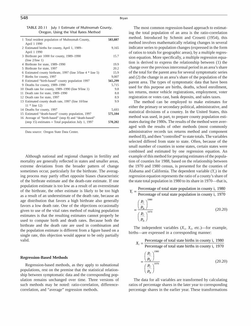
Although national and regional changes in fertility andmortality are generally reflected in states and smaller areas,extreme deviations from the broader pattern of changesometimes occur, particularly for the birthrate. The averag-ing process may partly offset opposite biases characteristicof the birthrate estimate and the death-rate estimate. If onepopulation estimate is too low as a result of an overestimateof the birthrate, the other estimate is likely to be too high as a result of an underestimate of the death rate, because anage distribution that favors a high birthrate also generallyfavors a low death rate. One of the objections occasionallygiven to use of the vital rates method of making populationestimates is that the resulting estimates cannot properly beused to compute birth and death rates. Because both thebirthrate and the death rate are used in combination and the population estimate is different from a figure based on asingle rate, this objection would appear to be only partiallyvalid.
Regression-Based Methods
Regression-based methods, as they apply to subnationalpopulations, rest on the premise that the statistical relation-ship between symptomatic data and the corresponding pop-ulation remains unchanged over time. Three versions of such methods may be noted: ratio-correlation, difference-correlation, and “average” regression methods.
The most common regression-based approach to estimat-ing the total population of an area is the ratio-correlationmethod. Introduced by Schmitt and Crosetti (1954), thismethod involves mathematically relating changes in severalindicator series to population changes (expressed in the formof ratios to totals for geographic areas), by a multiple regres-sion equation. More specifically, a multiple regression equa-tion is derived to express the relationship between (1) thechange over the previous intercensal period in an area’s shareof the total for the parent area for several symptomatic seriesand (2) the change in an area’s share of the population of theparent area. The types of symptomatic data that have beenused for this purpose are births, deaths, school enrollment,tax returns, motor vehicle registrations, employment, voterregistration or votes cast, bank deposits, and sales taxes.
The method can be employed to make estimates for either the primary or secondary political, administrative, andstatistical divisions of a country. In the United States, thismethod was used, in part, to prepare county population esti-mates during the 1980s. The results of the method were aver-aged with the results of other methods (most commonlyadministrative records tax returns method and componentmethod II), and then “controlled” to state totals. The variablesselected differed from state to state. Often, because of thesmall number of counties in some states, certain states werecombined and estimated by one regression equation. Anexample of this method for preparing estimates of the popula-tion of counties for 1988, based on the relationship betweenthe 1970 and 1980 census, is presented for the counties ofAlabama and California. The dependent variable (Yc) in theregression equation represents the ratio of a county’s share ofthe state total population in 1980 to its share in 1970—that is,
The independent variables (X1, X2, etc.)—for example,births—are expressed in a corresponding manner:
The data for all variables are transformed by calculatingratios of percentage shares in the later year to correspondingpercentage shares in the earlier year. These transformations
X
P
P
P
P
C
St
C
St
1
1980
1970
=
=
ÊË
ˆ¯
ÊË
ˆ¯
Percentage of total state births in county i, 1980Percentage of total state births in county i, 1970
Y
P
P
P
P
c
C
St
C
St
=
=
ÊË
ˆ¯
ÊË
ˆ¯
Percentage of total state population in county i, 1980Percentage of total state population in county i, 1970
1980
1970
548 Bryan
TABLE 20.11 July 1 Estimate of Multnomah County,Oregon, Using the Vital Rates Method
1 Total resident population of Multnomah County, 583,887April 1 1990
2 Estimated births for county, April 1, 1989– 9,165April 1 1990
3 Birthrate per 1000 for county, 1989–1990 15.7(line 2/line 1)
4 Birthrate for state, 1989–1990 19.95 Birthrate for state, 1997 20.26 Estimated county birthrate, 1997 (line 3/line 4 * line 5) 15.97 Births for county, 1997 9,0078 Estimated “birth-based” county population 1997 565,2999 Deaths for county, 1989–1990 5,715
10 Death rate for county, 1989–1990 (line 9/line 1) 9.811 Death rate for state, 1989–1990 8.812 Death rate for state, 1997 8.913 Estimated county death rate, 1997 (line 10/line 9.9
11 * line 12)14 Deaths for county, 1997 5,69315 Estimated “death-based” county population, 1997 575,10416 Average of “birth-based” (step 8) and “death-based”
(step 15) estimates = Total population July 1, 1997 570,202
Data source: Oregon State Data Center.
(20.20)
(20.20)
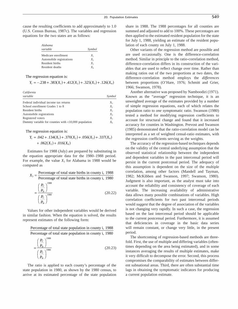
cause the resulting coefficients to add approximately to 1.0(U.S. Census Bureau, 1987c). The variables and regressionequations for the two states are as follows:
Alabamavariable Symbol
Medicare enrollment X1
Automobile registrations X2
Resident births X3
Resident deaths X4
Californiavariable Symbol
Federal individual income tax returns X1
School enrollment Grades 1 to 8 X2
Resident births X3
Automobile registrations X4
Registered voters X5
Dummy variable for counties with <10,000 population X6
Estimates for 1988 (July) are prepared by substituting inthe equation appropriate data for the 1980–1988 period. For example, the value X3 for Alabama in 1988 would becomputed as
Values for other independent variables would be derivedin similar fashion. When the equation is solved, the resultsrepresent estimates of the following form:
The ratio is applied to each county’s percentage of thestate population in 1980, as shown by the 1980 census, toarrive at its estimated percentage of the state population
Percentage of total state population in county i, 1988Percentage of total state population in county i, 1980
=
ÊË
ˆ¯
ÊË
ˆ¯
PP
PP
C
St
C
St
1988
1980
X
P
P
P
P
C
St
C
St
3
1988
1980
=
=
ÊË
ˆ¯
ÊË
ˆ¯
Percentage of total state births in county i, 1988Percentage of total state births in county i, 1980
The regression equation is:
Y X X X X
X Xc = + ( ) + ( ) + ( ) + ( )
+ ( ) + ( ). . . . .
. .
042 134 370 056 337
062 0161 2 3 4
5 6
The regression equation is:
Y X X X Xc = - + ( ) + ( ) + ( ) + ( ). . . . .238 383 412 325 1261 2 3 4
share in 1988. The 1988 percentages for all counties aresummed and adjusted to add to 100%. These percentages arethen applied to the estimated resident population for the statefor July 1, 1988, yielding an estimate of the resident popu-lation of each county on July 1, 1988.
Other variants of the regression method are possible andare used occasionally. One is the difference-correlationmethod. Similar in principle to the ratio-correlation method,difference-correlation differs in its construction of the vari-ables that are used to reflect change over time. Rather thanmaking ratios out of the two proportions at two dates, thedifference-correlation method employs the differencesbetween proportions (O’Hare, 1976; Schmitt and Grier,1966; Swanson, 1978).
Another alternative was proposed by Namboodiri (1971).Known as the “average” regression technique, it is anunweighted average of the estimates provided by a numberof simple regression equations, each of which relates thepopulation ratio to one symptomatic ratio. Swanson (1980)tested a method for modifying regression coefficients toaccount for structural change and found that it increasedaccuracy for counties in Washington. Prevost and Swanson(1985) demonstrated that the ratio-correlation model can beinterpreted as a set of weighted censal-ratio estimates, withthe regression coefficients serving as the weights.
The accuracy of the regression-based techniques dependson the validity of the central underlying assumption that theobserved statistical relationship between the independentand dependent variables in the past intercensal period willpersist in the current postcensal period. The adequacy of this assumption is dependent on the size of the multiple correlation, among other factors (Mandell and Tayman,1982; McKibben and Swanson, 1997; Swanson, 1980).Judgment is also important, as the analyst must take intoaccount the reliability and consistency of coverage of eachvariable. The increasing availability of administrative data allows many possible combinations of variables. Highcorrelation coefficients for two past intercensal periodswould suggest that the degree of association of the variablesis not changing very rapidly. In such a case, the regressionbased on the last intercensal period should be applicable to the current postcensal period. Furthermore, it is assumedthat deficiencies in coverage in the basic data series will remain constant, or change very little, in the presentperiod.
The shortcoming of regression-based methods are three-fold. First, the use of multiple and differing variables (often-times depending on the area being estimated), and in someinstances averaging the results of multiple estimates, makeit very difficult to decompose the error. Second, this processcompromises the comparability of estimates between differ-ent subnational areas. Third, there are often substantial timelags in obtaining the symptomatic indicators for producinga current population estimate.
20. Population Estimates 549
(20.22)
(20.23)

Regression-based methods have very limited applicationin the preparation of postcensal estimates of age-sex groupsfor small geographic areas. It is possible, of course, to applythe age distribution at the prior census date to a preassignedcurrent total for the area, or to extrapolate the last two censusage distributions to the current date and apply the extrapo-lated distribution to the current total. The resulting estimatesare subject to such large errors, however, that these methodsare viewed as having little value.
Census Ratio Methods: Housing-Unit Method
The housing unit method is one of the most widely usedmethods for preparing subnational population estimates. Themethod largely rests on the assumptions that everyone in thehousehold population of an area can be associated with somesort of identifiable, conventional shelter and that changes inthe number of occupied housing units essentially reflectchanges in population. The equation for the housing-unitmethod is
(20.24)
wherePt = population at time t,Ht = number of housing units at time t,Ot = housing-unit occupancy rate at time t,PPHt = persons per household at time t,and GQt = group quarters population at time t
Each of these variables must be compiled from adminis-trative records or estimated indirectly. Data on the numberof housing units may often be found in tax assessors’ offices.If the number of housing units needs to be estimated for anarea, building permits issued by local governments (for newconstruction, demolitions, and alterations) may be added tothe past census figure. Other indicators of housing stock mayinclude the number of electric, gas, or water utility connec-tions or customers, residential postal delivery “drops,” “cer-tificates of occupancy,” and so on (Smith and Lewis, 1980,1983).
As they are essentially multipliers of the number ofhousing units in the housing-unit method, accurate estimatesof the average number of persons occupying a housing unitand of vacancy rates are very important. Good sources ofinformation on changes in average household size and invacancy rates in the United States are the Current Popula-tion Survey and the American Housing Survey (Murdockand Ellis, 1991, pp. 186–187). These provide information onpostcensal changes at the national level, which may be usedto develop censal-ratio estimates of these variables for sub-national areas. If these data are lacking, it is possible toproject them from known past values using extrapolativeand other techniques (Bryan, 1996; Roe et al., 1992).
Finally, the size of the population living in group quar-ters (e.g., correctional facilities, rooming houses, college
P H O PPH GQt t t t t= * *( )[ ]+
dormitories, institutions, etc.) must be considered. Mostoften, these data are collected in administrative records,either by the group-quarters facilities themselves or by thelocal governmental unit within which the group-quartersfacility exists.
It should be apparent that once the data components ofthe housing-unit method are known, an exact determinationof the population is possible; that is, the formula preciselyspecifies the relationships between the variables. Any“error” is due to inaccuracies in calculations or the compo-nents, not to an inherent flaw in the method itself. Theseinaccuracies, however, are especially problematic for thevery small areas for which the housing-unit method is used.Therefore, it is again emphasized that the method be appliedto all coordinate small areas within a state or county area (orcorresponding region or province).
Composite Method
In general, a characteristic of the various methods of pop-ulation estimation described is that they are single methods,not combinations of methods, which measure change in thetotal population of an area “directly.” Uncertainties in pro-jecting censal ratios including vital rates and average size ofhousehold, resulting in part from changes in the age and sexcomposition of the population, suggest the desirability of analternative approach. The composite method is a “portfolio”of separate methods, each tailored to particular segments ofthe population. The results are combined to yield the “true”total population estimate. These results then may be adjustedto sum to the estimate for the larger area.
Many alternative “portfolios” are possible. For example,the number of deaths of persons 45 years and over distrib-uted by age may be used to estimate the population in thisage range. Likewise, the number of births may be used toestimate the number of females in the childbearing ages (18to 44 years), which, in turn, may be used to estimate thenumber of males in this age range. School enrollment datamay be used to estimate the population of school ages (5through 17 years); while the number of births in the previ-ous 5-year period, in conjunction with school enrollmentdata, may be used to estimate the population under 5 yearsof age. The ratio method, the component method, or math-ematical interpolation may be used to subdivide the popu-lations into single-year age groups as necessary. Theprincipal steps in applying this version of the compositemethod are as follows:
1. Population 45 years and over:a. Compute age-sex-race specific death rates by 10-year
age groups for the census year on the basis of the censuspopulation, starting with the population 45 to 54 years andending with 85 and over, for the country and each area.
b. Compute the corresponding death rates for the countryfor the 12-month period centered on the estimate date.
550 Bryan

c. Prepare estimates of the age-sex-race specific deathrates for each area for the 12-month period centered on theestimate date, on the assumption that the change in the deathrate for each area from the census year was the same as forthe country as a whole.
d. Compute the estimated population for each area on theestimate date in each age-sex group by dividing the numberof deaths for each group in the year centered on the estimatedate by its current specific death rate as obtained earlier. Inthe smaller areas, when deaths are distributed by age andsex, the numbers of deaths in some categories may beextremely small. The thinness of these data makes their useas a base for estimates very questionable. Consequently, invery small areas the procedure may be modified so that esti-mates are prepared for the age group 45 and over as a whole.
2. Population 18 to 44 years of age: Estimates of thenumber of females 18 to 44 years are first developed by thecensal-ratio method in a manner corresponding to steps athrough d using data on the number of births and the numberof females 18 to 44 years of age. As with the death rate 45and over, this method assumes that the change in age-specific birthrates for the local area was the same as for thecountry (or other large administrative area) as a whole.Then, the ratio of the number of civilian males to femalesat the last census in each area in this age range, adjusted for the change in this ratio for the country as a wholebetween the census date and the estimate date, is used toarrive at an estimate of the number of civilian males in the area. The number of civilian males, an estimate of military personnel, and the number of females are summedto yield an estimate of the total population 18 to 44 years of age.
3. Population under 18 years of age: The estimated population in this age group may be developed by a com-ponent procedure similar to that described for componentmethod II:
a. Obtain the census population in the cohort that wouldbe under 18 years on the estimate date.
b. Add births for the postcensal period.c. Subtract deaths for the cohort for the same period.d. Add an estimate of net migration.
The calculations may be carried out for two age groupsseparately, under 5 and 5 to 17 years. Estimates of net migra-tion for the group under 18 years of age are obtained fromthe migration rate of the school-age population derivedearlier as part of component method II. The factor used toconvert the migration rate for the school-age population tothe rate for the population under 18 years of age may bebased on national ratios of interstate or intercounty migrantsunder 18 years of age to interstate or intercounty migrantsin the school ages for the postcensal period.
The details of the composite method may be varieddepending on the kind and quality of data available. The
procedures of component method II may be applied to ages18 to 44 as well as ages under 5 and 5 to 17. On the otherhand, ages under 5 and 5 to 17 may be estimated by a censal-ratio procedure, using births and school enrollment as symp-tomatic data.
Total Subnational Population, Intercensal
As with national postcensal estimates, subnational post-censal estimates must be adjusted to account for the problemof error of closure in deriving intercensal estimates. Theproblem is typically greater for subnational areas thannational areas as less information is usually available withwhich to make the necessary adjustments. In addition, theintercensal estimates of change due to each component, pop-ulation change as a whole, or the population itself for allsubarea in each year must be adjusted to agree with the cor-responding intercensal figures established for the wholecountry. The error of closure for each subarea may be dis-tributed over the intercensal period in proportion to one ofthe components of change for the subarea (e.g., net migra-tion), the total population change, or the population itself.
Component Methods
Annual intercensal population estimates for geographicsubdivisions may be prepared by the component method if sat-isfactory data on births, deaths, and migration are available.
Even if a country has the required birth and death statis-tics for making intercensal estimates for geographic subdi-visions, it often lacks the required migration data or evendata symptomatic of migratory changes. If this is the case,intercensal estimates of population for such geographic sub-divisions may be developed on the basis of analyticallyderived estimates of net migration using these estimates todistribute the error of closure over the intercensal period.This procedure involves, first, estimating intercensal netmigration (including the error of closure) for each geo-graphic unit as a residual by the vital statistics method.Second, equal portions of the intercensal net migration maybe allocated to each year of the intercensal period. Finally,the preliminary estimates of net migration or population areadjusted to the independently established estimates of netimmigration or population (adjusted for error of closure) forthe entire country in each year of the intercensal period.
As with previous methods for intercensal estimates ofgeographic subdivisions, preliminary estimates of popula-tion for such areas should be adjusted to agree with the inde-pendently established intercensal estimates of the nationalpopulation (or other large administrative area). One methodof effecting this task is to adjust the geographic distributionof each component, particularly net migration, to agree with the established national estimate for that component
20. Population Estimates 551

(e.g., net immigration). A simpler method is to adjust thepreliminary estimates of the population of the subareas tothe established estimates of the national population withoutreference to the individual components.
Intercensal estimates of age groups involve an adjustmentfor the intercensal error of closure at each age and for incon-sistencies with annual estimates of the total population foreach area by age. In a cohort-component method, the annualpreliminary estimates of population by age and sex wouldbe computed for each geographic unit. Then, it is necessaryto determine the error of closure using previously mentionedtechniques for each age cohort and distribute the error ofclosure over the expected population by age cohorts (or thesame age groups). Then, the age-sex figures need to be “con-trolled” to area totals over all ages and to the national esti-mates for each age-sex group. Another procedure involvescalculation of the expected population by use of life tablesor death statistics and then allowing for net migration bycohorts as part of the adjustment for the error of closure.
Mathematical Interpolation and Extrapolation
As with national estimates, so for subnational estimates,mathematical extrapolation alone should only be used whendirect information on births, deaths, and migration arelacking. The mathematical curves most commonlyemployed for this purpose are straight lines and geometricand exponential growth curves (see, e.g., Chapter 11).However, a great variety of other forms may be employed(e.g., higher degree polynomials, reverse geometric curves,and more complex exponentials such as the logistic). Geo-metric extrapolation is more logical than linear extrapola-tion in making population estimates, especially inundeveloped nations, where birthrates may remain nearlyconstant at a high level and death rates are constant ordeclining. Linear extrapolation may be more appropriate forsome of the geographic subdivisions of these same countriesbecause growth rates may be falling as a result of outmi-gration. The subareas of the same country could reasonablybe treated differently, therefore, taking account of informa-tion identifying the areas of in- and outmigration. Theextrapolation process may be applied to percentages repre-senting the proportion that the population of an area consti-tutes of the population of some more inclusive area forwhich annual totals are available. The process of extrapola-tion is exactly as in Table 20.4, except that geographic unitsare extrapolated rather than age groups. In principle, mathematical methods involve adjustment to independentestimates for the parent area; in practice, no adjustment isnecessary if linear extrapolation is used for both the parentarea and its subdivisions and no adjustment is made if a sat-isfactory independent estimate is not available.
Another primarily mathematical method of estimatingsubnational population that also takes limited account of
current data is the apportionment method. This methodessentially involves distributing the postcensal increase inpopulation in the parent area (e.g., a country) among thecomponent parts of that area (e.g., states) in accordance with the distribution of the intercensal increase in the parentarea among the component parts. If a subarea lost popula-tion in the intercensal period, its population in the latestcensus is assumed to remain unchanged. Except for thespecial treatment of areas that lost population, the appor-tionment method is approximately equivalent to arithmeticextrapolation when the results by the latter method areadjusted pro rata to the independent estimate of the totalpopulation of the parent area. Like the other mathematicalmethods, this method requires a current total for the parentarea.
In general, these mathematical methods may prove lessaccurate than the various component methods and othermethods using symptomatic data for the simple reason thatthey have no connection, direct or symptomatic, with thepostcensal universe they are estimating. These methodsusually employ the assumption that population change in thepostcensal period is in the same direction and at the samepace as in the preceding intercensal period or periods. Whilethis is often not the case, mathematical methods have certainadvantages. Primarily, they are easy to apply, insofar as theytake relatively little time and require only readily availabledata, and are simple enough in principle for the layman tounderstand. As the evaluation studies show, the mathemati-cal methods are not very reliable for making postcensal pop-ulation estimates for geographic subdivisions of countries,although they may be necessary in the absence of sympto-matic data for the postcensal period. However, their relia-bility is quite different when they are used to prepareintercensal estimates.
As explained earlier in the section on national intercensalestimates, mathematical interpolation is a convenient andsimple method of making intercensal estimates, givenannual estimates of the total population of each area to which the estimates for subgroups (e.g., age groups) maybe adjusted. Alternatively, the percentage of the total popu-lation of the area in each subgroup (e.g., age group) may beinterpolated and applied to the estimates of the total popu-lation of the area at the estimate date.
EVALUATION OF METHODS
Design of Evaluation Studies
A variety of methods for making population estimates ofnations and their geographic subdivisions, by age and sex,have been discussed with relatively little concern for theiraccuracy. A population estimation system in fact involvesthree elements: (1) the necessary data, (2) a sound statisti-
552 Bryan

cal procedure to generate the estimates, and, (3) a system ofevaluation on to ensure that the estimates are reasonable. Asound evaluation procedure is imperative for any estimatesprogram, as it informs both the producers and the users ofthe estimates about the strengths and limitations of the estimators, or estimation formulas (National Academy ofSciences, 1980, p. 47). The motivation for evaluation comesboth from statistical concerns as well as the implications inprograms and applications based on the estimates.
An evaluation program may specifically assist in identi-fying statistical measures of error (or differences) thatpermit refinement of methods and improved techniques ofproducing estimates. Recall the most common applicationsof population estimates in funds allocation, denominatorsfor vital rates and per capita time series, survey controls,administrative planning, marketing guidance, and descrip-tive and analytical studies. Evaluating the accuracy ofmethodology necessarily raises questions about the equityof allocation of resources among units of government(Swanson, 1981, pp. 12–22). Further, accurately monitoringthe pace of demographic change is imperative for determin-ing the need and demand for public services such as healthcare as well recreational and educational services, for estab-lishing political boundaries, and for providing a host of publicly and privately furnished goods and services that aresensitive to changes in the size and composition of the resident populations.
Murdock and Ellis (1991, p. 242) identify five potentialapproaches to reviewing estimates: (1) examine the (esti-mates) in comparison with historical patterns of populationchange and of the components of population change, (2)evaluate the estimates relative to other estimates that havebeen made for the estimation area or areas similar to esti-mation area, (3) submit them to selected knowledgeablepersons in the estimation areas for their assessment of thevalidity of the assumptions and of the estimated populations,(4) conduct sensitivity analysis of the effects of alterations in assumptions about key parameter, and (5) conduct his-torical simulations in which the accuracy of the estimationmodel in estimating population in past periods is evaluated.
In any of these approaches, statistical measures need tobe used to perform the evaluation desired. Furthermore,standards need to be developed to assess whether the esti-mates meet standards of “accuracy.” Any consideration ofthe accuracy of methods depends on the availability of ade-quate standards against which to judge the methods and theestablishment of criteria of accuracy. Any definition of accu-racy is tenuous at best, as different standards are applicablein almost any estimating situation.
Statistical Measures
The most common statistical measures used to evaluateestimates and measure differences are as follows:
(20.25)
(20.26)
(20.27)
(20.28)
(20.29)
whereA is the actual populationE is the estimated populationt is the geographic area estimatedh is the number of geographic areas in a set
(Siegel, 2002, pp. 423–424)
The mean absolute error (MAE) is the average absoluteamount of error in each estimate, total error is the totalamount of error over all areas with signs regarded, meanabsolute percent error (MAPE) is a measure of accuracy,root mean square error (RMSE) is a measure of accuracygiving more weight to large errors than to small errors, andmean algebraic percent error (MALPE) is essentially ameasure of bias.
The rationale for using these measures is to detect changeand identify individual problematic estimates or estimateseries. It has been argued, however, that measures such asMAPE are invalid for evaluating error in that they may bestrongly affected by the right skewness of the distribution oferror (Swanson, Tayman, and Barr, 2000) and that theycannot effectively evaluate data series with wide ranges ofpopulation values. These shortcomings suggest that theseevaluation tools have been pushed to the limit of their use-fulness and that new tools should be examined. Severalmeasures, some new and some old, have been developed tohelp address these shortcomings. One is known as a “lossfunction,” which is designed to combine a weighted per-centage and weighted numeric difference to create a highlysensitive index of relative error (Bryan, 1996). A recent pro-posal is the transformed MAPE (Swanson, Tayman, andBarr, 2000). The MAPE measure is inherently based on a
Mean algebraic percent error MALPE( )
-( )=Â
:*
E AAh
t t
tt
h100
1
Root mean square error RMSE( )
-ÊË
ˆ¯
È
Î
ÍÍÍÍ
˘
˚
˙˙˙˙
=Â:
E A
Ah
t t
tt
h
1
1 2
Mean absolute percent error MAPE( )-( )
*[ ]=Â
:
E AA
h
t t
tt
h
1
100
Total error: E At tt
h-( )
=Â 1
Mean absolute error MAE( )-
=Â:
E A
h
t tt
h
1
20. Population Estimates 553

right-skewed, asymmetrical distribution of absolute percenterrors (APEs), and like any arithmetic average taken oversuch a set, it is prone to being pulled upward. The trans-formed MAPE addresses this issue by transforming theshape of the distribution of absolute percent errors (APEs)to produce an average that more accurately reflects the errorrepresented by most of the observations.
For now, however, MAPE is the tool most commonlyrelied on for evaluating estimates. Note that the tools devel-oped for performing evaluations of estimates are designedto detect the extent of error in the total population or thechange in the population. Errors in estimates may be imper-ceptible because no apparent change has taken place whenin fact substantial change has occurred in an estimate series.It is in these situations that submitting estimates series toexperts in local data review and performing sensitivityanalysis may be especially useful.
Although postcensal population estimates provide valu-able information, only a single value for the number beingestimated is usually presented. An issue frequently raisedconcerning population estimates (and more frequently pro-jections) is the amount of confidence estimators have inthese single values. One may point to a history of resultswith different methods in different situations and determinethat one method may be superior to another. However, thishistory in and of itself does not predict the amount of errorone may expect in estimates nor does it establish any degreeof confidence in an untested estimate. Theoretically, an idealenvironment is one that affords analysts the opportunity tomeasure confidence intervals surrounding estimates. Unfor-tunately, under the formal definition, confidence intervalscannot be constructed for postcensal estimates because theprobability distribution of errors is unknown. If assumptionsare made about the characteristics of the probability distri-bution of error in a set of estimates, then empirical confi-dence intervals may be constructed.
A logical assumption is that the distribution of estimateerrors remains stable over time. This assumption was testedin series of state population forecasts from 1920–1980 bySmith and Sincich (1988). The critical assumption that theprobability distribution of errors remains the same over timewas reasonably well satisfied. Smith and Sincich (1988) alsocreated empirical confidence intervals using a techniquefrom Williams and Goodman (1971) that accommodates anyerror distribution (including asymmetric and truncated dis-tributions) and additionally permits assessment of the con-fidence limits (by comparing the actual number of errorsfalling inside the limits with the expected number). Furtherresearch has also been done on developing confidence inter-vals. Swanson and Beck (1994) studied the distribution oferrors of the ratio-correlation method at the county levelover time using Washington State as a case study. Theyexamined estimates made for 1970, 1980, and 1990 againstcorresponding census counts and demonstrated that 67%
“prediction intervals” generated for the estimates provideda reasonable view of accuracy: (1) the 67% interval con-tained the 1970 census count in 30 of 39 counties (77%), (2)the 1980 census counts in 24 counties (62%), and (3) the1990 census counts in 31 counties (79%).
Without historical information on which to base assump-tions of stability (or amount of error), one may still createtenuous empirical confidence intervals by assuming a uni-modal, symmetric normal distribution (Blachman andMachol, 1987) or by relaxing the percentage confidenceintervals.
National Estimates Evaluation
Perhaps the most convenient and accurate way to evaluatea national population estimate is to compare it with theresults of an official census. Most often, estimates may beevaluated in an “ex-post”-style test whereby the selectedestimate method is used to derive an estimate on the censusdate, and the results are then compared using selected sta-tistical comparisons. When a national postcensal estimate ofthe total population is evaluated by comparison with thecensus count, the difference between the postcensal estimateand the later census count, i.e., the error of closure, and theratio of the error of closure to the census count may be takento reflect the amount and percent of error, respectively, inthe postcensal estimate, measured over a whole intercensalperiod. The errors of closure (e.g., total, age, sex) can beexamined to judge the accuracy of the postcensal estimatesin relation to their census counts. It is important to note thatnot only should the official estimate be subjected to evalu-ation but also the results of competing methods, so thatpotential improvements or revisions in the methods used forthe official estimates process may be considered.
The errors in postcensal estimates by age, as measuredby the errors of closure, tend to be considerably greater thanthe error in the total for an area, particularly because of theeffect of errors in reporting age in the two censuses. Theerrors in postcensal estimates represent in part the effect ofcarrying reporting errors at one age in the first censusforward to a later age at the second census. The structuringof the calculations by age cohorts results in good compara-bility of age estimates with the previous census figures forthe same birth cohorts but poor comparability with figuresfor the same age groups in either the first or second census.
The estimates of national population based on some population registers are viewed as being as accurate as acensus count. Estimates from population registers are, infact, closely akin to the estimates prepared by the compo-nent method. Commonly, at a census date the register isreviewed and corrected on the basis of the census results,and then the national total from the register, validated by theprevious census, is kept up to date by use of the componentdata from the register. The discrepancies between census
554 Bryan

counts and totals from population registers are quite smallin most countries having registers.
For the statistically less developed countries, the data oncomponents are often inadequate to serve as a firm basis forpreparing postcensal estimates. Where such data are used,the postcensal estimates are subject to considerable error.Whether this method or mathematical extrapolation isemployed, it is probable also that in these countries thecensus counts are fairly incomplete and less comparable incoverage with one another. However, some less developedareas have relatively good censuses but poor vital statistics.
In a program of estimate evaluation, the values from thecensus or population register are generally regarded as the“truth,” rendering any difference between it and an estimate wholly attributable to the estimate. For evaluative purposes,however, one should recognize that a population estimatemay actually be more accurate for a specific area than acensus or population register. In this context, a populationestimate may offer the basis for use of demographic analy-sis to evaluate the quality of the census results themselves.Countries may use different types and even combinations ofmethods of demographic analysis to evaluate census results.(see Chapters 4, 7, and 22).
Subnational Estimates, Evaluation
As with national estimates, a census provides the mostconvenient and accurate base for evaluating of subnationalestimates. In this regard, several important matters mustconsidered before estimates are compared with censusvalues. There is often a tendency to assume that the earlierand later censuses are completely consistent, but such con-sistency cannot be taken for granted. Subnational areas oftendiffer in land areas and populations covered, and census def-initions may change as well. If an estimate is based on a pastcensus that differs from the more recent census in any sig-nificant way, an accurate evaluation is compromised. Whenestimates comparable to the last census are sought, the samemethods of estimation may be employed as in the previousintercensal period, but the standard for evaluating the esti-mates is less evident, particularly for estimates of agegroups. Alternative representations of a “true” populationmay be made with a special registration or a population reg-ister, which may provide more correct figures than thecensus. In addition, comparisons may be made with officialestimates developed by local authorities.
There are several approaches to evaluation when theexact amount of error in the current census is not known.The first is simply to compare the census results with theestimates. While this comparison is affected by the error ofclosure, it illustrates how the estimates compare with theaccepted standards in the census. Second, the net undercountfor the past census may be added to the current estimate foreach subnational area. This approach may produce more
accurate postcensal estimates, but these estimates may nowbe less comparable with the later census and produce biasedestimates of error. Third, the estimated proportion of popu-lation that each subnational area is of the national (or otherparent area) total may be computed. This allows a test of theestimating procedure to determine how well it “predicts” thedistribution of the national population, compensating for thelarge national error of closure (U.S. Census Bureau/Starsinic, 1983, p. 3).
A large and growing number of studies have been carriedout, particularly in the United States and the Great Britain,designed to evaluate various methods of preparing subna-tional population estimates. The U.S. Census Bureau hascarried out an extensive program of evaluating postcensalestimates for states and local areas over the past severaldecades, and several important studies have been conductedby investigators in other settings. These studies typicallyemploy census counts as the standard by which the estimatesare judged.
First, the evaluation of major geographic subdivisions(states in the case of the United States) may be considered.The U.S. Census Bureau has made systematic comparisonsbetween census counts for states and the corresponding esti-mates derived by several different basic methods andselected averages of these basic methods (U.S. CensusBureau/Starsinic, 1983; Zitter and Shryock, 1964). It isimportant that these comparisons against the census be con-sidered “measures of difference” rather than “measures oferror” as it is impossible to determine precisely the degreeto which error in the census and error in the estimate con-tribute to the overall difference. Among other measures, theprimary indicator of error was the average absolute per-centage difference.
It is important to note that a direct “method-to-method”comparison is rarely possible when attempting to evaluatepopulation estimates. Often it may not be practicable to testthe most accurate method because of excessive time, cost,and resources. Other hindrances to doing this may includethe unavailability or inconsistency of necessary data. Fur-thermore, as will be seen, certain methods are better suitedto particularly large or particularly small geographic areas.While one method may generate good results at a nationallevel, it may be wholly inadequate for a province or town-ship. Thus, the amount of resources available and the geo-graphic level, as well as the historical accuracy of eachmethod, must always be considered.
U.S. System
U.S. Census Bureau Programs
We describe now the program for evaluating subnationalestimates at the U.S. Census Bureau, as it is one of the mostproductive in the world and then look briefly at evaluation
20. Population Estimates 555
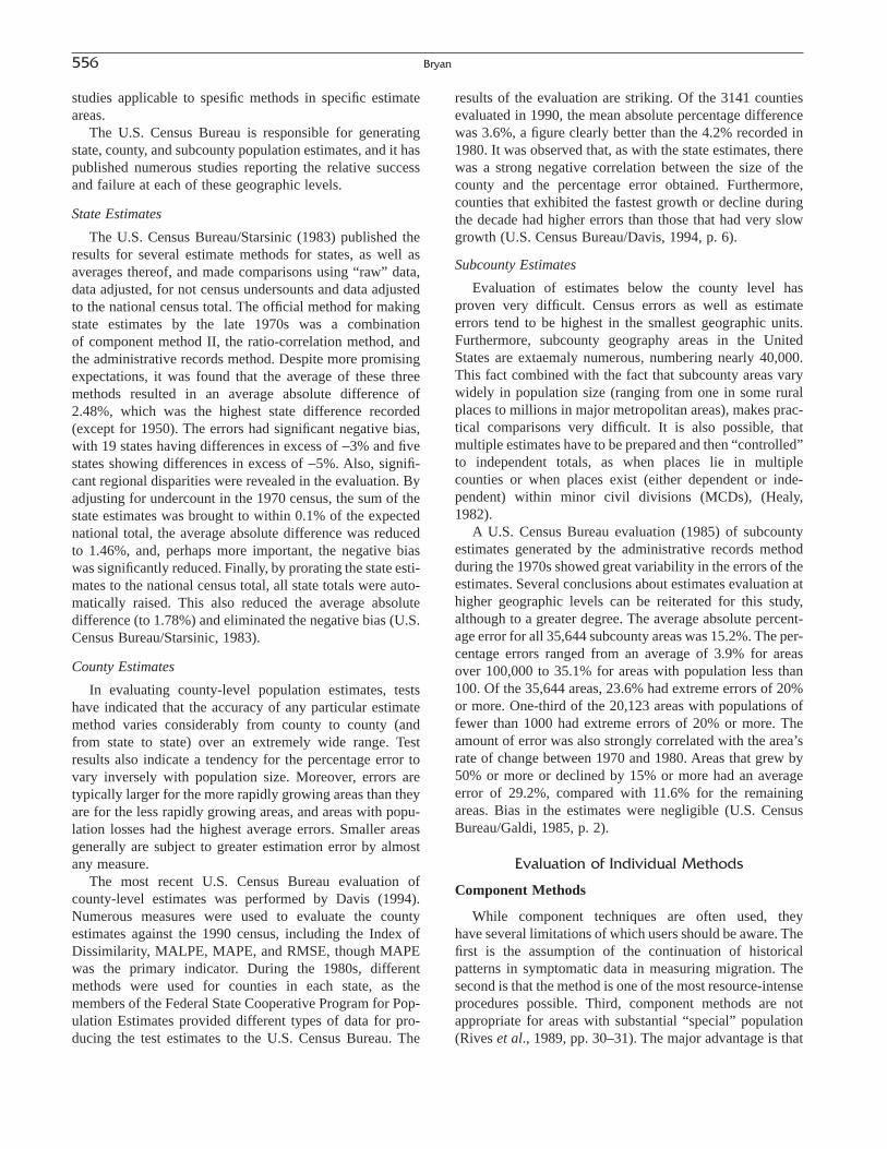
studies applicable to spesific methods in specific estimateareas.
The U.S. Census Bureau is responsible for generatingstate, county, and subcounty population estimates, and it haspublished numerous studies reporting the relative successand failure at each of these geographic levels.
State Estimates
The U.S. Census Bureau/Starsinic (1983) published theresults for several estimate methods for states, as well asaverages thereof, and made comparisons using “raw” data,data adjusted, for not census undersounts and data adjustedto the national census total. The official method for makingstate estimates by the late 1970s was a combination of component method II, the ratio-correlation method, andthe administrative records method. Despite more promisingexpectations, it was found that the average of these threemethods resulted in an average absolute difference of2.48%, which was the highest state difference recorded(except for 1950). The errors had significant negative bias,with 19 states having differences in excess of -3% and fivestates showing differences in excess of -5%. Also, signifi-cant regional disparities were revealed in the evaluation. Byadjusting for undercount in the 1970 census, the sum of thestate estimates was brought to within 0.1% of the expectednational total, the average absolute difference was reducedto 1.46%, and, perhaps more important, the negative biaswas significantly reduced. Finally, by prorating the state esti-mates to the national census total, all state totals were auto-matically raised. This also reduced the average absolutedifference (to 1.78%) and eliminated the negative bias (U.S.Census Bureau/Starsinic, 1983).
County Estimates
In evaluating county-level population estimates, testshave indicated that the accuracy of any particular estimatemethod varies considerably from county to county (and from state to state) over an extremely wide range. Testresults also indicate a tendency for the percentage error tovary inversely with population size. Moreover, errors aretypically larger for the more rapidly growing areas than theyare for the less rapidly growing areas, and areas with popu-lation losses had the highest average errors. Smaller areasgenerally are subject to greater estimation error by almost any measure.
The most recent U.S. Census Bureau evaluation ofcounty-level estimates was performed by Davis (1994).Numerous measures were used to evaluate the county estimates against the 1990 census, including the Index ofDissimilarity, MALPE, MAPE, and RMSE, though MAPEwas the primary indicator. During the 1980s, differentmethods were used for counties in each state, as themembers of the Federal State Cooperative Program for Pop-ulation Estimates provided different types of data for pro-ducing the test estimates to the U.S. Census Bureau. The
results of the evaluation are striking. Of the 3141 countiesevaluated in 1990, the mean absolute percentage differencewas 3.6%, a figure clearly better than the 4.2% recorded in1980. It was observed that, as with the state estimates, therewas a strong negative correlation between the size of thecounty and the percentage error obtained. Furthermore,counties that exhibited the fastest growth or decline duringthe decade had higher errors than those that had very slowgrowth (U.S. Census Bureau/Davis, 1994, p. 6).
Subcounty Estimates
Evaluation of estimates below the county level hasproven very difficult. Census errors as well as estimateerrors tend to be highest in the smallest geographic units.Furthermore, subcounty geography areas in the UnitedStates are extaemaly numerous, numbering nearly 40,000.This fact combined with the fact that subcounty areas varywidely in population size (ranging from one in some ruralplaces to millions in major metropolitan areas), makes prac-tical comparisons very difficult. It is also possible, that multiple estimates have to be prepared and then “controlled”to independent totals, as when places lie in multiple counties or when places exist (either dependent or inde-pendent) within minor civil divisions (MCDs), (Healy,1982).
A U.S. Census Bureau evaluation (1985) of subcountyestimates generated by the administrative records methodduring the 1970s showed great variability in the errors of theestimates. Several conclusions about estimates evaluation athigher geographic levels can be reiterated for this study,although to a greater degree. The average absolute percent-age error for all 35,644 subcounty areas was 15.2%. The per-centage errors ranged from an average of 3.9% for areasover 100,000 to 35.1% for areas with population less than100. Of the 35,644 areas, 23.6% had extreme errors of 20%or more. One-third of the 20,123 areas with populations offewer than 1000 had extreme errors of 20% or more. Theamount of error was also strongly correlated with the area’srate of change between 1970 and 1980. Areas that grew by50% or more or declined by 15% or more had an averageerror of 29.2%, compared with 11.6% for the remainingareas. Bias in the estimates were negligible (U.S. CensusBureau/Galdi, 1985, p. 2).
Evaluation of Individual Methods
Component Methods
While component techniques are often used, they have several limitations of which users should be aware. Thefirst is the assumption of the continuation of historical patterns in symptomatic data in measuring migration. Thesecond is that the method is one of the most resource-intenseprocedures possible. Third, component methods are notappropriate for areas with substantial “special” population(Rives et al., 1989, pp. 30–31). The major advantage is that
556 Bryan

they effectively represent the processes that directly affectpopulation change.
While the component method is a conceptually soundone, certain facts must be considered when using it to gen-erate age detail. The use of the method may lead to distortedand unacceptable results when the undercount rates in thecensus differ greatly by age groups, particularly those thatare adjacent. The problem is exacerbated by the possibilitythat the net undercount rate may change significantly overtime. Further, the recorded growth rate in an age group fromthe census date to the estimate date may be significantly dif-ferent from the corresponding growth rate based on popula-tions adjusted for net undercounts (U.S. Census Bureau/DasGupta and Passel, 1987a). For these reasons, componentmethods have not always fared well without a special adjust-ment, such as that represented by the inflation-deflation procedure.
Administrative Records
A major disadvantage of the administrative recordsmethod for general use lies in the inaccessibility of federalincome tax records, even in summary form, to the generalpublic. However, the Internal Revenue Service does makeavailable data on county-to-county migration flows (Riveset al., 1989, p. 79). Further, the estimates are subject to errorbecause of the inaccuracy of the preceding census, bound-ary problems, residency problems, and coverage problems,though the method is flexible in estimating changes in geo-graphic boundaries.
Trend Extrapolation
A comparison of intercensal changes for counties andeven states in the United States for 1970–1980 and for1980–1990 reveal numerous cases inconsistent with theassumption of trend extrapolation and emphasize the needfor using symptomatic data for subnational estimates. In thecase of the apportionment method, the assumption that thepostcensal growth in local areas is fixed to the earlier growthin the area, as indicated by the change in the parent area,may readily be challenged with census data. The method islogically inapplicable if the postcensal change in the parentarea moves in a different direction from the intercensalchange in that area. Although there is usually a high corre-lation between growth trends for a given area in two suc-cessive intercensal periods and between the growth trends of broader areas and their geographic subdivisions,the assumption of similarity in these cases is tenuous.
Housing-Unit Method
While the components of most estimation methods relyon data symptomatic of change, few rely so directly as thehousing-unit method. The results of other estimation
methods based on symptomatic data are included in the dis-cussions of the component method and regression method.Because of the ease of use, flexibility, and relative accuracyof the housing-unit method, it is heavily relied on by stateand local agencies to estimate populations. As of 1990 (U.S.Census Bureau, 1990a, p. 4), 234 out of 336 state and localagencies relied on this method alone for subnational esti-mates. While no comprehensive ex-post tests have been per-formed of the housing unit method against a decennialcensus, numerous tests have been performed for limited geographic areas.
Early tests of the housing-unit method can be found inthe research of Starsinic and Zitter (1968), who employed a variety of data sources and techniques to see which com-bination generated the best results. They compared theirresults with data gathered in special censuses in 47 citieswith populations of greater than 50,000. They found (1) themethod tends to generate estimates on the high side (of the47 cities for which building permit data are available andused for making the estimates, the deviations were positivein about 30 cases); (2) the use of utility data rather thanbuilding-permit data generally reduces the errors, althoughhere too there are substantially more positive than negativedeviations and thus with utility data the positive bias of themethod continues, although at somewhat a lower level; (3)smaller deviations result when average size of household isextrapolated than when the 1960 values are held constant;and (4) the average error in the estimate of the number ofhouseholds when either building-permit or utility data areused is also quite high.
Smith and Lewis (1980) performed further tests whenthey completed the first comprehensive intercensal test ofthe housing-unit method using several combinations oftechniques for estimating the number of households andpersons-per-household (PPH) ratios. Using special censusdata for 22 places in Florida, Lewis and Smith began byestimating the number of housing units by four differenttechniques: two based on residential building permits andtwo based on the number of electric customers. They thenused three different techniques to estimate PPH values. Thefirst simply used the PPH of the most recent census, in thiscase, 1970. The second used a linear extrapolation of thetrend between the 1960 and 1970 censuses. The third useda ratio of the PPH in a local area to the PPH in the UnitedStates times the proportional change in PPH for the UnitedStates since the most recent census.
Their study shows that the different techniques providedramatically different results and that the electric-utilityratio method generated the most accurate estimate ofhousing units, with an error of 7.5% (MAPE). This was fol-lowed by the “absolute number” electric utility method at10.4% (MAPE), the disaggregated building-permit methodat 11.2% (MAPE), and the aggregated building permitmethod at 11.5% (MAPE). The results of using the three dif-ferent PPH methods show that using PPH values unchanged
20. Population Estimates 557

from the previous census provides generally poor PPH esti-mates, yielding an error of 11.5% (MAPE). Simple extrap-olation of PPH provided significantly improved results, withan error of 6.8% (MAPE), but was bettered by the shift-sharemethod, which recorded an error of only 5.9% (MAPE).
In generating overall population estimates, Smith andLewis used five different combinations of PPH estimatesand housing-unit estimates. Of these combinations, the onejoining the ratio PPH method with the electric-utility ratiomethod generated the best results with a total averageabsolute error of 12.3%. The benefits of these tests are thatresearchers could now see a clear pattern of combining vari-ables in the framework of the housing-unit method so as toachieve more accurate population estimates.
Regression-Based Methods
The regression-based methods are perhaps the mostextensively studied and evaluated methods of generatingpopulation estimates. Simple regressions and numerousvariations have been studied and applied in an effort to estimate populations with a minimum of error. Most com-monly, several techniques are compared in a particular casestudy. The results of this research have usually shown thatthe “best” method often depends on the situation in whichit is applied and the quality of the data employed in theregression.
An instructive evaluation was performed by O’Hare(1976), who estimated the population of counties in Michigan in 1970. Comparing the difference-correlationtechnique to the ratio-correlation method, as well as thecomposite method, component method II, and vital ratesmethod, O’Hare derived favorable results for the difference-correlation technique, as shown in Table 20.12.
It should be noted that while the difference-correlationmethod provided the best results in this evaluation, all of themethods performed well with small average errors and stan-dard deviations. Mandell and Tayman (1982) evaluated the difference-correlation and ratio-correlation techniquesfurther in the context of the strength of the correlation and the temporal stability of the coefficients in estimates for the 67 counties in Florida in 1970. They showed that while the difference-correlation technique consistently achievedhigher R2 values, it exhibited less temporal stability of the coefficients of the variables and consequently greateraverage errors.
To evaluate the “average” regression technique, Nam-boodiri compared its percentage errors with those of theratio-correlation technique for estimating the population ofNorth Carolina counties in 1960 (Namboodiri, 1971). Using1950/1940 ratios, Namboodiri discovered in his study thatthe mean percentage of error provided by the average regres-sion method was sharply less than the ratio-correlation
method (5.8 against 9.5%) and that the ratio method had amuch greater tendency to underestimate populations and toproduce estimates with errors greater than 10%.
The conclusion that may be drawn from this mix ofresults is that no regression method uniformly or routinelyoutperforms another (O’Hare, 1980). While a high correla-tion may be indicative of a strong model, the temporal sta-bility of the regression coefficients must be considered,given the nature of the assumption that they will remain con-stant over the estimation period, as Namboodiri (1972) andothers (e.g., McCullagh and Zidek, 1987; Verma andBasavarajappa, 1987) have noted. Swanson (1980) andSwanson and Tedrow (1984) developed methods both forevaluating the stability of these coefficients and for makingadjustments to them as necessary, while McKibben andSwanson (1997) examined theoretical and substantive issuesunderlying the changes in the coefficients.
FINAL NOTE
Future developments in the uses, scope, and methodologyof population estimates are being guided by the astonishinggains in computing power and software developments. Con-ventional methods, as well as new ideas about estimatingpopulation, may be fully developed and tested with a time-liness and efficiency never before achievable. Improvementsin geographic information systems in particular are makingthe production of very small area estimates and data pres-entation, such as the demographic and economic mappingsystem (DEMS) of the San Diego Association of Govern-ments (sandag.cog.ca.us), vastly easier and more useful.Similarly, improvements in satellite imagery are providingthe opportunity to develop population estimates usingremote sensing (Wicks et al., 1999). Yet these increasinglysophisticated measures often come with a price of compro-mised privacy (whether perceived or real) of those beingestimated. Further, while pursuing elaborate measures, theanalyst should not forget that simple, naïve methods willsometimes yield more accurate estimates than elaborate,presumably sophisticated methods (Lee and Goldsmith,1982, p. 203).
558 Bryan
TABLE 20.12 The Mean and Standard Deviation ofAbsolute Percentage Errors for County Population Estimates
Produced by Five Different Methods
Standard deviationMethod MAPE of APE
Difference-correlation method 4.5 3.7Ratio-correlation method 4.7 3.9Composite method 4.9 3.8Component method II 6.1 5.5Vital rates method 6.3 4.2

References
Arriaga, E., P. Johnson, and E. Jamison. 1994. Population Analysis withMicrocomputers. Washington, DC: U.S. Census Bureau.
Blachman, N. M., and R. E. Machol. 1987. “Confidence Intervals Based onOne or More Intervals.” Institute of Electrical and Electronic EngineersTransactions on Information Theory, (IT-33): 373–382.
Bogue, D. J. 1950. “A Technique for Making Extensive Population Estimates.” Journal of the American Statistical Association (45):191–199.
Brass, W. 1975. Methods for Estimating Fertility and Mortality fromLimited and Defective Data. Laboratories for Population Statistics.Chapel Hill, NC: University of North Carolina.
Bryan, T. 1996. “Linear and Logarithmic Population Forecasting Techniques.” Paper presented at the Federal State Cooperative for Population Estimates Meetings, New Orleans, LA.
Canada, Statistics Canada. 1987. Population Estimation Methods, Canada. Catalogue 91-528E.
Davis, H. C. 1995. Demographic Projection Techniques for Regions andSmaller Areas. Vancouver, BC: University of British Columbia Press.
Goldberg, D., A. Feldt, and J. W. Smit. 1960. Michigan Population Studies,No. 1, “Estimates of Population Change in Michigan: 1950–60.” AnnArbor, MI: University of Michigan.
Healy, M. K. 1982. “Introduction to Basic Procedures.” In Population Estimates: Methods for Small Area Analysis. Beverly Hills, CA: Sage.
Illinois Department of Public Health. 1999. Survey of States on PopulationEstimates. Springfield, IL.
Lativia, Central Statistical Bureau of Latvia. 1999. Courtesy CSB Statisti-cian Ieva Kamenpusa, October 15, 1999.
Lee, E. S., and H. F. Goldsmith. 1982. Population Estimates: Methods forSmall Area Analysis. Beverly Hills, CA: Sage.
Land, K. C., and G. C. Hough, Jr. 1986. “Improving the Accuracy of Intercensal Estimates and Postcensal Projections of the Civilian Noninstitutional Population: A Parameterization of Institutional Prevalence Rates.” Journal of the American Statistical Association81(393): 62–74.
Long, J. 1993. Postcensal Population Estimates: States, Counties andPlaces. Technical Working Paper No. 3. Washington, DC: U.S. Bureauof the Census.
Mandell, M., and J. Tayman. 1982. “Measuring Temporal Stability inRegression Models of Population Estimation.” Demography 19(1):135–146.
Martin, J. H., and W. Serow. 1979. “Conflict and Cooperation in Produc-ing Population Estimates.” State Government 52(4): 182–186.
McCullagh, P., and J. V. Zidek. 1987. “Regression Methods and Perfor-mance Criteria for Small Area Population Estimation.” In R. Platek, J.N. K. Rao, C. E. Särndal and M. P. Singh (Eds.), Small Area Statistics:An International Symposium (pp. 62–72). New York: John Wiley andSons.
McKibben, J., and D. A. Swanson. 1997. “Linking Substance and Practice:A Case Study of the Relationship Between Socio-Economic Structureand Population Estimation.” Journal of Economic & Social Measure-ment 24: 135–147.
Murdock, S., and D. Ellis. 1991. Applied Demography. Boulder, CO: Westview Press.
Namboodiri, N. K. 1971. “The Average of Several Multiple RegressionEstimates as an Alternative to the Multiple Regression Estimate in Postcensal and Intercensal Population Estimation.” Rural Sociology36(2).
Namboodiri, N. K. 1972. “On the Ratio-Correlation and Related Methodsof Subnational Population Estimation.” Demography 9: 443–453.
National Academy of Sciences. 1980. Panel on Small-Area Estimates ofPopulation and Income. Estimating Population and Income of SmallAreas. Washington, DC: National Academy Press.
O’Hare, W. 1976. “Report on a Multiple Regression Method for MakingPopulation Estimates.” Demography 13(3): 369–379.
O’Hare, W. 1980. “A Note on the Use of Regression Methods for MakingPopulation Estimates.” Demography 17(3): 341–343.
Philippines National Statistical Coordination Board. 1991. 1991 PhilippineStatistical Yearbook.
Prevost, R., and D. Swanson. 1985. “A New Technique for Assessing Errorin Ratio-Correlation Estimates of Population: A Preliminary Note.”Applied Demography Interest Group Newsletter 1(November): 1–4.
Rives, N. W., W. J. Serow, A. S. Lee, and H. F. Goldsmith. 1989. SmallArea Analysis: Estimating Total Population. Rockville, MD: U.S.Department of Health and Human Services.
Roe, L., J. Carlson, and D. A. Swanson. 1992. A Variation of the HousingUnit Method for Estimating the Population of Small, Rural Areas: ACase Study of the Local Expert Procedure.” Survey Methodology 18(1):155–163.
Schmitt, R. C., and A. H. Crosetti. 1954. “Accuracy of Ratio-CorrelationMethod for Estimating Postcensal Population.” Land Economics 30(3):279–280.
Schmitt, R. C., and J. M. Grier. 1966. “A Method of Estimating the Population of Minor Civil Divisions. Rural Sociology 31: 355–361.
Siegel, J. S. 2002. Applied Demography: Applications to Business, Gov-ernment, Law, and Public Policy. San Diego: Academic Press.
Smith, S., and B. Lewis. 1980. “Some New Techniques for Applying theHousing Unit Method of Local Population Estimation.” Demography17(3): 323–339.
Smith, S., and B. Lewis. 1983. “Some New Techniques for Applying the Housing Unit Method of Local Population Estimation: Further Evidence.” Demography 20(3): 407–413.
Smith, S., and T. Sincich. 1988. “Stability over Time in the Distribution ofPopulation Forecast Errors.” Demography 25(3): 461–474.
Starsinic, D. E., and M. Zitter. 1968. “Accuracy of the Housing UnitMethod in Preparing Population Estimates for Cities.” Demography5(1): 475–484.
Swanson, D. A. 1978. “An Evaluation of Ratio and Difference regressionMethods for Estimating Small, Highly Concentrated Populations: TheCase of Ethnic Groups.” Review of Public Data Use 6: 18–27.
Swanson, D. A. 1980. “Improving Accuracy in Multiple Regression Estimates of Population Using Principles From Causal Modeling.”Demography 17: 413–427.
Swanson, D. A. 1981. “Allocation Accuracy in Population Estimates: An Overlooked Criterion with Fiscal Implications.” In Small Area Population Estimates—Methods and Their Accuracy. Washington, DC: U.S. Census Bureau (Small-Area Statistics Papers, Series GE-41,no. 7).
Swanson, D. A., and D. Beck. 1994. “A New Short-Term County Popula-tion Projection Method.” Journal of Economic and Social Measurement20: 25–50.
Swanson, D. A., J. Tayman, and C. Barr. 2000. “A Note on the Measure-ment of Accuracy for Subnational Demographic Estimates.” Demogra-phy 37: 193–291.
Swanson, D. A., and L. M. Tedrow. 1984. “Improving the Measurement of Temporal Change in Regression Models for County Population Estimates.” Demography 21: 373–381.
United Nations. 1982. Model Life Tables for Developing Countries, Population Studies No. 77. Series A. South Asia Pattern, Five-Year Life Table Survival Ratios.
United Nations. 1983. Manual X Indirect Techniques for DemographicEstimation. ST/ESA/SER.A/81 New York: United Nations.
United Nations. 1999. 1997 Demographic Yearbook. New York: UnitedNations.
U.S. Census Bureau. 1983. “Evaluation of Population Estimate Proceduresfor States, 1980: An Interim Report.” By D. Starsinic. Current Popu-lation Reports, P25-933. Washington, DC: U.S. Census Bureau.
20. Population Estimates 559
U.S. Census Bureau. 1985. “Evaluation of 1980 Subcounty Population Estimates.” By D. Galdi. Current Population Reports, P25-963. Wash-ington, DC: U.S. Census Bureau.
U.S. Census Bureau.1987a. “A Critical Review of the Census Bureau’sInflation-Deflation Method.” By Das Gupta P. and J. S. Passel. U.S.Census Bureau internal document.
U.S. Census Bureau. 1987b. “State Population and Household Estimates to1985, with Age and Components of Change.” Current PopulationReports, P25-998. Washington, DC: U.S. Census Bureau.
U.S. Census Bureau. 1987c. Current Population Reports Series P26, No.85-CA-C.
U.S. Census Bureau. 1990a. “State and Local Agencies Preparing Popula-tion and Housing Estimates.” Current Population Reports, Series P-25,No. 1063. Washington, DC: U.S. Census Bureau.
U.S. Census Bureau. 1990b. “Summary Tape File 1A Technical Documen-tation”. Washington, DC: U.S. Census Bureau.
U.S. Census Bureau. 1992. “U.S. Population Estimates, by Age, Sex, Race,and Hispanic Origin: 1980 to 1991.” Current Population Reports, P25-1095. Washington, DC: U.S. Census Bureau.
U.S. Census Bureau. 1994. “Evaluation Postcensal Courty Estimates for the 1980s.” By S. Davis. Population Division Working Paper, No. 5.Washington, DC: U.S. Census Bureau.
U.S. Census Bureau. 1995. “National and State Population Estimates,1990–1994.” Current Population Reports, P25-1127. Washington, DC:U.S. Census Bureau.
U.S. Census Bureau. 1999. Official County Population Estimates, 1999Series.
Verma, R. B. P., and K. G. Basavarajappa. 1987. “Recent Developments inthe Regression Method for Estimation of Population for Small Areas inCanada.” In R. Platek, J. N. K. Rao, C. E. Särndal, and M. P. Singh(Eds.), Small Area Statistics: An International Symposium (pp. 46–61).New York: John Wiley and Sons.
Wicks, J., R. Vincent, J. DeAlmeida, and D. Swanson, 1999. “PopulationEstimates from Remotely Sensed Data: A Discussion of Recent Tech-nological Developments and Future Plans.” Paper presented at theAnnual meeting of the Canadian Population Society, Lennoxville,Quebec, Canada.
Williams, W. H., and M. Goodman, 1971. “A Simple Method for the Con-struction of Empirical Confidence Limits for Economic Forecasts.”Journal of the American Statistical Association 66: 752–754.
Zitter, M., and H. S. Shryock, Jr. 1964. “Accuracy of Methods of Prepar-ing Postcensal Population Estimates for States and Local Areas.”Demography 1(1): 227–241.
Suggested Readings
Espenshade, T. J., and J. M. Tayman. 1982. “Confidence Intevals for Postcensal State Population Estimates.” Demography 19(2).
Harvey, J. 2000. “Small Area Population Estimation Using SatelliteImagery.” Statistics in Transition 4(4).
Lee, E. S., and H. F. Goldsmith, 1982. Population Estimates: Methods forSmall Area Analysis. Beverly Hills, CA: Sage.
Morrison, P. A., and D. A. Relles. 1975. “A Method for Monitoring Small-Area Population Change in Cities.” Public Data Use 3(2).
Murdock, S. H., and D. R. Ellis. 1991. Applied Demography: An Intro-duction to Basic Concepts, Methods and Data. Boulder, CO: WestviewPress.
National Academy of Sciences. Panel on Small-Area Estimates of Popula-tion and Income. 1980. Estimating Population and Income of SmallAreas. Washington, DC: National Academy Press.
Platek, R., J. N. K. Rao, C. E. Särndal, and M. P. Singh (Eds.). 1987. SmallArea Statistics: An International Symposium. New York: John Wileyand Sons.
Raymondo, J. 1992. Population Estimation and Projection. New York:Greenwood.
Rives, N. W., W. J. Serow, E. S. Lee, H. F. Goldsmith, and P. Voss, 1995.Basic Methods for Preparing Small-Area Population Estimates.Madison, WI: Applied Population Laboratory, University of Wisconsin.
Siegel, J. S. 2002. Applied Demography: Applications to Business, Gov-ernment, Law, and Public Policy. San Diego: Academic Press.
560 Bryan

ESTIMATES, PROJECTIONS, AND FORECASTS
Demographers are frequently called on to produce popu-lation information when census and related data are notavailable. Information about a present or past population notbased on a census or population register is called an esti-mate. As discussed in the previous chapter, there are manyways to make population estimates. Some methods updateinformation from the most recent census using censal ratio,regression, or component methods. They often use data fromsample surveys or administrative records. Others use varioustechniques of interpolation to develop estimates for datesbetween censuses. Some methods provide estimates only forthe total population, whereas others provide estimates forage, sex, race, and a variety of other demographic andsocioeconomic characteristics.
Demographers typically refer to information about thefuture as either a projection or a forecast. Although thesetwo terms are often used interchangeably, they can be differentiated according to the expected likelihood of theiroutcomes. A projection may be defined as the numericaloutcome of a particular set of assumptions regarding thefuture population. It is a conditional calculation showingwhat the future population would be if a particular set ofassumptions were to hold true. Because a projection doesnot attempt to predict whether those assumptions actuallywill hold true, it can be incorrect only if a mathematical error
is made in its calculation. Although a given projection canbe judged by the merits of its assumptions in relation to theuse to which it may be put, it can never be proven right orwrong by future events.
A forecast may be defined as the projection that isselected as the one most likely to provide an accurate pre-diction of the population. As such, it represents a specificviewpoint regarding the validity of the underlying data andassumptions. A forecast reflects a judgment, and it can beproven right or wrong by future events (or, more realisti-cally, it can be found to have a relatively small or largeerror). Projection is a more inclusive term than forecast: Allforecasts are projections but not all projections are forecasts.Projections and forecasts sometimes refer solely to totalpopulation, but often include information on age, sex, race,and other characteristics as well.
Distinctions among the terms estimate, projection, andforecast are not always clear-cut. When the data needed forpopulation estimates are not available, techniques ordinar-ily used for population projections are sometimes used forcalculations of current and past populations. A governmentstatistical agency may view its calculations of future popu-lation as projections, but data users may interpret them asforecasts. In this chapter we use the term estimate to referto a present or past population and projection to refer to afuture population, regardless of their intended uses or themethodology employed. We use the term forecast for par-ticular projections when discussing their accuracy.
USES OF POPULATION PROJECTIONS
Population projections can be used for a number of pur-poses. They provide a tool for analyzing the components of growth and the sensitivity of underlying assumptions.
561
C H A P T E R
21
Population Projections1
M. V. GEORGE, STANLEY K. SMITH, DAVID A. SWANSON, AND JEFF TAYMAN
The Methods and Materials of DemographyCopyright 2003, Elsevier Science (USA).
All rights reserved.
1 Like most chapters in this book, this chapter extends the originalchapter on the title subject in Shryock and Siegel (1973). For this purposeit uses material adapted from George (1999, 2001), Smith et al. (2001), Sta-tistics Canada (2001), and a variety of other sources.

Projections can raise our understanding of the determinantsof population change. For example, what impact would a20% decline in birthrates have on a country’s population sizeand age structure in 50 years? How would eliminating alldeaths due to a particular cause affect the population growthrate? How many people would move into a local area if anew factory employing 1000 people were opened?
Projections also can be used to provide information onpossible future scenarios. Because we cannot “see” into thefuture, it is helpful to consider a range of scenarios based ondifferent but reasonable assumptions. Alternative scenariosprovide an indication of potential variations in future demo-graphic trends, which facilitates planning for worst-caseoutcomes. Specific outcomes can be used to sound warningsabout the perceived negative implications of particulartrends and to call for actions directed toward preventingthose outcomes from occurring.
Perhaps the most important use of population projectionsis in the role they can play as a rational basis for decisionmaking. Changes in population size and composition havemany social, economic, environmental, and political im-plications; for this reason, population projections often serve as a basis for producing other projections (e.g., house-holds, families, school enrollment, income, and labor force).Population projections help decision makers in both thepublic and private sectors make informed choices.
National population projections, for example, can be usedto plan for future Social Security and Medicare obligations(Lee and Tuljapurkar, 1997; Miller, 2001). State projectionscan be used to determine future water demands (Texas WaterDevelopment Board, 1997) and need for welfare expendi-tures (Opitz and Nelson, 1996). Local projections can beused to determine the need for new public schools (Swansonet al., 1998) and to select sites for fire stations (Tayman,Parrott, and Carnevale, 1994). Business enterprises use fore-casts to predict demands for their products (Thomas, 1994)and to anticipate the health care costs of current and retiredemployees (Kintner and Swanson, 1994). Population projec-tions can be used to forecast the demand for housing (Mason,1996), the number of people with disabilities (Michaud,George, and Loh, 1996), and the number of sentenced crim-inals (Oregon Office of Economic Analysis, 2000).
Population projections take advantage of the two strongpoints of demography described in Chapter 1: the accuraterecording of demographic processes over a period of yearsand the momentum that links demographic processes for onetime period with those for another. Because the future is inti-mately tied to the past, projections based on past trends and relationships raise our understanding of the dynamics ofpopulation growth and often serve as forecasts of popula-tion change that are sufficiently accurate to support gooddecision making. The diverse and increasingly influentialroles played by population projections make them an impor-tant part of modern demographic analysis.
POPULATION PROJECTIONMETHODS
Population projections may be prepared using either sub-jective or objective methods. Subjective methods are thosein which data, techniques, and assumptions are not clearlyidentified; consequently, other analysts cannot replicatethem exactly. Objective methods are those for which data,techniques, and assumptions are clearly identified, such thatother analysts can replicate them exactly. We do not coversubjective methods in this chapter, but it is important to notethat even objective methods require choices regarding vari-ables, data sources, projection techniques, and so forth. Atsome level, every projection method requires the applicationof judgment.
Following Smith et al. (2001), we classify objectivemethods into three broad categories: (1) trend extrapolation,(2) cohort-component methods, and (3) structural models.Trend extrapolation methods are based on the continuationof observable historical trends. For methods of this type,future values of a variable are determined solely by its his-torical values. The cohort-component method divides thepopulation into age-sex groups or birth cohorts and accountsfor the fertility, mortality, and migration behavior of eachcohort. A variety of techniques can be used to project each of the three components of population growth. Structuralmodels rely on observed relationships between demographicand other variables (e.g., land uses, employment) and basepopulation changes on projected changes in those other vari-ables. The relationships in structural models are typicallydeveloped using regression analysis and variants thereof. Inactual application, methods in these three categories are notalways mutually exclusive. For example, applications of thecohort-component method often incorporate trend extrapola-tions of one type or another, and structural models are oftenused in conjunction with the cohort-component method.
DATA SOURCES
Population projections are influenced not only by themethods and assumptions used in their production, but alsoby the historical data series on which they are based. Cen-sus counts and postcensal estimates typically serve as theempirical foundation for the population on which projec-tions are based, while vital statistics and immigration dataserve as the empirical foundation for births, deaths, andimmigration. Other data used as a basis for population and related projections include Social Security records,school enrollment, employment files, voter registration lists,change-of-address records, and property tax records. Datafrom sample surveys are sometimes used as well. Accurateand comprehensive data are essential for the production ofuseful projections.
562 George, Smith, Swanson, and Tayman

ALTERNATIVE SERIES
The magnitude, distribution, and composition of futurepopulations are far from certain. To reflect this uncertainty,the producers of population projections often publish a number of alternative series rather than a single series. The production of alternative series based on differentassumptions is common in “official” population projectionsthroughout the world (Australian Bureau of Statistics, 2000;Bongaarts and Bulatao, 2000; George, 2001; and Mosert andvan Tonder, 1987). Alternative series are sometimes basedon different projection methods, but a more commonapproach is to apply different combinations of assumptionsusing a single method. In the cohort-component method, forexample, alternative series are frequently based on differentcombinations of assumptions concerning mortality, fertility,and migration. The number of alternative series can varyconsiderably; recent applications by the U. S. CensusBureau have had as many as 30 (Spencer, 1989) and as fewas 2 (Campbell, 1996). According to a 1988 survey onmethodological issues of national projections in 31 coun-tries, 23 computed more than one variant (Keilman, 1991).The most common practice is to produce two, three, or fouralternative series.
Several interpretations can be given to the alternativeseries in a set of projections. One is that each gives a rea-sonable view of future population change and that no oneseries is preferable to any other. The U.S. Census Bureaugave this interpretation to its projections of state populationsbetween the 1950s and early 1990s. Not only did the CensusBureau decline to designate a “most likely” series, but alsoit explicitly stated that none of the projections was intendedas a forecast (Wetrogan, 1990). Another interpretation isthat, although each alternative series is reasonable, one ispreferable to all the others. This is the interpretation theCensus Bureau gave its set of state projections in the mid-1990s (Campbell, 1996). Both interpretations are common,but the current tendency among the producers of populationprojections seems to be to designate one particular series asthe most likely (i.e., as the forecast). However, the produc-tion of alternative series is not the only way to deal withuncertainty.
GEOGRAPHIC AREAS
Population projections may be prepared for the world asa whole, for major regions of the world, for nations, and fora variety of subnational areas such as states, provinces,departments, cities, counties, census tracts, enumeration dis-tricts, postal areas, school districts, and individual blocks.Although many of the factors affecting the methodology andanalysis of population projections are the same for all geo-
graphic areas, there are important differences as well. First,data are more readily available and more reliable for nationsthan for subnational areas and for large subnational areasthan small subnational areas. Second, migration typicallyplays a greater role in population growth for subnationalareas than for nations and for small subnational areas thanfor large subnational areas. Third, population growth ratesare generally more variable for subnational areas than fornations and for small subnational areas than large sub-national areas. Consequently, choices regarding data, tech-niques, and assumptions may be different for projections atone geographic level than for projections at another.
Much of the research on the methodology and analysisof population projections has focused on projections at thenational, regional, and global levels (Bongaarts and Bulatao,2000; Lutz, Vaupel, and Ahlburg, 1999; O’Neill et al.,2001). However, some studies have dealt specifically withprojections for subnational areas (Davis, 1995; Pittenger,1976; Smith et al., 2001). Many of the issues we discuss inthis chapter are common to all population projections, butseveral relate primarily to small areas.
ORGANIZATION OF THIS CHAPTER
We start by discussing the major producers of interna-tional, national, and subnational projections. Next, weprovide a description of the methods and materials used inpreparing three basic types of population projections: (1)trend extrapolation, (2) the cohort-component method, and (3) structural modeling. We briefly discuss methods forpreparing related projections on such topics as school enroll-ment, employment, and households. We follow this with areview of issues that we believe should be considered whenpreparing or evaluating population projections, including adiscussion of forecast accuracy. We close with several con-clusions regarding the nature and utility of population projections.
Before proceeding, it is useful to define six terms that are frequently used in describing population projections.Although not universal, these terms are generally under-stood by those working in the field. They are (1) base year,(2) launch year, (3) target year, (4) base period, (5) projec-tion horizon, and (6) projection interval. The base year isthe year of the earliest data used to make a projection, thelaunch year is the year of the most recent data used to makea projection, and the target year is the year for which thepopulation is projected. The base period is the number ofyears between the base year and launch year, while the pro-jection horizon is the number of years between the launchyear and target year. The projection interval is the timeincrement for which projections are made (e.g., annually orevery 5 years).
21. Population Projections 563
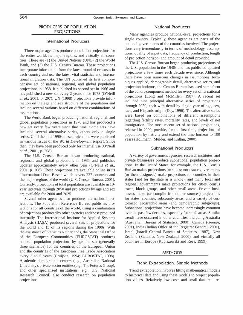
PRODUCERS OF POPULATIONPROJECTIONS
International Producers
Three major agencies produce population projections forthe entire world, its major regions, and virtually all coun-tries. These are (1) the United Nations (UN), (2) the WorldBank, and (3) the U.S. Census Bureau. These projectionsincorporate information from the latest round of censuses ineach country and use the latest vital statistics and interna-tional migration data. The UN published its first compre-hensive set of national, regional, and global populationprojections in 1958. It published its second set in 1966 andhas published a new set every 2 years since 1978 (O’Neillet al., 2001, p. 207). UN (1998) projections provide infor-mation on the age and sex structure of the population andinclude several variants based on different combinations ofassumptions.
The World Bank began producing national, regional, andglobal population projections in 1978 and has produced anew set every few years since that time. Some sets haveincluded several alternative series, others only a singleseries. Until the mid-1990s these projections were publishedin various issues of the World Development Report. Sincethen, they have been produced only for internal use (O’Neillet al., 2001, p. 208).
The U.S. Census Bureau began producing national,regional, and global projections in 1985 and publishesupdates approximately every other year (O’Neill et al.,2001, p. 208). These projections are available online in its“International Data Base,” which covers 227 countries andthe major regions of the world (U.S. Census Bureau, 2001).Currently, projections of total population are available in 10-year intervals through 2050 and projections by age and sexare available for 2000 and 2025.
Several other agencies also produce international pro-jections. The Population Reference Bureau publishes pro-jections for all countries of the world, using a combination of projections produced by other agencies and those producedinternally. The International Institute for Applied SystemsAnalysis (IIASA) produced several sets of projections for the world and 13 of its regions during the 1990s. With the assistance of Statistics Netherlands, the Statistical Officeof the European Communities (EUROSTAT) producesnational population projections by age and sex (generallythree scenarios) for the countries of the European Union and the countries of the European Free Trade Associationevery 3 to 5 years (Cruijsen, 1994; EUROSTAT, 1998). Academic demographic centers (e.g., Australian NationalUniversity), private-sector entities (e.g., The Futures Group),and other specialized institutions (e.g., U.S. NationalResearch Council) also conduct research on population projections.
National Producers
Many agencies produce national-level projections for asingle country. Typically, these agencies are parts of thenational governments of the countries involved. The projec-tions vary tremendously in terms of methodology, assump-tions, quality of input data, frequency of production, lengthof projection horizon, and amount of detail provided.
The U.S. Census Bureau began producing projections ofthe U.S. population in the 1940s and has published updatedprojections a few times each decade ever since. Althoughthere have been numerous changes in assumptions, tech-niques applied, demographic detail, alternative series, andprojection horizons, the Census Bureau has used some formof the cohort-component method for every set of its nationalprojections (Long and McMillen, 1987). A recent setincluded nine principal alternative series of projectionsthrough 2050, each with detail by single year of age, sex,race, and Hispanic origin (Day, 1996). The alternative serieswere based on combinations of different assumptionsregarding fertility rates, mortality rates, and levels of netimmigration. The most recent set of national projections,released in 2000, provide, for the first time, projections ofpopulation by nativity and extend the time horizon to 100years (Hollmann, Mulder, and Kallan, 2000).
Subnational Producers
A variety of government agencies, research institutes, andprivate businesses produce subnational population projec-tions. In the United States, for example, the U.S. CensusBureau makes projections for states; most state governments(or their designees) make projections for counties in theirstates (and for the state as a whole); and many local andregional governments make projections for cities, censustracts, block groups, and other small areas. Private busi-nesses make (or compile from other sources) projections for states, counties, subcounty areas, and a variety of cus-tomized geographic areas (and demographic subgroups). Subnational projections have become increasingly commonover the past few decades, especially for small areas. Similartrends have occurred in other countries, including Australia(Australian Bureau of Statistics, 2000), Canada (George,2001), India (Indian Office of the Registrar General, 2001),Israel (Israeli Central Bureau of Statistics, 1987), NewZealand (Statistics New Zealand, 2000), and virtually allcountries in Europe (Kupiszewski and Rees, 1999).
METHODS
Trend Extrapolation: Simple Methods
Trend extrapolation involves fitting mathematical modelsto historical data and using these models to project popula-tion values. Relatively low costs and small data require-
564 George, Smith, Swanson, and Tayman

ments make trend extrapolation useful, not only in demog-raphy, but in other fields as well (Armstrong, 2001).Although there are many different methods by which his-torical values can be modeled, it is convenient to organizethese methods into three categories: (1) simple extrapolationmethods, which require data for only two dates and forwhich we discuss three approaches: linear change, geomet-ric change, and exponential change; (2) complex extrapola-tion methods, which require data for a number of dates andfor which we discuss four approaches: linear trend, polyno-mial curve, logistic curve, and ARIMA time series; and (3)ratio extrapolation methods, in which the population of asmaller area is expressed as a proportion of the populationof its larger, “parent” area, and for which we discuss threeapproaches: constant share, shift share, and share of growth.
Although there are exceptions, trend extrapolationmethods are used much more frequently for projections oftotal population than for projections of population sub-groups (e.g., race or ethnic groups). We illustrate thesemethods using annual total population data for two counties,Island and Walla Walla, in the U.S. state of Washington, forthe period 1960 to 2000 (Washington State Office of Finan-cial Management, 2000). This constitutes a longer baseperiod than the 10 to 20 years that are generally sufficientfor applying trend extrapolation methods; we employ thisdata set simply as a heuristic device.
The Washington data are shown in Table 21.1, while pro-jections for 2005, 2010, and 2015 are shown in Table 21.2.Figure 21.1 shows the population change in both Island andWalla Walla counties from 1960 to 2000. Note that duringthis period, Island County grew rapidly while Walla WallaCounty grew very slowly. We return to this fact in oursummary comments on trend extrapolation methods.
Linear Change
This method assumes that in the future a population willchange by the same amount over a given period (e.g., a year)as occurred during the base period. Average absolute changeduring the base period can be computed as
(21.1)D = -( ) ( )P P yl b
where D is the average absolute change, Pl is the populationin the launch year, Pb is the population in the base year, andy is the number of years in the base period (i.e., the numberof years between the base year, b, and the launch year, l). Aprojection using this method can be computed as
(21.2)
where Pt is the population in the target year, Pl is the popu-lation in the launch year, and z is the number of years in theprojection horizon (i.e., the number of years between thetarget year, t, and the launch year, l), and D is the averageabsolute change computed for the base period.
P P zt l= + ( )( )D
21. Population Projections 565
TABLE 21.1 Total Annual Population for the State of Washington, Island County and Walla Walla County:
1960 to 2000
Year Time State Island Walla Walla
1960 1 2,853,214 19,638 42,1951961 2 2,897,000 20,300 42,0001962 3 2,948,000 20,900 42,2001963 4 2,972,000 21,100 41,6001964 5 3,008,000 21,700 41,5001965 6 3,065,000 22,400 41,4001966 7 3,125,000 23,100 41,2001967 8 3,229,000 24,200 42,0001968 9 3,336,000 25,000 41,3001969 10 3,397,000 25,700 41,0001970 11 3,413,250 27,011 42,1761971 12 3,436,300 27,400 42,6001972 13 3,430,300 29,500 42,1001973 14 3,444,300 31,600 42,6001974 15 3,508,700 33,200 42,8001975 16 3,567,890 34,700 43,5001976 17 3,634,891 36,300 43,8001977 18 3,715,375 37,528 44,4001978 19 3,836,200 41,200 44,9001979 20 3,979,200 42,200 46,1001980 21 4,132,353 44,048 47,4351981 22 4,229,278 45,443 47,1341982 23 4,276,549 46,559 47,7121983 24 4,307,247 47,551 48,2481984 25 4,354,067 48,225 48,3451985 26 4,415,785 49,661 48,2871986 27 4,462,212 51,024 48,1631987 28 4,527,098 52,436 48,1701988 29 4,616,886 54,370 48,0851989 30 4,728,077 56,523 48,2771990 31 4,866,663 60,195 48,4391991 32 5,000,371 62,700 49,3001992 33 5,116,671 64,800 50,5001993 34 5,240,900 66,500 51,8001994 35 5,334,400 67,900 52,6001995 36 5,429,900 68,900 52,7001996 37 5,516,800 70,300 53,4001997 38 5,606,800 71,600 54,0001998 39 5,685,300 72,500 54,6001999 40 5,757,400 73,300 54,6002000 41 5,803,400 74,200 54,200
Source: Washington State Office of Financial Management (2000).
FIGURE 21.1 Population change in Island and Walla Counties, Washing-ton, 1960–2000.

For Island County, a model expressing its average abso-lute change between 1960 and 2000 is computed as D =1364.05 = (74,200 - 19,638)/(40), and a projection for 2010 is computed as 87,840 (where 87,840 ª 74,200 +[(10)(1364.05)]). For Walla Walla County, a model express-ing average absolute change over the same 40-year periodis computed as D = 300.13 = (54,200 - 43,195)/(40), and aprojection for 2010 as 57,201 (where 57,201 ª 54,200 +[(10)(300.13)]). Projections for both counties in 2005 and2015 are found in Table 21.2.
Geometric Change
This method assumes that a population will change bythe same percentage rate over a given increment of time inthe future as during the base period. The average geometricrate of population change during the base period can be com-puted as
(21.3)
where r is the average annual geometric rate of change, Pl
is the population in the launch year, Pb is the population inthe base year, and y is the number of years in the base period.A projection using this method can be computed as
(21.4)
where Pt is the population in the target year, Pl is the populationin the launch year, r is the average annual geometric rate ofchange, and z is the number of years in the projection horizon.
For Island County, the annual rate of geometric changebetween 1960 and 2000 is computed as r = 0.0338 =
P P rt lz= ( ) +( )1
r P Pl by= ( )[ ] -( )1
1
[(74,200/19,638)(1/40)] - 1, and a projection for 2010 as103,459 ª [(74,200)(1 + 0.0338)10]. For Walla Walla County,its annual rate of geometric change for the same 40-yearperiod is computed as 0.0063 = [(54,200/42,195)(1/40)] - 1,and a projection for 2010 as 57,713 ª [(54,200)(1 +0.0063)10]. Projections for both counties in 2005 and 2015using these models are provided in Table 21.2.
Exponential Change
The model for exponential change is closely related to thegeometric one, but it views change as occurring continuouslyrather than at discrete intervals. The exponential rate of popu-lation change during the base period can be computed as
(21.5)
where r is the average annual exponential rate of change, lnrepresents the natural logarithm, Pl is the population in thelaunch year, Pb is the population in the base year, and y isthe number of years in the base period. A population projection using this method can be computed as
(21.6)
where Pt is the population in the target year, Pl is the popula-tion in the launch year, e is the base of the system of naturallogarithms (approximately 2.71828), r is the average annualexponential rate of change computed for the base period, andz is the number of years in the projection horizon.
For Island County, the annual rate of exponential change from 1960 to 2000 is computed as 0.0332 =[ln(74,200/19,638)]/(40), and a projection for 2010 as
P P et lrz= ( )( )
r ln P P yl b= ( )[ ] ( )
566 George, Smith, Swanson, and Tayman
TABLE 21.2 Projection Results for Island and Walla Walla Counties Using DifferentExtrapolation Methods: 2005–2015
Island county Walla Walla county
Method/year 2000 2005 2010 2015 2000 2005 2010 2015
SimpleLinear 74,200 81,020 87,841 94,661 54,200 55,701 57,201 58,702Geometric 74,200 87,617 103,459 122,166 54,200 55,929 57,713 59,554Exponential 74,200 87,599 103,416 122,091 54,200 55,934 57,724 59,572
ComplexLinear 74,200 81,837 89,358 96,879 54,200 55,472 57,263 59,053Quadratic 74,200 87,949 98,936 110,936 54,200 58,664 62,264 66,194Logistic 74,200 83,749 90,437 96,172 54,200 56,302 58,542 60,872ARIMA 74,200 77,287 78,889 79,719 54,200 53,870 53,863 53,863
RatioConstant share 74,200 78,430 83,692 89,337 54,200 57,319 61,133 65,257Shift share 74,200 82,999 93,352 104,803 54,200 53,139 52,216 50,978Share of growth 74,200 80,371 87,930 96,095 54,200 55,559 57,221 59,017
RangeAbsolute N/A 10,662 24,565 42,447 N/A 5,525 10,048 15,216Percent1 N/A 12.65 26.94 42.05 N/A 9.88 17.55 25.97
1 Base is mean of highest and lowest estimates.

103,416 ª (74,200)(e0.03332*10). For Walla Walla County, itsannual rate of exponential change for the same 40-yearperiod is computed as 0.0063 = [ln(54,200/42,195)]/(40),and a projection for 2010 as 57,724 ª (54,200)(e00.0063*10). Projections for both counties in 2005 and 2015 using thesemodels are provided in Table 21.2.
Complex Extrapolation Methods
Unlike simple methods, complex extrapolation methodsare constructed using base-period data for more than twodates. Accordingly, they can deal better with nonlinear pop-ulation change. They also offer a quantitative basis for con-structing measures of forecast uncertainty because statisticalalgorithms are used to estimate model parameters (Swansonand Beck, 1994). However, these features do not guaranteethat complex extrapolation methods provide more accurateforecasts than simple extrapolation methods.
Typically, three basic steps are followed when applyingcomplex extrapolation methods. The first is to assemble his-torical population data for different dates during the baseperiod. For a model to be valid, the data must be based onconsistently defined geographic boundaries for each date.The second step is to estimate the parameters of the modelselected to generate the projection. Typically, graphs and sta-tistical measures are used to determine how well a givenmodel fits the data for the base period while the choice of a particular model reflects judgment about the nature offuture population change. The final step is to generate pro-jections using the model(s) selected.
A critical issue in the use of complex extrapolationmethods is the selection of time units. This is importantbecause time can be measured in several different ways andthe one selected for a given problem affects the scale ofcertain parameters estimated by the curve-fitting process.Using the data in Table 21.1 as an example, consider twolinear trend models, one using the original units for time(i.e., 1960 through 2000) and one using a logically equiva-lent alternative (i.e., 1 through 41, where 1 corresponds to1960 and 41 corresponds to 2000). Both models will havethe same fit with the historical data (e.g., the r 2 values willbe the same), but the intercept will be different. Consistenttime units must be used when estimating complex modelsand using them to project population values.
Linear Models
Linear models are the simplest of the complex extrapo-lation methods. They assume that a population will changeby the same numerical amount in the future as in the past.This assumption is identical to that underlying the simplelinear method discussed earlier, but the model is computeddifferently:
(21.7)Y a b Xi i= + ( )
where Yi is a set of i observations of values of a “dependentvariable,” Xi is a set of i observations of an “independentvariable,” a is the constant term, and b is the slope of theline describing the “best fitting linear” relationship betweenX and Y, as found by, for example, the method of leastsquares (NCSS Inc., 1995, pp. 1309–1310). In using thisapproach for purposes of developing a population projectionmodel, it is convenient to recast X and Y as time and popu-lation, respectively. That is, as
(21.8)
where Pi is the population for a set of time points (e.g.,years) over the period i = b to l (b = base year and l = launchyear); a and b are the estimated intercept and slope, respec-tively, and Ti is time over the period i = b to l.
For Island County, a linear trend model using the NCSS“linear trend growth model” routine (NCSS Inc., 1995, pp. 1371–1388) was estimated as Pi = 12,639.64 +[(1,504.282)(Ti)], with an r 2 value of 0.986. The slope valueimplies that the population of Island County increased onaverage by 1054 persons each year of the base period. Withthis model, a projected population for Island County in 2010is 89,358 ª 12,639.64 + [1504.282)(51)]. For Walla WallaCounty, the linear trend model was estimated as Pi =39,002.14 + [(358.0467)(Ti)], with an r 2 value of 0.928.With this same model, a projected 2010 population for WallaWalla County is 57,263 ª 39,002.14 + [358.0467)(51)]. Pro-jections for both counties in 2005 and 2015 are shown inTable 21.2.
Polynomial Models
Polynomial models can be used for projections in whichchange is not constrained to be linear. The general formulafor a polynomial curve is
(21.9)
where Yi is a set of i observations of values of a dependentvariable, Xi is a set of i observations of an independent vari-able, a represents the constant term, and bj the slope of theline describing the “best-fitting” relationship between Xj
i
and Y, holding constant the effects of Xki, (where k π j).
Recasting X and Y as time and population, respectively, wehave
(21.10)
where Pi is the population for a set of time points over theperiod i = b to l (b = base year and l = launch year), a is theestimated intercept term, bi are the estimated partial slopecoefficients, and Ti is time over the period i = b to l.
In contrast to linear trend models, polynomial modelshave more than one term reflecting the independent variable(time). Consequently, there are more parameters to estimate.The coefficients of a polynomial curve (a, b1, b2, . . . bn) can
P a b T b T b T b Ti i i i n in= + ( ) + ( ) + ( ) + + ( )1 2
23
3 . . .
Y a b X b X b X b Xi i i i n in= + ( ) + ( ) + ( ) + + ( )1 2
23
3 . . .
P a b Ti i= + ( )
21. Population Projections 567

be estimated using OLS regression techniques (NCSS Inc.,1995, pp. 1309–1310). These coefficients include both ameasure of the linear trend (b1) and measures of the nonlin-ear patterns (b2, b3, . . . , bn).
To illustrate the use of a polynomial curve for populationprojections, we use a second-degree polynomial (sometimescalled a quadratic function). This function includes time (thelinear term) and time squared (also called the parabolicterm) on the right-hand side of the equation:
(21.11)
where b1 is the slope for the linear trend and b2 is the slopefor the nonlinear (parabolic) trend. A quadratic curve canproduce a variety of growth scenarios, such as a populationgrowing at an increasing rate, a population growing at adecreasing rate, a population declining at an increasing rate,or a population declining at a decreasing rate. Projectionsbased on a quadratic curve can lead to very high (or low)projections for places that were growing (or declining)rapidly during the base period. Although a polynomial ofany degree can be used, polynomials higher than second orat most third degree are seldom used for population projec-tions. Nonlinear trends in the historical data also can be projected using curves based on logarithmic or other trans-formations of the base data.
For Island County, a quadratic model using the NCSS“multiple regression” routine (NCSS Inc., 1995, pp. 155–188) was estimated as Pi = 16,432.8 + (974.998)(Ti) +(12.602)(Ti
2), with r 2 = 0.993. With this same model, a pro-jected population for Island County in 2010 is 98,936 ª16,432.8 + (974.998)(51) + (12.602)(512). For Walla WallaCounty, the quadratic model was estimated as Pi = 40,983.2+ (81.618)(Ti) + (6.5816)(Ti
2), with r2 = 0.963. With thismodel, a projected population for Walla Walla County in2010 is 62,264 ª 40,983.2 + (81.618)(51) + (6.5816)(512).Projections for both counties in 2005 and 2015 are shownin Table 21.2.
Logistic Models
Unlike the extrapolation methods considered so far, thelogistic approach explicitly allows one to place an upper limiton the ultimate size of the population for a given area. It isdesigned to yield an S-shaped pattern representing an initialperiod of slow growth rates, followed by a period of increas-ing growth rates, and finally a period of declining growthrates that approach zero as a population approaches its upperlimit. The logistic model is consistent with Malthusian andother theories of constrained population growth.
Keyfitz (1968, p. 215) provides the following formula fora three-parameter logistic curve:
(21.12)
where Y is the population, X is the time period, a reflects the upper asymptote, b and c are parameters that define the
Y a b e cX= + ( )[ ]-1
P a b T b Ti i i= + ( ) + ( )1 22
shape of the logistic curve, and e is the base of the naturallogarithm. Note that other formulas are available, someincluding more than three parameters (NCSS Inc., 1995, p.1375; Pielou, 1969, pp. 19–32).
In using the logistic curve, one must sometimes deter-mine the magnitude of the upper asymptote and the timerequired to reach it. Algorithms are available that estimatethese parameters within the context of the model, but likeparameters in an ordinary regression model (e.g., the inter-cept term), the estimated parameters may not be consistentwith a substantive interpretation (e.g., a may not representan actual upper population limit).
For our purposes, Keyfitz’s formula is rewritten as
(21.13)
where Pt is the population in the target year, a, b, and c arethe estimated parameters, and t is time. This model is usefulbecause it can be generated by the NCSS package withoutthe user having to provide predetermined population limits;rather, the NCSS algorithm uses the available historicalinformation to generate the needed parameters.
For Island County, a logistic model using the NCSS“three-parameter logistic model” routine (NCSS Inc., 1995,p. 1375) was estimated as Pt = (118,272.7)/[1 + (6.061401)(e-0.05843697t)] after 11 iterations, with r 2 = 0.995293. With thismodel, the projected population for Island County in 2010is 90,437 ª (118,272.7)/[1 + (6.061401)(e-0.05843697*51)]. ForWalla Walla County, the logistic model was estimated as Pt
= (41,712,310.00)/[1 + (1,059.927)(e-0.007814847t)] after 235iterations, with r 2 = 0.940. With this model, the projectedpopulation for Walla Walla County in 2010 is 58,542 ª(41,712,310.00)/[1 + (1,059.927)(e-0.007814847*51)]. Projectionsfor both counties in 2005 and 2015 using these models,respectively, are provided in Table 21.2.
ARIMA Time Series Models
ARIMA (“Autoregressive Integrated Moving Average”)models have occasionally been used in the analysis and pro-jection of populations as a whole and of their demographicattributes (Alho and Spencer, 1997; Carter and Lee, 1986;de Beer, 1993; Lee, 1993; and Pflaumer, 1992). The proce-dures used in ARIMA models are complicated, making themdifficult to implement and explain to data users. We suggestconsulting standard texts before attempting to apply thismethod (Box and Jenkins, 1976; Hanke et al., 2001; Yaffee,2000). It also may be useful to review the method of“moving averages,” which forms part of the foundation ofARIMA (Hanke et al., 2001, pp. 101–123). ARIMA modelsattempt to uncover the stochastic mechanisms that generatehistorical data series and use this information as a basis fordeveloping projections. Three processes can describe thestochastic mechanism: (1) autoregressive, (2) differencing,
P a b etct= ( ) + ( )( )[ ]-1
568 George, Smith, Swanson, and Tayman

and (3) a moving average. The autoregressive process has amemory in the sense that it is based on the correlation ofeach value of a variable with all preceding values. Theimpact of earlier values is assumed to diminish exponen-tially over time. The number of preceding values incorpo-rated into the model determines its “order.” For example, ina first-order autoregressive process, the current value isexplicitly a function only of the immediately precedingvalue. However, the immediately preceding value is a func-tion of the one before it, which is a function of the one beforeit, and so forth. Consequently, all preceding values influencecurrent values, albeit with a declining impact. In a second-order autoregressive process, the current value is explicitlya function of the two immediately preceding values; again,all preceding values have an indirect impact.
A stationary time series is very important for the con-struction of a given ARIMA model. The differencing processis used to create a stationary time series (i.e., one with con-stant differences over time). When a time series is nonsta-tionary, it can often be converted into a stationary time seriesby calculating differences between values. First differencesare usually sufficient, but second differences are occasion-ally required (i.e., differences between differences). Loga-rithmic and square-root transformations can also be used toconvert nonstationary to stationary time series. The movingaverage is used to represent any event that has a substantialbut short-lived impact on a time series pattern. The order ofthe moving average process defines the number of timeperiods affected by a given event.
The ARIMA method is usually written as ARIMA (p,d,q),where p is the order of the autoregression, d is the degree ofdifferencing, and q is the order of the moving average. (AnARIMA model based on time intervals of less than 1 yearmay also require a seasonal component.) The first and mostsubjective step in developing an ARIMA model is to iden-tify the values of p, d, and q. The d-value is determined firstbecause a stationary series is required to properly identifythe autoregressive and moving average processes. The valueof d is usually 0 or 1, but occasionally 2. Like the d-value,the p- and q-values are also relatively small (0, 1, or—atmost—2). The patterns of the autocorrelation function(ACF) and the partial autocorrelation function (PACF) andtheir standard errors are used to find the correct values forp and q (Box and Jenkins, 1976; Yaffee, 2000). For example,a first-order autoregressive model (ARIMA (1,0,0)) is characterized by an ACF that declines exponentially andquickly along with a PACF that has a statistically significantspike only at the first lag. Once p, d, and q are determined,maximum likelihood procedures are used to estimate theparameters of a given ARIMA model.
The final step involves assessing the suitability of a givenmodel. An adequate ARIMA model will have random resid-uals, no significant values in the ACF and PACF, and thesmallest possible values for p, d, or q. Only after an ARIMAmodel has passed this assessment should it be used.
It is not unusual to repeat this sequence of steps severaltimes before a suitable ARIMA model is found. In thisprocess, it is best to start simple (e.g., ARIMA (0,1,0)),check the results, and then add additional changes in a sys-tematic and incremental manner (e.g., ARIMA(1,1,0) if themodel is not found to be suitable. If a suitable model is notfound by the time one reaches, say, ARIMA (2,1,2), it isprobably wise to abandon this approach.
One characteristic of an autoregressive model is that projections will eventually reach and maintain a constantnumeric difference similar in value to the mean of the his-torical series (McCleary and Hay, 1980, p. 218). Conse-quently, population projections using ARIMA will often besimilar to projections based on linear extrapolation methods(Pflaumer, 1992; Voss and Kale, 1985). The formulas usedin computing projections from an ARIMA model depend onthe specification of the values of p, d, and q, each of whichis most easily determined using a computer packagedesigned for estimating them.
Using the 1960-through-2000 population figures shownin Table 21.1, the NCSS (1995, pp. 1427–1436) ARIMAroutine was used to develop models for Island and WallaWalla counties. Because the NCSS algorithm does not useordinary least squares, it employs “pseudo-r2” as a measureof fit rather than “r2.”
For Island County, a first-order autoregressive modelwith one degree of differencing and no moving average(ARIMA(1,1,0)) was found to be sufficient after 21 itera-tions and estimated as Pt+1 = [(0.876942)(Pt - Pt-1) + Pt],with “pseudo-r2” = 0.9982. With this same model, a projected population for Island County in 2010 is 78,889 ª[(0.876942)(78,646.5 - 78,370.4) + 78,646.5]. For Walla Walla County, a first-order autoregressive model with one degree of differencing and no moving average(ARIMA(1,1,0)) also was found to be sufficient after three iterations, with a “pseudo-r2” of 0.98505. In the caseof Walla Walla County, it was estimated as Pt+1 =[(0.4573916)(Pt - Pt-1) + Pt]. With this same model, a projected population for Walla Walla County in 2010 is53,863 ª [(0.4573916)(53,863 - 53,863) + 53,863]. Projections for both counties in 2005 and 2015 are shownin Table 21.2.
There are three important points to bear in mind whenusing ARIMA models. First, because a given ARIMA modelcan have a number of alternative configurations, those thathave values higher than 1 for p, d, and q, can be difficult tooperationalize manually. That is, it may be difficult to man-ually recreate projection results created by a given softwarepackage using the parameters shown. This may be of par-ticular concern for some users because it is not easy toexplain how the projections are calculated. Second, duringthe base period “projected values” from a given ARIMAmodel are generated using the actual historical values.However, once beyond the scope of the historical data, pro-jected values themselves are used to generate subsequent
21. Population Projections 569

projected values. There may be a period subsequent to thelaunch date when a combination of actual and projected datamay be used depending on the order and degree of differ-encing. Third, ARIMA (as well as the other complex extrap-olation techniques covered here) can be used to placeprobabilistic confidence intervals around their forecasts.
Ratio Extrapolation Methods
Ratio extrapolation methods may be used where an areacontaining the population to be projected is part of a larger(“parent”) area for which projections are available. They areoften used where areas exist in a perfect hierarchical struc-ture—that is, where geographic units at each level are mutu-ally exclusive and exhaustive and can be aggregated tohigher levels, culminating in one all-inclusive unit. As anexample, consider census blocks in the United States, whichcan be aggregated successively into block groups, censustracts, counties, states, and finally the country as a whole.Ratio methods also can be used where there is not a perfecthierarchy—for example, in a city that is part of a county inwhich the geographic area (population) covered by all citiesis less than the total area (population) of the county as awhole. In this case, the parent area is not the county but the area represented by all of the cities. Ratio methods canbe applied in situations where the area (population) of interest is linked to the “parent” area (population) throughconsiderations other than geography (this is akin to the “tar-geting” approach described later in regard to projecting mor-tality and fertility) and, in addition, ratios can be formed vialagged relationships.
We discuss three commonly used ratio methods: (1) theconstant-share, (2) the shift-share, and (3) the share-of-growth approaches. As noted, all three require projectionsof a “parent” area in which the area of interest is located.We use Washington State as the “parent” area for applyingthese methods to Island and Walla Walla counties. Projec-tions for Washington State are 6,137,403, 6,545,786, and6,987,273, for the years 2005, 2010, and 2015, respectively(Washington State Office of Financial Management, 2001).
Constant-Share Method
In this method, the smaller area’s share of the largerarea’s population is held constant at a level observed duringthe base period. Typically it is the share observed in thelaunch year. This constant-share method is expressed as
(21.14)
where Pit is the population projection for smaller area (i) inthe target year, Pil is the population of the smaller area in thelaunch year, Pjl is the population of the parent area ( j) in thelaunch year, and Pjt is the projection of the parent area in the target year.
P P P Pit il jl jt= ( )( )
The constant-share method requires historical data foronly one date; consequently, it is particularly useful for areaswhere changing geographic boundaries or poor recordsmake it difficult or impossible to construct a reliable histor-ical data series. Another requirement of this method is thatprojections for all of the smaller areas add exactly to the projection for the parent area. The main drawback of thismethod is that it assumes that all the smaller areas will growat the same rate as the parent area. In many instances, thiswill not be a reasonable assumption.
Using the 2000 population figures shown in Table 21.1for Island County and Washington State, a constant-sharemodel yielded a projected 2010 population for IslandCounty of 83,692 ª (74,200/5,803,400)(6,545,786). Usingthe 2000 population figures shown in Table 21.1 for WallaWalla County and Washington State, a constant share modelyielded a projected 2010 population for Walla Walla Countyof 61,133 ª (54,200/5,803,400)(6,545,786). Projections for2005 and 2015 using these models, respectively, are shownin Table 21.2.
Shift-Share Method
Unlike the constant-share method, the shift-share methodis designed to deal with changes in population shares. Here,we describe one of several methods in which populationshares are extrapolated linearly over time. This shift-sharemethod is expressed as
(21.15)
where the smaller area is denoted by i, the parent area by j,z is the number of years in the projection horizon, y is thenumber of years in the base period, and b, l, and t refer tothe base, launch, and target years, respectively.
There is a problem inherent in the shift-share method: itcan lead to substantial population losses in areas that grewvery slowly (or declined) during the base period, especiallywhen the projections cover long-range horizons (e.g., 20 or30 years). In fact, this method can even lead to negativenumbers. This problem can be dealt with by incorporatingconstraints on projected population shares or on the pro-jected rates of change in those shares. The method also canlead to absurdly high projections for areas that have beengrowing very rapidly. As with many extrapolation methods,the shift-share approach must be used very cautiously forlong-range projections, especially for places whose popula-tion shares have been declining (or increasing) rapidly.
Using the 1960 and 2000 population figures shown inTable 21.1, a shift-share model yielded a projected 2010population for Island County of 93,352 ª (6,545,786)[(74,200/5,803,400) + (10/40)((74,200/5,803,400) -(19,638/2,853,214))]. For Walla Walla County, a shift-sharemodel yielded a projected 2010 population of 52,216 ª (6,545,786)[(54,200/5,803,400) + (10/40)((54,200/
P P P P z y P P P Pit jt il jl il jl ib jb= ( ) ( ) + ( ) ( ) - ( )( )[ ]
570 George, Smith, Swanson, and Tayman

5,803,400) - (42,195/2,853,214))]. Projections for 2005 and2015 are shown in Table 21.2.
Share-of-Growth Method
The third ratio method deals with shares of populationchange rather than population size. In this method, it isassumed that the smaller area’s share of population changein the parent area will be the same over the projectionhorizon as it was during the base period. This share-of-growth method can be expressed as
(21.16)
where the components are defined as those in the shift-sharemethod.
In many instances, the share-of-growth method seems toprovide more reasonable projections than either the constant-or shift-share methods. However, it runs into problems whena growth rate in a smaller area has the opposite sign than that for the parent area. This can be dealt with using the“plus-minus” method described in Appendix C or by settingthe share to zero and not letting it change.
Using the 1960 and 2000 population figures shown in Table 21.1, a shift-share model yielded a projected 2010 population for Island County of 87,930 ª 74,200 +[((74,200 - 19,638)/(5,803,400 - 2,853,214))(6,545,786 -5,903,400)]. For Walla Walla County, a shift-share modelyielded a projected 2010 population of 57,221 ª 54,200 +[((54,200 - 42,195)/(5,803,400 - 2,853,214))(6,545,786 -5,803,400)]. Projections for 2005 and 2015 are shown inTable 21.2.
Summary Comments on Extrapolation Methods
Both simple and complex trend extrapolation methodssuffer from several shortcomings. They do not account fordifferences in demographic composition or for differencesin the components of growth. They provide little or no infor-mation on the projected demographic characteristics of thepopulation. Because they have no theoretical content, theycannot be related to theories of population growth, exceptperhaps the logistic model, which is consistent with aMalthusian view of population dynamics. Consequently,they have limited usefulness for analyzing the determinantsof population growth or for simulating the effects of changesin particular variables or assumptions. In addition, they canlead to unrealistic or even absurd results, even over rela-tively short horizons. In spite of their shortcomings, trendextrapolation methods have a number of advantages overother projection methods. They have few data requirementsand, with the exception of the ARIMA and polynomialmodels, are quick and easy to apply. They are particularlyuseful when data series are incomplete, time and budgets are
P P P P P P P Pit il il ib jl jb jt jl= + -( ) -( )( ) -( )[ ]
highly constrained, and information on population charac-teristics is not needed. Perhaps most important, they oftenprovide reasonably accurate forecasts over short and evenlong projection horizons. There is no empirical evidenceshowing that more complex or sophisticated methods con-sistently produce more accurate forecasts than trend extrap-olation methods.
As shown in Table 21.2, different methods sometimesproduce dramatically different results. Island County, forexample, grew rapidly between 1960 to 2000. Thus, it is notsurprising that the range of projections is quite large, extend-ing from 79,719 (logistic) to 122,166 (geometric) in 2015.The case is quite different for Walla Walla County, whichexperienced a much smaller population increase between1960 and 2000. Here, the range is much smaller than thatfor Island County: the largest projection for 2015 is providedby the quadratic method (66,194) and the smallest (50,978)by the shift-share method. If trend extrapolation methods areto be used, which one(s) should be chosen for these twocounties? Alternatively, should an average of projectionsfrom several methods be calculated? Should the samemethods be used in both counties? The use of trend extrap-olation methods does not remove the need to exercise judg-ment. We return to this issue toward the end of this chapter.
COHORT-COMPONENT METHOD
The cohort-component method was introduced byCannan (1895), subsequently used by Bowley (1924), andlater rediscovered independently by Whelpton (1928). It isthe most widely used method for producing national-levelpopulation projections. Although current applications aremore detailed and sophisticated than the earliest applica-tions, the basic framework of the method has changed littlesince the pioneering work by these three men.
The cohort-component method divides the launch-yearpopulation into age-sex groups (i.e., birth cohorts) andaccounts separately for the fertility, mortality, and migrationbehavior of each cohort as it passes through the projectionhorizon. It is a flexible and powerful method that can be usedto implement theoretical models or serve as an atheoreticalaccounting procedure. It can provide in-depth knowledge onpopulation dynamics. Also the cohort-component methodcan accommodate a wide range of assumptions and can beused at any geographic level—from the world as a wholedown to nations, states/provinces, counties, and subcountyareas.
For purposes of population projection, the division of thepopulation into age groups was an important methodologi-cal advance (de Gans, 1999). It allows one to account forthe differences in mortality, fertility, and migration ratesamong different age groups at a particular time and to con-sider how rates change over time for individual cohorts.
21. Population Projections 571

Cohort-component models typically use either singleyears or 5-year groups. The oldest age group is virtuallyalways “open-ended,” usually 75+, 85+, or 90+. Age groupsare typically divided by sex and are sometimes further sub-divided by race, ethnicity, and other characteristics (whereconsidered officially useful). Our discussion and examplesfocus on populations divided by age and sex, but the proce-dures we describe would be basically the same if the popu-lation were further subdivided by race, ethnicity, and othercharacteristics.
In the application of the method as originally developed,the first step in the projection process is to establish thelaunch-year population and calculate the number of personsin it who survive to the end of the projection interval (e.g.,one year). This is done by applying age-sex-specific survivalrates to each age-sex group in the launch-year population.The second step is to calculate migration during the projec-tion interval for each age-sex group. The application ofmigration rates provides a projection of the number ofpersons in each age-sex group moving into or out of an areaduring the projection interval (or, for models using netmigration rates, the net migration). The third step is to cal-culate the number of births occurring during the projectioninterval. This is accomplished by applying age-specificbirthrates to the female population in each age group. Thefinal step in the process is to add the number of births (sep-arating male and female births) to the rest of the population.
These calculations provide a projection of the population byage and sex at the end of the projection interval. This pop-ulation then serves as the starting point for the followinginterval (e.g., next year). The process is repeated until thefinal target year is reached. Figure 21.2 illustrates the stepsin this process. Figure 21.2 is meant to be illustrative. Noteach and every application of the cohort-component methodfollows the steps as shown. Illustrating this point, in theexamples for national and subnational projections providedlater for Canada, there are adjustments made to the basicsteps shown in Figure 21.2 to deal with the effect of migra-tion on births and deaths.
Projecting Mortality
The mortality rates (or their functional equivalents) usedin cohort-component projections can be projected in anumber of ways. The simplest is to assume that age-specificrates will remain unchanged at current levels. For short hori-zons, this will often be a reasonable assumption. For longerhorizons, however, this assumption may not be valid andmethods that incorporate changing rates then become nec-essary. Such methods include a variety of extrapolation techniques, techniques tying mortality rates in one area orpopulation to those in another, and structural models thatbase changes in mortality rates on changes in socioeconomicvariables.
572 George, Smith, Swanson, and Tayman
FIGURE 21.2 Overview of the cohort-component method for a projection interval.Source: Smith et al. (2001, p. 47).
The use of extrapolation techniques assumes that thefuture will mirror the past in certain important ways.Although this is not always a valid assumption, it has oftenled to reasonably accurate forecasts. Extrapolation tech-niques have been widely used for mortality projections,sometimes following fairly simple procedures and othertimes applying more sophisticated procedures such asARIMA time series models (Lee and Carter, 1992).
Extrapolation techniques are particularly appropriatewhen mortality trends are following a stable path. The crit-ical question is whether trends will remain stable in thefuture. The answer to this question depends on one’s viewsregarding the determinants of mortality trends (e.g., Ahlburgand Vaupel, 1990; Fries, 1989; Manton, Stallard, and Tolley,1991; Olshansky, 1988).
A number of techniques tie mortality rates in one population to those in another. For example, the “target-ing” approach is based on the idea that mortality rates in a given population will converge toward those observed inanother population (i.e., the target). A target population is chosen that provides a set of mortality rates believed to be realistic for the population to be projected. This choice is based on similarities in socioeconomic, cul-tural, and behavioral characteristics; levels of medical tech-nology; and primary causes of death (Olshansky, 1988, p. 500). It could be implemented using a “ratio” approach,as described earlier in this chapter in the section “Trend Extrapolation.”
One form of targeting is called “cause-delay.” In thisapproach, the target population is a younger cohort in thesame population rather than the same cohort in a differentpopulation. Cause-delay models focus on the implicationsof delaying (or completely eliminating) the occurrence ofone or more causes of death (Manton, Patrick, and Stallard,1980; Olshansky, 1987). The basic premise behind thisapproach is that changes in lifestyle and medical technologyhave delayed the occurrence of various types of deaths untilprogressively older ages. Consequently, as time goes by,each cohort faces lower mortality risks at each age than didthe previous cohort. Another form of targeting is to linkchanges in rates for the area in question to changes projectedfor a different area through the use of ratios.
Life tables are readily available for most areas of theworld and can be used as a base for mortality projections.As the reader may recall, life tables are prepared both by theUnited Nations and by the vital statistics agencies in mostcountries. In the United States, for example, national lifetables are published annually by the National Center forHealth Statistics and a few times each decade by the SocialSecurity Administration (Bell et al., 1992; U.S. NationalCenter for Health Statistics, 1997). State life tables are typ-ically constructed once every 10 years in the United States,when decennial census data become available to serve asdenominators for the mortality rates.
Projecting Fertility
In projecting births, one can use a period perspective, a cohort perspective, or a combination of the two. The period perspective focuses on births to women at the same age over a series of years. The cohort perspective is longitudinal, focusing on the fertility patterns of a cohort of women as they pass through their childbearingyears.
Although the cohort perspective is superior for some ana-lytical purposes, it is difficult to implement when construct-ing population projections. Data on completed cohortfertility do not become available until after a cohort haspassed through its childbearing years; for women under age50, only partial data are available. Birth histories of pastcohorts and the fertility expectations of current cohorts maybe used as proxies for the missing data, but they do not nec-essarily provide reliable fertility forecasts for current andfuture cohorts. In addition, projections for subnational areasare complicated by the lack of relevant data and by theeffects of migration, which may have a significant impacton the composition of an area’s population and its fertilitybehavior. Because of these problems and the complexity ofthe method, we believe that most practitioners will be betterserved by using a period perspective for the production offertility projections.
Several approaches may be used when applying theperiod fertility perspective. One is to hold current age spe-cific birthrates (ASBRs) constant throughout the projectionhorizon (Day, 1996; Treadway, 1997). These rates are oftenbased on data for the most recent year, but can also be basedon an average of data for several recent years. Holding ratesconstant can be justified not only by the expectation that theywill not change, but also by the belief that increases incurrent rates are as likely as declines. Another approach isto extrapolate historical trends. This approach is particularlyuseful for countries in the midst of the demographic transi-tion from high to low fertility rates, but can lead to prob-lems for countries in which the transition has already beencompleted. If no long-run trends are clearly discernible,recent changes in fertility rates may simply reflect short-runfluctuations and extrapolating those changes into the futuremay create large forecast errors. Time series techniques arefrequently used to develop nonlinear models for projectingASBRs (Carter and Lee, 1992; Land, 1986; Lee, 1993; Leeand Tuljapurkar, 1994).
The “targeting” approach described earlier is anothertechnique that can be used to project fertility rates (U.S.Bureau of the Census, 1979). Before applying this tech-nique, however, one must decide whether the convergenceof one set of rates toward another is a realistic assumption.Projected ASBRs also can be derived by forming ratios ofbirthrates in one area to those in another and applying thoseratios to the birthrates previously projected for the area of
21. Population Projections 573

interest. Finally, structural models can be developed. Suchmodels have occasionally been used for projecting fertilityrates at the national level (e.g., Ahlburg, 1999; Sanderson,1999), but have seldom been used at the subnational level(Isserman, 1985).
Even given our argument in favor of the period perspec-tive, it is nonetheless important to keep the cohort perspec-tive in mind when formulating assumptions about futurefertility rates. For example, if recent changes have occurredin ASBRs, the cohort perspective may offer clues as towhether those changes reflect a shift in the long-run trend inASBRs or simply a short-run change in the timing of births.It is in this sense that a combination of the period and cohortperspective may be useful. In addition, it is useful to notethat there is increased use of the cohort approach in theEuropean Economic Area, a development partially attri-buted to the availability of a long series of historical data(Cruijsen, 1994).
Fertility is often the most problematic part of nationalpopulation projections (Keyfitz, 1982; Ryder, 1990). Long(1989) found that differences in fertility assumptionsaccounted for more of the variation in long-run projectionsof the U.S. population than did differences in either mortal-ity or immigration assumptions. However, immigration wasconsidered the most problematic component for the 1993round of Canadian population projections (George, Loh, andVerma, 1997). For subnational areas in many countries, fertility may be less important than migration in explainingdifferences in rates of population growth (Congdon, 1992;Smith and Ahmed, 1990).
Projecting Migration
Migration often has a substantial impact on populationgrowth at the national and subnational levels. For projectionpurposes, we may view migration in two ways: (1) grossmigration and (2) net migration. As explained in Chapter 19, gross migration refers to the movement of people into and out of a given area; net migration refers to the difference between the two—that is, inmigration minus outmigration. For projecting population flows, each has its strengths and weaknesses. Gross migration models are“cleaner” from a theoretical and computational standpoint,but they require more data and are more complicated toapply than net migration models (Smith and Swanson,1998). Both approaches are widely used for population projections.
We discuss two basic techniques for projecting grossmigration. The first is based on the application of outmigra-tion rates and inmigration proportions for each area to beprojected. (U.S. Census Bureau, 1966, 1972, 1979). Wedescribe this technique using states as the unit of referenceand migration data based on 5-year time and age intervals.The same technique could be used for other geographic
areas and different lengths of migration intervals, if the dataare available. Under this technique, outmigration rates byage and sex are calculated for each state using outmigrationdata from the decennial census as the numerators and statepopulations by age and sex (5 years before the census) asthe denominators. These rates are then applied to the launchyear population to provide a projection of the total “pool”of interstate outmigrants for all states. Migrants in this poolare allocated to each state according to the proportion ofinterstate migrants each state received during the base period(by age and sex).
The second technique for projecting gross migration uses “multiregional models” (Rogers, 1985, 1995). In thesemodels, migration is viewed as part of an integrated systemof mortality, fertility, and origin-destination-specific popu-lation streams by age and sex (and sometimes by other char-acteristics as well). For example, interstate migration in amultiregional model of the United States could be repre-sented by a 51-by-51 matrix showing the number of peoplemoving from each state to every other state (including theDistrict of Columbia), by age and sex. Migration rates arecalculated by dividing destination-specific gross migrationstreams by the population of each state of origin, giving eachstate 50 sets of age-sex-specific outmigration rates, one foreach other state in the nation. Because these rates are basedon the population at risk of migration, they reflect the prob-abilities of moving from one state to another during a giventime period. A multiregional approach has been used by Sta-tistics Canada and is illustrated in the example provided later(see, e. g., Table 21.5).
Migration also can be projected using net rather thangross migration. Net migration can be projected using twoapproaches, either alone or in combination: (1) “top-down”and (2) “bottom-up.” The top-down approach distinguishesbetween the components of population growth (i.e., naturalincrease and net migration), but it focuses on estimates oftotal net migration rather than separate estimates for eachage-sex cohort. It requires two steps. First, projections oftotal net migration are made, based on recent levels, histor-ical trends, structural models, or some other design. Second,these projections are disaggregated by age-sex categories,on the base of distributions observed in the past. We call thisa top-down approach because projections for broad demo-graphic categories are made first and subcategories arederived from them; here, individual age-sex groups arederived from projections of total net migration. This was theapproach taken in the earliest sets of cohort-component pro-jections made for states and regions in the United States(Thompson and Whelpton, 1933; U.S. Bureau of the Census,1957). It is currently used for the international migrationcomponent of national population projections in the UnitedStates. Projections of the level of total net foreign immigra-tion are based on historical data and expectations regardingfuture levels; they are made for age, sex, and race/ethnicity
574 George, Smith, Swanson, and Tayman

categories according to the distributions observed in recenthistorical data (Day, 1996).
The second approach to projecting net migration focuseson the development of separate net migration rates for each age-sex cohort in the population. Projections are basedon the application of age-sex-specific net migration rates to the base population in this same detail. We call this abottom-up approach because figures for the broad categoriesare derived from those for the subcategories; here, the total volume of net migration projected for an area is thesum of the individual values projected for each age-sexgroup.
Net migration models generally combine internationaland internal migration. When net migration is calculated asa residual, this is the simplest approach. Separate projectionsof immigration could be made, however, by subtractingimmigration from total net migration in the base data, anddeveloping separate assumptions regarding future net flowsof foreign and domestic migrants.
One drawback of net migration models is that they do notbase migration rates on the population at risk. As a conse-quence, they create inconsistencies in projections for agroup of areas. Consider population projections for states.The application of constant net migration rates to states withrapidly growing populations leads to steadily increasinglevels of net inmigration over time, but the application ofconstant rates to states with slowly growing (or declining)populations leads to slowly growing (or declining) levels ofnet outmigration. Because net internal migration must sumto zero over all states (that is, the total number of interstateinmigrants must equal the total number of interstate outmi-grants), this creates an internal inconsistency within the setof state population projections. It can also lead to bias, asprojections based on net migration rates tend to be too highfor rapidly growing places and too low for slowly growingor declining places.
Some of the problems associated with net migrationmodels can be reduced by changing the denominators usedin constructing the migration rates. Net migration rates forrapidly growing areas can be based on the population of alarger geographic unit rather than of the area itself. Forexample, rates for rapidly growing states can be based onthe national population rather than the state population. Thischange has been found to reduce projected rates of increasefor rapidly growing states greatly (Smith, 1986). Alterna-tively, projections of net migration (or population) can beconstrained or controlled in various ways to prevent unrea-sonably large increases or declines (Smith and Shahidullah,1995).
Calculations for net migration and mortality can be com-bined to create a simplified version of the cohort-componentmethod (Hamilton and Perry, 1962). In this method, cohort-change ratios (CCR) covering the time interval between thetwo most recent censuses are calculated for each age-sex
cohort in the population. They are similar to national censussurvival rates in structure and are expressed as
(21.17)
where nPx+y is the population aged x + y to x + y + n in theyear of the most recent census, nPx is the population aged xto x + n in the second most recent census, and y is thenumber of years between these two successive censuses.Cohort-change ratios also can be calculated for differentrace/ethnic groups. Projections can then be made by multi-plying these ratios by the launch-year population in eachage-sex group:
(21.18)
where nPx+y,t is the population aged x + y to x + y + n in yeartarget year t, y years after l.
In many circumstances, especially for small areas, uniqueevents and special populations must be taken into accountwhen developing migration assumptions. Unique events arethose having a substantial but short-lived impact on an area’svolume and patterns of migration; for example, an economicboom or bust may have occurred during the base period. Insuch cases, one needs to decide if these conditions are likely to continue into the future and, if not, how to makeappropriate adjustments. Special populations are groups ofpeople who are in an area because of an administrative orlegislative action. These include refugees, college students,prison inmates, and military personnel. Changes in specialpopulations result from a different set of factors than thoseaffecting the rest of the population. If changes in specialpopulations are substantial, it is important to account forthem separately when implementing the cohort-componentmethod (Smith et al., 2001, pp. 239–277). Migration is con-siderably more responsive than either fertility or mortalityto changes in economic conditions, employment opportuni-ties, housing patterns, transportation conditions, and neigh-borhood characteristics. Social and cultural conflicts, naturaldisasters, and government policies typically have moreimpact on migration rates than on mortality and fertilityrates. Consequently, migration is generally more difficult toforecast accurately than either mortality or fertility, espe-cially for small areas. In general, the smaller the subnationalarea, the greater the difficulty in developing accurate migra-tion forecasts.
Implementing the Cohort-Component Method
Several issues must be considered when implementingthe cohort-component method. To preserve the integrity ofage cohorts as they progress through time, it is helpful tofollow a basic principle: The number of years in the projec-tion interval should be equal to the number of years in the
n x y t y n x n x lP CCR P+ = = ( ), ,
n x n x y n xCCR P P= +
21. Population Projections 575

age-groups or a multiple thereof. For example, 5-year agegroups are well suited for making projections in 5- or 10-year intervals, but are not well suited for making projectionsin 1-year intervals. The logic is simple: the survivors ofpeople aged 10 to 14 in 2005 will be 15 to 19 in 2010, butmaking projections of persons who will be 11 to 15 in 2006is more complicated and the results less precise. Typically,the model is applied separately for each demographic sub-group. These strata are then combined to create other cate-gories. The female stratum is typically projected firstbecause a projection of females is needed to determine theprojection of births. The procedures for applying the ratesfor compo-nents of change are the same for each subgroup.Cohort-component models are often constructed for 5-yearage groups, starting with 0 to 4 and ending with 75+ or 85+.The use of 5-year age groups is common because projec-tions of 5-year groups in 5-year intervals satisfy the needsof a wide range of data users and, in addition, can be readilyinterpolated both into single years of age and into individ-ual years within a 5-year projection interval (using proce-dures described in Appendix C).
Single-year cohort-component models also are widelyused, especially at the national level. Some county-level projections use this more detailed age breakdown. Cohort-component models with single years of age automaticallyprovide annual projections and offer an obvious advantageover models built from more aggregated age groupings.They make it easier to provide projections for customizedage groups (e.g., 5 to 17) required by data users in fieldssuch as education, health care, and the criminal justicesystem. In addition, single-year models provide a moreprecise reflection of population aging; by focusing on single-year cohorts as they move through time, they pick up sub-tleties missed by 5-year models.
Single-year models are considerably more time consum-ing and costly to construct and maintain than 5-year models.A single-year model with 100+ as the terminal age grouphas 202 age-sex categories. In contrast, a 5-year model with85+ as the terminal age category has only 36 age-sex cate-gories. For a 20-year projection horizon, a single-year modelrequires the application of 202 separate birth, death, andmigration rates for each of 20 distinct time periods. A 5-yearmodel requires only 36 birth, death, and migration rates forfour time periods. In spite of the widespread use of power-ful microcomputers, issues of data management for single-year models are still imposing, especially when three or fourrace/ethnic groups are added to the task.
In some circumstances migration data are available only in 10-year intervals for 5-year age groups (e.g.,between two decennial censuses). Strictly speaking, thiswould dictate the use of 10-year migration rates and 10-yearprojection intervals. However, one can transform 10-yearmigration rates into 5-year rates by taking the square rootsof 1 plus the migration rates, averaging the results for two
adjacent birth cohorts, and subtracting 1. Note that a given5-year cohort appears in two 10-year cohorts, but in differ-ent 5-year time periods. Another approach is to use censusdata on migration in the 5-year period preceding the census,or to combine the two “estimates.”
A final consideration before implementing the cohort-component method is the impact of data errors and data consistency. Data problems tend to increase as the level of demographic detail increases and as population sizedeclines. It is important to review historical population dataand, if necessary, to adjust the basic demographic ratesbefore running the projection model. In some cases, it maybe necessary to adjust for census enumeration and otherforms of error as well.
Example of a National Projection
We illustrate the cohort-component method for nationalpopulation projections using as an example StatisticsCanada’s “medium scenario” projection of the female popu-lation (Statistics Canada, 2001). Statistics Canada has beenpreparing population projections on a regular basis since1969. They are given for single years of age and sex, eachyear, with a horizon of 25 years for the provinces and territo-ries, and 50 years for Canada as a whole. Long-term projec-tions are generally revised every 5 years, following thenational census. The projections employ a regional cohort-component method. (The term “region” represents Canada’s10 provinces and three territories.) The input data for the pro-jections (population by age and sex, fertility, mortality, immi-gration, emigration, nonpermanent residents, and internalmigration) come from official population estimates publishedin Statistics Canada’s, Annual Demographic Statistics.
In order to produce consistent and comparable projec-tions for Canada and its provinces simultaneously, a “hybridbottom-up” projection model is used. In this model, assump-tions on fertility, mortality, immigration, emigration, andnonpermanent residents are developed at the national leveland consistent provincial assumptions, incorporating inter-nal migration assumptions, are derived from them. Themodel allows separate projections of each component at theprovincial/territorial level, thereby taking into accountregional differences (George and Loh, 2000). It has been thegeneral practice to include several alternate assumptions for fertility, mortality, and migration in preparing the pro-jections. The combination of assumptions yields numerousprojections from which a set of projections representingplausible maximum, medium, and minimum populationgrowth is selected for publication purposes.
Other special features of the projection model include (1)an adjustment of the base population for net census under-coverage; (2) the use of component parameters—fertility,mortality, emigration, and internal migration—based onpopulation estimates that also are adjusted for net census
576 George, Smith, Swanson, and Tayman

undercoverage; (3) the use of the “Pearson Type III curve”for projecting age-specific fertility rates; (4) the projectionof mortality using the Lee-Carter model (Lee and Carter,1992); (5) the use of age-specific emigration rates to projectemigration; (6) the use of the Rogers-Castro multiregionalmodel (Rogers and Castro, 1978) to project interregionalage-specific outmigration rates; and (7) taking the indirecteffects of migration (internal and international) on births anddeaths into account by “surviving” the population adjustedfor migration, rather than the launch population, as is gen-erally done in cohort-component projections.
The launch population in our example is the official setof estimates of Canada’s female population by age on July1, 2000 (first column of Table 21.3). Life expectancy at birth(eo), used to represent the mortality component, is based on(1) the trend of life expectancy at birth in Canada, (2) theobserved and projected mortality trends and patterns in other
industrialized countries, and (3) consideration of medicalprogress and health-related factors that are expected to affectfuture mortality. Three assumptions are developed in regardto future mortality; they incorporate a greater increase inmale life expectancy than female life expectancy and, hence,reductions in the gap between male and female lifeexpectancy at birth. (These assumptions are summarizedlater in Figure 21.4.)
The Lee-Carter model used to distribute the projectedgains in eo by age (in the form of age-specific death rates)involves the following equation:
(21.19)
where ln (mx) represents the logarithm of the central deathrates at age x, ax and bx represent age-specific constants, andkt represents time.
ln m a b kx x x t( ) = +
21. Population Projections 577
Table 21.3 Example of the Calculation of Projected Births, Canada: 2000–2001
Calendar year 2000 Calendar year 2001
Female Female Projected births,population Fertility population Fertility July 1, 2000, to
Age of July1 rates Births, July1 rates Births, June 30, 2001mother (1) (2) (3) = (1) ¥ (2) (4) (5) (6) = (4) ¥ (5) (7) = {(3) + (6)}/2
15 200,341 0.00548 1,098 200,725 0.00535 1,074 1,08616 200,917 0.00861 1,730 202,053 0.00842 1,701 1,71617 200,783 0.01302 2,614 202,684 0.01276 2,586 2,60018 201,164 0.01894 3,810 202,440 0.01861 3,767 3,78919 204,943 0.02656 5,443 203,345 0.02613 5,313 5,37820 204,680 0.03587 7,342 206,800 0.03536 7,312 7,32721 202,626 0.04670 9,463 206,939 0.04613 9,546 9,50522 200,593 0.05863 11,761 204,380 0.05802 11,858 11,81023 203,550 0.07101 14,454 202,822 0.07039 14,277 14,36624 205,067 0.08299 17,019 205,567 0.08241 16,941 16,98025 205,918 0.09364 19,282 207,255 0.09314 19,304 19,29326 201,925 0.10203 20,602 208,037 0.10166 21,149 20,87627 204,162 0.10740 21,927 204,000 0.10720 21,869 21,89828 208,697 0.10926 22,802 206,089 0.10925 22,515 22,65929 218,615 0.10746 23,492 210,782 0.10763 22,686 23,08930 219,846 0.10222 22,473 220,496 0.10255 22,612 22,54331 219,208 0.09406 20,619 221,512 0.09452 20.937 20,77832 220,974 0.08377 18,511 220,918 0.08431 18,626 18,56933 226,851 0.07222 16,383 222,732 0.07281 16,217 16,30034 239,975 0.06030 14,470 228,403 0.06088 13,905 14,18835 257,817 0.04877 12,574 241,593 0.04932 11,915 12,24536 266,928 0.03822 10,202 258,987 0.03872 10,028 10,11537 271,402 0.02904 7,882 267,849 0.02946 7,891 7,88738 267,494 0.02139 5,722 272,404 0.02173 5,919 5,82139 271,218 0.01528 4,144 268,253 0.01555 4,171 4,15840 269,080 0.01059 2,850 271,947 0.01080 2,937 2,89441 264,843 0.00713 1,888 269,641 0.00727 1,960 1,92442 262,199 0.00465 1,219 265,334 0.00476 1,263 1,24143 257,968 0.00295 761 262,484 0.00302 793 77744 250,841 0.00182 457 258,151 0.00186 480 469
Total 6,830,625 1.48002 322,995 6,824,622 1.48001 321,552 322,274
Source: Statistics Canada (2001).

To ensure a smooth transition from the last observationyear to the first projection year, ax is set equal to the loga-rithm of the 1996 age-specific death rates (mx) for each sex,so that when kt equals 0, the equation produces the 1996central death rates at each age. The bx series determines therate of mortality change at each age. It is set to distribute theprojected gains in eo by age, according to the age-specificrates of change observed over the 1971–1990 period for bothsexes at the national level. The kt values are calculated toyield the exact eo values assumed for each sex. Life tablevalues at ages above “zero” are calculated from projectedage-specific death rates. The required schedule of projectedsurvivorship probabilities at different ages for each sex (e.g.,Sx values for females in col. 7 of Table 21.4) is calculatedfrom the Lx values of the life tables for Canada. The pro-jected survival ratios by age for females are applied to thecorresponding female population adjusted for migration incol. 6 of Table 21.4 to obtain the annual number of survivors.The survivors of the births (155,990 in the table) areobtained by multiplying the total number of female birthsduring 2000 to 2001 (156,690) by the survival ratio frombirth to age “under 1 year.” The female births in this tableare obtained by multiplying total births (322,274) in Table21.3 by the proportion of female births (0.4862).
For projecting fertility, a Pearson Type III curve wasapplied to the TFRs shown in Figure 21.4 to derive projectedage-specific fertility rates. This required four parameters: (1)the total fertility rate (TFR), (2) the mean age of fertility, (3)the variance of the age-specific fertility rates, and (4) theskewness of the age-specific fertility rates. The first param-eter provides the level of fertility, while the other threeprovide a measure of the timing of births or age pattern of
childbearing. The application of the model rests on an analy-sis of each of these four parameters and the formulation ofassumptions on their future course over the projection period(Verma, et al., 1994). A comparison of actual age-specificfertility rates for Canada in 1991 and those obtained fromthe Pearson Type III curve is shown in Figure 21.3.
As described in Figure 21.4, three assumptions are devel-oped for the first parameter (TFR). Three assumptions arealso developed for the mean age of fertility, and one assump-tion is developed for the variance and skewness of the age-specific fertility rates. Given their small impact, values forthe latter two parameters are assumed to be constant overthe projection period at the level of the 3-year average for1995, 1996, and 1997.
In generating the age-specific fertility rates using theparametric model, the low fertility assumption is combinedwith a high value for mean age of fertility, which is assumedto increase from 28.5 in 1997 to 31.0 by 2026; and the highfertility assumption is combined with a low value for meanage of fertility, which is assumed to increase from 28.5 in1997 to 29.0 by 2026. For the medium fertility assumption,the mean age of fertility is assumed to increase from 28.5 in1997 to 30.0 by 2026.
Table 21.3 shows the derivation of projected births for2000–2001. Births at each age are calculated by multiply-ing the female population of each childbearing age (15 to44) by the corresponding fertility rates. Total births arederived by summing the values for each age so obtained.Because the projected population refers to July 1, an adjust-ment is required to convert calendar year births to “censusyear” births (i.e., July 1 of year t to June 30 of year t + 1).This adjustment is done by adding half of the births of year
578 George, Smith, Swanson, and Tayman
FIGURE 21.3 Comparison of actual and Pearson type III distributions of age-specific fertility rates, Canada, 1991.Source: Statistics Canada (2001)

TABLE 21.4 A Cohort-Component Example for Population Projections of the Female Population of Canada, 2000–2001 (medium projections)
Pop. at t Non- Pop. at t + 1(2000): Net Permanent (2001): First
“Launch International Residents Pop. adjusted Sx (Survival Survivors year ofYear” Immigrants Emigrants Migration (NPR) for migration ratio) at t + 1 Projection
Age (1) (2) (3) (4) = (2) - (3) (5) (6) = (1) + (4) - (5) (7) (8) = (6) ¥ (7) (9) = (8) + (5)
-1 156,690 0 0 0 0 156,690 0.9955360 158,410 1,947 169 1,778 66 160,122 0.999294 155,990 156,0561 167,170 1,513 206 1,307 230 168,247 0.999673 160,009 160,2392 170,843 1,476 245 1,231 371 171,703 0.999767 168,192 168,5633 176,343 1,500 290 1,210 403 177,150 0.999814 171,663 172,066
..
..14 199,459 1,593 437 1,156 1,145 199,470 0.99976915 200,341 1,588 406 1,182 1,300 200,223 0.999740 199,424 200,72416 200,917 1,520 378 1,142 1,878 200,181 0.999710 200,171 202,04917 200,783 1,496 332 1,164 2,557 199,390 0.999684 200,123 202,68018 201,164 1,715 266 1,449 3,109 199,504 0.999659 199,327 202,436
..
..49 217,997 686 378 308 464 217,841 0.99764550 213,697 634 334 300 381 213,616 0.997411 217,328 217,70951 210,634 568 301 267 385 210,516 0.997150 213,063 213,44852 210,510 514 270 244 299 210,455 0.996873 209,916 210,21553 210,399 513 234 279 274 210,404 0.996545 209,797 210,071
..
..95 7,165 1 0 1 2 7,164 0.82635496 5,535 2 0 2 1 5,536 0.810513 5,920 5,92197 3,871 1 0 1 0 3,872 0.793388 4,487 4,48798 2,655 0 0 0 0 2,655 0.774765 3,072 3,07299 1,832 1 0 1 0 1,832 0.697146 2,057 2,057
100+ 3,317 0 0 0 0 3,317 0.620460 3,335 3,335
Total 15,522,683 110,128 32,679 77,449 98,890 15,501,242 15,553,417 15,652,307.2
Note: The female population aged 0 at time t + 1 is obtained by first applying the proportion of female births (0.4862) to the total births (322,274), then applying the female survival ratio frombirth to age 0.

t and half those of year t + 1 (see Table 21.3). The adjustedbirths between July 1 and June 30, 2001, are then distrib-uted by sex using a sex ratio at birth of 105.68 boys to100.00 girls. Total births are multiplied by 0.4862 to obtainfemale births. Table 21.3 shows these calculations.
Statistics Canada deals with migration at the nationallevel by projecting immigrants and emigrants as separatecomponents. Net immigration accounted for 76% of the totalpopulation growth in Canada in 1999–2000. The impact ofthis component on growth is expected to increase sub-stantially in the coming years, even if the current below-replacement fertility level remains constant.
Two approaches have been used for projecting immigra-tion by Statistics Canada in the past. In the first, migrationassumptions were formulated on the basis of the analysis ofpast trends, focusing on recent periods. The second approachwas based on annual immigration government planninglevels. The method chosen in the projection example pre-sented here is a combination of these two approaches(George and Perreault, 1992). Given the increasing impor-tance of this component and the wide fluctuations in immi-gration (e. g., 84,000 to 250,000 immigrants per yearbetween 1985 and 1993), three assumptions (high, medium,and low) were formulated (see Figure 21.4). The age-sexcomposition of the projected numbers of immigrants wasderived using an assumed age-sex distribution based on theaverage of “stock” (census) and “flow” (immigration) data(Verma and George, 1993).
Statistics Canada decomposes emigration into three elements: emigrants, net variation in persons temporarilyabroad, and returning emigrants. The total numbers of emi-grants are thus obtained by subtracting returning emigrantsfrom the sum of emigrants and the net variation in personstemporarily abroad. Total emigration is projected by apply-ing age-sex specific emigration rates to the projected popu-lation for each year. The required emigration rates weredeveloped by calculating annual age-sex specific rates for
the years 1997–1998 and 1998–1999 and averaging them.In the single emigration assumption, these rates are keptconstant from 2000 onward, as shown in Figure 21.4.
The nonpermanent resident population (NPR) is a groupthat forms part of the initial population in year t. It consistsof the following persons and their dependants: (1) studentauthorization holders, (2) employment authorizationholders, (3) ministers’ permit holders, and (4) refugee statusclaimants. The size of the NPR population is expected toremain fairly stable. It is subject to natural increase but notto migration. Hence, the effect of NPRs in year t only onfertility and mortality (natural increase) is taken into accountfor projection purposes without actually “projecting” themto year t + 1. The following steps allow for this component.First, before the t + 1 year’s projected population is pro-duced, the number of NPRs disaggregated by age and sex issubtracted from equivalent age and sex groups in the totalpopulation (col. 1 of Table 21.4) in year t. Second, birthsand deaths of NPRs are then calculated separately for eachyear and are included in the totals for these components.Third, the stock of NPRs separated from the launch yearpopulation in year t is then added to the surviving perma-nent population in year t + 1. The process is continued foreach year until the end of the projection period. A singleassumption in terms of absolute numbers is developed forthis component, as is shown in Figure 21.4. The projectedNPR numbers are disaggregated by age and sex using anassumed distribution.
Table 21.4 presents the various steps involved in pro-jecting the female population of Canada from 2000 to 2001by the cohort-component method. As stated earlier, itincludes refinements that distinguish it from the illustrativeprocedure shown for the cohort-component method inFigure 21.2. As an example of these refinements, births arecalculated from “centered” birth rates, as shown in Table21.3. The “under 1 year” population in col. 1 of Table 21.4is based on female births derived from the calculation of
580 George, Smith, Swanson, and Tayman
FIGURE 21.4 Assumptions for national populationprojections, Canada.Source: Statistics Canada (2001)
total births, as shown in Table 21.3. The same procedure, asshown in Table 21.4, is used to produce the projected pop-ulation for males in Pt+1. The sum of female and male pop-ulations gives the total population for both sexes together inyear t + 1. The same process is continued for projecting themale, female, and total populations for each year until theend of the projection period (2026).
Example of a Subnational Projection
In the cohort-component method, the main differencebetween national and subnational projections is the additionof the component of internal migration. Although anassumption that future international migration will be neg-ligible can be justified for many countries, internal migra-tion plays a significant role in almost every country, and atthe subnational level it is often the most important andcomplex component of population change. The exampleprovided here is for the province of Ontario. The basicmethodology used is the same as that used at the nationallevel. As stated earlier, provincial projections of mortality,fertility, immigration, and emigration are tied to the nationalprojections of these components.
The provincial assumptions of life expectancy at birth(eo) are derived from the three national assumptions (Figure 21.4) by applying the 1995-and-1996-averageprovincial/national eo ratios. The differences in eo from oneprovince to another are assumed to continue during the pro-jection period. For example, the female provincial/nationaleo ratio for Ontario was 1.00. This ratio was applied to theprojected life expectancy value for Canada in 2026 to obtain84.0, the life expectancy at birth projected for Ontario in2026. The same approach with provincial/national ratios isused for other components to derive the correspondingprovincial values from the values at the national level. Therest of the calculations involved in deriving the survivalratios shown in Table 21.5 are the same as for mortality projections at the national level.
The assumptions of fertility for Ontario are derived fromthe national assumptions as shown in Figure 21.4. In usingthe ratio method (as illustrated for mortality), averageprovincial/national ratios were calculated for the three mostrecent years and consideration was given to the extent towhich Ontario (and each of the other regions) was “catch-ing up” with the national fertility level. The calculation offertility rates and births is made using the parametricapproach described for Canada as a whole and as illustratedin Table 21.3.
With respect to immigration for provinces, the threeassumed numbers at the national level were first distributedby province on the basis of the average distribution of im-migrants for each province for the most recent years(1997–1999). The provincial totals were then distributed byage and sex on the basis of an assumed age-sex distribution.
Emigration was projected by applying age-specific emigra-tion rates to the projected population at risk for eachprovince. The provincial emigration rates were derived fromthe single assumption of emigration at the national level.With regard to the nonpermanent residents (NPR), theassumed number at the national level was distributed byprovince according to an average province/Canada ratiobased on the distribution for the most recent years (see col.6 of Table 21.5).
The projections of internal migration for provinces arebased on a multiregional migration model (as illustrated inTable 21.5). The application of this model at the provinciallevel requires detailed migration data as follows: (1) origin-destination-specific migration streams disaggregated by ageand sex for each province at 1-year migration intervals for asubstantial time reaved and (2) the corresponding base pop-ulation to compute outmigration rates. Statistics Canada produces estimates of interprovincial migration using admin-istrative data files from three sources: Revenue Canadaincome tax files, Family Allowance files before 1993, andChild Tax Benefit Program files (which replaced FamilyAllowance files) since 1993 (Statistics Canada, 2002). Themigration estimates are available (with age and sex detail) onan annual basis for each year since 1966–1967.
The application of a multiregional migration modelrequires projected age-sex specific outmigration rates andorigin-destination proportions. The method has four basicsteps. First, projected crude outmigration rates and origin-destination proportions are developed according to a selectedmigration scenario. Second, corresponding age-sex specificrates are derived from the extrapolated crude outmigrationrates using the Rogers-Castro parametric model (Rogers andCastro, 1978; Bélanger, 1992). Third, these age-specific out-migration rates are applied to the corresponding provincialpopulation to yield outmigrants by age and sex. Fourth, theseoutmigrants are distributed as inmigrants to other provincialdestinations using the projected origin-destination propor-tions. (In this last step, it is assumed that the destination proportions do not vary by age or sex.) The assumed ratesand proportions are then assessed in terms of the reasonable-ness and acceptability of the resulting levels of net migration,taking account of local expertise and expert judgment.
The notation and the various steps in the calculation ofmigrants (outmigrants, inmigrants and net migration) usingthe multiregional model are as follows (for details, seeVerma and George, 2002):
Notation
M1 = Total interregional migrants (using age-specificrates); OM = outmigrants;
MD = migrants for a specific origin-destination combina-tion; IM = inmigrants; and NM = net migration;
x = age; s = sex; r = region; o = origin; d = destination;and t = year.
21. Population Projections 581

TABLE 21.5 A Cohort-Component Example for Population Projections of the Female Population of Ontario, 2000–2001 (medium projections)
Pop. at t Non- Pop. at t + 1(2000): Net Net Permanent (2001): First
“Launch International Internal Residents Pop. adjusted for Sx (Survival Survivors year ofYear” Immigrants Emigrants Migration Migration (NPR) migration ratio) at t + 1 Projection
Age (1) (2) (3) (4) = (2) - (3) (5) (6) (7) = (1) + (4) + (5) - (6) (8) (9) = (7) ¥ (8) (10) = (9) + (6)
-1 61,330 0 0 0 0 0 61,330 0.995670 61,525 886 88 798 219 31 62,511 0.99935 61,065 61,0961 65,168 798 107 691 202 121 65,940 0.99972 62,470 62,5912 66,361 804 127 677 185 184 67,039 0.99980 65,922 66,1063 68,452 813 150 663 169 209 69,075 0.99984 67,026 67,235
..
..14 75,848 844 220 624 123 571 76,024 0.9998015 75,750 857 204 653 159 572 75,990 0.99978 76,009 76,58116 74,834 827 188 639 207 754 74,926 0.99976 75,973 76,72717 74,561 820 166 654 249 1,053 74,411 0.99974 74,908 75,96118 73,734 929 134 795 296 1,247 73,578 0.99973 74,392 75,639
..
..49 80,975 343 188 155 82 232 80,980 0.9977550 79,518 342 167 175 76 174 79,595 0.99752 80,798 80,97251 78,365 308 150 158 74 194 78,403 0.99726 79,398 79,59252 79,434 269 137 132 67 139 79,494 0.99698 78,188 78,32753 80,595 275 121 154 62 141 80,670 0.99666 79,254 79,395
..
..95 2,660 1 0 1 1 2 2,660 0.8188796 2,054 1 0 1 1 1 2,055 0.80265 2,178 2,17997 1,435 0 0 0 0 0 1,435 0.78516 1,649 1,64998 984 0 0 0 0 0 984 0.76634 1,127 1,12799 679 0 0 0 1 0 680 0.74612 754 754
100+ 1,235 0 0 0 0 0 1,236 0.66318 1,327 1,327
Total 5,912,532 59,240 16,717 42,523 9,941 42,071 5,922,925 5,944,513 5,986,584
Note: The female population aged 0 at time t + 1 is obtained by first applying the proportion of female births (0.4862) to the total births (126,142), then applying the female survival ratio frombirth to age 0.

Multiply age-sex outmigration rates by the correspondingpopulation (P) to obtain outmigrants by age, sex, region:
OMx,s,r,t,t+1 = Mx,s,r,t,t+1 * Px,s,r,t. (21.20)
Sum to obtain total outmigrants by region (M1):
M1 r,t,t+1 = sum OMx,s,r,t,t+1 over a and s. (21.21)
Distribute outmigrants by destination using origin-destination (OD) proportions:
MDx,s,o,d,t,t+1 = OMx,s,r,t,t+1 * ODo,d,t,t+1. (21.22)
For each destination, aggregate by origin to obtain inmi-grants by age and sex:
IMx,s,d,t,t+1 = sum MDx,s,o,d,t,t+1 over x,s,o. (21.23)
Subtract outmigrants from inmigrants to get net migration:
NMx,s,r,t,t+1 = IMx,s,r,t,t+1 - OMx,s,r,t,t+1 (21.24)
Three scenarios (assumptions) are developed to provide arange of net migration for each province: “West,” “Central,”and “Medium.” The “West” scenario is based on the migrantdata for the years 1992–1993; the “Central” scenario is basedon the migrant data for the years 1984–1987; and the“Medium” scenario is the average of the “West” and“Central” scenarios. The West scenario is considered rela-tively favorable for a certain group of provinces, while theCentral scenario is relatively favorable for the remainingprovinces. The net-migration figures for Ontario presented incolumn 5 of Table 21.5 are taken from the Medium scenario.
The multiregional model described here is a sophisticated(and complex) method for projecting internal migration byage and sex (for further details, see Statistics Canada, 2001).Apart from the complexity of the method in terms of the data required and the projection process involved, the mostcumbersome step is to obtain projected net-migration figuresconsistent with provincial inputs based on local knowledgeor expert judement. One way to simplify the process may beto automate the implementation of the net-migration targets.This could hasten the crucial adjustment process required to improve the quality and acceptability of projectionresults.
Table 21.5 illustrates the various operations involved inprojecting the female population of Ontario according to the“medium” assumption for 1 year, 2000–2001. The steps fol-lowed are the same as shown in Table 21.4, the only differ-ence being the additional column of net internal migration(col. 5). The same process is continued for each year to 2026.
Summary Comments on the Cohort-Component Method
The cohort-component method is widely used, relativelyeasy to explain, and practical. It permits the use of alreadyavailable data and existing theoretical knowledge on the
dynamics of population growth, and it takes into accountcausal factors, at least at the level of basic components andcompositional factors. It has the capability to produce con-sistent and comparable national and subnational projectionsthat are easy to update on a regular basis. Much of the workrequired to use this method lies in the in-depth analysis anddevelopment of assumptions for each of the components ofchange. The cohort-component method also has its short-comings and limitations. One is that it does not explicitlyincorporate socioeconomic determinants of populationchange. For dealing with this issue, we now turn to a dis-cussion of structural modeling.
STRUCTURAL MODELS
Demographers and others often face questions thatcannot be answered using projection methods solely involv-ing demographic factors—the demographic consequences ofthe closing of a large manufacturing plant, for example.Structural models come into play here because populationprojections developed by this method can account for factorssuch as the economy, environment, land use, housing, andthe transportation system. We describe two general cate-gories of structural models: economic-demographic modelsand urban systems models. Economic-demographic modelsare typically used to project population and economic activ-ities for larger geographic areas such as counties, labormarket areas, states, and nations. Urban systems modelsfocus on small geographic areas such as census tracts andblocks and typically include projections of population, eco-nomic activities, land use, and transportation patterns. Inaddition to their differences in geographic scale, these twotypes of models often provide alternative explanations of the causes and consequences of population change. Somestructural models contain only a few equations and variables(Mills and Lubuele, 1995), while others contain hugesystems of simultaneous equations with many variables andparameters (Data Resources Incorporated, 1998; Waddell,2000). Our objective is to provide a general introduction andoverview of the use of structural models for population pro-jection. We do not provide details for building or imple-menting these kinds of models; such details can be found inPutman (1991), San Diego Association of Governments(1998, 1999), and Treyz (1993).
Economic-Demographic Models
Economic-demographic models sometimes focus on thetotal population, but most often they deal with one or moreof the components of population change. Only a few appli-cations have dealt with fertility and mortality; typically,these applications have focused on the entire area of nationsor regions where fertility and mortality are the most impor-
21. Population Projections 583

tant contributors to population growth (Ahlburg, 1999). Fer-tility and mortality models have also been proposed for sub-national areas, but have rarely been implemented (Isserman,1985). For population projections, internal migration hasbeen the predominant concern of economic-demographicmodels; consequently, we confine our discussion to modelsfor migration and total population of subnational areas.
Virtually all economic-demographic models of migrationare based on a premise, set forth more than a century ago,that people move principally “to ‘better’ themselves in mate-rial respects” (Ravenstein, 1889, p. 286). Economic factorssuch as job change, unemployment, and wages or incomeare therefore used to project migration or population. Theempirical evidence clearly shows that the strongest links arefound with job change rather than other economic factors(Isserman et al., 1985). The fact that jobs attract people andpeople create jobs underlies most economic-demographicmodels in use today. Migration and population change arealso influenced by noneconomic factors such as climate,coastal location, life-cycle changes, personal characteristics,and social networks (Astone and McLanahan, 1994;DaVanzo and Morrison, 1978; Fuguitt and Brown, 1990;Massey et al., 1987). A complete migration model includ-ing both economic and noneconomic factors, however, isproblematic for projecting migration or population becausethe independent variables themselves must be projected.Projections of these noneconomic variables are rarely avail-able, while projections of economic variables can beobtained from national, state, or county-level economicmodels.
We describe three general approaches for designing andimplementing economic-demographic models: (1) econo-metric models, which use regression methods to projectmigration as a statistical function of the economy; (2) bal-ancing models, which project migration as the differencebetween the projected supply and demand for labor; and (3) ratio-based models, which typically derive populationprojections directly from employment projections.
Econometric Models
The econometric approach uses equations that determinemigration from one or more economic variables. Parametersfor these equations are estimated from historical data usingregression techniques. Projections are then made by solvingthe equation(s) using the projected values of the independ-ent variable(s). The migration equation(s) are typically integrated into a large economic model that also providesprojections of the economic factors.
The most widely used econometric models of migrationare “recursive,” whereby migration is influenced by theeconomy but does not itself influence the economy. Recursivemodels cannot reflect the full range of interactions betweenmigration and the economy, but nonetheless they have proven
successful for projecting migration (Clark and Hunter, 1992;Greenwood, 1975; Greenwood and Hunt, 1991; San DiegoAssociation of Governments, 1999; Tabuchi, 1985). Recur-sive relationships have also been implemented in multire-gional migration models (Campbell, 1996; Foot and Milne,1989; Isserman et al., 1985; Rogers and Williams, 1986).Nonrecursive models attempt to capture the joint impacts ofmigration and the economy on each other. Although they aremore complicated and require larger resources than recursivemodels, “nonrecursive” models for projecting migration have been occasionally employed (Conway, 1990; Mills andLubuele, 1995; Treyz et al., 1993).
Equilibrium Model
The concept behind the equilibrium model is simple. Iflabor supply exceeds labor demand, workers migrate out ofthe area; if labor demand exceeds labor supply, workersmigrate into the area. Equilibrium models are typically lesscostly to implement and easier to use than econometricmodels because they do not require large-scale systems of equations, huge amounts of data, or the use of formal statistical procedures. However, they do require numerouscomputations and assumptions (see Murdock and Ellis,1991, for an example). Labor demand is often representedby a measure of job opportunities typically projected usingexport-base models, input-output models, and extrapolationtechniques (Greenberg et al., 1978; Murdock et al., 1984).Labor supply is determined by applying labor force partici-pation ratios to a projected population derived from acohort-component model that assumes zero net migration.The migration of workers is determined by the differencebetween projected labor supply and projected labor demand.As a final step, the migration of workers is converted into aprojection of all economic migrants, including other familymembers, through assumptions related to characteristicssuch as marital status and family size.
Population/Employment Ratio
The population/ employment (P/E) model projects totalpopulation directly; it does not consider any single compo-nent of change. Despite some drawbacks, the P/E model isthe easiest and least expensive way to incorporate economicfactors into a population projection. The simplest P/E modeluses a single ratio representing the relation of total popula-tion to total employment, holds the ratio constant at itscurrent value, and applies the ratio to a projection of employ-ment. This approach is no longer used very often because P/Eratios are known to change over time and vary according todemographic subgroup (Murdock and Ellis, 1991).
For many years, the “OBERS” model, developed by theU.S. Bureau of Economic Analysis (BEA) in the mid-1960s,was arguably the most widely used P/E model. Population,
584 George, Smith, Swanson, and Tayman

employment, and earnings projections for states and metro-politan areas were developed from this model until the mid-1990s (U.S. Bureau of Economic Analysis, 1995), whenbudget cutbacks forced the BEA to stop preparing projec-tions. The approach taken in OBERS divides the populationinto three age groups: pre–labor pool (less than 18), laborpool (18 to 64), and post–labor pool (65+). Projections ofthe labor pool population are directly related to changes inemployment and the pre–labor pool population projectionsare tied directly to the projections of the labor pool popula-tion. Post–labor pool projections are independent of eco-nomic changes. A numerical example of the OBERSapproach is found in Smith et al. (2001).
Urban Systems Models
Urban systems models are used throughout the world toproject the distribution of residential and nonresidentialactivities within urban or metropolitan areas. They differ inseveral important ways from economic-demographicmodels. First, they are designed to be used for much smallergeographic areas. Second, they use different independentvariables. Along with economic factors such as jobs andincome, urban systems models include land use characteris-tics (e.g., zoning, environmental constraints, land value, andland supply) and characteristics of the transportation system(e.g., travel times, cost, and distances). Third, they use geo-graphic information system (GIS) technology, which playsan important, perhaps an essential, role in urban systemsmodels (for a general discussion of GIS, see Appendix D).Fourth, urban systems models require considerably more
information, time, and resources to implement than eco-nomic-demographic models. Finally, urban systems modelsaddress many issues (e.g., air quality, traffic congestion, loss of open space, and public transportation) that cannot beconsidered in most economic-demographic models.
Urban systems models vary considerably in their theo-retical approaches, mathematical design, data requirements,and ease of implementation, but they typically consist ofthree major components—regional projections, land use andactivity, and transportation (see Figure 21.5). They areusually applied using 5-year time intervals. Population andeconomic projections are required for the region covered bythe model (e.g., metropolitan or labor market area). Theseregional projections are often produced using the economic-demographic models previously discussed. The land use andactivity component consists of a complex set of proceduresfor distributing the regional projections into zones within theregion. Applications typically involve between 150 and 300zones. These zones often comprise one or more censustracts, but land use and activity models have been developedfor smaller geographic areas such as census blocks, gridcells, and assessors’ parcels (San Diego Association of Governments, 1998; and Waddell, 2000). The transportationcomponent projects characteristics of the transportationsystem such as traffic volumes and speeds on roadways andon public transportation lines.
A fundamental characteristic of urban systems models isthe iterative and explicit relationships between land usecharacteristics, activity location, and the transportationsystem as shown in Figure 21.5. The distribution of popu-lation in virtually all such models relies on the link between
21. Population Projections 585
FIGURE 21.5 Components of an urban systems model.Source: Smith et al. (2001, p. 219).
home (residential location) and workplace (employmentlocation). These links are represented by travel probabilitiesbetween zones based on time, distance, or cost and com-muting patterns (Putman, 1991). Residential location influ-ences the spatial distribution of employment, particularlyemployment that serves a local population such as retailtrade and services. As Figure 21.5 indicates, this relation-ship is implemented by assuming a lag between residentiallocation and location of employment.
The transportation system both influences and is deter-mined by land use and land use characteristics play animportant role in determining the location of population andother activities. Urban system models contain procedures toreconcile the demand for land with its available supply (SanDiego Association of Governments, 1998; and Waddell,2000).
Comments on Structural Models
Structural models—especially urban systems models—require more resources and are more difficult to implementthan the other models discussed in this chapter. They oftenrequire extensive base data, sophisticated modeling skills,and complex statistical procedures and computer programs.Therefore, they are accessible only to a relatively narrowrange of practitioners, although the Transportation, Eco-nomic, and Land Use System (TELUS) may help reduce thebarriers to implementing this system (Pignataro and Epling,2000). In addition, there is no evidence to suggest that struc-tural models provide more accurate population forecaststhan other methods and, given their small geographic scale,their forecast accuracy is not likely to be high in many appli-cations. Yet structural models are used more frequentlytoday than ever before because of their ability to investigateand analyze a wide range of theoretical, planning, and policyquestions (Boyce, 1988; Tayman, 1996b; Treyz, 1995).Decision making and planning often require the analysis ofmany interrelated factors for different geographic areas. Forexample, planners and policy makers may be required tomeet the challenges posed by increasing traffic congestion,housing shortages, and deteriorating infrastructure. Struc-tural models can make important contributions to the plan-ning and decision-making process; they can, for example,provide warnings when proposed actions might lead to unin-tended or undesirable consequences (Schmidt, Barr, andSwanson, 1997; Tayman, 1996b). In some circumstances,preparing simulations and scenarios is more valuable thanany specific projection or forecast.
RELATED PROJECTIONS
Projections of households, school enrollment, poverty,employment, health, and other population-related character-istics are needed for many types of planning, budgeting, and
analysis. For simplicity, we refer to these as socioeconomicprojections. Because of the demand for socioeconomic pro-jections and their close link to projections of basic demo-graphic characteristics, it is not surprising that the formerare often made on the basis of the latter and that public andprivate-sector organizations around the world are involvedin the production of socioeconomic projections (CACI Inc.,2000; Fullerton, 1999; Kintner et al., 1994; Siegel, 2002, pp.508–510; Tayman, 1996b).
Much of the previous discussion of population projec-tions can be applied to socioeconomic projections as well—terminology, data sources, methods, and evaluation criteria.The projection of socioeconomic characteristics, however,has two important features that distinguish it from strictlydemographic projections.
The first is that some socioeconomic characteristics aredirectly affected by policy decisions (Opitz and Nelson,1996). For example, projections of university enrollment areaffected by changes in university entrance requirements,projections of prison populations are affected by changes insentencing guidelines, and projections of housing demandare affected by changes in eligibility requirements for homemortgages. In some instances, then, knowledge regardingthe details of public policy is essential to the production ofprojections of socioeconomic characteristics.
The second is that projections of socioeconomic charac-teristics involve achieved characteristics—those that canchange over one’s lifetime, such as marital status, income,educational attainment, occupation. As a result, projectionsof socioeconomic characteristics involve a variety ofassumptions in addition to those for projections of strictlydemographic characteristics. At high levels of aggregation,achieved characteristics are often related to ascribed char-acteristics (those that are set at birth, such as age and sex)in clearly identified patterns. For example, school enroll-ment is closely linked to the age structure of the population.These patterns form a basis for projecting socioeconomiccharacteristics.
Two fundamental approaches are frequently used toprepare such projections. The first approach is the “partici-pation ratio method” (also known as the “participation ratemethod,” “prevalence ratio method,” and “incidence ratemethod”). In this approach, socioeconomic characteristicsare related to demographic characteristics through the use ofratios (Siegel, 2002, pp. 509–511; Swanson and Klopfen-stein, 1987; United Nations, 1999). Once such ratios areestablished, they can be projected in a number of ways, suchas holding them constant at recent levels, extrapolatingrecent trends, tying them to ratios found in other areas, ordeveloping structural models that forecast changes in them.The second approach is the cohort-progression method. Inthis approach, projections are developed by “surviving”people with particular socioeconomic characteristics. TheHamilton-Perry Method discussed earlier in this chapter is
586 George, Smith, Swanson, and Tayman
an example of this approach. Because these two approachesare used so frequently for projections of socioeconomiccharacteristics, we discuss them in some detail.
It should be noted that virtually all socioeconomic pro-jections can be handled using structural models. In parti-cular, many structural models are designed to deal witheconomic activity, including employment according toindustry and occupation, income, and other variables (DataResources Incorporated, 1998; Treyz, 1993, 1995). In thecase of the “REMI” model, detailed user manuals show howone can “call” for particular projection outputs such as thetotal employed according to age and sex. It is worth notingthat many structural models such as “REMI” explicitlyaccommodate user judgment in the development of the pro-jections (Treyz, 1995).
Participation-Ratio Method
In this approach, current and historical data are used toconstruct participation ratios—that is, proportions of thepopulation (stratified by age, sex, and perhaps other demo-graphic characteristics) that have the socioeconomic char-acteristic of interest. These ratios are projected into thefuture using one or more of the techniques described previ-ously. The projected ratios are then applied to populationprojections (stratified by age, sex, and other characteristics)for the geographic area(s) under consideration to obtain a setof socioeconomic projections. The population projectionmust have sufficient demographic detail to match up con-ceptually and empirically with the denominator originallyused to construct the participation ratio of interest.
The steps used in this approach can be summarized asfollows:
1. Launch year participation ratio = Pdtc /Pdt
2. Projected participation ratio = (Pcdt+i/Pdt+i)
3. Independently projected population = Pdt+i
4. Projected population with the characteristic = Pcdt+i =
(Pcdt+i/Pdt+i) * (Pdt+i)
where
P = populationc = socioeconomic characteristic (e.g., number employed)d = demographic data (e.g., age-sex)t = launch datet + i = target date
As an example of this method, we show part of the resultsfrom a projection of “days of hospital care,” prepared in thelate 1980s by Kintner and Swanson (1994, p. 285), of maleretirees of the General Motors Corporation. The projectednumber of male retirees aged 75 to 79 for 1990 was 5719(using the cohort-component approach). Multiplying thisnumber by 4263.7 “days of care” per 1000 males in this agegroup (a value taken from the 1987 National Hospital
Discharge Survey), Kintner and Swanson obtained a pro-jected value of 24,384 days of care for this group (24,384 ª 5719*4.2637).
Cohort-Progression Method
In this approach, the numbers with the socioeconomiccharacteristic or the corresponding participation ratios areprojected on a cohort basis using information on changes inthe numbers or participation ratios between two previousdates. The conventional form of this method uses ratios ofthe number of persons aged a with a particular socioeco-nomic characteristic in year t to the number of persons ageda - y with that characteristic in year t - y. The initial pro-jections are made by applying these ratios to the number ofpersons with the characteristic of interest in the launch year.This method can be represented as follows:
1. Initial cohort progression ratio = Pca,t/ Pc
a-y,t-y
2. Projected cohort = Pca+y,t+y = (Pc
a,t/ Pca-y,t-y)* (Pc
a-y,t)
where the symbols generally have the same meaning thatthey had earlier, except that a has replaced d and y hasreplaced i.
The cohort progression method is applied recursively, asis done in any survivorship exercise. It is important toremember that cohort, progression ratios represent netcohort change rather than gross change. This distinction isimportant because fundamental patterns may be maskedwithout knowing the numbers “entering and exiting” a pop-ulation (Fullerton, 1999). The cohort-progression method inthe form of participation ratios is used less often than theversion of the method that employs absolute numbers. As anexample of this method, consider a projection for 2003 ofthe number of persons aged 14 who are expected to be enrolled in school in Fredonia. In 2001, 40,437 of the chil-dren aged 13 were enrolled, and 41,073 of this same cohort(now 14 years of age) were enrolled in 2002. The ratio of2002 to 2001 is 1.01573 = 41,073/40,437. Multiplying thisratio by the number of 13-year-olds enrolled in school in2002 (40,200) yields a projection for 2003 of 40,832 chil-dren aged 14 who are expected to be enrolled (40,832 ª1.01573*40,200).
Projecting Households and Families
Projections of households and families are required formany uses, particularly those that depend on informationregarding future numbers of consumer units. For manygoods and services, households and families are more effec-tive units of demand than the individual because they are thebasic units into which people are organized for purposes of consumption. In addition to demographic factors, thenumber of households depends on the supply and cost ofhousing, family income, and cultural norms regarding,
21. Population Projections 587

among other things, the number of generations livingtogether. Thus, procedures for projecting the number ofhouseholds and families may vary according to whether theyrepresent (1) extensions of past trends or (2) embodimentsof various norms relating to the size and composition ofhouseholds and assumptions regarding the supply and costof housing, family income, and other such factors. Short ofdeveloping a structural model, assessment of potentialchanges in nondemographic factors over time will be impor-tant in choosing the assumptions for future participationratios or cohort-progression ratios.
Participation-Ratio Method
A refined participation ratio would take into accountdemographic characteristics associated with household“headship.” The general procedure consists of applying tothe population, projected by age and sex, various estimatingratios that are related to marital, household, and familystatus, such as the proportion of the population in eachmarital category and the proportion of each age denominatedas “household heads” (“headship ratios”). This method isoften referred to as the “headship rate” method. In it, thetotal number of households is derived by summing thenumber of heads obtained by age and sex.
In a still more elaborate form of the participation ratiomethod, data on marital status, by age and sex, and data onvarious categories of family and household status, by age and sex of head, are combined, and the pertinent age-specific proportions and ratios are projected or held constant,as seems appropriate, to provide projections of marriedcouples and of households and families by type. Dependingon the data available and the procedure employed, one couldobtain, for example, the number of households by age andsex of head; the number of households headed by families,by type of family (e.g., husband-wife, male head, femalehead); the number of households headed by individuals, bysex; the number of (secondary) families who live with other(primary) families in the same household; or the number ofmarried couples and nuclear families, by whether they areliving in their own households or in the households of others.In sum a very useful way to project households is to combinethe projections of participation ratios with the results of afully elaborated cohort-component population-projectionmodel. This takes into account both changes in headshipratios and population composition.
Because of its operational simplicity, both in terms of theinput required and the design of the model, and perhaps itsreasonably good performance, the “headship ratio” approachhas been adopted by the United Nations and several coun-tries since it was first used in the United States as early as1938 (United Nations, 1973, p. 31). It can take into accountthe latest population projections as its base, specifically, theprojected adult population disaggregated by age and sex.
Cohort-Progression Method
We have already alluded to the use of the cohort approachin projecting the percentages in each socioeconomic cate-gory (e.g., marital status) when making projections ofnumbers in each category. The cohort approach may beextended to include the projection of the percentages ofheads when data on heads of households by age are avail-able for a series of dates. This general procedure is directlyapplicable to series like percentage married or percentageheads, which are essentially cumulative by age.
Projecting School Enrollment
Projections of the number of children who will beenrolled in school are needed to formulate educational poli-cies and plan educational programs and, specifically, to planfor needed schools, classrooms, and teachers. Becausealmost all children in the compulsory-attendance ages forelementary school attend school, projections of the totalpopulation of elementary school age, in relation to thenumber expected to attend, are also useful in determiningneeds. In addition, projections of school enrollment ratioscan be used in preparing projections of labor force partici-pation ratios because the two sets of ratios are inverselyrelated, especially at certain ages.
Projections of the educational attainment of a populationare also needed for national planning. The present andprospective educational attainment of a population influ-ences its development. Social and economic relationships ina population change in many ways as its educational levelchanges.
As was the case with the earlier discussion on householdprojections, this discussion covers the two principalmethods, the participation-ratio method and the cohort-progression method. A simple component method can alsobe employed (i.e., allowing for new entrants, dropouts,deaths) but is not usually practical.
Participation-Ratio Method
One way to project enrollment is to develop age-specificenrollment ratios (i.e., proportions of the population enrolledin school at each age) in combination with the projected population by age (Swanson et al., 1998). The assumptionrelating to future age-specific enrollment ratios may be quitesimple. One may assume, for example, that current age-specific enrollment ratios will continue into the future. Onecould also use one of the extrapolation techniques to projectage-specific enrollment ratios. Past trends in the ratios maybe assumed to continue as observed or to continue in a modified fashion. In those instances where the enrollmentratios approach 100% and extrapolation using a growth ratecould cause these enrollment ratios to exceed 100, the com-
588 George, Smith, Swanson, and Tayman

plements of the enrollment ratios may be projected instead.Legal requirements and practices with respect to the ages orgrades of school attendance have ordinarily been incorpo-rated into projections of school-age population and schoolenrollment. The possibility of developing projections ofenrollment that incorporate new norms representing moreinclusive age and grade spans, and even hypothetical enroll-ment ratios for the base year, needs to be considered if pro-vision is to be made in the future for upgrading the currentlevel of school services.
When projections of school enrollment are made by theparticipation-ratio method, they rarely contain detail ongrade or school level. To obtain such figures, one procedureis to prepare projections by age first, and then to distributethe projected total enrollment at each age by grade or schoollevel on the basis of recent census, survey, or administrativedata (holding the distribution constant or extrapolating it).Alternatively, projections of enrollment for broad schoollevels at each age may be calculated by the use of age-levelenrollment ratios (i.e., in relation to total population at eachage) and total enrollment at each age may then be derivedby summation.
Cohort-Progression Method
This method is particularly useful for providing separateinformation on entries into and withdrawals from school byage. Here, one begins with a distribution of persons enrolledby age and carries this population forward by use of age-specific rates of net school accession and net school with-drawal. A set of net accession rates and net withdrawal ratesmay be derived by taking the relative difference betweenenrollment ratios at successive ages given in a census. A netaccession rate is obtained for the ages where enrollmentratios are increasing, and a net withdrawal rate is obtainedwhere enrollment ratios are decreasing. Rates of net acces-sion are applied to the population not enrolled to derive newenrollees, who are added to the enrolled population, andrates of net withdrawal are applied to the enrolled popula-tion to derive dropouts and deaths, who are removed fromthe enrolled population.
The cohort-progression method may also be used todevelop enrollment projections for grades. In this procedure,the number of enrolled persons classified by grade is carriedforward to each subsequent calendar year by use of pro-jected grade-retention rates or grade-progression rates, rep-resenting the proportion of children in a given grade whowill advance to the next grade in the course of a year. A his-torical series of grade-retention rates may be developed onthe basis of survey data or data from the administrativerecords of the school system and then projected forward onan annual basis.
As with age-specific enrollment ratios, in projectinggrade-retention rates, the regular methods of extrapolation
can be used, but if the rates are very high (i.e., near 100%)and the trend is one of rapid increase, conventional methodscan produce values in excess of 100%. In this case, anasymptotic equation that prevents getting a projected valueof 100% or more can be used, or the complements of thegrade retention rates (i.e., grade-dropout rates) can beextrapolated on a geometric basis.
Projecting the Labor Force
Labor force projections are needed to indicate the numberof jobs that the economy must make available and as a pointof departure in making projections both of the economy asa whole (Fullerton, 1999) and of regional economies (Treyz,1993, 1995). Labor force projections must be matched byprojections of human resource requirements for effectivenational economic planning, however (Thompson, 1999). Itis worth noting that some labor force projections havetended to assume that labor force participation ratios areindependent of the general state of the economy, although,in fact, the number of persons seeking work does depend onthe demand for labor, the availability of jobs, and the needfor a job within the family (Rosenthal, 1999).
Participation Ratio Method
A simple age-specific ratio method may be employed:proportions of the population in the labor force by age andsex (i.e., labor force participation ratios or economic acti-vity ratios) are assumed for future dates and applied to pro-jections of the population of working age (e.g., 14 years andover) disaggregated by age and sex. In the simplest form ofthe method, these participation ratios are held constant at thelevel observed in the previous census or some recent survey.Such projections take account only of expected shifts in thefuture size, age, and sex composition of the population. Formany ages of males, say from 25 to 54, the best assumptionmay be to use current participation ratios because nearly allmales are in the labor force and likely to remain so. The projections may, however, allow explicitly for expectedchanges in participation ratios. The difficult problem is todetermine how the ratios might change for males at thefringe ages of economic activity, for females, and for raceand ethnic groups that historically have lagged in their laborforce participation. Accordingly, it is useful to take intoaccount the relationship between worker ratios and varioussocioeconomic variables affecting labor force participation.Because the variables of marital status and the presence orabsence of young children define quite different levels ofeconomic activity for female workers, it is especially usefulto consider ratios specific for these variables separately indeveloping projections for women. Average age at marriageand the number of children previously born may also betaken into account directly or indirectly. Consideration
21. Population Projections 589

may be given to the availability of public services and facilities, such as day care centers and nurseries, whichcould affect the participation ratios for women with children.
Cohort-Progression Method
A typical form of the cohort-progression method consistsof carrying forward the economically active population byage and sex to future dates by use of probabilities of netentry and probabilities of net withdrawal through death orretirement. The probabilities of net entry are applied to theinactive population to determine accessions for the first year,and the probabilities of net withdrawal, separately for retire-ment and death if possible, are applied to the active popu-lation to determine separations for the year. The estimatednew entrants are then subtracted from the inactive popula-tion and added to the active population. Similarly, separa-tions due to retirement are subtracted from the activepopulation and added to the inactive population (see, e.g.,Kintner and Swanson, 1994). Rates of net entry and of netwithdrawal due to retirement may be derived from the rela-tive change in activity rates at consecutive ages as given bycensus data. In the current data for the United States, untilabout age 35, these changes are positive and the rates areconsidered rates of net entry. At the older ages, the changesare negative and the rates are considered rates of net with-drawal. The rates can then be adjusted to exclude the effectof mortality. This variation of the cohort method has thevirtue of providing, as valuable by-products, the annualnumber of net entrants into, and net withdrawals from, thelabor force, disaggregated by age. Such information is ofspecific use in national economic planning, both for the uti-lization of new workers and for management of retirementand other programs for older ages.
Projecting Health Characteristics
Health and health care issues represent a major budgetand planning issue for many organizations (Kintner, 1989;Kintner and Swanson, 1994, 1996; Pol and Thomas, 2001).It has been estimated, for example, that General Motors Cor-poration spends 30% of its annual budget on health care forits employees and their dependents (Kintner and Swanson,1996). With huge amounts of resources at stake, it is littlewonder that the projection of health characteristics is ofwide interest. However, health characteristics are also ofinterest because of issues beyond budgets and planning. Forexample, by 2015, it has been projected that the populationof 29 African countries will be 8.1% smaller as a result ofthe impact of HIV/AIDS (United Nations, 1998, p. 31).
Participation-Ratio Method
As described in the beginning of this section, Kintner andSwanson (1994) used this approach in combination with the
cohort-component method in projecting hospitalizationlevels for a retiree cohort. In the first step, hospital utiliza-tion ratios according to age and sex were developed fromnational surveys in the United States. These ratios were keptconstant over the projection horizon, but they could havebeen modified by using one of the trend extrapolationmethods described earlier this chapter. Next, the numbers ofretirees was found by age and sex using a cohort-componentapproach. In the final step, the projected numbers in each age-sex group were multiplied by the corresponding hospi-tal utilization ratios, and specific “cohort utilization levels”were found annually by taking a weighted sum of the prod-ucts, where the weights are the number of surviving retireesin a given age-sex group for a given year.
Cohort-Progression Method
The projection of HIV/AIDS cases by the UN representsa variation on the cohort-progression method (UnitedNations, 1998). In the first step, models are used to estimatethe annual incidence of new infections. Second, estimates ofdeaths due to AIDS are estimated using assumptions aboutthe progression from HIV infection to AIDS and from AIDSto death. Third, these deaths are added to deaths expected in the absence of AIDS and revised life tables are calculated.Finally, the revised life tables are used in a cohort-component projection.
ADDITIONAL CONSIDERATIONS
The preceding sections of this chapter covered the nutsand bolts of producing population projections. Knowledgeof these methods and materials is essential to the projectionprocess but does not resolve all the issues related to con-structing and evaluating population projections and usingthem for planning and analysis. To maximize the usefulnessof population and related projections, a number of additionalissues must be considered. Among the most important arethe following.
Providing necessary detail refers to customizing projec-tions made for a specific use or data user, so as to fit exactlythe purposes for which they will be used (e.g., annual pro-jections covering a 10-year horizon of the number of chil-dren living in a school district, by single years of age). Inmany instances, however, projections are made without ref-erence to a particular use or data user. For these “generalpurpose” projections, it is much more difficult to determinewhich geographic areas, target years, and characteristics toinclude.
The needs of the largest number of data users can be met by making projections for a wide variety of geographicareas, characteristics, and target years. Using these buildingblocks, data users can put together projections that cover thespecific areas, characteristics, and time periods they need.
590 George, Smith, Swanson, and Tayman

The greater the amount of detail produced, however, thegreater the amount of time and resources needed to constructthe projections. Consequently, the producers of populationand related projections typically provide only a limitedamount of detail.
National government agencies generally make projec-tions at the national level and for major subnational unitssuch as states, provinces, or departments, often classified byage and sex. Related projections may include households,the labor force, and educational level. National projectionsoften extend 50 or even 100 years into the future, while pro-jections for subnational areas typically cover shorter hori-zons (e.g., 20 to 30 years). The level of detail included innational projections is often determined by the statisticalneeds of national government agencies.
Subnational (e.g., state, provincial, municipal) govern-mental agencies (or their designees) often make projectionsfor states/provinces and smaller geographic areas (e.g.,counties, cities, census tracts). The amount of socioeco-nomic and demographic detail included in these projectionsvaries tremendously from one area to another; again, it isfrequently determined by the statistical needs of govern-mental agencies. Some private companies make highlydetailed projections for very small areas (e.g., block groups),but they typically cover very short horizons (e.g., 5 years).
Face validity is the extent to which a projection is basedon appropriate methods, incorporates high-quality data, usesreasonable assumptions, and accounts for relevant factors.The appropriateness of a method depends primarily on the purposes for which a projection will be used and the type of data available. Many methods are appropriate forprojections of total population, but projections of age groupsusually require some type of cohort approach and pro-jections of economic-demographic interactions require astructural model. Other types of projections require data and techniques specific to the nature of those projections(e.g., labor force participation ratios, school enrollmentratios). Data quality is determined by the length of the data series as well as its completeness, reliability, and timeliness.
Although “reasonableness” (of assumptions) is a subjec-tive concept, assumptions can be judged according to theextent to which they fit current conditions, relevant theory,and changes in factors composing on affecting populationchange. These factors include population structure, mortal-ity, fertility, and migration and socioeconomic characteris-tics. For small areas, other factors may play an importantrole as well: the size of the area, constraints on growth (e.g.,flood plains, environmentally protected areas), location(e.g., distances from major employers and shoppingcenters), transportation characteristics (e.g., access to high-ways and railways), land-use policies (e.g., zoning and reg-ulatory restrictions), and special populations, such aspersons residing in prisons, college dormitories, and mili-tary barracks (Murdock et al., 1991). Information on factors
like these has been called “domain knowledge” (Ahlburg,2001; Armstrong, 2001, p. 778).
Plausibility is the extent to which a projection is consis-tent with historical trends, the assumptions inherent in themodel, and projections for other areas. Plausibility is closelyrelated to face validity but focuses on the outcomes of theprojection process rather than the inputs. If a projection isnot based on valid data, appropriate methods, and reason-able assumptions, it is not likely to provide plausible results.
Like face validity, plausibility is a subjective concept butcan be tested using a variety of internal and external evalu-ations. Internal evaluations address questions like: Are theprojected trends consistent with those observed in the past,prevailing demographic conditions, and demographic theo-ries? Consistency tests may be conducted by examiningselected age groups (e.g., less than 1 year, ages of schoolattendance, labor force, retirement ages) and comparing pro-jected demographic indices (e.g., growth rates, survivalrates, birthrates) with those observed over the past fewyears. External evaluations compare projections with thoseproduced for similar areas or those produced in other coun-tries at a similar stage of development.
Production cost is an important consideration. Labor isthe primary factor of production for most types of projec-tions, so that the cost of labor is the primary cost of pro-duction. A great deal of time must be spent consideringassumptions and relevant details; collecting, verifying, cor-recting, and adjusting input data; putting together projectionmodels; and evaluating the plausibility of projection results.Other costs (e.g., computer hardware and software, pur-chases of proprietary data) are typically small in com-parison. Costs increase with the level of methodologicalcomplexity and analytical sophistication required, theamount of socioeconomic and demographic detail included,the number of geographic units covered, and the extent towhich domain knowledge is incorporated in the methodol-ogy. In many instances, tradeoffs will have to be madebetween the scope of projections and cost.
Timeliness has several dimensions. One refers to therelease of input data. Some data are available only once perdecade; others are available annually or even monthly. Someare available shortly after their reference dates; others onlyafter a lag of several years. The more frequently and quicklydata become available, the greater their usefulness for pro-ducing projections. Another dimension is the amount of timeneeded to construct a set of projections. Other things beingequal, the more quickly projections become available to thedata user, the greater their potential usefulness. A thirddimension of timeliness is the frequency with which pro-jections are updated. Because shifting trends often reflectshort-run deviations rather than fundamental long-runchanges, the availability of recent projections may be moreimportant when dealing with short horizons than long hori-zons. There is no uniform practice among national agencies:Some update their projections annually, some every other
21. Population Projections 591

year, and some at irregular intervals. A survey of 30 indus-trialized countries in 1988 showed that 15 countries updatedtheir population projections only at intervals of 4 years orlonger (Cruijsen and Keilman, 1992, p. 23). In the UnitedStates, national projections are updated roughly once every4 years; in the United Kingdom, every 2 years; and in Australia, every 4 years. Statistics Canada revises long-runprojections for Canada and its provinces and territories following every quinquennial census and prepares short-run(5-year) updates every year (George, 2001).
Ease of application is determined by the amount of timeand the level of expertise needed to collect, verify, and adjustinput data, develop a projection model, and generate thedesired projections. This issue is particularly important forthose with limited training or expertise in constructing projections or who face severe time or budget constraints.Several computer software packages are available for apply-ing the cohort-component method at the national level (Bongaarts and Bulatao, 2000, Appendix A), but few, if any,software packages incorporate a variety of methods andaccount for the unique features of population growth anddemographic change in small areas. This concept also refersto the extent to which data sources, assumptions, and pro-jection techniques can be described clearly to data users.Some data users are interested only in the projections them-selves, not in how they were produced; for them, this issueis irrelevant. Others, however, can truly evaluate and prop-erly use a set of projections only if they understand preciselyhow they were made. For them, a clearer and more com-prehensive description of the methodology adds consider-able value to the projections.
Political considerations refer to the context in which pro-jections are made. All projections are influenced by thecontext in which they are produced and by the perspectivesof those who produce them—that is, all projections are judg-mental in the sense that they reflect a variety of choicesmade during their preparation. The outcomes of cohort-component models are determined by assumptions regard-ing future mortality, fertility, and migration rates; structuralmodels are affected by choices of variables and functionalforms; labor force and school enrollment projections areinfluenced by assumptions as to trends in labor force par-ticipation and school enrollment ratios. Even projectionsmade by simple trend extrapolation are affected by choicesof data, techniques, and length of the base period. Judgmentis sometimes influenced by political (i.e., nontechnical) con-siderations. As Moen (1984) noted, population growth isdeeply embedded in politics. A national government maywant to show that the elderly population is growing rapidlyin order to support its initiative to overhaul the current retire-ment system. A state government may want to show thatpoverty rates are declining to illustrate the effectiveness ofits economic policies. A business group may want to showthe need for additional public investment in infrastructure.
If such political concerns outweigh technical considerations,the credibility of the projections may be compromised.
Data users must become aware of the political context inwhich projections were made. Who made the projections?Did they have a personal stake in the results? What roleswere the projections expected to play? What data, tech-niques, and assumptions were applied? Political considera-tions do not uniformly compromise the objectivity ofprojections; in some instances, in fact, they may substan-tially improve their quality (Tayman, 1996a). Learning theanswers to questions like these, however, will help datausers evaluate projection results.
Forecast accuracy is, for many analysts and data users,the most important issue (Carbone and Armstrong, 1982;Mentzer and Kahn, 1995; Yokum and Armstrong, 1995).Without such information, the usefulness of projections formany purposes is limited. Fortunately, a substantial amountof information on forecast accuracy is available. Forecasterror can be defined as the difference between a projectednumber and an “actual” number (Smith et al., 2001, p. 302).For evaluating population projections, census counts aretypically used as proxies for actual numbers; population esti-mates are sometimes used as well. Although it is widely recognized that census counts and population estimates also contain errors, such errors have relatively little impacton the accuracy of long-range projections and are seldomaccounted for in evaluations of forecast accuracy.
Many measures of forecast accuracy can be used as sug-gested by the discussion in Chapter 20. The most commonare the mean absolute percent error (MAPE), mean (alge-braic) percent error (MPE or MALPE), median (or medianabsolute) percent error, root mean squared error, root meansquared percent error, and various transformations of thesemeasures or their underlying data (Ahlburg, 2001; Siegel,2002, pp. 471–484; Smith et al., 2001). Some measures(e.g., MAPE) refer to precision, or how close a projection isto an actual value; others (e.g., MPE) refer to bias, or thetendency for projections to be too high or too low. Forselected formulas, refer to Chapter 20.
Some generalizations on forecast accuracy are as follows.1. Precision tends to increase as population size
increases (Bongaarts and Bulatao, 2000; Isserman, 1977;Murdock et al., 1984; White, 1954). Large “places” typicallyhave smaller MAPEs than small “places,” but once a certainpopulation size has been reached, further increases in size generally do not lead to further increases in precision(Smith, 1987; Tayman, 1996b). Bias appears to have no con-sistent relationship with population size, as the tendency forprojections to be too high or too low is about the same forsmall places as large places.
2. Precision tends to be greatest for places with positivebut moderate population growth rates and to deteriorate as growth rates deviate in either direction from these levels (Isserman, 1977; Murdock et al., 1984; Smith, 1987;
592 George, Smith, Swanson, and Tayman

Tayman, 1996b). MAPEs are particularly large for placesthat have been either growing or declining rapidly. Bias isalso affected by growth rates, as projections for places thathave been losing population tend to be too low and projec-tions for places that have been growing rapidly tend to betoo high (Smith, 1987; Smith and Shahidullah, 1995).
3. Precision tends to decline as the length of the projec-tion horizon increases. This result has been found not onlyfor population projections (Bongaarts and Bulatao, 2000;Keilman, 1990; Keyfitz, 1981; Stoto, 1983), but for forecastsin other fields as well (Ascher, 1981; Batchelor and Dua,1990; Schnaars, 1986). MAPEs have often been found togrow about linearly with the projection horizon, at least for several decades (Ascher, 1981; Schmitt and Crosetti,1951; Smith and Sincich, 1991). The length of the projectionhorizon, however, appears to have no impact on the ten-dency for projections to be too high or too low (Smith andSincich, 1991).
4. Forecast accuracy is not the same for all launch years (Keilman, 1990; Keyfitz, 1982; Long, 1995). Althoughmeasures of precision often show some degree of stabilityover time, measures of bias vary dramatically from onelaunch year to another (Isserman, 1977; Kale et al., 1981;Smith and Sincich, 1988). The study of past forecast errorsmay therefore tell us something about the likely level of pre-cision of current projections, but it can tell us little ornothing about whether those projections are likely to be toohigh or too low.
5. The choice of projection method has no consistentimpact on forecast accuracy. No single method uniformlyproduces more accurate population projections than all othermethods. In particular, complex methods are no more likelyto provide accurate forecasts of total population than simplermethods (Long, 1995; Pflaumer, 1992; Smith and Sincich,1992; Stoto, 1983; White, 1954). Similar results have beenfound for other types of forecasts as well (Mahmoud, 1984;Pant and Starbuck, 1990; Schnaars, 1986). Causal modelshave been found to provide more accurate population fore-casts than noncausal models in a few instances (Sanderson,1999), but most studies have found no consistent differencesbetween causal and noncausal models (Kale et al., 1981;Murdock et al., 1984; Smith and Sincich, 1992).
6. Averaging projections based on different methods,data sets, or combinations of assumptions often leads togreater forecast accuracy than can be achieved by individ-ual projections. This result has been found for forecasts ofvariables as diverse as gross national product, corporateearnings, stock prices, electricity demand, psychiatric conditions, rainfall, and sunspot cycles (Clemen, 1989;Mahmoud, 1984; Schnaars, 1986). Raising the number ofprojections in the combination generally improves forecastaccuracy, but by diminishing increments. Combining pro-jections can be accomplished by using simple averages or various types of weighted averages. It improves forecast-
ing performance because each individual projection pro-vides unique information and the errors tend to offset each other to some degree. Combining projections reduces therisk of making large errors. Although this device has seldombeen used for population projections, there is some evidencethat its use may now be increasing (Ahlburg, 1999; Smithand Shahidullah, 1995).
Accounting for uncertainty has been the subject of manystudies conducted over the past 50 years. They have foundroughly similar results regarding the precision of populationforecasts. Table 21.6 shows “typical” MAPEs for a varietyof projection horizons and geographic levels. (These hypo-thetical errors are based on the assumption that there are noerrors in the launch-year populations.) Although errors forindividual places will vary—with some having much largererrors and others much smaller errors than those shownhere—this table provides rough but reasonable estimates ofthe average levels of precision that might be expected forcurrent forecasts of states, counties, and census tracts. Errorsfor nations vary according to population size, with MAPEsfor large countries generally being smaller than those shownhere for states and MAPEs for small countries generallyfalling somewhere between those shown for states and coun-ties (Bongaarts and Bulatao, 2000, pp. 38–44).
Given the widespread use of population projections fordecision making in both the public and private sectors—andthe high stakes often associated with those decisions—it isessential that data users have some understanding of theuncertainty inherent in population projections. Summariesof previous forecast errors are helpful, but they do notprovide information regarding the uncertainty of a specificcurrent set of projections. Such information can be providedin several ways. One approach is to construct several alter-native series based on different methods or different speci-fications of a particular method. The most common practiceis to produce several sets of cohort-component projectionsbased on different combinations of assumptions (Campbell,1996; Day, 1996; Statistics Canada, 2001). The primarybenefit of producing alternative series is that they show the
21. Population Projections 593
TABLE 21.6 “Typical” Mean Absolute Percentage Errors, by Geographic Level and Length of Horizon
Length of horizon (years)
Geographic Level 5 10 15 20 25 30
State 3 6 9 12 15 18County 6 12 18 24 30 36Census tract 9 18 27 36 45 54
Source: Smith et al. (2001, Table 13.7).

populations stemming from different but reasonable models,techniques, and combinations of assumptions. The primarylimitation is that they do not provide an explicit measure of uncertainty. The question, “How likely is it that the future population will fall within the range suggested by two alternative series?” cannot be answered using thisapproach.
Another approach is to construct prediction intervals toaccompany a particular population forecast. Prediction inter-vals can be based on specific models of population growth(e.g., time series models), empirical analyses of past fore-cast errors, or the subjective judgment of population experts(Bongaarts and Bulatao, 2000, pp. 200–204; Smith et al.,2001, pp. 334–339). The primary advantage of this approachis that it provides an explicit probability statement to accom-pany a particular population forecast. Disadvantagesinclude: (1) model-based prediction intervals are data-intensive, difficult to produce, and subject to a variety ofspecification errors; (2) empirically based prediction inter-vals require the collection of a large amount of historicaldata and are dependent on the assumption that future errordistributions will be similar to past error distributions; and(3) experts are often overconfident and tend to underestimatethe uncertainty inherent in their forecasts (Bongaarts andBulatao, 2000, p. 203). Alternative series and predictionintervals both provide useful information regarding theuncertainty of future population growth. Data users canincorporate this information into their deliberations andmake better decisions than would be possible if they had noknowledge of the likely range of future errors. Using formalor informal “loss functions,” they can assess the gains orlosses associated with different forecast errors (Bongaartsand Bulatao, 2000, p. 188). In some instances (e.g., when itis more costly to anticipate too little growth than too muchgrowth), the best choice may be to base decisions on highor low projections rather than the ones deemed most likelyto provide an accurate forecast of future growth.
CONCLUDING NOTE
The production of population and related projectionsinvolves many choices regarding data, techniques, andassumptions. Making the best choices requires takingaccount of the purposes for which the projections will beused and the constraints under which they are produced.Simple methods require less time, data, and expertise thanmore complex methods, but they provide less demographicand socioeconomic detail and offer fewer opportunities toanalyze the determinants and consequences of populationgrowth. Investigating input-data series and correcting errorscan improve data quality but are time consuming. Evaluat-ing the consistency of projections with historical trends can
uncover data and modeling errors but delays the release ofprojection results. Adjusting for special populations orunique events can improve forecast accuracy but requiresspecialized “domain knowledge.” Providing a range of pro-jections increases the amount of information available todata users but requires more production time and may openthe door to political misuse of the results (e.g., choosing the scenario that favors a particular political position regardless of its technical merits). Only after balancing the costs and benefits of all aspects of the projection processcan the analyst make optimal choices for any particularproject.
These choices require the application of professionaljudgment. No matter how objective and rigorous the pro-jection methodology, many subjective elements remain.Consequently, it is imperative that the analyst provide aclear, comprehensive explanation of the projection method-ology. Otherwise, data users cannot truly evaluate projectionvalidity and plausibility.
We believe that it is generally best to employ the sim-plest method(s) consistent with the purposes for which theprojections will be used. This allows scarce resources to bedirected toward activities that often have a substantial pos-itive impact on the quality of the projections (e.g., evaluat-ing and correcting input data, accounting for domainknowledge) rather than activities that have little or no impact(e.g., establishing an extensive database or developing acomplicated model). Devoting resources to the collection ofdomain knowledge is particularly important for small-areaprojections, where unique events and special circumstancesoften play a major role in population change. In manyinstances, averages based on a variety of methods or sets ofassumptions are preferable to projections based on a singlemodel.
All forecasts are subject to error. Given the errors shownin Table 21.6, why should the analyst even bother makingpopulation and related projections? Why should data userspay any attention to them? There are several reasons fordoing so. First, the projection process itself is educational,teaching a great deal about the components of populationgrowth and the determinants of changes in related variables.Second, projections are helpful in analyzing the impact of alternative scenarios or combinations of assumptions on population growth and demographic change, regardlessof the accuracy of specific forecasts. Finally, there is really no alternative to making projections: Ignoring poten-tial change is generally not the best way to plan for thefuture.
Accuracy is an important characteristic, but it is not theonly criterion on which projections can or should be judged.In the final analysis, projections can best be judged accord-ing to their “utility,” or the improvements they bring to thequality of information used in decision making (Tayman and
594 George, Smith, Swanson, and Tayman

Swanson, 1996). If these benefits are greater than the costsof production, then projections are worthwhile. Despite theirshortcomings as forecasts, population and related projec-tions can play an extremely important role in many types ofplanning and analysis.
References
Ahlburg, D. 1999. “Using Economic Information and Combining toImprove Forecast Accuracy in Demography.” Unpublished paper.Rochester, MN: Industrial Relations Center, University of Minnesota.
Ahlburg, D. 2001. “Population Forecasting.” In J. S. Armstrong, Principlesof Forecasting: A Handbook for Researchers and Practitioners (pp.557–575). Norwell, MA: Kluwer Academic Publishers.
Ahlburg, D., and W. Lutz. 1998. “Introduction: The Need to RethinkApproaches to Population Forecasts.” Population Development Review24: 1–14.
Ahlburg, D., and J. Vaupel. 1990. “Alternative Projections of the U. S. Population.” Demography 27: 639–652.
Alho, J., and B. Spencer. 1997. “The Practical Specification of the ExpectedError of Population Forecasts.” Journal of Official Statistics 13: 203–225.
Armstrong, J. 2001. “Principles of Forecasting: A Handbook forResearchers and Practitioners. Norwell, MA: Kluwer Academic Publishers.
Ascher, W. 1981. “The Forecasting Potential of Complex Models.” PolicySciences 13: 247–267.
Astone, N., and S. McLanahan. 1994. “Family Structure, ResidentialMobility and School Report: A Research Note.” Demography 31:575–584.
Australian Bureau of Statistics. 2000. Population Projections, Australia,1999 to 2101. Canberra, Australia: Australian Bureau of Statistics.
Batchelor, R., and P. Dua. 1990. “Forecaster Ideology, Forecasting Tech-nique, and the Accuracy of Economic Forecasts.” International Journalof Forecasting 6: 3–10.
Bélanger, A. 1992. “Estimating Parameterized Migration Age Schedules forCanada and Provinces.” Document de travail, Section des projectionsdémographiques, Division de la démographie, Statistique Canada,Ottawa, Canada.
Bell, F., A. Wade, and S. Goss. 1992. Life Tables for the United States So-cial Security Area 1900–2080. Washington, DC: Social SecurityAdministration.
Bongaarts, J., and R. Bulatao (Eds.). 2000. Beyond Six Billion: Forecast-ing the World’s Population. Washington, DC: National Academy Press.
Bowley, A. 1924. “Births and Population in Great Britain.” The EconomicJournal 334: 188–192.
Boyce, D. 1988. “Renaissance of Large Scale Models.” Papers of theRegional Science Association 65: 1–10.
Box, G., and G. Jenkins. 1976. Time Series Analysis: Forecasting andControl. San Francisco: Holden-Day.
CACI Inc. 2000. Sourcebook for Zip Code Demographics. Chantilly, VA:CACI Inc.
Campbell, P. 1996. “Population Projections for States by Age, Sex, Race,and Hispanic Origin: 1995 to 2050.” Report PPL-47. Washington, DC:U. S. Bureau of the Census.
Cannan, E. 1895. “The Probability of a Cessation of the Growth of Popu-lation in England and Wales during the Next Century.” The EconomicJournal 5: 506–515.
Carbone, R., and J. Armstrong. 1982. “Evaluation of Extrapolative Fore-casting Methods: Results of a Survey of Academicians and Practition-ers.” Journal of Forecasting 1: 215–217.
Carter, L., and R. Lee. 1986. “Joint Forecasts of U. S. Marital Fertility,Nuptiality, Births, and Marriages Using Time Series Models.” Journalof the American Statistical Association 81: 902–911.
Carter, L., and R. Lee. 1992. “Modeling and Forecasting U. S. Sex Differentials in Mortality.” International Journal of Forecasting 8:393–411.
Clark, D., and W. Hunter. 1992. “The Impact of Economic Opportunity,Amenities and Fiscal Factors on Age-Specific Migration Rates.”Journal of Regional Science 32: 349–365.
Clemen, R. 1989. “Combining Forecasts: A Review and Annotated Bibliography.” International Journal of Forecasting 5: 559–583.
Congdon, P. 1992. “Multiregional Demographic Projections in Practice: AMetropolitan Example.” Regional Studies 26: 177–191.
Conway, R. 1990. “The Washington Projection and Simulation Model.”International Regional Science Review 13: 141–165.
Cruijsen, H. 1994. “National Population Projections in the European Economic Area—A Field in Motion.” Joint ECE-Eurostat Work sessionon Demographic Projections, Luxembourg, (May). ECE Working Paper No. 4. Geneva, Switzerland: UN Economic Commission forEurope.
Cruijsen, H., and N. Keilman. 1992. “A Comparative Analysis of the Fore-casting Process. In N. Keilman and H. Cruijsen (Eds.), National Pop-ulation Forecasting in Industrialized Countries (pp. 3–25). Amsterdam:Swets and Zeitliinger.
Data Resources Incorporated. 1998. Review of the U. S. Economy: Long-Range Focus, Winter 97–98. Lexington, MA: Data ResourcesIncorporated.
DaVanzo, J., and P. Morrison. 1978. Dynamics of Return Migration:Descriptive Findings From a Longitudinal Study. Report P-5913. SantaMonica, CA: The Rand Corporation.
Davis, H. 1995. Demographic Projection Techniques for Regions andSmaller Areas. Vancouver, Canada: UBC Press.
Day, J. 1996. “Population Projections of the United States by Age, Sex,Race, and Hispanic origin: 1995 to 2050.” Current Population Reports,P25, No. 1130. Washington, DC: U. S. Bureau of the Census.
de Beer, J. 1993. “Forecast Intervals of Net Migration: The Case of theNetherlands.” Journal of Forecasting 12: 585–599.
de Gans, H. A. 1999. Population Forecasting 1895–1945: The Transitionto Modernity. Dordecht: Kluwer Academic Publishers.
EUROSTAT. 1998. “Long-Term Mortality Scenarios for the Countries ofthe European Economic Area.” By W. Van Hoorn and J. De Beer.EUROSTAT Working Papers, E. no.8.
Foot, D., and W. Milne. 1989. “Multiregional Estimation of Gross InternalMigration Flows.” International Regional Science Review 12: 29–43.
Fries, J. 1989. “The Compression of Morbidity: Near or Far?” The MilbankQuarterly 67: 208–232.
Fuguitt, G., and D. Brown. 1990. “Residential Preferences and PopulationRedistribution.” Demography 27: 589–600.
Fullerton, H. 1999. “Labor Force projections to 2008: Steady Growth andChanging Composition.” Monthly Labor Review 122: 19–32.
George, M. V. 1999. “On the Use and Users of Demographic Projectionsin Canada.” Joint ECE-Eurostat work session on demographic pro-jections, Perugia, Italy (May). ECE Working Paper no. 15. Geneva,Switzerland: UN Economic Commission for Europe.
George, M. V. 2001. “Population Forecasting in Canada: Conceptual andMethodological Development.” Canadian Studies in Population 28:111–154.
George, M. V., and S. Loh. 2000. “Top Down versus Bottom Up: StatisticsCanada’s Hybrid Bottom-Up Case of National and Provincial Popula-tion Projections.” Paper presented at the annual meeting of the Popu-lation Association of America, Los Angeles, CA.
George, M. V., S. Loh, and R. B. P. Verma. 1997. “Impact of Varying the Component Assumptions on Projected Total Population and
21. Population Projections 595
Age Structure in Canada.” Canadian Population Studies 24: 67–86.
George, M. V., and J. Perreault. 1992. “Methods of External Migration Projections and Forecasts.” In N. Keilman and H. Cruijsen (Eds.)National Population Forecasting in Industrialized Countries (pp.87–103). Amsterdam: Swets and Zeitlinger.
Greenberg, M., D. Krueckeberg, and C. Michaelson. 1978. Local Popula-tion and Employment Projection Techniques. New Brunswick, NJ:Rutgers University, Center for Urban Policy and Research.
Greenwood, M. 1975. “Simultaneity Bias in Migration Models: An Empir-ical Investigation.” Demography 12: 519–536.
Greenwood, M., and G. Hunt. 1991. “Forecasting State and Local Popula-tion Growth with Limited Data: The Use of Employment MigrationRelationships and Trends in Vital Rates.” Environment and Planning A23: 987–1005.
Hamilton, C., and J. Perry. 1962. “A Short Method for Projecting Popula-tion by Age from One Decennial Census to Another.” Social Forces 41:163–170.
Hanke, J. A., G. Reitsch, and D. Wichern. 2001. Business Forecasting, 7thed. Saddle River, NJ: Prentice Hall.
Hollmann, F. W., T. J. Mulder, and J. E. Kallan. 2000. “Methodology andAssumptions for the Population Projections of the United States:1999–2100.” Population Division Working Paper, No. 38. U. S. CensusBureau, Washington, DC.
Indian Office of the Registrar General. 2001. Chapter 4, “Population Pro-jections, Provisional Population Totals,” Census of India 2001, Series1. Dehli: Indian Office of the Registrar General.
Israeli Central Bureau of Statistics. 1987. Projections of Population inJudea, Samaria, and the Gaza Area up to 2002, Based on the Popula-tion in 1982. Jerusalem, Israel: Israeli Central Bureau of Statistics.
Isserman, A. 1977. “The Accuracy of Population Projections for SubcountyAreas.” Journal of the American Institute of Planners 43: 247–259.
Isserman, A. 1985. “Economic-Demographic Modeling with EndogenouslyDetermined Birth and Migration Rates: Theory and Prospects.” Envi-ronment and Planning A 17: 25–45.
Isserman, A., D. Plane, P. Rogerson, and P. Beaumont. 1985. “ForecastingInterstate Migration with Limited Data: A Demographic-EconomicApproach.” Journal of the American Statistical Association 80: 277–285.
Kale, B., P. Voss, C. Palit, and H. Krebs. 1981. “On the Question of Errorsin Population Projections.” Paper presented at the meeting of the Pop-ulation Association of America, Washington, DC.
Keilman, N. 1990. Uncertainty in National Population Forecasting: Issues,Backgrounds, Analysis, Recommendations. Amsterdam: Swets andZeitlinger.
Keilman, N. 1991. “National Projection Methods in Developed Countries.”In W. Lutz (Ed.), Future Demographic Trends in Europe and NorthAmerica: What Can We Assume Today? (pp. 465–486). San Diego, CA:Academic Press.
Keyfitz, N. 1968. An Introduction to the Mathematics of Population.Reading, MA: Addison-Wesley.
Keyfitz, N. 1981. “The Limits of Population Forecasting.” Population andDevelopment Review 7: 579–593.
Keyfitz, N. 1982. “Can Knowledge Improve Forecasts?” Population andDevelopment Review 8: 729–751.
Kintner, H. 1989. “Demographic Change in a Corporate Health BenefitsPopulation.” American Journal of Public Health 79: 1655–1656.
Kintner, H., T. Merrick, P. Morrison, and P. Voss (Eds.). 1994. “Demo-graphics: A Casebook for Business and Government.” Boulder, CO:Westview Press.
Kintner, H., and D. A. Swanson. 1994. “Estimating Vital Rates from Corporate Databases: How Long Will GM’s Salaried Retirees Live?”In H. Kintner, T. Merrick, P. Morrison, and P. Voss (Eds.), Demo-
graphics: A Casebook for Business and Government (pp. 265–295).Boulder, CO: Westview Press.
Kintner, H., and D. A. Swanson. 1996. “Ties That Bind: A Case Study ofthe Link between Employers, Families, and Health Benefits.” Popula-tion Research and Policy Review 15: 509–526.
Kupiszewski, M., and P. Rees. 1999. Lessons for the Projection of Internal Migration from Studies in Ten European Countries. WorkingPaper No. 40. Conference of European Statisticians, Joint ECE-EUROSTAT Work Session on Demographic Projections, Perugia, Italy, May.
Lee, R. 1993. “Modeling and Forecasting the Time Series of U.S. Fertility:Age Distribution, Range, and Ultimate Level.” International Journal ofForecasting 9: 187–212.
Lee, R., and L. Carter. 1992. “Modeling and Forecasting U.S. Mortality.”Journal of the American Statistical Association 87: 659–675.
Lee, R., and S. Tuljapurkar. 1994. “Stochastic Population Forecasts for the United States: Beyond High, Medium, and Low.” Journal of theAmerican Statistical Association 89: 1175–1189.
Lee, R., and S. Tuljapurkar. 1997. “Death and Taxes: Longer Life, Con-sumption and Social Security.” Demography 34: 67–81.
Long, J. 1989. The Relative Effects of Fertility, Mortality, and Immigrationon Projected Population Age Structure.” Paper presented at the meetingof the Population Association of America. Baltimore, MD.
Long, J. 1995. “Complexity, Accuracy, and Utility of Official PopulationProjections.” Mathematical Population Studies 5: 203–216.
Long, J., and D. McMillen. 1987. “A Survey of Census Bureau ProjectionMethods.” Climatic Change 11: 141–177.
Lutz, W., J. W. Vaupel, and D. A. Ahlburg (eds.). 1999. Frontiers of Pop-ulation Forecasting. New York: The Population Council (a supplementto Population and Development Review 24, 1998).
Mahmoud, E. 1984. “Accuracy in Forecasting: A Survey.” Journal of Fore-casting 3: 139–159.
Manton, K., C. Patrick, and E. Stallard. 1980. “Mortality Model Based on Delays in Progression of Chronic Diseases: Alternative to CauseElimination Model.” Public Health Reports 95: 580–588.
Manton, K., E. Stallard, and H. Tolley. 1991. “Limits to Human LifeExpectancy: Evidence Prospects, and Implications.” Population andDevelopment Review 17: 603–637.
Mason, A. 1996. “Population and Housing” Population Research andPolicy Review 15(5–6): 419–435.
Massey, D., R. Alarcon, J. Durand, and H. Gonzalez. 1987. Return toAztlan: The Social Process of International Migration from WesternMexico. Berkeley, CA: University of California Press.
McCleary, R., and R. Hay. 1980. Applied Time Series Analysis for the SocialSciences. Beverly Hills, CA: Sage.
Mentzer, J., and K. Kahn. 1995. “Forecasting Technique Familiarity, Satisfaction, Wage, and Application.” Journal of Forecasting 14: 465–476.
Michaud, J., M. V. George, and S. Loh. 1996. Projections of Persons withDisabilities (Limited at Work/Perception); Canada, Provinces, and Territories, 1993–2016. Ottawa, Canada: Statistics Canada.
Miller, T. 2001. “Increasing Longevity and Medicare Expenditures.”Demography 38: 215–226.
Mills, E., and L. Lubuele. 1995. “Projecting Growth in MetropolitanAreas.” Journal of Urban Economics 37: 344–360.
Moen, E. 1984. “Voodoo Forecasting: Technical, Political and EthicalIssues Regarding the Projection of Local Population Growth.” Popula-tion Research and Policy Review 3: 1–25.
Mosert, W., and J. van Tonder. 1987. Projections of the South African Population. Pretoria, South Africa: Institute for Sociological and Demographic Research, Human Sciences Research Council.
Murdock, S., and D. Ellis. 1991. Applied Demography: An Introduction of Basic, Concepts, Methods, and Data. Boulder, CO: Westview Press.
596 George, Smith, Swanson, and Tayman

Murdock, S., R. Hamm, P. Voss, D. Fannin, and B. Pecotte. 1991. “Evalu-ating Small Area Population Projections.” Journal of the AmericanPlanning Association 57: 432–443.
Murdock, S., F. Leistritz, R. Hamm, S. Hwang, and B. Parpia. 1984. “AnAssessment of the Accuracy of a Regional Economic-DemographicProjection Model.” Demography 21: 383–404.
NCSS Inc. 1995. NCSS 6.0 Users’ Guide. Kaysville, UT: NCSS.Olshansky, S. 1987. “Simultaneous/Multiple Cause-Delay (SIMCAD):
An Epidemiological Approach to Projecting Mortality.” Journal ofGerontology 42: 358–365.
Olshansky, S. 1988. “On Forecasting Mortality.” Milbank Quarterly 66:482–530.
O’Neill, B., D. Balk, M. Brickman, and M. Ezra. 2001. “A Guide to Global Population Projections.” Demographic Research 4(8): 204–288,www.demographic-research.org, retrieved July 2001.
Opitz, W., and H. Nelson. 1996. “Short-Term Population-Based Forecast-ing in the Public Sector: A Dynamic Caseload Simulation Model.” Population Research and Policy Review 15: 549–563.
Oregon Office of Economic Analysis. 2000. Oregon Corrections Popula-tion Forecast. Salem, OR: Oregon Department of Administrative Services, Office of Economic Analysis.
Pant, P., and W. Starbuck. 1990. “Innocents in the Forest: Forecasting andResearch Methods.” Journal of Management 16: 433–460.
Pflaumer, P. 1992. “Forecasting U.S. Population Totals with the Box-Jenkins Approach.” International Journal of Forecasting 8: 329–338.
Pielou, E. C. 1969. An Introduction to Mathematical Ecology. New York:Wiley-Interscience.
Pignataro, L., and Epling, J. 2000. “The TELUS Story: Information Toolfor Transportation Planning Makes Its Debut.” Transportation ResearchNews 210: 9–12, 25.
Pittenger, D. 1976. Projecting State and Local Populations. Cambridge,MA: Ballinger.
Pol, L., and R. Thomas. 2001. The Demography of Health and Health Care,2nd ed. New York: Kluwer Academic/Plenum Press.
Putman, S. 1991. Integrated Urban Models: II. London, UK: Pion Limited.Ravenstein, E. 1889. “The Laws of Migration.” The Journal of the Royal
Statistical Society, LII, 241–301.Rogers, A. 1985. Regional Population Projection Methods. Beverly Hills,
CA: Sage.Rogers, A. 1995. Multiregional Demography: Principles, Methods and
Extensions. Chichester, UK: John Wiley and Sons.Rogers, A., and L. Castro. 1978. “Model Migration Schedules and Their
Application.” Environment and Planning A 10: 457–502.Rogers, A., and P. Williams. 1986. Multistate demoeconomic modeling and
projection. In A. Isserman (Ed.). Population Change in the Economy:Social Science Theory and Methods (pp. 177–202). Boston, MA:Kluwer-Nijhoff.
Rosenthal, N. 1999. “The Quality of BLS Projections: A HistoricalAccount.” Monthly Labor Review 122: 27–35.
Ryder, N. 1990. “What Is Going to HAPPEN to American Fertility?” Pop-ulation and Development Review 16: 433–453.
Sanderson, W. 1999. “Knowledge Can Improve Forecasts: A Review ofSelected Socioeconomic Population Projection Models.” Populationand Development Review 24: 88–117.
San Diego Association of Governments. 1998. “Urban DevelopmentModel,” Volume 2: Technical description. San Diego, CA.
San Diego Association of Governments. 1999. “Demographic and EconomicForecasting Model,” Volume 2: Technical description. San Diego, CA.
Schmidt, R., C. Barr, and D. Swanson. 1997. “Socioeconomic Impacts ofthe Proposed Federal Gaming Tax.” International Journal of PublicAdministration 20: 1675–1698.
Schmitt, R., and A. Crosetti. 1951. “Accuracy of the Ratio Method forForecasting City Population.” Land Economics 27: 346–348.
Schnaars, S. 1986. “A Comparison of Extrapolation Models on Yearly SalesForecasts.” International Journal of Forecasting 2: 71–85.
Shryock, H., and J. Siegel. 1973. The Methods and Materials of Demog-raphy. Washington, DC: U.S. Government Printing Office.
Siegel, J. 2002. Applied Demography: Applications to Business, Govern-ment, Law, and Public Policy. San Dingo: Academic Press.
Smith, S. 1986. “Accounting for Migration in Cohort-Component Projections of State and Local Populations.” Demography 23: 127–135.
Smith, S. 1987. “Tests of Forecast Accuracy and Bias for County Popula-tion Projections.” Journal of the American Statistical Association 82:991-1003.
Smith, S., and B. Ahmed. 1990. “A Demographic Analysis of the Popula-tion Growth of States, 1950–1980.” Journal of Regional Science 30:209–227.
Smith, S., and M. Shahidullah. 1995. “An Evaluation of Population Pro-jection Errors for Census Tracts.” Journal of the American StatisticalAssociation 90: 64–71.
Smith, S., and T. Sincich. 1988. “Stability Over Time in the Distribution ofPopulation Forecast Errors. Demography 25: 461–474.
Smith, S., and T. Sincich. 1991. “An Empirical Analysis of the Effect ofthe Length of Forecast Horizon on Population Forecast Errors.” Demog-raphy 28: 261–274.
Smith, S., and T. Sincich. 1992. “Evaluating the Forecast Accuracy andBias of Alternative Population Projections for States.” InternationalJournal of Forecasting 8: 495–508.
Smith, S., and D. A. Swanson. 1998. “In Defense of the Net Migrant.”Journal of Economic and Social Measurement 24: 249–264.
Smith, S., J. Tayman, and D. A. Swanson. 2001. State and Local Popula-tion Projections: Methodology and Analysis. New York: Kluwer Academic/Plenum Publishers.
Spencer, G. 1989. “Projections of the Population of the United States byAge, Sex, and Race: 1988 to 2008.” Current Population Reports P-25,No. 1018. Washington, DC: U.S. Bureau of the Census.
Statistics Canada, 2001. Population Projections for Canada, Provinces,and Territories, 2000–2026. Catalogue No. 91-520. Demography Division. Ottawa, Ontario: Statistics Canada.
Statistics Canada, 2002. Annual Demographic Statistics, 2001. CatalogueNo. 91-213. Demography Division. Ottawa, Ontario: Statistics Canada.
Statistics New Zealand. 2000. Subnational Population Projections: 1996(Base) to 2021 (May 2000 Release). Last accessed May 2002 online atwww.stats.govt.nz.
Stoto, M. 1983. “The Accuracy of Population Projections.” Journal of theAmerican Statistical Association 78: 13–20.
Swanson, D., and D. Beck. 1994. “A New Short-Term County PopulationProjection Method.” Journal of Economic and Social Measurement 20:25–50.
Swanson, D., G. Hough, J. Rodriguez, and C. Clemans. 1998. “K-12Enrollment Forecasting: Merging Methods and Judgment.” ERS Spectrum 16: 24–31.
Swanson, D., and B. Klopfenstein. 1987. “How to Forecast VCR Penetra-tion.” American Demographics (December): 44–45.
Tabuchi, T. 1985. “Time Series Modeling of Gross Migration and DynamicEquilibrium.” Journal of Regional Science 25: 65–83.
Tayman, J. 1996a. “The Accuracy of Small-Area Population ForecastsBased on a Spatial Interaction Land-Use Modeling System. Journal ofthe American Planning Association 62: 85–98.
Tayman, J. 1996b. “Forecasting, Growth Management, and Public PolicyDecision Making.” Population Research and Policy Review 15:491–508.
Tayman, J., B. Parrott, and S. Carnevale. 1994. “Locating Fire Station Sites: The Response Time Component.” In H. Kintner, P. Voss, P. Morrison, and T. Merrick (Eds.), Applied Demographics: A Casebook
21. Population Projections 597

for Business and Government (pp. 203–217). Boulder, CO: WestviewPress.
Tayman, J., and D. Swanson. 1996. “On the Utility of Population Fore-casts.” Demography 33: 523–528.
Texas Water Development Board. 1997. “Water for Texas: A Consensus-Based Update to the State Water Plan,” Vol. II, technical planningappendix. Austin, TX: Texas Water Development Board.
Thomas, R. 1994. “Using Demographic Analysis in Health Services Planning: A Case Study in Obstetrical Services.” In H. Kintner, T.Merrick, P. Morrison, and P. Voss (Eds.), Demographics: A Casebookfor Business and Government (pp. 159–179). Boulder, CO: WestviewPress.
Thompson, A. 1999. “Industry Output and Employment Projections to2008.” Monthly Labor Review 122: 33–50.
Thompson, W., and P. Whelpton. 1933. Population Trends in the UnitedStates. New York: McGraw-Hill Book Company.
Treadway, R. 1997. “Population Projections for the State and Counties ofIllinois.” Springfield, IL: State of Illinois.
Treyz, G. 1993. Regional Economic Modeling: A Systematic Approach toEconomic Forecasting and Policy Analysis.” Boston, MA: Kluwer.
Treyz, G. 1995. “Policy Analysis: Application of REMI Economic Forecasting and Simulation Models.” International Journal of PublicAdministration 18: 13–42.
Treyz, G., D. Rickman, G. Hunt, and M. Greenwood. 1993. “The Dynam-ics of U.S. Internal Migration.” Review of Economics and Statistics 75:209–214.
United Nations. 1973. Manual VII. Methods of Projecting Households andFamilies. New York: United Nations.
United Nations. 1998. World Population Projections to 2150. New York:United Nations Population Division.
United Nations. 1999. World Population Prospects: The 1988 Revision.New York: United Nations Population Division.
U.S. Bureau of Economic Analysis. 1995. BEA Regional Projections to2045: Volume I: States. Washington, DC.
U.S. Bureau of the Census. 1957. “Illustrative Projections of the Popula-tion, by State, 1960, 1965, and 1970.” Current Population Reports, P-25, No. 160. Washington, DC.
U.S. Bureau of the Census. 1966. “Illustrative Projections of the Popula-tion of States: 1970 to 1985.” Current Population Reports, P-25, No.326. Washington, DC.
U.S. Bureau of the Census. 1972. “Preliminary Projections of the Popula-tion of States: 1975–1990.” Current Population Reports, P-25, No. 477.Washington, DC.
U.S. Bureau of the Census. 1979. “Illustrative Projections of State Popu-lations by Age, Race, and Sex: 1975 to 2000.” Current PopulationReports, P-25, No. 796. Washington, DC.
U.S. Census Bureau. 2001. International Data Base. Last Accessed March2002 online at www.census.gov/ipc/www/idbnew.html7/9/01.
U.S. National Center for Health Statistics. 1997. U.S. Decennial Life Tablesfor 1989–91. Volume 1, No. 1. Washington, DC.
Verma, R. B. P., and M. V. George. 1993. “Projecting the Age Distributionof Immigrants in Canada: An Alternative Approach by Linking Immi-grants Flow and Stock Data.” Paper prepared for the Conference ofEuropean Statisticians, Joint ECE/Eurostat Work Session on MigrationStatistics, Geneva, Switzerland.
Verma, R. B. P., and M. V. George. 2002. “Application of MultiregionalMigration Model for Interprovincial Migration Projections in Canada.”Puper presented at the annual meeting of the Southern DemographicAssociation, Austin, Texas.
Verma, R. B. P., S. Loh., S. Y. Dai, and D. Ford. 1994. “Fertility Projec-tions for Canada, Provinces and Territories, 1993–2016.” BackgroundPaper, Population Projections Section, Demography Division, StatisticsCanada. Ottawa, Ontario.
Voss, P., and B. Kale. 1985. “Refinements to Small-Area Population Pro-jection Models: Results of a Test Based on 128 Wisconsin Commu-nities.” Paper presented at the meeting of the Population Association of America. Boston, MA.
Waddell, P. 2000. “A Behavioral Simulation Model for Metropolitan PolicyAnalysis and Planning: Residential Location and Housing Market Com-ponents of UrbanSim.” Environment and Planning B 27: 247–263.
Washington State Office of Financial Management. 2000. Historical/Current Data Set: Total Resident Population by Year for County, Washington, 1960 to 2000. Olympia, WA: Washington State Office of Financial Management. Last accessed March, 2002 online atwww.ofm.wa.gov/pop6098/pop6098toc.htm12/28/01.
Washington State Office of Financial Management. 2001. Forecast of the State Population by Age and Sex, 1990 to 2030, November 2001Forecast. Olympia, WA: Washington State Office of Financial Management. Last accessed May, 2002 online at www.ofm.wa.gov/popagesex19702020/popagesex19702020toc.htm.
Wetrogan, S. 1990. “Projections of the Population of States by Age, Sex,and race: 1989–2010.” Current Population Reports, P-25, No. 1053.Washington, DC: U.S. Bureau of the Census.
Whelpton, P. 1928. “Population of the United States, 1925 to 1975.” American Journal of Sociology 34: 253–270.
White, H. 1954. “Empirical Study of the Accuracy of Selected Methods of Projecting State Populations.” Journal of the American Statistical Association 49: 480–498.
Yaffee, R. 2000. Introduction to Time Series Analysis and Forecasting, withApplications of SAS and SPSS. New York: Academic Press.
Yokum, J., and J. Armstrong. 1995. “Beyond Accuracy: Comparison of Criteria Used to Select Forecasting Methods.” International Journal ofForecasting 11: 591–597.
Suggested Readings
General Works
Ahlburg, D., W. Lutz, and J. Vaupel. 1998. “Ways to Improve PopulationForecasting: What Should Be Done Differently in the Future?” Popu-lation Development Review 24: 191–199.
Armstrong, J. 2001. Principles of Forecasting: A Handbook for Researchersand Practitioners. Norwell, MA: Kluwer Academic Publisher.
Makridakas, S., S. Wheelwright, and R. Hyndman. 1998. Forecasting:Methods and Applications. New York: Wiley.
Trend Extrapolation
Fildes, R. 1992. “The evaluation of Extrapolative Forecasting Methods.International Journal of Forecasting 8: 81–98.
Marchetti, C., P. Meyer, and J. Ausubel. 1996. “Human Population Dynamics Revisited with the Logistic Model: How Much Can BeModeled and Predicted.” Technological Forecasting and Social Change52: 1–30.
McNown, R., A. Rogers, and J. Little. 1995. “Simplicity and Complexityin Extrapolative Population Forecasting Models.” Mathematical Popu-lation Studies 5: 235–257.
Pearl, R., and L. Reed. 1920. “On the Rate of Growth of the Population ofthe United States Since 1790 and Its Mathematical Representation.”Proceedings of the National Academy of Science 6: 275–287.
Schmitt, R., and A. Crosetti. 1953. “Short-Cut Methods of Forecasting CityPopulation.” Journal of Marketing 17: 417–424.
598 George, Smith, Swanson, and Tayman

Swanson, D. A., D. Beck., and J. Tayman. 1995. “On the Utility of LaggedRatio-Correlation as a Short-Cut Population Projection Method: ACase Study of Washington State.” Journal of Economic and SocialMeasurement 21: 1–16.
Neural Networks
Adya, M., and F. Collopy. 1998. “How Effective are Neural Networks at Forecasting and Prediction: A Review and Evaluation. Journal ofForecasting 17: 481–495.
Hill, T., L. Marquez, M. O’Conner, and W. Remus. 1994. “Artificial NeuralNetwork Models for Forecasting and Decision Making. InternationalJournal of Forecasting 10: 5–15.
Wasserman, P. 1989. Neural Computing: Theory and Practice. New York:Van Nostrand Rheinhold.
Zhang, G., B. Patuwo, and M. Hu. 1998. “Forecasting with Artificial NeuralNetworks: The State of the Art.” International Journal of Forecasting14: 35–62.
Urban Systems Models
Hunt, D., and D. Simmons. 1993. “Theory and Application of an IntegratedLand-Use and Transport Modelling Framework.” Environment andPlanning B 20: 221–244.
Kim, T. 1989. Integrated Urban Systems Modeling: Theory and Applica-tions. Cambridge, MA: Harvard University Press.
Klosterman, R. 1994. “Large Scale Urban Models: Retrospect andProspects.” Journal of the American Planning Association 60: 3–6.
Landis, J. 1994. “The California Urban Futures Model: A New Generationof Metropolitan Simulation Models.” Environment and Planning B 31:399–420.
Landis, J. 1995. “Imagining Land Use Futures: Applying the CaliforniaUrban Futures Model.” Journal of the American Planning Association61: 438–457.
Landis, J., M. Zhang, and M. Zook. 1998. “CUFII: The Second Genera-tion of the California Urban Futures Model.” Berkeley, CA: UC Transportation Center, University of California.
Lowry, I. 1964. “A Model of Metropolis.” Report RM 4125-RC. SantaMonica, CA: The Rand Corporation.
Wegener, M. 1994. “Operation Urban Models: State of the Art.” Journal ofthe American Planning Association 60: 17–30.
Forecast Uncertainty and Accuracy
Alho, J. 1997. “Scenarios, Uncertainty and Conditional Forecasts of theWorld Population.” Journal of the Royal Statistical Society A 160, part1: 71–85.
Armstrong, J., and F. Collopy. 1992. “Error Measures for Generalizingabout Forecasting Methods: Empirical Comparisons.” InternationalJournal of Forecasting 8: 69–80.
Armstrong, J., and R. Fildes. 1995. “Correspondence on the Selection ofError Measures for Comparisons among Forecasting Methods.” Journalof Forecasting 14: 67–71.
Cohen, J. 1986. “Population Forecasts and the Confidence Intervals forSweden: A Comparison of Model-Based and Empirical Approaches.”Demography 23: 105–126.
Keilman, N. 1998. “How Accurate Are the United Nations World Popu-lation Projections?” In W. Lutz, J. Vaupel, and D. Ahlburg (Eds.), Frontiers of Population Forecasting (pp. 15–41). New York: The
Population Council. (A supplement to Population and DevelopmentReview 24.)
Makridakis, S. 1993. “Accuracy Measures: Theoretical and Practical Con-cerns.” International Journal of Forecasting 9: 527–529.
Pflaumer, P. 1988. “Confidence Intervals for Population Projections Basedon Monte Carlo Methods.” International Journal of Forecasting 4:135–142.
Shryock, H. S. 1954. “Accuracy of Population Projections for the UnitedStates.” Estadistica 12: 587–597.
Smith, S., and T. Sincich. 1990. “The Relationship between the Length of the Base Period and Population Forecast Errors.” Journal of theAmerican Statistical Association 85: 367–375.
Swanson, D., and J. Tayman. 1995. “Between a Rock and a Hard Place:The Evaluation of Demographic Forecasts.” Population Research andPolicy Review 14: 233–249.
Tayman, J., E. Schafer, and L. Carter. 1998. “The role of Population Sizein the Determination and Prediction of Population Forecast Errors: AnEvaluation Using Confidence Intervals for Subcounty Areas.” Popula-tion Research and Policy Review 17: 1–20.
Tayman, J., and D. Swanson. 1999. “On the Validity of MAPE as a Measureof Population Forecast Accuracy.” Population Research and PolicyReview 18: 299–322.
Subjective Methods
Dalkey, N., and O. Helmer. 1963. “An Experimental Application of theDelphi Method to the Use of Experts.” Management Science 9:458–467.
Lutz, W., P. Saariluoma, W. Sanderson, and S. Scherbov. 2000. “NewDevelopments in the Methodology of Expert- and Argument-BasedProbabilistic Population Projection.” Interim Report 1R-00-020. Laxenburg, Austria: IIASA.
Lutz, W., W. Sanderson, and S. Scherbov. 1998. “Expert-Based Prob-abilistic Population Projections.” In W. Lutz, J. Vaupel, and D. Ahlburg(Eds.), Frontiers of Population Forecasting. (pp. 139–155). New York:The Population Council. (A supplement to Population and Develop-ment Review, 24).
McNees, S. 1992. “The Uses and Abuses of ‘Consensus’ Forecasts.”Journal of Forecasting 11: 703–710.
Rowe, G., and G. Wright. 1999. “The Delphi Technique as a ForecastingTool: Issues and Analysis.” International Journal of Forecasting 15:353–375.
Projecting Mortality
Bennett, N., and S. Olshansky. 1996. “Forecasting U.S. Age Structure andthe Future of Social Security: The Impact of Adjustments to OfficialMortality Schedules.” Population and Development Review 22: 703–727.
Budlender, D., and R. Dorrington. 2002. ASSA AIDS and DemographicModels: User Guide. Cape Town, South Africa: Center for ActuarialResearch, University of Cape Town.
Horiuchi, S., and J. Wilmoth. 1998. “Deceleration in the Age Pattern ofMortality at Older Ages.” Demography 35: 391–412.
Olshansky, S., B. Carnes, and C. Cassel. 1990. “In Search of Methuselah:Estimating the Upper Limits to Human Longevity.” Science 250:634–640.
White, K., and S. Preston. 1996. “How Many Americans Are Alive Becauseof Improvements in Mortality?” Population and Development Review22: 415–429.
21. Population Projections 599
Projecting Fertility
Ahlburg, D. 1982. “How Accurate Are the U.S. Bureau of the Census Pro-jections of Total Live Births.” Journal of Forecasting 1: 365–374.
Ahlburg, D. 1983. “Good Times, Bad Times: A Study of the Future Pathof U.S. Fertility.” Social Biology 30: 17–23.
Akers, D. S. 1965. “Cohort Fertility versus Parity Progression as Methodsof Projecting Births.” Demography 2: 414–428.
Bloom, D., and J. Trussell. 1984. “What Are the Determinants of DelayedChildbearing and Permanent Childlessness in the United States?”Demography 21: 591–611.
Bumpass, L., and C. Westoff. 1969. “The Prediction of Completed Fertil-ity.” Demography 6: 445–454.
Easterlin, R. 1987. Birth and Fortune: The Impact of Numbers on PersonalWelfare, 2nd ed. Chicago, IL: University of Chicago Press.
Friedman, D., M. Hechter, and S. Kanazawa. 1994. “A Theory of the Valueof Children.” Demography 31: 375–401.
Golini, A. 1998. “How Low Can Fertility Be? An Empirical Exploration.”Population and Development Review 24: 59–73.
Lee, R. 1974. “Forecasting Births in Post-Transition Populations: Sto-chastic Renewal with Serially Correlated Fertility.” Journal of theAmerican Statistical Association 69: 607–617.
Lee, R. 1976. “Demographic Forecasting and the Easterlin Hypothesis.”Population and Development Review 2: 459–468.
Lesthaeghe, R., and P. Wilhems. 1999. “Is Low Fertility a Temporary Phenomenon in the European Union?” Population and DevelopmentReview 25: 211–228.
Mason, K. 1997. “Explaining Fertility Transitions.” Demography 34:443–454.
Projecting Migration
Clark, D., and J. Cosgrove. 1991. “Amenities versus Labor Market Oppor-tunities: Choosing the optimal distance to move.” Journal of RegionalScience 31: 311–328.
Clark, D., T. Knapp, and N. White. 1996. “Personal and Location-SpecificCharacteristics and Elderly Interstate Migration.” Growth and Change27: 327–351.
Clark, D., and C. Murphy. 1996. “Countywide Employment and Popula-tion Growth: An Analysis of the 1980s.” Journal of Regional Science36: 235–256.
Cushing, B. 1987. “A Note on the Specification of Climate Variables inModels of Population Migration.” Journal of Regional Science 27:641–649.
DaVanzo, J. 1978. “Does Unemployment Affect Migration? Evidence fromMicro-data.” Review of Economics and Statistic 60: 504–514.
Edmonston, B., and J. Passel. 1992. “Immigration and Immigrant Genera-tions in Population Projections.” International Journal of Forecasting8: 459–476.
Evans, A. 1990. “The Assumption of Equilibrium in the Analysis of Migration and Interregional Differences: A Review of Some RecentResearch.” Journal of Regional Science 30: 515–531.
Graves, P., and P. Mueser. 1993. “The Role of Equilibrium and Disequi-librium in Modeling Growth and Decline.” Journal of Regional Science33: 69–84.
Greenwood, M. 1981. “Migration and Economic Growth in the UnitedStates: National, Regional and Metropolitan Perspectives.” New York:Academic Press.
Greenwood, M. 1997. “Internal Migration in Developed Countries.” In M.Rosenzweig and O. Stark (Eds.), Handbook of Population and Family Economics (pp. 647–720). Amsterdam, Holland: ElsevierScience B.V.
Lee, E. 1966. “A Theory of Migration.” Demography 3: 47–57.
Long, L. 1991. “Residential Mobility Differences among Developed Coun-tries.” International Regional Science Review 14: 133–147.
Massey, D. 1999. “International Migration at the Dawn of the Twenty-FirstCentury: The Role of the States.” Population and Policy Review 25:303–322.
Massey, D., J. Arango, G. Hugo, A. Kouaouci, A. Pellegrino, and J. Taylor.1998. Worlds in Motion: Understanding International Migration at theEnd of the Millenium. Oxford, UK: Oxford University Press.
McHugh, K., T. Hogan, and S. Happel. 1995. “Multiple Residence andCyclical Migration: A Life Course Perspective.” Professional Geogra-pher 47: 251–267.
Meuser, P., and M. White. 1989. “Explaining the Association between Ratesof In-migration and Out-migration.” Papers of the Regional ScienceAssociation 67: 121–134.
Mohlo, I. 1986. “Theories of Migration: A Review.” Scottish Journal ofPolitical Economy 33: 396–419.
Morrison, P. 1971. “Chronic Movers and the Future Redistribution of Population: A Longitudinal Analysis.” Demography 8: 171–184.
Plane, D. 1989. “Population Migration and Economic Restructuring in the United States.” International Regional Science Review 12: 263–280.
Plane, D. 1993. “Demographic Influences on Migration.” Demography 27:375–383.
Rogers, A. 1992. Elderly Migration and Population Redistribution in theUnited States. In A. Rogers (Ed.), Elderly Migration and PopulationRedistribution (pp. 226–248). London, UK: Belhaven Press.
Rogers, A., and L. Castro. 1984. “Model Migration Schedules.” In A.Rogers (Ed.), Migration, Urbanization and Spatial Population Dynam-ics (pp. 41–88). Boulder, CO: Westview Press.
Smith, S., and H. Fishkind. 1985. “Elderly Migration in Rapidly GrowingAreas: A Time Series Approach.” Review of Regional Studies 15: 11–20.
Steinnes, D. 1982. “ ‘Do People Follow Jobs’ or ‘Do Jobs Follow People’?”A Causality Issue in Urban Economics.” Urban Studies 19: 187–192.
Vijverberg, W. 1993. “Labor Market Performance as a Determinant ofMigration.” Economica 60: 143–160.
Projecting Labor Force and Household Income
De Wolff, P. 1967. “Employment Forecasting by Professions.” In UnitedNations, World Population Conference (pp. 109–114), 1965 (Belgrade),Vol. III.
Fullerton, H. 1997. “Labor Force 2006: Slowing Down and Changing Com-position.” Monthly Labor Review 120: 23–38.
Goldstein, H. 1966. “Projections of Manpower Requirements and Supply.”Industrial Relations 5(3): 17–27.
Tilak, V. R. K. 1963. “The Future Manpower Situation in India, 1961–76.”International Labor Review 80: 435–446.
United Nations. 1993. Projection Methods for Integrating Population Vari-ables into Development Planning. Volume 1: Methods for Comprehen-sive Planning. Module 3: Techniques for Preparing Projections ofHousehold and Other Incomes, Household Consumption, and Savingsand Government Consumption and Investment. New York: UnitedNations.
Projecting Households and Families
George, M. V., and J. Perreault. 1993. “Projecting Households and Fami-lies in Canada by the Headship Rate Method. In K. Mahadevan and P.Krishnan (Eds.), Methodology for Population Studies and Development(pp. 385–402). New Delhi: Sage.
600 George, Smith, Swanson, and Tayman

Siegel, J. S. 1972. “Development and Accuracy of Projections of Population and Households in the United States.” Demography 9(1):51–68.
Van Imhoff, E., A. Kuijsten, P. Hooimeijer, and L. van Wissen. 1995.Household Demography and Household Modeling. New York: PlenumPress.
Walkden, A. H. 1961. “The Estimation of Future Numbers of PrivateHouseholds in England and Wales.” Population Studies 15: 174–186.
Zeng, Y., J. Vaupel, and Z. Wang. 1998. “Household Projection Using Con-ventional Demographic Data. In W. Lutz, J. Vaupel, and D. Ahlbrrg(Eds.), Frontiers of Population Forecasting (pp. 59–87). New York:The Population Council.
21. Population Projections 601

This Page Intentionally Left Blank

BASIC DEMOGRAPHIC STATISTICSFOR LESS DEVELOPED AREAS
Demographic information in less developed countriesvaries in the level of accuracy and detail much more than itdoes in the more developed countries. This is primarilybecause the more developed countries support the conductof periodic censuses and maintenance of vital registrationsystems or have population registers. Thus, virtually withoutexception the economically more advanced countries areable to describe the fundamental demographic processestaking place in their countries. At this writing almost allcountries of the world have conducted at least one census,but most still lack adequate vital registration systems. Thus,there is still a need for alternate techniques that can producemeaningful demographic statistics essential to demographicanalysis, which may be used to inform national developmentefforts.
An adequate description of the results of the basic demo-graphic processes of fertility and mortality (hence popula-tion change) requires the combined use of two types ofdemographic data, stock and flow date. These data allow tab-ulations of the composition of the population and form thebasis of rates of change that are used to create estimates andprojections used for planning and other purposes. Analysesof military needs, educational requirements, labor force,family composition, migration, aging, and retirement will,at the least, require these basic data. The combined systemof a periodic census and a vital registration that generatesdemographic information may be referred to as the “classi-cal system.” Both stock and flow data are used to estimatecurrent rates of change and project them. At the most basiclevel, the minimum demographic information that wouldprovide planners and others with the necessary informationneeded for economic and social development includes: (1)total population by age and sex and (2) birth, death, and net
migration rates, all disaggregated by geographic regions, if feasible.
Stock data are the numbers of persons at a given date,classified by various characteristics, geographic area, and soon. Stock data are recorded from censuses and normallyinclude such information as age, race, sex, marital status,and (sometimes) national origin. More detailed data areoften collected from sample surveys of the population or acensus that can include household relationships, home own-ership, occupation, income, place of work, family relation-ship, and so forth. Flow data are the collection or summationof events. At the most basic level this includes births, deaths,and migration flows occurring to, or originating from, thepopulation during some specified time period such as a cal-endar year. These data are used to illustrate the basic mech-anisms that change a population’s size, composition, andgeographic distribution. Flow data that arise from vital reg-istrations and other mechanisms provide the information totabulate changes in the population. That is, rates of changecan be derived from these data, such as rates of fertility, mortality, and migration.
SCOPE OF THE CHAPTER
The main focus of this chapter is on indirect methods ofestimation because many less developed countries lack complete systems of vital registrations and censuses thatallow direct estimation. Estimation methods for developingareas can be grouped into two general types (1) methodsbased on cross-sectional data, either from censuses, surveys,or both, and (2) methods utilizing data collected in sampleregistration areas, typically linked with census-type record-ing systems in various ways. One fundamental tool used isthe model life table whose basic features are discussed inthe first section. Short examples are given of various calcu-
603
C H A P T E R
22
Some Methods of Estimation for StatisticallyUnderdeveloped Areas
CAROLE POPOFF AND D. H. JUDSON
The Methods and Materials of DemographyCopyright 2003, Elsevier Science (USA).
All rights reserved.
lations using model life tables. Next, more examples usingmodel life tables are shown in combination with varioustypes of data the analyst might encounter in data from theless developed countries. These include (1) data from twosuccessive censuses using model life tables and model stablepopulations, (2) data from a single census or survey includ-ing surveys of children ever born and children living, and(3) data from sample registrations. Examples are providedto demonstrate the estimation of overall rates of naturalincrease, death rates, and birthrates. Other examples includeusing life expectancy at birth to determine the appropriatemodel life table, life expectancy at age x > 0, and fertilityrates and mean age using a standard age pattern of “natural”fertility from a stable population model, and so on. When-ever appropriate, comments on the results of applying alternative “regional” models to the same problem and comparing the results will be made. These examples are notexhaustive of the techniques that are available but are meantto be representative of general approaches to estimationusing deficient data. The reader is encouraged to refer toAppendixes B and C in this volume for a more complete dis-cussion of these topics. Preceding the two major sections inthis chapter is a general discussion of data sources and dataquality.
APROACHES TO OBTAININGDEMOGRAPHIC INFORMATION
Background
Vital statistics administrative-record systems came intouse before other Demographic data systems. The problemearly demographers faced was estimating rates from vitaldata only, a famous example being the astronomer Halley’sattempt to construct a life table from death statistics alone.Consequently, new techniques were developed that usedexisting census or census-type data as inputs. These datatypically came into use because, in statistically less devel-oped countries, they were far more abundant and generallyof much higher quality than were vital records data.
Implementing the “Classical” System
It is often thought that, in the long run, the best way toincrease the supply of basic demographic information in theless developed countries is to bring census taking and vitalregistration record keeping up to the level that exists in themore developed countries. In other words, the less devel-oped countries should adopt the so-called classical systemas soon as possible. There are, however, fundamentalreasons why this may not be feasible in the short run. First,data needs are immediate but implementing a vital registra-tion system and a periodic enumeration that is accurate and
has complete or broad coverage takes time. Second, there isa need for more demographic detail than these systems oftenprovide when they are first implemented. Finally, combin-ing these two data sets to produce more detail exacerbatesthe biases that are inherent weaknesses in each. Forexample, putting a comprehensive vital registration systeminto operation may be unobtainable in the near term formany less developed countries because implementationoften requires more resources than can be justified from aneconomic standpoint. Citizens’ attitudes can also play a role;people may not see it in their interest to voluntarily cooper-ate with the registrar, even if intensive educational programsand strict enforcement of the registration laws are imple-mented at the same time. Also, gross errors have beenobserved in vital registration data, even in systems that havebeen in existence for many decades. Finally, highly devel-oped countries’ experience reveals that the attainment of fullor nearly full coverage of vital events is a long and gradualprocess. Although, clearly, implementing a comprehensivevital registration system should be pursued, there are strongincentives to look for less costly methods that will producedemographic information in the near term while the systemis being put into place.
There are additional considerations. Even when both cen-suses and vital registration systems are reasonably accurate,these two data sources often do not meet all needs for demographic information. For example, to be useful, both acensus and a vital statistics registration system must havecomplete or, at least, widespread coverage. In addition, thedemographic information needed for social and economicadvancement must consist of more detail than is usually col-lected in a simple count or vital statistics registration system.However, this additional demographic information becomesa by-product because the ultinate objectives of enumerationsand vital registration systems are legal and administrative.Further, there is always a strong, but understandable, resist-ance to collecting more information than is actually neededto support these legal and administrative requirementsbecause of implementation and maintenance costs. Finally,the population may react negatively if they are asked toprovide more detailed information.
Another consideration is the nature of records data col-lection itself. Because these two sets of records are typicallygenerated by separate data-collecting agencies that have dif-ferent agendas and data needs, combining these data sets isproblematic. This results from the biases found in recordsdata; they arise from both the collection process and respon-dent behavior as well as general random response andrecording errors. While random errors tend to cancel eachother out, biases create distortions; thus, combining twobiased data sets simply exacerbates the problem. Forexample, it might be straightforward to calculate a simplemeasure of mortality (e.g., the crude death rate) from thecombination of these two data sets by relating the total
604 Popoff and Judson

number of deaths in a single year (a flow) to the stock of thetotal population enumerated at the midpoint of that year orestimated for that date. To disaggregate a crude death rateby sex is also relatively easy to accomplish because sex isusually unambiguously defined; thus both data sets may berelatively accurate. Creating age data from these two datasets, however, may be far more difficult because age is lesslikely to be reported accurately. These problems multiplyrapidly when one is trying to generate more specializedtypes of information (e.g., marital status, occupation, race,or religion) where the conceptualizations of these categoriesby respondents or the record-keeping agency may be subjectto varying interpretations. In addition, the items may notexist in both data sets.
Deficiencies of Demographic Statistics inLess Developed Countries
It appears that the availability of data from the less devel-oped countries has greatly improved in the past severalyears. Statistical offices in all countries have expanded orhave been built, and at least one census has been conductedin all but two countries (Arriaga, Johnson, and Jamison1994). However, collecting and warehousing data are notsufficient without accompanying analysis, which has beenlacking. In addition, vital registration systems are still notreliable sources of vital statistics. Because these deficienciesare largely a feature of the broader problem of limitedresources, one would suppose that economic and socialdevelopment should generate the resources to overcomethese deficiencies. However, social and economic advance-ment requires ever more detailed demographic informationthan the existing sources can supply. Hence there exists anurgent need to develop and disseminate methods for a betterutilization of the statistical data that already exist in thesecountries. This can, in turn, provide the incentive to increasethe supply of pertinent demographic information that willaid these countries’ development efforts.
New Approaches
Even when systems of census-taking and vital registra-tion are fully developed, there are still cost issues, organi-zational constraints, and issues of accuracy and coverage.This is why alternative sources of data and methods todevelop demographic information have been developed.Two general approaches have emerged from these efforts.One approach relies on special sample surveys and census-type information alone, the other on sample registrationsystems, usually in combination with sample surveys. Tech-niques were developed using these data produced fromsample registration systems or sample surveys to provideneeded demographic information at the level of detail usefulto a country’s socioeconomic development efforts.
Making estimates from census data alone can producereliable information. First, a cross-sectional view of the pop-ulation provided by a census reflects the cumulative resultsof past demographic flows and offers a base for estimatingsuch flows, particularly if more than one, not too widelyspaced, censuses have been taken. Flow data can also be collected during a census by including questions about pastevents, with or without a specified reference period, thatbecome a substitute for vital statistics information. In fact,efforts to improve or augment data sources have been aimedat utilizing precisely the capability of a cross-sectionalsurvey to generate flow-type data. The traditional census hasbeen used to collect this types of information by expandingthe number and types of questions asked. However, the costof a census rises with increases in the number and varietyof questions asked. Also, obtaining retrospective informa-tion of reasonable quality requires intense fieldwork, andhighly qualified field personnel that is seldom available fora full census in a less developed country. Thus, there hasbeen a shift toward sample surveys that are more limited insize as a substitute for, or more typically as a complementto, a conventional census. Sample surveys can be adminis-tered in a timely manner, can be repeated with much lesscost than an enumeration, and can be rich in content.However, one drawback is that sample surveys cannotprovide detail at lower geographic levels without raising thecost greatly.
Using cross-sectional surveys as a remedy for the lack ofcomplete vital registration data has required innovative ana-lytical techniques. Demographic models have been devel-oped that transform survey data into traditional demographicdata. These models must be able to produce reasonable esti-mates of general population characteristics from sample dataor fill in gaps in the existing information. A second type ofmethodological innovation is to collect vital registrationdata on a sample basis rather than have 100% coverage. Esti-mates can then be prepared using the sample data in con-junction with traditional census data or, more often, withdata obtained from special cross-sectional sample surveys,where the survey record can be linked with the vital regis-tration record or the census record. One notable feature isthat they may incorporate techniques ensuring a higher levelof control over omissions by matching or linking recordsfrom different sources.
In addition, these newer methods can provide the basisfor generating more information than merely creating com-plete vital statistics from information derived from a sampleor by comparing conventional flow or stock “rates” with“rates” derived from survey data alone. The refinement ofthese matching or record-linkage techniques, currently beingdeveloped and used, promise to provide a suite of demo-graphic tools that would supply not only almost all infor-mation that can be obtained from the conventional methodsbut that in some respects might be superior. Unfortunately,
22. Some Methods of Estimation for Statistically Underdeveloped Areas 605
these matching techniques require high levels of technicalskill and sophisticated equipment that are generally moreexpensive than the those needed to generate estimates basedon survey data alone.
The two main new approaches to generating data—sur-veys and sample registration—do not exhaust the full rangeof possible alternative methods to generate demographicdata. Some examples of nonconventional approaches to datacollection are continuous population registers, longitudinalpanel studies, and intensive observation of small subsets ofthe population utilizing all available tools for recordingdemographic facts (for example, the information typicallygathered in intensive anthropological fieldwork). As ageneral solution, however, these atypical techniques arelimited because of their cost, their extremely specializednature, or their narrow range of applicability.
ESTIMATION TECHNIQUES AND MODELS
Demographic models are generalized representations ofdemographic events or processes. This section focuses onsome estimation models with a brief discussion relating tothe use of limited data. Use of these models becomes par-ticularly important when the available data are limited orotherwise defective. If reliable and comprehensive demo-graphic data are available, these models are rarely needed.However, they can be indispensable in checking and adjust-ing data, in filling gaps in the available records, and in deriv-ing reliable estimates from fragmentary pieces of evidence.There are two important types of models that will be dis-cussed in some detail in this section because of their generalusefulness in methods of demographic estimation for the sta-tistically less developed areas. These are (1) model lifetables and (2) model stable populations. Other techniqueswill also be discussed, including some basic techniques toverify the accuracy of, or improve data from, censuses orvital registrations briefly mentioned earlier.
Age and Sex Composition
Age and sex distributions are the most basic informationthat is needed for future planning. Thus, it is important thatthese data be as accurate or representative as possible. Nor-mally, these data are secured by periodic population cen-suses; however, even basic information such as this can bemisreported or incomplete, or a significant proportion of thepopulation may simply not respond. For example, in manyless developed countries people do not know their age withaccuracy. Or there may be only one census from which tomake inferences. Age and sex data also play a crucial rolein the determination of mortality and fertility rates in theabsence of a very accurate vital registration system.
Methods to analyze age and sex composition are impor-tant demographic tools to determine data deficiencies suchas misreporting. Some of the more important analytic techniques for age analysis are graphical representation,evaluation using indices, and data smoothing techniques.
Age structure is a map of demographic history as well asa means to forecast the future. Graphical plots of the year ofbirth can reveal past fertility trends as well as indicate migra-tion or age misreporting or even errors or omissions in a census. The age pyramid displays the surviving cohorts byage and sex. For example, a smooth cone–shaped pyramidsuggests a population where fertility has not fluctuated in thepast, population has been little affected by net migration,mortality is following a typical trend, and the age reportingappears to be accurate. A pyramid with bulges can indicatesignificant past events in certain age groups such as a sharpdrop in fertility or a rise in mortality (caused by a war or asudden outbreak of a total disease like AIDS, for example).A pyramid that shows uneven percentages of males tofemales in a particular age range, for example, may indicatethe results of migration patterns. Overlaying plots of priorand current census data by age categories can show migra-tion patterns. Age misreporting can be detected in a linegraph of deviations of numbers reported at each age fromthe expected curve.
The main indices used to evaluate demographic data are(1) sex ratios, (2) age ratios, and (3) indices that can detectpreference for certain digits in age reporting. If there has notbeen significant migration, age ratios constructed by divid-ing one age cohort by the average of the leading and fol-lowing age cohorts can also indicate reporting errors orinconsistencies. The larger the fluctuations or deviations ofthese ratios from unity, the higher probability there has beenmisreporting of some type. Digit preference or heaping canbe detected using one of several indices Chapter 7. Rela-tively large departures of sex ratios from 100 indicate mis-reporting. Although allowance should be made for thegeneral decline of the sex ratio with age, any deviation canindicate either an event of note or misreporting. Recall thatthe United Nations developed a system of indices to evalu-ate population structure. It is composed of (1) an index ofsex-ratio score (SRS), the mean difference between sexratios for the successive age groups, averaged irrespectiveof sign, and (2) an index of the age-ratio score (ARSM andARSF for males and females, respectively) or the meandeviation of the age ratios from 100%, irrespective of sign.The Joint Score Index (JS) is defined as JS = 3 ¥ SRS +ARSM + ARSF. Based on empirical analysis, if the JS is lessthan 20, the population structure is considered accurate; ifthe JS is between 20 and 40, the population structure is considered inaccurate; for any JS score greater than 40, thepopulation structure is considered highly inaccurate.
Adjustment can be made for inaccuracies or irregularitiesin age distributions by smoothing techniques. There are
606 Popoff and Judson

numerous formulas. We can distinguish formulas that main-tain the original 5-year totals and those that modity them,even though lightly, they do go only. These formulas givesimilar results. See Appendix C for a more complete dis-cussion of smoothing and other data-adjustment techniques.
Mortality and the Effect of HIV/AIDS on MortalityLevels
Life expectancy is often used as an indicator of the via-bility of a country’s basic ability to provide for its citizens’well-being. Reliable information on mortality levels andrates, particularly for age groups, is a necessary ingredientfor tracking changes in mortality and understanding wherethere are improvements still to be made. With reliable demo-graphic information on deaths and total population, directestimation techniques can be used including the construc-tion of a life table. When these data are not reliable or simplynot available, some indirect techniques can be used, to bediscussed here.
A significant development that characterizes the latterpart of the 20th century is the global HIV/AIDS epidemic(U.S. Department of Commerce, 1999). Mortality has risenand growth has slowed in every world region, with the great-est impacts in many sub-Sahara African, Asian, and LatinAmerican countries. Mortality levels in these countries havebeen seriously affected; current estimates indicate that morethan 40 million people have become infected with HIV sinceabout 1970, and 11 million of those have died. Deaths fromAIDS has reversed the declines in infant mortality in manycountries; however, two-thirds of AIDS deaths occur afterthe first year of life. Methodologies to incorporate AIDS intopopulation analysis are discussed in detail in World Popu-lation Profile: 1996 (McDevitt, 1996; Stanecki and Way,1997).1 The basic approach is to (1) establish criteria forselecting countries that require taking AIDS into account;(2) determine the trend and an estimate of prevalence for aspecific date; (3) model the development and spread ofAIDS and generate alternate scenarios; (4) use the empiri-cal evidence from step 2 to establish a ranking for eachcountry based on the scenarios from step 3; (5) project adultHIV seroprevalence for the total country by locating thecountry’s weighted total adult seroprevalence on the totalcountry epidemic curve implied by interpolation; and (6)interpolate AIDS-related mortality rates, by age and sex,
implied by the estimated speed and level of HIV infectionfrom epidemiological results for a selected period. It shouldbe noted that levels of mortality and values of lifeexpectancy will change dramatically from those found inmodel life tables. However, the analyst should rememberthat model life tables represent consistent conditions overtime, whereas epidemics or other disasters represent phe-nomena that will wax and wane and thus, in some respects,represent temporary and unreular events.
A Note on Direct Estimation Techniques
Direct techniques require reliable information on popu-lation and deaths, usually from censuses and registrationsystems, to measure the level of mortality. Crude death ratesand life tables, with their life expectancies at birth, are theindices for the measurement of mortality levels. Infant mor-tality in particular, is considered an important measure of thestate of development of a country. Life expectancy, asummary of mortality of every age expressed in a singlenumber, and age-specific death rates also provide importantinformation.
Model Life Tables
The history of demographic analysis has numerous examples of attempts to formulate generalizations about theage pattern of human mortality (Coale and Demeny, 1966,1983). However, less developed countries may lack age-specific mortality data to the extent that a direct and reliabledescription of the pattern of mortality is not feasible. If it isuseful to have an estimate of the true level of mortality, aviable solution is to select an actual life table from a countrythat has similar characteristics and reliably recorded mor-tality experience, possibly a neighboring country. Ageneralization of this approach is to construct a set of modellife tables based on recorded data for a broad range of coun-tries. A simple example is the construction of life tables from observed data, where graduation, interpolation, andextrapolation often replace the raw data with a descriptivemodel of reality. This technique, however, is justifiable onlywhen the basic data are essentially reliable and the analystwishes to remove the effects of random deviations from theobserved values, to estimate the true underlying values, orneeds to obtain estimates for age intervals different fromthose in the original data. (See Appendix C for further discussion.)
Regional Model Life Tables
A fundamental observation is that the level of mortalityin any given age group can be closely predicted if the levelof mortality in an adjacent age group is known. Severalmodel-life-table systems exist. The best known, the Coale
22. Some Methods of Estimation for Statistically Underdeveloped Areas 607
1 The reports referred to in this section were sponsored by the U.S.Agency for International Development; the World Health Organization,Bureau for Global Programs, Field Support, and Research, under the Centerfor Population, Health and Nutrition; the U.S. Department of Commerce’sEconomics and Statistics Administration; and the U.S. Census Bureau. Thereader is encouraged to refer to the list of suggested readings as well as toaccess documents from these agencies for detailed reports.
and Demeny (1966, 1983) regional tables, first published in1966 and reproduced in part by the United Nations in 1967,consists of four sets of model life tables labeled “West,”“East,” “North,” and “South,” each representing an individ-ual mortality pattern. Originally, the “East” tables werebased mainly on Central European experience, whereas the“North” and “South” tables were derived from life tables ofScandinavian and South European countries, respectively.The “West” tables, on the other hand, are representative ofa broad residual group. This model set was based on some125 life tables from more than 20 countries, includingCanada, the United States, Australia, New Zealand, SouthAfrica, Israel, Japan, and Taiwan, as well as a number ofcountries from Western Europe. The mortality experience inthese countries did not show the systematic deviations frommean world experience found in the other three groups. Themortality levels shown in the male tables differ from the mortality level of the female tables with which they are paired; this difference reflects the typical relationshipbetween male and female mortality occurring in a particu-lar population. The original set (Coale and Demeny, 1966)contained 24 mortality levels corresponding to expectationsof life at birth. These are calculated for males and femalesseparately, with equal spacing of the values of the expecta-tion of life at birth for females, ranging from an e0 of 20years (labeled as level 1) to an e0 of 77.5 years (labeled aslevel 24). The second edition published in 1983 consists of25 levels from life expectancy at birth from 20 to 80 yearsand ages in each table going up to 100. Using a large numberof life tables of acceptable quality, primarily for Europeancountries, Coale and Demeny (1983) used graphical and sta-tistical analysis to identify the distinct patterns of mortalityfor the updated tables.
The United Nations Model Life Tables
The United Nations’ 1955 set of model life tables weremade available in a more elaborate form in 1956 (UnitedNations, 1956). These were constructed from parabolicregression equations indicating the relationships betweenadjacent pairs of life table nqx values as observed in 158 lifetables collected from a wide selection of countries and rep-resenting different periods of time. The basic method is tostart from a specified level of infant mortality, q0, fromwhich a value for 4q1 can be determined. From 4q1 a valueof 5q5 is estimated, which in turn serves as an estimator of5q10, and so on, until the life table is completed. By repeat-ing this procedure starting from various specified levels ofq0, a system of model life tables is obtained spanning theentire range of human mortality experience. The construc-tion of these tables, however, has been subject to variousquestions. Apart from the statistical bias introduced by theiterative use of a series of regression equations to constructthe life table, there are two main points of criticism. First, itmay be argued that the collection of life tables used in the
analysis is not sufficiently representative of the whole rangeof reliably recorded human mortality experience. Moreover,some of the tables in the collection themselves incorporatea great deal of actuarial manipulation and the outright useof models. For example, the life tables for India have aheavy influence on the pattern of mortality at low levels ofe0, shown in the UN model tables (1956). But the childhoodmortality values of these Indian tables are essentially extrap-olations from mortality at more advanced ages and, thus, arenot indicative of reliably recorded experience. Second, thesuggestion implicit in the UN model life tables that a singleparameter (such as q0 or any other life table value) can deter-mine all other life table values with sufficient precision isclearly dependent on the particular use of that life table.Although high mortality in one age group does tend to implyhigh mortality in all other age groups as well, the detailedage patterns of human mortality can display substantial vari-ation. To assume away the existence of such variation maybe legitimate for some applications but unacceptable forothers. In 1982, the United Nations issued an updated andmore sophisticated set of life tables that are used in some ofthe examples in this chapter.
The models developed by the United Nations (1982)display five distinct mortality patterns called “Latin American,” “Chilean,” “South Asian,” “Far Eastern,” and“General” They represent distinct geographic regions asnamed; “General” represents a common region. The lifetables constructed representing each mortality pattern arearranged by life expectancy at birth for each life expectancyfrom 35 to 75 years. Statistical and graphical analyses of anumber of evaluated and adjusted life tables for the lessdeveloped countries were used to identify the different patterns (United Nations, 1982; see also United Nations,1990). After experimentation with several approaches, thebasic technique used was a variation of the classical principle components analysis. Age patterns of mortalitycomprised the input data set that was clustered by statisticaland graphical procedures by distinct average age patterns of mortality. The principle components model was fitted to the deviations from average mortality patterns for eachage cluster. Life tables from countries in each of the named regions were used. The model life tables producedby the United Nations have proven useful in a wide range of practical applications, notably in preparing popu-lation projections with a specified pattern of mortalitychange.
The differences among the age (and sex) patterns of mor-tality in the four regional models of the Coale and Demenysystem or the five models of the United Nations are slightin some respects and pronounced in others. These differ-ences also vary in character as one moves from higher tolower levels of mortality. Thus, no simple rule can summa-rize the extent to which the use of one set, in preference toanother, will affect the outcome in any particular applica-tion. In general, the use of the “East,” “North,” and “South”
608 Popoff and Judson

models or the “Latin American,” “Chilean,” “South Asian,”and “Far Eastern” models are recommended only if there issome evidence suggesting that the mortality in the popula-tion is a close approximation to the model picked or hassome of the peculiarities that also characterize these models.Otherwise the use of the “West” or the “General” model ispreferred (United Nations, 1990).
The analyst must remember that the outcome of his orher analysis may be strongly affected by the choice of a par-ticular model. Although the rule just given favors the use ofthe “West” or “General” model, there is no assurance thatthe pattern in these models represents the true pattern.However, lacking substantive evidence there exists no soundbasis for deciding where a particular country’s mortality fits within the range represented by any of these regionalmodels. Any regional model may fail to span the rangecovered by mortality patterns in contemporary situations. Infact, the use of a regional model should serve as a constantwarning that the model describes only a certain type of expe-rience and that attempts to generalize from it can be risky.In reality, however, when the analyst has little or no reliableinformation concerning the true pattern of mortality, themodel life tables can be very useful and may be necessary.The following example illustrates the varying estimates ofmortality using different models.
Examples
Consider the problem of estimating infant mortality fromgiven values of the expectation of life at age 5. In thisexample, the levels of q0 for females are determined usingthe 1966 Coale and Demeny regional model life tables2 andin the UN set, assuming an e5 of 45, 55, and 65 years, respec-tively. The steps the analyst should follow are (1) locatethose tables that bracket the given values for e5; (2) find thecorresponding values of q0; and (3) then determine by inter-polation the values of q0, corresponding exactly to the givenvalue of e5. The results are demonstrated here:
Set of model tables q0 for e5 = 45.0 q0 for e5 = 55.0 q0 for e5 = 65.0
“West” .234 .126 .048“East” .331 .178 .070“North” .200 .112 .048“South” .238 .154 .092United Nations .210 .140 .058
As can be seen from this example, the values for q0 varyconsiderably; thus, any attempt to estimate infant mortalityfrom an estimated value of e5 is subject to the risk of con-siderable error. However, some applications will be moresensitive than others. For instance, given e5 = 45.0, the“West” and the “South” tables result in very similar valuesfor q0. However, another measure of early childhood mor-tality, 5q0, if derived from the same model tables (e5 = 45.0),yields quite different figures: .357 if the “West” tables areused and .439 if the “South” tables are applied. Withoutsome dependable indication of the true mortality pattern, the analyst must use caution in making estimates when the outcome will differ significantly on the basis of thechosen pattern. The analyst who has access to the sets ofregional tables is encouraged to follow similar proceduresroutinely. If the estimates are not overly sensitive to thechoice of model pattern, however, the analyst can have ahigh level of confidence in using either the “West” set or the“General” United Nations set.
Apart from the question of the reliability of the agepattern of mortality, recorded experience varies considerablywith the level of mortality; thus, the reliability of the tablesas representations of real experience will vary. Generallyspeaking, the tables are most reliable in a broad middlerange of mortality. At very low expectations of life, therecorded experience is very sparse; hence the models shouldbe considered as somewhat tentative approximations.Similar caution should be exercised in attributing signifi-cance to minor details of the age pattern shown in the modelsrepresenting very low levels of mortality.
Table B.1 (in Appendix B) presents abridged life tablesfor females only, from the “West” model (Coale andDemeny 1966) at five different levels of mortality, namelylevels 9, 11, 13, 15, and 17.3 The corresponding table formales at level 9 is also shown. Table B.2 gives a moredetailed description of mortality under age 5, in terms of thefunction lx for 12 mortality levels, levels 1, 3, . . . 21, and23, separately for males and females. Given that estimatesof lx for x = 1, 2, . . . 5 are often obtainable only for the twosexes together, this table also gives values for each sex,assuming a sex ratio at birth of 1.05. Tables in the Coale/Demeny system provide a sufficient density of informationsuch that values at intermediate mortality levels can beobtained by interpolation. Simple linear interpolation can beexpected to give sufficient precision in most applications.The following examples illustrate the method of calculatingvarious life table values not directly available from themodel life tables shown in the appendix. The “West” modelis used in the following calculations, assuming that the agepattern of mortality is well described by this model.
22. Some Methods of Estimation for Statistically Underdeveloped Areas 609
2 For the illustrations of the use of model life tables and model stablepopulations described in this chapter, we have used the earlier sets of modeltables published by Coale and Demeny (1966) rather than their more recentones (Coale and Demeny, 1983). Although this has been done in the interestof saving time and labor, it should be recognized that the new tables differonly slightly from the earlier ones and that the methodological expositionwould be the same with either set. In dealing with an actual problem, theanalyst is advised to use the more recent volume because of the greater scopeof the tables with respect to the levels of life expectation and the age spanand the greater availability of the more recent publication. 3 See footnote 2.

Example 1
Interpolate to find the proportion surviving from birth to age 27 among females assuming that the expectation oflife at birth is 49.2 years. To find the answer, the analyst willhave to interpolate between level 11 (e0 = 45) and level 13(e0 = 50). Also, because abridged life tables do not containinformation on l27/l0, interpolation is necessary between l25/l0
and l30/l0. From Appendix, Table B-1, we have the follow-ing figures (taking l0 as equal to 100,000, as usual):
e0 = 45.0 e0 = 50.0
l25 69,022 74,769l30 66,224 72,326
There are two approaches to the interpolation procedure(for convenience, apply the easier interpolation first): (1)calculate both l25 and l30 for e0 = 49.2, and then interpolatebetween l25 and l30 to obtain l27; or (2) calculate l27 for e0 = 45.0 and e0 = 50.0, and then interpolate between e0 =45.0 and e0 = 50.0 to obtain e0 = 49.2.
The following is a demonstration of the second calcula-tion. It should be noted that interpolation can be done either“up” from 45.0 or “down” from 50.0, in each case derivingthe required weight; the sum of the two fractions equals 1.
Step 1. Perform interpolation for l27 “up” from 45.0:
Step 2. (Alternate). Perform interpolation for l27 “down”from 50.0:
Note that the weighted average of the “margin” ages willequal the target age; for example, 49.5 = (45.0 ¥ .16) + (50.0¥ .84).
Step 3. Obtain the figures for levels l25 and l30 for e0 = 49.2 using these weighting factors:
Step 4. Interpolate between the levels 25 and level 30 to find the weights for level 27:
Step 5. Calculate the number surviving birth at l27
for e0 = 49.2:
l27 73 849 60 71 350 40 72 849= ¥( ) + ¥( ) =, . , . .
For forl l25 3027 2530 25
0 6 1 0 6 4: . : : . . .--
= - =
l
l25
30
69 022 16 74 769 84 73 849
66 225 16 72 326 84 71 350
= ¥( ) + ¥( ) == ¥( ) + ¥( ) =
, . , . ,
, . , . ,
weight
weight
150 0 49 250 0 45 0
0 85
16
2 1 00 16 84
=--
= =
= - =
. .
. ..
.
. . .
weight
weight
149 2 45 050 0 45 0
4 25
84
2 1 00 84 16
=--
= =
= - =
. .
. ..
.
. . .
Example 2
Calculate the joint male and female mortality level. Whatis the value of e65 at mortality level 9, for males and femalescombined? In general, a simple arithmetic mean of the maleand female 65 values will give a good approximation. Amore exact answer can be obtained by finding a value of T65
for males and females together and dividing this figure bythe corresponding value of l65. Assuming a sex ratio at birthof 1.05, the calculation is as follows:
Step 1. Find T65 and l65 for males (adjusted for sex ratio)and females as follows:
T65 I65
(1) Females, level 9 308,597 29,527(2) Males, level 9 229,910 24,006(3) Males, level 9, adjusted: line (2) ¥ 1.05 241,406 25,206(4) Males adjusted + females, level 9: line (1) 549,918 54,733
+ line (3)
Step 2. Calculate the value of e65 at mortality level 9, formales and females combined as follows:
Example 3
Interpolate to find the level of mortality corresponding tothe proportion dying under age 2. The value of 2q0 is esti-mated as .270 for both sexes combined. What is the impliedlevel of mortality? Proportions surviving to age 2 out of100,000 births (males and females combined) are tabulatedin Appendix Table B.2. In the present example, l2 is (1 -.270) ¥ 100,000 = 73,000. This figure is bracketed by levels7 and 9 in Table B.2:
Level l2
Step 7 71.112Step 9 75,813
Step 1. Interpolate to find the weights as follows:
Step 2. Calculate the level:
The level of mortality associated with any life tableparameters corresponding to level 7.80 can now be obtainedby applying the same weights to the appropriate values inlevel 7 and level 9 life tables.
For 7l2 73 000 1 402 9 402
7 598 9 402 7 80
= ¥ -( ) + ¥( )= ¥( ) + ¥( ) =
, ; . .
. . .
weight
weight
173 000 71 11275 813 71 112
1 8884 701
402
2 1 402 598
=--
= =
= - =
, ,, ,
,,
.
. .
e T l65 65 659 549 913 54 733 10 05at level = = =, , .
610 Popoff and Judson

Model Stable Populations
In demographic analysis, the assumption that currentbehavior can be used as a predictor of future behavior canbe a useful concept. For instance, the analyst may want tofind the ultimate level of vital rates in a closed population(i.e., where net migration is negligible) assuming currentage-specific death rates and fertility rates remain fixed. Theanswer requires the calculation of stable values, the funda-mental or stable rates to which current crude vital rateswould converge if the current conditions of fertility and mor-tality remain constant. The assumption that age-specific fer-tility and mortality rates remain the same over time definesthe conditions underlying the theory of stable populations.A special kind of stable population is a stationary popula-tion where the crude birthrate and the crude death rate areequal; thus, the population does not grow. Stable populationtheory relaxes the stationary population assumption suchthat the population can grow on decline even though the age-specific fertility and mortality rates remain stable.4
Although the theory of stable population and the compu-tational routines required to determine stable populationparameters had been worked out decades ago (Coale, 1988;Dublin and Lotka, 1925; Lotka, 1907), it was discovered thatfertility and mortality schedules are consistent for a widerange of human populations and are, also, a close approxi-mation for past schedules of fertility and mortality. This discovery implies that these populations as observed in thepresent must approximate a stable state. It provides demog-raphers with a powerful tool for estimating population char-acteristics for populations where demographic statistics aredeficient or erroneous but where the assumption of a stablepopulation is realistic.
The essence of the stable population estimating proce-dure consists of two basic steps: (1) a stable population isconstructed from the available evidence about a given population; and (2) the calculated parameters of the stablepopulation are used as estimates of the correspondingparameters in the actual population being studied. Thepower of the technique is that the constructed stable popu-lation can be made with confidence, often even on the basisof fragmentary data. Second, the resulting calculating yielda series of sophisticated measures for which no accurateinformation exists. However, this method has some weak-nesses. One is that the stable model may not represent the
actual situation. For example, the age and sex distributionswill be substantially different when a country experienceslarge migratory movements or some unique outbreak of afatal disease such as AIDS. Likewise, substantial, if tempo-rary, deviations from past fertility and mortality rates (e.g.,those created by epidemics, wars, or other unusual condi-tions) will have the same effect, even if both fertility andmortality have been following unchanging trends. System-atic changes in the level of fertility or mortality will alsochange the schedule. Last, even if the true situation is closeto a stable state, the available data may be too fragmentaryor biased to permit the derivation of the appropriate stablepopulation. In this situation, there will be no reliable basisfor choosing a particular stable model.
Despite these potential problems, the method, or modifi-cations thereof, has proven effective under many circum-stances. A significant portion of our current knowledge onworld demographic trends and characteristics comes directlyfrom applications of stable population analysis. Althoughthe volume and quality of demographic data in the lessdeveloped countries has been improving, these techniqueswill still be useful in the future because progress will comeslowly and unevenly.
The two basic steps in preparing stable estimates can bemade mechanically by following the detailed rules andexamples set forth later in this chapter. Even though in prac-tice the analyst might routinely use a precomputed set ofstable populations such as the Coale/Demeny regionalmodel life tables or the United Nations model life tables, itis important to have full understanding of the logic under-lying the method in order to apply the model in unusual sit-uations. This includes being familiar with the methods anddata used to derive these stable models as well as how theycan be used in combination with actual data to derive unique estimates of fertility, mortality, and the natural rateof increase.
The Stable Population Model
Suppose the analyst wants to estimate the number ofpersons by age in a particular population. Assume he or sheknows that during the relevant past this population (1) hasbeen closed to migration; (2) the number of births has beengrowing at a constant annual rate r; and (3) mortality, asdescribed by a life table, has been constant. First, define thenumber of live births during some year, say 1980, in afemale population as B1980. Here, the number of childrenunder 1 year of age at the end of 1980 will be the survivorsof the birth cohort of 1980; the 1-year-olds will be the survivors of the births in 1979; and, in general, the numberof x-year olds will be the survivors of all births that haveoccurred x years before 1980. (Ages are expressed as exactage at last birthday.) Thus, to answer the question posedearlier the analyst must calculate (1) the number of births in
22. Some Methods of Estimation for Statistically Underdeveloped Areas 611
4 Because such an assumption appears to be unrealistic under most cir-cumstances, it is sometimes charged that the assumption in question is atbest of an academic interest. Such a judgment is based on the misinterpre-tation of the stable measures, however. Just as a speedometer reading of 60miles an hour is a measure of the current speed, and the implied prediction(that the vehicle will be 60 miles away if current speed is maintained for anhour) is of secondary importance, so the calculated stable population and its various parameters are of primary interest as reflections of a currentsituation.

each of the 100 or so years preceding 1980 and (2) the survivors to the end of 1980.
Using the knowledge that in 1980 there were B1980 birthsand this number has been growing annually at the rate of r,we can generalize the calculation of the number of births.
The general calculation using 1980 as the base year is asfollows:
For example,
The exponential function will be used in the followingillustrations as it is computationally more convenient andalso corresponds better to the continuous nature of popula-tion growth than the annual compounding formula. Ofcourse, the two formulas yield results that are numericallyvery close to each other for values of r within the range of human experience, particularly when the absolute valueof r is small.
Next we determine the numbers of survivors by age atthe end of 1980. In general form (note that 1980 stands forany current year just ended):
For example,
The next step is to determine the rate of growth of thepopulation, remembering that mortality within each agegroup is constant from year to year, but births have beengrowing at a constant annual rate. With the assumption of aclosed population, the rate of natural increase is solely dueto the relative level of the birthrate and the death rate. Nowthe analyst can determine age-specific rates of growth.
Step 1. Consider first the rate of growth at an arbitrarilyselected age, for instance, those aged 38. The number of 38-year-olds at the end of 1980 (P38
1980) is obtained by calculat-ing first the size of the birth cohort for 1942 and multiplyingthat number by a factor indicating survival from birth to age38. Perform the same calculation for 38-years-olds born in1979:
(22.1)
(22.2)P B L l B e L lr381979
1941 38 0 197939
38 0= = -
P B L l B e L lr381980
1942 38 0 198038
38 0= = -
Persons at age 0
Persons at age 1
Persons at age 5
===
-
-
B L l
B e L l
B e L l
r
r
1980 0 0
1980 1 0
19805
5 0
Persons at age x = -B e L lxrx1980 0
Births in 1980
Births in 1979 or
Births in 1978 or
Births in 1942 or
== +( )= +( )= +( )
-
-
-
B
B r B e
B r B e
B r B e
r
r
r
1980
1980 1980
19802
19802
198038
198038
1
1
1
Births in 19xx equals
orxx xxB r B e r
19801980 19
19801980 191+( ) -( ) - -( )
Step 2. Calculate r, the rate of growth for 38-year-oldsin 1980. Divide the right-hand side of Equation (22.2) intothe right-hand side of Equation (22.1). The same reasoningholds for any other age group or any other time interval.Thus it can be seen that, because the rate of growth is con-stant across ages for any time interval, the population as awhole is also growing at the same annual rate. This alsoimplies that the size of each age group relative to any otherage group, or to the total population remains constant. Inother words, the age distribution is “stable.” Equation (22.3)is the general form to determine the population for any agegroup in 1980:
(22.3)
Step 3. Find the total population P. Sum the number ofpeople at each age group from age 0 to the highest age w asfollows:
(22.4)
Next, obtain the expression of the proportion of the population at age x in a stable population by dividing theright-hand side of the Equation (22.4) into Equation (22.3).Note that the equation no longer contains a dated quantitybecause r is consistent across all age cohorts:
(22.5)
Step 4. Determine the birthrate in a the stable populationunder study. To obtain the birthrate for 1980, we must divideB1980 by the population at mid-1980. As before, we mayobtain the total population by summing up individual agegroups. Following the form of Equation (22.4), the numberof those aged x at mid-1980 is expressed as follows:
(22.6)
Note that the expression B1980e-r(x+1/2) gives the number of births during yearly intervals, going backward from themidpoint of 1980, in terms of the number of births during thecalendar year 1980 and the annual rate of growth. Thus, forx = 0, the expression yields the number of births from mid-1979 to mid-1980. For x = 1 the number of births calculatedare those that took place between mid-1978 and mid-1979,and so on. Total population at mid-1980 is calculated as
(22.7)
Next the birth rate is calculated as follows:
(22.8)
bB
P
B
B e L l e L lr xx
r xx
= = =- - +( ) - +( )Â Â1980 1980
19801 2
01 2
0
1mid 1980
P P B e L lxmid
x
r x
xx
mid 1980 1980= ==
- +( )
=Â Â
01980
1 2
00
w w
P B e L lxr x
xmid 1980 = - +( )
19801 2
0
Ce L l
e L lx
rxx
rxx
=-
-Â0
0
P B e L l B e L lrxx
x
rxx
x
19801980 0
01980 0
0
= =-
=
-
=Â Â
w w
P B L l B e L lx x xrx
x1980
1980 0 1980 0= =-( )-
612 Popoff and Judson

Again, the expression does not contain quantities with atime subscript; in a stable population, the birthrate is con-stant. As the rate of growth of the population was shown tobe also constant, the death rate d is constant as well. Wederive d from the fundamental relationship between births,natural rate of increase, and deaths:
(22.9)
The same calculations can also be carried out if the initialstable conditions specify a life table and a constant set ofage-specific fertility rates, fx, because this type of combina-tion implies a rate of growth. This is so because the numberof births in 1980 is the cumulative product of the age-specific fertility rates and the number of women over all the childbearing ages from w1 to w2 (roughly from ages 15to 49):
(22.10)
Note that a set of age-specific fertility rates and a lifetable determine a unique stable population, with unique vitalrates and with a unique age distribution. Thus, Equation(22.10) has a unique solution for r.
On the other hand, specification of a stable growth rateand a fixed life table is not sufficient to determine the seriesof age-specific fertility rates because, for any fixed growthrate and life table, an arbitrarily large number of fx sched-ules can be constructed that would satisfy Equation (22.10).The determination of the fx schedule (female both only) andof measures of the stable population such as the gross repro-duction rate (GRR = Sfx) or the net reproduction rate [NRR= Sfx(Lx/lx)] requires a specification of the age pattern of fer-tility as well as the rate of growth and the life table. Supposethat such an age pattern of fertility is described by a fertil-ity schedule f*x , so that the true fertility schedule fx is simplya multiple k of f *x, at each age: fx = kf*x. If we know r, thelife table schedule Lx/l0, and the f*x schedule, equation(22.11) permits calculation of k as follows:
(22.11)
Once k is known, the true fertility schedule is kf*x, andconsequently such summary indices of reproduction as theGRR and the NRR are easily calculated. The preceding dis-cussion of the stable model is for the female population only.
k
e f L lr xx x
x
=- +( )
=Â
1
1 20
1
2
*w
w
B P f
P B e L l
B B e f L l
e f L l
xmid
xx
midyear r xx
x
r xx x
x
r xx x
19801980
1980 19801 2
0
1980 19801 2
0
1 20
1
2
1
2
1
2
1
=
=
=
=
=
- +( )
=
- +( )
=
- +( )
Â
Â
ÂÂ
w
w
w
w
w
w
d b r= -
A stable population model can be constructed for the malepopulation as well once a fixed annual increase of malebirths and a male life table have been specified.
Regional Stable Population Models
Despite the essential simplicity of the stable populationmodel, typical applications require time-consuming calcula-tions if attempted without access to a set of model stablepopulations. For example, can the birthrate in a male stablepopulation be determined given a proportion of personsunder age 10 and a given death rate? Because there existsno convenient analytical expression from which such abirthrate could be directly calculated, the only feasibleapproach is to calculate a trial stable population, to observeits proportion under 10 and its death rate, and, using the dif-ference between the observed values and the desired values,to calculate another stable population close to the desiredone. This procedure will usually have to be repeated severaltimes before the stable population can be obtained withexactly the desired proportion under 10 and with the desireddeath rate. Because actual populations are never exactlystable and because observed parameter values are often dis-torted by reporting errors, the analyst will need to performa series of calculations to observe the range of estimatesresulting from different combinations of observed parame-ters. The need for such exploration tends to make the set ofneeded computations prohibitively large.
Given that the task of calculating certain vital rates fromone stable population is an iterative process that could bevery resource-intensive, the ideal solution would be to havean existing tabulated network of stable populations spanningthe entire feasible range of mortality and fertility experience.A tabulation of this type is illustrated in Appendix Table B.3,which presents a series of stable populations excerpted fromthe volume, Regional Model Life Tables and Stable Popula-tions (Coale and Demeny, 1966). The tabulations printed inthe appendix tables are all from the “West” family. They wereobtained by combining various mortality levels in the “West”model life tables shown in Appendix Table B.1 (selectedtables only), with 13 evenly spaced values of the rate ofincrease ranging from r = -.010 to r = .050 (whole arrayshown only for levels 9 and 11). The tables are computed sep-arately for females and males. For each stable population,Appendix Table B.3 gives the proportionate age distribution,the cumulative age distribution (up to age 65), and variousstable parameters, such as the rates of birth and death, andgross reproduction rates associated with four values of themean age at maternity. The detailed characteristics of the lifetable underlying some of the stable populations can be estab-lished by referring to the model life tables in Table B.1.Linear interpolation may be used on any series of model lifetables to obtain the desired information when the observedparameters fall “between” the parameters calculated in the
22. Some Methods of Estimation for Statistically Underdeveloped Areas 613

model life tables. The method of calculating stable popula-tion parameters not directly available in Appendix Table B.3is illustrated in the following examples.
Example 1
Calculate the birthrate (b), the proportion under age 35[C(35)], and the gross reproduction rate (GRR) assuming amean age at maternity (m) of 28.2 years, GRR (28.2), in a“West” female stable population with e0 = 48.7 years and r= .0263. The sought-for stable population is bracketed bythe four stable populations tabulated for level 11 and level13 (e0 = 45.0 and 50.0 respectively) at r = .025 and r = .030.
Step 1. Interpolate between r = .025 and r = .030 inAppendix Table B.3 (levels 11 and 13, females), to obtaincolumns 1 and 2, both representing stable populations withr = .0263.
Step 2. Interpolate between columns 1 and 2 to obtain astable population having both r = .0263 and level 12.48 (e0
= 48.7), shown in column 3. The gross reproduction ratesare calculated in this exercise for m = 27 and m = 29.
Step 3. To obtain GRR (28.2), a final interpolation isrequired between GRR (27) and GRR (29). The result isgiven in the bottom line of column 3:
Level 11 Level 13 Level 12.48
Parameter e0 = 45.0 e0 = 50.0 e0 = 48.7r = .0263 r = .0263 r = .0363
(1) (2) (3)b .0456 .0421 .0430C (35) .7710 .7580 .7614GRR (27) 2.94 2.71 2.77GRR (29) 3.14 2.89 2.96GRR (28.2) 3.06 2.82 2.88
Other parameter values of the same stable population canbe obtained by similar interpolations. The reader may checkhis understanding by calculating values for C (10), the pro-portion under age 10, and l2/l0. (The answers are .3110 and.8399, respectively.)
Example 2
Find the sex ratio in the stable population defined by“West” level 9 mortality and a growth rate of .020. Find alsothe birth rate for the sexes combined assuming that the sexratio at birth is 1.05. From Table B.3 we have bfemale = .0433and bmale = .0456.
Step 1. Determine the number of female births and malebirths given the parameters in Appendix Table B.3. (Notethat the choice for the size of the current birth cohort is arbitrary and does not affect the final results.) For everyfemale birth, there are 1.05 male births.
Female population Male population
1,000 / .0433 = 23,095 1,000 / .0456 = 21,93021,930 ¥ 1.05 = 23,027
Step 2. Determine the sex ratio.
Step 3. Determine the births rate for the sexes combined.
Note that a sample anthentic mean of the male and femalebirth rates would give a very close approximation in mostinstances, as here.
Example 3
Find the net reproduction rate in a “West” female stablepopulation with an e0 = 45.0 and r = .025, assuming the meanage at maternity is 29 years. The needed calculation is summarized in Table 22.1. The expected person-years to belived in the childbearing ages by an original cohort of100,000 women shown in column 2 is taken from AppendixTable B.1 (females, level 11). The calculation in columns 2and 3 indicates that, with a fertility schedule assuming GRR(29) = 1.00, 66,554 female children would be born to a birthcohort of 100,000 women by the end of their childbearingages. However, Appendix Table B.3 shows that the actualGRR in the stable population defined earlier equals 3.03.Thus, the actual number of female children born to thecohort of 100,000 women will be 66,554 ¥ 3.03 = 201,659,or 2.02 per woman. A good estimate of the NRR can beobtained directly, and much more easily, by using theapproximation: NRR = GRR lm/l0. In this instance m = 29
2 0546 119
0445..
.=
23 02723 095
997,,
.=
614 Popoff and Judson
TABLE 22.1 Calculation of the Net Reproduction Rate (NRR) in a Model Stable Population (“West” Females,
e0 = 45.0, r = .025) Assuming a Mean Age at Maternity of 29 years (Implied GRR is 3.03)
Expected person-years Fertility schedule
(in birth cohort assumingof 100,000) GRR = 1.0 and Expected
Age (eo=45.0) m = 2921 births(x to x + 4) (1) (2) (2) ¥ (1) = (3)
15 to 19 years 363,207 0.0180 6,53820 to 24 years 351,543 0.0420 14,76525 to 29 years 338,115 0.0560 18,93430 to 34 years 323,525 0.0440 14,23535 to 39 years 307,872 0.0280 8,62040 to 44 years 291,388 0.0100 2,91445 to 49 years 273,969 0.0020 548
Total 2,349,619 5*Sfa = 1.0000 66,554
Source: Coale and Demeny (1966), See Appendix B, Tables B.1 andB.3.
1 Female births only.
NRR = ¥ =66 554 3 03
100 0002 02
, .
,.

and l29/l0 = .6678 (by interpolating between l25 and l30 in theappropriate life table). Thus, NRR = 3.03 ¥ .6678 = 2.02.
EXAMPLES OF METHODS USINGTHE MODEL LIFE TABLE SYSTEMS
AND DATA FROM CENSUSES AND SURVEYS
Indirect Estimation Techniques
In areas where vital registration systems are grossly defi-cient or nonexistent, that is, where it is impossible to applythe direct estimation procedures, indirect techniques are typ-ically used to estimate mortality (see, for example, Coale,Cho, and Goldman, 1980; United Nations, 1983). Thesemethods can be applied, for example, in the situation wherevital statistics systems are deficient or nonexistent but thepopulation has been enumerated in one or more censuses orone or more cross-sectional demographic surveys has beentaken. This situation is fairly typical in many, if not most, ofthe less developed areas in the contemporary world. In thissection, solutions are demonstrated to two broad questionsdemographers will be asked when these types of conditionsexist. First, given the available census and survey data, whatmethods can be applied to derive measures of demographicflows such as birth and death rates, gross reproduction rates,life expectancy, and so on? The answer depends on the exactnature of the available data. The analyst will have to carefullyconsider the problems unique to estimating the variable ofinterest, given the condition of the data. Second, given theexisting tool-kit demographers have available, what is thebest advice the analyst can give to the census and surveytaker as to the kinds of data to be collected? Again, no gen-erally correct answer can be given because the answer willnecessarily depend on weighing the needs of the users of thefinal estimates against the costs and efficiency of data-collecting in any particular situation. A fairly general rankingof the various pieces of data by order of importance can besuggested with some confidence, however.
In this section we demonstrate how estimates of growthrates can be made from two consecutive censuses. The firsttwo steps will be taken using two different model life tablesystems; the United Nations model life tables (1983) and thePopulation Analysis with Microcomputers (PAS) softwaresystem, developed by the U.S. Census Bureau’s Interna-tional Programs Center (IPC) (Arriaga, Johnson, andJamison, 1994).5 The PAS system, based on the Coale and
Demeny West regional model life tables, was developed bythe IPC to aid analysts in producing estimates of basic demo-graphic information using available census data and, ifavailable, the reported death rate.6 The way in which modellife tables are traditionally used in conjunction with two con-secutive censuses to generate estimates of the birthrate, thedeath rate, and the natural rate of increase is demonstrated.Using the United Nations model life tables, estimates of the1986 population of Fiji are constructed by varying the lifeexpectancy at birth (e0) until projections that bracket theactual census are obtained. A similar experiment is con-ducted using the PAS model in the same manner as theUnited Nations model life table example by varying oneinput, the crude death rate. The results from both model lifetable systems can be seen in Tables 22.3a and 22.4a for theUnited Nations model life tables and Tables 22.3b and 22.4bfor the PAS. Note that the examples consider the female pop-ulation only. Similar calculations can be done for the malepopulation and then combined growth rates can be calcu-lated by weighting the male and female rates.
Methods Based on Observed Intercensal Growth Rateand Census Survival Rates
Consider the information presented in Table 22.2 on thepopulation of Fiji. It summarizes perhaps the most basiccross-tabulation likely to be available in any census—thatis, population by age and sex. The table gives data for twoconsecutive censuses, those of 1976 and 1986. In thisexample we will estimate the annual growth rate, the deathrate, and the birthrate using these data. Because, during theintercensal years, the population of Fiji was essentiallyclosed to migration,7 a comparison of the total female pop-ulation figures yields the natural growth rate per annum (r)for the intercensal period t, for females only.
Derive the annual rate of growth, r, for the total femalepopulation.
351 679290 160
1 2120181 212018,
,.
log .= = =e r
trt e
22. Some Methods of Estimation for Statistically Underdeveloped Areas 615
1994. The documentation and spreadsheets are available from the Popula-tion Division at the U.S. Bureau of the Census. Volumes I and II includedescriptions of basic techniques, including the mathematical representa-tions, and come with a set of diskettes containing the spreadsheets. Theseare not copyrighted and thus are available for public use. They may alsobe accessed from the IPC website at www.census.gov/ipc/www/idbnew.html.
6 The PAS requires one set of census numbers by age and sex and acrude death rate. The output of the PAS model includes such summary sta-tistics as life expectancy, infant mortality rate, the crude birthrate, the crudedeath rate, the rate of natural increase, and the total number of deaths.
7 The reader should note that the United Nations model numbers usedare from printed tables. Thus the results presented here differ from resultsusing an electronic version becaused a lack of digits behind the decimaland rounding.
5 The Population Analysis with Microcomputers (PAS) software anddomumentation was developed by staff at the International ProgramsCenter (IPC), Population Division, U.S. Census Bureau in collaborationwith the International Institute for Vital Registration and Statistics and withfinancial support from the United Nations Population Fund (UNFPA) and the United States Agency for International Development (USAID) in

Given that the censuses were taken 10 years apart, t = 10:
If the actual enumerations did not take place on the same calendar day but within the same week or month, for example, the calculated growth rate will be a very close approximation. The exact annual growth rate could becalculated by use of a slightly different value of t.
Estimation of the Expectation of Life at Age x
Relying upon the data in Table 22.2 alone, crude deathrates can be constructed for the population that was 0 to 4years of age in 1976, and is now tabulated in the 10-to-14age category because the censuses were taken 10 years apart.In a closed population, the reduced amount from 1976 to1986 in each cohort indicates the number of persons in thatcohort who died in the intervering 10 years. However, thissimple calculation cannot be used to estimate the number ofdeaths in the population under age 10 because they were notalive at the 1976 census. Thus, comparison of two consec-utive census counts gives only a partial picture of thenumber of deaths in infancy and at the early childhood agesthat occurred in the intercensal period. However, a measureof the mortality at roughly age 5 and over is implicit in thedata of Table 22.2. If that mortality is calculated, an extrap-
r e= =log .
.1 21201810
0 019229 or 1.92% annual growth rate
olation to ages 0 to 4 will successfully complete the task ofstimating the level of overall mortality. The following dis-cussion and Tables 22.3 through 22.8 present various exam-ples of the types of estimates one can make from twoconsecutive censuses using the United Nations model lifetables (1983).
First, derive the level of mortality over age 5. One possibility is to calculate 10-year census survival rates andconstruct a life table from such rates. Under the typical conditions of age misreporting and differential underenu-meration that prevail in countries with inadequate statistics,this design is almost always unworkable. An alternativewould be to derive age-specific death rates for age ranges of10 to 14 and over and test for reasonableness using simplecomparisons to expected or normal patterns to detect irreg-ularities. If irregularities are found, there are two possiblesolutions. The age distributions or the calculated death ratescan be smoothed to reduce the effect of age misreporting(and possibly correct for net omissions) prior to calculatingthe census survival rates. Alternatively, a smoothing of thehighly erratic individual census survival rates can beattempted. Refer to Appendix C for a further discussion ofsmoothing methods.
A third solution uses the information provided in modellife tables, assuming they are available and broadly repre-sentative of the country of interest. In general this methodconsists of identifying the life table that represents the lifeexpectancy from birth (e0) that correspond to reported
616 Popoff and Judson
TABLE 22.2 Population of Fiji by Age and Sex as Enumerated: 1976 and 1986
Population1 Proportionate age distribution
Female Male Female Male
Age 1976 1986 1976 1986 1976 1986 1976 1986(x to x + n) (1) (2) (3) (4) (5) (6) (7) (8)
Total, all ages 290,160 351,679 295,871 361,333 1.0000 1.0000 1.0000 1.0000Under 5 years 39,764 49,242 41,542 52,044 0.1370 0.1400 0.1404 0.14405 to 9 years 38,249 45,302 39,719 47,850 0.1318 0.1288 0.1342 0.1324
10 to 14 years 40,994 38,667 41,586 40,358 0.1413 0.1099 0.1406 0.111715 to 19 years 36,339 36,546 36,829 37,070 0.1252 0.1039 0.1245 0.102620 to 24 years 28,975 36,997 27,833 36,731 0.0999 0.1052 0.0941 0.101725 to 29 years 22,644 31,456 22,435 31,988 0.0780 0.0894 0.0758 0.088530 to 34 years 18,567 25,371 18,753 25,337 0.0640 0.0721 0.0634 0.070135 to 39 years 16,063 20,682 15,931 21,035 0.0554 0.0588 0.0538 0.058240 to 44 years 12,591 17,199 13,191 17,570 0.0434 0.0489 0.0446 0.048645 to 49 years 10,386 14,351 10,827 14,451 0.0358 0.0408 0.0366 0.040050 to 54 years 7,987 11,162 8,657 11,502 0.0275 0.0317 0.0293 0.031855 to 59 years 6,610 8,320 7,114 8,749 0.0228 0.0237 0.0240 0.024260 to 64 years 4,716 5,845 5,227 6,198 0.0163 0.0166 0.0177 0.017265 to 69 years 2,926 4,581 2,934 4,609 0.0101 0.0130 0.0099 0.012870 to 74 years 1,849 2,911 1,889 3,097 0.0064 0.0083 0.0064 0.008675 years and over 1,500 3,047 1,404 2,744 0.0052 0.0087 0.0047 0.0076
1 The population for which age was not stated is omitted from the tabulation as it represented a negligible fraction (0.2%) of the total.Source: U.S. Census Bureau, International Data Base, Washington, D.C., www.census.gov/ipc/www/idbnew.html.

TABLE 22.3a Projections of the Female Population of Fiji from 1976 to 1986 Assuming Various Life Expectancies at Birth Usingthe United Nations “General” Model Life Tables
Projected population in 1986 using U.N.10-year survival rates in “General” model life tables, assuming various life
U.N. female model life tables for expectancies at birth
Populationvarious life expectancies at birth
e = 40 e = 43 e =46Age (years) 1976 e = 40 e = 43 e = 46 (1) ¥ (2) = (1) ¥ (3) = (1) ¥ (4) =(x to x + n) (1) (2) (3) (4) (5) (6) (7)
Under 5 39,764 0.8912 0.8935 0.90385 to 9 38,249 0.9490 0.9479 0.953310 to 14 40,994 0.9417 0.9375 0.9441 35,436 35,527 35,93915 to 19 36,339 0.9231 0.9167 0.9254 36,299 36,255 36,46420 to 24 28,975 0.9090 0.9032 0.9128 38,603 38,433 38,70425 to 29 22,644 0.8939 0.8929 0.9027 33,545 33,314 33,62730 to 34 18,567 0.8732 0.8839 0.8934 26,339 26,171 26,44835 to 39 16,063 0.8459 0.8729 0.8819 20,242 20,219 20,44140 to 44 12,591 0.8093 0.8509 0.8599 16,213 16,411 16,58845 to 49 10,386 0.7611 0.8107 0.8206 13,587 14,022 14,167
50 to 54 7,987 0.6963 0.7496 0.7608 10,190 10,714 10,82755 to 59 6,610 0.6067 0.6662 0.6785 7,905 8,420 8,52260 to 64 4,716 0.4934 0.5579 0.5707 5,561 5,987 6,07765 to 69 2,926 0.3721 0.4262 0.4389 4,010 4,404 4,48570 to 74 1,849 0.2639 0.2928 0.3036 2,327 2,631 2,69275 to 79 1,020 0.2223 0.2380 0.2492 1,089 1,247 1,28480 and over 1,149 0.2053 0.2268 0.2351 951 1,045 1,086
Total, all ages 290,829 X X X 252,2971 254,7991 257,3521
Source: United Nations, Demographic Yearbook, 1989, New York: United Nations, 1991, Table 7. In U.S. Census Bureau, International Data Base, Washington, DC, http://www.census.gov/ipc/www/idbnew.html. United Nations, Model Life Tables for Developing Countries, New York: United Nations,1982. Official Fiji national sources.
X Not applicable.1 10 years and over.
TABLE 22.3b Projections of the Female Population of Fiji from 1976 to 1986 Assuming Various Crude Death Rates Using thePAS Model System
Projected population in 1986 using U.N.10-year survival rates based on model life tables, assuming various crude
crude death rates estimated death rates
Populationusing the PAS model
7.78 12.78 17.78Age (years) 1976 7.78 12.78 17.78 (1) ¥ (2) = (1) ¥ (3) = (1) ¥ (4) =(x to x + n) (1) (2) (3) (4) (5) (6) (7)
Under 5 39,764 0.9701 0.9276 0.88405 to 9 38,249 0.9825 0.9626 0.945010 to 14 40,994 0.9782 0.9561 0.9365 38,574 36,887 35,15215 to 19 36,339 0.9718 0.9453 0.9221 37,578 36,818 36.14420 to 24 28,975 0.9664 0.9366 0.9104 40,102 39,194 38,39325 to 29 22,644 0.9611 0.9285 0.8996 35,314 34,353 33,51030 to 34 18,567 0.9542 0.9198 0.8890 28,002 27,138 26,37835 to 39 16,063 0.9443 0.9095 0.7879 21,763 21,025 20,37140 to 44 12,591 0.9281 0.8920 0.8587 17,717 17,079 16,50645 to 49 10,386 0.9020 0.8612 0.8234 15,169 14,610 14,102
50 to 54 7,987 0.8609 0.8119 0.7665 11,686 11,231 10,81255 to 59 6,610 0.7965 0.7381 0.6842 9,368 8,944 8,55160 to 64 4,716 0.7001 0.6357 0.5764 6,876 6,484 6,12265 to 69 2,926 0.5662 0.5014 0.4421 5,265 4,879 4,52270 to 74 1,849 0.2533 0.2141 0.1851 3,302 2,998 2,71875 to 79 1,020 1,657 1,467 1,29480 and over 1,149 9311 9001 8661
Total, all ages 290,829 X X X 273,3042 264,0072 255,4412
Source: United Nations, Demographic Yearbook, 1989, New York: United Nations, 1991, Table 7. In U.S. Census Bureau, International Data Base, Washington, DC, http://www.census.gov/ipc/www/idbnew.html. United Nations, Model Life Tables for Developing Countries, New York: United Nations,1982. U.S. Census Bureau, Population Analysis with Microcomputers, Washington, DC, 1994. Official Fiji national sources.
X Not applicable.1 Survivors 80 years and over, including estimates of survivors 85 and over from Table 22.3a.2 10 years and over.
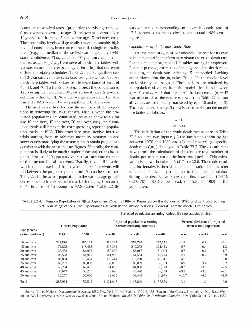
“cumulative survival rates” (proportions surviving from age0 and over at one census to age 10 and over at a census taken10 years later; from age 5 and over to age 15 and over, etc.).These mortality levels will generally show a reasonably highlevel of consistency, hence an estimate of a single mortalitylevel (e.g., the median of the series) can be generated withsome confidence. First, calculate 10-year survival rates—that is, as 5Lx + 10 / 5Lx from several model life tables withvarious values of life expectancy at birth (e0) that representdifferent mortality schedules. Table 22.3a displays three setsof 10-year survival rates calculated using the United Nationsmodel life tables with values of life expectancy at birth of40, 43, and 46. To finish this step, project the population to1986 using the calculated 10-year survival rates (shown incolumns 5 through 7). Note that we generate a similar tableusing the PAS system by varying the crude death rate.
The next step is to determine the accuracy of the projec-tions in reflecting the 1986 census. That is, when the pro-jected populations are cumulated (so as to show totals forage 10 and over, 15 and over, 20 and over, etc.), the cumu-lated totals will bracket the corresponding reported popula-tion totals in 1986. This procedure may involve iterativetrials starting from an arbitrary mortality assumption andsuccessively modifying the assumption to obtain projectionsconsistent with the actual census figures. Naturally, the com-putation is likely to be much simpler if the projections basedon the first set of 10-year survival rates are accurate estimatsof the true number of survivors. Usually, several life tableswill have to be used and the actual numbers of survivors willfall between the projected populations. As can be seen fromTable 22.4a, the actual population in the various age groupscorresponds to life expectancies at birth ranging from an e0
of 40 to an e0 of 46. Using the PAS system (Table 22.4b)
survival rates corresponding to a crude death rate of 17.3 generates estimates close to the actual 1986 censusfigures.
Calculation of the Crude Death Rate
The estimate of e5 is of considerable interest for its ownsake, but is itself not sufficient to obtain the crude death rate.For this calculation, model life tables are again employed.For that purpose, estimates of the age-specific death rates,including the death rate under age 5 are needed. Lackingother information, the nmx values “found” in the median levelcould simply be assigned. These values are obtained byinterpolation of values from the model life tables betweene0 = 40 and e0 = 46 that “bracket” the last census (e0 = 47was also used; as the reader can see from Table 22.4a, notall values are completely bracketed by e0 = 40 and e0 = 46).The death rate under age 5 (5m0) is calculated from the modellife tables as follows:
The calculation of the crude death rate as seen in Table22.6 requires two inputs: (1) the mean population by agebetween 1976 and 1986 and (2) the imputed age-specificdeath rates (nmx ) displayed in Table 22.5. These death ratesnow permit the calculation of the absolute total number ofdeaths per annum during the intercensal period. This calcu-lation is shown in column 3 of Table 22.6. The crude deathrate for females is then obtained as the ratio of the numberof calculated deaths per annum to the mean populationduring the decade, as shown in this example: (4914)/(320,170) = 0.0153 per head, or 15.3 per 1000 of the population.
l l
L L0 5
0 4 1
-+
618 Popoff and Judson
TABLE 22.4a Female Population of Fiji at Age x and Over in 1986 as Reported by the Census of 1986 and as Projected from1976 Assuming Various Life Expectancies at Birth in the United Nations “General” Female Model Life Tables
Projected population assuming various life expectancies at birth
Projected population assuming Percent deviation of projected
Age (years)Census Population various mortality schedules from actual population
(x to x and over) 1976 1986 e = 40 e = 43 e = 46 e = 40 e = 43 e = 46
10 and over 212,816 257,135 252,297 254,799 257,352 -1.9 -0.9 +0.115 and over 171,822 218,468 216,861 219,272 221,413 -0.7 +0.4 +1.320 and over 135,483 181,922 180,562 183,017 184,949 -0.7 +0.6 +1.725 and over 106,508 144,925 141,959 144,584 146,244 -2.1 -0.2 +0.930 and over 83,864 113,469 108,414 111,270 112,617 -4.5 -1.9 -0.835 and over 65,297 88,098 82,035 85,099 86,169 -6.9 -3.4 -2.240 and over 49,234 67,416 61,833 64,880 65,728 -8.3 -3.8 -2.545 and over 36,643 50,217 45,620 48,470 49,140 -9.2 -3.5 -2.150 and over 26,257 35,866 32,033 34,448 34,973 -10.7 -4.0 -2.5
Total 887,924 1,157,516 1,121,648 1,145,840 1,158,853 -3.1 -1.0 +0.9
Source: United Nations, Demographic Yearbook, 1989, New York: United Nations, 1991. In U.S. Bureau of the Census, International Data Base, Wash-ington, DC, http://www.census.gov/ipc/www/idbnew.html. United Nations, Model Life Tables for Developing Countries, New York: United Nations, 1982.

Calculation of the Crude Birthrate
The female crude birth rate now can be calculated as thesum of the observed rate of increase plus the death rate asestimated from census survival rates:
An exactly analogous but independent calculation may be followed with respect to the male population shown in Table 22.2. This calculation is left to the reader asan exercise. For the female population of Fiji during the1976–1986 period, we then have the following estimates:
Rate of natural increase 0.0192Death rate 0.0153Birth rate 0.0346
bf = + =0 0192 0 0153 0 0346. . .
Validity of Estimates Based on Observed Growth Rate andCensus Survival Rates
In preparing any estimate, the analyst should be able toindicate to what extent his estimates are insensitive, or“robust,” first, to the various assumptions incorporated in the
22. Some Methods of Estimation for Statistically Underdeveloped Areas 619
TABLE 22.4b Female Population of Fiji at Age x and Over in 1986 as Reported by the Census of 1986 and as Projected from1976 Assuming Various Crude Death Rates Using the PAS Model System
Projected population assuming various crude death rates
Projected population assuming Percent deviation of projected
Age (years)Census population various mortality schedules from actual population
(x to x and over) 1976 1986 7.78 12.78 17.78 7.78 12.78 17.78
10 and over 212,816 257,135 273,304 264,007 255,441 +6.3 +2.7 -0.715 and over 171,822 218,468 234,730 227,120 220,289 +7.4 +4.0 +0.620 and over 135,483 181,922 197,152 190,302 184,145 +8.4 +4.6 +1.225 and over 106,508 144,925 157,050 151,108 145,752 +8.4 +4.3 +0.630 and over 83,864 113,469 121,736 116,755 112,242 +7.3 +2.9 -1.135 and over 65,297 88,098 93,734 89,617 85,864 +6.4 +1.7 -2.540 and over 49,234 67,416 71,971 68,592 65,493 +6.8 +1.7 -2.945 and over 36,643 50,217 54,254 51,513 48,987 +8.0 +2.6 -2.450 and over 26,257 35,866 39,085 36,903 34,885 +7.0 +2.9 -2.7
Total 887,924 1,157,516 1,243,046 1,195,917 1,153,098 +7.0 +3.3 -0.4
Source: Same as Table 22.3b.
TABLE 22.5 Levels of Mortality of Fiji Females and Corresponding Expectations of Life at Age 5 Derived from
Proportions Surviving to Age x and Over in 1986 from Age x-10 and Over 10 Years Earlier
Age Actual value of e0 Value of e5
(x and over) (1) (2)
10 years and over 40.72 48.6015 years and over 39.80 48.0720 years and over 42.85 50.1625 years and over 40.48 48.4230 years and over 43.20 52.5935 years and over 43.27 53.1440 years and over 43.08 53.1345 years and over 41.59 49.2450 years and over 42.90 50.20
Median 42.85 50.16
Source: Same as Table 22.4a.
TABLE 22.6 Calculation of the Crude Death Rate for the Female Population of Fiji in the Period 1976–1986
Corresponding to the Recorded Age Distribution and to aLife Expectancy at Birth Estimated from Cumulated Census
Survival Rates
Mean annual Mean deaths
population Death rate 1976–19861976–1986 e0 = 42.85 (1) ¥ (2) =
Age (1) (2) (3)
Total 320,170 0.01531 4,913.72
Under 5 years 44,503 0.0307 1,364.85 to 9 years 41,776 0.0074 307.010 to 14 years 39,831 0.0043 172.715 to 19 years 36,443 0.0068 248.620 to 24 years 32,986 0.0094 311.125 to 29 years 27,050 0.0106 285.830 to 34 years 21,969 0.0119 261.735 to 39 years 18,373 0.0128 236.040 to 44 years 14,895 0.0138 205.145 to 49 years 12,369 0.0162 200.350 to 54 years 9,575 0.0210 201.255 to 59 years 7,465 0.0288 215.360 to 64 years 5,281 0.0405 213.865 to 69 years 3,754 0.0577 216.770 to 74 years 2,380 0.0843 200.775 years and over 1,524 0.1791 272.9
Source: Same as Table 22.4a.1 Derived by deviding 4,914 by 320,170.2 Derived by summelion.
estimating procedure and, second, to possible errors in thedata themselves. The most convenient way to effect this isto calculate multiple sets of estimates by making alternativeassumptions in applying the estimating procedure and byconsidering alternative hypotheses as to the accuracy of thebasic data. Such procedures, guided by the knowledge ofspecial local circumstances, should be routinely followed inorder to validate the results. Following are brief commentsmade in the present context concerning this topic.
It is important to consider that the model life table patternof mortality is a major assumption that is incorporated in thecalculations based on census survival rates (apart from anyassumption concerning completeness of data). The basicweakness of this method is that there exists no way to extractinformation on the entire mortality pattern from reported agedistributions alone. What, then, are the consequences ofselecting West model life tables in preference to othermodels? First, the estimates of mortality at age 5 and over,whether expressed in terms of the model life tables or ofsome other measure, are principally insensitive to the modelpattern chosen. Therefore, even the selection of sharply dif-fering life table patterns leaves the estimates of mortalityover age 5 largely unaffected. However, the opposite is true when mortality estimated for age 5 and over is extrap-olated to ages less than 5. The record indicates that histori-cally very different levels of early childhood mortality areassociated with a fixed level of mortality at higher ages. Ifthe life table pattern chosen underestimates the level ofinfant mortality, for example, the estimated total death ratewill be lower than actual experience. There will be an error of the same absolute magnitude and direction in theestimated birthrate.
Concerning errors in the basic data, the method of“cumulative census survival” is relatively insensitive toerrors of age misreporting. No such statement can be made,however, about the effect of differential net under-oroverenumeration of the population in two consecutive cen-suses. Obviously, such errors affect the observed intercensalgrowth rate, and censuses that are relatively close togetherwith large differences in the level of error will produce moreserious error.
Stable Population Estimates from Observed AgeDistribution and Intercensal Growth Rate
The discussion of the stable population model earlier inthis chapter indicated that, if some observed population’sparameters closely resemble those of a particular stable pop-ulation, then other parameters of that stable population maybe reliable estimates of the corresponding parameters in theobserved population. Ideally, derivation of stable popula-tion estimates should be attempted only if the existence ofapproximate stability can be verified by direct evidence. Forexample, if age distributions are consistent across consecu-
tive censuses and the intercensal growth rate is constant oversuccessive census intervals, then using the stable populationestimates would produce reliable results. Indications thatfertility and mortality behavior is relatively stable may alsopresent additional and important, if impressionistic, evi-dence to support the hypothesis that a population is approx-imately stable. (Note that when the data from censuses andthe registration system are deemed accurate, there is no needto apply stable analysis to measure a population’s basicparameters.)
Requirements for “proofs” of stability are, strictly speak-ing, not satisfied in the case of Fiji. Comparison of the 1976and 1986 censuses shows some minor changes in thereported age distribution (refer to columns 6 to 9 in Table22.2). There is evidence of an acceleration of the rate of pop-ulation growth and of a decline in mortality.
Most, if not all, countries will exhibit anomalies in theirdemographic processes that cause the analyst to question thevalidity of applying stable population analysis. Yet the technique of stable analysis is useful under a wide range of circumstances provided that such analysis contains a reasonably full exploration of the conflicting evidence pre-sented by the observed data. In fact, if the conditions of sta-bility are not fulfilled, the results of the analysis themselveswill show the differences.
In the instance of Fiji, the young age distribution doessuggest that no sustained and substantial decline of fertilitytook place prior to 1986. The examination of census survivalrates suggests some age misreporting and probably someomission of children under age 5. Variations in the observedage distributions thus may reflect differential occurrence ofsuch errors of enumeration in the censuses of 1976 and1986. It is also known that an orderly decline of mortalityhas only a relatively minor effect on the age distribution.Furthermore, a population that was initially stable but hasundergone a decline of mortality is always closely approxi-mated by a stable population having the current growth rateand the current life table of the actual population.
Given the considerations previously noted, an attempt to derive estimates of the vital rates for Fiji (or any like situation) by the stable technique can be justified. In thisexample, we will again demonstrate the estimation of thedeath rate and birthrate using the previously calculated rateof growth of .0192. Following that is an example of esti-mating a gross reproduction rate using a standard pattern of“natural” fertility. Again, the only data used in the analysisare those contained in Table 22.2. To determine stable pop-ulations corresponding to the recorded data, the observedintercensal rate of growth is combined with measures of theobserved age distribution in 1976. Naturally a large numberof indices of age distribution can be constructed, defining amore or less broad spectrum of stable populations, all char-acterized by the observed intercensal r. It is important toselect indices of age distribution such that they will be least
620 Popoff and Judson

affected by errors of age reporting. At the same time theindices should reflect a broad range of observations. Theseand other considerations, plus experience, suggest the selec-tion of proportions from the cumulative age distribution-aproportion under age 5, under age 10, under age x ingeneral, denoted as C(5), C(10), C(x) for this purpose. Goingbeyond C(45) in the analysis is not recommended.
Computational Routine
The technique is illustrated in Table 22.7 for the femalepopulation of Fiji. For this illustration, the Coale andDemeny (1966) model stable population tables are used,examples of which are found in Appendix B (see Table B.3).Column 1 shows the observed values of C(5), C(10), . . .C(45). When each of these nine indices of the age distribu-tion is combined with the same observed growth rate of.0192, they define nine different populations defined by 5-year age ranges within the tabulated network of a set of model stable populations.
First, locate these populations by constructing modelpopulations having a growth rate of .0192 (by interpolatingbetween columns with r = .015 and r = .020 for variouslevels of mortality). Select the mortality levels such that the various observed C(x) values are bracketed by the corresponding C(x) values in the models. (A similar processwas used in constructing Table 22.4a.) The results of thispart of the calculation are presented in columns 2 to 6. Notethat the parameters to be estimated (the birthrate, the deathrate, etc.) are shown along with the C(x) values in the bottomrows of Table 22.7.
Second, determine (for example) the birthrate in a “West”female stable population having an r of .0192 and a C(20)of .4827. The models shown in columns 4 and 5 bracketingthis value of C(20) give the corresponding values for C(20)as .4916 and .4771, respectively. Appropriate linear inter-polation, described earlier in this chapter, between these twobracketing populations yields the population with therequired C(20). When the same interpolation factors used inthis calculation are applied to the birthrates (.0354 and.0385), they yield the birth rate .0366, for the entry incolumn 7. Exactly analogous procedures result in variousestimated parameter values (columns 7 to 13) correspondingto all C(x) values shown in column 1.
Validity of the Stable Estimates
The analyst must be cautious about the interpretation ofthe results of Table 22.7, especially if there is no additionaloutside information or knowledge of special conditions ofthe area under study to inform the analysis. The graduallyincreasing estimates of the birthrate associated with C(20)to C(45) tend to suggest higher fertility in the past. However,accepting these birthrates (ranging from about .037 to .047)and values of other parameters as truth would imply a highdegree of confidence that the West model life tables describe
the true mortality pattern of Fiji. In addition, the validity ofthis analysis depends on the precision of the intercensalgrowth rate. For these reasons, the results do not necessar-ily imply reliability of the estimates because the twomethods are sensitive to similar biases.
The estimates associated with C(5) to C(15) show rela-tively lower levels of fertility (and mortality). This could beinterpreted as evidence of fertility decline during the decadeor so prior to 1986, or as a consequence of a tendency toexaggerate the ages of children in census reports or to omitchildren in the census, particularly in the youngest ages.Analysis of census survival rates suggests that the last expla-nation is correct or at least dominant.
These comments indicate the need for reliable age reportsin stable population analysis. Alternatively, the analystshould endeavor to obtain all information that is helpful indetermining the most reliable segments of the age distribu-tion or in isolating particular errors that affect age reports.From such information, the analyst can select particularindices (e.g., C(10) or C(35)) of the age distribution aspreferable to others or adjust the age distribution prior tostable analysis. In general, the former procedure is preferred.In the absence of particular reasons for preferring one indexof the age distribution to another, and in the absence of verymarked fluctuations in the estimates produced by variousC(x) values, the median of the series should be selected asthe single best estimate. The median of the birthrates is.0405 and of the death rates .0213. In the present instance,this rule favors the stable population associated with C(25)and mortality level 10.0 (e5 = 51.28).
The application of similar procedures to the male popu-lation is straightforward, and it is left to the reader as anexercise. For the total female population of Fiji, we obtainthe following stable estimates:
Rate of natural increase .0192Death rate .0213Birthrate .0405
It should be noted that knowledge of local conditionsoften suggests that the estimates for one sex are more accu-rate than for the other sex. For instance, when ages are inad-equately known and have to be estimated by enumerators,female age distributions are typically more amenable tocorrect interpretation than male age distributions. Undersuch circumstances it is preferable to derive the estimate formales, and for the total population, from stable analysis ofthe female population only.
Calculation of the Gross Reproduction Rate by Stable Population Analysis
In the preceding example (Table 22.7), two alternativevalues of the GRR were obtained corresponding to a mean age of the fertility schedule, GRR (m = 29) and
22. Some Methods of Estimation for Statistically Underdeveloped Areas 621

TABLE 22.7 Stable Population Estimates of Fertility and Mortality Based on the Age Distributionof the Female Population of Fiji as Reported in the Census of 1986 and on the Observed
Intercensal Growth Rate (r = 0.0192)
Values of C(x) and of various parameters in female stable Parameter values in stable populations with C(x) as shown in column (1) and populations with r = 0.0192 and levels of mortality as r = 0.0192
Proportionate indicatedpopulation Level ofup to age x Level 7 Level 9 Level 11 Level 13 Level 15 Birthrate Death rate mortality e0 e5 GRR(29) GRR(31)
Age x (1) (2) (3) (4) (5) (6) (7) (8) (9) (10) (11) (12) (13)
5 years 0.1400 0.1681 0.1590 0.1512 0.1445 0.1385 0.0335 0.0155 13.5 51.28 56.58 2.45 2.5910 years 0.2688 0.3036 0.2902 0.2787 0.2684 0.0355 0.0192 11.1 45.23 52.98 2.72 2.8915 years 0.3788 0.4220 0.4058 0.3916 0.3788 0.0354 0.0193 11.0 45.01 52.85 2.73 2.9020 years 0.4827 0.5256 0.5077 0.4916 0.4771 0.0366 0.0181 11.8 46.94 54.01 2.64 2.8025 years 0.5879 0.6152 0.5965 0.5795 0.0405 0.0213 10.0 42.48 51.28 2.79 2.9630 years 0.6774 0.6920 0.6734 0.0436 0.0273 8.6 38.93 49.08 2.97 3.1635 years 0.7495 0.7574 0.7396 0.0453 0.0255 7.9 37.21 47.99 3.16 3.3740 years 0.8083 0.8126 0.7962 0.0462 0.0246 7.5 36.30 47.42 3.26 3.4845 years 0.8572 0.8589 0.8443 0.0470 0.0239 7.2 35.58 46.96 3.34 3.57
Birth rate (b) 0.0476 0.0425 0.0385 0.0354 0.0328Death rate (d) 0.0284 0.0233 0.0193 0.0162 0.0135e0 35 40 45 50 55e5 46.59 49.75 52.84 55.86 58.70GRR (29) 3.41 2.85 2.73 2.50 2.31GRR (31) 3.64 3.02 2.90 2.64 2.43
Source: United Nations, Demographic Yearbook, 1989, New York: United Nations, 1991, In U.S. Bureau of the Census, International Data Base, Washington, D.C.,www.census.gov/ipc/www/idbnew.html; A. Coale and D. Demeny, Regional Model Life Tables and Stable Populations, Princeton: Princeton University Press, 1966.

GRR (m = 31). The median estimates were 2.79 and 2.96,respectively.
To arrive at a single estimate of the GRR, a prior esti-mate of the true value of m is necessary. When age-specificfertility rates are not available, as is likely to be the case, arough estimate can be made by various methods. The largelyself-explanatory calculation shown in Table 22.8 illustratesone such method. Its application is based on the assumptionthat fertility outside marriage is negligible and that withinmarriage little or no contraception is practiced. A standardage pattern of “natural” fertility (i.e., without contraception)shown in column 2 can then be combined with the propor-tions of married women as reported in the census to give thelikely pattern (but of course not the level) of age-specificfertility rates (column 3). The mean of this schedule is cal-culated as 31.5 years. The stable estimate of the gross repro-duction rate for Fiji can now be calculated as 3.37 byinterpolation between GRR (m = 31) and GRR (m = 33) toGRR (m = 31.5).
Quasi-stable Estimates
When an actual population is reasonably approximatedby the stable model, it is often described as being in the“quasi-stable state,” and the estimates derived from themodel are referred to as “quasi-stable estimates.” However,the two meanings of the term used by analysis should be dis-tinguished. In one sense, the expression is intended merelyas a reminder that the correspondence between the modeland the actual population is imperfect, because of both inade-quately fulfilled conditions of stability and distortions in thedata. In this loose interpretation, all estimates described here
as “stable” should be considered “quasi-stable.” Althoughuse of the term is a matter of definition, it is preferable torefer to such estimates simply as stable estimates. It shouldalways be understood that such estimates are subject tobiases owing to deviations of the actual population from thestable model used and owing to erroneous measurements.
In a second more precise meaning, the term “quasi-stable” is applied only to populations that were initiallystable (as always, only as a close approximation) but thathave undergone a process of “destabilization”, such as anorderly and sustained decline of mortality. Research hasbeen conducted on the impact of the resulting decline on theage distribution and the values of other parameters, as wellas on the biases in estimating population parameters for sucha population under the assumption of strict stability. Whenthe findings of this research are used to make appropriatenumerical adjustments on the stable estimates, taking intoaccount the decline of mortality, the final estimates arecalled quasi-stable in the more narrow, technical sense of theterm.
The special interest in studying populations where mortality has declined while fertility remained stable is, ofcourse, due to the prevalence of this condition in many contemporary populations. Proper quantitative adjustmentsfor quasi-stability require information on the duration andrapidity of the mortality decline that is seldom available inthe desired form and detail. Hence, the dimensions of themortality decline itself have to be estimated from oftenfragmentary pieces of evidence. For discussions and illus-trations of the estimating methods that have been workedout, the reader is referred to the specialized publications
22. Some Methods of Estimation for Statistically Underdeveloped Areas 623
TABLE 22.8 Calculation of the Mean of the Fertility Schedule for the Female Population of Fijifrom Proportions Married as Reported in the 1986 Census and from a Standard Age Pattern of
Fertility Rates Reflecting “Natural” Fertility
Proportions Age pattern of Weightedmarried, Age pattern of marital fertility, midpoint
females, Fiji, natural fertility Fiji Midpoint of ages19861 rates (1) ¥ (2) = age interval (3) ¥ (4) =
Age (x to x + 4) (1) (2) (3) (4) (5)
15 to 19 years 0.130 1.109 2 0.14417 17.5 2.5220 to 24 years 0.425 1.0000 0.42500 22.5 9.5625 to 29 years 0.746 0.9350 0.69751 27.5 19.1830 to 34 years 0.864 0.8530 0.73699 32.5 23.9535 to 39 years 0.892 0.6850 0.61102 37.5 22.9140 to 44 years 0.898 0.3490 0.31340 42.5 13.3245 to 49 years 0.880 0.0510 0.04488 47.5 2.13
Total, 15 to 49 years 2.97297 93.57Mean age of fertility schedule = 93.57 ∏ 2.97297 = 31.5
1 Source: Official census reports.2 Estimated as 1.2 - (.7* .130) = 1.109.Source: Same as Table 22.2.
(United Nations, 1967). However, the general effect of mor-tality change is to introduce a downward bias into the stableestimates of the birthrate (and of the GRR) when such esti-mates are obtained from observed intercensal growth ratesand from C(x) values for x at 20 years and over. If the declinein mortality was very rapid, and if the decline lasted forseveral decades, this downward bias can be quite pro-nounced—for example, the stable estimate of the birthrateassociated with C(35) may be .0.025 when the true (quasi-stable) birthrate is in fact 0.029. On the other hand, estimatesderived from C(10) or C(15) are likely to be only slightlyaffected by declining mortality.
Estimates Based on the Reverse Survival Technique
When two consecutive censuses contain no other demo-graphic information but age and sex distributions and thepopulation is not a stable one, the analyst may wish to applythe familiar reverse survival technique to estimate the crudebirthrate in the 5- or 10-year period preceding the secondcensus. The technique requires the construction of an appro-priate life table by which the population is projected “back-ward” by 5 or 10 years. A by-product of such a reverseprojection is the absolute number of births during the 5 or10 years prior to the census. These quantities are obtainedby dividing the populations under 5 and under 10 years oldby the factors 5L0/5l0 and 10L0/10l0, respectively. Dividing themean annual number of births during the given interval bythe total population calculated at the midpoint of the inter-val yields the estimated birth rate.
Insofar as the life table is estimated from census survivalrates (hence infant and early childhood mortality is essen-tially an extrapolation), the method is subject to a type ofuncertainty that plagues the previously discussed estimatesas well. In making reverse survival estimates, no assump-tion of stability is made; therefore, the method may appearattractive under many situations where the stable conditionsdo not exist. It can be shown, however, that regardless of theexistence of stability or the lack of it, the results of reversesurvival estimates and the stable estimates obtained from thepopulation under age 5 or 10 are essentially identical. In fact,using a set of tabulated model stable populations is a quickand efficient way to obtain reverse survival estimateswhether the population is stable or not. Thus, the first twolines of the example set forth in Table 22.7 illustrate theresults of a reverse survival analysis for Fiji. This examplecalls attention to a weakness of the method. By necessity,the estimate of the birthrate is obtained primarily from thenumbers under 5 and under 10 reported in the second census.However, frequent undercounting of the age group under 5years old in censuses creates measures of the age distribu-tion that are suspect. To avoid the pitfall of interpreting thelevel of fertility in the light of the recorded numbers in child-hood ages only, the analyst again may find it advantageous
to examine a full set of computations, such as those sum-marized in Table 22.7, even if the stability conditions arevery inadequately fulfilled.
Estimates Based on Data Collected in aSingle Census or Survey
Fertility Measures Derived from a Single Recorded Age Distribution
The most conspicuous common feature of the methodsdiscussed in the preceding sections was their reliance on theanalysis of the age distribution recorded in the most recentcensus. However, a prior census is an essential requirementfor the calculation of an intercensal growth rate or censussurvival rates, as demonstrated in the prior section. Thequestion posed in this section is, can general magnitudes offertility, mortality, and growth be derived from a singlerecorded age distribution alone? The answer is essentiallynegative.8 If age and sex distributions have been tabulatedfor numerous geographical subdivisions of the country,however, and are available for other subpopulations as well,such as racial or ethnic groups, internal comparisons andchecks may reveal sufficient consistency of age reporting sothat various measures of the age distributions may beaccepted as reliable. Because past fertility is the dominantfactor determining the shape of the age distribution and, inparticular, proportions in the youngest ages depend on recentfertility, a rough estimate of the level of the birthrate maybe obtained by an examination of a single age structure.Alternative assumptions concerning the level of mortality(e.g., contrasting a plausible low and a plausible highhypothesis for early childhood mortality) might show, forinstance, that either assumption leads to a birthrate of over40 per thousand. In most cases it will be true, however, thatthe uncertainty about the level of mortality removes evenqualitative “precision” from the estimate. Experimentationin the hands of a skilled analyst will normally result in deter-mining nontrivial thresholds or ceilings for the birthrate, butthe method will be unable to differentiate between, forexample, “very high” or just “moderately high” fertility.
The explicit introduction of assumptions concerningprobable mortality levels may be omitted if only compara-tive estimates of fertility levels are the aim. Thus, someindices of the age distribution that are, ceteris paribus,highly correlated with fertility levels may show sufficientregional contrasts to warrant valid conclusions concerningdifferential fertility. The most commonly used index of agedistribution for such purposes is the ratio of children underage 5 to the number of women in the childbearing ages(usually defined as ages 15 to 49), i.e., the child-womanratio. General indices of age distribution (e.g., proportions
624 Popoff and Judson
8 It appears, however, that the PAS system can be used for single surveys.

under age 5, 10, or 15) may perform as well or better forthis purpose, and there is less temptation to interpret theresults as a measure of fertility as such. The interest in dif-ferential patterns shown by such indices is greatly strength-ened if analysis (easily performed by means of tabulatedmodel stable populations) can show that mortality differen-tials, or plausible directions and magnitudes, do not quali-tatively affect the patterns. Information on the agedistribution alone is entirely insufficient to support mean-ingful estimates with respect to either absolute values or todifferentials in growth rates and mortality rates.
Estimates of Fertility from Retrospective Reports on Childbearing
By tradition, censuses have been used primarily to recorda cross-sectional view of the state of a population at a givenmoment in time. As we have seen, however, questions con-cerning past demographic events experienced by individu-als can also be included in a census or survey. When vitalregistration is deficient, the recording and analysis of suchevents may be especially rewarding. With respect to fertil-ity, two types of questions have appeared with increasingfrequency in recent censuses and surveys. One type of ques-tion concerns the number of births that have occurred duringa specified period, usually a year, preceding the survey.Another question inquires about the number of children everborn to each woman up to the time of the inquiry.
A priori reasoning as well as experience suggests,however, that reports by women on past births may besubject to serious biases. As to the question on births duringa specified period, a chief problem lies in the difficulty onthe part of the respondents of reporting the event in an exacttime frame, especially when no written record of that event is available. Thus, the mean length of time covered by the reports may span more or less than the intended 12-month period, often by a margin of several months.Accordingly, age-specific fertility rates, and hence total fertility, calculated from such statistics, may be under- oroverestimated.
With respect to children ever born, the possibility of over-reporting is rather remote. On the other hand, understate-ment of the true number appears to be common, owing tovarious factors, such as memory failure and omission ofdeceased children or children who have already left home.In particular, these biases are likely to affect reporting bywomen of older age and higher parity. Thus the value of theinformation that is of greatest interest, namely the numberof children ever born by the end of the childbearing age, isweakened by this circumstance. Clearly, under conditions ofapproximately constant fertility (and ignoring differentialmortality and migration), the mean number of children everborn to women of about age 50 would direclty supply anestimate of the current total fertility rate.
Methods that would permit the evaluation and correctionof distortions in retrospective fertility reports would, there-fore, greatly enhance the usefulness of such information. Atechnique worked out by Brass (1968, 1975) to serve thatpurpose is illustrated next through data taken from thePhilippines (U.S. Census Bureau, 2000). The data relate toa sample area covering the country; thus they also demon-strate the possibilities of retrospective fertility reports togenerate information for subpopulations, as well as for acountry as a whole.
Column 2 of Table 22.9 shows age-specific fertility ratescalculated from 12-month retrospective reports. Note that,because women in a given 5-year age group at the time ofthe survey were on the average half a year younger at thetime the births occurred, the age-specific fertility rates actu-ally relate to the unconventional age groups bounded byexact ages 14.5 and 19.5, 19.5 and 24.5, and so on. Thecumulative totals of these rates are shown in column 3(0.2662 children up to age 19.5, 1.3510 children up to age24.5, etc.). The cumulative total for the end of the child-bearing period gives an estimate of the current (1974–1975)total fertility rate of the population in question, assuming, of course, that the reports are correct. The estimated totalfertility rate from these “current” reports is different than theaverage number of children ever born reported by women atthe end of the childbearing period, as shown in column 6.This comparison is, however, inconclusive as to the validityof the current fertility reports; the number of children everborn is often underreported by older women or, alternatively,past fertility may have been higher than current fertility.
These considerations suggest that a comparison of cumu-lated current fertility with corresponding reports on childrenever born at younger age groups would provide more infor-mation. However, apart from the age at the end of the child-bearing period, columns 3 and 6 are not directly comparable.Column 3 shows cumulated fertility up to ages 19.5, 24.5,and so on, whereas in column 6 cumulative fertility relatesroughly to the midpoint of the age groups shown at the left(i.e., up to 17.5, 22.5, etc.). Adjusting to these ages thecumulated current fertility shown in column 3 by “linear”interpolation is a possibility, but assuming an even distribu-tion of fertility within each age interval is clearly unrealis-tic. To eliminate an unnecessary source of bias, a moresophisticated adjustment is performed in columns 4 and 5with the help of Appendix Table B.4. Here is found a set of adjustment factors wi to obtain values of cumulated“current” fertility (Fi) directly comparable to averagenumbers of children ever born (Pi) calculated for the conventional 5-year age groups of women.
The correction factors reflect the curvature of an under-lying set of model age-specific fertility rates. The appropri-ate model, hence the appropriate correction factor, isselected by either of two summary measures of the age-specific fertility rates. These are the mean of the fertility
22. Some Methods of Estimation for Statistically Underdeveloped Areas 625
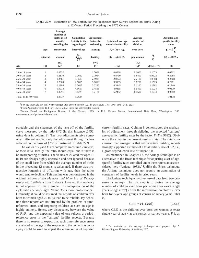
schedule and the steepness of the take-off of the fertilitycurve measured by the ratio fi/f2 (in this instance .2452,using data in column 2). The two adjustments give some-what different results; only the adjustment through factorsselected on the basis of fi/f2 is illustrated in Table 22.9.
The values of Pi and Fi are compared in column 7 in term,of their ratio. Ideally, the ratio should equal one if there isno misreporting of births. The values calculated for ages 15to 19 are always highly uncertain and best ignored becauseof the small base from which the average number of birthsin the preceding 12 months is calculated. If there was pro-gressive forgetting of offspring with age, then the ratioswould tend to decline. (This decline was demonstrated in theoriginal edition of the Methods and Materials of Demog-raphy with 1966 data from Turkey.) However, this tendencyis not apparent in this example. The interpretation of thePi/Fi ratios between ages 20 and 35 is more problematical.Ordinarily, it could be assumed that reports on children everborn to women aged 20 to 24 tend to be reliable. By defini-tion these reports are not affected by the problem of time-reference error, and forgetting children at such an age ishighly unlikely. Hence, any discrepancy between the valueof P2/F2 and the expected value of one reflects a period-reference error in the “current” fertility reports. Becausethere is no reason to expect that such time-reference errorsare related to the age of the respondent, the correction factorP2/F2 could be used to adjust the entire series of reported
current fertility rates. Column 8 demonstrates the mechan-ics of adjustment through deflating the reported “current”age-specific fertility rates by the factor P2/F2 (.9622). Obvi-ously the effect in the present case is trivial. The chief con-cluision that emerger is that retrospective fertility, reportsstrongly supportan estimate of a total fertility rate of 6.2, i.e.,a gross reproduction rate of indent 3.0.
As mentioned in Chapter 17, the Arriaga technique is analternative to the Brass technique for adjusting a set of age-specific fertility rates complied under the circumstances con-sidered here (Arriaga, 1983).9 Unlike the Brass technique,the Arriaga technique does not require an assumption ofconstancy of fertility levels in prior years.
The Arriaga technique involves use of data from two cen-suses or surveys. The first step is to derive the averagenumber of children ever born per woman for exact singleyears of age (CEBt
x) from the information on children everborn for 5-year age groups at census or survey years. Thatis,
(22.12)
where CEBtx is the children ever born per women at exact
single-year-of-age x at the census or survey year t, F is an
CEB F CEBxt
xt= ( )5
626 Popoff and Judson
TABLE 22.9 Estimation of Total Fertility for the Philippines from Survey Reports on Births Duringa 12-Month Period Preceding the 1975 Census
Averagenumber ofbirths in 12 Cumulative Adjustment Average Adjusted age-
months fertility to the factors for Estimated average number of specific fertilitypreceding the beginning of estimating cumulative fertility children rates
Age survey per interval age average Fi = (3) + wi fi ever born
interval woman1 fertility2 (3) + [(4) ¥ (2)] per woman (2) ¥ .9622 =
(Ei) (Wi) (Pi)Age (1) (2)3 (3) (4) = (5) (6)3 (6)/(5) = (7) (8)
15 to 19 years 1 0.0532 1.7068 0.0908 0.1000 1.1073 0.051220 to 24 years 2 0.2170 0.2662 2.7964 0.8730 0.8400 0.9622 0.208825 to 29 years 3 0.2461 1.3510 2.9918 2.0873 2.2100 1.0588 0.236830 to 34 years 4 0.2360 2.5815 3.1018 3.3135 3.8200 1.1529 0.227135 to 39 years 5 0.1808 3.7617 3.2232 4.3445 5.1100 1.1762 0.174040 to 44 years 6 0.0914 4.6657 3.4556 4.9815 5.9400 1.1924 0.087945 to 49 years 7 0.0291 5.1228 4.2171 5.2452 6.1600 1.1744 0.0280
Total, 15 to 49 years 1.0537 5.2684 1.0138
1 For age intervals one-half-year younger than shown in stub (i.e., in exact ages, 14.5–19.5, 19.5–24.5, etc.).2 From Appendix Table B-4 for f1/f2 = .2452; these are interpolated values.3 Source: Based on Philippines Bureau of the Census, 1975. In U.S. Census Bureau, International Data Base, Washington, D.C.,
www.census.gov/ipc/www/idenew.html.
P
Fi
i
5 f jj 0
i
=
=
Â1
f fP
Fi i
2
2
¢ =
9 The material on the Arriaga technique was prepared by A. Dharmalingam, University of Waikato, N.Z.

interpolation function, and 5CEBtx is the children ever born
per woman at age group x to x + 4.To get the CEBt
x values for single years of age, we needto find an appropriate interpolation function F. Althoughseveral functions follow the general pattern of children everborn per woman by age, a polynomial function that meetsthe following conditions seems to provide the best fit:
1. The polynomial is zero at age 15; the first derivativesof the polynomial at age 15 and at age 50 are zero.
2. The polynomial produces the average number of chil-dren ever born for the age groups 20 to 24, 25 to 29,30 to 34, 35 to 39, 40 to 44, and 45 to 49 at stact ages22.5, 27.5, 32.5, 37.5, 42.5, and 47.5, respectively. Thevalue for the age group 45 to 49 can be ignored if it issmaller than for ages 40 to 44 years. In this case, thedegree of the polynomial will be reduced by 1.
3. The integral of the polynomial between exact ages 15.0and 20.0 reproduces the average number of childrenever born per women for the age group 15 to 19.
Under these conditions, a ninth-degree polynomial can befitted to the data on children ever born per woman for the 5-year age groups 15 to 19, 20 to 24, . . . , 45 to 49. The fittedpolynomial can then be used to obtain the average numberof children ever born per woman for each single year of age,as in Equation 22.12.
Next, we estimate the average number of children everborn per women for the periods a year after the earliercensus or survey date and a year before the latest census orsurvey year:
(22.13a)
and
(22.13b)
where BAxt+1 is the average number of children ever born
per woman at exact age x during the year after the earliercensus or survey date, n is the number of years between thetwo censuses or surveys with information on children everborn, and BBx
(t+n)-1 is the average number of children everborn per woman at exact age x during the year before thelatest census or survey. By combining (22.12) and (22.13),the age-specific fertility rates can be derived as the cohortdifferences in the average number of children ever born perwoman:
(22.14a)
and
(22.14b)
where ASFRxt+0.5 is the age-specific fertility rate at age x
for the year after the earlier census or survey date, and
ASFR CEB BBxt n
xt n
xt n+( )-
++ +( )-= -0 5
11.
ASFR BA CEBxt
xt
xt+
++= -0 5
11.
BBn
CEBn
nCEBx
t nxt
xt n+( )- += ◊ +
-◊1 1 1
BAn
nCEB
nCEBx
txt
xt n+ +=
-◊ + ◊1 1 1
ASFRx(t+n)-0.5 is the age-specific fertility rate at age x for the
year before the latest census or survey date. From (22.14),the 5-year age-specific fertility rates can be obtained as
(22.15)
The 5-year age-specific rates can then be cumulated as
(22.16)
Similarly, the age pattern of fertility (APF) derived from thenumber of births during the previous 12 months or from reg-istration data can be cumulated as
(22.17)
Using (22.16) and (22.17), an adjustment factor is derivedas
(22.18)
Assuming that the cumulated fertility rates obtained fromusing information on children ever born, derived from Equa-tion (22.16), reflect the “true levels,” a set of estimated fer-tility rates is obtained by applying the adjustment factor (ki)to the age pattern of fertility (APF). In other words, the esti-mated fertility rates (F) are
(22.19)
As ki is likely to differ by age, it is recommended that oneselect the adjustment factor that corresponds to the age group whose mean is closest to the mean age of childbearing.
If the age pattern of fertility (APF) is not available, thenone can accept the fertility rates obtained from children everborn (Equation 22.16) as the “true ones.” However, theresults may be affected by the tendency among older womento underreport children ever born. This can be avoided byre-estimating the single-year-of-age-specific fertility ratesfor ages 40 to 49 by an extrapolation of cumulative fertilityrates for single years of age from 33 to 38. This involvesfitting a Gompertz function to cumulative single-year-of-age-specific fertility rates (CFR, obtained from Equation22.16) for ages 33 to 38 as follows:
(22.20)
From the fitted Gompertz function, the fertility rate for eachage from 39 to 49 can be derived as
(22.21)F k g k g for xxt c cx x= ◊ - ◊ =+1
39 40 49, , ,K
k g CFR for xc tx◊ = =+5 33 34 38, , ,K
5 5F k APFxt
i xt= ◊
kCF
CPFi
it
it
=
CPF APFit
xt
x
i
+=
= ◊ Â5 515
5
CF ASFRit
xt
x
i
+=
= ◊ Â5 515
5
5
415
ASFR ASFRxt
it
i x
x
==
+
Â
22. Some Methods of Estimation for Statistically Underdeveloped Areas 627
As the fertility rate derived from Equation (22.21) for age50 may not be zero, the extrapolated fertility rates for ages39 to 49 can be adjusted as follows:
(22.22)
Using Equation (22.15), fertility rates 5 year age group canbe calculated.
If the information on children ever born is available foronly one census or survey date, the Arriaga technique canstill be applied. In this case, it is assumed that the averagenumber of children ever born per woman by age of motherhas been constant during the past, and Equation (22.13)becomes irrelevant. The single-year-of-age-specific fertilityrates as in Equation (22.14) are obtained by taking the dif-ferences between the average numbers of children ever bornper woman for two consecutive single years of age. Then byfollowing Equations (22.16) to (22.19), a set of estimatedfertility rates can be obtained.
Estimates of Mortality from Retrospective Reports on Deaths
Using the analogy of estimating fertility from surveyreports on childbearing during a specified period prior to thesurvey, it seems intuitive to try to derive mortality estimatesfrom survey data on deaths obtained from retrospectivereports. In fact, a number of censuses as well as surveys haveexperimented with such ideas. In retrospective birth reports,the rate of omission or the degree of distortion with respectto the length of the reference period may reasonably beassumed to be insensitive to the age of the reporting women,hence the pattern of fertility shown by such reports can beaccepted as approximately correct. In contrast, any assump-tion of uniformity of errors in reported deaths with respectto age at death appears to be patently false. Differential com-pleteness is generated by the fact that the importance ofdeath to the survivors varies with the personal attributes ofthe deceased, and such attributes are highly correlated withage. Also, although retrospective birth reports are suppliedby a well-defined group, women in the childbearing age,directly connected with the event of birth and subject to lowmortality, no such logical respondent category exists withrespect to past deaths. Thus, retrospective death reportsoften contain not only errors of omission and of referenceperiod, but also of duplicate reporting of the same event.Furthermore, unlike the case of retrospective birth reports,no technique exists by which the average degree of the erro-neous lengthening or shortening of the reference period canbe estimated. Hence, no correction is possible for reference-period errors. The assumption that the reference-period erroris of the same magnitude as the one calculated for fertilityby the method described earlier is unacceptable, because thedistortion in the perception of time elapsed is likely to bedifferent for the two events.
adj xt
xt tF F F
xfor x= - ◊
-=50
3911
39 40 49, , ,K
Estimates of Infant and Child Mortality fromProportions Living among Children Ever Born
Data on children ever born and children living allow thecalculation of the proportion of children surviving and itscomplement, the proportion of deceased children. This can,in turn, provide measure of child mortality during the pre-censal period. Such a measure, by definition, contains no ref-erence-period error. Apart from minor biases, such as thoseoriginating from a possible relation between the mortality ofwomen according to the number of the children who havedied, it is likely to be affected only by underreporting (butonly if the degree of underreporting differs in the numera-tor and in the denominator of the measure.) The underre-porting would also tend to vary inversely with the recencyof the births concerned. It is almost always the case that pro-portionate underreporting affects the number of childrenever born more than the number reported as surviving,because children already dead at the time of the survey aremore likely to be omitted than children who are still alive.Thus, even if the magnitude of the bias in the value of theproportion dead is unknown, its direction is unambiguouslydefined and the resulting measure gives a minimum estimateof mortality.
Reported proportions dead (when specifice for age of the reporting women) supply a measure directly usablefor purposes of roughly describing patterns of mortality dif-ferencer. But the usefulness of the measure as a measure ofmortality is obviously limited unless it can be interpreted in terms of conventional mortality indices.
A method developed by Brass (1961, 1975) that permitssuch a translation is illustrated in Table 22.10 by data for the Philippines in 1977. Columns 2 and 3 present the rawstatistics of children ever born (P) and children surviving (S)by age of women. Calculated proportions deceased areshown in column 4. Clearly these proportions reflect thechances of dying from the moment of birth to some age x(in standard life table symbolism, xq0), where the value of xis an average determined by the lengths of time elapsedduring which births to women of various age groups wereexposed to the risk of dying. If the age pattern of fertilityand the age pattern of the risk of dying are known, or canbe estimated, the value of x can be calculated. When suchcalculations are performed for typical age patterns of fertil-ity and mortality, the value of x is found to be very close to1 for proportions dead reported by women 15 to 19 yearsold, very close to 2 for reports by women 20 to 24 years old,and so forth (see column 6). Thus, for example, proportionsdead reported by women 25 to 29 years old supply an esti-mate of 3q0, the probability of dying between birth (age zero)and age 3. It can be demonstrated that such estimates arerobust to known variations in the pattern of infant and childmortality. Very early or very late childbearing does affect theexact value of x, however. If childbearing is especially early,the true x is larger, and the converse is true if childbearing
628 Popoff and Judson

is very late. To obtain xq0 estimates for the desired roundvalues of x shown in column 6, it is therefore desirable tocorrect reported values of proportions of dead children totake into account the age pattern of fertility prevailing in thepopulation in question.
Multipliers that perform the needed correction are tabu-lated in Appendix Table B.5. The multipliers are to beselected on the basis of one or more of three alternativeindices of the age pattern of fertility shown in the bottomthree lines of Table B.5. These three indices are (1) the ratio,P1/P2, where P1 and P2 are the average number of childrenever born reported by women aged 15 to 19 and 20 to 24,respectively; (2) the mean of the fertility schedule m; and(3) the median of the fertility schedule m. The first of theseindices was used for determining correction factors in theexample shown in Table 22.10. The value of P1/P2 is deter-mined from column 2 of the table as the ratio the averagenumber of children ever born per woman in successive agecategories. The multipliers, obtained through linear interpo-lation from Table B.5, are given in column 5 of Table 22.10.The products of columns 4 and 5 give the final estimates forxq0, shown in column 7.
The original edition of this book recommended that theestimate of 1q0 derived from reports of women aged 15 to19 years old is “often affected by grave biases and is bestignored.” Table 22.10 illustrates why: The proportion deadby ages 15 to 19 shown in Table 22-10 is .193; this valuedrops to .072 in the next age category. Obviously, a person’scumulative probability of dying between birth and exact agex cannot decrease as x increases. This anomaly is caused bythe very small reporting base in the ages 15 to 19, whichcreates unstable estimates.
The xq0 values given in column 7 of Table 22.10 may beexpressed in terms of mortality levels through locatingmodel life tables (usually by interpolation) having the samexq0 values. Except for the age 15-to-19 category, the esti-
mates show an impressive consistency, suggesting a mor-tality level of roughly 18 (in terms of the “West” model lifetables) (i.e., an expectation of life at birth in the neighbor-hood of 60 years). Naturally, a translation of child mortalityinto e0 values implies an extrapolation to adult mortalityusing a particular model life table. The validity of such anoperation should be, if possible, corroborated by additionalevidence. Alternatively, various model life table patternsshould be used to gauge the sensitivity of the estimate toplausible variations in the age patterns of mortality.
Consistency of the estimates obtained from women ofvarious ages is not sufficient to assert that the model used iscorrect or that mortality has remained unchanged. It shouldbe remembered that the various estimates refer to varioustime periods prior to the census, depending on the age of thewomen reporting. The older the women reporting, the longerthe period represented. Thus, for 2q0 the reference period isroughly 4 to 5 years; for 3q0 it is 6 to 8 years prior to thecensus. For women over 30, the period is of course muchlonger. Accordingly, consistent estimates for mortality levelsmay be a fortuitous outcome of two biases pulling in oppo-site directions; increasing underestimation of mortality fromretrospective reports of older women, and relatively higherchild mortality in earlier years. The retrospective reportingmay be subject to errors of memory and to errors arisingfrom an aversion to mentioning dead children, especiallythose just recently deceased.
Reports of younger women, on the other hand, are likelyto contain only minor errors due to memory failure, becausethe events reported are recent and parity is low. Thesereasons single out the estimates of 2q0 and 3q0 as the mostreliable, as well as most interesting. In view of the fact thatthese estimates are to be regarded as minimum estimates ofmortality (as dead children are more likely to go unre-ported), it is notable that for typical less developed countriessuch estimates tend to indicate higher levels of child mor-
22. Some Methods of Estimation for Statistically Underdeveloped Areas 629
TABLE 22.10 Estimation of Values of xq0 (Proportions Dead by Age x) from Survey Reports onChildren Ever Born and Children Surviving
Average Averagenumber of number of
children ever children ProportionAge born per surviving per Proportion of Multipliers for Years dead by age
interval woman1 woman1 children dead column (4) to x (xq0)(i) (Pi) (Si) (1 - Si/Pi) P1/P2 = .0789 age x (4) ¥ (5) =
Age of woman (1) (2) (3) (4) (5)2 (6) (7)
15 to 19 years 1 0.0600 0.0500 0.167 1.160 1 0.19320 to 24 years 2 0.7600 0.7100 0.066 1.094 2 0.07225 to 29 years 3 2.0900 1.9300 0.077 1.038 3 0.07930 to 34 years 4 3.6800 3.3600 0.087 1.035 5 0.09035 to 39 years 5 5.1700 4.6600 0.099 1.043 10 0.10340 to 44 years 6 6.4100 5.6600 0.117 1.025 15 0.12045 to 49 years 7 6.6100 5.7400 0.132 1.025 20 0.135
1 Source: Same as Table 22.9.2 From Appendix Table B-5.

tality than estimates based on vital registration. Obtainingmore precise estimates of child mortality is of great interestbecause of the interest in measuring child mortality itselfand because of the use of such estimates as a tool in esti-mating fertility from a reported age distribution.
Estimates of Fertility from Child Mortality and Age Distribution
As noted earlier, a recorded age distribution reflects pastprocesses of fertility and mortality. In particular, an accuratecount of persons in childhood permits the reconstruction ofbirths in recent years, provided a satisfactory correction for child mortality can also be obtained. Estimates of childmortality obtained by the method just described from census or survey reports supply the data needed for such acorrection.
As before, a reported age distribution may be interpretedas arising from a stable population. If positive evidenceexists to show that the population is not stable, the analystmay choose to rely on estimates based on reverse survivalalone. Because stable analysis is also a simple way ofmaking reverse survival calculations, the method displayedin Table 22.11 is illustrated for that assumption only.Column 1 shows the reported female cumulative age distri-bution for the Philippines for which mortality estimates inTable 22.10 were obtained. Accepting the value of 3q0 =.079, from Table 22.10, column 7, as the most reliable esti-mate of the xq0 values, the “West” model tables (AppendixTable B-1) indicate a mortality level of about 18 for the twosexes combined. If the true sex pattern of mortality differs
from that shown by the model, as is likely to be the case inthis instance, this procedure will give biased estimates forboth males and females (such as estimates of the male andfemale birthrates). However, the biases will be equal in sizeand different in direction; thus, in the merged (average) esti-mates for both sexes, they will cancel out. Note that only thecalculation for the female population is illustrated here.
Columns 2 to 6 show various parameter values in “West” female stable populations that share the characteris-tic of having a mortality level of 18 and that have propor-tions under age 5, 10, . . . 45 as shown in column 1. Theparameter values are obtained by linear interpolation fromAppendix Table B.3; as the estimated 3q0 corresponds to a round mortality level, only one set of interpolations isnecessary.
An important difficulty arises here that the analyst shouldnot miss. Using the stable population tables, one finds thatno single pair of adjacent columns (e.g., r = .025 and r =.030) bounds the proportion of the female population for allof the age groups tabulated. Thus, it would not be possibleto interpolate between only two adjacent columns. The solu-tion in this case is to choose two columns that are not adja-cent, specifically, r = .025 and r = .035. This means that theinterpolations are much more suspect, because they takeplace between two points that are farther apart. This shouldalso be considered evidence that the stable model may notbe representative of this population.
An examination of column 2 of Table 22.11 shows a ten-dency toward lower birthrates when estimates are derivedfrom increasingly larger segments of the cumulated age dis-tribution. Explanations consistent with this finding include
630 Popoff and Judson
TABLE 22.11 Stable Population Estimates of Fertility and Mortality Based on theAge Distribution of the Female Population of the Philippines and on a Level of
Mortality Derived from Reported Child Survival Rates
Values of various parameters in female stable population with C(x) shown in column (1) and with mortality
Proportionate
level of 18
population Rate ofGross
cumulate up to age naturalreproduction rate
Exact x1 C(x) Birth rate Death rate increase m = 29 m = 31age x (1)1 (2) (3) (4) (5) (6)
5 years 0.1937 0.0448 0.0125 0.0323 2.95 3.1610 years 0.3032 0.0464 0.0124 0.0340 3.22 3.4715 years 0.4290 0.0408 0.0127 0.0281 2.74 2.9220 years 0.5411 0.0391 0.0127 0.0263 2.65 2.8125 years 0.6345 0.0474 0.0123 0.0352 3.40 3.6930 years 0.7081 0.0381 0.0128 0.0253 2.59 2.7635 years 0.7690 0.0383 0.0128 0.0255 2.61 2.7740 years 0.8215 0.0381 0.0128 0.0253 2.60 2.7645 years 0.8652 0.0379 0.0128 0.0251 2.59 2.75
1 Source: Same as Table 22.9.
gradually falling fertility in the decades prior to the surveyor distortion due to falling mortality (i.e., to quasi-stabilityin the strict sense).
These pieces of evidence indicate that the Philippinespopulation is poorly described by the stable model. Thus, acautious analysis should rely on the reverse survival tech-nique only, as summarized in the indices derived from pro-portions under age 5 and 10, and, to a lesser extent, underage 15. These parameters, in combination with the estimated3q0, suggest a crude birthrate between .045 and .046 perperson, a crude deathrate between .013 and .012, and agrowth rate somewhere between .032 and .034. The relia-bility of these estimates would be increased, and the rangeof uncertainty narrowed, if some additional information onage reporting were also available. Differences between theestimates of the crude birthrate derived from C(5) and C(10),for instance, may be explained by exaggeration of age ofchildren under 5, by differential omission of infants, or byfalling fertility. Elimination of some of these possibilities onthe basis of local evidence or confirmation of one of theinterpretations as the correct one would be most helpful forthe analyst.
Estimates of Fertility and Mortality throughReconstruction of Pregnancy Histories
Attempts to obtain information on past flows of vitalevents through retrospective reports in a census or surveycan be logically extended beyond the relatively simple goals of recording the number of children ever born and surviving or the number of children born (or dead) during aspecified period. A small but substantial step in this direc-tion may be to ask about vital events during a 24-monthperiod, instead of a 12-month period, prior to the survey.Even in reports for such recent periods, however, surveyexperience has shown that the respondent often makes errorsin placing the event in the correct time interval. Ideally, tabulation of such data would give a crude birthrate, as wellas various age-specific fertility rates, for two consecutiveyears. (See Chapter 16.)
Increasing the detail of such questions may conceivablylead to the establishment of a full pregnancy history for eachwoman past age 15, specifically to the recording of thetiming of each conception and its outcome: fetal loss, livebirth, or death (Bogue and Bogue, 1967). If such records areaccurate, a highly refined description of past fertility can beobtained, at least up to the point—perhaps 20 or 30 yearsbefore the date of the survey—where the effects of increas-ingly scarce survivors in the older ages and the correlationof fertility and mortality become strong enough to destroythe representativeness of retrospective reports.
Many persons, particularly in largely unsophisticatedpopulations, are unfamiliar with the more developed coun-tries’ calendar or the concept of chronological age. They
would, therefore, be unable to recall past events or to locatethese events with some precision on a time scale. These facts make the collection of usable pregnancy histories notonly costly but also an exceedingly difficult enterprise.Under many circumstances, in fact, even the most carefulfield work will fail to elicit the information sought. If theattempt is made, there may also be some danger that theresults will primarily reflect the judgment of enumerators onwhat is “normal” (e.g., with respect to birth intervals) rather than the actual situation. Naturally even under suchconditions various by-products of the pregnancy history,such as more reliable figures on children ever born and sur-viving, may still be highly useful and thus justify the extracosts.
The “own children” technique is a less ambitious effortto establish dated records of fertility performance of womenwith respect to children alive at the time of the census(Grabill and Cho, 1965). If almost all young children livewith their mothers in a particular population—that is, if theextent of adoption (including de facto adoption) is limited—household schedules obtained in a census can be used to record the number of live “own children” by age for each mother even without asking any direct questions on fer-tility. If children are fully counted and their recorded ages(as well as their mothers’) are accurate, age-specificbirthrates for some 10 years prior to the survey can be cal-culated on a year-by-year basis for any suitable subgroup ofwomen. Naturally, an allowance for mortality is necessary,specifically an estimate of infant and child mortality. As withreverse-survival estimates, a further problem with thismethod is that young children tend to be omitted from thecensus altogether or placed in the wrong age group. Whenthese distortions are mild or controllable, the “own children”technique may be a useful addition to the tool kit of the demographer ( Grabill et al., 1959: Grabill and Cho,1965). Cho (1969) has applied this technique to an Asianpopulation.
Data Requirements for Estimation inCensuses and Surveys
The analysis of existing census or survey data is largelycircumscribed by prior decisions that cannot be modified bythe analyst such as decisions about the questionnairecontent, coding, tabulation, and publication. In the light ofthe state of analytical techniques discussed earlier, the con-tents of past surveys and their form of presentation oftenseverely limit the possibilities of applying some of the morepowerful methods of estimating demographic measuresfrom survey data. Such limitations may result from the needto minimize the costs of a census or survey. One caveat tonote is that too few data elements may restrict the analyti-cal possibilities to such an extent that for some purposes,
22. Some Methods of Estimation for Statistically Underdeveloped Areas 631

such as estimating vital rates, the data may no longer beuseful at all.
On the other hand, deficiencies in survey content and in itsform of presentation often arise simply from a lack of coordi-nation between producers and users of the data. With bettercoordination such deficiencies could be easily avoided. Atthis point, a summary of the data requirements is provided.
In setting data requirements, obviously no general rulesare possible. It should be stressed, however, that when thereliability of the basic data is demonstrably weak, or at leastopen to suspicion, it is highly desirable that the same meas-ures be estimated on the basis of several methods. The sameprinciple suggests that statistics should be collected and tabulated in sufficient detail to permit the application ofvarious alternative methods and to facilitate checks withinthe methods themselves. For example, calculation of thebirthrate from the age distribution should be based, if possi-ble, on separate estimates of the male and female birthratesderived by means of sex-differentiated estimates of childmortality. The inconsistencies that are inevitably found whensuch procedures are applied will help the analyst to identifyboth strengths and weaknesses in the data. This enhances theability of the analyst to arrive at more reliable estimates.
Some flexibility and ranking of priorities are neverthelesscalled for even within a so-called minimum program. Abasic “menu” of tabulations determined by the data needsfor the application of basic techniques to estimate vital ratesfollows:
Symbol TabulationA Population by age, sex, and marital statusB Women by age; and total number of children born
alive, for each age group of womenC Women by age; and total number of children living,
for each age group of womenBX Women by parity and by ageBB Women by age; and total number of children born
alive, for each age group of women, by sexCC Women by age; and total number of children living,
for each age group of women, by sexD Number of women who have had a live birth during
the 12 months preceding the census, by ageDX Women by length of time that has elapsed since the
birth of their last live-born child, by age; separatelyfor currently married women and other women.
In all these tables, age classifications are assumed to bebased on standard 5-year age groups: for all ages in tabula-tion A, and at least for ages 15 to 49 in the other tabulations.In tabulation BX, parities at least up through parity 7 shouldnot be grouped. In tabulation DX, column headings mightbe “no live birth ever,” 0 to 2 months, 3 to 5 months, . . . 15to 17 months, 18 to 23 months, 24 to 29 months, and 30months or more.
From the above list, variants of a minimum tabulationprogram may be selected. The number of meaningful com-
binations is limited by needs of the various methods for jointtabulations. Tabulations BB, CC, and DX account for tabu-lations B, C, and D; given the former, the latter do not con-stitute separate tabulations. Tabulation BX accounts fortabulation B only if parities are given in full detail; this isseldom the case. (In practice, tabulation B would be inde-pendently tabulated rather than obtained from BX.) The fivebasic variants of a minimum tabulation program for obtain-ing estimates of vital rates from a census are as follows:
I II III IV V
A A A A AB B BB BB BBC C CC CC CC
BX BX BXD DX
Although the analytical possibilities would differ appre-ciably depending on which of the five specific programsfrom the table has been carried out, the feasibility of deriv-ing an accurate fertility estimate in each instance from thesame source (e.g., from reported age distribution plus childmortality) gives underlying unity to the various approachesthat would be adopted in the analysis. To have less thanvariant “I,” which is suggested here as a minimum, woulddrastically curtail the ability of the analyst to estimatecertain characteristics. On the other hand, to go beyond theprogram suggested in variant “V” (e.g., by introducing ageat marriage as a variable or, preferably, by preparing parity-specific tabulations of tabulation DX) would certainly bedesirable but would involve much greater complexity andappreciably higher cost.
METHODS OF ESTIMATION FROMSAMPLE REGISTRATION AREAS
The techniques relying on census or survey datadescribed in the preceding section represent the least expen-sive, quickest, and most flexible approach toward generat-ing estimates of vital rates in statistically underdevelopedcountries. However, although estimates obtained by suchtechniques may be perfectly adequate for some purposessuch as charting the basic parameters of the population situation in a given country, describing group patterns ofdemographic behavior, or for formulating general popula-tion policy, the precision needed for other, more complex,or detailed analyses is seriously lacking. For example, tomeasure the effects of a family planning program (particu-larly in the initial stages when the effects are small), surveydata typically lack sufficient precision. Similarly, the effec-tive management of a public health program would requiredetailed data on age at death by sex in combination withvarious other characteristics, notably cause of death. Suchdata cannot be reliably obtained from a survey, even if it isrepeated at regular intervals.
632 Popoff and Judson

Given these types of needs, reliance on survey and censusdata alone is merely a stopgap measure until such data maybe combined with information obtained from a continuousvital registration system. However, as was pointed outearlier, the building up of a reliable vital registration systemis both an expensive and necessarily long-drawn-out processfor less developed countries. In addition, these techniqueshave been tested in comparative studies by sampling regis-trations and administering surveys (see, for example,Narasimhan et al., 1997). Comparing results from bothsystems showed that misreporting, underregistration, andomission of births all occur.
Sample Registration
A possible solution for this dilemma is to substitute asample registration scheme for the standard system of com-prehensive registration. With such a sample, it may be pos-sible to achieve a far higher level of accuracy than could bethe case for the population as a whole. This can be done bya variety of administrative devices designed to compensatefor the lack of motivation on the part of the populace to reg-ister vital events, and for the often inadequate motivated onthe part of even the official registrars themselves. The rela-tively small size of a sample provides many opportunitiesfor improvements, even within the confines of a limitedbudget. Some opportunities are (1) to select better registrars;(2) to provide them with more thorough training, bettersupervision, and greater remuneration; (3) perhaps toemploy them on a full-time basis; and (4) to facilitate reg-istration through organizating a continuous house-to-housecanvass and through employing a network of informantswho have particularly easy access to relevant local infor-mation. Within the sample these improvements may beeffected through upgrading the existing deficient vital reg-istration system or through introducting an entirely newsystem, possibly organized under a different agency fromthe one responsible for the general vital registration system.The optimal mix of the various methods for promoting morecomplete coverage and the specific administrative arrange-ments for the scheme will obviously vary depending on localcircumstances.
If the sample is scientifically designed, it can be taken asa representation of the entire population, and vital ratesobserved in the sample may be used to estimate vital ratesfor the entire population within the limits of quantifiableerrors. Taken in isolation, the statistics supplied by sampleregistration, even when of a high quality, are not adequatefor a full description of demographic processes. For somepurposes, however, incompleteness of vital registration maynot be important when identification of a trend alone suf-fices. If the degree and type of incompleteness can be takenas roughly uniform over time, even grossly incomplete datamay reliably reveal a fall or a rise in the birthrate. Moreover,careful examination of flows alone—sometimes referred
to as numerator analysis—may reveal processes normallydescribed by indices based on both stock and flow data. Forinstance, shifts in the distribution of reported birth order of children may serve as an approximate index of changesin reproductive behavior. The obvious advantage of suchmeasures is their simplicity of calculation and their lack ofdependence on stock data. It remains true, however, thatmore sophisticated measures of fertility and mortality dorequire both data from continuous registration and stock dataobtainable from a census or survey. For practical purposes,therefore, registration on a sample basis must generally becombined with periodic surveys based on a correspondingsample.
DUAL SYSTEMS BASED ON SAMPLE REGISTRATION AREAS
AND SURVEYS
It follows from the proposition just made that the intro-duction of sample registration will require a dual system ofmeasurement, including a sample survey, which can be usedalso to obtain all information necessary for applying thetechniques that were discussed in the preceding section.Thus, the two approaches of estimation based on surveydata, on the one hand, and sample registration, on the other,are not competitive alternatives. Rather, they are comple-mentary and the letter may be considered a powerful exten-sion of techniques using survey data only. Obviously thisextension can only be achieved at the cost of a substantialincrease in the resources invested in the operation of thesystem.
It will be recalled that estimates of vital rates from surveydata alone can be generated by obtaining direct informationon events (e.g., births) during a specified time period froma cross-sectional investigation. In a dual system, however,in addition to such information, the same events are alsoobserved through continuous observation (i.e., throughsample registration). Thus, dual-systems analysis provides apossibility for comparing numbers of births and deathsobtained by alternative means. If the independence of thetwo approaches is scrupulously maintained (e.g., by assign-ing the two tasks to two different organizations and by pre-venting their collaboration through suitable administrative controls), such comparisons will permit the evaluation of the quality of the system and possibly the correction of anydeficiencies revealed.
The capacity of the analyst to make appropriate correc-tions will naturally depend on the nature of the comparisonsbetween the results obtained from the two systems. Obvi-ously, a simple comparison of the total number of births, forinstance, would not be particularly illuminating. If a dis-crepancy was found, the reasons for the discrepancy may notbe identifiable from the summary comparison. Similarly, ifthe two systems give essentially the same result, this
22. Some Methods of Estimation for Statistically Underdeveloped Areas 633
circumstance alone cannot be interpreted as a confirmationof the validity of the estimates, because both systems maybe affected by biases of identical magnitude and direction,even if originating from different sources.
If comparisons are performed for progressively smallerunits (e.g., by comparing numbers of births reported by thetwo systems in small territorial subdivisions of the totalsample), the pattern of the discrepancies found between theevents registered by the two systems may turn out to be quiteuneven, thus indicating the location and possible source ofunderlying weaknesses in the data. In any event, it is mostlikely that, by diminishing the size of the units compared,increasingly large discrepancies between the two sets of datawill be revealed. Hence, the more detailed such comparisonsare, the better the picture of the errors affecting the twosystems will emerge.
Options for Evaluating Coverage of Censusesor Registration Systems
Obviously, a vital registration system and a census havemuch in common. Both are intended to be 100% enumera-tions of their events of interest. Both have undercoverage tovarious degrees. Fellegi (1984) cataloged the options forevaluating coverage. Because his labels of the approachesare so descriptive, they are repeated here:
• Do it again, but better. In this method, a sample of areasis selected from the intended population, and these sampledareas are energetically enumerated using the best interview-ers, repeated follow-ups, and so on in an attempt to get a“true” result for these areas. The U.S. Census Bureau’s“CensusPlus” test was a test of this method in the UnitedStates (Mulry and Griffiths, 1996; Robinson, 1996; Treat,1996). While this approach is conceptually appealing, itappears to fail in practice; many of the people missed by theregistration or census can also be missed by the coveragesurvey, even given heroic efforts.
• Do it again, independently. This is the approach ofdual-systems estimation, which was briefly described inChapters 3 and 4, but is described move fully here. Ratherthan presume that the coverage survey can find people thatthe census of registration system cannot, this approach presumes that the two systems are statistically independent,thus allowing the analyst to estimate the cases missed both by the census or registration system and the coveragesurvey.
• Reverse record check. In a reverse record check in thecensus context, previously noted in Chapters 3 and 4, fourframes may be constructed: a time t - 1 census frame, a reg-ister of intercensal births, a list of legal immigrants, and asample of persons missed in the t - 1 census. A sample ofthese four frames is obtained, and they are “traced” to their
location in the time t (current) census, including a determi-nation whether they died or emigrated. If a sampled personcannot be found (after careful follow-up), has not died, andhas not emigrated from the country, then he or she is pre-sumed missed in the current census and in counted in an esti-mate of under coverage. While this method appears to workwell in Canada, with only 5 years between censuses, in theUnited States the 10-year gap, limitations of databases, andthe difficulty of tracing each have limited the application ofthis method (to the 1960 census). A description of the Cana-dian experience can be found in Fellegi (1980).
• The megalist method. The megalist method (Eriksenand Kadane, 1986) is an attempt to cover all the events inthe registration area by combining multiple lists. These listsare unduplicated, and the hope is that, since each list canonly increase coverage and not decrease it, the number ofmissed events can be driven to zero. It is similar to both the“do it again, but better” and “do it again, independently”methods. However, it relies heavily on the existence of mul-tiple lists, and on the ability to successfully unduplicateevents in those lists.
• Demographic analysis. The method of demographicanalysis attempts to rely on underlying regularities in demo-graphic phenomena (such as sex ratios at birth and at variousages) to evaluate coverage (Robinson et al., 1993). In theUnited States, demographic analysis is a key method usedto evaluate, census undercoverage, at the national level. Toapply it, one must have an estimates of the events oversevoral decades to evaluate the fundamental demographiccorrponent equation—that is, births, deaths, internationalimmigrants, and emigrants. (See Chapters 3, 4, and 7.)
Chandra Sekar and Deming’s Method—Dual-Systems Estimation
When the results of two systems—such as a samplesurvey and sample vital registration—are matched on thelevel of persons and housing units—it is possible to obtaina numerical estimate of the degree of completeness of bothsystems and hence to estimate the true total number ofpersons or events on the basis of assumptions describednext.
Case-by-case matching of data from a registration systemand a survey were employed in connection with the 1940and 1950 censuses of the United States and the Current Pop-ulation Survey in 1969–1970 (to measure completeness ofbirth registration, or of both infant underenumeration andbirth underregistration). It was employed in the 1970, 1980,1990, and 2000 censuses of the United States, with increas-ing levels of sophistication (see, e.g., Hogan, 1992, 1993,2000; Wolter, 1986), but also increasing levels of criticism(see, e.g., Darga, 1999, 2000; Freedman, 1991; and Wachterand Freedman, 2000).
634 Popoff and Judson

This technique of estimating the total number of eventswas developed and first tested by Chandra Sekar (nowknown as “Chandrasekaran”) and Deming (1949). Morerecent work in this area was done by Krótki (1977) andMarks, Seltzer, and Krótki (1974). The essential features ofthe Chandrasekaran-Deming procedure may be summarizedas follows (using statistics of births as an example). Supposethat births are recorded for a given year in a sample vitalregistration system and in a corresponding sample survey(conducted at the end of the year) in which a question onbirths during the 12-month period preceding the survey isasked. Suppose further that the two sets of birth records soobtained are matched event by event. From the matchingprocedure for the ith birth, the classification may be repre-sented in the following schematic table:10
List A (registration system)
In Out ofregistration registration
system system Total
In survey pi11 pi12 pi1+
List B (survey) Out of survey pi21 pi22 pi2+
Total pi+1 pi+2 pi++
Where Pi11 denotes the probability that birth event “i” falls into cell 11 (i.e., is “captured” by both systems).
For any class of individuals, let there be N people in the“true” population. Then, assuming independence betweenpeople, we have a count of the persons in each cell (Wolter,1986):
List A (Registration system)
In Out ofregistration registration
system system Total
In survey N11 N12 N1+
List B (survey) Out of survey N21 N22 N2+
Total N+1 N+2 N++
where
N11 is the number of people (events) counted in both theregistration and the survey
N12 is the number of people counted only in the surveyN21 is the number of people counted only in the registrationN22 is the number of people missed by both the registration
and the survey
N1+ is the total number of people counted in the surveyN+1 is the total number of people counted in the registrationN++ is the total number of people
Assuming the “capture” probabilities of people satisfypi1+ = p1+ or pi+1 = p+1 for all i = 1, . . . , N, the followingequation represents the standard Chandrasekaran-Demingmodel, or “dual systems estimator,” from which the standarddual-systems estimate (DSE) can be made.11
(22.23)
Adjusting the equation somewhat, the DSE can bethought of as
(22.24)
The equation reminds the analyst that the total popula-tion for the class of people is estimated by the number cap-tured in the registration system times the inverse ratio ofthose in both systems to those in the survey (i.e., the inverseof the coverage rate of the registration, as measured by thesurvey). From rearranging Formula (22.24), it can be seenthat the Chandrasekaran-Deming formula estimates thecompleteness of the coverage of the registration system asthe match rate of the survey, and estimates the completenessof the coverage of the survey as the match rate of the registration.
Readers should note that the results of the DSE, thoughdeveloped from a sample of registration cases, can naturallybe extended to the population of all cases using a version ofsynthetic estimation (discussed in Appendix C, “SelectedGeneral Methods”). The DSE will yield a DSE of the pop-ulation of class j, as well as any sum of classes. In thecontext of the United States, “j” might be the household pop-ulation of a state, of an ethnic group, or perhaps of an ethnicgroup within a state. Often, the DSE is combined with a syn-thetic assumption to produce estimates for areas of geogra-phy smaller than that defined by the estimator domain “j.”Requirements for estimating small or local populations, for example, age by sex, by race, by town, often far exceedthe capacity of even a very large sample. Using a syntheticassumption, a “correction factor” for the jth domain can beestimated (following the development in Hogan, 2000):
(22.25)
where
CFj is the net coverage correction factor for group jN̂j is the DSE of group j
CFN
Cj
j
j
=ˆ
ˆ .N N NN++ +
+= ( )11
11
N̂N N
N++
+ += 1 1
11
22. Some Methods of Estimation for Statistically Underdeveloped Areas 635
10 In the following section, we will use the term “registration system”.However, one can think of the “registration system” as a “census.” Theanalysys remains essentially unchanged.
11 Strictly speaking, pi1+ and pi+1 need only be uncorrelated. Zero cor-relation is easily visualized if one or both systems have constant “capture” probabilities.

Cj = SkShCjkh, where Cjkh is the measure of the populationavailable at the smaller level of geography k (i.e., town,tract, block) and finer demographic subclass h
Cj might not equal N+1 for the jth group in place k andsubclass h if place k and subclass h are heterogeneous (thatis, if their coverage factors for the jth group are not the sameas the estimated coverage factors for the jth group). As weshall see, N+1 is the number of people correctly included in the census. It is estimated from sample data and is notavailable for all small areas. C is normally the census or registration count, including imputations and erroneousinclusions (duplicates, etc.). Presumably, only the census orregistration count is available for all areas. So using the syn-thetic model,
(22.26)
Summing over group and subclass yields a measuredpopulation for a given geographic area (state, county, town).This is the final synthetic estimate using both the coveragefactor, estimated by the sample survey for group j, and thecount of events from the registration system or census dis-aggregated by place k and h.
(22.27)
For example, j may define all zero- to 18-year-old Asiansin the West region, while k may define Orange County, Cal-ifornia, and h may define 11-year-old girls.
In reviewing estimates based on a single system (survey), ithas been emphasized that comparisons of estimates based onalternative estimating procedures constitute essential checkson the quality of the results obtained. It is the great merit of thedual-systems method of estimating vital events that suchchecking is a built-in feature of the estimating procedure.Unfortunately, the simplicity of the estimating formulas con-ceals a number of difficulties in the practical application of themethod. The nature of the major problems will be discussedbriefly.
Suppose that in a dual system the number of births in agiven year and in a given geographic area is found to be1200 when recorded by birth registration, whereas thenumber registered in a retrospective survey is 1300. Supposealso that subsequent individual matching of the birthsrecorded in the two systems is successful in 900 instances.Using the notation given earlier, we have
Hence the estimated total number of births is obtained asN = 900 + 300 + 400 + 133 = 1,733. For simplicity, we willround this number to the nearest integer.12
N̂ N NN++ +
+= ( ) = ( ) =11
111200 1300 900 1733
ˆ ˆN N CF Cks
jkhs
hjj jkh
hj
= =ÂÂ ÂÂ
N̂ CF Cjkhs
j jkh=
Inserting these figures in our schematic table, the fol-lowing is obtained:
List A (Registration system)
In Not inregistration registration
system system Total
In survey 900 400 1300List B (Survey) Not in survey 300 133 933
(estimated)
Total 1200 533 1733
In other words, the completeness of the registration ofbirths is estimated as 69.2% (1200/1733 or 900/1300), andthe completeness of the listing of births in the survey is esti-mated as 75% (1300/1733 or 900/1200).
Consider now a mother matching situation, census andsurvay data on renters and homeowners. Suppose that thecensus coverage varies for these two groups (it might be thecase that renters are harder to enumerate than homeownersbecause of their higher mobility). First, a (hypothetical) DSEtable for renters is presented. Given N+1 = 1400, N1+ = 1300,and N11 = 1200:our DSE estimate of N++ is
List A (census)
In Not incensus census Total
In survey 1200 200 1400List B (Survey) Not in survey 100 17 117
Total 1300 217 1517
Seconds we derive the table for homeowners (again,rounding for simplicity). Given N+1 = 2700, N1+ = 2650, andN11 = 2500:
List A (census)
In Not incensus census Total
In survey 2500 200 2700List B (Survey) Not in survey 150 12 162
Total 2650 212 2862
From these two tables, we calculate two factors to adjustfor undercoverage in the census, one for renters ( j = 1) andone for homeowners ( j = 2):
ˆ .N N NN++ +
+= ( ) = ( ) =11
111400 1300 1200 1516 67
636 Popoff and Judson
12 Important note: For large-scale (e.g., country-wide) applications ofthe DSE technique, this rounding can cause serious biases unless it isapproached in a careful and mathematically principled way.
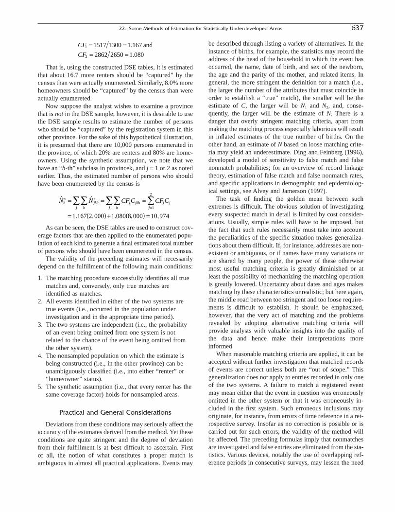
That is, using the constructed DSE tables, it is estimatedthat about 16.7 more renters should be “captured” by thecensus than were actually enumereted. Similarly, 8.0% morehomeowners should be “captured” by the census than wereactually enumereted.
Now suppose the analyst wishes to examine a provincethat is not in the DSE sample; however, it is desirable to usethe DSE sample results to estimate the number of personswho should be “captured” by the registration system in thisother province. For the sake of this hypothetical illustration,it is presumed that there are 10,000 persons enumerated inthe province, of which 20% are renters and 80% are home-owners. Using the synthetic assumption, we note that we have an “h-th” subclass in provincek, and j = 1 or 2 as notedearlier. Thus, the estimated number of persons who shouldhave been enumereted by the census is
As can be seen, the DSE tables are used to construct cov-erage factors that are then applied to the enumerated popu-lation of each kind to generate a final estimated total numberof persons who should have been enumereted in the census.
The validity of the preceding estimates will necessarilydepend on the fulfillment of the following main conditions:
1. The matching procedure successfully identifies all truematches and, conversely, only true matches are identified as matches.
2. All events identified in either of the two systems aretrue events (i.e., occurred in the population underinvestigation and in the appropriate time period).
3. The two systems are independent (i.e., the probabilityof an event being omitted from one system is notrelated to the chance of the event being omitted fromthe other system).
4. The nonsampled population on which the estimate isbeing constructed (i.e., in the other province) can beunambiguously classified (i.e., into either “renter” or“homeowner” status).
5. The synthetic assumption (i.e., that every renter has thesame coverage factor) holds for nonsampled areas.
Practical and General Considerations
Deviations from these conditions may seriously affect theaccuracy of the estimates derived from the method. Yet theseconditions are quite stringent and the degree of deviationfrom their fulfillment is at best difficult to ascertain. First of all, the notion of what constitutes a proper match isambiguous in almost all practical applications. Events may
ˆ ˆ
. , . , ,
N N CF C CF Cks
jkhs
hjj jkh
hjj j
j
= = =
= ( ) + ( ) =
ÂÂ ÂÂ Â=1
2
1 167 2 000 1 080 8 000 10 974
CF
CF1
2
1517 1300 1 167
2862 2650 1 080
= == =
.
.
and be described through listing a variety of alternatives. In theinstance of births, for example, the statistics may record theaddress of the head of the household in which the event hasoccurred, the name, date of birth, and sex of the newborn,the age and the parity of the mother, and related items. Ingeneral, the more stringent the definition for a match (i.e.,the larger the number of the attributes that must coincide inorder to establish a “true” match), the smaller will be theestimate of C, the larger will be N1 and N2, and, conse-quently, the larger will be the estimate of N. There is adanger that overly stringent matching criteria, apart frommaking the matching process especially laborious will resultin inflated estimates of the true number of births. On theother hand, an estimate of N based on loose matching crite-ria may yield an underestimate. Ding and Feinberg (1996),developed a model of sensitivity to false match and falsenonmatch probabilities; for an overview of record linkagetheory, estimation of false match and false nonmatch rates,and specific applications in demographic and epidemiolog-ical settings, see Alvey and Jamerson (1997).
The task of finding the golden mean between suchextremes is difficult. The obvious solution of investigatingevery suspected match in detail is limited by cost consider-ations. Usually, simple rules will have to be imposed, butthe fact that such rules necessarily must take into accountthe peculiarities of the specific situation makes generaliza-tions about them difficult. If, for instance, addresses are non-existent or ambiguous, or if names have many variations orare shared by many people, the power of these otherwisemost useful matching criteria is greatly diminished or atleast the possibility of mechanizing the matching operationis greatly lowered. Uncertainty about dates and ages makesmatching by these characteristics unrealistic; but here again,the middle road between too stringent and too loose require-ments is difficult to establish. It should be emphasized,however, that the very act of matching and the problemsrevealed by adopting alternative matching criteria willprovide analysts with valuable insights into the quality ofthe data and hence make their interpretations moreinformed.
When reasonable matching criteria are applied, it can beaccepted without further investigation that matched recordsof events are correct unless both are “out of scope.” Thisgeneralization does not apply to entries recorded in only oneof the two systems. A failure to match a registered event may mean either that the event in question was erroneouslyomitted in the other system or that it was erroneously in-cluded in the first system. Such erroneous inclusions mayoriginate, for instance, from errors of time reference in a ret-rospective survey. Insofar as no correction is possible or iscarried out for such errors, the validity of the method willbe affected. The preceding formulas imply that nonmatchesare investigated and false entries are eliminated from the sta-tistics. Various devices, notably the use of overlapping ref-erence periods in consecutive surveys, may lessen the need
22. Some Methods of Estimation for Statistically Underdeveloped Areas 637

for such investigations but only at the expense of carryingout a prior matching procedure for events reported for theoverlapping survey periods themselves.
Possible false entries in one of the two reporting systemsmay also make their appearance because of inmigration toor outmigration from the area covered. The effects of suchmigrations are often particularly strong on the phenomenaunder observation. Thus, deaths and births in a sample population may commonly occur in a hospital outside thesample area, or the sample area may contain a hospitalattracting outsiders. Similarly, many women often return totheir parents’ homes for the birth of a baby. Accordingly, ifsurvey and registration data are based on a de facto defini-tion of the population (which would be the simplest solutionfrom an administrative viewpoint), there is a definite riskthat the results will show false discrepancies and that totalbirths and deaths will be overestimated. This risk can bereduced or eliminated if the same rules are applied in bothcollection systems. (If many events occur in hospitals and ade facto approach is used, then hospitals should be sampledseparately to reduce sampling error.) By adopting a de jureconcept instead, the method can solve this problem, but onlyat the cost of following up residents moving out of the areaand keeping track of events affecting temporary residents.The technical difficulties involved in such a solution areformidable: The U.S. Census Bureau, having performeddual system estimation for decades, continues to strugglewith the proper rules for handling in-movers, out-movers,and the like (Hogan, 2000).
Finally, the previous formulas provide no correction forthe presumably not uncommon situation where certainevents tend to be omitted from both systems for the samereasons. A simple application of the estimating formulas willthen give an estimate of the completeness of coverage thatis biased upward. If, for example, both systems missed thesame 20% of births (e.g., all illegitimate births) but bothincluded all other births, the method would erroneously indi-cate full coverage for both systems.
Another manifestation of lack of independence betweenthe two systems may be that the general quality of each isinfluenced by the existence of the other. Although such influ-ences are typically positive and hence would normally bewelcome, they do make it difficult to derive conclusions asto the completeness of coverage that can be generalized forareas where only one system is in operation. It is by nomeans certain, however, that a dual registration system willtend to improve over time if maintained for a given area fora longer time period. Beyond the general difficulty of sus-taining a complicated and demanding system at a high levelof efficiency, it will be particularly hard to avoid the delete-rious effects of a possible collusion between the officialsresponsible for the operation of the two systems. Such col-lusion will naturally tend to be established as soon as it isunderstood that the quality of the work done by the regis-
trar and the survey takers can be evaluated by observingchanges in the match rates achieved in the survey and thevital registration.
Experience with dual-systems analysis of vital recordsand survay results described earlier was building up rapidlyduring the decades of the 1960s and 1970s in Africa, Asia,and Latin America. Marks, Seltzer, and Krotki (1974) havesummarized the results from a number of “populationgrowth estimation” studies conducted in Canada, the UnitedStates, the former Soviet Union, Asia, Africa, LatinAmerica, and the Caribbean. Although the underlying prin-ciples have generally been the same, a wide variety of spe-cific attempts have been made seeking to minimize thebiases just mentioned. Thus, attempts using sample regis-tration differ not only in the size of the sample and in thedesign of the sampling scheme, but even more with respectto the following characteristics:
• The length of the reference period and the peculiaritiesof the field operation
• The frequency and scope of the periodic surveys• The registrars’ mode of operation• In particular, the existence, detail, and quality of the
matching operation and of the investigation of the valid-ity of nonmatches.
Experience indicates that the measurement of coverageof either registration systems or censuses remains very dif-ficult, even by means of dual systems. Dual systems esti-mation has been heavily criticized in the United States andelsewhere. However, in lieu of new approaches that aredemonstrably superior, it remains a tool in the demogra-pher’s tool kit.
References
Alvey, W., and B. Jamerson. 1997. “Record Linkage Techniques—1997:Proceedings of an International Workshop and Exposition.” Washington,DC: Federal Committee on Statistical Methodology.
Arriaga, E. E. 1983. “Estimating Fertility from Data on Children Ever Born,by Age of Mother.” International Research Document No. 11. Wash-ington, DC: U.S. Census Bureau.
Arriaga, E. E., P. D. Johnson, and E. Jamison. 1994. Population Analysiswith Microcomputers, Vol. 1 and 2. Washington, DC: U.S. CensusBureau.
Brass, W. 1961. “The Construction of Life Tables from Child Ratios.”International Population Conference, New York, 1961. Liège: Interna-tional Union for the Scientific Study of Population, Vol. 1, pp. 294–301.
Brass, W., A. J. Coale, P. Demany, D. F. Heisel, F. Lorimer, A. Romaniuk,and E. van deWalk. 1968. The Demography of Tropical Africa, Prince-ton, NJ: Princeton University Press, pp. 89–104 and 140–142.
Brass, W. 1975. Methods for Estimating Fertility and Mortality fromLimited and Defective Data. Chapel Hill, NC: The University of NorthCarolina.
Bogue, D. J., and E. J. Bogue. 1967. “The Pregnancy History Approach toMeasurement of Fertility Change.” In Proceedings of the Social Statis-tics Section, American Statistical Association, pp. 212–231.
638 Popoff and Judson

Chandrasekaran, C., and Deming, W. 1949. “On a Method of EstimatingBirth and Death Rates and the Extent of Registration.” Journal of theAmerican Statistical Association 44: 101–115.
Cho, L. J. 1969. “Estimates of Fertility for West Malaysia (1957–67), Kuala Lumpur.” Research Paper No. 3. Malaysia, Department of Statistics.
Coale, A. J. 1988. “Convergence of a Human Population to Stable Form.”Journal of the American Statistical Association 63: 395–435.
Coale, A. J., L. J. Cho, and N. Goldman. 1980. Estimation of Recent Trendsin Fertility and Mortality in the Republic of Korea. Washington, DC:National Academy of Sciences.
Coale, A. J., and P. Demeny. 1966. Regional Model Life Tables and StablePopulations. Princeton, NJ: Princeton New Jersey Press.
Coale, A. J., P. Demeny, and B. Vaughan. 1983. Regional Model Life Tablesand Stable Populations, (2nd Ed.) New York: Academic Press.
Darga, K. 1999. Sampling and the Census. Washington, DC: AEI Press.Darga, K. 2000. Fixing the Census Until It Breaks. Lansing, MI: Michigan
Information Center.Ding, Y., and S. E. Feinberg. 1996. “Multiple Sample Estimation of Popu-
lation and Census Undercount in the Presence of Matching Errors.”Survey Methodology 22: 55–64.
Dublin, L., and A. J. Lotka. 1925. “On the True Rate of Natural Increase.”Journal of the American Statistical Association 20: 305–339.
Ericksen, E. P., and J. B. Kadane. 1986. “Using Administrative Lists to Estimate Census Omissions.” Journal of Official Statistics 2: 397–414.
Fellegi, I. 1980. “Should the Census Count Be Adjusted for Allocation Pur-poses: Equity Considerations.” Conference on Census Undercount.Washington, DC: U.S. Government Printing Office.
Fellegi, I. 1984. “Notes on Census Coverage Evaluation Methodologies.”Mimeographed, February 16, 1984.
Freedman, D. A. 1991. “Adjusting the 1990 Census.” Science 252:1233–1236.
Grabill, W., and L. J. Cho. 1965. “Methodology for the Measurement ofCurrent Fertility from Population Data on Young Children.” Demogra-phy 2: 50–73.
Grabill, W. H., C. V. Kiser, and P. K. Whelpton. 1959. The Fertility of American Women. New York: John Wiley and Sons.
Hogan, H. 1992. “The 1990 Post-Enumeration Survey: An Overview.” TheAmerican Statistician 46: 261–269.
Hogan, H. 1993. “The 1990 Post-Enumeration Survey: Operations andResults.” Journal of the American Statistical Association 88: 1047–1060.
Hogan, H. 2000. “Accuracy and Coverage Evaluation: Theory and Appli-cation.” Paper presented at the 2000 Joint Statistical Meetings, Indi-anapolis, IN, August 2–5, 2000.
Krótki, K. J. (Ed.). 1977. Developments in Dual System Estimation of Pop-ulation Size and Growth. Edmonton, Alberta, Canada: University ofAlberta Press.
Lotka, A. J. 1907. “Relation Between Birth Rates and Death Rates.” Science26: 21–22.
Marks, E. S., W. Seltzer, and K. J. Krótki. 1974. Population Growth Esti-mation: A Handbook of Vital Statistics Measurement. New York: ThePopulation Council.
McDevitt, T. M. 1996. World Population Profile: 1996. Washington, DC:UNAIDS/WHO.
Mulry, J. J., and R. Griffiths. 1996. “Integrated Coverage Measurement(ICM) Evaluation Project 12: Comparison of CensusPlus and DualSystem Estimates.” 1995 Census Test Results, Memorandum No. 42.U.S. Census Bureau.
Narasimhan, R. L., R. D. Retherford, V. Mishra, F. Arnold, and T. K. Roy.1997. “Comparison of Fertility Estimates from India’s Sample Regis-tration System and National Family Health Survey.” National FamilyHealth Survey Subject Reports, No. 4. Honolulu, HI: East-West CenterProgram on Population.
Robinson, J. G. 1996. “Integrated Coverage Measurement (ICM) Evalua-tion Project 15: Evaluation of CensusPlus and Dual System Estimateswith Independent Demographic Benchmarks.” Census Test Results,Memorandum No. 43. U.S. Census Bureau.
Robinson, J. G., B. Ahmed, P. Das Gupta, and K. A. Woodrow. 1993. “Esti-mation of Population Coverage in the 1990 United States Census Basedon Demographic Analysis.” Journal of the American Statistical Asso-ciation 88: 1061–1071.
Stanecki, K. A., and P. O. Way. 1997. “The Demographic Impacts ofHIV/AIDS, Perspectives from the World Population Profile: 1996.”U.S. Bureau of the Census. IPC Staff Paper No. 86.
Treat, J. B. 1996. “Integrated Coverage Measurement (ICM) EvaluationProject 9: Effect on the Dual System Estimate and the CensusPlus Estimate of the Adds and Deletes to the Census File.” 1995 Census Test Results, Memorandum No. 40. U.S. Census Bureau.
United Nations. 1956. Methods for Population Projections by Sex and Age.Series A, Population Studies, No. 25.
United Nations. 1967. Methods of Estimating Demographic Measures fromIncomplete Data. Manual IV. Manuals on Methods of Estimating Pop-ulation, Series A. Population Studies. No. 42.
United Nations. 1982. Model Life Tables for Developing Countries. Popu-lation Studies, No. 77. New York: United Nations.
United Nations. 1983. Manual X: Indirect Techniques for Demo-graphic Estimation. Population Studies, No. 81. New York: UnitedNations.
United Nations. 1989. Demographic Yearbook. New York: United Nations.U.S. Census Bureau, International Data Base. Accessed atwww.census.gov/ipc/www/idbnew.html.
United Nations. 1990. Step-by-Step Guide to the Estimation of Child Mortality, Population Studies No. 107. New York: United Nations.
U.S. Bureau of the Census. 2000. International Data Base. Washington, DC.Found at www.census.gov/ipc/www/idbnew.html on November, 19,2000.
U.S. Department of Commerce. 1999. HIV/AIDS in the Developing World.WP/98-2. Washington, DC.
Wachter, K. W., and D. A. Freedman. 2000. “Measuring Local Hetero-geneity with 1990 Census Data.” Demographic Research. Online document: www.demographic-research.org/Volumes/Vol3/10.Retrieved December 12, 2000.
Wolter, K. 1986. “Some Coverage Error Models for Census Data.” Journalof the American Statistical Association 81: 338–346.
Suggested Readings
Agrawal, B. L. 1969. “Sample Registration in India.” Population Studies(London) 23(3): 379–394.
Ahmed, N., and K. J. Krótki. 1963. “Simultaneous Estimations of Popula-tion Growth—the Pakistan Experiment.” Pakistan Development Review3(l): 37–65.
Alauddin Chowdhury, A. K. M., K. M. A. Aziz, and W. H. Mosley. 1969.Demographic Studies in Rural East Pakistan: Second Year, May,1967–April, 1968. Dacca, Pakistan SEATO Cholera Research Labora-tory. June 1969.
Arnold, F., and A. K. Blanc. 1990. “Fertility Levels and Trends.” Demo-graphic and Health Surveys Comparative Studies No. 2. Columbia,MD: Institute for Resource Development/Macro Systems.
Arriaga, E. E. 1967. “Rural-Urban Mortality in Developing Countries: AnIndex for Detecting Rural Underregistration.” Demography 4(l):98–107.
Blacker, J. G. C., and C. J. Martin. 1961. “Old and New Methods of Com-piling Vital Statistics in East Africa.” In International Population Conference, New York. Liège: International Union for the ScientificStudy of Population, Vol. 1, pp. 355–362.
22. Some Methods of Estimation for Statistically Underdeveloped Areas 639

Bogue, Donald J., and Bogue, Elizabeth J. 1967. “The Pregnancy HistoryApproach to Measurement of Fertility Change.” Proceedings of theSocial Statistics Section. Washington, DC: American Statistical Asso-ciation, pp. 212–231.
Bourgeois-Pichat, J. 1958. “Utilisation de la notion stable pour mesurer la mortalité et la fecondité des populations des pays sous-developpés.” Bulletin de l’Institut international de statistique36(2): 94–121. (Proceedings of the 30th Session, Stockholm, 1957).Uppsala.
Brass, W. 1961. “The Construction of Life Tables from Child Ratios.” InInternational Population Conference, New York, 1961 Liège: Interna-tional Union for the Scientific Study of Population, Vol. 1, pp. 294–301.
Brass, W., and A. J. Coale, Ansley J. 1968. “Methods of Analysis and Esti-mation.” In William Brass, A. J. Coale, P. Demeny, D. F. Heisel, F.Lorimor, A. Romaniuk, and E. van deWalle. The Demography of Trop-ical Africa, Princeton, Princeton University Press, Chapter 3, pp.88–150.
Carmen, A. G., and J. L. Somoza. 1965. “Survey Methods, Based on Peri-odically Repeated Interviews, Aimed at Determining DemographicRates.” Demography 2: 289–301.
Cavanaugh, J. A. 1961. “Sample Vital Registration Experiment” In Inter-national Population Conference, New York, 1961. Liège: InternationalUnion for the Scientific Study of Population, Vol. 11, pp. 363–371.
Chandra, S. C., and W. E. Deming. 1949. “On a Method of Estimating Birthand Death Rates and the Extent of Registration.” Journal of the American Statistical Association 44(245): 101–115.
Chandrasekaran, C. 1964. “Fertility Indices from Limited Data.” Interna-tional Population Conference, Ottawa 1963. Liège: International Unionfor the Scientific Study of Population, pp. 91–105.
Clairin, R. 1963. “Les données susceptibles d’etre utilisées pour une eval-uation du mouvement de la population en Afrique au sud du Sahara.”In International Population Conference, Ottawa, Liège, InternationalUnion for the Scientific Study of Population, 1964, pp. 107–120.
Coale, Ansley J., and E. M. Hoover. 1958. Population Growth and Eco-nomic Development in Low-Income Countries. Princeton, NJ: Prince-ton University Press, 1958, pp. 337–374.
Coale, A. J. 1961. “The Design of an Experimental Procedure for Obtain-ing Accurate Vital Statistics.” In International Population Conference,New York, Vol. II, pp. 372–375. Liège: International Union for the Sci-entific Study of Population.
Coale, A. J. 1963. “Estimates of Various Demographic Measures through the Quasi-Stable Age Distribution.” In Emerging Techniques inPopulation Research, New York, Milbank Memorial Fund, pp.175–193.
Cooke, D. S. 1969. “Population Growth Estimation Experiment in Pakistan.” Statistical Reporter (U.S. Bureau of the Budget), pp. 173–176.
Curtia, S. L. 1995. Assessment of the Quality of Data Used for Direct Esti-mation of Infant and Child Mortality in DHS-II Surveys. Calverton,MD: Macro International.
Demeny, P. 1965. ”Estimation of Vital Rates for Populations in the Processof Destabilization.” Demography 2: 516–530.
Demeny, P. 1967. “A Minimum Program for the Estimation of Basic Fer-tility Measures from Censuses of Population in Asian Countries withInadequate Demographic Statistics.” In International Population Conference, Sydney, Australia 1967, Liège: International Union for theScientific Study of Population, pp. 818–825.
Demeny, P., and F. C. Shorter. 1968. “Estimating Turkish Mortality, Fertil-ity, and Age Structure: Application of Some New, Techniques,” Publi-cation No. 218, Faculty of Economics, University of Istanbul, Istanbul,1968.
El-Badry, M. A. 1955. “Some Demographic Measurements for Egypt Basedon the Stability of Census Age Distributions.” Milbank Memorial FundQuarterly 33(3): 268–305.
El-Badry, M. A., and C. Chandrasekaran. 1961. “Some Methods for Obtain-ing Vital Statistics in India.” International Population Conference, NewYork. Liège: International Union for the Scientific Study of Population,Vol. 11, pp. 377–386.
Goldberg, D., and A. Adlackha. 1968. “Infant Mortality Estimates Basedon Small Surveys on the Ankara Area.” Chapter 7 in Turkish Demog-raphy: Proceedings of a Conference, Izmir, February 21–24, 1968.Hacettepe University, Publication No. 7, Ankara, Turkey, 1969, pp.133–145.
Grabill, Wilson H., and L. J. Cho. 1965. “Methodology for the Measure-ment of Current Fertility from Population Data on Young Children.”Demography 2: 50–73.
Heligman, L., G. Finch, and R. Kramer. 1978. “Measurement of InfantMortality in Less Developed Countries.” International Research Doc-ument No. 5. Washington, DC: U.S. Census Bureau.
Holzer, J. 1967. “Estimate of the Age Structure of Ghana’s Population. AnApplication of the Stable Population Model.” In International Popula-tion Conference, Sydney, Australia. Liège: International Union for theScientific Study of Population, pp. 838–849.
India, Office of the Registrar General. 1969. “Sample Registration in India:Report on Pilot Studies in Urban Areas: 1964–67.”
Indian Statistical Institute. 1961. “The Use of the National Sample Surveyin the Estimation of Current Birth and Death Rates in India.” Interna-tional Population Conference, New York. Liège: International Union forthe Scientific Study of Population, Vol. 11, pp. 395–402.
Johnson, P. J. 1980. “Techniques for Estimating Infant Mortality.” Inter-national Research Document No. 8. Washington, DC: U.S. Census Bureau.
Krótki, K. J. 1964. “First Report on the Population Growth Experiment.”In International Union for the Scientific Study of Population, Interna-tional Population Conference, Ottawa, 1963. Liège, International Unionfor the Scientific Study of Population, pp. 159–173.
Krótki, K. J. 1965. “Estimating Population Size and Growth from Inade-quate Data.” International Social Science Journal 17(2): 246–258.
Krótki, K. J. 1966. “The Problem of Estimating Vital Rates in Pakistan.”In World Population Conference, 1965. Belgrade. Liège: InternationalUnion for the Scientific Study of Population.
Lauriat, P. 1967. “Field Experience in Estimating Population Growth.”Demography 4(l): 228–243.
Liberia, Department of Planning and Economic Affairs. 1969. LiberianPopulation Growth Survey Handbook.
Marks, E. S., W. Seltzer, and K. J. Krotki. 1974. Population Growth Esti-mation: A Handbook of Vital Statistics Measurement. New York: ThePopulation Council.
Mauldin, W. P. 1966. “Estimating Rates of Population Growth.” In FamilyPlanning and Population Programs, Proceedings of the InternationalConference on Family Planning Programs, Geneva, August 1965.Chicago: University of Chicago Press, pp. 635–653.
Myburgh, C. A. L. 1956. “Estimating the Fertility and Mortality of AfricanPopulations from the Total Number of Children Ever Born and theNumber of these Still Living.” Population Studies (London) 10(2):193–206.
Pakistan Institute of Development Economics. 1968. Report of the Popu-lation Growth Estimation Experiment, Karachi.
Rele, J. R. 1967. “Estimation of Reproduction Rates for Asian Countriesfrom Census Data.” In International Population Conference, Sydney,Australia. Liège: International Union for the Scientific Study of Popu-lation, pp. 929–934.
Rele, J. R. 1967. Fertility Analyses through Extension of Stable PopulationConcepts, Berkeley, California. International Population and UrbanResearch, University of California, 1967.
Roberts, G. W. 1961. “Improving Vital Statistics in the West Indies.” Inter-national Population Conference, New York. Liège: International Unionfor the Scientific Study of Population, Vol. 11, pp. 420–426.
640 Popoff and Judson

Romaniuk, A. 1967. “Estimation of the Birth Rate for the Congo ThroughNon-conventional Techniques.” Demography 4(2): 688–709.
Sabagh, G., and C. Scott, Christopher. 1967. “A Comparison of DifferentSurvey Techniques For Obtaining Vital Data in a Developing Country.”Demography 4(2): 759–772.
Siegel, J. S. 2002. Applied Demogaphy: Applications to Business, Gov-erment, Law, and Public Policy. San Diego: Academic Press. Chapter 4.
Seltzer, W. 1969. “Some Results from Asian Population Studies.” Popula-tion Studies (London) 23(3): 395–406.
Som, R. K. 1967. “On Some Techniques of Demographic Analysis ofSpecial Relevance to the Asian Countries.” In International PopulationConference, Sydney, Australia. Liège: International Union for the Sci-entific Study of Population, pp. 807–813.
Srivastava, M. L. 1967. “The Relationships between Fertility and Mortal-ity Characteristics in Stable Female Populations.” Eugenics Quarterly14(3): 171–180.
Srivastava, M. L. 1967. “Selection of Model Life Tables and Stable Popu-lations.” In International Population Conference, Sydney, Australia.Liège: International Union for the Scientific Study of Population, pp.904–911.
United Nations. 1949. Methods of Using Census Statistics for the Calcula-tion of Life Tables and Other Demographic Measures, by GiorgioMortara, Series A, Population Studies, No. 7.
United Nations. 1956. Age and Sex Patterns of Mortality. Model Life Tablesfor Developing Countries, Series A, Population Studies, No. 22.
United Nations. 1967. Methods of Estimating Basic Demographic Measures from Incomplete Data, Series A, Population Studies, No. 42.
United Nations Population Fund. 1993. Readings in Population ResearchMethodology, Vol. 2. Chicago: Social Development Center.
United States National Center for Health Statistics. 1969, March. “Methodsfor Measuring Population Change: A Systems Analysis Summary” byForrest E. Linder. Vital and Health Statistics, Series 2, No 32.
Vallin. J., H. J. Pollard, and L. Heligman (Eds.). 1981. Methodologies forthe Collection and Analysis of Mortality Data. Liège: Ordina Editions,Chapter 5.
Wells, H. B., and B. L. Agrawal. 1967. “Sample Registration in India.”Demography 4(l): 374–387.
Zelnik, M., and M. R. Khan. 1965. “An Estimate of the Birth Rate in Eastand West Pakistan.” Pakistan Development Review 5(1): 64–93.
22. Some Methods of Estimation for Statistically Underdeveloped Areas 641

This Page Intentionally Left Blank

The tables in this appendix first appeared in Lowell J.Reed and Margaret Merrell, “A Short Method for Con-structing an Abridged Life Table,” American Journal ofHygiene 302 (2): 52–61, September 1939. (Copyright 1939by the American Journal of Hygiene, now the AmericanJournal of Epidemiology, The Johns Hopkins University.)
These tables provide a direct method for deriving the nqx
values, or probabilities of dying, from the observed nmx
values, or age-specific death rates, for constructing anabridged life table. The text of Chapter 13, “The Life Table,”provides instructions to the reader on the steps in calculat-ing the survivorship column (lx) and the column of deaths
(ndx) in the life table. The equations required for deriving theperson-years columns (nLx and Tx) by the Reed-Merrellmethod are given in the text. Once these values are known,it is a simple step to calculate the remaining basic columnof the life table, ex, from Tx and lx.
Chapter 13 describes other methods of constructingabridged life tables in addition to the Reed-Merrell method.An Excel program for constructing an abridged life tablethat requires only population and deaths by age as input isavailable from George C. Hough, Jr., of the PopulationResearch Center, Portland State University.
643
A P P E N D I X
A
Reference Tables for Constructing an AbridgedLife Table by the Reed-Merrell Method
The Methods and Materials of DemographyCopyright 2003, Elsevier Science (USA).
All rights reserved.

644 Appendix A. Reference Tables for Constructing an Abridged Life Table by the Reed-Merrell Method
TABLE A.1 Values of q0 Associated with m0 by the Equation q0 = 1 - e-m0(.9539-.5509m0)
m0 q0 D m0 q0 D m0 q0 D m0 q0 D
0.000 0.000 0.000 0.0000.000 0.000000 953 0.050 0.045261 857 0.100 0.085960 770 0.150 0.122510 6910.001 0.000953 951 0.051 0.046119 855 0.101 0.086730 769 0.151 0.123201 6900.002 0.001904 949 0.052 0.046974 854 0.102 0.087499 767 0.152 0.123891 6880.003 0.002853 947 0.053 0.047828 852 0.103 0.088266 765 0.153 0.124579 6870.004 0.003800 945 0.054 0.048679 850 0.104 0.089032 764 0.154 0.125266 685
0.005 0.004744 943 0.055 0.049529 848 0.105 0.089795 762 0.155 0.125951 6840.006 0.005687 941 0.056 0.050378 846 0.106 0.090557 760 0.156 0.126635 6820.007 0.006628 939 0.057 0.051224 845 0.107 0.091318 759 0.157 0.127317 6810.008 0.007567 937 0.058 0.052068 843 0.108 0.092077 757 0.158 0.127998 6790.009 0.008504 935 0.059 0.052911 841 0.109 0.092834 756 0.159 0.128677 678
0.010 0.009439 933 0.060 0.053752 839 0.110 0.093590 754 0.160 0.129355 6760.011 0.010372 931 0.061 0.054591 837 0.111 0.094344 752 0.161 0.130031 6750.012 0.011303 929 0.062 0.055429 836 0.112 0.095096 751 0.162 0.130706 6730.013 0.012232 927 0.063 0.056264 834 0.113 0.095847 749 0.163 0.131379 6720.014 0.013159 925 0.064 0.057098 832 0.114 0.096596 747 0.164 0.132051 670
0.015 0.014084 923 0.065 0.057930 830 0.115 0.097343 746 0.165 0.132722 6690.016 0.015008 921 0.066 0.058761 829 0.116 0.098089 744 0.166 0.133390 6670.017 0.015929 919 0.067 0.059589 827 0.117 0.098833 743 0.167 0.134058 6660.018 0.016848 917 0.068 0.060416 825 0.118 0.099576 741 0.168 0.134724 6640.019 0.017766 915 0.069 0.061241 823 0.119 0.100317 739 0.169 0.135388 663
0.020 0.018681 913 0.070 0.062064 821 0.120 0.101056 738 0.170 0.136051 6620.021 0.019594 912 0.071 0.062886 820 0.121 0.101794 736 0.171 0.136713 6600.022 0.020506 910 0.072 0.063705 818 0.122 0.102531 735 0.172 0.137373 6590.023 0.021416 908 0.073 0.064523 816 0.123 0.103265 733 0.173 0.138032 6570.024 0.022323 906 0.074 0.065339 814 0.124 0.103998 731 0.174 0.138689 656
0.025 0.023229 904 0.075 0.066154 813 0.125 0.104730 730 0.175 0.139345 6540.026 0.024133 902 0.076 0.066967 811 0.126 0.105460 728 0.176 0.139999 6530.027 0.025035 900 0.077 0.067778 809 0.127 0.106188 727 0.177 0.140652 6510.028 0.025935 898 0.078 0.068587 808 0.128 0.106915 725 0.178 0.141303 6500.029 0.026833 896 0.079 0.069395 806 0.129 0.107640 724 0.179 0.141953 649
0.030 0.027729 894 0.080 0.070200 804 0.130 0.108364 722 0.180 0.142602 6470.031 0.028624 892 0.081 0.071005 802 0.131 0.109086 720 0.181 0.143249 6460.032 0.029516 891 0.082 0.071807 801 0.132 0.109806 719 0.182 0.143895 6440.033 0.030407 889 0.083 0.072608 799 0.133 0.110525 717 0.183 0.144539 6430.034 0.031296 887 0.084 0.073407 797 0.134 0.111242 716 0.184 0.145182 641
0.035 0.032182 885 0.085 0.074204 796 0.135 0.111958 714 0.185 0.145823 6400.036 0.033067 883 0.086 0.074999 794 0.136 0.112672 713 0.186 0.146463 6390.037 0.033950 881 0.087 0.075793 792 0.137 0.113385 711 0.187 0.147102 6370.038 0.034832 879 0.088 0.076585 790 0.138 0.114096 710 0.188 0.147739 6360.039 0.035711 877 0.089 0.077376 789 0.139 0.114806 708 0.189 0.148374 634
0.040 0.036588 876 0.090 0.078165 787 0.140 0.115514 707 0.190 0.149009 6330.041 0.037464 874 0.091 0.078952 785 0.141 0.116220 705 0.191 0.149642 6320.042 0.038338 872 0.092 0.079737 784 0.142 0.116925 703 0.192 0.150273 6300.043 0.039210 870 0.093 0.080521 782 0.143 0.117629 702 0.193 0.150903 6290.044 0.040080 868 0.094 0.081303 780 0.144 0.118331 700 0.194 0.151532 627
0.045 0.040948 866 0.095 0.082083 779 0.145 0.119031 699 0.195 0.152159 6260.046 0.041814 865 0.096 0.082862 777 0.146 0.119730 697 0.196 0.152785 6250.047 0.042679 863 0.097 0.083639 775 0.147 0.120427 696 0.197 0.153410 6230.048 0.043542 861 0.098 0.084414 774 0.148 0.121123 694 0.198 0.154033 6220.049 0.044402 859 0.099 0.085188 772 0.149 0.121817 693 0.199 0.154655 620
0.050 0.045261 857 0.100 0.085960 770 0.150 0.122510 691 0.200 0.155275

Appendix A. Reference Tables for Constructing an Abridged Life Table by the Reed-Merrell Method 645
TABLE A.2 Values of q1 Associated with m1 by the Equation q1 = 1 - e-m1(.9510-1.921m1)
m1 q1 D m1 q1 D
0.000 0.0000.000 0.000000 949 0.050 0.041847 7250.001 0.000949 944 0.051 0.042572 7210.002 0.001893 939 0.052 0.043293 7170.003 0.002832 934 0.053 0.044009 7120.004 0.003766 930 0.054 0.044722 708
0.005 0.004696 925 0.055 0.045430 7040.006 0.005621 920 0.056 0.046134 7000.007 0.006541 916 0.057 0.046833 6960.008 0.007457 911 0.058 0.047529 6910.009 0.008368 906 0.059 0.048221 687
0.010 0.009275 902 0.060 0.048908 6830.011 0.010176 897 0.061 0.049591 6790.012 0.011074 893 0.062 0.050270 6750.013 0.011966 888 0.063 0.050945 6710.014 0.012854 883 0.064 0.051616 667
0.015 0.013738 879 0.065 0.052282 6630.016 0.014616 874 0.066 0.052945 6580.017 0.015491 870 0.067 0.053603 6540.018 0.016360 865 0.068 0.054258 6500.019 0.017225 861 0.069 0.054908 646
0.020 0.018086 856 0.070 0.055554 6420.021 0.018942 852 0.071 0.056196 6380.022 0.019794 847 0.072 0.056835 6340.023 0.020641 843 0.073 0.057469 6300.024 0.021483 838 0.074 0.058099 626
0.025 0.022321 834 0.075 0.058724 6220.026 0.023155 829 0.076 0.059346 6180.027 0.023984 825 0.077 0.059964 6140.028 0.024809 820 0.078 0.060578 6100.029 0.025629 816 0.079 0.061188 606
0.030 0.026445 811 0.080 0.061794 6020.031 0.027257 807 0.081 0.062396 5980.032 0.028064 803 0.082 0.062994 5940.033 0.028866 798 0.083 0.063588 5900.034 0.029664 794 0.084 0.064177 586
0.035 0.030458 789 0.085 0.064763 5820.036 0.031248 785 0.086 0.065345 5780.037 0.032033 781 0.087 0.065924 5740.038 0.032814 776 0.088 0.066498 5700.039 0.033590 772 0.089 0.067068 566
0.040 0.034362 768 0.090 0.067634 5620.041 0.035130 763 0.091 0.068196 5580.042 0.035893 759 0.092 0.068755 5540.043 0.036652 755 0.093 0.069309 5510.044 0.037407 751 0.094 0.069860 547
0.045 0.038158 746 0.095 0.070407 5430.046 0.038904 742 0.096 0.070949 5390.047 0.039646 738 0.097 0.071488 5350.048 0.040384 734 0.098 0.072023 5310.049 0.041117 729 0.099 0.072555 527
0.050 0.041847 725 0.100 0.073082
TABLE A.3 Values of 3q2 Associated with 3m2 by the Equation 3q2 = 1 - e-33m2-.008(3)33m2
2
3m2 3q2 D 3m2 3q2 D
0.00 0.000.000 0.000000 2996 0.010 0.029575 29110.001 0.002996 2987 0.011 0.032487 29030.002 0.005983 2979 0.012 0.035390 28950.003 0.008962 2970 0.013 0.038284 28860.004 0.011932 2962 0.014 0.041171 2878
0.005 0.014893 2953 0.015 0.044049 28700.006 0.017847 2945 0.016 0.046919 28620.007 0.020791 2936 0.017 0.049781 28540.008 0.023728 2928 0.018 0.052634 28450.009 0.026656 2920 0.019 0.055480 2837
0.010 0.029575 2911 0.020 0.058317
TABLE A.4 Values of 4q1 Associated with 4m1 by the Equation 4q1 = 1 - e-44m1(.9806-2.0794m1)
4m1 4q1 D 4m1 4q1 D
0.00 0.000.000 0.000000 3906 0.020 0.072369 33160.001 0.003906 3875 0.021 0.075686 32890.002 0.007781 3843 0.022 0.078975 32620.003 0.011624 3812 0.023 0.082237 32350.004 0.015436 3781 0.024 0.085472 3209
0.005 0.019217 3750 0.025 0.088681 31820.006 0.022967 3720 0.026 0.091864 31560.007 0.026687 3689 0.027 0.095020 31300.008 0.030376 3659 0.028 0.098150 31050.009 0.034035 3629 0.029 0.101255 3079
0.010 0.037665 3600 0.030 0.104334 30540.011 0.041265 3571 0.031 0.107388 30280.012 0.044835 3541 0.032 0.110416 30030.013 0.048376 3512 0.033 0.113419 29790.014 0.051889 3484 0.034 0.116398 2954
0.015 0.055373 3455 0.035 0.119352 29290.016 0.058828 3427 0.036 0.122281 29050.017 0.062255 3399 0.037 0.125186 28810.018 0.065654 3371 0.038 0.128067 28570.019 0.069026 3344 0.039 0.130924 2833
0.020 0.072369 3316 0.040 0.133758

646 Appendix A. Reference Tables for Constructing an Abridged Life Table by the Reed-Merrell Method
TABLE A.5 Values of 5qx Associated with 5mx by the Equation 5qx = 1 - e-55mX-.008(5)35m2x
5mx 5qx D 5mx 5qx D 5mx 5qx D
0.00 0.00 0.000.000 0.000000 4989 0.050 0.223144 3953 0.100 0.399504 31150.001 0.004989 4966 0.051 0.227096 3934 0.101 0.402619 31000.002 0.009954 4943 0.052 0.231031 3916 0.102 0.405720 30850.003 0.014897 4920 0.053 0.234946 3897 0.103 0.408805 30700.004 0.019817 4897 0.054 0.238843 3879 0.104 0.411875 3056
0.005 0.024714 4875 0.055 0.242722 3861 0.105 0.414931 30410.006 0.029589 4852 0.056 0.246583 3842 0.106 0.417972 30260.007 0.034442 4830 0.057 0.250425 3824 0.107 0.420998 30120.008 0.039272 4808 0.058 0.254249 3806 0.108 0.424009 29970.009 0.044080 4786 0.059 0.258056 3788 0.109 0.427007 2983
0.010 0.048866 4764 0.060 0.261844 3770 0.110 0.429989 29680.011 0.053629 4742 0.061 0.265614 3753 0.111 0.432957 29540.012 0.058371 4720 0.062 0.269367 3735 0.112 0.435911 29400.013 0.063091 4698 0.063 0.273102 3717 0.113 0.438851 29250.014 0.067789 4676 0.064 0.276819 3700 0.114 0.441777 2911
0.015 0.072465 4655 0.065 0.280519 3682 0.115 0.444688 28970.016 0.077120 4633 0.066 0.284201 3665 0.116 0.447585 28830.017 0.081753 4612 0.067 0.287866 3647 0.117 0.450468 28690.018 0.086365 4590 0.068 0.291513 3630 0.118 0.453338 28550.019 0.090955 4569 0.069 0.295143 3613 0.119 0.456193 28420.020 0.095524 4548 0.070 0.298756 3596 0.120 0.459035 2828
0.021 0.100072 4527 0.071 0.302352 3579 0.121 0.461862 28140.022 0.104599 4506 0.072 0.305931 3562 0.122 0.464676 28000.023 0.109105 4485 0.073 0.309493 3545 0.123 0.467477 27870.024 0.113590 4464 0.074 0.313038 3528 0.124 0.470264 2773
0.025 0.118054 4443 0.075 0.316566 3511 0.125 0.473037 27600.026 0.122498 4423 0.076 0.320077 3495 0.126 0.475797 27460.027 0.126921 4402 0.077 0.323572 3478 0.127 0.478543 27330.028 0.131323 4382 0.078 0.327050 3461 0.128 0.481276 27200.029 0.135705 4361 0.079 0.330511 3445 0.129 0.483996 2707
0.030 0.140066 4341 0.080 0.333956 3429 0.130 0.486703 26930.031 0.144407 4321 0.081 0.337385 3412 0.131 0.489396 26800.032 0.148728 4301 0.082 0.340797 3396 0.132 0.492076 26670.033 0.153029 4281 0.083 0.344193 3380 0.133 0.494743 26540.034 0.157310 4261 0.084 0.347573 3364 0.134 0.497398 2641
0.035 0.161571 4241 0.085 0.350937 3348 0.135 0.500039 26280.036 0.165812 4221 0.086 0.354284 3332 0.136 0.502667 26160.037 0.170033 4201 0.087 0.357616 3316 0.137 0.505283 26030.038 0.174234 4182 0.088 0.360932 3300 0.138 0.507886 25900.039 0.178416 4162 0.089 0.364232 3284 0.139 0.510476 2577
0.040 0.182578 4143 0.090 0.367516 3268 0.140 0.513053 25650.041 0.186721 4123 0.091 0.370784 3253 0.141 0.515618 25520.042 0.190844 4104 0.092 0.374037 3237 0.142 0.518170 25400.043 0.194948 4085 0.093 0.377274 3222 0.143 0.520710 25270.044 0.199033 4066 0.094 0.380496 3206 0.144 0.523237 2515
0.045 0.203099 4047 0.095 0.383702 3191 0.145 0.525752 25030.046 0.207146 4028 0.096 0.386893 3176 0.146 0.528255 24900.047 0.211174 4009 0.097 0.390069 3160 0.147 0.530745 24780.048 0.215182 3990 0.098 0.393229 3145 0.148 0.533223 2466
0.049 0.219172 3971 0.099 0.396374 3130 0.149 0.535689 2454
0.050 0.223144 3953 0.100 0.399504 3115 0.150 0.538143 2442
(continues)
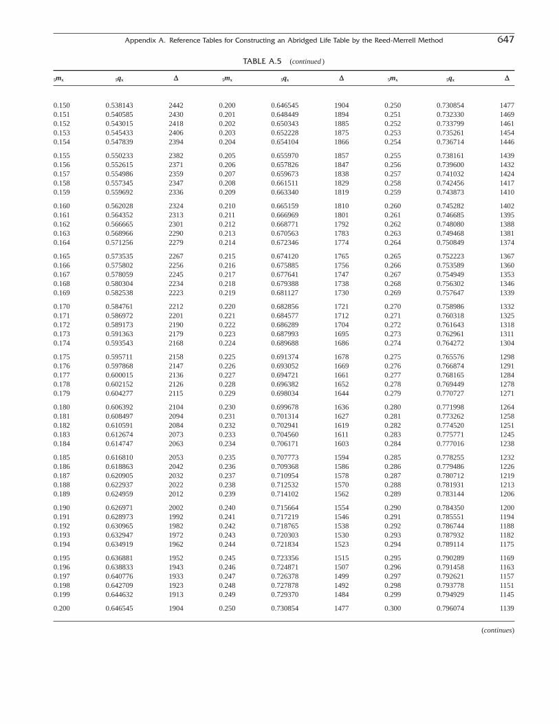
Appendix A. Reference Tables for Constructing an Abridged Life Table by the Reed-Merrell Method 647
TABLE A.5 (continued )
5mx 5qx D 5mx 5qx D 5mx 5qx D
0.150 0.538143 2442 0.200 0.646545 1904 0.250 0.730854 14770.151 0.540585 2430 0.201 0.648449 1894 0.251 0.732330 14690.152 0.543015 2418 0.202 0.650343 1885 0.252 0.733799 14610.153 0.545433 2406 0.203 0.652228 1875 0.253 0.735261 14540.154 0.547839 2394 0.204 0.654104 1866 0.254 0.736714 1446
0.155 0.550233 2382 0.205 0.655970 1857 0.255 0.738161 14390.156 0.552615 2371 0.206 0.657826 1847 0.256 0.739600 14320.157 0.554986 2359 0.207 0.659673 1838 0.257 0.741032 14240.158 0.557345 2347 0.208 0.661511 1829 0.258 0.742456 14170.159 0.559692 2336 0.209 0.663340 1819 0.259 0.743873 1410
0.160 0.562028 2324 0.210 0.665159 1810 0.260 0.745282 14020.161 0.564352 2313 0.211 0.666969 1801 0.261 0.746685 13950.162 0.566665 2301 0.212 0.668771 1792 0.262 0.748080 13880.163 0.568966 2290 0.213 0.670563 1783 0.263 0.749468 13810.164 0.571256 2279 0.214 0.672346 1774 0.264 0.750849 1374
0.165 0.573535 2267 0.215 0.674120 1765 0.265 0.752223 13670.166 0.575802 2256 0.216 0.675885 1756 0.266 0.753589 13600.167 0.578059 2245 0.217 0.677641 1747 0.267 0.754949 13530.168 0.580304 2234 0.218 0.679388 1738 0.268 0.756302 13460.169 0.582538 2223 0.219 0.681127 1730 0.269 0.757647 1339
0.170 0.584761 2212 0.220 0.682856 1721 0.270 0.758986 13320.171 0.586972 2201 0.221 0.684577 1712 0.271 0.760318 13250.172 0.589173 2190 0.222 0.686289 1704 0.272 0.761643 13180.173 0.591363 2179 0.223 0.687993 1695 0.273 0.762961 13110.174 0.593543 2168 0.224 0.689688 1686 0.274 0.764272 1304
0.175 0.595711 2158 0.225 0.691374 1678 0.275 0.765576 12980.176 0.597868 2147 0.226 0.693052 1669 0.276 0.766874 12910.177 0.600015 2136 0.227 0.694721 1661 0.277 0.768165 12840.178 0.602152 2126 0.228 0.696382 1652 0.278 0.769449 12780.179 0.604277 2115 0.229 0.698034 1644 0.279 0.770727 1271
0.180 0.606392 2104 0.230 0.699678 1636 0.280 0.771998 12640.181 0.608497 2094 0.231 0.701314 1627 0.281 0.773262 12580.182 0.610591 2084 0.232 0.702941 1619 0.282 0.774520 12510.183 0.612674 2073 0.233 0.704560 1611 0.283 0.775771 12450.184 0.614747 2063 0.234 0.706171 1603 0.284 0.777016 1238
0.185 0.616810 2053 0.235 0.707773 1594 0.285 0.778255 12320.186 0.618863 2042 0.236 0.709368 1586 0.286 0.779486 12260.187 0.620905 2032 0.237 0.710954 1578 0.287 0.780712 12190.188 0.622937 2022 0.238 0.712532 1570 0.288 0.781931 12130.189 0.624959 2012 0.239 0.714102 1562 0.289 0.783144 1206
0.190 0.626971 2002 0.240 0.715664 1554 0.290 0.784350 12000.191 0.628973 1992 0.241 0.717219 1546 0.291 0.785551 11940.192 0.630965 1982 0.242 0.718765 1538 0.292 0.786744 11880.193 0.632947 1972 0.243 0.720303 1530 0.293 0.787932 11820.194 0.634919 1962 0.244 0.721834 1523 0.294 0.789114 1175
0.195 0.636881 1952 0.245 0.723356 1515 0.295 0.790289 11690.196 0.638833 1943 0.246 0.724871 1507 0.296 0.791458 11630.197 0.640776 1933 0.247 0.726378 1499 0.297 0.792621 11570.198 0.642709 1923 0.248 0.727878 1492 0.298 0.793778 11510.199 0.644632 1913 0.249 0.729370 1484 0.299 0.794929 1145
0.200 0.646545 1904 0.250 0.730854 1477 0.300 0.796074 1139
(continues)

648 Appendix A. Reference Tables for Constructing an Abridged Life Table by the Reed-Merrell Method
TABLE A.5 (continued )
5mx 5qx D 5mx 5qx D 5mx 5qx D
0.300 0.796074 1139 0.350 0.846261 874 0.400 0.884675 6670.301 0.797213 1133 0.351 0.847135 869 0.401 0.885342 6630.302 0.798346 1127 0.352 0.848004 865 0.402 0.886005 6600.303 0.799474 1121 0.353 0.848869 860 0.403 0.886665 6560.304 0.800595 1115 0.354 0.849729 855 0.404 0.887321 653
0.305 0.801710 1109 0.355 0.850585 851 0.405 0.887974 6490.306 0.802820 1104 0.356 0.851435 846 0.406 0.888623 6460.307 0.803923 1098 0.357 0.852282 842 0.407 0.889269 6420.308 0.805021 1092 0.358 0.853124 837 0.408 0.889911 6390.309 0.806113 1086 0.359 0.853961 833 0.409 0.890549 635
0.310 0.807200 1081 0.360 0.854794 828 0.410 0.891184 6320.311 0.808280 1075 0.361 0.855622 824 0.411 0.891816 6280.312 0.809355 1069 0.362 0.856446 819 0.412 0.892444 6250.313 0.810425 1064 0.363 0.857265 815 0.413 0.893069 6210.314 0.811488 1058 0.364 0.858081 811 0.414 0.893690 618
0.315 0.812547 1053 0.365 0.858891 806 0.415 0.894308 6140.316 0.813599 1047 0.366 0.859698 802 0.416 0.894922 6110.317 0.814646 1042 0.367 0.860500 798 0.417 0.895534 6080.318 0.815688 1036 0.368 0.861298 793 0.418 0.896141 6040.319 0.816724 1031 0.369 0.862091 789 0.419 0.896746 601
0.320 0.817754 1025 0.370 0.862880 785 0.420 0.897347 5980.321 0.818780 1020 0.371 0.863665 781 0.421 0.897945 5950.322 0.819799 1014 0.372 0.864446 777 0.422 0.898539 5910.323 0.820814 1009 0.373 0.865222 772 0.423 0.899131 5880.324 0.821823 1004 0.374 0.865995 768 0.424 0.899719 585
0.325 0.822826 998 0.375 0.866763 764 0.425 0.900304 5820.326 0.823825 993 0.376 0.867527 760 0.426 0.900885 5780.327 0.824818 988 0.377 0.868287 756 0.427 0.901464 5750.328 0.825806 983 0.378 0.869043 752 0.428 0.902039 5720.329 0.826788 977 0.379 0.869794 748 0.429 0.902611 569
0.330 0.827766 972 0.380 0.870542 744 0.430 0.903180 5660.331 0.828738 967 0.381 0.871286 740 0.431 0.903746 5630.332 0.829705 962 0.382 0.872025 736 0.432 0.904308 5600.333 0.830667 957 0.383 0.872761 732 0.433 0.904868 5570.334 0.831624 952 0.384 0.873493 728 0.434 0.905424 553
0.335 0.832576 947 0.385 0.874221 724 0.435 0.905978 5500.336 0.833523 942 0.386 0.874944 720 0.436 0.906528 5470.337 0.834464 937 0.387 0.875664 716 0.437 0.907076 5440.338 0.835401 932 0.388 0.876380 712 0.438 0.907620 5410.339 0.836333 927 0.389 0.877092 708 0.439 0.908161 538
0.340 0.837260 922 0.390 0.877800 704 0.440 0.908700 5350.341 0.838182 917 0.391 0.878505 701 0.441 0.909235 5320.342 0.839099 912 0.392 0.879205 697 0.442 0.909767 5290.343 0.840011 907 0.393 0.879902 693 0.443 0.910297 5270.344 0.840918 902 0.394 0.880595 689 0.444 0.910823 524
0.345 0.841821 898 0.395 0.881284 685 0.445 0.911347 5210.346 0.842718 893 0.396 0.881970 682 0.446 0.911868 5180.347 0.843611 888 0.397 0.882652 678 0.447 0.912386 5150.348 0.844499 883 0.398 0.883330 674 0.448 0.912900 5120.349 0.845383 879 0.399 0.884004 671 0.449 0.913413 509
0.350 0.846261 874 0.400 0.884675 667 0.450 0.913922

Appendix A. Reference Tables for Constructing an Abridged Life Table by the Reed-Merrell Method 649
TABLE A.6 Values of 10qx Associated with 10mx by the Equation 10qx = 1 - e-1010mx-.008(10)310m2x
10mx 10qx D 10mx 10qx D 10mx 10qx D
0.00 0.00 0.000.000 0.000000 9958 0.050 0.405479 6391 0.100 0.660404 39190.001 0.009958 9875 0.051 0.411870 6332 0.101 0.664324 38790.002 0.019833 9792 0.052 0.418202 6273 0.102 0.668203 38400.003 0.029624 9709 0.053 0.424475 6214 0.103 0.672043 38000.004 0.039334 9627 0.054 0.430689 6156 0.104 0.675843 3762
0.005 0.048961 9546 0.055 0.436845 6098 0.105 0.679605 37230.006 0.058507 9465 0.056 0.442943 6041 0.106 0.683328 36850.007 0.067972 9385 0.057 0.448984 5984 0.107 0.687012 36470.008 0.077356 9305 0.058 0.454969 5928 0.108 0.690659 36090.009 0.086661 9225 0.059 0.460897 5872 0.109 0.694268 3572
0.010 0.095886 9146 0.060 0.466769 5817 0.110 0.697840 35350.011 0.105033 9068 0.061 0.472585 5761 0.111 0.701375 34980.012 0.114101 8990 0.062 0.478347 5707 0.112 0.704874 34620.013 0.123091 8913 0.063 0.484053 5652 0.113 0.708336 34260.014 0.132004 8836 0.064 0.489706 5599 0.114 0.711762 3390
0.015 0.140840 8760 0.065 0.495304 5545 0.115 0.715152 33550.016 0.149600 8684 0.066 0.500850 5492 0.116 0.718507 33200.017 0.158283 8609 0.067 0.506342 5440 0.117 0.721827 32850.018 0.166892 8534 0.068 0.511781 5387 0.118 0.725112 32510.019 0.175426 8459 0.069 0.517169 5336 0.119 0.728363 3217
0.020 0.183885 8385 0.070 0.522504 5284 0.120 0.731579 31830.021 0.192270 8312 0.071 0.527788 5233 0.121 0.734762 31490.022 0.200583 8239 0.072 0.533021 5183 0.122 0.737911 31160.023 0.208822 8167 0.073 0.538204 5132 0.123 0.741027 30830.024 0.216989 8095 0.074 0.543336 5082 0.124 0.744110 3050
0.025 0.225084 8024 0.075 0.548419 5033 0.125 0.747160 30180.026 0.233107 7953 0.076 0.553452 4984 0.126 0.750178 29860.027 0.241060 7882 0.077 0.558436 4935 0.127 0.753164 29540.028 0.248942 7812 0.078 0.563371 4887 0.128 0.756118 29230.029 0.256754 7743 0.079 0.568258 4839 0.129 0.759041 2891
0.030 0.264497 7674 0.080 0.573098 4792 0.130 0.761932 28600.031 0.272170 7605 0.081 0.577889 4745 0.131 0.764793 28300.032 0.279775 7537 0.082 0.582634 4698 0.132 0.767622 27990.033 0.287312 7469 0.083 0.587332 4652 0.133 0.770422 27690.034 0.294782 7402 0.084 0.591984 4606 0.134 0.773191 2740
0.035 0.302184 7336 0.085 0.596589 4560 0.135 0.775931 27100.036 0.309520 7270 0.086 0.601149 4515 0.136 0.778641 26810.037 0.316789 7204 0.087 0.605664 4470 0.137 0.781321 26520.038 0.323993 7139 0.088 0.610134 4425 0.138 0.783973 26230.039 0.331132 7074 0.089 0.614559 4381 0.139 0.786596 2594
0.040 0.338205 7009 0.090 0.618941 4337 0.140 0.789190 25660.041 0.345215 6946 0.091 0.623278 4294 0.141 0.791757 25380.042 0.352160 6882 0.092 0.627572 4251 0.142 0.794295 25110.043 0.359042 6819 0.093 0.631823 4208 0.143 0.796806 24830.044 0.365862 6757 0.094 0.636032 4166 0.144 0.799289 2456
0.045 0.372618 6695 0.095 0.640197 4124 0.145 0.801745 24290.046 0.379313 6633 0.096 0.644321 4082 0.146 0.804174 24020.047 0.385946 6572 0.097 0.648404 4041 0.147 0.806576 23760.048 0.392518 6511 0.098 0.652445 4000 0.148 0.808952 23500.049 0.399029 6451 0.099 0.656445 3959 0.149 0.811302 2324
0.050 0.405479 6391 0.100 0.660404 3919 0.150 0.813626 2298
(continues)

650 Appendix A. Reference Tables for Constructing an Abridged Life Table by the Reed-Merrell Method
TABLE A.6 (continued )
10mx 10qx D 10mx 10qx D 10mx 10qx D
0.00 0.00 0.000.150 0.813626 2298 0.200 0.901726 1289 0.250 0.950213 6930.151 0.815924 2273 0.201 0.903016 1274 0.251 0.950905 6840.152 0.818197 2248 0.202 0.904290 1259 0.252 0.951589 6750.153 0.820445 2223 0.203 0.905549 1244 0.253 0.952264 6660.154 0.822667 2198 0.204 0.906793 1229 0.254 0.952930 658
0.155 0.824865 2173 0.205 0.908021 1214 0.255 0.953588 6490.156 0.827039 2149 0.206 0.909236 1200 0.256 0.954237 6410.157 0.829188 2125 0.207 0.910435 1185 0.257 0.954878 6330.158 0.831313 2101 0.208 0.911620 1171 0.258 0.955511 6240.159 0.833415 2078 0.209 0.912791 1157 0.259 0.956135 616
0.160 0.835493 2055 0.210 0.913948 1143 0.260 0.956752 6080.161 0.837547 2031 0.211 0.915090 1129 0.261 0.957360 6010.162 0.839579 2009 0.212 0.916219 1115 0.262 0.957961 5930.163 0.841587 1986 0.213 0.917334 1102 0.263 0.958554 5850.164 0.843573 1964 0.214 0.918436 1088 0.264 0.959139 577
0.165 0.845537 1941 0.215 0.919524 1075 0.265 0.959716 5700.166 0.847478 1919 0.216 0.920599 1062 0.266 0.960286 5620.167 0.849398 1898 0.217 0.921661 1049 0.267 0.960848 5550.168 0.851295 1876 0.218 0.922710 1036 0.268 0.961403 5480.169 0.853171 1855 0.219 0.923746 1023 0.269 0.961951 541
0.170 0.855026 1834 0.220 0.924770 1011 0.270 0.962492 5340.171 0.856859 1813 0.221 0.925780 998 0.271 0.963026 5270.172 0.858672 1792 0.222 0.926779 986 0.272 0.963552 5200.173 0.860464 1771 0.223 0.927765 974 0.273 0.964072 5130.174 0.862235 1751 0.224 0.928739 962 0.274 0.964585 506
0.175 0.863986 1731 0.225 0.929701 950 0.275 0.965091 4990.176 0.865717 1711 0.226 0.930651 938 0.276 0.965590 4930.177 0.867428 1691 0.227 0.931590 927 0.277 0.966083 4860.178 0.869120 1672 0.228 0.932516 915 0.278 0.966569 4800.179 0.870792 1653 0.229 0.933432 904 0.279 0.967049 473
0.180 0.872444 1633 0.230 0.934336 893 0.280 0.967522 4670.181 0.874077 1614 0.231 0.935228 882 0.281 0.967989 4610.182 0.875692 1596 0.232 0.936110 871 0.282 0.968450 4550.183 0.877288 1577 0.233 0.936981 860 0.283 0.968905 4490.184 0.878865 1559 0.234 0.937840 849 0.284 0.969354 443
0.185 0.880424 1541 0.235 0.938689 838 0.285 0.969797 4370.186 0.881964 1523 0.236 0.939528 828 0.286 0.970233 4310.187 0.883487 1505 0.237 0.940355 817 0.287 0.970664 4250.188 0.884992 1487 0.238 0.941173 807 0.288 0.971090 4190.189 0.886479 1470 0.239 0.941980 797 0.289 0.971509 414
0.190 0.887949 1453 0.240 0.942777 787 0.290 0.971923 4080.191 0.889401 1435 0.241 0.943564 777 0.291 0.972331 4030.192 0.890837 1419 0.242 0.944341 767 0.292 0.972734 3970.193 0.892255 1402 0.243 0.945108 758 0.293 0.973131 3920.194 0.893657 1385 0.244 0.945866 748 0.294 0.973523 387
0.195 0.895043 1369 0.245 0.946614 738 0.295 0.973910 3810.196 0.896411 1353 0.246 0.947352 729 0.296 0.974291 3760.197 0.897764 1337 0.247 0.948081 720 0.297 0.974668 3710.198 0.899101 1321 0.248 0.948801 711 0.298 0.975039 3660.199 0.900421 1305 0.249 0.949511 702 0.299 0.975405 361
0.200 0.901726 1289 0.250 0.950213 693 0.300 0.975766 356
(continues)

Appendix A. Reference Tables for Constructing an Abridged Life Table by the Reed-Merrell Method 651
TABLE A.6 (continued )
10mx 10qx D 10mx 10qx D 10mx 10qx D
0.00 0.00 0.000.300 0.975766 356 0.350 0.988667 176 0.400 0.994908 830.301 0.976122 351 0.351 0.988842 173 0.401 0.994990 820.302 0.976474 347 0.352 0.989015 170 0.402 0.995072 800.303 0.976820 342 0.353 0.989186 168 0.403 0.995152 790.304 0.977162 337 0.354 0.989354 166 0.404 0.995232 78
0.305 0.977499 333 0.355 0.989519 163 0.405 0.995309 770.306 0.977832 328 0.356 0.989682 161 0.406 0.995386 760.307 0.978160 323 0.357 0.989843 158 0.407 0.995462 740.308 0.978483 319 0.358 0.990001 156 0.408 0.995536 730.309 0.978802 315 0.359 0.990158 154 0.409 0.995609 72
0.310 0.979117 310 0.360 0.990311 152 0.410 0.995681 710.311 0.979427 306 0.361 0.990463 149 0.411 0.995752 700.312 0.979733 302 0.362 0.990612 147 0.412 0.995822 690.313 0.980035 298 0.363 0.990759 145 0.413 0.995891 680.314 0.980332 293 0.364 0.990904 143 0.414 0.995959 67
0.315 0.980626 289 0.365 0.991047 141 0.415 0.996025 660.316 0.980915 285 0.366 0.991188 139 0.416 0.996091 650.317 0.981200 281 0.367 0.991327 137 0.417 0.996156 640.318 0.981482 277 0.368 0.991463 135 0.418 0.996219 630.319 0.981759 274 0.369 0.991598 133 0.419 0.996282 62
0.320 0.982033 270 0.370 0.991731 131 0.420 0.996343 610.321 0.982302 266 0.371 0.991861 129 0.421 0.996404 600.322 0.982568 262 0.372 0.991990 127 0.422 0.996464 590.323 0.982831 259 0.373 0.992117 125 0.423 0.996522 580.324 0.983089 255 0.374 0.992242 123 0.424 0.996580 57
0.325 0.983344 251 0.375 0.992365 121 0.425 0.996637 560.326 0.983596 248 0.376 0.992486 119 0.426 0.996693 550.327 0.983843 244 0.377 0.992606 118 0.427 0.996748 540.328 0.984088 241 0.378 0.992723 116 0.428 0.996803 530.329 0.984329 238 0.379 0.992839 114 0.429 0.996856 53
0.330 0.984566 234 0.380 0.992953 112 0.430 0.996909 520.331 0.984800 231 0.381 0.993066 111 0.431 0.996961 510.332 0.985031 228 0.382 0.993177 109 0.432 0.997012 500.333 0.985259 224 0.383 0.993286 107 0.433 0.997062 490.334 0.985483 221 0.384 0.993393 106 0.434 0.997111 49
0.335 0.985704 218 0.385 0.993499 104 0.435 0.997160 480.336 0.985922 215 0.386 0.993603 103 0.436 0.997207 470.337 0.986137 212 0.387 0.993706 101 0.437 0.997254 460.338 0.986349 209 0.388 0.993807 100 0.438 0.997301 460.339 0.986558 206 0.389 0.993907 98 0.439 0.997346 45
0.340 0.986764 203 0.390 0.994005 97 0.440 0.997391 440.341 0.986967 200 0.391 0.994101 95 0.441 0.997435 430.342 0.987167 197 0.392 0.994197 94 0.442 0.997479 430.343 0.987364 194 0.393 0.994290 92 0.443 0.997521 420.344 0.987558 192 0.394 0.994383 91 0.444 0.997563 41
0.345 0.987750 189 0.395 0.994473 90 0.445 0.997605 410.346 0.987938 186 0.396 0.994563 88 0.446 0.997645 400.347 0.988124 183 0.397 0.994651 87 0.447 0.997685 390.348 0.988308 181 0.398 0.994738 85 0.448 0.997725 390.349 0.988488 178 0.399 0.994823 84 0.449 0.997763 38
0.350 0.988667 176 0.400 0.994908 83 0.450 0.997802

This Page Intentionally Left Blank
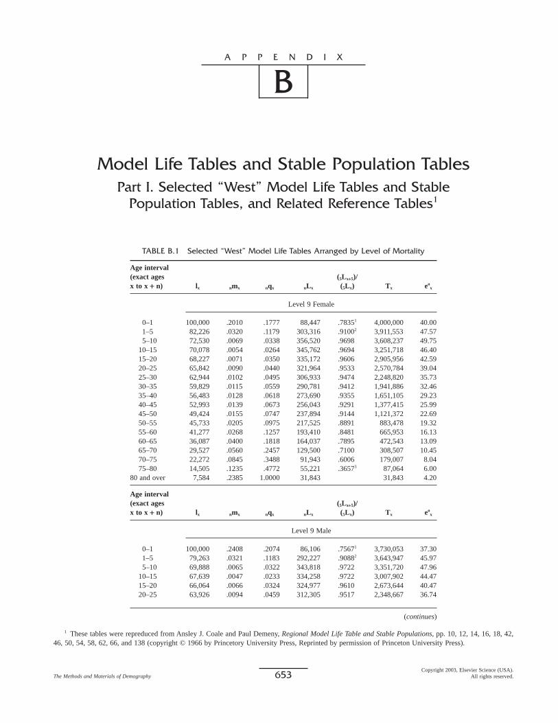
A P P E N D I X
B
653The Methods and Materials of DemographyCopyright 2003, Elsevier Science (USA).
All rights reserved.
Model Life Tables and Stable Population TablesPart I. Selected “West” Model Life Tables and Stable
Population Tables, and Related Reference Tables1
1 These tables were repreduced from Ansley J. Coale and Paul Demeny, Regional Model Life Table and Stable Populations, pp. 10, 12, 14, 16, 18, 42,46, 50, 54, 58, 62, 66, and 138 (copyright © 1966 by Princetory University Press, Reprinted by permission of Princeton University Press).
TABLE B.1 Selected “West” Model Life Tables Arranged by Level of Mortality
Age interval(exact ages (5Lx+5)/x to x + n) lx nmx nqx nLx (5Lx) Tx eo
x
Level 9 Female
0–1 100,000 .2010 .1777 88,447 .78351 4,000,000 40.001–5 82,226 .0320 .1179 303,316 .91002 3,911,553 47.575–10 72,530 .0069 .0338 356,520 .9698 3,608,237 49.75
10–15 70,078 .0054 .0264 345,762 .9694 3,251,718 46.4015–20 68,227 .0071 .0350 335,172 .9606 2,905,956 42.5920–25 65,842 .0090 .0440 321,964 .9533 2,570,784 39.0425–30 62,944 .0102 .0495 306,933 .9474 2,248,820 35.7330–35 59,829 .0115 .0559 290,781 .9412 1,941,886 32.4635–40 56,483 .0128 .0618 273,690 .9355 1,651,105 29.2340–45 52,993 .0139 .0673 256,043 .9291 1,377,415 25.9945–50 49,424 .0155 .0747 237,894 .9144 1,121,372 22.6950–55 45,733 .0205 .0975 217,525 .8891 883,478 19.3255–60 41,277 .0268 .1257 193,410 .8481 665,953 16.1360–65 36,087 .0400 .1818 164,037 .7895 472,543 13.0965–70 29,527 .0560 .2457 129,500 .7100 308,507 10.4570–75 22,272 .0845 .3488 91,943 .6006 179,007 8.0475–80 14,505 .1235 .4772 55,221 .36573 87,064 6.00
80 and over 7,584 .2385 1.0000 31,843 31,843 4.20
Age interval(exact ages (5Lx+5)/x to x + n) lx nmx nqx nLx (5Lx) Tx eo
x
Level 9 Male
0–1 100,000 .2408 .2074 86,106 .75671 3,730,053 37.301–5 79,263 .0321 .1183 292,227 .90882 3,643,947 45.975–10 69,888 .0065 .0322 343,818 .9722 3,351,720 47.96
10–15 67,639 .0047 .0233 334,258 .9722 3,007,902 44.4715–20 66,064 .0066 .0324 324,977 .9610 2,673,644 40.4720–25 63,926 .0094 .0459 312,305 .9517 2,348,667 36.74
(continues)

654 Appendix B. Model Life Tables and Stable Population Tables
TABLE B.1 (continued )
25–30 60,995 .0104 .0508 297,226 .9454 2,036,363 33.3930–35 57,895 .0121 .0585 281,009 .9365 1,739,137 30.0435–40 54,509 .0142 .0688 263,172 .9240 1,458,128 26.7540–45 50,760 .0175 .0837 243,182 .9088 1,194,955 23.5445–50 46,512 .0209 .0994 220,999 .8872 951,774 20.4650–55 41,887 .0273 .1277 196,068 .8572 730,775 17.4555–60 36,540 .0348 .1602 168,066 .8135 534,706 14.6360–65 30,686 .0489 .2177 136,730 .7510 366,640 11.9565–70 24,006 .0676 .2891 102,678 .6693 229,910 9.5870–75 17,066 .0967 .3893 68,718 .5598 127,231 7.4675–80 10,421 .1418 .5234 38,471 .34253 58,514 5.62
80 and over 4,967 .2478 1.0000 20,043 20,043 4.04
Age interval(exact ages (5Lx+5)/x to x + n) lx nmx nqx nLx (5Lx) Tx eo
x
Level 11 Female
0–1 100,000 .1615 .1461 90,502 .82191 4,500,000 45.001–5 85,388 .0250 .0937 320,442 .92882 4,409,498 51.645–10 77,389 .0055 .0272 381,683 .9758 4,089,056 52.84
10–15 75,285 .0043 .0212 372,430 .9752 3,707,373 49.2415–20 73,687 .0058 .0284 363,207 .9679 3,334,942 45.2620–25 71,596 .0073 .0360 351,543 .9618 2,971,735 41.5125–30 69,022 .0083 .0405 338,115 .9569 2,620,192 37.9630–35 66,224 .0094 .0459 323,525 .9516 2,282,077 34.4635–40 63,186 .0105 .0510 307,872 .9465 1,958,552 31.0040–45 59,963 .0116 .0562 291,388 .9402 1,650,680 27.5345–50 56,592 .0131 .0636 273,969 .9267 1,359,291 24.0250–55 52,996 .0175 .0837 253,884 .9309 1,085,322 20.4855–60 48,558 .0232 .1095 229,493 .8669 831,439 17.1260–65 43,239 .0347 .1596 198,946 .8127 601,946 13.9265–70 36,339 .0495 .2203 161,682 .7367 403,000 11.0970–75 28,333 .0758 .3184 119,112 .6304 241,319 8.5275–80 19,311 .1144 .4448 75,083 .38563 122,207 6.33
80 and over 10,722 .2275 1.0000 47,125 47,124 4.40
Age interval(exact ages (5Lx+5)/x to x + n) lx nmx nqx nLx (5Lx) Tx eo
x
Level 13 Female
0–1 100,000 .1282 .1183 92,310 .85661 5,000,000 50.001–5 88,169 .0188 .0717 335,996 .94532 4,907,690 55.665–10 81,848 .0043 .0214 404,871 .9810 4,571,694 55.86
10–15 80,100 .0034 .0166 397,178 .9804 4,166,823 52.0215–20 78,771 .0046 .0226 389,403 .9743 3,769,645 47.8620–25 76,990 .0059 .0289 379,397 .9693 3,380,242 43.9025–30 74,769 .0066 .0327 367,736 .9652 3,000,845 40.1330–35 72,326 .0076 .0370 354,934 .9608 2,633,107 36.4135–40 69,647 .0085 .0415 341,009 .9561 2,278,173 32.7140–45 66,756 .0095 .0464 326,031 .9500 1,937,165 29.0245–50 63,656 .0111 .0538 309,724 .9375 1,611,134 25.3150–55 60,234 .0149 .0717 290,374 .9170 1,301,410 21.6155–60 55,916 .0200 .0953 266,259 .8834 1,011,036 18.0860–65 50,587 .0301 .1401 235,225 .8332 744,777 14.7265–70 43,503 .0439 .1980 195,982 .7603 509,552 11.7170–75 34,890 .0683 .2918 149,002 .6566 313,570 8.9975–80 24,771 .1051 .4163 97,836 .40553 164,568 6.66
80 and over 14,424 .2162 1.0000 66,732 66,732 4.63
(continues)

Appendix B. Model Life Tables and Stable Population Tables 655
TABLE B.1 (continued )
Age interval(exact ages (5Lx+5)/x to x + n) lx nmx nqx nLx (5Lx) Tx eo
x
Level 15 Female
0–1 100,000 .0996 .0934 93,745 .88891 5,500,000 55.001–5 90,661 .0129 .0500 350,729 .96132 5,406,255 59.635–10 86,127 .0032 .0157 427,251 .9860 5,055,527 58.70
10–15 84,773 .0025 .0122 421,284 .9852 4,628,276 54.6015–20 83,740 .0035 .0174 415,061 .9800 4,206,992 50.2420–25 82,284 .0046 .0227 406,751 .9757 3,791,931 46.0825–30 80,416 .0053 .0259 396,874 .9724 3,385,180 42.1030–35 78,333 .0060 .0294 385,907 .9686 2,988,306 38.1535–40 76,029 .0068 .0334 373,805 .9643 2,602,399 34.2340–45 73,493 .0078 .0382 360,445 .9581 2,228,595 30.3245–50 70,686 .0094 .0458 345,343 .9464 1,868,150 26.4350–55 67,452 .0128 .0619 326,821 .9274 1,522,807 22.5855–60 63,276 .0175 .0840 303,101 .8966 1,195,986 18.9060–65 57,964 .0266 .1246 271,765 .8492 892,885 15.4065–70 50,742 .0398 .1808 230,771 .7783 621,120 12.2470–75 41,567 .0629 .2716 179,610 .6765 390,349 9.3975–80 30,277 .0984 .3948 121,501 .42353 210,740 6.96
80 and over 18,323 .2053 1.0000 89,239 89,238 4.87
Age interval(exact ages (5Lx+5)/x to x + n) lx nmx nqx nLx (5Lx) Tx eo
x
Level 17 Female
0–1 100,000 .0745 .0707 94,785 .91711 6,000,000 60.001–5 92,934 .0085 .0332 363,755 .97442 5,905,215 63.545–10 89,854 .0022 .0110 446,805 .9902 5,541,460 61.67
10–15 88,868 .0017 .0085 442,445 .9895 5,094,655 57.3315–20 88,110 .0025 .0125 437,800 .9855 4,652,210 52.8020–25 87,010 .0033 .0165 431,463 .9822 4,214,410 48.4425–30 85,575 .0039 .0191 423,798 .9795 3,782,947 44.2130–35 83,944 .0044 .0219 415,125 .9763 3,359,149 40.0235–40 82,106 .0052 .0255 405,299 .9722 2,944,024 35.8640–45 80,014 .0061 .0302 394,022 .9660 2,538,725 31.7345–50 77,595 .0077 .0379 380,623 .9550 2,144,704 27.6450–55 74,655 .0180 .0523 363,504 .9378 1,764,080 23.6355–60 70,747 .0151 .0727 340,876 .9097 1,400,576 19.8060–65 65,603 .0231 .1093 310,088 .8652 1,059,700 16.1565–70 58,432 .0356 .1633 268,300 .7968 749,612 12.8370–75 48,888 .0574 .2508 213,785 .6969 481,312 9.8575–80 36,626 .0917 .3729 148,989 .44313 267,528 7.30
80 and over 22,970 .1938 1.0000 118,539 118,538 5.16
1 Proportion surviving from birth to 0–4 years of age, 5L0/5l0.2
5L5/5L0.3 T80/T75.Source: Table B.1 (pp. 523–525) in H. Shryock, J. Siegel, and E. Stockwell, 1976, The Methods and
Materials of Demography, Condensed Edition, New York: Academic Press.

656 Appendix B. Model Life Tables and Stable Population Tables
TABLE B.2 Values of the Function lx for x = 1, 2, 3 and 5 in “West” Model LifeTables at Various Levels of Mortality, for Females, Males, and Both Sexes
[l0 = 100,000. The lx values for both sexes assume that the sex ratio at birth is 1.05]
Level l1 l2 l3 l5
Female1 63,483 55,000 51,199 46,8833 69,481 61,829 58,399 54,5065 74,427 67,671 64,643 61,2057 78,614 72,765 70,145 67,1699 82,226 77,271 75,051 72,530
11 85,388 81,300 79,468 77,38913 88,169 84,939 83,492 81,84815 90,661 88,364 87,324 86,12717 92,934 91,419 90,709 89,85419 95,006 94,143 93,724 93,20121 96,907 96,559 96,385 96,16023 98,484 98,377 98,321 98,248
Male1 58,093 50,308 46,898 43,0053 64,868 57,690 54,546 50,9575 70,454 64,015 61,195 57,9767 75,183 69,537 67,064 64,2429 79,263 74,425 72,307 69,888
11 82,835 78,800 77,032 75,01513 86,058 82,912 81,534 79,96115 88,864 86,523 85,498 84,32717 91,379 89,790 89,056 88,18419 93,713 92,796 92,338 91,77421 95,909 95,508 95,285 94,98923 97,856 97,719 97,636 97,521
Both Sexes1 60,722 52,597 48,996 44,8973 67,118 59,709 56,425 52,6885 72,392 65,798 62,877 59,5517 76,857 71,112 68,567 65,6709 80,709 75,813 73,646 71,177
11 84,080 80,019 78,220 76,17313 87,088 83,901 82,489 80,88115 89,740 87,421 86,389 85,20517 92,137 90,584 89,862 88,99919 94,144 93,453 93,011 92,45521 96,396 96,020 95,822 95,56023 98,162 98,040 97,970 97,876
Source: Table B.2 (p. 525) in H. Shryock, J. Siegel, and E. Stockwell, 1976, The Methods and Mate-rials of Demography, Condensed Edition, New York: Academic Press.
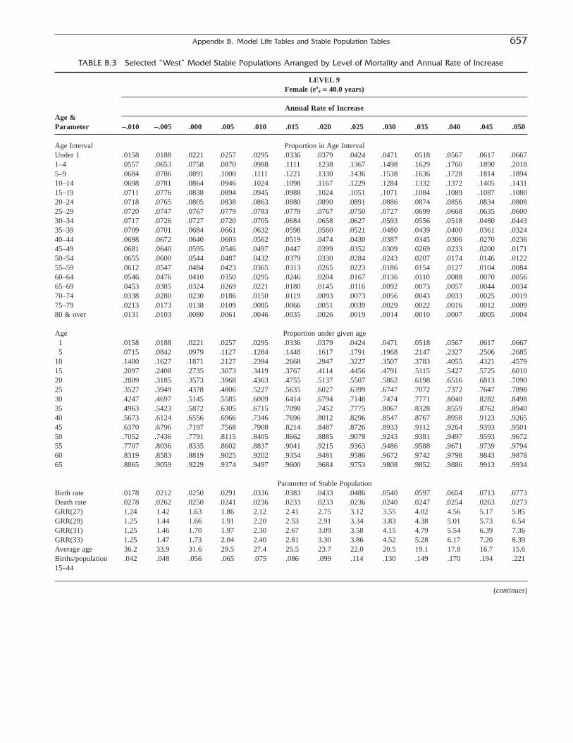
Appendix B. Model Life Tables and Stable Population Tables 657
TABLE B.3 Selected “West” Model Stable Populations Arranged by Level of Mortality and Annual Rate of Increase
LEVEL 9Female (eo
0 = 40.0 years)
Age &Annual Rate of Increase
Parameter -.010 -.005 .000 .005 .010 .015 .020 .025 .030 .035 .040 .045 .050
Age Interval Proportion in Age IntervalUnder 1 .0158 .0188 .0221 .0257 .0295 .0336 .0379 .0424 .0471 .0518 .0567 .0617 .06671–4 .0557 .0653 .0758 .0870 .0988 .1111 .1238 .1367 .1498 .1629 .1760 .1890 .20185–9 .0684 .0786 .0891 .1000 .1111 .1221 .1330 .1436 .1538 .1636 .1728 .1814 .189410–14 .0698 .0781 .0864 .0946 .1024 .1098 .1167 .1229 .1284 .1332 .1372 .1405 .143115–19 .0711 .0776 .0838 .0894 .0945 .0988 .1024 .1051 .1071 .1084 .1089 .1087 .108020–24 .0718 .0765 .0805 .0838 .0863 .0880 .0890 .0891 .0886 .0874 .0856 .0834 .080825–29 .0720 .0747 .0767 .0779 .0783 .0779 .0767 .0750 .0727 .0699 .0668 .0635 .060030–34 .0717 .0726 .0727 .0720 .0705 .0684 .0658 .0627 .0593 .0556 .0518 .0480 .044335–39 .0709 .0701 .0684 .0661 .0632 .0598 .0560 .0521 .0480 .0439 .0400 .0361 .032440–44 .0698 .0672 .0640 .0603 .0562 .0519 .0474 .0430 .0387 .0345 .0306 .0270 .023645–49 .0681 .0640 .0595 .0546 .0497 .0447 .0399 .0352 .0309 .0269 .0233 .0200 .017150–54 .0655 .0600 .0544 .0487 .0432 .0379 .0330 .0284 .0243 .0207 .0174 .0146 .012255–59 .0612 .0547 .0484 .0423 .0365 .0313 .0265 .0223 .0186 .0154 .0127 .0104 .008460–64 .0546 .0476 .0410 .0350 .0295 .0246 .0204 .0167 .0136 .0110 .0088 .0070 .005665–69 .0453 .0385 .0324 .0269 .0221 .0180 .0145 .0116 .0092 .0073 .0057 .0044 .003470–74 .0338 .0280 .0230 .0186 .0150 .0119 .0093 .0073 .0056 .0043 .0033 .0025 .001975–79 .0213 .0173 .0138 .0109 .0085 .0066 .0051 .0039 .0029 .0022 .0016 .0012 .000980 & over .0131 .0103 .0080 .0061 .0046 .0035 .0026 .0019 .0014 .0010 .0007 .0005 .0004
Age Proportion under given age1 .0158 .0188 .0221 .0257 .0295 .0336 .0379 .0424 .0471 .0518 .0567 .0617 .06675 .0715 .0842 .0979 .1127 .1284 .1448 .1617 .1791 .1968 .2147 .2327 .2506 .2685
10 .1400 .1627 .1871 .2127 .2394 .2668 .2947 .3227 .3507 .3783 .4055 .4321 .457915 .2097 .2408 .2735 .3073 .3419 .3767 .4114 .4456 .4791 .5115 .5427 .5725 .601020 .2809 .3185 .3573 .3968 .4363 .4755 .5137 .5507 .5862 .6198 .6516 .6813 .709025 .3527 .3949 .4378 .4806 .5227 .5635 .6027 .6399 .6747 .7072 .7372 .7647 .789830 .4247 .4697 .5145 .5585 .6009 .6414 .6794 .7148 .7474 .7771 .8040 .8282 .849835 .4963 .5423 .5872 .6305 .6715 .7098 .7452 .7775 .8067 .8328 .8559 .8762 .894040 .5673 .6124 .6556 .6966 .7346 .7696 .8012 .8296 .8547 .8767 .8958 .9123 .926545 .6370 .6796 .7197 .7568 .7908 .8214 .8487 .8726 .8933 .9112 .9264 .9393 .950150 .7052 .7436 .7791 .8115 .8405 .8662 .8885 .9078 .9243 .9381 .9497 .9593 .967255 .7707 .8036 .8335 .8602 .8837 .9041 .9215 .9363 .9486 .9588 .9671 .9739 .979460 .8319 .8583 .8819 .9025 .9202 .9354 .9481 .9586 .9672 .9742 .9798 .9843 .987865 .8865 .9059 .9229 .9374 .9497 .9600 .9684 .9753 .9808 .9852 .9886 .9913 .9934
Parameter of Stable PopulationBirth rate .0178 .0212 .0250 .0291 .0336 .0383 .0433 .0486 .0540 .0597 .0654 .0713 .0773Death rate .0278 .0262 .0250 .0241 .0236 .0233 .0233 .0236 .0240 .0247 .0254 .0263 .0273GRR(27) 1.24 1.42 1.63 1.86 2.12 2.41 2.75 3.12 3.55 4.02 4.56 5.17 5.85GRR(29) 1.25 1.44 1.66 1.91 2.20 2.53 2.91 3.34 3.83 4.38 5.01 5.73 6.54GRR(31) 1.25 1.46 1.70 1.97 2.30 2.67 3.09 3.58 4.15 4.79 5.54 6.39 7.36GRR(33) 1.25 1.47 1.73 2.04 2.40 2.81 3.30 3.86 4.52 5.28 6.17 7.20 8.39Average age 36.2 33.9 31.6 29.5 27.4 25.5 23.7 22.0 20.5 19.1 17.8 16.7 15.6Births/population .042 .048 .056 .065 .075 .086 .099 .114 .130 .149 .170 .194 .22115–44
(continues)
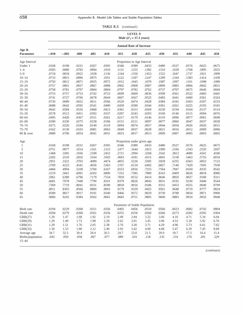
658 Appendix B. Model Life Tables and Stable Population Tables
TABLE B.3 (continued )
LEVEL 9Male (eo
0 = 37.3 years)
Age &Annual Rate of Increase
Parameter -.010 -.005 .000 .005 .010 .015 .020 .025 .030 .035 .040 .045 .050
Age Interval Proportion in Age IntervalUnder 1 .0168 .0198 .0231 .0267 .0305 .0346 .0389 .0433 .0480 .0527 .0576 .0625 .06751–4 .0583 .0680 .0783 .0894 .1010 .1131 .1255 .1382 .1510 .1639 .1768 .1895 .20225–9 .0718 .0818 .0922 .1028 .1136 .1244 .1350 .1453 .1552 .1647 .1737 .1821 .189910–14 .0733 .0815 .0896 .0975 .1051 .1122 .1187 .1247 .1299 .1344 .1383 .1414 .143815–19 .0750 .0812 .0871 .0925 .0972 .1012 .1045 .1070 .1087 .1097 .1101 .1098 .108920–24 .0757 .0801 .0837 .0867 .0888 .0902 .0908 .0907 .0899 .0885 .0866 .0842 .081525–29 .0758 .0781 .0797 .0804 .0804 .0797 .0782 .0762 .0737 .0707 .0675 .0640 .060430–34 .0753 .0757 .0753 .0742 .0723 .0699 .0669 .0636 .0599 .0561 .0522 .0483 .044535–39 .0741 .0727 .0706 .0678 .0644 .0607 .0567 .0525 .0483 .0441 .0400 .0361 .032440–44 .0720 .0689 .0652 .0611 .0566 .0520 .0474 .0428 .0384 .0342 .0303 .0267 .023345–49 .0688 .0642 .0592 .0541 .0490 .0439 .0390 .0344 .0301 .0261 .0225 ,0193 .016550–54 .0642 .0584 .0526 .0468 .0413 .0361 .0313 .0269 .0230 .0194 .0164 .0137 .011455–59 .0578 .0513 .0451 .0392 .0337 .0287 .0243 .0203 .0169 .0140 .0115 .0094 .007660–64 .0495 .0428 .0367 .0311 .0261 .0217 .0179 .0146 .0119 .0096 .0077 .0061 .004865–69 .0390 .0330 .0275 .0228 .0186 .0151 .0121 .0097 .0077 .0060 .0047 .0037 .002870–74 .0275 .0226 .0184 .0149 .0119 .0094 .0074 .0057 .0044 .0034 .0026 .0020 .001575–79 .0162 .0130 .0103 .0081 .0063 .0049 .0037 .0028 .0021 .0016 .0012 .0009 .000680 & over .0089 .0700 .0054 .0041 .0031 .0023 .0017 .0013 .0009 .0007 .0005 .0003 .0002
Age Proportion under given age1 .0168 .0198 .0231 .0267 .0305 .0346 .0389 .0433 .0480 .0527 .0576 .0625 .06755 .0751 .0877 .1014 .1161 .1315 .1477 .1644 .1815 .1990 .2166 .2343 .2520 .2697
10 .1468 .1695 .1936 .2189 .2452 .2721 .2994 .3268 .3542 .3813 .4080 .4341 .459615 .2202 .2510 .2832 .3164 .3502 .3843 .4181 .4515 .4841 .5158 .5463 .5755 .603420 .2951 .3322 .3703 .4089 .4474 .4855 .5226 .5585 .5928 .6255 .6563 .6853 .712325 .3709 .4123 .4541 .4956 .5363 .5767 .6134 .6492 .6827 .7140 .7429 .7695 .793830 .4466 .4904 .5338 .5760 .6167 .6553 .6916 .7253 .7564 .7847 .8104 .8335 .854235 .5219 .5661 .6091 .6502 .6890 .7252 .7585 .7889 .8163 .8409 .8626 .8818 .898640 .5961 .6389 .6796 .7179 .7534 .7859 .8152 .8414 .8646 .8850 .9027 .9180 .931145 .6681 .7078 .7448 .7790 .8101 .8379 .8626 .8843 .9031 .9192 .9330 .9446 .954450 .7369 .7719 .8041 .8331 .8590 .8818 .9016 .9186 .9331 .9453 .9555 .9640 .970955 .8011 .8303 .8566 .8800 .9003 .9179 .9329 .9455 .9561 .9648 .9719 .9777 .982460 .8589 .8817 .9017 .9191 .9340 .9466 .9572 .9659 .9730 .9788 .9834 .9871 .990065 .9084 .9245 .9384 .9502 .9601 .9683 .9751 .9805 .9849 .9883 .9910 .9932 .9948
Parameter of Stable PopulationBirth rate .0194 .0229 .0268 .0311 .0356 .0405 .0456 .0510 .0566 .0623 .0682 .0742 .0804Death rate .0294 .0279 .0268 .0261 .0256 .0255 .0256 .0260 .0266 .0273 .0282 .0292 .0304GRR(27) 1.29 1.47 1.68 1.92 2.19 2.49 2.84 3.22 3.66 4.16 4.71 5.34 6.04GRR(29) 1.29 1.49 1.72 1.98 2.28 2.62 3.01 3.45 3.96 4.53 5.18 5.92 6.76GRR(31) 1.29 1.51 1.76 2.05 2.38 2.76 3.20 3.71 4.29 4.96 5.73 6.61 7.62GRR(33) 1.30 1.53 1.80 2.12 2.49 2.92 3.42 4.00 4.68 5.47 6.39 7.45 8.69Average age 34.7 32.5 30.4 28.4 26.5 24.7 23.0 21.5 20.0 18.7 17.5 16.4 15.4Births/population .043 .050 .058 .067 .077 .089 .103 .118 .135 .154 .176 .201 .22915–44
(continues)

Appendix B. Model Life Tables and Stable Population Tables 659
TABLE B.3 (continued )
LEVEL 11Female (eo
0 = 45.0 years)
Age &Annual Rate of Increase
Parameter -.010 -.005 .000 .005 .010 .015 .020 .025 .030 .035 .040 .045 .050
Age Interval Proportion in Age IntervalUnder 1 .0142 .0170 .0201 .0235 .0272 .0311 .0352 .0396 .0440 .0487 .0534 .0582 .06311–4 .0516 .0610 .0712 .0822 .0939 .1061 .1187 .1316 .1447 .1579 .1711 .1842 .19715–9 .0643 .0743 .0848 .0957 .1069 .1181 .1292 .1401 .1506 .1606 .1702 .1792 .187510–14 .0660 .0743 .0828 .0911 .0992 .1069 .1141 .1206 .1265 .1316 .1360 .1396 .142515–19 .0676 .0743 .0807 .0867 .0920 .0967 .1006 .1038 .1061 .1077 .1086 .1087 .108220–24 .0688 .0738 .0781 .0818 .0847 .0868 .0881 .0887 .0884 .0875 .0860 .0840 .081625–29 .0696 .0727 .0751 .0767 .0775 .0775 .0767 .0753 .0732 .0707 .0677 .0645 .061130–34 .0700 .0714 .0719 .0716 .0706 .0688 .0664 .0635 .0603 .0568 .0531 .0493 .045535–39 .0700 .0696 .0684 .0665 .0639 .0607 .0572 .0534 .0494 .0453 .0413 .0375 .033740–44 .0697 .0676 .0648 .0614 .0575 .0533 .0490 .0446 .0402 .0360 .0320 .0283 .024945–49 .0689 .0651 .0609 .0563 .0514 .0465 .0417 .0370 .0326 .0284 .0247 .0213 .018250–54 .0671 .0619 .0564 .0508 .0433 .0400 .0349 .0302 .0260 .0221 .0187 .0157 .013155–59 .0637 .0574 .0510 .0448 .0390 .0335 .0286 .0241 .0202 .0168 .0138 .0114 .009360–64 .0581 .0510 .0442 .0379 .0321 .0270 .0224 .0185 .0151 .0122 .0098 .0079 .006265–69 .0496 .0425 .0359 .0300 .0248 .0203 .0165 .0132 .0105 .0083 .0065 .0051 .004070–74 .0384 .0321 .0265 .0216 .0174 .0139 .0110 .0086 .0067 .0052 .0039 .0030 .002375–79 .0255 .0207 .0167 .0133 .0104 .0081 .0063 .0048 .0036 .0027 .0020 .0015 .001180 & over .0170 .0134 .0105 .0081 .0062 .0047 .0035 .0026 .0019 .0014 .0010 .0007 .0005
Age Proportion under given age1 .0142 .0170 .0235 .0235 .0272 .0311 .0352 .0396 .0440 .0487 .0534 .0582 .06315 .0658 .0780 .1057 .1057 .1210 .1371 .1539 .1711 .1887 .2065 .2245 .2424 .2602
10 .1301 .1523 .2014 .2014 .2279 .2552 .2831 .3112 .3393 .3672 .3947 .4215 .447715 .1961 .2266 .2926 .2926 .3271 .3621 .3971 .4318 .4658 .4988 .5306 .5611 .590220 .2637 .3009 .3792 .3792 .4191 .4588 .4978 .5356 .5719 .6065 .6392 .6698 .698425 .3325 .3747 .4610 .4610 .5038 .5457 .5859 .6242 .6604 .6940 .7252 .7539 .780030 .4021 .4474 .5377 .5377 .5814 .6231 .6626 .6995 .7336 .7647 .7930 .8184 .841135 .4721 .5188 .6094 .6094 .6519 .6919 .7290 .7630 .7938 .8215 .8460 .8677 .886740 .5421 .5884 .6758 .6758 .7158 .7527 .7862 .8164 .8432 .8668 .8874 .9052 .920445 .6117 .6559 .7372 .7372 .7733 .8060 .8352 .8610 .8835 .9028 .9194 .9335 .945350 .6806 .7211 .7934 .7934 .8247 .8525 .8769 .8980 .9160 .9313 .9441 .9547 .963555 .7476 .7829 .8443 .8443 .8700 .8925 .9118 .9282 .9420 .9534 .9628 .9705 .976660 .8114 .8403 .8891 .8891 .9090 .9260 .9404 .9532 .9622 .9702 .9766 .9818 .985965 .8695 .8913 .9270 .9270 .9411 .9530 .9628 .9708 .9772 .9824 .9865 .9897 .9921
Parameter of Stable PopulationBirth rate .0156 .0188 .0222 .0260 .0302 .0346 .0393 .0443 .0494 .0547 .0602 .0658 .0715Death rate .0256 .0238 .0222 .0210 .0202 .0196 .0193 .0193 .0194 .0197 .0202 .0208 .0215GRR(27) 1.13 1.29 1.48 1.69 1.92 2.19 2.50 2.84 3.23 3.66 4.16 4.71 5.33GRR(29) 1.13 1.30 1.50 1.73 2.00 2.30 2.64 3.03 3.47 3.98 4.55 5.20 5.94GRR(31) 1.12 1.31 1.53 1.78 2.07 2.41 2.79 3.24 3.75 4.34 5.01 5.78 6.68GRR(33) 1.12 1.32 1.56 1.83 2.15 2.53 2.97 3.47 4.07 4.76 5.56 6.48 7.56Average age 37.6 35.2 32.9 30.6 28.5 26.4 24.6 22.8 21.2 19.7 18.4 17.2 16.1Births/population .038 .044 .051 .059 .068 .078 .090 .103 .118 .135 .155 .177 .20115–44
(continues)

660 Appendix B. Model Life Tables and Stable Population Tables
TABLE B.3 (continued )
LEVEL 13 LEVEL 15 LEVEL 17 LEVEL 19 LEVEL 21Female Female Female Female Female
eo0 = 50.0 eo
0 = 55.0 eo0 = 60.0 eo
0 = 65.0 eo0 = 70.0
Annual rate of Annual rate of Annual rate of Annual rate of Annual rate of
Age &increase increase increase increase increase
Parameter .025 .030 .035 .025 .030 .035 .025 .030 .035 .025 .030 .035 .025 .030 .035
Age Interval Proportion in Age IntervalUnder 1 .037 .042 .046 .035 .039 .044 .033 .037 .042 .032 .036 .040 .030 .034 .0391–4 .127 .140 .153 .123 .136 .149 .119 .133 .146 .116 .129 .143 .113 .126 .1405–9 .137 .148 .158 .134 .145 .156 .131 .142 .153 .128 .140 .151 .126 .137 .14910–14 .118 .125 .130 .117 .123 .129 .115 .121 .127 .113 .120 .126 .111 .118 .12415–19 .103 .105 .107 .101 .104 .107 .100 .103 .106 .099 .102 .105 .097 .101 .10420–24 .088 .088 .088 .088 .088 .088 .087 .088 .087 .086 .087 .087 .085 .087 .08725–29 .075 .074 .071 .076 .074 .072 .075 .074 .072 .075 .074 .072 .075 .074 .07230–34 .064 .061 .058 .065 .062 .059 .065 .062 .059 .065 .063 .060 .066 .063 .06035–39 .054 .051 .047 .055 .052 .048 .056 .053 .049 .057 .053 .049 .057 .054 .05040–44 .046 .042 .037 .047 .043 .039 .048 .044 .040 .049 .045 .041 .050 .046 .04145–49 .039 .034 .030 .040 .035 .031 .041 .037 .032 .042 .038 .033 .043 .039 .03450–54 .032 .027 .023 .033 .029 .025 .035 .030 .026 .036 .031 .027 .037 .032 .02855–59 .026 .022 .018 .027 .023 .019 .029 .024 .020 .030 .025 .021 .031 .027 .02260–64 .020 .017 .013 .022 .018 .014 .023 .019 .016 .024 .020 .017 .026 .021 .01865–69 .015 .012 .009 .016 .013 .010 .018 .014 .011 .019 .015 .012 .020 .017 .01370–74 .010 .008 .006 .011 .009 .007 .012 .010 .008 .014 .011 .008 .015 .012 .00975–79 .006 .004 .003 .067 .005 .004 .008 .006 .004 .009 .007 .005 .010 .008 .00680 & over .003 .003 .002 .004 .003 .002 .005 .004 .003 .006 .005 .004 .008 .006 .004
Age Proportion under given age1 .037 .042 .046 .035 .039 .044 .033 .037 .042 .032 .036 .040 .030 .034 .0395 .164 .182 .200 .158 .175 .193 .153 .170 .187 .148 .165 .182 .143 .161 .178
10 .301 .329 .357 .292 .320 .349 .284 .312 .340 .276 .305 .333 .269 .298 .32715 .420 .454 .487 .409 .443 .477 .398 .433 .468 .389 .424 .459 .380 .416 .45120 .522 .559 .595 .510 .548 .584 .498 .537 .573 .487 .526 .564 .477 .517 .55525 .610 .647 .682 .598 .636 .671 .585 .624 .661 .574 .613 .651 .562 .603 .64230 .685 .721 .753 .673 .710 .743 .661 .698 .733 .649 .687 .723 .637 .677 .71435 .750 .782 .811 .738 .771 .802 .726 .761 .792 .714 .750 .783 .703 .740 .77440 .804 .833 .858 .793 .823 .849 .782 .813 .841 .771 .803 .832 .760 .794 .82445 .850 .874 .895 .840 .866 .888 .830 .857 .880 .820 .848 .873 .810 .840 .86650 .889 .908 .925 .880 .901 .919 .871 .893 .913 .862 .886 .906 .853 .878 .90055 .920 .936 .948 .913 .930 .943 .906 .923 .938 .898 .917 .933 .890 .910 .92860 .946 .957 .966 .941 .953 .963 .934 .948 .959 .928 .942 .954 .921 .937 .95065 .966 .974 .980 .962 .970 .977 .957 .967 .974 .952 .963 .971 .947 .958 .967
Parameter of Stable PopulationBirth rate .041 .046 .051 .038 .043 .047 .035 .040 .045 .033 .038 .042 .032 .036 .040Death rate .016 .016 .016 .013 .013 .012 .010 .010 .010 .008 .008 .007 .007 .006 .005GRR(27) 2.62 2.98 3.38 2.43 2.76 3.14 2.28 2.59 2.95 2.16 2.45 2.79 2.06 2.34 2.66GRR(29) 2.78 3.19 3.66 2.58 2.96 3.39 2.41 2.77 3.17 2.28 2.61 3.00 2.17 2.49 2.85GRR(31) 2.96 3.43 3.97 2.74 3.17 3.67 2.55 2.96 3.43 2.41 2.79 3.23 2.28 2.65 3.07GRR(33) 3.17 3.71 4.34 2.92 3.42 4.00 2.71 3.18 3.72 2.55 2.99 3.50 2.41 2.83 3.31Average Age 23.5 21.8 20.3 24.2 22.4 20.8 24.8 23.0 21.3 25.4 23.5 21.8 26.0 24.1 22.3(Births)/ .095 .109 .124 .088 .101 .115 .082 .094 .103 .077 .089 .102 .073 .084 .097(Pop. 15–44)
Source: Table B.3 (pp. 526–529) in H. Shryock, J. Siegel, and E. Stockwell, 1976, The Methods and Materials of Demography, Condensed Edition, NewYork: Academic Press.
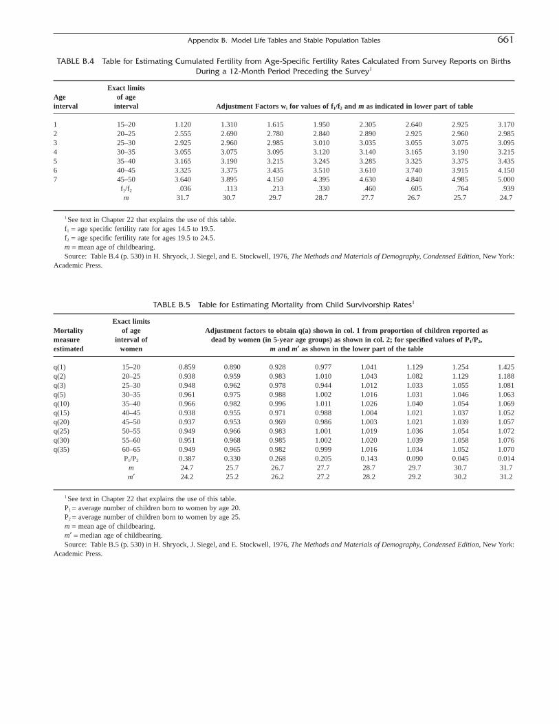
Appendix B. Model Life Tables and Stable Population Tables 661
TABLE B.4 Table for Estimating Cumulated Fertility from Age-Specific Fertility Rates Calculated From Survey Reports on BirthsDuring a 12-Month Period Preceding the Survey1
Exact limitsAge of ageinterval interval Adjustment Factors wi for values of f1/f2 and m as indicated in lower part of table
1 15–20 1.120 1.310 1.615 1.950 2.305 2.640 2.925 3.1702 20–25 2.555 2.690 2.780 2.840 2.890 2.925 2.960 2.9853 25–30 2.925 2.960 2.985 3.010 3.035 3.055 3.075 3.0954 30–35 3.055 3.075 3.095 3.120 3.140 3.165 3.190 3.2155 35–40 3.165 3.190 3.215 3.245 3.285 3.325 3.375 3.4356 40–45 3.325 3.375 3.435 3.510 3.610 3.740 3.915 4.1507 45–50 3.640 3.895 4.150 4.395 4.630 4.840 4.985 5.000
f1/f2 .036 .113 .213 .330 .460 .605 .764 .939m 31.7 30.7 29.7 28.7 27.7 26.7 25.7 24.7
1 See text in Chapter 22 that explains the use of this table.f1 = age specific fertility rate for ages 14.5 to 19.5.f2 = age specific fertility rate for ages 19.5 to 24.5.m = mean age of childbearing.Source: Table B.4 (p. 530) in H. Shryock, J. Siegel, and E. Stockwell, 1976, The Methods and Materials of Demography, Condensed Edition, New York:
Academic Press.
TABLE B.5 Table for Estimating Mortality from Child Survivorship Rates1
Exact limitsMortality of age Adjustment factors to obtain q(a) shown in col. 1 from proportion of children reported asmeasure interval of dead by women (in 5-year age groups) as shown in col. 2; for specified values of P1/P2,estimated women m and m¢ as shown in the lower part of the table
q(1) 15–20 0.859 0.890 0.928 0.977 1.041 1.129 1.254 1.425q(2) 20–25 0.938 0.959 0.983 1.010 1.043 1.082 1.129 1.188q(3) 25–30 0.948 0.962 0.978 0.944 1.012 1.033 1.055 1.081q(5) 30–35 0.961 0.975 0.988 1.002 1.016 1.031 1.046 1.063q(10) 35–40 0.966 0.982 0.996 1.011 1.026 1.040 1.054 1.069q(15) 40–45 0.938 0.955 0.971 0.988 1.004 1.021 1.037 1.052q(20) 45–50 0.937 0.953 0.969 0.986 1.003 1.021 1.039 1.057q(25) 50–55 0.949 0.966 0.983 1.001 1.019 1.036 1.054 1.072q(30) 55–60 0.951 0.968 0.985 1.002 1.020 1.039 1.058 1.076q(35) 60–65 0.949 0.965 0.982 0.999 1.016 1.034 1.052 1.070
P1/P2 0.387 0.330 0.268 0.205 0.143 0.090 0.045 0.014m 24.7 25.7 26.7 27.7 28.7 29.7 30.7 31.7m¢ 24.2 25.2 26.2 27.2 28.2 29.2 30.2 31.2
1 See text in Chapter 22 that explains the use of this table.P1 = average number of children born to women by age 20.P2 = average number of children born to women by age 25.m = mean age of childbearing.m¢ = median age of childbearing.Source: Table B.5 (p. 530) in H. Shryock, J. Siegel, and E. Stockwell, 1976, The Methods and Materials of Demography, Condensed Edition, New York:
Academic Press.

For many of the countries with no reliable mortality dataor no mortality data at all, models constructed on the basisof other countries’ mortality experience can be used to inferparameters. With the increased use of demographic andhealth surveys and with continued improvements in vital sta-tistics, many of these countries are now able to conductimproved analysis of the age pattern of mortality, at least incertain age segments (e.g., infancy and childhood, youngadulthood). Improved data collection has helped in devel-oping several new and better models to study the age patternof mortality.
A model for mortality may be a mathematical represen-tation of the age-specific mortality (or risk of death). Whenthe mortality pattern is U- or J-shaped, mathematical repre-sentation of the age pattern is difficult. The Gompertz orMakeham curve may not depict the mortality pattern of theentire age span; these curves may fit only certain segmentsof the human life span (Gompertz, 1825; Makeham, 1860).Because of the difficulty of finding simple mathematicalfunctions to represent the entire life span, model construc-tion has taken different directions. One such direction istoward empirically based models in which typical patternsare extracted from a collection of real life tables. Once thepatterns of mortality in these collections of life tables areidentified, simple analytical procedures are used to generatemodels by varying the level of mortality within each iden-tified pattern. Several model life tables of this type havebeen constructed. This chapter presents two in detail (Coaleand Demeny, 1983; United Nations, 1982).
A second way of constructing model life tables is the rela-tional model method. In this approach, a standard agepattern of mortality is specified and a mathematical equa-tion is also specified to relate the standard pattern to ageneral class of age patterns of mortality. A pattern of mor-tality is generated by changing the parameters in the speci-fied mathematical equation. This method has the advantageof being able to generate patterns of mortality that are notincluded in the empirically based procedures. The Brasslogit system of model life tables, which is based on the rela-tional principle (Brass et al., 1968), is presented in thisappendix. This appendix also presents a simple extension ofthe Brass model.
Because of the relationship between age-specific deathrates and life table functions such as the probability of dyingin an age interval (qx) or the proportion surviving to a spec-
ified age x (lx), some models used to study age patterns ofmortality are generated for these specific functions. Modelsconstructed using these functions have the advantage of being easily manipulated to generate other life table functions.
With modern computer power, renewed attempts havebeen made to formulate complex mathematical (parametric)models to represent the mortality experience of the entireage span. A brief discussion of such parametric models isalso included here (Di Pino and Pirri, 1998; Heligman andPollard, 1980; Rogers and Little, 1994).
EMPIRICALLY BASED SYSTEMS OFMODEL LIFE TABLES
The two significant attempts using the empiricalapproach are the first United Nations model life tables andLedermann’s (1969) system of model life tables. Theapproach taken in these systems of life tables paved the wayfor new and improved systems, described in detail later inthis section.
The Early United Nations System of Model Life Tables
The United Nations was the first to make a systematicattempt to construct model life tables with an empirical basis(United Nations, 1955). In this effort the key assumptionwas that the level of mortality in any age group was closelycorrelated with the level of mortality in an adjacent agegroup. Parabolic regression equations indicating the rela-tionship between adjacent pairs of life table nqx values wereconstructed using data from life tables of 158 countries. Thus, starting from a specified level of infant mortality, q0, a value of 4q1 could be determined. From thecalculated value of 4q1, a value of 5q5 could be estimatedusing the regression equation. This process was continuedin chain fashion to generate all the nqx values for the entirelife span. Thus, by specifying various levels of infant mor-tality (q0), one could generate a set of life tables. This set ofUN model life tables was criticized for several reasons.Using a series of regression equations in chain fashion intro-duced a bias into the estimated life table parameters because
662 Appendix B. Model Life Tables and Stable Population Tables
Part II. Model Life Tables
C. M. SUCHINDRAN

of the statistical errors in the estimated predictor variables.It was also argued that the collection of life tables that wentinto calculating the regression equation was not sufficientlyrepresentative of the whole range of reliably recordedhuman mortality experience. The system of life tables gen-erated with a single parameter, the infant mortality rate, (q0),also lacked flexibility because it could generate only oneplausible age pattern of mortality from among the manypotential patterns.
Ledermann’s System of Model Life Tables
Ledermann and Breas (1959) used factor analysis to analyze variations in mortality in the set of actual life tables used to construct the first United Nations model life table. They concluded that five significant factorscontribute to these variations in mortality: (1) the overalllevel of mortality, (2) the ratio of child to adult mortality,(3) old-age mortality, (4) pattern of infant and child mortal-ity, and (5) sex differences in mortality from ages 5 to 70.Taking into account these factors in the variation of mortal-ity, Ledermann (1969) constructed a system of life tables.The basis of these life tables, as in the case of the earlyUnited Nations life tables, is a system of regression equa-tions predicting the logarithm of the nqx with one or twoindependent variables. For example, the system of regres-sion equations consisting of two independent variables is ofthe form
(B.1)
where the pair of independent variables (Z1, Z2) can be anyof the following pairs: (5q0, 20q45), (15q0, 20q30), (15q0, m50+).
Ledermann’s system is much more flexible than the one-parameter system in the earlier United Nations set of modellife tables because regression equations are available withseveral choices of independent variables. However, theregression parameters are estimated using the same set oflife tables as that of the United Nations, which may not cover all the possible patterns. Moreover, reliable estimatesof the independent variables used in these equations may not be available in the less developed countries. Becausemost of the current methods of estimating the demographicparameters for the less developed countries seldom use Ledermann’s system of life tables, this system of life tablesis not discussed in detail here.
Other Empirically Based Systems of Model Life Tables
Two sets of model life tables that have wider use in coun-tries with limited mortality data are the Coale and Demenysystem of model life tables and the new United Nationsmodel life tables.
ln ln lnn xq x x Z x Z= ( ) + ( ) + ( )b b b0 1 1 2 2
Coale and Demeny System of Model Life Tables
Coale and Demeny first published a system of model lifetables in 1966 (Coale and Demeny, 1966). They publisheda revised system in 1983 (Coale and Demeny, 1983).
The basis of the Coale-Demeny life table system is themortality patterns exhibited in 192 actual life tables by sex.They chose these life tables from an original collection of326 male and 326 female life tables. The original set con-tained 23 pairs of life tables for the period before 1870, 189between the years 1871 and 1945, and the remaining 114 theperiod after 1945. Two hundred and forty-six of the original326 came from European and other developed countries. Ofthe original 326, those that exhibited large deviations fromthe “norm” were dropped. Only life tables derived from reg-istration data and from the complete enumeration of the pop-ulations to which they refer were included. The final set of192 life tables selected for the construction of model lifetables contained only 16 from Asia and Africa. The remain-ing 176 came from Europe, North America, Australia, andNew Zealand.
Analysis of these 192 life tables revealed four age pat-terns of mortality. These patterns were labeled North, South,East, and West. The characteristics of the age patterns of thefour regions are as follows:
1. North. This region’s age pattern of mortality is char-acterized by relatively low infant mortality, relatively highchild mortality, and low mortality after age 50. The highadult mortality (age 20 to 50) in this mortality pattern isattributed to a high incidence of tuberculosis. The life tablesthat exhibited this pattern were derived from nine observedtables from Norway (1856–1880), Sweden (1851–1890),and Iceland (1941–1950).
2. South. The South mortality pattern is characterizedby high mortality under age 5 (particularly among infants),low adult mortality from age 40 to age 60, and high mor-tality over age 65. The South model represents the agepattern of mortality of southern European countries such asSpain, Portugal, and Italy, from 1876 to 1957.
3. East. The East pattern of mortality exhibits relativelyhigh infant mortality and high old-age mortality. This patternappears mainly in the life tables of central European coun-tries such as Austria, Germany, north and central Italy,Czechoslovakia, and Poland.
4. West. The West pattern is derived from the largest setof observed life tables (130) and is considered to representthe most general mortality pattern. Its mortality pattern doesnot deviate significantly from the mortality pattern derivedwhen all the observed life tables are put together. This modelis based only on the tables that were not included in the derivation of the other three patterns. Coale and Demenyrecommended its use when reliable information is lackingfor choosing one of the other patterns.
Appendix B. Model Life Tables and Stable Population Tables 663
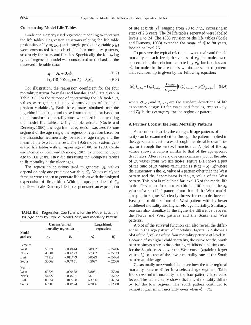
Constructing Model Life Tables
Coale and Demeny used regression modeling to constructthe life tables. Regression equations relating the life tableprobability of dying (nqx) and a single predictor variable (e0
10)were constructed for each of the four mortality patterns, separately for males and females. Specifically, the followingtype of regression model was constructed on the basis of theobserved life table data:
(B.8)
For illustration, the regression coefficient for the fourmortality patterns for males and females aged 0 are given inTable B.5. For the purpose of constructing the life tables nqx
values were generated using various values of the inde-pendent variable e0
10. Both the estimates obtained from thelogarithmic equation and those from the equation based on the untransformed mortality rates were used in constructingthe model life tables. Using simple criteria (Coale andDemeny, 1966), the logarithmic regression was used for onesegment of the age range, the regression equation based onthe untransformed mortality for another age range, and themean of the two for the rest. The 1966 model system gen-erated life tables with an upper age of 80. In 1983, Coaleand Demeny (Coale and Demeny, 1983) extended the upperage to 100 years. They did this using the Gompertz modelto fit mortality at the older ages.
The regression equations used to generate nqx valuesdepend on only one predictor variable, e0
10. Values of e010 for
females were chosen to generate life tables with the assignedexpectation of life at birth. With appropriate values of e0
10,the 1966 Coale-Demeny life tables generated an expectation
n x x x
n x x x
q A B e
q A B e
= +( ) = ¢ + ¢
100
10 10010 000ln ,
of life at birth (e00) ranging from 20 to 77.5, increasing in
steps of 2.5 years. The 24 life tables generated were labeledlevels 1 to 24. The 1983 revision of the life tables (Coaleand Demeny, 1983) extended the range of e0
0 to 80 years,labeled as level 25.
To preserve the typical relation between male and femalemortality at each level, the values of e0
10 for males werechosen using the relation exhibited by e0
10 for females ande0
10 for males in the life tables within the selected pattern.This relationship is given by the following equation:
(B.9)
where smales and sfemales are the standard deviations of lifeexpectancy at age 10 for males and females, respectively,and is the average e0
10 for the region or pattern.
A Further Look at the Four Mortality Patterns
As mentioned earlier, the changes in age patterns of mor-tality can be examined either through the pattern implied inthe age-specific death rates, through the life table quantitiesnqx, or through the survival function lx. A plot of the nqx
values shows a pattern similar to that of the age-specificdeath rates. Alternatively, one can examine a plot of the ratioof nqx values from two life tables. Figure B.1 shows a plotof the ratio of nqx values calculated as R(x) = nqx/nqW
x wherethe numerator is the nqx value of a pattern other than the Westpattern and the denominator is the nqx value of the Westpattern. This plot is calculated for level 15 of the model lifetables. Deviations from one exhibit the difference in the nqx
value of a specified pattern from that of the West model. The plot in Figure B.1 clearly shows, for example, how theEast pattern differs from the West pattern with its lowerchildhood mortality and higher old-age mortality. Similarly,one can also visualize in the figure the difference between the North and West patterns and the South and West patterns.
A plot of the survival function can also reveal the differ-ences in the age pattern of mortality. Figure B.2 shows a plot of the lx values of the four mortality patterns at level 15.Because of its higher child mortality, the curve for the Southpattern shows a steep drop during childhood and the curvefor the South crosses over the West curve (attaining largervalues lx) because of the lower mortality rate of the Southpattern at older ages.
Occasionally one would like to see how the four regionalmortality patterns differ in a selected age segment. Table B.6 shows infant mortality in the four patterns at selectedlevels. The table clearly shows that infant mortality differsby for the four regions. The South pattern continues toexhibit higher infant mortality even when e0
0 = 75.
e100
e e e emales males
males
femalesfemales females10
0100
100
100( ) - ( ) = ( ) - ( )[ ]s
s
664 Appendix B. Model Life Tables and Stable Population Tables
TABLE B.6 Regression Coefficients for the Model Equationfor Age Zero by Type of Model, Sex, and Mortality Pattern
Untransformed Logarithmic
Modelmortality regression regression
and sex A0 B0 A¢0 B¢0
FemalesWest .53774 -.008044 5.8992 -.05406North .47504 -.006923 5.7332 -.05133East .78219 -.011679 5.8529 -.05064South .52069 -.007051 4.5097 -.02566
MalesWest .63726 -.009958 5.8061 -.05338North .54327 -.008251 5.6151 -.05022East 1.07554 -.017228 6.3796 -.06124South .61903 -.008974 4.7096 -.02980
(B.7)

The 1982 United Nations Model Life Tables
The United Nations (1982) produced a set of model lifetables that, like Coale and Demeny’s (1983), are empiricallybased. However, unlike Coale and Demeny’s, most of thelife tables included in the UN set came from less developedcountries. After carefully evaluating the available life tablesfrom the less developed countries, 72 high-quality tables (36males and 36 females) were chosen as the basis for the construction of model life tables. These life tables camefrom 22 less developed countries and cover the period 1920
Appendix B. Model Life Tables and Stable Population Tables 665
FIGURE B.1 Relative proportion dying in North, East, and South models in relation to the West model (Level 15).
FIGURE B.2 Proportion surviving to a specified age by mortality pattern.
TABLE B.7 Values of Female Infant Mortality (q0) atSelected Mortality Levels by Pattern
Pattern Level 15 (e00 = 55) Level 19 (e0
0 = 65) Level 23 (e00 = 75)
West .093 .050 .015North .085 .048 .018East .116 .064 .021South .112 .077 .041

to 1973. The female life expectancy at birth in these lifetables ranged from 40.1 to 76.6 years.
Patterns of Mortality
An examination of the life tables selected by graphicaland statistical procedures, such as cluster analysis, revealedfour distinct age patterns of mortality. These patterns werelabeled Latin American, Chilean, South Asian, and FarEastern. A fifth general pattern was also constructed, whichis an average pattern derived from all the original life tablesselected. Each pattern is briefly described next.
The Latin American Pattern
The Latin American model has relatively high infant andchild mortality (caused mainly by excess diarrheal and parasitic diseases). Adult mortality is also high (primarilybecause of accidents). Old-age mortality is low (primarilybecause of low cardiovascular mortality).
The life tables that exhibited this pattern came fromColombia, Costa Rica, El Salvador, Guatemala, Honduras,Mexico, and Peru, as well as three Asian countries—thePhilippines, Sri Lanka, and Thailand.
The Chilean Pattern
The Chilean pattern has extremely high infant mortality(mainly because of deaths from respiratory diseases, andpossibly related to early weaning). This pattern is distinc-tive, found only in life tables from Chile.
The South Asian Pattern
This pattern has high mortality under 15 and over 55(attributed to diarrheal and parasitic diseases at young agesand to respiratory and diarrheal diseases at older ages) butrelatively low mortality in the intermediate ages. The lifetables included in this pattern came from India, Iran,Bangladesh, and Tunisia.
The Far Eastern Pattern
In this pattern, mortality at old ages was relatively highcompared to other patterns, especially among males (prob-ably due to a past history of tuberculosis). This clusterincluded life tables from Guyana, Hong Kong, Republic ofKorea, Singapore, and Trinidad and Tobago.
The General Pattern
The general pattern is an average of the life tables con-sidered. It is similar to the Coale and Demeny’s West modellife tables.
Construction of the Model Life Tables
The statistical method of principal component analysiswas used for the construction of the model life tables. The
age pattern of each life table analyzed was characterized byits nqx values. Specifically, the logit transformation of nqx wasused. The form of the logit transformation used is
(B.4)
Denote nYxij as the logit of the nqx function for life table j
of cluster i and nix as the average of the nYx
ij within cluster i.Then the k-component principal component model is spec-ified as
(B.5)
where Umx equals the element of the mth principal com-ponent vector corresponding to age group (x, x + n), k is thenumber of principal components, and amj equals the factorloading of the mth principal component vector for country jin the principal component analysis. When k = 1, the modelis referred to as a one-component model. Similar referencesare made to two-component and three-component models.Note that in the fitted model, the factor loading, amj, and theprincipal component vector, Umx, does not depend on thecluster pattern. In the United Nations’ collection of lifetables, for all ages combined, the percentage of variation infemale mortality explained by the model is 91.3, 95.2, and96.8, respectively for one-, two-, and three-componentmodels. For male life tables, the corresponding percentagesare 89.2, 94.7, and 96.7.
The average female patterns of mortality for specificcluster patterns defined by the logit values, n i
x, are shown inTable B.8. The age pattern of mortality implied in eachpattern is clearly reflected in the averages in Table B.8. Asnoted earlier, a three-component model captures nearly allthe variations in mortality. Table B.9 presents the first threeprincipal components (U1x, U2x, and U3x) for females.
The first principal component captures the change fromthe average in the overall level of mortality at each age.These component values show that the change is greatest in childhood and young adulthood and decreases as ageincreases. The second component reflects the characteristicdifferences in changes in mortality under age 5 in relationto that of mortality over 5. For females, the third componentreflects the mortality changes in the childbearing years.
As stated earlier, a life table for a particular pattern i canbe produced from a one-component model by generating the logit values of nqx (denoted as nYi
x) using the model equation
(B.6)
where a1 denotes the loading factor and U1x denotes the firstcomponent factor for age x. The model construction can beextended to include the second and third component
n xi
n xi
xY Y a U= + 1 1*
Y
n xij
n xi
mj mxm
k
Y Y a U= +=
Â1
Y
log lnit n xn x
n x
q[ ] =
-ÈÎÍ
˘˚̇
12 1
666 Appendix B. Model Life Tables and Stable Population Tables
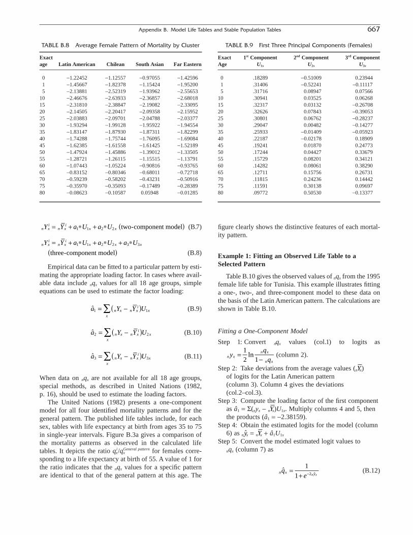
Appendix B. Model Life Tables and Stable Population Tables 667
TABLE B.8 Average Female Pattern of Mortality by Cluster
Exactage Latin American Chilean South Asian Far Eastern
0 -1.22452 -1.12557 -0.97055 -1.425961 -1.45667 -1.82378 -1.15424 -1.952005 -2.13881 -2.52319 -1.93962 -2.55653
10 -2.46676 -2.63933 -2.36857 -2.6801815 -2.31810 -2.38847 -2.19082 -2.3309520 -2.14505 -2.20417 -2.09358 -2.1595225 -2.03883 -2.09701 -2.04788 -2.0337730 -1.93294 -1.99128 -1.95922 -1.9455435 -1.83147 -1.87930 -1.87311 -1.8229940 -1.74288 -1.75744 -1.76095 -1.6908445 -1.62385 -1.61558 -1.61425 -1.5218950 -1.47924 -1.45886 -1.39012 -1.3350555 -1.28721 -1.26115 -1.15515 -1.1379160 -1.07443 -1.05224 -0.90816 -0.9376565 -0.83152 -0.80346 -0.68011 -0.7271870 -0.59239 -0.58202 -0.43231 -0.5091675 -0.35970 -0.35093 -0.17489 -0.2838980 -0.08623 -0.10587 0.05948 -0.01285
TABLE B.9 First Three Principal Components (Females)
Exact 1st Component 2nd Component 3rd ComponentAge U1x U2x U3x
0 .18289 -0.51009 0.239441 .31406 -0.52241 -0.111175 .31716 0.08947 0.07566
10 .30941 0.03525 0.0626815 .32317 0.03132 -0.2670820 .32626 0.07843 -0.3905325 .30801 0.06762 -0.2823730 .29047 0.00482 -0.1427735 .25933 -0.01409 -0.0592340 .22187 -0.02178 0.1890945 .19241 0.01870 0.2477350 .17244 0.04427 0.3367955 .15729 0.08201 0.3412160 .14282 0.08061 0.3829065 .12711 0.15756 0.2673170 .11815 0.24236 0.1444275 .11591 0.30138 0.0969780 .09772 0.50530 -0.13377
(B.7)
(B.8)
Empirical data can be fitted to a particular pattern by esti-mating the appropriate loading factor. In cases where avail-able data include nqx values for all 18 age groups, simpleequations can be used to estimate the factor loading:
(B.9)
(B.10)
(B.11)
When data on nqx are not available for all 18 age groups,special methods, as described in United Nations (1982, p. 16), should be used to estimate the loading factors.
The United Nations (1982) presents a one-componentmodel for all four identified mortality patterns and for thegeneral pattern. The published life tables include, for eachsex, tables with life expectancy at birth from ages 35 to 75in single-year intervals. Figure B.3a gives a comparison ofthe mortality patterns as observed in the calculated lifetables. It depicts the ratio qi
x/qxGeneral pattern for females corre-
sponding to a life expectancy at birth of 55. A value of 1 forthe ratio indicates that the nqx values for a specific patternare identical to that of the general pattern at this age. The
â Y Y Un x n xi
xx
3 3= -( )Â
â Y Y Un x n xi
xx
2 2= -( )Â
â Y Y Un x n xi
xx
1 1= -( )Â
n xi
n xi
x x xY Y a U a U a U= + + +( )
1 1 2 2 3 3* * *three-component model
n xi
n xi
x xY Y a U a U= + + ( )1 1 2 2* * two-component model figure clearly shows the distinctive features of each mortal-ity pattern.
Example 1: Fitting an Observed Life Table to aSelected Pattern
Table B.10 gives the observed values of nqx from the 1995female life table for Tunisia. This example illustrates fittinga one-, two-, and three-component model to these data onthe basis of the Latin American pattern. The calculations areshown in Table B.10.
Fitting a One-Component Model
Step 1: Convert nqx values (col.1) to logits as
(column 2).
Step 2: Take deviations from the average values (n x) of logits for the Latin American pattern (column 3). Column 4 gives the deviations(col.2–col.3).
Step 3: Compute the loading factor of the first componentas â1 = S(nyx - n x)U1x. Multiply columns 4 and 5, thenthe products (â1 = -2.38159).
Step 4: Obtain the estimated logits for the model (column6) as n x = n x + â1U1x
Step 5: Convert the model estimated logit values to nqx (column 7) as
(B.12)n x yq
e n xˆ
ˆ=
+ -
1
1 2
Yŷ
Y
Y
n xn x
n x
yq
q=
-12 1
ln
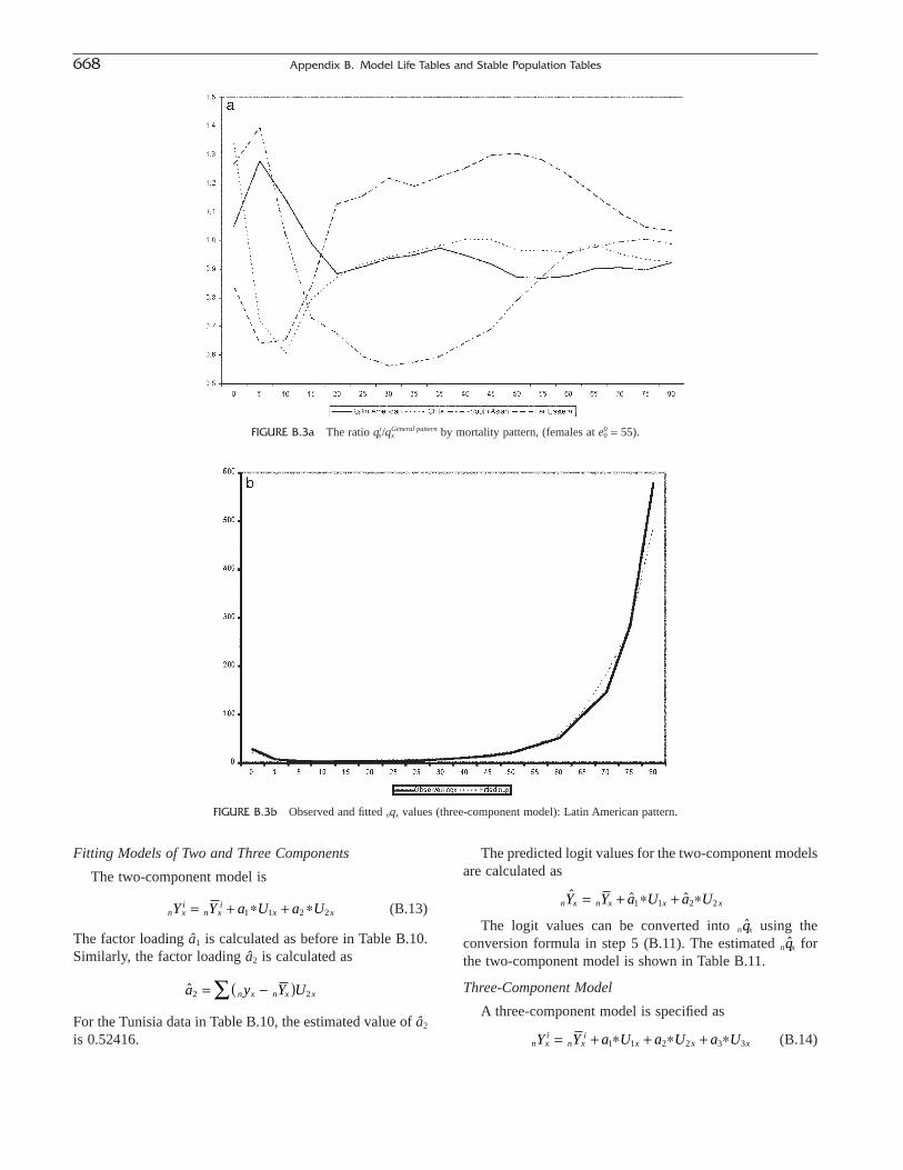
Fitting Models of Two and Three Components
The two-component model is
(B.13)
The factor loading â1 is calculated as before in Table B.10.Similarly, the factor loading â2 is calculated as
For the Tunisia data in Table B.10, the estimated value of â2
is 0.52416.
â y Y Un x n x x2 2= -( )Â
n xi
n xi
x xY Y a U a U= + +1 1 2 2* *
The predicted logit values for the two-component modelsare calculated as
The logit values can be converted into n x using the conversion formula in step 5 (B.11). The estimated n x forthe two-component model is shown in Table B.11.
Three-Component Model
A three-component model is specified as
(B.14)n xi
n xi
x x xY Y a U a U a U= + + +1 1 2 2 3 3* * *
q̂q̂
n x n x x xY Y a U a Uˆ ˆ * ˆ *= + +1 1 2 2
668 Appendix B. Model Life Tables and Stable Population Tables
FIGURE B.3a The ratio qix/qx
General pattern by mortality pattern, (females at e00 = 55).
FIGURE B.3b Observed and fitted nqx values (three-component model): Latin American pattern.

The factor loadings â1 and â2 are estimated as shown earlier.The factor loading â3 is estimated as
For the Tunisia data in Table B.10, the factor loading â3
is estimated to be -0.11071. The estimated three-componentlogit model is obtained for the data as
The logit values are converted into n x values as in step5. These values are shown in Table B.11.
The fit of the model is examined by computing the sumof the squares(ss) of the deviations of the observed from thefitted values, divided by thermometer of age groups as
(B.14)
where 18 is the number of age groups involved.The values of SS for the three fitted models are as follows:
Model SS
One component 0.05814Two components 0.01267Three components 0.01076
SS q qn x n xx
= -( )Â118
2ˆ
q̂
n x n x x x
x
Y Y U U
U
ˆ . * . *. *
= + +-
2 38159 0 52416
0 110711 2
3
â y Y Un x n x x3 3= -( )Â
Appendix B. Model Life Tables and Stable Population Tables 669
TABLE B.10 Fitting the Latin American Model to Tunisian 1995 Female Life Table
n x (Latin nYx - n x n x = n x + U1xâ1
Exact nqx nyx American pattern) (2) - (3) = U1x (3) + (5)(-2.38159) = n x
age (1)1 (2) (3)2 (4) (5)3 (6) (7)4
0 .02715 -1.78943 -1.22452 -0.56491 0.18289 -1.66009 0.034881 .00657 -2.50932 -1.45667 -1.05265 0.31406 -2.20463 0.012015 .00295 -2.91150 -2.13881 -0.77269 0.31716 -2.89415 0.00305
10 .00220 -3.05854 -2.46676 -0.59178 0.30941 -3.20365 0.0016415 .00280 -2.93767 -2.31810 -0.61957 0.32317 -3.08776 0.0020720 .00310 -2.88662 -2.14505 -0.74157 0.32626 -2.92207 0.0028825 .00374 -2.79246 -2.03883 -0.75363 0.30801 -2.77238 0.0038930 .00479 -2.66821 -1.93924 -0.72897 0.29047 -2.63102 0.0051535 .00683 -2.48979 -1.83147 -0.65832 0.25933 -2.44909 0.0074040 .01055 -2.27051 -1.74288 -0.52763 0.22187 -2.27128 0.0105345 .01391 -2.13057 -1.62385 -0.50672 0.19241 -2.08209 0.0153050 .02031 -1.93806 -1.47924 -0.45882 0.17244 -1.88992 0.0223155 .03589 -1.64537 -1.28721 -0.35816 0.15729 -1.66181 0.0347760 .05112 -1.46055 -1.07443 -0.38612 0.14282 -1.41457 0.0557765 .09872 -1.10576 -0.83152 -0.27424 0.12711 -1.13424 0.0937670 .14614 -0.88260 -0.59239 -0.29021 0.11815 -0.87377 0.1483575 .28289 -0.46509 -0.35970 -0.10539 0.11591 -0.63575 0.2190080 .57791 0.15710 -0.08623 0.24333 0.09772 -0.31896 0.34571
Source: 1 United Nations, Damographic Yearbook, 1996, New York: United Nations, 1998.2 Table B.8.3 Table B.9.4 Formula B.12.
q̂YŷYY
TABLE B.11 Observed and Fitted nqx Values for 1995Tunisian Female Life Table
Fitted n x values based on Latin American pattern
One Two ThreeAge Observed nqx
1 component1 components2 components2
0 0.02715 0.03488 0.02073 0.019681 0.00657 0.01201 0.00698 0.007155 0.00295 0.00305 0.00335 0.00329
10 0.00220 0.00164 0.00170 0.0016815 0.00280 0.00207 0.00214 0.0022720 0.00310 0.00288 0.00313 0.0034125 0.00374 0.00389 0.00417 0.0044430 0.00479 0.00515 0.00518 0.0053535 0.00683 0.00740 0.00729 0.0073940 0.01055 0.01053 0.01029 0.0098845 0.01391 0.01530 0.01560 0.0147850 0.02031 0.02231 0.02335 0.0217155 0.03589 0.03477 0.03777 0.0351260 0.05112 0.05577 0.06039 0.0557565 0.09872 0.09376 0.10877 0.1031670 0.14614 0.14835 0.18340 0.1786675 0.28289 0.21900 0.27776 0.2734880 0.57791 0.34571 0.47297 0.48036
1 Source: Table B.10.2 See text.
q̂

The reduction in SS shows how additional componentsimprove the fit of the model. However, a comparison of theobserved and fitted values (Figure B.3b) indicates that thethree-component model based on the Latin American patternmay not be the best-fitting pattern for the Tunisian databecause the fitted values deviate widely from the observedvalues at older ages.
Example 2: Identification of Mortality Pattern in anObserved Life Table
In this example, a one-component model is fitted to thenqx values of the 1995 Tunisian female life table using allfour mortality patterns. The average of the squared devia-tions (SS) is calculated using the fitted n x values for eachpattern. The pattern with the smallest value of the averagethe squared deviations is chosen as the appropriate patternfor the data.
The calculations used for a one-component model inExample 1 are repeated, replacing the Latin American averagepattern of mortality (n
ix) with the Chilean, South Asian, and
Far Eastern patterns. The fitted n x values and the correspon-ding average of the squared deviations are shown in TableB.12. The table shows that the sum of squared deviations is the lowest for the South Asian pattern, suggesting that theTunisia mortality graph is likely to follow this pattern.
q̂Y
q̂
RELATIONAL MODEL LIFE TABLES
Because of the restrictive nature of the data involved inthe construction of model life tables, the mortality patternof some countries may not fit very well into them. Forexample, because the United Nations database did notinclude any life tables from sub-Saharan Africa, the mortal-ity pattern observed in these countries may not fit well intoany of the four patterns identified in the UN life tables. Toovercome this difficulty, Brass (1964, 1971) suggestedmodel life table construction basing on the relational prin-ciple. In this system, a mathematical relationship is speci-fied to relate pairs of life tables.
The Brass Relational Two-Parameter Logit System
Brass (1964, 1971) proposed a two-parameter logitsystem to construct model life tables. In this system, themodel specifies a simple linear relationship between thetransformed lx values of two life tables. Specifically, thisrelationship is expressed as follows:
(B.15)12
1 12
1ln ln
-= +
-l
l
l
lx
x
xs
xs
a b
670 Appendix B. Model Life Tables and Stable Population Tables
TABLE B.12 Fit of One-Component Model of Selected Mortality Patterns to 1995Tunisian Female nqx
Fitting n x values according to specified pattern
Age Observed nqx1 LA Ch SA FE
0 0.02715 0.03488 0.04763 0.04924 0.025881 0.00657 0.01201 0.00720 0.01697 0.005285 0.00295 0.00305 0.00176 0.00351 0.00156
10 0.00220 0.00164 0.00144 0.00156 0.0012615 0.00280 0.00207 0.00225 0.00206 0.0023920 0.00310 0.00288 0.00321 0.00245 0.0033225 0.00374 0.00389 0.00428 0.00298 0.0046130 0.00479 0.00515 0.00568 0.00392 0.0059135 0.00683 0.00740 0.00805 0.00553 0.0086040 0.01055 0.01053 0.01192 0.00850 0.0130845 0.01391 0.01530 0.01773 0.01337 0.0206250 0.02031 0.02231 0.02609 0.02317 0.0322355 0.03589 0.03477 0.04060 0.03966 0.0500560 0.05112 0.05577 0.06382 0.06835 0.0771765 0.09872 0.09376 0.10677 0.11218 0.1198570 0.14614 0.14835 0.16180 0.17900 0.1795075 0.28289 0.21900 0.23621 0.26977 0.2573780 0.57791 0.34571 0.35219 0.39516 0.39164
0.00323 0.00300 0.00198 0.00211
1 Source: Table B.10.2 Source: Table B.11.
SS = -( )Â1
18
2n x n x
x
q q̂
q̂

where lsx denotes the survival function of a standard life table.
Let
(B.16)
Then l(lx) is the logit transformation of 1 - lx. The modelequation (B.22) can be re-expressed as
(B.17)
The model equation contains two parameters a and b. Bychoosing a standard life table and values for parameters a and b, one can generate a set of life tables. The steps inconstructing model life tables based on a standard life tableare as follows:
1. Compute l(lsx), the logit transformation of 1 - ls
x valuestaken form the chosen standard life table, using Equation (B.23).
2. Choose values of a and b.3. Use Equation (B.23) to compute the logit transforma-
tion 1 - lx of a life table, l(lx).4. Convert the computed l(lx) (i.e., logit values of 1 - lx)
to lx values using the relation
Thus, for a given standard life table one can generate aset of life tables by varying the parameters a and b.
The Choice of Standard
Potentially, one can choose as a standard any life tablethat seems appropriate. Brass, in his earlier studies of Africa,proposed an African standard. This standard is characterizedby relatively low infant mortality and relatively high childmortality. Later he proposed a general standard similar tothe West-model life-table mortality pattern in the Coale-Demeny life tables. These Brass standards are widely usedin many applications. Table B.14 reproduces the logit valuesat selected ages.
The Effect of Changing a and b Parameters
Figures B.4a and B.4b depict the effect that changing the a and b parameters has on the survival curve. When theintercept term a varies and b remains the same, the survivalcurves form a set of nonoverlapping curves (Figure B.4b).Values of lx decrease with increasing values of a.
When the slope parameter b changes, keeping a same,the survival curves form a set of intersecting curves (FigureB.4a). It is easy to verify that the curves cross at the median
le
xlxs
=+ + ( )
1
1 2 2a bl
l a bll lx xs( ) = + ( )
l lll
ll
l
lx
x
xxs x
s
xs
( ) =- ( ) =
-12
1 12
1ln lnand
age of the standard life table. When b is greater than 1, thesurvival probabilities are greater than the corresponding sur-vival probabilities of the standard curve until the median ageof the standard life table and then the order is reversed.
Fitting the Brass Model to a Observed Life Table
The Brass relational model can be fit to an actual lifetable to capture the essential features of the mortality patternin the observed data. The steps are
1. Convert observed life table lx values (with l0 = 1) intologit values l(lx) using Equation (B.2).
2. Obtain the logit values of the standard life table l(lsx).
3. Fit the regression model l(lx) = a + b l(lsx) using the
least squares method.
The procedure is illustrated here using the 1995 Tunisianfemale life table and the Brass African pattern as the stan-dard (shown in Table B.14). Table B.15 shows the necessarydata to fit the model.
The model parameters estimated by the least squares procedure are â = -1.1194 (standard error 0.0225) and
= 0.9644 (standard error 0.0327). The fitted model has anadjusted R-square of 98.1%. A high negative interceptparameter reveals the improvement in the level of mortalitycompared to the standard. The closeness of the slope para-meter to 1 (b � 1) suggests that the pattern of the curve hasnot changed drastically from the pattern of the standard. Thesurvival probabilities predicted by the model are given inTable B.15. These predicted probabilities show that themodel overestimates the lx values at the very young and veryold ages.
b̂
Appendix B. Model Life Tables and Stable Population Tables 671
TABLE B.14 General and African Standard Life Table Logit Values
Age (x) General standard l(l sx) African standard l(ls
x)
1 -0.8670 -0.99725 -0.6015 -0.6514
10 -0.5498 -0.549815 -0.5131 -0.513120 -0.4551 -0.455125 -0.3829 -0.382930 -0.3150 -0.315035 -0.2496 -0.249640 -0.1817 -0.181745 -0.1073 -0.107350 -0.0212 -0.021255 0.0832 0.083260 0.2100 0.210065 0.3746 0.374670 0.5818 0.581875 0.8611 0.861180 1.2433 1.243385 1.7810 1.7810

Extensions of the Two-Parameter Relational Model
Because of the failure of the two-parameter model toadequately fit several life table mortality patterns, severalextensions to it have been proposed. This section brieflydescribes these extended models.
Following Ewbank et al. (1983), Namboodiri (1990) pro-posed the following five-parameter model:
(B.18)
where l(lx) denotes the logit of lx and lsx denotes the lx
value in the standard life table. If in the model b1 = b2 = b,the model reduces to the four-parameter model proposed byEwbank et al. (1983). When b1 = b2 = b and c and d Æ 0,the model reduces to the two-parameter Brass relationalmodel. Also note that when a = 0, b1 = b2 = b = 1, and cand d = 0, the model specification reduces to l(lx) = l(ls
x)(i.e., the observed life table is the same as the standard lifetable).
In the present model, the a and b parameters have thesame interpretations as in the two-parameter relational logitmodel. Changes in the a parameter shifts the lx curve verti-cally. Changes in b cause a pivoting around the median ageof the standard curve. The changes in the c parameter affectthe steepness of the survival curve at the young ages (seeFigure B.5a). Similarly changes in the d parameter affect theolder ages (see Figure B.5b). A positive value of c increasesthe mortality (or decreases survival chances) at the youngages compared to the standard, and a negative valuedecreases the mortality (or increases survival chances). Sim-ilarly, negative values of d increase the mortality (decreasethe survival chances) at older ages, and positive values of ddecrease the mortality (increase survival chances) at olderages.
l a b l
a b l
l
l
le
cl
e
dl
x
c l
xs
d l
xs
xs
xs
( ) = +-[ ] ( ) <
= +-[ ] ( ) >
( )
( )
1
2
10
10
if
if
672 Appendix B. Model Life Tables and Stable Population Tables
FIGURE B.4 Survival curves showing the effect of varing the a and b parameters. (a graph: a = 0 b varies; b graph: a varies, b = 1)
TABLE B.15 1995 Tunisian Female Life Table Values
l(lx) l(lsx)
Age lx1 logit (1 - lx) African standard Predicted lx
0 1.0000 X X 1.00001 0.9728 -1.78848 -0.9972 0.98475 0.9664 -1.67953 -0.6514 0.9705
10 0.9636 -1.63805 -0.5498 0.964415 0.9615 -1.60892 -0.5131 0.961920 0.9588 -1.57362 -0.4551 0.957625 0.9558 -1.53691 -0.3829 0.951530 0.9522 -1.49587 -0.3150 0.945135 0.9477 -1.44852 -0.2496 0.938240 0.9412 -1.38651 -0.1817 0.930145 0.9312 -1.30264 -0.1073 0.920350 0.9183 -1.20974 -0.0212 0.907255 0.8997 -1.09695 0.0832 0.888860 0.8674 -0.93908 0.2100 0.862265 0.8230 -0.76840 0.3746 0.820070 0.7417 -0.52741 0.5818 0.753375 0.6334 -0.27342 0.8611 0.640680 0.4542 0.09186 1.2433 0.460285 0.1918 0.71918 1.7810 0.2320
X Not applicable.1 Source: United Nations Demographic Year book, 1996, New York:
United Nations, 1998.

Fitting of the Five-Parameter Model
Because of the nonlinear nature of the model, iterativeprocedures are required to fit it to observed data. The iterative procedure “NLIN” in SAS (SAS Institute, 1997)was used to fit the model to the Tunisian data in Table B.15.The estimated parameter values are as follows:
Parameter Estimate Standard error
a -1.7112 0.0117b1 1.3457 0.0952b2 1.0450 0.0373c 1.8518 0.2136d 0.0072 0.0400
The model fit indicated a sum of squares of the residualsof 0.00421 with 13 degrees of freedom and a correspondingextremely low residual mean square of 0.00032. Constrain-ing b1 = b2 = b reduces the model to the four-parametermodel suggested by Ewbank et al. (1983). The fit of the four-parameter model yields a sum of the squares of the residu-als of 0.00632 with a residual mean square of 0.00045. Thedifference in the sum of squares of residuals provides a one-degree-of-freedom test to see the improvement of the five-parameter model over the four-parameter model. In thisexample, the difference in the residual sum of squares is0.00211. The test of the hypothesis, b1 = b2 = b, gives a valueof 6.52 for the F-test statisticd with 1 and 13 degrees offreedom. In this case, the null hypothesis is rejected, favor-ing the five-parameter model.
The predicted values of lx under the four- and five-parameter models as well as under the two-parameter modelare given in Table B.16. The improvement in the fit of thefive-parameter model over Brass’s two-parameter model is clearly evident from the table. The five-parameter modelshows better predicted values at the very young and very oldages.
OTHER PARAMETRIC MODELS
Modern computer power has facilitated fitting complexmathematical models to describe the age pattern of mortal-ity. Three such models that have gained attention are brieflydescribed here.
Appendix B. Model Life Tables and Stable Population Tables 673
FIGURE B.5 Survival curves showing effect of changes in C parameter (graph a) and effect of changes in D parameter (graph b).
TABLE B.16 Comparison of the Fitted lx Values for the 1995Tunisian Female Life Table under Five-, Four-, and Two-
Parameter Models
Predicted lx
Five- Four- Two-Observed parameter parameter parameter
Age lx1 model model model (Brass)
0 1.0000 1.0000 1.0000 1.00001 0.9728 0.9725 0.9734 0.98475 0.9664 0.9665 0.9662 0.9705
10 0.9636 0.9634 0.9628 0.964415 0.9615 0.9621 0.9614 0.961920 0.9588 0.9597 0.9589 0.957625 0.9558 0.9561 0.9552 0.951530 0.9522 0.9519 0.9510 0.945135 0.9477 0.9467 0.9462 0.938240 0.9412 0.9403 0.9402 0.930145 0.9312 0.9312 0.9320 0.920350 0.9183 0.9167 0.9199 0.907255 0.8997 0.8974 0.9009 0.888860 0.8674 0.8703 0.8727 0.862265 0.8230 0.8261 0.8266 0.820070 0.7417 0.7547 0.7522 0.753375 0.6334 0.6312 0.6252 0.640680 0.4542 0.4334 0.4279 0.460285 0.1918 0.1972 0.2002 0.2320
1 Source: Table B.15.

Additive Multicomponent Model
Helligman and Pollard (1980) proposed an additive multicomponent model to describe the age pattern of humanmortality:
(B.19)
where f(x) is the age-specific death rate at age x. The firstcomponent depicts infant and child mortality. The A para-meter is the mortality at age 1, and B measures the differ-ence in mortality between ages 0 and 1. An increase in theB value indicates convergence of the two mortality rates.The C parameter captures the decline in child mortality withage. The second component tracks mortality at young adult-hood. The D parameter captures the intensity of mortality atvery young adulthood, E captures the young adult mortalityhump caused by accidents, and F captures the concentrationof mortality in young adulthood. The third componentdescribes mortality in older ages. The G parameter describesthe level and the H parameter describes the shape of the old-age mortality pattern. The model is nonlinear and needs aniterative procedure to estimate the model parameters fromdata on age-specific death rates.
Multiexponential Model
Rogers and Little (1994) proposed a multicomponentexponential model to describe the age pattern of mortality.The specific model is as follows:
where f(x) is the age-specific mortality rate, a0 is a constant,
f4(x) = a4e-a4x (B.20)
Note that f 2(x) and f 3(x) are double exponential distributions.
The first component describes childhood mortality andthe last component describes mortality at older ages. Thetwo middle components describe mortality at the middleages, including the hump caused by accidental mortality.
Generalized De Moivre Function
Di Pino and Pirri (1998) suggested a generalized DeMoivre function to describe the age pattern of mortality. Thespecific model is
f x a e x e x
3 33 3 3 3( ) = - -( )- -( )a m l m
f x a e x e x
2 22 2 2 2( ) = - -( )- -( )a m l m
f x a e x1 1
1( ) = ( )-a a single exponential function
f x a f x f x f x f x( ) = + ( ) + ( ) + ( ) + ( )0 1 2 3 4
f x A DeGH
GHx B E x F
x
x
C( ) = + ++
+( ) - -( )ln ln 2
1
(B.29)
The right-hand side is a polynomial, that as the sum of aseries of powers of age x. In practice it is found that a poly-nomial of degree 5 (k = 5) will fit the data well. The lower-power parameter influences the mortality of the young themost. The model is easy to fit to a set of data, and it doesnot require an iterative procedure.
CONCLUDING COMMENTS
This appendix presents several models that are used todescribe age patterns of mortality. The empirically basedones such as the Coale-Demeny and the United Nationsmodel life tables have seen widespread use in estimatingdemographic parameters from limited data. For the purposesof generating life tables for population projections wheredata are limited, any one of the models presented in thisappendix can be used. The empirically based models maynot always represent the mortality pattern of a country. Onthe other hand, some countries may not have the minimumdata needed to estimate sophisticated relational models aswell as the other parametric models.
References
Brass, W. 1964. “Uses of Census or Survey Data for Estimation of Vital Rates.” African Seminar on Vital Statistics. Addis Ababa: U. N.Economic Commission for Africa.
Brass, W. 1971. “On the Scale of Mortality.” In W. Brass (Ed.), Bio-logical Aspects of Demography. London: Taylor & Francis: 69–110.
Brass, W., A. J. Coale, P. Demeny, D. F. Heisel, F. Lorimer, A. Rumaniuk,and E. van de Walle. 1968. The Demography of Tropical Africa. Princeton, NJ: Princeton University Press.
Coale, A. J., and P. Demeny. 1966. Regional Model Life Tables and StablePopulations. Princeton, NJ: Princeton University Press.
Coale, A. J., and P. Demeny. 1983. With B. Vaughan. Regional Model LifeTables and Stable Populations, 2nd ed. New York: Academic Press.
Demeny, P., and F. C. Shorter. 1968. Estimating Turkish Mortality, Fertil-ity and Age Structure. Istanbul: Istanbul University, Statistics Institute.
Di Pino, A., and P. Pirri. 1998. “Analysis of Survival Functions by a Logis-tic Derivation Model: The ‘Generalized de Moivre’ Function.” GenusLIV (3–4): 35–54.
Ewbank, D. C., J. C. Gomez de Leon, and M. A. Stoto. 1983. “A ReducibleFour Parameter System of Model Life Tables.” Population Studies 37:105–127.
Gompertz, B. 1825. “On the Nature of the Function Expressive of the Lawof Human Mortality. Philos. Trans. R. Society 115: 513–593.
Heligman, L., and J. H. Pollard. 1980. “The Age Pattern of Mortality.” TheJournal of Institute of Actuaries 10: 49–80.
Ledermann, S. 1969. “Nouvelles tables-type de mortalité.” Travaux et documents, Cahier n.53. Paris: INED.
Ledermann, S., and J. Breas. 1959. “Les dimensions de la mortalité.” Pop-ulation 14 (4): 637–682.
Makeham, W. M. 1860. “On the Law of Mortality and the Construction ofAnnuity Tables.” Journal of Institute of Actuaries 8: 301–310.
ln . . .l
la a x a x a x a xx
xk
k
10 1 2
23
3
-= + + + + +
674 Appendix B. Model Life Tables and Stable Population Tables

Merli. M. G. 1998. “Mortality in Vietnam, 1979–1989.” Demography35(3): 345–360.
Namboodiri, N. K. 1990. Demographic Analysis: A Stochastic Approach.San Diego, CA: Academic Press.
Rogers, A., and J. S. Little. 1994. “Parameterizing Age Patterns of Demo-graphic Rates with the Multiexponential Model Schedules.” Mathe-matical Population Studies 4: 175–195.
SAS Institute. 1997. SAS/STAT Software: Changes and Enhancementsthrough Release 6.12: The NLIN Procedure. Cary, NC: SAS Institute.
United Nations. 1955. Age and Sex Patterns of Mortality: Model Life Tablesfor Under developed Countries. New York: United Nations.
United Nations. 1982. Model Life Tables for Developing Countries. NewYork: United Nations.
United Nations. 1983. Manual X: Indirect Techniques for DemographicEstimation. New York: United Nations.
United Nations. 1998. Demographic Yearbook, 1996. New York: UnitedNations.
Appendix B. Model Life Tables and Stable Population Tables 675

This Page Intentionally Left Blank

This appendix treats a variety of topics concerned with methods of measurement and analysis. None is strictly demographic; yet all are applicable to many fields of demography. The methods and basic concepts presented are ones that the demographer will find useful regardless ofhis or her special subject interest, but they are especially pertinent for work in population estimates and projections.1
This appendix will proceed in the following order:
• The first section of this appendix will give an overviewof sampling theory in demographic surveys and discuss bothsampling and nonsampling error in surveys, and use ofexternal information to add value to surveys, particularlyHorvitz-Thompson estimation, poststratification, statisticalmatching, and synthetic estimation.
• The second and third sections describe standardmethods for interpolating point and grouped data and curvefitting, and the general approach to parameterizing demo-graphic models. Such methods are standard parts of thedemographer’s tool kit.
• The fourth section describes methods for adjusting distributions to marginal totals, both classical multiwayadjustment methods and more modern loglinear methods. Such methods are frequently used in estimation contexts andwhen reconciling different estimation methods or datasources.
• The fifth section will present an overview of thegrowing role of computer models and databases in demo-graphic research. In particular, the section discusses how filehandling affects demographic analysis and common dataconfigurations and describes the features of massive data
warehouses (also known as administrative records) fordemographic work.
• The sixth section describes the features of and use ofmatrix methods in demography.
• The seventh section explores additional topics, such asmicrosimulations, system dynamics models, and regionaldemographic-economic models, that are relevant to thedemographer’s job, but for which space precludes a detailedexposition. This section will be necessarily brief on eachspecific topic.
SAMPLING, SAMPLING ERRORS,AND OTHER ERRORS IN SURVEYS
Sampling as an Alternative to “Complete” Data Collection
The basic principle that motivates the use of statisticalsampling is that a large number of measurements takenpoorly often yields less useful information than a smallnumber of measurements taken well. A quintessentialexample is an event that occurred in the Office of PriceAdministration during World War II in the United States. Atthat time, rubber was an extremely important commodity forthe war effort, but, because of the war, it was in short supply.The office attempted to send a survey to every automobiledealership in the United States, asking about automobiletires. As can be imagined, the response to this survey wassufficiently low that the estimates obtained by this “blanketsurvey” were extremely poor. The office instituted a sample,in which dealership data were vigorously pursued. Bymaking sure that nonresponse was kept to a minimum and that data were recorded accurately, a better pictureof the supply was obtained. Often, so-called complete data
677
A P P E N D I X
C
Selected General Methods
D. H. JUDSON AND CAROLE L. POPOFF
The Methods and Materials of DemographyCopyright 2003, Elsevier Science (USA).
All rights reserved.
1 Spreadsheets and programs implementing the models describedherein can be obtained from the authors.

collection is in fact less informative than a properly drawnand representative sample (Wallis and Roberts, 1962;Thompson, 1992).
Criteria for an Acceptable Sample Design
To draw acceptable inferences from the data collectedfrom a sample, it is necessary that the sample have measur-able reliability and that it be efficient and practical. Themeasurability requirement means that every member of thepopulation must have a known probability of being selectedin the sample; it is then possible to compute the reliabilityof the estimates made from the sample, using the sampledata only. The efficiency requirement means that the sampledesign that is used should give the most reliable informationpossible, considering the time and money available. Thepracticality requirement means that it can be carried out,operationally, as specified. Adequate supervision and controlare needed so that the methods specified are carried out correctly.
Variability in Surveys
Because a survey is based on a sample, the calculations(or estimates) generated from a particular sample design willdiffer from one sample to the next. If one took anothersample at the same data, using differently randomly selectedareas, households, establishments, or persons, one wouldobtain slightly different results from those based on the firstsample. Moreover, if one took a second sample on the heelsof the first, one would certainly obtain slightly differentresults than acquired from the first sample. There are twoprimary kinds of variability (or error) in sample results ofinterest: sampling variability refers to the variability causedonly by sampling itself; nonsampling variability refers to thedifferent responses repondents give over time, or limitationsof the survey instrument itself, including question wordingor varying patterns of nonresponse.
Sampling Variability
The sampling error of a sample survey can be measuredin several ways. The first measure usually desired is the vari-ance of the sample estimate. This is the average, over allpossible samples, of the squared deviations of the estimatesfrom their expected value. An estimate of the variance canbe obtained from the sample survey data themselves. If thereare nonsampling errors or the sample is biased, as is oftenthe case, then the deviations are taken around the true valueof the statistic and the measure is called the mean squareerror (MSE). Typically, the variance is denoted s2 and themean square error by MSE. Of these two measures, the MSEis more general, as illustrated by its formula. Suppose that
p is the value being estimated, and p̂ is the estimator of p;then the MSE of p̂ is given by:
(C.1)
If p̂ is unbiased, then the MSE is just the variance itself.
Nonsampling Variability and Error
In addition to the “error” of the estimates caused by sampling variability, there is another component of the total error in demographic data. Nonsampling error char-acterizes all surveys, whether sampling is used or not—including 100% surveys otherwise known as censuses. This component arises from mistakes made in the processof eliciting, recording, and processing the response of anindividual unit in the surveyed population. Every operationin a census or sample survey, and every factor within anoperation, may contribute to nonsampling error.
Because the nonsampling error arising from the respon-dent, in interaction with the interviewer and the question-naire is more serious and less amenable to measurement than errors arising from other operations, it is often calledresponse error. A typical example of response error arisingfrom respondents is the tendency of persons in many coun-tries to report their ages in years ending in zero and five(Ewbank, 1981). Often such response error requires specialdetection and smoothing methods; such methods aredescribed in Chapter 7 and later in this appendix.2
An interviewer’s tendency to change a respondent’sanswer to a question to conform more closely with his orher perception of the respondent’s socioeconomic class is an example of response error arising from the inter-action between respondent and interviewer. For example, ina working-class neighborhood, the interviewer may recordtotal income as wage and salary income and fail to inquireabout income other than wage and salary income (such asincome from investments or property rent).
The most important feature of nonsampling error is thatone often cannot reasonably assume that nonsampling erroris the same across different respondent groups. As noted byLessler and Kalsbeek (1992, p. 254), in the absence of anyhard data on bias, the assumption is often made that althoughthe measurements may be biased, the bias is the same foreach subgroup, so that subgroup comparisons remain valid.This assumption can be very wrong and should only be madewith extreme caution.
MSE p E p p E p E p E p p
E p E p E p p
p bias p
ˆ ˆ ˆ ˆ ˆ
ˆ ˆ ˆ
var ˆ ˆ
( ) = -( ) = - ( ) + ( ) -( )= - ( )( ) + ( ) -( )= ( ) + ( )
2 2
2 2
2
678 Judson and Popoff
2 Spreadsheets for performing detection and smoothing can be found at the U.S. Census Bureau, International Programs Center, atwww.census.gov/ipc/www/pam.html.
Use of Internal and External Information to Add Value
As noted earlier, estimates derived from sample surveyswill vary from the true population value because of both thesample itself and nonsampling errors. However, when extrainformation about the population is available, this infor-mation can be used to improve the survey estimates. The following section describes four methods for using extrainformation: the Horvitz-Thompson estimation theory(Horvitz and Thompson, 1952), poststratification, statisticalmatching, and synthetic estimation.
Horvitz-Thompson Theory
In any sampling plan where objects have nonequal probabilities of selection, a method for correcting for thisnonequal probability must be devised. For example, if, in asample survey, the sample design is such that households inrural areas are half as likely to be sampled as those in urbanareas, then each sampled rural household actually representstwice as many potential respondents as an equivalent urbanhousehold. This intuition is the basis of Horvitz-Thompson(Horvitz and Thompson, 1952) sampling theory.
If a sample of size n is selected from a population of sizeN, each with equal probability n/N, then any total in the pop-ulation can be estimated by multiplying the correspondingsample total by N/n. The quantity N/n is called the samplingweight or “raising” factor (Macro International, 1996) and,under equal probability sampling, corresponds to 1/p, wherep is the probability of selection. However, if selection prob-ability varies across the i units, then the “raising” factor forthe ith unit is 1/pi.
Consider estimating the mean of some quantity Y in thepopulation. If each sampled unit responds with value Yi, thenthe estimate of the population total is simply the sum overall responses:
where, as usual, the “hat” indicates that the calculated quan-tity is an estimate of a population parameter. However, whenindividual cases are sampled with unequal probability, thebasic approach of Horvitz-Thompson is to weight the ithcase by the inverse of its probability of selection, pi. Thus, the Horvitz-Thompson estimator of the population totalwould be
(C.2)
Consider what this implies: If a particular case is sampledwith probability 1, then it adds its full value to the estimate;but if a particular case is sampled with probability 1/2, thenit adds twice its value to the estimate. This conforms to theintuition stated earlier: If a household has a 1/2 chance of
ŶY
pi
ii
n
==Â
1
Ŷ Yii
n
==Â
1
being selected, then because it was selected it represents twohouseholds, itself and the other household that was notselected. Hence, it is doubly weighted.
For fixed n and pi known, and if pij is the probability thatboth unit i and unit j are included in the sample, the vari-ance of the Horvitz-Thompson estimator is
(C.3)
As noted by Thompson (1992, p. 49), if all the jointlyincluded probabilities pij are greater than zero, an unbiased estimator of this variance is given by
(C.4)
Thus, when the sample has known probabilities of selec-tion and joint probabilities of selection, the researcher canalways use this theory to estimate population means and the variance around those estimates. In cases where all unitshave equal probability of selection, the Horvitz-Thompsonestimator reduces to the “usual” estimator. The strength ofthis method of estimation is that if the probability of selec-tion can be known, it is an extremely general method ofaccount for the sample design effects.
Poststratification to External Data
The Horvitz-Thompson theory is used to account for nonequal probability of selection. However, this does notaccount for nonsampling errors such as undercoverage ofcertain population segments in the original sample frame orresponse biases. To account for these factors, poststratifica-tion to external data or adjustment to independent “controls”is often used.
Effectively, poststratification has the effect of “upweight-ing” cases that, for one reason or another, are underrepre-sented in the sample, and “downweighting” cases that areoverrepresented in the sample. But how is it determinedwhether some cases are over or underrepresented? Typi-cally, the demographic characteristics of the sample surveyare compared to estimated characteristics of those personsor households living in the comparable area. If a particulardemographic group appears less often in the sample than it“should”, on the basis of the external estimates, then thatgroup is given a weight greater than 1. If that group appearsmore often in the sample than it “should,” then it is given aweight less than 1. The poststratification estimator of a pop-ulation total is then
(C.5)
where wi is the poststratification weight for the ith case. Notethat if all weights are 1.0, then the poststratification estima-tor is the same as the usual estimator.
Ŷ w Yps i ii
n
==Â
1
Var Yp p
Yp p p
YYi ii
n
ii j ij
i ji ji
n
ˆ ˆ( ) = -ÊË
ˆ¯ + -Ê
ˈ¯= <=
 ÂÂ1 12
1 12
1
2
1
Var Yp
pY
p p p
p pYYi
ii
n
iij i j
i ji j
i ji
nˆ( ) =
-ÊË
ˆ¯
ÈÎÍ
˘˚̇
+-Ê
ˈ¯= π=
 ÂÂ1
1
2
1
Appendix C. Selected General Methods 679

Note that postratification and unequal probability ofselection can be incorporated simultaneously by includingboth weighting to external data via wi and sampling weightsvia pi. It is conceptually important, however, to maintain thedistinction between them because they are intended to dealwith different things. As noted by Lohr (1999, p. 115), post-stratification can be risky. One can obtain arbitrarily smallvariances if one chooses the strata after examining the data,just as one can always obtain statistically significant resultsif one decides on null and alternative hypotheses afterlooking at the data. Poststrata should be specified beforeexamining the data.
Statistical Matching
A modern approach to adding value to a survey is to use statistical matching to add donated data to the existingdata set. It has found particular application in the area ofmicrosimulation (Cohen, 1991), which will be describedlater. Suppose the researcher has two populations, labeledthe “target” population and the “donor” population. Thetarget population has a collection of variables unique to it,labeled 1. Both populations have a collection of commonvariables, which are labeled 1 for the target database and
2 for the donor database. Finally, the donor population hasa collection of variables unique to it, which are labeled 2.(When referring to the Y values in the target database, labeltheir 1.) The researcher takes samples from each populationusing some probability sampling mechanism (while thismust be taken into account in practice, it is not important tothis ex-position). Assume that the sample size of the targetdatabase is N1, and the sample size of the donor database isN2. To refer to the ith case in the target population, subscriptthe variables 1, and 1 and 2; i.e. 1i refers to the variablesunique to the target database for the ith case, while 1j refersto the variables common to both databases, but for the jthcase in the donor database.
With this terminology in mind, suppose that one wishesto add some variable Y from the donor population databaseto the target population database. The problem is to imputevalues for a variable that is missing in the target data set, but exists in the donor data set, i.e., to add value to the targetdata set. To simulate the variation in Y values that occurs inthe donor population as closely as possible, an individualunique donor amount is found for each record rather thanusing an average or a simple distribution. The problem maybe thought to be analogous to constructing a pseudo-controlgroup for an experimental design study when a randomassignment between treatment and control groups is not pos-sible (Rubin, 1979). It is also analogous to “imputation”methods—estimating a response when it was not given in asurvey.
There are essentially two methods for finding “donors”from one data set for the missing variable Y in the target data
rX
rZ
rX
rX
rZ
rY
rY
rX
rX
rZ
set. One method is to employ some distance-measure algo-rithm typically used in clustering techniques to find the“nearest neighbor” or single unique donor in the donor data-base, then set the value of the missing value Y in the targetdatabase equal to some function of the amount from thedonor. (It is a “function” of the donor amount because thereis additional uncertainty associated with the amount thedonor should give to the target.) Another method is toemploy a multiple regression model Ŷ = to generate theexpected value Ŷ2 of the variable of interest from the donordata set; calculate the expected value Ŷ1 for each record inthe target data set; perform a simple match using a distancemeasure on each estimated value. Finally, set the value ofthe missing variable equal to some function of the actualamount recorded for the donor. Each of these methods usesa set of variables common to both data sets that are believedto be reliable indicators of the missing variable. Forexample, if the missing variable is the value of the person’soccupied house, a set of reliable indicators might includehousehold income, persons per household (as a proxy fornumber of bedrooms), and some set of neighborhood characteristics.
Statistical matching algorithms can be constrained orunconstrained. In unconstrained matching, each member ofthe target data set must appear in the final, matched data, butit is not required that each member of the donor data setappear; in addition, a donor record can be used more thanone time. In constrained matching, either (1) all recordsfrom both files must appear on the final data set, replicatedif necessary, or (2) donors can be used only one time each.For the purpose of illustrating a statistical match, the nextsection compares two unconstrained matching algorithms: anearest-neighbor centroid method and a multiple regressionmodel-based method (e.g., Rubin, 1986).
Nearest-Neighbor Centroid Method
In the nearest-neighbor centroid method, the centroid of a cluster (the set of indicator variables) is the averagepoint in the multidimensional space defined by the variableschosen for matching. The difference—for example, simpleor squared Euclidean distance between the two clusters—is determined as the difference between centroids. Stan-dardized variables are used to mitigate different magnitudesof measure for each variable. The Mahalanobis distance is a standardized form of Euclidean distance wherein dataare standardized by scaling responses in terms of standard deviations, and adjustments are made for intercorrela-tions between the variables. Using the centroid technique,each recipient would be paired to an unique donor based on the minimum Mahalanobis distance (Hair et al., 1995).
Model-Based Method
The model-based method is also known as predictivemean matching (Ingram et al., 2000; Rubin, 1986). Multi-
r̂b
rX
680 Judson and Popoff

ple regression modeling was described earlier in this section.In this technique, the researcher uses multiple regression tofind the expected value of the variable of interest, then cal-culates the expected value for each record in both data sets.Then he or she performs a simple match using a distancemeasure on each estimated value and finally sets the valueof the missing variable equal to some function of the actualamount recorded for the donor. Using this technique, thematch would be performed on one variable, the expectedvalue of each case under a regression model. To pick theminimum distance, the distance measure should be eitherEuclidean, Squared Euclidean or City-Block (Manhattan)distance (absolute value) as they eliminate negative distancevalues. For the purposes of this example, this section shalluse squared Euclidean distance as the distance measure tominimize in the selection of donors.
Uses of Matched Data
The two most important criticisms of statistical matchingare that (1) it relies on strong assumptions about the data,namely, that Y and Z are conditionally independent given theX data, and (2) because additional variability is not incor-porated into the match, the matched data set may have lowervariance than implied in the donor population. While resultsare often reasonably close (e.g., Ingram et al., 2000), theycan still fail statistical tests to determine that the distribu-tions are the same (e.g., a chi-square test on a cross-tabulation). In simulations, several researchers (e.g., Draper,1992; Kadane, 1978; Paass, 1985) have noted that often thestatistically matched file does not reproduce the desired dis-tributional properties well. However, as Cohen (1991) noted,the potential for novel uses of statistically matched data, particularly in microsimulations and imputation situationswhere direct data collection is not available, continues togenerate research interest in the technique (e.g., Moriartyand Scheuren, 2001).
Synthetic Methods of Estimation
When one takes a survey designed to construct an esti-mate at a high geographic level (e.g., a state or province),various clients often desire to have similar estimates at lower geographic level (e.g., counties or cities). Often, thesample design or sample size will not support direct esti-mates. Either the sample size is too small to make reliableestimates, or the sample design itself omitted certain lowergeographic levels, thus precluding direct estimates in theseplaces.
However, there are methods that allow one to use higher-level survey data to generate lower-level estimates by “bor-rowing information” obtainable at the lower geographiclevel and using relationships between the obtainable information and the quantity one wishes to estimate. Thismethodology is known as synthetic estimation. Similar ideas
can be constructed by regression techniques such as the“empirical bayes” method employed by the U.S. CensusBureau in their Small Area Income and Poverty Estimatesprogram (Citro et al., 1997; U.S. Census Bureau, 2000). The basic description of a synthetic estimate is given in Gonzalez (1973, p. 33); see also Chattopadhyay et al., 1999;Gonzalez and Hoza, 1978; Levy and French, 1977a, 1977b;and Siegel, 2002 (pp. 497–502). An estimate is obtained for a larger area; then the estimate is used to derive estimates forthe subareas, on the assumption that, within specific groups,the small areas have the same characteristics as the largerareas.
A simple, archetypal situation is illustrated by the use ofthe public use microdata sample (PUMS) from the decen-nial census. This file is a 1% or 5% sample of householdsfrom the complete census record. It is a microdata file—thatis, a file with virtually complete information on the house-hold and the individuals in the household. Because it is amicrodata file, it is potentially extremely useful for esti-mating the characteristics of certain kinds of persons andhouseholds. However, to protect confidentiality, the onlygeographic identifiers provided for the household are forareas with quite large populations. This means that if onewishes to estimate a smaller area’s characteristics, say, thecharacteristics of the persons living in households in a small county, he or she simply does not have data from thePUMS file.
At this point enters the notion of synthetic estimation.The researcher uses the PUMS data at a higher level of geo-graphical aggregation, ties them to data that can be obtainedat the lower level of aggregation, and makes an estimate ofthe characteristics for the lower-level area. For example, ifthe researcher wishes to estimate the average income of asmall county, she or he might have at hand the number ofhousing units of the four basic types (single family detached,single family attached, multifamily, and mobile home) fromthe local tax assessor’s office. If he or she calculates theaverage income for households in each type of housing unit,using the higher-level PUMS data, she or he can then applythese averages to each type of housing unit in the county toderive a synthetic estimate of the average income in thecounty.
Such an approach rests, of course, on the assumption thatthere is some fairly stable relationship between the hous-ing unit and the income of the household(s) residing there.Without that stable relationship, the estimate would havelittle validity. In general, because the relationships are notexact, researchers have found that such estimates are biased.However, if they apply the sample results to any particulargroup, they typically obtain unbiased estimates, but esti-mates with high sampling variability because the samplesizes for subgroups are so small (see, e.g., Heeringa, 1993).The research and analytic question at this point is which kindof “error”, bias or variance, is more bearable.
Appendix C. Selected General Methods 681
How does this apply to adding value to survey data? First,later, define the phrase formal research data3 to describeresults or estimates in which the analyst has a great deal ofconfidence and the phrase target database4 to describe datain which the analyst either has limited confidence, or inwhich the analyst does not have the particular data item ofinterest and onto which the analyst wishes to place theformal research’s information. To summarize the procedure,the analyst wishes to use the information in the target data-base as an indicator variable to “project” the informationobtained by formal research onto the target database. Thetarget data will be the data used to make the projection; theformal research estimates will be “projected.” Although thetechnique is most commonly used for small area estimation,instead of speaking only of larger and smaller “areas,” onecan think in terms of different sources of information andproject from the one kind of group estimate onto other kindsof group estimates.
Following Gonzalez (1973), and Gonzalez and Hoza(1978); but modifying terminology to generalize to this newcontext, we wish to estimate a characteristic x in a groupfrom our target database. Assume that there are N cases inthe formal research database and A cases in the target data-base. Identify G subgroups of the population (in both data-bases) and index the groups j = 1, 2, . . . , G; the subgroupsmust be exclusive and exhaustive. Further assume that onecan identify C cells of the population and index the cells i= 1, 2, . . . , C. Presume that for each cell i and group j, fromthe formal research database there is an estimate xij. Fromthe latter we can also obtain estimates x.j for j = 1, 2, . . . ,G. Where the “dot” indicates that the sum is taken over all
cells, so that .
A synthetic estimate is desired for the ith cell, which iscontained in the population defined by the formal researchdatabase and in the target database. From the target data-base, one can calculate proportions that each group repre-sents of the population—that is, the ith cell and the jth groupin the population represents a proportion—and
Finally, the analyst wishes to obtain a synthetic estimateof x for the ith cell, denoted x*i . This estimate is defined as
p piji
C
ijj
C
= =Â Â= =
1 1
1 1and
x xj iji
C
. ==Â
1
(C.6)
Thus, this method uses pij to project the characteristic of theith cell from the population defined in the formal researchdatabase to the ith cell in the target database.
What assumptions are made in this estimate? Perhaps themost important one is that the x.j estimate for the jth groupdoes not vary across the i cells in the formal research data.While this is a simple method for estimation, this assump-tion has proven to be problematic in synthetic estimates inactual use. Because the method applies averages to obtain asynthetic estimate, it does not account for variation (or het-erogeneity) in the cells. As the borrowed information data-base moves further away from the formal research database (for example, if the formal research takes place at a specificdate and the analysts makes estimates beyond this date; orif the formal research applies to a population that is dissim-ilar from the target population), the procedure becomesmove problematic. This may lead to a biased estimate.Sarndal (1984) identified the bias in the estimator as
(C.7)
where
Nij = the number of cases in the ith cell and jth groupx̄i. = the mean of the characteristic of interest for the ith
cell, this average being taken over all groupsx̄ij = the mean of the characteristic of interest for the ith
cell and jth group
As Sarndal (1984) indicated, the bias of the synthetic esti-mator is zero if the mean for the ith cell is equal to the meanof the ith cell in the jth group. The hope in synthetic esti-mation, therefore, is that this quantity will be close to zero.Wachter and Freedman (2000) noted that, in the presence ofheterogeneity within cells, increasing the sample size of theformal research database will not reduce the bias: The het-erogeneity does not go away just because of a reduction in sampling variability.
To attempt to avoid the bias problem, an extension of thismethod was tested by Gonzalez and Hoza (1978) in whichthey used the synthetic estimate as an independent variablein a regression-based estimating method (leading to theterm, regression-synthetic estimate). Heeringa (1993) dis-cussed the possibility of developing composite estimatorsthat are a weighted combination of the formal-researchresults (in his case, sample survey or design-based esti-mates) and the administrative-records results (in his case,the synthetic estimator). Both of these extensions are possi-ble, and the reader should consult the extensive researchpublications for more details.
bias x N x xi iji
G
i ij* .( ) = -( )=Â
1
x p xi ij jj
G
* .==
Â1
682 Judson and Popoff
3 Examples of “formal research” are a population survey performedwith care; a sample of an administrative-records database for which wehave verified the information with great care; or a carefully controlledcensus.
4 The term applies to any database in which we have limited confidenceand do not wish to use in a “count-based” or “direct” way. It could be anadministrative-records database of uncertain coverage or quality, a compi-lation of age-race-sex-and-Hispanic-origin estimates, as we describe later;or a census itself (if the characteristic we wish to estimate is not measuredin the census).

An application of the synthetic methodology to generateestimates of the number of uninsured persons for countiesin the United States was presented in Sigmund, Judson, andPopoff (1998), for Oregon, and in Popoff, Fadali, and Judson(2000) for Nevada. In each case, the state had state data onthe uninsured; in Oregon, data were obtained from theOregon Population Survey and in Nevada, from the U.S.Current Population Survey. In both states, age-race-sex-and-Hispanic-origin estimates were available for single years ofage for counties. (Other specific examples of the use of syn-thetic methods for projecting information from one databaseto another can be found in Hogan, 2000; Levy and French,1977a, 1977b; Reder, 1994; and Siegel, 2002).
The basic equation for synthetic estimation is
(C.8)
where
a Π{0, . . . , 85+} for ages r Π{W, B, API, AI} for whites, blacks, Asian and Pacific
Islanders, and American Indianss Œ {M, F} for the sexesh Œ {H, �H} for household and nonhousehold populationPa,r,s,h = the number of persons of age a, race r, sex s, and
ethnicity hm̂a,r,s,h = the proportion of persons of age a, race r, sex s,
and ethnicity h that have the health-related characteris-tic of interest (in this case, who are uninsured), m̂a,r,s,h Œ[0, 1]
x̂a,r,s,h = the number of persons of age a, race r, sex s, andethnicity h that have the health-related characteristic ofinterest (in this case, who are uninsured)
ˆ ˆ ,, , , , , , , , ,x Pa r s h a r s h a r s h= ◊ m
Thus, one uses the known age/race/sex/Hispanic number,and an estimated group-specific proportion who are unin-sured, to estimate the number of uninsured persons of thespecific group. The reduced form of synthetic estimation is,of course, to multiply an overall population by an overallproportion to get an overall number. Again, we use the “dot”notation to describe this method in this framework. For any variable ya,r,s,h, we define: . Define
other sums similarly if a, s, or h are “dotted”; that is, whena subscript is “dotted,” it merely indicates that one shouldsum over all elements of that subscript or, using more infor-mal language, “collapse” that margin.
Using Pa,r,s,h as an example, the total population of an areais equivalent to “collapsing” all margins, or
(C.9)
If one wishes to multiply the total population by someoverall uninsured proportion in the population, express thisnotion as
(C.10)
However, the synthetic methodology goes beyond thissimple notion and instead makes the multiplication on a cell-by-cell basis.5 Figure C.1 illustrates the advantage of
Total population uninsured = = ¥ˆ .... .... ˆ ...., , , , , , , , ,x P m
Total population = = ÂÂÂÂP Pa r s hhsra
...., , , , , ,
y ya s h a r s hr
,., , , , ,= Â
Appendix C. Selected General Methods 683
Per
cent
age
FIGURE C.1 Proportion uninsured across the age span: Hypothetical distribution illustrating advantage of finer detailin synthetic estimation.
5 The equation x̂.,.,.,. = P.,.,.,. · m̂.,.,.,. implies that one is “summing first, then multiplying”; the synthetic method reverses the order: One “multi-plies first, then sums” over the individual cells. The two methods are notequivalent.

making estimates by individual ARSH cells. For the pur-poses of this illustration, assume that the population can bebroken into five age groups, 0 to 19, 20 to 39, 40 to 64, 64to 79, and 80+. Further assume that 12% of the total popu-lation is uninsured. However, this proportion is not distrib-uted uniformly across the age groups. This figure illustrateswhy breaking the population into finer groups must neces-sarily generate more correct estimates. Identify the dottedline in the figure as the “true” proportion uninsured forsingle years of age.
Now, suppose one wishes to use only the proportion unin-sured for the total population, 12%, to make an estimate ofthe number uninsured. This proportion is dramatically incor-rect for the age groups that deviate from this average, asidentified by Sarndal’s bias equation. A similar argumentapplies to the estimate using only two age groups, and ascan be seen, using five age groups improves the estimate,although without the full original age detail the estimate willnot be as good as achievable with age detail.
When these three synthetic estimates are compared to the(hypothetical) true data, the mean of absolute errors (esti-mated proportion minus true proportion by age, divided by86 age groups) goes down as more detail is added to the synthetic computations. For example, using only the popu-lation average as the estimate, the mean absolute error is.061, while using two age groups to make the estimatereduces the mean absolute error to .049, and using five agegroups to make the estimate reduces the mean absolute errorto .03.
The advantage of the synthetic technique is that it isbroadly applicable and, with the appropriate information inthe target database, very flexible. Its disadvantage is that itdoes not account for heterogeneity within estimation cells;hence it has the bias noted earlier.
Connections between These Methods
Note that all of these techniques could be used together:For example, one might have a sample survey with proba-bility weights, poststratify it to independent population esti-mates, then use the survey to generate a synthetic estimateat lower geographic levels. Of course, other combinationsof techniques are possible as well.
INTERPOLATION OF POINT DATA
Introduction
Some Definitions
Interpolation is narrowly defined as the art of inferringintermediate values within a given series of data by use ofa mathematical formula or a graphic procedure. Extrapola-tion is the art of inferring values that go beyond the given
series of data. Many of the techniques used for interpolationare suitable also for extrapolation; hence, the term inter-polation is often used to refer to both types of inference.Broadly considered, interpolation encompasses mathemati-cal and graphic devices not only for estimating inter-mediateor external values in a series (e.g., annual population esti-mates from decennial counts, survivors in a life table for single ages from survivors at every fifth age) but also forsubdividing grouped data into component parts (e.g., figuresfor single years of age from data for 5-year age groups) andfor inferring rates for subgroups from rates for broad groups(e.g., birthrates by duration of marriage). Typically, thesedevices reproduce, or are consistent with, the given values.In this case we say that the fit is exact. In other cases, mod-ified interpolation formulas are used and the interpolated series does not pass through the original values or maintainthe original group totals. Then, we say that the fit is approximate.
Interpolation is, in a sense, a form of estimation, but nor-mally “interpolation” relates only to those forms of estima-tion that involve the direct application of mathematical orgraphic devices to observed data. Sometimes, however, it isused loosely to include some forms of estimation involvinga simple use of some external series of data suggestive ofthe pattern or trend in the range of interpolation. A princi-pal type of “interpolation” of this kind is interpolation byprorating. We discuss this method later.
Though there is frequent need for interpolated estimatesin demographic work, the degree of precision required bythe user in practice or actually supported by the data is oftentoo low to justify use of anything more than the more simpleforms of interpolation. Indeed, for some purposes demo-graphic data could satisfactorily be interpolated by runninga smooth line by hand through a set of plotted points. Forothers, complex methods of interpolation are essential.Sometimes, however, where highly complex methods ofinterpolation appear necessary, the problem may be that theinitial data are too defective or the number and spacing ofthe observations are inadequate.
Interpolation by mathematical formula has the quality of imputing a regularity or smoothness to the given seriesof data or even imposing these characteristics on the data.The regularity imputed or imposed may be unrealistic,however. There are often true fluctuations in populationgrowth or in the age distribution due to past variations in births, deaths, and migration, especially if there have been wars, epidemics, population transfers, refugee move-ments, and so on. Interpolation may usefully serve to adjustdefective data, even though some real fluctuations areremoved, or to eliminate abnormalities from a series, suchas those due to war, when the underlying pattern or trend iswanted.
This section first considers the methods of interpola-ting “point” values in a series, such as a time series; and
684 Judson and Popoff
among these we consider first those methods that can beemployed to fit the given data exactly. These methodsinclude polynomial interpolation, use of some types of expo-nential functions, osculatory interpolation, and use of splinefunctions.
Polynomial Interpolation
General Form of Equation
Polynomial interpolation is interpolation where the seriesis assumed to conform to an equation of the general type, y = a + bx + cx2 + dx3. . . . More or fewer terms may be used.As is well known, the equation y = a + bx is a straight line,or linear equation, which can be passed through any twogiven points. The equation y = a + bx + cx2 is a quadratic,or parabola, which can be passed through any three givenpoints. The equation y = a + bx + cx2 + dx3 is a cubic, whichcan be passed through any four given points. More gener-ally, a polynomial equation of the nth degree can be passedthrough n + 1 given points. Although one has decided to fita polynomial of higher degree to the observed data and apolynomial of the nth degree will give an exact fit for n + 1observations, one must still decide how many observationsto use. The choice of the degree of the polynomial woulddepend on the nature of the data to be interpolated. Usually,the simplest equation that describes the data reasonably welland gives a smooth series is the one wanted. The criterionof a smooth fit of the given data normally requires use of ahigher-degree equation than a straight line. Greater smooth-ness would normally be achieved by employing at least twoobservations before, and two observations after, the point ofinterpolation. This would seem to call for at least 4-pointinterpolation by a third-degree polynomial, where possible,but often 3-point or even 2-point interpolation will giveabout the same results.
In what follows, we will need symbols for given points.The symbol f(a) means the value of the function when xequals a, f(b) the value of the function when x equals b, andso forth. Hence, the symbol f(a) will be the observed valueof the y ordinate for the abscissa6 x = a. The symbol f(b) willbe the observed value of f(b) for x = b, and so on. The symbolf(x) will be the desired interpolated value of the function ffor any x.
Methods of Application
Polynomials that pass through the given data may befitted in several different ways operationally while produc-
ing the identical results. One is by general solution of thepolynomial equation and derivation of the values of the constants a, b, c, d, and so on; another is by use of inter-polation coefficients; still another is by sequential linear interpolation; and a fourth is by use of “differences.”Usually in polynomial interpolation by exact fit, the methodinvolving the general solution of the polynomial equation isnot employed because it is too cumbersome to perform “byhand.” However, with the advent of computational tools,some computationally intensive forms of interpolation havebecome popular. One, cubic spline interpolation, will bedescribed in detail with a computational example later in thissection.
Waring’s Formula
The formulas for polynomial interpolation can be setforth in the form of linear compounds—that is, as the sumof the products of certain coefficients or multipliers andcertain given values. The Waring formula, also known as theLagrange formula or the Waring-Lagrange formula, is usedto derive the multipliers to interpolate for the f(x) value cor-responding to a given x value. The Waring formula for inter-polating between four points by a polynomial, (i.e., forfitting a cubic) is as follows:
This is equivalent to the polynomial y = a + bx +cx2 + dx3 passing through the four points f(a), f(b), f(c), and f(d) to derive f(x). The points do not have to be equally spaced. By the formula, a particular value of (x) can be obtained from given values of f(a), f(b), f(c), and f(d).
The formula is especially suitable for computing the coefficients or “multipliers” to be applied to the f(a), f(b), f(c), and f(d) values to obtain f(x). These multipliersmay be used again and again so long as a y value on the same x abscissa is being sought and there are four given points spaced in the same way. In this way, forexample, the same multipliers may be used for all the age-sex groups in a distribution or for all the states in acountry to secure interpolated values at the same date. Themultipliers for any particular interpolation formula add to1.00.
Similarly, the formula
f x f ax b x c x d
a b a c a d
f bx a x c x d
b a b c b d
f cx a x b x d
c a c b c d
f dx a
( ) = ( ) -( ) -( ) -( )-( ) -( ) -( )
+ ( ) -( ) -( ) -( )-( ) -( ) -( )
+ ( ) -( ) -( ) -( )-( ) -( ) -( )
+ ( ) -(( ) -( ) -( )-( ) -( ) -( )
x b x c
d a d b d c
Appendix C. Selected General Methods 685
6 As an aid to explanation, in a cartesian two-way graph of y againstx, the “abscissa” is often referred to as the “x-axis” and the “ordinate” isoften referred to as the “y-axis.”
(C.11)

(C.12)
is equivalent to the polynomial y = a + bx + cx2, a parabolapassing through three points f(a), f(b), and f(c). This isWaring’s 3-point formula. By this formula, f(x) can be obtainfrom given values of f(a), f(b), and f(c). Extension to morepoints or fewer points should be obvious from an inspectionof Formulas (C.11) and (C.12).
Suppose the population in 1980 is Pa, the population in1990 is Pb, the population in 2000 is Pc, and one desires touse 3-point interpolation to estimate the population in 1995.Then,
(C.13)
The reader should note that the computational work couldhave been simplified if, instead of using dates like 1980,1990, 1995, and 2000, x (representing 1995) had been takenas “0” and the other dates as -3, -1, and +1, for 1980, 1990and 2000, respectively. (The simplified recodes come bynoting that 1980 is three units of 5 years each before 1995,1990 is one unit of 5 years before 1995, and 2000 is one unitof 5 years past 1995.) Accordingly,
(C.14)
The a, b, c (and so forth) values may be recoded in anydesired way so long as they maintain the same relativevalues. Thus, they can be multiplied or divided by a con-stant, and the differences between them can be divided by aconstant without any effect on the results.
f x f( ) = ( ) =( ) -( )-( ) -( ) +
( ) -( )( ) -( ) +
( )( )( )( )
= - + +
0 Pa Pb Pc3
Pa Pb Pc
1 12 4
3 12 2
14 2
125 750 375. . .
Pa5
Pb15
Pc15
=( ) -( )
-( ) -( )
+( ) -( )
( ) -( )
+( )
510 20
510 10
5(( )( )( )
= - + +20 10
125 750 375. . .Pa Pb Pc
Population in 1995
Pa1995 – 19901980 – 1990
Pb1995 – 19801990 – 1980
Pc1995 – 19802000 – 1980
= ( )
=( )( )( )( )
+( )( )( )( )
+( )( )( )( )
f 1995
1995 20001980 2000
1995 20001990 2000
1995 19902000 1990
––
––
––
f x f ax b x c
a b a cf b
x a x c
b a b c
f cx a x b
c a c b
( ) = ( ) -( ) -( )-( ) -( ) + ( ) -( ) -( )
-( ) -( )
+ ( ) -( ) -( )-( ) -( )
Aitken’s Iterative Procedure
Aitken’s (1932) iterative procedure is a system of suc-cessive linear interpolations equivalent to interpolation by apolynomial of any desired degree.7 It is especially suitablefor use with desk calculators or electronic computers.
Waring’s 2-point formula,
(C.15)
can be rewritten as
(C.16)
which is an expression that will appear in Aitken’s procedure as outlined next. Aitken’s system is set up in thefollowing basic format for interpolation between four given points for the value of f(x):
Given Proportionateordinates Computational stages parts
(1) (2) (3)f(a) (a - x)f(b) f(x; a, b) (b - x)f(c) f(x; a, c) f(x; a, b, c) (c - x)f(d) f(x; a, d) f(x; a, b, d) f(x; a, b, c, d) (d - x)
Only the first two lines would be used for 2-point orlinear interpolation, and there would be just one computa-tional stage. The first three lines and two computationalstages would be used for 3-point interpolation. Additionallines and computational stages are used as required for morepoints. As many points as desired can be used. The firstcolumn, “given ordinates,” symbolizes the given data (i.e., the four observations). The “proportionate parts” in theextreme right-hand column are differences between thegiven abscissa and the one for which the interpolation iswanted. The abscissa values may be transformed into sim-plest terms in order to reduce the calculations, as in the caseof the Waring formula.
The entries in computational stage 1 are each calculatedby computing diagonal cross-products, “differencing” them,and dividing by the difference between the proportionateparts, as follows:
(C.17)
(C.18)
and
f x a cf a c x f c a x
c x a x; ,( ) =
( ) -( ) - ( ) -( )-( ) - -( )
f x a bf a b x f b a x
b x a x; ,( ) =
( ) -( ) - ( ) -( )-( ) - -( )
f xf a b x f b a x
b x a x( ) =
( ) -( ) - ( ) -( )-( ) - -( )
f x f ax b
a bf b
x a
b a( ) = ( ) -( )
-( ) + ( ) -( )-( )
686 Judson and Popoff
7 Note: Other assumptions are possible.
(C.11)

(C.19)
Each of the expressions f(x; a, b), f(x; a, c), f(x; a, d), andso on is an estimate of f(x) obtained by linear interpolationor extrapolation of f(a) and one of the subsequent f(b), f(c),or f(d) values. The general process of successive linear inter-polations is repeated for computational stage (2), but thistime we use the results of computational stage 1 and theirassociated diagonal multipliers. Thus,
(C.20)
and
(C.21)
Suppose, for example, one wants to interpolate the population of an area in 1975, given data on population in1960, 1970, 1980, and 1990. The calculations are sum-marized in Table C.1. Table C.1 can be easily constructed ina spreadsheet; likewise, computation can easily proceed byhand or with a hand calculator. Our final interpolated figurefor 1975, 40,002, is the result of computational stage 3. Thegiven observations need not be equally spaced as they arein the example. Also, their order of arrangement in the tablecan be mixed; that is, they do not have to follow a prescribedorder. This interpretation of the results assumes, however,that the given data are not too widely spaced for a reliableresult. If the given data are widely spaced and have a highdegree of curvature in the region of interpolation, none ofthe interpolation procedures, including Aitken’s, will yielda reliable result: Observations closer to the desired abscissamust be used. In interpolations of demographic data, thecomputational stages should probably stop at about the pointwhere it is clear that there is no longer a clear convergencefrom stage to stage.
Aitken’s iterative procedure involves a relatively largeamount of work to arrive at a single result if many obser-vations are used, and the same amount of work must berepeated each time another interpolation is carried out. It is
f x a b df x a b d x f x a d b x
d x b x; , ,
; , ; ,( ) =( ) -( ) - ( ) -( )
-( ) - -( )
f x a b cf x a b c x f x a c b x
c x b x; , ,
; , ; ,( ) =( ) -( ) - ( ) -( )
-( ) - -( )
f x a df a d x f d a x
d x a x; ,( ) =
( ) -( ) - ( ) -( )-( ) - -( )
efficient to use this procedure, therefore, when only a fewinterpolations at most are required. In contrast, it is moreefficient to use the Waring formula when many interpola-tions are being carried out for the same abscissa or x-value,especially ones based on relatively few observations. Underthese circumstances, the coefficients, once derived, can beused over and over again.
Osculatory Interpolation
One of the chief difficulties met in adjusting rough databy the usual (single polynomial) interpolation formulas, asdescribed earlier, is that at points where two interpolationcurves meet, there are sudden breaks in the values of the first-order differences. Various methods have beenemployed to effect a smooth junction of the interpolationsmade for one range of data with the interpolations made for the next (adjacent) range. Osculatory interpolation is amethod that accomplishes that purpose. It involves combin-ing two overlapping polynomials into one equation. One ofthe polynomials begins sooner and ends sooner than theother, and the interpolations are limited to the overlappingparts. The second of the two polynomials in the first rangethen becomes the first polynomial in the second range. Theuse of one polynomial in common for each pair of succes-sive ranges permits a continuous welding of results from range to range. The two overlapping polynomials are generally forced to have specified conditions in common atthe beginning and at the end of the range in which inter-polation is desired. The specified conditions may include acommon ordinate, a common tangent (slope), or a commonradius of curvature, usually accomplished by making thefirst derivative or the first two derivatives equal for the twopolynomials.
Illustrative Formulas
Although osculatory interpolation encompasses a widevariety of possible equations, only a few have seen muchuse. This section considers specifically Sprague’s fifth-difference equation, Karup-King’s third-difference equation,Beers’ six-term formulas, and cubic spline interpolation.
Sprague’s Fifth-Difference Equation
The fifth-difference equation developed by Sprague isexpressed in terms of leading differences (Sprague, 1881).The equation is based on two polynomials of the fourthdegree, forced to have a common ordinate, a commontangent, and a common radius of curvature at Yn+2 and at Yn+3:
(C.22)
yx
yx x
yx x x
y
x x x xy
x x xy
n x n n n
n n
+ +! ! !
! !
22 3
43
5
21
2 12
2 13
2 1 14
1 5 74
=+( )
++( ) +( )
++( ) +( )
++( ) +( ) -( )
+-( ) -( )
D D D
D D
Appendix C. Selected General Methods 687
TABLE C.1 Illustration of Aitken’s Iterative Procedure
1975
Interpolation date Computational stagesProportionate
Date Population (1) (2) (3) parts
1960 16,321 1960 - 1975 = -151970 30,567 37,690 1970 - 1975 = -51980 52,108 43,161 40,426 1980 - 1975 = 51990 87,724 52,023 41,273 40,002 1990 - 1975 = 15
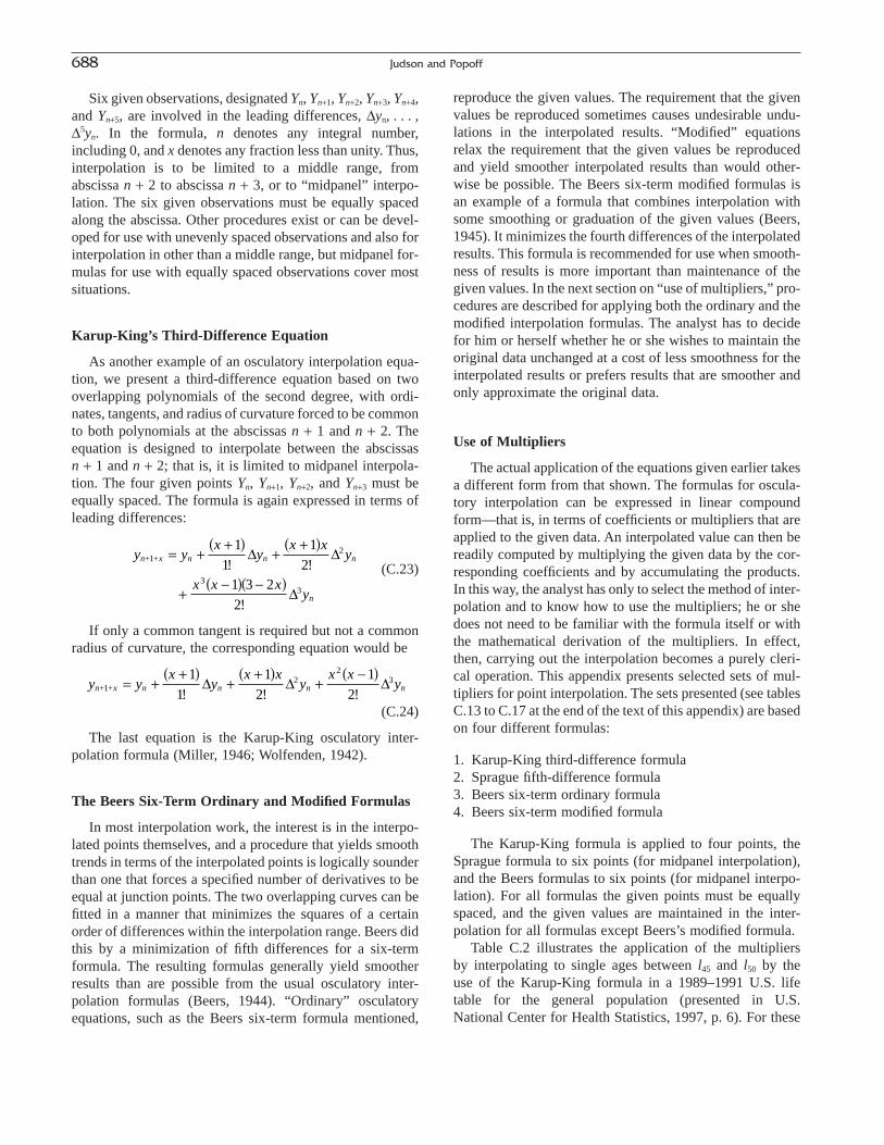
Six given observations, designated Yn, Yn+1, Yn+2, Yn+3, Yn+4,and Yn+5, are involved in the leading differences, Dyn, . . . ,D5yn. In the formula, n denotes any integral number, including 0, and x denotes any fraction less than unity. Thus,interpolation is to be limited to a middle range, fromabscissa n + 2 to abscissa n + 3, or to “midpanel” interpo-lation. The six given observations must be equally spacedalong the abscissa. Other procedures exist or can be devel-oped for use with unevenly spaced observations and also forinterpolation in other than a middle range, but midpanel for-mulas for use with equally spaced observations cover mostsituations.
Karup-King’s Third-Difference Equation
As another example of an osculatory interpolation equa-tion, we present a third-difference equation based on twooverlapping polynomials of the second degree, with ordi-nates, tangents, and radius of curvature forced to be commonto both polynomials at the abscissas n + 1 and n + 2. Theequation is designed to interpolate between the abscissas n + 1 and n + 2; that is, it is limited to midpanel interpola-tion. The four given points Yn, Yn+1, Yn+2, and Yn+3 must beequally spaced. The formula is again expressed in terms ofleading differences:
(C.23)
If only a common tangent is required but not a commonradius of curvature, the corresponding equation would be
(C.24)
The last equation is the Karup-King osculatory inter-polation formula (Miller, 1946; Wolfenden, 1942).
The Beers Six-Term Ordinary and Modified Formulas
In most interpolation work, the interest is in the interpo-lated points themselves, and a procedure that yields smoothtrends in terms of the interpolated points is logically sounderthan one that forces a specified number of derivatives to beequal at junction points. The two overlapping curves can befitted in a manner that minimizes the squares of a certainorder of differences within the interpolation range. Beers didthis by a minimization of fifth differences for a six-termformula. The resulting formulas generally yield smootherresults than are possible from the usual osculatory inter-polation formulas (Beers, 1944). “Ordinary” osculatoryequations, such as the Beers six-term formula mentioned,
y yx
yx x
yx x
yn x n n n n+1+! ! !
= ++( )
++( )
+-( )1
11
21
22
23D D D
y yx
yx x
y
x x xy
n x n n n
n
+1+! !
!
= ++( )
++( )
+-( ) -( )
11
12
1 3 22
2
33
D D
D
reproduce the given values. The requirement that the givenvalues be reproduced sometimes causes undesirable undu-lations in the interpolated results. “Modified” equationsrelax the requirement that the given values be reproducedand yield smoother interpolated results than would other-wise be possible. The Beers six-term modified formulas isan example of a formula that combines interpolation withsome smoothing or graduation of the given values (Beers,1945). It minimizes the fourth differences of the interpolatedresults. This formula is recommended for use when smooth-ness of results is more important than maintenance of thegiven values. In the next section on “use of multipliers,” pro-cedures are described for applying both the ordinary and themodified interpolation formulas. The analyst has to decidefor him or herself whether he or she wishes to maintain theoriginal data unchanged at a cost of less smoothness for theinterpolated results or prefers results that are smoother andonly approximate the original data.
Use of Multipliers
The actual application of the equations given earlier takesa different form from that shown. The formulas for oscula-tory interpolation can be expressed in linear compoundform—that is, in terms of coefficients or multipliers that areapplied to the given data. An interpolated value can then bereadily computed by multiplying the given data by the cor-responding coefficients and by accumulating the products.In this way, the analyst has only to select the method of inter-polation and to know how to use the multipliers; he or shedoes not need to be familiar with the formula itself or withthe mathematical derivation of the multipliers. In effect,then, carrying out the interpolation becomes a purely cleri-cal operation. This appendix presents selected sets of mul-tipliers for point interpolation. The sets presented (see tablesC.13 to C.17 at the end of the text of this appendix) are basedon four different formulas:
1. Karup-King third-difference formula2. Sprague fifth-difference formula3. Beers six-term ordinary formula4. Beers six-term modified formula
The Karup-King formula is applied to four points, theSprague formula to six points (for midpanel interpolation),and the Beers formulas to six points (for midpanel interpo-lation). For all formulas the given points must be equallyspaced, and the given values are maintained in the inter-polation for all formulas except Beers’s modified formula.
Table C.2 illustrates the application of the multipliers by interpolating to single ages between l45 and l50 by the use of the Karup-King formula in a 1989–1991 U.S. lifetable for the general population (presented in U.S. National Center for Health Statistics, 1997, p. 6). For these
688 Judson and Popoff

Appendix C. Selected General Methods 689
TABLE C.2 Karup-King Interpolation of an Except from Life Table for the Total Population, United States: 1989–1991
Karup-King interpolationx to x + 1 tqx lx tdx tLx Tx ex between 5-year intervals
Years0–1 0.00936 100,000 936 99,258 7,536,614 75.37 100,0001–2 0.00073 99,064 72 99,028 7,437,356 75.08 99,6282–3 0.00048 98,992 48 98,968 7,338,328 74.13 99,3553–4 0.00037 98,944 37 98,926 7,239,360 73.17 98,9584–5 0.0003 98,907 30 98,892 7,140,434 72.19 99,0045–6 0.00027 98,877 27 98,863 7,041,542 71.22 98,8776–7 0.00025 98,850 24 98,839 6,942,679 70.23 98,7907–8 0.00023 98,826 23 98,814 6,843,840 69.25 98,7618–9 0.0002 98,803 20 98,794 6,745,026 68.27 98,7639–10 0.00018 98,783 17 98,774 6,646,232 67.28 98,773
10–11 0.00016 98,766 16 98,758 6,547,458 66.29 98,76611–12 0.00016 98,750 16 98,742 6,448,700 65.3 98,74612–13 0.00022 98,734 21 98,723 6,349,958 64.31 98,72913–14 0.00032 98,713 32 98,697 6,251,235 63.33 98,70914–15 0.00047 98,681 46 98,658 6,152,538 62.35 98,68015–16 0.00063 98,635 62 98,604 6,053,880 61.38 98,635···40–41 0.00228 95,373 217 95,265 3,622,154 37.98 95,37341–42 0.0024 95,156 228 95,042 3,526,889 37.06 95,15642–43 0.00254 94,928 241 94,808 3,431,847 36.15 94,93243–44 0.00271 94,687 256 94,559 3,337,039 35.24 94,69544–45 0.00292 94,431 277 94,292 3,242,480 34.34 94,43845–46 0.00318 94,154 299 94,005 3,148,188 33.44 94,15446–47 0.00348 93,855 327 93,692 3,054,183 32.54 93,84847–48 0.0038 93,528 355 93,350 2,960,491 31.65 93,52648–49 0.00414 93,173 386 92,980 2,867,141 30.77 93,17849–50 0.00449 92,787 417 92,579 2,774,161 29.9 92,79550–51 0.0049 92,370 452 92,144 2,681,582 29.03 92,37051–52 0.00537 91,918 494 91,671 2,589,438 28.17 91,91052–53 0.0059 91,424 539 91,155 2,497,767 27.32 91,42053–54 0.00647 90,885 588 90,591 2,406,612 26.48 90,88954–55 0.00708 90,297 639 89,978 2,316,021 25.65 90,30555–56 0.00773 89,658 693 89,311 2,226,043 24.83 89,658···90–91 0.15135 17,046 2,580 15,757 76,698 4.5 17,04691–92 0.16591 14,466 2,400 13,266 60,941 4.21 14,54592–93 0.18088 12,066 2,182 10,975 47,675 3.95 12,17293–94 0.19552 9,884 1,933 8,918 36,700 3.71 9,97294–95 0.21 7,951 1,669 7,116 27,782 3.49 7,99395–96 0.22502 6,282 1,414 5,575 20,666 3.29 6,28296–97 0.24126 4,868 1,174 4,281 15,091 3.1 4,87597–98 0.25689 3,694 949 3,219 10,810 2.93 3,74098–99 0.27175 2,745 746 2,372 7,591 2.77 2,82499–100 0.28751 1,999 575 1,711 5,219 2.61 2,070100–101 0.30418 1,424 433 1,208 3,508 2.46 1,424101–102 0.32182 991 319 832 2,300 2.32 922102–103 0.34049 672 229 557 1,468 2.19 602103–104 0.36024 443 159 364 911 2.05 407104–105 0.38113 284 109 229 547 1.93 283105–106 0.40324 175 70 140 318 1.81 175106–107 0.42663 105 45 83 178 1.7 NA107–108 0.45137 60 27 46 95 1.59 NA108–109 0.47755 33 16 25 49 1.49 NA109–110 0.50525 17 8 13 24 1.39 NA
Notes: Bolded cells are the “reference” cells for the Karup-King interpolation formula.For interpolation of ages 0–1 to 4–5, the “first interval” coefficients are used.For interpolation of ages 101–102 to 105–106, the “last interval” coefficients are used.For interpolation of all other ages, the “middle interval” coefficients are used.
Because age 110 is not available, interpolations for 106–107 to 109–100 are not given (NA).Source: U.S. National Center for Health Statistics. U.S. Decennial Life Tables for 1989–1991, Volume 1, Number 1, United States Life Tables Hyattsville,
MD: U.S. National Center for Health Statistics, 1997.

interpolations, four points are used. The general form of theequation is simply
(C.25)
where x is a fraction between 0 and 1; N1, N2, N3, and N4
represent four known values; and m1, m2, m3, and m4 are thefour multipliers associated with the four given points. In thiscase, if one wishes to find l48, a value 0.6 of the way betweenl45 and l50, one has
(C.26)
or
(C.27)
The set of multipliers used for interpolating the middleinterval is given in Table C.13, Section A.
Selecting the multipliers for N2.6 from this table and thevalues of lx from the NCHS life table, then
Using the same formula with different coefficients, one canderive the following values for l46, l47, and l49
Computed bylx Karup-King formula Published
l45 94,154 94,154l46 93,848 93,855l47 93,526 93,528l48 93,178 93,173l49 92,795 92,787l50 92,370 92,370
As noted in Table C.2, the first group (ages 0 to 1 to 4 to5) uses the “first interval” coefficients, the last group (ages101 to 102 to 105 to 106) uses the “last interval” coefficients,and all others use the “middle interval” coefficients. Whileages 106+ are not calculated because age 110 (lno) is notavailable, if such interpolations were absolutely necessary,one could consider age 100 to 111 to be zero and use the“last interval” coefficients.
Once lx is calculated for single ages, the remainingcolumns of the left table may be completed by use of stan-dard formulas.
Cubic Splines
A method of interpolation of point data that has emergedstrongly with widespread access to electronic computers(although it existed in mechanical form earlier) is that ofcubic spline interpolation. Like other methods describedpreviously, it fits a piecewise cubic polynomial of the formy = a + bx + cx2 + dx3 to a portion of the data. However, withcubic splines, one constrains the relationship of one cubicspline to the next one in the series, specifically, so that theslope of the top end of the first polynomial must match the
l48 048 95 373 424 94 154
696 92 370 072 89 658 93 178
= - ( ) + ( )+ ( ) - ( ) =. , . ,
. , . , ,
l m l m l m l m l48 1 40 2 45 3 50 4 55= + + +
N m N m N m N m N2 6 1 40 2 45 3 50 4 55. = + + +
N m N m N m N m Nx2 1 1 2 2 3 3 4 4+ = + + +
slope of the bottom end of the next polynomial. This “com-plication” allows us to find a linear system of equations thatis solvable, thus giving us the collection of cubic spline coef-ficients needed.
Begin by presuming that one has an ordered collection of points x1, x2, x3, . . . , xn, along a continuum. To each ofthese points is associated some yj = f(xi). Following the derivation in Johnson and Percy (2000) and Burden andFaires (1993) closely, split the continuum into i intervals. Ineach interval the goal is to fit a cubic polynomial. Make thefollowing definition: hi = xi+1 - xi; that is, hi is just the dif-ference between two successive xi points in two successiveintervals. In the ith interval, one wishes to fit a polynomialof the form
(C.28)
where xi is the first x-value in the ith interval. Recall that, tofit a third-order polynomial, the interval must contain at leastfour points.
The goal at this point is to find solutions for ai, bi, ci, anddi, in the ith interval. We will proceed to develop these solu-tions, writing each coefficient, as much as possible, in termsof observed xi and yi values. At the lower end of the inter-val, the polynomial is simple; it is just
(C.29)
At the upper end of the interval, the polynomial is
(C.30)
Take first and second derivatives of this polynomial, andobtain
(C.31)
and
(C.32)
Again following the derivation in Johnson and Percy andBurden and Faires, write the coefficients in terms of thesecond derivative at each end of the interval. Thus, at thelower end of the ith interval,
(C.33)
and at the upper end of the ith interval,
(C.34)
Substitute the lower-end equation into the upper-endequation, and obtain
Sd y
dxa x x b a h bi
i
i i i i i i i++
+= ÊËÁ
ˆ¯̃ = -( ) + = +1
2
21
16 2 6 2
Sd y
dxa x x b bi
i
i i i i= ÊËÁ
ˆ¯̃ = -( ) + =
2
26 2 2
d y
dxa h bi i i
2
26 2= ( ) +
dy
dxa h b h ci i i i i= ( ) + +3 2
2
y a x x b x x c x x d
a h b h c h d
i i i i i i i
i i i i i i i
= -( ) + -( ) + -( ) +
= ( ) + ( ) + ( ) +
3 2
3 2
y a x x b x x c x x d di i i i i i i i i i i= -( ) + -( ) + -( ) + =3 2
y a x x b x x c x x di i i i i i i= -( ) + -( ) + -( ) +3 2
690 Judson and Popoff
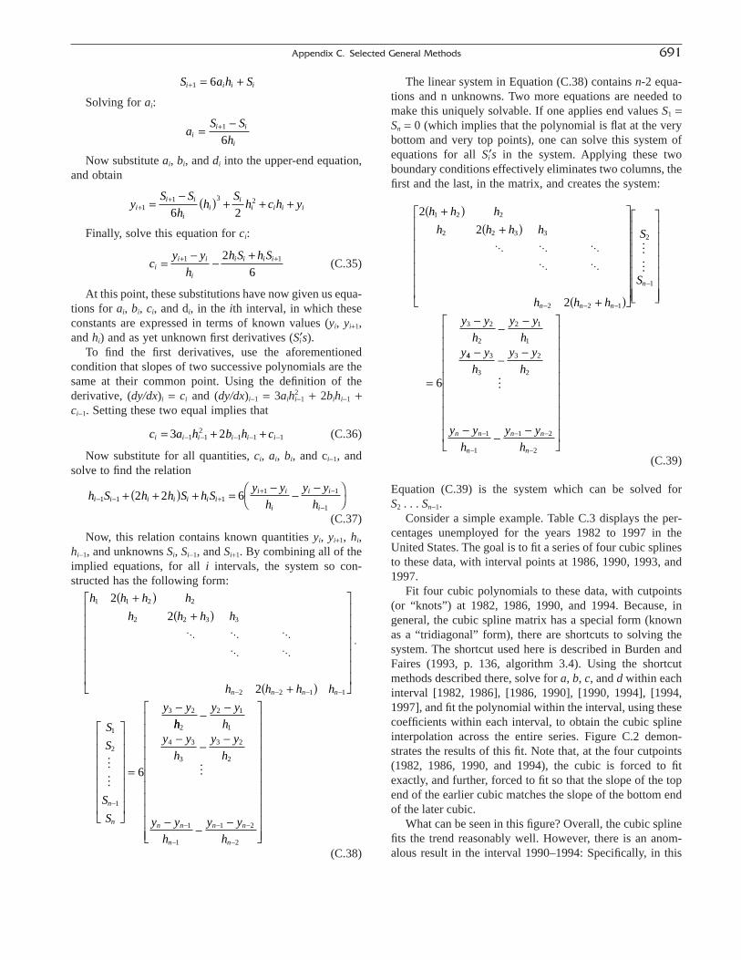
Solving for ai:
Now substitute ai, bi, and di into the upper-end equation,and obtain
Finally, solve this equation for ci:
(C.35)
At this point, these substitutions have now given us equa-tions for ai, bi, ci, and di, in the ith interval, in which theseconstants are expressed in terms of known values (yi, yi+1,and hi) and as yet unknown first derivatives (Si¢s).
To find the first derivatives, use the aforementioned condition that slopes of two successive polynomials are thesame at their common point. Using the definition of thederivative, (dy/dx)i = ci and (dy/dx)i-1 = 3aih2
i-1 + 2bihi-1 +ci-1. Setting these two equal implies that
(C.36)
Now substitute for all quantities, ci, ai, bi, and ci-1, andsolve to find the relation
(C.37)
Now, this relation contains known quantities yi, yi+1, hi,hi-1, and unknowns Si, Si-1, and Si+1. By combining all of theimplied equations, for all i intervals, the system so con-structed has the following form:
(C.38)
h h h h
h h h h
h h h h
S
S
S
S
y yn n n n
n
n
1 1 2 2
2 2 3 3
2 2 1 1
1
2
1
3 2
2
2
2
6
+( )+( )
◊◊◊ ◊◊◊ ◊◊◊◊◊◊ ◊◊◊
+( )
È
Î
ÍÍÍÍÍÍÍ
˘
˚
˙˙˙˙˙˙˙
◊
È
Î
ÍÍÍÍÍÍÍ
˘
˚
˙˙˙˙˙˙˙
=
-- - - -
-
:.:.
hh
y y
hy y
h
y y
h
y y
h
y y
hn n
n
n n
n
2
2 1
1
4 3
3
3 2
2
1
1
1 2
2
--
--
-
--
-
È
Î
ÍÍÍÍÍÍÍÍÍÍÍ
˘
˚
˙˙˙˙˙˙˙˙˙˙˙
-
-
- -
-
:.
h S h h S h Sy y
h
y y
hi i i i i i i
i i
i
i i
i- - +
+ -
-+ +( ) + =
--
-ÊË
ˆ¯1 1 1
1 1
1
2 2 6
c a h b h ci i i i i i= + +- - - - -3 21 12
1 1 1
cy y
h
h S h Si
i i
i
i i i i=-
-++ +1 126
yS S
hh
Sh c h yi
i i
ii
ii i i i+
+=- ( ) + + +1
1 3 2
6 2
aS S
hi
i i
i
=-+1
6
S a h Si i i i+ = +1 6 The linear system in Equation (C.38) contains n-2 equa-tions and n unknowns. Two more equations are needed tomake this uniquely solvable. If one applies end values S1 =Sn = 0 (which implies that the polynomial is flat at the verybottom and very top points), one can solve this system ofequations for all Si¢s in the system. Applying these twoboundary conditions effectively eliminates two columns, thefirst and the last, in the matrix, and creates the system:
(C.39)
Equation (C.39) is the system which can be solved for S2 . . . Sn-1.
Consider a simple example. Table C.3 displays the per-centages unemployed for the years 1982 to 1997 in theUnited States. The goal is to fit a series of four cubic splinesto these data, with interval points at 1986, 1990, 1993, and1997.
Fit four cubic polynomials to these data, with cutpoints(or “knots”) at 1982, 1986, 1990, and 1994. Because, ingeneral, the cubic spline matrix has a special form (known as a “tridiagonal” form), there are shortcuts to solving thesystem. The shortcut used here is described in Burden andFaires (1993, p. 136, algorithm 3.4). Using the shortcutmethods described there, solve for a, b, c, and d within eachinterval [1982, 1986], [1986, 1990], [1990, 1994], [1994,1997], and fit the polynomial within the interval, using thesecoefficients within each interval, to obtain the cubic splineinterpolation across the entire series. Figure C.2 demon-strates the results of this fit. Note that, at the four cutpoints(1982, 1986, 1990, and 1994), the cubic is forced to fitexactly, and further, forced to fit so that the slope of the topend of the earlier cubic matches the slope of the bottom endof the later cubic.
What can be seen in this figure? Overall, the cubic splinefits the trend reasonably well. However, there is an anom-alous result in the interval 1990–1994: Specifically, in this
2
2
2
6
1 2 2
2 2 3 3
2 2 1
2
1
3 2
2
2 1
1
h h h
h h h h
h h h
S
S
y y
h
y y
hy
n n n
n
+( )+( )
◊◊◊ ◊◊◊ ◊◊◊◊◊◊ ◊◊◊
+( )
È
Î
ÍÍÍÍÍÍÍ
˘
˚
˙˙˙˙˙˙˙
È
Î
ÍÍÍÍÍÍÍ
˘
˚
˙˙˙˙˙˙˙
=
--
-- - -
-
:.:.
44 3
3
3 2
2
1
1
1 2
2
--
-
--
-
È
Î
ÍÍÍÍÍÍÍÍÍÍ
˘
˚
˙˙˙˙˙˙˙˙˙˙-
-
- -
-
y
h
y y
h
y y
h
y y
hn n
n
n n
n
:.
Appendix C. Selected General Methods 691

interval, the unemployment rates are substantially higherthan the smoothed cubic values. Why does this occur? If oneexamines the graph closely, one can see that the slope at thelower cutpoint (1990) is downward. One can also see thatthe slope at the higher cutpoint (1994) is also downward.This means that, in the interval 1990–1994, the calculationis attempting to fit a cubic that is forced, by construction, to
slope downward at both ends. Needless to say, this, in com-bination with the limited number of data points available tous, limits how much “bend” the curve can have. Hence,while the cubic spline bends upward in the 1990–1994period, it cannot bend upward too far. As with any interpo-lation method, cubic splines, while attractive, have theirlimits.
692 Judson and Popoff
TABLE C.3 Employment Status of the Civilian Noninstitutional Population, United States: 1982–1997(Figures in thousands. Annual averages of monthly figurs.)
Civilian labor force Not in labor force
Civilian noninstitutionalized Unemployed Percent of PercentageYear population1 Total Employed number labor force Number of population
1982 172,271 110,204 99,526 10,678 9.7 62,067 36.01983 174,215 111,550 100,834 10,717 9.6 62,665 36.01984 176,383 113,544 105,005 8,539 7.5 62,839 35.61985 178,206 115,461 107,150 8,312 7.2 62,744 35.21986 180,587 117,834 109,597 8,237 7.0 62,752 34.71987 182,753 119,865 112,440 7,425 6.2 62,888 34.41988 184,613 121,669 114,968 6,701 5.5 62,944 34.11989 186,393 123,869 117,342 6,528 5.3 62,523 33.51990 189,164 125,840 118,793 7,047 5.6 63,324 33.51991 190,925 126,346 117,718 8,628 6.8 64,578 33.81992 192,805 128,105 118,492 9,613 7.5 64,700 33.61993 194,838 129,200 120,259 8,940 6.9 65,638 33.71994 196,814 131,056 123,060 7,996 6.1 65,758 33.41995 198,584 132,304 124,900 7,404 5.6 66,280 33.41996 200,591 133,943 126,708 7,236 5.4 66,647 33.21997 203,133 136,297 129,558 6,739 4.9 66,837 32.9
1 Population 16 years old and over. Source: U.S. Bureau of Labor Statistics, Bulletin 2307; and Employment and Earnings, monthly, January issues. Based on Current Population Survey.See U.S. Census Bureau, Statistical Abstract of the United States, 1999, Section 1, “Population”, and Appendix III, Washington, DC: U.S. Census Bureau,
2000.
FIGURE C.2 Percentage unemployed, United States, 1982–1997, with cubic spline interpolation.

Curve Fitting
Exponential Functions
Exponential functions are another class of mathematicalequations useful in interpolation and extrapolation of seriesof data. This class of curves is important in connection withthe measurement and analysis of population growth. Expo-nential equations are used for many other demographic pur-poses. The discussion here is intended to describe the typesof exponential functions and note their general relationshipto one another.
An exponential function is one in which one or more ofthe variables is expressed as a power of some parameter orconstant in the formula. Thus, y = ax is an exponential func-tion because x is a power of the parameters. Exponentialfunctions take many forms, as indicated here. One generalform of an exponential function, the power function, is
(C.40)
With modifications, this general equation lends itself tomany uses. Power functions are also known as growthcurves.
Geometric Curve
The simple geometric curve is a special case of the powerfunction. In the geometric curve, the given y values form ageometric progression while the corresponding x valuesform an arithmetic progression. The curve can be fittedexactly through two points. If there are more than two obser-vations, the simple geometric curve may be fitted approxi-mately by various methods (shown later). An example of thesimple geometric curve is the “compound interest” curve.This curve commonly takes the form of annual compound-ing, semiannual compounding, or quarterly compounding.For a quantity (population) compounded annually, theformula is
(C.41)
When the frequency of compounding is increased withoutlimit, we derive a quantity (population) compounded con-tinuously. The formula is
(C.42)
where
a is the initial amountx is the period of time over which growth occursb is the growth rate per unit of timee is the base of the system of natural logarithmsy is the amount (population) at time x
The formula for continuous compounding has severalapplications in demographic analysis. For example, it is thebasis for Lotka’s equations for a stable population. In con-
y aebx=
y a bx= +( )1
y abx=
structing the stable population, to convert the life table sur-vival P(x) proportions into proportions for a stable popula-tion growing or decreasing at a constant rate r, thecontinuous compounding formula is used in a reversefashion. The life table survival P(x) values are taken as the“present values,” or y values, and r is taken as the growthrate per year, in the continuous compounding formula y =aerx. Then, the coefficient a becomes the proportion thatpersons x years of age would constitute of the births (1.0000birth per year in the stable population). There would be adifferent “a” value for each age x, so it is made a functionof x, called a(x). The formula can now be written in the form
(C.43)
so that
(C.44)
or
(C.45)
This is the equation for computing the proportion a(x) of the population at age x in a stable population growing (or declining) at a constant rate r, from a life table series ofproportions P(x).
Other Growth Curves
As noted earlier, there are many possible modificationsof the general exponential equation y = abx in addition to thegeometric curves with annual or continuous compounding.These growth curves do not usually fit the given dataexactly; hence, they also belong under the heading “curvefitting.”The equation
(C.46)
is a modified exponential equation that yields an ascendingasymptotic curve when a is negative and b is a fractionalvalue between 0 and 1. It describes a series in which theabsolute growth in the y values decreases by a constant pro-portion. When x = 0, y = k - a. As x increases, y approachesk as an upper limit. In other variations, a is positive and bis between 0 and 1 or greater than 1.
More commonly used than the modified exponentialequation just described is the Gompertz curve, the equationof which is
(C.47)
which reduces to the equivalent logarithmic form:
(C.48)
The Gompertz curve is exactly like the modified exponen-tial curve except that it is the increase in the logarithms of
log log logy k b ax( ) = ( ) + ( )
y kabx=
y k abx= +
a x P x e rx( ) = ( ) -
a xP x
erx( ) =
( )
P x a x erx( ) = ( )
Appendix C. Selected General Methods 693

the y values that decreases by a constant proportion. TheGompertz curve fits many types of growth data much betterthan the modified exponential curve.
Another type of growth curve that has the same generalshape as the Gompertz curve is the logistic curve, alsoknown as the Pearl-Reed curve. The logistic curve has thegeneral equation
(C.49)
or when fitted by the method of selected points,
(C.50)
The reader is cautioned that no matter how well anasymptotic growth curve fits observed data, projections thatgo beyond the observations will not necessarily be realized.No empirically fitted curve can magically anticipate futurechanges when these are dependent on circumstances that arebeyond the ken of the curve. It is often easy to fit a varietyof modified logistic curves to the same observations in amanner that will yield very different projections.
Curve Fitting
Although a series of demographic data may not be subjectto any mathematical law, the data may follow a typical trendor pattern that can be represented empirically by some math-ematical equation. Curve fitting consists of finding a suit-able equation to represent that trend or pattern. Curves to befitted might be polynomials, osculatory equations, exponen-tial equations, trigonometric equations (useful for data thathave periodic fluctuations or seasonal patterns), or still othercurves. The aim may be to fit a curve to the data in anapproximate fashion, in which case crude methods, such asgraphic methods or moving averages, may be suitable, or tofit a curve by a more sophisticated method, as by the methodof moments or by the method of least squares. Whether ornot the fitted curve is suitable for interpolation or extrapo-lation depends on the nature of the given data, the choice ofcurve, and the goodness of fit. Probably demographers mostoften fit straight lines or polynomials of second or thirddegree in such applications.
Method of Least Squares
Curves are commonly fitted by the method of leastsquares or by the use of moments. Consider first the methodof least squares illustrated by fitting a second-degree poly-nomial (y = a + bx + cx2) to a time series of data on medianhousehold income in the United States for selected datesfrom 1967 to 1998. The method of least squares minimizesthe sum of the squares of the differences between theobserved or given points Y and the points calculated from
yk
ea bx=
+ +1
1y
k abx= +
the fitted curve Û. That is, given n points of data, leastsquares finds the Û that minimizes the sum:
(C.51)
where Yi is the observed value of y at the ith point, Ûi is thecorresponding value at the ith point from the fitted curve,and wi is a weight for the ith value (1 for each observed valueif all are assumed to be of equal precision, as in the presentexample). Three “normal” equations have to be solved. Thenormal equations in general form are
(C.52)
(C.53)
(C.54)
In every case, the sum is taken over the n observations.The origin (x = 0) is arbitrarily taken at the year l967, thefirst in the series. The following data, taken from Table C.4,is needed to solve the normal equations:
These values are now inserted in the normal equations asrequired to obtain the following of equations:
Solution of the three normal equations for a, b, and c by anyof a number of methods yields:8
a
b
c
== -=
36235
164 08
7 0206
.
,
1 141 362 31 10 416 246 016
17 990 484 496 10 416 246 016
380 563 510 10 416 246 016 6 197 520
, , , ,
, , , ,
, , , , , ,
= ( ) + ( ) + ( )= ( ) + ( ) + ( )= ( ) + ( ) + ( )
a b c
a b c
a b c
N
Y
X
X
X
X
XY
X Y
= ( )=
=
=
=
=
=
=
ÂÂ
ÂÂÂÂ
Â
31
1 141 362
496
10 416
246 016
6 197 520
17 990 484
380 563 510
2
3
4
2
observations
, ,
,
,
, ,
, ,
, ,
X Y a X b X c X2 2 3 4Â Â Â Â= + +
XY a X b X c XÂ Â Â Â= + +2 3
Y an b X c XÂ Â Â= + + 2
w Y Yi i ii
n
-( )=Â ˆ 2
1
694 Judson and Popoff
8 We used the commercial software package Maple VR4 (Waterloo,Inc.), but others such as Mathematica or MathCad could also be used. Ofcourse, one could also solve such a system by hand using regular or matrixalgebra. Because this is a standard regression equation solved by leastsquares, a statistics package or curve-fitting package is almost certainly thebest choice for fitting such an equation.
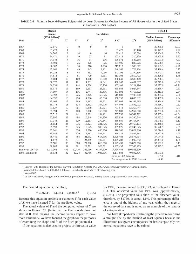
for 1999, the result would be $38,173, as displayed in FigureC.3. The observed value for 1999 was (approximately)$39,934. The projection falls short of the observed value,therefore, by $1760, or about 4.1%. This percentage differ-ence is one of the highest of any year within the range ofthe observed data and is noted as an example of the hazardsof extrapolation.
We have skipped over illustrating the procedure for fittinga straight line by the method of least squares because theillustration just given encompasses the basic steps. Only twonormal equations have to be solved:
Appendix C. Selected General Methods 695
TABLE C.4 Fitting a Second-Degree Polynomial by Least Squares to Median Income of All Households in the United States, in Constant (1998) Dollars
Median Fitted income Calculations
(1998 dollars)1 Median income PercentageYear Y X2 X2 X3 X4 X*Y X2Y (1998 dollars) difference
1967 32,075 0 0 0 0 0 0 36,235.0 12.971968 33,478 1 1 1 1 33,478 33,478 36,077.9 7.771969 34,706 2 4 8 16 69,412 138,824 35,934.9 3.541970 34,471 3 9 27 81 103,413 310,239 35,805.9 3.871971 34,143 4 16 64 256 136,572 546,288 35,691.0 4.531972 35,599 5 25 125 625 177,995 889,975 35,590.1 -0.021973 36,302 6 36 216 1,296 217,812 1,306,872 35,503.3 -2.201974 35,166 7 49 343 2,401 246,162 1,723,134 35,430.4 0.751975 34,224 8 64 512 4,096 273,792 2,190,336 35,371.7 3.351976 34,812 9 81 729 6,561 313,308 2,819,772 35,326.9 1.481977 35,004 10 100 1,000 10,000 350,040 3,500,400 35,296.3 0.831978 36,377 11 121 1,331 14,641 400,147 4,401,617 35,279.6 -3.021979 36,259 12 144 1,728 20,736 435,108 5,221,296 35,277.0 -2.711980 35,076 13 169 2,197 28,561 455,988 5,927,844 35,288.4 0.611981 34,507 14 196 2,744 38,416 483,098 6,763,372 35,313.9 2.3419823 34,392 15 225 3,375 50,625 515,880 7,738,200 35,353.4 2.801983 34,397 16 256 4,096 65,536 550,352 8,805,632 35,407.0 2.941984 35,165 17 289 4,913 83,521 597,805 10,162,685 35,474.6 0.881985 35,778 18 324 5,832 104,976 644,004 11,592,072 35,556.2 -0.621986 37,027 19 361 6,859 130,321 703,513 13,366,747 35,651.9 -3.7119873 37,394 20 400 8,000 160,000 747,880 14,957,600 35,761.6 -4.371988 37,512 21 441 9,261 194,481 787,752 16,542,792 35,885.4 -4.341989 37,997 22 484 10,648 234,256 835,934 18,390,548 36,023.2 -5.191990 37,343 23 529 12,167 279,841 858,889 19,754,447 36,175.1 -3.131991 36,054 24 576 13,824 331,776 865,296 20,767,104 36,340.9 0.801992 35,593 25 625 15,625 390,625 889,825 22,245,625 36,520.9 2.611993 35,241 26 676 17,576 456,976 916,266 23,822,916 36,714.8 4.181994 35,486 27 729 19,683 531,441 958,122 25,869,294 36,922.9 4.051995 36,446 28 784 21,952 614,656 1,020,488 28,573,664 37,144.9 1.921996 36,872 29 841 24,389 707,281 1,069,288 31,009,352 37,381.0 1.381997 37,581 30 900 27,000 810,000 1,127,430 33,822,900 37,631.1 0.131998 38,885 31 961 29,791 923,521 1,205,435 37,368,485 37,895.3 -2.55Sum over 1967–98: 1,141,362 496 10,416 246,016 6,197,520 17,990,484 380,563,5101999 (Estimated) 39,934 32 1,024 32,768 1,048,576 1,277,883 40,892,416 38,173.5
Error in 1999 forecast -1,760 416Percentage error in 1999 forecast -4.41
1 Source: U.S. Bureau of the Census, Current Population Reports, P60-206, www.census.gov/hhes/www/income.html.Constant dollars based on CPI-U-X1 deflator. Households as of March of following year.2 Year–1967.3 In 1983 and 1987, changes in data collection procedures occurred, making direct comparison with prior years suspect.
Ŷ
The desired equation is, therefore,
(C.55)
Because this equation predicts or estimates Y for each valueof X, we have inserted Ŷ for the predicted value.
The actual values of Y and the computed values of Ŷ areshown in Figure C.3. (Note that the Y-axis scale does notstart at 0, thus making the income values appear to havemore variability. We have focused the graph for the purposesof examining the shape and fit of the fitted polynomial.)
If the equation is also used to project or forecast a value
ˆ . .Y X X= - +36235 164 08 7 0206 2

(C.56)
(C.57)
Hence, we need to compute only SY, SX, SXY, and SX2.These have the same values as given previously. The normalequations, which we solve for a and b, then become
and the desired equation is
The pattern of the normal equations is evident. For fittinga third-degree polynominal by least squares, the normalequations are
(C.58)
(C.59)
(C.60)
(C.61)
The least squares method is only one of many methodsfor fitting functions to data, for estimating populationparameters from data, or for general maximization and min-imization of functions. The least squares method has tradi-tionally had the advantages that it is computationally simpleto implement and often has a closed form solution. Readerswho wish a full explanation of the principles of least squaresand related methods of estimation (such as the method ofmoments or the maximum-likelihood method) may wish to consult any of a variety of textbooks specializing in these topics. An introduction to these methods is given byKmenta (1986) Weisberg (1982) and Greene (1993). For afull account, including advanced topics, see Judge et al.(1985, 1988). Finally, for a mathematical development from
X Y a X b X c X d X3 3 4 5 6Â Â Â Â Â= + + +
X Y a X b X c X2 2 3 4Â Â Â Â= + +
XY a X b X c XÂ Â Â Â= + +2 3
Y an b X c XÂ Â Â= + + 2
ˆ .Y X= +36235 1 736
1 141 362 31 496
17 990 484 496 10 416
, ,
, , ,
= ( ) + ( )= ( ) + ( )
a b
a b
XY a X b XÂ Â Â= + 2
Y an b XÂ Â= +
first principles (that is, from the axiomatic probabilitymodels that serve as their foundation), see Bickel andDoksum (1977), Dudewicz and Mishra (1988), or Bain andEngelhart (1987).
INTERPOLATION OF GROUPED DATA
Introduction
We have been concerned in the preceding part of thisappendix with interpolation and curve fitting as applied to point data. We now consider interpolation as applied togrouped or “area” data. Interpolation of grouped data mayserve any of several purposes. The most common purposeprobably is the estimation of data in finer detail than is avail-able in published data, as for estimating numbers of personsin single years of age from published data for 5-year agegroups. Another purpose is the smoothing or graduation ofdata that are available in fine detail, as when interpolating5-year age data to obtain smoothed estimates of data bysingle years of age. It should be noted that the methods tobe described have one thing in common: They assume thatthe distribution pattern of grouped data is a valid indicationof the distribution pattern within groups. There are somekinds of demographic data where the distribution withingroups is known to have a special pattern that is not reflectedby grouped data. In such instances, the methods describedhere may not apply. For example, in the United States it iscommon for persons to work either 40 or 48 hours a week—a fact that is not evident from broad groupings of hoursworked.
“Interpolation” by Prorating
Sometimes the best estimates of the subdivisions ofgrouped data come not from elaborate mathematical tech-niques but rather from simple prorating. (In fact, in practicethis is probably the most common technique for disaggre-gating grouped data.) In this procedure, a distribution takenfrom some other similar group that has satisfactory detailedinformation is used to split up a known total for a givengroup. Such a procedure depends for its accuracy on howwell the distribution of the former group represents condi-tions in the latter group.
For example, a series of annual birth statistics for theyears in which persons now 25 to 29 years of age were bornmay be a useful basis for prorating the number of persons25 to 29 years of age so as to obtain estimates of the popu-lation for single years of age. It is not necessary to allow fordeaths since the birth period or for net migration, if it isthought that the distribution of the annual births is a rea-sonably good indicator of how the population is distributedby age within the 25-to-29 year age group currently. Fur-
696 Judson and Popoff
FIGURE C.3 Median household income versus values fitted by leastsquares 2nd degree polynomial.

thermore, the birth registration need not have been completeso long as the percent completeness was reasonably similarfrom year to year. Interpolations obtained in this mannermay be superior to interpolations from a mathematical equa-tion that involves an assumption of a smooth flow of eventsfrom age to age.
As another example of a type of problem where prorat-ing may be superior, consider the task of securing the per-centage married for single ages from the percentage marriedfor a 5-year age group, say for ages 15 to 19. A suggestedprocedure is to (1) multiply the percentage married for agegroup 15 to 19 in the given population, by 5 to obtain anapproximate value for the sum of the percentages for eachof the 5 single years of age, and then to (2) estimate the per-centages for single years of age by prorating this totalaccording to known single-year-of-age percentages fromsome other population. In the United States, the decennialcensus provides data on marital status by single years of age,but the data from the Current Population Survey are usuallytabulated only by broad age groups. The census data may bea good basis, therefore, for splitting up the current surveydata. Additional applications of prorating procedures are discussed in the section on “adjustment of distributions tomarginal totals.”
Use of a Rectangular Assumption
The simplest and perhaps the most commonly usedmethod of subdividing grouped data employs the assump-tion that the data are rectangularly (evenly) distributedwithin the interval to be subdivided. This assumption is thatthe values of the parts are all equal. They are derived, then,by dividing the total for the interval by the number of partsdesired. A rectangular assumption is a useful basis for deriv-ing rough estimates of detailed categories under many dif-ferent circumstances in demographic studies. For example,it may be employed to derive life table dx¢s in single years
of age from 5dx¢s or to derive the central dx in each 5-yearinterval. We illustrate with data based on an abridged 1996U.S. life table for the total population (U.S. National Centerfor Health Statistics/Anderson, 1998, Tables 1 and 2) inTable C.5 and Figure C.4.
As can be seen in this table and figure, the rectangularassumption works best when the underlying data are notchanging rapidly. In later years, when the number of deathsis increasing substantially with age, the rectangular assump-tion overestimates the number of the younger ages in theinterval, and underestimates the number of the older ages inthe interval.
Births or deaths on a calendar-year basis may be shifted to a “fiscal-year” (i.e., July-to-June) basis by simply assum-ing that one-half the births or deaths of each year occurs in the first or second half of the year. Even if there is a pro-nounced seasonal variation and a sharp trend up or downthrough the 2 years split up, the 12-month estimate may bequite adequate because the excess or deficit in the estimate forthe first half of the period may be largely offset by the deficitor excess in the estimate for the second half of the period.
Graphic Interpolation
Sometimes graphs are of special help in interpreting andsolving an interpolation problem. Suppose, for example, onewishes to compute separation factors for apportioningannual birth data by age of mother into the births occurringto mothers who would be of given ages at some date duringthe period. Specifically, we may wish to determine thenumber of births in a 12-month period ending on April 1,2000, which occurred to mothers who are x years of age onApril 1, 2000. A diagram of the type shown as Figure C.5may be helpful.
If the births are assumed to be uniformly distributed bydate of occurrence and age of mother, then the desired sep-aration factors can be figured from the proportionate parts
Appendix C. Selected General Methods 697
TABLE C.5 Excerpt of 1996 U.S. Life Table with Rectangular Interpolation
Official data1
RectangularOfficial data1
RectangularAge dx 5dx interpolation Age dx 5dx interpolation
10 14 117 23.411 14 23.412 19 23.413 28 23.414 42 23.415 56 386 77.216 70 77.217 81 77.218 88 77.219 91 77.220 95 499 99.8
1 Source: U.S. National Center for Health Statistics/Anderson, 1998.
55 635 3,776 755.256 684 755.257 744 755.258 816 755.259 897 755.260 985 5,760 115261 1074 115262 1158 115263 1235 115264 1308 1152

of the shaded areas. The procedure consists of estimatingdirectly the triangular area included in the shaded area foreach age and year; or estimating the rectangular area fromApril 1, 1999, to December 31, 1999 (3/4 year), and fromJanuary 1, 2000, to March 31, 2000 (1/4 year), and subtracting from it the triangular area that is not included inthe shaded area.
Proportion of births occurring to mothers of age “x” in2000 (the area labeled Bx
2000 in the figure):
Proportion of births occurring to mothers of age “x - 1”in 2000 (the area labeled Bx-1
2000 in the figure):
= - ¥ÊË
ˆ¯
ÈÎÍ
˘˚̇
=14
12
14
14
732
2000 2000B Bx x
698 Judson and Popoff
x-1
x
x-1
x
Official deaths
FIGURE C.4 Comparison of actual 1-year deaths versus deaths interpolated by rectangular assumption.
FIGURE C.5 Illustration of the graphic interpolation of births to mothers aged x-1 on April 1, 1999 and aged x on April1, 2000.

Proportion of births occurring to mothers of age “x” in1999 (the area labeled Bx
1999 in the figure):
Proportion of births occurring to mothers of age “x - 1”in 1999 (the area labeled Bx-1
1999 in the figure):
The width of the interval from January 1 to March 31,2000 is 1/4 year and the height of the January 1, 2000, ver-tical line is 3/4 year for the shaded area relating to age x and1/4 year for the shaded area relating to age x - 1. Hence, theshaded areas for 2000 are computed at 7/32 of 2000 birthsto mothers x years old at childbirth plus 1/32 of 2000 birthsto mothers x - 1 years old at childbirth. In a similar manner,the desired proportions for the interval between April 1 andDecember 31, 1999, are 9/32 of 1999 births to mothers xyears old at childbirth plus 15/32 of 1999 births to mothersx - 1 years old.
Midpoint and Cumulation-Differencing Methods
One general procedure for the interpolation of grouped data may be called, for want of a better term, the“midpoint” approach. Another, usually more reliableapproach, involves a cumulation and differencing calcula-tion. Polynomial interpolation, particularly in the form ofAitken’s procedure, is then ordinarily combined with one of these approaches to obtain the final results. Bothmethods will be briefly explained in terms of illustrativeexamples.
Midpoint Method Using Data on Percentages
Suppose one has data on the proportion of women evermarried for age groups 15 to 24, 25 to 34, 35 to 44, and 45and over and wants an estimate of the proportion evermarried for women 28 years of age. The lower limit of agegroup 15 to 24 is the 15th birthday (exact age 15.0) and theupper limit of that age group is the 25th birthday (exact age 25.0); the midpoint of age group 15 to 24 is, therefore,(15.0 + 25.0)/2, or 20.0. In a similar manner the midpointsof the other age groups in this example may be determinedto be, respectively, (25.0 + 35.0)/2 = 30.0 for age group 25to 34, (35.0 + 45.0)/2 = 40.0 for age group 35 to 44. Themidpoint of the desired year of age 28 is 28.5. By equatingthe given percentages ever married with the corresponding midpoints of age groups and by interpolating among the
= - ¥ÊË
ˆ¯
ÈÎÍ
˘˚̇
=- -34
12
34
34
1532
19991
19991B Bx x
= ¥ÊË
ˆ¯
ÈÎÍ
˘˚̇
=12
34
34
932
1999 1999B Bx x
= ¥ÊË
ˆ¯
ÈÎÍ
˘˚̇
=- -12
14
14
132
20001
20001B Bx x
former, we can obtain an estimate of the percentage evermarried corresponding to the midpoint of age 28 (i.e., forage 28).
In the following example of midpoint interpolation,Aitken’s iterative procedure is applied to marital data forfemales in the United States in 1990. Note that the “mid-point” of the highest age group is problematic in thiscontext; if one did not have a statement of the midpoint fromanother tabulation, one would either (1) use only the secondcomputational stage and not the third or (2) estimate themidpoint of the highest age group using other methods, and use that estimate. (In fact, this illustrates a weakness ofthe midpoint method.) In this case, we take the midpoint tobe halfway between 80.0 and 45.0, or 62.5. The interpola-tion table is presented in Table C.6.
The last figure in column 3 of the computations is thedesired result: We estimate that 70.4% of women of exactage 28 were ever-married as of the 1990 U.S. Census.Because so much of the female population is “ever married”by the time they reach age 45, the upper age group midpointmakes only a small difference to the estimate: If we assumedthe upper midpoint was (60 + 45)/2 = 52.5, the final esti-mate of percent of women of exact age 28 ever-marriedwould be 70.6%.
Cumulation-Differencing Method Using Data onAbsolute Numbers
The cumulation-differencing method has a sounder theoretical basis for interpolation of groups than the midpoint approach just described. This is because, in fact,group averages seldom apply exactly to the midpoints ofgroups, as is assumed in the midpoint approach; however, in the cumulation-differencing approach the observed dataare associated with the precise points to which they actuallyapply.
Consider the numbers of women in the age groups 15 to24, 25 to 34, 35 to 44, and 45 and older for the United Statesin 1990, as before. Tentatively, for illustrative purposes,
Appendix C. Selected General Methods 699
TABLE C.6 Illustration of Midpoint Method of Interpolationof Percents Using Aitken’s Procedure
Interpolation date28.5
PercentageComputational Stages
ProportionateMidpoint ever married (1) (2) (3) parts
20 20.97 20 - 28.5 = -8.530 75.52 67.34 30 - 28.5 = 1.540 90.23 50.41 69.88 40 - 28.5 = 11.562.51 94.85 35.75 68.80 70.43 62.5 - 28.5 = 34.0
1 Based on arbitrary assignment of 80.0 as upper limit of age group 45and over.
Source: 1990 U.S. census data.

assume that there are K females under age 15. (The numberK will drop out as the work progresses, so that its value doesnot matter; it is used here simply to help clarify the exposi-tion.) The upper limit of the age range under 14 is 15.0. Thenumber of females aged 15 to 24 plus K (the females under15) is then the cumulated number under 25 years old; theupper limit of that age range is 25.0. The population 25 to34 years old, plus the population 15 to 24 years old, plus K,is the cumulated number under 35 years old; the upper limitof that age range is 35.0. Continuing this process, oneobtains the cumulated numbers at exact ages 25.0, 35.0, and45.0. The cumulated data represent the “ogive” transforma-tion of the original data for groups into data for specificpoints along the age scale. The transformed data are thusassociated with precise points of age.
Interpolation of the transformed data can now be per-formed by any appropriate method but must be done twice—once for the upper limit of the subgroup for whichinterpolation is desired and once for the lower limit. Thus,to estimate the population in age 28 from the data for agegroups 15 to 24, 25 to 34, 35 to 44, and 45 and older, oneestimates the population under age 28 and then estimates thepopulation under age 29. The difference between the twoestimates will be the population between the 28th and 29thbirthdays. Because K is common to both the populationunder 28 and the population under 29, the subtraction causesK to vanish. This means that K can be taken as zero (insteadof some other arbitrary number), thereby simplifying theoperation. Table C.7 illustrates the calculation.
The figure of 24,577,639 in column 3 of the top table isthe interpolated estimate of the number of women cumulated
to exact age 28.0. We also need the cumulated number toage 29.0, and the figure of 26,793,458 in column 3 of thebottom table is that interpolated estimate. Therefore, thedesired estimate of the population from exact age 28.0 toexact age 29.0 is the difference (2,215,819) between the26,793,458 cumulated to age 29.0 and the 24,577,639 cumu-lated to age 28.0.
Cumulation-Differencing Method Using Data on Percentages
In applying the cumulation-differencing method to per-centage data, the percentages require weighting by the classintervals associated with them as a first step. The work thenproceeds in the same manner as for absolute numbers. Thefollowing example uses the same data as those used in theexample of interpolation of percentages by the midpointmethod, but in Table C.8 we interpolate for the value of the percentages ever married cumulated to age 29.0.
The figure of 416.72% in the last computational stage ofthe upper table is the interpolated estimate of percentagescumulated to age 28.0. We also need the cumulated figurefor age 29.0, and it is presented in the last computationalstage of the bottom table as 489.70%. The desired estimateof the percentage ever married for women from exact age28.0 to exact age 29.0 is the difference (73.0%) between thefigures for the upper (489.70%) and lower (416.72%) limitsof the year of age.
These examples employ Aitken’s iterative procedure. Ifone has many interpolations to make for the same spacingsof the abscissas (ages in this case), it might save time to use
700 Judson and Popoff
TABLE C.7 Illustration of Cumulation-Differencing Method of Interpolation of Absolute Numbers Using Aitken’s Procedure
Number of women
Cumulated fromComputational stages
ProportionateAge group Upper limit In age group youngest group (1) (2) (3) parts
Interpolation age 28.0
15–24 25.0 17,769,944 17,769,944 -3.025–34 35.0 21,757,561 39,527,505 24,297,212 7.035–44 45.0 19,012,425 58,539,930 23,885,442 24,585,452 17.045+ 80.0 42,884,185 101,424,115 22,332,899 24,603,772 24,577,639 52.0
Interpolation age 29.0
15–24 25.0 17,769,944 17,769,944 -4.025–34 35.0 21,757,561 39,527,505 26,472,968 6.035–44 45.0 19,012,425 58,539,930 25,923,941 26,802,385 16.045+ 80.01 42,884,185 101,424,115 23,855,884 26,821,913 26,793,458 51.0Estimated number of women from exact age 28.0 to exact age 29.0: 26,793,458 - 24,577,639 = 2,215,819.
1 Arbitrary assignment of upper limit of age group.Source: 1990 U.S. Census data.
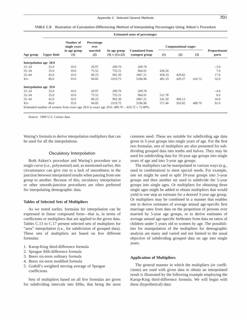
Waring’s formula to derive interpolation multipliers that canbe used for all the interpolations.
Osculatory Interpolation
Both Aitken’s procedure and Waring’s procedure use asingle curve (i.e., polynomial) and, as mentioned earlier, thiscircumstance can give rise to a lack of smoothness in thejunction between interpolated results when passing from onegroup to another. Because of this, osculatory interpolationor other smooth-junction procedures are often preferred for interpolating demographic data.
Tables of Selected Sets of Multipliers
As we noted earlier, formulas for interpolation can beexpressed in linear compound form—that is, in terms ofcoefficients or multipliers that are applied to the given data.Tables C.13 to C.17 present selected sets of multipliers for“area” interpolation (i.e., for subdivision of grouped data).These sets of multipliers are based on five different formulas:
1. Karup-King third-difference formula2. Sprague fifth-difference formula3. Beers six-term ordinary formula4. Beers six-term modified formula5. Grabill’s weighted moving average of Sprague
coefficients
Sets of multipliers based on all five formulas are givenfor subdividing intervals into fifths, that being the most
common need. These are suitable for subdividing age datagiven in 5-year groups into single years of age. For the firsttwo formulas, sets of multipliers are also presented for sub-dividing grouped data into tenths and halves. They may beused for subdividing data for 10-year age groups into singleyears of age and into 5-year age groups.
The multipliers can be manipulated in various ways (e.g.,used in combination) to meet special needs. For example,one set might be used to split 10-year groups into 5-yeargroups and then another set used to subdivide the 5-yeargroups into single ages. Or multipliers for obtaining threesingle ages might be added to obtain multipliers that wouldyield in one step an estimate for a desired 3-year age group.Or multipliers may be combined in a manner that enablesone to derive estimates of average annual age-specific firstmarriage rates from data on the proportion of persons evermarried by 5-year age groups, or to derive estimates ofaverage annual age-specific birthrates from data on ratios ofchildren under 5 years old to women by age. The possibili-ties for manipulation of the multipliers for demographicanalysis are many and varied and not limited to the usualobjective of subdividing grouped data on age into singleyears.
Application of Multipliers
The general manner in which the multipliers (or coeffi-cients) are used with given data to obtain an interpolatedresult is illustrated by the following example employing theKarup-King third-difference formula. We will begin withthese (hypothetical) data:
Appendix C. Selected General Methods 701
TABLE C.8 Illustration of Cumulation-Differencing Method of Interpolating Percentages Using Aitkon’s Procedure
Estimated sums of percentages
Number of Percentagesingle years ever Computational stagesin age group married In age group Cumulated from Proportionate
Age group Upper limit (1) (2) (3) = (1)* (2) youngest group (1) (2) (3) parts
Interpolation age 28.015–24 25.0 10.0 20.97 209.70 209.70 -3.025–34 35.0 10.0 75.52 755.21 964.91 436.26 7.035–44 45.0 10.0 90.23 902.30 1867.21 458.33 420.82 17.045+ 80.0 35.0 94.85 3319.75 5186.96 481.19 429.27 416.72 32.0
Interpolation age 29.015–24 25.0 10.0 20.97 209.70 209.70 -4.025–34 35.0 10.0 75.52 755.21 964.91 511.78 6.035–44 45.0 10.0 90.23 902.30 1867.21 541.20 494.13 16.045+ 80.0 35.0 94.85 3319.75 5186.96 571.46 503.82 489.70 91.0Estimated number of women from exact age 28.0 to exact age 29.0: 489.70 - 416.72 = 72.89%.
Source: 1990 U.S. Census data.
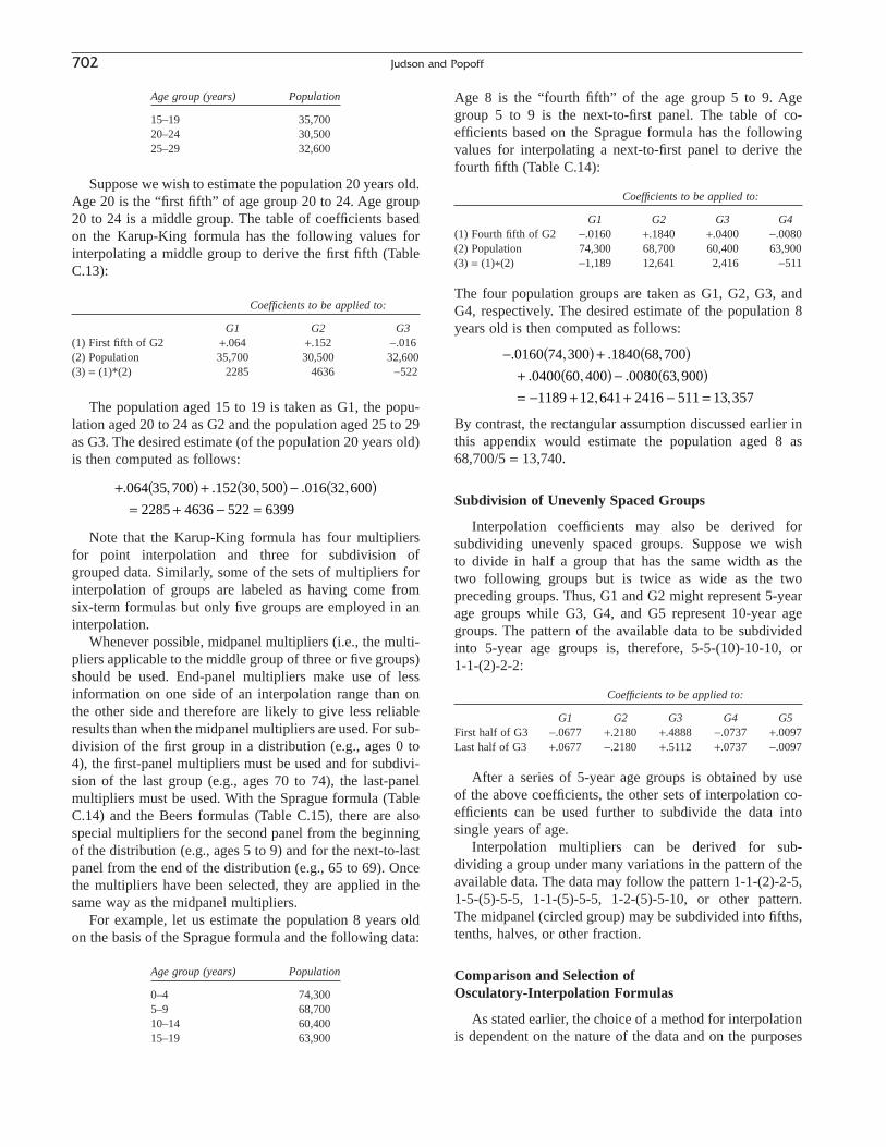
Age group (years) Population
15–19 35,70020–24 30,50025–29 32,600
Suppose we wish to estimate the population 20 years old.Age 20 is the “first fifth” of age group 20 to 24. Age group20 to 24 is a middle group. The table of coefficients basedon the Karup-King formula has the following values forinterpolating a middle group to derive the first fifth (TableC.13):
Coefficients to be applied to:
G1 G2 G3(1) First fifth of G2 +.064 +.152 -.016(2) Population 35,700 30,500 32,600(3) = (1)*(2) 2285 4636 -522
The population aged 15 to 19 is taken as G1, the popu-lation aged 20 to 24 as G2 and the population aged 25 to 29as G3. The desired estimate (of the population 20 years old)is then computed as follows:
Note that the Karup-King formula has four multipliers for point interpolation and three for subdivision of grouped data. Similarly, some of the sets of multipliers forinterpolation of groups are labeled as having come from six-term formulas but only five groups are employed in aninterpolation.
Whenever possible, midpanel multipliers (i.e., the multi-pliers applicable to the middle group of three or five groups)should be used. End-panel multipliers make use of lessinformation on one side of an interpolation range than onthe other side and therefore are likely to give less reliableresults than when the midpanel multipliers are used. For sub-division of the first group in a distribution (e.g., ages 0 to4), the first-panel multipliers must be used and for subdivi-sion of the last group (e.g., ages 70 to 74), the last-panelmultipliers must be used. With the Sprague formula (TableC.14) and the Beers formulas (Table C.15), there are alsospecial multipliers for the second panel from the beginningof the distribution (e.g., ages 5 to 9) and for the next-to-lastpanel from the end of the distribution (e.g., 65 to 69). Oncethe multipliers have been selected, they are applied in thesame way as the midpanel multipliers.
For example, let us estimate the population 8 years oldon the basis of the Sprague formula and the following data:
Age group (years) Population
0–4 74,3005–9 68,70010–14 60,40015–19 63,900
+ ( ) + ( ) - ( )= + - =
. , . , . ,064 35 700 152 30 500 016 32 600
2285 4636 522 6399
Age 8 is the “fourth fifth” of the age group 5 to 9. Age group 5 to 9 is the next-to-first panel. The table of co-efficients based on the Sprague formula has the followingvalues for interpolating a next-to-first panel to derive thefourth fifth (Table C.14):
Coefficients to be applied to:
G1 G2 G3 G4(1) Fourth fifth of G2 -.0160 +.1840 +.0400 -.0080(2) Population 74,300 68,700 60,400 63,900(3) = (1)*(2) -1,189 12,641 2,416 -511
The four population groups are taken as G1, G2, G3, andG4, respectively. The desired estimate of the population 8years old is then computed as follows:
By contrast, the rectangular assumption discussed earlier inthis appendix would estimate the population aged 8 as68,700/5 = 13,740.
Subdivision of Unevenly Spaced Groups
Interpolation coefficients may also be derived for subdividing unevenly spaced groups. Suppose we wish to divide in half a group that has the same width as the two following groups but is twice as wide as the two preceding groups. Thus, G1 and G2 might represent 5-yearage groups while G3, G4, and G5 represent 10-year agegroups. The pattern of the available data to be subdividedinto 5-year age groups is, therefore, 5-5-(10)-10-10, or 1-1-(2)-2-2:
Coefficients to be applied to:
G1 G2 G3 G4 G5First half of G3 -.0677 +.2180 +.4888 -.0737 +.0097Last half of G3 +.0677 -.2180 +.5112 +.0737 -.0097
After a series of 5-year age groups is obtained by use of the above coefficients, the other sets of interpolation co-efficients can be used further to subdivide the data intosingle years of age.
Interpolation multipliers can be derived for sub-dividing a group under many variations in the pattern of theavailable data. The data may follow the pattern 1-1-(2)-2-5,1-5-(5)-5-5, 1-1-(5)-5-5, 1-2-(5)-5-10, or other pattern. The midpanel (circled group) may be subdivided into fifths,tenths, halves, or other fraction.
Comparison and Selection of Osculatory-Interpolation Formulas
As stated earlier, the choice of a method for interpolationis dependent on the nature of the data and on the purposes
- ( ) + ( )+ ( ) - ( )= - + + - =
. , . ,
. , . ,
, ,
0160 74 300 1840 68 700
0400 60 400 0080 63 900
1189 12 641 2416 511 13 357
702 Judson and Popoff
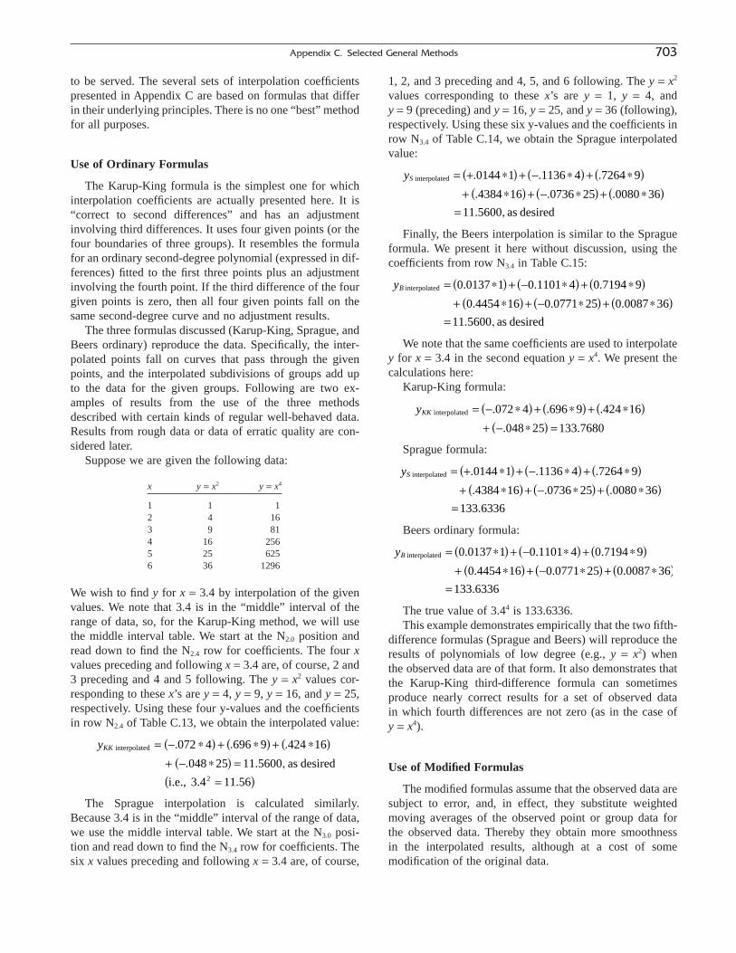
to be served. The several sets of interpolation coefficientspresented in Appendix C are based on formulas that differin their underlying principles. There is no one “best” methodfor all purposes.
Use of Ordinary Formulas
The Karup-King formula is the simplest one for whichinterpolation coefficients are actually presented here. It is“correct to second differences” and has an adjustmentinvolving third differences. It uses four given points (or thefour boundaries of three groups). It resembles the formulafor an ordinary second-degree polynomial (expressed in dif-ferences) fitted to the first three points plus an adjustmentinvolving the fourth point. If the third difference of the fourgiven points is zero, then all four given points fall on thesame second-degree curve and no adjustment results.
The three formulas discussed (Karup-King, Sprague, andBeers ordinary) reproduce the data. Specifically, the inter-polated points fall on curves that pass through the givenpoints, and the interpolated subdivisions of groups add upto the data for the given groups. Following are two ex-amples of results from the use of the three methodsdescribed with certain kinds of regular well-behaved data.Results from rough data or data of erratic quality are con-sidered later.
Suppose we are given the following data:
x y = x2 y = x4
1 1 12 4 163 9 814 16 2565 25 6256 36 1296
We wish to find y for x = 3.4 by interpolation of the givenvalues. We note that 3.4 is in the “middle” interval of therange of data, so, for the Karup-King method, we will usethe middle interval table. We start at the N2.0 position andread down to find the N2.4 row for coefficients. The four xvalues preceding and following x = 3.4 are, of course, 2 and3 preceding and 4 and 5 following. The y = x2 values cor-responding to these x’s are y = 4, y = 9, y = 16, and y = 25,respectively. Using these four y-values and the coefficientsin row N2.4 of Table C.13, we obtain the interpolated value:
The Sprague interpolation is calculated similarly.Because 3.4 is in the “middle” interval of the range of data,we use the middle interval table. We start at the N3.0 posi-tion and read down to find the N3.4 row for coefficients. Thesix x values preceding and following x = 3.4 are, of course,
yKK interpolated
2
as desired
i.e., 3.4
= - *( ) + *( ) + *( )+ - *( ) =
=( )
. . .
. . ,
.
072 4 696 9 424 16
048 25 11 5600
11 56
1, 2, and 3 preceding and 4, 5, and 6 following. The y = x2
values corresponding to these x’s are y = 1, y = 4, and y = 9 (preceding) and y = 16, y = 25, and y = 36 (following),respectively. Using these six y-values and the coefficients inrow N3.4 of Table C.14, we obtain the Sprague interpolatedvalue:
Finally, the Beers interpolation is similar to the Spragueformula. We present it here without discussion, using thecoefficients from row N3.4 in Table C.15:
We note that the same coefficients are used to interpolatey for x = 3.4 in the second equation y = x4. We present thecalculations here:
Karup-King formula:
Sprague formula:
Beers ordinary formula:
The true value of 3.44 is 133.6336.This example demonstrates empirically that the two fifth-
difference formulas (Sprague and Beers) will reproduce theresults of polynomials of low degree (e.g., y = x2) when the observed data are of that form. It also demonstrates thatthe Karup-King third-difference formula can sometimesproduce nearly correct results for a set of observed data in which fourth differences are not zero (as in the case of y = x4).
Use of Modified Formulas
The modified formulas assume that the observed data aresubject to error, and, in effect, they substitute weightedmoving averages of the observed point or group data for the observed data. Thereby they obtain more smoothness in the interpolated results, although at a cost of some modification of the original data.
yB interpolated = *( ) + - *( ) + *( )+ *( ) + - *( ) + *( )
=
0 0137 1 0 1101 4 0 7194 9
0 4454 16 0 0771 25 0 0087 36
133 6336
. . .
. . .
.
yS interpolated = + *( ) + - *( ) + *( )+ *( ) + - *( ) + *( )
=
. . .
. . .
.
0144 1 1136 4 7264 9
4384 16 0736 25 0080 36
133 6336
yKK interpolated = - *( ) + *( ) + *( )+ - *( ) =
. . .
. .
072 4 696 9 424 16
048 25 133 7680
yB interpolated
as desired
= *( ) + - *( ) + *( )+ *( ) + - *( ) + *( )
=
0 0137 1 0 1101 4 0 7194 9
0 4454 16 0 0771 25 0 0087 36
11 5600
. . .
. . .
. ,
yS interpolated
as desired
= + *( ) + - *( ) + *( )+ *( ) + - *( ) + *( )
=
. . .
. . .
. ,
0144 1 1136 4 7264 9
4384 16 0736 25 0080 36
11 5600
Appendix C. Selected General Methods 703

The extent to which the modifications alter the originaldata can perhaps best be seen by adding together the fivecoefficients for subdividing a central group into five equalparts according to the various interpolation schemes. Thesesums are as follows:
G1 G2 G3 G4 G5
Beers’s modified six-term minimized fourth-difference formula
-.0430 +.1721 +.7420 +.1720 -.0430
Grabill’s modification of Sprague coefficients
+.0164 +.2641 +.4390 +.2641 +.0164
Formulas that reproduce group totals without modification
0 0 1.0000 0 0
Note that all of these coefficients sum to 1.0 across therows. In this sense, they “weight” the different observations,G1 through G5, differently. These figures represent con-solidated coefficients which, if applied to the given G1, G2, G3, G4, and G5 groups, would yield the sums of the fiveinterpolated subdivisions of G3. It is apparent from the difference in weights assigned to the middle panel that theBeers modified formula involves a less drastic modificationof the original group values than Grabill’s coefficients.
Illustration of Comparative Results with Age Data
Comparative results for interpolating census data for 5-year age groups into single ages are shown in Table C.9,with graphical results in Figure C.6. In this table, we
have collapsed 1960 census data for Mexico into 5-year age groups. Using only the 5-year age groups, we then interpolate to single years of age using the Karup-King co-efficients, the Sprague coefficients, the Beers ordinary coefficients, the Beers modified coefficients, and the Grabillcoefficients.
Finally, we display the interpolated distributions for com-parison with the original, single-year-of-age data reported inthe 1960 Census of Mexico. Figure C.6 shows that the enu-merated data in single years fluctuate sharply as a result ofthe tendency of many persons to report ages that are multi-ples of five or two.
The table and the figure illustrate the digit preferencesclearly. The Karup-King formula smoothes out only part ofthese undulations because the group totals are maintained.The Sprague and Beers ordinary formulas generate interpo-lations that are very similar to the Karup-King formula. Useof Grabill’s coefficients shows how completely the undula-tions can be removed by a drastic smoothing procedure. TheBeers modified formula is similar in its effect as the Grabillformula; it removes most of the undulations, at the cost ofmodifying the 5-year age groups’ totals.
An alternative procedure for subdividing the last fewregular groups in the age distribution (e.g., 75 to 79, 80 to84 for Mexico, 1960) involves, first, splitting up the open-ended terminal group (e.g., 85 and over) into three groups(i.e., 85 to 89, 90 to 94, and 90 and over) and then applyingmidpanel coefficients for subdividing the groups just aheadof the terminal group. The precision of the results of subdi-viding the terminal group would have only a small effect on
704 Judson and Popoff
FIGURE C.6 Population of Mexico, 1960, by single years of age as enumerated and as interpolated from 5-year agegroups by the use of the Karup-King method and the Grabill method.Source: Table C.9 and unpublished calculations.

Appendix C. Selected General Methods 705
TABLE C.9 Results of Interpolating the Population of Mexico, 1960, for 5-year Age Groupsunder 20 and 65 to 84, by Single Years of Age, According to Several Methods (See text for
explanation of various types of interpolation.)
Interpolated population1
Age group Enumerated Single ages Enumerated Karup-King Sprague Beers ordinary Beers modified Grabill modification(years) Population2 (years) population formula formula formula formula of Sprague formula
Total, all ages 34,809,586 Total, all ages 34,809,586 34,809,586 34,809,586 34,809,586 34,809,586 (NA)Under 5 5,776,747 Under 5 5,776,747 5,776,747 5,776,747 5,776,747 5,776,747 (NA)5–9 5,317,044 Under 1 1,144,187 1,160,188 1,146,846 1,162,002 1,165,090 (NA)
10–14 4,358,316 1 1,059,321 1,169,745 1,160,676 1,163,085 1,165,241 (NA)15–19 3,535,265 2 1,171,914 1,167,326 1,164,419 1,159,921 1,160,371 (NA)20–24 2,947,072 3 1,219,205 1,152,930 1,159,093 1,152,185 1,150,479 (NA)25–29 2,504,892 4 1,182,120 1,126,558 1,145,713 1,139,554 1,135,565 (NA)30–34 2,051,635 5–9 5,317,044 5,317,044 5,317,044 5,317,044 5,289,752 (NA)35–39 1,920,680 5 1,158,544 1,108,169 1,125,294 1,121,652 1,115,684 (NA)40–44 1,361,324 6 1,143,140 1,097,766 1,098,851 1,098,155 1,091,005 (NA)45–49 1,233,608 7 1,071,375 1,075,385 1,067,401 1,068,900 1,061,845 (NA)50–54 1,063,359 8 1,070,475 1,041,028 1,031,959 1,033,994 1,028,728 (NA)55–59 799,899 9 873,510 994,695 993,540 994,343 992,490 (NA)60–64 744,710 10–14 4,358,316 4,358,316 4,358,316 4,358,316 4,381,343 4,394,26665–69 414,164 10 1,029,718 946,191 952,303 951,714 954,046 945,84070–74 333,371 11 756,819 905,671 908,406 908,621 914,517 912,38975–79 187,773 12 948,976 868,407 867,150 867,900 875,130 878,71680–84 128,338 13 814,823 834,399 831,264 831,478 836,935 845,21785 and over 131,389 14 807,980 803,648 799,192 798,603 800,716 812,104
15–19 3,535,265 3,535,265 3,535,265 3,535,265 3,543,350 3,609,61415 753,742 769,139 766,509 766,302 767,084 779,86116 703,138 732,460 733,929 734,004 736,000 749,20617 703,225 701,416 703,971 704,234 706,772 720,36918 798,608 676,010 677,396 677,471 679,461 693,09119 576,552 656,240 653,461 653,254 654,033 667,086. . .
65–69 414,164 414,164 414,164 414,164 450,270 482,73765 191,430 105,280 107,502 106,579 110,095 112,22266 60,826 88,063 88,888 89,223 98,187 103,96867 48,671 76,839 75,461 76,636 87,972 96,03468 78,878 71,609 70,750 71,085 79,923 88,67169 34,359 72,373 71,563 70,640 74,093 81,842
70–74 333,371 333,371 333,371 333,371 313,353 319,63970 200,200 74,175 71,427 71,939 69,982 74,29071 20,313 71,980 71,924 71,738 66,754 68,67972 52,712 68,230 70,172 69,520 63,236 63,62073 31,757 62,924 64,177 63,991 59,106 58,83474 28,389 56,063 55,671 56,183 54,276 54,216
75–79 187,773 187,773 187,773 187,773 194,265 (NA)75 88,484 47,824 48,619 47,921 48,970 (NA)76 28,812 40,621 42,518 40,749 43,524 (NA)77 19,474 35,487 36,865 35,562 38,288 (NA)78 36,715 32,420 31,902 32,507 33,633 (NA)79 14,288 31,421 27,869 31,034 29,850 (NA)
80–84 128,338 128,338 128,338 128,338 128,338 (NA)80 88,484 29,044 25,008 30,362 27,016 (NA)81 7,520 25,288 23,562 29,567 25,239 (NA)82 13,514 23,600 23,771 27,681 24,564 (NA)83 9,537 23,980 25,877 23,782 24,993 (NA)84 9,283 26,427 30,121 16,947 26,526 (NA)
(NA) Not available.1 Slight discrepancies in the last digit between the sums of interpolated single ages and the 5-year totals are due to rounding.2 Total excludes “unknowns”. Age was not reported for only 0.3 percent of the population.Source of census data: México, Secretaría de Industria y Comercio, Dirección General de Estadística, Censo de Población, 1960.

the interpolated single-year-of-age values for the precedingage groups. One device for subdividing the terminal groupis to employ the distribution of Lx from an appropriate lifetable (e.g., a life table for Mexico, 1959–1961). Another isto fit a polynomial to the last several observed values andzero for 100 and over (e.g., a third-degree polynomial tovalues for 75 and over, 80 and over, 85 and over, and 100and over). The appropriate population by age at the preced-ing census may be “aged” to the current census year, and thedistribution of survivors may then be used to subdivide thecurrent total for the terminal age group. At the beginning ofthe distribution, to the extent that the quality of the statisticspermit, birth statistics, or birth statistics adjusted for deaths,may be employed to subdivide the 5-year totals into singleages, as suggested in Chapter 7.
Parameterizing Demographic Models
Many demographic models have a common form, consisting of a curve or sequence of age-specific (orage/race/sex specific) numbers, rates, or proportions. FigureC.7 illustrates this idea with an array of 16 net-migrationvalues for 5-year age (birth) cohorts for a 10-year period(Murdock and Ellis, 1991, p. 207) and with an interpolatedcurve on top of the sequence of grouped data.
The interpolated curve provides the clue to simplifyingthe demographic model implied by the data. Instead of con-sidering 16 age-specific migration rates or numbers, we cansummarize the data by fitting a single curve with a limited
number of parameters that define its level and shape.9 Werefer to this as “parameterizing” the model. Once a modelhas been parameterized, it is then potentially broadly appli-cable—again because we are not calculating numerous age-specific numbers or rates, but can plot and manipulate thecurve itself, similar to working with model life tables.
As an example of the power of parameterizing a demo-graphic model, Castro and Rogers (1983) developed modelschedules for migration for a variety of cities and nations ofthe world. Instead of calculating a series of disconnectedage-specific migration counts or rates, they presumed thatthe age distribution of migrants could be split into threecomponents: A child/dependent component, an independent/adult component, and an older-age component.10 Theysimply added components together:
(C.62)
where
N1 is the proportion of migrants in the dependent component
N x N x N x N x( ) = ( ) + ( ) + ( )1 2 3
706 Judson and Popoff
Net migration
Initial ages of 10-year cohorts
FIGURE C.7 Data and model net migration schedule for age cohorts of females, McCleennan County, Texas, projected1980–1990.Source: Bars: Basedon Murdock and Ellis (1991, p. 207) Fitted curve: Calculated by authors.
9 The details of the curve-fitting technique are more advanced than thisappendix warrants. Programs and data are available from the authors.
10 Rogers and Castro (1986) later introduced a fourth component to account for post–labor force migration. We will not deal with that fourth component here except to note that it illustrates that migrationpropensities are in fact quite difficult to model adequately. Migration as a sequence of events is simply not as regular and easy to model as fertility or mortality.

N2 is the proportion of migrants in the independent component
N3 is the proportion of migrants in the older adult component
N(x) is the proportion of migrants at age x
Up to this point, the model is quite simple; it is merelythe sum of three conceptually different components. It ishere, however, that parameterization adds value. Castro andRogers then proposed the following three functions for each component:
(C.63)
(C.64)
(C.65)
One can always simply count up the number of migrantsin a particular group and divide by the total population atrisk, generating a rate for each age group. However, withthese models, the age-specific migration rates have been“summarized” by seven parameters, a1, a2, a1, a2, l2, m2, andc. If one can assume that older migration does not requireits own parameter, one can set c = 0 and reduce the load tosix parameters. Figure C.8 displays these three curves indi-vidually and their sum, using parameters for Rio de JaneiroCastro and Rogers. The older adult component is assumedto be zero, so the model migration schedule is the sum ofonly two schedules, the independent and the dependentschedules. Obviously, by fitting the curves to different age-specific migration data, one can generate a wide variety ofplausible migration schedules.
This procedure illustrates the power of parameterizing ademographic model: Once the shape of the overall curve (orcollection of curves) has been established, the analyst canuse the parameters of the curve in modeling and analysis.Further, for this particular application (migration), one canthen cast the events in a traditional life-table framework for
N x c3( ) =
N x a e x e x
2 22 2 2 2( ) = - -( )- - -( )a m ml
N x a e x1 1
1( ) = -a
further analysis (see, e.g., Long, 1984). Similar analyses, inthe context of mortality probabilities, are given in Heligmanand Pollard (1993). This observation is not unique to demog-raphy, but is true in statistical studies in general. By para-meterizing a relationship, one gains analytic power.
ADJUSTMENT OF DISTRIBUTIONS TOMARGINAL TOTALS
There are many instances where available distributionsof demographic data do not satisfy certain desired marginaltotals. The distribution(s) in question may be a univariatedistribution or multivariate cross-tabulations. The need toadjust to marginal totals, whether for a single distribution orfor a two- dimensional table, may arise in connection withthe following:
• The adjustment of sample data to agree with complete-count data or independent estimates
• The estimation of the frequencies in a distribution for agiven year on the basis of data for prior years and atotal or totals for the given year
• The adjustment of the detailed data for a given year(s)and area(s) to presumably more accurate marginaltotals for the same year(s) and area(s) obtained from adifferent source
• The adjustment of the frequencies in reported cate-gories of the variables to absorb the categories desig-nated as not reported
Commonly, the detailed data and the marginal total ortotals are all positive numbers—that is, neither zero nor negative. Zero cells may be encountered frequently insample data, and negative frequencies appear occasionallyin demographic data, as for example in a series on net migra-tion. Although the procedures for adjusting distributions
Appendix C. Selected General Methods 707
FIGURE C.8 Model migration rate schedule for males, Rio de Janiero.Source: Based on Rastro and Rogers (1983).

with negative cells are logical extensions of those with onlypositive or zero cells, somewhat different arithmetic stepsare involved. We shall therefore consider this case sepa-rately. We may then outline the types of situations consid-ered here as follows:
1. Single distributiona. Frequencies all positive or zerob. Frequencies include negatives
2. Two-dimensional tablea. Frequencies all positive or zerob. Frequencies include negatives
3. General multiway tables
In the case of 1b, 2b, and 3, the marginal totals may be positive, negative, or zero. The marginal totals are not likelyto be negative or zero if the basic distribution has only positive frequencies or a combination of positive and zerofrequencies.
Single Distribution
Distributions with All Positive or Zero Frequencies
The simplest case involves a single distribution with onlypositive frequencies, or positive and zero frequencies, and apositive assigned total. It is illustrated by a distribution ofpreliminary postcensal population estimates for states forwhich there is an independent estimate of the national pop-ulation, or a distribution of births by order of birth includ-ing a category “order not stated.” In the first case, we wishto adjust the preliminary state figures to the independentnational total; in the second case, we wish to eliminate the“unknowns” by distributing them over the known categoriesin such a way that the adjusted frequencies will add to therequired total. Assuming in the first case that we do not haveany information regarding the errors in the preliminary esti-mates, we may further assume that the discrepancy betweenthe sum of the preliminary state estimates and the inde-pendent national estimate has a distribution proportionate tothe preliminary state estimates. Similarly, assuming in thesecond case that we have no special information regardingthe distribution of the “unknowns”, we may further assumethat the “unknowns” have the same relative distribution asthe “known” categories.
Suppose that N is the required total, n is the sum of thegroups excluding the unknowns, and each ith group in thedistribution has ni cases. Then the simplest way of applyingthe “proportionate” assumption to obtain adjusted figures Ni
is to multiply each known category in the distribution (ni) bya factor representing the ratio of the required total (N) to thesum of the frequencies excluding the unknowns (Sni). Or
(C.66)NN
nni
ii= Ê
ˈ¯S
Such an adjustment of a distribution is known as prorateadjustment but is sometimes refined to informally as“raking.” In multiway contexts, the term “iterative propor-tional fitting” is used. It is a standard and very commonlyused tool for distributing one group among all the rest, pro-portional to the recipient group’s representation in thewhole, and it is regularly used to “control” subarea or sub-group populations to the total area or combined group. (See,e.g., Citro, Cohen, Kalton, and West, 1997, for its use in the U.S. Census Bureau’s Small Area Income and PovertyEstimates program.)
The adjustment of the reported distribution of deaths byage for Mexico in 1990 to include deaths of age not reportedis shown in Table C.10. The required total number of deathsis 422,803 for both sexes combined and the total of the dis-tribution excluding the cases not reported is 419,972 (=422,803 - 2,831). The adjustment factor (for both sexescombined) is equal to 422,803/419,972, or 1.006741. Givena fixed adjustment strategy, the results obtained for a par-ticular category (Ni) are unaffected by the number of categories in the distribution. For example, the adjustednumber of deaths for ages 0 to 4 and 5 to 9 combined wouldbe the same whether the deaths were adjusted separately orin combination. However, as can be clearly seen in the table,when two different groups are adjusted separately and thenadded together, their sum will not necessarily add up to thevalue when they are summed and adjusted as a total. Thiscan be seen in columns 6 and 7; in column 6, males andfemales were added together after being adjusted separately,while in column 7, males and females were added togetherand then adjusted. To simultaneously adjust two distribu-tions so that both fit, iterative multiway proportionate adjust-ment must be performed; it will be described later.
Distributions with Some Negative Frequencies
Occasionally a distribution that requires adjustment to amarginal total includes negative as well as positive values.This arises when a distribution of an element that “operates”negatively (e.g., deaths, outmigration) is superimposed onthe distribution of an element that “operates” positively(e.g., births, inmigration). Distributions such as those of netmigration or population change for the states of a country,or natural increase for the counties of a state, may have negative cells.
The marginal total for a “plus-minus” distribution maybe positive, negative, or zero. In this case, the use of a singleadjustment factor applied uniformly to all values wouldyield the required total but the original data would be subjectto excessive modification. A procedure, originally proposedby Akers and Siegel (1965), that minimizes the adjustmentrequires the use of two factors, one for the posi-tive itemsand one for the negative items. The formulas for the factorsare as follows:
708 Judson and Popoff

Factor for the positive values of ni:
(C.67)
Factor for the negative values of ni:
(C.68)
In these factors, represents the sum of the absolute
values (i.e., without regard to sign) of the original distribu-
tion, N the assigned total, and the algebraic sum of
the original observations. The factor for adjusting the posi-tive items represents the ratio of (1) the sum of the absolutevalues in the distribution plus the net amount of adjustmentrequired in the distribution to (2) the sum of the absolutevalues. The factor for adjusting the negative items in the dis-tribution represents the ratio of (1) the excess of the sum ofthe absolute values over the net amount of adjustmentrequired in the distribution to (2) the sum of the absolutevalues. The formulas are applied in the same way if the
n nii
= Â
nii
Â
n N n
n
ii
ii
- -( )ÂÂ
n N n
n
ii
ii
+ -( )ÂÂ
assigned total is zero. Akers and Siegel called this procedurethe plus-minus proportionate adjustment procedure.
The application of this procedure is illustrated in TableC.11. This table presents estimates of net migration for thenonmetropolitan counties of Louisana, separately for thewhite and nonwhite populations, for the decade 1950–1970,derived by the residual method. Specifically, the estimateswere derived by applying national census survival rates tothe population distributed by age, sex, and color in 1960 andbirths by sex and color for 1960–1970 and by subtractingthe survivors from the 1970 population. As explained inChapter 19, this method yields only estimates of net migra-tion for age (birth) cohorts over the decade. Different figuresfor all-ages net migration are obtained if the residual methodis applied with actual death statistics instead of nationalcensus survival rates. Theoretically, the latter estimates (thevital statistics estimates) are viewed as more accurate thanthe sum of the preliminary age estimates. Accordingly, thetask is to adjust the preliminary estimates of net migrationdistributed by age, separately for the two race groups, to thevital statistics estimates of net migration. The distributionscontain both plus entries and minus entries.
To generate net migration estimates for age cohortsadjusted to the all-ages vital statistics estimates, we use the
Appendix C. Selected General Methods 709
TABLE C.10 Number of Deaths, by Age and Sex, Mexico: 1990
Not reported allocated
Registered deaths Both sexes Both sexes(adjusted (adjusted
Both sexes Male Female Male Female separately) together)Age (years) (1) (2) (3) (4) = (2) ¥ 1.00746 (5) = (3) ¥ 1.00581 (6) = (4) + (5) (7) = (1) ¥ 1.00674
All ages 422,803 239,574 183,229 239,574.0 183,229.0 422,803.0 422,803.00–4 85,635 47,575 38,060 47,929.7 38,281.0 86,210.8 86,212.35–9 6,485 3,610 2,875 3,636.9 2,891.7 6,528.6 6,528.7
10–14 5,417 3,272 2,145 3,296.4 2,157.5 5,453.9 5,453.515–19 9,587 6,688 2,899 6,737.9 2,915.8 9,653.7 9,651.620–24 11,702 8,584 3,118 8,648.0 3,136.1 11,784.1 11,780.925–29 12,023 8,829 3,194 8,894.8 3,212.5 12,107.4 12,104.030–34 11,890 8,526 3,364 8,589.6 3,383.5 11,973.1 11,970.135–39 13,196 9,010 4,186 9,077.2 4,210.3 13,287.5 13,285.040–44 13,282 8,786 4,496 8,851.5 4,522.1 13,373.6 13,371.545–49 15,754 10,216 5,538 10,292.2 5,570.2 15,862.3 15,860.250–54 17,475 10,754 6,721 10,834.2 6,760.0 17,594.2 17,592.855–59 21,439 12,733 8,706 12,827.9 8,756.6 21,584.5 21,583.560–64 24,424 13,852 10,572 13,955.3 10,633.4 24,588.7 24,588.665–69 27,884 15,463 12,421 15,578.3 12,493.1 28,071.4 28,072.070–74 27,501 14,816 12,685 14,926.5 12,758.7 27,685.1 27,686.475–79 32,195 16,861 15,334 16,986.7 15,423.1 32,409.8 32,412.080–84 31,567 15,404 16,163 15,518.8 16,256.9 31,775.7 31,779.885+ 52,516 22,822 29,694 22,992.2 29,866.5 52,858.6 52,870.0Not reported 2,831 1,773 1,058
Adjustment factor = 1.00674 1.00746 1.00581
Source: Based on United Nations, 1994, Demographic Yearbook 1992, New York, United Nations, Table 22.
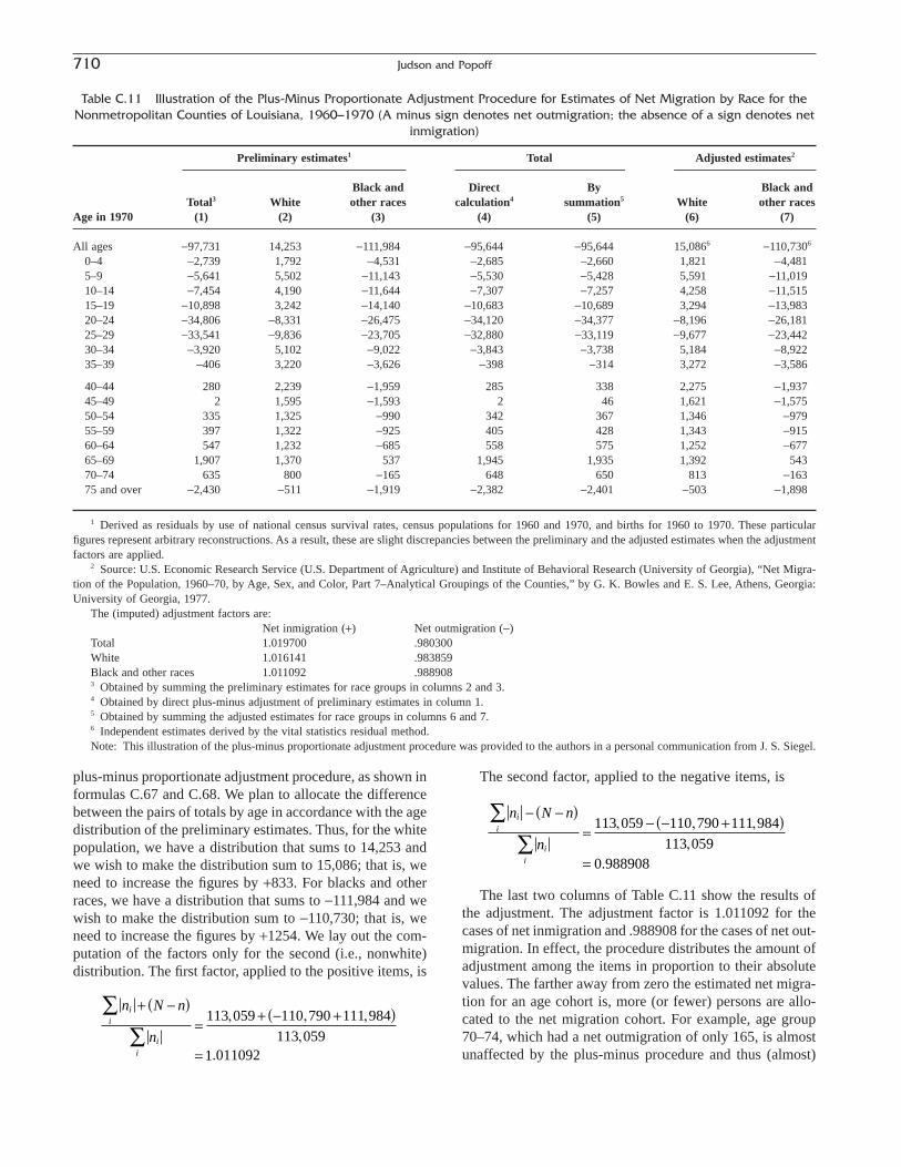
plus-minus proportionate adjustment procedure, as shown informulas C.67 and C.68. We plan to allocate the differencebetween the pairs of totals by age in accordance with the agedistribution of the preliminary estimates. Thus, for the whitepopulation, we have a distribution that sums to 14,253 andwe wish to make the distribution sum to 15,086; that is, weneed to increase the figures by +833. For blacks and otherraces, we have a distribution that sums to -111,984 and wewish to make the distribution sum to -110,730; that is, weneed to increase the figures by +1254. We lay out the com-putation of the factors only for the second (i.e., nonwhite)distribution. The first factor, applied to the positive items, is
n N n
n
ii
ii
+ -( )=
+ - +( )
=
ÂÂ
113 059 110 790 111 984113 059
1 011092
, , ,,
.
The second factor, applied to the negative items, is
The last two columns of Table C.11 show the results ofthe adjustment. The adjustment factor is 1.011092 for thecases of net inmigration and .988908 for the cases of net out-migration. In effect, the procedure distributes the amount ofadjustment among the items in proportion to their absolutevalues. The farther away from zero the estimated net migra-tion for an age cohort is, more (or fewer) persons are allo-cated to the net migration cohort. For example, age group70–74, which had a net outmigration of only 165, is almostunaffected by the plus-minus procedure and thus (almost)
n N n
n
ii
ii
- -( )=
- - +( )
=
ÂÂ
113 059 110 790 111 984113 059
0 988908
, , ,,
.
710 Judson and Popoff
Table C.11 Illustration of the Plus-Minus Proportionate Adjustment Procedure for Estimates of Net Migration by Race for theNonmetropolitan Counties of Louisiana, 1960–1970 (A minus sign denotes net outmigration; the absence of a sign denotes net
inmigration)
Preliminary estimates1 Total Adjusted estimates2
Black and Direct By Black andTotal3 White other races calculation4 summation5 White other races
Age in 1970 (1) (2) (3) (4) (5) (6) (7)
All ages -97,731 14,253 -111,984 -95,644 -95,644 15,0866 -110,7306
0–4 -2,739 1,792 -4,531 -2,685 -2,660 1,821 -4,4815–9 -5,641 5,502 -11,143 -5,530 -5,428 5,591 -11,01910–14 -7,454 4,190 -11,644 -7,307 -7,257 4,258 -11,51515–19 -10,898 3,242 -14,140 -10,683 -10,689 3,294 -13,98320–24 -34,806 -8,331 -26,475 -34,120 -34,377 -8,196 -26,18125–29 -33,541 -9,836 -23,705 -32,880 -33,119 -9,677 -23,44230–34 -3,920 5,102 -9,022 -3,843 -3,738 5,184 -8,92235–39 -406 3,220 -3,626 -398 -314 3,272 -3,586
40–44 280 2,239 -1,959 285 338 2,275 -1,93745–49 2 1,595 -1,593 2 46 1,621 -1,57550–54 335 1,325 -990 342 367 1,346 -97955–59 397 1,322 -925 405 428 1,343 -91560–64 547 1,232 -685 558 575 1,252 -67765–69 1,907 1,370 537 1,945 1,935 1,392 54370–74 635 800 -165 648 650 813 -16375 and over -2,430 -511 -1,919 -2,382 -2,401 -503 -1,898
1 Derived as residuals by use of national census survival rates, census populations for 1960 and 1970, and births for 1960 to 1970. These particularfigures represent arbitrary reconstructions. As a result, these are slight discrepancies between the preliminary and the adjusted estimates when the adjustmentfactors are applied.
2 Source: U.S. Economic Research Service (U.S. Department of Agriculture) and Institute of Behavioral Research (University of Georgia), “Net Migra-tion of the Population, 1960–70, by Age, Sex, and Color, Part 7–Analytical Groupings of the Counties,” by G. K. Bowles and E. S. Lee, Athens, Georgia:University of Georgia, 1977.
The (imputed) adjustment factors are:Net inmigration (+) Net outmigration (-)
Total 1.019700 .980300White 1.016141 .983859Black and other races 1.011092 .9889083 Obtained by summing the preliminary estimates for race groups in columns 2 and 3.4 Obtained by direct plus-minus adjustment of preliminary estimates in column 1.5 Obtained by summing the adjusted estimates for race groups in columns 6 and 7.6 Independent estimates derived by the vital statistics residual method.Note: This illustration of the plus-minus proportionate adjustment procedure was provided to the authors in a personal communication from J. S. Siegel.
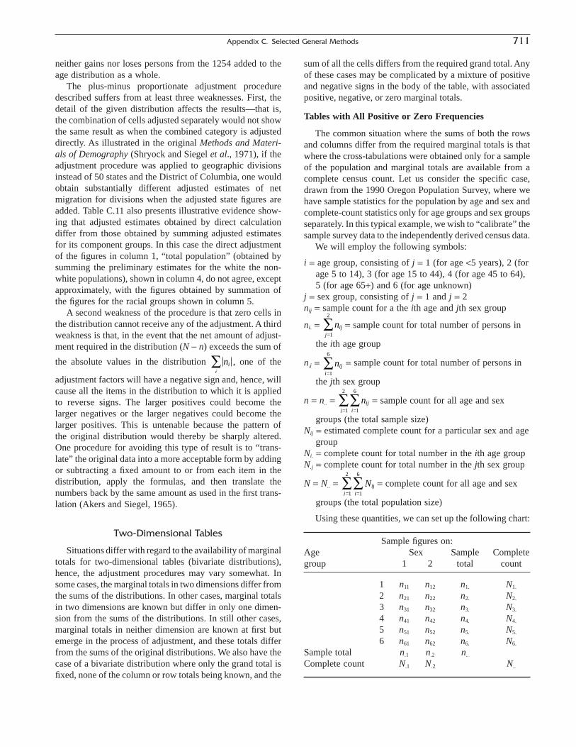
neither gains nor loses persons from the 1254 added to theage distribution as a whole.
The plus-minus proportionate adjustment proceduredescribed suffers from at least three weaknesses. First, thedetail of the given distribution affects the results—that is,the combination of cells adjusted separately would not showthe same result as when the combined category is adjusteddirectly. As illustrated in the original Methods and Materi-als of Demography (Shryock and Siegel et al., 1971), if theadjustment procedure was applied to geographic divisionsinstead of 50 states and the District of Columbia, one wouldobtain substantially different adjusted estimates of netmigration for divisions when the adjusted state figures areadded. Table C.11 also presents illustrative evidence show-ing that adjusted estimates obtained by direct calculationdiffer from those obtained by summing adjusted estimatesfor its component groups. In this case the direct adjustmentof the figures in column 1, “total population” (obtained bysumming the preliminary estimates for the white the non-white populations), shown in column 4, do not agree, exceptapproximately, with the figures obtained by summation ofthe figures for the racial groups shown in column 5.
A second weakness of the procedure is that zero cells inthe distribution cannot receive any of the adjustment. A thirdweakness is that, in the event that the net amount of adjust-ment required in the distribution (N - n) exceeds the sum of
the absolute values in the distribution , one of the
adjustment factors will have a negative sign and, hence, willcause all the items in the distribution to which it is appliedto reverse signs. The larger positives could become thelarger negatives or the larger negatives could become thelarger positives. This is untenable because the pattern of the original distribution would thereby be sharply altered.One procedure for avoiding this type of result is to “trans-late” the original data into a more acceptable form by addingor subtracting a fixed amount to or from each item in thedistribution, apply the formulas, and then translate thenumbers back by the same amount as used in the first trans-lation (Akers and Siegel, 1965).
Two-Dimensional Tables
Situations differ with regard to the availability of marginaltotals for two-dimensional tables (bivariate distributions),hence, the adjustment procedures may vary somewhat. Insome cases, the marginal totals in two dimensions differ fromthe sums of the distributions. In other cases, marginal totalsin two dimensions are known but differ in only one dimen-sion from the sums of the distributions. In still other cases,marginal totals in neither dimension are known at first butemerge in the process of adjustment, and these totals differfrom the sums of the original distributions. We also have thecase of a bivariate distribution where only the grand total isfixed, none of the column or row totals being known, and the
nii
Â
sum of all the cells differs from the required grand total. Anyof these cases may be complicated by a mixture of positiveand negative signs in the body of the table, with associatedpositive, negative, or zero marginal totals.
Tables with All Positive or Zero Frequencies
The common situation where the sums of both the rowsand columns differ from the required marginal totals is thatwhere the cross-tabulations were obtained only for a sampleof the population and marginal totals are available from acomplete census count. Let us consider the specific case,drawn from the 1990 Oregon Population Survey, where wehave sample statistics for the population by age and sex andcomplete-count statistics only for age groups and sex groupsseparately. In this typical example, we wish to “calibrate” thesample survey data to the independently derived census data.
We will employ the following symbols:
i = age group, consisting of j = 1 (for age <5 years), 2 (forage 5 to 14), 3 (for age 15 to 44), 4 (for age 45 to 64),5 (for age 65+) and 6 (for age unknown)
j = sex group, consisting of j = 1 and j = 2nij = sample count for a the ith age and jth sex group
ni. = = sample count for total number of persons in
the ith age group
n.j = = sample count for total number of persons in
the jth sex group
n = n.. = = sample count for all age and sex
groups (the total sample size)Nij = estimated complete count for a particular sex and age
groupNi. = complete count for total number in the ith age groupN.j = complete count for total number in the jth sex group
N = N.. = = complete count for all age and sex
groups (the total population size)
Using these quantities, we can set up the following chart:
Sample figures on:Age Sex Sample Completegroup 1 2 total count
1 n11 n12 n1. N1.
2 n21 n22 n2. N2.
3 n31 n32 n3. N3.
4 n41 n42 n4. N4.
5 n51 n52 n5. N5.
6 n61 n62 n6. N6.
Sample total n.1 n.2 n..
Complete count N.1 N.2 N..
Nijij =1
6
=1ÂÂ
2
nijij =1
6
=1ÂÂ
2
niji=1
6
Â
=1Ânijj
2
Appendix C. Selected General Methods 711
Method of Iterative Proportional Fitting
The adjustment of the sample data to sum to the complete-count marginal totals may be achieved by iterative sequen-tial “raking” of the original matrix, alternating with rows andcolumns, that is, first horizontally, then vertically, then hori-zontally, and so on, or first vertically, then horizontally, thenvertically, and so on. The procedure is illustrated in TableC.12 with sample data on age cross-classified by sex, andcomplete-count data on age and sex, separately, drawn fromthe 1990 Oregon Population Survey (for sample data) and the1990 census of the United States (for complete count data).Each step in the calculations is like that for adjusting singledistributions proportionately to an assigned total. This pro-cedure is called the method of iterative proportional adjust-ment or fitting, originally described in Deming and Stephan(1940) and Deming (1948).
Iterative proportional fitting proceeds as follows: Beginwith proportionate adjustment along each row to the mar-ginal row totals in Table C.12 (labeled “First proration byage”), then follow with proportionate adjustment of theresults along each column to the marginal column totals(labeled “First proration by sex”). The vertical adjustmentthrows the figures out of line with respect to the marginalrow totals; so adjust the figures to the marginal row totalsonce again (labeled “Second proration by age”). The read-justment of the rows to the marginal row totals then throwsthe figures out of line with respect to the marginal columntotals, and so adjust figures to the marginal column totalonce again (labeled “Second proration by sex”).
This sequence of adjustments is continued until it pro-duces complete convergence to a final unchanging matrix ofnumbers that add to the required row and column totals atonce; at this point further proration merely replicates thenumbers within a few digits. The convergence to marginalrow and column totals is usually rapid, requiring only a fewcycles (each consisting of a vertical adjustment and a hori-zontal adjustment) to achieve close agreement in one dimen-sion and precise agreement in the other. As this exampleshows, convergence to within a decimal occurs by the fourthproration, or two cycles.
The procedure is clearly laborious by hand calculation,but the operation is quite simple to carry out by electroniccomputer without concern for the number of cycles required.The calculation can be stopped at any required degree ofagreement with marginal totals, merely by setting a stoppingrule such as STOP when Nij(n+1) - Nij(n) < .01 for all i and jcells.
Deming does not give the mathematical proof that thesame results are obtained whether the columns or the rowsare “raked” first, but empirical testing indicates that theorder of raking is immaterial. In the case, however, whereone is attempting to “fit” a zero “margin”, the process maynot converge; see Bishop, Feinberg, and Holland (1975, pp.
90–91) for discussion. Note in the example given about thatthe “unknown” age group had a zero cell in the completecensus count, but the “margin” was not all zeros. Thus, itwas possible to fit the “margin” even when one of its cellswas zero. If, however, the entire margin were zeros, the pro-cedure would not have worked. This is a general principlefor iterative proportional fitting. (For extra details on zerocells and methods for handling them, see Agresti, 1990, pp. 245–250.)
Tables with Some Negative Frequencies
An earlier discussion indicated some of the complexitiesof the situation when single distributions with negatives areto be adjusted. Adjustment of bivariate distributions includ-ing negative values may be accomplished by an extensionof procedures already described. For example, the methodof iterative proportions may employ a two factor plus-minusproportionate procedure for each column and row.
General Multiway Tables
Since publication of the original Methods and Materialsof Demography (Shryock Siegel and Associates, 1971), ageneralization of the method of iterative proportions hasemerged, known as “loglinear” analysis in social science oras “analysis of cross-classifications” or even as “poissonregression.” This generalization allows the analyst to fitgeneral multiway cross-classifications of two, three, or evenmore variables—for example, age and race and sex simul-taneously. A comprehensive introduction to these methodscan be found in Agresti (1990), with a simpler exposition inAgresti (1996). This methodology puts the analysis of cate-gorical data in the framework of a generalized linear model(McCullagh and Nelder, 1990).
There are several key questions regarding the strategy foranalyzing a cross-classification of categorical data:
1. Is there a clear dependent variable?a. If NO (i.e., all one has is a three-way classification
of data), then “loglinear analysis” is an appropriatechoice to consider.
b. If YES, then “loglinear analysis” is not the bestchoice. Go to the next question.
2. Is the dependent variable categorical?a. If YES, then one would look at techniques like
logistic regression, multinomial logit or probit,ordinal logit and probit, discriminant analysis, andthe like.
b. If NO, then one would look at ordinary regression,tobit/censored normal, Heckman models, and the like.
The most important point, of course, is to choose the estimation method that corresponds to the sampling andother properties of the variables one has measured.
712 Judson and Popoff
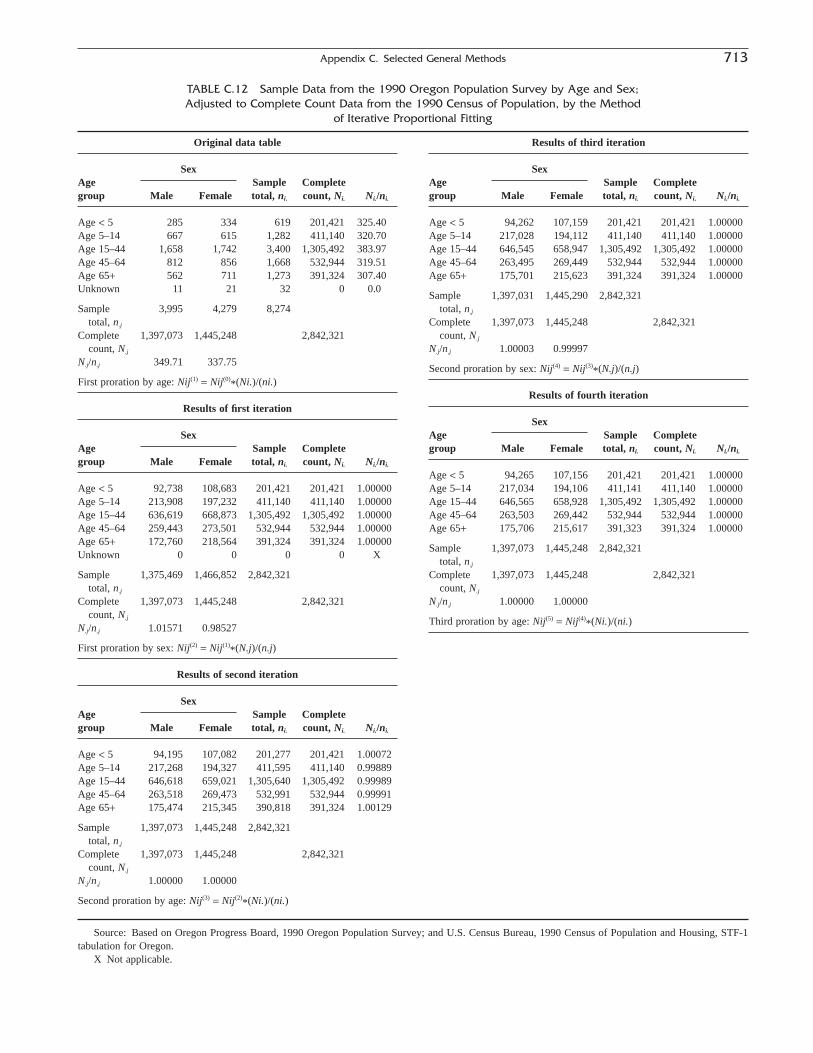
Appendix C. Selected General Methods 713
Original data table
SexAge Sample Completegroup Male Female total, ni. count, Ni. Ni./ni.
Age < 5 285 334 619 201,421 325.40Age 5–14 667 615 1,282 411,140 320.70Age 15–44 1,658 1,742 3,400 1,305,492 383.97Age 45–64 812 856 1,668 532,944 319.51Age 65+ 562 711 1,273 391,324 307.40Unknown 11 21 32 0 0.0
Sample 3,995 4,279 8,274total, n.j
Complete 1,397,073 1,445,248 2,842,321count, N.j
N.j/n.j 349.71 337.75
First proration by age: Nij(1) = Nij(0)*(Ni.)/(ni.)
Results of first iteration
SexAge Sample Completegroup Male Female total, ni. count, Ni. Ni./ni.
Age < 5 92,738 108,683 201,421 201,421 1.00000Age 5–14 213,908 197,232 411,140 411,140 1.00000Age 15–44 636,619 668,873 1,305,492 1,305,492 1.00000Age 45–64 259,443 273,501 532,944 532,944 1.00000Age 65+ 172,760 218,564 391,324 391,324 1.00000Unknown 0 0 0 0 X
Sample 1,375,469 1,466,852 2,842,321total, n.j
Complete 1,397,073 1,445,248 2,842,321count, N.j
N.j/n.j 1.01571 0.98527
First proration by sex: Nij(2) = Nij(1)*(N.j)/(n.j)
Results of second iteration
SexAge Sample Completegroup Male Female total, ni. count, Ni. Ni./ni.
Age < 5 94,195 107,082 201,277 201,421 1.00072Age 5–14 217,268 194,327 411,595 411,140 0.99889Age 15–44 646,618 659,021 1,305,640 1,305,492 0.99989Age 45–64 263,518 269,473 532,991 532,944 0.99991Age 65+ 175,474 215,345 390,818 391,324 1.00129
Sample 1,397,073 1,445,248 2,842,321total, n.j
Complete 1,397,073 1,445,248 2,842,321count, N.j
N.j/n.j 1.00000 1.00000
Second proration by age: Nij(3) = Nij(2)*(Ni.)/(ni.)
TABLE C.12 Sample Data from the 1990 Oregon Population Survey by Age and Sex; Adjusted to Complete Count Data from the 1990 Census of Population, by the Method
of Iterative Proportional Fitting
Results of third iteration
SexAge Sample Completegroup Male Female total, ni. count, Ni. Ni./ni.
Age < 5 94,262 107,159 201,421 201,421 1.00000Age 5–14 217,028 194,112 411,140 411,140 1.00000Age 15–44 646,545 658,947 1,305,492 1,305,492 1.00000Age 45–64 263,495 269,449 532,944 532,944 1.00000Age 65+ 175,701 215,623 391,324 391,324 1.00000
Sample 1,397,031 1,445,290 2,842,321total, n.j
Complete 1,397,073 1,445,248 2,842,321count, N.j
N.j/n.j 1.00003 0.99997
Second proration by sex: Nij(4) = Nij(3)*(N.j)/(n.j)
Results of fourth iteration
SexAge Sample Completegroup Male Female total, ni. count, Ni. Ni./ni.
Age < 5 94,265 107,156 201,421 201,421 1.00000Age 5–14 217,034 194,106 411,141 411,140 1.00000Age 15–44 646,565 658,928 1,305,492 1,305,492 1.00000Age 45–64 263,503 269,442 532,944 532,944 1.00000Age 65+ 175,706 215,617 391,323 391,324 1.00000
Sample 1,397,073 1,445,248 2,842,321total, n.j
Complete 1,397,073 1,445,248 2,842,321count, N.j
N.j/n.j 1.00000 1.00000
Third proration by age: Nij(5) = Nij(4)*(Ni.)/(ni.)
Source: Based on Oregon Progress Board, 1990 Oregon Population Survey; and U.S. Census Bureau, 1990 Census of Population and Housing, STF-1tabulation for Oregon.
X Not applicable.
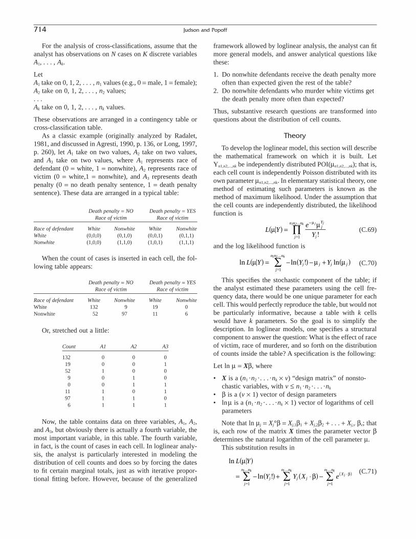
For the analysis of cross-classifications, assume that theanalyst has observations on N cases on K discrete variablesA1, . . . , Ak.
LetA1 take on 0, 1, 2, . . . , n1 values (e.g., 0 = male, 1 = female);A2 take on 0, 1, 2, . . . , n2 values;. . .Ak take on 0, 1, 2, . . . , nk values.
These observations are arranged in a contingency table orcross-classification table.
As a classic example (originally analyzed by Radalet,1981, and discussed in Agresti, 1990, p. 136, or Long, 1997,p. 260), let A1 take on two values, A2 take on two values,and A3 take on two values, where A1 represents race ofdefendant (0 = white, 1 = nonwhite), A2 represents race ofvictim (0 = white,1 = nonwhite), and A3 represents deathpenalty (0 = no death penalty sentence, 1 = death penaltysentence). These data are arranged in a typical table:
Death penalty = NO Death penalty = YESRace of victim Race of victim
Race of defendant White Nonwhite White NonwhiteWhite (0,0,0) (0,1,0) (0,0,1) (0,1,1)Nonwhite (1,0,0) (1,1,0) (1,0,1) (1,1,1)
When the count of cases is inserted in each cell, the fol-lowing table appears:
Death penalty = NO Death penalty = YESRace of victim Race of victim
Race of defendant White Nonwhite White NonwhiteWhite 132 9 19 0Nonwhite 52 97 11 6
Or, stretched out a little:
Count A1 A2 A3
132 0 0 019 0 0 152 1 0 09 0 1 00 0 1 1
11 1 0 197 1 1 06 1 1 1
Now, the table contains data on three variables, A1, A2,and A3, but obviously there is actually a fourth variable, themost important variable, in this table. The fourth variable,in fact, is the count of cases in each cell. In loglinear analy-sis, the analyst is particularly interested in modeling the distribution of cell counts and does so by forcing the datesto fit certain marginal totals, just as with iterative propor-tional fitting before. However, because of the generalized
framework allowed by loglinear analysis, the analyst can fitmore general models, and answer analytical questions likethese:
1. Do nonwhite defendants receive the death penalty moreoften than expected given the rest of the table?
2. Do nonwhite defendants who murder white victims getthe death penalty more often than expected?
Thus, substantive research questions are transformed intoquestions about the distribution of cell counts.
Theory
To develop the loglinear model, this section will describethe mathematical framework on which it is built. Let Yn1,n2,...,nk be independently distributed POI(mn1,n2,...,nk); that is,each cell count is independently Poisson distributed with itsown parameter mn1,n2,...,nk. In elementary statistical theory, onemethod of estimating such parameters is known as themethod of maximum likelihood. Under the assumption thatthe cell counts are independently distributed, the likelihoodfunction is
(C.69)
and the log likelihood function is
(C.70)
This specifies the stochastic component of the table; ifthe analyst estimated these parameters using the cell fre-quency data, there would be one unique parameter for eachcell. This would perfectly reproduce the table, but would notbe particularly informative, because a table with k cellswould have k parameters. So the goal is to simplify thedescription. In loglinear models, one specifies a structuralcomponent to answer the question: What is the effect of raceof victim, race of murderer, and so forth on the distributionof counts inside the table? A specification is the following:
Let ln m = Xb, where
• X is a (n1 ·n2 · . . . ·nk ¥ v) “design matrix” of nonsto-chastic variables, with v £ n1 ·n2 · . . . ·nk
• b is a (v ¥ 1) vector of design parameters• lnm is a (n1 ·n2 · . . . ·nk ¥ 1) vector of logarithms of cell
parameters
Note that ln mj = Xj°b = Xj,1b1 + Xj,2b2 + . . . + Xj,v bv; thatis, each row of the matrix X times the parameter vector bdetermines the natural logarithm of the cell parameter m.
This substitution results in
(C.71)
ln
ln !
L Y
Y Y X ejj
n n
j jj
n nX
j
n nk kj
k
m
b b
( )
= - ( ) + ◊( ) -Â Â Â ◊( )
=1
...
=1
...
=1
...1 1 1
ln ln ! lnL Y Y Yjj
n n n
j j j
k
m m m( ) = - ( ) - + ( )Â=1
...1 2
L Ye
Y
j j1 2 kjY
jj
n n ...n
mmm
( ) =-
’ !=1
714 Judson and Popoff

and, taking partial derivatives with respect to each parame-ter bm and setting them to zero, generates a system of equa-tions, one for each parameter bm, each of the form:
(C.72)
The root of this equation in each b can be found itera-tively using, for example, the Newton-Raphson algorithm.When that root is found, it is the maximum-likelihood esti-mates of the b’s that are then used to generate expected cellcounts under the model.
The key to this model is the design matrix X; it specifieswhat “margins” in the table the analyst wishes to control,interaction effects between marginal variables, and any othermodel-related aspects. So the question at this point becomes:What is X and how is it specified?
Because the only explanatory variables are A1, . . . , Ak,the table margins, X is a matrix of indicator variables spec-ifying unique parameters for specific cells. Consider theexample of the 2 ¥ 2 ¥ 2 death penalty table. Suppose theanalyst wished to specify the model that all the cell fre-quencies are the same. This means that
• All the Poisson counts are governed by the sameparameter
• Under the model the expected cell counts will all bethe same
• P[death penalty|nonwhite murderer] = P[deathpenalty|white murderer]
To do this, the analyst specifies X as a (n1 ·n2 · . . . ·nk ¥ 1)matrix and b as a 1 ¥ 1 vector. Thus,
If this model fits the data well, the analyst has simplifiedthe structure of the table, from a maximum of eight param-eters, one per cell, to this minimum of one. The analyst has,in effect, “fit” each observed cell count to be the same acrossthe table. This is, of course, a baseline model, and few real-world applications will be so simplistic. So consider a moresophisticated model. Suppose the analyst wished to specifythe following:
• A baseline level of occupants in each cell (a constant)• Plus an additional amount in all death penalty cells (to
let that variable affect the counts)
ln :. :.m b
bb
b
( ) =
È
Î
ÍÍÍÍ
˘
˚
˙˙˙˙
◊ [ ] =
È
Î
ÍÍÍÍ
˘
˚
˙˙˙˙
1
1
1
(
)
Note: ensures that this is a
maximum.
,=
...∂∂
2
22
1
1
0b
b
mj m
X
j
n n
X e jk
= - <◊Â
01 1
1 1
= = - -  ◊∂∂ b
b
mj j m
j
n nX
j
n n
j mY X e Xk
jk
,=
...
=
...
,
• An additional amount in all nonwhite victim cells (tolet that variable affect the counts)
• An additional amount in all nonwhite murderer cells (tolet that variable affect the counts)
This results in
A1 A2 A3 PARAMETERS
0 0 0 b0
0 0 1 b3
0 1 0 b2
1 0 0 b0+ b1
0 1 1 b0+ b2+ b3
1 0 1 b0+ b1+ b3
1 1 0 b0+ b1+ b2
1 1 1 b0+ b1+ b2+ b3
This is represented in the matrix:
or, equivalently, the equation:
This is known as the “independence” model because nointeraction is specified between the margins A1, A2, and A3.It does not specify that all cell probabilities and conditionalprobabilities are the same; rather, it forces the expected cellfrequencies under the model to fit the A1 margin in the table,the A2 margin in the table, and the A3 margin in the table.Thus, the expected cell frequencies will reproduce the threemarginal distributions. This is exactly what the earlierexample of iterative proportional fitting did.
The “Loglinear” Model Versus IterativeProportional Fitting for Multiway Tables
It should be clear at this point that the loglinear model iseffectively doing the same thing that the iterative propor-tional fitting model did earlier. In fact, Bishop, Feinberg, andHolland (1975) and earlier, Birch (1963) demonstrated thatthe two approaches generate equivalent results under avariety of sampling models. In practice, iterative propor-tional fitting might be used for simpler tables or modelsbecause of its easy interpretability, while a loglinear modelmight be used for a more complex model or a higher-dimensional table because of its flexibility. In addition,because the loglinear model is placed in a regression-likeframework, it is possible to evaluate standard errors of coef-
Ŷ A A A= + ◊ + ◊ + ◊b b b b0 1 1 2 2 3 3
0 0 0
0 0 1
0 1 0
1 0 0
0 1 1
1 0 1
1 1 0
1 1 1
1 0 0 0
1 1 0 0
1 0 1 0
1 0 0 1
1 1 1 0
1 1 0 1
1 0 1 1
1 1 1 1
, ,
, ,
, ,
, ,
, ,
, ,
, ,
, ,
( )( )( )( )( )( )( )( )
È
Î
ÍÍÍÍÍÍÍÍÍÍ
˘
˚
˙˙˙˙˙˙˙˙˙˙
=
È
Î
ÍÍÍÍÍÍÍÍÍÍÍ
˘
˚
˙˙˙˙˙˙˙˙˙˙
◊
È
Î
ÍÍÍÍ
˘
˚
˙˙˙˙
bbbb
0
1
2
3
Appendix C. Selected General Methods 715

ficients and to develop standard errors of the estimated cellfrequencies and similar useful statistics that allow one toevaluate the quality of the model and hence the quality ofthe fitting procedure itself.
COMPUTER USAGE, MODELS, AND METHODS
Use of Electronic Computers in Demographic Studies
Data Collection and Processing
Data collection in the demographic field has been dra-matically altered by new technologies, in particular thoseoffered by computerized data collection systems. The orig-inal Methods and Materials of Demography (Shryock,Siegel, and Associates, 1971) made reference to the use ofoptically scanned (“FOSDIC”) data collection forms in the1970 and 1980 U.S. censuses. In 2000, the U.S. CensusBureau invested in optical scanning of handwritten forms,and optical character recognition technology for processingthese handwritten responses.
Figure C.9 describes (approximately) the flow of files inthe U.S. 2000 Census.11 The original responses are collectedand maintained in the Decennial Response File (DRF1 and
2). These receive minimal editing, but most important, areunduplicated and compiled into the Hundred PercentUnedited File and Sample Census Unedited File (HCUF andSCUF). At this point, edits and imputations are applied. Asthe reader may recall from Chapter 3, these edits and impu-tations are not trivial; the edits cannot be applied in isola-tion (independent of one another) but instead must reflectthe covariance structure actually present in the data.
The HCUF and SCUF are easily the primary files foranalyses that are tied closely to respondents (although somestudies attempt to get even closer to the respondent via theDRF files or, closer yet, by reinterviews). As the readerknows, the U.S. Census Bureau uses a dual-systems method-ology for measuring differential census undercounts. Theimpact of this methodology is reflected in the HCEF andSCEF files, where coverage factors for undercounts areapplied. Further downstream, tabulation geography (e.g., cityboun- daries that split collection blocks) is added back in (viathe HEDF file), and tabulation products begin to be produced.
One might dismiss these processes as merely “data han-dling.” In fact, most users of census data work directly withthe tabulation products as if they were simply the “truth”and ignore the process of data handling. However, the trans-formations that these files require are not merely a matter ofmoving data around a computer system, but at each step ofthe process decisions must be made about the characteris-tics of persons and households, and these decisions aredemographically substantive. People are “created” and“deleted,” their characteristics (e.g., income) are estimated,their ages are edited and other such operations are per-formed. Demographers should pay attention to these opera-
716 Judson and Popoff
FIGURE C.9 A summary of U.S. census 2000 file construction: From original census forms to data products.
11 Mai Weismantle of the Housing, Household, and Economic Statis-tics Division of the U.S. Census Bureau developed the prototype for thisgraphic.
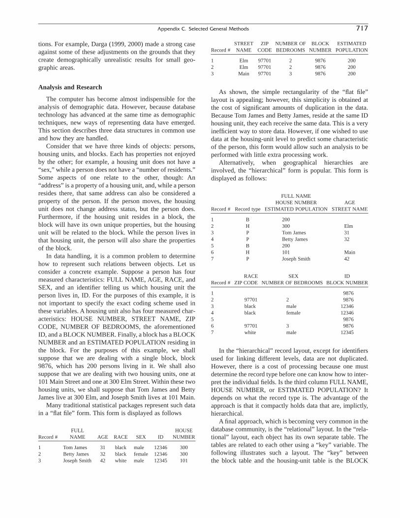
tions. For example, Darga (1999, 2000) made a strong caseagainst some of these adjustments on the grounds that theycreate demographically unrealistic results for small geo-graphic areas.
Analysis and Research
The computer has become almost indispensible for theanalysis of demographic data. However, because databasetechnology has advanced at the same time as demographictechniques, new ways of representing data have emerged.This section describes three data structures in common useand how they are handled.
Consider that we have three kinds of objects: persons,housing units, and blocks. Each has properties not enjoyedby the other; for example, a housing unit does not have a“sex,” while a person does not have a “number of residents.”Some aspects of one relate to the other, though: An“address” is a property of a housing unit, and, while a personresides there, that same address can also be considered aproperty of the person. If the person moves, the housing unit does not change address status, but the person does. Furthermore, if the housing unit resides in a block, the block will have its own unique properties, but the housingunit will be related to the block. While the person lives inthat housing unit, the person will also share the propertiesof the block.
In data handling, it is a common problem to determinehow to represent such relations between objects. Let us consider a concrete example. Suppose a person has fourmeasured characteristics: FULL NAME, AGE, RACE, andSEX, and an identifier telling us which housing unit theperson lives in, ID. For the purposes of this example, it isnot important to specify the exact coding scheme used inthese variables. A housing unit also has four measured char-acteristics: HOUSE NUMBER, STREET NAME, ZIPCODE, NUMBER OF BEDROOMS, the aforementionedID, and a BLOCK NUMBER. Finally, a block has a BLOCKNUMBER and an ESTIMATED POPULATION residing inthe block. For the purposes of this example, we shallsuppose that we are dealing with a single block, block 9876, which has 200 persons living in it. We shall alsosuppose that we are dealing with two housing units, one at101 Main Street and one at 300 Elm Street. Within these twohousing units, we shall suppose that Tom James and BettyJames live at 300 Elm, and Joseph Smith lives at 101 Main.
Many traditional statistical packages represent such datain a “flat file” form. This form is displayed as follows
FULL HOUSERecord # NAME AGE RACE SEX ID NUMBER
1 Tom James 31 black male 12346 3002 Betty James 32 black female 12346 3003 Joseph Smith 42 white male 12345 101
STREET ZIP NUMBER OF BLOCK ESTIMATEDRecord # NAME CODE BEDROOMS NUMBER POPULATION
1 Elm 97701 2 9876 2002 Elm 97701 2 9876 2003 Main 97701 3 9876 200
As shown, the simple rectangularity of the “flat file”layout is appealing; however, this simplicity is obtained atthe cost of significant amounts of duplication in the data.Because Tom James and Betty James, reside at the same IDhousing unit, they each receive the same data. This is a veryinefficient way to store data. However, if one wished to usedata at the housing-unit level to predict some characteristicof the person, this form would allow such an analysis to beperformed with little extra processing work.
Alternatively, when geographical hierarchies areinvolved, the “hierarchical” form is popular. This form isdisplayed as follows:
FULL NAMEHOUSE NUMBER AGE
Record # Record type ESTIMATED POPULATION STREET NAME
1 B 2002 H 300 Elm3 P Tom James 314 P Betty James 325 B 2006 H 101 Main7 P Joseph Smith 42
RACE SEX IDRecord # ZIP CODE NUMBER OF BEDROOMS BLOCK NUMBER
1 98762 97701 2 98763 black male 123464 black female 123465 98766 97701 3 98767 white male 12345
In the “hierarchical” record layout, except for identifiersused for linking different levels, data are not duplicated.However, there is a cost of processing because one mustdetermine the record type before one can know how to inter-pret the individual fields. Is the third column FULL NAME,HOUSE NUMBER, or ESTIMATED POPULATION? Itdepends on what the record type is. The advantage of theapproach is that it compactly holds data that are, implictly,hierarchical.
A final approach, which is becoming very common in thedatabase community, is the “relational” layout. In the “rela-tional” layout, each object has its own separate table. Thetables are related to each other using a “key” variable. Thefollowing illustrates such a layout. The “key” between the block table and the housing-unit table is the BLOCK
Appendix C. Selected General Methods 717

NUMBER field, while the “key” between the housing unittable and the person table is the ID field.
Block table
ESTIMATED BLOCKRecord # Record type POPULATION NUMBER
1 B 200 9876
Housing unit table
Record # Record type HOUSE NUMBER STREET NAME
1 H 300 Elm2 H 101 Main
NUMBER OF Record # ZIP CODE BEDROOMS ID BLOCK NUMBER
1 97701 2 12346 98762 97701 3 12345 9987
Person table
Record # Record type FULLNAME AGE RACE SEX ID
1 P Tom James 31 black male 123462 P Betty James 32 black female 123463 P Joseph Smith 42 white male 12345
It is easy to see that there is again almost no duplicationof data; furthermore, there is not the varying field meaningsthat the hierarchical record layout creates. The relationallayout form has become very popular because of theseadvantages. However, it has one notable disadvantage, par-ticularly when dealing with large data sets: If one wants toanalyze data across different tables, one must perform a“table join.” For example, if one wanted to analyze how thenumber of bedrooms in a house relates to a person’s age,race, or sex, one must join the housing unit table with theperson table, using the ID as the joining device. Even more,if one wished to examine how a block size relates to aperson’s age, race, or sex, the join is more complicated (fromperson ID to housing unit ID, then from housing unit ID toBLOCK NUMBER), to finally attach the ESTIMATEDPOPULATION of the block to the person. This is a compu-tationally intensive process.
Administrative Records Databases and Data Warehousing
In the late 20th and early 21st centuries, the growth ofadministrative records and computing power and storage hasmade massive databases available for demographic use.However, the principles of data collection and analysis havenot changed—only the (lowered) intensity of the data col-
lection effort and its widespread dissemination among manycollectors.
In response to this technological opportunity, the field of “data warehousing” has emerged (Inmon, 1996). FigureC.10 diagrams the basic features of a data warehouse, whichis the central concept in the “modern” use of administrativerecords. On the left are symbols representing the ongoing,operational databases: client contact records, tax returns,quarterly business reports, unemployment insurancerecords, credit card purchase data, insurance and medicaltreatment records, building permits, and so on. These data-bases are typically produced to support the ongoing opera-tions of the organization: Accounting (in the broadest senseof that term) is perhaps the most important use. They havenot been, and typically are not, designed for research analytic use.
In the center is the data warehouse itself. This is a repos-itory of recoded and maintained data and can be designedfor analytic access. The Oregon Shared Information System(Judson, 1993) and the U.S. Census Bureau’s StatisticalAdministrative Records System (Judson, 2000) are exam-ples of “set up” data warehouses designed for researchanalyses. The data warehouse serves the following func-tions, different from operational data:
• Developing common data definitions and maintaining arecord of those definitions as they evolve over time
• Matching operational data to create a master record ofthe object(s) of interest
• Maintaining panels or a time series of data (a mostimportant function, which operational databases may ormay not do)
• Summarizing data (creating decision-support reports)• Providing a flexible access structure (as opposed to
the quite rigid structures of many operational databases)
• Allowing users to construct ad hoc analyses of data
On the right of the figure is the end user of these data. Thedemographer, statistician, or geographic information sys-tems expert is typically considered the end user.
Challenges with Using Administrative Records
Despite their now widespread use, administrative recordsare not without pitfalls. Figure C.11 illustrates the processof data collection in the administrative records context(taken variously from Judson and Popoff, 1996; Ma, 1986;and Redman, 1996):
This figure identifies how records are created and used,and, at each step, where there is potential for error. A recordbegins as an event or an object in the “real world” outsidethe database. Some of these are actually identified (notealready that some events and objects that are really there donot get identified) as observed events and objects. Some of
718 Judson and Popoff

these observed events and objects get recorded (again, somedo not) and become part of the administrative record. Theseare then arranged in some form of database. Later, when the analyst approaches these records, he or she developsanalyses (“queries” in the language of data mining) andmakes presentation of the results. Finally, using either theusual statistical framework or policy-making framework,some decision is made.
At each step in this process there is potential for error ormisinterpretation. At the event/object level, policy changescan change the definition of an event or object (as when theU.S. welfare program Aid to Families with Dependent Children [AFDC] ceased to exist or when a mobile home isrecoded from “real” property to “personal” property). Asevents and objects become observed, the “ontologies” that
observers use to categorize the world (that is, the schemathat they use) enter in. Likewise, some events and objectsdo not reach a threshold for official notice (as where the“officer on the beat” makes a determination whether to iden-tify an event as a problem or not; see, e.g., Laudon, 1986;Light, 1990). Some of those observed events becomerecorded, and there are the possibilities of data entry errorsand limitations of coding schemes for mapping the real-world events into their database representations. As data aremoved from place to place in computer systems, data man-agement problems (corruption in transit, changes in format-ting, and so forth, documented in Stevens, Richmond,Haenn, and Michie, 1992, pp. 171–178) arise. Finally, as theanalyst extracts data using queries of various kinds, he orshe may discover that the query is either syntatically incor-
Appendix C. Selected General Methods 719
FIGURE C.10 An illustration of the data warehouse concept.
FIGURE C.11 How administrative records are created and used.
rect in a nonobvious way, or the query generates resultswhose structure itself is spurious.
Models for Use with Administrative Records
In virtually all cases, the administrative records analysthas no control over the data-collection process in adminis-trative records use—that is, the analyst does not control howthe administrative form asks a question or records a datum.As noted earlier, as with all data sets, random errors willoccur; but in the administrative records context, demogra-phers are most concerned with detecting biased data collection.
Because the analyst does not control data collection, thereare two contexts in which administrative records analysestake place: after data collection, but prior to analysis, andduring analysis. In the first context, the analyst is handlingdata and catching errors and anomalies when they occur.Tools used in the data-handling context include recordlinkage, editing and imputation, and direct testing for bias.During analysis, the strategies for dealing with the anom-alies in administrative records may change. Tools used in thecontext of analysis include: poststratification and syntheticestimation, dual systems analysis, measurement errormodels, and direct evaluations of bias.
Each of these tools has generated a substantial literatureon its own (Judson and Popoff, 1996).
MATRIX METHODS
Matrix Methods of Population Analysis
Matrix methods have been employed in the developmentof a number of recursive models, those where some mathe-matical relationship representing change in the population isassumed to be repeated again and again. A matrix is an arrayof data in one or two dimensions to which the special pro-cedures of matrix algebra can be applied. The basic popula-tion matrix changes according to the rates or probabilities,called transition probabilities, given in a transition matrix.The process of change in a model whose population movesfrom one state to another according to the probabilities inthe transition matrix is called a Markov process, and a modelthat has this characteristic is called a Markovian model. Thepopulation in the model may move in the direction of andattain a state of equilibrium (i.e., invariant once it has beenreached) that is completely independent of the initial distribution.
Markovian Models
There are two basic kinds of Markov processes, discrete-time and continuous-time (Schoen’s, 1988). Continuous
time models can usually be identified by the presence ofintegrals and differential equations, which indicate that timeis considered in a continuous fashion. Discrete time modelsare distinguished by the fact that events take place in dis-tinct jumps rather than occur continuously. A Markovprocess in discrete time is often called a Markov chain. Itusually requires conventional algebra and matrix algebra forunderstanding rather than the calculus and differential equa-tions. For the purpose of describing matrix methods ofanalysis, this section shall focus on discrete time models.
Imagine a population whose members are divided into Kdistinct states, which may be age “grades”, positions in anorganization, locations in a region, or some other status ofinterest. Each member falls into one and only one state atany time. Represent the numbers of persons in each state bya 1 ¥ (K + 1) row vector Nt , where time takes on the values0, 1, 2, 3, . . . , T, and movement between states occurs atthe time jumps.
Assume that for each person there exists a fixed proba-bility of moving from his or her current state into anotherstate. This is pij, which denotes the probability of movingfrom state i to state j. However, some of the states cannotbe exited (because the person is dead or because the personhas “left the system”). Let there be a K + 1st state that rep-resents leaving the system. This can be represented by a (K+ 1) ¥ (K + 1) matrix P of pij’s. The exit state is known asan absorbing state because people who enter it never leave.Hence, the probability of going from an absorbing state toitself is 1. Note also that there may be more than one absorb-ing state (exit due to death and exit due to migration or mar-riage, for instance). Recall that a life table that has thisproperty is referred to as a “multiple decrement” life table.
When the matrix P contains probabilities representing theprobability of a birth occurring to a female (thus generatinga new “entrant” to the system) and the probability of eachperson dying, then this matrix can be used to project popula-tion growth under the fixed fertility and mortality regimeimplied by the matrix. Leslie (1945) provided the best knownand most detailed analysis of this case, and the matrix he con-structed is often referred to as a “Leslie” matrix. (See dis-cussion later, Pollard, 1973, and Rogers, 1975, 1995, forextensive details and continuous time extensions.)
Stable Theory
If we temporarily ignore the absorbing state and onlyconsider the K ¥ K matrix P by dropping the K + 1st row andcolumn vectors, then there exists some machinery to assistin assessing the stable population implied by the matrix P.A “stable population” is a population in which the transitionprobabilities for ferlitety and mortality do not vary overtime. A “stationary population,” which is stable, also has thefeature that entries into and exits from it are equal inabsolute numbers, as in a standard life table.
720 Judson and Popoff

In a population without absorbing states, and satisfyingcertain conditions of regularity needed for a Markov chain,over time the population will tend toward a limiting distri-bution called stable.12 This limiting distribution will be inde-pendent of the starting distribution and will have membersin each state in fixed proportions. That is, the fraction ofpersons in each state will not change from time period totime period. In this case, the limiting distribution can befound simply using the following eigenvalue and eigenvec-tor methods.
In a stable state, the population matrix will obey the fol-lowing equation:
(C.73)
where N¢ is a K ¥ 1 column vector, the transpose of the rowvector Nt, ignoring the “exited” state, with the desired limiting distribution. This equation indicates that, in thestable limit, if we begin with the population in distributionN¢ and apply the transition probabilities to each member, weend with a population in the same distribution (hence the ter-minology: “stable” population). This equation implies
(C.74)
In this form, N¢ is an eigenvector of the matrix P corre-sponding to the dominant (largest) eigenvalue of that matrix.Brown (1993, p. 172) noted that this dominant eigenvaluehas a demographic interpretation: It will be l = enr, where nis the size of the age groups, and r is the “intrinsic” rate ofgrowth when in a stable state. Methods for finding eigen-values and eigenvectors corresponding to those eigenvaluesare standard (Press et al., 1989) and implemented in numer-ous computer packages.
Models with Entry and Exit Variation
In standard population models, a demographer typicallyspecifies that each female has children that fall into theyoungest age category. In multiple increment-decrementmodels, one need not make any such specification. Instead,new members of the population can enter into any of thestates. If states are age grades in a closed population, newmembers must enter at the youngest age grade; if states areschool grades, however, new members can enter at highergrades due to inmigration.
For now, assume that members enter the states in fixedproportions, although the number varies by time. Let E bea 1 ¥ (K + 1) row vector representing the proportion of newmembers who enter state j in any time period, and let rt bethe number of new recruits at time t.
P I N-( ) ¢ =l 0
PN N¢ = ¢l
To summarize:
P = a (K + 1) ¥ (K + 1) matrix consisting of the probabil-ity of moving from state i to state j, where state K + 1means “leaving the system”
E = a 1 ¥ (K + 1) row vector consisting of the proportionof new entrants that enter a particular state
rt = a scalar, the number of new recruits that enter at eachtime period
t = time, measured in discrete increments 0,1,2,3,4, and so on
In matrix algebra, the number of people in each state atany time can be represented by
(C.75)
where Nt = the 1 ¥ (K + 1) row vector representing thenumber of people in each state at time t, and the other ele-ments are as defined earlier.
Now, to find a solution to this process, apply the equa-tion repeatedly until reaching N0, which is the starting value.So
as in C.75
(C.76)
and so on.Starting at any arbitrary time t, and continuing substitut-
ing backward until reaching time t = 0,
(C.77)
and so on, which results in the general equation:
(C.78)
(For more details, see Bartholomew, 1982, pp. 50–53.)What does this mean? Simply this: If the analyst knows
1. The number of persons that start in each state (N0),2. The probability transition matrix P,3. The proportion that enter each state at each time period
(E), and4. The number of new entrants at each time period (r)
then the analyst can calculate exactly how many people will be in each state at any time in the future. The analyst needs to know a lot of information to work withthis model, but much of it is easily assumable from past trends (number 3 or number 4, for example) or couldbe statistically estimated from existing data (number 2 andnumber 3).
Note two important facts:
1. When the K + 1st state, the “dead” or “exited” state,is included, then the proportions in each state do not
N N P E r Pt tt
t
= ◊ + ◊ ÊËÁ
ˆ¯̃-
=Â0
0
1
ii
-
N N P r E
N P r E P r E
N P r E P r P r E
t t t
t t t
t t t t
= ◊ + ◊= ◊ + ◊( ) ◊ + ◊= ◊ + ◊( ) ◊ +( ) ◊ + ◊
- -
- -
- - -
1 1
2 1
3 2 1
N N P r Et t t- - -1 2 1= ◊ + ◊
N N P r Et t t= ◊ + ◊- ,1
N N P r Et t t= ◊ + ◊-1
Appendix C. Selected General Methods 721
12 Strictly speaking, in order for the following theory to hold, a stablepopulation must satisfy three additional conditions of regularity: the statesmust be recurrent with positive probability, all states must be reachable onefrom another, and the transitions must be aperiodic. Such a Markov chainis called irreducible and ergodic, and that is a necessary condition for a limiting distribution to exist (Ross, 1997, p. 173).

converge toward a stable value; the number of dead/exitedpeople keep increasing as the system keeps going. In a com-puter simulation, one could ignore this cell by just droppingthe dead/exited people and calculating the relative propor-tions of the remainder. However, the eigenvalue/eigenvec-tor methods used earlier would not apply, because includingthe “exited” state in the matrix violates an assumptionneeded for eigenvalue/eigenvector methods. (Specifically, itviolates the assumption that every state is reachable fromevery other state; once a person enters the exited/dead state,no other “alive” state is reachable by that person.)
2. If r is a constant value, then there exists a “closedform” solution to equation 79. “Closed form” means that onedoes not have to compute numbers iteratively, but one cansolve the system for any time using a single calculation.Judson (1990) included a program written in the GAUSSprogramming language, which allows the user to specifyhow these equations should interact and displays line graphsindicating the numbers of persons who are in each state overtime.
The Leslie Matrix
Using the theory developed in the previous section, andbasic life table concepts, we are able to derive the Lesliematrix for population projection, following closely thedevelopment in Plane and Rogerson (1994, pp. 160–169)and Brown (1993, pp. 168–176). This development shallignore entrants to the system other than births. In particular,it ignores migration, although migration shall return in themultiregional context. In addition, it represents only a one-sex model, although in practice, of course, a two-sex modelis more realistic.
Suppose that the analyst has a life table for his or her population in 5-year age increments, from age 0 to 4, 5 to 9,and so on to age 85+; then, as we know, for each age groupx to x + 4 (except the last one), the probability that the personwill survive 5 years (and thus appear in the next age group)can be defined as
(C.79)
The last age group requires special attention. Becausesurviving 5 years means that the person returns to the samestate, its treatment of probability must take that fact intoaccount. The ratio of the stationary population aged 85 andover (T85) to the stationary population aged 80 and over (T80)is the appropriate probability measure:
(C.80)
This specifies transition probabilities, the probability thata person of age x will survive into the next age group. Nowthe analyst must specify how new entrants (births) come into
sT
T80
85
80+ =
55 5
5
sL
Lx
x
x
= +
the system. The goal is to specify the probability that aperson of age x to x+4 will generate a birth in the next 5years, not necessarily the rate at which such births occur.Data on age-specific fertility rates can often be obtainedfrom vital registration. Note that for a particular cohort ofwomen starting in the interval beginning at age x, during thefirst half of the period they will be bearing children at the rate of their current group, age x to x + 4, but, during thesecond half of the period (for those that survive) they willbe bearing children at the rate of their new age group, agex + 5 to x + 9. Finally, the analyst will also need to accountfor infants born during the 5-year period that do not surviveinto the 6 - 4 age group.
Combining these two concepts, estimate the average fertility rate for the cohort at age x to x + 4 by taking theaverage of the two group-specific rates:
(C.81)
and account for mortality in the 0-to-4 age group by the ratio5L0/5l0. Combining these two terms, the probability that afemale of age x to x+4 generates a birth during the 5-yearinterval and that that birth survives to age 0–4, is given by
(C.82)
With these equations, all terms are accounted for, and theLeslie matrix L is
(C.83)
Now, to project the population one time period into the future, simply apply the Markovian model describedearlier:
(C.84)
where, as before, Nt is the row vector containing population counts at time t, and N¢t is the correspondingcolumn vector (this equation uses column vectors with thismatrix to conform to a standard description for the Lesliematrix). There are no new entrants in this equation becausethey have already been accounted for in the Leslie matrixitself.
¢ = ◊ ¢+N L Nt 5 t
L =
=
=
=◊◊
= =
È
Î
ÍÍÍÍÍÍÍÍÍÍÍÍ
˘
˚
˙˙˙˙˙˙˙˙˙˙˙˙+
0 0
0
0 0
0
0
0 0
0 0 0
5 10 15 45
05
0
510
5
1015
10
7580
7580
85
80
b b b
sL
L
sL
L
sL
L
sL
Ls
T
T
. . .:.
:.
:. :.:. :. . :.:. :. :.
55
5
5
5
5
5
05 5 5b
55
5
55
55
5
5
55 0
5 05
5 5
55 5
12
bL
lF
L
LFx x
x
xx= Ê
ˈ¯ +Ê
ˈ¯
ÈÎÍ
˘˚̇
++
5 55 5
55
12
F̂ FL
LFx x
x
xx= +Ê
ˈ¯
++
722 Judson and Popoff

Multiregional Models
With the development of matrix methods and the gener-ation of a wider array of data sources for demographic analysis, multiregional demography has emerged (Rogers,1975, 1995). Migration is clearly not a component in theLeslie matrix presented earlier. In the context of a one-region model, net migration can be included in the Lesliematrix by adding a net migration fraction to each survival cell. Thus, for example, to account for migrants
entering into the age group x to x + 4, the term
is replaced with , where 5nx is the net
migration rate for age group x to x + 4. A similar term canbe added to the first row to account for migrants in theyoungest age group. This method, while conceptuallysimple, can lead to serious biases in projection (Smith, 1986,and Isserman, 1993). This is because, while the region ofinterest may be growing in population due to inmigration,the regions contributing migrants are declining, thus expos-ing fewer members of their population to the risk of migra-tion. That reduction in population at risk is not accountedfor in this simple method.
In place of the simple model, Rogers (1975, 1995) andothers have proposed the multiregional model, whichdirectly accounts for the flows from one region to another,thus avoiding the biases of a one-region, net migrationmodel. Space precludes a full discussion here, but the devel-opment is similar to that of the Leslie matrix, with the addi-tion of migrants from place to place, each of whom bringtheir mortality and fertility experience with them.
OTHER TOPICS CONSIDERED BRIEFLY
This section will briefly touch on areas that have devel-oped substantially since the original Methods and Materials(Shryock, Siegel, and Associates, 1971), appeared but forwhich space precludes a full exposition. In each case, thissection provides readers with references to the substantialbody of putacatime the topic has generated.
Microsimulation Methods
With the emergence of computing power and databasessufficient to handle the task, analysts in the early to mid-1960s began to develop microsimulation models of demo-graphic and economic behavior. As defined by Citro andHanushek (1991, p. 101), a microsimulation model isintended to model the impact of a program at the level atwhich it actually operates, usually the household or indi-vidual level, rather than at an aggregate level. An examplewill illustrate. A standard demographic model of welfare
55 5
55s
L
Lnx
x
xx= ++
55 5
5
sL
Lx
x
x
= +
reform might multiply an aggregate tabulation of house-holds by a presumed “take up” rate of welfare participation.This result would generate an implied demand for thewelfare program. A microsimulation model, in contrast,would model the behavioral response of individual house-holds to a variety of economic factors, including the bene-fits and costs of welfare receipt. Typically, in the UnitedStates this model would use microdata from such datasources as the U.S. Survey of Income and Program Partici-pation or the U.S. Current Population Survey (Citro, 1991).After this behavioral model is designed, the programchanges would act as input to the behavioral model, whichwould then generate the predicted takeup of welfare. Thebehavioral model could be deterministic, in which case aprobability model is not used and there are no random com-ponents, or stochastic, in which case a probability model isestimated, and, in the simulation phase, a process of ran-domness is used to simulate whether a particular householdor person participates in the program.
System Dynamics Models
The success of many demographic models has been, inno small part, due to the fact that most basic demographicphenomena, particularly at a high level of geographicalaggregation, are very predictable, with few discontinuitiesand system shocks. War and AIDS notwithstanding, mortal-ity is, in fact, a very predictable process in aggregate.
However, as one moves down the geographical scale, or into social and household demography, complexityincreases. The smooth relationships that could be assumedat higher levels no longer hold. As noted by Pool (1964, p. 64), “The nemesis of applied social science up to now has been the hideous complexity of the systems of variables—nonlinear and discontinuous ones at that—withwhich they deal.”
System dynamics modeling (developed by Forrester,1968) is an attempt to handle the dynamic complexity ofsystems, including social systems. It is an exceptionallygeneral tool and has been used both for research and appliedpurposes. As examples of the former, applications includeexploration of hypothetical systems, thorough and criticalreview of knowledge concerning a phenomenon, and simu-lation experiments. As examples of the latter, applicationsinclude forecasting, system control and management, sta-bility under disturbances, and policy analyses.
System dynamics models consist of three main compo-nents: stocks, flows, and “intermediates”. Stock (quantity orlevel of something as people or firms) and flow (amount ofmovement between two levels, as births and migrants) havethe usual demographic meanings. An “intermediate” is aquantity that exists between stocks and flows, but is neitherof them. For example, the maximum potential birthrate puts
Appendix C. Selected General Methods 723

a limit on achieved birthrates. Intermediates typically conveyinformation about parameters or external states of a systemor about intervening variables that may be theoretical.
There are two positive features of these concepts:extreme generality and “structural” nature. Extreme gener-ality means that anything that can be represented as a quan-tity, even if unmeasurable, can be included. As a theory ormodel-generating tool, it does not limit the researcher toconcrete quantities, nor to observable variables.
The “structural” nature of these concepts is also a posi-tive feature. According to Mayhew (1980, p. 349), in struc-tural sociology the unit of analysis is always the socialnetwork, never the individual. In systems dynamics models,the unit of analysis is always the set of stocks, flows, andintermediates. These elements are structural quantities: Theymay or may not refer to individuals, and they may or maynot refer to components presumed to exist in persons.
Once the structure of systems dynamics models is deter-mined, the flow diagram is converted into a set of differenceequations approximating differential equations. From somestarting state consisting of the starting levels of each stock,the future dynamics of the system of difference equations is simulated iteratively into the future. A diagrammaticexample of a system dynamics model representing the basicdemographic estimating equation is given in Figure C.12(from Alfeld and Graham, 1976, p. 99):
In this figure, one can see that the basic “stock” is re-presented by population size. Two “flows” generate added
members: births and inmigration. The star-shaped figuresrepresent people coming from or going to “outside thesystem.” Two “flows” generate losses: deaths and outmi-gration. To illustrate the added value of the system dynam-ics approach, note that “population density” is a function ofarea and population, and that, finally, the “attractivenessmultiplier” decreases as density increases; this causes lowerinmigration. The “attractiveness multiplier” is a real, but noteasily measurable, concept that can be directly incorporatedinto the model even if it is not measurable in a conventionalway. This system as developed by Alfeld and Graham isexpressed as the following difference equations:
Equation number Equation
(1) Popt = Popt-1 + dt [B(t-1,t) + D(t-1,t) + IM(t-1,t) - OM(t-1,t)](2) B(t-1,t) = Popt-1*BN(3) D(t-1,t) = Popt-1*DN(4) OM(t-1,t) = Popt-1*OMN(5) IM(t-1,t) = Popt-1*AMMt*IMN(6) PDt = Popt/AREA(7) AMMt = f(PDt)
ParametersBN Birthrate normal = .03DN Death rate normal = .015IMN Inmigration normal = .1OMN Outmigration normal = .07AREA Land area = 9000P0 Starting population = 50000
724 Judson and Popoff
FIGURE C.12 Illustration of a simple urban system dynamics model.Source: Alfeld and Graham (1976, p. 99)

Given these equations, once the function relating theattractiveness-for-migration multiplier (AMM) to popula-tion density (PD) is specified, and the degree of approxima-tion represented by dt < 1 is specified, the system iscompletely specified. (Note that if dt = 1, we obtain the usualpopulation component equation.) By using numerical inte-gration techniques, the computer iterates these equationsinto the future in fine increments of dt. The system can thenbe simulated at will; parameters can be modified to reflectdifferent growth scenarios, and, the structure of the diagramand the equations it represents can also be changed.
This illustration provides an overview of the systemdynamics approach to modeling. Standard software pack-ages exist to specify and simulate such models (e.g., High-Performance Systems, 1996), and excellent, albeit dated,introductions to the methods can be found in Goodman(1974) or Randers (1980).
Demographic-Economic and Econometric Models
A major advance in the mid- to late 20th century was theexplicit exploration of the interaction between demographicphenomena (particularly migration, but also fertility, mor-tality, and population composition) and economic phenom-ena (see, e.g., Isard, 1960). For example, it became clear thatany account of migration, to be complete, needed an accountof job growth and income disparities between regions. Like-wise, fertility behavior could be understood as respondingto micro and macroeconomic forces (such as women’s laborforce participation opportunities). At the same time, econo-
mists realized that the demand side (for both private andpublic goods) of their models was heavily affected by thecomposition of the population making demands. It is easyto understand that older persons demand different publicservices than younger persons and young families; likewise,they demand different consumer goods and approach con-sumption with different disposable incomes.
In response to this new understanding, economists anddemo-graphers began developing models that becameknown as “economic-demographic” or “demographic-economic” models. The main focus of such models is toshow how the two sectors interact with one another. Atypical model has the following sectors:
1. A “basic” economic sector. In this case “basic” refersto those goods and services, produced within theregion, that are primarily sold outside the region andhence bring money in from outside.
2. A “nonbasic” economic sector. “Nonbasic” refers tothose goods and services, produced within the region,that are primarily sold inside the region and hence aredependent on the basic sector for their livelihood, butare also dependent on the demographic composition ofthe regional population.
3. A “demographic” sector, in which fertility and mortal-ity assumptions are made. Typically these assumptionsare fixed (and hence “exogenous” to the model),although occasionally fertility is allowed to vary as afunction of economic conditions.
4. A “labor market” sector, in which the growth or declineof the basic and nonbasic sectors are translated intolabor market demand.
Appendix C. Selected General Methods 725
FIGURE C.13 Illustration of the form of a regional demographic-economic model.

5. An “exogenous” sector, typically representing neighboring regions or the economy as a whole.
6. A “migration” sector. The migration sector is importantbecause it is the mechanism by which calibrationbetween labor market demand and labor market supplyis achieved; a certain proportion of in- or outmigrantsare presumably labor-market oriented, while others are
presumably nonlabor-market oriented (e.g. retiredmigrants).
These sectors are presented diagrammatically in Figure C.13.
A review of the usefulness of the basic/nonbasic distinc-tion in economic-demographic models is given in
726 Judson and Popoff
TABLE C.13 Interpolation Coefficients Based on the Karup-King Formula (The Karup-Kingformula is a four-term third-difference osculatory formula. It maintains the given values.
Given points or groups must be equally spaced.)
B. For subdivision of groups into fifths (Continued)
Interpolated Coefficients to be applied to
subgroup G1 G2 G3
Middle Panel
First fifth of G2 +.064 +.152 -.016Second fifth of G2 +.008 +.224 -.032Third fifth of G2 -.024 +.248 -.024Fourth fifth of G2 -.032 +.224 +.008Last fifth of G2 -.016 +.152 +.064
Last Panel
First fifth of G3 -.016 +.112 +.104Second fifth of G3 -.032 +.104 +.128Third fifth of G3 -.024 +.048 +.176Fourth fifth of G3 +.008 -.056 +.248Last fifth of G3 +.064 -.208 +.344
C. For subdivision of subgroups into tenths or halves
Interpolated Coefficients to be applied to
Subgroup G1 G2 G3
First tenth of G2 +.0405 +.0640 -.0045Second tenth of G2 +.0235 +.0880 -.0115Third tenth of G2 +.0095 +.1060 -.0155Fourth tenth of G2 -.0015 +.1180 -.0165Fifth tenth of G2 -.0095 +.1240 -.0145
Sum of coefficients for +.0625 +.5000 -.0625first five-tenths =coefficients for firsthalf of G2
Sixth tenth of G2 -.0145 +.1240 -.0095Seventh tenth of G2 -.0165 +.1180 -.0015Eigth tenth of G2 -.0155 +.1060 +.0095Ninth tenth of G2 -.0115 +.0880 +.0235Last tenth of G2 -.0045 +.0640 +.0405
Sum of coefficients for -.0625 +.5000 +.0625last five-tenths =coefficients for secondhalf of G2
A. For interpolation between given points at intervals of 0.2
Interpolated Coefficients to be applied to
point N1.0 N2.0 N3.0 N4.0
First interval
N1.0 +1.000 .000 .000 .000N1.2 +.656 +.552 -.272 +.064N1.4 +.408 +.856 -.336 +.072N1.6 +.232 +.984 -.264 +.048N1.8 +.104 +1.008 -.128 +.016
Middle interval
N2.0 .000 +1.000 .000 .000N2.2 -.064 +.912 +.168 -.016N2.4 -.072 +.696 +.424 -.048N2.6 -.048 +.424 +.696 -.072N2.8 -.016 +.168 +.912 -.064
Last interval
N3.0 .000 .000 +1.000 .000N3.2 +.016 -.128 +1.008 +.104N3.4 +.048 -.264 +.984 +.232N3.6 +.072 -.336 +.856 +.408N3.8 +.064 -.272 +.552 +.656N4.0 .000 .000 .000 +1.000
B. For subdivision of groups into fifths
Interpolated Coefficients to be applied to
subgroup G1 G2 G3
First panel
First fifth of G1 +.344 -.208 +.064Second fifth of G1 +.248 -.056 +.008Third fifth of G1 +.176 +.048 -.024Fourth fifth of G1 +.128 +.104 -.032Last fifth of G1 +.104 +.112 -.016
Source: The interpolation coefficients in Tables C.13, C.14, and C.17 were originally computed by Wilson H. Grabill, of the U.S. Bureau of the Census,from the basic formulas. Interpolation coefficients in Tables C.15 and C.16 are reproduced from the sources cated in these tables.

Appendix C. Selected General Methods 727
TABLE C.14 Interpolation Coefficients Based on the Sprague Formula (The Sprague formula is asix-term fifth-difference osculatory formula. It maintains the given values. Given points or groups
must be equally spaced.)
B. For subdivision of groups into fifths (Continued)
Interpolated Coefficients to be applied to
Subgroup G1 G2 G3 G4 G5
Next-to-first panel
First fifth of G2 +.0336 +.2272 -.0752 +.0144Second fifth of G2 +.0080 +.2320 -.0480 +.0080Third fifth of G2 -.0080 +.2160 -.0080 .0000Fourth fifth of G2 -.0160 +.1840 +.0400 -.0080Last fifth of G2 -.0176 +.1408 +.0912 -.0144
Middle panel
First fifth of G3 -.0128 +.0848 +.1504 -.0240 +.0016Second fifth of G3 -.0016 +.0144 +.2224 -.0416 +.0064Third fifth of G3 +.0064 -.0336 +.2544 -.0336 +.0064Fourth fifth of G3 +.0064 -.0416 +.2224 +.0144 -.0016Last fifth of G3 +.0016 -.0240 +.1504 +.0848 -.0128
Next-to-last panel
First fifth of G4 -.0144 +.0912 +.1408 -.0176Second fifth of G4 -.0080 +.0400 +.1840 -.0160Third fifth of G4 .0000 -.0080 +.2160 -.0080Fourth fifth of G4 +.0080 -.0480 +.2320 +.0080Last fifth of G4 +.0144 -.0752 +.2272 +.0336
Last panel
First fifth of G5 +.0176 -.0848 +.1968 +.0704Second fifth of G5 +.0160 -.0720 +.1360 +.1200Third fifth of G5 +.0080 -.0320 +.0400 +.1840Fourth fifth of G5 -.0080 +.0400 -.0960 +.2640Last fifth of G5 -.0336 +.1488 -.2768 +.3616
C. For subdivision of subgroups into tenths or halves
Interpolated Coefficients to be applied to
Subgroup G1 G2 G3 G4 G5
First tenth of G3 -.0076 +.0510 +.0660 -.0096 +.0002Second tenth of G3 -.0052 +.0338 +.0844 -.0144 +.0014Third tenth of G3 -.0022 +.0154 +.1036 -.0195 +.0027Fourth tenth of G3 +.0006 -.0010 +.1188 -.0221 +.0037Fifth tenth of G3 +.0027 -.0133 +.1272 -.0203 +.0037
Sum of coefficients -.0117 +.0859 +.5000 -.0859 +.0117for first five-tenths= coefficients for first half of G3
Sixth tenth of G3 +.0037 -.0203 +.1272 -.0133 +.0027Seventh tenth of G3 +.0037 -.0221 +.1188 -.0010 +.0006Eigth tenth of G3 +.0027 -.0195 +.1036 +.0154 -.0022Ninth tenth of G3 +.0014 -.0144 +.0844 +.0338 -.0052Last tenth of G3 +.0002 -.0096 +.0660 +.0510 -.0076
Sum of coefficients +.0117 -.0859 +.5000 +.0859 -.0117for last five-tenths = coefficients for first half of G3
A. For interpolation between given points at intervals of 0.2
Interpolated Coefficients to be applied to
point N1.0 N2.0 N3.0 N4.0 N5.0 N6.0
First interval
N1.0 +1.000 .0000 .0000 .0000 .0000N1.2 +.6384 +.6384 -.4256 +.1824 -.0336N1.4 +.3744 +.9984 -.5616 +.2304 -.0416N1.6 +.1904 +1.1424 -.4896 +.1904 -.0336N1.8 +.0704 +1.1264 -.2816 +.1024 -.0176
Next-to-first interval
N2.0 .0000 +1.000 .0000 .0000 .0000N2.2 -.0336 +.8064 +.3024 -.0896 +.0144N2.4 -.0416 +.5824 +.5824 -.1456 +.0224N2.6 -.0336 +.3584 +.8064 -.1536 +.0224N2.8 -.0176 +.1584 +.9504 -.1056 +.0144
Middle interval
N3.0 .0000 .0000 +1.000 .0000 .0000 .0000N3.2 +.0128 -.0976 +.9344 +.1744 -.0256 +.0016N3.4 +.0144 -.1136 +.7264 +.4384 -.0736 +.0080N3.6 +.0080 -.0736 +.4384 +.7264 -.1136 +.0144N3.8 +.0016 -.0256 +.1744 +.9344 -.0976 +.0128
Next-to-last interval
N4.0 .0000 .0000 +1.000 .0000 .0000N4.2 +.0144 -.1056 +.9504 +.1584 -.0176N4.4 +.0224 -.1536 +.8064 +.3584 -.0336N4.6 +.0224 -.1456 +.5824 +.5824 -.0416N4.8 +.0144 -.0896 +.3024 +.8064 -.0336
Last interval
N5.0 .0000 .0000 .0000 +1.000 .0000N5.2 -.0176 +.1024 -.2816 +1.1264 +.0704N5.4 -.0336 +.1904 -.4896 +1.1424 +.1904N5.6 -.0416 +.2304 -.5616 +.9984 +.3744N5.8 -.0336 +.1824 -.4256 +.6384 +.6384N6.0 .0000 .0000 .0000 .0000 +1.0000
B. For subdivision of groups into fifths
Interpolated Coefficients to be applied to
Subgroup G1 G2 G3 G4 G5
First panel
First fifth of G1 +.3616 -.2768 +.1488 -.0336Second fifth of G1 +.2640 -.0960 +.0400 -.0080Third fifth of G1 +.1840 +.0400 -.0320 +.0080Fourth fifth of G1 +.1200 +.1360 -.0720 +.0160Last fifth of G1 +.0704 +.1968 -.0848 +.0176
Source: See source note for Table C.13.
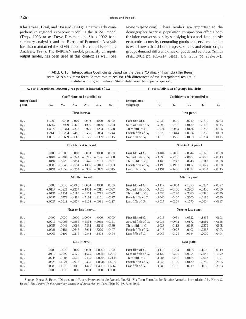
728 Judson and Popoff
Klosterman, Brail, and Bossard (1993); a particularly com-prehensive regional economic model is the REMI model(Treyz, 1993; or see Treyz, Rickman, and Shao, 1992, for asummary analysis), and the Bureau of Economic Analysishas also maintained the RIMS model (Bureau of EconomicAnalysis, 1997). The IMPLAN model, primarily an input-output model, has been used in this context as well (See
www.mig-inc.com). These models are important to thedemographer because population composition affects boththe labor market sectors by supplying labor and the nonbasiceconomic sectors by demanding goods and services—and itis well known that different age, sex, race, and ethnic-origingroups demand different kinds of goods and services (Smithet al., 2002, pp. 185–214; Siegel, J. S., 2002, pp. 232–237).
TABLE C.15 Interpolation Coefficients Based on the Beers “Ordinary” Formula (The Beersformula is a six-term formula that minimizes the fifth differences of the interpolated results. It
maintains the given values. Given data must be equally spaced.)
B. For subdivision of groups into fifths
Interpolated Coefficients to be applied to
subgroup G1 G2 G3 G4 G5
First panel
First fifth of G1 +.3333 -.1636 -.0210 +.0796 -.0283Second fifth of G1 +.2595 -.0780 +.0130 +.0100 -.0045Third fifth of G1 +.1924 +.0064 +.0184 -.0256 +.0084Fourth fifth of G1 +.1329 +.0844 +.0054 -.0356 +.0129Last fifth of G1 +.0819 +.1508 -.0158 -.0284 +.0115
Next-to-first panel
First fifth of G2 +.0404 +.2000 -.0344 -.0128 +.0068Second fifth of G2 +.0093 +.2268 -.0402 +.0028 +.0013Third fifth of G2 -.0108 +.2272 -.0248 +.0112 -.0028Fourth fifth of G2 -.0198 +.1992 +.0172 +.0072 -.0038Last fifth of G2 -.0191 +.1468 +.0822 -.0084 -.0015
Middle panel
First fifth of G3 -.0117 +.0804 +.1570 -.0284 +.0027Second fifth of G3 -.0020 +.0160 +.2200 -.0400 +.0060Third fifth of G3 +.0050 -.0280 +.2460 -.0280 +.0050Fourth fifth of G3 +.0060 -.0400 +.2200 +.0160 -.0020Last fifth of G3 +.0027 -.0284 +.1570 +.0804 -.0117
Next-to-last panel
First fifth of G4 -.0015 -.0084 +.0822 +.1468 -.0191Second fifth of G4 -.0038 +.0072 +.0172 +.1992 -.0198Third fifth of G4 -.0028 +.0112 -.0248 +.2272 -.0108Fourth fifth of G4 +.0013 +.0028 -.0402 +.2268 +.0093Last fifth of G4 +.0068 -.0128 -.0344 +.2000 +.0404
Last panel
First fifth of G5 +.0115 -.0284 -.0158 +.1508 +.0819Second fifth of G5 +.0129 -.0356 +.0054 +.0844 +.1329Third fifth of G5 +.0084 -.0256 +.0184 +.0064 +.1924Fourth fifth of G5 -.0045 +.0100 +.0130 -.0780 +.2595Last fifth of G5 -.0283 +.0796 -.0210 -.1636 +.3333
A. For interpolation between given points at intervals of 0.2
Interpolated Coefficients to be applied to
point N1.0 N2.0 N3.0 N4.0 N5.0 N6.0
First interval
N1.0 +1.000 .0000 .0000 .0000 .0000 .0000N1.2 +.6667 +.4969 -.1426 -.1006 +.1079 -.0283N1.4 +.4072 +.8344 -.2336 -.0976 +.1224 -.0328N1.6 +.2148 +1.0204 -.2456 -.0536 +.0884 -.0244N1.8 +.0819 +1.0689 -.1666 -.0126 +.0399 -.0115
Next-to first interval
N2.0 .0000 +1.000 .0000 .0000 .0000 .0000N2.2 -.0404 +.8404 +.2344 -.0216 -.0196 +.0068N2.4 -.0497 +.6229 +.5014 -.0646 -.0181 +.0081N2.6 -.0389 +.3849 +.7534 -.1006 -.0041 +.0053N2.8 -.0191 +.1659 +.9354 -.0906 +.0069 +.0015
Middle interval
N3.0 .0000 .0000 +1.000 1.0000 .0000 .0000N3.2 +.0117 -.0921 +.9234 +.1854 -.0311 +.0027N3.4 +.0137 -.1101 +.7194 +.4454 -.0771 +.0087N3.6 +.0087 -.0771 +.4454 +.7194 -.1101 +.0137N3.8 +.0027 -.0311 +.1854 +.9234 -.0921 +.0117
Next-to-last interval
N4.0 .0000 .0000 .0000 1.0000 .0000 .0000N4.2 +.0015 +.0069 -.0906 +.9354 +.1659 -.0191N4.4 +.0053 -.0041 -.1006 +.7534 +.3849 -.0389N4.6 +.0081 -.0181 -.0646 +.5014 +.6229 -.0497N4.8 +.0068 -.0196 -.0216 +.2344 +.8404 -.0404
Last interval
N5.0 .0000 .0000 .0000 .0000 +1.0000 .0000N5.2 -.0115 +.0399 -.0126 -.1666 +1.0689 +.0819N5.4 -.0244 +.0884 -.0536 -.2456 +1.0204 +.2148N5.6 -.0328 +.1224 -.0976 -.2336 +.8344 +.4072N5.8 -.0283 +.1079 -.1006 -.1426 +.4969 +.6667N6.0 .0000 .0000 .0000 .0000 .0000 +1.0000
Source: Hensy S. Beers, “Discussion of Papers Presented in the Record, No. 68: ‘Six-Term Formulas for Routine Actuarial Interpolation,’ by Henry S.Beers,” The Record fo the American Institute of Actuaries 34, Part I(69): 59–60, June 1945.

Appendix C. Selected General Methods 729
TABLE C.16 Interpolation Coefficients Based on the Beers “Modified” Formula (The Beers “mod-ified” formula is a six-term formula that minimizes the fourth differences of the interpolated
results. This formula combines interpolation with some smoothing or graduation of given values;end panels maintain the given values, however. Given data must be equally spaced.)
B. For subdivision of groups into fifths
Interpolated Coefficients to be applied to
subgroup G1 G2 G3 G4 G5
First panel
First fifth of G1 +.3332 -.1938 +.0702 -.0118 +.0022Second fifth of G1 +.2569 -.0753 +.0205 -.0027 +.0006Third fifth of G1 +.1903 +.0216 -.0146 +.0032 -.0005Fourth fifth of G1 +.1334 +.0969 -.0351 +.0059 -.0011Last fifth of G1 +.0862 +.1506 -.0410 +.0054 -.0012
Next-to-first panel
First fifth of G2 +.0486 +.1831 -.0329 +.0021 -.0009Second fifth of G2 +.0203 +.1955 -.0123 -.0031 -.0004Third fifth of G2 +.0008 +.1893 +.0193 -.0097 +.0003Fourth fifth of G2 -.0108 +.1677 +.0577 -.0153 +.0007Last fifth of G2 -.0159 +.1354 +.0972 -.0170 +.0003
Middle panel
First fifth of G3 -.0160 +.0973 +.1321 -.0121 -.0013Second fifth of G3 -.0129 +.0590 +.1564 +.0018 -.0043Third fifth of G3 -.0085 +.0260 +.1650 +.0260 -.0085Fourth fifth of G3 -.0043 +.0018 +.1564 +.0590 -.0129Last fifth of G3 -.0013 -.0121 +.1321 +.0973 -.0160
Next-to-last panel
First fifth of G4 +.0003 -.0170 +.0972 +.1354 -.0159Second fifth of G4 +.0007 -.0153 +.0577 +.1677 -.0108Third fifth of G4 +.0003 -.0097 +.0193 +.1893 +.0008Fourth fifth of G4 -.0004 -.0031 -.0123 +.1955 +.0203Last fifth of G4 -.0009 +.0021 -.0329 +.1831 +.0486
Last panel
First fifth of G5 -.0012 +.0054 -.0410 +.1506 +.0862Second fifth of G5 -.0011 +.0059 -.0351 +.0969 +.1334Third fifth of G5 -.0005 +.0032 -.0146 +.0216 +.1903Fourth fifth of G5 +.0006 -.0027 +.0205 -.0753 +.2569Last fifth of G5 +.0022 -.0118 +.0702 -.1938 +.3332
A. For interpolation between given points at intervals of 0.2
Interpolated Coefficients to be applied to
point N1.0 N2.0 N3.0 N4.0 N5.0 N6.0
First interval
N1.0 +1.000 .0000 .0000 . 0000 .0000 .0000N1.2 +.6668 +.5270 -.2640 +.0820 -.0140 +.0022N1.4 +.4099 +.8592 -.3598 +.1052 -.0173 +.0028N1.6 +.2196 +1.0279 -.3236 +.0874 -.0136 +.0023N1.8 +.0862 +1.0644 -.1916 +.0464 -.0066 +.0012
Next-to first interval
N2.0 .0000 +1.000 .0000 .0000 .0000 .0000N2.2 -.0486 +.8655 +.2160 -.0350 +.0030 -.0009N2.4 -.0689 +.6903 +.4238 -.0442 +.0003 -.0013N2.6 -.0697 +.5018 +.5938 -.0152 -.0097 -.0010N2.8 -.0589 +.3233 +.7038 +.0578 -.0257 -.0003
Middle interval
N3.0 -.0430 +.1720 +.7420 +.1720 -.0430 .0000N3.2 -.0270 +.0587 +.7072 +.3162 -.0538 -.0013N3.4 -.0141 -.0132 +.6098 +.4708 -.0477 -.0056N3.6 -.0056 -.0477 +.4708 +.6098 -.0132 -.0141N3.8 -.0013 -.0538 +.3162 +.7072 +.0587 -.0270
Next-to-last interval
N4.0 .0000 -.0430 +.1720 +.7420 +.1720 -.0430N4.2 -.0003 -.0257 +.0578 +.7038 +.3233 -.0589N4.4 -.0010 -.0097 -.0152 +.5938 +.5018 -.0697N4.6 -.0013 +.0003 -.0442 +.4238 +.6903 -.0689N4.8 -.0009 +.0030 -.0350 +.2160 +.8655 -.0486
Last interval
N5.0 .0000 .0000 .0000 .0000 +1.0000 .0000N5.2 +.0012 -.0066 +.0464 -.1916 +1.0644 +.0862N5.4 +.0023 -.0136 +.0874 -.3236 +1.0279 +.2196N5.6 +.0028 -.0173 +.1052 -.3598 +.8529 +.4099N5.8 +.0022 -.0140 +.0820 -.2640 +.5270 +.6668N6.0 .0000 .0000 .0000 .0000 .0000 +1.0000
Source: Henry S. Beers, “Modified Interpolation Formulas that Minimize Fourth Differences,” The Record of the American Institute of Actuaries 34, PartI(69): 19–20, June 1945.

730 Judson and Popoff
CONCLUDING NOTE
In so many pages, with so many applications and exam-ples, we have merely scratched the surface of the variety oftools now available to the demographer. Readers interestedin more details may consult the eight-volume set, Readingsin Population Research Methodology (Bogue, Arriaga, andAnderton, 1993) or any of a number of specialized texts.
References
Agresti, A. 1990. Categorical Data Analysis. New York: John Wiley andSons.
Agresti, A. 1996. An Introduction to Categorical Data Analysis. New York:John Wiley and Sons.
Aitken, A. C. 1932. “On Interpolation by Iteration of Proportionate Parts,without the Use of Differences.” Proceedings of the Edinburgh Mathematical Society, Series 2, 3: 56–76.
Akers, D. S., and J. S. Siegel. 1965. “National Census Survival Rates, byColor and Sex, for 1950–1960.” Current Population Reports, Series p.23, No. 15. Washington, DC: U.S. Bureau of the Census.
Alfeld, L. E., and A. K. Graham. 1976. Introduction to Urban Dynamics.Cambridge, MA: Wright-Allen Press.
Bain, L. J., and M. Engelhart. 1987. Introduction to Probability and Mathematical Statistics. Boston: Duxbury Press.
Bartholomew, D. J. 1982. Stochastic Models for Social Processes, 3rd ed.New York: John Wiley and Sons.
Beers, H. S. 1944. “Six-Term Formulae for Routine Actuarial Interpola-tion.” Record of the American Institute of Actuaries 33: 245–260.
Beers, H. S. 1945. “Modified-Interpolation Formulae that Minimize FourthDifferences.” Record of the American Institute of Actuaries 34: 14–20.
Bickel, P. J., and K. A. Doksum. 1977. Mathematical Statistics: Basic Ideasand Selected Topics. Engelwood Cliffs, NJ: Prentice Hall.
Birch, M. W. 1963. “Maximum Likelihood in Three-Way ContingencyTables.” Journal of the Royal Statistical Society B 25: 220–233.
Bishop, Y. V. V., S. E. Feinberg, and P. W. Holland. 1975. Discrete Multi-variate Analysis. Cambridge, MA: MIT Press.
Bogue, D. J., E. E. Arriaga, and D. H. Anderston. 1993. Readings in Population Research Methodology, Volumes 1–8. Chicago: SocialDevelopment Center and United Nations Population Fund.
Brown, R. L. 1993. Introduction to the Mathematics of Demography,2nd ed. Winsted, CT: ACTEX Publications.
Burden, R. L., and J. D. Faires. 1993. Numerical Analysis, 5th ed. Boston:PWS.
Bureau of Economic Analysis. 1997. Regional Multipliers: A User Handbook for the Regional Input-Output Modeling System (RIMS II).Washington, DC: U.S. Government Printing Office.
Castro, L. J., and A. Rogers. 1983. “What the Age Composition of MigrantsCan Tell Us.” Population Bulletin of the United Nations 15: 63–79.
Chattopadhyay, M., P. Lahiri, M. Larsen, and J. Reimnitz. 1999. “Com-posite Estimation of Drug Prevalences for Sub-State Areas.” SurveyMethodology 25: 81–86.
Citro, C. F. 1991. “Databases for Microsimulation: A Comparison of theMarch CPS and SIPP.” In C. F. Citro and E. Hanushek (Eds.), Improv-ing Information for Social Policy Decisions: The Uses of Microsimu-lation Modeling, Volume 1I: Technical Papers (pp. 11–61). Washington,DC: National Academy Press.
Citro, C. F., M. L. Cohen, G. Kalton, and K. K. West (Eds.). 1997. Small-Area Estimates of School-Age Children in Poverty: Interim Report 1:Evaluation of 1993 County Estimates for Title I Allocations.Washington, DC: National Academy Press.
Citro, C. F., and E. Hanushek (Eds.). 1991. Improving Information forSocial Policy Decisions: The Uses of Microsimulation Modeling,Volume 1. Washington, DC: National Academy Press.
Cohen, M. 1991. “Statistical Matching and Microsimulation Models.” InC. F. Citro and E. Hanushek (Eds.), Improving Information for SocialPolicy Decisions: The Uses of Microsimulation Modeling, Volume 1I:Technical Papers (pp. 62–85). Washington, DC: National AcademyPress.
Darga, K. 1999. Sampling and the Census. Washington, DC: AEI Press.Darga, K. 2000. Fixing the Census Until It Breaks. Lansing, MI: Michigan
Information Center.Deming, W. E. 1948. The Statistical Adjustment of Data. New York: John
Wiley and Sons.Deming, W. E., and F. F. Stephan. 1940. “On a Least Squares Adjustment
of a Sampled Frequency Table When the Expected Marginal Totals AreKnown.” Annals of Mathematical Statistics 11: 427–444.
Draper, D. 1992. Combining Information: Statistical Issues and Opportu-nities for Research. Washington, DC: National Academy Press.
Dudewicz, E. J., and S. N. Mishra. 1988. Modern Mathematical Statistics.New York: John Wiley and Sons.
Ewbank, D. C. 1981. Age Misreporting and Age-Selective Underenumera-tion: Sources, Patterns, and Consequences for Demographic Analysis.Washington, DC: National Academy Press.
Forrester, J. W. 1968. Principles of Systems. Cambridge, MA: Wright-AllenPress.
Gonzalez, M. E. 1973. “Use and Evaluation of Synthetic Estimates.” InAmerican Statistical Assocation, Proceedings of the Social StatisticsSection. Washington DC: American Statistical Association.
Gonzalez, M. E., and C. Hoza. 1978. “Small-Area Estimation with Appli-cation to Unemployment and Housing Estimates.” Journal of the American Statistical Association 73: 7–15.
Goodman, M. R. 1974. Study Notes in System Dynamics. Cambridge, MA:Wright-Allen Press.
Greene, W. H. 1993. Econometric Analysis, 2nd ed. Englewood Cliffs, NJ:Prentice-Hall.
Hair, J. F., R. E. Anderson, R. L. Tatham, and W. C. Black. 1995. Multi-variate Data Analysis, 4th ed. Upper Saddle River, NJ: Prentice Hall.
Heeringa, S. G. 1993. “Statistical Models for Small Area Estimation.” InD. J. Bogue, E. E. Arriaga, and D. L. Anderton (Eds.), Readings in Population Research Methodology, Volume 5: Population Models, Projections, and Estimates (pp. 20.58–20.64). Chicago: Social Development Center and United Nations Population Fund.
Heligman, L., and J. Pollard. 1993. “The Age Pattern of Mortality.” In D.J. Bogue, E. E. Arriaga, and D. L. Anderton (Eds.), Readings in Popu-lation Research Methodology, Volume 2: Mortality Research (pp.7.98–7.104). Chicago: Social Development Center and United NationsPopulation Fund.
TABLE C.17 Interpolation Coefficients Based on Grabill’sWeighted Moving Average of Sprague Coefficients (See text for derivation. Used for drastic smoothing.
Given groups must be equally spaced.)
Interpolated Coefficients to be applied to
subgroup G1 G2 G3 G4 G5
First fifth of G3 +.0111 +.0816 +.0826 +.0256 -.0009Second fifth of G3 +.0049 +.0673 +.0903 +.0377 -.0002Third fifth of G3 +.0015 +.0519 +.0932 +.0519 +.0015Fourth fifth of G3 -.0002 +.0377 +.0903 +.0673 +.0049Last fifth of G3 -.0009 +.0256 +.0826 +.0816 +.0111
Source: See source note for Table C.13.

Appendix C. Selected General Methods 731
High Performance Systems. 1996. An Introduction to Systems Thinking.Hanover, NH: High Performance Systems.
Horvitz, D. G., and D. J. Thompson. 1952. “A Generalization of Samplingwithout Replacement from a Finite Universe.” Journal of the AmericanStatistical Association 47: 663–685.
Ingram, D. D., J. O’Hare, F. Scheuren, and J. Turek. 2000. StatisticalMatching: A New Validation Case Study. Paper presented at the 2000Joint Statistical Meetings, Indianapolis, IN, August 5–11.
Inmon, W. H. 1996. Building the Data Warehouse. New York: Wiley.Isard, W. 1960. Methods of Regional Science: An Introduction to Regional
Analysis. Cambridge, MA: MIT Press.Isserman, A. 1993. “The Right People, the Right Rates.” Journal of the
American Planning Association 59: 45–64.Johnson, A., and D. Percy. 2000. Cubic Splines. Online document at
www.geol.pdx.edu/Courses/G423/Handouts/Spline/Derivation.html.Retrieved December 23, 2000.
Judge, G. G., W. E. Griffiths, R. C. Hill, H. Lutkepohl, and T-C. Lee. 1985.The Theory and Practice of Econometrics, 2nd ed. New York: JohnWiley and Sons.
Judge, G. G., R. C. Hill, W. E. Griffiths, H. Lutkepohl, and T-C. Lee. 1988.Introduction to the Theory and Practice of Econometrics, 2nd ed. NewYork: John Wiley and Sons.
Judson, D. H. 1990. Discrete Increment-Decrement Population Models: ADemonstration and Simulation. Sociological Data Processing CenterTechnical Report, Washington State University, April 25.
Judson, D. H. 1993. Performance Standards in the Shared InformationSystem: An Evaluation of the Uses of the Mobility Continuum Conceptfor the Workforce Quality Council. Salem, OR: Oregon EmploymentDepartment.
Judson, D. H. 2000. The Statistical Administrative Records System: SystemDesign, Challenges, and Successes. Paper presented at the NISS/Telcordia Data Quality Conference, Morristown, NJ, November30–December 1.
Judson, D. H., and C. L. Popoff. 1996. Research Use of AdministrativeRecords. Paper presented at the 6th International Conference onApplied and Business Demography, Bowling Green State University,Bowling Green, OH, September 19–21.
Kadane, J. B. 1978. “Statistical Problems of Merged Data Files.” In Com-pilation of OTA Papers, Vol. 1 (pp. 159–179). Washington, DC: Officeof Tax Analysis, U.S. Department of the Treasury.
Klosterman, R. E., R. K. Brail, and E. G. Bossard. 1993. SpreadsheetModels for Urban and Regional Analysis. New Brunswick, NJ: Rutgers,the State University of New Jersey.
Kmenta, J. 1986. Elements of Econometrics, 2nd ed. New York: MacMillan.Laudon, K. C. 1986. “Data Quality and Due Process in Large Interorgani-
zational Record Systems.” Communications of the ACM 29: 4–11.Leslie, P. H. 1945. “On the Use of Matrices in Certain Population Mathe-
matics.” Biometrika 33: 183–212.Lessler, J. T., and W. D. Kalsbeek. 1992. Nonsampling Error in Surveys.
New York: John Wiley and Sons.Levy, P. S., and D. K. French. 1977a. Synthetic Estimation of State Health
Characteristics Based on the Health Interview Survey. Hyattsville, MD:National Center for Health Statistics.
Levy, P. S., and D. K. French. 1977b. Synthetic Estimation of State HealthCharacteristics Based on the Health Interview Survey. U.S. Departmentof Health, Education, and Welfare, National Center on Health StatisticsSeries #275. Washington, DC: U.S. Government Printing Office.
Light, S. C. 1990. “Measurement Error in Official Statistics: Prison RuleInfraction Data.” Federal Probation 54: 63–68.
Lohr, S. L. 1999. Sampling: Design and Analysis. Pacific Grove, CA:Brooks/Cole.
Long, L. 1984. Migration and Residential Mobility in the United States.New York: Russell Sage Foundation.
Long, J. S. 1997. Regression Models for Categorical and Limited Depen-dent Variables. Thousand Oaks, CA: Sage.
Ma, J. M. 1986. A Modeling Approach to System Evaluation in ResearchData Management. Ph.D. thesis, University of North Carolina, ChapelHill, NC.
Macro International. 1996. Sampling Manual. DHS-III Basic Documenta-tion No. 6. Calverton, MD: Macro International.
Mayhew, B. H. 1980. “Structuralism versus Individualism: Part 1, Shadowboxing in the Dark.” Social Forces 59: 335–375.
McCullagh, P., and J. Nelder. 1990. Generalized Linear Models, 2nd ed.London: Chapman and Hall.
Méxice, Dirección General de Estadística. 1962. Censo General de Poblac-tíon—1960. Mexico City, Mexico: Secretaría de Industria y Comercio, Dirección General de Estadística.
Miller, M. D. 1946. Elements of Graduation. Chicago: Actuarial Society ofAmerica and American Institute of Actuaries.
Moriarty, C., and F. Scheuren. 2001. Statistical Matching: Pitfalls ofCurrent Procedures. Paper presented at the 2001 Joint Statistical Meet-ings, Atlanta, GA, August 5–11.
Murdock, S., and D. Ellis. 1991. Applied Demography: An Introduction toBasic Concepts, Methods, and Data. Boulder, CO: Westview Press.
Paass, G. 1985. “Statistical Record Linkage Methodology: State of the Artand Future Prospects.” In Proceedings of the 100th Session of the Inter-national Statistical Institute (pp. 9.3.1–9.3.16). Amsterdam: Interna-tional Statistical Institute.
Plane, D. A., and P. A. Rogerson. 1994. The Geographical Analysis of Population with Applications to Planning and Business. New York:John Wiley and Sons.
Pollard, J. H. 1973. Mathematical Models for the Growth of Human Populations. Cambridge: Cambridge University Press.
Pool, I. 1964. “Simulating Social Systems.” International Science andTechnology 27: 62–72.
Popoff, C. L., E. Fadali, and D. H. Judson. 2000. Methodology Explanation and Documentation for Nevada-Specific Estimates of the Uninsured. Online document at www.gbpca.org/Documents/methodology.htm. Retrieved December 12.
Press, W. H., B. P. Flannery, S. A. Teukolsky, and W. T. Vetterling. 1989.Numerical Recipes in Pascal: The Art of Scientific Computing. NewYork: Cambridge University Press.
Radelet, M. 1981. “Racial Characteristics and the Imposition of the DeathPenalty.” American Sociological Review 46: 918–927.
Randers, J. 1980. Elements of the System Dynamics Method. Cambridge,MA: MIT Press.
Reder, S. 1994. Synthetic Estimates of NALS Literacy Proficiences from1990 Census Microdata. Portland, OR: Northwest Regional EducationLaboratory.
Redman, T. J. 1996. Data Quality for the Information Age. Norwood, MA:Artech House.
Rogers, A. 1975. Introduction to Multiregional Mathematical Demography.New York: Wiley Interscience.
Rogers, A. 1995. Multiregional Demography: Principles, Methods andExtensions. New York: John Wiley and Sons.
Rogers, A., and L. Castro. 1986. “Migration” (pp. 157–210). In A. Rogersand F. Willikens (Eds.). Migration and Settlement: A MultiregionalComparative Study. Dordrecht, Netherlands: D. Reidel PublishingCompany.
Ross, S. M. 1997. Introduction to Probability Models, 6th ed. New York:Academic Press.
Rubin, D. B. 1979. “Using Multivariate Matched Sampling and RegressionAdjustment to Control Bias in Observational Studies.” Journal of theAmerican Statistical Association 74: 318–328.
Rubin, D. B. 1986. “Statistical Matching Using File Concatenation withAdjusted Weights and Multiple Imputations.” Journal of Business andEconomic Statistics 4: 87–94.
Sarndal, C. E. 1984. “Design-Consistent Versus Model-Dependent Estimation for Small Domains.” Journal of the American StatisticalAssociation 79: 624–631.

Schoen, R. 1988. Modeling Multigroup Populations. New York: PlenumPress.
Shryock, H. S., J. S. Siegel, and Associates. 1971. The Methods and Mate-rials of Demography. Washington, DC: U.S. Government PrintingOffice.
Siegel, J. S. 2002. Applied Demography: Applications to Business, Gov-ernment, Law, and Public Policy. San Diego: Academic Press.
Sigmund, C. L., D. H. Judson, and C. L. Popoff. 1998. A System for Syn-thetic Estimates of Health-Related Characteristics: Linking a Popula-tion Survey with Local Data. Paper presented at the 1999 meetings ofthe Population Association of America, New York.
Smith, S. K. 1986. “Accounting for Migration in Cohort-Component Projections of State and Local Populations.” Demography 23: 127–135.
Smith, S. K., J. Tayman, and D. Swanson. 2001. State and Local Popula-tion Projections: Methodology and Analysis. Boston: Kluwer Academic.
Sprague, T. B. 1881. “Explanation of a New Formula for Interpolation.”Journal of the Institute of Actuaries 22: 270.
Stevens, D. W., P. A. Richmond, J. F. Haenn, and J. S. Michie. 1992. Measuring Employment Outcomes Using Unemployment Insur-ance Wage Records. Washington, DC: Research and Evaluation Associates.
Thompson, S. K. 1992. Sampling. New York: John Wiley and Sons.Treyz, G. I. 1993. Regional Economic Modeling: A Systematic Approach
to Economic Forecasting and Policy Analysis. Boston: Kluwer Academic Publishers.
Treyz, G. I., D. S. Rickman, and G. Shao. 1992. “The REMI Economic-Demographic Forecasting and Simulation Model.” InternationalRegional Science Review 14: 221–253.
U.S. Census Bureau. 2000. Statistical Abstract of the United States: 1999.Washington, DC: U.S. Government Printing Office.
U.S. National Center for Health Statistics. 1997. U.S. Decennial Life Tablesfor 1989–91, vol 1 no 1. Hyattsville, MD: National Center for Health Statistics.
U.S. National Center for Health Statistics 1998. “United States AbridgedLife Tables, 1996.” By R. N. Anderson. National Vital Statistics Reports47(13): 1–20.
Wachter, K. W., and D. A. Freedman. 2000. “Measuring Local Hetero-geneity with 1990 Census Data.” Demographic Research. Online doc-ument at www.demographic-research.org/Volumes/Vol3/10. RetrievedDecember 12.
Wallis, W. A., and H. V. Roberts. 1962. The Nature of Statistics. New York:The Free Press.
Weisberg, S. 1982. Applied Linear Regression, 2nd ed. New York: JohnWiley and Sons.
Wolfenden, H. H. 1942. The Fundamental Principles of Mathematical Sta-tistics. New York: The Actuarial Society of America.
Suggested Readings
Sampling, Sampling Errors, and Other Errors in Surveys
Biemer, P. B., R. M. Groves, L. E. Lyberg, N. A. Mathiowetz, and S.Sudman (Eds.). 1991. Measurement Errors in Surveys. New York:Wiley-Interscience.
Fink, A. (Ed.). 1995. The Survey Kit, Volumes 1–9. Thousand Oaks, CA: Sage.Groves, R. M. 1989. Survey Errors and Survey Costs. New York:
Wiley-Interscience.
Kish, L. 1965/1995. Survey Sampling. New York: John Wiley and Sons.Siegel, J. S. 2002. Applied Demography: Applications to Business, Govern-
ment, Law, and Public Policy. Chapter 4. San Diego: Academic Press.
Interpolation
Brass, W. 1960. “The Graduation of Fertility Distributions by PolynomialFunctions.” Population Studies 14: 148–162.
Keyfitz, N. 1966. “A Unified Approach to Interpolation and Graduation.”Demography 3(2): 528–536.
Keyfitz, N. 1977. “Interpolation and Graduation.” Chapter 10 in Introduc-tion to the Mathematics of Population, with Revisions. Reading, MA:Addison-Wesley.
U.S. Census Bureau. 1994. Population Analysis with Microcomputers,Volumes I and II. By E. Arriaga, P. Johnson, and E. Jamison. Washing-ton, DC: U.S. Bureau of the Census.
Adjustment of Distributions to Marginal Totals
Deming, W. E. 1948. Statistical Adjustment of Data. New York: John Wiley& Sons.
Deming, W. E., and F. F. Stephan. 1940. “On a Least Squares Adjustmentof a Sampled Frequency Table When the Expected Marginal Totals areKnown.” The Annals of Mathematical Statistics 11(4): 427–444.
Feinberg, S. 1981. The Analysis of Cross-Classified Categorical Data.Cambridge, MA: MIT Press.
Computer Usage and Data Warehousing
Brackstone, George J. 1988. “Statistical Uses of Administrative Data:Issues and Challenges.” In J. W. Coombs and M. P. Singh (Eds.), Statistical Uses of Administrative Data : An International Symposium(pp. 5–16). Ottawa: Statistics Canada.
Coombs, J. W., and M. P. Singh (Eds.). 1988. Statistical Uses of Administrative Data: An International Symposium. Ottawa: StatisticsCanada.
English, L. P. 1999. Improving Data Warehouse and Business InformationQuality: Methods for Reducing Costs and Increasing Profits. New York:John Wiley and Sons, Inc.
Kilss, B., and W. Alvey (Eds.). 1984. Statistical Uses of AdministrativeRecords: Recent Research and Present Prospects, Volumes I and II.Washington, DC: Department of the Treasury, Internal RevenueService, Statistics of Income Division.
Naus, J. I. 1975. Data Quality Control and Editing. New York: MarcelDekker.
Silverston, L., W. H. Inmon, and K. Graziano. 1997. The Data ModelResource Book: A Library of Logical Data Models and Data WarehouseDesigns. New York: John Wiley and Sons.
Other Topics
Citro, C. F., and E. A. Hanushek. 1991. Improving Information for Social Policy Decisions: The Uses of Microsimulation Modeling.Volume II: Technical Papers. Washington, DC: National AcademyPress.
Forrester, J. W. 1971. “Counter-Intuitive Behavior of Social Systems.”Technology Review 73: 52–68.
Klir, G. J. 1991. Facets of Systems Science. New York: Plenum Press.
732 Judson and Popoff

How can geographic information systems (GIS) be usefulto demographers? At first glance this question seems trivial,in that the importance of maps, the fundamental GISproduct, is immediately obvious. Moreover, approximately85% of all databases contain some sort of geographic infor-mation (MapInfo Corporation, 1998, p. 2). However, at adeeper level, the question is not trivial—is it worthwhile to learn something about GIS capabilities? This appendixattempts to answer the latter question by providing anoverview of GIS, briefly describing its origins, discussingbasic GIS concepts and issues, and giving examples of itsuse. Because of the highly technical nature of GIS, thisappendix is not designed to be a GIS user’s manual. Such information can be found in the works listed in the Refer-ences and Suggested Readings provided at the end of thisappendix.
Aronoff (1989, p. 39) describes GIS as “a computer-based system that provides the following four sets of capabilities to handle ‘geo-referenced data:’ (1) input; (2)data management; (3) manipulation and analysis; and (4)output.” To operate a GIS one needs a computer, data withgeographic identifiers, and a software program that canmanipulate and display such data.1 The geographic identi-fiers may be based on physical or administrative geographyand may be as specific as latitude/longitude or a streetaddress.
However, GIS should be thought of as more than a utilitythat can create maps. It can be used as a research tool to helpexplore demographic data and search for patterns and rela-tionships. Social scientists have often used maps for descrip-tive purposes, but rarely for other applications. Prior to thearrival of high-powered computers and mapping software,
creating maps was a costly and time-consuming task. WithGIS, not only is map making inexpensive and fast, but theway is clear to conduct both spatial analysis and predictivemodeling quickly and efficiently (Fotheringham and Rogerson, 1994).
Spatial analysis affords one the ability to see geographictrends. For example, if there is an outbreak of sickness in acommunity, a map could be used in two ways. First, byshowing the location of each incident, a pattern of dispersalmay be revealed. Second, if a pattern is found, a map withlayers of additional features, such as water supply, winddirection, and other natural phenomena, can be easilycreated in a GIS, which can then be used to evaluate pat-terns and correlations.
An advanced application of spatial analysis is predictivemodeling. With each type of data in a GIS system, certaingeographic characteristics can be gathered. Distance is onesuch key characteristic. Calculating the distance betweentwo points, the length of a line, or the distance between apoint and the centroid of a polygon can all be useful in pre-dictive modeling. GIS can be used to measure the distancefrom a point to a particular shopping center, rather then fromthe centroid of a geographically defined area, such as a zipcode.
ORIGINS OF GIS
For the most part, GIS theory originated with researchersinterested in spatial analysis. In the 1950s and 1960s,demand for powerful analytical tools to address “real” prob-lems initiated GIS development. Fueled by such geography-oriented industries as public utilities, transportation, retailmarketing, and environmental management, GIS developedrapidly through the 1970s and 1980s, primarily in the UnitedStates. Many projects contributed to the development of
733
A P P E N D I X
D
Geographic Information Systems
KATHRYN NORCROSS BRYAN AND ROB GEORGE
The Methods and Materials of DemographyCopyright 2003, Elsevier Science (USA).
All rights reserved.
1 MapInfo, ArcView, Arc Info, GeoMedia, Infomark, Maptitude, AtlasGIS, and so forth.

what we know as modern GIS systems. Some of these pro-jects were taking place in the academic setting, some in the private sector, and some in various parts of government.Unfortunately, because all were in an evolutionary stage,little documentation of the simultaneity of ideas exists. AsGIS has become more popular and easier to use, a greaterinterest developed in its origins. The National Center forGeographic Information and Analysis (NCGIA), establishedin 1988, began a comprehensive “GIS History Project” in1996. The project is an attempt to document the history andorigins of GIS. NCGIA intends to research and documentnot only the development of today’s GIS software and data,but also the precursors and preconditions for its develop-ment, as well as a history of its applications in different cultural, political, and economic practices.
In early 1966, the Census Small Area Data AdvisoryCommittee began working on a case study in preparation forthe 1970 Census of the United States. A test census wastaken in New Haven, Connecticut, in 1967. With the infor-mation gathered, the committee began computer mappingexperiments and “geographic base file” (GBF) research.They found that converting the analog maps to numericallyencoded files was redundant. Streets were being digitizedmultiple times at the beginning of the project. Fortunatelyfor the Census Bureau, the problem was overcome by censusmathematician James Corbett. Based on the principles ofmap topology, his encoding scheme became known as“DIME” (dual independent map encoding). This laid thegroundwork for thematic mapping of census data and “GBF-DIME” files were digitized for U.S. cities during the 1970s.These were key components of the Census Bureau’s currentdigital database used to support its mapping system, nowknown as the “Topologically Integrated Geographic Encod-ing and Referencing (TIGER) Line files.” The TIGER/Linefiles were developed to support the data tabulating functionof the Census Bureau. Files for public use include digitaldata for map features, boundaries, names, coordinates, and(for populous areas) address ranges and zip codes. Cover-age is for all of the United States, including Puerto Rico andU.S. territories. They are grouped by state (or sets of states),by county (or sets of counties), and by statistical equivalentsin the territories. Census information is further disaggre-gated into census tracts and block groups.
Although much of the literature on the history of GISfocuses on developments in the United States, importantresearch was conducted elsewhere. Researchers in Canada,for example, played an important role in GIS development.One of the earlier systems developed in Canada resultedfrom the need to manage land and natural resources (Tomlinson, 1997, p. 38). In 1964, a team representing theAgricultural Rehabilitation and Development Act (ARDA)began work on the Canada Geographic Information System(CGIS). The system aimed to facilitate the inventory of land
use and land capability across Canada. By 1971, the systemwas already fully operational. As a result, the early 1970ssaw a boom in the use of GIS for various governmental projects in Canada.
The U.S. Geological Service developed “DLG” (digitalline graphs) in the early 1970s. This development occurredabout the same time as the U.S. Census bureau developed“DIME.” These two federal agencies were among the firstorganizations to experiment with data formats that couldserve many people for many purposes. Commercial datavendors soon followed, and by the 1980s, vendors began todevelop file translation and conversion software. Thisenabled data to be imported and exported between certainsystems and simplified the process of data acquisition. Oneof the most important standard file types is .dxf (drawingexchange format). The dxf standard (developed byAutodesk) is an ASCII format that describes the contents ofa CAD (computer-assisted drawing) file in a way that canbe interpreted by other software systems. Translators areavailable for all the major software. There are translatorsthat convert .dxf files into MapInfo table files or to Arcviewshape files, and vice versa. Translators are available from private vendors as well as the software companiesthemselves, and many of the GIS software available can recognize multiple file formats without going through thetranslation process. For example, in MapInfo one can openDbase, Excel, Lotus, ASCII, and Access file formats, inaddition to the MapInfo specific format.
BASIC GIS CONCEPTS AND ISSUES
Data
The data used in a GIS are of two types: spatial and non-spatial. Spatial data represent the geographic location of fea-tures. The nonspatial data describes variables such as names,addresses, type of feature, and so forth. When data areentered in a GIS, the two types of data need to be linked.There are five types of data entry systems that can be usedin GIS: (1) keyboard entry, (2) coordinate geometry, (3)manual digitizing, (4) scanning, and (5) transfer of existingfiles. As technology improved and demand increased, moredata much of which have already been scanned, digitized,or otherwise placed in digital form have become available.Existing digital data, of all types, are available at varyingdegrees of detail and accuracy from many sources. Manygovernmental agencies, such as the Census Bureau, providemuch of their data to the public (some free; some for a fee).In addition to governmental agencies, many private compa-nies also generate various types of data. The principles thataffect the cost of data are level of detail, size of coverage,and timeliness.
With the voluminous amount of data available today, theresults of primary research are virtually the only data that
734 Bryan and George

need to be entered manually by keyboard. Keyboard entryis used to add additional variables or observations to thespatial data that are being used. Information can easily beupdated and edited using the keyboard. In most cases, it ispossible to edit databases directly within the GIS software.GIS systems have the ability to add or delete fields andrecords and to edit existing information. It also is possibleto edit data in a spreadsheet program, and then bring the databack into a GIS.
Another technological component that increases preci-sion is provided by the global positioning system (GPS).GPS technology has evolved through efforts of the U.S.Department of Defense. It involves 24 satellites that orbitthe earth at an elevation of 12,000 miles and continuouslybeam their locations and temporal positions toward theearth’s surface. A GPS receiver can be used to collect datafrom at least three satellites so that the receiver’s latitudeand longitude can be calculated for two-dimensional read-ings. It is even possible to get three-dimensional accuracy(latitude, longitude, and altitude) if the receiver gets signalsfrom at least four satellites. With a GPS receiver, it is pos-sible to record the precise coordinates of any point on earth.The coordinates can then be entered into a GIS and a pointcan be located at its exact point in space. The coordinatesmay be recorded manually, although the data in most GPSreceivers can be downloaded digitally.
It is important to understand census geography whentalking about GIS. In the United States, for example, theCensus Bureau collects data for many types of geographicregions. Although discussed in greater detail earlier (Chap-ters 2, 4, and, particularly, 5), the following is a list (fromlargest to smallest) of the census statistical units for whichone can gather information:
RegionsDivisionsUrban/rural areasMetropolitan statistical areas (MSA)Primary metropolitan statistical areas (PMSA)Consolidated metropolitan statistical areasUrbanized areasCensus designated place (CDP)Census tractsBlock groupsBlocks
The following is a list (from largest to smallest) of thecensus political units for which one can gather information:
United StatesStates (all states, District of Columbia, Puerto Rico, and
the Virgin Islands)CountiesCounty subdivisions (townships)Places (boroughs, cities, and CDPs)
Accuracy
Considering that a GIS has the ability to collate andcross-reference many types of data by location, every timea new data set is added, a GIS has the potential to inheritand propagate errors. Data errors can make the results of aGIS analysis worthless.
There are many sources of error that can affect the qualityof a GIS data set. It is largely the user’s responsibility toprevent and manage error. Particular care should be devotedto checking for errors because a GIS is quite capable offooling the user into a false sense of accuracy existence. Theexistence of error, and especially a level of error that is intol-erable, must be acknowledged and accounted for by users.Data errors result from errors in field measurements, errorsin existing maps, errors in any of the additional data used, orthe incorrect recording and input of information. Reliabilityis affected by the number of observations used in the analy-sis. An insufficient number of observations (as in any statis-tical analysis) may not provide the level of resolutionrequired to adequately perform spatial analysis and deter-mine the patterns one is hoping to find. Data storage also is aconcern. A storage format may have insufficient numericalprecision and insufficient spatial precision. If latitude andlongitude numbers are rounded at too high a level, forexample, precision will be lost. Data manipulation errors canhappen for many reasons. If boundary files are incorrect,results may be less precise. Inappropriate class intervals arealso a concern. Methods of formatting digital information fortransmission, storage, and processing may introduce error inthe data. Multiple conversions from one format to anothermay create an effect similar to making copies of copies on aphotocopying machine—the more they are copied, the lessclear and less precise it becomes. Data output errors may becaused by the output device or the instability of the medium;scaling may become slightly inaccurate when printing isdone directly from a computer screen.
Sources of errors can be grouped into two classes: qualityof individual data elements and quality of data sets. Indi-vidual data element quality is related to positional accuracyand precision, attribute accuracy and precision, logical con-sistency, and resolution. Data set quality is affected by com-pleteness, time, and lineage (Aronoff, 1989, p. 138). Webegin with a discussion of individual data element quality.
The positional accuracy and precision of a data elementapplies to both horizontal and vertical positions. Positionalaccuracy refers to any difference between the representedgeographic position (on the map) of a point or feature andits true position on the earth. The geographic level (scale)determines the level of precision needed. For example, apoint showing Providence, Rhode Island, on a national mapdoes not need to be as precise as it would on a map of Prov-idence county. The lower the geographic level, the morepositional accuracy will be important. Maps D.1a, b, and c
Appendix D. Geographic Information Systems 735
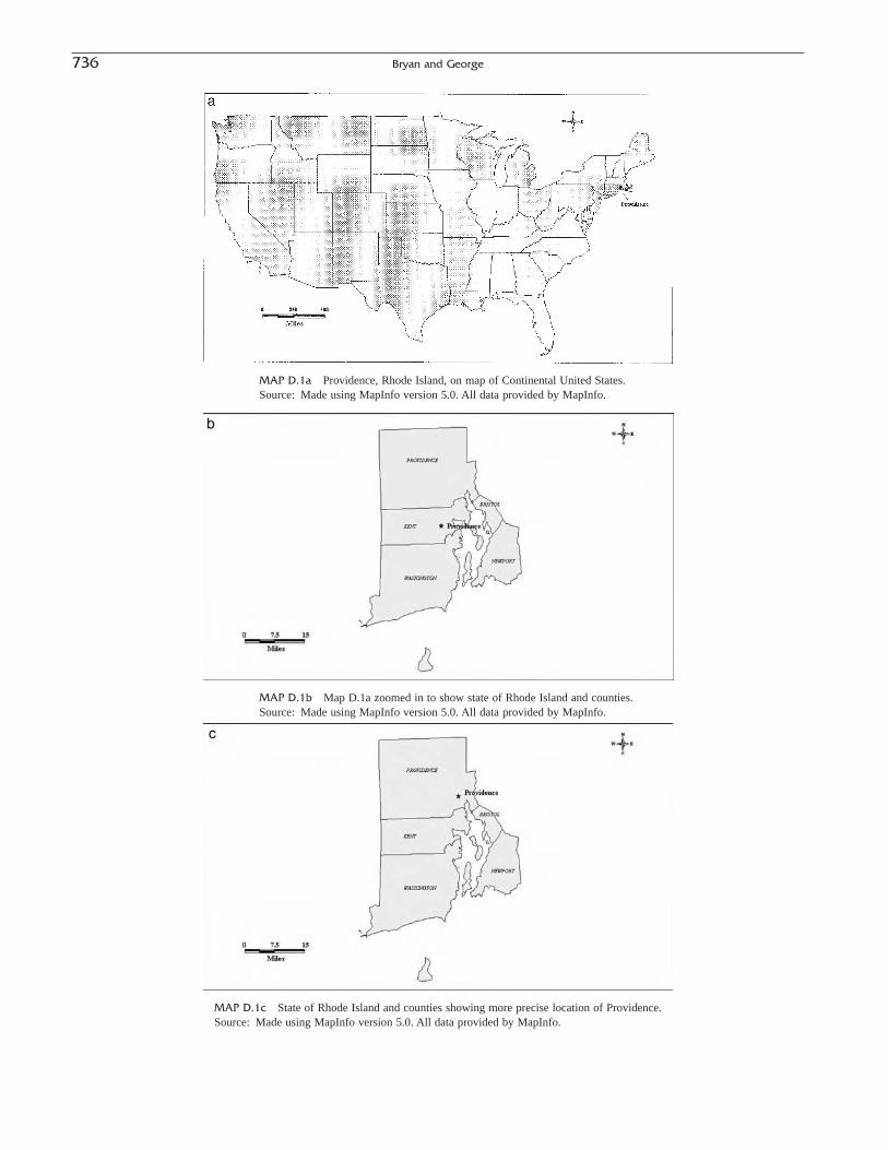
736 Bryan and George
MAP D.1b Map D.1a zoomed in to show state of Rhode Island and counties.Source: Made using MapInfo version 5.0. All data provided by MapInfo.
MAP D.1c State of Rhode Island and counties showing more precise location of Providence.Source: Made using MapInfo version 5.0. All data provided by MapInfo.
MAP D.1a Providence, Rhode Island, on map of Continental United States.Source: Made using MapInfo version 5.0. All data provided by MapInfo.

illustrate this point. Map D1-a shows Providence on a mapof the continental United States. Map D.1b shows that sameposition on a map of the state of Rhode Island. It is not veryaccurate, but it is sufficient for the national view. Map D.1cshows a more precise location of Providence on the statemap. GIS allows a user to “pan” and “zoom” at will to a dif-ferent scale and, as has been illustrated by the maps, this canbe problematic. Accuracy and precision are tied to the orig-inal map scale and do not change even if the user zooms inand out. Zooming in and out can mislead the user intobelieving that the accuracy and precision have improvedwhen in fact they have not.
Accuracy and precision of nonspatial data refers to thequality of the data about the places on a map. The locationof a data element may be correct, but if the data attached toit are wrong, having a correct location may be a moot point. Misclassified or incorrect data can affect the outcome of the analysis and the visual effect of the map. Incorrect datamay not always be obvious when looking at the map. Forexample, a pine forest may be incorrectly labeled as a spruceforest, thereby introducing error that may not be known ornoticeable to the map or data user. Mistakes made in the field(such as errors in digitizing, processing, measurement, orkeyboard entry) may be undetectable in the GIS projectunless the user has conflicting or corroborating informationavailable. If an error is not noticed, it very well may affectthe decision making in a project, report, or research.
Logical consistency refers to how well logical relationsamong data elements are maintained. In other words, do theboundaries in the county file match up with the boundariesof the states in a file of the entire United States? How welldo the edges line up? Logical consistency can be a problemin performing proportional queries or calculations. Areas ofcomparison may not be equal, and results may not add up.
The smaller the geographic unit being used, the greater theconsideration required. Map D.2 illustrates this point. If theuser ran a query to count the number of points in the state,points would be missed because of the fact that the bound-aries for states and counties are not the same in all places.This problem may result in the omission of data in an analy-sis. This may or may not have an impact on results, but it isa problem of which a user should be aware when using twoor more boundary files to conduct analysis.
Resolution is the smallest discernible unit or the smallestunit represented on the map. Resolution will be affected bythe purpose of the map, legibility (how many variables orfeatures are being represented), and the accuracy of thesource data. If the data are not especially accurate, the resultmay not be noticeable, depending on the scale. One maywant to use such a database only in its entirety rather thanin small parts for, if one were to zoom in closer, the inac-curacies of the data would be more noticeable. Geographicdata can be presented at any scale, and scale can be adjustedto fit the map, as is shown on Maps D1.a, b, and c.
Turning from the quality of individual data elements tothe quality of data sets, we again note that the latter isaffected by lineage, completeness, and time (Aronoff, 1989,p. 138). The lineage of a data set refers to its source and thesteps taken to produce it. When one is using primary data,one would know exactly what the sources are and the stepstaken to produce them. This becomes more of an issue whenthe data are from a secondary source. It is important to knowwhere the data came from, when they were collected, andwhich methods and assumptions, if any, were used toproduce the data. Finding this information is not alwayseasy. Lineage information should be available for all datayou acquire (and that you create). If it is not available, thereare questions you should try to answer before using them:
Appendix D. Geographic Information Systems 737
MAP D.2 Eastern Massachusetts: Differences in boundaries of state and county files.Source: Made using MapInfo version 5.0. All data provided by MapInfo.
What is the age of the data?Where do they come from?In what medium were they originally produced?What is the areal coverage of the data?To what map scale were the data digitized?What projection and coordinate system were used in
drawing maps?What was the density of observations used for their
compilation?How accurate are the data on positional and substantive
features?Do the data seem logical and consistent?Do cartographic representations look “clean”?Are the data relevant to the project at hand?In what format are the data kept?How were the data checked?Why were the data compiled?What is the reliability of the provider?
Completeness refers to the proportion of data availablefor an area. Complete coverage would mean 100% data fora given area. Data for an area may be completely lacking,or only partial information may be available. For example,a comparison of counties that have varying degrees of datacompleteness may not be as accurate as if they all had com-plete information. Uniform, essentially complete coveragemay not be available and the user must decide what level ofgeneralization is necessary or whether further collection ofdata is required.
The quality of a data set is also effected by Classificationissues. Any GIS depends on the abstraction and classifica-tion of real-world phenomena. A user determines the amountof information to be used and its classification. Sometimesa user may use inappropriate categories or misclassify infor-mation. Even if the correct categories are employed, indi-vidual data may be misclassified. On occasion, definitions,and have the counter, of categories may overlap. The wayclasses are defined will affect how consistently and accu-rately the features can be assigned to classes and how ana-lytically useful the classes are. For instance, assigning acause of death to males between 18 and 24 years old wouldprobably be significantly different from assigning it to aclass interval 18 to 39 years old. Data are most accuratelydisplayed and manipulated in smaller class intervals.
Timeliness is often important Many demographic data arevery time-sensitive, and data values can change significantlyover short periods of time. Attributes of a population and the geographic areas they occupy can change quickly. Past collection standards may be unknown, nonexistent, or notcurrently acceptable. Timeliness can become a problemwhen multiple data sets are used together. When using datasets collected at different times, especially when makingcomparisons of measures, extra caution must be used. Insuch cases, not only is it likely that the total population six
has changed, but its composition as well. Changes and shiftsin the economy may have taken place, as well as in geo-graphic boundaries. Reliance on old data may unknowinglybias or negate results.
Failure to control and manage sources of error can limitseverely or invalidate the results of a GIS analysis. We givea few simple guidelines that will help limit the error in GIS.Standards should always be set from the start. Standardsshould be established for both the spatial and nonspatial dataof the data set. Issues to be addressed include the accuracyand precision of the data, conventions for naming geo-graphic features, criteria for classifying data, and relatedissues. Everyone involved with the database should beaware of the established standards, and the database shouldbe checked occasionally. Standards for procedures and products should always be documented in writing. Data documentation should include information about how thedata were collected and from what sources, how they werepreprocessed and geocoded, how they were entered into thedatabase, and how they were classified and coded. Withoutclear documentation a data set can neither be expanded norknowledgeably used by others.
GIS data sets should be checked regularly against reality.Nonspatial data should also be checked either against realityor a source of equal or better quality. The type of data willdetermine how often this must be done. Solutions reachedby GIS analysis should be checked or calibrated againstreality. The best way to do this is to check the results of aGIS analysis against the findings produced from completelyindependent calculations.
Portrayal
Data can be illustrated and analyzed in a GIS as a point,line, or polygon. Point data represent a geographic phe-nomenon that is generally too small to be represented by apolygon, such as cities on a large national map. Line datarepresent connected points that are too small to be presentedas an area, or features that have an imperceptible width, suchas roads or highways. Polygons are data features that repre-sent areas of substantial size, such as regions. Examples ofdata typically portrayed as a polygon are states and largegeographic features such as lakes (Aronoff, 1989, pp.38–39). The portrayal of a feature is often relative to thescale of the map. A city on a national map may be portrayedas a point, but it may be portrayed as a polygon on a countymap. Lines that are created by common points bound poly-gons. Map D.3 displays points, lines, and polygons.
Media
The term “media” refers to how data are presented to the viewer. There are three formats of data media: soft copy, hard copy, and electronic. Soft-copy output is the data
738 Bryan and George

as viewed on a computer’s monitor. A hard-copy output is a permanent form of display. The most common hard-copy output is a printed map. Electronic output formats are computer compatible files, which are stored on electronicmedia such as a CD-ROM, and can be used at another location with other files or to produce hard or soft copies atthat site.
Mapping
Maps present data in ways spreadsheets and graphscannot. Not only does a map provide a visual representationof data but it also shows the location of the data and their relationship to other geographic units or their characteristicsover time. GIS is not just useful for creating maps, however.
GIS is much more than just a computer mapping device; itis a set of principles, methods, and tools that can be used tocapture, store, transform, analyze, model, simulate, anddisplay spatial and nonspatial data jointly (Aronoff, 1989, p.39). In addition to various types of maps, GIS also has the capability to produce reports, statistics, graphs (area, bar,pie, and line graphs), and other types of figures. These func-tions have become more and more versatile in recent years.Users can produce different types of graphs on the vari-able(s) they choose. Users have the ability to edit graphs bychanging font sizes, colors, scaling, and so forth. User canchoose the setup of reports, can perform grouping andsorting on the data, and can insert graphs and images. Forexample, Map D.4 shows customer data for states. FigureD.1 is an example of a bar graph showing the amount of
Appendix D. Geographic Information Systems 739
MAP D.3 Points, lines, and polygons.Source: Made using MapInfo version 5.0. All data provided by MapInfo.
MAP D.4 Company XYZ customers by state.Source: Made using MapInfo version 5.0. All data provided by MapInfo.

sales for states. Figure D.2 is a line graph detailing thenumber of customers for states.
Map making is a skill. Not everyone can master the artof map making, but with GIS, effective maps can be easilymade. Numerous studies have been conducted to determinethe best way to make a map. One good rule to follow is toview the map from the user’s perspective. If the reader ofthe map cannot understand your map, the map is not effec-tive. Another consideration is the amount of data being por-
trayed on a map. If you are going to make a map showingthe major highways of the United States, inclusion of surfacestreets would complicate the map to a degree that wouldrender it virtually useless. Following these simple consider-ations, maps can be efficiently made to clearly portray theright amount of information.
Two complementary types of maps (of the many typesproposed) meet most needs in the social sciences: graduated-point-symbol maps and thematic maps (also called choro-
740 Bryan and George
FIGURE D.1 Bar graph of Company XYZ sales by state.Source: Made using MapInfo version 5.0. All data provided by MapInfo.
FIGURE D.2 Line graph of Company XYZ customers by state.Source: Made using MapInfo version 5.0. All data provided by MapInfo.
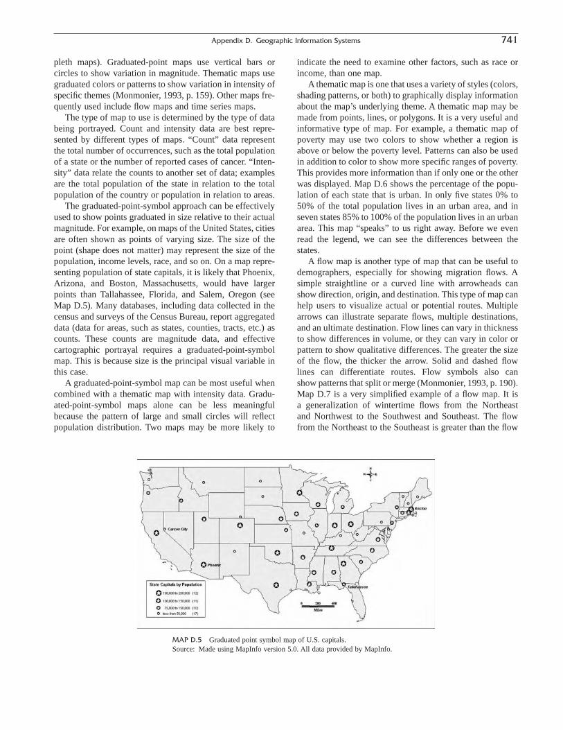
pleth maps). Graduated-point maps use vertical bars orcircles to show variation in magnitude. Thematic maps usegraduated colors or patterns to show variation in intensity ofspecific themes (Monmonier, 1993, p. 159). Other maps fre-quently used include flow maps and time series maps.
The type of map to use is determined by the type of databeing portrayed. Count and intensity data are best repre-sented by different types of maps. “Count” data representthe total number of occurrences, such as the total populationof a state or the number of reported cases of cancer. “Inten-sity” data relate the counts to another set of data; examplesare the total population of the state in relation to the totalpopulation of the country or population in relation to areas.
The graduated-point-symbol approach can be effectivelyused to show points graduated in size relative to their actualmagnitude. For example, on maps of the United States, citiesare often shown as points of varying size. The size of thepoint (shape does not matter) may represent the size of thepopulation, income levels, race, and so on. On a map repre-senting population of state capitals, it is likely that Phoenix,Arizona, and Boston, Massachusetts, would have largerpoints than Tallahassee, Florida, and Salem, Oregon (seeMap D.5). Many databases, including data collected in thecensus and surveys of the Census Bureau, report aggregateddata (data for areas, such as states, counties, tracts, etc.) ascounts. These counts are magnitude data, and effective cartographic portrayal requires a graduated-point-symbolmap. This is because size is the principal visual variable inthis case.
A graduated-point-symbol map can be most useful whencombined with a thematic map with intensity data. Gradu-ated-point-symbol maps alone can be less meaningfulbecause the pattern of large and small circles will reflectpopulation distribution. Two maps may be more likely to
indicate the need to examine other factors, such as race orincome, than one map.
A thematic map is one that uses a variety of styles (colors,shading patterns, or both) to graphically display informationabout the map’s underlying theme. A thematic map may bemade from points, lines, or polygons. It is a very useful andinformative type of map. For example, a thematic map ofpoverty may use two colors to show whether a region isabove or below the poverty level. Patterns can also be usedin addition to color to show more specific ranges of poverty.This provides more information than if only one or the otherwas displayed. Map D.6 shows the percentage of the popu-lation of each state that is urban. In only five states 0% to50% of the total population lives in an urban area, and inseven states 85% to 100% of the population lives in an urbanarea. This map “speaks” to us right away. Before we evenread the legend, we can see the differences between thestates.
A flow map is another type of map that can be useful todemographers, especially for showing migration flows. Asimple straightline or a curved line with arrowheads canshow direction, origin, and destination. This type of map canhelp users to visualize actual or potential routes. Multiplearrows can illustrate separate flows, multiple destinations,and an ultimate destination. Flow lines can vary in thicknessto show differences in volume, or they can vary in color orpattern to show qualitative differences. The greater the sizeof the flow, the thicker the arrow. Solid and dashed flow lines can differentiate routes. Flow symbols also can show patterns that split or merge (Monmonier, 1993, p. 190).Map D.7 is a very simplified example of a flow map. It is a generalization of wintertime flows from the Northeast and Northwest to the Southwest and Southeast. The flowfrom the Northeast to the Southeast is greater than the flow
Appendix D. Geographic Information Systems 741
MAP D.5 Graduated point symbol map of U.S. capitals.Source: Made using MapInfo version 5.0. All data provided by MapInfo.
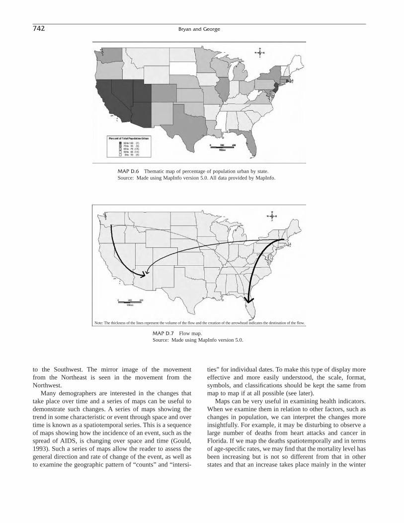
to the Southwest. The mirror image of the movement from the Northeast is seen in the movement from the Northwest.
Many demographers are interested in the changes thattake place over time and a series of maps can be useful todemonstrate such changes. A series of maps showing thetrend in some characteristic or event through space and overtime is known as a spatiotemporal series. This is a sequenceof maps showing how the incidence of an event, such as thespread of AIDS, is changing over space and time (Gould,1993). Such a series of maps allow the reader to assess thegeneral direction and rate of change of the event, as well asto examine the geographic pattern of “counts” and “intersi-
ties” for individual dates. To make this type of display moreeffective and more easily understood, the scale, format,symbols, and classifications should be kept the same frommap to map if at all possible (see later).
Maps can be very useful in examining health indicators.When we examine them in relation to other factors, such aschanges in population, we can interpret the changes moreinsightfully. For example, it may be disturbing to observe alarge number of deaths from heart attacks and cancer inFlorida. If we map the deaths spatiotemporally and in termsof age-specific rates, we may find that the mortality level hasbeen increasing but is not so different from that in otherstates and that an increase takes place mainly in the winter
742 Bryan and George
Note: The thickness of the lines represent the volume of the flow and the creation of the arrowhead indicates the destination of the flow.
MAP D.7 Flow map.Source: Made using MapInfo version 5.0.
MAP D.6 Thematic map of percentage of population urban by state.Source: Made using MapInfo version 5.0. All data provided by MapInfo.

months, when the population of Florida grows considerablybecause of the inflow of “snowbirds” and visitors.
The characteristics of a map determine its clarity, ease ofuse, and effectiveness. Features such as its intensity, scaling,and formats must be considered.
Areas or regions having values that vary are most oftenused for mapping intensity measures/rates (populationdensity, percent urban, infant mortality rate, etc.). A map thatdisplays raw data may not be very informative. Most demo-graphic and economic data appropriate for mapping arebased on censuses or surveys and the social scientist maywish to relate the raw counts to other data, to take accountof variation in land area, total population, or some other rel-evant magnitude.
A very important concept in map creation is “datascaling.” For graduated-point maps, this refers to the size of the point for each count portrayed and the number of different-size points (the number of categories). For the the-matic maps, data scaling refers to deciding how many categories are necessary to ensure that the map reflects sig-nificant differences or trends in the data. Experimentation isoften the best way to determine if a scale results in a patternof symbols that are too small, too cluttered, or too large.Sometimes fewer categories can be better than many. Care-fully chosen boundaries between categories can identifyareas having values above or below a meaningful value,such as a national or state average rate (Monmonier, 1993,p. 169). Class boundaries separating significantly high orlow data values may also be informative in some instances.The mean and standard deviation of an array are often usedas dividers of the data. When creating a thematic map, agiven GIS may offer the option of using an equal-intervalstrategy, natural clusters, or a quantile approach to createbreaks in the data. These options, although easy to apply
(with a click of the mouse), do not necessarily make the bestchoice of breaks in data and should be examined closelybefore being used.
Finally, if one is creating a series of maps that are makingcomparisons for the same area, identical scaling should beused so that differences will be indicated clearly. When acomparison of different areas is being made, if at all possi-ble, scaling should also be the same. If the same scaling isnot possible, be sure to point this anomaly out in the legendso as not to mislead the viewer. Maps D.8 and D.9 demon-strate how a map can be changed when different data scalingis used. Map D.8 uses the “default” scale that the programcreated. It really does not tell the reader very much. A largenumber of states fall within the 10 to 45% category. Ofcourse, 10% is much smaller than 45%; even 20% is muchsmaller. This category is worthless if the reader is lookingfor detailed information. Map D.9 was made with customscaling. The data scale was increased by two categories togive more specific information on a state’s level. The stateswith the largest and smallest population change fall into theirown category. It is a good idea to do this when differencesbetween values are significant.
The two fundamental digital map formats are raster andvector. Vector images are tied to a coordinate system. Everyfeature is defined as a point (or multiple points) on the imageand has an “x” and a “y” attached to it. Raster images aredivided into adjacent polygons of equal size, oftentimesresembling a grid. Each polygon is assigned a value basedon the attribute that is the subject of the map. A raster mapof rivers and streams would typically assign a value of oneto a square in which such a watercourse occurs and a zeroto any square where it does not occur. Unless the map ishigh-resolution with small polygons, the depiction ofsurface features on a raster map will often be inaccurate and
Appendix D. Geographic Information Systems 743
MAP D.8 Thematic map of percentage population change, 1990–1998, default scale.Source: U.S. Bureau of the Census data, MapInfo version 5.0.
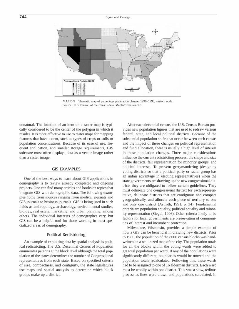
unnatural. The location of an item on a raster map is typi-cally considered to be the center of the polygon in which itresides. It is more effective to use to raster maps for mappingfeatures that have extent, such as types of crops or soils orpopulation concentrations. Because of its ease of use, fre-quent application, and smaller storage requirements, GISsoftware most often displays data as a vector image ratherthan a raster image.
GIS EXAMPLES
One of the best ways to learn about GIS applications indemography is to review already completed and ongoingprojects. One can find many articles and books on topics thatintegrate GIS with demographic data. The following exam-ples come from sources ranging from medical journals andGIS journals to business journals. GIS is being used in such fields as anthropology, archaeology, environmental studies,biology, real estate, marketing, and urban planning, amongothers. The individual interests of demographer vary, butGIS can be a helpful tool for those working in most spe-cialized areas of demography.
Political Redistricting
An example of exploiting data by spatial analysis is polit-ical redistricting. The U.S. Decennial Census of Populationenumerates persons at the block level although the total pop-ulation of the states determines the number of Congressionalrepresentatives from each state. Based on specified criteriaof size, compactness, and contiguity, the state legislaturesuse maps and spatial analysis to determine which blockgroups make up a district.
After each decennial census, the U.S. Census Bureau pro-vides new population figures that are used to redraw variousfederal, state, and local political districts. Because of thesubstantial population shifts that occur between each censusand the impact of these changes on political representationand fund allocation, there is usually a high level of interestin these population changes. Three major considerationsinfluence the current redistricting process: the shape and sizeof the districts, fair representation for minority groups, andpolitical interests. To prevent gerrymandering (designingvoting districts so that a political party or racial group hasan unfair advantage in electing representatives) when thestate governments are drawing up the new congressional dis-tricts they are obligated to follow certain guidelines. Theymust delineate one congressional district for each represen-tative, delineate districts that are contiguous and compactgeographically, and allocate each piece of territory to oneand only one district (Astroth, 1991, p. 34). Fundamentalcriteria are population equality, political equality and minor-ity representation (Siegel, 1996). Other criteria likely to befactors for local governments are preservation of communi-ties of interest and incumbent protection.
Milwaukee, Wisconsin, provides a simple example ofhow a GIS can be beneficial in drawing new districts. Priorto 1980, the population of the 8000 census blocks was hand-written on a wall-sized map of the city. The population totalsfor all the blocks within the voting wards were added to get total population per ward. If any of the populations weresignificantly different, boundaries would be moved and thepopulation totals recalculated. Following this, these wardshad to be assigned to one of 16 alderman districts. Each wardmust be wholly within one district. This was a slow, tediousprocess as lines were drawn and populations calculated. In
744 Bryan and George
MAP D.9 Thematic map of percentage population change, 1990–1998, custom scale.Source: U.S. Bureau of the Census data, MapInfo version 5.0.

1970, this process took 6 months and cost more than$60,000.
In 1980, the city began using a GIS to help with the redis-tricting process. The Census Bureau provided new popula-tion figures on a computer tape that could be matched witha file of the block boundaries. No longer was there a needfor writing on a wall map. With GIS software, the numberswere easily added to secure the population of the wards.Boundaries could be modified with a few clicks of a mouseand numbers recalculated in a matter of minutes. After theboundaries for the wards were determined, the same processwas used to create the alderman districts. GIS cut the timeto complete the process in half and costs to $24. As time andcost decreased, it is likely that accuracy and precisionincreased.
The previous example is rather simplified. GIS was usedto make the process quicker and easier; it did not create thewards for the city. In most cases, redistricting is much morecomplicated and there are many more guidelines to follow.Much has changed since 1980, and it is now possible to havethe GIS do more, or all of it, for you. MapInfo, for example,has a specific redistricting function. Not only can this func-tion be used for redistricting in the traditional sense, but alsofor determining school districts, sales territories, serviceregions—dividing any area into separate districts. The mostdynamic aspect of redistricting using a GIS is the ability tosee on-the-fly updates of record counts and data totals. Per-forming “what if” analyses in a matter of seconds, can beespecially useful for areas that are changing often. With thecomputer you can move a segment from one district toanother and observe what effects this change has on popu-lation totals and characteristics. These changes can be seenon the map and in the table browser. The map shows the dis-tricts shaded by colors and the browser window shows thedemographic data for the districts. Until the file is saved, theredistricting function does not change the map or perma-nently change its style. Any “mappable” table containingregion, line, or point objects that share the same districtinformation as a group can be (re)districted.
Epidemiology
Epidemiology focuses on geographic clusters, patterns,and the spread of disease. GIS can be a useful tool for dis-playing these clusters and patterns. Maps enable us com-prehend quickly, as well as see, the factors that may beimportant in understanding a health problem. One of the firstknown examples of using maps to help in analysis of ahealth problem occurred in 1849 when John Snow used amap to discover a distinct pattern of cholera cases inLondon, England. Snow learned that most cases were clus-tered around a particular water pump. When the pump wasclosed, the number of cholera cases declined. Snow used themap alone, without benefit of the automated spatial analy-
sis now possible with a GIS. Yet the map was all he neededto investigate the problem and find a solution. A reproduc-tion of the map he created is shown as Map D.10.
The regional distribution of disease(s) will naturally raisequestions about the cause and will often suggest possibili-ties for intervention; this information is essential for effec-tive and preventive education. In some cases, once thepattern of disease is identified, control and prevention meas-ures can be instituted. One of the first large-scale applica-tions of GIS in epidemiology occurred in the 1980s, duringthe spread of the AIDS virus. By using GIS to identify whereAIDS cases were increasing the most, and by learning thecharacteristics of these populations and how those infectedhad contracted the disease, targeting measures could bedeveloped and prevention and treatment resources could beassigned in the most efficient way possible.
Wartenberg (1992) gave a good example of how GIS canhelp in an epidemiological study. He analyzed screeningprograms for lead overexposure, which typically target high-risk populations, by identifying regions with common riskmarkers (older housing, poverty, etc.). A GIS can makescreening programs more effective and more cost-efficientby mapping cases of overexposure and identifying high-incidence and high-risk neighborhoods.
Kitron et al. (1994) demonstrated the use GIS for malariasurveillance in Israel, where there is a risk for localized out-breaks due to infection of local mosquitoes by imported cases.
Appendix D. Geographic Information Systems 745
MAP D.10 John Snow’s map of cholera cases in London, England, 1849.Source: www.nationalgeographic.com/resources/ngo/education/ideas912/912choleraho3.html.
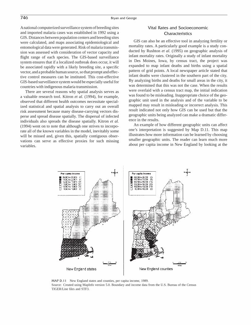
Anational computerized surveillance system of breeding sitesand imported malaria cases was established in 1992 using aGIS. Distances between population centers and breeding siteswere calculated, and maps associating epidemiological andentomological data were generated. Risk of malaria transmis-sion was assessed with consideration of vector capacity andflight range of each species. The GIS-based surveillancesystem ensures that if a localized outbreak does occur, it willbe associated rapidly with a likely breeding site, a specificvector, and a probable human source, so that prompt and effec-tive control measures can be instituted. This cost-effectiveGIS-based surveillance system would be especially useful forcountries with indigenous malaria transmission.
There are several reasons why spatial analysis serves asa valuable research tool. Kitron et al. (1994), for example,observed that different health outcomes necessitate special-ized statistical and spatial analysis to carry out an overallrisk assessment because many disease-carrying vectors dis-perse and spread disease spatially. The dispersal of infectedindividuals also spreads the disease spatially. Kitron et al.(1994) went on to note that although one strives to incorpo-rate all of the known variables in the model, inevitably somewill be missed and, given this, spatially contiguous obser-vations can serve as effective proxies for such missing variables.
Vital Rates and SocioeconomicCharacteristics
GIS can also be an effective tool in analyzing fertility ormortality rates. A particularly good example is a study con-ducted by Rushton et al. (1995) on geographic analysis ofinfant mortality rates. Originally a study of infant mortalityin Des Moines, Iowa, by census tract, the project wasexpanded to map infant deaths and births using a spatialpattern of grid points. A local newspaper article stated thatinfant deaths were clustered in the southern part of the city.By analyzing births and deaths for small areas in the city, itwas determined that this was not the case. When the resultswere overlaid with a census tract map, the initial indicationwas found to be misleading. Inappropriate choice of the geo-graphic unit used in the analysis and of the variable to bemapped may result in misleading or incorrect analysis. Thisresult indicated not only how GIS can be used but that thegeographic units being analyzed can make a dramatic differ-ence in the results.
An example of how different geographic units can affectone’s interpretation is suggested by Map D.11. This mapillustrates how more information can be learned by choosingsmaller geographic units. The reader can learn much moreabout per capita income in New England by looking at the
746 Bryan and George
MAP D.11 New England states and counties, per capita income, 1989.Source: Created using MapInfo version 5.0. Boundary and income data from the U.S. Bureau of the CensusTIGER/Line files and STF3.

county map rather than the state map. Depending on the issueone is trying to explore, it is normally wise to show thelowest geographic units possible (the lowest one can affordor has access to, that is).
The United Nations Statistics Division has recognized the importance of using GIS to portray and analyze popula-tion statistics. In 1997, the division published “Applicationsof Geographical Information Systems for Population and Related Statistics.” The project assists the less devel-oped countries in setting up GIS as a tool for analyzing pop-ulation statistics. The publication provides examples of GIStechniques in demographic studies in Nepal. It demonstratesthe capabilities of GIS to old in visualizing complex demo-graphic data sets, the use of digital maps and a linked database of characteristics and events to facilitate theexploratory analysis of demographic data sets, and theability of a GIS to model and aid policy planning.
First discussed is Nepal’s distinct physiographic patterns(topography) and their relation to the culture and demo-graphic characteristics of the country. The mountains, gla-ciers, rivers, and poor roads hinder accessibility to the fiveregions of Nepal. The impact of physiographic patterns canbe seen by mapping the population distribution between 1966 and 1991. Despite migration and urbanization, thehighest concentration of people remains in the same area(although magnitudes have changed). This can also be said ofeconomic patterns, literacy ratios, and religious affiliations.
Information on social and economic patterns is useful forplanning related decisions and understanding the distinctcultures and regional variations of the society. For example,family planning may be affected by religion, literacy, or eco-nomic status. These, along with the age distribution and fertility rates, can easily be mapped and analyzed. An exam-ination of the maps alone provides insight as to these pat-terns in Nepal. Fertility rates have risen in the moreurbanized area of Kathmandu, where the population is rela-tively young. Female literacy ratios are significantly lowerthan those for males throughout all regions of Nepal. Thehighest literacy ratios are around Kathmandu. Maps illus-trate variables that may be relevant in explaining the changein fertility in Nepal.
The UN generated statistics externally rather than withthe GIS. This is not always necessary; some GIS and statis-tical software packages are compatible (for example,MapInfo and SPSS for windows). The researchers were particularly interested in the regions where both female literacy ratios and contraceptive prevalence ratios (CPR)were low. They used a bivariate analysis to determinewhether CPR and literacy ratios were related. When theyhad determined the areas with low ratios of both, they con-ducted a multiveriate regression analysis using CPR as thedependent variable. Though the model was simple, theregression analysis indicated that values of CPR are associ-ated with all variables but one. The results are important for
the next section that describes the second half of the UNpublication.
Planning/Decision Making
The UN project stresses the planning and modeling possibilities offered through GIS. To do this, the UN givesa hypothetical example using spatial data for the analysis of the demand for health services. This type of analysis isespecially important for countries with limited resources(doctors and nurses, medical equipment) and access to thefacilities.
Matching the supply of health services to demand isimportant in any society. However, in less developed coun-tries, there is often insufficient information on how manypersons are being served and what services they are seeking.The UN study estimates the number of people served by theexisting hospitals (as well as determining if there is a largeportion of people not being served at all). The first step isdefining the areas from which people come to the hospitals,called “catchment” areas. GIS is helpful in this regard as it can determine time and difficulty of travel, in addition to distances.
The next step is to estimate the number of people livingwithin each catchment area. The district boundaries did notmatch the catchment boundaries, so the catchment bound-aries were overlaid with the detailed population informationby the GIS. A “needs assessment” was then made, based onnumber and characteristics of persons in the catchment.Although some of the areas looked smaller than others onthe map, they have much higher population densities thanother areas and thus a much greater demand for services.
CONCLUDING NOTE
GIS is a new resource for compiling, analyzing, and pre-senting data. Its ease of use and applications are growingrapidly with improvements in technology; yet developmentis always being outpaced by the demands of GIS users.Support groups around the country are growing, and datasources are becoming more abundant and less expensive.While GIS has already enjoyed substantial advances, itrequires substantial development before its use will be ascommon as word-processing and spreadsheet software.
The challenges to GIS development include improve-ments in presentation, analytical capabilities, and flexibility.Mapping in GIS systems need to be much more carto-graphically sound than they are so that a person with notraining in cartography can produce maps that make senseto the reader. Analysis needs to be simplified to layperson’sterms so that the novice can not only do simple tasks within
Appendix D. Geographic Information Systems 747

a GIS system but also perform some complex spatial analy-sis. Flexibility needs to be integrated into GIS systems toallow the users to customize their software to their needs.Many software packages are moving in these directions.Maps from the first GIS software systems and the maps fromtoday’s software systems are not comparable; the analysisthat is available to the novice today is much more powerful.The software companies have almost all created a program-ming language for users’ to customize their software to theusers’ needs, although some of the programming languagesare difficult to learn and use. GIS has become an importantresearch and application tool. As both its flexibility and itsease of use increase, more and more people are expected toincorporate GIS into their work.
References
Aronoff, S. 1989. Geographic Information Systems: A Management Perspective. Ottawa, Canada: WDL.
Astroth, J. 1991. “The Role of GIS in Redistricting: A Case Study in Missouri.” Geo Info Systems 1: 34–42.
Fotheringham, S., and P. Rogerson. 1994. Spatial Analysis and GIS.London: Taylor & Francis.
Gould, P. 1993. The Slow Plague: A Geography of the AIDS Pandemic.Oxford: Blackwell Publishing.
Kitron, U., H. Pener, C. Costin, L. Orshan, Z. Greenberg, and U. Shalom.1994. “Geographic Information System in Malaria Surveillance: Mos-quito Breeding and Imported Cases in Israel, 1992.” American Journalof Tropical Medicine & Hygiene 50: 550–556.
MapInfo Corporation. 1998. MapInfo Professional User’s Guide, V. 5.0.Troy, NY: MapInfo Corporation.
Mark, D. M., N. Chrisman, A. U. Frank, P. H. McHaffie, and J. Pickles withcontributions from M. Curry, J. Goss, F. Harvey, K. Hillis, R. Miller,E. Shepard, and D. Varanka. 1997. “The GIS History Project.” NationalCenter for Geographic Information and Analysis (NCGIA),www.geog.buffalo.edu/ncgia/gishist.
Monmonier, M. 1993. Mapping It Out: Expository Cartography for theHumanities and Social Sciences. Chicago: The University of ChicagoPress.
Niemann, B. J., Jr., and S. Niemann. 1998a. “Allan H. Schmidt: GIS Journeyman.” Geo Info Systems 8(5): 42–45.
Niemann, B. J., Jr., and S. Niemann. 1998b. “Thomas Karl Poiker: Algorithms and Academics.” Geo Info Systems 8(2): 36–39.
Rushton, G., D. Krishnamurti, R. Krishnamurti, and H. Song. 1995. “AGeographic Information Analysis of Urban Infant Mortality Rates.”Geo Info Systems 5: 52–56.
Siegel, J. S. 1996. “Geographic Compactness vs. race/ethnic Compactnessand other criteria in the delineation of legislative districts.” PopulationResearch and Policy Review 15: 147–164 (April).
Tomlinson, R. F. 1997. “Federal Influences in Early GIS Development inCanada.” Geo Info Systems 7: 38–39.
Wartenberg, D. 1992. “Screening for Lead Exposure Using a GeographicInformation System.” Environmental Research 59(2), 310–317.
Suggested Readings
GIS History
American Cartographer. 1988. Special Issue. “The Development of GISTechnology.” American Cartographer 15(3): 245–322.
Cartographic Journal. 1991. Special Issue. “British Cartography1987–1991: An Overview.” Cartographic Journal 28: 30–54.
Foresman, T. (Ed.). 1998. The History of GIS: Perspectives from Pioneers.Englewood Cliffs, NJ: Prentice Hall.
Mark, D. M., N. C. A. U. Frank, P. H. McHaffie, J. Pickles, with contri-butions from M. Curry, J. Goss, F. Harvey, K. Hillis, R. Miller, E. Shepard, and D. Varanka. 1997. “The GIS History Project.” TheNational Center for Geographic Information and Analysis (NCGIA),www.geog.buffalo.edu/ncgia/gishist.
GIS General
Bernhardsen, T. 1996. Geographic Information Systems. New York: JohnWiley & Sons.
Berry, J. K. 1993. Beyond Mapping: Concepts, Algorithms, and Issues inGIS. Fort Collins, CO: GIS World Books.
Clarke, K. 1998. Getting Started with Geographic Information Systems.Englewood Cliffs, NJ: Prentice Hall.
Congalton, R. G., and K. Green. 1992. “The ABC’s of GIS: An Introduc-tion to Geographic Information Systems.” Journal of Forestry 90:13–20.
Cressie, N. 1991. Statistics for Spatial Data. New York: John Wiley &Sons.
Daniel, L., and J. Slezak. 1995. “Street Talk: The Word on Address Matching.” Business Geographics 3: 53–59.
DeMers, M. 1996. Fundamentals of Geographic Information Systems. NewYork: John Wiley & Sons.
DeMers, M. 1996. “Dictionary of Abbreviations and Acronyms in Geo-graphic Information Systems, Cartography, and Remote Sensing,”www.lib.berkeley.edu/EART/abbrex.html#a.
ESRI. 1999. Getting to Know ArcView GIS. Redwood, CA: ESRI.Goodchild, M. F. 1992. “Geographical Information Science.” International
Journal of Geographical Information Science 6: 31–45.Heywood, I. 1990. “Geographic Information Systems in the Social
Sciences—Introduction.” Environment and Planning 22: 849–852.Kaplan, E. D. 1996. Understanding GPS: Principles and Applications.
Boston: Artech House.Martin, D. 1996. Geographic Information Systems: Socioeconomic Appli-
cations. New York: Routledge.Openshaw, S. 1990. “Spatial Analysis and Geographical Information
Systems: A Review of Progress and Possibilities.” Pp. 153–163. In H.J. Scholten and J. C. H. Stillwell (Eds.), Geographical InformationSystems for Urban and Regional Planning (pp. 153–163). Boston:Kluwer Academic.
Pickles, J. 1995. Ground Truth: The Social Implications of GeographicInformation Systems. New York: Guilford Press.
Rogerson, P. A., and A. S. Fotheringham. 1994. Spatial Analysis and GIS.London: Taylor and Francis.
Spitzer, T. 1996. “A Database Perspective on GIS: Part I.” DBMS 9:95–102.
Star, J., and J. Estes. 1990. Geographic Information Systems: An Introduc-tion. Englewood Cliffs, NJ: Prentice Hall.
General Mapping and Geography Sources
Clarke, K. 1995. Analytical and Computer Cartography. New York: Prentice Hall.
Fisher, H. T. 1982. Mapping Information: The Graphic Display of Quanti-tative Information. Cambridge, MA: ABT Books.
Garson, G. D., and R. S. Briggs. 1992. Analytic Mapping and GeographicDatabases. New York: Sage.
748 Bryan and George

Griffith, D., and C. Amrheun. 1997. Multivariate Statistical Analysis forGeographers. Englewood Cliffs, NJ: Prentice Hall.
Kraak, M.-J. 1996. Cartography: Visualization of Spatial Data. Reading,MA: Addison-Wesley.
MacEachren, A. 1995. How Maps Work: Representation, Visualization andDesign. New York: Guilford Press.
Plane, D. A., and P. A. Rogerson. 1994. The Geographical Analysis of Population. New York: John Wiley & Sons.
Robinson, A. H., J. L. Morrison, P. C. Muehrche, A. J. Kimerling, and S.C. Guptill. 1995. Elements of Cartography. New York: John Wiley andSons.
Shaw, G., and D. Wheeler. 1994. Statistical Techniques in GeographicalAnalysis. New York: John Wiley & Sons.
Wood, C., and C. P. Kellers. 1996. Cartographic Design: Theo-retical and Practical Perspectives. New York: John Wiley & Sons.
Wood, D. 1992. The Power of Maps. New York: Guilford Press.
Case Studies in GIS
Braddock, M., G. Lapidus, E. Cromley, R. Cromley, G. Burke, and L.Banco. 1994. “Using a Geographic Information System to UnderstandChild Pedestrian Injury.” American Journal of Public Health 84:1158–1161.
Danziger, J. N., W. H. Dutton, R. King, and K. L. Kraemer. 1982. Com-puters and Politics: High Technology in American Local Government.New York: Columbia University Press.
Davenhill, W. F. 1995. “Is There a Doctor in the Area?” Business Geo-graphics 3: 34–35.
De Lepper, M., H. Scholten, and R. Stern. 1995. “The Added Value of Geo-graphical Information Systems in Public and Environmental Health.”Geojournal Library, Volume 24. New York: Kluwer Academic Publishers.
Del Valle, J. C. 1996. Thesis: Retail Site Selection: An Integrated Approach.Gainesville, FL: University of Florida.
Friel, C. A. 1991. “A Zip Code-Based GIS Reveals the Geography ofRetirement.” Geo Info Systems 1: 48–56.
Gesler, W. 1986. “The Uses of Spatial Analysis in Medical Geography: AReview.” Social Science & Medicine 23: 963–973.
Glass, G., et al. 1994. “Environmental Risk Factors for Lyme Disease Iden-tified with Geographic Information Systems.” American Journal ofPublic Health 85: 944–948.
Gobalet, J., and R. Thomas. 1996. “Demographic Data and GeographicInformation Systems for Decision Making: The Case of Public Health.”Population Research and Policy Review 15: 537–548.
Gould, P. 1993. The Slow Plague: A Geography of the AIDS Pandemic.Oxford: Blackwell.
Lam, N. S. 1986. “Geographical Patterns of Cancer Mortality in China.”Social Science & Medicine 23: 241–247.
Levine, J., and J. D. Landis. 1989. “Geographic Information Systems forLocal Planning.” Journal of the American Planning Association 55:209–220.
Longley, P., and G. Clarke. 1996. GIS for Business and Service Planning.New York: John Wiley & Sons.
Maltz, M., A. Gordon, and W. Friedman. 1991. Mapping Crime in Its Com-munity Setting: Event Geography Analysis. New York: Springer-Verlag.
Martin, D. 1991. Geographic Information Systems and Their Socioeco-nomic Applications. Oxford: Routledge.
Plane, D., and P. Rogerson. 1994. Geographical Analysis of Population; withApplications to Planning and Business. New York: John Wiley & Sons.
Rushton, G., et al. 1995. “A Geographic Information Analysis of UrbanInfant Mortality Rates.” Geo Info Systems 5: 52–56.
Scholten, H., and J. Stillwell. 1990. Geographical Information Systems forUrban and Regional Planning. New York: Kluwer Academic.
Stallones, L., J. Nuckols, and J. Berry. 1992. “Surveillance around Hazardous Waste Sites: Geographic Information Systems and Reproductive Outcomes.” Environmental Research 59: 81–92.
Yeh, A. G. 1991. “The Development and Applications of Geographic Information Systems for Urban and Regional Planning in DevelopingCountries.” International Journal of Geographical Information Systems5: 5–27.
Data-Related Issues
Adam, N., and A. Gangopadhyay. 1997. Database Issues in GeographicInformation Systems. New York: Kluwer Academic Publishers.
Bolstad, P. V., and P. Gessler. 1990. “Positional Uncertainty in ManuallyDigitized Map Data.” International Journal of Geographical Informa-tion Systems 4: 399–412.
Goodchild, M., and S. Gopal. 1990. Accuracy of Spatial Databases.London: Taylor & Francis.
Guptill, S., and J. Morrison. 1995. Elements of Spatial Data Quality.Oxford: Pergamon Press.
Scott, L. M. 1994. “Identification of GIS Attribute Error Using ExploratoryData Analysis.” The Professional Geographer 46: 378–386.
Spitzer, T. “A Database Perspective on GIS, Part I,”www.dbmsmag.com/9611d15.html.
U.S. Census Bureau and GIS
Broome, F. R., and L. Godwin. 1988. “The Census Bureau’s PublicationMap Production System.” Cartography and Geographic InformationSystems 17: 79–88.
Broome, F. R., and D. B. Meixler. 1990. “The TIGER Data Base Struc-ture.” Cartography and Geographic Information Systems 17: 39–48.
Carbaugh, L. W., and R. W. Marx. 1990. “The TIGER System: A CensusBureau Innovation Serving Data Analysts.” Government InformationQuarterly 7: 285–306.
Trainor, T. F. 1990. “Fully Automated Cartography: A Major Transition atthe Census Bureau.” Cartography and Geographic Information Systems17: 21–26.
U.S. Census Bureau. 1977. “Mapping for Census and Surveys.” Washing-ton, DC: U.S. Bureau of the Census.
U.S. Bureau of the Census. 1990. “Strength in Numbers: Your Guide to1990 Census Redistricting Data from the U.S. Bureau of the Census.”Washington, DC: U.S. Bureau of the Census.
U.S. Census Bureau. 1992. “What Do I Need to Map Out 1990 CensusData?” Washington, DC: U.S. Bureau of the Census.
U.S. Census Bureau. 1993. “1992 TIGER Line Files: Helping You MapThings Out.” Washington, DC: U.S. Bureau of the Census, GeographyDivision.
U.S. Census Bureau. 1994. “Maps and More: Your Guide to Census BureauGeography.” Washington, DC: U.S. Bureau of the Census.
GIS Software Vendor Information
This is a selected list of GIS software packages with contact informa-tion. Given the rapidly changing nature of GIS software with respect toprice and function, no attempt has been made to describe or compare these packages.
MapInfo. MapInfo was the first company to develop and market PC-basedmapping software for business applications. www.mapinfo.com
ESRI (Environmental Systems Research Institute). A privately held con-sulting group, building software tools and products. ESRI’s first com-
Appendix D. Geographic Information Systems 749

mercial GIS product was ARC/INFO (1981). Later products include PCARC/INFO, ArcView GIS, ArcCAD, and MapObjects, ESRI also offersdata sets to compliment its products.www.esri.com
Intergraph Corporation. This global company offers a variety of hardwareand software products for Windows NT.www.intergraph.com
IDRISI (The Clark Labs). A research organization located within the Graduate School of Geography at Clark University. IDRISI is a raster GIS and image processing software developed at the lab. The labhas also developed a digitizing and editing software, CartaLinx. www.clarklabs.org
Caliper. Caliper produces transportation GIS software called Trans CAD,Maptitude GIS+, and Maptitude for Redistricting. www.caliper.com
GRASS. The U.S. Army Construction Engineering Research Laboratory’s(USA-CERL) Geographic Resources Analysis Support System(GRASS) was developed to provide management tools to army environmental planners and land managers. GRASS can handle different representations of data (raster, vector, and point).www.cecer.army.mil/grass/GRASS.main.html
Northwood Geoscience, Ltd. Vertical Mapper add-on program for MapInfo.www.northwoodgeo.com
Tydac Technologies, Inc. / PCI Geomatics Group—SPANS 7 and PAMAP.SPANS 7 is a complete spatial analysis software system that providesmodeling and analysis capabilities, data management, and professionalmap output. www.pci.on.ca
ComGrafix. MAPGRAFIX was the first desktop GIS complete with di-gitizing, printing/plotting, and analytical tools. The map elements are linked to the demographic data in databases using AppleScript tocreate automatic thematic maps. It has the built-in capability of importing ESRI files and supports many standard vector formats.www.comgrafix.com
Smallworld. www.smallworld-us.comCompusearch/Market Math. www.esri.com/partners/gissolutions/
compusrc/marketm.html
Private Sources
Many software vendors (listed earlier) repackage and sell data in theproprietary forms used by their software products. Because the data areusually checked and corrected as they are repackaged, the use of these con-verted datasets can save time.
Geographic Data Technology, Inc. (GDT) sells geographic databases spe-cializing in street network data. Formats compatible with ARC/INFO,ArcView, MapInfo, Tactician, AtlasGIS, and SAS/GIS are provided.www.gdt1.com
Cartotech of San Antonio, Texas, and GDT of New Hampshire, amongothers, are “conversion” firms that will build datasets to a user’s specifications.
ADC (American Digital Cartography) Worldmap. www.adci.comClaritas sells marketing data, demographic data, and boundary files for GIS.
Claritas provides formats for MapInfo, ArcView, Intergraph’s MGE,SAS/GIS and Tactician software.www.claritas.com
Equifax National Decision Systems is a major provider of demographic,geographic, business, consumer behavior, and industry-specific data.www.ends.com
Etak offers precise street map data, navigation technology, and geocodingtools. www.etak.com/corporate.html
The POLK Company offers a variety of data relating to motor vehicles,lifestyles, population, neighborhoods, businesses, geography, and pur-chasing behavior. www.polk.com
ACXIOM combines public record information with data from a variety ofother national information providers to produce comprehensive datasets on consumers and businesses. www.acxiom.com
Mediamark Research, Inc. offers comprehensive data on population andlifestyle. Custom studies are available using the Internet, telephone, andmail samples. www.mediamark.com
Spatial Logic maintains current district boundaries for mapping and GIS.Congressional, State legislature district boundaries are available. Fileformats available include Atlas GIS (AGF) , Atlas ASCII (BNA),AutoCAD (DXF), MapInfo Interchange Format (MIF), Arcview Shapfiles (SHP), and MapInfo files (TAB). www.spatialogic.com
Infotech. InfoTech offers comprehensive services in GIS conversion (dig-itization), mapping, and Software. http://infotech.stph.net/infotech.html
Center for International Earth science Information Network (CIESIN,Columbia University) provides demographic data, metadata, resources,interactive applications. www.ciesin.org
Public Sources
USGS (U.S. Geological Survey). www.usgs.govU.S. Census Bureau. www.census.govFederal Geographic Data Committee, Manual of Federal Geographic Data
Products. Washington, D.C.: Environmental Protection Agency, Officeof Information Resources Management, 1992.
The Historical United States Boundary Files (HUSCO) Home page offersvarious historical boundaries ranging from the years 1790 to 1970.www.cadgis.lsu.edu: 80/geoscipub
Oregon State Service Center for Geographic Information Systems.www.sscgis.or.gov
Connecticut Map and Geographic Information Center.http://magic.lib.uconn.edu
Geostrategies. Extensive data for Central and Eastern Europe.www.geo.strategies.ro
Australia Survey and Land Information Group (AUSLIG). Australia’sNational Mapping Agency; digital map infomation and more.www.auslig.gov.au/welcome.htm
ESRI Canada. www.esricanada.comEuropean Umbrella Organisation for Geographic Information.
www.eurogi.orgGIS Data Depot. www.gisdatadepot.comIndonesian Land Use Databank. www.geocities.com/Tokyo/2439
750 Bryan and George

ABORTION The expulsion of a fetus from the uterus. Aninduced abortion is the intentional removal of a fetus from theuterus. A spontaneous abortion is the premature and naturallyoccurring expulsion of a fetus from the uterus. In popular usage,the term is restricted to the former meaning. See also BIRTHand FETAL LOSS.
ABORTION RATE The estimated number of abortions per1000 women aged 15 to 44 years in a given year.
ABRIDGED LIFE TABLE See LIFE TABLE.
ACCEPTOR A person receiving service or advice from afamily-planning program.
ACCESSION RATE The entry rate of persons into a givenstatus, a function often shown in specialized life tables, such astables of working life.
ACTIVITIES OF DAILY LIVING (ADLs) Measures of func-tioning that typically are concerned with limitations in theability, or the inability, to carry out certain personal care rou-tines, such as eating, dressing, toileting, transferring into andout of bed, and bathing. See INSTRUMENTAL ACTIVITIESOF DAILY LIVING.
ACTUARIAL SCIENCE The science of risk, premium, andbenefit analysis, involving the preparation of life and actuarialtables that form the foundation of the business of insurance andrelated activities.
ACUTE CONDITION A health condition of rapid onset and arelatively short duration that usually ends with either recoveryor death.
ACUTE DISEASE A disease that has a rapid onset and gener-ally lasts for only a short period of time. See also CHRONICDISEASE.
ADJUSTED RATE See STANDARDIZATION.
ADJUSTED INFANT MORTALITY RATE This takes intoaccount the change in the number of births from the precedingyear by the use of appropriate separation fuctors. See alsoINFANT MORTALITY RATE.
ADMINISTRATIVE AREA A geographic area used in cen-suses for collection, tabulation, and analysis that corresponds toa political and or other administrative unit.
ADMINISTRATIVE RECORDS Data collected by govern-mental (and sometimes private) organizations for taxation, registration, fee collection, and other administrative purposesthat indirectly provide demographic information. These data areused by demographers for analyses, estimates, projections, andthe evaluation of data specifically collected for demographicpurposes. See also ADMINISTRATIVE RECORDSMETHOD.
ADMINISTRATIVE RECORDS METHOD In the UnitedStates, a member of the family of component methods for esti-mating population that relies on a past census, vital statisticsdata, and migration data derived from tax returns. See also POPULATION ESTIMATE.
AGE The length of time that a person has lived. A distinction ismade between completed age and exact age, with completedage usually defined in terms of the last birthday and exact age
751
Glossary
DAVID A. SWANSON AND G. EDWARD STEPHAN1
1 The authors thank Dean Judson, Nancy McGirr, Jerry McKibben, andPeter Morrison for their comments and suggestions. Sources of informa-tion used in compiling this Glossary include, but are not limited to, the following publications:
Namboodiri, K. 1991. Demographic Analysis: A Stochastic Approach.New York: Academic Press.
Peterson, W., and R. Peterson. 1986. Dictionary of Demography: Terms,concepts, and Institutions. Wisport , CT Greenword Press.
Population Reference Bureau. 2001. Glossary of Population Terms,accessed in August 2001 at www.prb.org/template.cfm?Section=Glossary.
Ross, J. A. (Editor). 1992. International Encyclopedia of Population.New York: Free Press.
Shryock, H., and J. Siegel. 1973. The Methods and Materials of Demography, Rev. ed. Washington, DC: U.S. Government Printing Office.
Smith, S. K., J. Tayman, and D. A. Swanson. 2001. State and LocalPopulation Projections: Methodology and Analysis. New York: KluwerAcademic/Plenum.
United Nations. 1953. The Determinants and Consequences of Popu-lation Trends. New York: United Nations.
United Nations. 1999. Dictionary of Demographic and ReproductiveHealth Terminology, accessed in August 2001 at www.popin.org/~unpopterms/.
United States Census Bureau. 2001. Glossary, last accessed in August2002 at www.census.gov/main/www.glossary.html.

being the exact time since birth. Conventions for determiningage vary somewhat between cultures and countries.
AGE ACCURACY INDEX The arithmetic average of theabsolute values of the differences between observed age ratiosand expected age ratios. See also AGE RATIO.
AGE CUMULATIVE FERTILITY RATE See CUMULA-TIVE FERTILITY RATE.
AGE DEPENDENCY RATIO A ratio in which the numeratorrepresents the total number of people not of working age (tooyoung or too old to work and therefore “dependent” on thosewho do), and the denominator represents the population ofworking age; often multiplied by 100, which yields the numberof dependents per 100 persons of working age. See ALSODEPENDENCY RATIO.
AGE DISTRIBUTION See POPULATION COMPOSITION.
AGE EFFECT An analytical perspective that attempts to deter-mine the effect of age on a variable of interest. Age effects areoften considered simultaneously with cohort and period effects.See also AGE-PERIOD-COHORT EFFECTS, COHORTEFFECT, and PERIOD EFFECT.
AGE GROUP Multiyear categories into which single years ofage are assembled for purposes of data presentation or analy-sis. The most frequently found age grouping is 0 to 4, 5 to 9,10 to 14, and so on.
AGE HEAPING A higher-than-expected proportion of ages withcertain terminal digits and a lower than expected proportion withother terminal digits, often adjacent, because of digit preferenceor digit avoidance. See also AGE MISREPORTING, AGE PREF-ERENCE, DIGIT AVOIDANCE, and DIGIT PREFERENCE.
AGE MISREPORTING The tendency for people to not reporttheir correct age because they do not know it exactly or becausethey prefer to report another age, often an adjacent age or agegroup. See also AGE HEAPING.
AGE PARITY GRID See FERTILITY PATTERN METHOD.
AGE-PERIOD-COHORT EFFECT The joint and separateeffects of age, period, and cohort membership on a dependentvariable of interest. See also AGE EFFECT, COHORTEFFECT, and PERIOD EFFECT.
AGE PREFERENCE The tendency for people to report an agedifferent than their actual age because of cultural, social, or per-sonal reasons. See also AGE-HEAPING.
AGE RATIO The ratio of a given age group to the average foundby summing the age group in question and two adjoining agegroups and dividing this sum by three. See also AGE-HEAPING.
AGE-SEX DISTRIBUTION See POPULATION COMPOSI-TION.
AGE-SEX POPULATION PYRAMID See POPULATIONPYRAMID.
AGE-SEX STRUCTURE See POPULATION COMPOSITION.
AGE-SPECIFIC PROPORTION A ratio that relates thepersons with a given demographic characteristic at a specificage (or age group) to the corresponding population in the sameage (or age group). Examples include the age-specific propor-
tion married and the (age-specific) labor force participationratio. See also GENERAL PROPORTION.
AGE-SPECIFIC RATE A rate that relates a given demographicevent at a specific age (or age group) to the corresponding at-risk population in the same age (or age group). Examplesinclude age-specific birthrate, age-specific marital birthrate, andage-specific death rate. See also CRUDE RATE, GENERALRATE, and RATE.
AGE STRUCTURE See POPULATION COMPOSITION.
AGED The latter stages of adulthood, usually specified by lawor culture in terms of a certain minimum age (e.g., those 75years and over are “aged”).
AGGREGATION The process of assembling individual ele-ments into summary form for purposes of presentation or analy-sis. For example, to assemble census records for individuals ina given area into a summary for the area as a whole.
AGGREGATION BIAS A type of distortion that can result by attributing relationships found among summaries to the individual elements from which the summaries were obtained.
AGING The process of growing older. For an individual it issimply measured in terms of age; for a population it is meas-ured by one of several indices. For example, the percentage age65 years and older, median age, or mean age.
ALIEN See FOREIGNER.
ALLIANCE INDEX A measure of male-female unions.
ALLOCATION The assignment of values to cases for which“item nonresponse” is found in a sample survey or census.Many allocation methods are available, including automatedalgorithms. See also IMPUTATION, NONRESPONSE, andSUBSTITUTION.
AMENORRHEA The temporary cessation of menstruation, fornormal or pathological reasons, usually the latter. It is not usedto refer to old age or prepuberty, but may be used to refer topregnancy or the post-partum condition. See also POST-PARTUM AMENORRHEA.
AMERICAN COMMUNITY SURVEY (ACS) In the UnitedStates, an ongoing household survey conducted by the CensusBureau on a “rolling” geographic basis that is designed toprovide demographic characteristics for counties, places, andother small areas. It may replace the long form in the 2010census.
ANNEXATION In the United States, the legal act of adding ter-ritory to a governmental unit, usually an incorporated place,through the passage of an ordinance, court order, or other legalaction.
ANNUITY A term used in actuarial science for a type of cashdistribution (e.g., payments on a life insurance policy) in whichthe distribution is fixed at a certain amount and date over agiven period of time. See also ACTUARIAL SCIENCE.
ANTENATAL See PRENATAL.
APPLIED DEMOGRAPHY A field of demography concernedwith applications of demographic data, methods, and perspec-
752 Swanson and Stephan

tives to the practical problems of business, government, andother institutions, aiding in the formulation and implementationof decisions and policies by these institutions.
AREA ANALYSIS Measurements collected on a number ofvariables for each of many administrative/statistical areas thatare usually analyzed using multivariate techniques.
ARRANGED MARRIAGE A union arranged by relatives (orother influential parties) of the couple to be married, with orwithout the agreement of the couple.
ASYLEE In the United States, an alien already in the country orat a port of entry who is found to be unable or unwilling toreturn to his or her country of nationality, or to seek the pro-tection of that country because of persecution or a well-foundedfear of persecution based on his or her race, religion, national-ity, membership in a particular social group, or politicalopinion. For an alien with no nationality, the country of nation-ality is considered to the country in which he or she last habit-ually resided. An asylee is eligible to adjust to lawful permanentresidence status after 1 year of continuous presence in theUnited States. See also INTERNALLY DISPLACED PERSONand REFUGEE.
AT-RISK POPULATION The persons to whom an event can potentially occur. In the form of the population at themiddle of a given period, such as a year, it is used as an ap-proximation of “person-years lived.” See also EXPOSURE,PERSON-YEARS LIVED, and PROBABILITY.
AVERAGE FAMILY SIZE The mean number of living childrenof an individual or couple.
BABY BOOM The dramatic increase in both birthrates andabsolute numbers of births in the United States, Canada, Aus-tralia, and New Zealand that started after World War II and lastedfor nearly 20 years. In the United States, for example, it lastedfrom approximately 1946 to 1964. See also BABY BUST.
BABY BUST The rapid decline in fertility rates to record lowlevels during the period immediately after the baby boom. Seealso BABY BOOM.
BACHUE MODELS A method primarily designed by the Inter-national Labor Organization in the 1970s to integrate demo-graphic variables into the planning process for developingcountries. Although they have fallen into disuse, the modelswere designed to study the relationship between populationgrowth and spatial distribution while controlling for the effectsof other variables.
BALANCING EQUATION A term attributed to A. J. Jaffe thatdescribes the basic population relation: Pt = P0 + I - O, wherePt equals a given population at time = 0 + t, P0 = the given population at time = 0, I = the number of persons entering thepopulation through birth and immigration between time = 0 andtime = 0 + t, and O = the number of persons exiting the popu-lation through death and emigration between time = 0 and time= 0 + t. See also COHORT-COMPONENT METHOD, COM-PONENT METHOD, ERROR OF CLOSURE, and RESID-UAL METHOD.
BASE PERIOD In a population projection, this is the periodbetween the initial year for which data are used to generate theprojection and the last year, which is known as the launch year.
See also LAUNCH YEAR, POPULATION PROJECTION,PROJECTION HORIZON, and TARGET YEAR.
BASELINE SURVEY A collection of data used for subsequentcomparison or control.
BELOW REPLACEMENT FERTILITY The level at whichthe total fertility rate is too low for the numbers of women ofchildbearing ages to be replaced in a generation. See alsoTOTAL FERTILITY RATE.
BIAS The deviation of an estimate or set of estimates from thecorrect value(s) in one direction (i.e., above or below the correctvalue(s)). See also TOTAL ERROR.
BIRTH This refers only to a live birth and is referenced by theissuance of a birth certificate in the United States. As definedby the World Health Organization and allied organizations, alive birth is the complete expulsion or extraction from itsmother of a product of conception, irrespective of the durationof pregnancy, which, after such separation, breathes or showsany other evidence of life such as beating of the heart, pulsa-tion of the umbilical cord, or definite movement of voluntarymuscles, whether or not the umbilical cord has been cut or theplacenta is attached; each product of such a birth is considered“live-born.” According to this definition, the period of gesta-tion, or the state of life or death at the time of registration, arenot relevant. The U.S. standard contains this definition plus astatement recommended by the American College of Obstetri-cians and Gynecologists to assist in the determination of whatshould be considered a live birth: “Heartbeats are to be distin-guished from transient cardiac contractions; respirations are tobe distinguished from fleeting respiratory efforts or gasps.” Seealso ABORTION and FETAL LOSS.
BIRTH COHORT Members of a population born in a givenperiod (e.g., 1950, 1975–1979).
BIRTH CONTROL An attempt to regulate the timing or occur-rence of births.
BIRTH HISTORY The date and outcome of each birth experi-enced by a woman.
BIRTH INTERVAL The period between two successive livebirths. In the case of the first birth interval, the period betweentime of entry into sexual union (e.g., marriage) and the first livebirth. In the case of the most recent live birth, it is the periodbetween it and a subsequent date (e.g., the date of a birth historyinterview). Where a period is bounded by either birth or time ofentry into sexual union, the interval is known as closed; where aperiod is bounded only on one side, the interval is known as open.
BIRTH ORDER The location of a given birth in the sequenceof births to a woman, starting with the first and ending with themost recent (e.g., first, second, third).
BIRTH-ORDER RATE Births of a given order during a givenperiod, divided by the number of women exposed during thesame period.
BIRTH REGISTRATION AREA In the United States, thestates and local governments complying with federal standardsfor the registration of births. It was established in 1915 and by1933 encompassed all states. See also DEATH REGISTRA-TION AREA.
BIRTH SPACING See CHILDSPACING.
Glossary 753

BIRTH WEIGHT The amount that an infant weighs at birth,usually expressed in grams.
BIRTHS EXPECTED The number of births that a woman orcouple expects to have in a specified future period or by the endof childbearing, usually obtained in a census or survey. See alsoDESIRED FAMILY SIZE.
BLOCK In the United States, the lowest level of geography forwhich census data are compiled. It is a typically a city block,but specifically is a small area bounded on all sides by identi-fiable features (e.g., roads, rivers, and city limits) that does notcross the boundaries of a given census tract. Each block is num-bered uniquely within census tracts. See also BLOCK GROUP,BLOCK NUMBERING AREA, CENSUS GEOGRAPHY, andCENSUS TRACT.
BLOCK GROUP In the United States, a cluster of blocks withina census tract that have the same first digit in their identifyingnumbers. See also BLOCK, BLOCK NUMBERING AREA,CENSUS GEOGRAPHY, and CENSUS TRACT.
BLOCK NUMBERING AREA In the United States, these areclusters of block groups used in the 1990 census as the frame-work for grouping and numbering blocks in counties that didnot have census tracts and provided coverage only for the block-numbered portion of a county. Starting with the 2000 decennialcensus, all U.S. counties have census tracts. See also BLOCK,BLOCK GROUP, CENSUS GEOGRAPHY, and CENSUSTRACT.
BONGAART’S DECOMPOSITION An equation named afterits developer, J. Bongaarts, that expresses the total fertility rateas the product of variables affecting fertility.
BRASS RELATIONAL MODEL LIFE TABLES A family oflife tables developed by W. Brass that is based on an age invari-ant linear function (logarithmic) of the ratio of the probabilityof dying to the probability of not dying before a given birthday.See also MODEL LIFE TABLE.
BRASS TECHNIQUE One of many methods of estimating thelevel and pattern of both fertility and mortality from limiteddemographic data, devised by W. Brass.
CASE-FATALITY RATE The ratio of deaths from a health con-dition per year to persons who have that health condition atmidyear. Alternatively, the population base can be the numberof persons who have that condition at any time during the year.
CAUSE-DELETED LIFE TABLE A life table calculated afterremoving one or more specific causes of death.
CAUSE-SPECIFIC DEATH RATE The ratio of the number ofdeaths due to one or more causes to the at-risk population.
CENSAL-RATIO METHOD A set of population estimationtechniques found within the “change in stock method” familythat uses crude rates (e.g., birth and death) as measured at themost recent census date(s) and post-censal administrativerecords. For example, a population estimate for 2002 can beobtained by dividing reported deaths for 2002 by the crudedeath rate measured in 2000 or by a crude death rate projectedfrom 2000 to 2002. Often a series of censal-ratio estimates areaveraged together. D. Swanson and R. Prevost showed in 1985that the ratio-correlation method is algebraically equivalent to
a weighted average of censal-ratio estimates in which regres-sion slope coefficients serve as weights. See also CHANGE INSTOCK METHOD, POPULATION ESTIMATE, RATIO-CORRELATION METHOD, and WEIGHTED AVERAGE.
CENSORED A condition affecting time-ordered data becausethe time frame for which data are collected does not cover theentire time span over which an event of interest may occur (e.g.,a pregnancy at future point beyond the time frame in which datawere collected). “Left-censored” is used to described the periodpreceding the data collection time frame and “right-censored,”the subsequent period.
CENSUS The count of a given population (or other phenomenaof interest) and record its characteristics, done at a specific pointin time and usually at regular intervals by a governmental entityfor the geographic area or subareas under its domain. See alsoCENSUS COVERAGE, CENSUS DEFINED RESIDENT,POPULATION, POPULATION ESTIMATE, and SAMPLE.
CENSUS COVERAGE An estimate of how complete a censuswas of a given population. See also COVERAGE ERROR,NET CENSUS UNDERCOUNT ERROR, and TRUE POPU-LATION.
CENSUS COVERAGE ERROR See COVERAGE ERROR.
CENSUS COUNTY DIVISION In the United States, a statisti-cal subdivision of counties in states established cooperativelyby the Census Bureau and local groups in which minor civildivisions (e.g., townships) are not suitable for presenting censusdata. See also CENSUS GEOGRAPHY.
CENSUS DEFINED RESIDENT The concept of definingpersons counted in a census in order to count each and everyperson once and only once. One of two counting bases is used:(1) de jure, which attempts to locate persons at their usual res-idence, and (2) de facto, which counts people where they arefound. The U.S. decennial census is based on the de juremethod. See also CENSUS, DE FACTO POPULATION, DEJURE POPULATION, DOMICLE, RESIDENCE, and USUALRESIDENCE.
CENSUS DESIGNATED PLACE (CDP) In the United StatesCensus, a concentration of population enumerated during thedecennial census in an area lacking legal boundaries, but rec-ognized by the residents (and others) as a distinctive area witha name. A CDP is defined cooperatively by local officials andthe Census Bureau. CDPs have been used since the 1980census; from 1940 to 1970, they were called unincorporatedplaces. See also CENSUS GEOGRAPHY.
CENSUS ERROR See COVERAGE ERROR.
CENSUS GEOGRAPHY In the United States, this refers to thehierarchical system of geographic areas that is used in con-junction with each decennial census. It consists of two majorcomponents: (1) areas defined by political or administrativeboundaries (e.g., states, counties, townships, and cities) and (2)areas defined by “statistical” boundaries (e.g., block, censusdesignated place, census tract). The areas so defined are usedfor analytical, political, and administrative purposes. Anycountry conducting a census uses some type of census geogra-phy. See also BLOCK, CENSUS COUNTY DIVISION,
754 Swanson and Stephan

CENSUS DESIGNATED PLACE, CENSUS TRACT, CITY,COUNTY. METROPOLITAN AREA.
CENSUS SURVIVAL RATE See NATIONAL CENSUS SUR-VIVAL RATE.
CENSUS TRACT In the United States, this is the lowest levelof “statistical geography” found in the decennial censusdesigned to be homogenous with respect to population and eco-nomic characteristics (note that blocks and block groups, whileat a lower level, are not designed with respect to population oreconomic homogeneity). Once established it is designed to beconsistent in its boundaries for a long period of time. Startingwith the 2000 census, all areas in the United States are tracted.See also BLOCK, BLOCK GROUP, BLOCK NUMBERINGAREA, and CENSUS GEOGRAPHY.
CENTRAL CITY Within the U.S. Census Bureau’s geographysystem, the core area in a metropolitan area. However, in othercontexts, it is usually viewed as the concentrated inner area ofa city consisting of business districts and urban housing.
CENTRAL RATE An event-exposure ratio where the numera-tor is the number of events in a given period and the denomi-nator is the number of people taken as the population as of themidpoint of the period.
CHAIN MIGRATION One migration leading to another,whether within a single migration cycle (a migrant) or amongmultiple cycles (among migrants).
CHANGE IN STOCK METHOD A family of techniques forestimating population that is based on the measuring the totalchange in population since the previous census rather than thecomponents of change. Examples include the censal-ratiomethod, the housing unit method, and the ratio-correlationmethod. See also COMPONENT METHOD, CENSAL-RATIOMETHOD, HOUSING UNIT METHOD, and POPULATIONESTIMATE.
CHILD MORTALITY Deaths to children between the ages of1 year and puberty.
CHILD SPACING The Pattern of intervals between successivebirths to a woman. Also the practice of controlling the spacingof one’s births.
CHILD SURVIVAL Number of survivors of a cohort of birthspast their fifth birthday.
CHILD-WOMAN RATIO A measure formed by dividing thenumber of children (aged 0 to 4) by the number of women ofchild-bearing age (aged either 15 to 49 or 15 to 44). See alsoEFFECTIVE FERTILITY.
CHILDREN EVER BORN The number of children born aliveto a woman, reported usually in a census or sample survey.
CHRONIC DISEASE A disease having a slow onset and lastingfor a long period of time, usually refers to diseases associatedwith later life such as cardiovascular diseases, malignont neo-plasms, and diabetes. See also ACUTE DISEASE.
CITIZEN A legal national of a given country. Citizenship maybe acquired by birth or naturalization.
CITY In the United States, a type of incorporated place. See alsoCENSUS GEOGRAPHY.
CIVILIAN LABOR FORCE See LABOR FORCE.
CIVILIAN NONINSTITUTIONAL POPULATION In theUnited States, persons 16 years and over who are not inmatesof institutions and who are not on active duty in the armedforces. See also CURRENT POPULATION SURVEY.
CIVILIAN POPULATION Persons who are not members ofthe armed forces, including dependents of members of thearmed forces.
CLOSED POPULATION A population for which inmigrationand outmigration are minimal, if they occur at all. For example,the population of the world as a whole is “closed,” whereas thepopulation of New York City is not.
COALE-DEMENY MODEL LIFE TABLES Sets of life tablesdeveloped by A. Coale and P. Demeny that represent the agepatterns of mortality of four different “regions” of the world.See also MODEL LIFE TABLE.
COALE-MCNEIL NUPTIALITY METHOD A mathematicalmodel developed by A. Coale and D. R. McNeil that is designedto estimate and analyze age patterns of first marriage by cohortsof women.
COALE-TRUSSELL FERTILITY MODEL A mathematicalmodel developed by A. Coale and J. Trussell that is used toestimate the relationship between marital fertility and naturalfertility by age of woman.
COALE’S FERTILITY DECOMPOSITION A method devel-oped by A. Coale that can be used to estimate marital birth patterns over time.
COEFFICIENT OF POPULATION CONCENTRATION Ameasure of urbanization based on the Gini index. See also GINIINDEX.
COHABITATION An unmarried couple living together in whatmay or may not be a stable union. See also CONSENSUALUNION.
COHORT A group of people who experience the same demo-graphic event during a particular period of time such as theiryear of marriage, birth, or death. Cohorts are typically definedon the basis of a initiating signal event (e.g., birth), but theyalso can be defined on the basis of a terminating signal event(e.g., death). See also COHORT ANALYSIS, COHORTEFFECT, COHORT MEASURE, and PERIOD.
COHORT ANALYSIS An analysis that traces the demographichistory of a cohort as it progresses through time. See also AGE-PERIOD-COHORT EFFECT, COHORT, LEXIS DIAGRAM,and PERIOD ANALYSIS.
COHORT CHANGE METHOD See HAMILTON-PERRYMETHOD.
COHORT CHANGE RATIO See HAMILTON-PERRYMETHOD.
COHORT-COMPONENT METHOD A projection techniquethat takes into account the components of population change,births, deaths, and migration, and a population’s age and sexcomposition. See also BALANCING EQUATION, COMPO-NENT METHOD, and POPULATION PROJECTION.
Glossary 755

COHORT EFFECT An analytical perspective that attempts todetermine the effect of cohort membership (as distinct from ageand period effects) on a variable of interest. See also AGE-EFFECT, AGE-PERIOD-COHORT EFFECT, COHORT, andPERIOD EFFECT.
COHORT LIFE TABLE See GENERATION LIFE TABLE.
COHORT MEASURE A summary measure of data collectedfor a given cohort that typically represent more than one period.It also refers to a one-year rate structured in cohort form (e.g.,a probability rather than a central rate). See also COHORTANALYSIS and PERIOD MEASURE.
COMMUTING A regular journey (typically one that occursdaily) between the place of residence and place of work. Seealso MIGRATION.
COMORBIDITY Multiple chronic conditions experienced byone individual at the same time.
COMPARATIVE MORTALITY INDEX A measure designedto indicate mortality change to a given population that is basedon a ratio of the population-weighted sum of age-specific deathrates at the end of the period to the population-weighted sumof age-specific death rates at the start of the period.
COMPARATIVE STUDY Method of relating two or more setsof data.
COMPLETE LIFE TABLE See LIFE TABLE.
COMPLETED FAMILY SIZE Total number of children born by end of the reproductive period of an individual or couple.
COMPLETED FERTILITY RATE The total number of chil-dren born to women by the end of the childbearing years (e.g.,aged 45 to 49 years) per 1000 women at these ages (e.g., 45 to49 years), usually obtained from censuses or surveys. When themeasure is obtained by adding age-specific fertility rates,whether on a period basis or a cohort basis, it is usually calledthe total fertility rate. See also TOTAL FERTILITY RATE.
COMPONENT METHOD In general, this refers to any technique for estimating population that incorporates births,deaths, and migration. Also known as a “flow method.” See alsoBALANCING EQUATION, CHANGE IN STOCK METHOD,COMPONENT METHOD I, COMPONENT METHOD II, andPOPULATION ESTIMATE.
COMPONENT METHOD I A component method of estimat-ing population that uses the relationship between local andnational school enrollment data to estimate the net migrationcomponent. See also COMPONENT METHOD, COMPO-NENT METHOD II, and POPULATION ESTIMATE.
COMPONENT METHOD II A component method of estimat-ing population that uses the relationship between expected (sur-vived) and actual local school enrollment data to estimate thenet migration component. See also COMPONENT METHOD,COMPONENT METHOD I, and POPULATION ESTIMATE.
COMPONENTS OF CHANGE There are four basic compo-nents of population change: births, deaths, inmigration, and out-migration. The excess of births over deaths results in naturalincrease, while the excess of deaths over births results in natural
decrease. The difference between inmigration and outmigrationis net migration. In an analysis of special characteristics orgroups, the number of components is broadened to include relevant additional factors (e.g., aging, marriages, divorces,annexations, and retirements), depending on the group. See also BALANCING EQUATION.
COMPOSITE METHOD A technique for estimating total population that is based on independent estimates of age or age-sex groups that are summed to obtain the total population. Seealso POPULATION ESTIMATE.
CONCEPTION The act of fertilization.
CONCEPTION PROBABILITY See FECUNDABILITY.
CONSANGUINITY A family relativeship based on blood;descended from the same ancestor.
CONSENSUAL UNION An unmarried couple who livetogether in what is thought of as a stable union. See alsoCOHABITATION.
CONSOLIDATED METROPOLITAN STATISTICAL AREASee METROPOLITAN AREA.
CONTRACEPTION. The act of preventing pregnancy whensexually active.
CONTRACEPTIVE EFFICACY The extent to which con-traction reduces the likelihood of becoming pregnant, usuallymeasured by comparing the pregnancy difference between con-traceptive users and nonusers. A distinction is made betweenuse-effectiveness and clinical effectiveness.
CONTRACEPTIVE EFFECTIVENESS See CONTRACEP-TIVE EFFICACY.
CONTROLLING The act of adjusting a distribution to an inde-pendently derived total value. See also CONTROLS.
CONTROLS Independently derived estimates of a “total value”to which distributions are adjusted for purposes of improvingaccuracy, reducing variance and bias, or maintaining consis-tency. Controls can be univariate (one-dimensional) or multi-variate (n-dimensional). Many methods may be used, includingthose that take account of whether the distributions have onlypositive values or both positive and negative values. See alsoCONTROLLING, ITERATIVE PROPORTIONAL FITTING,and PLUS-MINUS METHOD, and PRORATAADJUSTMENT.
CORRECTED CENSUS POPULATION A census populationcount that includes an adjustment for net census undercounterror. See NET CENSUS UNDERCOUNT ERROR.
COUNTERSTREAM The movement in the opposite directionof a migration stream. See also MIGRATION STREAM.
COUNTY In the United States, a type of governmental unit thatis the primary administrative subdivision of every state exceptAlaska and Louisiana. See also CENSUS GEOGRAPHY.
COUNTY BUSINESS PATTERNS In the United States, anannual report compiled by the Census Bureau that summarizeseconomic information about each county.
COUNTY EQUIVALENT In the United States, a geographicentity that is not legally recognized as a county but referred to
756 Swanson and Stephan

by the Census Bureau as the equivalent of a county for purposesof data presentation. Boroughs and certain statistically definedareas are county equivalents in Alaska and parishes are countyequivalents in Louisiana. See also COUNTY, and CENSUSGEOGRAPHY.
COVERAGE ERROR In principle, this refers to the differencebetween the “true population” and the number reported in a setof data such as a census, survey, or set of administrative records.In practice, it is the difference between an estimate of the truenumber and the number reported in a set of data such as acensus, survey, or set of administrative records. See alsoCENSUS, NET CENSUS UNDERCOUNT ERROR, TOTALERROR, and TRUE POPULATION.
CROSS-SECTIONAL ANALYSIS Studies that focus on phe-nomena that occur during a short time interval (such as a cal-endar year) among several cohorts. See also COHORTANALYSIS and PERIOD ANALYSIS.
CRUDE RATE A rate that relates a demographic event to thetotal population and makes no distinction concerning differentexposure levels to the event. Examples include the crude birthrate, crude death rate, crude divorce rate, crude marriage rate,and crude rate of natural increase. See also AGE-SPECIFICRATE, GENERAL RATE, and RATE.
CUMULATIVE FERTILITY RATE The cumulative numberof births a hypothetical cohort of 1000 women would have hadeach year of their lives at a given set of age-specific fertilityrates or ratios of children ever born. Alternatively, ratios of chil-dren ever born to women at each childbearing age. The latter isproblematic because it refers to surviving births rather than allbirths.
CURRENT POPULATION SURVEY (CPS) In the UnitedStates, a sample survey conducted monthly by the CensusBureau designed to represent the civilian noninstitutional pop-ulation that obtains a wide range of socioeconomic-demo-graphic data. See also CIVILIAN NONINSTITUTIONALPOPULATION.
CURVE A mathematical function, usually continuous and other-wise “well behaved,” that can be used as a model for a demo-graphic process such as the change in the size of a populationover time. Examples include the exponential, Geometric, gom-pertz, linear, logistic, and polynomial.
CURVE-FITTING The process of finding a mathematical func-tion that serves as a model for a given demographic process.
DATA AGGREGATION Compounding primary data into anaggregate to express data in summary form or compiling tabulardata into broader groups.
DATA LINKAGE See MATCHING.
DEATH The permanent disappearance of all evidence of life atany time after a live birth has taken place. The loss of a memberof a population, as recorded by a death certificate.
DEATH DENSITY FUNCTION The probability that a death(or more generally, an event) occurs during a given time inter-val, no matter how small the interval. It is a probability densityfunction, where the random variable is time. It is one of threealgebraically related functions broadly dealing with the issue of
“survival,” the other two being the “hazard function” and the“survivorship function.” The death density function is found bymultiplying the survivorship function by the hazard function.See also HAZARD FUNCTION and SURVIVORSHIPFUNCTION.
DEATH REGISTRATION AREA In the United States, thestates and local governments complying with federal standardsfor the registration of deaths. It was established in 1900 and by1933 encompassed all states. See also BIRTH REGISTRA-TION AREA.
DECREMENT The exit of an individual or set of individualsfrom a “population” of interest, where the population is oftendefined by a model. In the case of a model such as the standardlife table, such an exit would be due to death. See also INCRE-MENT and INCREMENT-DECREMENT LIFE TABLE.
DE FACTO POPULATION A census concept that defines anenumerated person on the basis of his or her actual location atthe time of the census. See also CENSUS DEFINED RESI-DENT and DE JURE POPULATION.
DE JURE POPULATION A census concept that defines anenumerated person on the basis of a person’s usual place of res-idence at the time of a census. See also CENSUS DEFINEDRESIDENT and DE FACTO POPULATION.
DEMOGRAPHIC ACCOUNTING The process of analyzingthe change in a population using “stocks” (e.g., conditions suchas the number of people in a given age-sex group) and “flows”(e.g., events such as births and deaths by age and sex) to showhow the flows affect stocks over time. Ideally the stocks andflows should be measured without error and form mutuallyexclusive and exhaustive categories.
DEMOGRAPHIC ANALYSIS Generally, this refers to themethods of examination, assessment, and interpretation of thecomponents and processes of population change, especiallybirths, deaths, and migration. In the United States, it also refersto a specific method of estimating net census undercount usingthe components and process of population change.
DEMOGRAPHIC TRANSITION In general, this refers to achange from high birth and death rates to low birth and deathrates resulting from industrialization or modernization. See alsoDEMOGRAPHIC TRANSITION THEORY, and LOGISTICCURVE.
DEMOGRAPHIC TRANSITION THEORY This theoryposits three stages in the evolution of a population experienc-ing the demographic transition: (1) pre-industrial, characterizedby high birth and death rates and low growth; (2) early indus-trial, characterized by high birth rates low death rates, and highgrowth; and (3) mature industrial, characterized by low birthand death rates and low population growth. This theory can bequantitatively expressed using the logistic model of populationchange. See also DEMOGRAPHIC TRANSITION.
DEMOGRAPHICS A popular term for demography also usedto represent demographic data and the application of demo-graphic data, methods, and perspectives to activities undertakenby nonprofit organizations, businesses, and governments. Seealso DEMOGRAPHY and APPLIED DEMOGRAPHY.
Glossary 757

DEMOGRAPHY The study of population, typically focused onfive aspects: (1) size, (2) geographic distribution, (3) composi-tion, (4) the components of change (births, deaths, migration),and (5) the determinants and consequences of populationchange. This term is usually used to refer to human populations,but it also is used to refer to nonhuman, particularly wildlife,populations. See also APPLIED DEMOGRAPHY DEMO-GRAPHICS, FAMILY DEMOGRAPHY, HOUSEHOLDDEMOGRAPHY, MATHEMATICAL DEMOGRAPHYORGANIZATIONAL DEMOGRAPHY, and POPULATION.
DENSITY The number of people per unit area (e.g., persons persquare kilometer).
DEPENDENCY BURDEN See DEPENDENCY RATIO.
DEPENDENCY RATIO The ratio of the number of persons ina given “dependent” age group of interest to the number in adifferent age group considered to contain those persons pro-viding support to those dependent (e.g., the number of personsless than 15 years of age divided by the number aged 15 to 64).See also AGE DEDENDENCY RATIO and ECOMONICDEPENDENCY RATIO.
DESIRED FAMILY SIZE The total number of children desiredby a woman or a couple. See also BIRTHS EXPECTED.
DESTINATION The place of residence of a migrant at the con-clusion of a given (migration) period. See also MIGRANT,MIGRATION, and ORIGIN.
DEVELOPED COUNTRIES Those nations that have a devel-oped industrial infrastructure. The United Nations’ compila-tions recognize a specific list of such countries. See alsoDEVELOPING COUNTRIES.
DEVELOPING COUNTRIES Those nations that do not havea developed industrial infrastructure. The United Nations’ com-pilations recognize a specific list of such countries. See alsoDEVELOPED COUNTRIES.
DIFFERENCE-CORRELATION METHOD See RATIO-CORRELATION METHOD.
DIGIT AVOIDANCE A tendency for people to avoid reportingages with certain terminal digits. See also AGE HEAPING andDIGIT PREFERENCE.
DIGIT PREFERENCE A tendency for people to prefer report-ing ages with certain terminal digits. See also AGE HEAPINGand DIGIT AVOIDANCE.
DIRECT ESTIMATION The measurement of demographicphenomena using data that directly represent the phenomena ofinterest. The term also is used by survey statisticians to describeestimates obtained by survey sampling. See also INDIRECTESTIMATION.
DIRECT STANDARDIZATION The adjustment of a summaryrate (e.g., the crude death rate) for a population in questionfound by computing a weighted average of group-specific rates(e.g., age-specific death rates) for the population in question,where the weights consist of specific groups (e.g., the propor-tion in each age group) found in a “standard” population. Thisprocedure is designed to produce a summary rate that controlsfor the effects of population composition (e.g., age) and is
usually used for purposes of comparison with directly stan-dardized rates for other populations computed using the samestandard population. To standardize a crude death rate by thedirect method, multiply the age-specific death rates for the pop-ulation in question by the age-specific proportions in a standardpopulation and sum the products. See also INDIRECTSTANDARDIZATION, STANDARD POPULATION, andSTANDARDIZATION.
DISEASE A morbid condition that is sufficiently pronounced torequire treatment or cessation of usual activity.
DISSIMILARITY INDEX See INDXEX OF DISSIMILAR-ITY.
DIURNAL FLUCTUATION For a given area, the change in itsde facto population over the course of a day (i.e., a 24-hourperiod). See also DE FACTO POPULATION.
DIVORCE A complete, legal termination of a marriage. See alsoMARRIAGE.
DOMESTIC MIGRATION The movement of people within agiven country across political or administrative boundaries.People leaving an area are outmigrants and those entering anarea are inmigrants. It is a synonym for internal migration. Seealso FOREIGN MIGRATION and MIGRATION.
DOMICILE A person’s fixed, permanent, and principal homefor legal purposes. See also HOUSEHOLD, HOUSING UNIT,RESIDENCE, and USUAL RESIDENCE.
DUAL CITIZENSHIP The state of having citizenship in twocountries simultaneously.
DUAL RESIDENCE The state of having two usual places ofresidence over a given period of time, which must be resolvedin a de jure census through the use of a set of proceduresdesigned to count persons once and only once.
DUAL-SYSTEMS ESTIMATION Estimation of the totalnumber of events or persons by matching the individual recordsin two data collections systems. See also MATCHING.
EASTERLIN HYPOTHESIS A hypothesis proposed by R.Easterlin that the level of income and consumption in parentalhouseholds influences fertility decisions, with the result thatlarge birth cohorts tend to give birth to small birth cohorts andvice versa.
ECOLOGY The science and practice dealing with the interrela-tionships between population factors and their environments.
ECONOMICALLY ACTIVE POPULATION The segment ofa population that engages in or attempts to engage in the pro-duction of goods and services during a given period. It includesboth civilians and military personnel. See also LABORFORCE.
ECONOMIC DEPENDENCY RATIO The ratio of economi-cally inactive population to the economically active populationregardless of age. See also DEPENDENCY RATIO.
EDUCATIONAL ATTAINMENT The highest grade com-pleted within the most advanced level attended in the educa-tional system of the country where the education was received,where grade is defined as a stage of instruction, usually a schoolyear.
758 Swanson and Stephan

EFFECTIVE FERTILITY A concept related to the number ofoffspring who are likely to survive sufficiently long to repro-duce. The child-woman ratio is an example of a measure thatcan be used to measure this concept. See also CHILD-WOMANRATIO.
EMIGRANT A resident of a given country who departs to takeup residence in another country. See also DOMESTIC MIGRA-TION, FOREIGN MIGRATION, and MIGRATION.
EMIGRATION See FOREIGN MIGRATION.
EMIGRATION RATE An outmigration rate for a country as awhole. See also FOREIGN MIGRATION and OUTMIGRA-TION RATE.
EMPLOYED PERSON In the United States, persons 16 yearsand over who worked for pay during the “reference week,” orwho worked unpaid for 15 hours or more in a family-ownedbusiness, or those who were temporarily absent from their jobsdue to illness, bad weather, vacation, labor dispute, or personalreasons. See also EMPLOYMENT.
EMPLOYMENT State of being engaged in an activity for com-pensation, with the exact definition dependent on whether it issubsumed under the economically active concept or the laborforce concept. See also EMPLOYED PERSON.
EMPLOYMENT STATUS The classification of an individualexercising an economic activity; as to whether he or she isemployed or unemployed.
ENUMERATION The act of counting the members of a popu-lation in a census.
ENUMERATION DISTRICT The area assigned to an enumer-ator during a census or survey of a given area.
EQUILIBRIUM MODEL A model used in labor force andemployment analysis to project employment in which projec-tions of labor supply (labor force) and projections of labordemand are reconciled.
EPIDEMIOLOGIC TRANSITION The shift in populationdisease patterns and causes of mortality from infectious andparasitic diseases to degenerative and chronic conditions.
EPIDEMIOLOGIC TRANSITION THEORY Based on thework of Omran (1971, 1982) this theory posits three stages inthe epidemiologic transition: (1) the age of pestilence andfamine, (2) the age of receding pandemics, and (3) the age ofdegenerative and “man-made” diseases.
EPIDEMIOLOGICAL STUDY Research that is concernedwith the distribution of diseases and injuries in human popula-tions and the possible risk factors associated with these diseases.
EPIDEMIOLOGY The study of the distribution and spread ofdiseases in a population, and the application of this study tocontrol diseases.
ERGODICITY A process whereby a closed population subjectto fixed or nearly fixed fertility and mortality schedules even-tually acquires a constant or nearly constant age compositionthat is independent of its starting age composition. See alsoSTABLE POPULATION.
ERROR OF CLOSURE The difference between the change inpopulation implied by census counts at two different dates andthe change implied by an estimate not dependent on both censuscounts. This also can refer to a term added to the demographicbalancing equation to account for errors in the components ofchange that cause them not to exactly match the change inmeasured independently for the population to which they apply.See also BALANCING EQUATION and RESIDUALMETHOD.
ESTIMATE See POPULATION ESTIMATE.
ETHNICITY A common cultural heritage that sets a group aparton the basis of national origin, ancestry, language, religion, andsimilar characteristics. In the U.S. decennial census, ethnicityis self-identified. See also RACE.
EVENT A change in condition or status (e.g., single to married.
EVENT-EXPOSURE RATIO See OCCURRENCE-EXPOSURE RATIO.
EVENT HISTORY ANALYSIS The study of longitudinal-event data using survival analysis and regression analysis withexplanatory variables. It typically examines transition ratesfrom one “status” to another over time (e.g., life to death, non-married to married to divorced, household with children toempty-nest household.
EVER MARRIED Persons who have at any time in their livesbeen married, as opposed to “never married,” those who havenever been married.
EXACT AGE The difference between one’s birthday and thedate of observation, expressed in a exact number. It refers to asingle point in the age continuum, such as a birthday, as com-pared with age in completed years, which expresses age in aband between two exact ages.
EXCESS MORTALITY Relatively high death rates among aparticular group or subpopulation.
EXPECTATION OF LIFE A statistical measure of the averageamount of time (usually measured in years) remaining for aperson or group of persons before death, usually estimatedusing a life table.
EXPECTED FAMILY SIZE Number of children a person orcouple anticipates raising See also BIRTHS EXPECTED.
EXPOSURE The condition of a population being at risk ofhaving an event occur to it during a specified period. See alsoAT-RISK POPULATION.
EXTENDED FAMILY A group within a specified degree ofconsanguinity or marriage who tend to collaborate in supportactivity for one another.
EXTINCT GENERATIONS A technique introduced by P.Vincent in the early 1950s that is designed to estimate thenumber of extremely old persons in a population at a given dateby cumulating deaths (to include, as needed, reported, esti-mated, and projected deaths) to given cohorts to the point whereall members of the given cohorts have expired.
EXTRAPOLATION The process of determining (estimating orprojecting) values that go beyond the last known data point in a series (e.g., the most recent census or estimate). It is typi-
Glossary 759

cally accomplished by using a mathematical formula, a graphic procedure, or a combination of the two. See also INTERPOLATION.
FAMILY In the United States, defined by the U.S. CensusBureau as those members of a household who are relatedthrough blood, adoption, or marriage. See also HOUSEHOLD.
FAMILY DEMOGRAPHY The study of the size, distribution,and composition of families, along with their components ofchange and the determinants and consequences of familychange. See also DEMOGRAPHY, FAMILY, HOUSEHOLDSand HOUSEHOLD DEMOGRAPHY.
FAMILY LIFE CYCLE The evolution of a family throughvarious critical stages (e.g., marriage, birth of first child, birthof last child, divorce, widowhood).
FAMILY PLANNING Voluntary planning and action by indi-viduals to have the number of children they want and to spacetheir births as they wish.
FAMILY SIZE See AVERAGE FAMILY SIZE.
FECUNDABILITY Generally defined as the probability that awoman capable of conception (i.e., neither using contraceptionnor sterile) will conceive in a given menstrual cycle. See alsoFECUNDITY.
FECUNDITY The physiological capacity of a woman, man,couple, or group to reproduce. See also FECUNDABILITY,FERTILITY, STERILITY, and SUBFECUNDITY.
FERTILITY The reproductive performance of a woman, man,couple, or group. Also a general term for the incidence of birthsin a population or group. One of the components of popula-tion change. See also COMPONENTS OF CHANGE andFECUNDITY.
FERTILITY DETERMINANTS Factors influencing births.
FERTILITY PATTERN METHOD A method of analyzingchanges in age-parity-specific birthrates in the presence of defi-cient data.
FERTILITY SCHEDULE A set of age-specific age-maritalspecific or marital-duration-specific fertility rates.
FERTILITY TRANSITION See DEMOGRAPHIC TRANSI-TION.
FERTILIZATION See CONCEPTION.
FETAL See FETUS.
FETAL LOSS The loss of a fetus in utero, where the reason forthe loss usually excludes abortion when abortion in the samecontext is limited to induced pregnancy termination. See alsoABORTION and FETUS.
FETUS The product of conception from a given period, such asthe end of the eighth week of development up to the momentof birth.
FETAL LOSS RATE The ratio of (late) fetal losses during ayear to the sum of births plus late fetal losses during the year.
FETAL LOSS RATIO The ratio of (late) fetal losses during ayear to births during the year.
FIPS CODE In the United States, one of a series of codes issuedby the National Institute of Standards and Technology for the
identification of geographic entities. FIPS stands for “FederalInformation Processing Standards.”
FIRST BIRTH The first child born to a woman or couple.
FIRST BIRTH INTERVAL The length of time between the firstbirth and a prior relevant “event” such as marriage.
FIRST TRIMESTER PREGNANCY See PREGNANCY.
FLOW METHOD See COMPONENT METHOD.
FOLLOW-UP STUDIES A collection of data in which the samegroup of persons or households is tracked over time by meansof repeated visits or other contacts.
FORCE OF MORTALITY Generally defined as the rate ofdeath during the smallest possible interval over which deathscan be measured (approaching a limit of zero), equivalent to thefirst-order differential of a continuous mortality function. Seealso HAZARD RATE.
FORCED MIGRATION See ASYLEES, INTERNALLY DIS-PLACED PERSONS, and REFUGEES.
FORECAST See POPULATION FORECAST.
FOREIGN MIGRATION See INTERNATIONALMIGRATION.
FOREIGNER A person in a given country who is a citizen ofanother country or otherwise owes allegiance to anothercountry.
FORMAL DEMOGRAPHY See MATHEMATICALDEMOGRAPHY.
FORWARD SURVIVAL METHOD A method that involvessurvival of a population group from a younger age to an olderage. Where a survival rate method is not further labeled,forward survival is to be assumed. See also FORWARD-REVERSE SURVIVAL METHOD, REVERSE SURIVALMETHOD and SURVIVAL RATE.
FORWARD-REVERSE SURVIVAL METHOD A techniqueused in estimating both intercensal populations and net migra-tion between two censuses in which an “average” is takenbetween the results of using forward and reverse survival ratesto age and “young” a given population, respectively, over theperiod between the two censuses. See also FORWARD SURVIVAL RATE, REVERSE SURVIVAL RATE, and SURVIVAL.
FORWARD SURVIVAL RATE A type of rate that expressessurvival of a population group from a younger age to an olderage. Where a survival rate is not further labeled, forward sur-vival is to be assumed. See also REVERSE SURVIVAL RATEand SURVIVAL.
GENERAL RATE A rate that relates a demographic event to aset of people in a given population generally thought to beexposed to the event of interest, but one for which no distinc-tion is made regarding different exposure levels to the event. AGENERAL RATE is distinguished from a CRUDE RATEbecause of the former’s attempt to limit the population at riskto those actually exposed to the event in question, typically onthe basis of age. Examples include the general activity rate,general divorce rate, general enrollment rate, and the generalfertility rate. See also AGE-SPECIFIC RATE, CRUDE RATE,and RATE.
760 Swanson and Stephan

GENERATION Often used as a synonym for “cohort” in demo-graphic analysis, but can refer to other concepts as well, suchas the mean age of childbearing in years. See also COHORTand MEAN LENGTH OF GENERATION.
GENERATION LIFE TABLE A type of life table based on themortality rates experienced by an actual cohort from the timeof its birth to its extinction. See also LIFE TABLE and PERIODLIFE TABLE.
GENERATION REPRODUCTION RATE A group of meas-ures of reproductivity based on the fertility and mortality expe-rience of a cohort of women during its reproductive years. Seealso REPRODUCTIVITY.
GEOCODING The assignment of geographic or spatial infor-mation to data, such as coordinates of latitude and longitude. It is the most fundamental operation in the development of a“GIS,” a geographic information system. See also GEO-GRAPHIC INFORMATION SYSTEM.
GEOGRAPHIC INFORMATION SYSTEM (GIS) A chain ofoperations involving the collection, storage, manipulation, anddisplay of data referenced by geographic or spatial coordinates(e.g., coded by latitude and longitude).
GINI INDEX A measure developed by C. Gini of the distribu-tional equality of two variables (e.g., the distribution of incomeacross a population, the relative geographic distribution of theHispanic population relative to the distribution of the non His-panic population over the same geography). It is based on theproportion of the total area under a diagonal that lies in the areabetween the diagonal and the Lorenz curve, where the diagonalrepresents a condition of equality in the distribution of two vari-ables and the Lorenz curve represents the actual distribution ofthe same two variables. See also COEFFICIENT OF POPU-LATION CONCENTRATION, INDEX OF DISSIMILARITY,and LORENZ CURVE.
GIS See GEOGRAPHIC INFORMATION SYSTEM.
GOMPERTZ CURVE A mathematical formulation of a “law”of mortality introduced by B. Gompertz in the early 19thcentury that describes the variation of the force of mortalitywith age. It assumes that the force of mortality increases in geo-metric progression with advancing age. At the highest ages,Gompertz proposed a formula that assumes a less rapid rise inthe force of mortality, specifically, that the growth incrementsof age-specific mortality rates decline at a constant proportionwith advancing age. See also GOMPERTZ FERTILITYMODEL and LOGISTIC CURVE.
GOMPERTZ FERTILITY MODEL Application to the analy-sis of fertility of the mathematical function developed by B. Gompertz for mortality analysis. See also GOMPERTZCURVE.
GRADUATION See SMOOTHING.
GRAVIDITY The state of pregnancy. See also PREGNANCYRATE.
GRAVITY MODEL A model (borrowed from classical physics)based on the hypothesis that movement (migration, commuting,retail purchasing, etc.) between two areas is directly related tothe population size of each area and inversely related to the dis-tance between the two areas.
GROSS INMIGATION The total number of inmigrants to anarea during a given period.
GROSS MIGRATION The sum of inmigration and out-migration for a given area. See also MIGRATION and NETMIGRATION.
GROSS OUTMIGRATION The total number of outmigrantsfrom an area during a given period.
GROUP QUARTERS In the United States, a term used by theCensus Bureau for places in which people reside that are notconsidered “housing units.” Such places include prisons, long-term care hospitals, military barracks, and school and collegedormitories. See also HOUSEHOLD POPULATION andHOUSING UNIT.
GROWTH RATE Often used as a general expression todescribe the rate of change in a given population, even one thatis declining. See also RATE and RATE OF CHANGE.
HAMILTON-PERRY METHOD A technique developed by H.Hamilton and J. Perry used in population projections that refersto a type of survival rate calculated for a cohort from two cen-suses. It includes not only the effects of mortality, but also theeffects of net migration and relative census enumeration error.See also SURVIVAL RATE.
HAZARD FUNCTION One of three algebraically related func-tions used in survival analysis, the other two being the “DeathDensity Function” and the “Survivorship Function.” The hazardfunction is found by dividing the death density function by thesurvivorship function. See also DEATH DENSITY FUNC-TION, HAZARD RATE, and SURVIVORSHIP FUNCTION.
HAZARD RATE The probability that an event occurs within agiven time interval, no matter how small the interval, given thatthe event has not occurred to the subject of interest prior to thestart of the interval. Typically, the event of interest is a “decre-ment” such as death. See also DECREMENT, FORCE OFMORTALITY, and HAZARD FUNCTION.
HEAD OF HOUSEHOLD A “marker” for a household, its typeand structure. It is usually defined as the principal wage earneror provider for a multiperson household or, alternatively, as theperson in whose name the housing unit is rented or owned.Persons living alone also are designated as heads of households.In principle, the number of households is equal to the numberof household heads. See also HOUSEHOLD.
HEADSHIP RATE Usually defined as the proportion of the(household) population who are “heads” of households (i.e.,divide the number of households by the household population),often by age. It is often used in conjunction with populationprojections to obtain household projections. See also HEAD OF HOUSEHOLD, HOUSEHOLD, and POPULATION PROJECTION.
HEAPING See AGE HEAPING.
HELIGMAN-POLLARD MODEL A refinement of the Gom-pertz curve developed by L. Heligman and J. Pollard, positingthat after the age of 50 the odds of dying in a given age inter-val increase exponentially with age. See also GOMPERTZCURVE, LEE-CARTER MODEL, and MCNOWN-ROGERSMODEL.
Glossary 761

HETEROGENEITY The presence of variation among themembers of a population with respect to a given characteristicof interest. See also HOMOGENEITY.
HISPANIC A person of Spanish or Latin American origin (alsoknown as “Latino”). In the U.S. decennial census, persons ofHispanic origin are self-identified. Persons of Hispanic originmay be of any race. See also ETHNICITY and RACE.
HISTORICAL DEMOGRAPHY A specialized branch ofdemography dealing with the study of populations in the past;more particularly concerned with the period before vital regis-tration was introduced or modern censuses were taken.
HOMELESS PERSON Member of a population without ahome or an official address usually found in shelters, on thestreets, in vacant lots, or vacant buildings.
HOMOGENEITY Lack of variation among the members of apopulation with respect to a given characteristic of interest. Seealso HETEROGENEITY.
HORIZON See PROJECTION HORIZON.
HOT DECK IMPUTATION See IMPUTATION.
HOUSEHOLD Either a single person or a group of peoplemaking provision for food and other essentials of living, occu-pying the whole, part of, or more than one housing unit or otherprovision for shelter. The definitions vary by country. See alsoDOMICLE, FAMILY, GROUP QUARTERS, HEAD OFHOUSEHOLD, HOMELESS PERSON, HOUSEHOLD POPULATION, and HOUSING UNIT.
HOUSEHOLD DEMOGRAPHY The study of the size, distri-bution, and composition of households, along with their com-ponents of change and the determinants and consequences ofhousehold change. Sometimes called HOUSING DEMOGRA-PHY. See also DEMOGRAPHY, FAMILY DEMOGRAPHY,and HOUSEHOLD.
HOUSEHOLD POPULATION Members of a populationliving in housing units (as opposed to those who are homelessor living in group quarters—e.g., prisons, long-term care hos-pitals, military barracks, and school and college dormitories).See also GROUP QUARTERS, HOMELESS PERSONS,HOUSEHOLD, and HOUSING UNIT.
HOUSING DEMOGRAPHY See HOUSEHOLD DEMOG-RAPHY.
HOUSING UNIT Generally a shelter intended for “separateuse” by its occupants, such that there is independent access tothe outside and the shelter is not a group quarters. A housingunit may be occupied or vacant. See also DOMICLE, FAMILY,GROUP QUARTERS, HOMELESS PERSONS, and HOUSE-HOLD.
HOUSING UNIT METHOD A population estimation tech-nique found within the “change in stock method” family thatuses current housing unit counts, vacancy estimates, and esti-mates of the number of persons per household to estimate thetotal household population, to which can be added an estimateof the group quarters population to obtain an estimate of thetotal population. See also CHANGE IN STOCK METHOD,HOUSEHOLD, HOUSING UNIT, GROUP QUARTERS, andPOPULATION ESTIMATE.
ILLEGAL ALIEN A person illegally in a given country whoeither is a citizen of another country or otherwise owes alle-giance to another country.
ILLEGAL MIGRANT A person who illegally enters a countrywith the intention of residing there.
ILLEGITIMACY State of being born of parents not married toeach other. Toward the end of the 20th century, this term beganto be replaced in many countries by others, such as “non-marital birth.”
ILLEGITIMACY RATE The number of illegitimate births per1000 nonmarried women. See also ILLEGITIMACY, ILLE-GITMACY RATIO, and NON-MARITAL BIRTH.
ILLEGITIMACY RATIO The number of illegitimate livebirths per 1000 total live births. See also ILLEGITIMACY andILLEGITIMACY RATE.
ILLEGITIMATE BIRTH See ILLEGITIMACY and NON-MARITAL BIRTH.
IMMIGRANT Residents of a given country entering anothercountry in order to take up permanent residence. See alsoDOMESTIC MIGRATION, FOREIGN MIGRATION, andMIGRATION.
IMMIGRATION See FOREIGN MIGRATION.
IMPAIRMENTS Chronic health conditions involving abnor-malities of body structure and appearance, the most commonbeing chronic sensory and musculoskeletal conditions.
IMPUTATION In a sample survey or census, a general termused to describe the assignment of values to cases for whichone or more variables have missing values due to “non-response.” Four common methods are (1) deductive imputation,which is based on other information available from the case inquestion; (2) hot-deck imputation, which is based on informa-tion from “closest-matching” cases; (3) mean-value imputation,which uses means of variables as the source of assignment; and(4) regression-based imputation, in which models are con-structed using cases with no missing values and a dependentvariable is the one whose missing values will be imputed andthe independent variables are those that yield acceptable regres-sion equations. See also ALLOCATION, NONRESPONSE,and SUBSTITUTION.
INCIDENCE RATE The frequency with which an event, suchas a new case of illness, occurs in a population at risk to theevent over a given period of time.
INCREMENT The entry of an individual or set of individualsinto a population of interest, where the population of interest isoften defined by a model. In the case of a model of nuptiality,such an entry would be marriage. See also DECREMENT andINCREMENT-DECREMENT LIFE TABLE.
INCREMENT-DECREMENT LIFE TABLE A life table inwhich there are both entries and exits to the population of inter-est. It is often used in reference to multiple increments and mul-tiple decrements. That is, when there is more than one way toenter and exit a population of interest (e.g., enter via marriageand inmigration and exit via divorce, death, and outmigration).In such a life table it is potentially possible to exit and reenter
762 Swanson and Stephan

the population of interest. See also DECREMENT, INCRE-MENT, LIFE TABLE, and MULTISTATE LIFE TABLE.
INCOME Revenues or receipts accruing from business enter-prise, labor, or invested capital.
INCOME DISTRIBUTION The way income is divided amongvarious societal groups.
INDEX OF CONCENTRATION A measure of population con-centration based on the Lorenz curve introduced by O. D.Duncan in 1957. It is algebraically equivalent to the index ofdissimilarity. See also INDEX OF DISSIMILARITY.
INDEX OF DISSIMILARITY An index with a potential rangefrom 0 to 1 that became accepted as a standard measure of seg-regation due to work reported by O.D. and B. Duncan in 1955.It is designed to measure the distributional equality of two vari-ables (e.g., the distribution of income across a population; thegeographic distribution of the Hispanic population relative tothe distribution of the non-Hispanic population over the samegeography). It is algebraically equivalent to the value that pro-vides the maximum vertical distance from the diagonal to theLorenz curve. It represents the proportion of cases for one variable that would have to be redistributed to achieve the samedistribution of the other variable. It is used in many applica-tions, but particularly as an index of residential segregation. Assuch, it is most identified with the “evenness” dimension of segregation. See also GINI INDEX, LORENZ CURVE, RESIDENTIAL SEPARATION, SEGREGATION, and SEG-REGATION INDEX.
INDIRECT ESTIMATION The measurement of demographicphenomena using data that do not directly represent the phe-nomena of interest. See also DIRECT ESTIMATION.
INDIRECT STANDARDIZATION The adjustment of asummary rate (e.g., the crude death rate) for a population inquestion found in part by computing a weighted average ofgroup-specific rates (e.g., age-specific death rates) of a “refer-ence” population, where the weights are the specific groups(e.g., proportion in each age group) of the population in ques-tion. This procedure is designed to produce a summary rate thatcontrols for the effects of population composition (e.g., age) andis usually used for purposes of comparison with indirectly stan-dardized rates for other populations computed using the samereference population. To standardize a crude (death) rate by theindirect method, first multiply the age-specific (death) rates inthe reference population by the population in the correspondingage groups of the population in question and sum the productsto get the “expected” total (deaths) for the population in question. Then divide the expected total (deaths) into the total reported (deaths) for the population in question and multiply this ratio by the crude (death) rate of the reference population. See also DIRECT STANDARDIZATION andSTANDARDIZATION.
INDUCED ABORTION See ABORTION.
INDUSTRY An economic product or activity (e.g., the makingof automobiles, the design of software, the selling of insurance),usually grouped by the type of product made or activity under-taken. See also NORTH AMERICAN INDUSTRIAL CLAS-SIFICATION SYSTEM and OCCUPATION.
INFANT A child under one year of age.
INFANT MORTALITY RATE The number of deaths to infantsbefore they reach one year of age, per 1000 live births in thesame time period. See also ADJUSTED INFANT MORTAL-ITY RAIE.
INFECUNDITY See STERILITY.
INFERTILITY A general term indicating an inability or dimin-ished ability to produce children. See also FECUNDITY,STERILITY, and SUBFECUNDITY.
INFLATION-DEFLATION METHOD A technique that com-pensates for census coverage error by adjusting the demo-graphic composition of the population of interest, but not itstotal number. It is sometimes used in conjunction with thecohort-component method of population projection, with thepopulation in the launch year subject to “inflation” and the sub-sequent projection(s) subject to a compensating “deflation.” Italso is employed in the preparation of the official estimates of the population of the United States by age, sex, race, and ethnicity (Hispanic and non-Hispanic). See also COHORT-COMPONENT METHOD, COVERAGE ERROR, LAUNCHYEAR, and POPULATION ESTIMATE.
INMIGRANT A person who takes up residence within a “migra-tion-defined” receiving area (the destination) after leaving a res-idence at a location outside of the receiving area (the origin),but one within the same country. For most countries, the desti-nation and origin must be in different areas as defined by a polit-ical, administrative, or statistically defined boundary. In theUnited States, the destination must be in a different county thanthe origin for a person to be classified as an in-migrant by theCensus Bureau. See also DESTINATION, IMMIGRANT,INMIGRATION RATE, MIGRANT, MIGRATION, MOVER,NET MIGRATION, NONMIGRANT, ORIGIN, and OUTMI-GRANT.
INMIGRATION See INMIGRANT.
INMIGRATION RATE The ratio of the number of inmigrantsto a receiving area (the destination) over a given period to anyone of a number of measures of the population of the receivingarea, including the population at the end of the period, the pop-ulation at the beginning of the period, and so on. Sometimes thedenominator is formed by using an approximation of the pop-ulation at risk of migrating (e.g., the national population outsideof the destination). See also DESTINATION, INMIGRANT,MIGRATION, NET MIGRATION RATE, and OUTMIGRA-TION RATE.
INSTANTANEOUS DEATH RATE See FORCE OF MORTALITY.
INSTRUMENTALACTIVITIES OF DAILY LIVING (IADLs)Measures of functioning that include certain more complex routines associated with independent living, such as using thetelephone, going shopping, and handling one’s own money. See ACTIVITIES OF DAILY LIVING.
INTERCENSAL The period between two successive censuses.
INTERMARRIAGE Marriage between members of differentcultural, ethnic, racial, or religious groups.
Glossary 763

INTERMEDIATE VARIABLES The biological and behavioralfactors through which social, economic, psychological, andenvironmental variables affect demographic outcomes.
INTERNAL MIGRATION See DOMESTIC MIGRATION.
INTERNALLY DISPLACED PERSON A person similar instatus to a refugee except that he or she is not outside his or hercountry of nationality. See also ASYLEE and REFUGEE.
INTERNATIONAL MIGRATION The movement across aninternational boundary for the purpose of establishing a newpermanent residence. See also DOMESTIC MIGRATION.
INTERPOLATION The calculation of intermediate values fora given series of numbers. It is typically accomplished by usinga mathematical formula, a graphic procedure, or a combinationof the two. It typically imparts or even imposes a regularity todata and can, therefore, be used for smoothing, whether or notthe imposed regularity is realistic. See also EXTRAPOLATIONand SMOOTHING.
INTERVENING OPPORTUNITIES A theory of migrationintroduced in 1940 by S. Stouffer in which it is postulated thatthe level of movement between two places is dependent on thenumber of intervening opportunities between them. The theorysuggests that the nature of places is more important than dis-tance in determining where migrants end up.
INTRINSIC RATE (OF NATURAL INCREASE) A rate thatwould eventually be reached if a given population were subjectto fixed mortality and fertility schedules, such that it became a“stable population” in the formal demographic sense. Intrinsicrates include the intrinsic birth rate, intrinsic death rate, and theintrinsic rate of increase. See also BIRTH RATE, DEATHRATE, and RATE OF NATURAL INCREASE.
ITEM NONRESPONSE See NONRESPONSE.
ITERATIVE PROPORTIONAL FITTING A method foradjusting a multiway distribution to a set of independentlyderived total values that approximates a least-squares approach.See also CONTROLLING, CONTROLS, and PLUS-MINUSMETHOD.
J-INDEX A measure of the intrinsic growth of a population in ageneration developed by A. J. Lotka that approximates the netreproduction rate and that, in turn, is approximated by thereplacement index. When divided by the mean length of a gen-eration it yields an estimate of the intrinsic rate of increase. Seealso MEAN LENGTH OF A GENERATION, NET REPRO-DUCTION RATE, REPLACEMENT INDEX, and INTRINSICRATE.
JUMP-OFF YEAR See LAUNCH YEAR.
KAP SURVEY A survey assessing “knowledge,” “attitude,” and“practice” (KAP) in regard to issues such as family planning ordisease prevention.
KARUP-KING METHOD A technique used to interpolatebetween given points or to subdivide groups based on a poly-nomial osculatory formula. See also INTERPOLATION.
KINSHIP NETWORK A family support system that operatesboth within and outside of a household.
LABOR FORCE Persons employed for pay or profit plus thosewho are unemployed but seeking work. In the United States,the total labor force of a given area includes the civilian laborforce and members of the armed forces, as counted by theirusual residence. See also ECONOMICALLY ACTIVE POPU-LATION and USUAL RESIDENCE.
LABOR FORCE PARTICIPATION RATE A conventionalterm for the proportion of a given age group in the labor force.See LABOR FORCE PARTICIPATION RATIO.
LABOR FORCE PARTICIPATION RATIO The proportionof a given age group (or age-sex group, etc.) in the labor force.
LATINO See HISPANIC.
LAUNCH YEAR The year in which a population projection islaunched, typically the year of the most recent census. Some-times referred to as the “jump-off” year, it is the starting pointof the projection horizon. See also BASE PERIOD, PROJEC-TION HORIZON, TARGET YEAR, and POPULATION PRO-JECTION.
LEE-CARTER MODEL A relational model developed by RLee and L. Carter for projecting mortality. See also GOM-PERTZ CURVE, HELIGMAN-POLLARD MODEL, andMCNOWN-ROGERS METHOD.
LEFT-CENSORED See CENSORED.
LESLIE MATRIX An approach to population projection devel-oped by P. H. Leslie in the late 1940s. It represents the calcu-lations for cohort-component projections of the age distributionof the population in terms of a square matrix incorporating age-specific birth rates and survival rates and a vector containingthe initial age composition of the population.
LESS DEVELOPED COUNTRIES See DEVELOPINGCOUNTRIES.
LEXIS DIAGRAM A graphic technique developed apparentlyindependently by several people, but largely attributed toWilhelm Lexis (hence, the name “Lexis diagram”), that isdesigned to reveal the relationship between age, time, and pop-ulation change, with particular applications to cohort analysis,life table construction, and population estimation. See alsoCOHORT ANALYSIS and LIFE TABLE.
LIFE CYCLE A sequence of significant events through whichan individual or group (e.g., family, household), passes overtime.
LIFE EXPECTANCY The average number of years of liferemaining to a group of persons who reached a given age, ascalculated from a life table. See also LIFE SPAN, LIFE TABLE,and SURVIVAL RATE.
LIFE SPAN The extreme upper limits of human life. Themaximum age that humans as a species could reach underoptimum conditions. See also LIFE EXPECTANCY.
LIFE TABLE A statistical model composed of a combination ofage-specific mortality rates for a given population. A period lifetable (also known as a cross-sectional life table) is constructedusing mortality and age data from a single point in time; a gen-eration life table (also known as a cohort life table) is based onthe mortality of an actual birth cohort followed over time (to its
764 Swanson and Stephan

extinction). A complete or unabridged life table contains mor-tality information for single years of age, while an abridgedtable contains information by age group. See also GENERA-TION LIFE TABLE, INCREMENT-DECREMENT LIFETABLE, LIFE EXPECTANCY, PERIOD LIFE TABLE, STAN-DARD LIFE TABLE, and SURVIVAL RATE.
LIFE TABLE FUNCTIONS The fundamental elements of a lifetable, to include the number surviving to a given age, thenumber of deaths to those surviving to a given birthday beforethey reach a subsequent birthday, the probability of dyingbefore reaching a subsequent birthday for those who survivedto a given birthday, the number alive between two birthdays,and the years of life remaining for those who survive to a givenbirthday (including birth). Life table functions can be inter-preted in two ways: (1) as a depiction of the lifetime mortalityexperience of a cohort of newborns and (2) as a stationary pop-ulation that would result from a fixed mortality schedule and aconstant number of annual births equal to the constant numberof annual deaths resulting from the fixed mortality schedule.See also LIFE TABLE.
LIFE TABLE SURVIVAL RATE See SURVIVAL RATE.
LIFETIME MIGRATION Migration that has occurredbetween birth and a given point in which a census or survey isconducted.
LIVE BIRTH See BIRTH.
LIVE-BIRTH PREGNANCY RATE The ratio of live births toconceptions.
LOGISTIC CURVE A mathematical model that depicts an S-Shaped curve indicative of three stages of population change:(1) an initial period of slow growth, (2) a subsequent period ofrapid growth, and (3) a final period in which growth slows andcomes to a halt. See also DEMOGRAPHIC TRANSITION.
LOGIT A mathematical transformation, often used in eventhistory analysis. For a number between 0 and 1, its logit isusually defined as the natural logarithm of the number dividedby one minus the same number: logit(n) = ln[n/(1 - n)], where0 < n < 1. Sometimes it is defined as logit(n) = (.5){ln[n/(1 -n)]}. See also EVENT HISTORY ANALYSIS, ODDS RATIO,and PROBIT.
LOGIT LIFE TABLE SYSTEM A system of model life tablesinitially developed by William Brass that relies on forminglogits of the proportion of deaths to those who survived to agiven birthday before reaching a subsequent birthday. See alsoLOGIT.
LOGIT TRANSFORM See LOGIT.
LONG FORM In the United States, the decennial census formgiven on a sample basis (approximately one in six households)that is designed to collect a wide range of population andhousing data. The data collected go well beyond the basic infor-mation collected in the short form, which is given to the remain-ing households. Note, however, that the questions on the shortform are contained in the long form. See also SHORT FORM.
LONG-TERM CARE The provision of health, personal care,and social services over time to individuals who have functionallimitations.
LONGEVITY See LIFE SPAN.
LONGITUDINAL STUDIES Those studies in which variablesrelating to an individual or group of individuals are assessedover a period of time.
LORENZ CURVE Named after M. Lorenz, who introduced itin 1905, it is used to measure the distributional equality of twovariables (e.g., the distribution of income across a population;the geographic distribution of the Hispanic population relativeto the distribution of the non-Hispanic population over the samegeography). To plot the curve, units in both variables are aggre-gated and the cumulative proportion of one variable is plottedagainst the corresponding cumulative proportion of the other(e.g., x% of the people have y% of all income). See also GINIINDEX, INDEX OF DISSIMILARITY, and SEGREGATIONINDEX.
LOW BIRTH WEIGHT Birth weight of 2500 grams or less.
MAJOR CIVIL DIVISION A “primary” subnational politicalarea established by law or a related process. See also CENSUSGEOGRAPHY and MINOR CIVIL DIVISION.
MALTHUSIAN GROWTH The hypothesis that unless nega-tive checks (i.e., T. Malthus’s idea of “moral restraint”) areintroduced, a population increases geometrically until sometype of positive check is imposed (i.e., famine, war, pestilence).
MALTHUSIANISM Doctrine based on the theory of populationgrowth proposed by T. space Malthus in the early 19th century.It is based on the idea that population growth must be limitedin order to maximize economic welfare. See also NEO-MALTHUSIANISM.
MARITAL FERTILITY The reproductive performance ofmarried couples.
MARITAL SEPARATION See SEPARATION.
MARKOV PROCESS (also known as a MARKOV CHAIN)A systems model named after A. A. Markov that is specified bytransition probabilities between the different states of thesystem, where the transition probabilities are dependent solelyon the present distribution of the population in these states. Seealso MULTISTATE LIFE TABLE and TRANSITION PROBABILITY.
MARRIAGE The social institution involving legal or religioussanction whereby men and women are joined together for thepurpose of founding a family unit. In some countries, marriageincludes couples joined for purposes other than founding afamily unit. See also DIVORCE, SINGLE, and WIDOWED.
MARRIAGE COHORT The set of marriages occurring at agiven point in time.
MARRIAGE POSTPONEMENT Delaying marriage beyondthe early reproductive years.
MARRIAGE SQUEEZE An imbalance in the number of suit-able marriage partners, as defined by social convention andcustom.
MASTER ADDRESS FILE (MAF) In the United States, the setof records maintained by the Census Bureau for purposes ofconducting the decennial census. It is intended to represent thegeographic location of every housing unit.
Glossary 765

MATCHED GROUPS A group constructed on a case-by-casebasis through matching of sets of records according to a limitednumber of characteristics.
MATCHING (of records) Assembly of data in a commonformat from different sources but pertaining to the same unit ofobservation (e.g., a person, household, or an event such asdeath). Also known as record matching and data linkage. Seealso DUAL SYSTEMS ESTIMATION.
MATHEMATICAL DEMOGRAPHY The field of demogra-phy that applies mathematical analysis to the interpretation,analysis, and solution of issues in demography, particularly withrespect to population structure and population dynamics.
MATERNAL MORTALITY Deaths to women in a given pop-ulation resulting from complications of pregnancy or childbirth.
MATERNAL MORTALITY RATE Deaths due to puerperalcauses during a year per 100,000 births during the year.
McNOWN-ROGERS METHOD A parameterized time seriesmodel developed by R. McNown and A. Rogers for mortalityprojections. See also GOMPERTZ CURVE, HELIGMAN-POLLARD MODEL, and LEE-CARTER METHOD.
MEAN AGE AT DEATH The arithmetic mean age at death ofthe reported deaths in a given year. In the life table the meanage at death of life table deaths is equal to the life expectancyat birth in the same life table.
MEAN GENERATIONAL LENGTH See MEAN LENGTHOF A GENERATION.
MEAN LENGTH OF A GENERATION A concept used instable population theory and reproductivity analysis to repre-sent the mean age of mothers at the birth of their daughters. Seealso STABLE POPULATION.
MEAN POPULATION AGE The average age of all membersof a population.
MEDIAN LENGTH OF LIFE The age by which half of anoriginal cohort of births has died according to a particular setof age-specific death rates. Corresponds to the median age atdeath in a life table. See also LIFE TABLE.
MEDIAN POPULATION AGE The age at which a populationis divided into two equally sized groups.
METROPOLITAN AREA In the United States, this refers to afamily of specific census geographies intended to represent alarge population nucleus and aggregations thereof. Specifictypes of include “primary metropolitan statistical area” and“standard consolidated statistical area.” See also CENSUSGEOGRAPHY, PRIMARY METROPOLITAN STATISTICALAREA, and STANARD CONSOLIDATED STATISTICALAREA.
METROPOLITAN STATISTICAL AREA A statistical areadefined in the censuses of some countries consisting of a centralcity and the surrounding political areas linked to the central cityby economic and urban bonds. In the United States it is a familyof geographic entities consisting a large population nucleus andthe densely populated aggregations thereof. Specific typesinclude “primary metropolitan statistical area” and “standardconsolidated statistical area.” See PRIMARY METROPOLI-
TAN STATISTICAL AREA and STANDARD CONSOLI-DATED STATISTICAL AREA.
MIGRANT A person who makes a relatively permanent changeof residence from one country, or region within a country (anorigin), to another (the destination) during a specified (migra-tion) period. For most countries, the change must be across apolitical, administrative, or statistically defined boundary for aperson to be classified as a migrant. In the United States, theorigin and destination must be in different counties for a personto be classified as a migrant. See also DESTINATION, EMI-GRANT, IMMIGRANT, INMIGRANT, MIGRATION,MOVER, NONMIGRANT, ORIGIN, and OUTMIGRANT.
MIGRATION A general term for the incidence of movement byindividuals, groups or populations seeking to make relativelypermanent changes of residence. One of the components of population change. See also ASYLEE, COMMUTING, COM-PONENTS OF CHANGE, DESTINATION, DOMESTICMIGRATION, EMIGRANT, FOREIGN-BORN, GROSSMIGRATION, IMMIGRANT, INMIGRANT, INTERNALLYDISPLACED PERSONS, INTERNATIONAL MIGRATION,MIGRANT, MOBILITY, MOVER, NATIVE, NET MIGRA-TION, NONMIGRANT, ORIGIN, OUTMIGRANT, andREFUGEE.
MIGRATION EFFECTIVENESS INDEX A measure of the“economy” of movement into an area or between two areas,representing the gap between the volume of movement actuallyachieved and the volume of movement required to effect theredistribution achieved. One such measure is the ratio of netmigration to a given area to the total number of interareamigrants.
MIGRATION HISTORY Information obtained in a census ora sample survey that provides lifetime migration data. See alsoLIFETIME MIGRATION.
MIGRATION PREFERENCE INDEX As defined by R. Bachiin 1957, the ratio of the actual to the expected number ofmigrants to a given area, where the expected number is directlyproportional to both the population at the origin and the destination.
MIGRATION STATUS See MOBILITY STATUS.
MIGRATION STREAM A group of migrants with a common origin and destination over a given period. See alsoCOUNTERSTREAM.
MILITARY DEPENDENT POPULATION Persons who aredependents of members of the armed forces.
MILITARY POPULATION Persons who are members of thearmed forces.
MINOR CIVIL DIVISION A “secondary” subnational politicalarea established by law or a related process. See also CENSUSGEOGRAPHY and MAJOR CIVIL DIVISION.
MINORITY GROUP A group constituting a numerical minor-ity within the general population, with characteristics that dis-tinguish it from the general population (e.g., race, ethnicity).
MISCARRIAGE A type of fetal loss occurring early in pregnancy that is spontaneous. See also ABORTION, FETALLOSS.
766 Swanson and Stephan

MOBILITY, GEOGRAPHIC Any move resulting in a change of residence. See also DOMESTIC MIGRATION andMIGRATION.
MOBILITY, OCCUPATIONAL See OCCUPATIONALMOBILITY.
MOBILITY, SOCIAL See SOCIAL MOBILITY.
MOBILITY RATE The ratio of the number of movers over agiven time period to the population at risk of moving over thesame period. In practice, the usual choice of base population isthe census (or estimated) population at the end of the period.See also INMIGRATION RATE, MIGRATION, and OUTMI-GRATION RATE.
MOBILITY STATUS A classification of people based on theirresidential locations at the beginning and end of a given timeperiod.
MODEL A generalized representation of a demographic process,set of demographic relationships, pattern of mortality, fertility,migration, or marriage, or method of population estimation orprojection.
MODEL LIFE TABLE A life table based on the generalizationof empirical relationships derived from a group of observed lifetables. See also BRASS RELATIONAL MODEL LIFETABLES and COALE-DEMENY MODEL LIFE TABLES.
MOMENTUM OF POPULATION GROWTH The tendencyof a population to increase for as many as 70 years after reaching replacement level fertility. It may be measured as theprojected percentage increase in the population between thecurrent level and the level when it is projected to reach sta-tionarity in the absence of migration. See also STATIONARYPOPULATION.
MORBIDITY A general term for any health condition thatencompasses diseases, injuries, and impairments in a popula-tion or group.
MORTALITY A general term for the incidence of deaths in apopulation or group. One of the components of populationchange. See also COMPONENTS OF CHANGE.
MOTHER TONGUE The language used in the householdduring earliest childhood; the initial language learned by aperson.
MOVER A person who reports in a census or survey that he orshe lived at a different address at an earlier date (e.g., 5 yearsbefore the census or survey). In the United States, a mover isclassified by the Census Bureau as a person who changed res-idence, but continued to reside within the same county. See alsoMIGRATION.
MULTIPARITY The state of a woman who has given birth tomore than one child.
MULTIPLE BIRTH More than one birth resulting from thesame pregnancy.
MULTIPLE DECREMENT TABLE See MULTISTATE LIFETABLE.
MULTIPLE INCREMENT TABLE See MULTISTATE LIFETABLE.
MULTIPLE INCREMENT-DECREMENT LIFE TABLESee MULTISTATE LIFE TABLE.
MULTIPLE INCREMENT-DECREMENT TABLE SeeMULTISTATE LIFE TABLE.
MULTIREGIONAL ANALYSIS An analysis of multiregionalsystems in which spatial and demographic factors are linked.
MULTISTATE LIFE TABLE An extension of the standard lifetable in which multiple transitions between states are possibleand the transitions are expressed in terms of transition proba-bilities between states. See also DECREMENT, INCREMENT,INCREMENT-DECREMENT LIFE TABLE, and MARKOVPROCESS.
MYER’S INDEX A measure of age heaping introduced by R.Myers in 1940 that involves a comparison of expected propor-tions of population at ages with each terminal digit and the“reported” proportions of the population at the ages with theseterminal digits. See also AGE HEAPING and WHIPPLE’SINDEX.
NAICS See NORTH AMERICAN INDUSTRIAL CLASSIFI-CATION SYSTEM.
NATALITY A general term for the factor of birth in populationchange. See also FERTILITY.
NATIONAL CENSUS SURVIVAL RATE A ratio that purportsto express the probability of survival from one age group toanother and from one date to another on the basis of twonational censuses. In addition to the effects of mortality, it alsocan include the effects of net immigration and net census under-count error where these latter two effects exist and for whichno special adjustments are made. See also HAMILTON-PERRY METHOD, NET CENSUS UNDERCOUNT ERROR,and SURVIVAL RATE.
NATIONALITY Political nationality refers to citizenship of aspecific nation. In some countries, ethnic nationality also is recognized, whereby residents are identified by ethnicity.
NATIVE Persons born in a particular country or region as dis-tinguished from foreign-born.
NATURAL DECREASE See NATURAL INCREASE.
NATURAL FERTILITY The level of fertility in a populationin which deliberate control of childbearing (e.g., contraception,abstinence) is not practiced.
NATURAL INCREASE The excess of births over deaths in apopulation is defined as natural increase; an excess of deathsover births is defined as natural decrease.
NATURALIZATION In the United States the conferring, byany of a variety of methods, of citizenship upon a person afterbirth.
NEO-MALTHUSIANISM The theory that only through thelimitation of births by the use of artificial contraceptives can thesize of a population be controlled to maximize economicwelfare. See also MALTHUSIAN.
NEONATAL The period of life from birth to 28 days.
NEONATAL DEATH RATE Deaths during the first 28 days oflife, per 1000 live births.
Glossary 767

NET CENSUS UNDERCOUNT ERROR The estimated level of coverage and reporting error in a census computed byalgebraically adding estimated overcounts and estimated under-counts for population groups (e.g., age-sex-race) and summingthem. See also CORRECTED CENSUS POPULATION, COV-ERAGE ERROR, NONRANDOM ERROR, and TRUE POP-ULATION.
NET MIGRATION The difference between the number ofinmigrants and the number of outmigrants for a given area (e.g.,a county) over a given period of time: Net = In - Out. See alsoGROSS MIGRATION, INMIGRANT, MIGRATION, NETMIGRATION RATE, and OUTMIGRANT.
NET MIGRATION RATE The ratio of net migration for agiven area (e.g., a county) over a given period to any one of anumber of measures of the population of the area, including thepopulation at the end of the period, the population at the begin-ning of the period, and so on. Sometimes the denominator isformed by using a population outside of the area (e.g., thenational population outside of the county). See also INMI-GRATION RATE, MIGRATION, NET MIGRATION, andOUTMIGRATION RATE.
NET NUMBER OF MIGRANTS See NET MIGRATION.
NET RATE OF REPRODUCTION See NET REPRODUC-TION RATE.
NET REPRODUCTION RATE Average number of daughtersborn per woman (or per 1000 women) by the end of her child-bearing years, subject to the age-specific birthrates and survivalrates of a given year. Takes into account that some women willdie before completing their childbearing years. See also POP-ULATION REPLACEMENT.
NONINTERVIEW See NONRESPONDENT.
NONMARITAL BIRTH State of being born of parents notmarried to each other. Toward the end of the 20th century thisterm began to replace “Illegitimacy” in many countries. SeeILLEGITIMACY.
NONMETROPOLITAN POPULATION The number ofpeople living outside large urban settlements. In the UnitedStates, this represents the population outside metropolitan statistical areas. See also CENSUS GEOGRAPHY.
NONMIGRANT In a census or survey, an individual whoresided in an area both at the beginning and end of the desig-nated migration period. Alternatively, an individual who hasneither migrated into nor migrated out of his or her area of res-idence. See also INMIGRANT, MIGRATION, MOVER, NETMIGRATION, and OUTMIGRANT.
NONRANDOM ERROR All errors not due to the effects ofrandom sample selection (i.e., random error). It can occur bothin a sample survey and in a population census. Examplesinclude nonresponse, incorrect answers by a valid respondentand answers given by a nonvalid respondent, as well as codingand other processing errors. Statistical inference can only beused to estimate random error, not nonrandom error. See alsoNET CENSUS UNDERCOUNT ERROR, NONRESPONSE,POPULATION, RANDOM ERROR, SAMPLE, and TOTALERROR.
NONRENEWABLE EVENT Something that can, in principle,be experienced only once by a member of a population of inter-est. See also RENEWABLE EVENT.
NONRESPONDENT In a sample survey or census, a respon-dent who refuses to be interviewed or is otherwise unable totake part. See also NONRESPONSE.
NONRESPONSE Missing data on a form used in a survey orcensus due to a number of reasons, including the refusal of arespondent to answer, the inability to locate a potential respon-dent, the inability of a respondent (or informant) to answerquestions, or the omission of answers due to a clerical or someother form of error. Total nonresponse refers to a case (i.e., anobservation) in which all variables have missing values, anditem nonresponse refers to a case in which fewer than all vari-ables have one or more missing values. Imputation is often used to estimate values for cases in which they are missing. See also IMPUTATION, NONRANDOM ERROR, and NONRESPONDENT.
NONRESPONSE ERROR See NONRESPONSE.
NORTH AMERICAN INDUSTRIAL CLASSIFICATIONSYSTEM (NAICS) In the United States, the standard classi-fication system for coding the industry reported by employedpersons in censuses and surveys, applicable since the 1997 eco-nomic census when it replaced the 1987 Standard IndustrialCode. See also INDUSTRY, OCCUPATION, STANDARDINDUSTRIAL CODE, and STANDARD OCCUPATIONALCODE.
NUCLEAR FAMILY A family composed of husband and wifewith their children.
NULLIPARITY The state of a woman who has never givenbirth to a child.
NUMBER OF CHILDREN See FAMILY SIZE.
NUPTIAL AGE See MARRIAGE AGE.
NUPTIALITY A general term for the incidence of both marriage formation and marital dissolution in a population. Seealso MARRIAGE.
NUPTIALITY TABLE An extension of the standard life tablethat incorporates increments and decrements such as first mar-riage, first divorce, second marriage, second divorce, and so on. Nuptiality tables may deal with marriage or marital disso-lution or combination of both. See also LIFE TABLE and NUPTIALITY.
OCCUPATION The type of work done (e.g., firefighter, laborer,librarian, teacher), a position in the labor force, usually groupedby similarity of work done or the skills and training required.See also INDUSTRY, OCCUPATIONAL STATUS, and STAN-DARD OCCUPATIONAL CODE.
OCCUPATIONAL STATUS The classification of an individualor group of persons with respect to their occupation. Forexample, one broad category of occupations is sales, another isprotective service. This also can refer to the position of an indi-vidual or group in relation to the social ranking of occupations.See also OCCUPATION.
768 Swanson and Stephan

OCCURRENCE-EXPOSURE RATIO The ratio of the numberof events occurring during a given period to the population atrisk during the same period. The population at risk may bemeasured in different ways.
ODDS RATIO As defined for a dichotomous variable, the ratioof the proportion of the population having a characteristic ofinterest to the proportion not having the characteristic. Forexample, the proportion of the population in poverty to the pro-portion not in poverty. The logarithm of the odds ratio is termeda logit. See also LOGIT.
OPEN-ENDED INTERVAL A class interval in a distribution ofgrouped data that is not bounded on one end. For example, ina distribution of data on income, the highest income class maybe given as $100,000 or more; in a life table, the last age inter-val may be given as 85 years and over. In a longitudinal analy-sis, the period between the most recent occurrence of an eventof interest (e.g., a live birth) and a subsequent time point. Forexample, in a survey of birth histories, the period between thesecond birth and the survey would constitute an open-endedinterval for a woman reporting two births, whereas the periodsbetween her first and second birth would be a closed interval.
OPEN INTERVAL See OPEN-ENDED INTERVAL.
OPEN LIVE-BIRTH INTERVAL The time elapsed since themost recent birth, typically measured as an average for a groupof women; an index that directly reflects the effect of increasedspacing between births.
ORGANIZATIONAL DEMOGRAPHY The study of the size,distribution, and composition of organizations (e.g., corpora-tions, book clubs, university alumni groups, farm cooperatives,the military), to include the organizations themselves, theirmembers, dependents, or even combinations thereof, along withtheir components of change and the determinants and conse-quences of change. See also DEMOGRAPHY.
ORIGIN The place of residence that a migrant left at the start ofa given (migration) period. See also DESTINATION,MIGRANT, and MIGRATION.
ORPHAN A child who has been abandoned or whose parents aredeceased.
ORPHANHOOD METHODS A set of survey and census-based techniques for estimating adult mortality in a populationthat lacks reliable mortality data. It is based on identifying theproportion of respondents with living mothers and fathers. Seealso SIBLING METHODS.
OSCULATORY INTERPOLATION An interpolation methodthat involves combining higher-order polynomial formulas intoone equation, designed to provide a smooth junction betweentwo adjacent groups of data (e.g., age group 5 to 9 and agegroup 10 to 14). See also INTERPOLATION.
OUTMIGRANT A person who leaves his or her residence in a“migration-defined” sending area (the origin) to take up resi-dence at a location outside of the sending area (the destination)but within the same country. For most countries, the origin anddestinaiton must be in different areas as defined by a political,administrative, or statistically defined boundary. In the UnitedStates, the origin must be in a different county than the desti-
nation for a person to be classified as an outmigrant by theCensus Bureau. See also DESTINATION, EMIGRANT, INMI-GRANT, MIGRANT, MIGRATION, MOVER, NET MIGRA-TION, NONMIGRANT, ORIGIN, and OUTMIGRATIONRATE.
OUTMIGRATION See INTERNAL MIGRATION.
OUTMIGRATION RATE The ratio of the number of outmi-grants from a sending area (the origin) over a given period tosome measure of the population of the sending area, includingthe population at the beginning of the period, the population atthe end of the period, and so on. See also INMIGRATIONRATE, MIGRATION, NET MIGRATION RATE, ORIGIN andOUTMIGRANT.
OVERCOUNT In a census, this can be due to counting somepeople more than once, counting people in a census who are notmembers of the population in question, or a combination ofboth. See also NET CENSUS UNDERCOUNT ERROR andUNDERCOUNT.
OWN-CHILD METHOD A census or survey-based method formeasuring fertility that uses counts of children living with theirmothers.
PALEODEMOGRAPHY See PREHISTORIC DEMOGRA-PHY.
PARITY The number of live births born to a woman.
PARITY PROGRESSION RATIO The proportion of womenof a given parity who proceed to have at least one additionallive birth. See also PARITY.
PARITY SPECIFIC BIRTH RATE Live births to women ofspecific parities. See also PARITY.
PARTIAL MIGRATION RATE The number of inmigrantsfrom a particular origin to a given destination relative to thepopulation of either the origin or destination.
PARTICIPATION RATE The proportion of a population orsegment of a population with a certain characteristic, usuallysocial or economic (e.g., the proportion aged 10 to 14 who areenrolled in school).
PEARL’S FORMULA A measure of contraceptive effective-ness developed by R. Pearl defined as the pregnancy rate per100 women-years of contraceptive use.
PERCENTAGE See PROPORTION.
PERINATAL DEATH RATE See PERINATAL MORTALITYRATE.
PERINATAL MORTALITY RATE The number of fetal lossesof 28 weeks gestation or more plus neonatal deaths in the firstseven days after birth, per 1000 live births in a given year. Seealso DEATH RATE, FETAL LOSS, and POSTNEONATALDEATH RATE.
PERIOD ANALYSIS The analysis of demographic dataobserved during a brief period of time (usually one year), suchas death registrations, or a single date, such as census data onmarital status, and sometimes at several points of time. The dataare typically composed of more than one cohort. See also AGE-PERIOD-COHORT EFFECT, COHORT ANALYSIS, PERIODEFFECT, and PERIOD MEASURE.
Glossary 769

PERIOD EFFECT An analytical perspective that attempts todetermine the effect of a period event (e.g., a war, famine, ornatural disaster) on a variable of interest (as distinct from anage or cohort effect). See also AGE EFFECT, AGE-PERIOD-COHORT EFFECT, COHORT EFFECT, and PERIODANALYSIS.
PERIOD LIFE TABLE A life table based on mortality data collected at a given point in time (1 year) or a short period (2or 3 years) for a given population. See also GENERATIONLIFE TABLE and LIFE TABLE.
PERIOD MEASURE A summary measure of data collectedduring a brief period of time (usually 1 year) that typically rep-resent more than one cohort. See also COHORT MEASUREand PERIOD ANALYSIS.
PERSON-YEARS LIVED The total number of years (and frac-tions thereof) lived by a given population or populationsegment during a given period of time. It is approximated bycomputing the product of (1) the number of persons in the pop-ulation or population segment and (2) the amount of time inyears (and fractions thereof) lived by these same persons duringthe time in question. See also AT-RISK POPULATION andLIFE TABLE.
PLACE In United States census geography, either an incorpo-rated area with a general purpose government or other concen-tration of population with recognized boundaries called acensus designated place.
PLACE OF RESIDENCE See USUAL RESIDENCE.
PLUS-MINUS METHOD A “controlling” technique thatattempts to compensate for both increasing and decreasingsubsets of a population of interest by using two separate adjust-ment factors. For example, one might use the plus-minusmethod in adjusting post-censal population estimates of censustracts to an estimate of the county containing the tracts if sometracts show growth since the last census and others showdecline. See also CONTROLLING, CONTROLS, and ITERA-TIVE PROPORTIONAL FITTING.
POPULATION In the demographic sense, the “inhabitants” ofa given area at a given time, where inhabitants could be definedeither on the de facto or de jure basis (but not a mixture of both).Note that the concept of “area” can be generalized beyond thegeographical sense to include, for example, formal organiza-tions. In the statistical sense, the term “population” refers to theentire set of persons (or phenomenon) of interest in a particu-lar study, as compared to a sample, which refers to a subset ofthe whole. See also CENSUS, DE FACTO POPULATION, DEJURE POPULATION, DEMOGRAPHY, SAMPLE, andSPECIAL POPULATION.
POPULATION AT RISK See AT-RISK POPULATION.
POPULATION CHANGE Change in the number of inhabitantsof an area. The change may be an increase, a decrease, or zero.
POPULATION COMPONENT EQUATION See BALANC-ING EQUATION.
POPULATION COMPOSITION The classification ofmembers of a population by one or more characteristics suchas age, sex, race, and ethnicity. It can be presented in either
absolute or relative numbers. “Population distribution” and“population structure” are often used as synonyms. See alsoPOPULATION DISTRIBUTION.
POPULATION DECREASE Reduction in the number ofinhabitants in an area.
POPULATION DENSITY Number of persons per unit of landarea.
POPULATION DISTRIBUTION Usually refers to the locationof a population over space at a given time, but sometimes usedas a synonym for population composition. See also POPULA-TION COMPOSITION.
POPULATION DYNAMICS Changes in population size andstructure due to fertility, mortality, and migration, or the analy-sis of population size and structure in these terms.
POPULATION ESTIMATE An approximation of a current orpast population of a given area at a given time, or its distribu-tion and composition, in the absence of a complete enumera-tion, ideally done in accordance with one of two standards fordefining a population, de facto or de jure. See also ADMINIS-TRATIVE RECORDS METHOD, CENSAL-RATIOMETHOD, CENSUS, CENSUS DEFINED RESIDENT,CHANGE IN STOCK METHOD, COMPONENT METHOD,COMPOSITE METHOD, DE FACTO POPULATION, DEJURE POPULATION, HOUSING UNIT METHOD, POPU-LATION PROJECTION, RATIO-CORRELATION METHOD,RATIO ESTIMATION, SYNTHETIC METHOD, and VITALRATES METHOD.
POPULATION FORECAST An approximation of the futuresize of the population for a given area, often including its com-position and distribution. A forecast usually is one of a set ofprojections selected as the most likely representation of thefuture. See also POPULATION ESTIMATE and POPULA-TION PROJECTION.
POPULATION MOMENTUM See MOMENTUM OF POPU-LATION GROWTH.
POPULATION POTENTIAL A measure of the influence ofpopulation on a given point (or alternatively, the accessibilityof a population to a given point). Influence is assumed to declinewith the distance from the point, so population potential ismeasured as the sum of the reciprocals of the distances of indi-viduals from the selected point. Points of equal influence maybe joined on a map to show contours. See also SITE POTEN-TIAL and WORKPLACE POTENTIAL.
POPULATION PROJECTION The numerical outcome of aparticular set of implicit and explicit assumptions regardingfuture values of the components of population change for agiven area in combination with an algorithm. Strictly speaking,it is a conditional statement about the size of a future popula-tion (often along with its composition and distribution), ideallymade in accordance with one of the two standards used in defin-ing a population, de facto or de jure. See also BASE PERIOD,CENSUS, CENSUS DEFINED RESIDENT, COHORT-COM-PONENT METHOD, DE FACTO POPULATION, DE JUREPOPULATION, LAUNCH YEAR, POPULATION ESTI-MATE, POPULATION FORECAST, PROJECTIONHORIZON, and TARGET YEAR.
770 Swanson and Stephan

POPULATION PYRAMID A graphic device that shows theage-sex composition of a given population and possibly othercharacteristics as well. It is in pyramidal form, ranging from anequilateral triangle to a near-rectangle, with the shape deter-mined by the effects of the components of population changeon a prior age-sex composition.
POPULATION REGISTER An administrative record systemused by many countries (e.g., China, Finland, Japan, andSweden) that requires residents to register their place of resi-dence, usually at a local police station. By itself, such a systemprovides limited demographic information (e.g., total popula-tion), but where it can be matched to other administrative recordsystems (e.g., tax, social and health care services), the result isoften a system that provides a wide range of longitudinal andcross-sectional demographic information.
POPULATION REPLACEMENT In general, the process ofrenewal by which a population replaces losses from deaths bymeans of births. In stable population theory, it refers to theextent to which women in the population are being replacedover the course of a generation or a year. It is measured by thenet reproduction rate for a generation and by the intrinsic rateof increase on an annual basis. These measures allow for boththe level of fertility and the level of mortality through the child-bearing ages. Exact replacement requires a net reproduction rateof 1.00. See also NET REPRODUCTION RATE.
POPULATION SIZE The number of persons inhabiting a givenarea at a given time. See also CENSUS and POPULATION.
POPULATION STATISTICS These are generally comprised ofvital statistics, migration statistics, and census and survey data,but they vary by country in that not all countries collect all typesof data. They also may include administrative record data,including population register data.
POPULATION STRUCTURE See POPULATION COMPOSITION.
POST-NEONATAL MORTALITY RATE Deaths to thoseaged 28 to 364 days, per 1000 live births.
POST-PARTUM AMENORRHEA The temporary cessation ofmenstruation following childbirth; including both normal andprolonged periods of cessation. See also AMENORRHEA.
POSTPONED CHILDBEARING See DELAYED CHILD-BEARING.
POVERTY An economic and social condition for an individual,family, or household in which the level of living is below thestandard of the community or some other reference. In theUnited States, the poverty level set is by the federal governmentfor families and their members on the basis of dollar thresholdsbased on money income received, size of family, number ofchildren, and age of family head (above and below age 65). Aminimum standard is set for a family of four and the otherthresholds are determined in relation to this standard.
PREGNANCY Condition of a woman having a developingembryo or fetus in the body after the union of a spermatozoonand an ovum. A first-trimester pregnancy is the period of preg-nancy from the first day of the last normal menstrual periodthrough the completion of the 14th week (98 days) of gestation.
A second-trimester pregnancy is the period of pregnancy fromthe beginning of the 15th week through the completion of the28th week (99 to 196 days) of gestation. A third-trimester preg-nancy is the period following completion of the 28th week.
PREGNANCY HISTORY A record of all pregnancies experi-enced by a woman, or group of women, either followed on apanel basis or reporting in a single survey.
PREGNANCY INTERVAL The period of time between twoconsecutive pregnancies.
PREGNANCY OUTCOME The end result of a given preg-nancy, including spontaneous abortion, induced abortion, fetalloss, and live birth.
PREGNANCY RATE The ratio of the number of conceptionsoccurring during a given time period to some measure (e.g., themean) of the number of women of reproductive age calculatedfor the same period.
PREGNANCY WASTAGE See FETAL LOSS.
PREHISTORIC DEMOGRAPHY The study of populationsthat existed prior to recorded history and the set of methodsdeveloped for this type of study.
PREMATURE BIRTH See PREMATURE INFANT.
PREMATURE INFANT A birth occurring before the normal 38weeks of gestation.
PREMATURE MORTALITY The years of potential life lost—that is, a death that occurs to a person prior to reaching the lifeexpectancy applicable to him or her. See also LIFE TABLE.
PREVALENCE The number of persons who have a given char-acteristic (e.g., disease, contraceptive use, impairment, laborforce participation) in a given population at a designated timeor who had the characteristic at any time during a designatedperiod, such as a year. See also PREVALENCE RATE.
PREVALENCE RATE (RATIO) The proportion of persons in a population who have a particular disease or attribute at aspecified time (point prevalence) or at any time during a desig-nated period, such as a year (period prevalence). See alsoPREVALENCE.
PRIMARY METROPOLITAN STATISTICAL AREA In theUnited States, a census-based piece of geography defined by theOffice of Management and Budget that is comprised of a centralcity and county and adjoining counties linked to the central cityby social and economic interactions that meet prescribed stan-dards. See also CENSUS GEOGRAPHY, METROPOLITANAREA, and STANDARD CONSOLIDATED AREA.
PRIMIPARITY The state of a woman who has given birth toher first and only child.
PROBABILITY A ratio in which the numerator consists ofthose in a population experiencing an event of interest (e.g.,death) over a specified period of time, while the denominatorconsists of the at-risk population. See also AT-RISK POPULA-TION, PROPORTION, RATE, and RATIO.
PROBIT A mathematical transformation, often used in eventhistory analysis, for “linearizing” the cumulative normal distri-bution of a variable of interest. The probit unit is y = 5 + Z(p),
Glossary 771

where p = the prevalence of response at each dose level andZ(p) = the corresponding value of the standard cumulativenormal distribution. See also EVENT HISTORY ANALYSISand LOGIT.
PROJECTED BIRTHS In reference to a population projection,this refers to the numerical outcome of a particular set ofimplicit and explicit assumptions regarding future values of fer-tility for a given population in combination with an algorithm.However, it is sometimes used as a synonym for “birthsexpected.” See BIRTHS EXPECTED and POPULATIONPROJECTION.
PROJECTION See POPULATION PROJECTION.
PROJECTION HORIZON In a population projection, theperiod between the launch year and the target year. See alsoBASE PERIOD, LAUNCH YEAR, and TARGET YEAR; alsosee POPULATION PROJECTION.
PROPORTION A ratio used to describe the status of a popula-tion with respect to some characteristic (e.g., married), wherethe numerator is part of the denominator. When multiplied by100, a proportion is known as a “percentage.” See also PROB-ABILITY, RATE, and RATIO.
PROPORTIONAL HAZARDS The examination of “exo-genous” explanatory variables in the analysis of survival timeand related data. See also PROPORTIONAL HAZARDSMODEL and SURVIVAL.
PROPORTIONAL HAZARDS MODEL A regression-basedapproach to the analysis of survival or duration data designedto examine survival time, failure time, or other duration data interms of the effect of exogenous explanatory variables. See alsoPROPORTIONAL HAZARDS.
PRORATA ADJUSTMENT Adjustment of a distribution to anassigned total in proportion to the frequencies in this distribution. See also CONTROLS.
PROXIMATE DETERMINANTS OF FERTILITY SeeINTERMEDIATE FERTILITY VARIABLES.
PUBLIC USE MICRODATA SAMPLE (PUMS) In the UnitedStates and elsewhere, this usually refers to a hierarchicallystructured data set that contains individual, family, and house-hold information in a given record and for which confidential-ity is maintained by deleting identifying information. It istypically obtained by sampling from census records.
QUASI-STABLE POPULATION A population not affected bymigration with constant fertility and gradually changing mor-tality. It also is used to refer specifically to a formerly stablepopulation in which fertility remains constant but mortality isgradually changing. See also STABLE POPULATION.
RACE In theory, classification of the members of a populationin terms of biological ancestry, in which a range of physicalcharacteristics, such as hair structure, cephalic index, and so on,is employed to assign persons to one category or another (oneof three principal races or unclassified). In demographic prac-tice, classification of the members of a population in terms ofsocially constructed definitions of membership in categories inwhich skin color and other characteristics, including nationalethnic affiliations, may be the basis of assignment by census
or survey enumerators or by self-enumeration. In the U.S. decennial census, persons are self-identified by race. See alsoETHNICITY.
RADIX (OF A LIFE TABLE) A hypothetical cohort of new-borns used as the starting point of a life table, typically 100,000.
RAKING See CONTROLLING and PRORATAADJUSTMENT.
RANDOM ERROR The difference between a statistic of inter-est (e.g., mean age) found in a sample unaffected by nonran-dom error and its corresponding parameter (e.g., mean age)found in the population from which the sample was drawn.Random error can only occur in a sample, never in a popula-tion. It is often referred to as sample error or sampling error.See also NONRANDOM ERROR, POPULATION, SAMPLE,and TOTAL ERROR.
RANK-SIZE RULE An empirical regularity in the distributionof cities by population size, whereby that the number of citiesin a population size interval tends to be inversely related to thesize level; given its most complete expression in the writingsof G. K. Zipf.
RATE Technically, this type of ratio is the same as a probabil-ity. However, the term is often applied to the type of ratioknown as a proportion, as in the case of “vacancy rate,” whichis the ratio of unoccupied housing units to all housing units. Itis also applied to other types of ratios in which the denomina-tors are not precisely the “at-risk populations,” as is the case ofthe crude birthrate. See also AT-RISK POPULATION, PROB-ABILITY, PROPORTION, and RATIO.
RATE-CORRELATION METHOD See RATIO-CORRELA-TION METHOD.
RATE OF CHANGE The change of population during a givenperiod expressed as a rate. The rate may relate to the entireperiod, in which case the denominator is usually the initial pop-ulation. Alternatively, it may be an average annual rate—inwhich case the rate may assume annual compounding, contin-uous compounding, or some other function. See also POPU-LATION CHANGE.
RATE OF NATURAL INCREASE The result of subtractingthe crude death rate from the crude birthrate. For a populationclosed to migration, it provides the rate of increase (or the rateof decrease if the crude death rate exceeds the crude birthrate).See also CRUDE BIRTH RATE, CRUDE DEATH RATE, andINTRINSIC RATE.
RATIO A single number that expresses the relative size of twoother numbers (i.e., a quotient, which is the result of dividingone number by another). See also PROBABILITY, PROPOR-TION, and RATE.
RATIO-CORRELATION METHOD A regression-based sub-national population estimation technique included within the“change in stock method” family. Introduced by R. Schmitt andA. Crosetti in the early 1950s: (1) the dependent variable con-sists of the ratio formed by dividing the most recent populationproportion for a set of subareas (e.g., proportion of a state pop-ulation in each of its counties at the most recent census) by thepopulation proportion for the same subareas at an earlier time
772 Swanson and Stephan

(i.e., the previous census); and (2) the independent variablesconsist of corresponding ratios of proportions for symptomaticindicators of population (e.g., school enrollment, automobileregistrations, births, deaths) available from administrativerecords. Variations of the ratio-correlation method include thedifference-correlation method, introduced by R. Schmitt and J.Gier in 1966, and the rate-correlation method, introduced by D.Swanson and L. Tedrow in 1984. See also CENSAL-RATIOMETHOD, CHANGE IN STOCK METHOD, POPULATIONESTIMATE, and WEIGHTED AVERAGE.
RATIO ESTIMATION A set of techniques used to estimatepopulation based on ratios across geographic areas, variables,or both. See also POPULATION ESTIMATE.
RECORD LINKAGE See MATCHING.
RECORD MATCHING See MATCHING.
REFERENCE POPULATION See STANRARD POPULA-TION.
REFUGEE An alien outside of his or her country of nationalitywho is unable or unwilling to return to his or her country ofnationality, or to seek the protection of that country, because ofpersecution or a well-founded fear of persecution based on hisor her race, religion, nationality, membership in a particularsocial group, or political opinion. Unlike an asylee, a refugeeapplies for and receives this status prior to entry into the UnitedStates. See also ASYLEE and INTERNALLY DISPLACEDPERSON.
RELATIONAL MODEL LIFE TABLES See BRASS RELA-TIONAL MODEL LIFE TABLES.
RELATIVE MORTALITY INDEX A weighted mean of theratios of age-specific death rates in a population of interest tothe age-specific death rates of a reference population.
REMARRIAGE Marriage after divorce or death of a previous spouse.
RENEWABLE EVENT Something that can, in principle, beexperienced more than once by a member of a population ofinterest. See also NONRENEWABLE EVENT.
REPLACEMENT FERTILITY See REPLACEMENTLEVEL OF FERTILITY.
REPLACEMENT INDEX A measure approximating the netreproduction rate and related to the intrinsic rate of increasethrough the mean length of a generation. It is typically com-puted by dividing the ratio of children to women of childbear-ing age in a population of interest by the corresponding ratio ina reference stationary population (e.g., a life table) or a refer-ence stable population. See also INTRINSIC RATE, J-INDEX,NET REPRODUCTION RATE, STABLE POPULATION, andSTATIONARY POPULATION.
REPLACEMENT LEVEL OF FERTILITY In the absence ofmigration, the (fixed) level of fertility and mortality in a popu-lation of interest at which women will replace themselves in ageneration. It corresponds to a net reproduction rate of 1.0 anda total fertility rate in the range of 2.04 to 2.10. See alsoINTRINSIC RATE, J-INDEX, NET REPRODUCTION RATE,STABLE POPULATION, and STATIONARY POPULATION.
REPRODUCTION The production of offspring.
REPRODUCTIVE BEHAVIOR Actions that reflect the repro-ductive performance of a person or a group.
REPRODUCTIVE PERIOD Women’s childbearing years,usually assumed as the ages from 15 to 44 for purposes ofanalysis, but 15 to 49, and 10 to 54 also are used.
REPRODUCTIVITY Field of analysis and measures describ-ing the joint contribution to population growth, particularly togenerational population replacement, of both fertility and mortality.
RESIDENCE The place where a person lives. Defined differ-ently in different censuses, but often interpreted as “usual res-idence,” which is the case in the U.S. decennial census basedon the de jure method. See also CENSUS, CENSUS-DEFINEDRESIDENT, DE JURE, DOMICLE, and USUAL RESI-DENCE.
RESIDENTIAL MOBILITY A change of residence, either inthe same city or town, or between cities, states, countries, orcommunities.
RESIDENTIAL SEGREGATION See SEGREGATION andRESIDENTIAL SEPARATION.
RESIDENTIAL SEPARATION Spatial separation or isolationof a race, ethnic, or socioeconomic group by residence. Pre-ferred to “segregation” as a value-free expression encompass-ing the several causes of spatial separation and isolation ofgroups.
RESIDUAL METHOD A technique that estimates intercensalnet migration for a given area by subtracting from the mostrecent census count the algebraic sum of intercensal births anddeaths added to the population counted at the preceding census.Resulting estimates are confounded by differences in net censusundercount error. See also BALANCING EQUATION, COM-PONENT METHOD, ERROR OF CLOSURE, and NETMIGRATION.
RETIREMENT The permanent withdrawal of a person from thelabor force, usually in older age, but also for medical and otherreasons. It is measured variously on the basis of responses toquestions on labor force participation or information on receiptof benefits from a disability or a retirement system, or a com-bination thereof.
RETURN MIGRATION A move back to point of origin,whether domestic or foreign. See also MIGRATION.
RETURNEES Persons who have been forced to move from theirhomes, such as internally displaced persons, who have returned.The term is limited to “international” movements, such as thoseof refugees, asylees, and other persons of interest to the inter-national refugee organizations.
REVERSE RECORD CHECK A technique used to estimatecensus coverage error that attempts to match a sample drawnfrom a reliable source of records independent of the census withdata collected in the census. For example, a reverse recordcheck may attempt to match a sample of births over a 10-yearperiod with children under 10 in the census, or a sample ofenrollees under Medicare with the elderly population in thecensus. See also CENSUS and COVERAGE ERROR.
Glossary 773

REVERSE STREAM See COUNTERSTREAM.
REVERSE SURVIVAL METHOD Any method of estimatingpopulation or migration involving backward “survival” of apopulation to an earlier date. See also SURVIVAL RATE.
RIGHT-CENSORED See CENSORED.
RISK ASSESSMENT The qualitative or quantitative estimationof the likelihood of adverse effects attributable to exposure tospecified health hazards or medical procedures or treatments,such as contraceptives.
RURAL POPULATION Usually defined as the residual popu-lation after the urban population has been identified. See alsoURBAN POPULATION.
RURAL-URBAN MIGRATION The migration from rural tourban areas, both internal and international.
SAMPLE A subset of a population (in the statistical sense) forwhich data are typically collected in a “survey,” which is a way of providing respondents with questions to be answered (e.g.,through personal interviews, telephone interviews, mail-out/mail-back questionnaires). Samples may also be selectedfrom administrative and other records such that interviews arenot needed because data are taken directly from the recordsthemselves (e.g., from Medicare files). Samples may be definedin a number of ways, but if statistical inference is to be used, asample’s elements should have a known probability of selec-tion, or at least a reasonable approximation thereof, so that“random error” can be estimated. See also CENSUS, NON-RANDOM ERROR, and POPULATION, RANDOM ERROR,and SAMPLE SURVEY.
SAMPLE ERROR See RANDOM ERROR.
SAMPLE SURVEY Collection of data from a subset of the pop-ulation, preferably a probability sample, through, for example,personal interviews, telephone interviews, and mail out/mailback questionnaires. See also CENSUS and SAMPLE.
SCHOOL-AGE POPULATION Children of school age,usually defined by the ages for which school attendance is com-pulsory, which varies from country to country and sometimeswithin a given country.
SEASONAL ADJUSTMENT A statistical modification to adata series to reduce the effect of seasonal variation. See alsoSEASONAL VARIATION.
SEASONAL VARIATION Seasonal differences in the occur-rence of data collected over time and reported at least quarterly.See also SEASONAL ADJUSTMENT.
SEGREGATION There are many different interpretations of theterm “segregation” and at least five dimensions of segregationhave been identified: (1) centralization, (2) concentration, (3)clustering, (4) evenness, and (5) exposure. In demography, seg-regation usually refers to the spatial separation or isolation of arace, ethnic, or socioeconomic group by residence. See alsoSEGREGATION INDEX.
SEGREGATION INDEX At least 20 indices have been devel-oped to measure the different dimensions of segregation, manyof which are algebraically related to one another. Those typi-cally used in demography are concerned with residential segre-
gation, with the most common being the index of dissimilarity.See also GINI INDEX, INDEX OF DISSIMILARITY,LORENZ CURVE, and SEGREGATION.
SELF-ENUMERATION A method of conducting a census orsample survey in which respondents fill out questionnaire them-selves, usually in connection with a mail-out/mail-back designfor distributing and retrieving the questionnaires.
SEPARATION FACTORS The proportions used to assigndeaths at each age in each calendar year to birth cohorts in con-nection with the calculation of probabilities of dying, especiallyfor constructing life tables. Special separation factors areapplied to infant deaths because of the tendency for deaths tobe concentrated in the earliest days, weeks, and months ofinfancy. See also INFANT MORTALITY RATE and LIFETABLE FUNCTIONS.
SEPARATED Related to a married person who does not livewith his or her spouse because of marital discord. See also SEPARATION.
SEPARATION The process of a married person becoming sep-arated from his or her spouse. See also SEPARATED.
SETTLEMENT AND RESETTLEMENT The relocation ofrefugees and other displaced persons in a new place. See alsoASYLEES, INTERNALLY DISPLACED PERSONS, andREFUGEES.
SEX COMPOSITION See POPULATION COMPOSITION.
SEX DISTRIBUTION See SEX COMPOSITION.
SEX RATIO The ratio of males to the number of females in apopulation, usually computed for age groups and expressed per100 females.
SEX STRUCTURE See POPULATION COMPOSITION.
SHORT FORM In the United States, the decennial census formasking a limited range of basic population and housing ques-tions and distributed to about five-sixths of the households, withthe so-called long form being distributed to the remaininghouseholds. Note, however, that the questions on the short formare contained in the long form, so in effect all householdsreceive the short form. See also LONG FORM.
SIBLING METHOD A set of survey and census-based tech-niques for measuring mortality in a population that lacks other-wise reliable mortality data. It is based on asking respondentsfor dates of birth and ages at death (if applicable) of brothersand sisters with living mothers and fathers. See also ORPHAN-HOOD METHODS.
SIC See STANDARD INDUSTRIAL CLASSIFICATION.
SINGLE A general term for a person not currently married. Itcould be applied to a person who has never been married or aperson who is divorced or widowed and not yet remarried. Seealso MARRIAGE.
SITE POTENTIAL A concept related to population potential.See POPULATION POTENTIAL.
SMALL AREA The subdivisions of the primary political subdi-visions of a country. In the United States, counties and theirsubdivisions are usually considered small areas, although some
774 Swanson and Stephan

limit the term to subcounty areas such as census tracts, blockgroups, and blocks and the areas that can be aggregated fromthem. See also CENSUS GEOGRAPHY.
SMOOTHING The adjustment of data to eliminate or reduceirregularities and other anomalies assumed to result from meas-urement and other errors. A common application of smoothingprocedures is in connection with single-year-of-age data thatappear to be affected by age heaping. See also AGE-HEAPINGand INTERPOLATION.
SOC See STANDARD OCCUPATIONAL CODE.
SOCIAL MOBILITY The movement or shifting of membershipbetween or within social classes by individuals or groups.
SPECIAL POPULATION Population groups identified sepa-rately for purposes of a census and or sample survey becauseof their distinctive living arrangements, such as college stu-dents, prison inmates, residents of nursing homes, and militarypersonnel and their dependents. Special populations usually arecharacterized by components of change very different from thebroader populations in which they are found, sometimesbecause of laws or regulations governing them. See also COM-PONENTS OF CHANGE and POPULATION.
SPONTANEOUS ABORTION See ABORTION.
SPOUSE A marriage partner.
STABLE POPULATION (MODEL) A population with anunchanging relative age composition and a constant rate ofchange in its total size, resulting from conditions of constantfertility and mortality rates over an extended period, about 70years. See also QUASI-STABLE POPULATION, POPULA-TION COMPOSITION, STABLE POPULATION METHOD,and STATIONARY POPULATION.
STABLE POPULATION METHOD The use of a “reference”stable population and its parameters approximating the condi-tions of an observed population to evaluate and estimate thecomposition and the fertility and mortality levels of an observedpopulation of interest. See also STABLE POPULATION.
STANDARD CONSOLIDATED AREA In the United States, acombination of primary metropolitan statistical areas, with atotal population of at least 1,000,000, established by the Officeof Management and Budget. See also CENSUS GEOGRAPHY,METROPOLITAN AREA, and PRIMARY METROPOLITANSTATISTICAL AREA.
STANDARD INDUSTRIAL CODE (SIC) In the United States,the standard classification system for coding the industryreported by employed persons in censuses and surveys, appli-cable up to 1997. Since the 1997 economic census this systemhas been replaced by NAICS, the North American IndustrialClassification System. See also INDUSTRY, NORTH AMERICAN INDUSTRIAL CLASSIFICATION SYSTEM,OCCUPATION, and STANDARD OCCUPATIONALCLASSIFICATION.
STANDARD LIFE TABLE A life table against which valuesfrom another life table are compared, or from which a life tablefor a population of interest is constructed. The term also is usedto refer to the conventional life table, representing the diminu-tion of a cohort of births through age-specific death rates of a
particular year or short group of years without additional decre-ments or any increments. See also LIFE TABLE.
STANDARD METROPOLITAN STATISTICAL AREA SeePRIMARY METROPOLITAN AREA.
STANDARD OCCUPATIONAL CLASSIFICATION (SOC)In the United States, the standard classification system forcoding the occupations reported by employed persons in cen-suses and surveys. See also OCCUPATION and STANDARDINDUSTRIAL CODE.
STANDARD POPULATION A “reference” population used forpurposes of analyzing a population of interest. Also, specifi-cally, a population whose age distribution is employed in thecalculation of standardized rates by the direct method. See alsoDIRECT STANDARDIZATION and STANDARDIZATION.
STANDARDIZATION The adjustment of a summary rate (e.g.,the crude death rate) to remove the effects of population com-position (e.g., age), usually done to compare rates across populations with different compositions. There are two generaltypes of standardization, direct and indirect. The type selectedis dependent on the data available for the population(s) of inter-est. See also CRUDE RATE, DIRECT STANDARDIZATION,INDIRECT STANDARDIZATION, POPULATION COMPO-SITION, STANDARD POPULATION, STANDARDIZEDRATE, and WEIGHTED AVERAGE.
STANDARDIZED RATE A rate that results from the standardization of a crude or general rate. See also STANDARDIZATION.
STANDARDIZED MORTALITY RATIO A measure of rela-tive mortality calculated by dividing the number of deaths in apopulation of interest by the number of deaths expected in thispopulation if it had the age-specific death rates of a referencepopulation. It is a form of indirect standardization. See alsoINDIRECT STANDARDIZATION and STANDARDIZEDRATE.
STATIONARY POPULATION A stable population in whichthe rate of increase is zero and the total size and both theabsolute and relative age composition are constant. It also rep-resents the number of Person-years lived by the survivirs ineach age group in a life table. See also MOMENTUM OF POPULATION GROWTH, PERSON-YEARS LIVED, andSTABLE POPULATION.
STATIONARITY The condition where a population is station-ary. See also STATIONARY POPULATION.
STATISTICAL AREA A geographic area defined for censuspurposes having boundaries that do not correspond to those ofa particular political or administrative area. Used for tabulationand presentation of data and useful for spatial analysis.
STERILITY A condition in which reproduction is not possiblebecause of reasons not related to contraception. See alsoFECUNDITY and SUBFECUNDITY.
STILLBIRTH See FETAL LOSS.
SUBFECUNDITY A limited physiological capacity to bear chil-dren, illustrated by the inability to have another child afterbearing one. See also FECUNDITY and STERILITY.
Glossary 775

SUBSTITUTION In a sample survey or census, the process ofassigning values for a case in which there is “total nonre-sponse.” Many substitution methods are available, includingautomated algorithms. See also ALLOCATION, IMPUTA-TION, and NONRESPONSE.
SUBURBAN A popular term referring to the residential area sur-rounding a central city. Such an area may follow the trans-portation lines and be dependent on the central city botheconomically and culturally but, increasingly, such areas arebecoming the equivalent of central cities to suburbs of theirown. See also URBAN FRINGE.
SUBURBANIZATION The spatial diffusion of populationgrowth affecting areas adjoining a city.
SURVEY See SAMPLE.
SURVIVAL Primarily a condition where an individual or groupremains alive after a specified interval, and secondarily a con-dition where an individual or group maintains membership inthe group of interest, such as a school enrollment cohort, mar-riage cohort, or the nonpoor population. See also SURVIVALRATE.
SURVIVAL CURVE A graph depicting a survivorship function.See also SURVIVORSHIP FUNCTION.
SURVIVAL RATE A rate expressing the probability of survivalof a population group, usually an age group, from one date toanother and from one age to another. A survival rate can bebased on life tables or two censuses. When based on two cen-suses, the rate includes not only the effects of mortality, but alsothe effects of net migration and relative census enumerationerror. See also FORWARD SURVIVAL RATE, HAMILTON-PERRY METHOD, LIFE TABLE, SURVIVAL, and SUR-VIVORSHIP FUNCTION.
SURVIVORSHIP See SURVIVAL.
SURVIVORSHIP FUNCTION The probability that an individ-ual survives to time = t before an event of interest (e.g., death)occurs. It is one of three algebraically related functions used insurvival analysis, the other two being the “death density func-tion” and the “hazard function.” The survivorship function isfound by dividing the death density function by the hazard func-tion. See also DEATH DENSITY FUNCTION, HAZARDFUNCTION, and SURVIVAL RATE.
SURVIVORSHIP RATIO See SURVIVAL RATE.
SYNTHETIC METHOD A member of the family of ratio esti-mation methods that is used to estimate characteristics of a pop-ulation in a subarea (e.g., a county) by reweighting ratios (e.g.,prevalence rates or incidence rates) obtained from survey orother data available at a higher level of geography (e.g., a state)that includes the subarea in question. See also POPULATIONESTIMATE, RATIO ESTIMATION, and WEIGHTEDAVERAGE.
TARGET YEAR In a population projection, the final year forwhich a population is projected. It is the end point of the pro-jection horizon. See also BASE PERIOD, LAUNCH YEAR,and POPULATION PROJECTION, and PROJECTIONHORIZON.
TEMPORARY MIGRATION A type of migration, both inter-nal and international, in which the duration of stay is tempo-rary. Data for temporary migration are not normally included inthe official data on internal or international migration and areusually obtained from a special sample survey.
TIGER See TOPOLOGICALLY INTEGRATED GEO-GRAPHIC ENCODING AND REFERENCING SYSTEM.
TOPOLOGICALLY INTEGRATED GEOGRAPHICENCODING AND REFERENCING SYSTEM (TIGER).A digital database of geographic features (e.g., roads, rivers,political boundaries, census statistical boundaries, etc.) cover-ing the entire United States. It was developed by the U.S.Census Bureau to facilitate computerized mapping and arealdata analysis. See also GEOGRAPHIC INFORMATIONSYSTEM.
TOTAL DIVORCE RATE An age-adjusted period measure oflifetime divorce, derived by summing age-specific divorce ratesover the age range from age 15 on in a given year (i.e., withequal weighting of the rates). The age-specific rates are com-puted as the ratio of divorces to total population in the agegroup. Analogous to the total fertility rate. See also TOTALFERTILITY RATE and TOTAL MARRIAGE RATE.
TOTAL ERROR In a sample, the theoretical sum of randomerror and nonrandom error, which in practice can at best onlybe roughly approximated because of the difficulty of estimat-ing nonrandom error. Also known as total sample error. In acensus, total error is composed solely of nonrandom error. Seealso BIAS, NONRANDOM ERROR, RANDOM ERROR, andTRUE POPULATION.
TOTAL FERTILITY RATE An age-adjusted, period measureof lifetime fertility, derived by summing age-specific birthratesin a given year over all ages of childbearing (i.e., with equalweighting of the rates). When the rates for the individual agesare combined (or rates for 5-year age groups are multiplied byfive and combined), the resulting figure represents the averagenumber of children a hypothetical cohort of 1000 women wouldhave in their lifetimes, in the absence of mortality before theend of childbearing. See also COMPLETED FERTILITYRATE and PERIOD MEASURE.
TOTAL FIRST MARRIAGE RATE A measure of lifetime firstmarriages, derived by adding age-specific first marriage ratesover all the adult ages for a given year (i.e., equal weight isgiven to each rate). The first-marriage rates are computed bydividing first marriages by the total population in each agegroup. Analogous to the total fertility rate. See also TOTALDIVORCE RATE, TOTAL FERTILITY RATE, and TOTALMARRIAGE RATE.
TOTAL MARRIAGE RATE A measure of lifetime marriage,derived by adding age-specific marriage rates over all the adultages for a given year (i.e., equal weight is given to each rate).The age-specific marriage rates are computed by dividing mar-riages by the total population in each age group. Analogous tothe total fertility rate. See also TOTAL DIVORCE RATE,TOTAL FERTILITY RATE, and TOTAL FIRST MARRIAGERATE.
776 Swanson and Stephan

TOTAL REMARRIAGE RATE The difference between thetotal marriage rate and the total first marriage rate. See TOTALFIRST MARRIAGE RATE and TOTAL MARRIAGE RATE.
TRADITIONAL METHODS OF FAMILY PLANNINGMethods of family planning that were available before theadvent of modern scientific methods (e.g., the rhythm method,abstinence, coitus interruptus, breast feeding, and herbal preparations).
TRANSITION PROBABILITY The probability of movingfrom one state to another during a specified time interval in amultistate transition matrix. The probabilities of moving fromany one state to all others (including the same state) must sumto one.
TREND EXTRAPOLATION See EXTRAPOLATION.
TRUE POPULATION In theory, the population that would becounted if there were no errors in a census. In practice, it is avalue representing the theoretical actual number for the popu-lation at a given date, which cannot be precisely measured butwhich can be roughly approximated by adjusting a census fornet census undercount error. See also CENSUS CORRECTEDPOPULATION, CENSUS POPULATION, and NET CENSUSUNDERCOUNT ERROR.
TRUNCATION BIAS Distortion of results due to the system-atic omission from an analysis of values that fall below or abovea given range.
TURNOVER A term sometimes employed to refer to the sumof the components of change during a period (i.e., births plusdeaths plus immigrants/inmigrants plus emigrants/outmigrants).
UNABRIDGED LIFE TABLE See LIFE TABLE.
UNDERCOUNT In a census, the omission of valid members ofthe population in question. See also NET CENSUS UNDER-COUNT ERROR and OVERCOUNT.
UNDER-ENUMERATION See UNDERCOUNT.
UNDER-REGISTRATION The omission of persons or eventsfrom a registration system or other administrative recordsystem.
UNDOCUMENTED IMMIGRANT Often used as a synonymfor illegal immigrant. For formal usage the latter term is pre-ferred as complementing the term legal immigrant.
UNEMPLOYED PERSON According to the labor forceconcept used in the United States, a member of the labor forcewho was not working or with a job and was actively lookingfor work during the week or other specified period prior to thecollection of data (e.g., a sample survey). Under the gainfulworker concept used in the United States, a worker who at thetime of data collection (e.g., a sample survey) is lacking againful activity that he or she normally exercises.
UNINCORPORATED PLACE See CENSUS DESIGNATEDPLACE.
URBAN FRINGE The densely settled area surrounding the corecity of an urbanized area. Sometimes population referred to asthe suburban area. See also SUBURBAN.
URBAN POPULATION Usually defined as a large populationin a densely packed area that meets criteria derived from geo-graphic, social, and economic factors, which, in turn, may varyby country. See also PLACE, RURAL POPULATION, andURBANIZED AREA.
URBANIZATION Growth in the proportion of persons living inurban areas; the process whereby a society changes from a ruralto an urban way of life.
URBANIZED AREA In the United States the combination ofan urban core and the surrounding closely settled territory or“urban fringe.” See also URBAN FRINGE.
USUAL RESIDENCE The place where one usually eats andsleeps, a concept associated with a de jure census. See alsoCENSUS, CENSUS-DEFINED RESIDENT, DE JURE,DOMICILE, LABOR FORCE, and RESIDENCE.
VERY LOW BIRTHWEIGHT A birthweight less than 1500grams.
VITAL EVENTS Births, deaths, fetal losses, abortions, mar-riages, annulments, divorces—any of the events relating to mor-tality, fertility, marriage, and divorce recorded in registrationsystems. See also VITAL STATISTICS.
VITAL INDEX A term attributed to R. Pearl that represents theratio of birth to deaths for a given population over a givenperiod, such as a year.
VITAL RATES METHOD A censal-ratio method of populationestimation introduced by D. Bogue in the 1950s that uses crudebirth and crude death rates. See also CENSAL-RATIOMETHOD and POPULATION ESTIMATE.
VITAL RECORDS See VITAL STATISTICS.
VITAL STATISTICS Data on births, deaths, fetal losses, abor-tions, marriages, and divorces usually compiled through regis-tration systems or other administrative record systems. See alsoVITAL EVENTS.
WASTAGE See FETAL LOSS.
WEIGHTED AVERAGE Usually an arithmetic mean of anarray of specific rates or ratios, with variable weights appliedto them representing the relative distribution of the populationson which the rates or ratios are based. More generally, asummary measure of a set of numbers (absolute numbers orratios), computed as the cumulative product of the numbers anda set of weights representing their relative importance in thepopulation. An unweighted average is one in which eachnumber in the set has the same weight (e.g., 1 or 1/n, where nis the total set of numbers). See also CENSAL RATIOMETHOD, STANDARDIZATION and SYNTHETICMETHOD.
WHIPPLE’S INDEX A measure of age heaping, calculated asthe ratio of the sum of populations ending in terminal digits 0and 5 in the range 23 to 62 years to one-fifth the total popula-tion 23 to 62 years. See also AGE HEAPING and MYER’SINDEX.
WIDOWED The state following the death of a spouse. See alsoMARRIAGE.
Glossary 777

WOOFTER’S METHOD A technique developed by T. J.Woofter in the early 1950s designed to estimate a fertilitymeasure he called the generation gross reproduction rate. Seealso GENERATION and GENERATION REPRODUCTIONRATE.
WORK FORCE See LABOR FORCE.
WORKING AGE POPULATION The population ranging var-iously from 15 to 64, 18 to 64, 15 to 59, or similar ages,designed to represent the principal ages at which members of apopulation work. It includes a substantial number of personswho are not in the labor force and excludes a substantial numberof persons, particularly above the range given, who are in thelabor force. See also LABOR FORCE.
WORKING-LIFE EXPECTANCY The average remainingyears a person will be in the labor force, as measured by a tableof working life. See also MULTISTATE LIFE TABLE andWORKING LIFE TABLE.
WORKING-LIFE TABLE A life table with increments of birthand labor force entry and decrements of death and labor forceexit. It discribes the life history of a birth cohort in terms of itslabor force porticipution and its work life and nonwork life
expctancy. It may be computed by the prevalence-ratio method,cohort-exposure method, or as a multistate life table. See alsoMULTISTATE LIFE TABLE and WORKING-LIFEEXPECTANCY.
WORKPLACE POTENTIAL A concept related to populationpotential. See POPULATION POTENTIAL.
YEARS OF SCHOOL COMPLETED See EDUCATIONALATTAINMENT.
ZERO POPULATION GROWTH A condition where a popu-lation does not grow (or decline) in total numbers. The conceptis not defined with respect to those cases where amounts ofincrease or decrease for sexes, ages, or other component demo-graphic categories offset one another.
ZIP CODE Administrative areas set up by the U.S. PostalService as postal delivery areas and used for marketing andrelated purposes in the United States. They have fluid bound-aries that do not correspond to any established political area orstatistical area of the decennial census but may approximatesome small areas defined by the census. See also CENSUSGEOGRAPHY.
778 Swanson and Stephan
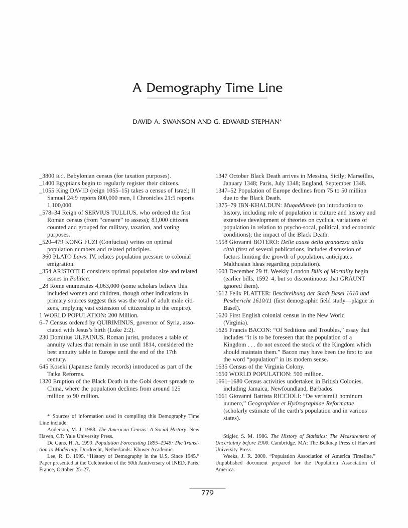
_3800 b.c. Babylonian census (for taxation purposes)._1400 Egyptians begin to regularly register their citizens._1055 King DAVID (reign 1055–15) takes a census of Israel; II
Samuel 24:9 reports 800,000 men, I Chronicles 21:5 reports1,100,000.
_578–34 Reign of SERVIUS TULLIUS, who ordered the firstRoman census (from “censere” to assess); 83,000 citizenscounted and grouped for military, taxation, and voting purposes.
_520–479 KONG FUZI (Confucius) writes on optimal population numbers and related principles.
_360 PLATO Laws, IV, relates population pressure to colonialemigration.
_354 ARISTOTLE considers optimal population size and relatedissues in Politica.
_28 Rome enumerates 4,063,000 (some scholars believe thisincluded women and children, though other indications inprimary sources suggest this was the total of adult male citi-zens, implying vast extension of citizenship in the empire).
1 WORLD POPULATION: 200 Million.6–7 Census ordered by QUIRIMINUS, governor of Syria, asso-
ciated with Jesus’s birth (Luke 2:2).230 Domitius ULPAINUS, Roman jurist, produces a table of
annuity values that remain in use until 1814, considered thebest annuity table in Europe until the end of the 17th century.
645 Koseki (Japanese family records) introduced as part of theTaika Reforms.
1320 Eruption of the Black Death in the Gobi desert spreads toChina, where the population declines from around 125million to 90 million.
1347 October Black Death arrives in Messina, Sicily; Marseilles,January 1348; Paris, July 1348; England, September 1348.
1347–52 Population of Europe declines from 75 to 50 milliondue to the Black Death.
1375–79 IBN-KHALDUN: Muqaddimah (an introduction tohistory, including role of population in culture and history andextensive development of theories on cyclical variations ofpopulation in relation to psycho-socal, political, and economicconditions); the impact of the Black Death.
1558 Giovanni BOTERO: Delle cause della grandezza dellacittà (first of several publications, includes discussion offactors limiting the growth of population, anticipates Malthusian ideas regarding population).
1603 December 29 ff. Weekly London Bills of Mortality begin(earlier bills, 1592–4, but so discontinuous that GRAUNTignored them).
1612 Felix PLATTER: Beschreibung der Stadt Basel 1610 undPestbericht 1610/11 (first demographic field study—plague inBasel).
1620 First English colonial census in the New World (Virginia).
1625 Francis BACON: “Of Seditions and Troubles,” essay thatincludes “it is to be foreseen that the population of aKingdom . . . do not exceed the stock of the Kingdom whichshould maintain them.” Bacon may have been the first to usethe word “population” in its modern sense.
1635 Census of the Virginia Colony.1650 WORLD POPULATION: 500 million.1661–1680 Census activities undertaken in British Colonies,
including Jamaica, Newfoundland, Barbados.1661 Giovanni Battista RICCIOLI: “De verisimili hominum
numero,” Geographiae et Hydrographiae Reformatae(scholarly estimate of the earth’s population and in variousstates).
A Demography Time Line
DAVID A. SWANSON AND G. EDWARD STEPHAN*
779
* Sources of information used in compiling this Demography TimeLine include:
Anderson, M. J. 1988. The American Census: A Social History. NewHaven, CT: Yale University Press.
De Gans, H. A. 1999. Population Forecasting 1895–1945: The Transi-tion to Modernity. Dordrecht, Netherlands: Kluwer Academic.
Lee, R. D. 1995. “History of Demography in the U.S. Since 1945.”Paper presented at the Celebration of the 50th Anniversary of INED, Paris,France, October 25–27.
Stigler, S. M. 1986. The History of Statistics: The Measurement ofUncertainty before 1900. Cambridge, MA: The Belknap Press of HarvardUniversity Press.
Weeks, J. R. 2000. “Population Association of America Timeline.”Unpublished document prepared for the Population Association ofAmerica.
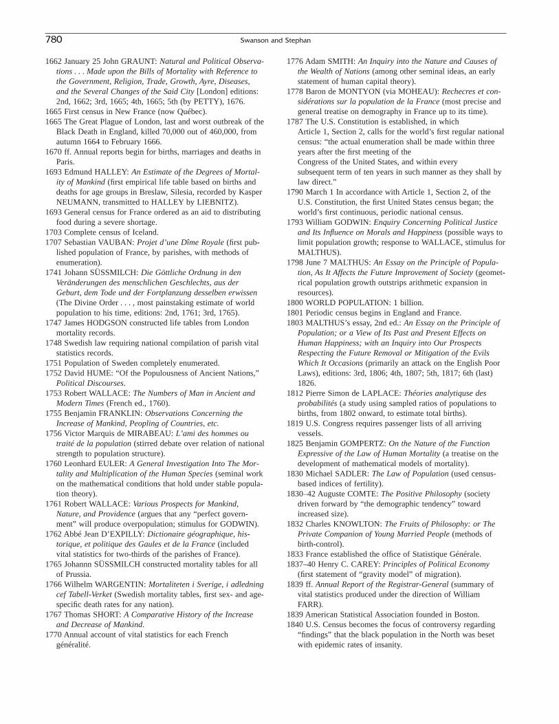
1662 January 25 John GRAUNT: Natural and Political Observa-tions . . . Made upon the Bills of Mortality with Reference tothe Government, Religion, Trade, Growth, Ayre, Diseases,and the Several Changes of the Said City [London] editions:2nd, 1662; 3rd, 1665; 4th, 1665; 5th (by PETTY), 1676.
1665 First census in New France (now Québec).1665 The Great Plague of London, last and worst outbreak of the
Black Death in England, killed 70,000 out of 460,000, fromautumn 1664 to February 1666.
1670 ff. Annual reports begin for births, marriages and deaths inParis.
1693 Edmund HALLEY: An Estimate of the Degrees of Mortal-ity of Mankind (first empirical life table based on births anddeaths for age groups in Breslaw, Silesia, recorded by KasperNEUMANN, transmitted to HALLEY by LIEBNITZ).
1693 General census for France ordered as an aid to distributingfood during a severe shortage.
1703 Complete census of Iceland.1707 Sebastian VAUBAN: Projet d’une Dîme Royale (first pub-
lished population of France, by parishes, with methods ofenumeration).
1741 Johann SÜSSMILCH: Die Göttliche Ordnung in denVeränderungen des menschlichen Geschlechts, aus derGeburt, dem Tode und der Fortplanzung desselben erwissen(The Divine Order . . . , most painstaking estimate of worldpopulation to his time, editions: 2nd, 1761; 3rd, 1765).
1747 James HODGSON constructed life tables from Londonmortality records.
1748 Swedish law requiring national compilation of parish vitalstatistics records.
1751 Population of Sweden completely enumerated.1752 David HUME: “Of the Populousness of Ancient Nations,”
Political Discourses.1753 Robert WALLACE: The Numbers of Man in Ancient and
Modern Times (French ed., 1760).1755 Benjamin FRANKLIN: Observations Concerning the
Increase of Mankind, Peopling of Countries, etc.1756 Victor Marquis de MIRABEAU: L’ami des hommes ou
traité de la population (stirred debate over relation of nationalstrength to population structure).
1760 Leonhard EULER: A General Investigation Into The Mor-tality and Multiplication of the Human Species (seminal workon the mathematical conditions that hold under stable popula-tion theory).
1761 Robert WALLACE: Various Prospects for Mankind,Nature, and Providence (argues that any “perfect govern-ment” will produce overpopulation; stimulus for GODWIN).
1762 Abbé Jean D’EXPILLY: Dictionaire géographique, his-torique, et politique des Gaules et de la France (includedvital statistics for two-thirds of the parishes of France).
1765 Johannn SÜSSMILCH constructed mortality tables for allof Prussia.
1766 Wilhelm WARGENTIN: Mortaliteten i Sverige, i adledningcef Tabell-Verket (Swedish mortality tables, first sex- and age-specific death rates for any nation).
1767 Thomas SHORT: A Comparative History of the Increaseand Decrease of Mankind.
1770 Annual account of vital statistics for each French généralité.
1776 Adam SMITH: An Inquiry into the Nature and Causes ofthe Wealth of Nations (among other seminal ideas, an earlystatement of human capital theory).
1778 Baron de MONTYON (via MOHEAU): Rechecres et con-sidérations sur la population de la France (most precise andgeneral treatise on demography in France up to its time).
1787 The U.S. Constitution is established, in which Article 1, Section 2, calls for the world’s first regular nationalcensus: “the actual enumeration shall be made within threeyears after the first meeting of the Congress of the United States, and within every subsequent term of ten years in such manner as they shall bylaw direct.”
1790 March 1 In accordance with Article 1, Section 2, of theU.S. Constitution, the first United States census began; theworld’s first continuous, periodic national census.
1793 William GODWIN: Enquiry Concerning Political Justiceand Its Influence on Morals and Happiness (possible ways tolimit population growth; response to WALLACE, stimulus forMALTHUS).
1798 June 7 MALTHUS: An Essay on the Principle of Popula-tion, As It Affects the Future Improvement of Society (geomet-rical population growth outstrips arithmetic expansion inresources).
1800 WORLD POPULATION: 1 billion.1801 Periodic census begins in England and France.1803 MALTHUS’s essay, 2nd ed.: An Essay on the Principle of
Population; or a View of Its Past and Present Effects onHuman Happiness; with an Inquiry into Our ProspectsRespecting the Future Removal or Mitigation of the EvilsWhich It Occasions (primarily an attack on the English PoorLaws), editions: 3rd, 1806; 4th, 1807; 5th, 1817; 6th (last)1826.
1812 Pierre Simon de LAPLACE: Théories analytiquse desprobabilités (a study using sampled ratios of populations tobirths, from 1802 onward, to estimate total births).
1819 U.S. Congress requires passenger lists of all arrivingvessels.
1825 Benjamin GOMPERTZ: On the Nature of the FunctionExpressive of the Law of Human Mortality (a treatise on thedevelopment of mathematical models of mortality).
1830 Michael SADLER: The Law of Population (used census-based indices of fertility).
1830–42 Auguste COMTE: The Positive Philosophy (societydriven forward by “the demographic tendency” towardincreased size).
1832 Charles KNOWLTON: The Fruits of Philosophy: or ThePrivate Companion of Young Married People (methods ofbirth-control).
1833 France established the office of Statistique Générale.1837–40 Henry C. CAREY: Principles of Political Economy
(first statement of “gravity model” of migration).1839 ff. Annual Report of the Registrar-General (summary of
vital statistics produced under the direction of WilliamFARR).
1839 American Statistical Association founded in Boston.1840 U.S. Census becomes the focus of controversy regarding
“findings” that the black population in the North was besetwith epidemic rates of insanity.
780 Swanson and Stephan

1841 Lemuel SHATTUCK: The Vital Statistics of Boston.1841 ff. Massachusetts State Registration Report.1846 Belgian census conducted by Adolphe QUETELET (influ-
ential, it introduced a careful analysis and critical evaluationof the data compiled).
1850 U.S. census collected individual-level data for the firsttime.
1850 ff. Otto L. HÜBNER: Geographisch-statistiche Tabellen(until 1919).
1850 7th U.S. census (new tabulation methods to enable moredetailed analyses; use of census data to provide vital statisticsfor preceding year).
1851 Adolphe QUETELET: Nuvelles tables de la mortalité pourla Belgique (influential construction of life tables).
1853 Adolphe QUETELET: Organized a series of internationalconferences on statistics, pushed data-gathering for quinquen-nial age groups.
1854 James DeBOW: Statistical View of the United States (asummary of the 7th U.S. census, including results of allearlier censuses).
1854 George DRYSDALE: Elements of Social Science (firstcomprehensive book outlining and defending the birth control movement on broad sociological and economicgrounds).
1854 Dr. John SNOW maps wells and cholera incidence forareas of London, and although subject to flaws, it was one ofthe first times “geographic information systems” were used toshape public policy (the closing of certain wells).
1855–65 Complete enumerations for 24 sovereign nations.1855 Achille GUILLARD: Eléments de statistique humaine ou
démographie comparée (coins the term “démographie”).1855 Frédéric LePLAY: Les ouvriers européens (comprehensive
statement of the relation of family structure to demographiccharacteristics).
1856–59 William FARR works on indirect age standardization,culminating with its appearance in the 1859 annual report ofthe Registrar General of England and Wales.
1859 Charles DARWIN: Origin of the Species by Means ofNatural Selection (esp. Chapter 3, “The Struggle for Existence,” which shows the influence of MALTHUS).
1860 W. M. MAKEHAM: “On the Law of Mortality and Con-struction of Annuity Tables,” J. Inst. Actuaries (developmentof general mortality formulas).
1861 Karl MARX: Theories of Surplus Value (esp. ChapterXIX—DARWIN’s demonstration that plants and animalsincrease geometrically, contradicts MALTHUS).
1868 Georg KNAPP: Über der Ermittlung der Sterblichkeit ausden Auszeichnungen der Bevölkerungs-Statistik (a treatise onthe theoretical aspects of life table construction).
1868 Meniji restoration reinstitution of Koseki (household regis-tration system) in Japan.
1871 Census of British India, the first modern census for a largenon-European country.
1874 Registration of vital events becomes obligatory in Englandand Wales.
1875 Wilhelm LEXIS: Einleitung in die Theorie derBevölkerungs-Statistik (a theoretical treatise on demographicstatistics; mortality in older ages).
1876 Georg von MAYR: Die bayerische Bevölkerung nach derGebürtigheit (a study of internal migration using census datafrom Bavaria).
1877 George DRYSDALE founds England’s Malthusian League.
1877 Annie BESANT: The Law of Population (influential treatiseon population control).
1878 Dr. Aletta JACOBS: World’s first birth-control clinic, Amsterdam, Netherlands.
1882 4th (or 5th) international congress on hygiene, at Geneva,newly titled “Congrès international d’Hygiène et Démogra-phie,” includes a section on demography.
1882 Chinese Exclusion Act (first nationality exclusion in theUnited States; followed by ban on Japanese, 1907, and on allAsians, 1917).
1883 Francis GALTON: Natural Inheritance (emphasis on differ-ential fertility).
1884 Columbia College offers the course “Statistics of Popula-tion” covering such demographic topics as density, age, sex,birth, death, marriage, mortality tables, emigration.
1884 Richard BÖCKH: Statistisches Jahrbuch der Stadt Berlin(first appearance of the net reproduction rate in a publication).
1885 Ernst Georg RAVENSTEIN: Laws of Migration (a treatisethat introduces the “gravity model” of migration).
1885 International Statistical Institute organized; Luigi BODIO isits first secretary-general.
1889–92 Êmile LEVASSEUR: Le Population françoise (a com-prehensive survey of population trends in France that includescomparisons with other nations).
1889 Ernst Georg RAVENSTEIN: Laws of Migration (II).1890 First census tabulated using electricity—mechanically
punched holes in cards are counted by a machine using elec-trical flows, designed and patented by Herman Hollerith; setsthe stage for the emergence of electronic computers and IBM.
1890 Arsène DUMONT: Dépopulation et civilisation (decliningfertility in France).
1891 director of 1890 census, Francis WALKER: “Immigrationand Degradation,” Forum (argued that foreign influx led todecline in native fertility).
1892 Office of Immigration established in the United States.1893 Émile DURKHEIM: On the Division of Labor in Society
(this book includes the hypothesis that demographic trendsdrive history).
1893 John S. BILLINGS: “The Diminishing Birth-Rate in the United States,” Forum (native versus immigrant fertility).
1895 Edwin CANNAN: “The Probability of a Cessation of theGrowth of Population in England and Wales during the NextCentury” Economic Journal (an early use of the cohort-component method of population projection).
1896 director of 1890 census, Francis WALKER: “Restriction ofImmigration,” Atlantic Monthly (another influential argumentthat foreign influx led to a decline in native fertility).
1897 Karl PEARSON: The Chances of Death and Other Studiesof Evolution (mortality patterns in old age).
1897 Vilfredo PARETO introduces what comes to be known asthe “80/20” or “Pareto” principle, which specifies a pre-dictable imbalance in the joint distribution of many two-variable sets.
A Demography Time Line 781
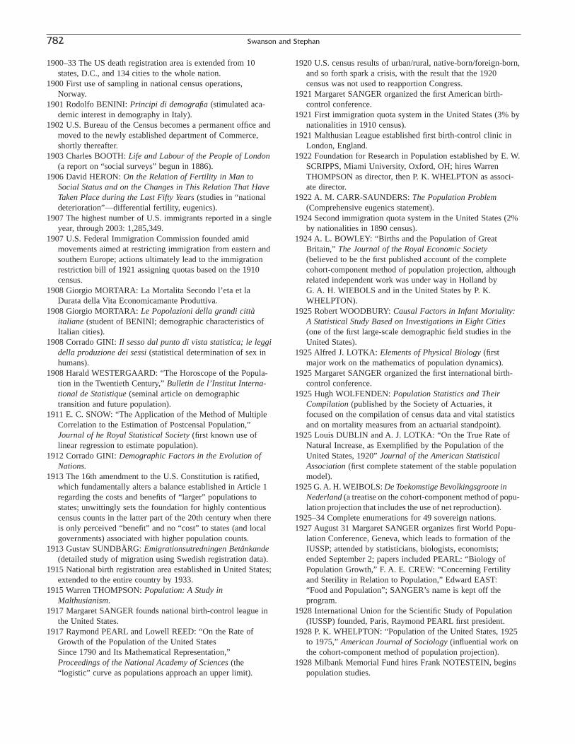
782 Swanson and Stephan
1900–33 The US death registration area is extended from 10states, D.C., and 134 cities to the whole nation.
1900 First use of sampling in national census operations,Norway.
1901 Rodolfo BENINI: Principi di demografia (stimulated aca-demic interest in demography in Italy).
1902 U.S. Bureau of the Census becomes a permanent office andmoved to the newly established department of Commerce,shortly thereafter.
1903 Charles BOOTH: Life and Labour of the People of London(a report on “social surveys” begun in 1886).
1906 David HERON: On the Relation of Fertility in Man toSocial Status and on the Changes in This Relation That HaveTaken Place during the Last Fifty Years (studies in “nationaldeterioration”—differential fertility, eugenics).
1907 The highest number of U.S. immigrants reported in a singleyear, through 2003: 1,285,349.
1907 U.S. Federal Immigration Commission founded amidmovements aimed at restricting immigration from eastern andsouthern Europe; actions ultimately lead to the immigrationrestriction bill of 1921 assigning quotas based on the 1910census.
1908 Giorgio MORTARA: La Mortalita Secondo l’eta et laDurata della Vita Economicamante Produttiva.
1908 Giorgio MORTARA: Le Popolazioni della grandi città italiane (student of BENINI; demographic characteristics ofItalian cities).
1908 Corrado GINI: Il sesso dal punto di vista statistica; le leggidella produzione dei sessi (statistical determination of sex inhumans).
1908 Harald WESTERGAARD: “The Horoscope of the Popula-tion in the Twentieth Century,” Bulletin de l’Institut Interna-tional de Statistique (seminal article on demographictransition and future population).
1911 E. C. SNOW: “The Application of the Method of MultipleCorrelation to the Estimation of Postcensal Population,”Journal of he Royal Statistical Society (first known use oflinear regression to estimate population).
1912 Corrado GINI: Demographic Factors in the Evolution ofNations.
1913 The 16th amendment to the U.S. Constitution is ratified,which fundamentally alters a balance established in Article 1regarding the costs and benefits of “larger” populations tostates; unwittingly sets the foundation for highly contentiouscensus counts in the latter part of the 20th century when thereis only perceived “benefit” and no “cost” to states (and localgovernments) associated with higher population counts.
1913 Gustav SUNDBÄRG: Emigrationsutredningen Betänkande(detailed study of migration using Swedish registration data).
1915 National birth registration area established in United States;extended to the entire country by 1933.
1915 Warren THOMPSON: Population: A Study in Malthusianism.
1917 Margaret SANGER founds national birth-control league inthe United States.
1917 Raymond PEARL and Lowell REED: “On the Rate ofGrowth of the Population of the United States Since 1790 and Its Mathematical Representation,” Proceedings of the National Academy of Sciences (the “logistic” curve as populations approach an upper limit).
1920 U.S. census results of urban/rural, native-born/foreign-born,and so forth spark a crisis, with the result that the 1920census was not used to reapportion Congress.
1921 Margaret SANGER organized the first American birth-control conference.
1921 First immigration quota system in the United States (3% bynationalities in 1910 census).
1921 Malthusian League established first birth-control clinic inLondon, England.
1922 Foundation for Research in Population established by E. W.SCRIPPS, Miami University, Oxford, OH; hires WarrenTHOMPSON as director, then P. K. WHELPTON as associ-ate director.
1922 A. M. CARR-SAUNDERS: The Population Problem(Comprehensive eugenics statement).
1924 Second immigration quota system in the United States (2%by nationalities in 1890 census).
1924 A. L. BOWLEY: “Births and the Population of GreatBritain,” The Journal of the Royal Economic Society(believed to be the first published account of the completecohort-component method of population projection, althoughrelated independent work was under way in Holland by G. A. H. WIEBOLS and in the United States by P. K.WHELPTON).
1925 Robert WOODBURY: Causal Factors in Infant Mortality:A Statistical Study Based on Investigations in Eight Cities(one of the first large-scale demographic field studies in theUnited States).
1925 Alfred J. LOTKA: Elements of Physical Biology (firstmajor work on the mathematics of population dynamics).
1925 Margaret SANGER organized the first international birth-control conference.
1925 Hugh WOLFENDEN: Population Statistics and TheirCompilation (published by the Society of Actuaries, itfocused on the compilation of census data and vital statisticsand on mortality measures from an actuarial standpoint).
1925 Louis DUBLIN and A. J. LOTKA: “On the True Rate ofNatural Increase, as Exemplified by the Population of theUnited States, 1920” Journal of the American StatisticalAssociation (first complete statement of the stable populationmodel).
1925 G. A. H. WEIBOLS: De Toekomstige Bevolkingsgroote inNederland (a treatise on the cohort-component method of popu-lation projection that includes the use of net reproduction).
1925–34 Complete enumerations for 49 sovereign nations.1927 August 31 Margaret SANGER organizes first World Popu-
lation Conference, Geneva, which leads to formation of theIUSSP; attended by statisticians, biologists, economists;ended September 2; papers included PEARL: “Biology ofPopulation Growth,” F. A. E. CREW: “Concerning Fertilityand Sterility in Relation to Population,” Edward EAST:“Food and Population”; SANGER’s name is kept off theprogram.
1928 International Union for the Scientific Study of Population(IUSSP) founded, Paris, Raymond PEARL first president.
1928 P. K. WHELPTON: “Population of the United States, 1925to 1975,” American Journal of Sociology (influential work onthe cohort-component method of population projection).
1928 Milbank Memorial Fund hires Frank NOTESTEIN, beginspopulation studies.
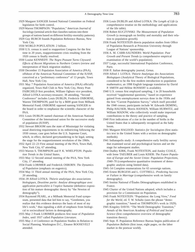
A Demography Time Line 783
1929 Margaret SANGER formed National Committee on Federallegislation for birth control.
1929 Warren THOMPSON: “Population,” American Journal ofSociology (seminal article that classifies nations into threegroups of nations based on different fertility-mortality patterns).
1929 Guy BURCH founds Population Reference Bureau, NewYork City.
1930 WORLD POPULATION: 2 billion.1930 U.S. census is used to reapportion Congress for the first
time in 20 years, reapportionment crisis resulting from the1920 census is finally resolved.
1930 Louise KENNEDY: The Negro Peasant Turns Cityward:Effects of Recent Migrations to Northern Centers (review andinterpretation of black migration studies).
1930 December 15 Population Association of America (PAA),offshoot of the American National Committee of the IUSSP,conceived at a “preliminary conference” of 13 people, TownHall, New York City.
1931 May 7 Population Association of America (PAA) officiallyorganized, Town Hall Club in New York City, Henry PrattFAIRCHILD first president, William Ogburn vice president,Alfred LOTKA secretary-treasurer; 38 attending, “SecondConference” includes Louis DUBLIN, Frederick OSBORNE,Warren THOMPSON; paid for by a $600 grant from MilbankMemorial Fund; OSBORNE opposed naming SANGER tothe board in order to emphasize the scientific character of thePAA.
1931 Louis DUBLIN named chairman of the American NationalCommittee of the International union for the successive studyof population (IUSSP).
1932 Stewart BROOM sues the state of Mississippi for violatingusual districting requirements in its redistricting following the1930 census; case goes before the U.S. Supreme Court,which, in effect, declared gerrymandering to be legal, settingthe stage for the reapportionment revolution of the 1960s.
1932 April 22–23 First annual meeting of the PAA, Town Hall,New York City, 67 attending.
1933 Warren S. THOMPSON and P. K. WHELPTON: Popula-tion Trends in the United States.
1933 May 12 Second annual meeting of the PAA, New YorkCity, 17 attending.
1934 Frank LORIMER and Frederick OSBORN: The Dynamicsof Population (emphasis on eugenics).
1934 May 11 Third annual meeting of the PAA, New York City,20 attending.
1934–39 Alfred LOTKA: Théorie analytique des associationsbiologiques, Deuxième partie: Analyse démographique avecapplication particulière à l’espèce humaine (definitive exposi-tion of his mature demographic theory by “the Newton ofdemography”).
1934 Raymond PEARL, at a Milbank Memorial Fund sympo-sium, presented data that led him to say, “Gentlemen, yourealize that this evidence destroys the basis of most of mylife’s work,” thus signaling a shift of emphasis from biologi-cal to sociocultural factors in demography.
1935 May 2 Frank LORIMER produces first issue of PopulationIndex, until 1937 called Population Literature.
1935 May 2–4 Conference on Population Studies in Relation toSocial Planning, Washington D.C., Eleanor ROOSEVELTattended.
1936 Louis DUBLIN and Alfred LOTKA: The Length of Life (acomprehensive treatise on the methodology and applicationsof the life table).
1936 Robert KUCZYNSKI: The Measurement of PopulationGrowth (a monograph on fertility and mortality and their rela-tion to population growth).
1936 Frank NOTESTEIN directs population studies from Officeof Population Research at Princeton University throughLeague of Nations’ sponsorship.
1936 A. M. CARR-SAUNDERS: World Population: PastGrowth and Present Trends (a comprehensive empiricalexamination of the world’s population).
1937 Large, successful International Population Conference,Paris.
1938 ff. Italian demography journal, Genus.1939 Alfred J. LOTKA: Théorie Analytique des Associations
Biologiques (Analytical Theory of Biological Populations,considered to be the first modern introduction to populationmathematics; an 1998 English language translation by DavidP. SMITH and Hélène ROSSERT is available).
1940 U.S. census first employed sampling, 1 in 20 householdsreceived “supplemental questions,” based on experiencegained from unemployment surveys done in the 1930s andthe first “Current Population Survey,” which itself precededthe 1940 census; participants include W. Edwards DEMING,Philip HAUSER, Morris HANSEN, William HURWITZ, andWilliam MADOW, who collectively would make importantcontributions to the theory and practice of sampling.
1940 First indications of a rise in the number of births in theUnited States that is subsequently recognized as the babyboom.
1941 Margaret HAGOOD: Statistics for Sociologists (first statis-tics text in the United States with a section on demographicmethods).
1941 Indianapolis study: A comprehensive early fertility surveythat examined social and psychological factors and set thestage for subsequent studies.
1944 Dudley KIRK, Frank NOTESTEIN, and Ansley COALE,with Irene TAEUBER and Louis KISER: The Future Popula-tion of Europe and the Soviet Union: Population Projections,1940–70 (comprehensive quantitative treatment of demo-graphic analysis using limited data).
1945–54 Complete enumerations for 65 sovereign nations.1945 Ernest BURGESS and L. COTTRELL: Predicting Success
or Failure in Marriage (comprehensive work on familydemography).
1945 Institut National d’Êtudes Démographiques established inFrance.
1945 Charter of the United Nations adopted, which includes aprovision for a Commission on Population.
1945 Frank NOTESTEIN: “Population: the Long View,” Foodfor the World, ed. T. W. Schultz (uses the phrase “demo-graphic transition,” based on THOMPSON’s work in 1929).
1945 Kingsley DAVIS: “The World Demographic Transition,”Annals of the American Academy of Political and SocialScience (first comprehensive overview of demographic transition theory).
1945 Sept. ff. Population Reference Bureau begins publication ofPopulation Bulletin (first issue, eight pages, on the labormarket in the postwar world).

1946 U.S. Congress enacts federal programs that use statisticalformulas in conjunction with census and other data forfunding purposes; sets the stage for a tremendous expansion of the use of such formulas from the 1950s to the1990s.
1946 Recognition begins to take hold of postwar baby boom inthe United States (see 1940, 1957, and 1961, and 1964);similar postwar booms subsequently recognized in Australiaand Canada.
1946 ff. French demography journal, Population.1946 P. H. LESLIE: “On the Use of Matrices in Certain Popula-
tion Processes,” Biometrika (seminal paper on population pro-jection using matrix algebra).
1947 ff. Population Studies (Population Investigation Committee,London School of Economics, first regularly publishedEnglish-language journal devoted to demography).
1948 ff. United Nations: Demographic Yearbook.1949 Louis DUBLIN, Alfred J. LOTKA, and Mortimer
SPIEGELMAN: Length of Life, revised edition of the bookthat first appeared in 1936 (comprehensive and seminal workon mortality, demography, and actuarial science).
1949 George ZIPF: Human Behavior and the Principle of LeastEffort: An Introduction to Human Ecology (detailed observa-tions on empirical regularities in population distribution andmigration).
1949 United Nations: Problems of Migration Statistics (seminalwork on data on overcoming data flaws in conjunction withthe analysis of migration).
1950 U.S. Census “supplemental questions” sampling frequencyincreased from 1 in 20 to 1 in 5 households. “FOSDIC”optical scanning system introduced as a means of electroni-cally capturing data on census forms.
1950 Peter COX: Demography (although oriented toward actuar-ies, the first comprehensive textbook on demography).
1950 Amos HAWLEY: Human Ecology: A Theory of CommunityStructure (comprehensive theoretical work on humanecology).
1951 Kingsley DAVIS: The Population of India and Pakistan(seminal work on population and development).
1951 UNIVAC I, first commercially available computer, deliv-ered to the U.S. Bureau of the Census for processing 1950census tabulations.
1951 A. J. JAFFE: Handbook of Statistical Methods for Demographers, preliminary edition, 2nd printing (publishedunder the auspices of the U.S. Bureau of the Census “inresponse to the many urgent requests received by the Bureau from technicians in foreign countries and the UnitedStates,” it is aimed at the analysis of census and related data).
1952 International Planned Parenthood Federation founded.1952 United Nations: Methods of Estimating Total Population
for Current Dates, Manual I.1953 Frank W. NOTESTEIN: Economic Problems of Population
Change (comprehensive neo-Malthusian work).1953 United Nations: The Determinants and Consequences of
Population Trends.1954 Robert C. SCHMITT and Albert H. CROSETTI: “Accuracy
of the Ratio-Correlation Method for Estimating Postcensal
Population,” Land Economics (seminal work on subnationalpopulation estimation).
1954 P. K. WHELPTON: Cohort Fertility: Native White Womenin the United States (a comprehensive presentation of thecohort approach to fertility analysis).
1954 Hugh WOLFENDEN: Population Statistics and TheirCompilation (comprehensive book on demographic methods).
1954 United Nations: Handbook of Population Census Methods.1954 First World Population Conference, sponsored by United
Nations, Rome; notable for the fact that participants wereexperts in their own right and did not represent countries.
1955 Mortimer SPIEGELMAN: Introduction to Demography (atextbook using mathematical formulations, and weightedheavily toward the study of mortality).
1955 United Nations: Age and Sex Patterns of Mortality, ModelLife Tables for Underdeveloped Countries.
1955 United Nations: Methods of Appraisal of Quality of BasicData from Population Estimates, Manual II.
1955 United Nations: Handbook of Vital Statistics Methods andPrinciples for a Vital Statistics System.
1955–60 Growth of American Families (fertility survey, Rockefeller Foundation, initial investigators: Arthur CAMPBELL, John PATTERSON, and P. K. WHELPTON).
1956 Kingsley DAVIS and Judith BLAKE: “Social Structure andFertility: An Analytic Framework,” Economic Developmentand Cultural Change (seminal work on the social analysis offertility).
1956 United Nations: Methods for Population Projections by Sexand Age, Manual III.
1956 United Nations: The Aging of Population and Its Economicand Social Consequences.
1957 Peak year of U.S. baby boom.1957 Princeton Fertility Survey (with re-interviews in 1960 and
1963–1967).1958 UNITED NATIONS: Multilingual Demography Dictionary.1958 George BARCLAY: Techniques of Population Analysis
(widely used as a text in demographic methods courses formany years).
1958 Ansley COALE and Edgar HOOVER: Population Growthand Economic Development in Low Income Countries (highlyinfluential neo-Malthusian analysis of the relationshipbetween development and population growth).
1958 Sidney GOLDSTEIN: Patterns of Mobility (comprehensiveempirical and theoretical work on domestic migration in acapitalistic system).
1958–59 United Nations: Principles and Recommendations forNational Population Censuses; Handbook of PopulationCensus Methods, Vol. I; General Aspects of a PopulationCensus, Vol. II; Economic Characteristics of the Population,Vol. III; Demographic and Social Characteristics of the Pop-ulation, Studies in Methods Series F.
1959 Wilson GRABILL, Clyde KISER, and P. K. WHELPTON:The Fertility of American Women.
1960 WORLD POPULATION: 3 billion.1960 U.S. Census is the last in which 100% door-to-door can-
vassing was attempted; self-enumeration introduced on amassive scale; the “long form” is introduced and thisbecomes the first census in which the sample segment isasked more questions than the 100% segment.
784 Swanson and Stephan

1960 May 9 U.S. Food and Drug Administration approves mar-keting “the pill” for birth control.
1960 Gary S. BECKER: “An Economic Analysis of Fertility,”Demographic and Economic Change in Developed Countries(seminal work on the economic approach to fertility).
1961 Beginning of steep decline in U.S. births.1961 Birth control pill comes on the market.1961 Otis D. DUNCAN, Ray CUZZORT, and Beverly
DUNCAN: Statistical Geography (a pioneering treatment of the statistical analysis of demographic and related dataaggregated by area).
1962 U.S. Supreme Court ruled malapportioned state legislaturesunconstitutional, setting the way for numerous lawsuits andthe reapportionment revolution of the 1960s.
1963 Ansley COALE and Melvin ZELNIK: New Estimates of Fertility and Population in the United States (seminal work on evaluating census and vital statistics data and developing estimates from deficient census and vital statisticsdata).
1963 ff. Studies in Family Planning.1964 ff. Demography (Population Association of America;
Donald BOGUE, first editor).1964 Recognition that the baby boom ends in the United States
and a “baby bust” begins—the last continuous year in whichthe number of births exceeded 4 million.
1964–68 The United States enacted federal civil rights, voting,and fair housing employment laws that rely on high-qualitycensus and other data for enforcement and compliance needs.
1965 Gladys BOWLES and James D. TARVER: Net Migrationof the Population, 1950–60, By Age, Sex, and Color (seminalempirical work on domestic migration).
1965, 1970, 1975 National Fertility Surveys (NICHD).1965 Norman RYDER: “The Cohort as a Concept in the Study
of Social Change,” American Sociological Review (seminalwork on the analytical utility of the cohort perspective).
1966 Ansley COALE and Paul DEMENY: Regional Model LifeTables and Stable Populations (comprehensive set of modellife tables and model stable populations for use in evaluatingand adjusting demographic data that are defective).
1966 P. K. WHELPTON, Arthur CAMPBELL, and John PAT-TERSON: Fertility and Family Planning in the United States.
1967 United Nations: Methods of Estimating Basic DemographicMeasures from Incomplete Data, Manual IV.
1968 William BRASS et al.: The Demography of Tropical Africa(important methodological developments for dealing withmissing and defective demographic data).
1968 Garrett HARDIN, “The Tragedy of the Commons,” Science(seminal prelude to popular concern over global populationgrowth and use of resources).
1968 Paul EHRLICH: The Population Bomb (another seminalprelude to popular concern over global population growth andneo-Malthusian ideas).
1968 Nathan KEYFITZ: Introduction to the Mathematics of Population.
1968 Mortimer SPIEGELMAN: Introduction to Demography,2nd edition (compact introduction to demography writtenwith mathematical formulation, based on the original editionpublished in 1955).
1968 United Nations: The Concept of a Stable Population:Applications to the Study of Populations of Countries withIncomplete Demographic Statistics.
1969 ff. Family Planning Perspectives (Alan Guttmacher Institute, NY).
1970 Census Bureau releases census data on machine readabletapes (first count through fourth count, etc.) with file docu-mentation and COBOL processing software written by GaryK. Hill and others at DUALABS, Inc.).
1970 First case in U.S. federal court regarding census undercount.1970 United Nations: Methods of Measuring Internal Migration,
Manual VI.1971 Controversy arose over privacy in the census of the Nether-
lands, leading to indefinite postponement of the 1981 census;mirrors privacy concerns elsewhere.
1971 Henry S. SHRYOCK, Jacob S. SIEGEL, and ASSOCI-ATES: The Methods and Materials of Demography(important comprehensive text book and reference work ondemography).
1971 Norman CARRIER and John HOBCRAFT: DemographicEstimation for Developing Societies: A Manual of Techniquesfor the Detection and Reduction of Errors in DemographicData (seminal work on methods of estimation using deficientdata).
1971 U.S. National Academy of Sciences: Rapid PopulationGrowth: Consequences and Policy Implications.
1971 United Nations: Methods of Projecting the EconomicallyActive Population, Manual V.
1972 MEADOWS et al.: The Limits to Growth: A Report for theClub of Rome’s Project on the Predicament of Mankind(opening neoMalthusian salvo that helps kick off environmen-talism movement).
1972 Ansley COALE: The Growth and Structure of Human Pop-ulations: A Mathematical Investigation (influential mathemat-ical treatment of demography).
1972 Samuel PRESTON, Nathan KEYFITZ, and RobertSCHOEN: Causes of Death Life Tables for National Popula-tions (appearance of a comprehensive set of cause-specificlife tables).
1972 U.S. Commission on Population Growth and the AmericanFuture: Population and the American Future (assessment ofU.S. population policy, concluding that it would be advanta-geous for the U.S. population to have lower fertility and alower maximum population than anticipated under prevailingtrends).
1973 Evelyn KITAGAWA and Philip HAUSER: DifferentialMortality in the United States: A Study in Socio-EconomicEpidemiology (comprehensive treatment of socioeconomicfactors and mortality).
1973 United Nations: Determinants and Consequences of Popu-lation Trends.
1973 United Nations: Methods of Projecting Households andFamilies, Manual VII.
1973 National Survey of Family Growth (National Center forHealth Statistics; cycle II, 1976; III 1982, IV 1988).
1973 Mindel C. SHEPS and Jane A. MENKEN: MathematicalModels of Conception and Birth (comprehensive treatment offertility that includes an extensive listing of computer modelsof human reproduction).
A Demography Time Line 785

1974 Leo GOODMAN, Nathan KEYFITZ, and ThomasPULLUM: “Family Formation and the Frequency of VariousKinship Relationships,” Theoretical Population Biology(seminal demographic paper on kinship).
1974 World Fertility Survey begins and runs for a number ofyears, with a comprehensive appraisal in a book edited by J.CLELAND, C. SCOTT, and D. WHITELEGGE, published in1987.
1975 WORLD POPULATION: 4 billion.1975 Andrei ROGERS: Introduction to Multiregional Mathemati-
cal Demography (comprehensive introduction to the multire-gional theory and methods).
1975 ff. Population and Development Review (PopulationCouncil).
1975 ff. International Family Planning Digest—evolved intoInternational Family Planning Perspectives and Digest 1978and International Family Planning Perspectives, 1979.
1978 Brian ARTHUR and Geoffrey McNICOLL: “Samuelson,Population, and Intergenerational Transfers,” InternationalEconomic Review (seminal paper contributing ideas to com-plexity theory).
1979 Roland PRESSAT: The Dictionary of Demography (inFrench).
1979 ff. American Demographics (the first periodical devoted tocommercial applications of demography; Peter FRANCESE,founder).
1979 United Nations: Manual IX: The Methodology of Measuring the Impact of Family Planning Programmes onFertility.
1980 U.S. Census becomes the focus of substantial litigation andrelated actions over “undercounts,” marking the start ofhighly contentious census counts.
1980 Evelyn KITAGAWA et al. (editors): Estimating Populationand Income for Small Places (comprehensive treatment ofsmall area population estimation).
1981 Louis HENRY: Dictionnaire Demographique Multilingue.1981 Gary S. BECKER: A Treatise on the Family (comprehen-
sive economic approach to family and household microde-mography).
1981 Ester BOSERUP: Population and Technological Change: AStudy of Long-Term Trends (a strong statement against theMalthusian thesis that more people yield more misery).
1981 Julian SIMON: The Ultimate Resource (another very strongstatement against the Malthusian thesis that more people yieldgreater misery).
1982 J. ROSS (ed.): International Encyclopedia of Population.1983 John BONGAARTS and Robert G. POTTER: Fertility,
Biology, and Behavior: An Analysis of the Proximate Deter-minants (comprehensive framework for analyzing fertilityusing the “proximate determinants” framework).
1983 United Nations: Indirect Techniques for Demographic Esti-mation, Manual X.
1984 Chin Long CHIANG: The Life Table and Its Applications(comprehensive stochastic treatment of the life table and itsfunctions).
1984 Charles MODE: Stochastic Processes in Demography andTheir Computer Implementation (comprehensive stochastictreatment of fertility, mortality in conjunction with population projections).
1985 Karen MASON OPPENHEIM: The Status of Women: AReview of Its Relationships to Fertility and Mortality (seminalwork on the relationship of the status of women to fertilityand mortality).
1985 William PETERSON and Renee PETERSON: Dictionaryof Demography (first comprehensive English languagedemography dictionary to appear; in the same year, however,a translation of PRESSAT’s French language dictionary ofdemography also appears, with Christopher WILSON aseditor).
1987 WORLD POPULATION: 5 billion.1987 Jerry WICKS and Jose PEREIRA DE ALMEIDA: IPSS
population projection system released (commercial appear-ance of “point and click” demographic software).
1987 Douglas MASSEY, Rafael ALARCON, Jorge DURAND, and Humberto GONZALEZ: Return to Aztlan: The Social Process of International Migration fromWestern Mexico (comprehensive theoretical and empiricalresponse to the human capital approach to migration—anargument for the importance of social factors in the migrationprocess).
1987 Richard EASTERLIN: Birth and Fortune (comprehensivetheory concerning economic opportunity and variation in thesize of birth cohorts).
1990 U.S. Census results distributed on diskettes along with pro-cessing software for use on “personal” computers. Resultssubject to contentious litigation and related actions over“undercounts.”
1990–1991 Number of legal U.S. immigrants exceeds 1.5 millionin each year.
1990–2000 Substantial efforts made by U.S. Census Bureau toimprove accuracy and quality in 2000 while reining in costs,leads to a proposal that “statistical adjustment” be used toreduce differential net undercount error; proposal is subject tointense litigation and related actions; U.S. Supreme Courtrules that the direct count must be used for apportionment andcannot be statistically adjusted for this purpose.
1994 International Conference on Population and Developmentin Cairo, attendance on a national basis and theme is morepolitical than technical.
1996 American Community Survey initiated, starting the process that could lead to collecting in a “continuous measurement” sample survey of the long form of the U.S.Census.
1999 WORLD POPULATION: 6 billion.2000 full “democratization of U.S. Census data” with worldwide
access to census results through American Fact Finder ingraphic and tabular forms via the Internet; electronic versionsof reports and maps replace paper copies.
2001 American Community Survey results available on the Internet, with worldwide access.
786 Swanson and Stephan

Thomas A. Bryan is lead statistician for Third waveResearch. He has a master’s degree in urban studies fromPortland State University and a master’s degree in informa-tion systems technology from George Washington Univer-sity. Mr. Bryan’s research interests are in developingsmall-area population estimates and statistical evaluationtechniques.
A. Dharmalingam is a lecturer in population studies atthe Department of Sociology and Social Policy and an associate of the Population Studies Centre, University ofWaikato, Hamilton, New Zealand. He is editor of the NewZealand Population Review. He has an MSc. in Mathemat-ical Economics from Madurai Kamaraj University (India)and a Ph.D. in demography from the Australian NationalUniversity. His research interests include the demographyand status of women in India, family formation in NewZealand, and household demography.
Barry Edmonston is director of the Population ResearchCenter and a professor in the School of Urban Studies andPlanning, Portland State University. He has a Ph.D., with aspecialization in population studies, from the University ofMichigan. He has been a faculty member at Stanford Uni-versity and Cornell University and served as a researcher atthe Urban Institute and the National Academy of Sciences.His current research interests are in the demographic effects of immigration, immigration statistics, internalmigration of the foreign-born, and demographic changes inhomeownership.
Sharon Estee is research supervisor in the Research andData Analysis Division of the Washington State Departmentof Social and Health Services. While completing the chapter
on natality measures using vital statistics, she was managerof research for the Washington State Center for Health Sta-tistics. Dr. Estee has managed research units in governmentagencies for more than 20 years and is currently investi-gating the social service needs of homeless families andmedical cost offsets associated with drug and alcohol treatment. She has a Ph.D. in sociology from Ohio StateUniversity.
Kimberly Faust is associate professor of Sociology atFitchburg State College in Massachusetts. She has an M.A.and Ph.D. from the University of North Carolina at ChapelHill. Dr. Faust has published numerous articles on marriageand family issues.
Linda Gage is liaison to demographic programs for theState of California after serving as chief of the state’s Demo-graphic Research Unit for two decades. She has managedand evaluated California’s demographic programs, adminis-tered the state’s Census Data Center, and served as the governor’s liaison for Census 2000. Ms. Gage serves on theU.S. Secretary of Commerce’s Decennial Advisory Com-mittee and the National Academy of Sciences’ Panel onFormula Allocations. She has an M.A. in sociology from theUniversity of California, Davis.
M. V. George has been chief of the Population Projec-tions, Demography Division, Statistics Canada, since 1979.He is also adjunct professor of the Department of Sociologyat the University of Alberta. He holds a Ph.D. in demogra-phy from the Australian National University.
Robert George is geographic business manager at SonicIndustries. He is responsible for all day-to-day demographic,geographic, and cartographic needs within the company. He has an M.S. in geography from the University ofAlabama.
Robert L. Heuser served in a number of capacities formany years with the U.S. National Center for Health Statis-tics. He is perhaps best known for his service as chief of theNatality, Marriage and Divorce Statistics Branch of theDivision of Vital Statistics.
787
Author Biographies1
1 Not listed here are authors of chapters in the original two-volume setof the Methods and Material of Demography, from which, however, mate-rial was drawn in different ways by the authors of the current edition. Theoriginal authors are identified in Table 1-1. Author disclaimer: The viewsexpressed in this book are those of the individual authors and do not reflectviews or positions held by their respective employers.

Frank Hobbs is chief of the Special Projects Staff in thePopulation Division of the U.S. Census Bureau. He has spe-cialized in age and sex composition (particularly ages 65 andover) and in international demography, especially analysesof developing countries (mainly in South Asia and theMiddle East). He served 6 years (1981–1984 and 1995–1998) as the demographic statistics advisor to the CentralDepartment of Statistics, Riyadh, Saudi Arabia. He has aB.S. in mathematics from the University of Maryland and an M.S. in sociology/demography from Florida StateUniversity.
George C. Hough, Jr., is coordinator of the Oregon StateData Center, Population Research Center, Portland StateUniversity, and research associate professor in the School ofUrban Studies and Planning at Portland State University. Hereceived a Ph.D. in sociology from the University of Texasat Austin. Dr. Hough’s research interests include demo-graphic and statistical methods, race and ethnic demo-graphic behavior, and urban sociology.
Dean H. Judson is group leader of the AdministrativeRecords Evaluation and Linkage Group at the U.S. CensusBureau. Formerly, he was the Nevada state demographer andhas worked as a private consultant with Decision Analytics,Inc. Dr. Judson received an M.S. in mathematics from theUniversity of Nevada and an M.A. and a Ph.D. in sociologyfrom Washington State University.
Hallie J. Kintner is a staff research scientist in the Enter-prise Systems Laboratory of General Motors Research andDevelopment Center. She has published extensively on mor-tality and applied demography, including co-editing Demo-graphics: A Casebook for Business and Government, thefirst collection of real-life case studies in applied demo-graphy. Dr. Kintner has chaired the Census Advisory Committee on Population Statistics for the U.S. Bureau ofthe Census. She received an M.A. and a Ph.D. in sociology/demography, as well as an M.S. in biostatistics, from theUniversity of Michigan.
Vicki L. Lamb is a research scientist at the Center forDemographic Studies, Duke University. She also is affiliatedwith the Howard Odum Institute for Research in SocialScience at the University of North Carolina, Chapel Hill. Dr.Lamb has numerous publications on estimates of healthy lifeexpectancy and other measures of health and disability, par-ticularly of older adults. She has a Ph.D. in sociology fromDuke University.
Douglas S. Massey is the Dorothy Swaine Thomas pro-fessor and chair of the Department of Sociology at the Uni-versity of Pennsylvania. He holds a Ph.D. in sociology fromPrinceton University and has published widely on topicsrelated to migration, human ecology, race, and ethnicity.
Mary A. McGehee is a researcher with the University of Texas, San Antonio. Her current research involves theinvestigation of social, economic, demographic, and environmental factors related to health disparities between
race/ethnic populations in the United States. She has a Ph.D.from Texas A&M University.
Jerome N. McKibben III is a visiting professor of soci-ology at Eastern Connecticut State University. He holds amaster’s degree in criminal justice from Syracuse Univer-sity and received a Ph.D. in applied demography fromBowling Green State University. Dr. McKibben has been avisiting professor at the Helsinki School of Economics.
Margaret Michalowski is chief of Development andDemographic Methods for Statistics Canada. She has ledmajor research projects on internal and international migra-tion in Canada and Poland. She has published extensivelyon different aspects of international migration, ethnicity, and demographic estimates and projections. She has a Ph.D.in statistics and demography from the Warsaw School of Economics, Poland.
Peter A. Morrison is the founding director of RAND’sPopulation Research Center, where he is a resident consult-ant. He has published extensively on the consequences ofdemographic trends for public policy and business. He hastaught at The RAND Graduate School and Helsinki Schoolof Economics. Dr. Morrison has been elected president of the Southern Demographic Association and served asadvisor to the National Academy of Sciences. He holds aPh.D. in sociology from Brown University.
Kathryn Norcross-Bryan was the lead mapping spe-cialist for Washington, D.C.-based Cogent Communica-tions. In addition to telecommunication experience, she hasdone retail site location analysis for Blockbuster Entertain-ment. She has an M.A. in sociology/demography fromFlorida State University.
William O’Hare directs the KIDS COUNT program atthe Annie E. Casey Foundation. He has published widely inthe areas of applied and social demography. He was a con-tributing editor to American Demographics magazine, direc-tor of Policy Studies at the Population Reference Bureau,and president of the Southern Demographic Association. Dr.O’Hare obtained a Ph.D. in sociology from Michigan StateUniversity.
Stephen Perz received a Ph.D. in sociology with a spe-cialization in demography from the University of Texas at Austin in 1997. He is now an assistant professor in theDepartment of Sociology and faculty affiliate to both theCenter for Latin American Studies and the College ofNatural Resources and Environment, University of Florida.Dr. Perz conducts interdisciplinary and internationalresearch on population and the environment, focusing on thedemographic and other social forces affecting land use andland-cover change in the Brazilian Amazon.
David Plane is a professor in the Department of Geography and Regional Development at the University ofArizona, where he served as head of department from 1990to 1997. His research has focused primarily on modeling thechanging geographic patterns of U.S. interregional migra-
788 Author Biographies
tion and on developing new methods for analyzing systemsof geographic movement. Dr. Plane is co-author (with PeterRogerson) of the textbook, The Geographical Analysis ofPopulation. He has served as president of the PacificRegional Science Conference Organization and co-edits theJournal of Regional Science. Dr. Plane received his Ph.D.from the University of Pennsylvania.
Kelvin M. Pollard is a research demographer at the Population Reference Bureau, Washington, D.C. He is theauthor of PRB’s United States Population Data Sheet andhas authored numerous articles for PRB publications. Heprovides data analysis and technical assistance for the AnnieE. Casey Foundation’s KIDS COUNT program. Mr. Pollardreceived a master’s degree in applied social research fromthe University of Michigan.
Carole L. Popoff is chief of the Modeling and OutreachBranch in the Housing and Household Economic StatisticsDivision at the U.S. Census Bureau, the primary focus ofwhich is to model program eligibility using householdsurveys. Formerly, she was the associate director forresearch at the Bureau of Business and Economic Research,University of Nevada, Reno, as well as president of Decision Analytics, Inc., a consulting firm that provides economic and demographic analysis for various state-levelprograms. Ms. Popoff has an M.S. in economics fromArizona State University and is currently finishing her dis-sertation for a Ph.D. in political science at the University ofNevada, Reno.
Thomas Pullum has a master’s degree in statistics and aPh.D. in sociology from the University of Chicago. He hastaught courses on demographic methods there as well as atseveral other universities, including the University of Texasat Austin, where he is professor of sociology and researchassociate in the Population Research Center.
Amy R. Ritualo was a data analyst in the InternationalProgramme on the Elimination of Child Labour at the Inter-national Labour Organization in Geneva. In this capacity, she carries out in-depth analyses of child labor data in orderto develop indicators of child labor, identify general andregional patterns of child labor, evaluate child labor collec-tion methodologies, and provide assistance in establishingpriorities and recommendations for policy and programdevelopment. Ms. Ritualo holds a master’s degree in demography from Georgetown University.
Jacob S. Siegel is currently a private consultant withinterests in methods of demographic analysis, applieddemography, and gerontological demography. He was formerly senior statistician for demographic analysis andresearch at the U.S. Census Bureau and senior researchscholar and professorial lecturer in demography at George-town University. He is a former president of the Population
Association of America and was a co-editor of the formereditions of The Methods and Materials of Demography. He holds an M.A. in sociology from the University of Pennsylvania.
Stanley K. Smith is professor of economics and direc-tor of the Bureau of Economic and Business Research at theUniversity of Florida. His research unit produces the officialstate and local population estimates and projections for thestate of Florida. His research interests include the method-ology and analysis of population estimates and projections,the determinants of population forecast accuracy, and thedemography of Florida, subjects on which he has publishedwidely. He has a Ph.D. in economics from the University ofMichigan.
G. Edward Stephan is professor emeritus at WesternWashington University. He has published widely on the sizeof territorial divisions, work summarized in his online bookDivision of Territory in Society. He received a Ph.D. in sociology from the University of Oregon.
C. M. Suchindran is professor of biostatistics and afellow at the Carolina Population Center, University ofNorth Carolina at Chapel Hill. He heads the demographytraining program in the Department of Biostatistics. He isalso a member of the statistical services core of the CarolinaPopulation Center. Dr. Suchindran is a fellow of the American Statistical Association.
David A. Swanson Professor of Sociology and Chair ofthe Department of Sociology and Anthropology, Universityof Mississippi. He has published more than 50 journal articleson various demographic topics and is co-author of severalbooks and monographs, including State and Local Popula-tion Projections: Methodology and Analysis (with Stanley K.Smith and Jeff Tayman). He holds a Ph.D. in sociology (pop-ulation studies) from the University of Hawaii.
Jeff Tayman is the director of Research and InformationSystems for the San Diego Association of Governments. Hehas published extensively in the areas of estimates and pro-jections, focusing on methodology and the measurement of error. Dr. Tayman has led major research projects on inte-grating geographic information systems into the develop-ment of demographic and economic estimates andprojections for census tracts, blocks, and other spatiallydefined areas. He has a Ph.D. in sociology/demography fromFlorida State University.
Janet Wilmoth is associate professor of sociology atSyracuse University and senior research associate for theCenter for Policy Research. Her published research exam-ines the older adult population, with an emphasis on migra-tion, living arrangements, social support, and health status.She has a Ph.D. in sociology/demography, with a minor ingerontology, from Pennsylvania State University.
Author Biographies 789

This Page Intentionally Left Blank

Arriaga, E., 339, 535, 559, 605, 615, 626, 638,730
Arthur, W. B., 170, 450–452Ascher, W., 593, 595Astone, N., 584, 595Astroth, J., 744, 748Ausubel, J., 598Ayad, M., 209Aziz, K., 639Azumi, K., 375, 403
BBachi, R., 98–99, 102–103, 139, 170, 519Bachu, A., 399, 403Backlund, E., 298Bader, J. M., 38Badets, J., 492Bain, L. J., 696, 730Baker, G., 369Balfour, J. L., 297Balk, D., 564, 597Banco, L., 749Band, P. R., 281, 296Banister, J., 134, 170Baochang, X., 173Barclay, G., xBarkalov, N. B., 404Barr, C., 553, 559Barrere, B., 209Bartholomew, D. J., 730Basavarajappa, K., 558, 560Batchelor, R., 593, 595Batten, R., 339Battistella, G., 492Beale, C., 89–90, 103, 237Bean, F., 480, 492Beaumont, P., 596Beck, D., 559, 597, 599Beck, J. C., 358, 367Beers, H., 688, 729–730Behr, M., 494, 519Belanger, A., 340, 358–359, 367, 581, 595Belanger, D., 207–208
A
Abramson, D., 188Adam, N., 749Adams, M., 375, 404Adams, O., 369Adya, M., 599Agrawal, B., 639, 641Agresti, A., 712, 714, 730Ahlburg, D., 563, 573–574, 584, 591, 593,
595–596, 598, 600Ahmed, A., 209Ahmed, B., 63, 75, 79, 171, 481, 574, 597,
639Ahmed, N., 639Aitken, A. C., 686, 730Akers, D., 492, 521, 600, 708, 711, 730Alarcon, R., 3, 8, 584, 596Alba, R., 466Alfeld, L. E., 724, 730Alho, J., 568, 595, 599Allison, P., 365–366, 368Almgren, G., 297Alsalam, N., 251Alter, G., 357, 366–367Alterman, H., 65, 79–80Alvey, W., 638, 732Amankwaa, A., 340Amrheun, C., 749Anderson, B. A., 172Anderson, M., 38, 49, 62–63, 74, 79–80, 779Anderson, R. M., 171Anderson, R. N., 299–300, 697, 732Andersson, G., 403Anderton, D., 118, 122, 730Andreev, K., 340Andrews, A., 188–189Anker, R., 250Arango, J., 492, 600Arel, D., 182, 186–187, 189Armstrong, B. K., 368Armstrong, J. S., 565, 591, 595, 598Armstrong, R., 339Arnold, F., 639Aronoff, S., 733, 735, 738, 748
Bell, F., 316, 338, 573, 595Bell, W., 54Bennett, N., 451, 599Bernard, W. S., 185, 189Bernhardsen, T., 748Bernstam, M. S., 404Bernstein, P., 38Berry, J. K., 748–749Bhat, M., 374, 403Bianchi, S. M., 401, 403Bickel, P. J., 696, 730Bideau, A., 298Biemer, P. B., 732Bilsborrow, R., 463, 492Birch, M. W., 715, 730Bishop, Y., 712, 715, 730Blachman, N., 559Black, W. C., 680, 730Blackburn, M., 240, 250–251Blacker, J., 639Blackwell, D., 6, 8Blanc, A., 639Blau, P., 519Blazer, D., 340, 359, 367Bloom, D., 600Bluestone, B., 123Blum, A., 183, 189Böckh, R., 430, 451Boertlein, C., 494, 502, 521Bogue, D., 90, 103, 500, 519–520, 547, 559,
631, 638, 640, 730Bogue, E., 631, 638Bohua, L., 173Bolstad, P. V., 749Bone, M. R., 369Bongaarts, J., 339, 376, 403, 442, 444–445,
451, 563, 592–595Borjas, G., 492Bossard, E., 728, 731Bound, J., 343, 367Bourgeois-Pichat, J., 278, 296–297, 640Bouvier, L., 170, 450–452, 492Bowles, G., 237, 340, 710Bowley, A., 595Box, G., 568–569, 595
Author Index
791

Boyce, D., 586, 595Boyd, M., 492Brackstone, G., 732Bradburn, N., 77, 79–80Braddock, M., 749Bradshaw, B., 237Brail, R., 728, 731Brainerd, C., 495, 508, 510, 520Brakman, S., 116, 122Branch, L., 358, 367–368Branson, M., 358, 367Brass, W., 170, 404, 442, 444, 451, 535, 559,
625, 628, 638, 640, 670–671, 674, 732Bratsberg, B., 492Bravo, J., 261, 263Bray, F., 367Brickman, M., 564, 597Briggs, R. S., 748Brody, J., 367, 369Broome, F. R., 749Brown, A., 31Brown, D., 584, 595Brown, R. L., 722, 730Bryan, T., 550, 559Bryant, B. E., 37Budd, J. W., 172Budlender, D., 599Bulatao, R., 404, 428, 563, 592–595Bulmer, M., 183, 189Bumpass, L., 600Burch, T., 1–2, 6, 8Burden, R. L., 690, 730Burke, G., 749Burton, C., 192, 208Byerly, E., 462
CCaldwell, J., 172Calhoun, S., 122Calot, G., 404Campbell, A. A., 428, 452Campbell, P., 3, 8, 563, 584, 593, 595Cannan, E., 37, 595Carbaugh, L. W., 749Carbone, R., 592, 595Carey, J. R., 338Carlson, J., 550, 559Carmen, A., 640Carnes, B., 278, 296, 298, 357, 367, 369,
599Carnevale, S., 562, 597Carrier, N., 139, 151, 170Carter, L., 568, 573, 577, 595–596, 599Caselli, G., 169–170, 298Cassel, C., 599Casterline, J., 352, 366, 404, 428Castro, L., 581, 597, 600, 706, 730–731Cavanaugh, J., 640Chadwick, B., 38Chahnazarian, A., 134, 170Chan, K., 123Chandra Sekar, C., 296–297, 404, 639–640Chandrasekaran, C., 640
Cushing, B., 600Cuzzort, R., 96, 100, 103
DDahmann, D., 89, 103Dai, S., 578, 598Daley, W., 78–79Dalkey, N., 599Daniel, L., 748Danziger, J. N., 749Darga, K., 634, 639, 717, 730Das Gupta, M., 134, 170Das Gupta, P., 63, 153, 170–172, 403, 639DaVanzo, J., 3, 8, 206, 209, 494, 502–503, 517,
519–521, 584, 595, 600Davenhill, W. F., 749Davern, M., 250Davila, A., 209Davis, H. C., 523, 533, 559, 563, 595Davis, K., 14, 37, 125, 170, 404Day, J., 564, 573, 575, 593, 595de Almedia, M. F., 375, 403, 558, 560Deardorff, K., 462de Beer, J., 568, 595Decoufle, P., 282, 296Deeg, D., 367DeFonso, T., 72, 79de Gans, H., 571, 595, 779De Lepper, M. H., 749Del Valle, J. C., 749de Mello, P., 375, 403Demeny, P., 150–151, 170, 285, 305, 338, 607,
609, 613–614, 635, 639, 653, 663–665,674
DeMers, M., 748Deming, W., 296–297, 404, 639–640, 730,
732DeNavas-Walt, C., 250Denton, N., 117–118, 120, 122–123Depoid, P., 446, 451Deshpande, V. A., 173Dever, G. E. A., 282, 296–297, 368Dewey, J., 368de Wolf, V., 9, 38De Wolff, P., 600Ding, Y., 639Di Pino, A., 662, 674Dodoo, F. N., 401, 403Doksum, K. A., 696, 730Dolin, P., 367Domschke, E. M., 15, 38Dorbritz, J., 404Dorn, H., 297, 442, 451Dorrington, R., 599Draper, D., 681, 730Driedger, L., 492Dua, P., 593, 595Dublin, L., x, 316, 338, 431, 433, 442, 451,
611, 639Dubos, R., 342, 367Dudewicz, E. J., 696, 730Duncan, B., 96, 100, 103, 117, 122, 158, 170Duncan, G. T., 9, 38
792 Author Index
Chang, M., 340Charles, E., 447, 451Chattopadhyay, M., 681, 730Chen, R., 404–405Cheung, M., 432, 436, 451Chiang, C., 319, 331, 338–339Chiswick, B., 492Cho, L. J., 439–441, 449, 451–453, 615, 631,
639–640Cho, N. H., 134, 171Choe, M., 449, 451Choldin, H., 38, 51, 62, 74, 76–77, 79–80Chrisman, N., 748Christenson, B., 211, 250Christopher, C., 641Chu, C. Y. C., 172Chui, T., 492Cifuentes, R., 115, 122Citro, C., 72–75, 79, 681, 723, 730, 732Clairin, R., 640Clark, D., 521, 584, 595, 600Clarke, G., 749Clarke, K., 748Clayton, C., 87, 103Cleland, J., 428Clemen, R., 593, 595Cleveland, R., 250Clive, J., 365, 368Clogg, C., 74–76, 79–80Coale, A., 73–75, 79, 134, 150, 152, 169–170,
172, 211, 250, 285, 305, 338, 404, 433,437–438, 449–452, 607, 609, 611,613–615, 639–640, 653, 663–665, 674
Cody, S., 210Cohen, J., 369Cohen, M. L., 72–75, 79, 680–681, 730Cohen, P., 80Cohen, R., 297Colen, C., 343, 367Collopy, F., 599Comstock, G. W., 297Congalton, R. G., 748Congdon, P., 574, 595Conway, R., 584, 595Cook, K., 37Cooke, D., 640Coombs, J. W., 732Cope, L. G., 172Corder, L., 369Cornelius, W., 492Cosgrove, J., 600Costa, D., 343, 367Costin, C., 745–746, 748Coughlan, J., 466Courgeau, D., 38Cox, D. R., 367Cox, P., xCressie, N., 748Crimmins, E., 297, 358–359, 361, 367, 369Cromley, E., 749Cromley, R., 749Crosetti, A., 559, 593, 597–598Croze, M., 520Cruijsen, H., 564, 592, 595Curtia, S., 640

Duncan, O. D., 96, 100, 103, 117, 122, 158,170, 519
Dunn, W., 37Durand, J., 584, 596Durand, R., 3, 8Dutton, W. H., 749Dye, C., 367Dymowski, R., 492
EEasterlin, R., 185, 189, 260, 263, 404, 495,
508, 510, 520, 600Edmonston, B., 38, 63, 77, 79–80, 462, 465,
480, 490, 492, 600Egan, K., 118, 122Eggers, M., 123, 171, 453El Badry, M., 172, 640Eldridge, H., 172, 500, 520Eller, T., 247Ellis, D., 550, 553, 559, 584, 596, 706, 731Ellis, M., 492Ellison, C. G., 319, 338Elman, C., 343, 367El-Mouelhy, M., 351, 368Elo, I. T., 171, 173Engelhart, M., 696, 730Engels, R., 521English, L. P., 732Epling, J., 597Ericksen, E. P., 72, 76, 79, 639Erulkar, A. S., 367Espenshade, T., 170, 450–452, 492, 560Estes, J., 748Evans, A., 600Ewbank, D., 142, 153, 170, 404, 673–674,
687Ezeh, A., 195, 209Ezra, M., 564, 597
FFadali, E., 731Faddle, M., 351, 368Faires, J. D., 690, 730Fannin, D., 584, 591–592, 597Farrag, A. M., 151, 170Faust, K., 182, 189, 192, 197, 209Fay, R., 128, 172Feagin, C. B., 176, 189Feagin, J. R., 176, 189Feeney, G., 376, 403–404, 442, 444–445, 451Feinberg, E. S., 730Feinleib, M., 367Feldt, A., 559Fellegi, I., 634, 639Fellmann, J., 88, 96, 103Ferlay, J., 367Fernandez, E., 482Festin, M., 350, 368Fidell, L., 184, 189Fienberg, S., 639, 712, 715, 732Fildes, R., 598Finch, G., 640
Finezza, A., 123Fingerhut, L. A., 375, 403Fink, A., 732Firebaugh, G., 123Fischer, M., 521Fisher, H. T., 748Fisher, P., 250Fishkind, H., 600Fix, M., 467, 492Flannery, B. P., 721, 731Fletcher, B., 297Flieger, W., 305, 338Folger, J., 220, 250Foot, D., 584, 595Foote, K., 404, 428Forbes, D., 297Ford, D., 578, 598Forrester, J. W., 723, 730, 732Foster, A., 173, 404, 452Fotheringham, A. S., 748Fotheringham, S., 748Fowler, F., 38Frank, A. U., 748Frase, M., 251Fraser. W., 247Frauenthal, J., 314, 338Freedman, D., 76, 79, 634, 639Freedman, V. L., 369Freeman, R. B., 492French, D. K., 681, 683, 731Friedman, D., 600Friedman, W., 749Friel, C. A., 749Fries, J., 369, 573, 595Frisbie, W. P., 297Fu, H., 173Fuguitt, G., 584, 595Fuller-Thompson, E., 208–209Fullerton, H., 586–587, 589, 595, 600
GGabaix, X., 116, 122Gage, T. B., 135, 171Gallagher, R. P., 281, 296Galloway, P., 261, 263Galvez, J., 262–263Gangopadhyay, A., 749Gann, M., 182, 189Garenne, M., 192, 205, 209Garnett, G. P., 171Garoogian, A., 38Garoogian, R., 38Garreau, J., 115–116, 122Garretsen, H., 116, 122Garson, G. D., 748Gendell, M., 250, 474George, M. V., 3, 8, 452, 456, 561–563, 574,
576, 580, 592, 595–596, 598, 600George, P. O. L., 96, 103Geronimus, A., 343, 367Gesler, W., 749Gessler, P., 749Getis, A., 88, 96, 103
Getis, J., 88, 96, 103Ghelfi, L., 113, 122Gibson, C. J., 463, 492Glass, D., 448, 451–452Glass, G., 749Glewwe, P., 242, 250Glick, P., 206, 209Gober, P., 493–494, 519Godwin, L., 749Goldberg, D., 559, 640Golden, H., 219, 250Goldman, N., 615, 639Goldscheider, C., 188–189, 209, 521Goldscheider, F., 206, 209, 401, 403, 521Goldsmith, H., 556–559Goldstein, H., 600Goldstein, S., 509, 520Goliber, T., 367Golini, A., 600Gomez de Leon, J., 673–674Gompertz, B., 674Gonzales, H., 3, 8, 584, 596Gonzalez, M. E., 681–682, 730Gonzolez, V., 374, 403Goodchild, M., 749Goodchild, M. F., 748Goodman, M., 554, 560Goodman, M. R., 725, 730Goody, J., 205, 209Gopal, S., 749Gordon, A., 749Goss, S., 316, 338, 573, 595Gotlieb, S. L. D., 375, 403Gottman, J., 208–209Gould, P., 742, 748–749Goyer, D., 15, 38Grabill, W., 378, 403, 428, 439–440, 451, 453,
631, 639–640, 726Grady, W., 339Graham, A. K., 724, 730–731Graves, P., 521, 600Graziano, K., 732Grebenik, E., 448, 451Green, K., 748Greenberg, M., 584, 596Greenberg, Z., 745–746, 748Greene, B., 192, 209Greene, W. H., 696, 730Greenwood, M., 3, 8, 517, 520–521, 584, 598,
600Greer, D. S., 367Gregorio, D., 297Gregory, I., 316, 338Gregson, S., 171Greville, T., 313, 329, 331, 338Gribble, J., 369Grier, J., 549, 559Griffith, D., 749Griffiths, P., 6, 8Griffiths, R., 634, 639Griffiths, W. E., 696, 731Grosh, M., 242, 250Groves, R. M., 732Guest, A., 297Gueye, M., 452
Author Index 793

Gugler, J., 123Guinnane, T., 172Gupta, P. D., 75, 79Guptill, S., 749Guptill, S. C., 749Guralnik, J. M., 298, 340, 359, 367Gutman, R., 28, 38
HHackenberg, R., 298Haenn, J. F., 719, 732Hagood, M., xHaines, M., 298Hair, J. F., 680, 730Hajnal, J., 201, 209, 376, 403–404, 448, 451,
453Halacy, D., 14, 38Hall, C., 375, 404Halli, S., 367, 492Hamilton, C. H., 472, 500, 504–505, 507–508,
520, 596Hamm, R., 584, 591–592, 597Hammel, E. A., 6, 8Hammond, E., 297Hanke, J., 568, 596Hansen, W., 101, 103Hanushek, E. A., 723, 732Happel, S., 494, 520, 600Hart, J. F., 98–99, 103Harvey, J., 560Hauser, P., 298Hay, R., 569, 596Hayward, M., 339, 358–359, 361, 367Healy, M., 521, 559Heaton, T., 38Heceitt, P. C., 367Hechter, M., 600Heeringa, S. G., 681, 730Heim, M., 3, 8Heisel, D., 170Heligman, L., 640–641, 662, 674, 707, 730Helmer, O., 599Henry, G., 57, 63Henry, L., 378, 400, 403–404Henson, M., 250Hermalin, A., 169, 171, 449, 451, 453Hernandez, R., 202, 209Heron, M., 367Herzog, A., 368Hetzel, A., 63Heuser, R., 404Heywood, I., 748Hickman, J. C., 368Hill, K., 492Hill, R. C., 696, 731Hill, T., 599Hillis, K., 748Himes, C., 74–76, 79–80, 171, 453Hinde, A., 6, 8, 428Hinze, K., 500, 520Hirschman, C., 135, 171Hobcraft, J., 404–405Hoem, J., 339
Johnson, P., 535, 559, 605, 615, 638, 640Johnson, R., 369Jones, F., 117, 122Jordan, C., 338–339Jorge, M. H., 375, 403Judge, D., 696, 731Judson, D., 683, 718, 720, 731
KKadane, J. B., 76, 79, 639, 681, 731Kahn, K., 192, 209, 592, 596Kale, B., 569, 593, 596, 598Kallan, J. E., 564, 596Kalsbeek, W. D., 678, 731Kalton, G., 681, 730Kamerschen, D., 219, 250Kamins, M., 9, 13, 38Kanazawa, S., 600Kane, R. A., 349, 367Kane, R. L., 349, 367Kannisto, V., 297Kaplan, E. D., 748Kaplan, G., 297Karmel, P., 443, 451, 453Katz, S., 358, 367Kaufman, G., 401, 403Kaufman, L., 184, 189Kaufman, P., 251Kawachi, I., 297Keilman, N., 592–593, 595–596, 599Keith, L., 405Keller, J., 298Kellers, C. P., 749Kennedy, B. P., 297Kennedy, S., 492Kephart, G., 256, 263Kerr, D., 54–55, 63Kertzer, K., 182, 187, 189Kestenbaum, B., 153–154, 171Keyfitz, N., 6, 8, 305, 308, 314–315, 338–339,
364, 367, 438, 450–451, 568, 574, 593,596, 732
Khan, M., 641Khattab, H., 351, 368Kilpatrick, S. J., 297Kilss, B., 732Kim, T., 599Kimerling, A. J., 749King, A., 480King, R., 749Kintner, H., 6, 8, 521, 562, 586–587, 590, 596Kirsch, I., 218, 251Kiser, C., 378, 403, 428, 631, 639Kish, L., 732Kitagawa, E., 297–298, 403Kitron, U., 745–746, 748Klebba, A., 276Klein, S., 251Kleinman, J. C., 375, 403Klir, G. J., 732Klosterman, R., 599, 728, 731Kmenta, J., 696, 731Knapp, T., 521, 600
794 Author Index
Hogan, H., 63, 72–73, 76, 79–80, 634–635,638–639
Hogan, T., 494, 520, 600Holland, P. W., 712, 715, 730Hollifield, J., 492Hollmann, F. W., 126, 171, 564, 596Holman, D., 340Holzer, J., 640Hoover, E., 640Hopkin, W. A. B., 448, 451Hoppensteadt, F., 451Horiuchi, S., 297, 451, 453, 599Hornseth, R., 450–451Horvitz, D. G., 679, 731Hough, G., 340, 538, 559Hovert, D., 299–300Hoza, C., 681–682, 730Hu, M., 599Hugo, G., 463, 492, 600Hull, T., 172Hummer, R., 274, 296–297, 319, 338, 369Humphries, N., 35, 38Hunt, D., 599Hunt, G., 521, 584, 596, 598Hunt, W., 39Hunter, W., 521, 584, 595Hussey, J. M., 297Hutchinson, E., 465Hwang, S., 597Hyndman, R., 598Hyrenius, H., 453
IIachine, I., 340Ingengneri, D., 369Ingram, D., 369, 680, 731Inmon, W. H., 731–732Isard, W., 725, 731Ishikawa, A., 339Islam, M., 209Isserman, A., 87, 103, 520, 584, 593, 596, 731
JJabine, T., 9, 38Jacobson, N., 350, 368Jacobson, P., 316, 338–339Jaffe, A., x, 236Jamerson, B., 638James, W. H., 172, 354, 367Jamison, E., 535, 559, 638Jargowsky, P. A., 123Jasso, G., 492Jefferson, M., 115, 122Jenkins, G., 568–569, 595Jenkins, L., 218, 251Jeter, J., 194, 209Jette, A., 369Johansson, S., 369Johnson, A., 690, 731Johnson, H. P., 509, 520Johnson, K., 89, 103Johnson, N. E., 211, 250

Knudsen, L., 405Koblinsky, M. A., 368Kochanek, K., 339Kominski, R., 220, 250Kosinski, M., 368Koskinen, S., 298Kosmin, B., 188–189Kouaouci, A., 492, 600Kpedekpo, G., 298Kraak, M. J., 749Krach, C., 154, 172Kraemer, K. L., 749Kraly, E., 30Kramer, R., 640Kramer, S., 367Krebs, H., 593, 596Krichefsky, G., 29Krishnamurti, D., 746, 748Krishnamurti, R., 746, 748Kritz, M., 492Krǒtki, K. J., 635, 638–640Krueckeberg, D., 584, 596Krueger, D., 298Kuczynski, R., x, 405, 431, 443, 448, 451Kulkarni, M., 521Kupiszewski, M., 564, 596
LLahiri, P., 681, 730Lalu, N. M., 135, 171Lam, D., 453Lam, N. S., 749Land, K., 340, 359, 367, 538, 559Landale, N., 193, 209Landis, J., 599Landis, J. D., 749Langhaar, H. L., 451Lansing, J. B., 495, 520Lapidus, G., 749Larsen, M., 681, 730Larsen, U., 340Laslett, P., 205, 209Latorre, R. D. O., 375, 403Laudon, K. C., 719, 731Lauriat, P., 640Lavin, M., 38Lavizzo-Mourey, R., 298, 368Ledent, J., 359, 367Ledermann, S., 663, 674Lee, A. S., 556–557, 559Lee, E., 340, 495, 508, 510, 520, 558–560,
600, 710Lee, R. D., 260, 263, 404, 428, 562, 568, 573,
577, 595–596, 600, 779Lee, S. M., 466, 492Lee, T. C., 696, 731Leete, R., 405Legare, J., 298Lennon, E., 463, 492Lesitritz, L., 597Leslie, P., 720, 731Lessler, J. T., 678, 731Lesthaeghe, R., 442, 445, 451, 600
Levenson, R., 208–209Levine, C., 228, 250Levine, J., 749Levy, F., 251Levy, P. S., 681, 683, 731Lew, E. A., 366, 368Lewis, B., 550, 559Lewis, R. A., 405Li, C., 79Lieberson, S., 183, 189Light, S. C., 719, 731Lim, L. L., 492Lin, S., 206, 209Lindeboom, M., 367Linneman, P., 521Litman, G., 364, 367Little, J., 598, 662, 674–675Lochner, K., 297Logan, J., 466Logan, W., 298Loh, S., 562, 574, 576, 578, 595–596, 598Lohr, S. L., 680, 731Loi, V. M., 135, 171Long, J., 38, 494, 501–502, 521, 523, 559, 564,
593, 596Long, J. S., 714, 731Long, L., 340, 493, 495, 497–498, 517, 520,
600, 707, 731Long, R., 340Longley, P., 749Lopez, A., 298, 361–363, 367Loprest, P., 246, 250Lorimer, F., 170, 172, 442, 449, 452Lotka, A., x, 316, 338, 431, 433, 437–439, 442,
451–453, 611, 639Lovelady, R., 509, 520Lowell, B., 462, 492Lowry, I., 599Lubuele, L., 583–584, 596Lugaila, T., 200–201, 207–209Luke, B., 405Lutkepohl, H., 696, 731Lutz, W., 403–405, 563, 595–596, 598–599Lyberg, L., 14Lyberg, L. E., 38, 732Lynch, J. W., 297
MMa, J. M., 718, 731MacEachren, A., 749Machol, R., 559Macionis, D., 122Macmahon, B., 134, 171Macunovich, D., 211, 250Madigan, F. C., 298Mahler, H., 342, 367Mahmoud, E., 593, 596Makeham, W., 674Makridakis, S., 598–599Maltz, M., 749Mandell, M., 549, 558–559Manning, W., 193, 209Mantel, N., 134, 171
Manton, K., 298, 338, 340, 364–368, 573, 596Marchetti, C., 598Mari Bhat, P. N., 134, 170, 172Mark, D. M., 748Marks, E. D., 75, 79Marks, E. S., 143, 171, 635, 638–640Marks, H. H., 298Markush, R., 297Marquez, L., 599Martelin, T., 298Martin, C., 639Martin, D., 748–749Martin, J., 559Martin, P., 492, 499, 520Martin, W. J., 298Martine, G., 135, 171Marx, R. W., 749Marzan, G., 466Mason, A., 261, 263, 562, 596Mason, K. O., 172, 600Massey, D., 3, 8, 117–118, 120, 122–123, 492,
584, 596, 600Mathers, C., 341, 367Mathiowetz, N. A., 732Mattei, H., 209Matthews, Z., 6, 8Mauldin, W., 268, 296, 640Maurer, J., 339Mausner, J., 367Mayhew, B. H., 724, 731McCallum, J., 369McCleary, R., 569, 596McCullagh, P., 558–559, 712, 731McDevitt, T., 377, 393, 404, 639McDonald, J., 86, 103McDowell, C., 349, 367McDowell, I., 349, 367McHaffie, P. H., 748McHugh, K., 494, 520–521, 600McKibben, J., 122, 182, 189, 192, 197, 209,
549, 558–559McLanahan, S., 210, 584, 595McLarty, C., 262–263McLaughlin, S., 339McMahan, C. A., 134, 171McMillen, D., 520, 564, 596McMillen, M., 340McNamara, D., 466McNees, S., 599McNown, R., 598Mendenhall, W., 9, 38Menken, J., 405Mensch, B. S., 366–367Mentzer, J., 592, 596Merli, M., 675Merrell, M., 312, 338, 643Meuser, P., 508, 521Meyer, P., 598Michaelson, C., 584, 596Michalowski, M., 482Michaud, J., 562, 596Michie, J. S., 719, 732Midgley, E., 492, 499, 520Miller, A., 495, 508, 510, 520Miller, M. D., 731
Author Index 795

Miller, R., 748Miller, T., 562, 596Mills, E., 583–584, 596Milne, W., 584, 595Miniño, A., 290Minkler, M., 208–209Mishra, S. N., 696, 730Mishra, V., 639Mitchel, E. F., 375, 404Moen, E., 592, 596Mohlo, I., 517, 520, 600Monmonier, M., 103, 741, 743, 748Moore, H. E., 86, 103Morgan, S. P., 211, 250, 404–405Moriarty, C., 681, 731Morissette, D., 482Moriyama, I., 298Morrill, R., 87, 103, 118, 122Morris, M. D., 282, 297Morrison, J., 749Morrison, J. L., 749Morrison, P., 2–3, 8, 493–494, 498, 502, 509,
517, 519–521, 560, 584, 595, 600Moseley, W., 639Mosert, W., 563, 596Muehrche, P. C., 749Mueller, E., 495, 520Mueser, P., 600Mulder, T. J., 564, 596Mulry, J., 634, 639Mulry, M., 76, 79Murdock, S., 550, 553, 559–560, 584,
591–592, 596–597, 706, 731Murphy, C., 600Murphy, M., 175, 189Murray, C. J. L., 341, 361–363, 367Murray, R., 218, 251Myburgh, C., 172, 640Myers, D., 38, 466Myers, G., 343, 364, 367Myers, R. J., 134, 138, 153, 171, 448, 452
NNam, C., 29, 220, 250, 274, 296, 298, 319,
338, 458, 521Namboodiri, N., 339–340, 405, 517, 520,
558–559, 675, 751Narasimham, R., 639Nault, F., 466Naus, J. I., 732Navidi, W., 76, 79Neft, D., 98, 102, 104Nelder, J., 712, 731Nelson, H., 562, 586, 597Neuberger, E., 31Newbold, K., 520Newman, G., 188–189Ng, E., 466Ni Bhrolchain, M., 376, 404–405, 444,
452–453Niemann, B. J., 748Niemann, S., 748Nijkamp, P., 521
Peterson, R., 340, 751Peterson, W., 458, 751Pflaumer, P., 568–569, 593, 597, 599Phua, V., 122Pickle, L. W., 282, 296Pickles, J., 748Pielou, E., 568, 597Pignataro, L., 597Ping, T., 173Piper, J. M., 375, 404Pirozhkov, S., 166, 171Pirri, P., 662, 674Pisani, P., 367Pittenger, D., 563, 597Plane, D., 87, 101, 103, 520–521, 596, 600,
722, 731, 749Pol, L., 368, 521, 590, 597Polednak, A., 298Pollard, J., 340, 662, 674, 707, 720, 730Pollard, K., 641Polonko, K., 192, 209Pool, I., 723, 731Popoff, C., 683, 718, 720, 731Portes, A., 492Portrait, F., 367Poston, D., 278, 296, 298Potter, R. G., 405Poulain, M., 463Press, W. H., 721, 731Pressat, R., 446, 452Preston, S., 135, 171, 173, 296, 298, 308,
338–339, 366–367, 369, 405, 438, 450,452–453, 599
Prevost, R., 559Prewitt, K., 78–79Price, D. O., 79, 507, 520Pritzker, L., 74, 79Prothrow-Smith, D., 297Pugh, T. F., 134, 171Pullum, T., 405, 444, 452
RRadelet, M., 714, 731Rallu, J., 405Ramachandran, K. V., 139, 171, 173Ramachandran, P., 359, 368Randers, J., 725, 731Rao, K. V., 367, 560Ratnayake, K., 441, 452Ravenstein, E., 500, 520, 584, 597Raviglione, M., 367Raymondo, J., 560Reardon, S., 123, 158, 171Reder, S., 683, 731Redman, T. J., 718, 731Reed, C. B., 116, 122Reed, L., 312, 338, 598, 643Reeder, R., 122Rees, P., 521Reher, D., 298Reimmitz, J., 681, 730Reitsch, G., 596Rele, J., 640
796 Author Index
Nobles, M., 183, 189Nogle, J., 210Norland, J. A., 172Notestein, F., 173Nuckols, J., 749Nusselder, W. J., 369
OOberai, A. S., 463, 492Obermeyer, C., 345, 350, 367Obler, R., 192, 209O’Conner, M., 599Odum, H., 86, 88, 103Offutt, K., 211, 250, 405O’Hare, J., 680, 731O’Hare, W., 549, 558–559Oliver, M., 249–250Olshansky, S. J., 278, 296, 298, 357, 367, 369,
573, 597, 599Omran, A., 357, 367Onate, B., 38O’Neill, B., 564, 597Openshaw, S., 748Opitz, W., 562, 586, 597Orshan, L., 745–746, 748Otto, J., 209
PPaass, G., 681, 731Pacque-Margollis, S., 441, 452Paganoni, A., 492Palen, J., 105, 122Palesch, Y. Y., 367Palit, C., 593, 596Pampel, F., 260, 263Pamuk, E., 297Pandey, A., 405Pandit, K., 87, 103Pant, P., 593, 597Papsidero, J., 358, 367Park, C. B., 134, 171Parker, T., 113, 122Parkin, D., 367Parnell, A., 405Parpia, B., 597Parrillo, V., 122Parrott, B., 562, 597Passel, J., 128, 153, 171–172, 467, 480–481,
490, 492, 600Pathania, V., 367Patrick, C., 367, 573, 596Patterson, J. E., 428Paturzo, D., 297Patuwo, B., 599Pearl, R., 598Pecotte, B., 584, 591, 597Pellegrino, A., 492, 600Pener, H., 745–746, 748Percy, D., 690, 731Perreault, J., 580, 596, 600Perry, J., 596Peters, H. E., 260, 263

Relles, D., 509, 520, 560Remus, W., 599Retherford, R., 441, 449, 451–452, 639Ricardo-Campbell, R., 404Richmond, P. A., 719, 732Rickman, D., 521, 584, 598, 728, 732Riley, J. C., 357, 366–367, 369Riley, M. W., 173Rindfuss, R., 211, 250, 405Rios, B., 112, 122Ritchie, K., 369Rives, N., 75, 79, 528, 538, 556, 559–560Roberts, G., 640Roberts, H. V., 678, 732Robine, J. M., 369Robinson, A. H., 749Robinson, J. G., 55, 63, 75, 79, 128, 171–172,
480–481, 634, 639Robson, C., 13, 38Rockett, I., 368Roe, L., 550, 559Roemer, M., 250Rogers, A., 340, 358–359, 367–368, 517, 521,
574, 581, 584, 597–598, 600, 662,674–675, 706, 720, 723, 730
Rogers, R., 211, 250, 275, 278, 296–298, 319,338, 340, 357–359, 367–368
Rogerson, P., 101, 103, 596, 722, 731, 748–749Romaniuk, A., 170, 641Romieu, I., 369Rosenberg, H., 271, 296, 298–300, 339Rosenthal, N., 589, 597Rosenwaike, I., 173, 271, 296Rosenzweig, M., 492Ross, J. A., 751Ross, S. M., 721, 731Rothwell, N., 74, 79Rousseeuw, P. J., 184, 189Rowe, G., 599Rowland, R., 405Roy, T., 639Rubenstein, J., 122Rubin, D. B., 680, 731Rubin, E., 173Ruder, A., 134, 171Rudolph, C., 492Ruggles, P., 250–251Rushton, G., 746, 748–749Ryder, N., 376, 404–405, 444, 447, 452, 574,
597
SSaariluoma, P., 599Sabagh, G., 641Safarova, G., 166, 171Saito, Y., 358–359, 361, 367, 369Sakamoto-Momiyama, M., 271, 296Salmon, L., 228, 250Salomon, J., 341, 367Saluter, A., 200–201, 207, 209Sanchez-Ayendez, M., 202, 209Sandar, G., 175, 189Sanderson, W., 574, 593, 597, 599
Šantruček, M., 275, 297Saracci, R., 368Sarndal, C. E., 731Saunders, N., 250Saw, S. H., 126, 171Scanzoni, J., 192, 209Schachter, J., 404, 514, 517, 519, 521Schafer, E., 599Scheele, S., 367Schenker, N., 76, 79Scherbov, S., 405, 599Scheuren, F., 680–681, 731Schick, F., 38Schick, R., 38Schmertmann, C., 340Schmid, C. F., 102–103Schmitt, R., 263, 549, 559, 593, 597–598Schnaars, S., 593, 597Schneider, E., 369Schnell, G., 103Schoen, R., 308, 338–339, 359, 368, 720,
732Schofield, R., 298Scholten, H., 749Schultze, C., 38, 77, 80Scott, C., 428Scott, J., 276Scott, L. M., 749Seltzer, W., 635, 638–641Serow, W., 29, 521, 528, 538, 556–557, 559Settersen, R. Jr., 206, 209Shah, I., 359, 368Shah, J. M., 359, 368Shahidullah, M., 575, 593, 597Shalom, U., 745–746, 748Shao, G., 728, 732Shapiro, S., 404Shapiro, T., 249–250Shaw, G., 749Shepard, E., 748Shorter, A., 210, 640Shorter, F., 151, 170, 674Shryock, H., x, 6, 8, 67–68, 79, 98–99, 103,
140, 198, 208–209, 224, 385, 404, 408,428, 493, 501, 512, 515–516, 520, 561,597, 599, 711, 732, 751
Siegel, J., x, 2, 6, 8, 72, 77, 79, 98–99, 103,118, 122, 140, 153, 171–173, 198, 205,208–209, 224, 285, 340, 385, 404, 408,428, 449, 452, 472, 474, 493, 504–505,507, 516, 518, 520, 527, 559, 561, 586,588, 592, 594, 597, 601, 641, 681, 683,708, 711, 728, 730, 732, 751
Siegel, P., 220, 250Sigle-Rushton, W., 210Sigmund, C. L., 683, 732Silcock, H., 296, 298Silver, B. D., 172Silverston, L., 732Simcox, D., 492Simmons, A., 492Simmons, D., 599Sincich, T., 554, 559, 593, 597, 599Singer, B., 366–367Singh, M. P., 732
Sirken, M., 315, 338–339Skeldon, R., 135, 171Slater, P., 87, 103Slezak, J., 748Sloan, J., 492Sly, D., 29, 521Smit, J. W., 559Smith, H., 405Smith, J., 465, 490Smith, L., 367, 369Smith, S. J., 335Smith, S. K., 6, 8, 210, 332, 338, 493–494,
501–502, 520–521, 546, 550, 554, 557,559, 561, 574–575, 585, 592–594, 597,599–600, 728, 732
Smith, T. L., 166, 171Smith, T. M., 251Smock, P., 209Snow, J., 745Snowden, M., 375, 404Soboll, L. M. S., 375, 403Soldo, B. J., 369Som, R., 641Somoza, J., 640Song, H., 746, 748Sorlie, P. D., 298South, S. J., 125, 171Sowards, K. A., 278, 296, 298Sowder, W. T., 298Speizer, I., 195, 209Spencer, B., 76, 79, 563, 595Spencer, G., 126, 154, 171, 568, 597Spiegelman, M., 298, 316, 338, 447, 452Spinelli, J. J., 281, 296Spitzer, T., 748Sprague, T. B., 732Squires, G., 123Srivastava, M., 641St. John, C., 118, 122Stahl, C., 39Stallard, E., 338, 340, 364–365, 367–368, 573,
596Stallones, L., 749Stanecki, K., 135, 171, 639Stanton, C. K., 350, 368Star, J., 748Starbuck, W., 593, 597Starsinic, D., 546, 557, 559Steffey, D., 77, 79–80Steffick, D., 343, 367Steinnes, D., 600Stephan, F. F., 730Stern, R., 749Stevens, D. W., 719, 732Stevenson, M., 123Stewart, C., 226Stewart, D., 9, 13, 38Stewart, J. Q., 99, 103Stewart, M. K., 350, 368Stewart, Q., 171Stigler, S. M., 779Stillwell, J., 749Stockwell, E. G., x, 6, 8, 208–209, 224, 278,
297, 385, 404, 408, 428, 493, 504–505,507, 516, 520
Author Index 797

Stoll, S., 369Stolnitz, G., 169, 171, 447, 452Stone, L., 504, 507, 520Stoto, M., 593, 597, 673–674Střiteský, M. S., 275, 297Stults, B., 466Suchindran, C. M., 339–340, 405Sudman, S., 732Suliman, S., 56, 63Sullivan, D. F., 357, 368Susser, M., 368Suzman, R., 366–367Swanson, D., 1–2, 6, 8, 215, 250, 278, 297,
493–494, 501–502, 520–521, 549–550,553, 558–559, 561–562, 572, 575,585–588, 590, 593, 596–599, 751
Swicegood, G., 405Szapocznik, J., 202, 209
TTabachnick, B., 184, 189Tabuchi, T., 584, 597Taeuber, C., 86, 103Taeuber, I., 25, 38, 510, 520Tapinos, G., 261, 263Tarver, J., 507–508, 520Tatham, L., 680, 730Taueber, I., 510, 520Taylor, J. E., 492, 600Taylor, P., 375, 404Tayman, J., 6, 8, 493–494, 501–502, 520, 549,
553, 558–562, 572, 575, 585–586, 588,592–593, 597–599
Teachman, J., 192, 209Tedrow, L., 1–2, 6, 8, 558–559Teitelbaum, M., 134, 171Termote, M. G., 400, 404Terrell, D., 492Teukolsky, S. A., 721, 731Theil, H., 123Thomas, R., 28, 38–39, 368, 562, 590, 598Thomas, T. L., 282, 296Thome, M., 452Thomlinson, R., 521Thompson, A., 574, 589, 598Thompson, D. J., 678, 731Thompson, S. K., 679, 732Thompson, W., 438, 452Thomson, E., 401, 404Threlfall, W. J., 281, 296Tien, H. Y., 173Tierney, J., 508, 521Tietze, C., 452Tilak, V., 600Tinker, A., 368Tolley, H., 366, 368, 573, 596Tollman, S., 192, 209Tomlinson, R. F., 734, 748Toulemon, L., 405Trainor, T. F., 749Treadway, R., 573, 598Treat, J., 634, 639
Wasserman, P., 599Way, K., 639Weber, E., 118, 122Weed, J. A., 182, 189Weeks, J., 779Wegener, M., 599Weinberg, D., 228, 250Weingart, P., 38Weinstein, M., 340Weisberg, S., 696, 732Weller, P., 188–189Weller, R., 29Wells, H., 641West, K. K., 681, 730Westoff, C., 368, 600Wetrogan, S., 501, 521, 598Wheeler, D., 749Wheeler, J., 493, 520Wheelwright, S., 598Whelpton, P., 36, 38, 76, 79, 378, 403, 428,
443–444, 446–447, 452–453, 574, 598,631, 639
White, E., 368White, H., 592, 598White, K. M., 599White, M., 122, 492, 520–521, 600White, N., 500, 508, 521, 600Whittlesey, D., 86, 104Wichern, D., 568, 596Wickens, B., 193, 209Wicks, J., 278, 297, 558, 560Wicksell, S., 447, 452Wilkins, R., 369Wilkinson, R., 298Willcox, W., 26, 38Willems, P., 442, 445, 451Williams, D., 298, 368Williams, P., 584, 597Williams, W., 554, 560Willikens, F., 340, 359, 368, 517, 521Wilmoth, J. R., 297, 599Winchester, H. P. M., 87, 104Windle, C., 220Wingard, D. L., 274, 297–298Winston, S., 134, 172Wolf, D., 340Wolfenden, H. H., x, 26, 38, 298, 732Wolinsky, F., 369Wolter, K., 79, 634, 639Wong, D., 118, 122Wood, C., 749Wood, D., 749Wood, J., 340Woodbury, M., 365–366, 368Woodrow, K. A., 63, 75, 79, 171, 480–481,
492, 639Woofter, T. J., 89, 104, 446–447, 452–453Word, D. L., 126, 171Wright, C., 39Wright, G., 599Wright, R., 492Wright, T., 78–79Wu, Z., 192, 209Wunsch, G., 400, 404
798 Author Index
Trent, K., 125, 171Treyz, G., 521, 583–584, 586–587, 598, 728,
732Trovato, F., 135, 171Truesdell, L., 108, 122Trussell, J., 600Tucker, C., 493, 520Tuljapurkar, S., 562, 573, 596Turck, J., 731
UUeda, R., 185, 189Urton, W., 493, 520Uvin, P., 183, 189
VVacek, M., 275, 297Valaoras, V. G., 169, 172–173, 449, 452Valkonen, T., 298Vallin, J., 169–170, 298, 641van den Berg, M., 116, 122van den Oever, P., 125, 170van de Walle, E., 152, 170, 172Van Imhoff, E., 601Van Marrewijk, C., 116, 122van Tonder, J., 563, 596Varanka, D., 748Vaughn, B., 305, 338Vaupel, J., 452, 563, 573, 596, 598, 601Velkoff, V., 154, 172Verbrugge, L., 369Verma, R., 558, 560, 574, 578, 580–581, 595,
598Vetterling, W. T., 731Vickers, M., 492Vijverberg, W., 600Villa, M., 208–209Vincent, P., 172, 443, 452, 558, 560Volkov, A., 405von Foerster, H., 452Voss, P., 569, 586, 591–592, 596–598
WWachter, K., 6, 8, 260, 263, 453, 634, 639, 682,
732Waddell, P., 583, 585–586, 598Wade, A., 316, 338, 573, 595Waidmann, T., 343, 367Waksberg, J., 75, 79, 143, 171Waldron, I., 172Walkden, A., 601Wallace, R., 368Wallis, W. A., 678, 732Walsh, S., 297Wang, Z., 601Ward, D., 185, 189Ware J. E., 368Warntz, W., 98–99, 102–104Warren, R. C., 30, 298, 368, 480Wartenberg, D., 745–746, 748

Y
Yaffee, R., 568–569, 598Yanagishita, M., 298Yashin, A., 340Yates, A., 195, 209Yates, F., 44, 48, 62Yeh, A. G., 749Yerushalmy, J., 173, 298Yi, Z., 173Yokum, J., 592, 598Yongping, L., 173You, P. S., 173
Younis, N., 351, 368Yun, J., 158, 171
ZZachariah, K., 521Zakharov, S., 405Zarkhovic, S., 220Zax, J., 494, 521Zeighami, E. A., 282, 297Zelinsky, W., 517, 521Zelnik, M., 172–173, 322, 339, 404, 641
Zeng, Y., 601Zenger, E., 298Zhang, G., 599Zhang, M., 599Zhang, W., 466Zhu, J., 405Zidek, J. V., 558–559Zipf, G., 116, 123Zitter, M., 555, 557, 559–560Zlotnik, H., 463, 492Zook, M., 599Zopf, P. E., 166, 171Zurayk, H., 351, 368
Author Index 799

This Page Intentionally Left Blank

A
Abortion, 134, 266, 353–354Abortion rate, 354Abortion ratio, 354Abridged life tables
construction of, 312–315description of, 302Greville’s method, 313–315Keyfitz-Frauenthal method, 314–315Reed-Merrell method, 312–313, 315for United States population, 305
Abroad, 69, 464Abroad, Americans, 69Absolute centralization index, 121Absolute concentration index, 120Absolute numbers, 699–700Absolute percent errors, 553–554Abstracts, statistical, 40–41Accessibility
aggregate, 101–102Hansen, 101threshold, 101
Accuracy and Coverage Evaluation Survey, 78Accuracy in forecasts, 592–593, 594Active life expectancy, 341, 357–361Activities of daily living, 349Activity ratio, 590Actuarial models, 366Acute conditions, 342, 346–347Additive multicomponent model, 674Address register, 85Adjustment to marginal totals, 709–717
general multiway tables, 714–716single distributions, all positive or zero
frequencies, 708–709some negative frequencies, 709–711two-dimensional tables, 712–714
Administrative records, 557, 718–720Admission statistics, 460–461, 461Adoption, 25, 26, 31, 62, 202, 204, 265, 301,
631Aerial photography, 46, 72, 92Africa, 65, 115, 131t, 188, 208, 377, 379, 381,
469–470, 487
African Americans, 177Age
age of householder (head), 588age-adjusted measures. See Age-standardized
measuresage-specific headship ratios, 588composition analysis
age dependency ratios, 160–161demographic factors for, 165–170indexes, 156–158median age, 158–159nature of age distributions, 155–156percentage changes by age, 156percentage distributions, 156population pyramid, 161–165time series charts, 161war effects, 166–167
datadeficiencies in, 136–155groups, 141–154quality of, 128–129securing of, 127sources of, 127–128stable population model evaluations, 152
date of birth information converted to, 127definition
in completed years, 126exact, 306, 313t, 314t, 316t, 325t, 326t,
330tlunar (Chinese), 126
description, 126misreporting of, 128, 142, 606old age, 153–154population pyramid, 606response variability of, 129underenumeration by, 129
Age Accuracy Index, 148–149Age at first marriage, 193, 199–200Age dependency, 160–161Age dependency ratio, 160–161Age distributions, 155–156, 408, 435
fertility estimates from, 630–631stable population estimates from, 620–624
Age group, 165–167Age heaping, 136–141
Age, lunar (Chinese), 126Age not reported, 154–155Age preference
description of, 136–137indexes of, 137–138
Age pyramid. See Population pyramidAge ratio, 606Age ratio analysis, 147–148, 150Age structure, 606Age-adjusted death rate, 291Age-adjusted ratio, 214–215Age-cause-specific disability prevalence ratio,
349Aged persons, 168Aged-child ratio, 159–160Age-dependency ratio, 235Age-level-specific enrollment ratio, 214Age-order-specific birthrate, 382–383, 384tAge-parity-specific birth probabilities, 399Age-sex accuracy index, 150Age-sex adjusted birth rate, 388–390Age-sex adjusted (standardized) activity ratio,
235Age-sex distributions, 438–439, 606–607Age-sex structure, 163, 168–169Age-sex-specific activity ratios, 235Age-specific birth probabilities, 399–400,
419–420Age-specific birth rates, 379–382, 439,
573–574Age-specific birthrate method of fertility
projection, 573Age-specific death rates, 271–274, 281–282,
323Age-specific enrollment ratios, 213–214Age-specific fertility rates, 401, 410–413,
446–447, 625–626Age-specific illiteracy rates, 219Age-specific marital birthrates, 385–386Age-specific marital fertility rates, 413–414Age-specific marriage rates, 197Age-specific mortality rates, 271–274Age-specific nonmarital birthrates, 385–386Age-specific (participation) ratio method of
demographic projection, 586, 589
Subject Index
801

Age-specific paternal birthrate, 401Age-specific prevalence ratios, 347–348Age-specific (school) dropout rate, 216–217Age-specific (school) dropout ratio, 217Age-standardized death rate, 282Age-standardized enrollment ratio, 214–215Age-standardized measures of morbidity, 348,
349tAge-standardized proportionate mortality ratio,
282Agglomeration, 87Aggregate income, 244Aging populations, 159–160, 450Aging Trends, 12Agricultural laborers, 233Agricultural population. See farm populationAid to Families with Dependent Children
(AFDC), 719AIDS. See HIV/AIDSAitken’s iterative procedure, 686–687,
700–701Alabama, 496, 499Alaska, 84, 88, 177, 496, 499Albania, 106, 183, 218Aleuts, 132Algeria, 65, 456Alien(s)
immigrant. See Immigrant(s)nonimmigrant, 29, 462population changes, 478
Alien address register, 466Allocation of characteristics. See ImputationAmerican Community Survey, 502American Housing Survey, 22–23, 502American Indian, 177American Statistics Index, 13Ancestry, 178Animal year. See Age lunar (Chinese)Annexations, 85, 254Annulled marriage, 192Annulment, 58, 192Applied demography, 1–2Apportionment
method of population estimation, 552, 557method of population projection, 565,
570–571political process, 18, 83, 85redistricting vs., 83, 85
Area(s)census considerations, 47enumeration, 46–47less developed, 603
Area of destination, 500Area of origin, 500Argentina, 164fARIMA. See Autoregressive Integrated Moving
AverageArizona, 496, 499Arkansas, 496, 499Armed Forces, 68Arriaga technique, 442, 626Arrival, area of, 500Arrival statistics, 461Asia, 65, 131t, 469, 487Asians, 177, 491
Birth rate(s)age-order-specific, 383–384age-sex adjusted, 388age-specific, 379–382, 573–574crude, 320, 377–378, 389, 407, 422–423,
619duration-specific marital birth ratio, 386intrinsic, 434–436monthly, 378–379nonmarital birth ratio, 386order-specific, 417parity-specific, 398underregistration-based adjustments,
378Birth registration
accuracy measurement methodsaggregate methods, 373–374match studies, 373
deficiencies in, 372–373in United States, 373
Birth registration area, 373Birth roster, 407Birth statistics
analysis of, 376completeness of registration effects, 372–
374deficiencies of, 372definition of, 371description of, 147natality measures based on, 376–403quality of, 372–375
Birth-residence index, 496, 499, 511–512Block(s), 94Block groups, 93–94Block numbering areas (BNAs), 93–94Block numbering groups, 93BLS. See U.S. Bureau of Labor StatisticsBolivia, 82, 159, 234, 357Bongaarts-Feeney method, 444–445Border control
collection, 458–462land, 459port, 459
Border control dataavailability of, 459–460collection of, 460–462description of, 459quality of, 462–463
Bosnia Herzegovina, 65, 470Botswana, 324Bottom-up model, 574–575
hybrid, 576Boundaries, in census taking, 46Brass techniques, 442, 625, 627Brazil, 183, 228, 257–258Breastfeeding, 344Bureau of Economic Analysis. See U.S. Bureau
of Economic AnalysisBurundi, 470
CCalifornia, 493, 496, 498, 499, 509Cambodia, 115, 177, 290
802 Subject Index
Asylees, 29, 469–470Attrition life table, 199Australia, 40, 55, 65, 188, 385, 387, 457, 467,
482, 487, 497Austria, 40, 65, 463, 497Autocorrelation, 569Autoregressive integrated moving average
(ARIMA), 565, 568–570Average age at first marriage, 199–200, 589Average duration of illness, 347Average future lifetime. See Life table(s),
expectation of life“Average” regression technique, 549Average survival-rate method, of estimating net
migration, 472, 473t, 475t, 505
BBaby boom, 192, 196, 423, 442Bachelors, 202Bachi index, 139–140Bachi index of digit preference, 139Bangladesh, 96Barbados, 96Base period, 563, 566Base period in population projections, 563Base year, 563Basic demographic statistics, 1–2BEA (US Bureau of Economic Analysis), 37,
80, 584–585Bed-disability day, 349Beers’ interpolation formulas, 151, 310, 688,
728–729Belgium, 40, 65, 96, 187, 463, 487, 497Bermuda, 96Bias, response, 129Birth(s), 58, 60t, 371, 430
accuracy of characteristics of, 374–375country of, 184defined, 371distribution by order, 382geographic allocation of, 374legitimate. See Marital fertilitylive. See Birth(s)to net migrants, 489order of, 382–383, 443place of, 184projecting of, 573sex ratios of, 133–134shifts in timing (spacing) of, 375–376,
397–398time allocation of, 375
Birth certificate, 375Birth date
lunar, 126questions regarding, 140
Birth expectations, 573Birth history, 409Birth order, 353, 376, 416–417, 425, 444–445Birth probabilities
age-parity-specific, 399age-specific, 387–388, 399, 419–420definition of, 417–418description of, 387, 417–420

Canada, 2, 458, 461, 464, 467, 468, 485, 487,497
birth projections, 577census statistics, 54–55economic activity data, 235ethnic categories, 183illegal immigration statistics, 482immigration statistics, 489intercensal net migration, 471male population, 530population estimates, 529–530population projections, 576statistical abstracts, 40temporary immigrants from, 468–469
Canadian Health Survey, 349Cancer registry, 343Canvasser method, 67Capital city, 81Carrier index of digit preference, 139Carrier-Farrag method, 151Cartography, 46Case-by-case matching. See Dual systems
estimationCase-control studies, 344Case-fatality rate, 341, 347–348Cause-delay models, 573Cause-elimination life tables
anatomy of, 329–330cautions when interpreting, 329construction of, 331description of, 329functions in, 329–330
Cause-of-death, 274–279, 290Cause-of-death life tables, 325, 328Cause-specific death rates, 274–279Cause-specific death ratio, 277Cause-specific mortality rates, 290–291Cause-specific prevalence ratios, 347–348CDC index of unhealthy days, 363Censal-ratio methods, 546–548Censoring
left, 346right, 346
Censusadministration of, 46boundaries, 46concepts used in, 45conduct, 49–51confidentiality issues, 18content of, 47–48data. See Census datade facto, 49, 65, 71de jure, 44, 49decennial. See Decennial censusdefinition of, 13demographic analysis of, 54–55description of, 13enumeration, 43, 421errors in, 14, 51–52, 53–54, 72estimation in, 631–632features of, 43–44federal, 21geographic considerations, 46–47health data obtained from, 343history of, 14–15
housing, 13instruments for, 47–49international, 15legal basis for, 46local, 21–22maps, 21migration data from, 501–502objectives of, 13, 44one-number, 77–78periodicity of, 44, 71planning of, 46post-enumeration evaluation of, 54preparatory work for, 46pretesting of, 49privacy concerns, 18procedures for evaluating, 46public influences on content of, 18publicity of, 46quality control considerations, 46questionnaires, 47–49, 51questions included in, 16t–18trecommendations, 45–57regional considerations, 48response burden, 50sampling in, 56–57schedule for, 15, 18–19school, 33, 544scope of, 14sex classification, 127–128simultaneity, 43–44, 71staff recruitment and training, 49state, 21–22strategic objectives of, 44subjects of, 47–48survey vs., 13, 43, 45tabulation program for, 48–49time reference of, 71topics for, 47–48United States, 15–22, 77universality within a defined territory, 43vital statistics from, 18, 61by year, 16t–18t
Census 2000description of, 19design of, 77–78economic activity questions on, 231electronic access to data, 19–21Hispanic origin, 179income-related questions, 242printed reports, 21race origin, 179tabulation of, 19United Nations recommendations, 182urban status criteria, 110–111
Census Bureau. See U.S. Census BureauCensus county division, 84–85Census coverage
counting errorserroneous enumerations, 72out-of-scope, 72
deliberate exclusions, 72description of, 71–72errors, 72evaluative methods for
demographic analysis, 73–74
description of, 72options for, 634post-enumeration surveys, 72–73, 75–
76reverse record check, 73in United States, 74–78
excluded groups or territories, 71–72Indians, not taxed, in U.S. census, 72omissions, 72by year, 74–78
Census datacivil divisions for, 82tcoding of, 52collection of, 52–53demographic analysis, 143–153description of, 408–409dissemination of, 55–56editing of, 51–52electronic dissemination of, 55–56errors in, 51–52evaluation of, 53–54international migration, 463–466mathematical graduation of, 151nonresponse rate measurement, 52–53processing of, 51–53review of, 53–55sex ratios for evaluation of, 136stable population model evaluations, 152storage of, 56verification of, 53
Census office, 45Census regions, 88–89Census survival rates, 324, 472, 505–508,
615–616Census tracts, 88, 93–94, 585Census validation survey, 14Census-CPS Match, 75Census-designated places, 85, 108Census-station method, 67Centenarians, 153–154Center of population
definition of, 98–99in United States, 100t
Centers for Disease Control and Prevention(CDC), 362–363
Centers for Medicare and Medicaid Services,343
Central age-specific rates, 273, 348Central city, 91Central disability incidence rate, 349Central (school) dropout rate, 216Central transfer rates, 359Centralization, 120–121Ceylon. See Sri LankaChandra Sekar-Deming Method, 267, 634–
637Channel Islands, 96Childbearing ages, 383Childlessness, 399Children
foster, 208households with, 207–208mortality rates, 287–290, 628–630number living, question on, 48presence of parents, 208, 208t
Subject Index 803

Children ever borndefined, 441description of, 408generation rates from, 447measures based on, 441–442questions on, 48uses of statistics, 441–442
Childspacing, 397–398Child-woman ratio, 409, 423Chile, 385China, 164f, 196, 468Chinese age, 126Chronic conditions, 342, 345–346Chronic diseases, 342Cities
description of, 85edge, 116primate, 115rank-size rule of, 116sex composition variations, 136
Citizens abroad, 478–479Citizenship, 184–186
in analysis of immigration, 483defined, 164
City block, 681City directories, 35, 509Civilian population, 66Classical system of data collection, 603–604Classification errors. See Content errorsClinical effectiveness, 355Clinical examinations, 350Clinical medicine, 345Clinical trials, 345–346Closed population, 433, 442, 450, 505–506,
513, 527, 611Close-out procedure in censuses/surveys, 51Cluster analysis, 183, 664Clustering indices, 121Coale and Demeny model life tables, 607–608,
663–665Coale-Demeny model stable populations, 611,
621Coding of census data, 52Cohabitation, 192–193Cohort
incomplete reproductivity of, 447life table as mortality experience of, 306marriage, 198, 448real, 289synthetic, 289, 424, 442
Cohort analysisdefined, 363–364description of, 363–364fertility, 394–401health study uses of, 363–364intercensal, 144–147life tables for, 317
Cohort (school) dropout rate, 217Cohort study, 344Cohort-change method, 575Cohort-change ratios, 575Cohort-component method, 552
description of, 529–531history of, 571
Content errors, 54Content evaluation study, 143Conterminous United States, 83Contingency table, 335Continuous measurement system, 23Continuous notation, 336–338Continuous variable, 158Continuous work history sample, 509Contour map, 103Contraception, 355–356Contraceptive practices, 344
measures, 355–356, 356t, 357tControl group, 344–345Conurbation, 86Core-based statistical area, 92Costa Rica, 65Counterstream, 500Counties
aggregation of, 91description of, 84, 89–91metropolitan, 112nonmetropolitan, 112–113
Counting errors, 72Country of birth
definition of, 184United States practices regarding, 185–186
Country of chargeability, 186Country of citizenship
definition of, 176, 184, 186United States practices regarding, 185–186
Country of former allegiance, 186Country of last residence, 186Country of origin, 176County and City Data Book, 13County equivalent, 84, 112, 541Covenant marriage, 193–194Coverage. See Census coverage, errors;
EnumerationCoverage errors, 53–54Croatia, 65, 470Crude birth rate, 320, 377–378, 407, 422–423,
619Crude death rate, 269–270, 294, 378, 618Crude divorce rate, 196Crude dropout rate, 216Crude economic activity ratio, 234Crude emigration rate, 485Crude enrollment ratio, 213Crude gross migration rate, 485Crude illiteracy ratio, 218–219Crude immigration rate, 485Crude marriage rate, 196Crude net migration rate, 485Crude rate of natural increase, 429Cuba, 402Cubic splines, 690–692Cumulation-differencing method
using absolute data, 699–700using percentage data, 700–701
Cumulative fertility, 396, 423–424Cumulative grade attainment ratio, 221Current Population Reports, 22, 36Current Population Survey, 22, 31, 71–73, 242,
332, 344, 514, 545
804 Subject Index
immigration estimation, 471–472intercensal, 471–472limited, 531, 575population estimation, 529–531, 536population projection, 562
Cohort-progression methoddescription of, 586–587health characteristics projections, 590household projections, 588labor force projections, 590school enrollment projections, 589
Cohort-progression method of projectionsgeneral, 586health characteristics, 590households, 588labor force, 590school enrollment, 589
College students, 68Color. See RaceColorado, 496, 499Common-law
marriage, 192–193union, 193
Commune, 82, 106Community medicine, 344Community studies, 344–345Commuting, 18, 91Comorbidity, 342Comparative mortality index, 294Competing risks, 329Completed fertility, 423Completed fertility rates
cohort analysis, 394–396description of, 395, 444in fertility projections, 423–424, 573
Completeness of enumeration, 635Completeness of vital registration, 372–374,
633, 635–636Component method, 557
description of, 10of population projections, 551
Component Method I, 545Component Method II, 545–546Composite method for population estimates,
550–551Compound interest formula, 258Computer simulations, 6Computer software, 717Computer usage, 716–720Concentration index, 120Confidence intervals, 408, 421, 481, 554Confidence limits, 5, 535Confidentiality
demographic records, 62description of, 44, 46, 50racial data, 179vital records, 62
Congressional District Data Book, 13Congressional districts, 85Connecticut, 496, 499Consensual unions, 191–193Consolidated metropolitan statistical areas, 91Constant-share method, 570Constrained matching, 680

Curve fitting, 693–696Cyclical change, 260–261Czech Republic, 40, 65, 292, 487Czechoslovakia. See Czech Republic; Slovakia
DData, survey, 409–410Data collection, 716–720Data scaling, 743Data warehousing, 718–720Date of birth
conversion to age, 127lunar, 126questions regarding, 140
Date of enumeration, 126Date of marriage, 295, 354, 386, 414, 448De facto census
countries that use, 65description of, 49time allocation, 71
De facto populationin birthrate computations, 374, 378definition of, 255description of, 65, 524
De jure censuscountries that use, 65coverage of, 71description of, 44, 49
De jure population, 65, 255, 524de Moivre function, 674Death. See also Fetal death; Infant mortality;
Mortalitycauses of, 274–277definition of, 58, 265–267, 372direct obstetric, 351endogenous, 278–280exogenous, 278–280geographic allocation of, 268maternal, 351–352median age at, 320net immigration estimates affected by, 474obstetric, 351sex ratio of, 134–135tabulation of, 268, 275time-based allocation of, 268
Death certificate, 355Death rate(s)
adjusteddirect standardization method, 291–293indirect standardization method, 293–295for population composition, 291–295to probability basis, 282–291
age-specific, 271–274, 281–282annual calculation of, 271cause-specific, 274–279central, 273crude, 269–270, 294, 378, 618by economic characteristics, 279, 281–282fetal, 295intrinsic, 434–436life table, 294monthly, 270–271occupation-based, 281
reduction in, 169sex-specific, 125by social characteristics, 279, 281–282
Death registrationinternational inadequacies in, 267underregistration of, 267–268
Death registration area, 267Death statistics
need for, 265problems with, 372quality of, 266–268tabulation of, 289
Decennial censusAmericans abroad, 69description of, 15, 30–31, 67, 528foreign citizens temporarily in the United
States, 69household population, 69–70special populations, 68–69usual residence, 68
Delaware, 496, 499Demographic analysis
census, 54–55census coverage evaluation, 73–74, 75,
143–144, 147–153, 634census data on age evaluated by, 143–153illegal immigration estimates by, 480immigration data and, 480–481population change, 263survey data, 480–481
Demographic and economic mapping, 558Demographic and Health Surveys, 15, 344Demographic effectiveness, 355Demographic forecasts, 366Demographic models, 706–707Demographic statistics
classical system, 604–605deficiencies of, 605description of, 604new approaches, 605–606
Demographic Yearbook, 11, 65, 83, 96, 230,267, 305, 524
Demographic-economic models, 725–730Demography
applied, 1–2basic, 1–2census evaluations, 54–55definition of, 1purposes of, 2–3roles of, 2–3subfields of, 1–2
Denmark, 40, 65, 463Densely settled core, 110Departure, area of, 500Dependence, 350Dependency ratio, 160, 235Deportation of illegal aliens, 462Depression of the 1930s, 442Descriptive statistics, 9Deterministic model, 723Diagnostic and Statistical Manual of Mental
Disorders, 342Difference-correlation technique, 558Digit preferences in age reporting, 139–140
Direct data for population estimates, 526Direct estimation methods, 607Direct obstetric death, 351Direct-interview method of enumeration, 50Directory of International Statistics, 11Disability
definition of, 342, 348prevalence ratios, 349–350, 358
Disability-adjusted life years, 341, 361–362Disability-free life expectancy. See Active life
expectancyDiscrete time hazard rate, 364Disease
classification of, 342definition of, 342
Disease registries, 343Dissimilarity, index of, 117–118, 157–158Distance moved, 516District of Columbia, 496, 499, 541Districts
congressional, 85other legislative, 85
Diurnal fluctuation of population, 71Diversity index. See Entropy index; Theil indexDivorce
definition of, 58description of, 191–192measures of, 196registration of, 27reporting of, 59sources on, 27
Divorce rate(s)age-specific, 197crude, 196description of, 196by duration of marriage, 199general, 196order-specific, 197refined, 196–197
Divorce registration area, 195Divorced persons, 193Domesday inquest, 14Dominant stream, 500Dominican Republic, 468, 487Donor/target data sets in statistical matching,
680Dot map, 102Double decrement table, 324Double-blind randomized samples, 345Doubling time, 115, 260Drivers license address changes, 509Dropout rates
age-specific, 216–217cohort, 217crude, 216
Dual residencedescription of, 68enumeration of persons with, 68
Dual systems estimation, 73, 142–143,633–638
desiderata of, 637false nonmatches, 637lack of independence, 637out-of-scope cases, 637
Subject Index 805

Duration of marriagedescription of, 410fertility rates by, 386–387, 400–401,
414–415Duration of residence, 516
EEarnings, 241East Model life tables, 663–665Easterlin cycles, 260Ecological analysis, 363Econometric models, 366, 584, 725–730Economic activity
age-sex-specific activity ratios, 235Census 2000 questions, 231concepts of, 226–230crude ratio, 234data
establishments that provide, 233–234international comparisons of, 239–240limitations of, 238–240sources of, 230–234uses of, 238–240
definition of, 226definitions, 226–230general ratio, 234–235job characteristics, 227–229labor force characteristics, 227length of period, 239measures, 234–238projections, 238projections of, 238variations in definition, 239
Economic areasBureau of Economic Analysis, 89state, 89–90
Economic Commission for Africa, 48Economic Commission for Europe, 48Economic Commission of Asia and the Far
East, 48Economic dependency ratios, 160–161, 235–
236, 236t. See also Age dependency ratio
Economic forecasts, 366Economic province, 90Economic regions, 89Economic sector, 725Economic subregions, 89Economic surveys, 23Economically active population, 226, 235, 239Economically inactive population, 227, 235Economic-demographic structural models,
583–585Ecuador, 487Edge cities, 115, 116Editing, 51–52Education
census statistics, 215description of, 212
Educational attainment. See also Years ofschool completed
age-specific measures, 224–225census questions regarding, 220–221
country of citizenship questions, 184–186international use of, 182language, 186–187race vs., 182religion as identifier of, 187–188
Ethnographic research in health studies, 345
Euclidean distance in statistical matching, 680
Eurasia Bulletin, 12Europe, 131t, 469, 487tEver-married persons, 192Evidence of a person in a census enumeration,
67Exogenous death rate, 279Exogenous deaths, 278–280Exogenous infant mortality rate, 290Expectation of active life, 238, 335Expectation of life at birth, 320Expectation of working life, 238Expected cases, 197–198Expected population, 147, 552Exponential change, 258–259, 566–567Exponential functions, 364–365, 693Extended city, 111Extinct generations, 153Extrapolations, 523, 531–534, 546, 557, 562,
684
FFace validity, 591Factor analysis, 663Faeroe Islands, 65Family
changes in, 206–207composition of, 207–208definition of, 204description of, 202dynamics of, 206generations in, 205life cycle of, 208mean income of, 244, 246nuclear, 205projections of, 587–588statistics, 205–208United Nations concepts and classifications,
203United States concepts and classifications,
203–204verticalization of, 205
Family cycle, 208Family Health International, 350Farm population, 111Fecundability, 356Fecundity, 371Federal census, 21Federal-state cooperative program
for population estimates, 22, 525for population projections, 37
Fertility. See also Natalityage pattern of, 627cohort analysis of, 394–401defined, 371
806 Subject Index
cumulative grade attainment ratio, 221Current Population Survey questions, 220data uses and limitations, 225–226definition of, 220measures of, 220–225
Educational progression, 216–217Egypt, 14, 377, 379, 381, 393, 402Eigenvector, 721El Salvador, 377, 379, 381, 388–392, 468Elderly population, 249Electronic birth/death certificate, 62Electronic dissemination, census results, 55Emigrant, 500Emigration statistics, 30, 178, 481–482,
580Employed, 226–227Employer, 229Employment location, 586Employment projections, 586Employment rate, 237Employment ratio, 237Employment status, 232tEndogenous death rate, 279Endogenous deaths, 278–280Endogenous diseases, 357Endogenous infant mortality rate, 290English-speaking ability, 186Enrollment. See School enrollmentEntrants with false documents, 456Entrants without inspection, 456Entropy index, 118–119Enumeration
canvasser method, 67description of, 43determination of population size, 67direct-interview method, 50group, 47householder method, 67methods, 49–50self-enumeration, 50, 68service-based, 69special populations, 68–69types of, 50
Enumeration areas, 47–48description of, 46precanvass of, 46–47
Enumerators, 50Epidemiological forecasts, 366Epidemiological studies, 344–346Epidemiological transition, 357Epidemiology, 745–746Equilibrium model, 584Error of closure, 552Errors. See specific errorErrors of closure, 554ERS County Typology, 112Estimate, 561Estimating techniques for population. See
Population estimatesEthiopia, 377, 379, 381Ethnic groups, 176Ethnic origin, 18, 178, 186, 483Ethnicity
ancestry vs., 178country of birth questions, 184–186

estimationfrom child mortality, 630–631from childbearing reports, 625–628description of, 625from one age distribution, 624–628
from child mortality, 630–631from pregnancy histories, 631from retrospective birth reports, 625–628from two age distributions, 620–623
life table analysis of, 322marriage cohorts, 400measures of, 410–422paternal, 401–403in population projections, 573–574projection of, 573–574, 578
Fertility rate(s)by age, 627age distribution for deriving, 624–625age-specific, 410–413, 446–447description of, 417by duration of marriage, 386–387, 400–401,
414–415general, 379, 423by marital status, 393–394order-specific, 382–383, 416–417by parity, 376total marital, 425total (TFR), 352t, 383, 391–393, 425, 430,
578Fetal death, 58, 60t, 265–266, 295, 352, 372Fetal death rate, 295Fetal death ratio, 295Fetal loss rate, 353–354Fetal loss ratio, 353t, 353–354Feto-infant mortality rate, 355Fiji, 615–617, 620, 623Finland, 2, 40, 463, 487First marriage
age at, 193, 199–200description of, 193
First marriage rate, 198Five-parameter relational model, 673Fixed period migration rate, 501–502, 513–516Florida, 493Flow data, 603, 633Flow map, 741Forecast
accuracy, 592definition of, 36, 561errors in, 594
Foreign borndescription of, 465, 467intercensal component method for, 474–478
Foreign citizens temporarily in the UnitedStates, 69
Forward survival rates, 505Forward-reverse survival rate method,
537–538FOSDIC (Film optical sensing device for input
to computers), 52, 716France, 40, 387, 455, 457, 497, 509Free Trade Agreement, 457Frontier control data, 462Functional economic area, 86–87Functional illiteracy, 217
G
Gainful worker concept, 230Gallup Poll, 74General abortion rate, 354General divorce rate, 196General economic activity ratio, 234–235General enrollment ratio, 213General fertility rate, 379, 423General fertility ratio, 438General legitimate fertility rate, 384General marital fertility rate, 384–385General marriage rate, 196, 197General nonmarital fertility rate, 385General order-specific fertility rate, 382General paternal fertility rate, 401General pregnancy rate, 354Generalized de Moivre function, 674Generation life table. See also Life table(s)
advantages and disadvantages, 317in cohort analysis, 317description of, 301, 315–316in population projections, 318–319uses of, 301–302
Generation reproduction rate, 407, 445–446Geocoding, 47Geographic allocation
of births, 374of deaths, 507
Geographic areasmunicipalities, 82–83percentage distribution, 96–97population projections, 563primary divisions, 81, 82tsecondary divisions, 82special units, 81–82tertiary divisions, 82
Geographic divisionsblock groups, 94block numbering areas, 93–94census tracts, 93–94definition of, 88–89economic areas, 89economic subregions, 89metropolitan areas, 90–92state groupings, 88–89subcounty statistical units, 93, 525urbanized areas, 92–93
Geographic Information Systems (GIS), 101,585
dataaccuracy of, 735–738description of, 734–735errors in, 735logical consistency, 737mapping, 739–744media for viewing, 738–739portrayal of, 738resolution, 737
decision-making uses of, 747description of, 585, 733epidemiology uses of, 745–746examples of, 744–747origins of, 733–734planning uses of, 747
political redistribution, uses of, 744–745socioeconomic characteristics obtained using,
746–747vital rates obtained using, 746–747
Geometric change, 258, 506Geometric curve, 693
annual compounding vs. continuouscompounding, 693
Georgia, 496, 499Germany, 40, 65, 183, 377, 379, 381, 391–392,
455, 457, 463, 470, 487Gestation, 295, 371Ghana, 373Gibraltar, 96Gini concentration ratio, 116–117, 245Gompertz curve, 260, 662, 693–694Gompertz function, 365, 627Gompertz-Makeham curve, 311Götebörg Study, Sweden, 344Government surveys, 22–23Grabill’s interpolation method, 730Grade of membership, 365Graduated-point-symbol map, 740–741Graduation, 216Graduation of census data, 151Graduation of mortality rates, 310Graduation of single-year-of-age data, 697Grandparent-headed households, 208Graphic analysis, 491–492Graphic interpolation
description of, 697of grouped data, 697–699
Great Britain, 458, 497Greece, 40Greenland, 65, 96Greville’s method of life table construction,
313–315Gross coverage error, 72Gross emigration, 484Gross enrollment ratio. See Level-specific
enrollment ratioGross immigration, 483–484Gross intercensal interchange of population,
500, 512Gross migration, 484, 498, 500, 574Gross nuptiality rate, 199Gross overenumeration, 129Gross rate of population interchange, 515Gross reproduction rate, 407, 431, 437, 441,
614, 621–623Gross underenumeration, 129Group quarters, 203Grouped data, 141–154, 696–707Growth curves, 693–694
Gompertz curve, 693logistic curve, 693modified exponential equation, 693
Growth rate, 619–620
HHaiti, 65Halley’s life table, 302Hamilton-Perry Method, 575, 586. See also
Cohort-change method
Subject Index 807

Handbooks of National Population Censuses,15
Handbooks of Population and HousingCensuses, 66
Handicap, 342Hansen accessibility, 101Hawaii, 88, 177, 496, 499Head of family, 203Head of household, 203. See also
HouseholderHeadship ratio, 588Headship-rate method of household projections,
588Health
of children, 344conditions, 342–343definition of, 342description of, 341population, 341projections of, 590surveys in less developed countries, 344of women, 344
Health care utilization records, 343–344Health data
description of, 343sources of
administrative records, 343–346censuses, 345, 343clinical trials, 345–346epidemiological studies, 344–346health care utilization records, 343–344national health surveys, 344problems associated with, 345–346qualitative, 345sample surveys, 344–345vital statistics, 343–345
Health functioning measuresdependence, 350description of, 348–349limitations, 349
Health index, 361Health indicators, 341, 742Health projection models, 366Health services, measures of use, 350Health statistics
nature of, 341uses of, 341
Health status measuresage-adjusted measures of morbidity, 348description of, 346disability-adjusted life years, 361–362incidence rates, 347prevalence ratios, 346–347quality-adjusted life years, 361relative index of overall physical health,
361Health Survey, England, 344Health-related quality of life, 341, 362–363Healthy life expectancy. See Active life
expectancyHealthy People 2010, 341Heaping, age. See Age heapingHigh school completion ratio, 221Hispanics, 177–178, 493HIV/AIDS, 208, 344, 346, 606–607
Imputationdescription of, 636hot-deck method of, 179, 680
Incidence rate(s), 346–347age- and cause-specific, 348cause-specific, 34definition of, 347disability, 349
Incidence rate method, 586Income
aggregate, 244Census 2000 questions, 242data
sources of, 241–242uses of, 240, 247
definition of, 240demographic characteristics and, 242description of, 240earnings vs., 241family, 244, 246farmers, 247–248mean, 244measures of, 240–241, 242–246median, 244–245noncash, 248of persons, 244self-employment, 241–242, 249underreporting of, 247
Income tax returns, 241, 481, 508Incorporated place, 84–85, 87. See also
Unincorporated placeIncrement-decrement tables, 331–332Indexes
of age preference, 137–138description of, 11of dissimilarity, 117–118, 157–158of relative clustering, 121of relative difference, 156–157of spatial proximity, 121
India, 96, 374, 468Indian, American, 177Indian reservations, 17–18, 21, 84Indiana, 496, 499Indigenous populations, 72Indirect data for population estimates, 526, 534Indirect methods of estimation, 603Indirect obstetric death, 351Indonesia, 3, 487Industrial area, 107Industry, 228
North American Industrial ClassificationSystem, 229
Inequality, of distributions, 116–119Infant death rate, 273, 274tInfant mortality
description of, 608estimation methods for, 628–630
Infant mortality rate. See also Neonatalmortality; Perinatal mortality; Post-neonatal mortality
adjusted, 283–287conventional, 283, 309endogenous, 290exogenous, 290expectation of life and, 320
808 Subject Index
Homeless persons, 69Hong Kong, 468, 497Horizon in population projections, 563Horvitz-Thompson estimator, 679
variance of, 679Horvitz-Thompson theory, 679Hospital births, 510Household(s)
change in number of, 206–207with children, 207–208composition, 207–208defined, 203description of, 203dynamics of, 206family, 203nonfamily, 203private, 203projections of, 587–588by size, 205, 205tsize of, 207type of, 203
Household population, 69–70Household rosters, 407Household-dwelling unit concept, 203Householder, 67, 203Housekeeping-unit concept, 203Housing census, 13Housing-unit method of population estimation,
550, 557–558Hungary, 40, 377, 379, 381, 385, 388, 389,
390, 402, 511, 518t
IIceland, 40, 65, 463, 487ICPSR (Inter-university Consortium for
Political and Social Research), 24Idaho, 496, 499Illegal immigration, 479–481Illegitimate birth(s), 638Illinois, 496, 499Illiteracy. See also Literacy
age-specific ratio, 219crude ratio, 218–219definition of, 217measures of, 218–219
Illnessaverage duration of, 347definition of, 342
Immigrantscharacteristics of, 465–466data sources regarding, 466–467definition of, 500description of, 29, 456, 463temporary, 467–469
Immigrationdata sources regarding, 466–467illegal, 479–481population growth and, 488timing of, 466
Immigration and Naturalization Service, 29–30,185, 460–461, 482, 508–509
Immigration rate for a region, 511Impairments, 342

Inferential statistics, 9Inflation-deflation method, 536, 557Informant, 59Inmigration, 262Inmigration rate, 262, 515Institute for Social Research, 24Institutionalized persons, 204, 525Institutions, 68Instrumental activities of daily living, 349Integrated census count, 77–78Interaction index, 120Inter-American Statistical Institute, 48Intercensal change in birth-residence index,
512Intercensal cohort analysis, 144–147Intercensal cohort component method,
471–474Intercensal component method
foreign-born population, 474–478total population, 471
Intercensal estimates, 523Intercensal growth rate, 256–257, 615–616Intercensal net immigration, 471–472Intercensal population estimates, 471–474,
535–538Intercensal survival rates, 507Internal migration
defined, 262description of, 30–31international migration vs., 498–499net, 544persons 65 years and over, 544in population estimation, 504–505questions for measuring, 495–496
Internal Revenue Service (IRS), 508, 557Internal Security Act, 466International Adult Literacy Survey, 218International Briefs, 12International censuses, 15International Classification of Diseases,
274–275, 342International Classification of Functioning,
Disability and Health, 343International Classification of Impairments,
Disabilities, and Handicaps, 342–343International Classification of Occupations,
228International conventional total, 66, 69International Data Base, 12International migration. See also Emigration;
Immigrationanalysis techniques of, 483–492border control data
availability of, 459–460collection of, 460–462description of, 459quality of, 462–463
census data, 458–470, 463–466definition of, 455internal migration vs., 498–499net population change due to, 488–489in population estimation, 28statistics, 470–482temporary, 457types of, 458
International Organization for Standardization,184
International partial registers, 32–33International Population Reports, 12International Programs Center, 12, 615International region, 86International Standard Classification of
Education, 212International Standard Classification of
Occupations, 228International Statistical Institute, 15International Union for the Scientific Study of
Population (IUSSP), 407International Women’s Health Coalition,
350Internet, 11Interpolation
applications of, 610approximate vs. exact fit, 693coefficients, 685, 688, 702–703cumulation-differencing, 698–702definition of, 536, 684description of, 536graphic, 699–700grouped data, 696–707linear, 536–538mathematical, 552, 684midpoint methods, 699–701multipliers. See Interpolation, coefficientsosculatory, 687–692, 701–706
modified vs. ordinary formulas, 688,703–704
selection of formulas, 703point data, 684–696polynomial, 685–687proration, 696–697spline, 691–692unevenly spaced groups, 703
Interpolation coefficients. See InterpolationInterregional migration rate, 511Interventional trial with sequential design, 345Intrinsic birthrate, 434–436Intrinsic death rate, 434–436Intrinsic rate of natural increase, 433–435, 437,
438Iowa, 496, 499Iran, 377, 379, 381, 468, 470Ireland, 40, 377, 379, 381, 382, 385, 387, 497Isolation index, 119–120Isopleth map, 103Israel, 65, 114, 114t, 377, 379, 381, 402, 463,
487, 497Italy, 40, 463, 470, 487Iterative method, 712Iterative proportional adjustment, 710,
712–716. See also Adjustment to marginaltotals
JJapan, 41, 96, 377, 379, 381, 387, 388, 389,
390, 463, 466, 468, 487, 497Job characteristics, 227–229Joint score index, 150–151, 606
Jordan, 458Journey to work, 18, 91
KKansas, 21, 70, 496, 499Karup-King-Newton quadratic interpolation
formula, 151Karup-King’s third-difference formula,
688–693, 702–703, 726applications, 688–691
Kentucky, 496, 499Keyfitz-Frauenthal method, for life table
construction, 314–315Korea, 468, 487
South, 41, 96, 144
LLabola, 192Labor force
concept of, 227description of, 227life tables, 237–238participation ratio, 235persons not in the, 227projections of, 238, 589–590statistics, 232–233
Labor market area, 405, 585Labor market sector, 725Labor mobility, 230Land use data, 585Language
census questions regarding, 186–187ethnicity defined on basis of, 186international practices, 186–187United States practices, 186
Last prior residence, 516Late maternal death, 351Latin America, 469Latino, 177–178Launch population, 577Launch year, 571
in population projections, 563Least squares method, 694–696Ledermann’s system of model life tables, 663Lee-Carter model, 577Legal nationality. See CitizenshipLegislative districts, 85Legitimacy. See Illegitimate birth(s);
Nonmarital birth ratioLeslie matrix, 722Less developed areas, 603Less developed countries, 351Level-specific enrollment ratio, 213–214Lexis diagram, 308, 308fLife cycle
family, 208household, 208
Life expectancyactive, 357–361at age 65, 320at birth, 328, 581computation of, 316, 336
Subject Index 809
Life expectancy (continued)country well-being and, 607definition of, 306–307estimation of, 616–620statistical tests, 319
Life span, 307Life table(s)
abridgedconstruction of, 312–315
reference to a standard table, 315description of, 302, 609Greville’s method, 313–315Keyfitz-Frauenthal method, 314–315Reed-Merrell method, 312–313, 315,
643–651for United States population, 305
advantages of, 301applications in population studies, 319–324availability of, 302–305cause-elimination
anatomy of, 329–330cautions when interpreting, 329construction of, 331description of, 329functions in, 329–330
cause-of-death, 325, 328Coale and Demeny model, 607–608,
663–665compilations of, 302construction of complete table, 302, 307–311continuous notation, 336–338conventional, 302current, 301description of, 301expectation of life, 320functions
in cause-elimination tables, 329–330combination of, 318–319definition of, 306derivation of, 311expectation of life at age 65, 320expectation of life at birth, 320interrelations of, 317–318manipulation of, 317–318in multiple-decrement tables, 325
generationadvantages and disadvantages, 317in cohort analysis, 317description of, 301, 315–316in population projections, 318–319uses of, 301–302
history of, 302interregional transfers, 517labor force, 237–238Ledermann’s system, 663model, 321–322, 607–610, 653–674mortality analysis using, 320–322as mortality experience of a cohort, 306mortality patterns in, 670mortality projections using, 573multiple decrements
anatomy of, 325–328construction of, 328–329definition of, 302description of, 324–325
Louisiana, 496, 499, 710Lunar (Chinese) birth date, 126Luxembourg, 41, 65, 242, 463
MMacao, 96Macedonia, 183Maine, 496, 499Major civil division, 50, 81, 218. See also
Primary divisionsMalaria, 746Male(s)
excess or deficit of, 130–131, 133fertility. See Paternal fertilitypercent of total population, 129–130
Mali, 377Malta, 96Malthusian growth, 260, 568Manpower, 226. See also Labor forceMaori, 187Mapping
geographic information systems for, 739–744
population density, 103population distribution, 102statistical, 102–103
Maps, 21Marginal totals
adjustment of distribution to, 707–716description of, 707
Marital analysis in projections of households,588
Marital fertility, 424Marital fertility rate
age-specific, 413–414general, 384–385
Marital history, 413Marital status
by age and sex, 195–202categories of, 191–192data
inconsistent responses, 195limitations of, 194quality of, 194–195response bias in, 194–195uses of, 194
fertility rates adjusted for, 393–394nonresponse, 195sex ratio and, 196in United States, 193–195
Markov chain, 720Markov process, 332Markovian models, 720Marriage. See also Annulment; Cohabitation
common-law, 192–193covenant, 193–194data sources regarding, 27, 191definition of, 58description of, 191dissolution tables, 199duration of, 194, 199, 386–387measures of, 196registration of, 27
810 Subject Index
features of, 325–328functions, 325increment-decrement table, 331–332
multistateanatomy of, 332construction of, 332, 359description of, 332
nature of, 301period, 301purpose of, 301regional model tables, 607–608as stationary population, 306–307, 433statistical analysis of, 319types of, 301–302United Nations model tables, 608–610,
665–668in United States, 302–304use of, 301working-life tables, 237–238, 332–336
Life table death rates, 294Life table population, 140Life-table survival rate. See also Census
survival ratecomputation of, 322–323description of, 311, 322, 505–506forward method, 476migration and, 323–324reverse method, 324, 475use of, 323–324
Lifetime immigration, 500Lifetime migration, 500Lifetime reproductive behavior, 344Lifetime risk of maternal death, 352, 352tLimitations, measures of
major activity, 348restricted activity. 349
Line files, 734Linear change, 257, 565–566Linear compound form in interpolation, 685,
688Linear extrapolation, 533Linear interpolation, 536–538, 613Linked Birth and Infant Death File, 182Literacy
census questions, 217–218concepts of, 217–218data sources, 218definitions, 217–218limitations, 219–220measures of, 218–219United Nations recommendations, 218uses, 219–220
Live birth. See BirthLocal censuses, 21–22Local mover, 500Locality, 87, 106–107Logistic curve, 260
Keyfitz three-parameter formula, 568Logistic models, 568Logistic regression, multivariate, 364Logit transformation, 364, 666Loglinear model, 714–716Longitudinal studies, 344Long-term care, 350Lorenz curve, 116f, 116–117, 245

same-sex, 191–192statistics on, 192
Marriage and divorce statistics program,discontinuation in United States, 194–195
Marriage dissolution table, 199Marriage formation table, 199, 324Marriage license, 27, 61, 192Marriage rate(s)
age-sex specific, 197crude, 196description of, 192general, 196order-specific, 197refined, 196standardized, 197–198total first, 198
Marriage registration area, 195Marriage squeeze, 195Married, spouse absent, 193Married, spouse present, 193Married couple, 204Martinique, 65Maryland, 496, 499Masculinity proportion, 129–130Masculinity ratio, 130Massachusetts, 21–22, 28, 496, 499Massachusetts Bay Colony, 26Master Address File (MAF), 77Matching studies
between census and registration data, 373
between census and reinterviews, 142description of, 142
Maternal death, 351–352Maternal health, 351–352Maternal mortality rate, 290, 351–352Maternal mortality ratio, 351, 352tMathematical extrapolation, 531–534, 536,
552Mathematical interpolation, 552Matrix methods, 359, 720–723Mauritania, 82, 347Mauritius, 106Maximum likelihood estimate, 696Mean absolute error, 553Mean absolute percent error, 553, 557–558,
592Mean age
at critical family life cycle events, 208at first marriage, 199, 208at first birth, 208
Mean age at first marriage, 198, 201–202Mean age of (childbearing) mothers, 380,
382order-specific, 445
Mean algebraic percent error, 553–554Mean generation length. See Mean length of
generationMean length of generation, 433–435Mean (number of) children ever born, 423–424Mean point of population. See Center of
populationMean size of household, 205Mean square error, 678Mean years of school completed, 224
Median ageof childbearing, 383at death, 320description of, 158–159at first marriage, 198–202, 200t, 208of mothers, 380other critical family life cycle events, 208
Median center of population, 99Median income, 244–245Median lines, 98Median point, 98Median years of school completed, 221–224Medicare, 33–34, 562Megalist method, 634Mental illnesses, 342Merchant seamen, 66Meta-analysis, 366Method of extinct generations, 153Metropolitan areas
counties as building blocks, 90–91description of, 87, 90, 109formation of, 91history of, 90population size for classification as, 91rural areas in, 109
Metropolitan counties, 112Metropolitan district, 90Metropolitan influence at a distance, 112Metropolitan Life Insurance Company, 166Metropolitan statistical areas
consolidated, 91size categories of, 91standard, 90–91
Metropolitan-nonmetropolitan classification,109
Mexico, 41, 65, 175, 270, 379, 458, 468, 704Michigan, 496, 499Microdata, 516–517Microfilming, 56Microsimulation techniques, 723Midpoint interpolation, 699Migrants
definition of, 495, 500description of, 494international, 456return, 500sex ratio of, 135–136
Migrationadministrative records for measuring, 31consequences of, 517–519, 519data sources, 501–509definition of, 28, 455, 493description of, 28, 450determinants of, 517–519gross, 484, 498intercensal, 31internal, 30–31, 455international, 28–29, 455length of, 494–495life table survival rates and, 323measurement of, 28, 499–501net, 262, 458, 479, 483–484, 498by place of birth, 509–511projection of, 574–575rates of, 485–488
rural-urban, 508sample survey data, 517–518theory of, 518–519United States statistics, 29–30
Migration differentials, 509Migration effectiveness index, 485Migration histories, 502–503Migration preference index, 515–516Migration rates, 500–501, 544Migration status, 514–515Migration stream, 500Migration turnover, 484Military population, 66, 68–69, 543Military service
international statistics, 32–33U.S. statistics, 34
Minnesota, 496, 499Minor civil divisions
definition of, 83, 525incorporated places, 84–85townships, 84types of, 84–85
Miscarriage, 266Misreporting, 225Mississippi, 496, 499Missouri, 496, 499Mixed race, 365
births, 182population, 183, 185
M-night, 68Mobility
definition of, 493description of, 493–494international comparisons of, 497–498rate of, 501
Mobility period, 499, 513Mobility status, 495, 499, 514–515Model(s)
life tables, 321–322, 604, 607–610, 670–673regions, 608
stable populations, 604Model state vital statistics law, 61Model-based estimation method, 680–681Moments, method of, 696Monaco, 96Montana, 496, 499Monthly birth rate, 378–379Monthly death rate, 270–271Morbid conditions, 341–342Morbidity
age-adjusted measures of, 348changes in, 357definition of, 342
Mortalityat ages 85 and over, 310–311at ages 5 to 84, 310at ages under 5 years, 309–310AIDS effects, 607Bills of, 25changes in, 357community-based variations, 268data sources, 266description of, 265–266environmental-based variations, 268–269HIV effects, 607
Subject Index 811

Mortality (continued)patterns of, 666perinatal, 354–355projections of, 572–573retrospective reports for estimating, 628
Mortality analysis, 268–269, 320–322Mortality rate(s)
age composition and, 291cause-specific, 290–291computation of, 308description of, 290estimation of, 628graduation of, 310infant, 283–285
adjusted, 283–285conventional, 283
maternal, 290perinatal, 296projection of, 572–573proportional, 282standardized, 291–293
direct, 291–292indirect, 293
Moversfrom abroad, 500average annual, 513–514definition of, 500number of, 495
Multicollinearity, 346Multiexponential model, 674Multiple regression modeling, 680Multiple-decrement life tables
anatomy of, 325–328construction of, 328–329definition of, 302description of, 324–325features of, 325–328functions, 325increment-decrement, 302, 331–332
Multipliers, 688–690, 701–702Multiregional model, 574, 581, 723Multistate life tables
anatomy of, 332construction of, 332, 359–360description of, 332health status assessments, 358–360
Multivariate logistic regression, 364Multiway tables, 712–714, 712–716Municipalities, 82–83Myers’ blended index, 138–139
NNatality. See also Fertility
data sources, 372definition of, 125, 371
Natality statisticsanalysis of, 375–376data sources, 372population registers for, 402–403
National Cancer Institute, 343National Center for Health Statistics (NCHS),
23–24, 27, 61, 181, 407National Center of Education Statistics, 111
Nonresponse errors, 45, 679Nonresponse rate, 52–53Nonsampling errors, 45, 678Nonsampling variability, 678–679Nonwhite population, 319Normal equations, 694–695North America, 131t, 469, 487North American Free Trade Agreement
(NAFTA), 457North American Industrial Classification
System (NAICS), 229North Carolina, 496, 499, 558North Dakota, 496, 499Norway, 41, 65, 463, 487Not economically active, 226Not reported, 51, 154–155Numerator analysis, 633Nuptial reproduction rates, 447–448Nuptiality, 125. See also Marriage formation
tableNuptiality table, 199, 324
OOBERS model, 584–585Obstetric death, 351Occupation
census consolidation of, 227death rates by, 281definition of, 227industry and, 228International Standard Classification of,
228Standard Occupational Classification (SOC)
system, 227–228Occupational Safety and Health Administration
(OSHA). See U.S. Occupational Safetyand Health Administration
Oceania, 65, 131t, 469, 487Odds ratio, 364Office of Management and Budget
description of, 19, 90, 109metropolitan/nonmetropolitan county
designations, 112racial data
classification, 176collection of, 178–179
Ohio, 496, 499Oklahoma, 496, 499Old age
description of, 153–154measures of, 159–160
Old Age and Survivors Insurance. See U.S.Bureau of Old-Age and SurvivorsInsurance
Omissions, 72One hundred percent stacked area chart, 161,
162fORC Macro, 344, 350Order of birth, 382–383, 443Oregon, 496, 499Osculatory interpolation, 687–688, 701–706Outmigrant, 500, 505Outmigration, 262
812 Subject Index
National census survival rates. See Censussurvival rates
National Education Data Resource Center,34–35
National Education Statistical InformationSystem (NESIS), 33
National growth rate method of estimating netmigration, 503
National Health Interview Survey, 23, 319Netherlands, 344United States, 344, 348
National Heart, Lung, and Blood Institute, 343National Opinion Research Center, 24National statistical offices, 45–46Nationality, 176, 183Nationals abroad. See Citizens abroadNative, 509Native place, 496, 499Nativity, 464–466Natural decrease, 262Natural fertility, 378, 604, 621Natural increase, 262, 429Nearest-neighbor centroid method, 680Nebraska, 496, 499Neonatal deaths, 283, 354Neonatal mortality rate, 283Net census error, 143–144Net census undercount, 129Net enrollment ratio. See Age-level-specific
enrollment ratioNet immigration, 262, 471, 477–478, 484, 488,
500Net lifetime immigration of foreign born, 465Net migration, 262, 458, 479, 483–484, 498,
574Net migration rate, 262, 511, 515Net population change due to net immigration.
See ImmigrationNet reproduction rate, 431–432, 437, 441Net underenumeration, 129, 147Netherlands, 41, 65, 96, 463, 487, 497, 502Nevada, 496, 499Never married, 193, 202, 399
proportion, 200t, 201t, 202Never marrying, 202New England, 91New Hampshire, 496, 499New Jersey, 496, 499New Mexico, 496, 499New York, 112, 496, 499New Zealand, 41, 97, 187, 430, 432, 466, 482,
663Nicaragua, 65, 468Niger, 377No usual place of residence, 68–69Nomads, 50, 66, 71, 75, 267, 372Nonfamily household, 203Nonimmigrant aliens, 462, 500, 517Nonmarital birth ratio, 386Nonmarital births, 384Nonmetropolitan counties, 112–113Nonmigrant, 500, 517Nonpermanent resident population, 580–581Nonresidents, 461Nonresponse, 195
Outmigration rate, 511, 515Overbounded city, 87, 111Overcoverage surveys, 55Own children, 439–441, 631Own-account worker, 229Own-child method, 408, 449
PPacific Islanders, 177Pakistan, 373, 470Palestine, 14, 115Panama, 377, 379, 381, 383, 387, 388, 389,
390, 402Panel study, 344Parameterizing of demographic models,
706–707Parameters, 661–663, 666, 706–707, 714–716Pareto curve, 244Parity, 376, 398, 416Parity progression ratio, 400, 425–428Parolees, 29–30, 461–462, 470Partial inmigration rate, 515Partial outmigration rate, 515Participation rate. See Participation ratioParticipation ratio method of projections
general, 586health characteristics, 590households, 587labor force, 589school enrollment, 588
Participation-ratio methoddescription of, 587health characteristics projections, 590household projections, 588labor force projections, 589–590school enrollment projections, 588–589
Passenger list, 459Passenger statistics, 458–459Passport, 466Paternal fertility, 401–403Paternal reproduction rate, 448–449Pearl-Reed curve, 694Pearson Type III curve, 577–578, 578fPediatric cardiomyopathy registry, 343Pennsylvania, 496, 499Percentage distribution, 96–97, 114, 156Percentage points, 97, 215Percentage pyramid, 161Perinatal death ratio, 355Perinatal mortality, 354–355Perinatal mortality rate, 296Perinatal mortality ratio, 296, 355Perinatal period, 354–355Period fertility, 443–444Period life table, 301Periodicity of census, 44, 71Permanent replacement index, 438–439Persons
aged 65 years and over, 544with dual residence, 68homeless, 69in institutions, 68living alone, 207, 207f
with no usual residence, 68–69per household ratios, 557
Philippines, 65, 159, 409–410, 412, 417, 420,421, 422–423, 425, 468, 476, 630
Pie chart, 131Place
of birth, 184, 509–511census-designated, 85, 108definition of, 85incorporated, 85, 87unincorporated, 87
Plausibility of projections, 591Plus-minus adjustment method, 708Point of minimum aggregate travel, 99–100Poisson distribution, 421Poland, 41, 114, 114t, 377, 385, 458, 487Political areas
description of, 81municipalities, 82–83population distribution statistics
limitations of, 83quality of, 83sources of, 83uses of, 83
primary divisions, 81, 82secondary divisions, 82tertiary divisions, 82in United States
annexations, 85congressional districts, 85counties, 84data uses, 86description of, 83legislative districts, 85minor civil divisions, 83–85states, 83–84
Polygamy, 191–192, 195Polynomial interpolation, 685–687Polynomial models, 567–568Population
aging of, 450center of, 98–99changes in definition of, 255–256composition of, 1, 256de facto, 65de jure, 65distribution of, 1dynamics of, 1household, 69–70mobility status, 495reasons for studying, 2–3
Population Analysis with Computers, 615n,624n
Population Association of America, 12–13Population at risk, 375Population Bulletin, 12Population census. See CensusPopulation change
absolute, 253components of, 262–263cyclical, 260–261demographic analysis of, 263description of, 132, 256–262direction of, 253exponential, 258–259
exponential curves, 259–260geometric, 258linear, 257linear trend, 259logistic curve, 260measurements
accuracy of, 262pitfalls in, 253–256
migration effects on, 488–491multiple periods, 259–260percentage, 253polynomial trends, 259population composition and, 256rates of, 257–259seasonal, 261–262territorial changes, 253–255
Population Council, 350Population density
definition of, 96mapping of, 103in United States, 96urban-rural classification based on, 108
Population distributionaccessibility measures, 101–102average location measures, 98–101concentration measures, 98–101description of, 81mapping devices, 102–103mapping of, 95f, 95–96urbanization effects, 115
Population estimatescomponent methods, 528–529, 540–546,
556–557cross-checking of, 527data for
choice of, 526direct, 526indirect, 526
description of, 35evaluation studies
design of, 552–553statistical measures, 553–554
history of, 35intercensal, 523international, 35–36, 524methods
averaging of, 526choice of data, 526conjectural procedures, 534evaluation of, 552–558
nationalcohort-component method of, 529–531,
536decisions regarding, 528description of, 524–526evaluation of, 554–555intercensal, 535–538limited national cohort-component method
of, 531mathematical extrapolation, 531–534national component methods of, 528–529other methods of, 534–535postcensal, 525–528
nature of, 523postcensal, 523, 525
Subject Index 813
Population estimates (continued)principles of, 526–528subcounty, 556subnational
“average” regression technique, 549composite method, 550–551evaluation of, 555housing-unit method, 550, 557–558postcensal, 538–551total, 551–552
types of, 523–524United Nations, 524United States history, 36–37, 524U.S. Census Bureau programs, 555–556use of, 523
Population forecasts. See Population projections
Population growth, 434, 488, 490, 574Population health, 341Population Index (Princeton), 12–13Population medicine. See Community medicinePopulation potential, 101Population projections
alternative series, 563cohort-component method
age groups used in, 572background of, 571–572description of, 562fertility projections, 573–574implementation of, 575–576merits of, 571, 583migration projections, 574–575mortality projections, 572–573national projections, 576–581single-year-of-age models, 576subnational projections, 581–583
data sources for, 562decision-making uses of, 593definition of, 561general issues in projections, 590–594geographic areas, 563international producers of, 564methods, 562national
cohort-component method for, 576–581producers of, 564
ratio extrapolation methodsconstant-share method, 570indications for, 570share-of-growth method, 571shift-share method, 570–571shortcomings, 571
structural modelsdescription of, 562, 583econometric models, 584economic-demographic models, 583–585equilibrium models, 584population/employment ratio, 584–585urban systems models, 585–586utility of, 586
subnational, 564trend extrapolation methods
complex, 567–570description of, 562exponential change, 566–567
Precanvass, 46–47Prediction intervals, 594Predictive modeling, 733Pregnancy histories, 630, 631Pregnancy losses
description of, 295–296induced, 354measures of, 352–355
Pregnancy wastage. See Pregnancy lossesPregnancy-related death, 351Pretesting of census, 49Prevalence ratio(s), 346–347, 347t
age-specific, 347–348cause-specific, 347–348disability, 349–350, 358relation to incidence rate, 347types of, 346–347
Prevalence ratio method, 586constructing life tables, 331, 357–358projecting population, 586–587
Primary divisions, 81Primary family, 588Primary statistics
definition of, 9sources of, 10
Primate city, 115, 115tPrincipal component analysis, 666
application of, 667–770Prior residence, 464Probability, 199Probability of dying, 306, 308–309Probability of incurring an injury, 348Probability of sample selection, 679Production cost, 591Projection(s)
definition of, 36, 523, 561families, 587–588forecast vs., 561general issues in, 590–594health characteristics, 590households, 587–588international uses of, 36labor force, 589–590local, 562population. See Population projectionsschool enrollment, 215, 588–589socioeconomic, 586–587state, 562in United States, 37
Proportionof aged persons, 159of children under age 15, 159
Proportion fully employed, 237Proportion underemployed, 237Proportional hazards models, 364–365, 408Proportionate mortality ratio, 282Proration, 155, 696–697Public use microdata areas (PUMA), 20, 93Public use microdata sample (PUMS), 20, 93,
408, 516–517, 681Public-use sample. See Public use microdata
samplePuerto Rico, 65, 193, 377, 402, 455, 543Purdah, 351Pyramid. See Population pyramid
814 Subject Index
geometric change, 566linear change, 565–566linear models, 567logistic models, 568polynomial models, 567–568shortcomings, 571simple, 564–567
U.S. Census Bureau, 564uses of, 561–562, 594–595
Population pyramid, 131, 161–165, 169–170,491, 606
Population Reference Bureau, 12, 305Population registers
construction of, 31definition of, 31, 57description of, 10international, 32, 463marital fertility measures based on, 403migration data from, 501natality statistics from, 402–403partial
description of, 32international, 32–33types of, 32–33United States, 33–35
paternal fertility measures based on, 403universal, 31–32uses of, 31–32vital statistics from, 61, 403
Population Research Center, 15Population size
definition of, 1description of, 65enumeration methods, 67evidence of a person, 67inclusion of certain groups, 66international standards, 66national practices, 65–67specific types of, 65–66urban-rural classification based on, 108
Population trend, 259Population/employment model. See also
OBERS modelpopulation projections, 584
Population/employment ratio, 584–585Portugal, 41, 468Postcensal population estimates, 523, 525,
528Postenumeration surveys (PES)
census coverage evaluated by, 72–76, 78description of, 14, 54purpose and design, 54strength of, 73
Post-neonatal mortality rate, 283Poststratification, 679–680. See also
Adjustment to marginal totalsPoverty
datasources of, 241–242vital statistics from, 239, 241
definition of, 241measures of, 246projections of, 586
Poverty ratio, 246Power function, 693
QQuadratic functions, 568Quality control, in census taking, 46Quality of life, health-related, 362–363Quality-adjusted life years, 361Quasi-stable population, 623, 624Questionnaires, census, 47, 51, 459Quintiles, 244–245
RRace
dataaggregation of, 180–181allocation of, 180–181bridging of, 179–180collection of, 178–179confidentiality of, 179presentation of, 180–181suppression of, 179tabulation of, 179–180
definition of, 176ethnicity vs., 182international classifications and practices
overview of, 182–183political influences, 183statistics, 183–184
measures, 184vital statistics reporting of, 181–182
Racial groupsdefinition of, 175–176national practices, 176Office of Management and Budget
classification of, 176other race, 177in United States
data collection, 178–179definition of, 176–177emigration statistics, 178Hispanics and, 177–178immigration statistics, 178Latinos and. See Racial Groups, Hispanics
and.residential separation, 117
Raking. See Proportional adjustment to totalsRamachandran index of digit preference, 139Randomized clinical trials, 345Randomized response technique, 365–366Rank of population size, 97–98Rank-size rule, 116Raster images, 743Rate(s)
central, 216description of, 10
Ratiodefinition of, 10masculinity, 130sex, 130
Ratio estimation. See Proportional adjustmentto totals
Ratio extrapolation methods of populationprojection, 570–571
Ratio of children to women, 423, 438–439. Seealso Own-child method
Ratio-correlation method of populationestimation, 548, 558
Real cohort, 289Record linkage, 605, 637Rectangular assumption, 697Recurrence models, 584Recursive model, 584Redistricting, 83, 85Reed-Merrell method, 312–313, 315, 643–651Reference maps, 21Reference to a standard table, 315Refugees, 29, 456, 469–470Region
definition of, 86, 88international, 86United States, 88
Regional Economic Models, Incorporated(REMI)
Regional model life tables, 607–608Regional stable population models, 613–615Registers, population. See Population registersRegistration area, 633–638Registration of birth statistics, 372–374Registration of vital events, 59Registration systems
accuracy measurement methodsaggregate methods, 373–374match studies, 373
definition of, 24description of, 24–25history of, 25, 408matching studies, 373vital statistics, 25–28, 57, 266
Regressionlogit, 408methods of, 547–550, 558Poisson, 408
Regression-synthetic estimate, 682Reinterviewing, 53, 142–143Relational model life tables, 670–673Relational model method, 662Relative centralization index, 121Relative clustering index, 121Relative concentration index, 120Relative difference index, 156–157Relative index of overall physical health, 361Relative mortality, 182Relative value of a year of life, 361Reliability, 9Religion, 187–188Remarriage, 191–192Replacement index, 438–439Replacement quota, 437, 447, 449Replacement rate, 237Replacement ratio, 237Reproduction rates, 407
conventionaldescription of, 430–433limitations of, 442–443
female, 443generation, 445–447gross, 407, 431, 437, 441male, 443, 448–449net, 431–432, 437, 441nuptial, 447–448
Reproductive healthcontraception, 355–356data sources, 350–351definition of, 350measurement of, 350–351pregnancy loss. See Pregnancy lossesrisk factors, 351
Reproductive morbidity, 346, 351Reproductivity
description of, 429, 432–433of marriage cohorts, 448measures of, 447–449
Research surveys, 23–24Research Triangle Institute, 24Residence
description of, 494place of, 494, 501
Resident population, 580Residential separation indices
centralization, 120–121clustering, 121concentration, 120description of, 117–118evenness, 118–119exposure, 119–120
Residual method of migration estimation,472–474, 503–508
Response bias, 129, 194–195Response error
marital status, 194–195Response variability, 129Retirement, 281Retrospective reporting, 625–628Return migrant, 500Reverse record check, 54–55, 73, 482, 634Reverse survival rate method, 472–474,
505Reverse survival technique, 624, 630–631Rhode Island, 496, 499Risk factors in disease, 346Rogers-Castro multiregional model, 577, 581,
583Root mean square error, 553Rural areas
definition of, 105metropolitan areas with, 109United Nations recommendations, 105–107United States definitions of, 111–113U.S. Census Bureau designation of, 111
Rural populationgrowth of, 115international, 115
Rural-farm population, 237Rural-Urban Continuum Codes, 112Rural-urban migration, 508Russia, 3
SSame-sex marriage, 191–192Sample design, 421–422, 678Sample registration, 633Sample registration areas, 604, 633–638Sample reliability, 678
Subject Index 815
Sample surveydescription of, 44–45health data obtained from, 344illegal immigration estimates from, 481methods, 56–57migration data from, 502, 517–518
Sample weight, 421Sampling
as data collection alternative, 677–678census use of, 56–57description of, 13
Sampling error, 45, 420Sampling ratio. See Sampling weightsSampling variability, 678Sampling weights, 679–680School attendance, 212School census
definition of, 544international statistics, 33U.S. statistics, 34
School district, rural, 112School enrollment
crude enrollment ratio, 213data
concepts associated with, 212definitions, 212description of, 544international, 33limitations of, 215–216quality of, 215–216sources of, 212–213United States, 34uses of, 215–216
description of, 550general enrollment ratio, 213group differences, 215measures of, 213–215projections of, 215, 586, 588–589
School retentiondefinition of, 216statistics regarding, 216–217
School-loss day, 349Seasonal change, 261–262Secondary divisions, 82Secondary family, 204Secondary individuals, 204Secondary statistics, 9Segregation indices, 117–118, 184. See also
Residential separation indicesSelf-assessed health, 346Self-enumeration, 50, 68Self-reported health, errors in, 345–346,
350Semilogarithmic graph, 263Separated persons, 193–194Separation factors, 284–286, 289, 308, 529Serbia, 470Service-based enumeration (SEB), 69Sex
classification of, 126–127data
quality of, 128–129securing, 127sources of, 127–128
Squatter settlements, 115Sri Lanka, 377, 379, 381, 468Stable population model
birthrate, 613–614, 620child mortality, from proportions living
among children ever born, 628–629death rate, 613–614, 619
estimates from retrospective reports ofdeaths, 626
description of, 152, 449, 611–613distribution by age, 612, 614estimates of fertility
from child mortality and age distribution,630–631
from retrospective reports of childbearing,625–628
from a single age distribution, 625–626through reconstruction of pregnancy
histories, 631estimating growth rates, 615–616expectation of life, 616, 619regions, 613–615reproduction rates, 613–614, 623sex ratio, 614
Stable population theory, 720Stable populations
age distribution used to estimate, 620–624definition of, 720description of, 433–438, 611gross reproduction rate calculation from,
621–623intercensal growth rate used to estimate,
620–624Standard distance, 98, 100–101Standard error, 420–421Standard Industrial Classification (SIC), 228Standard metropolitan statistical area (SMSA),
90–91Standard Occupational Classification (SOC),
227–228Standardization
direct, 291–293indirect, 293
Standardized mortality ratio, 281–282State(s)
census, 21–22geographic divisions of, 88–89grouping of, 88f, 88–89map of, 88fpopulation living in state of birth, 496, 499population projections, 575
State and Metropolitan Area Data Book, 13State economic areas, 89–90State of birth, 465Stateless person, 186States. See transition states.Stationary population, 170, 306–307, 312, 433,
720Stationary population model, 170Statistical Abstract of the United States, 13Statistical abstracts, national, 40–41Statistical areas
core-based, 92definition of, 86
816 Subject Index
definition of, 126–127misreporting of, 128
Sex compositionanalysis of changes in, 132–133country-specific measures, 131tnumerical measures for analyzing, 129–132
Sex ratioby age, 132, 132tanalysis, 148–151of births, 133–134, 134tcensus data evaluated by, 136of deaths, 134–135defined, 130description of, 130, 606deviation of, 136“expected,” 150by marital status, 196marriage rate and, 196of migrants, 135–136population subgroups, 132by race, 132, 132treproduction rate and, 435
Sex-age adjusted birth rate, 388–390Sex-ratio score, 606Sex-specific activity ratios, 235Sexually-transmitted diseases (STDs), 344Share-of-growth method, 571Shift-share method, 546, 570–571Short-distance mover, 500Simultaneity of census canvas, 43–44, 71Singapore, 96Single years of age, 136–141Size of locality, 114, 114tSlovakia, 41, 65Slovenia, 532Smoothing of data. See Graduation of single-
year-of-age dataS-night, 69Social insurance
international statistics, 32U.S. statistics, 33–34
Social Science Data Archives (SSDA), 24Social Security Administration. See U.S. Social
Security Administration.Socioeconomic projections, 586–587South Africa, 187, 487South America, 65, 131t, 487South Carolina, 496, 499South Dakota, 496, 499South Korea, 41, 96South model life tables. See Model(s), life tablesSpacing of births, 397–398Spain, 14, 41, 463Spatial analysis, 733Spatial proximity index, 121Special census, 21Spinster, 202Spline interpolation, 690–692
coefficients, 691cutpoints, 692
Spontaneous abortion, 354Spouse, 204Sprague’s interpolation method, 151, 687–688,
702, 727

functional economic areas, 86–87localities, 87regions, 86–87of United States, 88urban agglomeration, 87urban census tracts, 88
Statistical matching, 680–681limitations of, 681
Statistical offices, national, 45–46Statistical Yearbook, 11–12, 30Statistics
categories of, 9descriptive, 9inferential, 9primary
definition of, 9sources of, 10
secondary, 9sources of, 9–13
Statistics Canada, 580Status
defined, 503in employment, 229
Status at prior date, 503Stepfamily, 204Stillbirth, 266, 371Stochastic model, 723Stock data, 603, 633Stream. See Migration streamSubfamily, 204Subregions, 89Sudan, 470Sullivan method, 357–358. See also Prevalence
ratio methodSurvey. See also Postenumeration survey;
Sample surveycensuses vs., 13, 43, 45conduct of, 49–51content of, 48continuous measurement system for, 23definition of, 13–14disadvantages of, 45economic, 23errors in, 14, 678–679in estimates of population characteristics,
44–45estimation in, 631–632government, 22–23international, 15methods ofmigration data from, 502national, 22–23nonsampling errors, 45overcoverage, 55postenumeration, 14, 54purpose of, 13–14research, 23–24response burden, 50sample, 44–45sampling error, 45scope of, 14staff recruitment and training, 49time interval for, 45in United States, 22–24
Survey data, 409–410, 463–465Survey of Income and Program Participation
(SIPP), 31, 344, 502Survival curves, relation between mortality,
morbidity, and disability, 357, 358fSurvival rate method, 472, 505–507Survival rates
census. See Census survival ratesdescription of, 432life table. See Life-table survival ratenational census, 324notation, 440
Sweden, 41, 65, 164f, 376, 377, 379, 381, 385,387, 402–403, 463, 470, 487, 497
Switzerland, 41, 65, 463, 487, 497Synthetic cohort, 289Synthetic estimation, 424, 635–637, 679,
681–683, 681–684assumptions in, 682
Synthetic parity-progression ratios, 427–428System dynamics models, 723–725
TTabulation
census data, 48–49vital statistics, 59–60
Taiwan, 463, 468Tajikistan, 377, 379, 381Target year in population projections, 563Targeting in population projections, 573Temporary immigrants, 467–469Tennessee, 496, 499Tertiary divisions, 82Texas, 496, 499Thailand, 65Theil index, 118–119, 158Thematic map, 741Time allocation of births, 375Time reference of censuses, 71Time series, 161Timeliness in projections, 591T-night, 68Tobago, 468Topcoding, 244Top-down models, 574Topologically Integrated Geographic Encoding
and Referencing System (TIGER), 21, 86
Total dependency rate. See Dependency ratioTotal fertility, 423–424Total fertility rate, 383, 391–393, 425, 430,
444, 578Total marital fertility rate, 425Total marriage rate, 198Town, 90Township, 84Transition probabilities, 333t, 335, 348,
359Translation equation, 444Trend extrapolation, 546, 557, 562Trend of population, 259Trinidad, 468
True rate of natural increase. See intrinsic rateof natural increase
Tunisia, 377, 379, 381, 388, 389, 390Turkey, 41, 470Turnover rate, 511Two-dimensional tables, 711–712Two-parameter relational model, 670–672
U
Uncertaintyaccounting for, 593management of, 5, 593–594in population projections, 593–594
Unconstrained matching, 680Underbounded city, 90Undercount
net census, 129total. See Underenumeration
Underemployed, 226, 230Underenumeration, 129. See also Census,
errors; Postenumeration surveyUnderregistration of vital events. See
Completeness of vital registrationUnemployed, 226–227Unemployment ratio, 237Unequal probability of sample selection, 679Unevenly spaced groups, 702Unincorporated place, 87United Kingdom, 41, 187–188, 377, 379, 381,
468, 485–486United Nations
age-sex accuracy index, 150–151birth statistics recommendations, 374death as defined by, 265description of, 11–12, 15economic activity classifications, 226ethnicity-related data, 176family-related concepts and classifications,
203fetal death defined by, 295language-related questions, 187literacy definition, 217model life tables, 608–610, 662–663,
665–670national vital statistics program evaluation
criteria, 60population estimates, 524recommendations of, 182school enrollment data, 212urban agglomeration, definition by, 87
United Nations Children’s Fund, 218United Nations Educational, Scientific and
Cultural Organization (UNESCO), 33, 213
United Nations High Commission for Refugees(UNHCR), 469–470
United Statesbirth registration in, 373census coverage in, 74–78censuses in, 15–22center of population in, 100tcountry of birth questions, 185–186
Subject Index 817

United States (continued)country of citizenship questions, 185–186crude birthrate, 377–378decennial census. See Decennial censusdescription of, 13family-related concepts and classifications,
203–204general fertility rate, 377general marital fertility rates, 385marital status data, 193–195migration statistics, 29–30net migration estimates, 479nonmarital fertility rates, 385partial population registers, 33–35paternal birthrates, 402political areas
annexations, 85congressional districts, 85counties, 84data uses, 86description of, 83legislative districts, 85minor civil divisions, 83–85states, 83–84
population density in, 96population distribution in, 95f, 95–96population estimates, 36–37, 524–526projections, 37refugees in, 470regions of, 88, 88frural definitions in, 111–113sex ratio changes in, 133statistical areas of, 88surveys in, 22–24total fertility rate, 377urban population in, 107vital statistics in
federal publications, 27–28history of, 26–27National Center for Health Statistics’
functions, 61–62national-state relationships, 61state-based participation, 61–62uniformity of reporting, 61
Universal population register. See Populationregister
Unknowns. See Not reportedUnmarried couple, 204Unmarried partner, 204Unmarried persons, 204Unrelated individual, 204Urban
definition ofgeneral, 105in United States, 108–109
minimum size, 108national practices, 107–108United Nations recommendations, 105–107in United States
Census Bureau criteria, 109–110definition of, 108–110
Urban agglomeration, 87Urban census tracts, 88Urban cluster, 109–111Urban fringe, 109
geographic information systems for, 746–747
population estimation from, 449–450Vital records
confidentiality of, 62description of, 59dual-systems analysis, 638processing of, 62receipt of, 62
Vital statistics. See also Residual method ofmigration estimation
censuses for obtaining, 18, 61civil registration method, 58–59collection of, 58–59comparability with population census, 60compilation of, 59–60definition of, 57description of, 57events registered, 26functions of, 57generation rates from, 446–447health data obtained from, 343–344history of, 26–27international standards and practices, 25–26,
57–61life table functions based on, 320–321methods of obtaining, 60–61migration rates estimated from, 503–504natality data from, 372obtained in census/survey, 61population registers for obtaining, 61publications, 26race reporting in, 181–182registration system, 25–28, 57, 266sources of, 28surveys for obtaining, 61tabulation of, 59–60United States
federal publications, 27–28history of, 26–27National Center for Health Statistics’
functions, 61–62national-state relationships, 61state-based participation, 61–62uniformity of reporting, 61
Voter registrationinternational statistics, 33U.S. statistics, 34
WWar
age distribution effects, 135, 166–167sex distribution effects, 135
Waring’s formula, 685–686Washington, 496, 499, 565Wealth
datasources of, 241–242uses of, 239–240, 249
definition of, 241measures of, 246
West Virginia, 496, 499, 510Whipple’s index, 138
818 Subject Index
Urban Influence Codes, 112Urban population
international, 106–107in United States, 107t
Urban systems models, 585–586Urbanization, 114–116Urbanized area, 92–93, 108–109Urban-rural classification
description of, 105national practices, 107–108systems for, 107–108United Nations recommendations,
105–107in United States, 108–110
Urban-rural continuum, 112U.S. Agency for International Development,
344U.S. Bureau of Economic Analysis, 37, 80, 89,
584–585U.S. Bureau of Labor Statistics, 238U.S. Bureau of Old-Age and Survivors
Insurance, 233, 509U.S. Census Bureau
description of, 13, 525, 541, 545, 555origins of, 22population projections, 564racial classification and definitions, 176subnational estimates, 555–556urban status criteria, 109–110
U.S. Department of Defense, 543U.S. Geological Survey, 734U.S. Immigration and Naturalization Service,
482U.S. National Center for Health Statistics. See
National Center for Health StatisticsU.S. Occupational Safety and Health
Administration, 34U.S. Social Security Administration, 233,
509Use effectiveness, 355Usual residence
definition of, 68, 70persons without, 68–69
Usual residence, in U.S. censuses, 67Utah, 496, 499
VValidity of data, 9Vector images, 743Venezuela, 377, 379, 381, 402, 487Verification of data processing operations,
53Vermont, 496, 499Vietnam, 468Virgin Islands, 65Virginia, 496, 499, 510Visas, 456Vital events
definition of, 58registration of, 59
Vital index, 429Vital rates
description of, 449

White, 177Wisconsin, 496, 499Women by number of own children, 439–441Women in Development, 12Work disability, 344Work force. See Labor forceWorking-life tables, 237–238, 332–336Work-loss day, 349World Fertility Survey, 15, 407, 409World Health Organization, 26, 34, 265, 274,
296, 341, 342, 350, 352, 353, 354, 357,361
World Population Profile, 12, 607
World Population Prospects: 1998 Revision, 12World War I, 169World War II, 169, 183, 442–443, 460, 470Wyoming, 496, 499
YYears lived with a disability in a population,
362Years of life lost in a population, 362Years of school completed
mean, 224median, 221–224
misreporting of, 225Young Adult Literacy Survey, 218Yugoslavia, 65, 377, 379, 381, 402, 470, 517
ZZero cells, 707Zero frequencies, 708, 711–712Zero hour for census taking, 71Zero-parity, 398–399Zip code area, 86, 91Zip code tabulation area (ZCTA), 20Zipf’s law, 116
Subject Index 819

This Page Intentionally Left Blank
Copyright © 2022 FDOKUMEN