Statistical process monitoring with independent component analysis

Journal of Process Control 14 (2004) 467–485

www.elsevier.com/locate/jprocont

Statistical process monitoring with independent component analysis

Jong-Min Lee a, ChangKyoo Yoo b,1, In-Beum Lee a,*

a Department of Chemical Engineering, Pohang University of Science and Technology, San 31 Hyoja-Dong, Pohang 790-784, South Koreab BIOMATH, Ghent University, Coupure Links 653, B-9000 Gent, Belgium

Received 17 January 2003; received in revised form 5 August 2003; accepted 9 September 2003

Abstract

In this paper we propose a new statistical method for process monitoring that uses independent component analysis (ICA). ICA is

a recently developed method in which the goal is to decompose observed data into linear combinations of statistically independent

components [1,2]. Such a representation has been shown to capture the essential structure of the data in many applications, including

signal separation and feature extraction. The basic idea of our approach is to use ICA to extract the essential independent components

that drive a process and to combine them with process monitoring techniques. I2, I2e and SPE charts are proposed as on-line mon-

itoring charts and contribution plots of these statistical quantities are also considered for fault identification. The proposed moni-

toring method was applied to fault detection and identification in both a simple multivariate process and the simulation benchmark of

the biological wastewater treatment process, which is characterized by a variety of fault sources with non-Gaussian characteristics.

The simulation results clearly show the power and advantages of ICA monitoring in comparison to PCA monitoring.

� 2003 Elsevier Ltd. All rights reserved.

Keywords: Process monitoring; Fault detection; Independent component analysis; Kernel density estimation; Wastewater treatment process

1. Introduction

Monitoring and diagnosis are gaining importance in

process system engineering due to the increased number

of variables measured in chemical and biological plantsand improvements in the controllability of these vari-

ables. An important aspect of the safe operation of

chemical processes is the rapid detection of faults, pro-

cess upsets, or other special events, and the location and

removal of the factors causing such events. However,

hundreds of variables may be monitored in a single

operating unit, and these variables may be recorded

hundreds or thousands of times per day. In the absenceof an appropriate processing method, only limited in-

formation can be extracted from these data. Hence, a

tool is required that can project the high-dimensional

process space into a low-dimensional space amenable

to direct visualization, and that can also identify

key variables and important features of the data. The

need to analyze high-dimensional and correlated process

*Corresponding author. Tel.: +82-54-279-2274; fax: +82-54-279-

3499.

E-mail address: [email protected] (I.-B. Lee).1 Tel.: +32-9-264-6196; fax: +32-9-264-6220.

0959-1524/$ - see front matter � 2003 Elsevier Ltd. All rights reserved.

doi:10.1016/j.jprocont.2003.09.004

data has led to the development of many monitoring

schemes that use multivariate statistical methods based

on principal component analysis (PCA) and partial least

squares. These methods have been used and extended in

various applications [3–10].It is well known that many of the variables monitored

in process systems are not independent. The measured

process variables may be combinations of independent

variables that are not directly measurable (referred to as

latent variables in multivariate analysis). Independent

component analysis (ICA) can extract these underlying

factors or components from multivariate statistical data.

ICA defines a generative model for the observed multi-variate data, which are typically in the form of a large

database of samples. In this model, the data variables

are assumed to be linear mixtures of some unknown

latent variables, where the mixing matrix of coefficients

is also unknown. The latent variables, which are called

the independent components (ICs) of the observed data,

are assumed to be non-Gaussian and mutually inde-

pendent. ICA seeks to extract these independent com-ponents as well as the mixing matrix of coefficients [11].

Although ICA can be looked upon a useful extension

of PCA, its objective differs from that of PCA. PCA is a

dimensionality reduction technique that reduces the

mail to: [email protected]

468 J.-M. Lee et al. / Journal of Process Control 14 (2004) 467–485

data dimension by projecting the correlated variables

onto a smaller set of new variables that are uncorrelated

and retain most of the original variance. However, its

objective is only to decorrelate variables, not to makethem independent. PCA can only impose independence

up to second order statistics information (mean and

variance) while constraining the direction vectors to be

orthogonal, whereas ICA has no orthogonality con-

straint and involves higher-order statistics, i.e., not only

decorrelates the data (second order statistics) but also

reduces higher order statistical dependencies [12].

Hence, ICs reveal more useful information from ob-served data than principal components (PCs).

1.1. Motivating examples

In this paper, scalars are written in italic lower case,

vectors are written in bold lower case and matrices are

written in bold capitals.

To illustrate the superiority of ICA over PCA, weapplied the two types of analysis to a simple example

system, similar to that used by Hyv€arinen and Oja [11]

and Lee [12] except that a modified mixing matrix was

used in the present work. Let us consider two source

variables that have the uniform distributions shown in

Fig. 1(a). The source variables are linearly independent,

i.e., the values of one source variable do not convey any

information about the other source variable. Thesesources are linearly mixed as follows:

x ¼ As; ð1Þx1x2

� �¼ 1 3

1 1

� �s1s2

� �:

-2 -1 0 1 2-2

-1

0

1

2

S1

S2

-2 0 2-3

-2

-1

0

1

2

3

X2

X1

-2 0 2-3

-2

-1

0

1

2

3

U1

U2

-4 -2 0 2 4-4

-2

0

2

4

U1

U2

PC2

IC1 PC1

IC2

(a) (b)

(c) (d)

Fig. 1. (a) Scatter plot of the original source data; (b) the mixtures and

axes of PCA and ICA; (c) the recovered source data using PCA; (d) the

recovered source data using ICA [11,12].

Fig. 1(b) shows the scatter plot of the mixtures. Note

that the random variables x1 and x2 are not independentbecause it is possible to predict the value of one of them

from the value of the other. When PCA is applied tothese mixed variables, it gives two principal compo-

nents. The axes of the first and second PCs (PC1, PC2)

are shown in Fig. 1(b). The first PC is the axis capturing

the highest variance in the data and the second PC is the

axis orthogonal to the first PC. Fig. 1(c) shows the PCA

solution, which differs from the original because the

two principal axes are still dependent. However, the ICA

solution shown in Fig. 1(d) can recover original sourcessince ICA not only decorrelates the data but also ro-

tates it such that the axes of u1 and u2 are parallel to the

axes of s1 and s2 [12]. The axes of the first and second

independent components (IC1, IC2) are shown in Fig.

1(b).

The simple example given above clearly demon-

strates that if the latent variables follow non-Gaussian

distribution, the ICA solution extracts the originalsource signal to a much greater extent than the PCA

solution. Therefore, it is natural to infer that moni-

toring based on the ICA solution may give better re-

sults compared to PCA. To date, little literature exists

on the application of ICA techniques to the problem of

process monitoring. In the present article, the contin-

uous process monitoring method based on ICA is

suggested. The basic idea of this approach is to extractessential independent components that drive a process

and to combine them with process monitoring tech-

niques.

The remainder of this article is organized as follows.

Conventional PCA monitoring is introduced in the next

section, followed by a brief introduction to the ICA

algorithm. The monitoring statistics of ICA are then

suggested and an explanation is given for the kerneldensity estimation used to calculate the confidence limit

for non-Gaussian data. The superiority of process

monitoring using ICA is illustrated by applying the

proposed method both to a simple multivariate process

example and to the wastewater simulation benchmark.

Finally, a conclusion is given.

2. PCA monitoring

PCA can handle high dimensional, noisy, and corre-

lated data by projecting the data onto a lower dimen-

sional subspace which contains most of the variance of

the original data [5]. PCA decomposes the data matrix

Xp 2 Rn�d (where n is the number of samples and d is the

number of variables) as the sum of the outer product ofvectors ti and pi plus the residual matrix, Ep.

Xp ¼ TPT þ E ¼Xa

i¼1tip

Ti þ Ep; ð2Þ

J.-M. Lee et al. / Journal of Process Control 14 (2004) 467–485 469

where ti is a score vector which contains information

about relationship between samples, and pi is a loading

vector which contains information about relationship

between variables. Note that score vectors are ortho-gonal and loading vectors are orthonormal. Projection

into principal component space reduces the original set

of variables to a latent variables (LVs).

The portion of the measurement space corresponding

to the lowest d � a singular values can be monitored by

using the squared prediction error (SPE), also called the

Q statistic [13]. The SPE is defined as the sum of squares

of each row (sample) of Ep; for example, for the kthsample vector in Xp, xðkÞ 2 Rd :

SPEðkÞ ¼ eðkÞTeðkÞ ¼ xðkÞTðI� PaPTa ÞxðkÞ; ð3Þ

where eðkÞ is the kth sample vector of Ep, Pa is thematrix of the first a loading vectors retained in the PCA

model, and I is the identity matrix. The upper confidence

limit for the SPE can be computed from its approximate

distribution

SPEa ¼ H1

caffiffiffiffiffiffiffiffiffiffiffiffiffi2H2h20

pH1

"þ 1þH2h0ðh0 � 1Þ

H21

#1=h0

; ð4Þ

where ca is the standard normal deviate corresponding

to the upper ð1� aÞ percentile, kj is the eigenvalue as-sociated with the jth loading vector, Hi ¼

Pdj¼aþ1 k

ij for

i ¼ 1; 2; 3 and h0 ¼ 1� 2H1H3

3H22

.

A measure of the variation within the PCA model is

given by Hotelling’s T 2 statistic. T 2 at sample k is the

sum of the normalized squared scores, and is defined as

T 2ðkÞ ¼ tðkÞTK�1tðkÞ; ð5Þwhere K�1 is the diagonal matrix of the inverse of the

eigenvalues associated with the retained principal com-

ponents. The upper confidence limit for T 2 is obtainedusing the F -distribution

T 2a;n;a ¼

aðn� 1Þn� a

Fa;n�a;a; ð6Þ

where n is the number of samples in the data and a is the

number of principal components.

3. ICA monitoring

3.1. Independent component analysis

Independent component analysis (ICA) is a statisticaland computational technique for revealing hidden fac-

tors that underlie sets of random variables, measure-

ments, or signals. ICA was originally proposed to solve

the blind source separation problem, which involves

recovering independent source signals (e.g., different

voice, music, or noise sources) after they have been

linearly mixed by an unknown matrix, A [14].

The following ICA algorithm is based on the for-

malism presented in the survey article of Hyv€arinen and

Oja [11]. In the ICA algorithm, it is assumed that dmeasured variables x1; x2; . . . ; xd can be expressed aslinear combinations of m ð6 dÞ unknown independent

components s1; s2; . . . ; sm. The independent components

and the measured variables have means of zero. The

relationship between them is given by

X ¼ ASþ E; ð7Þwhere X ¼ ½xð1Þ; xð2Þ; . . . ;xðnÞ� 2 Rd�n is the data ma-

trix (in contrast to PCA, ICA employs the transposed

data matrix), A ¼ ½a1; . . . ; am� 2 Rd�m is the unknown

mixing matrix, S ¼ ½sð1Þ; sð2Þ; . . . ; sðnÞ� 2 Rm�n is the

independent component matrix, E 2 Rd�n is the residual

matrix, and n is the number of samples. Here, we assume

dPm (when d ¼ m, the residual matrix, E, becomes the

zero matrix). The basic problem of ICA is to estimateboth the mixing matrix A and the independent compo-

nents S from only the observed data X. Alternatively, we

could define the objective of ICA as follows: to find a

demixing matrix W whose form is such that the rows of

the reconstructed matrix S, given as

S ¼WX ð8Þbecome as independent of each other as possible. This

formulation is not really different from the previous one,

since after estimating A, its inverse gives W when dequals m.

From now on, we assume d equals m unless otherwisespecified. For mathematical convenience, we define that

the independent components have unit variance. This

makes the independent components unique, up to their

signs [11]. The initial step in ICA is whitening, also known

as sphering, which eliminates all the cross-correlation

between random variables. Consider a d-dimensional

random vector xðkÞ at sample k with covariance Rx ¼EðxðkÞxTðkÞÞ where E represents expectations. The eigen-decomposition of Rx is given by

Rx ¼ UKUT: ð9ÞThe whitening transformation is expressed as

zðkÞ ¼ QxðkÞ; ð10Þwhere Q ¼ K�1=2UT. One can easily verify that Rz ¼EðzðkÞzTðkÞÞ is the identity matrix under this transfor-

mation. After the transformation we have

zðkÞ ¼ QxðkÞ ¼ QAsðkÞ ¼ BsðkÞ; ð11Þwhere B is an orthogonal matrix as verified by the fol-

lowing relation:

EfzðkÞzTðkÞg ¼ BEfsðkÞsTðkÞgBT ¼ BBT ¼ I: ð12ÞWe have therefore reduced the problem of finding an

arbitrary full-rank matrix A to the simpler problem of

finding an orthogonal matrix B since B has fewer pa-

rameters to estimate as a result of the orthogonality


constraint. Then, from Eq. (11), we can estimate sðkÞ asfollows

sðkÞ ¼ BTzðkÞ ¼ BTQxðkÞ: ð13Þ

From Eqs. (8) and (13), the relation between W and B

can be expressed as

W ¼ BTQ: ð14Þ

To calculate B, each column vector bi is initializedand then updated so that ith independent component

si ¼ ðbiÞTz may have great non-Gaussianity. Hyv€arinenand Oja [11] showed that �non-Gaussian represents in-

dependence’ using the central limit theorem. There are

two common measures of non-Gaussianity: kurtosis and

negentropy. Kurtosis is sensitive to outliers. On the

other hand, negentropy is based on the information-

theoretic quantity of (differential) entropy. Entropy is ameasure of the average uncertainty in a random variable

and the differential entropy H of random variable y withdensity f ðyÞ is defined as

HðyÞ ¼ �Z

f ðyÞ log f ðyÞdy: ð15Þ

A Gaussian variable has maximum entropy among all

random variables with equal variance [11]. In order to

obtain a measure of non-Gaussianity that is zero for a

Gaussian variable, the negentropy J is defined as fol-

lows:

JðyÞ ¼ HðygaussÞ � HðyÞ; ð16Þ

where ygauss is a Gaussian random variable with the same

variance as y. Negentropy is nonnegative and measures

the departure of y from Gaussianity [15]. However, es-

timating negentropy using Eq. (16) would require anestimate of the probability density function. To estimate

negentropy efficiently, Hyv€arinen and Oja [11] suggested

simpler approximations of negentropy as follows:

JðyÞ � ½EfGðyÞg � EfGðvÞg�2; ð17Þ

where y is assumed to be of zero mean and unit variance,

v is a Gaussian variable of zero mean and unit variance,and G is any non-quadratic function. By choosing Gwisely, one obtains good approximations of negentropy.

Hyv€arinen and Oja [11] suggested a number of functions

for G:

G1ðuÞ ¼1

a1log coshða1uÞ; ð18Þ

G2ðuÞ ¼ expð�a2u2=2Þ; ð19Þ

G3ðuÞ ¼ u4; ð20Þ

where 16 a1 6 2 and a2 � 1. Among these three func-

tions, G1 is a good general-purpose contrast function

and was therefore selected for use in the present study.

The non-quadratic function G is described in detail in

the paper of Hyv€arinen [16].

Based on approximate form for the negentropy,

Hyv€arinen [17] introduced a very simple and highly ef-

ficient fixed-point algorithm for ICA, calculated over

sphered zero-mean vectors z. This algorithm calculatesone column of the matrix B and allows the identification

of one independent component; the corresponding IC

can then be found using Eq. (13). The algorithm is re-

peated to calculate each independent component. The

algorithm is as follows:

1. Choose m, the number of ICs to estimate. Set counter

i 1.2. Take a random initial vector bi of unit norm.

3. Let bi EfzgðbTi zÞg � Efg0ðbTi zÞgbi, where g is the

first derivative and g0 is the second derivative of G,where G takes the form of Eqs. (18), (19) or (20).

4. Do the following orthogonalization: bi bi�Pi�1j¼1ðbTi bjÞbj.

5. Normalize bi bikbik.

6. If bi has not converged, go back to step 3.7. If bi has converged, output the vector bi. Then, If

i6m set i iþ 1 and go back to step 2.

Note that the final vector bi ði ¼ 1; . . . ;mÞ given by

the algorithm equals one of the columns of the (or-

thogonal) mixing matrix B. After calculating B, we can

obtain sðkÞ and demixing matrix W from Eqs. (13) and

(14), respectively. For more details on the FastICA al-gorithm, see Hyv€arinen and Oja [11], Hyv€arinen [17,18],

Hyv€arinen et al. [19], and Li and Wang [20].

3.2. Ordering and dimension reduction of ICA

In chemical and biological processes, the measured

variables are quantitative (e.g., temperature, pressure,

and flow rate) and qualitative (e.g., key componentconcentration). Dimension reduction in ICA is based

on the idea that these measured variables are the mix-

ture of some independent variables [21]. An important

part of ICA monitoring is the selection of a small

number of dominant components from the list of all

independent components. This procedure has at least

two advantages [20]:

1. Robust performance: The dominant components re-

veal the majority of information about the stochastic

mechanism that gives rise to the observed series. The

model built based on these components will have ro-

bust performance in ICA monitoring, but without

considering trivial details.

2. Reduction of analysis complexity: To gain a good un-

derstanding of the mechanism behind the ICA moni-toring sometimes entails the interpretation of the

physical meaning of the independent components,

which is a nontrivial task. Concentrating on the dom-

inant components facilitates this analysis.


One approach to choosing the dominant components

is to separate the selection process into two steps:

Step 1 List all the independent components in the ap-propriate order.

Step 2 Select the first few components in the list as the

dominant ones.

In PCA, the order of the score vectors is determined

by their variance. Therefore, data dimension can be re-

duced by selecting dominant score vectors. However, the

ordering of components is very difficult in ICA andthere is no standard criterion. A number of methods

have been suggested to determine the component order.

For example, the components can be sorted according

to their non-Gaussianity [18]. Alternatively, Back and

Weigend [22] decided the component order according to

the L1 norm of each individual component. Cardoso

and Souloumica [23] used a Euclidean norm to sort the

rows of the demixing matrix W according to their con-tribution across all signals. Other criteria such as the

variance or data reconstruction criterion have also been

suggested to decide the order of independent compo-

nents [21,24]. However, these methods are based only on

the mean squared error (MSE) data reconstruction cri-

terion and the computation becomes prohibitively

complex when the number of variables is large.

In the present study we used a Euclidean norm ðL2Þ tosort the rows of the demixing matrix, W, because this

method is very simple and gives good results in ICA

monitoring. Hence, the order of the ICs is decided by the

L2 norm of each wi, the row of W [23]: argi Maxkwik2.That is, the ICs are sorted using an L2 norm in order to

1 2 30

5

10

15

20

25

30

35

40

45

50

Numb

% L

2 no

rm o

f eac

h ro

w o

f W

Fig. 2. Plot of percent L2 norm of eac

show only those ICs that cause dominant changes in the

process.

After the ordering of the ICs, it is important to select

the optimal number of ICs in order to achieve goodmonitoring and prediction; selecting too many ICs will

cause a magnification of noise and poor process moni-

toring performance. The data dimension can be reduced

by selecting a few rows of W based upon the assumption

that the rows with the largest sum of squares coefficient

have the greatest effect on the variation of S. This ap-

proach is based on the idea that the dominant process

variation can be monitored by considering the cumula-tive sums of only the first few dominant ICs [24]. We

used a graphical technique to determine the number of

ICs similar to the SCREE test of PCA. Fig. 2 gives a

representative plot of the percentage of the L2 norm of

the sorted demixing matrix (W) against the IC number.

The sorted demixing matrix is obtained from the normal

operating data of the wastewater treatment process

(WWTP, Section 4.2). Note that the L2 norms of lastfour ICs are much smaller than the rest, indicating a

break of some kind between the first three ICs and the

remaining four. The model constructed based on the ICs

in Fig. 2 would include three ICs.

3.3. Process monitoring statistics with ICA

On-line monitoring of measurement variables is car-

ried out with the aim of continuously analyzing andinterpreting the measurements in order to detect and

isolate disturbances and faults. The implementations of

the monitoring statistics of ICA are similar to those of

the monitoring statistics of PCA. The ICA model is

4 5 6 7

er of IC

h row of W against IC number.


based on historical data collected during normal oper-

ation, i.e., when product is being manufactured and only

common cause variation is present. Future process be-

havior is then compared against this �normal’ or �in-control’ representation.

In the normal operating condition, designated Xnormal,

W as well as Snormal are obtained from the FastICA al-

gorithm ðSnormal ¼WXnormalÞ under the assumption that

the number of variables is equal to the number of in-

dependent components. The matrices B, Q, and A used

in Eq. (11) are also obtained by whitening and the

FastICA algorithm. As mentioned in the previous sec-tion, the data dimension can be reduced by selecting a

few rows of W based upon the assumption that the rows

with the largest sum of squares coefficient have the

greatest effect on the variation of S. The selected a rows

of W constitute a reduced matrix Wd (dominant part of

W), and the remaining rows of W constitute a reduced

matrix We (excluded part of W). We can construct a

reduced matrix Bd by selecting the columns from Bwhose indices correspond to the indices of the rows se-

lected from W. Bd can also be computed directly using

Eq. (14), i.e., Bd ¼ ðWdQ�1ÞT. The remaining columns

of B constitute the matrix Be. Then, new independent

data vectors, snew dðkÞ and snew eðkÞ, can be obtained if

new data for sample k, xnewðkÞ, is transformed through

the demixing matrices Wd and We, i.e., snewdðkÞ ¼WdxnewðkÞ and snew eðkÞ ¼WexnewðkÞ, respectively.

In PCA, two types of statistics are calculated from the

process model in normal operation: the D-statistic for

the systematic part of the process variation and the Q-statistic for the residual part of the process variation.

Similarly, these statistics can be applied to ICA moni-

toring. The D-statistic for sample k, also known as the I2

statistic, is the sum of the squared independent scores

and is defined as follows:

I2ðkÞ ¼ snew dðkÞTsnewdðkÞ: ð21Þ

The Q-statistic for the nonsystematic part of the

common cause variation of new data, also known as theSPE statistic, can be visualized in a chart with confi-

dence limits. The SPE statistic at sample k is defined as

follows:

SPEðkÞ ¼ eðkÞTeðkÞ¼ ðxðkÞ � xðkÞÞTðxðkÞ � xðkÞÞ; ð22Þ

where xðkÞ can be calculated as follows:

x ¼ Q�1BdsðkÞ ¼ Q�1BdWdxðkÞ: ð23Þ

Simoglou et al. [25] proposed a second T 2 statistic for

monitoring the state of the system, which is based on the

excluded canonical variate analysis (CVA) states. Tak-

ing a similar approach, we propose a second I2 metrics

ðI2e Þ based on d � a excluded independent components

ðsnew eðkÞÞ. Monitoring the non-systematic part of the

measurements provides an additional fault detection

tool, which can detect special events entering the system.

The I2e statistic has the further advantage that it can

compensate for the error that results when an incorrectnumber of ICs is selected for the dominant part. The use

of I2 and I2e statistics allows the entire space spanned by

the original variables to be monitored through a new

basis. The I2e statistic is defined as follows:

I2e ðkÞ ¼ snew eðkÞTsnew eðkÞ: ð24ÞWhen a data-driven process monitoring technique is

executed, we assume that normal operating data con-

form to some fixed distribution. Hence, we need to

specify the distribution of normal operating data and

find its control limit before monitoring new data on-line.

In PCA monitoring, the confidence limit is based on a

specified distribution such as those shown in Eqs. (4) and

(6) based upon the assumption that the latent variables

follow a Gaussian distribution. In ICA monitoring,however, the independent components over some period

do not conform to a multivariate Gaussian distribution;

hence, the confidence limits of the I2, I2e and SPE statis-

tics cannot be determined directly from a particular

approximate distribution. Thus, we need to find an al-

ternative method. The confidence limits of the three

statistics, I2, I2e and SPE, can be obtained by kernel

density estimation, which will be explained in the nextsection.

3.4. Confidence bounds

Once a model has been developed that reflects the

normal operation region, it is necessary to detect anydeparture of the d-dimensional process from its stan-

dard behavior. That is, we must calculate the limit value

to determine whether the process is in control or not. In

PCA monitoring, Hotelling’s T 2 analysis and the SPE

charts are effective tools for extracting the critical fea-

tures of the data. These analyses are based on the as-

sumption that the probability density functions of the

latent variables follow a multivariate Gaussian distri-bution. However, contrary to this assumption, Martin

and Morris [26] reported that the latent variables in

many industrial processes rarely have a multivariate

Gaussian distribution through tests for multivariate

normality on the scores. Hence, the use of Hotelling’s T 2

analysis and the SPE chart may be inaccurate and mis-

leading [26]. An alternative approach to defining the

nominal operating regions is to use data-driven tech-niques such as non-parametric empirical density esti-

mates using kernel extraction [26,27].

Note that the latent variables in ICA monitoring do

not follow a Gaussian distribution; hence, the confidence

limit of I2 and SPE statistics cannot be determined di-

rectly from a particular approximate distribution. We

therefore use the kernel density estimation in calculating


the confidence limit of I2, I2e and SPE statistics of ICA

monitoring.

A univariate kernel estimator with kernel K is defined

by

f ðxÞ ¼ 1

nh

Xn

i¼1K

x� xih

n o; ð25Þ

where x is the data point under consideration, xi is an

observation value from the data set, h is the window

width (also known as the smoothing parameter), n is the

number of observations, and K is the kernel function.The kernel estimator is therefore a sum of �bumps’ lo-

cated at the observations. The kernel function K deter-

mines the shape of the bumps and satisfies the conditionZ 1

�1KðxÞdx ¼ 1: ð26Þ

There are a number of possible kernel functions. In

practice, the form of the kernel function is not very

important, and the Gaussian kernel function is the most

commonly used [28]. The Gaussian kernel is also em-

ployed in the present study.

In ICA monitoring, two-dimensional plots of scores

in the ICs plane are used to define the nominal operating

condition. In this case the kernel estimator is defined by

f ðx; yÞ ¼ 1

nh1h2

Xn

i¼1K

x� xih1

;y � yih2

� �; ð27Þ

where h1 and h2 are the smoothing parameters, x and y arecoordinates in the plane formed from two independent

components, and xi and yi are the independent compo-

nent coordinates in the normal operating condition.Many measures have been proposed for the estima-

tion of h, the window width or smoothing parameter.

The problem of choosing how much to smooth is of

crucial importance in density estimation. If h is too large

we ‘‘oversmooth’’, erasing detail. If h is to small we

‘‘undersmooth’’, and fail to filter out spurious detail.

Several methods exist that automatically choose an op-

timal (in some sense) value of h, although a subjectivechoice is often equally valid. One simplistic method for

automatically choosing h is to assume some underlying

distribution, for example the standard normal density,

and then estimate a smoothing parameter based upon

this assumption. However, if this assumption is not

valid, ‘‘oversmoothing’’ often results [29]. The more

advanced methods for selecting h are based on cross-

validation, for example least squares cross-validation(LSCV) and biased cross-validation [28]. Here, we use

LSCV to select h. For more details regarding kernel

density estimation, refer to the books of Silverman [28]

and Wand and Jones [29].

The control limits used in ICA monitoring charts can

be obtained using kernel density estimation as follows.

First, the I2, I2e or SPE values from normal operating

data are required. Then, the univariate kernel density

estimator is used to estimate the density function of the

normal I2, I2e or SPE values. The point, occupying the

99% area of density function, can be obtained and be-comes the control limit of normal operating data (I2, I2eor SPE values).

One major advantage of the confidence region ob-

tained using kernel density estimation is that it follows

the data more closely, and is less likely to incorpo-

rate regions of unknown operation, than confidence

regions obtained on the basis of Hotelling’s T 2 statistics

[26].

3.5. Contribution plots

In the previous section it was stated that process

faults are detected by computing three multivariate

control charts. However, the monitoring charts do not

detect a particular fault, they simply indicate the pres-

ence of a variation in the process that is not included

within the common-cause variations captured in theNOC data. Such anomalous variations usually correlate

with a problem in the process. The monitoring charts

give no information on what is wrong with the process,

or which process variables caused the process to be out

of control. Once a fault is detected by the statistical

monitoring method, the key approach to fault isolation

using the ICA model is the use of contribution plots. By

interrogating the underlying process model at the pointwhere an event has been detected, contribution plots

may reveal the group of process variables that most

influence the model or the residuals [30–33].

Let us now consider the T 2 and I2 statistics of PCA

and ICA. Large score values result in large values of T 2

and I2 which are detected and the corresponding object

isolated. However, variable loadings do not provide a

way to identify the variables that contribute to large T 2

and I2 values. It is important to understand that the

loadings indicate how the variables are correlated in the

model given by a set of calibration objects. On the other

hand, an individual object can deviate significantly from

the bulk of the calibration objects. If there are many

variables, say, tens of variables, it is not easy to identify

those variables that contributed the large T 2 and I2

values. Therefore, it is necessary to introduce the con-cept of variable contribution.

In PCA, the variable contributions to the T 2-value of

an object k are computed using the following equation

[33]:

Variable contribution for object ðPCAÞ

¼ tðkÞffiffiffiffiffiffiffiffiK�1

pPT ¼ xðkÞP

ffiffiffiffiffiffiffiffiK�1

pPT; ð28Þ

where K is a diagonal matrix which has diagonal ele-

ments equal to eigenvalues.

Training procedure

Data scaling and whitening

Develop the confidence limits of I2, Ie2 and SPE charts

using kernel density estimation

On-line monitoring procedure

Inform the operator and

deal with the detected faults.

I2 value>Confidence

Limit ?

SPE value > Confidence

Limit ?

For new data, calculate I2, Ie2 and SPE values

No

Yes

Fault in deterministic part of

ICA. Diagnose the faults.

Compare variable contribution.

Fault in residual space.

Diagnose the faults.

Compare variable contribution

Obtain ICA model from normal operation data

Fault in excluded part of ICA.

Diagnose the faults.

Compare variable contribution

Ie2 value>

Confidence Limit ?

No No

Yes Yes

Fig. 3. Process monitoring scheme of the proposed ICA method.


In ICA, the variable contributions of xðkÞ for I2ðkÞand I2e ðkÞ can be obtained using the following equations,

respectively.

xcdðkÞ ¼Q�1BdsnewdðkÞkQ�1BdsnewdðkÞk

ksnew dðkÞk; ð29Þ

xceðkÞ ¼Q�1Besnew eðkÞkQ�1Besnew eðkÞk

ksnew eðkÞk: ð30Þ

Eqs. (29) and (30) are generated based on the fact that

the sum of the squared variable contribution valuesshould equal the I2 and I2e values, respectively, i.e.,

xcdðkÞTxcdðkÞ ¼ I2ðkÞ and xceðkÞTxceðkÞ ¼ I2e ðkÞ. Simi-

larly, variable contributions can also be computed for

the SPE statistic, i.e., the variable contribution of the

residuals. Generally, the aberrant variables will have the

largest residuals. The residual at sample k, SPEðkÞ, isdefined as the sum of the squares of eðkÞ. Thus, the

vector eðkÞ contains information on the individual pre-diction errors of each process variable at sample k. Byplotting eðkÞ as a bar graph, the contributions to SPEðkÞcan be viewed. The relative size of the bars indicates the

contribution from each variable to the prediction error,

or the lack of fit of a sample to the model. In some

situations, especially those with varying SPE statistic, it

is a good idea to use a mean of the contribution to SPE

over some period. This is done by replacing the vector

eðkÞ by a vector expressing the mean error over a period

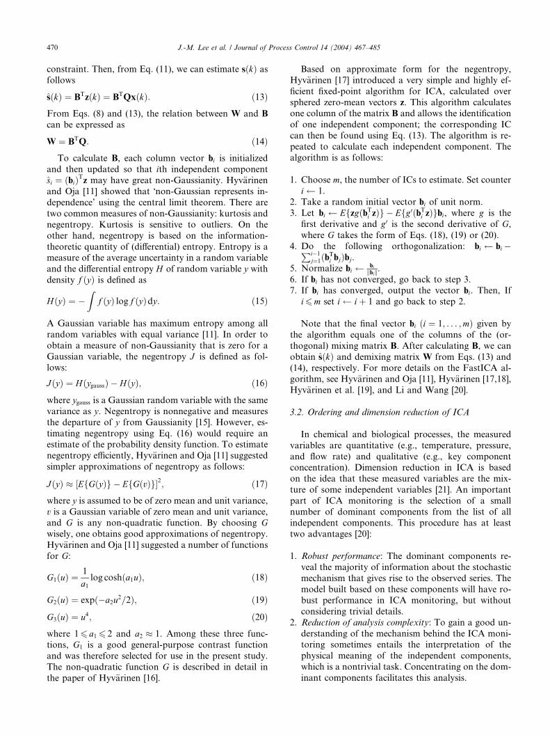
of length l.Our proposed strategy is depicted in Fig. 3. First, the

calibration model is built by ICA and kernel densityestimation and then the system is monitored through

two steps. As for conventional PCA monitoring, if the I2

statistic exceeds the limit, it indicates that a process

change in the model space has occurred, if the I2e statisticexceeds the limit, it indicates that a process change in the

excluded model space has occurred, and if the Q-statisticof residual space exceeds the confidence interval, it in-

dicates the occurrence of changes that violate the ICAmodel. We use contribution plots to identify and isolate

the nature of process faults.

4. Illustrative examples (comparison ICA with PCA)

PCA uses only the information contained in the co-

variance matrix of the data vector x, whereas ICA uses

information on the distribution of x that is not con-

tained in the covariance matrix. Hence, the use of ICA

for monitoring may give more sophisticated results be-

cause it uses the independent components rather than

the principle components. In this paper, the FastICA


algorithm developed by Hyv€arinen and Oja [11] was

applied to the detection and diagnosis of faults during

monitoring.

4.1. A simple multivariate process

Let us consider the following simple multivariate

process, which is a modified version of the system sug-

gested by Ku et al. [4].

zðkÞ ¼0:118 �0:191 0:2870:847 0:264 0:943�0:333 0:514 �0:217

24

35zðk � 1Þ

þ1 23 �4�2 1

24

35uðk � 1Þ; ð31Þ

yðkÞ ¼ zðkÞ þ vðkÞ; ð32Þwhere u is the correlated input:

uðkÞ ¼ 0:811 �0:2260:477 0:415

� �uðk � 1Þ

þ 0:193 0:689�0:320 �0:749

� �wðk � 1Þ: ð33Þ

The input w is a random vector of which each elementis uniformly distributed over the interval ð�2; 2Þ. Theoutput y is equal to z plus a random noise vector v. Each

element of v has zero mean and a variance of 0.1. Both

input u and output y are measured but z and w are not.

Normal data with 200 samples are used for analysis. The

data vector for analysis consists of xðkÞ ¼ ½yTðkÞuTðkÞ�T.The total 5 variables ðy1; y2; y3; u1; u2Þ are scaled to zero

mean and unit variance to prevent less important vari-

0 20 40 60 80 100

5

10

15

T2

0 20 40 60 80 100

1

2

3

4

5

6

Sample

SP

E

Fig. 4. PCA monitoring charts: T 2 and SPE plots

ables with large magnitudes overshadowing important

variables with small magnitudes.

Conventional PCA implicitly assumes that the ob-

servations at one time are statistically independent ofobservations at any past time. That is, it implicitly as-

sumes that the measured variable at one time instant not

only has serial independence within each variable series

at past time instants but also statistical inter-indepen-

dence between the different measured variable series at

past time instants. However, the dynamics of a typical

chemical or biological process cause the measurements

to be time dependent, which means that the data mayhave both cross-correlation and auto-correlation. PCA

methods can be extended to the modeling and moni-

toring of dynamic systems by augmenting each obser-

vation vector with the previous l observations [4]. Here,

we consider only static PCA and static ICA, although

dynamic PCA and dynamic ICA with time lagged

variables can be considered.

In PCA, a three principal component model is de-veloped, which captures about 87.5% of the variance of

the process. The disturbances for monitoring and diag-

nosis are as follows:

• Disturbance 1: A step change of w1 by 3 is introduced

at sample 50.

• Disturbance 2: w1 is linearly increased from sample

50 to 149 by adding 0:05ðk � 50Þ to the w1 value ofeach sample in this range, where k is the sample num-

ber.

The T 2 and SPE charts for PCA monitoring of the

process with disturbance 1 are shown in Fig. 4. The 99%

0 120 140 160 180 200

0 120 140 160 180 200

Number

of the data for disturbance 1 with three PCs.

0 20 40 60 80 100 120 140 160 180 2000

20

40

60

I2

0 20 40 60 80 100 120 140 160 180 2000

5

10

Ie2

0 20 40 60 80 100 120 140 160 180 2000

5

10

15

Sample Number

SP

E

Fig. 5. ICA monitoring charts: I2, I2e and SPE plots of the data for disturbance 1 with two ICs.


confidence limits are also shown. It is evident from these

charts that PCA cannot detect the disturbance, and

captures only the dominant randomness. However, ap-

plying ICA to the same process data gives the results

presented in Fig. 5, which show relatively correct dis-

turbance detection in comparison to PCA. The 99%confidence limits of I2, I2e and SPE are obtained from

kernel density estimation of normal operating condition

data. As shown in Fig. 5, I2 exceeds the confidence limit

from sample 51, a delay of only one sample. Also, the

superiority of ICA monitoring over the PCA-based ap-

(a)

PCs plot

Fig. 6. (a) Plot of two principal component values and (b) plot of two indepen

(95% and 99%) is indicated with dashed lines.

proach is evident in the plots shown in Fig. 6. The re-

gions of the process that are out of control are easily

seen in the ICs plot, whereas most samples are within

the region of normal operation in the PCs plot, despite

the presence of the fault.

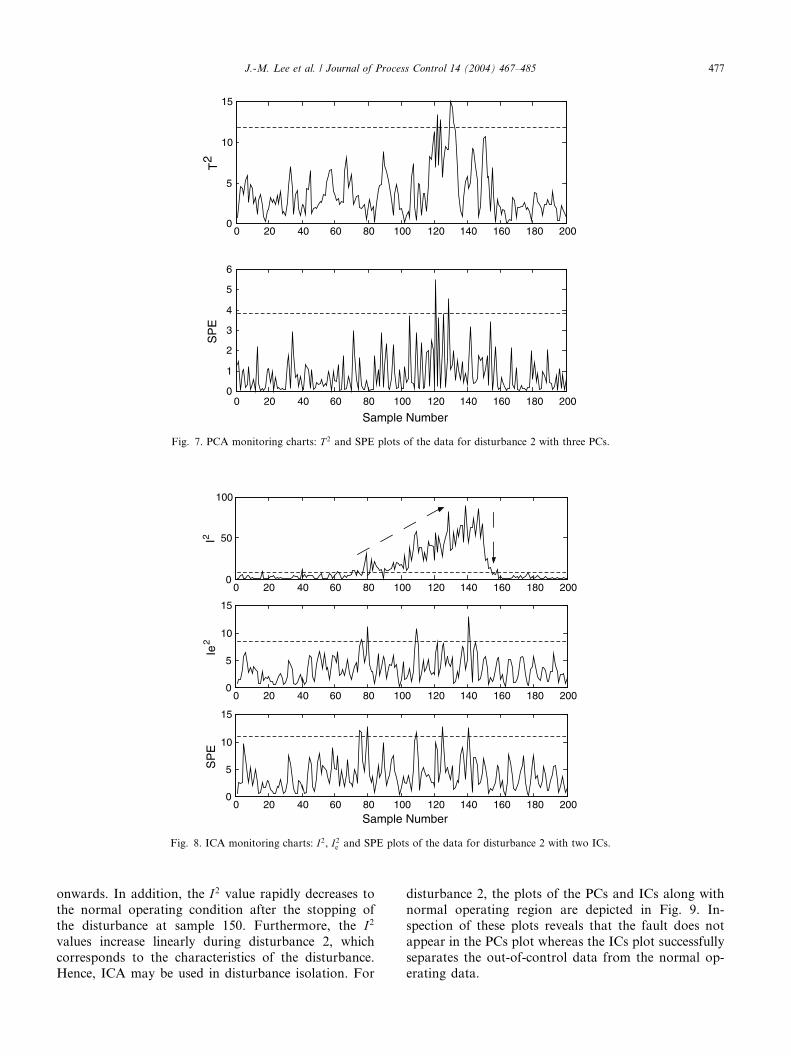
The T 2 and SPE charts for PCA monitoring of theprocess with disturbance 2 are shown in Fig. 7. With

PCA, the T 2 and SPE charts again fail to detect the

disturbance, although a few T 2 values exceed the 99%

control limit. With ICA (Fig. 8), the disturbance is well

detected by the I2 chart from about the 78th sample

(b)

ICs plot

dent component values for disturbance 1. The normal operating region

0 20 40 60 80 100 120 140 160 180 2000

5

10

15

T2

0 20 40 60 80 100 120 140 160 180 2000

1

2

3

4

5

6

Sample Number

SP

E

Fig. 7. PCA monitoring charts: T 2 and SPE plots of the data for disturbance 2 with three PCs.

0 20 40 60 80 100 120 140 160 180 2000

50

100

I2

0 20 40 60 80 100 120 140 160 180 2000

5

10

15

Ie2

0 20 40 60 80 100 120 140 160 180 2000

5

10

15

Sample Number

SP

E

Fig. 8. ICA monitoring charts: I2, I2e and SPE plots of the data for disturbance 2 with two ICs.


onwards. In addition, the I2 value rapidly decreases to

the normal operating condition after the stopping of

the disturbance at sample 150. Furthermore, the I2

values increase linearly during disturbance 2, which

corresponds to the characteristics of the disturbance.

Hence, ICA may be used in disturbance isolation. For

disturbance 2, the plots of the PCs and ICs along with

normal operating region are depicted in Fig. 9. In-

spection of these plots reveals that the fault does not

appear in the PCs plot whereas the ICs plot successfully

separates the out-of-control data from the normal op-

erating data.

(a) (b)

IC-2

PC

-2

PCs plot ICs plot

Fig. 9. (a) Plot of two principal component values and (b) plot of two independent component values for disturbance 2. The normal operating region

(95% and 99%) is indicated with dashed lines.


4.2. Wastewater treatment process

Advanced monitoring and control strategies for

WWTP have attracted much recent interest as a conse-

quence of the increasing stringency of environmental

regulations. However, some specific features about thisprocess are yet to be fully addressed. First, most changes

in this biological process are slow and recovery from

failures can be time-consuming and expensive, for ex-

ample it can take several months for the process to re-

cover from an abnormal operation. Therefore, early

detection of developing abnormalities is especially im-

portant for this process. Secondly, most WWTPs are

subject to large diurnal fluctuations in the flow rate andcomposition of the feed stream. Consequently, these

biological processes exhibit periodic characteristics, with

the values of the flow rate and composition of the feed

waste stream showing strong diurnal fluctuations. Since

the variables of such processes tend to fluctuate widely

over a cycle, their mean and variance do not remain

constant with time. Because of this, conventional mul-

Unit 1 Unit 2 Unit 3 UnQ0, Z0

Fig. 10. Process layout for the

tivariate statistical process monitoring (MSPM) meth-

ods like PCA, which implicitly assume a stationary

underlying process, may lead to numerous false alarms

and missed faults. Better treatment performance can be

expected from advanced monitoring and control strat-

egies that account for the non-Gaussianity of the peri-odic patterns in the biological process [34].

The ICA monitoring algorithm proposed here was

tested for its ability to detect various disturbances in

simulated data obtained from a benchmark simulation of

the WWTP. This simulation model combines nitrifica-

tion with predenitrification, the most commonly used

process for nitrogen removal. The activated sludge

model No. 1 (ASM1) and a ten-layer settler model wereused to simulate the biological reactions and the settling

process, respectively. Fig. 10 shows the flow diagram of

the modeled WWTP system. The plant was designed to

treat an average flow of 20,000 m3 d�1 with an average

biodegradable COD concentration of 300 mg l�1. The

plant consists of a 5-compartment bioreactor (6000 m3)

and a secondary settler (6000 m3). For the sludge con-

it 4 Unit 5

m = 1

m = 10

m = 6

Qa, Za

Qr, ZrQw, Zw

Qe, Ze

Qf, Zf

Qu, Zu

simulation benchmark.


centration of 3 kgm�3 this corresponds to a sludge load

of approximately 0.33 kgBOD5 kg�1 sludge day�1 which

is quite critical at 15 �C, so the effluent composition is

sensitive to the applied control strategy. The first twocompartments of the bioreactor are not aerated whereas

the others are aerated. All the compartments are con-

sidered to be ideally mixed whereas the secondary settler

is modeled with a series of 10 layers with one dimension.

For more detailed information about this benchmark,

refer to the website of the COST working group (http://

www.ensic.u-nancy.fr/COSTWWTP).

Influent data and operation parameters developed bya working group on the benchmarking of wastewater

treatment plants, COST 624, were used in the simulation

[35]. The data covered a period of two weeks. The

training model was based on a normal operation period

of one week of dry weather and validation data was used

on the data set for the last 7 days. The sampling time

was 15 min. The data used were the influent file and

outputs with noises suggested by the benchmark. Weselected seven variables, listed in Table 1, from among

the many variables used in the benchmark to build the

monitoring system. These variables were chosen because

Table 1

Variables used in the monitoring of the benchmark model

No. Symbol Meaning

1 SNH;in Influent ammonium concentration

2 Qin Influent flow rate

3 TSS4 Total suspended solid (reactor 4)

4 SO;3 Dissolved oxygen concentration (reactor 3)

5 SO;4 Dissolved oxygen concentration (reactor 4)

6 KLa5 Oxygen transfer coefficient (reactor 5)

7 SNO;2 Nitrate concentration (reactor 2)

-4 -2 0 2 4 60

0.05

0.1

0.15

0.2

0.25

0.3

0.35

0.4

Second score value (t2)

Den

sity

est

imat

e

(a)

Fig. 11. (a) Density estimate; (b) normality chec

they are typically monitored and important variables in

the real WWTP systems.

Two types of disturbances were tested using the

proposed method, external disturbances and internaldisturbances. External disturbances are defined as those

imposed upon the process from the outside and are

detectable when monitoring the influent characteristics.

Internal disturbances are caused by changes within the

process that affect the process behavior. For the external

disturbance, two short storm events were simulated,

while deterioration of nitrification was simulated to

study an internal disturbance [34,36].The density estimate and normal probability plot of

the second score vector ðt2Þ calculated by applying PCA

to the simulation benchmark of the normal operating

data (Fig. 11(a) and (b)) make it clear that the values of

t2 do not follow a Gaussian distribution. Thus, the cal-

culation of T 2 and SPE charts based on the assumption

that the data are Gaussian distributed may lead to poor

monitoring performance.

4.2.1. External disturbance (storm events)

We applied the proposed monitoring method to aprocess in which two sudden storm events occur after a

long period of dry weather. This example demonstrates

how external disturbances appear within the proposed

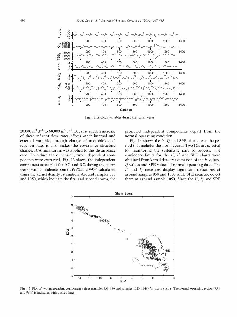
method. The pattern of measurement variables during

the storm weeks was taken from the storm condition in

the benchmark. The values of the measurement vari-

ables during the storm weeks are presented in Fig. 12

(first storm: samples 850–865 and second storm: samples1050–1110). The effects of the first storm can be seen at

around sample 850 and the effects of the second storm

can be seen at around sample 1050. During the storm

events, the average influent flow rate increases from

-2 0 2 4

0.0010.003

0.010.020.050.10

0.25

0.50

0.75

0.900.950.980.99

0.9970.999

Data

Pro

babi

lity

Normal Probability Plot

(b)

k of second score ðt2Þ obtained from PCA.

http://www.ensic.u-nancy.fr/COSTWWTP

http://www.ensic.u-nancy.fr/COSTWWTP

0 200 400 600 800 1000 1200 1400012

S-N

O2

Samples

0 200 400 600 800 1000 1200 1400

100200300

KLa

5 0 200 400 600 800 1000 1200 1400

246

S-O

4 0 200 400 600 800 1000 1200 1400024

S-O

3 0 200 400 600 800 1000 1200 1400200030004000

TSS 4 0 200 400 600 800 1000 1200 1400

200004000060000

Qin

0 200 400 600 800 1000 1200 14000

204060

SN

H,in

Fig. 12. X -block variables during the storm weeks.


20,000 m3 d�1 to 60,000 m3 d�1. Because sudden increase

of these influent flow rates affects other internal and

external variables through change of microbiological

reaction rate, it also makes the covariance structure

change. ICA monitoring was applied to this disturbancecase. To reduce the dimension, two independent com-

ponents were extracted. Fig. 13 shows the independent

component score plot for IC1 and IC2 during the storm

weeks with confidence bounds (95% and 99%) calculated

using the kernel density estimation. Around samples 850

and 1050, which indicate the first and second storm, the

-14 -12 -10 -8 -6-3

-2

-1

0

1

2

3

4

5

6

7

1055

106010651070

107510801085

1090

1095

Storm

IC-

IC-2

Fig. 13. Plot of two independent component values (samples 830–880 and sa

and 99%) is indicated with dashed lines.

projected independent components depart from the

normal operating condition.

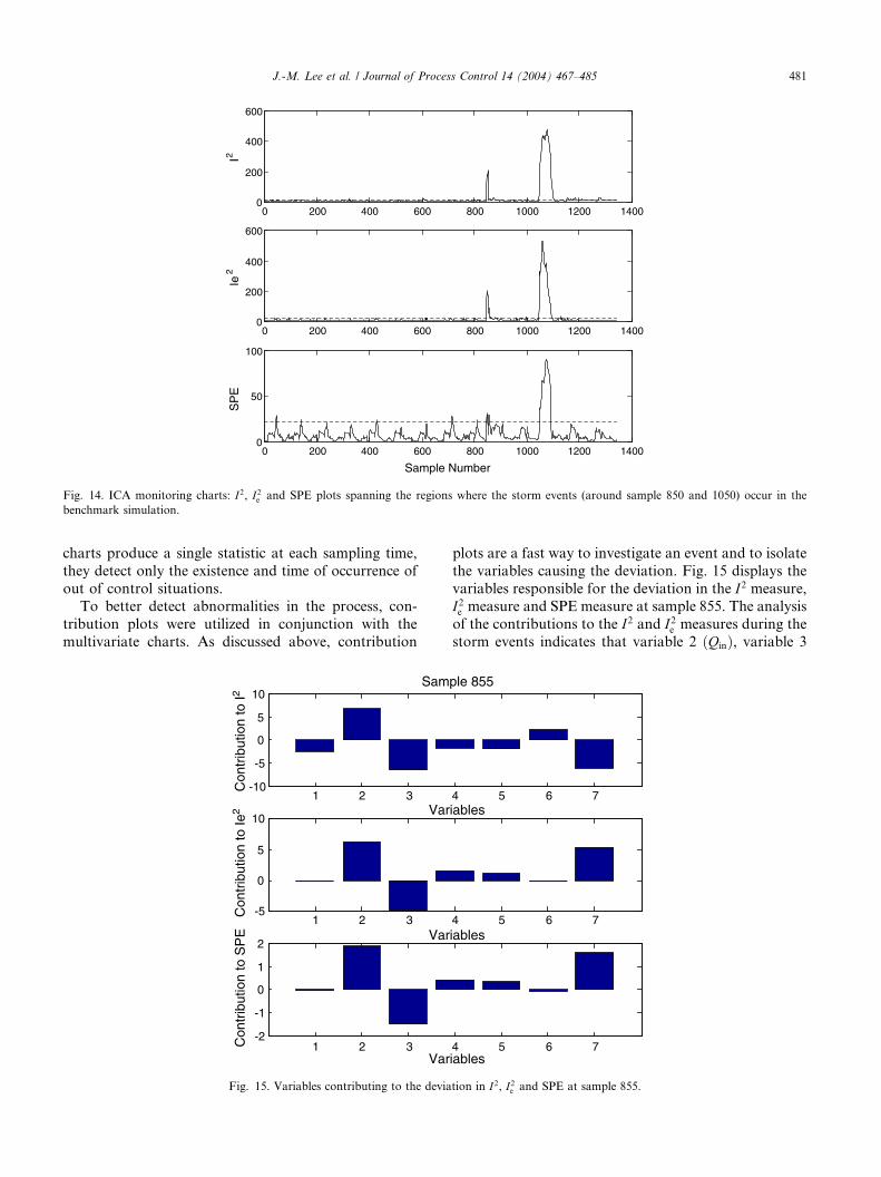
Fig. 14 shows the I2, I2e and SPE charts over the pe-

riod that includes the storm events. Two ICs are selected

for monitoring the systematic part of process. Theconfidence limits for the I2, I2e and SPE charts were

obtained from kernel density estimation of the I2 values,I2e values and SPE values of normal operating data. The

I2 and I2e measures display significant deviations at

around samples 850 and 1050 while SPE measure detect

them at around sample 1050. Since the I2, I2e and SPE

-4 -2 0 2 4

830

835

840845

850855

860865

870

875

880

10201025

1030

103510401045 10501100

110511101115

1120

1125

113011351140

Event

1

mples 1020–1140) for storm events. The normal operating region (95%

0 200 400 600 800 1000 1200 14000

200

400

600

I2

0 200 400 600 800 1000 1200 14000

200

400

600Ie

2

0 200 400 600 800 1000 1200 14000

50

100

Sample Number

SP

E

Fig. 14. ICA monitoring charts: I2, I2e and SPE plots spanning the regions where the storm events (around sample 850 and 1050) occur in the

benchmark simulation.


charts produce a single statistic at each sampling time,

they detect only the existence and time of occurrence of

out of control situations.To better detect abnormalities in the process, con-

tribution plots were utilized in conjunction with the

multivariate charts. As discussed above, contribution

1 2 3-10

-5

0

5

10Sam

Var

Con

trib

utio

n to

I2

1 2 3-5

0

5

10

Var

Con

trib

utio

n to

Ie2

1 2 3-2

-1

0

1

2

Var

Con

trib

utio

n to

SP

E

Fig. 15. Variables contributing to the devia

plots are a fast way to investigate an event and to isolate

the variables causing the deviation. Fig. 15 displays the

variables responsible for the deviation in the I2 measure,I2e measure and SPE measure at sample 855. The analysis

of the contributions to the I2 and I2e measures during the

storm events indicates that variable 2 ðQinÞ, variable 3

4 5 6 7

ple 855

iables

4 5 6 7iables

4 5 6 7iables

tion in I2, I2e and SPE at sample 855.

Table 2

Variance captured by the PCA model

PC number Eigenvalue of

covðX Þ% Variance

captured this PC

% Variance

captured total

1 4.600 65.71 65.71

2 1.630 23.34 89.05

3 0.479 6.85 95.89

4 0.149 2.13 98.02

5 0.077 1.10 99.12

6 0.055 0.79 99.91

7 0.006 0.09 100.00


ðTSS4Þ, and variable 7 ðSNO;2Þ are primarily responsible

for these deviations. This result can also be identified by

inspection of Fig. 12. From these contribution plots, an

�out-of-control’ situation is identified when the contri-butions of some variables are larger than anticipated.

The identification of the variables which have experi-

enced the greatest change, in conjunction with the expert

knowledge of the production engineer and operator,

makes it possible to relate a particular sequence of

changes to a particular process malfunction. This in-

formation can provide sufficient information to allow

operational personnel to narrow down the potentialcauses of the process problem.

In the case of external disturbances such as storm

events, conventional PCA with two PCs also gives good

monitoring results.

4.2.2. Internal disturbance (nitrification rate decrease)

The internal disturbance was imposed by decreasing

the nitrification rate in the biological reactor through a

decrease in the specific growth rate of the autotrophs

ðlAÞ. The autotrophic growth rate at sample 288 was

decreased rapidly from 0.5 to 0.4 day�1 and then linearly

decreased from 0.4 to 0.2 day�1 until sample 480, as il-lustrated in Fig. 16.

The PCA model is able to capture most of the vari-

ability of the X -block in two PCs, as shown in Table 2.

However, it is clear from the T 2 and SPE charts shown

in Fig. 17 that the PCA method with two PCs cannot

detect the internal disturbance because the periodic and

non-Gaussian features of the wastewater plant domi-

nate. In the SPE chart of PCA, the trace appears to startincreasing after observation 300. However, despite the

presence of the fault, most samples are below the con-

fidence limit, giving the process operator an incorrect

picture of the process status. In contrast to the PCA

result, the I2, I2e and SPE charts of ICA monitoring for

99% confidence limits, given in Fig. 18, show that the I2

0 100 200 3000.0

0.1

0.2

0.3

0.4

0.5

0.6

0.7

Nitr

ifica

tion

rate

Sample

Fig. 16. The form of the decrease in nitrification rate

chart successfully detects the internal disturbance. The

I2 measure increases rapidly around sample 288 and

reveals a diurnal variation, which indicates the detection

of successive faults. Furthermore, the pattern of internal

disturbance (step+ linear) is well reflected in the I2

chart.

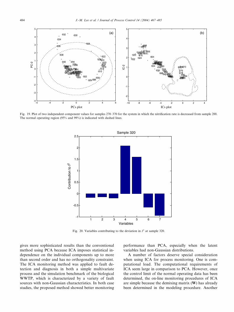
Fig. 19 shows the score plot for PC1 and PC2 and the

ICs plot for IC1 and IC2 from sample 270 to 370. In thePCs plot, most samples are within the normal operating

region despite the onset of the fault at sample 288, in-

dicating that PCA fails to detect the small internal dis-

turbance. In contrast, samples affected by the internal

disturbance are easily detected in the ICs plot. At these

affected samples, the ICs escape from their confidence

bounds, indicating that the internal disturbance has

distorted the internal mutual relations between thevariables and thus the process is not in the normal op-

eration mode. The process does not return to normal

operation mode within the remaining time of the test

period. Fig. 20 shows the contribution plots to the I2

measure at sample 320. From the contribution plot for

the I2 value, we can conclude that internal variables,

variables 4 ðSO;3Þ and 5 ðSO;4Þ, make the largest contri-

bution to the I2 statistic. If it were necessary to avoid theinfluence of single large variable we could construct the

contribution plots using the mean contribution over

some period.

400 500 600 700 Number

in the biological reactor (internal disturbance).

0 200 400 600 800 1000 1200 14000

5

10

15

T2

0 200 400 600 800 1000 1200 14000

1

2

3

4

5

6

Sample Number

SP

E

Fig. 17. PCA monitoring charts: T 2 and SPE plots spanning the region of deteriorating nitrification in the benchmark simulation.

0 200 400 600 800 1000 1200 14000

50

100

150

200

I2

0 200 400 600 800 1000 1200 14000

20

40

60

Ie2

0 200 400 600 800 1000 1200 14000

10

20

30

40

Sample Number

SP

E

Fig. 18. ICA monitoring charts: I2, I2e and SPE plots spanning the region of deteriorating nitrification in the benchmark simulation.


5. Conclusions

This paper proposes a new approach to process

monitoring that uses ICA to achieve multivariate sta-

tistical process control. The approach provides a new

statistic, the I2 statistic, to describe the state of data.

This statistic is an alternative to Hotelling’s T 2 statistic

used in PCA. In addition, methods for the calculation ofthe confidence limits, ordering and dimension reduction

of the independent components are described, along

with the use of contribution plots displaying the relative

contributions of the different variables. The proposed

strategy was shown to be able to detect and isolate the

effect of multivariate disturbances. ICA monitoring

(a) (b)P

C-2

IC-2

PCs plot ICs plot

Fig. 19. Plot of two independent component values for samples 270–370 for the system in which the nitrification rate is decreased from sample 288.

The normal operating region (95% and 99%) is indicated with dashed lines.

1 2 3 4 5 6 7-1

-0.5

0

0.5

1

1.5

2

2.5

Variables

Con

trib

utio

n to

I2

Sample 320

Fig. 20. Variables contributing to the deviation in I2 at sample 320.


gives more sophisticated results than the conventional

method using PCA because ICA imposes statistical in-

dependence on the individual components up to more

than second order and has no orthogonality constraint.

The ICA monitoring method was applied to fault de-

tection and diagnosis in both a simple multivariate

process and the simulation benchmark of the biologicalWWTP, which is characterized by a variety of fault

sources with non-Gaussian characteristics. In both case

studies, the proposed method showed better monitoring

performance than PCA, especially when the latent

variables had non-Gaussian distributions.

A number of factors deserve special consideration

when using ICA for process monitoring. One is com-

putational load. The computational requirements of

ICA seem large in comparison to PCA. However, once

the control limit of the normal operating data has beendetermined, the on-line monitoring procedures of ICA

are simple because the demixing matrix (W) has already

been determined in the modeling procedure. Another


issue that should be considered in ICA monitoring is

related to the kernel density estimation. In the present

work we have assumed that the underlying distribution

of normal operating data does not change over time.However, this underlying distribution can potentially

change. In fact, a small change in the distribution will

have a negligible effect on the control limits of I2, I2e and

SPE. When the underlying distribution changes sub-

stantially, the ICA model should be updated. Adaptive

ICA monitoring should be investigated in future re-

search.

Acknowledgement

This work was supported by a grant (no. R01-2002-

000-00007-0) from Korea Science & Engineering

Foundation.

References

[1] J.-F. Cardoso, Blind signal separation: statistical principles, Proc.

IEEE 86 (10) (1998) 2009–2025.

[2] P. Comon, Independent component analysis, a new concept,

Signal Process. 36 (1994) 287–314.

[3] P. Nomikos, J.F. MacGregor, Monitoring batch processes using

multiway principal component analysis, AIChE J. 40 (8) (1994)

1361–1375.

[4] W. Ku, R.H. Storer, C. Georgakis, Disturbance detection and

isolation by dynamic principal component analysis, Chemom.

Intell. Lab. Syst. 30 (1995) 179–196.

[5] B.M. Wise, N.B. Gallagher, The process chemometrics approach

to process monitoring and fault detection, J. Process Control 6 (6)

(1996) 329–348.

[6] D. Dong, T.J. McAvoy, Nonlinear principal component analysis-

based on principal curves and neural networks, Comp. Chem.

Eng. 20 (1) (1996) 65–78.

[7] B.R. Bakshi, Multiscale PCA with application to multivariate

statistical process monitoring, AICHE J. 44 (7) (1998) 1596–1610.

[8] C. Rosen, G. Olsson, Disturbance detection in wastewater

treatment plants, Water Sci. Technol. 37 (12) (1998) 197–205.

[9] P. Teppola, Multivariate process monitoring of sequential process

data––a chemometric approach, Ph.D. thesis, Lappeenranta Univ.

of Tech., Finland, 1999.

[10] W. Li, H. Yue, S.V. Cervantes, J. Qin, Recursive PCA for adaptive

process monitoring, J. Process Control 10 (2000) 471–486.

[11] A. Hyv€arinen, E. Oja, Independent component analysis: algo-

rithms and applications, Neural Networks 13 (4–5) (2000) 411–430.

[12] T. Lee, Independent Component Analysis: Theory and Applica-

tions, Kluwer Academic Publishers, Boston, USA, 1998.

[13] J.E. Jackson, G.S. Mudholkar, Control procedures for residuals

associated with principal component analysis, Technometrics 21

(1979) 341–349.

[14] R.N. Vig�ario, Extraction of ocular artifacts from EEG using

independent component analysis, Electroencephal. Clinical Neu-

rophysiol. 103 (1997) 395–404.

[15] T. Hastie, R. Tibshirani, J. Friedman, The Elements of Statistical

Learning, Springer, New York, USA, 2001.

[16] A. Hyv€arinen, New approximations of differential entropy for

independent component analysis and projection pursuit, Adv.

Neural Inform. Process. Syst. 10 (1998) 273–279.

[17] A. Hyv€arinen, Fast and robust fixed-point algorithms for inde-

pendent component analysis, IEEE Trans. Neural Networks 10

(1999) 626–634.

[18] A. Hyv€arinen, Survey on independent component analysis,

Neural Comput. Surveys 2 (1999) 94–128.

[19] A. Hyv€arinen, J. Karhunen, E. Oja, Independent Component

Analysis, John Wiley & Sons, Inc, New York, USA, 2001.

[20] R.F. Li, X.Z. Wang, Dimension reduction of process dynamic

trends using independent component analysis, Comp. Chem. Eng.

26 (2002) 467–473.

[21] Y.M. Cheung, L. Xu, An empirical method to select dominant

independent components in ICA time series analysis, Proc. Int.

Joint Conf. Neural Networks (1999) 3883–3887.

[22] A.D. Back, A.S. Weigend, A first application of independent

component analysis to extracting structure from stock returns,

Int. J. Neural Sys. 8 (4) (1997) 473–484.

[23] J.-F. Cardoso, A. Soulomica, Blind beamforming for non-

Gaussian signals, IEEE Proc. F 140 (6) (1993) 362–370.

[24] Y.M. Cheung, L. Xu, Independent component ordering in ICA

time series analysis, Neurocomputing 41 (2001) 145–152.

[25] A. Simoglou, E.B. Martin, A.J. Morris, Statistical performance

monitoring of dynamic multivariate process using state space

modeling, Comp. Chem. Eng. 26 (6) (2002) 909–920.

[26] E.B. Martin, A.J. Morris, Non-parametric confidence bounds for

process performance monitoring charts, J. Process Control 6 (6)

(1996) 349–358.

[27] Q. Chen, R.J. Wynne, P. Goulding, D. Sandoz, The application of

principal component analysis and kernel density estimation to

enhance process monitoring, Control Eng. Pract. 8 (2000) 531–

543.

[28] B.W. Silverman, Density Estimation for Statistics and Data

Analysis, Chapman & Hall, UK, 1986.

[29] M.P. Wand, M.C. Jones, Kernel Smoothing, Chapman & Hall,

London, UK, 1995.

[30] J.F. MacGregor, C. Jaeckle, C. Kiparissides, M. Koutoudi,

Process monitoring and diagnosis by multiblock PLS methods,

AIChE J. 40 (5) (1994) 826–838.

[31] C. Rosen, Monitoring wastewater treatment systems, MS Thesis,

Lund Univ., Sweden, 1998.

[32] J.A. Westerhuis, S.P. Gurden, A.K. Smilde, Generalized contri-

bution plots in multivariate statistical process monitoring, Che-

mom. Intell. Lab. Syst. 51 (2000) 95–114.

[33] P. Teppola, S.-P. Mujunen, P. Minkkinen, T. Puijola, P. Pursihe-

imo, Principal component analysis, contribution plots and feature

weights in the monitoring of sequential process data from a paper

machine’s wet end, Chemom. Intell. Lab. Syst. 44 (1998) 307–

317.

[34] C.K. Yoo, Process monitoring and control of biological waste-

water treatment process, Ph.D. Thesis, POSTECH, Korea, 2002.

[35] M.N. Pons, H. Spanjers, U. Jeppsson, Towards a benchmark for

evaluating control strategies in wastewater treatment plants by

simulation, Escape 9, Budapest, 1999.

[36] C.K. Yoo, S.W. Choi, I.-B. Lee, Dynamic monitoring method for

multiscale fault detection and diagnosis in MSPC, Ind. Eng.

Chem. Res. 41 (2002) 4303–4317.

Statistical process monitoring with independent component analysis

Documents

Transcript of Statistical process monitoring with independent component analysis