Lattice Independent Component Analysis for fMRI

Manuel Graña, Darya Chyzhyk, Maite García-Sebastián, Carmen Hernández

Computational Intelligence GroupDept. CCIA, UPV/EHU, Apdo. 649, 20080 San Sebastian, Spain

www.ehu.es/ccwintco

Abstract

We introduce a Lattice Independent Component Analysis (LICA) approach to fMRIanalysis based on an Incremental Lattice Source Induction Algorithm (ILSIA). The IL-SIA is grounded in recent theoretical results on Lattice Associative Memories (LAM).It aims to select a set of Strong Lattice Independent (SLI) vectors from the input dataset.Those SLI vectors can be assumed to be an Affine Independent set of vectors whichdefine a convex polytope on the input data space. We call them lattice sources. Theyare used to compute the linear unmixing of each voxel’s time series independently.The resulting mixing coefficients roughly correspond to the Independent ComponentAnalysis (ICA) mixing matrix, while the set of lattice sources corresponds to the statis-tically independent sources found by ICA. The proposed approach is unsupervised ormodel free because the design matrix containing the regressors is not fixed a priori butinduced from the data. Our approach does not impose any probabilistic model on thesearched sources, although we assume a linear mixture model. We show on simulatedfMRI data that our approach can discover the meaningful sources with efficiency com-parable to that of ICA. Besides, on a well-known case study our approach can discoveractivation patterns in good agreement with the state of the art Statistical ParametricMapping (SPM) software, and some state of the art ICA variants.

Key words: Lattice Independence, Lattice Associative Memories, fMRI, IndependentComponent Analysis

1. Introduction

Human brain mapping is a rapidly expanding discipline, and in recent years interesthas grown in novel methods for imaging human brain functionality. Noninvasive tech-niques can measure cerebral physiologic responses during neural activation. One ofthe relevant techniques is functional Magnetic Resonance Imaging (fMRI) [18], whichuses the blood oxygenation level dependent (BOLD) contrast to detect physiologicalalterations, such as neuronal activation resulting in changes of blood flow and bloodoxygenation. The signal changes are related to changes in the concentration of de-oxyhemoglobin, which acts as an intravascular contrast agent for fMRI. Most of thefMRI examinations are performed using T2 weighted spin echo pulse sequences orT2* weighted gradient echo pulse sequences. The various fMRI-methods have a good

Preprint submitted to Elsevier March 15, 2010

spatial and temporal resolution, limited only by the precision with which the autoregu-latory mechanisms of the brain adjust blood flow in space to the metabolic demands ofneuronal activity. Since these methods are completely noninvasive, using no contrastagent or ionizing radiation, repeated single-subject studies are becoming feasible [17].

An fMRI experiment consists of a functional template or protocol (e.g., alternat-ing activation and rest for a certain time) that induces a functional response in thebrain. The aim of the experiment is to detect the response to this time varying stimu-lus, through the examination of the signal resulting from the BOLD effect, in a definedvolume element (voxel). The functional information of a voxel has to be extracted fromits time series. One fMRI volume is recorded at each sampling time instant during theexperiment. The time sampling frequency is determined by the resolution of the fMRIimaging pulse sequence. The complete four-dimensional dataset (three dimensions inspace, one dimension in time) consists of subsequently recorded three-dimensional (3-D) volumes. The acquisition of these functional volumes runs over periods lasting upto several minutes.

The most extended analysis approach for fMRI signals is the Statistical ParametricMaps (SPM) [6, 5], which has evolved into a free software package. This methodconsists in the separate voxel estimation of the regression parameters of General LinearModel (GLM), whose design matrix has been built corresponding to the experimentaldesign. A contrast is then defined on the estimated regression parameters, which cantake the form of a t-test or an F-test. The theory of Random Fields is then applied tocorrect the test thresholds, taking into account the spatial correlation of the independenttest results.

There have been also approaches to the fMRI analysis based on the IndependentComponent Analysis (ICA) [3] assuming that the time series observations are linearmixtures of independent sources which can not be observed. ICA assumes that thesource signals are non-Gaussian and that the linear mixing process is unknown. Theapproaches to solve the ICA problem obtain both the independent sources and the linearunmixing matrix. These approaches are unsupervised because no a priori informationabout the sources or the mixing process is included, hence the alternative name of BlindDeconvolution.

In this paper we propose an approach that we call Lattice Independent ComponentAnalysis (LICA) that consists of two steps. Firts it selects Strong Lattice Independent(SLI) vectors from the input dataset using an incremental algorithm, the Incremen-tal Lattice Source Induction Algorithm (ILSIA). Second, because of the conjecturedequivalence between SLI and Affine Independence, it performs the linear unmixing ofthe input dataset based on these lattice sources. Therefore, the approach is a mixture oflinear and nonlinear methods.

The original works were devoted to unsupervised hyperspectral image segmenta-tion, therefore the use of the term endmembers for the selected vectors in previousworks, however we find more appropriate the term lattice source. We maintain thebasic assumption that the data is generated as a convex combination of a set of latticesources which are the vertices of a convex polytope covering some region of the inputdata. This assumption is similar to the linear mixture assumed by the ICA approach,however we do not impose any probabilistic assumption on the data. The lattice sourcesdiscovered by the ILSIA are equivalent to the GLM design matrix columns, and the

2

unmixing process is identical to the conventional least squares estimator. Therefore,LICA is a kind of unsupervised GLM whose regressor functions are mined from theinput dataset. If we try to establish correspondences to the ICA, the lattice sourcescorrespond to the unknown statistically independent sources and the mixing matrix isthe one given by the abundance coefficients computed by least squares estimation.

The ILSIA is an improved formulation of the Endmember Induction Heuristic Al-gorithm proposed in [7]. Our approach to lattice source selection from the data is basedon the conjecture equivalence between the Strong Lattice Independence and the AffineIndependence [24]. The SLI needs two conditions: Lattice Independence and max/mindominance. Lattice Independence is detected based on results on fixed points for Lat-tice Autoassociative Memories (LAM) [22, 24, 29], and max/min dominance is testedusing algorithms inspired in the ones described in [30]. An important improvementrelative to previous attempts is the use of Chebyshev best approximation results [29]in order to reduce the number of selected vectors. The ILSIA is a greedy incrementalalgorithm that passes only once over the sample. It starts with a randomly picked inputvector and tests each vector in the input dataset to add it to the set of lattice sources.

There are other methods [8, 24] based on LAM to obtain a set of SLI vectors. How-ever these methods produce initially a large set of lattice sources that must be reducedsomehow, either resorting to a priori knowledge or to selections based on Mutual In-formation or other similarity measures. In the ILSIA the candidate SLI vectors arediscarded on the basis of the existence of a fixed point that gives a good approxima-tion of it in the Chebyshev distance sense, which is a natural distance in this LatticeComputing setting.

The LICA approach falls in the field of Lattice Computing algorithms, which havebeen introduced in [7] as the class of algorithms that either apply lattice operatorsinf and sup or use lattice theory to produce generalizations or fusions of previous ap-proaches. In [7] an extensive and updated list of references that can be labeled LatticeComputing can be found. This paper is an extension of the one presented at the LBM2008 workshop inside the CLA 2008 conference [9].

The outline of the paper is as follows: Section 2 gives a brief recall of ICA. Section3 introduces the linear mixing model. Section 4 presents a sketch of the theoreticalrelation between Lattice Independence and Linear (Affine) Independence through theLAM theory. Section 6 gives results on synthetic fMRI like data. Section 5 gives thedefinition of our Incremental Lattice Source Induction Algorithm (ILSIA). Section 7presents results of the proposed approach on a case study. Section 8 provides someconclusions.

2. Independent Component Analysis (ICA)

The Independent Component Analysis (ICA) [13] assumes that the data is a linearcombination of non Gaussian, mutually independent latent variables with an unknownmixing matrix. The ICA reveals the hidden independent sources and the mixing ma-trix. That is, given a set of observations represented by a d-dimensional vector x, ICAassumes a generative model

x = As, (1)

3

where s is the M dimensional vector of independent sources and A is the d × M

unknown basis matrix. The ICA searches for the linear transformation of the data W,such that the projected variables

Wx = s, (2)

are as independent as possible. It has been shown that the model is completely iden-tifiable if the sources are statistically independent and at least M − 1 of them are nonGaussian. If the sources are gaussian the ICA transformation could be estimated upto an orthogonal transformation. Estimation of mixing and unmixing matrices can bedone maximizing diverse objective functions, among them the non gaussianity of thesources and the likelihood of the sample.

We have used the FastICA [14] algorithm implementation available at [26]. Wehave also used the implementations of Maximum Likelihood ICA [11] (ML-ICA)which is equivalent to Infomax ICA, Mean Field ICA [12] (MF-ICA), and Molgedeyand Schouster ICA (MS-ICA) based on dynamic decorrelation [16], which are avail-able at [27].

Application of ICA to fMRI has been reviewed by [3]. Reports on the research ap-plication of ICA to fMRI signals include the identification of signal types (task relatedand physiology related) and the analysis of multisubject fMRI data. The most commonapproach is the spatial ICA that looks for spatial disjoint regions corresponding to theidentified signal types. It has been claimed that ICA has identified several physiologi-cal noise sources as well as other noise sources (motion, thermodynamics) identifyingtask related signals. Diverse ICA algorithms have been tested in the literature with in-conclusive results. Among them, FastICA, the one that we will apply in the case study,did identify the task related signals consistently. Among the clinical applications, ICAhas been used to study the brain activation due to pain in healthy individuals versusthose with chronic pain [1], the discrimination of Alzheimer’s patients from healthycontrols [10], the classification of schizophrenia [4] and studies about the patterns ofbrain activation under alcohol intoxication [4].

3. The linear mixing model and the Lattice Independent Component Analysis

The linear mixing model can be expressed as follows:

x =

M∑

i=1

aiei + w = Ea + w, (3)

where x is the d-dimensional pattern vector corresponding to the fMRI voxel timeseries vector, E is a d × M matrix whose columns are the d-dimensional vectorsei, i = 1, .., M , which are called endmembers when they are the vertices of a con-vex region covering the data, a is the M -dimensional vector of linear mixing coef-ficients, which correspond to fractional abundances in the convex case, and w is thed-dimensional additive observation noise vector. The linear mixing model is subjectedto two constraints on the abundance coefficients when the data points fall into a simplexwhose vertices are the endmembers, all abundance coefficients must be non-negativeai ≥ 0, i = 1, .., M and normalized to unity summation

∑M

i=1 ai = 1. Under this

4

circumstance, we expect that the vectors in E are affinely independent and that theconvex region defined by them includes all the data points. We recall that a set ofvectors X = {x1, . . . ,xk} is said to be linearly independent if the unique solution tothe equation

∑k

i=1 aixi = 0 is given by ai = 0 for all i ∈ {1, . . . , k} . A set X is anaffinely independent set if the solution to the simultaneous equations

∑k

i=1 aixi = 0

and∑k

i=1 ai = 0 is given by ai = 0 for all i ∈ {1, . . . , k} . Therefore, linear indepen-dence is a necessary condition for affine independence but not viceversa. The model inequation (3) is shared by other linear analysis approaches, such as the General LinearModel (GLM) [5] and the Independent Component Analysis (ICA) [13] which do notview E as a set of endmembers but as regressors or independent sources.

Once the enmembers have been determined the unmixing process is the computa-tion of the matrix inversion that gives the coordinates of each data point relative to theconvex region vertices. The simplest approach is the unconstrained least squared error(LSE) estimation given by:

a =(ET E

)−1ET x. (4)

Even when the vectors in E are affine independent, the coefficients that result fromequation (4) do not necessarily fulfill the non-negativity and unity normalization. En-suring both conditions is a difficult computational problem. Some authors (i.e. [24])use Non Negative Least Squares algorithms [15] to ensure at least non-negative coef-ficients. However in our works we use these mixture coefficients in a more qualitativeway and we do not feel the need to enforce these conditions. Moreover, althoughthe heuristic algorithm described in section 5 always produces the vertices of convexregions, these simplices always lie inside the data cloud, so that enforcing the non-negative and normalization conditions on the linear mixing coefficients would be im-possible for some sample data points. Negative values are considered as zero values,for interpretation and visualization purposes, and the additivity to one condition is notimportant as long as we are looking for the maximum abundances to assign meaning tothe resulting spatial distribution of the coefficients. These coefficients are interpreted asthe regressor coefficients corresponding to the decomposition of the fMRI voxel timeseries into a basis of vectors. That is, high positive values are interpreted as high posi-tive correlation with the time pattern of the corresponding lattice source. Therefore, toavoid confusion with the orthodox meaning of endmember, we will call lattice sourceto the set of affine independent vectors found by our algorithm.

We call Lattice Independent Component Analysis (LICA) the approach groundedin the results and algorithm that will be described in the following sections. LICAconsists of two steps:

1. Induce from the given data a set of Strongly Lattice Independent vectors. In thispaper we apply the Incremental Lattice Source Induction Algorithm (ILSIA) de-scribed in section 5. These vectors are taken as a set of affine independent vec-tors. The advantages of this approach are (1) that we are not imposing statisticalassumptions, (2) that the algorithm is one-pass and very fast because it only usescomparisons and addition, (3) that it is unsupervised and incremental, and (4) thatit detects naturally the number of lattice sources.

2. Apply the unconstrained least squares estimation to obtain the mixing matrix.The detection results are based on the analysis of the coefficients of this matrix.

5

Therefore, the approach is a combination of Linear and Lattice Computing: alinear component analysis where the components have been discovered by non-linear algorithms based on Lattice Theory.

4. Theoretical background on Lattice Independence and Lattice AutoassociativeMemories

The work on Lattice Associative Memories (LAM) stems from the consideration ofthe bounded lattice ordered group (blog) (R±∞,∨,∧, +, +′) as the alternative to thecomputational framework given by the mathematical field (R, +, ·) for the definitionof Neural Network algorithms. There R denotes the set of real numbers, R±∞ the ex-tended real numbers, ∧ and ∨ denote, respectively, the binary max and min operations,and +, +′ denote addition and its dual operation. In our current context addition is self-dual. If x ∈ R±∞, then its additive conjugate is x∗ = −x. For a matrix A ∈ R

n×m±∞ its

conjugate matrix is given by A∗ ∈ Rn×m±∞ , where each entry a∗

ij = [A∗]ij is given bya∗

ij = (aji)∗.

The LAM were first introduced in [21, 20] as Morphological Associative Memo-ries, a name still used in recent publications [29], but we follow the new convention in-troduced in [22, 24] because it sets the works in the more general framework of LatticeComputing. Given a set of input/output pairs of pattern (X, Y ) =

{(xξ ,yξ

); ξ = 1, .., k

},

a linear heteroassociative neural network based on the pattern’s cross correlation is builtup as W =

∑ξ yξ ·

(xξ

)′. Mimicking this constructive procedure [21, 20] propose the

following constructions of Lattice Heteroassociative Memories (LHAM):

WXY =

k∧

ξ=1

[yξ ×

(−xξ

)′]and MXY =

k∨

ξ=1

[yξ ×

(−xξ

)′], (5)

where × is any of the ∨2 or ∧2 operators. Here ∨2 and ∧2 denote the max and minmatrix product [21, 20]. respectively defined as follows:

C = A ∨2 B = [cij ] ⇔ cij =∨

k=1,...,n

{aik + bkj} , (6)

C = A ∧2 B = [cij ] ⇔ cij =∧

k=1,...,n

{aik + bkj} . (7)

If X = Y then the LHAM memories are Lattice Autoassociative Memories (LAAM).Conditions of perfect recall by the LHAM and LAAM of the stored patterns proved in[21, 20] encouraged the research on them, because in the continuous case, the LAAM isable to store and recall any set of patterns: WXX ∨2 X = X = MXX ∧2 X, for any X .However, this result holds when we deal with noise-free patterns. Research on robustrecall [19, 23, 20] based on the so-called kernel patterns lead to the notion of morpho-logical independence, in the erosive and dilative sense, and finally to the definition ofLattice Independence (LI) and Strong Lattice Independence (SLI). We gather theoreti-cal results from [22, 24, 29, 30] that set the theoretical background for the approach tolattice source induction described in section 5.

6

Definition Given a set of vectors X ={x1, ...,xk

}⊂ R

n a linear minimax combina-tion of vectors from this set is any vector x ∈R

n±∞ which is a linear minimax sum of

these vectors:

x = L(x1, ...,xk

)=

∨

j∈J

k∧

ξ=1

(aξj + xξ

),

where J is a finite set of indices and aξj ∈ R±∞ ∀j ∈ J and ∀ξ = 1, ..., k.

Definition The linear minimax span of vectors{x1, ...,xk

}= X ⊂ R

n is the set ofall linear minimax sums of subsets of X, denoted LMS

(x1, ...,xk

).

Definition Given a set of vectors X ={x1, ...,xk

}⊂ R

n, a vector x ∈Rn±∞ is

lattice dependent if and only if x ∈ LMS(x1, ...,xk

). The vector x is lattice inde-

pendent if and only if it is not lattice dependent on X. The set X is said to be latticeindependent if and only if ∀λ ∈ {1, ..., k} , xλ is lattice independent of X\

{xλ

}={

xξ ∈ X : ξ 6= λ}

.

The definition of lattice independence supersedes and improves the early definitions[23] of erosive and dilative morphological independence. This definition of latticedependence is closely tied to the study of the fixed points of the LAAM’s taken asoperators.

Theorem 4.1. [22, 29] Given a set of vectors X ={x1, ...,xk

}⊂ R

n, a vectory ∈R

n±∞ is a fixed point of WXX , that is WXX ∨2 y = y, if and only if y is lattice

dependent on X .

Definition A set of vectors X ={x1, ...,xk

}⊂ R

n is said to be max dominant if andonly if for every λ ∈ {1, ..., k} there exists and index jλ ∈ {1, ..., n} such that

xλjλ

− xλi =

k∨

ξ=1

(x

ξjλ

− xξi

)∀i ∈ {1, ..., n} .

Similarly, X is said to be min dominant if and only if for every λ ∈ {1, ..., k} thereexists and index jλ ∈ {1, ..., n} such that

xλjλ

− xλi =

k∧

ξ=1

(x

ξjλ

− xξi

)∀i ∈ {1, ..., n} .

The expressions that compound this definition appeared in the early theorems aboutperfect recall of Morphological Associative Memories [21, 20]. Their value as an iden-tifiable property of the data has been discovered in the context of the formalizationof the relationship between strong lattice independence, defined below, and the affineindependence in the classical linear analysis.

Definition A set of lattice independent vectors{x1, ...,xk

}⊂ R

n is said to be stronglylattice independent (SLI) if and only if X is max dominant or min dominant or both.

7

As said before, min and max dominance are the conditions for perfect recall. Perconstruction, the column vectors of Lattice Autoassociative Memories are diagonallymin or max dominant, depending of their erosive or dilative nature, therefore they willbe strong lattice independent, if they are lattice independent.

Conjecture 4.2. [24] If X ={x1, ...,xk

}⊂ R

n is strongly lattice independent thenX is affinely independent.

This conjecture (stated as theorem in [22]) is the key result whose proof wouldrelate the linear convex analysis and the non-linear lattice analysis. If true, it means thatthe construction of the LAAM provides the starting point for obtaining sets of affineindependent vectors that could be used as lattice sources for the unmixing algorithmsdescribed in section 3. We have found it to be true in our computational experiences,but a formal proof is still lacking.

Theorem 4.3. [24] Let X ={x1, ...,xk

}⊂ R

n and let W ( M ) be the set of vectorsconsisting of the columns of the matrix WXX (MXX .). Let F (X) denote the set offixed points of the LAAM constructed from set X . There exist V ⊂ W and N ⊂ M

such that V and N are strongly lattice independent and F (X) = F (V ) = F (N) or,equivalently, WXX = WV V and MXX = MNN .

The key idea of this theorem is that it is possible to built a set of SLI vectorsfrom the column vectors of a LAAM. Taking into account that the column vectors ofa LAAM are diagonally max or min dominant (depending on the kind of LAAM), itsuffices to find a subset which is lattice independent. It is also grounded in the factthat a subset of a set of max or min dominant vectors is also min or max dominant.The proof of the theorem is constructive giving way to algorithms to find these sets ofSLI. It removes iteratively the detected lattice dependent column vectors. Detectionlies in the fact that WXX = WWW = WV V and MXX = MMM = MNN when thevectors removed from W or M to obtain V or N are lattice dependent on the remainingones. Algorithms discussed in [8, 24] apply this result. The experience shows thatmost of the column vectors of the LAAM are lattice independent, so that the sets ofSLI vectors are large and need some kind of selection algorithm to find the salientones. One way to perform this selection is discarding those that can be interpreted asclose approximations of others already selected, in the incremental framework of thealgorithm described in section 5.

To deal with approximation in this Lattice Computing setting it seems natural [29]to use the Chebyshev distance given by the greatest componentwise absolute differencebetween two vectors, it is denoted ς (x,y) and can be computed as follows: ς (x,y) =(x∗ ∨2 y) ∨ (y∗ ∨2 x). The Chebyshev-best approximation of c by f (x) subject tox ∈ S, is the minimization of ς (f (x) , c) subject to x ∈ S.

Theorem 4.4. [29] Given B ∈ Rm×n and c ∈ R

m, a Chebyshev-best solution tothe approximation of c by B ∨2 x subject to the constraint B ∨2 x < c is given byx# = B∗ ∧2 c and x# is the greatest such solution.

8

In our incremental algorithm we will need to solve the unconstrained minimizationproblem

min ς (B ∨2 x, c) ,

in order to decide if the input vector is already well approximated by a fixed point ofthe LAAM constructed from the selected enmembers.

Theorem 4.5. [29]Given B ∈ Rm×n and c ∈ R

m, a Chebyshev-best solution tothe approximation of c by B ∨2 x is given by µ + x# where µ is such that 2µ =ς(B ∨2 x#, c

)=

(B ∨2 x#

)∗∨2 c.

This theorem has resulted in enhanced robust recall for LAAM under general noiseconditions, compared with other Associative Memories proposed in the literature. Ithas also been applied to produce a lattice based nearest neighbor classification schemewith good results on standard benchmark classification problems.

5. Incremental Lattice Source Induction Algorithm (ILSIA)

The algorithm described in this section is a further step in the formulation of asearch of SLI sets of vectors from the Endmember Induction Heuristic Algorithm in-troduced in [8]. It is grounded in the formal results on continuous LAAM reviewed inthe previous section. The dataset is denoted by Y = {yj ; j = 1, . . . , N} ∈ R

n×N andthe set of lattice sources induced from the data at any step of the algorithm is denotedby X = {xj ; j = 1, . . . , K} ∈ R

n×K . The number of lattice sources K will varyfrom the initial value K = 1 up to the number of lattice sources found by the algo-rithm, we will skip indexing the set of lattice sources with the iteration time counter.The algorithm makes only one pass over the sample as in [8]. The auxiliary variabless1, s2,d ∈ R

n serve to count the times that a row has the maximum and minimum,and the component wise differences of the lattice source and input vectors. Borrow-ing Matlab notation, the expression (d == m1) denotes a vector of 0 and 1, where 1means that corresponding components are equal.

The algorithm aims to produce sets of SLI vectors extracted from the input dataset.Assuming the truth of conjecture 4.2 the resulting sets are affine independent, that is,they define convex polytopes that cover some (most of) the data points in the dataset.To ensure that the resulting set of vectors are SLI, we first ensure that they are latticeindependent in step 3(a) of Algorithm 1 by the application of theorem 4.1: each new in-put vector is applied to the LAAM constructed with the already selected lattice sources.If the recall response evoked by the vector is perfect, then it is lattice dependent on thelattice sources, and can be discarded. If not, then the new input vector is a candidatelattice source. We test in step 3(c) the min and max dominance of the set of latticesources enlarged with the new input vector. We need to test the whole enlarged latticesource set because min and max dominance are not preserved when adding a vector toa set of min/max dominant vectors. Note that this is contrary to the fact that subsets ofmin or max dominant sets of vectors are also min or max dominant [24]. Note also thatto test lattice independence we need only to build WXX because the set of fixed pointsis the same for both kinds of LAAM, i.e. F (WXX) = F (MXX) . However, we need

9

Algorithm 1 Incremental Lattice Source Induction Algorithm (ILSIA)1. Initialize the set of lattice sources X = {x1} with a randomly picked vector in

the input dataset Y .2. Construct the LAAM based on the strong lattice independent (SLI) vectors:

WXX .

3. For each data vector yj;j=1,. . .,N

(a) if yj = WXX ∨2 yj then yj is lattice dependent on the set of lattice sourcesX , skip further processing.

(b) if ς(WXX ∨2

(µ + x#

),yj

)< θ, where x# = W ∗

XX ∧2 yj and µ =12

((WXX ∨2 x#

)∨2 yj

), then skip further processing.

(c) test max/min dominance to ensure SLI, consider the enlarged set of latticesources X ′ = X ∪ {yj}

i. µ1 = µ2 = 0ii. for i = 1, . . . , K + 1

iii. s1 = s2 = 0

A. for j = 1, . . . , K + 1 and j 6= i

d = xi − xj ; m1 = max (d); m2 = min (d).s1 = s1 + (d == m1), s2 = s2 + (d == m2).

B. µ1 = µ1 + (max (s1) == K) or µ2 = µ2 + (max (s2) == K).iv. If µ1 = K +1 or µ1 = K +1 then X ′ = X ∪{yj} is SLI, go to 2 with

the enlarged set of lattice sources and resume exploration from j + 1.

4. The final set of lattice sources is X.

to test both min and max dominance because SLI needs one of them or both to hold.This part of the algorithm is an adaptation of the procedure proposed in [30].

If SLI was the only criteria to be tested to include input vectors in the set of latticesources, then we will end up detecting a large number of lattice sources so that therewill be little significance of the abundance coefficients because many of them will beclosely placed in the input vector space. This is in fact the main inconvenient of thealgorithms proposed in [8, 24] that use the columns of a LAAM constructed from thedata as the SLI vector set, after removing lattice dependent vectors. To reduce the setof lattice sources selected we apply the results on Chebyshev-best approximation intheorem 4.5 discarding input vectors that can be well approximated by a fixed point ofthe LAAM constructed from the current set of lattice sources. In step 3(b) this approx-imation of a candidate is tested before testing max/min dominance: if the Chebyshevdistance from the best approximation to the input vector is below a given threshold, theinput vector is considered a noisy version of a vector which is lattice dependent on thecurrent set of lattice sources.

10

0 50 100−1.5

−1

−0.5

0

0.5

1

1.5Task:1

0 50 100−1

−0.5

0

0.5

1Task:2

0 50 100−2

−1.5

−1

−0.5

0

0.5

1Task:3

0 50 100

0.4

0.5

0.6

0.7

0.8

0.9

1Task:4

0 50 1000.55

0.6

0.65

0.7

0.75

0.8

0.85

0.9

0.95Task:5

0 50 1000

0.2

0.4

0.6

0.8

1Task:6

0 50 100−0.2

0

0.2

0.4

0.6

0.8

1

1.2Task:7

0 50 100−2

−1.5

−1

−0.5

0

0.5Task:8

Figure 1: Simulated sources (time courses) in the experimental data.

6. Results on simulated fMRI images

We have used the simulated fMRI data [2, 31] 1. In fMRI the spatial distribu-tion of data sources can be classified into locations of interest and artifacts. The lo-cations of interest include task-related, transiently task-related, and function-relatedlocations. Their spatial distribution are typically super-gaussian in nature because ofthe high localization of brain functionality. A task-related location and its correspond-ing source (component) closely match the experimental paradigm. A transiently task-related source, on the other hand, is similar to a task-related source but with an acti-vation that may be pronounced during the beginning of each task cycle and may fadeout or change as time progresses. Functional locations are those activated areas whichare related to a particular functional area of the brain and the source for these may notexhibit a particular pattern. The class of uninteresting sources or artifacts include mo-tion related sources due to head movement, respiration, and cardiac pulsation. Figure1 shows the sources used in the simulated fMRI data. Source #1 corresponds to thetask related time course, source #6 corresponds to a transient task-related time course.Figure 2 shows the spatial distribution of the locations of the sources, corresponding tothe mixing matrices in the linear models of both ICA and LICA. Spatial locations #1and #6 are the ones with most interest from the task point of view. To form the fMRImixture, first the image data is reshaped into vectors by concatenating columns of theimage matrix. The source matrix is multiplied by the time course matrix to obtain amixture that simulates 100 scans of a single slice of fMRI data.

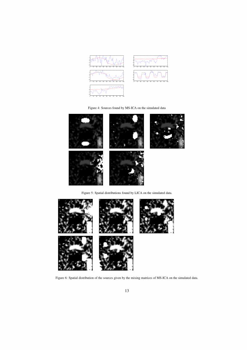
We have applied the LICA and MS-ICA algorithms to this simulated data. Weobtain five lattice sources with the LICA approach using standard settings of the algo-rithm, and we set the MS-ICA number of sources to that number. Figure 3 presents thelattice sources found by ILSIA, with the best correlated simulated time course overlaidin red. Figure 4 shows the sources found by the MS-ICA together with the best corre-lated simulated time course. Note that ILSIA finds both a task related and a function-related source. We show in figure 5 the abundance images that correspond to the spatial

1Simulated data can be generated with the tools provided inhttp://mlsp.umbc.edu/simulated_fmri_data.html

11

Task: 1 Task: 2 Task: 3 Task: 4

Task: 5 Task: 6 Task: 7 Task: 8

Figure 2: Simulated spatial distribution of location of the sources

0 10 20 30 40 50 60 70 80 90 100

−2

−1

0

1

2

0 10 20 30 40 50 60 70 80 90 100

−2

−1

0

1

2

0 10 20 30 40 50 60 70 80 90 100

−2

−1

0

1

2

0 10 20 30 40 50 60 70 80 90 100

−2

−1

0

1

2

0 10 20 30 40 50 60 70 80 90 100

−2

−1

0

1

2

Figure 3: Sources found by the ILSIA on the simulated data

distributions of the lattice sources. Notice that the spatial location of the task-relatedsource is well detected in the second image, while the transient task-related source lo-cation is also well detected despite that it does not appear as one of the best correlatedsources in figure 14. Because the LICA and ICA algorithms are unsupervised, theycan discover sources which indirectly help discover the spatial locations of interest, al-though the sources themselves are not precise matches of the underlying true sources.Figure 6 shows the spatial distribution of the MS-ICA sources. The detection is noisierthan in the results obtained by LICA, and the task-related spatial locations are not soclearly detected. Table 1 contains the quantitative measure of the goodness of spatialdiscovery, given by the Mutual Information similarity measure between the simulatedspatial distributions of the simulated sources and the mixing coefficients that give theestimation of the spatial distribution of the discovered sources. We have highlightedthe maximum values per column, and we have highlighted the closest one when it isnear the maximum of the column. The MS-ICA has more ambiguous columns than theLICA, which is in agreement with the visual assessment of figures 5 and 6.

12

0 10 20 30 40 50 60 70 80 90 100

−2

−1

0

1

0 10 20 30 40 50 60 70 80 90 100

−2

−1

0

1

0 10 20 30 40 50 60 70 80 90 100

−2

−1

0

1

0 10 20 30 40 50 60 70 80 90 100

−2

−1

0

1

0 10 20 30 40 50 60 70 80 90 100

−2

−1

0

1

Figure 4: Sources found by MS-ICA on the simulated data

Figure 5: Spatial distributions found by LICA on the simulated data.

Figure 6: Spatial distribution of the sources given by the mixing matrices of MS-ICA on the simulated data.

13

MS-ICA LICA

Source #1 #2 #3 #4 #5 #1 #2 #3 #4 #5#1 -0,16 0,15 0,03 1,18 -0,36 -0,52 2,51 -0,37 -0,23 0,02#2 -0,45 -0,78 -0,13 -0,38 -0,29 -0,48 -0,33 2,26 -0,13 -0,38#3 1,29 1,09 2,32 0,79 1,18 0,31 1,66 0,25 2,42 2,24#4 -0,28 0,68 -0,56 -0,63 -0,38 -0,57 -0,72 -0,53 -0,52 -0,50#5 -1,42 -1,05 -0,80 -0,69 -0,70 -0,71 -0,76 -0,70 -0,57 -0,72#6 1,33 -0,79 -0,30 -0,39 -0,60 2,26 -0,44 0,36 -0,50 -0,54#7 0,62 1,51 0,17 -0,24 0,80 0,30 -0,20 -0,57 -0,01 0,55#8 -0,92 -0,81 -0,72 -0,63 -0,62 -0,59 -0,71 -0,68 -0,47 -0,67

Table 1: Mutual Information similitude between the spatial locations discovered by LICA and MA-ICA andthe ground truth spatial locations.

7. Results on a standard case study

The experimental data for this benchmarking corresponds to auditory stimulationtest data of a single person2. These whole brain BOLD/EPI images were acquired ona modified 2T Siemens MAGNETOM Vision system. Each acquisition consisted of64 contiguous slices. Each slice being a 2D image of one head volume cut. Thereare 64x64x64 voxels of size 3mm x 3mm x 3mm. The data acquisition took 6.05s.,with the scan-to-scan repeat time (RT) set arbitrarily to 7s., 96 acquisitions were made(RT=7s.) in blocks of 6, i.e., 16 blocks of 42s. duration. The condition for successiveblocks alternated between rest and auditory stimulation, starting with rest. Auditorystimulation was bi-syllabic words presented binaurally at a rate of 60 per minute. Dueto T1 effects it is advisable to discard the first few scans (there were no "dummy" lead-in scans). We have discarded the first 10 scans. An standard results obtained with theSPM software is presented in figure 7 as localized in the Talairach space, in sagital,coronal and axial cuts.

There are a number of sources of noise in the fMRI signal [28] that must be dealtwith in appropriate preprocessing steps [25]. We have dealt with these noise sourcesfollowing the standard procedures in SPM software, so that all the algorithms ap-plied have the same input data quality. First, we realigned the volumes to account forhead motion artifacts. Second, we coregistered the functional volumes with the struc-tural MRI T1-weighted volume. Third, we performed spatial normalization guided bythe structural volume segmentation. Finally, we performed a smoothing step with anisotropic Gaussian kernel.

As already discussed in [9], we perform a Lattice Normalization, subtracting themean value of each voxel time series independently so that the plots are collapsedaround the origin. This mean subtraction corresponds to an scale normalization in theLattice Computing sense. It removes scale effects that hinder the detection of mean-ingful lattice independent vectors. Note that, although we are shifting the voxel vector

2The dataset is freely available from ftp://ftp.fil.ion.ucI.ac.uk/spm/data, the file name is snrfM00223.zip.The functional data starts at acquisition 4, image snrfMOO223-004.

14

Figure 7: Activation maps obtained with an execution of SPM software with nominal parameters over thecase study data.

15

# PCA ML-ICA MF-ICA MS-ICA FastICA LICA1 0.04 -0.14 -0.13 -0.04 -0.06 0.202 0.02 0.09 -0.14 0.22 -0.16 0.093 -0.08 -0.01 0.12 -0.07 0.08 -0.074 -0.22 -0.03 -0.13 0.07 -0.12 0.175 0.03 0.37 -0.13 -0.20 -0.18 0.146 0.10 0.12 -0.12 -0.13 0.11 0.097 0.33 0.12 -0.04 -0.07 -0.10 -0.158 0.34 -0.09 0.05 0.19 0.03 -0.079 -0.15 0.18 0.11 0.06 0.25 0.06

10 -0.09 -0.14 -0.18 0.16 0.05 0.0211 0.24 -0.15 0.15 -0.25 -0.07 0.09

Table 2: Correlation between lattice sources found by LICA, the sources found by the ICA algorithms, thePCA’s eigenvectors and the task control variable.

to the origin, we are not aiming to perform a normalization in the statistical sense.We have proceeded as follows: first we have applied the ILSIA algorithm, de-

scribed in section 5, obtaining a number of lattice sources. Then we have applied thecomparative algorithms (PCA, ML-ICA, MF-ICA, MS-ICA and FastICA) setting thenumber of lattice sources to the number obtained by LICA. Table 2 shows the corre-lation of the induced lattice sources and independent sources with the time plot of theexperiment control variable, which is zero during the resting state and one while theauditory stimulation is taking place. This correlation is a measure of how well eachlattice source/source is related to the task. The source with the maximum correlationfor each algorithm is an indication of the a corresponding spatial distribution of mixingcoefficients that may have the best similitude with the SPM activation results of figure7. To verify this hypothesis, we further computed the Mutual Information similitudemeasure among the mixing coefficients of each source and the SPM t-statistics map be-fore thresholding. Table 3 contains these Mutual Information values, which in generalconfirm the results of table 2. Therefore, we discover both the underlying task (whichis set for the GLM in SPM) and the activation pattern. A qualitative assessment of thealgorithms follows by visual comparison of the results of SPM (shown in figure 7) withthe voxel clusters detected on the mixing coefficient volumes with highest Mutual In-formation for each algorithm. Cluster detection in the abundance images correspondsto voxels with abundance value above the 99% percentile of the distribution of this lat-tice source/source abundance coefficients over the whole volume. Cluster detection isshown as white voxels in the corresponding images. The goal is to reproduce the activ-ity detection in the auditory cortex that the SPM is able to find. To asses this detectionwe reproduce selected axial, coronal and sagital cuts that correspond approximately tothe brain cuts shown in the reference SPM result image shown in figure 7. In figures8 to 13, the top row shows the axial and coronal cuts and the bottom row will showthe sagital cuts lying approximately in the auditory cortex at both sides of the brain.Notice that in some cases there are activations detected over the air region, which anundesirable result.

16

# PCA ML-ICA MF-ICA MS-ICA FastICA LICA1 -0.30 -0.21 -0.17 -0.37 -0.97 3,022 0.02 -045 -0.46 1.48 -1.60 -0.303 -0.30 -0.71 -0.46 -1.17 0.34 -0.304 -0.22 -0.85 -0.43 0.53 1.11 -0.305 -0.03 2.60 -0.46 -0.39 -0.76 -0.306 -0.30 -0.56 -0.46 -0.98 0.18 -0.307 0.33 -0.78 -0.46 -0.13 -0.59 -0.308 3.020 -0.09 -0.38 1.35 0.30 -0.309 -0.35 -0.52 0.02 -1.29 1.99 -0.30

10 -0.39 0.75 0.35 -0.21 -0.30 -0.3011 0.24 -0.06 2.91 1.17 0.31 -0.30

Table 3: Mutual Information similarity between the mixing volumes computed by LICA, the ICA algorithms,the PCA and the t-statistic computed by the SPM software (before thresholding).

Figure 8: Best matching activation detection over the abundances of the LICA approach.

17

Figure 9: Best matching activation detection over the abundances of the PCA approach.

Figure 10: Best matching activation detection over the abundances of the ML-ICA approach.

18

Figure 11: Best matching activation detection over the abundances of the MS-ICA approach.

Figure 12: Best matching activation detection over the abundances of the FastICA approach.

19

Figure 13: Best matching activation detection over the abundances of the MF-ICA approach.

0 10 20 30 40 50 60 70 80−4

−2

0

2

LICA Component:1

0 10 20 30 40 50 60 70 80−4

−2

0

2

LICA Component:2

0 10 20 30 40 50 60 70 80−4

−2

0

2

LICA Component:3

0 10 20 30 40 50 60 70 80−4

−2

0

2

LICA Component:4

0 10 20 30 40 50 60 70 80−4

−2

0

2

LICA Component:5

0 10 20 30 40 50 60 70 80−4

−2

0

2

LICA Component:6

0 10 20 30 40 50 60 70 80−4

−2

0

2

LICA Component:7

0 10 20 30 40 50 60 70 80−4

−2

0

2

LICA Component:8

0 10 20 30 40 50 60 70 80−4

−2

0

2

LICA Component:9

0 10 20 30 40 50 60 70 80−4

−2

0

2

LICA Component:10

0 10 20 30 40 50 60 70 80−4

−2

0

2

LICA Component:11

Figure 14: Lattice sources found by ILSIA, after normalization, for the LICA approach. Task indicatorvariable overlaid in red.

To show the degree of discovery of the control variable that models the control taskby each algorithm, we reproduce in figures 14 to 19 the sources found by each algo-rithm, the lattice sources of LICA, the statistically independent sources of ICA, and theeigenvectors of the PCA. For this visualization, each source has been normalized com-puting its z-score, in order to highlight its structure and made it visually comparablewith the control variable. The control variable plot is overlaid in read on each sourceplot.

We note that our approach gives qualitative and quantitative results comparable tothe well established ICA approaches. That seems to support the idea that Lattice Inde-pendence involves properties somehow least similar to that of Statistical Independence.

20

0 20 40 60 80

−2

0

2

ICA MF Component:1

0 20 40 60 80

−2

0

2

ICA MF Component:2

0 20 40 60 80

−2

0

2

ICA MF Component:3

0 20 40 60 80

−2

0

2

ICA MF Component:4

0 20 40 60 80

−2

0

2

ICA MF Component:5

0 20 40 60 80

−2

0

2

ICA MF Component:6

0 20 40 60 80

−2

0

2

ICA MF Component:7

0 20 40 60 80

−2

0

2

ICA MF Component:8

0 20 40 60 80

−2

0

2

ICA MF Component:9

0 20 40 60 80

−2

0

2

ICA MF Component:10

0 20 40 60 80

−2

0

2

ICA MF Component:11

Figure 15: Sources found by MF-ICA, after normalization. Task indicator variable overlaid in red.

0 20 40 60 80

−2

0

2

ICA ML Component:1

0 20 40 60 80

−2

0

2

ICA ML Component:2

0 20 40 60 80

−2

0

2

ICA ML Component:3

0 20 40 60 80

−2

0

2

ICA ML Component:4

0 20 40 60 80

−2

0

2

ICA ML Component:5

0 20 40 60 80

−2

0

2

ICA ML Component:6

0 20 40 60 80

−2

0

2

ICA ML Component:7

0 20 40 60 80

−2

0

2

ICA ML Component:8

0 20 40 60 80

−2

0

2

ICA ML Component:9

0 20 40 60 80

−2

0

2

ICA ML Component:10

0 20 40 60 80

−2

0

2

ICA ML Component:11

Figure 16: Sources found by ML-ICA, after normalization. Task indicator variable overlaid in red.

21

0 20 40 60 80

−2

0

2

FAST−ICA Component:1

0 20 40 60 80

−2

0

2

FAST−ICA Component:2

0 20 40 60 80

−2

0

2

FAST−ICA Component:3

0 20 40 60 80

−2

0

2

FAST−ICA Component:4

0 20 40 60 80

−2

0

2

FAST−ICA Component:5

0 20 40 60 80

−2

0

2

FAST−ICA Component:6

0 20 40 60 80

−2

0

2

FAST−ICA Component:7

0 20 40 60 80

−2

0

2

FAST−ICA Component:8

0 20 40 60 80

−2

0

2

FAST−ICA Component:9

0 20 40 60 80

−2

0

2

FAST−ICA Component:10

0 20 40 60 80

−2

0

2

FAST−ICA Component:11

Figure 17: Sources found by FastICA, after normalization. Task indicator variable overlaid in red.

0 20 40 60 80

−2

0

2

PCA Component:1

0 20 40 60 80

−2

0

2

PCA Component:2

0 20 40 60 80

−2

0

2

PCA Component:3

0 20 40 60 80

−2

0

2

PCA Component:4

0 20 40 60 80

−2

0

2

PCA Component:5

0 20 40 60 80

−2

0

2

PCA Component:6

0 20 40 60 80

−2

0

2

PCA Component:7

0 20 40 60 80

−2

0

2

PCA Component:8

0 20 40 60 80

−2

0

2

PCA Component:9

0 20 40 60 80

−2

0

2

PCA Component:10

0 20 40 60 80

−2

0

2

PCA Component:11

Figure 18: Eigenvectors found by PCA, after normalization. Task indicator variable overlaid in red.

22

0 20 40 60 80

−2

0

2

ICA MS Component:1

0 20 40 60 80

−2

0

2

ICA MS Component:2

0 20 40 60 80

−2

0

2

ICA MS Component:3

0 20 40 60 80

−2

0

2

ICA MS Component:4

0 20 40 60 80

−2

0

2

ICA MS Component:5

0 20 40 60 80

−2

0

2

ICA MS Component:6

0 20 40 60 80

−2

0

2

ICA MS Component:7

0 20 40 60 80

−2

0

2

ICA MS Component:8

0 20 40 60 80

−2

0

2

ICA MS Component:9

0 20 40 60 80

−2

0

2

ICA MS Component:10

0 20 40 60 80

−2

0

2

ICA MS Component:11

Figure 19: Sources found by MS-ICA, after normalization. Task indicator variable overlaid in red.

8. Summary and Conclusions

We have proposed and applied a Lattice Independent Component Analysis (LICA)to the model-free (unsupervised) analysis of fMRI. The LICA is based on the appli-cation of the Lattice Computing based algorithm ILSIA for the selection of the latticesources, and the linear unmixing of the data based on these lattice sources. We havediscussed the similarities of our approach with the application of ICA to fMRI ac-tivation detection [3, 25]. In our approach the temporal sources correspond to latticesources detected by the ILSIA algorithm and the spatial mixing coefficients correspondto the abundance volumes obtained by unmixing the voxel time series on the basis ofthe found lattice sources. We have benefited from recent results on the Chebyshev bestapproximation and on the equivalence between SLI and affine independence. After anormalization consisting in the subtraction of the vector mean value, we look for SLIvectors that can not be well approximated by a fixed point of the LAAM constructedwith the selected lattice sources. The LICA approach then uses this set of vectors tocompute the mixing coefficients that characterize the data and the lattice source. Weperform the activation detection thresholding these coefficients on the basis of its his-togram. Work on simulated fMRI data shows that LICA performance is comparable toor improves over the ICA approach in the sense of discovering task-related sources andtheir spatial locations. Working with a well-known case study, have found that LICAgives results consistent with the SPM standard approach. Compared to ICA algorithms,LICA reproduces also the SPM results. An important feature of our approach is that itis an unsupervised algorithm, where we do not need to postulate a priori information ormodels. Also, LICA does not impose a probabilistic model on the sources. The latticeindependence condition may be a more relaxed restriction to find meaningful sourcesin data where ICA approaches can fail due to their statistical properties.

23

Besides some other open theoretical questions, we want to state conveniently, andsolve, the problem of finding the right number of lattice sources, and the right latticesources. Those are non trivial problems in many other context (i.e. clustering), statedand solved as some kind of minimization problem. In our context, the problem is fur-ther complicated by the intrinsic non-linearity of ILSIA and the interleaving of thelinear and non-linear procedures in LICA. It is not evident at this moment how to for-mulate a well behaved objective function for such purposes. Besides these fundamentalproblems, we will extend the validation evidence that may give the confidence to applythe method to new fMRI data sets as an exploratory tool by itself. We wishfully thinkthat it could be applied to event oriented experiments, and to the task of discoveringnetworks of activation in the brain.

Acknowledgements

We are grateful to the comments of the anonymous reviewers, which have helpedus to improve the paper. The fruitful discussions with Dr. A. López de Munain and Dr.Sistiaga, from the Neurology Department, Donostia Hospital, which is embedded in theCentro de Investigación Biomédica en Red sobre Enfermedades Neurodegenerativas(CIBERNED) are also appreciated.

References

[1] A.L. Buffington, C.A. Hanlon, and M.J. McKeown. Acute and persistentpain modulation of attention-related anterior cingulate fmri activations. Pain,113:172–184, 2005.

[2] V. Calhoun, G. Pearlson, and T. Adali. Independent component analysis appliedto fMRI data: A generative model for validating results. The Journal of VLSISignal Processing, 37(2):281–291, June 2004.

[3] V.D. Calhoun and T. Adali. Unmixing fMRI with independent component analy-sis. Engineering in Medicine and Biology Magazine, IEEE, 25(2):79–90, 2006.

[4] V.D. Calhoun, J.J. Pekar, and G.D. Pearlson. Alcohol intoxication effects onsimulated driving: Exploring alcohol-dose effects on brain activation using func-tional mri. Neuropsychopharmacology, 29(11):2097–2107, 2004.

[5] K.J. Friston, J.T. Ashburner, S.J. Kiebel, T.E. Nichols, and Penny W.D. (eds.).Statistical Parametric Mapping, the analysis of functional brain images. Aca-demic Press, 2007.

[6] K.J. Friston, A.P. Holmes, K.J. Worsley, J.P. Poline, C.D. Frith, and R.S.J. Frack-owiak. Statistical parametric maps in functional imaging: A general linear ap-proach. Hum. Brain Map., 2(4):189–210, 1995.

[7] M. Graña. A brief review of lattice computing. In Proc. WCCI 2008, pages1777–1781, 2008.

24

[8] M. Graña, I. Villaverde, J.O. Maldonado, and C. Hernandez. Two lattice com-puting approaches for the unsupervised segmentation of hyperspectral images.Neurocomputing, 72(10-12):2111–2120, 2009.

[9] Manuel Graña, M. García-Sebastian, I. Villaverde, and E. Fernández. An ap-proach from lattice computing to fMRI analysis. In LBM 2008 (CLA 2008), Pro-ceedings of the Lattice-Based Modeling Workshop, pages 33–44, 2008.

[10] M.D. Greicius, G. Srivastava, A.L. Reiss, and V. Menon. Default-mode networkactivity distinguishes alzheimer’s disease from healthy aging: Evidence fromfunc- tional mri. Proc. Nat. Acad. Sci. U.S.A., 101(13):4637–4642, 2004.

[11] L. K. Hansen, J. Larsen, and T. Kolenda. Blind detection of independent dynamiccomponents. In proc. IEEE ICASSP’2001, 5:3197–3200, 2001.

[12] P. Højen-Sørensen, O. Winther, and L.K. Hansen. Mean field approaches to inde-pendent component analysis. Neural Computation, 14:889–918, 2002.

[13] A. Hyvärinen, J. Karhunen, and E. Oja. Independent Component Analysis. JohnWiley & Sons, New York, 2001.

[14] A. Hyvärinen and E. Oja. A fast fixed-point algorithm for independent componentanalysis. Neural Comp., 9:1483–1492, 1997.

[15] C.L. Lawson and H.J. Hanson. Solving least squares problems. Prentice-Hall,(1974) Englewoods Cliffs NJ, 1974.

[16] L. Molgedey and H. Schuster. Separation of independent signals using time-delayed correlations. Physical Review Letters, 72(23):3634–3637, 1994.

[17] H.-P. Muller, E. Kraft, A. Ludolph, and S.N. Erne. New methods in fMRI analy-sis. Engineering in Medicine and Biology Magazine, IEEE, 21(5):134–142, 2002.

[18] J.J. Pekar. A brief introduction to functional MRI. Engineering in Medicine andBiology Magazine, IEEE, 25(2):24–26, 2006.

[19] B. Raducanu, M. Graña, and X. Albizuri. Morphological scale spaces and asso-ciative morphological memories: results on robustness and practical applications.J. Math. Imaging and Vision, 19(2):113–122, 2003.

[20] G. X. Ritter, J. L. Diaz-de Leon, and P. Sussner. Morphological bidirectionalassociative memories. Neural Networks, 12:851–867, 1999.

[21] G. X. Ritter, P. Sussner, and J. L. Diaz-de Leon. Morphological associative mem-ories. IEEE Trans. on Neural Networks, 9(2):281–292, 1998.

[22] G.X. Ritter and P. Gader. Fixed points of lattice transforms and lattice associativememories. In P. Hawkes, editor, Advances in Imaging and Electron Physics,volume 144, pages 165–242. Elsevier, San Diego, CA., 2006.

25

[23] G.X. Ritter, G. Urcid, and L. Iancu. Reconstruction of patterns from noisy in-puts using morphological associative memories. J. Math. Imaging and Vision,19(2):95–112, 2003.

[24] G.X. Ritter, G. Urcid, and M.S. Schmalz. Autonomous single-pass endmemberapproximation using lattice auto-associative memories. Neurocomputing, 72(10-12):2101–2110, 2009.

[25] G.E. Sarty. Computing Brain Activation Maps from fMRI Time-Series Images.Cambridge University Press, 2007.

[26] FastICA site. http://www.cis.hut.fi/projects/ica/fastica/.

[27] ICA site. http://isp.imm.dtu.dk/toolbox/ica/index.html.

[28] S.C. Strother. Evaluating fMRI preprocessing pipelines. Engineering in Medicineand Biology Magazine, IEEE, 25(2):27–41, 2006.

[29] P. Sussner and M.E. Valle. Gray-scale morphological associative memories. IEEEtrans. Neural Networks, 17(3):559–570, 2006.

[30] G. Urcid and J.C. Valdiviezo. Generation of lattice independent vector sets forpattern recognition applications. In Mathematics of Data/Image Pattern Recog-nition, Compression, Coding, and Encryption X with Applications, volume 6700,pages 1–12. Proc of SPIE, 2007.

[31] W Xiong, Y-O Li, H. Li, T. Adali, and V. D Calhoun. On ICA of complex-valued fMRI: advantages and order selection. In Acoustics, Speech and SignalProcessing, 2008. ICASSP 2008. IEEE International Conference on, pages 529–532, April 2008.

26