Low-dimensional lattice basis reduction revisited
51
Low-Dimensional Lattice Basis Reduction Revisited PHONG Q. NGUYEN INRIA/ ´ Ecole Normale Sup´ erieure and DAMIEN STEHL ´ E CNRS/Universities of Macquarie, Sydney and Lyon/ ´ ENS Lyon/INRIA Lattice reduction is a geometric generalization of the problem of computing greatest common divisors. Most of the interesting algorithmic problems related to lattice reduction are NP-hard as the lattice dimension increases. This article deals with the low-dimensional case. We study a greedy lattice basis reduction algorithm for the Euclidean norm, which is arguably the most natural lattice basis reduction algorithm, because it is a straightforward generalization of an old two-dimensional algorithm of Lagrange, usually known as Gauss’ algorithm, and which is very similar to Euclid’s gcd algorithm. Our results are two-fold. From a mathematical point of view, we show that up to dimension four, the output of the greedy algorithm is optimal: the output basis reaches all the successive minima of the lattice. However, as soon as the lattice dimension is strictly higher than four, the output basis may be arbitrarily bad as it may not even reach the first minimum. More importantly, from a computational point of view, we show that up to dimension four, the bit-complexity of the greedy algorithm is quadratic without fast integer arithmetic, just like Euclid’s gcd algorithm. This was already proved by Semaev up to dimension three using rather technical means, but it was previously unknown whether or not the algorithm was still polynomial in dimension four. We propose two different analyzes: a global approach based on the geometry of the current basis when the length decrease stalls, and a local approach showing directly that a significant length decrease must occur every O(1) consecutive steps. Our analyzes simplify Semaev’s analysis in dimensions two and three, and unify the cases of dimensions two to four. Although the global approach is much simpler, we also present the local approach because it gives further information on the behavior of the algorithm. Categories and Subject Descriptors: F.2.1 [Theory of Computation]: Numerical Algorithms and Problems General Terms: Algorithms Additional Key Words and Phrases: Gauss’ algorithm, lattice reduction First author’s address: Phong Q. Nguyen, ´ Ecole Normale Sup´ erieure, D´ epartement d’informatique, 45 rue d’Ulm, 75230 Paris Cedex 05, France. http://www.di.ens.fr/~pnguyen/ Second author’s address: Damien Stehl´ e, Department of Mathematics and Statistics (F07), Uni- versity of Sydney, NSW 2006, Australia. http://perso.ens-lyon.fr/damien.stehle Permission to make digital/hard copy of all or part of this material without fee for personal or classroom use provided that the copies are not made or distributed for profit or commercial advantage, the ACM copyright/server notice, the title of the publication, and its date appear, and notice is given that copying is by permission of the ACM, Inc. To copy otherwise, to republish, to post on servers, or to redistribute to lists requires prior specific permission and/or a fee. c 2008 ACM. This is the author’s version of the work. It is posted here by permission of ACM for your personal use. Not for redistribution. The definitive version is to be published later on. ACM Journal Name, Vol. 0, No. 0, 00 2008, Pages 1–51.
-
Upload
independent -
Category
Documents
-
view
3 -
download
0
Transcript of Low-dimensional lattice basis reduction revisited
Low-Dimensional Lattice Basis Reduction
Revisited
PHONG Q. NGUYEN
INRIA/Ecole Normale Superieure
and
DAMIEN STEHLE
CNRS/Universities of Macquarie, Sydney and Lyon/ENS Lyon/INRIA
Lattice reduction is a geometric generalization of the problem of computing greatest commondivisors. Most of the interesting algorithmic problems related to lattice reduction are NP-hardas the lattice dimension increases. This article deals with the low-dimensional case. We studya greedy lattice basis reduction algorithm for the Euclidean norm, which is arguably the mostnatural lattice basis reduction algorithm, because it is a straightforward generalization of an oldtwo-dimensional algorithm of Lagrange, usually known as Gauss’ algorithm, and which is verysimilar to Euclid’s gcd algorithm. Our results are two-fold. From a mathematical point of view,we show that up to dimension four, the output of the greedy algorithm is optimal: the outputbasis reaches all the successive minima of the lattice. However, as soon as the lattice dimension isstrictly higher than four, the output basis may be arbitrarily bad as it may not even reach the firstminimum. More importantly, from a computational point of view, we show that up to dimensionfour, the bit-complexity of the greedy algorithm is quadratic without fast integer arithmetic, justlike Euclid’s gcd algorithm. This was already proved by Semaev up to dimension three usingrather technical means, but it was previously unknown whether or not the algorithm was stillpolynomial in dimension four. We propose two different analyzes: a global approach based onthe geometry of the current basis when the length decrease stalls, and a local approach showingdirectly that a significant length decrease must occur every O(1) consecutive steps. Our analyzessimplify Semaev’s analysis in dimensions two and three, and unify the cases of dimensions two tofour. Although the global approach is much simpler, we also present the local approach because
it gives further information on the behavior of the algorithm.
Categories and Subject Descriptors: F.2.1 [Theory of Computation]: Numerical Algorithmsand Problems
General Terms: Algorithms
Additional Key Words and Phrases: Gauss’ algorithm, lattice reduction
First author’s address: Phong Q. Nguyen, Ecole Normale Superieure, Departement d’informatique,45 rue d’Ulm, 75230 Paris Cedex 05, France. http://www.di.ens.fr/~pnguyen/
Second author’s address: Damien Stehle, Department of Mathematics and Statistics (F07), Uni-versity of Sydney, NSW 2006, Australia. http://perso.ens-lyon.fr/damien.stehle
Permission to make digital/hard copy of all or part of this material without fee for personalor classroom use provided that the copies are not made or distributed for profit or commercialadvantage, the ACM copyright/server notice, the title of the publication, and its date appear, andnotice is given that copying is by permission of the ACM, Inc. To copy otherwise, to republish,to post on servers, or to redistribute to lists requires prior specific permission and/or a fee.c© 2008 ACM. This is the author’s version of the work. It is posted here by permission of ACMfor your personal use. Not for redistribution. The definitive version is to be published later on.
ACM Journal Name, Vol. 0, No. 0, 00 2008, Pages 1–51.
2 · P. Q. Nguyen and D. Stehle
1. INTRODUCTION
A lattice is a discrete subgroup of Rn. Any lattice L has a lattice basis, i.e., a
set {b1, . . . ,bd} of linearly independent vectors such that the lattice is the set of
all integer linear combinations of the bi’s: L[b1, . . . ,bd] ={
∑di=1 xibi, xi ∈ Z
}
.
A lattice basis is usually not unique, but all the bases have the same number ofelements, called the dimension or rank of the lattice. In dimension higher thanone, there are infinitely many bases, but some are more interesting than others:they are called reduced. Roughly speaking, a reduced basis is a basis made ofreasonably short vectors that are almost orthogonal. Finding good reduced baseshas proved invaluable in many fields of computer science and mathematics, par-ticularly in cryptology (see for instance the survey [Nguyen and Stern 2001]); andthe computational complexity of lattice problems has attracted considerable atten-tion in the past few years (see for instance the book [Micciancio and Goldwasser2002]), following Ajtai’s discovery [1996] of a connection between the worst-caseand average-case complexities of certain lattice problems. Lattice reduction can beviewed as a geometric generalization of gcd computations.
There exist many different notions of reduction, such as those of Hermite [1850],Minkowski [1896], Hermite-Korkine-Zolotarev (HKZ) [Hermite 1905; Korkine andZolotarev 1873], Venkov [Ryskov 1972], Lenstra-Lenstra-Lovasz (LLL) [Lenstraet al. 1982], etc. Among these, the most intuitive one is perhaps Minkowski’s, andup to dimension four it is arguably optimal compared to all other known reductions,because it reaches all the so-called successive minima of a lattice. However, findinga Minkowski-reduced basis or a HKZ-reduced basis is NP-hard under randomizedreductions as the dimension increases, because such bases contain a shortest latticevector and the shortest vector problem is NP-hard under randomized reductions [Aj-tai 1998]. In order to better understand lattice reduction, it is tempting to studythe low-dimensional case. Improvements in low-dimensional lattice reduction maylead to significant running-time improvements in high-dimensional lattice reduc-tion, as the best lattice reduction algorithms known in theory [Gama and Nguyen2008; Schnorr 1987] and in practice [Schnorr and Euchner 1994; Schnorr and Horner1995] for high-dimensional lattices are based on a repeated use of low-dimensionalHKZ-reduction.
Lagrange’s algorithm [1773] computes in quadratic time (without fast integerarithmetic [Schonhage and Strassen 1971]) a Minkowski-reduced basis of any two-dimensional lattice. This algorithm, which is a natural generalization of Euclid’s gcdalgorithm, was also described later by Gauss [1801], and is often erroneously calledGauss’ algorithm. It was extended to dimension three by Vallee [1986] and Semaev[2001]: Semaev’s algorithm is quadratic without fast integer arithmetic, whereasVallee’s has cubic complexity. More generally, Helfrich [1985] showed by means ofthe LLL algorithm [Lenstra et al. 1982] how to compute in cubic time a Minkowski-reduced basis of any lattice of fixed (arbitrary) dimension, but the hidden com-plexity constant grows very fast with the dimension. Finally, Eisenbrand and Rotedescribed in [2001] a lattice basis reduction algorithm with a quasi-linear time com-plexity in any fixed dimension, but it is based on exhaustive enumerations and thecomplexity seems to blow up very quickly when the dimension increases. Moreover,they use fast integer arithmetic [Schonhage and Strassen 1971].
ACM Journal Name, Vol. 0, No. 0, 00 2008.
Low-Dimensional Lattice Basis Reduction Revisited · 3
In this paper, we generalize Lagrange’s algorithm to arbitrary dimension. Al-though the obtained greedy algorithm is arguably the simplest lattice basis reduc-tion algorithm known, its analysis becomes remarkably more and more complex asthe dimension increases. Semaev [2001] was the first to prove that the algorithmwas still polynomial time in dimension three, but the polynomial-time complexityand the output quality remained open for higher dimension (see [Semaev 2001,Remark 5]). We show that up to dimension four, the greedy algorithm computesa Minkowski-reduced basis in quadratic time without fast arithmetic (which giveshope for a quasi-linear lime algorithm using fast arithmetic). This immediately im-plies that a shortest vector and a HKZ-reduced basis can be computed in quadratictime up to dimension four. Independently of the running time improvement, wehope our analysis may help to design new lattice reduction algorithms.
We propose two different approaches, both based on geometric properties of low-dimensional lattices, which generalize two different analyzes of Lagrange’s algo-rithm. The global approach generalizes up to dimension four the two-dimensionalanalysis of Vallee [1991], and that of Akhavi [2000] where it was used to boundthe number of loop iterations of the so-called optimal LLL algorithm in any di-mension. Our generalization is different from this one. Roughly speaking, theglobal approach considers the following question: what does happen when the al-gorithm stops working well, that is, when it no longer shortens much the longestbasis vector? The local approach considers a dual question: can we bound directlythe number of consecutive steps necessary to significantly shorten the basis vec-tors? In dimension two, this method is very close to the argument given by Semaevin [2001], which is itself very different from previous analyzes of Lagrange’s algo-rithm [Kaib and Schnorr 1996; Lagarias 1980; Vallee 1991]. In dimension three,Semaev’s analysis [2001] is based on a rather exhaustive analysis of all the possiblebehaviors of the algorithm, which involves quite a few computations and makes itdifficult to extend to higher dimension. We replace the main technical argumentsby geometrical considerations on two-dimensional lattices. This makes it possibleto extend the analysis to dimension four, by carefully studying geometrical prop-erties of three-dimensional lattices, although a few additional technical difficultiesappear.
The global approach provides a quicker proof of the main result, but less insighton the local behavior of the algorithm, i.e., how the algorithm makes progress insuccessive loop iterations. The local approach relies on more subtle geometricalproperties of low-dimensional lattices, including the shapes of their Voronoı cells.
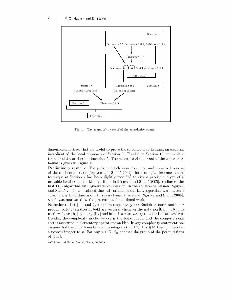
Road-map of the paper: In Section 2, we recall useful facts about lattices. InSection 3, we recall Lagrange’s algorithm and give two different complexity analyzes.In Section 4 we describe its natural greedy generalization. Section 5 provides anefficient low-dimensional closest vector algorithm, which is the core of the greedyalgorithm. In Section 6, we give our global approach to bound the number ofloop iterations of the algorithm, and in Section 7 we prove the claimed quadraticcomplexity bound. In Section 8 we give an alternative proof for the bound ofthe number of loop iterations, the so-called local approach. In dimension belowfour, the quadratic complexity bound can also be derived from Sections 8 and 7independently of Section 6. In Section 9, we prove geometrical results on low-
ACM Journal Name, Vol. 0, No. 0, 00 2008.
4 · P. Q. Nguyen and D. Stehle
PSfrag replacements
Section 7
Section 5
Section 6 Section 8
Section 9
(Local approach)(Global approach)
(211-case)
Theorem 6.0.5
Theorem 8.0.4
Lemmata 8.1.1, 8.1.3, 8.1.4Lemmata 8.1.1, 8.1.3, 8.1.4
Lemma 9.2.5
Lemma 8.2.1
Theorem 8.1.5
Lemmata 9.3.2, 9.3.3Lemma 9.3.4
Fig. 1. The graph of the proof of the complexity bound.
dimensional lattices that are useful to prove the so-called Gap Lemma, an essentialingredient of the local approach of Section 8. Finally, in Section 10, we explainthe difficulties arising in dimension 5. The structure of the proof of the complexitybound is given in Figure 1.
Preliminary remark: The present article is an extended and improved versionof the conference paper [Nguyen and Stehle 2004]. Interestingly, the cancellationtechnique of Section 7 has been slightly modified to give a precise analysis of aprovable floating-point LLL algorithm, in [Nguyen and Stehle 2005], leading to thefirst LLL algorithm with quadratic complexity. In the conference version [Nguyenand Stehle 2004], we claimed that all variants of the LLL algorithm were at leastcubic in any fixed dimension: this is no longer true since [Nguyen and Stehle 2005],which was motivated by the present low-dimensional work.
Notation: Let ‖ · ‖ and 〈·, ·〉 denote respectively the Euclidean norm and innerproduct of R
n; variables in bold are vectors; whenever the notation [b1, . . . ,bd]≤ isused, we have ‖b1‖ ≤ . . . ≤ ‖bd‖ and in such a case, we say that the bi’s are ordered.Besides, the complexity model we use is the RAM model and the computationalcost is measured in elementary operations on bits. In any complexity statement, weassume that the underlying lattice L is integral (L ⊆ Z
n). If x ∈ R, then bxe denotesa nearest integer to x. For any n ∈ N, Sn denotes the group of the permutationsof J1, nK.
ACM Journal Name, Vol. 0, No. 0, 00 2008.
Low-Dimensional Lattice Basis Reduction Revisited · 5
2. PRELIMINARIES
We assume the reader is familiar with geometry of numbers (see [Cassels 1971;Martinet 2002; Siegel 1989]).
2.1 Some Basic Definitions
We first recall some basic definitions related to Gram-Schmidt orthogonalizationand the first minima.
Gram matrix and orthogonality-defect. Let b1, . . . ,bd be vectors. The Grammatrix G(b1, . . . ,bd) of b1, . . . ,bd is the d × d symmetric matrix (〈bi,bj〉)1≤i,j≤d
formed by all the inner products. The vectors b1, . . . ,bd are linearly independentif and only if the determinant of G(b1, . . . ,bd) is not zero. The volume vol L of alattice L is the square root of the determinant of the Gram matrix of any basis of L.The orthogonality-defect of a basis (b1, . . . ,bd) of L is defined as δ⊥(b1, . . . ,bd) =
(∏d
i=1 ‖bi‖)/vol L: it is always greater than 1, with equality if and only if the basisis orthogonal.
Gram-Schmidt orthogonalization and size-reduction. Let (b1, . . . ,bd) belinearly independent vectors. The Gram-Schmidt orthogonalization (b∗
1, . . . ,b∗d) is
defined as follows: b∗i is the component of bi that is orthogonal to the subspace
spanned by the vectors b1, . . . ,bi−1. Any basis vector bi can be expressed asa (real) linear combination of the previous b∗
j ’s. We define the Gram-Schmidtcoefficients µi,j ’s as the coefficients of these linear combinations, namely, for any i ∈J1, dK:
bi = b∗i +
∑
j<i
µi,jb∗j .
We have the equality µi,j =〈bi,b
∗
j 〉‖b∗
j‖2 , for any j < i.
A lattice basis (b1, . . . ,bd) is said to be size-reduced if its Gram-Schmidt coef-ficients µi,j ’s all satisfy: |µi,j | ≤ 1/2. Size-reduction was introduced by Lagrange[1773], and can be easily achieved by subtracting to each bi a suitable linear com-
bination∑i−1
j=1 xjbj of the previous bj ’s, for each i = 2, . . . , d.
Successive minima and the Shortest Vector Problem. Let L be a d-dimen-sional lattice in R
n. For 1 ≤ i ≤ d, the i-th minimum λi(L) is the radius of thesmallest closed ball centered at the origin containing at least i linearly independentlattice vectors. The most famous lattice problem is the shortest vector problem(SVP): given a basis of a lattice L, find a lattice vector whose norm is exactly λ1(L).There always exist linearly independent lattice vectors vi’s such that ‖vi‖ = λi(L)for all i. Amazingly, as soon as d ≥ 4 such vectors do not necessarily form a latticebasis, and when d ≥ 5 there may not even exist a lattice basis reaching all theminima.
ACM Journal Name, Vol. 0, No. 0, 00 2008.
6 · P. Q. Nguyen and D. Stehle
2.2 Different Types of Strong Reduction
Several types of strong lattice basis reductions are often considered in the liter-ature. The following list is not exhaustive but includes the most frequent ones:Minkowski’s and Hermite-Korkine-Zolotarev’s. Notice that though mathematicallydifferent, these two reductions are computationally very close in low dimension:one can derive a reduced basis of one type from a reduced basis of the other typevery efficiently.
Minkowski reduction. A basis [b1, . . . ,bd]≤ of a lattice L is Minkowski-reducedif for all 1 ≤ i ≤ d, the vector bi has minimal norm among all lattice vectors bi
such that [b1, . . . ,bi]≤ can be extended to a basis of L. Equivalently:
Lemma 2.2.1. A basis [b1, . . . ,bd]≤ of a lattice L is Minkowski-reduced if andonly if for any i ∈ J1, dK and for any integers x1, . . . , xd such that xi, . . . , xd arealtogether coprime, we have:
‖x1b1 + . . . + xdbd‖ ≥ ‖bi‖.With the above statement, one might think that to ensure that a given basis
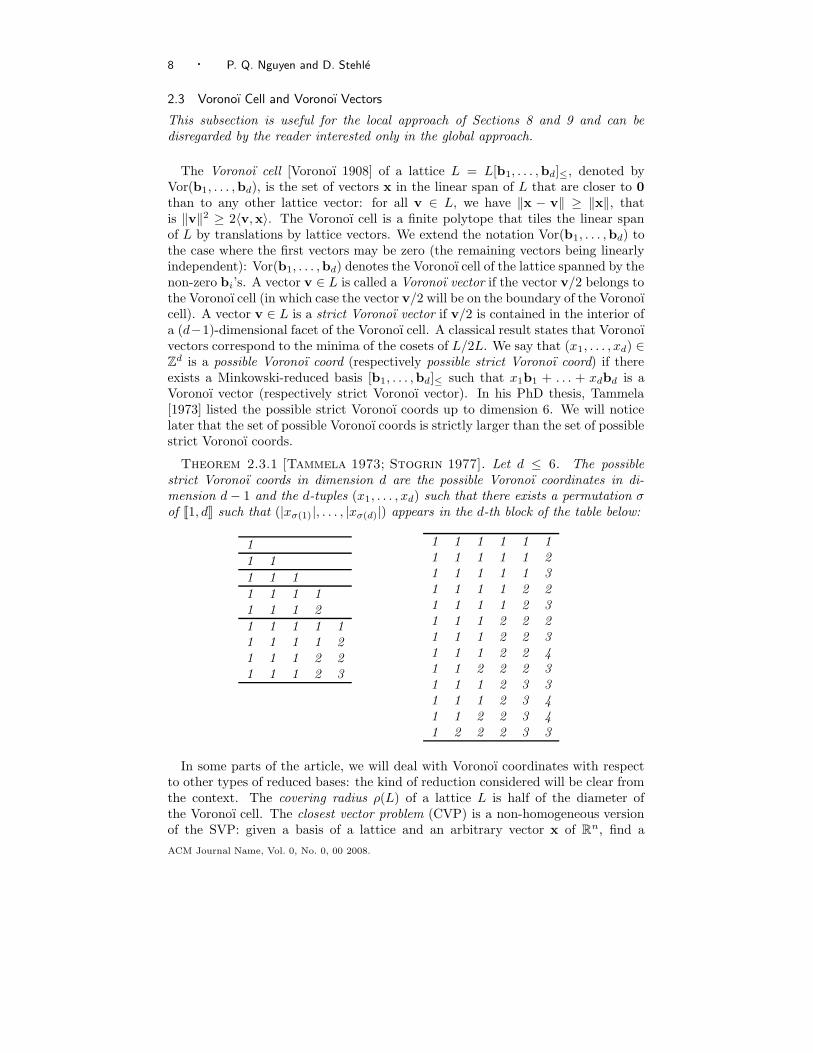
is Minkowski reduced, there are infinitely many conditions to be checked. Fortu-nately, a classical result states that in any fixed dimension, it is sufficient to checka finite subset of them. This result is described as the second finiteness theoremin [Siegel 1989]. Several sufficient sets of conditions are possible. We call Minkowskiconditions such a subset with minimal cardinality. Minkowski conditions have beenobtained by Tammela [1973] up to dimension 6. As a consequence, in low dimen-sion, one can check very quickly if a basis is Minkowski-reduced by checking theseconditions.
Theorem 2.2.2 [Minkowski conditions]. Let d ≤ 6. A basis [b1, . . . ,bd]≤of L is Minkowski-reduced if and only if for any i ≤ d and for any integers x1, . . . , xd
that satisfy both conditions below, we have the inequality:
‖x1b1 + . . . + xdbd‖ ≥ ‖bi‖.(1 ) The integers xi, . . . , xd are altogether coprime,
(2 ) For some permutation σ of J1, dK, (|xσ(1)|, . . . , |xσ(d)|) appears in the list below(where blanks eventually count as zeros).
1 11 1 11 1 1 11 1 1 1 11 1 1 1 21 1 1 1 1 11 1 1 1 1 21 1 1 1 2 21 1 1 1 2 3
Moreover this list is minimal, which means that if any condition is disregarded, thena basis can satisfy all the others without being Minkowski-reduced.
ACM Journal Name, Vol. 0, No. 0, 00 2008.
Low-Dimensional Lattice Basis Reduction Revisited · 7
A basis of a d-dimensional lattice that reaches the d minima must be Minkowski-reduced, but a Minkowski-reduced basis may not reach all the minima, exceptthe first four ones (see [van der Waerden 1956]): if [b1, . . . ,bd]≤ is a Minkowski-reduced basis of L, then for all 1 ≤ i ≤ min(d, 4) we have ‖bi‖ = λi(L), but the besttheoretical upper bound known for ‖bd‖/λd(L) grows exponentially in d. Therefore,a Minkowski-reduced basis is optimal in a natural sense up to dimension four. Arelated classical result (see [van der Waerden 1956]) states that the orthogonality-defect of a Minkowski-reduced basis can be upper-bounded by a constant that onlydepends on the lattice dimension.
Hermite reduction. Hermite [1905] defined different types of reduction, whichsometimes creates confusions. In particular, Hermite reduction differs from what wecall below Hermite-Korkine-Zolotarev reduction. An ordered basis [b1, . . . ,bd]≤ isHermite-reduced if it is the smallest basis of L for the lexicographic order: forany other basis [b′
1, . . . ,b′d]≤ of L, we must have ‖b1‖ = ‖b′
1‖, . . . , ‖bi−1‖ =‖b′
i−1‖ and ‖b′i‖ > ‖bi‖ for some i ∈ J1, dK. In particular a Hermite-reduced basis
is always Minkowski-reduced. The converse is true as long as d ≤ 6 (see [Ryskov1972]).
Hermite-Korkine-Zolotarev reduction. This reduction is often called moresimply Korkine-Zolotarev reduction. A basis (b1, . . . ,bd) of a lattice L is Hermite-Korkine-Zolotarev-reduced (HKZ-reduced for short) if ‖b1‖ = λ1(L) and for any i ≥2, the vector bi is a lattice vector having minimal nonzero distance to the linearspan of b1, . . . ,bi−1, and the basis is size-reduced, that is, its Gram-Schmidt co-efficients µi,j have absolute values ≤ 1/2. In high dimension, the reduction ofHermite-Korkine-Zolotarev [Hermite 1905; Korkine and Zolotarev 1873] seems tobe stronger than Minkowski’s: all the elements of a HKZ-reduced basis are knownto be very close to the successive minima (see [Lagarias et al. 1990]), while in thecase of Minkowski reduction the best upper bound known for for the approximationto the successive minima grows exponentially with the dimension [van der Waerden1956], as mentioned previously. In dimension two, HKZ reduction is equivalent toMinkowski’s. But in dimension three, there are lattices such that no Minkowski-reduced basis is HKZ-reduced:
Lemma 2.2.3. Let b1 = [100, 0, 0],b2 = [49, 100, 0] and b3 = [0, 62, 100]. ThenL[b1,b2,b3]≤ has no basis that is simultaneously Minkowski-reduced and HKZ-reduced.
Proof. First, the basis [b1,b2,b3]≤ is not HKZ-reduced because |µ3,2| = 62100 >
1/2. But it is Minkowski-reduced (it suffices to check the Minkowski conditions toprove it). Therefore [b1,b2,b3]≤ reaches the first three minima. More precisely, thevectors ±b1 are the only two vectors reaching the first minimum, the vectors ±b2
are the only two vectors reaching the second minimum and the vectors ±b3 arethe only two vectors reaching the third minimum. If the lattice L[b1,b2,b3]≤ hada basis which was both Minkowski-reduced and HKZ-reduced, this basis wouldreach the first three minima and would be of the kind [±b1,±b2,±b3]≤, whichcontradicts the fact that [b1,b2,b3]≤ is not HKZ-reduced.
ACM Journal Name, Vol. 0, No. 0, 00 2008.
8 · P. Q. Nguyen and D. Stehle
2.3 Voronoı Cell and Voronoı Vectors
This subsection is useful for the local approach of Sections 8 and 9 and can bedisregarded by the reader interested only in the global approach.
The Voronoı cell [Voronoı 1908] of a lattice L = L[b1, . . . ,bd]≤, denoted byVor(b1, . . . ,bd), is the set of vectors x in the linear span of L that are closer to 0
than to any other lattice vector: for all v ∈ L, we have ‖x − v‖ ≥ ‖x‖, thatis ‖v‖2 ≥ 2〈v,x〉. The Voronoı cell is a finite polytope that tiles the linear spanof L by translations by lattice vectors. We extend the notation Vor(b1, . . . ,bd) tothe case where the first vectors may be zero (the remaining vectors being linearlyindependent): Vor(b1, . . . ,bd) denotes the Voronoı cell of the lattice spanned by thenon-zero bi’s. A vector v ∈ L is called a Voronoı vector if the vector v/2 belongs tothe Voronoı cell (in which case the vector v/2 will be on the boundary of the Voronoıcell). A vector v ∈ L is a strict Voronoı vector if v/2 is contained in the interior ofa (d−1)-dimensional facet of the Voronoı cell. A classical result states that Voronoıvectors correspond to the minima of the cosets of L/2L. We say that (x1, . . . , xd) ∈Z
d is a possible Voronoı coord (respectively possible strict Voronoı coord) if thereexists a Minkowski-reduced basis [b1, . . . ,bd]≤ such that x1b1 + . . . + xdbd is aVoronoı vector (respectively strict Voronoı vector). In his PhD thesis, Tammela[1973] listed the possible strict Voronoı coords up to dimension 6. We will noticelater that the set of possible Voronoı coords is strictly larger than the set of possiblestrict Voronoı coords.
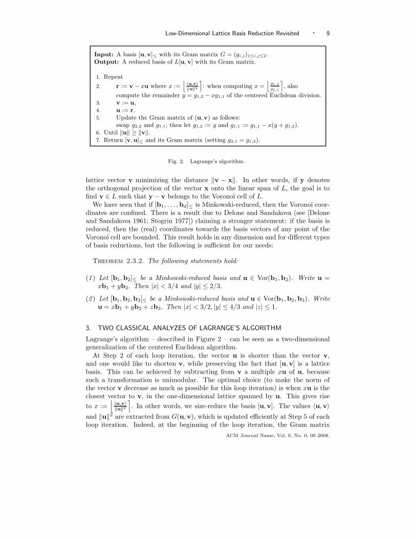
Theorem 2.3.1 [Tammela 1973; Stogrin 1977]. Let d ≤ 6. The possiblestrict Voronoı coords in dimension d are the possible Voronoı coordinates in di-mension d − 1 and the d-tuples (x1, . . . , xd) such that there exists a permutation σof J1, dK such that (|xσ(1)|, . . . , |xσ(d)|) appears in the d-th block of the table below:
11 11 1 11 1 1 11 1 1 21 1 1 1 11 1 1 1 21 1 1 2 21 1 1 2 3
1 1 1 1 1 11 1 1 1 1 21 1 1 1 1 31 1 1 1 2 21 1 1 1 2 31 1 1 2 2 21 1 1 2 2 31 1 1 2 2 41 1 2 2 2 31 1 1 2 3 31 1 1 2 3 41 1 2 2 3 41 2 2 2 3 3
In some parts of the article, we will deal with Voronoı coordinates with respectto other types of reduced bases: the kind of reduction considered will be clear fromthe context. The covering radius ρ(L) of a lattice L is half of the diameter ofthe Voronoı cell. The closest vector problem (CVP) is a non-homogeneous versionof the SVP: given a basis of a lattice and an arbitrary vector x of R
n, find a
ACM Journal Name, Vol. 0, No. 0, 00 2008.
Low-Dimensional Lattice Basis Reduction Revisited · 9
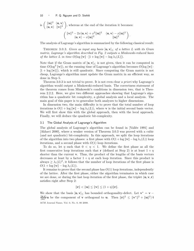
Input: A basis [u, v]≤ with its Gram matrix G = (gi,j)1≤i,j≤2.Output: A reduced basis of L[u, v] with its Gram matrix.
1. Repeat
2. r := v − xu where x :=j
〈u,v〉
‖u‖2
m
: when computing x =j
g1,2
g1,1
m
, also
compute the remainder y = g1,2 − xg1,1 of the centered Euclidean division.3. v := u,4. u := r,5. Update the Gram matrix of (u,v) as follows:
swap g2,2 and g1,1; then let g1,2 := y and g1,1 := g1,1 − x(y + g1,2).6. Until ‖u‖ ≥ ‖v‖.7. Return [v, u]≤ and its Gram matrix (setting g2,1 = g1,2).
Fig. 2. Lagrange’s algorithm.
lattice vector v minimizing the distance ‖v − x‖. In other words, if y denotesthe orthogonal projection of the vector x onto the linear span of L, the goal is tofind v ∈ L such that y − v belongs to the Voronoı cell of L.
We have seen that if [b1, . . . ,bd]≤ is Minkowski-reduced, then the Voronoı coor-dinates are confined. There is a result due to Delone and Sandakova (see [Deloneand Sandakova 1961; Stogrin 1977]) claiming a stronger statement: if the basis isreduced, then the (real) coordinates towards the basis vectors of any point of theVoronoı cell are bounded. This result holds in any dimension and for different typesof basis reductions, but the following is sufficient for our needs:
Theorem 2.3.2. The following statements hold:
(1 ) Let [b1,b2]≤ be a Minkowski-reduced basis and u ∈ Vor(b1,b2). Write u =xb1 + yb2. Then |x| < 3/4 and |y| ≤ 2/3.
(2 ) Let [b1,b2,b3]≤ be a Minkowski-reduced basis and u ∈ Vor(b1,b2,b3). Writeu = xb1 + yb2 + zb3. Then |x| < 3/2, |y| ≤ 4/3 and |z| ≤ 1.
3. TWO CLASSICAL ANALYZES OF LAGRANGE’S ALGORITHM
Lagrange’s algorithm – described in Figure 2 – can be seen as a two-dimensionalgeneralization of the centered Euclidean algorithm.
At Step 2 of each loop iteration, the vector u is shorter than the vector v,and one would like to shorten v, while preserving the fact that [u,v] is a latticebasis. This can be achieved by subtracting from v a multiple xu of u, becausesuch a transformation is unimodular. The optimal choice (to make the norm ofthe vector v decrease as much as possible for this loop iteration) is when xu is theclosest vector to v, in the one-dimensional lattice spanned by u. This gives rise
to x :=⌊
〈u,v〉‖u‖2
⌉
. In other words, we size-reduce the basis [u,v]. The values 〈u,v〉and ‖u‖2 are extracted from G(u,v), which is updated efficiently at Step 5 of eachloop iteration. Indeed, at the beginning of the loop iteration, the Gram matrix
ACM Journal Name, Vol. 0, No. 0, 00 2008.
10 · P. Q. Nguyen and D. Stehle
is
(
‖u‖2 〈u,v〉〈u,v〉 ‖v‖2
)
, whereas at the end of the iteration it becomes:
(
‖v‖2 − 2x〈u,v〉 + x2‖u‖2 〈u,v〉 − x‖u‖2
〈u,v〉 − x‖u‖2 ‖u‖2
)
.
The analysis of Lagrange’s algorithm is summarized by the following classical result:
Theorem 3.0.3. Given as input any basis [u,v]≤ of a lattice L with its Grammatrix, Lagrange’s algorithm described in Fig. 2 outputs a Minkowski-reduced basisof the lattice L in time O(log ‖v‖ · [1 + log ‖v‖ − log λ1(L)]).
Note that if the Gram matrix of [u,v]≤ is not given, then it can be computed intime O(log2 ‖v‖), so the running time of Lagrange’s algorithm becomes O(log ‖v‖ ·[1 + log ‖v‖]), which is still quadratic. Since computing the Gram matrix is notcheap, Lagrange’s algorithm must update the Gram matrix in an efficient way, asdone in Step 5.
Theorem 3.0.3 is not trivial to prove. It is not even clear a priori why Lagrange’salgorithm would output a Minkowski-reduced basis. The correctness statement ofthe theorem comes from Minkowski’s conditions in dimension two, that is Theo-rem 2.2.2. Here, we give two different approaches showing that Lagrange’s algo-rithm has a quadratic bit complexity, a global analysis and a local analysis. Themain goal of this paper is to generalize both analyzes to higher dimensions.
In dimension two, the main difficulty is to prove that the total number of loopiterations is O(1 + log ‖v‖ − log λ1(L)), where v is the initial second basis vector.We will first show this with the global approach, then with the local approach.Finally, we will deduce the quadratic bit-complexity.
3.1 The Global Analysis of Lagrange’s Algorithm
The global analysis of Lagrange’s algorithm can be found in [Vallee 1991] and[Akhavi 2000], where a weaker version of Theorem 3.0.3 was proved with a cubic(and not quadratic) bit-complexity. In this approach, we split the loop iterationsof the algorithm into two phases: a first phase with O(1+ log ‖v‖− logλ1(L)) loopiterations, and a second phase with O(1) loop iterations.
To do so, let η such that 0 < η < 1. We define the first phase as all thefirst consecutive loop iterations such that r (defined at Step 2) is at least 1 + ηshorter than the current v. Thus, the product of the lengths of the basis vectorsdecreases at least by a factor 1 + η at each loop iteration. Since this product isalways ≥ λ1(L)2, it follows that the number of loop iterations of the first phase isO(1 + log ‖v‖ − log λ1(L)).
It remains to prove that the second phase has O(1) loop iterations, independentlyof the lattice. After the first phase, either the algorithm terminates in which casewe are done, or during the last loop iteration of the first phase, the triplet (u,v, r)satisfies right after Step 2:
‖r‖ < ‖u‖ ≤ ‖v‖ ≤ (1 + η)‖r‖.We show that the basis [u,v]≤ has bounded orthogonality-defect. Let v∗ = v −〈u,v〉‖u‖2 u be the component of v orthogonal to u. Then ‖r‖2 ≤ ‖v∗‖2 + ‖u‖2/4
ACM Journal Name, Vol. 0, No. 0, 00 2008.
Low-Dimensional Lattice Basis Reduction Revisited · 11
because [u, r] is size-reduced. Since ‖u‖ ≤ ‖v‖ ≤ (1 + η)‖r‖, this implies that:
‖v∗‖2 ≥(
1
(1 + η)2− 1
4
)
· ‖v‖2,
where 1/(1 + η)2 − 1/4 > 0 since 0 < η < 1. It follows that [u,v]≤ has boundedorthogonality-defect, namely:
δ⊥(u,v) =‖v‖‖v∗‖ ≤ 1/
√
1
(1 + η)2− 1
4.
This implies that the second phase has O(1) loop iterations, where the constantis independent of the lattice. Indeed, because the algorithm is greedy, each newvector “ri” created during each Step 2 of the second phase cannot be longer than u.But the number of lattice vectors w ∈ L such that ‖w‖ ≤ ‖u‖ is O(1). To see this,write w as w = w1u+w2v where w1, w2 ∈ Z. Since |〈w,v∗〉| ≤ ‖v‖2, it follows that|w2| ≤ ‖v‖2/‖v∗‖2 = δ⊥(u,v)2. So the integer w2 has only O(1) possible values:note that if η is chosen sufficiently small, we can even ensure δ⊥(u,v)2 < 2 andtherefore |w2| ≤ 1. And for each value of w2, the number of possibilities for theinteger w1 is at most two.
3.2 The Local Analysis of Lagrange’s Algorithm
We provide another proof of the classical result that Lagrange’s algorithm hasquadratic complexity. Compared to other proofs, our local method closely resem-bles the recent one of Semaev [2001], itself relatively different from [Akhavi andMoreira dos Santos 2004; Kaib and Schnorr 1996; Lagarias 1980; Vallee 1991]. Theanalysis is not optimal (as opposed to [Vallee 1991]) but its basic strategy canbe extended up to dimension four. This strategy gives more information on thebehavior of the algorithm. Consider the value of x at Step 2:
—If x = 0, this must be the last iteration of the loop.
—If |x| = 1, there are two cases:
—If ‖v − xu‖ ≥ ‖u‖, then this is the last loop iteration.
—Otherwise we have ‖u−xv‖ < ‖u‖, which means that u can be shortened withthe help of v. This can only happen if this is the first loop iteration, becauseof the greedy strategy: the vector u is the former vector v.
—Otherwise |x| ≥ 2, which implies that xu is not a Voronoı vector of the latticespanned by u. Intuitively, this means that xu is far from Vor(u), so that v−xu isconsiderably shorter than v. More precisely, if v∗ denotes again the component ofthe vector v that is orthogonal to u, we have ‖v‖2 > 3‖v−xu‖2 if this is not the
last loop iteration. Indeed, recall that v = 〈v,u〉‖u‖2 u+v∗. Since x =
⌊
〈v,u〉‖u‖2
⌉
is ≥ 2,
one has ‖v‖2 ≥ (3/2)2‖u‖2 + ‖v∗‖2. Then since v− xu =(
〈v,u〉‖u‖2 −
⌊
〈v,u〉‖u‖2
⌉)
u +
v∗, one has ‖v‖2 ≥ 2‖u‖2+‖v−xu‖2, which is greater than 3‖v−xu‖2 providedthat this is not the last loop iteration.
This shows that the product of the norms of the basis vectors decreases by amultiplicative factor of at least
√3 at each loop iteration except possibly the
ACM Journal Name, Vol. 0, No. 0, 00 2008.
12 · P. Q. Nguyen and D. Stehle
first and last ones. Thus, the number τ of loop iterations is upper bounded byO(1 + log ‖v‖ − log λ1(L)).
3.3 Quadratic Bit-Complexity
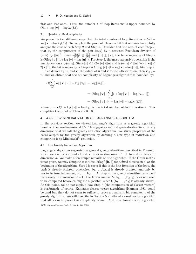
We proved in two different ways that the total number of loop iterations is O(1 +log ‖v‖−logλ1(L)). To complete the proof of Theorem 3.0.3, it remains to carefullyanalyze the cost of each Step 2 and Step 5. Consider first the cost of each Step 2,that is, the computation of the pair (x, y) by a centered Euclidean division of
〈u,v〉 by ‖u‖2. Since |〈u,v〉|‖u‖2 ≤ ‖v‖
‖u‖ and ‖u‖ ≤ ‖v‖, the bit complexity of Step 2
is O(log ‖v‖· [1+log‖v‖− log ‖u‖]). For Step 5, the most expensive operation is themultiplication x(y+g1,2). Since |x| ≤ 1/2+‖v‖/‖u‖ and |y+g1,2| ≤ ‖u‖2+|〈u,v〉| ≤2‖v‖2‖, the bit complexity of Step 5 is O(log ‖v‖· [1+log ‖v‖− log ‖u‖]) like Step 2.
If we denote by ui and vi the values of u and v at the i-th iteration, then vi+1 =ui and we obtain that the bit complexity of Lagrange’s algorithm is bounded by:
O(
τ∑
i=1
log ‖vi‖ · [1 + log ‖vi‖ − log ‖ui‖])
= O(log ‖v‖ ·τ∑
i=1
[1 + log ‖vi‖ − log ‖vi+1‖])
= O(log ‖v‖ · [τ + log ‖v‖ − log λ1(L)]),
where τ = O(1 + log ‖v‖ − log λ1) is the total number of loop iterations. Thiscompletes the proof of Theorem 3.0.3.
4. A GREEDY GENERALIZATION OF LAGRANGE’S ALGORITHM
In the previous section, we viewed Lagrange’s algorithm as a greedy algorithmbased on the one-dimensional CVP. It suggests a natural generalization to arbitrarydimension that we call the greedy reduction algorithm. We study properties of thebases output by the greedy algorithm by defining a new type of reduction andcomparing it to Minkowski’s reduction.
4.1 The Greedy Reduction Algorithm
Lagrange’s algorithm suggests the general greedy algorithm described in Figure 3,which uses reduction and closest vectors in dimension d − 1 to reduce bases indimension d. We make a few simple remarks on the algorithm. If the Gram matrixis not given, we may compute it in time O(log2 ‖bd‖) for a fixed dimension d, at thebeginning of the algorithm. Step 3 is easy: if this is the first iteration of the loop, thebasis is already ordered; otherwise, [b1, . . . ,bd−1] is already ordered, and only bd
has to be inserted among b1, . . . ,bd−1. At Step 4, the greedy algorithm calls itselfrecursively in dimension d − 1: the Gram matrix G(b1, . . . ,bd−1) does not needto be computed before calling the algorithm, since G(b1, . . . ,bd) is already known.At this point, we do not explain how Step 5 (the computation of closest vectors)is performed: of course, Kannan’s closest vector algorithms [Kannan 1983] couldbe used but they do not seem to suffice to prove a quadratic bit complexity of thegreedy algorithm. We will describe in Section 5 a tailored closest vector algorithmthat allows us to prove this complexity bound. And this closest vector algorithm
ACM Journal Name, Vol. 0, No. 0, 00 2008.
Low-Dimensional Lattice Basis Reduction Revisited · 13
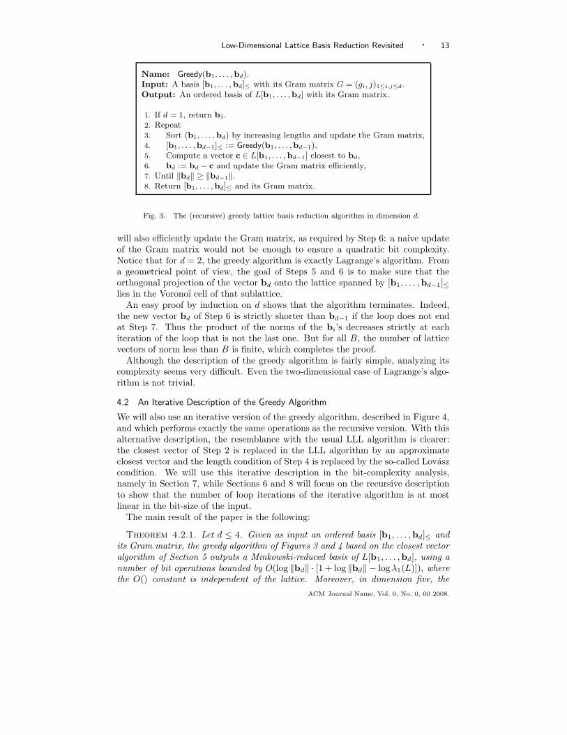
Name: Greedy(b1, . . . ,bd).Input: A basis [b1, . . . , bd]≤ with its Gram matrix G = (gi, j)1≤i,j≤d.Output: An ordered basis of L[b1, . . . ,bd] with its Gram matrix.
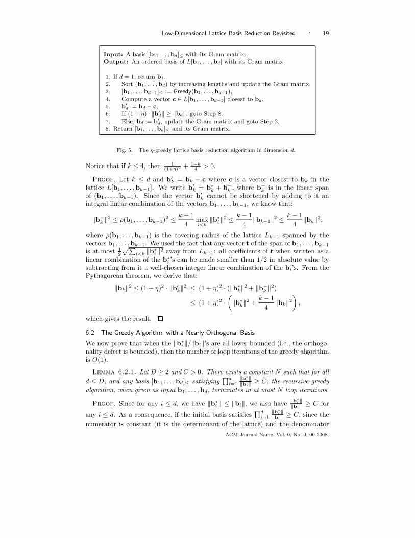
1. If d = 1, return b1.2. Repeat3. Sort (b1, . . . , bd) by increasing lengths and update the Gram matrix,4. [b1, . . . ,bd−1]≤ := Greedy(b1, . . . ,bd−1),5. Compute a vector c ∈ L[b1, . . . ,bd−1] closest to bd,6. bd := bd − c and update the Gram matrix efficiently,7. Until ‖bd‖ ≥ ‖bd−1‖.8. Return [b1, . . . , bd]≤ and its Gram matrix.
Fig. 3. The (recursive) greedy lattice basis reduction algorithm in dimension d.
will also efficiently update the Gram matrix, as required by Step 6: a naive updateof the Gram matrix would not be enough to ensure a quadratic bit complexity.Notice that for d = 2, the greedy algorithm is exactly Lagrange’s algorithm. Froma geometrical point of view, the goal of Steps 5 and 6 is to make sure that theorthogonal projection of the vector bd onto the lattice spanned by [b1, . . . ,bd−1]≤lies in the Voronoı cell of that sublattice.
An easy proof by induction on d shows that the algorithm terminates. Indeed,the new vector bd of Step 6 is strictly shorter than bd−1 if the loop does not endat Step 7. Thus the product of the norms of the bi’s decreases strictly at eachiteration of the loop that is not the last one. But for all B, the number of latticevectors of norm less than B is finite, which completes the proof.
Although the description of the greedy algorithm is fairly simple, analyzing itscomplexity seems very difficult. Even the two-dimensional case of Lagrange’s algo-rithm is not trivial.
4.2 An Iterative Description of the Greedy Algorithm
We will also use an iterative version of the greedy algorithm, described in Figure 4,and which performs exactly the same operations as the recursive version. With thisalternative description, the resemblance with the usual LLL algorithm is clearer:the closest vector of Step 2 is replaced in the LLL algorithm by an approximateclosest vector and the length condition of Step 4 is replaced by the so-called Lovaszcondition. We will use this iterative description in the bit-complexity analysis,namely in Section 7, while Sections 6 and 8 will focus on the recursive descriptionto show that the number of loop iterations of the iterative algorithm is at mostlinear in the bit-size of the input.
The main result of the paper is the following:
Theorem 4.2.1. Let d ≤ 4. Given as input an ordered basis [b1, . . . ,bd]≤ andits Gram matrix, the greedy algorithm of Figures 3 and 4 based on the closest vectoralgorithm of Section 5 outputs a Minkowski-reduced basis of L[b1, . . . ,bd], using anumber of bit operations bounded by O(log ‖bd‖ · [1 + log ‖bd‖ − log λ1(L)]), wherethe O() constant is independent of the lattice. Moreover, in dimension five, the
ACM Journal Name, Vol. 0, No. 0, 00 2008.
14 · P. Q. Nguyen and D. Stehle
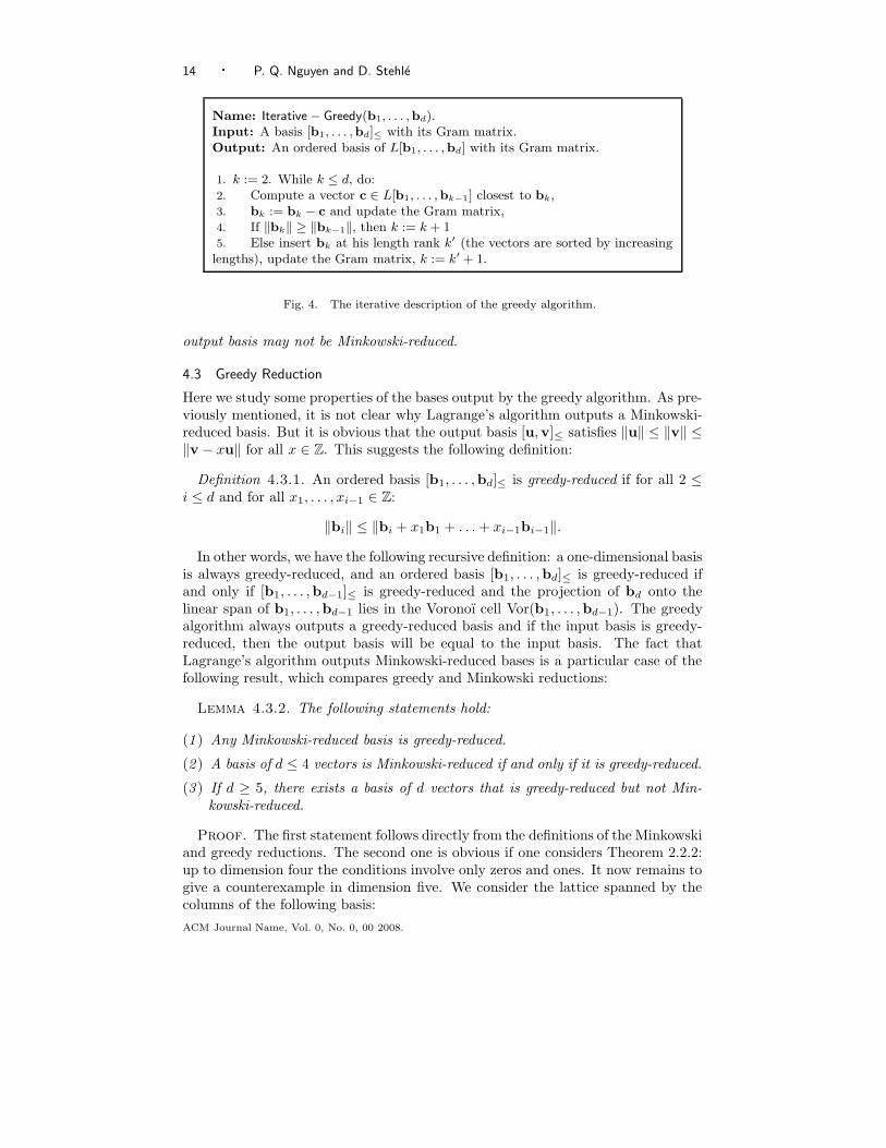
Name: Iterative − Greedy(b1, . . . ,bd).Input: A basis [b1, . . . ,bd]≤ with its Gram matrix.Output: An ordered basis of L[b1, . . . ,bd] with its Gram matrix.
1. k := 2. While k ≤ d, do:2. Compute a vector c ∈ L[b1, . . . ,bk−1] closest to bk,3. bk := bk − c and update the Gram matrix,4. If ‖bk‖ ≥ ‖bk−1‖, then k := k + 15. Else insert bk at his length rank k′ (the vectors are sorted by increasinglengths), update the Gram matrix, k := k′ + 1.
Fig. 4. The iterative description of the greedy algorithm.
output basis may not be Minkowski-reduced.
4.3 Greedy Reduction
Here we study some properties of the bases output by the greedy algorithm. As pre-viously mentioned, it is not clear why Lagrange’s algorithm outputs a Minkowski-reduced basis. But it is obvious that the output basis [u,v]≤ satisfies ‖u‖ ≤ ‖v‖ ≤‖v − xu‖ for all x ∈ Z. This suggests the following definition:
Definition 4.3.1. An ordered basis [b1, . . . ,bd]≤ is greedy-reduced if for all 2 ≤i ≤ d and for all x1, . . . , xi−1 ∈ Z:
‖bi‖ ≤ ‖bi + x1b1 + . . . + xi−1bi−1‖.
In other words, we have the following recursive definition: a one-dimensional basisis always greedy-reduced, and an ordered basis [b1, . . . ,bd]≤ is greedy-reduced ifand only if [b1, . . . ,bd−1]≤ is greedy-reduced and the projection of bd onto thelinear span of b1, . . . ,bd−1 lies in the Voronoı cell Vor(b1, . . . ,bd−1). The greedyalgorithm always outputs a greedy-reduced basis and if the input basis is greedy-reduced, then the output basis will be equal to the input basis. The fact thatLagrange’s algorithm outputs Minkowski-reduced bases is a particular case of thefollowing result, which compares greedy and Minkowski reductions:
Lemma 4.3.2. The following statements hold:
(1 ) Any Minkowski-reduced basis is greedy-reduced.
(2 ) A basis of d ≤ 4 vectors is Minkowski-reduced if and only if it is greedy-reduced.
(3 ) If d ≥ 5, there exists a basis of d vectors that is greedy-reduced but not Min-kowski-reduced.
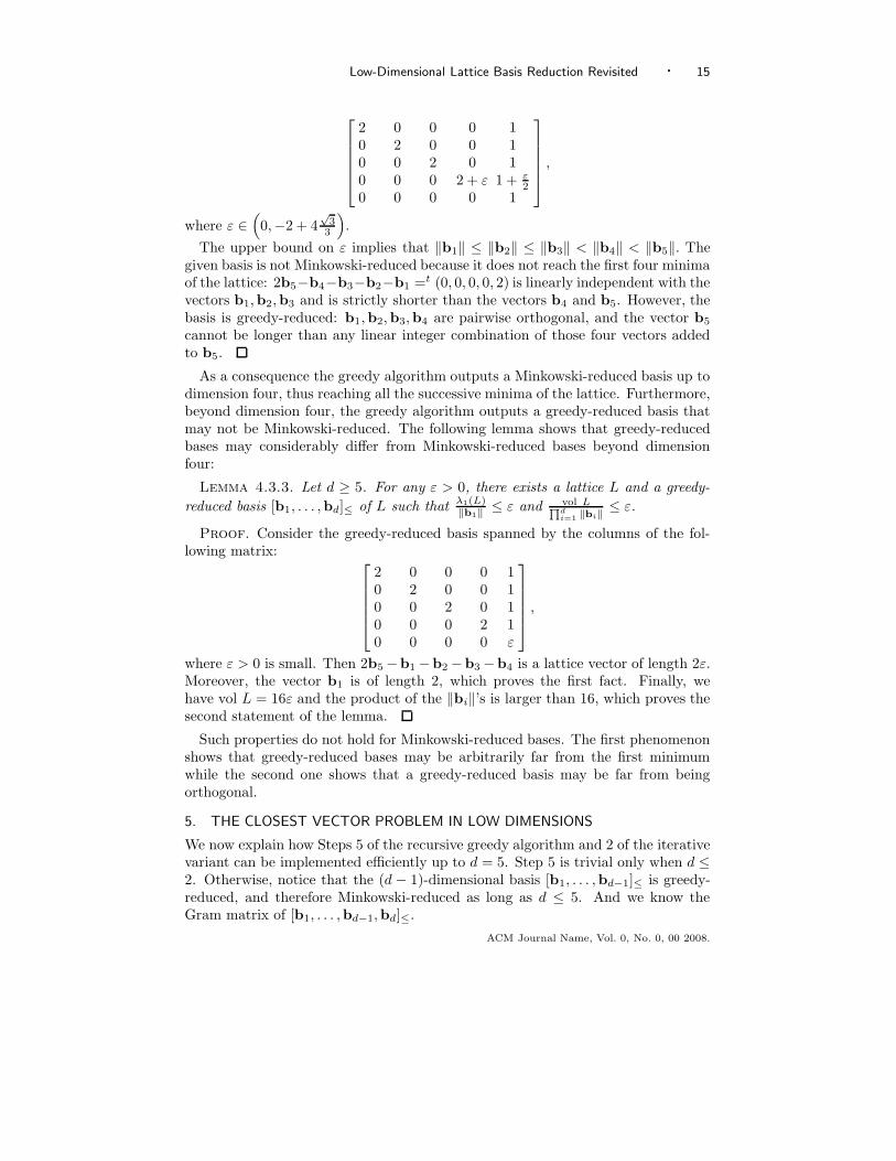
Proof. The first statement follows directly from the definitions of the Minkowskiand greedy reductions. The second one is obvious if one considers Theorem 2.2.2:up to dimension four the conditions involve only zeros and ones. It now remains togive a counterexample in dimension five. We consider the lattice spanned by thecolumns of the following basis:
ACM Journal Name, Vol. 0, No. 0, 00 2008.
Low-Dimensional Lattice Basis Reduction Revisited · 15
2 0 0 0 10 2 0 0 10 0 2 0 10 0 0 2 + ε 1 + ε
20 0 0 0 1
,
where ε ∈(
0,−2 + 4√
33
)
.
The upper bound on ε implies that ‖b1‖ ≤ ‖b2‖ ≤ ‖b3‖ < ‖b4‖ < ‖b5‖. Thegiven basis is not Minkowski-reduced because it does not reach the first four minimaof the lattice: 2b5−b4−b3−b2−b1 =t (0, 0, 0, 0, 2) is linearly independent with thevectors b1,b2,b3 and is strictly shorter than the vectors b4 and b5. However, thebasis is greedy-reduced: b1,b2,b3,b4 are pairwise orthogonal, and the vector b5
cannot be longer than any linear integer combination of those four vectors addedto b5.
As a consequence the greedy algorithm outputs a Minkowski-reduced basis up todimension four, thus reaching all the successive minima of the lattice. Furthermore,beyond dimension four, the greedy algorithm outputs a greedy-reduced basis thatmay not be Minkowski-reduced. The following lemma shows that greedy-reducedbases may considerably differ from Minkowski-reduced bases beyond dimensionfour:
Lemma 4.3.3. Let d ≥ 5. For any ε > 0, there exists a lattice L and a greedy-
reduced basis [b1, . . . ,bd]≤ of L such that λ1(L)‖b1‖ ≤ ε and vol L
Q
di=1
‖bi‖≤ ε.
Proof. Consider the greedy-reduced basis spanned by the columns of the fol-lowing matrix:
2 0 0 0 10 2 0 0 10 0 2 0 10 0 0 2 10 0 0 0 ε
,
where ε > 0 is small. Then 2b5 −b1 −b2 −b3 −b4 is a lattice vector of length 2ε.Moreover, the vector b1 is of length 2, which proves the first fact. Finally, wehave vol L = 16ε and the product of the ‖bi‖’s is larger than 16, which proves thesecond statement of the lemma.
Such properties do not hold for Minkowski-reduced bases. The first phenomenonshows that greedy-reduced bases may be arbitrarily far from the first minimumwhile the second one shows that a greedy-reduced basis may be far from beingorthogonal.
5. THE CLOSEST VECTOR PROBLEM IN LOW DIMENSIONS
We now explain how Steps 5 of the recursive greedy algorithm and 2 of the iterativevariant can be implemented efficiently up to d = 5. Step 5 is trivial only when d ≤2. Otherwise, notice that the (d − 1)-dimensional basis [b1, . . . ,bd−1]≤ is greedy-reduced, and therefore Minkowski-reduced as long as d ≤ 5. And we know theGram matrix of [b1, . . . ,bd−1,bd]≤.
ACM Journal Name, Vol. 0, No. 0, 00 2008.
16 · P. Q. Nguyen and D. Stehle
Theorem 5.0.4. Let d ≥ 1 be an integer. There exists an algorithm that, givenas input a Minkowski-reduced basis [b1, . . . ,bd−1]≤, a target vector t longer thanall the bi’s and the Gram matrix of [b1, . . . ,bd−1, t]≤, outputs a closest latticevector c to t (in the lattice spanned by the vectors b1, . . . ,bd−1) and the Grammatrix of (b1, . . . ,bd−1, t− c), in time:
O (log ‖t‖ · [1 + log ‖t‖ − log ‖bα‖]) ,
where α ∈ J1, dK is any integer such that [b1, . . . ,bα−1, t]≤ is Minkowski-reduced.
The index α appearing in the statement of the theorem requires an explanation.Consider the iterative version of the greedy algorithm. The index k can increaseand decrease rather arbitrarily. For a given loop iteration, the index α tells uswhich vectors have not changed since the last loop iteration for which the index khad the same value. Intuitively, the reason why we can make the index α appear inthe statement of the theorem is that we are working in the orthogonal complementof the vectors b1, . . . ,bα−1. The use of the index α is crucial. If we were using theweaker bound O(log ‖t‖ · [1+log ‖t‖− log ‖b1‖]), we would not be able to prove thequadratic bit complexity of the greedy algorithm. Rather, we would obtain a cubiccomplexity bound. This index α is also crucial for the quadratic bit complexity ofthe floating-point LLL described in [Nguyen and Stehle 2005].
Intuitively, the algorithm works as follows: an approximation of the coordinates(with respect to the bi’s) of the closest vector is computed using linear algebra andthe approximation is then corrected by a suitable exhaustive search.
Proof. Let h be the orthogonal projection of the vector t onto the linear spanof b1, . . . ,bd−1. We do not compute h but introduce it to simplify the description
of the algorithm. There exist y1, . . . , yd−1 ∈ R such that h =∑d−1
i=1 yibi. If c =∑d−1
i=1 xibi is a closest vector to t, then h−c belongs to Vor(b1, . . . ,bd−1). However,for any C > 0, the coordinates (with respect to any basis of orthogonality-defect ≤C) of any point inside the Voronoı cell can be bounded independently from thelattice (see [Stogrin 1977]). It follows that if we know an approximation of the yi’swith sufficient precision, then c can be derived from a O(1) exhaustive search,since the coordinates yi − xi of h − c are bounded (the orthogonality-defect ofthe Minkowski-reduced basis [b1, . . . ,bd−1]≤ is bounded). This exhaustive searchcan be performed in time O(log ‖t‖) since the Gram matrix of [b1, . . . ,bd−1, t]≤ isknown.
To approximate the yi’s, we use basic linear algebra. Let G = G(b1, . . . ,bd−1)
and H =(
〈bi,bj〉‖bi‖2
)
i,j<d. The matrix H is exactly G, where the i-th row has been
divided by ‖bi‖2. We have:
G ·
y1
...yd−1
= −
〈b1, t〉...
〈bd−1, t〉
, and thus
y1
...yd−1
= −H−1 ·
〈b1,t〉‖b1‖2
...〈bd−1,t〉‖bd−1‖2
. (1)
We use the latter formula to compute the yi’s with an absolute error≤ 1/2, within
the expected time. Let r = maxi
⌈
log |〈bi,t〉|‖bi‖2
⌉
. Notice that r = O(1 + log ‖t‖ −ACM Journal Name, Vol. 0, No. 0, 00 2008.
Low-Dimensional Lattice Basis Reduction Revisited · 17
log ‖bα‖), which can be obtained by bounding 〈bi, t〉 depending on whether i ≥ α:
if i < α, |〈bi, t〉| ≤ ‖bi‖2/2; otherwise, |〈bi, t〉| ≤ ‖bi‖2 · ‖t‖‖bi‖ ≤ ‖bi‖2 · ‖t‖
‖bα‖ . Notice
also that the entries of H are all ≤ 1 in absolute value (because [b1, . . . ,bd−1]≤ isMinkowski-reduced and therefore pairwise Lagrange-reduced), and that det(H) =
det(G)‖b1‖2...‖bd−1‖2 is lower bounded by some universal constant (because the orthogona-
lity-defect of the Minkowski-reduced basis [b1, . . . ,bd−1]≤ is bounded). It followsthat one can compute the entries of the matrix H−1 with an absolute precisionof Θ(r) bits, within O(r2) binary operations, for example by computing Θ(r)-bitlong approximations to both the determinant and the comatrix of H (though notefficient, it can be done with Leibniz formula). One eventually derives the yi’s withan absolute error ≤ 1/2, by a matrix-vector multiplication involving Θ(r) bit longapproximations to rational numbers.
From Equation (1) and the discussion above on the quantities 〈bi,t〉‖bi‖2 , we derive
that for any i, the integer |xi| ≤ |yi| + O(1) is O(1 + log ‖t‖ − log ‖bα‖) bit long.We now explicit the computation of the Gram matrix of (b1, . . . ,bd−1, t− c) fromthe Gram matrix of (b1, . . . ,bd−1, t). Only the entries from the last row (and lastcolumn, by symmetry) are changing. For the non-diagonal entries of the last row,we have:
〈bi, t − c〉 = 〈bi, t〉 −∑
j<d
xj〈bi,bj〉.
Because of the length upper bound on the xj ’s, this computation can be performedwithin the expected time. The same holds for the diagonal entry, by using theequality:
‖t− c‖2 = ‖t‖2 +∑
i<d
x2i ‖bi‖2 + 2
∑
i<j<d
xixj〈bi,bj〉 − 2∑
i<d
xi〈bi, t〉.
It can be proved that this result remains valid when replacing Minkowski reduc-tion by any kind of basis reduction that ensures a bounded orthogonality-defect, forexample LLL-reduction. Besides, notice that Theorem 2.3.2 can be used to makeTheorem 5.0.4 more practical: the bounds given in Theorem 2.3.2 help decreasingdrastically the cost of the exhaustive search following the linear algebra step.
6. THE GLOBAL APPROACH
In this section we describe the global approach to prove that there is a linear num-ber of loop iterations during the execution of the iterative version of the greedyalgorithm (as described in Figure 4). The goal of this global approach is to proveTheorem 6.0.5. The proof of this last theorem can be replaced by another one thatwe describe in Sections 8 and 9. We call this alternative proof the local approach.In both cases, the complexity analysis of the greedy algorithm finishes with Sec-tion 7. This last section makes use of the local and global approaches only throughTheorem 6.0.5.
In the present section, we describe a global analysis proving that the number ofloop iterations of the iterative greedy algorithm is at most linear in log ‖bd‖, as
ACM Journal Name, Vol. 0, No. 0, 00 2008.
18 · P. Q. Nguyen and D. Stehle
long as d ≤ 4. More precisely, we show that:
Theorem 6.0.5. Let d ≤ 4. Let b1, . . . ,bd be linearly independent vectors.The number of loop iterations performed during the execution of the iterative greedyalgorithm of Figure 4 given as input b1, . . . ,bd is bounded by O(1+log ‖bd‖−logλ1),where λ1 = λ1(L[b1, . . . ,bd]).
To obtain this result, we show that in any dimension d ≤ 4, there are at most N =O(1) consecutive loop iterations of the recursive algorithm described in Figure 3without a significant length decrease, i.e., without a decrease of the product of thelengths of the basis vectors by a factor higher than K for some constant K > 1. Thisfact implies that there cannot be more than Nd = O(1) consecutive loop iterationsof the iterative algorithm without a decrease of the product of the lengths of thebasis vectors by a factor higher than K. This immediately implies Theorem 6.0.5.More precisely, we prove the following:
Theorem 6.0.6. Let d ≤ 4. There exist two constants K > 1, N such that inany N consecutive loop iterations of the d-dimensional recursive greedy algorithmof Figure 3, the lengths of the current basis vectors decreases by at least a factor K.
Our proof of Theorem 6.0.6 is as follows. We first define two different phases inthe execution of the recursive d-dimensional greedy algorithm. In the first phase,when a vector is shortened, its length decreases by at least a factor of 1 + η forsome η > 0 to be fixed later. All these steps are good steps since they make theproduct of the lengths of the basis vectors decrease significantly. In the secondphase, the lengths of the vectors are not decreasing much, but we will show thatonce we enter this phase, the basis is nearly orthogonal and there remain very fewloop iterations.
6.1 Two Phases in the Recursive Greedy Algorithm
We divide the successive loop iterations of the recursive greedy algorithm into twophases: the η-phase and the remaining phase. The execution of the algorithmstarts with the η-phase. The loop iterations are in the η-phase as long as thenew vector bd of Step 6 is at least (1 + η) times shorter than the previous bd.Once there is no more a large length decrease, all the remaining loop iterations arein the remaining phase. More precisely, the η-phase is exactly made of the loopiterations of the η-greedy algorithm of Figure 5, which simulates the beginning ofthe execution of the greedy algorithm. The remaining phase corresponds to theexecution of the recursive greedy algorithm of Figure 3 given as input the outputbasis of the η-greedy algorithm.
It is clear that all loop iterations in the η-phase are good loop iterations: theproduct of the lengths of the basis vectors decreases by a factor higher than 1 + η.Moreover, if d ≤ 4, when the execution of the algorithm enters the remaining phase,the basis has a bounded orthogonality defect:
Lemma 6.1.1. Let d ≤ 4 and η ∈(
0,√
43 − 1
)
. Suppose the basis [b1, . . . ,bd]≤is invariant by the η-greedy algorithm of Figure 5. Then for any k ≤ d, we have:
‖b∗k‖2 ≥
(
1
(1 + η)2+
1 − k
4
)
· ‖bk‖2.
ACM Journal Name, Vol. 0, No. 0, 00 2008.
Low-Dimensional Lattice Basis Reduction Revisited · 19
Input: A basis [b1, . . . , bd]≤ with its Gram matrix.Output: An ordered basis of L[b1, . . . ,bd] with its Gram matrix.
1. If d = 1, return b1.2. Sort (b1, . . . , bd) by increasing lengths and update the Gram matrix,3. [b1, . . . ,bd−1]≤ := Greedy(b1, . . . ,bd−1),4. Compute a vector c ∈ L[b1, . . . ,bd−1] closest to bd,5. b′
d := bd − c,6. If (1 + η) · ‖b′
d‖ ≥ ‖bd‖, goto Step 8.7. Else, bd := b′
d, update the Gram matrix and goto Step 2.8. Return [b1, . . . , bd]≤ and its Gram matrix.
Fig. 5. The η-greedy lattice basis reduction algorithm in dimension d.
Notice that if k ≤ 4, then 1(1+η)2 + 1−k
4 > 0.
Proof. Let k ≤ d and b′k = bk − c where c is a vector closest to bk in the
lattice L[b1, . . . ,bk−1]. We write b′k = b∗
k + b−k , where b−
k is in the linear spanof (b1, . . . ,bk−1). Since the vector b′
k cannot be shortened by adding to it anintegral linear combination of the vectors b1, . . . ,bk−1, we know that:
‖b−k ‖2 ≤ ρ(b1, . . . ,bk−1)
2 ≤ k − 1
4maxi<k
‖b∗i ‖2 ≤ k − 1
4‖bk−1‖2 ≤ k − 1
4‖bk‖2,
where ρ(b1, . . . ,bk−1) is the covering radius of the lattice Lk−1 spanned by thevectors b1, . . . ,bk−1. We used the fact that any vector t of the span of b1, . . . ,bk−1
is at most 12
√∑
i<k ‖b∗i ‖2 away from Lk−1: all coefficients of t when written as a
linear combination of the b∗i ’s can be made smaller than 1/2 in absolute value by
subtracting from it a well-chosen integer linear combination of the bi’s. From thePythagorean theorem, we derive that:
‖bk‖2 ≤ (1 + η)2 · ‖b′k‖2 ≤ (1 + η)2 · (‖b∗
k‖2 + ‖b−k ‖2)
≤ (1 + η)2 ·(
‖b∗k‖2 +
k − 1
4‖bk‖2
)
,
which gives the result.
6.2 The Greedy Algorithm with a Nearly Orthogonal Basis
We now prove that when the ‖b∗i ‖/‖bi‖’s are all lower-bounded (i.e., the orthogo-
nality defect is bounded), then the number of loop iterations of the greedy algorithmis O(1).
Lemma 6.2.1. Let D ≥ 2 and C > 0. There exists a constant N such that for all
d ≤ D, and any basis [b1, . . . ,bd]≤ satisfying∏d
i=1‖b∗
i ‖‖bi‖ ≥ C, the recursive greedy
algorithm, when given as input b1, . . . ,bd, terminates in at most N loop iterations.
Proof. Since for any i ≤ d, we have ‖b∗i ‖ ≤ ‖bi‖, we also have
‖b∗
i ‖‖bi‖ ≥ C for
any i ≤ d. As a consequence, if the initial basis satisfies∏d
i=1‖b∗
i ‖‖bi‖ ≥ C, since the
numerator is constant (it is the determinant of the lattice) and the denominator
ACM Journal Name, Vol. 0, No. 0, 00 2008.
20 · P. Q. Nguyen and D. Stehle
decreases, then all the bases appearing in the execution of the greedy algorithm sat-isfy this condition. Any vector bi appearing during the execution of the algorithm
satisfies‖b∗
i ‖‖bi‖ ≥ C.
We define Xi = {(xi, . . . , xd), ∃(x1, . . . , xi−1) ∈ Zi−1, ‖∑j xjbj‖ ≤ ‖bi‖} for i ≤
d. We prove that |Xi| ≤ (1 + 2/C)d−i+1 by decreasing induction on i. Let b =x1b1 + . . . + xdbd with ‖b‖ ≤ ‖bd‖. By considering the component of the vector b
on b∗d, we have that |xd| ≤ 1/C. Suppose now that we want to prove the fact
for some i < d. Let b = x1b1 + . . . + xdbd with ‖b‖ ≤ ‖bi‖. Since the basis isordered, we have ‖b‖ ≤ ‖bi+1‖, which gives, by using the induction hypothesis,that (xi+1, . . . , xd) belongs to a finite set. Moreover, by taking the component of b
on b∗i , we obtain that:
∣
∣
∣
∣
∣
∣
xi +d∑
j=i+1
xj
〈bj ,b∗i 〉
‖b∗i ‖2
∣
∣
∣
∣
∣
∣
≤ 1/C.
This gives that for any choice of (xi+1, . . . , xd), there are at most 2/C + 1 possiblevalues for xi.
Consider now the execution of the greedy algorithm on such a basis: the numberof times a vector shorter than b1 is created is bounded by |X1| ≤ (1 + 2/C)d.Therefore we can subdivide the execution of the algorithm into phases in which b1
remains constant. Consider such a phase. Let b1, . . . ,bd be the initial basis of this
phase. It satisfies the condition∏d
i=1‖b∗
i ‖‖bi‖ ≥ C. At most |X2| ≤ (1+2/C)d−1 times
in this phase a vector shorter than b2 can be created: for any (x2, . . . , xd) ∈ X2,there are at most two possibilities for x1, because of the greedy choice in Steps 2of the iterative greedy algorithm and 5 of the recursive greedy algorithm. Thisshows that we can subdivide the execution of the algorithm into ≤ 2(1 + 2/C)2d−1
phases in which both b1 and b2 are constant. By using the bound on |Xi| and thefiniteness of the number of solutions for a closest vector problem instantiation (thisis the so-called kissing number, see [Conway and Sloane 1988]), this reasoning can beextended to subdivide the execution of the algorithm into phases in which b1, . . . ,bi
do not change, and we can bound the number of phases independently of the basis.The case i = d gives the result.
It follows that there are at most N loop iterations of the recursive algorithm withouta decrease of the product of the lengths of the basis vectors by a factor at leastK = 1 + η, where N is independent of the lattice. This implies that there are atmost Nd = O(1) consecutive loop iterations of the iterative algorithm without sucha decrease, which completes the proof of Theorem 6.0.5.
7. QUADRATIC BIT COMPLEXITY
In this subsection we use Theorems 5.0.4 and 6.0.5 of the two previous sectionsto prove the quadratic bit complexity claimed in Theorem 4.2.1. To do this, wegeneralize the cancellation phenomenon used in the analysis of Lagrange’s algorithmin Section 3.
Suppose that d ≤ 4. We consider the iterative version of the d-dimensional
greedy algorithm of Figure 4 and denote by [b(t)1 , . . . ,b
(t)d ]≤ the current ordered ba-
ACM Journal Name, Vol. 0, No. 0, 00 2008.
Low-Dimensional Lattice Basis Reduction Revisited · 21
PSfrag replacements
t
1
1 2
2
3
4
5 10 15
k(t) ϕ(7) = 6ϕ(16) = 13
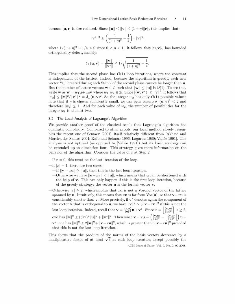
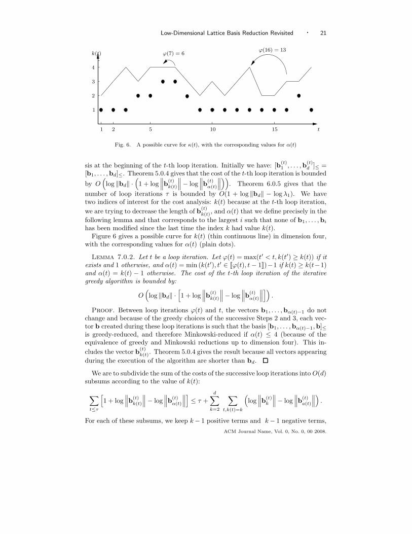
Fig. 6. A possible curve for κ(t), with the corresponding values for α(t)
sis at the beginning of the t-th loop iteration. Initially we have: [b(t)1 , . . . ,b
(t)d ]≤ =
[b1, . . . ,bd]≤. Theorem 5.0.4 gives that the cost of the t-th loop iteration is bounded
by O(
log ‖bd‖ ·(
1 + log∥
∥
∥b
(t)k(t)
∥
∥
∥− log
∥
∥
∥b
(t)α(t)
∥
∥
∥
))
. Theorem 6.0.5 gives that the
number of loop iterations τ is bounded by O(1 + log ‖bd‖ − log λ1). We havetwo indices of interest for the cost analysis: k(t) because at the t-th loop iteration,
we are trying to decrease the length of b(t)k(t), and α(t) that we define precisely in the
following lemma and that corresponds to the largest i such that none of b1, . . . ,bi
has been modified since the last time the index k had value k(t).Figure 6 gives a possible curve for k(t) (thin continuous line) in dimension four,
with the corresponding values for α(t) (plain dots).
Lemma 7.0.2. Let t be a loop iteration. Let ϕ(t) = max(t′ < t, k(t′) ≥ k(t)) if itexists and 1 otherwise, and α(t) = min (k(t′), t′ ∈ Jϕ(t), t − 1K)−1 if k(t) ≥ k(t−1)and α(t) = k(t) − 1 otherwise. The cost of the t-th loop iteration of the iterativegreedy algorithm is bounded by:
O(
log ‖bd‖ ·[
1 + log∥
∥
∥b
(t)k(t)
∥
∥
∥− log
∥
∥
∥b
(t)α(t)
∥
∥
∥
])
.
Proof. Between loop iterations ϕ(t) and t, the vectors b1, . . . ,bα(t)−1 do notchange and because of the greedy choices of the successive Steps 2 and 3, each vec-tor b created during these loop iterations is such that the basis [b1, . . . ,bα(t)−1,b]≤is greedy-reduced, and therefore Minkowski-reduced if α(t) ≤ 4 (because of theequivalence of greedy and Minkowski reductions up to dimension four). This in-
cludes the vector b(t)k(t). Theorem 5.0.4 gives the result because all vectors appearing
during the execution of the algorithm are shorter than bd.
We are to subdivide the sum of the costs of the successive loop iterations into O(d)subsums according to the value of k(t):
∑
t≤τ
[
1 + log∥
∥
∥b
(t)k(t)
∥
∥
∥− log
∥
∥
∥b
(t)α(t)
∥
∥
∥
]
≤ τ +
d∑
k=2
∑
t,k(t)=k
(
log∥
∥
∥b
(t)k
∥
∥
∥− log
∥
∥
∥b
(t)a(t)
∥
∥
∥
)
.
For each of these subsums, we keep k − 1 positive terms and k − 1 negative terms,
ACM Journal Name, Vol. 0, No. 0, 00 2008.
22 · P. Q. Nguyen and D. Stehle
and make the others vanish in a progressive cancellation. The crucial point to dothis is the following:
Lemma 7.0.3. Let k ∈ J2, dK and t1 < t2 < . . . < tk be loop iterations of theiterative greedy algorithm such that for any j < k, we have k(tj) = k. Then there
exists j < k with∥
∥
∥b
(tj)
α(tj)
∥
∥
∥≥∥
∥
∥b
(tk)k
∥
∥
∥.
Proof. We choose j = max (i ≤ k, α(ti) ≥ i). Here j is well-defined becausethe set of indices i is non-empty (it contains 1). Since α(tk) < k and k(tk) =k(tk−1) = k, there exists a first loop iteration Tk ∈ Jtk−1, tk − 1K such that k(Tk) ≥k ≥ k(Tk + 1). Because for a given index the lengths of the vectors are alwaysdecreasing, we have:
∥
∥
∥b
(tk)k
∥
∥
∥≤∥
∥
∥b
(Tk+1)k
∥
∥
∥≤∥
∥
∥b
(Tk)k−1
∥
∥
∥.
By definition of Tk the vectors b1, . . . ,bk−1 do not change between loop itera-tions tk−1 and Tk. Therefore:
∥
∥
∥b
(tk)k
∥
∥
∥≤∥
∥
∥b
(tk−1)k−1
∥
∥
∥.
If j = k−1, we have the result. Otherwise there exists a first loop iteration Tk−1 ∈Jtk−2, tk−1 − 1K such that k(Tk−1) ≥ k − 1 ≥ k(Tk−1 + 1). We have:
∥
∥
∥b
(tk−1)k−1
∥
∥
∥≤∥
∥
∥b
(Tk−1+1)k−1
∥
∥
∥≤∥
∥
∥b
(Tk−1)k−2
∥
∥
∥≤∥
∥
∥b
(tk−2)k−2
∥
∥
∥.
If j = k − 2 we have the result, otherwise we go on constructing such loop itera-tions Ti’s to obtain the result.
We can now finish the complexity analysis. Let k ∈ J2, dK and t1 < t2 < . . . <tτk
= {t ≤ τ, k(t) = k}. We have:
τk∑
i=1
(
log∥
∥
∥b
(ti)k
∥
∥
∥− log
∥
∥
∥b
(ti)α(ti)
∥
∥
∥
)
≤ k (log ‖bd‖ − log λ1)
+
τk∑
i=k
log∥
∥
∥b
(ti)k
∥
∥
∥−
τk−k+1∑
i=1
log∥
∥
∥b
(ti)α(ti)
∥
∥
∥,
where λ1 is the first minimum of the lattice we are reducing. Lemma 7.0.3 helpsbounding the right hand-side of the above bound. First, we apply it with t1, . . . , tk.
Thus there exists j < k such that ‖b(tk)k ‖ ≤ ‖b(tj)
α(tj)‖. The indices “i = k” in
the positive sum and “i = j” in the negative sum cancel out. Then we applyLemma 7.0.3 to tk+1 and the k − 1 first ti’s that remain in the negative sum. Itis easy to see that tk+1 is larger than any of them, so that we can have another“positive-negative” pair that cancels out. We perform this operation τk − k + 1times, to obtain:
τk∑
i=k
log∥
∥
∥b
(ti)k
∥
∥
∥−
τk−k+1∑
i=1
log∥
∥
∥b
(ti)α(ti)
∥
∥
∥≤ 0.
The fact that∑
k τk = τ = O (1 + log ‖bd‖ − log λ1) completes the proof of Theo-rem 4.2.1.
ACM Journal Name, Vol. 0, No. 0, 00 2008.
Low-Dimensional Lattice Basis Reduction Revisited · 23
8. THE LOCAL APPROACH
This section and the following give another proof for Theorem 6.0.6. They givea more precise understanding of the behavior of the algorithm but may be skippedsince they are not necessary to prove the main results of the paper.
In this section we give an alternative proof of Theorem 6.0.6 for d ≤ 4, that gen-eralizes the local analysis of Lagrange’s algorithm. The result is of the same flavor,but involves a more subtle analysis of the behavior of successive loop iterations.We will obtain that except for a few initial initial and final iterations, the productof the lengths of the basis vectors decreases by at least a factor K > 1 every d loopiterations.
Theorem 8.0.4. Let d ≤ 4. There exist three constants K > 1, I, F such that inany d consecutive loop iterations of the d-dimensional recursive greedy algorithm ofFigure 3, some of the iterations are in the I initial loop iterations or in the F finalloop iterations, or the product of the lengths of the current basis vectors decreasesby at least a factor K.
This result clearly implies Theorem 6.0.6. The global approach has the advantageof providing a quicker proof of Theorem 6.0.6 then the local approach. However, itprovides less insight on the behavior of the algorithm. The local approach explainswhy the algorithm actually makes progress in successive loop iterations, not onlyglobally.
8.1 A Unified Geometric Analysis Up To Dimension Four
The local analysis of Lagrange’s algorithm (Section 3) was based on the fact thatif |x| ≥ 2, the vector xu is far from the Voronoı cell of the lattice spanned by u. Theanalysis of the number of loop iterations of the greedy algorithm in dimensions threeand four relies on a similar phenomenon in dimensions two and three. However,the situation is more complex, as the following basic remarks hint:
—For d = 2, we considered the value of x, but if d ≥ 3, there will be severalcoefficients xi instead of a single one, and it is not clear which one will be usefulin the analysis.
—For d = 2, Step 4 cannot change the basis, as there are only two bases in dimen-sion one. If d ≥ 3, Step 4 may completely change the vectors, and it could behard to keep track of what is going on.
To prove Theorem 8.0.4, we introduce a few notations. Consider the i-th loop
iteration. Let[
a(i)1 , . . . , a
(i)d
]
≤denote the basis [b1, . . . ,bd]≤ at the beginning of
the i-th loop iteration. The basis[
a(i)1 , . . . , a
(i)d
]
≤becomes
[
b(i)1 , . . . ,b
(i)d−1, a
(i)d
]
≤
with∥
∥
∥b
(i)1
∥
∥
∥≤ . . . ≤
∥
∥
∥b
(i)d−1
∥
∥
∥after Step 4, and
(
b(i)1 , . . . ,b
(i)d
)
after Step 6, where
b(i)d = a
(i)d − c(i) and c(i) is the closest vector found at Step 5. Let pi be the
number of integers 1 ≤ j ≤ d such that∥
∥
∥b
(i)j
∥
∥
∥≤∥
∥
∥b
(i)d
∥
∥
∥. Let πi be the rank
of b(i)d once
(
b(i)1 , . . . ,b
(i)d
)
is sorted by length: for example, we have πi = 1
ACM Journal Name, Vol. 0, No. 0, 00 2008.
24 · P. Q. Nguyen and D. Stehle
if∥
∥
∥b
(i)d
∥
∥
∥<∥
∥
∥b
(i)1
∥
∥
∥. Notice that πi may not be equal to pi because there may
be several choices when sorting the vectors by length in case of length equalities.
Clearly 1 ≤ πi ≤ pi ≤ d, if pi = d then the loop terminates, and∥
∥
∥a
(i+1)πi
∥
∥
∥=
∥
∥
∥a
(i+1)pi
∥
∥
∥.
Now consider the (i+1)-th loop iteration for some i ≥ 1. Notice that by definition
of πi, we have a(i+1)πi = b
(i)d = a
(i)d − c(i), while
{
a(i+1)j
}
j 6=πi
={
b(i)j
}
j<d. The
vector c(i+1) belongs to L[
b(i+1)1 , . . . ,b
(i+1)d−1
]
= L[
a(i+1)1 , . . . , a
(i+1)d−1
]
: there exist
integers x(i+1)1 , . . . , x
(i+1)d−1 such that c(i+1) =
∑d−1j=1 x
(i+1)j a
(i+1)j .
We are to prove that there exists a universal constant K > 1 such that for anyexecution of the d-dimensional greedy algorithm with d ≤ 4, in any d consecutiveiterations of the loop (except eventually the first ones and the last ones), the productof the lengths of the current basis vectors decreases by some factor higher than K:
∥
∥
∥a
(i)1
∥
∥
∥. . .∥
∥
∥a
(i)d
∥
∥
∥
∥
∥
∥a
(i+d)1
∥
∥
∥. . .∥
∥
∥a
(i+d)d
∥
∥
∥
≥ K (2)
This will automatically ensure that the number of loop iterations is at most pro-
portional to log∥
∥
∥a
(1)d
∥
∥
∥− log λ1.
We deal with the first difficulty mentioned above: which one will be the useful
coefficient? The trick is to consider the value of x(i+1)πi , i.e., the coefficient of a
(i+1)πi =
a(i)d −c(i) in c(i+1), and to use the greedy properties of the algorithm. This coefficient
corresponds to the vector that has been created at the previous loop iteration.Since this vector has been created so that it cannot be shortened by adding to it acombination of the others, there are only two possibilities at the current iteration:
either the new vector is longer than a(i+1)πi , in which case pi increases (this cannot
happen during more than d successive iterations), either it is shorter and we musthave |xπi
| 6= 1.
Lemma 8.1.1. Among d consecutive iterations of the loop of the greedy algorithmof Figure 3, there is at least one iteration of index i + 1 such that pi+1 ≤ pi.
Moreover, for such a loop iteration, we have∣
∣
∣x
(i+1)πi
∣
∣
∣≥ 2, or this is the last loop
iteration.
Proof. The first statement is obvious. Consider one such loop iteration i + 1.
Suppose we have a small |x(i+1)πi |, that is x
(i+1)πi = 0 or
∣
∣
∣x
(i+1)πi
∣
∣
∣= 1.
—If x(i+1)πi = 0, then c(i+1) ∈ L
[
a(i+1)j
]
j 6=πi,j<d= L
[
b(i)1 , . . . ,b
(i)d−2
]
. We claim
that the (i+1)-th iteration must be the last one. Since the i-th loop iteration was
not terminal, we have a(i+1)d = b
(i)d−1. Moreover, the basis
[
b(i)1 , . . . ,b
(i)d−1
]
≤is
greedy-reduced because of Step 4 of the i-th loop iteration. These two facts imply
ACM Journal Name, Vol. 0, No. 0, 00 2008.
Low-Dimensional Lattice Basis Reduction Revisited · 25
that c(i+1) must be zero (or at least it does not make the length of a(i)d decrease
if there are several closest lattice vectors), and the (i + 1)-th loop iteration is thelast one.
—If |x(i+1)πi | = 1, we claim that pi+1 > pi. We have c(i+1) =
∑d−1j=1 x
(i+1)j a
(i+1)j
where a(i+1)πi = a
(i)d −c(i) and
{
a(i+1)j
}
j 6=πi
={
b(i)j
}
j<d. Thus, the vector c(i+1)
can be written as c(i+1) = ∓(
a(i)d − c(i)
)
− e where e ∈ L[
b(i)1 , . . . ,b
(i)d−1
]
.
Therefore a(i+1)d − c(i+1) = b
(i)d−1 ±
(
a(i)d − c(i)
)
+ e. In other words, we have∥
∥
∥a
(i+1)d − c(i+1)
∥
∥
∥=∥
∥
∥a
(i)d − f
∥
∥
∥for some f ∈ L
[
b(i)1 , . . . ,b
(i)d−1
]
. The greedy choice
of b(i)d at the i-th loop iteration implies that pi+1 ≥ 1 + pi, which completes the
proof of the claim.
We will see that in dimension three, any such loop iteration i + 1 implies that atleast one of the basis vectors significantly decreases in the (i + 1)-th loop iteration,or had significantly decreased in the i-th loop iteration. This is only “almost”true in dimension four: fortunately, we will be able to isolate the bad cases and toshow that when a bad case occurs, the number of remaining loop iterations can bebounded by some constant.
We now deal with the second difficulty mentioned above, that is the possi-ble change of the vectors during the recursive call in dimension d − 1. Recall
that c(i+1) =∑d−1
j=1 x(i+1)j a
(i+1)j but the basis
[
a(i+1)1 , . . . , a
(i+1)d−1
]
≤is not necessar-
ily greedy-reduced. We distinguish two cases:
(1) The ordered basis[
a(i+1)1 , . . . , a
(i+1)d−1
]
≤is somehow far from being greedy-
reduced. Then the vector b(i)d was significantly shorter than the replaced vec-
tor a(i)d . Notice that this length decrease concerns the i-th loop iteration and
not the (i + 1)-th.
(2) Otherwise, the basis[
a(i+1)1 , . . . , a
(i+1)d−1
]
≤is almost greedy-reduced. The fact
that∣
∣
∣x
(i+1)πi
∣
∣
∣≥ 2 roughly implies that the vector c(i+1) is somewhat far away
from the Voronoı cell Vor(
a(i+1)1 , . . . , a
(i+1)d−1
)
: this phenomenon will be pre-
cisely captured by the so-called Gap Lemma. When this is the case, the new
vector b(i+1)d is significantly shorter than a
(i+1)d .
To capture the property that a set of vectors is almost greedy-reduced, we intro-duce the so-called ε-greedy-reduction, which is defined as follows:
Definition 8.1.2. Let ε ≥ 0. A single vector [b1] is always ε-greedy-reduced;for d ≥ 2, a d-tuple [b1, . . . ,bd]≤ is ε-greedy-reduced if [b1, . . . ,bd−1]≤ is ε-greedy-reduced and the orthogonal projection of the vector bd onto the span of[b1, . . . ,bd−1]≤ belongs to (1 + ε) · Vor(b1, . . . ,bd−1).
ACM Journal Name, Vol. 0, No. 0, 00 2008.
26 · P. Q. Nguyen and D. Stehle
With this definition, a greedy-reduced basis is ε-greedy-reduced for any ε ≥ 0. Inthe definition of ε-greedy-reduction, we did not assume that the bi’s were nonzeronor linearly independent. This is because the Gap Lemma is essentially based oncompactness properties: the set of ε-greedy-reduced d-tuples needs being closed(from a topological point of view), while a limit of bases may not be a basis.
We can now give the precise statements of the two cases described just above.Lemma 8.1.3 corresponds to case 1, and Lemma 8.1.4 to case 2.
Lemma 8.1.3. Let 2 ≤ d ≤ 4. There exists a constant ε1 > 0 such that forany ε ∈ (0, ε1] there exists Cε > 1 such that the following statement holds. Considerthe (i + 1)-th loop iteration of an execution of the d-dimensional greedy algorithm.
If[
a(i+1)1 , . . . , a
(i+1)d−1
]
≤is not ε-greedy-reduced, then
∥
∥
∥a
(i)d
∥
∥
∥≥ Cε
∥
∥
∥b
(i)d
∥
∥
∥.
Proof. The statement is obvious for d = 2 since a single vector is always ε-
greedy-reduced. Suppose that d = 3 and that[
a(i+1)1 , a
(i+1)2
]
≤is not ε-greedy-
reduced. We have∣
∣
∣〈a(i+1)
2 , a(i+1)1 〉
∣
∣
∣≥ 1+ε
2
∥
∥
∥a
(i+1)1
∥
∥
∥
2
. Along with this, we must
have πi = 1 (otherwise[
a(i+1)1 , a
(i+1)2
]
≤=[
b(i)1 ,b
(i)2
]
≤would be Minkowski-
reduced), which implies that the vector a(i+1)1 = b
(i)3 cannot be shortened by adding
to it multiples of a(i+1)2 = b
(i)1 . We thus have
∣
∣
∣〈a(i+1)
1 , a(i+1)2 〉
∣
∣
∣≤∥
∥
∥a
(i+1)2
∥
∥
∥
2
/2.
These two inequalities give:
(1 + ε) ·∥
∥
∥a
(i+1)1
∥
∥
∥
2
≤∥
∥
∥a
(i+1)2
∥
∥
∥
2
.
The facts that a(i+1)1 = b
(i)3 and that
∥
∥
∥a
(i+1)2
∥
∥
∥≤∥
∥
∥a
(i)3
∥
∥
∥end the proof.
Suppose now that d = 4 and that the ordered basis[
a(i+1)1 , a
(i+1)2 , a
(i+1)3
]
≤is
not ε-greedy-reduced. Therefore the orthogonal projection of the vector a(i+1)2
onto the linear span of a(i+1)1 is not in (1 + ε) · Vor
(
a(i+1)1
)
, or the orthogonal
projection of the vector a(i+1)3 onto the linear span of
[
a(i+1)1 , a
(i+1)2
]
is not in
(1 + ε) ·Vor(
a(i+1)1 , a
(i+1)2
)
. We consider these two cases separately. Suppose first
that the orthogonal projection of the vector a(i+1)2 onto the linear span of a
(i+1)1
is not in Vor(
a(i+1)1
)
. Then∣
∣
∣〈a(i+1)
1 , a(i+1)2 〉
∣
∣
∣≥ 1+ε
2
∥
∥
∥a
(i+1)1
∥
∥
∥
2
. Moreover, we must
have πi = 1 (otherwise[
a(i+1)1 , a
(i+1)2
]
≤=[
b(i)1 ,b
(i)2
]
≤is Minkowski-reduced),
therefore the vector a(i+1)1 cannot be shortened by adding to it multiples of the
vector a(i+1)2 , which gives that
∣
∣
∣〈a(i+1)
1 , a(i+1)2 〉
∣
∣
∣≤∥
∥
∥a
(i+1)2
∥
∥
∥
2
/2. Then:
(1 + ε) ·∥
∥
∥b
(i)4
∥
∥
∥
2
= (1 + ε) ·∥
∥
∥a
(i+1)1
∥
∥
∥
2
≤∥
∥
∥a
(i+1)2
∥
∥
∥
2
≤∥
∥
∥a
(i)4
∥
∥
∥
2
.
We suppose now that the ordered vectors[
a(i+1)1 , a
(i+1)2
]
≤are ε-greedy-reduced
ACM Journal Name, Vol. 0, No. 0, 00 2008.
Low-Dimensional Lattice Basis Reduction Revisited · 27
and that the orthogonal projection of the vector a(i+1)3 onto the linear span of
[
a(i+1)1 , a
(i+1)2
]
≤belongs to the set (1+ε) ·Vor
(
a(i+1)1 , a
(i+1)2
)
. We distinguish two
subcases: πi = 1 and πi = 2. Suppose first that πi = 2. In this case[
a(i+1)1 , a
(i+1)2
]
≤
is Minkowski-reduced and the possible Voronoı coordinates of L[
a(i+1)1 , a
(i+1)2
]
are
the pairs (x1, x2) ∈ {−1, 0, 1}2 (see Lemma 9.1.2). Thus a vector u has its orthog-
onal projection onto the span of[
a(i+1)1 , a
(i+1)2
]
≤in Vor
(
a(i+1)1 , a
(i+1)2
)
if and only
if:
∀(x1, x2) ∈ {−1, 0, 1}2, ‖u‖ ≤∥
∥
∥u + x1a
(i+1)1 + x2a
(i+1)2
∥
∥
∥.
This implies that there exists a pair (x1, x2) ∈ {−1, 0, 1}2 such that∣
∣
∣〈a(i+1)
3 , x1a(i+1)1 + x2a
(i+1)2 〉
∣
∣
∣≥ 1 + ε
2
∥
∥
∥x1a
(i+1)1 + x2a
(i+1)2
∥
∥
∥
2
.
In the case when πi = 1, we can suppose that∥
∥
∥a
(i+1)1
∥
∥
∥≥ (1 − ε) ·
∥
∥
∥a
(i+1)2
∥
∥
∥, since
otherwise∥
∥
∥b
(i)4
∥
∥
∥=∥
∥
∥a
(i+1)1
∥
∥
∥≤ (1 − ε) ·
∥
∥
∥a
(i)4
∥
∥
∥. We will see in Subsection 9.2
(Lemma 9.2.5) that for a small enough ε > 0, the possible Voronoı coords ofsuch an ε-greedy-reduced basis are the same as for a Minkowski-reduced basis.Therefore, as in the previous subcase, there exists a pair (x1, x2) ∈ {−1, 0, 1}2 such
that∣
∣
∣〈a(i+1)
3 , x1a(i+1)1 + x2a
(i+1)2 〉
∣
∣
∣≥ 1+ε
2
∥
∥
∥x1a
(i+1)1 + x2a
(i+1)2
∥
∥
∥
2
. We now consider
the two subcases simultaneously. Suppose first that x2 = 0, then necessarily |x1| =
1. As in the case d = 3, the fact that the vector a(i+1)1 cannot be shortened by
adding to it multiples of the vector a(i+1)3 gives the result (this is obvious if πi = 1
and, if πi = 2, the basis[
a(i+1)1 , a
(i+1)3
]
≤=[
b(i)1 ,b
(i)2
]
≤is Minkowski-reduced).
The case x1 = 0 can be dealt with in the same way. Therefore, it remains toconsider the case |x1| = |x2| = 1. Wlog we suppose x1 = x2 = 1. We have:
∣
∣
∣〈a(i+1)
3 , a(i+1)1 + a
(i+1)2 〉
∣
∣
∣≥ 1 + ε
2
∥
∥
∥a
(i+1)1 + a
(i+1)2
∥
∥
∥
2
.
Since the vector a(i+1)πi cannot be shortened by adding to it integer linear combina-
tions of the two other vectors, we have∥
∥
∥a
(i+1)3 ±
(
a(i+1)1 + a
(i+1)2
)∥
∥
∥≥∥
∥
∥a
(i+1)πi
∥
∥
∥=
∥
∥
∥b
(i)4
∥
∥
∥. By considering the right choice for the “plus or minus” and using the fact
that∥
∥ai+13
∥
∥ ≤∥
∥
∥a
(i)4
∥
∥
∥, we obtain:
∥
∥
∥b
(i)4
∥
∥
∥
2
≤∥
∥
∥a
(i)4
∥
∥
∥
2
− 2∣
∣
∣〈a(i+1)
3 , a(i+1)1 + a
(i+1)2 〉
∣
∣
∣+∥
∥
∥a
(i+1)1 + a
(i+1)2
∥
∥
∥
2
≤∥
∥
∥a
(i)4
∥
∥
∥
2
− ε ·∥
∥
∥a
(i+1)1 + a
(i+1)2
∥
∥
∥
2
.
Since the basis[
a(i+1)1 , a
(i+1)2
]
≤is ε-greedy-reduced, we also have:
∥
∥
∥a
(i+1)1 + a
(i+1)2
∥
∥
∥
2
≥∥
∥
∥a
(i+1)1
∥
∥
∥
2
+∥
∥
∥a
(i+1)2
∥
∥
∥
2
− (1+ε) ·∥
∥
∥a
(i+1)1
∥
∥
∥
2
≥ (1−ε) ·∥
∥
∥a
(i+1)2
∥
∥
∥
2
,
ACM Journal Name, Vol. 0, No. 0, 00 2008.
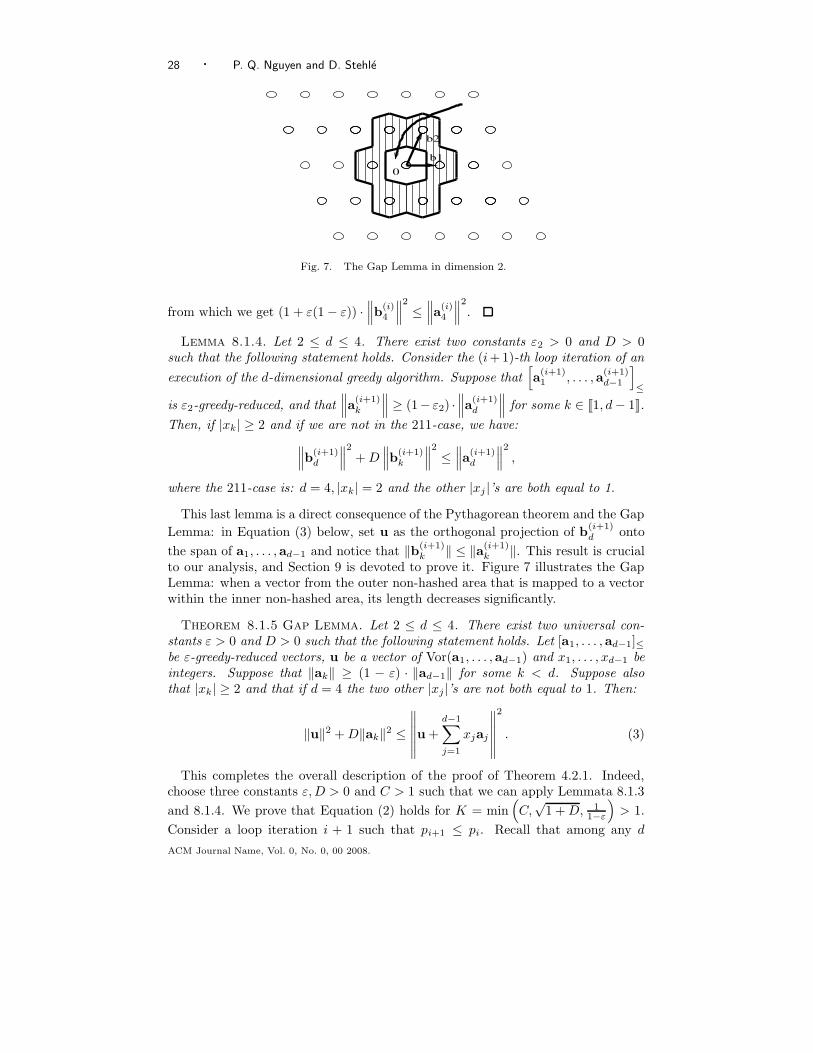
28 · P. Q. Nguyen and D. Stehle
0b1
b2
Fig. 7. The Gap Lemma in dimension 2.
from which we get (1 + ε(1 − ε)) ·∥
∥
∥b
(i)4
∥
∥
∥
2
≤∥
∥
∥a
(i)4
∥
∥
∥
2
.
Lemma 8.1.4. Let 2 ≤ d ≤ 4. There exist two constants ε2 > 0 and D > 0such that the following statement holds. Consider the (i+1)-th loop iteration of an
execution of the d-dimensional greedy algorithm. Suppose that[
a(i+1)1 , . . . , a
(i+1)d−1
]
≤
is ε2-greedy-reduced, and that∥
∥
∥a
(i+1)k
∥
∥
∥≥ (1− ε2) ·
∥
∥
∥a
(i+1)d
∥
∥
∥for some k ∈ J1, d − 1K.
Then, if |xk | ≥ 2 and if we are not in the 211-case, we have:
∥
∥
∥b
(i+1)d
∥
∥
∥
2
+ D∥
∥
∥b
(i+1)k
∥
∥
∥
2
≤∥
∥
∥a
(i+1)d
∥
∥
∥
2
,
where the 211-case is: d = 4, |xk| = 2 and the other |xj |’s are both equal to 1.
This last lemma is a direct consequence of the Pythagorean theorem and the Gap
Lemma: in Equation (3) below, set u as the orthogonal projection of b(i+1)d onto
the span of a1, . . . , ad−1 and notice that ‖b(i+1)k ‖ ≤ ‖a(i+1)
k ‖. This result is crucialto our analysis, and Section 9 is devoted to prove it. Figure 7 illustrates the GapLemma: when a vector from the outer non-hashed area that is mapped to a vectorwithin the inner non-hashed area, its length decreases significantly.
Theorem 8.1.5 Gap Lemma. Let 2 ≤ d ≤ 4. There exist two universal con-stants ε > 0 and D > 0 such that the following statement holds. Let [a1, . . . , ad−1]≤be ε-greedy-reduced vectors, u be a vector of Vor(a1, . . . , ad−1) and x1, . . . , xd−1 beintegers. Suppose that ‖ak‖ ≥ (1 − ε) · ‖ad−1‖ for some k < d. Suppose alsothat |xk| ≥ 2 and that if d = 4 the two other |xj |’s are not both equal to 1. Then:
‖u‖2 + D‖ak‖2 ≤
∥
∥
∥
∥
∥
∥
u +
d−1∑
j=1
xjaj
∥
∥
∥
∥
∥
∥
2
. (3)
This completes the overall description of the proof of Theorem 4.2.1. Indeed,choose three constants ε, D > 0 and C > 1 such that we can apply Lemmata 8.1.3
and 8.1.4. We prove that Equation (2) holds for K = min(
C,√
1 + D, 11−ε
)
> 1.
Consider a loop iteration i + 1 such that pi+1 ≤ pi. Recall that among any d
ACM Journal Name, Vol. 0, No. 0, 00 2008.
Low-Dimensional Lattice Basis Reduction Revisited · 29
consecutive iterations of the loop, there is at least one such iteration. For such an
iteration we have∣
∣
∣x
(i+1)πi
∣
∣
∣≥ 2. We distinguish four cases:
—The basis[
a(i+1)1 , . . . , a
(i+1)d−1
]
≤is not ε-greedy-reduced: then Lemma 8.1.3 gives
the result via the i-th loop iteration.
—We have∥
∥
∥a
(i+1)πi
∥
∥
∥< (1 − ε) ·
∥
∥
∥a
(i+1)d
∥
∥
∥. Indeed, because pi+1 ≤ pi, we have:
∥
∥
∥b
(i+1)d
∥
∥
∥≤∥
∥
∥b(i+1)
πi+1
∥
∥
∥≤∥
∥
∥a(i+1)
πi+1
∥
∥
∥=∥
∥
∥a(i+1)
pi+1
∥
∥
∥
≤∥
∥
∥a(i+1)
pi
∥
∥
∥=∥
∥
∥a(i+1)
πi
∥
∥
∥< (1 − ε) ·
∥
∥
∥a
(i+1)d
∥
∥
∥.
—We are in the 211-case, i.e., d = 4 with |xπi| = 2 and the other |xj |’s are all equal
to 1. Then we refer to Subsection 8.2.
—Otherwise we apply Lemma 8.1.4, which gives the expected result via the (i+1)-th loop iteration.
8.2 Concluding in Dimension Four
In the previous subsections, we showed that there is at most a linear number ofloop iterations in the iterative greedy algorithm in dimensions two and three, butwe noticed that a new difficulty arose in dimension four: the Gap Lemma is uselessin the so-called 211-case. This is because there are three-dimensional Minkowski-reduced bases [b1,b2,b3]≤ for which 2bi + s1bj + s2bk — with {i, j, k} = {1, 2, 3}and |s1| = |s2| = 1 — is a Voronoı vector. Indeed consider the lattice spanned bythe columns b1,b2,b3 of the following matrix:
M =
1 1 −11 −1 00 0 1
.
This basis is Minkowski-reduced and ‖b1 +b2 +2b3‖ = ‖b1 +b2‖ ≤ ‖(2k1 +1)b1 +(2k2 + 1)b1 + 2k3b3‖ for any k1, k2, k3 ∈ Z. Therefore, a vector in the translatedVoronoı cell centered in b1 +b2 +2b3 can avoid being significantly shortened whentranslated inside the Voronoı cell centered in 0.
The Gap Lemma cannot tackle this problem. However, we notice that (1, 1, 2)is rarely a Voronoı coordinate (with respect to a Minkowski-reduced basis), andwhen it is the case it cannot be a strict Voronoı coord: it can be proved easily thatif (1, 1, 2) is a Voronoı coord, then ‖b1 + b2‖ = ‖b1 + b2 + 2b3‖, which tells usthat b1 + b2 + 2b3 is not the only vector in its coset of L/2L reaching the lengthminimum. It turns out that the lattice spanned by the columns of M is essentiallythe only one for which (1, 1, 2) — modulo any change of sign and permutation ofcoordinates — can be a Voronoı coord. More precisely, if (1, 1, 2) — modulo anychange of sign and permutation of coordinates — is a Voronoı coord for a latticebasis, then the basis matrix can be written as rUM where r is any non-zero realnumber and U is any orthogonal matrix. Since a basis can be arbitrarily closeto one of them without actually being one of them, we need to consider a smallcompact set of normalized bases around the annoying ones. More precisely, this
ACM Journal Name, Vol. 0, No. 0, 00 2008.
30 · P. Q. Nguyen and D. Stehle
compact set consists in all ε-greedy-reduced bases [b1,b2,b3]≤ such that thereexists a permutation σ ∈ S3 with
∥
∥
∥
∥
1
‖b3‖2
∣
∣G(
bσ(1),bσ(2),bσ(3)
)∣
∣−∣
∣M tM∣
∣
∥
∥
∥
∥
∞≤ ε
for some sufficiently small ε > 0, where ‖M‖∞ is the maximum of the absolutevalues of the matrix M and |M | is the matrix made of the absolute values of theentries of M .
Now, consider we are in the 211-case at some loop iteration i+1. We distinguishthree cases:
—The basis[
a(i+1)1 , a
(i+1)2 , a
(i+1)3
]
≤is outside the compact. In this case, a variant
of the Gap Lemma (Lemma 9.3.4) proved in Section 9 is valid and can be used
to show that the vector b(i+1)4 is significantly shorter than the vector a
(i+1)4 .
—The basis[
a(i+1)1 , a
(i+1)2 , a
(i+1)3
]
≤is inside the compact but the orthogonal projec-
tion of the vector a(i+1)4 onto the linear span of
[
a(i+1)1 , a
(i+1)2 , a
(i+1)3
]
≤is far from
the Voronoı cell Vor(
a(i+1)1 , a
(i+1)2 , a
(i+1)3
)
. In this case, we can use Lemma 9.3.4
to show that the vector b(i+1)4 is significantly shorter than the vector a
(i+1)4 .
—Otherwise the geometry of the basis[
a(i+1)1 , a
(i+1)2 , a
(i+1)3 , a
(i+1)4
]
≤is very pre-
cisely known and we can show that there remain O(1) loop iterations.
More precisely, by using Lemma 9.3.4, we show that:
Lemma 8.2.1. There exist two constants K, ε > 0 such that the following holds.Consider an execution of the four-dimensional greedy algorithm, and a loop itera-tion i + 1 for which:
(1 ) pi+1 ≤ pi,
(2 ) |xπi| = 2 and
(∣
∣xσ(1)
∣
∣ ,∣
∣xσ(2)
∣
∣ ,∣
∣xσ(3)
∣
∣
)
= (1, 1, 2) for some σ ∈ S3,
(3 )[
a(i+1)1 , a
(i+1)2 , a
(i+1)3
]
≤is ε-greedy-reduced,
(4 )∥
∥
∥a
(i+1)πi
∥
∥
∥≥ (1 − ε) ·
∥
∥
∥a
(i+1)4
∥
∥
∥.
Then either∥
∥
∥a
(i+1)4
∥
∥
∥≥ (1 + K) ·
∥
∥
∥b
(i+1)4
∥
∥
∥or:
∥
∥
∥
∥
∥
∥
∥
1∥
∥
∥a
(i+1)4
∥
∥
∥
2
∣
∣
∣G(
a(i+1)σ(1) , a
(i+1)σ(2) , a
(i+1)σ(3) , a
(i+1)4
)∣
∣
∣− A
∥
∥
∥
∥
∥
∥
∥
∞
≤ ε, with A =
1 0 12 0
0 1 12 0
12
12 1 1
20 0 1
2 1
.
To prove this result, we restrict more and more the possible geometry of the
basis[
a(i)1 , a
(i)2 , a
(i)3 , a
(i)4
]
≤. Notice that this critical geometry corresponds to the
root lattice D4. This last case is considered in Lemma 8.2.2.
ACM Journal Name, Vol. 0, No. 0, 00 2008.
Low-Dimensional Lattice Basis Reduction Revisited · 31
Proof. The proof essentially relies on Lemma 9.3.4. We choose ε, C > 0 ac-cording to Lemma 9.3.4. The constant K will depend on C and ε. We firstshow that wlog we can suppose that the basis vectors have similar lengths, that
is (1 − ε)2 ·∥
∥
∥a
(i+1)4
∥
∥
∥≤∥
∥
∥a
(i+1)1
∥
∥
∥. We know that |xπi
| = 2 and the two other |xi|’sare 1. By hypothesis, we have
∥
∥
∥a
(i+1)πi
∥
∥
∥≥ (1− ε) ·
∥
∥
∥a
(i+1)4
∥
∥
∥. If πi = 1, we are done.
If πi = 2, then we apply Lemma 9.3.4 2), and if πi = 3 we apply Lemma 9.3.4 1),in both cases along with the Pythagorean theorem. So far, we have proved thatone of the following holds:
(1) ‖a(i+1)4 ‖2 ≥ (1 + C)‖b(i+1)
4 ‖2,
(2) (1 − ε)2‖a(i+1)4 ‖ ≤ ‖a(i+1)
1 ‖ ≤ ‖a(i+1)2 ‖ ≤ ‖a(i+1)
3 ‖ ≤ ‖a(i+1)4 ‖.
The remainder of the proof is the same for any of the possible configurationsof (x1, x2, x3), thus, for the sake of simplicity, we suppose now that (x1, x2, x3) =(2, 1, 1). The following step of the proof is to show that we can suppose that the
Gram matrix of[
a(i+1)1 , a
(i+1)2 , a
(i+1)3
]
≤is approximately:
∥
∥
∥a
(i+1)4
∥
∥
∥
2
·
1 − 12 − 1
2− 1
2 1 0− 1
2 0 1
.
This directly follows from Lemma 9.3.4 and the Pythagorean theorem, which givethat at least one of the following holds:
(1)∥
∥
∥a
(i+1)4
∥
∥
∥
2
≥ (1 + C)∥
∥
∥b
(i+1)4
∥
∥
∥
2
,
(2)∣
∣
∣〈a(i+1)
2 , a(i+1)3 〉
∣
∣
∣≤ ε
∥
∥
∥a
(i+1)3
∥
∥
∥
2
and
∣
∣
∣
∣
〈a(i+1)1 , a
(i+1)j 〉 + 1
2
∥
∥
∥a
(i+1)3
∥
∥
∥
2∣
∣
∣
∣
≤ ε∥
∥
∥a
(i+1)3
∥
∥
∥
2
for j ∈ {2, 3}.
It remains to consider the scalar products 〈a(i+1)4 , a
(i+1)k 〉 for k ∈ {1, 2, 3}. Recall
that the orthogonal projection of the vector b(i+1)4 = a
(i+1)4 − a
(i+1)3 − a
(i+1)2 −
2a(i+1)1 onto the linear span of
[
a(i+1)1 , a
(i+1)2 , a
(i+1)3
]
≤belongs to the Voronoı
cell Vor(
a(i+1)1 , a
(i+1)2 , a
(i+1)3
)
. Wlog we can suppose that∥
∥
∥a
(i+1)4
∥
∥
∥≥∥
∥
∥b
(i+1)4
∥
∥
∥≥
(1−ε) ·∥
∥
∥a
(i+1)4
∥
∥
∥, since otherwise have the result for K = 1
1−ε. By expanding ‖b4‖2,
we get:
(1 + 19ε) ·∥
∥
∥a
(i+1)4
∥
∥
∥
2
≥ 3∥
∥
∥a
(i+1)4
∥
∥
∥
2
− 2〈a(i+1)4 , 2a
(i+1)1 + a
(i+1)2 + a
(i+1)3 〉
≥ (1 − 19ε) ·∥
∥
∥a
(i+1)4
∥
∥
∥
2
,
where we used our knowledge of the Gram matrix of[
a(i+1)1 , a
(i+1)2 , a
(i+1)3
]
≤. Thus
we have:∣
∣
∣〈a(i+1)
4 , 2a(i+1)1 + a
(i+1)2 + a
(i+1)3 〉 −
∥
∥
∥a
(i+1)4
∥
∥
∥
∣
∣
∣≤ 19ε ·
∥
∥
∥a
(i+1)4
∥
∥
∥.
ACM Journal Name, Vol. 0, No. 0, 00 2008.
32 · P. Q. Nguyen and D. Stehle
This last equation gives that in order to end the proof, it is sufficient to prove
that the scalar products 〈a(i+1)4 , a
(i+1)2 〉 and 〈a(i+1)
4 , a(i+1)3 〉 are small. Let j ∈
{2, 3}. By hypothesis, for any x ∈ Z, we have∥
∥
∥a
(i+1)4 − 2a
(i+1)1 − xa
(i+1)j
∥
∥
∥≥
∥
∥
∥a
(i+1)4 − 2a
(i+1)1 − a
(i+1)2 − a
(i+1)3
∥
∥
∥. In particular, by choosing x = 0 and x = 2
and expanding the norms and using the knowledge of the Gram matrix of the
ordered basis[
a(i+1)1 , a
(i+1)2 , a
(i+1)3
]
≤, one can obtain an explicit positive integer k
such that∣
∣
∣〈a(i+1)
4 , a(i+1)1 〉
∣
∣
∣≤ kε ·
∥
∥
∥a
(i+1)4
∥
∥
∥.
Let K = min(
1 + C, 1(1−ε)2
)
. Altogether, we have proved that there exists a
constant K ′ = max(K, k, 16) such that:∥
∥
∥
∥
∥
∥
∥
1∥
∥
∥a
(i+1)4
∥
∥
∥
2 G(
a(i+1)1 , a
(i+1)2 , a
(i+1)3 , a
(i+1)4
)
− A
∥
∥
∥
∥
∥
∥
∥
∞
≤ K ′ε.
This completes the proof of the lemma.
At this point of the analysis of the 211-case, we have shown that we can suppose
that the shape of the basis[
a(i+1)1 , a
(i+1)2 , a
(i+1)3 , a
(i+1)4
]
≤is very specific: its Gram
matrix is very close to A. We treat this last case by applying the following lemma,which roughly says that if the Gram matrix of a basis is sufficiently close to someinvertible matrix, then the number of short vectors generated by the basis remainsbounded. Since the greedy algorithm always creates smaller bases for the lexico-graphic order based on the lengths, if the Gram matrix of the current basis is closeto the matrix A, then it remains O(1) loop iterations.
Lemma 8.2.2. Let A be a d×d invertible matrix, and B > 0. There exist ε, N >
0 such that for any basis (b1, . . . ,bd) satisfying∥
∥
∥
1‖bd‖2 G(b1, . . . ,bd) − A
∥
∥
∥
∞≤ ε,
we have:
|{(x1, . . . , xd), ‖x1b1 + . . . + xdbd‖ ≤ B‖bd‖}| ≤ N.
Proof. Let ε > 0 such that for any G, if ‖G − A‖∞ ≤ ε, then G is invertible(such an ε does exist since the set of invertible matrices is open). In that case,if X = (x1, . . . , xd), then
∣
∣
∣
∣
1
‖bd‖2‖x1b1 + . . . + xdbd‖2 − XAXt
∣
∣
∣
∣
= |X(G − A)Xt| ≤ d2ε · (XXt),
where G = 1‖bd‖2 G(b1, . . . ,bd). Therefore, if ‖x1b1 + . . . + xdbd‖ ≤ B‖bd‖, then,
by the triangular inequality, we obtain |XAX t| ≤ B2 +d2ε ·(XXt). But |XAXt| ≥1
‖A−1‖ (XXt), where ‖B‖ is defined as max(Y BY t, Y ∈ Rn and ‖Y ‖ = 1), which is
positive. Therefore:
(XXt) ·(
1
‖A−1‖ − d2ε
)
≤ B2.
We set ε < 1d2‖A−1‖ . The xi’s are integers such that the quantity (XX t) remains
ACM Journal Name, Vol. 0, No. 0, 00 2008.
Low-Dimensional Lattice Basis Reduction Revisited · 33
bounded, so that we are considering integer points in a d-dimensional hypersphere.There can only be finitely many such points.
9. THE GEOMETRY OF LOW-DIMENSIONAL LATTICES
In this section, we give some results about Voronoı cells in dimensions two andthree, which are crucial to the complexity analysis of the greedy algorithm describedin Section 4. More precisely, the analysis is based on the Gap Lemma (given inSubsection 9.3), which is derived from the study of Voronoı cells in the case of ε-greedy-reduced vectors (see Subsection 9.2), itself derived from the study of Voronoıcells for Minkowski-reduced bases (in Subsection 9.1).
9.1 Voronoı Cells in the Case of Minkowski-Reduced Bases
We start by giving some simple bounds on the diameter of the Voronoı cell and onthe Gram-Schmidt orthogonalization of a Minkowski-reduced basis:
Lemma 9.1.1. Let d ≥ 1. Let [b1, . . . ,bd]≤ be a basis of a lattice L. Then
ρ(L) ≤√
d2 · ‖bd‖. As a consequence, if the basis [b1, . . . ,bd]≤ is a Minkowski-
reduced basis, then ‖b∗d‖ ≥
√5−d2 · ‖bd‖.
Proof. The first part of the lemma is very classical and several different proofscan be found in the literature. For example, we can use the inequalities ρ(L)2 ≤14
∑
i≤d ‖b∗i ‖2 ≤ d
4‖bd‖2, where the first one derives from Babai’s nearest planealgorithm [Babai 1986].
Suppose now that the basis [b1, . . . ,bd]≤ is Minkowski-reduced. Then the or-thogonal projection of the vector bd onto the linear span of [b1, . . . ,bd−1]≤ isin Vor(b1, . . . ,bd−1). Therefore, by the Pythagorean theorem, we get: ‖b∗
d‖2 ≥‖bd‖2 − d−1
4 ‖bd−1‖2. The fact that ‖bd−1‖ ≤ ‖bd‖ completes the proof.
The following lemma provides the possible Voronoı vectors of a lattice of dimen-sion two given by a Minkowski-reduced basis (recall that we cannot directly useTheorem 2.3.1 because it only considers strict Voronoı coordinates). Such a basisconfines the coordinates of the Voronoı vectors:
Lemma 9.1.2. In dimension two, the possible Voronoı coords are (1, 0) and(1, 1), modulo any change of signs and permutation of coordinates, i.e., any nonzero(ε1, ε2) where |ε1|, |ε2| ≤ 1.
The proof relies on a detailed study of the quantity ‖(2x1 + ε1) ·b1 +(2x2 + ε2) ·b2‖2 − ‖ε1b1 + ε2b2‖2, where the basis [b1,b2]≤ is Minkowski-reduced, ε1, ε2 ∈{0, 1} and x1, x2 ∈ Z. Indeed, since the Voronoı coords of a lattice L are givenby the minima of the non-zero cosets of L/2L, it suffices to show that if x1 6= 0or x2 6= 0, then this expression is strictly positive.
Proof. Recall that the possible Voronoı coords can be obtained by consideringthe short elements of L/2L, given a Minkowski-reduced basis of L. Let [b1,b2]≤be a reduced basis. By eventually replacing the vector bi by −bi for i ∈ {1, 2},it is clearly sufficient to show that for any x1, x2 ≥ 0, and for any ε1, ε2 ∈ {0, 1},if x1 ≥ 1 or x2 ≥ 1, then:
‖(2x1 + ε1) · b1 + (2x2 + ε2) · b2‖2 > ‖ε1 · b1 + ε2 · b2‖2.
ACM Journal Name, Vol. 0, No. 0, 00 2008.
34 · P. Q. Nguyen and D. Stehle
First of all:
‖(2x1 + ε1) · b1 + (2x2 + ε2) · b2‖2 − ‖ε1 · b1 + ε2 · b2‖2
=(
(2x1 + ε1)2 − ε2
1
)
· ‖b1‖2 +(
(2x2 + ε2)2 − ε2
2
)
· ‖b2‖2
+2((2x1 + ε1)(2x2 + ε2) − ε1ε2) · 〈b1,b2〉.
Since x1, x2 ≥ 0, we have that (2x2+ε2)2−ε2
2 ≥ 0 and (2x1+ε1)(2x2+ε2)−ε1ε2 ≥ 0.Moreover, the basis [b1,b2]≤ is reduced and therefore ‖b2‖ ≥ ‖b1‖ and 2〈b1,b2〉 ≥−‖b1‖2. From these facts, we obtain:
‖(2x1 + ε1) · b1 + (2x2 + ε2) · b2‖2 − ‖ε1b1 + ε2b2‖2
≥ 2[
2x21 + 2x2
2 − 2x1x2 + x1(2ε1 − ε2) + x2(2ε2 − ε1)]
· ‖b1‖2.
This last expression is strictly positive as long as (x1, x2) 6= (0, 0). Indeed:
—if ε1 = ε2 = 0, the factor is 4(
(x1 − x2)2 + x1x2
)
,
—if ε1 = 0 and ε2 = 1, the factor is 2(
x22 + 2x2 + (x2 − x1)
2 + (x21 − x1)
)
,
—the case ε1 = 1 and ε2 = 0 is symmetric,
—if ε1 = ε2 = 1, the factor is 2(
(x2 − x1)2 + (x2
2 + x2) + (x21 + x1)
)
.
We generalize this analysis to the three-dimensional case. The underlying ideasof the proof are the same, but the increase of the number of variables makes theanalysis more tedious.
Lemma 9.1.3. In dimension three, the possible Voronoı coordinates are among(1, 0, 0), (1, 1, 0), (1, 1, 1) and (2, 1, 1), modulo any change of signs and permutationof coordinates.
Proof. We generalize the proof of Lemma 9.1.2. We show that for any inte-gers x1, x2, x3 and any ε1, ε2, ε3 ∈ {0, 1}, if (2x1 + ε1, 2x2 + ε2, 2x3 + ε3) is not inthe desired list of Voronoı coords, then:
‖(2x1 + ε1) · b1 + (2x2 + ε2) · b2 + (2x3 + ε3) · b3‖2 − ‖ε1b1 + ε2b2 + ε3b3‖2 > 0.
By replacing the vector bi by −bi, we see that wlog the proof can be restrictedto the case x1, x2, x3 ≥ 0. Moreover, because we already considered the two-dimensional case in Lemma 9.1.2, we can suppose that for any i ∈ {1, 2, 3}, wehave (xi, εi) 6= (0, 0).
From Lemma 9.1.1, we know that since the basis [b1,b2,b3]≤ is Minkowski-reduced, we have ‖b∗
3‖ ≥ ‖b3‖/√
2. As a consequence, if 2x3 + ε3 ≥ 5, then:
‖(2x1 + ε1) · b1 + (2x2 + ε2) · b2 + (2x3 + ε3) · b3‖2 ≥ 25 · ‖b∗3‖2 ≥ 25
2· ‖b3‖2,
and the triangular inequality gives that ‖ε1 ·b1 +ε2 ·b2 +ε3 ·b3‖2 ≤ 9 · ‖b3‖2. Thisgives the result when 2x3 + ε3 ≥ 5. The same argument holds for (x3, ε3) = (2, 0),and for (x3, ε3) ∈ {(1, 1), (1, 0)} with ε1 · ε2 = 0. Therefore, it remains to consider
ACM Journal Name, Vol. 0, No. 0, 00 2008.
Low-Dimensional Lattice Basis Reduction Revisited · 35
the three cases (x3, ε3) = (1, 1) with ε1 = ε2 = 1, (x3, ε3) = (1, 0) with ε1 = ε2 = 1,and (x3, ε3) = (0, 1).
Case 1: Suppose that (x3, ε3) = (1, 1) and ε1 = ε2 = 1. Since the orderedbasis [b1,b2,b3]≤ is Minkowski-reduced, we have 〈bi,bj〉 ≥ −‖bi‖2/2 for any1 ≤ i < j ≤ 3, which gives:
‖(2x1 + 1) · b1 + (2x2 + 1) · b2 + 3 · b3‖2 − ‖b1 + b2 + b3‖2
= 4(
x21 + x1
)
· ‖b1‖2 + 4(
x22 + x2
)
· ‖b2‖2 + 8 · ‖b3‖2
+4(3x1 + 1) · 〈b1,b3〉 + 4(3x2 + 1) · 〈b2,b3〉 + 4(2x1x2 + x1 + x2) · 〈b1,b2〉≥(
4x21 − 4x1x2 − 4x1 − 2x2 − 2
)
· ‖b1‖2 +(
4x22 − 2x2 − 2
)
‖b2‖2 + 8‖b3‖2.
If x2 = 0, it suffices to lower-bound(
x21 − x1
)
· ‖b1‖2 + ‖b3‖2, which is alwaysgreater than ‖b3‖2 and therefore strictly positive. Suppose now that x2 ≥ 1.Then 4x2
2 − 2x2 − 2 ≥ 0 and we obtain:
‖(2x1 + 1) · b1 + (2x2 + 1) · b2 + 3 · b3‖2 − ‖b1 + b2 + b3‖2
≥ 4(
x21 + x2
2 − x1x2 − x1 − x2 + 1)
· ‖b1‖2
≥ 4(
(x1 − x2)2 + (x1x2 − x1 − x2) + 1
)
· ‖b1‖2.
It is clear that this last expression is strictly positive for any x1, x2 ≥ 0 exceptwhen x1 = x2 = 1. In this last situation, we use the fact that ‖3 · b1 + 3 · b2 + 3 ·b3‖2 − ‖b1 + b2 + b3‖2 = 8 · ‖b1 + b2 + b3‖2.
Case 2: Suppose now that (x3, ε3) = (1, 0) and ε1 = ε2 = 1. Similarly, we have:
‖(2x1 + 1) · b1 + (2x2 + 1) · b2 + 2 · b3‖2 − ‖b1 + b2‖2
= 4(
x21 + x1
)
· ‖b1‖2 + 4(
x22 + x2
)
· ‖b2‖2 + 4 · ‖b3‖2
+4(2x1 + 1) · 〈b1,b3〉 + 4(2x2 + 1) · 〈b2,b3〉 + 4(2x1x2 + x1 + x2) · 〈b1,b2〉≥(
4x21 − 4x1x2 − 2x1 − 2x2 − 2
)
· ‖b1‖2 +(
4x22 − 2
)
· ‖b2‖2 + 4‖b3‖2.
If x2 = 0, it suffices to lower-bound(
2x21 − x1 − 1
)
· ‖b1‖2 + ‖b3‖2, which isstrictly positive if x1 ≥ 1. If x1 = 0, then we have one of the possible Voronoıcoords. Suppose now that x2 ≥ 1. In that case 4x2
2 − 2 ≥ 0, which ensures that:
‖(2x1 + 1) · b1 + (2x2 + 1) · b2 + 2 · b3‖2 − ‖b1 + b2‖2
≥ 2(
2x21 + 2x2
2 − 2x1x2 − x1 − x2
)
· ‖b1‖2
≥ 2(
(x1 − x2)2 + (x2
1 − x1) + (x22 − x2)
)
· ‖b1‖2.
If x1 ≥ 2 or x2 ≥ 2 or x1 6= x2, this is strictly positive. Therefore it remains toconsider the case x1 = x2 = 1. We have:
‖3·b1+3·b2+2·b3‖2−‖b1+b2‖2 = 4·(
‖b3‖2 + 3 · 〈b3,b1 + b2〉 + 2 · ‖b1 + b2‖2)
.
Since the basis [b1,b2,b3]≤ is reduced, we have 〈b3,b1 + b2〉 ≥ −‖b1 + b2‖2/2,
ACM Journal Name, Vol. 0, No. 0, 00 2008.
36 · P. Q. Nguyen and D. Stehle
which gives the expected result.
Case 3: Suppose now that (x3, ε3) = (0, 1). Similarly, we have the inequalities:
‖(2x1 + ε1) · b1 + (2x2 + ε2) · b2 + b3‖2 − ‖ε1 · b1 + ε2 · b2 + b3‖2
= 4(
x21 + ε1x1
)
· ‖b1‖2 + 4(
x22 + ε2x2
)
· ‖b2‖2 + 4x1 · 〈b1,b3〉+4x2 · 〈b2,b3〉 + 4(2x1x2 + x1ε2 + x2ε1) · 〈b1,b2〉
≥(
4x21 − 4x1x2 + (4ε1 − 2 − 2ε2)x1 − 2x2ε1
)
· ‖b1‖2
+(
4x22 + (4ε2 − 2)x2
)
· ‖b2‖2.
If x2 = 0, it suffices to lower-bound 4x21 +(4ε1 − 2− 2ε2)x1. It is strictly positive
as soon as x1 ≥ 1 except in the case (x1, ε1, ε2) = (1, 0, 1), which corresponds toone of the possible Voronoı coords. If x1 = 0, we only have possible Voronoı coords.Suppose now that x2 ≥ 1. In that case 4x2
2 + (4ε2 − 2)x2 ≥ 0 and:
‖(2x1 + ε1) · b1 + (2x2 + ε2) · b2 + b3‖2 − ‖ε1 · b1 + ε2 · b2 + b3‖2
≥(
4x21 + 4x2
2 − 4x1x2 + (4ε1 − 2 − 2ε2)x1 + (4ε2 − 2 − 2ε1)x2
)
· ‖b1‖2.
For (ε1, ε2) = (0, 0), we get 2(
(x1 − x2)2 + (x2
1 − x1) + (x22 − x2)
)
, which is strictlypositive as soon as x1 6= x2 or x1 ≥ 2 or x2 ≥ 2. The only remaining case that doesnot provide a possible Voronoı coord is x1 = x2 = 1. Notice that ‖2b1 + 2b2 +b3‖2 > ‖b3‖2 is equivalent to ‖b1 + b2‖2 + 〈b1 + b2,b3〉 > 0, which is impliedby 〈b1 +b2,b3〉 ≥ −‖b1 +b2‖2/2 (the vector b3 has its orthogonal projection ontothe span of [b1,b2] inside Vor(b1,b2)).
For (ε1, ε2) = (1, 0), we get 2(x1 −x2)2 +2(x2
2 − 2x2) + 2x21 +2x1. If x2 ≥ 2, this
is clearly strictly positive. If x2 = 1, we obtain 4x21 − 2x1, which is strictly positive
unless x1 = 0 (one of the possible Voronoı coords). We have already considered thecase x2 = 0. The case (ε1, ε2) = (0, 1) is symmetric.
Finally, if (ε1, ε2) = (1, 1), we obtain 2(
(x1 − x2)2 + x2
1 + x22
)
, which is strictlypositive unless x1 = x2 = 0 (one of the possible Voronoı coords). This completesthe proof of the lemma.
The possible Voronoı coord (2, 1, 1) creates difficulties when analyzing the greedyalgorithm in dimension four because it contains a two, which cannot be handledwith the greedy argument used for the ones. We tackle this problem as follows:we show that when (2, 1, 1) happens to be a Voronoı coord, the lattice has a veryspecific shape, for which the behavior of the algorithm is well-understood.
Lemma 9.1.4. Suppose the basis [b1,b2,b3]≤ is Minkowski-reduced.
(1 ) If (s1, s2, 2) is a Voronoı coord with si = ±1 for i ∈ {1, 2}, then ‖b1‖ = ‖b2‖ =‖b3‖, 〈b1,b2〉 = 0 and 〈bi,b3〉 = − si
2 · ‖b1‖2 for i ∈ {1, 2}.(2 ) If (s1, 2, s3) is a Voronoı coord with si = ±1 for i ∈ {1, 3}, then ‖b1‖ = ‖b2‖.
Moreover, if ‖b1‖ = ‖b2‖ = ‖b3‖, then 〈b1,b3〉 = 0 and 〈bi,b2〉 = − si
2 · ‖b1‖2
for i ∈ {1, 3}.(3 ) If (2, s2, s3) is a Voronoı coord with si = ±1 for i ∈ {2, 3} and ‖b1‖ = ‖b2‖ =
‖b3‖, then 〈b2,b3〉 = 0 and 〈bi,b1〉 = − si
2 · ‖b1‖2 for i ∈ {2, 3}.ACM Journal Name, Vol. 0, No. 0, 00 2008.
Low-Dimensional Lattice Basis Reduction Revisited · 37
Proof. Wlog we suppose that for any i, we have si = 1. In the first situation weconsider the inequality ‖b1 +b2 +2 ·b3‖2 ≤ ‖b1 +b2‖2: it is equivalent to ‖b3‖2 +〈b1,b3〉 + 〈b2,b3〉 ≤ 0. Since the basis is reduced, we must have 〈b1,b3〉 ≥−‖b1‖2/2 and 〈b2,b3〉 ≥ −‖b2‖2/2. Thus 2 · ‖b3‖2 − ‖b1‖2 − ‖b2‖2 ≤ 0. Conse-quently, the length equalities hold and the inequalities on the scalar products aboveare equalities. It remains to prove that 〈b1,b2〉 = 0. Since b1 is a shortest vector,we have ‖b3 + b2 + b1‖2 ≥ ‖b1‖2, which is equivalent to 〈b1,b2〉 ≥ 0. Moreover,we have 〈b1,b2〉 ≤ 0 from the expansion of ‖b1 + b2 + 2 · b3‖2 ≤ ‖b1 − b2‖2.
In the second situation, expanding ‖b1 + 2 · b2 + b3‖2 ≤ ‖b1 + b3‖2 gives thelength equality. In the case of the additional hypothesis ‖b1‖ = ‖b2‖ = ‖b3‖, thebasis [b1,b3,b2]≤ is also reduced and we can apply the result of the first situation.This last argument also holds in the third situation.
9.2 Voronoı Cells in the Case of ε-Greedy-Reduced Vectors
We extend the results of the previous subsection to the case of ε-greedy-reducedvectors. The idea is that if we compactify the set of Minkowski-reduced bases andslightly enlarge it, the possible Voronoı coords remain the same. Unfortunately,by doing so, some of the vectors we consider may be zero and this creates aninfinity of possible Voronoı coords: for example, if b1 = 0, any pair (x1, 0) isa Voronoı coord of [b1,b2]≤. To tackle this problem, we restrict to vectors bi
with “similar” lengths. More precisely, we use the so-called Topological Lemma:if we can guarantee that the possible Voronoı coords of the enlargement of theinitial compact set of bases are bounded, then for a sufficiently small enlargement,the possible Voronoı coords remain the same. We first give rather simple resultson ε-greedy-reduced vectors and their Gram-Schmidt orthogonalization, then weintroduce the Topological Lemma (Lemma 9.2.3), from which we finally derive therelaxed versions of Lemmata 9.1.2, 9.1.3 and 9.1.4.
Lemma 9.2.1. For any ε > 0, if [b1,b2,b3]≤ are ε-greedy-reduced, then thefollowing inequalities hold:
∀i < j, |〈bi,bj〉| ≤ 1 + ε
2· ‖bi‖2,
∀s1, s2 ∈ {−1, 1}, |〈b3, s1 · b1 + s2 · b2〉| ≤ 1 + ε
2· ‖s1 · b1 + s2 · b2‖2.
Proof. Since [b1,b2]≤ are ε-greedy-reduced, we have that b′2 ∈ (1+ε) ·Vor(b1),
where b′2 is the orthogonal projection of the vector b2 onto the span of b1. As a
consequence, we can write b′2 = (1 + ε) · u with u ∈ Vor(b1). By expanding the
inequalities ‖u ± b1‖2 ≥ ‖u‖2, we obtain that |〈u,b1〉| ≤ ‖b1‖2/2. Therefore,|〈b3,b1〉| ≤ 1+ε
2 · ‖b1‖2.Moreover [b1,b2,b3]≤ are ε-greedy-reduced, so that b′
3 ∈ (1 + ε) · Vor(b1,b2),where b′
3 is the orthogonal projection of the vector b3 onto the span of [b1,b2]≤.As a consequence, we can write b′
3 = (1 + ε) · u with u ∈ Vor(b1,b2). We proceedexactly as above by expanding the inequalities ‖u + s1 · b1 + s2 · b2‖2 ≥ ‖u‖2 forany s1, s2 ∈ {−1, 0, 1}, and this provides the result.
The previous lemma implies that if [b1, . . . ,bd]≤ are ε-greedy-reduced, the onlycase for which the bi’s can be linearly dependent is when some of them are zero,
ACM Journal Name, Vol. 0, No. 0, 00 2008.
38 · P. Q. Nguyen and D. Stehle
but this case cannot be avoided since we need compactifying the set of Minkowski-reduced bases. The following lemma generalizes Lemma 9.1.1. It shows that evenwith ε-greedy-reduced vectors, if the dimension is below four then the Gram-Schmidt orthogonalization process cannot arbitrarily decrease the lengths of theinitial vectors.
Lemma 9.2.2. There exists C > 0 such that for any 1 ≤ d ≤ 4 and anysufficiently small ε > 0, if [b1, . . . ,bd]≤ are ε-greedy-reduced vectors, then wehave ‖b∗
d‖ ≥ C · ‖bd‖.Proof. Since [b1, . . . ,bd]≤ are ε-greedy-reduced, we know that if b′
d is the or-thogonal projection of the vector bd onto the span of [b1, . . . ,bd−1]≤, then b′
d ∈(1 + ε) · Vor(b1, . . . ,bd−1). Therefore, because of Lemma 9.1.1 and because thevectors are ordered,
‖b′d‖ ≤ (1 + ε)
√d − 1
2· ‖bd−1‖ ≤ (1 + ε)
√d − 1
2· ‖bd‖.
Besides, from the Pythagorean theorem, we have ‖bd‖2 = ‖b∗d‖2 + ‖b′
d‖2, whichcompletes the proof.
The Topological Lemma is the key argument when extending the results on pos-sible Voronoı coords from Minkowski-reduced bases to ε-greedy-reduced vectors.When applying it, X0 will correspond to the xi’s, K0 to the bi’s that are ε-greedy-reduced, X to the possible Voronoı coordinates, K to a compact subsetof the Minkowski-reduced bases, and f to the continuous function of real vari-ables f : (yi)i≤d, (bi)i≤d −→ ‖y1b1 + . . . + ydbd‖.
Lemma 9.2.3 Topological Lemma. Let n, m ≥ 1. Let X0 and K0 be compactsets of R
n and Rm. Let f be a continuous function from K0×X0 to R. For any a ∈
K0 we define Ma = {x ∈ X0 ∩ Zn, f(a, x) = minx′∈X0∩Zn f(a, x′)}. Let K ⊂ K0 be
a compact and X = ∪a∈KMa ⊂ X0 ∩ Zn. With these notations, there exists ε > 0
such that if b ∈ K0 satisfies dist(b, K) ≤ ε, we have Mb ⊂ X.
Proof. First, all the notations of the result make sense: X0 ∩Zn is finite so the
minimum of f(a, ·) over it does exist and Ma is finite. Since X ⊂ X0 ∩ Zn, X is
finite. Finally, since K is compact, the notation dist(·, K) makes sense too.For each x ∈ X0 we define Kx = {a ∈ K0, x ∈ Ma}. The set Kx is compact.
Indeed, it is obviously bounded, and if (ak) is a sequence of elements of Kx thatconverges towards an a ∈ K0, we show that a ∈ Kx. For all x′ ∈ X0 ∩ Z
n and forall k, we have f(ak, x) ≤ f(ak, x′). By continuity, this holds for a too, which provesthat x ∈ Ma.
Now we fix an x ∈ X0 ∩ Zn \ X . Since Kx and K are both compact and x /∈ X
(which implies K ∩ Kx = ∅), dist(Kx, K) > 0. Finally, set
ε =1
2min (dist(Kx, K), x ∈ (X0 ∩ Z
n) \ X) ,
which exists since (X0∩Zn)\X is finite. Now, let b4 ∈ K0 such that dist(b, K) ≤ ε.
For any x0 ∈ Mb, we have b ∈ Kx0. Then necessarily x0 ∈ X , since otherwise one
would have dist(Kx0, K) > ε ≥ dist(b, K), which cannot be the case because b ∈
Kx0.
ACM Journal Name, Vol. 0, No. 0, 00 2008.
Low-Dimensional Lattice Basis Reduction Revisited · 39
In order to apply the Topological Lemma, we need to map the relaxed bases intoa compact set. For any ε ≥ 0 and any α ∈ [0, 1], we define:
K2(ε, α) = {(b1,b2),b1,b2 ε-greedy-reduced, α ≤ ‖b1‖ ≤ ‖b2‖ = 1}K3(ε, α) = {(b1,b2,b3),b1,b2,b3 ε-greedy-reduced,
α ≤ ‖b1‖ ≤ ‖b2‖ ≤ ‖b3‖ = 1}.Lemma 9.2.4. If ε ≥ 0 and α ∈ [0, 1], K2(ε, α) and K3(ε, α) are compact sets.
The following lemma is the relaxed version of Lemma 9.1.2. It can also be viewedas a reciprocal to Lemma 9.2.1.
Lemma 9.2.5. There exists ε > 0 such that for any α ∈ (0, 1], the possibleVoronoı coords of [b1,b2]≤ ∈ K2(ε, α) are the same as for Minkowski-reduced bases,i.e., (1, 0) and (1, 1), modulo any change of signs and permutation of coordinates.
Proof. Recall that there is a set of possible Voronoı coords for each non-zeroelement of (Z/2Z)2: we look at the minima of the cosets of L/2L. Since there isa finite number of such cosets (three in dimension two), we treat them separately.Let (a1, a2) ∈ {0, 1}2. We are looking for the pairs (k1, k2) ∈ Z
2 that minimize thequantity ‖(a1 + 2k1) · b1 + (a2 + 2k2) · b2‖, where [b1,b2]≤ are ε-greedy-reduced.We first prove that the minimum over (k1, k2) can be taken over a finite domain.Notice that if (k∗
1 , k∗2) is optimal:
2 ≥ ‖b1‖ + ‖b2‖ ≥ ‖a1 · b1 + a2 · b2‖ ≥ ‖(a1 + 2k∗1) · b1 + (a2 + 2k∗
2) · b2‖.Moreover, Lemma 9.2.2 gives that:
‖(a1 + 2k∗1) · b1 + (a2 + 2k∗
2) · b2‖ ≥ |a2 + 2k∗2 | · ‖b∗
2‖ ≥ |a2 + 2k∗2 |C,
which gives the result for k∗2 . By applying the triangular inequality, we get the
result for k∗1 :
|a1 + 2k∗1 |α ≤ ‖(a1 + 2k∗
1) · b1‖ ≤ 2 + ‖(a2 + 2k∗2) · b2‖ ≤ 2 + |a2 + 2k∗
2 |.From this we deduce that (k∗
1 , k∗2) ∈ Z
2 can be bounded independently of (b1,b2).From Lemma 9.2.4, we know that K2(ε, α) is compact and therefore we can applythe Topological Lemma. This gives the expected result.
We now relax Lemma 9.1.3 in the same manner. To do this, we proceed exactlylike in the proof above.
Lemma 9.2.6. There exists ε > 0 such that for any α ∈ (0, 1], the possibleVoronoı coords of [b1,b2,b3]≤ ∈ K3(ε, α) are the same as for Minkowski-reducedbases.
Proof. We consider each non-zero coset of L/2L separately (there are sevenof them in dimension three). Let (a1, a2, a3) ∈ {0, 1}3. We are looking for thetriples (k1, k2, k3) ∈ Z
3 minimizing the quantity ‖(a1 + 2k1) · b1 + (a2 + 2k2) ·b2 + (a3 + 2k3) · b3‖, where [b1,b2,b3]≤ are ε-greedy-reduced. In order to applyLemma 9.2.4, from which the result can be deduced easily, it is sufficient to provethat the minimum over (k1, k2, k3) can be taken over a finite domain. Notice thatif (k∗
1 , k∗2 , k∗
3) is optimal:
3 ≥ ‖a1 ·b1 +a2 ·b2 +a3 ·b3‖ ≥ ‖(a1 +2k∗1) ·b1 +(a2 +2k∗
2) ·b2 +(a3 +2k∗3) ·b3‖.
ACM Journal Name, Vol. 0, No. 0, 00 2008.
40 · P. Q. Nguyen and D. Stehle
Moreover, Lemma 9.2.2 gives that:
‖(a1 +2k∗1) ·b1 +(a2 +2k∗
2) ·b2 +(a3 +2k∗3) ·b3‖ ≥ |a3 +2k∗
3 | · ‖b∗3‖ ≥ |a3 +2k∗
3 |C,
for any sufficiently small ε > 0. This gives the result for k∗3 .
From the triangular inequality, Lemma 9.2.2, and the fact that ‖b2‖ ≥ α, wehave:
3+ |a3 +2k∗3 | ≥ ‖(a1 +2k∗
1) ·b1 +(a2 +2k∗2) ·b2‖ ≥ |a2 +2k∗
2 | · ‖b∗2‖ ≥ |a2 +2k∗
2 |Cα.
The fact that k∗3 is bounded ensures that k∗
2 is bounded.To obtain the result on k∗
1 , it suffices to apply the triangular inequality oncemore:
3 + |a3 + 2k∗3 | + |a2 + 2k∗
2 | ≥ ‖(a1 + 2k∗1) · b1‖ ≥ |a1 + 2k∗
1 |α.
The following result generalizes Lemma 9.1.4 about the possible Voronoı co-ord (1, 1, 2). As opposed to the two previous results, there is no need using theTopological Lemma in this case, because only a finite number of (x1, x2, x3)’s isconsidered.
Lemma 9.2.7. There exists c > 0 such that for any sufficiently small ε > 0,if [b1,b2,b3]≤ are ε-greedy-reduced and ‖b3‖ = 1, then:
(1 ) If (s1, s2, 2) is a Voronoı coord with si = ±1 for i ∈ {1, 2}, then: ‖b1‖ ≥1 − cε, |〈b1,b2〉| ≤ cε and
∣
∣〈bi,b3〉 + si
2 · ‖b1‖2∣
∣ ≤ cε for i ∈ {1, 2}.(2 ) If (s1, 2, s3) is a Voronoı coord with si = ±1 for i ∈ {1, 3}, then (1 − cε) ·
‖b2‖ ≤ ‖b1‖ ≤ ‖b2‖. Moreover, if ‖b1‖ ≥ 1 − ε, then: |〈b1,b3〉| ≤ cεand
∣
∣〈bi,b2〉 + si
2 · ‖b1‖2∣
∣ ≤ cε for i ∈ {1, 3}.(3 ) If (2, s2, s3) is a Voronoı coord with si = ±1 for i ∈ {2, 3} and if ‖b1‖ ≥ 1− ε,
then: |〈b2,b3〉| ≤ cε and∣
∣〈bi,b1〉 + si
2 · ‖b1‖2∣
∣ ≤ cε for i ∈ {2, 3}.The proof is a straightforward modification of the proof of Lemma 9.1.4.
Proof. Wlog we suppose that for any i, we have si=1. The proofs of the othercases are very similar. We only prove the statement in the case of the first situation.
We consider the inequality ‖b1 + b2 + 2 · b3‖2 ≤ ‖b1 + b2‖2: it is equivalentto ‖b3‖2+〈b1,b3〉+〈b2,b3〉 ≤ 0. Since [b1,b2,b3]≤ are ε-greedy-reduced, by usingLemma 9.2.1 we obtain that we must have 〈b1,b3〉 ≥ − 1+ε
2 · ‖b1‖2 and 〈b2,b3〉 ≥− 1+ε
2 · ‖b2‖2. Thus 2 · ‖b3‖2 − (1 + ε) · ‖b1‖2 − (1 + ε) · ‖b2‖2 ≤ 0. Consequently,the length “quasi-equality” holds, and the inequalities on the scalar products aboveare “quasi-equalities”.
It remains to prove that |〈b1,b2〉| is very small. Expanding the relation ‖b1 +b2 + 2 · b3‖2 ≤ ‖b1 − b2‖2 gives that 〈b1,b2〉 ≤ c1ε for some constant c1 > 0.Similarly, expanding the relation |〈b3,b1 + b2〉| ≤ 1+ε
2 · ‖b1 + b2‖2 (which comesfrom Lemma 9.2.1 gives 〈b1,b2〉 ≥ −c2ε for some constant c2 > 0.
9.3 The Gap Lemma
The goal of this subsection is to prove that even with relaxed bases, if one adds alattice vector with not too small coordinates to a vector of the Voronoı cell, this
ACM Journal Name, Vol. 0, No. 0, 00 2008.
Low-Dimensional Lattice Basis Reduction Revisited · 41
vector becomes significantly longer. This result was used the other way round: ifthe xi’s found at Step 5 of the recursive greedy algorithm are not too small, thenthe vector bd is significantly shorter than the vector ad. We first generalize thecompact sets K2 and K3. For any ε ≥ 0 and any α ∈ [0, 1], we define:
K ′2(ε, α) = {(b1,b2,u), (b1,b2) ∈ K2(ε, α) and u ∈ Vor(b1,b2)}
K ′3(ε, α) = {(b1,b2,b3,u), (b1,b2,b3) ∈ K3(ε, α) and u ∈ Vor(b1,b2)}.
Lemma 9.3.1. If ε ≥ 0 and α ∈ [0, 1], the sets K ′2(ε, α) and K ′
3(ε, α) are com-pact.
Proof. Since the proofs in the two and three dimensional cases are the same,we only consider K ′
2(ε, α). It is sufficient to show that K ′2(ε, α) is closed and
bounded. The fact it is bounded is obvious since ‖b1‖ ≤ ‖b2‖ = 1 and ‖u‖ ≤‖b1‖ + ‖b2‖ ≤ 2. We suppose now that K ′
2(ε, α) is not closed and we look for
a contradiction. Let(
b(n)1 ,b
(n)2 ,u(n)
)
be a sequence of elements of K ′2(ε, α) that
converges to (b1,b2,u) /∈ K ′2(ε, α). By definition of K ′
2(ε, α), there exists (x1, x2) 6=(0, 0) such that ‖x1 · b1 + x2 · b2 + u‖ > ‖u‖. Thus there exists an integer n ≥0 such that
∥
∥
∥x1b
(n)1 + x2b
(n)2 + u(n)
∥
∥
∥>∥
∥u(n)∥
∥. In that case, we have u(n) /∈Vor
(
b(n)1 ,b
(n)2
)
, which is impossible.
The next result is the two-dimensional version of the Gap Lemma.
Lemma 9.3.2. There exist two constants ε, C > 0 such that for any ε-greedy-reduced vectors [b1,b2]≤ and any u ∈ Vor(b1,b2), if at least one of the followingconditions holds, then: ‖u + x1b1 + x2b2‖2 ≥ ‖u‖2 + C‖b2‖2.
(1 ) |x2| ≥ 2,
(2 ) |x1| ≥ 2 and ‖b1‖ ≥ (1 − ε) · ‖b2‖.Proof. The proof involves three claims. The first one helps compactifying the
set of the variables [b1,b2]. The second one shows that we can suppose that thevectors b1 and b2 have similar lengths, and the third one is the key step whenshowing that we can use Lemma 9.2.5 to end the proof.
Claim 1: Wlog we can suppose ‖b2‖ = 1.
Let (∗) be the following statement: “There exist two constants ε, C > 0 such thatfor any ε-greedy-reduced vectors [b1,b2]≤ with ‖b2‖ = 1, and any u ∈ Vor(b1,b2),if one of the following conditions is not satisfied then ‖u + x1 · b1 + x2 · b2‖2 ≥‖u‖2 + C.
—A- |x2| ≥ 2,
—B- |x1| ≥ 2 and ‖b1‖ ≥ 1 − ε.”
We keep the same constants ε, C > 0. Let [b1,b2]≤ be ε-greedy-reduced vectors.If ‖b2‖ = 0, the result is obvious. Otherwise, let b′
i = 1‖b2‖ · bi for i ∈ {1, 2}. We
apply (∗) to the ε-greedy-reduced vectors [b′1,b
′2]≤. Let u ∈ Vor(b1,b2) and u′ =
1‖b2‖ · u. Then u′ ∈ Vor(b′
1,b′2). If condition (1) or condition (2) is satisfied,
ACM Journal Name, Vol. 0, No. 0, 00 2008.
42 · P. Q. Nguyen and D. Stehle
then ‖u′ + x1 · b′1 + x2 · b′
2‖2 ≥ ‖u′‖2 + C. Multiplying both sides by ‖b2‖2 givesthe result.
We now distinguish two cases: either the vector b1 has approximately the lengthof the vector b2, or it is far shorter (which cannot happen in situation (2)). Theidea of the following claim is that when b1 converges to 0, (b1,b2,u) convergesto (0,b2,u
′) where u′ is close to Vor(b2).
Claim 2: There exist C, α, ε > 0 such that for any (b1,b2,u) ∈ K ′2(ε, 0) with
‖b1‖ ≤ α, as soon as |x2| ≥ 2:
‖u + x1 · b1 + x2 · b2‖2 − ‖u‖2 ≥ C.
Since u ∈ Vor(b1,b2), we have |〈u,bi〉| ≤ ‖bi‖2/2 for i ∈ {1, 2}. Therefore:
‖u + x1 · b1 + x2 · b2‖2 − ‖u‖2 = ‖x1 · b1 + x2 · b2‖2 + 2〈u, x1 · b1 + x2 · b2〉≥ ‖x1 · b1 + x2 · b2‖2 − |x1| · ‖b1‖2 − |x2|≥ (x2
1 − |x1|) · ‖b1‖2 + (x22 − |x2|) − 2|x1x2| · |〈b1,b2〉|.
Since [b1,b2]≤ are ε-greedy-reduced, by Lemma 9.2.1 we have |〈b1,b2〉| ≤ 1+ε2 ·
‖b1‖2, from which we get:
‖u + x1 · b1 + x2 · b2‖2 − ‖u‖2 ≥ |x1|(|x1| − |x2|(1 + ε) − 1) · ‖b1‖2 + (x22 − |x2|).
We now minimize this last expression as regard to the variable |x1| (this is a degree-2
polynomial), and with the extremal choice “|x1| = (1+ε)|x2|+12 ” we obtain:
‖u + x1 · b1 + x2 · b2‖2 − ‖u‖2
≥ − (|x2|(1 + ε) + 12
4· ‖b1‖2 + (x2
2 − |x2|)
≥(
1 − α2(1 + ε)2
4
)
|x2|2 −(
1 +α2(1 + ε)
2
)
|x2| −α2
4
For a small enough α, the minimum of this degree-2 polynomial in |x2| is reachedfor “|x2| ≤ 2”, and is increasing as regard to |x2| ≥ 2. By hypothesis |x2| ≥ 2,therefore we have:
‖u + x1 · b1 + x2 · b2‖2 − ‖u‖2 ≥ 2 − α2(9/4 + 3ε + ε2),
which gives the result.
The constant α > 0 is fixed to satisfy the constraint of Claim 2, and we fix ε > 0to satisfy the constraints of Claim 2 and Lemmata 9.2.2 and 9.2.5. We now consider
a sequence(
b(k)1 ,b
(k)2 ,u(k), x
(k)1 , x
(k)2
)
ksuch that:
(1)(
b(k)1 ,b
(k)2 ,u(k)
)
∈ K ′2(ε, α),
(2) x(k)1 , x
(k)2 are integers with |x(k)
2 | ≥ 2 (respectively |x(k)1 | ≥ 2),
(3)∥
∥
∥u(k) + x
(k)1 · b(k)
1 + x(k)2 · b(k)
2
∥
∥
∥
2
−∥
∥u(k)∥
∥
2 → 0 when k → ∞.
ACM Journal Name, Vol. 0, No. 0, 00 2008.
Low-Dimensional Lattice Basis Reduction Revisited · 43
If no such sequence exists, then (1) (respectively (2)) is proved. To end the proofof Lemma 9.3.2, suppose to the contrary that such a sequence does exist: there willbe a contradiction with Voronoı coords.
Claim 3: For any sufficiently small ε > 0 and for any α > 0, the sequences x(k)2
and x(k)1 remain bounded.
Suppose that this is not the case. We show that this implies that the quantity∥
∥
∥u(k) + x
(k)1 · b(k)
1 + x(k)2 · b(k)
2
∥
∥
∥
2
−∥
∥u(k)∥
∥
2is not bounded, which is impossible. By
the Cauchy-Schwarz inequality, we have:
‖u(k) + x(k)1 · b(k)
1 + x(k)2 · b(k)
2 ‖2 −∥
∥
∥u(k)
∥
∥
∥
2
≥∥
∥
∥x
(k)1 · b(k)
1 + x(k)2 · b(k)
2
∥
∥
∥
(∥
∥
∥x
(k)1 · b(k)
1 + x(k)2 · b(k)
2
∥
∥
∥− 2
∥
∥
∥u(k)
∥
∥
∥
)
.
Since∥
∥u(k)∥
∥ is bounded, it suffices to show that∥
∥
∥x
(k)1 · b(k)
1 + x(k)2 · b(k)
2
∥
∥
∥is not
bounded. From Lemma 9.2.2, we have:∥
∥
∥x
(k)1 · b(k)
1 + x(k)2 · b(k)
2
∥
∥
∥≥∣
∣
∣x
(k)2
∣
∣
∣·∥
∥
∥b
(k)∗2
∥
∥
∥≥ C
∣
∣
∣x
(k)2
∣
∣
∣.
Therefore, the sequence x(k)2 is bounded. The triangular inequality and the fact
that∥
∥
∥b
(k)1
∥
∥
∥≥ α ensure that the sequence x
(k)1 remains bounded too.
The previous claim and Lemma 9.3.1 imply that(
b(k)1 ,b
(k)2 ,u(k), x
(k)1 , x
(k)2
)
re-
mains in a compact subset of R3n×Z
2. Therefore we can extract a subsequence thatconverges to a limit (b1,b2,u, x1, x2) that lies in the same compact and satisfies:‖u + x1 · b1 + x2 · b2‖ = ‖u‖. This means that x1 · b1 + x2 · b2 is a Voronoı vectorof the lattice spanned by [b1,b2]≤ ∈ K ′
2(ε, α), which contradicts Lemma 9.2.5.
We now give the three-dimensional Gap Lemma, on which relies the analysis ofthe four-dimensional greedy algorithm.
Lemma 9.3.3. There exist two constants ε, C > 0 such that for any ε-greedy-reduced vectors [b1,b2,b3]≤ and any u ∈ Vor(b1,b2,b3), if at least one of thefollowing conditions holds, then:
‖u + x1 · b1 + x2 · b2 + x3 · b3‖2 ≥ ‖u‖2 + C · ‖b3‖2.
(1 ) |x3| ≥ 3, or |x3| = 2 with (|x1|, |x2|) 6= (1, 1).
(2 ) ‖b2‖ ≥ (1 − ε) · ‖b3‖ and: |x2| ≥ 3, or |x2| = 2 with (|x1|, |x3|) 6= (1, 1).
(3 ) ‖b1‖ ≥ (1 − ε) · ‖b3‖ and: |x1| ≥ 3, or |x1| = 2 with (|x2|, |x3|) 6= (1, 1).
Proof. It is easy to see that similarly to Lemma 9.3.2 we can suppose that‖b3‖ = 1. We consider three cases: both vectors b1 and b2 are significantly shorterthan the vector b3, the vector b1 is very short but the vectors b2 and b3 have
ACM Journal Name, Vol. 0, No. 0, 00 2008.
44 · P. Q. Nguyen and D. Stehle
similar lengths, and finally all the vectors have similar lengths.
Claim 1: There exist C, α, ε > 0 such that for any (b1,b2,b3,u) ∈ K ′3(ε, 0)
with ‖b2‖ ≤ α, as soon as |x3| ≥ 2, we have ‖u+x1·b1+x2·b2+x3 ·b3‖2−‖u‖2 ≥ C.
Because the vector u lies in the Voronoı cell of the lattice spanned by the vec-tors b1,b2 and b3, and because of Lemma 9.2.1, we have the following inequalities:
‖u + x1 · b1 + x2 · b2 + x3 · b3‖2 − ‖u‖2
= ‖x1 · b1 + x2 · b2 + x3 · b3‖2 + 2〈u, x1 · b1 + x2 · b2 + x3 · b3〉≥(
x21 − (1 + ε)|x1|(|x2| + |x3|) − |x1|
)
· ‖b1‖2
+(
x22 − (1 + ε)|x2‖x3| − |x2|
)
· ‖b2‖2 + x23 − |x3|.
We minimize this degree-2 polynomial of the variable |x1|, and with the choice
“x1 = (1+ε)(|x2|+|x3|)+12 ”, we obtain that ‖u+ x1 ·b1 + x2 ·b2 + x3 ·b3‖2 −‖u‖2 is:
≥ − ((1 + ε)(|x2| + |x3|) + 1)2
4· ‖b1‖2 +
(
x22 − (1 + ε)|x2||x3| − |x2|
)
· ‖b2‖2
+x23 − |x3|
≥(
3 − 2ε − ε2
4x2
2 −(
3 + 4ε + ε2
2|x3| +
3 + ε
2
)
|x2| −((1 + ε)|x3| + 1)2
4
)
‖b2‖2
+x23 − |x3|,
because ‖b1‖ ≤ ‖b2‖. The left-hand term is a degree-2 polynomial in |x2|, whosefirst coefficient is positive (for a small enough ε > 0). It is lower-bounded by itsminimum over Z and the minimum is reached for |x2| = |x3| + 1 when ε = 0. Thisgives:
‖u+x1·b1+x2·b2+x3 ·b3‖2−‖u‖2 ≥(
a2(ε)x23 + a1(ε)|x3| + a0(ε)
)
·‖b2‖2+x23−|x3|,
where a2(ε) → −1, a2(ε) → −2 and a0(ε) → −1 when ε → 0. When ε > 0 is smallenough, the factor in front of ‖b2‖2 is negative, and since ‖b2‖ ≤ α, we get:
u + x1 · b1 + x2 · b2 + x3 · b3‖2 − ‖u‖2
≥(
1 + α2a2(ε))
x23 +
(
−1 + α2a1(ε))
|x3| + α2a0(ε).
For small enough constants α, ε > 0, this degree-2 polynomial of the variable |x3|is strictly increasing over [2,∞) so that we can replace |x3| by 2 in the right handside:
‖u+x1 ·b1 +x2 ·b2 +x3 ·b3‖2−‖u‖2 ≥ 4(
1 + α2a2(ε))
−2(
1 − α2a1(ε))
+α2a0(ε).
When α > 0 is small enough, this quantity becomes larger than a constant C > 0.
Claim 2: There exist C, c′′, ε, α > 0 such that for any (b1,b2,b3,u) ∈ K ′3(ε, 0)
with ‖b1‖ ≤ α and ‖b2‖ ≥ c′′α, as soon as |x3| ≥ 2, ‖u + x1 · b1 + x2 · b2 + x3 ·b3‖2 − ‖u‖2 ≥ C.
The proof looks like the one of Claim 2 of Lemma 9.3.2, but is slightly more
ACM Journal Name, Vol. 0, No. 0, 00 2008.
Low-Dimensional Lattice Basis Reduction Revisited · 45
technical. We have the following inequalities:
‖u + x1 · b1 + x2 · b2 + x3 · b3‖2 − ‖u‖2
= ‖x1 · b1 + x2 · b2 + x3 · b3‖2 + 2〈u, x1 · b1 + x2 · b2 + x3 · b3〉≥(
x21 − (1 + ε)|x1|(|x2| + |x3|) − |x1|
)
· ‖b1‖2
+‖x2 · b2 + x3 · b3‖2 + 2〈u, x2 · b2 + x3 · b3〉
≥ −α2
4((1 + ε)(|x2| + |x3|) + 1)
2+ ‖x2 · b2 + x3 · b3‖2 + 2〈u, x2 · b2 + x3 · b3〉.
We write u = u′ +u′′, where u′ is in the span of [b2,b3], and u′′ is orthogonal toit. It is clear that the vector u′ is in the Voronoı cell of L[b2,b3]. By Lemma 9.1.1,we know that ‖u′‖ ≤ 1/
√2. Besides, as soon as |x3| ≥ 2:
‖x2 · b2 + x3 · b3‖2 ≥(
x22 − (1 + ε)|x2x3|
)
· ‖b2‖2 + x23
≥ − ((1 + ε)|x3|)24
· ‖b2‖2 + x23
≥ x23
(
1 − (1 + ε)2
4
)
≥ 3 − 2ε− ε2.
Consequently√
2 ≤√
23−2cε−c2ε2 · ‖x2 · b2 + x3 · b3‖, which gives, by using the
Cauchy-Schwarz inequality:
〈u, x2 ·b2+x3 ·b3〉 ≥ −√
2
2·‖x2 ·b2+x3 ·b3‖ ≥ −1
2
√
2
3 − 2ε − ε2‖x2 ·b2+x3 ·b3‖2.
From this, we get:
‖u + x1 · b1 + x2 · b2 + x3 · b3‖2 − ‖u‖2
≥ −α2
4((1 + ε)(|x2| + |x3|) + 1)2 +
(
1 −√
2
3 − 2ε − ε2
)
· ‖x2 · b2 + x3 · b3‖2
≥ −α2
4((1 + ε)(|x2| + |x3|) + 1)2
+
(
1 −√
2
3 − 2ε − ε2
)
(
(x22 − (1 + 2ε)|x2‖x3|) · ‖b2‖2 + x2
3
)
.
Because |x2x3| ≤ (x22 + x2
3)/2, we obtain, for any sufficiently small ε > 0, a lowerbound of the form:
‖u + x1 · b1 + x2 · b2 + x3 · b3‖2 − ‖u‖2
≥(
α2f1(ε) + g1(ε) · ‖b2‖2)
x22 +
(
α2f2(ε) + g2(ε) · ‖b2‖2 + g3(ε))
x23 + α2f3(ε),
where, when ε converges to zero: fi(ε) = O(1), limε g1(ε) > 0, 0 ≤ | limε g2(ε)| <limε g3(ε). It follows that for a suitable c′′ > 0, there exists C ′ > 0 such that for anysufficiently small α > 0 and any sufficiently small ε > 0, and any (b1,b2,b3,u) ∈K ′
3(ε, 0) with ‖b1‖ ≤ α and ‖b2‖ ≥ c′′α, in the lower bound above, the coefficient
ACM Journal Name, Vol. 0, No. 0, 00 2008.
46 · P. Q. Nguyen and D. Stehle
of x22 is non-negative and the coefficient of x2
3 is greater than C ′. This completesthe proof of Claim 2.
The rest of the proof is identical to the end of the proof of Lemma 9.3.2: we choosean α > 0 satisfying the conditions of the two previous claims and we consider a
sequence(
b(k)1 ,b
(k)2 ,b
(k)3 ,u(k), x
(k)1 , x
(k)2 , x
(k)3
)
ksuch that:
(1)(
b(k)1 ,b
(k)2 ,b
(k)3 ,u(k)
)
∈ K ′3(ε, α),
(2) x(k)1 , x
(k)2 , x
(k)3 are integers with
∣
∣
∣x
(k)3
∣
∣
∣≥ 3 or
∣
∣
∣x
(k)3
∣
∣
∣= 2 and
(
|x(k)1 |, |x(k)
2 |)
6=(1, 1) (respectively
∣
∣
∣x
(k)i
∣
∣
∣≥ 3 or etc. for i ∈ {1, 2}),
(3)∥
∥
∥u(k) + x
(k)1 · b(k)
1 + x(k)2 · b(k)
2 + x(k)3 · b(k)
3
∥
∥
∥
2
−∥
∥u(k)∥
∥
2 → 0 when k → ∞.
If no such sequence exists, then the lemma is proved. We assume that there isone and we look for a contradiction with Voronoı coords.
Claim 3: For any sufficiently small ε, α > 0, the sequences x(k)3 , x
(k)2 and x
(k)1 are
bounded.
Suppose this is not the case. We show that this implies that the quantity∥
∥
∥u(k) + x
(k)1 · b(k)
1 + x(k)2 · b(k)
2 + x(k)3 · b(k)
3
∥
∥
∥
2
−∥
∥u(k)∥
∥
2is not bounded, which is
impossible. By the Cauchy-Schwarz inequality, we have:
∥
∥
∥u(k) + x
(k)1 · b(k)
1 + x(k)2 · b(k)
2 + x(k)3 · b(k)
3
∥
∥
∥
2
−∥
∥
∥u(k)
∥
∥
∥
2
≥∥
∥
∥x
(k)1 · b(k)
1 + x(k)2 · b(k)
2 + x(k)3 · b(k)
3
∥
∥
∥
·(∥
∥
∥x
(k)1 · b(k)
1 + x(k)2 · b(k)
2 + x(k)3 · b(k)
3
∥
∥
∥− 2
∥
∥
∥u(k)
∥
∥
∥
)
.
Since the sequence∥
∥u(k)∥
∥ is bounded, it suffices to show that the quantity∥
∥
∥x
(k)1 · b(k)
1 + x(k)2 · b(k)
2 + x(k)3 · b(k)
3
∥
∥
∥is not bounded. We take a small enough ε > 0
to apply Lemma 9.2.2. Let C > 0 denote the corresponding constant. We have:∥
∥
∥x
(k)1 · b(k)
1 + x(k)2 · b(k)
2 + x(k)3 · b(k)
3
∥
∥
∥≥∣
∣
∣x
(k)3
∣
∣
∣·∥
∥
∥b
(k)∗3
∥
∥
∥≥ C ·
∣
∣
∣x
(k)3
∣
∣
∣.
Therefore, the sequence x(k)3 is bounded. If the sequence x
(k)2 is bounded, by the
triangular inequality, so is the sequence x(k)1 . Now we show that the sequence x
(k)2
remains bounded. We have the following inequality:∥
∥
∥x
(k)1 · b(k)
1 + x(k)2 · b(k)
2 + x(k)3 · b(k)
3
∥
∥
∥≥∣
∣
∣x
(k)2
∣
∣
∣·∥
∥
∥b
(k)∗2
∥
∥
∥−∣
∣
∣x
(k)3
∣
∣
∣·∥
∥
∥b
(k)3
∥
∥
∥.
Since[
b(k)1 ,b
(k)2
]
≤are ε-greedy-reduced and 1 ≥
∥
∥
∥b
(k)2
∥
∥
∥≥∥
∥
∥b
(k)1
∥
∥
∥≥ α, we have
a situation similar to the third claim of Lemma 9.3.2 and this gives us a strictly
ACM Journal Name, Vol. 0, No. 0, 00 2008.
Low-Dimensional Lattice Basis Reduction Revisited · 47
positive lower bound on ‖b(k)∗2 ‖ that depends on ε and α. This completes the proof
of the claim.
This claim and Lemma 9.3.1 imply that(
b(k)1 ,b
(k)2 ,b
(k)3 ,u(k), x
(k)1 , x
(k)2 , x
(k)3
)
re-
mains in a compact subset of R4n+3. Therefore we can extract a subsequence that
converges to a limit (b1,b2,b3,u, x1, x2, x3) that is in the same compact and satis-fies: ‖u+x1 ·b1 +x2 ·b2 +x3 ·b3‖ = ‖u‖. This means that x1 ·b1 +x2 ·b2 +x3 ·b3
is a Voronoı vector of the lattice spanned by [b1,b2,b3]≤ ∈ K ′3(ε, α). From
Lemma 9.2.6, this is impossible.
Like in the previous subsections, we now consider the case of the possible Voronoıcoords (±1,±1,±2) modulo any permutation of coordinates.
Lemma 9.3.4. There exist two constants ε, C > 0 such that for any ε-greedy-reduced vectors [b1,b2,b3]≤ and any vector u ∈ Vor(b1,b2,b3), if at least one ofthe following conditions holds, then:
‖u + x1 · b1 + x2 · b2 + x3 · b3‖2 ≥ ‖u‖2 + C · ‖b3‖2.
(1 ) (x1, x2, x3) = (s1, s2, 2), |si| = 1 for i ∈ {1, 2} and at least one of the followingconditions holds:‖b1‖ ≤ (1 − ε)‖b3‖, or ‖b2‖ ≤ (1 − ε)‖b3‖, or |〈b1,b2〉| ≥ ε‖b3‖2, or∣
∣〈b1,b3〉 + s1
2 ‖b1‖2∣
∣ ≥ ε‖b3‖2, or∣
∣〈b2,b3〉 + s2
2 ‖b1‖2∣
∣ ≥ ε‖b3‖2.
(2 ) (x1, x2, x3) = (s1, 2, s3), |si| = 1 for i ∈ {1, 3} and ‖b1‖ ≤ (1 − ε)‖b2‖.(3 ) (x1, x2, x3) = (s1, 2, s3), |si| = 1 for i ∈ {1, 3}, ‖b1‖ ≥ (1 − ε)‖b3‖ and at
least one of the following conditions holds: |〈b1,b3〉| ≥ ε‖b3‖2, or |〈b1,b2〉 +s1
2 ‖b1‖2| ≥ ε‖b3‖2, or |〈b3,b2〉 + s3
2 ‖b1‖2| ≥ ε‖b3‖2.
(4 ) (x1, x2, x3) = (2, s2, s3), |si| = 1 for i ∈ {2, 3}, ‖b1‖ ≥ (1 − ε)‖b3‖ and atleast one of the following conditions holds: |〈b2,b3〉| ≥ ε‖b3‖2, or |〈b2,b1〉 +s2
2 ‖b1‖2| ≥ ε‖b3‖2, or |〈b3,b1〉 + s3
2 ‖b1‖2| ≥ ε‖b3‖2.
Proof. Wlog we suppose that ‖b3‖ = 1. We consider each subcase and eachtriple (x1, x2, x3) separately (there is a finite number of subcases and of triples toconsider). The constant ε > 0 is fixed such that if any of the conditions of theconsidered subcase is not fulfilled, then the result of Lemma 9.2.7 is wrong. Inthat case, the triple (x1, x2, x3) cannot be a Voronoı coord for the ε-greedy-reducedvectors [b1,b2,b3]≤. This implies that dist(V + x1 · b1 + x2 · b2 + x3 · b3, V ) > 0,where V = Vor(b1,b2,b3). The facts that the function dist(V + x1 · b1 + x2 ·b2 + x3 · b3, V ) is continuous as regard to the variables (b1,b2,b3) and that thevariables (b1,b2,b3) belong to a compact set provide the expected result.
10. DIFFICULTIES ARISING IN DIMENSION 5
We have seen that the greedy algorithm can output arbitrarily bad bases in di-mension 5. By using Minkowski’s conditions, it is easy to see that the followinggeneralization of the greedy algorithm computes a Minkowski-reduced basis in di-mensions five and six: at Steps 2 and 3 of the iterative version of the greedyalgorithm, instead of shortening the vector bk by using an integer linear combina-tion of b1, . . . ,bk−1, the algorithm may also use bk+1, . . . ,bd, see Figure 8. We
ACM Journal Name, Vol. 0, No. 0, 00 2008.
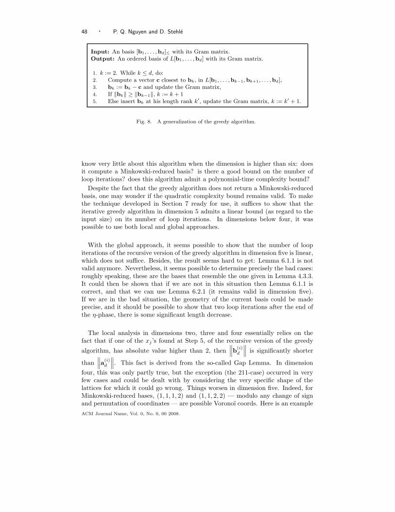
48 · P. Q. Nguyen and D. Stehle
Input: An basis [b1, . . . ,bd]≤ with its Gram matrix.Output: An ordered basis of L[b1, . . . ,bd] with its Gram matrix.
1. k := 2. While k ≤ d, do:2. Compute a vector c closest to bk, in L[b1, . . . ,bk−1, bk+1, . . . ,bd],3. bk := bk − c and update the Gram matrix,4. If ‖bk‖ ≥ ‖bk−1‖, k := k + 15. Else insert bk at his length rank k′, update the Gram matrix, k := k′ + 1.
Fig. 8. A generalization of the greedy algorithm.
know very little about this algorithm when the dimension is higher than six: doesit compute a Minkowski-reduced basis? is there a good bound on the number ofloop iterations? does this algorithm admit a polynomial-time complexity bound?
Despite the fact that the greedy algorithm does not return a Minkowski-reducedbasis, one may wonder if the quadratic complexity bound remains valid. To makethe technique developed in Section 7 ready for use, it suffices to show that theiterative greedy algorithm in dimension 5 admits a linear bound (as regard to theinput size) on its number of loop iterations. In dimensions below four, it waspossible to use both local and global approaches.
With the global approach, it seems possible to show that the number of loopiterations of the recursive version of the greedy algorithm in dimension five is linear,which does not suffice. Besides, the result seems hard to get: Lemma 6.1.1 is notvalid anymore. Nevertheless, it seems possible to determine precisely the bad cases:roughly speaking, these are the bases that resemble the one given in Lemma 4.3.3.It could then be shown that if we are not in this situation then Lemma 6.1.1 iscorrect, and that we can use Lemma 6.2.1 (it remains valid in dimension five).If we are in the bad situation, the geometry of the current basis could be madeprecise, and it should be possible to show that two loop iterations after the end ofthe η-phase, there is some significant length decrease.
The local analysis in dimensions two, three and four essentially relies on thefact that if one of the xj ’s found at Step 5, of the recursive version of the greedy
algorithm, has absolute value higher than 2, then∥
∥
∥b
(i)d
∥
∥
∥is significantly shorter
than∥
∥
∥a
(i)d
∥
∥
∥. This fact is derived from the so-called Gap Lemma. In dimension
four, this was only partly true, but the exception (the 211-case) occurred in veryfew cases and could be dealt with by considering the very specific shape of thelattices for which it could go wrong. Things worsen in dimension five. Indeed, forMinkowski-reduced bases, (1, 1, 1, 2) and (1, 1, 2, 2) — modulo any change of signand permutation of coordinates — are possible Voronoı coords. Here is an example
ACM Journal Name, Vol. 0, No. 0, 00 2008.
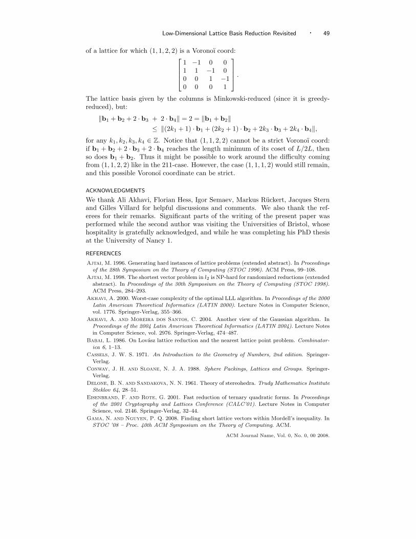
Low-Dimensional Lattice Basis Reduction Revisited · 49
of a lattice for which (1, 1, 2, 2) is a Voronoı coord:
1 −1 0 01 1 −1 00 0 1 −10 0 0 1
.
The lattice basis given by the columns is Minkowski-reduced (since it is greedy-reduced), but:
‖b1 + b2 + 2 · b3 + 2 · b4‖ = 2 = ‖b1 + b2‖≤ ‖(2k1 + 1) · b1 + (2k2 + 1) · b2 + 2k3 · b3 + 2k4 · b4‖,
for any k1, k2, k3, k4 ∈ Z. Notice that (1, 1, 2, 2) cannot be a strict Voronoı coord:if b1 + b2 + 2 · b3 + 2 · b4 reaches the length minimum of its coset of L/2L, thenso does b1 + b2. Thus it might be possible to work around the difficulty comingfrom (1, 1, 2, 2) like in the 211-case. However, the case (1, 1, 1, 2) would still remain,and this possible Voronoı coordinate can be strict.
ACKNOWLEDGMENTS
We thank Ali Akhavi, Florian Hess, Igor Semaev, Markus Ruckert, Jacques Sternand Gilles Villard for helpful discussions and comments. We also thank the ref-erees for their remarks. Significant parts of the writing of the present paper wasperformed while the second author was visiting the Universities of Bristol, whosehospitality is gratefully acknowledged, and while he was completing his PhD thesisat the University of Nancy 1.
REFERENCES
Ajtai, M. 1996. Generating hard instances of lattice problems (extended abstract). In Proceedingsof the 28th Symposium on the Theory of Computing (STOC 1996). ACM Press, 99–108.
Ajtai, M. 1998. The shortest vector problem in l2 is NP-hard for randomized reductions (extendedabstract). In Proceedings of the 30th Symposium on the Theory of Computing (STOC 1998).ACM Press, 284–293.
Akhavi, A. 2000. Worst-case complexity of the optimal LLL algorithm. In Proceedings of the 2000Latin American Theoretical Informatics (LATIN 2000). Lecture Notes in Computer Science,vol. 1776. Springer-Verlag, 355–366.
Akhavi, A. and Moreira dos Santos, C. 2004. Another view of the Gaussian algorithm. InProceedings of the 2004 Latin American Theoretical Informatics (LATIN 2004). Lecture Notesin Computer Science, vol. 2976. Springer-Verlag, 474–487.
Babai, L. 1986. On Lovasz lattice reduction and the nearest lattice point problem. Combinator-ica 6, 1–13.
Cassels, J. W. S. 1971. An Introduction to the Geometry of Numbers, 2nd edition. Springer-Verlag.
Conway, J. H. and Sloane, N. J. A. 1988. Sphere Packings, Lattices and Groups. Springer-Verlag.
Delone, B. N. and Sandakova, N. N. 1961. Theory of stereohedra. Trudy Mathematics InstituteSteklov 64, 28–51.
Eisenbrand, F. and Rote, G. 2001. Fast reduction of ternary quadratic forms. In Proceedingsof the 2001 Cryptography and Lattices Conference (CALC’01). Lecture Notes in ComputerScience, vol. 2146. Springer-Verlag, 32–44.
Gama, N. and Nguyen, P. Q. 2008. Finding short lattice vectors within Mordell’s inequality. InSTOC ’08 – Proc. 40th ACM Symposium on the Theory of Computing. ACM.
ACM Journal Name, Vol. 0, No. 0, 00 2008.
50 · P. Q. Nguyen and D. Stehle
Gauss, C. F. 1801. Disquisitiones Arithmeticæ. Springer-Verlag.
Helfrich, B. 1985. Algorithms to construct Minkowski reduced and Hermite reduced latticebases. Theoretical Computer Science 41, 125–139.
Hermite, C. 1850. Extraits de lettres de M. Hermite a M. Jacobi sur differents objets de latheorie des nombres, deuxieme lettre. Journal fur die reine und angewandte Mathematik 40,279–290.
Hermite, C. 1905. Œuvres. Gauthiers-Villars.
Kaib, M. and Schnorr, C. P. 1996. The generalized Gauss reduction algorithm. Journal ofAlgorithms 21, 3, 565–578.
Kannan, R. 1983. Improved algorithms for integer programming and related lattice problems. InProceedings of the 15th Symposium on the Theory of Computing (STOC 1983). ACM Press,99–108.
Korkine, A. and Zolotarev, G. 1873. Sur les formes quadratiques. Mathematische Annalen 6,336–389.
Lagarias, J. C. 1980. Worst-case complexity bounds for algorithms in the theory of integralquadratic forms. Journal of Algorithms 1, 142–186.
Lagarias, J. C., Lenstra, W. H., and Schnorr, C. P. 1990. Korkine-Zolotarev bases andsuccessive minimal of a lattice and its reciprocal lattice. Combinatorica 10, 333–348.
Lagrange, J. L. 1773. Recherches d’arithmetique. Nouveaux Memoires de l’Academie de Berlin.
Lenstra, A. K., Lenstra, Jr., H. W., and Lovasz, L. 1982. Factoring polynomials with rationalcoefficients. Mathematische Annalen 261, 513–534.
Martinet, J. 2002. Perfect Lattices in Euclidean Spaces. Springer-Verlag.
Micciancio, D. and Goldwasser, S. 2002. Complexity of lattice problems : a cryptographicperspective. Kluwer Academic Press.
Minkowski, H. 1896. Geometrie der Zahlen. Teubner-Verlag.
Nguyen, P. Q. and Stehle, D. 2004. Low-dimensional lattice basis reduction revisited (extendedabstract). In Proceedings of the 6th Algorithmic Number Theory Symposium (ANTS VI).Lecture Notes in Computer Science, vol. 3076. Springer-Verlag, 338–357.
Nguyen, P. Q. and Stehle, D. 2005. Floating-point LLL revisited. In Proceedings of Eurocrypt2005. Lecture Notes in Computer Science, vol. 3494. Springer-Verlag, 215–233.
Nguyen, P. Q. and Stern, J. 2001. The two faces of lattices in cryptology. In Proceedings of the2001 Cryptography and Lattices Conference (CALC’01). Lecture Notes in Computer Science,vol. 2146. Springer-Verlag, 146–180.
Ryskov, S. S. 1972. On Hermite, Minkowski and Venkov reduction of positive quadratic forms
in n variables. Soviet Mathematics Doklady 13, 1676–1679.
Schnorr, C. P. 1987. A hierarchy of polynomial lattice basis reduction algorithms. TheoreticalComputer Science 53, 201–224.
Schnorr, C. P. and Euchner, M. 1994. Lattice basis reduction: improved practical algorithmsand solving subset sum problems. Mathematics of Programming 66, 181–199.
Schnorr, C. P. and Horner, H. H. 1995. Attacking the Chor-Rivest cryptosystem by improvedlattice reduction. In Proceedings of Eurocrypt 1995. Lecture Notes in Computer Science, vol.921. Springer-Verlag, 1–12.
Schonhage, A. and Strassen, V. 1971. Schnelle Multiplikation grosser Zahlen. Computing 7,281–292.
Semaev, I. 2001. A 3-dimensional lattice reduction algorithm. In Proceedings of the 2001 Cryp-tography and Lattices Conference (CALC’01). Lecture Notes in Computer Science, vol. 2146.Springer-Verlag, 181–193.
Siegel, C. L. 1989. Lectures on the Geometry of Numbers. Springer-Verlag.
Stogrin, M. I. 1977. Regular Dirichlet-Voronoı partitions for the second triclinic group. Amer-ican Mathematical Society . English translation of the proceedings of the Steklov Institute ofMathematics, Number 123 (1973).
Tammela, P. P. 1973. On the reduction theory of positive quadratic forms. Soviet MathematicsDoklady 14, 651–655.
ACM Journal Name, Vol. 0, No. 0, 00 2008.
Low-Dimensional Lattice Basis Reduction Revisited · 51
Vallee, B. 1986. Une approche geometrique de la reduction des reseaux en petite dimension.
Ph.D. thesis, Universite de Caen.
Vallee, B. 1991. Gauss’ algorithm revisited. Journal of Algorithms 12, 556–572.
Voronoı, G. 1908. Nouvelles applications des parametres continus a la theorie des formes quadra-tiques. Journal fur die reine und angewandte Mathematik 134, 198–287.
van der Waerden, B. L. 1956. Die Reduktionstheorie der positiven quadratischen Formen. ActaMathematica 96, 265–309.
Received May 2006; revised October 2008; accepted xxxx
ACM Journal Name, Vol. 0, No. 0, 00 2008.